all ages lead model (aalm) - u.s. epa web server
TRANSCRIPT

United States National Center for EPA/600/R-05/102 Environmental Protection Environmental Assessment October 2005 Agency Research Triangle Park, NC 27711
Guidance Manual
for the
All Ages Lead Model (AALM)
Draft Version 1.05
Prepared by
National Center for Environmental Assessment Office of Research and Development
U. S. Environmental Protection Agency Research Triangle Park, N C 27711
Research and Development

9/27/2005 DRAFT: DO NOT QUOTE OR CITE 2
NOTICE
The U.S. Environmental Protection Agency, through its National Center for Environmental Assessment at Research Triangle Park, produced this report. This document is a preliminary draft. It has not been formally released by the U.S. Environmental Protection Agency and should not be construed to represent Agency policy. It is circulated as a guide for reviewers of the model.

9/27/2005 DRAFT: DO NOT QUOTE OR CITE 3
TABLE OF CONTENTS
AUTHORS AND CONTRIBUTORS.......................................................................................... 5
LIST OF FIGURES ...................................................................................................................... 6
SECTION 1: INTRODUCTION ................................................................................................. 8
SECTION 1: INTRODUCTION ................................................................................................. 8 1.1 INSTALLATION............................................................................................................................. 9 1.2 BACKGROUND AND BASIS FOR PARAMETER VALUES................................................... 9 1.3 RUNNING THE MODEL............................................................................................................. 10 1.4 A QUICK REVIEW OF THE MODEL ...................................................................................... 12
2: BUILDING THE MODEL RUN........................................................................................... 17 2.1. EDITING PARAMETERS ........................................................................................................... 19
2.1.1. MEDIA EXPOSURES ........................................................................................................... 19 2.2 EDITING EXPOSURE ACTIVITY PATTERNS ....................................................................... 28 2.3 SUMMARY AND CONCLUSIONS ............................................................................................ 28
SECTION 3: SPECIAL EXPOSURE FEATURES................................................................. 32 3.1 PICA EXPOSURE.......................................................................................................................... 32 3.2 DERMAL EXPOSURE.................................................................................................................. 32 3.3 HISTORICAL LEAD EXPOSURES............................................................................................ 33 3.4 MATERNAL EXPOSURE (Conceptual Design)......................................................................... 33
SECTION 4: ABSORPTION MODULE.................................................................................. 34 4.1 MODELING LEAD ABSORPTION ............................................................................................ 34 4.2 ABSORPTION OF INHALED LEAD.......................................................................................... 36 4.3 ABSORPTION OF INGESTED LEAD....................................................................................... 37
SECTION 5: BIOKINETICS MODULE ................................................................................. 39 5.1 MODEL SETTINGS ...................................................................................................................... 39
5.1.1 PARAMETERS WITH EXPLICIT VALUES ..................................................................... 39 5.2 BIOKINETIC PARAMETERS.................................................................................................... 42
5.2.1 Pb DECAY RATE. .................................................................................................................. 43 5.2.2 CORTICAL BONE TURNOVER. .................................................................................... 43 5.2.3. TRABECULAR BONE TURNOVER RATE. ............................................................. 44 5.2.3 TRANSFER FROM CORTICAL SURFACE TO BLOOD PLASMA. ......................... 46 5.2.4. TRANSFER FROM TRABECULAR SURFACE TO BLOOD PLASMA. .............. 47 5.2.6 CORTICAL SURFACE TO VOLUME TRANSFER. .................................................... 48 5.2.7 TRABECULAR SURFACE TO TRABECULAR VOLUME TRANSFER. ..................... 49 5.2.8 TOTAL TRANSFER FROM EXCHANGE BONE VOLUME. ......................................... 50 5.2.9. TRANSFER FROM THE EXCHANGE TO THE NON-EXCHANGE VOLUME. 50 5.2.10. TRANSFER FROM LIVER1............................................................................................. 51 5.2.11 TRANSFER FROM KIDNEY1. ......................................................................................... 51

9/27/2005 DRAFT: DO NOT QUOTE OR CITE 4
5.2.12 TRANSFER FROM BLADDER TO URINE. ................................................................... 51 5.2.13 TRANSFER FROM LIVER2.............................................................................................. 52 5.2.14 TRANSFER FROM KIDNEY2. ......................................................................................... 53 5.2.15 TRANSFER FROM FAST SOFT TISSUE. ...................................................................... 54 5.2.16 TRANSFER FROM INTERMEDIATE SOFT TISSUE. ................................................. 55 5.2.17 TRANSFER FROM SLOW SOFT TISSUE...................................................................... 56 5.2.18 TRANSFER RATES FROM BRAIN. ................................................................................ 57 5.2.19 DEPOSITION FRACTION IN URINE. ............................................................................ 58 5.2.20 DEPOSITION FRACTION IN BONE. .............................................................................. 59 5.2.21 TRABECULAR BONE DEPOSITION FRACTION. ...................................................... 60 5.2.22 DEPOSITION FRACTION IN COMPARTMENTS WITHOUT AGE VARIABIL. ... 61 5.2.23 DEPOSITION FRACTION FROM DIFFUSIBLE PLASMA TO FAST SOFT . ......... 62 5.2.24 DEPOSITION FRACTION FROM DIFFUSIBLE PLASMA TO INTERMEDIATE. 63 5.2.25 DEPOSITION FRACTION FROM DIFFUSABLE PLASMA TO SLOW SOFT. ....... 64 5.2.26 DEPOSITION FRACTION FROM DIFFUSIBLE PLASMA TO BRAIN. .................. 65 5.2.27 COMPONENTS OF THE CIRCULATORY SYSTEM. .................................................. 66 5.2.28 TRANSFER RATE FROM RBC TO PLASMA. .............................................................. 66 5.4.29 AMOUNT OF BLOOD........................................................................................................ 67 5.2.30 CHELATION FACTORS 1,2,and 3. .................................................................................. 68
SECTION 6. CONTROLLING THE MODEL OUTPUT...................................................... 69 6.1. A SIMPLE CONFIDENCE TEST ...............................................................................................69 6.2. BIOKINETIC OUTPUTS.............................................................................................................71
6.2.1 TABLES ................................................................................................................................... 71 6.1.2 PLOTTING.............................................................................................................................. 71 6.1.3 EDITING THE CHART......................................................................................................... 72
SECTION 7. REFERENCES……………….………………………………………………….74

9/27/2005 DRAFT: DO NOT QUOTE OR CITE 5
AUTHORS AND CONTRIBUTORS
Robert Elias, U.S. Environmental Protection Agency
Brian Gulson, Macquire University, Sidney Australia
Gary Diamond, Syracuse Research Corporation
Ramon Olivera, Lockheed-Martin Information Technology
Goeffrey Nonato, Lockheed Martin Information Technology
9/27/2005 DRAFT: DO NOT QUOTE OR CITE 6
LIST OF FIGURES
Figure 1. Opening screen with NCEA Logo and disclaimer.....................................................................................10 Figure 2: Window with prompt to create a new study or open an existing study. ....................................................11 Figure 3. Drop Down window that allows the Modeler to customize three features of the program setup..............11 Figure 4: Primary Window - Modeler defines the individual by sex, life span, and time frame...............................12 Figure 5: Model component selection window. Click on exposure to run this portion of the model. ......................13 Figure 6: Model status window. Select options to use historical data.....................................................................13 Figure 7: Retrieve model output file. ........................................................................................................................13 Figure 8: Output data file in spreadsheet format. ....................................................................................................14 Figure 9: Primary Window with Male gender, End Date computation, and one day time step selected..................15 Figure 10. Drop-down window for resetting the model date. .....................................................................................16 Figure 11. Bar along top of screen with Tools option. ...............................................................................................18 Figure 12. Tool Selection Menu.. ...............................................................................................................................18 Figure 13. Drop down window to select the output parameters to be displayed. .......................................................18 Figure 14: Primary window with full specifications for model run, ready for entering exposure parameters...........19 Figure 15. Save Current Study ...................................................................................................................................19 Figure 16. Select Exposure Parameters to review and modify the exposure portion of the model.............................20 Figure 17: Exposure options group with Air component ready for review and modification.....................................21 Figure 18: Options for Dietary exposure. ..................................................................................................................22 Figure 19. Dietary exposure with garden fruits and vegetables.................................................................................23 Figure 20: Exposure options for dust exposure..........................................................................................................24 Figure 21: Drop Down window for the Dust component of Media Exposure. ...........................................................25 Figure 22: Window for the Dust component of Media Exposure................................................................................25 Figure 23: Window for the dust component of Media Exposure. ...............................................................................26 Figure 24: Window for the Water component of Media Exposure with the default option of Fully Flushed Water. ..27 Figure 25: Window for the Water component of Media Exposure with the options for Other Water Sources. ..........27 Figure 26: Drop down window for the Activity Patterns component of Media Exposure. .........................................28 Figure 27: Following set of the Exposure Scenario, the model run is initiated by checking the Exposure. ...............29 Figure 28. Two files are available for review, *.mod and *.mpa. ..............................................................................30 Figure 29. Line by line output for the exposure module. *.mod .................................................................................30 Figure 30. Total exposure by age for each exposure category (*.mpa)......................................................................30 Figure 31: Exposure Model options with options to change internal exposure and growth parameters. ..................31 Figure 32: Window for the Pica component of Media Exposure................................................................................32 Figure 33: Window for the Dermal component of Media Exposure. ..........................................................................33 Figure 34. Schematic diagram of the Leggett Model..................................................................................................35 Figure 35: Drop down window for reviewing and revising........................................................................................36 Figure 36: Window for editing Absorption Parameters. ............................................................................................36 Figure 37: Drop down window for gastrointestinal absorption showing default values.............................................37 Figure 38: Plot of the default values for the gastrointestinal absorption fraction. ....................................................37 Figure 39: Default values for the gastrointestinal rate of movement function. ..........................................................38 Figure 40: Plot of the default values for the rate of gastrointestinal movement function...........................................38 Figure 41: Schematic Diagram of O’Flaherty Model. ...............................................................................................42 Figure 42: Window for editing the model settings.......................................................................................................41 Figure 43: Drop down window for editing the default Delta Step lengths. .................................................................42 Figure 44: Window for editing biokinetic parameters................................................................................................42 Figure 45. Schematic Diagram of Leggett Model.......................................................................................................43 Figure 46: Values for cortical bone turnover rate which decreases with age.. .........................................................44 Figure 47: Plot of default values for cortical bone turnover rate by age. ..................................................................44 Figure 48. Age-specific values for Surface to Volume in Trabecular Bone................................................................45 Figure 49. Plot of Trabecular Surface to Volume.......................................................................................................45 Figure 50: Values for trabecular bone turnover rate by age......................................................................................45 Figure 51: Plot of default values for trabecular bone turnover rate by age...............................................................46

9/27/2005 DRAFT: DO NOT QUOTE OR CITE 7
Figure 52: Dropdown window for editing the parameter for transfer from cortical surface to blood. ......................46 Figure 53: Plot of the default values for the parameter for transfer from cortical surface to blood..........................47 Figure 54: Drop down window for editing the parameter for the transfer rate for trabecular surface to blood. ......47 Figure 55: Plot of the default values for the transfer rate for trabecular surface to blood. .......................................48 Figure 56. Window for editing the value for transfer from cortical surface to volume. ..............................................48 Figure 57: Plot of the default values for transfer from cortical surface to volume. ...................................................49 Figure 58: Window for editing the values for transfer from trabecular surface to volume. .......................................49 Figure 59: Plot of the default values for transfer from trabecular surface to volume................................................50 Figure 60: Window for editing values for total transfer from the exchange bone volume. ........................................50 Figure 61: Window for editing values for total transfer from the non-exchange bone volume. ..................................51 Figure 62: Window for editing the values for the transfer of lead from the bladder to urine. ...................................52 Figure 63: Plot of the default values for the transfer of lead from the bladder to urine. ...........................................52 Figure 64. Age-related coefficients for transfer of lead from Liver2..........................................................................53 Figure 65. Plot of the transfer of lead from the liver 2 compartment. ........................................................................53 Figure 66: Drop down window for editing the default values for the transfer of lead from the kidney......................54 Figure 67: Plot of the default values for the transfer of lead from Kidney 2 (From Kidney to Bladder). ..................54 Figure 68: Drop down window for editing the default values for the deposition fraction of lead in fast soft tissue.. 55 Figure 69: Plot of the default values for the deposition fraction of lead in fast soft tissue. .......................................55 Figure 70: Drop down window for editing the default values for the deposition in intermediate soft tissue.. ...........56 Figure 71: Plot of the default values for the deposition fraction of lead in fast soft tissue. .......................................56 Figure 72: Drop down window for editing the default values for the deposition fraction in slow soft tissue..............57 Figure 73: Plot of the default values for the deposition fraction of lead in slow soft tissue. ......................................57 Figure 74: Drop down window for editing the default values for the deposition fraction of lead in the brain. ..........58 Figure 75: Plot of the default values for the deposition fraction of lead in the brain.................................................58 Figure 76. Deposition fraction in Bone. .....................................................................................................................59 Figure 77. Plot of Deposition Fraction in Bone. ........................................................................................................59 Figure 78. Bottom of biokinetic Parameters Window.................................................................................................60 Figure 79. Age-dependent Variables for Trabecular Bone Deposition Fraction. ......................................................60 Figure 80. Trabecular bone deposition fraction.........................................................................................................61 Figure 81: Plot of the default values for the transfer of lead from the liver. ..............................................................61 Figure 82. Age-dependent Variables for Diffusible Plasma to Fast Soft Tissue..........................................................62 Figure 83. Plot of the default values for the Diffusible Plasma to Fast Soft Tissue parameter. .................................63 Figure 84. Age-dependent Variables for Diffusible Plasma to Intermediate Soft Tissue............................................63 Figure 85. Plot of the default values for the diffusible Plasma to Intermediate Soft Tissue parameter......................64 Figure 86. Age-dependent Variables for Diffusible Plasma to Slow Soft Tissue. ........................................................64 Figure 87. Plot of the default values for the Slow Soft Tissue Parameter. .................................................................65 Figure 88. Age-dependent Variables for the Deposition Fraction from Diffusible Plasma to Brain. .........................65 Figure 89. Plot of the default values for the Deposition Fraction from Diffusible Plasma to Brain parameter.........66 Figure 90. Age-dependent variable for the Transfer Rate from RBC. ........................................................................67 Figure 91. Plot of the default values for the Transfer Rate for RBC parameter.........................................................67 Figure 92. Age-dependent variable for total volume of blood (deciliters. ..................................................................68 Figure 93. Plot of the default values for the Amount of Blood parameter. .................................................................68 Figure 94. Output with all default settings .................................................................................................................69 Figure 95. Total Blood lead with elevated dust lead exposure. ..................................................................................70 Figure 96. Using the Built in Graphic Feature. .........................................................................................................72

9/27/2005 DRAFT: DO NOT QUOTE OR CITE 8
SECTION 1: INTRODUCTION The purpose of the All Ages Lead Model (AALM) is to make available to the risk assessor a sufficiently complex, multi-compartment biokinetic model that predicts with reasonable accuracy the tissue concentrations of lead in humans and informs the modeler of the resulting changes in tissue concentrations that might occur over the lifetime of the modeled individual. The original model developed for this purpose, the Integrated Exposure Uptake Biokinetic Model for Lead in Children (IEUBK) met some of these objectives in that it is a multi-compartmental model that predicts blood concentrations of lead in humans, but the IEUIBK model makes this prediction only through age six and provides no information on the tissue concentrations (White et al, 1998). The AALM accomplishes this objective by providing an Exposure and Absorption interface to a biokinetic model. This interface guides the modeler toward a thorough, accurate description of the total daily exposure to lead, calculating the amounts of lead absorbed. The model then offers a choice of two biokinetic models to determine how the lead is distributed to the key body tissues1. These two models are referred to as the Leggett Model (Leggett, 1993) and the O’Flaherty Model O’Flaherty, 1998). One advantage of the Leggett Model is that it characterizes the distribution of lead based on the function of the human circulatory system, including the extracellular fluids. Likewise, the Leggett model also recognizes the chemical relationship between Pb and Ca. especially in describing the complexity of the bone compartments. There are some deficiencies in the Leggett model that can perhaps be overcome by the use of the O’Flaherty model, and we expect to make this feature available in the near future. This document takes you step-by-step through the process of getting the AALM up and running on your computer. As with all software packages, expertise is achieved by trial and error, and by aggressively investigating all model features. You will find that by starting from the simplest case and moving systematically to the more complex applications, you will soon develop expertise that matches your interests. This Guide takes into account comments and suggestions from many competent reviewers, evaluators and experienced modelers. It is not intended as a primary source of information regarding the source code for the AALM model, which is documented elsewhere. That document identifies the inherent structure of the three components of the AALM: lead exposure (intake) model, lead absorption (uptake) model, and biokinetic distribution model. It documents how the software system was designed to implement these models and describes each of the data elements used by the system, the functional flow of data through the system and the interfaces between the components. Model development is not an easy effort. In addition to the science behind the process, there are also concerns about the development process itself. During the AALM development, which occurred over a period of approximately eight years, several symposia and workshops were held, including one on Model Validation (Elias et al, 1998). At that workshop, two papers have 1 The O’Flaherty model is not fully implemented at this time. We expect to complete this task in the next few weeks. Meanwhile, if the O’Flaherty option is selected, the model will switch to the Leggett model and notify the modeler thereof.

9/27/2005 DRAFT: DO NOT QUOTE OR CITE 9
provided significant guidance to this project: Oreskes: Evaluation (Not Validation) of Quantitative Models; and Mickle: Structure, Use, and Validation of the IEUBK Model. The development of a large modeling system such as this is an ongoing process. The current version will, hopefully, meet the needs of most modelers. But in the process of developing this model, the planners recognized several features that could be incorporated with minimal effort, given the successful completion of the basic model. Construction of these additional features has been initiated and is discussed in Chapter 4 of this document. Comments are most welcome. 1.1 INSTALLATION AALM requires Windows 95 or later (Windows 98, or Windows NT, Windows 2000, Windows XP). If you already have a previous review version of the AALM installed, the new version includes a user option to automatically uninstall the previous version. AALM is distributed as a bundled package that, when activated, will place all required files in a single directory with a default designation of C:\Program Files\AALM. The AALM program is installed with InstallShield using the Add/Remove feature of the Windows Control Panel. Thus, a new subdirectory called will appear in this directory after installation, and the All Ages Lead Model icon should appear on your opening window. Unless you designate otherwise, your project files will be stored in a subdirectory of this directory. One additional file, DEMO1.xal has also been installed to assist you in becoming familiar with the AALM. You will have an opportunity to access this file as you work your way through this manual.
1.2 BACKGROUND AND BASIS FOR PARAMETER VALUES
The purpose of the All Ages Lead Model is to mathematically provide an exposure, absorption, and biokinetic infrastructure that allocates, by simulation, the simultaneous distribution of absorbed lead in several major body components and thereby predict at any point in time the concentration of lead in these components.
The All Ages Lead Model has about 190 parameters with assigned values that can be revised by the modeler to meet the description of a modeled individual designed by the modeler. All values for these parameters have default settings that permit the model to run to a conclusion, reaching an endpoint whereby the predicted outcome can be determined that is consistent with the modeled input. This means that the model will run in the default mode, and will produce reasonable results consistent with the default inputs. The modeler, therefore, has the option to change one or more of the input parameters and rerun the model to compare the new results with the default output, or to create and save another “default” model parameters consistent with the needs and requirements of his/her investigation. A companion document, the AALM Parameters and Equation Dictionary, describes these model components in greater detail.

9/27/2005 DRAFT: DO NOT QUOTE OR CITE 10
The AALM default values for the biokinetic parameters are based on published experimental values or ranges of values used for the Leggett and O’Flaherty models. Many of these default values have no meaning or significance other than as a place holder for a value that may be assigned by the modeler. With few exceptions, there are no documented values that can be validated by reliable literature reports. Consequently, the modeler must always be aware of the need to review the results rigorously, and establish internal constraints that adequately bracket the desired objective.
1.3 RUNNING THE MODEL
After installation, click on the All Ages Lead Model icon to open the program. The NCEA logo (Figure 1) should appear with text disclaiming responsibility prior to official release. Click OK. If you highlight box to “close the screen automatically”, the next time you run the model, this Logo screen will be displayed for about five seconds, then move on to the window in Figure 2.
Figure 1. Opening screen with NCEA Logo and disclaimer
This window gives you the option to create a new study or open an existing study. The default is to create a new study, but you may want to start your orientation with a demonstration study that will to provide you with a quick review of the model.

9/27/2005 DRAFT: DO NOT QUOTE OR CITE 11
Figure 2: Window with prompt to create a new study or open an existing study. Your new
file will be saved in a subdirectory of the AALM Program directory. You can change this default directory by clicking on Tools at the top of the screen, then Options. Type the new directory and any subdirectories in the window labeled Data.
Figure 3. Drop Down window that allows the Modeler to customize three features of the
program setup. The features of the Startup Preferences window are: The automatic closing of the opening screen after a 5 second delay, the choice to display or not to display the Select Action dialog box after the opening screen, and the opportunity to change the directory where the user-created output data files are stored. This last choice, which is, by default, the AALM subdirectory of the C:\Program directory, is especially important if the Modeler is accustomed to backing up only the files located in the C:\Documents and Settings directory, in which case, the AALM output files would not be saved. This Window may be accessed from the upper bar below the Screen Title by selecting the “Tools” option.

9/27/2005 DRAFT: DO NOT QUOTE OR CITE 12
1.4 A QUICK REVIEW OF THE MODEL If this is your first time using the model, perhaps it would be a good idea to begin with a demonstration file that will provide the required settings you will need to get started. Select ‘Open an existing study’ from the Select Action window, then choose Demo1.xal to get started. Follow these steps to run through the model. (You can return to this place in the Guidance Manual to continue your review of the model features): If you installed the program according to the instructions in Section 1.1, you should be able to select Demo1.xal from the File Open window. Click on the Open button to get the next screen, which is the hub of the model and is referred to in this manual as the Primary window. From here you can specify the input parameters for the model using the options on the screen. First note that this is a typical Windows® screen with drop down menus for many Windows® functions at the top. The model will use the default screen color format you have selected for your computer.
Figure 4: Primary Window - Modeler defines the individual by sex, life span, and time
frame, and accesses the parameter definition windows.
These settings will run the model using the default settings for the full lifetime of the hypothetical person that you define by entering or changing the appropriate values in the exposure section of the model. This file can be saved and used in your own research and studies, and you can create as many other study files as you need. In the Demo1 file, the individual is tracked through all age ranges. Press Run and you will begin this simulation leading to the next screen:

9/27/2005 DRAFT: DO NOT QUOTE OR CITE 13
Figure 5: Model component selection window. Click on exposure to run this portion of the
model. Select all three to run the full model. To run the full model, click the small boxes next to Exposure and Absorption (the Biokinetics box will automatically insert a √). Press Continue to get the next screen.
Figure 6: Model status window. Select options to use historical data.
Click Start, and the model will run for a few seconds. Then you will get two output files which can be viewed (Figure 7); these will be saved as a part of this study.
Figure 7: Retrieve model output file. The *.mod file has day by day record of values for
the list of selected output options. This list may take a few seconds to pop up on the screen, as it may contain over 32000 records, depending on your choice of age ranges.

9/27/2005 DRAFT: DO NOT QUOTE OR CITE 14
Press Continue to save these files using the same filename and to pass onto the next screen. In a few seconds, you will get a screen that looks like this:
Figure 8: Output data file in spreadsheet format. All output parameters may be selected,
and the file may be exported as a Lotus 123 file or Microsoft Excel file. This table shows the output for the model run, giving the lead concentrations (µg/g) in each of six compartments every one hundred days for the lifetime of the modeled individual. You can plot these now if you wish. At this point you should understand that the main purpose of the model is to estimate the concentration of lead in selected body tissues based on the exposure of the modeled individual over the desired age range (the model runs from birth to the highest selected age range). You will see later how you can use the plotting capabilities of the model to view the data in graphic form, or export the data to a spreadsheet and develop your own custom made plots and perform further statistical analyses to meet your specific data evaluation requirements. Now let’s get back to the screen-by-screen description of the model. Returning to the Primary Window, observe the following options:

9/27/2005 DRAFT: DO NOT QUOTE OR CITE 15
Figure 9: Primary Window with Male gender, End Date computation, and one day time
step selected.
You can:
1) Select Male or Female 2) Compute with an end date of today 3) Change the date from the default date, which is your computer’s date 3) Select a simulation timestep of one day or one hour2 4) Run the model through one to nine age ranges3.
The Calendar date cannot be changed by editing the date in the date window, because the program does not read this date back in to the study file. The date can be changed by clicking on this window, thereby calling up a calendar which is capable of recording your selected date in the study file (Figure 10). Click on the up/down arrow at the right of the year to change the year. Click on the month right or left arrow to change the month, and then click on the day to set the day of the month. Default options are preselected for all choices on this screen except the Age Range, and you need select only the highest Age Range that you want for your simulation. The rest will be populated for you. Take time to note that when you select an age range, the model displays the ages and the dates automatically. Thus, if you are interested in an exposure during a specific time period in this person’s life, you can make an upper age selection that will include this time period in the person’s life. You can also manually adjust the number of days in each age range.
2 Our experience to date has not revealed any situations where the assessment would be enhanced by a timestep more frequent than one day. 3 The Prenatal option is not fully implemented but is included for demonstration purposes. (See Section 4)

9/27/2005 DRAFT: DO NOT QUOTE OR CITE 16
Associated with each age range are one or more exposure scenarios that can be manipulated to define the daily exposure for one to four physical locations (e.g. Residential, School, Occupational, Recreational) during each of the life stages4.
When you are through with this exploration phase, exit the simulation and return to the main window. If you wish to reset the parameters to their default value you may do so on any of the Media Exposure windows.
Figure 10. Drop-down window for resetting the model date. Clicking on the date window
will give the calendar window as shown. The years is selected by toggling up or down on the small bars to the right of the year. The month is selected by clicking on the left or right arrow on the left or right of the top of the screen. The day is selected by clicking on the desired date.
4 The two youngest age groups do not have the Occupational option, and therefore have only three location options.

9/27/2005 DRAFT: DO NOT QUOTE OR CITE 17
2: BUILDING THE MODEL RUN
Building the model run consists of five steps:
1) define the individual 2) construct a full exposure scenario 3) modify the uptake and biokinetic parameters, if necessary 4) run the model to produce and save the output file 5) patch the output file into an Excel or Lotus spreadsheet from which you can perform
further graphic and statistical analyses. In every case throughout the model, default input values have been inserted when such a value is required for continuation. Accepting these values during the initial exploration of the model may enhance the learning curve and give you a feel for the range of values that will meet the needs of your study. With the default values that are provided, the model should run as installed with minimum modeler input. They can easily be changed and reset.
a. Age Range: Select the maximum age category you would like for this model run. This will automatically populate all younger age categories. Note that these age categories are for the purpose of creating the exposure scenario based on reasonable activity patterns. Later, you will see age-related distributions for absorption and biokinetic parameters that are independent of these exposure and activity pattern age groups.
b. Select the output you desire, with respect to the tissue concentrations. This is done by
clicking on the Tools option on the bar at the top of the screen (Figure 11), then selecting “Set Output.” See Figure 12. The Window is shown in Figure 13. Left click to place an ‘X’ in any box for which you want output, and remove the “X” from any box for which you don’t want output by left clicking on the “X.” Left click on OK when you are done selecting the output options.
For the purposes of graphic presentation, it is best to group your output selections so that they are approximately on the same scale and will display over about the same range. This can best be accomplished by trial and error.
c. Although there are several other options that could be brought into play, it might be best to run the model in default mode, just to get a feel for the type of output you can expect. Click the RUN button at the right of the box. You must save this study to a file. Click OK when asked “Save current study changes?” Clicking Cancel will stop the RUN mode at this point and wait for your further input. You can enter a new file name (the .xal extension will be added automatically) or click on a previous file from the list shown (Figure 14). Click SAVE.

9/27/2005 DRAFT: DO NOT QUOTE OR CITE 18
Figure 11. Bar along top of screen with Tools option. Clicking on Tools, then Set Output,
will give the drop down window in Figure 13.
Figure 12. Tool Selection Menu. Click on ‘Set Output’.
Figure 13. Drop down window to select the output parameters to be displayed and for
which data are needed for export. NOTE: The Insert Event option on the Opening window has been temporarily disabled.

9/27/2005 DRAFT: DO NOT QUOTE OR CITE 19
Figure 14: Primary window with full specifications for model run, ready for entering
exposure parameters.
Figure 15. Save Current Study 2.1. EDITING PARAMETERS
2.1.1. MEDIA EXPOSURES There is considerable flexibility in the AALM to change the assigned values of the media exposure parameters. Each exposure category (AIR, DIET, DUST, WATER, PICA, DERMAL) has a separate window, and you can reset the values for these six windows. Air, Diet, Dust, and Water ingestion values are set to typical U.S. values and are discussed in this section. Pica and Dermal exposure values are, by default, set to zero exposure because they apply to special situations not fully documented in the literature. Pica and Dermal exposure are available for research purposes and are discussed further in Section 4.

9/27/2005 DRAFT: DO NOT QUOTE OR CITE 20
Set the parameter window to “Media Exposure” and click the EDIT button. There are two options in Window 1a: “Exposure Parameters” and “Historical Exposure Settings.” At this time, select “Exposure Parameters” to gain access to Window 1a1: Media Exposure (Figure 17). [Historical Exposure Settings are under development and may not execute correctly for this evaluation]. The Exposure Parameter window has six tabs, one each for Air, Diet, Dust, Water, Pica, and Dermal Exposure. In each of these windows, you can set the values for the key parameters for each of the age range options that you have selected, shown in Figure 17 as Postnatal to Late Retirement. 2.1.1.1 Air The table for air exposure, shown on this figure, has eight rows of exposure data populated with two exposure parameters (amount of lead in air (µg Pb/m3 ) and amount of air inhaled (m3/day) for each exposure component: outdoor, residential, school, and occupational. In this way, air exposure is calculated as the product of the two parameters µg/m3 and m3/day, giving µg/day. In the case of air exposure in the three indoor environments, the amount of lead in air is, for convenience, expressed as a percentage of the outdoor lead concentration. The default values are set to 30% but may exceed 100% if the modeler chooses to do so. The exposure module uses a smoothing feature that assigns the value you select to the middle of the age range, then interpolates to the adjacent points of the younger and older age ranges when assigning values, day by day, to the intervening time steps.
Figure 16. Select Exposure Parameters to review and modify the exposure portion of the model.

9/27/2005 DRAFT: DO NOT QUOTE OR CITE 21
Figure 17: Exposure options group with Air component ready for review and modification. The default value of outdoor air is 0.1 µg Pb/m3 (Figure 17). Other options depend on the age range selected. The Clear button will clear all values in the “Air” window. The Clear All button will clear all six exposure categories and should not be used unless you plan to enter new values for all six windows. Likewise, the Default button will repopulate this window with the default values as shown, and the All to Default will do so for all six windows. The Historical Lead Concentration check window will be discussed in Section 4. 2.1.1.2 Diet The data for lead concentrations in food are taken from the Market Basket Food Survey conducted by the Food and Drug Administration. In this survey, specific food products in over two hundred categories are purchased at supermarkets periodically throughout the United States and sent to a central laboratory where they are prepared in a kitchen environment according to the manufacturer’s instructions. These are analyzed for many organic and inorganic components according to a strict analytical protocol. These data are reported quarterly and are available at the Food and Drug Administration website: Market Basket Survey: http://vm.cfsan.fda.gov/~lrd/pestadd.html Total Diet Study: http://www.cfsan.fda.gov/~comm/tds-hist.html#fca For this report, the data have been compiled, with some adjustments, and have been incorporated into the AALM for the periods 1982 to the present. Over the years, the categories of food have changed according to national food preferences, and the lead concentrations in these foods have declined dramatically, for several reasons5. From the standpoint of lifetime exposures to lead,
5 Food lead concentrations have decline considerably since the period 1982-85 with the removal of cans with

9/27/2005 DRAFT: DO NOT QUOTE OR CITE 22
this decline has been relatively recent (i.e. since 1985), and the historical food lead exposure of an individual born in the 1960s or earlier can be a significant component of the total body burden of lead. Select the “Diet” tab to move to the Dietary exposure mode as shown on Figure 19. The common features (age categories, dates, option buttons) are the same, and the rows of data are similar (amounts ingested, lead concentration) as for the air window. The default setting is for a Market Basket Survey Diet subdivided into the main items of Fruit, Vegetables, Meat and Fish. To access these alternate sources of food exposure, click on the window tab at the lower left corner shown in Figure 19 with the “Market Diet” label. Drop this window down to reveal options for Home Garden, Recreational Fishing/Hunting and Subsistence Fishing/Hunting. Figure 20 shows the selection of the Home Garden option that includes garden fruit and garden vegetables, each with a line for intake percent of diet and lead concentration. The intake percent has a default of zero, so that no exposure will be added to the total diet until a number is added to this row. You can do this one column at a time by entering a number in each cell or, for all age groups by entering a value in the window on the lower left. Note that the default lead concentrations are the same as for the market fruit above, so that no change will be seen in the diet until new lead concentrations for garden fruits are added, based on situational information.
Figure 18: Options for Dietary exposure.
soldered side seams. Air lead concentrations have also decreased, reducing the amount of lead in food crops.

9/27/2005 DRAFT: DO NOT QUOTE OR CITE 23
Figure 19. Dietary exposure with garden fruits and vegetables. The exposure information for garden fruits and vegetables may be entered in a similar manner, again with no change in the exposure unless values on the table are different from their default values. Other options include modifications if: 1) produce is home grown, or 2) recreational fishing/hunting, or 3) subsistence fishing/hunting are significant contributors to the diet. The Recreational Fishing and Hunting option provides the opportunity to account for lead exposure from the occasional ingestion of foods in the fish and meat category. Enter the data for recreational hunting/fishing category through the same process as for home gardening, and select garden fruit and vegetable options as well, if they apply. The third option is Subsistence Hunting and Fishing, and in this case the intent is to replace all market basket meats and fish with meat and fish from non-market sources. This option may also be used in conjunction with the home gardening option, in which case the assumption is that all food comes from non-market sources. Finally, it is important to note that alternate food sources may not necessarily be lower in lead content than market food. Historically, the main source of lead in market food was lead from cans with a lead-based seal on the side seam. These were removed from the commercial food production process during the period 1982-1985, resulting in a dramatic decline in the lead concentration of canned food. Likewise, the decline in air lead concentrations during the 1980s, with the banning of tetraethyl lead from gasoline, also resulted in a substantial reduction of lead in crops.

9/27/2005 DRAFT: DO NOT QUOTE OR CITE 24
2.1.1.3 Dust
Household dust (Figure 20) is assumed to be a mixture of deposited particles of atmospheric origin, tracked-in soil, deteriorating paint, dust from local commercial industries, and on occasion, certain dust generating activities related to the home environment. There are several options available with this exposure group. The first decision is to determine the manner in which the dust sample was taken: a wet wipe sample gives µg Pb per area sampled (µgPb/cm2 ); a dry vacuum sample can give µg Pb per area sampled or per gram of dust collected. If the total mass of dust sampled is available, then this can be related to an ingestion rate of dust mass/day, usually about 100 mg dust/day. If the mass of dust is not known and only the area sampled is known, then the modeler must base the exposure estimate on the hand-to-surface area contact and the hand-to-mouth activity of the individual. Furthermore, the efficiency of transfer at the time of surface contact, which depends largely on the dampness of the hand, should also be estimated.
Figure 20: Exposure options for dust exposure. The choice between the concentration method (Conc) (Figure 21) or the area method (Area) (Figure 22) can be made by dropping down the window in the lower part of the dust screen. The default option for Residential Dust using concentration measurements is shown below. The second dust decision is to determine the important sources of dust other than the home that might be associated with school, occupational or recreational activities. If this information is known or can be determined, these options can be implemented by dropping the window in the lower left part of the dust screen, the same window as the choice of [Conc] vs. [Area]. The alternate locations are the same options as for air, and are zeroed out until specific information is entered by the modeler. In determining how to distribute the dust exposure over several alternate sources, the modeler must make an estimate of the percent of total dust ingestion that occurs at each location, and the

9/27/2005 DRAFT: DO NOT QUOTE OR CITE 25
Figure 21: Drop Down window for the Dust component of Media Exposure with the
options for Other Dust Sources (as Concentration) shown in the lower left drop-down window.
Figure 22: Window for the Dust component of Media Exposure with the options for
Residential Dust sources (Area) shown in the sub-window at the lower left. concentration of lead in that dust. The contribution of lead from dust sources other than the home environment will remain at zero until the modeler makes the appropriate alternate dust source entries. Another option using the lead loading approach allows for exposure from school, occupational and recreational activities (Figure 22 and Figure 23).

9/27/2005 DRAFT: DO NOT QUOTE OR CITE 26
Figure 23: Window for the dust component of Media Exposure with the options for several
Dust Sources (as Area and Loading) shown in the sub-window at lower left.
2.1.1.4 Drinking Water As with the previous routes of exposure, conservative estimates of drinking water consumption are set at default values of one liter of fully flushed drinking water per day (Figure 24). This would include tap water used to prepare coffee or tea, and to reconstitute beverages such as frozen juices. It would not include canned or bottled soft drinks, which are treated as food items. On this basis, it is likely that the mean consumption of drinking water is higher than one liter, possibly 5-6 liters, but this varies by age, climate, season and several other factors, so that a conservative estimate seems appropriate as a baseline starting point. Lead exposure from drinking water is calculated as µg Pb/L x L/day = µg Pb/day. Other options allow for inputs from first draw water, fountain water and bottled water. These options may be accessed through the drop-down window at the lower left, by clicking the option “Other Water Sources” (Figure 25). This will add options for First Draw Tap Water, Drinking Fountain Tap Water, and Bottled Water. Unlike previous exposure sources, the Drinking Water options are fully implemented when the “Other Water Sources” button is selected. To change the default values, note that each source has a percent-of-total-volume option and this percent may be changed for each source and age group. Remember that bottled water and perhaps drinking fountains were not readily available in the early 1900s; likewise, there is little reliable site specific information on historical drinking water lead concentrations.

9/27/2005 DRAFT: DO NOT QUOTE OR CITE 27
Figure 24: Window for the Water component of Media Exposure with the default option of
fully Flushed Water in the sub-window at the lower left.
Figure 25: Window for the Water component of Media Exposure with the options for
Other Water Sources shown in the sub-window at lower left. [Pica and Dermal Exposure Factors Are Discussed in Chapter 3]

9/27/2005 DRAFT: DO NOT QUOTE OR CITE 28
2.2 EDITING EXPOSURE ACTIVITY PATTERNS Activity patterns determine the amount of time (hours) the modeled individual spends at each activity. There are 168 hours in a week. For each age group, these hours are distributed, as applicable, among four exposure locations (residential, school, occupational, and recreational) using the 168 hours, minus the designated sleep hours per day. Within each location, the modeler may designate a percentage of the time spent indoors, allowing for separate estimates of indoor/outdoor air and dust lead exposures. Three factors determine exposure: 1) the amount of time spent at a particular activity; 2) the amount of “media” ingested during that time; and 3) the concentration of lead in that media. For food and drinking water lead concentrations, the location may not be a factor if supermarket food and municipal water are consumed, as these are usually monitored closely and tend to be the same throughout the United States. Air and dust lead concentrations are likely to be different by location and are treated as such in this model. During the postnatal period, which lasts six months, the child is presumed to be in a highly protective environment with limited access to dust collecting surfaces and under continuous observation by a caregiver. Consequently, only one exposure environment, “Residential” is provided in the model. In the event there needs to be a second environment, this can be accomplished by reducing the time frame for Postnatal status and expanding the Toddler time frame.
Figure 26: Drop down window for the Activity Patterns component of Media Exposure
showing default values for activity patterns for Postnatal. 2.3 Summary and Conclusions This concludes the introduction to the General Guidance for Media Exposure. Most risk assessment problems for lead exposure can be handled with the development of an exposure scenario involving the model features discussed in this section followed by a statistical

9/27/2005 DRAFT: DO NOT QUOTE OR CITE 29
extrapolation of the predicted blood lead concentration for an individual to a mean blood lead concentration for a population of similarly exposed individuals. At this point, you may find it helpful to enter your own exposure settings and save the file as a useful starting point for further research or investigation. Section 4 provides guidance on special features and work-arounds for special problems and situations. If these features do not apply to your needs, you may proceed directly to Section 5 and begin adjusting the model for lead absorption. When you have completed constructing the exposure scenario for your subject, it is wise to give it a brief reality check. To determine whether you have correctly modeled the exposure of the individual, imagine yourself in that person’s place for one week and determine whether or not you would have captured all or most of your exposure for that time. Remember that, in some cases, you may account for exposure at two locations as they were one. That is, your exposure at the office may be, for all practical purposes, the same as at the library or at a concert hall, and could be treated as one location.
Figure 27: Following set of the Exposure Scenario, the model run is initiated by checking
the Exposure and Absorption boxes. The Biokinetics box will be automatically checked.
At this point you may choose to run just the exposure portion of the model by selecting that box in the Model Run Window (Figure 27). In this case, you will get two files, *.mod and *.mpa (Figure 28). The first (*.mod) is a complete list, day by day, of exposure and may contain up to 32841 lines of data for the six exposure categories (air, diet, water, dust, dermal and pica). The second file (*.mpa) contains a summary of these six exposure categories for each age category selected. You will also have an opportunity to view these files after the absorption/biokinetics portion of the model has been executed.

9/27/2005 DRAFT: DO NOT QUOTE OR CITE 30
Figure 28. Two files are available for review, *.mod and *.mpa.
Figure 29. Line by line output for the exposure module. *.mod
Figure 30. Total exposure by age for each exposure category (*.mpa)

9/27/2005 DRAFT: DO NOT QUOTE OR CITE 31
Figure 31: Exposure Model options with options to change internal exposure and growth parameters.

9/27/2005 DRAFT: DO NOT QUOTE OR CITE 32
SECTION 3: SPECIAL EXPOSURE FEATURES There are three model features that have been incorporated into the Exposure component of the All Ages Lead Model that reflect special cases with respect to human exposure to lead. These are pica ingestion, dermal absorption, and maternal (or prenatal) exposure. The AALM permits the modeler to explore these routes of exposure with the caveat that these features are under development and have not been fully tested. Furthermore, there is little scientific information available to document the basis for parameter inputs and very little guidance can be given. 3.1 PICA EXPOSURE This document defines pica as the habitual tendency or craving to ingest non-food items such as paint chips and soil. In the default mode, numeric values for the amount of ingested soil and paint chips are set at 0, so that no contribution from pica will be included in a study without the intentional specification of some positive value for this ingestion rate. To activate the pica mode, simply enter an estimate the amount of soil or paint chips that might be ingested during any of the life stages of the individual, and revise, if necessary, the lead concentration in that soil or dust (Figure 32). Experience will soon show that pica can, at reasonable ingestion rates, dominate the exposure of the individual.
Figure 32: Window for the Pica component of Media Exposure.
3.2 DERMAL EXPOSURE The frequency of lead exposure via the dermal route remains poorly defined in the literature, especially the mechanism by which it is absorbed into the body. Nevertheless, dermal absorption can be an important contributor to children playing in dusty situations, such as sand boxes. It may also occur with occupationally-exposed subjects working with fine dusts and under hot,

9/27/2005 DRAFT: DO NOT QUOTE OR CITE 33
sweaty conditions. The default values for dermal absorption parameters are arbitrary and not based on specific scientific studies. Like pica, dermal exposure is set to zero by default values for soil and paint chip ingestion (Figure 33) and may be activated by changing these values to some positive number.
Figure 33: Window for the Dermal component of Media Exposure.
3.3 HISTORICAL LEAD EXPOSURES In the case where the exposure scenario extends back in time to the early 1900s, the model default values for some parameters may not be accurate in light of high exposures, due to the use of food cans with lead soldered side seams and gasoline with tetraethyl lead. This feature, still under development, will allow the modeler to insert historical food data from 1982 to the present and actual air lead measurements from the early 1970s. This information will also provide guidance for reasonable estimates of exposure to these media for the years prior to the time accurate date were available. 3.4 MATERNAL EXPOSURE (Conceptual Design) Maternal exposure results from the transfer of lead from the mother to the developing fetus during the nine months of fetal development. The model treats this exposure as a single source (the mother’s blood) that determines the tissue concentrations of the infant at the time of birth. Thus, with this component activated, exposure begins at the formation of the embryo. Until birth, this developing fetus is modeled as a separate compartment of the mother’s model. At the time of birth, a new file is created, representing the child’s accumulated exposure with tissue and organ concentrations derived from maternal exposure rather than the default for the postnatal infant model.

9/27/2005 DRAFT: DO NOT QUOTE OR CITE 34
SECTION 4: ABSORPTION MODULE 4.1 MODELING LEAD ABSORPTION Similar to the Exposure Module, the Absorption Module has a set of parameters that represent specific body functions related to lead absorption, and these parameters can be adjusted to reflect the absorption of lead from the lungs and the digestive tract. A third absorption option would be dermal absorption when it is fully implemented. As with the Exposure module, all parameters in the Absorption module can be changed by replacing the default values with “exploratory” values that the modeler may find applicable to a specific situation. Two groups of parameters can be edited in this module, lung absorption and digestive tract absorption. Lung absorption is derived from the Leggett model, where there are four lung compartments, each with two absorption parameters (Figure 34). The first parameter (Fraction) is the fraction of the total amount of lung lead that is deposited in the lung, and the second parameter is the amount per day that is transferred to the blood compartment. For ingested food, the rate of movement through the gastrointestinal tract varies by more than just the age of the individual. No distinction is made in the model among the three sections of the small intestine (duodenum, jejunum, ileum) or their function. The gastro-intestinal absorption of lead in children and adults has been thoroughly described (Mushak, 1991). Issues that are of special interest for modeling purposes include the physical process of preparing the food for nutrient absorption, as well as the physiological and biochemical process of absorption. Following digestion in the stomach, absorption occurs across the epithelial lining of the intestinal mucosa, the additional folds of the submucosa, and the microscopic folds of the villi and microvilli. This gives the total absorbing surface not only a large physical area across which nutrients can pass, but a highly complex microenvironment whereby non-nutrients such as lead can pass into the blood stream with a high degree of localized variability. The rate of movement through the gastrointestinal tract is the reciprocal of the number of days the lead would reside in the G.I. tract (Leggett, 1993). During this time, several digestive and absorption mechanisms break down the food ingested into simpler chemical and biochemical components that can be transported across the wall of the small intestine. Among these are a group of nutrient elements, including calcium, iron, and phosphorus, that are chemically similar to lead. Lead is postulated to follow these essential nutrients by a combination of three mechanisms: diffusion, pinocytosis, and facilitated transport (Leggett, 1993). Stable isotope studies have shown, at least for adults, that fasting can greatly increase the rate of absorption (Maddeloni et al, 1998). Whereas the mechanism is not fully understood, it is highly likely that calcium plays a significant role is preventing the uptake of lead. Theoretically, if there is sufficient calcium in the digestive tract, lead will be excluded to some degree. But, at a micro-site of absorption that is partially isolated by the intricate folds of the submucossa, the calcium may be absorbed during fasting periods and not replenished, leaving the lead available at higher relative concentrations. Without modeling calcium ingestion and absorption at the same time as lead ingestion and absorption, it is difficult to correctly estimate the true rate of lead absorption.

9/27/2005 DRAFT: DO NOT QUOTE OR CITE 35
Figure 34. Schematic diagram of the Leggett Model. This model shows the routes of
absorption as the Respiratory Tract (RT Tract) and Gastrointestinal Tract (GI Tract) contributing lead to the Diffusible Plasma compartment. A further discussion of this model may be found in Chapter 5.
Recent data from stable isotopic studies suggest that the GI absorption fraction in children is similar to adults (Gulson, 2005). It is clear that much remains to be discovered with respect to the mechanisms of gastrointestinal absorption of lead. With its open architecture and flexible application of input parameters, the All Ages Lead Model is designed to facilitate continued research on such critical matters as the intake and absorption of lead, and to accommodate the results of that research through the adjustment of the key absorption parameters.
Brain
Liver 2
Liver 1
Liver
Diffusible Plasma
Extra-Vascular
RBC
Tenacious Turnover
Rapid Turnover
Intermediate Turnover
Other Soft Tissues
Cortical Surface
Trabecular Surface
Cortical VolumeNon-Exchange
Exchange
Trabecular VolumeNon-Exchange
Exchange
Skeleton
RT Tract
GI Tract
Other Kidney Tissue
Urinary Path
Kidneys
Bladder Contents
Urine
Feces
Losses in Hair, Nails, Skin
Sweat
Bound Plasma
BrainBrain
Liver 2
Liver 1
Liver
Diffusible Plasma
Extra-Vascular
Extra-Vascular
RBCRBC
Tenacious Turnover
Rapid Turnover
Intermediate Turnover
Other Soft Tissues
Tenacious Turnover
Tenacious Turnover
Rapid Turnover
Rapid Turnover
Intermediate Turnover
Intermediate Turnover
Other Soft Tissues
Cortical SurfaceCortical Surface
Trabecular Surface
Trabecular Surface
Cortical VolumeNon-Exchange
Exchange
Cortical VolumeNon-Exchange
Exchange
Trabecular VolumeNon-Exchange
Exchange
Trabecular VolumeNon-Exchange
Exchange
Skeleton
RT TractRT Tract
GI TractGI Tract
Other Kidney Tissue
Urinary Path
Kidneys
Other Kidney Tissue
Other Kidney Tissue
Urinary Path
Urinary Path
KidneysKidneys
Bladder ContentsBladder
Contents
UrineUrine
FecesFeces
Losses in Hair, Nails, Skin
Losses in Hair, Nails, Skin
SweatSweat
Bound PlasmaBound Plasma

9/27/2005 DRAFT: DO NOT QUOTE OR CITE 36
Figure 35: Drop down window for reviewing and revising Delta step values. These are the
internal time step functions for Absorption and Biokinetics, and, by default are set at 1 day of simulation. They can be varied individually. The model also interpolates between these steps using the Linear option. The other options for Interpolation Type are Floor, Ceiling, and Index, which have not been evaluated for AALM applications, but are included for research purposes.
Figure 36: Window for editing Absorption Parameters. 4.2 ABSORPTION OF INHALED LEAD This represents the amount of lead transferred from the lungs (through mucociliary lift into the stomach) and liver to the gastrointestinal tract where it is eliminated as feces. It does not include ingested lead that was not absorbed during digestion. The coefficient for the deposition fraction in feces (0.006) is smaller (slower) than urine (0.015) and is also constant for all age groups. Gastrointestinal absorption is treated as a simple percent of absorption through the small

9/27/2005 DRAFT: DO NOT QUOTE OR CITE 37
intestine, with no variation given to the type of food consumed or daily rhythms. This function includes lead that has passed from the stomach to the duodenum and lead in bile excreted from the liver. 4.3 ABSORPTION OF INGESTED LEAD
Figure 37: Drop down window for gastrointestinal absorption showing default values as a
decimal percentage by age range (in years). The age breakpoints are not the same as the breakpoints for exposure that are assigned on the Opening Menu. The absorption values may be reset within the range of 0.0-1.0. Data are plotted on Figure 38.
Figure 38
Figure 38: Plot of the default values for the gastrointestinal absorption fraction. Note that
the GI absorption fraction for the first three months, when the diet is largely liquid, is much higher than at age one year and higher.

9/27/2005 DRAFT: DO NOT QUOTE OR CITE 38
Figure 39: Default values for the gastrointestinal rate of movement function. Units are
fraction of whole mass per day (e.g. from age 0-1, the child passes food at the rate of 1.6 volumes per day). Data are plotted on Figure 40.
Figure 40: Plot of the default values for the rate of gastrointestinal movement function.
This function, in default form, reaches maturity at age 15 years and remains constant thereafter.

9/27/2005 DRAFT: DO NOT QUOTE OR CITE 39
SECTION 5: BIOKINETICS MODULE There are three groups of parameters in this module for which parameters may be edited. These are: Model Settings, Biokinetic Parameters, and Body Size. As with some absorption parameters in the previous section, there are several biokinetic parameters that may be adjusted according to age, thus giving considerable flexibility in the application of the model to a wide range of populations. 5.1 MODEL SETTINGS This set of seventeen functions (Figure 42), shown also in Table 1) has three types of parameters: that are assigned default values, at the initialization of the model. Some of these are simply on/off switches that turn on or off an optional model feature selected by the modeler for a particular function. Other parameters for which default values have been assigned can be changed by the modeler. Two parameters, Delta Step Lengths and Bone Computation, have drop down windows that allow the modeler to select a specific value or option. The Delta step lengths are the ‘inflection’ points along the age range, and are not necessarily the same points as for age categories for the earlier exposure model component. This option allows for changes, for example, in cortical bone turnover to be specified for times different from the age categories related to growth and exposure. 5.1.1 PARAMETERS WITH EXPLICIT VALUES These eight parameters have only one variable each (i.e., they are not age-dependent). This default value can be modified by the modeler. For example, the Exposure age (age at the beginning of exposure), which has a default of one day (0.00274 years) can be changed to 1, which would start the exposure at age one year. The Last Day has a maximum value of 32850 (days), as does the Maximum Cycles. If either of these is changed, the lower value would prevail. The Output Step Interval simplifies the output by tallying the results over each 100 day segment, and this interval can be changes as well. The RBC (Red Blood Cell) Threshold Concentration has a default value of 60 µg/dL, below which lead is taken up by red blood cells linearly; above that concentration, the uptake process is non-linear. One of the parameters of this nonlinearity (Parameter 2) has a value of 350, and a part of the equation is expressed to the power of 1.5. The Fixed Delta has a default value of 1.0 days, which may be changed by the modeler. Of the seven On/Off switches, five simply turn a specific function on or off (Fetal Exposure-default off; Fixed Length Delta option – default variable i.e. off; Acute/Chronic – default chronic

9/27/2005 DRAFT: DO NOT QUOTE OR CITE 40
exposure; Linear/Non Linear Model – default Linear; Chelation – default off; Body Size Curve – default off)6 One switch has four possible values: Mode of Intake: 0= injection, 1=inhalation, 2=ingestion, 3=combination; the default is combination and the model has not been tested for any other mode.
PARAMETER DEFAULT
VALUE TYPE Exposure age 0.002740 Function with default value Last Day 32850 Function with default value Maximum Cycles 32850 Function with default value Fetal Exposure 0 On/Off Switch Fixed Length Delta Option 0 On/Off Switch Delta Step Lengths EDIT Drop down window with age-related
variables Output Step Interval 100 Function with default value Acute/Chronic 2 On/Off Switch Mode of Intake 3 On/Off Switch Linear/Nonlinear 1 On/Off Switch RBC Threshold Concentration 60 Function with default value Nonlinear Parameter 2 350 Function with default value Power 1.5 Function with default value Chelation 0 On/Off Switch Fixed Delta 1.0 Function with default value Body Size Curve 0 On/Off Switch Bone Computation Use Leggett Drop down window to select the Leggett or
O’Flaherty method of bone lead kinetics Table 1. Biokinetic model settings showing the three types of editable variables (Function
with default value, On/Off Switch, or Drop Down window) common to several model options.
The second drop down window allows the modeler to select the bone methodology of either Leggett or O’Flaherty. The Leggett method is generally considered to be anatomically based and offers the modeler several options within the complex of bone compartments. The O’Flaherty method is physiologically based and promotes the concept of lead following the physiological pathway of calcium in bone tissue (O’Flaherty et al, 1998). This feature is a relatively new addition to the model and has not been fully implemented. The schematic diagram for the O’Flaherty model appears in Figure 41. 6 Note that one of the earlier uses of the Leggett model involved the removal of lead from blood by chelation. This feature is rarely used, but was retained against the possibility of some future use.

9/27/2005 DRAFT: DO NOT QUOTE OR CITE 41
Figure 42: Window for editing the model settings. Features other than the Delta Step
Length have options than do not vary with age.
R e s p i r a t o r y t r a c t
B l o o d p l a s m a
W e l l - p e r f u s e d t i s s u e s
P o o r l y - p e r f u s e d t i s s u e s
C o r t i c a l b o n e
T r a b e c u l a r b o n e
L i v e r
K i d n e y
U r i n e
A i r
D i e t , D u s t , P a i n t , S o i l ,
W a t e r
F e c e s
G a s t r o i n t e s t i n a l t r a c t
E l i m i n a t i o n p o o l s o ft h e b o d y
I n t a k e f r o m e n v i r o n m e n t a lM e d i a ( µ g / l e a d / y e a r )
B o d y c o m p a r t m e n t
Figure 41. Schematic Diagram of O'Flaherty Model. This model addresses the physiological process of lead movement in bone tissue and is currently being tested for compatibility with the All Ages Lead Model

9/27/2005 DRAFT: DO NOT QUOTE OR CITE 42
Figure 43: Drop down window for editing the default Delta Step lengths. 5.2 BIOKINETIC PARAMETERS The second option in the Biokinetic Parameter Window is the option to “Edit Biokinetic Parameters,” a window that lists 47 parameters, all of which have numeric values or age-related sets of numeric values. Most of these are directly or indirectly related to the arrows connecting the various compartments of the schematic model, Figure 45 (Pounds, J.G.; Leggett, R.W. (1998).
Figure 44: Window for editing biokinetic parameters. The bottom half of this window
includes parameters 24 through 47 and appears in Figure 78.
9/27/2005 DRAFT: DO NOT QUOTE OR CITE 43
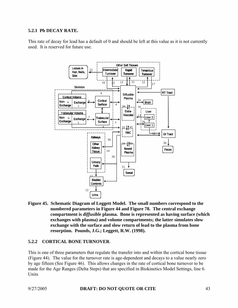
5.2.1 Pb DECAY RATE. This rate of decay for lead has a default of 0 and should be left at this value as it is not currently used. It is reserved for future use. Figure 45. Schematic Diagram of Leggett Model. The small numbers correspond to the
numbered parameters in Figure 44 and Figure 78. The central exchange compartment is diffusible plasma. Bone is represented as having surface (which exchanges with plasma) and volume compartments; the latter simulates slow exchange with the surface and slow return of lead to the plasma from bone resorption. Pounds, J.G.; Leggett, R.W. (1998).
5.2.2 CORTICAL BONE TURNOVER. This is one of three parameters that regulate the transfer into and within the cortical bone tissue (Figure 44). The value for the turnover rate is age-dependent and decays to a value nearly zero by age fifteen (See Figure 46). This allows changes in the rate of cortical bone turnover to be made for the Age Ranges (Delta Steps) that are specified in Biokinetics Model Settings, line 6. Units
40
36
26
13
18
34
14
3
2
39
4135
8
38
20
31 173315 32 16
22
10
21
12
9
9
5
4
8
7
6
30
11
Brain
Liver 2
Liver 1
Liver
Diffusible Plasma
Extra-Vascular
RBC
Tenacious Turnover
Rapid Turnover
Intermediate Turnover
Other Soft Tissues
Cortical Surface
Trabecular Surface
Cortical VolumeNon-Exchange
Exchange
Trabecular VolumeNon-Exchange
Exchange
Skeleton
RT Tract
GI Tract
Other Kidney Tissue
Urinary Path
Kidneys
Bladder Contents
Urine
Feces
Losses in Hair, Nails, Skin
Sweat
Bound Plasma
BrainBrain
Liver 2
Liver 1
Liver
Diffusible Plasma
Extra-Vascular
Extra-Vascular
RBCRBC
Tenacious Turnover
Rapid Turnover
Intermediate Turnover
Other Soft Tissues
Tenacious Turnover
Tenacious Turnover
Rapid Turnover
Rapid Turnover
Intermediate Turnover
Intermediate Turnover
Other Soft Tissues
Cortical SurfaceCortical Surface
Trabecular Surface
Trabecular Surface
Cortical VolumeNon-Exchange
Exchange
Cortical VolumeNon-Exchange
Exchange
Trabecular VolumeNon-Exchange
Exchange
Trabecular VolumeNon-Exchange
Exchange
Skeleton
RT TractRT Tract
GI TractGI Tract
Other Kidney Tissue
Urinary Path
Kidneys
Other Kidney Tissue
Other Kidney Tissue
Urinary Path
Urinary Path
KidneysKidneys
Bladder ContentsBladder
Contents
UrineUrine
FecesFeces
Losses in Hair, Nails, Skin
Losses in Hair, Nails, Skin
SweatSweat
Bound PlasmaBound Plasma

9/27/2005 DRAFT: DO NOT QUOTE OR CITE 44
Figure 46: Values for cortical bone turnover rate which decreases with age. Data are
plotted on Figure 47.
Figure 47: Plot of default values for cortical bone turnover rate by age. This Y-axis scale
appears to show values less than zero, but this is a rounding error. Above the age 25 years, this value is 0.000082
are percent fraction per day. The values decrease exponentially from age 0 to 25 years, from 0.01% at birth to 0.00008% at age 25 and older. Interpolation between age groups may be specified as linear, floor, ceiling, or index. During early development, cortical and trabecular bone turnover are modeled at nearly the same rate; by age 25, cortical turnover is about 17% of trabecular. 5.2.3. TRABECULAR BONE TURNOVER RATE. At one year and younger, the turnover for trabecular bone is modeled at the same rate as cortical (See Figure 48 et seq.). Above one year, the trabecular bone turnover rate decreases slightly less than cortical. Changes to trabecular bone turnover rates can be made for the same Age Ranges or independently of the changes for cortical bone turnover rates.
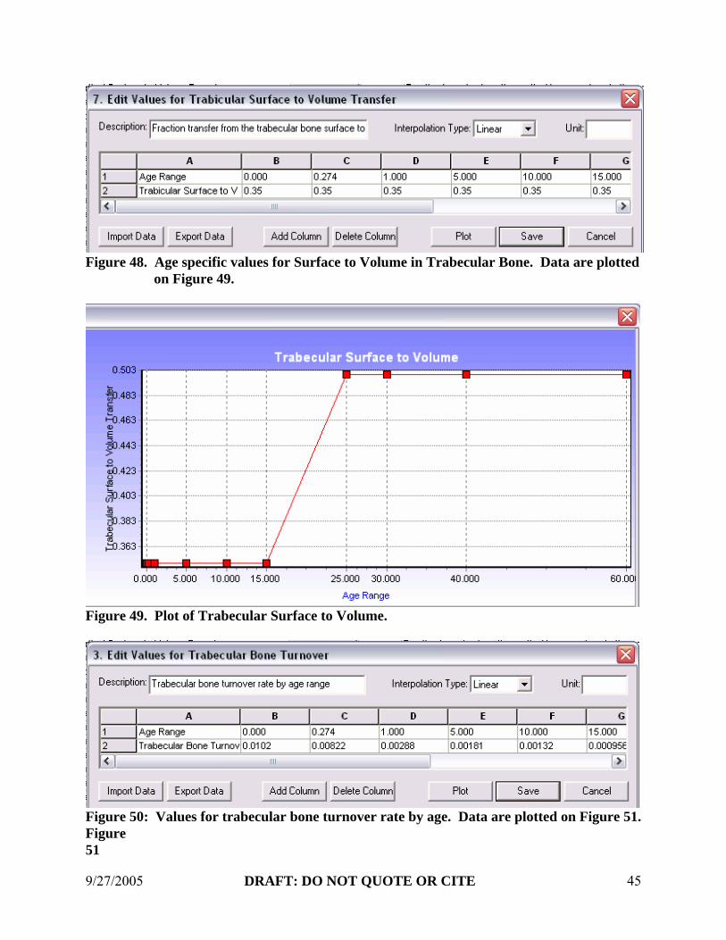
9/27/2005 DRAFT: DO NOT QUOTE OR CITE 45
Figure 48. Age specific values for Surface to Volume in Trabecular Bone. Data are plotted
on Figure 49.
Figure 49. Plot of Trabecular Surface to Volume.
Figure 50: Values for trabecular bone turnover rate by age. Data are plotted on Figure 51. Figure 51

9/27/2005 DRAFT: DO NOT QUOTE OR CITE 46
Figure 51: Plot of default values for trabecular bone turnover rate by age. 5.2.3 TRANSFER FROM CORTICAL SURFACE TO BLOOD PLASMA. The model treats the bone surface as the major route of transfer from cortical bone surface to both blood plasma and bone volume. In the case of adults, the transfer from the cortical bone surface is split evenly between transfer to blood plasma (Figure 52) and bone volume (Figure 56), thus the coefficient for ages over 15 is 0.5/day. For the younger age groups, this distribution differs between the two: 0.65/day to blood plasma and 0.35/day to cortical bone volume.
Figure 52: Dropdown window for editing the parameter for transfer from cortical surface
to blood. Data are plotted on Figure 53.
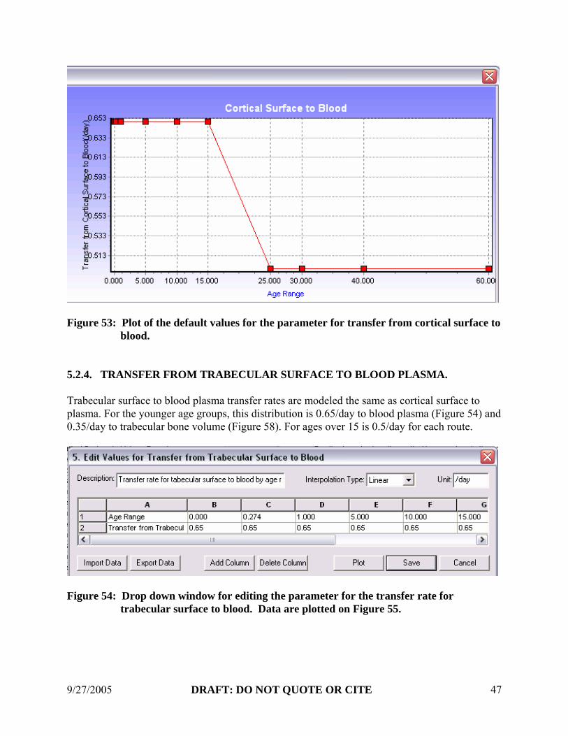
9/27/2005 DRAFT: DO NOT QUOTE OR CITE 47
Figure 53: Plot of the default values for the parameter for transfer from cortical surface to
blood. 5.2.4. TRANSFER FROM TRABECULAR SURFACE TO BLOOD PLASMA. Trabecular surface to blood plasma transfer rates are modeled the same as cortical surface to plasma. For the younger age groups, this distribution is 0.65/day to blood plasma (Figure 54) and 0.35/day to trabecular bone volume (Figure 58). For ages over 15 is 0.5/day for each route.
Figure 54: Drop down window for editing the parameter for the transfer rate for
trabecular surface to blood. Data are plotted on Figure 55.

9/27/2005 DRAFT: DO NOT QUOTE OR CITE 48
Figure 55: Plot of the default values for the transfer rate for trabecular surface to blood. 5.2.6 CORTICAL SURFACE TO VOLUME TRANSFER. This is the fraction per day that is transferred from the cortical bone surface to the volume of the cortical bone and is equal to [1-(transfer to blood)]. The default values are 0.35 for the younger ages (0-15 years), then 0.5 for the older ages.
Figure 56. Window for editing the value for transfer from cortical surface to volume. Data
are plotted on Figure 57.

9/27/2005 DRAFT: DO NOT QUOTE OR CITE 49
Figure 57: Plot of the default values for transfer from cortical surface to volume. 5.2.7 TRABECULAR SURFACE TO TRABECULAR VOLUME TRANSFER. Similar to the cortical surface to volume transfer, this parameter accounts for the fraction of trabecular surface lead that is transferred trabecular volume. The age-dependent default values are the same as the cortical counterpart, 0.35 for children and 0.5 for older children and adults.
Figure 58: Window for editing the values for transfer from trabecular surface to volume.
Data are plotted on Figure 59.

9/27/2005 DRAFT: DO NOT QUOTE OR CITE 50
Figure 59: Plot of the default values for transfer from trabecular surface to volume. 5.2.8 TOTAL TRANSFER FROM EXCHANGE BONE VOLUME. Based on radium data, the removal halftime of lead from the exchangeable bone volume is 30 days, during which time 20% of the lead passes to the non-exchangeable bone tissue and 80% returns to the bone surface, and is the same for cortical and trabecular bone. Although this is an age-dependent variable, the current default value is the same for all age groups (Figure 60).
Figure 60: Window for editing values for total transfer from the exchange bone volume.
The plot feature has been temporarily disabled. 5.2.9. TRANSFER FROM THE EXCHANGE TO THE NON-EXCHANGE VOLUME. This parameter combines the cortical and trabecular bone lead transfer from the exchange volume to the non-exchange volume compartments and has the same default value (0.2) for all age ranges (Figure 61).

9/27/2005 DRAFT: DO NOT QUOTE OR CITE 51
Figure 61: Window for editing values for total transfer from the non-exchange bone
volume. The plot feature has been temporarily disabled. 5.2.10. TRANSFER FROM LIVER1. This is the fraction per day that is transferred from Liver1 to the three compartments: Gastrointestinal tract, Diffusible Plasma and Liver 2. The default value of 0.0693 is constant for all age ranges. The liver and kidney compartments are excretion pathways. The liver may contain 2-3% of the total body burden of lead, and this is treated as residing in two compartments, Liver1 and Liver2. From Liver1, lead may pass to the small intestine, back to the Diffusible Plasma, or to the Liver2 compartment (Figure 45). 5.2.11 TRANSFER FROM KIDNEY1. Transfer from the kidney has two components: Kidney 1 from the kidney back to diffusible plasma and Kidney 2 to Kidney 1 from the bladder. Kidney 2 is discussed in Section 5.2.14. The fraction that is transferred from Kidney 1 has a transfer rate constant (0.139/day) for all ages. 5.2.12 TRANSFER FROM BLADDER TO URINE. Lead that enters the bladder passes from the diffusible plasma to the urinary bladder and from the renal tubules. Estimates of urinary excretion removal halftime in humans in vivo are about 0.1 day (Leggett, 1993). The model includes two routes: Diffusible Plasma to the Urinary Path and Diffusible Plasma to Other Kidney Tissue. From the Bladder to Urine is, for all practical purposes, instantaneous.
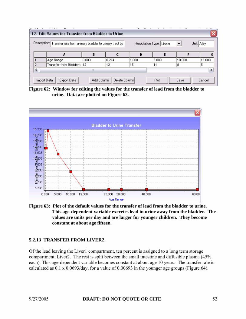
9/27/2005 DRAFT: DO NOT QUOTE OR CITE 52
Figure 62: Window for editing the values for the transfer of lead from the bladder to
urine. Data are plotted on Figure 63.
Figure 63: Plot of the default values for the transfer of lead from the bladder to urine.
This age-dependent variable excretes lead in urine away from the bladder. The values are units per day and are larger for younger children. They become constant at about age fifteen.
5.2.13 TRANSFER FROM LIVER2. Of the lead leaving the Liver1 compartment, ten percent is assigned to a long term storage compartment, Liver2. The rest is split between the small intestine and diffusible plasma (45% each). This age-dependent variable becomes constant at about age 10 years. The transfer rate is calculated as 0.1 x 0.0693/day, for a value of 0.00693 in the younger age groups (Figure 64).

9/27/2005 DRAFT: DO NOT QUOTE OR CITE 53
Figure 64. Age-related coefficients for transfer of lead from Liver2. Data are plotted on
Figure 65.
Figure 65. Plot of the transfer of lead from the liver 2 compartment. 5.2.14 TRANSFER FROM KIDNEY2. This transfer for Kidney 2 represents the amount of lead that passes to the Bladder from the kidney. The numeric values are the same as for Liver 2, and they are age specific (Figure 66).

9/27/2005 DRAFT: DO NOT QUOTE OR CITE 54
Figure 66: Drop down window for editing the default values for the transfer of lead from
the kidney. Data are plotted on Figure 67.
Figure 67: Plot of the default values for the transfer of lead from Kidney 2 (From Kidney
to Bladder). 5.2.15 TRANSFER FROM FAST SOFT TISSUE. Soft tissue consists of muscle, fat, and skin. Although this compartment represents a large fraction of the total body mass, the concentration of lead is low. This parameter is substantially larger than other values and is age-related (Figure 68). All of the soft tissue is in one compartment, but the binding capacity within that compartment is not uniform throughout. The model treats the binding capacity as three strengths, although in reality there may be a continuum from low to high. The three strengths are Tenacious Turnover, Intermediate Turnover, and Rapid Turnover. These three turnover rates, with one exception, return the lead to the Diffusible Plasma. The exception is hair, nails and skin, which are described below.

9/27/2005 DRAFT: DO NOT QUOTE OR CITE 55
Figure 68: Drop down window for editing the default values for the deposition fraction of
lead in fast soft tissue. Data are plotted on Figure 69.
Figure 69: Plot of the default values for the deposition fraction of lead in fast soft tissue. 5.2.16 TRANSFER FROM INTERMEDIATE SOFT TISSUE. This parameter is not age-related and is nearly three orders of magnitude lower than Fast Soft Tissue. Some of this lead is “excreted” in the form of hair, nails, and skin. Note the relative significance of the pathways for the deposition fraction of lead from the body: feces (0.006) urine (0.015, hair/skin/nails (0.4) and sweat (0.0035). The Intermediate Soft tissue excretion fraction (0.4) represents a major excretion route (Hair, Nails, and Skin), two orders of magnitude larger than sweat. This parameter is also not age-dependent.

9/27/2005 DRAFT: DO NOT QUOTE OR CITE 56
Figure 70: Drop down window for editing the default values for the deposition fraction of
lead in intermediate soft tissue. Data are plotted on Figure 71.
Figure 71: Plot of the default values for the deposition fraction of lead in fast soft tissue. 5.2.17 TRANSFER FROM SLOW SOFT TISSUE. This parameter is not age-related and is among the slowest, being more than an order of magnitude slower than Intermediate Soft Tissue.

9/27/2005 DRAFT: DO NOT QUOTE OR CITE 57
Figure 72: Drop down window for editing the default values for the deposition fraction of
lead in slow soft tissue. Data are plotted on Figure 73.
Figure 73: Plot of the default values for the deposition fraction of lead in slow soft tissue. 5.2.18 TRANSFER RATES FROM BRAIN. The default value for this age-dependent parameter is very small (0.00095/day) and is modeled the same for all age categories. The brain is especially vulnerable to lead, possible due to the role calcium plays in nerve conduction velocity. Although it contains very little lead, brain tissue is an important component of this biokinetic model. The small amount of lead taken up by the brain is strongly retained. The assumed deposition fraction for infants (0.00045) is arbitrarily three times higher than for older children and adults (0.00015), which is based on a removal half-time of two years (Figure 74) (Leggett, 1993).
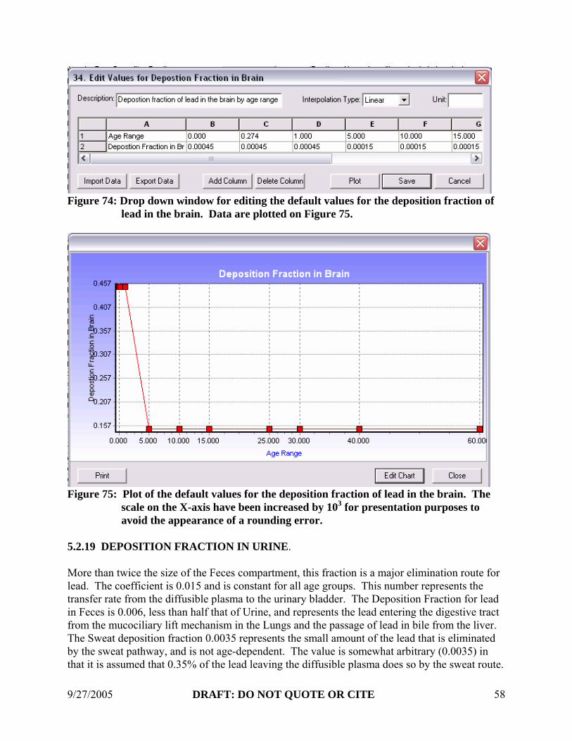
9/27/2005 DRAFT: DO NOT QUOTE OR CITE 58
Figure 74: Drop down window for editing the default values for the deposition fraction of
lead in the brain. Data are plotted on Figure 75.
Figure 75: Plot of the default values for the deposition fraction of lead in the brain. The
scale on the X-axis have been increased by 103 for presentation purposes to avoid the appearance of a rounding error.
5.2.19 DEPOSITION FRACTION IN URINE. More than twice the size of the Feces compartment, this fraction is a major elimination route for lead. The coefficient is 0.015 and is constant for all age groups. This number represents the transfer rate from the diffusible plasma to the urinary bladder. The Deposition Fraction for lead in Feces is 0.006, less than half that of Urine, and represents the lead entering the digestive tract from the mucociliary lift mechanism in the Lungs and the passage of lead in bile from the liver. The Sweat deposition fraction 0.0035 represents the small amount of the lead that is eliminated by the sweat pathway, and is not age-dependent. The value is somewhat arbitrary (0.0035) in that it is assumed that 0.35% of the lead leaving the diffusible plasma does so by the sweat route.

9/27/2005 DRAFT: DO NOT QUOTE OR CITE 59
5.2.20 DEPOSITION FRACTION IN BONE. This age-dependent variable represents deposition to bone surfaces and varies widely in children and young adults, up to age 25, after which it reaches a low, constant value of 0.08 (unitless), about one third that of a newborn child (Figure 76). This means that, for children under 20, the history of lead exposure, as released from their bone tissue, can be as important a contributor to blood lead as their current exposure.
Figure 76. Deposition fraction in Bone. Data are plotted on Figure 77.
Figure 77. Plot of Deposition Fraction in Bone. Given that the deposition of lead appears
to be similar to the deposition of alkaline earth elements calcium, strontium, and barium (Leggett, 1993), it follows that the spike at age 15, which probably represents a spurt in bone growth, would occur also for lead.

9/27/2005 DRAFT: DO NOT QUOTE OR CITE 60
Figure 78. Bottom of biokinetic Parameters Window. Parameter 47 is Chelation Factor 3
and has a value of 1250. 5.2.21 TRABECULAR BONE DEPOSITION FRACTION. The fraction of deposition going to trabecular bone ranges from 0.20 to 0.56 (Figure 79), increasing with age. As the bone grows, lead is incorporated into the crystalline structure of the bone tissue and replaces calcium. Later, as new bone tissue replaces old, the lead is released from the nonexchangeable trabecular volume and passes back to the Diffusible Plasma.
Figure 79. Age-dependent variable for Trabecular Bone Deposition Fraction. Data are
plotted on Figure 80.

9/27/2005 DRAFT: DO NOT QUOTE OR CITE 61
Figure 80. Trabecular bone deposition fraction.
Figure 81: Plot of the default values for the transfer of lead from the liver. 5.2.22 DEPOSITION FRACTION IN COMPARTMENTS WITHOUT AGE
VARIABILITY. This is the fraction of lead (0.04) deposited in Liver1 from Diffusible Plasma, and does not vary with age. This Liver 1 Fraction receives 4% of the lead released by Diffusible Plasma, giving a transfer rate of 80/day and a removal halftime of ten days. Ten percent (0.1) of the Liver 1

9/27/2005 DRAFT: DO NOT QUOTE OR CITE 62
fraction moves to the second liver component, Liver 2. Forty-five percent (0.45) of the Liver 1 fraction is deposited in the Small Intestine through the bile duct. Most of this is eliminated with feces; a small amount may be reabsorbed into the Diffusible Plasma. All of the lead from Liver 2 is passed back to the Diffusible Plasma compartment. Most of the lead in Liver1 passes into the bile duct and then to the small intestine. The rest (0.45) passes back to the Diffusible Plasma. The fraction deposited in Kidney 1 from Diffusible Plasma (0.02) is also called the Urinary Path (UP). It has a high deposition but a shorter retention than Kidney 2. The fraction deposited in Kidney 2 from Diffusible Plasma (0.0002) is also called “Other Kidney Tissue (OKT). Although it has a lower uptake than Kidney 1, Kidney 2 has a much larger retention time. Lead passes out to the Diffusible Plasma compartment from the OKT. 5.2.23 DEPOSITION FRACTION FROM DIFFUSIBLE PLASMA TO FAST
SOFT TISSUE. This fraction deposited in Fast Soft Tissue from Diffusible Plasma varies slightly with age and has a value from 0.08345 to 0.08875 for a transfer rate of 167-177/day. (Transfer Rate = Deposition Fraction x 2000/day) (Figure 82).
Figure 82. Age-dependent variable for Diffusible Plasma to Fast Soft Tissue. Data are
plotted on Figure 83.

9/27/2005 DRAFT: DO NOT QUOTE OR CITE 63
Figure 83. Plot of the default values for the Diffusible Plasma to Fast Soft Tissue
parameter. 5.2.24 DEPOSITION FRACTION FROM DIFFUSIBLE PLASMA TO INTERMEDIATE
SOFT TISSUE. This is the fraction deposited in Intermediate Soft Tissue from Diffusible Plasma with a turnover rate of 25 to 300 days and includes a component of permanent elimination (Hair, Nails, and Skin). This compartment has a Deposition Fraction from 0.005, giving a transfer rate of 0.00277/day to HNS and 0.00416 to Diffusible Plasma (Figure 84).
Figure 84. Age-dependent variable for Diffusible Plasma to Intermediate Soft Tissue.
Data are plotted on Figure 85.
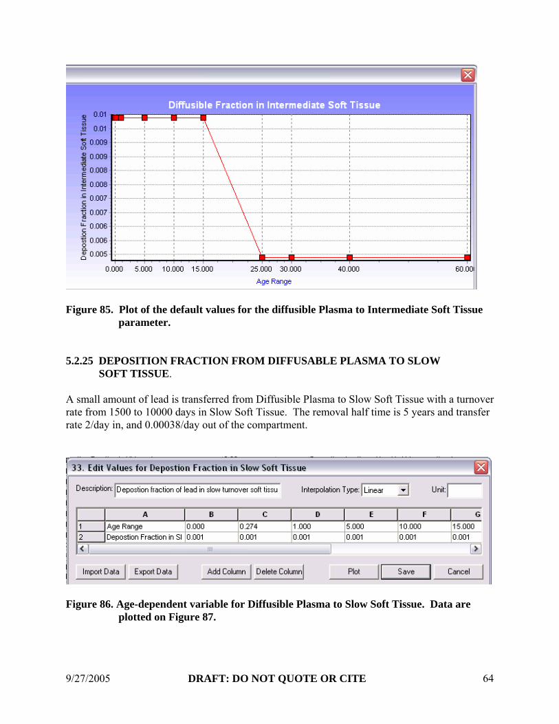
9/27/2005 DRAFT: DO NOT QUOTE OR CITE 64
Figure 85. Plot of the default values for the diffusible Plasma to Intermediate Soft Tissue
parameter. 5.2.25 DEPOSITION FRACTION FROM DIFFUSABLE PLASMA TO SLOW
SOFT TISSUE. A small amount of lead is transferred from Diffusible Plasma to Slow Soft Tissue with a turnover rate from 1500 to 10000 days in Slow Soft Tissue. The removal half time is 5 years and transfer rate 2/day in, and 0.00038/day out of the compartment.
Figure 86. Age-dependent variable for Diffusible Plasma to Slow Soft Tissue. Data are
plotted on Figure 87.

9/27/2005 DRAFT: DO NOT QUOTE OR CITE 65
Figure 87. Plot of the default values for the Slow Soft Tissue Parameter. 5.2.26 DEPOSITION FRACTION FROM DIFFUSIBLE PLASMA TO BRAIN. This is the fraction deposited in Brain from Diffusible Plasma, and is age-dependent.
Figure 88. Age-dependent variable for the Deposition Fraction from Diffusible Plasma to
Brain. Data are plotted on Figure 89.
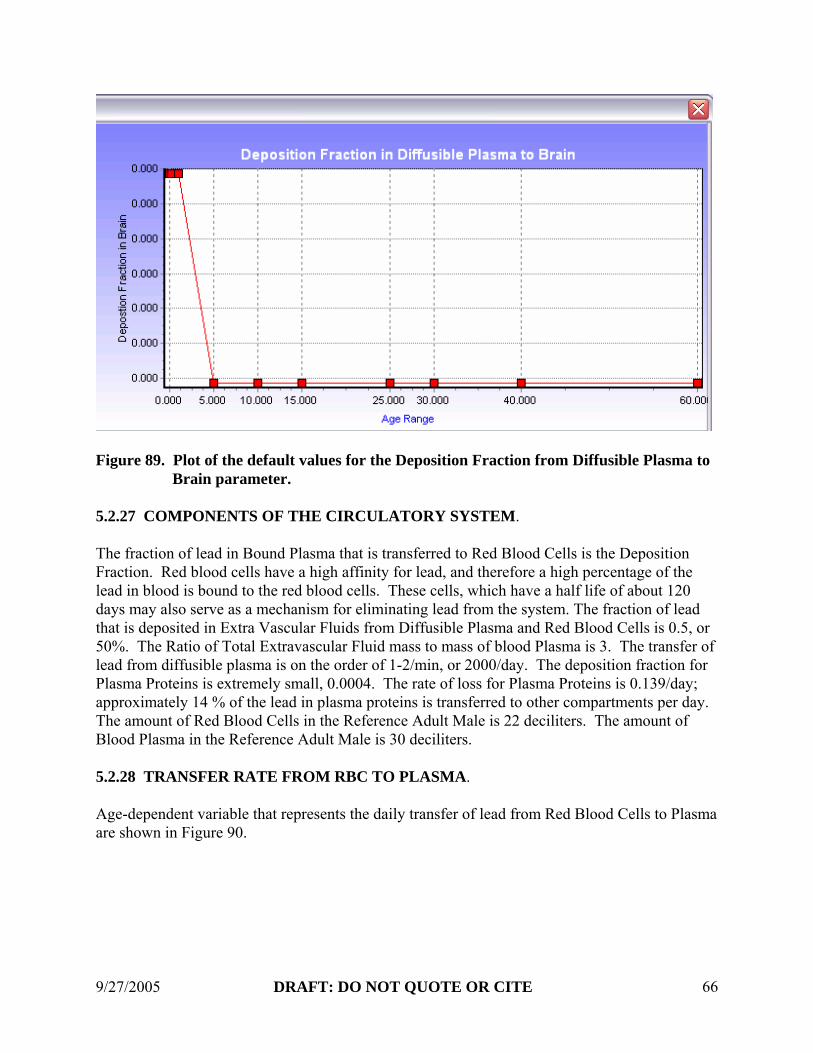
9/27/2005 DRAFT: DO NOT QUOTE OR CITE 66
Figure 89. Plot of the default values for the Deposition Fraction from Diffusible Plasma to
Brain parameter. 5.2.27 COMPONENTS OF THE CIRCULATORY SYSTEM. The fraction of lead in Bound Plasma that is transferred to Red Blood Cells is the Deposition Fraction. Red blood cells have a high affinity for lead, and therefore a high percentage of the lead in blood is bound to the red blood cells. These cells, which have a half life of about 120 days may also serve as a mechanism for eliminating lead from the system. The fraction of lead that is deposited in Extra Vascular Fluids from Diffusible Plasma and Red Blood Cells is 0.5, or 50%. The Ratio of Total Extravascular Fluid mass to mass of blood Plasma is 3. The transfer of lead from diffusible plasma is on the order of 1-2/min, or 2000/day. The deposition fraction for Plasma Proteins is extremely small, 0.0004. The rate of loss for Plasma Proteins is 0.139/day; approximately 14 % of the lead in plasma proteins is transferred to other compartments per day. The amount of Red Blood Cells in the Reference Adult Male is 22 deciliters. The amount of Blood Plasma in the Reference Adult Male is 30 deciliters. 5.2.28 TRANSFER RATE FROM RBC TO PLASMA. Age-dependent variable that represents the daily transfer of lead from Red Blood Cells to Plasma are shown in Figure 90.

9/27/2005 DRAFT: DO NOT QUOTE OR CITE 67
Figure 90. Age-dependent variable for the Transfer Rate from RBC. Data are plotted on
Figure 91.
Figure 91. Plot of the default values for the Transfer Rate for RBC parameter. 5.4.29 AMOUNT OF BLOOD. Total volume, in deciliters, of blood, which is age-dependent, is shown in Figure 92.

9/27/2005 DRAFT: DO NOT QUOTE OR CITE 68
Figure 92. Age-dependent variable for total volume of blood (deciliters) Data are plotted
on Figure 93.
Figure 93. Plot of the default values for the Amount of Blood parameter. 5.2.30 CHELATION FACTORS 1, 2, and 3. These chelation factors are not currently used. They were a part of the original Leggett model because chelation data were used at that time. The options are included against the possibility they might have some future use.

9/27/2005 DRAFT: DO NOT QUOTE OR CITE 69
SECTION 6. CONTROLLING THE MODEL OUTPUT 6.1. A SIMPLE CONFIDENCE TEST At this point, it is helpful to begin developing your familiarity with the model. First, observe the model output in the case where no changes have been made to the model defaults. Restart the model and select the option to “Create and new study.” Click on “Youth” to populate the age ranges through 13 years of age. Click Run, then OK to save the file; specify a new file named First Flight, and save this file; click “Exposure” and “Absorption,” then “Continue” “Start” and “Continue” to run the model with all default settings. Select “Plot” to produce the graph shown in Figure 94. This is a plot of the predicted blood lead concentration trough 4700 days, or thirteen years. Note that when only one parameter (Blood Pb) is plotted, the X and Y values are given as well.
Figure 94. Output with all default settings Now return to the opening window by closing out two windows in succession, and change the exposure by selecting Media Exposure and clicking Edit. Click edit again to get to the parameter array for Air. Click the Dust tab and change the lead concentration of dust ingested by a toddler, preschooler and youth from the default 200 µg Pb/g to 2000 µg Pb/g. Click OK and run the model as before. You should get:

9/27/2005 DRAFT: DO NOT QUOTE OR CITE 70
Figure 95. Total Blood lead with elevated dust lead exposure. Note that the Y-axis scale has changed to accommodate the range of values. While it appears that the effect of the increased exposure lasts only through 1900 days, the upper bound for the youth age range, a closer look will show that the blood lead concentrations will remain elevated throughout the next age range, adolescent, as the lead is recycled through other body tissues, including bone tissue, returning sometime later to the blood. Indeed, even at age nineteen, six years after the secession of the elevated lead exposure, the blood lead for the elevated exposure child is still about 15% higher than the child with the lower exposure. Take a moment to look at other body tissues to become familiar with the way the model distributes the lead over the various compartments throughout the lifetime of the individual. Remember that, as an experienced modeler, you will become adept at tweaking the biokinetic parameters according to information that you may have from your own studies, or to test the reality of data published by others. After editing the biokinetic parameters, close this option [X] and click RUN from the Primary window. The Model Run window appears next and offers you a choice of Exposure, Absorption, and Biokinetics. Click on any of these for which you want to see the output. Clicking on Absorption automatically triggers Biokinetics. Click CONTINUE and the Exposure Model Processing window appears. Click START. The processing time depends on the complexity of your inputs. The three options for historical diet, air and dust lead concentrations are under development and are not functional at this time.

9/27/2005 DRAFT: DO NOT QUOTE OR CITE 71
There is an option on the Exposure Model Processing window to select the exposure model output file to view or bypass this step. This is fully optional and is if value if you are troubleshooting the model. The *.mod file gives you a view of the stepwise values you have selected. This file can contain over 32,000 lines and may take a few moments to generate. The *.mpa file gives you the total exposure µPb for each age range. Both of these files may be exported to a spreadsheet. The next window allows you to view the Exposure model output files using different extensions for the same file name that you have designated. Filename.mpa (Exposure Model Output by Age) gives the total amount of lead to which the modeled person was exposed by the six different routes. All of these should be listed by the age category. 6.2. BIOKINETIC OUTPUTS 6.2.1 TABLES CLOSE on the Select window runs the model. The outputs are saved to the same location as that for the input files. In the example below, the output is for 100 day intervals as stipulated in the Primary window, Simulation time step 100 day(s). An explanation of the various outputs and units are given in Table 2. 6.1.2 PLOTTING Click PLOT on the window generates a default color plot of several parameters versus days. PRINT provides a copy of the chart.

9/27/2005 DRAFT: DO NOT QUOTE OR CITE 72
Figure 96. Using the Built in Graphic Feature. 6.1.3 EDITING THE CHART Click EDIT allows for several options. In the Editing Window, SERIES, ticking (or unticking) a box will automatically adjust the chart. a. Axis: (i) Unticking Automatic allows changes to the scales. For example, the Maximum and
Minimum ranges can be changed for the Y-(Left) axis and the number of decimal places. (ii) NOTE: The number of decimal places cannot be changed on the X- (Bottom) axis. (iii) Titles can be added to the Y-axis and also the X-axis. However, the default title for X-axis (‘Days’ in blue color) remains. This can be removed by going into Editing Titles, scrolling down from TITLES to FOOT and deleting ‘Days’( Fig. 39). (iv) The frequency of Ticks can be changed. (v) The main title can be edited in TITLES. For example, change Font size and Back Color. However, even though the title states it is black, the Black color needs to be clicked to achieve this (otherwise it stays yellow). (v) The background blue can be changed to white in PANEL by making START and END colors white.

9/27/2005 DRAFT: DO NOT QUOTE OR CITE 73
(vii) To change output style for each parameter, for example, YCORT, go to EDITING, CHART, SERIES, click on the color square, in Color Window change to desired color, click OK, click on BORDER, in the window Border Color Editor, change Style, Click OK. Change other parameters in the same way. PRINT chart.

9/27/2005 DRAFT: DO NOT QUOTE OR CITE 74
7.0 REFERENCES
Leggett, R.W. (1992b) A generic age-specific biokinetic model for calcium-like elements Radiat. Prot. Dosim. 41: 183-198.
Leggett, R.W. (1993a) An age-specific kinetic model of lead metabolism in humans. Environ. Health Perspect. 101: 598-615.
Mickle, M.H. (1998) Structure, use, and validation of the IEUBK model. Environ. Health Perspect. Suppl. 106: 1531-1534.
Mushak, P. (1991) Gastro-intestinal absorption of lead in children and adults: overview of biological and biophysico-chemical aspects. Chem. Speciat. Bioavail. 3: 87-104.
O'Flaherty, E.J. (1998) Physiologically based kinetic model for lead in children and adults. Environ. Health Perspect. Suppl. 106: 1495-1503.
O'Flaherty, E.J.; Inskip, M.J.; Franklin, C.A.; Durbin, P.W.; Manton, W.I.; Baccanale, C.L. (1998) Evaluation and modification of a physiologically based model of lead kinetics using data from a sequential isotope study in Cynomolgus monkeys. Toxicol. Appl. Pharmacol. 149: 1-16.
Oreskes, N. (1998) Evaluation (Not Validation) of Quantitative Models. Environ. Health Perspect. 106(Suppl 6): 1453-1460.
Pounds, J.G.; Leggett, R.W. (1998) The ICRP age-specific biokinetic model for lead: validations, empirical comparisons, and explorations. Environ. Health Perspect. Suppl. 106: 1505-1511.
U.S. EPA (1994a) Guidance Manual for the Integrated Exposure Uptake Biokinetic Model for Lead in Children. U.S. Environmental Protection Agency. EPA/540/R-93/081, PB93-963510.
U.S. EPA (1994b) Technical Support Document: Parameters and Equations Used in Integrated Exposure Uptake Biokinetic Model for Lead in Children (v0.99d). U.S. Environmental Protection Agency EPA/540/R-94/040, PB94-963505.
White, P.D.; Van Leeuwen, P.; Davis, B.D.; Maddaloni, M.; Hogan, K.A.; Marcus, A.H.; Elias, R.W. (1998) The conceptual structure of the integrated exposure uptake biokinetic model for lead in children. Environ. Health Perspect. 106(Suppl 6): 1513-1530.