alicefialowski - eötvös loránd universityweb.cs.elte.hu/~fialowsk/pubs-af/thesis.pdf · an...
TRANSCRIPT

Algebraic Deformation Theory
(Dissertation for the D.Sc. degree of the Hungarian Academy of Sciences)
Alice Fialowski
Eotvos Lorand UniversityInstitute of Mathematics
andAlfred Renyi Institute of Mathematics
email: [email protected]://www.cs.elte.hu/∼fialowsk/
Budapest
2008

To my family


v
Contents
Introduction 1
I. Versal Formal Deformations 18
1. Deformations of Lie Algebras 20Alice FialowskiMath. USSR Sbornik, 55 (1986), pp. 467–473
2. An Example of Formal Deformations of Lie Algebras 27Alice FialowskiDeformation Theory of Algebras and Structures and Applica-tions, Kluwer Acad. Publishers 1988, pp. 375–401
3. Construction of Miniversal Deformations of Lie Algebras 37Alice Fialowski and Dmitry FuchsJournal of Functional Analysis, 161 (1999), pp. 76–110
II. Nilpotent Lie Algebras and Cohomology 60
1. Classification of Graded Lie Algebras with Two Generators 62Alice FialowskiVestnik Moskovskogo Universiteta Matematika, 38 (1983),pp. 62–64English translation:Moscow University Mathematics Bulletin,38 (1983), 76-79
2. Deformations of Nilpotent Kac–Moody Algebras 66Alice FialowskiStudia Sci. Math. Hungar. 19 (1984), pp. 465–483
3. Cohomology in Infinite Dimensions 81Alice FialowskiAdvances in Math., 97 (1993), pp. 267–277
4. Deformations of the Lie Algebra m0 88Alice Fialowski and Friedrich WagemannJournal of Algebra, 318 (2007), pp. 1002–1026
III. Generalizations and Applications 108
1. Krichever-Novikov Witt Algebras 110Alice Fialowski and Martin SchlichenmaierCommun. in Contemporary Math., 5 (2003), pp. 921–945
2. Deformations of Four Dimensional Lie Algebras 129Alice Fialowski and Michael PenkavaCommun. in Contemporary Math., 9 (2007), pp. 41–79


Introduction
Part I: Versal Formal Deformations
Deforming a given mathematical structure is a tool of fundamental importancein most parts of mathematics, mathematical physics and physics. The theoryof deformations originated with the problem of classifying all possible pairwisenon-isomorphic complex structures on a given differentiable real manifold.The fundamental idea, which should be credited to Riemann, was to introducean analytic structure therein.The notion of local and infinitesimal deformations of a complex analytic man-ifold first appeared in the work of Kodaira and Spencer (1958). In particular,they proved that infinitesimal deformations can be parametrized by the cor-responding cohomology group. The deformation theory of compact complexmanifolds was devised by Kuranishi (1965) and Palamodov (1976). Shortlyafter the work of Kodaira and Spencer, algebro-geometric foundations weresystematically developed by Artin (1960) and Schlessinger (1968). Formaldeformations of arbitrary rings and associative algebras, and the related co-homology questions, were first investigated by Gerstenhaber (1964-1968). Thenotion of deformation was applied to Lie algebras by Nijenhuis and Richardson(1966-68).In this thesis I consider deformations of Lie algebras, although my generaltheory can be applied (and has already been applied) to other categories aswell.Deformation is one of the tools used to study a specific object, by deformingit into some families of “similar” structure objects. This way we get a richerpicture about the original object itself. But there is also another questionapproached via deformation. Roughly speaking, it is the question, can weequip the set of mathematical structures under consideration (may be up tocertain equivalence) with the structure of a topological or geometric space. Inother words, does there exist a moduli space for these structures. If so, thenfor a fixed object, deformations of this object should reflect the local structureof the moduli space at the point corresponding to this object.
Let L be a Lie algebra with Lie bracket µ0 over a field K.
a) Intuitive definition. A deformation of L is a one-parameter family Lt ofLie algebras with the bracket (possibly infinite series)
µt = µ0 + tϕ1 + t2ϕ2 + . . .
where ϕi are L-valued 2-cochains, i.e. elements of HomK(Λ2L,L) = C2(L;L),
and Lt is a Lie algebra for each t ∈ K. Two deformations, Lt and L′t are
equivalent if there exists a linear automorphism ψt = id + ψ1t+ ψ2t2 + . . . of
L where ψi are linear maps over K, i.e. elements of C1(L;L) such that
µ′t(x, y) = ψ−1t
(µt(ψt(x), ψt(y)
))for x, y ∈ L.
The Jacobi identity for the algebras Lt implies that the 2-cochain ϕ1 is indeeda cocycle, i.e. d2ϕ1 = 0. (Here di is the differential in the cochain complex.)If ϕ1 vanishes identically, the first non-vanishing ϕi will be a cocycle. If µ′t isan equivalent deformation with cochains ϕ′
i, then
ϕ′1 − ϕ1 = d1ψ1,
1
2 Introduction
hence every equivalence class of deformations defines uniquely an element ofH2(L;L). This definition was introduced by Nijenhuis and Richardson. Wecall a Lie algebra rigid, if it has no nontrivial deformations.
The classical one-parameter deformation theory is not satisfactory for study-ing the versal property of deformations.
For a more general deformation theory of Lie algebras I introduced the notionof a deformation with base and defined a versal formal deformation of a Liealgebra in [I.1] ∗.
b) General definition. Consider a deformation Lt not as a family of Lie alge-bras, but as a Lie algebra over the algebra K[[t]]. The natural generalization isto allow more parameters, or to take in general a commutative algebra over Kwith identity as base of a deformation. Let us fix an augmentation ε : A→ K,ε(1) = 1, and set Ker ε = m, which is a maximal ideal.Definition A deformation λ of L with base (A,m) is a Lie A-algebra structureon the tensor product A⊗K L with bracket [ , ]λ such that
ε⊗ id : A⊗ L → K⊗ L = Lis a Lie algebra homomorphism.Two deformations of a Lie algebra L with the same base A are called equivalent(or isomorphic) if there exists a Lie algebra isomorphism between the twocopies of A⊗ L with the two Lie algebra structures, compatible with ε⊗ id.A deformation with base A is called local if the algebra A is local, and it iscalled infinitesimal if, in addition to this, m2 = 0. For general commutativealgebra base, we call the deformation global.
c) Formal deformations. Let A be a complete local algebra (completeness
means that A =←−−limn→∞
(A/mn), where m is the maximal ideal in A). A formal
deformation of L with base A is a Lie A-algebra structure on the completed
tensor product A⊗L =←−−limn→∞
((A/mn)⊗ L
)s.t.
ε⊗id : A⊗L → K⊗ L = Lis a Lie algebra homomorphism.The previous notion of equivalence can be extended to formal deformationsin an obvious way.
d) Versal formal deformations. It is known that in the category of algebraicvarieties the quotient by a group action does not always exist (Hartshorne).Specifically, there is no universal deformation in general of a Lie algebra Lwith a commutative algebra base B with the property that for any otherdeformation of L with base A there exists a unique homomorphism f : B → Athat induces an equivalent deformation. If such a homomorphism exists (butnot unique), we call the deformation of L with base B versal.
Definition A formal deformation η of a Lie algebra L with a complete localalgebra base B is called miniversal, ifi) for any formal deformation λ of L with any complete local base A thereexists a homomorphism f : B → A s.t. the deformation λ is equivalent to thepush-out of η by f ;ii) if A satisfies m2 = 0, then f is unique.
∗This notation is for paper 1 in Part I of this Thesis.
Introduction 3
Using Schlessinger’s general set-up (1968), I was able to prove, that for com-plete local algebra base deformations, under some minor restriction, thereexists a miniversal deformation:
Theorem 1. [I.2] Let L be a Lie algebra. Assume that the space H2(L;L) isfinite-dimensional. Then there exists a versal formal deformation of L, andthe base of this versal deformation is formally embedded into H2(L;L), i.e. itcan be described in H2(L;L) by a finite system of formal equations.
Another question is how to construct such a deformation. I underlined aconstruction for the versal deformation in [I.1], using Harrison cohomology ofcommutative algebras. The construction is parallel to the general construc-tions in deformation theory, like Palamodov, Illusie, Laudal, Goldman-Milson,Kontsevich. The procedure needs a proper theory of Massey operations in thecohomology, and an algorithm for computing all the possible ways for a giveninfinitesimal deformation to extend to a formal deformation.
There is a confusion in the literature when one tries to describe all nonequiva-lent deformations of a given Lie algebra. There were several attempts to workout an appropriate theory for solving this basic problem in deformation the-ory, but none of them were completely adequate. In particular, the followingquestions remained open:
1) How many non-equivalent deformations have the same infinitesimal part?2) Are there any singular nontrivial deformations, i.e. deformations with zeroinfinitesimal part?
Let W pol =W1 be the Lie algebra of vector fields on the line with polynomialcoefficients f(x) d
dx . This Lie algebra has an additive algebraic basis
ei = xi+1 d
dx, i ≥ −1.
In this basis the bracket operation is
[ei, ej ] = (j − i)ei+j .
Let us introduce the subalgebra Li, i ≥ 0 of W1 which is generated by thebasis elements ei, ei+1, . . . . In [I.2] I investigated the subalgebra Lpol = L1.
It is naturally graded, the weight of ei equals i. With this grading Lpol1 is a
graded Lie algebra: Lpol1 =
∞⊕m=1
L(m)1 .
Using Feigin-Fuchs spectral sequence and some results of Feigin and Fuchs oncohomology with coefficients in tensor field modules, I was able to computethe 1- and 2-dimensional cohomology space of L1:
Theorem 2. [I.2] For q > 0, Hq(m)(L1;L1) ∼= Hq−1
(m) (L2;C). The cohomology
space Hq(L1;L1) has dimension 2q− 1 and is generated by elements of weight
−3q2−q2 +i, where i = 1, 2, . . . , 2q−1. In particular, H1(L1;L1) is of dimension
1 and has weight 0; the space H2(L1;L1) is three-dimensional with generatorsα, β, γ of weight −2,−3 and −4, while dimH3(L1;L1) = 5 with generators ofweight −7,−8,−9,−10 and −11.
Identifying explicit cocycles, I studied the Massey products of those. Theyare responsible for extending a deformation to higher order. The result is thefollowing:
4 Introduction
Theorem 3. [I.2] In the case of L1 the Massey products 〈α,α, . . . , α〉︸ ︷︷ ︸i
are zero
for all i, the brackets [β, β], [α, β] and [α, γ] are trivial, while [γ, γ] and [β, γ]are not. The only nontrivial 3-products are 〈β, β, β〉 and 〈α, β, β〉. The higheroperations are either not defined or they are trivial.
The proof of this Theorem follows from computing all the defined Masseybrackets and showing that some of them are nontrivial, while others are not.The nontrivial Massey brackets give the equations for the parameter space ofthe versal deformation.I was able to give the complete description of all nonequivalent formal defor-mations for the Lie algebra L1.Let us define three real deformations of the Lie algebra L1 with the brackets
[ei, ej ]1t = (j − i)(ei+j + tei+j−1);
[ei, ej ]2t =
(j − i)ei+j if i, j > 1,
(j − i)ei+j + tjej , if i = 1;
[ei, ej ]3t =
(j − i)ei+j if i, j 6= 2
(j − i)ei+j + tjej , if i = 2.
Denote the three Lie algebra families by L(1)1 , L
(2)1 and L
(3)1 .
Theorem 4. [I.2] The Lie algebra families L(1)1 , L
(2)1 and L
(3)1 are nontrivial
and pairwise non-isomorphic.
Based on my construction [I.1], Fuchs and I worked out a detailed straight-forward recursive form of my previous construction for a versal deformation,convenient for explicit computations in [I.3]. The starting point in the con-struction is to explicitly give the universal infinitesimal deformation, whichwe then extend step by step, with the help of Massey operations. In theone-dimensional base extensions we use Harrison cohomology of commuta-tive algebras. In [I.3] we also provide a scheme for computing the base of aminiversal deformation of a Lie algebra, convenient for practical use.
Part II: Nilpotent Lie Algebras and Cohomology
In the past decades, much attention has been payed to infinite dimensionalLie algebras, mainly because of their applications in mathematical physics.There are basically two kinds of infinite dimensional objects which are inten-sively studied: Lie algebras of geometric origin, like vector fields on a smoothmanifold, and the so called Kac-Moody algebras, the theory of which is closelyrelated to the theory of finite dimensional semisimple Lie algebras. Among theinfinite dimensional Lie algebras - as in finite dimension - the hardest to dealwith are the nilpotent ones. Any classification, cohomology or deformationresult for those is really valuable.
Let me recall an old question of Kac: Which are all the graded Lie algebrasg = ⊕∞
i=1gi over a field K of characteristic 0, for which dim gi = 1, withminimum possible number of generators. Obviously this number is 2.
There are three well-known Lie algebras of the above type: the Lie algebraL1 and the algebras n1 and n2 which are the maximal nilpotent subalgebras
in Kac-Moody algebras A(1)1 and A
(2)2 , respectively.
Introduction 5
In the algebra g = ⊕∞i=1gi we choose a basis of homogeneous elements ei ∈ gi.
The generators of g are e1 and e2. Note that [e1, e2] 6= 0 and [e1, [e1, e2]] 6= 0.
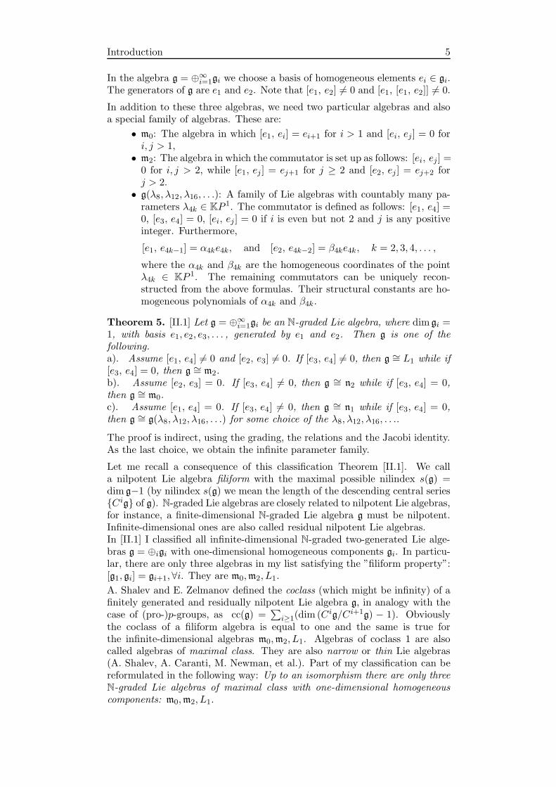
In addition to these three algebras, we need two particular algebras and alsoa special family of algebras. These are:
• m0: The algebra in which [e1, ei] = ei+1 for i > 1 and [ei, ej ] = 0 fori, j > 1,• m2: The algebra in which the commutator is set up as follows: [ei, ej ] =0 for i, j > 2, while [e1, ej ] = ej+1 for j ≥ 2 and [e2, ej ] = ej+2 forj > 2.• g(λ8, λ12, λ16, . . .): A family of Lie algebras with countably many pa-rameters λ4k ∈ KP 1. The commutator is defined as follows: [e1, e4] =0, [e3, e4] = 0, [ei, ej ] = 0 if i is even but not 2 and j is any positiveinteger. Furthermore,
[e1, e4k−1] = α4ke4k, and [e2, e4k−2] = β4ke4k, k = 2, 3, 4, . . . ,
where the α4k and β4k are the homogeneous coordinates of the pointλ4k ∈ KP 1. The remaining commutators can be uniquely recon-structed from the above formulas. Their structural constants are ho-mogeneous polynomials of α4k and β4k.
Theorem 5. [II.1] Let g = ⊕∞i=1gi be an N-graded Lie algebra, where dim gi =
1, with basis e1, e2, e3, . . . , generated by e1 and e2. Then g is one of thefollowing.a). Assume [e1, e4] 6= 0 and [e2, e3] 6= 0. If [e3, e4] 6= 0, then g ∼= L1 while if[e3, e4] = 0, then g ∼= m2.b). Assume [e2, e3] = 0. If [e3, e4] 6= 0, then g ∼= n2 while if [e3, e4] = 0,then g ∼= m0.c). Assume [e1, e4] = 0. If [e3, e4] 6= 0, then g ∼= n1 while if [e3, e4] = 0,then g ∼= g(λ8, λ12, λ16, . . .) for some choice of the λ8, λ12, λ16, . . ..
The proof is indirect, using the grading, the relations and the Jacobi identity.As the last choice, we obtain the infinite parameter family.
Let me recall a consequence of this classification Theorem [II.1]. We calla nilpotent Lie algebra filiform with the maximal possible nilindex s(g) =dim g−1 (by nilindex s(g) we mean the length of the descending central seriesCig of g). N-graded Lie algebras are closely related to nilpotent Lie algebras,for instance, a finite-dimensional N-graded Lie algebra g must be nilpotent.Infinite-dimensional ones are also called residual nilpotent Lie algebras.In [II.1] I classified all infinite-dimensional N-graded two-generated Lie alge-bras g = ⊕igi with one-dimensional homogeneous components gi. In particu-lar, there are only three algebras in my list satisfying the ”filiform property”:[g1, gi] = gi+1,∀i. They are m0,m2, L1.
A. Shalev and E. Zelmanov defined the coclass (which might be infinity) of afinitely generated and residually nilpotent Lie algebra g, in analogy with thecase of (pro-)p-groups, as cc(g) =
∑i≥1(dim (Cig/Ci+1g) − 1). Obviously
the coclass of a filiform algebra is equal to one and the same is true forthe infinite-dimensional algebras m0,m2, L1. Algebras of coclass 1 are alsocalled algebras of maximal class. They are also narrow or thin Lie algebras(A. Shalev, A. Caranti, M. Newman, et al.). Part of my classification can bereformulated in the following way: Up to an isomorphism there are only threeN-graded Lie algebras of maximal class with one-dimensional homogeneouscomponents: m0,m2, L1.
6 Introduction
This part of my Theorem [II.1] was rediscovered by Shalev and Zelmanov in1997.
An interesting question is to consider the maximal nilpotent subalgebra of anarbitrary affine Kac Moody type Lie algebra. Two of them appeared in theprevious classification. The cohomology with trivial coefficients are known. In[II.2] I computed cohomology with coefficients in the adjoint representation.By computing the one-dimensional cohomology space, we can classify theexterior derivations, while the two-dimensional cohomology space describesall infinitesimal deformations.Let A = ‖aij‖ be an integer n×n matrix with a11 = · · · = ann = 2 and aij ≤ 0for i 6= j. Suppose that A is symmetrisable, i.e. there exist positive numbers1, . . . , n such that the matrix ‖iaij‖ = A is symmetric. Define the Kac–
Moody Lie algebra gA with the Cartan matrix A as a complex Lie algebra withthe generators e1, . . . , en, f1, . . . , fn, h1, . . . , hn which satisfy certain relations.Here n is called the rank of gA.Suppose that A is non-decomposable, i.e. it can not become of the form(A1 00 A2
)under any simultaneous permutation of rows and columns.
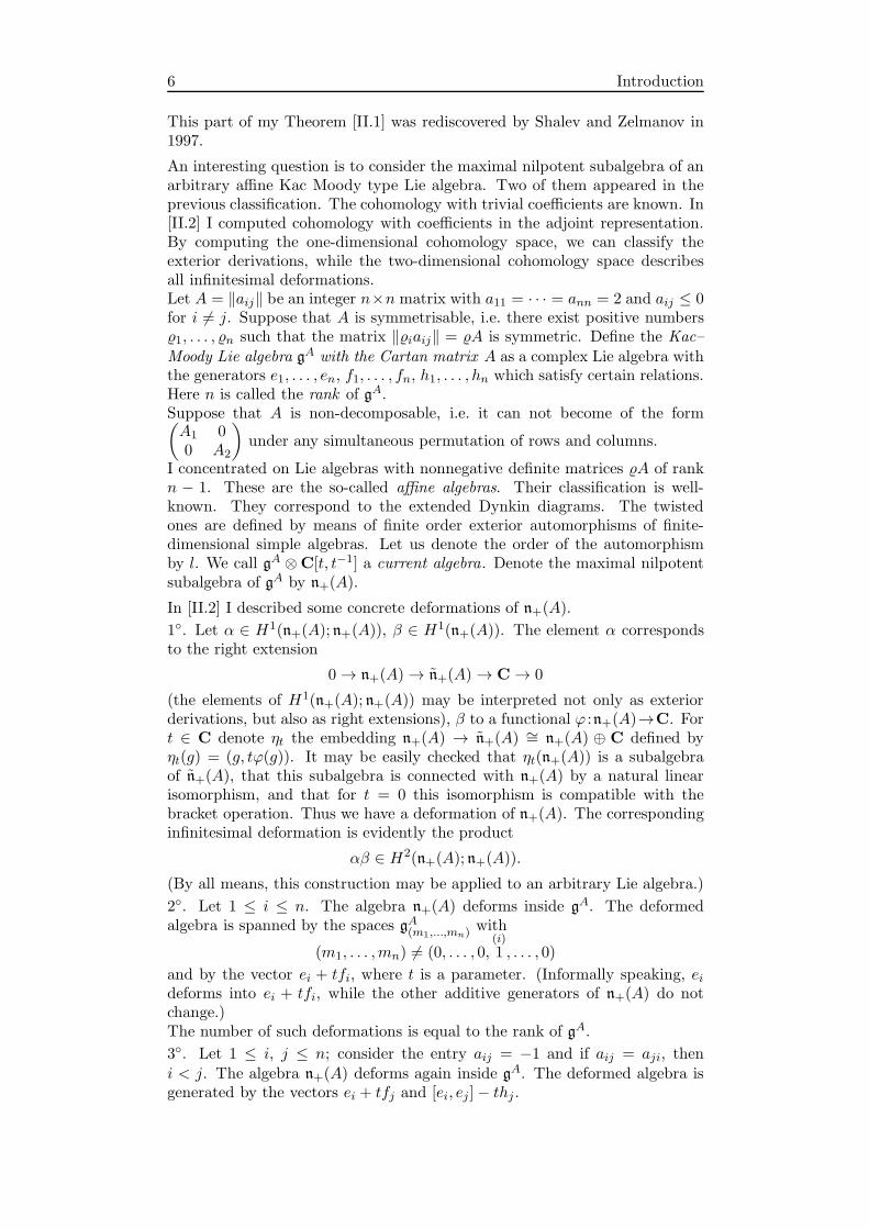
I concentrated on Lie algebras with nonnegative definite matrices A of rankn − 1. These are the so-called affine algebras. Their classification is well-known. They correspond to the extended Dynkin diagrams. The twistedones are defined by means of finite order exterior automorphisms of finite-dimensional simple algebras. Let us denote the order of the automorphismby l. We call gA ⊗C[t, t−1] a current algebra. Denote the maximal nilpotentsubalgebra of gA by n+(A).
In [II.2] I described some concrete deformations of n+(A).
1. Let α ∈ H1(n+(A); n+(A)), β ∈ H1(n+(A)). The element α correspondsto the right extension
0→ n+(A)→ n+(A)→ C→ 0
(the elements of H1(n+(A); n+(A)) may be interpreted not only as exteriorderivations, but also as right extensions), β to a functional ϕ :n+(A)→C. Fort ∈ C denote ηt the embedding n+(A) → n+(A) ∼= n+(A) ⊕ C defined byηt(g) = (g, tϕ(g)). It may be easily checked that ηt(n+(A)) is a subalgebraof n+(A), that this subalgebra is connected with n+(A) by a natural linearisomorphism, and that for t = 0 this isomorphism is compatible with thebracket operation. Thus we have a deformation of n+(A). The correspondinginfinitesimal deformation is evidently the product
αβ ∈ H2(n+(A); n+(A)).
(By all means, this construction may be applied to an arbitrary Lie algebra.)
2. Let 1 ≤ i ≤ n. The algebra n+(A) deforms inside gA. The deformedalgebra is spanned by the spaces gA(m1,...,mn)
with
(m1, . . . ,mn) 6= (0, . . . , 0,(i)
1 , . . . , 0)
and by the vector ei + tfi, where t is a parameter. (Informally speaking, eideforms into ei + tfi, while the other additive generators of n+(A) do notchange.)The number of such deformations is equal to the rank of gA.
3. Let 1 ≤ i, j ≤ n; consider the entry aij = −1 and if aij = aji, theni < j. The algebra n+(A) deforms again inside gA. The deformed algebra isgenerated by the vectors ei + tfj and [ei, ej ]− thj .

Introduction 7
The number of this type deformations is equal to the number of nonzero pairs(aij , aji) with i 6= j; this number we denote below by p.
Theorem 6. [II.2] Suppose that A 6= A1. Then(i) All the homogeneous infinitesimal deformations of n+(A) may be extendedto real deformations.(ii) The space of infinitesimal deformations H2(n+(A); n+(A)) is spanned bydeformations, corresponding to the above types 1, 2, 3. In other words, themapping
ψ :[H1(n+(A); n−(A))⊗H1(n+(A))
]⊕Cn ⊕Cp → H2(n+(A); n+(A))
defined by the infinitesimal deformations listed above is epimorphism.(iii) The kernel of the mapping ψ is contained in
H1(n+(A); n+(A))⊗H1(n+(A))
and its dimension is n.
Theorem 7. [II.2] (i) Infinitesimal deformations, corresponding to defor-
mations of type 1, 2 span in H2(n+(A1); n+(A1)
)a codimension 2 sub-
space. The complementary subspace is spanned by elements from H2(−1,−2) and
H2(−2,−1) respectively. These elements can not be extended to the deformation
of n+(A1).(ii) The kernel of the mapping
[H1(n+(A1); n+(A1))⊗H1(n+(A1))
]⊕C2 → H2(n+(A1); n+(A1))
may be described just as the kernel of ψ in part (iii) of the previous Theorem.
The proof of these theorems is based on introducing a filtration in these nilpo-tent graded Lie algebras and considering the Feigin-Fuchs spectral sequencecorresponding to this filtration. For each of the cases the terms and differen-tials of the spectral sequence may be explicitly determined, and this leads tothe calculation of the indicated cohomology. After having explicit cocycles,one can compute the squares.
On my visit to M.I.T., B. Kostant asked the following question: What isthe main difference between the cohomology of finite and infinite dimensionalnilpotent Lie algebras with coefficients in the adjoint representation, at whatpoints does the generalization of the finite dimensional situation fail?
Understanding this difference is especially important as the nilpotent Lie al-gebra cohomology is very hard to compute and in both finite and infinitedimensional cases only the one- and two-dimensional cohomology is known sofar.Let us recall the result on the Lie algebra cohomology H1(n; n) where n is themaximal nilpotent ideal of a Borel subalgebra of a finite dimensional simple Liealgebra g. Leger and Luks deduced the structure of H1(n; n) from Kostant’sgeneral result.Suppose that the dimension of the Cartan subalgebra h of g is l.
Theorem 8. [Leger-Luks] Except for the Lie algebra sℓ2,
H1(n; n) ∼= h⊕ h.
For sℓ2, dimH1(n; n) = 1.
8 Introduction
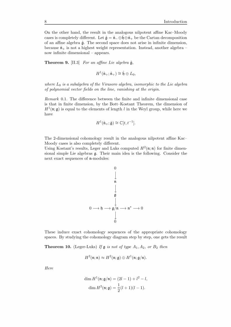
On the other hand, the result in the analogous nilpotent affine Kac–Moodycases is completely different. Let g = n−⊕h⊕n+ be the Cartan decompositionof an affine algebra g. The second space does not arise in infinite dimension,because n+ is not a highest weight representation. Instead, another algebra –now infinite dimensional – appears.
Theorem 9. [II.3] For an affine Lie algebra g,
H1(n+; n+) ∼= h⊕ L0,
where L0 is a subalgebra of the Virasoro algebra, isomorphic to the Lie algebraof polynomial vector fields on the line, vanishing at the origin.
Remark 0.1. The difference between the finite and infinite dimensional caseis that in finite dimension, by the Bott–Kostant Theorem, the dimension ofH1(n; g) is equal to the elements of length l in the Weyl group, while here wehave
H1(n+; g) ∼= C[t, t−1].
The 2-dimensional cohomology result in the analogous nilpotent affine Kac–Moody cases is also completely different.Using Kostant’s results, Leger and Luks computed H2(n; n) for finite dimen-sional simple Lie algebras g. Their main idea is the following. Consider thenext exact sequences of n-modules:
0ynygy
0 −→ h −→ g/n −→ n∗ −→ 0y0
These induce exact cohomology sequences of the appropriate cohomologyspaces. By studying the cohomology diagram step by step, one gets the result
Theorem 10. (Leger-Luks) If g is not of type A1, A2, or B2 then
H2(n; n) ≈ H2(n; g)⊕H1(n; g/n).
Here
dimH1(n; g/n) = (2l − 1) + l2 − l,
dimH2(n; g) =1
2(l + 1)(l − 1).
Introduction 9
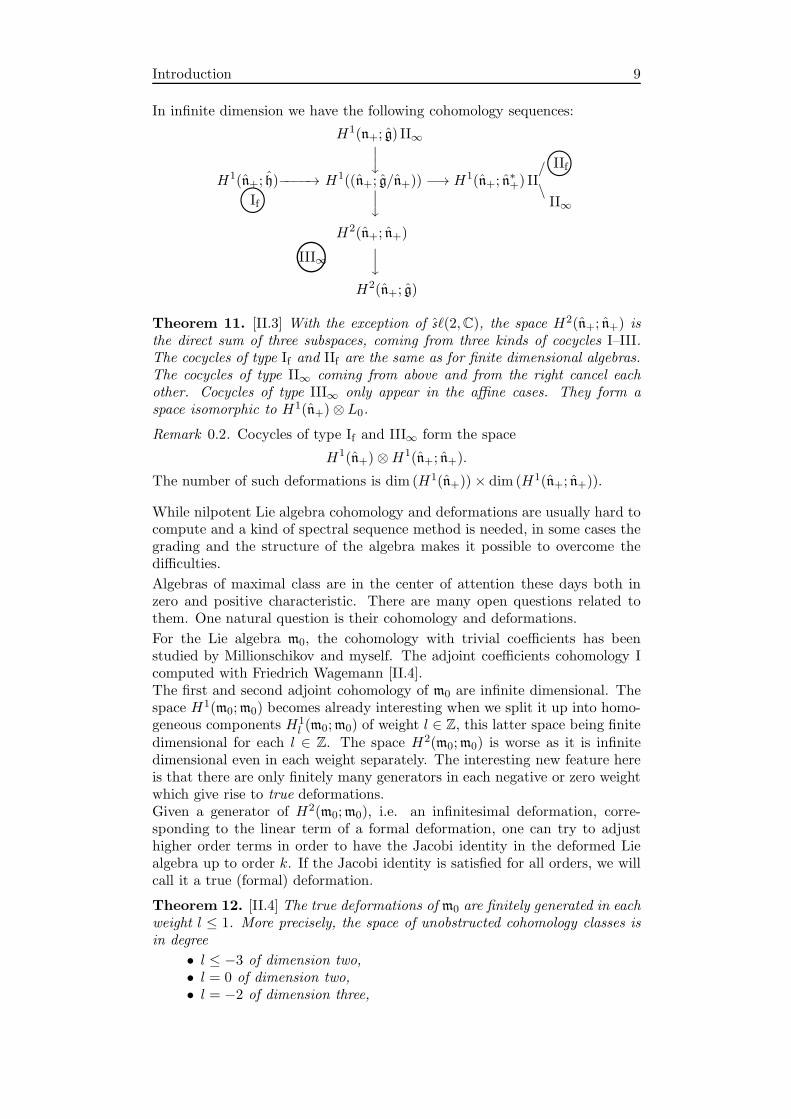
In infinite dimension we have the following cohomology sequences:
H1(n+; g) II∞yH1(n+; h)−−−−→ H1((n+; g/n+)) −→ H1(n+; n
∗+) II
/
\©IIfII∞©If y
H2(n+; n+)
©III∞ y
H2(n+; g)
Theorem 11. [II.3] With the exception of sℓ(2,C), the space H2(n+; n+) isthe direct sum of three subspaces, coming from three kinds of cocycles I–III.The cocycles of type If and IIf are the same as for finite dimensional algebras.The cocycles of type II∞ coming from above and from the right cancel eachother. Cocycles of type III∞ only appear in the affine cases. They form aspace isomorphic to H1(n+)⊗ L0.
Remark 0.2. Cocycles of type If and III∞ form the space
H1(n+)⊗H1(n+; n+).
The number of such deformations is dim (H1(n+))× dim (H1(n+; n+)).
While nilpotent Lie algebra cohomology and deformations are usually hard tocompute and a kind of spectral sequence method is needed, in some cases thegrading and the structure of the algebra makes it possible to overcome thedifficulties.
Algebras of maximal class are in the center of attention these days both inzero and positive characteristic. There are many open questions related tothem. One natural question is their cohomology and deformations.
For the Lie algebra m0, the cohomology with trivial coefficients has beenstudied by Millionschikov and myself. The adjoint coefficients cohomology Icomputed with Friedrich Wagemann [II.4].The first and second adjoint cohomology of m0 are infinite dimensional. Thespace H1(m0;m0) becomes already interesting when we split it up into homo-geneous components H1
l (m0;m0) of weight l ∈ Z, this latter space being finitedimensional for each l ∈ Z. The space H2(m0;m0) is worse as it is infinitedimensional even in each weight separately. The interesting new feature hereis that there are only finitely many generators in each negative or zero weightwhich give rise to true deformations.Given a generator of H2(m0;m0), i.e. an infinitesimal deformation, corre-sponding to the linear term of a formal deformation, one can try to adjusthigher order terms in order to have the Jacobi identity in the deformed Liealgebra up to order k. If the Jacobi identity is satisfied for all orders, we willcall it a true (formal) deformation.
Theorem 12. [II.4] The true deformations of m0 are finitely generated in eachweight l ≤ 1. More precisely, the space of unobstructed cohomology classes isin degree
• l ≤ −3 of dimension two,• l = 0 of dimension two,• l = −2 of dimension three,
10 Introduction
while there is no true deformation in weight l = −1. In weight l = 0, theseare deformations to m2 and L1. In weight l = 1, there are exactly two truedeformations, while in weight l ≥ 2, there are at least two.
We do not have more precise information about how many true deforma-tions there are in positive weight, but there are always at least two. As adeformation in these weights is a true deformation if and only if all of itsMassey squares are zero (as cochains !), true deformations are determined bya countable infinite system of homogeneous quadratic equations in countablyinfinitely many variables. We didn’t succeed in determining the space of solu-tions of this system. In weights l ≤ −1 we got the results using combinatoricsand the graded cocycle property.
We believe that the discussion of these examples of deformations are interest-ing as they go beyond the usual approach where the condition that H2(m0;m0)should be finite dimensional is the starting point for the examination of de-formations, namely the existence of a miniversal deformation.Another attractive point of our study is the fact that in some cases the Masseysquares and cubes involved are not zero because of general reasons, but be-cause of the combinatorics of the relations. Thus the second adjoint cohomol-ogy of m0 may serve as an example for studing explicitly obstruction theory.
Part III: Generalizations and Applications
There is another question approached via deformations. Roughly speaking, itis the question, can we equip the set of mathematical structures under consid-eration (maybe up to certain equivalences) with the structure of a topologicalor even geometric space. In other words, does there exist a moduli space forthese structures. If so, then for a fixed object the deformations of this objectshould reflect the local structure of the moduli space at the point correspond-ing to this object.In this respect, a clear success story is the classification of complex analyticstructures on a fixed topological manifold. Also in algebraic geometry onehas well-developed results in this direction. One of these results is that thelocal situation at a point [C] of the moduli space is completely governed bythe cohomological properties of the geometric object C.As a typical example recall that for the moduli spaceMg of smooth projectivecurves of genus g over C (or equivalently, compact Riemann surfaces of genusg) the tangent space T[C]Mg can be naturally identified with H1(C;TC), whereTC is the sheaf of holomorphic vector fields over C. This extends to higherdimension. In particular, it turns out that for compact complex manifolds M ,the condition H1(M ;TM ) = 0 implies that M is rigid. Rigidity means thatany differentiable family π : M → B ⊆ R, 0 ∈ B which contains M as thespecial member M0 := π−1(0) is trivial in a neighborhood of 0, i.e. for t smallenough Mt := π−1(t) ∼=M .Even more generally, for M a compact complex manifold and H1(M ;TM ) 6=0 there exists a versal family which can be realized locally as a family over acertain subspace of H1(M ;TM ) such that every appearing deformation familyis “contained” in this versal family.These positive results lead to the impression that the vanishing of the relevantcohomology spaces will imply rigidity with respect to deformations also in thecase of other structures.
There is a lot of confusion in the literature in the notion of a deformation.Several different (inequivalent) approaches exist. One of our aims with Martin

Introduction 11
Schlichenmaier was to clarify the difference between deformations of geomet-ric origin and so called formal deformations. Formal deformation theory hasthe advantage of using cohomology. It is also complete in the sense that undersome natural cohomology assumptions, there exists a versal formal deforma-tion, which induces all other deformations [I.2].
Formal deformations are deformations with a complete local algebra base. Adeformation with a commutative (non-local) algebra base gives a much richerpicture of deformation families, depending on the augmentation of the basealgebra. If we identify the base of deformation – which is a commutativealgebra of functions – with a smooth manifold, an augmentation correspondsto choosing a point on the manifold. So choosing different points should ingeneral lead to different deformation situations. In infinite dimension, thereis no tight relation between global and formal deformations.
One of my earlier results is that the Witt and Virasoro algebra are formallyrigid. In our work with Martin Schlichenmaier [III.1] we constructed globaldeformations of the Witt algebra by considering certain families of algebrasfor the genus one case (i.e. the elliptic curve case) and let the elliptic curvedegenerate to a singular cubic. The two points, where poles are allowed, arethe zero element of the elliptic curve (with respect to its additive structure)and a 2-torsion point. In this way we obtain families parameterized over theaffine line with the peculiar behavior that every family is a global deformationof the Witt algebra, i.e. W is a special member, whereas all other membersare mutually isomorphic but not isomorphic toW. Globally these families arenon-trivial, but infinitesimally and formally they are trivial. The construc-tion can be extended to the centrally extended algebras, yielding a globaldeformation of the Virasoro algebra.The results obtained do not have only relevance to the deformation theory ofalgebras but also to the theory of two-dimensional conformal fields and theirquantization. It is well-known that the Witt algebra, the Virasoro algebra, andtheir representations are of fundamental importance for the local description ofconformal field theory on the Riemann sphere (i.e. for genus zero). Kricheverand Novikov proposed in the case of higher genus Riemann surfaces the useof global operator fields which are given with the help of the Lie algebra ofvector fields of Krichever-Novikov type, certain related algebras, and theirrepresentations.
Algebras of Krichever-Novikov types are generalizations of the Virasoro alge-bra and all its related algebras. Let me introduce some of them.Let M be a compact Riemann surface of genus g, or in terms of algebraicgeometry, a smooth projective curve over C. Let N,K ∈ N with N ≥ 2 and1 ≤ K < N be numbers. Fix
I = (P1, . . . , PK), and O = (Q1, . . . , QN−K)
disjoint ordered tuples of distinct points (“marked points”, “punctures”) onthe curve. In particular, we assume Pi 6= Qj for every pair (i, j). The pointsin I are called the in-points, the points in O the out-points. Sometimes weconsider I and O simply as sets and A = I ∪O as a set.Denote by L the Lie algebra consisting of those meromorphic sections of theholomorphic tangent line bundle which are holomorphic outside of A, equippedwith the Lie bracket [., .] of vector fields. Its local form is
[e, f ]| = [e(z)d
dz, f(z)
d
dz] :=
(e(z)
df
dz(z) − f(z)de
dz(z)
)d
dz.

12 Introduction
To avoid cumbersome notation we use the same symbol for the section andits representing function.For the Riemann sphere (g = 0) with quasi-global coordinate z, I = 0 andO = ∞, the introduced vector field algebra is the Witt algebra. We denotefor short this situation as the classical situation.For infinite dimensional algebras and modules and their representation theorya graded structure is usually of importance to obtain structure results.The Witt algebra is a graded Lie algebra. In our more general context thealgebras will almost never be graded. But it was observed by Krichever andNovikov in the two-point case that a weaker concept, an almost-graded struc-ture, will be enough to develop an interesting theory of representations (Vermamodules, etc.).For the 2-point situation for M a higher genus Riemann surface and I = P,O = Q with P,Q ∈ M , Krichever and Novikov introduced an almost-graded structure of the vector field algebras L by exhibiting a special basisand defining their elements to be the homogeneous elements.We consider the genus one case, i.e. the case of one-dimensional complex torior equivalently the elliptic curve case.Recall that the elliptic curves can be given in the projective plane by
Y 2Z = 4X3 − g2XZ2 − g3Z3, g2, g3 ∈ C, with ∆ := g23 − 27g3
2 6= 0.
The condition ∆ 6= 0 assures that the curve will be nonsingular.Instead of the above elliptic curve expression we can use the description
Y 2Z = 4(X − e1Z)(X − e2Z)(X − e3Z)with
e1 + e2 + e3 = 0, and ∆ = 16(e1 − e2)2(e1 − e3)2(e2 − e3)2 6= 0.
These presentations are related via
g2 = −4(e1e2 + e1e3 + e2e3), g3 = 4(e1e2e3).
We set
B := (e1, e2, e3) ∈ C3 | e1 + e2 + e3 = 0, ei 6= ej for i 6= j.In the product B×P2 we consider the family of elliptic curves E over B definedvia the second expression (in product form). The family can be extended to
B := e1, e2, e3) ∈ C3 | e1 + e2 + e3 = 0.The fibers above B \ B are singular cubic curves. Resolving the one linear
relation in B via e3 = −(e1 + e2) we obtain a family over C2.Consider the complex lines in C2
Ds := (e1, e2) ∈ C2 | e2 = s · e1, s ∈ C, D∞ := (0, e2) ∈ C2.Set also
D∗s = Ds \ (0, 0)
for the punctured line. Now
B ∼= C2 \ (D1 ∪D−1/2 ∪D−2).
We have to introduce the points where poles are allowed. For our purposeit is enough to consider two marked points. We will always put one markingto ∞ = (0 : 1 : 0) and the other one to the point with the affine coordinate
(e1, 0). These markings define two sections of the family E over B ∼= C2. Withrespect to the group structure on the elliptic curve given by ∞ as the neutral
Introduction 13
element (the first marking) the second marking chooses a two-torsion point.All other choices of two-torsion points will yield isomorphic situations.For any elliptic curve E(e1,e2) over (e1, e2) ∈ C2 \ (D∗
1 ∪D∗−1/2 ∪D∗
−2) the Lie
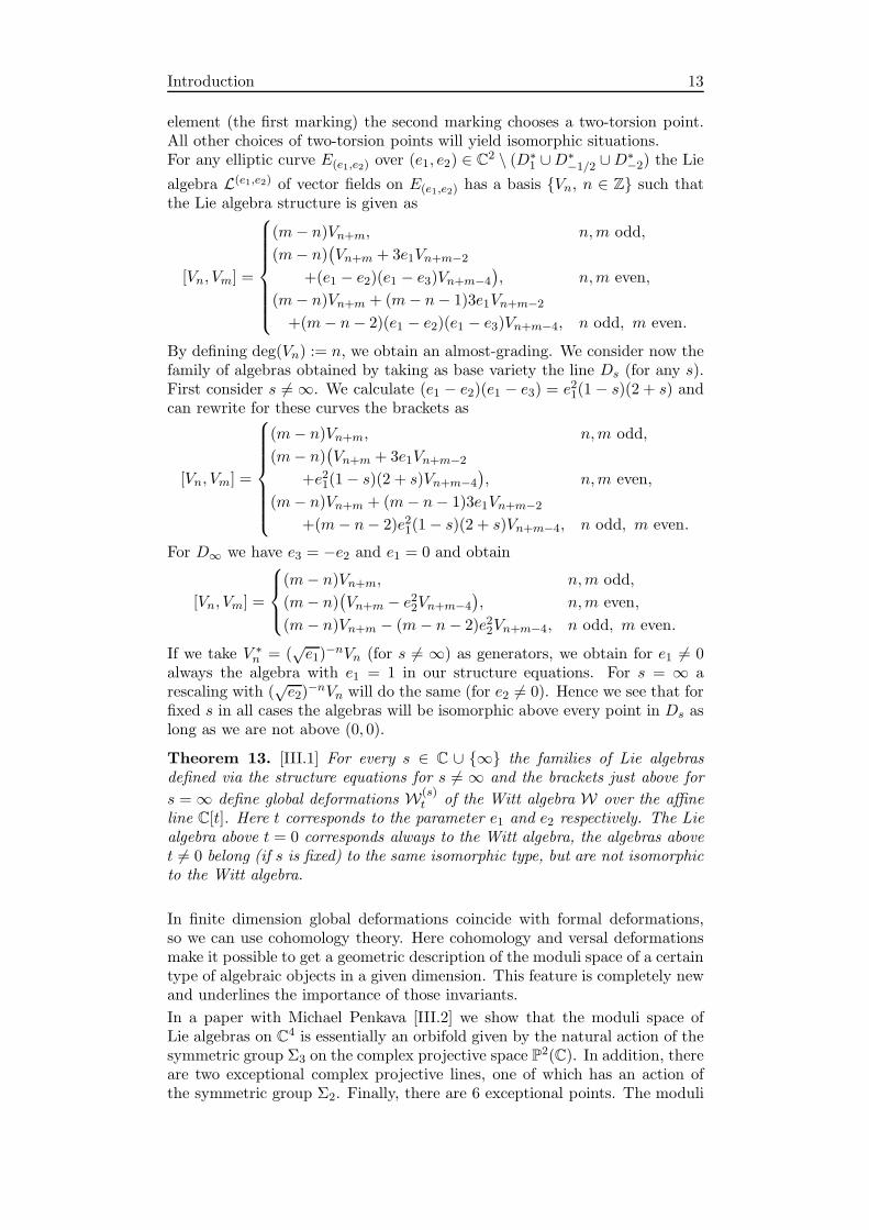
algebra L(e1,e2) of vector fields on E(e1,e2) has a basis Vn, n ∈ Z such thatthe Lie algebra structure is given as
[Vn, Vm] =
(m− n)Vn+m, n,m odd,
(m− n)(Vn+m + 3e1Vn+m−2
+(e1 − e2)(e1 − e3)Vn+m−4
), n,m even,
(m− n)Vn+m + (m− n− 1)3e1Vn+m−2
+(m− n− 2)(e1 − e2)(e1 − e3)Vn+m−4, n odd, m even.
By defining deg(Vn) := n, we obtain an almost-grading. We consider now thefamily of algebras obtained by taking as base variety the line Ds (for any s).First consider s 6=∞. We calculate (e1 − e2)(e1 − e3) = e21(1 − s)(2 + s) andcan rewrite for these curves the brackets as
[Vn, Vm] =
(m− n)Vn+m, n,m odd,
(m− n)(Vn+m + 3e1Vn+m−2
+e21(1− s)(2 + s)Vn+m−4
), n,m even,
(m− n)Vn+m + (m− n− 1)3e1Vn+m−2
+(m− n− 2)e21(1− s)(2 + s)Vn+m−4, n odd, m even.
For D∞ we have e3 = −e2 and e1 = 0 and obtain
[Vn, Vm] =
(m− n)Vn+m, n,m odd,
(m− n)(Vn+m − e22Vn+m−4
), n,m even,
(m− n)Vn+m − (m− n− 2)e22Vn+m−4, n odd, m even.
If we take V ∗n = (
√e1)
−nVn (for s 6= ∞) as generators, we obtain for e1 6= 0always the algebra with e1 = 1 in our structure equations. For s = ∞ arescaling with (
√e2)
−nVn will do the same (for e2 6= 0). Hence we see that forfixed s in all cases the algebras will be isomorphic above every point in Ds aslong as we are not above (0, 0).
Theorem 13. [III.1] For every s ∈ C ∪ ∞ the families of Lie algebrasdefined via the structure equations for s 6= ∞ and the brackets just above for
s =∞ define global deformations W(s)t of the Witt algebra W over the affine
line C[t]. Here t corresponds to the parameter e1 and e2 respectively. The Liealgebra above t = 0 corresponds always to the Witt algebra, the algebras abovet 6= 0 belong (if s is fixed) to the same isomorphic type, but are not isomorphicto the Witt algebra.
In finite dimension global deformations coincide with formal deformations,so we can use cohomology theory. Here cohomology and versal deformationsmake it possible to get a geometric description of the moduli space of a certaintype of algebraic objects in a given dimension. This feature is completely newand underlines the importance of those invariants.
In a paper with Michael Penkava [III.2] we show that the moduli space ofLie algebras on C4 is essentially an orbifold given by the natural action of thesymmetric group Σ3 on the complex projective space P2(C). In addition, thereare two exceptional complex projective lines, one of which has an action ofthe symmetric group Σ2. Finally, there are 6 exceptional points. The moduli

14 Introduction
space is glued together by the miniversal deformations, which determine theelements that one may deform to locally, so deformation theory determinesthe geometry of the space. The exceptional points play a role in refining thepicture of how this space is glued together. By orbifold, we mean essentiallya topological space factored out by the action of a group. In the case of Pn,there is a natural action of Σn+1 induced by the natural action of Σn+1 onCn+1. An orbifold point is a point which is fixed by some element in the group.In the case of Σn+1 acting on Pn, points which have two or more coordinateswith the same value are orbifold points, but there are some other ones, suchas the point (1 : −1) = (−1 : 1).In the classical theory of deformations, a deformation is called a jump de-formation if there is a 1-parameter family of deformations of a Lie algebrastructure such that every nonzero value of the parameter determines the samedeformed Lie algebra, which is not the original one. There are also deforma-tions which move along a family, meaning that the Lie algebra structure isdifferent for each value of the parameter. There can be multiple parameterfamilies as well.In the picture we assembled, both of these phenomena arise. Some of thestructures belong to families and their deformations simply move along thefamily to which they belong. If there is a jump deformation from an elementto a member of a family, then there will always be deformations from thatelement along the family as well, although they will typically not be jumpdeformations. In addition, there are sometimes jump deformations either toor from the exceptional points, so these exceptional points play an interestingrole in the picture of the moduli space.
In classical Lie algebra theory, the cohomology of a Lie algebra is studied byconsidering a differential on the dual space of the exterior algebra of the un-derlying vector space, considered as a cochain complex. If V is the underlyingvector space on which the Lie algebra is defined, then its exterior algebra
∧V
has a natural Z2-graded coalgebra structure as well. In this language, a Liealgebra is simply a quadratic odd codifferential on the exterior coalgebra ofa vector space. An odd codifferential is an odd coderivation whose square iszero. The space L of coderivations has a natural Z-grading L =
⊕Ln, where
Ln is the subspace of coderivations determined by linear maps φ :∧n V → V .
A Lie algebra is a codifferential in L2, in other words, a quadratic codifferen-tial.The space of coderivations has a natural structure of a Z2-graded Lie algebra.The condition that a coderivation d is a codifferential can be expressed in theform [d, d] = 0. The coboundary operator D : L → L is given simply by therule D(ϕ) = [d, ϕ] for ϕ ∈ L; the fact that D2 = 0 is a direct consequenceof the fact that d is an odd codifferential. Moreover, D(Ln) ⊆ Ln+1, whichmeans that the cohomology H(d) = kerD/ ImD has a natural decompositionas a Z-graded space: H(d) =
∏Hn(d), where
Hn(d) = ker(D : Ln → Ln+1)/ Im(D : Ln−1 → Ln).
The Lie algebra structures are codifferentials in L2. In order to represent acodifferential d as a matrix, we choose the following order for the increasingpairs I = (i1, i2) of indices:
(1, 2), (1, 3), (2, 3), (1, 4), (2, 4), (3, 4),
Introduction 15
and denote the ith element of this ordered set by S(i). Using this order andthe Einstein summation convention, we can express
d = aijϕS(j)i .
We summarize our results and give the Lie bracket operations in standardterminology in the Table below.
Type Bracketsd1(λ : µ) [e2, e3] = e3, [e1, e4] = (λ+ µ)e1,
[e2, e4] = λe2, [e3, e4] = e2 + µe3d3(λ : µ : ν) [e1, e4] = λe1, [e2, e4] = e1 + µe2, [e3, e4] = e2 + νe3d3(λ : µ) [e1, e4] = λe1, [e2, e4] = λe2, [e3, e4] = e2 + µe3d1 [e2, e4] = e1d♯1 [e2, e3] = e1, [e1, e4] = 2e1, [e2, e4] = e2, [e3, e4] = e3d∗2 [e1, e2] = e1, [e3, e4] = e2d♯2 [e1, e2] = e1, [e3, e4] = e3d3 [e1, e2] = e3, [e1, e3] = e2, [e2, e3] = e1d∗3 [e1, e4] = e1, [e2, e4] = e2, [e3, e4] = e3
Table 1. Table of Lie Bracket Operations
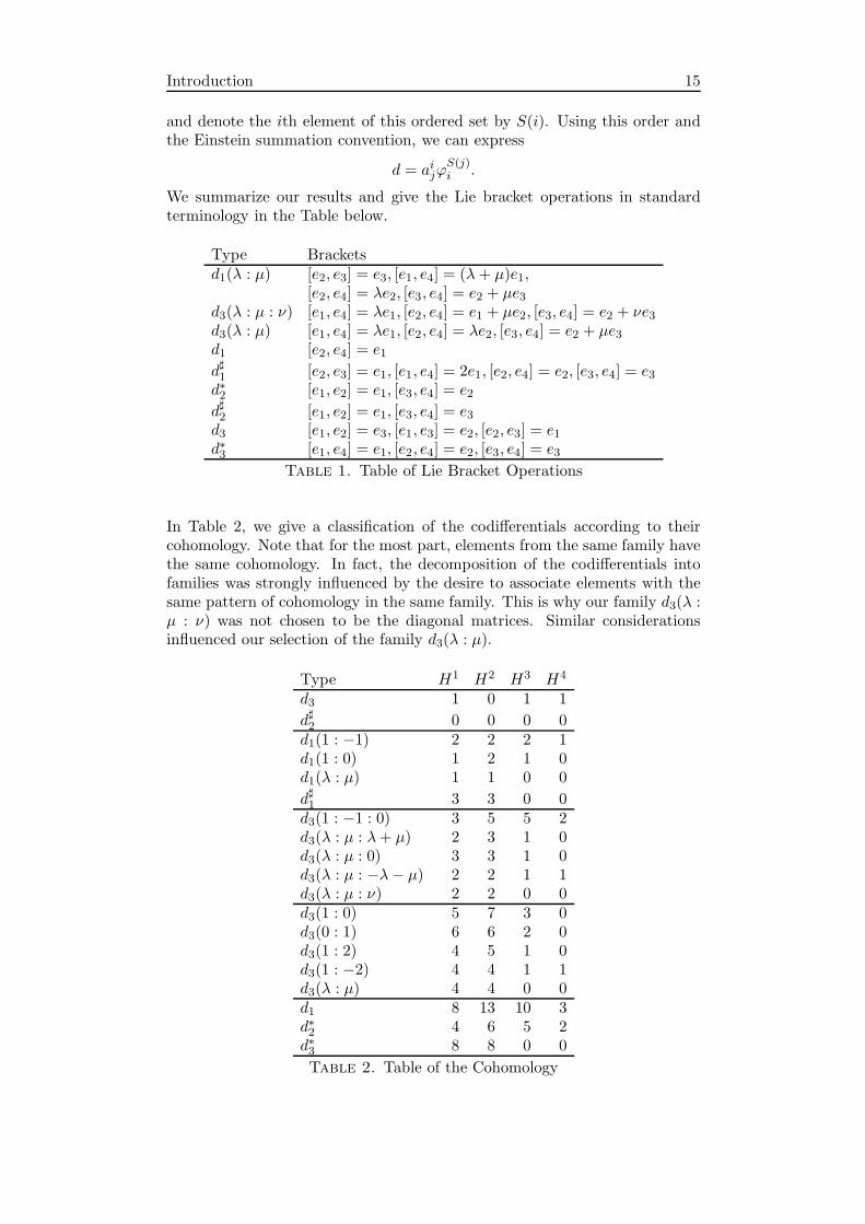
In Table 2, we give a classification of the codifferentials according to theircohomology. Note that for the most part, elements from the same family havethe same cohomology. In fact, the decomposition of the codifferentials intofamilies was strongly influenced by the desire to associate elements with thesame pattern of cohomology in the same family. This is why our family d3(λ :µ : ν) was not chosen to be the diagonal matrices. Similar considerationsinfluenced our selection of the family d3(λ : µ).
Type H1 H2 H3 H4
d3 1 0 1 1
d♯2 0 0 0 0d1(1 : −1) 2 2 2 1d1(1 : 0) 1 2 1 0d1(λ : µ) 1 1 0 0
d♯1 3 3 0 0d3(1 : −1 : 0) 3 5 5 2d3(λ : µ : λ+ µ) 2 3 1 0d3(λ : µ : 0) 3 3 1 0d3(λ : µ : −λ− µ) 2 2 1 1d3(λ : µ : ν) 2 2 0 0d3(1 : 0) 5 7 3 0d3(0 : 1) 6 6 2 0d3(1 : 2) 4 5 1 0d3(1 : −2) 4 4 1 1d3(λ : µ) 4 4 0 0d1 8 13 10 3d∗2 4 6 5 2d∗3 8 8 0 0
Table 2. Table of the Cohomology
16 Introduction
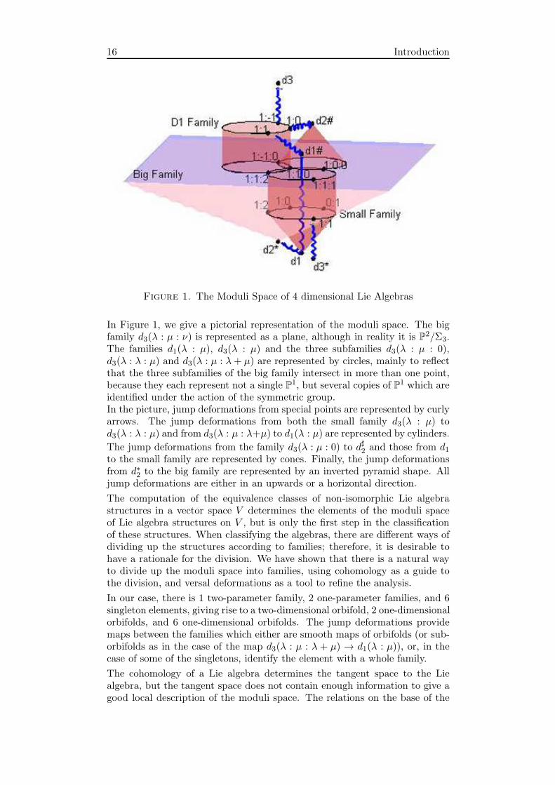
Figure 1. The Moduli Space of 4 dimensional Lie Algebras
In Figure 1, we give a pictorial representation of the moduli space. The bigfamily d3(λ : µ : ν) is represented as a plane, although in reality it is P2/Σ3.The families d1(λ : µ), d3(λ : µ) and the three subfamilies d3(λ : µ : 0),d3(λ : λ : µ) and d3(λ : µ : λ+ µ) are represented by circles, mainly to reflectthat the three subfamilies of the big family intersect in more than one point,because they each represent not a single P1, but several copies of P1 which areidentified under the action of the symmetric group.In the picture, jump deformations from special points are represented by curlyarrows. The jump deformations from both the small family d3(λ : µ) tod3(λ : λ : µ) and from d3(λ : µ : λ+µ) to d1(λ : µ) are represented by cylinders.
The jump deformations from the family d3(λ : µ : 0) to d♯2 and those from d1to the small family are represented by cones. Finally, the jump deformationsfrom d∗2 to the big family are represented by an inverted pyramid shape. Alljump deformations are either in an upwards or a horizontal direction.
The computation of the equivalence classes of non-isomorphic Lie algebrastructures in a vector space V determines the elements of the moduli spaceof Lie algebra structures on V , but is only the first step in the classificationof these structures. When classifying the algebras, there are different ways ofdividing up the structures according to families; therefore, it is desirable tohave a rationale for the division. We have shown that there is a natural wayto divide up the moduli space into families, using cohomology as a guide tothe division, and versal deformations as a tool to refine the analysis.
In our case, there is 1 two-parameter family, 2 one-parameter families, and 6singleton elements, giving rise to a two-dimensional orbifold, 2 one-dimensionalorbifolds, and 6 one-dimensional orbifolds. The jump deformations providemaps between the families which either are smooth maps of orbifolds (or sub-orbifolds as in the case of the map d3(λ : µ : λ + µ) → d1(λ : µ)), or, in thecase of some of the singletons, identify the element with a whole family.
The cohomology of a Lie algebra determines the tangent space to the Liealgebra, but the tangent space does not contain enough information to give agood local description of the moduli space. The relations on the base of the

Introduction 17
versal deformation determine the manner in which the moduli space contactsthe tangent space. It is clear that the cohomology is not sufficient to get anaccurate picture of the moduli space. Versal deformations provide importantdetail that characterizes the moduli space completely.
Part I: Versal Formal Deformations
1. Deformations of Lie Algebras 20Alice FialowskiMath. USSR Sbornik, 55 (1986), pp. 467–473
2. An Example of Formal Deformations of Lie Algebras 27Alice FialowskiDeformation Theory of Algebras and Structures and Applica-tions, Kluwer Acad. Publishers 1988, pp. 375–401
3. Construction of Miniversal Deformations of Lie Algebras 37Alice Fialowski and Dmitry FuchsJournal of Functional Analysis, 161 (1999), pp. 76–110
18
Introduction 19

appeared in: Math. USSR Sbornik, 55 (1986), pp. 467–473.
Deformations of Lie Algebras
Alice FialowskiAlfred Renyi Institute of Mathematics
Budapest
Abstract The author considers general questions of deformations of Liealgebras over a field of characteristic zero, and the related problems ofcomputing cohomology with coefficients in adjoint representations. Theconstruction of a versal family, and the construction of obstructions tothe extension of deformations are also considered.
In this paper, we consider general questions on deformations of Lie algebrasover a field of characteristic zero, and related problems of computing cohomol-ogy with coefficients in adjoint representations. We consider the constructionof a versal family and the nature of obstructions to the extension of deforma-tions. Our aim is to carry over general constructions of the modern theory ofdeformations and related properties of the cohomology of (local) commutativealgebras to Lie algebras in parallel with the papers [3], [10] and [11].
1. We shall require some information on the Harrison cohomology of commu-tative rings (see [12] and [8]). Harrison cohomology is the cohomology in thecategory of commutative rings. We shall only require the 1-dimensional and2-dimensional cohomology, and restrict ourselves to their explicit definition.(In contrast with the traditional indexing, we consider Harrison cohomologywith the indices increased by 1.)Let A be a commutative k-algebra, where k is a field of characteristic zero,
and let N be an A-module. We write down a cochain complex Nd0→ K1 d1→ K2,
whereK1 = Hom k(A,N) andK2 is the subspace of Hom k(S2A,N) consisting
of the maps ϕ for which
aϕ(b, c) − ϕ(ab, c) − cϕ(a, b) + ϕ(a, bc) = 0
for any three elements a, b, c ∈ A. The differentials d0 and d1 are arranged sothat
d0(n)(a) = an, a ∈ A, n ∈ N, d1θ(a, b) = aθ(b)−θ(ab)+bθ(a), a, b ∈ A.The spaces H1
Harr(A;N) and H2Harr(A;N) of 1-dimensional and 2-dimensional
cohomology are by definition Ker d1/Im d0 and K2/Im d1, respectively.
From the definition one can see that 1-cocycles are derivations. Let A be analgebra, m a maximal ideal, and A/m ∼= k. Then H1
Harr(A;k)∼= (m/m2)∗.
In other words, H1Harr(A;k) is isomorphic to the space of homomorphisms
A → k[t]/(t2) for which the kernel of the composition A → k[t]/(t2) → kis m.The 2-dimensional cohomology is interpreted as extension (see [9]). An ex-
tension of the algebra A by a module N is an exact sequence 0→ Ni→ B
π→A → 0, where B is a commutative algebra and i(N) is an ideal in B withtrivial multiplication such that bi(n) = π(b)n for b ∈ B and n ∈ N . To an
1980 Mathematics Subject Classification (1985 Revision). Primary 17B56; Secondary13D03.
20

Deformations of Lie Algebras 21
extension we assign a cochain ϕ ∈ K2 in the following way. Let η : A → Bbe a k-linear map for which πη = id. We put iϕ(a, b) = η(a)η(b) − η(ab). Itcan easily be verified that ϕ ∈ K2 and that for any other choice of the map ηthe cochain ϕ is changed by a coboundary. Thus from the extension we haveconstructed an element of the space H2
Harr(A;N). From the construction onecan see that to every element of H2
Harr(A;N) there corresponds an extension,and the extension is trivial (that is, B is a semidirect product) if and only ifthe corresponding cohomology class is zero.
An automorphism of the extension 0→ Ni→ B
π→ A→ 0 is an automorphismµ of the algebra B such that π(µ(b) − b) = 0 for all b ∈ B and µ(n) − n = 0if n ∈ i(N). The map θ : A → N , a 7→ (µ − 1)ηa depends on the choiceof η; namely, θ : A → N is a cocycle which, as η changes, is changed by acoboundary. Thus the set of automorphisms of the extension 0→ N → B →A→ 0 can be naturally identified with the space H1
Harr(A;N).
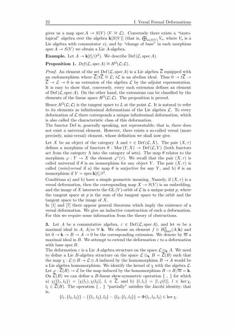
2. Now we move to the theory of deformations of Lie algebras. We beginwith a “naive” definition of deformation of Lie algebras. Let V be a linearspace, and S(V ) the set of all linear maps Λ2V → V satisfying the Jacobiidentity; S(V ) is hence the set of common zeros of a certain system of seconddegree polynomials on the space Λ2V ′ ⊗ V . This makes it possible to equipS(V ) with the structure of affine algebraic variety. The group GL(V ) acts onS(V ). The quotient L = S(V )/GL (V ) is the set of pairwise nonisomorphicLie algebra structures on the space V .It is well known (see [6]) that in the category of algebraic varieties the quotientby a group action does not always exist. In particular, L is not an algebraicvariety. However, one can define a functor assigning to each affine algebraicvariety X a would-be set of morphisms Mor (X,L). Namely, to X we assignD(X), which is the quotient of the set Mor (X,S(V )) by the action of thegroup of regular maps X → GL (V ). If the functor D(X) could be representedin the category of algebraic varieties, then L would admit the structure of analgebraic variety, and D(X) ∼= Mor (X,L).The study of the quotient D is the main problem in the theory of deforma-tions. We are mainly interested in the local theory of deformations; that is,we restrict ourselves to the subcategory Λ of the category of affine algebraicvarieties which consists of the varieties of the form spec A, where A is a localalgebra. We recall that a local algebra is an algebra with a unique maximalideal m, A/m ∼= k. We now define a functor responsible for the structure ofL in the neighborhood of a given point.Let L be a Lie algebra, and spec A an object of the category Λ. ThenDef (L, specA) is by definition the preimage of L under the mapD(A)→ D(k)induced by the morphism speck→ specA. Here we assume that V = L andthat L itself is an element of the set L. The elements of the set Def (L, specA)are called deformations of the Lie algebra L with the base specA.One distinguishes especially the so-called formal 1-parameter deformations ofa Lie algebra; that is, deformations over a ring of formal power series in onevariable (see [13]).
Now we give a more explicit description of the set Def (L, specA), wherespecA ∈ Λ. It is the set of classes by isomorphism of the following pairs:a) the Lie A-algebra L(A), which is free as an A-module, and b) the isomor-phism L(A)/mL(A) ∼= L, where m is a maximal ideal in A. The coincidenceof this definition with that of the preceding paragraph is obvious. Indeed, wechoose in the algebra L(A) a basis (over A). The Lie commutator in this basis
22 I. Versal Formal Deformations
gives us a map specA → S(V ) (V ∼= L). Conversely there exists a “tauto-logical” algebra over the algebra k[S(V )] (that is,
⊕s∈S(V ) Vs, where Vs is a
Lie algebra with commutator s), and by “change of base” in each morphismspecA→ S(V ) we obtain a Lie A-algebra.
Example. Let A→ k[t]/(t2). We describe Def (L, specA).Proposition 1. Def (L, specA) ∼= H2(L;L).Proof. An element of the set Def (L, specA) is a Lie algebra L equipped withan endomorphism where L/tL ∼= L; tL is an abelian ideal. Thus 0 → tL →L → L → 0 is an extension of the algebra L by the adjoint representation.It is easy to show that, conversely, every such extension defines an elementof Def (L, specA). On the other hand, the extensions can be classified by theelements of the linear space H2(L;L). The proposition is proved.
Hence H2(L;L) is the tangent space to L at the point L. It is natural to referto its elements as infinitesimal deformations of the Lie algebra L. To everydeformation of L there corresponds a unique infinitesimal deformation, whichis also called the characteristic class of this deformation.The functor Def is, generally speaking, not representable; that is, there doesnot exist a universal element. However, there exists a so-called versal (moreprecisely, mini-versal) element, whose definition we shall now give.
Let X be an object of the category Λ and τ ∈ Def (L,X). The pair (X, τ)defines a morphism of functors θ : Mor (Y,X) → Def (L, Y ) (both functorsact from the category Λ into the category of sets). The map θ relates to themorphism ϕ : Y → X the element ϕ∗(τ). We recall that the pair (X, τ) iscalled universal if θ is an isomorphism for any object Y . The pair (X, τ) iscalled (mini)versal if a) the map θ is surjective for any Y , and b) θ is anisomorphism if Y = speck[t]/t2.
Conditions a) and b) have a simple geometric meaning. Namely, if (X, τ) is aversal deformation, then the corresponding map X → S(V ) is an embedding,and the image of X intersects the GL (V )-orbit of L in a unique point p, wherethe tangent space at p is the sum of the tangent space to the orbit and thetangent space to the image of X.In [1] and [7] there appear general theorems which imply the existence of aversal deformation. We give an inductive construction of such a deformation.For this we require some information from the theory of obstructions.
3. Let A be a commutative algebra, ε ∈ Def (L, specA), and let m be amaximal ideal in A, A/m ∼= k. We choose an element f ∈ H2
Harr(A;k) andlet 0→ k→ B → A→ 0 be the corresponding extension. We denote by m amaximal ideal in B. We attempt to extend the deformation ε to a deformationwith base specB.The deformation ε is a Lie A-algebra structure on the space L⊗k A. We needto define a Lie B-algebra structure on the space L ⊗k B = L(B) such thatthe map χ : L⊗B → L⊗A induced by the homomorphism B → A would bea Lie algebra homomorphism. We identify the kernel of χ with the algebra L.Let ϕ : L(B)→ L be the map induced by the homomorphism B → B/m = k.On L(B) we can define a B-linear skew-symmetric operation , for whicha) χ(l1, l2) = [χ(l1), χ(l2)], li ∈ L, and b) l, l1 = [l, ϕ(l)], l ∈ kerχ,l1 ∈ L(B). The operation , “partially” satisfies the Jacobi identity; thatis,
l1, l2, l3 − l1, l2, l3 − l2, l1, l3 = Φ(l1, l2, l3) ∈ kerχ.
Deformations of Lie Algebras 23
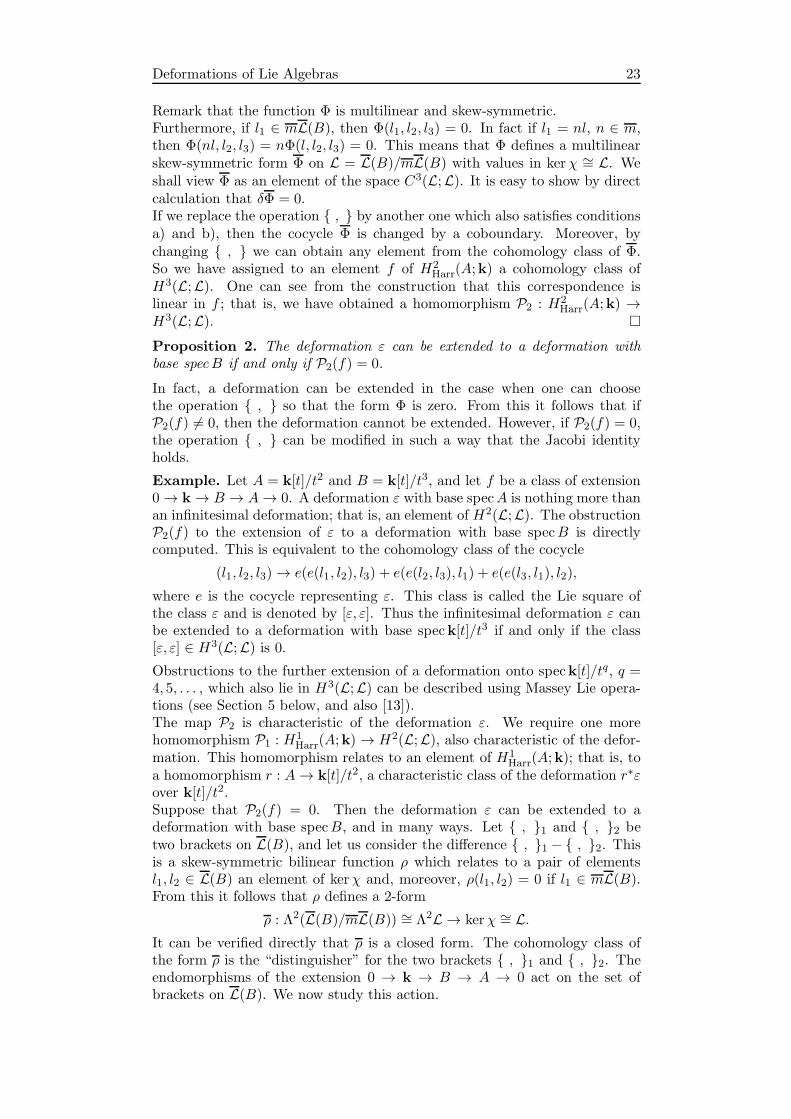
Remark that the function Φ is multilinear and skew-symmetric.Furthermore, if l1 ∈ mL(B), then Φ(l1, l2, l3) = 0. In fact if l1 = nl, n ∈ m,then Φ(nl, l2, l3) = nΦ(l, l2, l3) = 0. This means that Φ defines a multilinearskew-symmetric form Φ on L = L(B)/mL(B) with values in kerχ ∼= L. Weshall view Φ as an element of the space C3(L;L). It is easy to show by directcalculation that δΦ = 0.If we replace the operation , by another one which also satisfies conditionsa) and b), then the cocycle Φ is changed by a coboundary. Moreover, bychanging , we can obtain any element from the cohomology class of Φ.So we have assigned to an element f of H2
Harr(A;k) a cohomology class ofH3(L;L). One can see from the construction that this correspondence islinear in f ; that is, we have obtained a homomorphism P2 : H2
Harr(A;k) →H3(L;L).
Proposition 2. The deformation ε can be extended to a deformation withbase specB if and only if P2(f) = 0.
In fact, a deformation can be extended in the case when one can choosethe operation , so that the form Φ is zero. From this it follows that ifP2(f) 6= 0, then the deformation cannot be extended. However, if P2(f) = 0,the operation , can be modified in such a way that the Jacobi identityholds.
Example. Let A = k[t]/t2 and B = k[t]/t3, and let f be a class of extension0→ k→ B → A→ 0. A deformation ε with base specA is nothing more thanan infinitesimal deformation; that is, an element of H2(L;L). The obstructionP2(f) to the extension of ε to a deformation with base specB is directlycomputed. This is equivalent to the cohomology class of the cocycle
(l1, l2, l3)→ e(e(l1, l2), l3) + e(e(l2, l3), l1) + e(e(l3, l1), l2),
where e is the cocycle representing ε. This class is called the Lie square ofthe class ε and is denoted by [ε, ε]. Thus the infinitesimal deformation ε canbe extended to a deformation with base speck[t]/t3 if and only if the class[ε, ε] ∈ H3(L;L) is 0.Obstructions to the further extension of a deformation onto speck[t]/tq, q =4, 5, . . . , which also lie in H3(L;L) can be described using Massey Lie opera-tions (see Section 5 below, and also [13]).The map P2 is characteristic of the deformation ε. We require one morehomomorphism P1 : H1
Harr(A;k)→ H2(L;L), also characteristic of the defor-mation. This homomorphism relates to an element of H1
Harr(A;k); that is, toa homomorphism r : A→ k[t]/t2, a characteristic class of the deformation r∗εover k[t]/t2.Suppose that P2(f) = 0. Then the deformation ε can be extended to adeformation with base specB, and in many ways. Let , 1 and , 2 betwo brackets on L(B), and let us consider the difference , 1 − , 2. Thisis a skew-symmetric bilinear function ρ which relates to a pair of elementsl1, l2 ∈ L(B) an element of kerχ and, moreover, ρ(l1, l2) = 0 if l1 ∈ mL(B).From this it follows that ρ defines a 2-form
ρ : Λ2(L(B)/mL(B)) ∼= Λ2L → kerχ ∼= L.It can be verified directly that ρ is a closed form. The cohomology class ofthe form ρ is the “distinguisher” for the two brackets , 1 and , 2. Theendomorphisms of the extension 0 → k → B → A → 0 act on the set ofbrackets on L(B). We now study this action.
24 I. Versal Formal Deformations
Proposition 3. Let a be an automorphism of the extension 0 → k → B →A → 0, and let a be the corresponding element of the space H1
Harr(A;k).
Furthermore, let , be a bracket on L(B). Then the difference between thebracket a , and , is P1(a).The proof of this Proposition is obvious.
Corollary. Let ε ∈ Def (L, A) be a deformation for which the homomorphismP1 is a surjection, and let 0→ k→ B → A→ 0 be an extension for which εcan be extended to a deformation over specB. Then the automorphism groupof the extension acts transitively on the set of all extensions of ε.
4. We now move to the construction of a versal deformation. Let Σ be thesubcategory of the category of local algebras which consists of algebras Afor which m2 = 0, m is a maximal ideal, and A/m ∼= k. Then the functorDef (L, specA) can be represented on the category Σ; that is, it admits auniversal pair (X, ε) ε ∈ Def (L,X) (see [7]). We construct such a pair. Weput X = specA, where A = k⊗H2(L;L) (here H2(L;L) is an ideal in A withzero multiplication). We now remark that the space
H2(L;H2(L;L) · L) = H2(L;L)⊗H2(L;L),like every tensor product of dual spaces, has a distinguished element. Let v bea cochain representing this element. We now define a Lie A-algebra structureon the space
L⊗A = L ⊗ 1⊕ L⊗H2(L;L),by putting
[l1 ⊗ 1, l2 ⊗ 1] = [l1, l2]⊗ 1 + v(l1, l2), l1, l2 ∈ L.This is the Lie A-algebra that corresponds to the deformation ε.If C = k ⊕m, m2 = 0, is an object of the category Σ, then to each elementof the set Def (L, specC) there corresponds naturally (as in Proposition 1) anelement of H2(L;m⊗ L). This correspondence is one-to-one. We note that
H2(L;m⊗ L) ∼= Hom (H2(L;L),m) ∼= Hom(A,C) ∼= Def (L, specC).
But this implies that the pair (X, ε) is universal.Let A be a local algebra, m a maximal ideal, and let N = (H2(A;A/m))∗ ⊗k
A/m be an A-module. We identify the latter with the space H2Harr(A;k)
∗.The space
H2Harr(A;N) = H2
Harr(A;k) ⊗ (H2Harr(A,k))
∗
contains a canonical element u. We construct the corresponding extension0 → N → F (A) → A → 0. Let A = k[x1, . . . , xn]/m
2, m = (x1, . . . , xn).Then the projective limit of the system A ← F (A) ← F (F (A)) ← . . . is analgebra of formal series in n variables.Let (X, ε) be a universal pair in the category Σ, and let A = k[x]. Thedeformation ε gives us the homomorphism
P2 : H2Harr(A;k)→ H3(L;L).
Consider the dual map
P ∗2 : H3(L;L)→
(H2
Harr(A,k))∗,
and let u be the image of the class u ∈ H2(A; (H2
Harr(A,k))∗)under the
homomorphism
H2(A; (H2
Harr(A;k))∗)→ H2
(A; (H2
Harr(A,k))∗/ImP∗
2
).
Deformations of Lie Algebras 25
We construct the extension corresponding to u:
0→ H2Harr(A;k)
∗/ImP ∗2 → F (A)→ A→ 0.
From the constructions of Section 3 it follows that the family of ε can beextended to a family with base specF (A). From the corollary of Proposition 3it follows that the automorphism group of the extension acts transitively onthe set of extensions. This means that the Lie algebra L(F (A)) is uniquelydefined up to isomorphism. We apply the same construction to the algebraF (A) again, then once more, etc. We obtain a projective system of algebras:
· · · → F (A)→ F (A)→ A.
By v(L) we denote the projective limit of this system of algebras. From theabove it follows that v(L) is the quotient of the algebra k[[H2(L;L)]] by acertain ideal. So, in the obvious way, there is a deformation of L(v(L)) withbase spec v(L).Proposition 4. The deformation with base spec v(L) just constructed is ver-sal.
This proposition is proved by standard means. The proof of a similar resultfor local commutative algebras can be found in a paper by Schlessinger [7].The algebra v(L) is the quotient of k[[H2(L;L)]] by an ideal J . We assumethat dimH2(L;L) <∞. The algebra of formal power series in a finite numberof variables is Noetherian, and hence the ideal J has finitely many genera-tors. The space of generators for J can be identified (see [7]) with the space(H2
Harr(v(L),k))∗. From the construction of v(L) it follows that the mapH3(L;L) → (H2
Harr(v(L);k))∗ is surjective. Thus the coordinate ring of thebase of the versal deformation is the quotient of k[[H2(L;L)]] by the idealgenerated by the relations corresponding to the elements of H3(L;L).
5. In this section, following [4], we introduce certain cohomology operationswhich serve as the main means for computing the versal deformation. For thiswe require the standard homology complex of a Lie superalgebra. We do notquote its definition (see [2] or [5]).Let A = C∗(L) be the standard cochain complex consisting of cochains of theLie algebra L. Let A be a differential Z-graded algebra. By DerA we denotethe set of superderivations of the algebra A. The space DerA is equippedin the usual way with a Lie superalgebra structure. We note that DerA ∼=C∗(L;L) ∼= Λ∗(L∗) ⊗ L (an element ω1 ⊗ l ∈ Λ∗(L∗) ⊗ L is assigned thederivation ω1∂/∂l, l ∈ L, ω1 ∈ Λ∗(L∗)). The space DerA has a distinguishedelement δ to which there corresponds a commutation operator Λ2L → L. Thedifferential in the complex DerA is given by the formula u → [uδ]; so DerAis turned into a differential graded Lie superalgebra. The space H∗(L;L)inherits the Lie superalgebra structure.Let K be the standard complex of the superalgebra DerA; that is, K =DerA ← Λ2DerA ← . . . ; we recall that the exterior power is here under-stood in the super sense. We specify on this complex the filtration
Ki = DerA⊕ Λ2DerA⊕ · · · ⊕ ΛiDerA.
The first term of the associated spectral sequence, called the Quillen spectralsequence for superalgebras DerA (see [5]), is isomorphic to the standard com-plex of the superalgebra H∗(L;L). According to [5], if a Massey operation isdefined on the elements α1, . . . αn ∈ H∗(L;L), then a boundary differential isalso defined in the spectral sequence under consideration. Hence the images
26 I. Versal Formal Deformations
of the boundary differentials in this spectral sequence can naturally be calledgeneralized Massey Lie operations.Let us choose in H2(L;L) an element α. This element is even, and hence inthe standard complex H∗(L;L) the elements αn are defined. As computationsshow, the first differential is d1α
2 = 〈α,α〉 ∈ H2(L;L). If 〈α,α〉 = 0, then thedifferential
d2α3 ∈ H3(L;L)/d1(S2H2(L;L))
is defined (we assume that d2α3 = 〈α,α, α〉), and so on.
The equation 〈α,α〉 = 0 defines a quadratic cone in H2(L;L). If 〈α,α〉 =0, then the condition 〈α,α, α〉 ∋ 0 defines a subset of this quadratic cone.Iterating this procedure, we obtain a certain homogeneous subvariety V inH2(L;L). Let v(L) be the algebra constructed in the preceding section, let mbe a maximal ideal in v(L), and let v(L) be the graded algebra k⊕m/m2 ⊕m2/m3 ⊕ . . . .Proposition 5 (see [4]). The spectrum of the algebra v(L) is V .
Corollary. If for every α ∈ H2(L;L)〈α,α〉 = 0, 〈α,α, α〉 ∋ 0, . . . ,
then spec v(L) = H2(L;L); that is, the base of a versal deformation of thealgebra L is H2(L;L).
References
[1] M. Artin, Algebraization of formal moduli. I, Global Analysis (Papers in Honor of K.Kodaira), Univ. of Tokyo Press, Tokyo, and Princeton Univ. Press, Princeton. N. J.,1969, pp. 21–71.
[2] D. A. Leites, Cohomology of Lie superalgebras, Funktsional. Anal. i Prilozhen. 9 (1975),no. 4, 75–76; English transl. in Functional Anal. Appl. 9 (1975).
[3] V. P. Palamodov, Deformations of complex spaces, Uspekhi Mat. Nauk 31 (1976), no.3(189), 129–194; English transl. in Russian Math. Surveys 31 (1976).
[4] V. S. Retakh, The Massey operations in Lie superalgebras, and deformations of complex-analytic algebras, Funktsional. Anal. i Prilozhen. 11 (1977), no. 4. 88–89; English transl.in Functional Anal. Appl. 11 (1977).
[5] V. S. Retakh, The Massey operations in Lie superalgebras, and differentials of theQuillen spectral sequence, Funktsional. Anal. i Prilozhen. 12 (1978), no. 4. 91–92: Eng-lish transl. in Functional Anal. Appl. 12 (1978).
[6] Robin Hartshorne, Algebraic geometry, Springer-Verlag. 1977.[7] Michael Schlessinger, Functors of Artin rings, Trans. Amer. Math. Soc. 130 (1968),
208–222.[8] Michael Barr, Harrison homology, Hochschild homology and triples, J. Algebra 8 (1968),
314–323.[9] D. K. Harrison, Commutative algebras and cohomology, Trans. Amer. Math. Soc. 104
(1962), 191–204.[10] Luc Illusie, Complexe cotangent et deformations. I, Lecture Notes in Math., vol. 239,
Springer-Verlag, 1971.[11] Olav A. Laudal, Formal moduli of algebraic structures, Lecture Notes in Math., vol.
754, Springer-Verlag, 1979.[12] Daniel Quillen, On the (co-) homology of commutative rings, Applications of Categorical
Algebra, Proc. Sympos. Pure Math., vol. 17, Amer. Math. Soc., Providence, R. I., 1970,pp. 65–87.
[13] Murray Gerstenhaber, On the deformation of rings and algebras. I, III, Ann. of Math.(2) 79 (1964), 59–103: (2) 88 (1968), 1–34.
appeared in: Deformation Theory of Algebras and Structures and Applications,Kluwer Acad. Publishers 1988, 375–401.
An Example of Formal Deformations of Lie Algebras
Alice FialowskiInstitute of Mathematics
Eotvos Lorand University, Budapest
Introduction
In this work we are going to investigate the formal deformations of an infinite dimen-sional Lie algebra of vector fields on the line with polynomial coefficients. This Liealgebra L1 consists of the fields which vanish with their first derivative at the origin.For finding the deformations, we have to consider the cohomology with coefficientsin the adjoint representation.In Section 1 we recall – following Nijenhuis and Richardson [6] – the constructionof the differential Lie superalgebra structure in the cochain complex of an arbitraryLie algebra with coefficients in the adjoint representation. In Section 2 we apply thegeneral theory of Schlessinger [8] to the formal deformations of a Lie algebra. InSection 3 we compute the cohomology H•(L1;L1) with the help of the Feigin–Fuchsspectral sequences [1]. In Section 4 we deal with the obstruction theory of Lie algebrasand give concrete computations in the case of L1. In Section 5 we give examples ofdeformations of this infinite dimensional Lie algebra.This work was supported by the Swiss National Foundation.I would like to thank Professor A. Haefliger for the help during the preparation ofthis lecture and paper.
1. The differential Lie superalgebra C•(L;L)
Let L be a Lie algebra. For a positive integer q denote by Cq(L;L) the space of q-linear,antisymmetric, L-valued functions on L. This is the space of q-dimensional cochainsof L with coefficients in the adjoint representation. For q < 0 put Cq(L;L) = 0.Let dq = d denote the differential or coboundary operator dq = d : Cq(L;L) →Cq+1(L;L) which acts as follows.For q ≧ 0, ϕ ∈ Cq(L;L)
dϕ(g1, . . . , gq+1) :=∑
1≦s<t≦q+1
(−1)s+t−1ϕ([gs, gt], g1, s t. . ., gq+1)+
+∑
1≦s≦q+1
(−1)s[gs, ϕ(g1, s. . ., gq+1)
]
where ˆ means that the element with the indicated index is missing. For q < 0 letdq = 0. From the definition it follows that dq+1dq = 0, so we get a complex C•(L;L).By a differential Lie superalgebra we mean a complex C = (Xn, d)
∞n=0 with an oper-
ation [ , ] such that for x ∈ Xp, y ∈ Xq
[x, y] = −(−1)p·q[y, x] (1.1)
where p is the degree of x. The super-Jacobi identity is satisfied for x ∈ Xp, y ∈ Xq,z ∈ Xr:
(−1)p·q[[x, y], z] + (−1)q·r[[y, z], x] + (−1)r·p[[z, x], y] = 0 (1.2)
and the differential d of degree +1 is such that
d([x, y]) = [dx, y]− (−1)p[x, dy]. (1.3)
Proposition 1.1. The complex C•(L;L) is a differential Lie superalgebra, the degreeof a ∈ Cp(L;L) being p− 1.
27
28 I. Versal Formal Deformations
Proof. For a ∈ Cp(L;L) and b ∈ Cq(L;L) define the cochain ab ∈ Cp+q+1(L;L) by
ab(g1, . . . , gp+q−1) :=∑
σ
sgn (σ)a(b(gi1 , . . . , giq
), gj1 , . . . , gjp−1
)
where the sum runs over the shuffles
1, . . . , p+ q + 1 = i1, . . . , iq ∪ j1, . . . , jp−1(i1 < · · · < iq, j1 < · · · < jp−1).Put [a, b] = ab− (−1)(p−1)(q−1)ba.It is easy to verify that for this superbracket operation the identities (1.1)–(1.3) aresatisfied with c ∈ Cr(L;L).From (1.3) it follows that if a, b are cocycles then the superbracket [a, b] is also acocycle, and the cohomology class of [a, b] depends only on the class of a and b. Thatmeans that a multiplication can be defined in the cohomology space
Hp(L;L)⊗Hq(L;L) −→ Hp+q−1(L;L)
which satisfies (1.1) and (1.2) with a ∈ Hp(L;L), b ∈ Hq(L;L), c ∈ Hr(L;L).
Corollary. The Lie superalgebra structure on C•(L;L) induces a structure of Liesuperalgebra on the cohomology space, in which the usual grading is reduced by one.In this way we get an analogy with the Kodaira–Spencer theory (see [6]).
2. Formal deformations of Lie algebras. General theory
In this section we explain, how the general theory of Schessinger applies to formaldeformations of Lie algebras.
Let L be a Lie algebra over a field K. Let C be the category of local finite dimensionalalgebras A over K. For such an A there exists a unique maximal ideal mA such thatA/mA = K and dimK A is finite. Let us denote by ε the canonical map A −→A/mA = K. If t1, . . . , tn are elements of mA such that their images in mA/m
2A form
a basis, then A = K[[t1, . . . , tn]]/I where I contains a power of the maximal idealof K[[t1, . . . , tn]]. The morphisms in C are the homomorphisms of local algebras (socommuting with ε).A deformation LA of L parametrized by A ∈ C is a Lie algebra structure over A onL⊗K A such that the Lie algebra structure on
L = (LA)⊗A K = (L ⊗A)⊗A K
is the given one on L (obtained from LA by the extension of the scalars given by ε).If f : A → B is a morphism in C then the Lie algebra LB = (LA) ⊗A B is thedeformation of L parametrized by B induced by f from LA.
Two deformations LA and L′A of L parametrized by A are equivalent, if there exists aLie algebra isomorphism over A of LA on L′A inducing the identity of LA ⊗A K = Lon L′A ⊗A K = L.The functor F : C → Sets associates to A ∈ C the set F (A) of equivalence classes ofdeformations of L parametrized by A.The algebra A is of order less or equal to k if mk+1 = 0. (For instance if k = 1,K = C, t1, . . . , tn form a basis of m/m2, then A = C ·1⊕Ct1⊕· · ·⊕Ctn and titj = 0for all 1 ≦ i, j ≦ n.)A deformation LA is of order k if A is of order ≦ k. An infinitesimal deformation isa deformation of order 1, parametrized by K[t]/(t2).
More generally, let C be the category of complete local algebras A over K such thatA/mn
A ∈ C for all n (complete means that A = lim←A/mn
A).
A deformation of L parametrized by A is the projective limit lim←LA/m
nA of deforma-
tions of L parametrized by A/mnA. In other words, a deformation of L parametrized
by A ∈ C is a Lie algebra structure over A on L⊗A = lim←L ⊗ A/mn
A, inducing the
given structure on L.

An Example of Formal Deformations of Lie Algebras 29
There is an analogous definition for isomorphisms of deformations parametrized byA ∈ C. The functor F can be extended as a functor F : C → Sets.A deformation LR of L parametrized by R ∈ C is called formally versal if for anydeformation LA of L parametrized by A ∈ C there is a morphism f : R → A suchthat LR ⊗ RA is equivalent to LA and if the map mR/m
2R → mA/m
2A induced by
f is unique. (In particular, all the other deformations of L can be induced from theversal one.)
A versal deformation up to order k is defined similarly, where C is replaced by thesubcategory of algebras of order ≦ k.
Theorem (Schlessinger). If the space H2(L;L) is finite, then there exists a formalversal deformation of L.
Proof. This follows from the general Theorem of Schlessinger ([8, Theorem 2.11]),provided we check the following properties of the functor F .Let A′ → A and A′′ → A be morphisms in C. Consider the map
τ : F (A′ ×A A′′)→ F (A′)×F (A) F (A′′)
associating to the equivalence class of a deformation of L parametrized by A′ ×A A′′
the equivalence classes of the deformations of L parametrized by A′ and A′′ respec-tively, induced by the morphism A′ ×A A′′ → A′ and A′ ×A A′′ → A′′. Thena) τ is surjective whenever A′′ → A is surjective;b) τ is bijective when A = K.To check a) consider two deformations LA′ and LA′′ of L parametrized by A′ andA′′ respectively, and such that there exists an equivalence ξ of L′A = LA′ ⊗A′ Aon L′′A = LA′′ ⊗A′′ A of the associated deformations of L parametrized by A. Theequivalence classes of LA′ and LA′′ give an element of FA′×FA
FA′′ . As the morphismA′′ → A is surjective and as LA′′ is a free A′′-module, after changing LA′ in itsequivalence class, we can assume that the equivalence ξ is the identity of LA = L⊗A,using the canonical A-module isomorphism of L′A and L′′A with L⊗A. Then the imageby τ of the equivalence class of the deformation LA′ ×LA
LA′′ of L parametrized byA′ ×A A′′ will be the given element of FA′ ×FA
FA′′ .The condition b) can be easily verified because in that case B = A′×A A′′ is equivalentto K · 1 ⊕mA′ ⊕mA′′ with mA′ ·mA′′ = 0 and a deformation of L parametrized byA′×A A′′ is characterized by the induced deformation parametrized by A′ and A′′.
To link this section to the preceding one we can give a more concrete description ofthe Lie algebra LA.Suppose A ∈ C, then A = K[[t1, . . . , tn]]/I. We can express L⊗A in the formL⊗K[[t1, . . . , tn]]/I. The Lie algebra structure on LA will be described by a bilin-ear alternate map
µt : L× L→ L⊗K[[t1, . . . , tn]] such that
µt(x, y) = [x, yl ⊗ 1 +∑
|α|≧1
ϕα(x, y)⊗ tα
where ϕα ∈ C2(L;L) and µt(x, y) composed with the projection on L⊗A is equal to[x⊗ 1, y ⊗ 1]LA
. This lifting is unique mod I.The map µt will define a bracket in L⊗A verifying the Jacobi identity iff
2dϕ+ [ϕ, ϕ] ≡ 0 mod I
where d and [ , ] were defined in Section 2. This means that the coefficients of theformal power series obtained from
2∑
|α|≧1
(dϕα)tα +
∑
|α|≧1
∑
β+γ=α
[ϕβ , ϕγ ]tβtγ
by applying to each coefficient an arbitrary linear form on C2(L;L) belong to I.In case |α| = 1 we get dϕα = 0 for each α which means that ϕα is a cocycle.
30 I. Versal Formal Deformations
The elements of H2(L;L) correspond bijectively to the equivalent classes of infin-itesimal deformations. Suppose that dimH2(L;L) is finite. Let ϕ1, ϕ2, . . . , ϕn becocycles whose cohomology classes form a basis of H2(L;L). Then a versal deforma-tion of order 1 of L is parametrized by K[t1, . . . , tn]/(m
2) and is given by the bilinearalternate map
µt = µ0 + ϕ1t1 + · · ·+ ϕntn
where µ0 is the original bracket in L.Let us try to extend this deformation to a versal deformation of order 2 parametrizedby K[t1, . . . , tn]/I where I contains m3. The bracket should be of the form
µt = µ0 +
n∑
i=1
ϕiti +∑
ϕijtitj
with the conditions that
−2Σdϕijtitj ≡ Σ[ϕi, ϕj ]titj mod I.
This means that the right-hand side (which is always a three-cocycle) must becoboundary. So the ideal I is generated by the polynomials, obtained by compos-ing the cohomology class of the right-hand side with linear forms on H3(L;L), andm3. For ϕij one can choose any 2-cochain satisfying the above condition.
3. Computation of H•(L1;L1)
Let W pol = W1 be the Lie algebra of vector fields on the line with polynomialcoefficients f(x) ddx . This Lie algebra has an additive algebraic basis
ei = xi+1 d
dx, i ≧ −1.
In this basis the bracket operation is
[ei, ej ] = (j − i)ei+j .Let us introduce the subalgebra Li, i ≧ 0 of W1 which is generated by the basiselements ei, ei+1, . . . .We shall investigate the subalgebra L1. The Lie algebra L1 is naturally graded, the
weight of ei equals i. With this grading Lpol1 is a graded Lie algebra: Lpol
1 =∞⊕m=1
L(m)1 .
We consider the cohomology of L1 with coefficients in the adjoint representation. Thecochain complex is defined in the graded sense:
Cq(L1;L1) = ⊕Cq(m)(L1;L1),
where for the cochain ϕ ∈ Cq(m)(L1;L1) the weight of ϕ(ei1 , . . . , eiq ) ism+i1+· · ·+iq.The grading is inherited by the cohomology spaces Hq(L1;L1).
Theorem (see [2]). For q > 0, Hq(m)(L1;L1) ∼= Hq−1
(m) (L2;C). The cohomology space
Hq(L1;L1) has dimension 2q − 1 and is generated by elements of weight − 3q2−q2 + i
where i = 1, 2, . . . , 2q − 1.In particular, H1(L1;L1) is of dimension 1 and has weight 0; the space H2(L1;L1) isthree-dimensional with generators of weight −2,−3 and −4, while dimH3(L1;L1) = 5with generators of weight −7,−8,−9,−10 and −11.
Proof. Define the module Fλ over W1, where λ ∈ C is arbitrary, as the space ofexpressions f(x)dx−λ where f(x) is a formal power series of x (see [1]). Then theformula (
gd
dx
)fdx−λ = (gf ′ − λfg′)dx−λ
gives the action of W1 in Fλ. (For λ an integer they are modules of formal tensorfields; formal power series for λ = 0, formal differential 1-forms for λ = −1 and formal
An Example of Formal Deformations of Lie Algebras 31
vector fields for λ = 1.) The module Fλ has an additive basis fj | j = 0, 1, . . . wherefj = xjdx−λ and the action on the basis elements is
eifj = (j − (i+ 1)λ)fi+j .
Denote by Fλ the W1-module which is defined in the same way, only the index jruns over all integers. The adjoint modules F ′λ, F ′λ are defined as modules of linearfunctionals Fλ → C, Fλ → C which are finite in the sense that they take nonzero valueonly on a finite number of fj-s. That means F ′λ and F ′λ are generated by elements f ′j,and W1 acts on them by the formula
eif′j =
(−(j − i) + (i+ 1)λ)f ′j−i if f ′j ∈ F ′λ or j ≧ i,
0 if f ′j ∈ F ′λ and j < 0.
The correspondence f ′j ↔ f−1−j defines for any λ an isomorphism F ′λ = F−1−λ and
as F−1−λ = annFλ, it follows that F′λ = F−1−λ/F−1−λ.
For λ 6= 0 the W1-module Fλ is irreducible. But if we consider it as an L0-module, itis reducible. For obtaining the L0-submodules of the module Fλ it is sufficient to takethe subspace generated by those fj-s with j ≧ µ where µ is some positive integer.Denote the L0-module we get by Fλ,µ. We can define it directly as the subspace,generated – like Fλ – by the elements fj, j = 0, 1, . . . , on which L0 acts by
eifj = (j + µ− (i+ 1)λ)fi+j .
In this definition µ can be an arbitrary complex number. (For positive integer µthe embedding Fλ,µ → Fλ is defined by the formula fj 7→ fj+µ.) Let F ′λ,µ denotethe module, conjugate to Fλ,µ. At last define the modules Fλ,µ over W1 as Fλ,µabove, without requiring the positivity of j. Obviously F ′λ,µ = F−1−λ,−µ and F ′λ,µ =
F−1−λ,−µ/F−1−λ,−µ.All these modules are graded. Their basis elements fj are homogeneous and thegrading is defined by deg fj = j, deg f ′j = −j. (Mention that in Fλ,µ and Fλ,µ the
grading is independent of λ and µ.)Our aim is to calculate the homology of the Lie algebra L1 with coefficients in Fλ,µand Fλ,µ. (The calculations for the modules Fλ and Fλ see in [1] or [3].)
The space of chains C(m)q (L1;Fλ,µ) is generated by “monomials”, i.e. by the chains
fj ⊗ ei1 ∧ · · · ∧ eiq with j + i1 + · · ·+ iq = m.
Denote by GpC(m)q (L1;Fλ,µ) the subspace of the space C
(m)q (L1;Fλ,µ), generated by
monomials with i1 + · · · + iq ≦ p. Evidently, GpC(m)q (L1;Fλ,µ)p is a decreasing
filtration in C(m)• (L1;Fλ,µ).
Denote the spectral sequence corresponding to this filtration by E(λ,m−µ). In this
spectral sequence E0p,q = C
(p)p+q
(L1; (Fλ,µ)m−p
)where (Fλ,µ)m−p is considered as a
trivial L1-module, and d0p,q is the differential
dp+q : C(p)p+q(L1;C)→ C
(p)p+q−1(L1;C).
Hence
E1p,q = H
(p)p+q(L1;C).
From [5] it follows that E1p,q = C for p = 3r2±r
2 , p + q = r and E1p,q = 0 for other p
and q. We set Erp = ⊕q Erp,q; drp = ⊕q drp,q, then obviously
H(m)q (L1;C) ∼= E∞
3q2+q2
⊕ E∞3q2−q
2
.
If the coefficients are taken not in Fλ,µ but in Fλ,µ then the filtration is the same. Thenew spectral sequence can be mapped into the old one. On E1
p with p ≦ m this map
is an isomorphism, and for p > m we have in the new spectral sequence E1p = 0. If we
“truncate” the spectral sequence E(λ,m − µ) from the other side, leaving in it thepart corresponding to p ≧ m, then obviously we get a spectral sequence converging
to H(m)• (L1;F
′−1−λ,−µ). (We recall that F ′−1−λ,−µ = Fλ,µ/Fλ,µ.)
32 I. Versal Formal Deformations
Let us set e(t) = (3t2 + t)/2 (Euler polynomial) and define the k-th parabola (k =0, 1, 2, . . . ) as a curve on the complex plane with the parametric equations
λ = e(t)− 1
m− k = e(t) + e(t+ k)− 1.
If in the second equation we take a negative integer k then we get another parametricequation for the |k|-th parabola.For k1, k2 ∈ Z we set
P (k1, k2) = (e(k1)− 1, e(k1) + e(k2)− 1)
(the points P (k1, k2) are pairwise distinct) and let
P = P (k1, k2) | k1, k2 ∈ Z.Lemma. (i) If the point (λ,m− µ) does not lie on any parabola then in the spectralsequence E(λ,m− µ) all the first differentials are different from zero.(ii) If the point (λ,m−µ) lies on the k-th parabola but does not lie on parabolas withsmaller indices, and is not contained in P, then the differentials d1(r) with r ≦ kand d2(k + 2s, 1), d2(k + 2s− 1, 2) with s > 0 are nontrivial in the spectral sequenceE(λ,m− µ).For the proof of this Lemma see [1, Lemma 3.1.(A) and (B)].From the Lemma the generated version of Theorem 4.1(A) and 4.2(A) in [1] followseasily.
Theorem a). If (λ,m− µ) /∈ P then
H(m)• (L1;Fλ,µ) = 0;
if the point (λ,m− µ) does not lie on any of the parabolas of the Lemma then
H(m)q (L1;Fλ,µ) = H(m)
q (L2;C).
Another theorem we need is the generalization of Theorem 3.1 in [1] for F ′λ,µ-modules.
Theorem b). For those (λ,m− µ) considered in Theorem a),
H(m)q (L1;Fλ,µ/Fλ,µ) = H
(m)q−1(L1;Fλ,µ)⊕H(m)
q (L1;Fλ,µ).For the proof let us consider the short exact sequence
0→ Fλ,µ → Fλ,µ → Fλ,µ/Fλ,µ → 0.
One should check that the homomorphism Hq(L1;Fλ,µ) → Hq(L1;Fλ,µ) is alwaystrivial, which is evident from Theorem a) for dimensional reasons.
The adjoint representation is F1,1. Remark that Hq(L1;F1,1) is dual to Hq(L1;F′1,1)
in the graded sense, i.e.
Hq(−m)(L1;L1) = H(m)
q (L1;L′1) = H(m)
q (L1;F′1,1) = H(m)
q
(L1;F−2,−1/F−2,−1
).
In our case λ = −2, µ = −1. The line λ = −2 does not intersect any of the parabolasof the Lemma. From Theorem a) and b) we obtain that
dimHq(−m)(L1;L1) = dimHq
(−m)(L2;C).
The spaces H•(Lq;C) are calculated in [5]. By comparing the results of that calcula-tions with the above one we get the required Theorem.
Remark. A cocycle ϕ, representing a generator of H1(L1;L1) has the form ϕ(ei) =iei. We know that each element of H1(L1;L1) defines a Lie algebra, containing L1
as an ideal of codimension 1. In the present case we get L0.
Let us denote by α, β and λ the three homogeneous nonzero elements of weights−2,−3 and −4 in H2(L1;L1). It is not difficult to find cocycles in those cohomologyclasses.
An Example of Formal Deformations of Lie Algebras 33
Proposition 3.1. Representative cocycles are, for instance, α ∈ C2(−2)(L1;L1), β ∈
C2(−3)(L1;L1), γ ∈ C2
(−4)(L1;L1), defined as follows:
α(e2, e3) = 4e3,
α(e2, ej) = jej, α(e3, ej) = −(j − 1)ej+1 for j ≧ 4,
α(ei, ej) = 0 for other i, j;
β(e2, e3) = 8e2, β(e2, e4) = 4e3, β(e3, e4) = −10e4,β(e2, ej) = (j + 1)ej−1, β(e3, ej) = −2jej, β(e4, ej) = (j − 1)ej+1 for j ≧ 5,
β(ei, ej) = 0 for other i, j;
γ(e2, e3) = 14e1, γ(e2, e5) = 8e3, γ(e3, e4) = −24e3,γ(e3, e5) = −16e4, γ(e4, e5) = 18e5
γ(e2, ej) = (j + 2)ej−2, γ(e3, ej) = −3(j + 1)ej−1
γ(e4, ej) = 3jej, γ(e5, ej) = −(j − 1)ej+1
for j ≧ 6,
γ(ei, ej) = 0 for other i, j.
Proof. The fact that α, β and γ are cocycles, follows from direct computations, andthe fact that they are not cohomological to zero follows from the next
Lemma. Each class of H2(−m)(L1;L1) with m ≧ 2 is represented by a unique cocycle
ω, which vanishes on e1 : ω(e1, ej) = 0 for all j.
Remark. Using this lemma we can give an elementary proof of the fact that α, βand γ generate H2(L1;L1).
Remark. By constructing the cocycles α, β and λ we can give all the nonequivalentinfinitesimal deformations of the Lie algebra L1.
4. Obstructions
A natural question is when is it possible to extend an infinitesimal deformation to adeformation of higher order. To extend an infinitesimal deformation represented bya cocycle ϕ1 to a second order deformation, parametrized by C[t]/(t3) it is necessaryand sufficient that [ϕ1, ϕ1] is cohomological to zero. If ϕ2 is a cochain such that
−2dϕ2 = [ϕ1, ϕ1]
then we can define a 2-order deformation with the bracket
µt(x, y) = [x, y] + ϕ1(x, y)t+ ϕ2(x, y)t2.
Here ϕ2 is well-defined up to a 2-cocycle. The cohomology class of [ϕ1, ϕ1] is the firstobstruction to forming a one-parameter family of deformations whose first term iscohomological to ϕ1.To extend now a second order deformation to a third-order one, parametrized byC[t]/(t4), it is necessary and sufficient that [ϕ1, ϕ2] is also cohomological to zero. Ifϕ3 is a cochain such that
−2dϕ3 = [ϕ1, ϕ2]
then we can define a 3-order deformation with the bracket
µt = µ0 + ϕ1t+ ϕ2t2 + ϕ3t
3.
Here ϕ3 is also well-defined up to a 2-cocycle. The cohomology class of [ϕ1, ϕ2] isthe second obstruction to forming a one-parameter family of deformations whose firstterm is cohomological to ϕ1. If we take another cocycle ϕ
′2 = ϕ2+ c then the obstruc-
tion is the class of [ϕ1, ϕ2]+[ϕ2, c] which is in the factorspaceH3(L1;L1)/H2(L1;L1).
We can extend a given deformation step by step, until the first obstruction appears.As we see, each further step depends on the choice of the earlier ones.In general, let us define inH•(L;L) higher order operations, called Massey operations.These n-order operations are partially defined and they are well-defined mod the(n − 1)-order ones. The second-order operation is the superbracket. Suppose that
34 I. Versal Formal Deformations
y1 ∈ Hp(L;L), y2 ∈ Hq(L;L) and y3 ∈ Hr(L;L) are such that [yi, yj ] = 0, i.e. forcocycles xi representing yi, [xi, xj ] = dxij . Then the third-order 〈y1, y2, y3〉 Masseyoperation (cube) takes value in the factorspace
Hp+q+r−3(L;L)/[y1, H
q+r−2(L;L) + [y2, Hp+r−2(L;L)] + [y3, H
p+q−2(L;L)]
and is equal to the image of the cohomology class of the cocycle
[x12, x3] + [x1, x23] + (−1)q·r[x13, x2].The cohomology class of this cocycle depends on the choice of xij , but its image inthe factorspace is well-defined. The next Massey operation 〈y1, y2, y3, y4〉 is definedon four elements y1 ∈ Hp(L;L), y2 ∈ Hq(L;L), y3 ∈ Hr(L;L), y4 ∈ Hs(L;L) whenall the operations of lower order are defined and are cohomological to zero. It takesvalue in the factorspace
Hp+q+r+s−5(L;L)/[y1, H
q+r+s−3] + [y2, Hp+r+s−3]
+ [y3, Hp+q+s−3] + [y4, H
p+q+r−3]
etc. For the general definition see Retakh [7].If yi ∈ H2(L;L) then these operations take value in a factorspace of H3(L;L). TheMassey operations are closely connected with the “obstructions” to “extending” aninfinitesimal deformation of the Lie algebra.
Theorem (Retakh, [7]). Given an element α belonging to H2(L;L) there exists aformal deformation of the Lie algebra L parametrized by K[[t]] with infinitesimaldeformation α if and only if all the Massey products 〈α, . . . , α, α〉 are zero.
Remark. The question of convergence of this formal power series remains open ingeneral.
Theorem 14. In the case of L1 the Massey products 〈α, α, . . . , α〉︸ ︷︷ ︸i
are zero for all i,
the brackets [β, β], [α, β] and [α, γ] are trivial, while [γ, γ] and [β, γ] are not. The onlynontrivial 3-products are 〈β, β, β〉 and 〈α, β, β〉. The higher operations are either notdefined or they are trivial.
Proof. The superbrackets [α, α], [β, β] are trivial, because the weight of [α, α] and[β, β] equals −4 and −6 and any such three-dimensional cohomology class is zero.Similarly, by dimensional considerations we have [α, β] = [α, γ] = 0.The triviality of the class 〈α, α, . . . , α〉︸ ︷︷ ︸
i
for any i follows from the fact that there exists
a deformation with infinitesimal deformation, equal to − 13α. Namely, the deformation
is
[ei, ej]t = (j − i)ei+j + (j − i)tei+j−2.A geometric realization of this deformation is the following. Denote by L1(t) ⊂W1 thealgebra of vector fields (x2 + t)ϕ(x) ddx . Define a linear isomorphism εt : L1 → L1(t)by the formula
εt(ei) = (x2 + t)xi−1d
dx= ei + tei−2.
Then
[ei, ej ]t = ε−1t [εt(ei), εt(ej)]
gives the above deformation of the Lie algebra L1.To prove [γ, γ] 6= 0 substitute γ into the superbracket formula. The three-dimensionalcocycle we obtain is not cohomological to zero, as its value on a homology class ofweight −8 is different from zero. Direct computation shows that [γ, γ] has nonzerovalue on the class of weight −8.Let us verify that [β, γ] 6= 0. Here the triviality would imply that L1 has a deformationover K[t1, t2]/(t
21, t
22) such that in the deformed algebra
[ei, ej ]t1,t2 = (j − i)ei+j + β(ei, ej)t1ei+j−3 + γ(ei, ej)t2ei+j−4 + κ(ei, ej)t1t2ei+j−7.
An Example of Formal Deformations of Lie Algebras 35
Straight calculation shows that such an algebra cannot exist. Namely, the numbersκi,j = κ(ei, ej) can be defined step by step. At the 12-th step we get a system ofequations for κij from the Jacobi identities, which has no solution.The nontriviality of the class 〈β, β, β〉 is equivalent to the fact that for any Lie algebraover K[t]/(t4) with the basis ei, i = 1, 2, . . . the bracket cannot be of the followingform:
[ei, ej ]t = (j − i)ei+j + tβ(ei, ej)ei+j−3 + t2κ1(ei, ej)ei+j−6 + t3κ2(ei, ej)ei+j−9.
Here κ1(ei, ej) and κ2(ei, ej) can be defined step by step (i + j = 1, 2, . . . ) fromthe system of equations, following from the Jacobi identity. For i + j = 12 we get acontradiction.The three-bracket 〈α, α, β〉 is also defined, because the two-brackets are zero. It isdefined mod [β,H2(L1;L1)] + [α,H2(L1;L1)]. As the weight of [β, γ] equals to −7,the three-bracket 〈α, α, β〉 is trivial. The last three-bracket which can be defined is〈α, β, β〉. For computing it we have to choose a coboundary for [α, β], [α, α] and [β, β].It turns out that 〈α, β, β〉 is not containing zero.The only four-bracket which can be defined is 〈α, α, α, β〉 which occurs to be thetrivial cohomology class.
A versal deformation of the Lie algebra L1 of order 1 is given by the bilinear map
µt1,t2,t3 = µ0 + αt1 + βt2 + γt3
and is parametrized by C[t1, t2, t3]/(t2).
The nontrivial superbrackets give the equation for the parameter space of the versaldeformation of order 2:
[β, γ]t2t3 + [γ, γ]t23 = 0.
Since [β, γ] and [γ, γ] have different grading, we conclude that the parameter spaceis C[t1, t2, t3]/I, where I is generated by t2t3, t
23 and m3.
Theorem 15. A versal deformation of order two of the Lie algebra L1 is parametrizedby C[t1, t2, t3]/I and is of the form
µt1,t2,t3 = µ0 + αt1 + βt2 + γt3 +
3∑
i,j=1
ϕijtitj
where the coefficients ϕij satisfy the identity
−2∑
i,j
dϕijtitj =∑
i,j
[ϕi, ϕj ]titj mod I
(here ϕ1 = α, ϕ2 = β and ϕ3 = γ).
5. Examples of deformations
Let us now define three real deformations of the Lie algebra L1 with the brackets
[ei, ej]1t = (j − i)(ei+j + tei+j−1);
[ei, ej]2t =
(j − i)ei+j if i, j > 1,
(j − i)ei+j + tjej, if i = 1;
[ei, ej]3t =
(j − i)ei+j if i, j 6= 2
(j − i)ei+j + tjej, if i = 2.
These deformations have infinitesimal deformations of weight −1,−1 and −2. Denote
the three Lie algebra families by L(1)1 , L
(2)1 and L
(3)1 . They can be realized as families
of subalgebras of L0. In the first deformation ei deforms into ei + tei−1, i > 0. In
other words, L(1)1 consists of the vector fields on the line which vanish at 0 and t. In
the second one the ei-s, i > 1 remain and e1 deforms into e1 + te0, while in the thirdone e2 turns into e2 + te0 and the rest elements remain.
36 I. Versal Formal Deformations
Theorem. The Lie algebra families L(1)1 , L
(2)1 and L
(3)1 are nontrivial and pairwise
nonisomorphic.
Proof. The commutant [L(1)1 , L
(1)1 ] consists of vector fields, vanishing at 0 and t to-
gether with their first derivative. From this it follows that codim [L(1)1 , L
(1)1 ] = 2.
At the same time codim [L(2)1 , L
(2)1 ] = codim [L
(3)1 , L
(3)1 ] = 1 since [L
(2)1 , L
(2)1 ] is iso-
morphic to L2 and [L(3)1 , L
(3)1 ] is isomorphic to Ce1 ⊕ e3. Finally [L
(2)1 , L
(2)1 ] is not
isomorphic to [L(3)1 , L
(3)1 ], because the first Lie algebra has three generators: e2, e3, e4,
while the second one has only two: e1, e3. So the three families are pairwise noniso-morphic and the last two ones are nontrivial. The nontriviality of the first family isobvious.
Remark 1. In the third family the infinitesimal deformation is α. More exactly, thecocycle α3(e2, ej) = jej, α3(ei, ej) = 0 for i 6= 2 is cohomological to α, as α − α3 isthe coboundary of the one-cochain κ(e3) = e1, κ(ei) = 0 for i 6= 3.
Remark 2. The first two families have trivial infinitesimal deformations (the coeffi-cient of t is a coboundary). If we change the bracket with adding a trivial cocycle, wecan get an equivalent deformation with vanishing first term (see [4]). Let us investigatethe coefficient of the t2-term.
For the first family the cocycle ω1 : (ei, ej)→ (j − i)ei+j−1 is trivial, as there exists
a κ1 1-cochain for which dκ1 = ω1: κ1(e2i+1) = ie2i, i ≧ 0; κ1(e2i) = 2i−12 e2i−1,
i ≧ 1. With the transformation φt(k) = x+ tκ1(x) we get an equivalent deformation[ei, ej]
1t = φ−1t ([φt(ei), φt(ej)]) without t-term, where the coefficient ϕ2 of the t2-term
is a nontrivial cocycle. A straightforward calculation shows that α− 112ϕ2 is a trivial
cocycle.In the second family for the cocycle ω2 : (e1, ej) → jej , (ei, ej) → 0 if i 6= 1 thereexists a κ2 1-cochain for which dκ2 = ω2 : κ2(e1) = 0, κ2(e2i+1) = (i + 1)e2i, i ≧ 1;κ2(e2i) = 2i+1
2 e2i+1, i ≧ 1. With the x → x + tκ2(x) transformation we get an
equivalent deformation without a t-term, where the coefficient ϕ′2 of the t2-term is anontrivial cocycle and α is cohomological to 12
13ϕ′2.
References
[1] Feigin, B. L., Fuchs, D. B.: Homology of the Lie algebra of vector fields on the line.Funct. Anal. and Appl. Vol. 14 (1980), N3, 201–212.
[2] Fialowski, A.: Deformations of a Lie algebra of vector fields on the line. Russian Math.Surveys Vol. 38 (1983), N1, 201–202.
[3] Fuchs, D. B.: Cohomology of infinite dimensional Lie algebras. Moscow, Nauka, 1984(in Russian). Contemporary Soviet Math. Consultants Bureau, New York, 1986.
[4] Gerstenhaber, M.: On the deformation of rings and algebras. Ann. of Math. 79 (1964),59–104.
[5] Goncharova, L. V.: The cohomologies of Lie algebras of formal vector fields on the line.Funct. Anal. and Appl. Vol. 7 (1973), N2, 91–97.
[6] Nijenhuis, A., Richardson, R. W.: Deformations of Lie algebra structures. J. Math.Mech. 17 (1967), 89–105.
[7] Retakh, V. S.: Massey operations in the superalgebras and deformations of complexlyanalytic algebras. Funct. Anal. and Appl. Vol. 11 (1977), N4, 319–321.
[8] Schlessinger, M.: Functors of Artin Rings. Trans. Amer. Math. Soc. 130 (1968), 208–222.

appeared in: Journal of Functional Analysis, 161 (1999), pp. 76–110
Construction of Miniversal Deformations of Lie Algebras
Alice FialowskiInstitute of Mathematics
Eotvos Lorand University, Budapest
Dmitry FuchsDepartment of MathematicsUniversity of California, Davis
Introduction
In this paper we consider deformations of finite or infinite dimensional Lie algebrasover a field of characteristic 0. By “deformations of a Lie algebra” we mean the (affinealgebraic) manifold of all Lie brackets. Consider the quotient of this variety by theaction of the group GL. It is well-known (see [Hart]) that in the category of algebraicvarieties the quotient by a group action does not always exist. Specifically, there is ingeneral no universal deformation of a Lie algebra L with a commutative algebra baseA with the property that for any other deformation of L with base B there existsa unique homomorphism f : B → A that induces an equivalent deformation. If sucha homomorphism exists (but not unique), we call the deformation of L with base Aversal.
Classical deformation theory of associative and Lie algebras began with the worksof Gerstenhaber [G] and Nijenhuis-Richardson [NR] in the 1960’s. They studied one-parameter deformations and established the connection between Lie algebra coho-mology and infinitesimal deformations. They did not study the versal property ofdeformations.
A more general deformation theory for Lie algebras follows from Schlessinger’s work[Sch]. If we consider deformations with base specA, where A is a local algebra, thisset-up is adequate to study the problem of “universality” among formal deformations.This was worked out for Lie algebras in [Fi1], [Fi3]; it turns out that in this case undersome minor restrictions there exists a so-called miniversal element. The problem isto construct this element.
There is confusion in the literature when one tries to describe all the nonequivalentdeformations of a given Lie algebra. There were several attempts to work out anappropriate theory for solving this basic problem in deformation theory, but none ofthem were completely adequate.
The construction below is parallel to the general constructions in deformation theory,as in [P], [I], [La], [GoM], [K]. The general theory, which can provide a constructionof a local miniversal deformation, is outlined in [Fi1]. The procedure however needs aproper theory of Massey operations in the cohomology, and an algorithm for comput-ing all the possible ways for a given infinitesimal deformation to extend to a formaldeformation. The proper theory of Massey operations is developed in [FuL]. Our un-derstanding of the construction arose from the study of the infinite dimensional Liealgebra L1 of polynomial vector fields in C with trivial 1-jet at 0, in which case wecompletely described a miniversal deformation. In [FiFu] we proved that the base ofthe miniversal deformation of this Lie algebra is the union of three algebraic curves:two smooth curves and another curve with a cusp at 0, with the tangent lines to allthree curves coinciding at 0.
The structure of the paper is as follows: In Section 1 we give the necessary defini-tions and some facts on infinitesimal deformations. In Section 2 we recall Harrisoncohomology, in Section 3 discuss obstruction theory. Section 4 gives the theoreticalconstruction of a miniversal deformation, and some preliminary computations. Sec-tion 5 recalls the proper Massey product definition and describes its properties (see
37
38 I. Versal Formal Deformations
[FuL]). In Section 6 we calculate obstructions. Section 7 provides a scheme for com-puting the base of a miniversal deformation of a Lie algebra convenient for practicaluse. In Section 8 we apply the construction to the Lie algebra L1.
Acknowledgments
We thank the Erwin Schrodinger Institute for Mathematical Physics, Vienna, wherethe work began, the first author thanks the Max-Planck-Institute fur Mathematik,Bonn, for hospitality and partial support. Both authors thank Michael Penkava forreading the manuscript, correcting a number of misprints and making valuable sug-gestions.
1. Lie algebra deformations
1.1. Let L be a Lie algebra over a characteristic 0 field K, and let A be a commutativealgebra with identity over K with a fixed augmentation ε : A → K, ε(1) = 1; we setKer ε = m. To avoid transfinite induction, we will assume that dim(mk/mk+1) < ∞for all k.
Definition 1.1. A deformation λ of L with base (A,m), or simply with base A, isa Lie A-algebra structure on the tensor product A⊗K L with the bracket [ , ]λ, suchthat
ε⊗ id : A⊗ L→ K⊗ L = L
is a Lie algebra homomorphism. (We usually abbreviate ⊗K to ⊗.) See [Fi1], [Fi3].
Example 1.2. If A = K[t], then a deformation of L with base A is the same as analgebraic 1-parameter deformation of L. More generally, if A is the algebra of regularfunctions on an affine algebraic manifold X , then a deformation of L with base A isthe same as an algebraic deformation of L with base X .
Two deformations of a Lie algebra L with the same base A are called equivalent(or isomorphic) if there exists a Lie algebra isomorphism between the two copies ofA ⊗ L with the two Lie algebra structures, compatible with ε ⊗ id. A deformationwith base A is called local if the algebra A is local, and it is called infinitesimal if,in addition to this, m2 = 0. Let A be a complete local algebra (completeness means
that A =←−−limn→∞
(A/mn), where m is the maximal ideal in A).
Definition 1.3. A formal deformation of L with base A is a Lie A-algebra structure
on the completed tensor product A ⊗L =←−−limn→∞
((A/mn)⊗ L) such that
ε ⊗ id : A ⊗L→ K⊗ L = L
is a Lie algebra homomorphism (see [Fi3]) .The above notion of equivalence is extended to formal deformations in an obviousway.
Example 1.4. If A = K[[t]] then a formal deformation of L with base A is the sameas a formal 1-parameter deformation of L. See [G], [NR].
Let A′ be another commutative algebra with identity over K with a fixed augmenta-tion ε′ : A′ → K, and let ϕ : A→ A′ be an algebra homomorphism with ϕ(1) = 1 andε′ ϕ = ε.
Definition 1.5. If a deformation λ of L with base (A,m) is given, then the push-outϕ∗λ is the deformation of L with base (A′,m′ = Ker ε′), which is the Lie algebrastructure
[a′1 ⊗A (a1 ⊗ l1), a′2 ⊗A (a2 ⊗ l2)]′ = a′1a′2 ⊗A [a1 ⊗ l1, a2 ⊗ l2],
a′1, a′2 ∈ A′, a1, a2 ∈ A, l1, l2 ∈ L,
on A′ ⊗ L = (A′ ⊗A A) ⊗ L = A′ ⊗A (A ⊗ L). Here A′ is regarded as an A-modulewith the structure a′a = a′ϕ(a), and the operation [ , ] in the right hand side of theformula refers to the Lie algebra structure λ on A⊗ L.The push-out of a formal deformation is defined in a similar way.
Construction of Miniversal Deformations of Lie Algebras 39
1.2. For completeness’ sake, we recall the definition of Lie algebra cohomology (see[Fu]). We need only the case of cohomology with coefficients in the adjoint represen-tation, and therefore we restrict our definition to this case.Let
Cq(L;L) = Hom (ΛqL,L)
be the space of all skew-symmetric q-linear forms on a Lie algebra L with values inL. Define the differential
δ : Cq(L;L)→ Cq+1(L;L)
by the formula
(δγ)(l1, . . . , lq+1) =∑
1≤s<t≤q+1
(−1)s+t−1γ([ls, lt], l1, . . . ls . . . lt . . . , lq+1)
+∑
1≤u≤q+1
(−1)u[lu, γ(l1, . . . lu . . . , lq+1)],
where γ ∈ Cq(L;L), l1, . . . , lq+1 ∈ L. It may be checked that δ2 = 0, and thecohomology of the complex Cq(L;L), δ is denoted by Hq(L;L).For α ∈ Cp(L;L), β ∈ Cq(L;L), the Lie product [α, β] is defined be the formula
[α, β](l1, . . . , lp+q−1)
=∑
1≤j1<···<jq≤p+q−1(−1)Σs(js−s)α(β(lj1 , . . . , ljq ), l1, . . . lj1 . . . ljq . . . , lp+q−1)−
(−1)(p-1)(q-1)∑
1≤k1<···<kp≤p+q−1(−1)Σt(kt−t)β(α(lk1 , . . . , lkp), l1, . . . lk1 . . . lkp . . . , lp+q−1).
If one sets Cq = Cq+1(L;L), Hq = Hq+1(L;L), then this bracket operation (with thedifferential δ) makes C =
⊕Cq a differential graded Lie algebra (DGLA), and makes
H =⊕Hq a graded Lie algebra.
1.3. Here is the fundamental example of an infinitesimal deformation of a Lie algebra.Consider a Lie algebra L which satisfies the condition
dimH2(L;L) <∞.This is true, for example, if dimL <∞.(There are some ways to weaken if not to completely avoid this condition. For ex-ample, if the Lie algebra L is Z-graded, L =
⊕q∈Z L(q), [L(p), L(q)] ⊂ L(p+q), then
H2(L;L) also becomes graded, H2(L;L) =⊕
q∈ZH2(q)(L;L), and the construction
will be valid in a slightly modified form, if one supposes that dimH2(q)(L;L) <∞ for
all q. See the details in 7.4 below.)Consider the algebra
A = K⊕H2(L;L)′
with the second summand being an ideal with zero multiplication (′ means the dual).Fix some homomorphism
µ : H2(L;L)→ C2(L;L) = Hom (Λ2L,L)
which takes a cohomology class into a cocycle representing this class. Define a Liealgebra structure on
A⊗ L = (K ⊗ L)⊕ (H2(L;L)′ ⊗ L) = L⊕Hom(H2(L;L), L)
by the formula
[(l1, ϕ1), (l2, ϕ2)] = ([l1, l2], ψ),
where
ψ(α) = µ(α)(l1, l2) + [ϕ1(α), l2] + [l1, ϕ2(α)],
l1, l2 ∈ L, ϕ1, ϕ2 ∈ Hom(H2(L;L), L)), α ∈ H2(L;L).
(The Jacobi identity for this operation is implied by δµ(α) = 0.) This determines adeformation of L with base A which is clearly infinitesimal.
40 I. Versal Formal Deformations
Proposition 1.6. Up to an isomorphism, this deformation does not depend on thechoice of µ.
Proof. Let
µ′ : H2(L;L)→ C2(L;L)
be another choice for µ. Then there exists a homomorphism
γ : H2(L;L)→ C1(L;L) = Hom(L,L)
such that µ′(α) = µ(α) + δγ(α) for all α ∈ H2(L;L). Define a linear automorphismρ of the space A⊗ L = L⊕Hom(H2(L;L), L) by the formula
ρ(l, ϕ) = (l, ψ), ψ(α) = ϕ(α) + γ(α)(l),
l ∈ L, ϕ ∈ Hom(H2(L;L), L), α ∈ H2(L;L).
The map ρ is clearly an automorphism. The inverse of ρ is given by replacing γ with−γ in the formula. To prove that ρ is an isomorphism between the two Lie algebrastructures, one needs to check that for any l1, l2 ∈ L, ϕ1, ϕ2 ∈ Hom(H2(L;L), L), α ∈H2(L;L) one has
µ(α)(l1, l2) + [ϕ1(α), l2] + [l1, ϕ2(α)] + γ(α)([l1, l1])
= µ′(α)(l1, l2) + [ϕ1(α) + γ(α)(l1), l2] + [l1, ϕ2(α) + γ(α)(l2)];
but this follows directly from the equality µ′(α) = µ(α) + δγ(α).
We will denote the infinitesimal deformation of L constructed above by ηL.
1.4. The main property of ηL is its (co-)universality in the class of infinitesimaldeformations.
Let λ be an infinitesimal deformation of the Lie algebra L with the finite dimensionalbase A. Take ξ ∈ m′, or, equivalently, ξ ∈ A′ and ξ(1) = 0. For l1, l2 ∈ L set
αλ,ξ(l1, l2) = (ξ ⊗ id)[1⊗ l1, 1⊗ l2]λ ∈ K⊗ L = L.
Lemma 1.7. The cochain αλ,ξ ∈ C2(L;L) is a cocycle.
Proof. Let l1, l2, l3 ∈ L. Since [1⊗ l1, 1⊗ l2]λ − 1⊗ [l1, l2] ∈ m⊗ L, we have
[1⊗ l1, 1⊗ l2]λ = 1⊗ [l1, l2] +∑
i
mi ⊗ ki,
where mi ∈ m, ki ∈ L. Hence(ξ⊗ id)[1⊗ l1, 1⊗ l2, 1⊗ l3]λ = (ξ⊗ id)[1⊗ [l1, l2], 1⊗ l3]λ+(ξ⊗ id)
∑
i
mi[1⊗ki, 1⊗ l3].
The first summand here is αλ,ξ([l1, l2], l3). For the second summand
mi[1⊗ ki, 1⊗ l3] = mi(1⊗ [ki, l3] + h),
where h ∈ m⊗L. Since m2 = 0 we havemih = 0. Hencemi[1⊗ki, 1⊗l3] = mi⊗[ki, l3],and
(ξ ⊗ id)∑
i
mi[1⊗ ki, 1⊗ l3] =∑
i
(ξ ⊗ id)(mi ⊗ [ki, l3]) =∑
i
ξ(mi)[ki, l3]
=∑
i
[ξ(mi)ki, l3] = [(ξ ⊗ id)(∑
i
mi ⊗ ki), l3]
= [(ξ ⊗ id)([1⊗ l1, 1⊗ l2]λ − 1⊗ [l1, l2]), l3]
= [(ξ ⊗ id)[1⊗ l1, 1⊗ l2], l3] = [αλ,ξ(l1, l2), l3].
In the last step above we used that ξ(1) = 0. Thus
(ξ ⊗ id)[[1⊗ l1, 1⊗ l2]λ, 1⊗ l3]λ = αλ,ξ([l1, l2], l3) + [αλ,ξ(l1, l2), l3],
and the Jacobi identity for [ , ]λ shows that αλ,ξ is a cocycle.
Proposition 1.8. For any infinitesimal deformation λ of the Lie algebra L with afinite-dimensional base A there exists a unique homomorphism ϕ : K⊕H2(L;L)′ → Asuch that λ is equivalent to the push-out ϕ∗ηL.
Construction of Miniversal Deformations of Lie Algebras 41
Proof. For ξ ∈ m′ let aλ,ξ ∈ H2(L;L) be the cohomology class of the cocycle αλ,ξ.The correspondences ξ 7→ αλ,ξ, ξ 7→ aλ,ξ define homomorphisms
αλ : m′ → C2(L;L), δ αλ = 0,
aλ : m′ → H2(L;L).
We claim that(i) the deformation λ is fully determined by αλ;(ii) the deformations λ, λ′ are equivalent if and only if aλ = aλ′ ;(iii) if ϕ = id⊕ a′λ : K⊕H2(L;L)′ → K⊕m = L, then ϕ∗ηL is equivalent to λ.Since (ii) and (iii) obviously imply Proposition, it remains to prove (i)–(iii). Thestatement (i) is obvious. To prove (ii) notice that an A-automorphism ρ : A ⊗ L →A⊗ L, that is
L⊕ (m⊗ L)→ L⊕ (m ⊗ L),whose L→ L part is the identity (this is the condition of compatibility with ε⊗ id),is fully determined by its
L→ m⊗ Lpart, which we denote by bρ, and the latter may be chosen arbitrarily. This is anelement of
Hom (L,m⊗ L) = m⊗Hom(L,L) = m⊗ C1(L;L) = Hom (m′, C1(L;L)).
It is easy to check that ρ establishes an isomorphism between the Lie algebra struc-tures λ and λ′ if and only if
αλ′ − αλ = δ bρ,which proves (ii). Finally, it follows from the definitions that
αϕ∗ηL = µ aλ,which implies that aϕ∗ηL = aλ, and hence ϕ∗ηL and λ are isomorphic as was statedin (iii).
Remark 1.9. Technically, the mapping aλ : m′ → H2(L;L) constructed in the proof
will be more important for us than the map ϕ = id⊕ a′λ.Let A be a local algebra with dim (A/m2) < ∞. Obviously, A/m2 is local with themaximal ideal m/m2, and (m/m2)2 = 0. Recall that the dual space (m/m2)′ is calledthe tangent space of A; we denote it by TA.
Definition 1.10. Let λ be a deformation of L with base A. Then the mapping
aπ∗λ : TA = (m/m2)′ → H2(L;L),
where π is the projection A→ A/m2, is called the differential of λ and is denoted bydλ.The differential of a formal deformation is defined in a similar way.
It is clear from the construction that equivalent deformations or formal deformationshave equal differentials.
1.5. It is not possible to construct a local or formal deformation of a Lie algebrawith a similar universality property in the class of local or formal deformations. Butit becomes possible for an appropriate weakening of this property.
Definition 1.11. A formal deformation η of a Lie algebra L with base B is calledminiversal if(i) for any formal deformation λ of L with any (local) base A there exists a homo-morphism f : B → A such that the deformation λ is equivalent to f∗η;(ii) in the notations of (i), if A satisfies the condition m2 = 0, then f is unique (see[Fi1]).If η satisfies only the condition (i), then it is called versal.
Our goal is to construct a miniversal formal deformation of a given Lie algebra.
42 I. Versal Formal Deformations
2. Harrison cohomology.
2.1. We will need a special cohomology theory for commutative algebras introducedin 1961 by D. K. Harrison [Harr]. The following general definition is contained in thearticle [B].Let A be a commutative K-algebra. Consider the standard Hochschild complex forA: Cq(A), ∂. Here Cq(A) is the A-module Aq+1 = A ⊗ · · · ⊗ A (q + 1 factors), Aoperates on the last factor, and the differential ∂ : Cq(A) → Cq−1(A) is defined bythe formula
∂[a1, . . . , aq] = a1[a2, . . . , aq] +
q−1∑
i=1
(−1)i[a1, . . . , aiai+1, . . . , aq]
+ (−1)qaq[a1, . . . , aq−1],where b0[b1, . . . , bn] means b0 ⊗ b1 ⊗ · · · ⊗ bn ∈ Cn(A). A permutation from S(q) iscalled a (p, q−p)-shuffle if the inverse permutation (j1, . . . , jq) satisfies the conditionsj1 < · · · < jp, jp+1 < · · · < jq. Let Sh (p, q − p) ⊂ S(q) be the set of all (p, q − p)-shuffles. For a1, . . . , aq ∈ A and 0 < p < q set
sp(a1, . . . , aq) =∑
(i1,...,iq)∈Sh(p,q−p)sgn(i1, . . . , iq)[ai1 , . . . , aiq ] ∈ Cq(A).
Let Shq(A) be the A-submodule of Cq(A) generated by the chains sp(a1, . . . , aq) forall a1, . . . , aq ∈ A, 0 < p < q. It may be checked (see [B], Proposition 2.2) that∂(Shq(A)) ⊂ Shq−1(A), which yields a complex
Ch (A) = Chq(A) = Cq(A)/Shq(A), ∂.This is the Harrison complex.
Definition 2.1. For an A-module M we set
HHarrq (A;M) = Hq(Ch (A)⊗M),
HqHarr(A;M) = Hq(Hom (Ch (A),M);
these are Harrison homology and cohomology of A with coefficients in M . (For therelations between Harrison and Hochschild homology and cohomology see [B].)
We will need the following standard fact, which follows directly from the definition.
Proposition 2.2. Let A be a local commutative K- algebra with the maximal ideal m,and let M be an A-module with mM = 0. Then we have the canonical isomorphisms
HHarrq (A;M) ∼= HHarr
q (A;K)⊗M, HqHarr(A;M) ∼= Hq
Harr(A;K)⊗M.
2.2. We will need only 1- and 2-dimensional Harrison cohomology. Here is their directdescription (belonging to Harrison [Harr]). Let A and M be as above. Consider thecomplex
0→ Ch1d1−→Ch2
d2−→C3,
where
Ch1 = Hom(A,M), Ch2 = Hom(S2A,M), C3 = Hom(A⊗A⊗A,M),
d1ψ(a, b) = aψ(b)−ψ(ab)+bψ(a), d2ϕ(a, b, c) = aϕ(b, c)−ϕ(ab, c)+ϕ(a, bc)−cϕ(a, b),m ∈M, a, b, c ∈ A, ψ ∈ Ch1, ϕ ∈ Ch2.
Proposition 2.3. (i) H1Harr(A;M) is the space of derivations A→M . (ii) Elements
of H2Harr(A;M) correspond bijectively to isomorphism classes of extensions 0→M →
B → A→ 0 of the algebra A by means of M .
Proof. Part (i) is obvious. To prove (ii), consider an extension 0→Mi−→B
p−→A→0 and fix a section q : A→ B of p. Then b 7→ (p(b), i−1(b−qp(b))) is an isomorphismB → A⊕M . Let (a,m)q ∈ B be the inverse image of (a,m) ∈ A⊕M with respect tothis isomorphism. For a1, a2 ∈ A set ϕq(a1, a2) = i−1((a1, 0)q(a2, 0)q − (a1a2, 0)q) ∈M . Then the multiplication in B is (a1,m1)q(a2,m2)q = (a1a2, a1m2 + a2m1 +

Construction of Miniversal Deformations of Lie Algebras 43
ϕq(a1, a2))q, so it is determined by ϕq. Furthermore, the associativity of the alge-
bra B implies that ϕq ∈ Ch2 is a cocycle. For any other section q′ : A → B one has
i−1 (q′ − q) ∈ Ch1, and it is easy to check that ϕq′ = ϕq + d1(i−1 (q′ − q)). This
implies (ii).
Corollary 2.4. If A is a local algebra with the maximal ideal m, then H1Harr(A;K) =
(m/m2)′ = TA.
Proof Let ϕ : A → K be a derivation. If a ∈ m2, that is a = a1a2, a1, a2 ∈ m,then ϕ(a) = ϕ(a1a2) = a1ϕ(a2) + a2ϕ(a1) = 0 (since mK = 0). Furthermore,ϕ(1) = ϕ(1 · 1) = 1ϕ(1) + 1ϕ(1) = 2ϕ(1), hence ϕ(1) = 0. On the other hand,any homomorphism ϕ : A → K such that ϕ(m2) = 0, ϕ(1) = 0, is a derivation. Thusthe space of derivations A→ K is (m/m2)′.
Proposition 2.5. Let 0→Mi−→B
p−→A→ 0 be an extension of an algebra A . (i)If A has an identity, then so does B. (ii) If A is local with the maximal ideal m, thenB is local with the maximal ideal p−1(m).
Proof. (i) We use the notations of the previous proof. Fix a section q : A→ B of p.
Then we get a cocycle ϕ = ϕq ∈ Ch2. For any a ∈ A
d2ϕ(1, 1, a) = ϕ(1, a)− ϕ(1, a) + ϕ(1, a)− aϕ(1, 1) = 0,
which shows that ϕ(1, a) = aϕ(1, 1). Consider an arbitrary ψ ∈ Ch1 with ψ(1) =ϕ(1, 1). Let ϕ′ = ϕ− d1ψ. Then for any a ∈ A
ϕ′(1, a) = ϕ(1, a)− d1ψ(1, a)= ϕ(1, a)− ψ(a) + ψ(a)− aψ(1)= ϕ(1, a)− aϕ(1, 1) = 0.
According to the previous proof, ϕ′ = ϕq′ for some section q′ : A→ B, and one has
(1, 0)q′(a,m)q′ = (a,m+ ϕq(1, a))q′ = (a,m)q′ .
Hence, (1, 0)q′ ∈ B is the unit element.(ii) Let n ⊂ B be an ideal, and let n 6⊂ p−1(m). Then there is some b ∈ n suchthat p(b) = 1. Choose a section q : A → B with q(1) = b. Then b = (1, 0)q. For any(a,m)q ∈ B one has
(a,m)q = (1, 0)q(a,m− ϕq(1, a)) ∈ n,
and hence n = B.
2.3. The relationship between the second Harrison cohomology of a finite-dimensionallocal commutative algebra A and extensions of A may be also described in terms ofone remarkable extension. This is the extension
0→ H2Harr(A;K)′ → C → A→ 0, (1)
where the operation of A on H2Harr(A;K)′ is induced by the operation of A on K, and
the cocycle
fA : S2A→ H2Harr(A;K)′
is defined as the dual of a homomorphism
µ : H2Harr(A;K)→ Ch2(A;K) = (S2A)′,
which takes a cohomology class to a cocycle from this class. This extension does notdepend, up to an isomorphism, on the choice of µ (compare Proposition 1.6) andpossesses the following partial (co-)universality property.
Proposition 2.6. Let M be an A-module with mM = 0. Then the extension (1)admits a unique homomorphism into an arbitrary extension 0 → M → B → A → 0of A.
44 I. Versal Formal Deformations
Proof. The extension 0 → M → B → A → 0 corresponds to some element ofH2
Harr(A;M) = H2Harr(A;K)⊗M (see Proposition 2.2). The latter defines a mapping
H2Harr(A;K)′ →M , which implies, in turn, a mapping C → B. The resulting diagram
0 −→ H2Harr(A;K)′ −→ C −→ A −→ 0y
yyid
0 −→ M −→ B −→ A −→ 0
is an extension homomorphism. Its uniqueness is obvious.
2.4. H1Harr(A;M) is also interpreted as the set of automorphisms of any given exten-
sion 0 → Mi−→B
p−→A → 0 of A. An automorphism is an algebra automorphismf : B → B such that f i = i and p f = p. In previous notations (see Proof ofProposition 2.3), f(a,m)q = (f1(a,m), f2(a,m))q. The condition p f = p meansthat f1(a,m) = a. The condition f i = f means that f2(0,m) = m, which im-plies that f2(a,m) = f2(a, 0) + f2(0,m) = m + ψ(a) (where ψ(a) = f2(a, 0)). Themultiplicativity of f implies successively
f((a1, 0)q(a2, 0)q) = f(a1, 0)qf(a2, 0)q,
f(a1a2, ϕq(a1, a2))q = (a1, ψ(a1))q(a2, ψ(a2))q ,
(a1a2, ϕq(a1, a2) + ψ(a1a2))q = (a1a2, ϕq(a1, a2) + a1ψ(a2) + a2ψ(a1))q,
ψ(a1a2) = a1ψ(a2) + a2ψ(a1),
that is d1ψ = 0. Conversely, any ψ : A → M with d1ψ = 0 determines an algebraautomorphism f : B → B, (a,m)q 7→ (a,m+ ψ(a))q with the required properties.Notice that f(1, 0)q = (1, ψ(1))q = (1, 0)q, because ψ(1) = 0 for any derivation ψ.Hence f takes the unit element of B into the unit element of B (cf. Proposition 2.4).
2.5. In Section 4 we will use the following result due to Harrison.
Proposition 2.7. ([Harr], Theorems 11 and 18). Let A = K[x1, . . . , xn] be a polyno-mial algebra, and let m be the ideal of polynomials without constant terms. If an idealI of A is contained in m2, then
H2Harr(A/I;K) ∼= (I/(m · I))′.
Harrison’s work contains also an explicit construction of the above homomorphism,which implies the following description of the canonical extension
0→ H2Harr(B;K)′ → C → B → 0
of B = A/I (see 2.3).
Proposition 2.8. If A, m, and I are as in Proposition 2.7, then the preceding ex-tension for B = A/I is
0→ I/(m · I) i−→A/(m · I) p−→A/I → 0,
where i and p are induced by the inclusions I → A and m · I → I.
3. Obstructions to extending deformations
3.1. Let λ be a deformation of a Lie algebra L with a finite-dimensional local base
A, and let 0→ Ki−→B
p−→A→ 0 be a 1-dimensional extension of A, correspondingto a cohomology class f ∈ H2
Harr(A;K).Let I = i ⊗ id : L = K ⊗ L → B ⊗ L and P = p ⊗ id : B ⊗ L → A ⊗ L. Let alsoE = ε⊗ id : B ⊗L→ K⊗L = L, where ε is the augmentation of B. The Lie algebrastructure [ , ]λ in A⊗ L can be lifted to a B-bilinear operation , : Λ2B → B suchthat
(i) Pl1, l2 = [P (l1), P (l2)]λ for any l1, l2 ∈ B ⊗ L,(ii) I(l), l1 = I[l, E(l1)] for any l ∈ L, l1 ∈ B ⊗ L.The operation , partially satisfies the Jacobi identity, that is
ϕ(l1, l2, l3) := l1, l2, l3+ l2, l3, l1+ l3, l1, l2 ∈ KerP.
Construction of Miniversal Deformations of Lie Algebras 45
Remark that ϕ is multilinear and skew-symmetric, and ϕ(l1, l2, l3) = 0 if l1 ∈ KerE.(Indeed, if l1 = ml′1, where m ∈ m = Ker ε, then ϕ(l1, l2, l3) = ϕ(ml′1, l2, l3) =mϕ(l′1, l2, l3) = 0. Hence ϕ determines a multilinear form
ϕ : Λ3L = Λ3((B ⊗ L)/KerE)→ KerP = L,
that is an element ϕ of C3(L;L). It is easy to check that δϕ = 0.Let , ′ be another B-bilinear operation Λ2B → B satisfying the conditions (i),(ii) above. Then l1, l2′ − l1, l2 ∈ KerP for any l1, l2 ∈ B ⊗ L, and if l1 ∈ KerEthen l1, l2′ − l1, l2 = 0 (as above, if l1 = ml′1,m ∈ m, then l1, l2′ − l1, l2 =ml′1, l2′ − ml′1, l2 = m(l′1, l2′ − l1, l2) = 0. Hence the difference , ′ − , determines a form ψ : Λ2L = Λ2((B ⊗ L)/KerE)→ KerP = L, that is determines acochain ψ ∈ C2(L;L). Moreover, an arbitrary cochain ψ ∈ C2(L;L) may be obtainedas , ′ − , with an appropriate , ′.Using the cocycle fA, it is easy to check that if ϕ, ϕ′ ∈ C3(L;L) are the cochainscorresponding to , , , ′ in the sense of the construction above, then
ϕ′ − ϕ = δψ.
Let Oλ(f) ∈ H3(L;L) be the cohomology class of the cochain ϕ. It is obvious that
Oλ : H2Harr(A;K)→ H3(L;L), f 7→ Oλ(f)
is a linear map.We can summarize the argumentation above in the following
Proposition 3.1. The deformation λ with base A can be extended to a deformationof L with base B if and only if Oλ(f) = 0.
The cohomology class Oλ(f) is called the obstruction to the extension of the defor-mation λ from A to B.
3.2. Suppose now that Oλ(f) = 0, that is the deformation λ is extendible to adeformation with base B. We are going to study the set of all possible extensions.Let µ, µ′ be deformations of L with base B such that p∗µ = p∗µ′ = λ. Then, accordingto 3.1, the difference [ , ]µ′ − [ , ]µ determines and is determined by a certain cochainψ ∈ C2(L;L). Since [ , ]µ′ and [ , ]µ both satisfy the Jacobi identity, δψ = 0. Moreover,it is easy to check that if we replace any of the structures [ , ]µ, [ , ]µ′ with an equivalentone (see 1.1), then the cocycle ψ will be replaced by a cohomologous cocycle. Thusthe difference between two isomorphism classes of deformations µ of L with base Bsuch that p∗µ = λ is an arbitrary element of H2(L;L). In other words, H2(L;L)operates transitively on the set of these equivalence classes.On the other hand, the group of automorphisms of the extension
0→ Ki−→B
p−→A→ 0
also operates on the set of equivalence classes of deformations µ. According to 2.5, thisgroup is H1
Harr(A;K), and according to Corollary 2.4, H1Harr(A;K) = (m/m2)′ = TA.
Proposition 3.2. These two operations are related to each other by the differentialdλ : TA → H2(L;L) (see Definition 1.10). In other words, if r : B → B determines
an automorphism of the extension 0 → Ki−→B
p−→A → 0 which corresponds to anelement h ∈ H1
Harr(A;K) = TA, then for any deformation µ of L with base B suchthat p∗µ = λ, the difference between [ , ]r∗µ and [ , ]µ is a cocycle of the cohomologyclass dλ(h).
Proof is obvious.
Corollary 3.3. Suppose that the differential dλ : TA→ H2(L;L) is onto. Then the
group of automorphisms of the extensions 0 → Ki−→B
p−→A → 0 operates transi-tively on the set of equivalence classes of deformations µ of L with base B such thatp∗µ = λ. In other words, µ is unique up to an isomorphism and an automorphism ofthe extension 0→ K→ B → A→ 0.
3.3. The results of 3.1 and 3.2 may be generalized from the case of extension 0 →K → B → A → 0 to a more general case of extensions 0 → M
i−→Bp−→A → 0,

46 I. Versal Formal Deformations
where M is a finite-dimensional A-module satisfying the condition mM = 0. Theconstruction of 3.1 applied to a deformation λ of L with base A yields an element ofH3(L;M ⊗ L) =M ⊗H3(L;L).The same element may be obtained from the previous construction in a more directway. Let h ∈ M ′. We set Bh = (B ⊕ K)/Im (i ⊕ h) (that is Bh = B/i(Kerh) ifh 6= 0, and B0 = A ⊕ K). There is an obvious extension 0 → K → Bh → A → 0; letfh ∈ H2
Harr(A;K) be the corresponding cohomology class. The formula h 7→ Oλ(fh)defines an element of Hom (M ′, H3(L;L)) =M ⊗H3(L;L) which coincides with theobstruction constructed above.
Proposition 3.4. A deformation µ of L with base B such that p∗µ = λ exists if andonly if the element of M ⊗ H3(L;L) constructed above is equal to 0. If dλ : TA →H2(L;L) is onto then the deformation µ, if it exists, is unique up to an isomorphismand an automorphism of the extension 0→M → B → A→ 0.
Proof is as above (see 3.1).
4. Construction of a miniversal deformation
4.1. Suppose that dimH2(L;L) <∞.Let C0 = K, C1 = K⊕H2(L;L)′, and let
0→ H2(L;L)′i1−→C1
p′1−→K→ 0
be the canonical splitting extension. The deformation ηL of L with base C1 con-structed in 1.3 will be denoted here by η1. Suppose that for some k ≥ 1 we havealready constructed a finite-dimensional commutative algebra Ck and a deformationηk of L with base Ck. Consider the extension
0→ H2Harr(Ck;K)′
ik+1−→ Ck+1
p′k+1−→ Ck → 0 (2)
constructed in 2.3 using the cocycle fCk(the notation was different there). According
to 3.3, we obtain the obstruction
Oηk(fCk) ∈ H2
Harr(Ck,K)′ ⊗H3(L;L)
to the extension of ηk. This gives us a map
ωk : H2Harr(Ck,K)→ H3(L;L).
SetCk+1 = Ck+1/ik+1 ω′k(H3(L;L)′).
Obviously, the extension (2) factorizes to an extension
0→ (Kerωk)′ ik+1−→Ck+1
p′k+1−→Ck → 0. (3)
Notice that all the algebras Ck are local. Since Ck is finite-dimensional, the cohomol-ogy H2
Harr(Ck;K) is also finite-dimensional, and hence Ck+1 is finite-dimensional.
Proposition 4.1. The deformation ηk admits an extension to a deformation withbase Ck+1, and this extension is unique up to an isomorphism and an automorphismof an extension (3).
Proof. According to Proposition 3.4, the obstruction to the extension of the defor-mation ηk of L from Ck to Ck+1 is a homomorphism Kerωk → H3(L;L), and it iseasy to show that it is precisely the restriction of ωk. Hence it is equal to 0. Theuniqueness of the extension is stated explicitly in Proposition 3.4.
We choose an extended deformation and denote it by ηk+1.The induction yields a sequence of finite-dimensional algebras
Kp′1←−C1
p′2←− . . .p′k←−Ck
p′k+1←−Ck+1
p′k+2←− . . . ,
and a sequence of deformations ηk of L such that (p′k+1)∗ηk+1 = ηk.Taking the projective limit, we obtain a formal deformation η of L with base C =←−−limk→∞
Ck. In Theorem 4.5 below we will show that η is a miniversal deformation of L.
Construction of Miniversal Deformations of Lie Algebras 47
4.2. Denote the space H2(L;L) briefly by H. Below we assume that dimH <∞. Letm be the maximal ideal in K[[H′]].Proposition 4.2. Ck = K[[H′]]/Ik where
m2 = I1 ⊃ I2 ⊃ . . . , Ik ⊃ mk+1.
Proof. By construction,
C1 = K⊕H′ = K[[H′]]/m2.
Suppose that we already know that
Ck = K[[H′]]/Ik, m2 ⊃ Ik ⊃ mk+1.
Then, according to Proposition 2.8,
Ck+1 = K[[H′]]/(m · Ik),and by construction Ck+1 is the quotient of Ck+1 over an ideal contained in Ik/(m ·Ik) ⊂ m2/(m · Ik). Hence
Ck+1 = K[[H′]]/Ik+1, where m2 ⊃ Ik+1 ⊃ m · Ik ⊃ mk+2.
This completes the proof.
Corollary 4.3. For k ≥ 2 the projection p′k : Ck → Ck−1 implies an isomorphismTCk → TCk−1. In particular, the space TCk does not depend on k; TCk = TC1 =H2(L;L). More precisely, for any k ≥ 1 the differential dηk : TCk → H2(L;L) is anisomorphism.
Proposition 4.4. C = K[[H′]]/I, where I is an ideal contained in m2. Note thatsince K[[H′]] is Noetherian, then I is finitely generated.
Proof. By construction, C =←−−limk→∞
Ck (see 4.1). Proposition 4.2 gives an epimorphism
←−−limk→∞
K[[H′]]/mk+1 →←−−limk→∞
Ck,
that is
K[[H′]]→ C,
and
C = K[[H′]]/I, where I = ∩Ik =←−lim Ik.
4.3 Theorem 4.5. If dimH2(L;L) <∞, then the formal deformation η is a miniver-sal formal deformation of L.
Proof. Since TCk = H2(L;L) and dηk = id, then TC = H2(L;L) and dη = id. LetA be a complete local algebra with the maximal ideal m, and let λ be a deformationof L with base A. We put A0 = A/m = K and A1 = A/m2 = K⊕ (TA)′. Then we fixa sequence of 1-dimensional extensions
0→ Kjk+1−→Ak+1
qk+1−→Ak → 0, k ≥ 1
such that A =←−−limk→∞
Ak. Let Qk : A → Ak be the projection; we suppose that Q1 is
the natural projection A → A/m2. Let λk = (Qk)∗λ; it is a deformation of L withbase Ak. Obviously, λk = (qk+1)∗λk+1. We will construct inductively homomorphismsϕj : Cj → Aj , j = 1, 2, . . . compatible with the projections Cj+1 → Cj , Aj+1 → Ajand such that (ϕj)∗ηj = λj .Define ϕ1 : C1 → A1 as id⊕ (dλ)′ : K⊕H2(L;L)′ → K⊕ (TA)′; by definition of thedifferential, (ϕ1)∗η1 = λ1. Suppose that ϕk : Ck → Ak with (ϕk)∗ηk = λk has beenalready constructed. The homomorphism ϕ∗k : H
2Harr(Ak;K)→ H2
Harr(Ck;K) inducedby ϕk takes the class of extension 0 → K → Ak+1 → Ak → 0 into the class of someextension 0→ K→ B → Ck → 0, and we have a homomorphism
0 −→ K −→ B −→ Ck −→ 0yyψ
yϕk
0 −→ K −→ Ak+1 −→ Ak −→ 0
48 I. Versal Formal Deformations
Obviously, there exists a deformation ξ of L with base B which extends ηk (becausethe deformations λk and ηk have the same obstruction to extension) and such thatψ∗ξ = λk+1 (extensions of λk and ηk are both parameterized by H2(L;L)).According to Proposition 2.6, there exists a homomorphism
0 −−→ H2Harr(Ck;K)′
ik+1−−→ Ck+1
p′k+1−−→ Ck −−→ 0yryχ
yid
0 −−→ K −−→ B −−→ Ck −−→ 0
and since the deformation ηk is extended to B, it follows that the composition
r ω′k : H3(L;L)′ → K
is zero. Hence the last diagram may be factorized to
0 −→ (Kerωk)′ −→ Ck+1 −→ Ck −→ 0y
yχyid
0 −→ K −→ B −→ Ck −→ 0
Since dηk : TCk → H2(L;L) is an epimorphism (see 1.4.1), the two deformationsχ∗ηk+1 and ξ are related by some automorphism f : B → B of the extension 0 →K → B → Ck → 0. It remains to set ϕk+1 = ψ f χ : Ck+1 → Ak+1; indeed,(ϕk+1)∗ηk+1 = ψ∗ f∗ χ∗ηk+1 = ψ∗ξ = λk+1.The limit map ϕ : C → A obviously satisfies the condition ϕ∗η = λ. The uniquenessproperty (ii) in Definition 1.11 follows from the uniqueness in Proposition 1.8.
4.4 Theorem 4.6. If dimH2(L;L) < ∞, then the base of the miniversal formaldeformation of L is formally embedded in H2(L;L), that is, it may be described inH2(L;L) by a finite system of formal equations.
Proof. Follows directly from Proposition 4.4.
To make the computation of C more specific, we need an appropriate theory of Masseyproducts.
5. Massey products
5.1. The obstructionsωk : H
2Harr(Ck;K)→ H3(L;L)
which arise in the construction of the miniversal formal deformation of the Lie al-gebra L (see 4.1) may be described in terms of Massey products in H∗(L;L). Theappropriate theory of Massey products was developed by the second author and Lang[FuL]. We briefly recall this theory.
Definition 5.1. A differential graded Lie algebra (DGLA) is a vector space C overK with Z or Z2 grading C =
⊕i Ci and with commutator operation µ : L ⊗ L →
L, µ(α ⊗ β) = [α, β] of degree 0 and a differential β : C → C of degree +1 satisfyingthe conditions
[α, β] = −(−1)αβ[β, α],δ[α, β] = [δα, β] + (−1)α[α, δβ],[[α, β], γ] + (−1)α(β+γ)[[β, γ], α] + (−1)γ(α+β)[[γ, α], β] = 0,
where the degree of a homogeneous element is denoted by the same letter as thiselement.
Our main example of DGLA was introduced in 1.2: Ci = Ci+1(L;L).The cohomology of C with respect to δ is denoted as H =
⊕iHi. It is a graded Lie
algebra.
5.2. The construction of Massey products in H given below requires the followingdata. First, a graded cocommutative coassociative coalgebra, that is a Z or Z2 gradedvector space F over K with a degree 0 mapping ∆: F → F ⊗ F (comultiplication)satisfying the conditions S∆ = ∆, where S : F⊗F → F⊗F is defined as S(ϕ⊗ψ) =
Construction of Miniversal Deformations of Lie Algebras 49
(−1)ϕψ(ψ ⊗ ϕ), and (id ⊗∆) ∆ = (∆ ⊗ id) ∆. Second, a filtration F0 ⊂ F1 ⊂ Fsuch that F0 ⊂ Ker∆ and Im∆ ⊂ F1 ⊗ F1.
Proposition 5.2 (see [FuL], Proposition 3.1). Suppose a linear mapping α : F1 → Cof degree 1 satisfies the condition
δα = µ (α⊗ α) ∆. (4)
Then
µ (α⊗ α) ∆(F ) ⊂ Ker δ.
(The right-hand side of the last formula is well defined because ∆(F ) is contained inF1 ⊗ F1, the domain of α⊗ α).Definition 5.3. Let a : F0 → H and b : F/F1 → H be linear maps of degrees 1 and2. We say that b is contained in the Massey F -product of a, and write b ∈ 〈a〉F , orb ∈ 〈a〉, if there exists a degree 1 linear mapping α : F1 → C satisfying condition (4),and such that the diagrams
F0α|F0−−→ Ker δyid
yπF0
a−−→ H,
Fµ(α⊗α)∆−−−−−→ Ker δyπ
yπF/F1
b−−−−−→ Hare commutative, where the vertical maps labeled by π denote the projections of eachspace onto the quotient space.Note that the upper horizontal maps of the diagrams are well defined, since α(F0) ⊂α(Ker∆) ⊂ Ker δ by virtue of (4), and µ (α⊗α)∆(F ) ⊂ Ker δ by Proposition 5.2.Note also that the definition makes sense even in the case, when F1 = F . In this casewe do not need to specify any b, and we will simply say that a satisfies the conditionof triviality of Massey F -products.
Example 5.4. Let F be the dual of the maximal ideal of K[t]/(tn+1), F0 and F1
be the duals of maximal ideals of K[t]/(t2) and K[t]/(tn). Then F0 and F/F1 are1-dimensional and are generated respectively by t and tn. In this case a : F0 → H andb : F/F1 → H are characterized by a(t) ∈ H and b(tn) ∈ H, and it is easy to checkthat b ∈ 〈a〉F if and only if b(tn) belongs to the n-th Massey power of a(t) in theclassical sense. In particular, for n = 2, b ∈ 〈a〉F if and only if b(t2) = [a(t), a(t)].
5.3. The relationship between Massey products and Lie algebra deformations wasestablished in the article [FuL] by the following result.Let A be a finite-dimensional local algebra with the maximal ideal m. Put F = F1 =m′ and F0 = TA = (m/m2)′.
Proposition 5.5 ([FuL], Theorem 4.2). A linear map a : F0 → H2(L;L) is a differ-ential of some deformation with base A if and only if − 1
2a satisfies the condition oftriviality of Massey F -products.
A similar result holds for formal deformations.
6. Calculating obstructions
6.1. Adopt the notations of 4.1. Consider the sequence
Kp1−→C1
p2−→ . . .pk−→Ck
pk+1−→ Ck+1.
Recall that all Ci, Ci are finite-dimensional algebras,
C1 = K⊕H2(L;L)′,
and there is an extension
0→ H2Harr(Ck;K)′
ik+1−→ Ck+1
p′k+1−→ Ck → 0
and an obstruction homomorphism
ωk : H2Harr(Ck;K)→ H3(L;L).

50 I. Versal Formal Deformations
Recall also that
Ck+1 = Ck+1/Im (ik+1 ω′k).Let mi, mi be the maximal ideals in Ci, Ci. Then we also have the sequence
m1p2−→m2
p3−→ . . .pk−→mk
pk+1−→ mk+1.
Consider the dual sequence
m′1p′2←−m′2
p′3←− . . .p′k←−m′k
p′k+1←− m′k+1.
This is a sequence of successively embedded cocommutative coassociative coalgebras.Put m′k+1 = F, m′1 = F0, m
′k = F1. Then
F0 = H2(L;L), F/F1 = H2Harr(Ck;K).
We choose the grading in F to be trivial (degϕ = 0 for any ϕ ∈ F ).6.2. Theorem 6.1. 2ωk ∈ 〈id〉F (this inclusion refers to the Massey product in thesense of Definition 5.3 in the cohomology H =
⊕iHi, Hi = Hi+1(L;L), of the DGLA
C = ⊕i Ci, Ci = Ci+1(L;L)). Moreover, an arbitrary element of 〈id〉F is equal to 2ωk
for an appropriate extension of the deformation η1 = ηL of L with base C1 to adeformation ηk of L with base Ck.
Proof. The Lie Ck-algebra structure ηk on Ck⊗L is determined by the commutators[l1, l2]ηk ∈ Ck ⊗ L of elements of L = 1 ⊗ L ⊂ Ck ⊗ L. The difference [ , ]ηk − [ , ] isa linear map β : Λ2L → mk ⊗ L. This map may be regarded as a map m′k = F1 →Hom(Λ2L,L) = C2(L;L); we take the last map for α (see Definition 5.3). Obviously,α|F0 represents a = id: F0 → H2(L;L), and the Jacobi identity for [ , ]ηk meansprecisely that α satisfies condition (4). Moreover, it is clear, that different α’s withthese properties correspond precisely to different extensions ηk of η1.By definition, a map b : F/F1 → H3(L;L) from 〈a〉F is represented by µ (α ⊗ α) ∆: F → C3(L;L). On the other hand, the obstruction map ωk : H
2Harr(Ck;K) =
m′k+1/m′k = F/F1 → H3(L;L) is defined by means of lifting the commutator [ , ]ηk to
a skew-symmetric Ck+1-bilinear operation , (satisfying some additional conditions– see 3.1). Choose a basis m1, . . . ,ms in mk, and extend it to a basis m1, . . . , ms,ms+1, . . . , ms+t of mk+1. (We will also consider the dual bases m′i and m′i in m′kand m′k+1.) Then
[l1, l2]ηk = [l1, l2] +
s∑
i=1
mi ⊗ [l1, l2]i,
and the map α acts by the formula
α(m′i)(l1, l2) = [l1, l2]i, i = 1, . . . , , s.
We define , by the formula
l1, l2 = [l1, l2] +
s∑
i=1
mi ⊗ [l1, l2]i.
Let the multiplication in mk+1 be
mimj =
s+t∑
p=1
cpijmp;
then ∆: m′k+1 → mk ⊗mk acts by the formula
∆(m′p) =s∑
i,j=1
cpijm′i ⊗m′j .
We have
l1, l2, l3 = [l1, l2], l3] + · · ·+s∑
i,j=1
s+t∑
p=1
cpijmp ⊗ [[l1, l2]i, l3]j ,
Construction of Miniversal Deformations of Lie Algebras 51
where “. . . ” denotes the part corresponding to m1, . . . , ms. Thus the functional m′p ∈
m′k+1 takes
l1, l2, l3+ l2, l3, l1+ l3, l1, l2intos∑
i,j=1
cpij[α(m′j)(α(m
′i)(l1, l2), l3) + α(m′j)(α(m
′i)(l2, l3), l1) + α(m′j)(α(m
′i)(l3, l1), l2)
]
=1
2µ (α ⊗ α) ∆(m′p),
which shows that ωk =1
2b. Theorem 6.1 follows.
7. Further computations
7.1. The goal of this Section is to provide a scheme of computation of the base of aminiversal deformation of a Lie algebra, convenient for practical use. We begin withthe detailed description of the first two steps of this inductive computation.As in Section 4, we denote H2(L;L) by H, and also denote by m the maximal idealof the polynomial algebra K[H′]. As before, we assume that dimH < ∞. Also weadopt the notations Ck, Ck,mk, mk of 4.1 and 6.1, and to avoid confusion, we denotethe map α : m′k → C2(L;L) of 6.1 by αk.According to 4.1,
C1 = K⊕H′ = K[H′]/m2,
and hence
m1 = m/m2 = H′, m′1 = H.
According to 4.2,
C2 = K[H′]/m3,
and hence
m2 = m/m3, m′2 = H⊕ S2H.
The map
α1 : m′1 = H→ C2(L;L)
takes a cohomology class into a representing cocycle. Hence the map
µ (α1 ⊗ α1) ∆: m′2 → C3(L;L), (5)
where ∆: m′2 → m′1⊗m′1 is the comultiplication, acts as zero on H (because ∆|H = 0)and takes ξη ∈ S2H (where ξ, η ∈ H) into the product of the chosen cocyclesα1(ξ), α1(η) representing ξ, η. Obviously (and according to Proposition 5.2), the imageof the map (5) belongs to Ker δ, and the composition of this map with the projec-tion π : Ker δ → H3(L;L) acts as zero on H and coincides with the multiplication[ , ] : S2H→ H3(L;L) on S2H. Hence
m′2 = H⊕Ker ([ , ] : S2H→ H3(L;L)),
m2 =m
m3 + J2, where J2 = Im ([ , ]′)
C2 =K[H′]
m3 + J2.
Note that if dimH3(L;L) = q, then J2 is an ideal in K[H′] generated by (at most) qquadratic polynomials.Furthermore, according to 4.2,
C3 =K[H′]
m4 + (m · J2),
and hence
m3 =m
m4 + (m · J2), m′3 = H⊕ S2H⊕K,

52 I. Versal Formal Deformations
where K ⊂ S3H is the intersection of kernels of the maps
fϕ : S3H→ H3(L;L), ϕ ∈ H′,
fϕ(ξηζ) = ϕ(ξ)[η, ζ] + ϕ(η)[ζ, ξ] + ϕ(ζ)[ξ, η].
The mapα2 : m
′2 = H⊕Ker [ , ]→ C2(L;L)
coincides with α1 on H and takes∑ξiηi ∈ Ker [ , ] (ξi, ηi ∈ H) into a two-dimensional
cochain whose coboundary is∑
[α1(ξi), α1(ηi)]. Hence the composition
µ (α2 ⊗ α2) ∆: m′3 → C3(L;L), (6)
where ∆: m′3 → m′2 ⊗ m′2 is the comultiplication, coincides with the map (5) onH⊕ S2H and takes
∑ξiηiζi into
[α1(ξi), α2(ηi, ζi)] + [α1(ηi), α2(ζi, ξi)] + [α1(ζi), α2(ξi, ηi)].
According to Proposition 2.8, the latter is a cocycle, and the composition of the map(6) and the projection π : Ker δ → H3(L;L) acts as zero on H, as [ , ] on S2H, andas the “triple Massey product” on K. The kernel of this composition is m′3, and m3
is the dual of this kernel. Thus, by construction,
m3 =m
m4 + J3, C3 =
K[H′]
m4 + J3,
where J3 ∩ S2H′ = J2 ∩ S2H′.
7.2. Describe now the k-th induction step. Suppose that we have already constructed
Ck =K[H′]
mk+1 + Jk, mk =
m
mk+1 + Jk, αk : m
′k → C2(L;L).
Then, according to 4.2,
Ck+1 =K[H′]
mk+2 + (m · Jk), mk+1 =
m
mk+2 + (m · Jk),
m′k+1 ⊂ H⊕ S2H⊕ · · · ⊕ Sk+1H.
The image of the composition
µ (αk ⊗ αk) ∆: m′k+1 → C3(L;L), (7)
where ∆: m′k+1 → m′k⊗m′k is the comultiplication, is contained in Ker δ (Proposition5.2), and the composition
π µ (αk ⊗ αk) ∆: m′k+1 → H3(L;L)
acts as zero on m′k. We put
m′k+1 = Ker (π µ (αk ⊗ αk) ∆) ⊃ m′k.
The map αk : m′k → C2(L;L) is extended to the map αk+1 : m
′k+1 → C2(L;L) such
that δ αk+1 is the restriction of the map (7). The dual to m′k+1 is
mk+1 =m
mk+2 + Jk+1,
and we put
Ck+1 = K⊕mk+1 =K[H′]
mk+2 + Jk+1.
This completes the construction.
7.3. Two following useful observations are easily derived from the description of theconstruction given in 7.1 – 7.2.
Proposition 7.1. For l ≤ k,Jk+1 ∩ SlH′ = Jk ∩ SlH′.
Proof. We use induction with respect to k. For k = 2 this was proved in 7.1. Supposethat Jk ∩ Sl−1H′ = Jk−1 ∩ Sl−1H′. Then (m · Jk) ∩ SlH′ = (m · Jk+1)∩ SlH′. Hencem′k+1 and m′k have the same SlH′ component. Since ∆ has degree 0 with respect to
Construction of Miniversal Deformations of Lie Algebras 53
H′, and αk coincides with αk−1 on m′k−1, we may conclude that m′k+1 and m′k also
have the same SlH′ component. Proposition 7.1 follows.
Proposition 7.2. If dimH3(L;L) = q, then the ideal I =←−lim Ik =
←−lim Jk from
Proposition 4.4 has at most q generators. Less formally, the base of the miniversaldeformation of L is the zero locus of a formal map H2(L;L)→ H3(L;L).
Proof. By construction, mk = mk/Gk, where Gk is generated by the image of acertain map βk : H
3(L;L)′ → mk (namely, βk = (π µ (αk−1⊗αk−1) ∆)′, see 7.2).Actually, mk is a quotient of mk+1, and βk+1 is a lift of βk. Put
m∞ =←−−limk→∞
mk, m∞ =←−−limk→∞
mk.
Then m∞ = m∞/G∞, where G∞ is generated by the image of
β∞ =←−−limk→∞
βk : H3(L;L)′ → m∞.
Furthermore,
m∞ = m/I, m∞ = m/(m · I),where I =
←−lim Ik. Hence
G∞ = I/(m · I),and it is clear that generators of G∞ are lifted to generators of I. Since G∞ isgenerated by (at most) q generators, Proposition 7.2 follows.
7.4. We conclude this section with a brief discussion of the graded case. Suppose thatthe Lie algebra L is G-graded, where G is an Abelian group: L =
⊕g∈G Lq, [Lg, Lh] ⊂
Lg+h. In this case the cochains C and the cohomology H get an additional grading:Cq(L;L) =
⊕g∈G C
q(g)(L;L) (ϕ ∈ Cq(g)(L;L), if ϕ(l1, . . . , lq) ∈ Lg1+···+gq−g for l1 ∈
Lg1 , . . . , lq ∈ Lgq ), and Hq(L;L) =⊕
g∈GHq(g)(L;L). The condition dimH2(L;L) <
∞ may be replaced in this case by a weaker condition: dimH2(g)(L;L) <∞ for each
g. We preserve the notation H for H2(L;L), but H′ will denote⊕
g∈GH2(g)(L;L)
′.
All the spaces H,H′, Ck,mk, mk,m′k, m′k have natural G-gradings, and all the maps
αk have degree 0. The whole construction is modified correspondingly. We restrictourselves to the modified version of Proposition 7.2.
Proposition 7.3. The ideal I from Proposition 4.4 is always generated by homoge-neous elements. Moreover, if dimH3
(g)(L;L) = qg, then I has at most qg generators
of degree g. Less formally, the base of the miniversal deformation of L is the zerolocus of a formal map H2(L;L)→ H3(L;L) of degree 0.
8. Example: Deformations of the Lie algebra L1
8.1. Let L1 be the complex Lie algebra of polynomial vector fields p(x)d
dxon the
line such that p(0) = p′(0) = 0. The deformations of this Lie algebra were studied bythe first author ([Fi2], [Fi3]), and its formal miniversal deformation was completelydescribed in our joint paper [FiFu]. It turned out that geometrically the base of thisdeformation is the union of three algebraic curves with a common point: two non-singular, having a common tangent, and one with a cusp, where the tangent at thecusp coincides with the tangent to the smooth components.Below we show how these results can be obtained by the methods of this article. Wewill need some (surprisingly little) information about the cohomology and deforma-tions of the Lie algebra L1. All this information is contained in the articles [FeFu],[Fi2], [Fi3], [FiFu].
8.2. As a complex vector space, the Lie algebra L1 has the basis ei|i ≥ 1, ei =xi+1 d
dx, and the commutator operation is [ei, ej] = (j − i)ei+j . This Lie algebra is
Z-graded, deg ei = i.
54 I. Versal Formal Deformations
Proposition 8.1 ([FeFu], [Fi2]). The dimensions of H2(L1;L1) and H3(L1;L1) are
equal to 3 and 5. Moreover,
dimH2(q)(L1;L1) =
1 if 2 ≤ q ≤ 4,
0 otherwise;
dimH3(q)(L1;L1) =
1 if 7 ≤ q ≤ 11,
0 otherwise
Proposition 8.2 ([Fi3]). Let 0 6= α ∈ H2(2)(L1;L1), 0 6= β ∈ H2
(3)(L1;L1), 0 6= γ ∈H2
(4)(L1;L1). Then 0 6= [β, γ] ∈ H3(7)(L1;L1), 0 6= [γ, γ] ∈ H3
(8)(L1;L1). Furthermore,
0 6= 〈β, β, β〉 ∈ H3(9)(L1;L1).
The latter means that if b ∈ C2(3)(L1;L1) is a representative of β, and if [b, b] =
δg, g ∈ C2(6)(L1;L1), then the cohomology class of the cocycle [b, g] ∈ C3
(9)(L1;L1)
(which does not depend on the choice of b and g) is not equal to 0.
8.3. Here are some explicit constructions of deformations of the Lie algebra L1.
Proposition 8.3 ([Fi2]). The formulas
[ei, ej ]1t = (j − i)(ei+j + tei+j−1);
[ei, ej ]2t =
(j − i)ei+j if i 6= 1, j 6= 1,
(j − 1)ej+1 + tjej if i = 1, j 6= 1;
[ei, ej ]3t =
(j − i)ei+j if i 6= 2, j 6= 2,
(j − 2)ej+2 + tjej if i = 2, j 6= 2
determine three one-parameter deformations of the Lie algebra L1. All the three de-formations are pairwise not equivalent. Moreover, if L1
1, L21, L
31 are Lie algebras from
the three families corresponding to arbitrary non-zero values of the parameter (up toan isomorphism, they do not depend on the non-zero parameter value), then neithertwo of L1
1, L21, L
31 are isomorphic to each other.
Corollary 8.4. The base of any versal deformation of the Lie algebra L1 containsat least three different irreducible curves.
8.4. We will use the notations of Section 7. Let α, β, γ be a basis of H = H2(L1;L1)(as in Proposition 8.2), and let x, y, z be the dual basis in H′. The algebra S∗H′ =C[x, y, z] has the monomial basis xpyqzr. Let αpβqγr be the dual basis in thecoalgebra S∗H; the comultiplication ∆: S∗H→ S∗H⊗ S∗H acts by the formula
∆(αpβqγr) =
p∑
i=0
q∑
j=0
r∑
k=0
αiβjγk ⊗ αp−iβq−jγr−k.
Choose cocycles a ∈ C2(2)(L1;L1), b ∈ C2
(3)(L1;L1), c ∈ C2(4)(L1;L1) representing
α, β, γ. Thenα1 : m
′1 = H→ C2(L1;L1)
is defined by the formulas
α1(α) = a, α1(β) = b, α1(γ) = c.
Since H3(q)(L1;L1) = 0 for q < 7, there exist d ∈ C2
(4)(L1;L1), e ∈ C2(5)(L1;L1), f ∈
C2(6)(L1;L1), g ∈ C2
(6)(L1;L1), such that [a, a] = δd, [a, b] = δe, [a, c] = δf, [b, b] = δg
(the notation g has been already used in 8.2). Since c ∈ C2(4)(L1;L1) is a cocycle,
we can replace d with d+ tc, where t is an arbitrary complex number. Finally, sinceδ[a, d] = 0, we also have [a, d] = δh for some h ∈ C2
(6)(L1;L1).
The space m′2 = H ⊕ S2H is spanned by α, β, γ, α2, αβ, αγ, β2, βγ, γ2. The mapµ (α1 ⊗ α1) ∆: m′2 → C3(L1;L1) acts in the following way:
α, β, γ 7→ 0; α2 7→ δd, αβ 7→ 2δe, αγ 7→ 2δf, β2 7→ δg,
βγ 7→ 2[b, c] /∈ Im δ, γ2 7→ [c, c] /∈ Im δ.
Construction of Miniversal Deformations of Lie Algebras 55
Hence m′2 is generated by α, β, γ, α2, αβ, αγ, β2, and
α2 : m′2 → C2(L1;L1)
is defined as α1 on H and
α2(α2) = d+ tc, α2(αβ) = 2e, α2(αγ) = 2f, α2(β
2) = g.
Furthermore,
m2 =m
m3 + (yz, z2),
m3 =m
m4 + (m · (yz, z2)) =m
m4 + (xyz, xz2, y2z, yz2, z3),
and
m′3 = H⊕ S2H⊕K,where K is the subspace of S3H spanned by α3, α2β, α2γ, αβ2, β3. The map µ (α2⊗α2) ∆: m′3 → C3(L1;L1) acts as µ (α1 ⊗ α1) ∆ on H ⊕ S2H (see above), andacts on K in the following way:
α3 7→ 2[a, d+ tc] = δ(h+ tf),
α2β 7→ 4[a, e] + 2[b, d] + 2t[b, c],
α2γ 7→ 4[a, f ] + 2[c, d] + 2t[c, c],
αβ2 7→ 2[a, g] + 4[b, e],
β3 7→ 2[b, g] /∈ Im δ.
Since 4[a, e] + 2[b, d] ∈ Ker δ, [b, c] /∈ Im δ, and dimH3(7)(L1;L1) = 1, we can choose t
in such a way that the image of α2β is cohomologous to 0,
α2β 7→ δk, k ∈ C2(7)(L1;L1).
Since 4[a, f ]+2[c, d]+2t[c, c], 2[a, g]+4[b, e] ∈ Ker δ, dimH3(8)(L1;L1) = 1, and [c, c] /∈
Im δ, there exist complex numbers A,B such that the images of α2γ−Aγ2, αβ2−Bγ2are cohomologous to 0,
α2γ −Aγ2 7→ δl, l ∈ C2(8)(L1;L1),
αβ2 −Bγ2 7→ δm, m ∈ C2(8)(L1;L1).
Hence m′3 is generated by the generators ofm′2 (see above) and also α3, α2β, α2γ−Aγ2,αβ2 −Bγ2. Thus
m3 =m
m4 + (yz, z2 +Ax2z +Bxy2, y3).
To complete this description of the base of the miniversal deformation of L1, we needto continue the induction to calculatem4 andm5. This would require more informationabout the multiplications in the cohomology of L1. It turns out, however, that wecan avoid any additional computations if we use Corollary 8.4.
8.5. According to Propositions 7.3 and 8.1, the base of the miniversal deformationof L1 is C[[x, y, z]]/(F1, F2, F3, F4, F5), where F1, . . . , F5 are polynomials in x, y, z ofdegrees 7, . . . , 11 (with deg x = 2, deg y = 3, deg z = 4). The calculations of 8.4 showthat
F1 = yz + . . . ,
F2 = z2 +Ax2z +Bxy2 + . . . ,
F3 = y3 + . . . ,

56 I. Versal Formal Deformations
where “. . . ”, and F4, F5 as well, are linear combinations of 4- and 5-fold products ofx, y, z having appropriate degrees. These products are the following monomials.
degree 7: none,
degree 8: x4,
degree 9: x3y,
degree 10: x5, x3z, x2y2,
degree 11: x4y, x2yz.
We exclude the monomial x2yz, because it can be extinguished by adding a constanttimes x2F1, and get the following intermediate result.
Lemma 8.5. The base of the miniversal deformation of L1 is described in H2(L1;L1)by a system of formal equations
βγ = 0,
γ2 +Aα2γ +Bαβ2 + Cα4 = 0,
β3 +Dα3β = 0, (8)
Eα5 + Fα3γ +Gα2β2 = 0,
Hα4β = 0.
Consider the zero locus X of the first three equations (8).
Lemma 8.6. If C = BD, A2 6= 4C, and D 6= 0, then X is the union of three irreduciblecurves. Otherwise X does not contain three different irreducible curves.
Proof. Let (α, β, γ) ∈ X . The first equation (8) says that either β = 0, or γ = 0. Ifβ = 0, then the third equation holds, and the second equation becomes
γ2 +Aα2γ + Cα4 = (γ + uα2)(γ + vα2) = 0, (9)
where u 6= v if A2 6= 4C. Hence X ∩ β = 0 is the union of two parabolas. If γ = 0,then the second and the third equations become
α(Bβ2 + Cα3) = 0,
β(β2 +Dα3) = 0,
which describes just one point α = 0, β = 0 if C 6= BD, the semicubic parabolaβ2 + Dα3 = 0 if 0 6= C = BD, and the union of the same semicubic parabola andthe line β = 0 if 0 = C = BD. In the last case one of the curves (9) is also the lineβ = 0, γ = 0. Lemma 8.6 follows.
Theorem 8.7. The base of the miniversal deformation of the Lie algebra L1 is de-scribed in H2(L1;L1) by the system of formal equations
βγ = 0,
γ2 +Aα2γ +Bα(β2 +Dα3) = 0,
β(β2 +Dα3) = 0,
where A2 6= 4BD, and D 6= 0.
Proof. Corollary 8.4 and Lemma 8.6 imply that in equations (8) C = BD,A2 6= 4C,and D 6= 0. Hence the three curves, which are contained in the base of the miniversaldeformation according to Corollary 8.4, are
β = 0, γ + uα2 = 0;
β = 0, γ + vα2 = 0;
γ = 0, β2 +Dα3 = 0,
where u 6= v, u+v = A, uv = BD. Hence the left hand sides of the last two equations(8) should be equal to 0 on these curves. The monomial α4β is not equal to 0 onthe third of the curves; hence H = 0. If β = 0, then the fourth equation becomes

Construction of Miniversal Deformations of Lie Algebras 57
α3(Eα2 + Fγ) = 0, which cannot hold on both parabolas γ + uα2 = 0, γ + vα2 = 0unless E = F = 0. Finally, if γ = 0, then the fourth equation (with E = F = 0)becomes Gα2β2 = 0 which does not hold on the third curve unless G = 0.
8.6. Note that the computations made in the article [FiFu] let us find the constantsA,B,D from Theorem 8.7. Since these constants depend on a particular choice ofcocycles a ∈ C2
(2)(L1;L1), b ∈ C2(3)(L1;L1), c ∈ C2
(4)(L1;L1) representing generators
of H2(L1;L1), we need to specify these cocycles first.LetW be an L1-module spanned by ej with all j ∈ Z and with the L1-action ei(ej) =(j − i)ei+j . It is an extension of the adjoint representation. Define a cochain
µk ∈ C1(k)(L1;W ), k ≥ 2,
by the formula
µk(ei) = (−1)i+1
(k − 1
i− 2
)ei−k.
Proposition 8.8 [FiFu]. If k = 2, 3, 4, then δµk belongs to C2(k)(L1;L1) and is a
cocycle not cohomologous to 0.
Proposition 8.9 [FiFu]. If one chooses a, b, c to be δµ2, δµ3, δµ4, then
A = −2 · 11 · 375 · 132 , B =
4 · 7 · 173 · 25 · 13 , D =
32 · 27133
.
9. Bibliography
[B] Barr, M., “Harrison homology, Hochschild homology and triples,” J. Al-gebra, 8 (1963), 314–323.
[FeFu] Feigin, B., Fuchs, D., “Homology of the Lie algebras of vector fields onthe line,” Funct. Anal. Appl., 14:3 (1980), 45–60.
[Fi1] Fialowski, A., “Deformations of Lie Algebras,” Math. USSR- Sbornik,55:2 (1986), 467–473.
[Fi2] Fialowski, A., “Deformations of the Lie algebra of vector fields on theline,” Russian Math. Surveys, 38 (1983), 185–186.
[Fi3] Fialowski, A., “An Example of Formal Deformations of Lie Algebras,”NATO Conference on Deformation Theory of Algebras and Applications,Il Ciocco, Italy, 1986. Proceedings, Kluwer, Dordrecht, 1988, 375–401.
[FiFu] Fialowski, A., Fuchs, D., “Singular deformations of Lie algebras on anexample,” in Topics in Singularity Theory: V. I. Arnold’s 60th Anniver-sary Collection, A. Khovanskii, A. Varchenko, V. Vassiliev (Eds.), Transl.A.M.S. Ser. 2, 180, pp. 77–92, Amer. Math. Soc., Providence, RI, 1997.
[Fu] Fuchs, D., Cohomology of infinite-dimensional Lie Algebras, ConsultantsBureau, NY, London (1986).
[FuL] Fuchs, D., Weldon, L., “Massey brackets and deformations,” Journal ofPure and Applied Algebra, 156 (2001), pp. 215–229.
[G] Gerstenhaber, M., “On the deformation of rings and algebras, I, III,” Ann.Math. 79 (1964), 59–103; 88 (1968), 1–34.
[GoM] Goldman, W. M., Millson, J. J., “The Deformation Theory of Representa-tions of Fundamental Groups of Compact Kahler Manifolds,” IHES Pub.Math., 67 (1988), 43–96.
[Harr] Harrison, D.K., “Commutative algebras and cohomology,” Trans. Amer.Math. Soc., 104 (1962), 191–204.
[Hart] Hartshorne, R., Algebraic Geometry, Springer (1977).
58 I. Versal Formal Deformations
[I] Illusie, L., “Complexe cotangent et deformations I,” Lect Notes in Math.239, Springer (1971).
[K] Kontsevich, M., Topics in Algebra: Deformation Theory, Lecture Notes,Univ. Calif. Berkeley (1994).
[La] Laudal, O. A., “Formal Moduli of Algebraic Structures,” Lect. Notes 754,Springer (1979).
[NR] Nijenhuis, A., Richardson, R. W., “Cohomology and Deformations inGraded Lie Algebras,” Bull. Amer. Math. Soc., 72 (1966), 1–29.
[P] Palamodov, V.P., “Deformations of complex spaces,” Russian Math. Sur-veys, 31 (1976).
[Sch] Schlessinger, M., “Functors of Artin rings,” Trans. Amer. Math. Soc. 130(1968), 208–222.
Alice Fialowski, email : [email protected] Fuchs, email : [email protected]
Construction of Miniversal Deformations of Lie Algebras 59
thesis.ps
Part II: Nilpotent Lie Algebras and Cohomology
1. Classification of Graded Lie Algebras with Two Generators 62Alice FialowskiVestnik Moskovskogo Universiteta Matematika, 38 (1983)No. 2, pp. 62–64English translation:Moscow University Mathematics Bulletin,38 (1983) No. 2, 76-79
2. Deformations of Nilpotent Kac–Moody Algebras 66Alice FialowskiStudia Sci. Math. Hungar. 19 (1984), pp. 465–483
3. Cohomology in Infinite Dimensions 81Alice FialowskiAdvances in Math., 97 (1993), pp. 267–277
4. Deformations of the Lie Algebra m0 88
Alice Fialowski and Friedrich WagemannJournal of Algebra, 318, (2007), pp. 1002–1026
60

Construction of Miniversal Deformations of Lie Algebras 61

appeared in: Vestnik Moskovskogo Universiteta Matematika, 38 (1983) No. 2,62-64 English translation: Moscow University Mathematics Bulletin, 38 (1983)No. 2, 76-79
Classification of Graded Lie Algebras with Two Generators
Alice FialowskiMoscow State University
Abstract This article considers infinite-dimensional Lie algebras overa field of characteristic 0 with basis e1, e2, . . . which satisfy the condition
[ei, ej ] = cijei+j .
A complete description is given of such algebras with two generators. Inparticular, it follows from the proposed classification that if the numberof independent relations between the generators of a Lie algebra of thistype is finite, then it is equal to 2.
In this paper we classify the graded Lie algebras g = ⊕∞i=1gi over a field K of char-acteristic 0, for which dim gi = 1, with minimum possible number of generators.Obviously this number is equal to 2.There are three well-known Lie algebras of the above type: L1, n1, n2. The Lie algebraL1 consists of vector fields on the real line with polynomial coefficients which vanishtogether with their first derivative at the coordinate origin [1]. The algebras n1 and n2
are maximal nilpotent subalgebras in Kac-Moody algebras A(1)1 and A
(2)2 , respectively
[2].The problem of classification of algebras such as L1, n1, n2 is naturally related to theproblem formulated by V. Kac in [3], which involves the classification of all simplegraded Lie algebras L = ⊕i∈ZLi, where dimLi = 1.In the algebra g = ⊕∞i=1gi we choose a basis of homogeneous elements ei ∈ gi. Thegenerators of g are e1 and e2. Note that [e1, e2] 6= 0 and [e1, [e1, e2]] 6= 0. We specifythe explicit form of the commutator in the algebras L1, n1, n2 as follows.
: L1: [ei, ej ] = (j − i)ei+j ,
: n1: [ei, ej ] = aijei+j , where aij =
1 if j − i ≡ 1 mod 3
0 if j − i ≡ 0 mod 3
−1 if j − i ≡ −1 mod 3
,
: n2: [ei, ej] = bijei+j , where the numbers bij depend only on the residue ob-tained when dividing i and j by 8 according to the rule bij + bi′j′ = 0 if thenumbers i+ i′ and j+ j′ are divisible by 8. The accompanying table gives thenumbers bij (the remaining bij are determined from the relations bij = −bjiand bij + b8−i,8−j = 0.
i mod 8
j mod 8
1 2 3 4 5 6 7
0 1 -2 -1 0 1 2 -1
1 0 1 -1 3 -2 0 1
2 -1 0 0 0 1 -1 0
3 1 0 0 -3 1 1 -2
In addition to these three algebras, we will need two particular algebras and also aspecial family of algebras. These are:
: m0: The algebra in which [e1, ei] = ei+1 for i > 1 and [ei, ej ] = 0 for i, j > 1,: m2: The algebra in which the commutator is set up as follows: [ei, ej] = 0 fori, j > 2, while [e1, ej ] = ej+1 for j ≥ 2 and [e2, ej] = ej+2 for j > 2.
62

Classification of Graded Lie Algebras with Two Generators 63
: g(λ8, λ12, λ16, . . .): A family of Lie algebras with countably many parametersλ4k ∈ KP 1. The commutator is defined as follows: [e1, e4] = 0, [e3, e4] = 0,[ei, ej ] = 0 if i is even but not 2 and j is any positive integer. Furthermore,
[e1, e4k−1] = α4ke4k, and [e2, e4k−2] = β4ke4k, k = 2, 3, 4, . . . ,
where the α4k and β4k are the homogeneous coordinates of the point λ4k ∈KP 1. The remaining commutators can be uniquely reconstructed from theabove formulas. Their structural constants are homogeneous polynomials ofα4k and β4k. See the Appendix for some explicit formulas for the commuta-tors.
Example: For the algebra g(1, 1, 1, . . .) the commutators are
[e1, e2] = e3, [e1, e3] = e4
[e1, e2k+1] = [e2, e2k] = e2k+2 if k ≥ 2
[e2, e2k−1] = e2k+1 if k ≥ 2
the other commutators are 0.
Theorem . Let g = ⊕∞i=1gi be an N-graded Lie algebra, where dim gi = 1, with basise1, e2, e3, . . . , generated by e1 and e2. Then g is one of the following.
: a) Assume [e1, e4] 6= 0 and [e2, e3] 6= 0. If [e3, e4] 6= 0, then g ∼= L1 while if[e3, e4] = 0, then g ∼= m2.
: b) Assume [e2, e3] = 0. If [e3, e4] 6= 0, then g ∼= n2 while if [e3, e4] = 0, theng ∼= m0.
: c) Assume [e1, e4] = 0. If [e3, e4] 6= 0, then g ∼= n1 while if [e3, e4] = 0, theng ∼= g(λ8, λ12, λ16, . . .) for some choice of the λ8, λ12, λ16, . . ..
Proof: (sketch) The Jacobi identity yields a system of linear equations for the usualstructural constants cij ([ei, ej ] = cijei+j). The numbers c12 and c13 can be regardedas arbitrary but non-zero. To be specific, assume that c12 = 1. Then the coefficients c14and c23 can no longer be chosen arbitrarily since they must satisfy a linear equation.We fix some solution of this equation after which c15 and c24 are determined uniquely.At the next step we obtain two equations for c16, c25 and c34, etc.As an example we consider the case in which c14 6= 0, c23 6= 0, and c34 6= 0. Wecan assume that c13 = 2, c23 = c34 = 1. Solving this system step-by-step we findthat if c14c25 6= 9, then the system of equations for cij with i + j = 16 does nothave a non-zero solution. If, however, c14c25 = 9, then all the equations can be solvednon-trivially and uniquely so we obtain an algebra that is isomorphic to L1.We can similarly consider the cases in which some of the numbers c14, c23, and c34are zero.
Of interest are the relations that link the generators e1 and e2. It is easy to show thatthese generators should satisfy at least two independent relations of weights 5 and 7of the form
λ[e1, [e1, [e1, e2]]] + µ[e2, [e2, e1]] = 0,
α[e1, [e1, [e1, [e1, [e1, e2]]]]] + β[e2, [e2, [e2, e1]]] + γ[e1, [e1, [e2, [e2, e1]]]] = 0.(∗)
In the algebras L1, n1, n2, and m2, the relations (∗) make up a complete systemof defining relations while for the algebras m0 and g(λ8, λ12, λ16, . . .) this system isinfinite. Specifically, in the algebra n1 we should add relations of weights 13, 17, 21,... to (∗); the relations between generators in the algebras g(λ8, λ12, λ16, . . .) are notyet computed.
Corollary 0.1. If the number of relations between the generators of the Lie algebrag is finite, then g is isomorphic to one of the four algebras L1, n1, n2, and m2, andthe number of relations is 2.
Let us consider a Lie algebra with generators e1 and e2 and relations (∗). It turns outthat for most points (λ, µ, α, β, γ) ∈ K5 this algebra is finite-dimensional. One cancompute the following. If 6λ = µ, 120α = 3β+20γ, then the Lie algebra is isomorphic
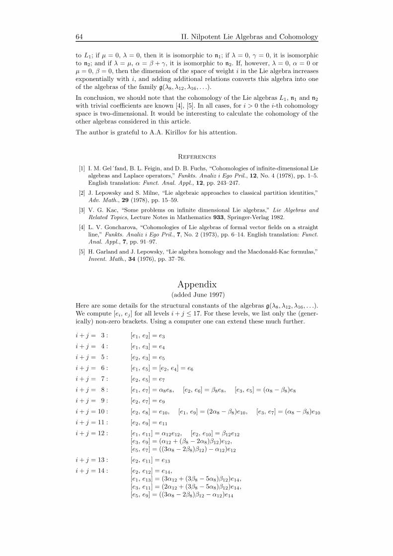
64 II. Nilpotent Lie Algebras and Cohomology
to L1; if µ = 0, λ = 0, then it is isomorphic to n1; if λ = 0, γ = 0, it is isomorphicto n2; and if λ = µ, α = β + γ, it is isomorphic to n2. If, however, λ = 0, α = 0 orµ = 0, β = 0, then the dimension of the space of weight i in the Lie algebra increasesexponentially with i, and adding additional relations converts this algebra into oneof the algebras of the family g(λ8, λ12, λ16, . . .).
In conclusion, we should note that the cohomology of the Lie algebras L1, n1 and n2with trivial coefficients are known [4], [5]. In all cases, for i > 0 the i-th cohomologyspace is two-dimensional. It would be interesting to calculate the cohomology of theother algebras considered in this article.
The author is grateful to A.A. Kirillov for his attention.
References
[1] I. M. Gel´fand, B. L. Feigin, and D. B. Fuchs, “Cohomologies of infinite-dimensional Liealgebras and Laplace operators,” Funkts. Analiz i Ego Pril., 12, No. 4 (1978), pp. 1–5.English translation: Funct. Anal. Appl., 12, pp. 243–247.
[2] J. Lepowsky and S. Milne, “Lie algebraic approaches to classical partition identities,”Adv. Math., 29 (1978), pp. 15–59.
[3] V. G. Kac, “Some problems on infinite dimensional Lie algebras,” Lie Algebras andRelated Topics, Lecture Notes in Mathematics 933, Springer-Verlag 1982.
[4] L. V. Goncharova, “Cohomologies of Lie algebras of formal vector fields on a straightline,” Funkts. Analiz i Ego Pril., 7, No. 2 (1973), pp. 6–14. English translation: Funct.Anal. Appl., 7, pp. 91–97.
[5] H. Garland and J. Lepowsky, “Lie algebra homology and the Macdonald-Kac formulas,”Invent. Math., 34 (1976), pp. 37–76.
Appendix(added June 1997)
Here are some details for the structural constants of the algebras g(λ8, λ12, λ16, . . .).We compute [ei, ej ] for all levels i+ j ≤ 17. For these levels, we list only the (gener-ically) non-zero brackets. Using a computer one can extend these much further.
i+ j = 3 : [e1, e2] = e3
i+ j = 4 : [e1, e3] = e4
i+ j = 5 : [e2, e3] = e5
i+ j = 6 : [e1, e5] = [e2, e4] = e6
i+ j = 7 : [e2, e5] = e7
i+ j = 8 : [e1, e7] = α8e8, [e2, e6] = β8e8, [e3, e5] = (α8 − β8)e8i+ j = 9 : [e2, e7] = e9
i+ j = 10 : [e2, e8] = e10, [e1, e9] = (2α8 − β8)e10, [e3, e7] = (α8 − β8)e10i+ j = 11 : [e2, e9] = e11
i+ j = 12 : [e1, e11] = α12e12, [e2, e10] = β12e12[e3, e9] = (α12 + (β8 − 2α8)β12)e12,[e5, e7] = ((3α8 − 2β8)β12)− α12)e12
i+ j = 13 : [e2, e11] = e13
i+ j = 14 : [e2, e12] = e14,[e1, e13] = (3α12 + (3β8 − 5α8)β12)e14,[e3, e11] = (2α12 + (3β8 − 5α8)β12)e14,[e5, e9] = ((3α8 − 2β8)β12 − α12)e14
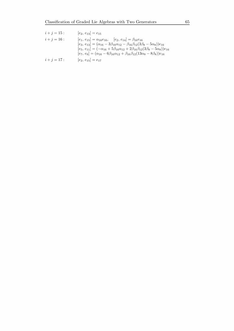
Classification of Graded Lie Algebras with Two Generators 65
i+ j = 15 : [e2, e13] = e15
i+ j = 16 : [e1, e15] = α16e16, [e2, e14] = β16e16[e3, e13] = (α16 − 3β16α12 − β16β12(3β8 − 5α8))e16[e5, e11] = (−α16 + 5β16α12 + 2β16β12(3β8 − 5α8))e16[e7, e9] = (α16 − 6β16α12 + β16β12(13α8 − 8β8))e16
i+ j = 17 : [e2, e15] = e17

appeared in: Studia Sci. Math. Hungar. 19 (1984), 465–483
Deformations of Nilpotent Kac–Moody Algebras
Alice FialowskiAlfred Renyi Institute of Mathematics
Budapest
The main goal of this article is the calculation of the one and two-dimensional co-homology of maximal nilpotent subalgebras of affine Kac–Moody type Lie algebras.This calculation allows us to classify the exterior derivations and deformations of theindicated algebras.The article consists of two sections: The first section contains basic definitions andstatements of the results, while the second one contains the proofs.‡
The author would like to thank Professor D. Fuchs for stimulating discussions andfriendly help.
1. 1. Definitions and the statements of the results
1. Let A = ‖aij‖ be an integer n×n matrix with a11 = · · · = ann = 2 and aij ≦ 0 fori 6= j. Suppose that A is symmetrisable, i.e. there exist positive numbers 1, . . . , nsuch that the matrix ‖iaij‖ = A is symmetric. From now on 1, . . . , n denote theminimal positive integers with the property above. Define the Kac–Moody Lie algebragA with the Cartan matrix A as a complex Lie algebra with the generators e1, . . . , en,f1, . . . , fn, h1, . . . , hn and the relations
[ei, fj] = δijhj , [hi, hj ] = 0,
[hi, ej] = aijej , [hi, fj ] = −aijfj ,[ei, [ei, . . . , [ei︸ ︷︷ ︸−aij+1
, ej ] . . . ]]= 0,
[fi, [fi, . . . , [fi︸ ︷︷ ︸−aij+1
, fj ] . . . ]]= 0 (i 6= j).
Define in gA a (multi-) gradation by
deg h = (0, . . . , 0︸ ︷︷ ︸n
), deg ei = (i
0, . . . , 0, 1, 0, . . . , 0︸ ︷︷ ︸n
),
deg fi = (0, . . . , 0,−i1, 0, . . . , 0︸ ︷︷ ︸).
Here n is called the rank of gA.
Suppose that A is nondecomposable, i.e. it can not become of the form
(A1 00 A2
)
under any simultaneous permutation of rows and columns.The Weyl group W = WA of gA is defined as the subgroup of GL(n,Z), generatedby the matrices σi = E − Ai where E is the unity and in Ai the ith row coincideswith the ith row of A, while the other rows are zeros. (The elements of W may beconsidered as transformations of the “weight lattice” Zn, which grades gA.)Remind some facts about the Kac–Moody Lie algebras (see [1], [2], [3]).(i) gA = n+(A) + h + n−(A), where n+(A) and n−(A) are subalgebras of gA, gener-ated by e1, . . . , en and f1 . . . , fn respectively, while h is n-dimensional (commutative)subalgebra, spanned by h1, . . . , hn.(ii) The defining relation system for the generators e1, . . . , en of n+(A) consists of[
ei, [ei, . . . , [ei︸ ︷︷ ︸−aij+1
, ej ] . . . ]]= 0.
∗1980 Mathematics Subject Classification. Primary 17B56; Secondary 17B65.‡Key words: Deformation, cohomology, Kac–Moody algebras, spectral sequence.‡For another proof of a part of these results see in [7].
66
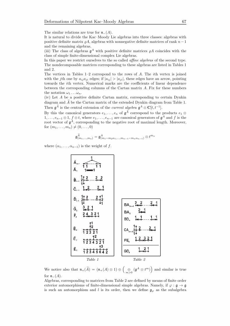
Deformations of Nilpotent Kac–Moody Algebras 67
The similar relations are true for n−(A).It is natural to divide the Kac–Moody Lie algebras into three classes: algebras withpositive definite matrix A, algebras with nonnegative definite matrices of rank n− 1and the remaining algebras.(iii) The class of algebras gA with positive definite matrices A coincides with theclass of simple finite-dimensional complex Lie algebras.In this paper we restrict ourselves to the so called affine algebras of the second type.The nondecomposable matrices corresponding to these algebras are listed in Tables 1and 2.The vertices in Tables 1–2 correspond to the rows of A. The ith vertex is joinedwith the jth one by aijaji edges; if |aij | > |aji|, these edges have an arrow, pointingtowards the ith vertex. Numerical marks are the coefficients of linear dependencebetween the corresponding columns of the Cartan matrix A. Fix for these numbersthe notation ω1 . . . ωn.(iv) Let A be a positive definite Cartan matrix, corresponding to certain Dynkin
diagram and A be the Cartan matrix of the extended Dynkin diagram from Table 1.
Then gA is the central extension of the current algebra gA ⊗C[t, t−1].
By this the canonical generators e1, . . . , en of gA correspond to the products e1 ⊗1, . . . , en−1 ⊗ 1, f ⊗ t, where e1, . . . , en−1 are canonical generators of gA and f is theroot vector of gA, corresponding to the negative root of maximal length. Moreover,for (m1, . . . ,mn) 6= (0, . . . , 0)
gA(m1,...,mn)= gA(m1−m2α1,...,mn−1−mnαn−1)
⊗ tmn
where (α1, . . . , αn−1) is the weight of f .
Table 1 Table 2
We notice also that n+(A) = (n+(A) ⊗ 1) ⊕(⊕m>0
(gA ⊗ tm))
and similar is true
for n−(A).Algebras, corresponding to matrices from Table 2 are defined by means of finite orderexterior automorphisms of finite-dimensional simple algebras. Namely, if ϕ : g → g
is such an automorphism and l is its order, then we define gϕ as the subalgebra
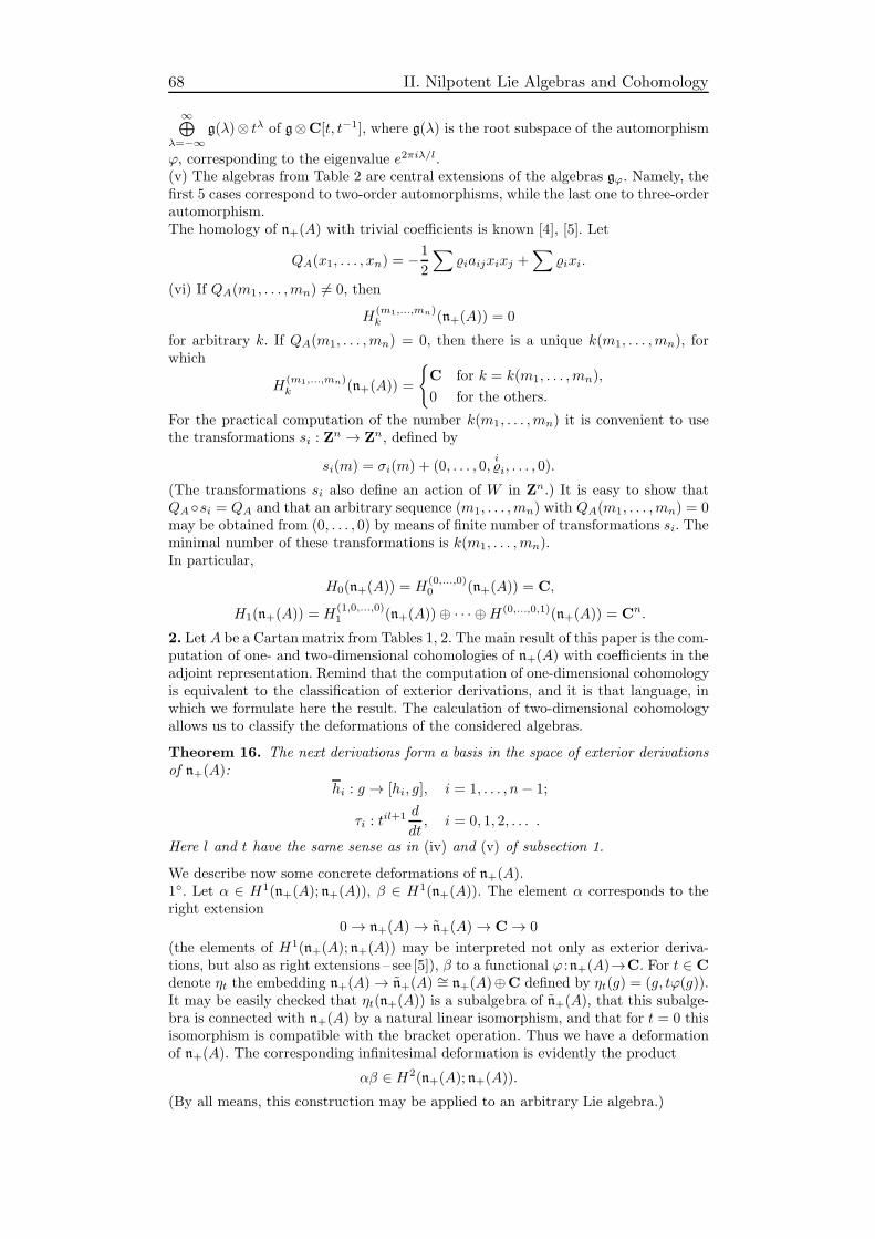
68 II. Nilpotent Lie Algebras and Cohomology
∞⊕λ=−∞
g(λ)⊗ tλ of g⊗C[t, t−1], where g(λ) is the root subspace of the automorphism
ϕ, corresponding to the eigenvalue e2πiλ/l.(v) The algebras from Table 2 are central extensions of the algebras gϕ. Namely, thefirst 5 cases correspond to two-order automorphisms, while the last one to three-orderautomorphism.The homology of n+(A) with trivial coefficients is known [4], [5]. Let
QA(x1, . . . , xn) = −1
2
∑iaijxixj +
∑ixi.
(vi) If QA(m1, . . . ,mn) 6= 0, then
H(m1,...,mn)k (n+(A)) = 0
for arbitrary k. If QA(m1, . . . ,mn) = 0, then there is a unique k(m1, . . . ,mn), forwhich
H(m1,...,mn)k (n+(A)) =
C for k = k(m1, . . . ,mn),
0 for the others.
For the practical computation of the number k(m1, . . . ,mn) it is convenient to usethe transformations si : Z
n → Zn, defined by
si(m) = σi(m) + (0, . . . , 0,ii, . . . , 0).
(The transformations si also define an action of W in Zn.) It is easy to show thatQAsi = QA and that an arbitrary sequence (m1, . . . ,mn) with QA(m1, . . . ,mn) = 0may be obtained from (0, . . . , 0) by means of finite number of transformations si. Theminimal number of these transformations is k(m1, . . . ,mn).In particular,
H0(n+(A)) = H(0,...,0)0 (n+(A)) = C,
H1(n+(A)) = H(1,0,...,0)1 (n+(A))⊕ · · · ⊕H(0,...,0,1)(n+(A)) = Cn.
2. Let A be a Cartan matrix from Tables 1, 2. The main result of this paper is the com-putation of one- and two-dimensional cohomologies of n+(A) with coefficients in theadjoint representation. Remind that the computation of one-dimensional cohomologyis equivalent to the classification of exterior derivations, and it is that language, inwhich we formulate here the result. The calculation of two-dimensional cohomologyallows us to classify the deformations of the considered algebras.
Theorem 16. The next derivations form a basis in the space of exterior derivationsof n+(A):
hi : g → [hi, g], i = 1, . . . , n− 1;
τi : til+1 d
dt, i = 0, 1, 2, . . . .
Here l and t have the same sense as in (iv) and (v) of subsection 1.
We describe now some concrete deformations of n+(A).1. Let α ∈ H1(n+(A); n+(A)), β ∈ H1(n+(A)). The element α corresponds to theright extension
0→ n+(A)→ n+(A)→ C→ 0
(the elements of H1(n+(A); n+(A)) may be interpreted not only as exterior deriva-tions, but also as right extensions – see [5]), β to a functional ϕ :n+(A)→C. For t ∈ Cdenote ηt the embedding n+(A)→ n+(A) ∼= n+(A)⊕C defined by ηt(g) = (g, tϕ(g)).It may be easily checked that ηt(n+(A)) is a subalgebra of n+(A), that this subalge-bra is connected with n+(A) by a natural linear isomorphism, and that for t = 0 thisisomorphism is compatible with the bracket operation. Thus we have a deformationof n+(A). The corresponding infinitesimal deformation is evidently the product
αβ ∈ H2(n+(A); n+(A)).
(By all means, this construction may be applied to an arbitrary Lie algebra.)
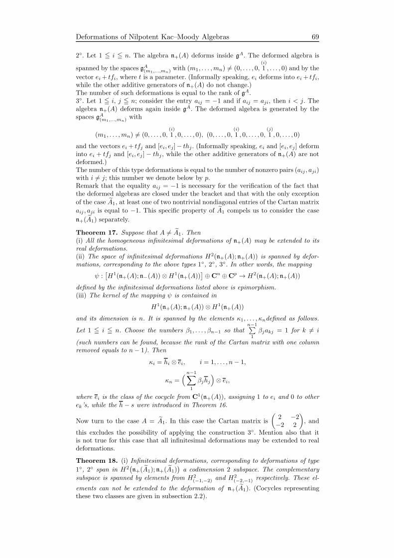
Deformations of Nilpotent Kac–Moody Algebras 69
2. Let 1 ≦ i ≦ n. The algebra n+(A) deforms inside gA. The deformed algebra is
spanned by the spaces gA(m1,...,mn)with (m1, . . . ,mn) 6= (0, . . . , 0,
(i)
1 , . . . , 0) and by the
vector ei+ tfi, where t is a parameter. (Informally speaking, ei deforms into ei+ tfi,while the other additive generators of n+(A) do not change.)The number of such deformations is equal to the rank of gA.3. Let 1 ≦ i, j ≦ n; consider the entry aij = −1 and if aij = aji, then i < j. Thealgebra n+(A) deforms again inside gA. The deformed algebra is generated by thespaces gA(m1,...,mn)
with
(m1, . . . ,mn) 6= (0, . . . , 0,(i)
1 , 0, . . . , 0), (0, . . . , 0,(i)
1 , 0, . . . , 0,(j)
1 , 0, . . . , 0)
and the vectors ei+ tfj and [ei, ej]− thj . (Informally speaking, ei and [ei, ej ] deforminto ei + tfj and [ei, ej] − thj , while the other additive generators of n+(A) are notdeformed.)The number of this type deformations is equal to the number of nonzero pairs (aij , aji)with i 6= j; this number we denote below by p.Remark that the equality aij = −1 is necessary for the verification of the fact thatthe deformed algebras are closed under the bracket and that with the only exception
of the case A1, at least one of two nontrivial nondiagonal entries of the Cartan matrix
aij , aji is equal to −1. This specific property of A1 compels us to consider the case
n+(A1) separately.
Theorem 17. Suppose that A 6= A1. Then(i) All the homogeneous infinitesimal deformations of n+(A) may be extended to itsreal deformations.(ii) The space of infinitesimal deformations H2(n+(A); n+(A)) is spanned by defor-mations, corresponding to the above types 1, 2, 3. In other words, the mapping
ψ :[H1(n+(A); n−(A))⊗H1(n+(A))
]⊕Cn ⊕Cp → H2(n+(A); n+(A))
defined by the infinitesimal deformations listed above is epimorphism.(iii) The kernel of the mapping ψ is contained in
H1(n+(A); n+(A))⊗H1(n+(A))
and its dimension is n. It is spanned by the elements κ1, . . . , κndefined as follows.
Let 1 ≦ i ≦ n. Choose the numbers β1, . . . , βn−1 so thatn−1∑1βjakj = 1 for k 6= i
(such numbers can be found, because the rank of the Cartan matrix with one columnremoved equals to n− 1). Then
κi = hi ⊗ ei, i = 1, . . . , n− 1,
κn =( n−1∑
1
βjhj
)⊗ ei,
where ei is the class of the cocycle from C1(n+(A)), assigning 1 to ei and 0 to otherek’s, while the h− s were introduced in Theorem 16.
Now turn to the case A = A1. In this case the Cartan matrix is
(2 −2−2 2
), and
this excludes the possibility of applying the construction 3. Mention also that itis not true for this case that all infinitesimal deformations may be extended to realdeformations.
Theorem 18. (i) Infinitesimal deformations, corresponding to deformations of type
1, 2 span in H2(n+(A1); n+(A1)
)a codimension 2 subspace. The complementary
subspace is spanned by elements from H2(−1,−2) and H2
(−2,−1) respectively. These el-
ements can not be extended to the deformation of n+(A1). (Cocycles representingthese two classes are given in subsection 2.2).
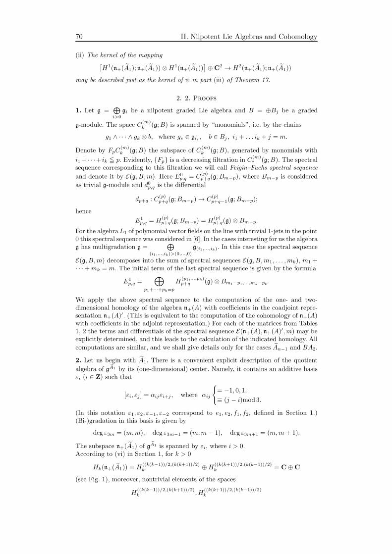
70 II. Nilpotent Lie Algebras and Cohomology
(ii) The kernel of the mapping[H1(n+(A1); n+(A1))⊗H1(n+(A1))
]⊕C2 → H2(n+(A1); n+(A1))
may be described just as the kernel of ψ in part (iii) of Theorem 17.
2. 2. Proofs
1. Let g =⊕i>0
gi be a nilpotent graded Lie algebra and B = ⊕Bj be a graded
g-module. The space C(m)k (g;B) is spanned by “monomials”, i.e. by the chains
g1 ∧ · · · ∧ gk ⊗ b, where gs ∈ gis , b ∈ Bj , i1 + . . . ik + j = m.
Denote by FpC(m)k (g;B) the subspace of C
(m)k (g;B), generated by monomials with
i1+ · · ·+ ik ≦ p. Evidently, Fp is a decreasing filtration in C(m)∗ (g;B). The spectral
sequence corresponding to this filtration we will call Feigin–Fuchs spectral sequence
and denote it by E(g, B,m). Here E0p,q = C
(p)p+q(g;Bm−p), where Bm−p is considered
as trivial g-module and d0p,q is the differential
dp+q : C(p)p+q(g;Bm−p)→ C
(p)p+q−1(g;Bm−p);
hence
E1p,q = H
(p)p+q(g;Bm−p) = H
(p)p+q(g)⊗Bm−p.
For the algebra L1 of polynomial vector fields on the line with trivial 1-jets in the point0 this spectral sequence was considered in [6]. In the cases interesting for us the algebrag has multigradation g =
⊕(i1,...,ik)>(0,...,0)
g(i1,...,ik). In this case the spectral sequence
E(g, B,m) decomposes into the sum of spectral sequences E(g, B,m1, . . . ,mk), m1 +· · ·+mk = m. The initial term of the last spectral sequence is given by the formula
E1p,q =
⊕
p1+···+pk=pH
(p1,...,pk)p+q (g)⊗Bm1−p1,...,mk−pk .
We apply the above spectral sequence to the computation of the one- and two-dimensional homology of the algebra n+(A) with coefficients in the coadjoint repre-sentation n+(A)
′. (This is equivalent to the computation of the cohomology of n+(A)with coefficients in the adjoint representation.) For each of the matrices from Tables1, 2 the terms and differentials of the spectral sequence E(n+(A), n+(A)′,m) may beexplicitly determined, and this leads to the calculation of the indicated homology. All
computations are similar, and we shall give details only for the cases An−1 and BA2.
2. Let us begin with A1. There is a convenient explicit description of the quotient
algebra of gA1 by its (one-dimensional) center. Namely, it contains an additive basisεi (i ∈ Z) such that
[εi, εj ] = αijεi+j , where αij
= −1, 0, 1,≡ (j − i)mod3.
(In this notation ε1, ε2, ε−1, ε−2 correspond to e1, e2, f1, f2, defined in Section 1.)(Bi-)gradation in this basis is given by
deg ε3m = (m,m), deg ε3m−1 = (m,m− 1), deg ε3m+1 = (m,m+ 1).
The subspace n+(A1) of gA1 is spanned by εi, where i > 0.
According to (vi) in Section 1, for k > 0
Hk(n+(A1)) = H((k(k−1))/2,(k(k+1))/2)k ⊕H((k(k+1))/2,(k(k−1))/2)
k = C⊕C
(see Fig. 1), moreover, nontrivial elements of the spaces
H((k(k−1))/2,(k(k+1))/2)k , H
((k(k+1))/2,(k(k−1))/2)k
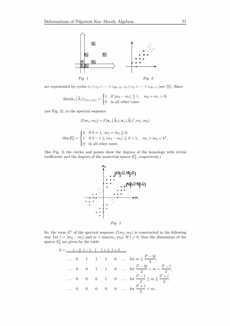
Deformations of Nilpotent Kac–Moody Algebras 71
Fig. 1 Fig. 2
are represented by cycles ε1 ∧ ε4 ∧ · · · ∧ ε3k−2, ε2 ∧ ε5 ∧ · · · ∧ ε3k−1 (see [5]). Since
dim(n+(A1))(m1,m2) =
1 if |m2 −m1| ≦ 1, m2 +m1 > 0,
0 in all other cases
(see Fig. 2), in the spectral sequence
E(m1,m2) = E(n+(A1), n+(A1)′,m1,m2)
dimE1k =
2 if k = 1, m1 = m2 ≦ 0,
1 if k − 1 ≦ |m2 −m1| ≦ k + 1, m1 +m2 < k2,
0 in all other cases.
(See Fig. 3; the circles and points show the degrees of the homology with trivialcoefficients and the degrees of the nontrivial spaces E1
k, respectively.)
Fig. 3
So, the term E1 of the spectral sequence E(m1,m2) is constructed in the followingway. Let l = |m2 −m1| and m = min(m1,m2). If l > 0, then the dimensions of thespaces E1
k are given by the table
k = . . . l − 2 l − 1 l l + 1 l + 2 . . .
. . . 0 1 1 1 0 . . . for m ≦l2 − 3l
2,
. . . 0 0 1 1 0 . . . forl2 − 3l
2< m <
l2 − l2
,
. . . 0 0 0 1 0 . . . forl2 − l2
≦ m ≦l2 + l
2,
. . . 0 0 0 0 0 . . . forl2 + l
2< m,

72 II. Nilpotent Lie Algebras and Cohomology
and if l = 0, then by the table
k = 0 1 2 . . .
1 2 0 . . . for m < 0
0 2 0 . . . for m = 0
0 0 0 . . . for m > 0.
Lemma. The non-trivial differentials d1k are the following ones:
d1l : E1l → E1
l−1, if l 6= 0, m ≦l2 − 3l
2,
d11 : E11 → E1
0 , if l = 0, m < 0;
the differentials drk with r > 1 are all trivial.
From this lemma it follows
Proposition 2.1.
H0(n+(A1); n+(A1)′) = 0;
dimH(m1,m2)1 (n+(A1); n+(A1)
′) =
2 if m1 = m2 = 0,
1 if m1 = m2 < 0,
0 in the other cases;
if k > 1, then
dimH(m1,m2)1 )(n+(A1); n+(Ai)
′) =
=
1 if |m1 −m2| = k − 1, m1 +m2 < k2 − 1
and if |m1 −m2| = k, (k − 1)2 < m1 +m2 ≦ k2 − 2,
0 in the other cases.
(See Fig. 4, on which the weights of one- and two-dimensional homologies are shown.)
Fig. 4
Lemma may be proved by performing a straight but not particularly short calculation.Since we are interested only in homology of dimension one and two, we give the proofhere only for the cases k ≦ 2. We have to show that the differentials
(i) d11 for m2 = m1 < 0,(ii) d11 for |m2 −m1| = 1, min(m1,m2) ≦ −1,(iii) d12 for m2 −m1| = 2, min(m1,m2) ≦ −1,(iv) d13 for |m2 −m1| = 3, min(m1,m2) ≦ 0
are non-trivial and
(v) d13 for m1 = 2, m2 = 0 and m1 = 0, m2 = 2
is trivial. Since the roles of m1 and m2 are symmetric, we may consider only the casem1 ≦ m2. The differential d
1k in the spectral sequence E(m1,m2) is non-trivial if there
Deformations of Nilpotent Kac–Moody Algebras 73
exists a chain
c ∈ C(m1,m2)k (n+(A1); n+(A1)
′) such that
c = ε1 ∧ · · · ∧ ε3k−2 ⊗ ε′1 + . . .
∂c = µε1 ∧ · · · ∧ ε3k−5 ⊗ ε′j + . . .
where µ 6= 0 and dots in the general case stand for terms of smaller filtration. Wefind such chains for the cases (i)–(iv), putting m = −m2.
(i) c = ε1 ⊗ ε′3m+1; ∂c = ε′3m,(ii) c = ε1 ⊗ ε′3m; ∂c = −ε′3m−1,(iii) c = ε1 ∧ ε4 ⊗ ε′3m − ε1 ∧ ε3 ⊗ ε′3m−1; ∂c = 2ε1 ⊗ ε′3m−4,(iv) c = ε1∧ε4∧ε7⊗ε′3m−
1
2ε1∧ε3∧ε7⊗ε′3m−1−
1
2ε1∧ε4∧ε6∧⊗ε′3m−1+
+3
2ε1 ∧ ε3 ∧ ε4 ⊗ ε′3m−4; ∂c = −ε1 ∧ ε4 ⊗ ε′3m−7.
The differential d1k is trivial, if there is a chain c of the above form, for which ∂c = 0.For the case (v) such a chain is the following:
(v)c = ε1 ∧ ε4 ∧ ε7 ⊗ ε′10 +
1
2ε1 ∧ ε3 ∧ ε7 ⊗ ε′9 +
1
2ε1 ∧ ε4 ∧ ε6 ⊗ ε′9−
−1
2ε1 ∧ ε3 ∧ ε6 ⊗ ε′8 − ε1 ∧ ε3 ∧ ε4 ⊗ ε′6 − ε1 ∧ ε2 ∧ ε4 ⊗ ε′5.
Now we describe cycles, representing bases in Hk(n+(A1); n+(A1)′) for k = 1, 2.
In C(0,0)1 : ε1 ⊗ ε′1, ε2 ⊗ ε′2.
In C(m,m)1 , m < 0: ε1 ⊗ ε′−3m+1 + ε2 ⊗ ε′−3m+2.
In C(0,2)2 : ε1 ∧ ε4 ⊗ ε′3 − ε1 ∧ ε3 ⊗ ε′2.
In C(1,2)2 : ε1 ∧ ε4 ⊗ ε′1.
In C(m,m+1)2 , m ≦ 0 : ε1 ∧ ε4 ⊗ ε′−3m+4 + ε1 ∧ ε3 ⊗ ε′−3m+3 + ε1 ∧ ε2 ⊗ ε′−3m+2.
Cycles in C(2,0)2 , C
(m+1,m)2 are given similarly, by substituting ε1 ↔ ε2, ε4 ↔ ε5, . . . .
Since dimHk(m1,m2)
= dimH(−m1,−m2)k , the cohomology needed for us is completely
computed. It is easy to see that the above result agrees with the corresponding partsof Theorems 1, 3.Cocycles, representing basis elements of the cohomology spaces are indicated in thenext table.
weight cocycle
(0,−2) (ε1, ε3j 7→ ε3j−1, (ε1, ε3j+1) 7→ −ε3j for j > 0,the rest 7→ 0.
(−2, 0) (ε2, ε3j) 7→ ε3j−2, (ε2, ε3j+2) 7→ −ε3j for j > 0,the rest 7→ 0.
(m,m− 1) (ε1, εj) 7→ jεj+3m for j 6= 1,m ≧ 0 the rest 7→ 0.
(m− 1,m) (ε2, εj) 7→ jεj+3m for j 6= 1,m ≧ 0 the rest 7→ 0.
(ε1, ε4) 7→ 9ε1, (ε1, εj) 7→ jεj−3 for j ≧ 5,(−1,−2) (ε3, ε3j) 7→ 2ε3j−1, (ε3, ε3j−2) 7→ −2ε3j−3 for j ≧ 2,
(ε4, ε3j−1) 7→ 5ε3j−1, (ε4, ε3j+4) 7→ −5ε3j+4 for j ≧ 1,the rest 7→ 0.
(ε2, ε5) 7→ 9ε2, (ε2, εj) 7→ jεj−3 for j = 4, 6, 7, . . . ,(−2,−1) (ε3, ε3j) 7→ ε3j−2, (ε3, ε3j+2) 7→ −ε3j for j ≧ 1,
(ε5, ε3j−2) 7→ 4ε3j−2, (ε5, ε3j+5) 7→ −4ε3j+5 for j ≧ 1,the rest 7→ 0.
We can easily verify that the indicated cochains are really cocycles and they do notvanish on the above cycles.It remained to show that infinitesimal deformations, determined by two-dimensionalcocycles of weight (0,−2), (−2, 0) and (m + 1,m), (m,m + 1) with m ≧ −1 can be
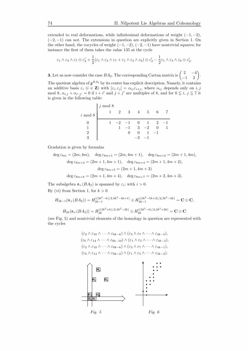
74 II. Nilpotent Lie Algebras and Cohomology
extended to real deformations, while infinitesimal deformations of weight (−1,−2),(−2,−1) can not. The extensions in question are explicitly given in Section 1. Onthe other hand, the cocycles of weight (−1,−2), (−2,−1) have nontrivial squares; forinstance the first of them takes the value 135 at the cycle
ε1 ∧ ε4 ∧ ε7 ⊗ ε′4 +1
2(ε1 ∧ ε3 ∧ ε7 + ε1 ∧ ε4 ∧ ε6)⊗ ε′3 −
1
2ε1 ∧ ε3 ∧ ε6 ⊗ ε′2.
3. Let us now consider the case BA2. The corresponding Cartan matrix is
(2 −4−1 2
).
The quotient algebra of gBA2 by its center has explicit description. Namely, it containsan additive basis εi (i ∈ Z) with [εi, εj ] = αijεi+j , where αij depends only on i, jmod 8, αi,j + αi′,j′ = 0 if i + i′ and j + j′ are multiples of 8, and for 0 ≦ i, j ≦ 7 itis given in the following table:
j mod 8
1 2 3 4 5 6 7i mod 8
0 1 −2 −1 0 1 2 −11 1 −1 3 −2 0 12 0 0 1 −13 −3 −1
Gradation is given by formulas
deg ε8m = (2m, 4m), deg ε8m+1 = (2m, 4m+ 1), deg ε8m+2 = (2m+ 1, 4m),
deg ε8m+3 = (2m+ 1, 4m+ 1), deg ε8m+4 = (2m+ 1, 4m+ 2),
deg ε8m+5 = (2m+ 1, 4m+ 3)
deg ε8m+6 = (2m+ 1, 4m+ 4), deg ε8m+7 = (2m+ 2, 4m+ 3).
The subalgebra n+(BA2) is spanned by εi; with i > 0.
By (vi) from Section 1, for k > 0
H2k−1(n+(BA2)) = H((3k2−k)/2,3k2−4k+1)2k−1 ⊕H((3k2−5k+2)/2,3k2−2k)
2k−1 = C⊕C,
H2k(n+(BA2)) = H((3k2+k)/2,3k2−2k)2k ⊕H((3k2−k)/2,3k2+2k)
2k = C⊕C
(see Fig. 5) and nontrivial elements of the homology in question are represented withthe cycles
(ε2 ∧ ε10 ∧ · · · ∧ ε8k−6) ∧ (ε3 ∧ ε7 ∧ · · · ∧ ε4k−5),(ε6 ∧ ε14 ∧ · · · ∧ ε8k−10) ∧ (ε1 ∧ ε5 ∧ · · · ∧ ε4k−3),(ε2 ∧ ε10 ∧ · · · ∧ ε8k−6) ∧ (ε3 ∧ ε7 ∧ · · · ∧ ε4k−1),(ε6 ∧ ε14 ∧ · · · ∧ ε8k−2) ∧ (ε1 ∧ ε5 ∧ · · · ∧ ε4k−3).
Fig. 5 Fig. 6
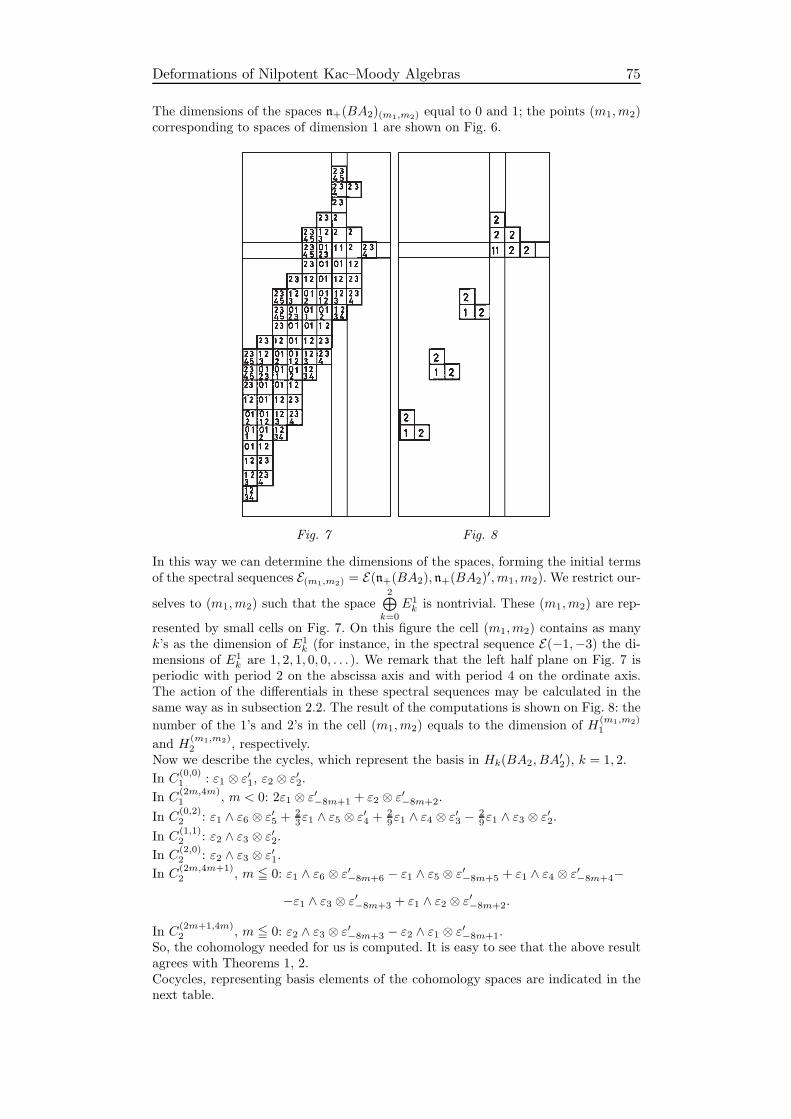
Deformations of Nilpotent Kac–Moody Algebras 75
The dimensions of the spaces n+(BA2)(m1,m2) equal to 0 and 1; the points (m1,m2)corresponding to spaces of dimension 1 are shown on Fig. 6.
Fig. 7 Fig. 8
In this way we can determine the dimensions of the spaces, forming the initial termsof the spectral sequences E(m1,m2) = E(n+(BA2), n+(BA2)
′,m1,m2). We restrict our-
selves to (m1,m2) such that the space2⊕
k=0
E1k is nontrivial. These (m1,m2) are rep-
resented by small cells on Fig. 7. On this figure the cell (m1,m2) contains as manyk’s as the dimension of E1
k (for instance, in the spectral sequence E(−1,−3) the di-mensions of E1
k are 1, 2, 1, 0, 0, . . . ). We remark that the left half plane on Fig. 7 isperiodic with period 2 on the abscissa axis and with period 4 on the ordinate axis.The action of the differentials in these spectral sequences may be calculated in thesame way as in subsection 2.2. The result of the computations is shown on Fig. 8: the
number of the 1’s and 2’s in the cell (m1,m2) equals to the dimension of H(m1,m2)1
and H(m1,m2)2 , respectively.
Now we describe the cycles, which represent the basis in Hk(BA2, BA′2), k = 1, 2.
In C(0,0)1 : ε1 ⊗ ε′1, ε2 ⊗ ε′2.
In C(2m,4m)1 , m < 0: 2ε1 ⊗ ε′−8m+1 + ε2 ⊗ ε′−8m+2.
In C(0,2)2 : ε1 ∧ ε6 ⊗ ε′5 + 2
3ε1 ∧ ε5 ⊗ ε′4 + 29ε1 ∧ ε4 ⊗ ε′3 − 2
9ε1 ∧ ε3 ⊗ ε′2.In C
(1,1)2 : ε2 ∧ ε3 ⊗ ε′2.
In C(2,0)2 : ε2 ∧ ε3 ⊗ ε′1.
In C(2m,4m+1)2 , m ≦ 0: ε1 ∧ ε6 ⊗ ε′−8m+6 − ε1 ∧ ε5 ⊗ ε′−8m+5 + ε1 ∧ ε4 ⊗ ε′−8m+4−
−ε1 ∧ ε3 ⊗ ε′−8m+3 + ε1 ∧ ε2 ⊗ ε′−8m+2.
In C(2m+1,4m)2 , m ≦ 0: ε2 ∧ ε3 ⊗ ε′−8m+3 − ε2 ∧ ε1 ⊗ ε′−8m+1.
So, the cohomology needed for us is computed. It is easy to see that the above resultagrees with Theorems 1, 2.Cocycles, representing basis elements of the cohomology spaces are indicated in thenext table.
76 II. Nilpotent Lie Algebras and Cohomology
weight cocycle
(ε1, ε8j 7→ −ε8j−1, (ε1, ε8j+1) 7→ −ε8j (j ≧ 0),(0,−2) (ε1, ε8j+3) 7→ −2ε8j+2, (ε1, ε8j+4) 7→ 3ε8j+3
j ≧ 0
(ε1, ε8j+5) 7→ −ε8j+4, (ε1, ε8j+6) 7→ ε8j+5
the rest 7→ 0.(ε1, ε8j−1) 7→ ε8j−3, (ε1, ε8j) 7→ −2ε8j−2(ε1, ε8j+2) 7→ ε8j , (ε1, ε8j+3) 7→ −ε8j+1
j ≧ 1
(−1,−1) (ε3, εj+1) 7→ ε8j+1
(ε3, ε8j+2) 7→ −2ε8j+2, (ε3, ε8j+5) 7→ ε8j+5j ≧ 0
(ε3, ε8j+6) 7→ 2ε8j+6, (ε3, ε8j+7) 7→ −ε8j+7
(ε1, ε3) 7→ −2ε1, the rest 7→ 0.(ε2, ε8j) 7→ 2ε8j−2, (ε2, ε8j+2) 7→ −ε8j (j ≧ 1)
(−2, 0) (ε2, ε8j+3) 7→ ε8j+1, (ε2, ε8j+7) 7→ −ε8j+5 (j ≧ 0)the rest 7→ 0.
(2m, 4m− 1) (ε1, εj) 7→ jεj+8m for j 6= 1,m ≧ 0 the rest 7→ 0.
(2m− 1, 4m) (ε2, εj) 7→ jεj+8m for j 6= 2,m ≧ 0 the rest 7→ 0.
4. Now consider the case An−1 with n ≧ 3. The case n = 3 is somewhat different fromthe general case (the main difference, from our point of view, is in the structure of thethree-dimensional homology with trivial coefficients). Nevertheless, the final formulais the same, and the differences in the proofs are not essential. Therefore from nowon we shall ignore the specific case n = 3, indirectly assuming that n ≧ 4.
The Cartan matrix of gAn−1 is:
2 −1 0 . . . 0 −1−1 2 −1 . . . 0 00 −1 2 . . . 0 0
. . . . . . . . . . . . . . . . . .0 0 0 . . . 2 −1−1 0 0 . . . −1 2
.
By (vi) in Section 1
dimH(m1,...,mn)∗ (n+(An−1)) =
1, if P (m1, . . . ,mn) = 0,
0 in the other cases,
where P (m1, . . . ,mn) = m21 + · · ·+m2
n − (m1m2 + · · ·+mn−1mn +mnm1)− (m1 +
· · · + mn). In more details, if k = 1, 2, 3 then the space H(m1...,mn)k (n+(An−1)) has
dimension 1 for the following sequences (m1, . . . ,mn):
k = 0 : (0, . . . , 0); k = 1 : (1, 0, . . . , 0);
k = 2 : (2, 1, 0, . . . , 0), (1, 0, . . . , 0︸ ︷︷ ︸>0
, 1, 0, . . . , 0︸ ︷︷ ︸>0
);
k = 3 : (2, 2, 0, . . . , 0), (2, 1, 2, 0, . . . , 0),
(3, 2, 1, 0, . . . , 0), (1, 3, 1, 0, . . . , 0),
(2, 1, 0, . . . , 0︸ ︷︷ ︸>0
, 1, 0, . . . , 0︸ ︷︷ ︸>0
), (1, 0, . . . , 0︸ ︷︷ ︸>0
, 1, 0, . . . , 0︸ ︷︷ ︸>0
, 1, 0, . . . , 0︸ ︷︷ ︸>0
),
and also for the cases, obtained from these by cyclic permutation and reflection; forthe remaining (m1, . . . ,mn) the named homology is 0.Next we give cycles which represent generators of the above homology (εij here andbelow stand for the matrix with 1 in the section of ith row and jth column and 0
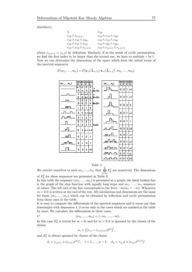
Deformations of Nilpotent Kac–Moody Algebras 77
elsewhere).
1, ε12,ε12 ∧ εi,i+1, ε12 ∧ ε13 ∧ ε23,ε12 ∧ ε13 ∧ ε23, ε12 ∧ ε14 ∧ ε34,ε12 ∧ ε13 ∧ ε14, ε13 ∧ ε23 ∧ ε24,ε12 ∧ ε13 ∧ εi,i+1, ε12 ∧ εi,i+1 ∧ εj,j+1,
where εn,n+1 = εn,1t by definition. Similarly, if as the result of cyclic permutation,we find the first index to be larger than the second one, we have to multiply ε by t.Now we can determine the dimensions of the space which form the initial terms ofthe spectral sequences
E(m1, . . . ,mn) = E(n+(An−1), n+(An−1)′,m1, . . . ,mn).
Table 3
We restrict ourselves to such m1, . . . ,mn that2⊕
k=0
E1k are nontrivial. The dimensions
of E1k for these sequences are presented in Table 3.
In this table the sequence (m1, . . . ,mn) is presented as a graph: the thick broken lineis the graph of the step function with equally long steps and m1, . . . , mn sequenceof values. The left end of the line corresponds to the level −m(m1 = −m). Wheneverm = 0 it is written at the end of the row. All calculations and dimensions are the samefor those (m1, . . . ,mn) which can be obtained by reflection and cyclic permutationfrom those ones in the table.It is easy to compute the differentials of the spectral sequences and it turns out thathomologies with dimension 1, 2 occur only in the cases which are marked in the tableby stars. We calculate the differentials in these cases.
1 (m1, . . . ,mn) = (−m, . . . ,−m).
In this case E10 is trivial for m = 0; and for m > 0 it is spanned by the classes of the
chains
αi =((εi,i − εi+1,i+1)t
m)′,
and E11 is always spanned by classes of the chains
βi = εi,i+1 ⊗ (εi,i+1tm)′, i = 1, . . . , n− 1, βn = εn,1t⊗ (εn,1t
m+1)′.

78 II. Nilpotent Lie Algebras and Cohomology
Evidently, dβi = αi for i = 1, . . . , n− 1 and dβn = −α1 − · · · − αn−1. So,
dimH(−m,...,−m)1 =
1 for m > 0
n for m = 0,H
(−m,...,−m)2 = 0.
One-dimensional cohomologies for m > 0 are spanned by the class of the chain β1 +· · ·+ βn, and for m = 0 by classes of the chains β1, . . . , βn.
2. (m1, . . . ,mn) = (−m, . . . ,−m︸ ︷︷ ︸i−1
,−m+ 1,−m, . . . ,−m), 1 ≦ i ≦ n.
In this case E10 is trivial for m = 0, and for m > 0 it is spanned by the class of the
chain
α = (εi+1,itm)′;
E11 is trivial for m = 0, and for m > 0 it is spanned by the classes of the chains
βj = εi,i+1 ⊗((εj,j − εj+1,j+1)t
m)′, j = 1, . . . , n− 1;
E12 is always spanned by the classes of the chains
γj = εi,i+1 ∧ εj,j+1 ⊗ (εj,j+1tm)′, j = 1, . . . , i− 2, i+ 2, . . . , n− 1
γn = εi,i+1 ∧ εn,1t⊗ (εn,1tm+1)′,
γi−1 = εi−1,i+1 ∧ εi,i+1 ⊗ (εi−1,i+1tm)′,
γi+1 = εi,i+1 ∧ εi,i+2 ⊗ (εi,i+2tm)′
(γi is absent). The differential d = d1 acts by
dβj =
−2α for j = i
α for j = i± 1,
0 in the other cases;
dγj =
βj for j 6= i, i± 1,
−β1 − · · · − βn−1 for j = n,
−2βi−1 − βi for j = i− 1,
βi + 2βi+1 for j = i+ 1.
So,
H(−m,...,−m+1,...,−m)1 = 0,
dimH(−m,...,−m+1,...,−m)2 =
1 for m > 0
n− 1 for m = 0.
The two-dimensional homologies for m > 0 are spanned by the class of the cycle
γ1 + · · ·+ γi−2 +1
2γi−1 +
1
2γi+1 + γi+2 + · · ·+ γn, while for m = 0 by the classes of
the cycles γ1, . . . , γi−1, γi+1, . . . , γn.
3. (m1, . . . ,mn) = (0, . . . , 0︸ ︷︷ ︸i−1
, 1, 1, 0, . . . , 0), 1 ≦ i ≦ n− 1.
In this case E10 = E1
1 = 0, E12 is spanned by the classes of the chains
γ1 = εi,i+1 ∧ εi,i+2 ⊗ (εi,i+1)′, γ2 = εi,i+2 ∧ εi+1,i+2 ⊗ (εi+1,i+2)
′,
E13 is spanned by the class of
δ = εi,i+1 ∧ εi,i+2 ∧ εi+1,i+2 ⊗ (εi,i+2)′;
the differential acts by dδ = γ1 − γ2. That means,
H(0,...,0,1,1,0,...,0)1 = 0
dimH(0,...,0,1,1,0,...,0)2 = 1.
The two-dimensional homologies are spanned by the class of γ1 (or γ2).The case (m1, . . . ,mn) = (1, 0, . . . , 0, 1) is similar to the above one.
Deformations of Nilpotent Kac–Moody Algebras 79
4. (m1, . . . ,mn) = (0, . . . , 0︸ ︷︷ ︸i−1
, 2, 0, . . . , 0), 1 ≦ i ≦ n.
In this case E10 = E1
1 = 0, E12 is spanned by the classes of
γi = εi,i+1 ∧ εi,i+2 ⊗ (εi+1,i+2)′, γ2 = εi−1,i+1 ∧ εi,i+1 ⊗ (εi−1,i)
′,
E13 is spanned by the class of the chain
δ = εi−1,i+1 ∧ εi,i+1 ∧ εi,i+2 ⊗ (εi−1,i+2)′;
the differential acts by dδ = γ1 − γ2. That means,
H(0,...,0,2,0,...,0)1 = 0,
dimH(0,...,0,2,0,...,0)2 = 1.
The two-dimensional homologies are spanned by the class of γ1 (or γ2).As usually, we have isomorphism between the cohomology and homology. As it isclear from the list of deformations given before Theorem 1 in Section 1, all classes of
two-dimensional cohomologies are represented by deformations of n+(An−1).
5. The general case of an affine algebra gA for A 6= A1 is quite similar to the abovecase. We restrict ourselves to formulate the final result.
dimH(m1,...,mn)1 (n+(A); n+(A)
′) =
=
n for (m1, . . . ,mn) = (0, . . . , 0),
1 for (m1, . . . ,mn) = (−mlω1, . . . ,−mlωn), m > 0,
0 in all other cases,
where ω1, . . . , ωn are the coefficients of linear dependence between the columns ofthe Cartan matrix, while l equals to 1 for the current algebras (Table 1) and for thematrices from Table 2 is indicated in (v), Section 1.
dimH(m1,...,mn)2 (n+(A); n+(A)
′) =
=
n− 1 for (m1, . . . ,mn) = (0, . . . , 0︸ ︷︷ ︸i−1
, 1, 0, . . . , 0), 1 ≦ i ≦ n
1 for (m1, . . . ,mn) =
= (−mlω1, . . . ,−mlωi−1,−mlωi + 1,−mlωi+1, . . . ,−mlωn)1 ≦ i ≦ n, m > 0
1 for (m1, . . . ,mn) = (0, . . . , 0︸ ︷︷ ︸i−1
, 2, 0, . . . , 0), 1 ≦ i ≦ n
1 for (m1, . . . ,mn) = (0, . . . , 0︸ ︷︷ ︸i−1
, 1, 0, . . . , 0
︸ ︷︷ ︸j−1
, 1, 0, . . . , 0)
1 ≦ i < j ≦ n, aij 6= 0
0 in all other cases.
As in the previous case, H(m1,...,mn)k = Hk
(−m1,...,−mn), and all the two-dimensional
cohomologies are represented as deformations.
References
[1] Kac, V. G., Simple irreducible graded Lie algebras of finite growth, Izv. Akad. Nauk.SSSR Ser. Mat. 32 (1968), 1323–1367 (in Russian). MR 41 # 4590.
[2] Moody, R. V., A new class of Lie algebras, J. Algebra 10 (1968), 211–230. MR 37 #5261.
[3] Macdonald, I. G., Affine Lie algebras and modular forms, Seminaire Bourbaki, 33eannee, 1980–81, no. 577. MR 84i: 17014.
[4] Garland, H., Lepowsky, J., Lie algebra homology and the Macdonald–Kac formulas,Invent. Math. 34 (1976), 37–76. MR 54 # 2744.
80 II. Nilpotent Lie Algebras and Cohomology
[5] Fuchs, D. B., Cohomology of infinite-dimensional Lie algebras, Moscow, Nauka, 1983(in Russian).
[6] Feigin, B. L., Fuchs, D. B.: Homology of the Lie algebra of vector fields on the line,Funkcional Anal. i Prilozen. 14 (1980), 45–60, 96 (in Russian). MR 82b: 17017.
[7] Feigin, B. L. and Fialowski, A., About the cohomology of nilpotent loop algebras, Dokl.Akad. Nauk SSSR 271 (1983), 813–816 (in Russian). MR 84k: 17013.
appeared in: Advances in Math., 97 (1993), 267–277
On the Cohomology of Infinite Dimensional Nilpotent LieAlgebras
Alice FialowskiDepartment of MathematicsUniversity of California, Davis
Abstract In the paper one- and two-dimensional cohomology is com-pared for finite and infinite nilpotent Lie algebras, with coefficients inthe adjoint representation. It turns out that, because the adjoint rep-resentation is not a highest weight representation in infinite dimension,the considered cohomology shows basic differences.
On my visit to M.I.T., B. Kostant asked the following question: What is the maindifference between the cohomology of finite and infinite dimensional nilpotent Liealgebras with coefficients in the adjoint representation, at what points does the gen-eralization of the finite dimensional situation fail?Understanding this difference is especially important as the nilpotent Lie algebracohomology is very hard to compute and in both finite and infinite dimensional casesonly the one- and two-dimensional cohomology is known so far.
1. Comparison of the One-Dimensional Cohomology Spaces
Let us recall the result on the Lie algebra cohomologyH1(n, n) where n is the maximalnilpotent ideal of a Borel subalgebra of a finite dimensional simple Lie algebra g.The result can be obtained from Theorem 5.14 of [K]. Leger and Luks deduced thestructure of H1(n; n) from Kostant’s general result.Suppose that the dimension of the Cartan subalgebra h of g is l.
Theorem 1.1 ([L-L, Theorem 3.1]). Except for the Lie algebra sℓ2,
H1(n; n) ∼= h⊕ h.
For sℓ2, dimH1(n; n) = 1.
Let us note that in finite dimension, n is a highest weight representation. Considerthe root space decomposition of n:
n =∑
α∈∆+
gα.
TheWeyl group in this case is generated by reflections on the simple roots sα1, . . . , sαl
.The one-dimensional cocycles arise from two different sources:(i) Dh = adhαi
. The number of these cocycles is l.(ii) Let λ be a highest weight of g.
D′α(eβ) =
esα(λ) if β = α
0 otherwise.
The number of such cocycles is l.The bracket operation in the Lie algebra H1(n; n) is
[Dh, D′α] =
(sα(λ)− α
)D′α.
On the other hand, the result in the analogous nilpotent affine Kac–Moody cases
is completely different. Let g = n− ⊕ h ⊕ n+ be the Cartan decomposition of anaffine algebra g. The second type (ii) of cocycles does not arise in infinite dimension,
∗The work was partly done during a fellowship of the Alexander von Humboldt-Stiftungat the Max-Planck-Institut fur Mathematik, Bonn, Germany.
81
82 II. Nilpotent Lie Algebras and Cohomology
because n+ is not a highest weight representation. Instead, another algebra – nowinfinite dimensional – appears.
Theorem 1.2. For an affine Lie algebra g,
H1(n+; n+) ∼= h⊕ L0,
where L0 is a subalgebra of the Virasoro algebra, isomorphic to the Lie algebra ofpolynomial vector fields on the line, vanishing at the origin.
Remark 1.3. Theorem 1.2 without proof was stated in a previous work of the au-thor with B. Feigin [F-F]. In [F] a proof was given by direct computation, countingexplicitly the cocycles in H1(n+; n+) in each affine case. Here we give another proofwhich shows more of the critical points of the difference between finite and infinitedimensional cases.
Proof. Consider the following exact sequence of n+-modules:
0→ n+ → g→ g/n+ → 0.
Here g/n+ is isomorphic to h + n− as vector space and n− is isomorphic to n∗+ bymeans of the Killing form. Consider the induced cohomology sequence:
H0(n+; g)→ H0(n+; h+ n∗+)→ H1(n+; n+)→ H1(n+; g)
→ H1(n+; h+ n∗+)→ · · · .
As H0(n+; h + n∗+) is isomorphic to h and in g there are no invariant elements, wehave
0 −→ h∂−→ H1(n+; n+)
µ−→ H1(n+; g)ν−→ H1(n+; h+ n∗+) −→ · · · .
Each element hαi∈ h defines a nontrivial cohomology class in H1(n+; n+) (just as in
finite dimension) with the cocycle
Dh = adhαi, hαi
∈ h.
The number of such cocycles is the number of simple roots (= rk g). On the otherhand, by the infinite dimensional analogue of the Bott–Kostant Theorem [F-F],
H1(n+; g) ∼= C[t, t−1] = C[t] + t−1C[t−1].
Each cohomology class can be represented by the cocycle of the form
f(t)∂P
∂t,
wheref(t) ∈ C[t, t−1] and P (t) = x0 + tx1 + t2x2 + · · · ∈ n+.
Proposition 1.4. The kernel of the map ν : H1(n+; g)→ H1(n+; g/n+) is tC[t](∂/∂t).
Proof. Any cocycle corresponding to a polynomial vector field P (t)(∂/∂t) is of theform ωp : f(t) 7→ P (∂f/∂t). So, if P ∈ C[t](∂/∂t), then for any f(t) ∈ n = n + tg +t2g+ · · · , P (t)(∂f/∂t) is in n+ and therefore ν(ωp) = 0.On the other hand, assume that P ∈ C[t−1] and ν(ωp) = 0. This means that for someP0 from g/n+, ωp is the differential of P0. By definition of the differential, for anyf ∈ n+,
P∂f
∂t− [P0, f ] ∈ n+ = n+ tg+ t2g+ · · · . (1.4)
Let P = αnt−n+ · · ·+ α0; P0 = Ant
−n + · · ·+A0 where αi ∈ C, Ai ∈ g. Apply (1.4)to f = X0 ∈ n (constant polynomial). Thus, for any X0 ∈ n,
∑ni=0[Ai, X0]t
−i ∈ n+;from this it follows that [Ai, X0] = 0 for i > 0 and [A0, X0] ∈ n. So, Ai for i > 0are the multiples of the highest weight vector vλ ∈ g; A0 ∈ h + n ⊂ g; P0(t) =(t−nβn + · · ·+ t−1β1)vλ +A0. Now, apply (1.4) to f(t) = tX1 where X1 ∈ g. We get(αnt
−n + · · ·+ α0)X1 − [A0, X1]t− (βnt−n + · · ·+ β1t
−1)[vλ, X1]t ∈ n+. Comparingcoefficients near t−i, we get αn = 0; αiX1 = βi+1[vλ, X1] for i > 0; but this may beso for any X1 ∈ g only when αi = βi+1 = 0. Also we get α0X1 ≡ β1[vλ, X1] (mod )n
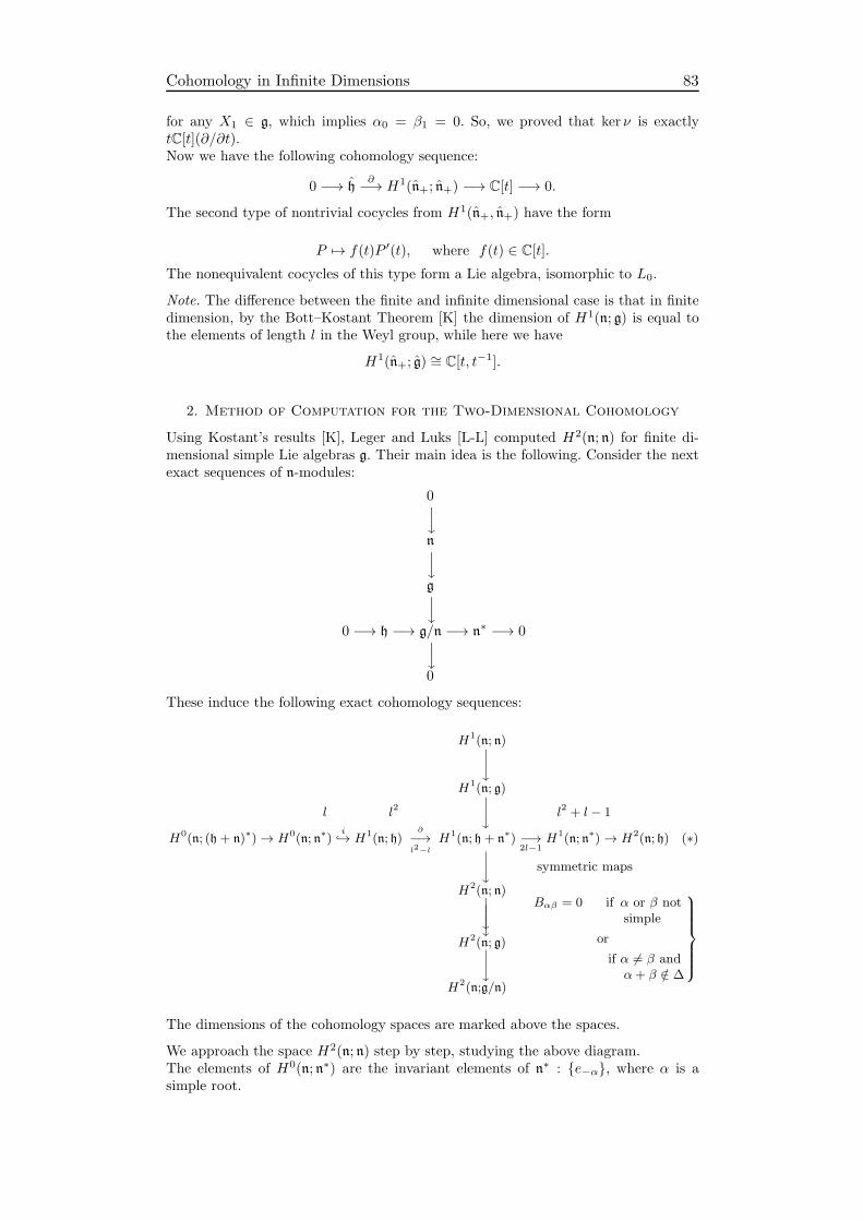
Cohomology in Infinite Dimensions 83
for any X1 ∈ g, which implies α0 = β1 = 0. So, we proved that ker ν is exactlytC[t](∂/∂t).Now we have the following cohomology sequence:
0 −→ h∂−→ H1(n+; n+) −→ C[t] −→ 0.
The second type of nontrivial cocycles from H1(n+, n+) have the form
P 7→ f(t)P ′(t), where f(t) ∈ C[t].
The nonequivalent cocycles of this type form a Lie algebra, isomorphic to L0.
Note. The difference between the finite and infinite dimensional case is that in finitedimension, by the Bott–Kostant Theorem [K] the dimension of H1(n; g) is equal tothe elements of length l in the Weyl group, while here we have
H1(n+; g) ∼= C[t, t−1].
2. Method of Computation for the Two-Dimensional Cohomology
Using Kostant’s results [K], Leger and Luks [L-L] computed H2(n; n) for finite di-mensional simple Lie algebras g. Their main idea is the following. Consider the nextexact sequences of n-modules:
0ynygy
0 −→ h −→ g/n −→ n∗ −→ 0y0
These induce the following exact cohomology sequences:
H1(n; n)
y
H1(n; g)
l l2
y
l2 + l − 1
H0(n; (h+ n)∗) → H0(n; n∗)i→ H1(n; h)
∂
−→l2−l
H1(n; h+ n∗) −→
2l−1
H1(n; n∗) → H2(n; h) (∗)
y
symmetric maps
H2(n; n)
y
y
H2(n; g)
y
H2(n;g/n)
Bαβ = 0 if α or β notsimple
or
if α 6= β andα+ β /∈ ∆
The dimensions of the cohomology spaces are marked above the spaces.
We approach the space H2(n; n) step by step, studying the above diagram.The elements of H0(n; n∗) are the invariant elements of n∗ : e−α, where α is asimple root.

84 II. Nilpotent Lie Algebras and Cohomology
Cocycles in H1(n; h) have the form
ϕ(eγ) = 0, γ 6= α
ϕ(eα) = hβ , if α, β are simple roots.
There are l2 such cocycles. Their images look the same in H1(n, h + n∗). Obviouslyamong them the ones with the form
ϕ(eα) = hα
ϕ(eγ) = 0, γ 6= α
are zero cocycles.It is easy to see that i is embedding into H1(n; h).The space n/[n, n] is generated by 〈eα〉, α simple, and h ∼= 〈hα〉, α simple and therank of such a homomorphism is l2.We compute im ∂: take L :
(〈eα〉 , α simple
)→
(〈hα〉 , α simple
), L(eα) =
∑β Lαβhβ.
Then as im ∂ we have to take the factor
〈L〉 / 〈L : Lαβ = 0, α 6= β〉 .dim = l2 dim = l
So from the left we get l2 − l cocycles.
3. The Spaces H1(n; n∗) and H2(n; n)
The main problem is to compute H1(n; n∗). The cocycles representing the cohomologyclasses in H1(n; n∗) are bilinear forms φ on n such that
φ([X,Y ], Z) = −φ(Y, [X,Z]) + φ(X, [Y, Z]).
Leger and Luks state [Theorem 4.1] that the cocycles are exactly the ones obtainedwith the help of a symmetric invariant form B,
φ(X,Y ) = B(TX,Z)−B(TY,X),
where T is a derivation.Note that Leger and Luks prove it for any finite dimensional Lie algebra, but thestatements are true for any Lie algebra.Now we have to count the symmetric bilinear forms on n. Their explicit form is
B(eα, eβ) = 1, α, β simple,
B(eγ , eδ) = 0, (γ, δ) 6= (α, β) (γ or δ is not simple).
The number of such forms in finite dimension is
l(α = α) +l(l − 1)
2(α 6= β simple) +
l(l+ 1)
2=l2 + l
2.
By Theorem 4.1 of Leger and Luks, in H1(n; n∗) we have (l2 + l)/2 classes. Considerthe differential
H1(n; n∗)∂−→ H2(n; h) = H2(n)⊗ h.
Let us compute ker ∂.Suppose that we have a functional ϕ on n defined by the cochain φ,
ϕ(X)(Y ) = B(TX, Y )−B(TY,X) if Y ∈ n
and assume that ϕ(X)(H) = 0 if H ∈ h. Let us continue it onto b+ = h + n∗. Thenits differential is
∂ϕ = Xϕ(Y )(H)− Y ϕ(X)(H) = ϕ(Y )([X,H ])− ϕ(X)([Y,H ])
= −B(TY, [X,H ]) +B(TX, [Y,H ]) +B(T [X,H ], Y )
−B(T [Y,H ], X).
Put X = eα, Y = eβ, where α, β are simple positive roots.
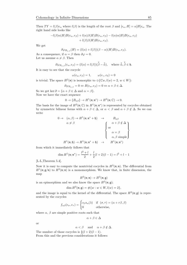
Cohomology in Infinite Dimensions 85
Then TY = l(β)eα where l(β) is the length of the root β and [eα, H ] = α[H ]eα. Theright hand side looks like
−l(β)α(H)B(eα, eβ) + l(α)β(H)B(eα, eβ)− l(α)α(H)B(eα, eβ)
+ l(β)β(H)B(eα, eβ).
We get
∂ϕBα,β(H) = (l(α) + l(β))(β − α)(H)B(eα, eβ).
As a consequence, if α = β then ∂ϕ = 0.Let us assume α 6= β. Then
∂ϕBα,β(eα, eβ) = (l(α) + l(β))(
v
β − v
α), wherev
α,v
β ∈ h.
It is easy to see that the cocycle
ω(eα, eβ) = 1, ω(eγ , eδ) = 0
is trivial. The space H2(n) is isomorphic to ⊕Cw, l(w) = 2, w ∈W:∂ϕBα,β
= 0⇔ B(eα, eβ) = 0⇔ α+ β ∈ ∆.
So we get ker ∂ = α+ β ∈ ∆ and α = β.Now we have the exact sequence
0→ Bαβ → H1(n; n∗)→ H2(n;C)→ 0.
The basis for the image of H2(n;C) in H1(n; n∗) is represented by cocycles obtainedby symmetric bilinear forms with α + β ∈ ∆, or α < β and α + β /∈ ∆. So we canwrite
0→ (α, β)→ H1(n; n∗ + h) → Bαβ
α 6= β
α+ β /∈ ∆
or
α = β
α, β simple
H1(n; h)→ H1(n; n∗ + h) → H1(n; n∗)
from which it immediately follows that
dimH1(n; n∗) =l2 + l
2+l
2(l + 2)(l − 1) = l2 + l − 1
[L-L,Theorem 5.4].
Now it is easy to compute the nontrivial cocycles in H2(n; n). The differential fromH1(n; g/n) to H2(n; n) is a monomorphism. We know that, in finite dimension, themap
H2(n; n)→ H2(n; g)
is an epimorphism and we also know the space H2(n; g);
dimH2(n; g) = #w : w ∈W, l(w) = 2,and the image is equal to the kernel of the differential. The space H2(n; g) is repre-sented by the cocycles
fαβ(eσ, eτ ) =
sβsα(λ) if (σ, τ) = (α+ rβ, β)
0 otherwise,
where α, β are simple positive roots such that
α+ β ∈ ∆
or
α < β and α+ β /∈ ∆.
The number of those cocycles is 12 (l + 2)(l − 1).
From this and the previous considerations it follows:
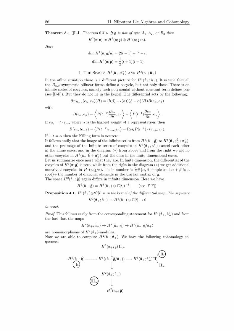
86 II. Nilpotent Lie Algebras and Cohomology
Theorem 3.1 ([L-L, Theorem 6.4]). If g is not of type A1, A2, or B2 then
H2(n; n) ≈ H2(n; g)⊕H1(n; g/n).
Here
dimH1(n; g/n) = (2l− 1) + l2 − l,
dimH2(n; g) =1
2(l + 1)(l − 1).
4. The Spaces H1(n+, n∗+) and H2(n+; n+)
In the affine situation there is a different picture for H1(n+; n+). It is true that allthe Bα,β symmetric bilinear forms define a cocycle, but not only those. There is aninfinite series of cocycles, namely each polynomial without constant term defines one(see [F-F]). But they do not lie in the kernel. The differential acts by the following:
∂ϕBα,β(eα, eβ)(H) = (l(β) + l(α))(β − α)(H)B(eα, eβ)
with
B(eα, eβ) =
⟨P (t−1)
∂eα∂t
, eβ
⟩+
⟨P (t−1)
∂eβ∂t
, eα
⟩.
If eβ0= t · e−λ where λ is the highest weight of a representation, then
B(eα, te−λ) =⟨P (t−1)e−λ, eα
⟩= RestP (t
−1) · (e−λ, eα).If −λ = α then the Killing form is nonzero.It follows easily that the image of the infinite series from H1(n+; g) to H
1(n+; h+n∗+),and the preimage of the infinite series of cocycles in H1(n+, n
∗+) cancel each other
in the affine cases, and in the diagram (∗) from above and from the right we get no
other cocycles in H1(n+; h+ n∗+) but the ones in the finite dimensional cases.Let us summarize once more what they are. In finite dimension, the differential of thecocycles of H1(n; g) is zero, while from the right in the diagram (∗) we get additionalnontrivial cocycles in H1(n; g/n). Their number is 1
2#α, β simple and α + β is aroot+the number of diagonal elements in the Cartan matrix of g.The space H2(n+; g) again differs in infinite dimension. Here we have
H2(n+; g) = H1(n+)⊗ C[t, t−1] (see [F-F]).
Proposition 4.1. H1(n+)⊗tC[t] is in the kernel of the differential map. The sequence
H2(n+; n+)→ H1(n+)⊗ C[t]→ 0
is exact.
Proof. This follows easily from the corresponding statement for H1(n+, n∗+) and from
the fact that the maps
H∗(n+; n+)→ H∗(n+; g)→ H∗(n+; g/n+)
are homomorphisms of H∗(n+)-modules.Now we are able to compute H2(n+; n+). We have the following cohomology se-quences:
H1(n+; g) II∞yH1(n+; h)−−−−→ H1((n+; g/n+)) −→ H1(n+; n
∗+) II
/
\©IIfII∞©If y
H2(n+; n+)
©III∞ y
H2(n+; g)
Cohomology in Infinite Dimensions 87
Theorem 4.2. With the exception of sℓ(2,C), the space H2(n+; n+) is the directsum of three subspaces, coming from three kinds of cocycles I–III. The cocycles oftype If and IIf are the same as for finite dimensional algebras. The cocycles of typeII∞ coming from above and from the right cancel each other. Cocycles of type III∞only appear in the affine cases. They form a space isomorphic to H1(n+)⊗ L0.
Remark 4.3. Cocycles of type If and III∞ form the space
H1(n+)⊗H1(n+; n+).
The number of such deformations is dim(H1(n+)) × dim(H1(n+; n+)). We comparethis result with the ones in [F], where they are called the cocycles of type (1).In the notation of [F], cocycles of type IIf give infinitesimal deformations of type 2
and 3. In [F], cocycles of type (2) are the following: Let 1 6 i 6 n. The algebran+ deforms inside g = gA where A is the Cartan matrix. The deformed algebra isspanned by the spaces gA(m1,...,mn)
with
(m1, . . . ,mn) 6= (0, . . . , 0,(i)1 , . . . , 0)
and by the vector ei + tfi where t is a parameter. The number of such cocycles isequal to the rank of g.Similarly cocycles of type (3) are the following: Let 1 6 i 6 n; consider the entryaij = −1 in the Cartan matrix A, and if aji = aij , then i < j. The algebra n+ deformsagain inside g. The deformed algebra is generated by the spaces
gA(m1,...,mn)with (m1, . . . ,mn)
6= (0, . . . , 0,(i)1 , 0, . . . , 0), (0, . . . , 0,
(i)1 , 0, . . . , 0,
(j)1 , 0, . . . , 0)
and the vectors ei+ tfj and [ei, ej ]− thj. The number of this type of cocycles is equalto the number of nonzero pairs (aij , aji) in the Cartan matrix with i 6= j.
The exceptional case sℓ(2,C) is also discussed in [F]. In this case, cocycles of type3 do not exist. Instead, there are two additional cocycles in H2(n+, n+). This Liealgebra is really exceptional in the deformation sense also: the two above-mentionedadditional cocycles cannot define an extendible deformation of n+, while all the othertypes of infinitesimal deformations for any affine Lie algebra are extendible.
References
[F] A. Fialowski, Deformations of nilpotent Kac–Moody algebras, Studia Sci.Math. Hungar. 19 (1984), 465–483.
[F-F] B. L. Feigin and A. Fialowski, On the cohomology of the nilpotentalgebras of flows, Soviet Math. Dokl. 28, No. 1 (1983), 178–181.
[K] B. Kostant, Lie algebra cohomology and the generalized Borel–Weil theo-rem, Ann. Math. 74, No. 2 (1961), 329–387.
[L-L] G. Leger and E. Luks, Cohomology of nilradicals of Borel subalgebras,Trans. Amer. Math. Soc. 195 (1974), 305–316.
appeared in: Journal of Algebra, Journal of Algebra 318 (2007), 1002–1026.
Cohomology and Deformations of the Infinite DimensionalFiliform Lie Algebra m0
Alice FialowskiInstitute of Mathematics
Eotvos Lorand University, Budapest
Friedrich WagemannLab. de mathematiques Jean Leray
Universite de Nantes
Abstract Denote m0 the infinite dimensional N-graded Lie algebradefined by basis ei i ≥ 1 and nontrivial relations [e1, ei] = ei+1 for alli ≥ 2. We compute in this article the bracket structure on H1(m0;m0),H2(m0;m0) and in relation to this, we establish that there are onlyfinitely many true deformations of m0 in each nonpositive weight, byconstructing them explicitly. It turns out that in weight 0 one gets ex-actly the other two filiform Lie algebras.
Introduction
Recall the classification of infinite dimensional N-graded Lie algebras g =⊕∞
i=1 giwith one-dimensional homogeneous components gi and two generators over a fieldof characteristic zero. A. Fialowski showed in [1] that any Lie algebra of this typemust be isomorphic to m0, m2 or L1. We call these Lie algebras infinite dimensionalfiliform Lie algebras in analogy with the finite dimensional case where the name wascoined by M. Vergne in [9]. Here m0 is given by generators ei, i ≥ 1, and nontrivialrelations [e1, ei] = ei+1 for all i ≥ 2, m2 with the same generators by nontrivialrelations [e1, ei] = ei+1 for all i ≥ 2, [e2, ej] = ej+2 for all j ≥ 3, and L1 with thesame generators is given by the relations [ei, ej ] = (j − i)ei+j for all i, j ≥ 1. L1
appears as the positive part of the Witt algebra given by generators ei for i ∈ Z withthe same relations [ei, ej ] = (j − i)ei+j for all i, j ∈ Z. The result was also obtainedlater by Shalev and Zelmanov in [8].
The cohomology with trivial coefficients of the Lie algebra L1 was studied in [6], theadjoint cohomology in degrees 1, 2 and 3 has been computed in [2] and also all ofits non equivalent deformations were given. For the Lie algebra m0, the cohomologywith trivial coefficients has been studied in [4], but neither the adjoint cohomology,nor related deformations have been computed so far. The reason is probably that -as happens usually for solvable Lie algebras - the cohomology is huge and thereforemeaningless. Our point of view is that there still remain interesting features. We tryto prove this in the present article by studying the adjoint cohomology of m0, whilewe reserve m2 for a forthcoming paper.
Indeed, it is true that the first and second adjoint cohomology of m0 are infinitedimensional. The space H1(m0;m0) becomes already interesting when we split it upinto homogeneous components H1
l (m0;m0) of weight l ∈ Z, this latter space beingfinite dimensional for each l ∈ Z. We compute the bracket structure on H1(m0;m0)in section 1.The space H2(m0;m0) is discussed in section 2. This space is worse as it is infinitedimensional even in each weight separately. The interesting new feature here is thatthere are only finitely many generators in each negative or zero weight which giverise to true deformations. Given a generator of H2(m0;m0), i.e. an infinitesimal de-formation, corresponding to the linear term of a formal deformation, one can try toadjust higher order terms in order to have the Jacobi identity in the deformed Lie
∗Keywords: Filiform Lie algebra, cohomology, deformation, Massey product†Mathematics Subject Classifications (2000): 17B65, 17B56, 58H15
88
Deformations of the Lie Algebra m0 89
algebra up to order k. If the Jacobi identity is satisfied to all orders, we will call it atrue (formal) deformation, see Fuchs’ book [5] for details on cohomology and [2] fordeformations of Lie algebras.In section 3 we discuss Massey products, in section 4 describe all true deformationsin negative weights. Section 5 deals with deformations in zero and positive weights.As obstructions to infinitesimal deformations given by classes in H2(m0;m0) are ex-pressed by Massey powers of these classes in H3(m0;m0), it is the vanishing of theseMassey squares, cubes etc which selects within the H2
l (m0;m0) of weight l a finitenumber of cohomology classes. The main result reads
Theorem 0.4. The true deformations of m0 are finitely generated in each weightl ≤ 1. More precisely, the space of unobstructed cohomology classes is in degree
• l ≤ −3 of dimension two,• l = 0 of dimension two,• l = −2 of dimension three,
while there is no true deformation in weight l = −1. In weight l = 0, these aredeformations to m2 and L1. In weight l = 1, there are exactly two true deformations,while in weight l ≥ 2, there are at least two.
We do not have more precise information about how many true deformations there arein positive weight, but there are always at least two. As a deformation in these weightsis a true deformation if and only if all of its Massey squares are zero (as cochains !),true deformations are determined by a countable infinite system of homogeneousquadratic equations in countably infinitely many variables. We didn’t succeed indetermining the space of solutions of this system.We believe that the discussion of these examples of deformations are interesting asthey go beyond the usual approach where the condition that H2(m0,m0) should befinite dimensional is the starting point for the examination of deformations, namelythe existence of a miniversal deformation [3].Another attractive point of our study is the fact that in some cases the Masseysquares and cubes involved are not zero because of general reasons, but because ofthe combinatorics of the relations. Thus the second adjoint cohomology of m0 mayserve as an example on which to study explicitly obstruction theory.
Acknowledgments: The work has been partially supported by the grants OTKAT034641 and T043034 and by the Erasmus program between Eotvos Lorand Univer-sity Budapest and Universite Louis Pasteur Strasbourg. Both authors are gratefulto IHES where some of this work was accomplished, to Yury Nikolayevsky for usefulremarks and to Matthias Borer who helped us to get hold on the weight l > 0 caseby MUPaD based computations.
1. The space H1(m0;m0)
The Lie algebra m0 is an N-graded Lie algebra m0 =⊕∞
i=1(m0)i with 1-dimensionalgraded components (m0)i and generated in degree 1 and 2. Choosing a basis ei of(m0)i, the only non-trivial brackets (up to skew-symmetry) read [e1, ei] = ei+1 forall i. We are computing in this section the first cohomology space H1(m0,m0) of m0
with adjoint coefficients. As Lie algebra and module are graded, the cohomology spacesplits up into homogeneous components, and we will always work with homogeneouscocycles ω(ei) = aiei+l for a scalar ai and a given weight l ∈ Z.Concerning the cocycle identity dω(ej , ei) = 0, let us first suppose that j = 1 andi > 1 (up to choosing the symmetric case j > 1 and i = 1). In this case, it reads
ω(ei+1) = [e1, ω(ei)]− [ei, ω(e1)]
or, putting in the expression of ω, for all l ≥ 0
ai+1ei+l+1 = aiei+l+1 + δl,0a1ei+l+1.
This means that for all l ≥ 0, we must have
ai+1 = ai + δl,0 a1,
90 II. Nilpotent Lie Algebras and Cohomology
while for l = −1, we get the previous equation for i ≥ 3 and a3 = 0, for l = −2,we get the previous equation for i ≥ 4 and a4 = a3 = 0, and for l ≤ −3, we get theprevious equation for i ≥ −l + 2 and a−l+2 = a−l+1 = 0, while there is no equationfor i < −l.The second situation where the cocycle identity has non-zero terms is when l ≤ −1,and i and j ≥ 2. In this case, there is only one non-zero term in the equation, andwe get ai = 0 for i+ l = 1.Now let us deduce the possible 1-cocycles in different weights:
case 1: l ≤ −1In case l ≤ −3, the first identity means that all ai for i ≥ −l + 2 must be equal anda−l+2 = a−l+1 = 0, therefore all ai = 0 for i ≥ −l + 1, while there is no constrainton a1, a2, . . . , a−l. This is compatible with the second situation.In case l = −1 and l = −2, the first constraint implies that all ai = 0 for i ≥ 3, whilethere is no constraint on a1 and a2. The second identity is then already satisfied forl ≤ −2, while for l = −1, it implies a2 = 0.But observe that the formula ω(ei) = aiei+l makes sense for l ≤ −1 only if i ≥ −l+1.Therefore all coefficients a1, . . . , a−l has to be set zero for l ≤ −1.In conclusion, all cohomology is zero in weight l ≤ −1.case 2: l ≥ 1In this case, the cocycle identity means that all ai for i ≥ 2 must be equal, whilethere is no constraint on a1.
case 3: l = 0In this case, the first identity means that all ai for i ≥ 3 are determined by a1 anda2, while there is no constraint on a1 and a2.Let us now examine the coboundaries: an element x ∈ m0 determines a 1-coboundaryby αx(y) := [x, y] for all y ∈ m0. In order to have a homogeneous coboundary, wemust take x = ei for some i > 0; αei is then homogeneous of weight i. Therefore wehave:
• dC0l (m0,m0) = 0 for l ≤ 0
• dC0l (m0,m0) is generated by del = [el,−] for l ≥ 1.
Observe that the coboundaries for l ≥ 2 are non-zero only on e1, thus they can modifyonly the a1-term of a cocycle. The coboundary for l = 1 is zero on e1 and non-zeroand constant on all other ei. It thus kills the cocycle where all ai for i ≥ 2 are equal.In conclusion, we have
Theorem 1.1.
dim H1l (m0;m0) =
1 for l ≥ 12 for l = 00 for l ≤ −1
Let us now determine representatives of the non-zero cohomology classes:In H1
0 (m0;m0), we have the generators ω1 (corresponding to a1 = 1 and a2 = 0) andω2 (corresponding to a1 = 0 and a2 = 1) defined by:
ω1(ek) =
e1 for k = 10 for k = 2
(k − 2)ek for k ≥ 3
ω2(ek) =
0 for k = 1ek for k ≥ 2
In H1l (m0;m0) for l ≥ 1, we have two different kinds of cocycles: there is γ for l = 1,
and αl for l ≥ 2:
γ(ek) =
ce2 for k = 10 for k ≥ 2
αl(ek) =
0 for k = 1
blek+l for k ≥ 2
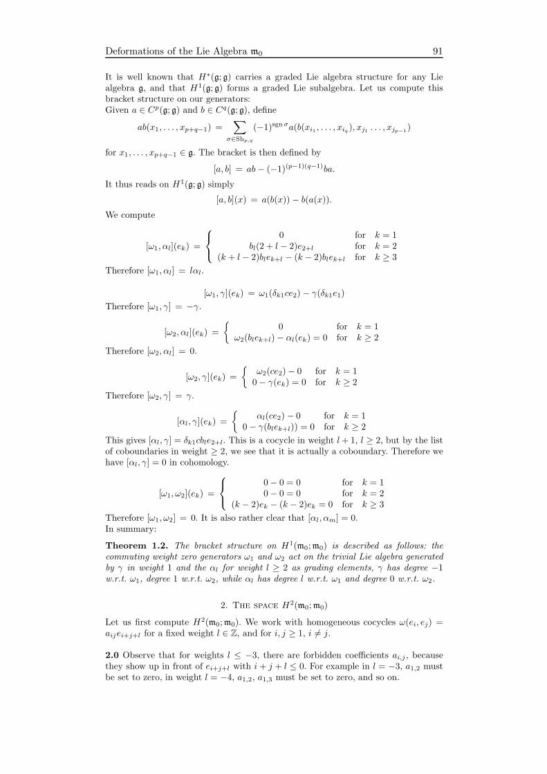
Deformations of the Lie Algebra m0 91
It is well known that H∗(g; g) carries a graded Lie algebra structure for any Liealgebra g, and that H1(g; g) forms a graded Lie subalgebra. Let us compute thisbracket structure on our generators:Given a ∈ Cp(g; g) and b ∈ Cq(g; g), define
ab(x1, . . . , xp+q−1) =∑
σ∈Shp,q
(−1)sgnσa(b(xi1 , . . . , xiq ), xj1 . . . , xjp−1)
for x1, . . . , xp+q−1 ∈ g. The bracket is then defined by
[a, b] = ab− (−1)(p−1)(q−1)ba.It thus reads on H1(g; g) simply
[a, b](x) = a(b(x)) − b(a(x)).We compute
[ω1, αl](ek) =
0 for k = 1bl(2 + l − 2)e2+l for k = 2
(k + l− 2)blek+l − (k − 2)blek+l for k ≥ 3
Therefore [ω1, αl] = lαl.
[ω1, γ](ek) = ω1(δk1ce2)− γ(δk1e1)Therefore [ω1, γ] = −γ.
[ω2, αl](ek) =
0 for k = 1
ω2(blek+l)− αl(ek) = 0 for k ≥ 2
Therefore [ω2, αl] = 0.
[ω2, γ](ek) =
ω2(ce2)− 0 for k = 10− γ(ek) = 0 for k ≥ 2
Therefore [ω2, γ] = γ.
[αl, γ](ek) =
αl(ce2)− 0 for k = 1
0− γ(blek+l)) = 0 for k ≥ 2
This gives [αl, γ] = δk1cble2+l. This is a cocycle in weight l+ 1, l ≥ 2, but by the listof coboundaries in weight ≥ 2, we see that it is actually a coboundary. Therefore wehave [αl, γ] = 0 in cohomology.
[ω1, ω2](ek) =
0− 0 = 0 for k = 10− 0 = 0 for k = 2
(k − 2)ek − (k − 2)ek = 0 for k ≥ 3
Therefore [ω1, ω2] = 0. It is also rather clear that [αl, αm] = 0.In summary:
Theorem 1.2. The bracket structure on H1(m0;m0) is described as follows: thecommuting weight zero generators ω1 and ω2 act on the trivial Lie algebra generatedby γ in weight 1 and the αl for weight l ≥ 2 as grading elements, γ has degree −1w.r.t. ω1, degree 1 w.r.t. ω2, while αl has degree l w.r.t. ω1 and degree 0 w.r.t. ω2.
2. The space H2(m0;m0)
Let us first compute H2(m0;m0). We work with homogeneous cocycles ω(ei, ej) =aijei+j+l for a fixed weight l ∈ Z, and for i, j ≥ 1, i 6= j.
2.0 Observe that for weights l ≤ −3, there are forbidden coefficients ai,j , becausethey show up in front of ei+j+l with i + j + l ≤ 0. For example in l = −3, a1,2 mustbe set to zero, in weight l = −4, a1,2, a1,3 must be set to zero, and so on.

92 II. Nilpotent Lie Algebras and Cohomology
2.1 The cocycle identity reads
dω(ei, ej , ek) = ω([ei, ej], ek) + ω([ej , ek], ei) + ω([ek, ei], ej)
−[ei, ω(ej , ek)]− [ej , ω(ek, ei)]− [ek, ω(ei, ej)] = 0.
Let us first suppose that one index is equal to 1. The identity reads then
(ai+1,j + ai,j+1)ei+j+l+1 = (ai,j − δj+l,0 aj,1 − δi+l,0 a1,i)ei+j+l+1, (2.5)
where i, j ≥ 2, i 6= j. This identity makes only sense for i+ j + l ≥ 2, because in theabove equation, the ai,j term shows up in front of the bracket of e1 with ei+j+l. It istherefore not valid uniformly for all i, j starting from l ≤ −4.For i+j+l < 0, there is no equation, while there is a special equation for i+j+l = 0, 1,namely
ai+1,j + ai,j+1 = 0.
Note that by 2.0, coefficients ai,j with i+ j + l ≤ 0 are set to zero.
2.2 The cocycle identity for ei, ej , ek for i, j, k ≥ 2, i 6= j, i 6= k, and j 6= k, givesa non-zero factor only if j + k + l = 1 or i + j + l = 1 or i + k + l = 1 (thus forl ≤ −4). One can always arrange that only one factor is possibly non-zero for given i,j with i+ j+ l = 1 (by choosing k = max(i+1, j+1), for example). Thus for weightl ≤ −4, the coefficient ai,j with i+ j = −l+1, i 6= j, i, j ≥ 2, must be zero (which iscompatible with the special equation !).
2.3 Let us now consider coboundaries: expressing that ω ∈ Z2l (m0,m0) is a cobound-
ary ω = dα for some 1-cochain α ∈ C1l (m0,m0), α(ei) = αiei+l for all i ≥ 1, gives by
evaluation on ei and ej :
ai,jei+j+l = α([ei, ej ])− [ei, α(ej)] + [ej , α(ei)].
This equation makes sense only for i+ j + l ≥ 1 as all terms are multiples of ei+j+l.Let us first take one index to be 1, then we get
a1,i = αi+1 − αi + α1 δl,0
for all i ≥ max(2,−l+ 2), because αi appears in front of the bracket of e1 with el+i.Thus all a1,i, i ≥ max(2,−l + 2), can be taken to be zero by adding a coboundary.For i = −l,−l+ 1 ≥ 2, we have the special equation
a1,i = αi+1.
It is now clear that, up to a coboundary, we may suppose for any l that the lasttwo terms in equation (2.5) are zero. Observe that the non-coboundary terms a1,i forl ≤ −3 in a general cocycle, namely the terms with i = 2, . . . ,−l− 1, must be set tozero by 2.0.
2.4 For weight l ≤ −1, we have additional coboundaries: indeed, there is a non-zeroterm in the coboundary equation for ei, ej , i, j ≥ 2, i 6= j yielding
a−l+1,j = −α−l+1
for all j ≥ 2, j 6= −l + 1. Be aware that the coefficient α−l+1 of the coboundary dαis linked to a1,−l by the equation α−l+1 = a1,−l (cf 2.3). Thus we cannot choose atthe same time to render a1,−l = 0 and a−l+1,j = 0 in weight l ≤ −1 by addition ofa coboundary, we can impose only one of these conditions. This means for examplethat the cocycle given by coefficients ai,j with a2,j = 1 for all j ≥ 3 and ai,j = 0 forall i, j 6= 2 (“the 2-family”, cf 2.5) is a coboundary in weight l = −1. Here a1,1 = 0and α2 are not linked. More generally, the cochain given by coefficients ai,j witham+1,j = 1 for all j ≥ m+ 2, ai,j = 0 for all other i, j > m + 1 (unless those whichmust be non-zero in order to respect antisymmetry) is cohomologous to the cocycleconsisting of the only non-trivial coefficient a1,m = 1 in weight l = −m ≤ −2.

Deformations of the Lie Algebra m0 93
Let us now reconsider the equations (2.5) in the stable range, i.e. with i and j suchthat i, j ≥ 2, i 6= j, and i+ j ≥ −l+ 2:
ai+1,j + ai,j+1 = aij (2.6)
We will adopt two different points of view on this system of equations:
2.5 First point of view: Call the equations a2,3 = a2,4, a3,4 = a3,5, a4,5 = a4,6, . . .diagonal equations, and the terms involved diagonal terms. The prescription
ai,i+1 = ai,i+2 =
1 for i = k0 for i 6= k
specifies uniquely (unicity is shown by induction) a solution to this system, called thekth family or k-series. For the kth family, all ar,s with r > k are zero, ar,s = 1 forr = k, ar,s is linear in k for r = k − 1 (and s sufficiently big), ar,s is quadratic in kfor r = k − 2 (and s sufficiently big), and so on.Let us consider some examples, while we refer to section 4.5 and 5.1 for more infor-mation; in the following expressions, all coefficients involving an index 1 are set tozero, and the first non-zero column starting from the RHS (i.e. the non-zero elementsof the column am,kk≥m+1) is normalized to 1.
The 2-family: a2,k = 1, aj,k = 0 for all j, k ≥ 3.
The 3-family: a3,k = 1, aj,k = 0 for all j, k ≥ 4, and a2,3 = a2,4 = 0, a2,k = −(k−4)for all k ≥ 5.
The 4-family: a4,k = 1, aj,k = 0 for all j, k ≥ 5, a3,4 = a3,5 = 0, a3,k = −(k − 5)
for all k ≥ 6, and a2,3 = a2,4 = a2,5 = a2,6 = 0, a2,k = (k−5)(k−6)2 for all k ≥ 7 (even
for all k ≥ 5).
The 5-family: a5,k = 1, aj,k = 0 for all j, k ≥ 6, a4,5 = a4,6 = 0, a4,k = −(k − 6)
for all k ≥ 7, a3,4 = a3,5 = a3,6 = a3,7 = 0, a3,k = (k−6)(k−7)2 for all k ≥ 8 (even for
all k ≥ 6), and a2,3 = a2,4 = a2,5 = a2,6 = a2,7 = a2,8 = 0, a2,k = − (k−6)(k−7)(k−8)3!
for all k ≥ 9 (even for all k ≥ 6).
2.6 Second point of view: One can specify a2,n for all n, in such a way thatthe diagonal equations are satisfied. This implies that by choosing pairs (a2,3, a2,4),(a2,5, a2,6), (a2,7, a2,8), and so on, the first member is free, while the second memberis determined by the corresponding diagonal equation.Indeed, in (a2,3, a2,4), a2,4 is determined by a2,3 = a2,4, in (a2,5, a2,6), a2,6 is deter-mined by a2,5 − a2,4 = a2,6 − a2,5 (which is just a3,4 = a3,5), in (a2,7, a2,8), a2,8 isdetermined by ((a2,7 − a2,6)− (a2,5 − a2,4)) = ((a2,3 − a2,7)− (a2,7 − a2,6)) (which isjust a4,5 = a4,6). All the other coefficients are then uniquely determined.
2.7 In conclusion, it is clear that for each weight l ∈ Z, there is a countably infinitenumber of independent 2-cohomology classes. More precisely, in weight l > −4, thek-families with k = 2, 3, . . . represent independent 2-cohomology classes. In weightl ≤ −4, 2.2 shows that the k family is contradictory for
k <
2 + −l−32 for l odd2 + −l−22 for l even
But there is still a countably infinite number of independent 2-cohomology classes ineach weight.
Theorem 2.1.
dim H2l (m0,m0) = ∞
for each weight l ∈ Z.
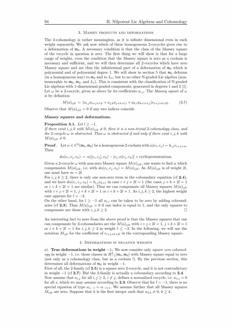
94 II. Nilpotent Lie Algebras and Cohomology
3. Massey products and deformations
The 2-cohomology is rather meaningless, as it is infinite dimensional even in eachweight separately. We ask now which of these homogeneous 2-cocycles gives rise toa deformation of m0. A necessary condition is that the class of the Massey squareof the cocycle in question is zero. The first thing we will show is that for a largerange of weights, even the condition that the Massey square is zero as a cochain isnecessary and sufficient, and we will then determine all 2-cocycles which have zeroMassey square and are thus the infinitesimal part of a deformation of m0 which ispolynomial and of polynomial degree 1. We will show in section 5 that m0 deforms(in a homogeneous way) to m2 and to L1, but to no other N-graded Lie algebra (non-isomorphic to m0, m2, and L1). This is consistent with the classification of N-gradedLie algebras with 1-dimensional graded components, generated in degrees 1 and 2 [1].Let ω be a 2-cocycle, given as above by its coefficients ai,j . The Massey square of ωis by definition
M(a)ijk = (ai,jai+j+l,k + aj,kaj+k+l,i + ak,iak+i+l,j)ei+j+k+2l . (3.7)
Observe that M(a)ijk = 0 if any two indices coincide.
Massey squares and deformations.
Proposition 3.1. Let l ≥ −1.If there exist i, j, k with M(a)ijk 6= 0, then it is a non-trivial 3-cohomology class, andthe 2-cocycle ω is obstructed. Thus ω is obstructed if and only if there exist i, j, k withM(a)ijk 6= 0.
Proof . Let α ∈ C2(m0,m0) be a homogeneous 2-cochain with α(ei, ej) = bi,jei+j+m.Then
dα(ei, ej , ek) = α([ei, ej], ek)− [ei, α(ej , ek)] + cyclicpermutations.
Given a 2-cocycle ω with non-zero Massey squareM(a)ijk, one wants to find α whichcompensates M(a)ijk, i.e. with dα(ei, ej , ek) = M(a)ijk . As M(a)ijk is of weight 2l,one must have m = 2l.For i, j, k ≥ 2, there is only one non-zero term in the coboundary equation (cf 2.4),and we have dα(ei, ej, ek) = bi,jek+1 in case i + j + 2l = 1 (the cases j + k + 2l = 1or i + k + 2l = 1 are similar). Thus we can compensate all Massey squares M(a)ijkwith i+ j + 2l = 1, j + k + 2l = 1 or i+ k + 2l = 1. As i, j, k ≥ 2, the highest weightcase appears for l = −2.On the other hand, for l ≥ −1 all a1,i can be taken to be zero by adding cobound-aries (cf 2.3). Thus M(a)ijk = 0 if one index is equal to 1, and the only squares tocompensate are those with i, j, k ≥ 2.
An interesting fact to note from the above proof is that the Massey squares that onecan compensate by 3-coboundaries are the M(a)ijk with i+ j+2l = 1, j+ k+2l = 1or i + k + 2l = 1 for i, j, k ≥ 2 in weight l ≤ −2. In the following, we will use thenotation Mijk for the coefficient of ei+j+k+2l in the corresponding Massey square.
4. Deformations in negative weights
a). True deformations in weight −1. We now consider only square zero cohomol-ogy in weight −1, i.e. those classes in H2
−1(m0,m0) with Massey square equal to zero(not only as a cohomology class, but as a cochain !). By the previous section, thisdetermines all deformations of m0 in weight −1.First of all, the 2-family (cf 2.5) is a square zero 2-cocycle, and it is not contradictoryin weight −1 (cf 2.7). But the 2-family is actually a coboundary according to 2.4.Now assume that ai,j for all i, j ≥ 2, i 6= j, defines a normalized cocycle, i.e. a1,s = 0for all s, which we may assume according to 2.3. Observe that for l = −1, there is nospecial equation of type a1,−l = α−l+1. We assume further that all Massey squaresMijk are zero. Suppose that k is the first integer such that a3,k 6= 0, k ≥ 4.
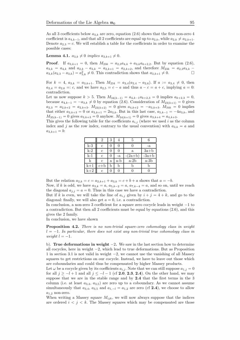
Deformations of the Lie Algebra m0 95
As all 3 coefficients below a3,k are zero, equation (2.6) shows that the first non-zero 4coefficient is a4,k−1, and that all 2 coefficients are equal up to a2,k, while a2,k 6= a2,k+1.Denote a2,3 = c. We will establish a table for the coefficients in order to examine thepossible cases:
Lemma 4.1. a3,k 6= 0 implies a3,k+1 6= 0.
Proof . If a3,k+1 = 0, then M23k = a2,3a4,k + a3,kak+2,2. But by equation (2.6),a3,k = a4,k and a2,k − a3,k = a2,k+1 = a2,k+2, and therefore M23k = a2,3a3,k −a3,k(a2,3 − a3,k) = a23,k 6= 0. This contradiction shows that a3,k+1 6= 0.
For k = 4, a3,k = a3,k+1. Then M234 = a3,4(a2,4 − a2,6). If a := a3,4 6= 0, thena2,4 = a2,6 =: c, and we have a2,5 = c − a and thus a − c = a + c, implying a = 0:contradiction.Let us now suppose k > 5. Then M34(k−1) = a4,k−1ak+2,3 = 0 implies ak+2,3 = 0,because a4,k−1 = −a3,k 6= 0 by equation (2.6). Consideration of M23(k+1) = 0 givesa2,3 = a2,k+2 = a2,k+3. M23(k+2) = 0 gives a4,k+2 = −a3,k+3. M34k = 0 impliesthat either a3,k+3 = 0 or a3,k+1 = 2a3,k. But in this last case, a5,k−1 = −4a3,k, andM35(k−1) = 0 gives a3,k+3 = 0 anyhow. M34(k+1) = 0 gives a3,k+4 = a4,k+3.This gives the following table for the coefficients ai,j (where we used i as the columnindex and j as the row index, contrary to the usual convention) with a3,k = a anda3,k+1 = b:
2 3 4 5 6
k-3 c 0 0 0 -ak-2 c 0 0 a 3a+bk-1 c 0 -a -(2a+b) -3a+bk c a a-b a-2b a-3b
k+1 c+b b b b bk+2 c 0 0 0 0
But the relation a2,k = c = a2,k+1 + a3,k = c+ b + a shows that a = −b.Now, if k is odd, we have a3,k = a, a5,k−2 = a, a7,k−4 = a, and so on, until we reachthe diagonal aj,j = a = 0. Thus in this case we have a contradiction.But if k is even, we will take the line of ai,j given by i + j = 4 + k, and go to thediagonal: finally, we will also get a = 0, i.e. a contradiction.In conclusion, a non-zero 3 coefficient for a square zero cocycle leads in weight −1 toa contradiction. But then all 2 coefficients must be equal by equations (2.6), and thisgives the 2 family.In conclusion, we have shown
Proposition 4.2. There is no non-trivial square-zero cohomology class in weightl = −1. In particular, there does not exist any non-trivial true cohomology class inweight l = −1.
b). True deformations in weight −2. We saw in the last section how to determineall cocycles, here in weight −2, which lead to true deformations. But as Proposition1 in section 3.1 is not valid in weight −2, we cannot use the vanishing of all Masseysquares to get restrictions on our cocycle. Instead, we have to leave out those whichare coboundaries and could thus be compensated by higher Massey products.Let ω be a cocycle given by its coefficients ai,j . Note that we can still suppose a1,j = 0for all j ≥ −l + 1 and all j ≤ −l − 1 (cf 2.0, 2.3, 2.4). On the other hand, we maysuppose that we are in the stable range and by 2.4 that the first terms in the 3column (i.e. at least a3,4, a3,5) are zero up to a coboundary. As we cannot assumesimultaneously that a3,4, a3,5 and a1,−l = a1,2 are zero (cf 2.4), we choose to allowa1,2 non-zero.When writing a Massey square Mijk, we will now always suppose that the indicesare ordered i < j < k. The Massey squares which may be compensated are those
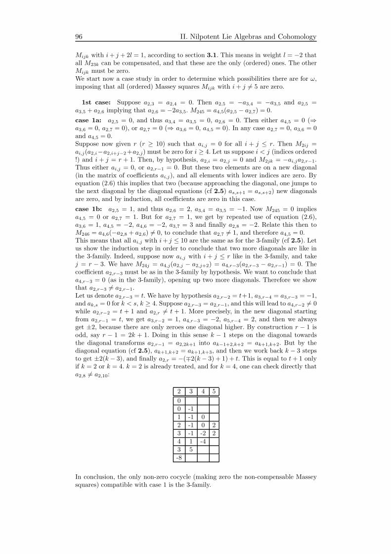
96 II. Nilpotent Lie Algebras and Cohomology
Mijk with i+ j + 2l = 1, according to section 3.1. This means in weight l = −2 thatall M23k can be compensated, and that these are the only (ordered) ones. The otherMijk must be zero.We start now a case study in order to determine which possibilities there are for ω,imposing that all (ordered) Massey squares Mijk with i+ j 6= 5 are zero.
1st case: Suppose a2,3 = a2,4 = 0. Then a2,5 = −a3,4 = −a3,5 and a2,5 =a3,5 + a2,6 implying that a2,6 = −2a3,5. M245 = a4,5(a2,5 − a2,7) = 0.
case 1a: a2,5 = 0, and thus a3,4 = a3,5 = 0, a2,6 = 0. Then either a4,5 = 0 (⇒a3,6 = 0, a2,7 = 0), or a2,7 = 0 (⇒ a3,6 = 0, a4,5 = 0). In any case a2,7 = 0, a3,6 = 0and a4,5 = 0.Suppose now given r (r ≥ 10) such that ai,j = 0 for all i + j ≤ r. Then M2ij =ai,j(a2,i−a2,i+j−2+a2,j) must be zero for i ≥ 4. Let us suppose i < j (indices ordered!) and i + j = r + 1. Then, by hypothesis, a2,i = a2,j = 0 and M2jk = −ai,ja2,r−1.Thus either ai,j = 0, or a2,r−1 = 0. But these two elements are on a new diagonal(in the matrix of coefficients ai,j), and all elements with lower indices are zero. Byequation (2.6) this implies that two (because approaching the diagonal, one jumps tothe next diagonal by the diagonal equations (cf 2.5) as,s+1 = as,s+2) new diagonalsare zero, and by induction, all coefficients are zero in this case.
case 1b: a2,5 = 1, and thus a2,6 = 2, a3,4 = a3,5 = −1. Now M245 = 0 impliesa4,5 = 0 or a2,7 = 1. But for a2,7 = 1, we get by repeated use of equation (2.6),a3,6 = 1, a4,5 = −2, a4,6 = −2, a3,7 = 3 and finally a2,8 = −2. Relate this then toM246 = a4,6(−a2,8 + a2,6) 6= 0, to conclude that a2,7 6= 1, and therefore a4,5 = 0.This means that all ai,j with i+ j ≤ 10 are the same as for the 3-family (cf 2.5). Letus show the induction step in order to conclude that two more diagonals are like inthe 3-family. Indeed, suppose now ai,j with i + j ≤ r like in the 3-family, and takej = r − 3. We have M24j = a4,j(a2,j − a2,j+2) = a4,r−3(a2,r−3 − a2,r−1) = 0. Thecoefficient a2,r−3 must be as in the 3-family by hypothesis. We want to conclude thata4,r−3 = 0 (as in the 3-family), opening up two more diagonals. Therefore we showthat a2,r−3 6= a2,r−1.Let us denote a2,r−3 = t. We have by hypothesis a2,r−2 = t+1, a3,r−4 = a3,r−3 = −1,and ak,s = 0 for k < s, k ≥ 4. Suppose a2,r−3 = a2,r−1, and this will lead to a4,r−2 6= 0while a2,r−2 = t + 1 and a2,r 6= t + 1. More precisely, in the new diagonal startingfrom a2,r−1 = t, we get a3,r−2 = 1, a4,r−3 = −2, a5,r−4 = 2, and then we alwaysget ±2, because there are only zeroes one diagonal higher. By construction r − 1 isodd, say r − 1 = 2k + 1. Doing in this sense k − 1 steps on the diagonal towardsthe diagonal transforms a2,r−1 = a2,2k+1 into ak−1+2,k+2 = ak+1,k+2. But by thediagonal equation (cf 2.5), ak+1,k+2 = ak+1,k+3, and then we work back k − 3 stepsto get ±2(k − 3), and finally a2,r = −(∓2(k− 3) + 1) + t. This is equal to t+ 1 onlyif k = 2 or k = 4. k = 2 is already treated, and for k = 4, one can check directly thata2,8 6= a2,10:
2 3 4 5
00 -11 -1 02 -1 0 23 -1 -2 24 1 -43 5-8
In conclusion, the only non-zero cocycle (making zero the non-compensable Masseysquares) compatible with case 1 is the 3-family.
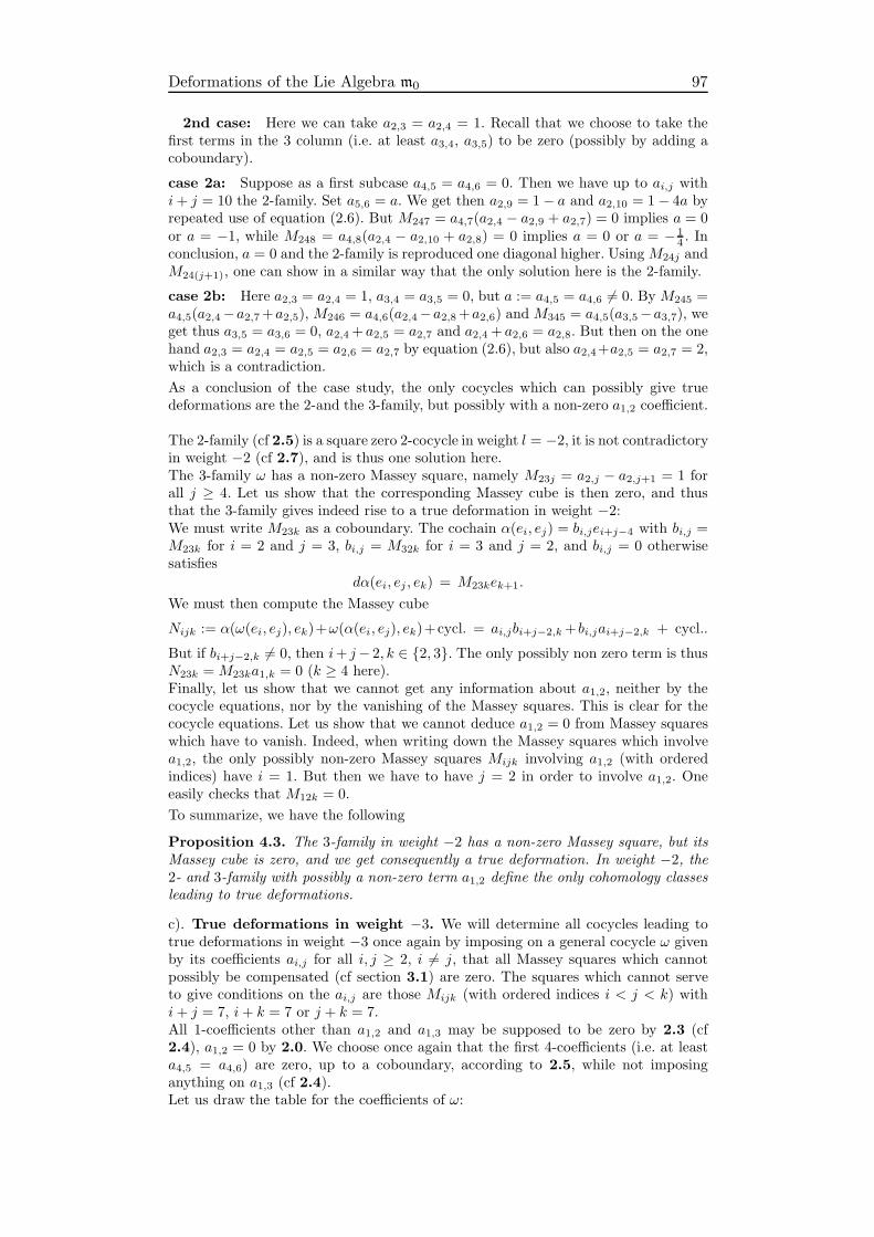
Deformations of the Lie Algebra m0 97
2nd case: Here we can take a2,3 = a2,4 = 1. Recall that we choose to take thefirst terms in the 3 column (i.e. at least a3,4, a3,5) to be zero (possibly by adding acoboundary).
case 2a: Suppose as a first subcase a4,5 = a4,6 = 0. Then we have up to ai,j withi+ j = 10 the 2-family. Set a5,6 = a. We get then a2,9 = 1− a and a2,10 = 1− 4a byrepeated use of equation (2.6). But M247 = a4,7(a2,4 − a2,9 + a2,7) = 0 implies a = 0or a = −1, while M248 = a4,8(a2,4 − a2,10 + a2,8) = 0 implies a = 0 or a = − 1
4 . Inconclusion, a = 0 and the 2-family is reproduced one diagonal higher. UsingM24j andM24(j+1), one can show in a similar way that the only solution here is the 2-family.
case 2b: Here a2,3 = a2,4 = 1, a3,4 = a3,5 = 0, but a := a4,5 = a4,6 6= 0. By M245 =a4,5(a2,4−a2,7+a2,5), M246 = a4,6(a2,4−a2,8+a2,6) and M345 = a4,5(a3,5−a3,7), weget thus a3,5 = a3,6 = 0, a2,4+ a2,5 = a2,7 and a2,4 + a2,6 = a2,8. But then on the onehand a2,3 = a2,4 = a2,5 = a2,6 = a2,7 by equation (2.6), but also a2,4+a2,5 = a2,7 = 2,which is a contradiction.
As a conclusion of the case study, the only cocycles which can possibly give truedeformations are the 2-and the 3-family, but possibly with a non-zero a1,2 coefficient.
The 2-family (cf 2.5) is a square zero 2-cocycle in weight l = −2, it is not contradictoryin weight −2 (cf 2.7), and is thus one solution here.The 3-family ω has a non-zero Massey square, namely M23j = a2,j − a2,j+1 = 1 forall j ≥ 4. Let us show that the corresponding Massey cube is then zero, and thusthat the 3-family gives indeed rise to a true deformation in weight −2:We must write M23k as a coboundary. The cochain α(ei, ej) = bi,jei+j−4 with bi,j =M23k for i = 2 and j = 3, bi,j = M32k for i = 3 and j = 2, and bi,j = 0 otherwisesatisfies
dα(ei, ej , ek) = M23kek+1.
We must then compute the Massey cube
Nijk := α(ω(ei, ej), ek)+ω(α(ei, ej), ek)+cycl. = ai,jbi+j−2,k+bi,jai+j−2,k + cycl..
But if bi+j−2,k 6= 0, then i+ j− 2, k ∈ 2, 3. The only possibly non zero term is thusN23k =M23ka1,k = 0 (k ≥ 4 here).Finally, let us show that we cannot get any information about a1,2, neither by thecocycle equations, nor by the vanishing of the Massey squares. This is clear for thecocycle equations. Let us show that we cannot deduce a1,2 = 0 from Massey squareswhich have to vanish. Indeed, when writing down the Massey squares which involvea1,2, the only possibly non-zero Massey squares Mijk involving a1,2 (with orderedindices) have i = 1. But then we have to have j = 2 in order to involve a1,2. Oneeasily checks that M12k = 0.
To summarize, we have the following
Proposition 4.3. The 3-family in weight −2 has a non-zero Massey square, but itsMassey cube is zero, and we get consequently a true deformation. In weight −2, the2- and 3-family with possibly a non-zero term a1,2 define the only cohomology classesleading to true deformations.
c). True deformations in weight −3. We will determine all cocycles leading totrue deformations in weight −3 once again by imposing on a general cocycle ω givenby its coefficients ai,j for all i, j ≥ 2, i 6= j, that all Massey squares which cannotpossibly be compensated (cf section 3.1) are zero. The squares which cannot serveto give conditions on the ai,j are those Mijk (with ordered indices i < j < k) withi+ j = 7, i+ k = 7 or j + k = 7.All 1-coefficients other than a1,2 and a1,3 may be supposed to be zero by 2.3 (cf2.4), a1,2 = 0 by 2.0. We choose once again that the first 4-coefficients (i.e. at leasta4,5 = a4,6) are zero, up to a coboundary, according to 2.5, while not imposinganything on a1,3 (cf 2.4).Let us draw the table for the coefficients of ω:

98 II. Nilpotent Lie Algebras and Cohomology
2 3 4 5
aa ba-b b 0a-2b b 0a-3b ba-4b
Now we write down the Massey squares that we may use: M236 = a2,6(a2,3 − a3,6 +a3,5) = a(a − 2b), M237 = a2,7(a2,3 − a3,7 + a3,6) = a(a − 3b), M246 = a2,4a3,6 +a4,6a7,2 + a6,2a5,4 = ab.In conclusion, a = 0. But then up to i + j = 10, the 3-family has built up. Let usshow by induction that the 3-family is the only possible solution:Suppose the ai,j up to i+ j = r for r ≥ 10 are like in the 3-family (cf 2.5). Considerthe Massey square
M23k = a2,3a2,k + a3,kak,2 + ak,2ak−1,3 = a2,k(a2,3 − a3,k + a3,k−1).
We may use its vanishing to deduce restrictions on the ai,j as soon as k ≥ 6. Fork ≥ 8 and with r = k + 2, M23k = 0 implies under the induction hypothesis thata3,k = a3,k−1, and we have therefore transmitted the 3-family to two more diagonals,showing the induction step.
In order to conclude, let us show that the 3-family is of Massey square zero:
Recall that the 3-family is defined by a3,k = a 6= 0, aj,k = 0 for all j, k ≥ 4, anda2,3 = a2,4 = 0, a2,k = −(k − 4)a for all k ≥ 5.It is clear that M(a)ijk = 0 for all i, j, k ≥ 4, by definition of the 3-family. Supposei = 3 (j = 3 or k = 3 would be a symmetric case):
M(a)3jk = a3,jaj,k + aj,kaj+k−3,3 + ak,3ak,j = aj,k(a3,j + aj+k−3,3 + a3,k).
This last expression is zero if both j and k are greater or equal to 4 (as then aj,k = 0),and also if one of them is equal to 2, because in this case the term in parenthesis iszero. Suppose now that i = 2.
M(a)2jk = a2,jaj−1,k + aj,kaj+k−3,2 + ak,2ak−1,j .
In case j, k ≥ 4, this expression reduces to a2,jaj−1,k + ak,2ak−1,j which is evidentlyzero if both j and k are greater or equal to 5, and in case j = 4, ak−1,j and a2,j arezero. It remains the case where j = 3, but then we get a3,kak,2 + ak,2ak−1,3 = 0.Finally, let us show that the possibly non-zero coefficient a1,3 cannot be shown tobe zero using the vanishing of Massey squares. The only Mijk (with ordered indices)involving a1,3 have i = 1.
M1jk = a1,jaj+1+l,k + aj,kaj+k+l,1 + ak,1ak+1+l,j .
Then for j = 3, we get M13k = 0, and for j + k = 6, we get also M1jk = 0, and theseare the only combinations (up to reordering) involving a1,3.To summarize, we get the following
Proposition 4.4. In weight −3, the 3-family, with a possibly non-zero a1,3 coeffi-cient, defines the only cohomology class leading to a true deformation.
d). True deformations in weight −4. We will determine all cocycles leading totrue deformations in weight −4 once again by imposing on a general cocycle ω givenby its coefficients ai,j for all i, j ≥ 2, i 6= j that all Massey squares which cannotpossibly be compensated (cf section 3.1) are zero. The squares which cannot serveto give conditions on the ai,j are those Mijk (with ordered indices i < j < k) withi+j = 9, i+k = 9 or j+k = 9. In weight l = −4, we have to be more careful with theconditions as we are not always in the stable range (cf 2.5). For example, 2.1 implies
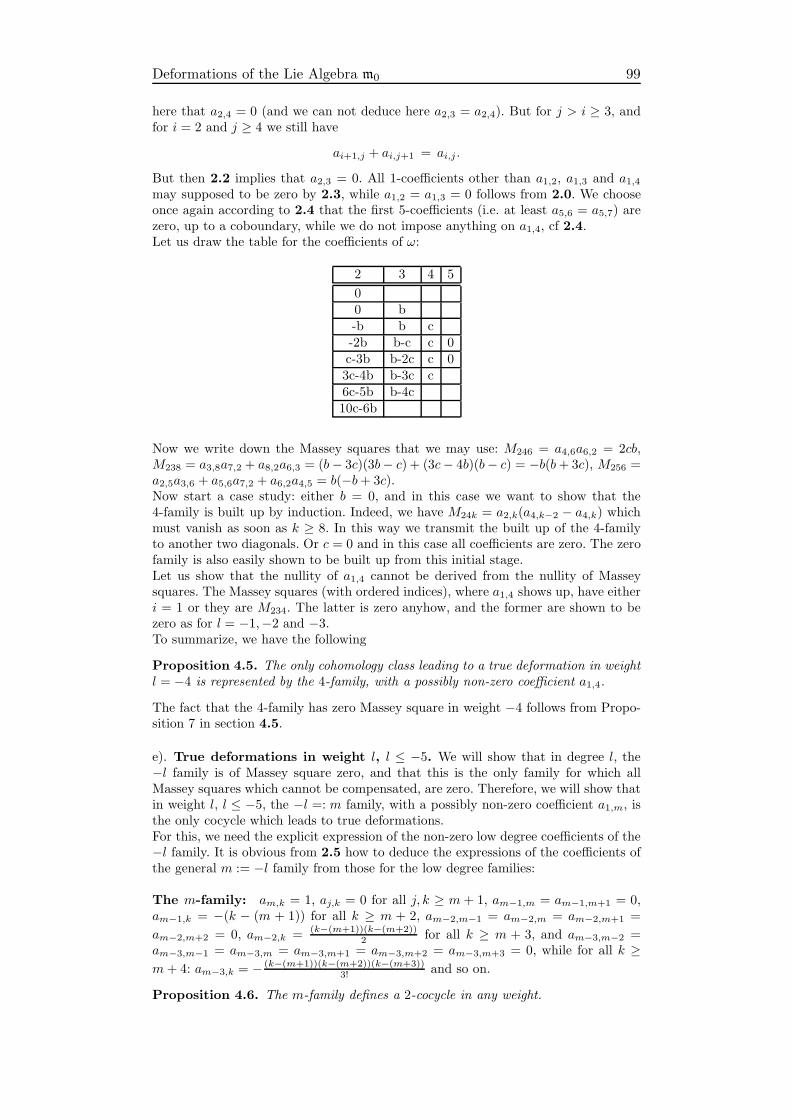
Deformations of the Lie Algebra m0 99
here that a2,4 = 0 (and we can not deduce here a2,3 = a2,4). But for j > i ≥ 3, andfor i = 2 and j ≥ 4 we still have
ai+1,j + ai,j+1 = ai,j .
But then 2.2 implies that a2,3 = 0. All 1-coefficients other than a1,2, a1,3 and a1,4may supposed to be zero by 2.3, while a1,2 = a1,3 = 0 follows from 2.0. We chooseonce again according to 2.4 that the first 5-coefficients (i.e. at least a5,6 = a5,7) arezero, up to a coboundary, while we do not impose anything on a1,4, cf 2.4.Let us draw the table for the coefficients of ω:
2 3 4 5
00 b-b b c-2b b-c c 0c-3b b-2c c 03c-4b b-3c c6c-5b b-4c10c-6b
Now we write down the Massey squares that we may use: M246 = a4,6a6,2 = 2cb,M238 = a3,8a7,2 + a8,2a6,3 = (b− 3c)(3b− c) + (3c− 4b)(b− c) = −b(b+ 3c), M256 =a2,5a3,6 + a5,6a7,2 + a6,2a4,5 = b(−b+ 3c).Now start a case study: either b = 0, and in this case we want to show that the4-family is built up by induction. Indeed, we have M24k = a2,k(a4,k−2 − a4,k) whichmust vanish as soon as k ≥ 8. In this way we transmit the built up of the 4-familyto another two diagonals. Or c = 0 and in this case all coefficients are zero. The zerofamily is also easily shown to be built up from this initial stage.Let us show that the nullity of a1,4 cannot be derived from the nullity of Masseysquares. The Massey squares (with ordered indices), where a1,4 shows up, have eitheri = 1 or they are M234. The latter is zero anyhow, and the former are shown to bezero as for l = −1,−2 and −3.To summarize, we have the following
Proposition 4.5. The only cohomology class leading to a true deformation in weightl = −4 is represented by the 4-family, with a possibly non-zero coefficient a1,4.
The fact that the 4-family has zero Massey square in weight −4 follows from Propo-sition 7 in section 4.5.
e). True deformations in weight l, l ≤ −5. We will show that in degree l, the−l family is of Massey square zero, and that this is the only family for which allMassey squares which cannot be compensated, are zero. Therefore, we will show thatin weight l, l ≤ −5, the −l =: m family, with a possibly non-zero coefficient a1,m, isthe only cocycle which leads to true deformations.For this, we need the explicit expression of the non-zero low degree coefficients of the−l family. It is obvious from 2.5 how to deduce the expressions of the coefficients ofthe general m := −l family from those for the low degree families:
The m-family: am,k = 1, aj,k = 0 for all j, k ≥ m + 1, am−1,m = am−1,m+1 = 0,am−1,k = −(k − (m + 1)) for all k ≥ m + 2, am−2,m−1 = am−2,m = am−2,m+1 =
am−2,m+2 = 0, am−2,k = (k−(m+1))(k−(m+2))2 for all k ≥ m + 3, and am−3,m−2 =
am−3,m−1 = am−3,m = am−3,m+1 = am−3,m+2 = am−3,m+3 = 0, while for all k ≥m+ 4: am−3,k = − (k−(m+1))(k−(m+2))(k−(m+3))
3! and so on.
Proposition 4.6. The m-family defines a 2-cocycle in any weight.
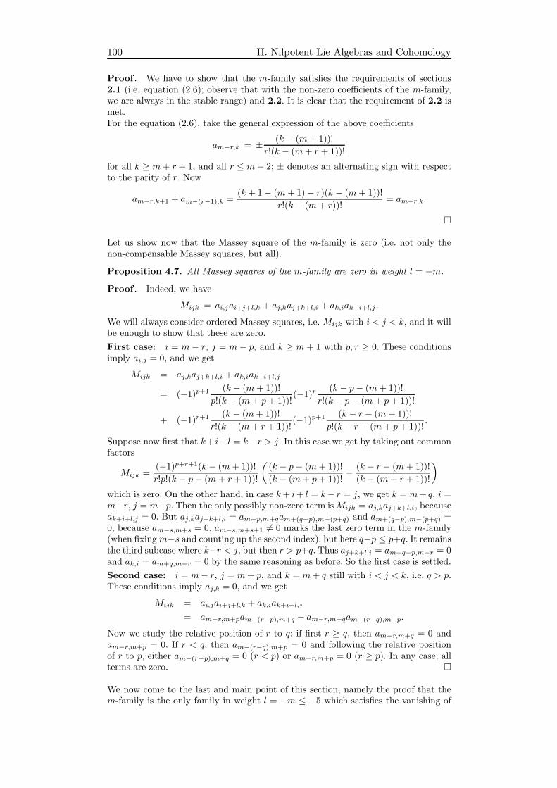
100 II. Nilpotent Lie Algebras and Cohomology
Proof . We have to show that the m-family satisfies the requirements of sections2.1 (i.e. equation (2.6); observe that with the non-zero coefficients of the m-family,we are always in the stable range) and 2.2. It is clear that the requirement of 2.2 ismet.For the equation (2.6), take the general expression of the above coefficients
am−r,k = ± (k − (m+ 1))!
r!(k − (m+ r + 1))!
for all k ≥ m+ r + 1, and all r ≤ m− 2; ± denotes an alternating sign with respectto the parity of r. Now
am−r,k+1 + am−(r−1),k =(k + 1− (m+ 1)− r)(k − (m+ 1))!
r!(k − (m+ r))!= am−r,k.
Let us show now that the Massey square of the m-family is zero (i.e. not only thenon-compensable Massey squares, but all).
Proposition 4.7. All Massey squares of the m-family are zero in weight l = −m.
Proof . Indeed, we have
Mijk = ai,jai+j+l,k + aj,kaj+k+l,i + ak,iak+i+l,j .
We will always consider ordered Massey squares, i.e. Mijk with i < j < k, and it willbe enough to show that these are zero.
First case: i = m− r, j = m − p, and k ≥ m + 1 with p, r ≥ 0. These conditionsimply ai,j = 0, and we get
Mijk = aj,kaj+k+l,i + ak,iak+i+l,j
= (−1)p+1 (k − (m+ 1))!
p!(k − (m+ p+ 1))!(−1)r (k − p− (m+ 1))!
r!(k − p− (m+ p+ 1))!
+ (−1)r+1 (k − (m+ 1))!
r!(k − (m+ r + 1))!(−1)p+1 (k − r − (m+ 1))!
p!(k − r − (m+ p+ 1))!.
Suppose now first that k+ i+ l = k−r > j. In this case we get by taking out commonfactors
Mijk =(−1)p+r+1(k − (m+ 1))!
r!p!(k − p− (m+ r + 1))!
((k − p− (m+ 1))!
(k − (m+ p+ 1))!− (k − r − (m+ 1))!
(k − (m+ r + 1))!
)
which is zero. On the other hand, in case k+ i+ l = k− r = j, we get k = m+ q, i =m−r, j = m−p. Then the only possibly non-zero term isMijk = aj,kaj+k+l,i, becauseak+i+l,j = 0. But aj,kaj+k+l,i = am−p,m+qam+(q−p),m−(p+q) and am+(q−p),m−(p+q) =0, because am−s,m+s = 0, am−s,m+s+1 6= 0 marks the last zero term in the m-family(when fixingm−s and counting up the second index), but here q−p ≤ p+q. It remainsthe third subcase where k−r < j, but then r > p+q. Thus aj+k+l,i = am+q−p,m−r = 0and ak,i = am+q,m−r = 0 by the same reasoning as before. So the first case is settled.
Second case: i = m− r, j = m+ p, and k = m+ q still with i < j < k, i.e. q > p.These conditions imply aj,k = 0, and we get
Mijk = ai,jai+j+l,k + ak,iak+i+l,j
= am−r,m+pam−(r−p),m+q − am−r,m+qam−(r−q),m+p.
Now we study the relative position of r to q: if first r ≥ q, then am−r,m+q = 0 andam−r,m+p = 0. If r < q, then am−(r−q),m+p = 0 and following the relative positionof r to p, either am−(r−p),m+q = 0 (r < p) or am−r,m+p = 0 (r ≥ p). In any case, allterms are zero.
We now come to the last and main point of this section, namely the proof that them-family is the only family in weight l = −m ≤ −5 which satisfies the vanishing of
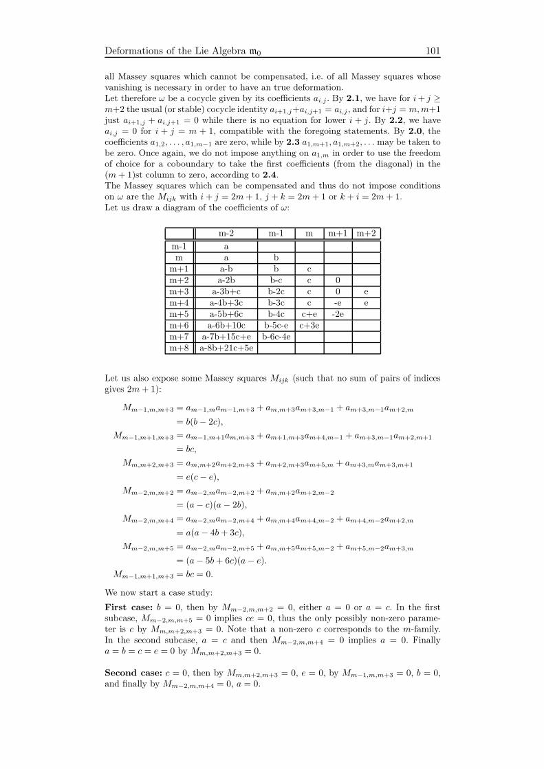
Deformations of the Lie Algebra m0 101
all Massey squares which cannot be compensated, i.e. of all Massey squares whosevanishing is necessary in order to have an true deformation.Let therefore ω be a cocycle given by its coefficients ai.j . By 2.1, we have for i+ j ≥m+2 the usual (or stable) cocycle identity ai+1,j+ai,j+1 = ai,j , and for i+j = m,m+1just ai+1,j + ai,j+1 = 0 while there is no equation for lower i + j. By 2.2, we haveai,j = 0 for i + j = m + 1, compatible with the foregoing statements. By 2.0, thecoefficients a1,2, . . . , a1,m−1 are zero, while by 2.3 a1,m+1, a1,m+2, . . . may be taken tobe zero. Once again, we do not impose anything on a1,m in order to use the freedomof choice for a coboundary to take the first coefficients (from the diagonal) in the(m+ 1)st column to zero, according to 2.4.The Massey squares which can be compensated and thus do not impose conditionson ω are the Mijk with i+ j = 2m+ 1, j + k = 2m+ 1 or k + i = 2m+ 1.Let us draw a diagram of the coefficients of ω:
m-2 m-1 m m+1 m+2
m-1 am a b
m+1 a-b b cm+2 a-2b b-c c 0m+3 a-3b+c b-2c c 0 em+4 a-4b+3c b-3c c -e em+5 a-5b+6c b-4c c+e -2em+6 a-6b+10c b-5c-e c+3em+7 a-7b+15c+e b-6c-4em+8 a-8b+21c+5e
Let us also expose some Massey squares Mijk (such that no sum of pairs of indicesgives 2m+ 1):
Mm−1,m,m+3 = am−1,mam−1,m+3 + am,m+3am+3,m−1 + am+3,m−1am+2,m
= b(b− 2c),
Mm−1,m+1,m+3 = am−1,m+1am,m+3 + am+1,m+3am+4,m−1 + am+3,m−1am+2,m+1
= bc,
Mm,m+2,m+3 = am,m+2am+2,m+3 + am+2,m+3am+5,m + am+3,mam+3,m+1
= e(c− e),Mm−2,m,m+2 = am−2,mam−2,m+2 + am,m+2am+2,m−2
= (a− c)(a− 2b),
Mm−2,m,m+4 = am−2,mam−2,m+4 + am,m+4am+4,m−2 + am+4,m−2am+2,m
= a(a− 4b+ 3c),
Mm−2,m,m+5 = am−2,mam−2,m+5 + am,m+5am+5,m−2 + am+5,m−2am+3,m
= (a− 5b+ 6c)(a− e).Mm−1,m+1,m+3 = bc = 0.
We now start a case study:
First case: b = 0, then by Mm−2,m,m+2 = 0, either a = 0 or a = c. In the firstsubcase, Mm−2,m,m+5 = 0 implies ce = 0, thus the only possibly non-zero parame-ter is c by Mm,m+2,m+3 = 0. Note that a non-zero c corresponds to the m-family.In the second subcase, a = c and then Mm−2,m,m+4 = 0 implies a = 0. Finallya = b = c = e = 0 by Mm,m+2,m+3 = 0.
Second case: c = 0, then by Mm,m+2,m+3 = 0, e = 0, by Mm−1,m,m+3 = 0, b = 0,and finally by Mm−2,m,m+4 = 0, a = 0.
102 II. Nilpotent Lie Algebras and Cohomology
Now it is clear how to perform an induction step showing that the m-family is trans-mitted to a next two diagonals. For example using Mm−2,m,m+7:
Mm−2,m,m+7 = am−2,m+7(am−2,m − am,m+7 + am,m+5),
and by assumption am−2,m+7 6= 0, am−2,m = 0, and thus by Mm−2,m,m+7 = 0,am,m+7 = am,m+5 = c which is the induction step. This shows that starting from the(m − 2)nd column, all coefficients are as in the m-family. In order to come to lowercoefficients, take for example
Mm−3,m+1,m+5 = am−3,m+1am−2,m+5 + am+1,m+5am+6,m−3 + am+5,m−3am+2,m+1.
Here, am+1,m+5 = am+2,m+1 = 0 and am−2,m+5 6= 0 by assumption, therefoream−3,m+1 = 0 which transmits the m-family to the (m− 3)rd column.Finally, let us argue that the coefficient a1,m cannot be shown to be zero by thevanishing of Massey squares. Indeed, in order to involve a1,m, the Massey squareMijk (with ordered indices) must have either i = 1 or i + j + l = 1, j + k + l = 1 ori+ k+ l = 1. The first alternative is rather easily seen to be zero. Fix i+ j+ l = 1 forthe second alternative. It describes a situation where the coefficient a1,m is multipliedby ai,j with i + j = m+ 1. This coefficient is zero.To summarize, we have the following
Proposition 4.8. The only non-zero cohomology class compatible with the vanishingof all Massey squares which cannot be compensated, is the m-family in weight l =−m ≤ −5, with a possibly non-zero coefficient a1,m.
5. Deformations in zero and positive weights
a). True deformations in weight l = 0. In weight l ≥ 0, a new phenomenon ishappening: we have a relation between the Massey squares. Recall that the cocyclecoefficients ai,j are supposed to be antisymmetric in i, j, and that ai,i is set to zerofor all i.
Proposition 5.1. Let i, j, k, be three integers, i, k ≥ 2 and j ≥ 3. We have therelation
Mijk +Mi(j−1)(k+1) +M(i+1)(j−1)k = Mi(j−1)k.
Proof . We have by definition
Mijk +Mi(j−1)(k+1) = ai,jai+j+l,k + aj,kaj+k+l,i +
ak,iai+k+l,j + ai,j−1ai+j−1+l,k+1 + aj−1,k+1aj+k+l,i + ak+1,iai+k+1+l,j−1.
We transform the terms aj,kaj+k+l,i + aj−1,k+1aj+k+l,i, using repeatedly the cocycleequation (2.6) to
aj+k+l,i(aj,k + aj−1,k+1) = aj+k+l,iaj−1,k = aj−1,k(aj+k−1+l,i − aj+k−1+l,i+1).
We transform the terms ai,jai+j+l,k + ai,j−1ai+j−1+l,k+1, using the equations (2.6)to
ai,jai+j+l,k + ai,j−1ai+j−1+l,k − ai,j−1ai+j+l,k.We transform the terms ak,iai+k+l,j + ak+1,iai+k+1+l,j−1, using the equations (2.6)to
ak,iai+k+l,j−1 − ak,iai+k+1+l,j−1 + ak+1,iai+k+1+l,j−1.
In these three transformations, the sum of the first term of the first, the second termof the second and the first term of the third give together
aj−1,kaj+k−1+l,i + ai,j−1ai+j−1+l,k + ak,iai+k+l,j−1 = Mi(j−1)k.
The remaining terms read
−aj−1,kaj+k−1+l,i+1+ai,jai+j+l,k−ai,j−1ai+j+l,k−ak,iai+k+1+l,j−1+ak+1,iai+k+1+l,j−1.
Here, the second and third term give
ai,jai+j+l,k − (ai,jai+j+l,k + ai+1,j−1ai+j+l,k) = −ai+j+l,kai+1,j−1,

Deformations of the Lie Algebra m0 103
while the last two terms give
−(ak+1,i + ak,i+1)ai+k+1+l,j−1 + ak+1,iai+k+1+l,j−1 = −ai+k+1+l,j−1ak,i+1,
still using the equations (2.6).In summary, the remaining terms give
−aj−1,kaj+k−1+l,i+1 − ai+j+l,kai+1,j−1 − ai+k+1+l,j−1ak,i+1 = −M(i+1)(j−1)k.
This ends the proof of Propositin 5.1.
Corollary 5.2.
Mi(i+1)k +Mi(i+2)(k−1) =Mi(i+1)(k−1).
Observe that also repeated indices may give interesting relations: for example, fori = 2, j = 4 and k = 4, we getM234 =M235. It is easily shown by these relations thatthe nullity ofM23k for all k ≥ 4 is necessary for the nullity of all Massey squares, andthat the nullity of M2rs for all r, s ≥ 3 is necessary and sufficient for the nullity ofall Massey squares. We believe that the minimal set of Massey squares whose nullityimplies the nullity of all Massey squares is somewhere in between these two sets, butwe could not get hold on it.Now, we will determine all square zero cocycles, i.e. all true deformations of m0, inweight l = 0: first of all, the 2-family is such a cocycle. Then, let us suppose that ωis a non-trivial 2-cocycle which is independent of the 2-family and has zero Masseysquares; as before, we think of ω as given by the coefficients ai,j , and we will distributeletters to its initial terms: a2,3 = a, a3,4 = b, and so on.Using equations (2.6), we establish the following diagram which is of course valid forall weights l; observe that the general expression for the coefficients in section 4.5,proof of Proposition 6, leads for general coefficients a2,3 =: u2 = a, a3,4 =: u3 =b, a4,5 =: u4 = c and so on (by linearity) to the formula
ai,j =
j−1∑
m=2
(−1)m−ium(j − (m+ 1))!
(m− i)!(j − 2m+ i− 1)!, (5.8)
which may be used to compute the coefficients in the following diagram more easily(than by a recursive formula).
2 3 4 5 6 7
3 a4 a b5 a-b b c6 a-2b b-c c d7 a-3b+c b-2c c-d d e8 a-4b+3c b-3c+d c-2d d-e e f9 a-5b+6c-d b-4c+3d c-3d+e d-2e e-f f10 a-6b+10c-4d b-5c+6d-e c-4d+3e d-3e+f e-2f11 a-7b+15c-10d+e b-6c+10d-4e c-5d+6e-f d-4e+3f12 a-8b+21c-20d+5e b-7c+15d-10e+f c-6d+10e-4f13 a-9b+28c-35d+15e-f b-8c+21d-20e+5f14 a-10b+36c-56d+35e-6f
From now on, we consider weight l = 0.
Order the Massey squares by their level, i.e. we say that Mijk has level i + j + k.Computing Massey squares and setting them equal to zero gives an infinite family ofhomogeneous quadratic equations for the infinite family of variables a, b, c, d, . . ..In level 9, the only Massey square is M234, and its nullity gives
3b2 − bc− 2ac = 0.
104 II. Nilpotent Lie Algebras and Cohomology
In level 10, the only Massey square is M235, and its nullity gives the same equation.In level 11, there are Massey squaresM236 andM245, and their nullity gives (possiblyby subtracting the previous equation) in both cases
2ad− 4bc− bd+ 6c2 − cd = 0.
In level 12, there are Massey squares M237, M246 and M345, and their nullity gives(possibly by subtracting the previous equations) in all cases
−3bd+ 4c2 − 3cd = 0.
Going higher in this hierarchy of equations and variables, there are at each new levelsome (possibly) linearly independent equations. Proposition 9 only tells us that thenullity of M2rs with 2 < r < s is enough in order to have all Massey squares zero.We don’t know which of these equations are in fact the independent ones.In Massey square level 14, we arrive at 5 equations for the 5 variables a, b, c, d, e,which read (after subtracting at each step multiples of the previous equations):
3b2 − bc− 2ac = 0
2ad− 4bc− bd+ 6c2 − cd = 0
−3bd+ 4c2 − 3cd = 0
e(−2a+ 3b− d) + 5bd− 15cd+ 10d2 = 0
e(−6a+ 15b− 4c− 11d)− 55cd+ 50d2 + 15bd = 0
The discussion of these equations (either by hand or by a system computing a Grobnerbasis for the homogeneous polynomials) gives as non-zero solutions the 2-family andone other family with coefficients a = 1
6 , b =160 , c =
1420 , etc. We describe this family
from another point of view in subsection 5.3, which will show that this family mustverify all equations and not only the five equations we wrote down. These are theonly square zero solutions in weight 0, and we have determined all true deformationsin this case.
b). True deformations in weight l > 0. In the weight l = 1 case, we get fromthe same diagram as in weight l = 0 up to Massey level 15 (where we took only theequations of type M23k in order to simplify) six homogeneous quadratic equations insix variables which read:
−3ac+ 4b2 − 3bc = 0
−5bc− 2bd+ 10c2 − 4cd+ 3ad = 0
5c2 − 4bd+ 2be+ ec− 6cd = 0
e(−3a+ 11b− 5d+ 3c)− 6bd+ 15c2 − 39cd+ 20d2 = 0
e(−9a+ 35b− 35d) + f(−4b+ 2c+ 2d)− 6bd+ 30c2 − 111cd+ 90d2 = 0
e(−18a+ 75b+ 11c− 186d+ 35e− 6f) + f(3a+ 20c− 24b+ 16d)
−4bd+ 50c2 − 234cd+ 252d2 = 0
By a computation with MUPaD which determines a Grobner basis for the homo-geneous polynomials corresponding to these equations (actually we took here allequations of type M2rs), one obtains as (non-zero) solutions the 2-family, a solu-tion a = 0, b = 0, c = 0, d = 0 and e = 1, f = 35
6 , and a further solution a = 1, b = 17 ,
c = 142 , d = 1
231 , e =5
21·286 , f = 121·286 . The solution with e = 1 and f = 35
6 does notsurvive the next level of Massey squares.But the solution starting with a = 1, b = 1
7 continues with g = 129172 , h = 1
138567 ,
i = 1646646 , j = 5
14872858 , k = 113520780 . We will describe this family from a different
point of view in section 5.3, and we will show there (implicitly) that this solutionsurvives to infinity.
Proposition 5.3. In weight l = 1, there are exactly two non-equivalent true defor-mations.

Deformations of the Lie Algebra m0 105
The problem of determining the explicit square zero cocycles in each weight l caseseems to be a rich problem. We tried to say something about the rank of the finiteJacobi matrix either associated to the set of equations of type M2rs = 0 for all r, s, orto those of typeM23r for all r, when we truncate the number of variables and consideronly those equations involving these variables. With this matrix, it is obvious thatthe set of solutions (of the truncated problem) is an algebraic variety of dimensiongreater or equal to 1 (because the equations are homogeneous), but we couldn’t decidewhether the dimension drops down to 1 in each weight. In fact, within the possibilitiesof our computer, we computed (using all equations of type M2rs = 0) the dimensionof this variety as far as possible for l = 2 and it remained 2. Is the set of solutionsalways a variety ? Is it always of finite dimension ? Can we give asymptotics or boundsor a formula for the dimension ?
c). Identifying the cocycles and the deformed algebras in weight zero. Wenow construct deformations from the previously determined weight l 2-cocycles givenby their coefficients ai,j in the following way: using still the ei for i ≥ 1 as a basis,the deformed bracket reads
[ei, ej]t = [ei, ej ] + tai,jei+j+l.
It is clear that all square zero 2-cocycles give in this way true deformations of m0 forwhich only the linear term is (possibly) non-zero; this means in particular that thebracket [−,−]t satisfies the Jacobi identity without adding terms containing higherpowers in t.The weight l = 0 case is the most interesting, because here deformations give auto-matically rise to N-graded Lie algebras which must fit in the classification [1]. In thisclassification, the three N-graded Lie algebras where e1 has non-zero brackets withall other basis elements are
(1) m0; brackets: [e1, ei] = ei+1 for all i ≥ 2,(2) m2; brackets: [e1, ei] = ei+1 for all i ≥ 2, [e2, ej ] = ej+1 for all j ≥ 3,(3) L1; brackets: [ei, ej] = (j − i)ei+j for all i, j ≥ 1.
The complete set of infinitesimal deformations of L1 and the complete set of formaldeformations of L1 is given in [2]. Let us consider in this section the same problemfor m0 in weight l = 0.Taking as 2-cocycle the 2-family, we get in weight l = 0 a Lie algebra m1
0(t) whichmust be N-graded and which is easily seen to be generated by e1 and e2: indeed,[e1, ei]t = [e1, ei] for all i ≥ 2. The complete relations for m1
0(t) are
[e1, ei]t = ei+1 ∀ i ≥ 2[e2, ej]t = tej+2 ∀ j ≥ 3
Thus this family describes the deformation of m0 to m2.Now there is also a cocycle describing the deformation of m0 to L1: observe that thegenerators ei for i ≥ 1 of m0 do not satisfy the right relations, seen as elements ofL1. Therefore, one must first perform a change of base: let us define e1 = e1, e2 = e2,e3 = e3, e4 = 1
2e4 and in general
ei =1
(i− 2)!ei
for all i ≥ 5. Then the relations are easily computed to be
[e1, ei] = (i− 1)ei+1.
The cocycle relation (2.6) for a cocycle given by coefficients bi,j transforms in thenew basis to
(j − 1)bj+1,k + (k − 1)bj,k+1 = (j + k + l − 1)bj,k.
It is easy to check that the 2-cochain given by the coefficients bi,j = (j − i) is indeeda 2-cocycle for l = 0. One also easily checks that the 2-cocycle bi,j = (j − i) is of
106 II. Nilpotent Lie Algebras and Cohomology
Massey square zero, i.e.
bi,jbi+j,k + bj,kbj+k,i + bk,ibk+i,j = 0.
It therefore determines a deformationm20(t) ofm0 in weight l = 0 to L1, and we showed
in the previous section that these are all possible deformations of m0 in weight 0.Let us finish with the identification of the deformations in weight l = 1. It is clearthat the 2-family leads to a non-trivial true deformation. This is then a weight 1variant of the Lie algebra m2. The other cocycle, determined using MUPaD, is moreinteresting. Indeed, there is a general procedure of constructing positive weight, truedeformations for m0: consider the Lie algebra L1, with its generators e1, e2, e3, etcand its relations [ei, ej] = (j − i)ei+j for all i, j ≥ 1. Define a Lie algebra L12 bygenerators e1, e3, e4 etc (the suppression of e2 is indicated by 2 in the notation !)and the relations of L1 for the remaining generators. Introduce a new basis f1 := e1,f2 := e3, f3 := e4 etc, and another new basis g1 := e1, gk := (k − 1)! fk for all k > 1.We compute the relations to
[g1, gk] = gk+1, [gk, gk+1] =k!(k − 1)!
(2k + 1)!g2k+2.
When interpreted as a deformation of m0, one can then compute the coefficients ai,jof the corresponding 2-cocycle. One obtains a2,3 = 2!1!
5! = 160 · 1, a3,4 = 3!2!
7! = 160 · 17 ,
a4,5 = 4!3!9! = 1
60 · 142 , a5,6 = 5!4!
11! = 160 · 1
231 , a6,7 = 6!5!13! = 1
60 · 521·286 , a7,8 = 7!6!
15! =160 · 1
21·286 , and so on. Thus, this deformation has as its infinitesimal cocycle the cocycle
we determined using MUPaD before, up to a factor 160 . By construction, it is clear
that it defines a cocycle and a true deformation, because L12 is a Lie algebra.In the same way, one can define L1m by the span of the vectors e1, em+1, em+2, etcfor anym > 2, in other words, by the suppression of all basis vectors from e2 up to andincluding em+1. This gives a non-trivial true deformation of weight m− 1. Togetherwith the deformation given by the 2-family, these two constitute two independenttrue deformations in any positive weight.
References
[1] Fialowski, Alice, “Classification of graded Lie algebras with two generators,” MoscowUniv. Math. Bull. 38, 2 (1983) 76–79
[2] Fialowski, Alice, “An example of formal deformations of Lie algebras,” in Deforma-tion Theory of Algebras and Structures and Applications, ed.: M. Hazewinkel and M.Gerstenhaber, 1988 Kluwer Academic Publishers
[3] Fialowski, Alice, Fuchs, Dmitry, “Construction of Miniversal Deformations of Lie Alge-bras,” J. Funct. Anal., 161 (1999) 76–110
[4] Fialowski, Alice, Millionschikov, Dmitri, “Cohomology of graded Lie algebras of maxi-mal class,” J. Algebra, 296, no. 1 (2006) 157–176
[5] Fuchs, Dmitry B., Cohomology of Infinite Dimensional Lie algebras, Consultants Bu-reau, New York, 1987.
[6] Gontcharova, L. V., “Cohomology of Lie algebras of formal vector fields on the line”Funct. Anal. Appl., 7(2) (1973), 6–14
[7] Hartshorne, Robin, Algebraic Geometry, Graduate Texts in Mathematics, No. 52.Springer-Verlag, New York-Heidelberg, 1977
[8] Shalev, Aner, Zelmanov, Efim I., “Narrow Lie algebras: A coclass theory and a charac-terization of the Witt algebra,” J. Algebra, 189 (1997) 294–331
[9] Vergne, Michele, “Cohomologie des algebres de Lie nilpotentes,” Bull. Soc. Math.France, 98 (1970) 81–116
Alice Fialowski, email : [email protected] Wagemann, email : [email protected]
Deformations of the Lie Algebra m0 107
Part III: Generalizations and Applications
1. Krichever-Novikov Witt Algebras 110
Alice Fialowski and Martin SchlichenmaierCommun. in Contemporary Math., 5 (2003), pp. 921–945
2. Deformations of Four Dimensional Lie Algebras 129
Alice Fialowski and Michael PenkavaCommun. in Contemporary Math., 9 (2007), pp. 41–79
108
Deformations of the Lie Algebra m0 109
appeared in: Commun. in Contemporary Math., 5 (2003), 921–945
Global Deformations of the Witt Algebra ofKrichever-Novikov Type
Alice FialowskiInstitute of Mathematics
Eotvos Lorand University, Budapest
Martin SchlichenmaierLaboratoire de MathematiquesUniversite du Luxembourg
We dedicate this article to the memory of our goodfriend Peter Slodowy who passed away in 2002
Abstract By considering non-trivial global deformations of the Witt(and the Virasoro) algebra given by geometric constructions it is shownthat, despite their infinitesimal and formal rigidity, they are globallynot rigid. This shows the need of a clear indication of the type of defor-mations considered. The families appearing are constructed as familiesof algebras of Krichever-Novikov type. They show up in a natural wayin the global operator approach to the quantization of two-dimensionalconformal field theory. In addition, a proof of the infinitesimal and for-mal rigidity of the Witt algebra is presented.
1. Introduction
Deformations of mathematical structures are important in most part of mathematicsand its applications. Deformation is one of the tools used to study a specific object,by deforming it into some families of ”similar” structure objects. This way we get aricher picture about the original object itself.But there is also another question approached via deformations. Roughly speaking,it is the question, can we equip the set of mathematical structures under considera-tion (maybe up to certain equivalences) with the structure of a topological or evengeometric space. In other words, does there exist a moduli space for these structures.If so, then for a fixed object the deformations of this object should reflect the localstructure of the moduli space at the point corresponding to this object.In this respect, a clear success story is the classification of complex analytic structureson a fixed topological manifold. Also in algebraic geometry one has well-developedresults in this direction. One of these results is that the local situation at a point [C]of the moduli space is completely governed by the cohomological properties of thegeometric object C. As typical example recall that for the moduli spaceMg of smoothprojective curves of genus g over C (or equivalently, compact Riemann surfaces ofgenus g) the tangent space T[C]Mg can be naturally identified with H1(C, TC), whereTC is the sheaf of holomorphic vector fields over C. This extends to higher dimension.In particular, it turns out that for compact complex manifolds M , the conditionH1(M,TM ) = 0 implies that M is rigid, [16, Thm. 4.4]. Rigidity means that anydifferentiable family π : M → B ⊆ R, 0 ∈ B which contains M as the specialmember M0 := π−1(0) is trivial in a neighbourhood of 0, i.e. for t small enoughMt := π−1(t) ∼= M . Even more generally, for M a compact complex manifold andH1(M,TM ) 6= 0 there exists a versal family which can be realized locally as a family
∗1991 Mathematics Subject Classification. Primary: 17B66; Secondary: 17B56, 17B65,17B68, 14D15, 14H52, 30F30, 81T40
†Key words and phrases. Deformations of algebras, rigidity, Virasoro algebra, Krichever-Novikov algebras, elliptic curves, Lie algebra cohomology, conformal field theory
‡The research of the first author was partially supported by the grants OTKA T030823,T29525. The last version of the work was completed during her stay at the Max-Planck-Institut fur Mathematik Bonn.
110

Krichever-Novikov Witt Algebras 111
over a certain subspace of H1(M,TM ) such that every appearing deformation familyis “contained” in this versal family (see also [18] for definitions, results, and furtherreferences).These positive results lead to the impression that the vanishing of the relevant co-homology spaces will imply rigidity with respect to deformations also in the case ofother structures.The goal of this article is to shed some light on this in the context of deformationsof infinite-dimensional Lie algebras. We consider the case of the Witt algebra W(see its definition further down). The cohomology “responsible” for deformations isH2(W ,W). It is known that H2(W ,W) = 0 (see Section 3). Hence, guided by theexperience in the theory of deformations of complex manifolds, one might think thatW is rigid in the sense that all families containing W as a special element will betrivial. But this is not the case as we will show. Certain natural families of Krichever-Novikov type algebras of geometric origin (see Section 4 for their definition) willappear which contain W as special element. But none of the other elements will beisomorphic to W . In fact, from H2(W ,W) = 0 it follows that the Witt algebra isinfinitesimally and formally rigid. But this condition does not imply that there are nonon-trivial global deformation families. The main point to learn is that it is necessaryto distinguish clearly the formal and the global deformation situation. The formalrigidity of the Witt algebra indeed follows from H2(W ,W) = 0, but no statementlike that about global deformations.How intricate the situation is, can be seen from the fact that for the subalgebra L1
of W , consisting of those vector fields vanishing at least of order two at zero, thereexists a versal formal family consisting of three different families parameterized overa collection of three curves in H2(L1, L1). Suitably adjusted each family correspondsto a scalar multiple of the same cohomology class ω [6],[7],[9] which gives their in-finitesimal deformations. It turns out that H2(L1, L1) is 3-dimensional, but only theinfinitesimal deformations corresponding to scalar multiples of ω can be extended toformal deformations.The results of this article will show that the theory of deformations of infinite-dimensional Lie algebras is still not in satisfactory shape. Hopefully, the appearingfeatures will be of help in a further understanding.Clearly, what will be done here, can also be done in the case of associative algebras.In particular, there will be global deformations of the associative algebra of Lau-rent polynomials of Krichever-Novikov type obtained by the same process as the onepresented here.First, let us introduce the basic definitions. Consider the complexification of the Liealgebra of polynomial vector fields on the circle with generators
ln := exp(inϕ)d
dϕ, n ∈ Z,
where ϕ is the angular parameter. The bracket operation in this Lie algebra is
[ln, lm] = (m− n)ln+m.We call it the Witt algebra and denote it by W . Equivalently, the Witt algebracan be described as the Lie algebra of meromorphic vector fields on the Riemannsphere P1(C) which are holomorphic outside the points 0 and∞. In this presentationln = zn+1 d
dz , where z is the quasi-global coordinate on P1(C).The Lie algebra W is infinite dimensional and graded with the standard gradingdeg ln = n. By taking formal vector fields with the projective limit topology we getthe completed topological Witt algebraWtop. Throughout this paper we will considerits everywhere dense subalgebra W .It is well-known thatW (up to equivalence and rescaling) has a unique nontrivial one-dimensional central extension, the Virasoro algebra V . It is generated by ln (n ∈ Z)and the central element c, and its bracket operation is defined by
[ln, lm] = (m− n)ln+m + 112 (m
3 −m)δn,−m c, [ln, c] = 0. (1.9)

112 III. Generalizations and Applications
In Section 2 we recall the different concepts of deformation. There is a lot of confu-sion in the literature in the notion of a deformation. Several different (inequivalent)approaches exist. One of the aims of this paper is to clarify the difference between de-formations of geometric origin and so called formal deformations. Formal deformationtheory has the advantage of using cohomology. It is also complete in the sense thatunder some natural cohomology assumptions there exists a versal formal deformation,which induces all other deformations.In this context see Theorem 2.7 and Corollary 2.8 which are quoted from [6],[9].Formal deformations are deformations with a complete local algebra as base. A de-formation with a commutative (non-local) algebra base gives a much richer picture ofdeformation families, depending on the augmentation of the base algebra. If we iden-tify the base of deformation – which is a commutative algebra of functions – with asmooth manifold, an augmentation corresponds to choosing a point on the manifold.So choosing different points should in general lead to different deformation situations.As already indicated above, in infinite dimension, there is no tight relation betweenglobal and formal deformations, as we will show in this paper.
In Section 3, we supply a detailed proof of the infinitesimal and formal rigidity of theWitt algebra W , by showing that H2(W ,W) = 0.
In Section 4 we introduce and recall the necessary properties of the Krichever-Novikovtype vector field algebras. They are generalizations of the Witt algebra (in its pre-sentation as vector fields on P1(C)) to higher genus smooth projective curves.
In Section 5 we construct global deformations of the Witt algebra by consideringcertain families of algebras for the genus one case (i.e. the elliptic curve case) andlet the elliptic curve degenerate to a singular cubic. The two points, where polesare allowed, are the zero element of the elliptic curve (with respect to its additivestructure) and a 2-torsion point. In this way we obtain families parameterized overthe affine line with the peculiar behaviour that every family is a global deformation ofthe Witt algebra, i.e.W is a special member, whereas all other members are mutuallyisomorphic but not isomorphic to W , see Theorem 5.3. Globally these families arenon-trivial, but infinitesimally and formally they are trivial. The construction canbe extended to the centrally extended algebras, yielding a global deformation of theVirasoro algebra. Finally, we consider the subalgebra L1 of W corresponding to thevector fields vanishing at least with order two at 0. This algebra is formally not rigid,and its formal versal deformation has been determined [6, 8]. We identify one of theappearing three families in our geometric context.
The results obtained do not have only relevance to the deformation theory of algebrasbut also to the theory of two-dimensional conformal fields and their quantization. Itis well-known that the Witt algebra, the Virasoro algebra, and their representationsare of fundamental importance for the local description of conformal field theory onthe Riemann sphere (i.e. for genus zero), see [1]. Krichever and Novikov [17] proposedin the case of higher genus Riemann surfaces the use of global operator fields whichare given with the help of the Lie algebra of vector fields of Krichever-Novikov type,certain related algebras, and their representations (Section 4).In the process of quantization of the conformal fields one has to consider families ofalgebras and representations over the moduli space of compact Riemann surfaces (orequivalently, of smooth projective curves over C) of genus g with N marked points.See [28] for a global operator version, and [29] for a sheaf version. In passing to theboundary of the moduli space one obtains the limit objects which are defined over thenormalization of curves of lower genus. Assuming good behaviour of the examinedobjects under deformation also in the limit (e.g. “factorization”), the degeneration isan important technique to obtain via induction from results for lower genus resultsfor all genera. See Tsuchiya, Ueno, and Yamada’s proof of the Verlinde formula [29]as an application of this principle.By a maximal degeneration a collection of P1(C)’s will appear. For the vector fieldalgebras (with or without central extension) one obtains families of algebras which are
Krichever-Novikov Witt Algebras 113
related to the Witt or Virasoro algebra or certain subalgebras respectively. Indeed,the examples considered in this article are exactly of this type. They appear as fam-ilies which are naturally defined over the moduli space of complex one-dimensionaltori (i.e. of elliptic curves) with two marked points. The full geometric picture behindit was discussed in [25]. In special cases the Witt and Virasoro algebra appear as de-generations of the Krichever-Novikov algebras. Considered from the opposite point ofview, in the sense of this article, the Krichever-Novikov algebras are global deforma-tions of the Witt and Virasoro algebra. Nevertheless, as we show here, the structureof these algebras are not determined by the Witt algebra, despite the formal rigidityof the latter.
2. Deformations and formal deformations
a). Intuitively. Let us start with the intuitive definition. Let L be a Lie algebrawith Lie bracket µ0 over a field K. A deformation of L is a one-parameter family Ltof Lie algebras with the bracket
µt = µ0 + tφ1 + t2φ2 + ... (2.10)
where the φi are L-valued 2-cochains, i.e. elements of HomK(∧2 L,L) = C2(L,L),
and Lt is a Lie algebra for each t ∈ K. (see [5, 11]). Two deformations Lt and L′t areequivalent if there exists a linear automorphism ψt = id+ψ1t+ψ2t
2 + ... of L whereψi are linear maps over K, i.e. elements of C1(L,L), such that
µ′t(x, y) = ψ−1t (µt(ψt(x), ψt(y)). (2.11)
The Jacobi identity for the algebra Lt implies that the 2-cochain φ1 is indeed acocycle, i.e. it fulfills d2φ1 = 0 with respect to the Lie algebra cochain complex ofL with values in L (see [10] for the definitions). If φ1 vanishes identically, the firstnonvanishing φi will be a cocycle. If µ′t is an equivalent deformation (with cochainsφ′i) then
φ′1 − φ1 = d1ψ1. (2.12)
Hence every equivalence class of deformations defines uniquely an element of H2(L,L).This class is called the differential of the deformation. The differential of a familywhich is equivalent to a trivial family will be the zero cohomology class.
b). Global deformations. Consider now a deformation Lt not as a family of Liealgebras, but as a Lie algebra over the algebra K[[t]]. The natural generalization is toallow more parameters, or to take in general a commutative algebra A over K withidentity as base of a deformation.In the following we will assume that A is a commutative algebra over the field K ofcharacteristic zero which admits an augmentation ǫ : A → K. This says that ǫ is aK-algebra homomorphism, e.g. ǫ(1A) = 1. The ideal mǫ := Ker ǫ is a maximal idealof A. Vice versa, given a maximal ideal m of A with A/m ∼= K, then the naturalfactorization map defines an augmentation.In case that A is a finitely generated K-algebra over an algebraically closed field K,A/m ∼= K is true for every maximal ideal m. Hence in this case every such A admitsat least one augmentation and all maximal ideals are coming from augmentations.Let us consider a Lie algebra L over the field K, ǫ a fixed augmentation of A, andm = Ker ǫ the associated maximal ideal.
Definition 1. A global deformation λ of L with the base (A,m) or simply with thebase A, is a Lie A-algebra structure on the tensor product A
⊗KL with bracket [., .]λ
such that
ǫ⊗
id : A⊗L → K
⊗L = L (2.13)
is a Lie algebra homomorphism (see [9]). Specifically, it means that for all a, b ∈ Aand x, y ∈ L,(1) [a
⊗x, b
⊗y]λ = (ab
⊗id )[1
⊗x, 1
⊗y]λ,
(2) [., .]λ is skew-symmetric and satisfies the Jacobi identity,

114 III. Generalizations and Applications
(3) ǫ⊗
id ([1⊗x, 1
⊗y]λ) = 1
⊗[x, y].
By Condition (1), to describe a deformation it is enough to specify the elements[1⊗x, 1
⊗y]λ for all x, y ∈ L. By condition (3) it follows that for them the Lie
product has the form
[1⊗x, 1
⊗y]λ = 1
⊗[x, y] +
∑i ai
⊗zi, (2.14)
with ai ∈ m, zi ∈ L.A deformation is called trivial if A
⊗KL carries the trivially extended Lie structure,
i.e. (2.14) reads as [1⊗x, 1
⊗y]λ = 1
⊗[x, y]. Two deformations of a Lie algebra L
with the same base A are called equivalent if there exists a Lie algebra isomorphismbetween the two copies of A
⊗L with the two Lie algebra structures, compatible withǫ⊗
id.We say that a deformation is local if A is a local K-algebra with unique maximal idealmA. By assumption, mA = Ker ǫ and A/mA
∼= K. In case that in addition mA2 = 0,
the deformation is called infinitesimal.
Example 2.1. If A = K[t], this is the same as an algebraic 1-parameter deformation ofL. In this case we sometimes use simply the expression “deformation over the affineline.” This can be extended to the case where A is the algebra of regular functionson an affine variety X . In this way we obtain algebraic deformations over an affinevariety. These deformations are non-local, and will be the objects of our study inSection 5.
Let A′ be another commutative algebra over K with a fixed augmentation ǫ′ : A′ → K,and let φ : A → A′ be an algebra homomorphism with φ(1) = 1 and ǫ′ φ = ǫ. If adeformation λ of L with base (A,Ker ǫ = m) is given, then the push-out λ′ = φ∗λ isthe deformation of L with base (A′,Ker ǫ′ = m′), which is the Lie algebra structure
[a′1⊗
A(a1⊗l1), a
′2
⊗A(a2
⊗l2)]λ′ := a′1a
′2
⊗A[a1
⊗l1, a2
⊗l2]λ
(a′1, a′2 ∈ A′, a1, a2 ∈ A, l1, l2 ∈ L) on A′
⊗L = (A′
⊗AA)
⊗L = A′
⊗A(A
⊗L). Here
A′ is regarded as an A-module with the structure aa′ = a′φ(a).
Remark 2.2. For non-local algebras there exist more than one maximal ideal, andhence in general many different augmentations ǫ. Let L be a K-vector space andassume that there exists a Lie A-algebra structure [., .]A on A
⊗KL. Given an aug-
mentation ǫ : A → K with associated maximal ideal mǫ = Ker ǫ, one obtains a LieK-algebra structure Lǫ = (L, [., .]ǫ) on the vector space L by
ǫ⊗
id ([1⊗x, 1
⊗y]A) = 1
⊗[x, y]ǫ. (2.15)
Comparing this with Definition 1 we see that by construction the Lie A-algebraA⊗
KL will be a global deformation of the Lie K-algebra Lǫ. On the level of structure
constants the described construction corresponds simply to the effect of “reducingthe structure constants of the algebra modulo mǫ.” In other words, for x, y, z ∈ Lbasis elements, let the Lie A-algebra structure be given by
[1⊗ x, 1⊗ y]A =∑
z
Czx,y(1⊗ z), Czx,y ∈ A. (2.16)
Then Lǫ is defined via
[x, y]ǫ :=∑
z
(Czx,y mod mǫ) z. (2.17)
In general, the algebras Lǫ will be different for different ǫ. The Lie A-algebra A⊗
KL
will be a deformation of different Lie K-algebras Lǫ.
Example 2.3. For a deformation of the Lie algebra L = L0 over the affine line,the Lie structure Lα in the fiber over the point α ∈ K is given by considering theaugmentation corresponding to the maximal ideal mα = (t − α). This explains thepicture in the geometric interpretation of the deformation.

Krichever-Novikov Witt Algebras 115
c). Formal deformations. Let A be a complete local algebra over K, so A =←−−limn→∞
(A/mn), where m is the maximal ideal of A and we assume that A/m ∼= K.
Definition 2. A formal deformation of L with base A is a Lie algebra structure on
the completed tensor product A⊗L =←−−limn→∞
((A/mn)⊗L) such that
ǫ⊗id : A⊗L → K⊗L = L
is a Lie algebra homomorphism.
Example 2.4. If A = K[[t]], then a formal deformation of L with base A is the sameas a formal 1-parameter deformation of L (see [11]).
There is an analogous definition for equivalence of deformations parameterized by acomplete local algebra.
d). Infinitesimal and versal formal deformations. In the following let the baseof the deformation be a local K-algebra (A,m) with A/m ∼= K. In addition we assumethat dim (mk/mk+1) <∞ for all k.
Proposition 2.5. ([9]) With the assumption dimH2(L;L) < ∞, there exists a uni-versal infinitesimal deformation ηL of the Lie algebra L with base B = K⊕H2(L;L)′,where the second summand is the dual of H2(L;L) equipped with zero multiplication,i.e.
(α1, h1) · (α2, h2) = (α1α2, α1h2 + α2h1).
This means that for any infinitesimal deformation λ of the Lie algebra L with finitedimensional (local) algebra base A there exists a unique homomorphism φ : K ⊕H2(L;L)′ → A such that λ is equivalent to the push-out φ∗ηL.
Although in general it is impossible to construct a universal formal deformation, thereis a so-called versal element.
Definition 3. A formal deformation η of L parameterized by a complete local algebraB is called versal if for any deformation λ, parameterized by a complete local algebra(A,mA), there is a morphism f : B → A such that
1) The push-out f∗η is equivalent to λ.
2) If A satisfies mA2 = 0, then f is unique (see [5, 9]).
Remark 2.6. A versal formal deformation is sometimes called miniversal.
Theorem 2.7. ([6],[9, Thm. 4.6]) Let the space H2(L;L) be finite dimensional.(a) There exists a versal formal deformation of L.(b) The base of the versal formal deformation is formally embedded into H2(L;L),i.e. it can be described in H2(L;L) by a finite system of formal equations.
A Lie algebra L is called (infinitesimally, formally, or globally) rigid if every (infini-tesimal, formal, global) family is equivalent to a trivial one. Assume H2(L;L) <∞ inthe following. By Proposition 2.5 the elements of H2(L;L) correspond bijectively tothe equivalence classes of infinitesimal deformations, as equivalent deformations upto order 1 differ from each other only in a coboundary. Together with Theorem 2.7,Part (b), follows
Corollary 2.8.(a) L is infinitesimally rigid if and only if H2(L;L) = 0.(b) H2(L;L) = 0 implies that L is formally rigid.
Let us stress the fact, that H2(L;L) = 0 does not imply that every global defor-mation will be equivalent to a trivial one. Hence, L is in this case not necessarilyglobally rigid. In Section 5 we will see plenty of nontrivial global deformations of theWitt algebra W . Hence, the Witt algebra is not globally rigid. In the next sectionwe will present the proof of H2(W ;W) = 0, which implies infinitesimal and formalrigidity of W .
116 III. Generalizations and Applications
3. Formal rigidity of the Witt and Virasoro algebras
As we pointed out in the Introduction, in formal deformation theory cohomology isan important tool.The Lie algebras considered in this paper are infinite dimensional. Such Lie algebraspossess a topology with respect to which all algebraic operations are continuous.In this situation, in a cochain complex it is natural to distinguish the sub-complexformed by the continuous cohomology of the Lie algebra (see [3]).It is known (see [7]) that the Witt and the Virasoro algebra are formally rigid inthe sense introduced in Section 2. The statement follows from a general result ofTsujishita [30], combined with results of Goncharova [14]. The goal of this section isto explain the relation in more detail.First we recall the result of Tsujishita. Recall that in this article the Witt algebraW isdefined to be the complexification of the Lie algebra of polynomial vector fields on S1.They constitute a dense subalgebra of the algebra VectS1 of all smooth vector fieldsVectS1. The results of Tsujishita concerns the continuous cohomology of VectS1
with values in formal tensor fields.In fact he deals with the cohomology of the algebra of vector fields on a generalsmooth compact manifold, but we only need his result in case of the unit circle S1.To formulate his results we have to introduce the space Y (S1) which is defined asfollows. Let us consider the trivial principal U(1)-bundle u(S1), associated with thecomplexification of the real tangent bundle of S1, and let U(S1) be its total space.Denote by x(S1) the trivial principal bundle S1 × S3 → S1 with structural groupSU(2) and base S1 and let ΩS3 be the loop space of S3. The space of sectionsSecx(S1) of the bundle x(S1) is the space Map(S1, S3) = S3 ×ΩS3. Consider u(S1)as a subbundle of x(S1). Now Y (S1) is the space
Y (S1) := (y, s) ∈ S1 × Secx(S1) | s(y) ∈ U(S1). (3.18)
The space Y (S1) is homeomorphic to S1×S1×ΩS3, as can be seen as follows. We notethat s(y) ∈ y×U(S1), so we can write the section in the form s(u) = (u, f(u)), u ∈ S1,where f : S1 → S3, f(u) ∈ U(1) ⊂ S3. Now let h be f right translated by f(1)−1, i.e.h(u) = f(u)f(1)−1. Then h takes 1 to 1 in S3 and we get the required mapping fromY (S1) to S1 × S1 ×ΩS3. On the other hand, take y ∈ S1, z ∈ S1 = U(1) and a looph ∈ ΩS3 such that h : S1 → S3, h(1) = 1. Then the section s(y) = (y, h(y)[h(y)−1z])defines an element of Y (S1).
Theorem 3.1. (Tsujishita [30], Reshetnikov [19])The cohomology ring H∗(VectS1;C∞(S1)) is isomorphic to H∗(Y (S1),R).
The real (topological) cohomology ring H∗(Y (S1);R) of the space Y (S1) is known tobe the free skew-symmetric R-algebra S(t, θ, ξ), where deg t = deg θ = 1, deg ξ = 2.Hence H∗(Y (S1);R) ∼= S(t, θ, ξ) as graded algebra.
Theorem 3.2. (Tsujishita [30]) For an arbitrary tensor gl(n,R)-module A and thespace A of the corresponding formal tensor fields, H∗(VectS1;A) is isomorphic tothe tensor product of the ring H∗(Y (S1);R) and Invgl(n,R)(H
∗(L1)⊗A), where L1
denotes the subalgebra of W with basis (l1, l2, ...).
See the book of Fuchs [10] concerning this form of the theorem and for related results.
Hence, for computing the cohomology ring, we need to know the cohomology (withtrivial coefficients) of the Lie algebra L1. This is computed by Goncharova [14]. Shecomputed the cohomology spaces for all Lie algebras Lk with basis (lk, lk+1, ...), butwe will only state the result we need now. We point out that her computation iscarried-out for graded cohomology.Let Hq(s) be the s-homogeneous part of the cohomology space Hq where the grading
is induced by the grading of W , i.e. by deg ln = n.
Krichever-Novikov Witt Algebras 117
Theorem 3.3. (Goncharova [14]) For q ≥ 0, the dimension of the graded cohomologyspaces is:
dimHq(s)(L1) =
1, s = 3q2±q
2 ,
0, s 6= 3q2±q2 .
(3.19)
For the manifold S1, all gl(1,R)-modules of formal tensor fields are of the formC∞(S1)dϕs for some integer s, where ϕ is the angular coordinate on the circle. UsingGoncharova’s and Tsujishita’s result we obtain
Theorem 3.4. For q ≥ 0
Hq(VectS1;C∞(S1)dϕs) =
Hq−r(Y (S1);R), s = 3r2±r
2 ,
0, s 6= 3r2±r2 .
(3.20)
In particular,
Corollary 3.5. In case s = −1, we have
H∗(VectS1; VectS1) = 0.
Especially, H2(VectS1; VectS1) = 0, so the algebra VectS1 is formally rigid.Consequently, for the algebra of complexified vector fields VectS1
⊗C we have
H2(VectS1⊗
C; VectS1⊗
C) = 0, and hence VectS1⊗
C is formally rigid as well.
Corollary 3.6.(a) For the Witt algebraW we have H2(W ;W) = 0, hence the Witt algebra is formallyrigid.(b) For the Virasoro algebra V we have H2(V ;V) = 0, hence the Virasoro algebra isformally rigid
Proof. The algebra W is the subalgebra of complexified polynomial vector fields ofVectS1
⊗C. By density arguments H2(W ;W) = 0 in the graded sense and the for-
mal rigidity follows from Corollary 2.8. The algebra V is a one-dimensional centralextension of W . Using the Serre-Hochschild spectral sequence we obtain that V as aV-module is an extension of W as a W-module. Statement (b) then follows from thelong exact cohomology sequence.
4. Krichever-Novikov algebras
a). The algebras with their almost-grading. Algebras of Krichever-Novikovtypes are generalizations of the Virasoro algebra and all its related algebras. In thissection we only recall the definitions and facts needed here. Let M be a compactRiemann surface of genus g, or in terms of algebraic geometry, a smooth projectivecurve over C. Let N,K ∈ N with N ≥ 2 and 1 ≤ K < N be numbers. Fix
I = (P1, . . . , PK), and O = (Q1, . . . , QN−K)
disjoint ordered tuples of distinct points (“marked points”, “punctures”) on the curve.In particular, we assume Pi 6= Qj for every pair (i, j). The points in I are called thein-points, the points in O the out-points. Sometimes we consider I and O simply assets and A = I ∪O as a set.Denote by L the Lie algebra consisting of those meromorphic sections of the holo-morphic tangent line bundle which are holomorphic outside of A, equipped with theLie bracket [., .] of vector fields. Its local form is
[e, f ]| = [e(z)d
dz, f(z)
d
dz] :=
(e(z)
df
dz(z)− f(z)de
dz(z)
)d
dz. (4.21)
To avoid cumbersome notation we will use the same symbol for the section and itsrepresenting function.For the Riemann sphere (g = 0) with quasi-global coordinate z, I = 0 and O =∞, the introduced vector field algebra is the Witt algebra. We denote for short thissituation as the classical situation.
118 III. Generalizations and Applications
For infinite dimensional algebras and modules and their representation theory agraded structure is usually of importance to obtain structure results. The Witt al-gebra is a graded Lie algebra. In our more general context the algebras will almostnever be graded. But it was observed by Krichever and Novikov in the two-pointcase that a weaker concept, an almost-graded structure, will be enough to develop aninteresting theory of representations (Verma modules, etc.).
Definition 4. Let A be an (associative or Lie) algebra admitting a direct decom-position as vector space A =
⊕n∈ZAn . The algebra A is called an almost-graded
algebra if (1) dimAn <∞ and (2) there are constants R and S with
An · Am ⊆n+m+S⊕
h=n+m+R
Ah, ∀n,m ∈ Z . (4.22)
The elements of An are called homogeneous elements of degree n.
For the 2-point situation for M a higher genus Riemann surface and I = P,O = Q with P,Q ∈ M , Krichever and Novikov [17] introduced an almost-gradedstructure of the vector field algebras L by exhibiting a special basis and defining theirelements to be the homogeneous elements. In [21, 22, 23, 24] its multi-point gener-alization was given, again by exhibiting a special basis. Essentially, this is done byfixing their order at the points in I and O in a complementary way. For every n ∈ Z,and p = 1, . . . ,K a certain element en,p ∈ L is exhibited. The en,p for p = 1, . . . ,Kare a basis of a subspace Ln and it is shown that L =
⊕n∈Z Ln .
Proposition 4.1. [21, 24] With respect to the above introduced grading the Lie alge-bras L are almost-graded. The almost-grading depends on the splitting A = I ∪O.
In the following we will have an explicit description of the basis elements for certaingenus zero and one situation. Hence, we will not recall their general definition.
b). Central extensions. To obtain the equivalent of the Virasoro algebra we have toconsider central extensions of the algebras. Central extensions are given by elements ofH2(L;C). The usual definition of the Virasoro cocycle is not coordinate independent.We have to introduce a projective connection R.
Definition 5. Let (Uα, zα)α∈J be a covering of the Riemann surface by holomorphiccoordinates, with transition functions zβ = fβα(zα). A system of local (holomorphic,meromorphic) functions R = (Rα(zα)) is called a (holomorphic, meromorphic)projective connection if it transforms as
Rβ(zβ) · (f ′β,α)2 = Rα(zα) + S(fβ,α), with S(h) =h′′′
h′− 3
2
(h′′
h′
)2
, (4.23)
the Schwartzian derivative. Here ′ denotes differentiation with respect to the coordi-nate zα.
Every Riemann surface admits a holomorphic projective connection R [15]. From(4.23) it follows that the difference of two projective connections will be a quadraticdifferential. Hence, after fixing one projective connection all others are obtained byadding quadratic differentials.For the vector field algebra L the 2-cocycle
γS,R(e, f) :=1
24πi
∫
CS
(1
2(e′′′f − ef ′′′)−R · (e′f − ef ′)
)dz (4.24)
defines a central extension. Here CS is a cycle separating the in-points from the out-
points. In particular, CS can be taken to be CS =∑K
i=1 Ci where the Ci are deformedcircles around the points in I. Recall that we use the same letter for the vector fieldand its local representing function.
Krichever-Novikov Witt Algebras 119
Theorem 4.2. [26, 21](a) The cocycle class of γS,R does not depend on the chosen connection R.(b) The cocycle γS,R is cohomologically non-trivial.(c) The cocycle γS,R is local, i.e. there exists an M ∈ Z such that
∀n,m : γ(Ln,Lm) 6= 0 =⇒ M ≤ n+m ≤ 0.
(d) Every local cocycle for L is either a coboundary or a scalar multiple of (4.24) withR a meromorphic projective connection which is holomorphic outside A.
The central extension L can be given via L = C ⊕ L with Lie structure (using thenotation e = (0, e), c = (1, 0))
[e, f ] = [e, f ] + γS,R c, [c,L] = 0. (4.25)
Using the locality, by defining deg c := 0, the almost-grading can be extended to the
central extension L.Note that Theorem 4.2 does not claim that there is only one non-trivial cocycle class(which in general is not true). It only says that there is, up to multiplication with ascalar, only one class such that it contains cocycles which are local with respect tothe almost-grading. Recall that the almost-grading is given by the splitting of A intoI ∪O.
5. The algebra for the elliptic curve case
a). The family of elliptic curves. We consider the genus one case, i.e. the caseof one-dimensional complex tori or equivalently the elliptic curve case. We have de-generations in mind. Hence it is more convenient to use the purely algebraic picture.Recall that the elliptic curves can be given in the projective plane by
Y 2Z = 4X3 − g2XZ2 − g3Z3, g2, g3 ∈ C, with ∆ := g23 − 27g3
2 6= 0. (5.26)
The condition ∆ 6= 0 assures that the curve will be nonsingular. Instead of (5.26) wecan use the description
Y 2Z = 4(X − e1Z)(X − e2Z)(X − e3Z) (5.27)
with
e1 + e2 + e3 = 0, and ∆ = 16(e1 − e2)2(e1 − e3)2(e2 − e3)2 6= 0. (5.28)
These presentations are related via
g2 = −4(e1e2 + e1e3 + e2e3), g3 = 4(e1e2e3). (5.29)
The elliptic modular parameter classifying the elliptic curves up to isomorphism isgiven as
j = 1728g32∆. (5.30)
We set
B := (e1, e2, e3) ∈ C3 | e1 + e2 + e3 = 0, ei 6= ej for i 6= j. (5.31)
In the product B × P2 we consider the family of elliptic curves E over B defined via(5.27). The family can be extended to
B := e1, e2, e3) ∈ C3 | e1 + e2 + e3 = 0. (5.32)
The fibers above B \B are singular cubic curves. Resolving the one linear relation in
B via e3 = −(e1 + e2) we obtain a family over C2.Consider the complex lines in C2
Ds := (e1, e2) ∈ C2 | e2 = s · e1, s ∈ C, D∞ := (0, e2) ∈ C2. (5.33)
Set alsoD∗s = Ds \ (0, 0) (5.34)
for the punctured line. Now
B ∼= C2 \ (D1 ∪D−1/2 ∪D−2). (5.35)
120 III. Generalizations and Applications
Note that above D∗1 we have e1 = e2 6= e3, above D∗−1/2 we have e2 = e3 6= e1, and
above D∗−2 we have e1 = e3 6= e2. In all these cases we obtain the nodal cubic. Thenodal cubic EN can be given as
Y 2Z = 4(X − eZ)2(X + 2eZ) (5.36)
where e denotes the value of the coinciding ei = ej (−2e is then necessarily theremaining one). The singular point is the point (e : 0 : 1). It is a node. It is up toisomorphism the only singular cubic which is stable in the sense of Mumford-Deligne.Above the unique common intersection point (0, 0) of all Ds there is the cuspidalcubic EC
Y 2Z = 4X3. (5.37)
The singular point is (0 : 0 : 1). The curve is not stable in the sense of Mumford-Deligne. In both cases the complex projective line is the desingularisation.In all cases (non-singular or singular) the point∞ = (0 : 1 : 0) lies on the curves. It isthe only intersection with the line at infinity, and is a non-singular point. In passingto an affine chart in the following we will loose nothing.For the curves above the points in D∗s we calculate e2 = se1 and e3 = −(1 + s)e1(resp. e3 = −e2 if s = ∞). Due to the homogeneity, the modular parameter j forthe curves above D∗s will be constant along the line. In particular, the curves in thefamily lying above D∗s will be isomorphic. For completeness let us write down
j(s) = 17284(1 + s+ s2)3
(1− s)2(2 + s)2(1 + 2s)2, j(∞) = 1728. (5.38)
b). The family of vector field algebras. We have to introduce the points wherepoles are allowed. For our purpose it is enough to consider two marked points. Moremarked points are considered in [25, 20]. We will always put one marking to∞ = (0 :1 : 0) and the other one to the point with the affine coordinate (e1, 0). These markings
define two sections of the family E over B ∼= C2. With respect to the group structureon the elliptic curve given by∞ as the neutral element (the first marking) the secondmarking chooses a two-torsion point. All other choices of two-torsion points will yieldisomorphic situations.In [25] for this situation (and for a three-point situation) a basis of the Krichever-Novikov type vector field algebras were given.
Theorem 5.1. For any elliptic curve E(e1,e2) over (e1, e2) ∈ C2 \(D∗1∪D∗−1/2∪D∗−2)the Lie algebra L(e1,e2) of vector fields on E(e1,e2) has a basis Vn, n ∈ Z such thatthe Lie algebra structure is given as
[Vn, Vm] =
(m− n)Vn+m, n,m odd,
(m− n)(Vn+m + 3e1Vn+m−2
+(e1 − e2)(e1 − e3)Vn+m−4), n,m even,
(m− n)Vn+m + (m− n− 1)3e1Vn+m−2+(m− n− 2)(e1 − e2)(e1 − e3)Vn+m−4, n odd, m even.
(5.39)
By defining deg(Vn) := n, we obtain an almost-grading.
Proof. This is proved in [25, Prop.3,Prop.4]. Our generators are
V2k+1 := (X − e1)kYd
dX, V2k := 1/2f(X)(X − e1)k−2
d
dX, (5.40)
with f(X) = 4(X − e1)(X − e2)(X − e3). Note that here Vn is the Vn−1 given in[25].
The algebras of Theorem 5.1 defined with the structure (5.39) make sense also forthe points (e1, e2) ∈ D1 ∪ D−1/2 ∪ D−2. Altogether this defines a two-dimensional
family of Lie algebras parameterized over C2. In particular, note that we obtain for(e1, e2) = 0 the Witt algebra.
Krichever-Novikov Witt Algebras 121
Let us remark that this two-dimensional family of geometric origin can also be writtenjust with the symbols p and q instead of 3e1 and (e1 − e2)(e1 − e3). In this form itwas algebraically found by Deck [2], (see also Ruffing, Deck and Schlichenmaier [20])as a two-dimensional family of Lie algebra. Guerrini [12, 13] related it later (again ina purely algebraic manner) to deformations of the Witt algebra over certain spaces ofpolynomials. Due to its geometric interpretation we prefer to use the parameterization(5.39). Further higher-dimensional families of geometric origin can be obtained if weconsider the multi-point situation for the elliptic curve and degenerate the curve tothe cuspidal cubic and let the marked points (beside the point at ∞) move to thesingularity. But no new effects will appear.We consider now the family of algebras obtained by taking as base variety the line Ds
(for any s). First consider s 6=∞. We calculate (e1 − e2)(e1 − e3) = e21(1 − s)(2 + s)and can rewrite for these curves (5.39) as
[Vn, Vm] =
(m− n)Vn+m, n,m odd,
(m− n)(Vn+m + 3e1Vn+m−2
+e21(1− s)(2 + s)Vn+m−4), n,m even,
(m− n)Vn+m + (m− n− 1)3e1Vn+m−2+(m− n− 2)e21(1 − s)(2 + s)Vn+m−4, n odd, m even.
(5.41)
For D∞ we have e3 = −e2 and e1 = 0 and obtain
[Vn, Vm] =
(m− n)Vn+m, n,m odd,
(m− n)(Vn+m − e22Vn+m−4
), n,m even,
(m− n)Vn+m − (m− n− 2)e22Vn+m−4, n odd, m even.
(5.42)
If we take V ∗n = (√e1)−nVn (for s 6= ∞) as generators, we obtain for e1 6= 0 always
the algebra with e1 = 1 in our structure equations. For s = ∞ a rescaling with(√e2)−nVn will do the same (for e2 6= 0).
Hence we see that for fixed s in all cases the algebras will be isomorphic above everypoint in Ds as long as we are not above (0, 0).
Proposition 5.2. For (e1, e2) 6= (0, 0) the algebras L(e1,e2) are not isomorphic to theWitt algebra.
Proof. Assume that we have a Lie isomorphism Φ : W = L(0,0) → L(e1,e2). Denotethe generators of the Witt algebra by ln, n ∈ Z. In particular, we have [l0, ln] =nln for every n. We assign to every ln, numbers m(n) ≤ M(n) such that Φ(ln) =∑M(n)
k=m(n) αk(n)Vk with αm(n)(n), αM(n)(n) 6= 0. From the relation in the Witt algebra
we obtain
[Φ(l0),Φ(ln)] =
M(0)∑
k=m(0)
M(n)∑
l=m(n)
αk(0)αl(n)[Vk, Vl] = n ·M(n)∑
l=m(n)
αl(n)Vl.
We can choose n in such a way that the structure constants in the expression of[Vk, Vl] at the boundary terms will not vanish. Using the almost-graded structure weobtain M(0)+M(n) =M(n) which implies M(0) = 0, and m(0)+m(n)− 4 = m(n)or m(0)+m(n)−2 = m(n) (for s = 1 or s = −2) which implies 2 ≤ m(0) ≤M(0) = 0which is a contradiction.
It is necessary to stress the fact, that in our approach the elements of the algebrasare only finite linear combinations of the basis elements Vn.In particular, we obtain a family of algebras over the base Ds, which is always theaffine line. In this family the algebra over the point (0, 0) is the Witt algebra andthe isomorphism type above all other points will be the same but different from thespecial element, the Witt algebra. This is a phenomena also appearing in algebraicgeometry. There it is related to non-stable singular curves (which is for genus oneonly the cuspidal cubic). Note that it is necessary to consider the two-dimensionalfamily introduced above to “see the full behaviour” of the cuspidal cubic EC .
122 III. Generalizations and Applications
Let us collect the facts:
Theorem 5.3. For every s ∈ C ∪ ∞ the families of Lie algebras defined via thestructure equations (5.41) for s 6=∞ and (5.42) for s =∞ define global deformations
W(s)t of the Witt algebra W over the affine line C[t]. Here t corresponds to the pa-
rameter e1 and e2 respectively. The Lie algebra above t = 0 corresponds always to theWitt algebra, the algebras above t 6= 0 belong (if s is fixed) to the same isomorphismtype, but are not isomorphic to the Witt algebra.
If we denote by g(s) := (1 − s)(2 + s) the polynomial appearing in the structureequations (5.41), we see that the algebras over Ds will be isomorphic to the algebrasover Dt if g(s) = g(t). This is the case if and only if t = −1− s. Under this map thelines D∞ and D−1/2 remain fixed. Geometrically this corresponds to interchangingthe role of e2 and e3.
c). The degenerations and the three-point algebras for genus zero. Next wewant to identify the algebras corresponding to the singular cubic situation. We havethree different possibilities:(I) All three e1, e2 and e3 come together. This implies necessarily that e1 = e2 =e3 = 0. We obtain the cuspidal cubic. The pole at (e1, 0) moves to the singular point(0, 0). This appears if we approach in our two-dimensional family the point (0, 0).(II) If 2 but not 3 of the ei come together, we obtain the nodal cubic and we have todistinguish 2 subcases with respect to the marked point:(IIa) e1 6= e2 = e3, then the point of a possible pole will remain non-singular. Thisappears if we approach a point of D∗−1/2.
(IIb) Either e1 = e2 6= e3 or e1 = e3 6= e2, then the singular point (the node) willbecome a possible pole. This situation occurs if we approach points from D∗1 ∪D∗−2.In the cases (IIa) and (IIb) we obtain the algebras by specializing the value of s in(5.41).We want to identify these exceptional algebras above Ds for s = 1,−1/2 and −2.First, clearly above (0, 0) there is always the Witt algebra corresponding to mero-morphic vector fields on the complex line holomorphic outside 0 and ∞. Thiscorresponds to situation (I).Next we consider the geometric situation M = P1(C), I = α,−α and O = ∞,α 6= 0. As shown in [25], a basis of the corresponding Krichever-Novikov algebra isgiven by
V2k := z(z−α)k(z+α)k ddz, V2k+1 := (z−α)k+1(z+α)k+1 d
dz, k ∈ Z. (5.43)
Here z is the quasi-global coordinate on P1(C). The grading is given by deg(Vn) := n.One calculates
[Vn, Vm] =
(m− n)Vn+m, n,m odd,
(m− n)(Vn+m + α2Vn+m−2), n,m even,
(m− n)Vn+m + (m− n− 1)α2Vn+m−2, n odd, m even.
(5.44)
If we set α =√e1 we get exactly the structure for the algebras obtained in the
degeneration (IIb). Hence,
Proposition 5.4. The algebras Lλ for λ ∈ D∗1 ∪D∗−2 are isomorphic to the algebraof meromorphic vector fields on P1 which are holomorphic outside ∞, α,−α.
Finally, we consider the subalgebra of the Witt algebra defined by the basis elements
V2k = z2k−3(z2 − α2)2d
dz= l2k − 2α2l2k−2 + α4l2k−4,
V2k+1 = z2k(z2 − α2)d
dz= l2k+1 − α2l2k−1.
(5.45)
Krichever-Novikov Witt Algebras 123
One calculates
[Vn, Vm] =
(m− n)Vn+m, n,m odd,
(m− n)(Vn+m − 2αVn+m−2 + α2Vn+m−4
), n,m even,
(m− n)Vn+m + (m− n− 1)(−2α)Vn+m−2+(m− n− 2)α2Vn+m−4, n odd, m even.
(5.46)
This is the algebra obtained by the degeneration (IIa) if we set α = i√3e1/2. Hence,
Proposition 5.5. The algebras Lλ for λ ∈ D∗−1/2 are isomorphic to the subalgebra
of the Witt algebra generated by the above basis elements.
This subalgebra can be described as the subalgebra of meromorphic vector fields van-ishing at α and −α, with possible poles at 0 and∞ and such that in the representationof V (z) = f(z)(z2 − α2) ddz the function f fulfills f(α) = f(−α).Clearly, as explained above, as long as α 6= 0, by rescaling, the case α = 1 can beobtained. Hence for α 6= 0 the algebras are all isomorphic.If we choose a line E in C2 not passing through the origin, by restricting our two-dimensional family to those algebras above E we obtain a family of algebras over anaffine line. A generic line will meet D1, D−2 and D−1/2. In this way we obtain globaldeformations of these special algebras.
d). Geometric interpretation of the deformation results. The identificationof the algebras obtained in the last subsection is not a pure coincidence. There isa geometric scheme behind, which was elaborated in [25]. To put the results in theright context we want to indicate the relation. In both cases of the singular cubic thedesingularisation (which will be also the normalization) will be the projective line.The vector fields given in (5.40) make sense also for the degenerate cases. Vector fieldson the singular cubic will correspond to vector fields on the normalization which haveat the points lying above the singular points an additional zero.In case of the cuspidal degeneration the possible pole moves to the singular point.Hence we will obtain the full Witt algebra. In the case of the nodal cubics we haveto distinguish the two cases. If (e1, 0) will not be the singular point, one obtains thesubalgebra of the Witt algebra consisting of vector fields which have a zero at α and−α (where α is the point lying above the singular point) and fulfill the additionalcondition on f (see above). If (e1, 0) becomes a singular point, a pole at (e1, 0) willproduce poles at the two points α and −α lying above (e1, 0). Hence we end up withthe 3-point algebra for genus zero.
e). Cohomology classes of the deformations. LetWt be a one-parameter defor-mation of the Witt algebra W with Lie structure
[x, y]t = [x, y] + tkω0(x, y) + tk+1ω1(x, y) + · · · , (5.47)
such that ω = ω0 is a non-vanishing bilinear form. The form ω will be a 2-cocycle inC2(W ,W). The element [ω] ∈ H2(W ,W) will be the cohomology class characterizingthe infinitesimal family. Recall that a class ω is per definition a coboundary if
ω(x, y) = (d1Φ)(x, y) := Φ([x, y]) − [Φ(x), y]− [x,Φ(y)] (5.48)
for a linear map Φ :W →W . For the global deformation families W(s)t appearing in
Theorem 5.3 we obtain with respect to the parameterization by e1 and e2 respectively,
124 III. Generalizations and Applications
as first nontrivial contribution the following two cocycles.
ω(ln, lm) =
0, n,m odd,
(m− n)3 ln+m−2, n,m even
(m− n− 1)3 ln+m−2, n odd ,m even,
and
ω(ln, lm) =
0, n,m odd,
−(m− n)ln+m−4, n,m even,
−(m− n− 1)ln+m−4, n odd ,m even.
(5.49)
From Section 3 we know that the Witt algebra is infinitesimally and formally rigid.Hence, the cohomology classes [ω] in H2(W ,W) must vanish. For illustration we willverify this directly. By a suitable ansatz one easily finds that ω = d1Φ for
Φ(ln) =
−3 ln−2, n even,
−3/2 ln−2, n odd,resp. Φ(ln) =
ln−4, n even,
1/2 ln−4, n odd.(5.50)
From the formal rigidity of W we can conclude that the family Wst considered as a
formal family over C[[t]] is equivalent to the trivial family. Hence on the formal levelthere is an isomorphism ϕ given by
ϕt(ln) = Vn +
∞∑
k=1
αktkVn−k. (5.51)
Here t is a formal variable. The formal sum (5.51) will not terminate, and even if wespecialize t to a non-zero number, the element ϕt(ln) will not live in our Krichever-Novikov algebra.
f). Families of the centrally extended algebras. In all families considered aboveit is quite easy to incorporate a central term as defined via the local cocycle (4.24). Inthe genus one case with respect to the standard flat coordinates (z−a) the projectiveconnection R ≡ 0 will do. The difference of two projective connections will be a qua-dratic differential. Hence, we obtain that any local cocycle is either a coboundary orcan be obtained as a scalar multiple of (4.24) with a suitable meromorphic quadraticdifferential R which has only poles at A. The integral (4.24) is written in the complexanalytic picture. But the integration over a separating cycle can be given by integra-tion over circles around the points where poles are allowed. Hence, it is given as sumof residues and the cocycle makes perfect sense in the purely algebraic picture. Forthe explicit calculation of the residue it is useful to use the fact that for tori T = C/Λwith lattice Λ = 〈1, τ〉Z, Im τ > 0, the complex analytic picture is isomorphic to thealgebraic elliptic curve picture via
z = z mod Λ→(℘(z) : ℘′(z) : 1), z 6= 0,
(0 : 1 : 0) =∞, z = 0.(5.52)
Here ℘ denotes the Weierstraß ℘-function. Recall that the points where poles areallowed in the algebraic picture are ∞ and (e1 : 0 : 1). They correspond to 0 and12 respectively in the analytic picture. The point 1
2 is a 2-torsion point. Replacing 12
by any one of the other 2-torsion points τ2 and τ+1
2 respectively, yields isomorphicstructures.Let W(s)
t be any of the above considered families parameterized over D∗s ∼= C \ 0with parameter t such that t = 0 corresponds to (0, 0). Then
W(s)t = C⊕W(s)
t withx = (0, x), c = (1, 0) with
[x, y] = [x, y] + c(t)γS,Rt(x, y) · c, [x, c] = 0, (5.53)
for c : C → C a non-vanishing algebraic function, and Rt a family of quadraticdifferentials varying algebraically with respect to t, will define a family of centrallyextended algebras.

Krichever-Novikov Witt Algebras 125
As shown above, the non-extended algebras for fixed s are mutually isomorphic. Recallfrom Section b) that choosing a different Rt gives only a different cocycle in the samecohomology class and that c(t) as long as c(t) 6= 0 is just a rescaling of the centralelement. Hence, we obtain that also the centrally extended algebras are mutuallyisomorphic over D∗s .The cocycle (4.24) expressed as residue and calculated at the point ∞ makes perfectsense also for t = 0. For t = 0 it will yield the Virasoro cocycle. In this way we obtaina nontrivial deformation family for the Virasoro algebra. Clearly, to obtain exampleswe might directly take c ≡ 1 and Rt ≡ 0.
Remark 5.6. A typical appearing in 2-dimensional conformal field theory of centrallyextended vector field algebras is via the Sugawara representation, i.e. by the modesof the energy-momentum tensor in representations of affine algebras (gauge algebras)or of algebras of b − c systems. The classical constructions extend also to the highergenus multi-point situation, [27, 21], i.e. if the 2-dimensional conformal field theory isconsidered for higher genus Riemann surfaces. If one studies families of such systemsvarying with the moduli parameters, corresponding to deformation of the complexstructure and moving the “insertions points”, one obtains in a natural way familiesof centrally extended algebras. In these cases c(t) and Rt might vary. In [2] and [20]for b− c-systems explicit formulas for the central term are given.
g). Deformations of the Lie algebra L1. Let L1 be the subalgebra of the Wittalgebra consisting of those vector fields which vanish of order ≥ 2 at 0, i.e. L1 = 〈ln |n ≥ 1〉. It was shown by Fialowski in [4] that this algebra is not formally rigid, and thatthere are three independent formal one-parameter deformations. They correspond topairwise non-equivalent deformations. Indeed any formal one-parameter deformationof L1 can be reduced by a formal parameter change to one of these deformations (seealso [8]):
[ln, lm](1)t := (m− n)(ln+m + tln+m−1);
[ln, lm](2)t :=
(m− n)ln+m, n 6= 1,m 6= 1
(m− 1)lm+1 + tmlm, n = 1,m 6= 1;
[ln, lm](3)t :=
(m− n)ln+m, n 6= 2,m 6= 2
(m− 2)lm+2 + tmlm, n = 2,m 6= 2.
(5.54)
The cocycles representing the infinitesimal deformations are given by
β(1)(ln, lm) := (m− n)ln+m−1;
β(2)(ln, lm) :=
mlm, n = 1,m 6= 1
0, n 6= 1,m 6= 1;
β(3)(ln, lm) :=
mlm, n = 2,m 6= 2
0, n 6= 2,m 6= 2.
(5.55)
It is shown in the above cited article that the cohomology classes [β(1)] = [β(2)] = 0and [β(3)] 6= 0. To avoid misinterpretations let us point out that these infinitesimalclasses are not invariant under formal equivalence of formal deformations. Take forthe first two families the Lie algebra 1-cocycles γ(i) with β(i) = d1γ
(i) (i = 1, 2). In
[6] it is shown that by the formal isomorphisms φ(i)t (x) = x + tγ(i)(x) each of these
two families is equivalent to a corresponding formal family for which the infinitesimalclass is a non-vanishing scalar multiple of [β(3)].In our geometric situation we consider the algebra W1,α2 := 〈Vn | n ≥ 1〉 with thestructure equations (5.44). If we vary α we obtain a family W1,α2 . These algebrascorrespond to the algebra of vector fields on P1(C) which might have a pole at thepoint ∞ and zeros of order at least 1 at the points α and −α. By Proposition 5.4 weknow that as long as α 6= 0 they are isomorphic to the corresponding subalgebra of
126 III. Generalizations and Applications
the vector field algebra Lλ for λ ∈ D∗1 ∪ D∗−2. As long as α 6= 0 we can rescale andobtain that all these subalgebras belong to the same isomorphism type.
Proposition 5.7. The algebras W1,α2 for α 6= 0 are not isomorphic to the algebraL1.
Proof. The proof again uses the almost-graded (respectively, graded) structure as inthe proof of Proposition 5.2. By the absence of l0 some additional steps are needed. Wewill only sketch them. Assume that there is an isomorphism φ : L1 → W1,α2 . Fromthe structure (5.44) we conclude that M(n) = nM(1) (notation as in the above-mentioned proof) with M(1) ∈ N. If we assume M(1) > 1, the basis element V1 willnot be in φ(L1). So φ cannot be an isomorphism. Hence,M(1) = 1. Now φ(l1) = α1V1,φ(l2) = α2V2 + α2,1V1 and in further consequence from [l1, l2] = 2l3 and [l1, l3] = 3l4it follows that φ(l3) = α3V3 and φ(l4) = α4V4. The relations [l1, l4] = 3l5 and [l3, l2] =−l5 in L1 lead under φ to two relations in W1,α2 which are in contradiction. Hencethere is no such φ.Note that an alternative way to see the statement is to use Proposition 5.9 furtherdown.
In this way we obtain a non-trivial global deformation family W1,t for the algebraL1. For its 2-cocycle we calculate
ω(ln, lm) =
0, n,m odd,
(m− n)ln+m−2, n,m even,
(m− n− 1)ln+m−2, n odd, m even.
(5.56)
Again with a suitable ansatz we find with
Φ(lm) :=
−m+86 lm−2, m even, m ≥ 4,
−m+56 lm−2, m odd, m ≥ 3,
0, m = 1,m = 2.
(5.57)
that ω − d1Φ = 13β
(3).From the structure equations (5.44) we can immediately verify
Lemma 5.8. For α 6= 0 the commutator ideal calculates to
[W1,α2 ,W1,α2 ] = 〈Vn | n ≥ 3〉, (5.58)
and we have
dimW1,α2/[W1,α2 ,W1,α2 ] = 2. (5.59)
Proposition 5.9. The family W1,α2 is formally equivalent to the first family [., .]1tin (5.54).
Proof. Clearly W1,α2 defines a formal family. From the above calculation we obtain
[ω] = 1/3[β(3)]. But [β(3)] 6= 0, hence considered as formal family it is also non-trivial.By the results about the versal family of L1 it has to be equivalent to one of the three
families of (5.54). Only the first family L(1)1 has dimL
(1)1 /[L
(1)1 , L
(1)1 ] = 2, for the other
two this dimension equals one. By Lemma 5.8 we obtain the claim.
References
[1] Belavin, A.A., Polyakov, A.M., Zamolodchikov, A.B.: Infinite conformal symmetry intwo-dimensional quantum field theory. Nucl. Phys. B 241, 333-380 (1084)
[2] Deck, Th.: Deformations from Virasoro to Krichever-Novikov algebras. Phys. Lett. B251, 535–540 (1990)
[3] Feigin, B. L., Fuchs, D. B.: Cohomologies of Lie Groups and Lie Algebras. In: Onishchik,A.L., and Vinberg, E.B. (eds) Lie groups and Lie algebras II. Encyclopaedia of Math.Sciences, Vol. 21, pp. 125–215, Springer, New-York, Berlin, Heidelberg, Tokyo, 2000
[4] Fialowski, A.: Deformations of the Lie algebra of vector fields on the line. Uspkhi Mat.Nauk, 38 201-202 (1983); English translation: Russian Math. Surveys, 38, No. 1, 185–186 (1983)
Krichever-Novikov Witt Algebras 127
[5] Fialowski, A.: Deformations of Lie algebras. Math. USSR Sbornik 55, 467-472 (1986)[6] Fialowski, A.: An example of formal deformations of Lie algebras. In: Proceedings of
NATO Conference on Deformation Theory of Algebras and Applications, Il Ciocco,Italy, 1986, pp. 375–401, Kluwer, Dordrecht, 1988
[7] Fialowski, A.: Deformations of some infinite-dimensional Lie algebras. J. Math. Phys.31, 1340-1343 (1990)
[8] Fialowski, A., and Fuchs, D.: Singular deformations of Lie algebras. Example: Defor-mations of the Lie algebra L1. In: Topics in singularity theory, V.I. Arnold’s 60thanniversary collection, Transl. Ser. 2, Am. Math. Soc. 180(34), pp.77-92, 1997
[9] Fialowski, A., and Fuchs, D.: Construction of miniversal deformations of Lie algebras.J. Funct. Anal. 161, 76-110 (1999)
[10] Fuchs, D.: Cohomology of infinite-dimensional Lie algebras, Consultants Bureau, N.Y.,London, 1986.
[11] Gerstenhaber, M.: On the deformation of rings and algebras I,II,III Ann. Math. 79,59-10 (1964), 84, 1-19 (1966), 88, 1-34 (1968)
[12] Guerrini, L.: Formal and analytic deformations of the Witt algebra. Lett. Math. Phys.46, 121-129 (1998)
[13] Guerrini, L.: Formal and analytic rigidity of the Witt algebra. Rev. Math. Phys. 11,303-320 (1999)
[14] Goncharova, I.V.: Cohomology of Lie algebras of formal vector fields on the line. Funct.Anal. Appl. 7, No.2, 6-14 (1973)
[15] Gunning, R.C.: Lectures on Riemann surfaces, Princeton Mathematical Notes. Prince-ton. N. J., Princeton University Press, 1966
[16] Kodaira, K.: Complex manifolds and deformation of complex structures, Springer, New-York, Berlin, Heidelberg, Tokyo, 1986
[17] Krichever I.M., and Novikov S.P.: Algebras of Virasoro type, Riemann surfaces andstructures of the theory of solitons, Funktional Anal. i. Prilozhen. 21, 46–63 (1987);Virasoro type algebras, Riemann surfaces and strings in Minkowski space. FunktionalAnal. i. Prilozhen. 21, 47–61 (1987); Algebras of Virasoro type, energy-momentumtensors and decompositions of operators on Riemann surfaces, Funktional Anal. i.Prilozhen. 23, 46–63 (1989)
[18] Palamodov, V.P.: Deformations of complex structures. In: Gindikin, S.G., Khenkin,G.M. (eds) Several complex variables IV. Encyclopaedia of Math. Sciences, Vol. 10, pp.105-194, Springer, New-York, Berlin, Heidelberg, Tokyo, 1990
[19] Reshetnikov, V.N.: On the cohomology of the Lie algebra of vector fields on a circle.Usp. Mat. Nauk 26, 231-232 (1971)
[20] Ruffing, A., Deck, Th., and Schlichenmaier, M.: String branchings on complex tori andalgebraic representations of generalized Krichever-Novikov algebras. Lett. Math. Phys.26), 23-32 (1992)
[21] Schlichenmaier, M.: Verallgemeinerte Krichever - Novikov Algebren und deren Darstel-lungen, University of Mannheim, June 1990.
[22] Schlichenmaier, M.: Krichever-Novikov algebras for more than two points. Lett. Math.Phys. 19, 151-165 (1990)
[23] Schlichenmaier, M.: Krichever-Novikov algebras for more than two points: explicit gen-erators. Lett. Math. Phys. 19, 327-336 (1990)
[24] Schlichenmaier, M.: Central extensions and semi-infinite wedge representations ofKrichever-Novikov algebras for more than two points, Lett. Math. Phys. 20, 33-46(1990)
[25] Schlichenmaier, M.: Degenerations of generalized Krichever-Novikov algebras on tori,Jour. Math. Phys. 34, 3809-3824 (1993)
[26] Schlichenmaier, M.: Local cocycles and central extensions for multi-point algebras ofKrichever-Novikov type. math/0112116, Jour. Reine u. Angewandte Math., 559 (2003),53–94.
[27] Schlichenmaier, M., and Sheinman, O.K.: The Sugawara construction and Casimir op-erators for Krichever-Novikov algebras., J. Math. Sci., New York 92, no. 2, 3807–3834(1998), q-alg/9512016.
[28] Schlichenmaier, M., and Sheinman, O.K.: Wess-Zumino-Witten-Novikov theory,Knizhnik-Zamolodchikov equations, and Krichever-Novikov algebras, I. Russian Math.Surv. (Uspeki Math. Naukii). 54, 213–250 (1999), math.QA/9812083
[29] Tsuchiya, A., Ueno,K., and Yamada Y.: Conformal field theory on universal family ofstable curves with gauge symmetries. Adv. Stud. Pure Math. 19, 459–566 (1989)
128 III. Generalizations and Applications
[30] Tsujishita, T.: On the continuous cohomology of the Lie algebra of vector fields. Proc.Japan Acad. 53, Sec. A, 134-138 (1977)
Alice Fialowski, email : [email protected] Schlichenmaier, email : [email protected]

appeared in: Commun. in Contemporary Math. 9 (2007), 41–79
Deformations of Four Dimensional Lie Algebras
Alice FialowskiInstitute of Mathematics
Eotvos Lorand University, Budapest
Michael PenkavaDepartment of Mathematics
University of Wisconsin, Eau Claire
Abstract We study the moduli space of four dimensional ordinaryLie algebras, and their versal deformations. Their classification is wellknown; our focus in this paper is on the deformations, which yield apicture of how the moduli space is assembled. Surprisingly, we get anice geometric description of this moduli space essentially as an orbifold,with just a few exceptional points.
1. Introduction
Lie algebras of small dimension are still a central area of research, although theirclassification is basically known up to order 7 (for instance, see [12, 14, 15, 10, 13]).The reason for this is that they play a crucial role in physical applications (especiallyin dimension 4). Despite the classification of these algebras, the moduli space ofLie algebras in a given dimension is not well understood. We should mention [9],on the variety of n dimensional Lie algebra structures. Moreover, in the existingclassifications there are often overlaps of families determined by parameters and themanner in which unique objects are singled out is somewhat artificial. Our solution ofthis problem is to consider the cohomology of the Lie algebras as well as their versaldeformations, and use this information as a guide to their division into families. Thisis the additional information which provides us with a natural division of the modulispace of Lie algebras into families, as well giving us a geometric picture of the structureof the moduli space. We did a similar study for 3-dimensional Lie algebras in [7].The goal of the present paper is to get an accurate picture of the moduli space ofcomplex 4-dimensional Lie algebras. The key ingredient in our description will be theversal deformations of the elements in the moduli space; therefore cohomology willbe a primary computational tool.In this paper we will show that the moduli space of Lie algebras on C4 is essentiallyan orbifold given by the natural action of the symmetric group Σ3 on the complexprojective space P2(C). In addition, there are two exceptional complex projectivelines, one of which has an action of the symmetric group Σ2. Finally, there are 6exceptional points. The moduli space is glued together by the miniversal deformations,which determine the elements that one may deform to locally, so deformation theorydetermines the geometry of the space. The exceptional points play a role in refiningthe picture of how this space is glued together. By orbifold, we mean essentially atopological space factored out by the action of a group. In the case of Pn, there is anatural action of Σn+1 induced by the natural action of Σn+1 on Cn+1. An orbifoldpoint is a point which is fixed by some element in the group. In the case of Σn+1
acting on Pn, points which have two or more coordinates with the same value areorbifold points, but there are some other ones, such as the point (1 : −1) = (−1 : 1).In the classical theory of deformations, a deformation is called a jump deformationif there is a 1-parameter family of deformations of a Lie algebra structure such thatevery nonzero value of the parameter determines the same deformed Lie algebra,which is not the original one (see [8]). There are also deformations which move alonga family, meaning that the Lie algebra structure is different for each value of theparameter. There can be multiple parameter families as well.In the picture we will assemble, both of these phenomena arise. Some of the structuresbelong to families and their deformations simply move along the family to which they
129
130 III. Generalizations and Applications
belong. If there is a jump deformation from an element to a member of a family, thenthere will always be deformations from that element along the family as well, althoughthey will typically not be jump deformations. In addition, there are sometimes jumpdeformations either to or from the exceptional points, so these exceptional points playan interesting role in the picture of the moduli space.The structure of this paper is as follows. After some preliminary definitions and expla-nation of notation, we will explain our classification of four dimensional Lie algebras,giving a comparison between our description of the isomorphism classes of Lie alge-bras and the ones in [2] and [1]. Our division of the algebras into families is basedprimarily on cohomological considerations; elements with the same cohomologicaldescription are placed into the same family in our decomposition. The correlationbetween our decomposition and the one in [1] is very close. The main differences ariseout of our intention to divide up our families as projective spaces, a point of viewwhich only partially occurs in [1].After giving a description of the elements of the moduli space, we then study in detailminiversal deformations of each element, and determine how the local deformationsbehave. The main tool used in this paper is a constructive approach to the compu-tation of miniversal deformations, which was first given in [5, 6]. We do not providecomplete details about the method of construction, but try to provide enough infor-mation that the reader might be able to reconstruct miniversal deformations fromthe data we provide. Our goal here is to use the constructions to give a picture of themoduli space, rather than to demonstrate the constructions themselves.Finally, we will assemble all the information we have collected to give a pictorialrepresentation of the moduli space.
2. Preliminaries
In classical Lie algebra theory, the cohomology of a Lie algebra is studied by consid-ering a differential on the dual space of the exterior algebra of the underlying vectorspace, considered as a cochain complex. If V is the underlying vector space on whichthe Lie algebra is defined, then its exterior algebra
∧V has a natural Z2-graded
coalgebra structure as well. In this language, a Lie algebra is is simply a quadraticodd codifferential on the exterior coalgebra of a vector space. An odd codifferential issimply an odd coderivation whose square is zero. The space L of coderivations has anatural Z-grading L =
⊕Ln, where Ln is the subspace of coderivations determined
by linear maps φ :∧n
V → V . A Lie algebra is a codifferential in L2, in other words,a quadratic codifferential. (L∞ algebras are just arbitrary odd codifferentials.)The space of coderivations has a natural structure of a Z2-graded Lie algebra. Thecondition that a coderivation d is a codifferential can be expressed in the form [d, d] =0. The coboundary operator D : L → L is given simply by the rule D(ϕ) = [d, ϕ]for ϕ ∈ L; the fact that D2 = 0 is a direct consequence of the fact that d is an oddcodifferential. Moreover, D(Ln) ⊆ Ln+1, which means that the cohomology H(d) =kerD/ ImD has a natural decomposition as a Z-graded space: H(d) =
∏Hn(d),
where
Hn(d) = ker(D : Ln → Ln+1)/ Im(D : Ln−1 → Ln).
Recall that for an arbitrary vector space V of dimension n, the dimension of∧k
V isjust
(nk
). If e1, ..., en is a basis of V , I = (i1, . . . , ik) is a multi-index with i1 < · · · <
ik, and we denote eI = ei1 · · · eik , then the eI-s give a basis of∧k
V . Define ϕIj ∈ Lkby φIj (eJ) = δIJej , where δ
IJ is the Kronecker delta. The elements of Lk are all even if
k is odd, and odd if k is even; to stress this difference, we will denote even elementsas φIj , but odd ones as ψIj . Because we will be working with a four dimensional space,only L0, L1, L2, L3 and L4 are nonzero, so 1 and 3 cochains are even, while 0, 2and 4 cochains are odd. In general, the dimension of Lk is just n
(nk
), so for our case,
dimL0 = 4, dimL1 = 16, dimL2 = 24, dimL3 = 16 and dimL4 = 4.The Lie algebra structures are codifferentials in L2. In order to represent a codiffer-ential d as a matrix, we choose the following order for the increasing pairs I = (i1, i2)
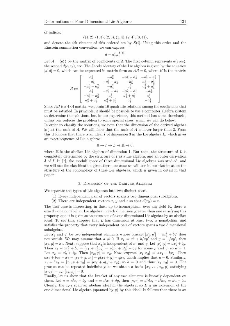
Deformations of Four Dimensional Lie Algebras 131
of indices:(1, 2), (1, 3), (2, 3), (1, 4), (2, 4), (3, 4),
and denote the ith element of this ordered set by S(i). Using this order and theEinstein summation convention, we can express
d = aijϕS(j)i .
Let A = (aij) be the matrix of coefficients of d. The first column represents d(e1e2),the second d(e1e3), etc. The Jacobi identity of the Lie algebra is given by the equation[d, d] = 0, which can be expressed in matrix form as AB = 0, where B is the matrix
B :=
a16 −a26 −a25 − a14 −a12 − a23−a15 −a36 − a14 −a35 a11 − a33
−a36 − a25 −a24 a34 a32 + a21a13 −a46 + a12 −a45 + a11 −a43
−a46 + a23 a22 a44 + a21 a42a45 + a33 a44 + a32 a31 −a41.
Since AB is a 4×4 matrix, we obtain 16 quadratic relations among the coefficients thatmust be satisfied. In principle, it should be possible to use a computer algebra systemto determine the solutions, but in our experience, this method has some drawbacks,unless one reduces the problem to some special cases, which we will do below.In order to classify the solutions, we note that the dimension of the derived algebrais just the rank of A. We will show that the rank of A is never larger than 3. Fromthis it follows that there is an ideal I of dimension 3 in the Lie algebra L, which givesan exact sequence of Lie algebras
0→ I → L→ K→ 0,
where K is the abelian Lie algebra of dimension 1. But then, the structure of L iscompletely determined by the structure of I as a Lie algebra, and an outer derivationδ of I. In [7], the moduli space of three dimensional Lie algebras was studied, andwe will use the classification given there, because we will use in our classification thestructure of the cohomology of these Lie algebras, which is given in detail in thatpaper.
3. Dimension of the Derived Algebra
We separate the types of Lie algebras into two distinct cases.
(1) Every independent pair of vectors spans a two dimensional subalgebra.(2) There are independent vectors x, y and z so that d(xy) = z.
The first case is interesting, in that, up to isomorphism, over any field K, there isexactly one nonabelian Lie algebra in each dimension greater than one satisfying thisproperty, and it is given as an extension of a one dimensional Lie algebra by an abelianideal. To see this, suppose that L has dimension at least two, is nonabelian, andsatisfies the property that every independent pair of vectors spans a two dimensionalsubalgebra.Let x′1 and y′ be two independent elements whose bracket [x′1, y
′] = ax′1 + by′ doesnot vanish. We may assume that a 6= 0. If x1 = x′1 + b/ay′ and y = 1/ay′, then[x1, y] = x1. Next, suppose that x
′2 is independent of x1 and y. Let [x′2, y] = ax′2+ by.
Then x1 + ax′2 + by = [x1 + x′2, y] = p(x1 + x′2) + qy for some p and q, so a = 1.Let x2 = x′2 + by. Then [x2, y] = x2. Now, express [x1, x2] = ax1 + bx2. Thenax1 + bx2 − x2 = [x1 + y, x2] = p(x1 + y) + qx2, which implies that a = 0. Similarly,x1 + bx2 = [x1, y + x2] = px1 + q(y + x2), so b = 0 and thus [x1, x2] = 0. Theprocess can be repeated indefinitely, so we obtain a basis x1, . . . , xn, y satisfying[xi, y] = xi, [xi, xj ] = 0.Finally, let us show that the bracket of any two elements is linearly dependent onthem. Let u = aixi + by and v = cixi + dy, then [u, v] = aidxi − cibxi = du − bv.Clearly, the xi-s span an abelian ideal in the algebra, so L is an extension of theone dimensional Lie algebra (spanned by y) by this ideal. It follows that there is an

132 III. Generalizations and Applications
abelian ideal of dimension n; moreover, this ideal coincides with the derived algebra,so the rank of the matrix A is precisely n, one less than the dimension of the vectorspace. In fact, the matrix A has precisely the form A = [ 0 I0 0 ], where I is the n × nidentity matrix. This completes the description of the first case.For the second case, suppose that there are linearly independent vectors such thatd(e1e2) = e3, so the matrix A of d satisfies a11 = a21 = a41 = 0, a31 = 1. One can easilycheck the possible solutions by considering subcases of this second case. For example,either e1, e2 and e3 span a subalgebra, or we can assume that d(e1e2) = e4. Sinceit is well known that the derived subalgebra of any 4 dimensional Lie algebra hasdimension at most 3, we will not give a detailed analysis of this issue, and simplypoint out that the division into subcases can be carried out relatively easily. However,we note that even without breaking up the second case into subcases, we can solve theJacobi identity using Maple, yielding around 40 solutions all of which have matricesof rank less than or equal to three. We note that the solutions are well defined overany field, so the fact that the derived algebra has dimension 3 is independent of thefield K as well.
4. Extensions of C by a three dimensional ideal
From now on, in this paper, we shall assume that we are working over the basefield C. It is not difficult to classify the moduli space over R as well. Over fields offinite characteristic, and over other fields, even the classification of 3 dimensional Liealgebras is quite complicated.Since the dimension of the derived algebra is never more than 3, every 4 dimensionalLie algebra is given as an extension of C by some three dimensional ideal. In [7], acomplete classification of three dimensional algebras and their cohomology was given.We summarize the results about the cohomology in Table 3. Here we have realigned
Type Codiff H1 H2 H3
d1 = n3 ψ231 4 5 2
d2 = r3,1(C) ψ131 + ψ23
2 3 3 0d2(1 : 1) = r3(C) ψ13
1 + ψ231 + ψ23
2 1 1 0d2(λ : µ) = r3,µ/λ(C) ψ13
1 λ+ ψ231 + ψ23
2 µ 1 1 0d2(1 : 0) = r2(C)⊕ C ψ13
1 + ψ231 2 1 0
d2(1 : −1) = r3,−1(C) ψ131 + ψ23
1 − ψ232 1 2 1
d3 = sl2(C) ψ123 + ψ13
2 + ψ231 0 0 0
Table 3. Cohomology of Three Dimensional Algebras
the family of codifferentials as presented in [7] in order to identify elements which havethe same cohomological type as belonging to the same family. The changes are actuallymodest: the family d2(λ : µ) coincides with d(µ/λ) of that paper except that the newelement d2 was given as d(1) in the paper, and the element d(1 : 1) correspondsto the element d2 in the previous paper. In addition, we have introduced projectivenotation for the family d2(λ : µ). It should be noted that d2(λ : µ) = d2(µ : λ), sothe family can be identified with P1(C)/Σ2, which makes it an orbifold with orbifoldpoints at d2(1 : 1) and d2(1 : −1), where there is some atypical phenomena in themoduli space. At the point d2(1 : 1), there is a doppelganger d2, whose neighborhoodscoincide with those of the point d2(1 : 1), and which also deforms infinitesimally intod2(1 : 1). At the point d2(1 : −1), there is a deformation in the d3 direction as wellas a deformation in the direction of the family. Otherwise, members of the familyd2(λ : µ) deform only in the direction of the family itself. The codifferential d1 hasdeformations into every other type of codifferential except d2, which accounts for whyit has such a large dimension of H2.
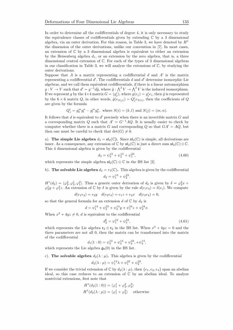
Deformations of Four Dimensional Lie Algebras 133
In order to determine all the codifferentials of degree 4, it is only necessary to studythe equivalence classes of codifferentials given by extending C by a 3 dimensionalalgebra, via an outer derivation. For this reason, in Table 3, we have denoted by H1
the dimension of the outer derivations, unlike our convention in [7]. In most cases,an extension of C by a 3 dimensional algebra is equivalent to either an extensionby the Heisenberg algebra d1, or an extension by the zero algebra, that is, a threedimensional central extension of C. For each of the types of 3 dimensional algebrasin our classification in Table 3, we will analyze the extensions of C, by studying theouter derivations.Suppose that A is a matrix representing a codifferential d and A′ is the matrixrepresenting a codifferential d′. The codifferentials d and d′ determine isomorphic Liealgebras, and we call them equivalent codifferentials, if there is a linear automorphism
g : V → V such that d′ = g−1dg, where g :∧2
V →∧2
V is the induced isomorphism.If we represent g by the 4×4 matrixG = (gij), where g(ej) = gijei, then g is represented
by the 6 × 6 matrix Q, in other words, g(eS(j)) = QijeS(i), then the coefficients of Qare given by the formula
Qij = gmk gnl − gml gnk , where S(i) = (k, l) and S(j) = (m,n).
It follows that d is equivalent to d′ precisely when there is an invertible matrix G anda corresponding matrix Q such that A′ = G−1AQ. It is usually easier to check bycomputer whether there is a matrix G and corresponding Q so that GA′ = AQ, butthen one must be careful to check that det(G) 6= 0.
a). The simple Lie algebra d3 = sl2(C). Since sl2(C) is simple, all derivations areinner. As a consequence, any extension of C by sl2(C) is just a direct sum sl2(C)⊕C.This 4 dimensional algebra is given by the codifferential
d3 = ψ123 + ψ13
2 + ψ231 , (4.60)
which represents the simple algebra sl2(C)⊕ C in the BS list [2].
b). The solvable Lie algebra d2 = r3(C). This algebra is given by the codifferential
d2 = ψ131 + ψ23
2 .
H1(d2) = 〈ϕ22, ϕ
12, ϕ
21〉. Thus a generic outer derivation of d2 is given by δ = ϕ2
2x +ϕ12y + ϕ2
1z. An extension of C by δ is given by the rule d(eie4) = δ(ei). We compute
d(e1e4) = e2y d(e2e4) = e1z + e2x d(e3e4) = 0,
so that the general formula for an extension d of C by d2 is
d = ψ131 + ψ23
2 + ψ142 y + ψ24
1 z + ψ242 x.
When x2 + 4yz 6= 0, d is equivalent to the codifferential
d♯2 = ψ121 + ψ34
3 , (4.61)
which represents the Lie algebra r2 ⊕ r2 in the BS list. When x2 + 4yz = 0 and thethree parameters are not all 0, then the matrix can be transformed into the matrixof the codifferential
d1(1 : 0) = ψ123 + ψ13
3 + ψ234 ,+ψ
144 ,
which represents the Lie algebra g8(0) in the BS list.
c). The solvable algebra d2(λ : µ). This algebra is given by the codifferential
d2(λ : µ) = ψ131 λ+ ψ23
1 + ψ232 .
If we consider the trivial extension of C by d2(λ : µ), then e1, e2, e4 span an abelianideal, so this case reduces to an extension of C by an abelian ideal. To analyzenontrivial extensions, first note that
H1(d2(1 : 0)) = 〈ϕ11 + ϕ2
2, ϕ32〉
H1(d2(λ : µ)) = 〈ϕ11 + ϕ2
2〉 otherwise
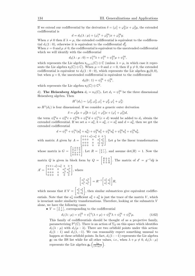
134 III. Generalizations and Applications
If we extend our codifferential by the derivation δ = (ϕ11 + ϕ2
2)x+ ϕ32y, the extended
codifferential isd = d2(λ : µ) + (ϕ14
1 + ϕ242 )x+ ϕ34
2 y.
When x 6= 0 then if λ = µ, the extended codifferential is equivalent to the codifferen-
tial d1(1 : 0), otherwise it is equivalent to the codifferential d♯2.When x = 0 and µ 6= 0, the codifferential is equivalent to the unextended codifferentialwhich we will identify with the codifferential
d3(λ : µ : 0) = ψ141 λ+ ψ24
1 + ψ242 µ+ ψ34
2 ,
which represents the Lie algebra r3,µ/λ(C)⊕ C (unless λ = µ, in which case it repre-sents the Lie algebra r3(C)⊕C). When µ = 0 and x = 0, then if y 6= 0, the extendedcodifferential is equivalent to d3(1 : 0 : 0), which represents the Lie algebra g2(0, 0),but when y = 0, the unextended codifferential is equivalent to the codifferential
d3(0 : 1) = ψ342 + ψ34
3 ,
which represents the Lie algebra r2(C)⊕ C2.
d). The Heisenberg Algebra d1 = n3(C). Let d1 = ψ231 be the three dimensional
Heisenberg algebra. Then
H1(d1) = 〈ϕ23, ϕ
32, ϕ
11 + ϕ2
2, ϕ11 + ϕ3
3〉so H1(d1) is four dimensional. If we consider a generic outer derivation
δ = ϕ23a+ ϕ3
2b+ (ϕ11 + ϕ2
2)c+ (ϕ11 + ϕ3
3)d,
the term ψ243 a + ψ24
2 c + ψ342 b + ψ34
3 d + ψ141 (c + d) would be added to d1 obtain the
extended codifferential. If we set a = a35, b = a26, c = a25 and d = a36, then we get theextended codifferential
d = ψ231 + ψ14
1 (a25 + a36) + ψ242 a
25 + ψ34
2 a26 + ψ24
3 a35 + ψ34
3 a36,
with matrix A given by A =
[0 0 1 a25+a
36 0 0
0 0 0 0 a25 a26
0 0 0 0 a35 a36
0 0 0 0 0 0
]. Let g be the linear transformation
whose matrix is G =
[1 0 0 00 p r 00 q s 00 0 0 1
]. Let R =
[ p rq s
], and assume det(R) = 1. Now the
matrix Q is given in block form by Q =
[R 0 00 I 00 0 R
]. The matrix of d′ = g−1dg is
A′ =
[0 0 1 a25+a
36 0 0
0 0 0 0 a′25 a′260 0 0 0 a′35 a′360 0 0 0 0 0
], where
[a′25 a′26a′35 a′36
]= R−1
[a25 a
26
a35 a36
]R,
which means that if V =
[a25 a
26
a35 a36
], then similar submatrices give equivalent codiffer-
entials. Note that the a14 coefficient a25 + a36 is just the trace of the matrix V , whichis invariant under similarity transformations. Therefore, looking at the submatrix Valone, we have the following cases
• V =[λ 10 µ
], corresponding to the codifferential
d1(λ : µ) = ψ231 + ψ14
1 (λ+ µ) + ψ242 λ+ ψ34
2 + ψ343 µ. (4.62)
This family of codifferentials should be thought of as a projective family,parameterizing P1(C). There is an action of Σ2 on this space which identifiesd1(λ : µ) with d1(µ : λ). There are two orbifold points under this action:d1(1 : 1) and d1(1,−1). We can reasonably expect something unusual tohappen at these orbifold points. In fact, d1(1 : −1) represents the Lie algebrag7 on the BS list while for all other values, i.e., when λ + µ 6= 0, d1(λ : µ)
represents the Lie algebra g8
(λµ
(λ+µ)2
).

Deformations of Four Dimensional Lie Algebras 135
The diagonal matrix V = diag(1, 1). This is the only nonzero diagonaliz-able matrix which does not show up in the case above. Its associated codif-ferential is given by the formula
d♯1 = ψ231 + 2ψ14
1 + ψ242 + ψ34
3 , (4.63)
representing the Lie algebra g6.•• V = [ 0 1
0 0 ]. Then the extended codifferential is equivalent to
d⋆2 = ψ241 + ψ34
2 , (4.64)
representing the Lie algebra n4(C).• V = 0. This is the original, unextended codifferential, which is equivalent tothe codifferential
d1 = ψ241 , (4.65)
representing the Lie algebra n3(C)⊕ C.
e). Extensions of C by an abelian ideal. Since H1(0) = L1(C3), the whole 9
dimensional cochain space, an extension of C by C3 is given by a matrix of the form
A =
0 0 0 a14 a15 a
16
0 0 0 a24 a25 a
26
0 0 0 a34 a35 a
36
0 0 0 0 0 0
. If we let V =
[a14 a
15 a
16
a24 a25 a
26
a34 a35 a
36
], then any matrix V ′ which is similar to
V up to multiplication by a nonzero constant determines an equivalent codifferential.Since matrices which are constant multiples of each other determine the same cod-ifferential, we can think of the nonequivalent codifferentials as being parameterizedprojectively. The decomposition of these matrices into distinct equivalence classes isas follows.
• The codifferential
d3(λ : µ : ν) = ψ141 λ+ ψ24
1 + ψ242 µ+ ψ34
2 + ψ343 ν (4.66)
for (λ : µ : ν) ∈ P2(C)/Σ3, where the action of Σ3 is given by permutationof the coordinates. These points determine an orbifold with orbifold pointsoccurring along certain lines (P1(C)) where some of the parameters coincide.It might seem more natural to use diagonal matrices to represent this twoparameter family; the choice here is based on cohomological considerations.
The codifferential
d3(λ : µ) = ψ141 λ+ ψ24
2 λ+ ψ342 + ψ34
3 µ (4.67)
for (λ : µ) ∈ P1(C). Here there is no action of the symmetric group.•• The Heisenberg algebra d1 = ψ24
1 . The only eigenvalue of the matrix is zero,and it has two Jordan blocks. We will see that every point in d3(λ, µ) isinfinitesimally close to this point.• The solvable algebra d∗2. The matrix has one Jordan block, with eigenvaluezero.• The identity matrix determines the codifferential
d∗3 = ψ141 + ψ25
2 + ψ342 , (4.68)
which represents the Lie algebra g1(1).• The zero algebra d = 0. Every point is infinitesimally close to this zero point.
We summarize these results and give the Lie bracket operations in standard termi-nology in the table below.
5. Comparison with the Burde-Steinhoff and Agaoka Lists
The comparison between the Burde-Steinhoff (BS) list and ours is slightly compli-cated. On the other hand, our decomposition is essentially the same as Agaoka’s list,so we will just note the corresponding element, which is of the form Li(α) (see [1]).
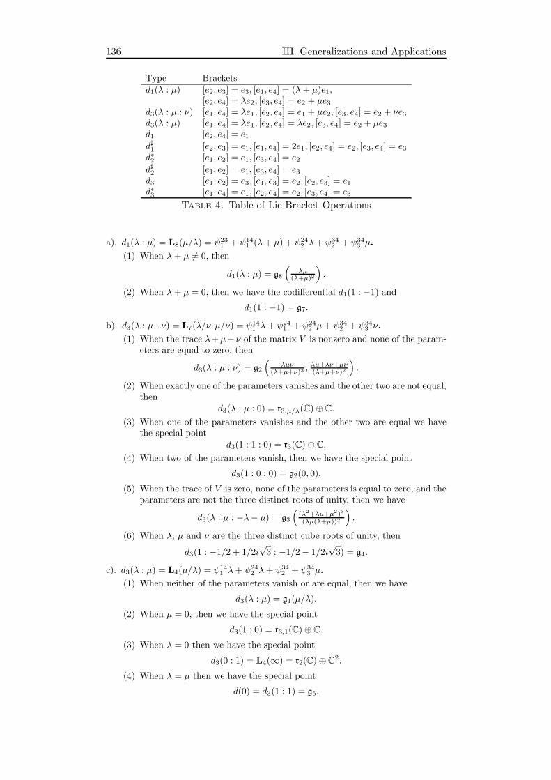
136 III. Generalizations and Applications
Type Bracketsd1(λ : µ) [e2, e3] = e3, [e1, e4] = (λ+ µ)e1,
[e2, e4] = λe2, [e3, e4] = e2 + µe3d3(λ : µ : ν) [e1, e4] = λe1, [e2, e4] = e1 + µe2, [e3, e4] = e2 + νe3d3(λ : µ) [e1, e4] = λe1, [e2, e4] = λe2, [e3, e4] = e2 + µe3d1 [e2, e4] = e1d♯1 [e2, e3] = e1, [e1, e4] = 2e1, [e2, e4] = e2, [e3, e4] = e3d∗2 [e1, e2] = e1, [e3, e4] = e2d♯2 [e1, e2] = e1, [e3, e4] = e3d3 [e1, e2] = e3, [e1, e3] = e2, [e2, e3] = e1d∗3 [e1, e4] = e1, [e2, e4] = e2, [e3, e4] = e3
Table 4. Table of Lie Bracket Operations
a). d1(λ : µ) = L8(µ/λ) = ψ231 + ψ14
1 (λ+ µ) + ψ242 λ+ ψ34
2 + ψ343 µ.
(1) When λ+ µ 6= 0, then
d1(λ : µ) = g8
(λµ
(λ+µ)2
).
(2) When λ+ µ = 0, then we have the codifferential d1(1 : −1) andd1(1 : −1) = g7.
b). d3(λ : µ : ν) = L7(λ/ν, µ/ν) = ψ141 λ+ ψ24
1 + ψ242 µ+ ψ34
2 + ψ343 ν.
(1) When the trace λ+µ+ ν of the matrix V is nonzero and none of the param-eters are equal to zero, then
d3(λ : µ : ν) = g2
(λµν
(λ+µ+ν)3 ,λµ+λν+µν(λ+µ+ν)2
).
(2) When exactly one of the parameters vanishes and the other two are not equal,then
d3(λ : µ : 0) = r3,µ/λ(C)⊕ C.
(3) When one of the parameters vanishes and the other two are equal we havethe special point
d3(1 : 1 : 0) = r3(C)⊕ C.
(4) When two of the parameters vanish, then we have the special point
d3(1 : 0 : 0) = g2(0, 0).
(5) When the trace of V is zero, none of the parameters is equal to zero, and theparameters are not the three distinct roots of unity, then we have
d3(λ : µ : −λ− µ) = g3
((λ2+λµ+µ2)3
(λµ(λ+µ))2
).
(6) When λ, µ and ν are the three distinct cube roots of unity, then
d3(1 : −1/2 + 1/2i√3 : −1/2− 1/2i
√3) = g4.
c). d3(λ : µ) = L4(µ/λ) = ψ141 λ+ ψ24
2 λ+ ψ342 + ψ34
3 µ.
(1) When neither of the parameters vanish or are equal, then we have
d3(λ : µ) = g1(µ/λ).
(2) When µ = 0, then we have the special point
d3(1 : 0) = r3,1(C)⊕ C.
(3) When λ = 0 then we have the special point
d3(0 : 1) = L4(∞) = r2(C)⊕ C2.
(4) When λ = µ then we have the special point
d(0) = d3(1 : 1) = g5.
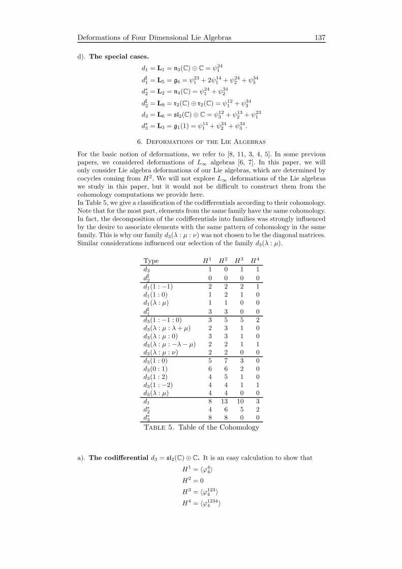
Deformations of Four Dimensional Lie Algebras 137
d). The special cases.
d1 = L1 = n3(C)⊕ C = ψ241
d♯1 = L5 = g6 = ψ231 + 2ψ14
1 + ψ242 + ψ34
3
d∗2 = L2 = n4(C) = ψ241 + ψ34
2
d♯2 = L9 = r2(C)⊕ r2(C) = ψ121 + ψ34
3
d3 = L6 = sl2(C)⊕ C = ψ123 + ψ13
2 + ψ231
d∗3 = L3 = g1(1) = ψ141 + ψ24
2 + ψ343 .
6. Deformations of the Lie Algebras
For the basic notion of deformations, we refer to [8, 11, 3, 4, 5]. In some previouspapers, we considered deformations of L∞ algebras [6, 7]. In this paper, we willonly consider Lie algebra deformations of our Lie algebras, which are determined bycocycles coming from H2. We will not explore L∞ deformations of the Lie algebraswe study in this paper, but it would not be difficult to construct them from thecohomology computations we provide here.In Table 5, we give a classification of the codifferentials according to their cohomology.Note that for the most part, elements from the same family have the same cohomology.In fact, the decomposition of the codifferentials into families was strongly influencedby the desire to associate elements with the same pattern of cohomology in the samefamily. This is why our family d3(λ : µ : ν) was not chosen to be the diagonal matrices.Similar considerations influenced our selection of the family d3(λ : µ).
Type H1 H2 H3 H4
d3 1 0 1 1
d♯2 0 0 0 0d1(1 : −1) 2 2 2 1d1(1 : 0) 1 2 1 0d1(λ : µ) 1 1 0 0
d♯1 3 3 0 0d3(1 : −1 : 0) 3 5 5 2d3(λ : µ : λ+ µ) 2 3 1 0d3(λ : µ : 0) 3 3 1 0d3(λ : µ : −λ− µ) 2 2 1 1d3(λ : µ : ν) 2 2 0 0d3(1 : 0) 5 7 3 0d3(0 : 1) 6 6 2 0d3(1 : 2) 4 5 1 0d3(1 : −2) 4 4 1 1d3(λ : µ) 4 4 0 0d1 8 13 10 3d∗2 4 6 5 2d∗3 8 8 0 0
Table 5. Table of the Cohomology
a). The codifferential d3 = sl2(C)⊕ C. It is an easy calculation to show that
H1 = 〈ϕ44〉
H2 = 0
H3 = 〈ϕ1234 〉
H4 = 〈ϕ12344 〉
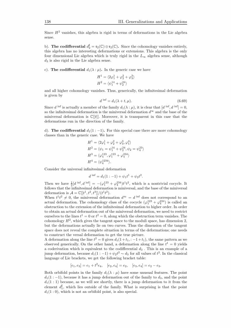
138 III. Generalizations and Applications
Since H2 vanishes, this algebra is rigid in terms of deformations in the Lie algebrasense.
b). The codifferential d♯2 = r2(C)⊕ r2(C). Since the cohomology vanishes entirely,this algebra has no interesting deformations or extensions. This algebra is the onlyfour dimensional Lie algebra which is truly rigid in the L∞ algebra sense, althoughd3 is also rigid in the Lie algebra sense.
c). The codifferential d1(λ : µ). In the generic case we have
H1 = 〈2ϕ11 + ϕ2
2 + ϕ33〉
H2 = 〈ψ141 + ψ24
2 〉and all higher cohomology vanishes. Thus, generically, the infinitesimal deformationis given by
d inf = d1(λ+ t, µ). (6.69)
Since d inf is actually a member of the family d1(λ : µ), it is clear that [d inf, d inf] = 0,so the infinitesimal deformation is the miniversal deformation d∞ and the base of theminiversal deformation is C[[t]]. Moreover, it is transparent in this case that thedeformations run in the direction of the family.
d). The codifferential d1(1 : −1). For this special case there are more cohomologyclasses than in the generic case. We have
H1 = 〈2ϕ11 + ϕ2
2 + ϕ33, ϕ
41〉
H2 = 〈ψ1 = ψ141 + ψ24
2 , ψ2 = ψ234 〉
H3 = 〈ϕ1234 , ϕ123
1 + ϕ2344 〉
H4 = 〈ψ12344 〉.
Consider the universal infinitesimal deformation
d inf = d1(1 : −1) + ψ1t1 + ψ2t
2.
Then we have 12 [d
inf, d inf] = −(ϕ1231 + ϕ234
4 )t1t2, which is a nontrivial cocycle. Itfollows that the infinitesimal deformation is miniversal, and the base of the miniversaldeformation is A = C[[t1, t2, t3]]/(t1t2).When t1t2 6= 0, the miniversal deformation d∞ = d inf does not correspond to anactual deformation. The cohomology class of the cocycle (ϕ123
1 + ϕ2344 ) is called an
obstruction to the extension of the infinitesimal deformation to higher order. In orderto obtain an actual deformation out of the miniversal deformation, we need to restrictourselves to the lines t1 = 0 or t2 = 0, along which the obstruction term vanishes. Thecohomology H2, which gives the tangent space to the moduli space, has dimension 2,but the deformations actually lie on two curves. Thus the dimension of the tangentspace does not reveal the complete situation in terms of the deformations; one needsto construct the versal deformation to get the true picture.A deformation along the line t2 = 0 gives d1(1+ t1, : −1+ t1), the same pattern as weobserved generically. On the other hand, a deformation along the line t1 = 0 yieldsa coderivation which is equivalent to the codifferential d3 . This is an example of ajump deformation, because d1(1 : −1)+ψ2t
2 ∼ d3 for all values of t2. In the classicallanguage of Lie brackets, we get the following bracket table:
[e1, e3] = e1 + t2e4, [e2, e4] = e2, [e3, e4] = e2 − e3.Both orbifold points in the family d1(λ : µ) have some unusual features. The pointd1(1 : −1), because it has a jump deformation out of the family to d3, and the pointd1(1 : 1) because, as we will see shortly, there is a jump deformation to it from the
element d♯1, which lies outside of the family. What is surprising is that the pointd1(1 : 0), which is not an orbifold point, is also special.
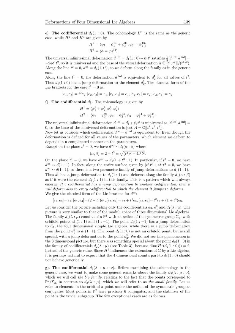
Deformations of Four Dimensional Lie Algebras 139
e). The codifferential d1(1 : 0). The cohomology H1 is the same as the genericcase, while H2 and H3 are given by
H2 = 〈ψ1 = ψ141 + ψ34
3 , ψ2 = ψ132 〉
H3 = 〈φ = ϕ1342 〉.
The universal infinitesimal deformation d inf = d1(1 : 0)+ψiti satisfies 1
2 [dinf, d inf] =
−2φt1t2, so it is miniversal and the base of the versal deformation is C[[t1, t2]]/(t1t2).Along the line t2 = 0, d∞ = d1(1, t
1), so we deform along the family as in the genericcase.Along the line t1 = 0, the deformation d inf is equivalent to d♯2 for all values of t2.
Thus d1(1 : 0) has a jump deformation to the element d♯2. The classical form of theLie brackets for the case t1 = 0 is
[e1, e3] = t2e2, [e2, e3] = e1, [e1, e4] = e1, [e2, e4] = e2, [e3, e4] = e2.
f). The codifferential d♯1. The cohomology is given by
H1 = 〈ϕ11 + ϕ2
2, ϕ23, ϕ
32〉
H2 = 〈ψ1 = ψ243 , ψ2 = ψ34
2 , ψ3 = ψ141 + ψ34
3 〉.
The universal infinitesimal deformation d inf = d♯1+ψiti is miniversal as [d inf, d inf] =
0, so the base of the miniversal deformation is just A = C[[t1, t2, t3]].Now let us consider which codifferential d∞ = d inf is equivalent to. Even though thedeformation is defined for all values of the parameters, which element we deform todepends in a complicated manner on the parameters.Except on the plane t1 = 0, we have d∞ ∼ d1(α : β) where
(α, β) = 2 + t3 ±√(t3)2 + 4t1t2.
On the plane t1 = 0, we have d∞ ∼ d1(1 + t3 : 1). In particular, if t3 = 0, we haved∞ ∼ d(1 : 1). In fact, along the entire surface given by (t3)2 + 4t1t2 = 0, we haved∞ ∼ d(1 : 1), so there is a two parameter family of jump deformations to d1(1 : 1).
Thus d♯1 has a jump deformation to d1(1 : 1) and deforms along the family d1(α : β)as if it were the element d1(1 : 1) in this family. This is a pattern which will alwaysemerge: If a codifferential has a jump deformation to another codifferential, then itwill deform also to every codifferential to which the element it jumps to deforms.We give the classical form of the Lie brackets for d∞:
[e2, e3]=e1, [e1, e4]=(2 + t3)e1, [e2, e4]=e2 + t1e3, [e3, e4]= t2e2 + (1 + t3)e3.
Let us consider the picture including only the codifferentials d3, d♯1 and d1(λ : µ). The
picture is very similar to that of the moduli space of three dimensional Lie algebras.The family d1(λ : µ) consists of a P1 with an action of the symmetric group Σ2, withorbifold points at (1 : 1) and (1 : −1). The point d1(1 : −1) has a jump deformationto d3, the four dimensional simple Lie algebra, while there is a jump deformation
from the point d♯1 to d1(1 : 1). The point d1(1 : 0) is not an orbifold point, but is still
special, with a jump deformation to the point d♯2. We did not see this phenomenon inthe 3 dimensional picture, but there was something special about the point d2(1 : 0) inthe family of codifferentials d2(λ : µ) (see Table 3), because dim(H1(d2(1 : 0))) = 2,instead of the generic value. Since H1 influences the extensions of C by a Lie algebra,it is perhaps natural to expect that the 4 dimensional counterpart to d2(1 : 0) shouldnot behave generically.
g). The codifferential d3(λ : µ : ν). Before examining the cohomology in thegeneric case, we want to make some general remarks about the family d3(λ : µ : ν),which we will call the big family, relating to the fact that the points correspond toP2/Σ3, in contrast to d3(λ : µ), which we will refer to as the small family. Let usrefer to elements in the orbit of a point under the action of the symmetric group asconjugates. Most points in P2 have precisely 6 conjugates, and the stabilizer of thepoint is the trivial subgroup. The few exceptional cases are as follows.

140 III. Generalizations and Applications
(1) The points (λ : λ : µ), where λ 6= µ and their conjugates are stabilized by asubgroup of order 2, so they each have only 3 conjugates.
(2) The point (1 : −1 : 0) and its 3 conjugates are also stabilized by a subgroupof order 2.
(3) The point (1 : r : r2), where r is a primitive cube root of unity, and its 2conjugates, are stabilized by the alternating group A3.
(4) The point (1 : 1 : 1) is stabilized by the entire group Σ3.
Next, consider the lines (P1) in P2 and the induced action of Σ3 on the set of lines.For most lines, the stabilizer of the line is just the trivial subgroup, but again, thereare a few exceptions.
(1) The line (λ : λ : µ) and its 3 conjugates are stabilized by subgroups of order2.
(2) The lines (λ : µ : c(λ + µ)) and their conjugates are also stabilized by sub-groups of order 2.
It turns out that when c = 0 or c = ±1, the cohomology of the codifferentialscorresponding to points on the line (λ : µ : c(λ + µ)) does not follow the genericpattern. The cohomology of the codifferentials corresponding to points on the line(λ : λ : µ) is the same as the generic case with the exception of the points (1 : 1 : 0),(1 : 1 : 2) and (1 : 1 : −2), which are the points of intersection of this line with thethree other special lines. Note also that the lines (λ : µ : c(λ + µ)) all intersect inprecisely the point (1 : −1 : 0), which makes this point very special.To determine the cohomology of a codifferential of type d3(λ : µ : ν), read Table5 in descending order, and whichever is the first pattern it matches, that gives itscohomology. However, we will present the description of the cohomology in ascendingorder, because it is more natural to begin with the generic pattern, and then proceedto the more exotic cases.
h). The codifferential d3(λ : µ : ν): the generic case. Generically, we have
H1 =〈ϕ11(λ− µ) + ϕ2
1 + ϕ22(µ− ν) + ϕ3
2,
ϕ11(−λµ+ λ2 − λν + µν) + ϕ2
1(λ− ν) + ϕ31〉.
For most generic values of (λ : µ : ν) a natural basis to choose for H2 would beH2 = 〈ψ24
2 , ψ343 〉. Then d inf = d3(λ, µ + t1, ν + t2), so there is no difficulty in seeing
what the deformations are equivalent to. However, for certain generic values of theparameters, the two cocycles above are not a basis of H2, so we need to work with amore complex solution, which yields a basis of H2 for all generic values. Let us take
H2 = 〈ψ1 = ψ243 , ψ2 = ψ14
3 〉.The universal infinitesimal deformation d inf = d3(λ : µ : ν) + ψit
i is miniversal,with base A = C[[t1, t2]]. It is a bit more difficult to identify what the miniversaldeformation d∞ = d inf is equivalent to when we take this more complicated basis ofH2. In fact, if we let x be a root of the polynomial
z3 + (−ν + 2λ− µ)z2 + (µν − λν − λµ+ λ2 − t1)z − t2,and y be a root of the polynomial
z2 + (−x− ν + µ)z + x2 + x(λ− µ)− t1,then if g is given by the matrix
G =
1 0 0 0x 1 0 0
x(λ − µ) + x2 y 1 00 0 0 1
,
we haveg∗(d∞) = d3(λ+ x : µ+ y − x : ν − y).
Thus for generic values of (λ : µ : ν), all deformations of d3(λ : µ : ν) simply movealong this same big family.

Deformations of Four Dimensional Lie Algebras 141
i). The codifferential d3(λ : µ : −λ−µ). In this case H1 is the same as the genericcase, and for most values of µ, one can use the cocycles ψ14
1 and ψ242 as the basis
of H2. Since the brackets of these two cocycles vanish, the resulting infinitesimaldeformation
d inf = d3(λ : µ : −λ− µ) + ψ141 t
1 + ψ242 t
2
is miniversal, and in fact coincides with d3(λ + t1, µ + t2,−µ − λ). In this case, itis obvious that the deformations of our codifferential just lie along the big family.The values for which these two elements do not form a basis of H2 are (1 : −1 : 0),which we will cover separately, and (1 : 1 : −2), for which ψ1 = ψ14
3 and ψ2 = ψ242
give a basis of H2. It is still true that the brackets of these cocycles vanish, and thedeformations lie along the big family, although the expression of the member of thefamily corresponding to the element d∞ is more complicated in this case, and will beomitted.Thus the family d3(λ : µ : −λ − µ) is not special in deformation theory. This is abit surprising, since H3 does not vanish for elements of this subfamily, so it wouldnot have been unreasonable to expect that there would be some obstructions to theextension of an infinitesimal deformation.
j). The codifferential d3(λ : µ : 0) = r3,µ/λ(C) ⊕ C. . The dimensions of H1 and
H2 increase to 3, and H3 is 1-dimensional as well. The two cocycles ψ1 and ψ2 chosenas basis elements for H2 in the generic case remain nontrivial and one can find anindependent nontrivial cocycle ψ13
1 + ψ232 . However, this choice of a basis turns out
to be inconvenient, and a slight modification of the basis will make the presentationsimpler. We have
H1 =〈ϕ11λ(λ− µ) + ϕ2
1λ+ ϕ31, ϕ
11 + ϕ2
2 + ϕ33, ϕ
43〉
H2 =〈ψ1 = ψ243 + ψ14
3 λ, ψ2 = ψ143 , ψ3 = ψ13
1 + ψ232 〉.
Let d inf = d3(λ : µ : 0) + ψiti. We compute
[ψ1, ψ3] = −ϕ1241 + ϕ234
3 + ϕ1343 λ+ ϕ124
2 λ = −D(ψ122 + ψ13
3 )
[ψ2, ψ3] = ϕ1343 + ϕ124
2 ,
so that12 [d
inf, d inf] = −D(ζ1)t1t3 + (ϕ134
3 + ϕ1242 )t2t3,
where ζ1 = ψ122 + ψ13
3 .Note that in the case t3 = 0, since ψ1 and ψ2 span the same subspace as the ones weused in the generic case, a deformation with t3 = 0 is equivalent to one in the family.Thus there is a two parameter family of deformations of d3(λ : µ : 0) along the bigfamily d3(α : β : η).On the other hand, when t3 does not vanish, we will have to consider how d inf
extends to a higher order deformation. It turns out that when λ = µ, the codifferentialϕ1343 + ϕ124
2 is a coboundary, but otherwise, it can be taken as a basis of H3, and sois an obstruction to the extension of d inf to a higher order deformation. We will firstconsider this obstructed case.
j).1. µ 6= λ. In this case we have
H3 = 〈φ = ϕ1343 + ϕ124
2 〉.We extend d inf to the second order deformation
d2 = d inf + ζ1t1t3.
Since 12 [d
2, d2] = φt2t3, the second order deformation is miniversal and the base of
the miniversal deformation is A = C[[t1, t2, t3]]/(t2t3).Thus any true deformation is given by taking d∞ = d2 with either t2 = 0 or t3 = 0.Since the case t3 = 0 has already been examined, we consider the case t2 = 0. In this
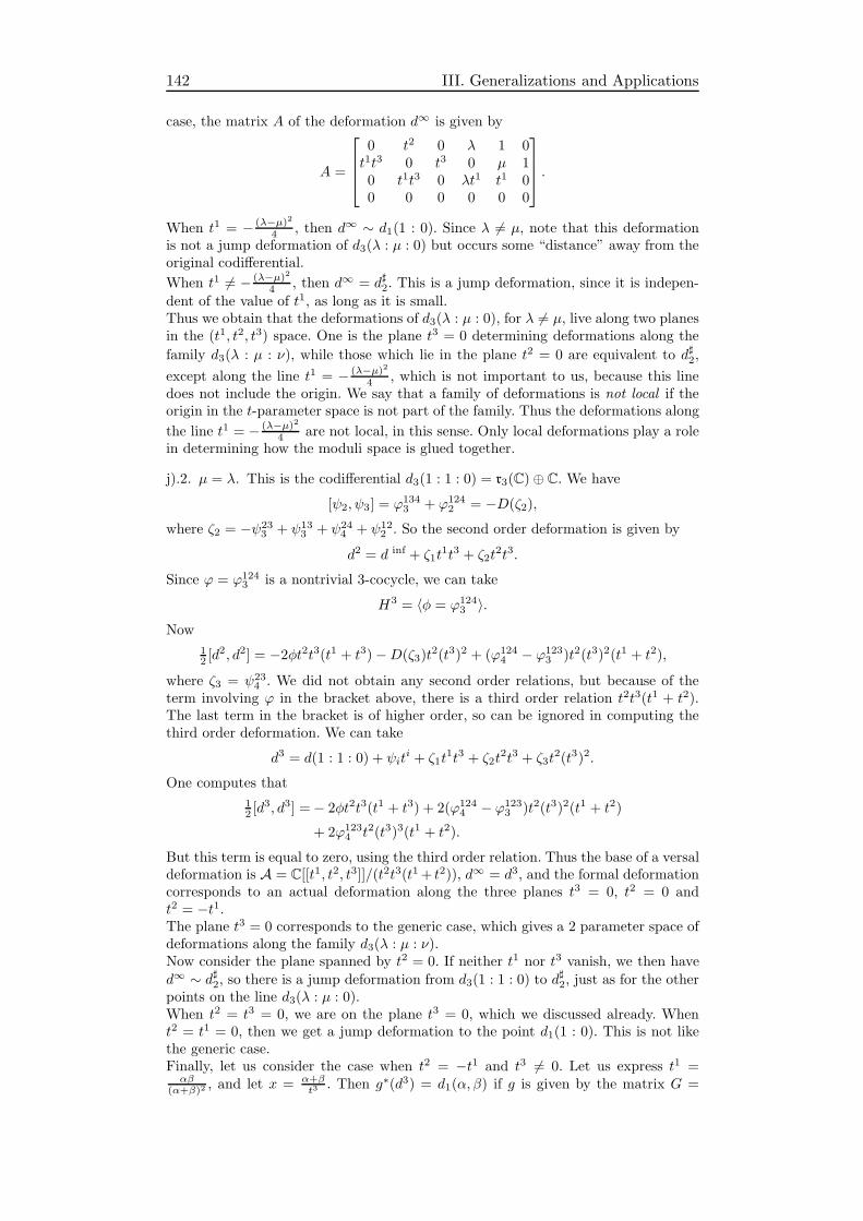
142 III. Generalizations and Applications
case, the matrix A of the deformation d∞ is given by
A =
0 t2 0 λ 1 0t1t3 0 t3 0 µ 10 t1t3 0 λt1 t1 00 0 0 0 0 0
.
When t1 = − (λ−µ)24 , then d∞ ∼ d1(1 : 0). Since λ 6= µ, note that this deformation
is not a jump deformation of d3(λ : µ : 0) but occurs some “distance” away from theoriginal codifferential.
When t1 6= − (λ−µ)24 , then d∞ = d♯2. This is a jump deformation, since it is indepen-
dent of the value of t1, as long as it is small.Thus we obtain that the deformations of d3(λ : µ : 0), for λ 6= µ, live along two planesin the (t1, t2, t3) space. One is the plane t3 = 0 determining deformations along the
family d3(λ : µ : ν), while those which lie in the plane t2 = 0 are equivalent to d♯2,
except along the line t1 = − (λ−µ)24 , which is not important to us, because this line
does not include the origin. We say that a family of deformations is not local if theorigin in the t-parameter space is not part of the family. Thus the deformations along
the line t1 = − (λ−µ)24 are not local, in this sense. Only local deformations play a role
in determining how the moduli space is glued together.
j).2. µ = λ. This is the codifferential d3(1 : 1 : 0) = r3(C)⊕ C. We have
[ψ2, ψ3] = ϕ1343 + ϕ124
2 = −D(ζ2),
where ζ2 = −ψ233 + ψ13
3 + ψ244 + ψ12
2 . So the second order deformation is given by
d2 = d inf + ζ1t1t3 + ζ2t
2t3.
Since ϕ = ϕ1243 is a nontrivial 3-cocycle, we can take
H3 = 〈φ = ϕ1243 〉.
Now
12 [d
2, d2] = −2φt2t3(t1 + t3)−D(ζ3)t2(t3)2 + (ϕ124
4 − ϕ1233 )t2(t3)2(t1 + t2),
where ζ3 = ψ234 . We did not obtain any second order relations, but because of the
term involving ϕ in the bracket above, there is a third order relation t2t3(t1 + t2).The last term in the bracket is of higher order, so can be ignored in computing thethird order deformation. We can take
d3 = d(1 : 1 : 0) + ψiti + ζ1t
1t3 + ζ2t2t3 + ζ3t
2(t3)2.
One computes that
12 [d
3, d3] =− 2φt2t3(t1 + t3) + 2(ϕ1244 − ϕ123
3 )t2(t3)2(t1 + t2)
+ 2ϕ1234 t2(t3)3(t1 + t2).
But this term is equal to zero, using the third order relation. Thus the base of a versaldeformation is A = C[[t1, t2, t3]]/(t2t3(t1+ t2)), d∞ = d3, and the formal deformationcorresponds to an actual deformation along the three planes t3 = 0, t2 = 0 andt2 = −t1.The plane t3 = 0 corresponds to the generic case, which gives a 2 parameter space ofdeformations along the family d3(λ : µ : ν).Now consider the plane spanned by t2 = 0. If neither t1 nor t3 vanish, we then have
d∞ ∼ d♯2, so there is a jump deformation from d3(1 : 1 : 0) to d♯2, just as for the otherpoints on the line d3(λ : µ : 0).When t2 = t3 = 0, we are on the plane t3 = 0, which we discussed already. Whent2 = t1 = 0, then we get a jump deformation to the point d1(1 : 0). This is not likethe generic case.Finally, let us consider the case when t2 = −t1 and t3 6= 0. Let us express t1 =αβ
(α+β)2 , and let x = α+βt3 . Then g∗(d3) = d1(α, β) if g is given by the matrix G =
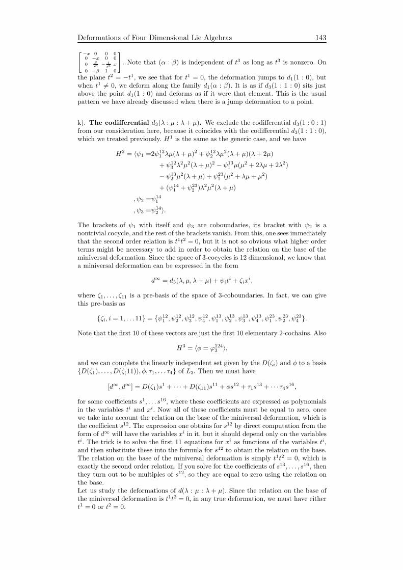
Deformations of Four Dimensional Lie Algebras 143
[−x 0 0 00 −x 0 0
0 β
t3− 1
t3x
0 −β 1 0
]. Note that (α : β) is independent of t3 as long as t3 is nonzero. On
the plane t2 = −t1, we see that for t1 = 0, the deformation jumps to d1(1 : 0), butwhen t1 6= 0, we deform along the family d1(α : β). It is as if d3(1 : 1 : 0) sits justabove the point d1(1 : 0) and deforms as if it were that element. This is the usualpattern we have already discussed when there is a jump deformation to a point.
k). The codifferential d3(λ : µ : λ+ µ). We exclude the codifferential d3(1 : 0 : 1)from our consideration here, because it coincides with the codifferential d3(1 : 1 : 0),which we treated previously. H1 is the same as the generic case, and we have
H2 = 〈ψ1 =2ψ121 λµ(λ + µ)2 + ψ12
2 λµ2(λ+ µ)(λ+ 2µ)
+ ψ123 λ
2µ2(λ+ µ)2 − ψ131 µ(µ
2 + 2λµ+ 2λ2)
− ψ132 µ
2(λ+ µ) + ψ231 (µ2 + λµ+ µ2)
+ (ψ141 + ψ23
2 )λ2µ2(λ + µ)
, ψ2 =ψ141
, ψ3 =ψ142 〉.
The brackets of ψ1 with itself and ψ3 are coboundaries, its bracket with ψ2 is anontrivial cocycle, and the rest of the brackets vanish. From this, one sees immediatelythat the second order relation is t1t2 = 0, but it is not so obvious what higher orderterms might be necessary to add in order to obtain the relation on the base of theminiversal deformation. Since the space of 3-cocycles is 12 dimensional, we know thata miniversal deformation can be expressed in the form
d∞ = d3(λ, µ, λ + µ) + ψiti + ζix
i,
where ζ1, . . . , ζ11 is a pre-basis of the space of 3-coboundaries. In fact, we can givethis pre-basis as
ζi, i = 1, . . . 11 = ψ121 , ψ
122 , ψ
123 , ψ
124 , ψ
131 , ψ
132 , ψ
133 , ψ
134 , ψ
231 , ψ
232 , ψ
234 .
Note that the first 10 of these vectors are just the first 10 elementary 2-cochains. Also
H3 = 〈φ = ϕ1243 〉,
and we can complete the linearly independent set given by the D(ζi) and φ to a basisD(ζ1), . . . , D(ζ(11)), φ, τ1, . . . τ4 of L3. Then we must have
[d∞, d∞] = D(ζ1)s1 + · · ·+D(ζ11)s
11 + φs12 + τ1s13 + · · · τ4s16,
for some coefficients s1, . . . s16, where these coefficients are expressed as polynomialsin the variables ti and xi. Now all of these coefficients must be equal to zero, oncewe take into account the relation on the base of the miniversal deformation, which isthe coefficient s12. The expression one obtains for s12 by direct computation from theform of d∞ will have the variables xi in it, but it should depend only on the variablesti. The trick is to solve the first 11 equations for xi as functions of the variables ti,and then substitute these into the formula for s12 to obtain the relation on the base.The relation on the base of the miniversal deformation is simply t1t2 = 0, which isexactly the second order relation. If you solve for the coefficients of s13, . . . , s16, thenthey turn out to be multiples of s12, so they are equal to zero using the relation onthe base.Let us study the deformations of d(λ : µ : λ + µ). Since the relation on the base ofthe miniversal deformation is t1t2 = 0, in any true deformation, we must have eithert1 = 0 or t2 = 0.
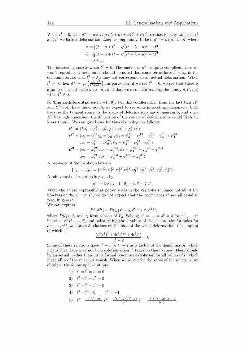
144 III. Generalizations and Applications
When t1 = 0, then d∞ = d3(λ : µ : λ+ µ) + ψ2t2 + ψ3t
3, so that for any values of t2
and t3 we have a deformation along the big family. In fact, d∞ ∼ d3(α : β : η) where
α =12 (λ+ µ+ t2 +
√(t2 + λ− µ)2 + 4t3)
β =12 (λ+ µ+ t2 −
√(t2 + λ− µ)2 + 4t3)
η =λ+ µ.
The interesting case is when t2 = 0. The matrix of d∞ is quite complicated, so wewon’t reproduce it here, but it should be noted that some terms have t3 − λµ in thedenominator, so that t3 = λµ may not correspond to an actual deformation. When
t1 6= 0, then d∞ ∼ g8
(λµ−t3(λ+µ)2
). In particular, if we set t3 = 0, we see that there is
a jump deformation to d1(λ : µ), and that we also deform along the family d1(λ : µ)when t3 6= 0.
l). The codifferential d3(1 : −1 : 0). For this codifferential, from the fact that H2
and H3 both have dimension 5, we expect to see some interesting phenomena, bothbecause the tangent space to the space of deformations has dimension 5, and sinceH3 has high dimension, the dimension of the variety of deformations would likely belower than 5. We can give bases for the cohomology as follows:
H1 = 〈2ϕ11 + ϕ2
2 + ϕ31, ϕ
11 + ϕ2
2 + ϕ33, ϕ
43〉
H2 = 〈ψ1 = ψ24, ψ2 = ψ14
3 , ψ3 = ψ123 − ψ13
3 − ψ233 + ψ14
4 + ψ244
,ψ4 = ψ231 − 2ψ23
2 , ψ5 = ψ124 − ψ13
4 − ψ234 〉
H3 = 〈φ1 = ϕ1241 , φ2 = ϕ124
3 , φ3 = ϕ1232 + ϕ123
3 − ϕ2344
,φ4 = ϕ1234 , φ5 = ϕ123
2 + ϕ1244 − ϕ234
4 〉.A pre-basis of the 3-coboundaries is
ζ1, . . . , ζ9 = ψ121 , ψ
122 , ψ
123 , ψ
124 , ψ
131 , ψ
132 , ψ
133 , ψ
134 , ψ
144 .
A miniversal deformation is given by
d∞ = d3(1 : −1 : 0) + ψiti + ζix
i,
where the xi are expressible as power series in the variables ti. Since not all of thebrackets of the ψi vanish, we do not expect that the coefficients xi are all equal tozero, in general.We can express
[d∞, d∞] = D(ζi)si + φis
9+i + τis14+i,
where D(ζi), φi and τi form a basis of L3. Solving s1 = · · · = s9 = 0 for x1, . . . , x9
in terms of t1, . . . , t9, and substituting these values of the xi into the formulas fors10, . . . , s14, we obtain 5 relations on the base of the versal deformation, the simplestof which is
(t3(t1)2 + 4t1t2t4 + 4t2t4)
t1 − 2= 0.
Some of these relations have t1 − 1 or t1 − 2 as a factor of the denominator, whichmeans that there may not be a solution when t1 takes on these values. There shouldbe an actual, rather than just a formal power series solution for all values of ti whichmake all 5 of the relations vanish. When we solved for the zeros of the relations, weobtained the following 5 solutions:
1) t1 =t2 = t4 = 0
2) t3 =t4 = t5 = 0
3) t2 =t3 = t5 = 0
4) t3 =t5 = 0, t1 = −1
5) t2 =−t1(t1−2)2
8 , t3 = t4(t1−2)2(t1+1)2t1 , t5 = (t4)2(t1−2)2(t1+1)
(t1)2 .
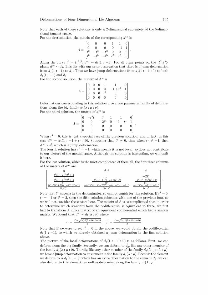
Deformations of Four Dimensional Lie Algebras 145
Note that each of these solutions is only a 2-dimensional subvariety of the 5-dimen-sional tangent space.For the first solution, the matrix of the corresponding d∞ is
A =
0 0 0 1 1 00 0 0 0 −1 1t3 −t3 −t3 0 0 0t5 −t5 −t5 t3 t3 0
.
Along the curve t5 = (t3)2, d∞ ∼ d1(1 : −1). For all other points on the (t3, t5)-plane, d∞ ∼ d3. This fits with our prior observation that there is a jump deformationfrom d1(1 : −1) to d3. Thus we have jump deformations from d3(1 : −1 : 0) to bothd1(1 : −1) and d3.For the second solution, the matrix of d∞ is
A =
0 0 0 1 1 00 0 0 0 −1 + t1 10 0 0 t2 0 00 0 0 0 0 0
.
Deformations corresponding to this solution give a two parameter family of deforma-tions along the big family d3(λ : µ : ν).For the third solution, the matrix of d∞ is
A =
0 −t4t1 t4 1 1 00 0 −2t4 0 −1 + t1 10 0 0 0 0 00 0 0 0 0 0
.
When t4 = 0, this is just a special case of the previous solution, and in fact, in thiscase d∞ = d3(1 : −1 + t1 : 0). Supposing that t4 6= 0, then when t1 6= −1, thend∞ ∼ d♯2 which is a jump deformation.The fourth solution has t1 = −1, which means it is not local, so does not contributeto our picture of the moduli space. Although the solution is interesting, we will omitit here.For the last solution, which is the most complicated of them all, the first three columnsof the matrix of d∞ are
0 t1t4 t4
t4(t1−2)2(t1+1)4 0 −2t4
t4(t1−2)4(t1+1)8t1
−t4(t1−2)2(−4+3(t1)2)8t1
−t4(t1−2)2(t1+1)2t1
(t4)2(t1+2)(t1−2)4(t1+1)8(t1)2
−(t4)2((t1)3−2(t1)2+4t1+8)(t1−2)28(t1)2
−(t4)2(t1+1)(t1−2)2(t1)2
.
Note that t1 appears in the denominator, so cannot vanish for this solution. If t4 = 0,t1 = −1 or t1 = 2, then the fifth solution coincides with one of the previous four, sowe will not consider these cases here. The matrix of A is so complicated that in orderto determine which standard form the codifferential is equivalent to three, we firsthad to transform A into a matrix of an equivalent codifferential which had a simplermatrix. We found that d∞ ∼ d1(α : β) where
α =t1+√
5(t1)2−16t1+16
2 , β =t1−√
5(t1)2−16t1+16
2 .
Note that if we were to set t1 = 0 in the above, we would obtain the codifferentiald1(1 : −1), to which we already obtained a jump deformation in the first solutionabove.The picture of the local deformations of d3(1 : −1 : 0) is as follows. First, we can
deform along the big family. Secondly, we can deform to d♯2, like any other member ofthe family d3(λ : µ : 0). Thirdly, like any other member of the family d3(λ : µ : λ+µ),we have a jump deformation to an element in the family d1(λ : µ). Because the elementwe deform to is d1(1 : −1), which has an extra deformation to the element d3, we canalso deform to this element, as well as deforming along the family d1(λ : µ).

146 III. Generalizations and Applications
m). The codifferential d3(λ : µ). This family does not have an action of the sym-metric group, which is important to keep in mind. Generically, H1 and H2 are 4dimensional. The generic basis of H2 below consists of elements which are linearlyindependent nontrivial cocycles for generic values of λ and µ except in the specialcase λ = µ, which we will treat separately. Of course, for those values of λ and µ forwhich dimH2 > 4, they do not span H2. Generically, we have
H1 = 〈ψ12 , ψ
22(λ− µ) + ψ3
2 , ψ22 + ψ3
3 , ψ21(λ− µ) + ψ3
1〉H2 = 〈ψ1 = ψ34
3 , ψ2 = ψ142 , ψ3 = ψ24
1 , ψ4 = ψ242 〉.
All of the brackets of these nontrivial cocycles vanish, so the miniversal deformationis just the first order deformation d∞ = d3(λ : µ) + ψit
i, and there are no relationson the base. The matrix of d∞ is given by
A =
0 0 0 λ t3 00 0 0 t2 λ+ t4 10 0 0 0 0 µ+ t1
0 0 0 0 0 0
.
If t3 6= 0, then d∞ ∼ d3(α, β, η), where
α = λ+t4 +
√(t4)2 + 4t2t3
2, β = λ+
t4 −√(t4)2 + 4t2t3
2, η = µ+ t1.
If t1 = t2 = t4 = 0, then d∞ ∼ d3(λ : λ : µ), so there is a jump deformationfrom d3(λ : µ) to d3(λ : λ : µ). Thus we see that the codifferential d3(λ : µ) sitsover the codifferential d3(λ : λ : µ) and deforms along the big family as if it werethat codifferential. All of the deformations of d3(λ : µ) which do not lie along thehyperplane t3 = 0 lie along the big family.Now, consider the hyperplane t3 = 0. The eigenvalues of the submatrix
B =
λ 0 0t2 λ+ t4 10 µ+ t1
are λ, λ+ t4 and µ+ t1. If these eigenvalues are all distinct, then d∞ ∼ d3(λ : λ+ t4 :µ+ t1). Otherwise, one of the conditions t4 = 0, t1 = λ− µ, or t1 − t4 = λ− µ holds.Of these conditions, only the first one is local, so we will not consider the other two.Consider the plane t3 = t4 = 0. Unless t2 = 0 or t1 = λ− µ, d∞ is still equivalent tod3(λ : λ + t4 : µ + t1). Again, the second condition is not local, so we will ignore it.On the line t2 = 0, we have d∞ ∼ d3(λ : µ + t1), so we get a deformation along thed3(λ : µ) family.To summarize the generic deformation behavior of an element of the family d3(λ : µ),we have the following picture. First, we can always deform along the family to whichan element belongs, so there is a deformation along the family d3(λ : µ). Secondly,there is a jump deformation to the element d3(λ : λ : µ) in the big family. Wheneverthere is a jump deformation, then we can deform in any manner in which the elementwe jump to deforms, and thus there is a deformation along the big family as well.Note that the line (λ : λ : µ), which is one of the lines in P2 with nontrivial stabilizer,is the target of our jump deformations, so the elements d3(λ : λ : µ) are special notin the sense that they have more deformations, but that there are extra deformationsto them.
n). The codifferential d3(1 : 1). Even though the dimension of H2 for this elementis the same as the generic case of d3(λ : µ), we have to use a different basis for H2
than in the generic case.
H2 = 〈ψ1 = ψ143 , ψ2 = ψ14
1 , ψ3 = ψ241 , ψ4 = ψ24
3 〉.
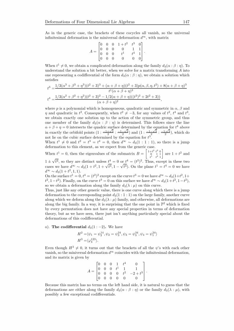
Deformations of Four Dimensional Lie Algebras 147
As in the generic case, the brackets of these cocycles all vanish, so the universalinfinitesimal deformation is the miniversal deformation d∞, with matrix
A =
0 0 0 1 + t2 t3 00 0 0 0 1 10 0 0 t1 t4 10 0 0 0 0 0
.
When t1 6= 0, we obtain a complicated deformation along the family d3(α : β : η). Tounderstand the solution a bit better, when we solve for a matrix transforming A intoone representing a codifferential of the form d3(α : β : η), we obtain a solution whichsatisfies
t3 =1/3(α3 + β3 + η3)(t2 + 3)3 + (α+ β + η)(t2 + 3)p(α, β, η, t2) + 8(α+ β + η)3
t1(α+ β + η)3
t4 =1/3(α2 + β2 + η2)(t2 + 3)2 − 1/2(α+ β + η)((t2)2 + 2t2 + 3))
(α + β + η)2,
where p is a polynomial which is homogeneous, quadratic and symmetric in α, β andη and quadratic in t2. Consequently, when t2 6= −3, for any values of t2, t4 and t3,we obtain exactly one solution up to the action of the symmetric group, and thusone member of the family d3(α : β : η) is determined. This follows since the lineα+ β + η = 0 intersects the quadric surface determined by the equation for t4 above
in exactly the orbifold points (1 : −1+√3
2 : −1−√3
2 ) and (1 : −1−√3
2 : −1:√3
2 ), which do
not lie on the cubic surface determined by the equation for t3.When t1 6= 0 and t2 = t3 = t4 = 0, then d∞ ∼ d3(1 : 1 : 1), so there is a jumpdeformation to this element, as we expect from the generic case.
When t1 = 0, then the eigenvalues of the submatrix B =
[1+t2 t3 00 1 1t1 t4 1
]are 1 + t2 and
1 ±√t4, so they are distinct unless t4 = 0 or t4 = (t2)2. Thus, except in these two
cases we have d∞ ∼ d3(1 + t2, 1 +√t4, 1 −
√t4). On the plane t1 = t4 = 0 we have
d∞ ∼ d3(1 + t2, 1, 1).On the surface t1 = 0, t4 = (t2)2 except on the curve t3 = 0 we have d∞ ∼ d3(1+t2, 1+t2, 1− t2). Finally, on the curve t3 = 0 on this surface we have d∞ ∼ d3(1+ t2, 1− t2),so we obtain a deformation along the family d3(λ : µ) on this curve.Thus, just like any other generic value, there is one curve along which there is a jumpdeformation to the corresponding point d3(1 : 1 : 1) on the large family, another curvealong which we deform along the d3(λ : µ) family, and otherwise, all deformations arealong the big family. In a way, it is surprising that the one point in P2 which is fixedby every permutation does not have any special properties in terms of deformationtheory, but as we have seen, there just isn’t anything particularly special about thedeformations of this codifferential.
o). The codifferential d3(1 : −2). We have
H2 =〈ψ1 = ψ142 , ψ2 = ψ24
3 , ψ3 = ψ343 , ψ4 = ψ24
1 〉H3 =〈ϕ123
4 〉.
Even though H3 6= 0, it turns out that the brackets of all the ψ’s with each othervanish, so the miniversal deformation d∞ coincides with the infinitesimal deformation,and its matrix is given by
A =
0 0 0 1 t4 00 0 0 t1 1 10 0 0 0 t2 −2 + t3
0 0 0 0 0 0
.
Because this matrix has no terms on the left hand side, it is natural to guess that thedeformations are either along the family d3(α : β : η) or the family d3(λ : µ), withpossibly a few exceptional codifferentials.

148 III. Generalizations and Applications
When t1 6= 0 we have a solution of the form
t3 =α+ β + η
q
t2 =− (α+ η − 2q)(α+ β − 2q)(β + η − 2q)
q2(α + β + η − 3q)
t4 =−(α− q)(β − q)(η − q)t1q2(α+ β + η − 3q)
,
where q is a nonzero free parameter. These equations are symmetric in α, β and η. Ift3 6= 0, then α+ β + η 6= 0, and we can solve the first equation for q and get
t2 =−((α+ β)t3 − 2(α+ β + η))((β + η)t3 − 2(α+ β + η))((α + η)t3 − 2(α+ β + η)
(α+ β + η)3(t3 − 3)
t4 =−(αt3 − (α+ β + η))(βt3 − (α+ β + η))(ηt3 − (α+ β + η))
t1(t3 − 3)(α+ β + η)3.
We can express these equations in the form
t2 =αβη(t3)3 + (α+ β + η)(t3 − 2)p(α, β, η, t3)
(α+ β + η)3(t3 − 3)
t4 =−αβη(t3)3 + (α+ β + η)r(α, β, η, t3)
t1(t3 − 3)(α+ β + η)3,
where p and q are homogeneous, quadratic and symmetric in α, β and η. The surfacesrepresented by these two equations are both cubic, so there are 9 points of intersection.Since every cubic which is given by a symmetric, homogeneous polynomial eithercontains the line α+β+η = 0 or intersects this line in precisely the points (1 : −1 : 0),(1 : 0 : −1) and (0 : 1 : −1), there are six points in the intersection of these two cubicsnot on this line, which uniquely determine the codifferential d3(α : β : η) to which d∞
is equivalent. The matrix representing the transformation can be chosen with nonzerodeterminant, as long as t3 6= 3. The condition t3 6= 0 can also be overcome, becauseif we substitute t3 = 0 in the above, then the problem still has a solution.Thus,whenever t1 6= 0 and t3 6= 3, the deformation is equivalent to a member of the familyd3(α : β : η).When t1 = 0, then as long as t2 6= 0 and t3 6= 1, d∞ ∼ d3(α : β : 1), where
α =t3 − 1 +
√(t3 − 3)2 + 4t2
2and β =
t3 − 1−√(t3 − 3)2 + 4t2
2.
When t1 = t2 = 0 and t4 6= 0 we have d∞ ∼ d3(1 : 1 : t3 − 2). As a consequence,if we set t3 = 0, we have a jump deformation from d3(1 : −2) to d3(1 : 1 : −2). Onthe other hand, when t1 = t2 = t4 = 0, then d∞ ∼ d3(1 : t3 − 2). When t1 = 0and t3 = 1, then we also have a deformation along the big family. The upshot of allthis analysis is that d3(1 : −2) is really not special in terms of deformation theory. Itdeforms along its own family, jumps to d3(1 : 1 : −2), and deforms along that family.
p). The codifferential d3(1 : 2). We have
H2 = 〈ψ1 = ψ122 − ψ12
3 + ψ132 + ψ13
3 , ψ2 = ψ141 + ψ34
3 ,
ψ3 = ψ142 , ψ4 = ψ34
3 , ψ5 = ψ241 〉
H3 = 〈ϕ1243 + ϕ134
2 〉.This time, we do have some nonzero brackets, but only those brackets of ψ1 withψ2, ψ4 and ψ5, with the first one being a nontrivial cocycle, so that the second orderrelation is t1t2 = 0. After some work, one obtains that there is one relation on thebase of the versal deformation,
t1t2(−1− t4 + t3t5) = 0,

Deformations of Four Dimensional Lie Algebras 149
so that there are three distinct solutions for a true deformation, given by the threefactors of the miniversal deformation. Notice that the third factor does not give riseto a local deformation.Let us study the first solution, when t1 = 0. This case is simplest. The matrix corre-sponding to d∞ is
A =
0 0 0 1 + t4 t5 00 0 0 t3 1 10 0 0 0 0 2 + t2 + t4
0 0 0 0 0 0
.
When t5 6= 0, then d∞ is equivalent to d3(α : β : 2 + t2 + t4), where α, β =2+t4±
√(t4)2+4t3t5
2 . If t2 = t3 = t4 = 0, then the deformation is equivalent to d3(1 : 1 :
2) for all t5 6= 0, giving the expected jump deformation.What happens if t5 = 0? As long as t2 6= −1 and t2t3 + t4t3 + t3 + t4 6= 0, then thedeformation is still along the big family. If t2 6= −1, but t2t3+ t4t3+ t3+ t4 = 0, thenas long as t3 6= 0 and t4 6= 0, the deformation is in the big family. If t4 = 0, thent3 = 0 or t2 = −1, and in both cases we deform along the family d3(α : β). Thus, thefirst solution to the relations on the base does not have any surprises.The second solution to the relations on the base is t2 = 0. We may as well assumethat t1 6= 0 and that −1− t4 + t3t5 6= 0 for this case. Then the matrix of d∞ is
A =
−t1t5 −t1t5−1−t4+t3t5
t1(t5)2
−1−t4+t3t5 1 + t4 t5 0
−t1 −t1−1−t4+t3t5
t1t5
−1−t4+t3t5 t3 1 1
t1(−1− t4 + t3t5) t1 −t1t5 0 0 2 + t4
0 0 0 0 0 0
.
The submatrix consisting of the first three columns of A has rank 1, so we cantransform this matrix into a simpler matrix.Recall that we assume that t1 6= 0. When t5 6= 0, then it turns out that d∞ ∼ d1(α :
β), where αβ(α+β)2 = 1−t4−t3t5
(2+t4)2 . Also, if t5 = 0 and t3 6= 0, then the deformation is
equivalent to d1(1 + t4 : 1). In particular, if t4 = 0, we see that there is a jumpdeformation from our codifferential to the codifferential d1(1 : 1). On the other hand,if t3 = 0 and t4 6= 0, we also deform to d1(1 + t4 : 1). When t3 = t4 = t5 = 0, there is
a jump deformation of d∞ to d♯1.The picture for this element is more intriguing than for d3(1 : −2). In addition to theusual deformations along the family d3(α, β), jump deformation to d3(1 : 1 : 2), anddeformations along the big family, we see that d3(1 : 2) has a jump deformation to the
codifferential d♯1. Because d♯1 itself has a jump deformation to d1(1 : 1), we get a jump
deformation to this element as well, and deformations along the family d1(λ : µ).Thus we pick up far more deformations than we would expect considering that thedimension of H2 is only one more than in the generic case. Again, the explanationfor this “impossibility” has to do with the fact that the three dimensional tangentspace to this element of the moduli space does not accurately reflect the nature ofthe deformations, which are all tangent to one of three planes in this space. The truepicture is captured by the versal deformation.
q). The codifferential d3(0 : 1) = r2(C)⊕ C2. The cohomology is given by
H1 = 〈ψ12 , ψ
21 − ψ3
1 , ψ22 − ψ3
2 , ψ41 , ψ
42 , ψ
11〉
H2 = 〈ψ1 = −ψ122 + ψ13
2 , ψ2 = ψ141 , ψ3 = ψ14
2 ,
ψ4 = ψ241 , ψ5 = ψ24
2 , ψ6 = ψ121 − ψ13
1 〉H3 = 〈ϕ124
1 , ϕ1243 〉.
Not all of the brackets of the nontrivial 2-cocycles vanish, so we obtain some relationson the base of the versal deformation. The second order relations are t1t2 + t3t6 = 0and t1t4 + t5t6 = 0. The relations on the base are obtained by adding higher orderterms to these second order relations. We will omit them for brevity, but instead will
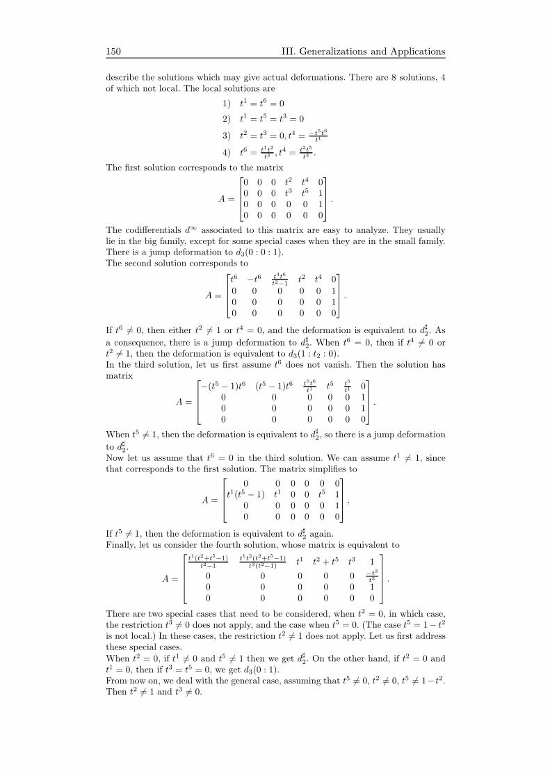
150 III. Generalizations and Applications
describe the solutions which may give actual deformations. There are 8 solutions, 4of which not local. The local solutions are
1) t1 = t6 = 0
2) t1 = t5 = t3 = 0
3) t2 = t3 = 0, t4 = −t5t6t1
4) t6 = t1t2
t3 , t4 = t2t5
t3 .
The first solution corresponds to the matrix
A =
0 0 0 t2 t4 00 0 0 t3 t5 10 0 0 0 0 10 0 0 0 0 0
.
The codifferentials d∞ associated to this matrix are easy to analyze. They usuallylie in the big family, except for some special cases when they are in the small family.There is a jump deformation to d3(0 : 0 : 1).The second solution corresponds to
A =
t6 −t6 t4t6
t2−1 t2 t4 0
0 0 0 0 0 10 0 0 0 0 10 0 0 0 0 0
.
If t6 6= 0, then either t2 6= 1 or t4 = 0, and the deformation is equivalent to d♯2. As
a consequence, there is a jump deformation to d♯2. When t6 = 0, then if t4 6= 0 ort2 6= 1, then the deformation is equivalent to d3(1 : t2 : 0).In the third solution, let us first assume t6 does not vanish. Then the solution hasmatrix
A =
−(t5 − 1)t6 (t5 − 1)t6 t5t6
t1 t5 t5
t1 00 0 0 0 0 10 0 0 0 0 10 0 0 0 0 0
.
When t5 6= 1, then the deformation is equivalent to d♯2, so there is a jump deformation
to d♯2.Now let us assume that t6 = 0 in the third solution. We can assume t1 6= 1, sincethat corresponds to the first solution. The matrix simplifies to
A =
0 0 0 0 0 0t1(t5 − 1) t1 0 0 t5 1
0 0 0 0 0 10 0 0 0 0 0
.
If t5 6= 1, then the deformation is equivalent to d♯2 again.Finally, let us consider the fourth solution, whose matrix is equivalent to
A =
t1(t2+t5−1)t2−1
t1t2(t2+t5−1)t3(t2−1) t1 t2 + t5 t3 1
0 0 0 0 0 −t2t3
0 0 0 0 0 10 0 0 0 0 0
.
There are two special cases that need to be considered, when t2 = 0, in which case,the restriction t3 6= 0 does not apply, and the case when t5 = 0. (The case t5 = 1− t2is not local.) In these cases, the restriction t2 6= 1 does not apply. Let us first addressthese special cases.
When t2 = 0, if t1 6= 0 and t5 6= 1 then we get d♯2. On the other hand, if t2 = 0 andt1 = 0, then if t3 = t5 = 0, we get d3(0 : 1).From now on, we deal with the general case, assuming that t5 6= 0, t2 6= 0, t5 6= 1− t2.Then t2 6= 1 and t3 6= 0.
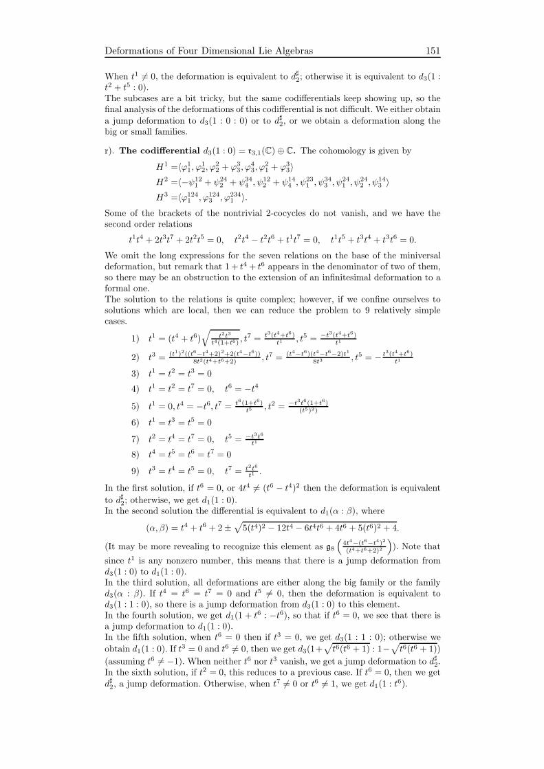
Deformations of Four Dimensional Lie Algebras 151
When t1 6= 0, the deformation is equivalent to d♯2; otherwise it is equivalent to d3(1 :t2 + t5 : 0).The subcases are a bit tricky, but the same codifferentials keep showing up, so thefinal analysis of the deformations of this codifferential is not difficult. We either obtain
a jump deformation to d3(1 : 0 : 0) or to d♯2, or we obtain a deformation along thebig or small families.
r). The codifferential d3(1 : 0) = r3,1(C)⊕ C. The cohomology is given by
H1 =〈ϕ11, ϕ
12, ϕ
22 + ϕ3
3, ϕ43, ϕ
21 + ϕ3
3〉H2 =〈−ψ12
1 + ψ242 + ψ34
4 , ψ122 + ψ14
4 , ψ231 , ψ
343 , ψ
241 , ψ
242 , ψ
143 〉
H3 =〈ϕ1241 , ϕ124
3 , ϕ2341 〉.
Some of the brackets of the nontrivial 2-cocycles do not vanish, and we have thesecond order relations
t1t4 + 2t3t7 + 2t2t5 = 0, t2t4 − t2t6 + t1t7 = 0, t1t5 + t3t4 + t3t6 = 0.
We omit the long expressions for the seven relations on the base of the miniversaldeformation, but remark that 1+ t4 + t6 appears in the denominator of two of them,so there may be an obstruction to the extension of an infinitesimal deformation to aformal one.The solution to the relations is quite complex; however, if we confine ourselves tosolutions which are local, then we can reduce the problem to 9 relatively simplecases.
1) t1 = (t4 + t6)√
t2t3
t4(1+t6) , t7 = t3(t4+t6)
t1 , t5 = −t3(t4+t6)t1
2) t3 = (t1)2((t6−t4+2)2+2(t4−t6))8t2(t4+t6+2) , t7 = (t4−t6)(t4−t6−2)t1
8t3 , t5 = − t3(t4+t6)t1
3) t1 = t2 = t3 = 0
4) t1 = t2 = t7 = 0, t6 = −t4
5) t1 = 0, t4 = −t6, t7 = t6(1+t6)t5 , t2 = −t3t6(1+t6)
(t5)2)
6) t1 = t3 = t5 = 0
7) t2 = t4 = t7 = 0, t5 = −t3t6t1
8) t4 = t5 = t6 = t7 = 0
9) t3 = t4 = t5 = 0, t7 = t2t6
t1 .
In the first solution, if t6 = 0, or 4t4 6= (t6 − t4)2 then the deformation is equivalent
to d♯2; otherwise, we get d1(1 : 0).In the second solution the differential is equivalent to d1(α : β), where
(α, β) = t4 + t6 + 2±√
5(t4)2 − 12t4 − 6t4t6 + 4t6 + 5(t6)2 + 4.
(It may be more revealing to recognize this element as g8
(4t4−(t6−t4)2(t4+t6+2)2
)). Note that
since t1 is any nonzero number, this means that there is a jump deformation fromd3(1 : 0) to d1(1 : 0).In the third solution, all deformations are either along the big family or the familyd3(α : β). If t4 = t6 = t7 = 0 and t5 6= 0, then the deformation is equivalent tod3(1 : 1 : 0), so there is a jump deformation from d3(1 : 0) to this element.In the fourth solution, we get d1(1 + t6 : −t6), so that if t6 = 0, we see that there isa jump deformation to d1(1 : 0).In the fifth solution, when t6 = 0 then if t3 = 0, we get d3(1 : 1 : 0); otherwise we
obtain d1(1 : 0). If t3 = 0 and t6 6= 0, then we get d3(1+√t6(t6 + 1) : 1−
√t6(t6 + 1))
(assuming t6 6= −1). When neither t6 nor t3 vanish, we get a jump deformation to d♯2.In the sixth solution, if t2 = 0, this reduces to a previous case. If t6 = 0, then we get
d♯2, a jump deformation. Otherwise, when t7 6= 0 or t6 6= 1, we get d1(1 : t6).
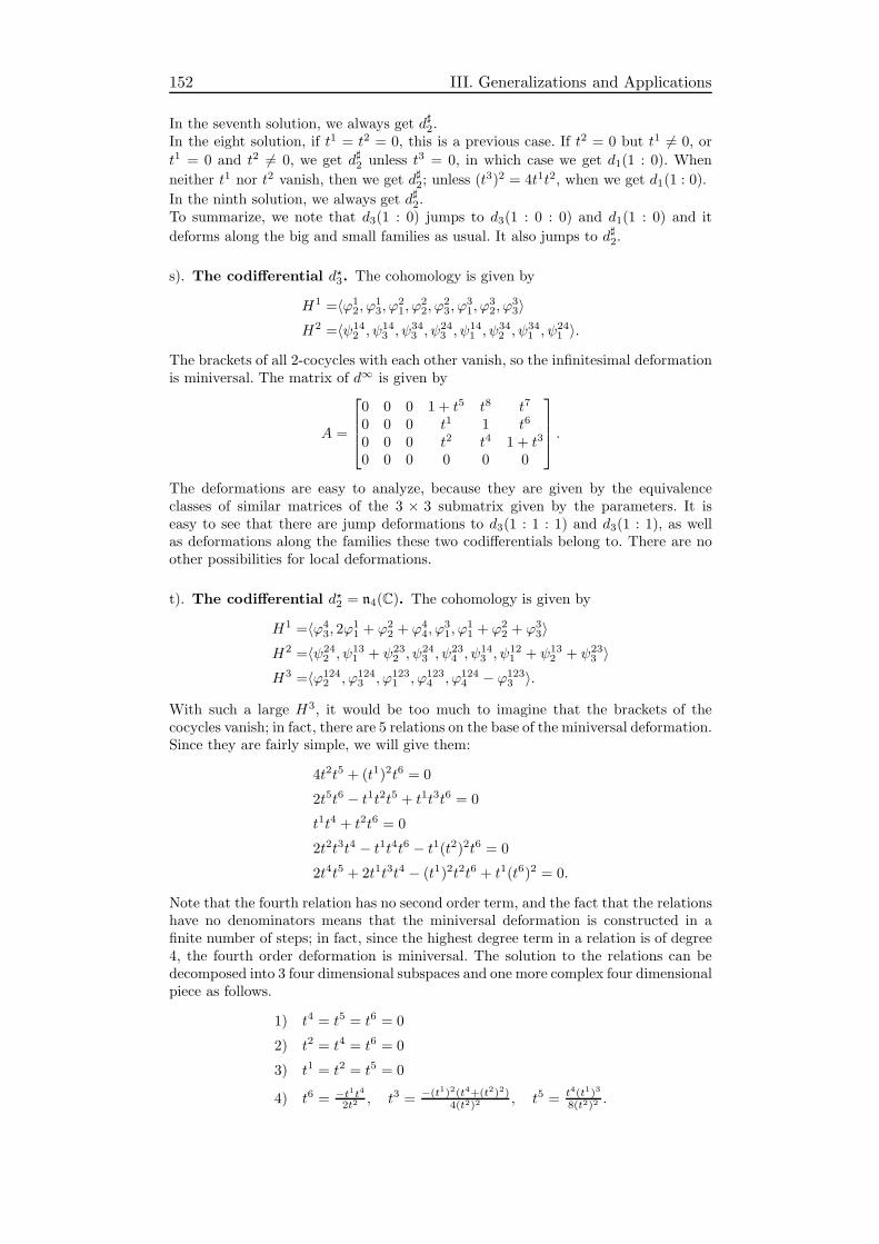
152 III. Generalizations and Applications
In the seventh solution, we always get d♯2.In the eight solution, if t1 = t2 = 0, this is a previous case. If t2 = 0 but t1 6= 0, or
t1 = 0 and t2 6= 0, we get d♯2 unless t3 = 0, in which case we get d1(1 : 0). When
neither t1 nor t2 vanish, then we get d♯2; unless (t3)2 = 4t1t2, when we get d1(1 : 0).
In the ninth solution, we always get d♯2.To summarize, we note that d3(1 : 0) jumps to d3(1 : 0 : 0) and d1(1 : 0) and it
deforms along the big and small families as usual. It also jumps to d♯2.
s). The codifferential d⋆3. The cohomology is given by
H1 =〈ϕ12, ϕ
13, ϕ
21, ϕ
22, ϕ
23, ϕ
31, ϕ
32, ϕ
33〉
H2 =〈ψ142 , ψ
143 , ψ
343 , ψ
243 , ψ
141 , ψ
342 , ψ
341 , ψ
241 〉.
The brackets of all 2-cocycles with each other vanish, so the infinitesimal deformationis miniversal. The matrix of d∞ is given by
A =
0 0 0 1 + t5 t8 t7
0 0 0 t1 1 t6
0 0 0 t2 t4 1 + t3
0 0 0 0 0 0
.
The deformations are easy to analyze, because they are given by the equivalenceclasses of similar matrices of the 3 × 3 submatrix given by the parameters. It iseasy to see that there are jump deformations to d3(1 : 1 : 1) and d3(1 : 1), as wellas deformations along the families these two codifferentials belong to. There are noother possibilities for local deformations.
t). The codifferential d⋆2 = n4(C). The cohomology is given by
H1 =〈ϕ43, 2ϕ
11 + ϕ2
2 + ϕ44, ϕ
31, ϕ
11 + ϕ2
2 + ϕ33〉
H2 =〈ψ242 , ψ
131 + ψ23
2 , ψ243 , ψ
234 , ψ
143 , ψ
121 + ψ13
2 + ψ233 〉
H3 =〈ϕ1242 , ϕ124
3 , ϕ1231 , ϕ123
4 , ϕ1244 − ϕ123
3 〉.
With such a large H3, it would be too much to imagine that the brackets of thecocycles vanish; in fact, there are 5 relations on the base of the miniversal deformation.Since they are fairly simple, we will give them:
4t2t5 + (t1)2t6 = 0
2t5t6 − t1t2t5 + t1t3t6 = 0
t1t4 + t2t6 = 0
2t2t3t4 − t1t4t6 − t1(t2)2t6 = 0
2t4t5 + 2t1t3t4 − (t1)2t2t6 + t1(t6)2 = 0.
Note that the fourth relation has no second order term, and the fact that the relationshave no denominators means that the miniversal deformation is constructed in afinite number of steps; in fact, since the highest degree term in a relation is of degree4, the fourth order deformation is miniversal. The solution to the relations can bedecomposed into 3 four dimensional subspaces and one more complex four dimensionalpiece as follows.
1) t4 = t5 = t6 = 0
2) t2 = t4 = t6 = 0
3) t1 = t2 = t5 = 0
4) t6 = −t1t42t2 , t3 = −(t1)2(t4+(t2)2)
4(t2)2 , t5 = t4(t1)3
8(t2)2 .
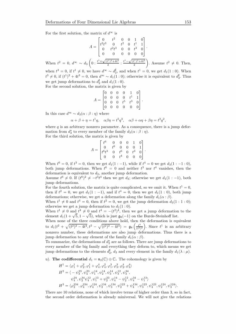
Deformations of Four Dimensional Lie Algebras 153
For the first solution, the matrix of d∞ is
A =
0 t2 0 0 1 0t2t3 0 t2 0 t1 10 t2t3 0 0 t3 00 0 0 0 0 0
.
When t2 = 0, d∞ ∼ d3
(0 :
t1+√
(t1)2+4t3
2 :t1−√
(t1)2+4t3
2
). Assume t2 6= 0. Then,
when t3 = 0, if t1 6= 0, we have d∞ ∼ d♯2, and when t1 = 0, we get d1(1 : 0). When
t3 6= 0, if (t1)2 + 4t3 = 0, then d∞ ∼ d1(1 : 0); otherwise it is equivalent to d♯2. Thus
we get jump deformations to d♯2 and d1(1 : 0).For the second solution, the matrix is given by
A =
0 0 0 0 1 00 0 0 0 t1 10 0 0 t5 t3 00 0 0 0 0 0
.
In this case d∞ ∼ d3(α : β : η) where
α+ β + η = t1q, αβη = t5q3, αβ + αη + βη = t3q2,
where q is an arbitrary nonzero parameter. As a consequence, there is a jump defor-mation from d∗2 to every member of the family d3(α : β : η).For the third solution, the matrix is given by
A =
t6 0 0 0 1 00 t6 0 0 0 1t6t3 0 t6 0 t3 00 0 t4 0 0 0
.
When t6 = 0, if t3 = 0, then we get d1(1 : −1), while if t4 = 0 we get d3(1 : −1 : 0),both jump deformations. When t6 = 0 and neither t3 nor t4 vanishes, then thedeformation is equivalent to d3, another jump deformation.Assume t6 6= 0. If (t6)2 6= −t3t4 then we get d3; otherwise we get d1(1 : −1), bothjump deformations.For the fourth solution, the matrix is quite complicated, so we omit it. When t1 = 0,then if t2 = 0, we get d1(1 : −1), and if t4 = 0, then we get d1(1 : 0), both jumpdeformations; otherwise, we get a deformation along the family d1(α : β).When t1 6= 0 and t4 = 0, then if t2 = 0, we get the jump deformation d3(1 : 1 : 0);otherwise we get a jump deformation to d1(1 : 0).When t1 6= 0 and t4 6= 0 and t4 = −(t2)4, then we get a jump deformation to the
element d1(1 +√5, 1−
√5), which is just g8(−1) on the Burde-Steinhoff list.
When none of the three conditions above hold, then the deformation is equivalent
to d1(t2 +
√(t2)2 − 4t4, t2 −
√(t2)2 − 4t4) = g8
(t4
(t2)2
). Since t1 is an arbitrary
nonzero number, these deformations are also jump deformations. Thus there is ajump deformation to any element of the family d1(α : β).To summarize, the deformations of d∗2 are as follows. There are jump deformations toevery member of the big family and everything they deform to, which means we get
jump deformations to the elements d♯2, d3 and every element in the family d1(λ : µ).
u). The codifferential d1 = n3(C)⊕ C. The cohomology is given by
H1 = 〈ϕ11 + ϕ2
2, ϕ11 + ϕ4
4, ϕ24, ϕ
31, ϕ
33, ϕ
42, ϕ
43〉
H2 = 〈 − ψ233 , ψ
234 , ψ
141 , ψ
142 , ψ
143 , ψ
123 , ψ
343 ,
ψ244 , ψ
342 ψ
124 , ψ
131 + ψ23
2 , ψ144 − ψ12
2 , ψ344 − ψ13
1 〉H3 = 〈ϕ234
2 , ϕ2344 , ϕ124
4 , ψ1342 , ψ134
3 , ψ1232 + ψ134
4 , ψ1233 , ψ123
4 , ψ1242 , ψ124
3 〉.There are 10 relations, none of which involve terms of higher order than 3, so in fact,the second order deformation is already miniversal. We will not give the relations
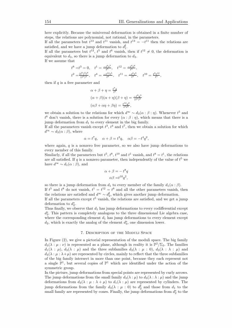
154 III. Generalizations and Applications
here explicitly. Because the miniversal deformation is obtained in a finite number ofsteps, the relations are polynomial, not rational, in the parameters.If all the parameters but t13 and t11 vanish, and t13 = −t11 then the relations are
satisfied, and we have a jump deformation to d♯1.If all the parameters but t12, t5 and t6 vanish, then if t12 6= 0, the deformation isequivalent to d3, so there is a jump deformation to d3.If we assume that
t8 =t3 = 0, t1 = −t6t7t5 , t12 = −t6t9
t5 ,
t2 = (t6)2t9
(t5)2 , t4 = −t12t5t6 , t11 = −t6t9
t5 , t10 = t6t12
t5 ,
then if q is a free parameter and
α+ β + η = t7qt5
(α+ β)(α + η)(β + η) = −t9q3(t5)2
(αβ + αη + βη) = t12q2
t5t6 ,
we obtain a solution to the relations for which d∞ ∼ d3(α : β : η). Whenever t5 andt6 don’t vanish, there is a solution for every (α : β : η), which means that there is ajump deformation from d1 to every element in the big family.If all the parameters vanish except t3, t4 and t7, then we obtain a solution for whichd∞ ∼ d3(α : β), where
α = t7q, α+ β = t3q, αβ = −t4q2,where again, q is a nonzero free parameter, so we also have jump deformations toevery member of this family.Similarly, if all the parameters but t5, t8, t10 and t1 vanish, and t8 = t1, the relationsare all satisfied. If q is a nonzero parameter, then independently of the value of t5 wehave d∞ ∼ d1(α : β), and
α+ β =− t8qαβ =t10q2,
so there is a jump deformation from d1 to every member of the family d1(α : β).If t5 and t8 do not vanish, t1 = t12 = t8 and all the other parameters vanish, then
the relations are satisfied and d∞ ∼ d♯2, which gives another jump deformation.If all the parameters except t5 vanish, the relations are satisfied, and we get a jumpdeformation to d∗2.Thus finally, we observe that d1 has jump deformations to every codifferential exceptd∗3. This pattern is completely analogous to the three dimensional Lie algebra case,where the corresponding element d1 has jump deformations to every element exceptd2, which is exactly the analog of the element d∗3, one dimension lower.
7. Description of the Moduli Space
In Figure (2), we give a pictorial representation of the moduli space. The big familyd3(λ : µ : ν) is represented as a plane, although in reality it is P2/Σ3. The familiesd1(λ : µ), d3(λ : µ) and the three subfamilies d3(λ : µ : 0), d3(λ : λ : µ) andd3(λ : µ : λ+µ) are represented by circles, mainly to reflect that the three subfamiliesof the big family intersect in more than one point, because they each represent nota single P1, but several copies of P1 which are identified under the action of thesymmetric group.In the picture, jump deformations from special points are represented by curly arrows.The jump deformations from the small family d3(λ : µ) to d3(λ : λ : µ) and the jumpdeformations from d3(λ : µ : λ + µ) to d1(λ : µ) are represented by cylinders. The
jump deformations from the family d3(λ : µ : 0) to d♯2 and those from d1 to thesmall family are represented by cones. Finally, the jump deformations from d∗2 to the
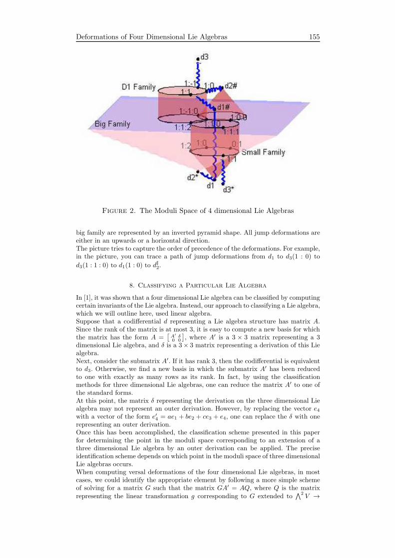
Deformations of Four Dimensional Lie Algebras 155
Figure 2. The Moduli Space of 4 dimensional Lie Algebras
big family are represented by an inverted pyramid shape. All jump deformations areeither in an upwards or a horizontal direction.The picture tries to capture the order of precedence of the deformations. For example,in the picture, you can trace a path of jump deformations from d1 to d3(1 : 0) to
d3(1 : 1 : 0) to d1(1 : 0) to d♯2.
8. Classifying a Particular Lie Algebra
In [1], it was shown that a four dimensional Lie algebra can be classified by computingcertain invariants of the Lie algebra. Instead, our approach to classifying a Lie algebra,which we will outline here, used linear algebra.Suppose that a codifferential d representing a Lie algebra structure has matrix A.Since the rank of the matrix is at most 3, it is easy to compute a new basis for whichthe matrix has the form A =
[A′ δ0 0
], where A′ is a 3 × 3 matrix representing a 3
dimensional Lie algebra, and δ is a 3× 3 matrix representing a derivation of this Liealgebra.Next, consider the submatrix A′. If it has rank 3, then the codifferential is equivalentto d3. Otherwise, we find a new basis in which the submatrix A′ has been reducedto one with exactly as many rows as its rank. In fact, by using the classificationmethods for three dimensional Lie algebras, one can reduce the matrix A′ to one ofthe standard forms.At this point, the matrix δ representing the derivation on the three dimensional Liealgebra may not represent an outer derivation. However, by replacing the vector e4with a vector of the form e′4 = ae1 + be2 + ce3 + e4, one can replace the δ with onerepresenting an outer derivation.Once this has been accomplished, the classification scheme presented in this paperfor determining the point in the moduli space corresponding to an extension of athree dimensional Lie algebra by an outer derivation can be applied. The preciseidentification scheme depends on which point in the moduli space of three dimensionalLie algebras occurs.When computing versal deformations of the four dimensional Lie algebras, in mostcases, we could identify the appropriate element by following a more simple schemeof solving for a matrix G such that the matrix GA′ = AQ, where Q is the matrixrepresenting the linear transformation g corresponding to G extended to
∧2V →
156 III. Generalizations and Applications
∧2V and A′ is a matrix representing one of the nine types of elements in the moduli
space.However, because our matrices involved many parameters, it was sometimes too dif-ficult for the computer to solve for the values of the parameters for which the A′ andA matrices are equivalent. In those cases, we followed the more complicated schemeoutlined above. In practice, we found that it was only necessary to follow the stepspartially, because after transforming the matrix to eliminate some of the rows, wethen were able to apply the simple scheme, and obtain a solution.
9. Conclusions
The computation of the equivalence classes of non-isomorphic Lie algebra structuresin a vector space V determines the elements of the moduli space of Lie algebrastructures on V , but is only the first step in the classification of these structures.When classifying the algebras, there are different ways of dividing up the structuresaccording to families; therefore, it is desirable to have a rationale for the division. Inthis paper, we have shown that there is a natural way to divide up the moduli spaceinto families, using cohomology as a guide to the division, and versal deformations asa tool to refine the analysis.The four dimensional Lie algebras can be decomposed into families, each of which isnaturally an orbifold. If one takes into account the information about jump deforma-tions, the division we have given is uniquely determined. The elements of the familywhich contain a Lie algebra structure d are precisely those Lie algebras which canbe obtained as smooth deformations of d, but which are not smooth deformationsof any Lie algebra structure d′ which is a jump deformation of d. This rule allowsus to distinguish between the algebra d∗3 and d3(1 : 1), for example. Even though d∗3has smooth deformations to the family d3(λ : µ), it also has a jump deformation tod3(1 : 1), which has smooth deformations to the same family. Thus d3(1 : 1), whichhas no jump deformations to any element having smooth deformations to the family,is the element which belongs to the family.According to this system, there is one two-parameter family, two one-parameterfamilies, and six singleton elements, giving rise to a two-dimensional orbifold, twoone-dimensional orbifolds, and six one-dimensional orbifolds. The jump deformationsprovide maps between the families which either are smooth maps of orbifolds (orsuborbifolds as in the case of the map d3(λ : µ : λ + µ)→ d1(λ : µ)), or, in the caseof some of the singletons, identify the element with a whole family.The cohomology of a Lie algebra determines the tangent space to the Lie algebra,but the tangent space does not contain enough information to give a good localdescription of the moduli space. The relations on the base of the versal deformationdetermine the manner in which the moduli space contacts the tangent space. In oneexample here, the tangent space was two dimensional, but deformations were onlyalong two curves. In another case, the tangent space was three dimensional, but thedeformations were confined to three planes. It is clear that the cohomology is notsufficient to get an accurate picture of the moduli space. Versal deformations provideimportant detail that characterizes the moduli space completely.
10. Acknowledgments
The authors would like to thank E. Vinberg for helpful discussions and the Max-Planck-Institut fur Mathematik, Bonn for hosting both authors while they were fin-ishing this paper.
References
1. Y. Agaoka, An algorithm to determine the isomorphism classes of 4-dimensional complexLie algebras, Linear Algebra and its Applications 345 (2002), 85–118.
2. D. Burde and C. Steinhoff, Classification of orbit closures of 4-dimensional complex Liealgebras, Journal of Algebra 214 (1999), 729–739.
Deformations of Four Dimensional Lie Algebras 157
3. A. Fialowski, Deformations of Lie algebras, Mathematics of the USSR-Sbornik 55
(1986), no. 2, 467–473.4. A. Fialowski, An example of formal deformations of Lie algebras, Proc. NATO Conf. on
Deformation Theory of Algebras and Appl., Kluwer 1988, 375–401.5. A. Fialowski and D. Fuchs, Construction of miniversal deformations of Lie algebras,
Journal of Functional Analysis (1999), no. 161(1), 76–110.6. A. Fialowski and M. Penkava, Deformation theory of infinity algebras, Journal of Algebra
255 (2002), no. 1, 59–88, math.RT/0101097.7. , Versal deformations of three dimensional Lie algebras as L∞ algebras, Commu-
nications in Contemporary Mathematics 7 (2005), no. 2, 145–165, math.RT/0303346.8. M. Gerstenhaber, On the deformations of rings and algebras I–IV, Annals of Mathe-
matics 79 (1964), 59–103; II, Annals of Mathematics 84 (1966), 1–19; III, Annals ofMathematics 88 (1968), 1–34; IV, Annals of Mathematics 99 (1974), 257–276.
9. A.A. Kirillov and Y.A. Neretin, The variety An of n-dimensional Lie algebra structures,Amer. Math. Soc. Transl. 137 (1987), no. 2, 21–30.
10. B. Komrakov and A. Tchourioumov, Small dimensional and linear Lie algebras, Inter-national Sophus Lie Centre Press, 2000.
11. A. Nijenhuis and R. Richardson, Deformations of Lie algebra structures, Jour. Math.Mech. 17 (1967), 89–105.
12. A.L. Onishik and and E.B. Vinberg (ed.) Lie Groups and Lie Algebras III.(Structure ofLie groups and Lie algebras), Encyclopaedia of Math. Sci., 1994.
13. R.O. Popovich, V.M. Boyko, M.O. Nesterenko, and M.W. Lutfullin, Realization of reallow-dimensional Lie algebras, Journal of Phys. A Math Gen. 36 (2003), 7337–7360.
14. M. Rhomdani, Classification of real and complex nilpotent Lie algebras of dimension 7,Linear and Multilinear Algebra 24 (1989), 167–189.
15. P. Turkowski, Literature on the structure of low-dimensional nonsemisimple Lie algebrasand its applications to cosmology, Acta Cosmologica 20 (1994), 147–153.
Alice Fialowski, email : [email protected] Penkava, email : [email protected]