Introduction to algorithms in bioinformatics

István Miklós, Rényi Institute 2010 Spring

(last update: 9/9/2013)

i

Table of Content Preface .................................................................................................................................. ii The history of genome rearrangement .................................................................................. 1 Genome rearrangement by double cut & join (DCJ) operations ........................................... 6 The Hannenhalli-Pevzner-(Bergeron) theory ........................................................................ 10 Sorting by block interchanges ............................................................................................... 18 Sorting by transpositions ....................................................................................................... 21 The principle of dynamic programming ................................................................................. 29 Pairwise sequence alignment ............................................................................................... 32 Multiple sequence alignment ................................................................................................ 39 Dynamic programming on trees ............................................................................................ 43 Transformational grammars .................................................................................................. 46 RNA secondary structure prediction ..................................................................................... 55 Graphical degree sequences ................................................................................................. 60

ii

Preface I have been teaching “Algorithmic aspects of bioinformatics” for mathematics BSc students at the Budapest Semester in Mathematics since 2008 fall, and I am going to teach a similar course for informatics BSc and MSc students at the Aquincum Institute of Technology starting 2010 summer. My course consists of several small topics that are not collected in a single textbook, therefore I decided to write some electronic notes as a supplementary material.

The notes are divided into 11 chapters covering almost 100 percentage of the material that is taught in this course. The first five chapters are about genome rearrangement. First the history of genome rearrangement is introduced briefly, followed by four chapters discussing the four most important genome rearrangement models and corresponding algorithms. The last six chapters are about dynamic programming algorithms. Many of the optimization problems in bioinformatics can be solved by dynamic programming, and these notes introduce the most important cases.

As the reader can see, this course is pretty much a computer science and combinatorics course with the aim to solve specific problems related to bioinformatics. Only as much biology is covered as necessary to understand why the introduced models and problems are important in biology. However, there will be two students’ presentations during the course. Students have to choose scientific papers from some selected papers, read, understand and present them during the class. There are two aims of the students’ presentation: the first aim is to demonstrate that the acquired knowledge is sufficient to understand moderate scientific papers, the second one is to show how these model work in practice, what kind of biological questions can be answered using the learned tools.

Each chapter ends with a bunch of exercises related to the material covered by the chapter. Some of them are easy exercises with the aim to deepen the knowledge of the students, but there are also exercises that are hard to solve. These exercises are marked with one or two asterisks, the ones with two asterisks considered to be the hardest. There are also software-writing exercises, which are especially for informatics students. Although these exercises are not mandatory for mathematics students, my opinion is that one learns a method best when s/he implements it in a program language. The solutions of the exercises are deliberately not presented in these notes. Some of the exercises will be homework, and the scoring of homework will be part of the evaluation of the students.

Finally, I hope the readers will find these electronic notes useful. If you enjoy reading it half as much I enjoyed writing it, it’s worth the effort. Budapest, Hungary István Miklós 2010 February

1

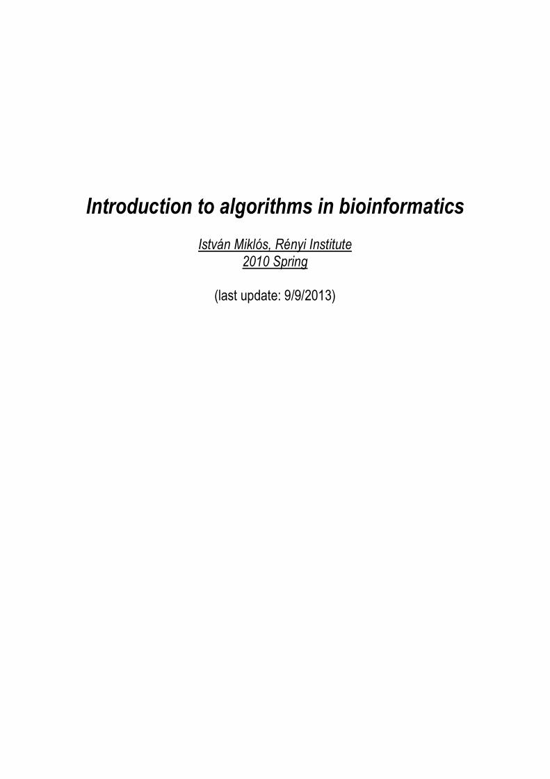
Chapter 1. The history of genome rearrangement 1.1. Discovering genes and genome rearrangement After nine years of laborious work, Gregor Mendel (Fig.1.1.) published his landmark paper on heredity of certain traits in pea plants, and showed that they obeyed some simple statistical rules. He introduced the idea of heredity units, which he called “factors”, called later genes. Mendel stated that each individual has two factors for each trait, one from each parent. The two factors may or may not contain the same information. If the two factors are identical, the individual is called homozygous for the trait. If the two factors have different information, the individual is called heterozygous. The alternative forms of a factor are called alleles. The genotype of an individual is made up of the many alleles it possesses. The physical appearance of an individual, or its phenotype, is determined by its alleles (and also by its environment). An individual possesses two alleles for each trait; one allele is given by the female parent and the other by the male parent. They are passed on when an individual matures and produces gametes: egg and sperm. When gametes form, the paired alleles separate randomly so that each gamete receives a copy of one of the two alleles. The presence of an allele doesn't guarantee that the trait will be expressed in the individual that possesses it. In heterozygous individuals the only allele that is expressed is the dominant. The recessive allele is present but its expression is hidden. Mendel summarized his findings in two laws, the Law of Segregation and the Law of Independent Assortment.

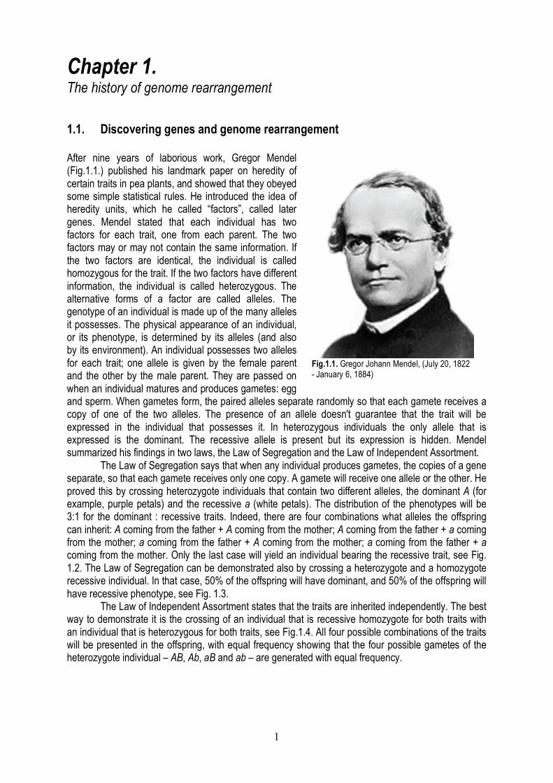
The Law of Segregation says that when any individual produces gametes, the copies of a gene separate, so that each gamete receives only one copy. A gamete will receive one allele or the other. He proved this by crossing heterozygote individuals that contain two different alleles, the dominant A (for example, purple petals) and the recessive a (white petals). The distribution of the phenotypes will be 3:1 for the dominant : recessive traits. Indeed, there are four combinations what alleles the offspring can inherit: A coming from the father + A coming from the mother; A coming from the father + a coming from the mother; a coming from the father + A coming from the mother; a coming from the father + a coming from the mother. Only the last case will yield an individual bearing the recessive trait, see Fig. 1.2. The Law of Segregation can be demonstrated also by crossing a heterozygote and a homozygote recessive individual. In that case, 50% of the offspring will have dominant, and 50% of the offspring will have recessive phenotype, see Fig. 1.3.

The Law of Independent Assortment states that the traits are inherited independently. The best way to demonstrate it is the crossing of an individual that is recessive homozygote for both traits with an individual that is heterozygous for both traits, see Fig.1.4. All four possible combinations of the traits will be presented in the offspring, with equal frequency showing that the four possible gametes of the heterozygote individual – AB, Ab, aB and ab – are generated with equal frequency.

Fig.1.1. Gregor Johann Mendel, (July 20, 1822 - January 6, 1884)

2

Figure 1.2. Crossing two heterozygote individuals yields 75% dominant phenotypes (purple color) and 25% recessive phenotypes (white color).

Figure 1.3. Crossing a heterozygote and a recessive homozygote individual yields 50% dominant and 50% recessive phenotypes.

Figure 1.4. Crossing of an individual that is recessive homozygote for both trait with an individual that is heterozygous for both traits. Here A and a are the genes for rough-smooth traits and B and b are the genes causing green and yellow phenotypes. All four combinations of the pair of phenotypes will be generated with equal probability.

3

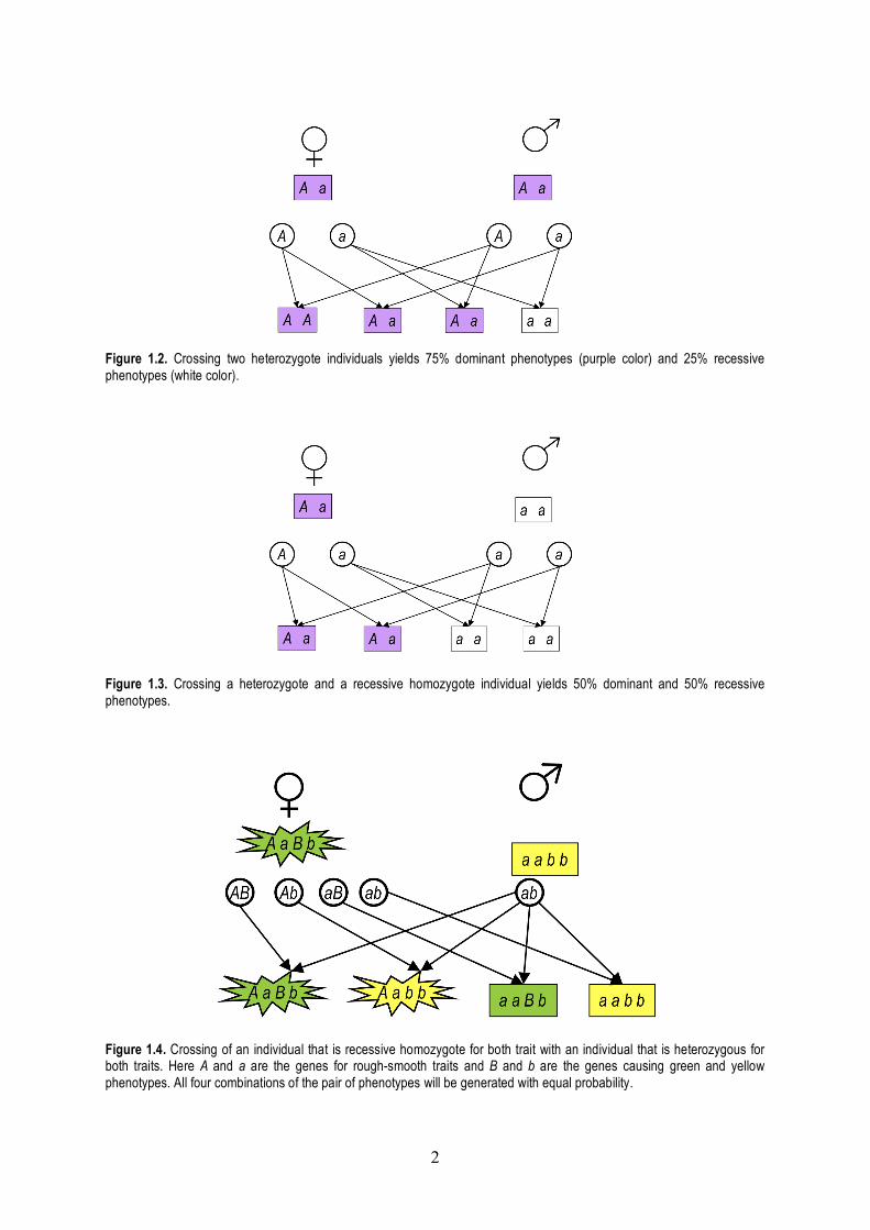
Figure 1.5. Schematic description of meiosis. In the interphase, the 2X number of chromosomes duplicated, thus 4X number of chromosomes will be in a cell. There are so-called recombination events, in which the paternal and maternal chromosomes change genetic material. Then two divisions yields four gametes, each having X number of chromosomes. During these two divisions, paternal and maternal chromosomes segregated randomly. (From Wikipedia) Mendel’s paper was published in a low impact journal, in the Proceedings of the Natural History Society of Brünn, and did not receive too much attention in the next 30 years. Remarkably, Charles Darwin was not aware of this paper. Mendel’s work has been rediscovered only after his death, in 1903, when Walter Sutton set up the hypothesis that chromosomes might be heredity units as they segregate during meiosis (see Fig. 1.5.) in a Mendelian way.

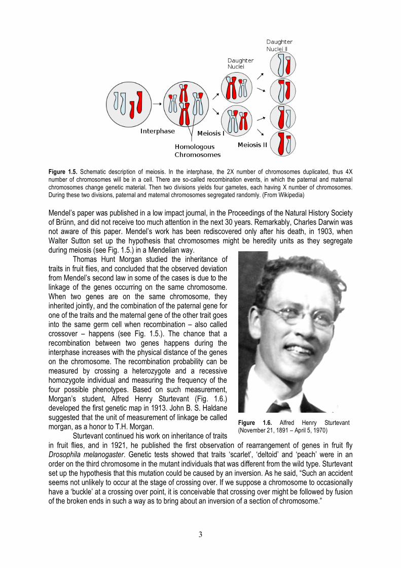
Thomas Hunt Morgan studied the inheritance of traits in fruit flies, and concluded that the observed deviation from Mendel’s second law in some of the cases is due to the linkage of the genes occurring on the same chromosome. When two genes are on the same chromosome, they inherited jointly, and the combination of the paternal gene for one of the traits and the maternal gene of the other trait goes into the same germ cell when recombination – also called crossover – happens (see Fig. 1.5.). The chance that a recombination between two genes happens during the interphase increases with the physical distance of the genes on the chromosome. The recombination probability can be measured by crossing a heterozygote and a recessive homozygote individual and measuring the frequency of the four possible phenotypes. Based on such measurement, Morgan’s student, Alfred Henry Sturtevant (Fig. 1.6.) developed the first genetic map in 1913. John B. S. Haldane suggested that the unit of measurement of linkage be called morgan, as a honor to T.H. Morgan.

Sturtevant continued his work on inheritance of traits in fruit flies, and in 1921, he published the first observation of rearrangement of genes in fruit fly Drosophila melanogaster. Genetic tests showed that traits ‘scarlet’, ‘deltoid’ and ‘peach’ were in an order on the third chromosome in the mutant individuals that was different from the wild type. Sturtevant set up the hypothesis that this mutation could be caused by an inversion. As he said, “Such an accident seems not unlikely to occur at the stage of crossing over. If we suppose a chromosome to occasionally have a ‘buckle’ at a crossing over point, it is conceivable that crossing over might be followed by fusion of the broken ends in such a way as to bring about an inversion of a section of chromosome.”

Figure 1.6. Alfred Henry Sturtevant (November 21, 1891 – April 5, 1970)

4

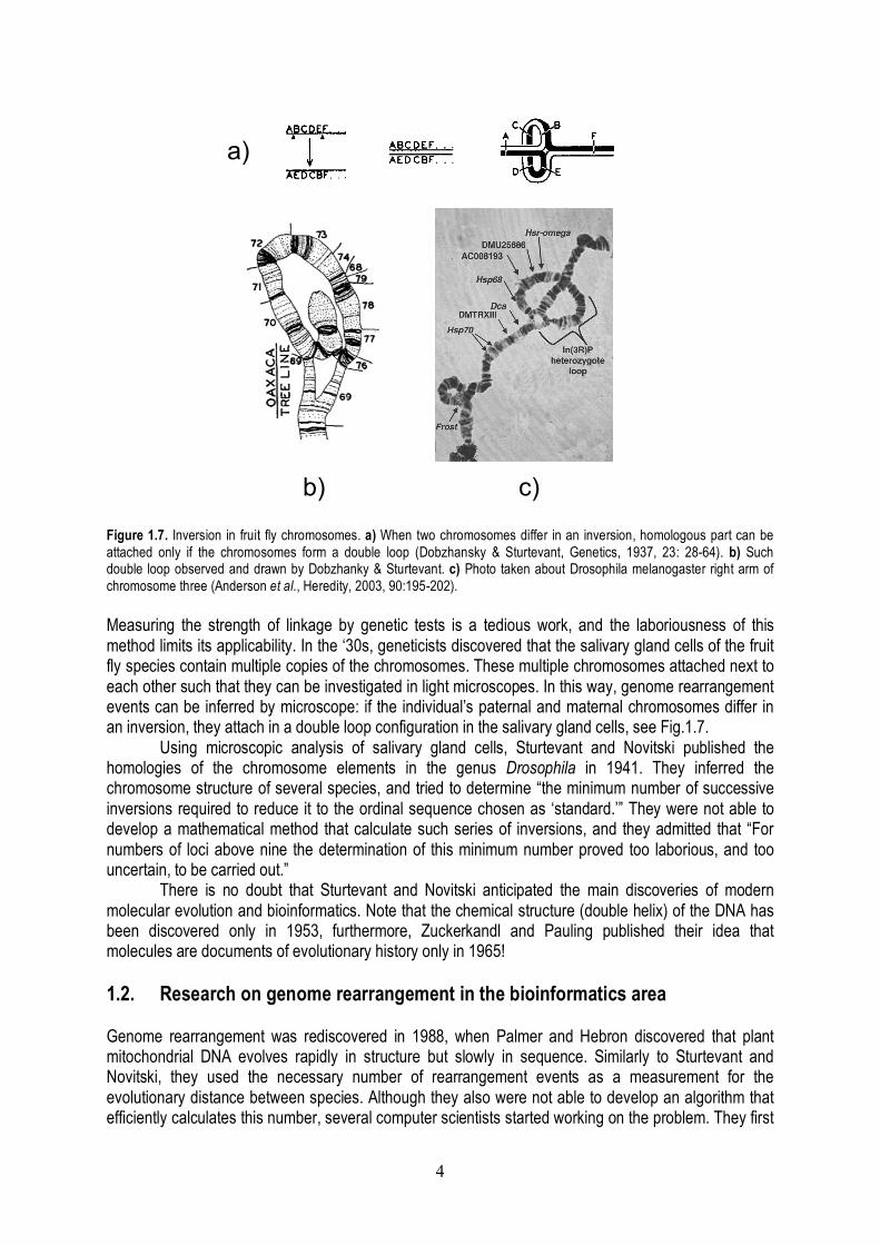
Figure 1.7. Inversion in fruit fly chromosomes. a) When two chromosomes differ in an inversion, homologous part can be attached only if the chromosomes form a double loop (Dobzhansky & Sturtevant, Genetics, 1937, 23: 28-64). b) Such double loop observed and drawn by Dobzhanky & Sturtevant. c) Photo taken about Drosophila melanogaster right arm of chromosome three (Anderson et al., Heredity, 2003, 90:195-202). Measuring the strength of linkage by genetic tests is a tedious work, and the laboriousness of this method limits its applicability. In the ‘30s, geneticists discovered that the salivary gland cells of the fruit fly species contain multiple copies of the chromosomes. These multiple chromosomes attached next to each other such that they can be investigated in light microscopes. In this way, genome rearrangement events can be inferred by microscope: if the individual’s paternal and maternal chromosomes differ in an inversion, they attach in a double loop configuration in the salivary gland cells, see Fig.1.7.

Using microscopic analysis of salivary gland cells, Sturtevant and Novitski published the homologies of the chromosome elements in the genus Drosophila in 1941. They inferred the chromosome structure of several species, and tried to determine “the minimum number of successive inversions required to reduce it to the ordinal sequence chosen as ‘standard.’” They were not able to develop a mathematical method that calculate such series of inversions, and they admitted that “For numbers of loci above nine the determination of this minimum number proved too laborious, and too uncertain, to be carried out.”

There is no doubt that Sturtevant and Novitski anticipated the main discoveries of modern molecular evolution and bioinformatics. Note that the chemical structure (double helix) of the DNA has been discovered only in 1953, furthermore, Zuckerkandl and Pauling published their idea that molecules are documents of evolutionary history only in 1965! 1.2. Research on genome rearrangement in the bioinformatics area Genome rearrangement was rediscovered in 1988, when Palmer and Hebron discovered that plant mitochondrial DNA evolves rapidly in structure but slowly in sequence. Similarly to Sturtevant and Novitski, they used the necessary number of rearrangement events as a measurement for the evolutionary distance between species. Although they also were not able to develop an algorithm that efficiently calculates this number, several computer scientists started working on the problem. They first

a)

b) c)

5

introduced some approximation algorithms that guarantee to find a solution that is not far from the optimal. In 1995, Hannenhalli and Pevzner eventually found the first polynomial algorithm finding the minimum number of inversions necessary to transform one genome into another. From computational point of view, transforming by inversions became the most successful part of the computational theory of genome rearrangement. The algorithm of Hannenhalli and Pevzner that generates a shortest series of inversions transforming one chromosome to another runs in O(n4) running time, where n is the number of loci considered. This has been reduced to

!

O n n log(n)( ) , and if one is interested only the

number of necessary inversions, then an O(n) algorithm is available. Furthermore, it has been proved that the inversion median problem, which asks for the median genome that minimizes the inversion distance from 3 given genomes, is an NP-complete problem. Although it is not proved, it is a widely accepted conjecture that there is no polynomial running time algorithm for any NP-complete problem. In 1996, Hannenhalli published a polynomial running time algorithm for the translocation distance problem that considers reciprocal translocations as result of recombination between non-homologous chromosomes above reversals.

By today, the applications of these algorithms are numerous. Genome rearrangement events not only happen at an evolutionary time scale (ie. in million of years), but also in cancer genomes, causing completely shuffled genomes and thus, malfunction in gene regulations, see Fig. 1.8. In the near future, we will achieve the “1000 dollar genome”, namely, we will be able to sequence a complete human genome for 1000 dollars. Together with other projects aiming to sequence thousands of different species, the amount of available genomic data will be tremendous, providing sufficient amount of work for computer scientists to develop newer and newer algorithms to analyze this data.

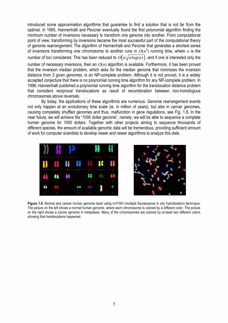
Figure 1.8. Normal and cancer human genome dyed using m-FISH (multiple fluorescence in situ hybridization) technique. The picture on the left shows a normal human genome, where each chromosome is colored by a different color. The picture on the right shows a cancer genome in metastasis. Many of the chromosomes are colored by at least two different colors showing that translocations happened.

6

Chapter 2. Genome rearrangement by double cut & join (DCJ) operations

The first model for genome rearrangement we consider here is sorting by double cut & join operations. This is not the most natural model from the biological point of view, and even not the first model from the historical point of view. However, mathematically it is the simplest to handle, and that is the reason to discuss it at the first place.

We will consider a genome as an ensemble of chromosomes. Chromosomes might be both linear, as the chromosomes of the Drosophyla species, and circular, like the Bacterial chromosomes. We will allow that a genome contain several, different types of chromosomes. This is biologically unrealistic, since Eukaryotes typically have several linear chromosomes, while Archea and Bacteria have only one circular chromosome. Although genomes consisting of a mixture of linear and circular chromosomes are known (for example, Agrobacterium tumefaciens C58, see also http://www.ncbi.nlm.nih.gov/pmc/articles/PMC206964/), this is considered to be rare.

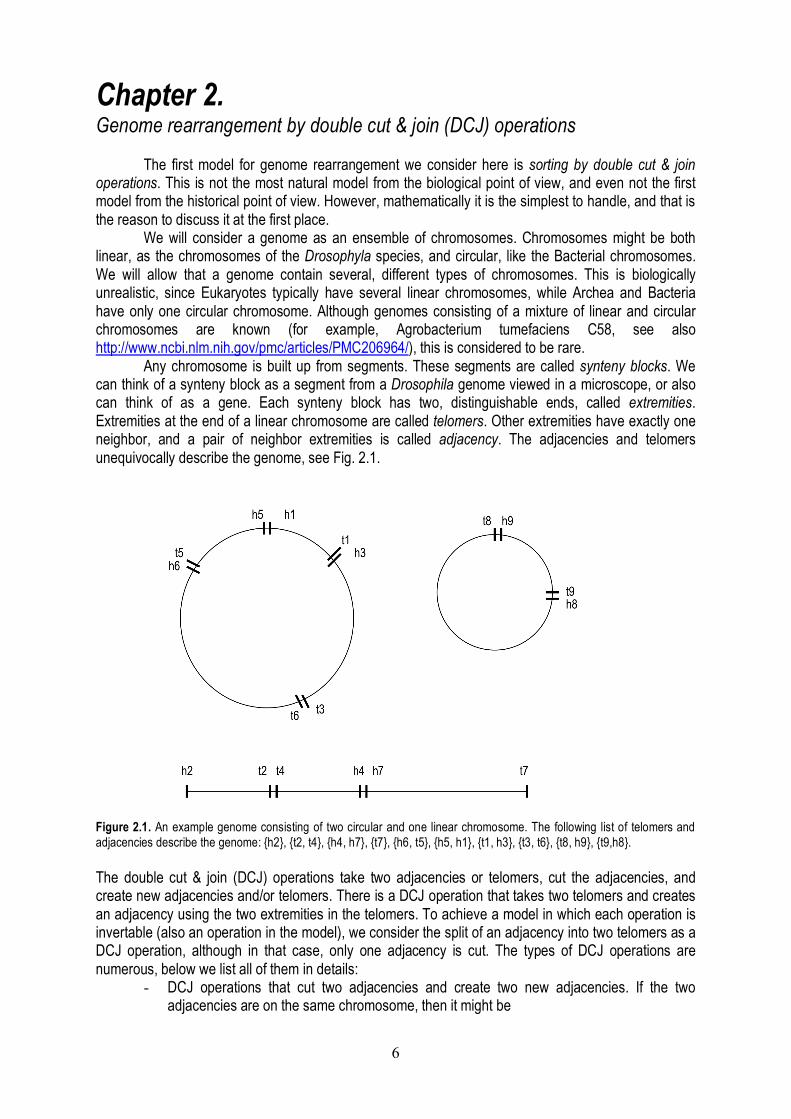
Any chromosome is built up from segments. These segments are called synteny blocks. We can think of a synteny block as a segment from a Drosophila genome viewed in a microscope, or also can think of as a gene. Each synteny block has two, distinguishable ends, called extremities. Extremities at the end of a linear chromosome are called telomers. Other extremities have exactly one neighbor, and a pair of neighbor extremities is called adjacency. The adjacencies and telomers unequivocally describe the genome, see Fig. 2.1.

Figure 2.1. An example genome consisting of two circular and one linear chromosome. The following list of telomers and adjacencies describe the genome: {h2}, {t2, t4}, {h4, h7}, {t7}, {h6, t5}, {h5, h1}, {t1, h3}, {t3, t6}, {t8, h9}, {t9,h8}. The double cut & join (DCJ) operations take two adjacencies or telomers, cut the adjacencies, and create new adjacencies and/or telomers. There is a DCJ operation that takes two telomers and creates an adjacency using the two extremities in the telomers. To achieve a model in which each operation is invertable (also an operation in the model), we consider the split of an adjacency into two telomers as a DCJ operation, although in that case, only one adjacency is cut. The types of DCJ operations are numerous, below we list all of them in details:

- DCJ operations that cut two adjacencies and create two new adjacencies. If the two adjacencies are on the same chromosome, then it might be

7

o An inversion, either on a linear or on a circular chromosome o A fission of a circular chromosome into two circular chromosome o A fission of a linear chromosome into a shorter linear and a circular chromosome

If the two adjacencies are on two chromosomes, then it might be o A fusion of two circular chromosomes o A fusion of a linear and a circular chromosomes o Reciprocal translocation between two linear chromosomes

- DCJ operations that cut an adjacency, take a telomer, and creata a new adjacency and a new telomer. If the adjacency and the telomer is on the same chromosome, then it might be

o A reversal o A fission of a linear chromosome into a shorter linear and a circular chromosome

If the adjacency and the telomer are on two chromosomes, then it might be o A fusion of a linear and a circular chromosome o A translocation

- DCJ operations that create an adjacency from two telomers. o If the two telomers are on the same chromosome than it is a circularization of a

linear chromosome o If the two telomers are on two chromosomes, then it is the fusion of two linear

chromosomes - DCJ operations that cut an adjacency into two telomers

o If the adjacency is on a circular chromosome, then it is a linearization o If the adjacency is on a linear chromosome, then it is the fission of a linear

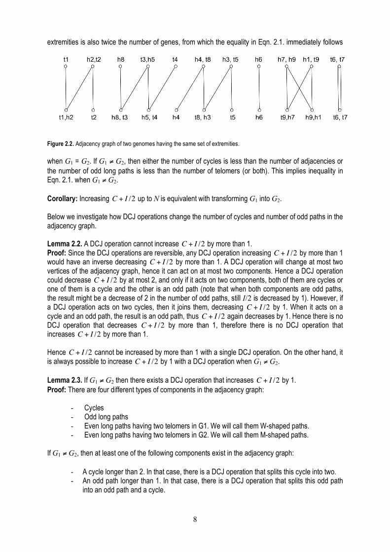
chromosome into two linear chromosomes. Although there are several types of DCJ operations, calculating the minimum number of DCJ operation necessary to transform one genome into another is easy. The following graph is very useful for this. Definition: Let two genomes, G1 and G2 with the same set of extremities be given, described by their adjacencies and telomers. The vertex set of their adjacency graph consists of the adjacencies and telomers of the two genomes. There are k edges between two vertices, if they have k common extremities. Since a telomer has one extremity and an adjacency has two extremities, there are at most two edges between two vertices.

An adjacency graph is a bipartite multigraph, see Fig. 2.2. for an example. The degree of the vertices is either 1 or 2, thus, the graph can be uniquely decomposed into cycles and paths. Since it is a bipartite graph, the length of any cycle is even. On the other hand, paths might be both even and odd.

Assume that we would like to transform G1 into G2. Let C denote the number of cycles in their adjacency graph, let I denote the number of odd paths in their adjacency graph, and let N denote the total number of genes in G1. Lemma 2.1. For any pair of genomes, G1 and G2, with the same set of extremities,

!

N "C +I2

(2.1)

and equality holds if and only if G1 = G2. Proof: If G1 = G2, then the adjacency graph consists of only 2 long cycles and 1 long paths. Moreover, the number of 2 long cycles is the number of adjacencies in one of the genome, and the number of 1-long paths is the number of telomers in one of the genomes. On the other hand, twice the number of adjacencies plus the number of telomers is exactly the number of extremities. The number of

8

extremities is also twice the number of genes, from which the equality in Eqn. 2.1. immediately follows

Figure 2.2. Adjacency graph of two genomes having the same set of extremities. when G1 = G2. If G1 ≠ G2, then either the number of cycles is less than the number of adjacencies or the number of odd long paths is less than the number of telomers (or both). This implies inequality in Eqn. 2.1. when G1 ≠ G2. Corollary: Increasing

!

C + I /2 up to N is equivalent with transforming G1 into G2. Below we investigate how DCJ operations change the number of cycles and number of odd paths in the adjacency graph. Lemma 2.2. A DCJ operation cannot increase

!

C + I /2 by more than 1. Proof: Since the DCJ operations are reversible, any DCJ operation increasing

!

C + I /2 by more than 1 would have an inverse decreasing

!

C + I /2 by more than 1. A DCJ operation will change at most two vertices of the adjacency graph, hence it can act on at most two components. Hence a DCJ operation could decrease

!

C + I /2 by at most 2, and only if it acts on two components, both of them are cycles or one of them is a cycle and the other is an odd path (note that when both components are odd paths, the result might be a decrease of 2 in the number of odd paths, still I/2 is decreased by 1). However, if a DCJ operation acts on two cycles, then it joins them, decreasing

!

C + I /2 by 1. When it acts on a cycle and an odd path, the result is an odd path, thus

!

C + I /2 again decreases by 1. Hence there is no DCJ operation that decreases

!

C + I /2 by more than 1, therefore there is no DCJ operation that increases

!

C + I /2 by more than 1. Hence

!

C + I /2 cannot be increased by more than 1 with a single DCJ operation. On the other hand, it is always possible to increase

!

C + I /2 by 1 with a DCJ operation when G1 ≠ G2. Lemma 2.3. If G1 ≠ G2 then there exists a DCJ operation that increases

!

C + I /2 by 1. Proof: There are four different types of components in the adjacency graph:

- Cycles - Odd long paths - Even long paths having two telomers in G1. We will call them W-shaped paths. - Even long paths having two telomers in G2. We will call them M-shaped paths.

If G1 ≠ G2, then at least one of the following components exist in the adjacency graph:

- A cycle longer than 2. In that case, there is a DCJ operation that splits this cycle into two. - An odd path longer than 1. In that case, there is a DCJ operation that splits this odd path

into an odd path and a cycle.

9

- An M-shaped path. It can be split into two odd paths by splitting an adjacency into two telomers.

- A W-shaped path. Its two telomers can be joined to an adjacency, yielding a cycle. Therefore we can get the following theorem: Theorem 2.1. The minimum number of DCJ operations necessary to transform genome G1 into genome G2 is

!

dDCJ (G1,G2) = N " C +I2

#

$ %

&

' ( (2.2)

Proof: The DCJ distance cannot be less than N - (C + I/2) according to Lemma 2.1. and 2.2. On the other hand, it is possible to transform G1 into G2 in N - (C + I/2) steps, according to Lemma 2.3. Exercises Exercise 2.1. How many linear and circular chromosomes do the two genomes on Fig. 2.2. have?

Exercise 2.2. What is the DCJ distance between the two genomes on on Fig. 2.2.?

Exercise 2.3. Construct a shortest DCJ sorting path between genomes {(t1, h3); (t3, t8); (h8, h1); (t7, h2); (t2, h5); (t5, h7); (h6); (t6, t4); (h4)} and {(t1, t7); (t3) (t8, h6); (h8, h7); (h3, h2); (t2, h5); (t5, h1); (t6, t4); (h4)} .

Exercise 2.4. How many shortest DCJ sorting paths exist between two genomes whose adjacency graph is a single, 8-long cycle?

Exercise 2.5. Write a computer program that reads two genomes given by their list of adjacencies and telomers as input, and calculates their DCJ distance. What is the running time of the algorithm?

Exercise 2.6. Write a computer program that reads two genomes given by their list of adjacencies and telomers as input, and prints a shortest DCJ sorting path transforming one into another. What is the running time of the algorithm?

Exercise 2.7. Characterize the DCJ operations that decrease the DCJ distance.

Exercise 2.8. Show that the number of shortest DCJ sorting paths might grow exponentially with the number of adjacencies and telomers.

Exercise 2.9.** Write a computer program that reads two genomes given by their list of adjacencies and telomers as input, and prints all shortest DCJ sorting path transforming one into another. Note that the running time of this program might be huge, according to the previous exercise. However, it is possible to design a program whose running time between printing two solutions grows only polynomially with the number of adjacencies and telomers.

10

Chapter 3. The Hannenhalli-Pevzner-(Bergeron) theory

The simplicity of the DCJ sorting comes from the fact that we can apply a so-called greedy algorithm: we can choose a DCJ operation that increases

!

C + I /2 by 1, and whatever is our choice, we will find again a DCJ operation that increases

!

C + I /2 by 1, and again and again till we transform one genome into another. Such greedy algorithm does not exist if we restrict the possible operations to the inversions only, hence transforming a genome into another using only inversions need more sophisticated methods, which we introduce in this chapter. The theorem is called the Hannenhalli-Pevzner theory after its developers. The theorem has been simplified since its first publication, most notably by Anne Bergeron.

We consider unichromosomal, linear genomes with the same set of synteny blocks. Such a genome can be described with a signed permutation, defined below. Definition: A signed permutation is such a permutation of numbers from 1 to n, where each number gets a + or - sign. For example, +4, -1, -6, +3, +2, +5 is a signed permutation of numbers from 1 to 6. The representation of unichromosomal linear genomes with signed permutations should be clear: each synteny block is assigned to a number. The sign of the number is the direction of the synteny block. In this chapter, we consider the transformation of unichromosomal linear genomes with inversions. If the unichromosomal linear genome is represented with a signed permutation, the effect of an inversion on the signed permutation is that both the order and the signs of the numbers are reverted in the segment on which the inversion acts. For example, if an inversion acts on the -6, +3, +2 segment of the genome represented by the +4, -1, -6, +3, +2, +5 permutation, then the resulting signed permutation will be +4, -1, -2, -3, +6, +5. Since algebrists have the scientific term ‘inversion’ with a different meaning, from now, inversions are renamed reversals to avoid confusion.

Since the numbering and the orientation of synteny blocks is arbitrary, without loss of generality, we can say that the target genome is +1, +2, ... +n. Hence, instead of transforming signed permutations, we can talk about sorting signed permutations, namely, transforming a signed permutation to the +1, +2, ... +n permutation.

We are interested in the minimum number of reversals necessary to sort a signed permutation. We will call it the reversal distance, and the reversal distance of a signed permutation

!

" will be denoted by

!

dREV (") . We introduce a combinatorial object called the graph of desire and reality, which plays a central role in sorting by reversals. This graph is not the usual graph we consider in graph theory, since the drawing of the graph is also considered. Below we define it. Definition: The graph of desire and reality of a signed permutation is given in the following way. Replace each signed number of the signed permutation with two unsigned numbers, replace +i with 2i-1, 2i, and replace -i with 2i, 2i-1. Frame this unsigned permutation between 0 and 2n+1. For example, +4, -1, -6, +3, +2, +5 will be replaced with 0, 7, 8, 2, 1, 12, 11, 5, 6, 3, 4, 9, 10, 13. Draw a graph whose vertices are the numbers in the unsigned permutation drawn onto a line in the order as they are in the permutation, see Fig. 3.1. Connect every other nodes starting with 0. They are the reality edges, as they show which numbers are next to each other. Connect each 2i, 2i+1 pair with an arc. These are the desire edges, since they tell what are the numbers that should be next to each other to get the +1, +2, ... +n permutation. This graph together with its prescribed drawing is called the graph of desire and reality.

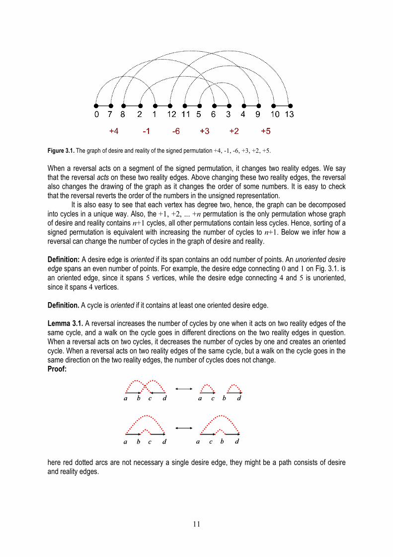
11

Figure 3.1. The graph of desire and reality of the signed permutation +4, -1, -6, +3, +2, +5. When a reversal acts on a segment of the signed permutation, it changes two reality edges. We say that the reversal acts on these two reality edges. Above changing these two reality edges, the reversal also changes the drawing of the graph as it changes the order of some numbers. It is easy to check that the reversal reverts the order of the numbers in the unsigned representation.

It is also easy to see that each vertex has degree two, hence, the graph can be decomposed into cycles in a unique way. Also, the +1, +2, ... +n permutation is the only permutation whose graph of desire and reality contains n+1 cycles, all other permutations contain less cycles. Hence, sorting of a signed permutation is equivalent with increasing the number of cycles to n+1. Below we infer how a reversal can change the number of cycles in the graph of desire and reality. Definition: A desire edge is oriented if its span contains an odd number of points. An unoriented desire edge spans an even number of points. For example, the desire edge connecting 0 and 1 on Fig. 3.1. is an oriented edge, since it spans 5 vertices, while the desire edge connecting 4 and 5 is unoriented, since it spans 4 vertices. Definition. A cycle is oriented if it contains at least one oriented desire edge. Lemma 3.1. A reversal increases the number of cycles by one when it acts on two reality edges of the same cycle, and a walk on the cycle goes in different directions on the two reality edges in question. When a reversal acts on two cycles, it decreases the number of cycles by one and creates an oriented cycle. When a reversal acts on two reality edges of the same cycle, but a walk on the cycle goes in the same direction on the two reality edges, the number of cycles does not change. Proof:

here red dotted arcs are not necessary a single desire edge, they might be a path consists of desire and reality edges.

a b c d

a b c d

a c b d

a c b d

a b c d

a b c d

a c b d

a c b d

12

Corollary:

!

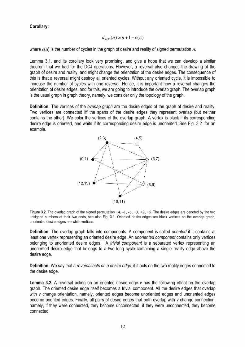
dREV (") # n +1$ c(") where c(π) is the number of cycles in the graph of desire and reality of signed permutation π. Lemma 3.1. and its corollary look very promising, and give a hope that we can develop a similar theorem that we had for the DCJ operations. However, a reversal also changes the drawing of the graph of desire and reality, and might change the orientation of the desire edges. The consequence of this is that a reversal might destroy all oriented cycles. Without any oriented cycle, it is impossible to increase the number of cycles with one reversal. Hence, it is important how a reversal changes the orientation of desire edges, and for this, we are going to introduce the overlap graph. The overlap graph is the usual graph in graph theory, namely, we consider only the topology of the graph. Definition: The vertices of the overlap graph are the desire edges of the graph of desire and reality. Two vertices are connected iff the spans of the desire edges they represent overlap (but neither contains the other). We color the vertices of the overlap graph. A vertex is black if its corresponding desire edge is oriented, and white if its corresponding desire edge is unoriented. See Fig. 3.2. for an example.

Figure 3.2. The overlap graph of the signed permutation +4, -1, -6, +3, +2, +5. The desire edges are denoted by the two unsigned numbers at their two ends, see also Fig. 3.1. Oriented desire edges are black vertices on the overlap graph, unoriented desire edges are white vertices. Definition: The overlap graph falls into components. A component is called oriented if it contains at least one vertex representing an oriented desire edge. An unoriented component contains only vertices belonging to unoriented desire edges. A trivial component is a separated vertex representing an unoriented desire edge that belongs to a two long cycle containing a single reality edge above the desire edge. Definition: We say that a reversal acts on a desire edge, if it acts on the two reality edges connected to the desire edge. Lemma 3.2. A reversal acting on an oriented desire edge v has the following effect on the overlap graph. The oriented desire edge itself becomes a trivial component. All the desire edges that overlap with v change orientation, namely, oriented edges become unoriented edges and unoriented edges become oriented edges. Finally, all pairs of desire edges that both overlap with v change connection, namely, if they were connected, they become unconnected, if they were unconnected, they become connected.

13

Proof: It is obvious that the oriented desire edge becomes a trivial component: since it is an oriented edge, the desire meets the reality after the reversal

A reversal overlapping with a desire edge changes the position of one of the reality edge – desire edge connections, hence change the orientation of the desire edge

Finally, since the order of desire edge ends are reversed, the connections of these edges will change:

Lemma 3.3. Any oriented component contains at least one oriented edge such that the reversal acting on it increases the number of cycles and does not create a non-trivial unoriented component. Proof: From Lemma 3.1., any reversal acting on an oriented desire edge increases the number of cycles, hence all we have to prove is that there is one such reversal that does not create a non-trivial unoriented component.

We choose the oriented edge v for which |U|-|O| is maximal, where U is the set of unoriented edges that v overlaps with, and O is the set of oriented edges that v overlaps with. We claim that the reversal acting on it does not create a non-trivial unoriented component: if it creates an unoriented component, it will be a trivial one.

Indeed, if the reversal makes an unoriented component, it contains an unoriented edge w. Before the reversal, w was connected to v, and hence it was an oriented edge. Let U’ and O’ be the sets of unoriented and oriented edges with which w overlapped before applying the reversal acting on v. All unoriented vertices that was connected to v had to be connected with w, too, otherwise they would be connected to w after the reversal, and become an oriented component (according to Lemma 2.), contradicting that w is an edge in an unoriented component after the reversal. Hence U’ ⊇U.

All oriented vertices that overlapped with w before the reversal had to be overlapped with v, too, otherwise they would remain oriented and connected to w, contradicting that w is part of an unoriented component. Hence O’ ⊆ O.

Since we chose a v for which |U|-|O| was maximal, U’ = U and O’ = O, otherwise |U’|-|O’| would be greater than |U|-|O|. Therefore w becomes a trivial unoriented component after the reversal, according to Lemma 3.2.

14

Lemma 3.4. It is only the identity permutation whose overlap graph is the empty, all-white overlap graph. Proof: The graph of desire and reality of the identity permutation consists of n+1 trivial cycles. Its overlap graph is indeed the empty, all-white graph. All we have to prove is that any unoriented desire edge that is not in the trivial cycle is crossed by another desire edge. This desire edge connects 2i with 2i+1, so it either does not contain 0 or does not contain 2n+1 as endpoint. If an unoriented desire edge is not in the trivial cycle, then its span contains at least 2 further vertices above its two vertices. Indeed, neighbor vertices that are not connected by reality edge are 2i and 2i-1, but 2i is connected with 2i+1 with a desire edge. Furthermore, the desire edge is unoriented, hence the number of vertices in its span is even. One of these further vertices is an even number, say 2k, then it is connected with 2k+1. If 2k+1 is outside of the span of the desire edge in question, then the desire edge (2k, 2k+1) crosses it. If 2k+1 is inside the span, then 2k+2 is too. This is connected with 2k+3, if this is outside, we have a cross, otherwise 2k+4 is also inside, etc. In this way, we can go up to 2n+1. The other vertex, 2k-1 is connected with 2k-2. Along this way, we can go down till 0, similarly to the 2n+1 case. Hence, at least in one of the direction, we have to cross the desire edge. Theorem 3.1. For a permutation π whose overlap graph does not contain a non-trivial unoriented component,

!

dREV (") = n +1# c(")

Proof: From the corollary of Lemma 3.1, we already know that

!

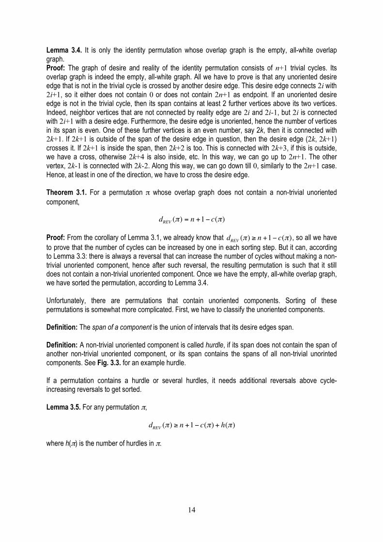
dREV (") # n +1$ c("), so all we have to prove that the number of cycles can be increased by one in each sorting step. But it can, according to Lemma 3.3: there is always a reversal that can increase the number of cycles without making a non-trivial unoriented component, hence after such reversal, the resulting permutation is such that it still does not contain a non-trivial unoriented component. Once we have the empty, all-white overlap graph, we have sorted the permutation, according to Lemma 3.4. Unfortunately, there are permutations that contain unoriented components. Sorting of these permutations is somewhat more complicated. First, we have to classify the unoriented components. Definition: The span of a component is the union of intervals that its desire edges span. Definition: A non-trivial unoriented component is called hurdle, if its span does not contain the span of another non-trivial unoriented component, or its span contains the spans of all non-trivial unorinted components. See Fig. 3.3. for an example hurdle. If a permutation contains a hurdle or several hurdles, it needs additional reversals above cycle-increasing reversals to get sorted. Lemma 3.5. For any permutation π,

!

dREV (") # n +1$ c(") + h(") where h(π) is the number of hurdles in π.

15

Figure 3.3. In this graph of desire and reality, the cycle containing vertices 11, 4, 3, 10, 5, 2 is a hurdle. Proof: We are going to prove that it is impossible to change Δ(c(π) – h(π)) more than 1 with a single reversal. Indeed, if a reversal acts on a hurdle, it might decrease h(π) by 1, but then it cannot increase the number of cycles, according to Lemma 1. If it acts on two hurdles, then it can decrease h(π) by 2, but then it acts on two different cycles, and hence it decreases the number of cycles by 1. Due to the definition of hurdles, the span of a reversal cannot overlap with more than two hurdles, hence cannot decrease the number of hurdles by more than 2. The following two definitions and lemmas show how the hurdles can be eliminated: Definition: A hurdle-cut is a reversal that creates an oriented component from a hurdle. Definition: A hurdle-merge is a reversal that makes a single oriented component from two hurdles. Lemma 3.6. For each hurdle there exist at least on hurdle-cut. Proof: We prove that the reversal acting on the leftmost desire edge of the hurdle is a hurdle-cut. This leftmost desire edge must intersect with at least one more desire edge, see the proof of Lemma 3.4. This desire edge becomes oriented and it will remain connected with the leftmost desire edge. Hence the component will remain a single one, and becomes oriented. Lemma 3.7. For each pair of hurdles, there exist at least one hurdle-merge. Proof: We prove that the reversal that acts on the rightmost reality edge of the left hurdle and the leftmost reality edge of the right hurdle is a hurdle merge. Indeed, such a reversal connects the rightmost desire edge of the left hurdle with the leftmost desire edge of the right hurdle, and above that it does not change the connectivity of desire edges of the two hurdles. (It might make other desire edges not belonging to the two hurdles connected to desire edges of the two hurdles). What follows is that the two hurdles become a single component. According to Lemma 3.1., it will be an oriented component. So we can always cut and merge hurdles. However, cutting or merging a hurdle might transform a non-hurdle unoriented component into a hurdle! We need two further definitions before we can state the main theorem. Definition: A hurdle is called super-hurdle, if either

- its span does not contain the span of another non-trivial unoriented component, and there is another unoriented component whose span contains the span of the hurdle, but does not contain the span of another non-trivial unoriented component or

- its span contains the span of all non-trivial unoriented components, and there exist another unoriented component whose span contains the span of all non-trivial components, except the span of the hurdle in question.

16

Definition: A permutation is called fortress if all of its hurdles are super-hurdles and their number is odd. Theorem 3.2. (Hannenhalli-Pevzner): For any permutation π,

!

dREV (") = n +1# c(") + h(") + f (")

where h(π) is the number of hurdles in π, and f(π) is 1 if π is a fortress, otherwise 0. Proof: We first prove that it is impossible to increase Δ(c(π) – h(π) – f(π)) by more than 1, then we prove that increasing by one is always possible.

If the permutation is not a fortress, we already proved in Lemma 3.5. that it is impossible to increase Δ(c(π) – h(π) – f(π)) by more than 1.

If a permutation is a fortress, then all of its hurdles are super-hurdles and their number is an odd number. The two possible ways to destroy a fortress is

a) transform one of its super-hurdles into a regular hurdle b) change the number of hurdles. Their number might be

I. decreased II. increased

In case a), we have to cut the hurdle or we have to transform the non-hurdle unoriented component that makes the hurdle a super-hurdle into an oriented component. In both cases, the reversal should act on an unoriented component, and hence, the number of cycles cannot be increased, according to Lemma 3.1.

In case b)I., the number of hurdles cannot be decreased without decreasing the number of cycles. Indeed, a single hurdle-cut will not work, as it makes the non-hurdle unoriented component above or below the super-hurdle a hurdle. Hence, the reversal must act on two cycles, and hence it decreases the number of cycles. When the number of hurdles is decreased by two, it does not destroy the fortress as the number of superhurdles remain an odd number, except when the number of superhurdles is 3.

In case of b)II., Δ(– h(π) – f(π)) ≤ 0, and hence the total change might be at most 1 when the number of cycles is increased by 1.

Hence so far we proved that

!

d(" ) # n+1$ c(" )+ h(" )+ f (" ). Now we are going to prove that Δ(c(π) – h(π) – f(π)) can always be increased by 1.

If the permutation is a fortress, merge the first and the third super-hurdle. We claim that it will decrease the number of hurdles by two, if there are more than 3 super-hurdles. Indeed, the second superhurdle remain a superhurdle, as well as the further superhurdles remain superhurdles, thus we do not create a new hurdle from an unoriented non-hurdle. When the number of superhurdles are 3 in the fortress, then merging the first and the third superhurdle destroys the fortress and decreases the number of hurdles by 1. In all cases, the number of cycles is decreased by 1, and hence Δ(c(π) – h(π) – f(π)) increased by 1. Hence eventually we destroy the fortress, and then we are going to prove that Δ(c(π) – h(π)) can always be increased by 1 without creating a fortress, if the permutation is not a fortress.

If the number of hurdles is an odd number in a permutation that is not a fortress, then there must be at least a single hurdle. Cutting this hurdle decreases the number of hurdles by 1, without changing the number of cycles. Once we have an even number of hurdles, when their number are more than 2, we can merge the first and the third hurdles without creating a new hurdle. In this way, we can decrease the number of hurdles by 2, while we decrease the number of cycles by 1. Moreover, the number of hurdles will remain an even number. When the number of hurdles is 2, we can merge them,

17

thus creating a permutation with only oriented and trivial unoriented components. This remaining permutation can be sorted as described in Theorem 3.1. Exercises Exercise 3.1. Prove that the overlap graph cannot contain a separated black vertex. Exercise 3.2. What is the smallest hurdle? Exercise 3.3. What is the smallest number of hurdles that a fortress might contain? Exercise 3.4. How long is the smallest fortrest? Exercise 3.5. How many shortest reversal sorting paths does the permutation -1, -2, -3, -4 have? Exercise 3.6.* Write a computer program that calculates the reversal distance. (There is a sophisticated algorithm that calculates the reversal distance in linear time, however, here any solution with polynomial running time is accepted.) Exercise 3.7.** Write a computer program that generates a shortest reversal sorting scenario for a signed permutation (The state-of-the-art is an

!

O n n log(n)( ) algorithm that works for any

permutation, and also an

!

O(n logn) algorithm exist for almost all permutations, however, here any polynomial solution is accepted.) Exercise 3.8. Prove that the number of shortest reversal sorting scenarios might grow exponentially with the length of the permutation. Exercise 3.9. Prove that there are black and white graphs which are not overlap graphs. Exercise 3.10.* Prove that any black and white graph can be transformed into an empty, all-white graph by pressing black vertices. The effect of pressing a black vertex is that all of its neighbors change color, all of its pairs of neighbors change connectivity, and the black vertex become a separated white vertex. Exercise 3.11.** A pressing path of a black and white graph is a series of black vertex pressings that yield an all-white, empty graph. Prove that any pressing path for a particular black and white graph has the same length.

18

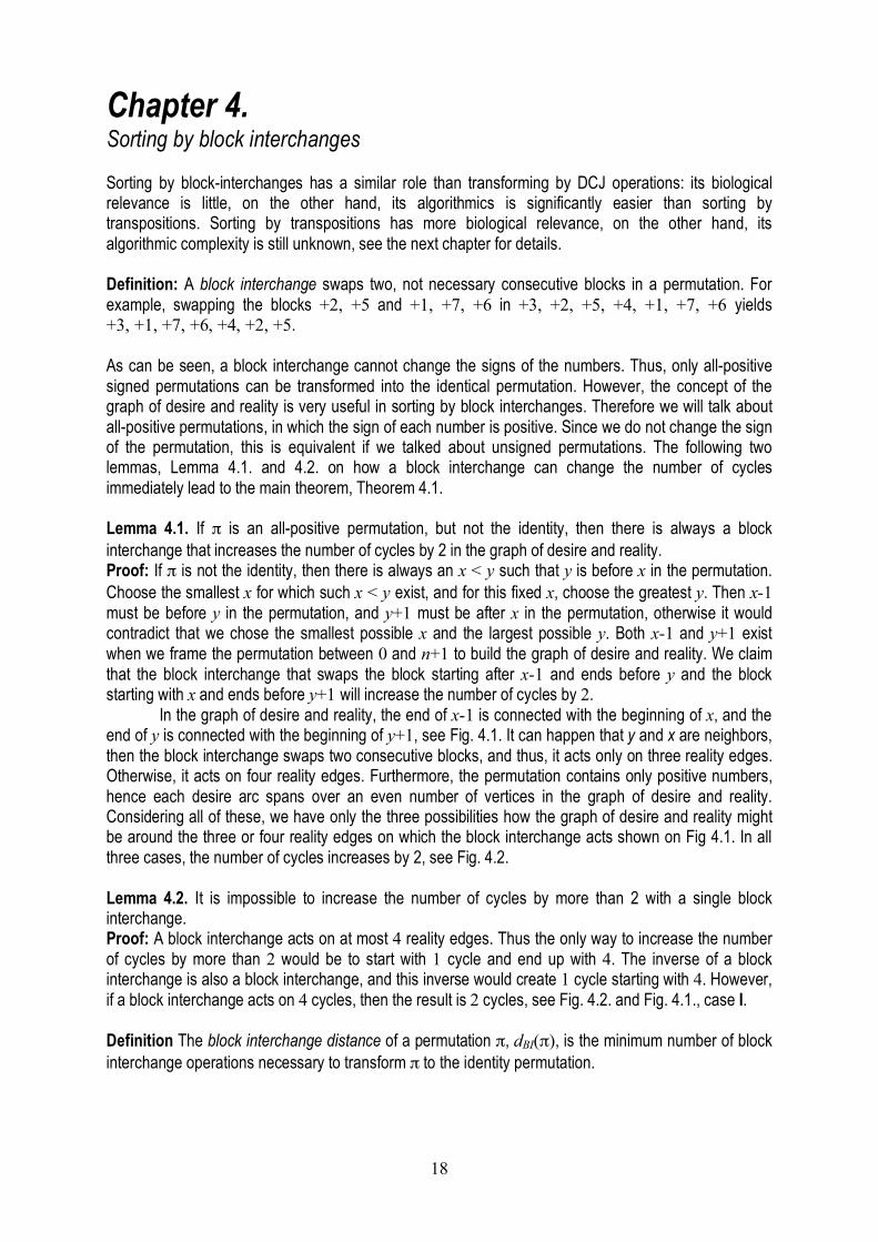
Chapter 4. Sorting by block interchanges Sorting by block-interchanges has a similar role than transforming by DCJ operations: its biological relevance is little, on the other hand, its algorithmics is significantly easier than sorting by transpositions. Sorting by transpositions has more biological relevance, on the other hand, its algorithmic complexity is still unknown, see the next chapter for details. Definition: A block interchange swaps two, not necessary consecutive blocks in a permutation. For example, swapping the blocks +2, +5 and +1, +7, +6 in +3, +2, +5, +4, +1, +7, +6 yields +3, +1, +7, +6, +4, +2, +5. As can be seen, a block interchange cannot change the signs of the numbers. Thus, only all-positive signed permutations can be transformed into the identical permutation. However, the concept of the graph of desire and reality is very useful in sorting by block interchanges. Therefore we will talk about all-positive permutations, in which the sign of each number is positive. Since we do not change the sign of the permutation, this is equivalent if we talked about unsigned permutations. The following two lemmas, Lemma 4.1. and 4.2. on how a block interchange can change the number of cycles immediately lead to the main theorem, Theorem 4.1. Lemma 4.1. If π is an all-positive permutation, but not the identity, then there is always a block interchange that increases the number of cycles by 2 in the graph of desire and reality. Proof: If π is not the identity, then there is always an x < y such that y is before x in the permutation. Choose the smallest x for which such x < y exist, and for this fixed x, choose the greatest y. Then x-1 must be before y in the permutation, and y+1 must be after x in the permutation, otherwise it would contradict that we chose the smallest possible x and the largest possible y. Both x-1 and y+1 exist when we frame the permutation between 0 and n+1 to build the graph of desire and reality. We claim that the block interchange that swaps the block starting after x-1 and ends before y and the block starting with x and ends before y+1 will increase the number of cycles by 2.

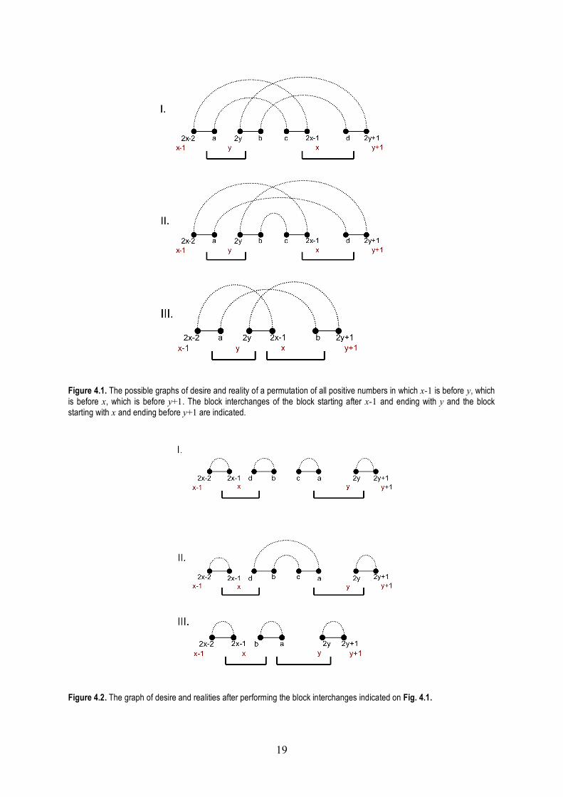
In the graph of desire and reality, the end of x-1 is connected with the beginning of x, and the end of y is connected with the beginning of y+1, see Fig. 4.1. It can happen that y and x are neighbors, then the block interchange swaps two consecutive blocks, and thus, it acts only on three reality edges. Otherwise, it acts on four reality edges. Furthermore, the permutation contains only positive numbers, hence each desire arc spans over an even number of vertices in the graph of desire and reality. Considering all of these, we have only the three possibilities how the graph of desire and reality might be around the three or four reality edges on which the block interchange acts shown on Fig 4.1. In all three cases, the number of cycles increases by 2, see Fig. 4.2. Lemma 4.2. It is impossible to increase the number of cycles by more than 2 with a single block interchange. Proof: A block interchange acts on at most 4 reality edges. Thus the only way to increase the number of cycles by more than 2 would be to start with 1 cycle and end up with 4. The inverse of a block interchange is also a block interchange, and this inverse would create 1 cycle starting with 4. However, if a block interchange acts on 4 cycles, then the result is 2 cycles, see Fig. 4.2. and Fig. 4.1., case I. Definition The block interchange distance of a permutation π, dBI(π), is the minimum number of block interchange operations necessary to transform π to the identity permutation.

19

Figure 4.1. The possible graphs of desire and reality of a permutation of all positive numbers in which x-1 is before y, which is before x, which is before y+1. The block interchanges of the block starting after x-1 and ending with y and the block starting with x and ending before y+1 are indicated.

Figure 4.2. The graph of desire and realities after performing the block interchanges indicated on Fig. 4.1.

20

Theorem 4.1. For any permutation π,

!

dBI (") =n +1# c(")

2

where n is the length of the permutation, and c(π) is the number of cycles in the graph of desire and reality. Proof: Only the identity permutation contains n+1 cycles, hence sorting is equivalent with increasing the number of cycles to n+1. Lemma 4.2. says that the block interchange distance is at least

!

n +1" c(#)( ) /2 . By Lemma 4.1., the block interchange distance is at most

!

n +1" c(#)( ) /2 , thus it is exactly

!

n +1" c(#)( ) /2 . Exercises Exercise 4.1. Prove that the block interchange distance can be calculated in O(n) time. Exercise 4.2. Write a program that reads a permutation and calculate its block interchange distance. Exercise 4.3. Prove that a shortest block interchange sorting scenario can be given in O(n2) time. Exercise 4.4. Write a program that reads a permutation and outputs a shortest block interchange sorting scenario. Exercise 4.5.** Write a computer program that generates all shortest block interchange sorting scenarios. Exercise 4.6. Prove that the number of shortest block interchange sorting scenarios might grow exponentially with the length of the permutation. Exercise 4.7. What is the greatest possible block interchange distance for an n long permutation? Exercise 4.8. Prove that there is no 7 long permutation for which the graph of desire and reality contains a single cycle. Exercise 4.9. Prove that there is no block interchange operation that changes the number of cycles by 1.

21

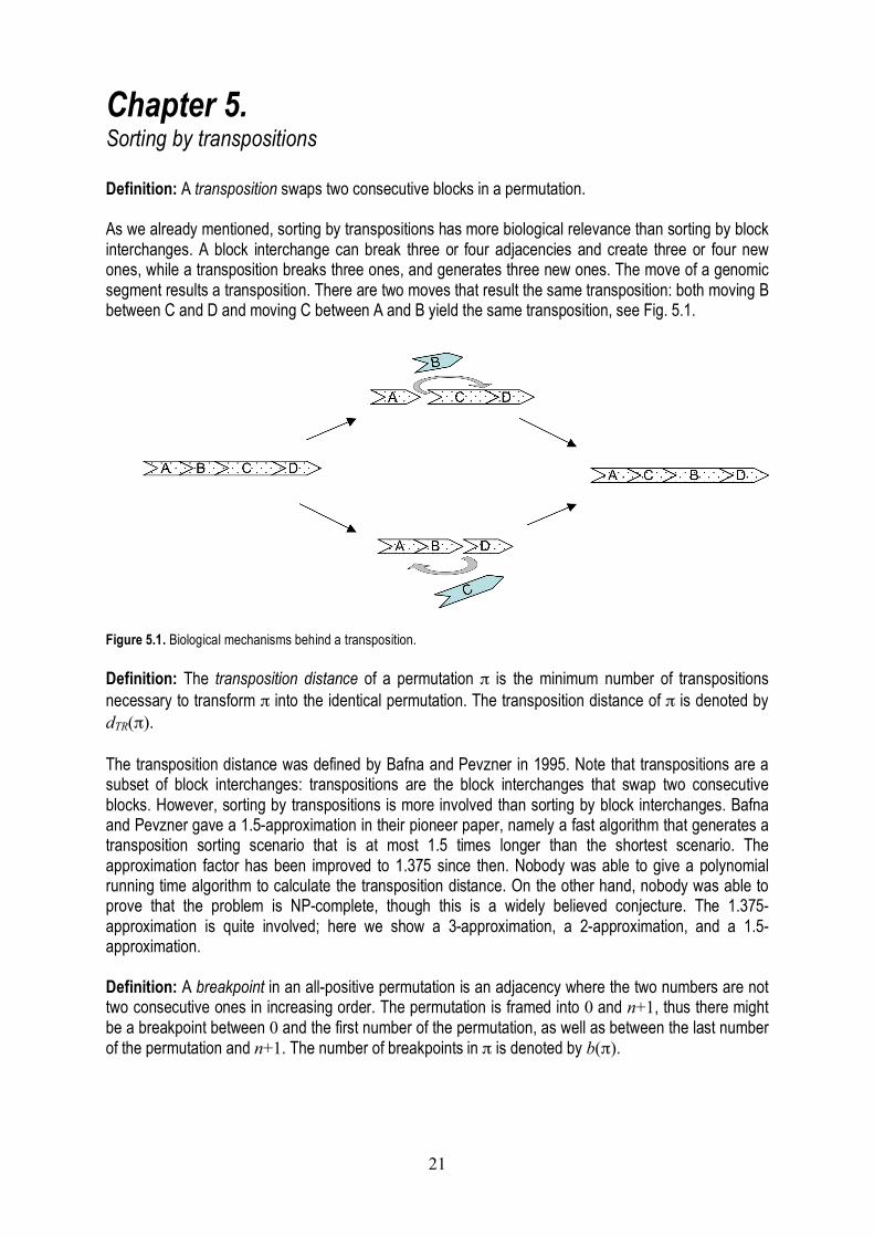
Chapter 5. Sorting by transpositions Definition: A transposition swaps two consecutive blocks in a permutation. As we already mentioned, sorting by transpositions has more biological relevance than sorting by block interchanges. A block interchange can break three or four adjacencies and create three or four new ones, while a transposition breaks three ones, and generates three new ones. The move of a genomic segment results a transposition. There are two moves that result the same transposition: both moving B between C and D and moving C between A and B yield the same transposition, see Fig. 5.1.

Figure 5.1. Biological mechanisms behind a transposition. Definition: The transposition distance of a permutation π is the minimum number of transpositions necessary to transform π into the identical permutation. The transposition distance of π is denoted by dTR(π). The transposition distance was defined by Bafna and Pevzner in 1995. Note that transpositions are a subset of block interchanges: transpositions are the block interchanges that swap two consecutive blocks. However, sorting by transpositions is more involved than sorting by block interchanges. Bafna and Pevzner gave a 1.5-approximation in their pioneer paper, namely a fast algorithm that generates a transposition sorting scenario that is at most 1.5 times longer than the shortest scenario. The approximation factor has been improved to 1.375 since then. Nobody was able to give a polynomial running time algorithm to calculate the transposition distance. On the other hand, nobody was able to prove that the problem is NP-complete, though this is a widely believed conjecture. The 1.375-approximation is quite involved; here we show a 3-approximation, a 2-approximation, and a 1.5-approximation. Definition: A breakpoint in an all-positive permutation is an adjacency where the two numbers are not two consecutive ones in increasing order. The permutation is framed into 0 and n+1, thus there might be a breakpoint between 0 and the first number of the permutation, as well as between the last number of the permutation and n+1. The number of breakpoints in π is denoted by b(π).

22

Theorem 5.1. For any all-positive permutation π,

!

b(")3

# dTR (") # b(")

Proof: Only the identity permutation contains 0 breakpoint: if a permutation does not contain a breakpoint, then 0 must be followed by 1, 1 must be followed by 2, etc., n must be followed by n+1, thus the permutation is the identical permutation. Hence, sorting a permutation is equivalent with decreasing the number of breakpoints to 0. A transposition changes three adjacencies, hence the number of breakpoints cannot be decreased by more than 3 with a single transposition. Therefore

!

b(")3

# dTR (")

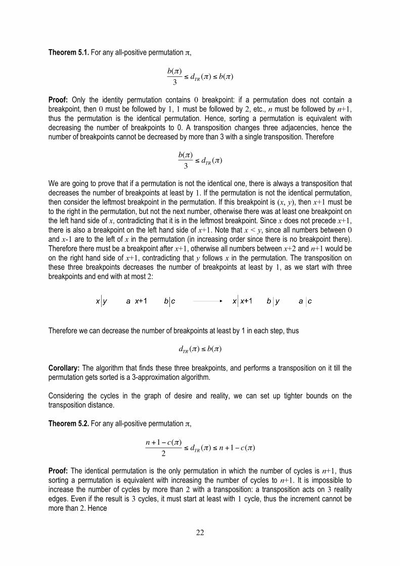
We are going to prove that if a permutation is not the identical one, there is always a transposition that decreases the number of breakpoints at least by 1. If the permutation is not the identical permutation, then consider the leftmost breakpoint in the permutation. If this breakpoint is (x, y), then x+1 must be to the right in the permutation, but not the next number, otherwise there was at least one breakpoint on the left hand side of x, contradicting that it is in the leftmost breakpoint. Since x does not precede x+1, there is also a breakpoint on the left hand side of x+1. Note that x < y, since all numbers between 0 and x-1 are to the left of x in the permutation (in increasing order since there is no breakpoint there). Therefore there must be a breakpoint after x+1, otherwise all numbers between x+2 and n+1 would be on the right hand side of x+1, contradicting that y follows x in the permutation. The transposition on these three breakpoints decreases the number of breakpoints at least by 1, as we start with three breakpoints and end with at most 2:

Therefore we can decrease the number of breakpoints at least by 1 in each step, thus

!

dTR (") # b(") Corollary: The algorithm that finds these three breakpoints, and performs a transposition on it till the permutation gets sorted is a 3-approximation algorithm. Considering the cycles in the graph of desire and reality, we can set up tighter bounds on the transposition distance. Theorem 5.2. For any all-positive permutation π,

!

n +1" c(#)2

$ dTR (#) $ n +1" c(#)

Proof: The identical permutation is the only permutation in which the number of cycles is n+1, thus sorting a permutation is equivalent with increasing the number of cycles to n+1. It is impossible to increase the number of cycles by more than 2 with a transposition: a transposition acts on 3 reality edges. Even if the result is 3 cycles, it must start at least with 1 cycle, thus the increment cannot be more than 2. Hence

23

!

n +1" c(#)2

$ dTR (#)

On the other hand, any block interchange can be mimicked by at most two transpositions. Therefore the transposition distance cannot be more than twice the block interchange distance, and hence

!

dTR (") # n +1$ c(") According to this, if a transposition sorting path mimics a shortest block interchange path, then at least every second step increases the number of cycles by 2. Therefore the following corollary exists: Corollary: In any all-positive permutation which is not the identity, there is a transposition that increases the number of cycles by two, or there is a transposition that does not change the number of cycles and can be followed with a transposition that increases the number of cycles by 2. Therefore any algorithm that finds a transposition sorting path mimicking a block interchange sorting path is a 2-approximation algorithm. To get a better approximation for sorting by transpositions, we need a more careful analysis. Any transposition does not change the total length of the cycles, and hence, it does not change the total length of cycles by modulo 2. Therefore, a transposition can change the number of odd cycles only by +2, 0 and -2. Since the identity permutation contains n+1 odd cycles, the following lemma is true: Lemma 5.1. For any all-positive permutation π,

!

n +1" codd (#)2

$ dTR (#)

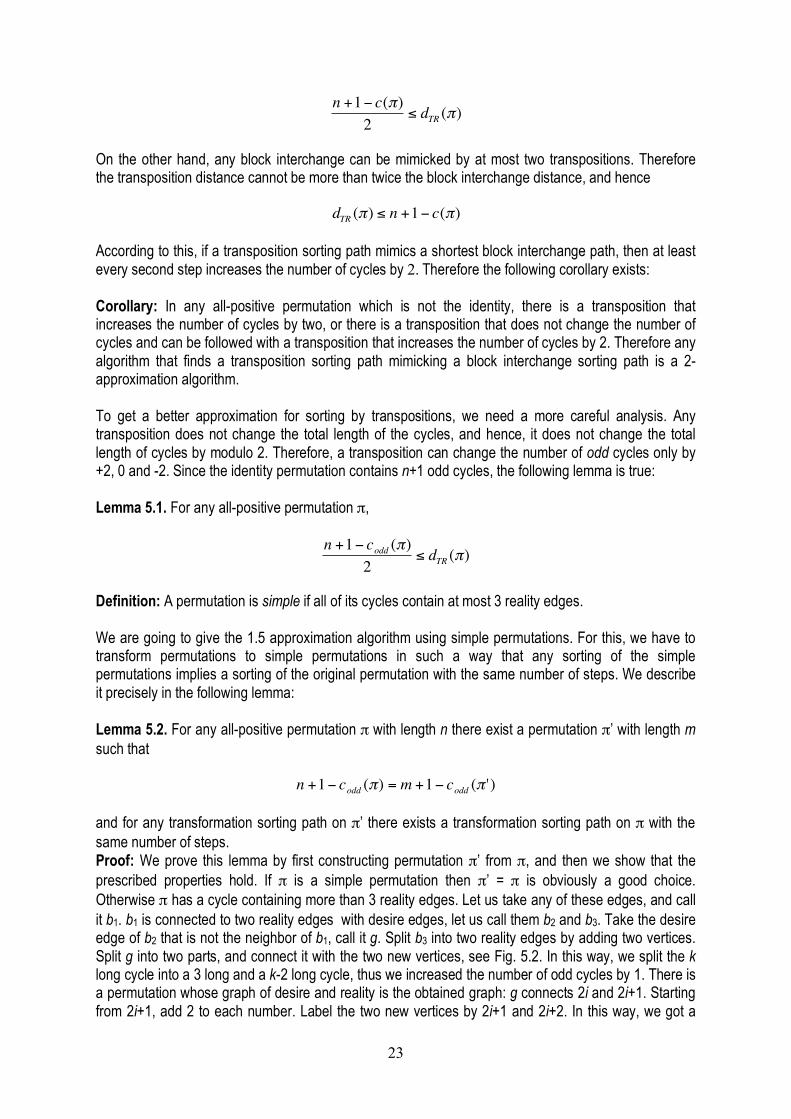
Definition: A permutation is simple if all of its cycles contain at most 3 reality edges. We are going to give the 1.5 approximation algorithm using simple permutations. For this, we have to transform permutations to simple permutations in such a way that any sorting of the simple permutations implies a sorting of the original permutation with the same number of steps. We describe it precisely in the following lemma: Lemma 5.2. For any all-positive permutation π with length n there exist a permutation π’ with length m such that

!

n +1" codd (#) = m +1" codd (# ') and for any transformation sorting path on π’ there exists a transformation sorting path on π with the same number of steps. Proof: We prove this lemma by first constructing permutation π’ from π, and then we show that the prescribed properties hold. If π is a simple permutation then π’ = π is obviously a good choice. Otherwise π has a cycle containing more than 3 reality edges. Let us take any of these edges, and call it b1. b1 is connected to two reality edges with desire edges, let us call them b2 and b3. Take the desire edge of b2 that is not the neighbor of b1, call it g. Split b3 into two reality edges by adding two vertices. Split g into two parts, and connect it with the two new vertices, see Fig. 5.2. In this way, we split the k long cycle into a 3 long and a k-2 long cycle, thus we increased the number of odd cycles by 1. There is a permutation whose graph of desire and reality is the obtained graph: g connects 2i and 2i+1. Starting from 2i+1, add 2 to each number. Label the two new vertices by 2i+1 and 2i+2. In this way, we got a

24

new permutation whose graph of desire and reality is exactly the obtained one. It is easy to prove that any sorting of the so-obtained permutation indicates a sorting of π. If the so-obtained permutation is simple, then let π’ be this permutation. Otherwise, iterate the split process till we get a simple permutation, and let π’ be that.

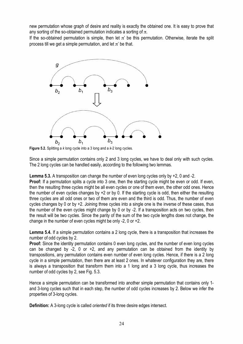
Figure 5.2. Splitting a k long cycle into a 3 long and a k-2 long cycles. Since a simple permutation contains only 2 and 3 long cycles, we have to deal only with such cycles. The 2 long cycles can be handled easily, according to the following two lemmas. Lemma 5.3. A transposition can change the number of even long cycles only by +2, 0 and -2. Proof: If a permutation splits a cycle into 3 one, then the starting cycle might be even or odd. If even, then the resulting three cycles might be all even cycles or one of them even, the other odd ones. Hence the number of even cycles changes by +2 or by 0. If the starting cycle is odd, then either the resulting three cycles are all odd ones or two of them are even and the third is odd. Thus, the number of even cycles changes by 0 or by +2. Joining three cycles into a single one is the inverse of these cases, thus the number of the even cycles might change by 0 or by -2. If a transposition acts on two cycles, then the result will be two cycles. Since the parity of the sum of the two cycle lengths does not change, the change in the number of even cycles might be only -2, 0 or +2. Lemma 5.4. If a simple permutation contains a 2 long cycle, there is a transposition that increases the number of odd cycles by 2. Proof: Since the identity permutation contains 0 even long cycles, and the number of even long cycles can be changed by -2, 0 or +2, and any permutation can be obtained from the identity by transpositions, any permutation contains even number of even long cycles. Hence, if there is a 2 long cycle in a simple permutation, then there are at least 2 ones. In whatever configuration they are, there is always a transposition that transform them into a 1 long and a 3 long cycle, thus increases the number of odd cycles by 2, see Fig. 5.3. Hence a simple permutation can be transformed into another simple permutation that contains only 1- and 3-long cycles such that in each step, the number of odd cycles increases by 2. Below we infer the properties of 3-long cycles. Definition: A 3-long cycle is called oriented if its three desire edges intersect.

25

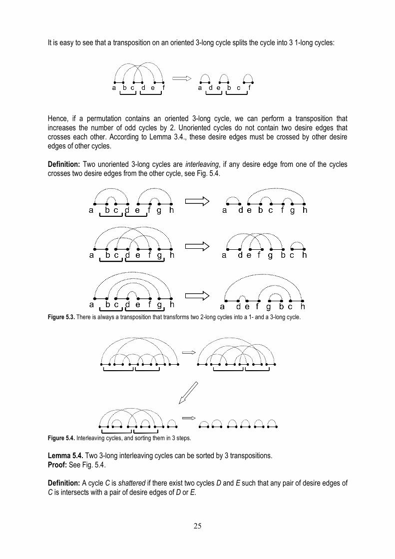
It is easy to see that a transposition on an oriented 3-long cycle splits the cycle into 3 1-long cycles:

Hence, if a permutation contains an oriented 3-long cycle, we can perform a transposition that increases the number of odd cycles by 2. Unoriented cycles do not contain two desire edges that crosses each other. According to Lemma 3.4., these desire edges must be crossed by other desire edges of other cycles. Definition: Two unoriented 3-long cycles are interleaving, if any desire edge from one of the cycles crosses two desire edges from the other cycle, see Fig. 5.4.

Figure 5.3. There is always a transposition that transforms two 2-long cycles into a 1- and a 3-long cycle.

Figure 5.4. Interleaving cycles, and sorting them in 3 steps. Lemma 5.4. Two 3-long interleaving cycles can be sorted by 3 transpositions. Proof: See Fig. 5.4. Definition: A cycle C is shattered if there exist two cycles D and E such that any pair of desire edges of C is intersects with a pair of desire edges of D or E.

26

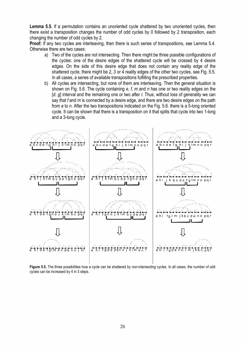
Lemma 5.5. If a permutation contains an unoriented cycle shattered by two unoriented cycles, then there exist a transposition changes the number of odd cycles by 0 followed by 2 transposition, each changing the number of odd cycles by 2. Proof: If any two cycles are interleaving, then there is such series of transpositions, see Lemma 5.4. Otherwise there are two cases:

a) Two of the cycles are not intersecting. Then there might be three possible configurations of the cycles: one of the desire edges of the shattered cycle will be crossed by 4 desire edges. On the side of this desire edge that does not contain any reality edge of the shattered cycle, there might be 2, 3 or 4 reality edges of the other two cycles, see Fig. 5.5. In all cases, a series of available transpositions fulfilling the prescribed properties.

b) All cycles are intersecting, but none of them are interleaving. Then the general situation is shown on Fig. 5.6. The cycle containing e, f, m and n has one or two reality edges on the [d, g] interval and the remaining one or two after l. Thus, without loss of generality we can say that f and m is connected by a desire edge, and there are two desire edges on the path from e to n. After the two transpositions indicated on the Fig. 5.6. there is a 5-long oriented cycle. It can be shown that there is a transposition on it that splits that cycle into two 1-long and a 3-long cycle.

Figure 5.5. The three possibilities how a cycle can be shattered by non-intersecting cycles. In all cases, the number of odd cycles can be increased by 4 in 3 steps.

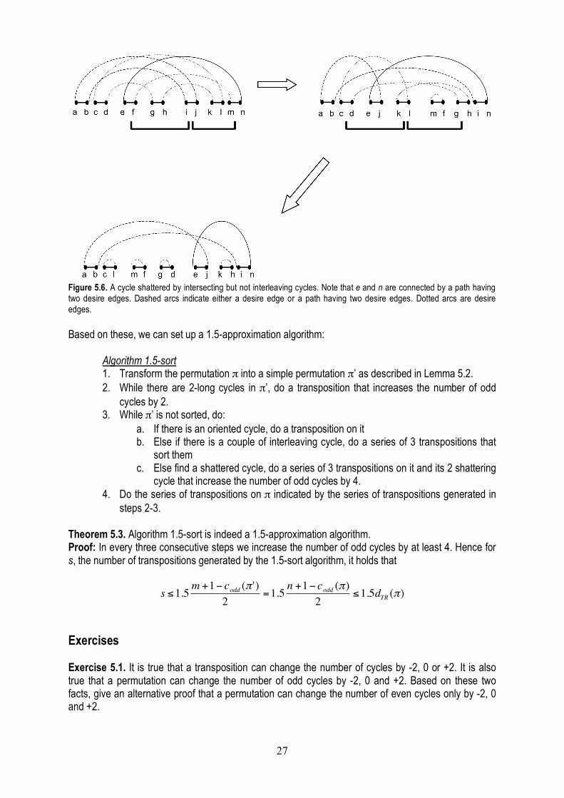
27

Figure 5.6. A cycle shattered by intersecting but not interleaving cycles. Note that e and n are connected by a path having two desire edges. Dashed arcs indicate either a desire edge or a path having two desire edges. Dotted arcs are desire edges. Based on these, we can set up a 1.5-approximation algorithm: Algorithm 1.5-sort

1. Transform the permutation π into a simple permutation π’ as described in Lemma 5.2. 2. While there are 2-long cycles in π’, do a transposition that increases the number of odd

cycles by 2. 3. While π’ is not sorted, do:

a. If there is an oriented cycle, do a transposition on it b. Else if there is a couple of interleaving cycle, do a series of 3 transpositions that

sort them c. Else find a shattered cycle, do a series of 3 transpositions on it and its 2 shattering

cycle that increase the number of odd cycles by 4. 4. Do the series of transpositions on π indicated by the series of transpositions generated in

steps 2-3. Theorem 5.3. Algorithm 1.5-sort is indeed a 1.5-approximation algorithm. Proof: In every three consecutive steps we increase the number of odd cycles by at least 4. Hence for s, the number of transpositions generated by the 1.5-sort algorithm, it holds that

!

s "1.5m +1# codd ($ ')2

=1.5 n +1# codd ($)2

"1.5dTR ($)

Exercises Exercise 5.1. It is true that a transposition can change the number of cycles by -2, 0 or +2. It is also true that a permutation can change the number of odd cycles by -2, 0 and +2. Based on these two facts, give an alternative proof that a permutation can change the number of even cycles only by -2, 0 and +2.

28

Exercise 5.2. Prove that for any oriented 5-long cycle, there is a transposition that splits it into a 3-long and two 1-long cycles. Exercise 5.3. Prove that the Algorithm 1.5-sort can be implemented such that the running time increases polynomially with the length of the input permutation. Exercise 5.4. * Implement Algorithm 1.5-sort. Exercise 5.5. Prove that

!

b(")3

#n +1$ c(")

2#n +1$ codd (")

2

Exercise 5.6. Prove that

!

n +1" c(#) $ b(#) Exercise 5.7 The transposition diameter of the symmetric group Sn is the greatest transposition distance amongst the n long permutation. Prove that the transposition diameter is greater or equal than

!

n2"

# " $

% $ .

Exercise 5.8. Prove that the transposition diameter is lower or equal than

!

3n4

"

# " $

% $ .

29

Chapter 6. The principle of dynamic programming Dynamic programming is one of the most important algorithmic techniques in bioinformatics. There are bioinformatics books that consider only dynamic programming algorithms. Indeed, many of the bioinformatics problems consider optimizations on sequences and trees, for which the dynamic programming idea is particularly useful. The aim of this chapter is to introduce dynamic programming.

Dynamic programming is a method for solving complex problems via solving simpler subproblems. Typically, a dynamic programming algorithm has two phases. The first phase is called the fill-in phase, in which a so-called dynamic programming table is filled in. The dynamic programming table contains the scores of the subproblems. By the end of the fill-in phase we know the score of the solution, but we do not know the solution itself. The solution can be obtained in the second phase, called the trace-back phase. We are going to introduce the dynamic programming method by solving the money change problem. The Money change problem is the following: given an amount of money, and a coin system, find the minimum number of coins necessary to change the money. For example, if the available coins are the 1, 2 and 5 unit coins, then the minimum number of coins necessary to change 8 is 3, as 1+2+5=8, and any two coins do not make a sum 8, and there is also no 8 unit coin. There are coin systems when the so-called greedy algorithm works. The greedy algorithm finds the largest coin less than the value of the remaining amount and its value is substracted. For example, if the amount to change is 8, then the largest coin that can be used is 5. 8-5=3. Then the largest coin less than 3 is 2, 3-2=1, and there is a 1-unit coin. Hence the greedy algorithm constructed the solution 8=5+2+1, which happens to be optimal in this case.

However, there are cases when the greedy algorithm does not work. For example, if the available coins have 1, 4 and 5 units, then the optimal solution to change 8 is to change it to two 4-unit coins. However, the greedy algorithm starts with 5, and eventually constructs the solution 8 = 5+1+1+1, which is not optimal. On the other hand, the dynamic programming algorithm always finds the optimal solution in the following way.

Let m(x) be the minimum number of coins necessary to change amount x, if x is changeable, otherwise let m(x) be infinite. Set m(x) to infinite for all x<0 and set m(0)=0. Let C denote the set of values available in the coin system. Theorem 6.1. The following equation is true for any x>0:

!

m(x) =minc"C

m(x # c) +1{ } (6.1.)

Proof: We prove it by induction, namely we prove it that it is true for x if it true for all y<x. If x is not changeable, then for all c∈C, x-c is also not changeable or x-c<0. Thus both side of the equation is infinite, hence the equality holds. If x is changeable, then consider a change with the minimum number of coins. Take one of the coins, let its value be c’. If we remove this coin, then the remaining amount is x-c’. We claim that the remaining number of coins must be m(x-c’). If the number of coins were more, then we could replace them with the minimum number of coins necessary to change x-c’, and together with the coin with value c’, we would get a change with smaller number of coins, contradicting that we have a minimum change for amount x. Furthermore, the number of coins for the amount of x-c’ cannot be less than the minimum number of necessary coins. Hence

30

!

m(x) = m(x " c ') +1#minc$C

m(x " c) +1{ }

On the other hand, for any c∈C, either x-c is not changeable, and then m(x-c) is infinite, or it is changeable, then a change of the amount of x-c plus a coin with value c will be also a change for amount x. Thus,

!

m(x) "minc#C

m(x $ c) +1{ }

Since

!

m(x) "minc#C

m(x $ c) +1{ }

and

!

m(x) "minc#C

m(x $ c) +1{ }

it follows that

!

m(x) =minc"C

m(x # c) +1{ }

Using Eqn. 6.1. we can calculate the minimum number of coins necessary to change amount x. The amount of computation necessary to calculate this number is

!

O xC( ) , namely, the computational time

grows linearly with both x and the size of the coin system. Using Eqn. 6.1. to calculate m(x’) for all x’≤x is called the fill-in phase. The trace-back phase of the dynamic programming algorithm constructs a solution with the calculated value. The pseudo-code of the trace-back for the money change problem is the following:

Set S to empty set, set y to x While y

!

" 0 do Find a c∈C for which m(y) = m(y-c)+1

Add c to S Set y to y-c Return with S

S will contain a minimum number of coins necessary to change x. Exercises Exercise 6.1. The cost of cutting a rectangle into two rectangles along a k long line is c(k). Develop a dynamic programming algorithm that calculates a series of cuts with minimum sum of costs that cuts an

!

n " m rectangle into unit squares. (Hint: the dynamic programming algorithm calculates the cost for any

!

n'"m' rectangles, n’≤n, m’≤m.) Exercise 6.2. Develop a dynamic programming algorithm that calculates the minimum number of (not necessary different) primes that sum to x. Exercise 6.3. Develop a dynamic programming algorithm that calculates the minimum number of different primes that sum to x. (Hint the dynamic programming calculates the minimum number of different primes amongst which the largest is p for each couple of x and p.)

31

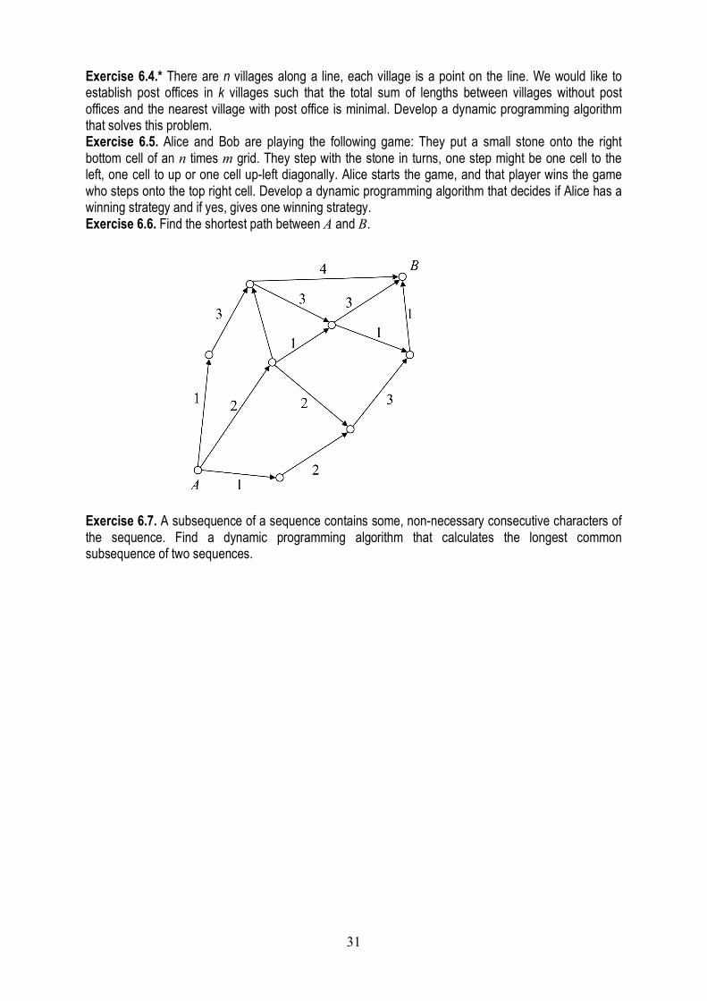
Exercise 6.4.* There are n villages along a line, each village is a point on the line. We would like to establish post offices in k villages such that the total sum of lengths between villages without post offices and the nearest village with post office is minimal. Develop a dynamic programming algorithm that solves this problem. Exercise 6.5. Alice and Bob are playing the following game: They put a small stone onto the right bottom cell of an n times m grid. They step with the stone in turns, one step might be one cell to the left, one cell to up or one cell up-left diagonally. Alice starts the game, and that player wins the game who steps onto the top right cell. Develop a dynamic programming algorithm that decides if Alice has a winning strategy and if yes, gives one winning strategy. Exercise 6.6. Find the shortest path between A and B.

Exercise 6.7. A subsequence of a sequence contains some, non-necessary consecutive characters of the sequence. Find a dynamic programming algorithm that calculates the longest common subsequence of two sequences.

32

Chapter 7. Pairwise sequence alignment 7.1. Pairwise sequence alignment with linear gap penalty

DNA contains the information of living cells. Before the duplication of cells, the DNA molecules are doubled, and both daughter cells contain one copy of DNA. The replication of DNA is not perfect, the stored information can be changed by random mutations. Random mutations create variants in the population, and these variants evolve to new species. Given two sequences from two modern species, we can ask how many mutations are needed to describe the evolutionary history of the two sequences. Since some types of mutations are significantly more frequent than others, it makes sense to weight them: rare mutations get greater weights, frequent mutations get lower weights. We define the weight of a series of mutations be the sum of the weights of the individual mutations. We also prescribe that a mutation and its reverse have the same weight, and we infer how a sequence can be transferred into another instead of evolving two sequences from a common ancestor. Assuming minimum evolution, we are seeking for the minimum weight series of mutations that transforms one sequence into another. An important question is how we can quickly find such a minimum weight series. The naive algorithm finds all the possible series of mutations and chooses the minimum weight. Since the possible number of series of mutations grows exponentially – as we are going to show it in this chapter –, the naive algorithm is obviously too slow.

Here we define precisely the optimization problem. Let Σ be a finite set of symbols, and let Σ* denote the set of finite long sequences over Σ. The n long prefix of A ∈ Σ* will be denoted by An, and an denotes the nth character of A. The following transformations can be applied for a sequence:

- Insertion of character a before position i, denoted by - →i a. - Deletion of character a at position i, denoted by a →i -. - Substitution of character a to character b at position i, denoted by a →i b.

The concatenation of mutations is denoted by the

!

o symbol. τ denotes the set of finite long concatenations of the above mutations, and T(A)=B denotes that T ∈ τ transforms sequence A into sequence B.

Let w : τ → ℜ+ ∪ {0} a weight function such that for any T1, T2, and S transformations satisfying

!

T1 oT2 = S it also holds that

!

w(T1) + w(T2) = w(S).

Furthermore, let w(a →i b) be independent from i. The transformation distance between two sequences, A and B, is the minimum weight of transformations transforming A into B:

!

"(A,B) =min{w(T) |T(A) = B} If we assume that w satisfies

!

w(a"b) = w(b"a)w(a"a) = 0w(a"b) + w(b"c) # w(a"c)

for any a, b, c ∈ Σ ∪ {-}, then the transformation distance δ is indeed a metric on Σ*. Since w() is a metric, it is enough to consider only transformations that change each position of a sequence at most once. Such series of transformations are depicted with sequence alignments. By convention, the

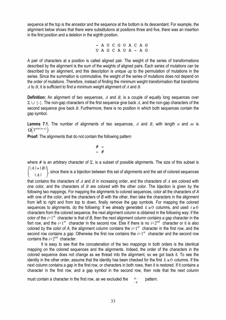
33

sequence at the top is the ancestor and the sequence at the bottom is its descendant. For example, the alignment below shows that there were substitutions at positions three and five, there was an insertion in the first position and a deletion in the eighth position.

- A U C G U A C A G U A G C A U A - A G

A pair of characters at a position is called aligned pair. The weight of the series of transformations described by the alignment is the sum of the weights of aligned pairs. Each series of mutations can be described by an alignment, and this description is unique up to the permutation of mutations in the series. Since the summation is commutative, the weight of the series of mutations does not depend on the order of mutations. Therefore, instead of finding the minimum weight transformation that transforms A to B, it is sufficient to find a minimum weight alignment of A and B. Definition: An alignment of two sequences, A and B, is a couple of equally long sequences over Σ ∪ {-}. The non-gap characters of the first sequence give back A, and the non-gap characters of the second sequence give back B. Furthermore, there is no position in which both sequences contain the gap symbol. Lemma 7.1. The number of alignments of two sequences, A and B, with length n and m is

!

" 3min{m,n}( )

Proof: The alignments that do not contain the following pattern

# - - #

where # is an arbitrary character of Σ, is a subset of possible alignments. The size of this subset is

!

| A |+ |B || A |

"

# $

%

& ' , since there is a bijection between this set of alignments and the set of colored sequences

that contains the characters of A and B in increasing order, and the characters of A are colored with one color, and the characters of B are colored with the other color. The bijection is given by the following two mappings. For mapping the alignments to colored sequences, color all the characters of A with one of the color, and the characters of B with the other, then take the characters in the alignment from left to right and from top to down, finally remove the gap symbols. For mapping the colored sequences to alignments, do the following: if we already generated

!

k " 0 columns, and used

!

i " 0 characters from the colored sequence, the next alignment column is obtained in the following way: if the color of the i+1st character is that of B, then the next alignment column contains a gap character in the fisrt row, and the i+1st character in the second row. Else if there is no i+2nd character or it is also colored by the color of A, the alignment column contains the i+1st character in the first row, and the second row contains a gap. Otherwise the first row contains the i+1st character and the second row contains the i+2nd character. It is easy to see that the concatenation of the two mappings in both orders is the identical mapping on the colored sequences and the alignments. Indeed, the order of the characters in the colored sequence does not change as we thread into the alignment, so we got back it. To see the identity in the other order, assume that the identity has been checked for the first

!

k " 0 columns. If the next column contains a gap in the first row, or characters in both rows, then it is restored. If it contains a character in the first row, and a gap symbol in the second row, then note that the next column

must contain a character in the first row, as we excluded the pattern.

# - - #

# -

- #

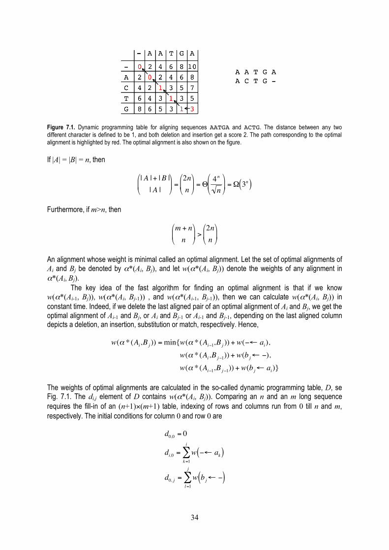
34

Figure 7.1. Dynamic programming table for aligning sequences AATGA and ACTG. The distance between any two different character is defined to be 1, and both deletion and insertion get a score 2. The path corresponding to the optimal alignment is highlighted by red. The optimal alignment is also shown on the figure. If |A| = |B| = n, then

!

| A |+ |B || A |

"

# $

%

& ' =

2nn

"

# $

%

& ' =(

4n

n"

# $

%

& ' =) 3n( )

Furthermore, if m>n, then

!

m + nn

"

# $

%

& ' >

2nn

"

# $

%

& '

An alignment whose weight is minimal called an optimal alignment. Let the set of optimal alignments of Ai and Bj be denoted by α*(Ai, Bj), and let w(α*(Ai, Bj)) denote the weights of any alignment in α*(Ai, Bj).

The key idea of the fast algorithm for finding an optimal alignment is that if we know w(α*(Ai-1, Bj)), w(α*(Ai, Bj-1)) , and w(α*(Ai-1, Bj-1)), then we can calculate w(α*(Ai, Bj)) in constant time. Indeed, if we delete the last aligned pair of an optimal alignment of Ai and Bj, we get the optimal alignment of Ai-1 and Bj, or Ai and Bj-1 or Ai-1 and Bj-1, depending on the last aligned column depicts a deletion, an insertion, substitution or match, respectively. Hence,

!

w(" * (Ai,B j )) = min{w(" * (Ai#1,B j )) + w(#$ ai), w(" * (Ai,B j#1)) + w(b j$ #), w(" * (Ai#1,B j#1)) + w(b j$ ai)}

The weights of optimal alignments are calculated in the so-called dynamic programming table, D, se Fig. 7.1. The di,j element of D contains w(α*(Ai, Bj)). Comparing an n and an m long sequence requires the fill-in of an (n+1)×(m+1) table, indexing of rows and columns run from 0 till n and m, respectively. The initial conditions for column 0 and row 0 are

!

d0,0 = 0

di,0 = w "# ak( )k=1

i

$

d0, j = w bj# "( )l=1

j

$

35

The table can be filled in using recursion

!

di, j = min{di"1, j + w("# ai), di, j"1 + w(b j# "), di"1, j"1 + w(b j# ai)}

The time requirement for the fill-in is

!

"(nm). After filling in the dynamic programming table, the set of all optimal alignments can be found in the following way, called trace-back. We go from the right bottom corner to the left top corner choosing the cell(s) giving the optimal value of the current cell (there might be more than one such cells). Stepping up from position di,j means a deletion, stepping to the left means an insertion, and the diagonal steps mean either a substitution or a match depending on whether or not ai = bj. Each step is represented with an oriented edge, in this way, we get an oriented graph, whose vertices are a subset of the cells of the dynamic programming table. The number of optimal alignments might grow exponentially with the length of the sequences, however, the set of optimal alignments can be represented in polynomial time and space. Indeed, each path from dn,m to d0,0 on the oriented graph obtained in the trace-back gives an optimal alignment. 7.2. Pairwise sequence alignment with arbitrary gap penalty Since deletions and insertions get the same weight, the common name of them is indel or gap and their weights are called gap penalty. Usually gap penalties do not depend on the deleted or inserted characters. The gap penalties used in the previous section grow linearly with the length of the gap. This means that a long indel is considered as the result of independent insertions or deletions of characters. However, the biological observation is that long indels can be formed in one evolutionary step, and these long indels are penalized too much with the linear gap penalty function. This observation motivated the introduction of more complex gap penalty functions. If the only restriction is that the gap penalty does not depend on the inserted or deleted characters, then a k long gap is penalized with gk. For example the weight of this alignment:

- - A U C G A C G U A C A G U A G U C - - - A U A G A G

is

!

g2 + w G" A( ) + g3 + w A" G( ) + w G" C( ) . We are still seeking for the minimal weight series of transformations transforming one sequence into another or equivalently for an optimal alignment. Since there might be a long indel at the end of the optimal alignment, above knowing

!

w " * Ai#1,B j#1( )( ) , we must know all

!

w " * Ak,B j( )( ) ,

!

0 " k < i and

!

w " * Ai,Bl( )( ) ,

!

0 " l < j to

calculate

!

w " * Ai,B j( )( ) . The dynamic programming recursion is given by the following equations:

!

di, j = min min0"k< i

{dk, j + gi#k},$ % &

min0" l< j

{di,l + g j# l},

di#1, j#1 + w(b j' ai)( ) *

The initial conditions are:

36

!

d0,0 = 0, di,0 = gi, d0, j = g j

The time requirement for calculating di,j is

!

"(i + j) , hence the running time of the fill-in part to calculate the weight of an optimal alignment is

!

"(nm(n +m)) . Similarly to the previous algorithm, the set of optimal alignments represented by paths from dn,m to d0,0 can be found in the trace-back part.

If |A| =|B| = n, then the running time of this algorithm is

!

" n3( ) . With restrictions on the gap

penalty function, the running time can be decreased. We are going to show an example in the next section. 7.3. Pairwise sequence alignment with affine gap penalty Definition: A gap penalty gk is affine if it satisfy

!

gk = o + (k "1)e Here o is the gap opening penalty, and e is the gap extension penalty. For affine gap penalty, a

!

" n2( ) running time algorithm is available. The key observation is that the

penalty of a particular alignment column containing a gap depends only on whether or not the previous column contained a gap in the same row. To keep this information, it is necessary to split the set of alignments into three subsets, depending on if the last alignment column contains an insertion, a deletion or an alignment of two characters. Three dynamic programming tables must be filled in, one for each subset. These three dynamic programming tables will be denoted by I (insertion, ik,l denotes an entry), D (deletion, dk,l denotes an entry) and M (match, mk,l denotes an entry). The entry ik,l stores the score of the best alignment of the k and l long prefixes with an insertion in the last alignment column. Similarly, dk,l stores the score of the best alignment of the k and l long prefixes with a deletion in the last alignment column. Finally, mk,l stores the score of the best alignment of the k and l long prefixes with an aligned couple of characters in the last alignment column. The dynamic programming recursions are:

!

mk,l =min mk"1,l"1,ik"1,l"1,dk"1,l"1{ } + w bl# ak( )

ik,l =min ik,l"1 + e,min mk,l"1,dk,l"1{ } + o{ }dk,l =min dk"1,l + e,min mk"1,l ,ik"1,l{ } + o{ }

Since each entry can be calculated in constant time, the running time of the fill-in phase takes only

!

"(nm) running time. The trace-back can be done in linear time, just like in the linear gap penalty case. 7.4. Similarity and local alignment We can measure not only the distance but also the similarity of two sequences. For measuring the similarity of two characters, S(a,b), the most frequently used function is the log-odds function:

!

S(a,b) = logp(a,b)q(a)q(b)"

# $

%

& '

37

where p(a,b) is the joint probability of the two characters (namely, the probability of observing them together in an alignment column), q(a) and q(b) are the marginal probabilities. These probability distributions are obtained from empirical data. For this, such sequences and parts of the sequences are used for which the alignment problem can be solved by eye and/or further biological data like structural information about protein sequences are available to solve the alignment problem without using computer algorithms. The similarity score is positive if p(a,b) > q(a)q(b), otherwise negative. Namely, the similarity score is positive for pair of characters that are coupled more frequently than their independent frequencies would indicate, and negative for pair of characters that are coupled less frequently than their independent frequencies would indicate. With other words, the similarity score is positive for characters that like to couple, and negative for those ones that avoid each other. If we penalize gaps with negative numbers then the above described, global alignment algorithms work with similarities by changing minimization to maximization.

The reason to introduce the similarity problem is that there is a special problem that works for similarities and does not work for distances. The local similarity problem or the local sequence alignment problem is the following. Given two sequences, a similarity and a gap penalty function, the problem is to give two substrings of the sequences whose similarity is maximal. A substring of a sequence is a consecutive part of the sequence. The distance version of this problem is indeed meaningless: if the two sequences share a common character, then the local alignment of them has 0 distance, and hence they have a minimal distant local alignment. Such trivial solutions make the distance version of the local alignment uninteresting.

On the other hand, the similarity version of the local alignment problem has a true biological motivation. Some parts of the biological sequences evolve slowly while other parts evolve fast, hence, scoring a particular mutation in the same way at each part of a sequence is unjustified. A possible improvement is to score only the slowly evolving parts and disregards the parts that accommodate many mutations. This is exactly the local sequence alignment problem, as it finds the most conserved part of the two sequences. Local alignment is widely used for homology searching in databases. The reason why local alignments works well for homology searching is that the local alignment score can separate homologue and non-homologue sequences better since the statistics is not decreased due to the variable regions of the sequences.

Although some kind of naïve algorithm for the local alignment problem works in polynomial running time, Smith and Waterman developed a significantly faster algorithm for the local alignment problem, widely known as the Smith-Waterman algorithm. Several versions of the Smith-Waterman algorithm are known, we introduce here the simplest one, the Smith-Waterman algorithm with linear gap penalty. First we describe the algorithm, then we explain its correctness.

The Smith-Waterman algorithm with linear gap penalties works in the following way. The initial conditions are:

!

d0,0 = di,0 = d0, j = 0

The dynamic programming table is filled in using the following recursions:

!

di, j = max{0, di"1, j"1 + S(ai,bj ), di"1, j + g, di, j" + g}

Here g, the gap penalty is a negative number. The best local similarity score of the two sequences is the maximal number in the table. The trace-back starts in the cell having the maximal number, and ends when first reaches a 0.

It is easy to prove that the alignment obtained in the trace-back will be locally optimal: if the alignment could be extended at the end with a sub-alignment whose similarity is positive then there would be a greater number in the dynamic programming table. If the alignment could be extended at the beginning with a subalignment having positive similarity then the value at the end of the traceback would not be 0.

38

Exercises

Exercise 7.1. Using the Stirling formula

!

n!~ 2n" ne#

$ % &

' ( n#

$ %

&

' ( , prove that

!

2nn

"

# $

%

& ' =(

4n

n"

# $

%

& '

Exercise 7.2. Prove that

!

m + nn

"

# $

%

& ' >

2nn

"

# $

%

& '

for any m>n. Exercise 7.3. Prove that the number of alignments of an n and an m long sequence is

!

(n +m " i)!(n " i)!(m " i)!i!i=0

min(n,m )

#

Exercise 7.4. Let w(a → b) = 1 for any

!

a " b, and let the gap penalty be 3. Calculate the optimal alignment of sequences AUCGACGUACAG and UAGUCAUAGAG. Exercise 7.5. Prove that the number of optimal alignments might grow exponentially with the length of the sequences. Exercise 7.6. Prove that

!

(i + j +1)j=1

n

"i=1

n

" =O n3( )

and hence, the dynamic programming algorithm with arbitrary gap penalty indeed runs in cubic time. Exercise 7.7. A dynamic programming algorithm to align sequences takes O(ij) to calculate entry dij. What is the running time of the algorithm? Exercise 7.8. Implement the dynamic programming algorithms described in this chapter in a computer language. Exercise 7.9. Work out the Smith-Waterman algorithm for the affine gap penalty case.

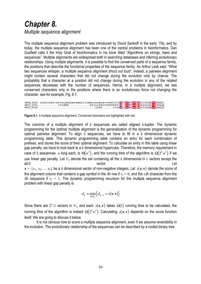
39

Chapter 8. Multiple sequence alignment The multiple sequence alignment problem was introduced by David Sankoff in the early ‘70s, and by today, the multiple sequence alignment has been one of the central problems in bioinformatics. Dan Gusfield calls it the Holy Grail of bioinformatics in his book titled “Algorithms on strings, trees and sequences”. Multiple alignments are widespread both in searching databases and inferring evolutionary relationships. Using multiple alignments, it is possible to find the conserved parts of a sequence family, the positions that describe the functional properties of the sequence family. As Arthur Lesk said: “What two sequences whisper, a multiple sequence alignment shout out loud”. Indeed, a pairwise alignment might contain several characters that did not change during the evolution only by chance. The probability that a character at a position did not change during the evolution in any of the related sequences decreases with the number of sequences. Hence, in a multiple alignment, we see conserved characters only in the positions where there is an evolutionary force not changing the character, see for example, Fig. 8.1.

Figure 8.1. A multiple sequence alignment. Conserved characters are highlighted with red. The columns of a multiple alignment of k sequences are called aligned k-tuples. The dynamic programming for the optimal multiple alignment is the generalization of the dynamic programming for optimal pairwise alignment. To align k sequences, we have to fill in a k dimensional dynamic programming table. This dynamic programming table contains an entry for each combination of prefixes, and stores the score of their optimal alignment. To calculate an entry in this table using linear gap penalty, we have to look back to a k dimensional hypercube. Therefore, the memory requirement in case of k sequences, n long each, is

!

" nk( ) , and the running time of the algorithm is

!

" 2k nk( ) if we

use linear gap penalty. Let Vk denote the set containing all the k dimensional 0-1 vectors except the all-0 vector. Let x = {x1, x2, ... xk} be a k dimensional vector of non-negative integers. Let

!

s x,v( ) denote the score of the alignment column that contains a gap symbol in the ith row if vi = 0, and the xith character from the ith sequence if vi = 1. The dynamic programming recursion for the multiple sequence alignment problem with linear gap penalty is

!

dx =minv"Vk

dx#v + s x,v( ){ }

Since there are 2k-1 vectors in Vk, and each

!

s x,v( ) takes

!

" 1( ) running time to be calculated, the

running time of the algorithm is indeed

!

" 2k nk( ). Calculating

!

s x,v( ) depends on the score function

itself. We are going to discuss it below. It is not obvious how to score a multiple sequence alignment, even if we assume reversibility in

the evolution. The evolutionary relationship of the sequences can be described by a rooted binary tree.

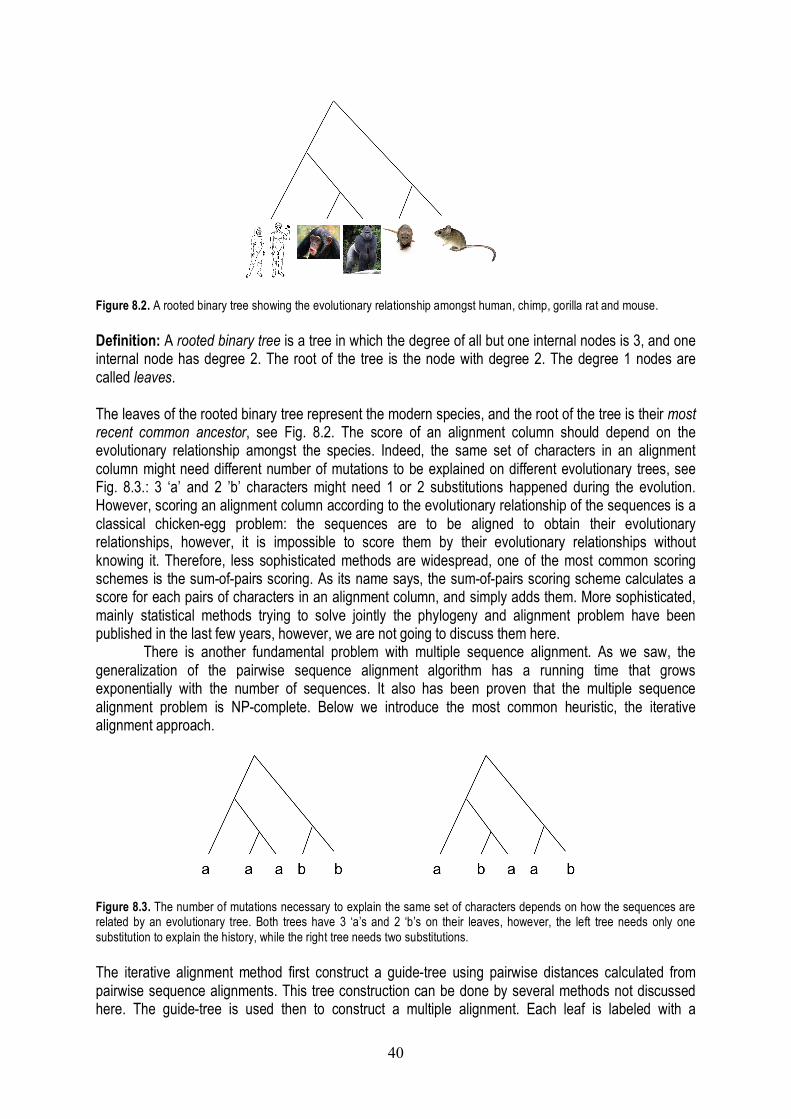
40

Figure 8.2. A rooted binary tree showing the evolutionary relationship amongst human, chimp, gorilla rat and mouse. Definition: A rooted binary tree is a tree in which the degree of all but one internal nodes is 3, and one internal node has degree 2. The root of the tree is the node with degree 2. The degree 1 nodes are called leaves. The leaves of the rooted binary tree represent the modern species, and the root of the tree is their most recent common ancestor, see Fig. 8.2. The score of an alignment column should depend on the evolutionary relationship amongst the species. Indeed, the same set of characters in an alignment column might need different number of mutations to be explained on different evolutionary trees, see Fig. 8.3.: 3 ‘a’ and 2 ’b’ characters might need 1 or 2 substitutions happened during the evolution. However, scoring an alignment column according to the evolutionary relationship of the sequences is a classical chicken-egg problem: the sequences are to be aligned to obtain their evolutionary relationships, however, it is impossible to score them by their evolutionary relationships without knowing it. Therefore, less sophisticated methods are widespread, one of the most common scoring schemes is the sum-of-pairs scoring. As its name says, the sum-of-pairs scoring scheme calculates a score for each pairs of characters in an alignment column, and simply adds them. More sophisticated, mainly statistical methods trying to solve jointly the phylogeny and alignment problem have been published in the last few years, however, we are not going to discuss them here.

There is another fundamental problem with multiple sequence alignment. As we saw, the generalization of the pairwise sequence alignment algorithm has a running time that grows exponentially with the number of sequences. It also has been proven that the multiple sequence alignment problem is NP-complete. Below we introduce the most common heuristic, the iterative alignment approach.

Figure 8.3. The number of mutations necessary to explain the same set of characters depends on how the sequences are related by an evolutionary tree. Both trees have 3 ‘a’s and 2 ‘b’s on their leaves, however, the left tree needs only one substitution to explain the history, while the right tree needs two substitutions. The iterative alignment method first construct a guide-tree using pairwise distances calculated from pairwise sequence alignments. This tree construction can be done by several methods not discussed here. The guide-tree is used then to construct a multiple alignment. Each leaf is labeled with a

41

sequence, and first the sequences in cherry-motives are aligned into each other. A cherry motif consists of two leaves and internal nodes connecting directly them. Once the cherry motifs are aligned, the pairwise alignments are put to the internal node of the cherry motives, and the two leaves are removed. In this way, the internal nodes of the cherry motives become leaves. We get a smaller tree whose leaves are labeled with sequences and leaves. From this point, alignments are aligned to sequences and alignments. It is done using the “once a gap – always gap” rule. This means that gaps already placed into an alignment cannot be modified when aligning the alignment to other alignment or sequence. The only possibility is to insert all-gap columns into an alignment. The aligned sequences are usually described with a profile. The profile is a

!

" +1( ) # L table, where L is the length of the

alignment. A column of a profile contains the statistics of the corresponding aligned k-tuple, the frequencies of characters and the gap symbol. The obtained multiple alignment can be used for constructing another guide-tree, that can be used for another iterative sequence alignment, and this procedure can be iterated till convergence.

The reason for the iterative alignment heuristic is that the optimal pairwise alignment of closely related sequences will be the same in the optimal multiple alignment. The drawback of the heuristic is that even if the previous assumption is true, there might be several optimal alignments for two sequences, and their number might grow exponentially with the length of the sequences. For example, let us consider the two optimal alignments of the sequences AUCGGUACAG and AUCAUACAG.

A U C G G U A C A G A U C G G U A C A G A U C - A U A C A G A U C A - U A C A G

We cannot choose between the two alignments, however, in a multiple alignment, it might happen that only one of them is optimal. For example, if we align the sequence AUCGAU to the two optimal alignments, we get the following locally optimal alignments:

A U C G G U A C A G A U C G G U A C A G A U C - A U A C A G A U C A - U A C A G A U C G A U - - - - A U C - G - A U - -

The left alignment is globally optimal, however, the right alignment is only locally optimal. Hence, the iterative alignment method yields only a locally optimal alignment. Another problem of this method is that it does not give an upper bound for the goodness of the approximation. In spite of its drawback, the iterative alignment methods are the most widely used ones for multiple sequence alignments in practice, since it is fast and usually gives biologically reasonable alignments. Recently some approximation methods for multiple sequence alignment have been published with known upper bounds for their goodness. However, the bounds biologically are not reasonable, and in practice, these methods usually give worse results than the heuristic methods.

We must mention a novel greedy method that is not based on dynamic programming. The DiAlign method first searches for gap-free homologue substrings by pairwise sequence comparison. The gap-free alignments of the homologous substrings are called diagonals of the dynamic programming name, hence the name of the method: Diagonal Alignment. The diagonals are scored according to their similarity value and diagonals that are not compatible with high-score diagonals get a penalty. Two diagonals are not compatible if they cannot be in the same alignment. After scoring the diagonals, they are aligned together a multiple alignment in a greedy way. First the best diagonal is selected, then the best diagonal that is comparable with the first one, then the third best alignment that is comparable with the first two ones, etc. The multiple alignment is the union of the selected diagonals that might not cover all the characters in the sequence. Those characters that were not in any of the selected diagonals are marked as “non alignable”. The drawback of the method is that sometimes it

42

introduces too many gaps due to not penalizing the gaps at all. However, DiAlign has been one of the best heuristic alignment approach and is widely used in the bioinformatics community. Exercises Exercise 8.1. We would like to align 10 sequences, each of them contains 200 characters. Assume that we can store an integer on 2 bytes. How much memory does it need to align these sequences? Exercise 8.2. A super-computer has 1 Peta-flop computer capacity, which means that it can do 1015 FLoating point Operations Per Second. Assume that 1 floating point operation is necessary for a comparision and an addition. How much time does it take to align 10 sequences containing 200 characters each, using a sum-of-pairs scoring scheme and linear gap penalty? What happens when we increase the number of sequences to 20? Exercise 8.3. What is the running time and memory need of the iterative sequence alignment algorithm? Exercise 8.4. Prove that it is impossible to obtain the globally optimal alignment without breaking the “once a gap – always gap” rule, namely, there is a set of sequences such that none of the optimal alignments of two of them yields a globally optimal multiple alignment of all of them.

43

Chapter 9. Dynamic programming on trees In this chapter, we are going to discuss two algorithms. The first is the algorithm of Sankoff and Rousseau for solving the small parsimony problem. The second one is the Felsenstein’s algorithm, which calculates the likelihood of a tree. 9.1. The large and the small parsimony problem Given a set of aligned sequences, A, or a set of sequences with the same length that does not need to be aligned, and a distance function, d, the large parsimony problem is to find the rooted binary tree, T(V,E), whose leaves labeled with the sequences, and the internal nodes are labeled with other sequences such that

!

d au,k,av,k( )k"

(u,v )#E" (9.1.)

is minimized, where au,k is the kth character of the sequence labeling node u. It is proven that the large parsimony problem is NP-complete, even if the alphabet has only two characters.

The small version of the parsimony problem is to find the best labeling of the internal nodes of a fixed binary tree with labeled leaves. This small version is a computationally easy problem that can be solved with a dynamic programming algorithm. It should be clear that the summation in Eqn. 9.1. could be swapped, and the minimization can be done for each position k independently. Therefore it is sufficient to solve the optimization problem when the leaves of the tree are labeled with single characters. The dynamic programming algorithm calculates for each subtree and each character the minimum score of the subtree labeled with the given character at its root. The algorithm visits first the leaves and propagates the recursion towards larger subtrees.

Let r(u,c) denote the score of the best labeling of the subtree whose root u us labeled with character c. Then the initialization for the leaves is:

!

r(u,c) =0 if u is labeled with c" otherwise# $ %

The recursion for an internal node u with two children v1 and v2:

!

r u,c( ) =minc1

r v1,c1( ) + d c,c1( ){ } +minc2

r v2,c2( ) + d c,c2( ){ } (9.2.)

The best score available for the entire tree is given by

!

minc

r(root,c){ } (9.3.)

The labeling corresponding to the best score can be done by first choosing the character that minimized Eqn. 9.3. Then we have to find recursively the characters labeling the children that gave the minimum in Eqn. 9.2. The traceback is different from those in sequence alignment algorithms as the traceback here constructs labeling on a tree instead of constructing a path. Hence there are bifurcations in the traceback. Technically, this can be implemented in many programming languages efficiently using recursive functions.

44

9.2. Felsenstein’s algorithm for calculating the likelihood of a tree The standard models for modeling substitution processes have been the continuous time Markov models. We are not going to discuss them in details, it is sufficient to know that in these models it is possible to calculate analytically or at least numerically for any two characters, c1 and c2 and for any time t>0 the probability that character c1 evolved to character c2 during time t. This probability is

denoted by

!

Pt c2 c1( ). The Markov process have an equilibrium distribution, π(c) denotes the

probability of character c in equilibrium. Given an edge weighted, rooted binary tree, T(V,E) labeled with equally long sequences at its leaves, the likelihood calculation problem is to calculate

!

K "(c0) Pt(u ,v ) cv,k cu,k( )(u,v )#E$

cn%2

&c1

&c0

&k$ (9.4)

where the inner product runs for all the edges (u,v) of the tree, v being the child of u, t(u,v) is the weight of the edge (u,v), and cv,k and cu,k are the characters labeling the nodes u and v in position k. There is a summation for each internal node labeling, amongst them c0 is the character labeling the root. The outer product goes for all positions k of the sequences. It is called the likelihood of the tree, and has the following meaning: what is the probability that a sequence drawn from the equilibrium distribution at the root of the tree evolves to the observed sequences at the leaves.

The brute force calculation of Eqn. 9.4. increases exponentially with the number of sequences. However, a faster calculation is available, published by Felsenstein in 1980. It should be clear that the entire formula in Eqn. 9.4. can be calculated quickly if the value for one k is calculated quickly. Hence it is sufficient to calculate the value of the expression for a fixed k. Let l(u,c) denote the likelihood of a subtree whose root u is labeled with character c. Namely, if the edges of the subtree are in the set E’, and the tree has i internal nodes, then

!

l(u,c) = K Pt( u,v ) cv,k cu,k( )(u,v )"E '#

ci

$c2

$c1

$

The initialization for the leaves is:

!

l(u,c) =1 if u is labeled with c0 otherwise" # $

The dynamic programming recursion for an internal node u with two children v1 and v2 connected with edges having weights t1 and t2 is:

!

l(u,c) = l(v1,c1)Pt1 (c1 | c)c1

"#

$ % %

&

' ( ( ) l(v2,c2)Pt2 (c2 | c)

c2

"#

$ % %

&

' ( (

And finally the likelihood can be calculated by

!

"(c)l(root,c)c#

Since the aim of the algorithm is to calculate a value, this algorithm does not have a traceback phase.

45

Example Let the evolutionary tree have 5 leaves, as on Fig. 9.1. Leaf ui will be labeled by observed character ai and the internal node vj will be labeled by character cj. The likelihood of the tree is

!

"(c0)Pt1 (c1 | c0)Pt2 (c2 | c0)Pt3 (a1 | c1)Pt4 (a2 | c1)Pt5 (c3 | c2)Pt6 (a5 | c2)Pt7 (a3 | c3)Pt8 (a4 | c3)c3

#c2

#c1

#c0

#

If we rearrange this summation such that we move the factors of the product that does not depend on the summation index, highlight some of the products and put some parentheses, we get:

!

"(c0)c0

# Pt1 (c1 | c0) Pt3 (a1 | c1) $ Pt4 (a2 | c1)( ) $c1

#%

& ' '

$ Pt2 (c2 | c0) Pt6 (a5 | c2) $ Pt5 (c3 | c2) Pt7 (a3 | c3) $ Pt8 (a4 | c3)( )c3

#%

& ' '

(

) * *

c2

#(

) * *

it is easy to see that the parenthesis-product structure of this formula:

!

• " •( ) " • " • " •( )( )( )

describes the topology of the tree. The left and the right factors of the products can be calculated independently from each other. If we replace the factors in the last level of parenthesis, we get back the finalization of the algorithm:

!

"(c0)c0

# L(root,c)

If we replace the last but one level of parenthesis with the conditional likelihood, we get back the last step of the dynamic programming:

!

"(c0)c0

# Pt1 (c1 | c0)L(u1,c1) $c1

#%

& ' '

$ Pt2 (c2 | c0)L(u2,c2)c2

#(

) * *

etc.

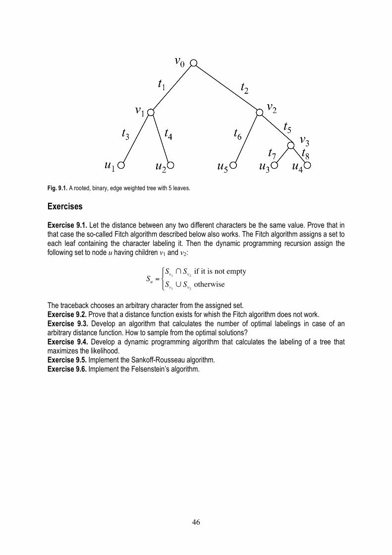
46

Fig. 9.1. A rooted, binary, edge weighted tree with 5 leaves. Exercises Exercise 9.1. Let the distance between any two different characters be the same value. Prove that in that case the so-called Fitch algorithm described below also works. The Fitch algorithm assigns a set to each leaf containing the character labeling it. Then the dynamic programming recursion assign the following set to node u having children v1 and v2:

!

Su =Sv1

" Sv2 if it is not empty

Sv1# Sv2

otherwise

$ % &

The traceback chooses an arbitrary character from the assigned set. Exercise 9.2. Prove that a distance function exists for whish the Fitch algorithm does not work. Exercise 9.3. Develop an algorithm that calculates the number of optimal labelings in case of an arbitrary distance function. How to sample from the optimal solutions? Exercise 9.4. Develop a dynamic programming algorithm that calculates the labeling of a tree that maximizes the likelihood. Exercise 9.5. Implement the Sankoff-Rousseau algorithm. Exercise 9.6. Implement the Felsenstein’s algorithm.

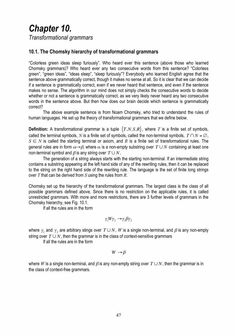
47

Chapter 10. Transformational grammars 10.1. The Chomsky hierarchy of transformational grammars “Colorless green ideas sleep furiously”. Who heard ever this sentence (above those who learned Chomsky grammars)? Who heard ever any two consecutive words from this sentence? “Colorless green”, “green ideas”, “ideas sleep”, “sleep furiously”? Everybody who learned English agree that the sentence above grammatically correct, though it makes no sense at all. So it is clear that we can decide if a sentence is grammatically correct, even if we never heard that sentence, and even if the sentence makes no sense. The algorithm in our mind does not simply checks the consecutive words to decide whether or not a sentence is grammatically correct, as we very likely never heard any two consecutive words in the sentence above. But then how does our brain decide which sentence is grammatically correct? The above example sentence is from Noam Chomsky, who tried to understand the rules of human languages. He set up the theory of transformational grammars that we define below. Definition: A transformational grammar is a tuple

!

T,N,S,R{ }, where T is a finite set of symbols, called the terminal symbols, N is a finite set of symbols, called the non-terminal symbols,

!

T "N =#, S ∈ N is called the starting terminal or axiom, and R is a finite set of transformational rules. The general rules are in form α→β, where α is a non-empty substring over

!

T "N containing at least one non-terminal symbol and β is any string over

!

T "N . The generation of a string always starts with the starting non-terminal. If an intermediate string contains a substring appearing at the left hand side of any of the rewriting rules, then it can be replaced to the string on the right hand side of the rewriting rule. The language is the set of finite long strings over T that can be derived from S using the rules from R. Chomsky set up the hierarchy of the transformational grammars. The largest class is the class of all possible grammars defined above. Since there is no restriction on the applicable rules, it is called unrestricted grammars. With more and more restrictions, there are 3 further levels of grammars in the Chomsky hierarchy, see Fig. 10.1. If all the rules are in the form

!

"1W" 2 #"1$" 2 where

!

"1 and

!

" 2 are arbitrary stings over

!

T "N , W is a single non-terminal, and β is any non-empty string over

!

T "N , then the grammar is in the class of context-sensitive grammars If all the rules are in the form

!

W "# where W is a single non-terminal, and β is any non-empty string over

!

T "N , then the grammar is in the class of context-free grammars.

48

Figure 10.1. The Chomsky hierarchy of grammars. Finally, if all the rules are in the form

!

W "aW 'W "aW "#

where W and W’ are single non-terminals, a is a single terminal symbol, and ε represents the empty string then the grammar is in the class of regular grammars.

The central decision question for transformational grammars is the following: given a transformational grammar and a finite string. Is the string part of the language of the grammar? The hardness of this decision question depends on at which level of the hierarchy the grammar is. It has been proved that this question is undecidable for the unrestricted grammars. This means that there is no general algorithm that could answer this question in finite time for any grammar. The heuristic explanation why we cannot guarantee that the algorithm will stop in finite time is the following. When generating a string in an unrestricted grammar, there is no threshold for the length of the intermediate sequence. Therefore any algorithm must infer all the intermediate cases, whose number is in fact infinite.

The above question is at least decidable for context-sensitive grammars. Indeed, the length of the intermediate sequences cannot decrease during generation, as always one non-terminal symbol is replaced to a non-empty string, thus here are finite number of possible intermediate strings, and finite number of paths to be considered. However, the decision problem is NP-complete for context-sensitive grammars, so it is very unlikely that a fast algorithm exists for this decision problem.

The two innermost classes of the Chomsky-hierarchy are significantly easier from the computational point of view. Nevertheless, they are widely applied in bioinformatics, as we will see in the next two subchapters.

49

10.2. Stochastic regular grammars and Hidden Markov Models Bioinformatics uses stochastic grammars. First we introduce them. Definition: A stochastic transformation grammar is a tuple

!

T,N,S,R,P{ } , where the first 4 in it is the same as in the transformational grammars, and P is a function mapping from the rules to the positive real numbers with the following property: for any α

!

P " #$( )"

% =1

A stochastic regular grammar (or SRG) is a stochastic transformational grammar

!

T,N,S,R,P{ } for which

!

T,N,S,R{ } is a regular grammar. The probability of a generation path is the product of the probabilities of the rules applied (with multiplicity). The probability of a sequence in the grammar is the sum of the probabilities of the generation paths that generate the sequence.

Instead of the decision question we are going to ask what is the most likely generation path and what is the probability of generating a particular sequence. Obviously, the answers for these questions also answer the question if the sequence can be generated by the grammar: if the generation probability is non-zero, then the sequence can be generated, otherwise it cannot be generated.

These two probabilities can be calculated with dynamic programming algorithms. The names of the two dynamic programming algorithms are the Viterbi algorithm and the Forward algorithm.

Viterbi algorithm Given an n long sequence A and a stochastic regular grammar, it calculates one of most likely generation paths. As usual, in the fill-in phase it calculates the probability of the most likely path, and in the trace-back phase, it generates the path. If the sequence is not part of the language, then the probability of the most likely generation is 0. Let v(i,W) denote the probability of the most likely generation of the intermediate sequence AiW. Since the generation must be started with the starting non-terminal, the initial condition is:

!

v 0,S( ) =1v 0,W( ) = 0 "W # S

The dynamic programming recursion is

!

v i,W( ) =maxW '

v i "1,W '( )P W '#aiW( ){ }

The termination is

!

pmax =maxW

v n "1,W( )P W #an( ),v n,W( )P W #$( ){ }

The most probable path can be obtained with the usual trace-back.

Forward algorithm Given an n long sequence A and a stochastic regular grammar, it calculates the probability of the sequence in the language. Let f(i,W) denote the sum of the probabilities of all the partial paths generating the intermediate sequence AiW. Since the generation must be started with the starting non-terminal, the initial condition is:

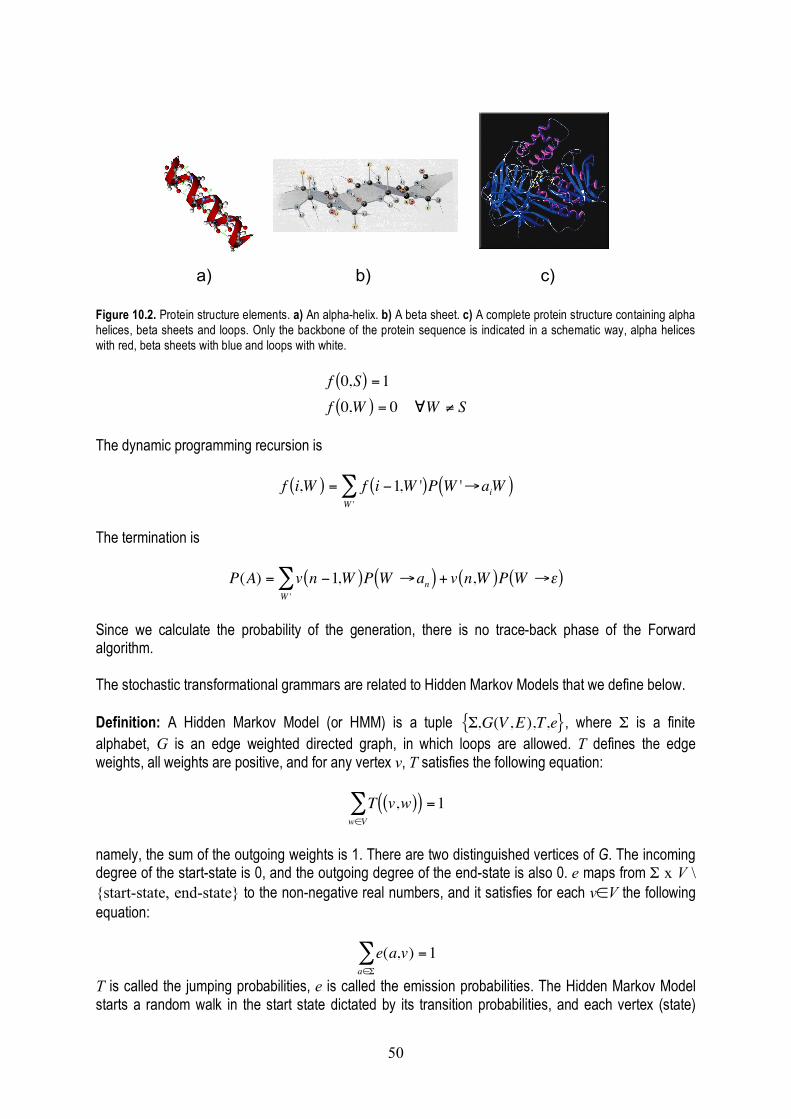
50

Figure 10.2. Protein structure elements. a) An alpha-helix. b) A beta sheet. c) A complete protein structure containing alpha helices, beta sheets and loops. Only the backbone of the protein sequence is indicated in a schematic way, alpha helices with red, beta sheets with blue and loops with white.

!

f 0,S( ) =1f 0,W( ) = 0 "W # S

The dynamic programming recursion is

!

f i,W( ) = f i "1,W '( )P W '#aiW( )W '$

The termination is

!

P(A) = v n "1,W( )P W #an( ) + v n,W( )P W #$( )W '%

Since we calculate the probability of the generation, there is no trace-back phase of the Forward algorithm. The stochastic transformational grammars are related to Hidden Markov Models that we define below. Definition: A Hidden Markov Model (or HMM) is a tuple

!

",G(V ,E),T,e{ }, where Σ is a finite alphabet, G is an edge weighted directed graph, in which loops are allowed. T defines the edge weights, all weights are positive, and for any vertex v, T satisfies the following equation:

!

T v,w( )( )w"V# =1

namely, the sum of the outgoing weights is 1. There are two distinguished vertices of G. The incoming degree of the start-state is 0, and the outgoing degree of the end-state is also 0. e maps from Σ x V \ {start-state, end-state} to the non-negative real numbers, and it satisfies for each v∈V the following equation:

!

e(a,v)a"#$ =1

T is called the jumping probabilities, e is called the emission probabilities. The Hidden Markov Model starts a random walk in the start state dictated by its transition probabilities, and each vertex (state)

a) b) c)

51

emits a random character at each visit according to the emission probabilities. The process stops when it reaches the end state. The process becomes hidden as the observer does not see the walk, only the emitted character.

Such HMMs are commonly used in bioinformatics for structure prediction. The HMM describes some structural properties of the biological sequences. For example, there are 3 different secondary structure elements in proteins: alpha helices, beta sheets and loops, see Fig. 10.2. It can be modeled by an HMM, in which the transition probabilities tell the probabilities that the next amino acid of a protein will form a structural element given the structural type of the previous amino acid. The emission probabilities tell the probabilities of the individual amino acids being in a structural element. The process is hidden, if we do not know the structure of a protein, and would like to predict from the model. The prediction is the most likely path generating the sequence, each character is predicted to be in the same a structural element than the state that emitted it in the HMM.

The relationship between HMMs and SRGs are given by the following theorem: Theorem 10.1. For any HMM

!

",G(V ,E),T,e{ }, there exists an SRG

!

T,N,S,R,P{ } such that for any sequence A over Σ, the probability of the most likely path in the HMM that generates A is the probability of the most likely generation of A in the SRG and the probability the HMM generates the string A is the probability of A in the language defined by the SRG. Proof: We construct a SRG such that any path in the HMM has a generation path in the SRG with the same probability. Let T=Σ and N=V\{end-state}. Let S be the start state. For any f=(X,Y)∈E, Y is not the end state, and a∈Σ, if e(a,Y)≠0, then create a rewriting rule X→aY with probability

!

P(X "aY ) = T(X,Y )e(a,Y ) For edges f=(X,end–state) ∈E, create a rewriting rule X→ε with probability

!

P(X "#) = T(X,end $ state) It is easy to check that the sum of the rewriting probabilities for each fixed left hand side non-terminal in the rules is indeed 1. Indeed, we need that

!

T X,Y( )( )e a,Y( )a"#$

Y %end -state$ +T X,end - state( )( ) =1

This is obviously true: for any fixed Y, the sum over the alphabet sums the emission probabilities up to 1, then summing over all the possible states having non-zero incoming degree also sums up to 1. Hence we generated a SRG, in which any combination of a transition and an emission is modeled by a rewriting rule, with the same probability than in the HMM. Corollary: The Viterbi and the Forward algorithm also work for HMMs. 10.3. Stochastic Context Free Grammars Similarly to the Stochastic Regular Grammars, we can define Stochastic Context Free Grammars (SCFGs). During the generation of a sequence in a context free grammar, several non-terminals might be presented. They might be rewritten in several orders, resulting several generation paths differ only in the order of rewritings. However, the order of the rewriting changes neither the probability of the generation path nor the possible applicable rewriting rules. Therefore we do not want to distinguish different paths, we consider only one canonical rewriting path, in which always the leftmost non-terminal is replaced. Similarly to SRGs, we can ask what the most likely generation is, and what the

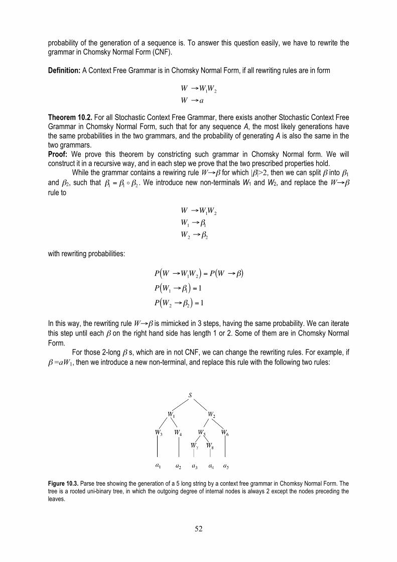
52

probability of the generation of a sequence is. To answer this question easily, we have to rewrite the grammar in Chomsky Normal Form (CNF). Definition: A Context Free Grammar is in Chomsky Normal Form, if all rewriting rules are in form

!

W "W1W2

W "a

Theorem 10.2. For all Stochastic Context Free Grammar, there exists another Stochastic Context Free Grammar in Chomsky Normal Form, such that for any sequence A, the most likely generations have the same probabilities in the two grammars, and the probability of generating A is also the same in the two grammars. Proof: We prove this theorem by constricting such grammar in Chomsky Normal form. We will construct it in a recursive way, and in each step we prove that the two prescribed properties hold.

While the grammar contains a rewiring rule W→β for which |β|>2, then we can split β into β1 and β2, such that

!

"1 = "1 o "2 . We introduce new non-terminals W1 and W2, and replace the W→β rule to

!

W "W1W2

W1 "#1W2 "#2

with rewriting probabilities:

!

P W "W1W2( ) = P W "#( )

P W1 "#1( ) =1

P W2 "#2( ) =1

In this way, the rewriting rule W→β is mimicked in 3 steps, having the same probability. We can iterate this step until each β on the right hand side has length 1 or 2. Some of them are in Chomsky Normal Form.

For those 2-long β s, which are in not CNF, we can change the rewriting rules. For example, if β =aW1, then we introduce a new non-terminal, and replace this rule with the following two rules:

Figure 10.3. Parse tree showing the generation of a 5 long string by a context free grammar in Chomksy Normal Form. The tree is a rooted uni-binary tree, in which the outgoing degree of internal nodes is always 2 except the nodes preceding the leaves.

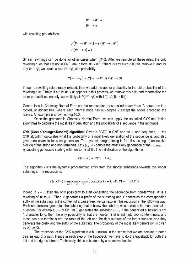
53

!

W "W 'W1

W '"a

with rewriting probabilities:

!

P W "W 'W1( ) = P W "aW '( )P W '"a( ) =1

Similar rewritings can be done for other cases when |β|>2. After we rewrote all these rules, the only rewriting rules that are not in CNF, are in form W→W’. If there is any such rule, we remove it, and for any W’→β, we create a rule W→β, with probability:

!

P W "#( ) = P W "W '( )P W "#( ) If such a rewriting rule already existed, then we add the above probability to the old probability of the rewriting rule. Finally, if a rule W→W appears in this process, we remove this rule, and renormalize the other probabilities, namely, we multiply all P(W→β) with 1/(1-P(W→W)). Generations in Chomsky Normal Form can be represented by so-called parse trees. A parse-tree is a rooted, uni-binary tree, where each internal node has out-degree 2 except the nodes preceding the leaves. An example is shown on Fig.10.3.

Once the grammar in Chomsky Normal Form, we can apply the so-called CYK and Inside algorithms to calculate the most likely derivation and the probability of a sequence in the language. CYK (Cocke-Younger-Kasami) algorithm: Given a SCFG in CNF and an n long sequence, A, the CYK algorithm calculates what the probability of a most likely generation of the sequence is, and also gives one example for such generation. The dynamic programming is for all substrings (consecutive blocks) of the string and non-terminals. Let c(i,j,W) denote the most likely generation of the ai, ai+1, ... aj substring generated starting with non-terminal W. The initialization of the algorithm is:

!

c(i,i,W ) = P(W "ai) The algorithm visits the dynamic programming entry from the shorter substrings towards the longer substrings. The recursion is:

!

c(i, j,W ) =maxi"k< j

maxXmaxY

c(i,k,X)c(k +1, j,Y )P W #XY( ){ }

Indeed, if

!

i " j , then the only possibility to start generating the sequence from non-terminal W is a rewriting of W to XY. Then X generates a prefix of the substring and Y generates the corresponding suffix of the substring. In the context of a parse tree, we can explain this recursion in the following way. Each non-terminal generates the substring that is below the sub-tree whose root is the non-terminal in question. For example, W5 of Fig. 10.3. generates the substring a3a4. If the generated substring is not 1 character long, then the only possibility is that the non-terminal is split into two non-terminals, and these two non-terminals are the roots of the left and the right subtree of the larger subtree, and they generate the prefix and the suffix of the substring. The probability of the most likely generation is given by c(1,n,S).

The traceback of the CYK algorithm is a bit unusual in the sense that we are seeking a parse tree instead of a path. Hence in each step of the traceback, we have to do the traceback for both the left and the right subtrees. Technically, this can be done by a recursive function.

54

The Inside algorithm: Given a SCFG in CNF and an n long sequence, A, the Inside algorithm calculates the probability of the sequence in the language, namely, the sum of the probabilities of the generations. Let s(i,j,W) denote the most likely generation of the ai, ai+1, ... aj substring generated starting with non-terminal W. The initialization of the algorithm is:

!

s(i,i,W ) = P(W "ai) The algorithm visits the dynamic programming entry from the shorter substrings towards the longer substrings. The recursion is:

!

s(i, j,W ) = s(i,k,X)s(k +1, j,Y )P W "XY( )Y#

X#

i$k< j#

The probability of the generation is given by s(1,n,S). Similarly to the Forward algorithm, the Inside algorithm does not have a trace-back phase, since it calculates only the total probability of generating a sequence by the grammar.

SCFGs are used in RNA structure prediction, as we will see in the next chapter. Exercises Exercise 10.1. Construct a regular grammar that generates all possible strings with odd number of as and even number of bs. Exercise 10.2. Prove that there is no regular grammar that can generate the following language: (), (()), ((())), (((()))), etc., namely all strings with the same number of opening and closing brackets, the closing brackets are after the opening brackets. Exercise 10.3. Give a context-free grammar that generates the language introduced in Exercise 10.2. Exercise 10.4.* Construct a context-free grammar that generates all legal algebraic expressions with two variables, a and b using +, -, x, : operations and parentheses. Exercise 10.5. Show that there is a SRG that cannot me mimicked with an HMM. Exercise 10.6.* A pair-HMM is an HMM that generates two sequences. Some of the states emit a character into one of the sequences and some states emit 1-1- character to both sequences. The observer can see only the emitted characters, and s/he even cannot see the co-emission pattern (what are the characters that emitted together). Describe the Viterbi and the Forwards algorithms for the pair-HMMs. Exercise 10.7.** Design a pair-HMM whose Viterbi algorithms returns with an alignment being also optimal by the score-based alignment algorithm using affine gap penalties. Note the similarity between the states of the pair-HMM and the dynamic programming layers needed for the affine gap penalty alignment algorithm. Exercise 10.8. Implement the Forward and the Viterbi algorithms. Exercise 10.9. Implement the Inside and the CYK algorithms. Exercise 10.10. What is the memory need and running time of the Viterbi, Forward, CYK and Inside algorithms? Exercise 10.11.** Why is it necessary to rewrite a context free grammar to CNF? Exercise 10.12. Rewrite the following grammar into Chomsky Normal form:

!

S"XYZ | aXbYX "aX | aaY | ZbaY "XZY | a | abaZ "ZZ | a

55

Exercise 10.13.** Write a computer program that rewrites a context free grammar into Chomky Normal Form. Exercise 10.14.** Develop a parse algorithm that calculates the most likely path for the following grammar in O(n2) running time, where n is the length of the input sequence:

!

S"LS | SR | aSu | cSg | gSc | uSa |FL"aL | cL | gL | uL | a | c | g | uR"Ra |Rc |Rg |Ru | a | c | g | uF "aF | cF | gF | uF | a | c | g | u

(Note: this is a grammar for special RNA secondary structures for the so-called miRNAs, see the next chapter).

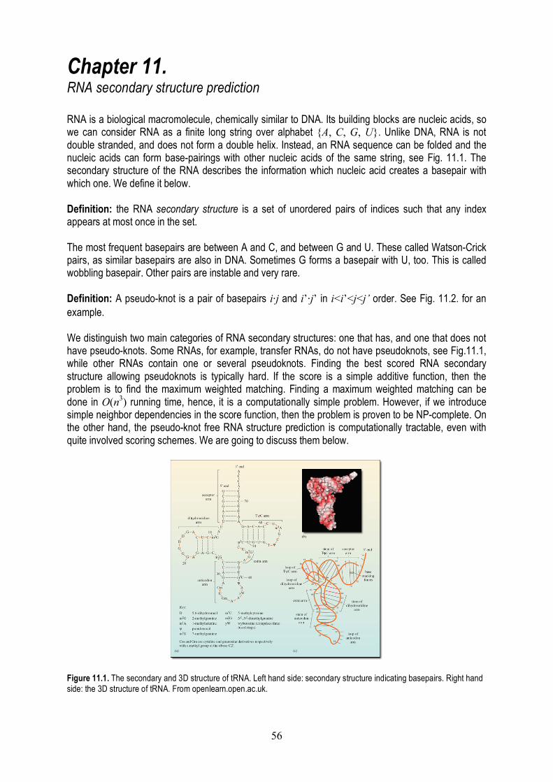
56

Chapter 11. RNA secondary structure prediction RNA is a biological macromolecule, chemically similar to DNA. Its building blocks are nucleic acids, so we can consider RNA as a finite long string over alphabet {A, C, G, U}. Unlike DNA, RNA is not double stranded, and does not form a double helix. Instead, an RNA sequence can be folded and the nucleic acids can form base-pairings with other nucleic acids of the same string, see Fig. 11.1. The secondary structure of the RNA describes the information which nucleic acid creates a basepair with which one. We define it below. Definition: the RNA secondary structure is a set of unordered pairs of indices such that any index appears at most once in the set. The most frequent basepairs are between A and C, and between G and U. These called Watson-Crick pairs, as similar basepairs are also in DNA. Sometimes G forms a basepair with U, too. This is called wobbling basepair. Other pairs are instable and very rare. Definition: A pseudo-knot is a pair of basepairs i⋅j and i’⋅j’ in i<i’<j<j’ order. See Fig. 11.2. for an example. We distinguish two main categories of RNA secondary structures: one that has, and one that does not have pseudo-knots. Some RNAs, for example, transfer RNAs, do not have pseudoknots, see Fig.11.1, while other RNAs contain one or several pseudoknots. Finding the best scored RNA secondary structure allowing pseudoknots is typically hard. If the score is a simple additive function, then the problem is to find the maximum weighted matching. Finding a maximum weighted matching can be done in O(n3) running time, hence, it is a computationally simple problem. However, if we introduce simple neighbor dependencies in the score function, then the problem is proven to be NP-complete. On the other hand, the pseudo-knot free RNA structure prediction is computationally tractable, even with quite involved scoring schemes. We are going to discuss them below.

Figure 11.1. The secondary and 3D structure of tRNA. Left hand side: secondary structure indicating basepairs. Right hand side: the 3D structure of tRNA. From openlearn.open.ac.uk.

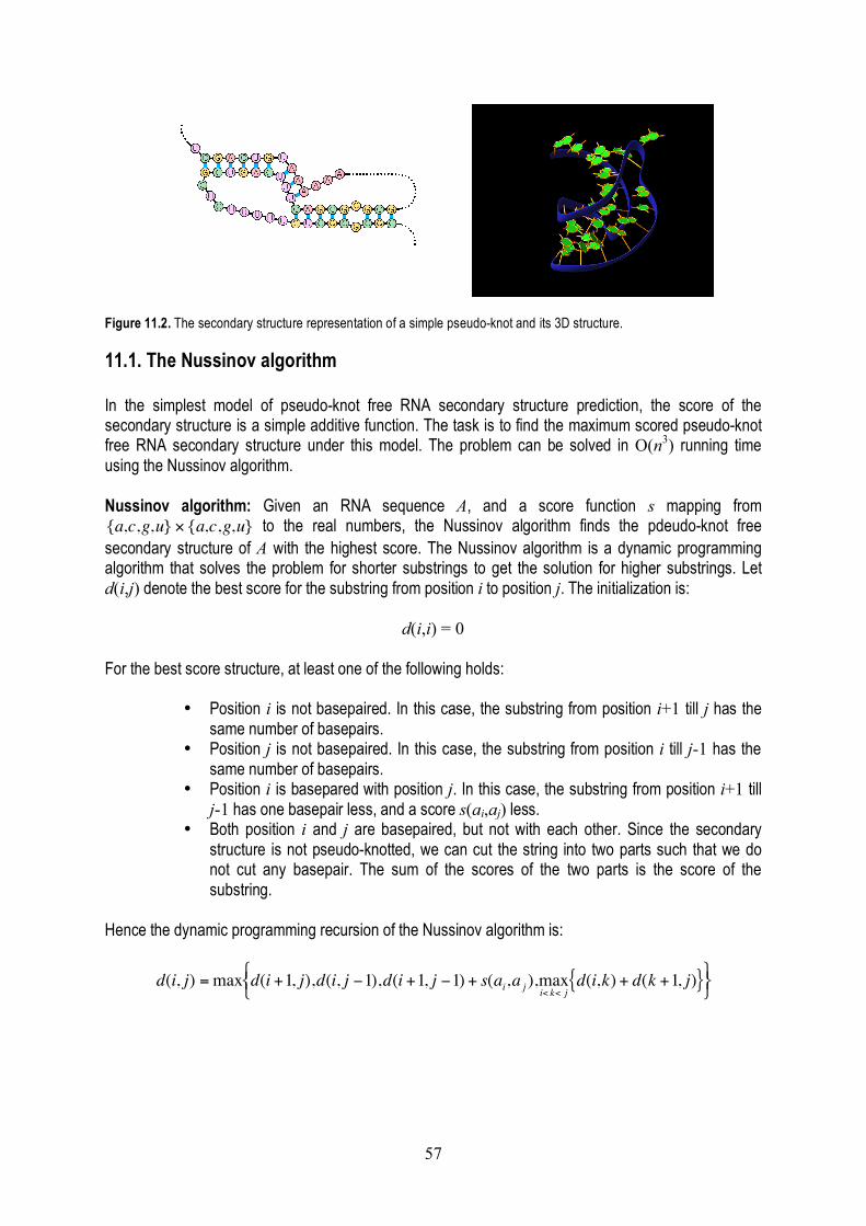
57

Figure 11.2. The secondary structure representation of a simple pseudo-knot and its 3D structure.

11.1. The Nussinov algorithm In the simplest model of pseudo-knot free RNA secondary structure prediction, the score of the secondary structure is a simple additive function. The task is to find the maximum scored pseudo-knot free RNA secondary structure under this model. The problem can be solved in O(n3) running time using the Nussinov algorithm. Nussinov algorithm: Given an RNA sequence A, and a score function s mapping from

!

{a,c,g,u} " {a,c,g,u} to the real numbers, the Nussinov algorithm finds the pdeudo-knot free secondary structure of A with the highest score. The Nussinov algorithm is a dynamic programming algorithm that solves the problem for shorter substrings to get the solution for higher substrings. Let d(i,j) denote the best score for the substring from position i to position j. The initialization is:

d(i,i) = 0 For the best score structure, at least one of the following holds:

• Position i is not basepaired. In this case, the substring from position i+1 till j has the same number of basepairs.

• Position j is not basepaired. In this case, the substring from position i till j-1 has the same number of basepairs.

• Position i is basepared with position j. In this case, the substring from position i+1 till j-1 has one basepair less, and a score s(ai,aj) less.

• Both position i and j are basepaired, but not with each other. Since the secondary structure is not pseudo-knotted, we can cut the string into two parts such that we do not cut any basepair. The sum of the scores of the two parts is the score of the substring.

Hence the dynamic programming recursion of the Nussinov algorithm is:

!

d(i, j) =max d(i +1, j),d(i, j "1),d(i +1, j "1) + s(ai,a j ),maxi< k< jd(i,k) + d(k +1, j){ }#

$ %

& ' (

58

11.2. The Knudsen-Hein grammar The Knudsen-Hein grammar is the following:

!

S"LS | LL"a | c | g | u | aFu | cFg | gFc | uFa | gFu | uFgF "aFu | cFg | gFc | uFa | gFu | uFg | LS

Definition: A hairpin loop is a subsequence of the RNA in which the beginning and the end nucleic acids creates a basepair, and there is no more basepair on that substring. Theorem 11.1. The secondary structures generated by the Knudsen-Hein grammar are the pseudo-knot free secondary structures in which the hairpin loops contain at least two unpaired nucleotides. Moreover, there is a 1-1 correspondence between the possible pseudo-knot free secondary structures of a given sequence and its generations by the Knudsen-Hein grammar. Proof: The basepairs are the nucleotides that generated together with F. Since all the characters generated from F will be at place of F, the generated structures are pseudo-knot free. Moreover, an F is replaced to at least two characters. Since the sequences cannot be shortened during generation, there are at least two characters between any baspairs. Hence, any generated secondary structure is pseudo-knot free and the hairpin loops contain at least two characters.

We show that any such structure can be generated. If there is no basepair in the structure, then the sequence can be generated by applying the S→ LS rule and finally the S→ L rule to generate as many L non-terminals than the number of characters in the sequence. Then replace each L to the needed terminal character. If there is ate least one basepair in the secondary structure, consider the basepair with the leftmost character. If the two positions are i and j, then consider the leftmost basepair after j, consider the leftmost basepair to the right of this basepair, etc. In this way, we selected k number of basepairs and l≥0 single characters. Apply the S→ LS rule k+l-1 times and then the S→ L rule to generate k+l number of Ls. Replace those Ls to terminal characters that are for unpaired characters, and to the appropriate pair of characters and F where the basepairs are. In this way, we for k number of F non-terminals, each generating a substring. If a substring does not have a basepair, then it has at least two non-basepairing characters. If the first character of the substring is basepaired with the last character of the substring, apply again the rule replacing F to a basepair and another F. Otherwise the number of basepairs and the number of single characters is at least 2, therefore we have to replace F to LS, and generate the appropriate number of Ls. By iterating these steps, we can generate any pseudo-knot free secondary structure with at least two unpaired nucleotides in the hairpin loops.

We can predict secondary structure with the Knudsen-Hein grammar, the predicted secondary structure is the one that is generated by the CYK algorithm. However, the predictive power of the Knudsen-Hein grammar on its own is very low, therefore it is combined with a phylogenetic model. The central assumption is that the structure is more conserved than the sequences, and thus, the common secondary structure of many sequences can be predicted together. In the phylogenetic model, single nucleotides evolve independently, and basepaired nucleotides together. The substitution pattern of jointly evolving pairs provides a statistical signal that significantly improves the predictive power of the method. The method is available online, see http://www.daimi.au.dk/~compbio/pfold/. Exercises Exercise 11.1. What is the memory need of the Nussinov algorithm? Prove that its running time is indeed O(n3). Exercise 11.2.* Develop a SCFG that mimics the Nussinov algorithm.

59

Exercise 11.3. Show that an O(n3) algorithm exists for parsing the Knudsen-Hein grammar without rewriting it into Chomsky Normal form. Exercise 11.4. A pseudo-knot is planar if all the baspairings might be indicated with an arc without any two arcs crossing each other. Show a pseudo-knotted structure that is not planar. Exercise 11.5.* Show that there is no CFG that could generate all possible pseudo-knot structures. Exercise 11.6. Implement the Nussinov algorithm. Exercise 11.7.* Implement the CYK and the Inside algorithms for the Knodsen-Hein grammar. Exercise 11.8.** Develop a dynamic programming algorithm that runs in O(n6) time and can predict the best scoring planar secondary structure. (Hint: the dynamic programming runs for all pair of non-overlapping substrings, and it calculates an entry in O(n2) time, cutting each substring into two parts in all possible way).

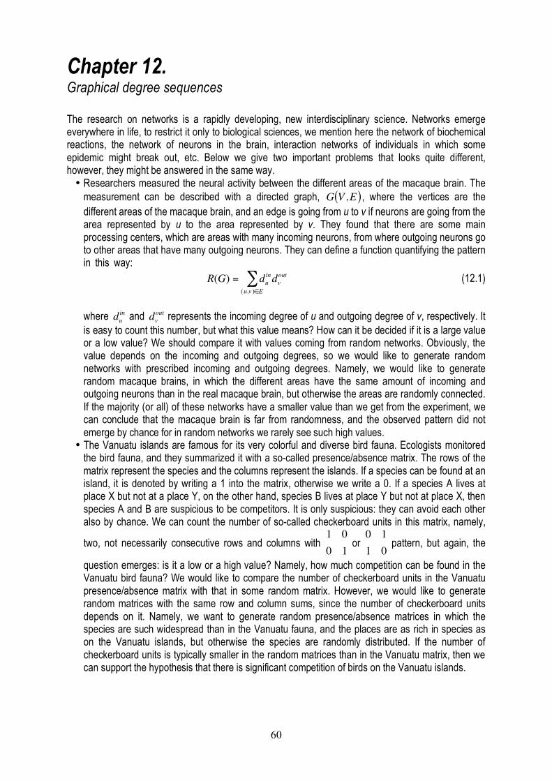
60

Chapter 12. Graphical degree sequences The research on networks is a rapidly developing, new interdisciplinary science. Networks emerge everywhere in life, to restrict it only to biological sciences, we mention here the network of biochemical reactions, the network of neurons in the brain, interaction networks of individuals in which some epidemic might break out, etc. Below we give two important problems that looks quite different, however, they might be answered in the same way. • Researchers measured the neural activity between the different areas of the macaque brain. The

measurement can be described with a directed graph,

!

G V ,E( ), where the vertices are the different areas of the macaque brain, and an edge is going from u to v if neurons are going from the area represented by u to the area represented by v. They found that there are some main processing centers, which are areas with many incoming neurons, from where outgoing neurons go to other areas that have many outgoing neurons. They can define a function quantifying the pattern in this way: x

!

R(G) = duindv

out

(u,v )"E# (12.1)

where

!

duin and

!

dvout represents the incoming degree of u and outgoing degree of v, respectively. It

is easy to count this number, but what this value means? How can it be decided if it is a large value or a low value? We should compare it with values coming from random networks. Obviously, the value depends on the incoming and outgoing degrees, so we would like to generate random networks with prescribed incoming and outgoing degrees. Namely, we would like to generate random macaque brains, in which the different areas have the same amount of incoming and outgoing neurons than in the real macaque brain, but otherwise the areas are randomly connected. If the majority (or all) of these networks have a smaller value than we get from the experiment, we can conclude that the macaque brain is far from randomness, and the observed pattern did not emerge by chance for in random networks we rarely see such high values.

• The Vanuatu islands are famous for its very colorful and diverse bird fauna. Ecologists monitored the bird fauna, and they summarized it with a so-called presence/absence matrix. The rows of the matrix represent the species and the columns represent the islands. If a species can be found at an island, it is denoted by writing a 1 into the matrix, otherwise we write a 0. If a species A lives at place X but not at a place Y, on the other hand, species B lives at place Y but not at place X, then species A and B are suspicious to be competitors. It is only suspicious: they can avoid each other also by chance. We can count the number of so-called checkerboard units in this matrix, namely,

two, not necessarily consecutive rows and columns with

!

1 00 1

or

!

0 11 0

pattern, but again, the

question emerges: is it a low or a high value? Namely, how much competition can be found in the Vanuatu bird fauna? We would like to compare the number of checkerboard units in the Vanuatu presence/absence matrix with that in some random matrix. However, we would like to generate random matrices with the same row and column sums, since the number of checkerboard units depends on it. Namely, we want to generate random presence/absence matrices in which the species are such widespread than in the Vanuatu fauna, and the places are as rich in species as on the Vanuatu islands, but otherwise the species are randomly distributed. If the number of checkerboard units is typically smaller in the random matrices than in the Vanuatu matrix, then we can support the hypothesis that there is significant competition of birds on the Vanuatu islands.

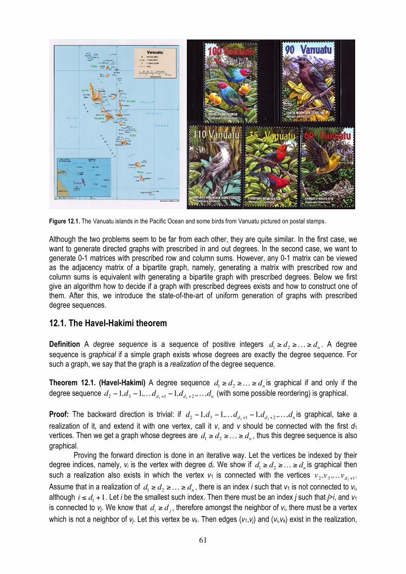
61

Figure 12.1. The Vanuatu islands in the Pacific Ocean and some birds from Vanuatu pictured on postal stamps. Although the two problems seem to be far from each other, they are quite similar. In the first case, we want to generate directed graphs with prescribed in and out degrees. In the second case, we want to generate 0-1 matrices with prescribed row and column sums. However, any 0-1 matrix can be viewed as the adjacency matrix of a bipartite graph, namely, generating a matrix with prescribed row and column sums is equivalent with generating a bipartite graph with prescribed degrees. Below we first give an algorithm how to decide if a graph with prescribed degrees exists and how to construct one of them. After this, we introduce the state-of-the-art of uniform generation of graphs with prescribed degree sequences.

12.1. The Havel-Hakimi theorem Definition A degree sequence is a sequence of positive integers

!

d1 " d2 "K " dn . A degree sequence is graphical if a simple graph exists whose degrees are exactly the degree sequence. For such a graph, we say that the graph is a realization of the degree sequence. Theorem 12.1. (Havel-Hakimi) A degree sequence

!

d1 " d2 "K " dn is graphical if and only if the degree sequence

!

d2 "1,d3 "1,Kdd1 +1 "1,dd1 +2,K,dn (with some possible reordering) is graphical.

Proof: The backward direction is trivial: if

!

d2 "1,d3 "1,Kdd1 +1 "1,dd1 +2,K,dn is graphical, take a

realization of it, and extend it with one vertex, call it v, and v should be connected with the first d1 vertices. Then we get a graph whose degrees are

!

d1 " d2 "K " dn , thus this degree sequence is also graphical. Proving the forward direction is done in an iterative way. Let the vertices be indexed by their degree indices, namely, vi is the vertex with degree di. We show if

!

d1 " d2 "K " dn is graphical then such a realization also exists in which the vertex v1 is connected with the vertices

!

v2,v3,Kvd1 +1.

Assume that in a realization of

!

d1 " d2 "K " dn , there is an index i such that v1 is not connected to vi, although

!

i " d1 +1. Let i be the smallest such index. Then there must be an index j such that j>i, and v1 is connected to vj. We know that

!

di " d j , therefore amongst the neighbor of vi, there must be a vertex

which is not a neighbor of vj. Let this vertex be vk. Then edges (v1,vj) and (vi,vk) exist in the realization,

62

and (v1,vi) and (vi,vk) do not exist. If we delete the before mentioned existing edges and add the not existing edges, we get a realization of

!

d1 " d2 "K " dn in which v1 is connected to vi, thus the first index i’ for which v1 is not connected to vi’ is greater than i. We can repeat this alteration such that eventually v1 is connected to

!

v2,v3,Kvd1 +1. Then deleting v1 and its edges leads to a realization of

!

d2 "1,d3 "1,Kdd1 +1 "1,dd1 +2,K,dn .

The proof is constructive, namely, it is also possible to construct a realization if such exists by following the proof: take n vertices, index it with v1, v2 ... vn. Connect v1 to

!

v2,v3,Kvd1 +1. Then take the

sequence

!

d2 "1,d3 "1,Kdd1 +1 "1,dd1 +2,K,dn , reorder it, moving the vertices together with the

degrees, so we get another degree sequence

!

d'1" d'2 "K " d'n#1. Take the corresponding v’1, connect it to the next d’1 vertices, modify the degrees accordingly, rearrange them, etc. In this way, either we construct a graph with the prescribed sequence or at some point, d1 will be greater than the number of remaining vertices, and thus, the degree sequence is not graphical. Similar theorem is true for bipartite graphs and it is left as an exercise. Similar theorem exists for directed graphs. First we need the definition of bi-degree sequences. Definition A sequence of non-negative integer pairs

!

d1in ,d1

out( ), d2in ,d2out( ),K dnin ,dn

out( ) is called bi-

degree sequence. Such a sequence is called graphical if a simple, directed graph exists whose in and out degrees are the given pairs. Theorem 12.2. (Havel-Hakimi for directed graphs) Let

!

d1in ,d1

out( ), d2in ,d2out( ),K dnin ,dn

out( ) be a bi-

degree sequence. Take any pair

!

diin ,di

out( ) such that

!

diout > 0 and rearrange the remaining pairs into

lexicographically decreasing order

!

d'1in ,d'1

out( ), d'2in ,d2out( ),K d'n"1in ,dn"1

out( ), namely, for each

!

1" i < n #1,

!

diin " di+1

in and

!

diout " di+1

out if

!

diin = di+1

in . Then

!

d1in ,d1

out( ), d2in ,d2out( ),K dnin ,dn

out( ) is

graphical if and only if

!

diin ,0( ) d'1in "1,d'1out( ), d'2in "1,d'2out( ),K d'

d iout

in "1,d'd iout

out( ), d'd iout +1in ,d'

d iout +1

out( )K d'n"1in ,d'n"1

out( ) (12.2)

is also graphical. Proof: Again, the backward direction is trivial: if the degree sequence in (12.2) is graphical, then take a realization of it, take the vertex with degree

!

diin ,0( ) , and connect it with the first

!

diout vertices. Then we

get a realization of

!

d1in ,d1

out( ), d2in ,d2out( ),K dnin ,dn

out( ) .

The forward way is also proved in an analogous way to the proof of Theorem 12.1. We prove if a realization exists for the bi-degree sequence

!

d1in ,d1

out( ), d2in ,d2out( ),K dnin ,dn

out( ) then also a

realization exists in which the outgoing edges of vi are going to

!

v'1 ,v '2Kv'd iout . Assume that this is not

the case, then take the smallest index j such that vi does not have an outgoing edge towards v’j. Then there exists a k > j such that vi does have an outgoing edge towards v’k. Since

!

d jin " dk

in there must be

a vertex v’l such that there is an edge going from v’l to v’j but not to vk. If l is not k, then we can delete edges (vi, v’k,) and (v’l, v’j,) and add edges (vi, v’j,) and (v’l, v’k,). If l is k but

!

d jin > dk

in or there is an edge

going from v’j to v’k, then there still is another l which is not k and there is an edge going from v’l to v’j but not to vk. If l is k,

!

d jin = dk

in and there is no edge going from v’j to v’k, then we can use the fact that

!

d jout " dk

out since the degree pairs are in lexicographically decreasing order, and we must be able to

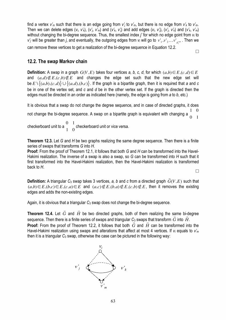
63

find a vertex v’m such that there is an edge going from v’j to v’m, but there is no edge from v’k to v’m. Then we can delete edges (vi, v’k), (v’j, v’m) and (v’k, v’j) and add edges (vi, v’j), (v’j, v’k) and (v’k, v’m) without changing the bi-degree sequence. Thus, the smallest index j’ for which no edge goint from vi to v’j’ will be greater than j, and eventually, the outgoing edges from vi will go to

!

v'1 ,v '2Kv'd iout . Then we

can remove these vertices to get a realization of the bi-degree sequence in Equation 12.2.

12.2. The swap Markov chain Definition: A swap in a graph

!

G(V ,E) takes four vertices a, b, c, d, for which

!

(a,b)" E,(c,d)" E and

!

(a,d)" E,(c,b)" E and changes the edge set such that the new edge set will be

!

E \ (a,b),(c,d){ }" (a,d),(b,c){ } . If the graph is a bipartite graph, then it is required that a and c be in one of the vertex set, and c and d be in the other vertex set. If the graph is directed then the edges must be directed in an order as indicated here (namely, the edge is going from a to b, etc.) It is obvious that a swap do not change the degree sequence, and in case of directed graphs, it does

not change the bi-degree sequence. A swap on a bipartite graph is equivalent with changing a

!

1 00 1

checkerboard unit to a

!

0 11 0

checkerboard unit or vice versa.

Theorem 12.3. Let G and H be two graphs realizing the same degree sequence. Then there is a finite series of swaps that transforms G into H. Proof: From the proof of Theorem 12.1, it follows that both G and H can be transformed into the Havel-Hakimi realization. The inverse of a swap is also a swap, so G can be transformed into H such that it first transformed into the Havel-Hakimi realization, then the Havel-Hakimi realization is transformed back to H.

Definition: A triangular C3 swap takes 3 vertices, a, b and c from a directed graph

!

r G (V ,E) such that

!

(a,b)" E,(b,c)" E,(c,a)" E and

!

(a,c)" E,(b,a)" E,(c,b)" E , then it removes the existing edges and adds the non-existing edges. Again, it is obvious that a triangular C3 swap does not change the bi-degree sequence. Theorem 12.4. Let

!

r G and

!

r H be two directed graphs, both of them realizing the same bi-degree

sequence. Then there is a finite series of swaps and triangular C3 swaps that transform

!

r G into

!

r H .

Proof: From the proof of Theorem 12.2, it follows that both

!

r G and

!

r H can be transformed into the

Havel-Hakimi realization using swaps and alterations that affect at most 4 vertices. If vi equals to v’m then it is a triangular C3 swap, otherwise the case can be pictured in the following way:

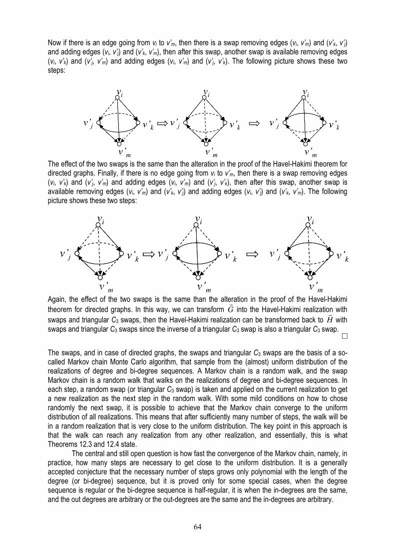
64

Now if there is an edge going from vi to v’m, then there is a swap removing edges (vi, v’m) and (v’k, v’j) and adding edges (vi, v’j) and (v’k, v’m), then after this swap, another swap is available removing edges (vi, v’k) and (v’j, v’m) and adding edges (vi, v’m) and (v’j, v’k). The following picture shows these two steps:

The effect of the two swaps is the same than the alteration in the proof of the Havel-Hakimi theorem for directed graphs. Finally, if there is no edge going from vi to v’m, then there is a swap removing edges (vi, v’k) and (v’j, v’m) and adding edges (vi, v’m) and (v’j, v’k), then after this swap, another swap is available removing edges (vi, v’m) and (v’k, v’j) and adding edges (vi, v’j) and (v’k, v’m). The following picture shows these two steps:

Again, the effect of the two swaps is the same than the alteration in the proof of the Havel-Hakimi theorem for directed graphs. In this way, we can transform

!

r G into the Havel-Hakimi realization with

swaps and triangular C3 swaps, then the Havel-Hakimi realization can be transformed back to

!

r H with

swaps and triangular C3 swaps since the inverse of a triangular C3 swap is also a triangular C3 swap.

The swaps, and in case of directed graphs, the swaps and triangular C3 swaps are the basis of a so-called Markov chain Monte Carlo algorithm, that sample from the (almost) uniform distribution of the realizations of degree and bi-degree sequences. A Markov chain is a random walk, and the swap Markov chain is a random walk that walks on the realizations of degree and bi-degree sequences. In each step, a random swap (or triangular C3 swap) is taken and applied on the current realization to get a new realization as the next step in the random walk. With some mild conditions on how to chose randomly the next swap, it is possible to achieve that the Markov chain converge to the uniform distribution of all realizations. This means that after sufficiently many number of steps, the walk will be in a random realization that is very close to the uniform distribution. The key point in this approach is that the walk can reach any realization from any other realization, and essentially, this is what Theorems 12.3 and 12.4 state. The central and still open question is how fast the convergence of the Markov chain, namely, in practice, how many steps are necessary to get close to the uniform distribution. It is a generally accepted conjecture that the necessary number of steps grows only polynomial with the length of the degree (or bi-degree) sequence, but it is proved only for some special cases, when the degree sequence is regular or the bi-degree sequence is half-regular, it is when the in-degrees are the same, and the out degrees are arbitrary or the out-degrees are the same and the in-degrees are arbitrary.

65

Exercises Exercise 12.1. Prove that the function in Equation 12.1 is the number of directed 3 long paths in the directed graph. Exercise 12.2. Let G and H be two bipartite graphs with the same degree sequence. Show that the adjacency matrices of G and H both contain at least one checkerboard unit. Exercise 12.3. State and prove the Havel-Hakimi theorem for bipartite graphs. Exercise 12.4. Give a realization of the degree sequence 5, 5, 4, 4, 4, 4, 1, 1, 1, 1. Exercise 12.5.* Which are the 0/1 matrices that do not contain any checkerboard unit? Exercise 12.6.* Give an example that the triangular C3 swaps are necessary to transform a directed graph into another one. Exercise 12.7.* Show that in the Havel-Hakimi algorithm an arbitrary vertex can be chosen which is connected to the maximal degree vertices. In each step, we can chose such arbitrary vertex, and thus, we can get several realizations. On the other hand, show that not all realizations of a degree sequence can be constructed in this way. Exercise 12.8** Prove that in case of regular bi-degree sequences, swaps are sufficient to transform any realization into any another realization.