algorithms - lagout theory/compression/fast... · algorithms for video compression and rate con...
TRANSCRIPT

Fast and E�cient Algorithms for Video
Compression and Rate Control
Dzung Tien Hoang and Je�rey Scott Vitter
c D. T. Hoang and J. S. Vitter
Draft, June 20, 1998

ii
Vita
Dzung Tien Hoang was born on April 20, 1968 in Nha Trang, Vietnam. He immi-grated to the United States of America in 1975 with his parents, Dzuyet D. Hoangand Tien T. Tran, and two sisters. He now has three sisters and one brother. Theyhave been living in Harvey, Louisiana.
After graduating in 1986 from the Louisiana School for Math, Science and theArts, a public residential high school in Natchitoches, Louisiana, he attended TulaneUniversity in New Orleans with a full-tuition Dean's Honor Scholarship and graduatedin 1990 with Bachelor of Science degrees in Electrical Engineering and ComputerScience, both with Summa Cum Laude honors.
He joined the Department of Computer Science at Brown University in Providence,Rhode Island, in 1990 under a University Fellowship and later under a National Sci-ence Foundation Graduate Fellowship. He received a Master of Science in ComputerScience from Brown in 1992 and a Doctor of Philosophy in Computer Science fromBrown in 1997. From 1993 to 1996, he was a visiting scholar and a research assistantat Duke University in Durham, North Carolina. From 1991 to 1995, he spent sum-mers working at the Frederick National Cancer Research Facility, the SupercomputingResearch Center, and the IBM T. J. Watson Research Center.
In August 1996, he joined Digital Video Systems, in Santa Clara, California, asa Senior Software Engineer. He is currently a Senior Software Systems Engineer atSony Semiconductor Company of America.
Je�rey Scott Vitter was born on November 13, 1955 in New Orleans, LA.He received a Bachelor of Science with Highest Honors in Mathematics from theUniversity of Notre Dame in 1977, and a Doctor of Philosophy in Computer Sciencefrom Stanford University in 1980. He was on the faculty at Brown University from1980 until 1993. He is currently the Gilbert, Louis, and Edward Lehrman Professorand Chair of the Department of Computer Science at Duke University, where hejoined the faculty in January 1993. He is also Co-Director and a Founding Memberof the Center for Geometric Computing at Duke.
Prof. Vitter is a Guggenheim Fellow, an ACM Fellow, an IEEE Fellow, an NSFPresidential Young Investigator, a Fulbright Scholar, and an IBM Faculty Develop-ment Awardee. He is coauthor of the book Design and Analysis of Coalesced Hashing
and is coholder of patents in the areas of external sorting, prediction, and approxi-
iii

iv
mate data structures. He has written numerous articles and has consulted frequently.He serves or has served on the editorial boards of Algorithmica, Communications of
the ACM, IEEE Transactions on Computers, Theory of Computing Systems (formerlyMathematical Systems Theory: An International Journal on Mathematical Computing
Theory), and SIAM Journal on Computing, and has been a frequent editor of specialissues. He serves as Chair of ACM SIGACT and was previously Member-at-Largefrom 1987{1991 and Vice Chair from 1991{1997. He was on sabbatical in 1986 at theMathematical Sciences Research Institute in Berkeley, and in 1986{1987 at INRIA inRocquencourt, France and at Ecole Normale Sup�erieure in Paris. He is currently anassociate member of the Center of Excellence in Space Data and Information Sciences.
His main research interests include the design and mathematical analysis of al-gorithms and data structures, I/O e�ciency and external memory algorithms, datacompression, parallel computation, incremental and online algorithms, computationalgeometry, data mining, machine learning, and order statistics. His work in analysis ofalgorithms deals with the precise study of the average-case performance of algorithmsand data structures under various models of input. Areas of application include sort-ing, information storage and retrieval, geographic information systems and spatialdatabases, and random sampling and random variate generation. Prof. Vitter's workon I/O-e�cient methods for solving problems involving massive data sets has helpedshape the sub�eld of external memory algorithms, in which disk I/O can be a bot-tleneck. He is investigating complexity measures and tradeo�s involving the numberof parallel disk accesses (I/Os) needed to solve a problem and the amount of timeneeded to update a solution when the input is changed dynamically. He is actively in-volved in developing e�cient techniques for text, image, and video compression, withapplications to GIS, e�cient prediction for data mining, and database and systemsoptimization. Other work deals with machine learning, memory-based learning, androbotics.

Contents
1 Introduction 1
2 Introduction to Video Compression 5
2.1 Digital Video Representation . . . . . . . . . . . . . . . . . . . . . . . 52.1.1 Color Representation . . . . . . . . . . . . . . . . . . . . . . . 62.1.2 Digitization . . . . . . . . . . . . . . . . . . . . . . . . . . . . 6
2.1.2a Spatial Sampling . . . . . . . . . . . . . . . . . . . . 62.1.2b Temporal Sampling . . . . . . . . . . . . . . . . . . . 72.1.2c Quantization . . . . . . . . . . . . . . . . . . . . . . 7
2.1.3 Standard Video Data Formats . . . . . . . . . . . . . . . . . . 82.2 A Case for Video Compression . . . . . . . . . . . . . . . . . . . . . . 102.3 Lossy Coding and Rate-Distortion . . . . . . . . . . . . . . . . . . . . 11
2.3.1 Classical Rate-Distortion Theory . . . . . . . . . . . . . . . . 112.3.2 Operational Rate-Distortion . . . . . . . . . . . . . . . . . . . 112.3.3 Budget-Constrained Bit Allocation . . . . . . . . . . . . . . . 12
2.3.3a Viterbi Algorithm . . . . . . . . . . . . . . . . . . . 142.3.3b Lagrange Optimization . . . . . . . . . . . . . . . . . 14
2.4 Spatial Redundancy . . . . . . . . . . . . . . . . . . . . . . . . . . . 172.4.1 Vector Quantization . . . . . . . . . . . . . . . . . . . . . . . 182.4.2 Block Transform . . . . . . . . . . . . . . . . . . . . . . . . . 182.4.3 Discrete Cosine Transform . . . . . . . . . . . . . . . . . . . . 18
2.4.3a Forward Transform . . . . . . . . . . . . . . . . . . . 192.4.3b Inverse Transform . . . . . . . . . . . . . . . . . . . 192.4.3c Quantization . . . . . . . . . . . . . . . . . . . . . . 192.4.3d Zig-Zag Scan . . . . . . . . . . . . . . . . . . . . . . 20
2.5 Temporal Redundancy . . . . . . . . . . . . . . . . . . . . . . . . . . 202.5.1 Frame Di�erencing . . . . . . . . . . . . . . . . . . . . . . . . 212.5.2 Motion Compensation . . . . . . . . . . . . . . . . . . . . . . 212.5.3 Block-Matching . . . . . . . . . . . . . . . . . . . . . . . . . . 24
2.6 H.261 Standard . . . . . . . . . . . . . . . . . . . . . . . . . . . . . . 242.6.1 Features . . . . . . . . . . . . . . . . . . . . . . . . . . . . . . 252.6.2 Encoder Block Diagram . . . . . . . . . . . . . . . . . . . . . 25
v

vi CONTENTS
2.6.3 Heuristics for Coding Control . . . . . . . . . . . . . . . . . . 272.6.4 Rate Control . . . . . . . . . . . . . . . . . . . . . . . . . . . 27
2.7 MPEG Standards . . . . . . . . . . . . . . . . . . . . . . . . . . . . . 292.7.1 Features . . . . . . . . . . . . . . . . . . . . . . . . . . . . . . 302.7.2 Encoder Block Diagram . . . . . . . . . . . . . . . . . . . . . 312.7.3 Layers . . . . . . . . . . . . . . . . . . . . . . . . . . . . . . . 322.7.4 Video Bu�ering Veri�er . . . . . . . . . . . . . . . . . . . . . 322.7.5 Rate Control . . . . . . . . . . . . . . . . . . . . . . . . . . . 35
3 Motion Estimation for Low Bit-Rate Video Coding 39
3.1 Introduction . . . . . . . . . . . . . . . . . . . . . . . . . . . . . . . . 393.2 PVRG Implementation of H.261 . . . . . . . . . . . . . . . . . . . . . 423.3 Explicit Minimization Algorithms . . . . . . . . . . . . . . . . . . . . 42
3.3.1 Algorithm M1 . . . . . . . . . . . . . . . . . . . . . . . . . . . 423.3.2 Algorithm M2 . . . . . . . . . . . . . . . . . . . . . . . . . . . 433.3.3 Algorithm RD . . . . . . . . . . . . . . . . . . . . . . . . . . . 433.3.4 Experimental Results . . . . . . . . . . . . . . . . . . . . . . . 44
3.4 Heuristic Algorithms . . . . . . . . . . . . . . . . . . . . . . . . . . . 443.4.1 Heuristic Cost Function . . . . . . . . . . . . . . . . . . . . . 453.4.2 Experimental Results . . . . . . . . . . . . . . . . . . . . . . . 49
3.4.2a Static Cost Function . . . . . . . . . . . . . . . . . . 493.4.2b Adaptive Cost Function . . . . . . . . . . . . . . . . 49
3.4.3 Further Experiments . . . . . . . . . . . . . . . . . . . . . . . 513.5 Related Work . . . . . . . . . . . . . . . . . . . . . . . . . . . . . . . 523.6 Discussion . . . . . . . . . . . . . . . . . . . . . . . . . . . . . . . . . 53
4 Bit-Minimization in a Quadtree-Based Video Coder 61
4.1 Quadtree Data Structure . . . . . . . . . . . . . . . . . . . . . . . . . 614.1.1 Quadtree Representation of Bi-Level Images . . . . . . . . . . 624.1.2 Quadtree Representation of Motion Vectors . . . . . . . . . . 63
4.2 Hybrid Quadtree/DCT Video Coder . . . . . . . . . . . . . . . . . . 644.3 Experimental Results . . . . . . . . . . . . . . . . . . . . . . . . . . . 664.4 Previous Work . . . . . . . . . . . . . . . . . . . . . . . . . . . . . . 664.5 Discussion . . . . . . . . . . . . . . . . . . . . . . . . . . . . . . . . . 67
5 Lexicographically Optimal Bit Allocation 69
5.1 Perceptual Quantization . . . . . . . . . . . . . . . . . . . . . . . . . 705.2 Constant Quality . . . . . . . . . . . . . . . . . . . . . . . . . . . . . 715.3 Bit-Production Modeling . . . . . . . . . . . . . . . . . . . . . . . . . 715.4 Bu�er Constraints . . . . . . . . . . . . . . . . . . . . . . . . . . . . 72
5.4.1 Constant Bit Rate . . . . . . . . . . . . . . . . . . . . . . . . 735.4.2 Variable Bit Rate . . . . . . . . . . . . . . . . . . . . . . . . . 745.4.3 Encoder vs. Decoder Bu�er . . . . . . . . . . . . . . . . . . . 75
CONTENTS vii
5.5 Bu�er-Constrained Bit Allocation Problem . . . . . . . . . . . . . . . 755.6 Lexicographic Optimality . . . . . . . . . . . . . . . . . . . . . . . . . 775.7 Related Work . . . . . . . . . . . . . . . . . . . . . . . . . . . . . . . 785.8 Discussion . . . . . . . . . . . . . . . . . . . . . . . . . . . . . . . . . 80
6 Lexicographic Bit Allocation under CBR Constraints 81
6.1 Analysis . . . . . . . . . . . . . . . . . . . . . . . . . . . . . . . . . . 826.2 CBR Allocation Algorithm . . . . . . . . . . . . . . . . . . . . . . . . 88
6.2.1 DP Algorithm . . . . . . . . . . . . . . . . . . . . . . . . . . . 896.2.2 Correctness of DP Algorithm . . . . . . . . . . . . . . . . . . 906.2.3 Constant-Q Segments . . . . . . . . . . . . . . . . . . . . . . . 906.2.4 Verifying a Constant-Q Allocation . . . . . . . . . . . . . . . . 906.2.5 Time and Space Complexity . . . . . . . . . . . . . . . . . . . 91
6.3 Related Work . . . . . . . . . . . . . . . . . . . . . . . . . . . . . . . 916.4 Discussion . . . . . . . . . . . . . . . . . . . . . . . . . . . . . . . . . 92
7 Lexicographic Bit Allocation under VBR Constraints 95
7.1 Analysis . . . . . . . . . . . . . . . . . . . . . . . . . . . . . . . . . . 967.2 VBR Allocation Algorithm . . . . . . . . . . . . . . . . . . . . . . . . 104
7.2.1 VBR Algorithm . . . . . . . . . . . . . . . . . . . . . . . . . . 1047.2.2 Correctness of VBR Algorithm . . . . . . . . . . . . . . . . . 1057.2.3 Time and Space Complexity . . . . . . . . . . . . . . . . . . . 107
7.3 Discussion . . . . . . . . . . . . . . . . . . . . . . . . . . . . . . . . . 107
8 A More E�cient Dynamic Programming Algorithm 109
9 Real-Time VBR Rate Control 111
10 Implementation of Lexicographic Bit Allocation 113
10.1 Perceptual Quantization . . . . . . . . . . . . . . . . . . . . . . . . . 11310.2 Bit-Production Modeling . . . . . . . . . . . . . . . . . . . . . . . . . 113
10.2.1 Hyperbolic Model . . . . . . . . . . . . . . . . . . . . . . . . . 11410.2.2 Linear-Spline Model . . . . . . . . . . . . . . . . . . . . . . . 115
10.3 Picture-Level Rate Control . . . . . . . . . . . . . . . . . . . . . . . . 11710.3.1 Closed-Loop Rate Control . . . . . . . . . . . . . . . . . . . . 11710.3.2 Open-Loop Rate Control . . . . . . . . . . . . . . . . . . . . . 11810.3.3 Hybrid Rate Control . . . . . . . . . . . . . . . . . . . . . . . 119
10.4 Bu�er Guard Zones . . . . . . . . . . . . . . . . . . . . . . . . . . . . 11910.5 Encoding Simulations . . . . . . . . . . . . . . . . . . . . . . . . . . . 120
10.5.1 Initial Experiments . . . . . . . . . . . . . . . . . . . . . . . . 12010.5.2 Coding a Longer Sequence . . . . . . . . . . . . . . . . . . . . 129
10.6 Limiting Lookahead . . . . . . . . . . . . . . . . . . . . . . . . . . . . 13410.7 Related Work . . . . . . . . . . . . . . . . . . . . . . . . . . . . . . . 134
viii CONTENTS
10.8 Discussion . . . . . . . . . . . . . . . . . . . . . . . . . . . . . . . . . 135
11 Extensions of the Lexicographic Framework 137
11.1 Applicability to Other Coding Domains . . . . . . . . . . . . . . . . . 13711.2 Multiplexing VBR Streams over a CBR Channel . . . . . . . . . . . . 138
11.2.1 Introduction . . . . . . . . . . . . . . . . . . . . . . . . . . . . 13811.2.2 Multiplexing Model . . . . . . . . . . . . . . . . . . . . . . . . 13911.2.3 Lexicographic Criterion . . . . . . . . . . . . . . . . . . . . . . 14111.2.4 Equivalence to CBR Bit Allocation . . . . . . . . . . . . . . . 142
11.3 Bit Allocation with a Discrete Set of Quantizers . . . . . . . . . . . . 14211.3.1 Dynamic Programming . . . . . . . . . . . . . . . . . . . . . . 14311.3.2 Lexicographic Extension . . . . . . . . . . . . . . . . . . . . . 143
Bibliography 143
A Appendix 153

List of Figures
2.1 Block diagram of a video digitizer. . . . . . . . . . . . . . . . . . . . 62.2 Scanning techniques for spatial sampling of a video image. . . . . . . 72.3 Example of uniform quantization. . . . . . . . . . . . . . . . . . . . . 82.4 Color subsampling formats, as speci�ed in the MPEG-2 standard. . . 92.5 Rate-distortion function for a Gaussian source with � = 1. . . . . . . 122.6 Sample operational rate-distortion plot. . . . . . . . . . . . . . . . . . 132.7 Comparison of coders in a rate-distortion framework. . . . . . . . . . 132.8 Example of a trellis constructed with the Viterbi algorithm. . . . . . 152.9 Graphical interpretation of Lagrange-multiplier method. . . . . . . . 172.10 Typical quantization matrix applied to 2D-DCT coe�cients. . . . . . 202.11 Zig-zag scan for coding quantized transform coe�cients . . . . . . . . 202.12 Block diagram of a simple frame-di�erencing coder. . . . . . . . . . . 212.13 Block diagram of a generic motion-compensated video encoder. . . . . 222.14 Illustration of frames types and dependencies in motion compensation. 232.15 Reordering of frames to allow for causal interpolative coding. . . . . . 232.16 Illustration of the block-translation model. . . . . . . . . . . . . . . . 242.17 Structure of a macroblock. . . . . . . . . . . . . . . . . . . . . . . . . 252.18 Block diagram of a p� 64 source coder. . . . . . . . . . . . . . . . . . 262.19 Heuristic decision diagrams for coding control from Reference Model
8 [5]. . . . . . . . . . . . . . . . . . . . . . . . . . . . . . . . . . . . . 282.20 Block diagram of rate control in a typical video coding system. . . . . 292.21 Feedback function controlling quantization scale based on bu�er fullness. 302.22 Block diagram of a typical MPEG encoder. . . . . . . . . . . . . . . . 312.23 Block diagram of the MPEG Video Bu�ering Veri�er. . . . . . . . . . 332.24 Block diagram of a �xed-delay CBR video transmission system. . . . 332.25 Block diagram of a stored-video system using double bu�ering. . . . . 34
3.1 Distribution of bits for intraframe coding of the Miss America sequence. 413.2 Comparison of explicit-minimization motion estimation algorithms . . 453.3 Density plots of DCT coding bits vs. MAD prediction error. . . . . . 473.4 Density plots of MSE reconstruction distortion vs. MAD prediction error. 483.5 Results of static heuristic cost function. . . . . . . . . . . . . . . . . . 543.6 Results of adaptive heuristic cost function. . . . . . . . . . . . . . . . 55
ix

x LIST OF FIGURES
3.7 Frame 27 of the Miss America sequence as encoded using the PVRGand explicit-minimization motion estimation algorithms. . . . . . . . 56
3.8 Frame 27 of the Miss America sequence as encoded using the heuristicmotion estimation algorithms. . . . . . . . . . . . . . . . . . . . . . . 57
3.9 Estimated motion vectors for frame 27 of the Miss America sequencefor the PVRG, RD, H1-WH, and H2-WH coders. . . . . . . . . . . . 58
3.10 Performance of motion estimation algorithms on eight test sequences. 593.11 Distribution of bits for coding the Miss America sequence with adaptive
heuristics. . . . . . . . . . . . . . . . . . . . . . . . . . . . . . . . . . 60
4.1 A simple quadtree and corresponding image. . . . . . . . . . . . . . . 624.2 Representation of a triangle using a quadtree of depth 5. . . . . . . . 634.3 Quadtree representation of a motion �eld. . . . . . . . . . . . . . . . 644.4 MSE vs. Rate for Trevor . . . . . . . . . . . . . . . . . . . . . . . . . 66
5.1 Sample plot of bu�er fullness for CBR operation. . . . . . . . . . . . 745.2 Sample plot of bu�er fullness for VBR operation. . . . . . . . . . . . 76
6.1 Sketch for proof of Lemma 6.2. . . . . . . . . . . . . . . . . . . . . . 836.2 Illustration of search step in dynamic programming algorithm. . . . . 89
10.1 Several instances of a simple \hyperbolic" bit-production model. . . . 11510.2 Example of a linear-spline interpolation model. . . . . . . . . . . . . . 11710.3 Guard zones to safeguard against under ow and over ow of VBV bu�er.11910.4 Evolution of bu�er fullness for CBR coders. . . . . . . . . . . . . . . 12310.5 Evolution of bu�er fullness for VBR coders. . . . . . . . . . . . . . . 12410.6 Nominal quantization scale for CBR coders. . . . . . . . . . . . . . . 12510.7 Nominal quantization scale for VBR coders. . . . . . . . . . . . . . . 12610.8 PSNR for CBR coders. . . . . . . . . . . . . . . . . . . . . . . . . . . 12710.9 PSNR for VBR coders. . . . . . . . . . . . . . . . . . . . . . . . . . . 12810.10Evolution of bu�er fullness for coding IBM Commercial. . . . . . . . 13110.11Nominal quantization scale for coding IBM Commercial. . . . . . . . 13210.12PSNR for coding IBM Commercial. . . . . . . . . . . . . . . . . . . . 133
11.1 Example of how three VBR bitstreams can be multiplexed into thesame channel as two CBR bitstreams, for a statistical multiplexinggain of 1.5. . . . . . . . . . . . . . . . . . . . . . . . . . . . . . . . . . 139
11.2 System for transmitting multiple sequences over a single channel. . . 14011.3 Block diagram of encoder/multiplexer. . . . . . . . . . . . . . . . . . 14011.4 Operation of multiplexer. . . . . . . . . . . . . . . . . . . . . . . . . . 14011.5 Block diagram of demultiplexer/decoder. . . . . . . . . . . . . . . . . 141

List of Tables
3.1 Distribution of bits for intraframe coding of the Miss America sequence 40
3.2 Results of static heuristic cost function. . . . . . . . . . . . . . . . . . 49
3.3 Results of adaptive heuristic cost function. . . . . . . . . . . . . . . . 54
10.1 Parameters for MPEG-2 Simulation Group software encoder used toencode the SIF-formatted video clips. . . . . . . . . . . . . . . . . . . 121
10.2 Summary of initial coding experiments. . . . . . . . . . . . . . . . . . 122
10.3 Parameters for MPEG-2 Simulation Group software encoder used toencode the IBM commercial. . . . . . . . . . . . . . . . . . . . . . . . 130
10.4 Summary of coding simulations with IBM Commercial. . . . . . . . . 131
xi

Chapter 1
Introduction
In this book, we investigate the compression of digital data that consist of a sequenceof symbols chosen from a �nite alphabet. In order for data compression to be mean-ingful, we assume that there is a standard representation for the uncompressed datathat codes each symbol using the same number of bits. For example, digital videocan be represented by a sequence of frames, and each frame is an image composed ofpixels, which are typically represented using a binary code of a �xed length. Com-pression is achieved when the data can be represented with an average length persymbol that is less than that of the standard representation.
Not all forms of information are digital in nature. For example, audio, image,and video exist at some point as waveforms that are continuous both in amplitudeand in time. Information of this kind is referred to as analog signals. In order to berepresentable in the digital domain, analog signals must be discretized in both timeand amplitude. This process is referred to as digital sampling. Digitally sampled datais therefore only an approximation of the original analog signal.
Data compression methods can be classi�ed into two broad categories: lossless
and lossy. As its name suggests, in lossless coding, information is preserved by thecompression and subsequent decompression operations. The types of data that aretypically compressed losslessly include natural language texts, database �les, sen-sitive medical images, scienti�c data, and binary executables. Of course, losslesscompression techniques can be applied to any type of digital data; however, thereis no guarantee that compression will actually be achieved for all cases. Althoughdigitally sampled analog data is inherently lossy, no additional loss is incurred whenlossless compression is applied.
On the other hand, lossy coding does not preserve information. In lossy coding,the amount of compression is typically variable and is dependent on the amount ofloss that can be tolerated. Lossy coding is typically applied to digitally sampled dataor other types of data where some amount of loss can be tolerated. The amount ofloss that can be tolerated is dependent to the type of data being compressed, andquantifying tolerable loss is an important research area in itself.
1

2 CHAPTER 1. INTRODUCTION
By accepting a modest amount of loss, a much higher level of compression can beachieved with lossy methods than lossless ones. For example, a digital color imagecan typically be compressed losslessly by a factor of roughly two to four. Lossytechniques can compress the same image by a factor of 20 to 40, with little or nonoticeable distortion. For less critical applications, the amount of compression canbe increased even further by accepting a higher level of distortion.
To stress the importance of data compression, it should be noted that some appli-cations would not be realizable without data compression. For example, a two-hourmovie would require about 149 gigabytes to be stored digitally without compression.The proposed Digital Video Disk (DVD) technology would store the same movie incompressed form using only 4.7 gigabytes on a single-sided optical disk. The e�cacyof DVD, therefore, relies on the technology to compress digital video and associatedaudio with a compression ratio of about 32:1, while still delivering satisfactory �delity.
A basic idea in data compression is that most information sources of practicalinterest are not random, but possess some structure. Recognizing and exploiting thisstructure is a major theme in data compression. The amount of compression thatis achievable depends on the amount of redundancy or structure present in the datathat can be recognized and exploited. For example, by noting that certain letters orwords in English texts appear more frequently than others, we can represent themusing fewer bits than the less frequently occurring letters or words. This is exactlythe idea behind Morse Code, which represents letters using a varying number of dotsand dashes. The recognition and exploitation of statistical properties of a data sourceare ideas that form the basis for much of lossless data compression.
In lossy coding, there is a direct relationship between the length of an encodingand the amount of loss, or distortion, that is incurred. Redundancy exists whenan information source exhibits properties that allow it to be coded with fewer bitswith little or no perceived distortion. For example, in coding speech, distortion inhigh frequency bands is not as perceptible as that in lower frequency bands. As aresult, the high frequency bands can be coded with less precision using fewer bits.The nature of redundancy for lossy coding, especially as it relates to video coding, isexplored in Chapter 2.
In data compression, there is a natural tradeo� between the speed of a compressorand the level of compression that it can achieve. In order to achieve greater com-pression, we generally require more complex and time-consuming algorithms. In thismanuscript, we examine a range of operational points within the tradeo� possibilitiesfor the application of video compression.
Motion Estimation at Low Bit Rates
In Chapter 3, we explore the speed-compression tradeo�s possible with a range ofmotion estimation techniques operating within a low-bit-rate video coder that adheresto the H.261 international standard for video coding. At very low rates, hybrid video

3
coders that employ motion compensation in conjunction with transform coding of theresidual typically spends a signi�cant portion of the bandwidth to code the motioninformation. We focus on motion estimation with hopes of improving the compressionperformance.
Initially, we construct motion estimation algorithms that explicitly minimize bitrate and a combination of rate and distortion. In coding experiments, these computa-tionally intensive algorithms produce better compression (with comparable quality)compared to the standard motion estimation algorithm, which does not require asmuch computation. Based on insights gained from the explicit minimization algo-rithms, we propose a new technique for motion estimation that minimizes a quicklycomputed heuristic function of rate and distortion. The new technique gives com-pression e�ciency comparable to the computationally intensive explicit-minimizationalgorithms while running almost as fast as the standard algorithm.
In Chapter 4, the bit-minimization philosophy is further applied to a non-standard quadtree-based video coder that codes motion information hierarchically us-ing variable-sized blocks. The motivation is to explore the limits of bit-minimizationwhen applied to an e�cient scheme for coding motion vectors. By designing thequadtree encoding so that a subtree is coded independently of other disjoint sub-trees, we are able to compute motion vectors that globally minimize the total bitrate using a dynamic programming algorithm. Experimental results con�rm that thequadtree-based coder gives additional gains over the H.261-based coders.
Optimal Rate Control
In Chapters 5 through 11, we focus our attention on optimal rate control algorithmsfor video coders. Existing optimal rate control techniques typically regulate the cod-ing rate to minimize a sum-distortion measure. While these techniques can leveragethe wealth of tools from least-mean-square optimization theory, they do not guaranteeconstant-quality video, an objective often mentioned in the literature. We propose aframework that casts rate control as a resource allocation problem with continuousvariables, non-linear constraints, and a novel lexicographic optimality criterion thatis motivated for uniform video quality. With this framework, we rede�ne the conceptof coding e�ciency to better re ect the constancy in quality that is generally desiredfrom a video coder.
Rigorous analysis within this framework reveals a set of necessary and su�cientconditions for optimality for coding at both constant and variable bit rates. Withthese conditions, we are able to construct polynomial-time algorithms for optimal ratecontrol. Experimental implementations of these algorithms con�rm the theoreticalanalysis and produce encodings that are more uniform in quality than that achievedwith existing rate control methods. As evidence of the generality and exibility of theframework, we show how to extend the framework to allocate bits among multiplevariable-bit-rate bitstreams that are to be transmitted over a common constant-bit-

4 CHAPTER 1. INTRODUCTION
rate channel and to encompass the case of discrete variables.

Chapter 2
Introduction to Video Compression
In this chapter, we present an introduction to aspects of video compression that willbe useful for understanding the later chapters. We begin by describing the generationand representation of digital video. With standard representations de�ned, we thenmotivate video compression with several illustrative examples that underscore theneed for lossy compression. To better understand the tradeo�s inherent in lossycoding systems, an introduction to rate-distortion theory and practice is presented.Next, we describe existing international standards for video coding and present anoverview of the fundamentals of these standards. This chapter is by no means intendedto be comprehensive; for an in-depth introduction to video coding fundamentals, thereader is referred to [2, 26, 57, 59].
2.1 Digital Video Representation
Video belongs to a class of information called continuous media. Continuous me-dia is characterized by the essentially continuous manner in which the informationis presented.1 This is in contrast to discrete media, in which there is no essentialcontinuous temporal component. Text, images, and graphics are examples of discretemedia, while movies, sound, and computer animation are examples of continuousmedia. Even though a slide show is a time-based presentation of images, it is not acontinuous medium since each image is viewed as an individual item instead of a partof a bigger entity. On the other hand, a video clip, while also consisting of a sequenceof images, is a continuous medium since each image is perceived in the context ofpast and future images.
For compression to be meaningful, a standard representation should be de�nedfor the data to be compressed. In this section, we give an overview of some of themore popular standard representations for digital video that are in use today.
1The information may be discrete in representation, but it should be presented to give an illusion
of continuity.
5

6 CHAPTER 2. INTRODUCTION TO VIDEO COMPRESSION
amplifierdigitized
videosensor
filter
red/green/blue
temporalraster
scanner samplerquantizer
Figure 2.1: Block diagram of a video digitizer.
2.1.1 Color Representation
Excluding synthetic (computer-generated) sources, video originates in the physi-cal world. In a general sense, video can be characterized as a time-varying, two-dimensional mix of electromagnetic signals. Being too general, this characterizationis not practical for representing visual information relevant to human observers. Al-though visible light consists of a continuum of wavelengths, it has been known forseveral centuries that a small set of primary colors, mixed in the right proportions,can simulate any perceived color. In painting, for example, one system of primarycolors is cyan, magenta, and yellow; this is a subtractive system since the absenceof all primary colors yields the color white. Red, green, and blue light sources formanother set of primary colors; this is an additive system since the presence of all theprimary colors at their maximum intensities results in the perception of the colorwhite. This phenomenon of color perception is caused by the way that the humaneye detects and processes light, which makes it possible to represent a visual imageas a set of three intensity signals in two spatial dimensions.
2.1.2 Digitization
In order to be processed by computers, analog video that is captured by a light sen-sor must �rst be digitized. Digitization of video consists of three steps: 1) spatialsampling, 2) temporal sampling, and 3) quantization. A block diagram of the digiti-zation process is depicted in Figure 2.1 for one color component. The steps need notbe performed in the order indicated and some steps can even be combined into oneoperation.
2.1.2a Spatial Sampling
Spatial sampling consists of taking measurements of the underlying analog signal at a�nite set of sampling points in a �nite viewing area (or frame). To simply the process,the sampling points are restricted to lie on a lattice, usually a rectangular grid, sayof size N �M . The two dimensional set of sampling points are transformed into aone-dimensional set through a process called raster scanning. The two main waysto perform raster scanning are shown in Figure 2.2: progressive and interlaced. Ina progressive (or non-interlaced) scan, the sampling points are scanned from left toright and top to bottom. In an interlaced scan, the points are divided into odd and

2.1. DIGITAL VIDEO REPRESENTATION 7
(a) Progressive Scan (b) Interlaced Scan
Figure 2.2: Scanning techniques for spatial sampling of a video image.
even scan lines. The odd lines are scanned �rst from left to right and top to bottom.Then the even lines are scanned. The odd (respectively, even) scan lines make upa �eld. In an interlaced scan, two �elds make up a frame. It is important to notethat the odd and even �elds are sampled and displayed at di�erent time instances.Therefore the time interval between �elds in an interlaced scan is half of that betweenframes. Interlaced scanning is commonly used for television signals and progressivescanning is typically used for �lm and computer displays.
2.1.2b Temporal Sampling
The human visual system is relatively slow in responding to temporal changes. Bytaking at least 16 samples per second at each grid point, an illusion of motion is main-tained. This observation is the basis for motion picture technology, which typicallyperforms temporal sampling at a rate of 24 frames/sec. For television, sampling ratesof 25 and 30 frames/sec are commonly used. (With interlaced scanning the numberof �elds per second is twice the number of frames per second.)
2.1.2c Quantization
After spatial and temporal sampling, the video signal consists of a sequence of contin-uous intensity values. The continuous intensity values are incompatible with digitalprocessing, and one more step is needed before this information can be processed bya digital computer. The continuous intensity values are converted to a discrete set ofvalues in a process called quantization (or discretization.
Quantization can be viewed as a mapping from a continuous domain to a discrete

8 CHAPTER 2. INTRODUCTION TO VIDEO COMPRESSION
-6
-4
-2
0
2
4
6
-8 -7 -6 -5 -4 -3 -2 -1 0 1 2 3 4 5 6 7 8
Qua
ntiz
ed v
alue
Continuous value
Figure 2.3: Example of uniform quantization.
range.2 A particular quantization mapping is called a quantizer. An example is shownin Figure 2.3. In the �gure, there are eleven discrete quantization levels, also calledbins. Each bin has an associated size, which is the extent of the continuous valuesthat map to that bin. In the example, each bin, except for the bins for �5, 0, and5, has the same size, which is sometimes referred to as the quantizer step size. Thistype of quantizer is called a uniform quantizer.
A binary encoding can be assigned to each of the bins. Typically the initialquantization of a continuous source is done using a number of quantization levelsthat is a power of 2, so that a �xed number of bits can be used to represent thequantized value.3 This process of representing a continuous value by a �nite numberof levels using a binary code is often referred to as pulse code modulation (PCM).Thus, after spatial sampling, temporal sampling, and quantization, we have N �Mdata points, commonly called pixels or pels, represented using a �xed number of bits.
2.1.3 Standard Video Data Formats
To promote the interchange of digital video data, several formats for representingvideo data have been standardized. We now review some of the more popular standardrepresentations.
The CCIR-601 [4] format for video frames speci�es spatial sampling of 720� 480and temporal sampling at 30 frames/sec for NTSC (U.S. and Japan) television sys-tems and 720� 576 at 25 frames/sec for PAL (Europe) television systems. Color is
2This de�nition is intended also to encompass mappings from a discrete domain to a discreterange.
3Further quantization of digitized data may use a number of quantization levels that is not apower of 2 and employ variable-length entropy coding.

2.1. DIGITAL VIDEO REPRESENTATION 9
Luminance samples Chrominance samples
(a) 4:2:2 subsampling
Luminance samples Chrominance samples
(b) 4:2:0 subsampling
Figure 2.4: Color subsampling formats, as speci�ed in the MPEG-2 standard.
represented using three components: a luminance (Y) component and two chromi-nance components (Cb and Cr). The luminance component encodes the brightnessor intensity of each pixel and the chrominance components encode the color values.4
Each component is quantized linearly using eight bits. For NTSC (respectively, PAL),there are 720� 480 (720� 576) luminance values, one for each pixel, and 360� 480(360 � 576) values for each chrominance component. The chrominance componentsare subsampled horizontally with respect to the luminance component to take advan-tage of reduced human sensitivity to color. This subsampling process is referred toas the 4:2:2 format and is depicted in Figure 2.4(a).
The Source Input Format (SIF) speci�es spatial sampling of 360 � 240 (respec-tively, 360 � 288) and temporal sampling at 30 (25) frames/sec for NTSC (PAL)television systems. As with CCIR-601, color is represented using three components:Y, Cb, and Cr. Each component is quantized linearly using eight bits. For NTSC (re-spectively, PAL), there are 360�240 (360�288) luminance values, one for each pixel,and 180�120 (180�144) values for each chrominance component. This subsamplingformat is referred to as the 4:2:0 format5 and is depicted in Figure 2.4(b).
One drawback with the CCIR-601 and SIF formats is that they specify di�erent
4The Y-Cb-Cr color space is related to the red-green-blue (RGB) color space by a matrix multi-plication.
5This should not be confused with the older 4:1:1 format in which the chrominance componentsare subsampled by a factor of 4 only in the horizontal direction.

10 CHAPTER 2. INTRODUCTION TO VIDEO COMPRESSION
spatial and temporal sampling parameters for NTSC and PAL systems. As its namesuggests, the Common Intermediate Format (CIF) was proposed as a bridge betweenNTSC and PAL. As with CCIR-601, color is represented using three components, eachquantized linearly using eight bits. The CIF format uses 4:2:0 color subsampling withan image size of 352� 288. Temporal sampling is set at 30 frames/sec. For use withPAL systems, the CIF format requires conversion of the frame rate to 25 frames/sec.For NTSC systems, a spatial resampling may be necessary.
For videoconferencing and other low-bit-rate, low-resolution applications, a scaled-down version of CIF called Quarter-CIF (or QCIF) is commonly used. QCIF speci�esan image with half the resolution of CIF in each spatial dimension: 176 � 144. Formany low-bit-rate applications, the frame rate is reduced from 30 frames/sec to aslow as �ve frames/sec.
2.2 A Case for Video Compression
Now that we have standard representations for digital video, we can estimate thecompression ratio required for typical applications.
For a two-hour movie encoded in NTSC CCIR-601 format, the uncompressedvideo representation would require about 149 gigabytes to store:
# bytes = (720�480+2�360�480) bytesframe
�30framessecond
�3600secondshour
�2 hours = 1:493�1011 bytes:
In order to store the movie on one single-sided digital video disk (DVD), which hasa capacity of 4.7 gigabytes, we need to compress the video by a factor of about 32:1.To allow room for audio and other auxiliary data (such as text captioning), an evenhigher compression ratio is needed.
As another example, consider low-bit-rate videoconferencing over a 28.8 kbits/secmodem. Assuming that the uncompressed video is encoded in QCIF format at10 frames/sec, the uncompressed rate is computed to be:
#bits
second= (176 � 144 + 2 � 88 � 144) bytes
frame� 8 bitsbyte
� 10framessecond
= 4:055 � 106 bits
second:
To transmit video in this format over a 28.8 kbits/sec modem would require a compres-sion ratio of 141:1. At such a high compression ratio, depending upon the complexityof the video sequence, the quality of the compressed video may have to be sacri�ced.Alternatively, the frame rate could be reduced to increase the image quality, at theexpense of increased jerkiness in the motion.
The above examples show why compression is a must for some important digitalvideo applications. For example, without compression, a single-sided DVD can holdless than four minutes of CCIR-601 digital video!
2.3. LOSSY CODING AND RATE-DISTORTION 11
2.3 Lossy Coding and Rate-Distortion
The examples in Section 2.2 show that existing video applications require high com-pression ratios, over an order of magnitude higher than what is typically possible forthe lossless compression methods. These high levels of compression can be realizedonly if we accept some loss in �delity between the uncompressed and compressedrepresentations. There is a natural tradeo� between the size of the compressed rep-resentation and the �delity of the reproduced images. This tradeo� between rate anddistortion is quanti�ed in rate-distortion theory.
2.3.1 Classical Rate-Distortion Theory
Let D be a measure of distortion according to some �delity criterion and R be thenumber of bits in a compressed representation of an information source. In classicalrate-distortion theory, as pioneered by Claude Shannon [78], a rate-distortion func-tion, R(D), is de�ned to be the theoretical lower bound on the best compressionachievable as a function of the desired distortion D for a given information source, byany compressor. In general, the �delity criterion can be any valid metric; in practice,a squared-error distortion is often used; that is, D(x; x̂) = (x� x̂)2.
For a discrete source, R(0) is simply the entropy of the source and corresponds tolossless coding (D = 0). In cases where the distortion is bounded above by Dmax, thenR(Dmax) = 0. Furthermore, it can be shown that R(D) is a non-increasing convexfunction of D (see, e.g., [17]).
For some speci�c information sources and distortion measures, closed form ex-pressions for the rate-distortion function have been determined. As an example, for azero-mean Gaussian source with variance �2 and a squared-error distortion measure,
R(D) =
(12log2
�2
D; 0 � D � �2;
0; D > �2:
This is plotted for � = 1 in Figure 2.5.
2.3.2 Operational Rate-Distortion
In practice, classical rate-distortion theory is not directly applicable to complex en-coding and decoding systems since sources are typically not well-characterized andR(D) is di�cult, if not impossible, to determine. Even though not directly com-putable, the existence of a hypothetical rate-distortion function for a given type ofinformation source allows a comparison to be made between competing encodingsystems and algorithms.
A more practical approach is taken in [12, 79]. By measuring actual rates and dis-tortion achieved by the coder under study, an operational rate-distortion plot similarto Figure 2.6 can be constructed. It is sometimes useful to show the convex hull of

12 CHAPTER 2. INTRODUCTION TO VIDEO COMPRESSION
0
0.5
1
1.5
2
2.5
3
0 0.2 0.4 0.6 0.8 1 1.2 1.4 1.6 1.8 2
R(D
)
D
Figure 2.5: Rate-distortion function for a Gaussian source with � = 1.
the data points to �ll in the gap between points. Data points are typically generatedby varying the level of quantization or other coding parameters under study.
By plotting operational rate-distortion curves for various competing coders, acomparison can be made of their e�ectiveness. A basic idea is that the more e�ec-tive and capable a coder is, the closer is its operational rate-distortion curve to thehypothetical rate-distortion function. In Figure 2.7, Coder 1 performs better thanCoder 2 for rates greater than about 600 bits per coding unit , where a coding unit isa generic term for a block of data. At rates less than 600 bits/unit, Coder 2 performsbetter.
The mean square error (MSE) distortion measure is commonly used in the litera-ture since it is a convenient measure that lends itself to mathematical analysis usingleast-mean-square theory. For images and video, however, MSE is not an ideal mea-sure since it is not a good model of human visual perception. For example, in manycases, two encodings with the same MSE can have remarkably di�erent perceptualquality. In keeping with convention, we will assume the use of MSE as the distortionmeasure, unless otherwise stated.
2.3.3 Budget-Constrained Bit Allocation
A common problem that serves well to illustrate the operational rate-distortion frame-work is the budget-constrained bit allocation problem. The problem is stated below.Without loss of generality, quantization is the coding parameter to be adjusted.
Problem 2.1 Given a set of quantizers fq1; q2; : : : ; qMg, a sequence of blocks hx1; x2; : : : xNi,and a target bit budget B, determine an assignment of quantizers Q =

2.3. LOSSY CODING AND RATE-DISTORTION 13
0
200
400
600
800
1000
0 2 4 6 8 10
Rat
e (b
its/u
nit)
Distortion (MSE)
Empirical DataConvex Hull
Figure 2.6: Sample operational rate-distortion plot. Plotted is rate versus averagedistortion.
0
200
400
600
800
1000
1200
1400
1600
0 2 4 6 8 10
Rat
e (b
its/u
nit)
Distortion (MSE)
Hypothetical R(D)Coder 1Coder 2
Figure 2.7: Comparison of coders in a rate-distortion framework.

14 CHAPTER 2. INTRODUCTION TO VIDEO COMPRESSION
hQ1; Q2; : : : ; QNi to each block that minimizes a distortion measure D(Q) and
uses R(Q) � B bits.
2.3.3a Viterbi Algorithm
Problem 2.1 can be solved using a dynamic programming algorithm commonly re-ferred to as the Viterbi algorithm (VA) [22, 83]. Assuming that quantization alwaysproduces an integral number of bits, the Viterbi algorithm works by �rst construct-ing a trellis of nodes and then �nding a shortest path through the trellis. Each noderepresents a state and each edge a transition between states. For the bit allocationproblem, we identify each state with a tuple (b; t; d; p), where t is a time index, b is thetotal number of bits used in an allocation for the sequence of blocks hx1; x2; : : : ; xti, dis the minimum sum distortion for any allocation to those blocks using exactly b bits,and p is a pointer back to a previous state. There is a single start state labeled(0; 0; 0; 0).
Starting with the start state, we construct the trellis by adding an edge for eachchoice of quantizer and creating a corresponding set of new states. The new statesrecord the number of bits and minimum distortion for all choices of quantizer forcoding the �rst block. There may be more than one edge entering a new state ifmore than one quantizer results in the same number of bits. However, only theminimum distortion is recorded as d, and p is made to point to a source state thatresults in the minimum distortion. In case more than one incoming edge producesthe minimum distortion, the pointer can point to any of the edges with the minimumdistortion. This process is repeated so that new states for time index k + 1 areconstructed by adding edges corresponding to the quantization of block xk+1 to thestates with time index k. In the trellis construction, we prune out those states whosebit consumption exceeds the bit budget B. After all the states with time index Nhave been constructed, we pick a state with time index N that has the minimumdistortion. A bit allocation can then be constructed by following the pointers p backfrom the end state to the start state.
A simple example with M = 2 and N = 3 is shown in Figure 2.8 to illustrate theViterbi algorithm. In the example, the shaded node marks a state that exceeds thebit budget B and can be pruned. An optimal path is shown with thick edges. As inthis example, there may be more than one path with the minimum distortion.
2.3.3b Lagrange Optimization
Although the Viterbi algorithm �nds an optimal solution to Problem 2.1, it is com-putationally expensive. There could potentially be an exponential number of statesgenerated, on the order of MN .
In [79], Shoham and Gersho give an e�cient bit allocation algorithm based onthe Lagrange-multiplier method [21]. In this method, Problem 2.1, a constrained

2.3. LOSSY CODING AND RATE-DISTORTION 15
Time
Bits
(0,0,0,0)
budget B
Figure 2.8: Example of a trellis constructed with the Viterbi algorithm. The shadednode marks a state that exceeds the bit budget B and can be pruned. An optimalpath is shown with thick edges. Note that there may be more than one path with theminimum distortion.
optimization problem, is transformed to the following unconstrained optimizationproblem.
Problem 2.2 Given a set of quantizers fq1; q2; : : : ; qMg, a sequence of blocks hx1; x2; : : : xNi,and a parameter �, determine an assignment of quantizers Q = hQ1; Q2; : : : ; QMi toeach block that minimizes the cost function C�(Q) = D(Q) + �R(Q).
Here, the parameter � is called the Lagrange multiplier. Let Q�(�) denote anoptimal solution given � and R�(�) � R(Q�(�)) denote the resulting total numberof bits allocated. Note that there may be more than one solution with a given �.It can be shown that a solution to Problem 2.2 is also a solution to Problem 2.1when R�(�) = B. This is proved in [21], and we reproduce the theorem and proof aspresented in [79].
Theorem 2.1 For any � � 0, a solution Q�(�) to Problem 2.2 is also a solution to
Problem 2.1 with the constraint R(Q) � B, where B = R�(�).
Proof : For the solution Q�, we have
D(Q�) + �R(Q�) � D(Q) + �R(Q)
for all quantizer allocations Q. Equivalently, we have
D(Q�)�D(Q) � �(R(Q)�R(Q�))

16 CHAPTER 2. INTRODUCTION TO VIDEO COMPRESSION
for all quantizer allocations Q. In particular, this result applies for all quantizerallocations Q belonging to the set
S� = fQ : R(Q) � R(Q�)g :
Since � � 0 and R(Q)�R(Q�) � 0 for Q 2 S�, we have
D(Q�)�D(Q) � 0; for Q 2 S�:
Therefore Q� is a solution to the constrained problem, and the theorem is proved. 2
It should be noted that Theorem 2.1 does not guarantee that, in general, a so-lution for the constrained Problem 2.1 can be found by solving the unconstrainedProblem 2.2. Theorem 2.1 only applies for cases where there is a value for � suchthat the number bits used in a solution (there may be more than one for a given �)to Problem 2.2 is the same as the bit budget B in Problem 2.1.
The Lagrange multiplier � can be viewed as determining a tradeo� between rateand distortion. A low value for � favors minimizing distortion over rate, and a highvalue favors minimizing rate over distortion. In the limit, when � = 0, we are min-imizing distortion; as � ! 1, we minimize rate. Lagrange optimization can beinterpreted graphically as shown in Figure 2.9. The minimization of the Lagrangecost function C� can be viewed as �nding the last point or points intersected in therate-distortion plane as a line with slope �� is swept from right to left. In the ex-ample shown, there are two such points. From this graphical view, we can easily seethat the only points that can be selected with Lagrange optimization are those thatlie on the convex hull of the set of all points.
For a given bit budget B, in order to apply the Lagrange-multiplier method, weneed to know what value of � to use. In practice, an iterative search procedure canbe used to determine the proper value. The search procedure takes advantage ofa useful property of Lagrange optimization: the solution rate R(Q�(�)) is a non-increasing function of �. With appropriate initial upper and lower bounds for �, abisection search can be performed to �nd the proper value for �. Details of the searchprocedure can be found in [79].
For an additive distortion measure, the distortion D(Q) can be expressed as
D(Q) =NXi=1
Di(Qi);
where Di(Qi) is the distortion for block i when using the quantizer speci�ed by Qi.If we assume that the coding of each block is independent of the quantization choicesof other blocks, the rate R(Q) can be expressed as
R(Q) =NXi=1
Ri(Qi);

2.4. SPATIAL REDUNDANCY 17
0
200
400
600
800
1000
0 2 4 6 8 10
Rat
e (b
its/u
nit)
Distortion (MSE)
Sweep
Figure 2.9: Graphical interpretation of Lagrange-multiplier method. Lagrange mini-mization can be viewed as �nding the last point(s) intersected by a right-to-left sweepof a line with slope ��. In this example, the two data points circled are found in theminimization.
where Ri(Qi) is the rate for block i when using the quantizer speci�ed by Qi. Theminimization of C� in Problem 2.2 can then be expressed as
minQ
C�(Q) = minQfR(Q) + �D(Q)g
= minQ
(NXi=1
Ri(Qi) + �NXi=1
Di(Qi)
)
=NXi=1
�minQi
fRi(Qi) + �Di(Qi)g�:
That is to say, the cost function C� can be minimized by minimizingRi(Qi)+�Di(Qi)separately for each block.
2.4 Spatial Redundancy
Redundancy exists in a video sequence in two forms: spatial and temporal. Theformer, also called intraframe redundancy, refers to the redundancy that exists withina single frame of video, while the latter, also called interframe redundancy, refers tothe redundancy that exists between consecutive frames within a video sequence.
Reducing spatial redundancy has been the focus of many image compression al-gorithms. Since video is just a sequence of images, image compression techniquesare directly applicable to video frames. Here, we outline some popular image codingtechniques applicable to lossy video coding.

18 CHAPTER 2. INTRODUCTION TO VIDEO COMPRESSION
2.4.1 Vector Quantization
In vector quantization (VQ) [24], an image is segmented into same-sized blocks of pixelvalues. The blocks are represented by a �xed number of vectors called codewords. Thecodewords are chosen from a �nite set called a codebook. This is analogous to thequantization described in Section 2.1.2 except that now quantization is performed onvectors instead of scalar values. The size of the codebook a�ects the rate (numberof bits needed to encode each vector) as well as the distortion; a bigger codebookincreases the rate and decreases the average distortion while a smaller codebook hasthe opposite e�ects.
With vector quantization, encoding is more computationally intensive than de-coding. Encoding requires searching the codebook for a representative codeword foreach input vector, while decoding requires only a table lookup. Usually, the samecodebook is used by the encoder and the decoder. The codebook generation processis itself computationally demanding. As with lossless dictionary coding, a VQ code-book can be constructed statically, semi-adaptively, or adaptively. Some applicationsof VQ in video compression can be found in [23, 84].
2.4.2 Block Transform
In block-transform coding, an image is divided into blocks, as with vector quantiza-tion. Each block is mathematically transformed into a di�erent representation, whichis then quantized and coded. The mathematical transform is chosen so as to \pack"most of the useful information into a small set of coe�cients. The coe�cients arethen selectively quantized so that after quantization most of the \unimportant" coef-�cients are 0 and can be ignored, while the \important" coe�cients are retained. Inthe decoder, a dequantization process is followed by an inverse transformation.
Block-transform coding can be viewed as an instance of vector quantization wherethe codebook is determined by the transform and quantization performed. Viewedin this way, for any source, a vector quantizer can be designed that will be at leastas good (in a rate-distortion sense) as a particular block transform. A motivationfor using block transforms is that for certain block transforms with fast algorithms,encoding can be done faster than full-blown vector quantization. However, with blocktransforms, decoding has approximately the same complexity as encoding, which ismore complex than decoding with vector quantization.
2.4.3 Discrete Cosine Transform
For images, the two-dimensional discrete cosine transform (2D-DCT) is a popularblock transform that forms the basis of the lossy JPEG standard [65] developed bythe Joint Photographic Experts Group. Because of its success within JPEG, the 2D-DCT has been adopted by many video coding standards as well. We now describethe mathematical basis of the DCT and show how it is applied to code an image.

2.4. SPATIAL REDUNDANCY 19
2.4.3a Forward Transform
The JPEG standard speci�es a block size of 8� 8 for performing the 2D-DCT. Thisblock size is small enough for the transform to be quickly computed but big enoughfor signi�cant compression. For an 8� 8 block of pixel values f(i; j), the 2D-DCT isde�ned as
F (u; v) =1
4C(u)C(v)
7Xi=0
7Xj=0
f(i; j) cos�u(2i+ 1)
16cos
�v(2j + 1)
16; (2.1)
where F (u; v) are the transform coe�cients and
C(x) =
8><>:
1p2
x = 0;
1 otherwise.
2.4.3b Inverse Transform
To be useful for coding, a block transform needs an inverse transform for purposes ofdecoding. The two-dimensional inverse discrete cosine transform (2D-IDCT) for an8� 8 block is de�ned as
f(i; j) =1
4
7Xu=0
7Xv=0
F (u; v)C(u)C(v) cos�u(2i+ 1)
16cos
�v(2j + 1)
16: (2.2)
2.4.3c Quantization
Since the DCT and IDCT are transform pairs, they do not result in any compressionby themselves. Compression is achieved by subsequent quantization of the transformcoe�cients.
Quantization as applied to transform coe�cients can be viewed as division fol-lowed by integer truncation. Speci�cally, the transform coe�cients are �rst dividedby a (prespeci�ed) matrix of integers that is weighted by a quantization scale. Afterdivision, the results are truncated to integer values. In the dequantization, the quan-tized values are multiplied by the quantization matrix and adjusted according to thequantization scale. Typically 8 to 12 bits of precision are used.
An example of a quantization matrix is shown in Figure 2.10. The coe�cients canbe speci�ed to exploit properties of the human visual system. Since the human eye ismore sensitive to low spatial frequencies and less sensitive to high spatial frequencies,the transform coe�cients corresponding to high spatial frequencies can be quantizedmore coarsely than those for low spatial frequencies. This selective quantization isshown in Figure 2.10.

20 CHAPTER 2. INTRODUCTION TO VIDEO COMPRESSION
266666666666664
8 16 19 22 26 27 29 3416 16 22 24 27 29 34 3719 22 26 27 29 34 34 3822 22 26 27 29 34 37 4022 26 27 29 32 35 40 4826 27 29 32 35 40 48 5826 27 29 34 38 46 56 6927 29 35 38 46 56 69 83
377777777777775
Figure 2.10: Typical quantization matrix applied to 2D-DCT coe�cients.
DC
FrequencyHorizontal
Fre
quen
cyV
ertic
al
0 1 2 3 4 5 6 7
0
1
2
3
4
5
6
7
Figure 2.11: Zig-zag scan for coding quantized transform coe�cients as an one-dimensional sequence. Run-length encoding of zero values results in e�cient coding.
2.4.3d Zig-Zag Scan
Because of the coarse quantization of coe�cients corresponding to high spatial fre-quencies, those coe�cients are often quantized to 0. An e�ective way to code theresulting set of quantized coe�cients is with a combination of a zig-zag scan of thecoe�cients as shown in Figure 2.11 and run-length encoding of consecutive zeros.Typically, the DC coe�cient, F (0; 0), is coded separately from the other coe�cientsand is not included in the zig-zag scan.
2.5 Temporal Redundancy
Successive frames in a video sequence are typically highly correlated, especially forscenes where there is little or no motion. The spatial decorrelation techniques de-scribed in the previous section only operate within a single frame and do not exploitthe redundancy that exists between frames. We now review some basic techniquesfor reducing temporal redundancy.
2.5. TEMPORAL REDUNDANCY 21
Frame Buffer
Frame
Encoder
Frame
Decoder
OutputInput
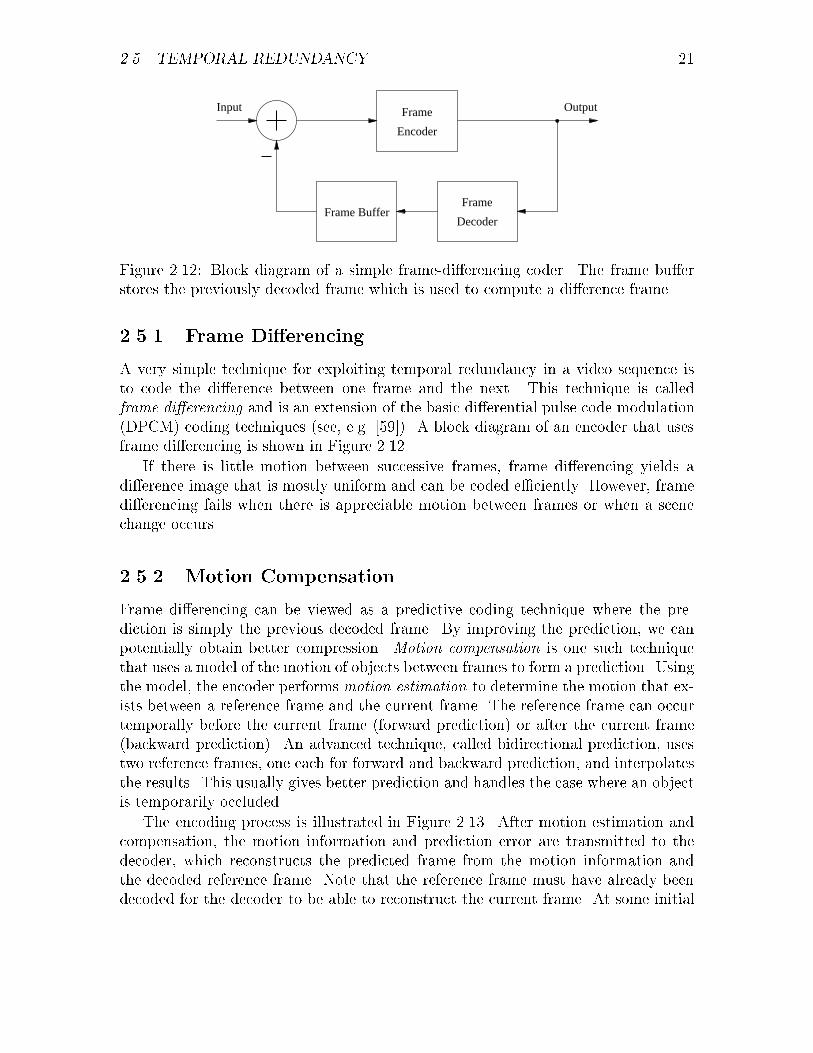
Figure 2.12: Block diagram of a simple frame-di�erencing coder. The frame bu�erstores the previously decoded frame which is used to compute a di�erence frame.
2.5.1 Frame Di�erencing
A very simple technique for exploiting temporal redundancy in a video sequence isto code the di�erence between one frame and the next. This technique is calledframe di�erencing and is an extension of the basic di�erential pulse code modulation(DPCM) coding techniques (see, e.g. [59]). A block diagram of an encoder that usesframe di�erencing is shown in Figure 2.12.
If there is little motion between successive frames, frame di�erencing yields adi�erence image that is mostly uniform and can be coded e�ciently. However, framedi�erencing fails when there is appreciable motion between frames or when a scenechange occurs.
2.5.2 Motion Compensation
Frame di�erencing can be viewed as a predictive coding technique where the pre-diction is simply the previous decoded frame. By improving the prediction, we canpotentially obtain better compression. Motion compensation is one such techniquethat uses a model of the motion of objects between frames to form a prediction. Usingthe model, the encoder performs motion estimation to determine the motion that ex-ists between a reference frame and the current frame. The reference frame can occurtemporally before the current frame (forward prediction) or after the current frame(backward prediction). An advanced technique, called bidirectional prediction, usestwo reference frames, one each for forward and backward prediction, and interpolatesthe results. This usually gives better prediction and handles the case where an objectis temporarily occluded.
The encoding process is illustrated in Figure 2.13. After motion estimation andcompensation, the motion information and prediction error are transmitted to thedecoder, which reconstructs the predicted frame from the motion information andthe decoded reference frame. Note that the reference frame must have already beendecoded for the decoder to be able to reconstruct the current frame. At some initial
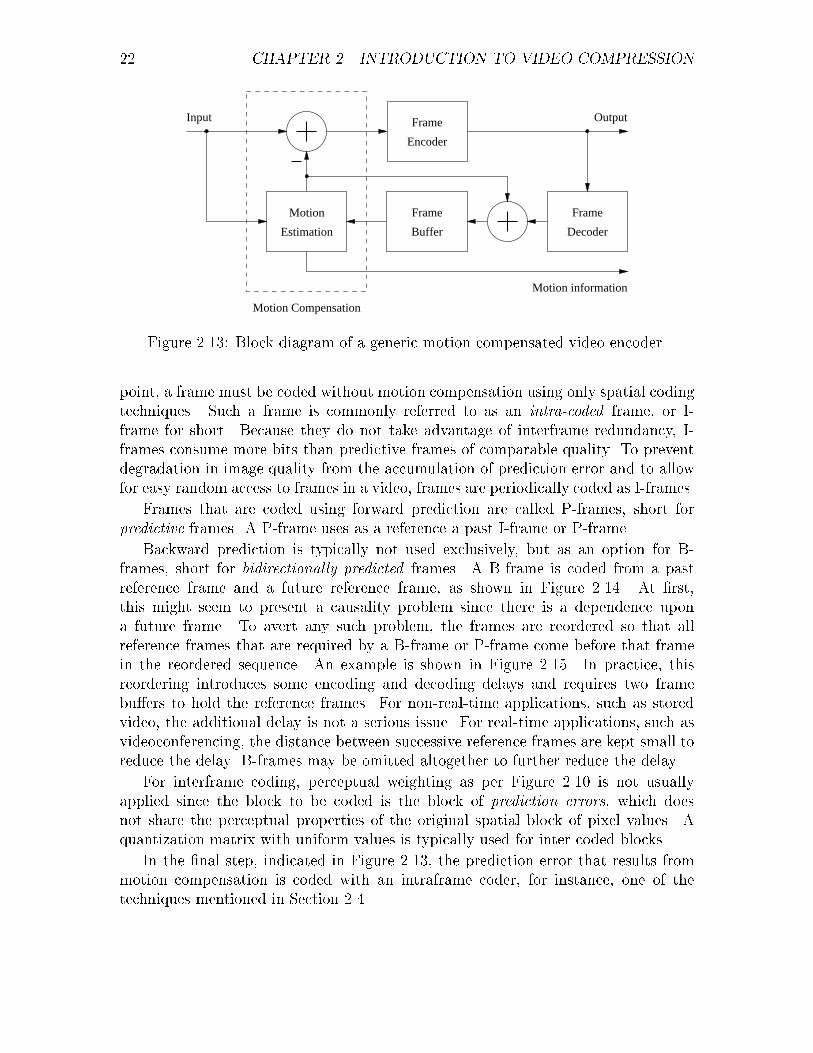
22 CHAPTER 2. INTRODUCTION TO VIDEO COMPRESSION
Motion
Estimation
Frame
Buffer
Frame
Encoder
Frame
Decoder
Input Output
Motion information
Motion Compensation
Figure 2.13: Block diagram of a generic motion-compensated video encoder.
point, a frame must be coded without motion compensation using only spatial codingtechniques. Such a frame is commonly referred to as an intra-coded frame, or I-frame for short. Because they do not take advantage of interframe redundancy, I-frames consume more bits than predictive frames of comparable quality. To preventdegradation in image quality from the accumulation of prediction error and to allowfor easy random access to frames in a video, frames are periodically coded as I-frames.
Frames that are coded using forward prediction are called P-frames, short forpredictive frames. A P-frame uses as a reference a past I-frame or P-frame.
Backward prediction is typically not used exclusively, but as an option for B-frames, short for bidirectionally predicted frames. A B-frame is coded from a pastreference frame and a future reference frame, as shown in Figure 2.14. At �rst,this might seem to present a causality problem since there is a dependence upona future frame. To avert any such problem, the frames are reordered so that allreference frames that are required by a B-frame or P-frame come before that framein the reordered sequence. An example is shown in Figure 2.15. In practice, thisreordering introduces some encoding and decoding delays and requires two framebu�ers to hold the reference frames. For non-real-time applications, such as storedvideo, the additional delay is not a serious issue. For real-time applications, such asvideoconferencing, the distance between successive reference frames are kept small toreduce the delay. B-frames may be omitted altogether to further reduce the delay.
For interframe coding, perceptual weighting as per Figure 2.10 is not usuallyapplied since the block to be coded is the block of prediction errors, which doesnot share the perceptual properties of the original spatial block of pixel values. Aquantization matrix with uniform values is typically used for inter-coded blocks.
In the �nal step, indicated in Figure 2.13, the prediction error that results frommotion compensation is coded with an intraframe coder, for instance, one of thetechniques mentioned in Section 2.4.

2.5. TEMPORAL REDUNDANCY 23
I B PB
Figure 2.14: Illustration of frames types and dependencies in motion compensation.
Frame Type: I B B P B B P B I
Temporal Index: 1 2 3 4 5 6 7 8 9
(a) Original Sequence (Temporal Order)
Frame Type: I P B B P B B I B
Temporal Index: 1 4 2 3 7 5 6 9 8
(b) Reordered Sequence (Encoding Order)
Figure 2.15: Reordering of frames to allow for causal interpolative coding.

24 CHAPTER 2. INTRODUCTION TO VIDEO COMPRESSION
Current FrameReference Frame
Figure 2.16: Illustration of the block-translation model.
2.5.3 Block-Matching
A motion model that is commonly used is the block-translation model developed byJain and Jain [39]. In this model, an image is divided into non-overlapping rectangu-lar blocks. Each block in the predicted image is formed by a translation of a similarlyshaped source region from the reference frame. The source region needs not coincidewith the block boundaries. This model does not consider any rotation or scaling ofthe blocks, simpli�ng the motion estimation procedure at the expense of decreasedaccuracy. A motion vector may be speci�ed in integer or fractional pixel (pel) incre-ments. Fractional-pel motion compensation involves interpolation of the pixel valuesin the source block. The block-translation model is illustrated in Figure 2.16. Foreach block, the encoder transmits a motion vector that speci�es the displacement inthe translation model.
Motion estimation algorithms using the block-translation model are commonlycalled block-matching algorithms since the procedure involves matching (regularly-positioned) blocks in the current frame with (arbitrarily-positioned) blocks in thereference frame. Because of its simplicity, block-matching is commonly used withcurrent video coding standards.
2.6 H.261 Standard
In 1990, the International Telegraph and Telephone Consultative Committee(CCITT)6 approved an international standard for video coding at bit rates of p� 64kbits/sec, where p is an integer between 1 and 30, inclusive [6, 52]. O�cially knownas CCITT Recommendation H.261, it is informally called the p� 64 standard and isintended for low-bit-rate applications such as videophone and videoconferencing. We
6The CCITT has since changed its name to the International Telecommunication Union (ITU-T).
2.6. H.261 STANDARD 25
CR CB
Y
Y
Y
Y
8
8 8
8
16
16
Figure 2.17: Structure of a macroblock.
now provide a summary of some key aspects of the standard.
2.6.1 Features
The p � 64 standard uses a combination of block-matching motion compensation(BMMC) and 2D-DCT coding, as described in Sections 2.4.2 and 2.5.3. Since p �64 is intended for real-time videoconferencing applications, there is a requirementfor low encoding delay. This precludes the use of bidirectional predictive motioncompensation. Therefore only intraframe coding and forward predictive coding areused, with a predicted block depending only upon the previous frame. The real-timerequirement also restricts the complexity of higher-level algorithms, such as motionestimation and rate control.
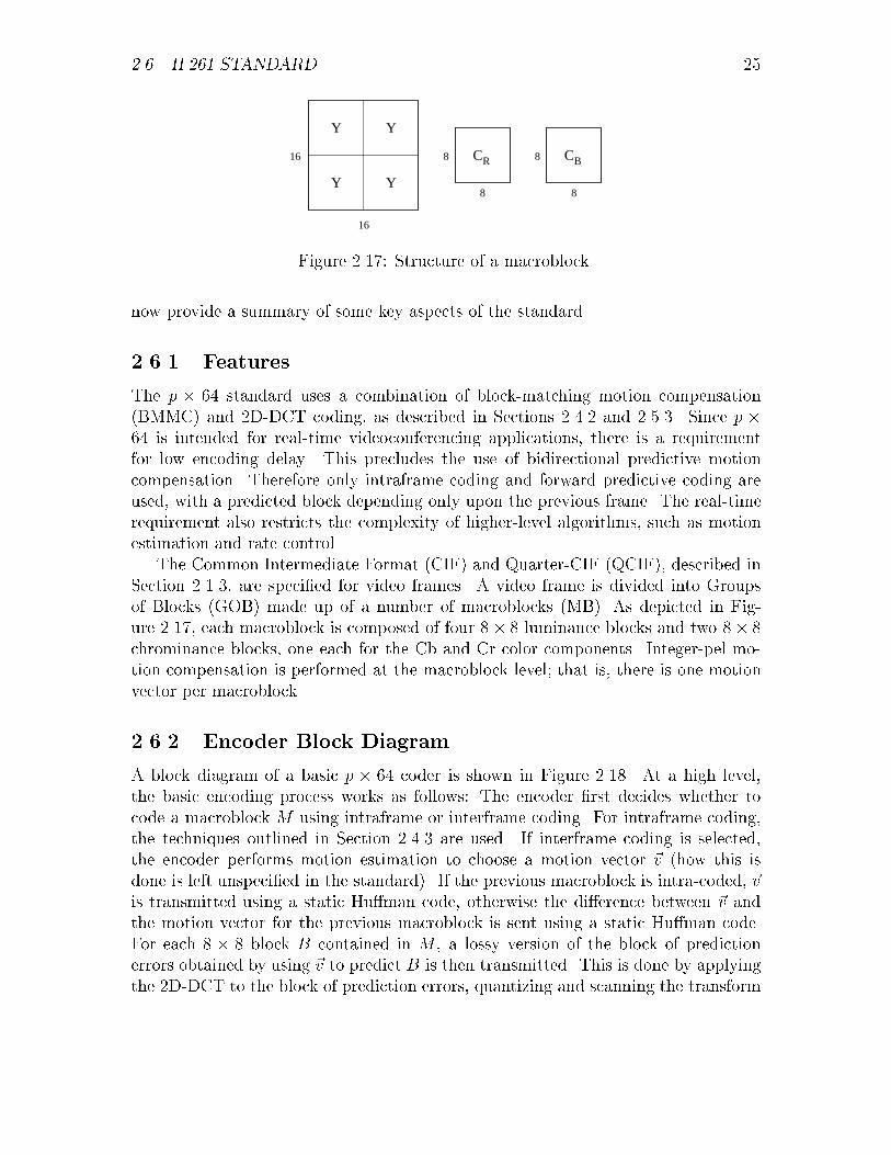
The Common Intermediate Format (CIF) and Quarter-CIF (QCIF), described inSection 2.1.3, are speci�ed for video frames. A video frame is divided into Groupsof Blocks (GOB) made up of a number of macroblocks (MB). As depicted in Fig-ure 2.17, each macroblock is composed of four 8� 8 luminance blocks and two 8� 8chrominance blocks, one each for the Cb and Cr color components. Integer-pel mo-tion compensation is performed at the macroblock level; that is, there is one motionvector per macroblock.
2.6.2 Encoder Block Diagram
A block diagram of a basic p � 64 coder is shown in Figure 2.18. At a high level,the basic encoding process works as follows: The encoder �rst decides whether tocode a macroblock M using intraframe or interframe coding. For intraframe coding,the techniques outlined in Section 2.4.3 are used. If interframe coding is selected,the encoder performs motion estimation to choose a motion vector ~v (how this isdone is left unspeci�ed in the standard). If the previous macroblock is intra-coded, ~vis transmitted using a static Hu�man code, otherwise the di�erence between ~v andthe motion vector for the previous macroblock is sent using a static Hu�man code.For each 8 � 8 block B contained in M , a lossy version of the block of predictionerrors obtained by using ~v to predict B is then transmitted. This is done by applyingthe 2D-DCT to the block of prediction errors, quantizing and scanning the transform

26 CHAPTER 2. INTRODUCTION TO VIDEO COMPRESSION
CC
T Q
T�1
����
PF
���� q
q
q
qa
a���
���
-
-
-
- - -
-
-
-
��
-
-
6 -
-
Video In
p
tqz
q
v
f �
�
�� To VideoMultiplexCoder
T: TransformQ: QuantizerP: Picture Memory with motion-
compensated variable delayF: Loop Filter
CC: Coding Control
p: Flag for INTRA/INTERt: Flag for transmitted or not
qz: Quantizer indicationq: Quantizing index for transform
coe�cientsv: Motion vectorf: Switching on/o� of the loop �lter
?
Q�1
?
?
q
6
q
q
q
?
?
Figure 2.18: Block diagram of a typical p� 64 source coder [6].

2.6. H.261 STANDARD 27
coe�cients, and encoding the results using a run-length/Hu�man coder, as prescribedin Section 2.4.3.
The encoder has the option of changing certain aspects of the above process.First, the encoder may simply not transmit the current macroblock; the decoder isthen assumed to use the corresponding macroblock in the previous frame in its place.If motion compensation is used, there is an option to apply a linear �lter to theprevious decoded frame before using it for prediction.
2.6.3 Heuristics for Coding Control
The p � 64 standard does not specify how to make coding decisions. However, toaid in the evaluation of di�erent coding techniques, the CCITT provides an encodersimulation model called Reference Model 8 (RM8) [5]. Motion estimation is performedto minimize the mean absolute di�erence (MAD) of the prediction errors. A fastthree-step search, instead of an exhaustive full-search, is used for motion estimation.RM8 speci�es several heuristics used to make the coding decisions.
The variance VP of the prediction errors for the luminance blocks inM after motioncompensation using ~v is compared against the variance VY of the original luminanceblocks in M to determine whether to perform intraframe or interframe coding. Theintra/inter decision diagram, as speci�ed in RM8, is plotted in Figure 2.19(a). Ifinterframe motion compensation mode is selected, the decision of whether to usemotion compensation with a zero motion vector or with the estimated motion vectoris made by comparing the MAD of motion compensation with zero motion againstthat with the estimated motion vector. If the zero motion vector is chosen, thisis indicated by a special coding mode and no motion vector is sent. The decisiondiagram, as recommended in [5], are shown in Figure 2.19(b). The loop �lter isenabled if a non-zero motion vector is used. The decision of whether to transmit theblock-transform coe�cients is made individually for each block in a macroblock byconsidering the values of the quantized transform coe�cients. If all the coe�cientsare zero for a block, they are not transmitted for that block.
2.6.4 Rate Control
Video coders often have to operate within �xed bandwidth limitations. Since the p�64standard uses variable-length entropy coding of quantized transform coe�cients andside information, resulting in a variable bit rate, some form of rate control is requiredfor operation on bandwidth-limited channels. For example, if the coder's outputexceeds the channel capacity, then frames could be dropped or the quality decreasedin order to meet the bandwidth constraints. On the other hand, if the coder's outputis well below the channel's capacity, the quality and/or frame-rate can be increasedto better utilize the channel.

28 CHAPTER 2. INTRODUCTION TO VIDEO COMPRESSION
0
32
64
96
128
160
0 32 64 96 128 160
Var
ianc
e of
ori
gina
l blo
ck
Variance of motion compensated prediction error
Interframemotion compensation
Intraframemotion compensation
y=x
(a) Intraframe/interframe decision
0
0.5
1
1.5
2
2.5
3
3.5
4
4.5
5
5.5
0 1 2 3 4 5 6
MA
D w
ith e
stim
ated
mot
ion
vect
or
MAD with zero motion vector
Zero displacementmotion compensation
Motion vectorcompensation
y=x/1.1
0.5
1.5
2.7
(b) Motion vector decision
Figure 2.19: Heuristic decision diagrams for coding control from Reference Model8 [5].

2.7. MPEG STANDARDS 29
QuantizerCoder
EntropyBuffer
Rate
ControllerQs Bf
transform
coefficients
encoded
bitstream
Figure 2.20: Block diagram of rate control in a typical video coding system.
A simple technique for rate control that is speci�ed in RM8 uses a bu�ered en-coding model as shown in Figure 2.20. In this model, the output of the encoder isconnected to a bu�er whose purpose is to even out the uctuations in bit rate. Bymonitoring the fullness of the bu�er, the rate controller can adjust the quantizationscale Qs, which a�ects the encoder's bit rate, to prevent the bu�er from under owingor over owing. In the model, the bu�er is de�ned for the purpose of regulating theoutput bit rate and may or may not correspond to an actual encoder bu�er.
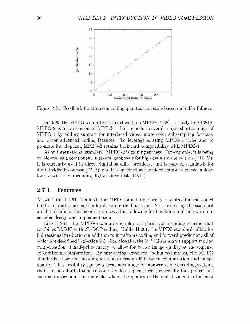
RM8 gives some parameters and prescriptions for the rate control process. Thesize of the bu�er is speci�ed to be p � 6:4 kbits, which translates to a maximumbu�ering delay of 100 ms. For purposes of rate control, the �rst frame is codedusing a �xed quantization scale that is computed from the target bit rate. After the�rst frame is coded, the bu�er is reset to be half full. The quantization scale Qs isdetermined from the bu�er fullness Bf using the formula:
Qs = min(b32Bfc + 1; 31);
where Qs has a integral range of [1; 31], and Bf is normalized to have a real-valuedrange of [0; 1]. This feedback function is plotted in Figure 2.21. The quantizationscale is adjusted once for each GOB (11 macroblocks in RM8).
2.7 MPEG Standards
In 1988, the International Standards Organization (ISO) formed the Moving PicturesExpert Group (MPEG), with the formal designation ISO-IEC/JTC1 SC29/WG11, todevelop standards for the digital encoding of moving pictures (video) and associatedaudio. In 1991, the MPEG committee completed its �rst international standard,MPEG-1 [36, 44], formally ISO 11172.
As a generic video coding speci�cation, MPEG-1 supports multiple image for-mats, including, CIF, SIF, and QCIF. Image sizes up to 4; 095�4; 095 are supported.However, only progressive scan and 4:2:0 color subsampling are supported. WhileMPEG-1 proved successful for the computer entertainment industry, its lack of sup-port for interlaced scan prevented its use in digital television.
30 CHAPTER 2. INTRODUCTION TO VIDEO COMPRESSION
0
5
10
15
20
25
30
35
0 0.2 0.4 0.6 0.8 1
Qua
ntiz
atio
n Sc
ale
Normalized Buffer Fullness
Figure 2.21: Feedback function controlling quantization scale based on bu�er fullness.
In 1990, the MPEG committee started work on MPEG-2 [38], formally ISO 13818.MPEG-2 is an extension of MPEG-1 that remedies several major shortcomings ofMPEG-1 by adding support for interlaced video, more color subsampling formats,and other advanced coding features. To leverage existing MPEG-1 titles and topromote its adoption, MPEG-2 retains backward compatibility with MPEG-1.
As an international standard, MPEG-2 is gaining success. For example, it is beingconsidered as a component in several proposals for high de�nition television (HDTV);it is currently used in direct digital satellite broadcast and is part of standards fordigital video broadcast (DVB); and it is speci�ed as the video compression technologyfor use with the upcoming digital video disk (DVD).
2.7.1 Features
As with the H.261 standard, the MPEG standards specify a syntax for the codedbitstream and a mechanism for decoding the bitstream. Not covered by the standardare details about the encoding process, thus allowing for exibility and innovation inencoder design and implementation.
Like H.261, the MPEG standards employ a hybrid video coding scheme thatcombines BMMC with 2D-DCT coding. Unlike H.261, the MPEG standards allow forbidirectional prediction in addition to intraframe coding and forward prediction, all ofwhich are described in Section 2.5. Additionally, the MPEG standards support motioncompensation at half-pel accuracy to allow for better image quality at the expenseof additional computation. By supporting advanced coding techniques, the MPEGstandards allow an encoding system to trade o� between computation and imagequality. This exibility can be a great advantage for non-real-time encoding systemsthat can be a�orded time to code a video sequence well, especially for applicationssuch as movies and commercials, where the quality of the coded video is of utmost

2.7. MPEG STANDARDS 31
DCT
Coding Control
Quantizer
MotionEstimator
FrameBuffers
InverseQuantizer
IDCT
CompensationMotion
Predictor
VLC Encoderand Multiplexer
Embedded
Decoder
0
Inter/Intra
Q
Input
Picture Type
BufferBitstream
Inter/Intra
Motion vectors
Motion vectors
Buffer fullness
Figure 2.22: Block diagram of a typical MPEG encoder.
importance since the video will be played many times. However, by using a subset ofthe coding features, the MPEG standards can also be used for real-time applicationssuch as videoconferencing, news, and other live broadcasts.
2.7.2 Encoder Block Diagram
A basic encoder block diagram is shown in Figure 2.22, with the embedded decoderhighlighted. The structure of the encoder is very similar to that in Figure 2.18.The main di�erences, as outlined above, are hidden in the Coding Control, MotionEstimation, and Motion Compensation blocks.

32 CHAPTER 2. INTRODUCTION TO VIDEO COMPRESSION
2.7.3 Layers
In the syntax of the MPEG standards, a video sequence is partitioned into a hierar-chy of layers. The presence of a layer in the bitstream is indicated by a start code
indicating the layer type followed by a header that speci�es parameters for that layer.At the top of the hierarchy is the sequence layer. The sequence header speci�es in-formation for the entire video sequence, such as the frame size, frame rate, bit rate,and quantization matrix . Below the sequence layer is the group of pictures (GOP)layer. A GOP is structured as a set of contiguous frames that contains at least oneI-frame. A GOP can start with either a B-frame or an I-frame and end with eitheran I-frame or a P-frame. The GOP structure is designed to support random access,indexing, and editing. An example of a GOP unit can be found in Figure 2.14(a).If a GOP begins with a frame that does not depend upon a preceding frame, it canbe decoded and displayed independently of the previous GOP and is called a closed
GOP. GOP's that are not closed are referred to as open.
Below the GOP layer is the picture layer. The picture header contains informationabout each picture7 coded, such as picture type (I, P, or B) and temporal reference. Apicture is divided into slices, which consists of a segment of consecutive macroblocks.Dividing a picture into slices limits the e�ects of transmission errors and allows thedecoder to recover from these errors.
A macroblock consists of a number of 8 � 8 blocks of intensity and chrominancevalues. The number of blocks in a macroblock depends upon the color subsamplingscheme used (see Figure 2.4). For 4:2:0 subsampling, the structure of a macroblockis shown in Figure 2.17. For 4:2:2 subsampling, a macroblock contains four Y blocks,two Cb blocks, and two Cr blocks. MPEG-2 supports an additional color subsamplingmode, 4:4:4, in which the Cb and Cr color components have the same spatial resolu-tion as the luminance component Y. Thus for 4:4:4 color subsampling, a macroblockconsists of a total of twelve blocks.
As with JPEG and H.261, the 8� 8 block is the basic unit for DCT coding andquantization.
2.7.4 Video Bu�ering Veri�er
In addition to de�ning a bitstream syntax and decoding process, the MPEG videostandards de�ne an idealized decoder model called the Video Bu�ering Veri�er
(VBV). The purpose of the VBV is to put quanti�able limits on the variability in thecoding rate such that an encoded bitstream can be decoded with reasonable bu�er-ing requirements. As diagrammed in Figure 2.23, the VBV consists of a decoderbu�er, a decoder, and a display unit. The decoder bu�er stores the incoming bits forprocessing by the decoder. At regular display intervals, the decoder instantaneously
7With progressive scan, a picture in MPEG's terminology is equivalent to what we have beencalling a frame. With interlaced scan, a picture may refer to a single �eld.

2.7. MPEG STANDARDS 33
Decoder
BufferDisplay
bitstreamencoded
channel
rate R
high
bandwidth
connection
Decoder
max
size Bvbv
Figure 2.23: Block diagram of the MPEG Video Bu�ering Veri�er.
Encoder Buffer
fixed-delayCBR channel
Buffer Decoder
Figure 2.24: Block diagram of a �xed-delay CBR video transmission system.
removes, decodes, and displays the earliest picture in the bu�er. It should be stressedthat the VBV is only a idealized decoder model and not a prescription of how to builda decoder or how an actual decoder would function. The VBV model, however, isuseful in establishing rate constraints on encoded video such that the encoding wouldbe decodable with speci�ed bu�ering requirements.
The VBV has three prescribed modes of operation: a constant bit rate (CBR)mode and two variable bit rate (VBR) modes. MPEG-1 supports only the CBRmode while MPEG-2 supports all three modes. In CBR mode, bits enter the decoderbu�er at a constant rate Rmax as speci�ed in the sequence header. Initially, the bu�eris empty and �lls for a prespeci�ed amount of time before bits for the �rst picture areremoved and decoded. Afterwards, the bu�er continues to �ll at the channel rate Rmax
while the decoder removes bits for coded pictures at regular display intervals. TheCBR mode models operation of a decoder connected to a constant-bit-rate channelwith a �xed channel delay, as shown in Figure 2.24.
The amount of time that the start code for a given picture is to reside in theVBV bu�er before that picture is decoded is speci�ed in the picture header with aparameter called vbv delay.8 In CBR mode, vbv delay is related to the VBV bu�erfullness Bf in the following manner:
vbv delay =90000 �Bf
Rmax
:
In the �rst VBR mode, the compressed bits for picture n enter the bu�er at a con-stant rate R(n) that may vary from picture to picture, up to the maximum rate Rmax
speci�ed in the sequence header. The relationship between R(n) and vbv delay isas follows:
R(n) =sn
�(n)� �(n + 1) + t(n + 1)� t(n) ;
8The parameter vbv delay is coded as an integer in the range [0; 65534] and is expressed in unitsof 1/90000 sec.
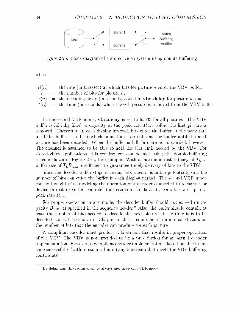
34 CHAPTER 2. INTRODUCTION TO VIDEO COMPRESSION
Disk
Buffer 1
Buffer 2
VideoBufferingVerifier
Figure 2.25: Block diagram of a stored-video system using double bu�ering.
where
R(n) = the rate (in bits/sec) at which bits for picture n enter the VBV bu�er;sn = the number of bits for picture n;�(n) = the decoding delay (in seconds) coded in vbv delay for picture n, andt(n) = the time (in seconds) when the nth picture is removed from the VBV bu�er.
In the second VBR mode, vbv delay is set to 65535 for all pictures. The VBVbu�er is initially �lled to capacity at the peak rate Rmax before the �rst picture isremoved. Thereafter, in each display interval, bits enter the bu�er at the peak rateuntil the bu�er is full, at which point bits stop entering the bu�er until the nextpicture has been decoded. When the bu�er is full, bits are not discarded, however.The channel is assumed to be able to hold the bits until needed by the VBV. Forstored-video applications, this requirement can be met using the double-bu�eringscheme shown in Figure 2.25, for example. With a maximum disk latency of TL, abu�er size of TLRmax is su�cient to guarantee timely delivery of bits to the VBV.
Since the decoder bu�er stops receiving bits when it is full, a potentially variablenumber of bits can enter the bu�er in each display period. The second VBR modecan be thought of as modeling the operation of a decoder connected to a channel ordevice (a disk drive for example) that can transfer data at a variable rate up to apeak rate Rmax.
For proper operation in any mode, the decoder bu�er should not exceed its ca-pacity BVBV as speci�ed in the sequence header.9 Also, the bu�er should contain atleast the number of bits needed to decode the next picture at the time it is to bedecoded. As will be shown in Chapter 5, these requirements impose constraints onthe number of bits that the encoder can produce for each picture.
A compliant encoder must produce a bitstream that results in proper operationof the VBV. The VBV is not intended to be a prescription for an actual decoderimplementation. However, a compliant decoder implementation should be able to de-code successfully (within resource limits) any bitstream that meets the VBV bu�eringconstraints.
9By de�nition, this requirement is always met in second VBR mode.

2.7. MPEG STANDARDS 35
2.7.5 Rate Control
As with H.261, the MPEG standards do not specify how to perform rate control. Toallow for testing and experimentation using a common set of encoder routines, MPEGcreated a series of test models. Here, we describe the rate control strategy outlinedin the MPEG-2 Test Model 5 (TM5) [37]. In TM5, rate control is broken down intothree steps:
1. Target bit allocation. In this step, the complexity of the current picture isestimated based on the encoding of previous pictures to allocate a number ofbits to code the picture.
2. Rate control. A reference quantization scale is determined using a virtualbu�er in a feedback loop to regulate the coding rate so as to achieve the targetbit allocation.
3. Adaptive quantization. The reference quantization scale is modulated ac-cording to the spatial activity in each macroblock to determine the actual quan-tization scale with which to code the macroblock.
Target Bit Allocation. The number of bits to be allocated to a picture dependsupon its type: I, P, or B. For each picture type, there is a complexity model thatattempts to relate the number of bits that would result from coding a picture of agiven type to the quantization scale used. The complexity models are of the form
Si =Xi
Qi
; Sp =Xp
Qp
; Sb =Xb
Qb
;
where S, X, and Q denote number of bits, complexity, and quantization scale, re-spectively; and the subscript indicate the picture type.
Initially the complexity values are set to:
Xi =160 � bit rate
115; Xp =
60 � bit rate115
; Xb =42 � bit rate
115;
where bit rate is measured in bits/sec.After a picture of a given type is coded, its associated complexity model is updated
based on the average quantization scale used and number of bits produced:
Xi = SiQi; Xp = SpQp; Xb = SbQb:
Bit allocation is performed with the goal that the average bit rate is achievedat the GOP layer. A corresponding number of bits is assigned to code each GOP.Bits are allocated to each picture in a GOP based on the complexity models, thenumber of bits available to code the remaining pictures in the GOP, and the numberof remaining I, P, and B pictures in the GOP. Let N be the total number of pictures

36 CHAPTER 2. INTRODUCTION TO VIDEO COMPRESSION
in a GOP. Let Ni, Np, and Nb be the number of remaining I, P, and B pictures,respectively. The bit target for each type of picture is calculated according to
Ti = max
8<: R
1 + NpXp
KpXi
+ NbXb
KbXi
;bit rate
8 � picture rate
9=;
Tp = max
8<: R
Np +NbKpXb
KbXp
;bit rate
8 � picture rate
9=;
Tb = max
8<: R
Nb +NpKbXp
KpXb
;bit rate
8 � picture rate
9=;
where Kp and Kb are constants that depend upon the quantization matrices,10 andR is the number of bits available to code the remaining pictures in the GOP.
After all the pictures in a GOP have been coded, any di�erence between the targetand actual bit allocation is carried over to the next GOP.
Rate Control. Given a target bit allocation for a picture, a virtual encoding bu�eris used to determine a reference quantization scale similar to the procedure in Sec-tion 2.6.4 for the p � 64 standard. A separate virtual bu�er is maintained for eachpicture type. The reference quantization scale is computed for each macroblock fromthe bu�er fullness as:
Qj =31 � djr
;
where Qj is the reference quantization for macroblock j, dj is the bu�er fullness,and r is a reaction parameter given by
r =2 � bit ratepicture rate
:
Adaptive Quantization. The rate control step provides a reference quantizationscale to code each macroblock. The reference quantization scale is modulated withan activity factor that is determined from a measure of the spatial activity of themacroblock. The rationale is that a macroblock that has little spatial activity, suchas a smooth region, should be quantized �ner than a macroblock with high spatialactivity, such as a textured region, since quantization error is typically more notice-able in smooth regions than in textured regions. This is an attempt at equalizingperceptual quality for a given quantization scale.
For macroblock j, an activity factor actj is computed as one plus the minimum ofthe variances of the luminance blocks within the macroblock. A normalized activityfactor is then computed based on the average of the activity factor of the last encoded
10For the matrices speci�ed in TM5, Kp = 1:0 and Kb = 1:4.

2.7. MPEG STANDARDS 37
picture:
Nact =2 � actj + avg act
actj + 2 � avg act:
For the �rst picture, avg act = 400. The actual quantization scale Qs used to codethe macroblock is computed as:
Qs = min(Qj �Nact; 31):
It should be noted that the TM5 rate control strategy does not take into ac-count the VBV and therefore does not guarantee VBV compliance. Also, TM5 onlyperforms rate control for CBR operation and not for VBR.

38 CHAPTER 2. INTRODUCTION TO VIDEO COMPRESSION

Chapter 3
Motion Estimation for Low
Bit-Rate Video Coding
Low Bit-Rate Video Coding
3.1 Introduction
As described in the previous chapter, hybrid video coding that combines block-matching motion compensation (BMMC) with transform coding of the residual isa popular scheme for video compression, adopted by international standards suchas H.261 [6, 52] and the MPEG standards [36, 38, 44]. Motion compensation is atechnique that exploits the typically strong correlation between successive frames ofa video sequence by coding motion vectors that tell the decoder where to look onthe previous frame for predictions of the intensity of each pixel in the current frame.With BMMC, the current frame is divided into blocks (usually 8�8 or 16�16) whosepixels are assigned the same motion vector ~v. The residual from motion compensa-tion is then coded with a lossy transform coder, such as the 2D-DCT, followed by avariable-length entropy coder.
In previous work on BMMC, motion vectors are typically chosen to minimizeprediction error, and much of the emphasis has been on speeding up the motionsearch [39, 42, 71, 80]. However, for low bit-rate applications, the coding of motionvectors takes up a signi�cant portion of the bandwidth, as evidenced with a codingexperiment summarized in Table 3.1 and Figure 3.1. This observation has previouslybeen made in [45]. In this chapter, we investigate the use of cost measures that takeinto account the e�ects of the choice of motion vector on rate and distortion. We�rst develop and present computationally intensive coders that attempt explicitly tooptimize for rate and distortion. Insights from these implementations lead to fastercoders that minimize an e�ciently computed heuristic function. Experiments showthat using these measures yields substantially better rate-distortion performance thanmeasures based solely upon prediction error.
39

40CHAPTER 3. MOTION ESTIMATION FOR LOWBIT-RATE VIDEO CODING
QuantizerStep Size Bits/Frame MV Bits Side Bits DCT Bits31 1793:92 694:24 1002:86 96:8230 1803:66 692:26 1004:92 106:4829 1808:18 694:28 1004:88 109:0228 1814:78 677:92 1008:04 128:8227 1822:32 676:98 1009:22 136:1226 1826:88 668:20 1008:62 150:0625 1833:42 668:30 1010:08 155:0424 1867:10 662:98 1015:84 188:2823 1875:54 664:44 1013:26 197:8422 1920:16 659:14 1018:24 242:7821 1924:52 652:84 1019:76 251:9220 1987:80 654:08 1025:48 308:2419 1997:84 640:94 1027:58 329:3218 2062:24 635:34 1033:54 393:3617 2095:80 626:74 1037:14 431:9216 2198:60 619:34 1045:66 533:6015 2243:52 614:54 1050:12 578:8614 2374:58 591:92 1061:48 721:1813 2442:98 592:34 1065:44 785:2012 2666:88 556:58 1083:72 1026:58
Table 3.1: Distribution of bits for intraframe coding of the Miss America sequence atvarious bit rates with a standard p � 64 coder. All quantities are averaged over theentire sequence.

3.1. INTRODUCTION 41
�� ��
��
����
��
��
��
��
��
12 14 16 18 20 22 24 26 28 30 32
500
1000
2000
2500
Quantizer Step Size
Ave
rage
Bits
/Fra
me
3000
1500
Side Information
DCT Coefficients
Motion Vector
Figure 3.1: Distribution of bits for intraframe coding of the Miss America sequenceat various bit rates with a standard p� 64 coder.
We implemented and tested our motion estimation algorithms within the H.261standard, also known informally as the p � 64 standard. The p � 64 standard isintended for applications like videophone and videoconferencing, where low bit ratesare required, not much motion is present, and frames are to be transmitted essentiallyas they are generated. Our experimental results are for benchmark videos typical ofthe type for which the p � 64 standard was intended: they consist of a \head-and-shoulders" view of a single speaker.
In the next section, we brie y describe an existing implementation of the p �64 standard that we use as a basis for comparison. We then show how to modifythe base implementation, but remain within the p � 64 standard, to choose motionvectors that more directly minimize rate and distortion. Experiments show thatwhen transmitting two benchmark QCIF video sequences, Miss America and Claire,at 18 kbits/sec using rate control, choosing motion vectors explicitly to minimizerate improves average PSNR by 0.87 dB and 0.47 dB respectively. In the p � 64standard, two binary coding decisions must be made from time to time.1 In thebase implementation, heuristics based upon prediction error are used to make thesedecisions. When bit minimization is also applied to make the coding decisions, theimprovement in PSNR becomes a signi�cant 1.93 dB for Miss America and 1.35 dBfor Claire. If instead of minimizing the bit rate, we minimize a combination of rateand distortion, we observe improvements of 2.09 dB and 1.45 dB respectively.
In Section 3.4 we describe coders that minimize a heuristic function of the pre-diction error and motion vector code-length. These heuristic coders give compres-sion performance comparable to the explicit minimization coders while running much
1These are 1) whether to use motion compensation and 2) whether to use the loop �lter withmotion compensation.

42CHAPTER 3. MOTION ESTIMATION FOR LOWBIT-RATE VIDEO CODING
faster. Experimental results are presented in Sections 3.3.4 and 3.4.2.
Preliminary descriptions of this work can be found in [29, 30, 31, 32].
3.2 PVRG Implementation of H.261
As a basis for comparing the di�erent motion estimation schemes proposed in thischapter, we use the p � 64 coder supplied by the Portable Video Research Group(PVRG) [34]. The block diagram for a basic p� 64 coder is shown in Figure 2.18.
In the base PVRG implementation, a motion vector ~v is determined for each mac-roblock M using standard full-search block-matching. Only the luminance blocks arecompared to the determine the best match, with the mean absolute di�erence (MAD)being used as the measure of prediction error. Decisions on how to code individualblocks are made according to Reference Model 8 [5], as described in Section 2.6.3.
3.3 Explicit Minimization Algorithms
In the PVRG coder, motion estimation is performed to minimize the MAD of the pre-diction error. A rationale for this is that minimizing the mean square error (MSE) ofthe motion-compensated prediction, which is approximated with the MAD, is equiv-alent to minimizing the variance of the 2D-DCT coe�cients of the prediction error,which tends to result in more coe�cients being quantized to zero. However, minimiz-ing the variance of the DCT coe�cients does not necessarily lead to a minimum-lengthencoding of the quantized coe�cients, especially since the quantized coe�cients arethen Hu�man and run-length coded. Furthermore, since coding decisions are typi-cally made independently of motion estimation, the e�ect of motion estimation onrate is further made indirect.
In this section, we describe two algorithms that perform motion estimation ex-plicitly to minimize rate and a third algorithm that minimizes a combination of rateand distortion. We then present results of experiments that compare these algorithmswith the standard motion estimation algorithm used by the PVRG coder.
3.3.1 Algorithm M1
In Algorithm M1, motion estimation is performed explicitly to minimize (locally) thecode-length of each macroblock. The decisions of whether to use motion compensa-tion and whether to use the loop �lter are made in the same way as in the PVRGimplementation. We invoke the appropriate encoding subroutines for each choice ofmotion vector within the search area, picking the motion vector that results in theminimum code-length for the entire macroblock. The computed code-length includes

3.3. EXPLICIT MINIMIZATION ALGORITHMS 43
the coding of the transform coe�cients for the luminance blocks,2 the motion vec-tor, and all other side information. When choosing the motion vector to minimizethe coding of the current macroblock, we use the fact that the motion vectors forprevious macroblocks (in scan order) have been determined in order to compute thecode-length. However, since the choice of a motion vector for the current macroblocka�ects the code-length of future macroblocks, this is a greedy minimization procedurewhich may not result in a globally minimal code-length.
3.3.2 Algorithm M2
Algorithm M2 di�ers from Algorithm M1 in that the decisions of whether to usemotion compensation and the loop �lter are also made to minimize rate: all threecombinations of the decisions are tried, and the one resulting in the minimum code-length is used. Since M2 is able to make decisions on how to code each macroblock,it is able to take into account the coding of side information in minimizing the rate.For low bit rates, where the percentage of side information is signi�cant compared tothe coding of motion vectors and transform coe�cients, we would expect M2 to bee�ective in reducing the code-length of side information.
3.3.3 Algorithm RD
With Algorithms M1 and M2, we minimize rate without regard to distortion and thenchoose the quantization step size to achieve the desired distortion level. This is notalways the best policy. There may be cases where the choice of motion vector andcoding decisions that minimize rate results in a relatively high distortion, whereasanother choice would have a slightly higher rate but substantially lower distortion.In terms of rate-distortion tradeo�, the second choice may be better. Since theultimate goal is better rate-distortion performance, we expect further improvementsif we minimize a combination of rate and distortion. M1 and M2 call encoder routinesin the minimization steps. By adding calls to decoder routines, we can compute theresulting distortion. We incorporate this idea into Algorithm RD.
Algorithm RD minimizes a linear combination of rate and distortion. Let B(~v;~c)denote the number of bits to code the current macroblock using motion vector ~v andcoding decisions ~c. Similarly, let D(~v;~c) be the resulting mean squared error. RDminimizes the objective function
CRD(~v;~c) = B(~v;~c) + �D(~v;~c): (3.1)
This objective function is very similar to the Lagrange cost function C� presented
2The transform coding of the chrominance blocks could be included as well. However, we chosenot to do so in order to make a fair comparison to the base PVRG coder. This is also the policy forthe other coders described in this chapter.

44CHAPTER 3. MOTION ESTIMATION FOR LOWBIT-RATE VIDEO CODING
in Section 2.3.3.3 However, there are notable di�erences. In Section 2.3.3, the La-grange cost C� is used to solve a budget-constrained bit allocation problem. Whilewe could recast motion estimation as such a problem, where the motion vectors arethe parameters being controlled, there are several disadvantages of taking such anapproach. First, this would require setting a bit budget for coding each frame andthus involves complex rate-control issues. Secondly, since in p � 64 a motion vec-tor is coded with reference to a previous motion vector, there is dependence at themacroblock level, further complicating the problem.
Instead, we view CRD as simply being a weighted sum of distortion and rate.However, noting the connection between CRD and C�, we can choose a value for �based upon the operational rate-distortion curve for the input video. A good choice isto set � to be equal to the negative of the slope of the line tangent to the operationaldistortion vs. rate curve at the operating point. This can be determined, for example,by preprocessing a portion of the input video to estimate the rate-distortion curve.An on-line iterative search method could also be used [79]. In our experiments, wecode the test sequence several times with di�erent quantizer step sizes to estimate therate-distortion function, and �x � based upon the slope of the function at the desiredoperating point. Our purpose is to explore the performance improvement o�ered bysuch an approach.
3.3.4 Experimental Results
For our experiments, we coded 49 frames of the Miss America sequence and 30frames of the Claire sequence, both in QCIF format sampled at 10 frames/sec.These are \head and shoulders" sequences typical of the type found in videophoneand videoconferencing applications. We present results here for coding at 18 kbits/secusing the rate controller outlined in Reference Model 8. The average PSNR for eachcoded frame is plotted for the Miss America and Claire sequences in Figure 3.2. Theaverage PSNR for inter-coded frames are tabulated in Table 3.2. For each sequence,all the coders used the same quantization step size for the initial intra-coded frame.
3.4 Heuristic Algorithms
While Algorithms M1, M2, and RD generally exhibit better rate-distortion perfor-mance than the base PVRG coder, they are computationally expensive. The ad-ditional computation is in the explicit evaluation of the rate (and distortion in thecase of RD). To reduce the computational complexity, we propose to minimize an
3An obvious di�erence is the placement of the multiplier �. In principle, the placement of � doesnot matter since the objective function is being minimized. Multiplying the objective function by 1
�
would convert between the two forms. We choose this particular formulation for CRD because it isconvenient to think of the cost function as being in unit of bits with � being a conversion factorbetween distortion and bits.

3.4. HEURISTIC ALGORITHMS 45
33
34
35
36
37
38
39
0 5 10 15 20 25 30 35 40 45 50
PS
NR
(dB
)
Frame
PSNR for Coding Miss America Sequence at 18 kb/s
PVRGM1M2RD
(a) Miss America
32
33
34
35
36
0 5 10 15 20 25 30
PS
NR
(dB
)
Frame
PSNR for Coding Claire Sequence at 18 kb/s
PVRGM1M2RD
(b) Claire
Figure 3.2: Comparison of explicit-minimization motion estimation algorithms forcoding the Miss America and Claire sequences at 18 kbits/sec.
e�ciently computed model of rate and distortion. The idea is that the predictionerror (MSE, MAD, or similar measure) can be used to estimate the rate and distor-tion for transform coding. This estimate is then combined with the motion vectorcode-length, which is readily available with a table lookup. We develop such a costfunction below and use it in two heuristic coders H1 and H2 that are analogous tothe explicit minimization coders M1 and M2. Both H1 and H2 choose motion vectorsto minimize the cost function. However, H1 makes coding decisions using the samedecision functions that the PVRG and M1 coders use, while H2 chooses the codingcontrol that minimizes the coding rate given the estimated motion vectors. Since H2has to try out three coding control choices, it will be about three times slower thanH1. However, H2 gives us an indication of the performance that is achievable by im-proving the coding control. Also, H2 is easily parallelized, using duplicated hardwarefor example.
3.4.1 Heuristic Cost Function
Let ~E(~v) denote a measure of the prediction error that results from using motionvector ~v to code the current macroblock. For example, the error measure could bede�ned as ~E(~v) = hMAD(~v);DC(~v)i, where MAD(~v) is the mean absolute predictionerror and DC(~v) is the average prediction error. Suppose we have a modelH( ~E(~v); Q)that gives us an estimate of the number of bits needed to code the motion compen-sation residual, where ~E(~v) is de�ned above and Q is the quantization step size. Wecould then combine this estimate with B(~v), the number of bits to code the motionvector ~v. The result is a cost function that we can use for motion estimation:
CH(~v;Q) = H( ~E(~v); Q) +B(~v): (3.2)
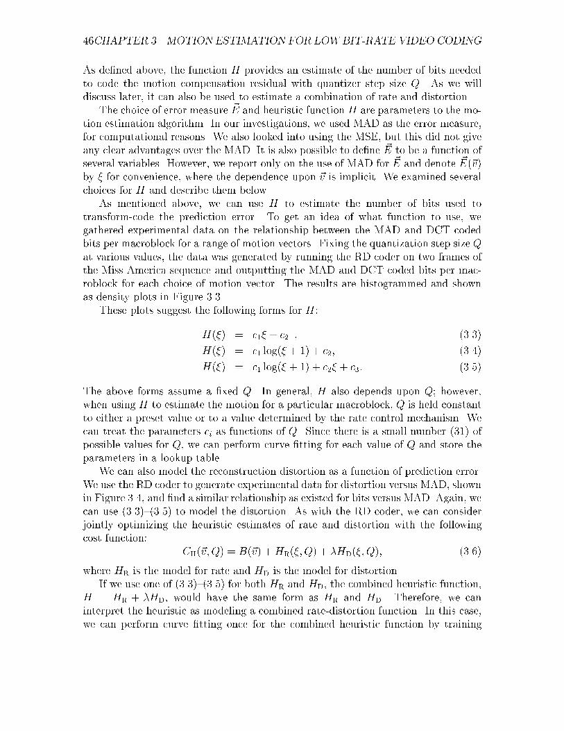
46CHAPTER 3. MOTION ESTIMATION FOR LOWBIT-RATE VIDEO CODING
As de�ned above, the function H provides an estimate of the number of bits neededto code the motion compensation residual with quantizer step size Q. As we willdiscuss later, it can also be used to estimate a combination of rate and distortion.
The choice of error measure ~E and heuristic function H are parameters to the mo-tion estimation algorithm. In our investigations, we used MAD as the error measure,for computational reasons. We also looked into using the MSE, but this did not giveany clear advantages over the MAD. It is also possible to de�ne ~E to be a function ofseveral variables. However, we report only on the use of MAD for ~E and denote ~E(~v)by � for convenience, where the dependence upon ~v is implicit. We examined severalchoices for H and describe them below.
As mentioned above, we can use H to estimate the number of bits used totransform-code the prediction error. To get an idea of what function to use, wegathered experimental data on the relationship between the MAD and DCT codedbits per macroblock for a range of motion vectors. Fixing the quantization step size Qat various values, the data was generated by running the RD coder on two frames ofthe Miss America sequence and outputting the MAD and DCT coded bits per mac-roblock for each choice of motion vector. The results are histogrammed and shownas density plots in Figure 3.3.
These plots suggest the following forms for H:
H(�) = c1� + c2 ; (3.3)
H(�) = c1 log(� + 1) + c2; (3.4)
H(�) = c1 log(� + 1) + c2� + c3: (3.5)
The above forms assume a �xed Q. In general, H also depends upon Q; however,when using H to estimate the motion for a particular macroblock, Q is held constantto either a preset value or to a value determined by the rate control mechanism. Wecan treat the parameters ci as functions of Q. Since there is a small number (31) ofpossible values for Q, we can perform curve �tting for each value of Q and store theparameters in a lookup table.
We can also model the reconstruction distortion as a function of prediction error.We use the RD coder to generate experimental data for distortion versus MAD, shownin Figure 3.4, and �nd a similar relationship as existed for bits versus MAD. Again, wecan use (3.3){(3.5) to model the distortion. As with the RD coder, we can considerjointly optimizing the heuristic estimates of rate and distortion with the followingcost function:
CH(~v;Q) = B(~v) +HR(�; Q) + �HD(�; Q); (3.6)
where HR is the model for rate and HD is the model for distortion.If we use one of (3.3){(3.5) for both HR and HD, the combined heuristic function,
H = HR + �HD, would have the same form as HR and HD. Therefore, we caninterpret the heuristic as modeling a combined rate-distortion function. In this case,we can perform curve �tting once for the combined heuristic function by training

3.4. HEURISTIC ALGORITHMS 47
5 10 15 20 25 30 35
MAD Prediction Error
20
40
60
80
100
120
140
DCT Bits
DCT Bits vs. MAD for Q=28
5 10 15 20 25 30 35
MAD Prediction Error
20
40
60
80
100
120
DCT Bits
DCT Bits vs. MAD for Q=31
5 10 15 20 25 30 35
MAD Prediction Error
50
100
150
200
DCT Bits
DCT Bits vs. MAD for Q=20
5 10 15 20 25 30 35
MAD Prediction Error
25
50
75
100
125
150
DCT Bits
DCT Bits vs. MAD for Q=24
5 10 15 20 25 30 35
MAD Prediction Error
50
100
150
200
250
300
350DCT Bits
DCT Bits vs. MAD for Q=12
5 10 15 20 25 30 35
MAD Prediction Error
50
100
150
200
250
DCT Bits
DCT Bits vs. MAD for Q=16
Figure 3.3: Density plots of DCT coding bits vs. MAD prediction error for �rstinter-coded frame of Miss America sequence at various levels of quantization.

48CHAPTER 3. MOTION ESTIMATION FOR LOWBIT-RATE VIDEO CODING
5 10 15 20 25 30 35
MAD Prediction Error
0
50
100
150
200
250
300
MSE Distortion
Distortion vs. MAD for Q=28
5 10 15 20 25 30 35
MAD Prediction Error
0
50
100
150
200
250
300
350
MSE Distortion
Distortion vs. MAD for Q=31
5 10 15 20 25 30 35
MAD Prediction Error
0
25
50
75
100
125
150
175
MSE Distortion
Distortion vs. MAD for Q=20
5 10 15 20 25 30 35
MAD Prediction Error
0
50
100
150
200
MSE Distortion
Distortion vs. MAD for Q=24
5 10 15 20 25 30 35
MAD Prediction Error
0
20
40
60
80
MSE Distortion
Distortion vs. MAD for Q=12
5 10 15 20 25 30 35
MAD Prediction Error
0
20
40
60
80
100
120
MSE Distortion
Distortion vs. MAD for Q=16
Figure 3.4: Density plots of MSE reconstruction distortion vs. MAD prediction errorfor �rst inter-coded frame of Miss America sequence at various levels of quantization.

3.4. HEURISTIC ALGORITHMS 49
Sequence PVRG M1 M2 RD H1-A H1-B H1-C H2-A H2-B H2-C
Miss America 34.58 35.44 36.51 36.67 35.60 35.72 35.58 36.63 36.77 36.68
Claire 32.77 33.24 34.12 34.22 33.68 33.50 33.60 34.47 34.36 34.39
Table 3.2: Results of static heuristic cost function. Shown is average PSNR (indB) of inter-coded frames for coding test sequences at 18 kbits/sec. H1-A (H2-A),H1-B (H2-B), and H1-C (H2-C) use the heuristic functions (3.3), (3.4), and (3.5),respectively.
on the statistic R + �D, where R is the DCT bits for a macroblock and D is thereconstruction distortion for the macroblock. As with Algorithm RD, the parameter �can be determined from the operational rate-distortion curve, for example.
3.4.2 Experimental Results
To test the H1 and H2 coders, we used the same test sequences and followed theprocedures outlined in Section 3.3.4. In the next section, we verify these results withexperiments on eight di�erent test sequences.
3.4.2a Static Cost Function
Here, we present results using a static set of coe�cients. To determine the coe�-cients for the heuristic functions, we performed linear least squares regression, �ttingdata generated by the RD coder to the R + �D statistic, as discussed earlier. Aset of regression coe�cients are stored in a lookup table, indexed by the quantizerstep size Q. We tested the di�erent forms for the heuristic function given in (3.3){(3.5). Comparative plots of the resulting PSNR are shown in Figure 3.5. The averagePSNR for coding at 18 kbits/sec is tabulated in Table 3.2. These results show thatthe heuristic coders perform comparably to the explicit minimization coders. In par-ticular, the heuristic coders seem more robust than M1 and M2, most likely becausethe heuristic functions correlate well with both rate and distortion, whereas M1 andM2 only consider rate.
3.4.2b Adaptive Cost Function
The above results rely on pretraining the model parameters ci for each value of Q foreach video sequence. This is a tedious and time-consuming operation. Instead, wecan use an adaptive on-line technique, such as the Widrow-Ho� learning rule [86, 28],to train the model parameters. The training examples could be generated each timewe encode a macroblock using motion compensation mode. However, we cannotpossibly hope to train one model for each value of Q simply because there wouldnot be enough training examples. We need a single model whose parameters are

50CHAPTER 3. MOTION ESTIMATION FOR LOWBIT-RATE VIDEO CODING
independent of Q. The curve �tting results from the pretraining trials show a strongcorrelation between the model parameters and Q�1. This agrees well with previouswork on rate-quantization modeling [19]. Therefore we propose the following form forthe cost function:
H(�; Q) = c1�
Q+ c2: (3.7)
This can be simpli�ed as
H( ) = c1 + c2; (3.8)
where � �=Q. Since the simple linear model performed well with static costfunctions, we do not consider more complex models here.
We conducted experiments using the Widrow-Ho� training rule on the Miss Amer-ica and Claire sequences. As applied to the current context, the Widrow-Ho� ruleis a technique for learning an objective function f( ). With H( ) as an estimateof f( ), the Widrow-Ho� rule gives us a way to adapt the weights c1 and c2 of (3.8)when given and the value of f( ). For the experiments, we chose the objectivefunction
f( ) = R( ) + �D( ); (3.9)
where R( ) is the actual number of bits used to code the DCT coe�cients andD( ) isthe resulting distortion, both of which can be evaluated by invoking encoder routines.Given an initial set of weights c1 and c2, a new set of weights c01 and c
02 can be computed
as:
c01 = c1 + � � f( )�H( )
2 + 1; (3.10)
c02 = c2 + � � f( )�H( )
2 + 1; (3.11)
where �, the learning rate, is a parameter that determines how quickly the weightsare adapted.
With the static cost function, we trained and evaluated the heuristic functionbased on the combined prediction error for the four luminance blocks that make upa macroblock. In order to gather more training examples for the adaptive heuristics,we evaluate and update the heuristic function once for each luminance block. Thisstrategy increased the PSNR slightly at the expense of some extra computation.
In the experiments, the learning rate � was determined in a trial-and-error phaseand �xed for both sequences. The parameter � was also determined by trial-and-errorand held constant for both test sequences. Comparative plots of the resulting PSNRare shown in Figures 3.6. The average PSNR for coding at 18 kbits/sec is tabulated inTable 3.3. These results show that the adaptive heuristic coders perform comparablyto and sometimes better than the static heuristic coders and the explicit minimizationcoders. Furthermore, the adaptive heuristic coders perform well on both sequenceswith the same initial parameter values.

3.4. HEURISTIC ALGORITHMS 51
As a comparison of visual quality, Frame 27 of the Miss America sequence isdecoded and shown in Figure 3.7 for the PVRG and explicit-minimization codersand in Figure 3.8 for the heuristic coders. The motion vector �eld for the PVRG,RD, adaptive H1, and adaptive H2 coders are shown in Figure 3.9. Frame 27 waschosen because it is in a di�cult scene with much head motion, resulting in morenoticeable coding artifacts. The RD and adaptive heuristic coders give smoothermotion �elds than the reference PVRG coder, especially for the background region.Note also that for the former coders, no motion is indicated for the relatively uniformbackground except following macroblocks with detected foreground motion on thesame row. Intuitively, this results in an economical encoding of the motion vectors,which are di�erentially encoded. Since the background is relatively uniform, codingmotion in this area results in relatively small motion compensation residual.
3.4.3 Further Experiments
Here, we present results of further experiments to con�rm the e�cacy of the variousmotion estimation algorithms operating within the p� 64 standard. We applied thevarious algorithms to code eight test video sequences4 without rate control, sweepingthe quantization scale from 12 to 31 to determine the operational rate-distortion plotsshown in Figure 3.10. Each test sequence consists of 50 frames in QCIF format codedat 10 frames/sec.
The results show that the adaptive heuristic algorithms perform consistently wellcompared to the base PVRG and explicit-minimization implementations, though thelevel of improvement varies among sequences. The anomalies observed in coding theGrandma sequence at low rates with the PVRG and adaptive H1 coders, as evidencedby the steep slope and unevenness in the RD curve, seem to indicate a breakdownof the RM8 coding control heuristics, which were not optimized for operation atvery low rates. This conclusion is supported by the lack of such anomalies whenbit-minimization is used to perform coding control, as with the M2, H2, and RDcoders.
The distributions of bits for coding the Miss America sequence with the H1 andH2 coders are plotted in Figure 3.11. Compared to Figure 3.1, these plots show thatthe H1 and H2 coders both reduce the percentage of bits used for coding motionvectors, while increasing the percentage of bits used to code the DCT coe�cients.Furthermore, with the H2 coder, which applies bit-minimization to coding control,the number of bits used for coding side information is also reduced.
4The Miss America sequence in this test suite was obtained from a di�erent source than the MissAmerica sequence used in the earlier experiments and has di�erent rate-distortion characteristics.

52CHAPTER 3. MOTION ESTIMATION FOR LOWBIT-RATE VIDEO CODING
3.5 Related Work
In related work, Chung, Kossentini and Smith [15] consider rate-distortion optimiza-tions for motion estimation in a hybrid video coder based upon subband coding andblock-matching motion compensation. The input frames are �rst decomposed intosubbands, which are divided into uniform rectangular blocks. For each block, a La-grangian cost function is used to select between intraframe and interframe modes andto select between a small number of candidate motion vectors, which are coded witha lossy two-dimensional vector quantizer.
Independent of our work, rate-distortion optimization for motion estimation hasbeen reported in [9]. The authors consider operational rate-distortion optimization ina dependent-coding environment where motion vectors are coded using DPCM tech-niques. The authors formulate motion estimation as a budget-constrained bit alloc-ation problem where the distortion to be minimized is the displaced frame di�erence(DFD), or prediction error, and propose to solve the problem using the Lagrange-multiplier approach. After �rst constructing a motion-vector dependency graph, theViterbi dynamic programming algorithm is used to �nd a path that minimizes anadditive Lagrangian cost function. Noting the computational complexity of this ap-proach, the authors propose a reduced-complexity algorithm that considers only asmall fraction of the possible states for each motion-compensated block. Even so,this reduced-complexity algorithm has a considerable processing and memory over-head associated with the dynamic programming algorithm, which is performed ontop of traditional block matching. In comparison, our adaptive heuristic cost func-tion requires minimal overhead over block matching.
In another independent work [77], the authors also apply operational rate-distortion optimization to motion estimation in a dependent-coding environment.Similar to [9], they cast motion estimation as a budget-constrained bit allocationproblem and solve it using a combination of Lagrange minimization and dynamicprogramming. The authors also consider joint optimization of motion estimation andquantization using the same framework. Notably, they also provide a solution to bothproblems that minimizes the maximum (minimax) distortion.
In [87], rate-distortion optimization is applied to the selection of coding controlfor low-bit-rate video coding under the H.263 standard, a newer standard than theH.261 standard that we consider here. A greedy optimization strategy is adopted toavoid the exponential complexity that a global optimization would entail. Limiteddependencies between the coding control of neighboring blocks is considered andthe coding control is computed using the Viterbi dynamic programming algorithmto minimize a Lagrangian cost function. Even with simplifying assumptions, therate-distortion optimization is computationally complex and may not be suitable forreal-time implementation, as the authors readily admit.
Ribas-Corbera and Neuho� [75] describe a procedure for minimizing rate in alossless motion-compensated video coder. They explore the allocation of bits between

3.6. DISCUSSION 53
the coding of motion vectors and the coding of prediction error. They assume thatthe prediction error has a discrete Laplacian distribution and derive an expression forthe total rate as a function of the number of bits allocated to code the motion vectors.It is not clear whether this work can be extended to lossy coding since distortion isnot taken into account in the formulation.
A linear relationship between MAD and both rate and distortion has been inde-pendently observed in [57]. The authors mention the possibility of performing motionvector search to minimize the bit rate, but conclude that just minimizing MAD wouldhave a similar e�ect.
3.6 Discussion
In this chapter, we have demonstrated that, at low bit rates, choosing motion vectorsto minimize an e�ciently computed heuristic cost function gives substantially betterrate-distortion performance than the conventional approach of minimizing predictionerror. Furthermore, by adapting the heuristic function to the input sequence, we areable to achieve coding performance comparable to more computationally expensivecoders that explicitly minimize rate or a combination of rate and distortion.
In the experiments, full-search block-matching was employed by all the coders.Our fast heuristic coders are also compatible with 2D logarithmic and many otherreduced-search motion estimation techniques. Since the heuristic cost function factorsin the motion vector code-length, the cost function has a strong monotonic componentand is well-suited for the reduced-search techniques that assume monotonicity in thecost function.
We have considered only the simple case of using a �xed parameter � to tradeo�rate and distortion. An on-line adaptation of � to track variations in the inputsequence is certainly possible and would result in more robust coders. On the otherhand, we observed that the behavior of these algorithms is quite robust with respectto moderate variations in �, and that, for example, the best setting of � for one testsequence worked well when used for the other. Thus, it seems that �xing � is safe inpractice. Still, since � in uences rate to some extent, it can be used in conjunctionwith the quantization step size in performing rate control. Automatic control of �based upon bu�er feedback as described in [11] is a possibility.
Although the methods presented here have been implemented within the H.261standard, it should be generally applicable to any video coder that employs motioncompensation in a low bit rate setting. In particular, the H.263 standard is similarenough to H.261 that it seems clear that these methods will work well with H.263.As a case in point, in the next chapter we show how the bit-minimization frameworkcan be applied in a non-standard coder that chooses motion vectors to optimize ahierarchical encoding of the motion information within a block-matching frameworkwith variable block sizes.

54CHAPTER 3. MOTION ESTIMATION FOR LOWBIT-RATE VIDEO CODING
34
35
36
37
0 5 10 15 20 25 30 35 40 45 50
PS
NR
(dB
)
Frame
PSNR for Coding Miss America Sequence at 18 kb/s
PVRGM1
H1-AH1-BH1-C
(a) Miss America
32
33
34
35
0 5 10 15 20 25 30
PS
NR
(dB
)
Frame
PSNR for Coding Claire Sequence at 18 kb/s
PVRGM1
H1-AH1-BH1-C
(b) Claire
34
35
36
37
38
0 5 10 15 20 25 30 35 40 45 50
PS
NR
(dB
)
Frame
PSNR for Coding Miss America Sequence at 18 kb/s
PVRGM2RD
H2-AH2-BH2-C
(c) Miss America
32
33
34
35
36
0 5 10 15 20 25 30
PS
NR
(dB
)
Frame
PSNR for Coding Claire Sequence at 18 kb/s
PVRGM2RD
H2-AH2-BH2-C
(d) Claire
Figure 3.5: Results of static heuristic cost function for coding Miss America andClaire sequences at 18 kbits/sec with rate control. In (a) and (b), we compare theH1 coder with the PVRG and M1 coders. In (c) and (d), we compare the H2 coderwith PVRG, M2 and RD coders. H1-A (H2-A), H1-B (H2-B), and H1-C (H2-C) usethe heuristic functions (3.3), (3.4), and (3.5), respectively.
Video PVRG M1 M2 RD H1-A H1-WH H2-A H2-WH
Miss America 34.58 35.44 36.51 36.67 35.60 35.83 36.63 36.84
Claire 32.77 33.24 34.12 34.22 33.68 33.58 34.47 34.51
Table 3.3: Results of adaptive heuristic cost function. Shown is average PSNR (in dB)of inter-coded frames for coding test sequences at 18 kbits/sec. H1-A and H2-A usethe heuristic function (3) with static parameters. H1-WH and H2-WH use adaptiveparameters.

3.6. DISCUSSION 55
34
35
36
37
38
0 5 10 15 20 25 30 35 40 45 50
PS
NR
(dB
)
Frame
PSNR for Coding Miss America Sequence at 18 kb/s
PVRGM1
H1-AH1-WH
(a) Miss America
32
33
34
35
0 5 10 15 20 25 30
PS
NR
(dB
)
Frame
PSNR for Coding Claire Sequence at 18 kb/s
PVRGM1
H1-AH1-WH
(b) Claire
34
35
36
37
38
39
0 5 10 15 20 25 30 35 40 45 50
PS
NR
(dB
)
Frame
PSNR for Coding Miss America Sequence at 18 kb/s
PVRGM2RD
H2-AH2-WH
(c) Miss America
32
33
34
35
36
0 5 10 15 20 25 30
PS
NR
(dB
)
Frame
PSNR for Coding Claire Sequence at 18 kb/s
PVRGM2RD
H2-AH2-WH
(d) Claire
Figure 3.6: Results of adaptive heuristic cost function for coding Miss America andClaire sequences at 18 kbits/sec with rate control. In (a) and (b), we compare theadaptive H1 coder with the static H1, PVRG and M1 coders. In (c) and (d), wecompare the adaptive H2 coder with the static H2, PVRG, M2 and RD coders. H1-Aand H2-A use the heuristic function (3).

56CHAPTER 3. MOTION ESTIMATION FOR LOWBIT-RATE VIDEO CODING
(a) PVRG (b) RD
(c) M1 (d) M2
Figure 3.7: Frame 27 of the Miss America sequence as encoded using the PVRG andexplicit-minimization motion estimation algorithms. Only the luminance componentis shown.

3.6. DISCUSSION 57
(a) H1-A (b) H2-A
(c) H1-WH (d) H2-WH
Figure 3.8: Frame 27 of the Miss America sequence as encoded using the heuristicmotion estimation algorithms. Only the luminance component is shown.

58CHAPTER 3. MOTION ESTIMATION FOR LOWBIT-RATE VIDEO CODING
(a) PVRG (b) RD
(c) H1-WH (d) H2-WH
Figure 3.9: Estimated motion vectors for frame 27 of the Miss America sequence forthe PVRG, RD, H1-WH, and H2-WH coders. Only the magnitude of the motionvectors are shown.

3.6. DISCUSSION 59
30
40
50
60
70
80
90
100
110
120
130
140
1000 2000 3000 4000 5000 6000
MS
E
Average Bits/Frame
PVRGM1
Adaptive H1M2
Adaptive H2RD
(a) Carphone
10
20
30
40
50
60
70
80
1000 1500 2000 2500 3000
MS
E
Average Bits/Frame
PVRGM1
Adaptive H1M2
Adaptive H2RD
(b) Claire
40
60
80
100
120
140
160
180
1000 2000 3000 4000 5000 6000 7000 8000 9000
MS
E
Average Bits/Frame
PVRGM1
Adaptive H1M2
Adaptive H2RD
(c) Foreman
30
40
50
60
70
80
90
100
800 1200 1600 2000 2400 2800
MS
E
Average Bits/Frame
PVRGM1
Adaptive H1M2
Adaptive H2RD
(d) Grandma
10
15
20
25
30
35
40
45
800 1200 1600 2000 2400 2800
MS
E
Average Bits/Frame
PVRGM1
Adaptive H1M2
Adaptive H2RD
(e) Miss America
30
40
50
60
70
80
90
100
110
120
1000 2000 3000 4000
MS
E
Average Bits/Frame
PVRGM1
Adaptive H1M2
Adaptive H2RD
(f) Mother and Daughter
20
30
40
50
60
70
80
90
1000 2000 3000 4000
MS
E
Average Bits/Frame
PVRGM1
Adaptive H1M2
Adaptive H2RD
(g) Suzie
30
40
50
60
70
80
90
100
110
120
130
2000 3000 4000 5000 6000
MS
E
Average Bits/Frame
PVRGM1
Adaptive H1M2
Adaptive H2RD
(h) Trevor
Figure 3.10: Performance of motion estimation algorithms on eight test sequences.

60CHAPTER 3. MOTION ESTIMATION FOR LOWBIT-RATE VIDEO CODING
�� ��
��
����
��
��
��
��
��
12 14 16 18 20 22 24 26 28 30 32
500
1000
2000
2500
Quantizer Step Size
Ave
rage
Bits
/Fra
me
3000
1500
Side Information
DCT Coefficients
Motion Vector
(a) H1 Coder
�� ��
��
����
��
��
��
��
��
12 14 16 18 20 22 24 26 28 30 32
500
1000
2000
2500
Quantizer Step Size
Ave
rage
Bits
/Fra
me
3000
1500
Side Information
DCT Coefficients
Motion Vector
(b) H2 Coder
Figure 3.11: Distribution of bits for coding the Miss America sequence with adaptiveheuristics.

Chapter 4
Bit-Minimization in a
Quadtree-Based Video Coder
Quadtree-Based Video Coder
Like the underlying image data that they are computed from, motion vector �eldsoften exhibit signi�cant spatial correlation. Approaches such as the p� 64 standardexploit this observation by coding the di�erences between successive motion vectorsin a one-dimensional scan order. Potentially better results can be achieved by di-rectly exploiting the two-dimensional correlation of motion vectors. A quadtree datastructure can be used for this purpose by representing the motion �eld hierarchi-cally in two dimensions [70, 3, 7, 20]. The quadtree approach works by identifyingvariable-sized regions of uniform motion and providing an e�cient encoding of themotion �eld. For video sequences where there are large regions of uniform motion,a quadtree decomposition reduces the number of bits required to encode the motion�eld by coding only a few motion vectors. When the motion �eld is smoothly varying,the hierarchical structure of the quadtree allows the correlated motion vectors to bee�ciently coded.
In this chapter, we consider the instantiation of the bit-minimization principle ina video coder that uses a quadtree to code motion vectors, thereby departing fromthe p� 64 standard. The contents of this chapter were originally presented in [29].
4.1 Quadtree Data Structure
Often used as a representation for bi-level images, the quadtree can also be used tocode motion vectors. We �rst describe the quadtree in the context of bi-level imagerepresentation and later show how to use it to code a motion �eld.
61

62CHAPTER 4. BIT-MINIMIZATION IN A QUADTREE-BASED VIDEOCODER
0 1 2
30 31 32 33
(a) Quadtree
������������������������������������������������������������������
������������������������������������������������������������������
������������������
������������������
���������������������
���������������������
0
2
30 31
32
1
33
(b) Image
Figure 4.1: A simple quadtree and corresponding image.
4.1.1 Quadtree Representation of Bi-Level Images
The root node of a quadtree represents the entire image. For the trivial case wherean image contains all white or all black pixels, its quadtree representation is the rootnode colored either white or black, respectively. Otherwise the image is divided intofour quadrants, each a child of the root node. If a quadrant is totally white or totallyblack, it is represented as a leaf node appropriately colored; otherwise it is representedin the quadtree by an internal node and is further divided into subquadrants. Thedivision proceeds recursively up to a maximum depth or until all subdivisions containuniform pixels. A simple quadtree and its corresponding image is shown in Figure 4.1.
In Figure 4.2, a decomposition of a triangle is shown using a quadtree of depth5. The image is divided into the regions shown in Figure 4.2(a). Since the depth ofthe quadtree is �nite, the triangle can only be approximated with limited precision.Adopting a policy that each of the smallest subdivision is colored with the predomi-nant color of the underlying image, we can represent the triangle using the quadtreestructure shown in Figure 4.2(b). Note that some of the regions identi�ed in (a) havebeen merged in (b) since they are assigned the same color and have a common parent.
The structure of a quadtree can be represented linearly by traversing the tree.Labeling an internal node as I, a black leaf as B, and a white leaf as W, we canrepresent the tree in Figure 4.1 with the string IWBWIWBWB. This corresponds to apreorder traversal of the quadtree.
The quadtree can be extended to code greyscale and color images by storing ateach leaf a greyscale or color value, chosen to minimize some measure of distortion.
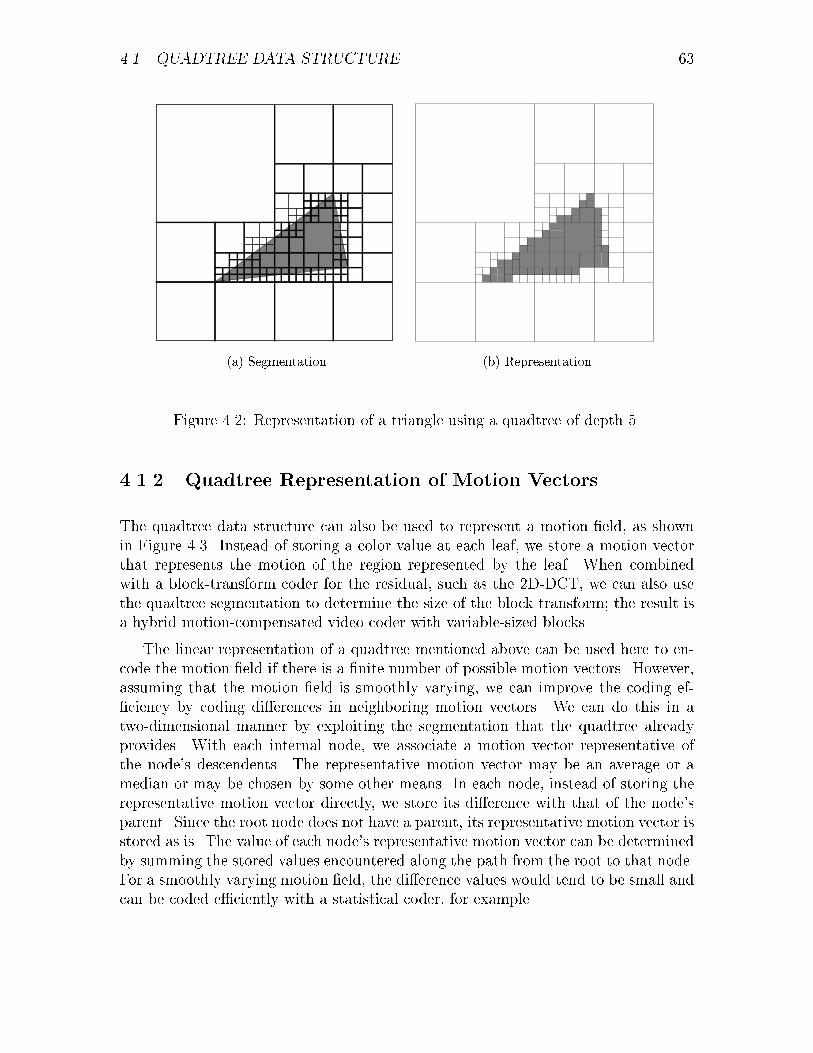
4.1. QUADTREE DATA STRUCTURE 63
�������
���
���
���
(a) Segmentation (b) Representation
Figure 4.2: Representation of a triangle using a quadtree of depth 5.
4.1.2 Quadtree Representation of Motion Vectors
The quadtree data structure can also be used to represent a motion �eld, as shownin Figure 4.3. Instead of storing a color value at each leaf, we store a motion vectorthat represents the motion of the region represented by the leaf. When combinedwith a block-transform coder for the residual, such as the 2D-DCT, we can also usethe quadtree segmentation to determine the size of the block transform; the result isa hybrid motion-compensated video coder with variable-sized blocks.
The linear representation of a quadtree mentioned above can be used here to en-code the motion �eld if there is a �nite number of possible motion vectors. However,assuming that the motion �eld is smoothly varying, we can improve the coding ef-�ciency by coding di�erences in neighboring motion vectors. We can do this in atwo-dimensional manner by exploiting the segmentation that the quadtree alreadyprovides. With each internal node, we associate a motion vector representative ofthe node's descendents. The representative motion vector may be an average or amedian or may be chosen by some other means. In each node, instead of storing therepresentative motion vector directly, we store its di�erence with that of the node'sparent. Since the root node does not have a parent, its representative motion vector isstored as is. The value of each node's representative motion vector can be determinedby summing the stored values encountered along the path from the root to that node.For a smoothly varying motion �eld, the di�erence values would tend to be small andcan be coded e�ciently with a statistical coder, for example.

64CHAPTER 4. BIT-MINIMIZATION IN A QUADTREE-BASED VIDEOCODER
(a) Motion Field (b) Quadtree Representation
Figure 4.3: Quadtree representation of a motion �eld.
4.2 Hybrid Quadtree/DCT Video Coder
In [7], Chan, Yu, and Constantinides describe several coding schemes using quadtreesin which the split/merge operations used to construct the tree are controlled byprediction error criteria. We propose to use a quadtree to encode motion vectors fora block-matching motion-compensated video coder in which the tree is constructedusing the bit-minimization principle. The basic coder design is similar to the p� 64coder shown in Figure 2.18. The di�erence is that now motion vectors are codedwith a quadtree whose leaves represent regions of uniform motion. Conceptually, onemight associate a motion vector with each node of the quadtree, which, for internalnodes, is re�ned further down the tree. Using this viewpoint, for each node otherthan the root, the di�erence between the node's and its parent's motion vectors istransmitted. Thus, one can construct the motion vector for each leaf by adding theroot's motion vector to the sum of the di�erences encountered along the path fromthe root to the given leaf.
We propose to combine the quadtree encoding of motion vectors with the basicmotion-compensated video coder speci�ed in the p� 64 standard. Conceptually, themain di�erence between this coder and the p � 64 coder is in the encoding of themotion vectors. Each leaf in the quadtree encodes a motion vector for a number of8� 8 blocks. Therefore, the quadtree decomposition ends at the 8� 8 level.
Given a motion �eld and its quadtree decomposition, we code the structure of thetree using an adaptive arithmetic code to indicate whether a node is a leaf or not (adi�erent adaptive coder is used for each level). The motion vector di�erences at each
4.2. HYBRID QUADTREE/DCT VIDEO CODER 65
node are coded using another adaptive arithmetic code (again, using a di�erent coderfor each level). For each leaf node, the 8� 8 transform coded blocks subsumed by thenode are transmitted in scan order. The decision of how to code the block (choosingfrom among alternatives similar to those in the p� 64 standard) is also transmittedusing an adaptive arithmetic coder. If the quantized transform coe�cients are trans-mitted, this is done using the run-length/Hu�man coding method from the p � 64standard. The counts for the adaptive arithmetic coder are updated once after eachframe is coded.
To perform motion estimation, we adopt the bit-minimization strategy elaboratedin Chapter 3. The quadtree coding structure described in Section 4.1.2 has severalnice properties that make a dynamic programming solution possible for �nding anoptimal set of motion vectors that minimizes the sum of the code-lengths neededto encode the motion vectors and the transform-coded prediction error. Since thearithmetic code used for the motion vector di�erences at each node doesn't changeduring the coding of a particular frame, the optimal number of bits to code the motionvector di�erences for any subtree is independent of the coding of any other disjointsubtree. Similarly, the transform coding of the prediction errors is independent fordisjoint subtrees.
We now describe a dynamic programming algorithm for choosing an optimalquadtree. For each node in the tree, we store a table indexed by the (absolute)motion vector of the node's parent. For each possible motion vector ~v of the parent,this table gives the minimum code-length to code the subtree rooted at the currentnode given that the parent's motion vector is ~v. Also stored with each table entryis a motion vector giving the minimum code-length. Construction of the tables isperformed in a bottom-up fashion, starting at the 8� 8 block level. For a node p,the table is constructed by �nding, for each choice of motion vector ~v0 for the parentnode, a motion vector for p that results in the minimum code-length for the subtreerooted at p. If p is at the 8� 8 block level, this is done by computing the transformcode-length of the prediction error for each motion vector in the search range S andnoting the minimum code-length and the corresponding motion vector. Otherwise weconsider for each motion vector ~v in S the code-length needed to transform-code theprediction errors if the quadtree is pruned at p. (This quantity can be computed ina preprocessing step.) We also consider the code-length if the quadtree is not prunedat p. This code-length is computed by indexing the tables of children of p with ~vand summing. The minimum of these two quantities is added to the number of bitsto code ~v0 � ~v. The result is the minimum code-length required to code the subtreerooted at p given motion ~v0 at p's parent node.
Once the minimum code-length is computed for the root of the quadtree, themotion vectors for each node in the tree are determined by going back down the tree,using the tables constructed on the way up. The optimal motion vector for the rootnode is made known to its children. Each child uses this to index its table to �nd itsoptimal motion vector. Pruning of the tree is also performed as a result.

66CHAPTER 4. BIT-MINIMIZATION IN A QUADTREE-BASED VIDEOCODER
0
20
40
60
80
100
120
140
0 0.05 0.1 0.15 0.2 0.25 0.3 0.35 0.4
MS
E
Rate (bits per pixel per frame)
PVRGM1M2QT
Figure 4.4: MSE vs. Rate for Trevor
The dynamic programming algorithm requires O(N jSj2) time, where N is thenumber of 8� 8 blocks in the frame and S is the search region for block-matching.The space requirement is O(N jSj).
4.3 Experimental Results
The quadtree coder is implemented using routines from the PVRG coder for motioncompensation, transform coding, quantization, and run-length/Hu�man coding of thequantized transform coe�cients. The quadtree structure and motion vector informa-tion are not actually coded; however, adaptive probability models are maintained andused to compute the number of bits that an ideal arithmetic coder would produce.Our objective is to explore the limits in performance improvement by aggressivelyoptimizing the coding of motion vectors.
We performed coding simulations using 50 frames of the grayscale 256� 256\Trevor" sequence. The p � 64 coders were modi�ed to accept input at 256� 256resolution. An operational rate-distortion plot for the quadtree and p � 64 codersis given in Figure 4.4. The quadtree coder gives better rate-distortion performancefor rates under about 0.25 bits/pixel. Furthermore, the range of achievable rates isextended to well below the 0.05 bits/pixel achievable with M2, albeit with higherdistortion.
4.4 Previous Work
Puri and Hang [70] considered an algorithm for motion-compensated video codingwhich, when an 8� 8 block B is not coded well (that is, when coding it requires a lotof bits), chooses a separate motion vector for each ofB's four 4� 4 subblocks. Bierling

4.5. DISCUSSION 67
[3] described a hierarchical algorithm for choosing motion vectors in which initiallymotion vectors are chosen for large blocks (64� 64) by minimizing the predictionerror.1 Then for each large block B, motion vectors are chosen for subblocks of Bagain by minimizing prediction error, except looking only at motion vectors close tothe motion vector chosen for B. This process results in a smoother motion �eld,and experiments suggest that it is closer to the \true" motion than is a motion �eldobtained by separately minimizing error on the small blocks. While Bierling did notdiscuss how to code motion vectors obtained through by his method, Chan, Yu, andConstantinides [7] described a method where motion vectors are again chosen in atop-down fashion, starting with large blocks and re�ning with smaller blocks. Whenthe average squared prediction error for a given block B is above a given threshold,the algorithm re�nes the motion vector chosen for B by looking at subblocks of B.Similarly, if the use of separate motion vectors for the subblocks of B does not reducethe error signi�cantly, the subblocks of B are \merged" with B. After this process iscompleted, the tree obtained by making a given block the parent of its subblocks istransmitted, together with motion vectors for each of the leaves. Methods for takinga tree structure like the above (except expanded completely) and then \smoothing"the motion vectors by making children tend to be like their parents and vice-versa,were discussed by Dufaux and Kunt [20]. Zhang, Cavenor, and Arnold [88] consideredvarious ways of using quadtrees to code the prediction error.
4.5 Discussion
In this chapter, we have presented a non-standard hybrid block-matching DCT videocoder that further optimizes the coding of motion vectors by representing the motion�eld using a quadtree decomposition. Although motivated for e�cient coding ofmotion vectors, the quadtree decomposition can be viewed as performing motioncompensation using variable-sized blocks.
Preliminary experimental results suggest that a quadtree-based technique may besuitable for video coding at rates below that achievable by the p� 64 standard.
While only the bit-minimization strategy has been examined for the quadtree-based coder, the heuristic cost function of Chapter 3 can certainly be used to speedup the operation of the coder.
1In fact, a heuristic search [39, 42] was used to only approximately minimize the error.

68CHAPTER 4. BIT-MINIMIZATION IN A QUADTREE-BASED VIDEOCODER

Chapter 5
Lexicographically Optimal Bit
Allocation
In any lossy coding system, there is an inherent trade-o� between the rate of the codeddata and the distortion of the reconstructed signal. Often the transmission (storage)medium is bandwidth (capacity) limited. The purpose of rate control is to allocatebits to coding units and to regulate the coding rate to meet the bit-rate constraintsimposed by the transmission or storage medium while maintaining an acceptable levelof distortion. We consider rate control in the context of the MPEG-1 and MPEG-2standards.
In addition to specifying a syntax for the encoded bitstream and a mechanismfor decoding it, the MPEG standards de�ne a hypothetical decoder called the VideoBu�ering Veri�er (VBV), which places quanti�able limits on the variability in codingrate. The VBV is diagrammed in Figure 2.23 and described in Section 2.7.
As outlined in Section 2.7.5, the overall rate control process can be broken downinto three steps:
1. a high level bit allocation to coding units (video pictures),
2. a low level control of the quantization scale within a coding unit to achieve thebit allocation,
3. adjustment to the quantization scale to equalize perceptual quality.
In this chapter, we develop a framework for bit allocation under VBV constraints,with an additional constraint on the total number of bits coded. This frameworkconsists of three components: 1) a bit-production model, 2) a novel lexicographicoptimality criterion, and 3) a set of bu�er constraints for constant and variable bitrate operation. Initially, we formalize bit allocation as a resource allocation problemwith continuous variables and non-linear constraints, to which we apply a globallexicographic optimality criterion.
69

70 CHAPTER 5. LEXICOGRAPHICALLY OPTIMAL BIT ALLOCATION
The global nature of the optimization necessitates the use of o�-line techniqueswherein the complexities of all the coded pictures, as speci�ed with bit-productionmodels, are known prior to computing a global bit allocation. One way to view thisis as a serial computation with unlimited lookahead, wherein the inputs are the bit-production models for each picture. In practice, this would entail making multiplepasses over the video sequence in order to construct the models, compute an optimalallocation, and compress the sequence using the computed allocation. In Chapter 10,we explore some techniques for reducing the computation by limiting the amount oflookahead used.
In the next two chapters, we use our new framework to analyze bit allocationunder constant bit rate and variable bit rate operation. The analyses yield necessaryand su�cient conditions for optimality that lead to e�cient bit allocation algorithms.In Chapter 10, we describe an implementation of these algorithms within a softwareMPEG-2 encoder and present simulation results.
5.1 Perceptual Quantization
As shown in Figure 2.20, the output bit rate of a video coder can be regulated by ad-justing the quantization scale Qs. Increasing Qs reduces the output bit rate but alsodecreases the visual quality of the compressed pictures. Similarly, decreasing Qs in-creases the output bit rate and increases the picture quality. Therefore by varying Qs,we can trace out a rate vs. distortion curve, such as that shown in Figure 2.5.
Although Qs can be used to control rate and distortion, coding with a constantvalue of Qs generally does not result in either constant bit rate or constant perceivedquality. Both of these factors depend upon the scene content as well. Studies intohuman visual perception suggest that perceptual distortion is correlated to certainspatial (and temporal) properties of an image (video sequence) [61, 1]. These stud-ies lead to various techniques, called perceptual quantization or adaptive perceptual
quantization, that take into account properties of the Human Visual System (HVS)in determining the quantization scale [82, 69, 40, 14, 47, 85, 16].
Based upon this body of work, we propose a separation of the quantization scaleQs
into a nominal quantization Q and a perceptual quantization function P (I; Q) suchthat Qs = P (I; Q), where I denotes the block being quantized. The function P ischosen so that if the same nominal quantization Q were used to code two blocksthen the blocks would have the same perceptual distortion. In this way, the nominalquantization parameter Q would correspond directly to the perceived distortion andcan serve as the object for optimization. We favor a multiplicative model whereP (I; Q) = �IQ.
1 Where quantization noise is less noticeable, such as in highly-textured regions, we can use a larger value for �I than regions where quantization
1The MPEG-2 Test Model 5 [37] also uses a multiplicative formulation while an additive formu-lation is proposed in [66].

5.2. CONSTANT QUALITY 71
noise is more noticeable, such as in relatively uniform areas. In this regards, �I canbe viewed as a perceptual weighting factor. Our bit rate allocation, however, workswith any perceptual quantization function.
The problem of determining P (I; Q) has been studied elsewhere [82, 13] and is notconsidered in this manuscript. Here, we address the assignment ofQ to each picture togive constant or near-constant quality among pictures while satisfying rate constraintsimposed by the channel and decoder. We propose to compute Q at the picturelevel; that is, we compute one Q for each picture to be coded. Besides decreasingthe computation over computing di�erent Q for each block, this method results inconstant perceptual quality within each picture given that perceptual quantizationis employed at the block level. The framework can certainly be generalized to othercoding units, and in principle can be applied to code other types of data, such asimages and speech.
5.2 Constant Quality
Previous approaches in optimal rate control generally seeks to minimize a distortionmeasure, typically mean-squared error (MSE), averaged over coding blocks [63, 73].While this approach leverages the wealth of tools from optimization theory and op-erations research, it does not guarantee the constancy of quality that is generallydesired from a video coding system. For example, a video sequence with a constantor near-constant level of distortion is more desirable than one with lower average dis-tortion but higher variability, because human viewers tend to �nd frequent changesin quality more noticeable and annoying. A long video sequence typically containssegments that, even if encoded at a fairly low bit rate, will not contain any disturbingquantization artifacts, so that improving the quality of pictures in those segments isfar less important than improving the quality of pictures in segments that are moredi�cult to encode.
To address these issues, we propose a lexicographic optimality criterion that betterexpresses the desired constancy of quality. The idea is to minimize the maximum(perceptual) distortion of a block (or picture) and then minimize the second highestblock distortion, and so on. The intuition is that doing so would equalize distortionby limiting peaks in distortion to their minimum. As we will show later, if a constantquality allocation is feasible, then it must necessarily be lexicographically optimal.
5.3 Bit-Production Modeling
For simplicity, we assume that each picture has a bit-production model that relates thepicture's nominal quantization Q to the number of coded bits B. This assumes thatthe coding of one picture is independent of any other. This independence holds foran encoding that uses only intraframe (I) pictures, but not for one that uses forward

72 CHAPTER 5. LEXICOGRAPHICALLY OPTIMAL BIT ALLOCATION
predictive (P) or bidirectionally predictive (B) pictures, for example. In practice,the extent of the dependency is limited to small groups of pictures. Nonetheless, weinitially assume independence to ease analysis and defer treatment of dependenciesuntil a later chapter where we consider practical implementations.
We specify Q and B to be non-negative real-valued variables. In practice, thequantization scale Qs and B are positive integers with Qs = b�I � Qc. However, tofacilitate analysis, we assume that there is a continuous function for each picture thatmaps Q to B.
For a sequence of N pictures, we de�ne N corresponding bit-production mod-els ff1; f2; : : : ; fNg that map nominal quantization scale to bits: bi = fi(qi), wherefi : [0;1] 7! [li; ui], with 0 � li < ui. (We number pictures in encoding order andnot temporal display order. See Section 2.15.) We require the models to have thefollowing properties:
1. fi(0) = ui,
2. fi(1) = li,
3. fi is continuous and monotonically decreasing.
From these conditions, it follows that fi is invertible with qi = gi(bi), where gi =f�1i and gi : [li; ui] 7! [0;1]. We note that gi is also continuous and monotonicallydecreasing. Although monotonicity does not always hold in practice, it is a generallyaccepted assumption.
In video coding systems, the number of bits produced for a picture also dependsupon a myriad of coding choices besides quantization scale, such as motion compen-sation and the mode used for coding each block. We assume that these choices aremade independent of quantization and prior to performing rate control.
5.4 Bu�er Constraints
The MPEG standards specify that an encoder should produce a bitstream that can bedecoded by a hypothetical decoder referred to as the Video Bu�ering Veri�er (VBV),as shown in Figure 2.23 and described in Section 2.7. Data can be transferred to theVBV either at a constant or variable bit rate.2 In either mode of operation, the num-ber of bits produced by each picture must be controlled so as to satisfy constraintsimposed by the operation of the decoder bu�er, whose size BVBV is speci�ed in thebitstream by the encoder. The encoder also speci�es the maximum transfer rate Rmax
into the VBV bu�er and the amount of time the decoder should wait before decod-ing the �rst picture. In this section, we consider constraints on the number of bitsproduced in each picture that follow from analysis of the VBV.
2The MPEG-1 standard only de�nes VBV operation with a constant bit rate while the MPEG-2standard also allows for variable bit rate.
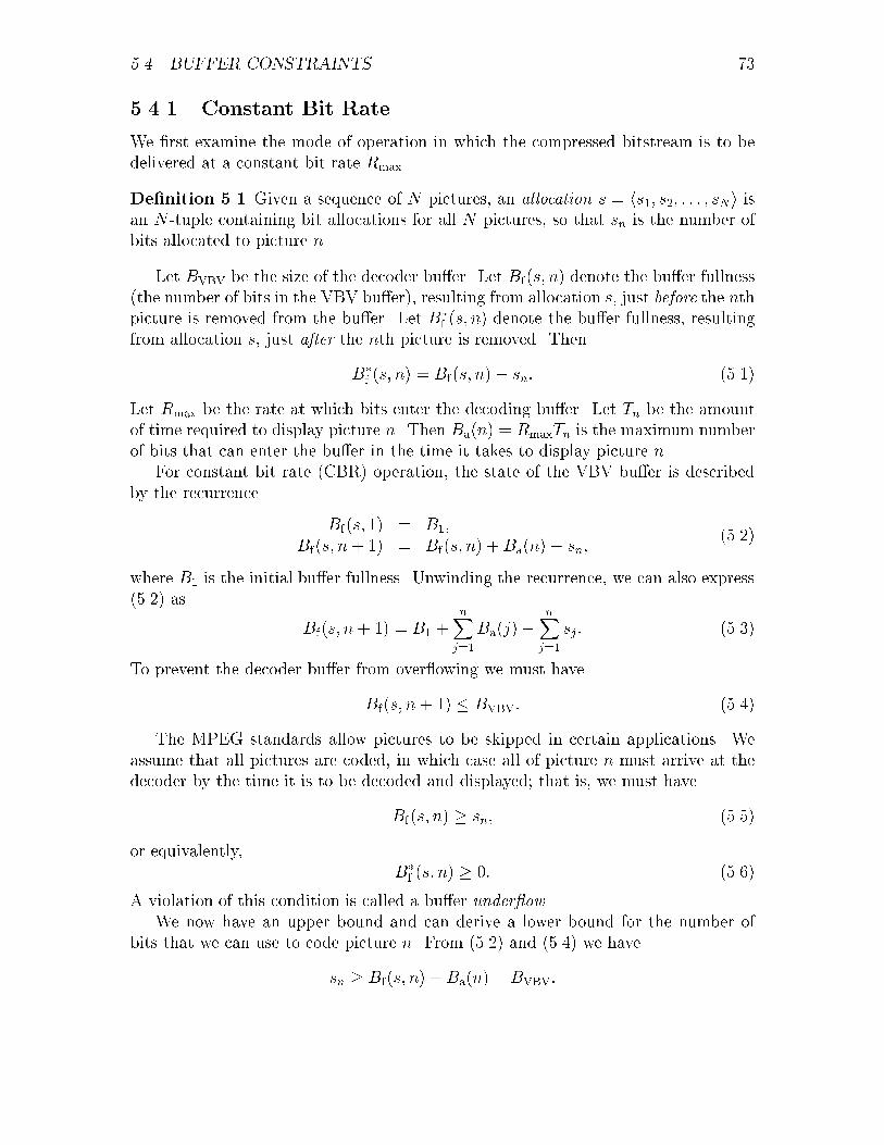
5.4. BUFFER CONSTRAINTS 73
5.4.1 Constant Bit Rate
We �rst examine the mode of operation in which the compressed bitstream is to bedelivered at a constant bit rate Rmax.
De�nition 5.1 Given a sequence of N pictures, an allocation s = hs1; s2; : : : ; sNi isan N -tuple containing bit allocations for all N pictures, so that sn is the number ofbits allocated to picture n.
Let BVBV be the size of the decoder bu�er. Let Bf(s; n) denote the bu�er fullness(the number of bits in the VBV bu�er), resulting from allocation s, just before the nthpicture is removed from the bu�er. Let B�
f (s; n) denote the bu�er fullness, resultingfrom allocation s, just after the nth picture is removed. Then
B�f (s; n) = Bf(s; n)� sn: (5.1)
Let Rmax be the rate at which bits enter the decoding bu�er. Let Tn be the amountof time required to display picture n. Then Ba(n) = RmaxTn is the maximum numberof bits that can enter the bu�er in the time it takes to display picture n.
For constant bit rate (CBR) operation, the state of the VBV bu�er is describedby the recurrence
Bf(s; 1) = B1;
Bf(s; n+ 1) = Bf(s; n) +Ba(n)� sn;(5.2)
where B1 is the initial bu�er fullness. Unwinding the recurrence, we can also express(5.2) as
Bf(s; n+ 1) = B1 +nXj=1
Ba(j)�nXj=1
sj: (5.3)
To prevent the decoder bu�er from over owing we must have
Bf(s; n+ 1) � BVBV: (5.4)
The MPEG standards allow pictures to be skipped in certain applications. Weassume that all pictures are coded, in which case all of picture n must arrive at thedecoder by the time it is to be decoded and displayed; that is, we must have
Bf(s; n) � sn; (5.5)
or equivalently,B�f (s; n) � 0: (5.6)
A violation of this condition is called a bu�er under ow.We now have an upper bound and can derive a lower bound for the number of
bits that we can use to code picture n. From (5.2) and (5.4) we have
sn � Bf(s; n) +Ba(n)� BVBV:

74 CHAPTER 5. LEXICOGRAPHICALLY OPTIMAL BIT ALLOCATION
U2
T0 T0+T T0+2T T0+3T T0+4T
L2Bi
Ful
lnes
sB
uffe
r
BVBV
Time
00
Figure 5.1: Sample plot of bu�er fullness for CBR operation. Bits enter the decoderbu�er at a constant rate until time T0, when the �rst picture is removed. Succes-sive pictures are removed after a time interval T . Upper and lower bounds on thenumber of bits that can be produced for the second picture are shown as U2 and L2,respectively.
Since we cannot produce a negative number of bits, the lower bound on sn is
sn � maxfBf(s; n) +Ba(n)� BVBV; 0g: (5.7)
In summary, for constant bit rate operation, in order to pass video bu�er veri�-cation, an allocation s must satisfy the following for all n:
maxfBf(s; n) +Ba(n)� BVBV; 0g � sn � Bf(s; n): (5.8)
An exemplary plot of the evolution of the bu�er fullness over time for CBR op-eration is shown in Figure 5.1. In this example, the decoder waits T0 seconds beforedecoding the �rst picture, at which time the bu�er fullness is B1. The time to displayeach picture is assumed to be a constant T seconds. In the plot, the upper and lowerbounds for the number of bits to code picture 2 are shown as U2 and L2, respectively.
5.4.2 Variable Bit Rate
We now examine the scenario where the compressed video bitstream is to be deliveredat a variable bit rate (VBR). Speci�cally, we adopt the second VBR mode of theMPEG-2 VBV model (see Section 2.7.4) where bits always enter the decoder bu�er

5.5. BUFFER-CONSTRAINED BIT ALLOCATION PROBLEM 75
at the peak rate Rmax until the bu�er is full.3 Depending upon the state of the bu�er,
bits enter during each display interval at a rate that is e�ectively variable up to thepeak rate Rmax. The maximum number of bits entering the bu�er in the time it takesto display picture n is Ba(n) = RmaxTn.
For VBR operation, the state of the VBV bu�er is described by:
Bf(s; 1) = BVBV;
Bf(s; n+ 1) = minfBVBV; Bf(s; n) +Ba(n)� sng:(5.9)
Unlike the CBR case, the decoder bu�er is prevented from over owing by theminimization in (5.9). When Bf(s; n) + Ba(n) � sn > BVBV, we say that picture nresults in a virtual over ow. When a virtual over ow occurs, the e�ective input rateto the VBV bu�er during that display interval is less than the peak rate. Like theCBR case, under ow is possible and to prevent it (5.5) must hold. The evolution ofthe bu�er fullness is shown for VBR operation in Figure 5.2. The time to display eachpicture is assumed to be a constant T seconds. As shown in the plot, the numberof bits that enter the bu�er during each display interval is variable, with virtualover ows occurring for pictures 2 and 4.
5.4.3 Encoder vs. Decoder Bu�er
In the above discussion, we have focused solely on the decoder bu�er whereas Fig-ure 2.20 shows the Rate Controller monitoring the fullness of the encoder bu�er. Byassuming a �xed channel delay the encoder bu�er fullness can be shown to mirrorthe decoder bu�er fullness, except for an initial startup period. That is, an emptydecoder bu�er would correspond to a full encoder bu�er, and vice versa. The readeris referred to [74] for a more complete discussion of bu�er constraints in video codersystems.
5.5 Bu�er-Constrained Bit Allocation Problem
Using the bit-production model and VBV constraints de�ned above, we now formalizethe bu�er-constrained bit allocation problem.
De�nition 5.2 A bu�er-constrained bit allocation problem P is speci�ed by a tuple
P = hN;F;Btgt; BVBV; B1; Bai ;3We note that with the same bit allocation, the VBV bu�er fullness for the second VBR mode is
always equal to or higher than the fullness when operating in the �rst VBR mode. Intuitively, if thechannel bit rate is not further constrained, a lexicographically optimal bit allocation for the secondVBR mode should not be worse (lexicographically) than an optimal bit allocation for the �rst VBRmode, given the same total bit budget.

76 CHAPTER 5. LEXICOGRAPHICALLY OPTIMAL BIT ALLOCATION
U2
T T T T T0 0 0 0 0+T +2T +3T +4T
Ful
lnes
sB
uffe
r
B
0
VBV
Time
0
Figure 5.2: Sample plot of bu�er fullness for VBR operation. Bits enter the decoderbu�er at a constant rate until time T0, when the �rst picture is removed. Successivepictures are removed after a time interval T . When the bu�er becomes full, no morebits enter until the next picture is removed.
where N is the number of pictures; F = hf1; f2; : : : ; fNi is a sequence of N func-tions, as speci�ed in Section 5.3, that model the relationship between the nominalquantization scale and the number of coded bits for each picture; Btgt is the targetnumber of bits to code all N pictures; BVBV is the size of the VBV bu�er in bits; B1
is the number of bits initially in the VBV bu�er; Ba is a function that gives the max-imum number of bits that can enter the decoding bu�er while each picture is beingdisplayed.
For convenience, in the sequel we shall use the shorter term \bit allocation prob-lem" to refer to the bu�er-constrained bit allocation problem.
De�nition 5.3 Given a bit allocation problem P = hN;F;Btgt; BVBV; B1; Bai, anallocation s is a legal allocation if the following conditions hold:
1.PN
j=1 sj = Btgt
2. Equation (5.5) holds: Bf(s; n) � sn.
3. For CBR only, (5.7) holds: sn � maxfBf(s; n) +Ba(n)�BVBV; 0g.
In order for a CBR bit allocation problem to have a legal allocation, we must have
BVBV � maxjBa(j): (5.10)

5.6. LEXICOGRAPHIC OPTIMALITY 77
Also, the bu�er fullness at the end of the sequence must be within bounds. For anallocation s, from (5.1) and (5.3) we have
B�f (s;N) = B1 +
N�1Xj=1
Ba(j)� Btgt: (5.11)
The bound on B�f (s;N) is thus
0 � B�f (s;N) � BVBV: (5.12)
From (5.11) and (5.12), we have the following CBR bounds on Btgt:
B1 +N�1Xj=1
Ba(j)� BVBV � Btgt � B1 +N�1Xj=1
Ba(j): (5.13)
A VBR bit allocation problem does not have a lower bound for the targetbit rate Btgt since the VBV does not impose a lower bound on the number ofbits produced by each picture. The upper bound for Btgt depends upon whethermax1�j�NfBa(j)g > BVBV. In general, the VBR upper bound on Btgt is
Btgt � B1 +N�1Xj=1
minfBa(j); BVBVg: (5.14)
However, in the sequel, we assume that maxj Ba(j) � BVBV. We also assume thatbit allocation problems are given so that a legal allocation exists.
5.6 Lexicographic Optimality
We now formally de�ne the lexicographic optimality criterion. As mentioned in Sec-tion 5.1, we equate nominal quantization scale with perceptual distortion and de�nethe optimality criterion based upon the nominal quantization Q assigned to eachpicture.
Let S be the set of all legal allocations for a bit allocation problem P . For anallocation s 2 S, let Qs = hQs
1; Qs2; : : : ; Q
sNi be the values of Q to achieve the bit
allocation speci�ed by s. Thus Qsi = gi(si), where gi is as de�ned in Section 5.3.
Ideally, we would like an optimal allocation to use a constant nominal quantizationscale. However, this may not be feasible because of bu�er constraints. We couldconsider minimizing an lk norm ofQs. However, as discussed earlier, such an approachdoes not guarantee constant quality where possible and may result in some pictureshaving extreme values of Qi.
Instead, we would like to minimize the maximum Qi. Additionally, given that themaximum Qi is minimized, we want the second largest Qi to be as small as possible,and so on. This is referred to as lexicographic optimality in the literature (e.g., [35]).

78 CHAPTER 5. LEXICOGRAPHICALLY OPTIMAL BIT ALLOCATION
We de�ne a sorted permutation DEC on Qs such that for DEC(Qs) =hqj1; qj2 ; : : : ; qjN i, we have qj1 � qj2 � � � � � qjN . Let rank(s; k) be the kth elementof DEC(Qs); that is, rank(s; k) = qjk . We de�ne a binary relation � on allocationsas follows: s = hs1; : : : ; sNi � s0 = hs01; : : : ; s0Ni if and only if rank(s; j) = rank(s0; j)for j = 1 ,2 ,. . . , k � 1 and rank(s; k) > rank(s0; k) for some 1 � k � N . We alsode�ne s � s0 if and only if s0 � s; s � s0 if and only if rank(s; j) = rank(s0; j) forall j; s � s0 if and only if s � s0 or s � s0; and s � s0 if and only if s � s0 or s � s0.
De�nition 5.4 A legal allocation s� is lexicographically optimal if s� � s for all otherlegal allocation s.
Lemma 5.1 (Constant-Q) Given a bit allocation problem P = hN;F;Btgt; BVBV; B1; Bai,if there exists a legal allocation s and a quantization q such that gn(sn) is the constantquantization q for all n, where gn is de�ned as in Section 5.3, then s is the only
lexicographically optimal allocation for P .
Proof : First we prove that s is optimal. Since s is a legal allocation, we have
NXj=1
sj =NXj=1
fj(q) = Btgt:
Suppose that s is not optimal. Let s0 be an optimal allocation. Then rank(s0; k) <rank(s; k) = q for some k, and rank(s0; j) � rank(s; j) for all j. Therefore s0l > fl(q)for some l and s0j � fj(q) for all j since fj is a decreasing function. Thus
NXj=1
s0j >NXj=1
fj(q) = Btgt:
So s0 is not a legal allocation, a contradiction. Therefore s is optimal.Now we show that s is the only optimal allocation. Let s0 be an optimal allocation.
Since s and s0 are both optimal, s � s0 and s � s0, implying s � s0. Then rank(s; j) =rank(s0; j) for all j. Therefore rank(s0; j) = q for all j. Thus s0 = s. 2
Lemma 5.1 establishes a desirable property of the lexicographic optimality cri-terion: If a constant-Q allocation is legal, it is the only lexicographically optimalallocation. This meets our objective of obtaining a constant-quality allocation (viaperceptual quantization) when feasible.
5.7 Related Work
In [79], the budget-constrained bit allocation problem (see Section 2.3.3) is examinedin the context of a discrete set of independent quantizers. A bit allocation algorithmbased upon Lagrangian minimization is presented as a more e�cient alternative to the

5.7. RELATED WORK 79
well-known dynamic programming solution based upon the Viterbi algorithm [83, 22].This work lays the foundation for much of the ensuing work on optimal bit allocation.
Optimal budget-constrained bit allocation in a dependent, predictive coding set-ting is examined in [81]. A parametric rate-distortion model is proposed for in-traframe coding and forward predictive coding. The model has an exponential formand is motivated by theoretical rate-distortion results for stationary Gaussian sources.Lagrangian minimization is chosen as the optimization technique and a closed-formsolution is obtained in terms of known statistics and the Lagrange multiplier. Asearch over the Lagrange multiplier then yields a solution to the budget-constrainedproblem. The authors acknowledge that minimizing sum-distortion does not lead touniform distortion. They reformulate the problem to minimize the maximum (mini-max) picture distortion by equating the distortion among pictures.4
Budget-constrained minimax bit allocation for dependent coding is also consideredin [77]. The authors provide a minimax solution by �rst showing how to �nd aminimum-rate solution given a maximum distortion and then using an bisection searchto �nd the maximum distortion corresponding to the desired rate. However, thebisection search is not guaranteed to converge in a �nite number of iterations.
In [74], bit-rate constraints for bu�ered video coders are derived for a generalvariable-bit-rate channel, such as that provided by an ATM network. The constraintstake into account both the encoder and decoder bu�ers. The bit-rate constraints areused in an ad-hoc algorithm that jointly selects the channel and encoder rates.
The problem of optimal bit allocation in a bu�ered video coder is consideredin [62]. The authors consider video coding with CBR bu�er constraints and formu-late bit allocation as an integer programming problem. They assume a �nite set ofquantization scales, an integral number of coded bits, and independent coding. Theproblem is optimally solved using a dynamic programming algorithm based upon theViterbi algorithm (as described in Section 2.3.3a). Heuristic methods based uponLagrangian minimization and other ad-hoc techniques are proposed to provide moree�cient, but sub-optimal, solutions.
The discrete optimization framework of [62] is extended in [72] to handle depen-dent coding. Except for a simple illustrative case, computing an optimal bit allocationunder the dependent framework requires time and space exponential in the numberof coding units. A heuristic pruning technique is proposed to reduce the numberof states considered. However, the e�ectiveness of the heuristic depends upon therate-distortion characteristics of the source.
In [33], the work of [62] is further extended to include transmission over a variable-bit-rate channel with delay constraints. Besides bu�er and delay constraints, theauthors also consider constraints imposed by several policing mechanisms proposedfor ATM networks. Assuming a discrete set of quantizers and a discrete set of trans-mission rates, the quantization and transmission rate can be jointly optimized using
4A minimax solution is produced by our lexicographic framework since lexicographic optimalityis a re�nement of minimax.

80 CHAPTER 5. LEXICOGRAPHICALLY OPTIMAL BIT ALLOCATION
the Viterbi algorithm to produce a minimum sum-distortion encoding. In the con-struction of the trellis used by the Viterbi algorithm, states that violate the variousconstraints are discarded. Unlike our framework, there is no explicit constraint onthe total number of bits used.
Joint control of encoder and channel rate is also considered in [18]. Instead ofconsidering global optimality, this work focuses on real-time control algorithms. Analgorithm is proposed that separates rate control into a \short-term" process and a\long-term" process. The long term rate control sets a base quantization scale Qs
called the sequence quantization parameter.5 In normal operation, Qs is used tocode each picture. Long-term rate control monitors the average fullness of a virtualencoder bu�er and adjusts Qs to maintain the bu�er fullness between two thresholds.Short-term rate control is applied when the upper bound on encoder rate needs to beenforced. Several methods are proposed for performing short-term rate control.
In [8], a model relating bits, distortion, and quantization scale is derived for block-transform video coders. Assuming a stationary Gaussian process, the authors derivea bit-production model containing transcendental functions. The model is applied tocontrol the frame rate of motion-JPEG and H.261 video coders.
In the operations research literature, lexicographic optimality has been appliedto such problems as resource location and allocation (e.g., [25, 41, 53, 55, 60, 67])and is sometimes referred to as lexicographic minimax , since it can be viewed as are�nement of minimax theory.
5.8 Discussion
As described above, much of the previous work on optimal rate control for videocoding use the conventional rate-distortion approach of minimizing a sum-distortionmeasure with budget and bu�er constraints. A drawback of this approach is that itdoes not directly achieve the constancy in quality that is generally desired. In con-trast, our proposed framework, based upon a novel lexicographic optimality criterion,is aimed at achieving constant or near-constant quality video. We incorporate intothe framework a set of bu�er constraints based upon the Video Bu�ering Veri�er ofthe popular MPEG video coding standards.
In the following chapters, we analyze rate control under both CBR and VBRconstraints. We derive a set necessary and su�cient conditions for optimality. Theseconditions, intuitive and elegant, lead to e�cient algorithms for computing optimalallocations in polynomial time and linear space.
In Chapter 11, we describe some extensions to the lexicographic framework. Weshow how to apply the framework to allocate bits to multiple VBR streams for trans-port over a CBR channel. We also show how to adapt the discrete framework of [62]to perform lexicographic optimization.
5This is similar to the nominal quantization scale de�ned in Section 5.1.

Chapter 6
Lexicographic Bit Allocation under
CBR Constraints
CBR Constraints
In this chapter, we analyze the bu�er-constrained bit allocation problem underconstant-bit-rate VBV constraints, as described in Section 5.4.1. The analysis leadsto an e�cient dynamic programming algorithm for computing a lexicographicallyoptimal solution.
Before proceeding with a formal theoretical treatment, we �rst present some intu-ition for the results that follow. If we consider a video sequence as being composed ofsegments of di�ering coding di�culty, a segment of \easy" pictures can be coded ata higher quality (lower distortion) than an immediately following segment of \hard"pictures if we code each segment at a constant bit rate. Since we have a decoderbu�er, we can vary the bit rate to some degree, depending upon the size of the bu�er.If we could somehow \move" bits from the easy segment to the hard segment, wewould be able to code the easy segment at a lower quality than before and the hardsegment at a higher quality, thereby reducing the di�erence in quality between thetwo segments. In terms of the decoder bu�er, this corresponds to �lling up the bu�erduring the coding of the easy pictures, which are coded with less than the averagebit rate. By use of the accumulated bits in the bu�er, the hard pictures can be codedwith e�ectively more than the average bit rate.
Similarly, suppose we have a hard segment followed by an easy segment. We wouldlike to empty the bu�er during the coding of the hard pictures to use as many bitsas the bu�er allows to code the hard pictures at above the average bit rate. Thissimultaneously leaves room in the bu�er to accumulate excess bits resulting fromcoding the easy pictures below the average bit rate.
This behavior of emptying and �lling the bu�er is intuitively desirable since thismeans that we are taking advantage of the full capacity of the bu�er. In the followinganalysis, we will show that such a behavior is indeed exhibited by a lexicographicallyoptimal bit allocation.
81
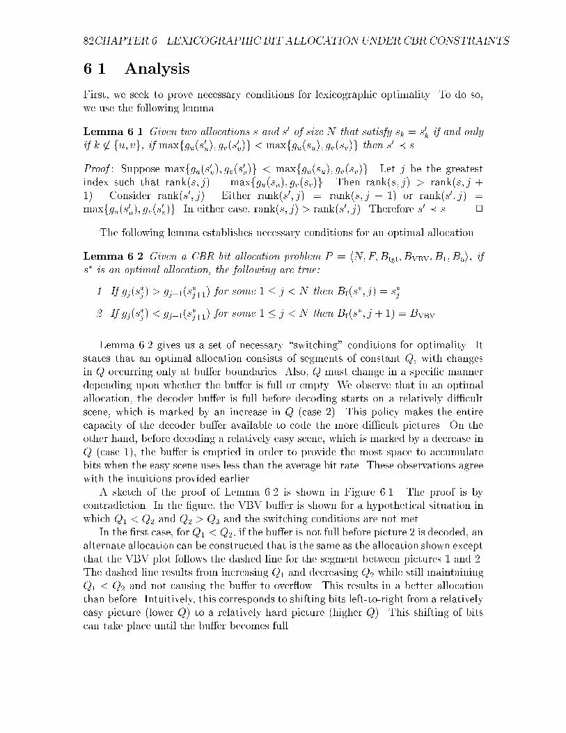
82CHAPTER 6. LEXICOGRAPHIC BIT ALLOCATION UNDERCBR CONSTRAINTS
6.1 Analysis
First, we seek to prove necessary conditions for lexicographic optimality. To do so,we use the following lemma.
Lemma 6.1 Given two allocations s and s0 of size N that satisfy sk = s0k if and only
if k 62 fu; vg, if maxfgu(s0u); gv(s0v)g < maxfgu(su); gv(sv)g then s0 � s.
Proof : Suppose maxfgu(s0u); gv(s0v)g < maxfgu(su); gv(sv)g. Let j be the greatestindex such that rank(s; j) = maxfgu(su); gv(sv)g. Then rank(s; j) > rank(s; j +1). Consider rank(s0; j). Either rank(s0; j) = rank(s; j + 1) or rank(s0; j) =maxfgu(s0u); gv(s0v)g. In either case, rank(s; j) > rank(s0; j). Therefore s0 � s. 2
The following lemma establishes necessary conditions for an optimal allocation.
Lemma 6.2 Given a CBR bit allocation problem P = hN;F;Btgt; BVBV; B1; Bai, ifs� is an optimal allocation, the following are true:
1. If gj(s�j) > gj+1(s
�j+1) for some 1 � j < N then Bf(s
�; j) = s�j .
2. If gj(s�j) < gj+1(s
�j+1) for some 1 � j < N then Bf(s
�; j + 1) = BVBV.
Lemma 6.2 gives us a set of necessary \switching" conditions for optimality. Itstates that an optimal allocation consists of segments of constant Q, with changesin Q occurring only at bu�er boundaries. Also, Q must change in a speci�c mannerdepending upon whether the bu�er is full or empty. We observe that in an optimalallocation, the decoder bu�er is full before decoding starts on a relatively di�cultscene, which is marked by an increase in Q (case 2). This policy makes the entirecapacity of the decoder bu�er available to code the more di�cult pictures. On theother hand, before decoding a relatively easy scene, which is marked by a decrease inQ (case 1), the bu�er is emptied in order to provide the most space to accumulatebits when the easy scene uses less than the average bit rate. These observations agreewith the intuitions provided earlier.
A sketch of the proof of Lemma 6.2 is shown in Figure 6.1. The proof is bycontradiction. In the �gure, the VBV bu�er is shown for a hypothetical situation inwhich Q1 < Q2 and Q2 > Q3 and the switching conditions are not met.
In the �rst case, for Q1 < Q2, if the bu�er is not full before picture 2 is decoded, analternate allocation can be constructed that is the same as the allocation shown exceptthat the VBV plot follows the dashed line for the segment between pictures 1 and 2.The dashed line results from increasing Q1 and decreasing Q2 while still maintainingQ1 < Q2 and not causing the bu�er to over ow. This results in a better allocationthan before. Intuitively, this corresponds to shifting bits left-to-right from a relativelyeasy picture (lower Q) to a relatively hard picture (higher Q). This shifting of bitscan take place until the bu�er becomes full.

6.1.ANALYSIS
83
1Q
2Q
3Q
1Q
2Q
<
Q2
Q3
>
0
0
B
B
TT
+T
T+
2TT
+3T
Tim
e
Buffer
00
00
i
VB
V
Fullness
Figu
re6.1:
Sketch
forproofof
Lem
ma6.2.
Inthesecon
dcase,
forQ2>Q3 ,
ifthebu�er
isnot
empty
afterpictu
re2is
deco
ded,an
alternate
allocation
canbecon
structed
that
isthesam
eas
theallo
cationshow
nexcep
tthat
theVBV
plot
followsthedotted
linefor
thesegm
entbetw
eenpictu
res2and3.
Thedotted
lineresu
ltsfrom
decreasin
gQ2andincreasin
gQ3while
stillmain
tainingQ2>Q3andnot
causin
gthebu�er
tounder
ow.Thisresu
ltsin
abetter
allocation
than
before.
Intuitively,
thiscorresp
ondsto
shiftin
gbits
right-to-left
fromarelatively
easypictu
re(low
erQ)to
arelatively
hard
pictu
re(high
erQ).This
shiftin
gof
bits
cantake
place
until
thebu�er
becom
esem
pty.
Wenote
that
Lem
ma5.1
followsdirectly
fromLem
ma6.2.
Proo
fofLem
ma6.2:
Case
1.
Weprove
Case
1bycon
tradiction
.Suppose
Bf (s
�;j)6=
s�j .
Let
�=
Bf (s
�;j)�s�j .
Then
by(5.5),
�>0.
Consid
eran
allocation
s0that
di�ers
froms�
only
forpictu
resjandj+1;that
is,
s0k=s�k
fork2f1;:::;N
gnfj;j
+1g
and
s0k 6=
s�k
fork2fj;j
+1g:
(6.1)In
order
toshow
acon
tradiction
,wewantto
�ndan
assignmenttos0jands0j+1that
makes
s0alegal
allocation
and\better"
than
s�.By\better"
wemean
gj (s
0j );gj+1 (s
0j+1 )<gj (s
�j ):(6.2)
Equivalen
tly,wewant
s0j>s�j
(6.3)
and
s0j+1>fj+1 (g
j (s�j )):
(6.4)

84CHAPTER 6. LEXICOGRAPHIC BIT ALLOCATION UNDERCBR CONSTRAINTS
To meet the target bit rate, we must have
s0j + s0j+1 = s�j + s�j+1: (6.5)
Let � = s0j � s�j . Then s�j+1 � s0j+1 = �. By (6.3), we want � > 0. We want to showthat s0 is a legal allocation for some value of � > 0. To avoid VBV violations, (5.8)must hold for all pictures under the allocation s0. From (6.1) and (6.5), we have
Bf(s0; k) = Bf(s
�; k) for k 6= j + 1: (6.6)
Since s� is a legal allocation, there are no VBV violations for pictures 1, 2, : : :,j � 1 under s0. Furthermore, if our choice for s0j does not cause a VBV violation forpicture j, then we are assured that there would be no VBV violations in picturesj + 1, j + 2, : : :, N . So we must choose s0j subject to (5.8) and (6.3). Therefore
s�j < s0j � s�j +�: (6.7)
If 0 < � � �, then s0 is a legal allocation. We also want (6.4) to hold. For this weneed
� < s�j+1 � fj+1(gj(s�j)): (6.8)
Since gj(s�j) > gj+1(s
�j+1), we have fj+1(gj(s
�j)) < s�j+1. Therefore s
�j+1�fj+1(gj(s�j)) >
0. So for0 < � � minf�; s�j+1 � fj+1(gj(s�j))g (6.9)
s0 is a legal allocation that meets condition (6.2). By Lemma 6.1, s� � s0 and s� isnot an optimal allocation, a contradiction.
Case 2. We prove Case 2 by contradiction. Suppose Bf(s�; j + 1) 6= BVBV. Let
� = BVBV � Bf(s�; j + 1). Then by (5.4), � > 0. Consider an allocation s0 that
di�ers from s� only for pictures j and j + 1; that is,
s0k = s�k for k 2 f1; : : : ; Ng n fj; j + 1g : (6.10)
We want to �nd an assignment to s0j and s0j+1 that makes s0 a legal allocation and
\better" than s�, in order to show a contradiction. By \better" we mean
gj(s0j); gj+1(s
0j+1) < gj+1(s
�j+1): (6.11)
Equivalently, we wants0j+1 > s�j+1 (6.12)
ands0j > fj(gj+1(s
�j+1)): (6.13)
To meet the target bit rate, we must have
s0j + s0j+1 = s�j + s�j+1: (6.14)

6.1. ANALYSIS 85
Let � = s0j+1 � s�j+1. Then s�j � s0j = �. By (6.12), we want � > 0. We want to showthat s0 is a legal allocation for some value of � > 0. To avoid VBV violations, (5.8)must hold for all pictures under the allocation s0. From (6.10) and (6.14), we have
Bf(s0; k) = Bf(s
�; k) for k 6= j + 1: (6.15)
Since s� is a legal allocation, there are no VBV violations for pictures 1 to j�1 unders0. Furthermore, if our choice for s0j does not cause a VBV violation, then we areassured that there would be no VBV violations in pictures j + 1 to N . So we mustchoose s0j subject to (5.8) and (6.12).
Bf(s0; j + 1) = Bf(s
0; j) +Ba(j)� s0jBf(s
0; j + 1) = Bf(s�; j) +Ba(j)� s0j
Bf(s�; j + 1) = Bf(s
�; j) +Ba(j)� s�jBf(s
0; j + 1) = Bf(s�; j + 1) + s�j � s0j
Bf(s0; j + 1) = BVBV ��+ � � BVBV
From the above, we require � � �. If 0 < � � �, then s0 is a legal allocation. Wealso want (6.13) to hold. For this we need
� < s�j � fj(gj+1(s�j+1)): (6.16)
Since gj+1(s�j+1) > gj(s
�j), we have fj(gj+1(s
�j+1)) < s�j . Therefore s
�j�fj(gj+1(s�j+1)) >
0. So for0 < � � minf�; s�j � fj(gj+1(s�j+1))g (6.17)
s0 is a legal allocation that meets condition (6.13). By Lemma 6.1, s� � s0 and s� isnot an optimal allocation, a contradiction.
2
The theorem that follows is the main result of this section and shows that theswitching conditions are also su�cient for optimality. But �rst we prove a usefullemma that will be helpful in the proof of the theorem.
Lemma 6.3 Given bit allocations s and s0 with sj � s0j for u � j � v and Bf(s; u) �Bf(s
0; u), we have Bf(s; v + 1) = Bf(s0; v + 1) if and only if Bf(s; u) = Bf(s
0; u) andsj = s0j for u � j � v.
Proof : We use (5.3) to express Bf(s; v + 1) in terms of Bf(s; u).
Bf(s; v + 1) = B1 +vX
j=1
(Ba(j)� sj)
Bf(s; u) = B1 +u�1Xj=1
(Ba(j)� sj)
Bf(s; v + 1) = Bf(s; u) +vX
j=u
(Ba(j)� sj) :

86CHAPTER 6. LEXICOGRAPHIC BIT ALLOCATION UNDERCBR CONSTRAINTS
Similarly,
Bf(s0; v + 1) = Bf(s
0; u) +vX
j=u
�Ba(j)� s0j
�:
First we prove the \if" part. Suppose Bf(s; u) = Bf(s0; u) and sj = s0j for u � j �
v. Then
Bf(s; v + 1) = Bf(s; u) +vX
j=u
(Ba(j)� sj)
= Bf(s0; u) +
vXj=u
�Ba(j)� s0j
�
= Bf(s0; v + 1):
Now we prove the \only if" part. Suppose Bf(s; v + 1) = Bf(s0; v + 1). Then
Bf(s; v + 1) = Bf(s0; v + 1)
Bf(s; u) +vX
j=u
(Ba(j)� sj) = Bf(s0; u) +
vXj=u
�Ba(j)� s0j
�
Bf(s; u)� Bf(s0; u) =
vXj=u
(sj � s0j): (6.18)
But Bf(s; u) � Bf(s0; u) and sj � s0j for u � j � v. Therefore Bf(s; u)�Bf(s
0; u) � 0and
Pvj=u(sj � s0j) � 0. Combined with (6.18), this implies that Bf(s; u) = Bf(s
0; u)and
Pvj=u sj =
Pvj=u s
0j. Since sj � s0j for u � j � v, this implies that sj = s0j for
u � j � v. 2
Theorem 6.1 Given a CBR bit allocation problem P = hN;F;Btgt; BVBV; B1; Bai,a legal allocation s is optimal if and only if the following conditions hold. Also, the
optimal allocation is unique.
1. If gj(sj) > gj+1(sj+1) for some 1 � j < N , then Bf(s; j) = sj.
2. If gj(sj) < gj+1(sj+1) for some 1 � j < N , then Bf(s; j + 1) = BVBV.
Proof : Lemma 6.2 established these condition as necessary for optimality. Nowwe need to show that these conditions are also su�cient for optimality and implyuniqueness. Let s be a legal allocation that meets both conditions of the theorem.
Let s� be an optimal allocation for P . Let Qmax = max1�j�Nfgj(sj)g. Considerthe segments of consecutive pictures that are assigned Qmax by allocation s. Let ube the index of the start of such a segment. There are two cases: u = 1 and u > 1.If u = 1, then Bf(s; u) = Bf(s
�; u) = B1. If u > 1, then since u is the index ofthe start of the segment, gu�1(su�1) < gu(su) which implies that Bf(s; u) = BVBV by

6.1. ANALYSIS 87
condition 2. Since s� is a legal allocation, Bf(s�; u) � BVBV = Bf(s; u). In either case
we haveBf(s; u) � Bf(s
�; u): (6.19)
Let v be the index of the end of the segment. Since s� is optimal, gj(s�j) � Qmax
for all j, ands�j � sj for u � j � v: (6.20)
ThereforeBf(s
�; j) � Bf(s; j) for u � j � v: (6.21)
There are two cases for v: v = N and v < N . If v = N , then Bf(s; v + 1) =Bf(s
�; v + 1) = B1 +PN�1
j=1 Ba(j) � Btgt. If v < N , then since v is the index of theend of the segment, gv(sv) > gv+1(sv+1) which implies that
Bf(s; v) = sv (6.22)
by condition 1. Since s� is a legal allocation, Bf(s�; v) � s�v. Combine this with (6.22)
and (6.20) we haveBf(s
�; v) � Bf(s; v): (6.23)
Combining (6.21) and (6.23), we have Bf(s�; v) = Bf(s; v) and s
�v = sv. As a result,
Bf(s�; v+1) = Bf(s; v+1). In either case, Bf(s
�; v+1) = Bf(s; v+1). By Lemma 6.3,Bf(s
�; u) = Bf(s; u) and s�j = sj for u � j � v. As a consequence, Bf(s; j) = Bf(s
�; j)for u � j � v.
We partition pictures 1 through N into segments, where, according to allocations, the pictures in a segment use the same value of Q, either the �rst picture in thesegment is picture 1 or the �rst picture in the segment uses a value of Q di�erentfrom the previous picture, and either the last picture in the segment is picture N orthe last picture in the segment uses a value of Q di�erent from the next picture. LetM be the number of such segments. We order the segments so that segment k uses avalue of Q greater than or equal to the value of Q used in segment j for j < k, anddenote the value of Q used by segment k as Q
(s)k .
We will show that allocation s� uses the same number of bits as allocation s foreach picture in segment k, for 1 � k � M . This will establish the conditions in thetheorem as necessary and show that the optimal allocation is unique. We will provethis by induction on k. The base case of k = 1 has already been proven.
Inductive Hypothesis: For all segments of pictures u to v with u = 1 or gu�1(su�1) 6=gu(su), v = N or gv(sv) 6= gv+1(sv+1), and gj(sj) = Q
(s)k , we have s�j = sj and
Bf(s; u) = Bf(s�; u) for u � j � v.
Let us assume that the hypothesis is true for 1 � k < m. We will show that isis also true for k = m. Consider a segment of consecutive pictures that are assignedquantization Q(s)
m by allocation s. Let u be the index of the start of the segment andv the index of the end of the segment.

88CHAPTER 6. LEXICOGRAPHIC BIT ALLOCATION UNDERCBR CONSTRAINTS
By the inductive hypothesis, s and s� use the same values of Q for all pictures forwhich s uses Q > Q(s)
m . Because s� is optimal, gj(s�j) � gj(sj) = Q(s)
m for u � j � v,and thus
s�j � sj for u � j � v: (6.24)
We consider all cases for the segment boundaries. For the left segment boundarythere are three cases: u = 1, gu�1(su�1) > gu(su), and gu�1(su�1) < gu(su). If u = 1,then Bf(s
�; u) = Bf(s; u) = B1. If gu�1(su�1) > gu(su), then from the inductivehypothesis, we have Bf(s
�; u�1) = Bf(s; u�1) and s�u�1 = su�1; therefore Bf(s�; u) =
Bf(s; u). If gu�1(su�1) < gu(su), then from condition 2, we have Bf(s; u) = BVBV;since s� is a legal allocation, Bf(s
�; u) � BVBV = Bf(s; u). For all three cases we have
Bf(s�; u) � Bf(s; u): (6.25)
For the right segment boundary there are three cases: v = N , gv(sv) < gv+1(sv+1),and gv(sv) > gv+1(sv+1). If v = N , then Bf(s
�; v + 1) = Bf(s; v + 1) = B1 +PN�1j=1 Ba(j) � Btgt. If gv(sv) < gv+1(sv+1), then from the inductive hypothesis, we
have Bf(s�; v + 1) = Bf(s; v + 1).
If gv(sv) > gv+1(sv+1), then from condition 1 we have Bf(s; v) = sv. From (6.24)and (6.25) we have
Bf(s�; j) � Bf(s; j) for u � j � v: (6.26)
Since s� is a legal allocation,
Bf(s�; v) � s�v � sv = Bf(s; v): (6.27)
Combining (6.26) and (6.27), we have Bf(s�; v) = Bf(s; v) and s�v = sv. Therefore
Bf(s�; v + 1) = Bf(s; v + 1).For all three cases we have
Bf(s�; v + 1) = Bf(s; v + 1): (6.28)
From (6.24), (6.25), (6.28), and Lemma 6.3, we have s�j = sj for u � j � v. Itfollows that Bf(s; j) = Bf(s
�; j) for u � j � v. By induction, we have s�j = sj for allj, and so s = s�. 2
6.2 CBR Allocation Algorithm
Theorem 6.1 is a powerful result. It says that to �nd the optimal allocation we needonly to �nd a legal allocation that meets the stated switching conditions. In thissection, we use the technique of dynamic programming (DP) to develop an algorithmto compute a lexicographically optimal CBR allocation in polynomial time and linearspace.

6.2. CBR ALLOCATION ALGORITHM 89
Initial Buffer
Fullness
Bot[1] Bot[2] Bot[k]
Top[1] Top[2] Top[k]
Next State
Figure 6.2: Illustration of search step in dynamic programming algorithm.
6.2.1 DP Algorithm
The basic idea behind dynamic programming is to decompose a given problem interms of optimal solutions to smaller problems. All we need to do is maintain invariantthe conditions stated in Theorem 6.1 for each subproblem we solve. We do this byconstructing optimal bit allocations for pictures 1 to k that end up with the VBVbu�er in one of two states: full or empty. These states are exactly the states where achange in Q may occur. Let Topk be the optimal allocation for pictures 1 to k thatend up with the VBV bu�er full, if such an allocation exists. Similarly, let Botk bethe optimal allocation for pictures 1 to k that end up with the VBV bu�er empty.Suppose that we have computed Topi and Boti for 1 � i � k. To compute Topk+1,we search for a legal allocation among
n;;Top1; : : : ;Topk;Bot1; : : : ;Botk
o, where ;
denotes the empty allocation, to which we can concatenate a constant-Q segment togive a legal allocation s such that the switching conditions are met and the bu�erends up full, that is, Bf(s; k + 1) = BVBV. Similarly, for Botk+1 we search for apreviously computed allocation that, when extended by a constant-Q segment, meetsthe switching conditions and results in the bu�er being empty, that is, Bf(s; k+1) =sk+1.
The basic step in the DP algorithm is illustrated in Figure 6.2. The round nodesrepresent bu�er states for which we have previously computed optimal allocations.Each node stores the lastQ used in the optimal allocation for that state and the originof the last constant-Q segment leading to that state. The square node representsthe next state that we wish to compute. The dashed lines represent a constant-Qallocation that connects the respective nodes. To compute a solution for the squarenode, we need to search for an edge that connects the square node with a round nodesuch that the switching conditions are met. For each edge, the switching conditionsare checked by comparing the Q used for the edge against the last Q used in theoptimal solution for the round node that the edge connects. The allocation impliedby each edge is also checked for VBV compliance.
Once we have computed TopN�1 and BotN�1, we can compute the optimal alloc-ation for all N pictures in a process similar to the one above for computing Topk
and Botk, except that the �nal allocation results in a �nal bu�er state that gives the

90CHAPTER 6. LEXICOGRAPHIC BIT ALLOCATION UNDERCBR CONSTRAINTS
desired target number of bits Btgt.
6.2.2 Correctness of DP Algorithm
When computing Topk and Botk for 1 � k � N � 1, we have insured that the condi-tions of Theorem 6.1 are met. Additionally in the �nal computation, the conditionsare also met. Therefore we end up with a legal allocation that meets the conditionsof Theorem 6.1 and is thus optimal.
6.2.3 Constant-Q Segments
We have used the concept of a constant-Q segment extensively in the above discus-sion. We now formalize this concept. First, we de�ne a family of bit-productionfunctions fFi;j(q)g that gives the number of bits resulting from allocating a constantvalue of Q for pictures i to j, inclusive:
Fi;j(q) =X
i�k�j
fk(q): (6.29)
What we are really interested in, though, is the inverse of Fi;j. We denote the inverseas Gi;j so that Gi;j = F�1
i;j . Then Gi;j(B) gives the constant Q that results in B bitsbeing produced by pictures i to j collectively. Since fi is monotonically decreasing,so is Fi;j, and thus Gi;j is monotonically increasing.
6.2.4 Verifying a Constant-Q Allocation
The DP algorithm for CBR bit allocation needs to verify whether a constant-Q alloc-ation meets VBV bu�er constraints. This can be done in time linear in the lengthof the allocation by simulating the VBV. In the DP algorithm, O(N2) veri�cationsof constant-Q allocations are needed. If each veri�cation requires linear time, thistranslates to at least cubic time complexity for the DP algorithm.
We observe that the constant-Q allocations to be veri�ed start with the bu�ereither full, empty, or at its initial state; and end with the bu�er either full, empty,or at its �nal state. We also note that for an allocation to a segment of pictures,say from i to j, with a �xed initial bu�er state, say B1, and using BT bits, there isa continuous range of Q values that results in a legal allocation. When additionalpictures are considered, this range of legal Q values never widens. Furthermore, theupper bound for Q is simply the minimum Q among the constant-Q allocations forpictures i to j in which the bu�er is exactly full for some picture k, where i � k < j.More formally,
Gi;j(BT) � mini�k<j
nGi;k
�B1 +
Xi�m�k
Ba(m)� BVBV
�o: (6.30)

6.3. RELATED WORK 91
Similarly, the lower bound for Q is the maximumQ among the constant-Q allocationsfor pictures i to j in which the bu�er is exactly empty for some picture k, wherei � k < j. More formally,
Gi;j(BT) � maxi�k<j
nGi;k
�B1 +
Xi�m<k
Ba(m)�o: (6.31)
We can use these observations to perform all the VBV veri�cations in constant timeper veri�cation with linear-time preprocessing.
6.2.5 Time and Space Complexity
The time complexity of the DP algorithm depends upon two main factors: the timeto compute a constant-Q allocation and the time to verify whether a sub-allocationis legal.
We assume that fi and Gi;j can be evaluated in constant time with O(N) prepro-cessing time and space. An example is fi(q) = �i=q + �i, where
Gi;j(B) =
Pi�k�j �k
B �Pi�k�j �k:
We can precompute the pre�x sums of �i and �i in linear time and space and thenuse these to compute Gi;j in constant time. The same technique can be used forbit-production models of the form: fi(q) = �i=q
2 + �i=q + i, fi(q) = �i=q3 + �i=q
2 + i=q+�i, and fi(q) = �i=q
4+ �i=q3+ i=q
2+�i=q+ �i. Examples of other functionalforms for fi with a closed-form solution for Gi;j can be found in [54]. Of course, weneed to insure that the models are monotonically decreasing.
Since VBV veri�cation and constant-Q calculation can be done in constant timewith linear-time preprocessing, computing Topk and Botk takes O(k) time. Therefore,to compute an optimal allocation for a sequence ofN pictures would take
PNk=1O(k) =
O(N2) time. If we store pointers for tracing the optimal sequence of concatenations,the algorithm requires O(N) space.
In Chapter 8, we show how to use some sophisticated data structures for com-putational geometry to reduce the running time to O(N log2N) in the worst case,although in practice the running time is roughly linear.
6.3 Related Work
Conditions similar to the switching conditions of Theorem 6.1 have been describedin [46] for optimal bu�ered bit allocation under a minimum sum-distortion crite-rion and assuming independent convex rate-distortion functions. In this work, theLagrange multiplier method is used to �nd a bit allocation that is optimal withina convex-hull approximation. The optimal vector of Lagrange multipliers consists of

92CHAPTER 6. LEXICOGRAPHIC BIT ALLOCATION UNDERCBR CONSTRAINTS
constant-valued segments that increase (decrease, respectively) only when the decoderbu�er is full (empty).
In [76], the theory of majorization [56] is applied to reduce the variability intransmission rate for stored video. In this setting, the problem is to determine afeasible transmission schedule by which a pre-compressed video bitstream can betransmitted over a communications channel to the decoder without under owing orover owing the decoder bu�er. As applied to this problem, majorization results inminimizing the peak and variance in transmission rate. The authors provide anoptimal smoothing algorithm that runs in time linear in the length of the videosequence.
It can be easily shown that the majorization solution to optimal smoothing of [76]is in fact equivalent to lexicographic minimization of the transmitted rates, subjectto the constraint that the total number of bits transmitted is �xed. The linearrunning time is possible because the bu�ering constraints are manifested as �xedupper and lower bounds on the cumulated number of bits transmitted. In comparison,in bu�er-constrained bit allocation, there is no �xed relationship between the bu�eringconstraints and the nominal quantization (equivalently, distortion) that is the objectof optimization. In a sense, the bu�er-constrained bit allocation problem that weconsider is \harder" than optimal smoothing. A more sophisticated data structure,which we discuss in Chapter 8, is needed in order to reduce the running time tonear-linear time.
6.4 Discussion
The analyses presented here are based upon simpli�cations of the actual video codingprocess. In particular, one of the prerequisites is an accurate bit-production model foreach picture of the video sequence. Another prerequisite is proper adaptive perceptualquantization.
The bit-production model described in Section 5.3 assumes that the coding of aparticular picture is independent of the coding of any other picture. As noted earlier,this independence assumption does not hold for video coders that employ a di�erentialcoding scheme such as motion compensation. In this case, the coding of a referencepicture a�ects the coding of subsequent pictures that are coded with respect to it.Therefore, the bit-production model for picture i would depend causally not onlyupon the quantization scale used for picture i but also upon the quantization scalesused for its reference pictures. The dependent coding problem has been addressedin the traditional distortion-minimization framework in [73]. Whether the results ofthis chapter can be extended to a dependent-coding framework is an open problem.
The dynamic programming solution in Section 6.2 ignores some of the structurethat exists in the framework due to the monotonicity assumption and focuses solelyon achieving the switching conditions of Theorem 6.1 by \brute force." For example,a \blind" search strategy is used to �nd the edge that connects the end state with a

6.4. DISCUSSION 93
previously-computed optimal sub-allocation and meets the switching conditions. Afeasible connector that fails the switching conditions may yield some knowledge thatcan be used to reduce the search space. Improving the time-complexity is a promisingopen problem.

94CHAPTER 6. LEXICOGRAPHIC BIT ALLOCATION UNDERCBR CONSTRAINTS

Chapter 7
Lexicographic Bit Allocation under
VBR Constraints
VBR Constraints
In this chapter, we analyze the bu�er-constrained bit allocation problem undervariable-bit-rate VBV constraints, as described in Section 5.4.2. The analysis leadsto an e�cient iterative algorithm for computing a lexicographically optimal solution.
In CBR operation, the total number of bits that a CBR stream can use is dictatedby the channel bit rate and the bu�er size. With VBR operation, the total numberof bits has no lower bound, and its upper bound is determined by the peak bit rateand the bu�er size. Consequently, VBR is useful and most advantageous over CBRwhen the average bit rate needs to be lower than the peak bit rate. This is especiallycritical in storage applications, where the storage capacity, and not the transfer rate,is the limiting factor. Another important application of VBR video coding is formultiplexing multiple video bitstreams over a CBR channel [27]. In this application,statistical properties of the multiple video sequences allow more VBR bitstreams witha given peak rate Rmax to be multiplexed onto the channel than CBR bitstreams codedat a constant rate of Rmax.
For typical VBR applications, then, the average bit rate is lower than the peak.In this case, bits enter the decoder bu�er at an e�ective bit rate that is less thanthe peak during the display interval of many pictures. In interesting cases, there willbe segments of pictures that will be coded with an average bit rate that is higherthan the peak. This is possible because of the bu�ering. During the display of thesepictures, the VBV bu�er �lls at the peak rate. Since these pictures require morebits to code than the peak rate, they are \harder" to code than the other \easier"pictures.
In order to equalize quality, the easy pictures should be coded at the same basequality. It does not pay to code any of the hard pictures at a quality higher than thatof the easy pictures. The bits expended to do so could instead be better distributedto raise the quality of the easy pictures. Among the hard pictures, there are di�erent
95
96CHAPTER 7. LEXICOGRAPHIC BIT ALLOCATION UNDERVBR CONSTRAINTS
levels of coding di�culty. Using the same intuitions from the CBR case, we can drawsimilar conclusions about the bu�er emptying and �lling behavior among the hardpictures.
In the following analysis, we show that a lexicographically optimal VBR bit alloc-ation possesses the properties described above. In particular, the hard segments ofpictures in a VBR bit allocation behave as in a CBR setting. In fact, the VBRalgorithm invokes the CBR algorithm to allocate bits to segments of hard pictures.
7.1 Analysis
The following two lemmas characterize the \easy" pictures in an optimal allocation,that is, the pictures that are coded with the best quality (lowest Q).
Lemma 7.1 Given a VBR bit allocation problem P = hN;F;Btgt; BVBV; B1; Bai andan optimal allocation s�, if Bf(s
�; j) + Ba(j) � s�j > BVBV for 1 � j � N , then
gj(s�j) = min1�k�Nfgk(s�k)g.
Proof : Let Qmin = min1�k�Nfgk(s�k)g. Let j be an index such that Bf(s�; j)+Ba(j)�
s�j > BVBV. Let � = Bf(s�; j) +Ba(j)� s�j � BVBV. Thus, � > 0.
Suppose that gj(s�j) > Qmin. Let u be an index such that gu(s
�u) = Qmin. Consider
an allocation s that di�ers from s� only for pictures j and u. We want to assignvalues to sj and su that make s a legal allocation with gj(sj); gu(su) < gj(s
�j), from
which s� � s, a contradiction.The idea is that we want to shift a (positive) number of bits, say �, from picture u
to picture j but still have a legal allocation. Let sj = s�j + � and su = s�u � � with� > 0. Then gj(sj) < gj(s
�j) and
PNk=1 sk =
PNk=1 s
�k = Btgt. We now need to show
that s does not result in a VBV bu�er under ow, that is, Bf(s; k) � sk for 1 � k � N .There are two cases to consider: u < j and u > j.
Case 1 : u < j. Since sk = s�k for k < u, we have Bf(s; k) = Bf(s�; k) for 1 � k � u.
Since su < s�u and sk = s�k for u < k < j, we have Bf(s; k) � Bf(s�; k) for u < k � j.
Therefore pictures 1 to j � 1 cannot cause any VBV bu�er under ows. If we choose0 < � < �, then Bf(s; j + 1) = BVBV and picture j also cannot cause a VBV bu�erunder ow. Since sk = s�k for k > j and Bf(s; j + 1) = Bf(s
�; j + 1), pictures j + 1 toN also cannot cause any VBV bu�er under ows.
Case 2 : u > j. Since sk = s�k for k < j, we have Bf(s; k) = Bf(s�; k) for 1 � k � j.
If we choose 0 < � < �, then Bf(s; j + 1) = BVBV and picture j also cannot cause aVBV bu�er under ow. Since sk = s�k for j < k < u, and Bf(s; j + 1) = Bf(s
�; j + 1)(by a suitable choice of �), pictures j + 1 to u� 1 also cannot cause any VBV bu�erunder ows. Since su < s�u, we have Bf(s; k) � Bf(s
�; k) for k : k � u. Thereforepictures u to N also cannot cause any VBV bu�er under ows.

7.1. ANALYSIS 97
Therefore s is a legal allocation with gj(sj) < gj(s�j). We need to guarantee that
gu(su) < gj(s�j). Let = gj(s
�j) � gu(s�u). Since gj(s�j) > gu(s
�u), we have > 0. Let
� = s�u � fu(gu(s�u) + =2). Since fu is decreasing and > 0, we have � > 0 and
s�u � � = fu(gu(s�u) + =2)
gu(s�u � �) = gu(s
�u) + =2
< gu(s�u) +
= gj(s�j):
Consider the assignment � = minf�;�=2g. There are two cases: � � �=2 and� > �=2. If � � �=2, we have � = � from which gu(su) = gu(s
�u� �) = gu(s
�u� �) <
gj(s�j); since 0 < � < �, the allocation s is legal. If � > �=2, we have � = �=2.
Since gu is decreasing and � > �=2, we have gu(s�u � �=2) < gu(s
�u � �) and thus
gu(su) = gu(s�u � �) = gu(s
�u � �=2) < gj(s
�j). Since 0 < � < �, the allocation s is
legal.Since s is a legal allocation that di�ers from s� only for pictures u and j with
gu(su) < gj(s�j) and gj(sj) < gj(s
�j), from Lemma 6.1 we have s� � s, but s� is not
optimal, a contradiction. Therefore gj(s�j) = min1�k�Nfgk(s�k)g. 2
Lemma 7.2 Given a VBR bit allocation problem P = hN;F;Btgt; BVBV; B1; Bai andan optimal allocation s�, if Bf(s
�; N) > s�N then gN(s�N) = min1�k�Nfgk(s�k)g.
Proof : Let Qmin = min1�k�Nfgk(s�k)g. Let j be an index such that Bf(s�; j)+Ba(j)�
s�j > BVBV. Let � = Bf(s�; N)� s�N . Since Bf(s
�; N) > s�N , we have � > 0. Supposethat gN(s
�N ) > Qmin. Let u be an index such that gu(s
�u) = Qmin. Now consider an
allocation s that di�ers from s� only for pictures u and N . We want to assign valuesto sN and su that make s a legal allocation with gN(sN); gu(su) < gN(s
�N), from which
s� � s, thereby arriving at a contradiction. Let sN = s�N + � and su = s�u � � with� > 0. Then gN(sN ) < gN(s
�N) and
PNk=1 sk =
PNk=1 s
�k = Btgt. We now need to show
that s does not result in a VBV bu�er under ow, that is, Bf(s; k) � sk for 1 � k � N .Since sk = s�k for k < u, we have Bf(s; k) = Bf(s
�; k) for 1 � k � u. Since su < s�uand sk = s�k for u < k < N , we have Bf(s; k) � Bf(s
�; k) for u < k � N . Thereforepictures 1 to N �1 cannot cause any VBV bu�er under ows. For picture N , we haveBf(s;N) � Bf(s
�; N) = � + s�N = � + sN � �. Therefore if we choose � < �, thenBf(s;N) > sN and picture N also cannot cause a VBV bu�er under ow.
Therefore s is a legal allocation with gN(sN ) < gN(s�N). We need to guarantee that
gu(su) < gN(s�N ). Let = gN(s
�N) � gu(s�u). Since gN(s�N ) > gu(s
�u), we have > 0.
Let � = s�u � fu(gu(s�u) + =2). Since fu is decreasing and > 0, we have � > 0 and
s�u � � = fu(gu(s�u) + =2)
gu(s�u � �) = gu(s
�u) + =2
< gu(s�u) +
= gN(s�N):

98CHAPTER 7. LEXICOGRAPHIC BIT ALLOCATION UNDERVBR CONSTRAINTS
Consider the assignment � = minf�;�=2g. There are two cases: � � �=2 and� > �=2. If � � �=2, we have � = � from which gu(su) = gu(s
�u� �) = gu(s
�u� �) <
gN(s�N); since 0 < � < �, the allocation s is legal. If � > �=2, we have � = �=2.
Since gu is decreasing and � > �=2, we have gu(s�u � �=2) < gu(s
�u � �) and thus
gu(su) = gu(s�u � �) = gu(s
�u ��=2) < gN(s
�N). Since 0 < � < �, the allocation s is
legal.Since s is a legal allocation that di�ers from s� only for pictures u and N with
gu(su) < gN(s�N) and gN(sN) < gN(s
�N), from Lemma 6.1, we have s� � s, and s� is
not optimal, a contradiction. Therefore gN(s�N ) = min1�k�Nfgk(s�k)g. 2
The next lemma gives a set of switching conditions for changes in Q that aresimilar to the results of Lemma 6.2.
Lemma 7.3 Given a VBR bit allocation problem P = hN;F;Btgt; BVBV; B1; Bai, ifs� is an optimal allocation, the following are true:
1. If gj(s�j) > gj+1(s
�j+1) for 1 � j < N , then Bf(s
�; j) = s�j .
2. If gj(s�j) < gj+1(s
�j+1) for 1 � j < N , then Bf(s
�; j + 1) = BVBV and Bf(s�; j +
1) +Ba(j + 1)� s�j+1 � BVBV.
Proof :Case 1. The proof is identical to the proof of Case 1 of Lemma 6.2, except thatcondition (5.5) now holds instead of (5.8).Case 2. Suppose that Case 2 is false. Then either Bf(s
�; j + 1) < BVBV orBf(s
�; j + 1) + Ba(j + 1) � s�j+1 > BVBV. Suppose that Bf(s�; j + 1) + Ba(j + 1) �
s�j+1 > BVBV. Then by Lemma 7.1, gj+1(s�j+1) � gj(s
�j), a contradiction. Therefore
Bf(s�; j + 1) +Ba(j + 1)� s�j+1 � BVBV.Suppose that Bf(s
�; j + 1) < BVBV. Let � = BVBV � Bf(s�; j + 1). Then � > 0.
Consider an allocation s that di�ers from s� only for pictures j and j + 1. We wantto assign values to sj and sj+1 that make s a legal allocation with gj(sj); gj+1(sj+1) <gj+1(s
�j+1), from which s� � s, thereby arriving at a contradiction.
Let = gj+1(s�j+1) � gj(s
�j) and � = s�j � fj(gj(s
�j) + =2). Since gj(s
�j) <
gj+1(s�j+1), we have > 0. Since fj is decreasing and > 0, we have � > 0 and
s�j � � = fj(gj(s�j) + =2)
gj(s�j � �) = gj(s
�j) + =2
< gj(s�j) +
= gj+1(s�j+1):
Consider the assignments sj = s�j � � and sj+1 = s�j+1 + �, where � = minf�;�=2g.By this assignment, we have gj+1(sj+1) < gj+1(s
�j+1). We now show that gj(sj) <
gj+1(s�j+1). There are two cases: � � �=2 and � > �=2. If � � �=2, we have � = �

7.1. ANALYSIS 99
from which gj(sj) = gj(s�j � �) = gj(s
�j � �) < gj+1(s
�j+1). If � > �=2, we have
� = �=2. Since gj is decreasing and � > �=2, we have gj(s�j � �=2) < gj(s
�j � �)
and thus gj(sj) = gj(s�j � �) = gj(s
�j � �=2) < gj+1(s
�j+1). In either case, we have
gj(sj) < gj+1(s�j+1).
We now need to show that allocation s as de�ned above is a legal allocation.Since sk = s�k for k < j, we have Bf(s; k) = Bf(s
�; k) for 1 � k � j. Thereforethere are no VBV bu�er violations in pictures 1 to j � 1. Since sj < s�j , we haveBf(s; j+1) > Bf(s
�; j+1). Therefore picture j cannot cause a VBV bu�er under ow.Now we need to show that pictures j + 1 to N also cannot cause a VBV bu�er
under ow. Since Bf(s�; j + 1) < BVBV, we have Bf(s
�; j + 1) = Bf(s�; j) +Ba(j)� s�j
and
Bf(s; j) +Ba(j)� sj = Bf(s�; j) +Ba(j)� (s�j � �)
= Bf(s�; j + 1) + �
< Bf(s�; j + 1) + �
= BVBV:
Thus Bf(s; j+1) = Bf(s; j)+Ba(j)� sj. We have already shown that Bf(s�; j+1)+
Ba(j + 1)� s�j+1 � BVBV. Therefore Bf(s�; j + 2) = Bf(s
�; j + 1) +Ba(j + 1)� s�j+1.Now,
Bf(s; j + 1) +Ba(j + 1)� sj+1 = Bf(s; j) +Ba(j)� sj +Ba(j + 1)� sj+1= Bf(s
�; j + 1) + � +Ba(j + 1)� (s�j+1 + �)
= Bf(s�; j + 1) +Ba(j + 1)� s�j+1
= Bf(s�; j + 2)
� BVBV:
Therefore Bf(s; j+2) = Bf(s�; j+2). Since sk = s�k for k > j +1, we have Bf(s; k) =
Bf(s�; k) for k > j + 1. Therefore pictures j + 1 to N cannot cause a VBV bu�er
under ow and s is a legal allocation.Since s is a legal allocation that di�ers from s� only for pictures j and j + 1 and
we have gj(sj) < gj+1(s�j+1) and gj+1(sj+1) < gj+1(s
�j+1), from Lemma 6.1 we have
s� � s, but s� is not optimal, a contradiction. 2
The following theorem is the main result of this section. It shows that theminimum-Q and switching conditions in the previous lemmas are also su�cient foroptimality.
Theorem 7.1 Given a VBR bit allocation problem P = hN;F;Btgt; BVBV; B1; Bai,a legal allocation s is optimal if and only if the following conditions hold. Also, the
optimal allocation is unique.

100CHAPTER 7. LEXICOGRAPHIC BIT ALLOCATION UNDER VBR CONSTRAINTS
1. If Bf(s; j)+Ba(j)�sj > BVBV for 1 � j � N , then gj(sj) = min1�k�Nfgk(sk)g.
2. If Bf(s�; N) > s�N then gN(s
�N) = min1�k�Nfgk(s�k)g.
3. If gj(sj) > gj+1(sj+1) for 1 � j < N , then Bf(s; j) = sj.
4. If gj(sj) < gj+1(sj+1) for 1 � j < N , then Bf(s; j + 1) = BVBV and Bf(s; j +1) +Ba(j + 1)� sj+1 � BVBV.
Proof : Lemmas 7.1, 7.2, and 7.3 establish these as necessary conditions. Now we needto show that these conditions are also su�cient for optimality and imply uniqueness.
The proof for su�ciency and uniqueness is similar to that of Theorem 6.1 exceptfor segments with the minimum Q. Here we consider only segments that use theminimum Q.
Let s� be an optimal allocation, Qmin = min1�j�Nfgj(sj)g, and Jmin =fj : gj(sj) = Qming. By condition 2, if gN(sN) > Qmin then it must be thatBf(s;N) = sN , or equivalently, Bf(s;N +1) = Ba(N). Therefore Bf(s;N) is known ifpicture N does not use the minimum Q, and we can use arguments of Theorem 6.1.Following the steps of Theorem 6.1, we can show that s�j = sj for j : gj(sj) > Qmin.
Since s� is optimal, we have gj(s�j) � gj(sj) for j 2 Jmin. Therefore
s�j � sj for j 2 Jmin: (7.1)
Since the total number of bits allocated is the same for s and s�, we have the numberof bits to be allocated to pictures in J must also be the same. That is,
Xj2Jmin
s�j =X
j2Jmin
sj: (7.2)
But (7.1) and (7.2) both hold if and only if s�j = sj for j 2 Jmin. Therefore s = s�. 2
Although Theorem 7.1 is an important result, it does not show us how to computethe minimum Q with which to code the \easy" pictures. The following lemmas andtheorem show that, if we relax the bit budget constraint, we can �nd the minimumQ,and therefore the optimal allocation, to meet the bit budget by an iterative process.Furthermore, the iterative process is guaranteed to converge to the optimal allocationin a �nite number of steps.
Lemma 7.4 Given two VBR bit allocation problems P (1) =DN;F;B
(1)tgt ; BVBV; B1; Ba
Eand P (2) =
DN;F;B
(2)tgt ; BVBV; B1; Ba
Ethat have optimal allocations s(1) and s(2), re-
spectively, with B(1)tgt < B
(2)tgt , then s
(1) � s(2).

7.1. ANALYSIS 101
Proof : Let Jover =nj : Bf(s
(1); j) +Ba(j)� s(1)j > BVBV
o. Then Jover contains ex-
actly the pictures that result in virtual over ows, as de�ned in Section 5.4.2. If westart with allocation s(1), it is clear that we can use more bits for the pictures in Joverwithout changing the bu�er fullness Bf(s
(1); n). Let Bover =P
j2Jover
�Bf(s
(1); j) +
Ba(j)� s(1)j � BVBV
�: Then Bover is the maximum number of bits we can add to the
pictures in Jover without changing the bu�er fullness. Let � = B(2)tgt �B(1)
tgt . There aretwo cases to consider: � � Bover and � > Bover.
Case 1 : � � Bover. Consider an allocation s for problem P (2) constructed as follows.Let sj = s
(1)j for j 62 Jover. We then distribute � bits to the pictures in Jover without
changing the bu�er fullness. Then sj � s(1)j which implies that gj(sj) � gj(s
(1)j ).
Since � > 0, we also have sj > s(1)j for some j 2 Jover. Since Bf(s; j) = Bf(s
(1); j) for
all j, s does not cause any bu�er under ows. Since we used B(1)tgt +� = B
(2)tgt bits in
s, s is a legal allocation for P (2).
Case 2 : � > Bover. Consider an allocation s for problem P (2) constructed as follows.Let sj = s
(1)j for j 62 Jover [ fNg. We then distribute Bover bits to pictures in Jover.
We do this with the assignments: sj = s(1) + (Bf(s(1); j) + Ba(j) � s(1)j � BVBV) for
j 2 Jover. Finally, we distribute the remaining � � Bover bits to picture N withsN = s
(1)N +�� Bover.
We have shown how to create a legal allocation s for P (2) starting with s(1). Whenwe add more bits to s(1) to form s, we strictly decrease Q for the pictures that we addbits to and never increase Q anywhere. Therefore s(1) � s. Since s(2) is the optimalallocation for P (2), we have s � s(2). Therefore s(1) � s(2). 2
Lemma 7.5 Given two VBR bit allocation problems P (1) =DN;F;B
(1)tgt ; BVBV; B1; Ba
Eand P (2) =
DN;F;B
(2)tgt ; BVBV; B1; Ba
Ethat have optimal allocations s(1) and s(2),
respectively, with B(1)tgt < B
(2)tgt , then s
(1)j = s
(2)j for j such that gj(s
(1)j ) >
min1�k�Nfgk(s(1)k )g:
Proof : We provide an inductive proof similar to that used to prove Theorem 6.1.First we assume that s(1) is not a constant-Q allocation, for if it were, the lemmawould hold vacuously.
Let Q(1)k be the kth largest value of Q assigned by allocation s(1). Let Q
(1)min be the
minimum value of Q.
Inductive Hypothesis: For all segments of pictures u to v with u = 1 or gu�1(su�1) 6=gu(su), v = N or gv(sv) 6= gv+1(sv+1), and gj(sj) = Q
(1)k > Q
(1)min, we have s
(1)j = s
(2)j
and Bf(s(1); j) = Bf(s
(2); j) for u � j � v.

102CHAPTER 7. LEXICOGRAPHIC BIT ALLOCATION UNDER VBR CONSTRAINTS
We �rst prove the base case of k = 1. Consider the segments of consecutivepictures that are assigned quantization Q
(1)1 by allocation s(1). Let u be the index
of the start of such a segment. We consider two cases: u = 1 and u > 1. If u = 1,then Bf(s
(1); u) = Bf(s(2); u) = B1. If u > 1, then since u is the index of the start of
the segment, we have gu�1(s(1)u�1) < gu(s
(1)u ), which implies that Bf(s
(1); u) = BVBV byLemma 7.3; since s(2) is a legal allocation, we have Bf(s
(2); u) � BVBV. In either casewe have
Bf(s(1); u) � Bf(s
(2); u) (7.3)
Let v be the index of the end of the segment. We consider two cases: v = N andv < N . If v = N , then by the contrapositive of Lemma 7.2, Bf(s
(1); v) = s(1)v . (Herewe use the condition that Q
(1)1 > Q
(1)min.) If v < N , then since v is the index of the end
of the segment, we have gv(s(1)v ) > gv+1(s
(1)v+1), which implies that Bf(s
(1); v) = s(1)v byLemma 7.3. In either case we have
Bf(s(1); v) = s(1)v : (7.4)
From Lemma 7.4, we have s(1) � s(2). Therefore gj(s(2)j ) � Q
(1)1 for all j and thus
s(1)j � s
(2)j for u � j � v: (7.5)
From (7.3) and (7.5) we have
Bf(s(1); j) � Bf(s
(2); j) for u � j � v: (7.6)
Since s(2) is a legal allocation, we have
Bf(s(2); v) � s(2)v � s(1)v = Bf(s
(1); v): (7.7)
Combining (7.6) and (7.7), we have Bf(s(1); v) = Bf(s
(2); v) and s(1)v = s(2)v . There-
fore Bf(s(1); v + 1) = Bf(s
(2); v + 1). Since Q(1)1 > Q
(1)min, by the contrapositive of
Lemma 7.2, we see that the bu�er fullness for pictures u to v is updated as withCBR operation. Therefore we can use the results of Lemma 6.3, which implies thatBf(s
(1)j ) = Bf(s
(2); j) and s(1)j = s
(2)j for u � j � v.
Let us assume that the inductive hypothesis is true for 1 � k < m. We needto show that it is also true for k = m where Q(1)
m > Q(1)min. Consider a segment of
consecutive pictures that are assigned quantization Q(1)m . Let u be the index of the
start of the segment and v the index of the end of the segment. We consider allcases for the segment boundaries. For the left segment boundary we consider threecases: u = 1, gu�1(s
(1)u�1) > gu(s
(1)u ), and gu�1(s
(1)u�1) < gu(s
(1)u ). If u = 1, then we
have Bf(s(1); u) = Bf(s
(2); u) = B1. If gu�1(s(1)u�1) > gu(s
(1)u ), then from the inductive
hypothesis, we have Bf(s(1); u � 1) = Bf(s
(2); u � 1) and s(1)u�1 = s
(2)u�1; therefore
Bf(s(1); u) = Bf(s
(2); u). If gu�1(s(1)u�1) < gu(s
(1)u ), then from Lemma 7.3, we have

7.1. ANALYSIS 103
Bf(s(1); u) = BVBV; since s
(2) is a legal allocation, we have Bf(s(2); u) � BVBV =
Bf(s(1); u). For all three cases we have
Bf(s(2); u) � Bf(s
(1); u): (7.8)
For the right segment boundary we consider three cases: v = N , gv(s(1)v ) >
gv+1(s(1)v+1), and gv(s
(1)v ) < gv+1(s
(1)v+1). If v = N , then by the contrapositive of
Lemma 7.2, Bf(s(1); v) = s(1)v . (We use the condition that Q(1)
m 6= Q(1)min.) If
gv(s(1)v ) > gv+1(s
(1)v+1), then by Lemma 7.3, Bf(s
(1); v) = s(1)v . If gv(s(1)v ) < gv+1(s
(1)v+1),
then from the inductive hypothesis, we have Bf(s(1); v + 1) = Bf(s
(2); v + 1). For the�rst two cases, we have
Bf(s(1); v) = s(1)v (7.9)
From Lemma 7.4, we have s(1) � s(2). Therefore gj(s(2)j ) � Q(1)
m for u � j � v andthus
s(1)j � s
(2)j for u � j � v: (7.10)
From (7.8) and (7.10) we have
Bf(s(1); j) � Bf(s
(2); j) for u � j � v: (7.11)
Since s(2) is a legal allocation, we have
Bf(s(2); v) � s(2)v � s(1)v = Bf(s
(1); v): (7.12)
Combining (7.11) and (7.12), we have Bf(s(1); v) = Bf(s
(2); v) and s(1)v = s(2)v .Therefore Bf(s
(1); v + 1) = Bf(s(2); v + 1). So for all three cases for v, we have
Bf(s(1); v + 1) = Bf(s
(2); v + 1).
Since Q(1)n > Q
(1)min, by the contrapositive of Lemma 7.2, we see that the bu�er
fullness for pictures u to v is updated the same as with CBR operation. Thereforewe can use the results of Lemma 6.3, which implies that Bf(s
(1)j ) = Bf(s
(2); j) and
s(1)j = s
(2)j for u � j � v.
By induction, we have s(1)j = s
(2)j for all j such that gj(s
(1); j) > Q(1)min. 2
Lemma 7.6 Given two VBR bit allocation problems P (1) =DN;F;B
(1)tgt ; BVBV; B1; Ba
Eand P (2) =
DN;F;B
(2)tgt ; BVBV; B1; Ba
Ethat have optimal allocations s(1) and s(2), re-
spectively, with B(1)tgt < B
(2)tgt , then min1�j�Nfgj(s(1)j )g > min1�j�Nfgj(s(2)j )g:
Proof : Let Q(1)min = min1�j�Nfgj(s(1)j )g and Q
(2)min = min1�j�Nfgj(s(2)j )g. From
Lemma 7.4 we have s(1) � s(2). From Lemma 7.5, the only pictures that can beassigned a di�erent Q by s(1) and s(2) are those that are assigned quantization Q
(1)min
by s(1). But s(1) � s(2) which implies that s(2) must assign to some picture a quanti-zation lower than Q
(1)min. Therefore Q
(1)min > Q
(2)min. 2

104CHAPTER 7. LEXICOGRAPHIC BIT ALLOCATION UNDER VBR CONSTRAINTS
We summarize Lemmas 7.4, 7.5, and 7.6 with the following theorem.
Theorem 7.2 Given two VBR bit allocation problems P (1) =DN;F;B
(1)tgt ; BVBV; B1; Ba
Eand P (2) =
DN;F;B
(2)tgt ; BVBV; B1; Ba
Ethat have optimal allocations s(1) and s(2), re-
spectively, with B(1)tgt < B
(2)tgt , then
1. s(1) � s(2),
2. s(1)j = s
(2)j for j such that gj(s
(1)j ) > min1�k�Nfgk(s(1)k )g, and
3. min1�j�Nfgj(s(1)j )g > min1�j�Nfgj(s(2)j )g.
7.2 VBR Allocation Algorithm
Theorems 7.1 and 7.2 give us a way to �nd the optimal allocation for a given VBRallocation problem. If we know the minimum Q that the optimal allocation uses,then it would be straightforward to �nd the optimal allocation. However, in generalwe do not know what that minimum Q would be. Theorem 7.2 gives us an iterativeway to �nd the minimum Q.
7.2.1 VBR Algorithm
Here we sketch an iterative algorithm for computing a VBR allocation.
1. Mark all pictures as easy. Let Beasy Btgt.
2. Allocate Beasy bits to easy pictures using a constant Q. Let Qmin be the valueof Q used.
3. Simulate operation of VBV to identify hard and easy segments of pictures. Ahard segment contains pictures that lead to a bu�er under ow and consists ofpictures that follow the most recent virtual over ow up to and including thepicture that caused the over ow. After identifying a hard segment, reset thebu�er fullness to empty and continue the simulation.
4. Allocate bits to each newly identi�ed hard segment according to the CBR al-gorithm, with a bit budget such that the under ow is just prevented. By pre-venting under ow in the hard segments, we are left with extra unallocated bits.
5. Let Bhard be the total number of bits allocated to hard pictures. Let Beasy Btgt � Bhard.
6. If a new hard segment has been identi�ed in Step 3, goto Step 2.

7.2. VBR ALLOCATION ALGORITHM 105
7.2.2 Correctness of VBR Algorithm
Here we prove that the VBR algorithm computes a lexicographically optimal alloc-ation. We do this by showing that the algorithm computes an allocation that satis�esthe switching conditions of Theorem 7.1.
First, we make several observations about the VBR algorithm.
1. Pictures marked \easy" are assigned the same value of Q,
2. \Hard" pictures are marked in segments that start either at the beginning ofthe video sequence or with the bu�er full and that end with the bu�er empty.
3. Segments of hard pictures are allocated using the CBR algorithm.
The correctness of the CBR algorithm insures that within hard segments condi-tions 3 and 4 of Theorem 7.1 hold. In order to show that the other conditions alsohold, we �rst need to show that the CBR algorithm does not assign a Q lower thanthe Qmin computed in Step 2.
Lemma 7.7 Let s be an allocation computed by the VBR algorithm. Let i and j de-
note the indices of the beginning and end, respectively, of a hard segment as identi�ed
in Step 3. Then
mini�k�j
fgk(sk)g � Qmin:
Proof : Let s0 be an allocation that is the same as s except for pictures i to j, wheres0 uses Qmin. Thus, in a VBV simulation using s0 for pictures i to j, s0 does not causea virtual over ow and under ows only at picture j. Let u and v mark the beginningand end, respectively, of a segment with the minimum Q in the CBR allocation forpictures i to j. We consider two cases for u: u = i and u > i. If u = i, then wehave Bf(s; u) = Bf(s
0; u) since sk = s0k for k < i. If u > i, then since u marks thebeginning of a segment with minimum Q in the CBR allocation for pictures i to j,from Theorem 6.1, Bf(s; u� 1) = su�1. This implies that Bf(s; u) = Ba(u� 1). Sinces0 does not cause an under ow for picture u� 1, Bf(s
0; u� 1) � s0u�1, which impliesthat Bf(s
0; u) � Ba(u� 1). In either case, we have
Bf(s0; u) � Bf(s; u): (7.13)
We consider two cases for v: v = j and v < j. If v = j, then Bf(s0; v) < s0v
since an under ow occurs at picture j. Thus Bf(s0; v + 1) < Ba(v). But since s is
a legal allocation, Bf(s; v + 1) � Ba(v). If v < j, then since v marks the end of asegment with minimumQ in the CBR allocation for pictures i to j, from Theorem 6.1,Bf(s; v + 1) = BVBV. Since s
0 does not cause virtual over ow, Bf(s0; v + 1) � BVBV.
In either case,Bf(s
0; v + 1) � Bf(s; v + 1): (7.14)

106CHAPTER 7. LEXICOGRAPHIC BIT ALLOCATION UNDER VBR CONSTRAINTS
Expanding for Bf(s; u) and Bf(s; v + 1) we have
Bf(s; u) = B1 +u�1Xk=1
Ba(k)�u�1Xk=1
sk; (7.15)
Bf(s; v + 1) = B1 +vX
k=1
Ba(k)�vX
k=1
sk: (7.16)
Subtracting (7.16) from (7.15), canceling like terms, and rearranging, we have
vXk=u
sk =vX
k=u
Ba(k) +Bf(s; u)� Bf(s; v + 1): (7.17)
The same manipulations with Bf(s0; u) and Bf(s
0; v + 1) yield
vXk=u
s0k =vX
k=u
Ba(k) +Bf(s0; u)� Bf(s
0; v + 1): (7.18)
Combining (7.13), (7.14), (7.17), and (7.18) we have
vXk=u
sk �vX
k=u
s0k: (7.19)
Pictures u to v use a constant Q in both allocations s and s0, where s uses Q =mini�k�jfgk(sk)g and s0 uses Qmin. Therefore we have
Fu;v�mini�k�j
fgk(sk)g�� Fu;v(Qmin): (7.20)
Since Fu;v is a monotonically decreasing function (see Section 6.2.3), we have
mini�k�j
fgk(sk)g � Qmin:
2
From Lemma 7.7, we can conclude that after each iteration of the VBR algorithm,Qmin is indeed the minimum Q. Since hard segments do not include pictures thatcause a virtual over ow and does not include the last picture if it does not cause abu�er under ow, conditions 1 and 2 of Theorem 7.1 also hold.
We are now ready to state the main result of this section.
Theorem 7.3 (Correctness of VBR Algorithm) Each pass through the VBR al-
gorithm results in an allocation that is lexicographically optimal for the number of bits
actually allocated.

7.3. DISCUSSION 107
7.2.3 Time and Space Complexity
We note that the loop in the VBR algorithm terminates when no more hard segmentsare identi�ed. This implies that the algorithm terminates after at most N iterations,where N is the number of pictures.
Assuming that Gi;j can be evaluated in constant time, we have shown in Sec-tion 6.2.5 that the CBR algorithm operates in O(N2) time and uses O(N) space. Notcounting the executions of the CBR algorithm, each iteration of the VBR algorithmtakes O(N) time and space. Since at most O(N) iterations are performed, the timecomplexity excluding the executions of the CBR algorithm is O(N2).
We can defer actually invoking the CBR algorithm in Step 4 of the VBR algorithmuntil the end. This would avoid invoking the CBR algorithm more than once for eachhard picture. Let M be the number of hard segments found by the VBR algorithmand Li be the size of the ith segment. The time consumed by execution of the CBRalgorithm can be expressed as
TCBR(N) =MXi=1
O(L2i ) = O
� MXi=1
L2i
�: (7.21)
SincePM
i=1 Li � N , we have
MXi=1
L2i �
� MXi=1
Li�2� N2:
Therefore the time complexity of the VBR algorithm is O(N2), the same as thatfor the CBR algorithm. For cases where there are relatively few hard segments,computing an optimal VBR allocation will likely be faster in practice than computinga CBR allocation. Furthermore, Theorem 7.3 guarantees that we can halt the VBRalgorithm after any number of iterations and have an optimal allocation. The decisionto continue depends upon whether the achieved bit consumption is acceptable. Witheach iteration the number of bits allocated increases.
7.3 Discussion
The above complexity analysis is performed in the context of o�-line global optimiza-tion. The vast majority of CBR video coders in operation today work in real-timemode without the luxury of lookahead processing. Since VBR coders can potentiallygive better quality for the same bit budget, they are targeted for quality-sensitiveapplications (such as encoding a Hollywood movie) where expensive o�-line process-ing is a viable option. However, the above analysis does allow for \one-pass" VBRencoding. By substituting a real-time CBR algorithm for the optimal one invokedby the VBR algorithm, we can construct a one-pass real-time VBR encoder. Thoughnecessarily sub-optimal, the resulting coder would have complexity comparable toexisting CBR coders. An approach along these lines is discussed in Chapter 9.

108CHAPTER 7. LEXICOGRAPHIC BIT ALLOCATION UNDER VBR CONSTRAINTS

Chapter 8
A More E�cient Dynamic
Programming Algorithm
More E�cient Dynamic Programming
[This chapter is still being developed, so only a brief summary is included here.]
In this chapter, we develop an improved dynamic programming approach to CBR(and thus VBR) bit allocation to the ones covered earlier in Chapters 6 and 7.
The algorithm is a modi�cation of the Lee-Preparata approach for �nding shortestpaths within rectilinear boundaries [43]. Instead of maintaining the two double endedqueues (deques) from the actual queue size at each time instance as in the currentalgorithm, the deques instead are replaced by a data structure developed by Preparataand Vitter [68] for hidden-line elimination and convex hulls on terrains. The datastructure maintains the recursive structure of the lower convex hull of points (for theupper boundary) and the upper convex hull of points (for the lower boundary). Inthe context of rate control, it allows queries such as determining from a given startingpoint and queue size the smallest value of Q that causes over ow (before it wouldcause under ow). The process is like computing the tangent from a point to a convexsurface.)
The important point is that we need a data structure that can be queried fromany bu�er fullness at relevant times, not just from the bu�er fullness in the schedule,which in the original algorithm is at the top boundary or the bottom boundary. Inour new algorithm, we'll need to handle frames one at a time, not several at a timewith the same Q, since the bu�er fullness value may need to be corrected after eachframe.
When we consider the lower convex hull of the upper boundary, we mean theset of paths (each with a constant Q) that go from one time to another. That'swhat's maintained in the deque associated with the upper boundary in the linear-time algorithm. What we're really storing is not a convex hull but a set of pathssuch that the Q values for the paths are strictly increasing. (The paths are in a senseconvex.)
109

110CHAPTER 8. AMORE EFFICIENT DYNAMIC PROGRAMMING ALGORITHM
It is anticipated that the basic algorithm without the sophisticated terrain datastructure of [68] will run in linear time in practice. We will report on the full detailsof the algorithms and the timings in the �nal version.

Chapter 9
Real-Time VBR Rate Control
[This chapter is still being developed; a copy of a related article, entitled \Real-Time
VBR Rate Control of MPEG Video Based upon Lexicographic Bit Allocation" is in-
cluded in the Appendix.]
111

112 CHAPTER 9. REAL-TIME VBR RATE CONTROL

Chapter 10
Implementation of Lexicographic
Bit Allocation
Implementation
In this chapter, we describe an implementation of rate control using the lexico-graphically optimal bit allocation algorithms presented in Chapters 6 and 7 withina publicly available software MPEG-2 encoder [58]. With this implementation, weaim to: 1) verify the e�ectiveness of lexicographic optimality, 2) assess the practicalimplications of the assumptions made in the framework, namely independent codingand continuous variables, 3) explore various bit-production models, and 4) developrobust techniques for recovering from errors with the approximate models.
10.1 Perceptual Quantization
For perceptual quantization, we use the TM5 adaptive quantization scheme (describedin Section 2.7.5), where the nominal quantization scale is modulated by an activityfactor that is computed from the spatial activity of the luminance blocks within amacroblock. In TM5, the actual quantization scale used for coding a particular mac-roblock is determined from an initially computed (global) reference quantization scale,a (local) feedback factor that is dependent of the state of a virtual encoding bu�er,and the activity factor. For modeling purposes, we de�ne the nominal quantizationfor a picture as the average of the product of the reference quantization scale and thebu�er-feedback factor over all coded macroblocks.
10.2 Bit-Production Modeling
The framework in Chapter 5 presumes the existence of an exact continuous bit-production model for each picture. In practice, the rate-distortion function of a
113
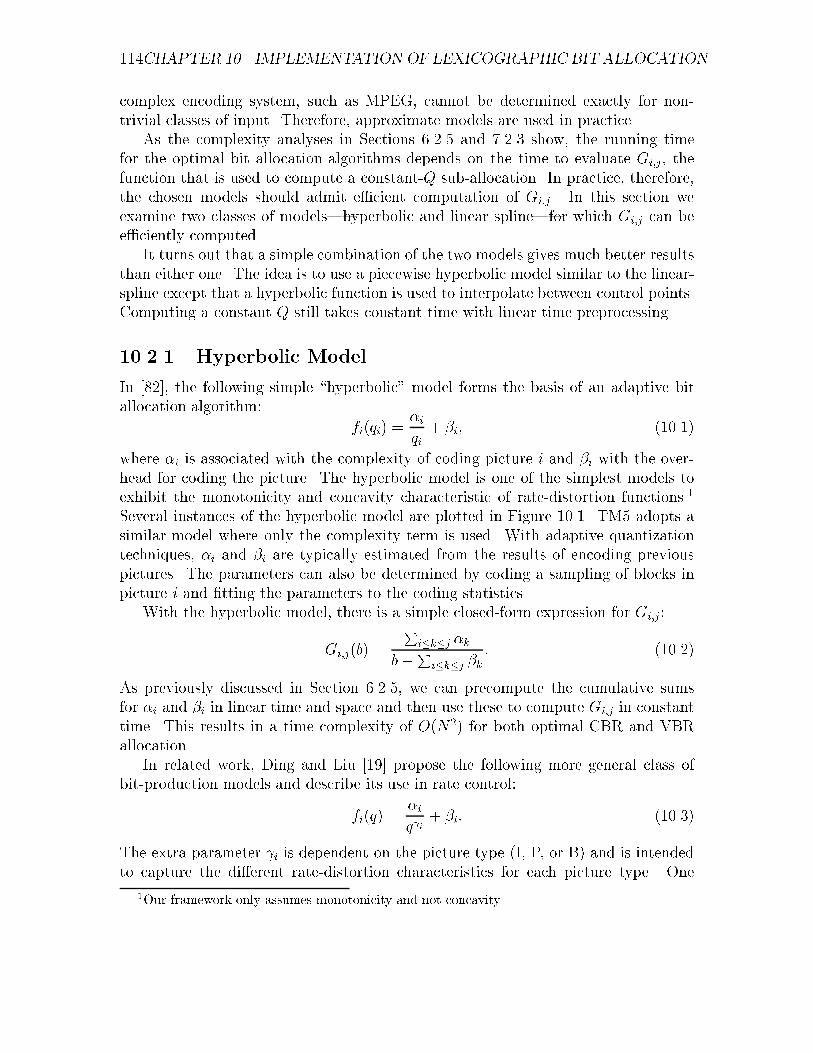
114CHAPTER 10. IMPLEMENTATION OF LEXICOGRAPHIC BIT ALLOCATION
complex encoding system, such as MPEG, cannot be determined exactly for non-trivial classes of input. Therefore, approximate models are used in practice.
As the complexity analyses in Sections 6.2.5 and 7.2.3 show, the running timefor the optimal bit allocation algorithms depends on the time to evaluate Gi;j, thefunction that is used to compute a constant-Q sub-allocation. In practice, therefore,the chosen models should admit e�cient computation of Gi;j. In this section weexamine two classes of models|hyperbolic and linear spline|for which Gi;j can bee�ciently computed.
It turns out that a simple combination of the two models gives much better resultsthan either one. The idea is to use a piecewise hyperbolic model similar to the linear-spline except that a hyperbolic function is used to interpolate between control points.Computing a constant Q still takes constant time with linear time preprocessing.
10.2.1 Hyperbolic Model
In [82], the following simple \hyperbolic" model forms the basis of an adaptive bitallocation algorithm:
fi(qi) =�i
qi+ �i; (10.1)
where �i is associated with the complexity of coding picture i and �i with the over-head for coding the picture. The hyperbolic model is one of the simplest models toexhibit the monotonicity and concavity characteristic of rate-distortion functions.1
Several instances of the hyperbolic model are plotted in Figure 10.1. TM5 adopts asimilar model where only the complexity term is used. With adaptive quantizationtechniques, �i and �i are typically estimated from the results of encoding previouspictures. The parameters can also be determined by coding a sampling of blocks inpicture i and �tting the parameters to the coding statistics.
With the hyperbolic model, there is a simple closed-form expression for Gi;j:
Gi;j(b) =
Pi�k�j �k
b�Pi�k�j �k: (10.2)
As previously discussed in Section 6.2.5, we can precompute the cumulative sumsfor �i and �i in linear time and space and then use these to compute Gi;j in constanttime. This results in a time complexity of O(N2) for both optimal CBR and VBRallocation.
In related work, Ding and Liu [19] propose the following more general class ofbit-production models and describe its use in rate control:
fi(q) =�i
q i+ �i: (10.3)
The extra parameter i is dependent on the picture type (I, P, or B) and is intendedto capture the di�erent rate-distortion characteristics for each picture type. One
1Our framework only assumes monotonicity and not concavity.

10.2. BIT-PRODUCTION MODELING 115
0
20
40
60
80
100
120
140
0 5 10 15 20 25 30
Bits
Quantization
f(q) = 100/q + 10f(q) = 200/q + 20f(q) = 400/q + 10f(q) = 500/q + 30
Figure 10.1: Several instances of a simple \hyperbolic" bit-production model.
drawback to (10.3) is that the model is non-linear with respect to the parameters,and we know of no closed-form solution to Gi;j in the general setting. Althoughnumerical techniques can be used to solve for Gi;j, this could adversely a�ect thecomputational e�ciency of the bit allocation algorithms.
In preliminary experiments, we �nd that the hyperbolic model works well nearthe operating point where �i and �i have been determined, but is not reliable at adistant operating point. This observation leads us to formulate the following encodingstrategy.
1. Encode the sequence using the standard TM5 coder, keeping statistics (for eachpicture) of the average nominal quantization scale, the total number of bitsused, and the number of bits used to code the quantized DCT coe�cients.
2. Compute �i and �i from the statistics gathered in the previous encoding pass.Allocate bits to pictures with the lexicographic bit allocation algorithm andencode the sequence using this allocation, gathering statistics as before.
3. Repeat Step 2.
The idea is that with each encoding, the accuracy of the bit models will improve asthe operating Q is determined and re�ned for each picture.
10.2.2 Linear-Spline Model
As noted above, the hyperbolic model works well with small changes in the quanti-zation scale Q. However, with a large variation in Q between successive pictures, asmay occur with a scene change, the model becomes less reliable. This is because themodel is de�ned by only two parameters �i and �i. Previously, we have compensated

116CHAPTER 10. IMPLEMENTATION OF LEXICOGRAPHIC BIT ALLOCATION
for this by performing multiple encoding passes to ensure that the parameters aredetermined close to the actual operating point. We now consider a di�erent approachwhere more e�ort is expended to construct more accurate bit models that are thenused to encode the video sequence in a single pass.
Lin, Ortega, and Kuo [51, 50] propose using cubic-spline interpolation models ofrate and distortion in conjunction with a gradient-based rate control algorithm [48,49]. The spline models are computed by �rst encoding each picture several timesusing a select set of M quantization scales, fx1, x2, : : :, xMg with x1 < x2 < � � � <xM , and measuring the actual rate. Each quantization/rate pair is called a control
point. For picture i, the function between two consecutive control points (xk; yi;k)and (xk+1; yi;k+1) has the form
fki (xk) = aikx3 + bikx
2 + cikx+ dik: (10.4)
The parameters aik, bik, cik, and dik are computed from four control points(xk�1; yi;k�1), (xk; yi;k), (xk+1; yi;k+1), and (xk+2; yi;k+2), such that fki (xk) = yi;k andfk+1i (xk+1) = yi;k+1 and the �rst-order derivatives of fki and fk+1i are continuous atthe control points. The authors suggest using the Fibonacci-like set f1, 2, 3, 5, 8, 13,21, 31g for the control quantization scales to exploit the exponential-decay typical ofrate-distortion functions.
One drawback of a cubic-spline model is that it is generally not monotonic. Toensure monotonicity, we consider a simpler linear-spline interpolation model, wherea line segment is used to interpolate the bit-production function between controlpoints. For picture i, the function between two consecutive control points (xk; yi;k)and (xk+1; yi;k+1) has the form
fki (xk) = �i;kx + �i;k: (10.5)
As in [48, 49], we choose the control quantization scales to be f1, 2, 3, 5, 8, 13, 21,31g to exploit the exponential-decay property of rate-distortion functions. In casethe control points themselves do not exhibit monotonicity, we enforce monotonicityby skipping those control points where the monotonicity property is violated. Forquantization scales less than x1 or greater than xM , we extrapolate using the param-eters (�i;k; �i;k) or (�i;M�1; �i;M�1), respectively. An example of a linear-spline modelis shown in Figure 10.2.
The linear-spline model has a simple closed-form expression for Gi;j if we knowthe two control points that bracket the operating point. Because of the monotonicityproperty, we can determine the two bracketing points using binary search. Betweenthe control points xk and xk+1, Gi;j can be computed as
Gi;j(b) =b�Pi�m�j �m;kP
i�m�j �m;k: (10.6)
If xk � Gi;j � xk+1 then the correct operating point has been found. If Gi;j < xk,the operating point must lie between two control points with lower indices. Similarly,

10.3. PICTURE-LEVEL RATE CONTROL 117
0
100
200
300
400
500
600
700
0 10 20 30 40 50 60
Bits
Quantization
Control Points
Figure 10.2: Example of a linear-spline interpolation model.
if Gi;j > xk+1, the operating point must lie between two control points with higherindices. A simple binary search procedure can be used to �nd the operating point.
Since there are a �xed number of control points, we can compute Gi;j in constanttime with linear-time preprocessing. As with the hyperbolic model, we can computeoptimal CBR and VBR allocations in quadratic time.
The cubic-spline model of [51, 50] is used in a dependent-coding framework, wherethe e�ects of coding previous pictures are taken into account in the modeling. Ourframework assumes independent coding and does not take these e�ects into account.However, from the switching theorems, we note that an optimal allocation has seg-ments of constant Q. This provides a basis for estimating the linear-spline modelparameters. By encoding the video sequence multiple times with a constant Q deter-mined from the control points, we can construct a linear-spline interpolation modelfor each picture. We expect these models to be reasonably accurate within a segmentof constant Q. At the boundary between segments, however, we can expect somediscrepancy in the models for dependent pictures (P and B types).
10.3 Picture-Level Rate Control
Even with accurate bit-production models, the actual number of bits produced willinevitably depart from the model. There are essentially two ways to cope with bit-modeling errors.
10.3.1 Closed-Loop Rate Control
A popular approach taken in TM5 is to regulate the quantization scale at the mac-roblock level while coding a picture so that the desired bit allocation is met. This

118CHAPTER 10. IMPLEMENTATION OF LEXICOGRAPHIC BIT ALLOCATION
is achieved with a closed-loop feedback mechanism using the fullness of a virtual en-coder bu�er to control the macroblock quantization. One drawback of this techniqueis that the coded quality within a picture may vary considerably, especially for apicture that contains regions of varying complexity. With gross errors in the bit-production models, the actual average quantization scale may di�er markedly fromthe desired quantization scale, thereby adversely a�ecting the coded quality.
10.3.2 Open-Loop Rate Control
Another approach is to perform open-loop control where the assigned (nominal) quan-tization scale is used to code a picture. We can then adjust the bit allocation of theremaining uncoded pictures to compensate for the di�erence between desired andactual bit production. An advantage of this approach is that the quality is more con-stant within a picture. In addition, less processing is required to code each picture.A disadvantage is that, since the bit production is not controlled below the picturelayer, the actual bit production may vary from the target and potentially cause thebu�er to over ow or under ow.
After coding a picture, we can reallocate bits to the remaining pictures optimally(for the given models). Instead of recomputing an optimal allocation from scratchand incurring an extra factor of N in the time complexity, we can take advantage ofdynamic programming to increase the time complexity by only a constant factor. Wedo this for a CBR allocation and for hard pictures in a VBR allocation by constructingthe dynamic programming table in the CBR algorithm in reverse.
As presented in Section 6.2, the dynamic programming algorithm works by solvingfor sub-allocations for pictures 1 to k for increasing values of k. We can also reworkthe dynamic programming to compute optimal sub-allocations for pictures k to N fordecreasing values of k. We do this by computing optimal allocations that start withthe bu�er empty or full at picture k and ends with the bu�er at the �nal bu�er stateafter picture N .
With a reverse dynamic programming table, we can compute a revised allocationfor picture k, after encoding picture k� 1, by searching for a proper constant-Q con-nector starting with the known VBV bu�er fullness before picture k is removed. Withthe reverse dynamic programming table available, this search consumes O(N) timefor the hyperbolic and linear-spline interpolation models. The total additional timeto recover from bit-production errors is then O(N2), the same as the time complexityfor computing the initial allocation.
As stated, the above procedure applies to a CBR allocation and to hard pictures ina VBR allocation (which are allocated using the CBR routine). For easy pictures in aVBR allocation, we can simply recompute a new value for Qmin. Here, we assume thaterrors in bit-production modeling are not severe enough to change the classi�cationof hard and easy pictures.

10.4. BUFFER GUARD ZONES 119
BVBV
Ful
lnes
sB
uffe
r
VBV0.95 B
VBV0.05 B0
Guard Zones
Figure 10.3: Guard zones to safeguard against under ow and over ow of VBV bu�er.A bit allocation is computed so that the bu�er fullness remains between the guardzones.
10.3.3 Hybrid Rate Control
In early experiments, we observed that closed-loop rate control resulted in rapid uctuations in the nominal quantization scale2 between pictures owing to the bu�er-feedback mechanism. With accurate bit-production models, however, the need toperform low-level rate control below the picture level is questionable. This suggestsusing open-loop control. As noted earlier, since we assume independent coding, wecan expect more errors in the bit-production models at pictures where the assignedQ changes. With these observations, we propose a hybrid rate control strategy whereclosed-loop control is used for pictures at the boundaries of a constant-Q segmentand open-loop control is used for the rest. Another motivation for using closed-loopcontrol for boundary pictures is that the VBV bu�er should be either nearly emptyor nearly full for these pictures, and the bit rate must be carefully controlled to avoidunder owing or over owing the bu�er.
10.4 Bu�er Guard Zones
Even with the picture-level rate control strategies outlined above, there is still thepossibility of the VBV bu�er over owing or under owing. To safeguard against this,we compute a bit allocation using a slightly smaller bu�er than that speci�ed in theMPEG bitstream so that we can have guard zones near the top and bottom of thebu�er. For the experiments with CBR, have we chosen to place the guard zones at5% and 95% of maximum bu�er size. This is illustrated in Figure 10.3. For VBRmode, the upper guard zone is not needed since bu�er over ow is not a concern.
2By nominal quantization scale, we mean the average measured macroblock quantization scalewith perceptual quantization factored out.

120CHAPTER 10. IMPLEMENTATION OF LEXICOGRAPHIC BIT ALLOCATION
10.5 Encoding Simulations
To assess the behavior and e�ectiveness of the lexicographic bit allocation algorithms,the bit-production models, and the rate control strategies outlined above, we con-ducted encoding simulations using several short (� 100 pictures) benchmark videosequences (flower garden, football, mobile, and table tennis) in SIF formatand a longer (3,660 pictures) promotional video clip courtesy of IBM Corporation.
10.5.1 Initial Experiments
Initially, we used the short video clips to evaluate the bit-production models andrate control strategies. To simulate scene changes, we concatenated the four shortvideo clips into a 418{picture video sequence in the following order: flower garden,mobile, football, table tennis.
We implemented the rate control algorithms within the software encoder providedby the MPEG-2 Simulation Group [58]. The coding parameters are listed in Ta-ble 10.1. For CBR mode, we speci�ed a peak bit rate of 1.0 Mbits/sec. For VBR,we used an average bit rate of 1.0 Mbits/sec and a peak bit rate of 1.2 Mbits/sec.The VBV bu�er size was set to 720,896 bits. For reference, we also ran the encoderwith TM5 rate control using the sample parameters.3 In order to reduce factors thatwould a�ect the actual bit production, full-search motion estimation was initiallyperformed using a �xed nominal quantization scale of 13, and the same motion vec-tors were then used for all the encodings. The coding decisions, however, were stilldetermined on-line.
In the �rst set of simulations, we used the hyperbolic model and performed mul-tiple encoding passes. The results of the encodings are presented in Table 10.2 andFigures 10.4 to 10.9. The table collects some summary statistics for the variouscoders. Figures 10.4 and 10.5 show the evolution of the bu�er fullness. Figures 10.6and 10.7 plot the computed and observed sequence of nominal quantization Q. Thecomputed Q consists of piecewise constant segments, as dictated by theory.
The initial pass of the Hyperbolic CBR and VBR coders used statistics gatheredwith the TM5 coder in order to determine the parameters of the bit-production mod-els. Later passes of the Hyperbolic CBR (VBR) coder used statistics gathered fromthe previous pass. From the results in Table 10.2 and Figure 10.4, the HyperbolicCBR coder does not exhibit much change between passes. However, the HyperbolicVBR coder does show reduction in the standard deviation in PSNR and nominal Qand better usage of the VBV bu�er with later passes.
As evident from Figure 10.4, the TM5 coder uses only a fraction of the VBV bu�erand maintains the bu�er relatively level. In contrast, the lexicographic coders make
3A minor modi�cation was made to the TM5 model in that the levels of the virtual encodingbu�ers used to regulate the quantization scale are restricted to the range [0; 2r], where r is thereaction parameter de�ned in Section 2.7.5.

10.5. ENCODING SIMULATIONS 121
Value Description418 number of frames
1 number of first frame
15 N (# of frames in GOP)
3 M (I/P frame distance)
0 ISO/IEC 11172-2 stream
0 0:frame pictures, 1:field pictures
352 horizontal_size
240 vertical_size
2 aspect_ratio_information 1=square pel, 2=4:3, 3=16:9, 4=2.11:1
5 frame_rate_code 1=23.976, 2=24, 3=25, 4=29.97, 5=30 frames/sec
1000000.0 bit_rate (bits/sec)
44 vbv_buffer_size (in multiples of 16 kbit)
0 low_delay
0 constrained_parameters_flag
4 Profile ID: Simple = 5, Main = 4, SNR = 3, Spatial = 2, High = 1
8 Level ID: Low = 10, Main = 8, High 1440 = 6, High = 4
1 progressive_sequence
1 chroma_format: 1=4:2:0, 2=4:2:2, 3=4:4:4
2 video_format: 0=comp., 1=PAL, 2=NTSC, 3=SECAM, 4=MAC, 5=unspec.
5 color_primaries
5 transfer_characteristics
4 matrix_coefficients
352 display_horizontal_size
240 display_vertical_size
0 intra_dc_precision (0: 8 bit, 1: 9 bit, 2: 10 bit, 3: 11 bit
0 top_field_first
1 1 1 frame_pred_frame_dct (I P B)
0 0 0 concealment_motion_vectors (I P B)
1 1 1 q_scale_type (I P B)
1 0 0 intra_vlc_format (I P B)
0 0 0 alternate_scan (I P B)
0 repeat_first_field
1 progressive_frame
0 P distance between complete intra slice refresh
0 rate control: r (reaction parameter)
0 rate control: avg_act (initial average activity)
0 rate control: Xi (initial I frame global complexity measure)
0 rate control: Xp (initial P frame global complexity measure)
0 rate control: Xb (initial B frame global complexity measure)
0 rate control: d0i (initial I frame virtual buffer fullness)
0 rate control: d0p (initial P frame virtual buffer fullness)
0 rate control: d0b (initial B frame virtual buffer fullness)
3 3 23 23 P: forw_hor_f_code forw_vert_f_code search_width/height
1 1 7 7 B1: forw_hor_f_code forw_vert_f_code search_width/height
2 2 15 15 B1: back_hor_f_code back_vert_f_code search_width/height
2 2 15 15 B2: forw_hor_f_code forw_vert_f_code search_width/height
1 1 7 7 B2: back_hor_f_code back_vert_f_code search_width/height
Table 10 1: Parameters for MPEG 2 Simulation Group software encoder used to

122CHAPTER 10. IMPLEMENTATION OF LEXICOGRAPHIC BIT ALLOCATION
Average Std. Dev. Average Std. Dev. Maximum MinimumMethod PSNR (dB) of PSNR Nom. Q of Nom. Q Nom. Q Nom. Q
TM5 CBR 26:66 3:06 16:19 4:48 26:20 6:70
HyperbolicCBR, Pass 1 26:48 2:67 16:19 3:44 22:63 7:78HyperbolicCBR, Pass 2 26:48 2:66 16:23 3:40 21:44 7:43HyperbolicCBR, Pass 3 26:48 2:67 16:28 3:41 20:68 7:20
HyperbolicVBR, Pass 1 26:54 2:36 15:95 2:77 21:15 9:16HyperbolicVBR, Pass 2 26:52 2:10 16:00 2:14 19:60 9:34HyperbolicVBR, Pass 3 26:49 1:99 16:09 1:83 19:22 9:76
Linear-SplineCBR, Hybrid 26:73 2:68 15:80 3:36 19:48 8:29
Linear-SplineVBR, Hybrid 26:66 1:87 15:83 1:13 17:59 12:97
Table 10.2: Summary of initial coding experiments.
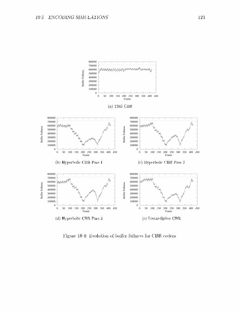
10.5. ENCODING SIMULATIONS 123
0
100000
200000
300000
400000
500000
600000
700000
800000
0 50 100 150 200 250 300 350 400 450
Buf
fer
Fulln
ess
Frame
(a) TM5 CBR
0
100000
200000
300000
400000
500000
600000
700000
800000
0 50 100 150 200 250 300 350 400 450
Buf
fer
Fulln
ess
Frame
(b) Hyperbolic CBR Pass 1
0
100000
200000
300000
400000
500000
600000
700000
800000
0 50 100 150 200 250 300 350 400 450
Buf
fer
Fulln
ess
Frame
(c) Hyperbolic CBR Pass 2
0
100000
200000
300000
400000
500000
600000
700000
800000
0 50 100 150 200 250 300 350 400 450
Buf
fer
Fulln
ess
Frame
(d) Hyperbolic CBR Pass 3
0
100000
200000
300000
400000
500000
600000
700000
800000
0 50 100 150 200 250 300 350 400 450
Buf
fer
Fulln
ess
Frame
(e) Linear-Spline CBR
Figure 10.4: Evolution of bu�er fullness for CBR coders.

124CHAPTER 10. IMPLEMENTATION OF LEXICOGRAPHIC BIT ALLOCATION
0
100000
200000
300000
400000
500000
600000
700000
800000
0 50 100 150 200 250 300 350 400 450
Buf
fer
Fulln
ess
Frame
(a) Hyperbolic VBR Pass 1
0
100000
200000
300000
400000
500000
600000
700000
800000
0 50 100 150 200 250 300 350 400 450B
uffe
r Fu
llnes
sFrame
(b) Hyperbolic VBR Pass 2
0
100000
200000
300000
400000
500000
600000
700000
800000
0 50 100 150 200 250 300 350 400 450
Buf
fer
Fulln
ess
Frame
(c) Hyperbolic VBR Pass 3
0
100000
200000
300000
400000
500000
600000
700000
800000
0 50 100 150 200 250 300 350 400 450
Buf
fer
Fulln
ess
Frame
(d) Linear-Spline VBR
Figure 10.5: Evolution of bu�er fullness for VBR coders.

10.5. ENCODING SIMULATIONS 125
5
10
15
20
25
0 50 100 150 200 250 300 350 400 450
Nom
inal
Q
Frame
(a) TM5 CBR
5
10
15
20
25
0 50 100 150 200 250 300 350 400 450
Nom
inal
Q
Frame
ActualTarget
(b) Hyperbolic CBR Pass 1
5
10
15
20
25
0 50 100 150 200 250 300 350 400 450
Nom
inal
Q
Frame
ActualTarget
(c) Hyperbolic CBR Pass 2
5
10
15
20
25
0 50 100 150 200 250 300 350 400 450
Nom
inal
Q
Frame
ActualTarget
(d) Hyperbolic CBR Pass 3
5
10
15
20
25
0 50 100 150 200 250 300 350 400 450
Nom
inal
Q
Frame
ActualTarget
(e) Linear-Spline CBR
Figure 10.6: Nominal quantization scale for CBR coders.

126CHAPTER 10. IMPLEMENTATION OF LEXICOGRAPHIC BIT ALLOCATION
5
10
15
20
25
0 50 100 150 200 250 300 350 400 450
Nom
inal
Q
Frame
ActualTarget
(a) Hyperbolic VBR Pass 1
5
10
15
20
25
0 50 100 150 200 250 300 350 400 450N
omin
al Q
Frame
ActualTarget
(b) Hyperbolic VBR Pass 2
5
10
15
20
25
0 50 100 150 200 250 300 350 400 450
Nom
inal
Q
Frame
ActualTarget
(c) Hyperbolic VBR Pass 3
5
10
15
20
25
0 50 100 150 200 250 300 350 400 450
Nom
inal
Q
Frame
ActualTarget
(d) Linear-Spline VBR
Figure 10.7: Nominal quantization scale for VBR coders.

10.5. ENCODING SIMULATIONS 127
20
25
30
35
40
0 50 100 150 200 250 300 350 400 450
PSN
R (
dB)
Frame
(a) TM5 CBR
20
25
30
35
40
0 50 100 150 200 250 300 350 400 450
PSN
R (
dB)
Frame
(b) Hyperbolic CBR Pass 1
20
25
30
35
40
0 50 100 150 200 250 300 350 400 450
PSN
R (
dB)
Frame
(c) Hyperbolic CBR Pass 2
20
25
30
35
40
0 50 100 150 200 250 300 350 400 450
PSN
R (
dB)
Frame
(d) Hyperbolic CBR Pass 3
20
25
30
35
40
0 50 100 150 200 250 300 350 400 450
PSN
R (
dB)
Frame
(e) Linear-Spline CBR
Figure 10.8: PSNR for CBR coders.

128CHAPTER 10. IMPLEMENTATION OF LEXICOGRAPHIC BIT ALLOCATION
20
25
30
35
40
0 50 100 150 200 250 300 350 400 450
PSN
R (
dB)
Frame
(a) Hyperbolic VBR Pass 1
20
25
30
35
40
0 50 100 150 200 250 300 350 400 450PS
NR
(dB
)Frame
(b) Hyperbolic VBR Pass 2
20
25
30
35
40
0 50 100 150 200 250 300 350 400 450
PSN
R (
dB)
Frame
(c) Hyperbolic VBR Pass 3
20
25
30
35
40
0 50 100 150 200 250 300 350 400 450
PSN
R (
dB)
Frame
(d) Linear-Spline VBR
Figure 10.9: PSNR for VBR coders.

10.5. ENCODING SIMULATIONS 129
better use of the VBV bu�er.
Comparing hyperbolic modeling with closed-loop rate control on the one hand withlinear-spline modeling with hybrid rate-control on the other, we see that the latteroutperforms the former in all aspects. It is noteworthy that the hyperbolic modelseems to underestimate the bit production while the linear-spline model overestimatesthe bit production. The result is that the actual nominal quantization scales used arehigher than the target for the hyperbolic model and lower for the linear-spline model.
10.5.2 Coding a Longer Sequence
Since the video clips used in the initial experiments are short and we had to concate-nate them to form somewhat arti�cial scene changes, we were not able to detect muchperceptual di�erence between the di�erent encodings. To assess the perceptual gainsof lexicographically optimal bit allocation, we performed additional coding simula-tions using a longer video sequence with varied and dynamic content. The sequenceconsists of 3,660 frames of a commercial produced by the IBM Corporation to demon-strate its MPEG-2 encoding chipset. The clip starts with a fade-in to a spokeswomanstanding in front of a slowing changing background. A block diagram in one cornerof the picture then rotates and zooms to �ll the screen. The diagram then remainsstatic with some illumination changes before fading back to the spokeswoman. Onone side of the picture, a collage of di�erent video clips scroll up the screen. Oneof the clips zooms to occupy the full picture. The clips cycle through a variety ofaction-�lled scenes from horses running to a skydiver rotating on a skateboard to abicycle race and �nally to highlights from a basketball game.
The video sequence is in NTSC CCIR-601 format. We coded the sequence in CBRmode at 3 Mbits/sec and in VBR mode at 3 Mbits/sec average and 4.5 Mbits/secpeak. The encoding parameters used are shown in Table 10.3. The VBV bu�er sizeis 1,835,008 bits. We used linear-spline interpolation models in conjunction with thehybrid rate control strategy.
Some encoding statistics are listed in Table 10.4. The bu�er fullness, nominalQ, and PSNR plots are shown in Figures 10.10, 10.11, and 10.12, respectively. Thedi�erences between the di�erent coders are much more pronounced with these simu-lations than with the previous ones. The lexicographic CBR coder is able to controlthe quantization to a narrower range than the TM5 coder, with a resulting increasein PSNR. The lexicographic VBR coder sacri�ces quality in earlier pictures in or-der to code better the later more complex pictures. The result is that the nominalquantization is nearly constant and the PSNR plot is more even.
Visually, the lexicographic VBR coder produced near constant-quality video withfew noticeable coding artifacts. In contrast, both CBR coders produced noticeableblocking artifacts in scenes with high motion, especially in the basketball scene. How-ever, the lexicographic CBR coder fared noticeably better than TM5 at maintainingconstant quality through scene changes and reducing artifacts during complex scenes

130CHAPTER 10. IMPLEMENTATION OF LEXICOGRAPHIC BIT ALLOCATION
Value Description3660 number of frames
0 number of first frame
15 N (# of frames in GOP)
3 M (I/P frame distance)
0 ISO/IEC 11172-2 stream
0 0:frame pictures, 1:field pictures
720 horizontal_size
480 vertical_size
2 aspect_ratio_information 1=square pel, 2=4:3, 3=16:9, 4=2.11:1
4 frame_rate_code 1=23.976, 2=24, 3=25, 4=29.97, 5=30 frames/sec
3000000.0 bit_rate (bits/sec)
112 vbv_buffer_size (in multiples of 16 kbit)
0 low_delay
0 constrained_parameters_flag
4 Profile ID: Simple = 5, Main = 4, SNR = 3, Spatial = 2, High = 1
8 Level ID: Low = 10, Main = 8, High 1440 = 6, High = 4
0 progressive_sequence
1 chroma_format: 1=4:2:0, 2=4:2:2, 3=4:4:4
2 video_format: 0=comp., 1=PAL, 2=NTSC, 3=SECAM, 4=MAC, 5=unspec.
5 color_primaries
5 transfer_characteristics
4 matrix_coefficients
720 display_horizontal_size
480 display_vertical_size
0 intra_dc_precision (0: 8 bit, 1: 9 bit, 2: 10 bit, 3: 11 bit
1 top_field_first
0 0 0 frame_pred_frame_dct (I P B)
0 0 0 concealment_motion_vectors (I P B)
1 1 1 q_scale_type (I P B)
1 0 0 intra_vlc_format (I P B)
0 0 0 alternate_scan (I P B)
0 repeat_first_field
0 progressive_frame
0 P distance between complete intra slice refresh
0 rate control: r (reaction parameter)
0 rate control: avg_act (initial average activity)
0 rate control: Xi (initial I frame global complexity measure)
0 rate control: Xp (initial P frame global complexity measure)
0 rate control: Xb (initial B frame global complexity measure)
0 rate control: d0i (initial I frame virtual buffer fullness)
0 rate control: d0p (initial P frame virtual buffer fullness)
0 rate control: d0b (initial B frame virtual buffer fullness)
4 4 63 63 P: forw_hor_f_code forw_vert_f_code search_width/height
2 2 15 15 B1: forw_hor_f_code forw_vert_f_code search_width/height
3 3 31 31 B1: back_hor_f_code back_vert_f_code search_width/height
3 3 31 31 B2: forw_hor_f_code forw_vert_f_code search_width/height
2 2 15 15 B2: back_hor_f_code back_vert_f_code search_width/height
Table 10 3: Parameters for MPEG 2 Simulation Group software encoder used to

10.5. ENCODING SIMULATIONS 131
Average Std. Dev. Average Std. Dev. Maximum MinimumMethod PSNR (dB) of PSNR Nom. Q of Nom. Q Nom. Q Nom. Q
TM5 CBR 33:34 4:95 14:00 9:88 48:86 1:95Linear-SplineCBR, Hybrid 33:45 4:77 13:01 7:97 29:62 2:61Linear-SplineVBR, Hybrid 33:08 2:58 11:80 2:07 17:68 8:00
Table 10.4: Summary of coding simulations with IBM Commercial.
02000004000006000008000001e+06
1.2e+061.4e+061.6e+061.8e+06
0 500 1000 1500 2000 2500 3000 3500 4000
Buf
fer
Fulln
ess
Frame
(a) TM5 CBR
02000004000006000008000001e+06
1.2e+061.4e+061.6e+061.8e+06
0 500 1000 1500 2000 2500 3000 3500 4000
Buf
fer
Fulln
ess
Frame
(b) Linear-Spline CBR
02000004000006000008000001e+06
1.2e+061.4e+061.6e+061.8e+06
0 500 1000 1500 2000 2500 3000 3500 4000
Buf
fer
Fulln
ess
Frame
(c) Linear-Spline VBR
Figure 10.10: Evolution of bu�er fullness for coding IBM Commercial.

132CHAPTER 10. IMPLEMENTATION OF LEXICOGRAPHIC BIT ALLOCATION
0
10
20
30
40
50
60
0 500 1000 1500 2000 2500 3000 3500 4000
Nom
inal
Q
Frame
(a) TM5 CBR
0
10
20
30
40
50
60
0 500 1000 1500 2000 2500 3000 3500 4000
Nom
inal
Q
Frame
ActualTarget
(b) Linear-Spline CBR
0
10
20
30
40
50
60
0 500 1000 1500 2000 2500 3000 3500 4000
Nom
inal
Q
Frame
ActualTarget
(c) Linear-Spline VBR
Figure 10.11: Nominal quantization scale for coding IBM Commercial.

10.5. ENCODING SIMULATIONS 133
20
25
30
35
40
45
50
0 500 1000 1500 2000 2500 3000 3500 4000
PSN
R (
dB)
Frame
(a) TM5 CBR
20
25
30
35
40
45
50
0 500 1000 1500 2000 2500 3000 3500 4000
PSN
R (
dB)
Frame
(b) Linear-Spline CBR
20
25
30
35
40
45
50
0 500 1000 1500 2000 2500 3000 3500 4000
PSN
R (
dB)
Frame
(c) Linear-Spline VBR
Figure 10.12: PSNR for coding IBM Commercial.

134CHAPTER 10. IMPLEMENTATION OF LEXICOGRAPHIC BIT ALLOCATION
of short duration.
10.6 Limiting Lookahead
The above rate control algorithms compute an allocation for the entire video sequence.This may not be feasible when the sequence consists of many pictures, as in a feature-length movie, for example. One way to deal with this is to partition the sequenceinto blocks consisting of a small number of consecutive pictures. Optimal allocationcan then be performed on the blocks separately. In order to do this, the starting andending bu�er fullness must be speci�ed for each block for the CBR case. For theVBR case, the bit budget must also be speci�ed for each block. This approach isglobally suboptimal; however, it is easy to parallelize since the block allocations areindependent of each other.
Another approach is to use limited lookahead in conjunction with hybrid ratecontrol. Using a lookahead window of size W and a step size S � W , the procedureis as follows:
1. Compute a bit allocation for the next W pictures not yet coded by computinga reverse dynamic programming table.
2. Code the next S pictures using hybrid rate control, using the dynamic program-ming table to recover from model errors.
3. Repeat Step 1.
This procedure can be thought of as performing lookahead with a sliding window.Another approach similar to the hybrid rate control method is to use the allocation
computed from a given model and only recompute the allocation when the bu�erfullness breach preset bu�er boundaries, such as 10% and 90% of bu�er fullness. Aswith hybrid rate control, reverse dynamic programming can be used to speed up thereallocation.
10.7 Related Work
A suite of heuristic methods is proposed in [62] to reduce the complexity as com-pared to an optimal bit allocation based on the Viterbi algorithm. A Lagrangianoptimization technique is applied to recompute an allocation incrementally for eachpicture, similar to technique described in Section 10.3.2. In addition, the Lagrangianoptimization is performed with a �nite window size. In essence, this method imple-ments limited lookahead with a sliding window, similar to the technique describedin Section 10.6. The authors also describe the heuristic of recomputing a allocationonly when the bu�er reaches prede�ned threshold levels.

10.8. DISCUSSION 135
In this chapter, we have considered a simple hyperbolic model and a linear-splinemodel of bit production. In [8], a bit-production model is derived for block-transformcoders based on rate-distortion theory and assuming a stationary Gaussian process.The model is applied for VBR coding with motion JPEG and H.261 coders. In [10],an adaptive tree-structured piecewise linear bit-production model is proposed andapplied to MPEG video coding using a one-pass encoding strategy. A cubic-splinemodel of rate and distortion is proposed in [51, 50] for use with a gradient-basedrate-control algorithm [48, 49] that attempts to minimize MSE. The model takes intoaccount the temporal dependencies introduced by predictive coding.
10.8 Discussion
In this chapter, we have described an implementation of the bit allocation algorithmsof Chapters 6 and 7 within an MPEG-2 software encoder. In addition to evalu-ating two types of bit-production models, we have developed robust techniques forrecovering from errors in the bit-production models. Since we can view coding depen-dencies as contributing to errors in the (independent) bit-production models, theseerror-recovery techniques e�ectively allow us to apply the bit-allocation frameworkto predictive video coders.

136CHAPTER 10. IMPLEMENTATION OF LEXICOGRAPHIC BIT ALLOCATION

Chapter 11
Extensions of the Lexicographic
Framework
Extensions
In Chapters 5 through 7, we laid a theoretical foundation for lexicographic bitallocation, and in Chapter 10 we demonstrated that the framework works well inpractice. In this chapter, we provide evidence that the framework is also exibleand general by showing how it can be readily applied to other domains, extended toperform statistical multiplexing, and used in a discrete optimization setting.
11.1 Applicability to Other Coding Domains
While the lexicographic bit allocation framework was originally motivated and for-mulated for MPEG video coding, it can be applied equally well in other lossy codingdomains for which bu�er-constrained bit allocation is a valid problem and where aperceptual distortion measure needs to be equalized among coding units. Obviousexamples include lossy image coding (such as speci�ed by the JPEG standard [65]),where the coding unit would logically be a block of pixels, and audio coding, wherea coding unit might correspond to half a second of sampled sound.
In the original formulation, we identi�ed a perceptually-adjusted quantizationscale as the object of optimization. In general, any signal or combination of signalsthat can be controlled to a�ect the bit production of the encoder can be used.
137

138 CHAPTER 11. EXTENSIONS OF THE LEXICOGRAPHIC FRAMEWORK
11.2 Multiplexing VBR Streams over a CBR
Channel
11.2.1 Introduction
There are many scenarios where multiple compressed video streams are to be trans-mitted through a common channel. Two obvious examples are networked video anddigital video broadcasting. In these types of applications, the transmission channel istypically bandwidth-limited. With the available bandwidth, we would like to provideas much video programming as possible without having to sacri�ce quality.
An often-cited motivation for VBR video encoding is that VBR encoding canpotentially allow for the simultaneous transmission of more video streams over acommon channel than CBR encoding at the same quality level. The main reasoningis provided through a concept called statistical multiplexing. Statistical multiplex-ing is based on the observation that the bit rate of constant-quality video is highlyvariable from frame to frame. In order to achieve image quality that is not less lexi-cographically than that of a constant-quality VBR encoding, a CBR encoding wouldrequire a bit rate that would correspond to the peak rate of the VBR encoding. Sincea VBR encoding typically requires the peak rate for only a small percentage of time,it uses less bandwidth on average than a comparable CBR encoding. Furthermore,assuming that the VBR streams have independent bit-rate characteristics, we cantransmit more VBR streams than CBR streams over a common channel with a lowprobability that the combined instantaneous bit rate would exceed the channel rate.
As an example, consider a channel with a bandwidth of 100 Mbits/sec. Supposethat for a desired level of quality, a peak rate of 10 Mbits/sec is required for codinga suite of video programming. Using CBR encoding, up to 10 sequences can betransmitted through the channel simultaneously. Since the peak rate is requiredonly a small percentage of the time, suppose that the actual average rate is only5 Mbits/sec. Then using VBR encoding with a peak rate of 10 Mbits/sec and averagerate of 5 Mbits/sec, we can potentially transmit 20 simultaneous sequences. Thiswould correspond to a statistical multiplexing gain of 2.
In order to transmit the 20 VBR sequences simultaneously, however, the instan-taneous bit rate for the 20 sequences must not exceed the channel capacity for anextended period of time, which is determined by the amount of bu�ering present.Assuming that the bit rates of the di�erent video streams are uncorrelated in time,there is a low probability that the channel capacity would be exceeded in any timeinterval. Quantifying and minimizing this probability are central themes of research.
The advantage of VBR encoding over CBR is illustrated through a simple examplein Figure 11.1. In this example, three VBR encodings are shown multiplexed usingat most the same bandwidth required by a CBR encoding of only two of the sources.
In the remainder of this section, we will show how our basic lexicographic bitallocation framework can be readily extended to handle the multiplexing of multiple

11.2. MULTIPLEXING VBR STREAMS OVER A CBR CHANNEL 139
Con
sum
ptio
nB
andw
idth
Program 1 Program 2
Time
(a) Multiplexing of 2 CBR Bitstreams
Program 2 Program 3Program 1
Time
Ban
dwid
thC
onsu
mpt
ion
(b) Multiplexing of 3 VBR Bitstreams
Figure 11.1: Example of how three VBR bitstreams can be multiplexed into the samechannel as two CBR bitstreams, for a statistical multiplexing gain of 1.5.
VBR bitstreams over a CBR channel. However, in contrast to typical statisticalmultiplexing techniques, as exempli�ed in Figure 11.1, our method allocates bits tothe VBR bitstreams in a deterministic manner, making full use of all the availablechannel bandwidth.
In related work, a bu�ered rate control scheme for multiplexing VBR sourcesonto a CBR channel is described in [64]. This work is based on the rate-distortionframework of [63] and [11] and uses a multiplexing model very similar to the one weare about to present. As described in the paper, the basic allocation unit is taken tobe a GOP.
11.2.2 Multiplexing Model
We �rst elaborate a model for multiplexing multiple VBR bitstreams onto a CBRchannel. Since our bit allocation framework is deterministic and uses lookahead, weassume that complete statistics of the multiple video sources are available to the bitallocation algorithm. This requirement can be met by providing a centralized encoderfor the multiple sources, as depicted in Figure 11.2. In the �gure, M video sourcesenter a encoder/multiplexer that produces a single multiplexed stream for transportover a CBR channel. On the receiving end, a demultiplexer/decoder performs de-multiplexing and decoding to reproduce the M video sequences. This multiplexingmodel is similar to that proposed in [27].
This model is applicable to applications such as a video server where the videosequences to be multiplexed are known in advance. An especially noteworthy case isthat of near-video-on-demand (NVOD), where a single sequence is to be transmitted

140 CHAPTER 11. EXTENSIONS OF THE LEXICOGRAPHIC FRAMEWORK
Encoder/Multiplexer
Input 1
Input 2
Input M
Demultiplexer/Decoder
Output 1
Output 2
Output M
CBR Channel
Figure 11.2: System for transmitting multiple sequences over a single channel.
Multiplexer
Buffer
CBR ChannelVBR EncoderInput 2
VBR EncoderInput 1
VBR EncoderInput M
Figure 11.3: Block diagram of encoder/multiplexer.
simultaneously with di�erent starting times. For example, 20 copies of a 2-hour longmovie can be multiplexed so that the viewing of the movie can begin every six minutes.
The encoder/multiplexer block is expanded in Figure 11.3. As shown, the inputvideo sources are encoded individually and time-division multiplexed and stored in abu�er before being output to the channel at a constant bit rate. The encoders aresynchronized so that they output the encoding of a picture at the same time every T
seconds. The multiplexer then concatenates the multiple encodings in order as shownin Figure 11.4.
The demultiplexer/decoder block is expanded in Figure 11.5. The demulti-
Program 2 Program 3Program 1
Frame 2 Frame 1
Time
To Channel
Figure 11.4: Operation of multiplexer.

11.2. MULTIPLEXING VBR STREAMS OVER A CBR CHANNEL 141
Decoder
Decoder
Decoder
Output 1
Output 2
Output M
CBR Channel
Buffer
Demultiplexer
Figure 11.5: Block diagram of demultiplexer/decoder.
plexer/decoder mirrors the operation of the encoder/multiplexer. Incoming bits fromthe channel are stored in a decoding bu�er. Every T seconds, the demultiplexer in-stantaneously removes from the bu�er all bits needed to decode the next picture of allsequences and routes the bitstreams to the appropriate decoders, which then outputthe reconstructed video.
The multiplexing model described above resembles the operation of the single-stream encoder and decoder system implied by the MPEG Video Bu�ering Veri�er.If we view the di�erent input sources as providing \slices" of the same picture, theresemblance would be very close indeed. This construction is intentional and allowsus to apply the lexicographic framework to allocate bits optimally to the multipleVBR bitstreams.
11.2.3 Lexicographic Criterion
Before we can apply our lexicographic bit allocation framework, we need to de�nean optimality criterion. Since there are multiple sources, a lexicographical criterionbased on the encoding of a single video sequence is certainly not appropriate. Weneed to consider the quality of all the sequences. A simple way to do this is toconsider the concatenation of all the sequences and de�ne a lexicographic criterion onthe concatenated video stream. By doing this, we are putting equal weight to eachpicture of each video sequence. We can also consider extending the lexicographiccriterion to compare vectors of length M instead of scalar quantities. However, as wewill see, this is equivalent to just considering the concatenation of the M sequences.

142 CHAPTER 11. EXTENSIONS OF THE LEXICOGRAPHIC FRAMEWORK
11.2.4 Equivalence to CBR Bit Allocation
In this section, we show in the multiplexing model put forth above that the problemof optimal bit allocation for multiple VBR streams reduces to a CBR bit allocationproblem for a single stream.
The multiplexing model follows the operation of the MPEG Video Bu�ering Ver-i�er (VBV). We can view the bu�er, the demultiplexer, and the bank of M decodersin Figure 11.5 as comprising a single VBV. The lexicographic framework of Chapter 5can then be applied. Since the transmission channel operates at a constant bit rate,the CBR constraints of Chapter 6 would apply.
For display interval i, we need to consider the quantization scales used to codepicture i of each of the M video sequences. Given a �xed bit budget for codingpicture i of each video sequence, it is easy to show that the same quantization scalemust be used to code picture i of all sequences to achieve lexicographic optimality; ifthe quantization scales di�er, we can always shift bits around to reduce the highestquantization scale by increasing a lower quantization scale. This result also holds ifwe formulate the lexicographic criterion using vectors of quantization scales.
By using a combined bit-production model that is the sum of the bit-productionmodels for the individual sequences, we can then allocate bits jointly to the sequencesusing the CBR algorithm of Chapter 6.
While the above technique guarantees that the bu�er in Figure 11.5 does notover ow or under ow, it should be noted that doing so does not guarantee MPEGVBV compliance for the individual sequences, except when the individual VBV bu�ersare at least the size of the bu�er in Figure 11.5. A multiplexing model that explicitlyincludes individual decoder bu�ers is certainly possible. However, analysis of thissituation is not as straightforward as the above model and remains an open problem.
11.3 Bit Allocation with a Discrete Set of Quan-
tizers
One of the assumptions made in Chapter 5 is that there is a continuous relationshipbetween quantization (distortion) and rate. As shown in Chapters 6 and 7, this as-sumption facilitates rigorous analysis of the bu�er-constrained bit allocation problemunder the lexicographic optimality criterion and results in an elegant characteriza-tion of the optimal solution. In order to apply directly the results of the analysis, weneed to construct a continuous model of the relationship between quantization andrate. As demonstrated in Chapter 10, this can be done by gathering statistics duringmultiple encoding passes and �tting these to a chosen functional form. Because ofthe inevitable error in the modeling, some form of error recovery is needed, such asthe scheme proposed in Chapter 10.
In most practical coders, however, both the set of available quantizers and the

11.3. BIT ALLOCATION WITH A DISCRETE SET OF QUANTIZERS 143
number of bits produced are discrete and �nite. The problem of bu�er-constrainedbit allocation under these conditions have been examined by Ortega, Ramchandran,and Vetterli [63]. They provide a dynamic programming algorithm to �nd a CBRallocation that minimizes a sum-distortion metric. In this section, we brie y describetheir algorithm and show how it can be readily extended to perform lexicographicminimization.
11.3.1 Dynamic Programming
The dynamic programming algorithm described in [63] is based on the Viterbi al-gorithm outlined in Section 2.3.3a for solving the budget-constrained bit allocationproblem. To handle the additional bu�er constraints, the bu�er fullness is recordedat each state instead of the total number of bits used so far; for CBR coding, thenumber of bits used can be determined from the bu�er fullness. We can use therecurrence equations in Section 5.4.1 to update the bu�er fullness and create a trellis.Instead of pruning states that exceed a given bit budget, we instead prune states thatover ow or under ow the bu�er. At each stage in the construction of the trellis, wecompare the current sum distortion associated with edges that enter a new state andrecord the minimum distortion along with a pointer to the source state. At the laststage of trellis construction, we identify the state with the minimum sum distortionand backtrack through the stored pointers to recover an optimal bit allocation. Sincean integral number of bits is generated, the maximum number of states that can begenerated at each stage is equal to the size of the bu�er. Therefore, with M quantiz-ers, N pictures, and a bu�er of size B, the dynamic programming algorithm of [63]requires O(MBN) time to compute an optimal bit allocation.
11.3.2 Lexicographic Extension
It is straightforward to modify the dynamic programming algorithm of [63] to performlexicographic minimization. Instead of keeping track of a minimum sum distortionvalue, a scalar, we keep track of a lexicographic minimum, a vector. A naive imple-mentation would store a vector of length k for a state at the kth stage in the trellis,where the vector records the quantizers used for coding the �rst k pictures. However,since the set of quantizers is �nite and we are only concerned with the number of timesa given quantizer is used and not with the order in which the quantizers are used,we only need to store M values at each state, where M is the number of quantizers.Each of these M values count the number of times a given quantizer has been usedto code the �rst k pictures in an optimal path ending at the given state. Given twovectors of quantizer counts, a lexicographic comparison can be performed in O(M)time. With this modi�cation, we can �nd a lexicographically optimal bit allocationin O(M2BN) time.

144 CHAPTER 11. EXTENSIONS OF THE LEXICOGRAPHIC FRAMEWORK

Bibliography
[1] V. R. Algazi, Y. Kato, M. Miyahara, and K. Kotani. Comparison of image codingtechniques with a picture quality scale. In Proceedings of SPIE, Applications of
Digital Image Processing XV, pages 396{405, San Diego, CA, July 1992.
[2] V. Bhaskaran and K. Konstantinides. Image and Video Compression Standards.Kluwer Academic Publishers, Boston, MA, 1995.
[3] M. Bierling. Displacement estimation by hierarchical blockmatching. SPIE Vol.
1001 Visual Communications and Image Processing, pages 942{951, 1988.
[4] CCIR Recommendation 601. Encoding parameters of digital television for stu-dios, 1982.
[5] CCITT. Description of reference model 8 (RM8), June 1989. Study GroupXV|Document 525.
[6] CCITT. Video codec for audiovisual services at p � 64 kbit/s, August 1990.Study Group XV|Report R 37.
[7] M. H. Chan, Y. B. Yu, and A. G. Constantinides. Variable size block match-ing motion compensation with applications to video coding. IEE proceedings,137(4):205{212, 1990.
[8] J.-J. Chen and H.-M. Hang. A transform video coder source model and itsapplication. In Proceedings ICIP'94, volume 2, pages 967{971, 1994.
[9] M. C. Chen and Jr. A. N. Willson. Rate-distortion optimal motion estimationalgorithm for video coding. In Proceedings 1996 International Conference on
Acoustics, Speech and Signal Processing, volume 4, pages 2096{2099, Atlanta,GA, May 1996.
[10] J.-B. Cheng and H.-M. Hang. Adaptive piecewise linear bits estimation modelfor MPEG based video coding. In Proceedings ICIP'95, volume 2, pages 551{554,1995.
145

146 BIBLIOGRAPHY
[11] J. Choi and D. Park. A stable feedback control of the bu�er state using thecontrolled lagrange multiplier method. IEEE Transactions on Image Processing,3(5):546{557, September 1994.
[12] P. A. Chou, T. Lookabaugh, and R. M. Gray. Entropy-constrained vector quan-tization. IEEE Transactions on Signal Processing, 37(1):31{42, January 1989.
[13] K. W. Chun, K. W. Lim, H.D. Cho, and J. B. Ra. An adaptive perceptual quanti-zation algorithm for video coding. IEEE Transactions on Consumer Electronics,39(3):555{558, August 1993.
[14] T.-Y. Chung, K.-H. Jung, Y.-N. Oh, and D.-H. Shin. Quantization control forimprovement of image quality compatible with MPEG2. IEEE Transactions on
Consumer Electronics, 40(4):821{825, November 1994.
[15] W. C. Chung, F. Kossentini, and M. J. T. Smith. A new approach to scalablevideo coding. In Proceedings 1995 Data Compression Conference, pages 381{390,Snowbird, UT, March 1995. IEEE Computer Society Press.
[16] G. Cicalini, L Favalli, and A. Mecocci. Dynamic psychovisual bit allocation forimproved quality bit rate in MPEG-2 transmission over ATM links. Electronic
Letters, 32(4):370{371, February 1996.
[17] T. M. Cover and J. A. Thomas. Elements of Information Theory. Wiley-Interscience, New York, 1991.
[18] W. Ding. Joint encoder and channel rate control of VBR video over ATM net-works, April 1996. preprint.
[19] W. Ding and B. Liu. Rate control of MPEG video coding and recording by rate-quantization modeling. IEEE Transactions on Circuits and Systems for Video
Technology, 6(1):12{20, February 1996.
[20] F. Dufaux and M. Kunt. Multigrid block matching motion estimation with anadaptive local mesh re�nement. SPIE Vol. 1818 Visual Communications and
Image Processing, pages 97{109, 1992.
[21] H. Everett. Generalized langrange multiplier method for solving problems ofoptimum allocation of resources. Operation Research, 11:399{417, 1963.
[22] G. D. Forney. The viterbi algorithm. Proceedings of the IEEE, 61:268{278, March1973.
[23] J. E. Fowler and S. C. Ahalt. Di�erential vector quantization of real-time video.In Proceedings 1994 Data Compression Conference, pages 205{214, Snowbird,UT, March 1994. IEEE Computer Society Press.

BIBLIOGRAPHY 147
[24] A. Gersho and R. M. Gray. Vector Quantization and Signal Compression. KluwerAcademic Press, 1992.
[25] J. B. Ghosh. Siting facilities along a line when equity of service is desirable.Journal of Operation Research Society, 47(3):435{445, March 1996.
[26] B. G. Haskell, A. Puri, and A. N. Netravali. Digital Video: An Introduction to
MPEG{2. Chapman & Hall, New York, NY, 1997.
[27] B. G. Haskell and A. R. Reibman. Multiplexing of variable rate encoded streams.IEEE Transactions on Circuits and Systems for Video Technology, 4(4):417{424,August 1994.
[28] J. Hertz, A. Krogh, and R. G. Palmer. Introduction to the Theory of Neural
Computation. Addison-Wesley, Redwood City, CA, 1991.
[29] D. T. Hoang, P. M. Long, and J. S. Vitter. Explicit bit-minimization for motion-compensated video coding. In Proceedings 1994 Data Compression Conference,pages 175{184, Snowbird, UT, March 1994. IEEE Computer Society Press.
[30] D. T. Hoang, P. M. Long, and J. S. Vitter. Rate-distortion optimizations formotion estimation in low-bitrate video coding. Technical Report CS-1995-16,Duke University, Dept. of Computer Science, 1995.
[31] D. T. Hoang, P. M. Long, and J. S. Vitter. E�cient cost measures for motioncompensation at low bit rates. In Proceedings 1996 Data Compression Confer-
ence, pages 102{111, Snowbird, Utah, March 1996.
[32] D. T. Hoang, P. M. Long, and J. S. Vitter. Rate-distortion optimizations for mo-tion estimation in low-bit-rate video coding. In V. Bhaskaran, F. Sijstermans,and S. Panchanathan, editors, Digital Video Compression: Algorithms and Tech-
nologies 1996, pages 18{27, 1996. Proc. SPIE 2668.
[33] C.-Y. Hsu, A. Ortega, and A. R. Reibman. Joint selection of source and channelrate for VBR video transmission under ATM policing constraints. IEEE Journal
on Selected Areas in Communications, 1997. To appear.
[34] A. C. Hung. PVRG-p64 codec 1.1, 1993.URL: ftp://havefun.stanford.edu/pub/p64.
[35] T. Ibaraki and N. Katoh. Resource Allocation Problems. MIT Press, Cambridge,MA, 1988.
[36] ISO. Cd11172-2: Coding of moving pictures and associated audio for digitalstorage media at up to about 1.5 mbits/s, November 1991.

148 BIBLIOGRAPHY
[37] ISO-IEC/JTC1/SC29/WG11/N0400. Test model 5, April 1993. Document AVC-491b, Version 2.
[38] ISO-IEC/JTC1/SC29/WG11/N0802. Generic coding of moving pictures andassociated audio information: Video, November 1994. MPEG Draft Recommen-dation ITU-T H.262, ISO/IEC 13818-2.
[39] J. R. Jain and A. K. Jain. Displacement measurement and its application ininterframe coding. IEEE Transactions on Communications, COM-29(12):1799{1808, 1981.
[40] N. S. Jayant, J. Johnson, and R. Safranek. Signal compression based on modelsof human perception. Proceedings of the IEEE, 81:1385{1422, October 1993.
[41] R. S. Klein, H. Luss, and D. R. Smith. Lexicographic minimax algorithm for mul-tiperiod resource allocation. Mathematical Programming, 55(2):213{234, June1992.
[42] T. Koga, K. Iinuma, A. Hirano, Y. Iijima, and T. Ishiguro. Motion-compensatedinterframe coding for video conferencing. In Proceedings IEEE National Telecom-
munication Conference, volume 4, pages G5.3.1{G5.3.5, November 1981.
[43] D. T. Lee and Franco P. Preparata. Euclidean Shortest Paths in the Presence ofRectilinear Barriers. Networks, 14(3):393{410, 1984.
[44] D. J. LeGall. MPEG: A video compression standard for multimedia applications.Communications of the ACM, 34(4):46{58, April 1991.
[45] H. Li, A. Lundmark, and R. Forchheimer. Image sequence coding at very low bi-trates: A review. IEEE Transactions on Image Processing, 3(5):589{609, Septem-ber 1994.
[46] D. W. Lin and J.-J. Chen. E�cient bit allocation under multiple constraints oncumulated rates for delayed video coding. In J. Biemond and E. J. Delp, editors,Visual Communications and Image Processing '97, pages 1370{1381, February1997. Proc. SPIE 3024.
[47] F.-H. Lin and R. M. Mersereau. An optimization of MPEG to maximize subjec-tive quality. In Proceedings ICIP'95, volume 2, pages 547{550, 1995.
[48] L.-J. Lin, A. Ortega, and C.-C. J. Kuo. Gradient-based bu�er control techniquesfor MPEG. In Proceedings VCIP'95, Taipei, Taiwan, May 1995.
[49] L.-J. Lin, A. Ortega, and C.-C. J. Kuo. A gradient-based rate control algorithmwith applications to MPEG video. In Proceedings ICIP'95, Washington, D.C.,October 1995.

BIBLIOGRAPHY 149
[50] L.-J. Lin, A. Ortega, and C.-C. J. Kuo. Cubic spline approximation of rateand distortion functions for MPEG video. In V. Bhaskaran, F. Sijstermans, andS. Panchanathan, editors, Digital Video Compression: Algorithms and Technolo-
gies 1996, pages 169{180, 1996. Proc. SPIE 2668.
[51] L.-J. Lin, A. Ortega, and C.-C. J. Kuo. Rate control using spline-interpolatedR-D characteristics. In Proceedings VCIP'96, 1996.
[52] M. Liou. Overview of the p� 64 kbit/s video coding standard. Communications
of the ACM, 34(4):60{63, April 1991.
[53] M. Luptacik and F. Turnovec. Lexicographic geometric programming. EuropeanJournal of Operational Research, 51(2):259{269, March 1991.
[54] H. Luss and S. K. Gupta. Allocation of e�ort resources among competitiveactivities. Operations Research, 23:360{366, 1975.
[55] E. Marchi and J. A. Oviedo. Lexicographic optimality in the multiple objectivelinear programming. The nucleolar solution. European Journal of Operational
Research, 57(3):355{359, March 1992.
[56] A. W. Marshall and I. Olkin. Inequalities: Theory of Majorization and its Ap-
plications. Academic Press, 1979.
[57] J. L. Mitchell, W. B. Pennebaker, C. E. Fogg, and D. J. LeGall, editors. MPEG
Video Compression Standard. Chapman & Hall, New York, NY, 1997.
[58] MPEG Software Simulation Group. MPEG-2 encoder/decoder version 1.1a, July4, 1994. URL: http://www.mpeg.org/MSSG.
[59] A. N. Netravali and B. G. Haskell. Digital Pictures: Representation, Compres-
sion, and Standards. Plenum Press, second edition, 1995.
[60] W. Ogryczak. On the lexicographic minimax approach to location{allocationproblems. Technical Report IS - MG 94/22, Universit�e Libre de Bruxelles, De-cember 1994.
[61] L. A. Olzak and J. P. Thomas. Seeing spatial patterns. In K. Bo�, L. Kaufman,and J. Thomas, editors, Handbook of Perception and Human Performance. Wiley,1986.
[62] A. Ortega, K. Ramchandran, and M. Vetterli. Optimal bu�er-constrained sourcequantization and fast approximations. In Proceedings 1992 International Sym-
posium on Circuits and Systems, pages 192{195, San Diego, CA, May 1992.

150 BIBLIOGRAPHY
[63] A. Ortega, K. Ramchandran, and M. Vetterli. Optimal trellis-based bu�eredcompression and fast approximations. IEEE Transactions on Image Processing,3(1):26{40, January 1994.
[64] D. Park and K. Kim. Bu�ered rate-distortion control of MPEG compressed videochannel for DBS applications. In Proceedings IEEE Internation Conference on
Communications, volume 3, pages 1751{1755, 1995.
[65] W.B. Pennebaker and J. L. Mitchell. JPEG|Still Image Data Compression
Standard. Van Nostrand Reinhold, New York, 1993.
[66] M. R. Pickering and J. F. Arnold. A perceptually e�cient VBR rate controlalgorithm. IEEE Transactions on Image Processing, 3(5):527{532, September1994.
[67] A. Premoli and W. Ukovich. Piecewise lexicographic programming. A new modelfor practical decision problems. Journal of Optimization Theory and Applica-
tions, 72(1):113{142, January 1992.
[68] F. P. Preparata and J. S. Vitter. A simpli�ed technique for hidden-line elimina-tion in terrains. International Journal of Computational Geometry & Applica-
tions, 3(2):167{181, 1993.
[69] A. Puri and R. Aravind. Motion-compensated video coding with adaptive per-ceptual quantization. IEEE Transactions on Circuits and Systems for Video
Technology, 1(4):351{361, December 1991.
[70] A. Puri and H.-M. Hang. Adaptive schemes for motion-compensated coding.SPIE Vol. 1001 Visual Communications and Image Processing, pages 925{935,1988.
[71] A. Puri, H.-M. Hang, and D. L. Schilling. An e�cient block-matching algorithmfor motion compensated coding. In Proceedings 1987 International Conference
on Acoustics, Speech and Signal Processing, pages 25.4.1{25.4.4, 1987.
[72] K. Ramchandran, A. Ortega, and M. Vetterli. Bit allocation for dependentquantization with applications to MPEG video coders. In Proceedings 1993 In-
ternational Conference on Acoustics, Speech and Signal Processing, volume 5,pages 381{384, 1993.
[73] K. Ramchandran, A. Ortega, and M. Vetterli. Bit allocation for dependentquantization with applications to multiresolution and MPEG video coders. IEEETransactions on Image Processing, 3(5):533{545, September 1994.
[74] A. R. Reibman and B. G. Haskell. Constraints on variable bit-rate video for ATMnetworks. IEEE Transactions on Circuits and Systems for Video Technology,2(4):361{372, December 1992.

BIBLIOGRAPHY 151
[75] J. Ribas-Corbera and D. L. Neuho�. Optimal bit allocations for lossless videocoders: Motion vectors vs. di�erence frames. In Proceedings ICIP'95, volume 3,pages 180{183, 1995.
[76] J. D. Salehi, Z.-L. Zhang, J. F. Kurose, and D. Towsley. Supporting stored video:Reducing rate variability and end-to-end resource requirements through optimalsmoothing. In Proceedings 1996 ACM International Conference on Measurement
and Modeling of Computer Systems (ACM SIGMETRICS), May 1996.
[77] G. M. Schuster and A. K. Katsaggelos. Rate-Distortion Based Video Compres-
sion: Optimal Video Frame Compression and Object Boundary Encoding. KluwerAcademic Publishers, Boston, MA, 1997.
[78] C. E. Shannon. A mathematical theory of communication. Bell System Technical
Journal, 27:379{423, July 1948.
[79] Y. Shoham and A. Gersho. E�cient bit allocation for an arbitrary set of quantiz-ers. IEEE Transactions on Acoustics, Speech, and Signal Processing, 36(9):1445{1453, September 1988.
[80] R. Srinivasan and K. R. Rao. Predictive coding based on e�cient motion esti-mation. In Proceedings International Conference on Communications, volume 1,pages 521{526, 1988.
[81] K. M. Uz, J. M. Shapiro, and M. Czigler. Optimal bit allocation in the presence ofquantizer feedback. In Proceedings 1993 International Conference on Acoustics,
Speech and Signal Processing, volume 5, pages 385{388, 1993.
[82] E. Viscito and C. Gonzales. A video compression algorithm with adaptive bitallocation and quantization. In SPIE Proceedings: Visual Communications and
Image Processing, volume 1605, pages 58{72, November 1991.
[83] A. J. Viterbi and J. K. Omura. Principles of Digital Communication and Coding.McGraw-Hill, 1979.
[84] X. Wang, S. M. Shende, and K. Sayood. Online compression of video sequencesusing adaptive vq codebooks. In Proceedings 1994 Data Compression Conference,pages 185{194, Snowbird, UT, March 1994. IEEE Computer Society Press.
[85] S. J. P. Westen, R. L. Lagendijk, and J. Biemond. Perceptual optimization ofimage coding algorithms. In Proceedings ICIP'95, volume 2, pages 69{72, 1995.
[86] B. Widrow and M. E. Ho�. Adaptive switching circuits. In 1960 IRE WESCON
Convention Record, volume 4, pages 96{104, 1960.
152 BIBLIOGRAPHY
[87] T. Wiegand, M. Lightstone, D. Mukherjee, T. G. Campbell, and S. K. Mitra.Rate-distortion optimized mode selection for very low bit rate video coding andthe emerging H.263 standard. IEEE Transactions on Circuits and Systems for
Video Technology, 6(2):182{190, April 1996.
[88] X. Zhang, M. C. Cavenor, and J. F. Arnold. Adaptive quadtree coding of motion-compensated image sequences for use on the broadband ISDN. IEEE Transac-
tions on Circuits and Systems for Video Technology, 3(3):222{229, 1993.

Appendix A
Appendix
153