algorithms for model checking (2iw55) - tu/etimw/downloads/amc2013/lecture4.pdf · algorithms for...
TRANSCRIPT

Department of Mathematics and Computer Science
Algorithms for Model Checking (2IW55)Lecture 4
The µ-Calculus(Chapter 7 in Model Checking by Clarke, Grumberg & Peled)
Tim Willemse([email protected])
http://www.win.tue.nl/∼timwMF 7.073

2/29
Department of Mathematics and Computer Science
Outline
µ-Calculus: syntax and semantics
Complexity
Emerson-Lei Algorithm
Embedding CTL-formulae
Conclusions
Exercise
3/29
Department of Mathematics and Computer Science
µ-Calculus: syntax and semantics
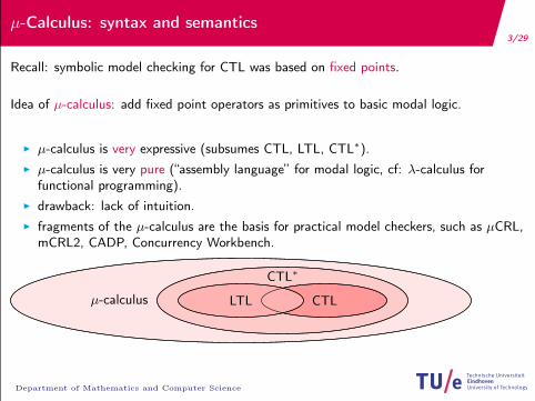
Recall: symbolic model checking for CTL was based on fixed points.
Idea of µ-calculus: add fixed point operators as primitives to basic modal logic.
I µ-calculus is very expressive (subsumes CTL, LTL, CTL∗).I µ-calculus is very pure (“assembly language” for modal logic, cf: λ-calculus for
functional programming).I drawback: lack of intuition.I fragments of the µ-calculus are the basis for practical model checkers, such as µCRL,
mCRL2, CADP, Concurrency Workbench.
LTL CTL
CTL∗
µ-calculus

4/29
Department of Mathematics and Computer Science
µ-Calculus: syntax and semantics
Kripke Structures and Labelled Transition Systems
Mix of Kripke Systems and Labelled Transition Systems: M = 〈S ,Act,R, L〉 over a set APof atomic propositions:
I S is a set of statesI Act is a set of action labelsI R is a labelled transition relation: R ⊆ S × Act× SI L is a labelling: L ∈ S → 2AP
Notation: s a−→ t denotes (s, a, t) ∈ R
Special cases:I Kripke Structures: Act is a singleton (only one transition relation)I LTS (process algebra): AP is empty (only propositions true and false)

5/29
Department of Mathematics and Computer Science
µ-Calculus: syntax and semantics
Let the following sets be given:I AP (atomic propositions),I Act (action labels) andI Var (formal variables).
The syntax of µ-calculus formulae f , g is defined by the following grammar:
f , g ::= true | p | X | ¬f | f ∧ g | [a]f | νX .f
Note:I p ∈ AP,X ∈ Var, a ∈ Act.I [a]f means “for all direct a-successors, f holds” (compare to CTL: A X f ).

6/29
Department of Mathematics and Computer Science
µ-Calculus: syntax and semantics
Some notation and terminology:
I An occurrence of X is bound by a surrounding fixed point symbol νX . Unboundoccurrences of X are called free.
I A formula is closed if it has no free variables, otherwise it is called openI An environment e interprets the free formal variables X as a set of states
• Mixed Kripke Structure M = 〈S ,Act,R, L〉• e : Var→ 2S
• e[X := V ] is an environment like e, but X is set to V :
e[X := V ](Y ) :=
{V if Y = Xe(Y ) otherwise
I The semantics of a formula f is a set of states of a Mixed Kripke Structure

7/29
Department of Mathematics and Computer Science
µ-Calculus: syntax and semantics
Fix a system: M = 〈S ,Act,R, L〉I [[f ]]e denotes the set of states where f holds given context e : Var → 2S :
[[true]]e = S[[p]]e = {s | p ∈ L(s)}[[X ]]e = e(X )
[[¬f ]]e = S \ [[f ]]e[[f ∧ g ]]e = [[f ]]e ∩ [[g ]]e
[[[a]f ]]e = {s | ∀t. s a−→ t ⇒ t ∈ [[f ]]e}
[[νX .f ]]e = ν(Z 7→ [[f ]]e[X :=Z ])
I [[νX .f ]]e requires monotonicity of [[f ]]e[X :=Z ].I Syntactic Monotonicity Criterion: monotonicity is guaranteed if, in νX .f , formal
variable X occurs under an even number of negations (¬) in f .
The semantics immediately gives rise to a naive algorithm for model checking µ-calculus(compute gfp by iteration).

8/29
Department of Mathematics and Computer Science
µ-Calculus: Positive Normal Form
I Extend the grammar with the following shorthands with semantics:
false := ¬true [[false]]e = ∅f ∨ g := ¬((¬f ) ∧ (¬g)) [[f ∨ g ]]e = [[f ]]e ∪ [[g ]]e
〈a〉f := ¬([a](¬f )) [[〈a〉f ]]e = {s | ∃t.s a−→ t ∧ t ∈ [[f ]]e}
µX .f := ¬(νX .¬f [X := ¬X ]) [[µX .f ]]e = µ(Z 7→ [[f ]]e[X :=Z ])
I A µ-calculus formula is in positive normal form if negations occur only in front ofpropositions.
I Transform a formula into positive normal form by driving negations inward.I Syntactic monotonicity prevents single negations in front of formal variables.

9/29
Department of Mathematics and Computer Science
Outline
µ-Calculus: syntax and semantics
Complexity
Emerson-Lei Algorithm
Embedding CTL-formulae
Conclusions
Exercise

10/29
Department of Mathematics and Computer Science
Complexity
Complexity of naive µ-Calculus algorithm
I We check formula f with at most k nested fixed points on the Kripke StructureM = 〈S ,R,Act, L〉.
I In νX1. 〈a〉(µX2. (X1 ∧ h) ∨ 〈a〉X2
):
• The outermost (greatest) fixed point can decrease at most |S | times (recall that S isfinite)
• In total, the innermost fixed point of formula f is evaluated at most |S |2 times.
I In general: the innermost fixed point of formula f is evaluated at most |S |k times.I Each iteration requires up to |M| × |f | steps.I Total time complexity of naive algorithm: O((|S |+ |R|)× |f | × |S |k).
A more careful analysis will yield a more optimal treatment for nested fixed points of thesame type.

11/29
Department of Mathematics and Computer Science
Complexity
I Let Act = {a}:• E G f . . . . . . . . . . . . . . . . . . . . . . . . . . . . . . . . . . . . . . . . . . . . . . . . . . . . . . . . . . . . . . . . . .νX .f ∧ 〈a〉X• E [f U g ] . . . . . . . . . . . . . . . . . . . . . . . . . . . . . . . . . . . . . . . . . . . . . . . . . . . . . . . . µX .g ∨ (f ∧ 〈a〉X )
• Every p is inevitably followed by a q: νX1.
((p ⇒ (µX2. q ∨ [a]X2)
)∧ [a]X1
)I Special case: X1 does not occur within the scope of µX2.I The last formula can therefore be evaluated “inside-out”:
X 02 = false X 0
1 = trueX 1
2 = q ∨ [a]X 02 X 1
1 = (p ⇒ Xω2 ) ∧ [a]X 0
1X 2
2 = q ∨ [a]X 12 =⇒ X 2
1 = (p ⇒ Xω2 ) ∧ [a]X 1
1... Xω
2 = q ∨ [a]Xω2 ... Xω
1 = (p ⇒ Xω2 ) ∧ [a]Xω
1

12/29
Department of Mathematics and Computer Science
Complexity
A more difficult case
I On some path, h holds infinitely often: νX1. 〈a〉(µX2. (X1 ∧ h) ∨ 〈a〉X2
)I Problem: the inner fixed point depends crucially on X1.
X 01 = true
X 002 = false
X 012 = (X 0
1 ∧ h) ∨ 〈a〉X 002
X 022 = (X 0
1 ∧ h) ∨ 〈a〉X 012
... X 0ω2 = (X 0
1 ∧ h) ∨ 〈a〉X 0ω2
X 11 = 〈a〉X 0ω
2X 10
2 = falseX 11
2 = (X 11 ∧ h) ∨ 〈a〉X 10
2... X 1ω
2 = (X 11 ∧ h) ∨ 〈a〉X 1ω
2X 2
1 = 〈a〉X 1ω2
... Xω1 = 〈a〉Xωω
2

13/29
Department of Mathematics and Computer Science
Complexity
The complexity of a µ-calculus formula depends on the fixed points (analogue: thecomplexity of first-order formulae depends on the universal/existential quantifiers and theiralternations)
I Basic idea: find a syntactic complexity measure that approaches the semanticcomplexity
I Nesting Depth:maximum number of nested fixed points in a positive normal form
ND(f ) := 0 for f ∈ {p,¬p,X}ND( a©f ) := ND(f ) for a© ∈ {[a], 〈a〉}
ND(f �g) := max(ND(f ),ND(g)) for � ∈ {∧,∨}ND(µν X .f ) := 1+ ND(f ) for µ
ν∈ {µ, ν}
I Example: ND((µX1. νX2. X1 ∨ X2) ∧ (µX3. µX4. (X3 ∧ µX5. p ∨ X5))
)
I X3,X4 and X5 have no alternation between fixed point signs

13/29
Department of Mathematics and Computer Science
Complexity
The complexity of a µ-calculus formula depends on the fixed points (analogue: thecomplexity of first-order formulae depends on the universal/existential quantifiers and theiralternations)
I Basic idea: find a syntactic complexity measure that approaches the semanticcomplexity
I Nesting Depth:maximum number of nested fixed points in a positive normal form
ND(f ) := 0 for f ∈ {p,¬p,X}ND( a©f ) := ND(f ) for a© ∈ {[a], 〈a〉}
ND(f �g) := max(ND(f ),ND(g)) for � ∈ {∧,∨}ND(µν X .f ) := 1+ ND(f ) for µ
ν∈ {µ, ν}
I Example: ND((µX1. νX2. X1 ∨ X2) ∧ (µX3. µX4. (X3 ∧ µX5. p ∨ X5))
)= 3
I X3,X4 and X5 have no alternation between fixed point signs

14/29
Department of Mathematics and Computer Science
Complexity
I Capture alternationI Alternation Depth: number of alternating fixed points of a formula in positive normal
form.
AD(f ) := 0 for f ∈ {p,¬p,X}AD( a©f ) := AD(f ) for a© ∈ {[a], 〈a〉}
AD(f �g) := max(AD(f ),AD(g)) for � ∈ {∧,∨〉}AD(µX .f ) := 1+ max{AD(g) | g is a ν-subformula of f }AD(νX .f ) := 1+ max{AD(g) | g is a µ-subformula of f }
I Examples:
AD((µX1. νX2. X1 ∨ X2) ∧ (µX3.µX4. (X3 ∧ µX5.p ∨ X5))
)AD
((µX1. νX2. X1 ∨ X2) ∧ (µX3.νX4. (X3 ∧ µX5.p ∨ X5))
)
I X5 does not depend on X3 and X4

14/29
Department of Mathematics and Computer Science
Complexity
I Capture alternationI Alternation Depth: number of alternating fixed points of a formula in positive normal
form.
AD(f ) := 0 for f ∈ {p,¬p,X}AD( a©f ) := AD(f ) for a© ∈ {[a], 〈a〉}
AD(f �g) := max(AD(f ),AD(g)) for � ∈ {∧,∨〉}AD(µX .f ) := 1+ max{AD(g) | g is a ν-subformula of f }AD(νX .f ) := 1+ max{AD(g) | g is a µ-subformula of f }
I Examples:
AD((µX1. νX2. X1 ∨ X2) ∧ (µX3.µX4. (X3 ∧ µX5.p ∨ X5))
)= 2
AD((µX1. νX2. X1 ∨ X2) ∧ (µX3.νX4. (X3 ∧ µX5.p ∨ X5))
)= 3
I X5 does not depend on X3 and X4

15/29
Department of Mathematics and Computer Science
Complexity
I Dependent Alternation Depth (dAD): number of alternating fixed points, such thatthe innermost fixed point depends on the outermost.
I The definition of dAD is identical to AD, except for
dAD(µX .f ) := max(dAD(f ),1+ max{dAD(g) |
g is a ν-subformula of f and X occurs in g}dAD(νX .f ) := max(dAD(f ),
1+ max{dAD(g) |g is a µ-subformula of f and X occurs in g}
I Examples:
dAD((µX1. νX2. X1 ∨ X2) ∧ (µX3.µX4. (X3 ∧ µX5.p ∨ X5))
)dAD
((µX1. νX2. X1 ∨ X2) ∧ (µX3.νX4. (X3 ∧ µX5.p ∨ X5))
)

15/29
Department of Mathematics and Computer Science
Complexity
I Dependent Alternation Depth (dAD): number of alternating fixed points, such thatthe innermost fixed point depends on the outermost.
I The definition of dAD is identical to AD, except for
dAD(µX .f ) := max(dAD(f ),1+ max{dAD(g) |
g is a ν-subformula of f and X occurs in g}dAD(νX .f ) := max(dAD(f ),
1+ max{dAD(g) |g is a µ-subformula of f and X occurs in g}
I Examples:
dAD((µX1. νX2. X1 ∨ X2) ∧ (µX3.µX4. (X3 ∧ µX5.p ∨ X5))
)= 2
dAD((µX1. νX2. X1 ∨ X2) ∧ (µX3.νX4. (X3 ∧ µX5.p ∨ X5))
)= 2

16/29
Department of Mathematics and Computer Science
Outline
µ-Calculus: syntax and semantics
Complexity
Emerson-Lei Algorithm
Embedding CTL-formulae
Conclusions
Exercise

17/29
Department of Mathematics and Computer Science
Emerson-Lei Algorithm
I Given a finite set S and a monotonic τ : 2S → 2S in the partial order (2S ,⊆).I We used to compute the least fixed point from ∅:
∅ ⊆ τ(∅) ⊆ τ2(∅) ⊆ ... ⊆ τ i (∅) = τ i+1(∅)
then µX .τ(X ) = τ i (∅)I Actually, instead of ∅, we can start in any set known to be smaller than the fixed
point:
• Assume W ⊆ µX .τ(X ), so we have:
∅ ⊆W ⊆ τ i (∅)• By monotonicity and the definition of fixed points:
τ i (∅) ⊆ τ i (W ) ⊆ τ2i (∅) = τ i (∅)• So if W ⊆ µX .τ(X ) we compute the least fixed point as:
W , τ(W ), τ2(W ), ... , τ j (W ) = τ j+1(W )
This converges at some j ≤ i (may be j < i)

17/29
Department of Mathematics and Computer Science
Emerson-Lei Algorithm
I Given a finite set S and a monotonic τ : 2S → 2S in the partial order (2S ,⊆).I We used to compute the least fixed point from ∅:
∅ ⊆ τ(∅) ⊆ τ2(∅) ⊆ ... ⊆ τ i (∅) = τ i+1(∅)
then µX .τ(X ) = τ i (∅)I Actually, instead of ∅, we can start in any set known to be smaller than the fixed
point:• Assume W ⊆ µX .τ(X ), so we have:
∅ ⊆W ⊆ τ i (∅)• By monotonicity and the definition of fixed points:
τ i (∅) ⊆ τ i (W ) ⊆ τ2i (∅) = τ i (∅)• So if W ⊆ µX .τ(X ) we compute the least fixed point as:
W , τ(W ), τ2(W ), ... , τ j (W ) = τ j+1(W )
This converges at some j ≤ i (may be j < i)
18/29
Department of Mathematics and Computer Science
Emerson-Lei Algorithm
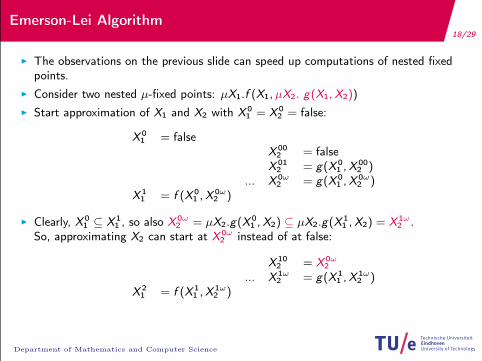
I The observations on the previous slide can speed up computations of nested fixedpoints.
I Consider two nested µ-fixed points: µX1.f (X1,µX2. g(X1,X2))
I Start approximation of X1 and X2 with X 01 = X 0
2 = false:
X 01 = false
X 002 = false
X 012 = g(X 0
1 ,X 002 )
... X 0ω2 = g(X 0
1 ,X 0ω2 )
X 11 = f (X 0
1 ,X 0ω2 )
I Clearly, X 01 ⊆ X 1
1 , so also X 0ω2 = µX2.g(X 0
1 ,X2) ⊆ µX2.g(X 11 ,X2) = X 1ω
2 .So, approximating X2 can start at X 0ω
2 instead of at false:
X 102 = X 0ω
2... X 1ω
2 = g(X 11 ,X 1ω
2 )X 2
1 = f (X 11 ,X 1ω
2 )

19/29
Department of Mathematics and Computer Science
Emerson-Lei Algorithm
Given:I Mixed Kripke Structure: M = 〈S ,R,Act, L〉I A µ-Calculus formula f and an environment e
Returns: [[f ]]e , the set of states in S where f holds.
Idea:I The function eval(f ) proceeds by recursion on f , using iteration for the fixed points.I The value of the current approximation for variable Xi is stored in array A[i ], in order
to reuse it in later iterations.I Reset A[i ] only if:
• a higher Xj of different sign changed, and• µν Xi .f contains free variables.

20/29
Department of Mathematics and Computer Science
Emerson-Lei algorithm
Initialisation:for all variables Xi do
if Xi is bound by a µ then A[i ] := false;else if Xi is bound by a ν then A[i ] := true;else A[i ] := e(Xi )end if
end for

21/29
Department of Mathematics and Computer Science
Emerson-Lei algorithm
function eval(f )if f = Xi then return A[i ]else if f = g1 ∨ g2 then return eval(g1) ∪ eval(g2)else if ... then ...else if f = µXi .g(Xi ) then
if the surrounding binder of f is a ν thenfor all open subformulae of f of the form µXk .g do A[k] := falseend for
end ifrepeat
Xold := A[i ]; {continue from previous value}A[i ] := eval(g);
until A[i ] = Xold
return A[i ]end if
end function

22/29
Department of Mathematics and Computer Science
Emerson-Lei algorithm
Given a formula νX1.νX2.µX3.µX4.(X1 ∨ X2 ∨ (µX5.X5 ∧ p))I When computing νX2, µX4 and µX5: no reset is needed because the surrounding
binder has the same sign.I When computing X3:
• Reset X3,X4: their subformula contains X1 and X2 as free variables• Do not reset X5: the subformula (µX5.X5 ∧ p) is closed
Modifications with respect to the book (p. 105):
I We identified e and A[i ] (they play the same role)I The restriction to reset open formulae only makes the algorithm more efficient. This
is essential for CTL (see later).I The book has a slightly different algorithm (correctness unclear to me): we presented
the original Emerson and Lei algorithm (1986).

23/29
Department of Mathematics and Computer Science
Emerson-Lei algorithm
Complexity analysis
I Let formula f be given, with dependent alternation depth dAD(f ) = d .I Let the Kripke Structure be 〈S ,Act,R, L〉.I Take a block of fixed points of the same type:
• its length is at most |f |.• the value of each fixed point in it can grow/shrink at most |S | times.
I In total, the innermost block will have no more than (|f | · |S |)d iterations of therepeat-loop.
I Each iteration requires time at most O(|f | · (|S |+ |R|)).I Hence: the overall complexity of the Emerson-Lei algorithm isO(|f | · (|S |+ |R|) · (|f | · |S |)d )

24/29
Department of Mathematics and Computer Science
Outline
µ-Calculus: syntax and semantics
Complexity
Emerson-Lei Algorithm
Embedding CTL-formulae
Conclusions
Exercise

25/29
Department of Mathematics and Computer Science
Embedding CTL-formulae
Again, assume Act = {a}. Given the fixed point characterisation of CTL, there is astraightforward translation of CTL to the µ-calculus:
I Tr(p) = pI Tr(¬f ) = ¬Tr(f )I Tr(f ∧ g) = Tr(f ) ∧ Tr(g)I Tr(E X f ) = 〈a〉 Tr(f )I Tr(E G f ) = νY .(Tr(f ) ∧ 〈a〉 Y )
I Tr(E [f U g ]) = µY .(Tr(g) ∨ (Tr(f ) ∧ 〈a〉 Y ))
Note:I Tr(f ) is syntactically monotoneI Tr(f ) is a closed µ-calculus formulaI dAD(Tr(f )) ≤ 1, which is called the alternation free fragment of the µ-calculusI AD(Tr(f )) is not bounded!

26/29
Department of Mathematics and Computer Science
Outline
µ-Calculus: syntax and semantics
Complexity
Emerson-Lei Algorithm
Embedding CTL-formulae
Conclusions
Exercise

27/29
Department of Mathematics and Computer Science
Conclusions
I the µ-calculus incorporates least and greatest fixed points directly in the logic.I the naive algorithm is exponential in the nesting depth of fixed points.I a careful analysis leads to an algorithm which is exponential in the (dependent)
alternation depth only,I Hence: alternation free µ-calculus is linear in the Kripke Structure and polynomial in
the formula.I CTL translates into the alternation free fragment of the µ-calculus.I for the latter we essentially needed the dependent alternation depth.I fairness constraints typically lead to one extra alternation (dAD(f ) = 2)

28/29
Department of Mathematics and Computer Science
Outline
µ-Calculus: syntax and semantics
Complexity
Emerson-Lei Algorithm
Embedding CTL-formulae
Conclusions
Exercise

29/29
Department of Mathematics and Computer Science
Exercise
Consider the following µ-calculus formula φ and LTS L:
φ := νX .
([a]X ∧ νY .µZ .(〈b〉Y ∨ 〈a〉Z)
) s1 s2
s3 s4
a
a
b
b a
I Compute the set of states where φ holds with the naive algorithm (give allintermediate approximations).
I Compute the set of states where φ holds with the Emerson-Lei’s algorithm (give allintermediate approximations).
I Explain in natural language the meaning of formula φ.