RICE UNIVERSITY

Numerically Stable and Statistically Efficient Algorithms for Large Scale Exponential Fitting

by

Jeffrey M. Hokanson

A THESIS FOR THE D EGREE

Doctor of Philosophy

THESIS COMMITTEE:

air

tational and Applied Mathematics

Steven J. Co , o-c air Professor of ompu ational and Applied

~tP:~ Athanasios C. Antoulas Professor of Electrical and Computer Engineer· g

at thias Hein schloss Professor of mputational and Applied Mathematics

Houston, Texas

August, 2013

ABSTRACT

Numerically Stable and Statistically Efficient Algorithms for Large Scale

Exponential Fitting

by

Jeffrey M. Hokanson

The exponential fitting problem appears in diverse applications such as magnetic

resonance spectroscopy, mechanical resonance, chemical reactions, system identifi-

cation, and radioactive decay. In each application, the exponential fitting problem

decomposes measurements into a sum of exponentials with complex coefficients plus

noise. Although exponential fitting algorithms have existed since the invention of

Prony’s Method in 1795, the modern challenge is to build algorithms that stably re-

cover statistically optimal estimates of these complex coefficients while using millions

of measurements in the presence of noise. Existing variants of Prony’s Method prove

either too expensive, most scaling cubically in the number of measurements, or too

unstable. Nonlinear least squares methods scale linearly in the number of measure-

ments, but require well-chosen initial estimates lest these methods converge slowly or

find a spurious local minimum.

We provide an analysis connecting the many variants of Prony’s Method that have

been developed in different fields over the past 200 years. This provides a unified

framework that extends our understanding of the numerical and statistical properties

of these algorithms.

We also provide two new algorithms for exponential fitting that overcome several

practical obstacles. The first algorithm is a modification of Prony’s Method that

can recover a few exponential coefficients from measurements containing thousands

of exponentials, scaling linearly in the number of measurements. The second al-

gorithm compresses measurements onto a subspace that minimizes the covariance of

the resulting estimates and then recovers the exponential coefficients using an existing

nonlinear least squares algorithm restricted to this subspace. Numerical experiments

suggest that small compression spaces can be effective; typically we need fewer than

20 compressed measurements per exponential to recover the parameters with 90%

efficiency. We demonstrate the efficacy of this approach by applying these algorithms

to examples from magnetic resonance spectroscopy and mechanical vibration.

Finally, we use these new algorithms to help answer outstanding questions about

damping in mechanical systems. We place a steel string inside vacuum chamber and

record the free response at multiple pressures. Analyzing these measurements with

our new algorithms, we recover eigenvalue estimates as a function of pressure that

illuminate the mechanism behind damping.

Acknowledgments

First and foremost, I would like to thank Professor Mark Embree for imparting in me

an appreciation for the aesthetics of mathematics and for giving me the freedom to

explore the results that became this thesis. I could not have completed this project

without his tireless help, countless revisions, and endless patience. Mark took me

under his wing when I was a junior and gave me my first real taste of research.

Together, we have eaten good cheese, admired fine typography and graphic design,

and built lab equipment. In the process we have built a relationship that has shaped

me into both a better mathematician and a wiser person.

I would also like to thank the members of my committee for their help in shaping

this thesis. Along with Mark Embree, Professor Steve Cox provided the inspiration

to try to solve inverse eigenvalue problems using real experimental data. Professor

Matthias Heinkenschloss provided invaluable insight into the wide field of optimiza-

tion methods. A series of conversations with Professor Thanos Antoulas showed me

how my research fits into the context of system identification. I am immensely grateful

for all their contributions.

I would also like to thank Ion-Victor Gosea for pointing out errors in an early

draft of Section 3.5.3.

I would also like to thank the NSF for providing the funding for both the Physics

of Strings Seminar and the Eigenvalue Clinic through which the ideas in this thesis

were refined. NSF funding also supported the experimental work described in this

thesis.

Many people provided assistance in building and operating these experiments.

Professor Stan Dodds provided considerable guidance through the perils of experi-

v

mental science and help in improving the vacuum chamber. His sense of humor and

his open door have been an important part of my life at Rice. Jeffrey Bridge designed

the improved photodetectors and worked with me to build the apparatus for the vac-

uum experiment. Jeff was not only a great experimental partner but also a loyal and

inspiring friend.

Nor could this experiment have been built without the patience and good humor

of many of the shop staff. In particular, I would like to thank Joe Gesenhus for many

hours of assistance in the machine shop and Michael Dye for his jokes and his help

with electrical components of the experiment. I would also like to thank Dwight Dear

for teaching me how to use a machine shop, Carlos Amaro for letting me play with

his toys, and Dick Chronister for being awesome.

I would also like to thank the staff of the CAAM department, particularly Daria

Lawrence, Ivy Gonzales, Brenda Aune, Eric Aune, and Fran Moshiri. They have

provided not only advice and assistance but also warmth and compassion. Second to

Mark Embree, Daria has play the greatest role in seeing me and this thesis through.

Finally I would like to thank my friends and family. I am forever grateful for my

many wonderful friends who have gotten me into and out of trouble and reminded

me that there was a life outside of my thesis. From rocket supplies to telescopes to

my education at Rice, my parents have given flight to my dreams and enabled me

to become who I am today. Their love and support has been a constant force in my

life. Lastly, I would like to thank my girlfriend Kimberly DeBruler who, in addition

to providing assistance monitoring the vacuum chamber experiment, has given me an

appreciation for many new things in life. Her love and affection have made finishing

this thesis possible.

Contents

Abstract iiAcknowledgments ivList of Illustrations xList of Tables xiiList of Algorithms xiii

1 Introduction 11.1 Formulation of the Exponential Fitting Problem . . . . . . . . . . . . 5

1.1.1 Special Cases for Real Measurements . . . . . . . . . . . . . . 81.1.2 Existence and Uniqueness . . . . . . . . . . . . . . . . . . . . 81.1.3 Nonparametric Methods . . . . . . . . . . . . . . . . . . . . . 10

1.2 A Prototypical Exponential Fitting Application . . . . . . . . . . . . 111.3 Exponential Fitting and System Identification . . . . . . . . . . . . . 151.4 A Brief History of Algorithms for Exponential Fitting . . . . . . . . . 17

2 Variations on a Theme of Prony 212.1 Derivation of Prony’s Method . . . . . . . . . . . . . . . . . . . . . . 222.2 Equivalent Reformulations of Prony’s Method . . . . . . . . . . . . . 25

2.2.1 Prony Least Squares . . . . . . . . . . . . . . . . . . . . . . . 252.2.2 Nullspace Method . . . . . . . . . . . . . . . . . . . . . . . . . 272.2.3 Prony Matrix Pencil Method . . . . . . . . . . . . . . . . . . . 282.2.4 Prony Determinant Method . . . . . . . . . . . . . . . . . . . 31

2.3 Statistics of Prony’s Method . . . . . . . . . . . . . . . . . . . . . . . 332.3.1 First Order . . . . . . . . . . . . . . . . . . . . . . . . . . . . 342.3.2 Second Order Bias . . . . . . . . . . . . . . . . . . . . . . . . 36

2.4 Maximum Likelihood Prony Methods . . . . . . . . . . . . . . . . . . 372.4.1 Householder’s Method . . . . . . . . . . . . . . . . . . . . . . 412.4.2 Osborne’s Method . . . . . . . . . . . . . . . . . . . . . . . . 45

2.5 Extraneous Exponentials . . . . . . . . . . . . . . . . . . . . . . . . . 482.5.1 Kumaresan and Tufts Method . . . . . . . . . . . . . . . . . . 522.5.2 Matrix Pencil Method . . . . . . . . . . . . . . . . . . . . . . 542.5.3 Kung’s Method . . . . . . . . . . . . . . . . . . . . . . . . . . 562.5.4 Hankel Total Least Squares . . . . . . . . . . . . . . . . . . . 572.5.5 Prony Maximum Likelihood with Extraneous Exponentials . . 58

2.6 Autocovariance-Based Prony Variants . . . . . . . . . . . . . . . . . . 58

vii

2.6.1 Yule-Walker Method . . . . . . . . . . . . . . . . . . . . . . . 582.6.2 Pisarenko’s Method . . . . . . . . . . . . . . . . . . . . . . . . 61

2.7 Compressed Prony’s Method . . . . . . . . . . . . . . . . . . . . . . . 632.7.1 Cornell’s Method . . . . . . . . . . . . . . . . . . . . . . . . . 662.7.2 Method of Moments . . . . . . . . . . . . . . . . . . . . . . . 662.7.3 Compressed Maximum Likelihood Prony Method . . . . . . . 67

2.8 Compressed Matrix Pencil Methods for Localized Exponentials . . . . 682.8.1 Filtered Matrix Pencil Method . . . . . . . . . . . . . . . . . . 692.8.2 Orthogonalized Matrix Pencil Method . . . . . . . . . . . . . 70

3 Nonlinear Least Squares Methods 743.1 Nonlinear Least Squares Algorithms . . . . . . . . . . . . . . . . . . . 76

3.1.1 Gradient Descent . . . . . . . . . . . . . . . . . . . . . . . . . 763.1.2 Newton’s Method . . . . . . . . . . . . . . . . . . . . . . . . . 773.1.3 Gauss-Newton Approximation . . . . . . . . . . . . . . . . . . 783.1.4 Variable Projection . . . . . . . . . . . . . . . . . . . . . . . . 783.1.5 Box Constraints . . . . . . . . . . . . . . . . . . . . . . . . . . 80

3.2 Perturbation Analysis for Nonlinear Least Squares . . . . . . . . . . . 803.2.1 Asymptotic Perturbation . . . . . . . . . . . . . . . . . . . . . 813.2.2 Asymptotic Covariance . . . . . . . . . . . . . . . . . . . . . . 81

3.3 Perturbation Analysis for Separable Nonlinear Least Squares . . . . . 823.3.1 Asymptotic Perturbation . . . . . . . . . . . . . . . . . . . . . 833.3.2 Covariance . . . . . . . . . . . . . . . . . . . . . . . . . . . . . 84

3.4 Heuristics for Initial Conditions . . . . . . . . . . . . . . . . . . . . . 853.4.1 Random Imaginary Part . . . . . . . . . . . . . . . . . . . . . 863.4.2 Roots of Unity . . . . . . . . . . . . . . . . . . . . . . . . . . 903.4.3 Peaks of the Fourier Transform . . . . . . . . . . . . . . . . . 903.4.4 Prony-type Methods . . . . . . . . . . . . . . . . . . . . . . . 933.4.5 Prior Knowledge . . . . . . . . . . . . . . . . . . . . . . . . . 93

3.5 Estimating the Number of Exponentials . . . . . . . . . . . . . . . . 943.5.1 Hankel Singular Values . . . . . . . . . . . . . . . . . . . . . . 943.5.2 Akaike Information Criterion . . . . . . . . . . . . . . . . . . 983.5.3 Small Amplitudes . . . . . . . . . . . . . . . . . . . . . . . . . 99

3.6 Peeling . . . . . . . . . . . . . . . . . . . . . . . . . . . . . . . . . . . 100

4 Compression for Exponential Fitting 1044.1 Compression Subspace Efficiency . . . . . . . . . . . . . . . . . . . . 1094.2 Updating Subspace Efficiency . . . . . . . . . . . . . . . . . . . . . . 113

4.2.1 Updating the Singular Values for the General Problem . . . . 1144.2.2 Updating the Covariance for the General Problem . . . . . . . 1154.2.3 Updating the Singular Values for the Separable Problem . . . 1164.2.4 Updating the Covariance for the Separable Problem . . . . . . 117

viii

4.3 Closed Form Inner Products for Block Fourier Matrices . . . . . . . . 1194.3.1 U∗V(ω) . . . . . . . . . . . . . . . . . . . . . . . . . . . . . . 1194.3.2 U∗V′(ω) . . . . . . . . . . . . . . . . . . . . . . . . . . . . . . 120

4.4 Subspace Selection for Exponential Fitting . . . . . . . . . . . . . . . 1214.4.1 Initial Subspace . . . . . . . . . . . . . . . . . . . . . . . . . . 1224.4.2 Candidate Set Selection . . . . . . . . . . . . . . . . . . . . . 1234.4.3 Quality Measures . . . . . . . . . . . . . . . . . . . . . . . . . 124

4.5 Block Dimensions for Exponential Fitting . . . . . . . . . . . . . . . 1284.5.1 Truncation and Decimation . . . . . . . . . . . . . . . . . . . 1304.5.2 Fixed Blocks . . . . . . . . . . . . . . . . . . . . . . . . . . . 1324.5.3 Geometric Blocks . . . . . . . . . . . . . . . . . . . . . . . . . 1324.5.4 Rationally Chosen Blocks . . . . . . . . . . . . . . . . . . . . 1364.5.5 Optimizing Block Dimensions . . . . . . . . . . . . . . . . . . 140

4.6 Linking Compression and Optimization . . . . . . . . . . . . . . . . . 1414.6.1 Precomputed Compression Subspaces . . . . . . . . . . . . . . 1434.6.2 Dynamically Computed Compression Subspaces . . . . . . . . 146

5 Damping in Vibrating Strings 1515.1 Experimental Apparatus . . . . . . . . . . . . . . . . . . . . . . . . . 152

5.1.1 String . . . . . . . . . . . . . . . . . . . . . . . . . . . . . . . 1545.1.2 String Mounting . . . . . . . . . . . . . . . . . . . . . . . . . 1555.1.3 Excitation and Driver . . . . . . . . . . . . . . . . . . . . . . 1565.1.4 Photodetector . . . . . . . . . . . . . . . . . . . . . . . . . . . 158

5.2 Data Analysis . . . . . . . . . . . . . . . . . . . . . . . . . . . . . . . 1645.3 Matching Reality to Physical Models . . . . . . . . . . . . . . . . . . 165

5.3.1 First Order Model . . . . . . . . . . . . . . . . . . . . . . . . 1655.3.2 Energy in Bending . . . . . . . . . . . . . . . . . . . . . . . . 1695.3.3 Air Damping . . . . . . . . . . . . . . . . . . . . . . . . . . . 1715.3.4 Frequency Shift Due to Damping . . . . . . . . . . . . . . . . 1765.3.5 Thermal Effects . . . . . . . . . . . . . . . . . . . . . . . . . . 1775.3.6 Eigenvalue Splitting and Nonlinear Effects . . . . . . . . . . . 1785.3.7 Further Refinement . . . . . . . . . . . . . . . . . . . . . . . . 178

5.4 Conclusion . . . . . . . . . . . . . . . . . . . . . . . . . . . . . . . . . 181

6 Conclusions and Future Work 1826.1 Further Extensions of Prony’s Method . . . . . . . . . . . . . . . . . 183

6.1.1 Numerically Stable Maximum Likelihood Prony Methods . . . 1836.1.2 Improving Performance . . . . . . . . . . . . . . . . . . . . . . 1836.1.3 Restarted Matrix Pencil Method . . . . . . . . . . . . . . . . . 184

6.2 Improving Compression for Exponential Fitting . . . . . . . . . . . . 1856.2.1 New Compression Parent Coordinates . . . . . . . . . . . . . . 1856.2.2 Alternative Trust Region Quadratic Models . . . . . . . . . . 186

ix

6.2.3 Block Coordinate Descent . . . . . . . . . . . . . . . . . . . . 1866.3 Applying Compression to System Identification Problems . . . . . . . 187

6.3.1 Multiple Output Impulse Response System Identification . . . 1886.3.2 Frequency Domain System Identification . . . . . . . . . . . . 1886.3.3 System Identification with Known Inputs . . . . . . . . . . . . 190

6.4 Applying Compression to Other Nonlinear Least Squares Problems . 192

A Statistics 193A.1 Definitions . . . . . . . . . . . . . . . . . . . . . . . . . . . . . . . . . 193A.2 Complex Gaussian Random Vectors . . . . . . . . . . . . . . . . . . . 194A.3 Estimators . . . . . . . . . . . . . . . . . . . . . . . . . . . . . . . . . 195A.4 Asymptotics . . . . . . . . . . . . . . . . . . . . . . . . . . . . . . . . 197A.5 Fisher Information and the Cramér-Rao Bound . . . . . . . . . . . . 198A.6 Principle of Invariance . . . . . . . . . . . . . . . . . . . . . . . . . . 198

B Wirtinger Derivatives and Complex Optimization 200B.1 Least Squares . . . . . . . . . . . . . . . . . . . . . . . . . . . . . . . 200

Bibliography 203

Illustrations

1.1 Two equivalent harmonic oscillators. . . . . . . . . . . . . . . . . . . 121.2 Covariance of recovered parameters using exponential fitting . . . . . 14

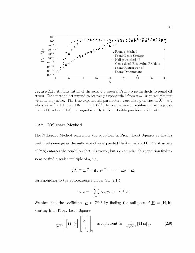
2.1 An illustration of the sensity of several Prony-type methods to roundoff errors . . . . . . . . . . . . . . . . . . . . . . . . . . . . . . . . . . 27

2.2 Performance of asymptotic estimates for Prony’s Method . . . . . . . 382.3 An illustration of the sensitivity of Maximum Likelihood Prony

Methods to round off errors . . . . . . . . . . . . . . . . . . . . . . . 412.4 Comparison of Maximum Likelihood Prony Methods applied to an

ill-conditioned example . . . . . . . . . . . . . . . . . . . . . . . . . . 422.5 Two examples of extraneous roots along a one dimensional subspace . 502.6 Bias and covariance of Prony Least Squares using extraneous

exponentials . . . . . . . . . . . . . . . . . . . . . . . . . . . . . . . . 532.7 An illustration of the sensity of several Prony-type methods that

include extraneous exponentials to round off errors . . . . . . . . . . 542.8 Comparison of Prony Methods using extraneous exponentials applied

to an ill-conditioned example . . . . . . . . . . . . . . . . . . . . . . . 552.9 Statistical efficiency of variants of Prony’s Method including

extraneous exponentials . . . . . . . . . . . . . . . . . . . . . . . . . 562.10 Bias in Pisarenko’s method for small n . . . . . . . . . . . . . . . . . 632.11 Error in Pisarenko’s method as a function of n . . . . . . . . . . . . . 642.12 Fourier transform of y . . . . . . . . . . . . . . . . . . . . . . . . . . 712.13 Performance of Filtered and Orthogonalized Matrix Pencil Methods . 71

3.1 Relative accuracy of an asymptotic covariance estimate . . . . . . . . 823.2 The appearance of local minima as noise increases. . . . . . . . . . . 873.3 Failure rate for initial estimate heuristics . . . . . . . . . . . . . . . . 883.4 The norm of the residual for a single exponential . . . . . . . . . . . . 893.5 Examples of peaks in the Fourier transform . . . . . . . . . . . . . . 923.6 Hankel singular values from a magnetic resonance spectroscopy

example with noise. . . . . . . . . . . . . . . . . . . . . . . . . . . . . 973.7 Peeling with complex data . . . . . . . . . . . . . . . . . . . . . . . . 102

4.1 Compression spaces are tailored to specific parameter values . . . . . 106

xi

4.2 Efficiency for truncation, decimation, incremental gradient, and idealsubspaces . . . . . . . . . . . . . . . . . . . . . . . . . . . . . . . . . 107

4.3 Optimial columns from various parent coordinates computed by acombinatorial search . . . . . . . . . . . . . . . . . . . . . . . . . . . 125

4.4 Failure rate for fast updates and heuristics . . . . . . . . . . . . . . . 1294.5 Efficiency of truncation and decimation strategies . . . . . . . . . . . 1314.6 Efficiency of greedily chosen subspaces from Fixed (Kq) and

Geometric (Gq) parent coordinates . . . . . . . . . . . . . . . . . . . 1334.7 Upper and lower bounds on the efficiency subspaces generated from

parent coordinates of fixed Fourier blocks and geometric blocks . . . . 1344.8 A visualization of block Fourier matrices . . . . . . . . . . . . . . . . 1354.9 Efficiency of the best three dimensional subspace from G4(100) as a

function of ω . . . . . . . . . . . . . . . . . . . . . . . . . . . . . . . 1354.10 Picking the block dimensions for the ‘best’ block parent coordinates . 1374.11 Comparison of tailored compression subspace efficiency. . . . . . . . . 1394.12 Optimized sets of block dimensions . . . . . . . . . . . . . . . . . . . 1404.13 Shape of the compressed residual for VARPRO with different parent

coorindates . . . . . . . . . . . . . . . . . . . . . . . . . . . . . . . . 1424.14 Fixed compression space for undamped exponentials . . . . . . . . . . 1444.15 The statistical efficiency for several high efficiency single undamped

exponential fitting algorithms . . . . . . . . . . . . . . . . . . . . . . 1474.16 Wall clock time for several blind exponential fitting algorithms . . . . 149

5.1 Cutaway diagram showing the vacuum chamber and string apparatus. 1535.2 The electromagnetic drive coil. . . . . . . . . . . . . . . . . . . . . . . 1575.3 The photodetector apparatus . . . . . . . . . . . . . . . . . . . . . . 1595.4 Fourier transform of string at rest . . . . . . . . . . . . . . . . . . . . 1615.5 The experimental probability density function of background signal . 1625.6 Measurements of the displacement-voltage relationship . . . . . . . . 1635.7 The imaginary part of the measured eigenvalues compared to the first

order model . . . . . . . . . . . . . . . . . . . . . . . . . . . . . . . . 1685.8 Stiffness corrections to eigenvalue frequencies . . . . . . . . . . . . . . 1705.9 Eigenvalues of a vibrating string as a function of atmospheric pressure 1725.10 Reynolds number . . . . . . . . . . . . . . . . . . . . . . . . . . . . . 1735.11 Expected eigenvalues using Lin’s damping model . . . . . . . . . . . . 1765.12 Dependence of frequency on damping and pressure . . . . . . . . . . 1775.13 Resolved eigenvalue splitting . . . . . . . . . . . . . . . . . . . . . . . 1795.14 Unresolved eigenvalues . . . . . . . . . . . . . . . . . . . . . . . . . . 180

Tables

1.1 A sampling of papers from fields in which exponential fitting occurs. . 31.2 Applications of exponential fitting . . . . . . . . . . . . . . . . . . . . 9

3.1 Failure rate for increasing numbers of exponentials . . . . . . . . . . . 86

5.1 Material properties of the string . . . . . . . . . . . . . . . . . . . . . 1545.2 Properties of Air . . . . . . . . . . . . . . . . . . . . . . . . . . . . . 171

xiii

Algorithms

2.1 Prony’s Method . . . . . . . . . . . . . . . . . . . . . . . . . . . . . . 242.2 Prony Least Squares . . . . . . . . . . . . . . . . . . . . . . . . . . . . 262.3 Nullspace Method . . . . . . . . . . . . . . . . . . . . . . . . . . . . . 282.4 Prony Matrix Pencil Method . . . . . . . . . . . . . . . . . . . . . . . 302.5 Prony Generalized Eigenvalue Problem . . . . . . . . . . . . . . . . . . 302.6 Prony Determinant Method . . . . . . . . . . . . . . . . . . . . . . . . 332.7 Maximum Likelihood Prony Method . . . . . . . . . . . . . . . . . . . 402.8 Householder’s Method . . . . . . . . . . . . . . . . . . . . . . . . . . . 442.9 Bresler and Macovski . . . . . . . . . . . . . . . . . . . . . . . . . . . 472.10 Osborne’s Method . . . . . . . . . . . . . . . . . . . . . . . . . . . . . 472.11 Kung’s Method . . . . . . . . . . . . . . . . . . . . . . . . . . . . . . . 642.12 Pisarenko’s Method . . . . . . . . . . . . . . . . . . . . . . . . . . . . 642.13 Compressed Maximum Likelihood Prony Method . . . . . . . . . . . . 682.14 Filtered Matrix Pencil Method . . . . . . . . . . . . . . . . . . . . . . 702.15 Orthogonalized Matrix Pencil Method . . . . . . . . . . . . . . . . . . 73

3.1 Pseudocode computing the Variable Projection residual and Jacobian . 793.2 Peeling for Exponential Fitting . . . . . . . . . . . . . . . . . . . . . . 101

4.1 Greedy subspace selection for exponential fitting. . . . . . . . . . . . . 1224.2 Candidate selection algorithm for exponential fitting. . . . . . . . . . . 1254.3 Computing the covariance drop . . . . . . . . . . . . . . . . . . . . . . 1274.4 Estimating a single undamped exponential with a fixed subspace . . . 145

1

Chapter 1

Introduction

Exponential signals abound: from the decay of radioactive isotopes, sine waves in ra-

dio, and decaying sinusoids in Magnetic Resonance Spectroscopy (MRS) experiments.

In all cases, the signal takes the form

y(t) = g(t) +

p−1∑k=0

akeωkt, (1.1)

where ak ∈ C is the amplitude, ωk ∈ C the complex frequency, and g ∈ C some

random noise. The complex frequency ωk takes several forms: real and negative for

radioactive decay, purely imaginary for radio waves, and in the left half of the com-

plex plane for MRS experiments. The goal of exponential fitting is to recover the

parameters a = [a0, · · · , ap−1]> and ω = [ω0, · · · , ωp−1]

> that best approximate a

finite number of samples of y(t). These parameters a and ω reveal important in-

formation: the presence of isotopes, velocities of radar targets through the Doppler

effect, resonant frequencies of mechanical structures, and the structure of organic

compounds. Algorithms for exponential fitting descend in two distinct lineages: one

beginning with Prony’s Method in 1795 [127] and the other beginning with nonlinear

least squares circa 1805 (Legendre). Prony’s Method has profound numerical and

statistical flaws: it yields biased estimates of ω, the covariance of ω typically exceeds

the Cramér-Rao lower bound by several orders of magnitude, and the estimates of

ω are extremely sensitive to rounding errors even for moderate numbers of exponen-

tials (p ≈ 20). Dozens of variants of Prony’s Method have been developed in the

2

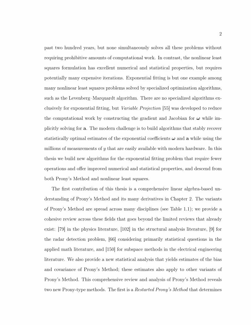
past two hundred years, but none simultaneously solves all these problems without

requiring prohibitive amounts of computational work. In contrast, the nonlinear least

squares formulation has excellent numerical and statistical properties, but requires

potentially many expensive iterations. Exponential fitting is but one example among

many nonlinear least squares problems solved by specialized optimization algorithms,

such as the Levenberg–Marquardt algorithm. There are no specialized algorithms ex-

clusively for exponential fitting, but Variable Projection [55] was developed to reduce

the computational work by constructing the gradient and Jacobian for ω while im-

plicitly solving for a. The modern challenge is to build algorithms that stably recover

statistically optimal estimates of the exponential coefficients ω and a while using the

millions of measurements of y that are easily available with modern hardware. In this

thesis we build new algorithms for the exponential fitting problem that require fewer

operations and offer improved numerical and statistical properties, and descend from

both Prony’s Method and nonlinear least squares.

The first contribution of this thesis is a comprehensive linear algebra-based un-

derstanding of Prony’s Method and its many derivatives in Chapter 2. The variants

of Prony’s Method are spread across many disciplines (see Table 1.1); we provide a

cohesive review across these fields that goes beyond the limited reviews that already

exist: [79] in the physics literature, [102] in the structural analysis literature, [9] for

the radar detection problem, [66] considering primarily statistical questions in the

applied math literature, and [150] for subspace methods in the electrical engineering

literature. We also provide a new statistical analysis that yields estimates of the bias

and covariance of Prony’s Method; these estimates also apply to other variants of

Prony’s Method. This comprehensive review and analysis of Prony’s Method reveals

two new Prony-type methods. The first is a Restarted Prony’s Method that determines

3

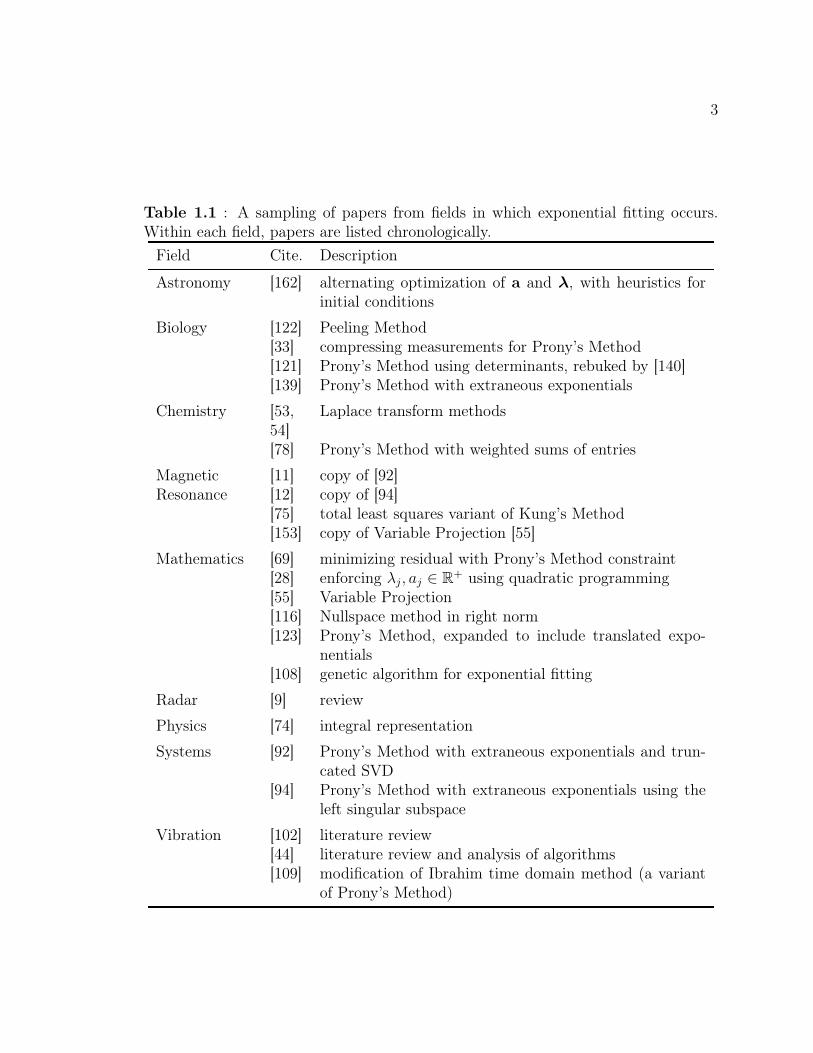
Table 1.1 : A sampling of papers from fields in which exponential fitting occurs.Within each field, papers are listed chronologically.

Field Cite. Description

Astronomy [162] alternating optimization of a and λ, with heuristics forinitial conditions

Biology [122] Peeling Method[33] compressing measurements for Prony’s Method[121] Prony’s Method using determinants, rebuked by [140][139] Prony’s Method with extraneous exponentials

Chemistry [53,54]

Laplace transform methods

[78] Prony’s Method with weighted sums of entries

MagneticResonance

[11] copy of [92][12] copy of [94][75] total least squares variant of Kung’s Method[153] copy of Variable Projection [55]

Mathematics [69] minimizing residual with Prony’s Method constraint[28] enforcing λj, aj ∈ R+ using quadratic programming[55] Variable Projection[116] Nullspace method in right norm[123] Prony’s Method, expanded to include translated expo-

nentials[108] genetic algorithm for exponential fitting

Radar [9] review

Physics [74] integral representation

Systems [92] Prony’s Method with extraneous exponentials and trun-cated SVD

[94] Prony’s Method with extraneous exponentials using theleft singular subspace

Vibration [102] literature review[44] literature review and analysis of algorithms[109] modification of Ibrahim time domain method (a variant

of Prony’s Method)

4

a few exponentials among many exponentials, inspired by the Implicitly Restarted

Arnoldi Method [142]. The second is the Maximum Likelihood Prony Method that is a

fast, stable variant Householder’s Method that yields maximum likelihood estimates

of exponential parameters.

Another contribution of this thesis is the framework of compression to solve non-

linear least squares problems (Chapter 4). Rather than solving the full nonlinear least

squares problem

θ = argminθ‖y − f(θ)‖22, (1.2)

this approach compresses (1.2) onto the subspace W ⊂ Cn spanned by W ∈ Cn×m,

(with W∗W = I) and instead solves

θW = argminθ‖W∗y −W∗f(θ)‖22. (1.3)

Whereas existing techniques such as Incremental Gradient [50] choose W from ran-

dom columns of the identity matrix I, we choose W deterministically to minimize the

covariance of θ, and measure the increase of the covariance using a generalization of

Fisher’s efficiency. By choosing matrices W where W∗f(θ) has a closed form expres-

sion, we are able to reduce the computational burden while maintaining statistical

accuracy. For the exponential fitting problem, we build W from columns of a block

diagonal matrix composed of discrete Fourier transform blocks. Typically, twenty

columns per exponential (m = 20p) are sufficient to recover θW with 90% efficiency.

When solving the exponential fitting problem using optimization, such as in the

compressed case discussed above, both the number of exponentials and initial esti-

mates of ω (and sometimes a) are required. In Chapter 3, we review existing tech-

niques for choosing the number of exponentials and providing initial estimates. One

contribution we make is to update the Peeling Method [122] to use complex data and

5

initial parameter estimates provided by the Restarted Prony Method. We also review

existing statistical criteria for selecting the number of exponentials using the Akaike

Information Criterion and the singular values of a Hankel matrix. In Corollary 3.1

we improve the Hankel matrix singular value criteria by providing a new, accurate

estimate of singular values corresponding to noise.

In this chapter, begin by formulating the exponential fitting problem, discussing

existence and uniqueness. Then, we use the simple harmonic oscillator to illustrate

how many systems described by differential equations have solutions that consist of

sums of complex exponentials. By determining the exponential coefficients ω, we can

infer parameters of the underlying differential equation. We then show that expo-

nential fitting is a special case of system identification that arises from free response

measurements. As history of exponential fitting is intertwined with many fields,

including system identification, we provide a brief historical sketch in Section 1.4

including work from the present day.

1.1 Formulation of the Exponential Fitting Problem

Recalling (1.1), the exponential fitting problem seeks to recover estimates ω and a of

the true parameters ω and a from the noisy measurements of (1.1) at times tj:

y(tj) = gj +

p−1∑k=0

akeωktj ∈ C, 0 ≤ j < n, (1.4)

where gj is some random noise.1 In this thesis, we make three further common

assumptions.

1Tildes (e.g., ωj) denote perturbed quantities; hats (e.g., ωj) true values.

6

First, we assume that y is sampled at a regular rate, i.e., tj = δj, resulting in

y(δj) =: yj = gj +

p−1∑k=0

akeωkj ∈ C 0 ≤ j < n, (1.5)

where δ has been absorbed into ω. Regularly sampled measurements are a by-product

of the hardware used to acquire measurements in many fields (e.g., radar, magnetic

resonance, mechanical resonance) and consequently, in most large scale problems

(n > 104), y is sampled regularly. This assumption is also necessary to use Prony-

type methods. When measurements are sampled irregularly, as in astronomy, we can

either use nonlinear least squares methods, which do not require regular sampling,

or construct regularly sampled measurements by interpolating the irregular measure-

ments. Interpolation can result in systematic error, especially when y(δ(j+1))−y(δj)

is large.

The second assumption is that noise components gj ∈ C are normally distributed

random variables, The third assumption is that we seek maximum likelihood estimates

of ω and a. Hence if g samples a standard complex normal distribution with zero

mean and covariance Σ, then the maximum likelihood estimates are given by

[ω, a] = argminω,a∈Cp

‖y − f([ω, a])‖Σ, (1.6)

where [f([ω, a])]j =∑p−1

k=0 akeωkj and ‖x‖2Σ = x∗Σ−1x. The assumption of normally

distributed noise is both reasonable and practical: reasonable, because if there are

many sources of noise, the central limit theorem guarantees the resulting noise will

be approximately normally distributed; practical, because the resulting maximum

likelihood estimates minimize a weighted `2 norm and the inner product associated

with this norm gives additional structure that aids solving (1.6). If g samples an-

other distribution, an alternative objective function is required. For example, the

7

noise in radioactive decay samples a Poisson distribution. However, for large radioac-

tive samples, the Poisson distribution approximates a normal distribution [17, §2.4].

Maximum likelihood estimates are not the only approach for computing estimates ω

and a; some authors take a Bayesian approach (see, e.g., [3]) that assumes some prior

knowledge about the true parameter values ω and a [24].

We can measure the efficiency of any exponential fitting algorithm by comparing

the covariance of θ = [ω>, a>]> to the Cramér-Rao lower bound. The Cramér-Rao

bound provides a lower bound on the covariance of any technique that estimates

parameters θ from noisy measurements y = g + f(θ). If θ is an unbiased estimate

of θ and g samples a complex normal distribution with zero mean and covariance Σ,

then the Cramér-Rao bound gives

Cov[θ] := E[(θ − θ)(θ − θ)∗] (F(θ)∗Σ−1F(θ))−1 =: I(θ)−1 (1.7)

where [F(θ)]·,j = ∂/∂θjf(θ) [137, eq. (6.51)]. Sections 3.2 and 3.3 give expressions

for the Fisher information matrix I particular to the exponential fitting problem. A

similar bound for biased estimates of θ also exists [137, eq. (6.50)], and sometimes

biased estimates can have a smaller covariance than unbiased estimates – although

this does not appear to be the case for the exponential fitting problem. To measure the

effectiveness of an exponential fitting algorithm, we generalize Fisher’s efficiency [49,

§4] to multivariate problems, defining the efficiency of an estimator that yields θ as

ηθ,Σ :=Tr I(θ)−1

Tr Cov[θ]. (1.8)

This efficiency is typically reported as a percentage. Typically we consider the limit

where Σ → 0 uniformly. Section 4.1 motivates this definition, as Tr Cov[θ] corre-

sponds to the expected `2 error of θ.

8

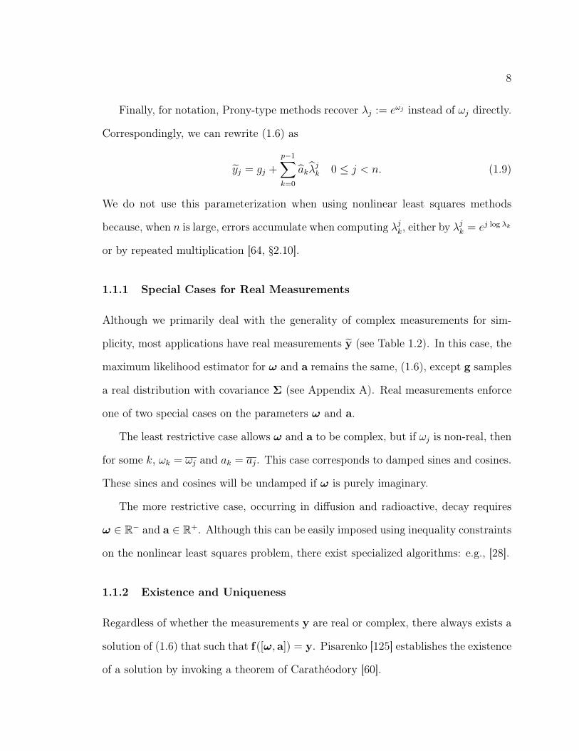
Finally, for notation, Prony-type methods recover λj := eωj instead of ωj directly.

Correspondingly, we can rewrite (1.6) as

yj = gj +

p−1∑k=0

akλjk 0 ≤ j < n. (1.9)

We do not use this parameterization when using nonlinear least squares methods

because, when n is large, errors accumulate when computing λjk, either by λjk = ej log λk

or by repeated multiplication [64, §2.10].

1.1.1 Special Cases for Real Measurements

Although we primarily deal with the generality of complex measurements for sim-

plicity, most applications have real measurements y (see Table 1.2). In this case, the

maximum likelihood estimator for ω and a remains the same, (1.6), except g samples

a real distribution with covariance Σ (see Appendix A). Real measurements enforce

one of two special cases on the parameters ω and a.

The least restrictive case allows ω and a to be complex, but if ωj is non-real, then

for some k, ωk = ωj and ak = aj. This case corresponds to damped sines and cosines.

These sines and cosines will be undamped if ω is purely imaginary.

The more restrictive case, occurring in diffusion and radioactive, decay requires

ω ∈ R− and a ∈ R+. Although this can be easily imposed using inequality constraints

on the nonlinear least squares problem, there exist specialized algorithms: e.g., [28].

1.1.2 Existence and Uniqueness

Regardless of whether the measurements y are real or complex, there always exists a

solution of (1.6) that such that f([ω, a]) = y. Pisarenko [125] establishes the existence

of a solution by invoking a theorem of Carathéodory [60].

9

Table 1.2 : Applications of exponential fitting. Problems with complex data (y ∈Cn) are marked by . Problems with real data (y ∈ Rn) and minimal restraints on ωand a are marked by ×. Problems with real data that enforce ω ∈ R− and a ∈ R+

are marked by +.Field Cite. Type Applications

Biology [41] ×+ multi-compartment models[76] + pulse fluorometry[122] + gas absorption

Chemistry [53] + multiple species chemical reaction rates[152] magnetic resonance spectroscopy

Electronics [80] + power systems

Physics [88] + radioactive decay[15] × lack hole mergers[74] + underwater explosions[70] × musical instruments[100] × crack detection[132] × normal modes of the earth

Vibration [46] × modal analysis

Theorem 1.1 (C. Carathéodory). Let y ∈ Cn, y 6= 0, n > 0. There exists an integer

1 ≤ p ≤ n and constants a ∈ Rp+, ω ∈ [0, 2π]p, with ωj 6= ωk if j 6= k and

yk =

p−1∑j=0

ajeikωj k = 0, 1, . . . , n− 1. (1.10)

The integer p and the constants a,ω are uniquely determined.

A crude way to construct this solution is to use the discrete Fourier transform. If

we choose ω to be the nth roots of unity (ωj = 2πj/n) then a is given by the discrete

Fourier transform of y, i.e.,

a = F∗ny (1.11)

where [Fn]j,k = n−1/2e2πijk/n.

Solutions to the exponential fitting problem are not unique, as we are free to

permute the entries of ω and a simultaneously. To compare two solutions ω and ω,

10

we always use the marriage norm that permutes ω to minimize the mismatch, i.e.,

minπ‖λπ − λ‖2, (1.12)

where π is a permutation. This permutation can be constructed in at most p2 oper-

ations using the Marriage Algorithm developed by Gale and Shapley [51].

In practice, we are not interested in solving (1.6) as stated, but instead solve (1.6)

while assuming a statistically justified number of exponentials, as discussed in Sec-

tion 3.5. Determining the number of exponentials is related to the minimum realiza-

tion problem in system identification, which seeks the smallest model order p that

accurately describes the system; see, e.g., [58].

1.1.3 Nonparametric Methods

Parametric signal processing problems, such as exponential fitting, assume the signal

y is determined by a known model with some unknown parameters (i.e., ω). Non-

parametric methods are an alternative for exploratory data analysis that attempt to

extract instantaneous frequency information as a function of time. The most basic

of these methods is the spectrogram: taking the discrete Fourier transform of small

segments of y. The time and frequency resolution of the spectrogram is limited by the

size of the Fourier transform, with smaller segments yielding finer time resolution but

coarser frequency information. Wavelet analysis fixes the resolution problem in the

spectrogram, providing a uniform resolution over frequency and time; see, e.g., [48].

The results of wavelet transforms are sometimes hard to interpret, prompting the

use of the Hilbert-Huang transform [73]. The Hilbert-Huang transform breaks y into

a combination of so called ‘intrinsic mode functions’ and reveals the time-frequency

dependence using the Hilbert transform of each of these mode functions, providing a

more concentrated representation of energy in frequency and time [73].

11

Although these nonparametric methods can be used to estimate the exponential

parameters ω, direct parametric methods will provide better estimates provided y

fits the model, in our case, exponentials plus noise (1.1).

1.2 A Prototypical Exponential Fitting Application

The simple harmonic oscillator is a prototypical example that illustrates how exponen-

tial fitting originates in many fields, and also shows the infrequent case of degenerate

exponentials and the complications that can arise in parameter recovery. Two com-

mon forms of the simple harmonic oscillator are the mass-spring-damper system or

the resistor-capacitor-inductor circuit, both illustrated in Figure 1.1. We consider the

general case where u solves the second order differential equation

u′′(t) + 2γu′(t) + c2u(t) = 0, u(0) = u0, u′(0) = v0. (1.13)

We can describe u as the sum of two exponentials. Linearizing (1.13) yields the

coupled, first order differential equationu′(t)u′′(t)

=

x1(t)x2(t)

′

=

0 1

−c2 −2γ

x1(t)x2(t)

⇔ x′ = Ax, x(0) = x0 =

u0v0

.(1.14)

When A is diagonalizable, we can decompose A as AV = VΩ, where V is the matrix

of eigenvectors and Ω = diag(ω+, ω−) is the matrix of eigenvalues:

ω± = −γ ±√γ2 − c2, V =

[v+ v−

]=

1 1

ω+ ω−

. (1.15)

Then the matrix exponential gives the solution to (1.14):

x(t) = eAtx0 = VetΩV−1x0

= v+etω+w∗

+x0 + v−etω−w∗

−x0

where V−1 = W =

w∗+

w∗−

.

12

Mass-Spring-Damper System Resistor-Inductor-Capacitor Circuit

mass, m

γγγγ κ

uC

2R

u

L

mu′′ + 2γu′ + κu = 0 Lu′′ + 2Ru′ + 1/Cu = 0

Figure 1.1 : Two equivalent harmonic oscillators.

Since u(t) = [x(t)]0 = e>0 x(t), where ek is the k column of the identity matrix, then

u(t) = e>0 x(t) =[e>0 v+w

∗+x(0)

]etω+ +

[e>0 v−w

∗−x(0)

]etω−

= a+etω+ + a−e

tω− .

(1.16)

Linearization of other differential equations will always result in a sum of exponentials,

provided A is diagonalizable. Then we can recover ω and a from noisy measurements

yj = u(δj) + gj by solving the exponential fitting problem (1.6).

Not every differential equation will result in the sum of exponentials. In the simple

harmonic oscillator example when γ = c, then ω+ = ω− = −γ and A has a Jordan

block. Then the solution for u(t) has polynomial terms as well as exponentials. If

AV = VJ is the Jordan normal form, where

V =

1 0

−γ 1

and J =

−γ 1

0 −γ

, (1.17)

then writing J = Ω+N, where N is the nilpotent part of J,

x(t) = eAtx0 = VeΩt+NtV−1x0 = e−γtV(I+ tN)V−1x0 = e−γtx0 + te−γt(VNV−1x0).

13

Consequently, u exhibits exponential decay with a polynomial component,

u(t) = (e>0 x0)e−γt + (e>0 VNV−1x0)te

−γt = a0e−γt + a1te

−γt. (1.18)

In practice, we are unable to distinguish between non-diagonalizable systems resulting

in non-exponential behavior from those that are diagonalizable and do have exponen-

tial behavior. The matrix exponential is a continuous function, and as diagonalizable

matrices are dense in the set of all matrices, an arbitrary perturbation of measure-

ments u(t) from a non-diagonalizable system will correspond to a diagonalizable sys-

tem (possibly with exotic transient behavior). However, if this structure is known a

priori, then specialized techniques can be used such as modifying f in (1.6) or exploit-

ing generalizations of the Vandermonde-Hankel decomposition [151, Thm. 4.12].

We can also use exponential fitting to infer γ and c from the original differential

equation. Rather than developing a specialized algorithm to find these parameters,

we first recover the eigenvalues of A (the exponential parameters ω) and from these,

estimate the desired parameters. For example, to recover γ from noisy measurements

y, we first estimate ω and then solve

γ = argmaxγ

∥∥∥∥∥∥∥ω+

ω−

−−γ +

√γ2 − c2

−γ −√γ2 − c2

∥∥∥∥∥∥∥Σ

, (1.19)

where Σ is the covariance of ω. Then the Principle of Invariance (§ A.6) guarantees

that γ is a maximum likelihood estimate of γ. We must be careful when measurements

are real: if ω+ is complex, then ω− = ω+, and these two are correlated and we must

consider the covariance of the real and imaginary parts separately. Figure 1.2 provides

an example of this recovery.

Recovering parameters from the underlying differential equation for other prob-

lems follows a similar procedure: compute maximum likelihood estimates ω (eigen-

14

0 0.2 0.4 0.6 0.8 1 1.2 1.4 1.6 1.8 2

10−21

10−19

10−17

10−15

γ

Cov

γ

Experimental covarianceCRB using ω

CRB using ω,a

Figure 1.2 : Covariance of γ recovered from ω via Monte-Carlo experiments us-ing (1.19) as compared to the Cramér-Rao lower bound (denoted CRB). In this ex-ample, we used initial conditions u0 = 1 and v0 = 0 with c = 1 and record n = 100measurements sampled at tj = j polluted by g with covariance Σ = 10−16I. Ignor-ing the additional information encoded by the initial conditions and revealed by a,causes the Cramér-Rao bound to increase. The numerical experiments do not matchthe Cramér-Rao bound, as the computation of the bound in this example ignores thefact ω comes in conjugate pairs.

····

... ····• ... ... ... ····· ................................................ .-

15

values of A) from measurements y and, from knowledge of the structure of A, com-

pute the desired underlying parameters. This second step is called an inverse eigen-

value problem, for which there are many specialized algorithms, see, e.g., Chu and

Golub [30]. In Chapter 5, we are concerned with recovering a damping model for a

vibrating string. Assuming the damping originates from a variable viscous damping

symmetric about the center of the string, Cox and Embree provide an algorithm to

recover this unknown damping function [37]. However, most authors are concerned

only with the inverse eigenvalue problem and do not attempt to estimate eigenvalues

from actual measurements; a notable exception is Cox, Embree, and Hokanson who

reconstructed the mass distribution of a beaded string from experimental data [38].

However, none of these inverse eigenvalue algorithms use the covariance of ω to in-

form the recovery of the underlying system as (1.19) does. Hence, although an inverse

eigenvalue algorithm may recover the underlying parameters exactly in the absence

of noise, in the presence of noise, they will not yield maximum likelihood estimates of

the sought-after parameters, and hence the covariance of their estimates will exceed

the Cramér-Rao bound.

1.3 Exponential Fitting and System Identification

Exponential fitting is a special case of the deterministic realization or system identi-

fication problem in systems theory (see, e.g., [83, §2.2] or [154]). This problem seeks

to recover matrices A, B, C, and D from a known input u and measured output y

related by either the continuous time model

x′(t) = Ax(t) +Bu(t), x(0) = x0

y(t) = Cx(t) +Du(t)

(1.20)

16

or the discrete time model

xk+1 = Axk +Buk x0 given, k ≥ 0.

yk = Cxk +Duk

(1.21)

The realization problem is equivalent to exponential fitting if y ∈ C and if there is

no input, as in the case of ‘free response’ measurements where u = 0 and x0 6= 0.

Then assuming A is diagonalizable, the output y is a sum of exponentials. In the

continuous time case, using the eigendecomposition of A, AV = VΩ

y(t) = CVeΩtV−1x0 =

p−1∑k=0

([CV]·,k[V

−1x0]k)eωjt, (1.22)

or in the discrete case, with eigendecomposition AV = VΛ (to correspond with (1.9))

yk = CVΛkV−1x0 =

p−1∑k=0

([CV]·,k[V

−1x0]k)λkj . (1.23)

The simple harmonic oscillator from the previous section fits into the continuous time

system theory framework using the same A and setting C = [1 0]>; both B and D

are empty matrices as there is no input. In addition to free response measurements,

‘impulse response’ measurements can also be used. Impulse response measurements

assume the initial conditions are zero (x0 = 0) and the input vanishes at all times

past t > 0; i.e., input u(t) is a Dirac delta in the continuous time case, u(t) = δ0,tu0,

or a Kronecker delta input in the discrete time case, uk = δ0,ku0.

Due to the relation between exponential fitting and system identification, many

exponential fitting algorithms are parallelled by results in the systems literature. For

example, the Ho-Kalman Method for system identification [85, §6.2] is related to

Kung’s Method [94], as both estimate A using the left singular vectors of a Hankel

matrix of observations, but Kung’s Method goes one step further, estimating the

exponential coefficients λ as eigenvalues of A.

17

1.4 A Brief History of Algorithms for Exponential Fitting

The history of the exponential fitting problem begins in 1795 with the publication

of the first exponential fitting algorithm (for λ ∈ Rp) by Gaspard Riche de Prony

in Journal de l’Ecole Polytechnique [127] and continues to the modern day. Expo-

nential fitting algorithms descend from the 18th century in two distinct lineages: one

beginning with Prony’s Method and the other that solves the nonlinear least squares

problem (1.6) using an optimization algorithm. The first use of least squares to first

fit a function to measurements is the subject of a priority dispute between Legendre,

who published first 1805, and Gauss, who claimed to have developed the method

in 1795 but did not publish his result until 1809; see [47] for a history. However,

Gauss did develop the justification of least squares: minimizing the sum of squares

yields a maximum likelihood estimate when noise is normally distributed. Over the

next two hundred years, other authors would modify each of these methods. Prony’s

Method is both numerically unstable and yields very inefficient estimates (in the sense

of (1.8)); subsequent modifications focus on improving these properties. In contrast,

nonlinear least squares methods are both numerically stable and statistically efficient,

but require many, potentially expensive, iterations to converge; consequently, most

improvements attempt to reduce the computational cost.

The earliest modification of Prony’s Method was developed by Yule (1927) [166]

and Walker (1931) [156] to determine the period of sunspot numbers; see [104, §1.2].

Their method is similar to Prony’s Method, except it computes an autoregressive

model using autocorrelation measurements rather than the direct measurements y

(see Section 2.6). This spawned a series of algorithms that parallel developments in

exponential fitting, such as Pisarenko’s Method [125] (paralleling Prony’s Method),

MUSIC [10] (paralleling the Kumaresan and Tufts Method [92]), and ESPRIT [134]

18

(paralleling Kung’s Method [94]). These papers by Yule and Walker are also the

origin of the Yule-Walker equations used to construct autoregressive models given

autocorrelation measurements.

Until digital computers became common for research during the 1950s, Prony’s

Method appeared in many numerical methods textbooks of the period with simi-

lar prominence to polynomial interpolation; for example: Whittaker and Robinson

(1924) [159, §180], Lanczos (1956) [95, §IV.23], and Hildebrand (1956) [65, §9.4].

However, by 1959, Prony’s Method and its variants had fallen out favor, replaced by

nonlinear least squares methods using gradient descent [54, §II].

In 1949, Householder not only identified that Prony’s Method yields inefficient

estimates of ω (a fact that still eludes some authors), but also provided an iteration

that yields the efficient, maximum likelihood estimate of ω. Unfortunately these

results went entirely unnoticed and similar maximum likelihood Prony Methods were

reinvented twice: once in 1975 by Osborne [116] and again in 1986 by Bresler and

Macovski [23] (see Section 2.4).

In 1957, there was the first publication of a nonlinear least squares approach for

exponential fitting [88]. However, early methods like this one only used gradient

descent to solve (1.6). Later developments during the 1960s and 1970s provided

more sophisticated algorithms to solve the nonlinear least squares problem such as

the Levenberg-Marquardt Method; see, e.g., [40]. Variable Projection began as a

specialized optimization algorithm for exponential fitting that implicitly solved for

the linear parameters a [138] (1970). Then in 1973 This approach was generalized by

Golub and Pereyra for arbitrary separable nonlinear least squares problems [55].

During the 1960s and 1970s, exponential fitting frequently appeared in the appli-

cation literature; a 1978 bibliography counts 116 papers concerning applications of

19

exponential fitting [84]. Most algorithms that appear are either variations of Prony’s

Method or original graphical techniques. For example, Perl reported the Peeling

Method that fits multiple real exponentials by inspection in 1960 [122]; additional

information is provided in [79, VI.B.1]. However, a similar, more robust approach by

Cornell in 1956 [34, §II.3], predates Perl’s example. Prony’s Method reappears, both

directly, reinvented by Parsons [121], and indirectly, where the role of y as in Prony’s

Method has been replaced by linear combinations of y in Cornell’s Method [33] and the

Method of Moments (1973) [78] (see Section 2.8). During this period, some authors

attempted to solve the exponential fitting problem by finding peaks of the inverse

Laplace transform of y(t) [54, 53]. However, these techniques proved ultimately un-

successful as computing the inverse Laplace transform is exponentially ill-conditioned ;

see [45, Fig. 6.4]

Starting in 1980 and continuing until the mid 1995, there was a burst of interest

in the exponential fitting problem in the electrical engineering literature. Two forces

conspired to push exponential fitting to the fore: increasing digital signal processing

capabilities and funding motivated by military the applications of radar target iden-

tification [9] and the direction of arrival problem [136]. As speed is critical in digital

signal processing, these methods were variants of Prony’s Method, but improved the

efficiency. The main breakthrough was to include spurious exponentials and using a

low rank SVD solution by Kumaresan and Tufts in 1982 [92]. A system theoretic ap-

proach by Kung, Arun, and Rao in 1983 [94] used the same ingredients, but removed

the problem of separating spurious from non-spurious exponentials. The theoretical

basis for these algorithms was later developed by Rao in 1988 [129]. It was during

this time that the autocorrelation based algorithms MUSIC and ESPRIT were devel-

oped for the direction of arrival problem. The final major algorithm in this vein is

20

Hankel Total Least Squares (HTLS), a total least squares variant of Kung’s Method

developed in 1994 [75].

Since then, exponential fitting continues to appear in many application areas:

magnetic resonance spectroscopy [152] and harmonic suppression in power systems [80]

are particularly active. However, many application fields remain unaware of the ad-

vancements in exponential fitting. For example [132] (2008) discusses an optimiza-

tion approach to exponential fitting that includes polynomial terms that could be

improved using Variable Projection; [155] (2012) uses Prony’s Method without any

modifications that almost certainly results in a poor fit, and [15] (2007) provides a

literature review for fitting exponentials to numerical simulations without noise, but

omits significant methods such as Householder’s Method, Osborne’s Method, Kung’s

Method, and Variable Projection.

In addition to these applications of exponential fitting using physical measure-

ments, there is continued interest exponential fitting from a theoretical perspective.

Exponential fitting is deeply connected to Padé approximation [157] and appears in

many other contexts in applied math [4]. Related to these underyling problems, sev-

eral recent papers investigate exponential fitting in the `∞ norm; e.g., [18] (2005),

[123] (2011), and [14] (2013).

21

Chapter 2

Variations on a Theme of Prony

Prony’s Method has spawned many variants and improvements since its initial devel-

opment in 1795 [127]. These algorithms share a common property: they identify the

exponential coefficients using algebraic relationships — eigenvalues, roots of polyno-

mials, etc. Some of these methods go unrecognized as variants of Prony’s Method, and

the lack of a common derivation hinders the study of each of these variant’s numerical

and statistical properties. In this chapter we present a new, common derivation of

each of these methods, beginning with Prony’s Method in Section 2.1. This improves

and extends an earlier unification of Prony’s Method, Pisarenko’s Method and the

Matrix Pencil Method by Ouibrahim [118].

The numerous variations of Prony’s Method point to the profound statistical and

numerical problems with Prony’s Method. In the presence of noise, Prony’s Method

provides biased estimates of ω whose covariance is several orders of magnitude larger

than the Cramér-Rao lower bound on the covariance of ω. This was first noticed

and corrected by Householder in 1949 [69], and was subsequently rediscovered by

Osborne in 1975 [116] and Bresler and Macovski in 1986 [23]. These three methods

are discussed in Section 2.4. Prony’s Method is also unstable when there are many

exponentials (e.g., p > 20) due to the sensitivity of roots of a polynomial to pertur-

bations of its coefficients. This instability affects many variations of Prony’s Method,

unless these methods implicitly include additional, extraneous roots to reduce the

sensitivity of the true roots to perturbation, as discussed in Section 2.5.

22

In this chapter, we also provide an analysis of the bias and covariance of Prony’s

Method, including a new second order bias estimate in Section 2.3, extending the

work of Hua [71]. Due to the common derivation, we can then extend these estimates

to numerically stable variants of Prony’s Method, such as Kung’s Method.

In organizing these many variants of these Prony’s Method, we also built sev-

eral new variations. One variation provides numerically stable maximum likelihood

estimates by including extraneous exponentials. Another new variant, the Orthogo-

nalized Matrix Pencil Method in Section 2.8, can isolate a few exponentials among

many by orthogonalizing against unwanted exponentials.

2.1 Derivation of Prony’s Method

Prony’s Method consists of two steps: building an autoregressive model that explains

the measurements and then recovering the exponential parameters from this model.

An autoregressive model of order p assumes that the value of yk depends linearly

on the preceding p values in y via the formula

yk = −p−1∑j=0

αp−jyk−j k ≥ p. (2.1)

The first step of Prony’s Method recovers the lag coefficients α by combining p copies

of (2.1) with different k values into a p× p system of linear equations1

y0 y1 y2 · · · yp−1

y1 y2 y3 · · · yp...

......

yp−1 yp yp+1 · · · y2p−2

α0

α1

...

αp−1

= −

yp

yp+1

...

y2p−1

,

1Some authors (e.g., [120]) prefer flipping the order of α, thus flipping the order of columns in

H and resulting in a matrix with Toeplitz structure rather than the Hankel structure.

23

which we write as

Hα = −h. (2.2)

Given this structure, H is called a Hankel matrix.

The second step of Prony’s Method recovers the exponential parameters from α.

We note the autoregressive model (2.1) can be rewritten as a first order difference

equation in state-space form

yk−p+1

yk−p+2

...

yk

=

0 1

. . . . . .

0 1

−α0 · · · −αp−2 −αp−1

yk−p

yk−p+1

...

yk−1

,

which we abbreviate as

k ≥ p (2.3)

xk = Axk−1 (2.4)

with the initial condition xp. Then measurements yk correspond to the output of the

system viewed through C = e>p (see (1.21)) ; i.e., yk = Cxk. If, for the moment, we

assume that A is diagonalizable, then A = VΛV−1, and

xk = Ak−pxp = VΛk−pV−1xp.

Hence yk is

yk = Cxk = e>p xk =

p−1∑j=0

(λ−p[e∗pV]j[V

−1xp]j)λkj =

p−1∑j=0

ajλkj . (2.5)

Thus, the desired exponential parameters λj = eωj are the eigenvalues of A.

As A is a companion matrix, its eigenvalues are the roots of the polynomial

q(t) = tp + αp−1tp−1 + · · ·+ α1t+ α0 =

∑k

(t− λk)rk ,∑k

rk = p. (2.6)

24

Algorithm 2.1: Prony’s MethodInput : Measurements y0, y1, . . . , y2p−1 ∈ C and model order p.Output: Exponential parameters λ0, λ1, . . . , λp−1.

1 Form H ∈ Cp×p with [H]j,k = yj+k and h ∈ Cp with [h]j = yj+p;2 Compute α = −H−1h;3 Find roots λk of q(t) = tp + αp−1t

p−1 + αp−2tp−2 + · · ·+ α1t+ α0.

Prony’s Method, as classically posed [127], found the roots of q(t) rather than the

eigenvalues of A, as is now much more common. The polynomial (2.6) is both the

characteristic and minimal polynomial of A. If q(t) has any repeated roots, these

correspond to Jordan blocks of dimension rk in A [68, Thm. 3.3.6]. Hence A is diag-

onalizable only when the roots λk are distinct. In the exponential fitting setting (1.1)

, the assumption that A is diagonalizable always holds. Measurements yk are of the

form yk =∑

j ajλkj ; if one exponential is repeated, say, λj = λ`, we can combine

these two exponentials, dropping the `th term and setting aj ← aj + a`. Thus the

eigenvalues of A will always be distinct in the absence of noise.

Prony’s Method is summarized in Algorithm 2.1. As the number of exponen-

tials, p, grows, Prony’s Method becomes increasingly susceptible to the severe ill-

conditioning that can famously arise in root finding computations [160]. Polynomial

roots are extremely sensitive perturbations of the monomial coefficients α. If α is

perturbed to α = α+ εα(1), then the roots λj of the perturbed polynomial

q(t) = tp + αp−1tp−1 + · · ·+ α1t+ α0

obey, asymptotically, in the limit of ε→ 0 [161, §7.4],

λj = λj − ε∑p−1

k=0 α(1)k λkj∏

j 6=k(λj − λk)+O(ε2). (2.7)

In exponential fitting, unperturbed roots will typically be in the neighborhood of

the unit circle. Hence, the numerator is typically small, on the order of ‖α(1)‖1.

25

However, the denominator can be arbitrarily small if roots λj cluster, causing λk to

be extremely sensitive to perturbations.2

2.2 Equivalent Reformulations of Prony’s Method

Prony’s Method has deep connections with many existing algorithms. These connec-

tions often go unnoticed (with the exception of [118]) because there are four equivalent

ways to reformulate Prony’s Method. This section reviews these four methods, not-

ing that despite their differences, each becomes increasingly ill-conditioned as the

number exponentials grows, just like Prony’s Method. This ill-conditioning is very

strong: even in the absence of noise, round off error in double precision arithmetic

prevents the recovery of p = 20 exponentials. The ill-conditioning of these methods

can sometimes be mitigated adding extraneous exponentials, described in Section 2.5.

The presence of noise in the measurements adds further complications as discussed

in Section 2.3. None of these methods obtains the Cramér-Rao lower bound on the

covariance of the recovered, noisy λ. Moreover, these methods have a second order

bias that can make the mean of λ far away from its true value.

2.2.1 Prony Least Squares

As Prony’s Method (1795) predated the development of least squares (circa 1805),

Prony found the lag coefficients α with a square H ∈ Cp×p, neglecting any information

in y past the 2p entry. A natural extension of Prony’s Method includes this additional

information by appending additional rows to the matrix H in (2.2), finding the least

2In Wilkinson’s polynomial, the ill-conditioning emerges as a result of the high polynomial order

rather than clustering roots. There, he takes λj = j + 1 for j = 0, 1, . . . , 19; then the perturbation

of λ19 contains terms like 2019/(19!)α(1)19 .

26

Algorithm 2.2: Prony Least SquaresInput : Measurements y0, y1, . . . , yn−1 ∈ C and model order p.Output: Exponential parameters λ0, λ1, . . . , λp−1.

1 Form H ∈ C(n−p)×p with [H]j,k = yj+k and h ∈ Cn−p with [h]j = yj+p;2 Compute α = −H+h;3 Find roots λk of q(t) = tp + αp−1t

p−1 + αp−2tp−2 + · · ·+ α1t+ α0.

squares estimate of the overdetermined system:

minα∈Cp

∥∥∥∥∥∥∥∥∥∥∥∥∥∥

y0 y1 · · · yp−1

y1 y2 · · · yp...

......

yn−p−1 yn−p · · · yn−2

︸ ︷︷ ︸

H ∈ C(n−p)×p

α0

α1

...

αp−1

︸ ︷︷ ︸α ∈ Cp

+

yp

yp+1

...

yn−1

︸ ︷︷ ︸h ∈ Cn−p

∥∥∥∥∥∥∥∥∥∥∥∥∥∥

2

2

. (2.8)

It is unknown who first combined Prony’s Method with least squares, but this Prony

Least Squares approach (Algorithm 2.2) appears in several early textbooks; e.g., Whit-

taker and Robinson (1924) [159, §180] and Hildebrand (1956) [65, §9.4].

In the absence of noise, Prony Least Squares is equivalent to Prony’s Method, as

h is in the range of H. However, the additional rows tend to improve the condition

number of H, fortifying Prony Least Squares against round off error as compared to

Prony’s Method as Figure 2.1 illustrates. This formulation also exposes why Prony’s

Method provides poor estimates of λ in the presence of noise: the norm (2.8) does

not minimize the mismatch between model and measurements, but instead correlates

errors in y with α. Section 2.3 analyzes how this affects the estimates of λ in the

presence noise.

27

0 5 10 15 20 25 30 35 4010−16

10−14

10−12

10−10

10−8

10−6

10−4

10−2

100

102

p

‖λ−

λ‖ 2 Prony’s Method

Prony Least SquaresNullspace MethodGeneralized Eigenvalue ProblemProny Matrix PencilProny Determinant

Figure 2.1 : An illustration of the sensity of several Prony-type methods to round offerrors. Each method attempted to recover p exponentials from n = 103 measurementswithout any noise. The true exponential parameters were first p entries in λ = eω,where ω = [1i 1.1i 1.2i 1.3i . . . 5.9i 6i]>. In comparison, a nonlinear least squaresmethod (Section 3.1.4) converged exactly to λ in double precision arithmetic.

2.2.2 Nullspace Method

The Nullspace Method rearranges the equations in Prony Least Squares so the lag

coefficients emerge as the nullspace of an expanded Hankel matrix H. The structure

of (2.8) enforces the condition that q is monic, but we can relax this condition finding

so as to find a scalar multiple of q, i.e.,

q(t) = αptp + αp−1t

p−1 + · · ·+ α1t+ α0

corresponding to the autoregressive model (cf. (2.1))

αpyk = −p∑

j=1

αp−jyk−j, k ≥ p.

We then find the coefficients α ∈ Cp+1 by finding the nullspace of H = [H,h].

Starting from Prony Least Squares

minα∈Cp

∥∥∥∥∥∥∥[H h

] α

−1

∥∥∥∥∥∥∥2

is equivalent to minα∈Cp+1

‖Hα‖2 . (2.9)

28

Algorithm 2.3: Nullspace MethodInput : Measurements y0, y1, . . . , yn−1 ∈ C and model order p.Output: Exponential parameters λ0, λ1, . . . , λp−1.

1 Form H ∈ C(n−p)×(p+1) with [H]j,k = yj+k;2 Compute SVD of H = UΣV∗ where [Σ]j,j = σj and σj ≥ σk for all j > k ;3 Set α = [V]·,p+1 ∈ Cp+1;4 Find roots λk of q(t) = αpt

p + αp−1tp−1 + αp−2t

p−2 + · · ·+ α1t+ α0.

There are an infinite number of solutions to the problem on the right; Prony’s Method

chooses the one corresponding to αp+1, while the Nullspace Method chooses the one

where ‖α‖2 = 1. In the presence of noise, H is unlikely to have a nullspace, so we es-

timate the true nullspace as the smallest right singular vector of H (see Algorithm 2.3

for details).

The Nullspace Method only shows up once in the literature for exponential fitting

methods that directly use measurements y. When Golub was asked by Dudly in 1977

how to improve the stability of Prony’s Method, he suggested normalizing ‖α‖2 =

1 [43, p.17]. As Figure 2.1 illustrates, this does improve the conditioning: the error

using the Nullspace Method is less than the error using Prony Least Squares. However,

this idea is prominent in methods that use autocovariance information about y such as

Pisarenko’s Method (described in Section 2.6.2) and the Minimum Norm Method [93].

2.2.3 Prony Matrix Pencil Method

A third reformulation of Prony Least Squares (2.8) finds the exponential parameters

λ directly as eigenvalues of a rectangular matrix pencil, rather than as roots of a

polynomial. Although we might hope this avoids the numerical instabilities of Prony’s

Method, the matrix pencil approach is equally flawed.

29

The matrix pencil approach starts by appending columns from H to the left of h,

resulting in the linear system

y0 y1 · · · yp−1

y1 y2 · · · yp...

......

yn−p−1 yn−p · · · yn−2

0 −α0

1. . . .... . . 0 −αp−2

1 −αp−1

=

y1 y2 · · · yp

y2 y3 · · · yp+1

......

...

yn−p yn−p+1 · · · yn−1

.

(2.10)

We call the first Hankel matrix H0 ∈ C(n−p)×p ([H0]j,k = yj+k), the second Hankel

matrix H1 ∈ C(n−p)×p ([H1]j,k = yj+k+1), and the companion matrix C. Notice that

C = A>, where A is the same matrix from (2.4); as such, the eigenvalues of C are the

exponential parameters λ. One approach to compute λ would be to form C directly

as C = H+0 H1 and then compute the spectrum of C. Another approach would be to

note the eigenvalues of C are also the eigenvalues of the matrix pencil

λH0x = H1x, (2.11)

since if (λj,xj) is an eigenpair of C, then

H0Cxj = λjH0xj = H1xj.

Most modern Prony-type methods form a matrix similar to C from H0 and H1,

and then compute the eigenvalues of C to recover λ as described in Algorithm 2.4. For

example, the Matrix Pencil Method [72] forms C using a rank-truncated pseudoinverse

of H0. Kung’s Method [94, 12] is similar, computing C from left singular vectors of

H0. More details on these methods are provided in Section 2.5.

The direct matrix pencil formulation (2.11) is not often used in practice, because

rectangular matrix pencil problems are fraught with numerical challenges. Although

in the absence of noise there exist p distinct solutions λj, infinitesimal perturbations

30

Algorithm 2.4: Prony Matrix Pencil MethodInput : Measurements y0, y1, . . . , yn−1 ∈ C and model order p.Output: Exponential parameters λ0, λ1, . . . , λp−1.

1 Form H0 ∈ C(n−p)×p with [H0]j,k = yj+k;2 Form H1 ∈ C(n−p)×p with [H1]j,k = yj+k+1;3 Solve C = H+

0 H1 ;4 Find eigenvalues λk of C.

Algorithm 2.5: Prony Generalized Eigenvalue ProblemInput : Measurements y0, y1, . . . , y2p−1 ∈ C and model order p.Output: Exponential parameters λ0, λ1, . . . , λp−1.

1 Form H0 ∈ Cp×p with [H0]j,k = yj+k;2 Form H1 ∈ Cp×p with [H1]j,k = yj+k+1;3 Find eigenvalues λj of the generalized eigenvalue problem λH0x = H1x.

will, in general, cause there to be no solution (cf., [164]). One approach correcting

this is to find λj as an eigenvalue of the smallest perturbation of H0 and H1 [22]; e.g.,

minE0,E1,λ,x

‖E0‖2F + ‖E1‖2F

such that λ(H0 + E0)x = (H1 + E1)x and ‖x‖2 = 1.

(2.12)

Not only does this approach not enforce the Hankel structure that E0 and E1 must

have, but it uses different perturbations E0 and E1 for each λj. We can avoid the

difficulties of solving the matrix pencil problem (2.11) by truncating the bottom rows

of H0 and H1, resulting in a square generalized eigenvalue problem, yielding λj as

described in Algorithm 2.5.

Although this approach does not explicitly find the roots of a polynomial, it

still suffers from the same ill-conditioning whether we estimate C or directly solve

the generalized eigenvalue problem. We can analyze either approach by using the

rectangular matrix pencil and finding C = H+0 H1 (C = H−1

0 H1 in the generalized

31

eigenvalue case).3 The eigenvalue condition number for eigenvalue λj in C is

κ(λj) =‖zj‖‖xj‖|z∗jxj|

, (2.13)

where zj and xj are the left and right eigenvectors of C. Since C is a companion

matrix, the left and right eigenvectors are [149, eq. (10), (11)]

xj =

[1 λ λ2 · · · λp−1

]>and

zj =

[b0 b1 b2 · · · bp−1

]>where

p−1∑j=0

bjzj =

q(z)− q(λ)z − λ

.

This special structure gives z∗jxj = q′(λj) and hence

κ(λj) =‖zj‖|q′(λj)|

√1− |λj|2p1− |λj|2

. (2.14)

This condition number does not include the ill-conditioning that derives from noisy

data, as perturbations to H0 and H1 (E0 and E1) yield amplified perturbations to C:

C = (H0 + E0)+(H1 + E1) = C−H+

0 E0C+H+0 E1 +O(‖E0‖2). (2.15)

The resulting condition number comparable to that for Prony Least Squares (2.7), as

illustrated in the computations in Figure 2.1.

2.2.4 Prony Determinant Method

A fourth variation of Prony’s Method computes the coefficients of the polynomial

q using the determinant. First note that the Hankel matrix H ∈ C(p+1)×p can be

decomposed into the product of two Vandermonde matrices Vm(λ) ∈ Cm×p where

[V(λ)]j,k = λjk and a diagonal matrix A = diag(a):

Hn,m = Vn(λ)AVm(λ)> ∈ Cn×m. (2.16)

3Generalized eigenvalue perturbation analysis is more intricate and does not apply to the rect-

angular case; see, e.g., [143, Ch. 6].

32

This is an immediate result of matrix multiplication and can be generalized to ar-

bitrary Hankel matrices using confluent Vandermonde matrices [151, Ch. 4]. Then,

consider the determinate of the matrix

q(t) = det

[Hp+1,p Vp+1(t)

]= det

[Vp+1(λ)AVp(λ)

> Vp+1(t)

]. (2.17)

As there are p distinct exponentials, Vp(λ) has full rank; hence the rank of this

matrix is only decreased when t is one of the exponential coefficients λj. Thus q has

roots λj. The polynomial q is given by

q(t) = det

y0 y1 · · · yp−1 t0

y1 y2 · · · yp t1

......

......

yp yp+1 · · · y2p−1 tp

=

p∑j=0

tj detHj (2.18)

where Hj is Hp+1,p with the jth row deleted.

This approach shows up once in the Method of Moments [78, App. I], although in

that algorithm linear combinations of measurements yj are used for each entry in the

Hankel matrix; see Section 2.7.2 for more details. Although similar, this is not Prony’s

Method with α found using Cramer’s Rule [68, § 0.8.3]. As might be expected, this

method is very numerically unstable. The additional round off errors accumulated

in computing the determinant result in an even more numerically sensitive algorithm

(given in Algorithm 2.6), as Figure 2.1 illustrates. Every other method in this section

can be improved by adding extraneous exponentials, as discussed in Section 2.5, but

this determinant method fails, as Hp+2,p+1 is rank deficient.

33

Algorithm 2.6: Prony Determinant MethodInput : Measurements y0, y1, . . . , y2p−1 ∈ C and model order p.Output: Exponential parameters λ0, λ1, . . . , λp−1.

1 Form H ∈ C(p+1)×p with [H]j,k = yj+k and h ∈ Cp with [h]j = yj+p;2 for j = 0, . . . , p− 1 do3 Form Hj by deleting the jth row of H;4 αj = detHj;

5 Find roots λk of q(t) = αptp + αp−1t

p−1 + αp−2tp−2 + · · ·+ α1t+ α0.

2.3 Statistics of Prony’s Method

The existing analysis of Prony’s Method treats the large n limit, invoking the Law

of Large Numbers to place very weak restrictions on the classes of perturbations

considered (e.g., [82]). In contrast, we are interested in the performance of Prony’s

Method for a finite n under the assumption that measurements y are perturbed by

additive noise sampling a normal distribution. We record noisy measurements y:

y = y + εg where g ∼ N ( 0,Σ). (2.19)

Then, the perturbation y results in perturbations of H and h, H and h. These yield

the perturbed Prony Least Squares estimate

α = argminα‖Hα+ h‖2. (2.20)

In this section, we derive estimates of α in the limit ε→ 0, expanding α in a power

series

α = α+ εα(1) + ε2α(2) +O(ε3),

where, for clarity, α is the true, unperturbed value of the lag coefficients. These

estimates show that in the limit ε → 0, the covariance of α fails to obtain the

34

Cramér-Rao bound and E[α(2)] 6= 0. Both effects are amplified by the ill-conditioning

of roots λ to perturbations of the lag coefficients α; see (2.7). This leads to estimates

λ where ‖λ− λ‖ is large and the covariance of λ is orders of magnitude larger than

the Cramér-Rao bound.

Our derivation follows Osborne (1975) [116] who first corrected Prony’s Method

to work in the proper norm (see Section 2.4). Although he did not derive covariance

estimates for α and λ, these are latent in his work. We also extend these results,

providing a new second order bias estimate.

2.3.1 First Order

To obtain the first order perturbation α(1), we first rearrange (2.8)

Hα+ h = (H+ εE)α+ (h+ εe) = Hα+ h+ ε(Eα+ e),

where [E]j,k = gj,k and [e]j = gj+p. Then, Eα+ e is a linear combination of g:

g0 g1 . . . gp−1

g1 g2 . . . gp...

......

gn−p−1 gn−p . . . gn−2

α0

α1

...

αp−1

+

gp

gp+1

...

gn−1

=

α0 α1 · · · αp−1 1

α0 α1 · · · αp−1 1

. . . . . . . . . . . .

α0 α1 · · · αp−1 1

g0

g1...

gn−1

(2.21)

We call the right matrix T(α). Hence, in the presence of noise, Prony Least Squares

solves

α = argminα‖Hα+ h+ εT(α)g‖2. (2.22)

To compute α(1), we apply the perturbation expansion of α

minα(1)‖H(α+ εα(1)) + h+ εT(α)g +O(ε2)‖2,

35

and match orders, yielding

α(1) = −H+T(α)g. (2.23)

As α(1) is a linear combination of normally distributed random variables, it is also

a normally distributed random variable. As such α(1) is completely described by its

mean

E[α(1)

]= −H+T(α)E[g] = 0. (2.24)

and its covariance

Cov[α(1)

]= E

[α(1)(α(1))∗

]= H+T(α)E [gg∗]T∗(α)H+∗

= H+T(α)ΣT∗(α)H+∗.

(2.25)

From these perturbation estimates of α, we can derive perturbation estimates of

λ = λ+ ελ(1) +O(ε2) using (2.7),

λ(1) = Lα(1) =

∏p−1j=0j 6=0

(λ0 − λj)−1

. . . ∏p−1j=0

j 6=p−1

(λp−1 − λj)−1

λ00 · · · λ

p−10

......

λ0p−1 · · · λp−1p−1

α(1).

(2.26)

Then, we can apply this perturbation estimate to estimate the asymptotic covariance

of λ:

Cov[λ] = ε2LCov[α(1)]L∗ +O(ε3) = ε2LH+T(α)ΣT(α)∗H+∗L∗ +O(ε3). (2.27)

When two true roots λ are close, L will be large, amplifying perturbations to α.

Figure 2.2 illustrates that this effect can be extreme; the Prony Least Squares estimate

of λ has a covariance two orders of magnitude larger than the Cramér-Rao bound for

a well conditioned λ and six orders of magnitude larger for an ill-conditioned λ.

36

2.3.2 Second Order Bias

In addition to the large covariance of λ, Prony Least Squares has a second order

bias; i.e., E[α(2)] 6= 0. We note this by solving Prony Least Squares using the normal

equations

H∗Hα = −H

∗h. (2.28)

Expanding α in a power series, we obtain:

H∗Hα = −H∗h,

H∗Hα(1) = −H∗e− E∗h− (E∗H+H∗E)α,

H∗Hα(2) = −E∗e− (E∗H+H∗E)α(1) − E∗Eα.

As expectation is a linear operator, (H∗H)−1 can be applied at the last step as to

recover α(2). Thus, to determine E[α(2)], we compute the expectation of the terms

on the right side of the ε2 equation. For the first term E∗e,

E[E∗e]j = E

g0 g1 . . . gp−1

g1 g2 . . . gp...

......

gm−1 gm . . . gm+p−2

∗

gp

gp+1

...

gm+p−1

j

= E

[m−1∑i=0

g∗i+jgi+p

]= mδj,p,

for 0 ≤ j < p; hence E[E∗e] = 0. The expectation of the E∗E term follows a similar

pattern

E[E∗E]j,k = E

[m−1∑i=0

g∗i+jgi+k

]= mδj,k.

Hence E[E∗E] = mI. To compute the expectation of the middle term, we replace α(1)

using the O(ε) equation:

(E∗H+H∗E)α(1) = (E∗H+H∗E)(H∗H)−1(−H∗e− E∗h− (E∗H+H∗E)α).

37

Upon taking the expectation, only terms with g∗ and g remain,

E[(E∗H+H∗E)α(1)]=− E[E∗H(H∗H)−1H∗(e+Eα)]− E[H∗E(H∗H)−1E∗(h+Hα)].

Since Hα = −h, the second term vanishes. To evaluate the first term, define P =

H(H∗H)−1H∗ (the orthogonal projector onto the range of H). Then,

[w]i = [E∗P(e+ Eα)]i =m−1∑j=0

g∗i+j[P(−e+ Eα)]j

=m−1∑j=0

m−1∑k=0

g∗i+j[P]j,k([e]k + [Eα]k) =

m−1,m−1,p−1∑j,k,`=0

g∗i+j[P]j,k(gk+p + [E]k,`α`)

=

m−1,m−1,p−1∑j,k,`=0

g∗i+j[P]j,k(gk+p + gk+`α`) =m−1∑j=0

[P]j,i+j−p +

m−1,p−1∑j,`=0

[P]j,i+j−`α`.

Combining these results gives the second order bias:

E[α(2)] = −m(H∗H)−1α+ (H∗H)−1w

where [w]i =

m−1,p−1∑j,`=0

[P]j,i+j−`α` +m−1∑j=0

[P]j,i+j−p.(2.29)

For Prony’s Method, which is Prony Least Squares with m = p, then P = I and

w = pα, hence

E[α(2)] = 0 if m = p. (2.30)

As Figure 2.2 illustrates, this bias has a dramatic effect on the roots λ. In the

well-conditioned example, perturbations of size ε = 10−1 lead to perturbations of

roots of order 1. The ill-conditioned example is even worse; perturbations of size

ε = 10−5 move one the recovered roots λ to the other size of the complex plane from

its true location – an error of approximately 2.

2.4 Maximum Likelihood Prony Methods

Prony Least Squares fails to achieve the Cramér-Rao bound since (2.8) estimates α in

the wrong norm. By changing the norm in (2.8), we can modify Prony Least Squares

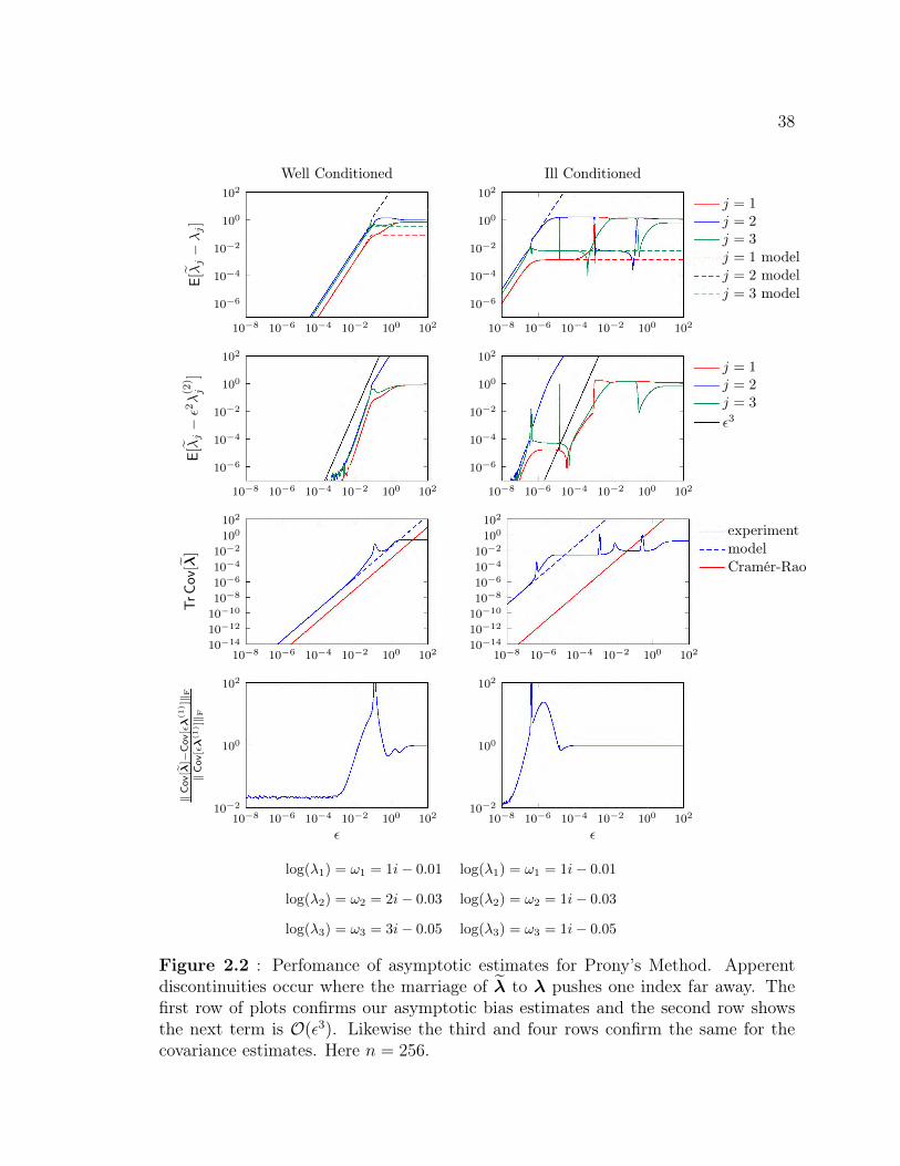
38

10−8 10−6 10−4 10−2 100 102

10−6

10−4

10−2

100

102E[λ

j−λj]

Well Conditioned

10−8 10−6 10−4 10−2 100 102

10−6

10−4

10−2

100

102

Ill Conditioned

j = 1j = 2j = 3j = 1 modelj = 2 modelj = 3 model

10−8 10−6 10−4 10−2 100 102

10−6

10−4

10−2

100

102

E[λ

j−ε2λ(2

)j

]

10−8 10−6 10−4 10−2 100 102

10−6

10−4

10−2

100

102

j = 1j = 2j = 3

ε3

10−8 10−6 10−4 10−2 100 10210−14

10−12

10−10

10−8

10−6

10−4

10−2

100102

TrCov[λ]

10−8 10−6 10−4 10−2 100 10210−14

10−12

10−10

10−8

10−6

10−4

10−2

100102

experimentmodelCramér-Rao

10−8 10−6 10−4 10−2 100 10210−2

100

102

ε

‖Cov[λ]−

Cov[ελ

(1)]‖

F

‖Cov[ελ

(1)]‖

F

10−8 10−6 10−4 10−2 100 10210−2

100

102

ε

log(λ1) = ω1 = 1i− 0.01 log(λ1) = ω1 = 1i− 0.01

log(λ2) = ω2 = 2i− 0.03 log(λ2) = ω2 = 1i− 0.03

log(λ3) = ω3 = 3i− 0.05 log(λ3) = ω3 = 1i− 0.05

Figure 2.2 : Perfomance of asymptotic estimates for Prony’s Method. Apperentdiscontinuities occur where the marriage of λ to λ pushes one index far away. Thefirst row of plots confirms our asymptotic bias estimates and the second row showsthe next term is O(ε3). Likewise the third and four rows confirm the same for thecovariance estimates. Here n = 256.

39

to provide a maximum likelihood estimate of α. Suppose instead of solving (2.8) in

the `2-norm, we do so in the yet unspecified Γ-norm

minα‖Hα+ h‖2Γ = min

α‖Γ−1/2(Hα+ h)‖22.

Expanding the error following (2.22),

Γ−1/2(Hα+ h) = Γ−1/2(Hα+ h) + εΓ−1/2T(α)g.

If α is a maximum likelihood estimate, then the residual Γ−1/2T(α)g should be

normally distributed with zero mean and unit covariance I; i.e.,

I = Cov[Γ−1/2T(α)g] = Γ−1/2T(α)ΣT(α)∗Γ−1/2. (2.31)

This constraint is satisfied if we choose

Γ(α) := T(α)ΣT(α)∗. (2.32)

Thus, the maximum likelihood estimate α of α is

α = argminα‖Hα+ h‖2Γ(α) = argmin

α‖Γ(α)−1/2(Hα+ h)‖22. (2.33)

Since α is a maximum likelihood estimate, then λ is also a maximum likelihood

estimate by the Principle of Invariance [167]. There are two approaches to solve (2.33):

either using a gradient decent method or a fixed point iteration where, given αk, the

next iterate is

αk+1 = −(Γ(αk)−1/2H)+(Γ(αk)

−1/2h). (2.34)

We call this second approach the Maximum Likelihood Prony Method, given in Algo-

rithm 2.7.

The Maximum Likelihood Prony Method is a protype for reformulations of Prony’s

Method yielding maximum likelihood estimates of α. Similar approaches were devel-

oped independently three times: by Householder in 1949 [69], Osborne in 1975 [116],

40

Algorithm 2.7: Maximum Likelihood Prony MethodInput : Measurements y0, y1, . . . , yn−1 ∈ C, model order p, covariance Σ, and

convergence tolerance τOutput: Exponential parameters λ0, λ1, . . . , λp−1.

1 Form H ∈ C(n−p)×p with [H]j,k = yj+k and h ∈ Cn−p with [h]j = yj+p;2 Compute α = −H+h;3 Compute the Cholesky decomposition LL∗ ← Σ;4 while ‖α′ −α‖ > τ do5 α′ ← α;6 Compute the R in the QR-decomposition QR← L∗T(α)∗;7 α← −(R−∗H)−1(R−∗h);

8 Find roots λk of q(t) = tp + αp−1tp−1 + αp−2t

p−2 + · · ·+ α1t+ α0.

and Bresler and Macovski in 1986 [23]. Householder’s derivation yields an iteration

similar to (2.34) using the normal equations; Osborne’s solves the equivalent of (2.33)

in the Nullspace Method setting using gradient decent yielding a nonlinear eigenvalue

problem iteration; Bresler and Marcovski’s Iterative Quadratic Maximum Likelihood

also solves the equivalent of (2.33) in the Nullspace Method setting, but uses a fixed

point iteration similar to (2.34). Despite these three independent discoveries, these

corrections to Prony’s Method never supplanted methods that work in the wrong

norm.

In this section, we derive both Householder’s Method and Osborne’s Method

(Bresler and Macovski’s Method is a special case). These methods are subject to

the same instability problems as other variants of Prony’s Method as they still com-

pute the roots of q; Figure 2.3 provides an example of this behavior. When noise

is small, each method obtains Cramér-Rao lower bound the covariance of λ, but

when noise grows, these methods suddenly loose accuracy at a critical point when the

perturbations are sufficient to prevent convergence.

l

41

0 5 10 15 20 25 30 35 40

10−16

10−14

10−12

10−10

10−8

10−6

10−4

10−2

100

102

p

‖λ−λ‖ 2

Osborne’s MethodHouseholder’s MethodHouseholder’s Method ImprovedBMBM Improved

Figure 2.3 : An illustration of the sensitivity of Maximum Likelihood Prony Methodsto round off errors. This uses the same parameters as in Figure 2.1.

2.4.1 Householder’s Method

The basic approach of Householder’s Method [69] is to minimize the mismatch be-

tween measurements y and the model y(α) subject to an equality constraint forcing

the residual r(α) = y − y(α) to satisfy the autoregressive model (2.1) exactly. The

equality constraint is enforced by requiring T(α)r(α) = 0; hence we wish to solve

minα‖r(α)‖2Σ such that T(α)r(α) = 0. (2.35)

To solve (2.35), we introduce Lagrange multipliers ` ∈ Cn−p and solve the augmented

problem

minα,`‖r(α)‖2Σ + `∗T(α)r(α). (2.36)

Definite φ(α, `) as the quantity minimized above. Although we can directly solve (2.36),

Householder uses several clever properties to yield a fixed point iteration for α di-

rectly.

At the minima, the derivative of φ with the respect to the residual should be zero,

t,, DD +

~ D - +

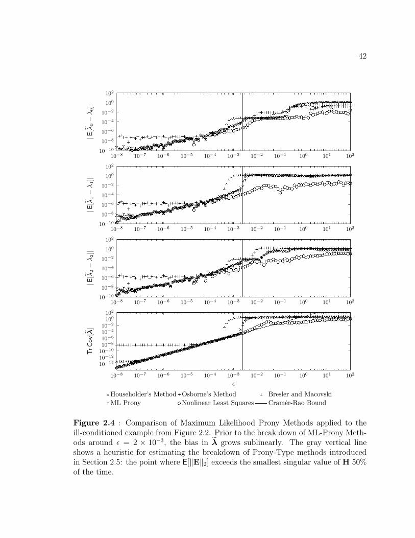
42

10−8 10−7 10−6 10−5 10−4 10−3 10−2 10−1 100 101 10210−10

10−8

10−6

10−4

10−2

100

102|E

[λ0−λ0]|

10−8 10−7 10−6 10−5 10−4 10−3 10−2 10−1 100 101 10210−10

10−8

10−6

10−4

10−2

100

102

|E[λ

1−λ1]|

10−8 10−7 10−6 10−5 10−4 10−3 10−2 10−1 100 101 10210−10

10−8

10−6

10−4

10−2

100

102

|E[λ

2−λ2]|

10−8 10−7 10−6 10−5 10−4 10−3 10−2 10−1 100 101 102

10−1410−1210−1010−810−610−410−2100102

ε

TrCov[λ]

Householder’s Method Osborne’s Method Bresler and MacovskiML Prony Nonlinear Least Squares Cramér-Rao Bound

Figure 2.4 : Comparison of Maximum Likelihood Prony Methods applied to theill-conditioned example from Figure 2.2. Prior to the break down of ML-Prony Meth-ods around ε = 2 × 10−3, the bias in λ grows sublinearly. The gray vertical lineshows a heuristic for estimating the breakdown of Prony-Type methods introducedin Section 2.5: the point where E[‖E‖2] exceeds the smallest singular value of H 50%of the time.

X

y

+ 0

p::tts:oo oCO:xi~ 0

43

hence4,

0 =∂φ

∂r(α, `) = r∗Σ−1 + `∗T(α). (2.37)

This corresponds to [69, eq. (16a)]. Next we consider a perturbation expansion of

T(α)y(α) about α

T(α)y(α) =T(α)y(α) +T(α) (y(α)− y(α))

+

p−1∑j=0

T(ej)y(α)(αj − αj) +O(‖αj −αj‖22)(2.38)

where T(ej) ∈ C(n−p)×n is zero except for ones along the jth super diagonal. We

simplify this expression noting the sum gives H(α)(α−α), where H(α) is the Hankel

matrix constructed from y(α) instead of y. Further, T(α)y(α) = 0 since y(α)

satisfies the equality constraints exactly. To enforce the equality constraint, we seek α

such that T(α)y = T(α)y(α). Combining this with the above equation and making

the assumption that the next step provides the exact solution (i.e., y = y(α(1))) so

r(α) = y(α(1))− y(α(0)), then

T(α)y = T(α)r(α) +H(α)(α−α). (2.39)

This equation corresponds to [69, eq. (16b)]. Using (2.37), we note r = ΣT(α)∗` and

hence

T(α)y = T(α)ΣT(α)∗`+H(α)(α−α).

Rearranging and inverting gives the Lagrange multipliers

` = Γ(α)−1 [T(α)y −H(α)(α−α)] (2.40)

where Γ(α) = T(α)ΣT(α)∗. The Lagrange multipliers must satisfy the first order

necessary conditions,

0 =∂φ

∂α=∂φ

∂r

∂r

∂α= (r∗Σ−1 + `∗T(α))

∂r

∂α.

4See the [137, App. A2.2] for information on complex derivatives.

44

In the limit of a small residual, the first term vanishes and we can compute the second

term implicitly from (2.38),

T(α)∂φ

∂α= `∗

p−1∑j=0

T(ej)y(α) = `∗H(α). (2.41)

Thus we set `∗H(α) = 0 and combining with (2.40) yields

0 = H(α)∗` = H(α)∗Γ(α)−1 [T(α)y −H(α)(α−α)] . (2.42)

Then, making the approximation H(α)→ H and T(α)→ T(α), yields a fixed point

iteration updating α→ α:

α = α+ (H∗Γ(α)−1H)−1H

∗Γ(α)−1T(α)y. (2.43)

Algorithm 2.8: Householder’s MethodInput : Measurements y0, y1, . . . , y2p−1 ∈ C, model order p, noise covariance

Σ, and covergence tolerance τ .Output: Exponential parameters λ0, λ1, . . . , λp−1.

1 Form H ∈ C(n−p)×p with [H]j,k = yj+k and h ∈ Cn−p with [h]j = yj+p;2 Compute α = −H−1h;3 while ‖α(1)‖ > τ do4 Form Γ(α) = T(α)ΣT(α)∗;5 Solve H

∗Γ(α)−1Hα(1) = H

∗Γ(α)−1y for α(1);

6 α← α+α(1);

7 Find roots λk of q(t) = tp + αp−1tp−1 + αp−2t

p−2 + · · ·+ α1t+ α0.

Householder used Prony Least Squares to provide the initial estimate of α for

his algorithm, given in Algorithm 2.8. Although this fixed point iteration converges

rapidly and yields maximum likelihood estimates of α for moderate amounts of noise,

this method went unnoticed except for a few authors, including Osborne [116, 117]

who failed to notice the connections between his method and Householder’s Method.

45

2.4.2 Osborne’s Method

Osborne’s Method similarly fixes the norm in (2.8), but unlike Householder’s Method,

begins from the Nullspace Method rather than Prony Least Squares. Recall the

Nullspace Method solves

minα∈Cp+1

‖α‖2=1

‖Hα‖2 (2.44)

where H are noisy measurements H = [H, h]. Separating noise g, following (2.22),

Hα = Hα+ εT(α)g (2.45)

where T(α) is a modification of T(α) from (2.21),

T(α) :=

α0 α1 · · · αp−1 αp

α0 α1 · · · αp−1 αp

. . . . . . . . . . . .

α0 α1 · · · αp−1 αp

. (2.46)

This implies that the error εT(α)g is normally distributed with zero mean and co-

variance Γ(α) = T(α)ΣT(α)∗ (c.f., Section 2.3 for Prony Least Squares). To minize

errors with covariance Γ(α), we work in the Γ(α) norm minimizing,

‖Hα‖Γ(α) = ‖Γ(α)−1/2Hα‖2 = ‖Γ(α)−1/2Hα+ Γ(α)−1/2T(α)g‖2. (2.47)

Hence, we now wish to solve minα φ(α) where

φ(α) := α∗ H∗Γ(α)−1H α = ‖H α‖2

Γ(α). (2.48)

This is a nonlinear eigenvalue problem for the smallest eigenvector of H∗Γ(α)−1H.

A simple iteration to solve (2.48) was suggested by Bresler and Macovski [23]: given

αk find the next iterate αk+1 as the eigenvector of smallest eigenvalue of

µαk+1 = H∗Γ(αk)

−1Hαk+1. (2.49)

46

Bresler and Macovski call this the Iterative Quadratic Maximum Likelihood method;

see Algorithm 2.9. Experience shows this iteration converges rapidly.

Osborne proposed an alternative to this iteration that instead chooses αk+1 using

gradient descent. This implies finding a stationary point of φ where ∂φ/∂α = 0.

Invoking Wirtinger Calculus,

∂φ

∂α(α) = α∗H

∗Γ(α)−1H+

p∑k=0

(α∗H

∗Γ(α)−1∂Γ(α)

∂αk

Γ(α)−1Hα

)e∗k and,

∂Γ(α)

∂αk

=∂

∂αk

T(α)ΣT(α)∗ = T(ek)ΣT(α)∗.

To simplify these expressions, we define

z(α) := Γ(α)−1Hα and Z(α) :=

p∑k=0

T(ek)∗v(α)e∗k. (2.50)

Then we write the second term asp∑

k=0

z(α)∗T(ek)ΣT(α)∗z(α)e∗k =

p∑k=0

z(α)>T(α)Σ>T(ek)>z(α)e∗k

= z(α)>T(α)Σ>Z(α).

We extract an α on the left, noting:(z(α)>T(α)

)∗= T(α)>z(α) =

p∑k=0

T(ek)>z(α)αk

=

p∑k=0

T(ek)>z(α)ekα = Z(α)α.

Hence,

∂φ

∂α(α) = α∗H

∗Γ(α)−1H+α∗Z(α)∗Σ>Z(α).

Imposing the constraint that ‖α‖ = 1, adds the Lagrangian multiplier −α∗ leading

to the nonlinear eigenvalue problem (after taking the complex conjugate)[H

∗Γ(αk)

−1H+ Z(αk)∗ΣZ(αk)− µI

]αk+1 = 0. (2.51)

47

Algorithm 2.9: Bresler and MacovskiInput : Measurements y0, y1, . . . , y2p−1 ∈ C, model order p, noise covariance

Σ.Output: Exponential parameters λ0, λ1, . . . , λp−1.

1 Form H ∈ C(n−p)×(p+1) with [H]j,k = yj+k;2 Compute SVD of H = UΣV∗ where [Σ]j,j = σj and σj ≥ σk for all j > k ;3 Set α = [V]·,p+1 ∈ Cp+1;4 repeat5 A← H∗Γ(α)−1H ;6 Compute the smallest eigenvector of A, v;7 α← v;8 until convergence;

Algorithm 2.10: Osborne’s MethodInput : Measurements y0, y1, . . . , yn−1 ∈ C, model order p, and convergence

tolerance τ ; optionally λ

Output: Exponential parameters λ0, λ1, . . . , λp−1.1 Form H ∈ Cn−p×p+1 with [H]j,k = yj+k;2 if λ provided then3

∑pk=0 αkt

k =∏p−1

j=0(t− λj);4 else5 Set α = [0 0 0 . . . 0 1]> ;

6 i← 0;7 while µ > τ‖A‖ and i less than some maximum number of iterations do8 LL∗ ← T(α)ΣT(α)∗ Cholesky decomposition;9 K← L−1H ;

10 A← K∗K;11 if i > 0 or inital estimates of λ provided then12 z← L−∗(Kα) ;13 Form Z according to (2.50);14 A← A+V∗ΣV;

15 Find smallest eigenvalue of A, µ: Aα = µα;16 i← i+ 1;

17 Find roots λk of q(t) = αptp + αp−1t

p−1 + αp−2tp−2 + . . .+ α1t+ α0.

I

L -

48

This is a similar eigenvalue problem to (2.49), with a correction to include the variable

norm that vanishes near the minima. Successive iterations solving (2.51) as described

in Algorithm 2.10 tend to converge rapidly (see [116, §5]). However, the addition of

the variable norm term does not improve the resulting estimates of α when ε is small

as Figure 2.4 suggests. Rather, this addition increases sensitivity to rounding errors,

preventing estimates of α from converging to the same accuracy as methods without

this correction (e.g., Householder’s Method, Maximum Likelihood Prony).

2.5 Extraneous Exponentials

One approach to fix numerical ill-conditioning of Prony’s Method is to include an

additional p′ extraneous exponentials to improve the recovery of the p exponentials

present in the data. Simon was the first to note this in 1970 [139, §3], recommending

including an extra p′ = p exponentials. However, Simon’s observation went unnoticed

until reintroduced independently by Kumaresan and Tufts in the electrical engineer-

ing literature in 1982 [92], generalized to include an arbitrary number of extraneous

exponentials. Although Kumaresan and Tufts hint at why adding extraneous expo-

nentials improves the recovery of the non-extraneous exponentials, Rao (1988) [129,

§III] was the first to provide a rigorous explanation: the recovered roots λ are sensitive

to perturbations in α (2.7),

λj = λj − ε∑p−1

k=0 α(1)k λkj∏

j 6=k(λj − λk)+O(ε2). (2.52)

The extraneous exponentials tend to be uniformly distributed inside the unit circle

(see, e.g., [91, 19]) and hence increase the denominator, making λ more robust to

perturbations. In this section we review these results, adding new insight that suggests

the extraneous roots are placed near the roots of unity. We also demonstrate methods

49

like Kung’s Method [94], the Matrix Pencil Method [72], and the Hankel Total Least

Squares Method [75] benefit by implicitly including these extraneous exponentials but

compute only the non-spurious roots.

A prototype for these algorithms that include extraneous exponentials begins with

Prony Least Squares for p+ p′ exponentials:

Hα = −h, H ∈ Cm×(p+p′), α ∈ Cp+p′ , h ∈ Cm. (2.53)

In the absence of noise H has rank p, and as h is in the range of H (see (2.16)), there

is a p′ dimensional subspace defining solutions for α. One solution can be found by

partitioning H into two blocks: H0 ∈ Cm×p′ and Hp′ ∈ Cm×p,

[H0 Hp′

] 0

αp′

= −h, (2.54)

where αp′ are coefficients of q from Prony Least Squares using only p exponentials.

The remaining solutions add a vector from the nullspace of H; if H has the SVD

H =

[Up Up′

]Σp 0

0 0

V∗

p

V∗p′

, (2.55)

then solution set for α is

α(x) =

0

αp′

+V∗p′x, x ∈ Cp′ . (2.56)

Figure 2.5 shows one dimension of this solution space. Finally, this method chooses

α(x) with the smallest norm and computes the roots of the degree p+ p′ polynomial

q separating spurious roots from non-spurious roots using a heuristic.

Using minimum norm solution of α ∈ Cp+p′ has two advantages. One benefit

is the minimum norm solution corresponds to the pseudoinverse of H; i.e., in the

50

−1 −0.5 0.5 1

−1

−0.5

0.5

1

−1 −0.5 0.5 1

−1

−0.5

0.5

1

0

0.5

1

1.5

2

γ

Figure 2.5 : Two examples of extraneous roots along a one dimensional subspace.The least squares solution for α gives roots marked by ‘×’. Thei colored curves showthe roots resulting from α(γx) (2.54) for γ ∈ [0, 2] and with x chosen such that α(x)is the least squares solution.

presence of noise

α = VpΣ−1

p U∗ph. (2.57)

The left and right singular vectors of H are relatively stable to small perturbations

εE = H−H. We can bound the diagonal matrix canonical angles Φ ∈ Cp×p between

RanUp and RanUp and the canonical angles Θ ∈ Cp×p between RanVp and RanVp

using a combination of Wedin’s Theorem [143, Thm. V.4.1] and Weyl’s Theorem,

‖ sinΦ‖2F + ‖ sinΘ‖2F ≤2ε2‖E‖2Fσp − ε‖E‖2

. (2.58)

Using Corollary 3.1 we can estimate the expected value of this bound

E

[2‖E‖2F

σp − ‖E‖2

].

2ε2(n− p− p′)(p+ p′)

σp − ε√−2n log(1− n

√r)

with probability r. (2.59)

Provided ε is small, the left and right singular subspaces remain relatively unper-

turbed, and hence in the presence of noise, the rank-p pseudoinverse acts to remove

perturbations of h that are not in the range of H.

X

X

51

The other benefit of the minimum norm choice of α is that it tends to place

spurious roots near a complex rotation of p+p′ roots of unity and this acts to decrease

the sensitivity of λ to perturbations of α. Previous authors have demonstrated that

these roots must fall inside the unit circle, e.g., [91] from a filter perspective and [19,

Prop. 2.6] from a linear algebra perspective, and in the limit p′ → ∞ the spurious

roots tend to be uniformly distributed inside the unit circle [119]. We suggest a

new intuitive explanation why the spurious roots are placed near the roots of unity

(evident in Figure 2.5 and [92, Fig. 1(h)]). If q be the degree p+p′ polynomial defined

by α, then we can express α as the solution to the linear system

1 t0 t20 · · · tp+p′

0

1 t1 t21 · · · tp+p′

1

......

......

1 tp+p′ t2p+p′ · · · tp+p′

p+p′

α0

α1

...

αp+p′

=

q(t0)

q(t1)

...

q(tp+p′)

(2.60)

where αp+p′ = 1. By choosing tj = eiθe2πij/(p+p′+1) (rotated p+ p′ + 1 roots of unity),

the Vandermonde matrix on the left is a multiple of the discrete Fourier transform

matrix Fp+p′+1. As Fp+p′+1 is unitary, then inverting Fp+p′+1 gives

1 + ‖α‖2 =√p+ p′ + 1

∥∥∥∥∥∥∥∥∥∥∥∥∥e−iθF∗

p+p′+1

q(t0)

q(t1)

...

q(tp+p′)

∥∥∥∥∥∥∥∥∥∥∥∥∥2

=√p+ p′ + 1

∥∥∥∥∥∥∥∥∥∥∥∥∥

q(t0)

q(t1)

...

q(tp+p′)

∥∥∥∥∥∥∥∥∥∥∥∥∥2

.

(2.61)

Hence minimizing α minimizes the values of q at the rotated p + p′ + 1 roots of

unity. In practice, spurious roots tend to align at the p′ points furthest away from the

non-spurious roots as seen on the right side of Figure 2.5. The rotation eiθ provides

an additional degree of freedom that further explains the placement seen.

52

One remaining question is how many extraneous exponentials to include? Most

authors suggest setting p + p′ = bn/2c in an attempt to maximize the smallest sin-

gular value of H, however Hua and Sarkar, recommend p + p′ = bn/3c based on a

perturbation analysis of the p = 1 case [72]. We can extend Hua and Sarkar’s analysis

to the multiple exponential case by using the perturbation analysis from Section 2.3

where H has been replaced with its rank-p approximation. Figure 2.6 shows the

bias and covariance of the desired exponentials as a function of the number of extra-

neous exponentials p′. This confirms Hua and Sarkar’s observation that the choice

p+ p′ = bn/3c yields minimum covariance estimates for this class of algorithms.

Finally, before reviewing methods that use extraneous exponentials, we note that

Rao suggested that ‖‖2 < σp is a sufficient condition for SVD-methods to succeed [129,

p. 1031]. This follows from the singular vector perturbation estimate (2.59) and seems

to accurately predict where these methods fail in Figure 2.8 (using p+ p′ = bn/2c).

2.5.1 Kumaresan and Tufts Method

The Kumaresan and Tufts Method [92] follows the outline of the method above except

that they reverse the order of y. Then, instead of seeing exponential decay, we see

exponential growth. Since the extraneous exponentials are inside the unit circle and

correspond to exponential decay, this provides a criteria for separating spurious and

non-spurious exponentials. This method is numerically stable (Figure 2.7), and yields

reasonable estimates of λ (Figure 2.8) however the covariance of these estimates is

larger than the Cramér-Rao bound, corresponding to an efficiency of about 70% for

this ill-conditioned example (Figure 2.9).

53

Bias Covariance

ε=

10−8

0 100 200

10−14

10−12

10−10

10−8

10−6

10−4

n3

n2

E‖λ

−λ‖ 2

0 100 20010−16

10−14

10−12

10−10

10−8

n3

n2

TrCov

λ

ε=

10−4

0 100 20010−6

10−4

10−2

100

n3

n2

p′

E‖λ

−λ‖ 2

0 100 20010−8

10−6

10−4

10−2

100

n3

n2

p′

TrCov

λ

Figure 2.6 : Using the ill-conditioned example from Figure 2.2 with different num-bers of extraneous exponentials, we see that the bias and covariance obey the esti-mates from Section 2.3. The asymptotic estimates of the bias from (2.29) (gray line)matches the bias estimated using a Monte-Carlo approach (black dots). Similarly, theasymptotic covariance (2.27) (gray line) matches the Monte-Carlo covariance (blackdots); however, the covariance exceeds the Cramér-Rao bound (black line).

54

0 5 10 15 20 25 30 35 4010−16

10−14

10−12

10−10

10−8

10−6

10−4

10−2

100

102

p

‖λ−

λ‖ 2 Kung’s Method

HTLSML Prony extraProny Least Squares

Figure 2.7 : An illustration of the sensity of several Prony-type methods that includeextraneous exponentials to round off errors. This uses the same parameters as inFigure 2.1. “ML Prony extra” refers to the Maximum Likelihood Prony Methodusing extraneous exponentials to improve stability.

2.5.2 Matrix Pencil Method

The Matrix Pencil Method of Hua and Sarkar [72] follows the matrix pencil variant

of Prony’s Method in Section 2.2.3, however it enlarges the matrices H0 and H1 to

be in C(n−`)×` rather than C(n−p)×p. Rather than directly computing the generalized

eigenvalues, this method uses a rank-truncated pseudoinverse to construct a matrix

with a related spectrum, C. Starting with the rank-p SVD H0 = UpΣpV∗p, this

method forms C as

H0C = H1

C := Σ+

p U∗pH1Vp ∈ Cp×p.

This formulation fixes one of the hardest parts of the Kumaresan and Tufts Method:

determining which roots (or in this case eigenvalues) are significant. By using a

rank-p pseudoinverse, C has only p eigenvalues that we assume correspond to the

non-spurious exponentials.

+ +

+ +

+ +

+ + +

+ + + +

+ + +

+ + + + + + + + + + + + + + + + + + + + _

0

D

+

- ~ ; ~ ~ ~ ~ ~ ~ ~ ~ ~ fi.l ~ ~ ~ ~ 9 ~ ~ ~ lil ~ g ~ ~ ~ ~ ~ ~ g ~ ~ g g ~ ~ ~ ~ el I~ ' ' '

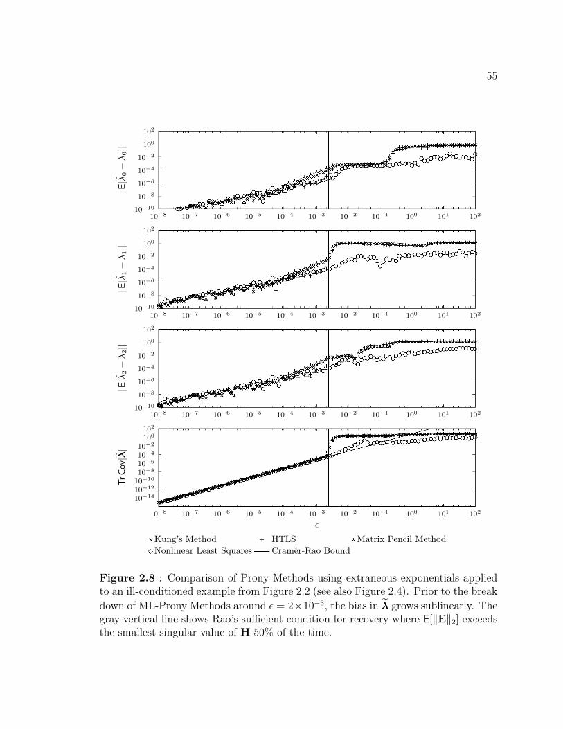
55

10−8 10−7 10−6 10−5 10−4 10−3 10−2 10−1 100 101 10210−10

10−8

10−6

10−4

10−2

100

102|E

[λ0−λ0]|

10−8 10−7 10−6 10−5 10−4 10−3 10−2 10−1 100 101 10210−10

10−8

10−6

10−4

10−2

100

102

|E[λ

1−λ1]|

10−8 10−7 10−6 10−5 10−4 10−3 10−2 10−1 100 101 10210−10

10−8

10−6

10−4

10−2

100

102

|E[λ

2−λ2]|

10−8 10−7 10−6 10−5 10−4 10−3 10−2 10−1 100 101 102

10−1410−1210−1010−810−610−410−2100102

ε

TrCov[λ]

Kung’s Method HTLS Matrix Pencil MethodNonlinear Least Squares Cramér-Rao Bound

Figure 2.8 : Comparison of Prony Methods using extraneous exponentials appliedto an ill-conditioned example from Figure 2.2 (see also Figure 2.4). Prior to the breakdown of ML-Prony Methods around ε = 2×10−3, the bias in λ grows sublinearly. Thegray vertical line shows Rao’s sufficient condition for recovery where E[‖E‖2] exceedsthe smallest singular value of H 50% of the time.

X + 0

56

10−8 10−7 10−6 10−5 10−4 10−3 10−20%

20%

40%

60%

80%

100%

ε

Effi

cien

cy

Kung’s Method HTLSMatrix Pencil Method Nonlinear Least Squares

Figure 2.9 : Statistical efficiency of variants of Prony’s Method that include extra-neous exponentials. This figure uses the same data as Figure 2.8.

In comparison to other methods in this class, the Matrix Pencil Method yields

worse estimates of λ; see Figures 2.8 and 2.9.

2.5.3 Kung’s Method

In the Matrix Pencil Method, the SVD is only applied to one of the matrices, not both.

Kung’s Method [94] (also known as HSVD [12]), developed prior to the Matrix Pencil

Method, corrects this and further removes noise, by estimating C using only the left

singular values of H ∈ C(n+1−`)×`. Combining the Vandermonde decomposition of a

Hankel Matrix (2.16) with the matrix pencil formulation of Prony’s Method, we have

Vn−`(λ)AV`(λ)>C = Vn−`(λ)AΛV`(λ)

>. (2.62)

By assumption both A and Λ are full rank, and since λ has distinct entries, V`(λ)>

also has full rank. As such, both are invertible, and instead of finding the eigenvalues

of C, we can find the eigenvalues of the similar matrix D, where

Vn−`(λ)D = Vn−`(λ)Λ. (2.63)

i*************************************************++ AJ..J..J..AJ...J..J...J..J..AJ..J..J..AJ...J..J..J..J..J..J..J..J..J..J...J..J..J..J..AJ..J...J...J..J..J...J..J..J..J..J..J...J...J...J..J.. ~x+ - J..J... A x+

;_ X ;_

;_

0

0

0 -

O_ 'h

I _,,.,_.., -•--• 1 -•- 1

X

;_

+ 0

57

Rather than finding Vn−`(λ) and Vn−`(λ)Λ, Kung’s Method estimates similar matri-

ces using the left singular vectors of H ∈ C(n+1−`)×`. If Up are the first p left singular

vectors of H, then

Vn−`(λ) ≈ U↑pR

Vn−`(λ)Λ ≈ U↓pR,

where ↑ denotes removing the bottom row of a matrix and ↓ the top row. This saves

us from having to compute two SVDs: one of H0 and H1. As a result of the additional

filtering and since both U↑p and U

↓p are well conditioned (nearly unitary), the estimate

D = (U↑p)

+U↓p (2.64)

approximates D in a numerically stable fashion. This procedure can be computation-

ally simplified by using the Sherman-Morrison formula to compute the pseudoinverse

of U↑p. Noting U

↑p only subtracts the last row of Up, u∗, we have

(U↑p)

∗U↑p = (Up − en+1−`u

∗)∗(Up − en+1−`u∗) = U

∗pUp − uu∗ = I− uu∗. (2.65)

Hence,

D =

(I+

uu∗

1− u∗u

)(U

↑p)

∗U↓p. (2.66)

The steps in this method are summarized in Algorithm 2.11.

2.5.4 Hankel Total Least Squares

A further modification of Kung’s Method is to construct D using the total least

squares solution [56, §12.3]of (2.64) instead of the least squares solution. This accounts

for both errors in the left and right hand side of (2.64), but does so in the wrong norm.

The performance of this method is similar to Kung’s Method, but yields less biased

58

and more efficient estimates of λ in a narrow range from ε = 10−4 to ε = 2 · 10−3 in

Figures 2.8 and 2.9.

2.5.5 Prony Maximum Likelihood with Extraneous Exponentials

In Section 2.4, we saw that every Prony-type method that yields maximum likelihood

estimates of λ is numerically unstable (Figure 2.3). Including spurious exponentials

and using a rank-p pseudoinverse instead of H+

can make these methods numerically

stable as we illustrate with one variant in Figure 2.7.

2.6 Autocovariance-Based Prony Variants

In this section, we discuss two variants of Prony’s Method that use autocorrelation

measurements rather than y. These two variants parallel Prony’s Method and the

Nullspace Method; generalizations of these approaches that include extraneous expo-

nentials exist, such as MUSIC [10] and ESPRIT [134].

2.6.1 Yule-Walker Method

The Yule-Walker Method is Prony’s Method where the determination of the autore-

gressive model by (2.2) has been replaced with the Yule-Walker equations [144, §4.4].

Unlike Prony’s Method, the Yule-Walker Method can be biased even in the absence

of noise.

The Yule-Walker equations determine the lag coefficients α using measurements

of the autocorrelation of y

ck = E [yj+kyj] . (2.67)

This assumes that yjn−1j=0 is a stationary sequence (i.e., independent of k). Under

-

59

these assumptions, the Yule-Walker equations for the lag coefficents α solve

cq−p+1 cq−p+2 · · · cq

cq−p+2 cq−p+3 · · · cq−p+2

...... . . . ...

cq cq+1 · · · cq+p−1

α0

α1

...

αp−1

= −

cq+1

cq+2

...

cq+p

; (2.68)

see, e.g., [104, § 6.5].5 Calling the matrix on the left Cq ∈ Cp×p and the vector on

the right cq, we have a system that resembles (2.2):

Cqα = cq. (2.69)

We could immediately solve for α using (2.69); however, in the presence of noise,

we must make a special choice of q. Let yj be noisy measurements of yj obeying the

autoregressive model

yk =

p∑j=1

−αp−j yk−j + σgk, k ≥ p, (2.70)

where gk is an independent standard complex Gaussian random variable.6 Then the

corresponding autocorrelation obeys cj = cj + δ0,jσ2. So, if we solved for α using

q = 0, then the answer would be spurious:

C0α = (C0 + σ2J)α = c0 = c0, (2.71)

where J is the flipped identity matrix. Instead we choose q = p so that c0 does not

appear in Cq or cq; hence Cp = Cp.

5The method was originally presented in [166, 156].6Everywhere else in this thesis, yj refers to additive Gaussian noise, yj = yj + gj .

60

If we have a single sequence of measurements y, we can estimate cq by one of two

approaches [144, § 2.2.2]:

a biased estimate: cj ≈1

n

n−j−1∑k=0

yk+jyj, or (2.72)

an unbiased estimate: cj ≈1

n− k

n−j−1∑k=0

yk+jyj. (2.73)

To recover α, we fill Cp with these estimates of autocorrelations cq and solve for α.

We can arrive at an approximation of Cp starting from a modified Hildebrand’s

Method, and this reveals why the Yule-Walker Method is biased. Hildebrand’s

Method applies no matter where in the sequence of yjn−1j=0 we start. Starting with

the pth entry, we solve

Hpα =

[hp hp+1 · · · h2p−1

]α = −h2p, (2.74)

where [Hp]j,k = yj+k+p and [h2p]j = yj+2p. Next, we multiply on the left by a matrix

by H0 with its columns flipped,

T∗0Hpα =

h∗p−1

h∗p−2

...

h∗0

[hp hp+1 · · · h2p−1

]α = −

h∗p−1

h∗p−2

...

h∗0

h2p

h∗p−1hp h∗

p−1hp+1 · · · h∗p−1h2p−1

h∗p−2hp h∗

p−2hp+1 · · · h∗p−1h2p−1

......

h∗0hp h∗

0hp+1 · · · h∗0h2p−1

α = −

h∗p−1h2p

h∗p−2h2p

...

h∗0h2p

.

Examining the entries of the matrix on the left, we notice that these approximate a

scalar multiple of the autocovariance:

h∗jhk =

n−2p−1∑`=0

yj+`yk+` ≈ nck−j. (2.75)

61

Thus, T∗0Hp is a scaled approximation of Cp. Since the solution of T∗

0Hpα = T∗0h2p is

identical to (2.74), we conclude that the Yule-Walker method is biased because nCp

only approximates T∗0Hp. In the limit n→∞, both estimates of the autocovariance

coverge to 1nh∗khk+j,

As solving Hildebrand’s Method directly does not have the bias present in the

Yule-Walker equations, we cannot advise using the Yule-Walker Method unless the

autocovariance measurements are directly given.

.

2.6.2 Pisarenko’s Method

Pisarenko’s Method [125] is the analog of the Nullspace Method using the autoco-

variance cj in place of yj. We can see this by noting the autocorrelation also obeys

the same autoregressive model:

yk+j =

p∑`=1

−αp−`yk+j−`

ck = E[yk+jyj] =

p∑`=1

−αp−` E[yk+j−`yj] =

p∑`=1

−αp−`ck−`.

Hence,

c−p c−p+1 · · · c−1 c0

c−p+1 c−p+2 · · · c0 c1...

......

...

c−1 c0 · · · cp−2 cp−1

c0 c1 · · · cp−1 cp

α0

α1

...

αp−1

1

=

0

0

...

0

0

. (2.76)

If we allow the scaling of the left vector to be free, we have

Cp+1α = 0. (2.77)

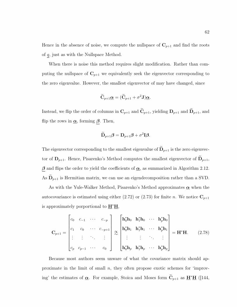
62

Hence in the absence of noise, we compute the nullspace of Cp+1 and find the roots

of q, just as with the Nullspace Method.

When there is noise this method requires slight modification. Rather than com-

puting the nullspace of Cp+1 we equivalently seek the eigenvector corresponding to

the zero eigenvalue. However, the smallest eigenvector of may have changed, since

Cp+1α = (Cp+1 + σ2J)α.

Instead, we flip the order of columns in Cp+1 and Cp+1, yielding Dp+1 and Dp+1, and

flip the rows in α, forming β. Then,

Dp+1β = Dp+1β + σ2Iβ.

The eigenvector corresponding to the smallest eigenvalue of Dp+1 is the zero eigenvec-

tor of Dp+1. Hence, Pisarenko’s Method computes the smallest eigenvector of Dp+1,

β and flips the order to yield the coefficients of α, as summarized in Algorithm 2.12.

As Dp+1 is Hermitian matrix, we can use an eigendecomposition rather than a SVD.

As with the Yule-Walker Method, Pisarenko’s Method approximates α when the

autocovariance is estimated using either (2.72) or (2.73) for finite n. We notice Cp+1

is approximately porportional to H∗H,

Cp+1 =

c0 c−1 · · · c−p

c1 c0 · · · c−p+1

...... . . . ...

cp cp−1 · · · c0

∝∼

h∗0h0 h∗

1h0 · · · h∗ph0

h∗0h1 h∗

1h1 · · · h∗ph1

...... . . . ...

h∗0hp h∗

1hp · · · h∗php

= H∗H. (2.78)

Because most authors seem unware of what the covariance matrix should ap-

proximate in the limit of small n, they often propose exotic schemes for ‘improv-

ing’ the estimates of α. For example, Stoica and Moses form Cp+1 as H∗H ([144,

63

0.2 0.3 0.4 0.5 0.6 0.70.5

0.6

0.7

0.8

0.9

1

Undamped

0.2 0.3 0.4 0.5 0.6 0.70.5

0.6

0.7

0.8

0.9

1

Damped

Unit circle Biased λ1 Biased λ2 Unbiased λ1 Unbiased λ2

Figure 2.10 : Bias in Pisarenko’s method for small n. In this example there are twoexponentials λ1 = e1i and λ2 = e1.1i on the left and λ1 = e1i−0.05 and λ2 = e1i−0.03

on the right (marked by +). In both cases a1 = 1 and a2 = eiθ. As θ swept through0 to 2π the recovered values of λ using Pisarenko’s method using both biased andunbiased covariance estimates generated the curves seen above. Here n = 10.

eqs. (4.5.14), (4.8.1)]), but then noting it does not have the Toeplitz structure ex-

pected, recommend averaging the diagonal entries to enforce this structure [144,

p. 159]. This can only make performance worse, because H∗H already provides exact

estimates of α in the absence of noise.

2.7 Compressed Prony’s Method

Compressed variants of Prony’s Method, such as the Method of Moments, com-

bine measurements y resulting in new pseudo-measurements z and use a Prony-type

method to then recover the exponential parameters λ. This has two advantages.

During the 1960s and 1970s, computing resources were limited; combining measure-

64

Algorithm 2.11: Kung’s MethodInput : Measurements y0, y1, . . . , yn−1 ∈ C, model order pOutput: Exponential parameters λ0, λ1, . . . , λp−1.

1 Form H ∈ C(n+1−`)×` with [H]j,k = yj+k;2 Compute the SVD: UΣV∗ ← H;

3 Form D← (U↑p)

+U↓p;

4 Compute the eigenvalues λ of D;

Algorithm 2.12: Pisarenko’s MethodInput : Measurements y0, y1, . . . , yn−1 ∈ C and model order p.Output: Exponential parameters λ0, λ1, . . . , λp−1.

1 Estimate covariances using either cj = 1n

∑n−j−1k=0 yk+jyj (biased) or

cj =1

n−k

∑n−j−1k=0 yk+jyj (unbiased) for j = −p, . . . , p;

2 Form C ∈ Cp+1×p+1 where [C]j,k = cj−k (c−k = ck);3 Compute eigendecomposition of C, CV = VΛ where [Λ]j,j = λj andλj ≥ λk∀j > k ;

4 Set α = [V]·,p+1 ∈ Cp+1;5 Find roots λk of q(t) = αpt

p + αp−1tp−1 + αp−2t

p−2 + . . .+ α1t+ α0.

101 102 103 10410−14

10−12

10−10

10−8

10−6

10−4

10−2

100

n

‖λ−λ‖ 2

Undamped

101 102 103 10410−14

10−12

10−10

10−8

10−6

10−4

10−2

100

n

‖λ−λ‖ 2

Damped

Biased Unbiased Nullspace Normal

Figure 2.11 : Error in Pisarenko’s method as a function of n using the undampedand damped parameters in Figure 2.10. Nullspace normal refers to taking C = H∗H.

65

ments was a promising alternative to solving a potentially large least squares problem.

Also, by combining measurements, the covariance of the pseudo-measurements zj is

reduced relative to yj and if errors in y are not normally distributed, the summation

of measurements tends to make errors normally distributed as a result of the Central

Limit Theorem.

A prototype of these methods begins with Prony Least Squares

α = argminα‖Hα+ h‖2 H ∈ Cm×p, h ∈ Cm (2.79)

and compresses these measurements by multiplying on the left by a full rank matrix

W ∈ Cm×p, yielding the compressed estimate

αW = argminα‖W∗Hα+W∗h‖2. (2.80)

Following (2.23), the first term in the perturbation expansion of α is

α(1)W = −(W∗H)+W∗T(α)g. (2.81)

One trivial choice picks W that spans the range of H with orthogonal columns;

this simply yields the least squares estimate for α. Another choice would take W to

be columns of the discrete Fourier matrix Fm corresponding to frequencies of interest;

Mandelshtam takes a similar approach in Filter Diagonalization [103]. Other, more

exotic choices of W are possible, such as Finite Impulse Response filters [29].

In the remainder of this section, we review existing compressed techniques and

discuss a new variation of the Maximum Likelihood Prony Method that uses com-

pression to reduce the cost of the norm correction step.

66

2.7.1 Cornell’s Method

Cornell’s Method [33] is a modification of Prony’s Method that partitions y into sums

of m = bn/(2p)c adjacent measurements, yielding p pseudo-measurements

zk =m−1∑j=0

yj+km 0 ≤ k < 2p. (2.82)

The method then continues with Prony’s Method, replacing y with z

z0 z1 z2 · · · zp−1

z1 z2 z3 · · · zp...

......

zp−1 zp zp+1 · · · z2p−2

α0

α1

...

αp−1

= −

zp

zp+1

...

z2p−1

, (2.83)

and recovers roots mλ of the polymial q.

2.7.2 Method of Moments

The Method of Moments was developed by Isenberg and Dyson in 1969 to study

fluoresce of biological compounds [77], and was expanded upon in 1973 [78] and

1983 [76]. This method uses the determinant formulation of Prony’s Method discussed

in Section 2.2.4 applied to scaled moments µk. The moments are defined with respect

to the continuous signal y(t),

µk :=

∫ ∞

0

tky(t) dt =∫ ∞

0

tkp−1∑j=0

ajλtj dt =

p−1∑j=0

ajk!

(log λj)k+1. (2.84)

Then the Method of Moments computes the scaled moments

gk :=µk

k!=

p−1∑j=0

ajτk (2.85)

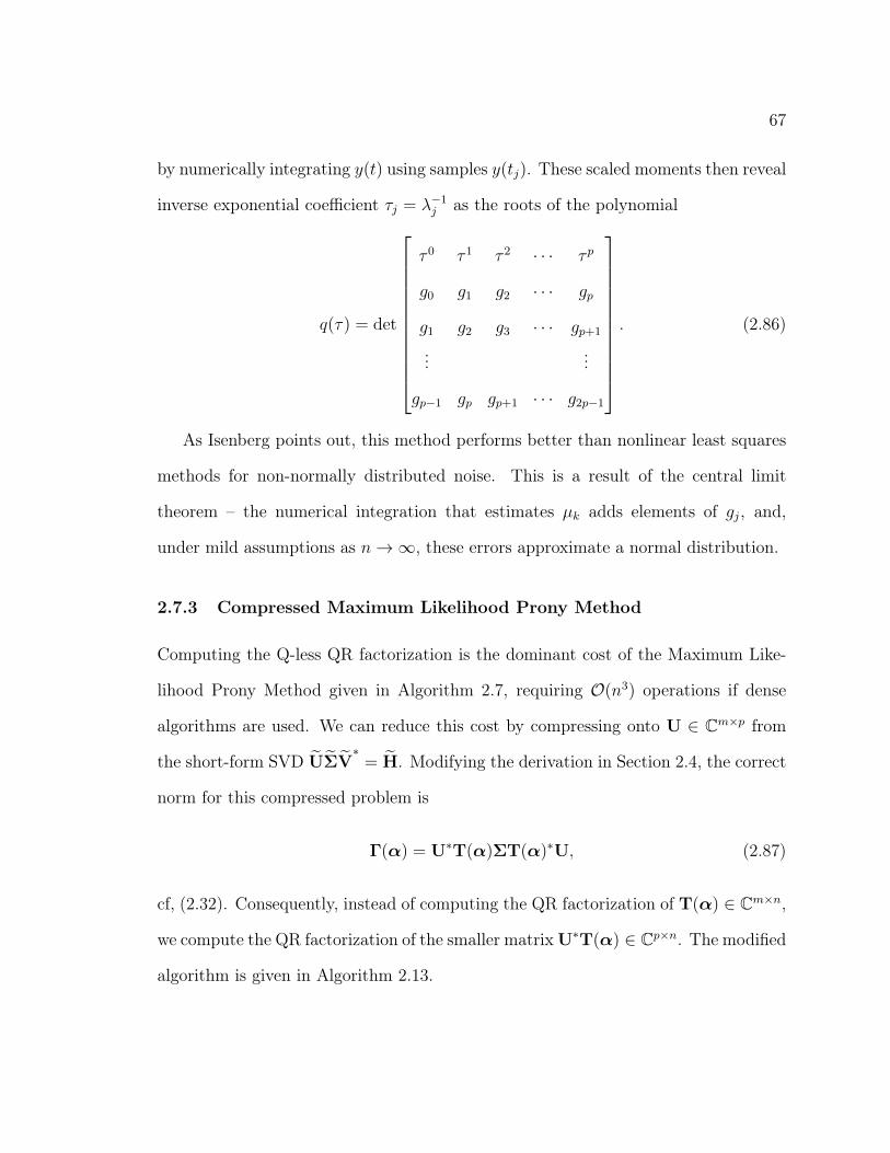
67

by numerically integrating y(t) using samples y(tj). These scaled moments then reveal

inverse exponential coefficient τj = λ−1j as the roots of the polynomial

q(τ) = det

τ 0 τ 1 τ 2 · · · τ p

g0 g1 g2 · · · gp

g1 g2 g3 · · · gp+1

......

gp−1 gp gp+1 · · · g2p−1

. (2.86)

As Isenberg points out, this method performs better than nonlinear least squares

methods for non-normally distributed noise. This is a result of the central limit

theorem – the numerical integration that estimates µk adds elements of gj, and,

under mild assumptions as n→∞, these errors approximate a normal distribution.

2.7.3 Compressed Maximum Likelihood Prony Method

Computing the Q-less QR factorization is the dominant cost of the Maximum Like-

lihood Prony Method given in Algorithm 2.7, requiring O(n3) operations if dense

algorithms are used. We can reduce this cost by compressing onto U ∈ Cm×p from

the short-form SVD UΣV∗= H. Modifying the derivation in Section 2.4, the correct

norm for this compressed problem is

Γ(α) = U∗T(α)ΣT(α)∗U, (2.87)

cf, (2.32). Consequently, instead of computing the QR factorization of T(α) ∈ Cm×n,

we compute the QR factorization of the smaller matrix U∗T(α) ∈ Cp×n. The modified

algorithm is given in Algorithm 2.13.

68

Algorithm 2.13: Compressed Maximum Likelihood Prony MethodInput : Measurements y0, y1, . . . , yn−1 ∈ C, model order p, covariance Σ, and

convergence tolerance τOutput: Exponential parameters λ0, λ1, . . . , λp−1.

1 Form H ∈ C(n−p)×p with [H]j,k = yj+k and h ∈ Cn−p with [h]j = yj+p;2 Compute α = −H+h;3 Compute the short form SVD: UΣV∗ = H;4 Form H← U∗H and h← U∗h;5 Compute the Cholesky decomposition LL∗ ← Σ;6 while ‖α′ −α‖ > τ do7 α′ ← α;8 Compute the R in the QR-decomposition QR← L∗T(α)∗U;9 α← −(R−∗H)−1(R−∗h);

10 Find roots λk of q(t) = tp + αp−1tp−1 + αp−2t

p−2 + · · ·+ α1t+ α0.

2.8 Compressed Matrix Pencil Methods for Localized Expo-

nentials

Oftentimes we are interested in determining a few critical exponential coefficients

among thousands in our dataset. Determining all these exponential coefficients would

be impractical since the computational cost Prony-type methods grows cubically in

the number of exponentials (nonlinear least squares methods grow quadratically). In

this section, we develop two new algorithms based on the matrix pencil formulation

of Prony’s Method that use a pair of compression matrices W and Y to recover only

a desired set of exponentials located near a target frequency.

We start with the matrix pencil formulation, building overdetermined matrices

H0 and H1 (there is no requirement for them to be square), and then reducing the

dimension of the matrix pencil with using left and right compression matrices W and

l

69

Y that yield a square generalized eigenvalue problem

λW∗H0Yx = W∗H1Yx. (2.88)

We choose the two matrices W and Y by noting that the Hankel matrices H0 and H1

decompose into a product of a Vandermonde matrix [V(λ)]j,k = λjk and two diagonal

matrices, A = diag(a) and Λ = diag(λ):

H0 = V(λ)AV(λ)>, H1 = V(λ)AΛV(λ)>. (2.89)

If we seek some subset of wanted eigenvalues λw, we would ideally choose W to have

range V(λw) and nullspace V(λu), where λu are the unwanted eigenvalues. Similarly,

we would find Y with range V(λ) and nullspace V(λu).

2.8.1 Filtered Matrix Pencil Method

If we know the desired exponential parameters λw fall in some frequency range, we can

choose W and Y to contain columns of the Fourier matrix with a similar frequency. In

particular, if I is a set of indices near argλw (i.e., F∗·,IV(λw) is large), we choose W =

F·,I and Y = F·,I . This choice approximately filters out exponentials from outside the

frequency range selected, as F∗·,IV(λ) is small, but preserves those frequencies inside

it. As our previous discussions have noted, including additional, spurious exponentials

improves numerical stability and removes error due to exponentials outside the desired

frequency region. If additional exponentials are included, an additional SVD step can

be used to remove the spurious exponentials as described in Algorithm 2.14. However,

this simple approach can never remove the corrupting influence of other exponentials

outside the desired range.

We can see this corrupting influence in Figure 2.13. Here, we consider y with 100

exponentials that grow increasingly close in imaginary part as shown in Figure 2.12.

70

Algorithm 2.14: Filtered Matrix Pencil MethodInput : Measurements y ∈ Cn, desired number of exponentials pw, an

undesired number of exponentials pu ≥ 1, a target frequency ω.Output: ω ∈ Cpw

1 p← pu + pw;2 m← bn/2c;3 Form h0 ∈ Cm×m and h1 ∈ Cm×m from y ;4 Find indices I corresponding to the p smallest values of |eφk − eω| whereφk = 2πik/m and 0 ≤ k < m;

5 Form W← [Fm]·,I ;6 Form Y ← [Fm]·,I ;7 Compute the rank pw skinny SVD: UΣV∗ ←W∗H0Y ;8 Compute eigenvalues λ of Σ1/2U∗W∗H1YVΣ1/2;9 ω ← log(λ);

Using the Filtered Matrix Pencil Method, we recover the single exponential ωj with

an error about 10−3 that gets worse as the exponentials get closer together. One

approach to remove this error leds to the Orthogonalized Matrix Pencil Method that

orthogonalizes against the unwanted exponentials.

2.8.2 Orthogonalized Matrix Pencil Method

Rather than use a fixed pair of compression matrices, the Orthogonalized Matrix

Pencil Method updates W and Y using the estimates of the wanted exponentials λw

and the unwanted exponentials λu. Starting from columns of the Fourier matrix as

in the Filter Matrix Pencil Method, we remove the recovered, unwanted exponentials

λu by orthogonalizing W against them:

W← (I−QQ∗)W where QR = V(λu)

Y ← (I− QQ∗)Y where QR = V(λu).

71

0 0.5 1 1.5 2 2.5 3 3.5 4 4.5 5 5.5 6

100

101

102

Frequency

F∗ y

Figure 2.12 : Fourier transform of y with 100 exponentials where ωj = i(π − 3 ·0.85j−1) for 0 ≤ j < 50 and ωj = i(π+3 · 0.8599−j) for 50 ≤ j ≤ 99. For all j, aj = 1.The black ticks above denote the location of ω.

0 10 20 30 40 50

10−15

10−13

10−11

10−9

10−7

10−5

10−3

10−1

j

|ωj−

ωj|

Filtered

0 10 20 30 40 50

10−15

10−13

10−11

10−9

10−7

10−5

10−3

10−1

j

|ωj−

ωj|

Orthogonalized

1 unwanted 2 unwanted 3 unwanted 5 unwanted 10 unwanted

Figure 2.13 : Performance of Filtered and Orthogonalized Matrix Pencil Methods.Each algorithm was tasked with finding the single exponential with frequency ωj

from y given in Figure 2.12 using between one and ten unwanted exponentials. Asj increases, the exponentials become more closely packed, and for j > 30, errordecreases due to the packing.

I I I IIIIIIIIIIHl•IHIIIIIIIIII I I I

- .

I ,I,,_,,

•l.fi

72

Then we reorthogonalize W and Y for numerical stability by applying another QR

factorization. It is important that Y is orthogonalized against V(λu), as in the

Vandermonde decomposition of H0 and H1, the product V(λ)>Y appears. As we

repeat this procedure, W and Y become increasingly orthogonal to the unwanted

elements of λ, even though each iteration may not compute all the λj present. These

steps are summarized in Algorithm 2.15. This algorithm assumes a target frequency

ω, but more sophisticated rules for separating wanted and unwanted exponentials can

be applied.

As we see in Figure 2.13, the Orthogonalized Matrix Pencil Method can yield esti-

mates of ωj accurate to rounding error when the exponentials are well separated and

a number of unwanted exponentials are included. However, as the exponentials get

closer together as j increases, this proceedure yields increasingly inaccurate estimates.

Part of the complication is V(λu) is close to parallel to V(λw), leading W and Y to

capture little of the desired exponentials. One correction would be to restart W and

Y using the current estimates of λw; i.e., build W and Y from V(λw) and near by

columns of the Fourier matrix. As with all restarting, this would sacrifice information

gained about the unwanted λ.

73

Algorithm 2.15: Orthogonalized Matrix Pencil MethodInput : Measurements y ∈ Cn, desired number of exponentials pw, an

undesired number of exponentials pu ≥ 1, a target frequency ω.Output: ω ∈ Cpw

1 p← pu + pw;2 m← bn/2c;3 Form H0 ∈ Cm×m and H1 ∈ Cm×m from y ;4 Find indices I corresponding to the p smallest values of |eφk − eω| whereφk = 2πik/m and 0 ≤ k < m;

5 Form W← [Fm]·,I ;6 Form Y ← [Fm]·,I ;7 repeat8 Solve λW∗H0Wv = W∗H1Wv, yielding eigenvalues λ;9 Separate λ into: wanted λw nearest eω; place the remainder in λu;

10 QR-Factorization QR← V(λu);11 W← (I−QQ∗)W;12 Orthogonalize W, replacing W;13 Y ← (I−QQ>)Y;14 Orthogonalize Y, replacing Y;15 until convergence;16 ω ← log(λ).

74

Chapter 3

Nonlinear Least Squares Methods

Maximum likelihood methods are the alternative to Prony’s Method and its modifi-

cations. The basic premise, as the name implies, is to maximize the likelihood of the

parameters θ given noisy measurements y. The likelihood function is defined as

L(θ) := p(y|θ), (3.1)

where p is the probability distribution associated with the noise (see Appendix A).

This leads to the maximum likelihood estimate of θ:

θML := argmaxθ

L(θ). (3.2)

In practice, we often assume the noise is additive, e.g., y = y + g = f(θ) + g, and

g samples a proper complex normal distribution, g ∼ N (0,Γ). This transforms the

maximum likelihood problem (3.2) into an equivalent nonlinear least squares problem:

θML = argminθ‖y − f(θ)‖2Γ, where ‖x‖2Γ = x∗Γ−1x. (3.3)

Although normally distributed noise is common (a result of the Central Limit The-

orem), the practical benefit is that the least squares problem (3.3) is easier to solve

than (3.2). Many algorithms exploit the additional structure to reduce computational

costs; e.g., the Gauss-Newton and Levenberg-Marquard algorithms. Additionally, in

this setting maximum likelihood methods obtain the Cramér-Rao lower bound on the

covariance of θ. Unfortunately, the optimization algorithms used to solve (3.2) and

75

(3.3) require initial estimates of θ, something Prony’s Method does not require. Poor

initial estimates can cause optimization algorithms to converge to the wrong value,

which we observe in our practical computations.

In this chapter, we briefly review the important parts of the optimization algo-

rithms for nonlinear least squares problems: the Gauss-Newton approximation of

the second derivative and the Variable Projection functional for separable problems.

This overview provides the framework for asymptotic estimates for both the general

and separable least squares problems. These show that we do indeed obtain the

Cramér-Rao bound. Importantly, these asymptotic estimates lay the foundation for

computing the efficiency of the compressed problem in the next chapter. Finally, we

address a common complaint about nonlinear least squares methods for exponential

fitting: that nonlinear least squares methods require initial estimates of ω and are

prone to converge to spurious local minima (e.g., [39]). The final three sections discuss

how these concerns can be addressed using various heuristics. Section 3.4 compares

various techniques to provide initial parameter estimates for optimization tailored to

exponential fitting. Section 3.5 discusses three different techniques for determining

the number of exponentials in a signal y and develops a new bound based on the

singular values of a Hankel matrix. Finally, Section 3.6, updates the Peeling Method,

originally developed by Perl [122], that sequentially removes exponentials. This new

version treats complex data, using the Akaike Information Criterion to determine

the number of exponentials and a filtered Matrix Pencil Method to provide initial

estimates. Combined, these techniques significantly address all the complaints about

nonlinear least squares methods, excepting speed: for small n, Prony-type methods

are often faster. Compression, a technique developed in the next chapter, speeds the

solution exponential fitting by sacrificing a small amount of statistical accuracy.

76

3.1 Nonlinear Least Squares Algorithms

There exists a vast array of algorithms for solving nonlinear least squares problems

like (3.3): e.g., Gradient Descent, Conjugate Gradient, BGFS, Gauss-Newton, and

Levenberg-Marquard; see Björck [20, Ch. 9] or Nocedal and Wright [114, Ch. 10]

for more detail. For our purposes, we briefly provide sufficient background for the

perturbation analysis in the next section.

In solving (3.3), we minimize the function

φ(θ) = r(θ)∗Γ−1r(θ), where r(θ) = y − f(θ). (3.4)

For simplicity, we can remove Γ by equivalently placing it onto the residual vector r,

r← Γ−1/2r, allowing us to take φ = r∗r. The derivative of r is the Jacobian, denoted

J(θ), where

[J(θ)]·,k =∂

∂θkr(θ). (3.5)

3.1.1 Gradient Descent

Using the first-order Taylor expansion of φ (see Appendix B),

φ(θ) = φ(θ0) + 2Re [r(θ0)∗J(θ0)(θ − θ0)] +O(‖θ − θ0‖2), (3.6)

we notice that φ decreases most in the opposite direction of the gradient g(θ0) =

J(θ0)∗r(θ0). Using this fact, starting from our initial estimate θ0, we advance the

estimate of θ by following pk = −g(θk),

θk+1 = θk + αkpk (3.7)

using αk to control the step-size and ensure convergence via, e.g., the Wolfe condi-

tions [114, eq. 1.7]. This method is called Gradient Descent and θk converges at best

linearly.

--

77

3.1.2 Newton’s Method

Including the second derivative of φ yields an improved quadratic model. The first

three terms in the Taylor expansion of φ about θ0 are

φ(θ + p) = φ(θ) + Re

[2r∗Jp+ p∗J∗Jp+

∑k

pkr∗ ∂J

∂θkp

]+O(‖p‖3). (3.8)

The second derivative matrix implicit above is called the Hessian, H(θ),

[H(θ)]j,k =∂2φ

∂θj∂θk. (3.9)

This provides a quadratic model of φ,

ψk(p) = φ(θ) + g(θ)∗p+1

2p∗H(θ)p = φ(θ + p) +O(‖p‖3). (3.10)

If H is positive definite, pk = −H−1g is the unique minimizer of ψk. We then iterate

with θk+1 = θk + pk. This algorithm, Newton’s Method, converges quadratically.

However, H may not always be positive definite, nor the quadratic model ψ accu-

rate if p is large. One approach is to limit the motion of p to be within a trust region

‖p‖2 ≤ ∆. Finding a p in this trust region is equivalent to finding a nonnegative

scalar λ that regularizes the problem, equivalently solving

(H+ λI)p = −g

λ(∆− ‖p‖2) = 0

H+ λI 0;

(3.11)

see Sorensen [141, Lem. 4.2] for further details.

For exponential fitting, we also need to impose constraints on ω. The function

f rapidly diverges as ω enters the right half plane, causing the estimate of ψk to be

inaccurate. To avoid this, we apply box constraints to ω, which allow only slight

movement into the right half plane. Coleman and Li provide an easy way to apply

these box constraints by modifying the Hessian in the trust region subproblem [31].

78

3.1.3 Gauss-Newton Approximation

The Gauss-Newton approximation of the Hessian neglects the pure second derivatives

∂J/∂θk, leaving

HGN = J∗J. (3.12)

Often this approximation is used to avoid explicitly computing the second derivative.

Although for exponential fitting computing additional is possible, the Gauss-Newton

approximation reduces the condition number of the trust region subproblem. Rather

than solving (H + λI)p = −g to compute p, we may instead use the least squares

estimate

p = −

J√λI

+ r

0

; (3.13)

see, e.g., [114, eq. (10.41)].

3.1.4 Variable Projection

In the exponential fitting problem, there are two kinds of variables: ω, a truly non-

linear parameter and a, that enters linearly. To see this, we write f(θ) in terms of ω

and a separately; f(θ) = V(ω)a where [V(ω)]j,k = ejωk . Then, in place of (3.3), we

solve (taking Γ = I for simplicity)

minω,a‖y −V(ω)a‖22. (3.14)

Such a problem is called a separable nonlinear least squares problem.

Variable Projection (VARPRO) solves separable problems by implicitly solving

for the linear variable a. If ω is fixed, the pseudoinverse gives the solution for a;

a = V(ω)+y. Applying this result we extract the projector P(ω):

y −V(ω)V(ω)+y = (I−V(ω)V(ω)+)y = P(ω)y.

-

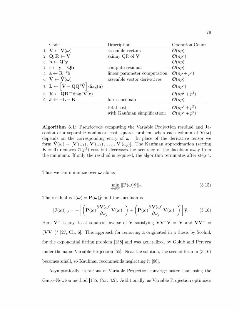
79

Code Description Operation Count1. V← V(ω) assemble vectors O(np)2. Q,R← V skinny QR of V O(np2)3. b← Q∗y O(np)4. r← y −Qb compute residual O(np)5. a← R−1b linear parameter computation O(np+ p2)

6. V← V(ω) assemble vector derivatives O(np)7. L←

[V −QQ∗V

]diag(a) O(np2)

8. K← QR−∗diag(V∗r) O(np2 + p3)

9. J← −L−K form Jacobian O(np)total cost: O(np2 + p3)with Kaufman simplification: O(np2 + p2)

Algorithm 3.1: Pseudocode computing the Variable Projection residual and Ja-cobian of a separable nonlinear least squares problem when each column of V(ω)depends on the corresponding entry of ω. In place of the derivative tensor weform V(ω) = [V′(ω1) , V

′(ω2) , . . . , V′(ωp)]. The Kaufman approximation (setting

K = 0) removes O(p3) cost but decreases the accuracy of the Jacobian away fromthe minimum. If only the residual is required, the algorithm terminates after step 4.

Thus we can minimize over ω alone:

minω∈Cp

‖P(ω)y‖2. (3.15)

The residual is r(ω) = P(ω)y and the Jacobian is

[J(ω)]·,j = −[(

P(ω)∂V(ω)

∂ωj

V(ω)−)+

(P(ω)

∂V(ω)

∂ωj

V(ω)−)∗]

y. (3.16)

Here V− is any ‘least squares’ inverse of V satisfying VV−V = V and VV− =

(VV−)∗ [27, Ch. 6]. This approach for removing a originated in a thesis by Scolnik

for the exponential fitting problem [138] and was generalized by Golub and Pereyra

under the name Variable Projection [55]. Near the solution, the second term in (3.16)

becomes small, so Kaufman recommends neglecting it [86].

Asymptotically, iterations of Variable Projection converge faster than using the

Gauss-Newton method [135, Cor. 3.2]. Additionally, as Variable Projection optimizes

80

over half the number of variables as the general nonlinear least squares problem (3.3),

each iteration typically requires fewer operations. Variable Projection is also faster

than alternating methods that switch between fixing ω and solving for a using linear

least squares and then fixing a and solving for ω using nonlinear least squares. For

details, see the numerical experiments of Ruhe and Wedin [135]1.

3.1.5 Box Constraints

The exponential fitting problem contains one additional challenge: V(ω) diverges as

n→∞ if Reω > 0 so even small excursions of ω into the right half plane can cause

breakdown. To avoid this, we impose box constraints on the value of ω such that

Reω < ωmax following [31]. Experience shows that ω must be allowed to slightly

enter the right half plane to avoid slow convergence, and ωmax is proscribed to keep

‖V(ω)‖∞ below a fixed value (≈ 100).

3.2 Perturbation Analysis for Nonlinear Least Squares

We seek a perturbation expansion of the recovered solution θ as a function of g in

the limit that g is small. That is, we seek a power series expansion of

θ(εg) := argminθ‖f(θ) + g − f(θ)‖Γ. (3.17)

Using this expansion, we then estimate the asymptotic covariance.

1Ruhe and Wedin call Variable Projection ‘Algorithm I,’ Variable Projection with Kaufman’s

simplification ‘Algorithm II,’ and alternating methods ‘Algorithm III’.

81

3.2.1 Asymptotic Perturbation

First, we write a power series expansion of θ: θ = θ+ εθ(1) +O(ε2) and expand f(θ)

in a Taylor series, f(θ) = f(θ) + εF(θ)θ(1) + O(ε2), where [F(θ)]j,k = ∂fj(θ)/∂θk.

Substituting in (3.17) we obtain

‖f(θ) + εg − f(θ)‖Γ = ε‖Γ−1/2g − Γ−1/2F(θ)θ(1)‖2 +O(ε2).

The first order correction minimizes the norm, yielding

θ(1) =(Γ−1/2F(θ)

)+Γ−1/2g =

(F(θ)∗Γ−1F(θ)

)−1

F(θ)∗Γ−1/2g. (3.18)

(The last step above requires F to have full column rank — a condition that holds

for exponential fitting provided θ is distinct.) When Γ = I, this reduces to the least

squares estimate,

θ(1) = F+g. (3.19)

3.2.2 Asymptotic Covariance

The asymptotic covariance follows directly from the asymptotic perturbation;

Cov[θ] = E[(θ − θ)(θ − θ)∗]

= ε2(Γ−1/2F(θ)

)+Γ−1/2 E[gg∗]Γ−1/2

(Γ−1/2F(θ)

)+∗+O(ε3)

= ε2(Γ−1/2F(θ)

)+ (Γ−1/2F(θ)

)+∗+O(ε3)

= ε2(F(θ)∗Γ−1F(θ)

)−1

+O(ε3). (3.20)

For this problem, the Fisher information matrix is (see Appendix A.5)

I(θ) := (∇f(θ))∗(ε2Γ)−1(∇f(θ)) = ε−2F(θ)∗Γ−1F(θ), (3.21)

and the Cramér-Rao bound states

Cov[θ] I(θ)−1 = ε2(F(θ)∗Γ−1F(θ)

)−1

. (3.22)

82

−10010203040506070

0

0.1

0.2

SNR (dB)

Rel

ativ

eco

vari

ance

erro

r

Tr(ε−

2Cov

θ−

I(θ)−

1)/

TrI(

θ)−

1

10−2 10−1 100 101

ε

Figure 3.1 : The relative accuracy of the asymptotic covariance estimate (3.20) forlarge noise in an MRS example [153, Table 1] with p = 11 exponentials. Error barsdenote error the sample covariance. The covariance estimate remains accurate upuntil the signal to noise ratio (SNR) reaches about 3 (10 dB).

Hence, in the limit ε → 0, Cov[ω] = I(θ)−1 – the maximum likelihood estimator

asymptotically obtains the Cramér-Rao bound. In our numerical experiments, the

asymptotic estimate (3.20) holds even for fairly large values of ε, as seen in Figure 3.1.

3.3 Perturbation Analysis for Separable Nonlinear Least Squares

Computing the perturbation expansion for the separable problem follows the same

approach as the general problem in the previous section. We define

ω(g) := argminω‖P(ω)(V(ω)a+ g)‖22 = argmin

ω‖P(ω)y‖22 (3.23)

and seek a power series expansion for ω in the small g limit. The covariance of ω cor-

responds to the previous result, but this expression is useful in selecting compression

spaces in the next chapter.

83

3.3.1 Asymptotic Perturbation

As before, we expand ω in a power series: ω = ω+ εω(1)+O(ε2). We begin with the

Taylor expansion of P(ω) given in [55, Lem. 4.1] using the tensor product notation

of Kolda and Bader [90, §2.5],2

P(ω + εω(1)) = P(ω) + εJ (ω)×3ω(1) +O(ε2) as ε→ 0, (3.24)

where [J (ω)]·,·,j = −(P(ω)

∂V(ω)

∂ωj

V(ω)−)−(P(ω)

∂V(ω)

∂ωj

V(ω)−)∗. (3.25)

From this 3-tensor J ∈ Cn×n×m we can compute the Jacobian J(ω) as

J(ω) = J (ω)×2 y. (3.26)

Next, we apply this expansion to the perturbed measurements y = V(ω)a+ εg,

P(ω)y = P(ω) [V(ω)a+ εg] + ε(J (ω)×3ω(1)

)V(ω)a+O(ε2). (3.27)

Immediately we notice P(ω)V(ω) vanishes as P(ω) is a projector onto the space

perpendicular to V(ω). The second term can be rearranged using the rules of tensor

multiplication,

(J (ω)×3ω(1)

)V(ω)a = (J (ω)×2 (V(ω)a))ω(1).

Expanding the product J (ω)×2V(ω)a,

J (ω)×2V(ω)a=m∑j=1

−P(ω)∂V(ω)

∂ωj

V(ω)−V(ω)a−V(ω)−∗(∂V(ω)

∂ωj

)∗P(ω)V(ω)a

2The symbol ×j denotes the inner product along the jth mode; for example

[J (λ)×2 y]j,` =n∑

k=1

[J (λ)]j,k,` yk.

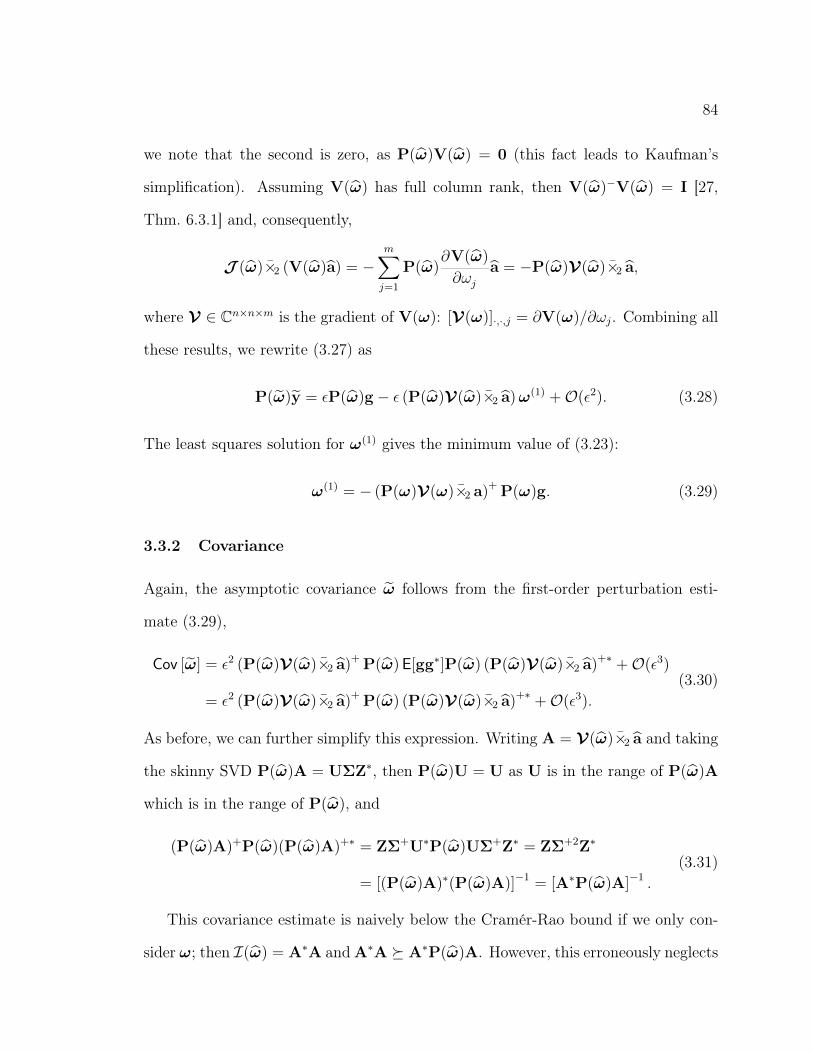
84

we note that the second is zero, as P(ω)V(ω) = 0 (this fact leads to Kaufman’s

simplification). Assuming V(ω) has full column rank, then V(ω)−V(ω) = I [27,

Thm. 6.3.1] and, consequently,

J (ω)×2 (V(ω)a) = −m∑j=1

P(ω)∂V(ω)

∂ωj

a = −P(ω)V(ω)×2 a,

where V ∈ Cn×n×m is the gradient of V(ω): [V(ω)]·,·,j = ∂V(ω)/∂ωj. Combining all

these results, we rewrite (3.27) as

P(ω)y = εP(ω)g − ε (P(ω)V(ω)×2 a)ω(1) +O(ε2). (3.28)

The least squares solution for ω(1) gives the minimum value of (3.23):

ω(1) = − (P(ω)V(ω)×2 a)+P(ω)g. (3.29)

3.3.2 Covariance

Again, the asymptotic covariance ω follows from the first-order perturbation esti-

mate (3.29),

Cov [ω] = ε2 (P(ω)V(ω)×2 a)+P(ω)E[gg∗]P(ω) (P(ω)V(ω)×2 a)+∗ +O(ε3)

= ε2 (P(ω)V(ω)×2 a)+P(ω) (P(ω)V(ω)×2 a)+∗ +O(ε3).(3.30)

As before, we can further simplify this expression. Writing A = V(ω)×2 a and taking

the skinny SVD P(ω)A = UΣZ∗, then P(ω)U = U as U is in the range of P(ω)A

which is in the range of P(ω), and

(P(ω)A)+P(ω)(P(ω)A)+∗ = ZΣ+U∗P(ω)UΣ+Z∗ = ZΣ+2Z∗

= [(P(ω)A)∗(P(ω)A)]−1 = [A∗P(ω)A]−1 .

(3.31)

This covariance estimate is naively below the Cramér-Rao bound if we only con-

sider ω; then I(ω) = A∗A and A∗A A∗P(ω)A. However, this erroneously neglects

85

the latent variables a, assuming they are constant. Correctly computing the Cramér-

Rao bound shows Cov ω obtains this bound. Considering the general nonlinear least

squares covariance (3.20), taking θ = [ω, a], the gradient is

F(θ) =

[V(ω)×2 a V(ω)

].

Adopting the shorthand for A above, the covariance splits into four blocks:

Cov θ = ε2[F(θ)∗F(θ)

]−1

+O(ε3)

= ε2

A∗A A∗V

V∗A V∗V

−1

+O(ε3) = ε2

(A∗P⊥VA)−1 ∗

∗ (V∗P⊥AV)−1

+O(ε3),(3.32)

where P⊥A is the orthogonal projector onto the space perpendicular to the range of

A. We immediately identify the (1, 1) block with the covariance computed above, as

P(ω) is, by definition, P⊥V.

3.4 Heuristics for Initial Conditions

The main disadvantage of nonlinear least squares methods, when compared to Prony-

type methods, is their requirement for initial estimates of ω. Without good initial

estimates of ω, the optimization of ω can easily be lead astray into spurious local

minima. When there is a single exponential without noise, the minimum is very clear

(see Figure 3.4) and convergence to the right minimum is typical regardless of the ini-

tial estimate. However, as Figure 3.3 illustrates, as few as two exponentials and small

amounts of noise can cause poor initial estimates to converge to a spurious minium.

We can see the appearance of spurious minima in Figure 3.2; there is even a local

minimum in the absence of noise at the average of ω. Spurious local minima become

increasingly problematic as the number of exponentials increases. For example in Ta-

86

Table 3.1 : Failure rate for increasing numbers of exponentials p. The table showsthe precentage of failures from 100 random trials with n = 103, where samples ωj ∈[−0.1, 0]× [0, 2π)i uniformly, and |aj| = 1 with uniform random phase.

p Roots of Unity Largest Fourier Peeling

1 13 0 02 23 12 03 43 20 04 56 31 05 58 36 06 68 45 07 73 66 08 71 61 19 76 57 010 81 73 0

ble 3.1, using the p roots of unity as initial estimates causes convergence to spurious

minima with increasing probability as the number of exponentials, p, increases.

Good initial estimates of ω combat this, helping the nonlinear least squares solver

converge to the true parameter values by placing the initial estimate near the true

minimum. Assuming the number of exponentials is already known, we examine one of

five different strategies for choosing the initial estimate ω0 for the exponential fitting

problem: choosing ω0 randomly, setting ω0 to be the pth roots of unity, picking ω0

as peaks of the Fourier transform, solving a Prony-type method to provide ω0, and

by using prior knowledge about ω.

3.4.1 Random Imaginary Part

The easiest approach for choosing the initial estimate ω0 is to randomly guess. For ex-

ample, choosing each ω0 independently and uniformly distributed in [−1, 0]× [0, 2π)i

87

ε = 0

0 2 4 6

10−1

100

101

F∗ y

Fourier Transform

0.8 0.9 1 1.1 1.20.8

0.9

1

1.1

1.2

Imω2

Residual Norm

0.200

0.400

0.600

0.800

1.000

ε = 2

0 2 4 6

10−1

100

101

F∗ y

0.8 0.9 1 1.1 1.20.8

0.9

1

1.1

1.2Im

ω2

0.850

0.900

0.950

1.000

ε = 4

0 2 4 6

10−1

100

101

Fourier frequency

F∗ y

0.8 0.9 1 1.1 1.20.8

0.9

1

1.1

1.2

Imω1

Imω2

0.940

0.960

0.980

1.000

Figure 3.2 : The appearance of local minima as noise increases. For fixed randomvector g, we perturb y = y + εg. The left plots show the Fourier transform ofthe noisy signal F∗y as red dots and the original unperturbed transform as a blackline. The right plots show the norm of the residual ‖P(ω)y‖2. As ε increases, thetrue minimum becomes shallower and spurious minima appear. (Note the changingcolorbar scale.)

-· .. ·, =·

=·

. . . , .. . . . .. .

•.: ~ .... :-. . .. .,. ... • • ••• : I • • .... • . : . . ... ·-

.. . .. ' . .... .. .......... ·· .. ; : .... ~- .... ·: ...

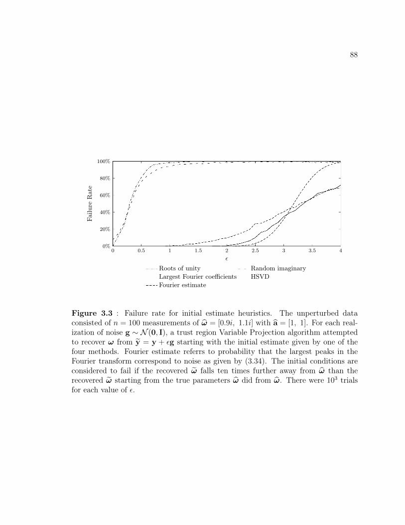
88

0 0.5 1 1.5 2 2.5 3 3.5 40%

20%

40%

60%

80%

100%

ε

Failu

reR

ate

Roots of unity Random imaginaryLargest Fourier coefficients HSVDFourier estimate

Figure 3.3 : Failure rate for initial estimate heuristics. The unperturbed dataconsisted of n = 100 measurements of ω = [0.9i, 1.1i] with a = [1, 1]. For each real-ization of noise g ∼ N (0, I), a trust region Variable Projection algorithm attemptedto recover ω from y = y + εg starting with the initial estimate given by one of thefour methods. Fourier estimate referrs to probability that the largest peaks in theFourier transform correspond to noise as given by (3.34). The initial conditions areconsidered to fail if the recovered ω falls ten times further away from ω than therecovered ω starting from the true parameters ω did from ω. There were 103 trialsfor each value of ε.

/· I

,, 1.' I

i I ,. / ,.,

II

·'' .', I

i' I

- - - - - -

--------------1

89

−2 −1 00

1

2

3

4

5

6

Reω

Imω

ω = 1i

0.70.8

0.9

0.9

0.9

−2 −1 00

1

2

3

4

5

6

Reω

Imω

ω = 1i− 0.1

0.4 0.5

0.5

0.6

0.6

0.7

0.7

0.7

0.8

0.8

0.8

0.9

0.9

0.9

11

1

−2 −1 00

1

2

3

4

5

6

Reω

Imω

ω = 1i− 0.4

Figure 3.4 : The norm of the residual for a single exponential. Each plot showscontours of ‖P(ω)V(ω)‖2/‖V(ω)‖2 with spacing 0.1.

90

of the complex plane. However, if ω0 ventures too far away from the imaginary

axis, then V(ω0) is ill-conditioned and can lead to erroneous Newton steps. Enforce

Reω = 0 can avoid this form of ill-conditioning, but V(ω0) can still be ill-conditioned

if |[ω0]j−[ω0]k| is small. Hence, this approach is prone to failure. As Figure 3.3 shows,

even when there is no noise, randomly choosing Imω0 leads to convergence away from

ω in 7% of the simulations.

3.4.2 Roots of Unity

Osborne notes that his method implicitly uses the initial estimate that ω are the pth

roots of unity [116], i.e., [ω0]j = 2πij/p for j = 0, . . . , p− 1. Unlike randomly choos-

ing ω0, choosing the roots of unity makes V(ω0) well conditioned, as its columns

are approximately orthogonal (exactly orthogonal if n is an integer multiple of p).

However, this approach fails even in the absence of noise; Table 3.1 provides one ex-

ample. Once noise is introduced, this approach provides even worse initial estimates;

for example, in Figure 3.3. The origin of the failure is simple; ω0 might be far away

from true value ω, placing ω0 such that optimization converges to local minimum

near ω0 rather than finding the minimum associated with ω.

3.4.3 Peaks of the Fourier Transform

A well known fact in signal processing is that peaks of the Fourier transform of y

correspond to the imaginary part of ω. This is a result of the geometric sum formula

applied to F∗V(ω) (cf., (4.37)):

[F∗V(ω)]k =1√n

1− eωn−2πik

1− eω−2πik/nω 6= 2πik/n. (3.33)

There are ‘peaks’ in F∗V(ω) near where the denominator vanishes, Imω ≈ 2πik/n.

As y = V(ω)a, then F∗y is a sum of these peaks; i.e., F∗y = F∗V(ω)a. (See

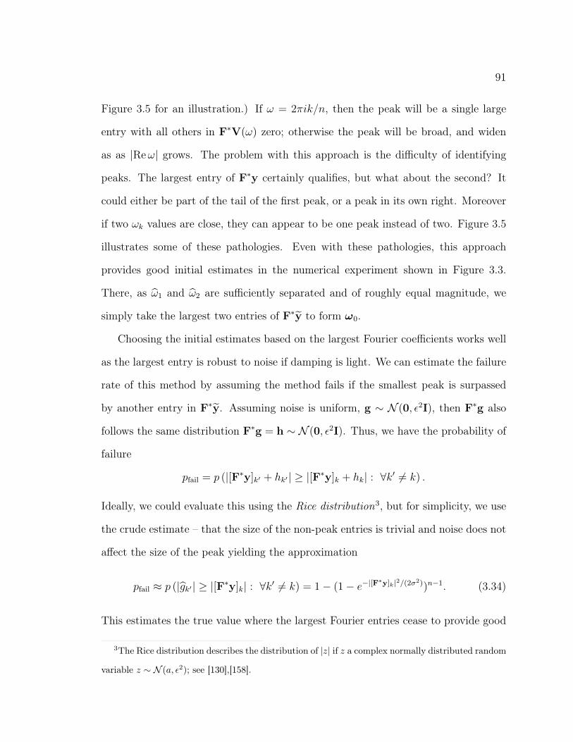
91

Figure 3.5 for an illustration.) If ω = 2πik/n, then the peak will be a single large

entry with all others in F∗V(ω) zero; otherwise the peak will be broad, and widen

as as |Reω| grows. The problem with this approach is the difficulty of identifying

peaks. The largest entry of F∗y certainly qualifies, but what about the second? It

could either be part of the tail of the first peak, or a peak in its own right. Moreover

if two ωk values are close, they can appear to be one peak instead of two. Figure 3.5

illustrates some of these pathologies. Even with these pathologies, this approach

provides good initial estimates in the numerical experiment shown in Figure 3.3.

There, as ω1 and ω2 are sufficiently separated and of roughly equal magnitude, we

simply take the largest two entries of F∗y to form ω0.

Choosing the initial estimates based on the largest Fourier coefficients works well

as the largest entry is robust to noise if damping is light. We can estimate the failure

rate of this method by assuming the method fails if the smallest peak is surpassed

by another entry in F∗y. Assuming noise is uniform, g ∼ N (0, ε2I), then F∗g also

follows the same distribution F∗g = h ∼ N (0, ε2I). Thus, we have the probability of

failure

pfail = p (|[F∗y]k′ + hk′| ≥ |[F∗y]k + hk| : ∀k′ 6= k) .

Ideally, we could evaluate this using the Rice distribution3, but for simplicity, we use

the crude estimate – that the size of the non-peak entries is trivial and noise does not

affect the size of the peak yielding the approximation

pfail ≈ p (|gk′ | ≥ |[F∗y]k| : ∀k′ 6= k) = 1− (1− e−|[F∗y]k|2/(2σ2))n−1. (3.34)

This estimates the true value where the largest Fourier entries cease to provide good

3The Rice distribution describes the distribution of |z| if z a complex normally distributed random

variable z ∼ N (a, ε2); see [130],[158].

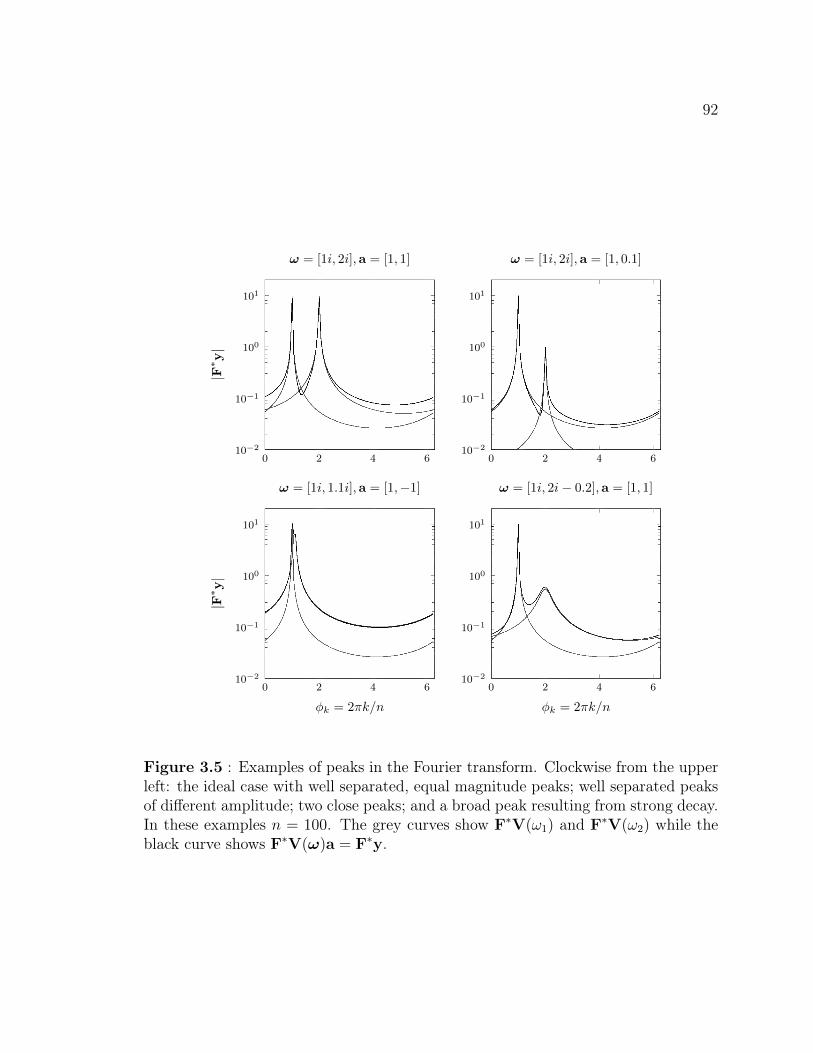
92

0 2 4 610−2

10−1

100

101

|F∗ y

|

ω = [1i, 2i],a = [1, 1]

0 2 4 610−2

10−1

100

101

ω = [1i, 2i],a = [1, 0.1]

0 2 4 610−2

10−1

100

101

φk = 2πk/n

|F∗ y

|

ω = [1i, 1.1i],a = [1,−1]

0 2 4 610−2

10−1

100

101

φk = 2πk/n

ω = [1i, 2i− 0.2],a = [1, 1]

Figure 3.5 : Examples of peaks in the Fourier transform. Clockwise from the upperleft: the ideal case with well separated, equal magnitude peaks; well separated peaksof different amplitude; two close peaks; and a broad peak resulting from strong decay.In these examples n = 100. The grey curves show F∗V(ω1) and F∗V(ω2) while theblack curve shows F∗V(ω)a = F∗y.

93

initial estimates to within a factor of two, as seen in Figure 3.3, and over estimates

the failure rate as noise increases.

Finally note we note this method must produce a well conditioned V(ω0). The ini-

tial estimates ω0 are Fourier frequencies, and hence, V(ω0) consists of the orthogonal

columns of F.

3.4.4 Prony-type Methods

Since Prony-type methods do not require initial estimates, they provide an obvious

source for the initial estimates needed by optimization routines. This second compu-

tation of the exponentials might seem redundant, but it can be beneficial when using

one of the compressed Prony variants from Sections 2.8 and 2.8. We can easily ob-

tain fast, crude, estimates of ω0 using the Filtered Matrix Pencil method in a region

indicated by peaks in the Fourier transform.

Although we are the first to propose use of a compressed Prony-type method, the

idea had its origin’s in Householder’s Method, where the full Prony’s Method was used

to provide initial estimates for the maximum likelihood method for lag coefficients

α [69]. Others would later use the High Order Yule-Walker method [145] to provide

initial estimates for a Newton method for optimizing ω.

3.4.5 Prior Knowledge

Exponential fitting rarely occurs in the absence of other information about the un-

derlying problem. This frequently yields prior knowledge about ω from the structure

of the problem. For example, in the case of damped wave equation in one dimension,

we know the imaginary part of ω are approximately integer multiples of some fun-

damental frequency, while the real part of ω is negative. For other lightly damped

94

mechanical systems like drums, beams, or plates we have similar knowledge about

the structure of Imω. In general, we also may assume that Reω is in the left half

plane as a result of conservation of energy.

3.5 Estimating the Number of Exponentials

Although these five methods are sufficient to provide initial estimates of ω, we still

need to know the size of ω, i.e., p, the number of exponentials present. There are three

standard approaches for determining p: one motivated by the Hankel construction

seen Section 2.2.3, one statistically motivated, and one by the size of aj, The last

two approaches are conducive to an approach called peeling, where exponentials are

appended sequentially until no longer justified (see Section 3.6).

3.5.1 Hankel Singular Values

In Section 2.2.3, we saw that the Hankel matrix of measurements [H]j,k = yj+k can be

decomposed as H = V(ω)diag(a)V(ω)>. Hence, the range of H is the range of V(ω)

and thus H has exactly p non-zero singular values (provided ω has distinct entries).

This leads to a widely used heuristic: choose p as the number of large singular values.

However noise increases the zero singular values, threatening the ability distinguish

the large singular values revealing p from singular values associated with noise. The

following new result allow us to bound the growth of the singular values associated

with noise. The first result bounds the perturbation of singular values, obtaining a

bound on the norm of a finite dimensional Hankel Matrix using a method reminiscent

of that used for the infinite dimensional case [21, p. 13]. The second result provides

a bound on the expected value of the norm of this random Hankel matrix.

Theorem 3.1. If H, H ∈ Cm×n are both Hankel matrices where E := H − H has

95

entries [E]j,k = gj+k, then the singular values σj and σj of H and H obey

|σj − σj| ≤√n+m− 1 max

k|[Fn+mg]k|. (3.35)

Proof. From Weyl’s Theorem [143, Cor. 4.9], we have

|σj − σj| ≤ ‖H−H‖2 = ‖E‖2.

We bound the norm of E by embedding E inside a circulant matrix C with flipped

columns

C =

gm−1 · · · g0 gn+m−2 · · · gm... . . . ...

... . . . ...

gn+m−2 · · · gn−1 gn−2 · · · g0

g0 · · · gn gn−1 · · · g1... . . . ...

... . . . ...

gm−2 · · · gn+m−2 g0 · · · gn−1

∈ C(n+m−1)×(n+m−1). (3.36)

Using the definition of the `2 norm,

‖E‖2 = maxx∈Cn

‖Ex‖2‖x‖2

≤ maxx∈Cn+m

xj=0 ∀j≥n

‖Cx‖2‖x‖2

≤ ‖C‖2.

Circulant matrices are diagonalized by the Fourier transform with eigenvalues λ =

√n+m− 1Fn+m−1c, where c is the first column of C; i.e., C = F∗

n+m−1ΛFn+m−1

for Λ = diag(λ). As Fn+m−1 is unitary then,

‖C‖2 = ‖Λ‖2 = maxk|λk|.

Finally, as we are only interested in the magnitude of λk, we can apply the DFT

shift theorem to write λk in terms of the Fourier transform of g ∈ Cn+m−1. If

96

D` ∈ C(n+m−1)×(n+m−1) is a diagonal matrix with [D`]k,k = e2πik`/(n+m−1) and S is the

circulant shift matrix [Sg]k = gk−1 mod n+m−1, then the DFT shift theorem implies

[Fn+m−1S`x]k = [D`Fn+m−1x]k.

Hence, taking ` = n− 1,

maxk|λk| =

√n+m− 1max

k|[D`Fn+m−1c]k| =

√n+m− 1max

k|[Fn+m−1g]k|.

Using this theorem, the following Corollary evaluates the expected value of this

bound on |σj − σj| when g is a complex random vector.

Corollary 3.1. If g ∼ N (0, ε2I), then

|σj − σj| ≤√n+m− 1 γ with probability p(γ) = (1− e−γ2/(2ε2))n+m. (3.37)

Proof. As g is normally distributed with mean 0 and covariance σ2I and Fn+m−1 is a

unitary transform, then h = Fn+m−1g is also normally distributed with mean 0 and

covariance ε2I. Then |hk| follows a follows a Rayleigh distribution4 with covariance ε2

such that p(hk < x) = 1− e−x2/(2ε2). As the hk are independent, the probability that

n+m− 1 of these are bounded above by γ is given by p(hk < γ)n+m−1.

Using this criteria, singular values associated with noise g using a total of n

measurements are bounded above by

σk < ε

√−2n log(1− n

√r) k > p (3.38)

with probability r. Thus p can be estimated as the number of singular values breaking

this bound. Figure 3.6 provides an example of this bound in practice, illustrating its

power at distinguishing signal from noise.

4A special case of the χ distribution with two degrees of freedom.

D

D

97

r = 0.9

r = 0.5

2 4 6 8 10 12 14 16 18 20 22 24 26 28 30

102

103

104

k

σk

Range of σk

Mean of σkσk

Bound (3.38)σ√n/2

Figure 3.6 : Hankel singular values from a magnetic resonance spectroscopy examplewith noise. Using the example from [153, Table 1] with p = 11, n = 256, and noiseσ = 10 for 105 trials, we show the maximum, minimum, and mean singular values σk ofH. The bound from Corollary 3.1 (black line) successfully distinguishes a significantsingular value σ11 from a noise singular value σ12 with high probability. However theapproach of de Groen and de Moor (dashed line) does a poor job of bounding σ12.

An alternative approach of de Groen and de Moor [39, §4] provides a less effective

estimate. Their approach estimates a bound on the singular values associated noise

by considering the eigenvalues of E[H∗H]:

E[H∗H] = H∗H+ E[E∗H] + E[H∗E] + E[E∗E] = H∗H+ nε2I,

where n is the number of rows in H. As the singular values are eigenvalues of H∗H,

we note σ2j ≈ σ2

j + nε2. This approach is performs poorly, as the estimate computes

the eigenvalues of E[H∗H] rather than the eigenvalues of H

∗H,

These results about the singular values of H also apply to systems theory. There,

yj corresponds to the jth Markov parameter of a discrete time linear system with

system matrices A = diag(λ) where λ = eω, C = 1> (the vector of ones), and

B = diag(a). In this context H corresponds to the product of the controllability

•

98

and observability matrices [83, §2.2, eq. 49]. More sophisticated approaches for

determining p using SVD are still being developed, often under the name of rank

determination (after the rank of A); see, e.g., [165].

3.5.2 Akaike Information Criterion

The advantage of the Hankel singular value approach is that we can estimate the

number of exponentials p without determining ω or a. Model selection criteria pro-

vide another approach that allows us to compare models with different numbers of

exponentials provided knowledge of maximum likelihood estimates of ω and a. An-

other approach is to use model selection criteria to compare models with different

numbers of exponentials. One such model selection criteria is the Akaike Information

Criterion (AIC) [26, §2.2] that ranks candidate models with q parameters by

A(q) = 2q − 2 log

(maxθ∈RqLq(θ)

), (3.39)

where Lq is the likelihood function associated with a q parameter model; cf., (A.10).

The best model has a value of q that minimizes A(q). The AIC is an asymptotic

result in the limit of n → ∞ measurements; for a finite number of samples n, there

is a second order correction, called the AICc due to Sugiura [148]

Ac(q) = A(q) +2q(q + 1)

n− q − 1. (3.40)

For real measurements y the there are 2p parameters (ω ∈ Rp and a ∈ Rp) and if

y = y + g, where g ∼ (0,Σ) (real), the AIC is

A(p) = 2p− 2 log

[maxθ∈R2p

1√(2π)n detΣ

e−(y−f(θ))>Σ−1(y−f(θ))/2

]

= 2p+ n log 2π + log detΣ+ minθ∈R2p

‖y − f(θ)‖2Σ.

99

As we are interested in only the smallest value of A, we neglect the terms that do not

depend on p terms and compute

A(p) = 2p+ minθ∈R2p

‖y − f(θ)‖2Σ. (3.41)

If noise is independent and identically distributed, then Σ = ε2I and

A(p) = 2p+ ε−2 minθ∈R2p

‖y − f(θ)‖22.

The correction for the AICc for real measurements is 4p(2p+ 1)/(n− 2p− 1).

For complex measurements there are 4p parameters and 2n measurements; similar

results follow. The AIC is

A(p) = 4p− 2 log

[maxθ∈Cp

1

πn detΣe−(y−f(θ)>)Σ−1(y−f(θ))

]= 4p+ 2n log π + 2 log detΣ+ 2min

θ‖y − f(θ)‖2Σ.

Neglecting the constant terms yields

A(p) = 4p+ 2minθ‖y − f(θ)‖2Σ. (3.42)

This is a scaled version of (3.41), but the correction for the AICc for complex data

is not a scalar multiple of the real case. The AICc correction for complex data is

8p(4p+ 1)/(2n− 4p− 1).

3.5.3 Small Amplitudes

A strategy often used by practitioners simply fits an excessive number of exponentials,

and then removes the exponentials with amplitudes below some tolerance τ ; see,

e.g., [123, 126]. This avoids the complicated machinery of the singular values of the

Hankel matrix H or the AIC, but provides only a crude heuristic. In this section we

provide a truncation tolerance τ based on the AIC.

100

Suppose we have measurements y = V(ω)a+εg where g ∼ N (0, I) and ω, a ∈ Cp

and we then fit y with p+p′ exponentials. The AIC dictates that the p+p′ exponential

is a better model if A(p+ p′)−A(p) < 0.

A(p+ p′)−A(p) = 4p′ + 2ε−2 minω,a∈Cp+p′

‖y −V(ω)a‖2 − 2ε−2 minω,a∈Cp

‖y −V(ω)a‖2

≤ 4p′ + 2ε−2 minω,a∈Cp′

‖g −V(ω)a‖2 − 2ε−2‖g‖2.

Fixing the minimum of the p′ sized problem as ω, a, we invoke the reverse triangle

inequality to find

A(p+ p′)−A(p) ≤ 4p′ − 2ε−2‖V(ω)a‖2.

Setting p′ = 1, we find the p+1 exponentials are not justified according to the AIC if

|a| <√2ε

‖V(ω)‖. (3.43)

If we require Reωj = 0, then |a| must be less than ε/n (we loose a factor of two

since there are now half as many parameters). This yields the truncation tolerance

τ = ε/n. For general ω, ‖V(ω)‖ may be as small as one, hence we require |a| to be

less than√2ε, yielding the truncation tolerance τ =

√2ε. A similar analysis would

yield truncation tolerances where the error g is a result of rounding errors.

3.6 Peeling

Now we combine these elements – initial estimates of ω in Section 3.4 and the estima-

tion of the number of exponentials in Section 3.5 – into a single algorithm. Although

each of these techniques is not new, the combination is, and allows us to use nonlinear

least squares algorithms without initial estimates or a priori knowledge of p. This

101

Algorithm 3.2: Peeling for Exponential FittingInput : Noisy measurements y ∈ Cn, noise estimate εOutput: Exponential coefficients ω, a ∈ Cp

Initial estimate of p.1 Compute the singular values σk of H in decreasing order where [H]j,k = yj+k;2 pest ← argmink σk > ε

√−2n log(1− n

√r) ;

3 p← 0;4 r← y;5 repeat6 p← p+ 1;7 Estimate ωp ← 2πi/n argmaxk |[F∗

nr]k|;8 Update ω ← [ω, ωp];9 Apply a nonlinear least squares algorithm to refine ω and recover a;

10 r← y −V(ω)a;11 until p ≥ pest and Ac(p− 1) < Ac(p);12 ω ← [ω]0:p−2;13 a← [a]0:p−2;14 Apply a nonlinear least squares algorithm to refine ω and recover a.

technique is sketched in Algorithm 3.2: we sequentially add exponentials until the

AICc dictates the fit is not sufficiently better to warrant another exponential. We

use the largest entry in the residual to estimate the next value of ωp following Sec-

tion 3.4.3 and can further refine this estimate if necessary using the Filtered Matrix

Pencil method. Figure 3.7 shows this approach in action.

This approach mimics a graphical approach for fitting real exponentials called

peeling [122], prominent before the advent of computers [79, VI.B.1]. Peeling consists

of fitting a line to a log plot of y, removing the fit, and then repeating the procedure

until the signal vanishes. In the same way, our updated Peeling Algorithm 3.2 iter-

atively removes exponentials and uses the residual to estimate the next value of ω.

102

F∗rω0 ω1 ω2 ω3 ω4

a0 a1 a2 a3 a4

0.001 + 2.010i

−0.725 + 0.069i

−0.001 + 1.000i 0.001 + 2.010i

1.283 + 0.001i −0.726 + 0.078i

0.000 + 1.000i 0.000 + 2.010i −0.505 + 4.201i

1.000 + 0.008i −0.933 − 0.010i 50.739− 0.107i

0.000 + 1.000i −0.100 + 2.002i −0.000 + 2.010i −0.496 + 4.200i

0.999 + 0.001i 1.020 − 0.023i −1.006 − 0.002i 50.078+0.063i

0.000 + 1.000i −0.098 + 2.002i −0.000 + 2.010i −0.499 + 4.200i −0.010 + 4.201i

0.999 + 0.001i 1.000 − 0.021i −1.006 − 0.002i 50.031+0.062i 0.094 − 0.004i

True solution 0.000 + 1.000i −0.100 + 2.000i 0.000 + 2.010i −0.500 + 4.200i −0.010 + 4.200i

1.000 + 0.000i 1.000 + 0.000i −1.000 + 0.000i 50.000+0.000i 0.100 + 0.000i

Figure 3.7 : Peeling with complex data. We recover five exponentials using thePeeling Algorithm 3.2, with n = 512. The black curve shows the original residual,F∗y, and the dots F∗rk where rk is the residual at the kth step.

. .. . . . . ~ . .. . . ...... -"-~;.,,;.~..:: . .:,.~ --1~~,.~ ..... ·-~.::--;-·ii.~ •• ':J•.s•.1':"'..,,..: ~-(".,.., •• ---i:~"'"C": .... , •. :-.--~ •• --.,· ....... 1:f': • ,"·,&\e-:-e-t . -.0:. ·:~-., :.· .. · ...... · .. . . : . · ..... \,•. . . : . , ... '

103

We use the Hankel singular values to provide an initial estimate of p, since for early

values of k < p, there are situations where Ac(p) < Ac(k) < Ac(k + 1), leading our

single look-ahead approach astray.

The updated peeling algorithm works well in some situations. For a randomly

distributed exponentials exponential in noise, the numerical simulation in Table 3.1

illustrates that peeling frequently ensures convergence to the proper minimum. How-

ever, problems can emerge if exponentials are clustered. In Section 4.6.2, the Peeling

Method produces poor estimates when multiple exponentials have similar imaginary

components. Although the Peeling Method is not without its faults, it provides cheap

estimates of initial conditions for large exponential fitting problems.

104

Chapter 4

Compression for Exponential Fitting

Solving large scale exponential fitting problems is expensive. Fitting p parameters θ

to n measurements y using nonlinear least squares requires O(np2) operations per it-

eration that refines θ. Numerically stable Prony variants such as HSVD are even more

expensive, requiring O(n3) operations if implemented naively or O(pn log n+np2+p3)

operations using fast inner-products and an Arnoldi based SVD [96]. Although the

operation count grows only linearly in n for nonlinear least squares iterations, each

iteration is too expensive for the millions or billions of measurements easily obtained

with modern hardware. To combat this, practitioners throw away measurements to

make each iteration feasible in one of three ways: discarding the last n − m mea-

surements (truncation), keeping every qth measurement – equivalent to reducing the

sample rate – (decimation), or keeping a random subset of measurements (Incremental

Gradient; see [50]). By discarding information in y, the covariance of the parameters

θ increases. In this chapter, we build a new, fourth approach that sacrifices a mini-

mum amount of information in y about θ by compressing y onto a carefully chosen

subspace of Cn. The result is an exponential fitting algorithm that solves a nonlinear

least squares problem over m compressed measurements in O(mp2) operations per it-

eration plus an O(n log n) starting cost. Most importantly, the number of compressed

measurements m required to attain a fixed accuracy is small and independent of n;

typically m ≈ 10p is sufficient for 90% accuracy. Although this algorithm is tailored

to the structure of exponential fitting, the framework developed in Sections 4.1 and

105

4.2 can apply to any nonlinear least squares problem.

The key to this approach is building an efficient compression space W ⊂ Cn from

a set of parent coordinates. In comparison to the full problem

θ = argminθ‖y − f(θ)‖2Γ, (4.1)

the compressed problem solves (4.1) with y restricted to the subspace W ⊆ Cn,

spanned by the columns of W ∈ Cn×m, a subset of the parent coordinates that form

the columns of U. The compressed estimate of θ, denoted θW . solves instead

θW = argminθ‖W∗y −W∗f(θ)‖2

ΓΓ =

[(W∗W)−1W∗Γ−1W∗(W∗W)−1

]−1.

(4.2)

In the important case where the columns of W are orthonormal in the unweighted

norm, then Γ = (W∗Γ−1W)−1. In this framework decimation, truncation, and in-

cremental gradient correspond to taking parent coordinates U = I, where decimation

chooses columns I = 0:q :n− 1, truncation I = 0:m− 1, and Incremental Gradient

a random column subset I.

By discarding measurements, the covariance of θW must be larger than the covari-

ance of θ. We quantify this in a single number called the efficiency of the subspaceW ,

defined as the limit of the respective covariances as noise vanishes uniformly (Γ→ εΓ)

ηθ(W) := limε→0

Tr Cov θ

Tr Cov θW∈ [0, 1]. (4.3)

This generalizes Fisher’s notion of efficiency to multiple variables [49, §4]. Following

Fisher, we report ηθ(W) as a percentage. Efficiency depends strongly on both the

model function f and the value θ, as Figure 4.1 shows.

None of the compression subspaces generated by existing approaches are very

efficient (see Figure 4.2). Better compression spaces can be generated by tailoring

106

−0.2 −0.15 −0.1 −0.05 0

0.6

0.8

1

1.2

1.4

Reω

Imω

Efficiency of W spanning [V(1i),V′(1i)]

0%

20%

40%

60%

80%

100%

ηθ(W)

Figure 4.1 : Compression spaces are tailored to specific parameter values. Herewe pick a subspace built to recover ω = 1i exactly and record the efficiency forneighboring parameter values. Efficiency drops off rapidly from ω = 1i.

W to the current estimate of θ, and as subsequent iterations improve θ, changing

W to match. For example, the ideal compression space for any problem (not just

exponential fitting) contains the partial derivatives of f evaluated at θ. This effec-

tively solves (4.2) using a QR-factorization of (4.1) – nothing novel. As we show

in Lemma 4.3, this compression space has full efficiency (ηθ(W) = 1) but efficiency

falls off rapidly for θ away from θ as Figure 4.1 shows. However there are two other

problems with this ideal compression space. These set conditions on compression

spaces such that the compressed is computationally advantageous. The problem with

the ideal subspace is as W is updated, recomputing W∗y takes O(nm) operations

– a cost dependent on n we hope to avoid. To fix this, we impose the condition

that W is chosen from a static set of parent coordinates U so that when we update

W , only a few additional inner products of [U]∗·,jy need be computed, not m. The

107

−1 00

2

4

6

Reω

Imω

Truncation

−1 00

2

4

6

Reω

Decimation

−1 00

2

4

6

Reω

Random

−1 00

2

4

6

Reω

Random

−1 00

2

4

6

Reω

Ideal

0%

20%

40%

60%

80%

100%

ηθ(W)

Figure 4.2 : Efficiency for truncation, decimation, incremental gradient, and idealsubspaces. In this example all subspaces are of dimension m = 10. Truncation workswell for rapidly decaying signals, but poorly for undamped exponentials. Decimationworks well for an intermediate decay, and for undamped signals has an efficiency of10%. The two realizations of the random subspace from Incremental Gradient bothprovide poor subspaces that obtain a maximum expected efficiency of 10%. The idealsubspace for ω = [1i, 1i − 0.25, 1i − 0.5, 1i − 0.75, 1i − 1] and a = [1, 1, 1, 1, 1]provides very accurate estimates near Imω = 1, but poorer estimates further away.

108

second problem with the ideal subspace, and most fatal, is that we need to compute

W∗f(θ) and the derivative W∗F(θ) but in a way that avoids matrix multiplication

requiring O(nm) and O(nmp) operations. One condition fixing this problem would

be to require U∗f(θ) and U∗F(θ) can be computed row wise in closed form. These

restrictive conditions make finding efficient parent coordinates difficult for an arbi-

trary problem. We may take U = I for any problem, but it may not yield efficient

compression spaces.

However, for the exponential fitting problem there is a class of parent coordinates

satisfying these conditions. To satisfy the second condition, we choose parent coor-

dinate built from blocks of the Discrete Fourier Transform (DFT) matrix Fb ∈ Cb×b,

where [Fb]j,k = b−1/2e−2πijk/b,

U(b) = diag(Fb0 ,Fb1 , · · · ,Fbq−1) for b ∈ Nq. (4.4)

As required, we can compute [U∗f ]j and [U∗F]j,· in closed form using a generalization

of the geometric sum formula in Theorem 4.1. Following the outline above, we could

compute U∗y as columns of U are added to W. However, it is faster to can compute

U∗y at once using the Fast Fourier Transform (FFT), requiring fewer thanO(qn log n)

operations.

This leaves two remaining challenges: choosing the columns of U(b) to form W

and the picking block dimensions b. We pick columns of U using greedy search

maximizing the efficiency ofW . Section 4.1 motivates our generalization of efficiency

and provides basic results. As computing efficiency is expensive, Section 4.2 derives

fast updating formulas for the covariance and, thereby, the efficiency, Section 4.3 gives

the closed form inner products used to compute W∗f and W∗F quickly. Section 4.4

details how to pick the initial set of indices for the greedy search and accelerates

this search by restricting to a set of candidates. The choice of block dimensions

109

b is discussed in Section 4.5. Although we are unable to build an optimal set of

blocks, we explore several options, finding that block sizes that grow geometrically

(e.g., bj = 4j) work well. Other attempts to pick bj using heuristics result in similar

performance. Finally, Section 4.6 details how to use compression in conjunction with

optimization and demonstrates that compression results in significant speed gains for

large problems.

4.1 Compression Subspace Efficiency

It is natural to compare compression spaces by their covariances, but this alone cannot

provide the ranking necessary for finding the best subspace. Recall from (3.20) the

asymptotic covariance for θ is

Cov[θ] = ε2(F(θ)∗Γ−1F(θ)

)−1

+O(ε3). (4.5)

The same derivation applies to the compressed problem (4.2) (since it also is a non-

linear least squares problem) yielding the asymptotic covariance

Cov[θW ] = ε2(F(θ)∗WW∗Γ−1WW∗F(θ)

)−1

+O(ε3) when W∗W = I. (4.6)

Both asymptotic covariance matrices are, by construction, positive definite, and pos-

itive definite matrices have a partial ordering. For two positive definite matrices A

and B, A B if x∗Ax > x∗Bx for all x. However, there are pairs of matrices that

are not comparable – e.g., the inequality goes both ways: for some x, x∗Ax > x∗Bx

and for some y, y∗Ay < y∗By. Hence two compression subspaces W1 and W2 may

not be comparable. Efficiency ηθ resolves this problem of ordering by measuring the

expected `2 error in θ. This allows us to construct a preorder1 of compression spaces

where W1 >W2 if ηθ(W1) > ηθ(W2).

1Preorders lack the requirement that a ≥ b and a ≤ b implies a = b.

110

Using our standard model where errors are of the form y = y+g = f(θ)+g with

g ∼ N (0,Γ), the expected `2 error in θ is

E[‖θ − θ‖22

]=

∫Cn

[ε2‖Fg‖2 +O(ε3)

] e−g∗g/ε2

(επ)ndg,

where F is the first order perturbation matrix F = (F(θ)∗Γ−1F(θ))−1F(θ)∗Γ−1/2. If

F(θ) has full rank, we evaluate the first term by taking the SVD of F, F = UΣV∗,

and by changing integration coordinates, g = εV∗g, we have∫

Cn

‖Fg‖22e−g∗g/ε2

(επ)ndg =

∫Cn

g∗Σ2ge−g∗g/ε2

(επ)ndg

=

p∑j=1

σ2j

n∏k=1

∫C|gj|2

e−|gk|2/ε2

επdgk =

1

2

p∑j=1

σ2j .

This last expression has several equivalent formulations: the (scaled) square of the

Frobenius norm of F, the trace of the covariance matrix, or the sum of squares of

singular values, where σj(F) denotes the jth singular value (descending) of F:

limε→0

ε−2 E[‖θ − θ‖22

]=

1

2‖F‖2F (4.7)

=1

2Tr(F(θ)∗Γ−1F(θ)

)−1

(4.8)

=1

2

∑j

σj

(Γ−1/2F(θ)

)−2

(4.9)

=1

2limε→0

ε−2 Tr Cov[θ]. (4.10)

If F(θ) does not have full rank, the expected `2 error is undefined. The same expected

error result holds for the compressed problem:

limε→0

ε−2 E[‖θW − θ‖22

]=

1

2Tr(F(θ)∗WW∗Γ−1WW∗F(θ)

)−1

(4.11)

=1

2

∑j

σj

(Γ−1/2WW∗F(θ)

)−2

(4.12)

=1

2limε→0

ε−2 Tr Cov[θW

]. (4.13)

111

In the definition of efficiency (4.3), we normalize by the full problem, since the Cramér-

Rao lower bound guarantees that Cov θW Cov θ. Then efficiency is bounded be-

tween zero and one:

ηθ(W) := limε→0

Tr Cov θ

Tr Cov θW=

∑j σj(Γ

−1/2F(θ))−2∑j σj(Γ

−1/2WW∗F(θ))−2∈ [0, 1]. (4.14)

We know that ηθ(W) ≤ 1 from the Cramér-Rao bound, but we can also see this

immediately from linear algebra as well.

Lemma 4.1.

limε→0

ε−2 Cov[θ] lim

ε→0ε−2 Cov

[θW

]. (4.15)

Proof. Abbreviating F(θ) = F, since WW∗ is an orthogonal projector onto W the

covariance of the full (4.5) and compressed (4.6) problems obey

x∗F∗WW∗Γ−1WW∗Fx ≤ x∗F∗Γ−1Fx.

Hence F∗WW∗Γ−1WW∗F F∗Γ−1F. Then by [68, Cor. 7.7.4], (F∗Γ−1F)−1

(F∗WW∗Γ−1WW∗F)−1.

We also know that if one compression subspace W1 is a subspace of W2, then the

efficiency of W1 is bounded above by the efficiency of W2.

Lemma 4.2. If W1 ⊆ W2, then ηθ(W1) ≤ ηθ(W2).

Proof. If W1 is an orthogonal basis for W1 and W2 for W2, then W1W∗1 W2W

∗2.

Consequently,

F∗W1W∗1Γ

−1W1W∗1F F∗W2W

∗2Γ

−1W2W∗2F

(F∗W1W∗1Γ

−1W1W∗1F)

−1 (F∗W2W∗2Γ

−1W2W∗2F)

−1

Tr(F∗Γ−1F)−1

Tr(F∗W1W∗1Γ

−1W1W∗1F)

−1≤ Tr(F∗Γ−1F)−1

Tr(F∗W2W∗2Γ

−1W2W∗2F)

−1.

D

D

112

Finally, we have a necessary and sufficient condition for W to have full efficiency.

Lemma 4.3. If and only if ∂/∂θjf(θ) ∈ W for all j, then ηθ(W) = 1.

Proof. Suppose W is an orthogonal basis for W and F = F(θ). If ∂/∂θjf(θ) ∈ W

for all j, then WW∗F = F, and hence F∗WW∗ΓWW∗F = F∗ΓF, thus ηθ(W) =

1. Alternatively, if ηθ(W) = 1, then Tr(F∗ΓF)−1 = Tr(F∗WW∗ΓWW∗F)−1. By

Lemma 4.1, then F∗ΓF = F∗WW∗ΓWW∗F and the range of W must contain the

range of F.

We can also define efficiency with respect to the frequencies ω by considering

only the covariance with respect to ω. If we order θ = [ω, a], then Cov ω :=

[Cov θ]0:p−1,0:p−1, and correspondingly

ηω(W) = limε→0

∑p−1j=0[Cov θ]j,j∑p−1

j=0[Cov θW ]j,j. (4.16)

We can avoid computing the covariance of θ by noting the upper left block of Cov θ

is given by the Variable Projection asymptotic covariance (3.30),

limε→0

ε−2 Cov[θ]0:p−1,0:p−1 = (P(ω)V(ω)×2 a)+P(ω) (P(ω)V(ω)×2 a)+∗ . (4.17)

We can do the same for the compressed problem. Recall, the compressed problem

solves

ωW = argminω

mina‖W∗y −W∗V(ω)a‖22. (4.18)

The Variable Projector for this compressed problem is

PW(ω) = I− (W∗V(ω))(W∗V(ω))∗, (4.19)

and consequently the first order perturbation of ωW follows the same derivation

as (3.29):

ω(1)W = −(PW(ω)W∗V(ω)×2 a)+PW(ω)g. (4.20)

D

113

Consequently, we have

limε→0

ε−2 Cov[ωW ] = (ω(1)W )(ω

(1)W )∗

= (PW(ω)W∗V(ω)×2 a)+PW(ω) (PW(ω)W∗V(ω)×2 a)+∗ .

(4.21)

The same options for computing the trace are available as before. The SVD provides

an efficient and comparatively stable approach, so we take

ηω(W) =

∑pj=1 σj(P(ω)V(ω)×2 a)−2∑p

j=1 σj (PW(ω)W∗V(ω)×2 a)−2 . (4.22)

4.2 Updating Subspace Efficiency

With efficiency defining the ordering of compression subspaces, we now seek the

best subspace for a given set of parameters. In the absence of a better approach,

finding the best subspace of dimension m requires computing the efficiency of(nm

)possible subspaces. This is easily more expensive than solving the full optimization

problem (i.e., optimizing without compression). Rather than finding the best possible

subspace, we pick a good enough subspace by greedily adding columns from the parent

coordinates to the current compression subspace. Even this greedy approach is too

expensive if we consider all of the n − m possible columns. Rather, we consider

columns from a small set of candidate columns C. Then the dominant cost becomes

computing the SVD of W∗F(θ) to compute the covariance trace of θW , since we need

not compute the covariance trace of θ, as it is constant for all candidate subspaces.

In this section, we develop rank-1 update formulas for these singular values when we

append the column i to the current set of columns I. Although these formulas can

be unstable, they provide insight into how to pick the initial set of columns I and

how to form the candidate set C for any problem. Later, Section 4.4 specializes these

results for the exponential fitting problem.

114

For simplicity, we will assume that noise is white (Γ = γI), parent coordinates

U are orthonormal, and U has already been applied to f(θ) (e.g., f(θ) ← U∗f(θ)).

Thus instead of considering what columns of U to add to W, we consider which rows

of f(θ) to include. We abbreviate the rows I ⊆ N of f(θ) and its derivative F(θ) by

fI = [f(θ)]I FI = [F(θ)]I,·.

Further, as γ appears in both the numerator and denominator of efficiency, we can

ignore it, assuming γ = 1. We develop four update formulas: one for the singular

values, and one for the covariance for both the general problem (θ = [ω, a]) and the

separable problem (ω alone). These formulas use the Sherman-Morrison formula, but

can easily be generalized to allow multiple rows to be appended simultaneously using

the Woodbury identity.

4.2.1 Updating the Singular Values for the General Problem

At stepm−1 of a greedy search, we have the index set Im−1 and the SVD of FIm−1 . We

then seek the row i /∈ Im−1 minimizing the covariance of θWm , whereWm = spanU·,Im

and Im = Im−1 ∪ i. Under this section’s assumptions, we can simplify (4.12):

∑j

σj

(Γ−1/2WmW

∗mF(θ)

)−2

=∑j

σj

(W∗

mF(θ))−2

=∑j

σj(FIm)−2.

We update the SVD of FIm−1 to that of FIm , noting

FIm =

FIm−1

Fi

=

FIm−1

0

+ emFi. (4.23)

The singular values of FIm are then a rank-1 perturbation of the original singular

values

F∗ImFIm = F∗

Im−1FIm−1 + F∗

iFi = V[Σ2 + (FiV)∗(FiV)

]V∗ (4.24)

115

that can be computed using the secular equation (dlaed4 in LAPACK [6]; see [56,

§8.5.3] for details). This requires only one O(mp2) operation to compute the SVD

of FIm−1 and O(p) operations per candidate i, rather than O(mp2) operations to

compute the SVD of FIm for each candidate.

4.2.2 Updating the Covariance for the General Problem

Alternatively we could update the covariance using the Sherman-Morrison formula.

Starting from (4.11), we note that since Wm is orthonormal and Γ = I,

Tr(F(θ)∗WmW

∗mΓ

−1WmW∗mF(θ)

)−1

=Tr(F(θ)∗WmW

∗mF(θ)

)−1

=Tr(F∗ImFIm)

−1.

Splitting FIm as in (4.23), we apply the Sherman-Morrison inverse update formula [56,

eq. (2.1.4)] to the result above, yielding

Tr[(F∗

ImFIm)−1]= Tr

[(F∗

Im−1FIm−1)

−1 − cic∗i

1 + βi

]= Tr(F∗

Im−1FIm−1)

−1 − c∗i ci1 + βi

,

(4.25)

where ci = (F∗Im−1

FIm−1)−1F∗

i and βi = c∗iF∗i . As the first term is constant, the best

i has the largest drop

∆g(i) :=c∗i ci1 + βi

. (4.26)

When this is a one dimensional problem, we can further simply our choice of the

new index i. Then (F∗Im−1

FIm−1)−1 is a scalar γ and the best Fi minimizes the drop

∆g(i) = −γ2‖Fi‖2

1 + γ‖Fi‖2. (4.27)

As this function monotonically decreases in ‖Fi‖2 regardless of γ, the largest drop

corresponds to the largest row in F(θ) not already in I.

116

4.2.3 Updating the Singular Values for the Separable Problem

Similar update formulas are available when considering ω as well. We do so by

updating the singular values of PW(ω)W∗V(ω)×2 a through the eigenvalues of SIm :

SIm = A∗ImPImAIm , (4.28)

where AIm := [V(ω)]Im,·,·×2 a and PIm := P⊥[V(ω)]Im,·

, the orthogonal projector onto

the subspace perpendicular to the range of [V]Im,·. As with the general problem,

adding a new index to Im−1 results in a rank-1 update to SIm−1 to form SIm .

If i is the new index added to Im−1 to form Im, we write AIm and VIm =

[V(ω)]Im,· as updates of Im−1:

VIm = VIm−1 + emVi AIm = AIm−1 + emAi ,

where both VIm−1 and AIm−1 are padded with a row of zeros at the bottom. For

brevity, V and A without subscripts will denote VIm−1 and AIm−1 . Starting with the

orthogonal projector

PIm = I−VIm(V∗ImVIm)

−1V∗Im ,

we expand the middle term B = V∗V using the Sherman-Morrison update,

B := (V∗ImVIm)

−1 = (B+V∗iVi)

−1 = B−1 − bib∗i

1 + α,

where bi = B−1V∗i and αi = b∗

iV∗i ∈ R. We then write the orthogonal projector onto

VIm as

VImB−1V∗

Im =VB−1V∗ +αieme

∗m + emb

∗iV

∗ +Vbie∗m −Vbib

∗iV

∗

1 + α.

When AIm is applied to both sides, most cross terms vanish due to orthogonality of

117

the update to both A and V:

A∗ImVImB

−1V∗

ImAIm =A∗VB−1V∗A

+αiA

∗iAi +A∗

ib∗iV

∗A+A∗VbiAi −A∗Vbib∗iV

∗A

1 + α.

Defining di = A∗Vbi, we expand

SIm = A∗ImAIm −A∗

ImVImB−1V∗

ImAIm

= A∗A+A∗iAi −A∗VB−1V∗A− αiA

∗iAi +A∗

id∗ + diAi − did

∗i

1 + α.

Further simplification reveals the rank-one update to SIm−1 :

SIm = SIm−1 +1

1 + α(A∗

i − di)(A∗i − di)

∗. (4.29)

We can now update the eigenvalues of SIm using the secular equation and hence the

singular values needed by (4.22) to compute efficiency.

4.2.4 Updating the Covariance for the Separable Problem

Rather than updating the singular values, alternatively, we can invoke the Sherman-

Morrison formula and update S−1Im−1

to S−1Im by

S−1Im = S−1

Im−1− 1

1 + αi

cic∗i

1 + βi(1 + αi), (4.30)

where ci = S−1(A∗i − di) and β = c∗i (A

∗i − di). From here, the updated trace is

TrS−1Im = TrS−1

Im−1− 1

1 + αi

c∗i ci1 + βi(1 + αi)

, (4.31)

with analogous drop

∆s(i) :=1

1 + αi

c∗i ci1 + βi(1 + αi)

. (4.32)

Unfortunately, two applications of the Sherman-Morrison formula can make this for-

mulation sensitive to round off errors; see Figure 4.4 showing that ∆s choses the

wrong best column for the exponential fitting problem.

118

When both ω and a are scalars, we can further simply ∆s, resulting in the one

dimension drop ∆s1,

∆s1(i) :=−1

1 + η−2|Vi|2σ−2|a|2|V′

i − χη−2Vi|2

1 + σ−1|a|2|V′i − χη−2Vi|2(1 + η−2|Vi|2)

;

where σ = SIm−1 , η = ‖VIm−1‖2, χ = V∗Im−1

V′Im−1

.

(4.33)

Certain limits of this formulation yield the same heuristics as before in (4.26). In the

limit of η → 0, we recover

limη→0

∆s1(i) = −η−2 σ−1

|Vi|4. (4.34)

Hence, if VIm−1 is small, the next index should attempt to increase this value by

maximizing |Vi|. In the opposite limit η →∞,

limη→∞

∆s1(i) = −σ−2|V′

i|2

1 + σ−1|V′i|2.

Just like (4.26), this a monotonically decreasing function in |V′i|, so our best choice

is to maximize V′i.

The drop ∆s1 is sensitive to errors in SIm−1 . If we make the approximation

|Vi|/η = 0, assuming individual entries Vi are small compared to ‖VIm−1‖, many

terms drop out. The remainder is a monotonic function of |V′i − χη−2Vi|2,

∆s1(i) ≈ ∆s2(i) :=−σ−2|a|2|V′

i − χη−2Vi|2

1 + σ−1|a|2|V′i − χη−2Vi|2

. (4.35)

Then the approximate best new index solves

mini

∣∣∣∣∣V′i −

V′∗Im−1

VIm−1

V∗Im−1

VIm−1

Vi

∣∣∣∣∣2

. (4.36)

As the approximation |Vi|/η = 0 is only valid when there are many entries in Im−1,

this heuristic performs poorly for small subspaces. Consequently, building compres-

sion spaces using this heuristic can yield significantly malformed subspaces.

119

4.3 Closed Form Inner Products for Block Fourier Matrices

We now turn to developing specialized results for the exponential fitting problem.

The first component is the inner product of the parent coordinates U with the model

function f(θ) and the derivative F(θ), where U is a block Fourier matrix (4.4). To

compute U∗f(θ) and U∗F(θ) for exponential fitting, we use the formulations from

Variable Projection (3.14):

f(θ) = V(ω)a and [F(θ)]·,k =∂

∂ωk

V(ωk)ak = V′(ωk)ak,

where [V(ω)]j,k = ejωk . So to compute the inner products U∗f(θ) and U∗F(θ) in

closed form, we need only compute U∗V(ωk) and U∗V′(ωk) in closed form.

4.3.1 U∗V(ω)

Computing U∗V(ω) is a simple application of the geometric sum formula. We split

V(ω) into q chunks v`(ω) each corresponding to a Fourier block of dimension bj:

U∗V(ω) =

F∗b0

F∗b1

. . .

F∗bq−1

v0(ω)

v1(ω)

...

vq−1(ω)

=

F∗b0v0(ω)

F∗b1v1(ω)

...

F∗bq−1

vq−1(ω)

.

Each row of F∗b`v`(ω) is a geometric sum

[F∗

b`v`(ω)

]k=

b`−1∑j=0

e−2πijk/b`

√b`

e(s`+j)ω =

es`ω√b`

1− eb`ω−2πik

1− eω−2πik/b`, ω 6= 2πik/b`;

√b`e

s`ω, ω = 2πik/b`,

(4.37)

where s` =∑

j<` bj is the start of each block (with s0 = 0) and 0 ≤ k ≤ b` − 1.

120

4.3.2 U∗V′(ω)

Computing the inner product with the derivative V′(ω) requires more work. Splitting

this vector into analogous blocks v′`(ω), we seek a closed form expression for the sum

[F∗

b`v′`(ω)

]k=

b`−1∑j=0

e−2πijk/b`

√b`

(s` + j)e(s`+j)ω, 0 ≤ k ≤ b` − 1. (4.38)

This could be computed using the polylogarithm

Lin(z) =∞∑k=1

zk

kn; (4.39)

see, e.g. [99, eq. (7.1)] or using Sterling or Eulerian numbers following the results

of Wood [163]. These expressions are unwieldy so we develop a generalization of the

finite geometric sum formula provided by Theorem 4.1.

Theorem 4.1. Given n1, n2 ∈ Z with n1 < n2, β a nonnegative integer, and ω ∈ C,

n2−1∑k=n1

kβeωk =

β∑k=0

χn1(β, k)e(n1+k)ω − χn2(β, k)e

(n2+k)ω

(1− eω)k+1, ω 6= 0;

Bβ+1(n2)−Bβ+1(n1)

β + 1, ω = 0,

(4.40)

where the function χn : N× N→ Z is defined by the recurrence

χn(`+ 1, k) = (n+ k)χn(`, k) + kχn(`, k − 1), `, k ≥ 0

χn(0, k) = δk,0,

(4.41)

and Bβ+1 denotes the β + 1 Bernoulli polynomial.

Proof. The ω = 0 case follows directly from an existing result [111, eq. (24.4.9)].

When ω 6= 0, we first extract derivatives and apply the geometric sum formula

n2−1∑k=n1

kβeωk =∂β

∂ωβ

n2−1∑k=n1

eωk =∂β

∂ωβ

eωn1 − eωn2

1− eω. (4.42)

121

We then apply these derivatives, by induction showing

∂β

∂ωβ

enω

1− eω=

β∑k=0

χn(β, k)e(n+k)ω

(1− eω)k+1. (4.43)

The base case β = 0 holds as χn(0, 0) = 1. Taking the derivative, we show the

inductive step

∂

∂ω

β∑k=0

χn(β, k)e(n+k)ω

(1− eω)k+1=

β+1∑k=0

[χn(β, k)(n+ k) + χn(β, k − 1)k]e(n+k)ω

(1− eω)k+1

=

β+1∑k=0

χn(β + 1, k)e(n+k)ω

(1− eω)k+1.

Subtracting the n2 case from the n1 case gives the first case of (4.40).

Using this theorem, each row of F∗b`v′`(ω) can then be evaluated by

[F∗

b`v′`(ω)

]k=

es`ω√b`

[s`(1− eb`φ)− b`eb`φ

1− eφ+ eφ

1− eb`φ

(1− eφ)2

], ω 6= 2πik/b`;

b2` + 2b`s` − b`2√b`

, ω = 2πik/b`,

(4.44)

where φ = ω − 2πik/b`.

4.4 Subspace Selection for Exponential Fitting

With closed form expressions for U∗·,iV(ω) and U∗

·,iV′(ω), the next question is: Which

columns of U should form W? Our basic approach is a greedy search maximizing the

efficiency ofW given by either ηθ(W) or ηω(W). Often the greedy search will result in

the optimal subspace for a fixed dimension, but there are rare exceptions, as Figure 4.3

shows. Even if the compression subspace is slightly suboptimal, the alternative is a

computationally infeasible search over the(nm

)possible subspaces of dimension m.

The basic outline of this greedy search is given in Algorithm 4.1, but three details

must be explained. First, as efficiency is undefined when m < 2p, we need an initial

D

122

Algorithm 4.1: Greedy subspace selection for exponential fitting.Input : Parameters ω, a ∈ Cp, block dimensions b, desired subspace

dimension m or efficiency η, and current index set I (optional).Output: Index set I

1 C ← initial columns for each ωj;2 I ← I ∪ C ;3 while |I| < 2p do4 C ← candidate columns based on I ;5 for k = 1, . . . , p do6 I ← I ∪ argmaxi∈C eq. (4.36) ;

7 while |I| < m or ηω(U·,I) < η do8 C ← candidate columns based on I ;9 I ← I ∪ argmaxi∈C q(I, i,ω, a) for some quality function q ;

set of columns to start the greedy optimization. Second, for the purposes of speed,

we need to restrict the set of candidate columns from the n −m that make up the

complement of I to a smaller set of candidates C. And third, computing the efficiency

of every candidate in C can be too expensive, so we briefly discuss the update formulas

and heuristics developed in Section 4.2 as applied to exponential fitting. For clarity,

we index the columns of U by pairs (j, k) referring to the block j and the kth column

in block; i.e., [F∗bjvj(ω)]k.

4.4.1 Initial Subspace

Efficiency is undefined when the compression subspace has fewer columns than there

are parameters. Recalling the heuristic in which there is one parameter (4.26), good

subspaces should contain rows with large entries of U∗F(θ). For the exponential

fitting problem, these rows correspond to large rows of F∗bjvj(ω) and F∗

bjv′j(ω). By

knowing ω, we know approximately which blocks and the entry in the blocks that will

123

be largest; these should be in the initial column set. For both F∗bjvj(ω) and F∗

bjv′j(ω),

the largest row in each block corresponds to the column in Fbj with frequency closest

to Imω; i.e., column (j, k), where

k = dIm ωbj2π

mod bj − 1/2e.

The block with the largest component mostly depends on the sign of Reω. If Reω <

0, the first block contains the largest entry of V(ω) and the block containing the

b−1/Reωc entry contains the largest entry from V′(ω). This does not necessarily

mean that these rows of U∗V(ω) and U∗V′(ω) are largest – this depends on bj and

Imω as well (see the G2, ω = 2i case in Figure 4.3, there, the first block is not chosen)

– but this is often close enough. Similarly, when ω ≥ 0, both V(ω) and V′(ω) are

the largest in the last block. To generate the initial set of columns, we repeat this

procedure for every ωk, appending these indices to the set I.

If this procedure does not produce a sufficiently large subspace, we continue to ap-

pend columns according the one-dimensional heuristic for minimizing the covariance

of ω in (4.36). This may not produce an optimal set of starting columns, as (4.36)

is valid only in the limit that W∗V(ω) is large; however it is better than randomly

picking from the candidate set.

4.4.2 Candidate Set Selection

We build the candidate set using the same heuristics as for the initial set: we want

to include large rows of U∗V(ω) and U∗V′(ω). Looking at the closed form expres-

sions for these quantities, (4.37) and (4.44), if we allow k to be a real number, both

[F∗b`v`(ω)]k and [F∗

b`v′`(ω)]k are continuous functions of k (modulo bj). Thus, we

should add new indices inside the block, adjacent to those already in I modulo bj;

--

124

e.g.,

(j, k + 1 mod bj) ∪ (j, k − 1 mod bj).

Similarly, if we allow sj to be a continuous variable, then [F∗b`v`(ω)]k and [F∗

b`v′`(ω)]k

are continuous functions of sj. Hence, we should add blocks to the candidate set that

are adjacent to the blocks in I. As we desire large rows inside these blocks, we should

enter these new blocks with k corresponding to the nearest Fourier frequency to Imω;

e.g.,

(j ± 1, k±) k± ≈ Imω

2πbj±1

.

This candidate selection heuristic is summarized in Algorithm 4.2. Figure 4.3 illus-

trates that this heuristic is obeyed by the optimal index sets Im of dimension m for

several different parameter values and parent coordinates. In this example, 220 − 21

possible subspaces were evaluated, and in every case the next index came from the

candidate set. Only once were the subspaces not nested, an assumption of our greedy

search, meaning the greedy search would have returned a suboptimal index set. How-

ever, this would be corrected on the next iteration.

4.4.3 Quality Measures

In building compression spaces for exponential fitting we have two choices for measur-

ing efficiency: either using all the parameters θ = [ω>, a>]> by ηθ or only frequencies

ω by ηω. These yield similar subspaces, but using all parameters results in more accu-

rate estimates of a. However, computing ηθ and ηω is expensive, requiring O(np2+p3)

operations. Thus we construct quality functions q that mimic the behavior of ηθ and

ηω but are easier to evaluate.

The easiest simplification sacrifices nothing. We note that the covariance of the

full problem is constant with respect to I, so maximizing ηθ and ηω is equivalent to

125

Algorithm 4.2: Candidate selection algorithm for exponential fitting.Input : I and exponential parameters ω

Output: Candidate set C1 C ← ∅ ;2 for (j, k) ∈ I do3 for ω ∈ ω do

Add adjacent columns inside the current Fourier block:4 C ← C ∪ (j, k − 1 mod bj) ∪ (j, k + 1 mod bj) ;

Add columns with closest frequency in adjacent blocks:5 C ← C ∪ (j + 1, dImω/2πbj+1 mod bj+1 − 1/2e) ;6 C ← C ∪ (j − 1, dImω/2πbj−1 mod bj−1 − 1/2e) ;

m = 2 5 10 15 20 I0.00i •••••••••••••••••••(0, 0)0.00i ••••••••••••••(1, 0)3.14i •••••••••••••••(1, 1)0.00i •••••••••••(2, 0)1.57i ••••••••••••••••••(2, 1)3.14i ••••••••••••••••(2, 2)4.71i ••••••••••(2, 3)0.00i •••••(3, 0)0.48i •••••••(3, 1)0.97i •••••••••(3, 2)1.45i •••••••••••••(3, 3)1.93i •••••••••••••••••••(3, 4)2.42i •••••••••••••••••(3, 5)2.90i ••••••••••••(3, 6)3.38i ••••••••(3, 7)3.87i ••••••(3, 8)4.35i ••••(3, 9)4.83i ••(3, 10)5.32i •(3, 11)5.80i •••(3, 12)

m = 2 5 10 15 20 I0.00i •••••••••••••••••(0, 0)0.00i •••••••••••••••(1, 0)3.14i ••••••••••••••••••(1, 1)0.00i ••••••••(2, 0)1.57i •••••••••••••••••••(2, 1)3.14i ••••••••••••(2, 2)4.71i ••••••(2, 3)0.00i •••••(3, 0)0.48i •••••••••(3, 1)0.97i •••••••••••(3, 2)1.45i ••••••••••••••(3, 3)1.93i •••••••••••••••••••(3, 4)2.42i ••••••••••••••••(3, 5)2.90i •••••••••••••(3, 6)3.38i ••••••••••(3, 7)3.87i •••••••(3, 8)4.35i ••••(3, 9)4.83i ••(3, 10)5.32i •(3, 11)5.80i •••(3, 12)

m = 2 5 10 15 20 I0.00i ••••••••••••(0, 0)1.57i ••••••••••••••••••(0, 1)3.14i • •••••••••••••••••(0, 2)4.71i •••••••••••(0, 3)0.00i ••••••••(1, 0)1.57i •••••••••••••••••••(1, 1)3.14i •••••••••••••••(1, 2)4.71i ••••••(1, 3)0.00i •••••••••(2, 0)1.57i ••••••••••••••••••(2, 1)3.14i •••••••••••••(2, 2)4.71i •••••••(2, 3)0.00i •••••(3, 0)1.57i ••••••••••••••••(3, 1)3.14i ••••••••••(3, 2)4.71i •••(3, 3)0.00i ••(4, 0)1.57i ••••••••••••••(4, 1)3.14i ••••(4, 2)4.71i •(4, 3)

G2, ω = 2i− 0.2 G2, ω = 2i K4, ω = 2i− 0.2

Figure 4.3 : Optimal columns from various parent coordinates computed by a com-binatorial search. Along the top runs the dimension of the compression subspace; onthe left, the frequency of the column in the Fourier block; on the right, the coordi-nates of the column; dots show which columns were selected for a given compressionsubspace dimension m. The left diagram shows a typical case where all the heuristicshold. The center diagram shows a case where the first block is not necessarily picked.The right diagram shows one of the rare cases where successive subspaces are notnested, i.e., Im 6⊂ Im+1. Here I2 6⊂ I3.

126

maximizing

qg(I, i,ω, a) = −p∑

j=1

σj(W∗F([ω, a]))−2, W = U·,I∪i, (4.45)

qs(I, i,ω, a) = −p∑

j=1

σj (PW(ω)W∗V(ω)×2 a)−2 . (4.46)

This avoids the O(np2 + p3) cost of computing the full covariance, and only costs

O(mp2+p3) operations per candidate. If we still wanted to evaluate ηθ or ηω, we could

compute the full covariance using Theorem 4.1 to provide a closed form expression

for entries of F(θ)∗F(θ); e.g.,

F(θ)∗F(θ) =

A B

B∗ C

, where

[A]j,k = ajakV′(ωj)

∗V′(ωk) = ajak

n−1∑`=0

`2e(ωj+ωk)`

[B]j,k = ajV′(ωj)

∗V(ωk) = aj

n−1∑`=0

`e(ωj+ωk)`

[C]j,k = V(ωj)∗V(ωk) =

n−1∑`=0

e(ωj+ωk)`.

Hence we could form Tr(F(θ)∗F(θ))−1 in O(p3) operations, but this form requires

care when ωj + ωk is close to zero, due to rounding errors.

Other quality functions are much faster to evaluate than qg and qs. For the

efficiency of θ = [ω>, a>]>, we could compute qg using the singular value update

formula (4.24). Despite this being the fastest asymptotic approach, requiring only

O(p) operations per candidate, the overhead of the Matlab implementation makes

this approach prohibitively expensive. Alternatively, we can use the drop (4.26):

qg1(I, i,ω, a) =c∗i ci1 + βi

, (4.47)

127

Code Description Operations0. Q,R← [U∗

ImF(θ)] QR factorization update O(mp)1. Fi ← U∗

iF(θ) candidate row O(p)2. ci ← R−1

(R−∗F∗

i

)O(p2)

3. βi ← Re (c∗iF∗i ) O(p)

4. qg1(Im, i,ω, a)← (1 + βi)−1∑2p−1

j=0 |[ci]j| Covariance of ω and a O(p)5. qs1(Im, i,ω, a)← (1 + βi)

−1∑p−1

j=0 |[ci]j| Covariance of ω O(p)initialization cost: O(mp)per candidate cost: O(p2)

Algorithm 4.3: Computing the covariance drop for both θ = [ω>, a>]> and ω alone.Step 0 updates the QR factorization from the existing QR factorization of UIm−1F(θ)once [56, §12.5.3]. The remaining steps are repeated for each candidate columns i ∈ Cusing either line 4 or line 5 to compute the covariance drop.

where ci = R−1R−∗F∗i , βi = c∗iF

∗i , and the QR Factorization QR = FIm−1 . This ap-

proach requires O(p2) operations per candidate, plus a one-time cost of O(mp2) oper-

ations for the QR Factorization. When m is small, it may be advantageous to update

the QR Factorization rather than computing the QR factorization of FIm−1 afresh,

as this requires O(mp) operations but O(m2) storage; see Algorithm 4.3 and [56,

§ 12.5.3]. Both of these approaches appear to be stable; each provides the right next

index in the numerical experiments of Figure 4.4. It is tempting to add only the

largest row of F following (4.27), resulting in the quality function

qg2(I, i,ω, a) = −‖Fi‖∞. (4.48)

Unfortunately, this quality function almost always picks the wrong index, as Figure 4.4

illustrates.

Quality functions considering only the covariance of ω follow as similar pattern

to those based on the covariance of θ, except numerical stability is a larger concern.

The singular value update formula (4.29) appears stable, but again the overhead is

128

prohibitive in Matlab. We can use the drop (4.32) to provide a quality function:

qs1(I, i,ω, a) =1

1 + αi

c∗i ci1 + βi(1 + αi)

. (4.49)

Unfortunately this approach is often unstable, as Figure 4.4 illustrates. The Sherman-

Morrison formula is often ill-conditioned, and the two nested applications to arrive

at (4.32) exacerbate this problem in comparison to qg1. A stable alternative is to

use (4.47). The upper left block in Cov[θ] is perturbed by cic∗i where ci = [ci]0:p−1,

hence the trace of Cov[ω] is modified by c∗i ci. This leads to the quality function

qsg(I, i,ω, a) =c∗i ci1 + βi

. (4.50)

This strategy works well; in the numerical experiments of Figure 4.4, this quality

function gives the right subspace in every instance. Finally, we consider the one

parameter approximation from (4.36):

qs2(i) = maxj

∣∣∣∣U∗·,iV(ωj)−U∗

·,iV′(ωj)

χj

κj

∣∣∣∣ , (4.51)

where χj = (U∗·,IV(ωj))

∗(U·,IV′(ωj)) and κj = ‖U∗

·,IV(ωj)‖22 are precomputed and

shared between candidate indices. For the same reasons as qg2, this is not an appealing

quality function.

In conclusion, we recommend using qg1 to maximize the efficiency of θ and qsg to

maximize the efficiency of ω. If the overhead of invoking dlaed4 to solve the seculare

equation can be reduced, updating the singular values would be the best approach:

the asymptotic cost per candidate is only O(p) for the SVD update approach instead

of O(p2) for the drop approach.

4.5 Block Dimensions for Exponential Fitting

Our choice of block dimensions greatly affects the efficiency of the generated com-

pression subspaces. Ideally, we would like to choose block dimensions that maximize

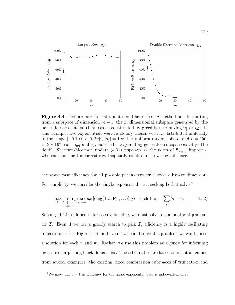
129

20 30 40 500%

20%

40%

60%

80%

100%

m

Failu

reR

ate

vsη θ

Largest Row, qg2

20 30 40 500%

20%

40%

60%

80%

100%

m

Failu

reR

ate

vsη ω

Double Sherman-Morrison, qs2

Figure 4.4 : Failure rate for fast updates and heuristics. A method fails if, startingfrom a subspace of dimension m− 1, the m dimensionial subspace generated by theheuristic does not match subspace constructed by greedily maximizing ηθ or ηω. Inthis example, five exponentials were randomly chosen with ωj distributed uniformlyin the range [−0.1, 0]× [0, 2π]i, |aj| = 1 with a uniform random phase, and n = 100.In 3× 104 trials, qg1 and qsg matched the ηθ and ηω generated subspace exactly. Thedouble Sherman-Morrison update (4.31) improves as the norm of SIm−1 improves,whereas choosing the largest row frequently results in the wrong subspace.

the worst case efficiency for all possible parameters for a fixed subspace dimension.

For simplicity, we consider the single exponential case, seeking b that solves2

maxb

minθ=[ω,a]>

ω∈C−

max|I|=m

ηθ([diag(Fb0 ,Fb1 , . . .)]·,I) such that∑j

bj = n. (4.52)

Solving (4.52) is difficult: for each value of ω, we must solve a combinatorial problem

for I. Even if we use a greedy search to pick I, efficiency is a highly oscillating

function of ω (see Figure 4.9), and even if we could solve this problem, we would need

a solution for each n and m. Rather, we use this problem as a guide for informing

heuristics for picking block dimensions. These heuristics are based on intuition gained

from several examples: the existing, fixed compression subspaces of truncation and

2We may take a = 1 as efficiency for the single exponential case is independent of a.

130

decimation (Section 4.5.1) and new sets of parent coordinates that use fixed blocks

bj = r (Section 4.5.2) and geometric blocks (bj = rj) (Section 4.5.3). Using intuition

from these examples, we build block dimensions that solve an approximation of (4.52)

(Section 4.5.4). We term these block dimensions rationally chosen blocks, since they

built to solve (4.52) rather than some preconcived rule. These rationally constructed

subspaces turn out to have comparable performance to the much simpler geometric

blocks. Attempts to solve (4.52) starting with block dimensions provided by these

heuristics provides only marginally better subspaces (Section 4.5.5). For simplicity, we

recommend using geometric blocks with a growth rate of r = 4, i.e., G4(n). However,

if ω is restricted to a small subset of the complex plane, there may be better parent

coordinates than G4(n).

4.5.1 Truncation and Decimation

An existing compression approach is to either truncate the measurements, removing

the last n − m entries in y, or decimate the measurements, keeping only every rth

measurement. Both correspond to taking parent coordinates with n size 1 blocks.

However, there is no tailoring of subspaces specific to ω; these coordinates are fixed

from the outset. This avoids the cost of constructing a subspace, but yields inefficient

subspaces in comparison to tailored compression spaces. As Figure 4.5 illustrates,

truncation works well when decay is strong as there is little information in the tail of

the signal; decimation works well when decay is weak as a longer base line allows more

accurate frequency measurements. However, decimation risks aliasing exponentials

with high frequencies, making them appear with a lower frequency.

131

512

256m = 16

−101 −100 −10−1 −10−2 −10−3 −10−40%

20%

40%

60%

80%

100%

Reω

η ω(W

)

Truncation, W = I·,1:m

r = 2 m = 512

3 341

4 256

8 128

−101 −100 −10−1 −10−2 −10−3 −10−40%

20%

40%

60%

80%

100%

1/2

1/3

1/41/5

1/8

Reω

Decimation, W = I·,1:r:n

Figure 4.5 : The efficiency of truncating and decimating measurements. The leftplot shows efficiency for various lengths of the truncated y in powers of two; theright plot show the same for decimation rates two through eight. In these examplesn = 1024, and since there is only a single exponential, performance is independent ofIm (ω).

132

4.5.2 Fixed Blocks

Inspired by the short time Fourier transform, the first set of novel block dimensions

splits U into equal sized Fourier blocks, giving parent coordinates

Kr(n) = diag(Fr,Fr, . . . ,Fr,Fr mod n). (4.53)

There are two important limits: r = n yields the Fourier transform (Kn(n) = Fn)

and r = 1 yields the identity matrix (K1(n) = I).

As Figure 4.6 shows, this approach does not yield efficient subspaces for all

amounts of damping. When r = n, good subspaces are generated for lightly damped

exponentials (−1 Reω < 0), but poor subspaces are generated for strongly damped

exponentials (Reω 0). Conversely, taking r = 1 has the opposite behavior: it gen-

erates good subspaces for strong damping but bad subspaces for weak damping. The

middle way, taking r ≈√n does well for intermediate values, but scales poorly as

n→∞, as Figure 4.7 shows.

4.5.3 Geometric Blocks

To better choose blocks, consider the two limits for the real part of ω. If Reω 0,

then most of the energy in V(ω) and V′(ω) is concentrated in the first few entries.

As these vectors decay rapidly, they are strongly non-periodic and, correspondingly,

their energy will be spread through out all the entires of F∗b0v0(ω). So all the entries

of the first block will likely need to be in the index set I; hence a large first block

would be inefficient. Conversely, if damping is light (−1 Reω < 0), then V(ω) is

well approximated by a few columns of F∗bjvj(ω). The larger the block, the better the

resolution, as Imω will be closer to a Fourier frequency φk = e2πik/bj , and the larger

the block, the larger the biggest entry in F∗bjvj(ω). As weak damping implies V(ω)

-

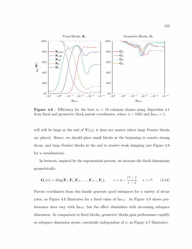
133

−101 −100 −10−1 −10−2 −10−3 −10−40%

20%

40%

60%

80%

100%

Reω

η ω(W

)Fixed Blocks, Kr

K1024

K128

K32

K8

K1

−101 −100 −10−1 −10−2 −10−3 −10−40%

20%

40%

60%

80%

100%

Reω

Geometric Blocks, Gr

G2

G3

G4

G5

Figure 4.6 : Efficiency for the best m = 10 columns chosen using Algorithm 4.1from fixed and geometric block parent coordinates, where n = 1024 and Imω = 1.

will still be large at the end of V(ω), it does not matter where large Fourier blocks

are placed. Hence, we should place small blocks at the beginning to resolve strong

decay, and large Fourier blocks at the end to resolve weak damping (see Figure 4.8

for a visualization).

In between, inspired by the exponentials present, we increase the block dimensions

geometrically:

Gr(n) = diag(F1,Fr,Fr2 , . . . ,Frq−1 ,Fs), s = n− rq − 1

r − 1, s > rq. (4.54)

Parent coordinates from this family generate good subspaces for a variety of decay

rates, as Figure 4.6 illustrates for a fixed value of Imω. As Figure 4.9 shows per-

formance does vary with Imω, but the effect diminishes with increasing subspace

dimension. In comparison to fixed blocks, geometric blocks gain performance rapidly

as subspace dimension grows, essentially independent of n, as Figure 4.7 illustrates.

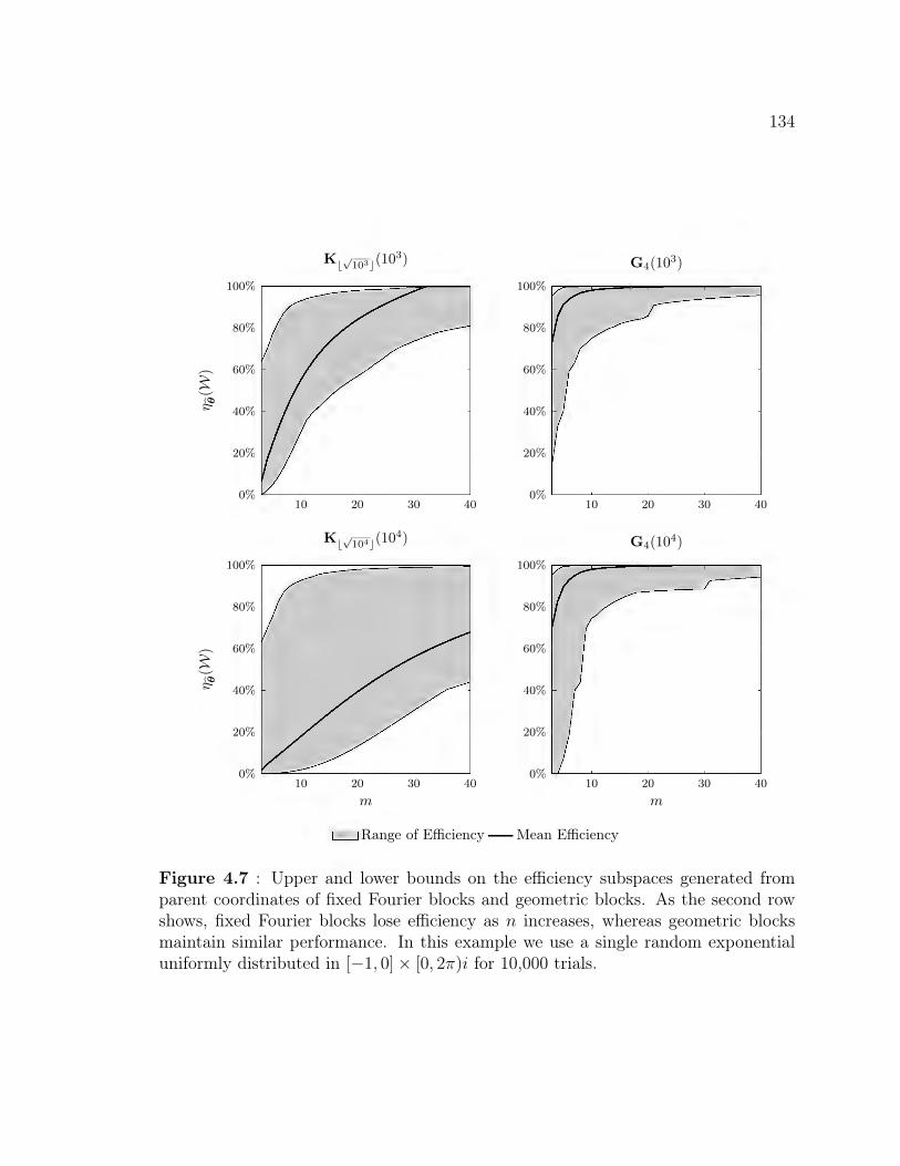
134

10 20 30 400%

20%

40%

60%

80%

100%

η θ(W

)

Kb√103c(10

3)

10 20 30 400%

20%

40%

60%

80%

100%

G4(103)

10 20 30 400%

20%

40%

60%

80%

100%

m

η θ(W

)

Kb√104c(10

4)

10 20 30 400%

20%

40%

60%

80%

100%

m

G4(104)

Range of Efficiency Mean Efficiency

Figure 4.7 : Upper and lower bounds on the efficiency subspaces generated fromparent coordinates of fixed Fourier blocks and geometric blocks. As the second rowshows, fixed Fourier blocks lose efficiency as n increases, whereas geometric blocksmaintain similar performance. In this example we use a single random exponentialuniformly distributed in [−1, 0]× [0, 2π)i for 10,000 trials.

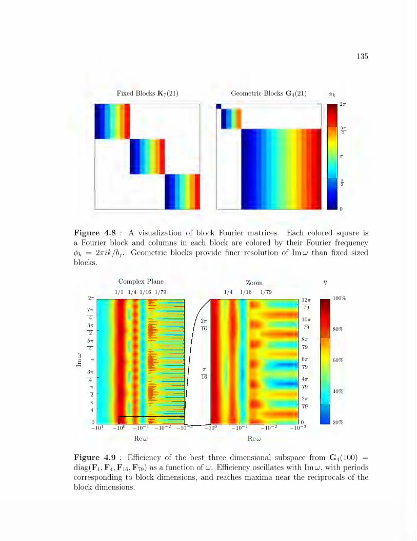
135

Fixed Blocks K7(21) Geometric Blocks G4(21)

0

π2

π

3π2

2π

φk

Figure 4.8 : A visualization of block Fourier matrices. Each colored square isa Fourier block and columns in each block are colored by their Fourier frequencyφk = 2πik/bj. Geometric blocks provide finer resolution of Imω than fixed sizedblocks.

−10−3−10−2−10−1−100−1010

π

4

π

2

3π

4

π

5π

4

3π

2

7π

4

2π1/791/161/41/1

Reω

Imω

Complex Plane

−10−3−10−2−10−1−1000

2π

79

4π

79

6π

79

8π

79

10π

79

12π

79

1/791/161/4

π

16

2π

16

Reω

Zoom

20%

40%

60%

80%

100%

η

Figure 4.9 : Efficiency of the best three dimensional subspace from G4(100) =diag(F1,F4,F16,F79) as a function of ω. Efficiency oscillates with Imω, with periodscorresponding to block dimensions, and reaches maxima near the reciprocals of theblock dimensions.

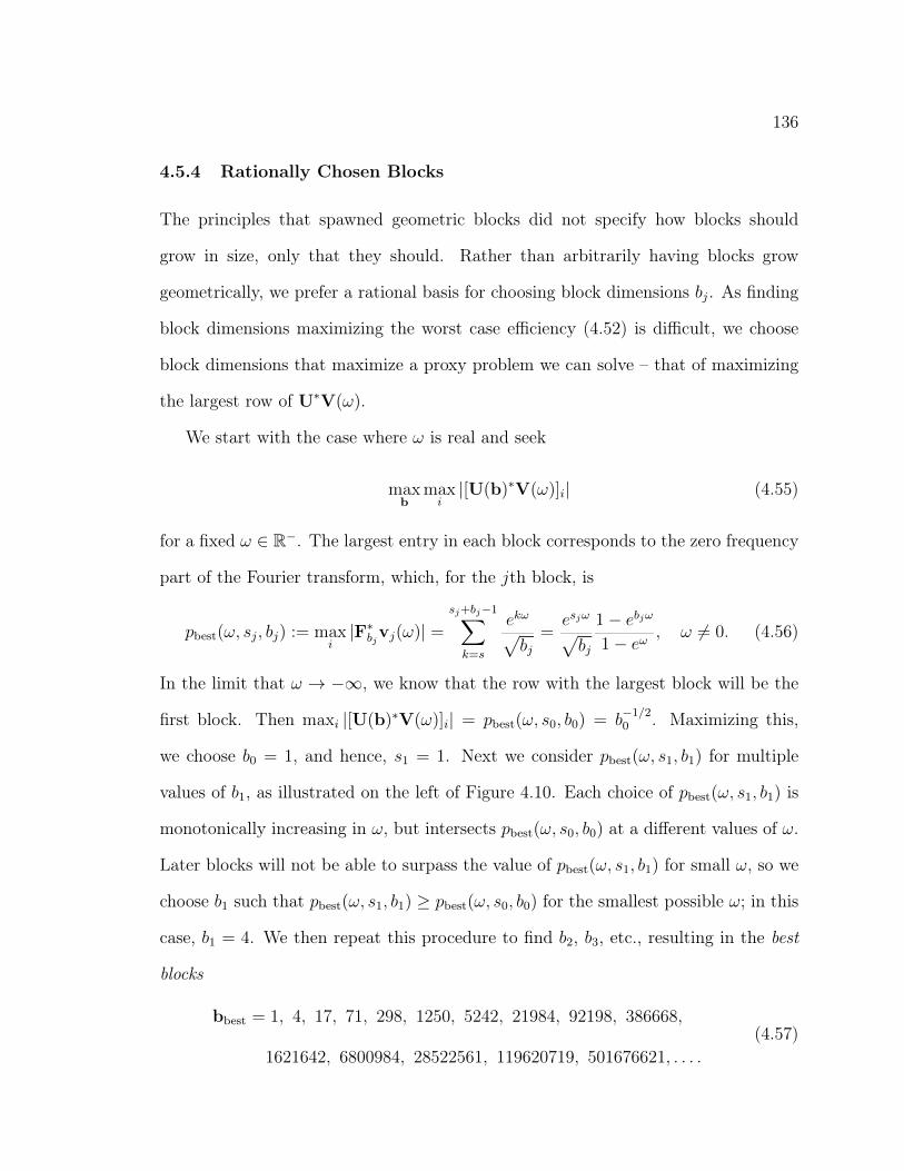
136

4.5.4 Rationally Chosen Blocks

The principles that spawned geometric blocks did not specify how blocks should

grow in size, only that they should. Rather than arbitrarily having blocks grow

geometrically, we prefer a rational basis for choosing block dimensions bj. As finding

block dimensions maximizing the worst case efficiency (4.52) is difficult, we choose

block dimensions that maximize a proxy problem we can solve – that of maximizing

the largest row of U∗V(ω).

We start with the case where ω is real and seek

maxb

maxi|[U(b)∗V(ω)]i| (4.55)

for a fixed ω ∈ R−. The largest entry in each block corresponds to the zero frequency

part of the Fourier transform, which, for the jth block, is

pbest(ω, sj, bj) := maxi|F∗

bjvj(ω)| =

sj+bj−1∑k=s

ekω√bj

=esjω√bj

1− ebjω

1− eω, ω 6= 0. (4.56)

In the limit that ω → −∞, we know that the row with the largest block will be the

first block. Then maxi |[U(b)∗V(ω)]i| = pbest(ω, s0, b0) = b−1/20 . Maximizing this,

we choose b0 = 1, and hence, s1 = 1. Next we consider pbest(ω, s1, b1) for multiple

values of b1, as illustrated on the left of Figure 4.10. Each choice of pbest(ω, s1, b1) is

monotonically increasing in ω, but intersects pbest(ω, s0, b0) at a different values of ω.

Later blocks will not be able to surpass the value of pbest(ω, s1, b1) for small ω, so we

choose b1 such that pbest(ω, s1, b1) ≥ pbest(ω, s0, b0) for the smallest possible ω; in this

case, b1 = 4. We then repeat this procedure to find b2, b3, etc., resulting in the best

blocks

bbest = 1, 4, 17, 71, 298, 1250, 5242, 21984, 92198, 386668,

1621642, 6800984, 28522561, 119620719, 501676621, . . . .

(4.57)

137

The largest of the resulting curves of pbest(ω, sj, bj) is maxi |[U(bbest)∗V(ω)]i| and

approximates ‖V(ω)‖2, as shown in the right side of Figure 4.10.

123468

4

−102 −101 −100 −10−1 −10−20

1

2

3

4

5

Reω

‖V(ω‖2SelectedUnselected

−102 −100 −10−2 −10−4 −10−610−1

100

101

102

103

Reω

‖V(ω)‖2Selected

Figure 4.10 : Picking the block dimensions for the ‘best’ block parent coordinates.On the left, the horizontal red line shows the partial sum of the first block pbest(ω, 1, 0).The other red and blue lines show pbest(ω, 1, b1) for various b1 values (b1 = 1, 2, . . . , 8)indicated by the number to the right of the curve. The choice intersecting pbest(ω, 1, 0)earliest is b1 = 4 (in red). The value for pbest(ω, sj, bj) is bounded above by ‖V(ω)‖2(for n =∞), shown in black. On the right, we see a sequence of pbest resulting fromoptimal choices of sj and bj. The maximum of these curves approximates ‖V(ω)‖2.

We call these the best blocks because restricting to ω ∈ R− is a best case scenario.

For any Fourier block, 0 is Fourier frequency and ‖F∗bjvj(α+ iβ)‖∞ attains one of its

bj maxima over β when β = 0 (the remaining being the bj roots of unity). In contrast,

the worst case scenario is when β is precisely between two Fourier frequencies. We

can define the largest entry for the worst case imaginary part of ω, in an analogous

way to pbest:

pworst(ω, sj, bj) :=

∣∣∣∣∣∣sj+bj−1∑

k=s

ekω+iπ/bj√bj

∣∣∣∣∣∣ . (4.58)

Following the same procedure to generate bbest, using pworst instead, results in the

138

worst blocks

bworst = 1, 11, 60, 319, 1279, 5119, 20479, 81919, 327679, 1310719,

5242879, 20971519, 83886079, 335544319, 1342176956, . . . .

(4.59)

The best and worst blocks were generated by maximizing U(b)∗V(ω), but we

could also consider the derivative U(b)∗V′(ω). The analogous functions to pbest and

pworst are not monotonic for the first two blocks. Defining the first two entries using

the same values as in bbest and bworst results in the sequences

b′best = 1, 4, 7, 18, 45, 113, 285, 717, 1806, 4548, 11452, 28837, 72615, . . . ;

b′worst = 1, 11, 27, 84, 265, 838, 2650, 8381, 26506, 83828, . . . .

None of the sequences in this section correspond to known integer sequences,

but all grow approximately geometrically with a growth coefficient around four. Fig-

ure 4.11 illustrates the performance for each of set of block dimensions. If n is not the

sum of the block dimensions, the last block is enlarged (as with geometric blocks).

For example, if n = 100 then bbest(100) = [1, 4, 17, 78]. In this example, each

block sequence has similar worst case performance, but best blocks has a larger mean

performance, similar to G4.

There are many alternative ways to construct sets of block dimensions. For ex-

ample, we could work from ω = 0 towards −∞ (customized to a particular value

of n) or we could balance performance over a range rather than seeking the block

dimension with the earliest intersect. However, as these procedures only consider the

largest row, and not a larger subspace, none of these procedures are likely to yield

significantly better compression subspaces.

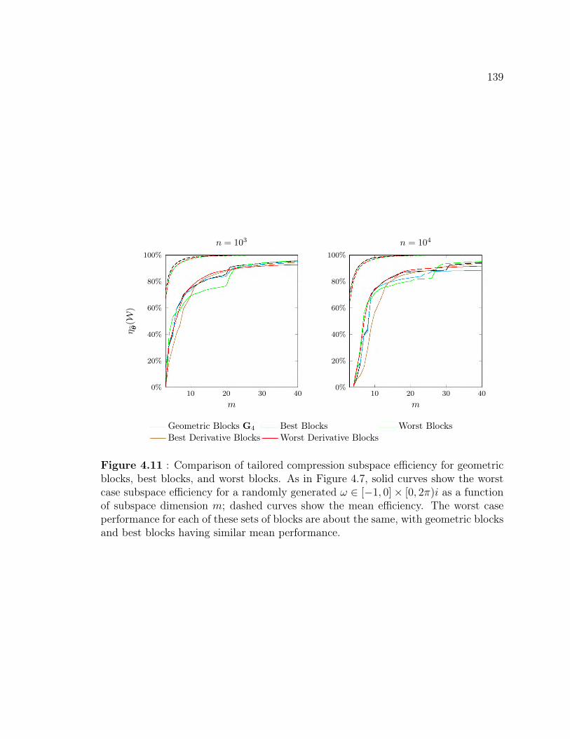
139

10 20 30 400%

20%

40%

60%

80%

100%

m

η θ(W

)

n = 103

10 20 30 400%

20%

40%

60%

80%

100%

m

n = 104

Geometric Blocks G4 Best Blocks Worst BlocksBest Derivative Blocks Worst Derivative Blocks

Figure 4.11 : Comparison of tailored compression subspace efficiency for geometricblocks, best blocks, and worst blocks. As in Figure 4.7, solid curves show the worstcase subspace efficiency for a randomly generated ω ∈ [−1, 0]× [0, 2π)i as a functionof subspace dimension m; dashed curves show the mean efficiency. The worst caseperformance for each of these sets of blocks are about the same, with geometric blocksand best blocks having similar mean performance.

/;;~­f' , , , ,

140

10−610−510−410−310−210−110010110265%

70%

75%

80%

85%

90%

95%

100%

Reω

min

Imω∈[0,2π)η ω

(W)

G4 G4 optimizedbbest bbest optimizedbworst bworst optimized

G4(104) 1 4 16 64 256 1024 8635

optimized 1 3 17 64 256 1024 8635bbest(10

4) 1 4 17 71 298 1250 8359optimized 1 4 17 70 298 1251 8359bworst(10

4) 1 11 60 319 1279 8330optimized 1 11 60 320 1279 8329

Figure 4.12 : Optimized sets of block dimensions maximizing (4.52). The optimizedblock dimensions improve the worst case performance by about 5% for G4 and bbest,but decrease efficiency for other values of Reω. In contrast, the performance of bworst

only mildly improves, but also decreases efficiency for other values of Reω. Blocksthat increased in size are marked in red, those that decreased in blue. In this example,n = 10, 000.

4.5.5 Optimizing Block Dimensions

Optimizing block dimensions is difficult. Minimizing the worst-case subspace effi-

ciency requires first finding it, and as Figure 4.9 shows, efficiency of the best subspace

is a highly oscillatory function of Imω. Fortunately, the oscillations have periods cor-

responding to the block dimensions, allowing us to estimate the worst-case ω. Taking

uniform random samples on a line with a fixed real part, we fit a cosine series with

periods corresponding to the block dimensions. The minimum of this series is then

used as the starting value for an optimization iteration (Matlab’s fminsearch), that

141

returns the minimum efficiency ω for a given Reω. This optimization is then repeated

over a grid of Reω to find the worst-case ω in the left half plane. The results are

fed to an outer optimization routine that adjusts the size of the blocks by ±1. The

block dimensions optimized by this procedure are shown in Figure 4.12. The block

dimensions do not move far from their initial values, each initial set of blocks shifting

a single entry between two blocks in the optimized blocks. The resulting parent co-

ordinates have slightly better worst-case performance, but decrease performance for

other Reω.

Due to the cost of computing optimum block dimensions and the minimal im-

provement, we recommend using a precomputed set of block dimensions. As the best

and worst blocks do not do substantially better than G4(n), we recommend using

G4(n) for all problems.

4.6 Linking Compression and Optimization

Compression can introduce many spurious local minima away from where the com-

pression space is tailored. This effect is especially dramatic when small subspaces

are drawn from the geometric block parent coordinates, as illustrated in Figure 4.13.

To prevent convergence to a spurious minimum, as θ moves during optimization the

compression space must remain efficient.

We propose two approaches to maintain an efficient compression space as θ is

optimized. The faster approach is to precompute an efficient compression space based

on prior knowledge of θ. If we know θ ∈ T ⊂ Cp, we can build a fixed subspace W

where ηθ(W) > η for all θ ∈ T . Then if the initial estimate is sufficiently close,

iterations of θ should remain in T . To build this subspace, we can sample θ ∈ T

uniformly, and for each sample append indices maximizing ηθ(W), as described in

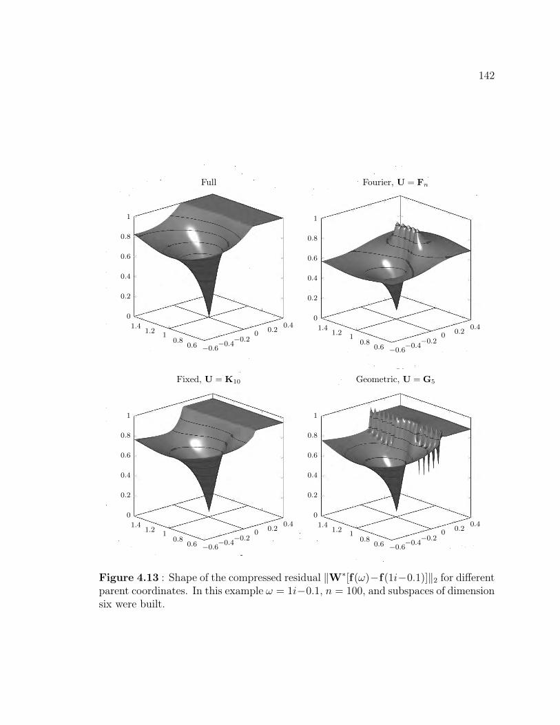
142

−0.6−0.4

−0.20

0.20.4

0.60.8

11.2

1.4

0

0.2

0.4

0.6

0.8

1

Full

−0.6−0.4

−0.20

0.20.4

0.60.8

11.2

1.4

0

0.2

0.4

0.6

0.8

1

Fourier, U = Fn

−0.6−0.4

−0.20

0.20.4

0.60.8

11.2

1.4

0

0.2

0.4

0.6

0.8

1

Fixed, U = K10

−0.6−0.4

−0.20

0.20.4

0.60.8

11.2

1.4

0

0.2

0.4

0.6

0.8

1

Geometric, U = G5

Figure 4.13 : Shape of the compressed residual ‖W∗[f(ω)−f(1i−0.1)]‖2 for differentparent coordinates. In this example ω = 1i−0.1, n = 100, and subspaces of dimensionsix were built.

143

Section 4.4, until the threshold is reached. However, this precomputed subspace

approach may not be viable if T is unknown or T is large, as the dimension of

W may be on the order of n. Alternatively, we can refine the compression space

alongside the optimization of θ, interspersing updates to W between iterations of θ.

The following two sections give an example of each approach.

4.6.1 Precomputed Compression Subspaces

In this example, we consider the canonical signal processing problem of determining

the frequency ω ∈ iR of a single undamped exponential yk = aωk from n mea-

surements. This problem appears in many real-time applications (e.g., Doppler

radar) and has been a topic of continued interest in electrical engineering since

the 1970s [131]. The simplest approach uses the largest entry of the Fourier trans-

form k = argmaxj |[F∗y]j|, estimating ω = 2πik/n (see discussion in Section 3.4.3).

The resolution of this approach is limited to ±πi/n, leading many authors to seek

high resolution estimates using interpolation (e.g., [81, 128]), an iterative procedure

(e.g., [2, 106]), or a combination of the two (e.g., [107]). The goal is a fast algorithm

for computing ω in real time that can be constructed either in hardware or low level-

software. In the following example, we show how compression can provide a more

accurate and faster estimate of ω. Moreover, unlike previous algorithms, compression

allows us to prescribe the accuracy of the estimator arbitrarily.

For parent coordinates, we choose the Fourier matrix F, as ω is purely imaginary

in this application. Additionally, due to the shift invariance of the Fourier transform,

if we find a set of parent coordinates for ω = 0, then shifting all the coordinates by

k mod n yields a set of coordinates tailored to 2πik/n; i.e., if I0 is tailored to ω = 0,

144

3

4

5

6

10

90

−1 −0.5 0 0.5 165%

70%

75%

80%

85%

90%

95%

100%

Imω nπ

η ω(W

)Compression Space Efficiency

m minω∈[−π

n,πn]iηω(W) I

1 · 02 36.8% 13 67.4% 10234 74.0% 25 80.9% 10226 83.7% 37 86.5% 10218 88.0% 49 90.0% 102010 90.5% 1019...

......

90 99.0% 979

Figure 4.14 : Fixed compression space for undamped exponentials. The figure onthe left the efficiency for compression spaces of increasing dimension between bins ofthe Fourier transform ([−π/n, π/n]) for subspaces of increasing dimension. The tableon the right shows the minimum efficiency of these subspaces for a given dimensionm, and the near optimal nested index set I is read down the right column.

then

Ik = j + k mod n : ∀j ∈ I0 (4.60)

is tailored to 2πik/n. To estimate ω, we perform the three steps summarized in Algo-

rithm 4.4. First, we find the largest value in the Fourier transform, k = argmaxj |[F∗y]|j,

yielding the initial estimate ω = 2πik/n. Next, we use the interpolation algorithm of

Quinn [128] to improve the estimate of ω, requiring O(1) operations. Finally, we opti-

mize ω on Wk = span F·,Ik using Variable Projection with Kaufman’s simplification.

As we see in Figure 4.15, starting from the nearest Fourier frequency, Gauss-Newton

requires three iterations to converge. However, starting from Quinn’s interpolation

estimate reduces this requirement to a single iteration.

Compression requires fewer operations than other high efficiency algorithms, as

145

Algorithm 4.4: Estimating a single undamped exponential with a fixed sub-spaceInput : Measurements y ∈ Cn, compression space I for ω = 0

Output: Frequency ω, amplitude a1 w← F∗y;2 k ← argmaxj |[w]j|;3 I ← j + k mod n : j ∈ I;4 w← [w]I ;5 ω ← 2πik/n;6 Use Quinn’s interpolation to improve estimate of ω;

Gauss-Newton loop using VARPRO functional.7 for j = 1, 2, . . . , N do8 V← [F∗V(ω)]I ;9 V← [F∗V(ω)]I ;

10 α← V∗V;11 a← α−1(V∗w);12 r← w −Va;

Kaufman’s simplification of the VARPRO Jacobian.13 J← a[V − α−1V(V∗V)];14 x← (J∗r)/(J∗J);15 ω ← ω + Im (x);

146

shown in Figure 4.15. Each algorithm begins with anO(n log n) fast Fourier transform

to compute the nearest Fourier frequency. Then fixed point methods, such as those

proposed by Aboutanios and Mulgrew [2] and Minhas and Gaydecki [107] require

2n operations per iteration, with Aboutanios and Mulgrew’s algorithm requiring two

iterations and Minhas and Gaydecki’s algorithm only one. However starting from

Quinn’s interpolation estimate, an O(1) operation, our compressed approach requires

only O(8m) operations. Hence compression is the fastest algorithm, requiring only

≈ 720 flops beyond the Fourier transform to estimate ω to higher than 99% efficiency

when n = 1024, whereas Minhas and Gaydecki’s algorithm requires ≈ 2048 flops.

Moreover, compression gives a simple mechanism to generate estimators with a

prescribed efficiency. Further improvements may be possible with other parent coor-

dinates (e.g., G4) and explicit consideration of the covariance of a purely imaginary

ω versus a complex ω in constructing the compression space. Additionally, some ap-

plications also seek decay rates (i.e., ω ∈ C−), e.g., [1, 16]. Compression can also be

applied here in a similar fashion to build fast estimators.

4.6.2 Dynamically Computed Compression Subspaces

If building a fixed compression space is impractical, an alternative is to buildW while

optimizing θ, at a penalty of an additional O(p2) operations per candidate to update

the compression space. In practice, this additional cost is small, as the following

example shows.

One situation requiring a dynamic compression space is the blind exponential

fitting problem: given only measurements y and the number of exponentials p, this

problem seeks the exponential parameters ω and a. Figure 4.16 shows a numerical ex-

periment that compares four variants of the Peeling Method (Section 3.6) to Kung’s

147

0

1

23

−1 −0.5 0 0.5 10%

10%

20%

30%

40%

50%

60%

70%

80%

90%

100%

Imω nπ

η ωCompression, Nearest

1

2

−1 −0.5 0 0.5 10%

10%

20%

30%

40%

50%

60%

70%

80%

90%

100%

Imω nπ

η ω

Aboutanios and Mulgrew (Alg. 1)

0

1

−1 −0.5 0 0.5 10%

10%

20%

30%

40%

50%

60%

70%

80%

90%

100%

Imω nπ

η ω

Compression, Quinn Interpolation

1

−1 −0.5 0 0.5 10%

10%

20%

30%

40%

50%

60%

70%

80%

90%

100%

Imω nπ

η ωMinhas and Gaydecki

Figure 4.15 : The statistical efficiency for several high efficiency single undampedexponential fitting algorithms. Each plot shows estimates of the efficiency of eachestimator for different values of ω from 105 trials, where n = 1024 and ε = 1 (cor-responding to a signal-to-noise ratio of 0 dB). The left side shows a new algorithmbased on compression, and the right side shows two existing algorithms. The topleft shows iterations of VARPRO with Kaufman’s simplification, starting from thenearest Fourier frequency, and the number indicates how many iterations were taken.The bottom left shows the same, but starting from Quinn’s interpolation estimateof ω. In these examples an m = 90 subspace was used, with a minimum efficiencyof 99%. The right plots show two existing algorithms, where, again, numbers showhow many iterations were taken. Compression starting from Quinn’s interpolationestimate requires ≈ 65% fewer operations beyond the FFT than the current leader,Minhas and Gaydecki.

148

Method, representative of the numerically stable variants of Prony’s Method, and

Variable Projection using the true values ω as initial estimates. As Kung’s Method

solves a dense SVD of size n/2, the computational cost grows cubically in the number

of measurements n. In contrast, the cost Variable Projection with the true initial

estimates grows linearly in n for the full problem, whereas the cost is approximately

constant for the compressed problem. The four variants of the Peeling Method use

either the Orthogonalized Matrix Pencil Method (OMPM) (Section 2.8) or the largest

entry in the Fourier transform of the residual (Section 3.4.3) and either solve the com-

pressed problem or the full problem at each iteration. One hopes the Orthogonalized

Matrix Pencil Method will provide better initial estimates of ω, requiring fewer op-

timization iterations to converge. However, the additional computation required to

use the OMPM and the occasional poor initial estimates of ω make this approach

unviable. In contrast, the largest entry in the Fourier transform of the residual is

faster and provides better estimates. This experiment also shows that compression is

only computationally advantageous for large problems, say n > 800. Although in this

example, the compressed problems are of dimension m ≈ 10p, the smaller compressed

matrices W∗V(ω) and W∗V(ω) cost more to compute. The large increase in wall

clock time between n = 104 to n = 4 ·104 and beyond n = 105 for the Peeling Method

using the largest entries in the Fourier transform of the residual and compression

correspond to where the initial values led to a spurious minima. The additional com-

putation time is a result of solving the full problem with the estimates from Peeling.

In most cases, the cost of this additional step is small, since the estimates of ω are

approximately local minima. However, when Peeling converges to a spurious min-

ima, many steps of the full problem are required until the convergence criteria are

met. This combination of the Peeling Method with compression provides a promising,

149

3

1

103 104 10510−2

10−1

100

101

102

Problem size n

Tim

e(s

econ

ds)

Wall Clock Time for Blind Exponential Fitting

Peeling, OMPM, fullPeeling, OMPM, comp.Peeling, LFR, fullPeeling, LFR, comp.VARPRO, TF, fullVARPRO, TF, comp.Kung’s Method

Figure 4.16 : Wall clock time for several blind exponential fitting algorithms. Wecompare four variants of the Peeling Method using initial conditions provided bythe Orthogonalized Matrix Pencil Method (OMPM) or by the largest entry of theFourier transform of the residual (LFR) and that solve either the full or compressedproblem. For comparison, we also include the wall clock times of Kung’s Method andVariable Projection (VARPRO) using the true values of ω as initial estimates (TF).The measurements y were generated from the p = 11 model from [153, Table 1]adding complex noise of standard deviation 1, Reported times were averaged overten trials of each method implemented in Matlab 7.14 running in Linux on a Inteli3-2120 CPU with a 3MiB L1 cache and 3781MB RAM.

fast solution to the blind exponential fitting problem with superior performance to

existing methods such as Kung’s Method (O(n log n) versus O(n3)).

We can guarantee that the compressed estimates converge provided the compres-

sion space always grows in dimension. At the kth step, compression provides an

approximate gradient gk of the true gradient gk with error ek, where3

gk = gk + ek = ek +∑j∈I

∇x[U∗f(θ)]j|θ=θk

. (4.61)

If we used a gradient descent method with step size ‖H(θk)‖−12 , successive iterates of

θ have weak linear convergence by [50, Thm. 2.2] provided ‖ek‖22 ≤ Bk and |I| grows

such that limk→∞Bk+1/Bk ≤ 1 (e.g., |I| grows linearly in k). Our box-constrained

------------------+-------+---

150

trust region method will generally have better performance, since these gradient de-

scent steps are included in the search space. Further, if full efficiency estimates are

required, we can solve increasingly large compressed problems until they converge,

and then use only a few final iterations of the full problem to refine ω.

3We write the compressed gradient in this form to emphasize the connection to incremental

gradient methods, cf. [50, §3, first equation]. We omit the normalization by |I| since the selected

rows are not typical.

151

Chapter 5

Damping in Vibrating Strings

Our investigation of the exponential fitting algorithm described in the previous chap-

ters was motivated by the desire to approximate spectral properties of a damped,

vibrating string. A simple description of the transverse motion of a thin elastic string

subjected to viscous damping is given by

utt(s, t) = c2uss(s, t)− 2δ(s)ut(s, t)

u(0, t) = u(π, t) = 0, u(s, 0) = u0(s), ut(s, t) = u1(s),

(5.1)

where u(s, t) is the transverse displacement, s is the position along the rest config-

uration string of length π, and t is time; see, e.g. [147, § 131]. After separation of

variables, for constant δ

u(s, t) =∑n6=0

aneωnt sin(ns), (5.2)

the eigenvalues ωn of the differential operator associated with (5.1) are

ω±n = −δ ±√δ2 − c2n2, n = 1, 2, . . . . (5.3)

A challenging class of modern problems seeks information about the underlying

differential equation from knowledge of the spectrum. One such inverse eigenvalue

problem recovers δ(s) from knowledge of ωnn6=0. Cox and Embree have recently

provided an algorithm to perform this reconstruction for an even damping function

δ(s) [37]. We would like to ask: can we perform this reconstruction using experimen-

tal data? This is not without precedent: recently Cox, Embree, and Hokanson were

152

able to determine the masses and locations of beads on a string from eigenvalue esti-

mates [38], realizing in the laboratory the classical inverse spectral theory for discrete

self-adjoint systems [52]. However, reconstructing the damping function is challeng-

ing. Rather than simply requiring Imω, as the (undamped) beaded string does, for

damped problems Reω is needed as well. Further, the reconstruction algorithm of

Cox and Embree hinges on specific asymptotic eigenvalue estimates that can

In this chapter, we investigate how well the vibrations of a metal piano wire

match the theoretical model of a viscously damped string. First we describe the

experimental apparatus, examine the background effects, and calibrate the detectors.

Next, we build a robust variant of compressed exponential fitting to estimate Reω.

Finally, we compare these eigenvalue estimates to those predicted by string models of

increasing accuracy, with the goal of determining the appropriate model of a vibrating

string. With better knowledge of the physical model, future researchers should be able

to recover δ(s) from experimental measurements of ω by modifying the Cox-Embree

algorithm to apply to a more physically realistic non self-adjoint system.

5.1 Experimental Apparatus

In our experiments we seek to recover the eigenvalues of the linear operator that

describes the motion of a string, parameterized by the pressure of the surrounding

air. We are particularly interested in how the pressure affects the real parts of these

eigenvalues, which describe the asymptotic rate at which energy decays in the string;

see, e.g., [36]. This objective differs from previous experimental work which observed

chaos and other nonlinear effects in vibrating strings; see, e.g., [62, 110]. As a result,

our apparatus and procedure differs from these previous experiments, which drove the

string continuously and measured the equilibrium amplitude of vibration. Although

153

vacuum chamber

collet and vice collet and vice

photointerrupterforce transducer tensioner

magnetic driverstring

Aluminium U-channel

Figure 5.1 : Cutaway diagram showing the vacuum chamber and string apparatus.

the amplitude at equilibrium does correspond to the real part of the eigenvalues,

nonlinear effects easily influence this value. Instead, we measure free response motion

of the string, with initial conditions provided by driving the string at a frequency near

resonance. The resulting time series is, to first approximation, a sum of exponentials

plus noise, where the exponential coefficients correspond to the desired eigenvalues.

Our apparatus derived from the set-up described in [38], originally built with

assistance from Sean Hardesty based on a design by Mr. Fan Tao of J. D’Addarío &

Co. The electronics were built by Jeffrey Bridge, and Stan Dodds provided assistance

in the assembly of the vacuum chamber. As illustrated in Figure 5.1, our apparatus

consists of a steel string that is connected at one end to a force transducer and, at

the other end, wound along a spindle to apply tension. In between the string passes

through two collets, mounted in collet vises, clamping the string to enforce Dirichlet

boundary conditions. Between the collets, the string passes through a photodetector

l I 1 - j • t -

154

Table 5.1 : Material properties of the string

Property Value

Standard ASTM A228Description Plated Steel Music WireManufacturer Mapes Piano String CompanyDiameter 0.015 inLength 433/16 inDensity 7850 kg/m3

Yield Strength 2500MPa to 2880MPaYoung’s Modulus 210GPaPoisson’s Ratio 0.313Shear Modulus 80.0GPaComposition C (0.7–1.0%); Fe (97.8–99%); Mn (0.20–0.60%);

P (≤ 0.025%); Si (0.10–0.30%); S (≤ 0.030%)

measuring the displacement of the string (described in §5.1.4) and an electromagnetic

drive coil (described in §5.1.3). Rather than being placed on an optical table as in [38],

the string and its supports are mounted on an aluminum U-channel to fit inside the

16 in diameter PVC pressure vessel. The remainder of this section provides further

detail on each component of this experiment.

5.1.1 String

For our string we use a 0.015 in diameter steel music wire (ASTM A228), whose

properties are listed in Table 5.1. This alloy and tempering of steel is often used in

metal music instrument strings, either by itself or wound with a soft metal wire to

increase mass without increasing bending stiffness.

This steel wire has many advantages from an experimental standpoint. First, we

can place the string under a high tension, typically from 100N to 200N. Increased

tension decreases the amplitude of vibrations, given a constant energy, which de-

155

creases errors due to the linearization in Section 5.3.1. Second, although tension is

high, we are still well within the elastic limit: at 200N, the string is under a stress

of 1.75GPa, well below the yield strength of 2.5GPa. The string would need to dis-

place 4 cm from equilibrium at the midpoint in the fundamental mode to exceed this

yield strength – a far larger oscillation than experimentally observed. Consequently,

we can assume that the stress-strain relationship is linear to high accuracy. Third,

non-metal string materials like Nylon tend to creep, increasing in length while under

tension over a period of hours [105, §1.3]. Steel does not exhibit this effect unless

heated to a large fraction of its melting point. Finally, steel strings can be driven

electromagnetically, as we describe in Section 5.1.3.

5.1.2 String Mounting

The string is mounted on a 5 ft long, 9 in wide, and 4 in tall aluminum U-channel with

1/2 in side walls and a 3/8 in thick base. The U-channel then slides inside a 16 in

diameter schedule 40 PVC pipe, which is used as a pressure vessel; the U-channel is

supported by the walls of the pipe. The ends of the pipe are sealed with a 3/8 in thick

aluminum plates with a 16 in O-ring making a pressure seal against the PVC pipe;

the plates are held in place with non-pressure rated PVC end caps. The minimum

pressure this chamber reached was 0.006 bar.

Two holes were drilled in the side of the pressure vessel. One was connected via a

hose to a vacuum pump. The other contained an pass through for the electrical wires

carrying power and returning data from the string and was sealed using epoxy.

156

5.1.3 Excitation and Driver

With the string sealed inside the vacuum chamber, we must excite motion within

the closed chamber. There are three typical approaches: add a mechanical plucker

or shaker (e.g., [63]), place a portion of the string in a magnetic field and run a

current through the string (e.g., [62]), or use an electromagnetic coil to periodically

attract the string (e.g., [42]). The mechanical approach requires either transmitting

the stimulation through the boundary conditions or connecting the interior of the

string to the shaker; both introduce perturbations to the wave equation for which

it is difficult to account for. Passing a current through the string leads to resistive

heating that causes a time-dependent increase in the effective length of the string and,

correspondingly, decreases the frequencies of the eigenvalues [110, §3]. In previous

studies, this was not a significant effect, as the string is conductively cooled by the

surrounding air [62, p. 1551]. However at low pressures the string is only cooled by

radiation and convection through the endpoints – these may not be sufficient to keep

the string cool. Hence, we drive the string with an electromagnet.

The electromagnetic drive coil consists of a rectangular soft iron core and 180 turns

of magnet wire, pictured in Figure 5.2. Although the iron core limits high frequency

transmission, it increases the effect of the electromagnet on the string. The closed loop

contains the magnetic flux, and one end is beveled to a create gradient of magnetic

flux across the gap. When the coil is active, it induces a dipole moment in the wire

which in turn feels a force proportional to gradient of the magnetic field. However,

as the steel string moves in the direction of the gradient, regardless of the polarity of

the field, we drive the electromagnet with a half sine wave: min(a sin(ωt), 0).

157

Figure 5.2 : The electromagnetic drive coil.

158

5.1.4 Photodetector

We record the position of the string by measuring how much the string occults a beam

of light between an LED and a phototransistor mounted on either side of the string.

This resembles the detector described in [62, Fig. 2], but we use a polynomial model of

the detector to better infer the actual position of the string, rather than assuming the

response is linear. In our device, both the LED and phototransitors are part of a single

Fairchild QVE00034 package. Two of these LED/phototransistor pairs are mounted

in a plastic block at right angles, allowing us to measure the motion of the string in

the two transverse planes of motion, pictured in Figure 5.3. The attached printed

circuit board (designed by Jeffrey Bridge) converts the current response of the diodes

to light to a voltage, which is then read by a National Instruments USB-6251 data

acquisition board (DAQ). Unless otherwise specified, all experiments record voltages

at 105 samples per second in both axes. There is a 5× 10−6 s lag between the time

when the x and y channels are read that we consider negligible. The whole assembly

is mounted on a 2-axis micrometer stand, allowing us to position the detector in an

optimal location to measure the motion of the string – near where both channels read

0V.

Background

To determine the background noise in the photodetector, we conduct two experi-

ments: one with the string starting from rest and another starting from rest with

a cloth placed over a part of the string to damp vibrations. The additional damp-

ing removes vibrations induced by the environment. Figure 5.4 shows the discrete

Fourier transform for both measurements. Without the cloth present, some peaks

grow larger by a factor of 1.5. This indicates that although there is some transmis-

159

Figure 5.3 : The photodetector apparatus. A pair of phototransistors are embeddedin the white block on the right and moved by the black micrometer stand on thefar right. The printed circuit board amplifies and converts the current output of thephototransistor to a voltage.

160

sion of energy from the environment, the size of these peaks (0.07V) indicates the

amount of mechanical energy transmitted is minimal.

However, several large peaks remain. These peaks in the Fourier transform are

large in comparison to the background noise: however this noise is orders of magnitude

smaller than the signal from physical vibrations of the string. Multiples of 1000Hz

(and, to a lesser extent, 500Hz) appear in both axes. Due to its purity and frequency,

this is likely background electrical noise; this signal remains despite changing the

sample rate of the data acquisition card. Another set of peaks center near 20Hz. We

attributed these to the resonances of table on which the vacuum chamber is mounted.

Finally, there is broad hump around 14 kHz in the X-axis and 12 kHz in the Y-axis.

We attribute this to the 12.6 kHz fundamental of the pier on which the photodetector

is mounted (a 4 in× 1 in× 1 in block of aluminum)1. The splitting of this resonance

is due to the additional moment of inertia from the photodetector assembly in one

axis, but not the other.

Least squares methods assume the residual is normally distributed. However, the

data acquisition card samples a finite number of voltages due to its inherent 16-bit

resolution. To be justified in using least squares methods, the background should be

approximately normally distributed. Examining a histogram of the voltage readings

in Figure 5.5, we see that a normal distribution describes the tails well. However, the

peak of both distributions does not fit the measurements as well; this may be due to

the background noise that has not been removed.

1It is well known that the fundamental of a cantilevered beam is approximately 3.515L2

√EI/(ρA)

where E is the elastic modulus, I the moment of inertia, L the length, and ρA the linear density.

161

0 5 10 15 20 25 30 35 40 45 5010−4

10−3

10−2

10−1

100

Frequency (kHz)

Vol

tsX-Axis

0 5 10 15 20 25 30 35 40 45 5010−4

10−3

10−2

10−1

100

Frequency (kHz)

Vol

ts

Y-Axis

0 200 400 600 800 1,000 1,200 1,400 1,600 1,800 2,00010−4

10−3

10−2

10−1

100

Frequency (Hz)

Vol

ts

Low Frequency X-Axis

0 200 400 600 800 1,000 1,200 1,400 1,600 1,800 2,00010−4

10−3

10−2

10−1

100

Frequency (Hz)

Vol

ts

Low Frequency Y-Axis

Figure 5.4 : Fourier transform of string at rest. The top two plots show F∗y fora large range of frequencies; the bottom two show the low frequency response. Theblack curves show the spectrum when a cloth was placed on the string; the red curveshows the string when this extra damping was absent.

162

σx = 4.5mV

0.79 0.8 0.81 0.82 0.83 0.840

20

40

60

80

100

Volts

Pro

babi

lity

Den

sity

X-axis

σy = 5.0mV

0.34 0.35 0.36 0.37 0.38 0.390

20

40

60

80

100

Volts

Pro

babi

lity

Den

sity

Y-axis

Figure 5.5 : The experimental probability density function of background signal.Each dot shows the probability of the corresponding discrete 16-bit voltage reading,and the curve shows the normal distribution fit, with the standard deviation shownin the upper right hand corner. The different mean voltage in each axis is due to thelocation of the string when these measurements were taken.

Calibration

To convert voltage readings from the data acquisition card into position measure-

ments, we construct a polynomial model of the detector. Moving the photodetector

relative to the string with the micrometer stand, we record the voltages in both axes

as a function of position, resulting in Figure 5.6. After examining multiple models,

we conclude that position is best described by a fourth-order polynomial in one axis

plus a linear contribution from the other:

vx(x, y) = β0 + β1x+ β2x2 + β3x

3 + β4x4 + β5y + β6xy

vy(x, y) = γ0 + γ1y + γ2y2 + γ3y

3 + γ4y4 + γ5x+ γ6xy.

(5.4)

The least squares fits for these models are shown in Figure 5.6, and result in a residual

norm of less than 3% of the original signal. (Further increases of polynomial order

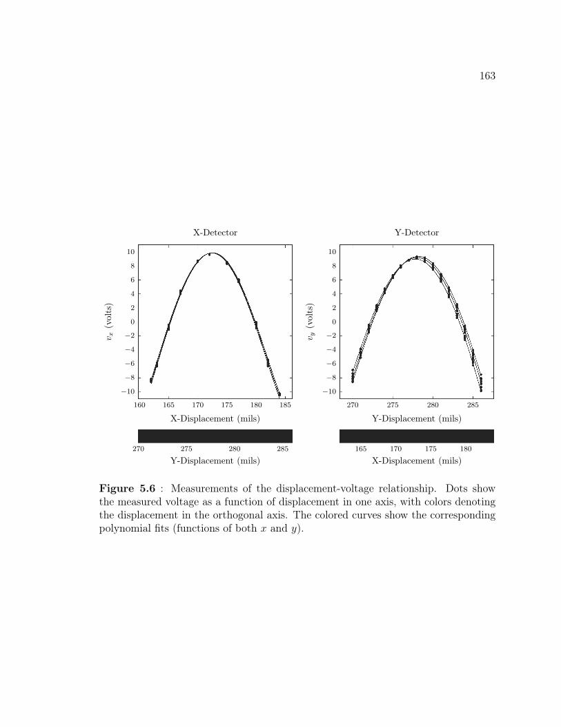
163

160 165 170 175 180 185

−10

−8

−6

−4

−2

0

2

4

6

8

10

X-Displacement (mils)

v x(v

olts

)

X-Detector

270 275 280 285

Y-Displacement (mils)

270 275 280 285

−10

−8

−6

−4

−2

0

2

4

6

8

10

Y-Displacement (mils)

v y(v

olts

)

Y-Detector

165 170 175 180

X-Displacement (mils)

Figure 5.6 : Measurements of the displacement-voltage relationship. Dots showthe measured voltage as a function of displacement in one axis, with colors denotingthe displacement in the orthogonal axis. The colored curves show the correspondingpolynomial fits (functions of both x and y).

164

yield negligible improvements.) To invert the position-voltage map given by (5.4), we

use Newton’s Method, assuming the string remains in a proscribed quadrant with an

initial estimate corresponding to 0V in both axes.

Combining these polynomial fits with the noise model given in Figure 5.5 yields

a standard deviation for the absolute displacement of the string that depends on

the location of the string in the detector. For the range the string occupied during

the experiments described in this chapter (−2V to 2V in both axes), the maximum

standard deviation assocated with displacement is 0.98 µm (0.039mils).

5.2 Data Analysis

After removing the effects of the detector, we have a single complex vector y ∈ Cn,

where Rey and Imy are the displacements in the X and Y axes. Although an ideal

string has eigenvalues whose frequencies are approximately linearly separated, a real

string can have pairs of eigenvalues that are approximately linearly separated, one for

each axis of motion; see Section 5.3.6.

To recover a single eigenvalue instead of a pair (or more), and to remove the effects

of any nonlinearities or poor initial estimates, we apply the following algorithm to

estimate ω. First, we compute ω using compressed exponential fitting, starting from

a list of initial estimates and enforcing that eigenvalues must come in conjugate pairs

(since motion in each axis is real). Next, we partition V(ω) and y into length q

segments using rows qj to q(j + 1)− 1, yielding Vj and yj, and compute

aj = V(ω)+yj. (5.5)

Finally, we determine the decay rate γk of the kth eigenvalue by fitting a single

exponential to eRe (ωk)qj‖[aj]k,k′‖2, where k and k′ are the indices of conjugate pairs

165

(ωk = ωk′). Then ωk is updated to γk + Imωk and the process is repeated until ω

converges. This ensures that Reωk is robust to slight changes in Imωk.

5.3 Matching Reality to Physical Models

In this section we derive models of increasing fidelity to our experimental measure-

ments. Our approach combines on Lagrangian mechanics, following Rayleigh [147],

with the rigor of Antman’s derivation [7]. This Lagrangian approach uses Hamilton’s

Principle of Stationary Action [35, §IV.10] to derive the equations of motion from the

kinetic and potential energy in the system. As a result, we can easily incorporate

additional effects, like bending stiffness, without deriving a new constitutive relation.

5.3.1 First Order Model

Suppose we have a string of rest length `0 stretched between two supports positioned

length ` apart. Without loss of generality, we assume that the line between the two

supports is se1`0s=0, and that e2 and e3 are the remaining orthogonal coordinates

for a right-handed Cartesian coordinate system. Then the displacement of the string

is written u(s, t) ∈ R3 where s ∈ [0, `0] is the position along the string in the rest

configuration at time t ∈ [0,∞). Further, we assume that each end of the string is

subject to Dirichlet boundary conditions: u(0, t) = 0 and u(`0, t) = 0.

In the Lagrangian Mechanics, the equations of motion are derived from the ki-

netic and potential (strain) energy in the system. Kinetic energy in the string is

proportional to the square of velocity:

T (t) =1

2

∫ `0

0

(ρA)(s)‖ut(s, t)‖22 ds, (5.6)

where (ρA) is the product of density and cross-sectional area (cf. [7, Ch. 2, eq. (10.9)]).

166

Assuming the string is elastic, the force per unit length of the string n(s, t) is pro-

portional to the stretch ν(s, t) := ‖us(s, t)‖2 and tangent to the string

n(s, t) = N(ν, s)us(s, t)

‖us(s, t)‖2(5.7)

(cf. [7, Ch. 2, eq. (2.10b), (2.11)]). The potential energy in the string comes from

integrating this force n(s, t) per unit length from the reference configuration ν = 1

to the current state

W (ν, s) :=

∫ ν

1

N(β, s) dβ (5.8)

(cf. [7, Ch. 2, eq. (10.10)]). Then integrating this energy density over the length of

the string gives the total potential energy

V (t) :=

∫ `0

0

W (ν(s, t), s) ds; (5.9)

(cf. [7, Ch. 2, eq. (10.11)]).

For elastic materials, like the steel string used in these experiments, the stress-

strain relationship is linear provided the tension is below the yield strength. Our steel

string appears to stay in the linear regime provided stretch is less than 1.01; hence,

N(ν, s) = (EA)(s)(ν − 1) for ν ∈ (0.99, 1.01), (5.10)

where (EA)(s) is the product of the Young’s modulus and cross-sectional area. After

integrating (5.8), the potential energy is2

V (t) =1

2

∫ `0

0

(EA)(s)(‖us(s, t)‖22 − 2‖us(s, t)‖2 + 1) ds. (5.11)

2Authors frequently omit the ‖us(s, t)‖ term, as, in the limit of small vibration, this term only

adds a scaling in the resulting differential equation. Rayleigh omits this term in The Theory of

Sound [147, §128, eq. (3)]. Antman does the same by taking N(ν, s) = (EA)(s)ν [7, Ch. 2, eq. (7.1)],

violating the assumption that the rest state is natural, N(1, s) = 0.

167

The motion u(s, t) is a stationary point of the action functional∫ t1

t0

L(u,ut, t) dt, where L = T − V (5.12)

with respect to u [35, § IV.10]. The terms in the kinetic and potential energy with re-

spect to ‖ut‖22 and ‖us‖22 follow directly, and the constant term is negligible. However,

the ‖us‖2 term must be expanded in terms of the series

u(s, t) = u(0)(s, t) + εu(1)(s, t) + ε2u(2)(s, t) + · · · . (5.13)

Here, the zeroth order term corresponds to the string at rest. Under the assumption

that the string is uniform, u(0)(s, t) = s`/`0e1. Defining ν := `/`0 and u = u− u(0),

we expand the ‖us‖2 term as

‖us‖2 = ν

√1 + 2ν−1e>1 us + ν−2u>

s us

= ν

(1 +

1

2(ν−12e>1 us + ν−2u>

s us)−1

8(2ν−1e>1 us + ν−2u>

s us)2

)+O(‖us‖32)

= ν + e>1 us +1

2ν

([us]

22 + [us]

23

)+O(‖us‖32).

Upon integration, the [us]1 term vanishes as a result of the Dirichlet boundary con-

ditions, leaving∫ `0

0

‖us(s, t)‖2 ds = `+`02`

∫ `0

0

[us]22 + [us]

32 ds+O(‖us‖32).

This leaves the Lagrangian, omitting constants and terms of order ε2 and above,

L(t) =1

2

∫ `0

0

(ρA)(s)‖u(1)t (s, t)‖22 − (EA)(s)

[[us]

21 +

`− `0`

[u(1)s ]22 +

`− `0`

[u(1)s ]23

]ds.

(5.14)

If ρA and EA are independent of s, then the solution is given by [35, § IV.10]:

ρA[u(1)tt ]1 = EA[u(1)

ss ]1

ρA[u(1)tt ]2 =

EA(`− `0)`

[u(1)ss ]2

ρA[u(1)tt ]3 =

EA(`− `0)`

[u(1)ss ]3.

(5.15)

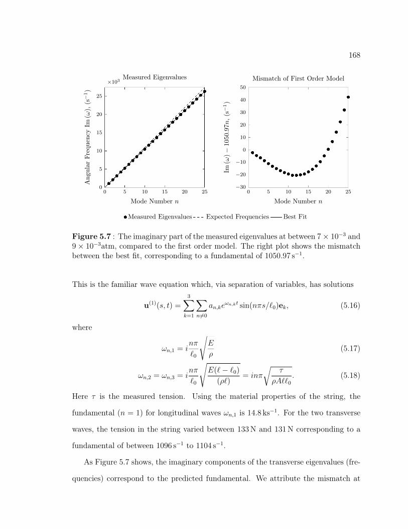
168

0 5 10 15 20 250

5

10

15

20

25

×103

Mode Number n

Ang

ular

Freq

uenc

yIm

(ω),

(s−1)

Measured Eigenvalues

0 5 10 15 20 25−30

−20

−10

0

10

20

30

40

50

Mode Number n

Im(ω

)−1050

.97n

,(s−

1)

Mismatch of First Order Model

Measured Eigenvalues Expected Frequencies Best Fit

Figure 5.7 : The imaginary part of the measured eigenvalues at between 7× 10−3 and9× 10−3atm, compared to the first order model. The right plot shows the mismatchbetween the best fit, corresponding to a fundamental of 1050.97 s−1.

This is the familiar wave equation which, via separation of variables, has solutions

u(1)(s, t) =3∑

k=1

∑n6=0

an,keωn,kt sin(nπs/`0)ek, (5.16)

where

ωn,1 = inπ

`0

√E

ρ(5.17)

ωn,2 = ωn,3 = inπ

`0

√E(`− `0)

(ρ`)= inπ

√τ

ρA``0. (5.18)

Here τ is the measured tension. Using the material properties of the string, the

fundamental (n = 1) for longitudinal waves ωn,1 is 14.8 ks−1. For the two transverse

waves, the tension in the string varied between 133N and 131N corresponding to a

fundamental of between 1096 s−1 to 1104 s−1.

As Figure 5.7 shows, the imaginary components of the transverse eigenvalues (fre-

quencies) correspond to the predicted fundamental. We attribute the mismatch at

••• •• •• •• • •••••••

•

•

• •

•

•

• •

169

higher frequencies to a slow creep of the wire, causing a gradual decrease in tension

that cannot be measured. After fitting a new fundamental based on these experi-

ments, the residual shows a quadratic trend, indicating the presence of another effect:

resistance to bending.

5.3.2 Energy in Bending

The shift of frequencies seen in Figure 5.7 is a well known effect due to stiffness [147,

§ 188]. As the string has a finite size, bending causes compression and expansion

around the central axis of the string, increasing the potential energy in the string.

According to the Euler-Bernoulli beam theory, the energy due to bending is

Vbend =1

2

∫ `0

0

(EI2)(s)[uss]22 + (EI3)(s)[uss]

23 ds (5.19)

where EI2 and EI3 are the product of Young’s Modulus and the second moment

of area in each axis. This is an incomplete model, as it omits twisting and other

motions; see Antman for a full model [7, Ch. 8]. Unlike these fuller models, we can

treat stiffness without introducing additional degrees of freedom.

Under the assumption that EI2 and EI3 are constant, the stationary solution u

of the action functional solves [35, § IV.10]

ρA[u(1)tt ]2 =

EA(`− `0)`

[u(1)ss ]2 − EI2[u(1)

ssss]2

ρA[u(1)tt ]3 =

EA(`− `0)`

[u(1)ss ]3 − EI3[u(1)

ssss]3.

(5.20)

The higher-order term necessitates two additional boundary conditions to specify a

unique solution.

If the additional boundary conditions are hinged, uss(0, t) = uss(`0, t) = 0, the

same separation of variables as (5.16) may be applied, yielding eigenvalues

ωn,k = in

√τπ2

ρA``0+EIkρA

(π

`0

)4

n2 k = 2, 3. (5.21)

170

0 5 10 15 20 25−30

−20

−10

0

10

20

30

40

50

Mode Number n

Im(ω

)−10

50.97n

,(s−

1)

Mismatch of First Order Model

0 5 10 15 20 25−1

−0.5

0

0.5

1

1.5

2

2.5

Mode Number n

Im(ω

)−Im

(ωst

iffn,2)

(s−1)

Mismatch with Stiffness

Measured Eigenvalues Expected Frequencies Best Fit

Figure 5.8 : Stiffness corrections to eigenvalue frequencies. Using the linear model inFigure 5.7, the left plot shows the residual from the linear fit using a fundamental of1050.97 s−1 and the curve shows the best fit (5.23). The right plot shows the residualbetween (5.23) and the measured eigenvalues.

The second moment of area for a circular cylinder about a perpendicular axis is

I = πr4/4, where r is the radius of the cylinder. Using the measured values of these

parameters, we have

ωn,2 ≈ i

√(1 201 000 s−1)n2 + (16.327 s−2)n4, (5.22)

This compares favorably to the least squares fit in Figure 5.8:

ωstiffn,2 ≈ i

√(1 098 661 s−1)n2 + (15.001 s−2)n4. (5.23)

Even if the boundary conditions are not hinged, we can treat the stiffness term as

a perturbation, since EI/`20 = 3.6× 10−4 N is much smaller than τ = 131N. Then

the separation of variables in (5.16) corresponds to the unperturbed system and the

perturbed eigenvalues are given by (5.21).

- I

-,

•

- . •

• • ••• •

• •

•• • ••

• • ••••

• •

' •

171

Table 5.2 : Properties of AirParameter Symbol Approximate Value

Density ρa 1.2 kg/m3

Viscosity µ 18.6 µPa sKinematic viscosity ν = µ

ρa1.55× 10−5 m2/s

An alternative boundary condition enforces zero slope at each end, termed clamped

endpoints, us(0, t) = us(`0, t) = 0. The spacial component in the separation of

variables then depends on the root of a transcendental equation [147, § 189]. As we

are unsure what boundary condition the collets enforce, this may account for the

pattern in the residuals in Figure 5.8; however this effect is on the order of 5 s−1, the

same order of magnitude as the unaccounted for frequency shift due to damping in

Section 5.3.4, so an identification is unwarranted.

5.3.3 Air Damping

The experimental results just discussed were performed in our pressure vessel at

0.008 atm. We now study the effect of pressure on the recovered spectrum. As Fig-

ure 5.9 shows, the decay rate of the eigenvalues depends strongly on the pressure. The

primary mechanism coupling of the string to the surrounding air is the Naiver-Stokes

equations. An additional effect is slight change in thermal conduction efficiency from

the string into the surrounding air (see Section 5.3.5).

Fluid flow is characterized by the Reynolds number [13, §4.7, p. 245],

Re =ρvd

µ=vd

ν(5.24)

where ρa is the density of the fluid, v, the mean velocity, d, the characteristic length, µ

the dynamic viscosity of the fluid, and ν = µ/ρ the kinematic viscosity; approximate

172

0.0080.10.20.30.40.50.60.70.81.0

−0.8 −0.7 −0.6 −0.5 −0.4 −0.3 −0.2 −0.1 00

2

4

6

8

10

12

14

16

18

20

22

24

26

28

30

×103

Decay Parameter Reω, s−1

Freq

uenc

yPar

amet

erIm

ω,s

−1

Eigenvalues as a Function of Pressure

0

0.1

0.2

0.3

0.4

0.5

0.6

0.7

0.8

0.9

1

Pressure (Atm.)

Figure 5.9 : Eigenvalues of a vibrating string as a function of atmospheric pressure.These eigenvalues were estimated using the decay-robust exponential fitting algorithmgiven in Section 5.2, from measurements described in Section 5.1.

173

−0.8 −0.7 −0.6 −0.5 −0.4 −0.3 −0.2 −0.1 00

2

4

6

8

10

12

14

16

18

20

22

24

26

28

30·103

Decay Parameter Reω, s−1

Freq

uenc

yPar

amet

erIm

ω,s

−1

Reynolds Number for Each Measured Eigenvalue

10−3.0

10−2.5

10−2.0

10−1.5

10−1.0

Reynolds Number

Figure 5.10 : Reynolds number

values are given in Table 5.2. For a vibrating string, the characteristic length is the

diameter d = 0.015 in and the characteristic velocity for the kth mode is the maximum

velocity aImω under the assumption [u(s, t)]k = Re [aeωt] sin(nπs) for the transverse

modes k = 2, 3.

Using these parameters, the Reynolds number for the string at pressure P is

Re = (24 s/m) aImωP

1 atm. (5.25)

The effects of frequency and amplitude on the Reynolds number generally cancel:

high frequency modes tend to have smaller vibrations, as seen in Figure 5.10.

The quasi-steady approach models the string as moving at a constant velocity.

Although there is no steady state solution to the Stokes equations around an infinite

cylinder due to Stokes’ paradox, Oseen’s equations resolve this paradox and yield a

_. • • • • • • • • • • • •• • • • • • • - •• • • • • • - •• • • • • • - - • • • • • • • - • • • • • • • • • • • • • • • • • • • • - • • • • • • • •• •• • • • • • • • •• • • • • • • • •• •• • • • • • • • • •• • • • • • • • • • • • • • • • • •• • • • • • • • • • • • • • • • • • • • • • • • • • • • • • • • • • • • • ·-· • • • • • • • • • • • • • • •• • • • • • • ••• • • • • • ••••• •• • • ••• • • • ........ •

174

drag per unit length of

D = 2πµvC = 2πµv2

log(7.4/Re)=

4πµv

log(7.4)− log(ρd/µ)− log(v), (5.26)

[13, eq. (4.10.13), (4.10.15)]. Applying this drag formula to a vibrating string is com-

plicated by the nonlinear dependence on v, both directly and through Re. Decreasing

velocity decreases the drag coefficient C, so we may bound the energy lost due to air

with C corresponding to the maximum Reynolds number.

Drag following (5.26) adds an external force opposing the motion of the string:

fD(ut) = [0, δ[ut]2, δ[ut]3]> , where δ =

4πµ

log(7.4/Re). (5.27)

This adds an external forcing term to (5.20) in both transverse axes [35, § IV.10]

ρA[u(1)tt ]1 = EA[u(1)

ss ]1

ρA[u(1)tt ]k =

EA(`− `0)`

[u(1)ss ]k − EI3[u(1)

ssss]k + δ[u(1)t ]k, k = 2, 3.

. (5.28)

Solving these equations using separation of variables, the eigenvalues of the two trans-

verse modes are

ωn,k = −δ

ρA+ in

√τπ2

ρA``0+EIkρA

(π

`0

)4

n2 − δ

ρA, k = 2, 3. (5.29)

For our string, Re = 0.3 is an appropriate upper bound on the Reynolds number,

giving δ/(ρA) ≈ 0.14 s−1.

Although this quasi-steady flow drag estimate gives the right order of magni-

tude, changes in pressure only coupled through the changing Reynolds number (5.25).

Rather than using the quasi-steady estimate, Lin [101] directly couples the wave equa-

tion to a solution of the Stokes equation in the limit of either small Reynolds number

(Re 1) or small oscillation a b, where a is the amplitude of oscillation and

175

b = d/2 the radius of the cylinder (string). This second case applies to this experi-

ment; the largest amplitude vibration is 8 µm, much smaller than the 381 µm diameter

of the string. Then, following [101, eq. (6)], the force opposing motion is

fD(τ)

ρaν= πv(τ) +

16

π

∫ τ

0

∫ ∞

0

v(λ)e−x2(τ−λ)

x(J20 (x) + Y 2

0 (x))dx dλ (5.30)

where τ(b2/ν) = t, v denotes differentiation with respect to τ , and J0 and Y0 are Bessel

functions of the first and second kind. Coupling this damping model to the motion

of the string results in an integro-differential equation [101, eq. (10)]. However, since

there is no known solution, we treat this force as a perturbation to u(1), estimating

the drag coefficient while assuming motion is restricted to a plane. Treating each term

separately in (5.16), we have vn(s, t) = ωn,2eωn,2t and vn(t) = ω2

n,2(b2/ν). Changing

the order of integration yields∫ τ

0

∫ ∞

0

v(λ)e−x2(τ−λ)

x(J20 (x) + Y 2

0 (x))dx dλ =

b2

ν

∫ ∞

0

ω2n,2e

−x2τ

x(J20 (x) + Y 2

0 (x))

∫ τ

0

e(ωn,2+x2)λ dλ dx

=b2

νeωn,2τ

∫ ∞

0

ω2n,2(1− e−x2τ )

x(J20 (x) + Y 2

0 (x))(ωn,2 + x2)dx.

Taking the limit τ →∞ removes the time dependent term, leaving

Φ(ωn,2) :=

∫ ∞

0

ωn,2

x(J20 (x) + Y 2

0 (x))(ωn,2 + x2)dx, (5.31)

with force per mode:

fD(τ)

ρab2≈ πω2

n,2eωn,2t + ωn,2e

ωn,2t16

πΦ(ωn,2). (5.32)

Adding this forcing term to (5.20) yields the following equation for the eigenvalues:

ρAω2n,2 = −

τ`0`(nπ/`0)

2 − EI2(nπ/`0)4 − (ρab2π)ω2

n,2 − ωn,216ρab

2

πΦ(ωn,2). (5.33)

Figure 5.11 shows the predicted damping versus pressure. While this model is off by

roughly a factor of two from measurements at one atmosphere and underestimates

176

−0.8 −0.7 −0.6 −0.5 −0.4 −0.3 −0.2 −0.1 00

2

4

6

8

10

12

14

16

18

20

22

24

26

28

30·103

Decay Parameter Reω, s−1

Freq

uenc

yPar

amet

erIm

ω,s

−1

Eigenvalues Using Lin’s Damping Model Versus Measured

0

0.2

0.4

0.6

0.8

1

Pressure (atm)

Figure 5.11 : Expected eigenvalues using Lin’s damping model. Dots show themeasured eigenvalues while curves show the expected decay rate using Lin’s dampingmodel. Lin’s model appears accurate to within a factor of two of the true dampingfor pressures near one atmosphere, but underestimates damping at low pressures.

damping at 0.008 atm, it qualitatively captures the effects of pressure and frequency

on the damping that we observe in our physical experiments.

5.3.4 Frequency Shift Due to Damping

Two effects conspire to decrease the frequencies: increased damping and the added

mass captured by Lin’s model. The solutions for the eigenvalues in (5.33) are

ωn,2 = −8ρa

π2(ρ+ ρa)Φ(ωn,2)+ni

√τπ2

``0A(ρ+ ρa)+

EIπ4

`40A(ρ+ ρa)n2 − 8ρa

π2(ρ+ ρa)Φ(ωn,2).

(5.34)

This formula predicts a shift of at most 0.07 s−1 for the fundamental (n = 1); however

Figure 5.12 shows a shift of 3 s−1. The mismatch in the shift grows with increasing

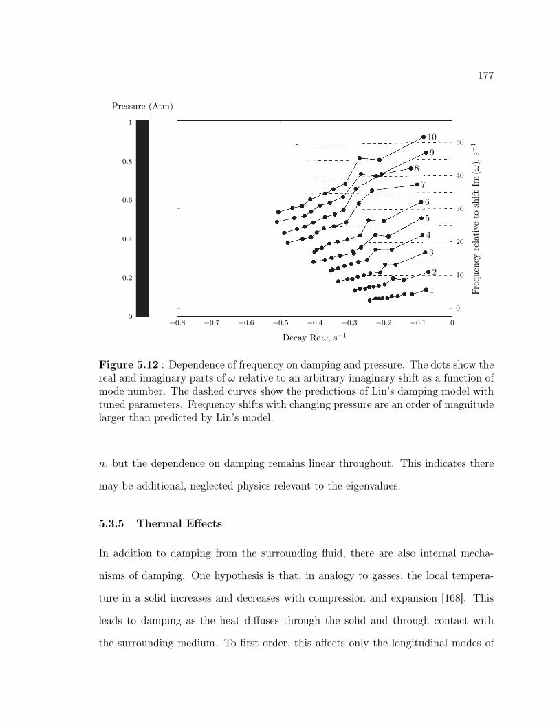
177

1

2

3

4

5

6

7

8

9

10

−0.8 −0.7 −0.6 −0.5 −0.4 −0.3 −0.2 −0.1 0

0

10

20

30

40

50

Decay Reω, s−1

Freq

uenc

yre

lati

veto

shift

Im(ω

),s−

1

0

0.2

0.4

0.6

0.8

1

Pressure (Atm)

Figure 5.12 : Dependence of frequency on damping and pressure. The dots show thereal and imaginary parts of ω relative to an arbitrary imaginary shift as a function ofmode number. The dashed curves show the predictions of Lin’s damping model withtuned parameters. Frequency shifts with changing pressure are an order of magnitudelarger than predicted by Lin’s model.

n, but the dependence on damping remains linear throughout. This indicates there

may be additional, neglected physics relevant to the eigenvalues.

5.3.5 Thermal Effects

In addition to damping from the surrounding fluid, there are also internal mecha-

nisms of damping. One hypothesis is that, in analogy to gasses, the local tempera-

ture in a solid increases and decreases with compression and expansion [168]. This

leads to damping as the heat diffuses through the solid and through contact with

the surrounding medium. To first order, this affects only the longitudinal modes of

178

vibration, since transverse motion only induces an infinitesimal compression propor-

tional to EIussss(s, t). Figure 5.11 may show evidence of this at low pressure, as the

eigenvalues have much stronger decay than predicted by Lin’s model, but this also

may be due to the approximations in Lin’s model. For further discussion of thermal

effects, see Antman [7, §12.14].

5.3.6 Eigenvalue Splitting and Nonlinear Effects

Thus far, we have treated the two transverse axes of motion [u(1)]2 and [u(1)]3 as

identical. This yields two identical eigenvalues, described by the preceding estimates

of ωn,2 and ωn,3. However, slight difference in the material properties in each axis can

split the duplicate eigenvalues into two distinct, but close, eigenvalues. This effect

is difficult to resolve. Figure 5.13 shows one example where this frequency splitting

is successfully resolved. However, for other modes this effect is not well resolved, as

illustrated in Figure 5.14. This may be due to either convergence to a spurious minima

by the exponential fitting routine or an additional (nonlinear) term perturbing the

solution u(s, t).

5.3.7 Further Refinement

There are many additional effects that may change the eigenvalues and these may

explain the mismatch between theory and measurements. For example, the decay

rates predicted by Lin’s damping model are too large at atmospheric pressure and

too low at vacuum. This may be due to the second term in the series expansion

of the Navier-Stokes equations, which exposes a four-fold symmetric boundary layer

around the string that is confirmed by experiments [67]. Alternatively, damping at

low pressure may be dominated by internal friction mechanisms. Further affecting the

179

600 800 1,000 1,200 1,400 1,60010−5

10−4

10−3

10−2

10−1

100

101

Frequency (s−1)

Am

plit

ude

(mm

)

One Exponential

Reω Imω |a|

−0.197703 1,045.993 1.983 · 10−6

−0.197703 627,272.537 2.036 · 10−6

600 800 1,000 1,200 1,400 1,60010−5

10−4

10−3

10−2

10−1

100

101

Frequency (s−1)

Am

plit

ude

(mm

)

Two Exponentials

Reω Imω |a|

−0.314306 1,045.934 4.223 · 10−7

−0.205932 1,046.013 1.975 · 10−6

−0.314306 627,272.596 1.156 · 10−6

−0.205932 627,272.518 1.171 · 10−6

Figure 5.13 : Resolved eigenvalue splitting. The top row shows the Fourier transformof y and the residual (gray). The table below shows the fitted parameters of pairs ofconjugate exponentials. This example shows the n = 10 mode at 0.008 atm. Althoughthe units of the vertical axis are millimeters, the amplitude of a peak correspondingto a unit sine wave has amplitude

√n = 103; hence the amplitude of the mode shown

here is ≈1 µm.

180

600 800 1,000 1,200 1,400 1,60010−8

10−7

10−6

10−5

10−4

10−3

10−2

Frequency (s−1)

Am

plit

ude

(m)

One Exponential

Reω Imω |a|

−0.225299 1,045.884 5.684 · 10−6

−0.225299 627,272.647 5.633 · 10−6

600 800 1,000 1,200 1,400 1,60010−8

10−7

10−6

10−5

10−4

10−3

10−2

Frequency (s−1)

Am

plit

ude

(m)

Two Exponentials

Reω Imω |a|

−0.084469 1,046.493 2.944 · 10−8

−0.229081 1,045.885 5.739 · 10−6

−0.084469 627,272.038 1.91 · 10−7

−0.229081 627,272.646 5.629 · 10−6

Figure 5.14 : Unresolved eigenvalues. Identical to Figure 5.13, except this figureshows the fit for the fundamental n = 1 at 1 atm. In this example, the mode isnot clearly resolved into two exponentials, either due to poor initial estimates or aphysical effect.

181

damping parameters, the diameter of the string may change in response to elongation

in a process called necking.

The one unexplained phenomenon is the unexpected frequency shift with changing

pressure and decay rate described in Section 5.3.4. Capturing this effect requires a

more sophisticated beam model, introducing utttt terms corresponding to the kinetic

energy of the wire with respect to rotations about the transverse axes, as well as

additional potential energy due to shearing. These models include Timoshenko’s

beam model (e.g., [32, §7.7], experiments [133]) and Antman’s rod theory [7, Ch. 8].

5.4 Conclusion

Using the compressed exponential fitting routines developed in Chapter 4, we were

to obtain accurate estimates of the eigenvalues of a string from measurements of its

evolution. Each of the 2,894 experiments took one million measurements of string

displacement. Compression made it possible to quickly and efficiency analyse this

data, thus illustrating how compression can provide insight into other mechanical

systems, such as those applications described in [102].

182

Chapter 6

Conclusions and Future Work

In this thesis, we have focused on two classes of exponential fitting algorithms: those

similar to Prony’s Method that recover the complex frequencies ω through an implicit

autoregressive model, and those that use an optimization approach maximizing the

likelihood of ω. Chapter 2 summarized existing theoretical results for many variants

of Prony’s Method, provided new asymptotic estimates of the bias and covariance in

Prony’s Method, and extended these results to Kung’s Method. We also developed

new variants of Prony’s Method, including the Maximum Likelihood Prony Method,

the Filtered Matrix Pencil Method, and the Orthogonalized Matrix Pencil Method.

In the maximum likelihood framework, we provided a new technique for compressing

general nonlinear least squares problems onto small subspaces. We generalized Fis-

cher’s efficiency for multi-parameter problems and used this to construct subspaces

that capture the salient features of the data. A closed-form inner product between the

model function f(θ) and the basis for the compression space W allows optimization

steps to be independent of the number of measurements. For the exponential fitting

problem, compression spaces built from columns of block diagonal Fourier parent

coordinates satisfy both qualities: the inner product can be implmented in closed-

form inner product and provides an efficient subspace that could be constructed for

every ω.

Exponential fitting, although an important problem in many fields, is a simple

example of a nonlinear least squares problem. Compression may yield improved

183

performance for other, more challenging nonlinear least squares problems. In this

final chapter, we discuss remaining open problems involving Prony’s Method and

examine how compression can be applied to other areas of research.

6.1 Further Extensions of Prony’s Method

Chapter 2 focused on the statistical and numerical properties of many variations

of Prony’s Method and built several new algorithms. This investigation pointed to

several remaining extensions and improvements of Prony’s Method we discuss here.

6.1.1 Numerically Stable Maximum Likelihood Prony Methods

As illustrated in Figure 2.3, many maximum likelihood Prony methods are numeri-

cally unstable when fitting more than 20 exponentials. This instability can be fixed

by including extraneous exponentials, as shown in Figure 2.7, but these extraneous

exponentials are a nuisance to remove. Numerically stable Prony variants, such as

Kung’s Method, implicitly remove these spurious exponentials, but fail to provide

maximum-likelihood estimates. An ideal variant of Prony’s Method would provide

both maximum likelihood estimates while implicitly filtering the spurious exponen-

tials.

6.1.2 Improving Performance

The computational cost for many numerically stable Prony-type methods is domi-

nated by the cost of computing the singular value decomposition. Most implementa-

tions developed in the 1980s use classical dense algorithms for this operation, but two

new classes of algorithms exist: Krylov subspace methods and randomized matrix

factorizations.

184

The Implicitly Restarted Arnoldi Method (IRAM) [142] in ARPACK [98], a Krylov

subspace method, computes the rank-k SVD of an n× n matrix using multiple itera-

tions of the Arnoldi cycle, each requiring k matrix-vector products and O(nk2 + k3)

additional operations. Combined with fast Hankel-vector products [113, §3.4] that

require only O(kn log n) operations, IRAM can provide the rank-k SVD much faster

than classical dense SVD algorithms that require O(n3) operations. The combination

IRAM and the fast Hankel-vector products with Kung’s Method was discussed in a

2005 thesis by Laudadio [96, Ch. 3].

Randomized matrix factorizations are a recent alternative for large problems [61].

Although these methods are still in their infancy, they may provide significant speed

improvements for Prony-type algorithms applied to huge problems (n > 106) for

which even Krylov methods are infeasible. These fast random factorizations deliver

left singluar vectors whose accuracy satsifies probabilistic error bounds. The effect of

the resulting approximation on Kung’s Method or HTLS should be explored before

these two algorithms are combined.

6.1.3 Restarted Matrix Pencil Method

The Orthogonalized Matrix Pencil Method (Algorithm 2.15) developed in this thesis

can estimate ω near specified frequencies to high precision, provided the frequen-

cies are well separated — a feature not shared by other variants of Prony’s Method.

However, when the frequencies to recover are clustered, this technique fails to con-

verge. Inspired by the Implicitly Restarted Arnoldi Method [142], we would like to

restart the Orthogonalized Matrix Pencil Method using a new compression space that

utilizes information about the current estimates, both wanted and unwanted, to fil-

ter unwanted exponentials in future iterations. Ideally when this method converges,

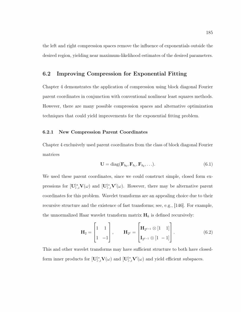
185

the left and right compression spaces remove the influence of exponentials outside the

desired region, yielding near maximum-likelihood estimates of the desired parameters.

6.2 Improving Compression for Exponential Fitting

Chapter 4 demonstrates the application of compression using block diagonal Fourier

parent coordinates in conjunction with conventional nonlinear least squares methods.

However, there are many possible compression spaces and alternative optimization

techniques that could yield improvements for the exponential fitting problem.

6.2.1 New Compression Parent Coordinates

Chapter 4 exclusively used parent coordinates from the class of block diagonal Fourier

matrices

U = diag(Fb0 ,Fb1 ,Fb2 , . . .). (6.1)

We used these parent coordinates, since we could construct simple, closed form ex-

pressions for [U]∗·,iV(ω) and [U]∗·,iV′(ω). However, there may be alternative parent

coordinates for this problem. Wavelet transforms are an appealing choice due to their

recursive structure and the existence of fast transforms; see, e.g., [146]. For example,

the unnormalized Haar wavelet transform matrix Hk is defined recursively:

H2 =

1 1

1 −1

, H2` =

H2`−1 ⊗ [1 1]

I2`−1 ⊗ [1 − 1]

. (6.2)

This and other wavelet transforms may have sufficient structure to both have closed-

form inner products for [U]∗·,iV(ω) and [U]∗·,iV′(ω) and yield efficient subspaces.

186

6.2.2 Alternative Trust Region Quadratic Models

The trust-region optimization method used in Chapters 3 and 4 used a quadratic

model of the residual,

‖y − f(θ + p)‖ ≈ φ(θ) + g(θ)∗p+1

2p∗H(θ)p, (6.3)

to construct the next iterate of θ by minimizing the right hand size over p subject to

the constraint ‖p‖ ≤ ∆. This is called the trust region subproblem, solved by (3.11).

The choice of a quadratic model is motivated by simplicity and generality. Taylor’s

theorem implies that for smooth functions and a fixed error, there exists an region on

which the quadratic model does not exceed the specified error. However, there may

be more appropriate models for a particular residual.

Inspired by Bunch, Nielsen, and Sorensen’s [25] rational-Newton method for com-

puting the roots of the secular equation in symmetric eigenvalue computations, we

too might seek a rational model of the residual. If we consider the residual under the

Fourier transform,

[F∗y − F∗V(ω)a]k = [F∗y]k −1√n

p−1∑j=0

1− enωj−2πik

1− eωj−2πik/naj, (6.4)

each entry of the residual is the square of a constant minus a sum of rational functions

of the form (1−λn)/(1−λ). A better model function would generate better iterates of

ω, reducing the computational cost by decreasing the number of iterations necessary.

6.2.3 Block Coordinate Descent

When there are many exponentials, the dominant cost for optimization is the O(p3)

cost for solving a dense, p× p linear system to find the minimum of the trust region

subproblem. One approach to reduce this cost is block coordinate descent, also known

187

as the Gauss-Seidel-Newton Method [115, Ch. 7, eq. (28)]. This technique splits

the nonlinear variables ω into (perhaps disjoint) sets ωk and optimizes these subsets

sequentially. Compression adds separate compression spaces for each ωk,Wk. In this

variant, each iteration would update ωk, solving the exponential fitting problem with

the remaining variables fixed; i.e.,

ωk ← argminω

mina

∥∥∥∥∥Wk

(y −V(ω)a−

∑j 6=k

V(ωj)aj

)∥∥∥∥∥2

. (6.5)

Convergence is typically linear [112], and this approach is beneficial if the computa-

tional savings of splitting the domain outweigh the convergence penalty incurred.

Recently, Nesterov developed a block coordinate descent using a compression space

formed from randomly chosen columns of the identity matrix, and showed that for

some problems convergence is quadratic [112]. Compression provides an alternative

interpretation of these results in a statistical context, and could inform better com-

pression spaces.

6.3 Applying Compression to System Identification Problems

As discussed in Section 1.3, exponential fitting is equivalent to finding the eigenvalues

ω of the matrix A from samples of the impulse response

y(t) = CetAx0. (6.6)

As compression is effective for the exponential fitting problem, we ask: can compres-

sion be applied to other system identification problems? In this section, we discuss

several such problems and in two cases show how the block Fourier matrices provide

compression subspaces with closed-form inner products with the model function f via

Theorem 4.1.

188

6.3.1 Multiple Output Impulse Response System Identification

Throughout this thesis, for simplicity, we restricted ourselves to the case where y(t)

is a scalar. The general case where y(t) is a vector corresponds to a multiple output

system, with C ∈ Cm×p. Assuming that noise in the measurements is independent

and normally distributed with uniform covariance, we can pose this as the nonlinear

least squares problem

minω∈Cp,a`∈Cp

m−1∑`=0

‖[Y]·,` −V(ω)a`‖2 where [Y]·,j = [y(tj)]`. (6.7)

Using the n-mode matrix product notation of Bader and Kolda [90, §2.5], we can

rewrite (6.7) without the sum

minω∈Cp,A∈Cp×m

‖Y −V(ω)×2 A‖F, [X×2 A]j,k :=∑`

[X]j,`[A]`,k. (6.8)

The structure of this nonlinear least squares problem can be exploited to reduce

storage and operation counts using the ideas of Kaufman, Sylvester, and Wright [87].

Compression for this problem follows the same outline as the exponential fitting

problem. The results in Section 4.3 provide closed-form inner products for block

Fourier matrices with V(ω). The only complication is selecting columns from the

parent coordinates where a modified heuristic is necessary. The new heuristic should

follow the procedure in Section 4.4, replacing Y − V(ω) ×2 A with the vectorized

version vec(Y)− (Im ⊗V(ω)) vec(A), where ⊗ is the Kronecker product.

6.3.2 Frequency Domain System Identification

Whereas the time domain system identification determines the eigenvalues ω of A

from samples of y(t), the frequency domain system identification determines ω from

samples of the transfer function,

H(s) = C(sI−A)−1B+D. (6.9)

189

In general, the transfer function of a finite dimension system is written as the ratio

of two polynomials,

H(s) =

∑pj=0 βjs

j

sp +∑p−1

j=0 αjsj, (6.10)

which, if A is diagonalizable, can be written more simply in pole-residue form:

H(s) =

p−1∑j=0

[A]·,·,js− ωj

. (6.11)

This special case of the rational approximation problem is the frequency domain

counterpart to the exponential fitting problem. The Loewner (Löwner) framework

developed by Anderson and Antoulas [5] plays the role of Prony’s Method in the

frequency domain; see also [89, 97]. The Loewner framework uses a generalized

eigenvalue problem to reveal the signal poles ω, paralleling the matrix pencil variant

of Prony’s Method. However, unlike Prony’s Method, numerical experiments sug-

gest that when the number of measurements matches the number of parameters, the

Loewner framework produces maximum likelihood estimates. Further, as the number

of measurements increases, performance decreases slightly (i.e., ≈ 95%) in a similar

manner to Kung’s Method.

The associated maximum likelihood formulation for ω and A when the noise in the

measurements [H]·,·,k = H(sk) is independently and identically normally distributed,

yields the following nonlinear least squares problem for the poles ω and residues A:

minω,A‖H−A×3 (R(ω)>)‖F, where [R(ω)]j,k = (sj − ωk)

−1. (6.12)

Here, the n-mode matrix product is

[A×3 X]i1,i2,i3 =∑j

[A]i1,i2,j[X]j,i3 .

Compression can be applied to the rational approximation problem; however, at this

point, we know of no parent coordinates that satisfy the closed-form property other

190

than the identity matrix. However, the identity matrix parent coordinates is likely

efficient, since entries of R(ω)> are only large when sj is near some ωk.

6.3.3 System Identification with Known Inputs

Finally, we can use compression to find a realization of a system subject to a known

input. For an arbitrary deterministic system subject to a known input u(t), the

output is

y(t) = Du(t) + etAx0 +

∫ t

0

Ce(t−s)ABu(s) ds. (6.13)

For notational simplicity, we include the initial condition term in the input u(s) by

replacing u(s) with u(s)+δ+(t)x0 where δ+(t) is the right-sided Dirac delta function.

If we again make the assumption that A is diagonalizable with eigenvalues ω, the

solution for y(t) is the convolution of eωt with u(t):

y(t) = Du(t) +

p−1∑j=0

[CV]·,j[V−1B]j,·

∫ t

0

eωj(t−s)u(s) ds. (6.14)

Sampling u(t) and y(t) into matrices [U]j,k = [u(kδ)]j and [Y]j,k = [y(kδ)]j, we seek

eigenvalues ω and linear parameters D and X solving

minω∈Cp,D∈Cq×q ,X∈Cm×q×p

∥∥∥∥∥Y − (DU>)> −p−1∑`=0

([X ]·,·,`Vu(ω`)>)>

∥∥∥∥∥F

where [Vu(ω)]j,k =

∫ δj

0

e(δj−s)ω[u(s)]k ds.

(6.15)

As with the previous problems, we can apply the insights of [87] to reduce the com-

putational burden of this problem.

Although Vu(ω`) is more complicated that V(ω) for the exponential fitting prob-

lem, we can apply the closed form inner product results of Section 4.3 by approximat-

ing u(t) in a basis for which Vu(ω`) does have a closed form expression. One such

191

basis contains polynomials, exponentials, and the Heaviside step function Θ(t):

uq,φ,τ (t) = tqk eφktΘ(t− τk). (6.16)

The convolution of this element with an exponential is then

∫ t

0

eω(t−s)uq,φ,τ (s) ds =

eωt e(φ−ω)s

(q∑

`=0

(−1)` q` sq−`

(φ− ω)`

)∣∣∣∣∣t

s=min(0,τ)

, φ 6= ω;

eωtsq+1

q + 1

∣∣∣∣ts=min(0,τ)

, φ = ω;

(6.17)

where q` is the falling factorial power [59, eq. (2.43)], q` = q(q − 1) . . . (q − ` + 1).

Then, since each of these expressions in (6.17) is the product of an exponential and

a polynomial, Theorem 2.5 provides a formula for a Fourier matrix times Vuq,φ,τ(ω).

The set of functions uq,φ,τ(t)q∈Z+,φ∈C,τR+ is quite general; it includes polynomi-

als, piecewise polynomials, sines, and cosines. As such, a sum of these functions can

approximate any continuous function to arbitrary accuracy. However, the challenge

is finding a compact representation of u in these functions; both additional terms

and high polynomial orders increase the number of operations required to compute

Vu. Further, the geometric block parent coordinates that proved so successful for the

exponential fitting problem will provide poor subspaces here. For example, if u con-

sists of a single step halfway through the measurements, then G4 will not efficiently

capture rapidly decaying eigenvalues expressed at this transition, as the step occurs

in the last and largest block. Instead, new compressions spaces are necessary, likely

built on wavelet bases, and these compression spaces may need knowledge of u to be

efficient.

192

6.4 Applying Compression to Other Nonlinear Least Squares

Problems

In the previous section, we saw how compression can be extended from the expo-

nential fitting problem to several problems in system identification. We ask: can

compression be applied to other problems as well? The modern approach to parame-

ter identification problems with vast numbers of measurements is to randomly sample

subset of these measurements [50]. In settings where this current approach is applied,

compression could replace random sampling to choose a set of measurements that

contain significant information about the desired parameters. This could accelerate

convergence, even if the compression spaces correspond keeping rows of the original

data. Combined with Nesterov’s block coordinate descent, compression might play

an invaluable role in solving large scale, many parameter models, such as seismic

inversion [8].

193

Appendix A

Statistics

Throughout this thesis we use statistics to measure the efficiency of our recovered

parameters. Our main concern is with the expected value (to check for bias) and

covariance of λ or ω. Most results employed are standard, but the setting is slightly

different. Statistics generally treats real random variables, but here we use complex

random variables of a particular type that correspond to the complex `2 norm. Most

asymptotic statistical results are in the limit of a large number of measurements; here,

we assume the number of measurements is fixed, but instead the covariance of the

noise decreases uniformly. By treating this limit, we expose biases that emerge when

only a few measurements are used.

Most of the definitions follow Schreier and Scharf, wherein more information about

complex random variables can be found [137].

A.1 Definitions

For simplicity, we restrict ourselves to continuous random variables z that map a

sample space Ω to Cn; z : Ω → Cn. For each event we assign a probability measure

p describing the probability of z in some measurable set A ⊆ Cn

P[z ∈ A] :=∫Ap(z) dz; P[z ∈ Cn] = 1. (A.1)

194

(More general, measure based formulations are available; see, e.g., [124].) Using p we

can define the expectation of z,

E[z] :=

∫Ω

z p(z) dz. (A.2)

For real random vectors x : Ω → Rn, covariance is defined as the outer product

E[xx>]. For complex random vectors, we need to consider both the covariance of z

and its conjugate z with each other. Taking inspiration from Wirtinger, we treat the

augmented vector

z =

zz

.We can then consider the covariance of z

Cov[z] =

E[zz∗] E[zz>]

E[zz∗] E[zz>]

=

E[zz∗] E[zz>]

E[zz>] E[zz∗]

. (A.3)

This matrix is similar to the real covariance associated with Re z and Im z treated

as separate random variables [137, eq. 2.4]. When E[zz>] = 0, z is a proper random

variable and the covariance is

Cov[z] = E[zz∗]. (A.4)

A sufficient condition for z to be proper is Re z and Im z are independent and iden-

tically distributed.

A.2 Complex Gaussian Random Vectors

Most of this thesis considers Gaussian random vectors. We can define these in gen-

erality, for z : Ω→ Cn

p(z) =1

πn√detΣ

e−1/2(z−µ)∗Σ−1(z−µ) (A.5)

195

has mean µ and augmented covariance Σ. Notice Σ can still encode a nonzero

covariance between z and z.

Whereas a proper (or circular) complex Gaussian random vector, z and z are

uncorrelated. This makes the probabilty density function a function of only z;

p(z) =1

πn detΣe−(z−µ)∗Σ−1(z−µ). (A.6)

This convient formulation is related to the inner-product on Cn. We can define the

inner product 〈u,v〉Σ = u∗Σ−1v with corresponding norm ‖u‖2Σ = u∗Σ−1u, allowing

the probability density function to be rewritten

p(z) =1

πn det(Γ)e−‖z−µ‖2Γ . (A.7)

Notationally, we say z ∼ N (µ,Γ).

For the majority of this thesis, we will consider noise that is a proper Gaussian

random vector g : Ω → Cn with covariance Σ = σI resulting in the probability

density function

p(g) =1

πnσne−‖g‖22/σ. (A.8)

A.3 Estimators

Suppose we measure y ∈ Cn that combines of a vector that depends on a set of

parameters θ ∈ Cp through f : Cp → Cn and random vector g;

y = y + g = f(θ) + g. (A.9)

(Here we denote vectors perturbed by random noise with hats, e.g., y). Our goal is to

build function, termed an estimator in statistical parlance, that takes y and returns

an estimate of θ. We call this function t(y) = θ.

196

One way to construct an estimator is to choose t that maximizes the likelihood of

θ explains the data. If g ∼ N (0,Γ), the likelihood function is:

L(θ) := p(y|θ) = p(y − f(θ)) =1

πn det(Γ)e−‖y−f(θ)‖2Γ . (A.10)

The maximum likelihood estimator chooses θ maximizing L. After taking the loga-

rithm of (A.10), maximizing L is equivalent to minimizing the norm

t(y) := argminθ‖y − f(θ)‖2Γ = θ. (A.11)

We have arrived at a weighted least squares problem.

Often times we have that g : Ω → Rn rather than Cn. In this case, we still

minimize the same norm, but the normalization on the probability density function

p is different. Observe

Other approaches for exponential fitting qualify as estimators for θ. The key

question we to ask about these algorithms is do they exhibit a bias, e.g., E[t(y)] 6= θ?

Do they have minimum covariance? If so, t is called a minimum variance unbiased

estimator (MVUE) [57, Def. 1.3.3]. As almost all examples are nonlinear functions

of y, it is difficult to compute the expected value

E[θ] =

∫Cn

t(y + g)p(g) dg

and the covariance

Cov[θ] =

∫Cn

[t(y + g)− θ

] [t(y + g)− θ

]∗p(g) dg

in closed form. Instead we satify ourselves with two approaches: estimating the ex-

pected value and covariance through many random trials and considering the asymp-

totic limit of small noise.

197

A.4 Asymptotics

In the limit of small noise, we make the assumption that g is small, so we can

approximate t by its Taylor expansion about y to first order

t(y + g) = t(y) +Tg +O(‖g‖2) = t(y) +Tg +T′g +O(‖g‖2).

For maximum likelihood estimators of θ, we have t(y) = θ and T = F(θ)+ and

[F(θ)]j,k = ∂fk(θ)/∂θj and T′ = 0 if f is analytic. Similar T′ = 0 for Prony type

methods as roots of a polynomial are analytic functions of their parameters if their

are no repeated roots.1

Using the Taylor expansion (provided t is analytic), we can evaluate these integrals

in the uniform limit of σ → 0 where g ∼ N (0, σ2Σ). This is equivalent to simply

scaling g→ σg keeping the same probability density function p as before (i.e., without

σ). Hence, evaluating the integrals for expectation

limσ→0

E[θ] = limσ→0

∫Cn

(t(y) + σTg)p(g) dg = t(y).

Similarly for the covariance, if t(y) = θ,

limσ→0

Cov[θ] = limσ→0

∫Cn

σ2Tgg∗Tp(g) dg = limσ→0

σ2TΣT∗.

Statistician’s often work in the limit of a large number of measurments n →

∞ allowing them to invoke the Central Limit Theorem and there by prove their

estimators are ‘asymptotically optimal.’ With exponential fitting, this limit is not

appropreate. If Reωj < 0, as n → ∞ we recover less and less information about ωj.

We could be careful, keeping nω constant (essentially increasing the sampling rate

of our measurements). Instead, throughout this paper we work in the limit of small

1through Kato; Knopp II, ch.5

198

noise ‖Γ‖ → 0 and instead invoke perturbation results to establish that in the limit

of small noise, our estimators are asymptotically optimial.

A.5 Fisher Information and the Cramér-Rao Bound

Key to most of this thesis is the question: how does our algorithm for estimating

ω perform as a function of noise in the measurements y. This is different than the

(equally important) question of numerical stability.

I(θ) = Eg s(θ,g)s(θ,g)∗ [s(θ,g)]j =∂

∂θjlog p(g;θ). (A.12)

[137, eq. 6.49]

In the case where we have additive noise, and f is analytic with first derivative F,

then

I(θ) = F(θ)∗Σ−1F(θ). (A.13)

The Cramér-Rao Bound states

Cov[θ] ≥ I(θ)−1 (A.14)

for any unbiased estimator [137, eq. 6.51]

A.6 Principle of Invariance

Principle of Invariance [167]. This yields two important results in this thesis. Max-

imum likelihood estiamtes of exponential parameters yield maximum likelihood es-

timates of parameters derived from the exponential parameters. This means that

rather than building specialized parameter estimators, we can use an exponential

fitting algorithm followed by parameter recovery.

199

Second, that when Prony’s method recovers polynomial coefficients whose roots

are the expoential parameters if we recover the coefficients in a maximum likelihood

sense then the exponential parameters are also recovered in a maximum likelihood

sense (at least asymptoticially).

200

Appendix B

Wirtinger Derivatives and Complex Optimization

At several points in this thesis we compute gradients with respect to real functions of

complex variables. Some concern should be present because these functions are not

analytic.

The basic idea is we parameterize with respect to two derivatives:

∂

∂z=

1

2

(∂

∂Re z− i ∂

∂Im z

)and

∂

∂z=

1

2

(∂

∂Re z+ i

∂

∂Im z

). (B.1)

When a function is analytic, ∂f∂z

corresponds to the regular complex derivative and

∂f∂z

= 0 since f satifies the Cauchy-Riemann equations.

B.1 Least Squares

Consider the problem

minx∈Cp

f(x) f(x) := r(x)∗r(x), r : Cp → Cn, analytic (B.2)

This is the typical least squares problem. As f is not analytic, we regard it as a

function of both x and x. Taking the Taylor expansion of f and applying the Chain

Rule, we have

f(x) = f(x0) +

[∂f

∂x(x0)

∂f

∂x(x0)

]x− x0

x− x0

+O(‖x− x0‖2).

201

Applying the Chain Rule again,

∂f

∂x=∂f

∂r

∂r

∂x+∂f

∂r

∂r

∂x;

∂f

∂x=∂f

∂r

∂r

∂x+∂f

∂r

∂r

∂x.

Consulting [137, §A2.2] we have

∂f

∂r= r∗,

∂r

∂x=∂r

∂x

∂f

∂r= r>,

∂r

∂x=

(∂r

∂x

)= 0,

and [ ∂r∂x]j,k =

∂rk∂xj

. Hence

f(x) = f(x0) + r∗(x0)∂r

∂x(x0)(x− x0) + r>(x0)

(∂r

∂x(x0)

)(x− x0) +O(‖x− x0‖2)

= f(x0) + 2Re

[r∗(x0)

∂r

∂x(x0)(x− x0)

]+O(‖x− x0‖2).

From here, we note as [137] does, that to satisfy the first order optimiality conditions

we can ignore the real component and simply find x solving

r∗(x)∂r

∂x(x) = r∗(x)J(x) = 0. (B.3)

We can go one step further and write the next term in the Taylor expansion as

202

well

f(x) =f(x0) + r∗(x0)J(x0)(x− x0) + r>(x0)J(x0)(x− x0)

+∑k

r(x)∗∂J

∂xk(x0)(x− x0)(xk − x0k) + (x− x0)

>J(x0)>J(x0)(x− x0)

+∑k

r(x)>∂J

∂xk(x0)(x− x0)(xk − x0k) + (x− x0)

∗J(x0)∗J(x0)(x− x0)

+O(‖x− x0‖3)

=f(x0) + 2Re [r(x0)∗J(x0)(x− x0)]

+ Re

[∑k

r(x)∗∂J

∂xk(x0)(x− x0)(xk − x0k) + (x− x0)

∗J(x0)∗J(x0)(x− x0)

]

+O(‖x− x0‖3)

From here, we can still apply our typical Hessian approximation strategy, neglecting

the second derivative of f .

203

Bibliography

[1] Elias Aboutanios. Estimation of the frequency and decay factor of a decayingexponential in noise. IEEE Transactions on Signal Processing, 58(2):501–509,February 2010.

[2] Elias Aboutanios and Bernard Mulgrew. Iterative frequency estimation by in-terpolation on Fourier coefficients. IEEE Transactions on Signal Processing,53(4):1237–1242, April 2005.

[3] Moritz Allmaras, Wolfgang Bangerth, Jean Marie Linhard, Javier Polanco, FangWang, Kainan Wang, Jennifer Webster, and Sarah Zedler. Estimating parame-ters in physical models through Bayesian inversion: A complete example. SIAMReview, 55(1):149–167, 2013.

[4] G. Ammar, W. Dayawansa, and C. Martin. Exponential interpolation: Theoryand numerical algorithms. Applied Mathematics and Computation, 41:189–232,1991.

[5] B. D. O. Anderson and A. C. Antoulas. Rational interpolation and state-variable realizations. Linear Algebra and its Applications, 138:479–509, 1990.

[6] E. Anderson, Z. Bai, C. Bischof, S. Blackford, J. Demmel, J. Dongarra,J. Du Croz, A. Greenbaum, S. Hammarling, A. McKenney, and D. Sorensen.LAPACK Users’ Guide. Society for Industrial and Applied Mathematics,Philadelphia, PA, third edition, 1999.

[7] S. S. Antman. Nonlinear Problems in Elasticity. Springer, New York, secondedition, 2005.

[8] Aleksandr Aravkin, Michael P. Friedlander, Felix J. Hermann, and Tristan vanLeeuwen. Robust inversion, dimensionality reduction, and randomized sam-pling. Mathematical Programming, 134(1):101–125, 2012.

[9] Jon R. Auton and Michael L. Van Blaricum. Investigation of procedures for au-tomatic resonance extraction from noisy transient electromagnetics data. Tech-nical Report 79, General Research Corporation, Santa Barbara, CA, 1981.

[10] Arthur J. Barabell. Improving the resolution performance of eigenstructure-based direction-finding algorithms. In IEEE International Conference on Acous-tics, Speech, and Signal Processing, volume 8, pages 336–339, 1983.

204

[11] H. Barkhuijsen, R. de Beer, W. M. M. J. Bovée, and D. van Ormondt. Retrievalof frequencies, amplitudes, damping factors, and phases from time-domain sig-nals using a linear least squares procedure. Journal of Magnetic Resonance,61:465–481, 1985.

[12] H. Barkhuijsen, R. de Beer, and D. van Ormondt. Improved algorithm for nonit-erative time-domain model fitting to exponentially damped magnetic resonancesignals. Journal of Magnetic Resonsance, 73:553–557, 1987.

[13] G. K. Batchelor. An Introduction to Fluid Dynamics. Cambridge UniversityPress, Cambridge, 1967.

[14] Dmitry Batenkov and Yosef Yomdin. On the accuracy of solving confluent Pronysystems. SIAM Journal on Matrix Analysis and Applications, 73(1):134–154,2013.

[15] Emanuele Berti, Vitor Cardoso, José A. González, and Ulrich Sperhake. Min-ing information from binary black hole mergers: A comparison of estimationmethods for complex exponentials in noise. Physical Review D, 75, 2007.

[16] Matteo Bertocco, Carlo Offelli, and Dario Petri. Analysis of damped sinusodialsignals via a frequency-domain interpolation algorithm. IEEE Transactions onInstrumentation and Measurement, 43(2):245–250, 1994.

[17] Philip R. Bevington and D. Keith Robinson. Data Reduction and Error Analysisfor the Physical Sciences. McGraw-Hill, Boston, 2003.

[18] Gregory Beylkin and Lucas Monzón. On approximation of functions by ex-ponential sums. Applications of Computational Harmonic Analysis, 19:17–48,2005.

[19] LH Bezerra and FSV Bazan. Eigenvalue locations of generalized compan-ion predictor matrices. SIAM Journal on Matrix Analysis and Applications,19(4):886–897, October 1998.

[20] Åke Björck. Numerical Methods for Least Squares Problems. SIAM, Philadel-phia, PA, 1996.

[21] Albrecht Böttcher and Bernd Silbermann. Introduction to Large TruncatedToeplitz Matrices. Springer, New York, 1998.

[22] Gregory Boutry, Michael Elad, Gene H. Golub, and Peyman Milanfar. The gen-eralized eigenvalue problem for nonsquare pencils using a minimal perturbationapproach. SIAM Journal on Matrix Analysis and Applications, 27(2):582–601,2005.

205

[23] Yoram Bresler and Albert Macovski. Exact maximum likelihood parameterestimation of superimposed exponential signals in noise. IEEE Transactions onAcoustics, Speech, and Signal Processing, 34(5):1081–1089, 1986.

[24] G. Larry Bretthorst, William C. Hutton, Joel R. Garbow, and Joseph J. H. Ack-erman. Exponential parameter estimation (in NMR) using Bayesian probabilitytheory. Concepts in Magnetic Resonance Part A, 27(2):55–63, 2005.

[25] James R. Bunch, Christopher P. Nielsen, and Danny C. Sorensen. Rank-one modification of the symmetric eigenproblem. Numericshe Mathematik,31:31–48, 1978.

[26] Kenneth P. Burnham and David R. Anderson. Model Selection and MultimodelInference. Springer, New York, 2002.

[27] Stephen L. Campbell and C. D. Meyer, Jr. Generalized Inverses of LinearTransformations. Pitman, Boston, 1979.

[28] David G. Cantor and John W. Evans. On approximation by positive sums ofpowers. SIAM Journal on Applied Mathematics, 18(2):380–388, 1970.

[29] Hua Chen, Sabine Van Huffel, and Joos Vandewalle. Bandpass prefilteringfor exponential data fitting with known frequency region of interest. SignalProcessing, 48:135–154, 1996.

[30] Moody T. Chu and Gene H. Golub. Inverse Eigenvalue Problems: Theory,Algorithms, and Applications. Oxford University Press, Oxford, 2005.

[31] Thomas F. Coleman and Yuying Li. An interior trust region approach fornonlinear minimization subject to bounds. SIAM Journal on Optimization,6(2):418–445, May 1996.

[32] A. R. Collar and A. Simpson. Matrices and Engineering Dynamics. Ellis Hor-wood Limited, Chichester, West Sussex, England, 1987.

[33] R. Cornell. A method for fitting linear combinations of exponentials. Biomet-rics, 18:104–113, 1962.

[34] R. G. Cornell. A new estimation procedure for linear combinations of exponen-tials. Technical Report ORNL 2120, Oak Ridge National Laboratory, 1956.

[35] R. Courant and D. Hilbert. Methods of Mathematical Physics, volume 1. Inter-science, New York, 1953.

[36] Steven Cox and Enrique Zuazua. The rate at which energy decays in a dampedstring. Communications in Partial Differential Equations, 19:212–243, 1994.

206

[37] Steven J. Cox and Mark Embree. Reconstructing an even damping from a singlespectrum. Inverse Problems, 27:1–18, 2011.

[38] Steven J. Cox, Mark Embree, and Jeffrey M. Hokanson. One can hear thecomposition of a string: experiments with an inverse eigenvalue problem. SIAMReview, 54(1):157–178, 2012.

[39] P. de Groen and B. de Moor. The fit of a sum of exponentials to noisy data.Journal of Computational and Applied Mathematics, 20:175–187, 1987.

[40] J. Dennis, Jr. and J. Moré. Quasi-Newton methods, motivation and theory.SIAM Review, 19(1):46–89, 1977.

[41] Joseph J. DiStefano, III and Elliot M. Landaw. Multiexponential, multicom-partmental, and noncompartmental modeling. I. methodological limitations andphysiological interpretations. American Journal of Physiology, 246:R651–R664,1984.

[42] Stan Dodds. Standing waves. Unpublished lab manual for Physics 231, RiceUniversity, 2013.

[43] D. G. Dudly. Fitting noisy data with a complex exponential series. Technicalreport, Lawrence Livermore Laboratory, 1977.

[44] Michael Elad, Peyman Milanfar, and Gene H. Golub. Shape from moments– an estimation theory prespective. IEEE Transactions on Signal Processing,52(7):1814–1829, 2004.

[45] Charles L. Epstein and John Schotland. The bad truth about Laplace’s trans-form. SIAM Review, 50(3):504–520, 2008.

[46] D. J. Ewins. Modal Testing: Theory and Practice. Research Studies Press LTD.,Letchworth, Hertfordshire, England, 1984.

[47] Richard William Farebrother. Fitting Linear Relationships: A History of theCalculus of Observations 1750-1900. Springer, New York, 1999.

[48] Marie Farge. Wavelet transforms and their applications to turbulence. AnnualReview of Fluid Mechanics, 24:395–458, 1992.

[49] R. A. Fisher. On the mathematical foundations of theoretical statistics. Philo-sophical Transactions of the Royal Society of London, Series A, 222:309–368,1922.

[50] Michael P. Friedlander and Mark Schmidt. Hybrid deterministic-stochasticmethods for data fitting. SIAM Journal on Scientific Computing,34(3):A1380–A1405, 2012.

207

[51] D. Gale and L. S. Shapley. College admissions and the stability of marriage.The American Mathematical Monthly, 69(1):9–15, 1962.

[52] F. R. Gantmacher and M. G. Krein. Oscillation Matrices and Kernels andSmall Vibrations of Mechanical Systems. AMS Chelsea, Providence, RI, revisededition, 2002.

[53] Donald G. Gardner. Resolution of multi-component exponential decay curvesusing Fourier transforms. Annals of the New York Academy of Sciences,108:195–203, 1963.

[54] Donald G. Gardner, Jeanne C. Gardner, George Laush, and W. Wayne Meinke.Method for the analysis of multicomponent exponential decay curves. TheJournal of Chemical Physics, 31(4):978–986, 1959.

[55] Gene H. Golub and Victor Pereyra. The differentiation of pseudo-inverses andnonlinear least squares problems whose variables separate. SIAM Journal onNumerical Analysis, 10(2):413–432, April 1973.

[56] Gene H. Golub and Charles F. Van Loan. Matrix Computations. Johns HopkinsUniversity Press, Baltimore, MD, third edition, 1996.

[57] Graham C. Goodwin and Robert L. Payne. Dynamic System Identification:Experiment Design and Data Analysis. Academic Press, New York, 1977.

[58] William B. Gragg and Anders Lindquist. On the partial realization problem.Linear Algebra and its Applications, 50:277–319, 1983.

[59] Ronald L. Graham, Donald E. Knuth, and Oren Patashnik. Concrete Math-ematics: a foundation for computer science. Addison-Wesley, Reading, Mas-sachusetts, 1989.

[60] Ulf Grenander and Gabor Szegö. Toepliz forms and their applications. Univer-sity of California Press, Berkeley, 1958.

[61] N. Halko, P. G. Martinsson, and J. A. Tropp. Finding structure with random-ness: Probabilistic algorithms for constructing approximate matrix decomposi-tions. SIAM Review, 53(2):217–288, 2011.

[62] Roger J. Hanson, James M. Anderson, and H. Kent Macomber. Measurementsof nonlinear effects in a driven vibrating wire. Journal of the Acoustical Societyof America, 96(3):1549–1556, 1994.

[63] Umer Hassan, Zubair Usman, and Muhammad Sabieh Anwar. Video-basedspatial portraits of a nonlinear vibrating string. American Journal of Physics,80(10):862–869, 20012.

208

[64] Nicholas J. Higham. Accuracy and Stability of Numerical Algorithms. SIAM,Philadelphia, 2002.

[65] F. B. Hildebrand. Introduction to Numerical Analysis. McGraw-Hill, New York,1956.

[66] Kenneth Holmström and Jöran Petersson. A review of the parameter estima-tion problem of fitting positive exponential sums to empirical data. Appliedmathematics and computation, 126:31–61, 2002.

[67] J. Holtsmark, I. Johnsen, T. Sikkeland, and S. Skavlem. Boundary layer flownear a cylindrical obstacle in an oscillating, incompressible fluid. Journal of theAcoustical Society of America, 26(1):26–39, January 1954.

[68] Roger A. Horn and Charles R. Johnson. Matrix Analysis. Cambridge UniversityPress, Cambridge, 1985.

[69] A. S. Householder. On Prony’s method of fitting exponential decay curves andmultiple-hit survival curves. Technical Report ORNL 445, Oak Ridge NationalLaboratory, 1949.

[70] V. E. Howle and Lloyd N. Trefethen. Eigenvalues and musical instruments.Journal of Computational and Applied Mathematics, 135:23–40, 2001.

[71] Yingbo Hua. On Techniques for Estimating Parameters of ExponentiallyDamped/Undamped Sinusoids in Noise. PhD thesis, Syracuse University, 1988.

[72] Yingbo Hua and Tapan K. Sarkar. Matrix pencil method for estimating parame-ters of exponentially damped/undamped sinusoids in noise. IEEE Transactionson Acoustics, Speech, and Signal Processing, 38(5):814–824, 1990.

[73] Norden E. Huang, Zheng Shen, Steven R. Long, Manli C. Wu, Hsing H. Shih,Quanan Zheng, Nai-Chyuan Yen, Chi Chao Tung, and Henry H. Lui. The empir-ical mode decomposition and the Hilbert spectrum for nonlinear non-stationarytime series analysis. Proceedings of the Royal Society, Series A, 454:903–995,1998.

[74] G. E. Hudson. Trend analysis of physical data. American Journal of Physics,21(5):362–367, May 1953.

[75] Sabine Van Huffel, Hua Chen, Caroline Decanniere, and Paul Van Hecke. Algo-rithm for time-domain NMR data fitting based on total least squares. Journalof Magnetic Resonance, Series A, 110:228–237, 1994.

[76] Irvin Isenberg. Robust estimation in pulse fluorometry: A study of the methodof moments and least squares. Biophysical Journal, 43:141–148, August 1983.

209

[77] Irvin Isenberg and Robert D. Dyson. The analysis of fluorescence decay by amethod of moments. Biophysical Journal, 9:1337–1350, 1969.

[78] Irvin Isenberg, Robert D. Dyson, and Richard Hanson. Studies on the analysisof fluorescence decay data by the method of moments. Biophysical Journal, 13,1973.

[79] Andrei A. Istratov and Oleg F. Vyvenko. Exponential analysis in physicalphenomena. Rev. Sci. Instrum., 70:1233–1257, 1999.

[80] Sachin K. Jain and S. N. Singh. Harmonics estimation in emerging power sys-tem: key issues and challenges. Electric Power Systems Research, 81:1754–1766,2011.

[81] Vijay K. Jain, William L. Collins, Jr., and David C. Davis. High-accuracyanalog measurements via interpolated FFT. IEEE Transactions on Instrumen-tation and Measurement, IM-28(2):113–122, June 1979.

[82] M. H. Kahn, M. S. Mackisack, M. R. Osborne, and G. K. Smyth. On the con-sistency of Prony’s method and related algorithms. Journal of Computationaland Graphical Statistics, 1(4):329–349, 1992.

[83] Thomas Kailath. Linear Systems. Prentice-Hall, Inc., Englewood Cliffs, NJ,1980.

[84] David W. Kammler and Robert J. McGlinn. A bibliography for approximationwith exponential sums. Journal of Computational and Applied Mathematics,4(2):167 – 173, 1978.

[85] Tohru Katayama. Subspace Methods for System Identification. Springer, Lon-don, 2005.

[86] Linda Kaufman. A variable projection method for solving separable non-linear least squares problems. BIT Numerical Mathematics, 15:49–57, 1975.10.1007/BF01932995.

[87] Linda Kaufman, Garrett S. Sylvester, and Margaret H. Wright. Structuredlinear least-squares problems in system identification and separable nonlineardata fitting. SIAM Journal on Optimization, (4):847–871, 1994.

[88] G. R. Keepin, T. F. Wimett, and R. K. Zeigler. Delayed neutrons fromfissionable isotopes of Uranium, Plutonium and Thorium. Physical Review,107(4):1044–1049, August 1957.

[89] Luc Knockaert. A simple and accurate algorithm for barycentric rational inter-polation. IEEE Signal Processing Letters, 15:154–157, 2008.

210

[90] Tamara G. Kolda and Brett W. Bader. Tensor decompositions and applications.SIAM Review, 51:455–500, August 2009.

[91] Ramdas Kumaresan. On the zeros of the linear prediction-error filter for deter-ministic signals. IEEE Transactions on Acoustics, Speech, and Signal Process-ing, 31(1):217–220, 1983.

[92] Ramdas Kumaresan and Donald W. Tufts. Estimating the parameters of expo-nentially damped sinusoids and pole-zero modeling in noise. IEEE Transactionson Acoustics, Speech, and Signal Processing, 30(6):833–840, December 1982.

[93] Ramdas Kumaresan and Donald W. Tufts. Estimating the angles of arrival ofmultiple plane waves. IEEE Transactions on Aerospace and Electronic Systems,19(1), 1983.

[94] S. Y. Kung, K. S. Arun, and Bhaskar D. V. Rao. State-space and singular-value decomposition-based approximation methods for the harmonic retrievalproblem. Journal of the Optical Society of America, 83(12):1799–1811, 1983.

[95] Cornelius Lanczos. Prentice-Hall, Englewood Cliffs, NY.

[96] Teresa Laudadio. Subspace-based quantification of magnetic resonance spec-troscopy data using biochemical prior knowledge. PhD thesis, Katholieke Uni-versiteit Leuven, 2005.

[97] Sanda Lefteriu and Athanasios C. Antoulas. A new approach to modeling mul-tiport systems from frequency-domain data. IEEE Transactions on Computer-Aided Design of Integrated Circuits and Systems, 29(1):14–27, 2010.

[98] R. B. Lehoucq, D. C. Sorensen, and C. Yang. ARPACK User’s Guide: Solutionof Large-Scale Eigenvalue Problems with Implicitly Restarted Arnoldi Methods.SIAM, Philadelphia, 1998.

[99] Leonard Lewin. Polylogarithms and associated functions. North-Holland Pub-lishing Co., New York, 1981.

[100] Hai-Ping Lin. Direct and inverse methods on free vibration analysis of simplysupported beams with a crack. Engineering Structures, 26:427–436, 2004.

[101] S. P. Lin. Damped vibration of a string. Journal of Fluid Mechanics,72(4):787–797, 1975.

[102] N. M. M. Maia and J. M. M. Silva. Modal analysis identification techniques.Philosophical Transactions of the Royal Society A, 359:29–40, 2001.

211

[103] V. A. Mandelshtam. FDM: the filter diagonalization method for data processingin NMR experiments. Progress in Nuclear Magnetic Resonance Spectroscopy,38:159–196, 2001.

[104] S. Lawrence Marple, Jr. Digital Spectral Analysis with Applications. Prentice-Hall, Englewood Cliffs, New Jersey, 1987.

[105] L. W. McKeen. The Effect of Creep and Other Time Related Factors on Plasticsand Elastomers. Elsevier Science, Oxford, 2009.

[106] Shahab Minhas and Elias Aboutanios. Estimation of the frequency of a complexexponential. In Proceedings of the IEEE International Conference on Acoustics,Speech, and Signal Processing, pages 3693–3696, 2008.

[107] Shahab Faiz Minhas and Patrick Gaydecki. A non-iterative approach to fre-quency estimation of complex exponential in noise by interpolation of fourier co-efficients. In 18th International Conference on Digital Signal Processing, pages1–6, 2013.

[108] Sharmishtha Mitra and Amit Mitra. A genetic algorithms based technique forcomputing the nonlinear least squares estimates of the parameters of sum ofexponentials model. Expert Systems with Applications, 39:6370–6379, 2012.

[109] P. Mohanty and D. J. Rixen. A modified Ibrahim time domain algorithm foroperational modal analysis including harmonic excitation. Journal of Soundand Vibration, 275(1-2):375 – 390, 2004.

[110] Timothy C. Molteno and Nicholas B. Tufillaro. An experimental investigationinto the dynamics of a string. American Journal of Physics, 72(9):1157–1169,2004.

[111] National Institute of Standards and Technology. Digital Library of Mathemat-ical Functions, May 2010.

[112] Yu. Nesterov. Efficiency of coordinate descent methods on huge-scale optimiza-tion problems. SIAM Journal on Optimization, 22(2):341–262, 2012.

[113] Michael K. Ng. Iterative Methods for Toeplitz Systems. Oxford University Press,New York, 2004.

[114] Jorge Nocedal and Stephen J. Wright. Numerical Optimization. Springer, NewYork, 2006.

[115] James M. Ortega and W. C. Rheinboldt. Iterative Solution of Nonlinear Equa-tions in Several Variables. Academic Press, New York, 1970.

212

[116] M. R. Osborne. Some special nonlinear least squares problems. SIAM Journalon Numerical Analysis, 12(4):571–592, 1975.

[117] M. R. Osborne and G. K. Smyth. A modified Prony algorithm for fitting func-tions defined by difference equations. SIAM Journal on Scientific and StatisticalComputing, 12(2):362–382, March 1991.

[118] H. Ouibrahim. Prony, Pisarenko, and the matrix pencil: a unified presentation.IEEE Transactions on Acoustics, Speech, and Signal Processing, 37(1):133 –134,January 1989.

[119] Lewis Pakula. Asymptotic zero distribution of orthogonal polynomials in si-nusoidal frequency estimation. IEEE Transactions on Information Theory,33(4):569–576, 1987.

[120] Haesun Park, Sabine Van Huffel, and Lars Eldén. Fast algorithms for expo-nential data modeling. In IEEE International Conference on Acoustics, Speech,and Signal Processing, volume 4, pages 25–28, 1994.

[121] D. H. Parsons. Biological problems involving sums of exponential functions oftime: A mathematical analysis that reduces experimental time. MathematicalBiosciences, 2:123–128, 1968.

[122] W Perl. A method for curve-fitting by exponential functions. InternationalJournal of Applied Radiation and Isotopes, 8:211–222, 1960.

[123] Thomas Peter, Daniel Potts, and Manfred Tasche. Nonlinear approximation bysums of exponentials and translates. SIAM Journal on Scientific Computing,33(4):1920–1947, 2011.

[124] Paul E. Pfeiffer. Probability for Applications. Springer-Verlag, New York, 1990.

[125] V. F. Pisarenko. The retrieval of harmonics from a covariance function. Geo-physical Journal of the Royal Astronomical Society, 33(3):347–366, 1973.

[126] Daniel Potts and Manfred Tasche. Parameter estimation for exponential sumsby approximate Prony method. Signal Processing, 90:1631–1642, 2010.

[127] R. Prony. Essai expérimental et analytique sur les lois de la dilatabilité et surcelles de la force expansive de la vapeur de l’eau et de la vapeur de l’alkool, àdifférentes températures. J. de l’Ecole Polytechnique, 1:24–76, 1795. Englishtranslation in [151, App. A].

[128] Barry G. Quinn. Estimating frequency by interpolation using Fourier coeffi-cients. IEEE Transactions on Signal Processing, 42(5):1264–1268, May 1994.

213

[129] Bhaskar D. Rao. Perturbation analysis of an SVD-based linear predictionmethod for estimating the frequencies of multiple sinusoids. IEEE Transac-tions on Acoustics, Speech, and Signal Processing, 36(7):1026–1035, 1988.

[130] S. O. Rice. Statistical properties of random noise currents. Bell System Tech-nical Journal, 24:46–156, 1945.

[131] D. C. Rife and G. A. Vincent. Use of the discrete Fourier transform in themeasurement of frequencies and levels of tones. The Bell System TechnicalJournal, pages 197–228, February 1970.

[132] Severine Rosat, Toshio Fukushima, Tadahiro Sato, and Yoshiaki Tamura. Ap-plication of a non-linear damped harmonic analysis method to the normal modesof the Earth. Journal of Geodynamics, 45:63–71, 2008.

[133] H. E. Rosinger and I. G. Ritchie. On Timoshenko’s correction for shear invibrating isotropic beams. Journal of Physics D: Applied Physics, 10, 1977.

[134] Richard Roy and Thomas Kailath. ESPRIT–estimation of signal parametersvia rotational invariance techniques. IEEE Transactions on Acoustics, Speech,and Signal Processing, 37(7):984–995, 1989.

[135] Axel Ruhe and Per Ake Wedin. Algorithms for separable nonlinear least squaresproblems. SIAM Review, 22(3):318–337, 1980.

[136] Ralph Schmidt. Multiple emitter location and singal parameter estimation. InProceedings of the RADC Spectrum Estimation Workshop, pages 243–258, 1979.

[137] Peter J. Schreier and Louis L. Scharf. Statistical Signal Processing of Complex-Valued Data: Theory of Improper and Noncircular Signals. Cambridge Univer-sity Press, Cambridge, 2010.

[138] H. D. Scolnik. On the solution of nonlinear least squares problems. PhD thesis,University of Zurich, 1970.

[139] William Simon. A method of exponential separation applicable to small com-puters. Physics in Medicine and Biology, 15(2):355–360, 1970.

[140] M. W. Simpson-Morgan. A note on fitting multiexponential functions of timeto experimental data. Mathematical Biosciences, 5:195–199, 1969.

[141] D. C. Sorensen. Newton’s method with a model trust region modification. SIAMJournal on Optimization, 19(2):409–426, 1982.

[142] D. C. Sorensen. Implicit application of polynomial filters in a k-step Arnoldimethod. SIAM Journal on Matrix Analysis and Applications, 13(1):357–385,1992.

214

[143] G. W. Stewart and Ji Guang Sun. Matrix Perturbation Theory. AcademicPress, Boston, 1990.

[144] Petre Stoica and Randolph Moses. Introduction to Spectral Analysis. PrenticeHall, Upper Saddle River, NJ, 1997.

[145] Petre Stoica, Randolph L. Moses, Benjamin Friedlander, and Torsten Söder-ström. Maximum likehihood estimation of the parameters of multiple sinusoidsfrom noisy measurements. IEEE Transactions on Acoustics, Speech, and SignalProcessing, 37(3), March 1989.

[146] Gilbert Strang and Truong Nguyen. Wavelets and Filter Banks. Wellesley-Cambridge, Wellesley, MA, 1996.

[147] John William Strutt. The Theory of Sound. Macmillan, London, 1877.

[148] N. Sugiura. Further analysis of the data by Akaike’s information criterionand the finite corrections. Communications in Statistics, Theory and Methods,A7:13–26, 1978.

[149] Kim-Chuan Toh and Lloyd N. Trefethen. Pseudozeros of polynomials and pseu-dospectra of companion matrices. Numerische Mathematik, 68:403–425, 1994.

[150] Alle-Jan Van Der Veen, Ed F. Deprettere, and A. Lee Swindlehurst. Subspace-based signal analysis using singular value decomposition. Proceedings of theIEEE, 81(9):1277–1308, 1993.

[151] David Vandevoorde. A fast exponential decomposition algorithm and its appli-cations to structured matrices. PhD thesis, Rensselaer Polytechnic Institute,1996.

[152] Leentie Vanhamme, Tomas Sudin, Paul Van Hecke, and Sabine Van Huffel.MR spectroscopy quantitation: a review of time-domain methods. NMR inBiomedicine, 14:233–246, 2001.

[153] Leentje Vanhamme, Aad van den Boogaart, and Sabine Van Huffel. Improvedmethod for accurate and efficient quantification of MRS data with use of priorknowledge. Journal of Magnetic Resonance, 129:35–43, 1997.

[154] Michel Verhaegen and Vincent Verdult. Filtering and System Identification.Cambridge, 2007.

[155] Jan P. B. Vreeberg. Prony analysis of flat-spin motion from accelerometer data.IEEE Transactions on Aerospace and Electronic Systems, 48(2), 2012.

[156] Gilbert Walker. On periodicity in series of related terms. Philosophical Trans-actions of the Royal Society of London, Series A, 131(818):518–532, June 1931.

215

[157] L. Weiss and R. N. McDonough. Prony’s method, z-transforms, and Padéapproximation. SIAM Review, 5(2), April 1963.

[158] Eric W. Weisstein. The CRC concise encyclopedia of mathematics. CRC Press,Boca Raton, Florida, 1998.

[159] E. T. Whittaker and G. Robinson. The Calculus of Observations. Blackie &Son Limited, London, 1924.

[160] J. H. Wilkinson. The evaluation of zeros of ill-conditioned polynomials, part I.Numerische Mathematik, 1(1):150–166, 1959.

[161] J. H. Wilkinson. The Algebraic Eigenvalue Problem. Clarendon Press, Oxford,1965.

[162] W. J. Wiscombe and J. W. Evans. Exponential-sum fitting of radiative trans-mission functions. Journal of Computational Physics, 24(4):416 – 444, 1977.

[163] David Wood. The computation of polylogarithms. Technical Report 15-92*,Computing Laboratory, University of Kent, Canterbury, UK, June 1992.

[164] Thomas G. Wright and Lloyd N. Trefethen. Pseudospectra of rectangular ma-trices. IMA Journal on Numerical Analysis, 22:501–519, 2002.

[165] Shiyong Yang and Hongwei Li. Estimating the number of harmonics usingenhanced matrix. IEEE Signal Processing Letters, 14(2):137 – 140, 2007.

[166] G. Udny Yule. On a method of investigating periodicities in disturbed series,with special reference to Wolfer’s sunspot numbers. Philosophical Transactionsof the Royal Society of London, Series A, 226:267–298, 1927.

[167] Peter W. Zehna. Invariance of maximum likelihood estimators. Annals ofMathematical Statistics, 37:744, 1966.

[168] Clarence Zener. Internal friction in solids: I. Theory of internal friction in reeds.Physical Review, 52:230–235, 1937.