algorithms for bivariate singularity analysis timothy devries mathematics · algorithms for...
TRANSCRIPT

ALGORITHMS FOR BIVARIATE SINGULARITY ANALYSIS
Timothy DeVries
A Dissertation
in
Mathematics
Presented to the Faculties of the University of Pennsylvania in Partial Fulfillment ofthe Requirements for the Degree of Doctor of Philosophy
2011
Supervisor of Dissertation:
Robin Pemantle, Merriam Term Professor of Mathematics
Graduate Group Chairperson:
Jonathan Block, Professor of Mathematics
Dissertation Committee:
Herman Gluck, Professor of Mathematics
James Haglund, Associate Professor of Mathematics
Robin Pemantle, Merriam Term Professor of Mathematics

Acknowledgments
There are many people without whom this thesis would not exist, not least among whom
are the professors I have worked with while a student at the University of Pennsylvania. I
am eternally grateful to my advisor Robin Pemantle. Robin was a perfect advisor, quickly
ascertaining both my strengths and my interests and guiding my research accordingly. I
would also like to thank Mark Ward, in whose course I was first exposed to the joys of
symbolic combinatorics. Together, Robin and Mark have opened a special place in my life
for analytic combinatorics.
In the course of working on my thesis I have had the chance to work with and learn
from many brilliant mathematicians. I thank Mark Wilson and Alex Raichev for producing
the seed from which the first two chapters of this thesis grew. I thank Joris van der Hoeven
for his work on rigorous numerics, and for our upcoming collaboration on implementing
the algorithms described in this paper. I thank Philippe Flajolet and Robert Sedgewick for
writing Analytic Combinatorics, the book that reignited by interest in discrete math.
The process of producing this thesis was arduous, but I was fortunate enough to have
been around people who made the process easier. I would like to thank all the students
who made graduate life more enjoyable, especially Jen Hom and Michael Lugo. Our con-
versations and commiseration kept my mind at ease. And without the fantastic staff of the
ii

math department, things would have been a mess. Janet Burns, Monica Pallanti, Robin
Toney and Paula Scarborough: I thank you.
Of course I would not be studying mathematics at all without the influence of many
outstanding educators. Specifically, I would like to thank Carolyn Petite and Wade Tolleson,
my high school computer science and calculus teachers, respectively. Their encouragement
came at a critical time in my life, and gave me confidence in my abilities. I am also indebted
to Louis Billera, whose course in combinatorics at Cornell steered my main mathematical
interest.
I would like to give my sincerest thanks to my family. My father, Paul DeVries, and my
mother, Emily DeVries, have supported me in every decision I have made. They provided
me with every opportunity and trusted me to make the right choices. I thank my Dad for
always being available to listen to and help with my (non-math) problems. I thank my
brother Chris DeVries for sharing his knowledge of academia, and for understanding the
trials I have faced. I thank my brother Matt DeVries for taking me backstage and forcing
me to have fun every once in a while.
Most of all I would like to thank Jenna Thompson, soon to be Jenna DeVries. All that
I have produced and all that I will ever be is touched by the light you bring to my life. I
love you.
iii
ABSTRACT
ALGORITHMS FOR BIVARIATE SINGULARITY ANALYSIS
Timothy DeVries
Robin Pemantle, Advisor
An algorithm for bivariate singularity analysis is developed. For a wide class of bivariate,
rational functions F = P/Q, this algorithm produces rigorous numerics for the asymptotic
analysis of the Taylor coefficients of F at the origin. The paper begins with a self-contained
treatment of multivariate singularity analysis. The analysis itself relies heavily on the ge-
ometry of the pole set VQ of F with respect to a height function h. This analysis is then
applied to obtain asymptotics for the number of bicolored supertrees, computed in a purely
multivariate way. This example is interesting in that the asymptotics can not be computed
directly from the standard formulas of multivariate singularity analysis. Motivated by the
topological study required by this example, we present characterization theorems in the
bivariate case that classify the geometric features salient to the analysis. These character-
ization theorems are then used to produce an algorithm for this analysis in the bivariate
case. A full implementation of the algorithm follows.
iv
Contents
1 Singularity Analysis Background 1
1.1 Introduction . . . . . . . . . . . . . . . . . . . . . . . . . . . . . . . . . . . . 1
1.2 Coefficient representation . . . . . . . . . . . . . . . . . . . . . . . . . . . . 6
1.3 The residue theorem . . . . . . . . . . . . . . . . . . . . . . . . . . . . . . . 9
1.4 Critical points of the height function . . . . . . . . . . . . . . . . . . . . . . 16
2 Application to Bicolored Supertrees 20
2.1 Problem specification . . . . . . . . . . . . . . . . . . . . . . . . . . . . . . . 20
2.2 Describing the variety . . . . . . . . . . . . . . . . . . . . . . . . . . . . . . 23
2.3 Representing the intersection cycle . . . . . . . . . . . . . . . . . . . . . . . 27
2.4 Saddle location and contour analysis . . . . . . . . . . . . . . . . . . . . . . 30
2.5 Saddle point integration . . . . . . . . . . . . . . . . . . . . . . . . . . . . . 37
3 Homology of the Intersection Class 41
3.1 Setup and assumptions . . . . . . . . . . . . . . . . . . . . . . . . . . . . . . 41
3.2 Describing the variety at large height . . . . . . . . . . . . . . . . . . . . . . 43
3.3 Unveiling the rest of the singular variety . . . . . . . . . . . . . . . . . . . . 52
v

3.4 The intersection cycle . . . . . . . . . . . . . . . . . . . . . . . . . . . . . . 58
3.5 First characterization theorem . . . . . . . . . . . . . . . . . . . . . . . . . . 61
3.6 Generalized characterization theorem . . . . . . . . . . . . . . . . . . . . . . 69
4 Algorithmic Implementation 74
4.1 Introduction . . . . . . . . . . . . . . . . . . . . . . . . . . . . . . . . . . . . 74
4.2 Describing the pseudo-language . . . . . . . . . . . . . . . . . . . . . . . . . 77
4.3 Examining the height near infinity . . . . . . . . . . . . . . . . . . . . . . . 83
4.4 Finding solutions to a polynomial system . . . . . . . . . . . . . . . . . . . 86
4.5 Finding the saddle and non-smooth points . . . . . . . . . . . . . . . . . . . 87
4.6 Computing possible height values . . . . . . . . . . . . . . . . . . . . . . . . 89
4.7 Computing a terminal condition . . . . . . . . . . . . . . . . . . . . . . . . 90
4.8 Determining a local parameterization variable . . . . . . . . . . . . . . . . . 93
4.9 Isolating roots . . . . . . . . . . . . . . . . . . . . . . . . . . . . . . . . . . . 94
4.10 Finding a parameterization neighborhood . . . . . . . . . . . . . . . . . . . 96
4.11 Calculating the degeneracy of a saddle point . . . . . . . . . . . . . . . . . . 101
4.12 Finding a neighborhood for ascent steps . . . . . . . . . . . . . . . . . . . . 102
4.13 Computing a single ascent step . . . . . . . . . . . . . . . . . . . . . . . . . 109
4.14 Chaining the ascent steps together . . . . . . . . . . . . . . . . . . . . . . . 110
4.15 The main algorithm . . . . . . . . . . . . . . . . . . . . . . . . . . . . . . . 112
vi

List of Figures
2.1 The zero sets of Im f and f . . . . . . . . . . . . . . . . . . . . . . . . . . . . 25
2.2 The branch cuts where parameterization by x fails. . . . . . . . . . . . . . . 26
2.3 The Riemann surface for√
f(x). . . . . . . . . . . . . . . . . . . . . . . . . 26
2.4 A constructive view of the topology of VQ. . . . . . . . . . . . . . . . . . . . 28
2.5 The pentagonal path p. . . . . . . . . . . . . . . . . . . . . . . . . . . . . . 32
3.1 The region VQ local to σ0 with respect to height h. . . . . . . . . . . . . . . 57
3.2 The region VQ local to σ0 with respect to height h. . . . . . . . . . . . . . . 57
3.3 The cycle ∂X>c−ε/2 local to a saddle σ of degeneracy k = 3. . . . . . . . . . 65
3.4 The cycle ∂X>c−ε/2 local to a saddle σ of degeneracy k = 3. . . . . . . . . . 65
3.5 The difference between the cycles ∂X>c−ε/2 and ∂X>c−ε/2. . . . . . . . . . 65
3.6 A representation of κ0 local to a saddle σ. . . . . . . . . . . . . . . . . . . . 67
3.7 A representation of κ0 after preliminary alterations. . . . . . . . . . . . . . 67
3.8 A representation of κ after final alterations. . . . . . . . . . . . . . . . . . . 68
4.1 The geometric structure local to a saddle point. . . . . . . . . . . . . . . . . 105
vii
Chapter 1
Singularity Analysis Background
1.1 Introduction1
Let A denote a combinatorial class, i.e. a set of combinatorial objects. For example, A
could be the set of all trees of a particular type, or the set of all walks on a two-dimensional
grid having a particular structure, or any other manner of combinatorial object. We assume
that A admits a natural partition into a collection of finite subsets Ar indexed by d-tuples
r = (r1, . . . , rd) of natural numbers. For example Ar could denote the set of trees with r1
nodes (indexed by 1-tuples), or the set of paths on an r1 by r2 grid (indexed by 2-tuples),
etc. The main task in enumerative combinatorics is to count the objects of A by obtaining
formulas for the sizes ar := |Ar| of these partitions. Often it is difficult to obtain exact
formulas for the ar directly, and so instead we shall seek asymptotic approximations for the
ar as r → ∞.
Our analysis begins with the construction of the ordinary generating function of the
1Portions of Chapters 1 and 2 were first published in Contemporary Mathematics in volume 520, published
by the American Mathematical Society, c© 2010 by the American Mathematical Society.
1

class A, which is the d-variable formal power series defined by
F (x) =∑
r∈Nd
arxr
(where xr is shorthand for xr11 · · · · · xrdd ). The combinatorial structure of A often reveals F
to be an analytic function in a neighborhood of the origin 0 ∈ Cd, leading to a closed-form
representation for F . It is then hoped that analytic properties of F may be used to extract
information about its coefficients, freeing the problem from its discrete roots and opening it
up to the techniques of analysis. This method is known as singularity analysis, due to the
strong relationship between the asymptotic growth of the coefficients ar and the singular
set of the generating function F .
Singularity analysis in the univariate, d = 1 case has been studied thoroughly (see
[FS09]) and is well understood, e.g. formulas exist for computing asymptotics for univari-
ate generating functions that are rational, algebraic-logarithmic, or even of several more
complicated or implicitly defined classes. The multivariate, d ≥ 2 case is far less well un-
derstood. Recently, however, a line of research begun by Robin Pemantle and Mark Wilson
(see [PW02] and [PW08]) has proved to be a fruitful generalization of singularity analysis
to higher dimensions.
The singularity analysis of Pemantle and Wilson has the following basic structure: be-
gin with Cauchy’s Integral Formula, manipulate the integral/integrand, and end with sad-
dle point integration. To be more explicit, we assume that the generating function of
a particular combinatorial class takes the form F = η/Q, with η : Cd → C entire and
Q ∈ Q [x1, . . . , xd] . Cauchy’s Integral Formula then expresses the coefficients of F as an
integral of a particular d-form. By appropriately adjusting this integral, we can rewrite this
as the integral of a related (d− 1)-form defined on the variety VQ = {x : Q(x) = 0} along a
2
cycle C ⊆ VQ. We define a height function h on the variety VQ related to the rate of decay
of this new integrand. We then push this cycle down along VQ, minimizing the maximum
of h along C at critical points of the function h. Under the right conditions, the coefficients
can finally be approximated as saddle point integrals along C in small neighborhoods of a
finite set of these critical points, known as the contributing points. We shall study these
techniques in more detail in the remainder of Chapter 1.
It is shown in [PW02] and [PW08] how these techniques produce automatic asymp-
totic formulas for many bivariate rational generating functions. Specifically when all the
contributing points are minimal — that is, on the generating function’s boundary of conver-
gence — then an explicit algorithm exists for determining which critical points contribute
and computing the saddle point integral near these points (in the bivariate case). And when
the generating function is combinatorial, i.e. when all its coefficients are non-negative, then
the contributing points will all be minimal (under the standing assumption of [PW08],
Assumption 3.6).
Hoping to extend this analysis to algebraic generating functions, it was noted by Alex
Raichev and Mark Wilson in [RW08] that the algebraic case reduces to the rational case,
albeit in one higher dimension. This is due to Safonov’s algorithm, which realizes the
coefficients of any algebraic generating function as a so-called diagonal of the coefficients of
a rational function in one more variable [Saf00]. It is then hoped that the results of [PW02]
will be applicable to this newly-formed rational function. An analysis of this form is carried
out in Chapter 2 to count the number of bicolored supertrees, but an obstacle prevents
this analysis from being a straightforward application of the formulas in [PW02]. The
obstacle is that the rational function produced by Safonov’s algorithm is not necessarily
3
combinatorial; only along a diagonal do the coefficients in this new generating function
actually count something, and off the diagonal the coefficients are free to be (and often are)
negative.
In the non-combinatorial case, [PW02] does not provide us with the locations of the
contributing points. Worse than that, however, is that even once the contributing points
have been found, there is no formula automatically producing the correct saddle point
computation in a neighborhood of these points. This is because the structure of C local
to the contributing points is not automatically known. (On the contrary, for minimal
contributing points, an explicit construction for C near these points is known; see [PW02]).
This is particularly bad when the contributing point is a degenerate saddle point for the
height function. Since the height on C is locally maximized at the contributing point, it
must locally approach and depart along ascent and descent paths. A greater degree of
degeneracy means more ascent/descent paths, hence more possibilities for the local path
followed by C. And indeed in the case of bicolored supertrees the contributing point is a
degenerate saddle point of the height function.
Understanding the saddle point integration near these degenerate saddles is particularly
important because degenerate saddles arise frequently in combinatorial applications (despite
the fact that they are nongeneric). A careful analysis of [PW02] reveals that, in the absence
of such degenerate saddles, one obtains leading term asymptotics only of the form cAnnp/2
(for constants c, A and integer p). By Safonov’s algorithm, any univariate algebraic gen-
erating function can be realized as the diagonal of a bivariate rational generating function.
But by univariate asymptotic methods, we know that the coefficients of such univariate
functions can produce leading term asymptotics of the form cAnnp/q for arbitrary q ∈ N
4
(see [FS09, Section VII.7]), and so a multivariate analysis of the corresponding bivariate
rational function should turn up a degenerate saddle whenever q > 2.
In Chapter 3 we explore the topology of VQ (for bivariate Q) and the homology class
of the cycle C on VQ. Under certain assumptions on Q and the height function h, we will
ultimately produce a topological characterization of the set of contributing points and of
the structure of the cycle C local to these points. This characterization is particularly nice
in that it is effectively computable, though this is not obvious. Finally in Chapter 4 we
use the topological characterization of Chapter 3 to present a fully implemented algorithm
for locating the contributing points and describing the structure of C local to these points.
Note that portions of Chapters 3 and 4 will appear in a forthcoming work, [DPvdH11].
Chapter 2 is a case study in the techniques developed in the subsequent chapters. It
shall serve as a motivating example for understanding how to apply singularity analysis to
a possibly non-combinatorial rational generating function F = P/Q. Though the results of
Chapter 2 are subsumed in the later work, the intuition behind the more general results will
be better understood after seeing an example. Note that the techniques applied to describe
VQ in Chapter 2 are somewhat ad-hoc, and not appropriate for an automatic computation.
The next task is to explain the basic technique of singularity analysis in more detail,
laying the groundwork for later chapters.
5
1.2 Coefficient representation
For the duration of this paper, let F : Cd → C be a function analytic in a neighborhood of
the origin, having representation
F (x) =∑
r∈Nd
arxr,
where xr is shorthand notation for xr11 . . . xrdd . The goal is to obtain an asymptotic expansion
for the coefficients ar given F, and the main tool for this is Cauchy’s Integral Formula.
Theorem 1.2.1 (Cauchy’s Integral Formula). Let F be as above, analytic in a polydisc
D0 = {x : |xj | < εj ∀ j}, for some positive, real εj . Assume further that F is continuous on
the distinguished boundary T0 of D0, a product of loops around the origin in each coordinate,
each one positively oriented with respect to the complex orientation of its respective plane.
Then
ar =
∫
T0
ωF ,
where
ωF =1
(2πi)d· F (x)
x1 · . . . · xdx−r dx.
Cauchy’s Integral Formula can be found in most textbooks presenting complex analysis
in a multivariable setting, and follows easily as an iterated form of the single variable
formula. See, for example, [Sha92, p. 19].
We wish to use the structure of Cauchy’s formula to obtain an asymptotic formula for
ar as r → ∞, but first we need to be more precise about what is meant by “r → ∞.”
There are many ways to send the vector r to infinity, but one of the most natural ways is
to fix a direction in the positive d-hyperoctant and send r to infinity along this direction.
6

Specifically, define the (d− 1)-simplex ∆d−1 by
∆d−1 =
(r1, . . . , rd) : rj ≥ 0 ∀j,d∑
j=1
rj = d
,
where we choose the convention that the rj sum to d for later notational convenience. Then
any r in the positive d-hyperoctant can be written uniquely as r = |r|r, where |r| ∈ R+ and
r ∈ ∆d−1. We examine r as |r| → ∞ and r → r0 for some fixed direction r0 ∈ ∆d−1.
Now we turn to the structure of the integrand ωF , specifically x−r (the portion that
changes as we vary r). With an eye on the end goal of reducing our computation to a saddle
integral, we use the following representation (away from the coordinate axes):
x−r = exp
−d∑
j=1
rj log xj
= exp (|r|Hr(x)) ,
where we define the multi-valued function
Hr(x) := −d∑
j=1
rj log xj . (1.2.1)
When no confusion exists, we will simply refer to the function Hr as H. Now the over-
all magnitude of the integrand will be an important factor in computing an asymptotic
expansion for ar, and so we next examine the magnitude of exp (|r|Hr(x)) . We have
|exp (|r|Hr(x))| = exp (|r|ReHr(x)) = exp (|r|hr(x)) ,
where we define the single-valued function
hr(x) := ReHr = −d∑
j=1
rj log |xj |. (1.2.2)
When no confusion exists, we will simply refer to the function hr as h. The geometry of the
height function h will play an important role in our analysis.
7

As |r| → ∞, the above equations show that the magnitude of the integrand grows at
an exponentially slower rate along points further away from the origin (where the height
function h is smaller). This motivates pushing the domain of integration out towards infinity,
reducing the growth rate of the integrand on the domain over which it is integrated. Of
course if F has poles they will present an obstruction, but we can still try push the domain
of integration around these poles. In the end we obtain an integral over two domains: one
near the pole set of F (obtained by pushing the original domain around the poles), and one
past the pole set of F (far away from the origin). This idea is formalized in the theorem
below.
Theorem 1.2.2. Let F = P/Q, with P,Q : Cd → C entire, where the vanishing set VQ of
Q is smooth. Let T0 be a torus as in Cauchy’s Integral Formula. Let T1 ⊆ Cd be a torus
homotopic to T0 under a homotopy
K : T × [0, 1] → Cd, with T0 = T × {0}, T1 = T × {1},
passing through VQ transversely. Identifying K with its image in Cd, assume further that
K does not intersect the coordinate axes, and that ∂K ∩ VQ = ∅. Define
C = K ∩ VQ.
Then for any tubular neighborhood ν of of C in K, we have
ar =
∫
T0
ωF =
∫
∂νωF +
∫
T1
ωF ,
given the proper orientation of ∂ν.
Note: when we say VQ is smooth we mean that VQ has the structure of a smooth
manifold (see [Bre93, p. 68]). And when we say that K passes through VQ transversely we
8
mean that the image of K intersects with VQ transversely as (real) submanifolds of Cd (see
[Bre93, p. 84]).
Proof. Counting (real) dimensions, dimVQ = 2d − 2 and dimK = d + 1. Hence their
transverse intersection C is a d− 1 real-dimensional subspace of K.
Now take any tubular neighborhood ν of C in K. As ν is a full-dimensional submanifold
of the orientable manifold K, ν is orientable and hence its boundary ∂ν is orientable too.
Given the proper orientation of ∂ν, we have that
∂(K \ ν) = T1 − T0 + ∂ν.
Note that ωF is holomorphic on K \ ν. By Stokes’ Theorem ([Bre93, p. 267]) and the
fact that ωF is an exact form we get
∫
T1−T0+∂νωF =
∫
K\νdωF =
∫
K\ν0 = 0,
leading to the equality of the theorem.
When T1 is far enough away from the origin,∫
T1ωF is negligible (possibly even 0), and
so the asymptotic analysis of the coefficients ar reduces to an integral near the pole set of
F. In the next section, we reduce this further to an integral on the pole set of F.
1.3 The residue theorem
In this section we present a theory generalizing the theory of residues of the complex analysis
of one variable. The theory was developed by Jean Leray in 1959, and more details regarding
the construction can be found in [AY83, Section 16]. The main result we obtain is Theorem
9

1.3.6 below, an analogue of the Cauchy Residue Theorem in one variable. Its application
to coefficient analysis is found in Corollary 1.3.7.
We restrict our attention to a limited part of Leray’s theory, focusing on meromorphic
d-forms in Cd.
Definition 1.3.1. Let η be a meromorphic d-form, represented as
η =P
Qdx on a domain U ⊆ Cd
where P and Q are holomorphic on U. Denote by VQ the zero set of Q on U, and assume
that η has a simple pole everywhere on VQ. Denote by ι : VQ → U the inclusion map. Then
we define the residue of η on VQ by
Res(η) = ι∗θ,
where ι∗ denotes pullback by ι (see [Bre93, p. 263]), and where θ is any solution to
dQ ∧ θ = P dx.
Before delving into the existence and uniqueness of the residue, we do a few example
computations.
Example 1.3.2. For η = P/Qdx as above, wherever Qi =∂Q∂xi
does not vanish we have the
representation
Res(η) = (−1)i−1 P
Qidx1 ∧ · · · ∧ dxi−1 ∧ dxi+1 ∧ · · · ∧ dxd.
As a special case, note that for Q = x1 we obtain
Res(η) = P (0, x2, . . . , xd) dx2 ∧ · · · ∧ dxd.
10
In the case where d = 1, this reduces to Res(P (x)/x) = P (0), which is precisely the ordinary
residue of P (x)/x at x = 0. This motivates the above definition as a genuine extension of
the single variable residue.
Example 1.3.3. As the most pertinent case of the Example 1.3.2, we examine Res(ωF ) where
F = P/Q is meromorphic. Away from the coordinate axes, ωF can be written as
ωF =
1(2πi)d
· P (x)x1...xd
exp(|r|H(x))
Q(x)dx,
where the numerator and denominator are holomorphic functions. So wherever Qd and the
xj do not vanish (for all j), we have
Res(ωF ) =(−1)d−1
(2πi)d· P (x)
x1 . . . xdQd(x)e|r|H(x)dx1 ∧ · · · ∧ dxd−1.
We now show existence and uniqueness of the residue form along the simple pole set
VQ.
Proposition 1.3.4. Let η be as in Definition 1.3.1. Then for any point p ∈ VQ, there is a
neighborhood V ⊆ U of p and a holomorphic (d− 1)-form θ on V solving the equation
dQ ∧ θ = P dx. (1.3.1)
Furthermore, the restriction ι∗θ induced by the inclusion ι : VQ ∩ V → V is unique.
Proof. First, we prove the existence of a solution θ to (1.3.1) in a neighborhood of p. As Q
has a simple zero at p, the implicit function theorem implies that for some neighborhood
V of p there is a biholomorphic function ψ : Cd → V such that Q(ψ(x)) = x1. Define the
form θ0 by
θ0 = (P ◦ ψ)|J | dx2 ∧ · · · ∧ dxd,
11

where J is the Jacobian of the function ψ. The claim is that θ = (ψ−1)∗θ0 is a solution to
(1.3.1).
Indeed, by definition of θ0 we have that dx1∧θ0 = (P ◦ψ)|J | dx. Pulling back both sides
of this equation by ψ−1 yields
d(ψ−1(x)1) ∧ (ψ−1)∗θ0 = P · (ψ−1)∗(|J | dx),
which simplifies to dQ ∧ θ = P dx, as desired.
To prove uniqueness, assume that we have two (d−1)-forms θ and θ such that dQ∧ θ =
P dx and dQ ∧ θ = P dx. Then dQ ∧ (θ − θ) = 0, which implies
ψ∗(dQ ∧ (θ − θ)) = dx1 ∧ ψ∗(θ − θ) = 0.
But this means that ψ∗(θ− θ) is a multiple of dx1. Pulling back by (ψ−1)∗, this implies that
θ− θ is a multiple of dQ. Finally, pulling back by ι∗, this implies that ι∗(θ− θ) is a multiple
of d(Q ◦ ι) = 0. Thus ι∗(θ − θ) vanishes, and so ι∗θ = ι∗θ.
Remark 1.3.5. Let η be as in the definition of the residue form, and let ψ : V → U be a
biholomorphic function. Then
1. The residue form is natural, i.e. Res(η) does not depend on the particular P and Q
chosen to represent η as (P/Q) dx.
2. The residue form is functorial, i.e. Res(ψ∗η) = ψ∗Res(η) (where on the right side of
the equation, ψ is restricted to the domain ψ−1(VQ) = VQ◦ψ).
Theorem 1.3.6 (Cauchy-Leray Residue Theorem). Let η be a meromorphic d-form on
domain U ⊆ Cd, with pole set V ⊆ U along which η has only simple poles. Let N be a
12
d-chain in U, locally the product of a (d − 1)-chain C on V with a circle γ in the normal
slice to V , oriented positively with respect to the complex structure of the normal slice. Then
∫
Nη = 2πi
∫
CRes(η).
Proof. We proceed by examining the structure of the integral locally. So fix an arbitrary
p ∈ C. In a neighborhood V ⊆ Cd of p, the surrounding space looks like a direct product
of V ∩ V (isomorphic to Cd−1 for V small) and the normal space to V ∩ V (isomorphic to
C). Hence there is a biholomorphic function
ϕ : V → C× Cd−1
x 7→ (ϕ1(x), ϕ2(x))
where the map ϕ−12 is a parametrization of V ∩ V, and
ϕ(V ∩ V ) = {0} × ϕ2(V ∩ V ),
ϕ(N ∩ V ) = γ × ϕ2(C ∩ V ),
where γ ⊆ C is a loop around the origin, positively oriented. Furthermore, if V is chosen
small enough, we can guarantee that the meromorphic form (ϕ−1)∗η has a global represen-
tation as P/Qdx. Note that, by the structure of η and definition of ϕ, Q must vanish on
the set
ϕ(V ∩ V ) = {x ∈ Cd : x1 = 0},
where it has only simple zeros.
I claim that if we can prove the equality stated in the residue theorem restricted to
V , we will be done with the theorem. This is due to the additivity of integration and the
13
compactness of C: we can split up a tubular neighborhood of C (containing N) into finitely
many such neighborhoods on which the theorem holds, then prove the theorem by breaking
the integral into a sum over these pieces.
So without loss of generality, we may assume that this local structure holds globally on
C and that the domain of the map ϕ is all of Cd. By changing variables, we get
∫
Nη =
∫
γ×ϕ2(C)
P
Qdx =
∫
p∈ϕ2(C)
(
∫
γ×{p}
P
Qdx1
)
dx2 ∧ · · · ∧ dxd. (1.3.2)
the upshot being the ability to split the above into an iterated integral, by the product
structure of γ × ϕ2(C).
The next step is to compute the inner integral from (1.3.2) by the ordinary residue
theorem, but doing so will require a change of variables. To that end, define the function
ψ : Cd → Cd by
ψ(x) = (Q(x), x2, x3, . . . , xd),
and fix some p ∈ Cd−1. The claim is that ψ is biholomorphic in a neighborhood W ⊆ Cd
of (0,p). By the inverse function theorem, this is true if and only if |J(p)| = Q1(p) 6= 0,
where J is the Jacobian of ψ. As Q has a simple zero at p, it can’t be true that Qi(p) = 0
for all i. But Qi(p) = 0 for all i 6= 1, because Q is constant (equal to 0) on the entire plane
x1 = 0. Thus Q1(p) 6= 0, as desired. Note that ψ−1 must have the form
ψ−1(x) = (f(x), x2, x3, . . . , xd)
for some function f, and that Q ◦ ψ−1 = x1.
We’d like to perform a change of variables and compute the inner integral from (1.3.2)
over the domain ψ(γ × {p}). The only problem with this is that there is no guarantee that
γ × ϕ2(C) ⊆W. But we can make this guarantee by shrinking N, i.e. shrinking the loop γ
14

closer to the origin, and by (potentially) restricting our attention to a small portion of C.
Note that shrinking N has no effect on the original integral (the new N will differ from the
old N by a boundary, and we are integrating a closed form), and that, as we have already
stated, we need only prove the residue theorem locally. Thus we may assume without loss
of generality that γ × ϕ2(C) is contained entirely within the domain of ψ.
After the suggested change of variables, we obtain
∫
Nη =
∫
p∈ϕ2(C)
(
∫
ψ(γ×{p})
P ◦ ψ−1
x1
∂f
∂x1dx1
)
dx2 ∧ . . . ∧ dxn.
By the form of ψ, ψ(γ × {p}) is simply a loop around the origin in the plane {x ∈ Cd :
(x2, . . . , xd) = p}. So by the ordinary residue theorem we can compute
∫
ψ(γ×{p})
P ◦ ψ−1
x1
∂f
∂x1dx1 = 2πi · P (ψ−1(0,p))
∂f
∂x1(0,p).
Substituting back into (1.3.2) yields
∫
Nη = 2πi
∫
p∈ϕ2(C)P (ψ−1(0,p))
∂f
∂x1(0,p) dx2 ∧ . . . ∧ dxn
= 2πi
∫
{0}×ϕ2(C)Res
(
P ◦ ψ−1 · ∂f∂x1
x1dx
)
,
where the second equality comes from the residue computation of Example 1.3.2.
But note that
(ψ−1)∗(
P
Qdx
)
=P ◦ ψ−1
x1
d∑
j=1
∂f
∂xjdxj
∧ dx2 ∧ · · · ∧ dxd
=P ◦ ψ−1
x1
∂f
∂x1dx,
and so the integral equation becomes
∫
Nη = 2πi
∫
{0}×ϕ2(C)Res
(
(ψ−1)∗(
P
Qdx
))
= 2πi
∫
{0}×ϕ2(C)Res
(
(ψ−1)∗(ϕ−1)∗η)
.
15

Finally, by the functoriality of the residue form, we obtain
∫
Nη = 2πi
∫
{0}×ϕ2(C)(ψ−1)∗(ϕ−1)∗Res(η) = 2πi
∫
CRes(η).
The residue theorem applies directly to the coefficient analysis of the previous section
by the following corollary.
Corollary 1.3.7. Under the assumptions and notation of Theorem 1.2.2
ar = 2πi
∫
CRes(ωF ) +
∫
T1
ωF ,
given the proper orientation of C.
Proof. By the residue theorem,∫
∂ν ωF = 2πi∫
C Res(ωF ). The result follows by substituting
this equality into the conclusion of Theorem 1.2.2.
And thus the asymptotic coefficient analysis reduces to the integration of a d− 1 form
along a cycle on the pole set of the coefficient generating function. The final step is to
compute this integral by means of the saddle point method.
1.4 Critical points of the height function
The goal is to obtain an asymptotic expansion for 2πi∫
C Res(ωF ), where F = P/Q for some
entire functions P and Q, F is analytic in a neighborhood of the origin, and VQ is smooth.
By Example 1.3.3 we can expect Res(ωF ) to take the form
Res(ωF ) =(−1)d−1
(2πi)d· P (x)
x1 . . . xdQd(x)e|r|H(x)dx1 ∧ · · · ∧ dxd−1
16
(where Qd does not vanish), and as before we see that the exponential growth of this form
is governed by the height function h. This motivates a deformation of the cycle C along VQ,
pushing C down to a homologous cycle C on which the maximum modulus of h is minimized.
This procedure is obstructed when the cycle gets trapped on a saddle point of h on VQ,
and the idea is to arrange C so that the local maxima of h along C are all achieved at such
saddle points. Away from the highest saddle points (the contributing points) the integral
will contribute asymptotically negligible quantities, and near the contributing points the
integral will be amenable to the saddle point method.
Thus the first task is to identify the location of the critical points of hr|VQ. We denote
this set of points by Σr, or simply by Σ when the direction r is understood. Then the points
of Σr can be realized as the zero set of d equations, as exhibited below.
Theorem 1.4.1 (Location of Critical Points). Assume rd 6= 0. Then the set Σr consists
precisely of the points p ∈ Cd satisfying the following d equations:
Q(p) = 0,
rdpjQj(p)− rjpdQd(p) = 0 ∀ j 6= d.
In the case d = 2, these critical points are actually saddle points of hr|VQ.
For the purposes of computation it should be noted that when Q is a polynomial, the
above set of critical points is generically finite and can be found algorithmically by the
method of Grobner bases (see [CLO05, Section 1.3]).
Proof. The equation Q(p) = 0 is clear: any critical point of h|VQwill have to be on VQ. So
we turn to the remaining d− 1 equations.
17
Fix a point p ∈ VQ (not on the coordinate axes). By the Cauchy-Riemann equations, p
is a critical point of Re(
H|VQ
)
if and only if it is a critical point of Im(
H|VQ
)
. Thus p is
a critical point of h|VQexactly when
∇(H|VQ)(p) = 0.
But ∇(H|VQ)(p) is simply the projection of ∇H(p) onto the tangent space TpVQ. Hence
the previous equation is true if and only if
∇H(p) || ∇Q(p),
as ∇Q(p) is a vector normal to the tangent space to VQ at p. This condition reduces to the
equation(−r1p1
, . . . ,−rdpd
)
= λ (Q1(p), . . . , Qd(p))
for some scalar λ, which is captured by the remaining d− 1 equations of the theorem.
For the d = 2 case, let p be any critical point of h|VQ(hence a critical point of H|VQ
by
the above). In a chart map in a neighborhood of the origin, we can write
H|VQ(z) = c0 + ckz
k(1 +O(z)),
for some constants c0 and ck and k ≥ 2. As h = Re(H), it follows that h|VQhas a kth order
saddle at p.
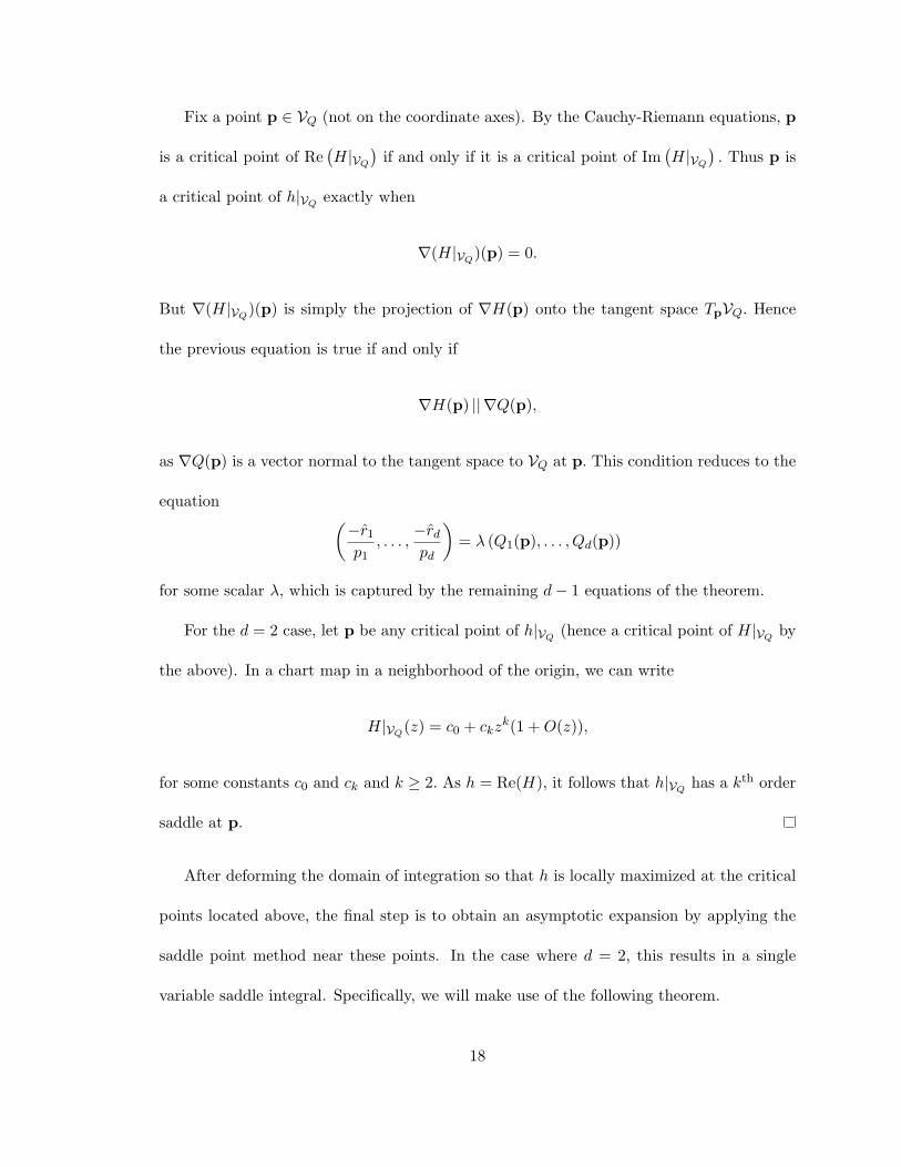
After deforming the domain of integration so that h is locally maximized at the critical
points located above, the final step is to obtain an asymptotic expansion by applying the
saddle point method near these points. In the case where d = 2, this results in a single
variable saddle integral. Specifically, we will make use of the following theorem.
18
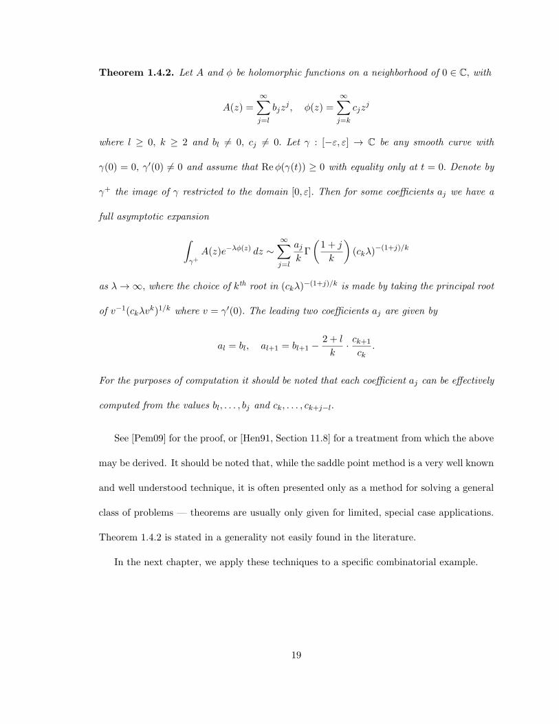
Theorem 1.4.2. Let A and φ be holomorphic functions on a neighborhood of 0 ∈ C, with
A(z) =∞∑
j=l
bjzj , φ(z) =
∞∑
j=k
cjzj
where l ≥ 0, k ≥ 2 and bl 6= 0, cj 6= 0. Let γ : [−ε, ε] → C be any smooth curve with
γ(0) = 0, γ′(0) 6= 0 and assume that Reφ(γ(t)) ≥ 0 with equality only at t = 0. Denote by
γ+ the image of γ restricted to the domain [0, ε]. Then for some coefficients aj we have a
full asymptotic expansion
∫
γ+A(z)e−λφ(z) dz ∼
∞∑
j=l
ajkΓ
(
1 + j
k
)
(ckλ)−(1+j)/k
as λ→ ∞, where the choice of kth root in (ckλ)−(1+j)/k is made by taking the principal root
of v−1(ckλvk)1/k where v = γ′(0). The leading two coefficients aj are given by
al = bl, al+1 = bl+1 −2 + l
k· ck+1
ck.
For the purposes of computation it should be noted that each coefficient aj can be effectively
computed from the values bl, . . . , bj and ck, . . . , ck+j−l.
See [Pem09] for the proof, or [Hen91, Section 11.8] for a treatment from which the above
may be derived. It should be noted that, while the saddle point method is a very well known
and well understood technique, it is often presented only as a method for solving a general
class of problems — theorems are usually only given for limited, special case applications.
Theorem 1.4.2 is stated in a generality not easily found in the literature.
In the next chapter, we apply these techniques to a specific combinatorial example.
19
Chapter 2
Application to Bicolored
Supertrees
2.1 Problem specification
We define the class K of bicolored supertrees as follows. First, denote by G the class of
Catalan trees, i.e. rooted, unlabeled, planar trees, counted by the number of nodes. The
class G has generating function
G(x) =1
2
(
1−√1− 4x
)
,
whose coefficients are the Catalan numbers. Denote by G the class of bicolor-planted Catalan
trees: Catalan trees having an extra red or blue node attached to the root (likewise counted
by the number of nodes). The class G has generating function
G(x) = 2xG(x).
20
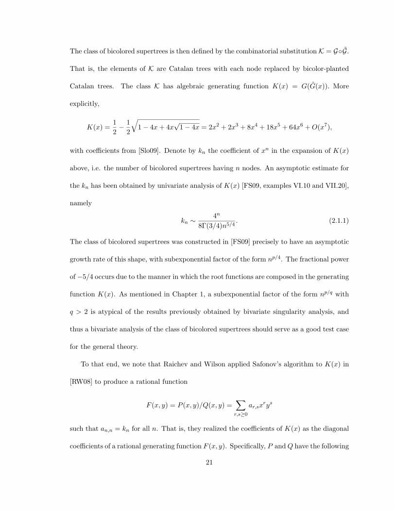
The class of bicolored supertrees is then defined by the combinatorial substitution K = G◦G.
That is, the elements of K are Catalan trees with each node replaced by bicolor-planted
Catalan trees. The class K has algebraic generating function K(x) = G(G(x)). More
explicitly,
K(x) =1
2− 1
2
√
1− 4x+ 4x√1− 4x = 2x2 + 2x3 + 8x4 + 18x5 + 64x6 +O(x7),
with coefficients from [Slo09]. Denote by kn the coefficient of xn in the expansion of K(x)
above, i.e. the number of bicolored supertrees having n nodes. An asymptotic estimate for
the kn has been obtained by univariate analysis of K(x) [FS09, examples VI.10 and VII.20],
namely
kn ∼ 4n
8Γ(3/4)n5/4. (2.1.1)
The class of bicolored supertrees was constructed in [FS09] precisely to have an asymptotic
growth rate of this shape, with subexponential factor of the form np/4. The fractional power
of −5/4 occurs due to the manner in which the root functions are composed in the generating
function K(x). As mentioned in Chapter 1, a subexponential factor of the form np/q with
q > 2 is atypical of the results previously obtained by bivariate singularity analysis, and
thus a bivariate analysis of the class of bicolored supertrees should serve as a good test case
for the general theory.
To that end, we note that Raichev and Wilson applied Safonov’s algorithm to K(x) in
[RW08] to produce a rational function
F (x, y) = P (x, y)/Q(x, y) =∑
r,s≥0
ar,sxrys
such that an,n = kn for all n. That is, they realized the coefficients of K(x) as the diagonal
coefficients of a rational generating function F (x, y). Specifically, P andQ have the following
21

specification:
P (x, y) = 2x2y(
2x5y2 − 3x3y + x+ 2x2y − 1)
,
Q(x, y) = x5y2 + 2x2y − 2x3y + 4y + x− 2.
(2.1.2)
We wish to use produce asymptotics on an,n as n → ∞, recapturing the result of equation
(2.1.1). Recall that, due to the non-combinatorial nature of F , we can not use the formulas
of [PW02] to obtain the result we desire automatically. Thus we follow the procedure
outlined in Chapter 1 in full.
We carry over the notation of Chapter 1. In the case of bicolored supertrees this means
F =P
Q, P and Q defined as in (2.1.2)
|r| = n, r = r0 = (1, 1),
H(x, y) = − log x− log y
h(x, y) = − log |x| − log |y|.
Then as outlined in Chapter 1, the procedure will be as follows.
1. Reduce the asymptotic computation to an integral on the variety VQ using Corollary
1.3.7.
2. Locate the critical points of h|VQand deform the contour of integration so as to
minimize the maximum of h at such points.
3. Compute an asymptotic expansion for this integral by applying Theorem 1.4.2 near
these maxima and bounding the order away from these maxima.
These three steps will be carried out in the sections that follow. Thanks to all the work laid
out in the previous chapter, many of these steps will be automatic. The most difficult step
22
will be step (2), finding the new saddle point contour and actually proving that it possesses
the right properties (Lemma 2.4.3). The rest will be a matter of applying the theorems
when appropriate.
Before jumping into computations, however, we will need to do some initial work on
describing the variety VQ.
2.2 Describing the variety
Because Q is quadratic in the variable y, we can explicitly solve Q = 0 for y as a function
of x. This will allow us to parametrize VQ by x where possible. So define
y1(x) =−x2 + x3 − 2 +
√x4 + 4x2 − 4x3 + 4
x5,
y2(x) =−x2 + x3 − 2−
√x4 + 4x2 − 4x3 + 4
x5,
where in each case the principal root is chosen. Then by the quadratic formula
VQ = {(x, yj(x)) : x ∈ C \ {0}, j = 1, 2} ∪ {(0, 1/2)},
(though note that we may write (0, 1/2) = (0, y1(0)) by analytically continuing y1 at x = 0).
To parametrize VQ by x, we define the parametrization functions
ι1(x) = (x, y1(x)), ι2(x) = (x, y2(x)),
where in the construction of ι1 we assume that the singularity at x = 0 has been removed.
For the purposes of later computation, it will be nice to know the domain on which these
parametrization functions are holomorphic.
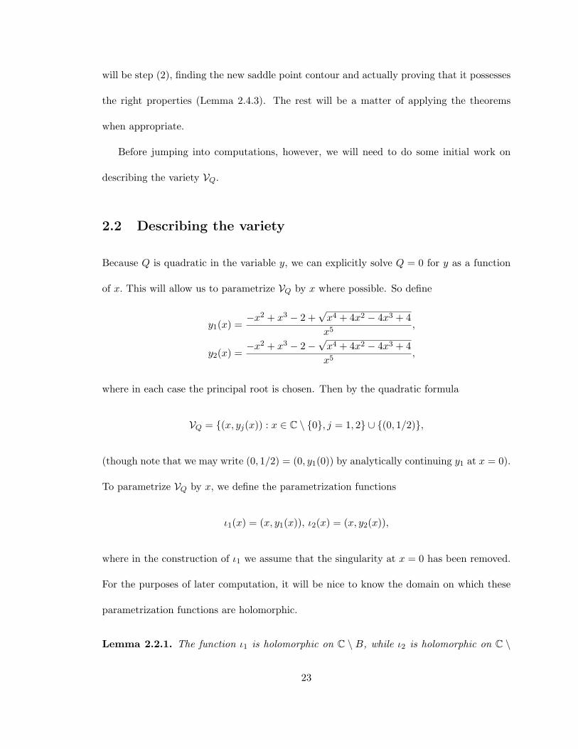
Lemma 2.2.1. The function ι1 is holomorphic on C \ B, while ι2 is holomorphic on C \
23
({0} ∪B), where
B :={
x = a+ ib ∈ C : a2 − 2a− b2 = 0, |b| ≥ Im(
1 +√1 + 2i
)}
.
Proof. By definition of the functions y1 and y2, the only points where ι1 and ι2 may fail to
be holomorphic are when x = 0 (in the case of ι2 only) or f(x) = x4 + 4x2 − 4x3 + 4 ≤ 0
(by the choice of principal square root). Thus we examine when f(x) is a nonpositive real
number.
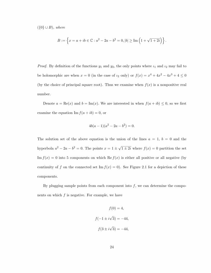
Denote a = Re(x) and b = Im(x). We are interested in when f(a + ib) ≤ 0, so we first
examine the equation Im f(a+ ib) = 0, or
4b(a− 1)(a2 − 2a− b2) = 0.
The solution set of the above equation is the union of the lines a = 1, b = 0 and the
hyperbola a2 − 2a − b2 = 0. The points x = 1 ±√1± 2i where f(x) = 0 partition the set
Im f(x) = 0 into 5 components on which Re f(x) is either all positive or all negative (by
continuity of f on the connected set Im f(x) = 0). See Figure 2.1 for a depiction of these
components.
By plugging sample points from each component into f , we can determine the compo-
nents on which f is negative. For example, we have
f(0) = 4,
f(−1± i√3) = −44,
f(3± i√3) = −44,
24

Imx
Rex
Figure 2.1: The zero sets of Im f and f .
and so we see that f(x) < 0 exactly on the four components contained in the set B, i.e.
along the branches of the hyperbola that lie outside the strip
Im(
1±√1− 2i
)
< Imx < Im(
1±√1 + 2i
)
.
For the purposes of constructing an appropriate cycle along which to integrate, we will
only need the fact that ι1 and ι2 are holomorphic on the punctured strip
{
x ∈ C \ 0 : Im(
1±√1− 2i
)
< Imx < Im(
1±√1 + 2i
)}
.
For the sake of completeness, however, we note that the details of Lemma 2.2.1 enable us to
understand the global topology of VQ as a Riemann surface. We take a moment to sketch
the construction.
Recall that the Riemann surface for√x is constructed by taking two copies of the slit
plane C \ {x : x ≤ 0} and gluing the “top” of the branch cut on one sheet to the “bottom”
25

Imx
Rex
Figure 2.2: The complex plane with
four branch cuts (the components of
B).
Figure 2.3: The Riemann surface for
√
f(x).
of the branch cut on the other, and vice versa.
Similarly the Riemann surface for√x4 + 4x2 − 4x3 + 4 can be constructed by beginning
with two copies of C \ B, i.e. two copies of the complex plane each with four branch cuts
along which f(x) = x4 + 4x2 − 4x3 + 4 ≤ 0. Local to the points x = 1 ±√1± 2i where
f(x) = 0, the Riemann surface for√
f(x) should look like the Riemann surface for√x, and
the branch cuts are glued together accordingly. Specifically, the tops of each of the branch
cuts on one sheet are glued to the bottoms of the corresponding branch cuts on the other
sheet, and vice versa. See Figure 2.2 for a representation of one of the sheets used in this
construction, and Figure 2.3 for a depiction of the Riemann surface of√
f(x).
The Riemann surface representation for VQ is then the same as the Riemann surface for
√
f(x), however with with a puncture point added to one sheet owing to the fact that ι2(x)
is not defined at x = 0. The upshot of this representation is that we can use it to classify
the the topology of VQ. Namely, the singular variety is homeomorphic to a single-holed
26

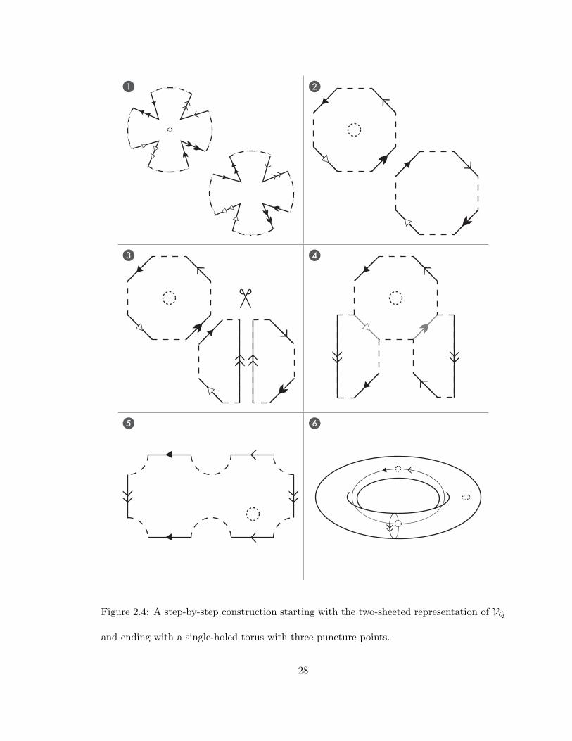
torus with three puncture points. See Figure 2.4 on page 28 for a step-by-step construction
demonstrating this fact.
Finally, as evidenced by Example 1.3.3, it will be useful for representing the residue
form along VQ to know where Qy =∂Q∂y is nonzero. Computing a Grobner basis of the ideal
〈Q,Qy〉 in Maple ([Wat08]) via the command
Basis([Q,diff(Q,y)],plex(y,x));
we obtain the univariate polynomial x4 + 4x2 − 4x3 + 4 as the first basis element. Hence
the x coordinate of any point where Q and Qy simultaneously vanish must be a root of this
polynomial. This justifies the following remark.
Remark 2.2.2. Along VQ, Qy is nonzero whenever x 6= 1±√1± 2i (the roots of the equation
x4 + 4x2 − 4x3 + 4 = 0).
2.3 Representing the intersection cycle
The following lemma accounts for the first step of the analysis: using Corollary 1.3.7 to
reduce the computation of an,n to an integral on VQ.
Lemma 2.3.1. For ε > 0, define
Cε = {x ∈ C : |x| = ε},
the circle of radius ε about 0 ∈ C, oriented counterclockwise. Then for sufficiently small
ε > 0,
an,n = 2πi
∫
ι1(Cε)Res(ωF ) + 2πi
∫
ι2(Cε)Res(ωF ). (2.3.1)
27
21
43
65
Figure 2.4: A step-by-step construction starting with the two-sheeted representation of VQ
and ending with a single-holed torus with three puncture points.
28
Proof. We first verify that the variety VQ is smooth. This is true only if Q, Qx and Qy do
not simultaneously vanish, which is true if and only if the variety I = 〈Q,Qx, Qy〉 is trivial
(the whole polynomial ring). We check this algorithmically, using Grobner bases. In Maple,
we compute the Grobner basis of I with the command
Basis([Q,diff(Q,x),diff(Q,y)],plex(y,x));
Maple returns the basis [1] for I, so the ideal is indeed trivial.
Now, let ε > 0, δ > 0 be sufficiently small so that
an,n =
∫
T0
ωF , where T0 = {(x, y) ∈ C2 : |x| = ε, |y| = δ}
by Cauchy’s Integral Formula. Define the quantities
m0 = inf{|yj(x)| : x ∈ Cε, j = 1, 2},
M0 = sup{|yj(x)| : x ∈ Cε, j = 1, 2}.
For ε sufficiently small, note that M0 < ∞ (by continuity of the yj ; see Lemma 2.2.1) and
m0 > 0 (the x-axis intersects VQ only at the point (2, 0)).
Assume δ is chosen small enough so that δ < m0. Fix any M > M0. Then define the
homotopy
K : T0 × [0, 1] → C2
(x, y, t) 7→(
x, y(
1 + t(
Mδ − 1
)))
,
expanding T0 in the y direction past VQ. Then K intersects VQ in the set C = ι1(Cε)∪ι2(Cε)
and avoids the coordinate axes. Furthermore, K intersects VQ transversely (as K expands
in the y direction, intersecting VQ where it is a graph of x). Thus, by Corollary 1.3.7 we
29
obtain
an,n = 2πi
∫
ι1(Cε)Res(ωF ) + 2πi
∫
ι2(Cε)Res(ωF ) +
∫
T1
ωF , (2.3.2)
where Cε is oriented counterclockwise (determined by examination of Theorem 1.2.2 and
the Residue Theorem).
Now fix n large and letM vary. As the rest of the terms in (2.3.2) have noM dependence,
∫
T1ωF must be a constant function of M. But by trivial bounds, we can show that
∫
T1
ωF = O(M1−n) as M → ∞,
as P(2πi)2xyQ
= O(1), exp(nH) = O(M−n) and the area of T1 is O(M). For n > 1, M1−n → 0
as M → ∞. Hence the only constant∫
T1ωF can be equal to is 0.
2.4 Saddle location and contour analysis
Step (2) in the analysis is to locate the saddle points of h|VQand deform the contour of inte-
gration appropriately, using this information. The saddle points can be found automatically
as follows.
Lemma 2.4.1. h|VQhas three saddle points, located at
(
2, 18)
= ι1(2),
(
1−√5, 3+
√5
16
)
= ι1(1−√5),
(
1 +√5, 3−
√5
16
)
= ι2(1 +√5).
Proof. By Theorem 1.4.1, the critical points of h|VQare those points where Q and xQx−yQy
simultaneously vanish. We can compute these points algorithmically by computing the
30
Grobner basis for the ideal I = 〈Q, xQx − yQy〉 . This is done in Maple with the command
Basis([Q,x*diff(Q,x)-y*diff(Q,y)],plex(y,x));
which returns a basis consisting of the following two polynomials:
32− 8x2 − 32x+ 20x3 − 8x4 + x5, x4 − 48− 6x3 + 8x2 + 128y + 16.
The first polynomial factors as (x2 − 2x − 4)(x − 2)3, with roots x = 2 and x = 1 ±√5.
Substituting these values of x into the second polynomial and solving for y yields the critical
points claimed in the lemma.
We note here the interesting geometry near the critical point (2, 1/8), which will turn
out to be the sole contributing point. Expanding H(ι1(x)) near x = 2, we obtain
H(ι1(x)) = H(ι1(2)) +1
16(x− 2)4 +O((x− 2)6),
and hence h|VQhas a degenerate saddle (of order 4) near this critical point, with steepest
descent directions emanating from x = 2 at angles π/4+ j(π/2) radians (j = 1, 2, 3, 4.). We
also see that along the path |x| = 2, h(ι1(x)) is locally minimized at x = 2, as this path
passes through the critical point along ascent directions. Hence x = 2 is a local maximum
for |y1(x)| along this path, and so there are points (x, y) ∈ VQ near (2, 1/8) such that |x| = 2
and |y| < 1/8. Because VQ cuts in toward the origin near ι1(2), this critical point is not on
the boundary of the domain of convergence of F. In the terminology of the introduction,
this critical point is not minimal.
Knowing where the saddle points of h are, the next task is to deform the contour of
integration in (2.3.1) so as to minimize the maximum modulus of h along the new contour
at said saddle points. The integral over domain ι2(Cε) will actually be shown to vanish,
31
Imx
Rex
p2p3
p4
p5p1
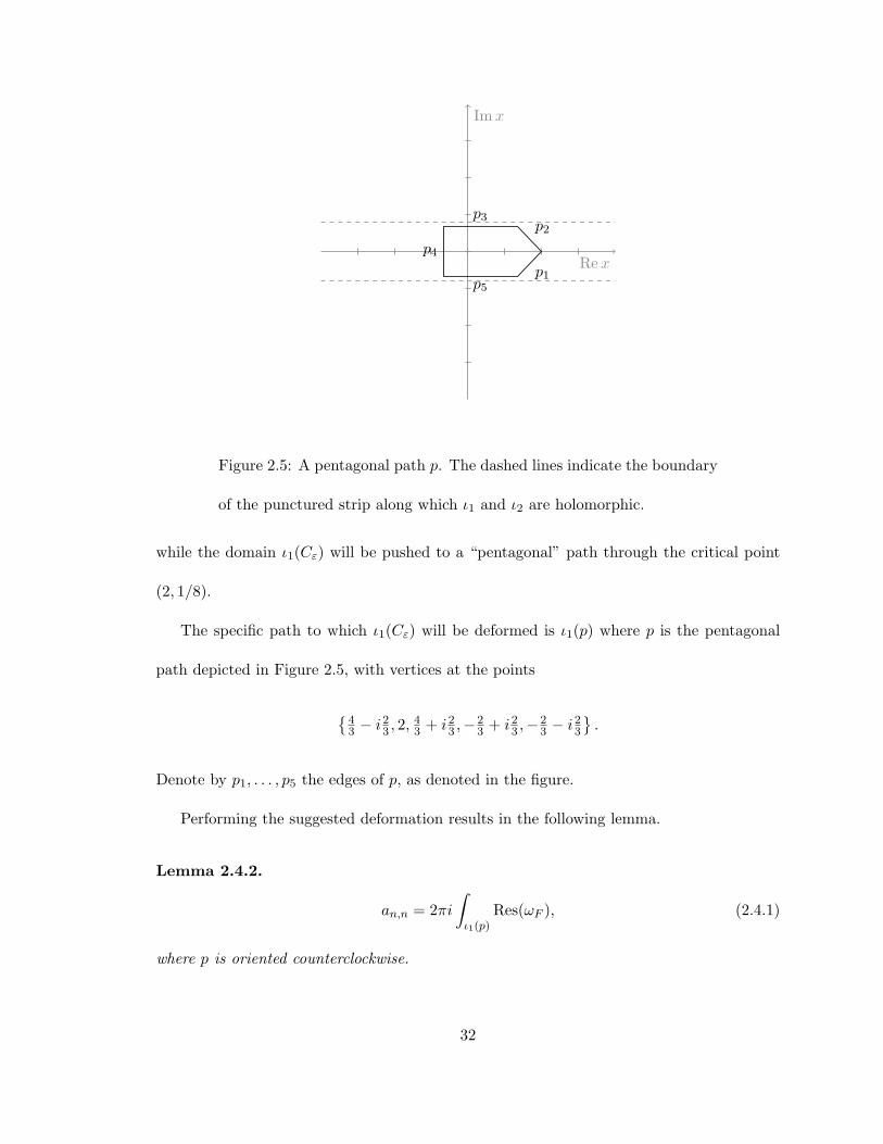
Figure 2.5: A pentagonal path p. The dashed lines indicate the boundary
of the punctured strip along which ι1 and ι2 are holomorphic.
while the domain ι1(Cε) will be pushed to a “pentagonal” path through the critical point
(2, 1/8).
The specific path to which ι1(Cε) will be deformed is ι1(p) where p is the pentagonal
path depicted in Figure 2.5, with vertices at the points
{
43 − i23 , 2,
43 + i23 ,−2
3 + i23 ,−23 − i23
}
.
Denote by p1, . . . , p5 the edges of p, as denoted in the figure.
Performing the suggested deformation results in the following lemma.
Lemma 2.4.2.
an,n = 2πi
∫
ι1(p)Res(ωF ), (2.4.1)
where p is oriented counterclockwise.
32
Proof. For δ < ε, let K be a homotopy shrinking the circle Cε to the circle Cδ. By holo-
morphicity of ι2 (Lemma 2.2.1), ι2 ◦K is a homotopy from ι2(Cε) to ι2(Cδ) along VQ, and
Res(ωF ) is holomorphic along this homotopy. By Stokes’ Theorem we obtain
∫
ι2(Cε)Res(ωF ) =
∫
ι2(Cδ)Res(ωF ).
Now fix n large and let δ vary. Note that as the left hand side of the above equation
has no δ dependence, neither does the right.
By the fact that y2(x) = −4x−5(1 + O(x)) as x → 0, we get that −P(2πi)2xyQy
= O(δ−4),
exp(nH) = O(δ4n) and the area of ι2(Cδ) is O(δ−4) as δ → 0. This implies that
∫
ι2(Cδ)Res(ωF ) =
∫
ι2(Cδ)
1
(2πi)2· −PxyQy
enH dx = O(δ4n−8)
as δ → 0 (note that this representation of the residue is valid by Remark 2.2.2). For n > 2,
δ4n−8 → 0 as δ → 0. Thus we must have that this integral is equal to 0.
As for the the integral over ι1(Cε) in (2.3.1), let K now be a homotopy expanding the
circle Cε to the pentagonal path p. Then by Lemma 2.2.1, ι1 ◦K is a homotopy from ι1(Cε)
to ι2(p) along VQ, and Res(ωF ) is likewise holomorphic along the image of this homotopy.
Then by Stokes’ Theorem,
∫
ι1(Cε)Res(ωF ) =
∫
ι1(p)Res(ωF ),
where p is oriented counterclockwise. The theorem follows.
Now we show that h is indeed maximized on ι1(p) uniquely at the point (2, 1/8). That
this is true local to the saddle point (2, 1/8) is clear from the form of H near this point, as
explored following the proof of Lemma 2.4.1. To show that this is true globally will require
more effort.
33
Lemma 2.4.3. h(ι1(x)) < h(ι1(2)) = log 4 ∀x ∈ p \ {2}.
Proof. Because h(ι1(x)) is continuous on the connected set p, we need only show that
h(ι1(x)) 6= log 4 for all x ∈ p \ {2}, and that h(ι1(x)) < log 4 for some x ∈ p \ {2}. The
latter condition can be easily checked by plugging some arbitrary point into h(ι1(x)). As
for the former condition, the idea will be to cook up some polynomial equations that must
be satisfied in order for it to be true that h(ι1(x)) = log 4. We then use techniques from
computational algebra to show that these equations can not be satisfied for any (x, y) with
x ∈ p \ {2} and y = y1(x).
The conditions from which we will derive our polynomial equations are as follows:
1. x ∈ pj for some j ∈ {1, . . . , 5}.
2. y such that (x, y) ∈ VQ.
3. h(x, y) = log 4, or eh(x,y) = 4.
Each of these conditions implies a (set of) polynomial equations in the variables Re(x),
Im(x), Re(y) and Im(y), as we will show shortly. Note that we are throwing away some
important information in condition 2 above, namely we want y = y1(x), not y = y2(x). This
will be important later in the proof.
We examine first the case where x ∈ p3. Denote a = Re(x), b = Im(x), c = Re(y) and
d = Im(y). Then condition 1 implies the polynomial constraint:
P1 = b− 2
3= 0.
Note: condition 1 implies the additional constraint a ∈ [−2/3, 4/3], which we will make use
of shortly.
34

Condition 2 implies the following two polynomial constraints:
P2 = Re(Q(a+ ib, c+ id)) = 0,
P3 = Im(Q(a+ ib, c+ id)) = 0.
Finally, condition 3 translates to 4|x||y| = 1, or
P4 = 16(a2 + b2)(c2 + d2)− 1 = 0.
We are interested in whether these four polynomial equations have a common real-valued
solution, and we will use Grobner bases and Sturm sequences to answer this question. Since
we expect the variety generated by I = 〈P1, P2, P3, P4〉 to be finite — I is generated by four
polynomials in four unknowns — we hope to use Grobner bases to eliminate variables and
produce a univariate polynomial B(a) ∈ I. Any point (a, b, c, d) solving Pj = 0 for all j will
likewise solve B = 0. Then we try to use Sturm sequences to that such a B has no real
roots a ∈ [−2/3, 4/3], proving that h(ι1(x)) 6= log 4 for x ∈ p3.
We compute the Grobner basis with the command
Basis([P1,P2,P3,P4],plex(d,c,b,a))
and find that the first element B of the basis is univariate in the variable a, a polynomial
of degree 16. We can check that B(−2/3) 6= 0 and B(4/3) 6= 0 by direct computation in
Maple. To check whether or not B has any roots on the interval (−2/3, 4/3) we employ
Sturm’s Theorem (see [BPR06, p. 52]).
To employ Sturm’s Theorem, we must verify that B is squarefree. This is true if and
only if the ideal 〈B,B′〉 is equal to the trivial ideal 〈1〉 . Indeed, computing the Grobner
basis for 〈B,B′〉
35
Basis([B,diff(B,a)],plex(a));
returns the trivial basis [1], i.e. B is squarefree.
Then to count the number of roots in (−2/3, 4/3) via Sturm’s Theorem, we enter the
command
sturm(sturmseq(B,a),a,-2/3,4/3)
and Maple returns that there are 0 real roots on the interval (−2/3, 4/3).
Computations are similar for p4 and p5, but things are a bit more complicated along p1
and p2. Let’s look at p2. The first polynomial equation becomes
P1 = a+ b− 2 = 0,
with a ∈ [4/3, 2], while the rest of the polynomial equations remain the same. Going through
the same procedure as before, we can produce a Grobner basis for 〈P1, P2, P3, P4〉 with an
element B(a) univariate in a. B(a) factors as
B(a) = (a− 2)4B(a),
where by direct computation we see that B is nonzero at a = 4/3 and a = 2. Note: we
expected that B would have a root at a = 2, corresponding to the fact that h(ι1(2)) = log 4.
The next step would be to attempt to show that B has no roots on the interval (4/3, 2),
but this is not true. Using Sturm sequences, one can show that B has exactly one root
a0 ∈ (4/3, 2), and this is because there is a pair x, y with x ∈ p2 \ {2} and h(x, y) = log 4.
The claim is that this corresponds to a point where y = y2(x), not where y = y1(x).
To see that there must be such a pair, note that y2(x) → 0 as x→ 2. Hence h(ι2(x)) → ∞
as x → 2. But by direct computation we can show that h(ι2(4/3)) < log 4. As h(ι2(x)) is
36

continuous on p2 \ {2}, there must be some x ∈ p2 \ {2} such that h(ι2(x)) = log 4. This
pair x, y = y2(x) satisfies the polynomial equations Pj = 0.
Now assume by way of contradiction that h(ι1(x)) = log 4 for some x ∈ p2\{2}. Because
B has just one root a0 ∈ (4/3, 2), it must be that this occurs at the same x value for which
h(ι2(x)) = log 4, specifically x0 = a0 + (2− a0)i. Hence we have
|x0||y1(x0)| = |x0||y2(x0)| =1
4,
which implies that |y1| = |y2| at the point x0. So at this value of x we have
c2 + d2 = |y|2 = |y1y2| =|x− 2||x|5
The preceding equation implies that |x|10(c2 + d2)2 = |x − 2|2, which translates into the
polynomial equation
P5 = (a2 + b2)5(c2 + d2)2 − ((a− 2)2 + b2) = 0.
We now have a new polynomial equation that must be satisfied in order to have that
h(ι1(x)) = log 4 on p2 \ {2}. But if we compute a Grobner basis for 〈P1, . . . , P5〉 , we get
the trivial basis [1], meaning that the polynomials have no common solution. Hence
h(ι1(x)) 6= log 4 for x ∈ p2 \ {2}. Analogous methods can be used to handle the case of
p1.
2.5 Saddle point integration
The final step in the analysis is to use saddle point techniques and order bounds to prove
(2.1.1).
37
Theorem 2.5.1.
kn = an,n ∼ 4n
8Γ(3/4)n5/4.
Proof. We proceed from Lemma 2.4.2. The theorem will be proved in 2 steps: bounding
the integral in (2.4.1) outside a neighborhood of the critical point, then applying saddle
point techniques near that critical point.
For any neighborhood N of x = 2, we look at∫
ι1(p\N)Res(ωF ), which can be written as
∫
ι1(p\N)
1
(2πi)2· −PxyQy
enH dx
(note that this representation is valid by Remark 2.2.2). As h ◦ ι1 is continuous on the
compact set p \N, h ◦ ι1 achieves an upper bound M on p \N. By Lemma 2.4.3, M < log 4.
Thus by trivial bounds we have
∫
ι1(p\N)Res(ωF ) = O(eMn) = o((4− δ)n)
for sufficiently small δ > 0, as n→ ∞. Hence
an,n = 2πi
∫
ι1(p∩N)Res(ωF ) + o((4− δ)n). (2.5.1)
for any neighborhood N of x = 2, provided δ is sufficiently small.
For N small enough, p ∩ N = (p1 ∩ N) ∪ (p2 ∩ N). We examine the integral over
ι1(p1 ∩N) and ι1(p2 ∩N) separately, starting with ι1(p2 ∩N). By using the aforementioned
representation of the residue form (and changing variables), we obtain
2πi
∫
ι1(p2∩N)Res(ωF ) =
∫
p2∩N
1
2πi· −P (ι1(x))xy1(x)Qy(ι1(x))
enH(ι1(x)) dx.
After another change of variables (x→ x+2) and a suitable choice of neighborhood N, the
above integral can be rewritten as
4n∫
γ+A(x)e−nφ(x) dx,
38

where we have, for some fixed ε > 0,
γ(x) = (i− 1)x; x ∈ [−ε, ε],
A(x) =1
2πi· −P (ι1(x+ 2))
(x+ 2)y1(x+ 2)Qy(ι1(x+ 2)),
φ(x) = log 4−H(ι1(x+ 2)),
and we recall that γ+ is the restriction of the image of γ to the domain [0, ε]. The series
expansion of A and φ at x = 0 begin
A(x) =i
16πx3 +
i
32πx4 +O(x5),
φ(x) =−1
16x4 +O(x6),
and Reφ(x) is uniquely minimized on γ+ at x = 0 where we have φ(0) = 0, as a consequence
of Lemma 2.4.3. Thus this is exactly the situation where the saddle point technique of
Theorem 1.4.2 can be applied. The values of bj and cj are as in the expansions above. Then
v = γ′(0) = i− 1, and we compute the principal root
(cknvk)1/k
v=
((−1/16)n(i− 1)4)1/4
i− 1=
−1− i
2√2n1/4.
The conclusion of Theorem 1.4.2 is then
2πi
∫
ι1(p2∩N)Res(ωF ) ∼ 4n
(
−i4πn−1 +
(1 + i)√2Γ(5/4)
8πn−5/4 +O(n−3/2)
)
As for the integral over ι1(p1 ∩N), the same argument yields
2πi
∫
ι1(p1∩N)Res(ωF ) = −4n
∫
γ+A(x)e−nφ(x) dx,
where A and φ are the same but γ is defined by γ(x) = (−i − 1)x (and the negative sign
out in front comes from a reversal of orientation). For v = γ′(0) = −i− 1, we compute the
39
principal root
(cknvk)1/k
v=
((−1/16)n(−i− 1)4)1/4
−i− 1=
−1 + i
2√2n1/4.
Then by Theorem 1.4.2 we obtain
2πi
∫
ι1(p1∩N)Res(ωF ) ∼ 4n
(
i
4πn−1 +
(1− i)√2Γ(5/4)
8πn−5/4 +O(n−3/2)
)
.
Adding up the contribution over each piece and plugging into (2.5.1) yields
an,n ∼ 4n
(√2Γ(5/4)
4πn−5/4 +O(n−3/2)
)
+ o((4− δ)n) ∼ 4n√2Γ(5/4)
4πn−5/4.
Using the identity Γ(5/4)Γ(3/4) = π/(2√2), the theorem follows.
40
Chapter 3
Homology of the Intersection Class
3.1 Setup and assumptions
We would like to produce an algorithm automating the analysis applied in the previous chap-
ter. Tracing through the asymptotic analysis of bicolored supertrees, it becomes apparent
that the main difficulty in realizing this goal will be achieving a sufficient understanding
of the homology class of the intersection cycle. To obtain a homologous representative of
the intersection cycle amenable to saddle point methods requires some global description of
the singular variety – a potentially complicated space. Thus to begin, we must produce a
description of the singular variety amenable to algorithmic study.
The idea will be to tackle this problem in stages, first focusing on understanding a
small subset of the singular variety. Once we are done with that, we will begin revealing
more and more of the surface, understanding how the topology changes along the way. The
mechanism enabling this study is known as Morse Theory, in which a manifold M is studied
with respect to some height function h : M → R. The manifold M is first restricted to
41
those points of sufficiently high (or low) value with respect to the height function, and the
methods of Morse Theory reveal how the topology changes as regions of lower (or higher)
height are unveiled. More details will be given in the following sections.
Portions of the following analysis will rely on topological properties of the bivariate
case, and thus from here onward we will assume that d = 2 variables. Hence the notation
and the setup of the problem will be similar to that employed in the previous chapter.
We write z = (x, y) rather than x = (x1, x2) to indicate points in C2. Similarly we write
r = (r, s) = n(r, s) rather than r = (r1, r2) = |r| (r1, r2).
We further impose the following assumptions on our analysis:
Assumption 3.1.1. Assume that r and s are positive rationals.
The preceding assumption is so that the points in Σ (the critical points of h on VQ)
can be found algorithmically using Grobner bases. The additional assumption that r and
s both be nonzero is to guarantee that this problem does not reduce to one of univariate
rational asymptotics.
Assumption 3.1.2. Assume that Σ is a finite set.
Note that the preceding assumption is generically true, but may fail for certain directions
(r, s).
Assumption 3.1.3. Assume that VQ is smooth.
Our analysis will apply under the preceding assumptions, with one last technical as-
sumption to come later. Note that the assumption that VQ be smooth will be relaxed
slightly at the end of this chapter.
42
3.2 Describing the variety at large height
Our Morse-theoretic analysis of VQ begins with the selection of a suitable height function.
For the singular variety VQ, we have the somewhat natural height function h = h(r,s), the
function governing the exponential growth rate of the integrand from which we compute
the asymptotics. Our first goal will be to describe what VQ looks like for very large values
of h. Consequently, we develop the following notation for better describing such sets.
Definition 3.2.1. For each constant M ∈ R we define the set
V>M = {z ∈ VQ :M < h(z) <∞} .
We define the sets V≥M , V<M and V≤M similarly.
Note that implicit to the preceding definition is the fact that the variety VQ is endowed
with a specific height function. Later, when we describe VQ relative to an auxiliary height
function, we will indicate this by modifying our notation for the variety itself.
We next wish to develop a description for V>M for sufficiently large M . By definition of
h we know that the height along VQ is arbitrarily large only when |x| or |y| are sufficiently
small, so we first turn to understanding the variety near such points. We have the following
useful characterization of a complex variety local to any x or y value:
Theorem 3.2.2. Let B ⊆ C be a circular neighborhood of x0 ∈ C slit along a ray emanating
from x0. If the radius of B is sufficiently small, then on B every branch of Q(x, y) = 0
admits a representation y = f(x) of the form
f(x) =∑
j≥j0cj(x− x0)
j/k,
43
for a fixed determination of (x− x0)1/k, where j0 ∈ Z and k ∈ N. The function f is called
a Puiseux expansion of y.
See [FS09, Theorem VII.7] for a proof, or [BK86] for a more in-depth discussion. Note
that a similar result holds for obtaining the Puiseux expansion of x in terms of y near any
fixed value y = y0.
This local representation allows us to prove the following theorem.
Theorem 3.2.3. The set VQ ∩{(x, y) : 0 < |x| < R}, for sufficiently small R, is diffeomor-
phic to a finite set of disjoint, punctured open disks.
Each such diffeomorphism takes the form
G : U −→ D
z 7−→ (zk, g(z))
for some integer k ≥ 1, where U is the punctured disk BR1/k(0) − {0} and g is some
holomorphic function on U .
Proof. By Theorem 3.2.2, for x restricted to a small enough slit neighborhood of 0 in C,
any branch of VQ can be represented as (x, f(x)) for some fractional expansion
f(x) =∑
j≥j0cjx
j/k.
We may assume that f has been represented such that k is as small as possible. Removing
the slit, f can be extended to a neighborhood of the form
{x ∈ C : |x| < R, x 6= 0}
by analytic continuation to a multiple-valued, locally holomorphic function. The goal is
then to better characterize this full branch (x, f(x)) in VQ.
44

Begin by defining the function
g(x) =∑
j≥j0cjx
j ,
a function holomorphic on the punctured disk U = BR1/k(0) \ {0}. From this, we define the
function
G : U −→ C2
z 7−→ (zk, g(z))
The goal is to show that G is actually a diffeomorphism between the punctured disk and
the previously described branch, thus completing the theorem.
The first step is to show that G is one-to-one, so begin by assuming that it is not. Then
there are z1 6= z2 in U satisfying
zk1 = zk2
g(z1) = g(z2)
Denote z0 = zk1 = zk2 . This means that for two fixed determinations z1 and z2 of z1/k0 ,
g(z1) = g(z2). Now we can write z2 = ξz1 for some kth root of unity ξ 6= 1. This means
that
g(z1) = g(ξz1),
and so
zm1 g(z1) = zm1 g(ξz1),
where m = max (0,−j0). But the functions zmg(z) and zmg(ξz) are holomorphic on the
disk BR1/k(0) (multiplying by zm was done precisely to force holomorphicity at z = 0), and
so by the properties of complex analytic functions there are only two possibilities. Either:
45

1. The functions zmg(z) and zmg(ξz) agree on BR1/k(0), or
2. By sufficiently minimizing the radius R, we can assure that zmg(z) and zmg(ξz) agree
nowhere except possibly at the origin.
In the first case, it must be that the coefficients in the Taylor expansions of zmg(z) and
zmg(ξz) all agree, which means that cj = cjξj for all j ≥ j0. Hence cj = 0 whenever ξj 6= 1.
This means that cj 6= 0 only when j ∈ sZ for s ≥ 2 equal to the order of ξ, a divisor of k.
But this implies that the fractional expansion f(x) can be written in terms of the (k/s)th
roots x(k/s), contradicting the minimality of k. Thus we must be in the second case.
Hence by sufficiently minimizing the radius R for each possible kth root of unity ξ, we
can guarantee that the function G is indeed one-to-one. The inverse function G−1 is locally
smooth because the function z 7→ zk has a locally smooth inverse away from z = 0. Hence
G−1 is smooth, and so we see that G is indeed a diffeomorphism.
Note that a similar result holds if we restrict to sufficiently small magnitudes of y rather
than x. And furthermore, because Q(0) 6= 0 (as P/Q was assumed to be holomorphic near
0 ∈ C), we can find a sufficiently small value of R so that no (x, y) ∈ VQ satisfies both
|x| < R and |y| < R. The fact that these neighborhoods can be made disjoint will be
important later on.
Now that we have a good understanding of the topology of VQ near x = 0 and near y = 0,
the next thing we wish to do is to evaluate the height function on these neighborhoods. As
a first step, we would like to show that the height function is eventually monotonically
increasing or decreasing to ±∞ as x or y go to 0. Unfortunately this is not always the case,
and requires a final assumption regarding the direction in which asymptotics are taken.
46
Assumption 3.2.4. By the Puiseux expansion, we know that we can parameterize each
branch of VQ local to x = 0 in terms of x by writing
y = cxα(1 + o(1))
as x→ 0 for some constants c 6= 0 and α. We assume that
α 6= −rs
for all such branches.
Similarly, we can parameterize each branch of VQ local to y = 0 in terms of y by writing
x = cyβ(1 + o(1))
as y → 0 for some constants c 6= 0 and β. We assume that
β 6= −sr
for all such branches.
This assumption precludes us from taking asymptotics in only finitely many directions,
as there are only finitely many branches of VQ near x = 0 and y = 0. We also note that
the finitely many possible values of α and β may be read from Newton polygon of the
polynomial Q; see section 4.3 for further details.
The idea behind this assumption is to guarantee that h does not remain bounded as
x→ 0 and, necessarily, y → ∞ (or vice versa). This assumption is essential to the following
lemma.
Lemma 3.2.5. As in the conclusion of Theorem 3.2.3, fix a branch of VQ near x = 0
that is diffeomorphic to a punctured disk. By the fractional expansion y = f(x) in this
47
neighborhood, we can write y ∼ cxα as x→ 0, for some α ∈ Q and some constant c. Then,
for sufficiently small R and any θ ∈ [0, 2π], the function
hθ : (0, R] −→ R
ρ 7−→ h(ρeiθ, f(ρeiθ))
is monotone. That is, if the punctured disk is sufficiently small, the height function is
monotone along rays emanating from the origin.
Furthermore, as ρ → 0, the height hθ approaches ∞ or −∞ according to whether α >
−r/s or α < −r/s, respectively.
Proof. Locally, thanks to the Puiseux expansion of y in terms of x, we can consider the
functions H and h to be functions of a single complex variable. Namely
H(x) = −r log x− s log f(x), and h(x) = ReH(x).
Then dhθdρ is simply the derivative of h(x) with respect to ρ, where x = ρeiθ. As h = ReH,
this can be represented as
dhθdρ
=
(
RedH
dx
)
cos θ −(
ImdH
dx
)
sin θ
∣
∣
∣
∣
x=ρeiθ
So we turn to evaluating dHdx .
By the Puiseux expansion, we can write f(x) = cxα(1 + g(x)) for some fractional ex-
pansion g(x) that is o(1) as x→ 0. Then
H(x) = −r log x− s log (cxα(1 + g(x)))
= (−r − sα) log x− s log (1 + g(x))− s log c.
48
We note briefly from the above form for H that ReH approaches ±∞ as x → 0 according
to the sign of (−r− sα), as claimed in the statement of the lemma. Now dHdx takes the form
H ′(x) =−r − sα
x− g′(x)
1 + g(x)
=1
x
(
−r − sα− xg′(x)1 + g(x)
)
∼ −r − sα
x
as x→ 0.
We can rewrite 1/x as cos θ/|x| − i sin θ/|x|, from which we obtain that
RedH
dx∼ (−r − sα) cos θ
|x|
and
ImdH
dx∼ (r + sα) sin θ
|x| .
And so dhθdρ ∼ −r−sα
|x| as x → 0. But −r−sα|x| → ±∞ as x → 0, and so we see that on a
sufficiently small neighborhood, this derivative can never vanish. Hence we have mono-
tonicity.
And again, note that there is nothing special about focusing our attention on branches
near x = 0. An analogous lemma holds on branches near y = 0.
We now have enough information to describe the space VQ at sufficiently large height.
Theorem 3.2.6. For sufficiently large M , the set V>M is diffeomorphic to a finite set of
disjoint, punctured open disks.
Proof. Pick R sufficiently small so that
1. If Q(x, y) = 0, then either |x| < R or |y| < R but not both.
49

2. The sets VQ ∩{(x, y) : 0 < |x| < R} and VQ ∩{(x, y) : 0 < |y| < R} are each
diffeomorphic to finite sets of disjoint, punctured open disks (as in the conclusion of
Theorem 3.2.3).
By the structure of h we now pick M large enough so that h(x, y) ≥ M requires either
that |x| < R or |y| < R. Note that this implies that
V≥M ⊆ VQ ∩{(x, y) : 0 < |x| < R or 0 < |y| < R}.
We examine a particular punctured disk D, say one arising from a branch (x, f(x)), where
f(x) = xα(1 + o(1))
is a Puiseux expansion of y in x. We look at the parametrization of D that we get from
Theorem 3.2.3:
G : U −→ D
z 7−→ (zk, g(z))
where U = BR1/k(0) \ {0} and g(z) = f(zk) for some positive integer k.
By Lemma 3.2.5, h ◦G is monotone on U along radial paths emanating from the origin
(note that G sends rays to rays). As h(x, y) < M along ∂D by construction, we have two
possibilities:
1. If h ◦G is monotone decreasing to −∞ as |z| → 0 in U , then V≥M ∩D = ∅.
2. Otherwise, h ◦ G is monotone increasing to ∞ as |z| → 0 in U , and so for each
θ ∈ [0, 2π] we obtain a unique ρ(θ) ∈ (0, R1/k) such that h(G(ρ(θ)eiθ)) = M . Note
that the function ρ(θ) is continuous by the continuity of h ◦G.
50
So in this second case we obtain a simple closed curve s defined by
s : [0, 2π] −→ U
θ 7−→ ρ(θ)eiθ
which traces out the preimage of M under the map h ◦ G. By monotonicity, this implies
that the set V>M ∩D is parametrized by G∣
∣
U0, where
U0 = {ρeiθ ∈ C : 0 < ρ < ρ(θ)},
which is homeomorphic to U (hence to a punctured, open disk). By applying this argument
to every such D, and using the fact that V>M is contained in the union of all such disks D,
the conclusion of the theorem follows.
To further better describe how the components of V>M are structured (for sufficiently
large M), we introduce the following notation.
Definition 3.2.7. For M ∈ R, we partition the set V>M into its connected components as
V>M = {Rj : j ∈ J}.
Then we define the set X>M ⊆ V>M by
X>M = {Rj : ∀ ε > 0, ∃ (x, y) ∈ Rj s.t. |x| < ε},
i.e. the set of all components of V>M containing points of arbitrarily small x-coordinate.
Similarly we define the set Y >M by
Y >M = {Rj : ∀ ε > 0, ∃ (x, y) ∈ Rj s.t. |y| < ε}.
We call the components of X>M the x-components of V>M , and similarly the components
of Y >M are called the y-components of V>M .
51

We define the sets X≥M and Y ≥M analogously.
Note that it may be possible that either X>M or Y >M is empty for a given M . As we
shall see in the next section, however, it can not be the case that X>M and Y >M are both
empty unless VQ is empty itself.
We also note that there may be overlap between the x- and y-components of V>M , but
as evidenced in the proof of the preceding theorem this does not happen for sufficiently large
M . For large enough M , the space V>M decomposes uniquely into x- and y-components,
each of which is homeomorphic to an open, punctured disk.
3.3 Unveiling the rest of the singular variety
Having understood V>M for sufficiently large M , we begin revealing the rest of the variety
by decreasing the value of M . We use Morse theory to examine how the topology changes
as we do so.
There are two important structural theorems that will allow us to accomplish our task,
which are as follows.
Theorem 3.3.1 (First Structure Theorem). Let m1 < m2 ∈ R be such that h has no
critical values in the interval [m1,m2]. Then V>m1 is topologically equivalent to V>m2; in
fact V>m2 is a deformation retract of V>m1.
For a discussion, see [Mil63]. The only special feature of h that is used in the preceding
theorem is the fact that h is proper on VQ. This is guaranteed by Assumption 3.2.4, which
implies that the inverse images under h∣
∣
VQof bounded sets are again bounded.
The second structural theorem, which deals with when the topology changes, is as
52
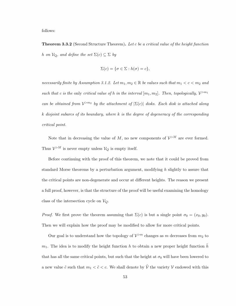
follows:
Theorem 3.3.2 (Second Structure Theorem). Let c be a critical value of the height function
h on VQ, and define the set Σ(c) ⊆ Σ by
Σ(c) = {σ ∈ Σ : h(σ) = c},
necessarily finite by Assumption 3.1.2. Let m1,m2 ∈ R be values such that m1 < c < m2 and
such that c is the only critical value of h in the interval [m1,m2]. Then, topologically, V>m1
can be obtained from V>m2 by the attachment of |Σ(c)| disks. Each disk is attached along
k disjoint subarcs of its boundary, where k is the degree of degeneracy of the corresponding
critical point.
Note that in decreasing the value of M , no new components of V>M are ever formed.
Thus V>M is never empty unless VQ is empty itself.
Before continuing with the proof of this theorem, we note that it could be proved from
standard Morse theorems by a perturbation argument, modifying h slightly to assure that
the critical points are non-degenerate and occur at different heights. The reason we present
a full proof, however, is that the structure of the proof will be useful examining the homology
class of the intersection cycle on VQ.
Proof. We first prove the theorem assuming that Σ(c) is but a single point σ0 = (x0, y0).
Then we will explain how the proof may be modified to allow for more critical points.
Our goal is to understand how the topology of V>m changes as m decreases from m2 to
m1. The idea is to modify the height function h to obtain a new proper height function h
that has all the same critical points, but such that the height at σ0 will have been lowered to
a new value c such that m1 < c < c. We shall denote by V the variety V endowed with this
53
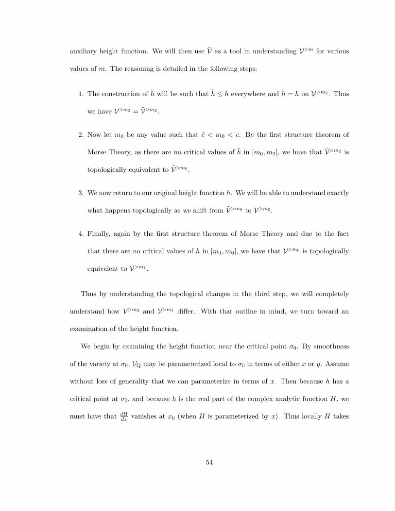
auxiliary height function. We will then use V as a tool in understanding V>m for various
values of m. The reasoning is detailed in the following steps:
1. The construction of h will be such that h ≤ h everywhere and h = h on V>m2 . Thus
we have V>m2 = V>m2 .
2. Now let m0 be any value such that c < m0 < c. By the first structure theorem of
Morse Theory, as there are no critical values of h in [m0,m2], we have that V>m2 is
topologically equivalent to V>m0 .
3. We now return to our original height function h. We will be able to understand exactly
what happens topologically as we shift from V>m0 to V>m0 .
4. Finally, again by the first structure theorem of Morse Theory and due to the fact
that there are no critical values of h in [m1,m0], we have that V>m0 is topologically
equivalent to V>m1 .
Thus by understanding the topological changes in the third step, we will completely
understand how V>m2 and V>m1 differ. With that outline in mind, we turn toward an
examination of the height function.
We begin by examining the height function near the critical point σ0. By smoothness
of the variety at σ0, VQ may be parameterized local to σ0 in terms of either x or y. Assume
without loss of generality that we can parameterize in terms of x. Then because h has a
critical point at σ0, and because h is the real part of the complex analytic function H, we
must have that dHdx vanishes at x0 (when H is parameterized by x). Thus locally H takes
54

the form:
H(x) = c+ id+
∞∑
j=k
cj(x− x0)j ,
where k ≥ 2 and ck 6= 0. Denoting C = c+ id and g(x) =∑∞
j=k cj(x− x0)j−k we get
H(x) = C + (x− x0)kg(x),
where g(x0) 6= 0.
Now as g(x0) 6= 0, we have in a small neighborhood of x0 that g(x)1/k, the kth principal
root of g(x), is an analytic function. Thus locally the function
w = (x− x0)g(x)1/k
is analytic, and by inspection we see that the derivative dwdx does not vanish at x = x0. So
by the inverse function theorem we can parameterize H locally by w. Note that, in terms
of the variable w, H takes on the relatively nice form:
H(w) = C + wk.
Next we move our attention from H to the actual height function h. Representing w in
polar coordinates as w = ρeiθ, we get
H(ρ, θ) = C + ρkeikθ,
so h = ReH takes the form
h(ρ, θ) = c+ ρk cos(kθ).
under this parameterization. Now let δ > 0 be sufficiently small so that the ball Bδ(0)
about w = 0 lies within the region on which this parameterization holds, and such that
δ < (m2 − c)1/k. The second condition guarantees that h(w) < m2 on Bδ(0), which we will
need later.
55
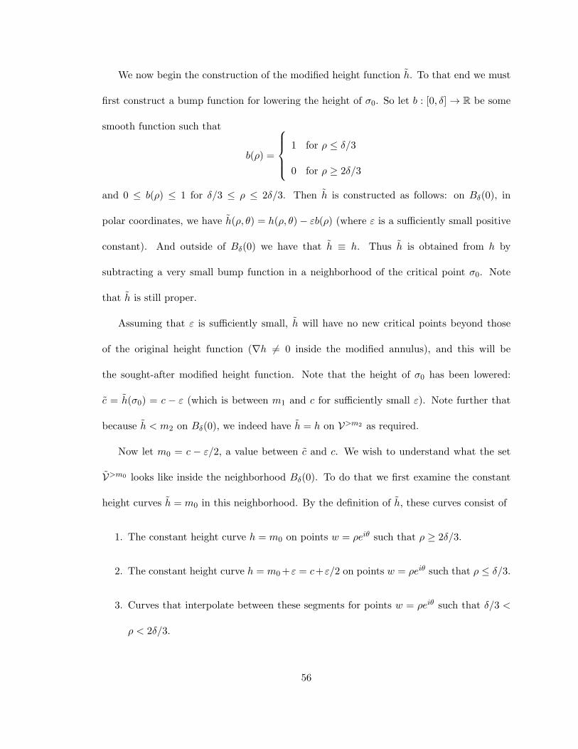
We now begin the construction of the modified height function h. To that end we must
first construct a bump function for lowering the height of σ0. So let b : [0, δ] → R be some
smooth function such that
b(ρ) =
1 for ρ ≤ δ/3
0 for ρ ≥ 2δ/3
and 0 ≤ b(ρ) ≤ 1 for δ/3 ≤ ρ ≤ 2δ/3. Then h is constructed as follows: on Bδ(0), in
polar coordinates, we have h(ρ, θ) = h(ρ, θ)− εb(ρ) (where ε is a sufficiently small positive
constant). And outside of Bδ(0) we have that h ≡ h. Thus h is obtained from h by
subtracting a very small bump function in a neighborhood of the critical point σ0. Note
that h is still proper.
Assuming that ε is sufficiently small, h will have no new critical points beyond those
of the original height function (∇h 6= 0 inside the modified annulus), and this will be
the sought-after modified height function. Note that the height of σ0 has been lowered:
c = h(σ0) = c − ε (which is between m1 and c for sufficiently small ε). Note further that
because h < m2 on Bδ(0), we indeed have h = h on V>m2 as required.
Now let m0 = c − ε/2, a value between c and c. We wish to understand what the set
V>m0 looks like inside the neighborhood Bδ(0). To do that we first examine the constant
height curves h = m0 in this neighborhood. By the definition of h, these curves consist of
1. The constant height curve h = m0 on points w = ρeiθ such that ρ ≥ 2δ/3.
2. The constant height curve h = m0+ε = c+ε/2 on points w = ρeiθ such that ρ ≤ δ/3.
3. Curves that interpolate between these segments for points w = ρeiθ such that δ/3 <
ρ < 2δ/3.
56

Figure 3.1: The region VQ local to
σ0, where V>m0 is shaded and the
degeneracy k = 3.
Figure 3.2: The region VQ local to
σ0, where V>m0 is shaded and the
degeneracy k = 3.
Then we see that the set V>m0∩Bδ(0) is composed of k connected components bound inside
Bδ(0) by the curves described above. See Figure 3.1 for an example with k = 3.
Finally, we wish to return to our original height function, and see how the topology
changes when we go from V>m0 to V>m0 . Because h and h only differ on the set B2δ/3(0),
we see that the change is only local to σ0. And by inspection, we see that V>m0 is obtained
from V>m0 by adding a “star-shaped” region that joins the k components of V>m0 ∩Bδ(0).
See Figure 3.2 for a picture. This proves the theorem in the case that |Σ(c)| = 1.
If |Σ(c)| > 1 we proceed as before, however the height function h is now obtained from
h by subtracting non-overlapping bump functions in a neighborhood of each of the points
in Σ(c).
Thus we have our piecewise understanding of the topology of VQ. Before proceeding
with an investigation of the intersection cycle, we note the following corollary of the first
57
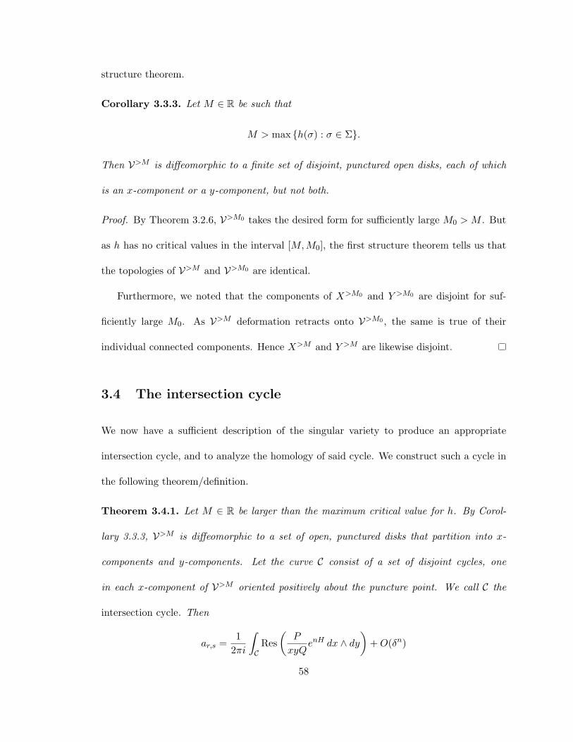
structure theorem.
Corollary 3.3.3. Let M ∈ R be such that
M > max {h(σ) : σ ∈ Σ}.
Then V>M is diffeomorphic to a finite set of disjoint, punctured open disks, each of which
is an x-component or a y-component, but not both.
Proof. By Theorem 3.2.6, V>M0 takes the desired form for sufficiently large M0 > M . But
as h has no critical values in the interval [M,M0], the first structure theorem tells us that
the topologies of V>M and V>M0 are identical.
Furthermore, we noted that the components of X>M0 and Y >M0 are disjoint for suf-
ficiently large M0. As V>M deformation retracts onto V>M0 , the same is true of their
individual connected components. Hence X>M and Y >M are likewise disjoint.
3.4 The intersection cycle
We now have a sufficient description of the singular variety to produce an appropriate
intersection cycle, and to analyze the homology of said cycle. We construct such a cycle in
the following theorem/definition.
Theorem 3.4.1. Let M ∈ R be larger than the maximum critical value for h. By Corol-
lary 3.3.3, V>M is diffeomorphic to a set of open, punctured disks that partition into x-
components and y-components. Let the curve C consist of a set of disjoint cycles, one
in each x-component of V>M oriented positively about the puncture point. We call C the
intersection cycle. Then
ar,s =1
2πi
∫
CRes
(
P
xyQenH dx ∧ dy
)
+O(δn)
58

as n→ ∞, for any arbitrarily small δ > 0.
The cycle C is not the exact intersection cycle as constructed in Chapter 1, but is a
representative of the same homology class. Note that C is defined to be the empty cycle if
X>M is empty for sufficiently large M .
Proof. Let R be sufficiently small and M sufficiently large so that
1. M > max {h(σ) : σ ∈ Σ}.
2. If Q(x, y) = 0, then either |x| < R or |y| < R but not both.
3. The sets VQ ∩{(x, y) : 0 < |x| < R} and VQ ∩{(x, y) : 0 < |y| < R} are each
diffeomorphic to finite sets of disjoint, punctured open disks (as in Theorem 3.2.3).
4. The set V>M is diffeomorphic to a finite set of disjoint, punctured open disks (as in
Theorem 3.2.6).
5. The set V>M is a subset of the set VQ ∩{(x, y) : 0 < |x| < R or 0 < |y| < R}, i.e.
h(x, y) > M implies that either |x| < R or |y| < R.
Now fix rx < R and ry sufficiently small so that
ar,s =1
(2πi)2
∫
T0
P
xyQenH dx ∧ dy,
where T0 = {(x, y) ∈ C2 : |x| = rx, |y| = ry}. Define
M0 = sup {|y| : (x, y) ∈ VQ and |x| = rx}
m0 = inf {|y| : (x, y) ∈ VQ and |x| = rx}
Note thatM0 <∞ because y is locally a function of x along the designated set, andm0 ≥ R
by choice of R: |x| and |y| can not simultaneously be less than R.
59
Now fix any positive m1 < min {ry,m0} and define the torus T = {(x, y) ∈ C2 : |x| =
rx, |y| = m1}. Then fix any M1 > M0 and define the homotopy
K : T × [0, 1] −→ C2
(x, y, t) 7−→(
x, y
(
1 + t
(
M1
m1− 1
)))
K intersects VQ in the set
C = {(x, y) ∈ VQ : |x| = rx},
and the intersection itself is transverse – the homotopy K is obtained by expanding in the
norm of y through points on the variety where VQ is locally parameterizable in terms of x.
By Theorem 1.2.2, this means that
ar,s =1
2πi
∫
CRes
(
P
xyQenH dx ∧ dy
)
+1
(2πi)2
∫
T1
P
xyQenH dx ∧ dy.
where T1 = K(T × {1}). By trivial bounds, we have
1
(2πi)2
∫
T1
P
xyQenH dx ∧ dy = O
((
1
rrxMs1
)n)
as n→ ∞,
as the only n dependence in the integral comes from the enH term. As M1 may have been
chosen to be arbitrarily large, this term is O(δn) for any arbitrarily small, positive δ.
We now turn our attention to the cycle C. C consists of a set of cycles, one on each
punctured disk in the set VQ ∩{(x, y) : 0 < |x| < R}, oriented positively around the puncture
point. We examine such a disk D and one such portion C0 of the intersection cycle.
By Lemma 3.2.5, there are only two possibilities for the behavior of h on the punctured
diskD: either h→ −∞, eventually and monotonically, as x→ 0 (in the case that α < −r/s)
or h→ ∞, eventually and monotonically, as x→ 0 (in the case that α > −r/s).
60

In the former case, by shrinking C0 closer to |x| = 0, we may assume that the maximum
value of h along C0 is arbitrarily large negative – for instance, by properly shrinking C0 to
the puncture point we may assume that the maximum height along C0 is less than log δ for
any small, positive δ. Then again by trivial bounds, this leads to
1
2πi
∫
C0
Res
(
P
xyQenH dx ∧ dy
)
=1
2πi
∫
C0
−PxyQy
enH dx = O(δn)
as n → ∞. This we may drop this portion C0 of the intersection cycle, and collect the
difference into the O(δn) error term.
In the latter case we have that h→ ∞ near the puncture point of D. This implies that
D contains one of the x-components from the set V>M . By shrinking C0 sufficiently close
to |x| = 0, we may assume that C0 is contained entirely within this x-component.
Doing this for every such D and piece C0 of the intersection cycle, we obtain a new cycle
C such that
ar,s =1
2πi
∫
CRes
(
P
xyQenH dx ∧ dy
)
+O(δn),
where γ consists of one cycle per x-component of V>M , oriented positively around the
puncture points.
To finish the theorem, we have to show that this works not just for sufficiently large
height M but for any M larger than all critical values of h. But this follows exactly from
the first structure theorem of Morse theory (see Corollary 3.3.3).
3.5 First characterization theorem
We are nearly ready to characterize the homology class [C] ∈ H1(VQ). We simply need
several definitions.
61
Definition 3.5.1. We define the number cxy by
cxy = inf {c ∈ R : X>c ∩ Y >c = ∅} ∈ [−∞,∞).
Thus the value cxy captures the largest height c at which the components of X≥c and
Y ≥c overlap. Note by the first structure theorem that this can only occur at a critical value
for h, i.e. if cxy > −∞ then cxy is a critical value for the height function.
Definition 3.5.2. Define Ξ to be the set of all σ ∈ Σ such that
1. h(σ) = cxy, and
2. For arbitrarily small neighborhoods U ⊆ VQ of σ, U ∩X>cxy and U ∩ Y >cxy are both
non-empty.
We call Ξ the set of contributing points.
Intuitively, the set Ξ is the set of saddles at which x- and y-components first join.
Finally, we characterize the structure of VQ local to any saddle point σ ∈ Σ.
Definition 3.5.3. For σ ∈ Σ, denote by k ≥ 2 the degree of degeneracy of h at σ. As
detailed in the proof of the second structure theorem, there is a parameterization of VQ
local to σ on which h takes the form
h(w) = h(σ) + Rewk.
Thus on any neighborhood U of σ on which this parameterization holds, we see that U ∩
V>h(σ) consists of k connected components, which we term ascent regions. Similarly we see
that U ∩ V<h(σ) consists of k connected components, which we term descent regions.
Then we have the following theorem, which characterizes the homology class [C] in a
manner amenable to saddle point analysis.
62

Theorem 3.5.4 (First Characterization Theorem). If the set Ξ is non-empty, then the
homology class [C] contains a representative cycle κ such that
1. The height along κ is maximized precisely at the points in Ξ, and
2. For a fixed σ ∈ Ξ and U ⊆ VQ a sufficiently small neighborhood of σ, denote the
ascent regions in U by A0, . . . , Ak−1 (ordered counterclockwise about σ). Denote by
Dj the descent region between Aj and Aj+1 mod k. Then for each j there is a curve γj
in U , starting at σ and traveling down Dj, such that
κ ∩ U =k−1∑
j=0
(X(j + 1 mod k)−X(j))γj ,
where X(j) := 1 if Aj ⊆ X>cxy while X(j) := 0 if Aj ⊆ Y >cxy (well-defined by
definition of cxy).
If the set Ξ is empty, then the homology class [C] contains a representative cycle κ supported
on V≤m for arbitrarily small m ∈ R.
We pause to note that the prescribed representative κ is in some sense the best we can
get in that there are local obstructions to lowering the height any further. Specifically, for
σ ∈ Ξ and for U a sufficiently small neighborhood of σ, the cycle κ ∩ U is a nontrivial
element of the relative homology group H1(U,U ∩ V≤cxy−ε) (for ε > 0 sufficiently small).
Proof. We begin by assuming that Ξ is non-empty, and we want to use our Morse-theoretic
understanding of the space VQ to find a cycle κ sought by the theorem. To begin with, let
M0 ∈ R be any value larger than all critical values of h. We examine C on V>M0 . Recall
that C is composed of a disjoint set of cycles, one in each x-component of V>M0 oriented
positively about the puncture points. Note that C is homologous to ∂X>M0 (along which
63
h ≡ M0). We wish to show that this characterization of [C] remains true when M0 is
replaced by any M ∈ (cxy,M0]. We do so inductively.
By the first structure theorem of Morse theory, the topology of V>M (and hence the
characterization of [C]) changes only as M passes through critical values of h. So let c ∈
(cxy,M0] denote some critical value of h, and assume that C is homologous to ∂X>M in
V>M for any M ∈ (c,M0]. Using the proof of the second structure theorem as a guide, we
examine the topological changes that occur local to Σ(c) as M is decreased below c.
Exactly as in the the proof of the second structure theorem, we form a new height
function h that differs from our old height function only in small neighborhoods of the
points in Σ(c), on which h = h − εb for some sufficiently small ε > 0 and some bump
function b. Denote by X>M and Y >M the x- and y-components of V>M as prescribed by
this new height function h. By the definition of h, we know that X>c+ε/2 and X>c+ε/2 are
topologically equivalent, and hence that C is homologous to ∂Xc+ε/2. This implies that C
is homologous to ∂Xc−ε/2, there being no critical values of h in [c − ε/2, c + ε/2]. Finally,
we wish to show that ∂Xc−ε/2 is homologous to ∂Xc−ε/2.
First, note that ∂X>c−ε/2 and ∂X>c−ε/2 agree outside of small neighborhoods of the
points in Σ(c). So we examine these cycles local to said critical points. As c > cxy, there
are only two possibilities for each σ ∈ Σ(c):
1. The ascent regions local to σ are all in Y >c, or
2. The ascent regions local to σ are all in X>c.
We examine each possibility in turn.
In the first case, there is no piece of ∂X>c−ε/2 or of ∂X>c−ε/2 local to σ. So assume
that we are in the second case. Denote by k the degeneracy of the saddle σ. Then local
64

Figure 3.3: The cycle ∂X>c−ε/2 local
to a saddle σ of degeneracy k = 3.
Figure 3.4: The cycle ∂X>c−ε/2 local
to a saddle σ of degeneracy k = 3.
Figure 3.5: The difference between the cycles repre-
sented in Figure 3.3 and Figure 3.4.
to σ, ∂X>c−ε/2 consists of k curves bounding the k disjoint components where h > c− ε/2
(see Figure 3.3 for an example with k = 3). But note that in this small neighborhood, this
cycle is homologous to ∂X>c−ε/2, as their difference is a boundary (see Figures 3.4 and 3.5).
And thus globally the difference between ∂X>c−ε/2 and ∂X>c−ε/2 is a finite union of such
boundaries, which shows that these cycles are homologous.
Thus we have that C is homologous to ∂X>c−ε/2, and by induction we can see that C is
homologous to ∂X>M for M ∈ (cxy,M0). So what happens to [C] as M is lowered beyond
65

cxy? We examine the topological changes that occur local to the set Σ(cxy). The analysis is
similar to our prior analysis but with the added kink that there are points from both X>cxy
and Y >cxy local to the contributing points.
As before we form a modified height function h that locally pushes down the points of
Σ(cxy). With respect to this new function we again have that C is homologous to ∂X>cxy−ε/2
for some small ε > 0. So define the cycle κ0 = ∂X>cxy−ε/2. With a few alterations, we will
be able to turn κ0 into the desired representative.
Outside of small neighborhoods of the points in Σ(cxy) we have that h ≡ h, and hence the
height h along κ0 is equal to cxy − ε/2 away from these points. And by the same reasoning
as in the inductive argument above, we can alter κ0 local to the points of Σ(cxy) \ Ξ to
obtain a homologous cycle whose height h is bounded below cxy local to these points. What
remains is to examine κ0 local to the points of Ξ.
In a sufficiently small neighborhood U of any σ ∈ Ξ, the cycle κ0∩U consists of one curve
for each ascent region in X>cxy (see Figure 3.6, with two ascent regions from X>cxy and one
ascent region from Y >cxy). Each such curve enters the neighborhood at some point p1 and
leaves at some point p2, where p1 and p2 lie in separate descent regions (see Figure 3.6).
And each such curve is homotopic to a curve whose height is maximized at the saddle point,
namely one that travels straight from p1 to σ (contained within one descent region), and
then from σ to p2 (contained within a separate descent component). See Figure 3.7. Making
these adjustments to κ0 at every such contributing point results in a cycle homologous to
C along which h is maximized precisely at the points of Ξ.
To complete the construction, a few more changes must be made to κ0. Note that
currently, in a sufficiently small neighborhood U of any contributing point σ, κ0∩U consists
66

X
Xp1
Y
p2
Figure 3.6: A representation of κ0
local to σ with two ascent regions
in X>cxy and one ascent region in
Y >cxy . The set V>cxy−ε/2 is shaded.
X
Xp1
Y
p2
Figure 3.7: A representation of the
two pieces of κ0 after performing the
alteration described in the text.
of a set of curves in the descent regions Dj local to σ as follows:
1. If Dj is located between an ascent region in X>cxy and an ascent region in Y >cxy
(in that order, counterclockwise about σ), then κ0 ∩Dj consists of a single curve γj
traveling up Dj to σ.
2. If Dj is located between an ascent region in Y >cxy and an ascent region in X>cxy
(in that order, counterclockwise about σ), then κ0 ∩Dj consists of a single curve γj
traveling down Dj from σ.
3. If Dj is located between two ascent regions in Y >cxy , then κ0 ∩Dj = ∅.
4. If Dj is located between two ascent regions in X>cxy , then κ0 ∩ Dj consists of two
pieces, a curve entering σ and a curve exiting σ.
See Figure 3.7 for an example. Note that in case (4) above, the portion of κ0 in said descent
67
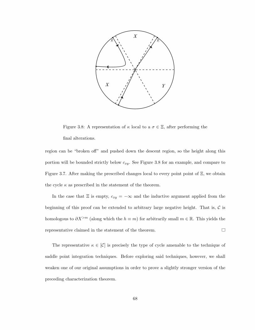
X
Xp1
Y
p2
Figure 3.8: A representation of κ local to a σ ∈ Ξ, after performing the
final alterations.
region can be “broken off” and pushed down the descent region, so the height along this
portion will be bounded strictly below cxy. See Figure 3.8 for an example, and compare to
Figure 3.7. After making the prescribed changes local to every point point of Ξ, we obtain
the cycle κ as prescribed in the statement of the theorem.
In the case that Ξ is empty, cxy = −∞ and the inductive argument applied from the
beginning of this proof can be extended to arbitrary large negative height. That is, C is
homologous to ∂X>m (along which the h ≡ m) for arbitrarily small m ∈ R. This yields the
representative claimed in the statement of the theorem.
The representative κ ∈ [C] is precisely the type of cycle amenable to the technique of
saddle point integration techniques. Before exploring said techniques, however, we shall
weaken one of our original assumptions in order to prove a slightly stronger version of the
preceding characterization theorem.
68

3.6 Generalized characterization theorem
In this this section we begin by weakening Assumption 3.1.3 to obtain the following.
Assumption 3.6.1. Assume that the critical points of VQ are isolated (and hence finite).
For the purpose of our impending algorithmic study of VQ, we note that the preced-
ing assumption is equivalent to the condition that the polynomial ideal 〈Q,Qx, Qy〉 be
0-dimensional, a fact that can be checked via Grobner basis computation.
Under this assumption, we have the following definitions:
Definition 3.6.2. We define the constant c0 by
c0 = max {h(z0) : z0 ∈ VQ, VQ is not smooth at z0},
and we define the constant cxy by
cxy = inf {c > c0 : X>c ∩ Y >c = ∅} ∈ [c0,∞)
Note that this definition of cxy generalizes the previous one if we adopt the convention
that c0 = −∞ in the case that VQ is smooth. We similarly generalize the definition of Ξ as
follows.
Definition 3.6.3. Define the set Ξ to be the set of all σ ∈ Σ such that
1. h(σ) > c0,
2. h(σ) = cxy, and
3. For arbitrarily small neighborhoods U ⊆ VQ of σ, U ∩X>cxy and U ∩ Y >cxy are both
non-empty.
69

We call Ξ the set of contributing points.
Note that Ξ is empty if cxy = c0.
Then the key is to notice that V>c0 is a smooth manifold, and that on this surface the
analyses carried out up to this point still hold. Thus we can define the intersection cycle C
on V>M for sufficiently large M , we can use the structure theorems of Morse theory to find
representatives for [C] as we decrease M , and generally implement all the methods from
before – as long as we restrict our attention to V>c0 . If Ξ is not empty, this enables us
to find a cycle κ ∈ [C] exactly as before. On the other hand if Ξ = ∅, then we can find
representative cycles for [C] along which the height is arbitrarily near, but greater than, c0.
This yields the following corollary to the first characterization theorem.
Corollary 3.6.4 (Generalized Characterization Theorem). If the set Ξ is non-empty, then
the homology class [C] contains a representative cycle κ just as in Theorem 3.5.4. On the
other hand if Ξ is empty, then [C] contains a representative cycle κ supported on V≤M for
any M > c0.
Applying the method of steepest descent to the cycle κ described in the characterization
theorem, we obtain the following corollary for the asymptotic analysis of the ar,s.
Corollary 3.6.5. Denote Ξ = {σ1, . . . , σm} and let κ be the cycle as prescribed in the
characterization theorem. If Ξ is not empty then we have
ar,s ∼m∑
i=1
enH(σi)∞∑
j=0
ui,jn−(1+j)/ki ,
where ki ≥ 2 is the degree of degeneracy of σi. Moreover, the coefficients ui,j are computable,
assuming computability of the σi and of the tangent direction of the pieces of κ local to each
σi.
70
On the other hand if Ξ is empty, then we have that
ar,s = o(enM )
for any M > c0.
Proof. We begin by assuming that the set Ξ is non-empty. Recall that by Theorem 3.4.1
we can write
ar,s =1
2πi
∫
κRes
(
P
xyQenH dx ∧ dy
)
+O(δn) (3.6.1)
for arbitrarily small δ > 0. We will apply the method of steepest descent to obtain an
asymptotic expansion for the preceding integral.
For each i ∈ {1, 2, . . . ,m}, let Ui be a small neighborhood of σi in VQ. Let U =⋃mi=1 Ui.
Then we can split the cycle γ0 into two pieces
κ = κ1 + κ2,
where κ1 = κ ∩ U and κ2 = κ \ κ1. Then because h < cxy along the compact curve κ2, we
can find a sufficiently small ε such that
h(z) ≤ c− ε for z ∈ κ2
But the residue form Res(
PxyQe
nH dx ∧ dy)
admits the form
−PxyQy
enH dx orP
xyQxenH dy
(according to when Qy 6= 0 or Qx 6= 0), and so by trivial bounds we have that
1
2πi
∫
κ2
Res
(
P
xyQenH dx ∧ dy
)
= O(en(c−ε)).
Thus equation 3.6.1 reduces to
ar,s =1
2πi
∫
κ1
Res
(
P
xyQenH dx ∧ dy
)
+O(en(c−ε)),
71
and the computation is reduced to a set of integrals local the points of Ξ.
Local to a particular saddle point σi, smoothness of VQ guarantees that one of Qy or
Qx does not vanish. Assume without loss of generality that Qy 6= 0. Then locally we have
Res
(
P
xyQenH dx ∧ dy
)
=−PxyQy
enH dx = enH(σi)A(x)e−nφ(x),
where
A(x) =−PxyQy
φ(x) = H(σi)−H
parameterized locally by x.
Assuming that Ui is sufficiently small, the curve Ui ∩ κ1 consists of pieces exiting σi
and traveling down certain descent regions and pieces entering σi by traveling up certain
descent regions. To finish the theorem we must integrate over these pieces and finally sum
over all such i from 1 to m.
So let γ be an arbitrary curve segment exiting σi and traveling down a descent region.
We have
1
2πi
∫
γRes
(
P
xyQenH dx ∧ dy
)
=enH(σi)
2πi
∫
γA(x)e−nφ(x) dx
where A and φ satisfy the conditions of Theorem 1.4.2. Thus we get a series expansion of
the form∫
γA(x)e−nφ(x) dx ∼
∞∑
j=0
ajn−(1+j)/ki
where ki is the index of the first non-vanishing term of φ(x), also the degree of degeneracy of
h at the saddle point σi. Note that the coefficients aj are computable from the coefficients
of A and φ and from the tangent direction in which γ exits σi. The coefficients of A and
72

φ are in turn computable from the partials of P , Q and H at σi. Thus computability of
the asymptotic expansion rests on computability of the saddle point σi and the directions
of each γ in the description of κ local to Ξ.
Integrating over Ui ∩ κ1 consists of integrating over finitely many such γ either with
positive or negative orientation, and by summing over corresponding expansions we get an
expansion of the following form
1
2πi
∫
Ui∩κ1Res
(
P
xyQenH dx ∧ dy
)
∼ enH(σi)∞∑
j=0
ui,jn−(1+j)/ki .
Summing similar computations over all such points σi ∈ Ξ yields the desired result.
On the other hand if Ξ is empty, then by Theorem 3.6.4 we can find a cycle κ ∈ [C]
along which h ≤M for any M > c0. Then again by trivial bounds we obtain
1
2πi
∫
κRes
(
P
xyQenH dx ∧ dy
)
= O(enM ).
And as ar,s = O(enM ) for all M > c0, we must have ar,s = o(enM ) for all M > c0.
By this corollary we see that computing an asymptotic series/bound for the ar,s reduces
to locating the points of Ξ and computing the structure of κ local to the points of Ξ. In
the next chapter, we produce an algorithm for this task.
73

Chapter 4
Algorithmic Implementation
4.1 Introduction
In the following chapter we present rigorous numerics for computing the location of Ξ and
the directions of κ ∈ [C] local to the points of Ξ, where Ξ and κ are as characterized
in Corollary 3.6.4. That is, we exhibit a rigorous algorithm for computing the preceding
information to within arbitrary numerical accuracy. As indicated in Corollary 3.6.5, this
information can then be used to compute asymptotic formulas/bounds for the coefficients
ar,s.
Motivated by the characterization theorem, we begin by examining the structure of V>c
local to any σ ∈ Σ, where c = h(σ). On a sufficiently small neighborhood U ⊆ VQ of σ, we
have that U ∩ V>c decomposes into k ascent regions, where k is the degeneracy of h at σ.
Assuming that c ≥ cxy and c > c0, we know that each such region A belongs either to X>c
or to Y >c, but not both. If we can determine which occurs for each region A and for every
such saddle point σ, we will have exactly the information necessary to construct Ξ and the
74

relevant cycle κ ∈ [C] local to the points in Ξ.
So let σ ∈ Σ be such that h(σ) ≥ cxy and h(σ) > c0, and let A be any local ascent
region. Let γ : [0, 1) → VQ be any path that begins at γ(0) = σ, travels out through A, is
monotonically increasing with respect to h and approaches arbitrarily large height. (Note
that the existence of such a path follows directly from the Morse-theoretic decomposition of
VQ.) Because h(γ(t)) → ∞ as t→ 1, we must have that γ((0, 1)) includes points arbitrarily
close to x = 0 and/or y = 0. But we can’t have both, as the condition c ≥ max {cxy, c0}
assures that X>c and Y >c are disjoint. Thus if it can be determined whether γ comes
arbitrarily close to x = 0 or y = 0, then it can be determined whether A belongs to X>c or
Y >c.
This suggests the following outline for an algorithm:
1. Input Q, r and s.
2. Use Grobner basis computations to find the points of VQ where h has saddle points
(the set Σ) and where the variety VQ is not smooth. Terminate if any of these points
are not isolated. Denote by c0 the height of the highest non-smooth point (c0 = −∞
if the variety is smooth).
3. Step through each σ ∈ Σ in decreasing order of height, while h(σ) > c0. For each such
σ, do the following:
(a) Use Grobner basis computations to compute the degree of degeneracy k of h at
σ.
(b) Compute the k steepest ascent directions for h at σ, i.e. the directions of the k
ascent regions.
75

(c) For each ascent region A, follow a strictly ascending path along VQ beginning
at σ and traveling through A. Follow each such path until it is clear whether
the path will approach arbitrarily close to x = 0 or y = 0. Keep track of this
information, which determines to which of X>c or Y >c each ascent component
belongs.
4. In the preceding loop: if ever a σ is found for which some of the ascent components
belong to X>c while others belong to Y >c, note the height cxy = h(σ) and add σ to
Ξ. Continue through the rest of the saddles at height cxy, adding them to Ξ according
to the same rule. Terminate the loop when done with the saddles at height cxy.
5. The algorithm terminates with the following conditions
(a) If Ξ is empty, then there is a cycle κ ∈ [C] such that supκ h ≤M for any M > c0.
This gives a bound on the growth of the coefficients ar,s as prescribed in Corollary
3.6.5.
(b) If Ξ is not empty, then there is a cycle κ ∈ [C] such that the height along κ
is maximized precisely at the points of Ξ, and the structure of κ local to Ξ is
as prescribed in the characterization theorem. Note that all of the information
necessary to describe this local structure is contained in the steps of the preceding
algorithm.
Of course it remains to be shown that an algorithm of this form can be effectively imple-
mented. In what follows, we demonstrate this to be so by presenting a complete pseudo-code
implementation. The first step is to sufficiently develop the notations/assumptions of the
pseudo-language that we shall use.
76
4.2 Describing the pseudo-language
Central to the pseudo-language is a suitable means of representation for certain computable
numbers, and a system whereby these numbers can be acted upon by certain computable
functions and operations. Specifically, we draw upon the construct of ball numbers and ball
arithmetic as developed in Mathemagix ([vdH08]). Note that the exact notation and func-
tions developed below may not be as implemented in Mathemagix, but equivalent functions
either exist or can be produced in this language.
We begin by describing the ball data type, which we shall use to represent certain
computable numbers to within arbitrary precision. Each variable b of type ball, or ball
number, represents some computable number b ∈ C. Associated to b are a variable (b.tol)
and two functions (b.approx() and b.mod()). The variable b.tol is a positive rational
number set at the time of b’s initialization, but may be changed by the user at any time. It
stores a computation tolerance. The function b.approx() then returns an element b ∈ Q[i]
such that |b − b| is less than the tolerance b.tol. The user may also pass an optional
argument to b.approx(); if we call b.approx(r) with r a positive rational number, then
this function will return an approximation of b to within a tolerance of r (regardless of, and
without changing, the value of b.tol). Finally, the function b.mod() returns an element of
Q that approximates |b| to within a tolerance of b.tol. And as with b.approx(), b.mod()
also accepts an optional rational argument for specifying a temporary tolerance value.
The pseudo-language also includes two ball number subtypes: real ball numbers (de-
noted by the type realball), and algebraic ball numbers (denoted by the type algball).
The realball data type is nearly identical to the ball data type, but is used only in the
representation of computable real numbers. In this case, the approx() subfunction always
77
returns an element of Q. The algball data type is used for specifically to represent al-
gebraic numbers. An algebraic ball number b representing some algebraic b ∈ C includes
all the attributes associated to a generic ball number, but also includes a new subfunc-
tion: b.poly(). This function takes an indeterminate as its input (e.g. x), and outputs a
rational-coefficient polynomial in that indeterminate (e.g. P(x)) of which b is a root. Note:
if it is not clear which data type is to be used in initializing an expression, the type will be
expressly indicated using functional notation; e.g., realball(expression).
Central to the construction of the ball data types is the existence of a sort of arithmetic
of ball numbers. Namely many of the usual computable functions/operations that can be
applied to elements of C can be applied to ball numbers, resulting in a ball number output
representing the result of the computation. Specifically, the pseudo-language allows us
to apply all arithmetic operations, roots, exponentiation, complex conjugation, complex
modulus, trigonometric functions and the real logarithm to ball numbers. In the case of the
complex modulus function, the output is assumed to be a real ball number. In the case of
the real logarithm, the input is assumed to be a real ball number.
Having specified the structure of ball numbers, we must take some time to discuss the
origin of said objects. For certain fundamental computable constants (e.g. π), we assume
that a ball number representation is available in the language (e.g. Pi). The vast majority of
ball numbers, however, will come from solving univariate polynomial equations. Specifically,
we assume the existence of a function solve(), whose input is a univariate polynomial P with
coefficients in Q[i] and whose output is an array of algebraic ball numbers corresponding
to the distinct roots of P. Note that such a function exists and has been implemented in
Mathemagix. We further assume that the roots in this array are initialized with the same
78

tolerance, and that the tolerance has been suitably shrunk; specifically, that the tolerance
is less than three times the distance between any two distinct roots of P. These assumptions
will be useful later on, allowing us to bound subsequent root approximations away from
one another (the distance between any two such approximations being greater than this
initial tolerance). We will also make use of a similar function realsolve(), whose input is
a univariate polynomial P with coefficients in Q and whose output is an array of algebraic
ball numbers corresponding to the distinct real roots of P.
In addition to the ball data type, we also construct two special data types for the
representation of saddle and singular points. These data types are nothing more than
specialized arrays containing the many pieces of information that we wish to store about
such points. Note that each element of the array is empty at the time of initialization, and
is set in the course of the algorithm.
The simpler of the two data types is that which is used for singular points: the type
nonSmooth. An element p of nonSmooth includes three pieces of information: algebraic
ball numbers p.x and p.y, and a real ball number p.height. The numbers p.x and p.y
represent the x- and y-coordinates of a singular point (x, y), while the number p.height
represents the exponential of its height, eh(x,y).
The data type for saddle points – saddle – includes far more information. Let sigma
be an arbitrary saddle variable, meant to represent a saddle point σ ∈ Σ. In addition to
the location and height information (sigma.x, sigma.y and sigma.height), sigma also
includes the following eight pieces of information:
1. sigma.byX – a boolean value which is set to True if VQ is locally parameterizable by
x in a neighborhood of σ. In this case we think of x as an independent variable and
79

y as a dependent variable. It is set to False otherwise, in which case the roles of x
and y are reversed. Note that this boolean is only used for saddle points higher than
c0, where VQ is smooth.
2. sigma.Ri – a positive rational number. This denotes the “radius of the independent
variable.” sigma.Ri is the radius of a neighborhood in the plane of the independent
variable on which parameterization by the independent variable holds.
3. sigma.Rd – a positive rational number. This denotes the “radius of the dependent
variable.” When VQ is parameterized by the independent variable on a disk of radius
sigma.Ri, the corresponding value of the dependent variable remains in a disk of
radius sigma.Rd.
4. sigma.R – a rational number. The number sigma.R < sigma.Ri represents a radius
on which parameterization by the independent variable is geometrically nice (in a
sense to be described in Lemma 4.12.1 below). This radius is used in the construction
of short ascent paths as parameterized by the independent variable.
5. sigma.pathToX – an array of boolean values. The length of sigma.pathToX is equal
to the degeneracy of h at σ, and the value of sigma.pathToX[i] is set to True if an
ascent path from σ through the ith ascent component local to σ is found to approach
x = 0. It is set to False otherwise.
6. sigma.xPole – a boolean value. sigma.xPole is set to True if all of the values in
the array sigma.pathToX are set to True. It is set to False if all of the values in
the array sigma.pathToX are set to False. This is to keep track of whether σ is in
X≥h(σ) or Y ≥h(σ). Note that this value is not initialized for h(σ) ≤ cxy.
80

7. sigma.out – an array of ball numbers. If sigma is found to be a contributing saddle,
then by the characterization theorem there is an κ ∈ [C] whose structure local to σ
consists of a set of short paths emanating from σ in various directions. sigma.out is
an array of those directions along which κ is parameterized to flow away from σ (as
parameterized by the independent variable).
8. sigma.in – an array of ball numbers. This is similar to the array sigma.out, but
stores the directions of curves along which κ is parameterized to flow into σ.
Concerning functions, we assume that the pseudo-language includes a full implementa-
tion of Grobner basis computation. We use Maple ([Wat08]) as a notational guide. Specifi-
cally we make use of a function Basis(), whose input consists of an array I of generators of
a polynomial ideal, and an ordering O on monomials. The function then outputs a Grobner
basis for that ideal as an array of polynomials, where the first element in the array is the
elimination polynomial. That is, if the ideal I is zero-dimensional, then the first element of
Basis(I,O) is a univariate polynomial in the indeterminate of smallest order. We make use
of a function plex() for producing orderings. The usage is as follows: plex(x1,x2,...,xn)
produces the pure lexicographic ordering on monomials induced by the relation x1 > x2 >
... > xn on the indeterminates.
All remaining functions that we shall use are relatively simple, and the vast majority
are described in the following list:
• diff() – This function takes two inputs: a rational function R (in any number of
indeterminates), and an indeterminate z. The output is the partial derivative of R
with respect to z.
81

• Re() and Im() – These functions take as input a polynomial (in any number of
indeterminates) having coefficients in Q[i]. Let P be such a polynomial. We can write
P uniquely as P1 + I*P2, where P1 and P2 are polynomials with coefficients in Q, and
I represents i ∈ C. Then the output of Re(P) is P1 while the output of Im(P) is P2.
• abs() – This function takes as input a polynomial∑
j ajxj with rational coefficients,
and outputs the polynomial∑
j |aj|xj. It is used in upper bounding polynomials by
the triangle inequality.
• subs() – This function takes two inputs: an expression of the form z=n (where z is
an indeterminate and n is a number), and a polynomial P (in any number of indeter-
minates). The function returns the result of substituting n in for z in the polynomial
P.
• exponents() – This function takes two variables: a polynomial P in any number of
indeterminates, and an array [x1,x2,...,xn] of the indeterminates in P. The output
is an array of lists of exponents, where [i1,i2,...,in] is an element of the output
if and only if the monomial x1^i1*x2^i2*...*xn^in has nonzero coefficient in P.
• dotprod() – This function takes as input two same-length arrays (vectors) of rational
numbers, and returns their dot product as a rational number.
• BAFZ() – This function takes as input a ball number b that is known to be non-zero.
The function then progressively lowers the value of b.tol until b.mod is greater than
2*b.tol. Thus a call to the function b.approx() will subsequently be bounded away
from 0 by a distance of at least b.tol.
82

• type() – This function takes as input any variable, and outputs the variable’s type;
e.g. integer or ball, etc.
• len() – This function takes an array as an input, and outputs the length of the array
as an integer.
• a.append() – To any array a is associated the function a.append(), which takes any
variable as an argument and appends it to the end of the array a.
It is hoped that the use of any functions not explicitly detailed will be clear from context.
We make two additional notes about the structure of the pseudo-language. First, to
improve readability of the algorithm, comments are included. The comment character is %.
Consequently any text that appears after the symbol % on a given line of code a comment,
and is immaterial to the functioning of the code. Second, note that the scope of all loops
and if/then statements is indicated by level of indentation.
We are now ready to construct the functions necessary to carry out our algorithm.
The supporting functions are constructed one-by-one, section-by-section, culminating in
the creation of the main algorithm itself: main().
4.3 Examining the height near infinity
Specification of finiteHeight()
Input:
• Q(x,y) – a polynomial with rational coefficients in variables x and y. This is the
singular polynomial Q(x, y) of the generating function under investigation.
83
• r – a rational number. Together with s, this defines the direction [r,s] = (r, s) in
which asymptotics are taken.
• s – a rational number. Together with r, this defines the direction [r,s] = (r, s) in
which asymptotics are taken.
Description: This function examines the variety VQ and searches for branches along which
the height h approaches a constant as x → ∞ (and hence as y → 0) or as y → ∞ (and
hence as x→ 0). By Assumption 3.2.4, this is exactly when there are branches of the form
y ∼ cx−r/s as x→ 0 or x ∼ cy−s/r as y → 0 (c 6= 0).
Output: FHAI – a boolean variable. FHAI stands for Finite Height At Infinity. It is set
to True if the height function is ever bounded as x → ∞ or as y → ∞ on VQ. It is set to
False otherwise.
Supporting Theorem
The key theorem on which the implementation of this function relies is Newton’s polygon
method. We begin with a definition.
Definition 4.3.1. To any polynomial Q(x, y) =∑
j∈J cjxajybj with non-zero coefficients
cj , we define the Newton diagram of Q to be the set of points
{(aj , bj) : j ∈ J} ⊆ N× N.
Then we have the following theorem.
Theorem 4.3.2 (Newton Polygon Method). There exists a branch of VQ with y ∼ cxα (as
x → 0) if and only if α corresponds to one of the inverse slopes of the left-most convex
envelope of the Newton diagram of Q.
84

See [FS09, section VII.7.1]. As a corollary, we obtain the following.
Corollary 4.3.3. The height function h approaches a constant as x → ∞ or as y → ∞
along VQ if and only if s/r is the slope of a line-segment on the left-most or right-most
convex envelope of the Newton diagram of Q.
Proof. By Newton’s Polygon Method, there exists a branch of VQ of the form y ∼ cx−r/s as
x → 0 if and only if the left-most convex envelope of the Newton diagram of Q includes a
line segment of slope s/r. Similarly, there is a branch of VQ of the form x ∼ cy−s/r as y → 0
if and only if the left-most convex envelope of the Newton diagram of R(x, y) := Q(y, x)
includes a line segment of slope r/s. But the Newton diagram of R is simply the Newton
diagram of Q reflected over the line x = y, and hence this will be true if and only if the
right-most convex envelope of the Newton diagram of Q includes a line segment of slope
s/r.
Implementation
finiteHeight(Q(x,y),r,s)
FHAI = False % FHAI stands for Finite Height At Infinity
diagram = exponents(Q,[x,y])
% Cycle through pairs of points in the Newton diagram
j = 0
while ((FHAI == False) AND (j < len(diagram))):
k = 0
onLine = False; sideA = False; sideB = False
while(((sideA AND sideB) == False) AND (k < len(diagram)))
if (j != k):
% Where does point k lie with respect to the line of slope s/r through
% the point j? Check with a dot product.
position = dotprod(diagram[j] - diagram[k],[-s,r])
if (position == 0):
onLine = True % the line through j and k has slope s/r
else if (position < 0):
sideA = True % k is to one side of the line
else:
85

sideB = True % k is to the other side of the line
k = k + 1
% Was a point found on the line of slope s/r through point j, with the
% rest of the Newton diagram either to the left or the right?
if ((onLine == True) AND ((sideA AND sideB) == False)):
FHAI = True
j = j + 1
return FHAI
4.4 Finding solutions to a polynomial system
Specification of solveSystem()
Input:
• P1(x) – a polynomial in x with rational coefficients.
• xroots – an array of algebraic ball numbers. Each of the numbers in this array is
assumed to be a root of P1(x).
• P2(y) – a polynomial in y with rational coefficients.
• yroots – an array of algebraic ball numbers. Each of the numbers in this array is
assumed to be a root of P2(y).
• system – an array of polynomials in x and y with rational coefficients.
Description: This function uses Grobner basis computations to find solutions (x, y) to
the system of polynomials system, where the x and y come from xroots and yroots,
respectively.
Output: solutions – an array of pairs of algebraic ball numbers. The array consists of
the pairs [x0,y0] (x0 from xroots and y0 from yroots) such that R(x0,y0) = 0 for every
polynomial R in the array system.
86
Implementation
solveSystem(P1,xroots,P2,yroots,system)
solutions = empty array
membership = len(xroots) by len(yroots) matrix of 1s
for P(x,y) in system:
% Construct a polynomial in t whose solutions are the possible values
% of P(x0,y0) for x0 in xroots and y0 in yroots
B = Basis([P1,P2,t-P],plex(x,y,t))
Pt = B[0]
troots = solve(t*Pt) % multiply by t to ensure t = 0 is a root
for j from 0 to (len(xroots) - 1):
for k from 0 to (len(yroots) - 1):
% Approximate the modulus of P(xroots[j],yroots[k]). If it is
% sufficiently close to 0 it must be 0.
evaluate = P(xroots[j],yroots[k]) % a ball number
if (evaluate.mod(troots[0].tol) > troots[0].tol):
membership[j,k] = 0
for j from 0 to (len(xroots) - 1):
for k from 0 to (len(yroots) - 1):
if membership[j,k] == 1:
solutions.append([xroots[j],yroots[k]])
return solutions
4.5 Finding the saddle and non-smooth points
Specification of findPoints()
Input:
• saddleBX – an array of polynomials with rational coefficients in variables x and y.
This is a Grobner basis defining the set Σ, whose first entry eliminates the variable y.
• saddleBY – an array of polynomials with rational coefficients in variables x and y. This
is a Grobner basis defining Σ as well, however the first entry in this array eliminates
the variable x.
• smoothBX – an array of polynomials with rational coefficients in variables x and y.
87

This is a Grobner basis defining the set of singular points on VQ, whose first entry
eliminates the variable y.
• smoothBY – an array of polynomials with rational coefficients in variables x and y. This
is a Grobner basis defining the singular points as well, however the first polynomial
in this array eliminates the variable x.
• isSmooth – a boolean. This value is set to True if VQ is a smooth manifold. It is set
to False if it contains isolated singular points.
Description: This function computes the locations (x, y) of all saddle and non-smooth
points of VQ such that x 6= 0 and y 6= 0.
Output: points – an array of numbers of type saddle or nonSmooth. This array consists
of all the saddle points and singularities of VQ not on the coordinate axes, initialized to
include their x- and y-coordinate data.
Implementation
findPoints(saddleBX,saddleBY,smoothBX,smoothBY,isSmooth)
points = empty array
Px = saddleBX[0] % Poly of possible x values for saddles
% Divide Px by the highest degree of x possible, so 0 isn’t a soln.
n = min(exponents(Px,[x])); Px = Px/(x^n) % now Px(0) != 0
xroots = solve(Px)
Py = saddleBY[0] % Poly of possible y values for saddles
n = min(exponents(Py,[y])); Py = Py/(y^n) % now Py(0) != 0
yroots = solve(Py)
polyArray = saddleBX[1..(len(saddleBX) - 1)] % Cut elimination poly
% Find all points [x0,y0] solving the saddle point Groebner basis
saddles = solveSystem(Px,xroots,Py,yroots,polyArray)
% Initialize them as saddle points and add to the point vector
for [x0,y0] in saddles:
b = new variable of type: saddle
b.x = x0
b.y = y0
88
points.append(b)
if (isSmooth == False):
Px = smoothBX[0] % Poly of possible x values for singularities
n = min(exponents(Px,[x])); Px = Px/(x^n) % now Px(0) != 0
xroots = solve(Px)
Py = smoothBY[0] % Poly of possible y values for singularities
n = min(exponents(Py,[y])); Py = Py/(y^n) % now Py(0) != 0
yroots = solve(Py)
polyArray = smoothBX[1..(len(smoothBX) - 1)] % Cut elim poly
% Find all points [x0,y0] solving the singular point Groebner basis
singular = solveSystem(Px,xroots,Py,yroots,polyArray)
% Initialize them as nonSmooth points and add them to the point vector
for [x0,y0] in singular:
b = new variable of type: nonSmooth
b.x = x0
b.y = y0
points.append(b)
return points
4.6 Computing possible height values
Specification of possHeight()
Input:
• Px – a polynomial with rational coefficients in the variable x. The x-coordinates of
every saddle and singular point of VQ are assumed to be roots of this polynomial.
• Py – a polynomial with rational coefficients in the variable y. The y-coordinates of
every saddle and singular point of VQ are assumed to be roots of this polynomial.
• r and s – as in previous functions.
Description: This function is ultimately used to order all saddle/singular points by height.
To do so, the function uses a Grobner basis computation to construct a polynomial Pt whose
89

real roots include all possible values of
eh(x,y) = |x|−r|y|−s,
such that (x, y) is a singular or saddle point (and x 6= 0, y 6= 0). The key fact is that eh is
algebraic in the real and imaginary parts of x and y. After constructing Pt, the function
returns its real roots.
Output: troots – an array of real ball numbers. These are possible values of eh at the
saddle points and singular points of VQ.
Implementation
possHeights(Px,Py,r,s)
n = lcm(denominator(r),denominator(s))
% Construct a polynomial whose solutions are t = e^h(a+I*b,c+I*d)
hPoly = (t^(2*n))*((a^2 + b^2)^(n*r))*((c^2 + d^2)^(n*s)) - 1
% Use Groebner bases to construct a polynomial in t whose real roots
% include all e^h(x,y) where x solves Px and y solves Py
I = [Re(Px(a+I*b)),Im(Px(a+I*b)),Re(Py(c+I*d)),Im(Py(c+I*d)),hPoly]
B = Basis(I,plex(a,b,c,d,t))
Pt = B[0] % Pt is the desired polynomial
troots = solvereal(Pt)
return troots
4.7 Computing a terminal condition
Specification of termCriteria()
Input:
• Q(x,y), r and s – as in previous functions.
Description: This function creates a set of termination criteria for the eventual path
climbing algorithm. Ultimately this will guarantee the construction of each ascent path to
90

terminate after a finite number of steps, and to determine which plane (x = 0 or y = 0) the
path approaches.
Output: [hStop,epsilon] – an array consisting of two rational numbers. Their role in
the termination of ascent paths is described following the subsequent lemma.
Supporting Lemma
The utility of this function relies on the following lemma.
Lemma 4.7.1. Let Q ∈ Q[x, y] such that Q(0) 6= 0 and such that the variety VQ has
finitely many non-smooth points. Fix r, s > 0, and define the height function h(x, y) =
−r log |x| − s log |y|. Let ε > 0 be sufficiently small so that
|x| < ε and |y| < ε⇒ |Q(x, y)| > 0,
and define
M = −r log ε− s log ε.
Then for any (x, y) ∈ VQ such that h(x, y) > M and such that (x, y) is higher than any
non-smooth point of VQ, we have either that |x| < ε or |y| < ε, but not both. If |x| < ε,
then (x, y) ∈ X>M . Otherwise, (x, y) ∈ Y >M .
The function termCriteria computes such an ε (epsilon) by the triangle inequality,
producing a lower bound for |Q(x, y)| when |x|, |y| ≤ ε and sufficiently shrinking ε until this
lower bound is positive. The function returns epsilon along with a rational upper bound
for M (hStop). These values can then be used to determine if an ascent path that climbs
higher than hStop is in a component of X>M or Y >M : simply check the values of |x| and
|y| to determine which is less than epsilon.
91
Proof. Let (x0, y0) ∈ VQ, and assume both that h(x0, y0) > M and that (x0, y0) is higher
than any non-smooth point of VQ. First note by the structure of h that we cannot have
h(x0, y0) > M unless at least one of |x0| or |y0| is less than ε. But note that by definition
of ε we cannot have both: Q(x0, y0) 6= 0 for both |x0| < ε and |y0| < ε.
To prove the second part of the lemma, let γ : [0, 1) → VQ be a curve that starts at
(x0, y0), is non-decreasing in height, and approaches arbitrarily large values of h. (The
existence of such a curve follows from the Morse-theoretic decomposition of V≥h(x0,y0).)
Denote γ(t) = (x(t), y(t)). In order for h(γ(t)) → ∞ as t → 1, we must have that x(t) or
y(t) approaches arbitrarily close to 0. Now assume that |x0| < ε. We claim that |y(t)| ≥ ε
for all t, and hence that x(t) must approach arbitrarily close to 0. This will prove that
(x0, y0) is in X>M . A symmetric argument then shows that |y0| < ε implies that (x0, y0)
belongs to Y >M .
To prove this final claim, we assume by way of contradiction that |y(t)| < ε for some
value of t. Define
t0 = inf {t ∈ (0, 1) : |y(t)| < ε}.
Then there exist arbitrarily small δ > 0 such that |y(t0 + δ)| < ε, and hence such that
|x(t0 + δ)| ≥ ε (as h(γ(t0 + δ)) > M). Taking the limit as δ → 0, this implies that
|x(t0)| ≥ ε and y|(t0)| ≤ ε. But |y(t0)| ≥ ε, as |y(t)| ≥ ε for all t < t0, and hence |y(t0)| = ε.
Thus we have
h(γ(t0)) ≤ −r log ε− s log ε =M,
which contradicts the assumption that γ is non-decreasing.
Implementation
termCriteria(Q(x,y),r,s)
92
epsilon = 16 % arbitrary starting point
Qbound = abs(Q(0,0)) - abs(Q(x,x) - Q(0,0)) % poly in x
% Shrink epsilon until until |Q(epsilon,epsilon)| > 0
while (Qbound(epsilon) <= 0):
epsilon = epsilon / 2
height = realball(-r*log(epsilon) - s*log(epsilon))
% Compute an upper bound for height -- this is the terminal height
hStop = height.approx(0.01) + 0.01 % tolerance is arbitrary
return [hStop, epsilon]
4.8 Determining a local parameterization variable
Specification of paramByX
Input:
• Q(x,y) – as in previous functions.
• x0 – a ball number. This represents the x-coordinate of a point (x0, y0) ∈ VQ.
• y0 – a ball number. This represents the y-coordinate of a point (x0, y0) ∈ VQ.
Description: Given a polynomial Q and a point (x0, y0) on VQ at which Q is known to be
smooth, this function determines a variable (either x or y) with respect to which VQ admits
a local parameterization. This is accomplished by computing Qy(x0, y0) and Qx(x0, y0) to
greater and greater accuracy, until it can be determined that one of these two values is
non-zero. The rest follows from the implicit function theorem.
Output: byX – a boolean. byX is set to True if the set Q(x,y) = 0 is parameterizable local
to the point [x0,y0] by x. It is set to False if it is found to be locally parameterizable in
terms of y.
93

Implementation
paramByX(Q(x,y),x0,y0)
% Compute partials of Q at the point (x0,y0)
Qx = diff(Q,x); Qx0 = Qx(x0,y0)
Qy = diff(Q,y); Qy0 = Qy(x0,y0)
tolerance = 1 % ball approximation tolerance
nonZeroX = False; nonZeroY = False
% Compute Qx0 and Qy0 to greater and greater precision until it can
% be verified that one is not zero.
while ((nonZeroX == False) AND (nonZeroY == False)):
if (Qx0.mod(tolerance) > tolerance): % is Qx(x0,y0) not 0?
nonZeroX = True
if (Qy0.mod(tolerance) > tolerance): % is Qy(x0,y0) not 0?
nonZeroY = True
tolerance = tolerance / 2
if (nonZeroY == True):
byX = True % if dQ/dy is nonzero, parameterize by x
else:
byX = False % otherwise, parameterize by y
return byX
4.9 Isolating roots
Specification of isoRoot
Input:
• Q(w,z) – a polynomial with rational coefficients in variables w and z. This is the same
singular polynomial Q from before, but in a new coordinate system. The variables x
and y have been replaced by w and z (either by w = x and z = y or vice versa). The
manner in which the new variables have been selected is to assure that Qz is non-zero
at the point [w0,z0] on VQ(w,z). Hence locally we may assume the singular variety is
parameterizable by w.
• w0 – an algebraic ball number. This is the w-coordinate of a point on VQ(w,z).
94
• z0 – an algebraic ball number. This is the z-coordinate of a point on VQ(w,z).
Description: This function finds a neighborhood in the z-plane on which the only root of
Q(w0, z) = 0 is z = z0.
Output: isolate – a rational number. The number isolate satisfies the condition that
if Q(w0,z) = 0 and |z - z0| is less than isolate, then z = z0.
Supporting Lemma
The construction of the number isolate depends principally on the following lemma.
Lemma 4.9.1. Let Q ∈ Q[w, z] and (w0, z0) ∈ C2 such that Q(w0, z0) = 0 and Qz(w0, z0) 6=
0. Let ε > 0 be such that
1
|z − z0||Q(w0, z)− (z − z0)Qz(w0, z0)| < |Qz(w0, z0)| (4.9.1)
for z 6= z0 such that |z − z0| < ε. Then Q(w0, z) = 0 and |z − z0| < ε implies that z = z0.
Note that the function
f(z) :=Q(w0, z)− (z − z0)Qz(w0, z0)
z − z0
appearing on the left-hand side of the inequality (4.9.1) is O(z − z0) as z → z0. The
function isoRoot thus constructs an ε > 0 for which the preceding inequality holds by
upper bounding |f(z)| given a starting bound on |z − z0| (z 6= z0), then by shrinking the
bound on |z − z0| until it can be shown that |f(z)| must be less than |Qz(w0, z0)|.
Proof. Let ε be as prescribed, and let z be such that |z− z0| < ε and z 6= z0. Motivated by
expanding Q(w0, z) in z about z = z0, we write
Q(w0, z) = (z − z0)
(
Qz(w0, z0) +1
z − z0(Q(w0, z)− (z − z0)Qz(w0, z0))
)
.
95

From this, we obtain
|Q(w0, z)| ≥ |z − z0| ·(
|Qz(w0, z0)| −∣
∣
∣
∣
1
z − z0(Q(w0, z)− (z − z0)Qz(w0, z0))
∣
∣
∣
∣
)
> |z − z0| · (|Qz(w0, z0)| − |Qz(w0, z0)|) = 0
where the second inequality is by definition of ε. Thus Q(w0, z) 6= 0. That is, the only root
of Q(w0, z) = 0 with |z − z0| < ε is z = z0.
Implementation
isoRoot(Q(w,z),w0,z0)
isolate = 16 % arbitrary starting value for isolating radius
% Compute a lower bound for diff(Q,z) at (w0,z0)
Qz = diff(Q,z)
Q0 = ball(Qz(w0,z0))
BAFZ(Q0);
Qlb = Q0.mod() - Q0.tol % lower bound for |Qz(w0,z0)|
% Compute upper bounds for |w0| and |z0|
w0ub = w0.mod(0.1) + 0.1
z0ub = z0.mod(0.1) + 0.1
% Construct a polynomial for the Lemma inequality; bound from above
P = (1/D)*(Q(a,b + D) - Qz(a,b)*D - Q(a,b)) % poly in a, b and D
P = abs(P)
P = subs(a = w0ub, P)
P = subs(b = z0ub, P) % P is now a poly in D
% NOTE: P has no constant term!
while(P(isolate) >= Qlb):
isolate = isolate / 2
return isolate
4.10 Finding a parameterization neighborhood
Specification of paramNbd()
Input:
• Q(w,z), w0 and z0 – as in previous functions.
96
Description: This function produces a neighborhood of (w0, z0) in C2 on which the variety
VQ is parameterizable by w.
Output: [delta,epsilon] – an array of two rational numbers. Local to the point [w0,z0],
the variety VQ is parameterizable by w on the neighborhood |w - w0| < delta. The cor-
responding z value is in the neighborhood |z - z0| < epsilon.
Supporting Lemma
The following lemma will be used to characterize the appropriate radii of a polydisc on which
VQ(w,z) can be parameterized by w. Note that lemma is presented in (x, y) coordinates,
assuming local parameterization by x. This is for ease of notation in later lemmas, where
the height function will be invoked.
Lemma 4.10.1. Let Q ∈ Q[x, y], and let (x0, y0) ∈ VQ ⊆ C2 such that Qy(x0, y0) 6= 0. Let
δ, ε be positive constants such that
Q(x0, y) = 0 and |y − y0| < ε =⇒ y = y0,
and such that for all (x, y) with x ∈ Bδ(x0) and y ∈ B2ε(y0) \Bε(y0), the following inequal-
ities hold:
|Qy(x, y0)−Qy(x0, y0)| <1
2|Qy(x0, y0)| , (4.10.1)
1
|y − y0||Q(x, y)−Q(x, y0)− (y − y0)Qy(x, y0)| <
1
4|Qy(x0, y0)| , (4.10.2)
|Q(x, y0)| <ε
4|Qy(x0, y0)| . (4.10.3)
Then VQ∩D is parameterizable by x, where D := Bδ(x0)×Bε(y0) (a polydisc about (x0, y0)).
97

The function paramNbd() will construct such δ and ε. The method used is analogous to
the upper bounding technique employed in the function isoRoot().
Proof. The first task is to show that, under the assumptions of the theorem, the equation
Q(x, y) = 0 has no solutions (x, y) ∈ Bδ(x0)× (B2ε(y0) \Bε(y0)). To that end, we fix some
such (x, y) and examine Q(x, y).
We begin by writing Q as a partial expansion
Q(x, y) = Q(x, y0) + (y − y0)Qy(x, y0) +R(x, y),
where the remainder function R is defined by
R(x, y) = Q(x, y)−Q(x, y0)− (y − y0)Qy(x, y0).
Hence by the triangle inequality we have that
|Q(x, y)| ≥ |y − y0| ·(
|Qy(x, y0)| −|R(x, y)||y − y0|
)
− |Q(x, y0)| . (4.10.4)
From the upper bound in (4.10.1) we get the lower bound |Qy(x, y0)| > 12 |Qy(x0, y0)|.
Combined with the upper bound (4.10.2) and the fact that |y − y0| > ε, this yields
|y − y0| ·(
|Qy(x, y0)| −|R(x, y)||y − y0|
)
>ε
4|Qy(x0, y0)| .
Finally, applying the preceding lower bound together with the upper bound (4.10.3) to the
inequality (4.10.4) yields
|Q(x, y)| > ε
4|Qy(x0, y0)| −
ε
4|Qy(x0, y0)| = 0.
In other words, Q(x, y) 6= 0, as we wished to show.
We wish to use this property to show that VQ ∩D is parameterizable by x. We make
use of the fact that, as x varies over C, the corresponding y-roots of Q(x, y) = 0 vary
98

continuously with x (assuming we include ∞ as a possible y-root in the usual way). This
can be seen, for instance, by expressing each y-root locally as a Puiseux expansion in x.
Now by assumption, there is exactly one y-root of Q(x0, y) = 0 that lies in the ball
Bε(y0). In fact there is only one such root when counted with multiplicity, as Qy(x0, y0) 6= 0.
And because Q(x0, y) has no y-roots in the annulus B2ε(y0) \ Bε(y0), all other such y-
roots must lie in C \ B2ε(y0). As x varies over the ball Bδ(x0), the corresponding y-roots
of Q(x, y) = 0 vary continuously and never enter the annulus B2ε(y0) \ Bε(y0). Thus
for x ∈ Bδ(x0) there is one and only one y-root in Bε(y0) such that Q(x, y) = 0; on a
neighborhood of x0 we have effectively isolated one y-root from all others. This enables us
to construct a well-defined implicit function
f : Bδ(x0) → Bǫ(y0)
by the rule Q(x, f(x)) = 0.
Assuming that f is analytic, we have constructed the desired parametrization of VQ on
the polydisc D. But again, we can see this by the Puiseux expansion theorem. Representing
f local to any x1 ∈ Bδ(x0) by a Puiseux expansion, we see that f fails to be holomorphic at
x1 if and only if either: the expansion has non-trivial singular part (in which case y → ∞
as x → x1) or the expansion contains non-integral powers of (x − x1) (in which case there
will be a coalescence of roots as x→ x1). By the isolation exhibited earlier, neither of these
cases is possible. Thus f is analytic, and the theorem follows.
Before proceeding with with the implementation of this algorithm, we pause to draw
attention to a useful property of this parameterization that was uncovered in the proof.
When parameterizing VQ near (x0, y0) by x on Bδ(x0), the corresponding y root is the
99

unique root of Q(x, y) = 0 in Bε(y0), and all other roots of Q(x, y) = 0 lie outside the
region B2ε(y0). This isolation will be particularly useful when we parameterize a path on
VQ by one variable and must analytically continue the other to the correct corresponding
value.
Implementation
paramNbd(Q(w,z),w0,z0)
% Isolate the z0 root
isolate = isoRoot(Q(w,z),w0,z0)
Qz = diff(Q,z)
Q0 = ball(Qz(w0,z0))
BAFZ(Q0); BAFZ(w0); BAFZ(z0)
Qlb = Q0.mod() - Q0.tol % rational lower bound for |Qz(w0,z0)|
wlb = w0.mod() - w0.tol % rational lower bound for |w0|
zlb = z0.mod() - z0.tol % rational lower bound for |z0|
% Bound w and z away from 0
delta = wlb/2; epsilon = min(isolate,zlb/2) % attempt at radii
% Obtaining the first inequality from the lemma:
P1 = Qz(a + D,b) - Qz(a,b) % polynomial in a, b and D
P1 = abs(P1)
P1 = subs(a = w0.mod() + w0.tol,P1)
P1 = subs(b = z0.mod() + w0.tol,P1) % P1 is now a poly in D only
% NOTE: P1 has no constant term!
while(P1(delta) >= Qlb/2):
delta = delta/2
% Obtaining the second inequality from the Lemma:
P2 = (Q(a+D,b+E) - Q(a+D,b) - E*Qz(a+D,b))/E % poly in a,b,D,E
P2 = abs(P2)
P2 = subs(a = w0.mod() + w0.tol,P2)
P2 = subs(b = z0.mod() + z0.tol,P2)
P2 = subs(D = delta) % P2 is now a poly in E only
% NOTE: P2 has no constant term!
while(P2(2*epsilon) >= Qlb/4):
epsilon = epsilon/2
% Obtaining the third inequality from the lemma:
P3 = Q(a + D,b) - Q(a,b) % polynomial in a, b and D
P3 = abs(P3)
P3 = subs(a = w0.mod() + w0.tol,P3)
P3 = subs(b = z0.mod() + z0.tol,P3) % P3 is now a poly in D only
% NOTE: P3 has no constant term!
while(P3(delta) >= Qlb*epsilon/4):
100
delta = delta/2
return [delta, epsilon]
4.11 Calculating the degeneracy of a saddle point
Specification of degeneracy()
Input:
• Q(w,z), w0, z0, r, s, byX – as in previous functions.
Description: This function calculates the degree of degeneracy of the height function at
the point represented by [w0,z0], assumed to be a saddle. This is accomplished by repeated
differentiation and applications of the function solveSystem().
Output: [n,DH] – an array of two elements: an integer n and a rational function DH in
variables w and z. The integer n is the degeneracy of h at [w0,z0], while DH is a formula
for dn
dwnH(w, z(w)) local to this point (in terms of w and z).
Implementation
degeneracy(Q(w,z),w0,z0,r,s,byX)
% Compute Dz, the derivative of z with respect to w on Q = 0.
Dz = -diff(Q,w)/diff(Q,z)
% Compute DH, the first derivative of H with respect to w.
if (byX == True):
DH = -r/w - (s/z)*Dz
else:
DH = (-r/z)*Dz - (s/w)
n = 2
% Set DH equal to the second derivative of H with respect to w.
DH = diff(DH,w) + diff(DH,z)*Dz
Hnum(w,z) = numerator(DH)
% Is (w0,z0) a solution of DH = 0?
solns = solveSystem(w0.poly(x),[w0],z0.poly(y),[z0],[Hnum(x,y)])
% While (w0,z0) is such a solution, set DH to the next derivative
while (solns is not empty):
101
n = n + 1
DH = diff(DH,w) + diff(DH,z)*Dz
Hnum(w,z) = numerator(DH)
solns = solveSystem(w0.poly(x),[w0],z0.poly(y),[z0],[Hnum(x,y)])
return [n,DH]
4.12 Finding a neighborhood for ascent steps
Specification of ascentNbd()
Input:
• w0, z0, r, s, byX – as in previous functions.
• Ri – a rational number. This is the “radius of the independent variable.” We assume
that VQ(w,z) is parameterizable by w for |w - w0| < Ri. This is an output of the
function paramNbd().
• Rd – a rational number. This is the “radius of the dependent variable.” When pa-
rameterizing by w on the neighborhood described above, the corresponding z satisfy
|z - z0| < Rd. This is an output of the function paramNbd().
• n – an integer. This is the degree of degeneracy of the height function at the point
[w0,z0].
• DH – a rational function in variables w and z. This is a local formula for dn
dwnH(w, z(w))
near the point [w0,z0].
Description: This function finds a neighborhood on which the parameterization of VQ(w,z)
by w is particularly nice in a geometric sense (to be detailed following Lemma 4.12.1). In
particular, this neighborhood is perfectly suited to constructing local ascent paths.
102

Output: R – a rational number. The number R < Ri is the radius of a neighborhood of
w0 on which parameterization by w is well-understood geometrically.
Supporting Lemma
We will require significant setup/notation to construct a geometrically useful neighborhood
of parameterization, which we now develop.
For a given Q ∈ Q[x, y], let (x0, y0) ∈ VQ be such that x0 6= 0, y0 6= 0 and Qy(x0, y0) 6= 0.
Now let δ, ε be positive constants as in the conclusion of Lemma 4.10.1, so that VQ is
parameterizable by x on the polydisc D = Bδ(x0) × Bε(y0). Assume further that δ and ε
are sufficiently small so that 0 /∈ Bδ(x0) and 0 /∈ Bε(y0).
Denote by
ι : Bδ(x0) → VQ ∩D
this parametrization, and define the function H on Bδ(x0) by H(x) = H(ι(x)) (for any
determination of H local to (x0, y0)). Define
n = inf {k ≥ 1 : H(k)(x0) 6= 0},
which is well-defined assuming thatH has isolated critical points on VQ. Define the constant
M by
M =
√
(r log (|x0| − δ) + s log (|y0| − ε))2 + (2π(r + s))2,
and let ρ ∈ (0, 1) be sufficiently small so that
ρ
(1− ρ)2(n+ 1− nρ) <
δn∣
∣H(n)(x0)∣
∣
(n− 1)!M√2.
We conclude the following:
103

Lemma 4.12.1. For any any θ ∈ R such that
2nθ + 2arg(
H(n)(x0))
+ π/2 ∈ [0, π] mod 2π,
define the curve γθ : [0, ρδ] → C by γθ(t) = x0 + teiθ. Then the height along ι ◦ γθ is
monotone (that is, the function Re (H ◦ γθ) is monotone).
Similarly for c < ρδ and any θ ∈ R such that
2nθ + 2arg(
H(n)(x0))
= π/2 mod 2π,
define the curve σc,θ : [0, π/2n] → C by σc,θ(t) = x0+ cei(θ+t). Then the height along ι ◦σc,θ
is monotone.
This lemma may seem quite technical, but the message is relatively simple. Within
a wedge of angle π/2n of the 2n steepest ascent/descent directions, the height along the
radial paths exiting (x0, y0) (the γθ paths) is monotone (as parameterized by x on Bρδ(x0)).
Similarly, within a wedge of angle π/2n of the 2n constant height directions, the height
along circumferential paths about (x0, y0) (the σc,θ paths) is monotone (again, on a small
neighborhood as parameterized by x). See Figure 4.1.
The function ascentNbd() thus produces a radius of the form ρδ as prescribed in the
lemma.
Proof. Let γθ be as prescribed. We wish to show that the height along ι ◦ γθ is monotone.
We do so by showing that
d
dtReH(γθ(t)) = Re
(
H′(x0 + teiθ)eiθ)
6= 0
for t ∈ (0, ρδ). Thus we simply need to show that the expression
H′(x0 + teiθ)eiθ
104

Figure 4.1: The geometric structure on a computable neighborhood lo-
cal to a point σ at which h has degeneracy of degree 2. The height is
monotone along indicated paths.
is not purely imaginary. We examine this expression in more detail.
By using the Taylor expansion for H about x0, we can rewrite this as
H′(x0 + teiθ)eiθ = eiθ∞∑
k=n
H(k)(x0)
(k − 1)!
(
teiθ)k−1
= einθH(n)(x0)tn−1
(n− 1)!(1 +R(t)) ,
where
R(t) =(n− 1)!
H(n)(x0)
∞∑
k=n+1
H(k)(x0)
(k − 1)!
(
teiθ)k−n
. (4.12.1)
Then we can write
arg(
H′(x0 + teiθ)eiθ)
= arg(
einθH(n)(x0))
+ arg (1 +R(t)).
105
But by our choice of θ, we have either that
arg(
einθH(n)(x0))
∈ [−π/4, π/4], or
arg(
einθH(n)(x0))
∈ [3π/4, 5π/4]
Thus we can assure that H′(x0+teiθ)eiθ is not purely imaginary by showing arg (1 +R(t)) ∈
(−π/4, π/4). We accomplish this by showing that |R(t)| <√2/2.
To obtain this upper bound on the |R(t)|, we will need upper bounds on the derivatives
H(k)(x0). We can use Cauchy’s integral formula to write
H(k)(x0) =k!
2πi
∫
C
H(x)
(x− x0)k+1dx, (4.12.2)
where C is a circle of radius δ0 < δ centered at x0, oriented positively. To upper bound the
preceding integral we seek an upper bound on H on Bδ(x0). So we examine the function
H(x, y) = −r log x− s log y
on the polydisc D. Choose a branch of log x holomorphic on Bδ(x0) such that Im (log x) ∈
[−2π, 2π] for x ∈ Bδ(x0). Choose a similar branch of log y on Bε(y0). Then on D,
|H(x, y)| =√
(ReH)2 + (ImH)2
≤√
(r log (|x0| − δ) + s log (|y0| − ε))2 + (2π(r + s))2 =M.
Returning to equation (4.12.2), we obtain
∣
∣
∣H(k)(x0)
∣
∣
∣≤ k!
2π2πδ0
M
(δ0)k+1.
Simplifying and letting δ0 → δ, we have
∣
∣
∣H(k)(x0)
∣
∣
∣≤ k!
M
δk.
106
Finally, applying this bound to equation (4.12.1), we get
|R(t)| = (n− 1)!∣
∣H(n)(x0)∣
∣
∣
∣
∣
∣
∣
∞∑
k=n+1
H(k)(x0)
(k − 1)!
(
teiθ)k−n
∣
∣
∣
∣
∣
≤ (n− 1)!∣
∣H(n)(x0)∣
∣
∞∑
k=n+1
k!
(k − 1)!
M
δk(ρδ)k−n
=Mρ1−n(n− 1)!
δn∣
∣H(n)(x0)∣
∣
∞∑
k=n+1
kρk−1.
But note that
∞∑
k=n+1
kρk−1 =d
dρ
∞∑
k=n+1
ρk =d
dρ
(
ρn+1
1− ρ
)
=(n+ 1)ρn − nρn+1
(1− ρ)2,
which yields
|R(t)| ≤ M(n− 1)!
δn∣
∣H(n)(x0)∣
∣
· ρ (n+ 1− nρ)
(1− ρ)2<
1√2,
by definition of ρ. This is as we wished to show.
The proof that monotonicity of the height along each ι ◦ σc,θ is proved by the same
general method.
We note that the preceding lemma allows us to conclude the following.
Corollary 4.12.2. In the notation of Lemma 4.12.1, let (x1, y1) ∈ VQ such that |x1−x0| <
ρδ and |y1 − y0| < ε. Define c = min {h(x0, y0), h(x1, y1)}. Then (x1, y1) and (x0, y0) are
in the same component of V≥c.
This corollary will be used to determine whether or not a point (x1, y1) sufficiently close
to a saddle point (x0, y0) lies in a component of X≥c or Y ≥c, assuming that information to
be known of the saddle point.
Proof. First, we begin by assuming that c = h(x1, y1), so that h(x1, y1) ≤ h(x0, y0). The
claim is that there is an ascent path from (x1, y1) to (x0, y0), which will prove the claim in
this case.
107

By the results of Lemma 4.12.1, there is a neighborhood of (x0, y0) containing (x1, y1),
parameterized by x, which has the nice geometric structure as depicted in Figure 4.1. In
said neighborhood we deal with two cases: either (x1, y1) lies in a wedge on which the radial
paths to (x0, y0) are monotone in height, or it lies in a wedge on which the circumferential
paths about (x0, y0) are monotone in height.
In the former case, the path directly from (x1, y1) to (x0, y0) is the desired ascent. In
the latter case, we can traverse a circumferential ascent path within this wedge to some
intermediate point (x2, y2) such that h(x2, y2) = h(x0, y0). From there, we can travel along
the constant height path within this wedge until reaching (x0, y0). In either case, there is a
non-decreasing path from (x1, y1) to (x0, y0), as we wished to show.
On the other hand if h(x0, y0) ≤ h(x1, y1), a similar argument can be used to construct
a path of non-increasing height from (x1, y1) to (x0, y0), in which case we also obtain the
desired claim.
Implementation
ascentNbd(w0,z0,r,s,byX,Ri,Rd,n,DH)
% Compute a positive lower bound for |DH| at the point (w0,z0)
H0 = DH(w0,z0) % a ball number
BAFZ(H0)
Hlb = H0.mod() - H0.tol % lower bound for |DH(w0,z0)|
% Compute lower bounds for |w0| - Ri, |z0| - Rd
w1 = realball(|w0| - Ri); z1 = realball(|z0| - Rd)
BAFZ(w1); BAFZ(z1)
wlb = w1.approx() - w1.tol; zlb = z1.approx() - z1.tol()
% Compute an upper bound for M from the lemma
if (byX == True)
logBound = realball(r*log(wlb) + s*log(zlb))
else
logBound = realball(r*log(zlb) + s*log(wlb))
M = (logBound^2 + (2*Pi*(r+s))^2)^(1/2)
Mub = M.mod() + M.tol % upper bound for |M|
% Construct a rho satisfying the inequality for the lemma
108

rho = 0.8 % arbitrary starting value in (0,1)
bound = (Hlb*((Ri)^n))/((n-1)!*Mub*1.4143) % 1.4143 UB for sqrt(2)
while ((n + 1 - n*rho)*rho/(1-rho)^2 >= bound):
rho = rho/2
R = rho*Ri
return R
4.13 Computing a single ascent step
Specification of pathStep
Input:
• Q(w,z), w0, z0, n, DH, r, s – as in previous functions.
• dir – a ball number. dir represents one of the steepest ascent directions local to
[w0,z0] as parameterized by w.
Description: This algorithm constructs a single step along the variety VQ(w,z) that is guar-
anteed to be non-decreasing in height. It does so by calling paramNbd() and ascentNbd()
to find a geometrically nice neighborhood on which to parameterize by the variable w. Then
a step is taken in w within a wedge of angle π/2n of the direction dir. By Lemma 4.12.1,
this guarantees an ascent. The corresponding z-root is found according to the note following
the proof of Lemma 4.10.1.
Output: [w1,z1] – an array of two ball numbers (in fact, w1 is rational). These are the
coordinates of a point that can be reached from [w0,z0] by an ascent path parameterized
by w.
Implementation
pathStep(Q(w,z),w0,z0,n,DH,r,s,byX,dir)
109

% Compute radii for parametrization and ascent neighborhoods
[Ri,Rd] = paramNbd(Q(w,z),w0,z0)
R = ascentNbd(w0,z0,r,s,byX,Ri,Rd,n,DH)
m = realball(0.8*sin(Pi/(4*n)))
BAFZ(m)
tolerance = min(m.approx() - m.tol,0.2)
% Compute w1 such that the straight line from w0 to w1 lifts to an
% ascent, assuming that dir is a direction of steepest ascent
w1 = w0 + 0.8*R*dir % ball number
% Compute a complex rational approximation to w1, within small enough
% tolerance to keep it in the wedge of angle Pi/2*n of dir.
w1 = w1.approx(tolerance)
% Compute z roots corresponding to w1
P(z) = Q(w1,z) % polynomial in z with rational complex coefficients
zroots = solve(P(z))
% Find the z root within distance Rd of z0; this is the correct root
j = 0
rootFound = False
while (rootFound == False):
dist = z0 - zroots[j] % ball number
if (dist.mod(Rd/3) <= 4*Rd/3):
rootFound = True
z1 = zroots[j]
j = j + 1
return [w1,z1]
4.14 Chaining the ascent steps together
Specification of path
Input:
• Q(x,y), x0, y0, r, s – as in previous functions.
• hStop, radius – two rational numbers. These are the termination criteria as output
by termCriteria().
• saddles – an array of elements of type saddle. These are the saddle points on VQ
that are higher than the height c of the point [x0,y0].
110
Description: This function chains together calls to pathStep() in order to construct a
global ascent path. Each step is parameterized either by x or by y, where the particular
variable chosen is determined by a call to paramByX() at the beginning of each step. The
function terminates when it can be determined whether or not the path lies in X≥c or Y ≥c.
This occurs either when the height of the path is sufficiently large (see Lemma 4.7.1), or
when the path gets sufficiently close to a saddle point (see Corollary 4.12.2).
Output: xPole – a boolean. xPole is set to True if it is determined that the path is in
X≥c. It is set to False otherwise.
Implementation
path(Q(x,y),x0,y0,r,s,hStop,radius,saddles)
high = False; nearSaddle = False
while ((high == False) AND (nearSaddle == False)):
j = 0
% Cycle through saddles; examine distance from each saddle to (x0,y0)
while ((nearSaddle == False) AND (j < len(saddles))):
if (saddles[j].byX == True):
sw = saddles[j].x
sz = saddles[j].y
w0 = x0; z0 = y0
else:
sw = saddles[j].y
sz = saddles[j].x
w0 = y0; z0 = x0
R = saddles[j].R
Rd = saddles[j].Rd
wdist = sw - w0
% If distance is suff. small, ascent (x0,y0) and saddle have same type
if (wdist.mod(R/4) < 3*R/4):
zdist = sz - z0
if (zdist.mod(Rd/2) < 3*Rd/2):
nearSaddle = True
xPole = saddles[j].xPole
j = j + 1
if (nearSaddle == False):
height = realball(-r*log(|x0|) - s*log(|y0|))
height = height.approx(0.01) % tolerance arbitrary
111
% If the height of (x0,y0) is higher than hstop, determine pole type
if (height > hstop + 0.01):
high = True
tolerance = 0.1 % arbitrary pole-finding tolerance
poleFound = False
while (poleFound == False):
if (x0.mod(tolerance) < radius - tolerance):
poleFound = True; xPole = True
else if (y0.mod(tolerance) < radius - tolerance):
poleFound = True; xPole = False
else:
tolerance = tolerance / 2
% If no reason to terminate has been found, take another ascent step
if ((high == False) AND (nearSaddle == False)):
byX = paramByX(Q(x,y),x0,y0)
if (byX == True):
H1old(x,y) = -r/x + (s/y)*(diff(Q,x)/diff(Q,y))
H1(w,z) = H1old(w,z)
dir0 = conjugate(H1(x0,y0)) % ball number
[w1,z1] = pathStep(Q(w,z),x0,y0,1,H1,r,s,byX,dir0/|dir0|)
x0 = w1; y0 = z1
else:
H1old(x,y) = -s/y + (r/x)*(diff(Q,y)/diff(Q,x))
H1(w,z) = H1old(z,w)
dir0 = conjugate(H1(y0,x0)) % ball number
[w1,z1] = pathStep(Q(z,w),y0,x0,1,H1,r,s,byX,dir0/|dir0|)
x0 = z1; y0 = w1
return xPole
4.15 The main algorithm
We are finally ready to chain the preceding functions together to reproduce the algorithm
sketched at the beginning of this chapter.
Implementation of the main algorithm
main()
% Initialize the set of contributing points
contrib = empty array
% Input the polynomial Q and the direction [r,s]
Print "Please enter the polynomial Q(x,y): "
112
Input Q % a polynomial in x and y
Print "Please enter the direction for asymptotics, [r,s]: "
Input [r,s] % a pair of rational numbers
if ((r == 0) OR (s == 0)):
Print "This is a univariate asymptotics problem."
TERMINATE
if (finiteHeight(Q,r,s) == True):
Print "There are points at infinity of finite height."
TERMINATE
% Collect Groebner basis information on where V_Q is not smooth:
smooth = True
smoothBX = Basis([Q,diff(Q,x),diff(Q,y)],plex(y,x))
if smoothBX is not equal to [1]:
smooth = False
% Check if the elimination polynomial still has a y in it:
if (diff(smoothBX[0],y) is not equal to 0):
Print: "Nontrivial non-smooth portion."
TERMINATE
smoothBY = Basis([Q,diff(Q,x),diff(Q,y)],plex(x,y))
if (smooth == True):
smoothBY = [1]
% Collect Groebner basis information on where H has saddles on V_Q
saddleBX = Basis([Q,s*x*diff(Q,x) - r*y*diff(Q,y)],plex(y,x))
if (saddleBX == [1]):
Print "There are no saddles."
saddleBY = [1]
if (smooth == True)
TERMINATE
% Check if the elimination polynomial still has a y in it:
if (diff(saddleBX[0],y) is not equal to 0):
print "Nontrivial saddle portion."
TERMINATE
if (saddleBX != [1]):
saddleBY = Basis([Q,s*x*diff(Q,x) - r*y*diff(Q,y)],plex(x,y))
% Find points at which V_Q has saddles and/or is non-smooth
points = findPoints(saddleBX,saddleBY,smoothBX,smoothBY,smooth)
Px = smoothBX[0]*saddleBX[0]
Py = smoothBY[0]*saddleBY[0]
% Initialize the exponential heights of these special points
troots = possHieght(Px,Py,r,s)
tolerance = troots[0].tol
for p in points
p.height = realball(|p.x|^(-r)*|p.y|^(-s))
sort points: decreasing by .height.tol(tolerance)
saddles = points
if (smooth == False):
113

% Look for singularities
j = 0
while (type(points[j]) == saddle):
j = j + 1
% Truncate to remove all points at or below the highest singularity
k = 0
distance = |points[k].height - points[j].height|
while (distance.approx(tolerance) >= 2*tolerance):
k = k + 1
distance = |points[k].height - points[j].height|
saddles = points[0..(k-1)]
badHeight = points[k].height % e^height, highest singularity
if (saddles is an empty array):
Print "No saddles above highest singularity."
TERMINATE
% Initialize an e^height c at which to stop examining saddle points
c = badHeight
[hStop,radius] = termCriteria(Q,r,s)
for j from 0 to (len(saddles) - 1): % loop through the saddles
p = saddles[j]
addToContrib = False
% Check if the height of the saddle p is >= log(c)
heightCheck = p.height - c
if (heightCheck.approx(tolerance) + tolerance >= 0):
% Determine a parameterization variable and relevant neighborhoods
p.byX = paramByX(Q(x,y),p.x,p.y)
if (p.byX == True):
Qnew(w,z) = Q(w,z)
w0 = p.x; z0 = p.y
else:
Qnew(w,z) = Q(z,w)
w0 = p.y; z0 = p.x
[p.Ri,p.Rd] = paramNbd(Qnew,w0,z0)
[n,DH] = degeneracy(Qnew,w0,z0,r,s,p.byX)
p.pathToX = empty array of length n
p.R = ascentNbd(w0,z0,r,s,p.byX,p.Ri,p.Rd,n,DH)
dir0 = DH(w0,z0)
dir0 = (conjugate(dir0))^(1/n)
dir = dir0/|dir0| % a direction of steepest ascent
% For each ascent region: follow ascending path through that region
for k from 0 to (n - 1):
rotate = exp(k*2*Pi*I/n)
direction = dir*rotate
[w1,z1] = pathStep(Qnew,w0,z0,n,DH,r,s,p.byX,direction)
if (p.byX == True):
toX = path(Q,w1,z1,r,s,hStop,radius,saddles[0..(j-1)])
114

else:
toX = path(Q,z1,w1,r,s,hStop,radius,saddles[0..(j-1)])
p.pathToX[k] = toX % where does each path go?
% Check if the saddle p has paths going to x=0 and y=0
for k from 0 to (n - 1):
if (p.xPole[k] != p.xPole[(k+1) mod n]):
c = p.height % c_xy = log(c)
addToContrib = True
rotate = exp(k*2*Pi*I/n + Pi*I/n)
if (p.xPole[k] == True):
p.in.append(dir*rotate)
else:
p.out.append(dir*rotate)
if (addToContrib == False):
p.xPole = p.pathToX[0] % all paths go to a single pole
else:
contrib.append(p)
if (contrib is an empty array):
Print "No saddles stopped the flow of the intersection cycle."
else:
Print "A non-trivial contributing set was found."
TERMINATE
The main theorem
Theorem 4.15.1. The program main() terminates in finitely many steps. If Assump-
tions 3.1.2, 3.2.4 or 3.6.1 are not satisfied, the program terminates with an error message.
Otherwise, there are two possibilities for the program’s final state:
1. Ξ is empty, in which case contrib is an empty array. Or,
2. Ξ is not empty. In this case, σ ∈ Ξ if and only if there is an element p of type saddle
in contrib such that σ = (p.x,p.y).
In case (1), VQ is smooth if and only if the boolean variable smooth is set to True. If VQ
is smooth, then there is a cycle κ ∈ [C] contained in V≤m for arbitrarily small m. If on
the other hand VQ is not smooth, then the real ball number log(badHeight) represents the
115

height c0 of the highest critical point. In this case, there is a cycle κ ∈ [C] contained in
V≤c0+ε for arbitrarily small ε.
In case (2), there is a cycle κ ∈ [C] along which the height is maximized exactly at the
points in Ξ. Let σ ∈ Ξ be such a saddle, represented by p in contrib. Then on a sufficiently
small neighborhood U ⊆ VQ of σ, κ takes the form
κ ∩ U =∑
j
γj −∑
j
γj ,
where each γj is a path exiting σ in the direction of p.out[j] (as parameterized by x if
p.byX == True, as parameterized by y otherwise), and each γj is a path exiting σ in the
direction of p.in[j] (with similar parameterization conditions).
Proof. It should be clear by the characterization theorem and the structure of the algorithm
that, should the algorithm terminate, it will terminate with the prescribed conditions. Thus
we will be done if we can prove that the algorithm terminates in a finite number of steps.
Tracing the algorithm, we note that there is but one loop that does not terminate
simply by its structure alone: the loop in path(). The path algorithm loops through calls
to pathStep(), stopping only when the height of the path is sufficiently large or when the
path approaches sufficiently close to a saddle point. By way of contradiction, we assume
that these terminal conditions are never obtained for some call to path().
By non-termination, we must have that the height is bounded from above (and below,
as the path is non-decreasing). But path() is only called on varieties VQ along which the
height approaches ±∞ as x or y go to 0 or ∞. Thus the path is strictly bounded away from
0 and ∞. Similarly the path must be strictly bounded away from all critical points of h,
lest the loop terminate. Hence there is some compact set K ⊂ VQ on which this path lies,
where K includes no saddle points of h. Note further that we may assume VQ to be smooth
116

on K, as path() is only initialized at points above the height of the highest non-smooth
point.
Now we look at those steps of the path that are parameterized by x, hereupon called
x-steps. We denote the jth such step by
ιj(γj(t)) : [0, εj ] → VQ
where εj > 0, γj(t) = x0 + ct for some x0, c ∈ C with |c| = 1, and ιj is some local
parameterization of VQ by x. First, we claim that path ascent algorithm is constructed in
such a way that these x-steps are bounded away from the points where Qy vanish. Why is
this so?
Smoothness of VQ along the compact set K gives us a lower bound for max {|Qx| , |Qy|}
on K. Thus when |Qy| is sufficiently small, |Qx| will be large enough to force the variable of
parameterization to be y (see the function paramByX()). This bounds the point of initiation
of any x-step away from the points where |Qy| = 0. But note further that each x-step is
constructed so that the value of |Qy| decreases by no more than half along the ascent
segment (see paramNbd()). Thus the entirety of each x-step is bounded away from such
points. Hence we have that all x-steps are supported on a compact set K0 ⊆ K on which
Qy does not vanish.
We now turn to examining the derivative of the height function along any such x-step.
The derivative takes the form
d
dth(ιj(γj(t)) = Re [c ·G (ιj(γj(t)))]
where the function G is defined by
G(x, y) =sxQx(x, y)− ryQy(x, y)
xyQy(x, y)
117

we examine G(x, y) on K0.
Note that G is continuous on K0, because xyQy never vanishes on K0. G also never
vanishes on K0, as sxQx − ryQy only vanishes at saddle points. Thus, by compactness, we
have uniform continuity of G and a nonzero lower bound for |G| on K0. Consequently there
exist some m, δ1 > 0 such that for any (x, y), (x1, y1) ∈ K0 we have
m ≤ |G(x, y)|, and
|x− x1| < δ1, |y − y1| < δ1 ⇒ |G(x, y)−G(x1, y1)| < m/2.
And again by compactness, we also get uniform continuity over all of the parameterization
functions ιj . That is, there is some δ2 > 0 such that for x, x1 in the domain of some ιj , we
have
|x− x1| < δ2 ⇒ |ιj(x)− ιj(x1)| < δ1.
Putting this together, for t < δ := min {εj , δ1, δ2} we have
arg (G(ιj(γj(t)))−G(ιj(x0))) ∈(
sin−1
(−m/2m
)
, sin−1
(
m/2
m
))
=(
−π6,π
6
)
,
and hence
arg (c ·G(ιj(γj(t)))) ∈(
−π6− π
4,π
6+π
4
)
,
by the manner in which the direction c of the x-step is chosen. Thus c ·G(ιj(γj(t))) is not
purely imaginary for such values of t. In other words, the derivative of the height function
is bounded away from 0 on an initial segment of the x-step.
If we can show that the set of all εj is bounded away from 0, i.e. that there is a nonzero
lower bound on the length of any x-step, then the preceding will imply that there is a
nonzero lower bound on the height ascended by any such x-step. This will prove that there
can be at most finitely many x-steps, lest the path itself be unbounded in height.
118

But by inspection of the functions paramNbd, isoRoot and ascentNbd, we see that as
long as |x| and |y| are bounded away from 0 and ∞, and as long as |Qy| and |sxQx− ryQy|
are bounded away from 0, then the length of each ascent step will be bounded away from
0. Hence there can be only finitely many x-steps.
But by analogous reasoning, there can be only finitely many y-steps. And so the algo-
rithm does terminate after finitely many steps.
Note that the preceding proof hints at the factors that drive up the runtime of main().
Specifically, if calls to pathStep() are made in neighborhoods where |sxQx− ryQy| is small,
the lower bound on the height ascended by such a step is likewise small. This can occur, for
instance, if the ascent neighborhoods around the saddle points are particularly small. Thus
if the direction (r, s) is near a direction in which the saddle points of h on VQ coalesce –
thus forcing the ascent neighborhoods of such points to be small – we would expect a rise
in the number of steps before main() terminates.
119
Future Research
The next step in this line of research is to implement the algorithm described in the previous
chapter. This project is slated to begin in the coming months, in collaboration with Joris
van der Hoeven. The case of bicolored supertrees, meeting the assumptions of Chapter 3
and being well-understood, will serve as a perfect test case for the algorithm.
Beyond implementation, there are many avenues along which future research may con-
tinue. Below we list just two; a short-term and long-term goal of algorithmic singularity
analysis.
Extending the bivariate algorithm
One immediate goal is to further relax the assumptions introduced in Chapter 3, thus
extending the current bivariate algorithm to handle a wider class of rational functions. The
assumption most suitable for attack is likely Assumption 3.2.4, which requires that the
height function be unbounded on any portion of VQ along which x or y approaches ∞. One
of the reasons for which we would like to drop this assumption is hinted at in [RW08].
In [RW08], Raichev and Wilson attempt to use bivariate singularity analysis to produce
asymptotics for the function x/√1− x. By Safonov’s algorithm, they produced a bivariate
120
rational function
F (x, y) =P (x, y)
Q(x, y)=xy(−3y + 3xy2 − 2 + 2xy + x− 2y2 + 2xy3)
−y + xy2 − 2 + 2xy + x=∑
r,s≥0
ar,sxrys
such that local to the origin,
x√1− x
=∞∑
n=0
an,nxn.
The variety VQ is smooth, but in analyzing the height function h along VQ in the direction
(r, s) = (1, 1) it was found that h has no critical points. A quick analysis of the Newton
Diagram of Q reveals a branch along which y ∼ x−1 as x → 0, and thus h(x, y) ∼ 0 as
x→ 0 and y → ∞ here. Hence F (x, y) fails Assumption 3.2.4.
It turns out that by properly compactifying this branch – adding a point (x, y) = (0,∞)
to VQ and suitably extending the height function – it can be shown that h has a critical
point at the compactification point. Applying a generalization of the ascent path algorithm
indicates how to obtain an asymptotic analysis of the an,n by integrating over an appropriate
cycle local to the point at infinity. The relevant details will appear in a forthcoming work.
One would like to generalize this technique, adding a point at infinity for each branch
of VQ that leads to the failure of Assumption 3.2.4. How best to do this remains an open
question. One possibility (suitable for the example described above) is to rotate in the
relevant point at infinity. Specifically, we view VQ ⊆ C2 ⊆ CP 2. Representing the points
of CP 2 by homogeneous coordinates in C3, we can then rotate in points at infinity by
performing a linear transformation on C3. Note that after this transformation, however,
the variety VQ may not be smooth at the relevant point.
121

Algorithms for trivariate singularity analysis
As mentioned previously, Safonov’s algorithm reduces the asymptotic analysis of n-variate
algebraic generating functions to the analysis of (n + 1)-variate rational generating func-
tions. As such, the bivariate asymptotics algorithm of Chapter 4 can be used to analyze
certain univariate algebraic generating functions (such as the generating function for bivari-
ate supertrees discussed in Chapter 2). There are perhaps simpler techniques for analyzing
univariate algebraic functions, but the coefficients of bivariate algebraic functions are less
well understood. Thus an algorithm for trivariate rational singularity analysis would be a
breakthrough.
Unfortunately, the Morse-theoretic decomposition is more difficult to understand in
this case. Specifically, when the singular variety is a two (or more) complex-dimensional
object, we can no longer guarantee that the critical points of the height function have
a saddle structure amenable to a local Morse decomposition. Still, it is hoped that the
characterization theorems in the bivariate case will lead to similar theorems for three (and
more) variables. This should be a main goal of any future research.
122

Bibliography
[AY83] Lev A. Aızenberg and Aleksandr P. Yuzhakov, Integral representations and
residues in multidimensional complex analysis, Translations of Mathematical
Monographs, vol. 58, American Mathematical Society, Providence, RI, 1983,
Translated from the Russian by H. H. McFaden, Translation edited by Lev J.
Leifman.
[BK86] Egbert Brieskorn and Horst Knorrer, Plane algebraic curves, Birkhauser Verlag,
Basel, 1986, Translated from the German by John Stillwell.
[BPR06] Saugata Basu, Richard Pollack, and Marie-Francoise Roy, Algorithms in real
algebraic geometry, second ed., Algorithms and Computation in Mathematics,
vol. 10, Springer-Verlag, Berlin, 2006.
[Bre93] Glen E. Bredon, Topology and geometry, Graduate Texts in Mathematics, vol.
139, Springer-Verlag, New York, 1993.
[CLO05] David A. Cox, John Little, and Donal O’Shea, Using algebraic geometry, second
ed., Graduate Texts in Mathematics, vol. 185, Springer, New York, 2005.
123

[DPvdH11] Timothy DeVries, Robin Pemantle, and Joris van der Hoeven, Automatic
asymptotics for coefficients of smooth, bivariate rational functions, preprint,
2011.
[FS09] Philippe Flajolet and Robert Sedgewick, Analytic combinatorics, Cambridge
University Press, Cambridge, 2009.
[Hen91] Peter Henrici, Applied and computational complex analysis. Vol. 2, Wiley Clas-
sics Library, John Wiley & Sons Inc., New York, 1991, Special functions—
integral transforms—asymptotics—continued fractions, Reprint of the 1977
original, A Wiley-Interscience Publication.
[Mil63] John Milnor, Morse theory, Based on lecture notes by M. Spivak and R. Wells.
Annals of Mathematics Studies, No. 51, Princeton University Press, Princeton,
N.J., 1963.
[Pem09] Robin Pemantle, Analytic combinatorics in more than one variable: Chapter 5,
2009, http://www.math.upenn.edu/~pemantle/581-html/chapter05.pdf.
[PW02] Robin Pemantle and Mark C. Wilson, Asymptotics of multivariate sequences.
I. Smooth points of the singular variety, J. Combin. Theory Ser. A 97 (2002),
no. 1, 129–161.
[PW08] , Twenty combinatorial examples of asymptotics derived from multivari-
ate generating functions, SIAM Rev. 50 (2008), no. 2, 199–272.
[RW08] Alexander Raichev and Mark C. Wilson, A new approach to asymptotics of
Maclaurin coefficients of algebraic functions, Report CDMTCS-322, Centre for
124

Discrete Mathematics and Theoretical Computer Science, University of Auck-
land, New Zealand, April 2008, http://www.cs.auckland.ac.nz/CDMTCS/
researchreports/322alexmcw.pdf.
[Saf00] Konstantin V. Safonov, On power series of algebraic and rational functions in
Cn, J. Math. Anal. Appl. 243 (2000), no. 2, 261–277.
[Sha92] Boris V. Shabat, Introduction to complex analysis. Part II, Translations of
Mathematical Monographs, vol. 110, American Mathematical Society, Provi-
dence, RI, 1992, Functions of several variables, Translated from the third (1985)
Russian edition by J. S. Joel.
[Slo09] Neil J. A. Sloane, The on-line encyclopedia of integer sequences, no. A168506,
2009, http://www.research.att.com/~njas/sequences/A168506.
[vdH08] Joris van der Hoeven, Mathemagix, version 0.4, Paris, France, 2008.
[Wat08] Waterloo Maple Inc., Maple, version 12, Waterloo, Ontario, 2008.
125