AlgorithmicTrading

Session 2

Success and Risk Factors of

Quantitative Trading Strategies

Oliver Steinki, CFA, FRM

Outline

Introduction

Performance Drivers of Quantitative Trading Strategies

Basic Concepts

Mathematical Expectation

To Reinvest Trading Profits or not?

What Is the Best Way to Reinvest?

Kelly Criteria

Finding the optimal f

Summary and Questions

2Contact Details: osteinki@faculty.ie.edu or +41 76 228 2794

3

The performance of any trading strategy is driven by the mathematical expectation of the strategy and

the position size taken. Obviously, position sizing (money management) is related to the size of your account

level, but how exactly does it relate?

We do not have control whether the next trade will be profitable or not as it is a mathematical expectations game.

Yet, we do have control over the quantity we have on. Since one does not dominate the other, our resources are

better spent concentrating on putting on the right quantity

Risk management is about decision making strategies that aim to maximize the risk / return ratio within a given

level of acceptable risk.

Example: Your client gives you a drawdown limit of 5%. Hence, you would like to optimize your trading

strategy in terms of risk / return tradeoff, however it has to be done in a way that it must not breach the

drawdown constraint

Several concepts of money management will be explained by using gambling concepts. The mathematics of money

management and the principles involved in trading and gambling are quite similar. The main difference is that in the

math of gambling we are usually dealing with Bernoulli outcomes (only two possible outcomes), whereas in trading

we are dealing with an entire probability distribution that the PnL may take

IntroductionRisk / Money Management as a Performance Driver

4

Quantitative Investment Strategies are driven by four success factors: trade frequency, success ratio, return

distributions when right/wrong and leverage ratio

The higher the success ratio, the more likely it is to achieve a positive return over a one year period. Higher

volatility of the underlying – assuming constant success ratio – will lead to higher expected returns

The distribution of returns when being right / wrong is especially important for strategies with heavy long or short

bias. Strategies with balanced long/short positions and hence similar distributions when right/wrong are less

impacted by these distributional patterns. Downside risk can further be limited through active risk/money

management, e.g. stop loss orders

Leverage plays an important role to scale returns and can be seen as an “artificial” way to increase the volatility of

the traded underlying. It is at the core of the money management question to determine the ideal betting size. For

example, a 10 times leveraged position on an asset with 1% daily moves is similar to a full non-leveraged position

on an asset with 10% daily moves

Performance Drivers Performance Drivers of Quantitative Trading Strategies I

5

Van Tharp introduced the concept of R multiple. 1 R measures the initial risk of a position, which is equal to the

distance between entry and stop loss level. This assumes that one would be executed at stop loss level. Exit levels

should be chosen so that the gains are higher than 1R. This is another way of saying cut losses short and let profits

run. Example: Enter long position at 10 EUR with stop loss order at 9 EUR. 1R= initial risk = 10%

In mathematical terms, the expected profit of a trading strategy is:

Gain in %= frequency of trades * (winning % * avg. winning size – loosing % * avg. loosing size) * leverage ratio

loosing % = 1 – winning % and avg. winning size = n * R, with n = average win to loss ratio

Gain in % = frequency of trades * (winning % * n * R – (1 – winning %) * R) * leverage ratio * 1/100

Example: A strategy trades daily, has a success ratio of 60%, equal average winning and losing size of 1 % and

trades a leverage ratio of 200% of equity. In this case, the expected yearly gain is:

Gain = 250 * (60% * 1 % – 40% * 1 %) * 2 = 100% p.a.

Gain = 250 * (60% * 1/1 * 10% – (1 – 60%) * 10%) * 2 = 100% p.a.

Performance DriversPerformance Drivers of Quantitative Trading Strategies II

6

Ultimately, we have no control over whether the next trade will be profitable or not. Yet we do have control over

the quantity we have on. Since one does not dominate the other, our resources are better spent concentrating on

putting on the tight quantity

The worst case loss on any given trade (which could be ensured through a stop loss, but does not necessarily have

to) together with the level of equity in your account, should be the base for your position sizing, e.g. how many

contracts to trade

The divisor f of this biggest perceived loss is a number between 0 and 1 which determines how many contracts to

trade. Assuming a portfolio of $50.000, a worst case loss of $5.000 per contract and a position of five contracts,

this divisor is calculated as:

$50.000 / ($5000 / f) = 5,

Thus, you trade 1 contract per $10.000 in equity with a divisor f of 0.5

This divisor we will call by its variable name f. Thus, whether consciously or subconsciously, on any given trade

you are selecting a value for f when you decide how many contracts or shares to put on.

Basic Concepts

7

Mathematical Expectation (ME) is the amount you expect to make or lose, on average, each bet (trade)

ME = ∑ 𝑖 = 1,𝑁 (𝑃𝑖 ∗ 𝐴𝑖), with

P = Probability of winning

A = Amount won or lost

N = Number of possible outcomes

The mathematical expectation is computed by multiplying each possible gain or loss by its corresponding

probability and then summing these products

Exampe: Consider a game with a 50% chance of winning $2 and a (1-50%) = 50% chance of losing $1

ME = (0.5*$2) + (0.5*(-$1)) = $0.5

The expected profit per game is hence $0.5. This is a typical example of a game with an edge as the ME in a fair

game should be $0.

In a negative expectation game, there is no money management scheme that will create a winning strategy. If you

continue to trade a negative expectation game, you will lose your entire stake in the long run.

Mathematical Expectation

8

Reinvesting trading profits can turn a winning system into a losing system but not vice versa. A winning system

becomes a losing system if returns are not consistent enough

Changing the order or sequence of trades does not affect the final outcome, neither on a non reinvestment basis,

nor on a reinvestment basis

Reinvesting turns the linear growth function of a trading strategy with positive mathematical expectation into an

exponential growth function

The geometric mean is the best system to measure the tradeoff between profitability and consistency. It is

calculated as the Nth root of the Terminal Wealth Relative (TWR). TWR represents the return on your stake as a

multiple of your initial investment

𝑇𝑊𝑅 = ∏ 1,𝑁 𝐻𝑃𝑅, with

HPR = Holding Period Returns

For the three systems analyzed in excel, the TWRs and geometric means are as follows:

The geometric mean expresses your growth factor per trade:

𝐺 = (𝐹𝑖𝑛𝑎𝑙 𝑆𝑡𝑎𝑘𝑒

𝑆𝑡𝑎𝑟𝑡𝑖𝑛𝑔 𝑆𝑡𝑎𝑘𝑒)𝑁𝑢𝑚𝑏𝑒𝑟 𝑜𝑓 𝑇𝑟𝑎𝑑𝑒𝑠

Reinvest Trading Profits or Not?

System TWR Geometric Mean

System A 0.918 0.979

System B 1.071 1.017

System C 1.041 1.010

9

So far, we have shown that reinvestment of returns leads to the highest geometric return and should therefore be

used. We have implicitly assumed that we would reinvest at any time 100% of our equity. However, this is not

ideal.

Consider again our coin toss game: 50% chance of winning $2, 50% chance of losing 1%. What would be the ideal

size to bet? If you bet 100% each time, you will be wiped out sooner or later. If you only bet $1 each time, you do

not reinvest. Hence, the ideal betting size is somewhere in between these extremes

Consider the ideal strategy for a negative expectancy game: You want to bet on as few trades as possible as your

likelihood of losing increases with the number of trials.

Example: You are forced to play a game with 49% chance of winning $1, 51% chance of losing $1. The more

often you bet, the greater the likelihood you will lose, hence you should only bet once.

Returning to the positive expectancy game: The quantity f, that a trader can put on, lies between 0 and 1. f

represents the trader’s quantity relative to the perceived loss and total equity. As you know you have an edge over

N bets, but not which bets will be losers/winners and by how much, the best way is to bet a constant percentage of

your total equity. We are hence investigating the question of how to best exploit a positive expectation game?

The answer: For an independent trials process, this is achieved by reinvesting a fixed fraction f of your total stake

What Is the Best Way to Reinvest?

10

The Kelly criteria deals with the question of optimal f in a gambling context. It states that we should bet that fixed

fraction of our stake (f) which maximizes the growth function G(f) for events with two possible outcomes:

𝐺 𝑓 = 𝑃 ∗ ln 1 + 𝐵 + 𝑓 + 1 − 𝑃 ∗ ln 1 − 𝑓 , with

f = the optimal fixed fraction

P = the probability of a winning bet

B = ratio of amount won to amount lost if bet won/lost

ln = the natural logarithm function

Kelly formula applicable for events with equal wins and losses:

𝑓 = 𝑃 − 𝑄 , or 𝑓 = (2 ∗ 𝑃) −1, which are equivalent, with

Q = complement of P (1 – P)

Example: Consider the following stream of bets: -1,+1,+1,-1,-1,+1,+1,-1,+1,+1

f = 0.6 – 0.4 = 0.2 or (0.6 * 2) – 1 = 0.2

Kelly Criteria

11

Kelly formula applicable for events with unequal wins and losses:

𝑓 = ( 𝐵 + 1 ∗ 𝑃 − 1)/𝐵, with notation as before

Example: the two to one coin toss example

f = ((2+1) * .5 – 1) / 2

= (3 * 0.5 – 1) /2 = 0.5 / 2 = 0.25

However, the Kelly formula is only applicable to outcomes that have a Bernoulli distribution. A Bernoulli

distribution has only two possible discrete outcomes. Hence, the Kelly formula is applicable for gambling, but not

for trading, where we have more than two possible outcomes and the Kelly formula would yield wrong results for

the optimal f

In case of gambling with a Bernoulli distributed outcome, the optimal f is:

f = ME / B = 0.5 / 2 = 0.25 in the two to one coin toss example

Kelly Criteria

12

To find the optimal f for trading, we must amend our formula to find Holding Period Returns (HPR):

𝐻𝑃𝑅 = 1 + 𝑓 ∗−𝑇𝑟𝑎𝑑𝑒

𝐵𝑖𝑔𝑔𝑒𝑠𝑡 𝐿𝑜𝑠𝑠, with

f = the value we are using for f

-Trade = the inverse of the PnL on any given trade (profits are negative, losses positive numbers)

Biggest Loss = The PnL that resulted in the biggest loss (always negative)

𝑇𝑊𝑅 = ∏ 𝑖 = 1,𝑁 (1 + 𝑓 ∗−𝑇𝑟𝑎𝑑𝑒𝑖

𝐵𝑖𝑔𝑔𝑒𝑠𝑡 𝐿𝑜𝑠𝑠)

𝐺 = ∏ 𝑖 = 1,𝑁 (1 + 𝑓 ∗ (−𝑇𝑟𝑎𝑑𝑒𝑖

𝐵𝑖𝑔𝑔𝑒𝑠𝑡 𝐿𝑜𝑠𝑠)(1/𝑁)

), with notation as before and

N = total number of trades

G = Geometric mean of the HPRs

We find the f that results in the highest G by looping through all possible f values starting at 0 in 0.01 increments

and stop as soon as G starts decreasing as the f function has only one peak

Finding the Optimal f

13

Consider the following sequence of trades: +9, +18,+7,+1+10,-5,-3,-17,-7

Wrong Way: Kelly, f = 0.16 with a TWR of 1.085

Correct way: f = 0.24 with a TWR of 1.096

Comparison after x number of loops

As you see, using the optimal f does not appear to offer much advantage over the short run, but over the long run it

becomes more and more important. The point is, you must give the program time when trading at the optimal f

and not expect miracles in the short run. The more time (i.e., bets or trades) that elapses, the greater the difference

between using the optimal f and any other money-management strategy

Finding the Optimal f

Examples

# of loops correct f TWR wrong f TWR Difference

1 1.096 1.085 1%

20 6.220 5.125 21%

50 96.506 59.453 62%

100 9,313.314 3,534.708 163%

Summary and Questions

14

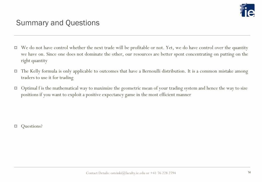
We do not have control whether the next trade will be profitable or not. Yet, we do have control over the quantity

we have on. Since one does not dominate the other, our resources are better spent concentrating on putting on the

right quantity

The Kelly formula is only applicable to outcomes that have a Bernoulli distribution. It is a common mistake among

traders to use it for trading

Optimal f is the mathematical way to maximize the geometric mean of your trading system and hence the way to size

positions if you want to exploit a positive expectancy game in the most efficient manner

Questions?

Contact Details: osteinki@faculty.ie.edu or +41 76 228 2794