algorithmic trading: a buy-side perspective

8/11/2019 Algorithmic Trading: A Buy-side Perspective

http://slidepdf.com/reader/full/algorithmic-trading-a-buy-side-perspective 1/24

Algorithmic Trading: A Buy-side Perspective

Ananth Madhavan

Barclays Global Investors

Q Group Seminar

October 2007

© Barclays Global Investors. All Rights Reserved

This material may not be distributed beyond its intended audience



P A G E N o. 1

Agenda

I. Algorithmic trading primer

• Market structure and “low touch” trading

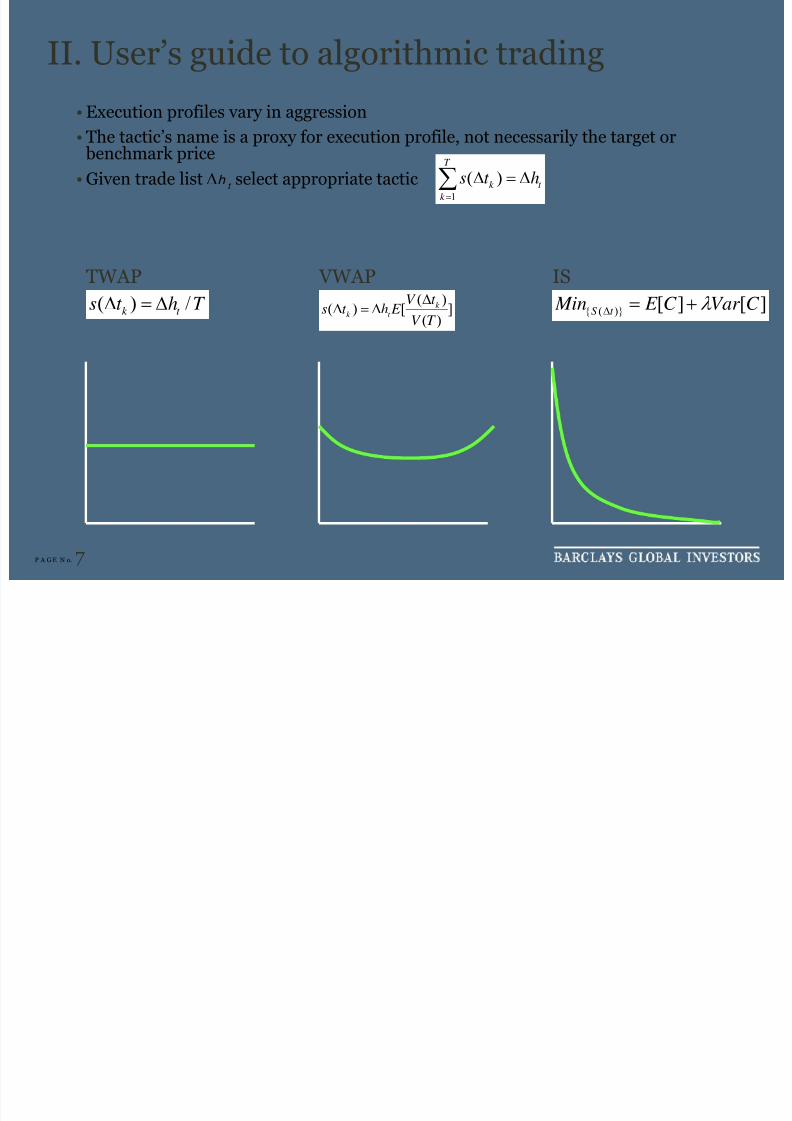
II. User’s guide to algorithmic trading• Conceptual framework for a quantitative investor

III. What lies ahead?

• Algorithms as dynamic limit orders



P A G E N o. 2

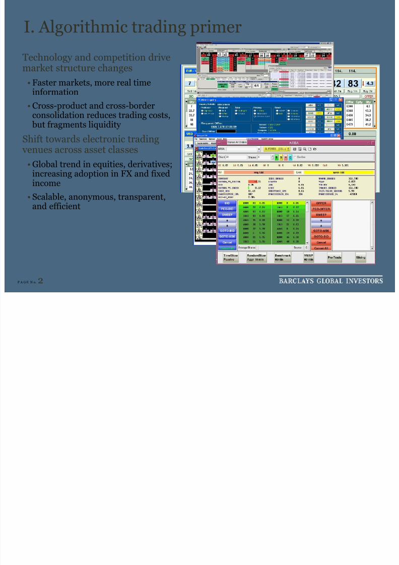
I. Algorithmic trading primer

Technology and competition drivemarket structure changes

• Faster markets, more real timeinformation

• Cross-product and cross-borderconsolidation reduces trading costs, but fragments liquidity

Shift towards electronic trading

venues across asset classes• Global trend in equities, derivatives;

increasing adoption in FX and fixedincome

• Scalable, anonymous, transparent,

and efficient



P A G E N o. 3

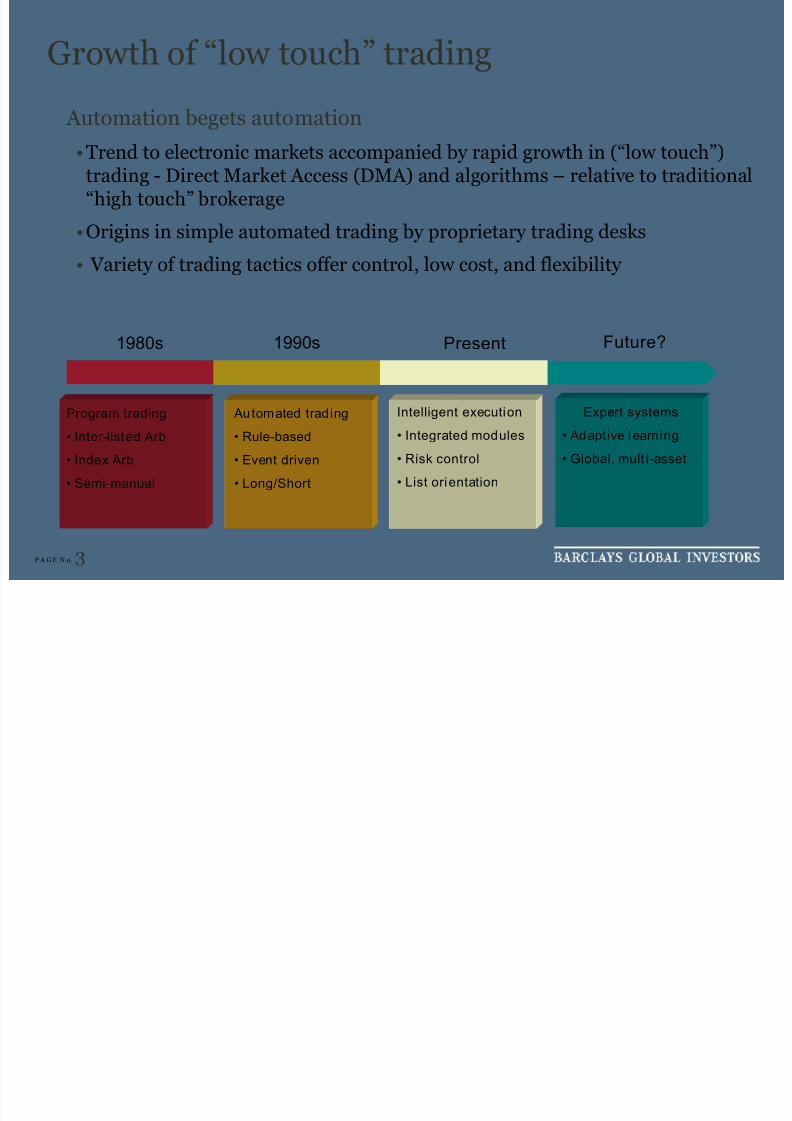
Growth of “low touch” trading

Automation begets automation

•Trend to electronic markets accompanied by rapid growth in (“low touch”)trading - Direct Market Access (DMA) and algorithms – relative to traditional

“high touch” brokerage•Origins in simple automated trading by proprietary trading desks

• Variety of trading tactics offer control, low cost, and flexibility

1980s Present1990s Future?

Program trading

• Inter-listed Arb

• Index Arb

• Semi-manual

Automated trading

• Rule-based

• Event driven

• Long/Short

Expert systems

• Adapt ive learning

• Global, mult i-asset

Intelligent execution

• Integrated modules

• Risk control

• List orientation



P A G E N o. 4

Anatomy of an algorithm

Key elements

• Select execution profile for parent order and level of aggression

• Child order placement logic

1. Micro limit order management (queue, price, cancel & correct)

2. Choice variables include start/end time, risk aversion, tolerance etc.

• Smart routing/Smart posting

• Access multiple liquidity pools; venue specific protocols

• Blend into the flow…

1. Avoid detection (see Prix, Loistl, and Huetl, 2007)

2. Avoid gaming, including in “dark pools”



P A G E N o. 5

Drivers of algorithmic trading

Increased buy-side use reflects many factors:

• Automation helps scale the trading desk

•Traders become “macro-managers”

• Anonymity and low cost

•Controlled crossing

•Explicit selection of aggression, execution profile

•Increased adoption of algorithms drives order size down, furtherreinforcing use of low touch trading

Market efficiency implications

•Edelen and Kadlec (2007) argue that use of VWAP benchmarks causesa divergence in incentives between portfolio manager and traders andresults in price-adjustment delays



P A G E N o. 6

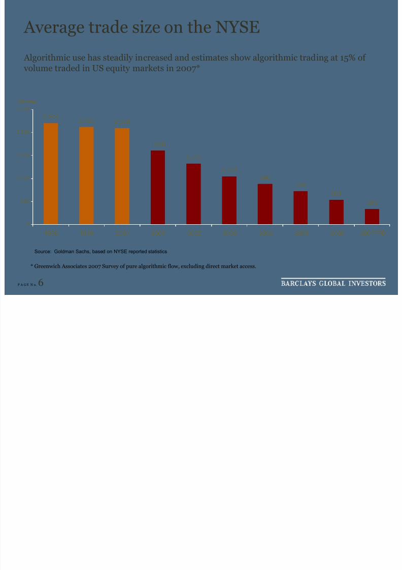
Average trade size on the NYSE

Source: Goldman Sachs, based on NYSE reported statistics

1,048

880

724

336

531

1,319

1,600

2,0962,1202,204

0

500

1,000

1,500

2,000

2,500

1998 1999 2000 2001 2002 2003 2004 2005 2006 2007YTD

Shares

Algorithmic use has steadily increased and estimates show algorithmic trading at 15% of volume traded in US equity markets in 2007*

* Greenwich Associates 2007 Survey of pure algorithmic flow, excluding direct market access.



P A G E N o. 8

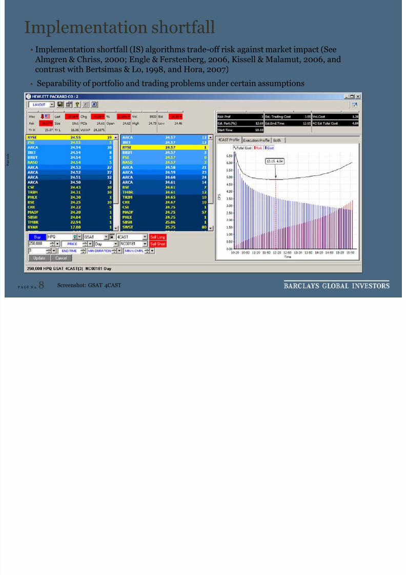
Implementation shortfall

P a g e c o

d e

• Implementation shortfall (IS) algorithms trade-off risk against market impact (See Almgren & Chriss, 2000; Engle & Ferstenberg, 2006, Kissell & Malamut, 2006, andcontrast with Bertsimas & Lo, 1998, and Hora, 2007)

• Separability of portfolio and trading problems under certain assumptions

Screenshot: GSAT 4CAST



P A G E N o. 9

Quantitative manager’s challenge

Two basic questions

1. How do traders select among tactics?

• Quantitative considerations including liquidity, risk, strategy

type, calendar effects (time of day, expiration dates, earningsrelease, etc.)

• Qualitative considerations including urgency, motivation,preferences, etc.

2. How do we evaluate an algorithm’s performance?

• Systematic analysis of execution data

• Cannot examine costs of execution without understanding choice

of tactics



P A G E N o. 10

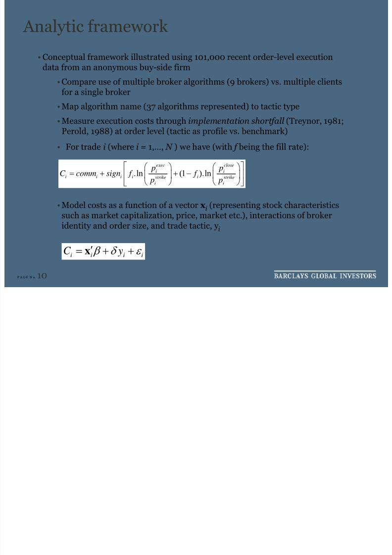
Analytic framework

• Conceptual framework illustrated using 101,000 recent order-level executiondata from an anonymous buy-side firm

• Compare use of multiple broker algorithms (9 brokers) vs. multiple clientsfor a single broker

• Map algorithm name (37 algorithms represented) to tactic type

• Measure execution costs through implementation shortfall (Treynor, 1981;Perold, 1988) at order level (tactic as profile vs. benchmark)

• For trade i (where i = 1,…, N ) we have (with f being the fill rate):

• Model costs as a function of a vector xi (representing stock characteristicssuch as market capitalization, price, market etc.), interactions of brokeridentity and order size, and trade tactic, y i

i i i iC y β δ ε ′= + +x

.ln (1 ).lnexec close

i ii i i i istrike strike

i i

p pC comm sign f f

p p

⎡ ⎤⎛ ⎞ ⎛ ⎞= + + −⎢ ⎥⎜ ⎟ ⎜ ⎟

⎝ ⎠ ⎝ ⎠⎣ ⎦



P A G E N o. 11

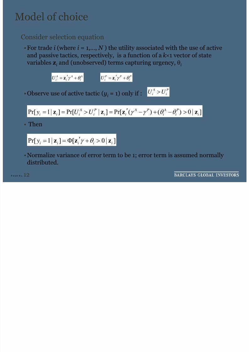
Choice of tactics

• Distinguish between “active” (i.e., front-loaded, aggressive) tradingtactics (y i = 1) and passive (TWAP/VWAP, passive participation)

strategies (y i = 0)

• Factors driving selection:1. Liquidity: Market impact costs for a front-loaded profile are greater

in less liquid stocks (measured by proxies like market capitalization,exchange listing, etc.)

2. Information leakage: Less likelihood of revelation of trade intentionsfor orders that are quickly executed (Sofianos, 2006)

3. Risk: More aggressive trading can reduce trade list risk (However,trade lists might be small relative to holdings)

4. Urgency: Prefer more rapid execution for urgent orders (Note: theseare not necessarily highest alpha orders – urgency can be driven by binding constraints, hedging transactions, etc.)



P A G E N o. 13

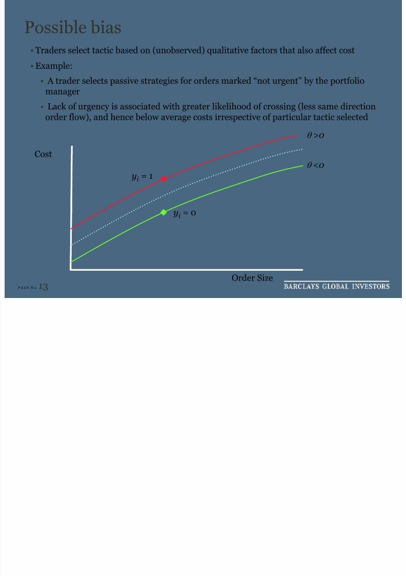
Possible bias

• Traders select tactic based on (unobserved) qualitative factors that also affect cost• Example:

• A trader selects passive strategies for orders marked “not urgent” by the portfoliomanager

• Lack of urgency is associated with greater likelihood of crossing (less same directionorder flow), and hence below average costs irrespective of particular tactic selected

Order Size

yi = 1

yi = 0

Cost

θ >0

θ <0



P A G E N o. 14

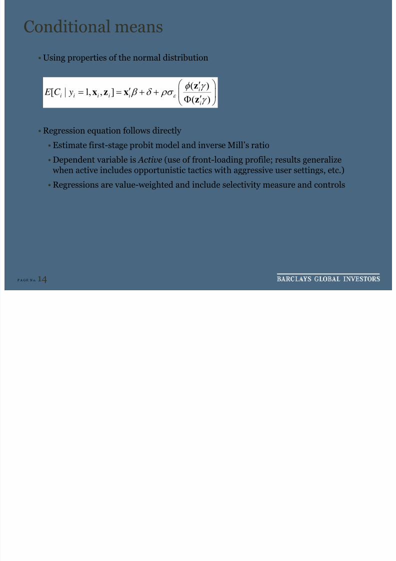
Conditional means

• Using properties of the normal distribution

• Regression equation follows directly

• Estimate first-stage probit model and inverse Mill’s ratio

• Dependent variable is Active (use of front-loading profile; results generalize when active includes opportunistic tactics with aggressive user settings, etc.)

• Regressions are value-weighted and include selectivity measure and controls

( )[ | 1, , ]

( )

ii i i i i

i

E C y ε

φ γ β δ ρσ

γ

⎛ ⎞′′= = + + ⎜ ⎟′Φ

⎝ ⎠

z

x z x

z



P A G E N o. 15

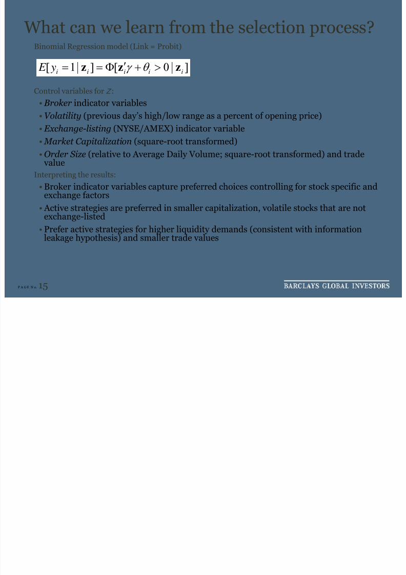
What can we learn from the selection process?Binomial Regression model (Link = Probit)

Control variables for Z :

• Broker indicator variables• Volatility (previous day’s high/low range as a percent of opening price)

• Exchange-listing (NYSE/AMEX) indicator variable

• Market Capitalization (square-root transformed)

• Order Size (relative to Average Daily Volume; square-root transformed) and trade value

Interpreting the results:

• Broker indicator variables capture preferred choices controlling for stock specific andexchange factors

• Active strategies are preferred in smaller capitalization, volatile stocks that are notexchange-listed

• Prefer active strategies for higher liquidity demands (consistent with informationleakage hypothesis) and smaller trade values

[ 1| ] [ 0 | ]i i i i i E y γ θ ′= = Φ + >z z z



P A G E N o. 16

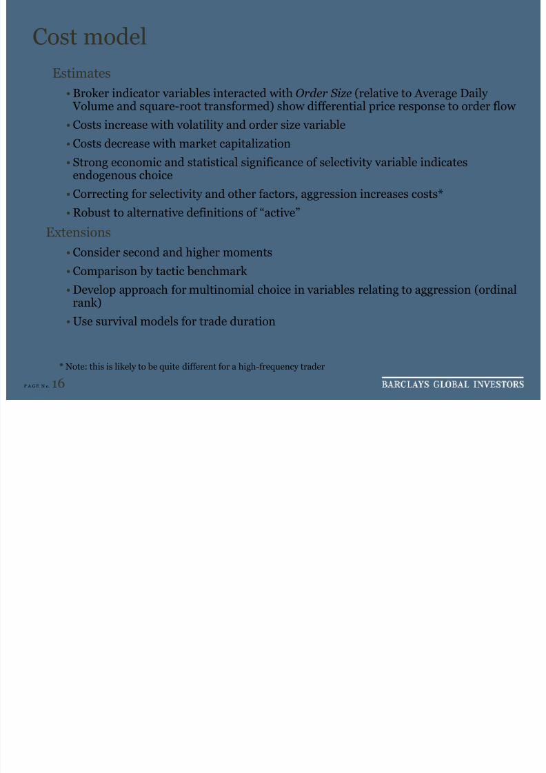
Cost model

Estimates• Broker indicator variables interacted with Order Size (relative to Average Daily Volume and square-root transformed) show differential price response to order flow

• Costs increase with volatility and order size variable

• Costs decrease with market capitalization• Strong economic and statistical significance of selectivity variable indicates

endogenous choice

• Correcting for selectivity and other factors, aggression increases costs*

• Robust to alternative definitions of “active”Extensions

• Consider second and higher moments

• Comparison by tactic benchmark

• Develop approach for multinomial choice in variables relating to aggression (ordinalrank)

• Use survival models for trade duration

* Note: this is likely to be quite different for a high-frequency trader



P A G E N o. 17

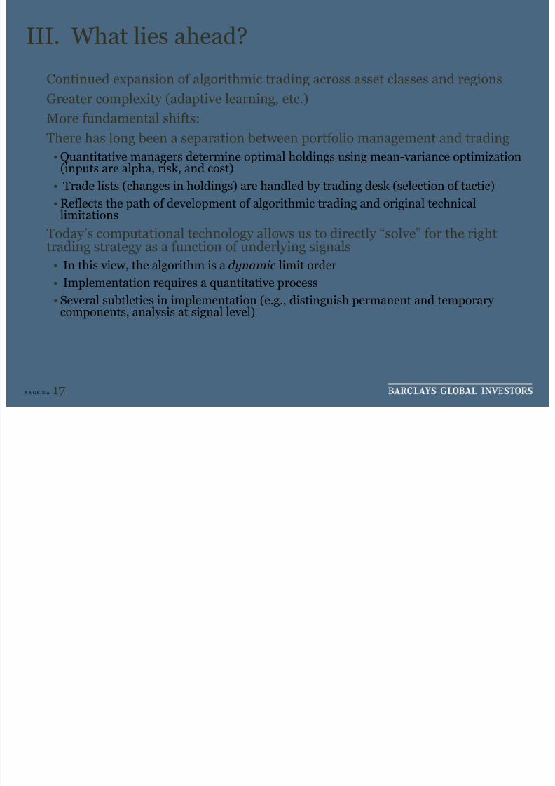
III. What lies ahead?

Continued expansion of algorithmic trading across asset classes and regions

Greater complexity (adaptive learning, etc.)

More fundamental shifts:

There has long been a separation between portfolio management and trading

• Quantitative managers determine optimal holdings using mean-variance optimization(inputs are alpha, risk, and cost)

• Trade lists (changes in holdings) are handled by trading desk (selection of tactic)

• Reflects the path of development of algorithmic trading and original technical

limitationsToday’s computational technology allows us to directly “solve” for the righttrading strategy as a function of underlying signals

• In this view, the algorithm is a dynamic limit order

• Implementation requires a quantitative process• Several subtleties in implementation (e.g., distinguish permanent and temporary

components, analysis at signal level)



P A G E N o. 18

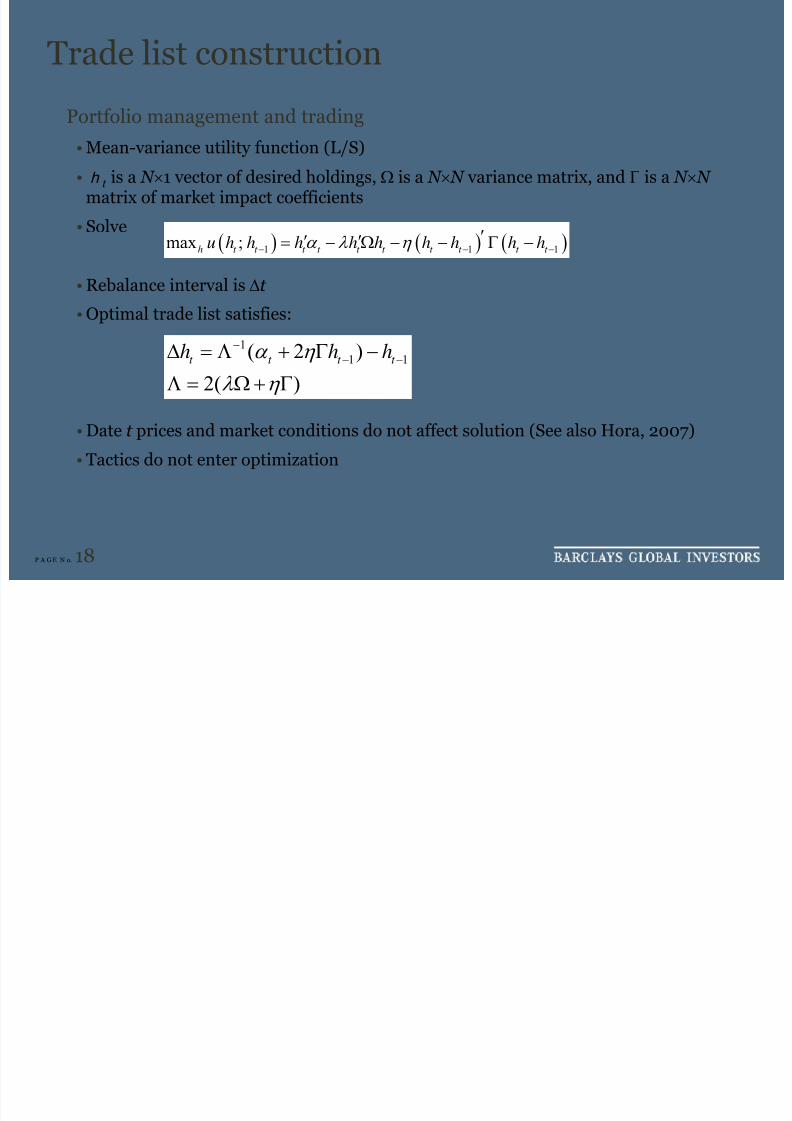
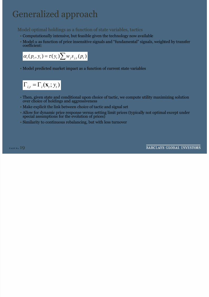
Trade list construction

Portfolio management and trading

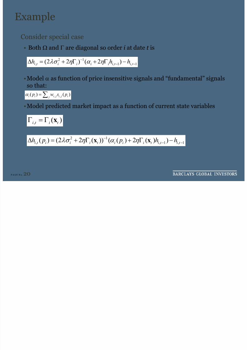
• Mean-variance utility function (L/S)

• h t

is a N ×1 vector of desired holdings, Ω is a N × N variance matrix, and Γ is a N × N matrix of market impact coefficients

• Solve

• Rebalance interval is Δt

• Optimal trade list satisfies:

• Date t prices and market conditions do not affect solution (See also Hora, 2007)

• Tactics do not enter optimization

( ) ( ) ( )1 1 1max ;h t t t t t t t t t t u h h h h h h h h hα λ η − − −′′ ′= − Ω − − Γ −

11 1( 2 )

2( )

t t t t h h hα η

λ η

−− −Δ = Λ + Γ −

Λ = Ω + Γ



P A G E N o. 21

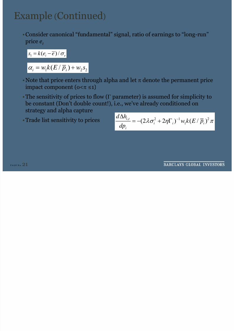
Example (Continued)

•Consider canonical “fundamental” signal, ratio of earnings to “long-run”price e

t

•Note that price enters through alpha and let π denote the permanent priceimpact component (o<π ≤1)

•The sensitivity of prices to flow (Γ parameter) is assumed for simplicity to be constant (Don’t double count!), i.e., we’ve already conditioned onstrategy and alpha capture

•Trade list sensitivity to prices

1 ( ) /i e

s k e e σ = −

, 2 1 2

1(2 2 ) ( / )i t

i i i

i

d h

w k E pdp λσ η π −Δ

= − + Γ

1 2 2( / )i i

w k E p w sα = +



P A G E N o. 22

Conclusions

Algorithmic trading continues to evolve

•More complex, robust tactics

•Buy-side needs to answer fundamental questions that must be jointlyaddressed, in the context of alpha generation

• As technology evolves, algorithms will evolve into dynamic limitorders

•Requires us to specify explicitly the link between current market state(prices, volumes, news, etc.) and the determinants of the trade list –alpha, risk, and expected cost

algorithmic trading: a buy-side perspective

Documents