algorithmic reconstruction methods in
TRANSCRIPT

ALGORITHMIC RECONSTRUCTION METHODS IN
DIFFRACTION MICROSCOPY USING A PRIORI
INFORMATION
A DISSERTATION
SUBMITTED TO THE DEPARTMENT OF ELECTRICAL
ENGINEERING
AND THE COMMITTEE ON GRADUATE STUDIES
OF STANFORD UNIVERSITY
IN PARTIAL FULFILLMENT OF THE REQUIREMENTS
FOR THE DEGREE OF
DOCTOR OF PHILOSOPHY
Leili Baghaei Rad
August 2010

This dissertation is online at: http://purl.stanford.edu/qq648sr9801
© 2010 by Leili Baghaei Rad. All Rights Reserved.
Re-distributed by Stanford University under license with the author.
ii

I certify that I have read this dissertation and that, in my opinion, it is fully adequatein scope and quality as a dissertation for the degree of Doctor of Philosophy.
R Pease, Primary Adviser
I certify that I have read this dissertation and that, in my opinion, it is fully adequatein scope and quality as a dissertation for the degree of Doctor of Philosophy.
Piero Pianetta, Co-Adviser
I certify that I have read this dissertation and that, in my opinion, it is fully adequatein scope and quality as a dissertation for the degree of Doctor of Philosophy.
Jianwei Miao
Approved for the Stanford University Committee on Graduate Studies.
Patricia J. Gumport, Vice Provost Graduate Education
This signature page was generated electronically upon submission of this dissertation in electronic format. An original signed hard copy of the signature page is on file inUniversity Archives.
iii

Abstract
Recent technological and algorithmic advances have enabled lensless imaging tech-
niques, paving the way for high resolution three dimensional analysis. In these meth-
ods, a coherent x-ray source illuminates a sample and the amplitude of the far-field
diffraction pattern is recorded. Reconstruction of the sample object requires recov-
ery of the missing phase information by exploiting additional side information in
conjunction with a computational reconstruction algorithm.
Two different sources of additional information are considered. First, the phase
recovery problem is formulated as an optimization problem where knowledge of the
form of the object (smoothness, positivity, particular material characteristics) are
included as part of the objective or enforced as constraints. This problem is then
approximated as a convex problem and solved using existing methods. The second
approach assumes that the prior knowledge is in the form of a low resolution image
of the sample and uses the wavelet domain to express this information. Experimental
limitations include coherence, noise and missing data as well as algorithmic limitations
such as data centering, support determination and complex valued reconstructions.
Reconstruction results include those of optical equivalent experiments and of both
soft and hard x-ray experiments. In all three settings the two proposed sources of
information are successfully used to obtain reconstructions for a variety of objects.
For the application of non-destructively examining the buried metallization pat-
tern of integrated circuits, we employed a coherent beam of 0.17nm X-rays to image
a 100 nm metal pattern. The metal layer was fabricated on a 100 micron silicon sub-
strate and buried beneath one micron of siliocn dioxide. From the diffraction pattern
were able to successfully reconstruct the image of the metal pattern.
iv
Acknowledgements
First and foremost, I want to express my deepest gratitude to Fabian Pease, my
primary advisor for this thesis work. It has been an honor and privilege to be his last
Ph.D. student and I am proud to have been part of the Pease Group. Working with
Fabian has been a great pleasure from the beginning to the end and I want to thank
him for his guidance, patience and constant support not just in my academic life but
also my personal life. I also want to thank Fabian for his willingness to allow me to
pursue new avenues of research and also entrepreneurship. He is truly inspirational.
I am indebted to Piero Pianetta, my co-advisor, for his support and many stimu-
lating discussions. It has been a lot of fun working with Piero, he always had a smile
on his face and was welcoming, encouraging and enthusiastic about my research. It
was a pleasure working with him and getting to know him over the years.
Next, I would like to thank Jianwei (John) Miao for his willingness to pass on his
expertise in the field and for supervising my research. I am especially grateful for the
opportunity to use the SPring8 synchrotron in Japan with him and his outstanding
research group.
I would like to thank my industry mentor, Steve Moffatt, for being so encouraging
and supportive over the past two years. I would like to thank Applied Materials Inc.
and David Kyser for assisting with the funding of my research. Next, I would like
to thank Pierre Thibault for sharing his source code, many stimulating conversations
and answering many questions.
I would like to take this opportunity to thank the following people for their impact
on my life; Maurice and Alice Lynch, Graham and Kathleen Bennett, Richard Wells,
Nicki, Cody and Christie Marrian, Marybelle Cody, and Cindy Hanson.
v

I would like to thank the members of the Pease research Group; Jun Ye, Mark
McCord, Rafael, Bipin, Zhi, Filip, Bing, Sayaka, Hesaam, and Dan.
I would like to thank my friends who have made this journey a lot more enjoy-
able. I can not name them all but I would like to name a few; Parastoo Nikaeen,
Mona Jarrahi, Mohammad Hekmat, Narges Bani Asadi, Bahar Behdad and Shahram
Taghavi, Maryam Vareth, Maryam Ziaei-Moayyed and Mike Safai, Jacob Mattingley,
Ali Faghfuri, Kosar B. Parizi, Pooya and Ava Rahbar, Mehdi Mohseni, Bita Nezam-
far, Sahar Tabesh and Amin Arbabian, Neda Beheshti, AmirAli Kia, Kokab B. Parizi,
Mohammad Shoheybi, Brano Kusy, Sam Kavusi, and Pedram Mokrian.
I thank my parents-in-law, Colin and Gaye, and James, Christine, Elisabeth and
their families for their support and love.
I want to thank my wonderful family for their constant support and for their many
sacrifices that allowed me to be where I am today. I thank my mother Parvin, my
father AbolFazl, my brother Ali and my grandmother, for giving me the inspiration
and balance I needed to continue. I also want to thank my family in Iran who are so
close despite being so far away. This thesis is dedicated to my parents.
Finally, I would like to thank my best friend and husband Ian, without his love
and support none of this work would have been possible.
Part of my study has been supported by the New Zealand Federation of Gradu-
ate Women Fellowship, Texas Instrument Fellowship, Applied Materials Fellowship,
SPIE Scholarship, J. R. Templin Scholarship and the US Government under contract
number N66001-05-1-8914 awarded by the Navy.
vi

Contents
Abstract iv
Acknowledgements v
1 Introduction 1
2 Theoretical Background 3
2.1 Preliminaries . . . . . . . . . . . . . . . . . . . . . . . . . . . . . . . 3
2.1.1 Fourier Transform . . . . . . . . . . . . . . . . . . . . . . . . . 3
2.1.2 Wavelet Transform . . . . . . . . . . . . . . . . . . . . . . . . 6
2.1.3 Haar wavelet . . . . . . . . . . . . . . . . . . . . . . . . . . . 8
2.2 Scattering of light from inhomogeneous media . . . . . . . . . . . . . 10
2.2.1 Diffraction Scattering . . . . . . . . . . . . . . . . . . . . . . . 11
2.3 Diffraction Imaging . . . . . . . . . . . . . . . . . . . . . . . . . . . . 11
2.3.1 Phase Information Loss . . . . . . . . . . . . . . . . . . . . . . 11
2.3.2 Phase Recovery Techniques . . . . . . . . . . . . . . . . . . . 11
3 Reconstruction Algorithms 13
3.1 Iterative Algorithms . . . . . . . . . . . . . . . . . . . . . . . . . . . 13
3.1.1 Constraint sets . . . . . . . . . . . . . . . . . . . . . . . . . . 13
3.1.2 Projections . . . . . . . . . . . . . . . . . . . . . . . . . . . . 13
3.1.3 Iterative formulation . . . . . . . . . . . . . . . . . . . . . . . 16
3.1.4 Difference map algorithm . . . . . . . . . . . . . . . . . . . . . 16
3.2 Projection operators . . . . . . . . . . . . . . . . . . . . . . . . . . . 17
vii

3.2.1 Diffraction projections . . . . . . . . . . . . . . . . . . . . . . 17
3.2.2 Direct space projections . . . . . . . . . . . . . . . . . . . . . 19
3.2.3 Wavelet Projection . . . . . . . . . . . . . . . . . . . . . . . . 20
3.3 Convex optimization . . . . . . . . . . . . . . . . . . . . . . . . . . . 22
3.3.1 Convex formulation . . . . . . . . . . . . . . . . . . . . . . . . 24
3.3.2 Heuristics . . . . . . . . . . . . . . . . . . . . . . . . . . . . . 25
3.3.3 Scaling to 3D datasets . . . . . . . . . . . . . . . . . . . . . . 26
4 Working with Experimental Data 29
4.1 Experiment limitations . . . . . . . . . . . . . . . . . . . . . . . . . . 29
4.1.1 Noise . . . . . . . . . . . . . . . . . . . . . . . . . . . . . . . . 29
4.1.2 Systematic errors . . . . . . . . . . . . . . . . . . . . . . . . . 31
4.1.3 Source Coherence . . . . . . . . . . . . . . . . . . . . . . . . . 31
4.1.4 Missing Data . . . . . . . . . . . . . . . . . . . . . . . . . . . 32
4.1.5 Dynamic Range . . . . . . . . . . . . . . . . . . . . . . . . . . 33
4.2 Data Preparation . . . . . . . . . . . . . . . . . . . . . . . . . . . . . 33
4.2.1 Background subtraction . . . . . . . . . . . . . . . . . . . . . 34
4.2.2 Data centering . . . . . . . . . . . . . . . . . . . . . . . . . . 34
4.2.3 Recovering Missing Information . . . . . . . . . . . . . . . . . 37
5 Reconstructions and Simulations 38
5.1 Simulation . . . . . . . . . . . . . . . . . . . . . . . . . . . . . . . . . 38
5.1.1 Wavelet domain constraints . . . . . . . . . . . . . . . . . . . 38
5.1.2 Convex optimization formulation . . . . . . . . . . . . . . . . 39
5.2 Scaled Optical Experiment . . . . . . . . . . . . . . . . . . . . . . . . 43
5.3 Soft X-ray Experiment . . . . . . . . . . . . . . . . . . . . . . . . . . 46
5.4 Hard X-ray Experiment . . . . . . . . . . . . . . . . . . . . . . . . . 46
6 Conclusion 50
Bibliography 52
viii

List of Figures
2.1 Continuous Haar wavelet basis. . . . . . . . . . . . . . . . . . . . . . 8
2.2 2D wavelet decomposition. . . . . . . . . . . . . . . . . . . . . . . . . 9
3.1 General phase retrieval constraint problem. . . . . . . . . . . . . . . . 14
4.1 Dynamic range of a typical diffractogram. . . . . . . . . . . . . . . . 34
4.2 Background subtraction . . . . . . . . . . . . . . . . . . . . . . . . . 35
4.3 Centering experimental data . . . . . . . . . . . . . . . . . . . . . . . 36
5.1 Iterative phase reconstruction using wavelet domain constraints. . . . 40
5.2 Example of a 1-D reconstruction escaping local minima. . . . . . . . . 41
5.3 Example of a 1-D reconstruction with faster convergence using heuristics. 42
5.4 3D simulation . . . . . . . . . . . . . . . . . . . . . . . . . . . . . . . 43
5.5 Experimental optical laser setup. . . . . . . . . . . . . . . . . . . . . 45
5.6 Reconstruction of isolated samples from optical diffraction measurement. 45
5.7 Reconstructions of extended samples from optical diffraction measure-
ments. . . . . . . . . . . . . . . . . . . . . . . . . . . . . . . . . . . . 46
5.8 Experimental soft x-ray setup at Stanford Synchrotron Radiation Lab-
oratory. . . . . . . . . . . . . . . . . . . . . . . . . . . . . . . . . . . 47
5.9 Reconstruction of a 2-D sample using a priori information. . . . . . . 47
5.10 caption short . . . . . . . . . . . . . . . . . . . . . . . . . . . . . . . 48
5.11 Hard x-ray experiment: SEM micrograph and reconstruction . . . . . 49
ix
Chapter 1
Introduction
This thesis describes recent work in several distinct areas of algorithmic reconstruction
methods for coherent x-ray diffraction microscopy. This field has gained considerable
attention as a potential high-resolution microscopy tool for 2- and 3-dimensional
nano-scale imaging of both biological and non-biological samples.
Diffractive imaging techniques fundamentally depart from other microscopy imag-
ing techniques by being lensless. Rather than rely on an objective lens to refract and
combine the light, diffractive techniques illuminate the sample with a coherent wave
and measure the diffraction pattern. This approach is advantageous in that it avoids
the aberration and resolution limits of lenses, but it brings about the phase retrieval
problem resulting from recording only the intensity, and not also the phase, of the
scattered light. This problem can often be solved algorithmically, leading to the term
algorithm reconstruction where computer algorithms are used in place of the objective
lens.
This thesis is organized as a review of the theory and algorithmic reconstruction
techniques of coherent diffraction microscopy. The original contribution of this work
has both theoretical and experimental aspects.
Chapter 2 introduces the necessary theory for the discussions present in this thesis.
It first covers the physical phenomena occurring in diffraction microscopy and then
examines the theoretical aspects of diffraction imaging, in particular, oversampling
and over-determination of the of the solution.
1

CHAPTER 1. INTRODUCTION 2
Chapter 3 continues by presenting the mathematical formalism of existing algo-
rithmic reconstruction algorithms. This includes the difference map algorithm, a
generalized iterative algorithm and a selection of projections that can be used. This
includes introduced a new, novel, projection where constraints are expressed in the
wavelet domain. The chapter continues by introducing a new formulation of the phase
retrieval problem as a convex optimization problem.
Chapter 4 discusses the practical aspects of coherent diffractive imaging. Topics
such as noise, missing data and data alignment are considered.
Chapter 5 presents the results of applying the techniques of this thesis to a se-
lection of both real and simulated samples. The experimental results were obtained
from a scaled optical experiment and both soft and hard x-ray sources.

Chapter 2
Theoretical Background
This chapter provides an overview of the main theoretical concepts that are necessary
to understand the later chapters of this thesis.
2.1 Preliminaries
We first provide a summary of the signal processing tools that are used to describe
the diffraction image formation process and later used in the development of new
object reconstruction algorithms.
2.1.1 Fourier Transform
The continuous Fourier transform is
f(q) = Ff =
∫ ∞
−∞f(x)e−iqxdx (2.1)
and the inverse continuous transform is
f(x) = F−1f =1√2π
∫ ∞
−∞f(q)eiqxdq. (2.2)
3

CHAPTER 2. THEORETICAL BACKGROUND 4
We will denote Fourier pairs with a double arrow like
f(x)⇔= f(q)Ff. (2.3)
Throughout this thesis, a quantity as a function of spatial coordinates is said to be
in real, or direct, space (domain). The Fourier transform of such a quantity is said to
be in Fourier or reciprocal space (domain). Real space coordinates will be expressed
with the notation x for a single dimension or r = (x, y, z) for three dimensions, and
q = (qx, qy, qz) for Fourier space coordinates.
For square integrable functions f(x) and g(x), Parseval’s theorem states
∫ ∞
−∞f(x)g(x)dx =
∫ ∞
−∞f(q)g(q)dq. (2.4)
From this, the Plancherel theorem (equivalent to Parseval’s theorem) states that
∫ ∞
−∞|f(x)|2dx =
∫ ∞
−∞|f(q)2|dq. (2.5)
The Plancherel theorem can be interpreted as saying that the Fourier transform pre-
serves the energy of the original quantity.
If f(x) is a purely real even function, then f(q) is also purely real and even. If
f(x) is purely real and odd then f(q) is purely imaginary and odd.
A shift (translation) in direct space results in a linear phase ramp in Fourier space.
f(x− a)⇔ e−iaqf(q) (2.6)
The dual of this also applies. Such a translation in Fourier space may occur, for
example, if the center of the diffraction pattern is not precisely known.
e2πaxf(x)⇔ f(q − a). (2.7)
The Fourier transform of a real function f(x) = f ∗(x) has the property of inversion

CHAPTER 2. THEORETICAL BACKGROUND 5
through the origin
f(q) = f ∗(q) (2.8)
In diffraction, this arises in Friedel’s Law which states that members of a Friedel pair,
f(q) and f(−q), have equal amplitude and opposite phase.
Convolution,
(f ∗ g)(x) =
∫f(x′)g(x− x′)dx′, (2.9)
in one domain corresponds to multiplication in the other. For example, convolution
in direct space:
(f ∗ g)(x)⇔ f(q)g(q). (2.10)
Similarly, for cross-correlation,
(f ~ g)(x) =
∫f(x′)g∗(x′ − x)dx′
⇔ f(q)g∗(q).(2.11)
Of particular note is the autocorrelation,
(f ~ f)(x)⇔ |f(q)|2 (2.12)
As with most signal processing applications the data analysis is performed on
a digital computer and so, combined with the spatially sampled detector, the data
values are discretized to a digital representation rather than a continuous real number.
This necessitates the use of the discrete Fourier transform (DFT),
fn = Ff =1√N
N−1∑
m=0
fme2πinm/N (2.13)
and the corresponding inverse discrete Fourier transform,
fn = F−1f =1√N
N−1∑
m=0
fme2πimm/N . (2.14)
The discrete Fourier transform of a (assumed periodic) continuous function is

CHAPTER 2. THEORETICAL BACKGROUND 6
approximated by sampling the function on an appropriately fine grid,
fm = f(m∆x). (2.15)
Sampling in the spatial domain leads to periodic extension and sampling in the fre-
quency domain,
f(n∆q) = fn, (2.16)
where the spatial and frequency grid spacings are related as follows:
∆x∆q =2π
N. (2.17)
A naıve implementation of the DFT requires O(N 2 ) operations. In practice one of
the fast Fourier transforms is used which is O(N log N ), such as [4].
As alluded to the sampling of the continuous function must be performed on an
appropriately fine grid. For a grid defined by ∆x the maximum frequency present in
the discrete Fourier transform is given as the Nyquist frequency
qN =Nδq
2=
π
∆x(2.18)
If the sampling is not sufficiently fine then qN is less than the maximum frequency
present in the signal and aliasing occurs where those frequency components higher
than qm are aliased and appear at lower frequencies. If the maximum signal frequency
is less than the Nyquist frequency then no aliasing occurs and the signal can be
perfectly reconstructed from its samples using the sinc function as
f(x) =∑
n
fnsin(x− n∆x)
x− n∆x. (2.19)
2.1.2 Wavelet Transform
Fourier analysis is based on the complex exponential as a basis function. The complex
exponential has a precisely defined frequency but is infinite in spatial extent. The
result is that the Fourier transform is excellent at analysing the frequency components

CHAPTER 2. THEORETICAL BACKGROUND 7
of a signal but with the drawback that it cannot localize the spatial position where
that frequency component originates.
One approach to mitigate these limitations is to use a windowed complex expo-
nential basis function but this implies a constant spatial resolution for all frequency
components. For many applications a more preferable transform would have reduced
spatial resolution but high frequency resolution for low frequency components and
good spatial with poor frequency resolution for high frequency components.
These needs lead to considering the alternative where the basis function vary in
both ’frequency’ and spatial extent. Such a transform is able to provide an excellent
time-frequency representation of a signal with time and frequency localization. The
continuous wavelet transform provides such an analysis tool where the components
are given at a scale, a > 0, and translation value, b ∈ R by the following transform
Gw(a, b) =1√a
∫ ∞
−∞g(x)ψ∗
(x− ba
)dx, (2.20)
where ψ(x), known as the mother wavelet, is a continuous function in both spatial and
frequency domains. The mother wavelet is a generator of daughter wavelet functions,
translated and scaled versions of the mother wavelet function. The inverse transform
is
g(x) =
∫ ∞
0
∫ ∞
−∞
1
a2Gw(a, b)
1√|a|ψ
(x− ba
)db da. (2.21)
where ψ(x) is the dual function of ψ(x). The dual function can be chosen to be
C−1ψ ψ(x) with,
Cψ =1
2
∫ ∞
−∞
∣∣∣ψ(η)∣∣∣2
|η| dη, (2.22)
and subject to the admissibility condition, 0 < Cψ < ∞. This in turn can be shown
to imply that the wavelet must integrate to zero, ψ(0) = 0.

CHAPTER 2. THEORETICAL BACKGROUND 8
2.1.3 Haar wavelet
The simplest continuous wavelet is the Haar wavelet which consists of a single positive
and negative cycle. Figure 2.1 shows the mother wavelet ψ(x) and several of the
daughter wavelets, both scaled and shifted.
The discrete Haar wavelet can be represented be the 2× 2 Haar matrix,
H2 =
[1 1
1 −1
]. (2.23)
The Haar wavelet transform can be derived from the Haar matrix. The 4 × 4 Haar
transform matrix is
H2 =1√4
1 1 1 1
1 1 −1 −1√2 −
√2 0 0
0 0√
2 −√
2
. (2.24)
1
-1-1-1
-1
-1
-1
-1
1
11
1
11
ψ1,1 = ψ(2x− 1)
ψ2,0 = ψ(4x) ψ2,1 = ψ(4x− 1) ψ2,0 = ψ(4x− 2) ψ2,3 = ψ(4x− 3)
ψ0,0 = ψ(x)
ψ1,0 = ψ(2x)
1
1111
1
1ψ(x) =
1 0 ≤ x < 12
−1 12 < x ≤ 1
0 otherwise
Figure 2.1: Several of the continuous Haar wavelets. The mother wavelet ψ(x) isscaled and shifted.
The 2D wavelet transform can be accomplished by applying 1D transforms in
orthogonal directions consecutively as shown in figure 2.2.

CHAPTER 2. THEORETICAL BACKGROUND 9
Figure 2.2: The 2D wavelet decomposition of an image occurs with down-samplingin both x and y directions consecutively.

CHAPTER 2. THEORETICAL BACKGROUND 10
Further information about the wavelet transform can be found in many references,
including [51].
2.2 Scattering of light from inhomogeneous media
In this section we briefly examine the basic elements of the scalar theory of scattering
of light. Rather than re-derive the wave equation completely we summarize the
analysis of Thibault, 2007 and [50].
Starting from Maxwell’s equations,
∇ · [ε(r)E](r) = 0
∇ ·H(r) = 0
∇× E(r) = iωµH(r)
∇×H(r) = −iωε(r)E(r)
(2.25)
where ε(r) is the electric permittivity and µ is the magnetic permeability. Under the
assumption that variations in the dielectric medium occur on a length scale greater
than the wavelength of the electromagnetic field, i.e.
∇ε� k|ε|, (2.26)
with wavenumber k = 2π/λ, then the scalar Helmholtz wave equation can be derived.
∇2Ψ + k2n2Ψ = 0, (2.27)
where k = ω/c and n2 = c2εµ. The Helmholtz equation can only be solved ana-
lytically in certain scenarios and must generally be solved by numerical means or
approximated.
At x-ray wavelengths, n is usually expressed in complex form as,
n = 1− δ − iβ (2.28)
where δ represents the purely refractive component and β the absorptive component.

CHAPTER 2. THEORETICAL BACKGROUND 11
Both components are very small (|δ + iβ| � 1) so n2 is well approximated by 1 −2(δ + iβ). A consequence of δ being very small is that x-rays are only very weakly
refracted by any matter and a focusing lens would have to be both strongly curved
and very thick. However, although β is small it is high in comparison and such lens
would have high absorption, make such lenses impractical.
2.2.1 Diffraction Scattering
For diffraction experiments it is the amplitude of the wave field in a plane transverse
to the direction of propagation that is measured. After separating out the trans-
verse (r⊥ = (x, y)) and parallel (z) components and assuming the back-propagating
component is zero, then the well known far-field diffraction equation can be derived,
I(u) = |Ψfar-field(zu)|2 ∝ 1
1 + u2
∣∣Ψ(q⊥ = κu)∣∣2 . (2.29)
That is, the far-field diffraction pattern is proportional to the absolute value of the
Fourier transform of the exit wave field.
2.3 Diffraction Imaging
2.3.1 Phase Information Loss
In diffraction imaging experiments it is the intensity of the wave field that is measured.
Since the wave field is a complex variable the phase information about the wave field
is lost [8, 3]. This information is critical and must be recovered from either redundant
information contained within the amplitude information or from an external source
[1, 2, 3, 15, 12, 32, 11, 16, 19].
2.3.2 Phase Recovery Techniques
Most coherent diffractive imaging (CDI) methods rely on far-field diffraction data
to retrieve the complex-valued projection or three-dimensional density of a sample.
Unless the sample is periodic, as is the case in crystallography, finite coherence length
CHAPTER 2. THEORETICAL BACKGROUND 12
and fixed dimensions of the detector pixels impose a limit on the amount of infor-
mation carried by the wave for the problem to be tractable [5, 23, 24, 10]. For this
reason, all CDI techniques require “oversampling” of the diffraction pattern, i.e. that
the region in real-space contributing to the diffraction data does not extend beyond
a limit predefined by the experimental conditions. In many experiments, oversam-
pling is achieved with a plane wave incident on an isolated specimen [7]. Despite
the successes of this approach [22, 37, 43, 29] the requirement for sufficiently small
and isolated samples is an important obstacle to a wider application of the technique
[34, 20, 26, 39].
Chapter 3
Reconstruction Algorithms
3.1 Iterative Algorithms
3.1.1 Constraint sets
The phase recovery problem is often posed as a two-constraint satisfaction problem
where the first constraint is based on the measured diffraction intensities and the
second represents known information in direct space [29, 31, 30, 43, 28, 9, 13, 6, 35,
33, 36, 27, 47]. Formally the two-constraint problem is defined as follows:
Definition 1 (The two-constraint satisfaction problem). Given two constraint sets
C1 and C2, find an x ∈ C1 ∩ C2, i.e. simultaneously satisfying both constraints.
3.1.2 Projections
A key concept to many constraint satisfaction problems is that of taking an element
not contained within a constraint set and using this to find one that is. This idea is
made more precise with the following definitions.
We assume that there exists an underlying vector space W with the usual vector
space axioms:
1. associativity of addition
13

CHAPTER 3. RECONSTRUCTION ALGORITHMS 14
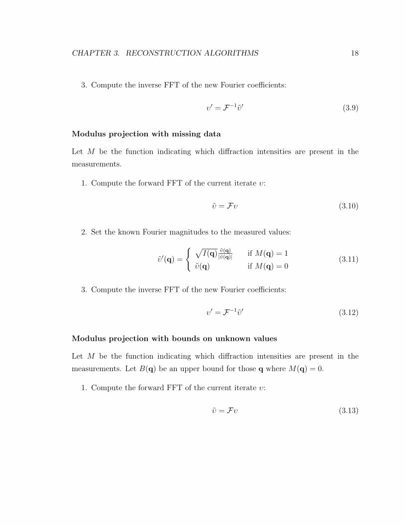
Fourier modulus constraint
• enforce the modulus ofthe Fourier transform to‘match’ measurements
Other constraints
• Finite support
• Wavelet coefficients (low res.)
• Smoothness
• Positivity
• Close match to specifications
Look for solution meeting both sets of constraints
Figure 3.1: General phase retrieval constraint problem. The known information formsconstraints sets and a solution is sought which simultaneously satisfies both sets ofconstraints. One constraint set uses the measured Fourier modulus values. The otherconstraint set can be formed from different forms of a priori information. For example,this might be knowledge of the spatial support of the object or a low-resolution imageof the object.
2. commutativity of addition
3. identity of addition
4. inverse elements of addition
5. distributivity of scalar multiplication with respect to vector addition
6. distributivity of scalar multiplication with respect to field addition
7. compatibility of scalar multiplication with field multiplication
8. identity element of scalar multiplication.
On this vector space we can define the general projection as follows:
Definition 2 (Projection). A projection P is a linear transformation that is idem-
potent, meaning that P 2 = P . In this context this means that once the projection has
been applied any subsequent projection (using the same projection) returns the same
element.
With W as the underlying vector then the projection operator P induces subspaces
U and V as the range and null spaces of P respectively. The following basic properties
hold:

CHAPTER 3. RECONSTRUCTION ALGORITHMS 15
1. P is the identity operator I on U : ∀x ∈ U : Px = x
2. There is the direct sum W = U⊕V . Every vector x can be decomposed uniquely
as x = u + v where u ∈ U and is given by u = Px, and v ∈ V and is given by
v = x− Px;
For a vector space equipped with an inner product then an orthogonal projection
can be defined as follows:
Definition 3 (Orthogonal Projection). For a vector space W equipped with an inner
product, a projection is orthogonal if and only if it is self-adjoint, i.e. the associated
matrix P is symmetric relative to an orthonormal basis: P = P T (or, in the complex
case, P = P ∗). For such a projection the range and null, U and V respectively, are
orthogonal subspaces of W .
In more practical terms, the orthogonal projection of a vector to a subspace finds
the vector that is nearest. That is, given x ∈ W , then u = Px is the point in U
that minimizes the distance (as defined by the inner product of W ) ||x − u||. If the
subspace U is convex then the orthogonal projection is unique while for non-convex
subspaces there may exist multiple vectors with the same distance to x.
The orthogonal projection distance can be considered as the error, or amount, by
which a vector fails to satisfy a constraint. For a vector x we say that the constraint
set C1 is satisfied if PC1x = x for the orthogonal projection PC1 since the error is
given by ||x−Px|| = 0. If the two-constraint satisfaction problem is feasible then all
solutions satisfy the condition:
xsol = PC1x = PC2x
The determination of suitable projection operators is problem-specific and de-
pends on the constraint spaces that are used. Later, in 3.2, several commonly used
projections will be discussed as well as a new projection based on wavelets.

CHAPTER 3. RECONSTRUCTION ALGORITHMS 16
3.1.3 Iterative formulation
In general, the large search space and complicated constraint spaces mean that most
algorithms are iterative in nature. Such algorithms repeatedly apply an operator F
xn+1 = F (xn)
until a fixed point is reached where
xn+1 = F (xn) = xn = x∗.
The algorithm is then said to converge, however this point may be one of a set
of solutions or may not even be a solution at all, depending on the nature of the
constraint sets.
3.1.4 Difference map algorithm
The difference map algorithm [29] is defined as:
xn+1 = xn + βD(xn). (3.1)
where
D(x) = y2(x)− y1(x), (3.2)
and
y1 = P1[(1 + γ2)P2(x)− γ2x], y2 = P2[(1 + γ1)P1(x)− γ1x]. (3.3)
The operators, P1 and P2, are projections and are most often orthogonal projections.
The parameters β, γ1 and γ2 are complex but usually taken as real and can be chosen
as ±1 to simplify 3.1.
From an initial starting point x0 the difference map is iteratively applied until
some termination criteria is met. Assuming for now that the map converges, then

CHAPTER 3. RECONSTRUCTION ALGORITHMS 17
this will occur when a fixed point is reached,
x∗ = x∗ + βD(x) (3.4)
which requires that D(x) = 0, i.e.,
y1(x∗) = y2(x∗). (3.5)
The fixed point, x∗, will be a solution to the two-constraint problem since it must lie
somewhere in the intersection of the two constraint spaces, C1 and C2.
The progress of the iterative map can be monitored by observing the difference
map error, defined as the norm of the difference between successive iterate values:
εn = ||xn+1 − xn|| (3.6)
3.2 Projection operators
In this section we present the well known projections for diffraction and direct space
as well as introduce wavelet space projections.
3.2.1 Diffraction projections
Modulus projection
Let I(q) be the measured diffraction intensities.
1. Compute the forward FFT of the current iterate υ:
υ = Fυ (3.7)
2. Set the Fourier magnitudes to the measured values:
υ′(q) =√I(q)
υ(q)
|υ(q)| (3.8)
CHAPTER 3. RECONSTRUCTION ALGORITHMS 18
3. Compute the inverse FFT of the new Fourier coefficients:
υ′ = F−1υ′ (3.9)
Modulus projection with missing data
Let M be the function indicating which diffraction intensities are present in the
measurements.
1. Compute the forward FFT of the current iterate υ:
υ = Fυ (3.10)
2. Set the known Fourier magnitudes to the measured values:
υ′(q) =
{ √I(q) υ(q)
|υ(q)| if M(q) = 1
υ(q) if M(q) = 0(3.11)
3. Compute the inverse FFT of the new Fourier coefficients:
υ′ = F−1υ′ (3.12)
Modulus projection with bounds on unknown values
Let M be the function indicating which diffraction intensities are present in the
measurements. Let B(q) be an upper bound for those q where M(q) = 0.
1. Compute the forward FFT of the current iterate υ:
υ = Fυ (3.13)

CHAPTER 3. RECONSTRUCTION ALGORITHMS 19
2. Set the known Fourier magnitudes to the measured values and bound the un-
known values:
υ′(q) =
{ √I(q) υ(q)
|υ(q)| if M(q) = 1
min (B(q), υ(q)) if M(q) = 0(3.14)
3. Compute the inverse FFT of the new Fourier coefficients:
υ′ = F−1υ′ (3.15)
3.2.2 Direct space projections
Complementing the projections for Fourier space there is a set of projections that are
used to enforce constraints in direct space. The most basic of these projections is
the support projection where the compact support of the sample is used to set values
outside of the support to zero. This is easily seen to be the orthogonal projection
since it does not affect those values inside the support, only setting those outside the
support to zero, but still respecting the constraint [17].
Basic support projection
Let S be the finite support. The basic finite support projection sets those points
outside the support to zero:
1.
υ′(r) =
{υ(r) if r ∈ S0 otherwise
(3.16)
Support projection with threshold
Let T be a threshold for |υ(r)|, then the projection is:
1.
υ′(r) =
υ(r) if |υ(r)| ≥ T
T υ(r)|υ(r)| if T
2< |υ(r)| < T
0 otherwise
(3.17)

CHAPTER 3. RECONSTRUCTION ALGORITHMS 20
Positivity projection
1.
υ′(r) =
{υ(r) if υ(r) ≥ 0
0 otherwise(3.18)
3.2.3 Wavelet Projection
Although much success has been achieved with the finite support constraint, sev-
eral reasons motivate exploring other types of constraint sets particularly for specific
applications:
1. The finite support constraint restricts the method to reconstructing isolated
objects [44, 45]. Many applications would benefit from being able to image
extended structures.
2. It is often that more detailed spatial information such as low-resolution SEM
or x-ray transmission images may be available. Existing algorithms frequently
use this to fill in data values that are missing due to a beam stop [23].
3. Rather than precise knowledge of the support the prior information may be more
qualitative in nature. For example, it may be that the structure is semi-regular
or that it is generally composed of a small number of homogeneous areas.
In this work we introduce the use of a low-resolution version of the real space object
as a priori information. It explicitly is not assumed that the sample is compactly
supported as previously required. The constraint set is now the set of all images which
have a low-resolution approximation matching the measured values. It is expected
that the resolution could be lower by perhaps a factor of 16 or 32.
This a priori data directly provides information about the low frequency com-
ponents in the Fourier domain, both the phase and magnitude. The magnitude
information can prove useful as a beam stop generally obscures the center portion of
the image sensor. The low-resolution information sets the approximate structure of
the object and resolves phase and translation ambiguities.

CHAPTER 3. RECONSTRUCTION ALGORITHMS 21
The low-resolution constraint may be applied in the spatial domain but can be
more readily expressed in a wavelet domain. The Haar wavelet is suitable partly
because of its simplicity but also because the structure of the wavelet matches the
shape of the expected features the test sample. For other sample types one of the
other wavelets may be more suitable. Figure 2.1 shows the continuous Haar mother
wavelet and several translated and scaled wavelets. Figure 2.2 illustrates the wavelet
decomposition of a two-dimensional image. For the Haar wavelet a single level of
decomposition produces four smaller images (12
the size in each dimension). The first
image is the (normalized) approximation sub-image where the sum of each 2×2 block
is computed. The second, third and fourth images are detail sub-images where the
difference between sample values horizontally, vertically and diagonally are computed.
Additional levels of decomposition can be recursively performed on the sum image.
In Figure 2.2 four levels of decomposition are shown with the shaded block indicated
the approximation coefficients which will be used as a priori information.
It is assumed that the diffraction data is of size (n× n) for some n = 2k where k
is a positive integer and that the low-resolution information is of size (2l × 2l) where
l is also a positive integer and l < k. The approximation coefficients of the (k − l)thwavelet transform, Wk−1, are then constrained to match the a priori information in
wavelet space XmeasW . Figure 2.2 shows the approximation coefficients for the fourth
level decomposition. The constraint set is
Bw = {x | [Wk−l(x)]approx. = XmeasW }. (3.19)
The orthogonal projection is obtained by performing the (k − l) level wavelet trans-
form, setting the approximation coefficients to the low-resolution measurements and
then performing the inverse wavelet transform
PBw =W−1k−l
([Wk−l(x)]detail , [Xmeas.
W ]approx.). (3.20)
Because the orthogonal projection sets the low-resolution approximation coeffi-
cients the change in value is uniformly distributed over all of the sample points which
contribute to each coefficient. This leads to the adjustment being performed on blocks

CHAPTER 3. RECONSTRUCTION ALGORITHMS 22
of size 2k−l in the projected iterate. This leads to artificial discontinuities between
blocks which can be greatly reduced by distributing the required change to values in a
smooth non-uniform way across all of the sample points. A non-orthogonal projection
can be defined as
PBw = x+ γ, (3.21)
where γ is the solution of the following optimization problem:
minimize ||Wk−l(γ)−XmeasW ||2 + ||δvert.||2 + ||δhoriz.||2, (3.22)
where || · ||2 is the l2 norm and δvert. and δhoriz. are the difference vectors formed by the
pairwise differences of adjacent sample values in the vertical and horizontal directions
respectively. The solution of the minimization problem has low-resolution coefficients
that match the known data (from the first term) and is smooth in both the vertical
and horizontal directions (the second and third terms).
3.3 Convex optimization
The optimal solution in the spatial domain has a Fourier magnitude which agrees
with the measurements obtained and has certain properties related to the prior in-
formation. These additional properties provide information to determine a solution
for the unknown phase. The basic phase reconstruction problem has previously been
formulated as a convex problem, see [21, 25, 28, 18, 14].
For simplicity in the mathematical formulation we consider only a one dimensional
problem. The formulation can be extended to two and three dimensions as necessary.
We say that the magnitude of the Fourier transform of the solution agrees with
the (noisy) measurements in the least-squares sense. Mathematically this can be
expressed asn∑
j=1
(|Fx|2j − bj)2 (3.23)
where
x ∈ Cn represents the samples of the unknown spatial structure
CHAPTER 3. RECONSTRUCTION ALGORITHMS 23
b ∈ Rn are the intensity measurements of the diffraction pattern
F ∈ Cn×n is the Fourier matrix such that Fx = DFT(x)
The best solution, considering only the measurements, will give the smallest value for
expression (3.23).
The prior information from the specification is incorporated by saying that an
optimal solution should agree with the specification as much as possible. In other
words, the disagreement between the solution and the original specification should be
sparse. Mathematically we express this as
n∑
j=1
|xj − xj| (3.24)
where
x ∈ Cn represents the samples of the specification spatial structure
Furthermore, we assume that the solution is generally smooth. Physically, this
corresponds to adjacent samples being highly likely to be the same material. This is
expressed asn−1∑
j=1
|xj+1 − xj| (3.25)
Expressions (3.23 - 3.25) can be combined to form an objective function where
we seek the solution that obtains the minimum value for the objective. The relative
weights of the three terms can be controlled by the regularization parameters σ and
γ. The solution is constrained by requiring that each sample must correspond to the
diffraction coefficient of a known material. We call the discrete set of possible values
D. The optimization problem can finally be expressed as follows
minimizem∑
j=1
(|Fx|2j − bj
)2+ σ
n∑
j=1
|xj − xj|+ γ
n−1∑
j=1
|xj+1 − xj|
subject to xj ∈ D, j = 1, . . . , n
(3.26)

CHAPTER 3. RECONSTRUCTION ALGORITHMS 24
3.3.1 Convex formulation
The problem as expressed is non-convex in both the objective function and in the
constraints. The first term of the objective is not convex due the complex modulus.
The inner term of the quadratic cannot be guaranteed to be positive or negative and
thus the composition is not convex. The constraint that x ∈ D is not convex since
D is not a convex set. This can be easily relaxed by replacing D by the convex hull
convD. The effects of this relaxation will be discussed when the precise formulation
of the solution is given.
In [41] there are several approaches presented for local optimization. In this
problem the prior information in the assumed structure provides an excellent initial
guess.
We first note that the non-convex part of the problem formulated above is known
as the magnitude-squared-least-squares problem. A closely related problem is the
magnitude-least-squares problem
minimizem∑
j=1
(|Fjx| − cj)2(3.27)
with x ∈ Cn. An equivalent problem can be obtained without the complex modulus
as
minimizem∑
j=1
(Fjx− cjzj)2
subject to |zj| = 1, j = 1, . . . , n
(3.28)
with x ∈ Cn and z ∈ Cn. The unit-modulus variables zj are introduced to represent
the phases of the Fjx terms. This new formulation can be used for a variable exchange
method where first x is minimized for a fixed z and then z is computed from the
phases of Fjx. With no regularization terms the solution for x is a linear least
squares problem. With the additional terms it a standard convex problem. Using

CHAPTER 3. RECONSTRUCTION ALGORITHMS 25
this method and assuming no prior known values we have the following
minimizem∑
j=1
(wj(Fjx− cjzj))2 + γ
n−1∑
j=1
|xj+1 − xj|+ σ
n∑
j=1
|xj − xj|
subject to xj ∈ convD, j = 1, . . . , n
|zj| = 1, j = 1, . . . , n
(3.29)
where cj =√bj and the optimization is only over x.
The convex optimization problem in equation (3.29) is in standard form and can
be solved using existing commercial or open source solvers. The CVX Matlab based
modeling system was used to solve the examples given in this paper [48, 49].
3.3.2 Heuristics
This formulation is appropriate for a general matrix F . In the problem considered F
is actually the Fourier matrix where Fjk = e−2πijkn and the value Fjx is the jth Fourier
coefficient for x. We take the convention of i =√−1. For the structures considered
in this problem the distribution of energy in the Fourier domain is roughly known.
Generally most of the energy is concentrated at lower frequencies with less at higher
frequencies. Intuitively it makes sense to weight the lower frequency components
more, leading to them being optimized first and establishing the general structure.
As the sequential optimization progresses the reconstruction is refined and the higher
frequency components are optimized. Experimentally, weighting the terms was found
to have a considerable effect and lead to faster convergence. In addition it was
experimentally observed that the weighting modified the problem sufficiently such
that in some cases the correct solution was obtained whereas without weighting a local
minimum existed that was not the global minimum. A simple quadratic weighting is
used where wj = (−1 + jn)2 + 0.5.
A further heuristic can be added to improve the speed of convergence. After each
iteration the history of each xj can be examined. As each xj converges to its optimal
value it generally does this by following the line segment connecting the initial value
and the final value. This can be detected by performing a least squares linear fit

CHAPTER 3. RECONSTRUCTION ALGORITHMS 26
to some number of the previous values. If the fit is determined to be good and
the projected line is close to another value dj ∈ D then xj can be set as dj. This
is performed only when the objective value is decreasing slowly. Since this abrupt
change can disrupt the optimization following the value being modified it is held
constant for several iterations.
The algorithm is then:
1. Choose a tolerance ε > 0 and εjump > 0.
2. Take the initial x to be the assumed diffraction values, x.
3. Compute the phase (argument) terms, zj = eiarg(Ajx), j = 1, . . . , n.
4. Solve the convex problem in equation (3.29).
5. If objective decrement is less than εjump perform a least squares linear fit to the
history of each value. If the fit for xj is good and the line extends to a known
value dj ∈ D then set xj = dj.
6. Repeat steps (3) to (5) until the decrease in objective is less than the tolerance
ε.
3.3.3 Scaling to 3D datasets
The computational feasibility of solving the convex optimization problem is a major
hurdle to its usage. In this section we briefly examine how the structure of the
phase retrieval problem in particular can be exploited through the use of oracle based
methods to reduce the necessary computation.
A general optimization problem can be written as
min .{g(x) | x ∈ X}.
An oracle based solver for such problems typically only needs first order information.
For example the OBOE1 solver requires the following at each step:
1https://projects.coin-or.org/OBOE

CHAPTER 3. RECONSTRUCTION ALGORITHMS 27
x feasible: value of g(x) and an element of the subdifferential of g at x.
x infeasible: hyperplane separating x from the feasible set.
To illustrate this we will consider the 1D version of the variable exchange problem
with a simple finite support constraint. The objective and constraint set are:
g(x) =N−1∑
k=0
(|Xk|2 − (bkzk)
2)2
X = {x | xk = 0 : k ∈ S},
where Xk is the kth coefficient of the discrete Fourier transform of x and S is the com-
plement of the finite support set S. The 1D DFT can be written as an N ×N matrix
multiplication X = Wx where W is the Vandermonde matrix (up to normalization)
of the Nth root of unity, e−2πiN . The objective is then written as
g(x) =N−1∑
k=0
(|wHk x|2 − bk
)2,
where wk = WHk are the Hermitian transposes of the rows of the Fourier matrix W .
The objective is a function of the complex vector x ∈ Cn but it can be rewritten
as a function of a real-valued vector in R2n. We can split each vector into real and
imaginary parts giving xR, xI, wkR, and wk I allowing us to write
|wHk x|2 =
[xR
xI
]T [wkR −wk I
wk I wkR
][wTkR wTk I
−wTk I wTkR
][xR
xI
].
This can be simplified by introducing W and u as
Wk =
[wkR −wk I
wk I wkR
](3.30)
u =
[xR
xI
]. (3.31)

CHAPTER 3. RECONSTRUCTION ALGORITHMS 28
The objective function is now
g(u) =N−1∑
k=0
(uTWkWT
k u− (bkzk)2)2
(3.32)
=N−1∑
k=0
gk(u)2 (3.33)
For x feasible an element of the subdifferential must be found but since each gk(u) is
differentiable the subdifferential ∂g(u) is simply {∇g(u)} which is given by
∇g(u) = 2N−1∑
k=0
gk(u)∇gk(u) (3.34)
= 4N−1∑
k=0
(uTWkWT
k u− (bkzk)2)WkWT
k u. (3.35)
We now turn to the case when x is infeasible and a separating hyperplane must
be computed. The finite support constraint requires that certain components of x be
zero. For each of these components considered separately a separating hyperplane is
simply sgn(xkR)xkR ≤ ε xkR with ε some small positive real number. A separating
hyperplane for all of the components can be constructed using indicator functions as
[1Txk∈S· sgn(xR)T 1T
xk∈S· sgn(xI)
T] [xR
xI
]≤ ε min{xkR, xk I : xk ∈ S},
where · denotes element-wise multiplication.
The principal benefit of an oracle based solver is that the structure of the DFT
matrix can be exploited. In the above formulation the matrix W has been used to
compute the DFT requiring O(N2) operations. This DFT computation is used for
evaluating the objective and also to find the gradient where, for example, WTk u gives
the real and imaginary parts of the kth DFT coefficient of x. Any computation involv-
ing the DFT can be significantly accelerated by employing a FFT algorithm to exploit
the structure , achieving O(N logN) complexity. For large and/or multidimensional
problems the savings can be considerable.

Chapter 4
Working with Experimental Data
In this chapter we consider experimental diffraction microscopy and how it is different
from the theory presented in Chapter 3. We look first at experimental limitations,
including inherent limitations due to noise and coherence, followed by more practical
limitations such as missing data and detector dynamic range. In light of these limi-
tation we then look at steps required to prepare experimental data for use as input
to a reconstruction algorithm.
4.1 Experiment limitations
4.1.1 Noise
Diffraction-based imaging techniques are based on the measurement of particle flux
at discrete detector positions over a finite exposure time. The measurement is the
count of (or related to through some transfer function) the discrete particles arriving
randomly over time and exhibits statistical fluctuations. These fluctuations, com-
monly known as ‘shot noise’, provide an upper bound on the detection signal-to-noise
that is independent of the detection mechanism. We first discuss shot noise before
examining other noise sources, both true random noise and also systematic errors
that can be considered as forms of noise.
Photon arrival at a detector site is a stochastic process. Individual arrivals occur
29

CHAPTER 4. WORKING WITH EXPERIMENTAL DATA 30
continuously and independently of each other and therefore the process is a Poisson
process. The probability distribution of the total count, N(t), is a Poisson distribu-
tion. The number of arrivals in an interval between time a and b is N(b) − N(a)
and also has a Poisson distribution. The process is characterized by its rate param-
eter λ which is the expected number of arrivals that occur per unit time. For a
homogeneous process the rate parameter is constant in time but, in general, for a
non-homogeneous process where the rate may vary over time, the generalized rate is
the expected number of arrivals over the time interval,
λa,b =
∫ b
a
λ(t)dt.
In diffractogram measurements it is usual for the intensity to be measured and, assum-
ing a monochromatic source, the rate can be found from the time averaged intensity,
λI =1
I0
∫ b
a
I(t)dt,
where I0 is the energy of a single particle. Finally, the particle count distribution is,
f(n) =eλIλnIn!
, (4.1)
where n is the particle count.
For a given count, nm, the expected measured intensity is nmI0, with measurement
error δn = n1/2I0. The error can be reduced by increasing the measurement time and
thus the particle count. It is worth noting that this noise component varies on a
per-pixel basis and depends inverse quadratically on the particle count.
The particle count can also be undesirably increased due to other sources, includ-
ing radiation and heat. In general, these sources will be static in time, after possibly
a suitable warm-up period, and can be eliminated by first measuring the signal ob-
tained under the same experimental conditions but with the source removed. The
resulting measurement can then simply be subtracted from the actual measurements.
CCD detectors introduce an additional source of noise at data readout (caused by

CHAPTER 4. WORKING WITH EXPERIMENTAL DATA 31
the signal amplifiers and other electronics). This gives an apparent additional count,
nr, which contributes to the count and is (generally, again after a suitable warm-
up period) not time or signal dependent. The signal-to-noise ratio can therefore be
written as,
S/N =√t
√Fm√
1 + Fb/Fm + nr/(Fmt), (4.2)
where t is the measurement time, Fm is the measurement particle detection rate and
Fb is the background rate. Longer exposures increase the signal count resulting in
higher signal-to-noise ratios, but exposure time is bounded by the dynamic range and
well saturation level of the CCD detector.
4.1.2 Systematic errors
In contrast to random errors, systematic errors can arise which could, in principle, be
removed before measurement if they are known. A common cause of systematic error
is the presence of additional, undesirable, scatterers. These may be in the form of
dust particles or imperfections in sample substrates or base material. The measured
diffraction pattern is then the sum of the diffraction pattern from the sample and
the contaminant. If the scatterer is not accounted for the constraints may make the
reconstruction infeasible or, at least, of lower quality. For example, for the common
constraint of a finite support, if the scatterer is outside of the assumed sample finite
support then this would potentially lead to the reconstruction algorithm failing to
converge. If the support was extended to include the scatterer then the reconstruction
would successfully recover both the sample and the scatterer, assuming oversampling
conditions are still met.
4.1.3 Source Coherence
Source coherence is essential to achieving good diffractograms and subsequent re-
constructions. Indeed, the sign of good coherence is the ability to form interference
patterns with good contrast. In this section we briefly introduce spatial and temporal
coherence before commenting on their effects on the quality of diffraction information.

CHAPTER 4. WORKING WITH EXPERIMENTAL DATA 32
Temporal coherence measures the correlation between the phase of the light wave
at longitudinally separated points (along the direction of propagation). Temporal
coherence is determined by the monochromaticity of the source. If a source emits
waves of wavelength λ ± δλ then the waves will constructively and destructively
interfere over some path delay due to the different wavelengths. The delay over which
the waves significantly interfere is called the coherence time τc and the coherence
length is the distance the wave travels in τc.
Spatial coherence considers the correlation between the phase of the light at trans-
versely separated points (transverse to the direction of propagation). Spatial coher-
ence is determined by collimation and tells us how uniform the phase of the wavefront
is.
Poor temporal coherence has the result of limiting the usable extent of the diffrac-
tion pattern, reducing the maximum resolution. Poor spatial coherence affects the
entire diffraction pattern, possibly rendering reconstruction impossible.
4.1.4 Missing Data
Measured diffraction patterns are often incomplete due to experimental limitations.
For both x-ray and optical laser experiments the undiffracted photon flux is very high
and can damage, or at least saturate, the detector. Saturated detector wells lead to
non-linearities in the count and can also lead to charge spill over into adjacent wells,
both significantly degrade the measurement. Although only the center, undiffracted,
part of the beam must be blocked due to physical construction considerations the
beam stop is often a rectangular shape and blocks an entire quadrant (more precisely,
slightly more than a quadrant).
The finite dimensions of the detector mean that only a fraction of the scattered
photons are counted. Photons scattered by more than some angle are lost, giving
rise to the maximum possible spatial resolution. In experiments of 3D samples only
a small number of discrete 2D slices of the full 3D diffraction pattern are recorded.
In both classes of missing data it does not necessarily lead to problems in recon-
struction. In the case of a missing quadrant and centro-symmetry the information
CHAPTER 4. WORKING WITH EXPERIMENTAL DATA 33
can be found in another quadrant. Otherwise, if the missing data is bounded in size
(typically less than the speckle size) then the necessary information will be contained
in redundant data in the remainder of the oversampled diffraction pattern or obtained
from the constraints.
Reconstruction difficulties can occur for some situations. Iterative algorithms em-
ploying a spatial support constraint do not cope well if large regions of low frequency
information are absent since it is this information that is used to determine the ob-
ject’s basic shape. This can be understood by noting that if the missing regions are
larger than the speckle size then there are functions well localized in both Fourier
and direct space which meet the constraints. Although functions perfectly localized
in both domains are impossible, there are functions in which the power is less than
the noise power.
4.1.5 Dynamic Range
Diffractograms can exhibit an extremely high range of values, often differing by six or
more orders of magnitude, and pose a significant challenge to the successful capture
of such information. The range of values is referred to as the dynamic range, the
difference between the largest and smallest data values. In practice, the dynamic
range of a CCD is much less than that present in the diffractogram. For example,
the Sony ICX429AK Exview CCD (used in the scaled optical experiment of Chapter
5) has a full-well capacity of at least 70,000 electrons and readout noise of less than
12 electrons RMS, leading to a maximum dynamic range of 70, 000/12 = 5, 833 or
approximately 12.5 bits. This limited dynamic range necessitates the combining of
multiple exposures covering the desired range. Figure 4.1 demonstrates the use of
different exposure times to capture a range wider than that of the detector.
4.2 Data Preparation
The true test of a successful experiment lies in the quality of the reconstructed im-
age. However, obtaining this image requires analyzing and processing the acquired

CHAPTER 4. WORKING WITH EXPERIMENTAL DATA 34
Figure 4.1: Diffractograms can exhibit a very high dynamic range, often six or moreorders of magnitude between the small and largest values, and exceeding the dynamicrange of the detector. In this sequence of exposures the exposure time is increasedby a factor of four for each exposure. In the shortest exposure the high frequencyinformation is buried in noise while for the longest exposure the low frequency signalis saturating the detector. A dynamic range larger than that of the detector can beachieved by combining multiple exposures, each of different exposure times.
measurements. Although no amount of data analysis can correct poorly obtained
measurements, good data quality may prove useless if not analyzed well. Hence these
pre-reconstruction procedures play a crucial role in lens-less imaging, and here we
give them a fair amount of attention.
4.2.1 Background subtraction
In order to minimize the amount of stray scattering and instrument readout noise, we
start by subtracting the background. This step is performed independently for each
set of experimental conditions (exposure time, beam stop position and possibly sample
rotation). If the background exposure shorter in duration than the measurement
exposure then it must be rescaled. For measured intensities, IM , and background
intensity, IB the rescaling factor, α can be found by minimizing the difference between
IM and IB over a region S located behind the beam stop. Figure 4.2 illustrates the
improvement in contrast after the background is subtracted.
4.2.2 Data centering
The position of the center of the measured diffraction pattern is not precisely known
but may be essential knowledge for the reconstruction. If the center position is not

CHAPTER 4. WORKING WITH EXPERIMENTAL DATA 35
Figure 4.2: Background subtraction is achieved by normalizing the background frameusing a region blocked by the beamstop. After background subtraction the contrastof the diffraction pattern is significantly improved.
measured then it must be deduced from the data itself.
From the fundamental properties of the Fourier transform, the translation of a
diffraction pattern manifests as a linear phase ramp in the direct space image. If a
simple finite support constraint is used then this phase ramp has no effect on the
projection and thus on the convergence of iterative algorithms. Complications arise
when more complicated constraints are required. In an optically thick specimen the
exit wave is expected to have values confined to one half of the complex plane (the
imaginary part of the refractive index is always negative) but the phase ramp can
interfere with this.
In the absence of a beam stop and detector saturation the center pixel could
be identified as the brightest. Instead, the center must be recovered using other
information. For centro-symmetric data 1, the center may be found by inducing this
symmetry as follows: choose a region in the vicinity of the center, and compare it
with possible match regions to find the best match. Figure 4.3 illustrates this process.
1This is the case in most of our data as we deal with high energy x-rays.

CHAPTER 4. WORKING WITH EXPERIMENTAL DATA 36
Figure 4.3: The center of centro-symmetric data can be found by comparing differentregions which would be symmetric for some choice of center position. The positionthat produces the minimum difference between regions is selected as the center.

CHAPTER 4. WORKING WITH EXPERIMENTAL DATA 37
4.2.3 Recovering Missing Information
The center position can be used to recover a missing quadrant. Once the center is
determined, the missing quadrant data can be recovered by flipping the respective
second quadrant.

Chapter 5
Reconstructions and Simulations
5.1 Simulation
Simulation was used to test both of the new approaches presented in Chapter 3,
utilizing low resolution information through enforcing wavelet coefficients and the
new formulation of the phase recovery problem as a convex optimization problem.
The quality of the reconstructions was also compared to results obtained using stan-
dard reconstruction algorithms such as the hybrid input-output and difference map
algorithms.
5.1.1 Wavelet domain constraints
The SEM image of Figure 5.1(a) was assumed as the exit surface wave of the diffract-
ing object. The image values were real and positive. This wave was propagated into
the far field by the discrete Fourier transform. The amplitudes of the Fourier coeffi-
cients were retained and used as the simulated diffraction measurement data for both
reconstruction algorithms.
The low-resolution data to be used as a priori information, shown in Figure 5.1(b),
was obtained by first transforming the SEM image of Figure 5.1(a) to the wavelet
domain with four levels of decomposition. All of the detail coefficients were then set
to zero and the image was reconstructed. This has the effect of replacing each 16×16
38

CHAPTER 5. RECONSTRUCTIONS AND SIMULATIONS 39
block of the original image with the average of the block.
The low-resolution information of 5.1(b) was used in the wavelet constraint and
projection of equation 3.20. Figure 5.1(c) shows the reconstruction after 500 itera-
tions. The successful reconstruction illustrates that even without a finite support the
low-resolution information is sufficient. For comparison Figure 5.1(d) shows the re-
sult of 500 iterations of the hybrid input-output algorithm where the same diffraction
data was used with the minimal rectangular support which covered the structure.
The support was not refined over time with a dynamic support such as the “shrink
wrap” algorithm [32]. The second copy of the structure is due to a phase ambiguity.
In both cases the algorithms were initialized with random phases and both reliably
converged to the results as shown across many initializations.
Low-resolution sample information is indeed sufficient to allow reconstruction from
Fourier magnitude data. This indicates that it may be worthwhile to examine a
range of different possible constraints to augment or supplant the existing widespread
use of a finite spatial support constraint. These early results are qualitative only
and no direct quantitative comparison to existing reconstruction methods has been
performed. This is the subject of ongoing research.
This section demonstrated a successful reconstruction from simulated diffraction
data without requiring a finite spatial support. Additional information in the form of
a low-resolution image of the diffracting sample was used. This information formed
a second constraint space which was expressed in the Haar wavelet domain. A suit-
able projection operator was given such that the framework of the Difference Map
algorithm could be applied to reconstruct the sample. The reconstruction was suc-
cessful and qualitatively was similar to the reconstruction from the well-studied HIO
algorithm.
5.1.2 Convex optimization formulation
A reference sample was used with a single base value and two sections of a different
value. A set of four possible values was used to form D. These values do not represent

CHAPTER 5. RECONSTRUCTIONS AND SIMULATIONS 40
(a) original SEM sample (b) low-resolution approximation
(c) wavelet constraint reconstruc-tion
(d) reconstruction from spatial sup-port
Figure 5.1: Iterative phase reconstruction where constraints are enforced in theFourier domain and in the wavelet domain. (a) shows the original sample fromwhich diffraction measurements are obtained (b) shows the low-resolution approxi-mation used for the wavelet constraint (c) shows the reconstruction using constraintsin wavelet space while (d) shows a reconstruction using a basic finite support con-straint (the support is not modified as the algorithm progresses—as such the phaseambiguity is not resolved).

CHAPTER 5. RECONSTRUCTIONS AND SIMULATIONS 41
actual diffraction coefficients but serve to illustrate the behaviour of the algorithm.
β = [0.39, 0.18, 0.28, 0.22]
δ = [0.24, 0.11, 0.13, 0.22]
Dj = 1− βj − iδj, j = 1, . . . , 4
A variety of modifications were then made to this reference sample. In the follow-
ing figures it should be noted that in most cases the actual values are not visible since
the reconstruction perfectly matches the actual values. Also, note that the complex
magnitudes are shown and thus the value indicated is used to indicate dj ∈ D. Figure
5.2 changes the width of the two components and adds a further two components of
different widths.
0 20 40 60 80 100 120 1400.65
0.7
0.75
0.8
0.85
0.9original
0 20 40 60 80 100 120 1400.65
0.7
0.75
0.8
0.85
0.9actual
0 20 40 60 80 100 120 1400.65
0.7
0.75
0.8
0.85
0.9reconstructed
(a) reconstruction
0 5 10 15 20 25 30 35 40 459
9.5
10
10.5
11
11.5
12
(b) objective value
Figure 5.2: In this example the widths of both existing structures are changed and twoadditional structures are added. The samples forming the structure are consideredpurely as samples with no associated physical scale. For (a) the upper graph showsthe specification structure, the mid graph shows the actual structure and the lowergraph shows the reconstruction at the final step. The reconstruction closely matchesthe actual structure. In (b) the objective value is seen to undergo two steps. Thesesteps occur when the algorithm correctly escapes local minima.

CHAPTER 5. RECONSTRUCTIONS AND SIMULATIONS 42
In the previous example the actual values were perfectly reconstructed and con-
vergence was generally good with between 20 and 45 iterations required. Figure 5.3
is an example where the correct reconstruction was not obtained. However, since all
phase information has been lost and the modification is symmetric this solution is
equally valid. The convergence of the optimization is initially very slow, most likely
due to the phase ambiguity. This can be accelerated by an additional step of the
algorithm where a guess is made of the correct value. The effect of this is shown by
a temporary increase in the objective before it converges.
0 20 40 60 80 100 120 1400.65
0.7
0.75
0.8
0.85
0.9original
0 20 40 60 80 100 120 1400.65
0.7
0.75
0.8
0.85
0.9actual
0 20 40 60 80 100 120 1400.65
0.7
0.75
0.8
0.85
0.9reconstructed
(a) reconstruction
0 5 10 15 20 25 30 35 40 45 505
5.5
6
6.5
7
7.5
8
8.5
9
9.5
(b) objective value
Figure 5.3: This example illustrates the ambiguity present with no phase information.The samples forming the structure are considered purely as samples with no associatedphysical scale. The initial structure shown in the top graph of (a) has two identicalstructures. The mid graph shows the modified structure where one width is increased.The reconstruction at the final step detects the change in width but for the incorrectstructure. Due to the symmetry and loss of phase information this solution is entirelyconsistent with the measurements and the prior information. The solid objectivecurve shows where a guess on the correct value (step 5 of the algorithm) leads tofaster convergence.

CHAPTER 5. RECONSTRUCTIONS AND SIMULATIONS 43
Figure 5.4: 3D simulation
5.2 Scaled Optical Experiment
Experiments were performed using an optical diffraction experimental setup. The
wavelength of the source (helium-neon) laser, 632.8 nm is considerably greater than
hard x-rays but other experimental conditions were scaled to make the experiment
comparable [46, 42]. We begin this section by detailing the experimental conditions
before demonstrating reconstructions of scaled objects using the algorithms of Chap-
ter 3.
A helium-neon (HeNe) laser was used with wavelength 632.8 nm. These low cost
lasers offer a highly coherent beam with a coherence length exceeding 30 cm and are
well collimated (typical divergence 1 to 2.5 mR). The beam is narrow but because of
the collimation it can be expanded through a beam expander to a suitable diameter.
Figure 5.5 illustrates the optical pathway of the experimental setup.
The scaling factor of the optical experiment is the ratio of the HeNe laser wave-
length to the x-ray wavelength,
λHeNe
λx-ray
=632.8nm
1.4A = 4520.
To properly scale the experiment the sample structures must be scaled by this scaling
factor, resulting in structures that are of the order of 150µm. To achieve the nec-
essary indices of refraction microfluidic channel structures were formed on a PDMS
CHAPTER 5. RECONSTRUCTIONS AND SIMULATIONS 44
substrate.
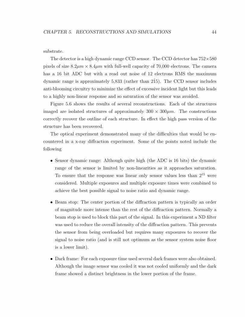
The detector is a high dynamic range CCD sensor. The CCD detector has 752×580
pixels of size 8.2µm× 8.4µm with full-well capacity of 70,000 electrons. The camera
has a 16 bit ADC but with a read out noise of 12 electrons RMS the maximum
dynamic range is approximately 5,833 (rather than 215). The CCD sensor includes
anti-blooming circuitry to minimize the effect of excessive incident light but this leads
to a highly non-linear response and so saturation of the sensor was avoided.
Figure 5.6 shows the results of several reconstructions. Each of the structures
imaged are isolated structures of approximately 300 × 300µm. The constructions
correctly recover the outline of each structure. In effect the high pass version of the
structure has been recovered.
The optical experiment demonstrated many of the difficulties that would be en-
countered in a x-ray diffraction experiment. Some of the points noted include the
following
• Sensor dynamic range: Although quite high (the ADC is 16 bits) the dynamic
range of the sensor is limited by non-linearities as it approaches saturation.
To ensure that the response was linear only sensor values less than 215 were
considered. Multiple exposures and multiple exposure times were combined to
achieve the best possible signal to noise ratio and dynamic range.
• Beam stop: The center portion of the diffraction pattern is typically an order
of magnitude more intense than the rest of the diffraction pattern. Normally a
beam stop is used to block this part of the signal. In this experiment a ND filter
was used to reduce the overall intensity of the diffraction pattern. This prevents
the sensor from being overloaded but requires many exposures to recover the
signal to noise ratio (and is still not optimum as the sensor system noise floor
is a lower limit).
• Dark frame: For each exposure time used several dark frames were also obtained.
Although the image sensor was cooled it was not cooled uniformly and the dark
frame showed a distinct brightness in the lower portion of the frame.

CHAPTER 5. RECONSTRUCTIONS AND SIMULATIONS 45
HeNe laser 1mW
CCD CameraResolution: 752× 580Pixel size: 8.2µm× 8.4µmADC range: 16 bit
f = 300 mm f = 120 mm
f = 20 mm
ND filter: 1,2,4
sample holder
Figure 5.5: Experimental setup. The narrow coherent laser source is expanded toa wider beam before illuminating the sample. A lens focuses the diffraction patternon to the CCD image sensor. Rather than use a beam stop a ND filter was used toattenuate so that the CCD was not overloaded.
(a) reconstruction I (b) reconstruction II (c) reconstruction III
Figure 5.6: Reconstructions of various isolated structures. Notice that the high fre-quency has been reconstructed correctly but that the low frequency information isabsent. In these reconstructions the central part of the diffraction data had satu-rated the detector and was removed. During the reconstruction these missing valueswere allowed to float and thus the low frequency components of the samples were notaccurately recovered.

CHAPTER 5. RECONSTRUCTIONS AND SIMULATIONS 46
Figure 5.7: Reconstructions of several extended objects. Note that in these recon-structions the low frequency information did not saturate the detector and was usedduring the reconstruction.
5.3 Soft X-ray Experiment
Both algorithms presented in Chapter 3 were tested on soft x-ray experimental data.
The experiments were conducted at the Stanford Synchrotron Radiation Laboratory
using 1.38 nm soft x-rays. The fabricated samples were simple, isolated structures
approximately 100um×100um. The experiment setup and reconstructions are shown
in Figure 5.8 and Figure 5.9.
5.4 Hard X-ray Experiment
To explore the use of x-ray diffraction microscopy for buried structures on thick
substrates several experiments were conducted using hard x-rays (0.18 nm or 7 KeV
photons). This work was undertaken at the SPring8 facility in Harima Science Park
City, Hyogo Prefecture, Japan. A photo of the experimental setup is shown in figure
5.10.
The samples that were prepared were fabricated as a single copper layer (100 nm
high, 50 nm wide) on a 700 um silicon substrate. After fabricating the features a
SEM was taken before the structures were buried under 1 um of SiO2. An exemplary
sample and its reconstruction are shown in figure 5.11.
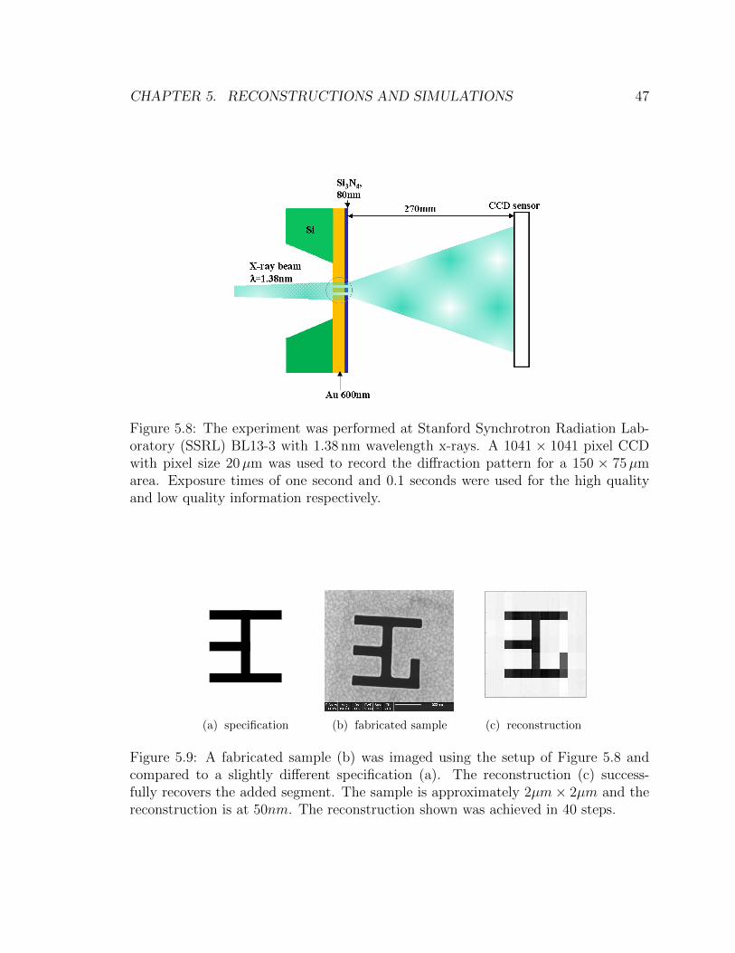
CHAPTER 5. RECONSTRUCTIONS AND SIMULATIONS 47
Figure 5.8: The experiment was performed at Stanford Synchrotron Radiation Lab-oratory (SSRL) BL13-3 with 1.38 nm wavelength x-rays. A 1041 × 1041 pixel CCDwith pixel size 20µm was used to record the diffraction pattern for a 150 × 75µmarea. Exposure times of one second and 0.1 seconds were used for the high qualityand low quality information respectively.
(a) specification (b) fabricated sample (c) reconstruction
Figure 5.9: A fabricated sample (b) was imaged using the setup of Figure 5.8 andcompared to a slightly different specification (a). The reconstruction (c) success-fully recovers the added segment. The sample is approximately 2µm× 2µm and thereconstruction is at 50nm. The reconstruction shown was achieved in 40 steps.
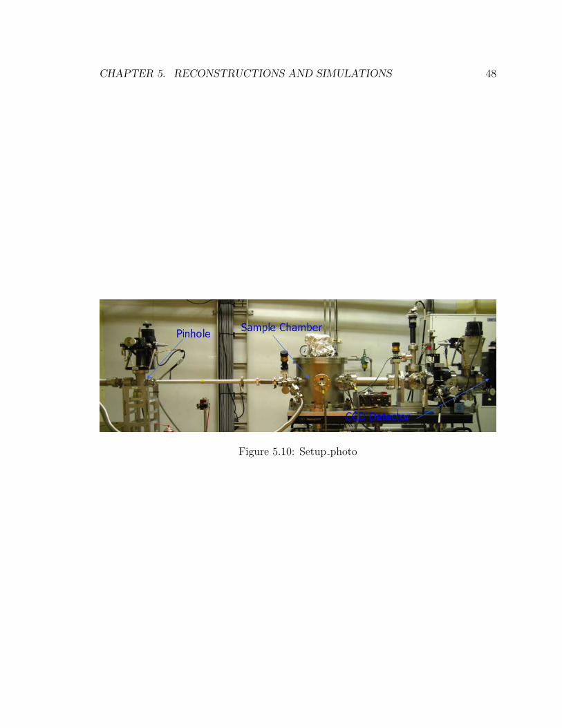
CHAPTER 5. RECONSTRUCTIONS AND SIMULATIONS 48
Figure 5.10: Setup photo

CHAPTER 5. RECONSTRUCTIONS AND SIMULATIONS 49
(a) SEM micrograph
(b) Sample reconstruction
Figure 5.11: Sub-figure (a) shows a SEM micrograph of the sample before the SiO2
was applied. The samples consisted of a single layer of copper wise (100 nm high and50 nm wide) fabricated on a 700 um thick silicon substrate. Sub-figure (b) shows thesuccessful reconstruction of the buried sample.

Chapter 6
Conclusion
Diffractive imaging of non-periodic objects has rapidly advanced over the past decade
and, as the field matures, different lines of research are now just beginning to converge
to a common understanding of the theoretical underpinnings of the phase reconstruc-
tion problem. Yet, there is still much to do, both in theoretical understanding and
in overcoming the challenges presented on the experimental side. The use of diffrac-
tive imaging has been demonstrated in numerous fields and, particularly with new
advances in coherent sources, it promises to expand into new directions.
In this thesis we have examined the recent progress of the algorithmic phase re-
trieval aspect of diffractive imaging. We began with a brief summary of the physical
processes involved in light diffraction microscopy before describing the dominant fam-
ily of methods of phase retrieval: iterative algorithms. We described the origins of
the additional information necessary in existing algorithms with the requirement that
the object has a finite spatial support. This is severely constraining as a key future
application of coherent x-ray diffraction microscopy is inspection of fabricated inte-
grated circuits. Such objects are spatially constrained but are much larger than the
field of view of any source/detector and require modifications to existing algorithms
and/or new algorithms. We have also discussed some of the technical challenges in
experimental diffraction microscopy and provided guidance on experimental setup
and data preparation.
One of the most promising future applications of diffraction microscopy is the
50

CHAPTER 6. CONCLUSION 51
imaging of single macromolecules by an x-ray free electron laser. The very short
pulse of the laser are destructive but many diffractograms of identical molecules can
be obtained and assembled to form a complete dataset suitable for reconstruction
[38, 40]. This assembly is extremely challenging as the individual diffractograms are
both noisy and of random orientation but early results have already shown successful
reconstructions.

Bibliography
[1] D. Sayre. Some implications of a theorem due to Shannon. Acta Cryst., 5:843,
1952.
[2] D. Sayre. The squaring method: a new method for phase determination, 1952.
[3] A. Walther. The question of phase retrieval in optics. Acta Cryst., 10(1):41–49,
1963.
[4] J. Cooley and J. Tukey. An algorithm for the machine calculation of complex
Fourier series. Mathematics of Computation, 19(90):297–301, 1965.
[5] L. Mandel and E. Wolf. Coherence properties of optical fields. Rev. Mod. Phys.,
37(2):237–287, 1965.
[6] R. W. Gerchberg and W. O. Saxton. A practical algorithm for the determination
of phase from image and diffraction plane pictures. Optik, 35:237–246, 1972.
[7] D. Misell. A method for the solution of the phase problem in electron microscopy.
J. Phys. D: Appl. Phys., 6, 1973.
[8] Y. M. Bruck and L. G. Sodin. On the ambiguity of the image reconstruction
problem. Optics Communications, 30(3):304–308, 1979.
[9] J. R. Fienup. Reconstruction of an object from the modulus of its Fourier
transform. Opt. Lett., 3(1):27–29, 1979.
[10] R. D. Millane. Phase retrieval in crystallography and optics. J. Opt. Soc. Am.,
7(3):394–411, 1980.
52

BIBLIOGRAPHY 53
[11] R. Bates. Fourier phase problems are uniquely solvable in more than one dimen-
sion. Optik, 61(3):247–262, 1982.
[12] J. R. Fienup. Phase retrieval algorithms: a comparison. Applied Optics,
21(15):2758–2769, 1982.
[13] J. R. Fienup, T. R. Crimmins, and W. Holsztynski. Reconstruction of the support
of an object from the support of its correlation. J. Opt. Soc. Am., 72:610–624,
1982.
[14] D. C. Youla and H. Webb. Image restoration by the method of convex projections:
Part 1 – theory. IEEE Trans. on Med. Imag., 1(2):81–94, 1982.
[15] J. R. Fienup. Reconstruction of a complex-valued object from the modulus of its
Fourier transform using a support constraint. J. Opt. Soc. Am. A, 4(1):118–123,
1987.
[16] R. G. Lane. Recovery of complex images from Fourier magnitude. Optics Com-
munications, 63(1):6–10, 1987.
[17] T. Crimmins, J. R. Fienup, and B. Thelen. Improved bounds on object support
from autocorrelation support and application to phase retrieval. J. Opt. Soc.
Am., 7(1):3–13, 1990.
[18] M. Ibrahim Sezan. An overview of convex projection theory and its application
to image recovery problems. Ultramicroscopy, 40(1):55–67, 1992.
[19] M. Maleki and A. Devaney. Noniterative reconstruction of complex-valued ob-
jects from two intensity measurements. Optical Engineering, 33:3243, 1994.
[20] P. Nellist, B. C. McCallum, and J. M. Rodenburg. Resolution beyond the ‘infor-
mation limit’ in transmission electron microscopy. Nature, 374:630–632, 1995.
[21] H. H. Bauschke and J. M. Borwein. On projection algorithms for solving convex
feasibility problems. SIAM Review, 38(3):367–426, 1996.

BIBLIOGRAPHY 54
[22] J. Miao, D. Sayre, and H. N. Chapman. Phase retrieval from the magnitude of
the Fourier transform of non-periodic objects. J. Opt. Soc. Am. A, 15:1662–1669,
1998.
[23] J. Miao, P. Charalambous, J. Kirz, and D. Sayre. Extending the methodology
of x-ray crystallography to allow imaging of micrometer-sized non-crystalline
specimens. Nature, 400:342–344, 1999.
[24] J. Miao and D. Sayre. On possible extensions of x-ray crystallography through
diffraction-pattern oversampling. Acta Cryst., 56:596–506, 2000.
[25] H. H. Bauschke, P. L. Combettes, and D. Luke. Phase retrieval, error reduction
algorithm and Fienup variants: a view from convex optimization. J. Opt. Soc.
Am., 19(7):1334–1335, 2002.
[26] J. Miao, T. Ishikawa, B. Johnson, E. H. Anderson, B. Lai, and K. O. Hodgson.
High resolution 3D X-ray diffraction microscopy. Phys. Rev. Lett., 89:1–4, 2002.
[27] J. C. H. Spence, U. Weierstall, and M. R. Howells. Phase recovery and lensless
imaging by iterative methods in optical, x-ray and electron diffraction. Phil.
Trans. R. Soc. London, 360:875–895, 2002.
[28] H. H. Bauschke, P. L. Combettes, and D. Luke. Hybrid projection-reflection
method for phase retrieval. J. Opt. Soc. Am., pages 1025–1034, 2003.
[29] V. Elser. Phase retrieval by iterated projections. J. Opt. Soc. Am., 20:40–55,
2003.
[30] V. Elser. Random projections and the optimization of an algorithm for phase
retrieval. J. Phys., 36(12):2995–3007, 2003.
[31] V. Elser. Solution of the crystallographic phase problem by iterated projections.
Acta Cryst., 59(3):201–209, 2003.
[32] S. Marchesini, H. He, H. N. Chapman, S. P. Hau-Riege, A. Noy, M. R. Howells,
U. Weierstall, and J. C. H. Spence. X-ray image reconstruction from a diffraction
pattern alone. Phys. Rev. B, 68(14):140101, Oct 2003.

BIBLIOGRAPHY 55
[33] S. Marchesini, H. He, H. N. Chapman, S. P. Hau-Riege, A. Noy, M. R. Howells,
U. Weierstall, and J. C. H. Spence. X-ray image reconstruction from a diffraction
pattern alone. Phys. Rev., 68, 2003.
[34] K. A. Nugent, A. G. Peele, H. N. Chapman, and A. P. Manuso. Unique phase
recovery for non-periodic objects. Phys. Rev. Lett., 91:1–4, 2003.
[35] S. Marchesini. Benchmarking iterative projection algorithms for phase retrieval.
2004.
[36] W. McBride, N. L. O’Leary, K. A. Nugent, and L. J. Allen. Retrieval of a
complex-value object from its diffraction pattern. Phys. Rev. Lett., 93(23), 2004.
[37] K. Robinson and J. Miao. Three dimensional x-ray diffraction microscopy. MRS
Bulletin, 29:177–181, 2004.
[38] Q. Shen, I. Bazarov, and P. Thibault. Diffractive imaging of non-periodic mate-
rials with future coherent x-ray sources. J. Synch. Rad., 11(5):432–438, 2004.
[39] W. Chao, B. Harteneck, J. Liddle, E. Anderson, and D. Attwood. Soft x-ray
microscopy at a spatial resolution of better than 15 nm. Nature, 435(7046):1210–
1213, 2005.
[40] D. Shapiro, P. Thibault, T. Beetz, V. Elser, M. R. Howells, C. Jacobsen, J. Kirz,
E. Lima, H. Miao, A. M. Nieman, and D. Sayre. Biological imaging by soft x-ray
diffraction microscopy. Proc. Natl Acad. Sci., 102(43):15343–15346, 2005.
[41] P. Kassakian. Convex Approximation and Optimization with Applications in
Magnitude Filter Design and Radiation Pattern Synthesis. PhD thesis, University
of California, Berkeley, 2006.
[42] P. Thibault, V. Elser, C. Jacobsen, D. Sayre, and D. Shapiro. Reconstruction of
a yeast cell from x-ray diffraction data. Acta Cryst., 62(4):248–261, 2006.
[43] V. Elser, I. Rankenburg, and P. Thibault. Searching with iterated maps. In
Proceedings of the National Academy of Sciences, pages 418–423, 2007.

BIBLIOGRAPHY 56
[44] J. M. Rodenburg, A. C. Hurst, and A. G. Cullis. Transmission microscopy
without lenses for objects of unlimited size. Ultramicroscopy, 107:227–231, 2007.
[45] J. M. Rodenburg, A. C. Hurst, B. R. Dobson, F. Pfeifer, O. Bunk, C. David,
K. Jefimovs, and I. Johnson. Hard x-ray lensless imaging of extended objects.
Phys. Rev. Lett., 98:1–4, 2007.
[46] P. Thibault and I. Rankenburg. Optical diffraction microscopy in a teaching lab.
Am. J. of Phys., 2007.
[47] G. J. Williams, M. A. Pfeifer, I. A. Vartanyants, and I. K. Robinson. Effectiveness
of iterative algorithms in recovering phase in the presence of noise. Acta Cryst.,
63:36–42, 2007.
[48] M. Grant and S. Boyd. CVX: Matlab software for disciplined convex program-
ming. http://stanford.edu/~boyd/cvx, August 2008.
[49] M. Grant and S. Boyd. Graph implementations for nonsmooth convex programs.
Recent Advances in Learning and Control (a tribute to M. Vidyasagar), pages
95–110, 2008.
[50] M. Born and E. Wolf. Principles of Optics: Electromagnetic Theory of Prop-
agation, Interference and Diffraction of Light. Cambridge University Press, 7
edition, 1999.
[51] S. Mallat. A Wavelet Tour of Signal Processing, The Sparse Way. Academic
Press, 2008.