algorithmic mathematics - qmul mathsleonard/ambook.pdf · algorithmic mathematics ... we shall...
TRANSCRIPT

Algorithmic Mathematics
a web-book by Leonard Soicher & Franco Vivaldi
This is the textbook for the course MAS202 Algorithmic Mathematics. This material isin a fluid state —it is rapidly evolving— and as such more suitable for on-line use thanprinting. If you find errors, please send an e-mail to: [email protected].
Last updated: January 8, 2004c© The University of London.

ii

Preface
This text contains sufficient material for a one-semester course in mathematical algo-rithms, for second year mathematics students. The course requires some exposure to thebasic concepts of discrete mathematics, but no computing experience.
The aim of this course is twofold. Firstly, to introduce the basic algorithms for com-puting exactly with integers, polynomials and vector spaces. In doing so, the student isexpected to learn how to think algorithmically and how to design and analyze algorithms.
Secondly, to provide a constructive approach to abstract mathematics, algebra inparticular. When introducing the elements of ring and field theory, algorithms offerconcrete tools, constructive proofs, and a crisp environment where the benefits of rigourand abstraction become tangible.
We shall write algorithms in a straightforward language, which incorporates freelystandard mathematical notation. The specialized constructs are limited to the if-structureand the while-loop, which are universal.
Exercises are provided. They have a degree of difficulty comparable to that of ex-amination questions. Some of the exercises consist of short essays; in this context, thenotation [6 ε ] indicates that mathematical symbols are not permitted in the essay. Starredsections contain optional material, which is not examinable.
The Algorithmic Mathematics’s web page is:
algorithmicmathematics.com
iii

iv

Contents
1 Basics 1
1.1 The language of algorithms . . . . . . . . . . . . . . . . . . . . . . . . . . 2
1.1.1 Expressions . . . . . . . . . . . . . . . . . . . . . . . . . . . . . . . 2
1.1.2 Assignment statement . . . . . . . . . . . . . . . . . . . . . . . . . 3
1.1.3 Return statement . . . . . . . . . . . . . . . . . . . . . . . . . . . . 4
1.1.4 If-structure . . . . . . . . . . . . . . . . . . . . . . . . . . . . . . . 5
1.1.5 While-loops . . . . . . . . . . . . . . . . . . . . . . . . . . . . . . . 7
1.2 Boolean calculus . . . . . . . . . . . . . . . . . . . . . . . . . . . . . . . . 9
1.3 Characteristic functions . . . . . . . . . . . . . . . . . . . . . . . . . . . . 11
2 Arithmetic 15
2.1 Divisibility of integers . . . . . . . . . . . . . . . . . . . . . . . . . . . . . 15
2.2 Prime numbers . . . . . . . . . . . . . . . . . . . . . . . . . . . . . . . . . 16
2.3 Factorization of integers . . . . . . . . . . . . . . . . . . . . . . . . . . . . 18
2.4 Digits . . . . . . . . . . . . . . . . . . . . . . . . . . . . . . . . . . . . . . 20
2.5 Nested algorithms . . . . . . . . . . . . . . . . . . . . . . . . . . . . . . . . 22
2.5.1 Counting subsets of the integers . . . . . . . . . . . . . . . . . . . . 23
2.6 The halting problem∗ . . . . . . . . . . . . . . . . . . . . . . . . . . . . . . 24
3 Relations and partitions 31
3.1 Relations . . . . . . . . . . . . . . . . . . . . . . . . . . . . . . . . . . . . . 31
3.2 Partitions . . . . . . . . . . . . . . . . . . . . . . . . . . . . . . . . . . . . 33
4 Modular arithmetic 39
4.1 Addition and multiplication in Z/(m) . . . . . . . . . . . . . . . . . . . . . 40
4.2 Invertible elements in Z/(m) . . . . . . . . . . . . . . . . . . . . . . . . . . 42
4.3 Commutative rings with identity . . . . . . . . . . . . . . . . . . . . . . . 43
v

vi CONTENTS
5 Polynomials 47
5.1 Loop invariants . . . . . . . . . . . . . . . . . . . . . . . . . . . . . . . . . 49
5.2 Recursive algorithms . . . . . . . . . . . . . . . . . . . . . . . . . . . . . . 52
5.3 Greatest common divisors . . . . . . . . . . . . . . . . . . . . . . . . . . . 53
5.4 Modular inverse . . . . . . . . . . . . . . . . . . . . . . . . . . . . . . . . . 58
5.5 Polynomial evaluation . . . . . . . . . . . . . . . . . . . . . . . . . . . . . 60
5.6 Polynomial interpolation∗ . . . . . . . . . . . . . . . . . . . . . . . . . . . 62
6 Algorithms for vectors 69
6.1 Echelon form . . . . . . . . . . . . . . . . . . . . . . . . . . . . . . . . . . 70
6.2 Constructing an echelon basis . . . . . . . . . . . . . . . . . . . . . . . . . 74
6.3 An example . . . . . . . . . . . . . . . . . . . . . . . . . . . . . . . . . . . 77
6.4 Testing subspaces . . . . . . . . . . . . . . . . . . . . . . . . . . . . . . . . 79
7 Some Proofs∗ 83
7.1 A note on ring theory . . . . . . . . . . . . . . . . . . . . . . . . . . . . . . 83
7.2 Uniqueness of quotient and remainder . . . . . . . . . . . . . . . . . . . . . 83
8 Hints for exercises 85

Chapter 1
Basics
Informally, an algorithm is a finite sequence of unambiguous instructions to perform aspecific task. In this course, algorithms are introduced to solve problems in discretemathematics.
An algorithm has a name, begins with a precisely specified input, and terminates with aprecisely specified output. Input and output are finite sequences of mathematical objects.An algorithm is said to be correct if given input as described in the input specifications:(i) the algorithm terminates in a finite time; (ii) on termination the algorithm returnsoutput as described in the output specifications.
Example 1.1.
Algorithm SumOfSquares
INPUT: a, b,∈ ZOUTPUT: c, where c = a2 + b2.
c := a2 + b2;
return c;
end;
The name of this algorithm is SumOfSquares. Its input and output are integer sequencesof length 2 and 1, respectively.
In this course all algorithms are functions, whereby the output follows from the in-put through a finite sequence of deterministic steps; that is, the outcome of each stepdepends only on the outcome of the previous steps. In the example above, the domain ofSumOfSquares is the the set of integer pairs, the co-domain is the set of non-negative inte-gers, and the value of SumOfSquares(−2,−3) is 13. This function is clearly non-injective;its value at (a, b) is the same as that at (−a,−b), or (b, a), etc. It also happens to benon-surjective (see exercises).
(Algorithms do not necessarily represent functions. The instruction: ‘Toss a coin; ifthe outcome is head, add 1 to x, otherwise, do nothing’ is legitimate and unambiguous,but not deterministic. The output of an algorithm containing such instruction is not afunction of the input alone. Algorithms of this kind are called probabilistic.)
1

2 CHAPTER 1. BASICS
It is expedient to regard the flow from input to output as being parametrized by time.This viewpoint guides the intuition, and even when estimating run time is not a concern,time considerations always lurk in the background (will the algorithm terminate? If so,how many operations will it perform?).
1.1 The language of algorithms
The general form of an algorithm is the following
Algorithm 〈 algorithm name 〉INPUT: 〈 input specification 〉OUTPUT: 〈 output specification 〉〈 statement 〉;〈 statement 〉;
...
〈 statement 〉;end;
(A quantity in angle brackets defines the type of an object, rather than the object itself.)
The heart of the algorithm is its statement sequence, which is implemented by alanguage. The basic elements of any algorithmic language are surprisingly few, and use avery standard syntax. We introduce them in the next sections.
1.1.1 Expressions
In this course, expressions are the data processed by an algorithm. We do not require aprecise definition of what we regard to be a valid expression, since we shall consider onlyexpressions of very basic type.
We begin with arithmetical and algebraic expressions, which are formed by assem-bling in familiar ways numbers and arithmetical operators. Algebraic expressions differfrom arithmetical ones in that they contain indeterminates or variables. All expressionsconsidered here will be finite, e.g.,
1 +1
2 +1
3 +1
4 +1
5
(x− y)(x+ y)(x2 + y2)(x4 + y4)
x8 − y8
By combining expressions, we can construct composite expressions representing sequences,sets, etc.
(x− 1, x+ 1, x2 + x+ 1, x2 + 1)
{0, 1,
1
2,
1
3,
2
3,
1
4,
3
4
}.
1.1. THE LANGUAGE OF ALGORITHMS 3
We are not concerned with the practicalities of evaluating expressions, and assumethat a suitable computational engine is available for this purpose. In this respect, anexpression such as
‘ the smallest prime number greater than 1000 1000 ’
is perfectly legitimate, since its value is unambiguously defined (because there are infinitelymany primes). We also ignore the important and delicate problem of agreeing on how thevalue of an expression is to be represented. For instance, the value of the expression ‘thelargest real solution of x4 + 1 = 10x2’ can be represented in several ways, e.g.,
√2 +√
3 =
√5 + 2
√6 = 3.1462643699419723423 . . .
and there is no a priori reason for choosing any particular one.
1.1.2 Assignment statement
The assignment statement allows the management of data within an algorithm.
SYNTAX: 〈 variable 〉:=〈 expression 〉;EXECUTION: evaluate the expression and assign its value to the variable.
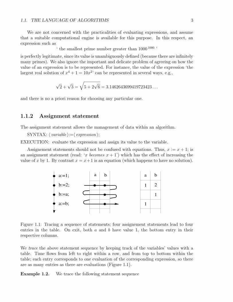
Assignement statements should not be confused with equations. Thus, x := x + 1; isan assignment statement (read: ‘x becomes x+ 1’) which has the effect of increasing thevalue of x by 1. By contrast x = x+1 is an equation (which happens to have no solution).
ba a b
21
1
1
a:=1;
b:=2;
b:=a;
a:=b;
Figure 1.1: Tracing a sequence of statements; four assignement statements lead to fourentries in the table. On exit, both a and b have value 1, the bottom entry in theirrespective columns.
We trace the above statement sequence by keeping track of the variables’ values with atable. Time flows from left to right within a row, and from top to bottom within thetable; each entry corresponds to one evaluation of the corresponding expression, so thereare as many entries as there are evaluations (Figure 1.1).
Example 1.2. We trace the following statement sequence

4 CHAPTER 1. BASICS
i := 3;
i := (i4 + 10)/13;
n := 4− i;S := (i, |n|);n := 3n+ i;
i := i+ n;
S := (|i|, S);
i n S37 −3 (7, 3)−2
5 (5, (7, 3))
Persuade yourself that re-arranging the columns may change the number of rows.
Before a variable can be used in an expression it must have a value, which is eitherassigned on input or by an assignment statement. Assigning a value on input works asfollows. Suppose we have
Algorithm A
INPUT: 〈 a1, . . . , ak, and their properties 〉OUTPUT: 〈 output specification 〉〈 statement sequence 〉
end;
Then a1, . . . , ak are variables for algorithm A. When A is executed, it must be given an inputsequence v1, . . . , vk of values. Then a1 is assigned the value v1, a2 is assigned the valuev2, etc., . . ., ak is assigned the value vk, before the statement sequence of A is executed(bearing in mind that the values assigned may be indeterminates). Thus, assigning valueson input is analogous to evaluating A, as a function, at those values; this process could bereplaced by a sequence of assignment statements at the beginning of the algorithm. Thiswould be, of course, very inefficient, being equivalent to defining the function at a singlepoint.
1.1.3 Return statement
The return statement produces an output sequence.
SYNTAX: return 〈 expression 1 〉, . . . ,〈 expression k 〉EXECUTION: first expression 1, . . ., expression k are evaluated, obtaining values v1, . . .,vk, respectively. Then the sequence (v1, . . . , vk) is returned as the output of the algorithm,and the algorithm is terminated.
We treat an output sequence (v1) of length 1 as a simple value v1.

1.1. THE LANGUAGE OF ALGORITHMS 5
Example 1.3. The expressions
i := 5;
return 32, i+ 5, 27;
returns the sequence (9, 10, 27) as output.
1.1.4 If-structure
A boolean constant or a boolean value, is an element of the set {TRUE, FALSE} (oftenabbreviated to {T, F}). A boolean (or logical) expression is an expression that evaluatesto a boolean value. We postpone a detailed description of boolean expressions untilsection 1.2. For the moment we consider expressions whose evaluation involves testing asingle (in)equality, called relational expressions. For instance, the boolean value of
103 < 210, 93 + 103 6= 13 + 123
is TRUE and FALSE, respectively. Evaluating more complex expressions such as
2 13,466,917 − 1 is prime, 2(2 13,466,917 − 1) − 1 is prime (1.1)
can be reduced to evaluating finitely many relational expressions, although this mayinvolve formidable difficulties. Thus several weeks of computer time were required toprove that the leftmost expression above is TRUE, giving the largest prime known todate. This followed nearly two and half years of computations on tens of thousandsof computers, to test well over 100,000 unsuccessful candidates for the exponent. Bycontrast, the value of the rightmost boolean expression is not known, and may never beknown.
The if-structure makes use of a boolean value to implement decision-making in analgorithmic language. It is defined as follows:
SYNTAX:
if 〈 boolean expression 〉 then〈 statement-sequence 1 〉
else
〈 statement-sequence 2 〉fi;
EXECUTION: if the value of the boolean expression is TRUE, the statement-sequence 1is executed, and not statement-sequence 2. If the boolean expression evaluates to FALSE,then statement-sequence 2 is executed, and not statement-sequence 1.
The boolean expression that controls the if-structure is called the if control expression.
Example 1.4.

6 CHAPTER 1. BASICS
if i > 0 then
t := t− i;else
t := t+ i;
fi;
We remark that an if-structure is logically equivalent to a single statement. A variantof the above construct is given by
SYNTAX:
if 〈 boolean expression 〉 then〈 statement-sequence 〉
fi;
The execution is the same as the execution of
if 〈 boolean expression 〉 then〈 statement-sequence 〉
else
fi;
which is obtained from the general form by having an empty statement sequence, whichdoes nothing.
Example 1.5.
if θ > 0 then
θ := 5 θ (1− θ);fi;
If the above if-statement starts execution with θ ≤ 0, then the statement has no effect.
Example 1.6.
Algorithm MinimumInt
INPUT: a, b,∈ ZOUTPUT: c, where c is the minimum of a and b.
if a < b then
return a;
else
return b;
fi;
end;
The input and output are integer sequences of length 2 and 1, respectively. When regardedas a function, the domain of MinimumInt is the the set Z2 of integer pairs, the co-domain

1.1. THE LANGUAGE OF ALGORITHMS 7
is Z, and the value of MinimumInt(−2, 12) is −2.
1.1.5 While-loops
A loop is the structure that implements repetition. Loops come in various guises, themost basic of which is the while-loop.
SYNTAX:
while 〈 boolean-expression 〉 do〈 statement sequence 〉
od;
EXECUTION:
(i) Evaluate the boolean expression.
(ii) If the boolean expression evaluates to TRUE, then execute the statement sequence,and repeat from step (i). If the boolean expression is FALSE, do not execute thestatement sequence but terminate the while-loop and continue the execution of thealgorithm after the “od”.
The boolean expression that controls the loop is called the loop control expresssion.
Example 1.7. The loop
while 0 6= 1 do
od;
will run forever and do nothing. The loop
while 0 = 1 do
· · ·od;
will not run at all.
Example 1.8. We trace the following statements
i := 2;
k := i;
while i3 > 2i do
i := i+ 3;
k := k − i;od;
Besides the variables i and k, we also trace the value of the boolean expression that

8 CHAPTER 1. BASICS
controls the loopi k i3 > 2i
2 2 TRUE
5 −3 TRUE
8 −11 TRUE
11 −22 FALSE
This example illustrates a general property of loops: on exit, the value of the loop controlexpression is necessarily FALSE, lest the loop would not be exited. By contrast, the boolenexpression controlling an if-statement, can have any value on exit (Figure 1.2).
β is FALSE
β is TRUE β is FALSE
β is TRUE
β
β
Figure 1.2: The basic structures of algorithms: loops and if-statements. The evaluation ofthe boolean expression β gives rise to a bifurcation point in the execution of the algorithm.
It may be difficult, even impossible, to decide how many times a given while-loopwill be executed (or indeed, whether the loop will terminate at all, see section 2.6 for anexample).
As an example, consider the following algorithm
Algorithm NextPrime
INPUT: n, a positive integer.
OUTPUT: p, where p is the least prime greater than n.
p := n+ 1;
while p is not prime do
p := p+ 1;
od;
return p;
end;
Since the number of primes is infinite, we know the loop will terminate, but we do not knowhow many times it will be executed. Indeed, it is possible to show (see exercises) thatarbitrarily large gaps between consecutive primes exist, hence arbitrarily large number ofrepetitions of the above loop.
A structure is nested if it appears inside another structure. Nesting is a means of

1.2. BOOLEAN CALCULUS 9
constructing complex algorithms from simple ingredients, so tracing a nested structurecan be laborious.
Example 1.9.
while 〈 boolean-expression 〉 dowhile 〈 boolean-expression 〉 do
〈 expression 〉;od;
〈 expression 〉;if 〈 boolean-expression 〉 then〈 expression 〉;
else
〈 expression 〉;fi;
od;
In this example, the body of the outer loop consists of three expressions, two of which arestructures (Figure 1.3).
Figure 1.3: Nested structures: a loop containing a loop and an if-statement.
1.2 Boolean calculus
Boolean expressions may be constructed from boolean constants and relational expres-sions by means of boolean operators. This process is analogous to the construction ofarithmetical expressions from arithmetical constants (i.e., numbers) and operators (+, −,etc.).
The basic boolean operators are NOT , and AND . The operator NOT is unary, thatis, it takes just one boolean operand and produces a boolean result. The operator AND
is binary, which means that it acts on two operands and produces a boolean result.

10 CHAPTER 1. BASICS
The following table, called a truth table, defines the value of NOT and AND on allpossible choices of boolean operands
NOTP PF TT F
P P ANDQ QT T TT F FF F TF F F
Other binary operators may be constructed from the above two. The most commonlyused are OR , =⇒, and ⇐⇒ . We define them directly with truth tables, although theycan also be defined in terms of NOT and AND (see remarks following proposition 1,below).
P P ORQ QT T TT T FF T TF F F
P P =⇒ Q QT T TT F FF T TF T F
P P ⇐⇒ Q QT T TT F FF F TF T F
(1.2)
We note that if A = TRUE and B = FALSE, then
(A =⇒ B) 6= (B =⇒ A)
that is, the operator =⇒ is non-commutative.
Example 1.10.
P := 2 < 3;
Q := 2 ≥ 3;
R := (P ORQ) =⇒ (P ANDQ);
S := (P ANDQ) =⇒ (P ORQ);
P Q P ORQ P ANDQ R ST F T F F T
Proposition 1 For all P,Q,∈ {TRUE,FALSE}, the following holds
(i) NOT (P ORQ) = ( NOTP ) AND ( NOTQ)
(ii) NOT (P ANDQ) = ( NOTP ) OR ( NOTQ)
(iii) P =⇒ Q = ( NOTP ) ORQ

1.3. CHARACTERISTIC FUNCTIONS 11
(iv) P ⇐⇒ Q = ((P =⇒ Q) AND (Q =⇒ P )).
Proof: The proof consists of evaluating each side of these equalities for all possible P,Q.We prove (iv). The other proofs are left as an exercise. The left-hand side of (iv) wasgiven in (1.2). Let R be the right-hand side. We compute R explicitly.
P P =⇒ Q R Q =⇒ P QT T T T TT F F T FF T F F TF T T T F
Hence the left hand side is equal to the right hand side for all P,Q ∈ {TRUE,FALSE}.
The statements (i) and (ii) are known as De Morgan’s laws. Using Proposition 1, onecan express the operators OR , =⇒, ⇐⇒ in terms of NOT and AND (see exercises).
1.3 Characteristic functions
Characteristic functions link boolean quantities to sets.
Def: A characteristic function is a function assuming boolean values.
Let X be a set and A ⊆ X. The function
CA : X → {TRUE,FALSE} x 7→{
TRUE if x ∈ AFALSE if x 6∈ A
is called the characteristic function of A (in X). Conversely, let f : X → {TRUE,FALSE}be a characteristic function. Then f = CA, where A = f−1(TRUE). So there is a bi-uniquecorrespondence between the characteristic functions defined on X, and the subsets of X.
Theorem 2 Let X be a set, and let A,B ⊆ X. The following holds
(i) NOT CA = CX\A(ii) CA AND CB = CA∩B(iii) CA OR CB = CA∪B(iv) CA =⇒ CB = CX\(A\B)
(v) CA ⇐⇒ CB = C(A∩B)∪ (X\(A∪B))
Proof: To prove (i) we note that the function x 7→ NOT CA(x) evaluates to TRUE ifx 6∈ A and to FALSE otherwise. However, x 6∈ A ⇐⇒ x ∈ (X \ A), from the definitionof difference between sets.
Next we prove (iv). Let P := x ∈ A and Q := x ∈ B. Then, from (1.2), we have thatP =⇒ Q is TRUE precisely when (P,Q) 6= (TRUE,FALSE). This means that x is suchthat the expression
NOT (x ∈ AAND ( NOTx ∈ B)) = NOT (x ∈ A \B) = x ∈ (X \ (A \B))

12 CHAPTER 1. BASICS
is TRUE, from part (i). But the rigthmost expression is the definition of the characteristicfunction of the set X \ (A \B).
The proof of (ii), (iii), (v) is left as an exercise.
Example 1.11. The functions x 7→ (x ≥ a) and x 7→ (x ≤ b) are the characteristicfunctions of two rays. If a ≤ b, then x 7→ ((x ≥ a) AND (x ≤ b)) is the characteristicfunction of the closed interval [a, b].
Exercises
Exercise 1.1. Use a table to trace the values of a, b, b > 0, a > b, as the statementsequence below is executed.
a := 15;
b := 10;
while b > 0 do
while a > b do
a := a− 2;
od;
b := b− 3;
od;
(The table should have 4 columns and 12 rows.)
Exercise 1.2. Use a table to trace the execution of the following statement sequence:
x := 3;
y := 0;
while |x| ≥ |y| doif x is even then
x := x/2− y;
else
x := (x+ 1)/2− y;
y := y − x;
fi;
od;
Exercise 1.3. Prove that the function SumOfSquares: Z2 → N of Example 1.1 is notsurjective.
Exercise 1.4. Evaluate each of the following boolean expressions
(a) ((26 > 70) OR (28 > 250)) AND (210 > 1000)
(b)21
34<
34
55=⇒ 34
55<
55
89

1.3. CHARACTERISTIC FUNCTIONS 13
(c)√
2 >7
5AND
√2 <
17
12
(d)1
(√
3− 2)2< 14
(e) ((‘93 is prime’ =⇒ ‘97 is prime’) OR ‘87 is prime’) ⇐⇒ ‘91 is prime’
(f) ‘47 is the sum of two squares’.
Use only integer arithmetic. In part (f) aim for precision and conciseness.
Exercise 1.5. Show that
(P =⇒ Q) = (( NOTQ) =⇒ ( NOTP ))
for all P,Q ∈ {TRUE,FALSE}.Exercise 1.6. Describe in one sentence. Get the essence, not the details. [6 ε ]
X OR Y = NOT (( NOTX) AND ( NOTY )) ∀X,Y ∈ {TRUE,FALSE}.
Exercise 1.7. Complete the proof of Proposition 1, hence express OR , =⇒, and ⇐⇒in terms of NOT and AND .
Exercise 1.8. Complete the proof of Theorem 2.
Exercise 1.9.
(a) Write an algorithm to the following specifications:
Algorithm Min3Int
INPUT: a, b, c ∈ Z.
OUTPUT: m, where m is the minimum of a, b, c.
(b) Explain in one sentence [6 ε ] what goes wrong in your algorithm if the inputspecification is changed to INPUT: a, b, c ∈ C, while leaving everything else unchanged.
Exercise 1.10. Explain concisely what this algorithm does, and how. [ 6 ε ]
INPUT: x, e ∈ Z, x 6= 0, e ≥ 0.
OUTPUT: ??
a := 1;
while e > 0 do
a := a · x;
e := e− 1;
od;
return a;
end;

14 CHAPTER 1. BASICS
Exercise 1.11. Consider the following algorithm
Algorithm A
INPUT: n, S, where n is a positive integer and S = (S1, . . . , Sn)
is a sequence of n integers.
OUTPUT: ??
Z := 0;
i := 1;
while i ≤ n do
j := i;
while j ≤ n do
Z := Z + Si;
j := j + 1;
od;
i := i+ 1;
od;
return Z;
end;
(a) Write the output specifications.
(b) Rewrite the algorithm in such a way that it has only one loop.
Exercise 1.12. Write an algorithm to the following specifications
Algorithm IsSumOfSquares
INPUT: x ∈ ZOUTPUT: TRUE, if x is the sum of two squares, FALSE otherwise.
The algorithm should use integer arithmetic only.
Chapter 2
Arithmetic
2.1 Divisibility of integers
Let a, b,∈ Z. We say that b divides a (and write b|a) if a = bc for some c ∈ Z. Thestatements that a is a multiple of b and b is a divisor of a have the same meaning.
Example 2.12. The expression b|a is boolean, while the expressions b/a is arithmeti-cal.
3|6 = TRUE, 3/6 = 1/2, 6|3 = FALSE, 0|5 = FALSE.
The expression 5/0 is undefined.
Let a ∈ Z. Then
• 1|a since a = 1 · a• a|a since a = a · 1• a| − a since −a = a · −1
• a|0 since 0 = a · 0.
Note that if 0|a then a = 0 · c for some c ∈ Z, in which case a = 0.
Theorem 3 Let b ∈ Z, with b 6= 0. Then there exist unique integers q, r such that
a = bq + r 0 ≤ r < |b|.
The proof will be found in chapter 7.
We denote such q and r by aDIV b and aMOD b, respectively. If a ≥ 0 and b > 0,we can calculate aDIV b and aMOD b by long division. When a ≥ 0 and b > 0, then qis the quotient of division of a by b, that is, the integer part of a/b (the largest integernot exceeding a/b). The non-negative integer r is the remainder of such integer division,that is, r/b is the fractional part of a/b. By the same token, b · q is the largest multipleof b not exceeding a, etc. When a or b are negative, the value of q and r is a bit lessstraightforward.
15

16 CHAPTER 2. ARITHMETIC
Example 2.13. Check these calculations carefully
293 DIV 8 = 36 293 MOD 8 = 5−293 DIV 8 = −37 −293 MOD 8 = 3
293 DIV−8 = −36 293 MOD−8 = 5−293 DIV−8 = 37 −293 MOD−8 = 3
Let a, b ∈ Z, with b 6= 0. If aMOD b = 0, then a = bq + 0, for some q ∈ Z, =⇒ b|a.Conversely, if b|a, then a = bq for some q ∈ Z, =⇒ a = bq + 0 =⇒ aMOD b = 0.
Thus, b|a ⇐⇒ aMOD b = 0.
Def: Let n ∈ Z. We say that n is even if 2|n; otherwise n is odd.
Thus, n is even iff nMOD 2 = 0, and odd iff nMOD 2 = 1.
Example 2.14. We construct the characteristic function of the integers divisible by agiven integer m. The case m = 0 has to be treated separately.
Algorithm Multiple
INPUT: (x,m) ∈ Z2.
OUTPUT: TRUE if x is a multiple of m, FALSE otherwise.
if m = 0 then
return x = 0
else
return xMODm = 0
fi;
end;
2.2 Prime numbers
Def: An integer n is said to be prime if (i) |n| ≥ 2 and (ii) the only divisors of n are1,−1, n,−n.
Example 2.15. The integers −1, 9, 0 are not prime. The integers 2,−2,−17 areprime.
We have that n is prime iff −n is prime (see exercise). Since |n| = n or |n| = −n, weconclude that n is prime iff |n| is prime. We now consider the problem of testing whethera given non-negative integer is prime.
Lemma 4 Let b, n ∈ Z. Then b|n if and only if −b|n.
Proof: (=⇒): b|n =⇒ ∃ c ∈ Z s.t. n = bc. Thus, n = (−b)(−c) =⇒ −b|n.
2.2. PRIME NUMBERS 17
(⇐=): −b|n =⇒ −(−b)|n (from (=⇒)) =⇒ b|n.
Now let n ∈ Z, n ≥ 0. Then n is prime iff n ≥ 2 and the only positive divisors of nare 1 and n. Furthermore, if n > 0 and b ∈ Z, b > n, then b 6 |n. Thus, if n ≥ 2, then n isprime iff i 6 |n for i = 2, . . . n− 1. This gives us a crude way of testing if n is prime.
Lemma 5 Let i, a be positive integers, and suppose i|a, 1 < i < a, and i2 > a. Then∃ j ∈ Z such that j|a and 1 < j2 < a.
Proof: Since i|a, there is a j ∈ Z such that a = ij. We see that j|a. Next, 1 < i <a =⇒ j = a/i > 1. Now a2 = (ij)2 = i2j2 and i2 > a =⇒ j2 = a2/i2 < a2/a = a.
Proposition 6 Let a ∈ Z, a ≥ 2. Then a is prime if and only if no integer i such that1 < i2 ≤ a divides a.
Proof: (=⇒): Suppose a is prime. Then the only positive divisors of a are 1 and a.As a ≥ 2, we have a2 > a, so there is no integer i such that i|a and 1 < i2 ≤ a.
(⇐=): Suppose i 6 |a for each i with 1 < i2 ≤ a. Then by the previous lemma, there isno i dividing a with 1 < i < a and i2 > a. We conclude that i 6 |a for all i with 1 < i < a,and since a ≥ 2, a must be prime.
Let a ∈ Z, a ≥ 0. If a is even, then a is prime iff a = 2 (0 is not prime, 2 is prime, ifa is even and a > 2, then 2|a and 1 < 2 < a). If a is odd, then no even integer 2k dividesa, because otherwise a = 2kl for some l ∈ Z, and a would be even.
We have now justified the algorithm IsPrime, which tests primality. More precisely,IsPrime is the characteristic function of the set of primes in Z.
Algorithm IsPrime
INPUT: n ∈ Z.
OUTPUT: TRUE if n is prime, FALSE if n is not prime.
a := |n|; (* n is prime iff a is prime. We shall test if a is prime *)
if a < 2 then (* a is not prime *)
return FALSE;
fi;
if 2|a then
return (a = 2); (* a is prime iff a = 2 *)
fi;
(* at this point, a ≥ 3 and a is odd. *)
i := 3;
while i2 ≤ a do
if i|a then

18 CHAPTER 2. ARITHMETIC
return FALSE; (* a is not prime *)
fi
i := i+ 2; (* i is set to the next odd number *)
od;
(* at this point, odd a ≥ 3 has no odd prime divisor i > 1,
such that i2 ≤ a. It follows that a is prime *)
return TRUE;
end;
Example 2.16. IsPrime(107)
a a < 2 2|a i i2 i2 ≤ a i|a107 F F 3 9 T F
5 25 T F7 49 T F9 81 T F11 121 F
return TRUE, so 107 is prime.
Example 2.17. IsPrime(-2468)
a a < 2 2|a i i2 i2 ≤ a i|a2468 F T
return (a = 2) = FALSE, so −2468 is not prime.
Example 2.18. IsPrime(91)
a a < 2 2|a i i2 i2 ≤ a i|a91 F F 3 9 T F
5 25 T F7 49 T T
return FALSE, so 91 is not prime.
2.3 Factorization of integers
We begin with the fundamental theorem of arithmetic
Theorem 7 Let n ∈ Z, n > 1. Then n has a unique factorization of the form
n = pa11 · pa2
2 · . . . · pammsuch that p1, . . . , pm are positive primes, a1, . . . , am are positive integers, and p1 < p2 <· · · < pm.
2.3. FACTORIZATION OF INTEGERS 19
Example 2.19.
719 = 7191, 720 = 6! = 24 · 32 · 51, 721 = 71 · 1031.
The algorithmic problem is: given n > 1, find its unique factorization into primes.This is a very difficult problem, in general. Some cryptosystems are based on it.
We begin with some preliminaries. Let
A = (a1, . . . , ak) B = (b1, . . . , bl)
be finite sequences of length k and l, respectively. We define:
1. The concatenation A&B of A and B is a sequence of length k + l given by
A&B = (a1, . . . , ak, b1, . . . , bl). (2.1)
The operator & is called the concatenation operator. If (a) is a one-element sequence, wewrite A& a for A& (a).
2. Equality of sequences. We say that A = B if
k = l and a1 = b1, a2 = b2, . . . , ak = bk. (2.2)
Thus,
(0, 0) 6= (0) 6= ((0)), (3, 4, 4,−1) 6= (3, 4,−1,−1), (2, 1) 6= (1, 2), (1, 2, 1) = (1, 2, 1).
Equality of sets has a quite different meaning
{0, 0} = {0}, {{0}} 6= {0}, {1, 2} = {2, 1} = {1, 2, 1}.
3. Length of a sequence. We denote the cardinality of A by #A. (We use thisnotation for sets as well as sequences.)
We now have all we need to develop the following
Algorithm IntegerFactorization
INPUT: n, an integer > 1.
OUTPUT: (p1, . . . , pk), such that p1, . . . , pk are positive primes,
p1 ≤ p2 ≤ . . . ≤ pk, and n = p1 · p2 · · · pk.
P := ( );
while 2|n do
n := n/2;
P := P & 2;
od;
i := 3;

20 CHAPTER 2. ARITHMETIC
while i2 ≤ n do
while i|n do
n := n/i;
P := P & i;
od;
i := i+ 2;
od;
if n > 1 then
P := P &n;
fi;
return P ;
end;
Example 2.20. IntegerFactorization(4018)
n P 2|n i i2 ≤ n i|n n > 14018 () T2009 (2) F 3 T F
5 T F7 T T
287 (2,7) T41 (2,7,7) F
9 F T(2,7,7,41)
return (2, 7, 7, 41).
Thus, 4018 = 21 · 72 · 411 is the factorization of 4018 into primes.
2.4 Digits
Let n, b be integers, with n ≥ 0 and b > 1. The representation of n in base b is given by
n =∑
k≥0
dk bk dk ∈ {0, 1, . . . , b− 1}. (2.3)
The coefficients dk are the digits of n in base b. The sum (2.3) contains only finitely manynonzero terms, since each term is non negative.
Example 2.21. Digits of n = 103, for various bases b.

2.4. DIGITS 21
b (d0, d1, . . . )
2 (0, 0, 0, 1, 0, 1, 1, 1, 1, 1)7 (6, 2, 6, 2)
29 (14, 5, 1)1001 (1000)
We develop an algorithm to construct the digits an integer in a given base. We define
nl :=∑
k≥0
dk+l bk l = 0, 1, . . .
giving
nl = dl +∑
k≥1
dk+l bk = dl + b
∑
k≥0
dk+l+1 bk = dl + b nl+1. (2.4)
Because, by construction, 0 ≤ dl < b, we have that dl = nl MOD b, and nl+1 = nl DIV b,and therefore nl+1 and dl are uniquely determined by nl and b (Theorem 3). We obtainthe recursion relation
n0 = n nl+1 = nl DIV b l ≥ 0
which shows that the entire sequence (nl) is uniquely determined by the initial conditionn0 = n, and by b. It then follows that the entire sequence of digits (dl) is also uniquelydetermined by n and b.
It is plain that nl+1 < nl, and since the nl are non-negative integers, this sequenceeventually reaches zero.
We have proved the uniqueness of the sequence of digits of n to base b, as well as thecorrectness of the following algorithm:
Algorithm Digits
INPUT: n, b,∈ Z, n ≥ 0, b > 1.
OUTPUT: D, where D is the sequence of digits of n in base b,
beginning from the least significant one.
if n = 0 then
return 0;
fi;
D := ( );
while n > 0 do
D := D&nMOD b;
n := nDIV b;
od;
return D;
end;
Of note is the fact that no indices representing subscripts are needed.

22 CHAPTER 2. ARITHMETIC
From equation (2.3) we find
b n = d0b+ d1b2 + d2b
3 · · ·n− d0
b= d1 + d2b+ d2b
2 + · · ·
So, multiplication and division by the base b correspond to shifts of digits
n ←→ (d0, d1, d2, . . . )b n ←→ (0, d0, d1, . . . )
n− d0b
←→ (d1, d2, d3, . . . ).
A much used base is b = 2, because it suits computers. The following algorithmperforms the multiplication of two integers using only addition, as well as multiplicationand division by 2 (see exercises).
Algorithm Mult
INPUT: m,n, with m,n ∈ Z, and n ≥ 0.
OUTPUT: l, such that l = mn.
l := 0;
while n > 0 do
if (nMOD 2) = 0 then
m := 2m;
n := n/2;
else
l := l +m;
n := n− 1;
fi;
od;
return l;
end;
2.5 Nested algorithms
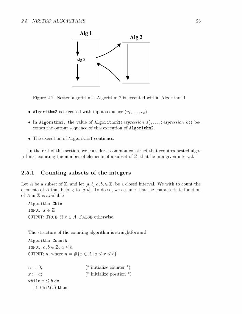
In the process of evaluating a function, we may have to evaluate another function, i.e.,sin(x+tan(x)). Likewise, within Algorithm1, we may wish to execute Algorithm2 (Figure2.1). Within an expression in Algorithm1, the expression
Algorithm2(〈 expression 1 〉, . . . ,〈 expression k 〉);is executed as follows:
• The execution of Algorithm1 is suspended.
• 〈 expression 1 〉, . . . ,〈 expression k 〉 are evaluated to values v1, . . . , vk, respectively.
2.5. NESTED ALGORITHMS 23
Alg 2
Alg 1Alg 2
Figure 2.1: Nested algorithms: Algorithm 2 is executed within Algorithm 1.
• Algorithm2 is executed with input sequence (v1, . . . , vk).
• In Algorithm1, the value of Algorithm2(〈 expression 1 〉, . . . ,〈 expression k 〉) be-comes the output sequence of this execution of Algorithm2.
• The execution of Algorithm1 continues.
In the rest of this section, we consider a common construct that requires nested algo-rithms: counting the number of elements of a subset of Z, that lie in a given interval.
2.5.1 Counting subsets of the integers
Let A be a subset of Z, and let [a, b] a, b,∈ Z, be a closed interval. We with to count theelements of A that belong to [a, b]. To do so, we assume that the characteristic functionof A in Z is available
Algorithm ChiA
INPUT: x ∈ ZOUTPUT: TRUE, if x ∈ A, FALSE otherwise.
The structure of the counting algorithm is straightforward
Algorithm CountA
INPUT: a, b ∈ Z, a ≤ b.
OUTPUT; n, where n = #{x ∈ A | a ≤ x ≤ b}.
n := 0; (* initialize counter *)
x := a; (* initialize position *)
while x ≤ b do
if ChiA(x) then

24 CHAPTER 2. ARITHMETIC
n := n+ 1; (* increase counter *)
fi;
x := x+ 1; (* increase position *)
od;
return n;
end;
Example 2.22. A prime p such that p+ 2 is also prime, is called called a twin prime.The sequence of twin primes is conjectured to be infinite
3, 5, 11, 17, 29, 41, . . .
although no proof of this conjecture is know.
The characteristic function of the set of twin primes is easily constructed
Algorithm IsTwinPrime
INPUT: x ∈ NOUTPUT: TRUE, if x is a twin prime, FALSE otherwise.
return IsPrime(x) AND IsPrime(x+ 2);
end;
To count twin primes in an interval, it suffices to replace CharA with IsTwinPrime inthe algorithm CountA.
2.6 The halting problem∗
We recall that an algorithm is said to be correct, if it terminates in a finite time forall valid input, giving the correct output. We now provide a simple but telling examplewhere defining what constitutes valid input, is essentially impossible; for even though theproblem is simply formulated, one cannot be certain that the algorithm will terminategiven arbitrary input. This is the celebrated halting problem of the theory of algorithms.
Let us consider the so-called ‘3x+ 1’ function
T : N 7→ N T (x) =
{x/2 x even3x+ 1 x odd
which is easily implemented.
Algorithm T
INPUT: x ∈ N.
OUTPUT; y, where y is the image of x under the ‘3x+ 1’ function.

2.6. THE HALTING PROBLEM∗ 25
if (xMOD 2) = 0 then
return x/2;
else
return 3x+ 1;
fi;
end;
Since domain and image of T coincide, we can iterate this function; we choose anarbitrary initial condition x ∈ N, compute T (x) to obtain a new point in N, then applyT to this point, and so on. If we choose x = 1, we obtain
1 7→ 4 7→ 2 7→ 1 7→ 4 7→ · · ·a periodic integer sequence. Let us call the cycle (4,2,1) a limit cycle for T . The ‘3x+ 1’conjecture says that any initial condition will eventually lead to that cycle, i.e.,
9, 28, 14, 7, 22, 11, 34, 17, 52, 26, 13, 40, 20, 10, 5, 16, 8, 4
and it is easy to persuade oneself that one can access such cycle only through the pointx = 4. Proving this conjecture seems beyond the reach of modern mathematics.
The craziness of this phenomenon becomes apparent when we construct an directedgraph, called the Collatz graph, whose vertices are the natural integers, and where thereis a edge joining x to y if y = T (x). The ‘3x+1’ conjecture can now be phrased by sayingthat the Collatz graph is connected, and has only one cycle. Alternatively, removing thevertices 1 and 2, and the related edges, one obtains a tree, rooted at 4.
4
21
8
32
16
5
10
20
40
13
26
52
17
34
11
36
12
7
18
9
14
2822
44
Figure 2.2: The Collatz graph, in a neighbourhood of the limit cycle (4, 2, 1).
We thus introduce the transit function T as the time it takes to get to the limit cycle(4,2,1)
T (8) = 1 T (9) = 17.

26 CHAPTER 2. ARITHMETIC
The ‘3x + 1’ conjecture states that T is well-defined, that is, that T (x) < ∞, for allpositive integers x.
Algorithm TransitTime
INPUT: x ∈ NOUTPUT: t, where t is the transit time from x to the (1, 4, 2)-cycle of T .
if x < 3 then
return 0;
fi;
t := 0:
while x 6= 4 do
t := t+ 1;
x := T(x);
od;
return t;
end;
Plainly, for some value of the input, this algorithm may not halt. However, no evidenceof such phenomenon has ever been found, so these integers, if they exist, are necessarilyvery large.
Exercises
Exercise 2.1. List all divisors of n = 120. List all primes p such that 120 < p < 140.
Exercise 2.2.
(a) Let a, b, c, x, y be integers, such that a divides b and a divides c. Show that adivides xb+ yc.
(b) Let n be an integer. Show that if −n is not prime, then n is not prime. Use thisto prove that n is prime if and only if −n is prime.
(c) Show that, if n is odd, then (n2 MOD 8) = 1.
(d) Using the above, show that x2 + y2 = z2 cannot be true in integers, when both xand y are odd. Give an example.
Exercise 2.3. Using the operators DIV and MOD , write an algorithm to the followingspecifications:
Algorithm Nint
INPUT: a, b ∈ Z, b 6= 0.
OUTPUT: c, where c is an integer nearest to a/b.
(Note: an integer, not the integer, so you may have a choice. Begin with the case a, b > 0.)
Exercise 2.4. Apply the algorithm IsPrime to each of the integers 433, 437, to determinewhich of these integers is prime.
Exercise 2.5. Apply the algorithm IntegerFactorization to each of the integers 127, 216, 4018

2.6. THE HALTING PROBLEM∗ 27
to determine their factorization into primes.
Exercise 2.6. How many divisions will IsPrime have to perform to verify that
p = 2127 − 1 = 170141183460469231731687303715884105727
is prime? (Lucas showed that p is prime in 1876). On the fastest computer on earth(∼ 1012 divisions per second), how many years will it take to complete the calculation?
The largest known prime is the prime on the left in (1.1). On the fastest computeron earth, and assuming that the lifetime of the universe is 20 billion years, how manylifetimes of universes will it take to test its primality with IsPrime?
Exercise 2.7. Consider the following algorithm
INPUT a, b ∈ Z, a ≥ 0, b > 0.
OUTPUT ??
while a ≥ 0 do
a := a− b;od
return a+ b;
end;
Write the output specifications of this algorithm, and explain how it works, keeping theuse of mathematical symbols to a minimum. What happens if the constraints a ≥ 0,b > 0 are removed from the input?
Exercise 2.8. Write an algorithm to the following specifications:
Algorithm NumMul
INPUT: a, b, x ∈ Z, x > 0, 0 < a < b.
OUTPUT: n, where n is the number of multiples of x
which are greater than a and smaller than b.
Try to make the computation efficient.
Exercise 2.9. Write an algorithm to the following specifications:
Algorithm Test
INPUT: x, a, b ∈ Z, a, b 6= 0.
OUTPUT: TRUE if x is divisible by a or by b, but not by both,
and FALSE otherwise.
Exercise 2.10. An integer is square-free if it is not divisible by any square greater than1.
(a) Find all square-free integers in the interval [40, 60].
(b) Consider the following algorithm

28 CHAPTER 2. ARITHMETIC
Algorithm SquareFree
INPUT: n, a positive integer.
OUTPUT: TRUE if n is square-free, FALSE otherwise.
Explain how to use IntegerFactorization to construct SquareFree. [ 6 ε, 50]
(c) Write the algorithm SquareFree, using IntegerFactorization.
Exercise 2.11. A Sophie Germain (SG) prime is an odd prime p such that 2p+ 1 is alsoprime.
(a) There are 6 SG-primes smaller than 50: find them. Can you find all SG-primesbetween 50 and 100?
(b) Using IsPrime, write an algorithm to the following specifications
Algorithm SGprime
INPUT: x ∈ N.
OUTPUT: TRUE if x is a SG-prime, and FALSE otherwise.
Try to make it efficient (think of the calculation in part (a)).
(c) Write an algorithm to the following specifications
Algorithm NumberSGprimes
INPUT: a, b ∈ N, a < b.
OUTPUT: n, where n is the number of SG-primes in the closed interval [a, b].
Exercise 2.12. Consider the following algorithm
Algorithm Square
INPUT: n, a positive integer.
OUTPUT: TRUE, if n is a square, FALSE otherwise.
(a) Explain how the algorithm IntegerFactorization can be used to constructSquare. [6 ε, 50]
(b) Write the algorithm Square, using IntegerFactorization.
Exercise 2.13. Let n be a positive integer, and recall that
n! = n · (n− 1) · · · 2 · 1.
Show that there is no prime p such that n! + 2 ≤ p ≤ n! + n. (Thus, there are arbitrarilylarge gaps between consecutive primes.)
Exercise 2.14. Find the smallest integer x for which NextPrime(x)−x = 8. (see Section1.1.5). The previous problem guarantees that such x does not exceed 10!, which is a verypoor upper bound.
Exercise 2.15. Consider the algorithm Mult (Section 2.4).
2.6. THE HALTING PROBLEM∗ 29
(a) Trace it with the following input (m,n):
(7, 6), (12, 18), (−13, 4).
In each case, use a table to show how the values of m, n and l change as Mult is executed,and indicate what is returned as output.
(b) Prove its correctness.

30 CHAPTER 2. ARITHMETIC

Chapter 3
Relations and partitions
We introduce a basic concept of higher mathematics: an equivalence relation. Our mainapplication will be modular arithmetic, in Chapter 4.
3.1 Relations
The cartesian product of two sets X and Y is defined as
X × Y = {(x, y) |x ∈ X, y ∈ Y }.
If X = Y , we often write X2 for X ×X.
Example 3.23. The cartesian product R2 is called the cartesian plane. The domainof the algorithm SumOfSquares of Example 11 is the set Z2.
Def: A relation from X to Y is a subset of X × Y . A relation from X to X is called arelation on X.
If R is a relation from X to Y we write xRy to mean (x, y) ∈ R (think of this as “xis related by R to y”). The expression xRy is therefore boolean. Note that the symbolR is used here to represent two different objects: a set (as in R ⊆ X 2) and a relationaloperator (as in xRy). The meaning of the notation will be clear from the context, andwill not lead to ambiguity.
Example 3.24. Let
X = {1, 2, 3} R = {(1, 2), (1, 3), (2, 2), (2, 3), (3, 1)}.
Then R is a relation on X. We have that 2R 3 is TRUE but 3R 2 is FALSE.
The relation R on X can be represented as a directed graph, whose vertices are theelements of X, and where an arc joins x to y if xRy (Figure 3.1).
Def: Let R be a relation on X.
31

32 CHAPTER 3. RELATIONS AND PARTITIONS
1 2
3
Figure 3.1: Directed graph of the relation of Example 3.24.
• R is reflexive if for all x ∈ X, xRx.
• R is symmetric if for all x, y ∈ X, xRy =⇒ yRx.
• R is transitive if for all x, y, z ∈ X, (xRy AND yRz) =⇒ xRz.
• R is an equivalence relation if R is reflexive, symmetric and transitive.
Checking the above properties amounts to evaluating boolean expressions. Specifically,we define the following functions
ρ : X → {TRUE,FALSE} x 7→ xRxσ : X2 → {TRUE,FALSE} (x, y) 7→ xRy =⇒ yRxτ : X3 → {TRUE,FALSE} (x, y, z) 7→ (xRy AND yRz) =⇒ xRz
Thus, for instance, R is symmetric precisely when the function σ assume the value TRUE
everywhere on X2.
We begin with the relations on X corresponding to the trivial subsets of X 2, namelythe empty set and X2. The relation R = {} is the empty relation on X. For everyx, y, z ∈ X, we have x{}y = y{}z = x{}z = FALSE, and therefore the boolean expression(x{}y AND y{}x) =⇒ x{}z evaluates to TRUE. We conclude that {} is transitive. By asimilar argument one shows that {} is symmetric. (Is {} reflexive?) Let now R = X 2.Because for all x, y ∈ X the expression xX2y evaluates to TRUE, so do the booleanexpressions defining reflexivity, symmetry and transitivity. We conclude that X 2 is anequivalence relation on X. The corresponding graph is a complete graph.
Example 3.25. Consider the following relations R on Z
xRy reflexive? symmetric? transitive? equivalence?(i) x = y yes yes yes yes(ii) x ≤ y yes no yes no(iii) x|y yes no yes no(iv) x+ y = 6 no yes no no(v) 2|x− y yes yes yes yes
(ii) is not symmetric: 3 ≤ 4 but 4 6≤ 3.

3.2. PARTITIONS 33
(iii) is transitive. Suppose x|y and y|z. Then y = xa for some a ∈ Z and z = yb for someb ∈ Z, so that z = xab =⇒ x|z.
(iv) is not reflexive (1+1 6= 6), and not transitive (1+5 = 6 and 5+1 = 6, but 1+1 6= 6).
(v) is a special case of a more general construct, with is dealt with in the following
Theorem 8 Let m be an integer, and define the relation ≡m on Z by x ≡m y if m|x− y.Then ≡m is an equivalence relation.
Proof:
(i) Let x ∈ Z. Then
m|0 =⇒ m|x− x =⇒ x ≡m x
i.e., ≡m is reflexive.
(ii) Let x, y ∈ Z, and suppose x ≡m y. Then
m|x− y =⇒ m| − (x− y) =⇒ m|y − x =⇒ y ≡m z
so z ≡m is symmetric.
(iii) Let x, y, z ∈ Z, and suppose that x ≡m y and y ≡m x. Then
=⇒ m|x− y and m|y − z=⇒ m|(x− y) + (y − z)
=⇒ m|x− z=⇒ x ≡m z,
i.e., ≡m is transitive. Because ≡m is reflexive, symmetric and transitive, ≡m is an equiv-alence.
3.2 Partitions
Def: A partition P of a set X is a set of non-empty subsets of X, such that each elementof X is in exactly one element of P (Figure 3.2).
The elements of a partition are called parts. If P is a partition of X and x ∈ X, wedenote by P (x) the unique part in P containing x. Note that, for all x, y ∈ X, eitherP (x) = P (y) or P (x) ∩ P (y) = {}; furthermore P = {P (x) |x ∈ X}.
Example 3.26. Let X = {1, 2, 3}, P = {{1, 3}, {2}}. Then P is a partition of X withparts {1, 3} and {2}:
P (1) = {1, 3} = P (3) P (2) = {2}.
Def: Let P be a partition on X. We define the relation RP on X by xRPy if P (x) =P (y).

34 CHAPTER 3. RELATIONS AND PARTITIONS
3
56 8
7
4
1 2
Figure 3.2: Partition of the set {1, 2, 3, 4, 5, 6, 7, 8} into 3 parts. We have P (1) = P (5) ={1, 3, 5}.
Example 3.27. Let X = {1, 2, 3}, P = {{1, 3}, {2}}. Then
RP = {(1, 1), (1, 3), (3, 1), (3, 3), (2, 2)}.
(Draw RP as a directed graph.) One verifies that RP is an equivalence relation. This isalways the case, as shown by the following
Theorem 9 If P is a partition of X, then RP is an equivalence relation on X.
Proof:
(i) RP is reflexive because, for all x ∈ X, P (x) = P (x).
(ii) RP is symmetric because, for all x, y ∈ X, P (x) = P (y) =⇒ P (y) = P (x).
(iii) RP is transitive because, for all x, y, z ∈ X, P (x) = P (y) and P (y) = P (z) =⇒P (x) = P (z).
Example 3.28. Let
X = {a, b, c, d, e, f, g, h, i, j} P = {{a, b, c, d}, {e, f, g}, {h, i}, {j}}.
The equivalence RP is displayed in Figure 3.3 as the union of complete graphs.
f
i
j
he
g
b
cd
a
Figure 3.3: Directed graph of the equivalence generated by the partition of Example 3.28.

3.2. PARTITIONS 35
Example 3.29. Suppose E is the equivalence relation on X = {1, 2, 3, 4, 5} given by
E = {(1, 1), (1, 3), (2, 2), (2, 4), (3, 1), (3, 3), (4, 2), (4, 4), (5, 5)}.
To construct a partition from E, we proceed as follows. We choose an arbitrary pointin X, x = 1, say, and we let P (1) := {y ∈ X | 1Ey}. We find P (1) = {1, 3}. Of theremaining points in X \ P (1), we choose x = 2 and repeat the construction, to obtainP (2) := {y ∈ X | 2Ey} = {2, 4}. There is only one point left: P (5) = {y ∈ X | 5Ey} ={5}. Now, P (1), P (2) and P (5) are non empty, disjoint (because E is an equivalencerelation, think about it), and their union is X. Thus we have obtained a partition of X:P = {P (1), P (2), P (3)}. One verifies that E = RP , from the definition of RP .
The above construction works in general. Suppose we know an equivalence relation Eon X, and we want to determine a partition P of X such that E = RP . We construct Pas follows. Let x ∈ X. Then P (x) —the part containing x— is equal to
{y ∈ X |P (x) = P (y)} = {y ∈ X |xE y}.
Knowing each part of P , we then know P , since P = {P (x) |x ∈ X}. In the last formula,the requirement x ∈ X may be highly redundant; to construct P algorithmically, onewould instead identify recursively a representative x from each part of P , as we did in theprevious example.
Do all equivalence relations originate from partitions? In other words, if we start withan arbitrary equivalence relation E on X, is it true that E = RP for some partition P ofX? The answer to this question is affirmative:
Theorem 10 Let E be an equivalence relation on a set X, and for each x ∈ X, defineE(x) to be the set {y ∈ X |xE y}. Let P = {E(x) |x ∈ X}. Then (i) P is a partition ofX, and (ii) E = RP .
Proof: (i) Each element E(x) of P is a subset of X. Furthermore, x ∈ E(x) (becauseE is reflexive), so E(x) 6= {}, and each element x ∈ X is in some element of P . We nowonly need to show that no element of X can be in more than one element of P . To do hiswe suppose x ∈ X, x ∈ E(y) and x ∈ E(z), and then show we must have E(y) = E(z).
We first show that E(y) ⊆ E(z). Let t ∈ E(y). Then we have
yEx AND zEx AND yEt =⇒ zEx AND xEy AND yEt (E symmetric)=⇒ zEy AND yEt (E transitive)=⇒ zEt (E transitive)=⇒ t ∈ E(z).
Thus, t ∈ E(y) =⇒ t ∈ E(z), so
E(y) ⊆ E(z). (3.1)
Interchanging the role of y and z in the above argument, we obtain E(z) ⊆ E(y), which,together with (3.1), implies that E(y) = E(z). This concludes the proof that P is apartition of X.
36 CHAPTER 3. RELATIONS AND PARTITIONS
(ii) We have shown that P = {E(x) |x ∈ X} is a partition of X. Since x ∈ E(x),we have that E(x) = P (x), the unique part of P containing x.
Let x, y ∈ X. Then
xEy ⇐⇒ y ∈ E(x) (by def. of E(x))⇐⇒ y ∈ E(x) AND y ∈ E(y) (since y ∈ E(y))⇐⇒ y ∈ E(x) = E(y) (since P is a partition)⇐⇒ P (x) = P (y)⇐⇒ xRPy.
Thus, E = RP .
Def: Let E be an equivalence relation on X, and x ∈ X. Then E(x) = {y ∈ X |xEy}is called the equivalence class (of E) containing x, and the partition {E(x) |x ∈ X} isdenoted by X/E.
Note that we have proved that E = RX/E .
Let θ be the map from the set of equivalence relations on X to the set of partitions ofX, defined by
θ(E) = X/E
for each equivalence relation E on X.
Theorem 11 (i) The map θ is a bijection (one-to-one and onto); (ii) If P is a partitionof X, then θ−1(P) = RP .
Proof: (i) We first prove that θ is one-to-one. Suppose E1 and E2 are equivalencerelations on X, and θ(E1) = θ(E2). This means
X/E1 = X/E2 =⇒ E1 = RX/E1 = RX/E2 = E2
(using previous theorem, part (ii)).
We now prove that θ is onto. Let P be a partition of X. We have that RP = RX/RP(by the previous theorem, part (ii)), hence P = X/RP (since P is completely determinedby RP), and therefore P = θ(RP).
(ii) θ is a bijection, so θ is invertible. The proof that θ is onto shows that θ(RP) = Pfor each partition P of X. Therefore θ−1(P) = RP .
Schematically, the content of the last theorem is the following
equivalences onX partitions ofX
Eθ−→ X/E
RPθ−1
←− P
3.2. PARTITIONS 37
Exercises
Exercise 3.1. Let X = {a, b, c}.(a) Determine all partitions of X.
(b) Determine all equivalence relations on X (as a subset of X ×X).
Exercise 3.2. Let X = {1, 2, 3, 4}.(a) Determine all the partitions P of X such that P has exactly two parts.
(b) For each such partition P , write down the corresponding equivalence relation RP .
Exercise 3.3. Let X = {1, 2, 3}. Determine relations R1, R2, R3 on X, such that
(a) R1 is symmetric and transitive, but not reflexive.
(b) R2 is reflexive and transitive, but not symmetric.
(c) R3 is reflexive and symmetric, but not transitive.
In each case, try to make relations have as few elements as possible.
Exercise 3.4. Let X = {1, 2, 3, 4, 5, 6, 7}, and let
R = {(1, 7), (1, 4), (3, 1), (4, 3), (6, 2)}
be a relation on X. Suppose E is an equivalence relation on X such that R ⊆ E and Ehas as few elements as possible.
(a) Determine the partition X/E corresponding to this equivalence.
(b) How many elements does E have?
Exercise 3.5. Determine the possible cardinalities of an equivalence relation on a set of5 elements.
Exercise 3.6. Let R be an equivalence relation on a finite set X. Prove that #R hasthe same parity as #X.
Exercise 3.7. Let P be a partition of a finite set X, and let P (x) be the part of Pcontaining x.
(a) Explain why the formula P = {P (x) : x ∈ X} does not translate into an efficientalgorithm for constructing P from the knowledge of X and P .
(b) Write an algorithm to the following specifications
Algorithm Partition
INPUT: X,P
OUTPUT: PYou may use set operators (union, etc.), and represent the elements of a set using subscriptsA = {A1, A2, . . .}. Be careful that P is a set of sets.
38 CHAPTER 3. RELATIONS AND PARTITIONS
Exercise 3.8. Let f be the characteristic function of a relation R ⊆ X 2, where X ={1, 2, . . . , n}, n ≥ 1. Write an algorithm to the following spefifications
Algorithm IsSymm
INPUT: n, P
OUTPUT: TRUE, if R is symmetric, FALSE otherwise.
Chapter 4
Modular arithmetic
The sum of two odd integers is even, their product is odd. Modular arithmetic affords avast generalization of statements of this type, by defining arithmetical operations betweeninfinite families of integers, of which the even and the odd integers are a special example.
Let m ∈ Z. Recall that the relation ≡m on Z, defined by i ≡m j if m|i − j is anequivalence relation on Z (Theorem 8). Such relation is called a congruence, and thecorresponding equivalence classes are called congruence classes or residue classes.
Let i, j ∈ Z. Then
i ≡m j ⇐⇒ j ≡m i
⇐⇒ m|j − i⇐⇒ j − i = mk for some k ∈ Z⇐⇒ j = i+mk for some k ∈ Z.
Thus, the equivalence class containing i is
{j ∈ Z | i ≡m j} = {i+mk | k ∈ Z}.
We denote the equivalence class containing i by [i]m.
Example 4.30. The following is readily verified from the definition
[3]5 = {3 + 5 k | k ∈ Z} = {. . . ,−12,−7,−2, 3, 8, 13, . . .} = [−12]5.
Remarks:
(i) [i]0 = {i+ 0 k | k ∈ Z} = {i}
(ii) [i]1 = {i+ 1 k | k ∈ Z} = Z
(iii) [i]−m = {i+ (−m)k | k ∈ Z} = {i+mk | k ∈ Z} = [i]m.
39

40 CHAPTER 4. MODULAR ARITHMETIC
Equality (i) says that the relations = and ≡0 are the same on Z, so the case m = 0is trivial. Equality (iii) says that considering negative moduli is superfluous. So in therest of this chapter we assume m > 0. Then Theorem 3 tells us that there are uniqueintegers q, r such that i = qm+ r and 0 ≤ r < m. (Recall that such q and r are denotedby iDIVm and iMODm, respectively.) In particular, we see that i ≡m (iMODm) so[i]m = [iMODm]m.
The partition Z/ ≡m, corresponding to the equivalence relation ≡m is usually denotedby Z/(m), and called the set of integers modulo m. Thus
Z/(m) = Z/ ≡m= {[i]m | i ∈ Z}= {[iMODm]m | i ∈ Z} (4.1)
= {[0]m, [1]m, . . . , [m− 1]m}.
Now suppose that 0 ≤ i, j, < m, and [i]m = [j]m. Then i = km + j for some k ∈ Z,hence iMODm = j (since 0 ≤ j < m). But iMODm = i, so we must have i = j. Thistells us that [0]m, [1]m, . . . , [m− 1]m are distinct, so
Z/(m) = ([0]m, [1]m, . . . , [m− 1]m)
has size m. The integers 0, 1, . . . ,m − 1 are a common choice for representatives ofequivalence classes, and are called the least non-negative residues modulo m.
The notation x ≡m y is shorthand for Gauss’ notation
x ≡ y (mod m).
The symbol MOD for remainder of division, as well as the term modular arithmetic derivefrom it.
4.1 Addition and multiplication in Z/(m)
Theorem 12 Let m, a, b, c, d ∈ Z, such that a ≡m c and b ≡m d. Then
(i) a+ b ≡m c+ d (ii) ab ≡m cd.
So congruences can be added and multiplied together: in this respect they behave likeequations.
Proof: a ≡m c means c = a + km for some k ∈ Z, and b ≡m d means d = b + lm forsome l ∈ Z.
(i) We have
c+ d = a+ km+ b+ lm
= (a+ b) + (k + l)m ≡m a+ b.

4.1. ADDITION AND MULTIPLICATION IN Z/(M) 41
(ii) We have
cd = (a+ km)(b+ lm)
= ab+ alm+ kmb+ kmlm
= ab+ (al + kb+ klm)m ≡m ab
Now, define addition and multiplication in Z/(m) by
[a]m + [b]m = [a+ b]m [a]m[b]m = [ab]m.
The above theorem implies that these operations are well-defined, in the sense that theresult does not depend on our choice of representatives for equivalence classes.
Example 4.31. Check the following equalities carefully.
[3]5 + [2]5 = [5]5 = [0]5 [3]5[2]5 = [6]5 = [1]5
[3]6 + [2]6 = [5]6 [3]6[2]6 = [6]6 = [0]6
Theorem 13 For all a, b, c ∈ Z/(m) the following holds
(i) a+ b ∈ Z/(m), ab ∈ Z/(m)
(ii) (a+ b) + c = a+ (b+ c), (ab)c = c(bc)
(iii) a+ b = b+ a, ab = ba
(iv) a+ [0]m = a, a[1]m = a
(v) there is an element −a ∈ Z/(m) such that a+ (−a) = [0]m
(vi) a(b+ c) = ab+ ac
Proof: (i) follows from definitions of addition and multiplication. The properties (ii),(iii) and (vi) are inherited from Z. For example, we prove (vi) in detail. Suppose a = [i]m,b = [j]m, c = [k]m. Then
a(b+ c) = [i]m([j]m + [k]m)
= [i]m[j + k]m
= [i(j + k)]m
= [ij + ik]m
= [ij]m + [ik]m
= [i]m[j]m + [i]m[k]m
= ab+ ac.
The proofs of (ii) and (iii) are similar (try them!).

42 CHAPTER 4. MODULAR ARITHMETIC
(iv) Suppose a = [i]m. Then
a+ [0]m = [i]m + [0]m = [i+ 0]m = [i]m = a
a[1]m = [i]m[1]m = [i 1]m = [i]m = a.
(v) Suppose a = [i]m, and define −a = [−i]m. (This is well-defined, verify it.) Then
a+ (−a) = [i]m + [−i]m = [i+ (−i)]m = [0]m.
This completes the proof.
4.2 Invertible elements in Z/(m)
Def: Let a ∈ Z/(m). We say that a is invertible if there exists an element b ∈ Z/(m)such that ab = [1]m.
Proposition 14 Suppose a, b, c ∈ Z/(m), a is invertible, and ab = ac = [1]m. Thenb = c.
Proof: We find
ab = ac =⇒ bab = bac
=⇒ abb = abc
=⇒ [1]mb = [1]mc
=⇒ b = c.
Suppose a is an invertible element of Z/(m). The above proposition says there is aunique b ∈ Z/(m) such that ab = [1]m. We call this unique b the (multiplicative) inverseof a, which is denoted by a−1. (Similarly, the additive inverse of an element of Z/(m) isunique.)
Let a, b ∈ Z/(m). The notation a− b means a+ (−b), and if b is invertible a/b meansab−1.
Example 4.32. In Z/(4) we have
a [0]4 [1]4 [2]4 [3]4−a [0]4 [3]4 [2]4 [1]4a−1 − [1]4 − [3]4
Also[2]4 − [1]4
[3]4= ([2]4 − [1]4) [3]−1
4 = [1]4[3]4 = [3]4.
4.3. COMMUTATIVE RINGS WITH IDENTITY 43
When we are working in Z/(m) and there is no risk of confusion, we will use i todenote [i]m. Thus in Z/(5)
3
2+ 4 ≡ 3 · 3 + 4 ≡ 9 + 4 ≡ 13 ≡ 3 (mod 5).
The number of invertible elements of Z/(m) is denoted by φ(m). Thus φ(4) = 2. Thefunction φ is called Euler’s φ-function.
4.3 Commutative rings with identity
Theorem 13 shows that Z/(m) is an example of a commutative ring with identity, definedas follows.
Def: Let R be a set on which two binary operations, addition + and multiplication · aredefined. Then R is said to be a commutative ring with identity if R contains elements 0and 1, and the following rules hold for all a, b, c ∈ R
(i) a+ b ∈ R, a · b ∈ R. [closure laws for addition and multiplication]
(ii) (a+ b) + c = a+ (b+ c),(a · b) · c = c · (b · c) [associative laws for addition and multiplication]
(iii) a+ b = b+ a, a · b = b · a [commutative laws for addition and multiplication]
(iv) a+ 0 = a, a · 1 = a [additive and multiplicative identity elements]
(v) There exists −a ∈ R such that a+ (−a) = 0. [existence of additive inverse]
(vi) a · (b+ c) = a · b+ a · c. [distributive law for multiplication over addition]
Note that in Z/(m), the additive and multiplicative identities 0 and 1 are [0]m and [1]m,respectively. Familiar examples of commutative rings with identity include Z,Q,R,C, aswell as polynomials (chapter 5).
The additive and multiplicative identities can be shown to be unique. Furthermorefor all a, b,∈ R, we have
(i) a · 0 = 0
(ii) (−a) · b = −(a · b).
See Section 7.1 for proofs.
Example 4.33. The set [0]2 is a commutative ring without identity, while [1]2 is nota ring at all, since it is not closed under addition.

44 CHAPTER 4. MODULAR ARITHMETIC
Exercises
Exercise 4.1. (All quantities here are integers.) Let a ≡m b; prove that
(a) if d is a divisor of m, then a ≡d b(b) if n > 0, then an ≡m bn.
Exercise 4.2. Determine all solutions to the equation x2 = x in each of Z/(6), Z/(7),and Z/(8).
Exercise 4.3. Let m be an integer, and s, t ∈ Z/(m).
(a) Determine all invertible elements in each of Z/(6), Z/(7), Z/(8).
(b) Prove that if s and t are invertible, then so is s−1 and st.
(c) Suppose that t is invertible. Prove that st = [0]m if and only if s = [0]m.
Exercise 4.4. Evaluate the following expressions in Z/(7). In each case show your cal-culations, and give an answer of the form [k]7, where 0 ≤ k < 7. (In the computation,you may use congruence notation.)
(a) [7004]7[7003]7 + [1000]7 (b) [−11]7[−2]−17 + [−8]
27
(c)6∑
k=1
[1]7[k]7
(d) [3]30000017
Exercise 4.5. Let n be a non-negative integer, whose decimal notation is dkdd−1 . . . d0.
(a) Show that if m = 3 or m = 9, then
[n]m = [d0 + d1 + · · ·+ dk]m.
(b) Show that if m = 3 or m = 9, then m divides n if and only if m divides d0 + d1 +· · ·+ dk.
(c) Using (b), find a 10-digit integer which is divisible by 3, but not by 9.
Exercise 4.6. Let x ∈ Z/(m). We say that x is a square if there exists y ∈ Z/(m) suchthat x = y2.
(a) Find all squares in Z/(13).
(b) Write an algorithm to the following specifications
Algorithm MSquare
INPUT: a,m ∈ Z, m > 1.
OUTPUT: TRUE is [a]m is a square in Z/(m), and FALSE otherwise.
Exercise 4.7. The additive order of [x]m ∈ Z/(m) is the smallest positive integer t suchthat [tx]m = [0]m. Write an algorithm to the following specifications
Algorithm AddOrder
INPUT: x,m ∈ Z, m > 0.

4.3. COMMUTATIVE RINGS WITH IDENTITY 45
OUTPUT: t, where t is the additive order of [x] in Z/(m).
Prove that your algorithm terminates, i.e., that the additive order exists for every elementof Z/(m).
Exercise 4.8. The multiplicative order of [x] ∈ Z/(m) is the smallest positive integer t
such that [x]t
= [1]. Such integer does not necessarily exist.
(a) Compute the multiplicative order of [11] in Z/(13).
(b) Describe the structure of the sequence t 7→ xt in the case in which the multiplicativeorder of x ∈ Z/(m) is not defined. [6 ε ]

46 CHAPTER 4. MODULAR ARITHMETIC

Chapter 5
Polynomials
We are familiar with polynomials with real coefficients. We now consider polynomials withother types of coefficients. Let R = Z,Q,R,C or Z/(m) (or indeed, any commutative ringwith identity).
Def: A polynomial a with coefficients in R (also called a polynomial over R), is anexpression of the form
a = a0x0 + a1x
1 + · · · + an−1xn−1 + anx
n =n∑
k=0
akxk
where a0, a1, . . . , an ∈ R. The quantity x is called the indeterminate; each summand akxk
is a monomial.
One normally writes a1x and a0 for a1x1 and a0x
0, respectively. Furthermore, terms ofthe form 0xi are usually left out, and one writes xi for 1xi. Finally, to represent coefficientsof a polynomial over Z/(m), we use the shorthand notation i for [i]m.
Example 5.34. Let R = Z/(6), the polynomial
[−5]6 x3 + [12]6 x
2 + [1]6 x1 + [−3]6 x
0
is written as −5x3 + x− 3 or x3 + x+ 3, etc.
Let a0 + a1x + · · · + anxn be a polynomial with coefficients in R. We call a the
zero polynomial, and write a = 0, if a0 = a1 = · · · = an = 0. (Recall that 0 = [0]m ifR = Z/(m).)
Def: The degree deg(a) of a polynomial a 6= 0 is the greatest integer k such that ak 6= 0.If a is the zero polynomial, we let deg(a) = −1.
Example 5.35. R = Z.
deg(0x4 + 3x2 + 2x− 3) = 2 deg(−1) = 0 deg(0) = −1.
47

48 CHAPTER 5. POLYNOMIALS
Def: The leading coefficient ldcf(a) of a non-zero polynomial a is adeg(a). If a = 0, wedefine ldcf(0) = 0.
Example 5.36. Let R = Z/(5), and a = −10x4 + 8x2 + 3. Then a = 3x2 + 3 and soldcf(a) = [3]5 (deg(a) = 2).
Let a = a0 +a1x+ · · ·+anxn, b = b0 + b1x+ · · ·+ blx
l be polynomials with coefficientsin R. We consider a and b to be equal, and write a = b, if deg(a) = deg(b) and ai = bifor i = 0, 1, . . . , deg(a). Thus a = b precisely when equality holds for the correspondingsequences of coefficients
(a0, a1, . . . ) = (b0, b1, . . . )
in the sense of equation (2.2), Section 2.3.
We denote by R[x] the set of all polynomials with coefficients in R. Let a, b ∈ R[x].Then we can add and multiply the polynomials a and b in the usual way, taking care toadd and multiply the coefficients correctly in R. Then x+ b ∈ R[x] and ab ∈ R[x].
In the theory of polynomials the indeterminate does not play an active role: its purposeis to organize the coefficients is such a way that the arithmetical operations can be definednaturally. Polynomials over R could be defined as finite sequences of elements of R,without any reference to an indeterminate.
Example 5.37. Let R = Z/(6), and let a, b ∈ R[x] be given by
a = 2x2 + x+ 1 b = 3x3 + 5x2 + 2x+ 3.
Then
a+ b = (0 + 3)x3 + (2 + 5)x2 + (1 + 2)x+ (1 + 3)
= 3x3 + x2 + 3x+ 4.
ab = 2x2b+ xb+ b
= 6x5 + 10x4 + 4x3 + 6x2 + 3x4 + 5x3
+2x2 + 3x+ 3x3 + 5x2 + 2x+ 3
= x4 + x2 + 5x+ 3.
Note that in this case deg(ab) = 4 6= deg(a) + deg(b) = 5.
It can be shown that if R is a commutative ring with identity, then so is R[x] (with1 = 1x0 and 0 = 0x0).
Def: Let a ∈ R, a commutative ring with identity. We say that a is invertible if thereexists an element b ∈ R such that ab = 1.
In Z, the only invertible elements are 1 and −1. In Q, R and C all elements except 0are invertible. We shall show that if p is a prime, then all elements of Z/(p), except 0 areinvertible, which will give the arithmetic modulo a prime a special status.

5.1. LOOP INVARIANTS 49
Theorem 15 Let R be a commutative ring with identity, let a, b ∈ R[x], with b 6= 0, andlet ldcf(b) be an invertible element of R. Then there are unique polynomials q, r,∈ R[x]such that
a = bq + r deg(0) ≤ deg(r) < deg(b). (5.1)
The proof is given in chapter 7. Note the structural similarity with Theorem 3, chapter2.
We denote this unique q and r by aDIV b and aMOD b, respectively. The quantitiesaDIV b and aMOD b can be calculated by ‘long division of polynomials’.
Example 5.38. Let R = Z/(3), and let a = x4 + 1, b = 2x2 + x + 2 ∈ R[x]. Wecompute aDIV b and aMOD b by long division
2x2 +2x = aDIV b
2x2 + x+ 2∣∣∣ x4 +1
−(x4 +2x3 +x2)
x3 +2x2 +1−(x3 +2x2 +x)
2x +1 = aMOD b
To develop an algorithm for quotient and remainder of polynomial division, we requirethe notion of a loop invariant.
5.1 Loop invariants
Proving statements about algorithms that contain loops, requires a variant of the methodof induction, which is based on the notion of a loop invariant.
Def: Let W be a while-loop with loop control expression β. A loop invariant L for W isa boolean expression which evaluates to TRUE when β is evaluated.
Whether L is evaluated before or after β is immaterial, since the evaluation of aboolean expression does not alter the value of any variable. Thus a loop invariant isTRUE when the loop first starts execution, and is TRUE after each complete executionof the statement-sequence of that loop. Therefore, proving that L is a loop invariant ismathematical induction in disguise.
The base case consists of showing that L is TRUE when W is first entered (beforeits statement-sequence is executed even once). The inductive hypothesis amounts toassuming that L is TRUE at the beginning of the execution of W’s statement-sequence.The inductive step amounts to proving that then L is also TRUE at the end of theexecution of statement-sequence (it does not matter if L is FALSE at some other point inthe statement-sequence).

50 CHAPTER 5. POLYNOMIALS
is TRUEL
β is FALSEβ is TRUE
Lβ
Figure 5.1: A loop with loop invariant L and loop control expression β. The filled-incircles denote expressions, which may change the value of L and β. However, inside theloop, the value of L is eventually restored to TRUE.
Suppose we are given a while-loop W of the form
while β do
〈 statement-sequence 〉od;
where L is a proven loop invariant for W. Then, if W terminates execution normally (afterthe od;), we know that on this terminations of W we must have that L is TRUE and βis FALSE (see Figure 5.1). This knowledge can help us prove that an algorithm works.Clearly, any boolean expression that always evaluates to TRUE (such as TRUE, or 2 < 3)is a trivial loop invariant for any loop. The difficulty lies in identifying ‘useful’ loopinvariants.
As an illustration of loop invariance, we develop an algorithm for quotient and remain-der of polynomial division. Let R = Z, Q, R, C or Z/(m) (or indeed, any commutativering with identity).
Algorithm PolynomialQuoRem
INPUT: a, b ∈ R[x], b 6= 0, and ldcf(b) invertible.
OUTPUT: q, r ∈ R[x], such that q = aDIV b and r = aMOD b.
q := 0;
r := a;
γ := ldcf(b)−1;
while deg(r) ≥ deg(b) do
t := γ · ldcf(r) · xdeg(r)−deg(b);
q := q + t; (* the quotient is updated *)
r := r − tb; (* the degree of r is lowered *)
od;

5.1. LOOP INVARIANTS 51
return (q, r); (* now, a = bq + r and deg(r) < deg(b) *);
end;
In this algorithm q stores the current value of the quotient, and r that of the remainder.The statement t := γ · ldcf(r) · xdeg(r)−deg(b); achieves the purpose of matching degree andleading coefficient of r and tb: deg(tb) = deg(r) ≥ 0, and ldcf(tb) = ldcf(r). Because theloop control expression is deg(r) ≥ deg(b), and a = bq+ r is a loop invariant (see below),on termination, equation 5.1 holds.
Example 5.39. Let R = Z/(3), and let f = x4 + 1, g = 2x2 + x+ 2 ∈ R[x]. We trace
PolynomialQuoRem(f, g)
a b q r γ deg(r) ≥ deg(b) tx4 + 1 2x2 + x+ 2 0 x4 + 1 2 T 2x2
2x2 x3 + 2x2 + 1 T 2x2x2 + 2x 2x+ 1 F
return (2x2 + 2x, 2x+ 1)
Thus f DIV g = 2x2 + 2x and f MOD g = 2x+ 1, as we found in Example 5.38.
Proposition 16 The algorithm PolynomialQuoRem is correct.
We first prove by induction that a = bq + r is a loop invariant for the while-loop ofPolynomialQuoRem.
(Induction basis.) When this while-loop first starts execution, we have q = 0, and r = a,so
bq + r = 0 + a = a.
We next show that if a = bq + r holds at the beginning of the while-loop’s statement-sequence, then a = bq + r holds at the end of that statement-sequence.
(Induction step.) Let q′ and r′ be the respective values of q and r at the beginning ofthe statement-sequence, and assume that a = bq ′ + r′. Now the statement-sequence doesnot change the values of a and b, but does change the values of q and r, by assigning thevalue q′ + t to q, and r′ − tb to r. Thus at the end of the statement-sequence, we have
bq + r = b(q′ + t) + r′ − tb= bq′ + r′ + bt− tb= a+ 0
= a,
as required. This completes the proof of the loop invariant of the while-loop of thealgorithm PolynomialQuoRem.

52 CHAPTER 5. POLYNOMIALS
Now each time the statement-sequence of the while-loop of PolynomialQuoRem is ex-ecuted, the degree of r is decreased, and b is unchanged. Thus, after finitely manyexecutions of this statement-sequence, we will have deg(r) < deg(b) (because deg(b) ≥ 0),and the while-loop will terminate.
Upon this termination we know that the loop invariant a = bq + r is TRUE, anddeg(r) ≥ deg(b) is FALSE. Thus a = bq + r and deg(r) < deg(b), which means thatq = aDIV b, and r = aMOD b. Thus PolynomialQuoRem works, terminating after a finitetime and returning the correct output.
5.2 Recursive algorithms
We have seen (Section 2.5) that one algorithms can call another algorithm. An algorithmis said to be recursive when it calls itself. More precisely, a recursive algorithm calls adifferent and independent execution of the same algorithm.
Example 5.40. A recursive algorithm to compute n!.
Algorithm Factorial
INPUT: n, a positive integer.
OUTPUT: n!.
if n = 1 then
return 1;
else
return n · Factorial(n− 1);
fi;
end;
Example 5.41. We execute Factorial(4) = Factorial1(4).
Factorial1(4)
Alg n n = 1 n · Factorialk(n− 1) return
Factorial1 4 F 4 · Factorial2(3) 24
Factorial2 3 F 3 · Factorial3(2) 6
Factorial3 2 F 2 · Factorial4(1) 2
Factorial4 1 T 1
return 24

5.3. GREATEST COMMON DIVISORS 53
Induction is the most common device used to prove the correctness of a recursivealgorithm.
Proposition 17 The algorithm Factorial is correct.
Proof: By induction of the input n.
(Induction basis.) If n = 1, then Factorial terminates and returns the correct result 1.
(Induction step.) Let k be an arbitrary, but fixed positive integer, and assume thatalgorithm Factorial works correctly with input n = k. Then if n = k+ 1, the algorithmreturns
(k + 1) · Factorial(k) = (k + 1) · k!
= (k + 1) · k (k − 1) · · · 2 · 1= (k + 1)!
which is correct.
5.3 Greatest common divisors
In this section we introduce Euclid’s algorithm, one of the best known recursive algorithmsof discrete mathematics.
Def: A field F is a commutative ring with identity, which contains at least 2 elements,and such that if 0 6= α ∈ F , then α is invertible.
The sets Q,R,C are fields. The commutative ring with identity Z/(2) = {[0]2, [1]2} isa field, because its only nonzero element [1]2 is invertible, as easily verified. We will provelater that Z/(p), where p is a prime is a field.
Let F be a field. If a, b ∈ F [x], with b 6= 0, then aDIV b and aMOD b are always defined(since ldcf(b) is invertible), and we have
a = (aDIV b)b+ aMOD b deg(0) ≤ deg(aMOD b) < deg(b).
Recall that a similar situation holds in Z. If a, b,∈ Z, b 6= 0, then
a = (aDIV b)b+ aMOD b |0| ≤ |aMOD b| < |b| (5.2)
and for this reason we shall deal with division with integers and with polynomials over afield in a unified manner.
Thus let E = Z, or E = F [x], and a, b ∈ E. We say that b divides a, and write b|a, ifa = bc for some c ∈ E. We call d ∈ E a common divisor of a and b if d|a and d|b. Wecall g a greatest common divisor (or gcd) of a and b if
(i) g is a common divisor of a and b
(ii) if d is any common divisor of a and b, then d|g.

54 CHAPTER 5. POLYNOMIALS
Example 5.42. Let E = Z, a = −18, b = 24. The common divisors of a and b are
1,−1, 2,−2, 3,−3, 6,−6.
The greatest common divisors of a and b are 6 and −6.
Theorem 18 Let E = Z or E = F [x], where F is a field, and let a, b ∈ E. The followingholds:
(i) if b = 0, then a is a gcd of a and b;
(ii) if b 6= 0, then g is a gcd of a and b iff g is a gcd of b and aMOD b.
Proof: Part (i) follows immediately from the fact that a divides 0 and a. To prove (ii),we first show that
g|a AND g|b ⇐⇒ g|a AND g|(aMOD b).
Indeed
(=⇒) suppose g|a and g|b. Then g|b and g|a− b(aDIV b) = aMOD b.
(⇐=) Suppose g|b and g|aMOD b. Then g|b(aDIV b) + aMOD b = a, and g|b.Thus, if a, b ∈ E and b 6= 0, the pairs a, b and b, aMOD b have exactly the same set of
common divisors. This implies they also have the same set of greatest common divisors.
Let F be a field, and let E = Z or E = F [x]. For the gcd algorithms below, weassume that if E = F [x], then we have algorithms for exact computations in F (which iscertainly the case when F = Q or Z/(p), p prime). We begin with the celebrated Euclid’salgorithm
Algorithm GCD
INPUT: a, b ∈ E.
OUTPUT: g ∈ E, such that g is a gcd of a and b.
if b = 0 then
return a;
else
return GCD(b, aMOD b);
fi;
end;
Next, we consider the extended Euclid’s algorithm, which, in addition to computing agreatest common divisor, also expresses it as a linear combination of the input data.

5.3. GREATEST COMMON DIVISORS 55
Algorithm ExtendedGCD
INPUT: a, b ∈ E.
OUTPUT: g, s, t ∈ E, such that g is a gcd of a and b, and g = sa+ tb.
if b = 0 then
return (a, 1, 0);
else
(g, s, t) := ExtendedGCD(b, aMOD b);
return (g, t, s− t (aDIV b));
fi;
end;
Of note is the assignment to a sequence: (g, s, t) := ExtendedGCD(b, aMOD b), wherebyeach variable on the left hand side is assigned the value of the corresponding output ofExtendedGCD.
Example 5.43. Let F = Z/(5), E = F [x]. We determine GCD(x2 + 2x+ 1, x2 + 4).
GCD1(x2 + 2x+ 1, x2 + 4)
Alg a b b = 0 aMOD b GCDk(b, aMOD b) return
GCD1 x2 + 2x+ 1 x2 + 4 F 2x+ 2 GCD2(x2 + 4, 2x+ 2) 2x+ 2
GCD2 x2 + 4 2x+ 2 F 0 GCD3(2x+ 2, 0) 2x+ 2
GCD3 2x+ 2 0 T 2x+ 2
return 2x+ 2
Def: Let E = Z or F [x], where F is a field. For a ∈ E, define δ(a) = |a| if a is aninteger, and δ(a) = deg(a) if a is a polynomial.
Suppose a and b are in E. Then we always have that δ(b) is an integer, with δ(b) ≥ δ(0).In fact, δ(b) = δ(0) if and only if b = 0. Furthermore, if b is nonzero, we have thatδ(0) ≤ δ(aMOD b) < δ(b).
Proposition 19 The algorithm ExtendedGCD is correct.
Proof:
We do this by strong induction on n = δ(b), proving that for all n ≥ δ(0), the algorithmExtendedGCD works correctly for all input a, b ∈ E, with δ(b) = n. (Note that this coversall possible input a, b to ExtendedGCD.)

56 CHAPTER 5. POLYNOMIALS
(Induction basis.) If n = δ(b) = δ(0), then b = 0 so a is a gcd of a and b, anda = 1a+ 0b. Thus when n = δ(0) the algorithm ExtendedGCD terminates with the correctoutput (a, 1, 0).
(Induction step.) Now assume that n = δ(b) > δ(0), and that ExtendedGCD workscorrectly with input a′, b′ in E, whenever δ(b′) < n.
Since δ(b) > δ(0), b must be nonzero, and ExtendedGCD first sets
(g, s, t) := ExtendedGCD(b, aMOD b).
Since δ(aMOD b) < δ(b), from our inductive hypothesis, we have that g is a gcd of b andaMOD b, and that g = sb+ t(aMOD b).
It follows that g is a gcd of a and b (by Theorem 18, page 54), and that
g = sb+ t(aMOD b)
= sb+ t(a− b(aDIV b))
= ta+ (s− t(aDIV b))b.
Thus ExtendedGCD terminates and returns the correct result (g, t, s− t(aDIV b)), andthe proof is complete.
The proof that algorithm GCD is correct is a simplified version of the above proof, andit is left as an exercise.
Example 5.44. We compute a greatest common divisor g of the polynomials a = x6 +2x5 +x and b = x4 +3x3 +2x2 +4x+4 in Z/(5), and then express g as a linear combinationof a and b. The computation of ExtendedGCD(x6 + 2x5 +x, x4 + 3x3 + 2x2 + 4x+ 4), givenin Table I, returns the sequence
(g, s, t) := (x+ 3, 3x2 + 3x+ 4, 2x4 + x2 + x+ 2).
We verify
sa+ tb = (3x2 + 3x+ 4) (x6 + 2x5 + x)
+ (2x4 + x2 + x+ 2) (x4 + 3x3 + 2x2 + 4x+ 4)
= 5x8 + 15x7 + 15x6 + 20x5
+ 15x4 + 15x3 + 15x2 + 16x+ 8
= x+ 3.
Let F be a field, let E = Z or F [x], and let a, b ∈ E. Recall that a gcd of a and b isdefined to be a common divisor of g of a and b, such that g is divisible by each commondivisor of a and b. It follows that, if E = Z, then g is a gcd of a and b if and only if −gis a gcd of a and b.
Now suppose that E = F [x], and that g and g′ are both gcds of a and b. Since g andg′ are both common divisors of a and b, it follows from the definition of gcd that g|g ′ and

5.3.G
RE
AT
EST
CO
MM
ON
DIV
ISO
RS
57
TABLE I Tracing the calls to ExtendedGCD of Example 5.44, over Z/(5).
ExtendedGCD1(x6 + 2x5 + x, x4 + 3x3 + 2x2 + 4x+ 4)
Alg a b b = 0 aMOD b EGCDk g s t aDIV b return
EGCD1 x6 + 2x5 + x x4 + 3x3+ F 3x2 + x+ 1 EGCD2 x+ 3 1 3x2+ x2 + 4x+ 1 (x+ 3,2x2 + 4x+ 4 3x+ 4 3x2 + 3x+ 4,
2x4 + x2 + x+ 2)
EGCD2 x4 + 3x3+ 3x2 + x+ 1 F x+ 3 EGCD3 x+ 3 0 1 2x2 + 2x+ 1 (x+ 3, 1,2x2 + 4x+ 4 3x2 + 3x+ 4)
EGCD3 3x2 + x+ 1 x+ 3 F 0 EGCD4 x+ 3 1 0 3x+ 2 (x+ 3, 0, 1)
EGCD4 x+ 3 0 T (x+ 3, 1, 0)
return (x+ 3, 3x2 + 3x+ 4, 2x4 + x2 + x+ 2)

58 CHAPTER 5. POLYNOMIALS
and g′|g. We must therefore have (see exercises) that deg(g) = deg(g ′) and that g′ = fgfor some degree zero polynomial f in F [x]. Furthermore, for all degree zero polynomialsf in F [x], fg really is a gcd of a and b (see exercises).
Conclusion: if E = Z then {−g, g} is the set of gcds of a and b. If E = F [x], then{fg | f ∈ F [x], deg(f) = 0} is a set of gcds of a and b.
5.4 Modular inverse
Theorem 20 Let m and i be integers. Then [i]m is an invertible element of Z/(m) ifand only if 1 is a gcd of m and i.
Proof: (=⇒) Suppose [i]m is an invertible element of Z/(m), and let [j]m = [i]−1m . Then
[1]m = [i]m[j]m = [ij]m
which implies that 1 = ij+km for some integer k. We also see from this that any commondivisor of m and i also divides 1, which is also a common divisor of m and i. From thedefinition of gcd, we have that 1 is a gcd of m and i.
(⇐=) Suppose 1 is a gcd of m and i. Then 1 = sm + ti, for some integers s and t,from the extended Euclid’s algorithm (if the algorithm returns −1 as a gcd, then t and sare the negatives of the corresponding values in the output sequence). Therefore
[1]m = [sm+ ti]m
= [s]m[m]m + [t]m[i]m
= [s]m[0]m + [t]m[i]m
= [t]m[i]m.
Thus [i]m is invertible, and [t]m = [i]−1m .
The above theorem and proof show us how to determine if an element of Z/(m) isinvertible, and if so, how to find its inverse. We implement this method in the algorithmInverse
Algorithm Inverse
INPUT: i,m ∈ Z, with m > 1.
OUTPUT: t, such that [t]m = [i]−1m , if [i]m is invertible;
the empty sequence otherwise.
(g, s, t) := ExtendedGCD(m, i);
if g = 1 then
return t; (* since 1 = sm+ ti *)
fi;
if g = −1 then
return −t; (* since 1 = −sm− ti *)

5.4. MODULAR INVERSE 59
fi;
return (); (* at this point we know that 1 is not a gcd of m, i *)
end
Example 5.45. Trace Inverse(19, 21).
i m i ExtendedGCD(m, i) g s t g = 1 g = −1 return
19 21 19 ExtendedGCD1(21, 19) 1 −9 10 T 10
We trace all calls to ExtendedGCD in a single table, writing EGCD for ExtendedGCD
Alg a b b = 0 aMOD b EGCD(m, i) g s t aDIV b return
EGCD1 21 19 F 2 EGCD2(19, 2) 1 1 −9 1 (1,−9, 10)
EGCD2 19 2 F 1 EGCD3(2, 1) 1 0 1 9 (1, 1,−9)
EGCD3 2 1 F 0 EGCD4(1, 0) 1 1 0 1 (1, 0, 1)
EGCD4 1 0 T (1, 1, 0)
return10
Thus [19]21 is invertible, and [19]−121 = [10]21.
Theorem 21 Let m > 1 be an integer. Then each nonzero element of Z/(m) is invertibleif and only if m is prime.
Proof: (=⇒) (By contradiction.) Suppose m is not prime. Then m = ij for someintegers i, j, with 1 < i < m. Note that [i]m is a nonzero element of Z/(m). Since i,−iare the gcds of m and i, we have that 1 is not a gcd of m and i, and applying Theorem20, we see that [i]m is not invertible.
(⇐=) Suppose m is prime. Then the only divisors of m are 1,−1,m,−m. Thuswhen 1 ≤ i < m, we have that 1 is a gcd of m and i. Applying Theorem 20, we have that[i]m is invertible for each i = 1, 2, . . . ,m− 1.
Let m be an integer. Applying Theorem 21, we deduce the following important
Corollary 22 The set Z/(m) is a field if and only if m is prime.
These are prominent examples of finite fields. It can be shown that every field whosecardinality is a prime number p, is equal to Z/(p) (more precisely, it has the same arith-metic).

60 CHAPTER 5. POLYNOMIALS
5.5 Polynomial evaluation
Let R = Z, Q, R, C, Z/(m) (or indeed, let R be any commutative ring with identity),and let f = f0 + f1x+ · · ·+ fnx
n ∈ R[x]. Then f defines a function as follows
f : R→ R α 7→ f(α) = f0 + f1α + · · ·+ fnαn.
We say that f(α) is the polynomial f evaluated at α. Note that for f, g ∈ R[x], α ∈ R,we have
(f + g)(α) = f(α) + g(α)
(f · g)(α) = f(α) · g(α)
(−f)(α) = −f(α)
which follow from the way addition, subtraction and multiplication are defined for poly-nomials. The operators +,−, · appearing on the left-hand side of the above equationshave a very different meaning from those on the right-hand side. Indeed, the former referto arithmetic in R[x], the latter to arithmetic in R.
Example 5.46. Let f = x3 + x+ 1, g = 2x+ 1 ∈ Z/(3)[x]. Then
f(0) = 03 + 0 + 1 = 1 f(1) = 13 + 1 + 1 = 0 f(2) = 23 + 2 + 1 = 2.
g(0) = 2 · 0 + 1 = 1 g(1) = 2 · 1 + 1 = 0 g(2) = 2 · 2 + 1 = 2.
Thus, f 6= g (as polynomials), but f(x) = g(x) as functions from Z/(3) to Z/(3).
If f(α) = 0, then we call α a zero of f .
Proposition 23 Let f ∈ R[x], α ∈ R. Then α is a zero of f if and only if (x− α) | f .
Proof: Since ldcf(x − α) = 1 is invertible (Theorem 20, Section 5.4), we have thatf = (x − α)q + r, for q, r ∈ R[x], with deg(r) < deg(x − α) = 1. So we have twopossibilities: either deg(r) = −1 and r = 0, or deg(r) = 0 and r = β x0, for some0 6= β ∈ R.
(=⇒) Suppose that α is a zero of f , but that r = βx0 6= 0. Then
0 = f(α) = (α− α)q(α) + r(α) = 0 + β = β 6= 0,
a contradiction.
(⇐=) Suppose (x − α) | f . Then f = (x − α)g for some g ∈ R[x], and thereforef(α) = (α− α)g(α) = 0.
Now, given f = f0 + f1x+ · · ·+ fnxn ∈ R[x], and α ∈ R, how can we determine f(α)
efficiently? The trick is to write
f = f0 + x(f1 + f2x+ · · ·+ fnxn−1)
= f0 + x(f1 + x(f2 + f3x+ · · ·+ fnxn−2))
...
= f0 + x(f1 + x(f2 + x(f3 + · · ·+ x(fn−1 + x(fn)) · · · ))).This leads to Horner’s algorithm to evaluate f at α

5.5. POLYNOMIAL EVALUATION 61
Algorithm Evaluate
INPUT: f = f0 + f1x+ · · ·+ fnxn ∈ R[x], α ∈ R.
OUTPUT: f(α).
if f = 0 then
return 0;
fi;
result := ldcf(f);
i := deg(f)− 1;
while i ≥ 0 do
result := fi + α · result;i := i− 1;
od;
return result;
end;
Example 5.47. Let f ∈ Z/(5)[x] be given by
f = 4 + x+ 2x3 + 3x4
= 4 + x (1 + x (0 + x (2 + x (3)))).
We compute f(3). One sees that using the nested expression for f , this will involve fourmultiplication and four additions.
Evaluate(f, 3)
result i3 3
3 · 3 + 2 = 1 23 · 1 + 0 = 3 13 · 3 + 1 = 0 03 · 0 + 4 = 4 −1
Thus, f(3) = 4.
Proposition 24 The algorithm Evaluate is correct.
Proof: If f = 0, then Evaluate terminates with the correct output 0.
Now suppose deg(f) = n ≥ 0. The statement-sequence of the while-loop executes foreach i = n−1, n−2, . . . , 0, exactly n times (performing n additions and n multiplicationsin R), then result is returned, and the algorithm terminates.

62 CHAPTER 5. POLYNOMIALS
To prove correctness, we prove the loop invariant
result =
n∑
j=i+1
fj · αj−(i+1).
On entry to the loop, i = n− 1, and
result = ldcf(f) = fn =
n∑
j=(n−1)+1
fnαj−n
and the loop invariant holds.
Now suppose we are at the beginning of the statement-sequence of the loop, i = k ≥ 0,and the loop invariant holds. Thus
result =n∑
j=k+1
fj · αj−(k+1).
We now execute the loop’s statement-sequence, and then show that the loop invariantstill holds. We have
result = fi + α · result
= fk + αn∑
j=k+1
fjαj−(k+1)
= fkα0 +
n∑
j=k+1
fjαj−k
=n∑
j=k
fjαj−k.
Then i := i− 1, and the loop statement-sequence is finished. But now k = i+ 1, so that
result =n∑
j=k
fj · αj−k =n∑
j=i+1
fj · αj−(i+1)
and the loop invariant still holds.
When the loop terminates, we have i = −1 and the loop invariant holding. Thus, ontermination of the loop result =
∑nj=0 fjα
j, and the algorithm returns the correct result.
5.6 Polynomial interpolation∗
Let F = Q, R, C, or Z/(p), p prime (or indeed, let F be any field). Suppose we aregiven α1, . . . , αn, β1, . . . , βn ∈ F . Does there exist an f ∈ F [x] such that f(α1) =β1, . . . , f(αn) = βn? If so, can we calculate one of degree smaller than n?
The answer to both questions is affirmative, using the algorithm Interpolate below.It turns out that such f is unique, as we shall prove later.

5.6. POLYNOMIAL INTERPOLATION∗ 63
Algorithm Interpolate
INPUT: α1, . . . , αn, β1, . . . , βn ∈ F , with n ≥ 1 and α1, . . . , αn distinct.
OUTPUT: f ∈ F [x] such that f(α1) = β1, . . . , f(αn) = βn and deg(f) < n.
b := 1x0;
i := 1;
f := β1x0;
while i < n do
b := b(x− αi);i := i+ 1;
f := f +βi − f(αi)b(αi)
b;
od;
return f ;
end;
Example 5.48. Let F = Z/(3).
Interpolate((0, 1, 2), (1, 0, 1))
.
b i f1x0 1 1x0
1x0 2 1 + (0−1)1x = 2x+ 1
x(x− 1) = 3 (2x+ 1) + (1+1)2b =
x2 + 2x 2x+ 1 + 1(x2 + 2x) = x2 + x+ 1
return x2 + x+ 1
Check. Letting f = x2 + x + 1 ∈ Z/(3)[x], we find f(0) = 1, f(1) = 1 + 1 = 1 = 0,f(2) = 22 + 2 + 1 = 1, as desired.
Proposition 25 The algorithm Interpolate is correct.
Proof: Termination follows from the fact that the while-loop executes its statement-sequence for each i = 1, 2, . . . , n− 1, and then terminates.
We prove the loop invariant L, defined as
b =i∏
l=1
(x− αl) AND f(αl) = βl, l = 1, . . . , i AND deg(f) < i.
The loop is first entered with
b := 1x0 i := 1 f := β1x0.
64 CHAPTER 5. POLYNOMIALS
which implies
b = 1x0 =0∏
l=1
(x− αl), f(α1) = β1, deg(f) < 1,
that is, L is TRUE on entry.
Now suppose L is TRUE on the loop entry, for some 1 ≤ i = k < n. Then
b =k−1∏
l=1
(x− αl), f(αl) = βl, l = 1, . . . , k, deg(f) < k.
And we have the assignments
b := b (x− αk) = (x− α1) · · · (x− αk−1)(x− αk)i := i+ 1 = k + 1.
Now consider
f ∗ = f +βk+1 − f(αk+1)
b(αk+1)· b
If j ≤ k, then
f ∗(αj) = f(αj) +βk+1 − f(αk+1)
b(αk+1)· b(αj)
= f(αj) +βk+1 − f(αk+1)
b(αk+1)· 0 = βj
f ∗(αk+1) = f ∗(αk+1) +βk+1 − f(αk+1)
b(αk+1)· b(αk+1)
= βk+1.
Also, deg(f ∗) ≤ max(deg(f), deg(b)) = k < i = k+ 1. Now the new f := f ∗, and we haveshown that the loop invariant holds after the execution of the loop’s statement-sequence.
On termination of the while-loop, we have i = n, and L is TRUE, so the algorithmreturns the correct output on termination.
Theorem 26 Let F be a field, and let α1, . . . , αn, β1, . . . , βn ∈ F , with α1, . . . , αn distinct.Then there exists a unique polynomial f ∈ F [x], such that f(α1) = β1, . . . , f(αn) = βn,and deg(f) < n.
Proof: The existence of f is given by Proposition 25. As to uniqueness, suppose f, g ∈F [x], with
f(α1) = g(α1) = β1, · · · , f(αn) = g(αn) = βn deg(f) < n, deg(g) < n.
Consider the polynomial h = f − g. We have
h(αi) = f(αi)− g(αi) i = 1, . . . , n.

5.6. POLYNOMIAL INTERPOLATION∗ 65
Thus, if h 6= 0, h = a (x−α1) · · · (x−αn), for some 0 6= a ∈ F [x]. Thus, deg(h) ≥ n. Butthis contradicts the fact that
h = f − g deg(f) < n deg(g) < n.
Thus, h− 0 and f = g.
Exercises
Exercise 5.1. Let R = Z/(4), and let a = 2x3 + 2x2 + 3, b = 3x3 + 2x2 + x + 3 bepolynomials in R[x]. Determine
deg(a2), ldcf(b)−1, ab, a+ a, a+ b, aMOD b.
Exercise 5.2. Let R = Z/(7), and let a = 4x3 + 2x+ 1, b = 3x2 + x+ 4 be polynomialsin R[x]. Use the algorithm PolynomialQuoRem to determine
aDIV b, aMOD b, bDIV a, bMOD a.
Exercise 5.3. In the statements below, let m and n assume integer values, and let W
denote the while-loop.
a := m;
b := n;
c := 0;
while b 6= 0 do
c := c+ a;
b := b− 1;
od;
(a) For which integer values of n will W terminate? Explain your answer.
(b) Prove that ab+ c = mn is a loop invariant for W.
(c) Suppose that W terminates. Show that on termination we have that c = mn.
Exercise 5.4. Consider the statements below, where the variables m and n are assumedto have integer values, with n ≥ 0, and let W denote the while-loop in these statements.
a := m;
b := n;
c := 0;
while b > 0 do
if 2 | b thena := 2a;

66 CHAPTER 5. POLYNOMIALS
b := b/2;
else
c := c+ a;
b := b− 1;
fi;
od;
(a) Prove that ab+ c = mn is a loop invariant for W. b odd separately.]
(b) Why must W terminate? Why must b = 0 on this termination?
(c) Show that on the termination of W, we have that c = mn.
(d) Is this approach to computing mn faster or slower than the approach in theprevious problem? Justify your answer.
Exercise 5.5. Prove that the algorithm GCD is correct.
Exercise 5.6. Apply the algorithm GCD, to determine the greatest common divisor of11468 and 5551.
Exercise 5.7. Let F = Z/(3), and let c = x3 +2x2 +x+2 and d = 2x2 +1 be polynomialsin F [x]. Apply the algorithm ExtendedGCD to determine g, s, t ∈ F [x], such that g is agcd of c and d, and g = sc+ td.
Exercise 5.8. Write down all the invertible elements of Z/(30).
Exercise 5.9. Apply the algorithm Inverse to determine whether [27]38 is invertible,and if so, to find its inverse.
Exercise 5.10. Let f and g be non zero polynomials in F [x]. Prove that deg(fg) =deg(f) + deg(g).
Exercise 5.11. Suppose that g is a gcd of polynomials a and b in F [x], F a field. Provethat if f is a degree zero polynomial in F [x], then fg is also a gcd of a and b.
Exercise 5.12. Let K = Z/(5), b ∈ K[x] and suppose that 2x2 + x + 3 is a greatestcommon divisor of a and b. Write down all the greatest common divisors of a and b.
Exercise 5.13. The Euler’s φ-function is defined on the positive integers, as follows:φ(1) = 1; for m > 1, φ(m) is the number of invertible elements in Z/(m). Write thealgorithm to the following specifications:
Algorithm Phi
INPUT: m, a positive integer.
OUTPUT: φ(m).
Exercise 5.14. Consider the recursive algorithm
Algorithm A
INPUT: x ∈ Z, x > 0
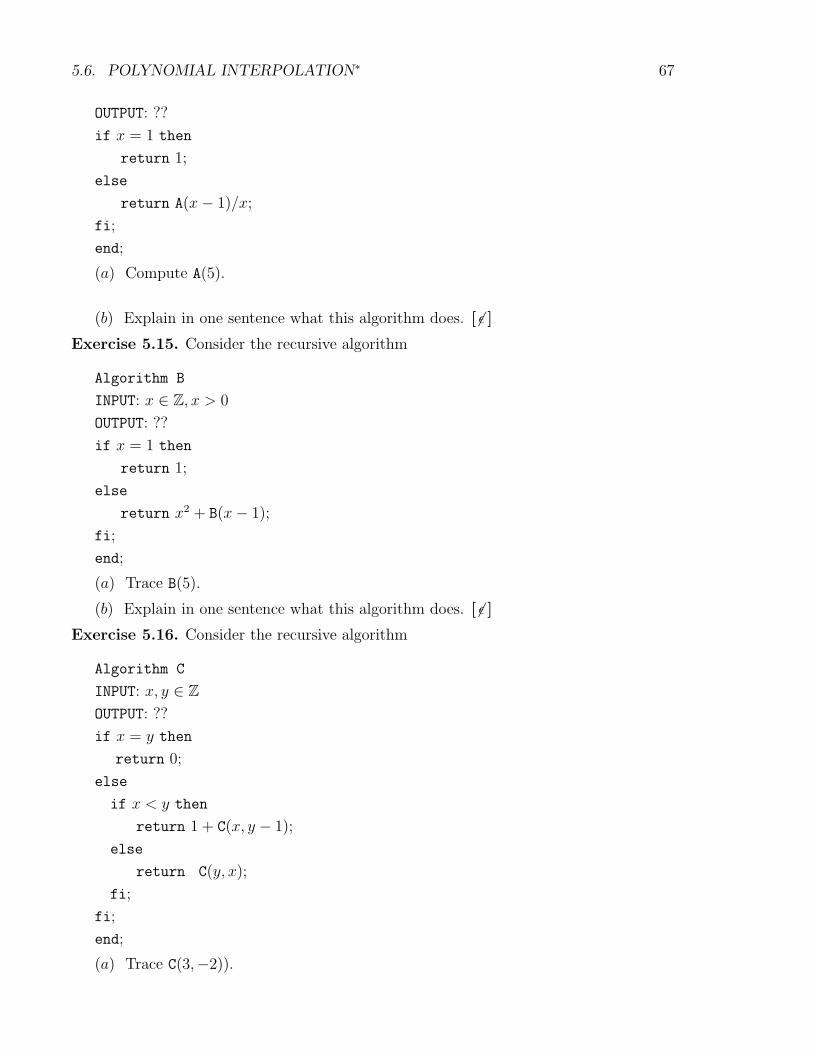
5.6. POLYNOMIAL INTERPOLATION∗ 67
OUTPUT: ??
if x = 1 then
return 1;
else
return A(x− 1)/x;
fi;
end;
(a) Compute A(5).
(b) Explain in one sentence what this algorithm does. [6 ε ]
Exercise 5.15. Consider the recursive algorithm
Algorithm B
INPUT: x ∈ Z, x > 0
OUTPUT: ??
if x = 1 then
return 1;
else
return x2 + B(x− 1);
fi;
end;
(a) Trace B(5).
(b) Explain in one sentence what this algorithm does. [6 ε ]
Exercise 5.16. Consider the recursive algorithm
Algorithm C
INPUT: x, y ∈ ZOUTPUT: ??
if x = y then
return 0;
else
if x < y then
return 1 + C(x, y − 1);
else
return C(y, x);
fi;
fi;
end;
(a) Trace C(3,−2)).

68 CHAPTER 5. POLYNOMIALS
[Hint: there should be 7 calls to the algorithm.]
(b) Explain in one sentence what this algorithm does. [6 ε ]
Exercise 5.17. Find two integers a, b, with 0 ≤ b < a such that the recursive computa-tion of GCD(a, b) involves 10 calls to the function GCD. Explain what you are doing.
Chapter 6
Algorithms for vectors
Let F be a field (for example, Q,R,C, or Z/(p), where p is a prime). In this course, avector v of dimension n over F is a sequence v = (a1, a2, . . . , an), of length n, such thata1, a2, . . . , an ∈ F .
We consider two vectors v = (a1, a2, . . . , an) and w = (b1, b2, . . . , bm) over F to beequal if they are equal as sequences (cf. equation (2.2)).
We denote by F n the set of all vectors of dimension n over F . Thus
F n = {(a1, a2, . . . , an) | a1, a2, . . . , an ∈ F}.
Example 6.49. A relation on a field F is a collection of two-dimensional vectors overF , that is, a subset of F 2 (chapter 3).
Example 6.50. If F = Z/(p), with p a prime, then F is a field (Corollary 22, page59) and F n has exactly pn elements (see exercises). In the following example, p = 3 andn = 2
(Z/(3))2 = { (0, 0), (0, 1), (0, 2), (1, 0), (1, 1), (1, 2), (2, 0), (2, 1), (2, 2) }.
We call (0, 0, . . . , 0) ∈ F n, the zero vector, and if there is no danger of confusion,denote it by 0 or 0.
Let v = (a1, . . . , an) ∈ F n, v 6= 0. Let l be the smallest integer in the range 1 ≤ l ≤ nfor which al 6= 0. Then we call l the leading index of v, and denote it by ldindx(v),and we call al the leading term of v, and denote it by ldterm(v). In other words, theleading index of a vector identifies the location of the leading term. Thus, the vector(0, 0, 0, 2, 0, 1) ∈ Z/(3)6 has leading index 4 and leading term [2]3.
If v = 0, then we define the leading index of v to be n + 1, but leave ldterm(v)undefined.
Let v = (a1, . . . , an) and w = (b1, . . . , bn) be vectors in F n. We define the sumof vectors v and w by v + w = (a1 + b1, . . . , an + bn) and the scalar multiple of v
69

70 CHAPTER 6. ALGORITHMS FOR VECTORS
by c ∈ F cv = (ca1, . . . , can). We also define −v = (−a1, . . . ,−an) and v − w =v + (−w). Let w1, . . . , wk ∈ F n. We say that w is a linear combination of w1, . . . , wk ifw = c1w1 + · · ·+ ckwk for some c1, . . . , ck ∈ F .
The linear span of w1, . . . , wk, denoted by 〈w1, . . . , wk〉, is defined to be the set of alllinear combinations of w1, . . . , wk. In symbols
〈w1, . . . , wk〉 = {c1w1 + · · ·+ ckwk | c1, . . . , ck ∈ F}.In the parlance of linear algebra, W = 〈w1, . . . , wk〉 is a subspace of the vector spaceF n, often called the subspace generated by, or spanned by, w1, . . . , wk. We shall use theshorthand notation 〈W 〉 for 〈w1, . . . , wk〉.
Example 6.51. Let F = Z/(2), and let w1 = (1, 0, 1), w2 = (1, 1, 0) ∈ F 3. Then
〈w1, w2〉 = {0w1 + 0w2, 0w1 + 1w2, 1w1 + 0w2, 1w1 + 1w2 }= {(0, 0, 0), (1, 1, 0), (1, 0, 1), (0, 1, 1)}.
6.1 Echelon form
The general problem is the following. Suppose we have a field F , w1, . . . , wk ∈ F n, andwe want to determine whether v ∈ 〈w1, . . . , wk〉. Furthermore, if v ∈ 〈w1, . . . , wk〉, wewant to determine a1, . . . , ak ∈ F such that v = a1w1 + · · · + akwk, that is, we want towrite v as a linear combination of w1, . . . , wk.
These problems can be solved by the algorithm Sift if the sequence (w1, . . . , wk) is inso-called echelon form.
Def: Let F be a field and w1, . . . , wk ∈ F n. We say that the sequence (w1, . . . , wk) is inechelon form if the following holds
(i) wi 6= 0 for i = 1, . . . , k,
(ii) ldterm(wi) = 1, for i = 1, . . . , k,
(iii) ldindx(w1) < ldindx(w2) < · · · < ldindx(wk).
For formal reasons, we shall regard the empty sequence ( ) to be in echelon form.
Example 6.52. Let F = Z/(3), n = 3
vectors echelon form?((1,1,2),(0,0,1)) yes((2,1,1),(0,0,1)) no((0,0,1),(1,1,2)) no
((1,1,2),(0,0,0),(0,0,1)) no((0,0,1)) yes
( ) yes

6.1. ECHELON FORM 71
Let F be a field and n a non-negative integer. The algorithm Sift below computesin F n, and we assume that we have algorithms for exact computation in F , which iscertainly the case when F = Q or Z/(p) (p prime).
Algorithm Sift
INPUT: v, W , such that v ∈ F n, and W = (w1, . . . , wk)
is a sequence in echelon form of k vectors in F n.
OUTPUT: u, (a1, . . . , ak), such that u ∈ F n, a1, . . . , ak ∈ F ,
v = u+ a1w1 + · · ·+ akwk,
and ldindx(u) 6∈ {ldindx(w1), . . . , ldindx(wk)}.
k := #W ;
L := {ldindx(w1), . . . , ldindx(wk)};aj := 0, for j = 1, . . . , k;
u := v;
while ldindx(u) ∈ L do (* Loop invariant: v = u+ a1w1 + · · ·+ akwk *)
i := the integer i such that ldindx(wi) = ldindx(u);
ai := ldterm(u);
u := u− aiwi; (* this step increases ldindx(u), since ldterm(wi) = 1 *)
od;
return (u, (a1, . . . , ak));
end;
The assignment ‘i :=the integer i such that ldindx(wi) = ldindx(u)’ is to be implementedas ‘i :=MatchLeadingIndex(u,W)’, where MatchLeadingIndex is a suitable algorithm(see exercises).
Proposition 27 The algorithm Sift is correct.
Proof: Let S be the statement sequence of the while-loop of Sift. Then each time S
is executed, ldindx(u) is increased, being made greater than ldindx(wi) = ldindx(u), fora different i each time S is executed. This shows that S is executed at most k times,after which Sift returns a result and terminates. This also shows that the statementai = ldterm(u) is executed at most once for each i. Indeed, before ai = ldterm(u) isexecuted, we have ai = ai+1 = · · · = ak = 0. We shall use this fact later.
We now show, by induction, that v = u+ a1w1 + · · ·+ akwk is a loop invariant for thewhile-loop of Sift.
(Induction basis.) When the while-loop of Sift first starts execution, we have u = v, andaj = 0, for j = 1, . . . , k. Thus, at this point, we have u+ a1w1 + · · ·+ akwk = v + 0 = v,as required.
(Induction step.) Suppose we are at the beginning of S. Let u′ be the value of u at this
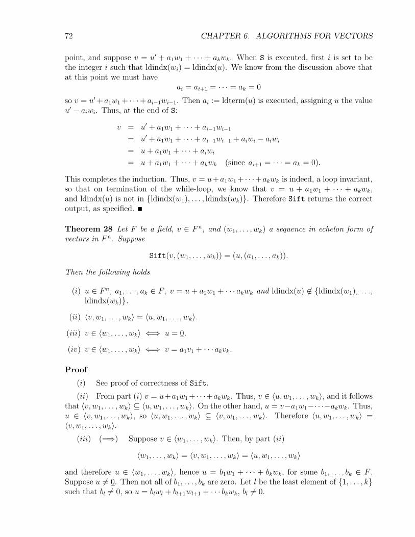
72 CHAPTER 6. ALGORITHMS FOR VECTORS
point, and suppose v = u′ + a1w1 + · · · + akwk. When S is executed, first i is set to bethe integer i such that ldindx(wi) = ldindx(u). We know from the discussion above thatat this point we must have
ai = ai+1 = · · · = ak = 0
so v = u′+a1w1 + · · ·+ai−1wi−1. Then ai := ldterm(u) is executed, assigning u the valueu′ − aiwi. Thus, at the end of S:
v = u′ + a1w1 + · · ·+ ai−1wi−1
= u′ + a1w1 + · · ·+ ai−1wi−1 + aiwi − aiwi= u+ a1w1 + · · ·+ aiwi
= u+ a1w1 + · · ·+ akwk (since ai+1 = · · · = ak = 0).
This completes the induction. Thus, v = u+a1w1 + · · ·+akwk is indeed, a loop invariant,so that on termination of the while-loop, we know that v = u + a1w1 + · · · + akwk,and ldindx(u) is not in {ldindx(w1), . . . , ldindx(wk)}. Therefore Sift returns the correctoutput, as specified.
Theorem 28 Let F be a field, v ∈ F n, and (w1, . . . , wk) a sequence in echelon form ofvectors in F n. Suppose
Sift(v, (w1, . . . , wk)) = (u, (a1, . . . , ak)).
Then the following holds
(i) u ∈ F n, a1, . . . , ak ∈ F , v = u + a1w1 + · · · akwk and ldindx(u) 6∈ {ldindx(w1), . . .,ldindx(wk)}.
(ii) 〈v, w1, . . . , wk〉 = 〈u,w1, . . . , wk〉.
(iii) v ∈ 〈w1, . . . , wk〉 ⇐⇒ u = 0.
(iv) v ∈ 〈w1, . . . , wk〉 ⇐⇒ v = a1v1 + · · · akvk.
Proof
(i) See proof of correctness of Sift.
(ii) From part (i) v = u+a1w1 + · · ·+akwk. Thus, v ∈ 〈u,w1, . . . , wk〉, and it followsthat 〈v, w1, . . . , wk〉 ⊆ 〈u,w1, . . . , wk〉. On the other hand, u = v−a1w1−· · ·−akwk. Thus,u ∈ 〈v, w1, . . . , wk〉, so 〈u,w1, . . . , wk〉 ⊆ 〈v, w1, . . . , wk〉. Therefore 〈u,w1, . . . , wk〉 =〈v, w1, . . . , wk〉.
(iii) (=⇒) Suppose v ∈ 〈w1, . . . , wk〉. Then, by part (ii)
〈w1, . . . , wk〉 = 〈v, w1, . . . , wk〉 = 〈u,w1, . . . , wk〉
and therefore u ∈ 〈w1, . . . , wk〉, hence u = b1w1 + · · · + bkwk, for some b1, . . . , bk ∈ F .Suppose u 6= 0. Then not all of b1, . . . , bk are zero. Let l be the least element of {1, . . . , k}such that bl 6= 0, so u = blwl + bl+1wl+1 + · · · bkwk, bl 6= 0.
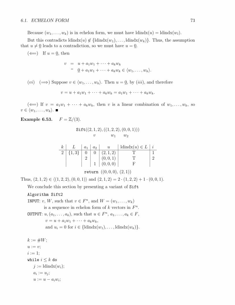
6.1. ECHELON FORM 73
Because (w1, . . . , wk) is in echelon form, we must have ldindx(u) = ldindx(wl).
But this contradicts ldindx(u) 6∈ {ldindx(w1), . . . , ldindx(wk)}. Thus, the assumptionthat u 6= 0 leads to a contradiction, so we must have u = 0.
(⇐=) If u = 0, then
v = u+ a1w1 + · · ·+ akwk= 0 + a1w1 + · · ·+ akwk ∈ 〈w1, . . . , wk〉.
(vi) (=⇒) Suppose v ∈ 〈w1, . . . , wk〉. Then u = 0, by (iii), and therefore
v = u+ a1w1 + · · ·+ akwk = a1w1 + · · ·+ akwk.
(⇐=) If v = a1w1 + · · · + akwk, then v is a linear combination of w1, . . . , wk, sov ∈ 〈w1, . . . , wk〉.
Example 6.53. F = Z/(3).
Sift((2, 1, 2), ((1, 2, 2), (0, 0, 1))v w1 w2
)
k L a1 a2 u ldindx(u) ∈ L i2 {1, 3} 0 0 (2, 1, 2) T 1
2 (0, 0, 1) T 21 (0, 0, 0) F
return ((0, 0, 0), (2, 1))
Thus, (2, 1, 2) ∈ 〈(1, 2, 2), (0, 0, 1)〉 and (2, 1, 2) = 2 · (1, 2, 2) + 1 · (0, 0, 1).
We conclude this section by presenting a variant of Sift
Algorithm Sift2
INPUT: v, W , such that v ∈ F n, and W = (w1, . . . , wk)
is a sequence in echelon form of k vectors in F n.
OUTPUT: u, (a1, . . . , ak), such that u ∈ F n, a1, . . . , ak ∈ F ,
v = u+ a1w1 + · · ·+ akwk,
and ui = 0 for i ∈ {ldindx(w1), . . . , ldindx(wk)}.
k := #W ;
u := v;
i := 1;
while i ≤ k do
j := ldindx(wi);
ai := uj;
u := u− aiwi;

74 CHAPTER 6. ALGORITHMS FOR VECTORS
i := i+ 1;
od;
return (u, (a1, . . . , ak));
end;
This algorithm makes use of all echelon vectors to maximize the number of zero elementsof u. It can be shown that the condition on u is stronger than the corresponding conditionin Sift, and that Theorem 28 holds for Sift2 as well (see exercises). Note that Sift2
does not require a matching function for the leading index.
6.2 Constructing an echelon basis
Let F be a field. Suppose we are given w1, w2, . . . , wk ∈ F n, and we wish to study W ,where
W = 〈w1, w2, . . . , wk〉.Suppose we could determine u1, u2, . . . , uj ∈ F n such that (i) (u1, u2, . . . , uj) is in echelonform, and (ii) 〈u1, u2, . . . , uj〉 =W .
Then, given v ∈ F n, we could determine whether or not v ∈ W , by using the algorithmSift as follows. Suppose (u, (a1, . . . , aj)) = Sift(v, (u1, . . . , uj)). Then, from Theorem28
u = 0 ⇐⇒ v ∈ 〈u1, . . . , uj〉 =W .
Some remarks are in order here:
(i) (u1, . . . , uj) in echelon form =⇒ (u1, . . . , uj) is a linearly independent sequence ofvectors (prove it!).
(ii) (u1, . . . , uj) a linearly independent sequence of vectors and 〈u1, . . . , uj〉 = W =⇒(u1, . . . , uj) is an ordered basis for W .
(iii) (u1, . . . , uj) is an ordered basis for W =⇒ dim(W) = j.
Let F be a field. For the algorithm Echelonize below, we assume that we havealgorithms for exact computation in F , which is certainly the case when F = Q or Z/(p),p prime.
Algorithm Echelonize
INPUT: W = (w1, . . . , wk), a sequence of k vectors in F n.
OUTPUT: U , a sequence in echelon form of vectors in F n,
such that 〈U〉 = 〈w1, . . . , wk〉.
k := #W ; (* compute the number of elements of W *)
U := ( ); (* initialize U to the empty sequence *)
i := 1;
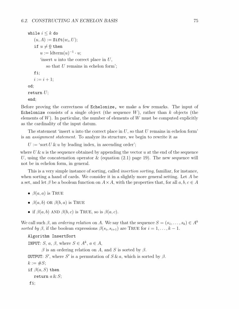
6.2. CONSTRUCTING AN ECHELON BASIS 75
while i ≤ k do
(u,A) := Sift(wi, U);
if u 6= 0 then
u := ldterm(u)−1 · u;
‘insert u into the correct place in U ,
so that U remains in echelon form’;
fi;
i := i+ 1;
od;
return U ;
end;
Before proving the correctness of Echelonize, we make a few remarks. The input ofEchelonize consists of a single object (the sequence W ), rather than k objects (theelements of W ). In particular, the number of elements of W must be computed explicitlyas the cardinality of the input datum.
The statement ‘insert u into the correct place in U , so that U remains in echelon form’is an assignment statement. To analyze its structure, we begin to rewrite it as
U := ‘sortU &u by leading index, in ascending order’;
where U &u is the sequence obtained by appending the vector u at the end of the sequenceU , using the concatenation operator & (equation (2.1) page 19). The new sequence willnot be in echelon form, in general.
This is a very simple instance of sorting, called insertion sorting, familiar, for instance,when sorting a hand of cards. We consider it in a slightly more general setting. Let A bea set, and let β be a boolean function on A×A, with the properties that, for all a, b, c ∈ A
• β(a, a) is TRUE
• β(a, b) OR β(b, a) is TRUE
• if β(a, b) AND β(b, c) is TRUE, so is β(a, c).
We call such β, an ordering relation on A. We say that the sequence S = (s1, . . . , sk) ∈ Aksorted by β, if the boolean expressions β(si, si+1) are TRUE for i = 1, . . . , k − 1.
Algorithm InsertSort
INPUT: S, a, β, where S ∈ Ak, a ∈ A,
β is an ordering relation on A, and S is sorted by β.
OUTPUT: S ′, where S ′ is a permutation of S& a, which is sorted by β.
k := #S;
if β(a, S) then
return a&S;
fi;

76 CHAPTER 6. ALGORITHMS FOR VECTORS
i := 2;
while i ≤ k do
if β(a, S) then
return ((s1, . . . , si−1, a, si, . . . , sk));
fi;
i := i+ 1;
od;
return S&a ;
end;
(A permutation of the elements of a sequence is a rearrangement of them.) Thus, A = Z,and β : (x, y) 7→ x ≤ y, corresponds to sorting integers in ascending order. Returning toEchelonize, we have A = F n, and the ordering relation
β : F n × F n → {TRUE, FALSE} (u, v) 7→ ldindx(u) ≤ ldindx(v)
satisfies the above conditions (because the integers do). With this β, we rewrite ourassignment as
U := InsertSort(U, u, β);
which now features a more familiar syntax.
Proposition 29 The algorithm Echelonize is correct.
Proof: We first show that the boolean expression
L := ‘U is in echelon form’ AND 〈U〉 = 〈w1, . . . , wi−1〉
is a loop invariant for the while-loop W of the algorithm Echelonize.
(Induction basis.) When W first starts executing, i = 1, and U = ( ), which is in echelonform. Also 〈U〉 = 〈 〉 = 〈w1, . . . , w0〉, as required.
(Induction step.) Suppose now that we are executing at the beginning of the statement-sequence of W, i ≤ k, and statement L is true, and U = (u1, . . . , uj), for some j ≥ 0 (If j =0, then U is empty). Then U is in echelon form, and 〈U〉 = 〈u1, . . . , uj〉 = 〈w1, . . . , wi−1〉.
If u = 0, then = 〈u1, . . . , uj〉 = 〈u1, . . . , uj, u〉 = 〈w1, . . . , wi〉.If u 6= 0, then we first set u := ldterm(u)−1 · u and we still have 〈u1, . . . , uj, u〉 =
〈w1, . . . , wi〉 (see exercises). Now, ldterm(u) = 1, and (due to the output specification ofSift) ldindx(u) is not in the set {ldindx(u1), . . . , ldindx(uj)}. Thus, we can (and do),insert u into the correct place in U , so that U remains in echelon form, but now containsj + 1 elements.
In either case, we now have U in echelon form, and 〈U〉 = 〈w1, . . . , wi〉. Thus, aftersetting i := i + 1, L holds, and we are finished executing the statement-sequence of W.This completes the proof that L is a loop invariant for W.

6.3. AN EXAMPLE 77
The rest of the proof that Echelonize works is straightforward. The statement-sequence of W is executed exactly k times, so the algorithm terminates. On termination ofthe execution of W, we have i = k+1 and L holds. Therefore, at that point, U is in echelonforms and 〈U〉 = 〈w1, . . . , w(k+1)−1〉 = 〈w1, . . . , wk〉 so the correct output is recorded.
6.3 An example
Let F = Z/(7) and
w1 = (5, 3, 1, 3), w2 = (3, 6, 2, 6), w3 = (6, 5, 4, 1), w4 = (2, 6, 6, 0) ∈ F 4.
We wish to study the subspaceW = 〈w1, w2, w3, w4〉 of F 4, and determine whether or nota given vector belongs to it.
We first use the algorithm Echelonize to determine a sequence of vectors (u1, . . . , uj)in echelon form, such that 〈u1, . . . , uj〉 =W .
Echelonize(((5, 3, 1, 3), (3, 6, 2, 6), (6, 5, 4, 1), (2, 6, 6, 0))w1 w2 w3 w4
)
k U i i ≤ k Sift(wi, U) u u 6= 04 ( ) 1 T ((5,3,1,3),( )) (5,3,1,3) T
(1,2,3,2)((1,2,3,2)) 2 T ((0,0,0,0),(3)) (0,0,0,0) F
3 T ((0,0,0,3),(6)) (0,0,0,3) T(0,0,0,1)
((1,2,3,2), (0,0,0,1)) 4 T ((0,2,0,3),(2,0)) (0,2,0,3) T(0,1,0,5)
((1,2,3,2), (0,1,0,5), (0,0,0,1)) 5 F
return ((1, 2, 3, 2), (0, 1, 0, 5), (0, 0, 0, 1))
Sift((5, 3, 1, 3), ( )v W
)
k L u ldindx(u) ∈ L i0 { } (5, 3, 1, 3) F
return ((5, 3, 1, 3), ( ))Note that there are no columns for the aj in the tracing of Sift, because when k = 0,
the assignment statement aj := 0; , j = 1, . . . , k is empty.
Sift((3, 6, 2, 6), ((1, 2, 3, 2))v w1
)
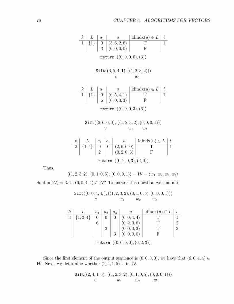
78 CHAPTER 6. ALGORITHMS FOR VECTORS
k L a1 u ldindx(u) ∈ L i1 {1} 0 (3, 6, 2, 6) T 1
3 (0, 0, 0, 0) F
return ((0, 0, 0, 0), (3))
Sift((6, 5, 4, 1), ((1, 2, 3, 2))v w1
)
k L a1 u ldindx(u) ∈ L i1 {1} 0 (6, 5, 4, 1) T 1
6 (0, 0, 0, 3) F
return ((0, 0, 0, 3), (6))
Sift((2, 6, 6, 0), ((1, 2, 3, 2), (0, 0, 0, 1))v w1 w2
)
k L a1 a2 u ldindx(u) ∈ L i2 {1, 4} 0 0 (2, 6, 6, 0) T 1
2 (0, 2, 0, 3) F
return ((0, 2, 0, 3), (2, 0))
Thus,
〈(1, 2, 3, 2), (0, 1, 0, 5), (0, 0, 0, 1)〉 =W = 〈w1, w2, w3, w4〉.So dim(W) = 3. Is (6, 0, 4, 4) ∈ W? To answer this question we compute
Sift((6, 0, 4, 4, ), ((1, 2, 3, 2), (0, 1, 0, 5), (0, 0, 0, 1))v w1 w2 w3
)
k L a1 a2 a3 u ldindx(u) ∈ L i3 {1, 2, 4} 0 0 0 (6, 0, 4, 4) T 1
6 (0, 2, 0, 6) T 22 (0, 0, 0, 3) T 3
3 (0, 0, 0, 0) F
return ((0, 0, 0, 0), (6, 2, 3))
Since the first element of the output sequence is (0, 0, 0, 0), we have that (6, 0, 4, 4) ∈W . Next, we determine whether (2, 4, 1, 5) is in W .
Sift((2, 4, 1, 5), ((1, 2, 3, 2), (0, 1, 0, 5), (0, 0, 0, 1))v w1 w2 w3
)

6.4. TESTING SUBSPACES 79
k L a1 a2 a3 u ldindx(u) ∈ L i3 {1, 2, 4} 0 0 0 (2, 4, 1, 5) T 1
2 (0, 0, 2, 1) F
return ((0, 0, 2, 1), (2, 0, 0))
Since (0, 0, 2, 1) 6= (0, 0, 0, 0) we conclude that (2, 4, 1, 5) 6∈ W .
6.4 Testing subspaces
Let F be a field, and
v1, . . . , vl, w1, . . . , wk ∈ F n, V = 〈v1, . . . , vl〉, W = 〈w1, . . . , wk〉.
How can we determine whether or not V ⊆ W?
We proceed as follows. First, let U := Echelonize((w1, . . . , wk)). Then U is inechelon form, and 〈U〉 =W . Suppose U = (u1, . . . , uj). Now V ⊆ W iff vi ∈ W for eachi = 1, . . . , l. Thus, V ⊆ W iff Sift(vi, (u1, . . . , uj)) returns (0, Ai), for each i = 1, . . . , l.(We do not care what is Ai for this application.)
Thus, from our previous example (section 6.3), we conclude that
〈(6, 0, 4, 4)〉 ⊆ W 〈(6, 0, 4, 4), (2, 4, 1, 5)〉 6⊆ W .
We can also test whether or not V = W , since V = W iff V ⊆ W and W ⊆ V .Alternatively, V =W iff V ⊆ W and dim(V) = dim(W).
Exercises
Exercise 6.1. Let F = Z/(2).
(a) Write down all the elements of F 3.
(b) Write down all the sequences in echelon form of elements of F 2.
Exercise 6.2. Let w1 = (1, 1, 0), w2 = (2, 2, 2) be vectors in (Z/(3))3, and let W =〈w1, w2〉.
(a) Write down all the elements of W .
(b) For each w ∈ W , determine ldindx(w), and if w 6= 0, determine ldterm(w).
Exercise 6.3. Let v, w1, w2, w3 ∈ Q3, with
v = (4/7,−3/5, 5/7); w1 = (1, 1/2, 1), w2 = (0, 1, 2), w3 = (0, 0, 1).
(a) Trace Sift(v, (w1, w2, w3)).
(b) Write v as a linear combination of w1, w2, w3, verifying your calculation explicitly.

80 CHAPTER 6. ALGORITHMS FOR VECTORS
Exercise 6.4. Let F = Z/(11), and let
w1 = (1, 0, 7, 3) w2 = (0, 1, 3, 4) w3 = (0, 0, 0, 1) ∈ F 4.
(a) Use the algorithm Sift to prove that (5, 2, 4, 3) 6∈ 〈w1, w2, w3〉.(b) Use the algorithm Sift to prove that v = (6, 2, 4, 3) ∈ 〈w1, w2, w3〉. Hence write
v as a linear combination of w1, w2, w3, verifying your calculation explicitly.
Exercise 6.5. Let F = Q, R, C, or Z/(p), p a prime (or indeed let F be any field), andlet v1, . . . , vk ∈ F n.
(a) Let 0 6= α ∈ F . Prove that
〈v1, . . . , vk−1, αvk〉 = 〈v1, . . . , vk〉.
(b) Prove that if the sequence (v1, . . . , vk) is in echelon form, then v1, . . . , vk arelinearly independent.
(c) Let F = Z/(p), p a prime. Using Echelonize, prove that if W is the subspaceof F n generated by the vectors W = (w1, . . . , wm), then #W = ps, for some s, with0 ≤ s ≤ n. Explain what is s.
Exercise 6.6. Let F = Z/(2), and let v1 = (0, 1, 0, 1), v2 = (0, 0, 0, 0) v3 = (1, 1, 0, 1),v4 = (1, 0, 1, 0), v5 = (0, 1, 1, 1) be in F 4. Use the algorithm Echelonize to determine asequence U , in echelon form, of vectors in F 4, such that 〈U〉 = 〈v1, . . . , v5〉.Exercise 6.7. Let F = Z/(5), and let
v1 = (4, 3, 1, 3) v2 = (1, 3, 4, 1) v3 = (2, 3, 3, 2) ∈ F 4.
(a) Use the algorithm Echelonize to determine a sequence U , in echelon form, ofvectors in F 4, such that 〈U〉 = 〈v1, v2, v3〉.
(b) Let V = 〈v1, v2, v3〉.Which of the following vectors belong to V?
(2, 1, 3, 1) (3, 1, 4, 2) (2, 2, 4, 3).
In each case, explain why.
Exercise 6.8.
(a) Let A be any set. Write an algorithm to the following specifications
Algorithm Match
INPUT: a, S where a ∈ A and S = (s1, . . . , sn) ∈ AnOUTPUT: i, where i is the smallest integer such that a = si,
if such i exist, or the empty sequence otherwise.
(b) Using Match, write the algorithm MatchLeadingIndices, introduced at page 71in connection with the algorithm Sift.
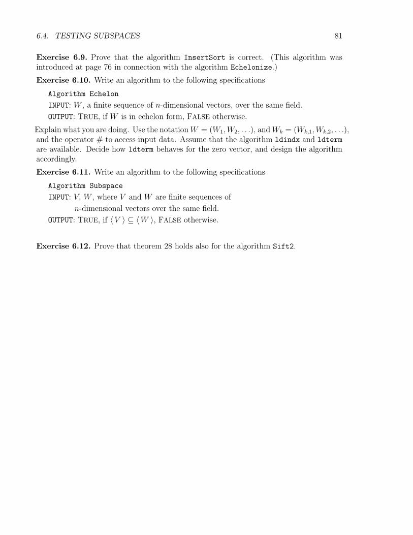
6.4. TESTING SUBSPACES 81
Exercise 6.9. Prove that the algorithm InsertSort is correct. (This algorithm wasintroduced at page 76 in connection with the algorithm Echelonize.)
Exercise 6.10. Write an algorithm to the following specifications
Algorithm Echelon
INPUT: W , a finite sequence of n-dimensional vectors, over the same field.
OUTPUT: TRUE, if W is in echelon form, FALSE otherwise.
Explain what you are doing. Use the notationW = (W1,W2, . . .), andWk = (Wk,1,Wk,2, . . .),and the operator # to access input data. Assume that the algorithm ldindx and ldterm
are available. Decide how ldterm behaves for the zero vector, and design the algorithmaccordingly.
Exercise 6.11. Write an algorithm to the following specifications
Algorithm Subspace
INPUT: V, W , where V and W are finite sequences of
n-dimensional vectors over the same field.
OUTPUT: TRUE, if 〈V 〉 ⊆ 〈W 〉, FALSE otherwise.
Exercise 6.12. Prove that theorem 28 holds also for the algorithm Sift2.

82 CHAPTER 6. ALGORITHMS FOR VECTORS

Chapter 7
Some Proofs∗
7.1 A note on ring theory
Let R be a commutative ring with identity, and a, b,∈ R. In our proofs we have beenusing the fact that
(i) a0 = 0
(ii) (−a)b = −(ab).
We now prove these facts using the definition of a commutative ring with identity. (Asusual a− b means a+ (−b).)
Proof of (i). We have a0 = a(0 + 0) = a0 + a0 (distributive law). Thus, a0 − (a0) =(a0 + a0)− (a0) = a0 + (a0− (a0)) (associative law), hence 0 = a0 + 0 = a0.
Proof of (ii). We have, using the distributive law ab+ (−a)b = (a− a)b = 0b = 0, thelast step deriving from (i). Thus, (−a)b = −(ab), since additive inverses are unique in R,for if s, t ∈ R and a+ s = a+ t = 0 then
s+ a+ s = s+ a+ t =⇒ 0 + s = 0 + t =⇒ s = t.
[Note also that additive identities are unique in R, as are multiplicative identities, for ifr, s ∈ R, 0 + r = 0 =⇒ r = 0 and 1s = 1 =⇒ s = 1.]
7.2 Uniqueness of quotient and remainder
We prove the uniqueness of aDIV b and aMOD b for integers and polynomials.
Theorem 30 Suppose a, b,∈ Z, b 6= 0, and a = bq1 +r1 = bq2 +r2 such that q1, q2, r1, r2 ∈Z and 0 ≤, rr, r2 < |b|. Then q1 = q2 and r1 = r2.
83

84 CHAPTER 7. SOME PROOFS∗
Proof: From the fact that bq1 + r1 = bq2 + r2 we have that b(q1 − q2) = r2 − r1.
Case (i): q1 = q2. Then b(q1 − q2) = 0, hence r1 − r2 = 0 and r1 = r2.
Case (ii): q1 6= q2. Then
|r2 − r1| = |b(q1 = q2)| = |b| |q1 − q2| ≥ |b|.
However, 0 ≤ r1, r2 < |b|, hence |r1 − r2| < |b|, a contradiction. Thus, q1 = q2, so, bycase (i), r1 − r2.
Theorem 31 Let R be a commutative ring with identity, a, b,∈ R[x], b 6= 0, and ldcf(b)invertible. Suppose a = bq+r1 = bq+r2 such that q1, q2, r1, r2 ∈ R[x] and deg(r1), deg(r2) <deg(b). Then q1 = q2 and r1 = r2.
Proof: As in the proof of the previous theorem, we have that b(q1 − q2) = r2 − r1.
Case (i): q1 = q2. Then b(q1 − q2) = 0, hence r1 − r2 = 0 and r1 = r2.
Case (ii): q1 6= q2. Then
deg(r2 − r1) = deg(b(q1 = q2)) = deg(b) + deg(q1 − q2) ≥ deg(b)
where the first equality follows from the fact that ldcf(b) is invertible and q1 − q2 = 0.
But deg(r2 − r1) < deg(b), a contraction. Thus, q1 = q2, so, by case (i), r1 − r2.

Chapter 8
Hints for exercises
Chapter 1
Exercise 1.3. Find a counterexample (you do not have to look too far).
Exercise 1.4. Part (f): 47 is the sum of two squares if and only if, for some squarex2 ≤ 47, we have that 47− x2 is also a square (necessarily in the same range).
Exercise 1.9. Part (b): there is only one thing that can go wrong.
Exercise 1.12. First do exercise 1.4 (f). You may find it convenient to build the sequenceof squares not exceeding x.
Chapter 2
Exercise 2.2. Part (c): remember that aMOD b = r means a = qb+ r, for some q. Howdo you represent an odd integer?Part (d): treat the case z even and odd separately.
Exercise 2.11. Part (c): do you need to test even integers?
Exercise 2.9. The difficulty lies in turning the sentence ‘but not by both’ into a booleanexpression. What boolean operator corresponds to ‘but’?
Exercise 2.10. Part (b): the output of IntegerFactorization is a finite sequence P ;denote its cardinality by #P , and its elements by Pi, i = 1, . . . ,#P . Treat the case n = 1separately.
Exercise 2.15. Part (b): represent n in base 2.
Chapter 3
Exercise 3.5. Analyze the possible partitions of a set with 5 elements, and for each countthe number of elements of the corresponding equivalence relation.
85

86 CHAPTER 8. HINTS FOR EXERCISES
Exercise 3.7. Measure efficiency by the number of evaluations of the function P . Howmany evaluations are involved in the above formula? How could such number be reduced?Look at concrete examples involving small sets X.
Exercise 3.8. The formulation of this exercise is deliberately cryptic: give yourself timeto think about it. You’ll need a nested loop.
Chapter 4
Exercise 4.1. Part (b): use Theorem 12, page 40, and induction.
Exercise 4.8. Part (b): examine some examples, then infer from them the general phe-nomenon. The essay should contain no reference to specific examples.
Chapter 5
Exercise 5.3. Part (b): see how the loop invariant for the while-loop of algorithmPolynomialQuoRem was proved.
Exercise 5.4. Part (a) when analyzing the effect of the statement-sequence of W, considerthe cases b even and b odd separately.
Chapter 6
Exercise 6.5. Part (a): show that the left-hand side is contained in the rigth-hand side,and vice-versa.Part (b): this is linear algebra.Part (c): use the result of the previous problem..
Exercise 6.10. The problem is that if ldterm(0) = (), then expressions of the type () = 1make no sense.

Index
additionadditive inverse, 42, 43, 79additive order, 44in Z/(m), 41
algorithmdeterministic, 1nested, 22probabilistic, 1recursive, 52, 54
cartesian plane, 31characteristic function, 11, 16, 17, 23congruence, 39constant
boolean, 5
De Morgan’s laws, 11Digits, 21digits
shift, 22DIV, 15, 16, 40, 49–53do, 7
echelon form, 68Echelonize, 71, 73, 74, 76
else, 5equivalence relation, see relationEuclid’s algorithm, see greatest common
divisorEuler’s φ-function, 43, 66Evaluate, 60, 61expression
algebraic, 2arithmetical, 2, 15boolean, 5, 9, 15, 31relational, 5
Factorial, 52, 53fi, 5
field, 64fields, 53, 62, 68
finite, 59fundamental theorem of arithmetic, 18
graphCollatz graph, 25complete, 34of a relation, 31, 32
greatest common divisorEuclid’s algorithm, 54extended Euclid’s algorithm, 54ExtendedGCD, 54, 55, 58GCD, 54, 55
halting problem, 24Horner’s algorithm, 60
ifif control expressions, 5
if, 5indeterminate, see polynomialsinduction, 49, 51, 53
strong, 55input, 1insertion sorting, 72Interpolate, 62, 63invertible element, 42
Inverse, 58inverse, 42, 43
limit cycle, 25long division, 15, 49loop
loop control expressions, 7loop invariant, 49–51, 62, 63, 69, 71,
73Lucas, 27
MOD, 15, 16, 21, 22, 40, 49, 51–53
87
88 INDEX
multiplicationidentity element, 53in Z/(m), 41multiplicative inverse, see invertible
elementmultiplicative order, 45
nested structures, 8nonomial, 47
od, 7operator
binary, 9boolean, 9concatenation, 19, 72unary, 9
ordering relation, 72output, 1
permutation, 73polynomials, 47
degree, 47equality of, 48indeterminate, 47over a field, 55, 56over a fields, 54zero polynomial, 47, 60
primes, 16IntegerFactorization, 19IsPrime, 17largest know prime, 5NextPrime, 8Sophie Germain primes, 28twin primes, 24
relationequivalence relation, 32on a field, 67on a set, 31
return, 1, 4rings, 43, 80
additive identity, 43associative laws, 43commutative laws, 43multiplicative identity, 43without identity, 43
sequencesconcatenation, 19equality, 19length, 19
setscardinality, 19cartesian product, 31partition, 33
Sift, 69, 71statement
assignment, 3, 4, 72statement sequence, 2
then, 5tracing, 3truth table, 10
vectors, 67dimension, 67equal, 67leading index, 67leading term, 67linear combination, 68linear span, 68scalar multiple, 68subspace, 68sum, 67zero vector, 67
while, 7, 8, 17, 21, 50, 60, 62