algorithmic complexity for psychology: a user-friendly

Algorithmic complexity for psychology: A user-friendlyimplementation of the coding theorem method.Nicolas Gauvrit

CHArt (PARIS-reasoning), Ecole Pratique des HautesEtudes, Paris, France

Henrik SingmannInstitut fur Psychologie, Albert-Ludwigs-Universitat

Freiburg, Freiburg, Germany.

Fernando Soler-ToscanoGrupo de Logica, Lenguaje e Informacion, Universidad de

Sevilla, Spain.

Hector ZenilUnit of Computational Medicine, Center for Molecular

Medicine, Karolinska Institute, Stockholm, Sweden

Corresponding author: Nicolas Gauvrit, [email protected]

Kolmogorov-Chaitin complexity has long been believed to be impossible to approximatewhen it comes to short sequences (e.g. of length 5-50). However, with the newly developedcoding theorem method the complexity of strings of length 2-11 can now be numericallyestimated. We present the theoretical basis of algorithmic complexity for short strings (ACSS)and describe an R-package providing functions based on ACSS that will cover psychologists’needs and improve upon previous methods in three ways: (1) ACSS is now available not onlyfor binary strings, but for strings based on up to 9 different symbols, (2) ACSS no longerrequires time-consuming computing, and (3) a new approach based on ACSS gives access toan estimation of the complexity of strings of any length. Finally, three illustrative examplesshow how these tools can be applied to psychology.

Keywords: algorithmic complexity, randomness, subjective probability, coding theoremmethod

Randomness and complexity are two concepts which are in-timately related and are both central to numerous recent de-velopments in various fields, including finance (Taufemback,Giglio, & Da Silva, 2011; Brandouy, Delahaye, Ma, &Zenil, 2012), linguistics (Gruber, 2010; Naranan, 2011),neuropsychology (Machado, Miranda, Morya, Amaro Jr, &Sameshima, 2010; Fernandez et al., 2011, 2012), psychiatry(Yang & Tsai, 2012; Takahashi, 2013), genetics (Yagil, 2009;Ryabko, Reznikova, Druzyaka, & Panteleeva, 2013), sociol-ogy (Elzinga, 2010) and the behavioral sciences (Watanabeet al., 2003; Scafetta, Marchi, & West, 2009). In psychol-ogy, randomness and complexity have recently attracted in-terest, following the realization that they could shed light ona diversity of previously undeciphered behaviors and mentalprocesses. It has been found, for instance, that the subjectivedifficulty of a concept is directly related to its “boolean com-plexity”, defined as the shortest logical description of a con-cept (Feldman, 2000, 2003, 2006). In the same vein, visualdetection of shapes has been shown to be related to contourcomplexity (Wilder, Feldman, & Singh, 2011).

Henrik Singmann is now at the Department of Psychology, Uni-versity of Zurich (Switzerland).We would like to thank William Matthews for providing the datafrom his 2013 manuscript.

More generally, perceptual organization itself has beendescribed as based on simplicity or, equivalently, likelihood(Chater, 1996; Chater & Vitanyi, 2003), in a model recon-ciling the complexity approach (perception is organized tominimize complexity) and a probability approach (percep-tion is organized to maximize likelihood), very much in linewith our view in this paper. Even the perception of similaritymay be viewed through the lens of (conditional) complexity(U. Hahn, Chater, & Richardson, 2003).

Randomness and complexity also play an important rolein modern approaches to selecting the “best” among a setof candidate models (i.e., model selection; e.g., Myung,Navarro, & Pitt, 2006; Kellen, Klauer, & Broder, 2013), asdiscussed in more detail below in the section called “Rela-tionship to complexity based model selection”.

Complexity can also shed light on short term memorystorage and recall, more specifically, on the process un-derlying chunking. It is well known that the short termmemory span lies between 4 and 7 items/chunks (Miller,1956; Cowan, 2001). When instructed to memorize longersequences of, for example, letters or numbers, individualsemploy a strategy of subdividing the sequence into chunks(Baddeley, Thomson, & Buchanan, 1975). However, the waychunks are created remains largely unexplained. A plausibleexplanation might be that chunks are built via minimizing thecomplexity of each chunk. For instance, one could split thesequence “AAABABABA” into the two substrings “AAA”

2 NICOLAS GAUVRIT

and “BABABA”. Very much in line with this idea, Mathyand Feldman (2012) provided evidence for the hypothesisthat chunks are units of “maximally compressed code”. Inthe above situation, both “AAA” and “BABABA” are suppos-edly of low complexity, and the chunks tailored to minimizethe length of the resulting compressed information.

Outside the psychology of short term memory, the com-plexity of pseudo-random human-generated sequences is re-lated to the strength of executive functions, specifically to in-hibition or sustained attention (Towse & Cheshire, 2007). Inrandom generation tasks, participants are asked to generaterandom-looking sequences, usually involving numbers from1 to 6 (dice task) or digits between 1 and 9. These tasks areeasy to administer and very informative in terms of higherlevel cognitive abilities. They have been used in investiga-tions in various areas of psychology, such as visual percep-tion (Cardaci, Di Gesu, Petrou, & Tabacchi, 2009), aesthet-ics (Boon, Casti, & Taylor, 2011), development (Scibinetti,Tocci, & Pesce, 2011; Pureza, Goncalves, Branco, Grassi-Oliveira, & Fonseca, 2013), sport (Audiffren, Tomporowski,& Zagrodnik, 2009), creativity (Zabelina, Robinson, Coun-cil, & Bresin, 2012), sleep (Heuer, Kohlisch, & Klein, 2005;Bianchi & Mendez, 2013), and obesity (Crova et al., 2013),to mention a few. In neuropsychology, random number gen-eration tasks and other measures of behavioral or brain activ-ity complexity have been used to investigate different disor-ders, such as schizophrenia (Koike et al., 2011), autism (Laiet al., 2010; Maes, Vissers, Egger, & Eling, 2012; Fournier,Amano, Radonovich, Bleser, & Hass, 2013), depression(Fernandez et al., 2009), PTSD (Pearson & Sawyer, 2011;Curci, Lanciano, Soleti, & Rime, 2013), ADHD (Sokunbi etal., 2013), OCD (Bedard, Joyal, Godbout, & Chantal, 2009),hemispheric neglect (Loetscher & Brugger, 2009), aphasia(Proios, Asaridou, & Brugger, 2008), and neurodegenera-tive syndromes such as Parkinson’s and Alzheimer’s disease(Brown & Marsden, 1990; T. Hahn et al., 2012).

Perceived complexity and randomness are also of theutmost importance within the “new paradigm psychologyof reasoning” (Over, 2009). As an example, let us con-sider the representativeness heuristic (Tversky & Kahne-man, 1974). Participants usually believe that the sequence“HTHTHTHT” is less likely to occur than the sequence“HTHHTHTT” when a fair coin is tossed 8 times. This ofcourse is mathematically wrong, since all sequences of 8heads or tails, including these two, share the same proba-bility of occurrence (1/28). The “old paradigm” was con-cerned with finding such biases and attributing irrationalityto individuals (Kahneman, Slovic, & Tversky, 1982). In the“new paradigm” on the other hand, researchers try to dis-cover the ways in which sound probabilistic or Bayesian rea-soning can lead to the observed errors (Manktelow & Over,1993; U. Hahn & Warren, 2009).

We can find some kind of rationality behind the wrong an-swer, by assuming that individuals do not estimate the prob-ability that a fair coin will produce a particular string s butrather the “inverse” probability that the process underlyingthis string is mere chance. More formally, if we use s todenote a given string, R to denote the event where a string

has been produced by a random process, and D to denotethe complementary event where a string has been producedby a non-random (or deterministic) process, then individualsmay assess P(R|s) instead of P(s|R). If they do so withinthe framework of formal probability theory (and the newparadigm postulates that individuals tend to do so), then theirestimation of the probability should be such that Bayes’ the-orem holds:

P(R|s) =P(s|R)P(R)

P(s|R)P(R) + P(s|D)P(D). (1)

Alternatively, we could assume that individuals do not es-timate the complete inverse P(R|s) but just the posterior oddsof a given string being produced by a random rather than adeterministic process (Williams & Griffiths, 2013). Again,these odds are given by Bayes’ theorem:

P(R|s)P(D|s)

=P(s|R)P(s|D)

×P(R)P(D)

. (2)

The important part of Equation 2 is the first term on theright-hand side, as it is a function of the observed string sand independent of the prior odds P(R)/P(D). This likeli-hood ratio, also known as the Bayes factor (Kass & Raftery,1995), quantifies the evidence brought by the string s basedon which the prior odds are changed. In other words, this partcorresponds to the “amount of evidence [s] provides in favorof a random generating process” (Hsu, Griffiths, & Schreiber,2010).

The numerator of the Bayes factor, P(s|R), is easily com-puted, and amounts to 1/28 in the example given above.However the other likelihood, the probability of s giventhat it was produced by an (unknown) deterministic pro-cess, P(s|D), is more problematic. Although this probabilityhas been informally linked to complexity, to the best of ourknowledge no formal account of that link has ever been pro-vided in the psychological literature, although some authorshave suggested such a link (e.g., Chater, 1996). As we willsee, however, computer scientists have fruitfully addressedthis question (Solomonoff, 1964a, 1964b; Levin, 1974). Onecan think of P(s|D) as the probability that a randomly se-lected (deterministic) algorithm produces s. In this sense,P(s|D) is none other than the so-called algorithmic probabil-ity of s. This probability is formally linked to the algorithmiccomplexity K(s) of the string s by the following formula (seebelow for more details):

K(s) ≈ − log2(P(s|D)). (3)

A normative measure of complexity and a way to makesense of P(s|D) are crucial to several areas of research inpsychology. In our example concerning the representative-ness heuristic, one could see some sort of rationality in theusually observed behavior if in fact the complexity of s1 =“HTHTHTHT” were lower than that of s2 = “HTHHTHTT”(which it is, as shown below). Then following Equation 3,P(s1|D) > P(s2|D). Consequently, the Bayes factor for astring being produced by a random process would be larger

ALGORITHMIC COMPLEXITY FOR PSYCHOLOGY: A USER-FRIENDLY IMPLEMENTATION OF THE CODING THEOREM METHOD. 3

for s2 than for s1. In other words, even when ignoring thequestion of the priors for a random versus deterministic pro-cess (which are inherently subjective and debatable) s2 pro-vides more evidence for a random process than s1.

Researchers have hitherto relied on an intuitive percep-tion of complexity, or in the last decades developed andused several tailored measures of randomness or complex-ity (Towse, 1998; Barbasz, Stettner, Wierzchon, Piotrowski,& Barbasz, 2008; Schulter, Mittenecker, & Papousek, 2010;Williams & Griffiths, 2013; U. Hahn & Warren, 2009) inthe hope of approaching algorithmic complexity. Becauseall these measures rely upon choices that are partially sub-jective and each focuses on a single characteristic of chance,they have come under strong criticism (Gauvrit, Zenil, De-lahaye, & Soler-Toscano, 2013). Among these measures,some have a sound mathematical basis, but focus on partic-ular features of randomness. For that reason, contradictoryresults have been reported (Wagenaar, 1970; Wiegersma,1984). The mathematical definition of complexity, known asKolmogorov-Chaitin complexity theory (Kolmogorov, 1965;Chaitin, 1966), or simply algorithmic complexity, has beenrecognized as the best possible option by mathematicians (Li& Vitanyi, 2008) and psychologists (Griffiths & Tenenbaum,2003, 2004). However, because algorithmic complexity wasthought to be impossible to approximate for the short se-quences we usually deal with in psychology (sequences of5-50 symbols, for instance), it has seldom been used.

In this article, we will first briefly describe algorithmiccomplexity theory and its deep links with algorithmic proba-bility (leading to a formal definition of the probability that anunknown deterministic process results in a particular obser-vation s). We will then describe the practical limits of algo-rithmic complexity and present a means to overcome them,namely the coding theorem method, the root of algorithmiccomplexity for short strings (ACSS). A new set of tools, bun-dled in a package for the statistical programming languageR (R Core Team, 2014) and based on ACSS, will then bedescribed. Finally, three short applications will be presentedfor illustrative purposes.

Algorithmic complexity for shortstrings

Algorithmic complexityAs defined by Alan Turing, a universal Turing machine is

an abstraction of a general-purpose computing device capa-ble of running any computer program. Among universal Tur-ing machines, some are prefix free, meaning that they onlyaccept programs finishing with an “END” symbol. The al-gorithmic complexity (Kolmogorov, 1965; Chaitin, 1966) –also called Kolmogorov or Kolmogorov-Chaitin complexity– of a string s is given by the length of the shortest com-puter program running on a universal prefix-free Turing ma-chine U that produces s and then halts, or formally written,KU(s) = min{|p| : U(p) = s}. From the invariance theo-rem (Calude, 2002; Li & Vitanyi, 2008), we know that theimpact of the choice of U (that is, of a specific Turing ma-chine), is limited and independent of s. It means that for

any other universal Turing machine U′, the absolute valueof KU(s) − KU′ (s) is bounded by some constant CU,U′ whichdepends on U and U′ but not on the specific s. So K(s) isusually written instead of KU(s).

More precisely, the invariance theorem states that K(s)computed on two different Turing machine will differ at mostby an additive constant c, which is independent of s, but thatcan be arbitrary large. One consequence of this theorem isthat there actually are infinitely many different complexities,depending on the Turing machine. Talking about “the al-gorithmic complexity” of a string is a shortcut. This theo-rem also guarantees that asymptotically (or for long strings),the choice of the Turing machine will have limited impact.However, for short strings we are considering here, the im-pact could be important, and different Turing machines canyield different values, or even different orders. This limita-tion is not due to technical reasons, but the fact that thereis no objective default universal Turing machine one couldpick to compute “the” complexity of a string. As we will ex-plain below, our approach seeks to overcome this difficultyby defining what could be thought of as a “mean complex-ity” as computed with random Turing machines. Becausewe do not choose a particular Turing machine but samplethe space of all possible Turing machine (running on a blanktape), the result will be an objective estimation of algorith-mic complexity, although it will of course differ from mostspecific KU .

Algorithmic complexity gave birth to a definition of ran-domness. To put it in a nutshell, a string is random if it iscomplex (i.e. exhibit no structure). Among the most strik-ing results of algorithmic complexity theory is the conver-gence in definitions of randomness. For example, using mar-tingales, Schnorr (1973) proved that Kolmogorov random(complex) sequences are effectively unpredictable and viceversa; Chaitin (2004) proved that Kolmogorov random se-quences pass all effective statistical tests for randomness andvice versa, and are therefore equivalent to Martin-Lof ran-domness (Martin-Lof, 1966), hence the general acceptanceof this measure. K has become the accepted ultimate univer-sal definition of complexity and randomness in mathematicsand computer science (Downey & Hirschfeldt, 2008; Nies,2009; Zenil, 2011a).

One generally offered caveat regarding K is that it is un-computable, meaning there is no Turing machine or algo-rithm that, given a string s, can output K(s), the length ofthe shortest computer program p that produces s. In fact, thetheory shows that no computable measure can be a universalcomplexity measure. However, it is often overlooked that Kis upper semi-computable. This means that it can be effec-tively approximated from above. That is, that there are effec-tive algorithms, such as lossless compression algorithms, thatcan find programs (the decompressor + the data to reproducethe string s in full) giving upper bounds of Kolmogorov com-plexity. However, these methods are inapplicable to shortstrings (of length below 100), which is why they are seldomused in psychology. One reason why compression algorithmsare unadapted to short strings is that compressed files includenot only the instructions to decompress the string, but also

4 NICOLAS GAUVRIT

file headers and other data structures. It makes that for ashort string s, the size of a compressed text file with just s islonger than |s|. Another reason is that, as it is the case withthe complexity KU associated with a particular Turing ma-chine U, the choice of the compression algorithm is crucialfor short strings, because of the invariance theorem.

Algorithmic probability and its relationship to al-gorithmic complexity

A universal prefix-free Turing machine U, can also beused to define a probability measure m on the set of all pos-sible strings by setting m(s) =

∑p:U(p)=s 1/2|p|, where p is

a program of length |p|, and U(p) the string produced bythe Turing machine U fed with program p. The Kraft in-equality (Calude, 2002) guarantees that 0 ≤

∑s m(s) < 1.

The number m(s) is the probability that a randomly selecteddeterministic program will produce s and then halt, or sim-ply the algorithmic probability of s, and provides a formaldefinition of P(s|D), where D stands for a generic determin-istic algorithm (for a more detailed description see Gauvritet al., 2013). Numerical approximations to m(s) using stan-dard Turing machines have shed light on the stability androbustness of m(s) in the face of changes in U, providing ex-amples of applications to various areas leading to semanticmeasures (Cilibrasi & Vitanyi, 2005, 2007), which today areaccepted as regular methods in areas of computer science andlinguistics, to mention but two disciplines.

Recent work (Delahaye & Zenil, 2012; Zenil, 2011b) hassuggested that approximating m(s) could in practice be usedto approximate K for short strings. Indeed, the algorithmiccoding theorem (Levin, 1974) establishes the connection asK(s) = − log2 m(s) + O(1), where O(1) is bounded indepen-dently of s. This relationship shows that strings with lowK(s) have the highest probability m(s), while strings withlarge K(s) have a correspondingly low probability m(s) ofbeing generated by a randomly selected deterministic pro-gram. This approach, based upon and motivated by algorith-mic probability, allows us to approximate K by means otherthan lossless compression, and has been recently applied tofinancial time series (Brandouy et al., 2012; Zenil & Dela-haye, 2011) and in psychology (e.g. Gauvrit, Soler-Toscano,& Zenil, 2014). The approach is equivalent to finding thebest possible compression algorithm with a particular com-puter program enumeration.

Here, we extend a previous method addressing the ques-tion of binary strings’ complexity (Gauvrit et al., 2013) inseveral ways. First, we provide a method to estimate thecomplexity of strings based on any number of different sym-bols, up to 9 symbols. Second, we provide a fast and user-friendly algorithm to compute this estimation. Third, we alsoprovide a method to approximate the complexity (or the localcomplexity) of strings of medium length (see below).

The invariance theorem and the problem with shortstrings

The invariance theorem does not provide a reason to ex-pect − log2(m(s)) and K(s) to induce the same ordering over

short strings. Here, we have chosen a simple and stan-dard Turing machine model (the Busy Beaver model; Rado,1962)1 in order to build an output distribution based on theseminal concept of algorithmic probability. This output dis-tribution then serves as an objective complexity measure pro-ducing results in agreement both with intuition and with K(s)to which it will converge for long strings guaranteed by theinvariance theorem. Furthermore, we have found that esti-mates of K(s) are strongly correlated to those produced bylossless compression algorithms as they have traditionallybeen used as estimators of K(s) (compressed data is a suffi-cient test of non-randomness, hence of low K(s)), when bothtechniques (the coding theorem method and lossless com-pression) overlap in their range of application for mediumsize strings in the order of hundreds to 1K bits.

The lack of guarantee in obtaining K(s) from − log2(m(s))is a problem also found in the most traditional method toestimate K(s). Indeed, there is no guarantee that some loss-less compressor algorithm will be able to compress a stringthat is compressible by some (or many) other(s). We dohave statistical evidence that, at least with the Busy Beavermodel, extending or reducing the Turing machine samplespace does not impact the order (Zenil, Soler-Toscano, De-lahaye, & Gauvrit, 2012; Soler-Toscano, Zenil, Delahaye, &Gauvrit, 2014, 2013). We also found a correlation in outputdistribution using very different computational formalisms,e.g. cellular automata and Post tag systems (Zenil & Dela-haye, 2010). We have also shown (Zenil et al., 2012) that− log2(m(s)) produces results compatible with compressionmethods K(s), and strongly correlates to direct K(s) calcula-tion (length of first shortest Turing machine found producings; Soler-Toscano et al., 2013).

The coding theorem method in practiceThe basic idea at the root of the coding theorem method

is to compute an approximation of m(s). Instead of choosinga particular Turing machine, we ran a huge sample of Tur-ing machines, and saved the resulting strings. The distribu-tion of resulting strings gives the probability that a randomlyselected Turing machine (equivalent to a universal Turingmachine with a randomly selected program) will result in agiven string. It therefore approximates m(s). From this, weestimate an approximation K of the algorithmic complexityof any string s using the equation K(s) = − log2(m(s)). Toput it in a nutshell again: A string is complex and henceforthrandom if the likelihood of it being produced by a randomlyselected algorithm is low, which we estimated as describedin the following.

To actually build the frequency distributions of stringswith different numbers of symbols, we used a Turing ma-chine simulator, written in C++, running on a supercomputerof middle-size at CICA (Centro Informatico Cientıfico deAndalucıa). The simulator runs Turing machines in (n,m)(n is the number of states of the Turing machine, and m thenumber of symbols it uses) over a blank tape and stores the

1 A demonstration is available online athttp://demonstrations.wolfram.com/BusyBeaver/


(n,m) Steps Machines Time(5,2) 500 9 658 153 742 336 450 days(4,4) 2000 3.34 × 1011 62 days(4,5) 2000 2.14 × 1011 44 days(4,6) 2000 1.8 × 1011 41 days(4,9) 4000 2 × 1011 75 days

Table 1Data of the computations to build the frequency distributions

output of halting computations. For the generation of ran-dom machines, we used the implementation of the MersenneTwister in the Boost C++ library.

Table 1 summarizes the size of the computations to buildthe distributions. The data corresponding to (5, 2) comesfrom a full exploration of the space of Turing machines with5 states and 2 symbols, as explained in Soler-Toscano, Zenil,Delahaye and Gauvrit (2014, 2013). All other data, previ-ously unpublished, correspond to samples of machines. Thesecond column is the runtime cut. As the detection of non-halting machines is an undecidable problem, we stopped thecomputations exceeding that runtime. To determine the run-time bound, we first picked a sample of machines with anapt runtime T . For example, in the case of (4, 4), we ran1.68 × 1010 machines with a runtime cut of 8000 steps. Forhalting machines in that sample, we built the runtime distri-bution (Fig. 1). Then we chose a runtime lower than T withan accumulated halting probability very close to 1. That waywe chose 2000 steps for (4, 4). In Soler-Toscano et al. (2014)we argued that, following this methodology, we were able tocover the vast majority of halting machines.

The third column in Table 1 is the size of the sample, thatis, the machines that were actually run at the C++ simula-tor. After these computations, several symmetric comple-tions were applied to the data, so in fact the number of ma-chines represented in the samples is greater. For example,we only considered machines moving to the right at the ini-tial transition. So we complemented the set of output stringswith their reversals. More details about the shortcuts to re-

2000 4000 6000 8000

0.999997

0.999998

0.999998

0.999999

0.999999

1.000000

Figure 1. Runtime distribution in (4, 4). More than 99.9999%of the Turing machines that stopped in 8000 steps or less actuallyhalted before 2000 steps.

duce the computations and the completions can be foundelsewhere (Soler-Toscano et al., 2013). The last column inTable 1 is an estimate of the time the computation would havetaken on a single processor at the CICA supercomputer. Aswe used between 10 and 70 processors, the actual times thecomputations took were shorter. In the following paragraphswe offer some details about the datasets obtained for each setof symbols.

(5,2). This distribution is the only one previously pub-lished (Soler-Toscano et al., 2014; Gauvrit et al., 2013). Itconsists of 99 608 different binary strings. All strings up tolength 11 are included, and only 2 strings of length 12 aremissing.

(4,4). After applying the symmetric completions to the3.34 × 1011 machines in the sample, we obtained a datasetrepresenting the output of 325 433 427 739 halting machinesproducing 17 768 208 different string patterns2. To reducethe file size and make it usable in practice, we selected onlythose patterns with 5 or more occurrences, resulting in a totalof 1 759 364 string patterns. In the final dataset, all stringscomprising 4 symbols up to length 11 are represented bythese patterns.

(4,5). After applying the symmetric completions,we obtained a dataset corresponding to the output of220 037 859 595 halting machines producing 39 057 551 dif-ferent string patterns. Again, we selected only those patternswith 5 or more occurrences, resulting in a total of 3 234 430string patterns. In the final dataset, all strings comprising 5symbols up to length 10 are represented by these patterns.

(4,6). After applying the symmetric completions,weobtained a dataset corresponding to the output of192 776 974 234 halting machines producing 66 421 783different string patterns. Here we selected only thosepatterns with 10 or more occurrences, resulting in a total of2 638 374 string patterns. In the final dataset, all strings with6 symbols up to length 10 are represented by these patterns.

(4,9). After applying the symmetric completions, we ob-tained 231 250 483 485 halting Turing machines producing165 305 964 different string patterns. We selected only thosewith 10 or more occurrences, resulting in a total of 5 127 061string patterns. In the final dataset, all strings comprising 9symbols up to length 10 are represented by these patterns.

Summary. We approximated the algorithmic complexityof short strings (ACSS) using the coding theorem method byrunning huge numbers of randomly selected Turing machines(or all possible Turing machines for strings of only 2 sym-bols) and recorded their halting state. The resulting distribu-tion of strings obtained approximates the complexity of each

2 Two strings correspond to the same pattern if one is obtainedfrom the other by changing the symbols, such as “11233” and“22311”. The pattern is the structure of the string, in this exam-ple described as “one symbol repeated once, a second one, and athird one repeated once”. Given the definition of Turing Machines,strings with the same patterns always share the same complexity.

6 NICOLAS GAUVRIT

string; a string that was produced by more Turing machinesis less complex (or random) than one produced by fewer Tur-ing machines. The results of these computations, one datasetper number of symbols (2, 4, 5, 6, and 9), were bundled andmade freely available. Hence, although the initial computa-tion took weeks, the distributions are now readily availablefor all researchers interested in a formal and mathematicallysound measure of the complexity of short strings.

The acss packages

To make ACSS available, we have released two packagesfor the statistical programming language R (R Core Team,2014) under the GPL license (Free Software Foundation,2007) which are available at the Central R Archive Network(CRAN; http://cran.r-project.org/). An introduc-tion to R is, however, beyond the scope of this manuscript.We recommend the use of RStudio (http://www.rstudio.com/) and refer the interested reader to more comprehen-sive literature (e.g., Jones, Maillardet, & Robinson, 2009;Maindonald & Braun, 2010; Matloff, 2011).

The first package, acss.data, contains only the cal-culated datasets described in the previous section in com-pressed form (the total size is 13.9 MB) and should notbe used directly. The second package, acss, contains (a)functions to access the datasets and obtain ACSS and (b)functions to calculate other measures of complexity, andis intended to be used by researchers in psychology whowish to analyze short or medium-length (pseudo-)randomstrings. When installing or loading acss the data-only pack-age is automatically installed or loaded. To install bothpackages, simply run install.packages("acss") at theR prompt. After installation, the packages can be loaded withlibrary("acss").3 The next section describes the mostimportant functions currently included in the package.

Main functions

All functions within acss have some common features.Most importantly, the first argument to all functions isstring, corresponding to the string or strings for which onewishes to obtain the complexity measure. This argument nec-essarily needs to be a character vector (to avoid issues stem-ming from automatic coercion). In accordance with R’s gen-eral design, all functions are fully vectorized, hence stringcan be of length > 1 and will return an object of correspond-ing size. In addition, all functions return a named object,the names of the returned objects corresponding to the initialstrings.

Algorithmic complexity and probability. The main objec-tive of the acss package is to implement a convenient ver-sion of algorithmic complexity and algorithmic probabilityfor short strings. The function acss() returns the ACSS ap-proximation of the complexity K(s) of a string s of lengthbetween 2 and 12 characters, based on alphabets with ei-ther 2, 4, 5, 6, or 9 symbols, which we shall hereafter callK2,K4,K5,K6 and K9. The result is thus an approximation

of the length of the shortest program running on a Turingmachine that would produce the string and then halt.

The function acss() also returns the observed probabil-ity D(s) that a string s of length up to 12 was produced by arandomly selected deterministic Turing machine. Just like K,it may be based on alphabets of 2, 4, 5, 6 or 9 symbols, here-after called D2,D4, ...,D9. As a consequence of returningboth K and D, acss() per default returns a matrix 4. Notethat the first time a function accessing acss.data is calledwithin a R session, such as acss(), the complete data of allstrings is loaded into the RAM which takes some time (evenon modern computers this can take more than 10 seconds).

> acss(c("aba", "aaa"))K.9 D.9

aba 11.90539 0.0002606874aaa 11.66997 0.0003068947

Per default, acss() returns K9 and D9, which can be usedfor strings up to an alphabet of 9 symbols. To obtain valuesfrom a different alphabet one can use the alphabet argu-ment (which is the second argument to all acss functions),which for acss() also accepts a vector of length > 1. If astring has more symbols than are available in the alphabet,these strings will be ignored:

> acss(c("01011100", "00030101"), alphabet = c(2, 4))K.2 K.4 D.2 D.4

01011100 22.00301 24.75269 2.379222e-07 3.537500e-0800030101 NA 24.92399 NA 3.141466e-08

Local complexity. When asked to judge the randomnessof sequences of medium length (say 10-100) or asked to pro-duce pseudo-random sequences of this length, the limit ofhuman working memory becomes problematic, and individ-uals likely try to overcome it by subdividing and performingthe task on subsequences, for example, by maximizing thelocal complexity of the string or averaging across local com-plexities (U. Hahn, 2014; U. Hahn & Warren, 2009). Thisfeature can be assessed via the local complexity() func-tion, which returns the complexity of substrings of a stringas computed with a sliding window of substrings of lengthspan, which may range from 2 to 12. The result of the func-tion as applied to a string s = s1s2 . . . sl of length l with aspan k is a vector of l − k + 1 values. The i-th value is thecomplexity (ACSS) of the substring s[i] = sisi+1 . . . si+k−1.

As an illustration, let’s consider the 8-character long stringbased on a 4-symbol alphabet, “aaabcbad”. The local com-plexity of this string with span = 6 will return K4(aaabcb),K4(aabcba), and K4(abcbad), which equals (18.6, 19.4, 19.7):

3 More information is available at http://cran.r-project.org/package=acss and the documentation for all functionsis available at http://cran.r-project.org/web/packages/acss/acss.pdf.

4 Remember (e.g., Equation 3) that the measures D and K arelinked by simple relations derived from the coding theorem method:

K(s) = −log2(D(s)) D(s) = 2−K(s).


> local_complexity("aaabcbad", alphabet=4, span=6)$aaabcbadaaabcb aabcba abcbad

18.60230 19.41826 19.71587

Bayesian approach. As discussed in the introduction,complexity may play a crucial role when combined withBayes’ theorem (see also Williams & Griffiths, 2013; Hsu etal., 2010). Instead of the observed probability D we actuallymay be interested in the likelihood of a string s of length lgiven a deterministic process P(s|D). As discussed before,this likelihood is trivial for a random process and amountsto P(s|R) = 1/ml, where m, as above, is the size of thealphabet. To facilitate the corresponding usage of ACSS,likelihood d() returns the likelihood P(s|D), given the ac-tual length of s. This is done by taking D(s) and normalizingit with the sum of all D(si) for all si with the same lengthl as s (note that this also entails performing the symmetriccompletions). As expected in the beginning, the likelihood of“HTHTHTHT” is larger than that of “HTHHTHTT” under adeterministic process:

> likelihood_d(c("HTHTHTHT","HTHHTHTT"), alphabet=2)HTHTHTHT HTHHTHTT

0.010366951 0.003102718

With the likelihood at hand, we can make full use ofBayes’ theorem, and acss contains the corresponding func-tions. One can either obtain the likelihood ratio (Bayesfactor) for a random rather than deterministic process viafunction likelihood ratio(). Or, if one is willing tomake assumptions on the prior probability with which a ran-dom rather than deterministic process is responsible (i.e.,P(R) = 1 − P(D)) one can obtain the posterior probabilityfor a random process given s, P(R|s), using prob random().The default for the prior is P(R) = 0.5.

> likelihood_ratio(c("HTHTHTHT", "HTHHTHTT"),alphabet = 2)HTHTHTHT HTHHTHTT0.3767983 1.2589769> prob_random(c("HTHTHTHT", "HTHHTHTT"),alphabet = 2)HTHTHTHT HTHHTHTT0.2736772 0.5573217

Entropy and second-order entropy. Entropy (Barbasz etal., 2008; Shannon, 1948) has been used for decades as ameasure of complexity. It must be emphasized that (first or-der) entropy does not capture the structure of a string, andonly depends on the relative frequency of the symbols in thesaid string. For instance, the string “0101010101010101”has a greater entropy than “0100101100100010” because thefirst string is balanced in terms of 0’s and 1’s. According toentropy, the first string, although it is highly regular, shouldbe considered more complex or more random than the secondone.

Second-order entropy has been put forward to over-come this inconvenience, but it only does so partially.Indeed, second-order entropy only captures the narrowly

local structure of a string. For instance, the string“01100110011001100110...” maximizes second-order en-tropy, because the four patterns 00, 01, 10 and 11 share thesame frequency in this string. The fact that the sequenceis the result of a simplistic rule is not taken into account.Notwithstanding these strong limitations, entropy has beenextensively used. For that historical reason, acss includestwo functions, entropy() and entropy2() (second orderentropy).

Change complexity. Algorithmic complexity for shortstrings is an objective and universal normative measure ofcomplexity approximating Kolmogorov-Chaitin complexity.ACSS helps in detecting any computable departures fromrandomness. This is exactly what researchers seek whenthey want to assess the formal quality of a pseudo-randomproduction. However, psychologists may also wish to assesscomplexity as it is perceived by human participants. In thatcase, algorithmic complexity may be too sensitive. For in-stance, there exists a (relatively) short program computingthe decimals of π. However, faced with that series of digits,humans are unlikely to see any regularity: algorithmic com-plexity identifies as non-random some series that will lookrandom to most humans.

When it comes to assessing perceived complexity, thetool developed by Aksentijevic and Gibson (2012), named“change complexity”, is an interesting alternative. It is basedon the idea that humans’ perception of complexity dependslargely on the changes between one symbol and the next. Un-fortunately, change complexity is, to date, only available forbinary strings. As change complexity is to our knowledgenot yet included in an R-package, we have implemented it inacss in function change complexity().

A comparison of complexity measures

There are several complexity measures based on the cod-ing theorem method, because the computation depends onthe set of possible symbols the Turing machines can manip-ulate. To date, the package provides ACSS for 2, 4, 5, 6 and9 symbols, giving 5 different measures of complexity. Aswe will see, however, these measures are strongly correlated.As a consequence one may use K9 to assess the complexityof strings with 7 or 8 different symbols, or K4 to assess thecomplexity of a string with 3 symbols. Thus in the end anyalphabet size between 2 and 9 is available. Also, these mea-sures are mildly correlated to change complexity, and poorlyto entropy.

Any binary string can be thought of as an n-symbol string(n ≥ 2) that happens to use only 2 symbols. For instance,“0101” could be produced by a machine that only uses 0sand 1s, but also by a machine that uses digits from 0 to 9.Hence “0101” may be viewed as a word based on the alpha-bet {0, 1}, but also based on {0, 1, 2, 3, 4}, etc. Therefore, thecomplexity of a binary string can be rated by K2, but also byK4 or K5. We computed Kn (with n ∈ {2, 4, 5, 6, 9}), entropyand change complexity of all 2047 binary strings of length upto 11. Table 2 displays the resulting correlations and Figure

8 NICOLAS GAUVRIT

Figure 2. Scatter plot showing the relation between measuresof complexity on every binary string with length from 1 to 11.“Change” stands for change complexity

2 shows the corresponding scatter plots. The different al-gorithmic complexity estimates through the coding theoremmethod are closely related, with correlations above 0.999 forK4,K5,K6 and K9. K2 is less correlated to the others, but ev-ery correlation stands above 0.97. There is a mild linear rela-tion between ACSS and change complexity. Finally, entropyis only weakly linked to algorithmic and change complexity.

The correlation between different versions of ACSS (thatis, Kn) may be partly explained by the length of the strings.Unlike entropy, ACSS is sensitive to the number of symbolsin a string. This is not a weakness. On the contrary, if thecomplexity of a string is linked to the evidence it brings tothe chance hypothesis, it should depend on length. Throwinga coin to determine if it is fair and getting HTHTTTHH is

K2 K4 K5 K6 K9 EntK4 0.98K5 0.97 1.00K6 0.97 1.00 1.00K9 0.97 1.00 1.00 1.00Ent 0.32 0.36 0.36 0.37 0.38Change 0.69 0.75 0.75 0.75 0.75 0.50

Table 2Correlation matrix of complexity measures computed on allbinary strings of length up to 11. “Ent” stands for entropy,and “Change” for change complexity.

K4

32 36 40 36 40 44

3236

40

3236

40

K5

K6

3438

42

3640

44

K9

32 36 40 34 38 42 0.8 1.2 1.6 2.0

0.8

1.2

1.6

2.0

Entropy

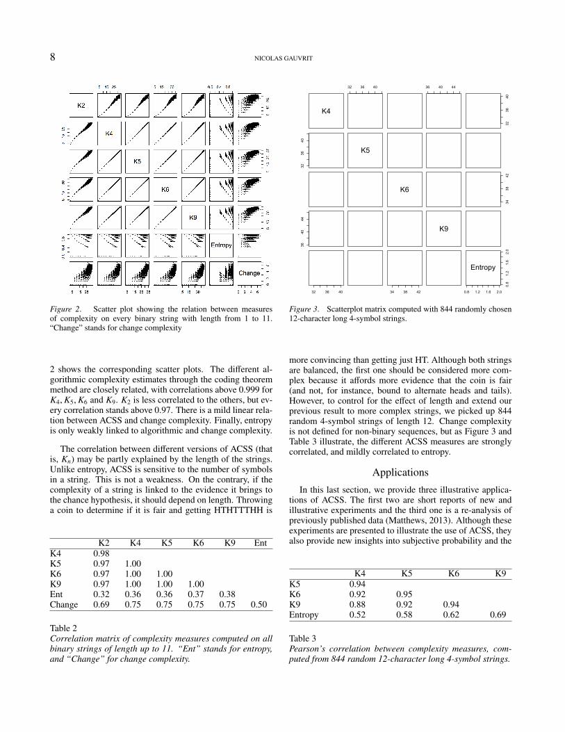
Figure 3. Scatterplot matrix computed with 844 randomly chosen12-character long 4-symbol strings.

more convincing than getting just HT. Although both stringsare balanced, the first one should be considered more com-plex because it affords more evidence that the coin is fair(and not, for instance, bound to alternate heads and tails).However, to control for the effect of length and extend ourprevious result to more complex strings, we picked up 844random 4-symbol strings of length 12. Change complexityis not defined for non-binary sequences, but as Figure 3 andTable 3 illustrate, the different ACSS measures are stronglycorrelated, and mildly correlated to entropy.

Applications

In this last section, we provide three illustrative applica-tions of ACSS. The first two are short reports of new andillustrative experiments and the third one is a re-analysis ofpreviously published data (Matthews, 2013). Although theseexperiments are presented to illustrate the use of ACSS, theyalso provide new insights into subjective probability and the

K4 K5 K6 K9K5 0.94K6 0.92 0.95K9 0.88 0.92 0.94Entropy 0.52 0.58 0.62 0.69

Table 3Pearson’s correlation between complexity measures, com-puted from 844 random 12-character long 4-symbol strings.


24 26 28 30 32 34

Human

All

Figure 4. Violin plot showing the distribution of complexity ofhuman strings vs. every possible pattern of strings, with 4-symbolalphabet and length 10.

perception of randomness. Note that all the data and analysisscripts for these applications are also part of acss.

Experiment 1: Humans are “better than chance”

Human pseudo-random sequential binary productionshave been reported to be overly complex, in the sense thatthey are more complex than the average complexity of trulyrandom sequences (i.e., sequences of fixed length producedby repeatedly tossing a coin; Gauvrit et al., 2013). Here,we test the same effect with non-binary sequences based on4 symbols. To replicate the analysis, type ?exp1 at the Rprompt after loading acss and execute the examples.

Participants. A sample of 34 healthy adults participated inthis experiment. Ages ranged from 20 to 55 (mean = 37.65,SD = 7.98). Participants were recruited via e-mail and didnot receive any compensation for their participation.

Methods. Participants were asked to produce at their ownpace a series of 10 symbols using “A”, “B”, “C”, and “D” thatwould “look as random as possible, so that if someone elsesaw the sequence, she would believe it to be a truly randomone”. Participants submitted their responses via e-mail.

Results. A one sample t-test showed that the mean com-plexity of the responses of participants is significantly largerthat the mean complexity of all possible patterns of length 10(t(33) = 10.62, p < .0001). The violin plot in Figure 4 showsthat human productions are more complex than random pat-terns because humans avoid low-complexity strings. On theother hand, human productions did not reach the highest pos-sible values of complexity.

Discussion. These results are consistent with the hypothe-sis that when participants try to behave randomly, they in facttend to maximize the complexity of their responses, leadingto overly complex sequences. However, whereas they suc-ceed in avoiding low-complexity patterns, they cannot buildthe most complex strings.

Experiment 2: The threshold of complexity – acase study

Humans are sensitive to regularity and distinguish trulyrandom series from deterministic ones (Yamada, Kawabe,& Miyazaki, 2013). More complex strings should be morelikely to be considered random than simple ones. Here, webriefly address this question through a binary forced choicetask. We assume that there exists an individual threshold ofcomplexity for which the probability that the individual iden-tifies a string as random is .5. We estimated that threshold forone participant. The participant was a healthy adult male, 42years old. The data and code are available by calling ?exp2.

Methods. A series of 200 random strings of length 10 froman alphabet of 6 symbols, such as “6154256554”, were gen-erated with the R function sample(). For each string, theparticipant had to decide whether or not the sequence ap-peared random.

Results. A logistic regression of the actual complexitiesof the strings (K6) on the responses is displayed in Figure 5.The results showed that more complex sequences were morelikely to be considered random (slope = 1.9, p < .0001, cor-responding to an odds ratio of 6.69). Furthermore, a com-plexity of 36.74 corresponded to the subjective probabilityof randomness 0.5 (i.e., the individual threshold was 36.74).

K6

Pro

babi

lity

"ran

dom

"

0.0

0.2

0.4

0.6

0.8

1.0

34 35 36 37 38

Figure 5. Graphical display of the logistic regression with actualcomplexities (K6) of 200 strings as independent variable and theobserved responses (appears random or not) of one participant asdependent variable. The gray area depicts 95%-confidence bands,the black dots at the bottom the 200 complexities. The dotted linesshow the threshold where the perceived probability of randomnessis 0.5.

10 NICOLAS GAUVRIT

The span of local complexity

In a study of contextual effect in the perception of random-ness, Matthews (2013, Experiment 1) showed participantsseries of binary strings of length 21. For each string, par-ticipants had to rate the sequence on a 6-point scale rangingfrom “definitely random” to “definitely not random”. Re-sults showed that participants were influenced by the contextof presentation: sequences with medial alternation rate (AR)were considered highly random when they were intermixedwith low AR, but as relatively non-random when intermixedwith high AR sequences. In the following, we will analyzethe data irrespective of the context or AR.

When individuals judge whether a short string of, for ex-ample, 3-6 characters, is random, they probably consider thecomplete sequence. For these cases, ACSS would be theright normative measure. When strings are longer, such as alength of 21, individuals probably cannot consider the com-plete sequence at once. Matthews (2013) and others (e.g.,U. Hahn, 2014) have hypothesized that in these cases indi-viduals rely on the local complexity of the string. If this weretrue, the question remains as to how local the analysis is. Toanswer this, we will reanalyze Matthews’ data.

For each string and each span ranging from 3 to 11, wefirst computed the mean local complexity of the string. Forinstance, the string “XXXXXXXOOOOXXXOOOOOOO”with span 11 gives a mean local complexity of 29.53. Thesame string has a mean local complexity of 11.22 with span5.

> sapply(local_complexity("XXXXXXXOOOOXXXOOOOOOO",11, 2), mean)XXXXXXXOOOOXXXOOOOOOO

29.52912> sapply(local_complexity("XXXXXXXOOOOXXXOOOOOOO",5, 2), mean)XXXXXXXOOOOXXXOOOOOOO

11.21859

For each span, we then computed R2 (the proportion ofvariance accounted for) between mean local complexity (aformal measure) and the mean randomness score given bythe participants in Matthews’ (2013) Experiment 1. Figure 6shows that a span of 4 or 5 best describes the judgments withR2 of 54% and 50%. Furthermore, R2 decreases so fast thatit amounts to less than 0.002% when the span is set to 10.These results suggest that when asked to judge if a string israndom, individuals rely on very local structural features ofthe strings, only considering subsequences of 4-5 symbols.This is very near the suggested limit of the short term mem-ory of 4 chunks (Cowan, 2001). Future researchers couldbuild on this preliminary account to investigate the possible“span” of human observation in the face of possibly randomserial data. The data and code for this application are avail-able by calling ?matthews2013.

4 6 8 10

0.0

0.1

0.2

0.3

0.4

0.5

R2

Span

Figure 6. R2 between mean local complexity with span 3 to 11 andthe subjective mean evaluation of randomness.

Relationship to complexity basedmodel selection

As mentioned in the beginning, complexity also playsan important role in modern approaches to model selection,specifically within the minimum description length frame-work (MDL; Grunwald, 2007; Myung et al., 2006). Modelselection in this context (see e.g. Myung, Cavagnaro, & Pitt,In press) refers to the process of selecting, among a set ofcandidate models, the model that strikes the best balance be-tween goodness-of-fit (i.e., how well does the model describethe obtained data) and complexity (i.e., how well does themodel describe all possible data or data in general). MDLprovides a principled way of combining model fit with aquantification of model complexity that originated in infor-mation theory (Rissanen, 1989) and is, similar to algorithmiccomplexity, based on the notion of compressed code. The ba-sic idea is that a model can be viewed as an algorithm that, incombination with a set of parameters, can produce a specificprediction. A model that describes the observed data well(i.e., provides a good fit) is a model that can compress thedata well as it only requires a set of parameters and there arelittle residuals that need to be described in addition. Withinthis framework, the complexity of a model is the shortestpossible code or algorithm that describes all possible datapattern predicted by the model. The model selection index isthe length of the concatenation of the code describing param-eters and residuals and the code producing all possible datasets. As usual, the best model in terms of MDL is the modelwith the lowest model selection index.

The MDL approach differs from the complexity approach


discussed in the current manuscript as it focuses on a spe-cific set of models. To be selected as possible candidates,models usually need to satisfy other criteria such as provid-ing explanatory value, need to be a priori plausible, and theparameters should be interpretable in terms of psychologi-cal processes (Myung et al., In press). In contrast, algorith-mic complexity is concerned with finding the shortest possi-ble description considering all possible models leaving thoseconsiderations aside. However, given that both approachesare couched within the same information theoretic frame-work, MDL converges towards algorithmic complexity if theset of candidate models becomes infinite (Wallace & Dowe,1999). Furthermore, in the current manuscript we are onlyconcerned with short strings, whereas even in compressedform data and the prediction space of a model are usuallycomparatively large.

Conclusion

Until the development of the coding theorem method(Soler-Toscano et al., 2014; Delahaye & Zenil, 2012), re-searchers interested in short random strings were constrainedto use measures of complexity that focused on particular fea-tures of randomness. This has led to a number of (unsatis-factory) measures (Towse, 1998). Each of these previouslyused measures can be thought of as a way of performing aparticular statistical test of randomness. In contrast, algo-rithmic complexity affords access to the ultimate measure ofrandomness, as the algorithmic complexity definition of ran-domness has been shown to be equivalent to defining a ran-dom sequence as one which would pass every computabletest of randomness. We have computed an approximation ofalgorithmic complexity for short strings and made this ap-proximation freely available in the R package acss.

Because human capacities are limited, it is unlikely thathumans will be able to recognize every kind of deviationfrom randomness. Subjective randomness does not equalalgorithmic complexity, as Griffiths and Tenenbaum (2004)remind us. Other measures of complexity will still be usefulin describing the ways in which human pseudo-random be-haviors or the subjective perception of randomness or com-plexity differ from objective randomness, as defined withinthe mathematical theory of randomness and advocated in thismanuscript. But to achieve this goal of comparing subjec-tive and objective randomness, we also need an objectiveand universal measure of randomness (or complexity) basedon a sound mathematical theory of randomness. Althoughthe uncomputability of Kolmogorov complexity places somelimitations on what is knowable about objective randomness,ACSS provides a sensible and practical approximation thatresearchers can use in real life. We are confident that ACSSwill prove very useful as a normative measure of complexityin helping psychologists understand how human subjectiverandomness differs from “true” randomness as defined by al-gorithmic complexity.

References

Aksentijevic, A., & Gibson, K. (2012). Complexity equals change.Cognitive Systems Research, 15-16, 1–16.

Audiffren, M., Tomporowski, P. D., & Zagrodnik, J. (2009). Acuteaerobic exercise and information processing: modulation of ex-ecutive control in a random number generation task. Acta Psy-chologica, 132(1), 85–95.

Baddeley, A. D., Thomson, N., & Buchanan, M. (1975). Wordlength and the structure of short-term memory. Journal of VerbalLearning and Verbal Behavior, 14(6), 575–589.

Barbasz, J., Stettner, Z., Wierzchon, M., Piotrowski, K. T., & Bar-basz, A. (2008). How to estimate the randomness in random se-quence generation tasks?. Polish Psychological Bulletin, 39(1),42 - 46.

Bedard, M.-J., Joyal, C. C., Godbout, L., & Chantal, S. (2009).Executive functions and the obsessive-compulsive disorder: Onthe importance of subclinical symptoms and other concomitantfactors. Archives of Clinical Neuropsychology, 24(6), 585–598.

Bianchi, A. M., & Mendez, M. O. (2013). Methods for heart ratevariability analysis during sleep. In Engineering in medicine andbiology society (embc), 2013 35th annual international confer-ence of the ieee (pp. 6579–6582).

Boon, J. P., Casti, J., & Taylor, R. P. (2011). Artistic forms andcomplexity. Nonlinear Dynamics-Psychology and Life Sciences,15(2), 265.

Brandouy, O., Delahaye, J.-P., Ma, L., & Zenil, H. (2012). Algorith-mic complexity of financial motions. Research in InternationalBusiness and Finance, 30(C), 336–347.

Brown, R., & Marsden, C. (1990). Cognitive function in parkin-son’s disease: from description to theory. Trends in Neuro-sciences, 13(1), 21–29.

Calude, C. (2002). Information and randomness. an algorithmicperspective (2nd, revised and extended ed.). Springer-Verlag.

Cardaci, M., Di Gesu, V., Petrou, M., & Tabacchi, M. E. (2009).Attentional vs computational complexity measures in observingpaintings. Spatial vision, 22(3), 195–209.

Chaitin, G. (1966). On the length of programs for computing finitebinary sequences. Journal of the ACM, 13(4), 547-569.

Chaitin, G. (2004). Algorithmic information theory (Vol. 1). Cam-bridge University Press.

Chater, N. (1996). Reconciling simplicity and likelihood principlesin perceptual organization. Psychological Review, 103(3), 566-581.

Chater, N., & Vitanyi, P. (2003). Simplicity: A unifying principlein cognitive science? Trends in Cognitive Sciences, 7(1), 19-22.

Cilibrasi, R., & Vitanyi, P. (2005). Clustering by compression.Information Theory, IEEE Transactions on, 51(4), 1523–1545.

Cilibrasi, R., & Vitanyi, P. (2007). The google similarity distance.Knowledge and Data Engineering, IEEE Transactions on, 19(3),370–383.

Cowan, N. (2001). The magical number 4 in short-term memory:A reconsideration of mental storage capacity. Behavioral andBrain Sciences, 24(1), 87–114.

Crova, C., Struzzolino, I., Marchetti, R., Masci, I., Vannozzi, G.,Forte, R., et al. (2013). Cognitively challenging physical activ-ity benefits executive function in overweight children. Journalof Sports Sciences, ahead-of-print, 1–11.

Curci, A., Lanciano, T., Soleti, E., & Rime, B. (2013). Nega-tive emotional experiences arouse rumination and affect workingmemory capacity. Emotion, 13(5), 867–880.

Delahaye, J.-P., & Zenil, H. (2012). Numerical evaluation of algo-rithmic complexity for short strings: A glance into the innermost

12 NICOLAS GAUVRIT

structure of randomness. Applied Mathematics and Computa-tion, 219(1), 63–77.

Downey, R. R. G., & Hirschfeldt, D. R. (2008). Algorithmic ran-domness and complexity. Springer.

Elzinga, C. H. (2010). Complexity of categorical time series. Soci-ological Methods & Research, 38(3), 463–481.

Feldman, J. (2000). Minimization of boolean complexity in humanconcept learning. Nature, 407(6804), 630–633.

Feldman, J. (2003). A catalog of boolean concepts. Journal ofMathematical Psychology, 47(1), 75-89.

Feldman, J. (2006). An algebra of human concept learning. Journalof Mathematical Psychology, 50(4), 339-368.

Fernandez, A., Quintero, J., Hornero, R., Zuluaga, P., Navas, M.,Gomez, C., et al. (2009). Complexity analysis of spontaneousbrain activity in attention-deficit/hyperactivity disorder: diag-nostic implications. Biological Psychiatry, 65(7), 571–577.

Fernandez, A., Rıos-Lago, M., Abasolo, D., Hornero, R., Alvarez-Linera, J., Paul, N., et al. (2011). The correlation between white-matter microstructure and the complexity of spontaneous brainactivity: A difussion tensor imaging-meg study. Neuroimage,57(4), 1300–1307.

Fernandez, A., Zuluaga, P., Abasolo, D., Gomez, C., Serra, A.,Mendez, M. A., et al. (2012). Brain oscillatory complexityacross the life span. Clinical Neurophysiology, 123(11), 2154–2162.

Fournier, K. A., Amano, S., Radonovich, K. J., Bleser, T. M., &Hass, C. J. (2013). Decreased dynamical complexity duringquiet stance in children with autism spectrum disorders. Gait &Posture.

Free Software Foundation. (2007). GNU general public license.Retrieved from http://www.gnu.org/licenses/gpl.html

Gauvrit, N., Soler-Toscano, F., & Zenil, H. (2014). Natural scenestatistics mediate the perception of image complexity. VisualCognition, 22(8), 1084-1091.

Gauvrit, N., Zenil, H., Delahaye, J.-P., & Soler-Toscano, F. (2013).Algorithmic complexity for short binary strings applied to psy-chology: A primer. Behavior Research Methods, 46(3), 732-744.

Griffiths, T. L., & Tenenbaum, J. B. (2003). Probability, algorith-mic complexity, and subjective randomness. In R. Alterman &D. Kirsch (Eds.), Proceedings of the 25th annual conference ofthe cognitive science society (p. 480-485). Mahwah, NJ: Erl-baum.

Griffiths, T. L., & Tenenbaum, J. B. (2004). From algorith-mic to subjective randomness. In S. Thrun, L. K. Saul, &B. Scholkopf (Eds.), Advances in neural information processingsystems (Vol. 16, p. 953-960). Cambridge, MA: MIT Press.

Gruber, H. (2010). On the descriptional and algorithmic complexityof regular languages. Justus Liebig University Giessen.

Grunwald, P. D. (2007). The minimum description length principle.MIT press.

Hahn, T., Dresler, T., Ehlis, A.-C., Pyka, M., Dieler, A. C., Saathoff,C., et al. (2012). Randomness of resting-state brain oscilla-tions encodes gray’s personality trait. Neuroimage, 59(2), 1842–1845.

Hahn, U. (2014). Experiential limitation in judgment and decision.Topics in Cognitive Science, 6(2), 229–244.

Hahn, U., Chater, N., & Richardson, L. B. (2003). Similarity astransformation. Cognition, 87(1), 1-32.

Hahn, U., & Warren, P. A. (2009). Perceptions of randomness:Why three heads are better than four. Psychological Review,116(2), 454–461.

Heuer, H., Kohlisch, O., & Klein, W. (2005). The effects of

total sleep deprivation on the generation of random sequencesof key-presses, numbers and nouns. The Quarterly Journal ofExperimental Psychology A: Human Experimental Psychology,58A(2), 275 - 307.

Hsu, A. S., Griffiths, T. L., & Schreiber, E. (2010). Subjectiverandomness and natural scene statistics. Psychonomic Bulletin& Review, 17(5), 624–629.

Jones, O., Maillardet, R., & Robinson, A. (2009). Introductionto scientific programming and simulation using R. Boca Raton,FL: Chapman & Hall/CRC.

Kahneman, D., Slovic, P., & Tversky, A. (1982). Judgment un-der uncertainty: Heuristics and biases. Cambridge UniversityPress.

Kass, R. E., & Raftery, A. E. (1995, June). Bayes factors.Journal of the American Statistical Association, 90(430), 773–795. Retrieved from http://www.tandfonline.com/doi/abs/10.1080/01621459.1995.10476572

Kellen, D., Klauer, K. C., & Broder, A. (2013). Recognition mem-ory models and binary-response ROCs: a comparison by mini-mum description length. Psychonomic Bulletin& Review, 20(4),693–719.

Koike, S., Takizawa, R., Nishimura, Y., Marumo, K., Kinou, M.,Kawakubo, Y., et al. (2011). Association between severe dorso-lateral prefrontal dysfunction during random number generationand earlier onset in schizophrenia. Clinical Neurophysiology,122(8), 1533–1540.

Kolmogorov, A. (1965). Three approaches to the quantitative def-inition of information. Problems of Information and Transmis-sion, 1(1), 1-7.

Lai, M.-C., Lombardo, M. V., Chakrabarti, B., Sadek, S. A., Pasco,G., Wheelwright, S. J., et al. (2010). A shift to randomness ofbrain oscillations in people with autism. Biological Psychiatry,68(12), 1092–1099.

Levin, L. A. (1974). Laws of information conservation (nongrowth)and aspects of the foundation of probability theory. ProblemyPeredachi Informatsii, 10(3), 30–35.

Li, M., & Vitanyi, P. (2008). An introduction to kolmogorov com-plexity and its applications. Springer Verlag.

Loetscher, T., & Brugger, P. (2009). Random number generationin neglect patients reveals enhanced response stereotypy, but noneglect in number space. Neuropsychologia, 47(1), 276 - 279.

Machado, B., Miranda, T., Morya, E., Amaro Jr, E., & Sameshima,K. (2010). P24-23 algorithmic complexity measure of EEG forstaging brain state. Clinical Neurophysiology, 121, S249–S250.

Maes, J. H., Vissers, C. T., Egger, J. I., & Eling, P. A. (2012). Onthe relationship between autistic traits and executive functioningin a non-clinical Dutch student population. Autism, 17(4), 379–389.

Maindonald, J., & Braun, W. J. (2010). Data analysis and graph-ics using R: An example-based approach (3rd ed.). Cambridge:Cambridge University Press.

Manktelow, K. I., & Over, D. E. (1993). Rationality: Psychologicaland philosophical perspectives. Taylor & Frances/Routledge.

Martin-Lof, P. (1966). The definition of random sequences. Infor-mation and control, 9(6), 602–619.

Mathy, F., & Feldman, J. (2012). What’s magic about magic num-bers? Chunking and data compression in short-term memory.Cognition, 122(3), 346–362.

Matloff, N. (2011). The art of R programming: A tour of statisticalsoftware design (1st ed.). San Francisco: No Starch Press.

Matthews, W. (2013). Relatively random: Context effects on per-ceived randomness and predicted outcomes. Journal of Exper-


imental Psychology: Learning, Memory, and Cognition, 39(5),1642-1648.

Miller, G. A. (1956). The magical number seven, plus or minustwo: some limits on our capacity for processing information.Psychological Review, 63(2), 81–97.

Myung, J. I., Cavagnaro, D. R., & Pitt, M. A. (In press). New hand-book of mathematical psychology, vol. 1: Measurement andmethodology. In W. H. Batchelder, H. Colonius, E. Dzhafarov,& J. I. Myung (Eds.), (chap. Model evaluation and selection).Cambridge University Press.

Myung, J. I., Navarro, D. J., & Pitt, M. A. (2006). Model selectionby normalized maximum likelihood. Journal of MathematicalPsychology, 50(2), 167–179.

Naranan, S. (2011). Historical linguistics and evolutionary genetics.based on symbol frequencies in tamil texts and dna sequences.Journal of Quantitative Linguistics, 18(4), 337–358.

Nies, A. (2009). Computability and randomness (Vol. 51). OxfordUniversity Press.

Over, D. E. (2009). New paradigm psychology of reasoning. Think-ing & Reasoning, 15(4), 431–438.

Pearson, D. G., & Sawyer, T. (2011). Effects of dual task interfer-ence on memory intrusions for affective images. InternationalJournal of Cognitive Therapy, 4(2), 122–133.

Proios, H., Asaridou, S. S., & Brugger, P. (2008). Random numbergeneration in patients with aphasia: A test of executive func-tions. Acta Neuropsychologica, 6, 157-168.

Pureza, J. R., Goncalves, H. A., Branco, L., Grassi-Oliveira, R., &Fonseca, R. P. (2013). Executive functions in late childhood:Age differences among groups. Psychology & Neuroscience,6(1), 79–88.

R Core Team. (2014). R: A language and environment for statis-tical computing [Computer software manual]. Vienna, Austria.Retrieved from http://www.R-project.org/

Rado, T. (1962). On non-computable functions. Bell System Tech-nical Journal, 41, 877-884.

Rissanen, J. (1989). Stochastic complexity in statistical inquirytheory. World Scientific Publishing Co., Inc.

Ryabko, B., Reznikova, Z., Druzyaka, A., & Panteleeva, S. (2013).Using ideas of Kolmogorov complexity for studying biologicaltexts. Theory of Computing Systems, 52(1), 133–147.

Scafetta, N., Marchi, D., & West, B. J. (2009). Understandingthe complexity of human gait dynamics. Chaos: An Interdisci-plinary Journal of Nonlinear Science, 19(2), 026108.

Schnorr, C.-P. (1973). Process complexity and effective randomtests. Journal of Computer and System Sciences, 7(4), 376–388.

Schulter, G., Mittenecker, E., & Papousek, I. (2010). A computerprogram for testing and analyzing random generation behaviorin normal and clinical samples: The Mittenecker pointing test.Behavior Research Methods, 42, 333-341.

Scibinetti, P., Tocci, N., & Pesce, C. (2011). Motor creativity andcreative thinking in children: The diverging role of inhibition.Creativity Research Journal, 23(3), 262–272.

Shannon, C. E. (1948). A mathematical theory of communication,part I. Bell Systems Technical Journal, 27, 379–423.

Sokunbi, M. O., Fung, W., Sawlani, V., Choppin, S., Linden, D. E.,& Thome, J. (2013). Resting state fMRI entropy probes com-plexity of brain activity in adults with ADHD. Psychiatry Re-search: Neuroimaging, 214(3), 341–348.

Soler-Toscano, F., Zenil, H., Delahaye, J.-P., & Gauvrit, N. (2013).Correspondence and independence of numerical evaluations ofalgorithmic information measures. Computability, 2(2), 125-140.

Soler-Toscano, F., Zenil, H., Delahaye, J.-P., & Gauvrit, N. (2014).

Calculating Kolmogorov complexity from the output frequencydistributions of small turing machines. PLOS One, 9(5),e96223.

Solomonoff, R. J. (1964a). A formal theory of inductive inference.Part I. Information and Control, 7(1), 1–22.

Solomonoff, R. J. (1964b). A formal theory of inductive inference.Part II. Information and Control, 7(2), 224–254.

Takahashi, T. (2013). Complexity of spontaneous brain activity inmental disorders. Progress in Neuro-Psychopharmacology andBiological Psychiatry, 45, 258–266.

Taufemback, C., Giglio, R., & Da Silva, S. (2011). Algorithmiccomplexity theory detects decreases in the relative efficiency ofstock markets in the aftermath of the 2008 financial crisis. Eco-nomics Bulletin, 31(2), 1631–1647.

Towse, J. N. (1998). Analyzing human random generation behav-ior: A review of methods used and a computer program for de-scribing performance. Behavior Research Methods, 30(4), 583-591.

Towse, J. N., & Cheshire, A. (2007). Random number generationand working memory. European Journal of Cognitive Psychol-ogy, 19(3), 374-394.

Tversky, A., & Kahneman, D. (1974). Judgment under uncertainty:Heuristics and biases. Science, 185(4157), 1124-1131.

Wagenaar, W. A. (1970). Subjective randomness and the capacityto generate information. Acta Psychologica, 33, 233-242.

Wallace, C. S., & Dowe, D. L. (1999). Minimum message lengthand Kolmogorov complexity. The Computer Journal, 42(4),270–283.

Watanabe, T., Cellucci, C., Kohegyi, E., Bashore, T., Josiassen, R.,Greenbaun, N., et al. (2003). The algorithmic complexity ofmultichannel EEGs is sensitive to changes in behavior. Psy-chophysiology, 40(1), 77–97.

Wiegersma, S. (1984). High-speed sequantial vocal response pro-duction. Perceptual and Motor Skills, 59, 43-50.

Wilder, J., Feldman, J., & Singh, M. (2011). Contour complexityand contour detectability. Journal of Vision, 11(11), 1044.

Williams, J. J., & Griffiths, T. L. (2013). Why are people bad atdetecting randomness? a statistical argument. Journal of Exper-imental Psychology: Learning, Memory, and Cognition, 39(5),1473–1490.

Yagil, G. (2009). The structural complexity of dna templatesimpli-cations on cellular complexity. Journal of Theoretical Biology,259(3), 621–627.

Yamada, Y., Kawabe, T., & Miyazaki, M. (2013). Pattern random-ness aftereffect. Scientific Reports, 3.

Yang, A. C., & Tsai, S.-J. (2012). Is mental illness complex? Frombehavior to brain. Progress in Neuro-Psychopharmacology andBiological Psychiatry, 45, 253–257.

Zabelina, D. L., Robinson, M. D., Council, J. R., & Bresin, K.(2012). Patterning and nonpatterning in creative cognition: In-sights from performance in a random number generation task.Psychology of Aesthetics, Creativity, and the Arts, 6(2), 137–145.

Zenil, H. (2011a). Randomness through computation: Some an-swers, more questions. World Scientific.

Zenil, H. (2011b). Une approche experimentale de la theorie algo-rithmique de la complexite. Unpublished doctoral dissertation,Universidad de Buenos Aires.

Zenil, H., & Delahaye, J.-P. (2010). On the algorithmic nature of theworld. In G. Dodig-Crnkovic & M. Burgin (Eds.), Informationand computation (p. 477-496). World Scientific.

Zenil, H., & Delahaye, J.-P. (2011). An algorithmic information

14 NICOLAS GAUVRIT

theoretic approach to the behaviour of financial markets. Jour-nal of Economic Surveys, 25(3), 431–463.

Zenil, H., Soler-Toscano, F., Delahaye, J., & Gauvrit, N.(2012). Two-dimensional Kolmogorov complexity and valida-

tion of the coding theorem method by compressibility. CoRR,abs/1212.6745. Retrieved from http://arxiv.org/abs/1212.6745

algorithmic complexity for psychology: a user-friendly

Documents