algorithmic aspects of machine learning - people | mit csail
TRANSCRIPT

Algorithmic Aspects of Machine Learning
Ankur Moitra

Contents
Contents i
Preface v
1 Introduction 3
2 Nonnegative Matrix Factorization 7
2.1 Introduction . . . . . . . . . . . . . . . . . . . . . . . . . . . . . . . . 7
2.2 Algebraic Algorithms . . . . . . . . . . . . . . . . . . . . . . . . . . . 17
2.3 Stability and Separability . . . . . . . . . . . . . . . . . . . . . . . . 26
2.4 Topic Models . . . . . . . . . . . . . . . . . . . . . . . . . . . . . . . 35
2.5 Exercises . . . . . . . . . . . . . . . . . . . . . . . . . . . . . . . . . . 43
3 Tensor Decompositions: Algorithms 45
3.1 The Rotation Problem . . . . . . . . . . . . . . . . . . . . . . . . . . 46
3.2 A Primer on Tensors . . . . . . . . . . . . . . . . . . . . . . . . . . . 48
i

ii CONTENTS
3.3 Jennrich’s Algorithm . . . . . . . . . . . . . . . . . . . . . . . . . . . 55
3.4 Perturbation Bounds . . . . . . . . . . . . . . . . . . . . . . . . . . . 62
3.5 Exercises . . . . . . . . . . . . . . . . . . . . . . . . . . . . . . . . . . 72
4 Tensor Decompositions: Applications 75
4.1 Phylogenetic Trees and HMMs . . . . . . . . . . . . . . . . . . . . . . 76
4.2 Community Detection . . . . . . . . . . . . . . . . . . . . . . . . . . 85
4.3 Extensions to Mixed Models . . . . . . . . . . . . . . . . . . . . . . . 92
4.4 Independent Component Analysis . . . . . . . . . . . . . . . . . . . . 102
4.5 Exercises . . . . . . . . . . . . . . . . . . . . . . . . . . . . . . . . . . 108
5 Sparse Recovery 111
5.1 Introduction . . . . . . . . . . . . . . . . . . . . . . . . . . . . . . . . 111
5.2 Incoherence and Uncertainty Principles . . . . . . . . . . . . . . . . . 116
5.3 Pursuit Algorithms . . . . . . . . . . . . . . . . . . . . . . . . . . . . 120
5.4 Prony’s Method . . . . . . . . . . . . . . . . . . . . . . . . . . . . . . 124
5.5 Compressed Sensing . . . . . . . . . . . . . . . . . . . . . . . . . . . 129
5.6 Exercises . . . . . . . . . . . . . . . . . . . . . . . . . . . . . . . . . . 137
6 Sparse Coding 139
6.1 Introduction . . . . . . . . . . . . . . . . . . . . . . . . . . . . . . . . 140
6.2 The Undercomplete Case . . . . . . . . . . . . . . . . . . . . . . . . . 144

CONTENTS iii
6.3 Gradient Descent . . . . . . . . . . . . . . . . . . . . . . . . . . . . . 152
6.4 The Overcomplete Case . . . . . . . . . . . . . . . . . . . . . . . . . 159
6.5 Exercises . . . . . . . . . . . . . . . . . . . . . . . . . . . . . . . . . . 167
7 Gaussian Mixture Models 169
7.1 Introduction . . . . . . . . . . . . . . . . . . . . . . . . . . . . . . . . 170
7.2 Clustering-Based Algorithms . . . . . . . . . . . . . . . . . . . . . . . 175
7.3 Discussion of Density Estimation . . . . . . . . . . . . . . . . . . . . 181
7.4 Clustering-Free Algorithms . . . . . . . . . . . . . . . . . . . . . . . . 186
7.5 A Univariate Algorithm . . . . . . . . . . . . . . . . . . . . . . . . . 194
7.6 A View from Algebraic Geometry . . . . . . . . . . . . . . . . . . . . 200
7.7 Exercises . . . . . . . . . . . . . . . . . . . . . . . . . . . . . . . . . . 206
8 Matrix Completion 207
8.1 Introduction . . . . . . . . . . . . . . . . . . . . . . . . . . . . . . . . 208
8.2 Nuclear Norm . . . . . . . . . . . . . . . . . . . . . . . . . . . . . . . 212
8.3 Quantum Golfing . . . . . . . . . . . . . . . . . . . . . . . . . . . . . 218
Bibliography 225

iv CONTENTS

Preface
The monograph is based on the class “Algorithmic Aspects of Machine Learning”
taught at MIT in Fall 2013, Spring 2015 and Fall 2017. Thank you to all the stu-
dents and postdocs who participated in this class, and made teaching it a wonderful
experience.
v

To Diana and Olivia, the sunshine in my life
1

2 CONTENTS

Chapter 1
Introduction
Machine learning is starting to take over decision-making in many aspects of our
life, including:
(a) keeping us safe on our daily commute in self-driving cars
(b) making an accurate diagnosis based on our symptoms and medical history
(c) pricing and trading complex securities
(d) discovering new science, such as the genetic basis for various diseases.
But the startling truth is that these algorithms work without any sort of provable
guarantees on their behavior. When they are faced with an optimization problem,
do they actually find the best solution or even a pretty good one? When they posit
a probabilistic model, can they incorporate new evidence and sample from the true
posterior distribution? Machine learning works amazingly well in practice, but that
doesn’t mean we understand why it works so well.
3

4 CHAPTER 1. INTRODUCTION
If you’ve taken traditional algorithms courses, the usual way you’ve been ex-
posed to thinking about algorithms is through worst-case analysis. When you have
a sorting algorithm you measure it’s running time based on how many operations
it takes on the worst possible input. That’s a convenient type of bound to have,
because it means you can say meaningful things about how long your algorithm
takes without ever worrying about the types of inputs you usually give it.
But what makes analyzing machine learning algorithms — especially modern
ones — so challenging is that the types of problems they are trying to solve really are
NP -hard on worst-case inputs. When you cast the problem of finding the parameters
that best fit your data as an optimization problem, there are instances where it is
NP -hard to find a good fit. When you posit a probabilistic model and want to use
it to perform inference, there are instances where that is NP -hard as well.
In this book, we will approach the problem of giving provable guarantees for
machine learning by trying to find more realistic models for our data. In many
applications, there are reasonable assumptions we can make based on the context in
which the problem came up, that can get us around these worst-case impediments
and allow us to rigorously analyze heuristics that are used in practice, as well as
design fundamentally new ways of solving some of the central, recurring problems
in machine learning.
To take a step back, the idea of moving beyond worst-case analysis is an
idea that is as old1 as theoretical computer science itself [95]. In fact there are
many different flavors of what it means to understand the behavior of algorithms
on “typical” instances, including:
1After all, heuristics performing well on real life inputs are old as well (long predating modernmachine learning) and hence so is the need to explain them.

5
(a) probabilistic models for your input — or even hybrid models that combine
elements of worst-case and average-case analysis like semi-random models [38,
71] or smoothed analysis [39, 130]
(b) ways to measure the complexity of your problem, and ask for algorithms that
are fast on simple inputs, as in parameterized complexity [66]
(c) notions of stability that attempt to articulate what instances of your problem
have meaningful answers and are the ones you actually want to solve [20, 32]
This is by no means an exhaustive list of topics or references. Regardless, in this
book, we will approach machine learning problems armed with these sorts of insights
about what are ways to get around intractability.
Ultimately, we hope that theoretical computer science and machine learning
have a lot left to teach each other. Understanding why heuristics like expectation-
maximization or gradient descent on a non-convex function work so well in practice
is a grand challenge for theoretical computer science. But to make progress on these
questions, we need to understand what types of models and assumptions make sense
in the context of machine learning. On the other hand, if we make progress on these
hard problems and develop new insights about why heuristics work so well, we can
hope to engineering them better. We can even hope to discover totally new ways to
solve some of the important problems in machine learning, especially by leveraging
modern tools in our algorithmic toolkit.
In this book, we will cover the following topics:
(a) nonnegative matrix factorization
(b) topic modeling

6 CHAPTER 1. INTRODUCTION
(c) tensor decompositions
(d) sparse recovery
(e) sparse coding
(f) learning mixtures models
(g) matrix completion
I hope that more chapters will be added in later versions, as the field develops and
makes new discoveries.

Chapter 2
Nonnegative Matrix Factorization
In this chapter, we will explore the nonnegative matrix factorization problem. It will
be helpful to first compare it to the more familiar singular value decomposition. In
the worst-case, the nonnegative matrix factorization problem is NP -hard (seriously,
what else did you expect?) but we will make domain-specific assumptions (called
separability) that will allow us to give provable algorithms for an important special
case of it. We then apply our algorithms to the problem of learning the parameters
of a topic model. This will be our first case-study in how to not back down in the
face of computational intractability, and find ways around it.
2.1 Introduction
In order to better understand the motivations behind the nonnegative matrix fac-
torization problem and why it is useful in applications, it will be helpful to first
introduce the singular value decomposition and then compare them. Eventually, we
7

8 CHAPTER 2. NONNEGATIVE MATRIX FACTORIZATION
will apply both of these to text analysis later in this section.
The Singular Value Decomposition
The singular value decomposition (SVD) is one of the most useful tools in linear
algebra. Given an m× n matrix M , its singular value decomposition is written as
M = UΣV T
where U and V are orthonormal and Σ is a rectangular matrix with non-zero entries
only along the diagonal and its entries are nonnegative. Alternatively we can write
M =r∑i=1
σiuivTi
where ui is the ith column of U , vi is the ith column of V and σi is the ith diagonal
entry of Σ. Throughout this section we will fix the convention that σ1 ≥ σ2 ≥ ... ≥
σr > 0. In this case, the rank of M is precisely r.
Throughout this course, we will have occasion to use this decomposition as
well as the (perhaps more familiar) eigendecomposition. If M is an n × n matrix
and is diagonalizable, its eigendecomposition is written as
M = PDP−1
where D is diagonal. For now the important facts to remember are:
(1) Existence: Every matrix has a singular value decomposition, even if it is

2.1. INTRODUCTION 9
rectangular. In contrast, a matrix must be square to have an eigendecompo-
sition. Even then not all square matrices can be diagonalized, but a sufficient
condition under which M can be diagonalized is that all its eigenvalues are
distinct.
(2) Algorithms: Both of these decompositions can be computed efficiently. The
best general algorithms for computing the singular value decomposition run in
time O(mn2) if m ≥ n. There are also faster algorithms for sparse matrices.
There are algorithms to compute an eigendecomposition in O(n3) time and
there are further improvements based on fast matrix multiplication, although
it is not clear whether such algorithms are as stable and practical.
(3) Uniqueness: The singular value decomposition is unique if and only if its
singular values are distinct. Similarly, the eigendecomposition is unique if and
only if its eigenvalues are distinct. In some cases, we will only need that the
non-zero singular values/eigenvalues are distinct because we can ignore the
others.
Two Applications
Two of the most important properties of the singular value decomposition are that
it can be used to find the best rank k approximation, and that it can be used for
dimension reduction. We explore these next. First let’s formalize what we mean by
the best rank k approximation problem. One way to do this is to work with the
Frobenius norm:
Definition 2.1.1 (Frobenius norm) ‖M‖F =√∑
i,jM2i,j

10 CHAPTER 2. NONNEGATIVE MATRIX FACTORIZATION
It is easy to see that the Frobenius norm is invariant under rotations. For example,
this follows by considering each of the columns of M separately as a vector. The
square of the Frobenius norm of a matrix is the sum of squares of the norms of its
columns. Then left-multiplying by an orthogonal matrix preserves the norm of each
of its columns. An identical argument holds for right-multiplying by an orthogonal
matrix (but working with the rows instead). This invariance allows us to give an
alternative characterization of the Frobenius norm which is quite useful:
‖M‖F = ‖UTMV ‖F = ‖Σ‖F =√∑
σ2i
The first equality is where all the action is happening, and uses the rotational
invariance property we established above.
Then the Eckart-Young Theorem asserts that the best rank k approximation
to some matrix M (in terms of Frobenius norm) is given by its truncated singular
value decomposition:
Theorem 2.1.2 (Eckart-Young) argminrank(B)≤k
‖M −B‖F =∑k
i=1 σiuivTi
Let Mk be the best rank k approximation. Then from our alternative definition of
the Frobenius norm it is immediate that ‖M −Mk‖F =√∑r
i=k+1 σ2i .
In fact, the same statement – that the best rank k approximation to M is its
truncated singular value decomposition – holds for any norm that is invariant under
rotations. As another application consider the operator norm:
Definition 2.1.3 (operator norm) ‖M‖ = max‖x‖≤1 ‖Mx‖

2.1. INTRODUCTION 11
It is easy to see that the operator norm is also invariant under rotations, and more-
over ‖M‖ = σ1, again using the convention that σ1 is the largest singular value.
Then the Eckart-Young Theorem with respect to the operator norm asserts:
Theorem 2.1.4 (Eckart-Young) argminrank(B)≤k
‖M −B‖ =∑k
i=1 σiuivTi
Again let Mk be the best rank k approximation. Then ‖M −Mk‖ = σk+1. As a
quick check, if k ≥ r then σk+1 = 0 and the best rank k approximation is exact and
has no error (as it should). You should think of this as something you can do with
any algorithm for computing the singular value decomposition of M – you can find
the best rank k approximation to it with respect to any rotationally invariant norm.
In fact, it is remarkable that the best rank k approximation in many different norms
coincides! Moreover the best rank k approximation to M can be obtained directly
from its best rank k + 1 approximation. This is not always the case, as we will see
in the next chapter when we work with tensors.
Next, we give an entirely different application of the singular value decompo-
sition in the context of data analysis, before we move on to applications of it in text
analysis. Recall that M is an m× n matrix. We can think of it as defining a distri-
bution on n-dimensional vectors, which we obtain from choosing one of its columns
uniformly at random. Further suppose that E[x] = 0 – i.e. the columns sum to the
all zero vector. Let Pk be the space of all projections onto a k-dimensional subspace.
Theorem 2.1.5 argmaxP∈Pk
E[‖Px‖2] =∑k
i=1 uiuTi
This is another basic theorem about the singular value decomposition, that
from it we can readily compute the k-dimensional projection that maximizes the

12 CHAPTER 2. NONNEGATIVE MATRIX FACTORIZATION
projected variance. This theorem is often invoked in visualization, where one can
visualize high-dimensional vector data by projecting it to a more manageable, lower
dimensional subspace.
Latent Semantic Indexing
Now that we have developed some of the intuition behind the singular value de-
composition we will see an application of it to text analysis. One of the central
problems in this area (and one that we will return to many times) is given a large
collection of documents we want to extract some hidden thematic structure. Deer-
wester et al. [60] invented latent semantic indexing (LSI) for this purpose, and their
approach was to apply the singular value decomposition to what is usually called
the term-by-document matrix:
Definition 2.1.6 The term-by-document matrix M is an m× n matrix where each
row represents a word, each column represents a document where
Mi,j =count of word i in document j
total number of words in document j
There are many popular normalization conventions, and here we have chosen to
normalize the matrix so that each of its columns sums to one. In this way, we can
interpret each document as a probability distribution on words. Also in constructing
the term-by-document matrix, we have ignored the order in which the words occur.
This is called a bag-of-words representation, and the justification for it comes from a
thought experiment. Suppose I were to give you the words contained in a document,
but in a jumbled order. It should still be possible to determine what the document

2.1. INTRODUCTION 13
is about, and hence forgetting all notions of syntax and grammar and representing
a document as a vector loses some structure but should still preserve enough of the
information to make many basic tasks in text analysis still possible.
Once our data is in vector form, we can make use of tools from linear algebra.
How can we measure the similarity between two documents? The naive approach is
to base our similarity measure on how many words they have in common. Let’s try:
〈Mi,Mj〉
This quantity computes the probability that a randomly chosen word w from doc-
ument i and a randomly chosen word w′ from document j are the same. But what
makes this a bad measure is that when documents are sparse, they may not have
many words in common just by accident because of the particular words each author
chose to use to describe the same types of things. Even worse, some documents could
be deemed to be similar because both of them contain many of the same common
words which have little to do with what the documents are actually about.
Deerwester et al. [60] proposed to use the singular value decomposition of M to
compute a more reasonable measure of similarity, and one that seems to work better
when the term-by-document matrix is sparse (as it usually is). Let M = UΣV T and
let U1...k and V1...k be the first k columns of U and V respectively. The approach is
to compute:
〈UT1...kMi, U
T1...kMj〉
for each pair of documents. The intuition is that there are some topics that occur
over and over again in the collection of documents. And if we could represent each

14 CHAPTER 2. NONNEGATIVE MATRIX FACTORIZATION
document Mi in the basis of topics then their inner-product in that basis would
yield a more meaningful measure of similarity. There are some models – i.e. a
hypothesis for how the data is stochastically generated – where it can be shown that
this approach provable recovers the true topics [118]. This is the ideal interaction
between theory and practice – we have techniques that work (somewhat) well, and
we can analyze/justify them.
However there are many failings of latent semantic indexing, that have moti-
vated alternative approaches. If we associate the top singular vectors with topics
then:
(1) topics are orthonormal
However topics like politics and finance actually contain many words in common.
(2) topics contain negative values
Hence if a document contains such words, their contribution (towards the topic)
could cancel out the contribution from other words. Moreover a pair of documents
can be judged to be similar because of particular topic that they are both not about.
Nonnegative Matrix Factorization
For exactly the failings we described in the previous section, nonnegative matrix
factorization is a popular alternative to the singular value decomposition in many
applications in text analysis. However it has its own shortcomings. Unlike the sin-
gular value decomposition, it is NP -hard to compute. And the prevailing approach
in practice is to rely on heuristics with no provable guarantees.
2.1. INTRODUCTION 15
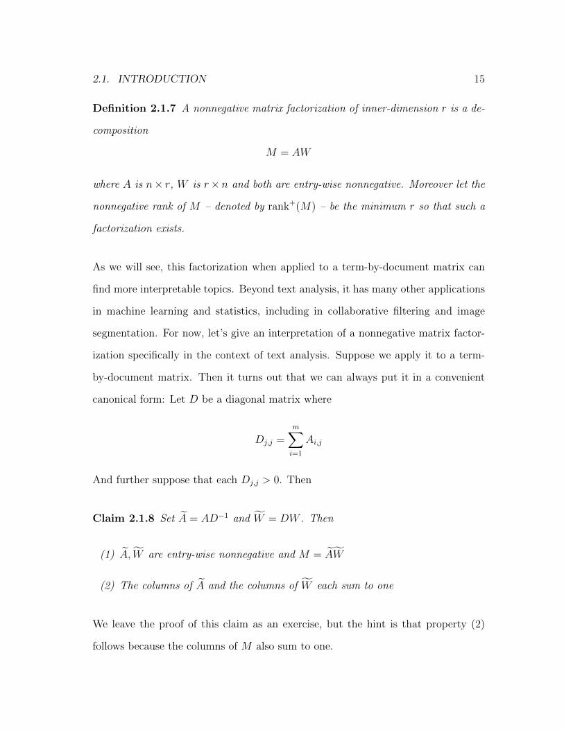
Definition 2.1.7 A nonnegative matrix factorization of inner-dimension r is a de-
composition
M = AW
where A is n× r, W is r× n and both are entry-wise nonnegative. Moreover let the
nonnegative rank of M – denoted by rank+(M) – be the minimum r so that such a
factorization exists.
As we will see, this factorization when applied to a term-by-document matrix can
find more interpretable topics. Beyond text analysis, it has many other applications
in machine learning and statistics, including in collaborative filtering and image
segmentation. For now, let’s give an interpretation of a nonnegative matrix factor-
ization specifically in the context of text analysis. Suppose we apply it to a term-
by-document matrix. Then it turns out that we can always put it in a convenient
canonical form: Let D be a diagonal matrix where
Dj,j =m∑i=1
Ai,j
And further suppose that each Dj,j > 0. Then
Claim 2.1.8 Set A = AD−1 and W = DW . Then
(1) A, W are entry-wise nonnegative and M = AW
(2) The columns of A and the columns of W each sum to one
We leave the proof of this claim as an exercise, but the hint is that property (2)
follows because the columns of M also sum to one.

16 CHAPTER 2. NONNEGATIVE MATRIX FACTORIZATION
Hence we can without loss of generality assume that our nonnegative matrix
factorization M = AW is such that the columns of A and the columns of W each
sum to one. Then we can interpret this factorization as follows: Each document is
itself a distribution on words, and what we have found is:
(1) A collection of r topics – the columns of A – that are themselves distributions
on words
(2) For each document i, a representation of it – given by Wi – as a convex
combination of r topics so that we recover its original distribution on words
Later on, we will get some insight into why nonnegative matrix factorization
is NP -hard. But what approaches are used in practice to actually compute such a
factorization? The usual approach is alternating minimization:
Alternating Minimization for NMF
Input: M ∈ Rm×n
Output: M ≈ A(N)W (N)
Guess entry-wise nonnegative A(0) of dimension m× r
For i = 1 to N
Set W (i) ← argminW ‖M − A(i−1)W‖2F s.t. W ≥ 0
Set A(i) ← argminA ‖M − AW (i)‖2F s.t. A ≥ 0
End
Alternating minimization is quite general, and throughout this course we will come

2.2. ALGEBRAIC ALGORITHMS 17
back to it many times and find that problems we are interested in are solved in
practice using some variant of the basic approach above. However, it has no provable
guarantees in the traditional sense. It can fail by getting stuck in a locally optimal
solution that is much worse than the globally optimal one. In fact, this is inevitable
because the problem it is attempting to solve really is NP -hard.
However in many settings we will be able to make progress by working with
an appropriate stochastic model, where we will be able to show that it converges to
a globally optimal solution provably. A major theme in this course is to not take
heuristics that seem to work in practice for granted, because being able to analyze
them will itself provide new insights into when and why they work, and also what
can go wrong and how to improve them.
2.2 Algebraic Algorithms
In the previous section, we introduced the nonnegative matrix factorization problem
and described some of its applications in machine learning and statistics. In fact,
(because of the algebraic nature of the problem) it is far from clear that there is any
finite time algorithm for computing it in the worst-case. Here we will explore some
of the fundamental results in solving systems of polynomial equations, and derive
algorithms for nonnegative matrix factorization from these.
Rank vs. Nonnegative Rank
Recall that rank+(M) is the smallest value r such that M has a nonnegative matrix
factorization M = AW with inner-dimension r. It is easy to see that the following

18 CHAPTER 2. NONNEGATIVE MATRIX FACTORIZATION
is another, equivalent definition:
Claim 2.2.1 rank+(M) is the smallest r such that there are r entry-wise nonnega-
tive rank one matrices Mi that satisfy M =∑
iMi.
We can now compare the rank and the nonnegative rank. There are of course
many equivalent definitions for the rank of a matrix, but the most convenient defi-
nition to compare the two is the following:
Claim 2.2.2 rank(M) is the smallest r such that there are r rank one matrices
Mi that satisfy M =∑
iMi.
The only difference between these two definitions is that the former stipulates that
all of the rank one matrices in the decomposition are entry-wise nonnegative while
the latter does not. Thus it follows immediately that:
Fact 2.2.3 rank+(M) ≥ rank(M)
Can the nonnegative rank of a matrix be much larger than its rank? We encourage
the reader to think about this question before proceeding. This is equivalent to
asking whether for an entry-wise nonnegative matrix M , one can without loss of
generality require the factors in its rank decomposition to be entry-wise nonnegative
too. It is certainly true for a rank one matrix, and turns out to be true for a rank
two matrix too, but...
In general, the nonnegative rank cannot be bounded by any function of the
rank alone. In fact, the relationship (or lack thereof) between the rank and the
nonnegative rank is of fundamental importance in a number of areas in theoretical

2.2. ALGEBRAIC ALGORITHMS 19
computer science. Fortunately, there are simple examples that illustrate that the
two parameters can be far apart:
Example: Let M be an n× n matrix where Mij = (i− j)2.
It is easy to see that the column space of M is spanned by the following three vectors
1
1
...
1
,
1
2
...
n
,
1
4
...
n2
Hence rank(M) ≤ 3. (In fact, rank(M) = 3). However, M has zeros along the diag-
onal and non-zeros off of it. Furthermore for any rank one, entry-wise nonnegative
matrix Mi, its pattern of zeros and non-zeros is a combinatorial rectangle – i.e. the
intersection of some set of rows and columns – and it can be shown that one needs
at least log n such rectangles to cover the non-zeros of M without covering any of
its zeros. Hence:
Fact 2.2.4 rank+(M) ≥ log n
A word of caution: For this example, a number of authors have incorrectly tried
to prove a much stronger lower bound (e.g. rank+(M) = n). In fact (and somewhat
surprisingly) it turns out that rank+(M) ≤ 2 log n. The usual error is in thinking
that because the rank of a matrix is the largest r such that it has r linearly inde-
pendent columns, that the nonnegative rank is the largest r such that there are r
columns where no column is a convex combination of the other r − 1. This is not
true!

20 CHAPTER 2. NONNEGATIVE MATRIX FACTORIZATION
Systems of Polynomial Inequalities
We can reformulate the problem of deciding whether rank+(M) ≤ r as a problem of
finding a feasible solution to a particular system of polynomial inequalities. More
specifically, rank+(M) ≤ r if and only if:
(2.1)
M = AW
A ≥ 0
W ≥ 0
has a solution. This system consists of quadratic equality constraints (one for each
entry of M), and linear inequalities that require A and W to be entry-wise nonneg-
ative. Before we worry about fast algorithms, we should ask a more basic question
(whose answer is not at all obvious):
Question 1 Is there any finite time algorithm for deciding if rank+(M) ≤ r?
This is equivalent to deciding if the above linear system has a solution, but
difficulty is that even if there is one, the entries of A and W could be irrational. This
is quite different than, say, 3-SAT where there is a simple brute-force algorithm.
In contrast for nonnegative matrix factorization it is quite challenging to design
algorithms that run in any finite amount of time.
But indeed there are algorithms (that run in some fixed amount of time) to
decide whether a system of polynomial inequalities has a solution or not in the
real RAM model. The first finite time algorithm for solving a system of polynomial
inequalities follows from the seminal work of Tarski, and there has been a long line of
2.2. ALGEBRAIC ALGORITHMS 21
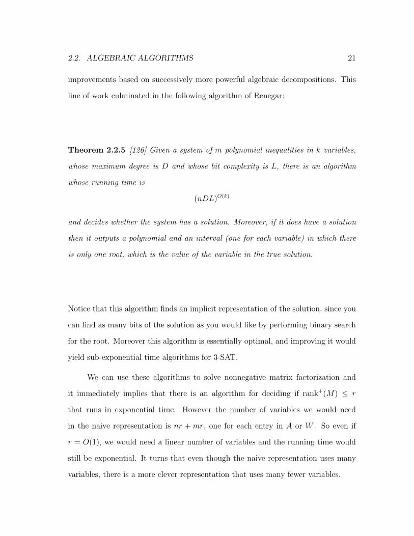
improvements based on successively more powerful algebraic decompositions. This
line of work culminated in the following algorithm of Renegar:
Theorem 2.2.5 [126] Given a system of m polynomial inequalities in k variables,
whose maximum degree is D and whose bit complexity is L, there is an algorithm
whose running time is
(nDL)O(k)
and decides whether the system has a solution. Moreover, if it does have a solution
then it outputs a polynomial and an interval (one for each variable) in which there
is only one root, which is the value of the variable in the true solution.
Notice that this algorithm finds an implicit representation of the solution, since you
can find as many bits of the solution as you would like by performing binary search
for the root. Moreover this algorithm is essentially optimal, and improving it would
yield sub-exponential time algorithms for 3-SAT.
We can use these algorithms to solve nonnegative matrix factorization and
it immediately implies that there is an algorithm for deciding if rank+(M) ≤ r
that runs in exponential time. However the number of variables we would need
in the naive representation is nr + mr, one for each entry in A or W . So even if
r = O(1), we would need a linear number of variables and the running time would
still be exponential. It turns that even though the naive representation uses many
variables, there is a more clever representation that uses many fewer variables.

22 CHAPTER 2. NONNEGATIVE MATRIX FACTORIZATION
Variable Reduction
Here we explore the idea of finding a system of polynomial equations that expresses
the nonnegative matrix factorization problem using many fewer variables. In [13,
112], Arora et al. and Moitra gave a system of polynomial inequalities with f(r) =
2r2 variables that has a solution if and only if rank+(M) ≤ r. This immediately
yields a polynomial time algorithm to compute a nonnegative matrix factorization
of inner-dimension r (if it exists) for any r = O(1). These algorithms turn out to
be essentially optimal in a worst-case sense, and prior to this work the best known
algorithms even for the case r = 4 ran in exponential time.
We will focus on a special case, to illustrate the basic idea behind variable
reduction. Suppose that rank(M) = r, and our goal is to decide whether or not
rank+(M) = r. This is called the simplicial factorization problem. Can we find an
alternate system of polynomial inequalities that expresses this decision problem but
uses many fewer variables? The following simple but useful observation will pave
the way:
Claim 2.2.6 In any solution to the simplicial factorization problem, A and W must
have full column and row rank respectively.
Proof: If M = AW then the column span of A must contain the columns of M
and similarly the row span of W must contain the rows of M . Since rank(M) = r
we conclude that A and W must have r linearly independent columns and rows
respectively. Since A has r columns and W has r rows, this implies the claim.
Hence we know that A has a left pseudo inverse A+ and W has a right pseudo
inverse W+ so that A+A = WW+Ir where Ir is the r × r identity matrix. We will

2.2. ALGEBRAIC ALGORITHMS 23
make use of these pseudo-inverses to reduce the number of variables in our system
of polynomial inequalities. In particular:
A+AW = W
and so we can recover the columns of W from a linear transformation of the columns
of M . Similarly we can recover the rows of A from a linear transformation of the
rows of M . This leads to the following alternative system of polynomial inequalities:
(2.2)
MW+A+M = M
MW+ ≥ 0
A+M ≥ 0
A priori, it is not clear that we have made progress since this system also has
nr + mr variables corresponding to the entries of A+ and W+. However consider
the matrix MW+. If we represent S+ as an n× r matrix then we are describing its
action on all vectors, but the crucial observation is that we only need to know how
S+ acts on the rows of M which span an r dimensional space. Hence we can apply
a change of basis to write
MC = MU
where U is an n× r matrix that has a right pseudo inverse. Similarly we can write
MR = VM

24 CHAPTER 2. NONNEGATIVE MATRIX FACTORIZATION
where V is an r×m matrix that has a left pseudo inverse. Now we get a new system:
(2.3)
MCSTMR = M
MCS ≥ 0
TMR ≥ 0
Notice that S and T are both r × r matrices, and hence there are 2r2 variables in
total. Moreover this formulation is equivalent to the simplicial factorization problem
in the following sense:
Claim 2.2.7 If rank(M) = rank+(M) = r then (2.3) has a solution.
Proof: Using the notation above, we can set S = U+W+ and T = A+V +. Then
MCS = MUU+W+ = A and similarly TMR = A+V +VM = W and this implies
the claim.
This is often called completeness, since if there is a solution to the original
problem we want that there is a valid solution to our reformulation. We also need
to prove soundness, that any solution to the reformulation yields a valid solution to
the original problem:
Claim 2.2.8 If there is a solution to (2.3) then there is a solution to (2.1).
Proof: For any solution to (2.3), we can set A = MCS and W = TMR and it
follows that A,W ≥ 0 and M = AW .
It turns out to be quite involved to extend the ideas above to nonnegative
matrix factorization in general. The main idea in [112] is to first establish a new

2.2. ALGEBRAIC ALGORITHMS 25
normal form for nonnegative matrix factorization, and use the observation that
even though A could have exponentially many maximal sets of linearly independent
columns, their psueudo-inverses are algebraically dependent and can be expressed
over a common set of r2 variables using Cramer’s rule. Additionallly Arora et al.
[13] showed that any algorithm that solves even the simplicial factorization problem
in (nm)o(r) time yields a sub-exponential time algorithm for 3-SAT, and hence the
algorithms above are nearly optimal under standard complexity assumptions.
Further Remarks
Earlier in this section, we gave a simple example that illustrates a separation between
the rank and the nonnegative rank. In fact, there are more interesting examples of
separations that come up in theoretical computer science, where a natural question
is to express a particular polytope P in n dimensions which has exponentially many
facets as the projection of a higher dimensional polytope Q with only polynomially
many facets. This is called an extended formulation, and a deep result of Yannakakis
is that the minimum number of facets of any such Q – called the extension complexity
of P – is precisely equal to the nonnegative rank of some matrix that has to do
with the geometric arrangement between vertices and facets of P [144]. Then the
fact that there are explicit polytopes P whose extension complexity is exponential is
intimately related to finding explicit matrices that exhibit large separations between
their rank and nonnegative rank.
Furthermore, the nonnegative rank also has important applications in commu-
nication complexity, where one of the most important open questions – the log-rank
conjecture [108] – can be reformulated as asking: Given a Boolean matrix M , is

26 CHAPTER 2. NONNEGATIVE MATRIX FACTORIZATION
log rank+(M) ≤ (log rank(M))O(1)? Thus, in the example above, the fact that the
nonnegative rank cannot be bounded by any function of the rank could be due to
the fact that the entries of M take on many distinct values.
2.3 Stability and Separability
Here we will give a geometric (as opposed to algebraic) interpretation of nonnegative
matrix factorization that will lend new insights into why it is hard in the worst-case,
and what types of features make it easy. In particular, we will move beyond worst-
case analysis and we will work with a new assumption called separability that will
allow us to give an algorithm that runs in polynomial time (even for large values of
r). This assumption was first introduced to understand conditions under which the
nonnegative matrix factorization problem has a unique solution [65], and this is a
common theme in algorithm design
Theme 1 Looking for cases where the solution is unique and robust, will often point
to cases where we can design algorithms with provable guarantees in spite of worst-
case hardness results.
Cones and Intermediate Simplicies
Here we will develop some geometric intuition about nonnegative matrix factoriza-
tion – or rather, an important special case of it called simplicial factorization that
we introduced in the previous section. First, let us introduce the notion of a cone:

2.3. STABILITY AND SEPARABILITY 27
Definition 2.3.1 Let A be an m×r matrix. Then the cone generated by the columns
of A is
CA = Ax|x ≥ 0
We can immediately connect this to nonnegative matrix factorization.
Claim 2.3.2 Given matrix M,A of dimension m× n and m× r respectively, there
is an entry-wise nonnegative matrix W of dimension r × n with M = AW if and
only if CM ⊆ CA.
Proof: In the forwards direction, suppose M = AW where W is entry-wise non-
negative. Then any vector y ∈ CM can be written as y = Mx where x ≥ 0, and then
y = AWx and the vector Wx ≥ 0 and hence y ∈ CA too. In the reverse direction,
suppose CM ⊆ CA. Then any column Mi ∈ CA and we can write Mi = AWi where
Wi ≥ 0. Now we can set W to be the matrix whose columns are Wii and this
completes the proof.
What makes nonnegative matrix factorization difficult is that both A and W
are unknown (if one were known – say A – then we could solve for the other by setting
up an appropriate linear program which amounts to representing each column of M
in CA).
Vavasis [139] was the first to introduce the simplicial factorization problem,
and one of his motivations was because it turns out to be connected to a purely
geometric problem about fitting a simplex in between two given polytopes. This is
called the intermediate simplex problem:
28 CHAPTER 2. NONNEGATIVE MATRIX FACTORIZATION
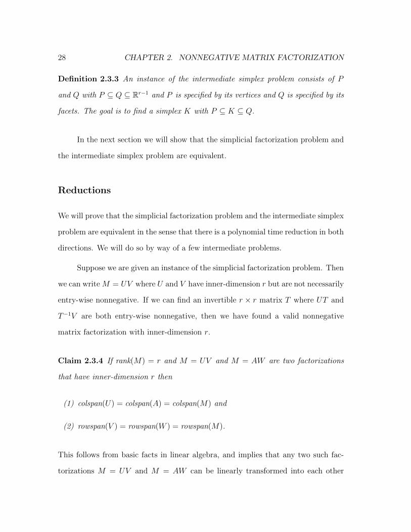
Definition 2.3.3 An instance of the intermediate simplex problem consists of P
and Q with P ⊆ Q ⊆ Rr−1 and P is specified by its vertices and Q is specified by its
facets. The goal is to find a simplex K with P ⊆ K ⊆ Q.
In the next section we will show that the simplicial factorization problem and
the intermediate simplex problem are equivalent.
Reductions
We will prove that the simplicial factorization problem and the intermediate simplex
problem are equivalent in the sense that there is a polynomial time reduction in both
directions. We will do so by way of a few intermediate problems.
Suppose we are given an instance of the simplicial factorization problem. Then
we can write M = UV where U and V have inner-dimension r but are not necessarily
entry-wise nonnegative. If we can find an invertible r × r matrix T where UT and
T−1V are both entry-wise nonnegative, then we have found a valid nonnegative
matrix factorization with inner-dimension r.
Claim 2.3.4 If rank(M) = r and M = UV and M = AW are two factorizations
that have inner-dimension r then
(1) colspan(U) = colspan(A) = colspan(M) and
(2) rowspan(V ) = rowspan(W ) = rowspan(M).
This follows from basic facts in linear algebra, and implies that any two such fac-
torizations M = UV and M = AW can be linearly transformed into each other

2.3. STABILITY AND SEPARABILITY 29
via some invertible r × r matrix T . Hence the intermediate simplex problem is
equivalent to:
Definition 2.3.5 An instance of the problem P1 consists of an m × n entry-wise
nonnegative matrix M with rank(M) = r and M = UV with inner-dimension r. The
goal is to find an invertible r × r matrix where both UT and T−1V are entry-wise
nonnegative.
Caution: The fact that you can start out with an arbitrary factorization and ask to
rotate it into a nonnegative matrix factorization of minimum inner-dimension, but
you haven’t painted yourself into a corner, is particular to the simplicial factorization
problem only! It is in general not true when rank(M) < rank+(M).
Now we can give a geometric interoperation of P1.
(1) Let u1, u2, ..., um be the rows of U .
(2) Let t1, t2, ..., tr be the columns of T .
(3) Let v1, v2, ..., vn be columns of V .
We will first work with an intermediate cone problem, but its connection to the
intermediate simplex problem will be immediate. Towards that end, let P be the
cone generated by u1, u2, ..., um, and let K be the cone generated by t1, t2, ..., tr.
Finally let Q be the cone give by:
Q = x|〈ui, x〉 ≥ 0 for all i
It is not hard to see thatQ is a cone in the sense that it is generated as all nonnegative

30 CHAPTER 2. NONNEGATIVE MATRIX FACTORIZATION
combinations of a finite set of vectors (its extreme rays), but we have instead chosen
to represent it by its supporting hyperplanes (through the origin).
Claim 2.3.6 UT is entry-wise nonnegative if and only if t1, t2, ..., tr ⊆ Q.
This follows immediately from the definition of Q, because the rows of U are its
supporting hyperplanes (through the origin). Hence we have a geometric reformu-
lation of the constraint UT is entry-wise nonnegative in P1. Next, we will interpret
the other constraint, that T−1V is entry-wise nonnegative too.
Claim 2.3.7 T−1V is entry-wise nonnegative if and only if v1, v2, ..., vm ⊆ K.
Proof: Consider xi = T−1vi. Then Txi = T (T−1)vi = vi and hence xi is a repre-
sentation of vi as a linear combination of t1, t2, ..., tr. Moreover it is the unique
representation, so and this completes the proof.
Thus P1 is equivalent to the following problem:
Definition 2.3.8 An instance of the intermediate cone problem consists of cones P
and Q with P ⊆ Q ⊆ Rr−1 and P is specified by its extreme rays and Q is specified
by its supporting hyperplanes (through the origin). The goal is to find a cone K with
r extreme rays and P ⊆ K ⊆ Q.
Furthermore the intermediate cone problem is easily seen to be equivalent to the
intermediate simplex problem by intersecting the cones in it with a hyperplane, in
which case a cone with extreme rays becomes a convex hull of the intersection of
those rays with the hyperplane.

2.3. STABILITY AND SEPARABILITY 31
Geometric Gadgets
Vavasis made use of the equivalences in the previous section to construct certain
geometric gadgets to prove that nonnegative matrix factorization is NP -hard. The
idea was to construct a two-dimensional gadget where there are only two possible
intermediate triangles, which can then be used to represent the truth assignment
for a variable xi. The description of the complete reduction, and the proof of its
soundness are involved (see [139]).
Theorem 2.3.9 [139] Nonnegative matrix factorization, simplicial factorization,
intermediate simplex, intermediate cone and P1 are all NP -hard.
Arora et al. [13] improved upon this reduction by constructing low dimensional
gadgets with many more choices. This allows them to reduce from the d-SUM
problem, where we are given a set of n numbers and the goal is to find a set of d
of them that sum to zero. The best known algorithms for this problem run in time
roughly ndd/2e. Again, the full construction and the proof of soundness is involved.
Theorem 2.3.10 Nonnegative matrix factorization, simplicial factorization, inter-
mediate simplex, intermediate cone and P1 all require time at least (nm)Ω(r) unless
there is a subexponential time algorithm for 3-SAT.
In all of the topics we will cover, it is important to understand what makes the
problem hard in order to hope to identify what makes it easy. The common feature
in all of the above gadgets is that the gadgets themselves are highly unstable and
have multiple solutions, and so it is natural to look for instances where the answer
itself is robust and unique in order to identify instances that can be solve more
efficiently than in the worst case.

32 CHAPTER 2. NONNEGATIVE MATRIX FACTORIZATION
Separability
In fact, Donoho and Stodden [64] were one of the first to explore the question of
what sorts of conditions imply that the nonnegative matrix factorization of minimum
inner-dimension is unique. Their original examples came from toy problem sin image
segmentation, but it seems like the condition itself can most naturally be interpreted
in the setting of text analysis.
Definition 2.3.11 We call A separable if, for every column i of A, there is a row
j where the only nonzero is in the ith column. Furthermore, we call j an anchor
word for column i.
In fact, separability is quite natural in the context of text analysis. Recall that
we interpret the columns of A as topics. We can think of separability as the promise
that these topics come with anchor words; informally, for each topic there is an
unknown anchor word that if it occurs in a document, the document is (partially)
about the given topic. For example, 401k could be an anchor word for the topic
personal finance. It seems that natural language contains many such, highly specific
words.
We will now give an algorithm for finding the anchor words, and for solving
instances of nonnegative matrix factorization where the unknown A is separable in
polynomial time.
Theorem 2.3.12 [13] If M = AW and A is separable and W has full row rank
then the Anchor Words Algorithm outputs A and W (up to rescaling).
Why do anchor words help? It is easy to see that if A is separable, then the

2.3. STABILITY AND SEPARABILITY 33
rows of W appear as rows of M (after scaling). Hence we just need to determine
which rows of M correspond to anchor words. We know from our discussion in
Section 2.3 that (if we scale M , A and W so that their rows sum to one) the convex
hull of the rows of W contain the rows of M . But since these rows appear in M as
well, we can try to find W by iteratively deleting rows of M that do not change its
convex hull.
Let M i denote the ith row of M and let M I denote the restriction of M to
the rows in I for I ⊆ [n]. So now we can find the anchor words using the following
simple procedure:
Find Anchors [13]
Input: matrix M ∈ Rm×n satisfying the conditions in Theorem 2.3.12
Output: W = M I
Delete duplicate rows Set I = [n]
For i = 1, 2, ..., n
If M i ∈ conv(M j|j ∈ I, j 6= i), set I ← I − i
End
Here in the first step, we want to remove redundant rows. If two rows are scalar
multiples of each other, then one being in the cone generated by the rows of W
implies the other is too, so we can safely delete one of the two rows. We do this for
all rows, so that in the equivalence class of rows that are scalar multiples of each
other, exactly one remains. We will not focus on this technicality in our discussion

34 CHAPTER 2. NONNEGATIVE MATRIX FACTORIZATION
though.
It is easy to see that deleting a row of M that is not an anchor word will not
change the convex hull of the remaining rows, and so the above algorithm terminates
with a set I that only contains anchor words. Moreover at termination
conv(M i|i ∈ I) = conv(M jj)
Alternatively the convex hull is the same as at the start. Hence the anchor words
that are deleted are redundant and we could just as well do without them.
Anchor Words [13]
Input: matrix M ∈ Rn×m satisfying the conditions in Theorem 2.3.12
Output: A,W
Run Find Anchors on M , let W be the output
Solve for nonnegative A that minimizes ‖M − AW‖F (convex programming)
End
The proof of theorem follows immediately from the proof of correctness of
Find Anchors and the fact that conv(M ii) ⊆ conv(W ii) if and only if there
is a nonnegative A (whose rows sum to one) with M = AW .
The above algorithm when naively implemented would be prohibitively slow.
Instead, there have been many improvements to the above algorithm [33], [100] [78],
and we will describe one in particular that appears in [12]. Suppose we choose a

2.4. TOPIC MODELS 35
row M i at random. Then it is easy to see that the furthest row from M i will be an
anchor word.
Similarly, if we have found one anchor word the furthest row from it will be
another anchor word, and so on. In this way we can greedily find all of the anchor
rows, and moreover this method only relies on pair-wise distances and projection
so we can apply dimension reduction before running this greedy algorithm. This
avoids linear programming altogether in the first step in the above algorithm, and
the second step can also be implemented quickly because it involves projecting a
point into an k − 1-dimensional simplex.
2.4 Topic Models
In this section, we will work with stochastic models for generating a collection of
documents. These models are called topic models, and our goal is to learn their
parameters. There are a wide range of types of topic models, but all of them fit into
the following abstract framework:

36 CHAPTER 2. NONNEGATIVE MATRIX FACTORIZATION
Abstract Topic Model
Parameters: topic matrix A ∈ Rm×r, distribution µ on the simplex in Rr
For i = 1 to n
Sample Wi from µ
Generate L words by sampling i.i.d. from the distribution AWi
End
This procedure generates n documents of length L, and our goal is to infer A
(and µ) from observing samples from this model. Let M be the observed term-by-
document matrix. We will use this notation to distinguish it from its expectation
E[M |W ] = M = AW
In the case of nonnegative matrix factorization we were given M and not M . How-
ever these matrices can be quite far apart! Hence even though each document is
described as a distribution on words, we only have partial knowledge of this dis-
tribution in the form of L samples from it. Our goal is to design algorithms that
provably work even in these challenging models.
Now is a good time to point out that this model contains many well-studied
topic models as a special case. All of them correspond to different choices of µ, the
distribution that is used to generate the columns of W . Some of the most popular
variants are:
(a) Pure Topic Model: Each document is about only one topic, hence µ is a
distribution on the vertices of the simplex and each column in W has exactly

2.4. TOPIC MODELS 37
one non-zero.
(b) Latent Dirichlet Allocation [36] : µ is a Dirichlet distribution. In par-
ticular, one can generate a sample from a Dirichlet distribution by taking
independent samples from r (not necessarily identical) Gamma distributions
and then renormalizing so that their sum is one. This topic model allows doc-
uments to be about more than one topic, but its parameters are generally set
so that it favors relatively sparse vectors Wi.
(c) Correlated Topic Model [35] : Certain pairs of topics are allowed to be
positively or negatively correlated, and µ is constrained to be log-normal.
(d) Pachinko Allocation Model [105] : This is a multi-level generalization of
LDA that allows for certain types of structured correlations.
In this section, we will use our algorithm for separable nonnegative matrix factor-
ization to provably learn the parameters of a topic model for (essentially) any topic
model where the topic matrix is separable. Thus this algorithm will work even in
the presence of complex relationships between the topics.
The Gram Matrix
In this subsection, we will introduce two matrices G and R – which we will call
the Gram matrix and the topic co-occurrence matrix respectively. The entries of
these matrices will be defined in terms of the probability of various events. And
throughout this section, we will always have the following experiment in mind: We
generate a document from the abstract topic model, and let w1 and w2 denote the

38 CHAPTER 2. NONNEGATIVE MATRIX FACTORIZATION
random variables for its first and second word respectively. With this experiment in
mind, we can define the Gram matrix:
Definition 2.4.1 Let G denote the m×m matrix where
Gj,j′ = P[w1 = j, w2 = j′]
Moreover for each word, instead of sampling from AWi we can sample from
Wi to choose which column of A to sample from. This procedure still generates a
random sample from the same distribution AWi, but each word w1 = j is annotated
with the topic from which it came, t1 = i (i.e. which column of A we sampled it
from). We can now define the topic co-occurrence matrix:
Definition 2.4.2 Let R denote the r × r matrix where
Ri,i′ = P[t1 = i, t2 = i′]
Note that we can estimate the entries of G directly from our samples, but we cannot
directly estimate the entries of R. Nevertheless these matrices are related according
to the following identity:
Lemma 2.4.3 G = ARAT

2.4. TOPIC MODELS 39
Proof: We have
Gj,j′ = P[w1 = j, w2 = j′] =∑i,i′
P[w1 = j, w2 = j′|t1 = i, t2 = i′]P[t1 = i, t2 = i′]
=∑i,i′
P[w1 = j|t1 = i]P[w2 = j′|t2 = i′]P[t1 = i, t2 = i′]
=∑i,i′
Aj,iAj′,i′Ri,i′
where the second-to-last line follows because conditioned on their topics, w1 and w2
are sampled independently from the corresponding columns of A. This completes
the proof.
The crucial observation is that G = A(RAT ) where A is separable and RAT
is nonnegative. Hence if we renormalize the rows of G to sum to one, the anchor
words will be the extreme points of the convex hull of all of the rows and we can
identify them through our algorithm for separable nonnegative matrix factorization.
Can we infer the rest of A?
Recovery via Bayes Rule
Consider the posterior distribution P[t1|w1 = j]. This is the posterior distribution
on which topic generated w1 = j when you know nothing else about the document.
The posterior distributions are just renormalizations of A so that the rows sum to
one. Then suppose j is an anchor word for topic i. We will use the notation j = π(i).
It is easy to see
P[t1 = i′|w1 = π(i)] =
1, if i′ = i
0 else

40 CHAPTER 2. NONNEGATIVE MATRIX FACTORIZATION
Now we can expand:
P[w1 = j|w2 = j′] =∑i′
P[w1 = j|w2 = j′, t2 = i′]P[t2 = i′|w2 = j′]
=∑i′
P[w1 = j|t2 = i′]P[t2 = i′|w2 = j′]
In the last line we have used the following identity:
Claim 2.4.4 P[w1 = j|w2 = j′, t2 = i′] = P[w1 = j|t2 = i′]
We leave the proof of this claim as an exercise. We will also use the identity below:
Claim 2.4.5 P[w1 = j|t2 = i′] = P[w1 = j|w2 = π(i′)]
Proof:
P[w1 = j|w2 = π(i′)] =∑i′′
P[w1 = j|w2 = π(i′), t2 = i′′]P[t2 = i′′|w2 = π(i′)]
= P[w1 = j|w2 = π(i′), t2 = i′]
where the last line follows because the posterior distribution on the topic t2 = i′′
given that w2 is an anchor word for topic i′ is equal to one if and only if i′′ = i′.
Finally the proof follows by invoking Claim 2.4.4.
Now we can proceed:
P[w1 = j|w2 = j′] =∑i′
P[w1 = j|w2 = π(i′)]P[t2 = i′|w2 = j′]︸ ︷︷ ︸unknowns

2.4. TOPIC MODELS 41
Hence this is a linear system in variables P[w1 = j|w2 = π(i′)] and it is not hard to
show that if R has full rank then it has a unique solution.
Finally by Bayes Rule we can compute the entries of A
P[w = j|t = i] =P[t = i|w = j]P[w = j]
P[t = i]
=P[t = i|w = j]P[w = j]∑j′ P[t = i|w = j′]P[w = j′]
And putting it all together we have the following algorithm:
Recover [14], [12]
Input: term-by-document matrix M ∈ Rn×m
Output: A,R
Compute the Gram matrix G
Compute the anchor words via Separable NMF
Solve for P[t = i|w = j]
Compute P[w = j|t = i] from Bayes Rule
Theorem 2.4.6 [14] There is a polynomial time algorithm to learn the topic matrix
for any separable topic model, provided that R is full-rank.
Remark 2.4.7 The running time and sample complexity of this algorithm depend
polynomially on m,n, r, σmin(R), p, 1/ε, log 1/δ where p is a lower bound on the prob-
ability of each anchor word, ε is the target accuracy and δ is the failure probability.

42 CHAPTER 2. NONNEGATIVE MATRIX FACTORIZATION
Note that this algorithm works for short documents, even for L = 2.
Experimental Results
Now we have provable algorithms for nonnegative matrix factorization and topic
modeling, under separability. But are natural topic models separable or close to
being separable? Consider the following experiment:
(1) UCI Dataset: Collection of 300, 000 New York Times articles
(2) MALLET: A popular topic modeling toolkit
We trained MALLET on the UCI dataset and found that with r = 200, about 0.9
fraction of the topics had a near anchor word – i.e. a word where P[t = i|w = j]
had a value of at least 0.9 on some topic. Indeed, the algorithms we gave can be
shown to work in the presence of some modest amount of error – deviation from the
assumption of separability. But can they work with this much modeling error?
We then ran the following additional experiment:
(1) Run MALLET on the UCI dataset. learn a topic matrix (r = 200)
(2) Use A to generate a new set of documents synthetically from an LDA model
(3) Run MALLET and our algorithm on a new set of documents, and compare
their outputs to the ground truth. In particular, compute the minimum cost
matching between the columns of the estimate and the columns of the ground
truth.
2.5. EXERCISES 43
It is important to remark that this is a biased experiment – biased against our
algorithm! We are comparing how well we can find the hidden topics (in a setting
where the topic matrix is only close to separable) to how well MALLET can find
its own output again. And with enough documents, we can find it more accurately
and hundreds of times faster! This new algorithm enables us to explore much larger
collections of documents than ever before.
2.5 Exercises
Problem 2-1: Which of the following are equivalent definitions of nonnegative
rank? For each, give a proof or a counter-example.
(a) the smallest r such thatM can be written as the sum of r rank one, nonnegative
matrices
(b) the smallest r such that there are r nonnegative vectors v1, v2, ..., vr such that
the cone generated by them contains all the columns of M
(c) the largest r such that there are r columns of M , M1,M2, ...,Mr such that
no column in set is contained in the cone generated by the remaining r − 1
columns
Problem 2-2: Let M ∈ Rn×n where Mi,j = (i− j)2. Prove that rank(M) = 3 and
that rank+(M) ≥ log2 n. Hint: To prove a lower bound on rank+(M) it suffices to
consider just where it is zero and where it is non-zero.
Problem 2-3: Papadimitriou et al. [118] considered the following document model:
M = AW and each column of W has only one non-zero and the support of each

44 CHAPTER 2. NONNEGATIVE MATRIX FACTORIZATION
column of A is disjoint. Prove that the left singular vectors of M are the columns
of A (after rescaling). You may assume that all the non-zero singular values of M
are distinct. Hint: MMT is block diagonal, after applying a permutation π to its
rows and columns.
Problem 2-4: Consider the following algorithm:
Greedy Anchorwords [13]
Input: matrix M ∈ Rn×m satisfying the conditions in Theorem 2.3.12
Output: A,W
Set S = ∅
For i = 2 to r
Project the rows of M orthogonal to the span of vectors in S
Add the row with the largest `2 norm to S
End
Let M = AW where A is separable and the rows of M , A and W are normalized to
sum to one. Also assume W has full row rank. Prove that Greedy Anchorwords
finds all the anchor words and nothing else. Hint: the `2 norm is strictly convex —
i.e. for any x 6= y and t ∈ (0, 1), ‖tx+ (1− t)y‖2 < t‖x‖2 + (1− t)‖y‖2.

Chapter 3
Tensor Decompositions:
Algorithms
In this chapter, we will study tensors and various structural and computational
problems we can ask about them. Generally, many problems that are easy over
matrices become ill-posed or NP -hard when working over tensors instead. Contrary
to popular belief, this isn’t a reason to pack up your bags and go home. Actually
there are things we can get out of tensors that we just can’t get out of matrices.
We just have to be careful about what types of problems we try to solve. More
precisely, in this chapter we will give an algorithm with provable guarantees for
low-rank tensor decomposition — that works in natural but restricted settings —
as well as some preliminary applications of it to factor analysis.
45

46 CHAPTER 3. TENSOR DECOMPOSITIONS: ALGORITHMS
3.1 The Rotation Problem
Before we study the algorithmic problems surrounding tensors, let’s first understand
why they’re useful. To do this, we’ll need to introduce the concept of factor analysis
where working with tensors instead of matrices will help us circumvent one of the
major stumbling blocks. So what is factor analysis? It’s a basic tool in statistics
where the goal is to take many variables and explain them away using a much fewer
number of hidden variables, called factors. But it’s best to understand it through
an example. And why not start with a historical example? It was first used in
the pioneering work of Charles Spearman who had a theory about the nature of
intelligence — he believed that there are fundamentally two types of intelligence:
mathematical and verbal. I don’t agree, but let’s continue anyways.
He devised the following experiment to test out his theory: He measured the
performance of one thousand students, each on ten different tests and arranged his
data into a 1000 × 10 matrix M . He believed that how a student performed on a
given test was determined by some hidden variables that have to do with the student
and the test. Imagine that each student is described by a 2-dimensional vector where
the two coordinates give numerical scores quantifying his mathematical and verbal
intelligence, respectively. Similarly, imagine that each test is also described by a
2-dimensional vector but where the coordinates represent the extent to which it
tests mathematical and verbal reasoning. Spearman set out to find this set of 2-
dimensional vectors, one for each student and one for each test, so that how a student
performs on a test is given by the inner-product between their two respective vectors.
Let’s translate the problem into a more convenient language. What we are

3.1. THE ROTATION PROBLEM 47
looking for is a particular factorization
M = ABT
where A is size 1000× 2 and B is size 10× 2 that validates Spearman’s theory. The
trouble is, even if there is a factorization M = ABT where the columns of A and the
rows of B can be given some meaningful interpretation — that would corroborate
Spearman’s theory — how can we find it? There can be many other factorizations
of M that have the same inner-dimension but are not the factors we are looking for.
To make this concrete, suppose that O is a 2 × 2 orthogonal matrix. Then we can
write
M = ABT = (AO)(OTBT )
and we could just as easily have found the factorization M = ABT where A = AO
and B = BO instead. So even if there is a meaningful factorization that would
explain our data, there is no guarantee that we find it and in general what we find
might be an arbitrary inner-rotation of it that itself is difficult to interpret. This is
called the rotation problem. This is the stumbling block that we alluded to earlier,
that we encounter if we use matrix-techniques to perform factor analysis.
What went wrong here is that low-rank matrix decompositions are not unique.
Let’s elaborate on what exactly we mean by unique, in this context. Suppose we
are given a matrix M and are promised that it has some meaningful low-rank de-
composition
M =r∑i=1
a(i)(b(i))T
Our goal is to recover the factors a(i) and b(i). The trouble is we could compute the

48 CHAPTER 3. TENSOR DECOMPOSITIONS: ALGORITHMS
singular value decomposition M = UΣV T and find another low-rank decomposition
M =r∑i=1
σiu(i)(v(i))T
These are potentially two very different sets of factors that just happen to recreate
the same matrix. In fact, the vectors u(i) are necessarily orthonormal because they
came from the singular value decomposition, even though there is a priori no reason
to think that the true factors a(i) that we are looking for are orthonormal too. So
now we can qualitatively answer the question we posed at the outset. Why are we
interested in tensors? It’s because they solve the rotation problem and their decom-
position is unique under much weaker conditions than their matrix decomposition
counterparts.
3.2 A Primer on Tensors
A tensor might sound mysterious but it’s just a collection of numbers. Let’s start
with the case we’ll spend most of our time on. A third order tensor T has three
dimensions, sometimes called rows, columns and tubes respectively. If the size of T
is n1 × n2 × n3 then the standard notation is that Ti,j,k refers to the number in row
i, column j and tube k in T . Now a matrix is just a second order tensor because
it’s a collection of numbers indexed by two indices. And of course you can consider
tensors of any order you’d like.
We can think about tensors many different ways, and all of these viewpoints
will be useful at different points in this chapter. Perhaps the simplest way to think
of an order three tensor T is as nothing more than a collection of n3 matrices, each

3.2. A PRIMER ON TENSORS 49
of size n1 × n2, that are stacked on top of each other. Before we go any further, we
should define the notion of the rank of a tensor. This will allow us to explore when
a tensor is not just a collection of matrices, but when and how these matrices are
interrelated.
Definition 3.2.1 A rank one, third-order tensor T is the tensor product of three
vectors u, v and w, and its entries are
Ti,j,k = uivjwk
Thus if the dimensions of u, v and w are n1, n2 and n3 respectively, T is of size
n1 × n2 × n3. Moreover, we will often use the following shorthand
T = u⊗ v ⊗ w
We can now define the rank of a tensor:
Definition 3.2.2 The rank of a third-order tensor T is the smallest integer r so
that we can write
T =r∑i=1
u(i) ⊗ v(i) ⊗ w(i)
Recall, the rank of a matrix M is the smallest integer r so that M can be written
as the sum of r rank one matrices. The beauty of the rank of a matrix is how many
equivalent definitions it admits. What we have above is the natural generalization of
one of the many definitions of the rank of a matrix, to tensors. The decomposition
above is often called a CANDECOMP/PARFAC decomposition.

50 CHAPTER 3. TENSOR DECOMPOSITIONS: ALGORITHMS
Now that we have the definition of rank in hand, let’s understand how a low-
rank tensor is not just an arbitrary collection of low-rank matrices. Let T·,·,k denote
the n1 × n2 matrix corresponding to the kth slice through the tensor.
Claim 3.2.3 Consider a rank r tensor
T =r∑i=1
u(i) ⊗ v(i) ⊗ w(i)
Then for all 1 ≤ k ≤ n3,
colspan(T·,·,k) ⊆ span(u(i)i)
and moreover
rowspan(T·,·,k) ⊆ span(v(i)i)
We leave the proof as an exercise to the reader. Actually, this claim tells us why not
every stacking of low-rank matrices yields a low-rank tensor. True, if we take a low-
rank tensor and look at its n3 different slices we get matrices of dimension n1 × n2
with rank at most r. But we know more than that. Each of their column spaces is
contained in the span of the vectors u(i). Similarly their row space is contained in
the span of the vectors v(i).
Intuitively, the rotation problem comes from the fact that a matrix is just one
view of the vectors u(i)i and v(i)i. But a tensor gives us multiple views through
each of its slices, that helps us resolve the indeterminacy. If this doesn’t quite make
sense yet, that’s alright. Come back to it once you understand Jennrich’s algorithm
and think about it again.

3.2. A PRIMER ON TENSORS 51
The Trouble with Tensors
Before we proceed, it will be important to dispel any myths you might have that
working with tensors will be a straightforward generalization of working with ma-
trices. So what is so subtle about working with tensors? For starters, what makes
linear algebra so elegant and appealing is how things like the rank of a matrix M
admit a number of equivalent definitions. When we defined the rank of a tensor, we
were careful to say that what we were doing was taking one of the definitions of the
rank of a matrix and writing down the natural generalization to tensors. But what
if we took a different definition for the rank of a matrix, and generalized it in the
natural way? Would we get the same notion of rank for a tensor? Usually not!
Let’s try it out. Instead of defining the rank of a matrix M as the smallest
number of rank one matrices we need to add up to get M , we could have defined
the rank through the dimension of its column/row space. This next claim just says
that we’d get the same notion of rank.
Claim 3.2.4 The rank of a matrix M is equal to the dimension of its column/row
space. More precisely,
rank(M) = dim(colspan(M)) = dim(rowspan(M))
Does this relation hold for tensors? Not even close! As a simple example, let’s
set n1 = k2, n2 = k and n3 = k. Then if we take the n1 columns of T to be the
columns of a k2 × k2 identity matrix, we know that the n2n3 columns of T are all
linearly independent and have dimension k2. But the n1n3 rows of T have dimension
at most k because they live in a k-dimensional space. So for tensors, the dimension

52 CHAPTER 3. TENSOR DECOMPOSITIONS: ALGORITHMS
of the span of the rows is not necessarily equal to the dimension of the span of the
columns/tubes.
Things are only going to get worse from here. There are some nasty subtleties
about the rank of a tensor. First, the field is important. Let’s suppose T is real-
valued. We defined the rank as the smallest value of r so that we can write T as
the sum of r rank one tensors. But should we allow these tensors to have complex
values, or only real values? Actually this can change the rank, as the following
example illustrates.
Consider the following 2× 2× 2 tensor:
T =
1 0
0 1
;0 −1
1 0
where the first 2×2 matrix is the first slice through the tensor, and the second 2×2
matrix is the second slice. It is not hard to show that rankR(T ) ≥ 3. But it is easy
to check that
T =1
2
1
−i
⊗1
i
⊗ 1
−i
+
1
i
⊗ 1
−i
⊗1
i
So even though T is real-valued, it can be written as the sum of fewer rank one ten-
sors if we are allowed to use complex numbers. This issue never arises for matrices.
If M is real-valued and there is a way to write it as the sum of r rank one matrices
with (possibly) complex-valued entries there is always a way to write it as the sum
of at most r rank one matrices all of whose entries are real. This seems like a happy
accident, now that we are faced with objects whose rank is field-dependent.

3.2. A PRIMER ON TENSORS 53
Another worrisome issue is that there are tensors of rank 3 but that can be
arbitrarily well-approximated by tensors of rank 2. This leads us to the definition
of border rank:
Definition 3.2.5 The border rank of a tensor T is the minimum r such that for
any ε > 0 there is a rank r tensor that is entry-wise ε-close to T .
For matrices, the rank and border rank are the same! If we fix a matrix M with rank
r then there is a finite limit (depending on M) to how well we can approximate it
by a rank r′ < r matrix. One can deduce this from the optimality of the truncated
singular value decomposition for low-rank approximation. But for tensors, the rank
and border rank can indeed be different, as our final example illustrates.
Consider the following 2× 2× 2 tensor:
T =
0 1
1 0
;1 0
0 0
It is not hard to show that rankR(T ) ≥ 3. Yet it admits an arbitrarily good rank
two approximation using the following scheme. Let
Sn =
n 1
1 1n
;1 1
n
1n
1n2
and Rn =
n 0
0 0
;0 0
0 0
.Both Sn and Rn are rank one, and so Sn−Rn has rank at most two. But notice that
Sn−Rn is entry-wise 1/n-close to T and as we increase n we get an arbitrarily good
approximation to T . So even though T has rank 3, its border rank is at most 2.
You can see this example takes advantage of larger and larger cancellations. It also

54 CHAPTER 3. TENSOR DECOMPOSITIONS: ALGORITHMS
shows that the magnitude of the entries of the best low-rank approximation cannot
be bounded as a function of the magnitude of the entries in T .
A useful property of matrices is that the best rank k approximation to M
can be obtained directly from its best rank k + 1 approximation. More precisely,
suppose that B(k) and B(k+1) are the best rank k and rank k + 1 approximations
to M in terms of (say) Frobenius norm, respectively. Then we can obtain B(k) as
the best rank k approximation to B(k+1). However for tensors, the best rank k and
rank k + 1 approximations to T need not share any common rank one terms at all.
The best rank k approximation to a tensor is unwieldy. You have to worry about
its field. You cannot bound the magnitude of its entries in terms of the input. And
it changes in complex ways as you vary k.
To me, the most serious issue at the root of all of this is computational com-
plexity. Of course the rank of a tensor is not equal to the dimension of its column
space. The former is NP -hard (by a result of Hastad [85]) and the latter is easy to
compute. You have to be careful with tensors. In fact, computational complexity is
such a pervasive issue, with so many problems that are easy to compute on matrices
turning out to be NP -hard on tensors, that the title of a well-known paper of Hillar
and Lim [86] sums it up:
“Most Tensor Problems are Hard”
To back this up, Hillar and Lim [86] proved that a laundry list of other problems,
such as finding the best low-rank approximation, computing the spectral norm and
deciding whether a tensor is nonnegative definite are NP -hard too. If this section
was a bit pessimistic for you, keep in mind that all I’m trying to do is set the stage
so that you’ll be as excited as you should be, that there actually is something we

3.3. JENNRICH’S ALGORITHM 55
can do with tensors!
3.3 Jennrich’s Algorithm
In this section, we will introduce an algorithm for computing a minimum rank
decomposition that works in a natural but restricted setting. This algorithm is
called Jennrich’s Algorithm. Interestingly, it has been rediscovered numerous times
(for reasons that we will speculate on later) and to the best of our knowledge the
first place that it appeared is in a working paper of Harshman [84] where the author
credits it to Dr. Robert Jennrich.
In what follows, we will assume we are given a tensor T which we will assume
has the following form
T =r∑i=1
u(i) ⊗ v(i) ⊗ w(i)
We will refer to the factors u(i), v(i) and w(i) as the hidden factors to emphasize that
we do not know them, but want to find them. We should be careful here. What
do we mean by find them? There are some ambiguities that we can never hope to
resolve. We can only hope to recover the factors up to an arbitrary reordering (of
the sum) and up to certain rescalings that leave the rank one tensors themselves
unchanged. This motivates the following definition, which takes into account these
issues:
Definition 3.3.1 We say that two sets of factors
(u(i), v(i), w(i))
ri=1
and
(u(i), v(i), w(i))ri=1

56 CHAPTER 3. TENSOR DECOMPOSITIONS: ALGORITHMS
are equivalent if there is a permutation π : [r]→ [r] such that for all i
u(i) ⊗ v(i) ⊗ w(i) = u(π(i)) ⊗ v(π(i)) ⊗ w(π(i))
The important point is that two sets of factors that are equivalent produce two
decompositions
T =r∑i=1
u(i) ⊗ v(i) ⊗ w(i) =r∑i=1
u(i) ⊗ v(i) ⊗ w(i)
that have the same set of rank one tensors in their sums.
The main question in this section is: Given T , can we efficiently find a set of
factors that are equivalent to the hidden factors? We will state and prove a version
of Jennrich’s Algorithm that is more general, following the approach of Leurgans,
Ross and Abel [103].
Theorem 3.3.2 [84], [103] Suppose we are given a tensor of the form
T =r∑i=1
u(i) ⊗ v(i) ⊗ w(i)
where the following conditions are met:
(1) the vectors u(i)i are linearly independent,
(2) the vectors v(i)i are linearly independent and
(3) every pair of vectors in w(i)i are linearly independent
3.3. JENNRICH’S ALGORITHM 57
Then there is an efficient algorithm to find a decomposition
T =r∑i=1
u(i) ⊗ v(i) ⊗ w(i)
and moreover the factors (u(i), v(i), w(i)) and (u(i), v(i), w(i)) are equivalent.
The original result of Jennrich [84] was stated as a uniqueness theorem that under the
conditions on the factors u(i), v(i) and w(i) above any decomposition of T into at most
r rank one tensors must use an equivalent set of factors. It just so happened that
the way that Jennrich proved this uniqueness theorem was by giving an algorithm
that finds the decomposition, although in the paper it was never stated that way.
Intriguingly, this seems to be a major contributor to why the result was forgotten.
Much of the subsequent literature cited a stronger uniqueness theorem of Kruskal
whose proof is non-constructive, and seemed to forget that the weaker uniqueness
theorem of Jennrich comes along with an algorithm. Let this be a word of warning:
If you not only proved some mathematical fact but your argument readily yields an
algorithm, then say so!

58 CHAPTER 3. TENSOR DECOMPOSITIONS: ALGORITHMS
Jennrich’s Algorithm [84]
Input: tensor T ∈ Rm×n×p satisfying the conditions in Theorem 3.3.2
Output: factors uii, vii and wii
Choose a, b ∈ Sp−1 uniformly at random; set
T (a) =
p∑i=1
aiT·,·,i and T (b) =
p∑i=1
biT·,·,i
Compute the eigendecomposition of T (a)(T (b))+ and ((T (a))+T (b))T
Let U and V be the eigenvectors corresponding to non-zero eigenvalues
Pair up u(i) and v(i) iff their eigenvalues are reciprocals
Solve for w(i) in T =∑r
i=1 u(i) ⊗ v(i) ⊗ w(i)
End
Recall that T·,·,i denotes the ith matrix slice through T . Thus T (a) is just the weighted
sum of matrices slices through T , each weighted by ai.
The first step in the analysis is to express T (a) and T (b) in terms of the hidden
factors. Let U and V be size m× r and n× r matrices respectively, whose columns
are u(i) and v(i). Let D(a) and D(b) be r × r diagonal matrices whose entries are
〈w(i), a〉 and 〈w(i), b〉 respectively. Then
3.3. JENNRICH’S ALGORITHM 59
Lemma 3.3.3 T (a) = UD(a)V T and T (b) = UD(b)V T
Proof: Since the operation of computing T (a) from T is linear, we can apply it to
each of the rank one tensors in the low-rank decomposition of T . It is easy to see
that if we are given the rank one tensor u ⊗ v ⊗ w then the effect of taking the
weighted sum of matrices slices, where the ith slice is weighted by ai, is we obtain
the matrix 〈w, a〉u⊗ v.
Thus by linearity we have
T (a) =r∑i=1
〈w(i), a〉u(i) ⊗ v(i)
which yields the first part of the lemma. The second part follows analogously with
a replaced by b.
It turns out that we can now recover the columns of U and the columns of
V through a generalized eigendecomposition. Let’s do a thought experiment. If we
were given a matrix M of the form M = UDU−1 where the entries along the diagonal
matrix D are distinct and non-zero, the columns of U will be eigenvectors except
that they are not necessarily unit vectors. Since the entries of D are distinct, the
eigendecomposition of M is unique and this means that we can recover the columns
of U (up to rescaling) as the eigenvectors of M .
Now if we are instead given two matrices of the form A = UD(a)V T and B =
UD(b)V T then if the entries of D(a)(D(b))−1 are distinct and non-zero, we can recover
the columns of U and V (again up to rescaling) through an eigendecomposition of
AB−1 = UD(a)(D(b))−1U−1 and (A−1B)T = V D(b)(D(a))−1V −1

60 CHAPTER 3. TENSOR DECOMPOSITIONS: ALGORITHMS
respectively. It turns out that instead of actually forming the matrices above we
could instead look for all the vectors v that satisfy Av = λvBv, which is called
a generalized eigendecomposition. In any case, this is the main idea behind the
following lemma, although we need to take some care since in our setting the matrices
U an V are not necessarily square let alone invertible matrices.
Lemma 3.3.4 Almost surely, the columns of U and V are the unique eigenvectors
corresponding to non-zero eigenvalues of T (a)(T (b))+ and ((T (a))+T (b))T respectively.
Moreover the eigenvalue corresponding to u(i) is the reciprocal of the eigenvalue cor-
responding to v(i).
Proof: We can use the formula for T (a) and T (b) in Lemma 3.3.3 to compute that
T (a)(T (b))+ = UD(a)(D(b))+U+
The entries of D(a)(D(b))+ are 〈w(i), a〉/〈w(i), b〉. Then because every pair of vectors
in w(i)i are linearly independent, we have that almost surely over the choice of a
and b the entries along the diagonal of D(a)(D(b))+ will all be non-zero and distinct.
Now returning to the formula above for T (a)(T (b))+ we see that it is an eigen-
decomposition and that moreover the non-zero eigenvalues are distinct. Thus the
columns of U are the unique eigenvectors of T (a)(T (b))+ with non-zero eigenvalue,
and the eigenvalue corresponding to u(i) is 〈w(i), a〉/〈w(i), b〉. An identical argument
shows that the columns of V are the unique eigenvectors of
((T (a))+T (b))T = V D(b)(D(a))+V +
3.3. JENNRICH’S ALGORITHM 61
with non-zero eigenvalue. And by inspection we have that the eigenvalue corre-
sponding to v(i) is 〈w(i), b〉/〈w(i), a〉, which completes the proof of the lemma.
Now to complete the proof of the theorem, notice that we have only recovered
the columns of U and the columns of V up to rescaling — i.e. for each column, we
recovered the corresponding unit vector. We will push this rescaling factor in with
the missing factors w(i). Thus the linear system in the last step of the algorithm
clearly has a solution, and what remains is to prove that this is its only solution.
Lemma 3.3.5 The matricesu(i)(v(i))T
ri=1
are linearly independent.
Proof: Suppose (for the sake of contradiction) that there is a collection of coeffi-
cients that are not all zero where
r∑i=1
αiu(i)(v(i))T = 0
Suppose (without loss of generality) that α1 6= 0. Because by assumption the vectors
v(i)i are linearly independent, we have that there is a vector a which satisfies that
〈v(1), a〉 6= 0 but is orthogonal to all other v(i)’s. Now if we right multiply the above
identity by a we get
α1〈v(1), a〉u(1) = 0
which is a contradiction, because the left hand side is non-zero.
This immediately implies that the linear system over the w(i)’s has a unique
solution. We can write the linear system as an mn×r matrix each of whose columns
represent a matrix u(i)(v(i))T but in vector form, times an unknown r × p matrix

62 CHAPTER 3. TENSOR DECOMPOSITIONS: ALGORITHMS
whose columns represent the vectors w(i). The product of these two matrices is
constrained to be equal to an mn × p matrix whose columns represent each of the
p matrix slices through the tensor T , but again in vector form. This completes the
proof of Theorem 3.3.2.
If you want a nice open question, note that the conditions in Jennrich’s algo-
rithm can only ever hold if r ≤ min(n1, n2) because we need that the vectors u(i)i
and v(i)i are linearly independent. This is called the undercomplete case because
the rank is bounded by the largest dimension of the tensor. When r is larger than
either n1, n2 or n3 we know that the decomposition of T is generically unique. But
are there algorithms for decomposing generic overcomplete third order tensors? This
question is open even when r = 1.1 max(n1, n2, n3).
3.4 Perturbation Bounds
This section is good medicine. What we have so far is an algorithm (Jennrich’s
algorithm) that decomposes a third-order tensor T under some natural conditions on
the factors, but under the assumption that we know T exactly. In our applications,
this just won’t be enough. We’ll need to handle noise. The aim of this section is
to answer the question: If we are given T = T + E instead (you can think of E as
representing sampling noise), how well can we approximate the hidden factors?
Our algorithm won’t change. We will still use Jennrich’s algorithm. Rather,
what we want to do in this section is track how the errors propagate. We want to
give quantitative bounds on how well we approximate the hidden factors, and the
bounds we give will depend on E and properties of T . The main step in Jennrich’s
3.4. PERTURBATION BOUNDS 63
algorithm is to compute an eigendecomposition. Naturally, this is where we will
spend most of our time — in understanding when eigendecompositions are stable.
From this, we will easily be able to see when and why Jennrich’s algorithm works
in the presence of noise.
Prerequisites for Perturbation Bounds
Now let’s be more precise. The main question we’re interested in is the following:
Question 2 If M = UDU−1 is diagonalizable and we are given M = M + E, how
well can we estimate U?
The natural thing to do is to compute a matrix that diagonalizes M — i.e. U where
M = UDU−1 — and quantify how good U is as an estimate for U . But before we
dive right in, it’s good to do a thought experiment.
There are some cases where it just is not possible to say that U and U are close.
For example, if there are two eigenvalues of M that are very close to each other,
then the perturbation E could in principle collapse two eigenvectors into a single
two dimensional eigenspace and we would never be able to estimate the columns of
U . What this means is that our perturbation bounds will have to depend on the
minimum separation between any pair of eigenvalues of M .
Just like this, there is one more thought experiment we can do which tells us
another property of M that must make its way into our perturbation bounds. But
before we get there, let’s understand the issue in a simpler setup. This takes us to
an important notion from numerical linear algebra.

64 CHAPTER 3. TENSOR DECOMPOSITIONS: ALGORITHMS
Definition 3.4.1 The condition number of a matrix U is defined as
κ(U) =σmax(U)
σmin(U)
where σmax(U) and σmin(U) are the maximum and minimum singular values of U ,
respectively.
The condition number captures how errors amplify when solving systems of
linear equations. Let’s be more precise: Consider the problem of solving for x in
Mx = b. Suppose that we are given M exactly, but we only know an estimate
b = b+ e of b. How well can we approximate x?
Question 3 If we obtain a solution x that satisfies Mx = b, how close is x to x?
We have x = M−1b = x+M−1e = x+M−1(b− b). So
‖x− x‖ ≤ 1
σmin(M)‖b− b‖.
Since Mx = b, we also have ‖b‖ ≤ σmax(M)‖x‖. It follows that
‖x− x‖‖x‖
≤ σmax(M)
σmin(M)
‖b− b‖‖b‖
= κ(M)‖b− b‖‖b‖
.
The term ‖b− b‖/‖b‖ is often called the relative error and is a popular distance to
measure closeness in numerical linear algebra. What the discussion above tells us is
that the condition number controls the relative error when solving a linear system.
Now let’s tie this back in to our earlier discussion. It turns out that our per-
turbation bounds for eigendecompositions will also have to depend on the condition
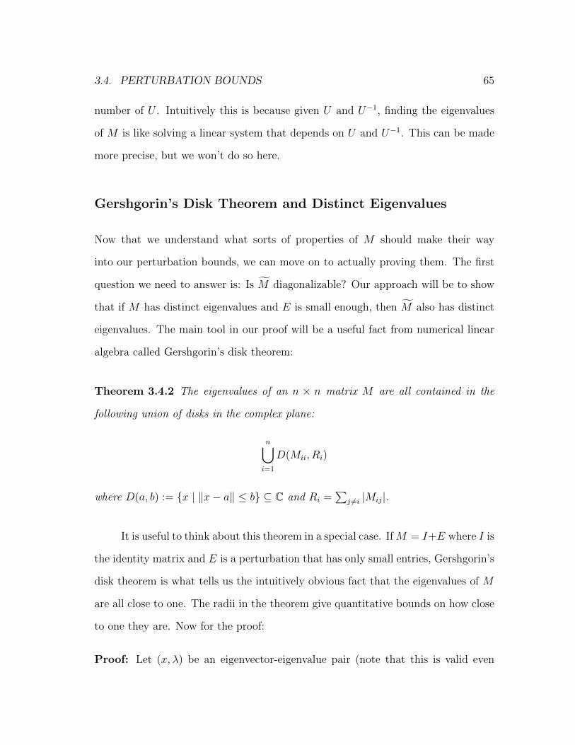
3.4. PERTURBATION BOUNDS 65
number of U . Intuitively this is because given U and U−1, finding the eigenvalues
of M is like solving a linear system that depends on U and U−1. This can be made
more precise, but we won’t do so here.
Gershgorin’s Disk Theorem and Distinct Eigenvalues
Now that we understand what sorts of properties of M should make their way
into our perturbation bounds, we can move on to actually proving them. The first
question we need to answer is: Is M diagonalizable? Our approach will be to show
that if M has distinct eigenvalues and E is small enough, then M also has distinct
eigenvalues. The main tool in our proof will be a useful fact from numerical linear
algebra called Gershgorin’s disk theorem:
Theorem 3.4.2 The eigenvalues of an n × n matrix M are all contained in the
following union of disks in the complex plane:
n⋃i=1
D(Mii, Ri)
where D(a, b) := x | ‖x− a‖ ≤ b ⊆ C and Ri =∑
j 6=i |Mij|.
It is useful to think about this theorem in a special case. IfM = I+E where I is
the identity matrix and E is a perturbation that has only small entries, Gershgorin’s
disk theorem is what tells us the intuitively obvious fact that the eigenvalues of M
are all close to one. The radii in the theorem give quantitative bounds on how close
to one they are. Now for the proof:
Proof: Let (x, λ) be an eigenvector-eigenvalue pair (note that this is valid even

66 CHAPTER 3. TENSOR DECOMPOSITIONS: ALGORITHMS
when M is not diagonalizable). Let i denote the coordinate of x with the maximum
absolute value. Then Mx = λx gives∑
jMijxj = λxi. So∑
j 6=iMijxj = λxi−Miixi.
We conclude:
|λ−Mii| =
∣∣∣∣∣∑j 6=i
Mijxjxi
∣∣∣∣∣ ≤∑j 6=i
|Mij| = Ri.
Thus λ ∈ D(Mii, Ri).
Now we can return to the task of showing that M is diagonalizable. The idea
is straightforward and comes from digesting a single expression. Consider
U−1MU = U−1(M + E)U = D + U−1EU.
What does this expression tell us? The right hand side is a perturbation of a diagonal
matrix, so we can use Gershgorin’s disk theorem to say that its eigenvalues are close
to those of D. Now because left multiplying by U−1 and right multiplying by U is
a similarity transformation, this in turn tells us about M ’s eigenvalues.
Let’s put this plan into action and apply Gershgorin’s disk theorem to under-
stand the eigenvalues of D = D+U−1EU . First we can bound the magnitude of the
entries of E = U−1EU as follows. Let ‖A‖∞ denote the matrix max norm which is
the largest absolute value of any entry in A.
Lemma 3.4.3 ‖E‖∞ ≤ κ(U)‖E‖
Proof: For any i and j, we can regard Ei,j as the quadratic form of the ith row
of U−1 and the jth column of U on E. Now the jth column of U has Euclidean
norm at most σmax(U) and similarly the ith row of U−1 has Euclidean norm at most
σmax(U−1) = 1/σmin(U). Together, this yields the desired bound.

3.4. PERTURBATION BOUNDS 67
Now let’s prove that under the appropriate conditions, the eigenvalues of M
are distinct. Let R = maxi∑
j |Ei,j| and let δ = mini 6=j |Di,i−Dj,j| be the minimum
separation of the eigenvalues of D.
Lemma 3.4.4 If R < δ/2 then the eigenvalues of M are distinct.
Proof: First we use Gershgorin’s disk theorem to conclude that the eigenvalues of
D are contained in disjoint disks, one for each row. There’s a minor technicality
that Gershgorin’s disk theorem works with a radius that is the sum of the absolute
values of the entries in a row, except for the diagonal entry. But we leave it as an
exercise to check that the calculation still goes through.
Actually we are not done yet1. Even if Gershgorin’s disk theorem implies that
there are disjoint disks (one for each row) that contain the eigenvalues of D, how do
we know that no disk contains more than one eigenvalue, and that no disk contains
no eigenvalues? It turns out that the eigenvalues of a matrix are a continuous
function of the entries, so as we trace out a path
γ(t) = (1− t)D + t(D)
from D to D as t goes from zero to one, the disks in Gershgorin’s disk theorem are
always disjoint and no eigenvalue can jump from one disk to another. Thus at D
we know that there really is exactly one eigenvalue in each disk, and since the disks
are disjoint we have that the eigenvalues of D are distinct as desired. Of course
the eigenvalues of D and M are the same because they are related by a similarity
transformation. 1Thanks to Santosh Vempala for pointing out this gap in an earlier version of this book. See
also [79].
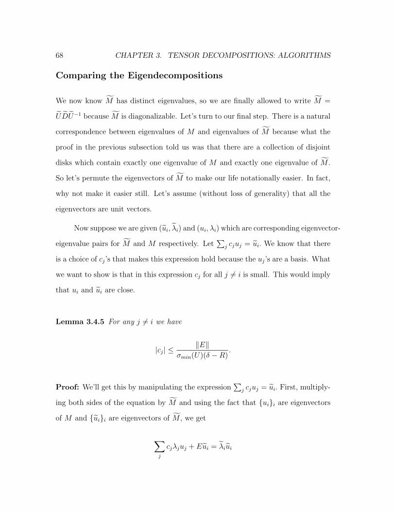
68 CHAPTER 3. TENSOR DECOMPOSITIONS: ALGORITHMS
Comparing the Eigendecompositions
We now know M has distinct eigenvalues, so we are finally allowed to write M =
UDU−1 because M is diagonalizable. Let’s turn to our final step. There is a natural
correspondence between eigenvalues of M and eigenvalues of M because what the
proof in the previous subsection told us was that there are a collection of disjoint
disks which contain exactly one eigenvalue of M and exactly one eigenvalue of M .
So let’s permute the eigenvectors of M to make our life notationally easier. In fact,
why not make it easier still. Let’s assume (without loss of generality) that all the
eigenvectors are unit vectors.
Now suppose we are given (ui, λi) and (ui, λi) which are corresponding eigenvector-
eigenvalue pairs for M and M respectively. Let∑
j cjuj = ui. We know that there
is a choice of cj’s that makes this expression hold because the uj’s are a basis. What
we want to show is that in this expression cj for all j 6= i is small. This would imply
that ui and ui are close.
Lemma 3.4.5 For any j 6= i we have
|cj| ≤‖E‖
σmin(U)(δ −R).
Proof: We’ll get this by manipulating the expression∑
j cjuj = ui. First, multiply-
ing both sides of the equation by M and using the fact that uii are eigenvectors
of M and uii are eigenvectors of M , we get
∑j
cjλjuj + Eui = λiui

3.4. PERTURBATION BOUNDS 69
which rearranging terms yields the expression∑
j cj(λj − λi)uj = −Eui.
Now what we want to do is pick out just one of the coefficients on the left hand
side, and use the right hand side to bound it. To do this, let wTj be the jth row of
U−1 and left multiplying both sides of the expression above by this vector we obtain
cj(λj − λi) = −wTj Eui.
Now let’s bound the terms in this expression. First, for any i 6= j we have |λj− λi| ≥
|λj − λi| − R ≥ δ − R using Gershgorin’s disk theorem. Second, ui is a unit vector
by assumption and ‖wj‖ ≤ 1/σmin(U). Using these bounds and rearranging terms
now proves the lemma.
The three lemmas we have proven can be combined to give quantitative bounds
on how close U is to U , which was our goal at the outset.
Theorem 3.4.6 Let M be an n× n matrix with eigendecomposition M = UDU−1.
Let M = M + E. Finally let
δ = mini 6=j|Di,i −Dj,j|
i.e. the minimum separation of eigenvalues of M .
(1) If κ(U)‖E‖n < δ2
then M is diagonalizable.
(2) Moreover if M = UDU−1 then there is a permutation π : [n] → [n] such that
for all i
‖ui − uπ(i)‖ ≤2‖E‖n
σmin(U)(δ − κ(U)‖E‖n)

70 CHAPTER 3. TENSOR DECOMPOSITIONS: ALGORITHMS
where uii are the columns of U and uii are the columns of U .
Proof: The first part of the theorem follows by combining Lemma 3.4.3 and
Lemma 3.4.4. For the second part of the theorem, let’s fix i and let P be the
projection onto the orthogonal complement of ui. Then using elementary geometry
and the fact that the eigenvectors are all unit vectors, we have
‖ui − uπ(i)‖ ≤ 2‖Puπ(i)‖.
Moreover we can bound the right hand side as
‖Puπ(i)‖ = ‖∑j 6=i
cjPuj‖ ≤∑j 6=i
|cj|.
Lemma 3.4.5 supplies the bounds on the coefficients cj, which completes the proof
of the theorem.
You were warned early on that the bound would be messy! It is also by no
means optimized. But what you should instead take away is the qualitative corollary
that we were after: If ‖E‖ ≤ poly(1/n, σmin(U), 1/σmax(U), δ) (i.e. if the sampling
noise is small enough compared to the dimensions of the matrix, the condition
number of U and the minimum separation) then U and U are close.
Back to Tensor Decompositions
Now let’s return to Jennrich’s algorithm. We’ve stated enough messy bounds for my
taste. So let’s cheat from here on out and hide messy bounds using the following

3.4. PERTURBATION BOUNDS 71
notation: Let
AE→0−→ B
signify that as E goes to zero, A converges to B at an inverse polynomial rate. We’re
going to use this notation as a placeholder. Every time you see it, you should think
that you could do the algebra to figure out how close A is to B in terms of E and
various other factors we’ll collect along the way.
With this notation in hand, what we want to do is qualitatively track how the
error propagates in Jennrich’s algorithm. If we let T = T + E then TE→0−→ T and
T (a) E→0−→ T (a) where T (a) =∑
i aiT·,·,i. We leave it as an exercise to the reader to
check that there are natural conditions where
(T (b))+ E→0−→ (T (b))+.
As a hint, this convergence needs to depend on the smallest singular value of T (b).
Or to put it another way, if E is not small compared to the smallest singular value
of T (b) then in general we cannot say that (T (b))+ and (T (b))+ are close.
In any case, combining these facts, we have that
T (a)(T (b))+ E→0−→ T (a)(T (b))+.
Now we are in good shape. The eigenvectors of the right hand side are the columns
of U . Let the columns of U be the eigenvectors of the left hand side. Since the
left hand side is converging to the right hand side at an inverse polynomial rate,
we can invoke our perturbation bounds on eigendecompositions (Theorem 3.4.6) to
conclude that their eigenvectors are also converging at an inverse polynomial rate.

72 CHAPTER 3. TENSOR DECOMPOSITIONS: ALGORITHMS
In particular UE→0−→ U where we have abused notation because the convergence
above is only after we have applied the appropriate permutation to the columns of
U . Similarly we have VE→0−→ V .
Finally we compute W by solving a linear system in U and V . It can be shown
that WE→0−→ W using the fact that U and V are close to well-conditioned matrices
U and V which means that the linear system we get from taking the tensor product
of the ith column in U with the ith column in V is also well-conditioned.
This is the full, gory details of how you can prove that Jennrich’s algorithm
behaves well in the presence of noise. If we make our life easy and in what follows
we analyze our learning algorithms in the no noise case (E = 0), we can always
appeal to various perturbation bounds for eigendecompositions and track through
how all the errors propagate to bound how close the factors we find are to the true
hidden factors. This is what I meant by good medicine. You don’t need to think
about these perturbation bounds every time you use tensor decompositions, but
you should know that they exist because they really are what justifies using tensor
decompositions for learning problems where there is always sampling noise.
3.5 Exercises
Problem 3-1:
(a) Suppose we want to solve the linear system Ax = b (where A ∈ Rn×n is square
and invertible) but we are only given access to a noisy vector b satisfying
‖b− b‖‖b‖
≤ ε

3.5. EXERCISES 73
and a noisy matrix A satisfying ‖A − A‖ ≤ δ (in operator norm). Let x be
the solution to Ax = b. Show that
‖x− x‖‖x‖
≤ ε σmax(A) + δ
σmin(A)− δ
provided δ < σmin(A).
(b) Now suppose we know A exactly, but A may be badly conditioned or even
singular. We want to show that it may still be possible to recover a specific
coordinate xj of x. Let x be any solution to Ax = b and let ai denote column
i of A. Show that
|xj − xj| ≤‖b− b‖Cj
where Cj is the norm of the projection of aj onto the orthogonal complement
of span(aii 6=j).
Problem 3-2: In the multi-reference alignment problem we observe many noisy
copies of the same unknown signal x ∈ Rd, but each copy has been circularly shifted
by a random offset (as pictured).
Figure: Three shifted copies of the true signal x are shown in gray. Noisysamples yi are shown in red. (Figure credit: [23])
Formally, for i = 1, 2, . . . , n we observe
yi = R`ix+ ξi
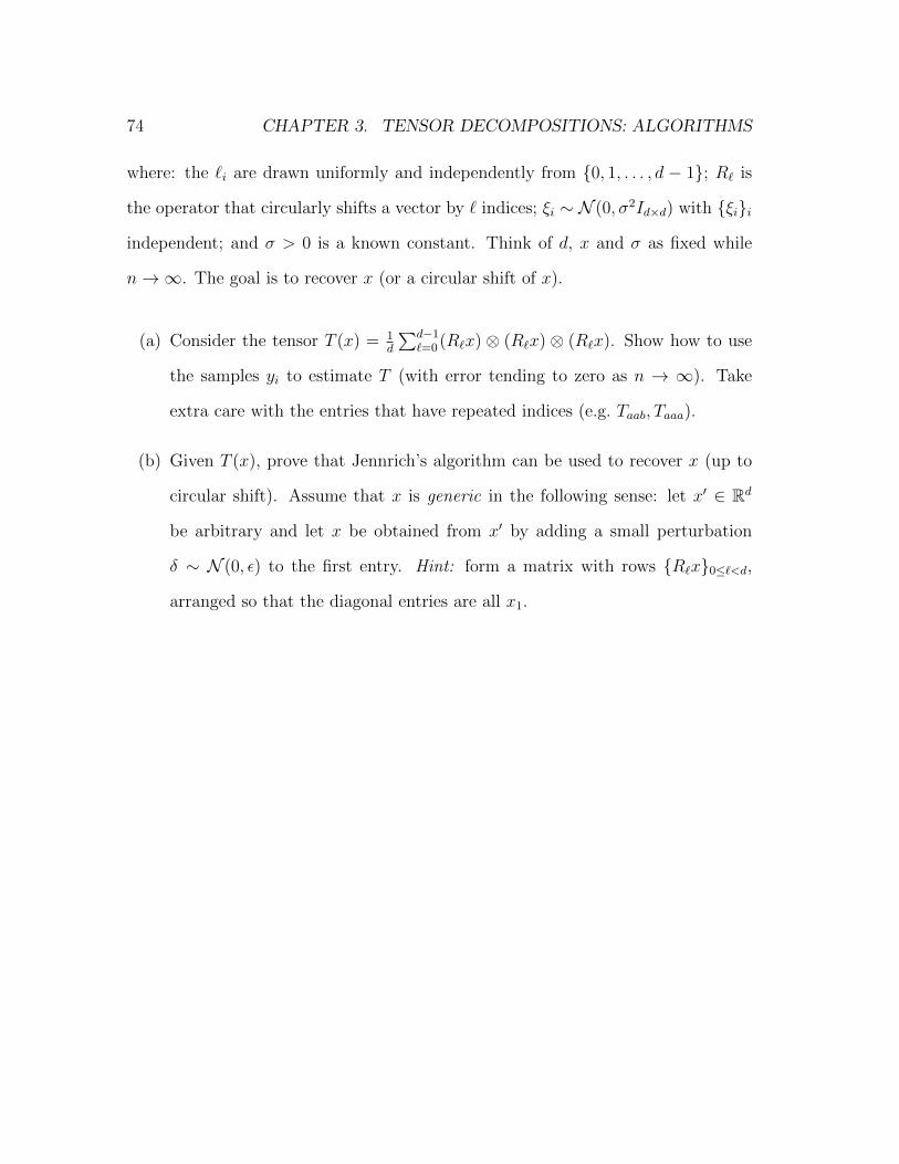
74 CHAPTER 3. TENSOR DECOMPOSITIONS: ALGORITHMS
where: the `i are drawn uniformly and independently from 0, 1, . . . , d − 1; R` is
the operator that circularly shifts a vector by ` indices; ξi ∼ N (0, σ2Id×d) with ξii
independent; and σ > 0 is a known constant. Think of d, x and σ as fixed while
n→∞. The goal is to recover x (or a circular shift of x).
(a) Consider the tensor T (x) = 1d
∑d−1`=0 (R`x) ⊗ (R`x) ⊗ (R`x). Show how to use
the samples yi to estimate T (with error tending to zero as n → ∞). Take
extra care with the entries that have repeated indices (e.g. Taab, Taaa).
(b) Given T (x), prove that Jennrich’s algorithm can be used to recover x (up to
circular shift). Assume that x is generic in the following sense: let x′ ∈ Rd
be arbitrary and let x be obtained from x′ by adding a small perturbation
δ ∼ N (0, ε) to the first entry. Hint: form a matrix with rows R`x0≤`<d,
arranged so that the diagonal entries are all x1.

Chapter 4
Tensor Decompositions:
Applications
Many exciting problems fit into the following paradigm: First, we choose some
parametric family of distributions that are rich enough to model things like evolution,
writing, and the formation of social networks. Second, we design algorithms for
learning the unknown parameters — which you should think of as a proxy for finding
hidden structure in our data, like a tree of life that explains how species evolved from
each other, the topics that underly a collection of documents, or the communities
of strongly connected individuals in a social network. In this chapter, all of our
algorithms will be based on tensor decomposition. We will construct a tensor from
the moments of our distribution and apply Jennrich’s algorithm to find the hidden
factors which in turn will reveal the unknown parameters of our model.
75

76 CHAPTER 4. TENSOR DECOMPOSITIONS: APPLICATIONS
4.1 Phylogenetic Trees and HMMs
Our first application of tensor decomposition is to learning phylogenetic trees. Before
we go into the details of the model, it is helpful to understand the motivation. A
central problem in evolutionary biology is to piece together the tree of life which
describes how species evolved from each other. More precisely, it is a binary tree
whose leaves represent extant species (i.e. species that are currently living) and
whose internal nodes represent extinct species. When an internal node has two
children, it represents a speciation event where two populations split off into separate
species.
We will work with a stochastic model defined on this tree where each edge
introduces its own randomness that represents mutation. More precisely our model
has the following components:
(a) A rooted binary tree with root r (the leaves do not necessarily have the same
depth)
(b) A set Σ of states, for example Σ = A,C,G, T. Let k = |Σ|.
(c) A Markov model on the tree; i.e. a distribution πr on the state of the root and
a transition matrix P uv for each edge (u, v).
We can generate a sample from the model as follows: We choose a state for the
root according to πr and for each node v with parent u we choose the state of v
according to the distribution defined by the ith row of P uv, where i is the state of
u. Alternatively, we can think of s(·) : V → Σ as a random function that assigns

4.1. PHYLOGENETIC TREES AND HMMS 77
states to vertices where the marginal distribution on s(r) is πr and
P uvij = P(s(v) = j|s(u) = i),
Note that s(v) is independent of s(t) conditioned on s(u) whenever the (unique)
shortest path from v to t in the tree passes through u.
In this section, our main goal is to learn the rooted tree and the transition
matrices when given enough samples from the model. Now is a good time to connect
this back to biology. What does a sample from this model represent? If we have
sequenced each of the extant species and moreover these sequences have already
been properly aligned, we can think of the ith symbol in each of these sequences as
being represented by the configuration of states of the leaves in a sample from the
above model. Of course this is an oversimplification of the biological problem but it
still captures many interesting phenomena.
There are really two separate tasks: (a) learning the topology and (b) estimat-
ing the transition matrices. Our approach for finding the topology will follow the
foundational work of Steel [133] and Erdos, Steel, Szekely, and Warnow [69]. Once
we know the topology, we can apply tensor decompositions to find the transition
matrices following the approach of Chang [47] and Mossel and Roch [115].
Learning the Topology
Here we will focus on the problem of learning the topology of the tree. The amazing
idea due to Steel [133] is that there is a way to define an evolutionary distance. What
is important about this distance is that it (a) assigns a nonnegative value to every

78 CHAPTER 4. TENSOR DECOMPOSITIONS: APPLICATIONS
edge in the tree and (b) can be evaluated for any pair of nodes given just their joint
distribution. So what magical function has these properties? First, for any pair of
nodes a and b, let F ab be a k × k matrix that represents their joint distribution:
F abij = P(s(a) = i, s(b) = j).
Definition 4.1.1 Steel’s evolutionary distance on an edge (u, v) is
νuv = − ln |det(P uv)|+ 1
2ln
∏i∈[k]
πu(i)
− 1
2ln
∏i∈[k]
πv(i)
.
Steel [133] proved the two following fundamental properties of this distance
function, captured in the following lemma:
Lemma 4.1.2 Steel’s evolutionary distance satisfies:
(a) νuv is nonnegative and
(b) for any pair of nodes a and b, we have
ψab := − ln |det(F ab)| =∑
(u,v)∈pab
νuv
where pab is the shortest path connecting a and b in the tree.
What makes this distance so useful for our purposes is that for any pair of
leaves a and b, we can estimate F ab from our samples, and hence we can (approx-
imately) compute ψab on the leaves. So from now on we can imagine that there is
some nonnegative function on the edges of the tree and that we have an oracle for
computing the sum of the distances along the path connecting any two leaves.

4.1. PHYLOGENETIC TREES AND HMMS 79
Reconstructing Quartets
Now we will use Steel’s evolutionary distance to compute the topology by piecing
together the picture four nodes at a time.
a
d
c
b
(a)
a
d
b
c
(b)
a
c
b
d
(c)
Figure 4.1: Possible quartet topologies
Our goal is to determine which of these induced topologies is the true topology,
given the pairwise distances.
Lemma 4.1.3 If all distances in the tree are strictly positive, then it is possible to
determine the induced topology on any four nodes a, b, c and d given an oracle that
can compute the distance between any pair of them.
Proof: The proof is by case analysis. Consider the three possible induced topologies
between these nodes given in Figure 4.1. Here by induced topology, we mean delete
edges not on any shortest path between any pair of the four leaves, and contract
paths to a single edge if possible.
It is easy to check that under topology (a) we have
ψ(a, b) + ψ(c, d) < min ψ(a, c) + ψ(b, c), ψ(a, d) + ψ(b, d) .

80 CHAPTER 4. TENSOR DECOMPOSITIONS: APPLICATIONS
But under topology (b) or (c) this inequality would not hold. There is an analogous
way to identify each of the other topologies from the others. What this means is
that we can simply compute three values ψ(a, b) + ψ(c, d), ψ(a, c) + ψ(b, c), and
ψ(a, d) + ψ(b, d). Whichever is the smallest determines the induced topology as
being (a), (b) or (c) respectively.
Indeed from just these quartet tests we can recover the topology of the tree.
Lemma 4.1.4 If for any quadruple of leaves a, b, c and d we can determine the
induced topology, it is possible to determine the topology of the tree.
Proof: The approach is to first determine which pairs of leaves have the same parent,
and then determine which pairs have the same grandparent, and so on. First, fix a
pair of leaves a and b. It is easy to see that they have the same parent if and only if
for every other choice of leaves c and d, the quartet test returns topology (a). Now
if we want to determine if a pair of leaves a and b have the same grandparent, we
can modify the approach as follows: They have the same grandparent if and only if
for every other choice of leaves c and d neither of which is a sibling for a or b, the
quartet test returns topology (a). Essentially, we are building up the tree by finding
the closest pairs first.
An important technical point is that we can only approximate F ab from our
samples. This translates into a good approximation of ψab when a and b are close,
but is noisy when a and b are far away. Ultimately, the approach in [69] of Erdos,
Steel, Szekely, and Warnow is to only use quartet tests where all of the distances
are short.

4.1. PHYLOGENETIC TREES AND HMMS 81
Estimating the Transition Matrices
Now we will assume that we know the topology of the tree and set our sights on
estimating the transition matrices. Our approach is to use tensor decompositions.
To that end, for any triple of leaves a, b and c, let T abc be the k × k × k tensor
defined as follows:
T abcijk = P(s(a) = i, s(b) = j, s(c) = k).
These are third order moments of our distribution that we can estimate from sam-
ples. We will assume throughout this section that the transition matrices are full
rank. This means that we can reroot the tree arbitrarily. Now consider the unique
node that lies on all of the shortest paths among a, b, and c. Let’s let this be the
root. Then
T abc =∑`
P(s(r) = `)P(s(a) = ·|s(r) = `)⊗ P(s(b) = ·|s(r) = `)⊗ P(s(c) = ·|s(r) = `)
=∑`
P(s(r) = `)P ra` ⊗ P rb
` ⊗ P rc`
where we have used P rx` to denote the `th row of the transition matrix P rx.
We can now apply the algorithm in Section 3.3 to compute a tensor decom-
position of T whose factors are unique up to rescaling. Furthermore the factors are
probability distributions and hence we can compute their proper normalization. We
will call this procedure a star test. (Indeed, the algorithm for tensor decompositions
in Section 3.3 has been re-discovered many times and it is also called Chang’s lemma
[47]).
In [115], Mossel and Roch use this approach to find the transition matrices of

82 CHAPTER 4. TENSOR DECOMPOSITIONS: APPLICATIONS
a phylogenetic tree, given the tree topology, as follows. Let us assume that u and
v are internal nodes and that w is a leaf. Furthermore suppose that v lies on the
shortest path between u and w. The basic idea is to write
P uw = P uvP vw
and if we can find P uw and P vw (using the star tests above) then we can compute
P uv = P uw(P vw)−1 since we have assumed that the transition matrices are invertible.
However there are two serious complications:
(a) As in the case of finding the topology, long paths are very noisy.
Mossel and Roch showed that one can recover the transition matrices also using
only queries to short paths.
(b) We can only recover the tensor decomposition up to relabeling.
In the above star test, we could apply any permutation to the states of r and permute
the rows of the transition matrices P ra, P rb and P rc accordingly so that the resulting
joint distribution on a, b and c is unchanged.
However the approach of Mossel and Roch is to work instead in the framework
of probably approximately correct learning of Valiant [138] where the goal is to learn
a generative model that produces almost the same joint distribution on the leaves.
In particular, if there are multiple ways to label the internal nodes to produce the
same joint distribution on the leaves, we are indifferent to them.

4.1. PHYLOGENETIC TREES AND HMMS 83
Remark 4.1.5 Hidden Markov models are a special case of phylogenetic trees where
the underlying topology is a caterpillar. But note that for the above algorithm, we
need that the transition matrices and the observation matrices are full-rank.
More precisely, we require that the transition matrices are invertible and that
the observation matrices whose row space correspond to a hidden node and whose
column space correspond to the output symbols each have full row rank.
Beyond Full Rank?
The algorithm above assumed that all transition matrices are full rank. In fact if
we remove this assumption, then it is easy to embed an instance of the noisy parity
problem [37] which is a classic hard learning problem. Let us first define this problem
without noise:
Let S ⊂ [n], and choose X(j) ∈ 0, 1n independently and uniformly at ran-
dom, for j = 1, . . . ,m. Given X(j) and b(j) = χS(X(j)) :=∑
i∈S X(j)i mod 2 for
each j, the goal is to recover S.
This is quite easy: Let A be the matrix whose jth row is X(j) and let b be a
column vector whose jth entry is b(j). It is straightforward to see that 1S is a solution
to the linear system Ax = b where 1S is the indicator function for S. Furthermore
if we choose Ω(n log n) samples then A is with high probability full column rank
and so this solution is unique. We can then find S by solving a linear system over
GF (2).
Yet a slight change in the above problem does not change the sample com-
plexity but makes the problem drastically harder. The noisy parity problem is the

84 CHAPTER 4. TENSOR DECOMPOSITIONS: APPLICATIONS
same as above but for each j we are independently given the value b(j) = χS(X(j))
with probably 2/3 and otherwise b(j) = 1−χS(Xj). The challenge is that we do not
know which labels have been flipped.
Claim 4.1.6 There is an exponential time algorithm that solves the noisy parity
problem using m = O(n log n) samples
Proof: For each T , calculate the fraction of samples where χT agrees with the
observed label — i.e.
1
m
m∑j=1
1χT (X(j))=b(j)
From standard concentration bounds, it follows that with high probability this value
is larger than (say) 3/5 if and only if S = T .
The state-of-the-art due to Blum, Kalai and Wasserman [37] has running time
and sample complexity 2n/ logn. It is widely believed that there is no polynomial
time algorithm for noisy parity even given any polynomial number of samples. This
is an excellent example of a problem whose sample complexity and computational
complexity are (conjectured) to be wildly different.
Next we show how to embed samples from a noisy parity problem into an
HMM, however to do so we will make use of transition matrices that are not full
rank. Consider an HMM that has n hidden nodes, where the ith hidden node
encodes is used to represent the ith coordinate of X and the running parity
χSi(X) :=
∑i′≤i,i′∈S
X(i′) mod 2.

4.2. COMMUNITY DETECTION 85
Hence each node has four possible states. We can define the following transition
matrices. Let s(i) = (xi, si) be the state of the ith internal node where si = χSi(X).
We can define the following transition matrices:
if i+ 1 ∈ S P i,i+1 =
12
(0, si)
12
(1, si + 1 mod 2)
0 otherwise
if i+ 1 /∈ S P i,i+1 =
12
(0, si)
12
(1, si)
0 otherwise
.
At each internal node we observe xi and at the last node we also observe χS(X)
with probability 2/3 and otherwise 1 − χS(X). Each sample from the noisy parity
problem is a set of observations from this HMM, and if we could learn the transition
matrices of it we would necessarily learn S and solve the noisy parity problem.
Note that here the observation matrices are certainly not full rank because
we only observe two possible emissions even though each internal node has four
possible states! Hence these problems become much harder when the transition (or
observation) matrices are not full rank!
4.2 Community Detection
Here we give applications of tensor methods to community detection. There are
many settings in which we would like to discover communities — that is, groups of

86 CHAPTER 4. TENSOR DECOMPOSITIONS: APPLICATIONS
strongly connected individuals. Here we will focus on graph theoretic approaches,
where we will think of a community as a set of nodes that are better connected
to each other than to nodes outside of the set. There are many ways we could
formalize this notion, each of which would lead to a different optimization problem
e.g. sparsest cut or k-densest subgaph.
However each of these optimization problems is NP -hard, and even worse are
hard to approximate. Instead, we will formulate our problem in an average-case
model where there is an underlying community structure that is used to generate a
random graph, and our goal is to recover the true communities from the graph with
high probability.
Stochastic Block Model
Here we introduce the block stochastic model, which is used to generate a random
graph on V with |V | = n. Additionally, the model is specified by parameters p and
q and a partitioning specified by a function π:
• π : V → [k] partitions the vertices V into k disjoint groups (we will relax this
condition later);
• Each possible edge (u, v) is chosen independently with:
P[(u, v) ∈ E] =
q π(u) = π(v)
p otherwise
.
In our setting we will set q > p which is called the assortative case, but this model

4.2. COMMUNITY DETECTION 87
also makes sense when q < p which is called the disassortative case. For example
when q = 0 we are generating a random graph that has a planted k-coloring. Re-
gardless, we observe a random graph generated from the above model and our goal
is to recover the partition described by π.
When is this information theoretically possible? In fact even for k = 2 where
π is a bisection, we need
q − p > Ω(√ log n
n
)in order for the true bisection to be the uniquely smallest cut that bisects the
random graph G with high probability. If q − p is smaller, then it is not even
information theoretically possible to find π. Indeed, we should also require that
each part of the partition is large, and for simplicity we will assume that k = O(1)
and |u|π(u) = i| = Ω(n).
There has been a long line of work on partitioning random graphs in the block
stochastic model, culminating in the work of McSherry [109]:
Theorem 4.2.1 [109] There is an efficient algorithm that recovers π (up to rela-
beling) if
q − pq
> c
√log n/δ
qn
and succeeds with probability at least 1− δ.
This algorithm is based on spectral clustering, where we think of the observed adja-
cency matrix as the sum of a rank k matrix which encodes π and an error term. If
the error is small, then we can recover something close to the true rank k matrix by
finding the best rank k approximation to the adjacency matrix. For the full details,
see [109].

88 CHAPTER 4. TENSOR DECOMPOSITIONS: APPLICATIONS
We will instead follow the approach in Anandkumar et al. [9] that makes use of
tensor decompositions. In fact, their algorithm also works in the mixed membership
model where we allow each node to be a distribution over [k]. Then if πu and
πv are the probability distributions for u and v, the probability of an edge (u, v)
is∑
i πui π
vi q +
∑i 6=j π
ui π
vj p. We can interpret this probability as: u and v choose
a community according to πu and πv respectively, and if they choose the same
community there is an edge with probability q and otherwise there is an edge with
probability p.
Counting Three Stars
What’s really going on when we use tensor decompositions is we are finding condi-
tionally independent random variables. That’s what we did when we used them for
learning the transition matrices of a phylogenetic tree. There, the states of a, b and
c were independent once we conditioned on the state of the unique node r where the
shortest paths between them meet. We will do something similar here.
If we have four nodes a, b, c and x and we condition on which community x
belongs to then whether or not (a, x), (b, x) and (c, x) are edges in our graph are all
independent random variables. When all three edges are present this is called a three
star. We will set up a tensor that counts three stars as follows. First we partition
V into four sets X, A, B, and C. Now let Π ∈ 0, 1V×k represent the (unknown)
assignment of nodes to communities, so that each row of Π contains exactly one 1.
Finally let R be the k× k matrix whose entries are the connection probabilities. In

4.2. COMMUNITY DETECTION 89
particular,
(R)ij =
q i = j
p i 6= j
.
Consider the product ΠR. The ith column of ΠR encodes the probability that
there is an edge from a node in community i to the node corresponding to the given
row.
(ΠR)xi = Pr[(x, a) ∈ E|π(a) = i].
We will use (ΠR)Ai to denote the matrix ΠR restricted to the ith column and
the rows in A, and similarly for B and C. Moreover let pi be the fraction of nodes
in X that are in community i. Then our algorithm revolves around the following
tensor
T =∑i
pi(ΠR)Ai ⊗ (ΠR)Bi ⊗ (ΠR)Ci .
The key claim is:
Claim 4.2.2 Let a ∈ A, b ∈ B and c ∈ C, then
Ta,b,c = P[(x, a), (x, b), (x, c) ∈ E]
where the randomness is over x chosen uniformly at random from X and the edges
included in G.
This is immediate from the discussion above. With this tensor in hand, the key
things we need to prove are:
(a) The factors (ΠR)Ai i, (ΠR)Bi i, and (ΠR)Bi i are linearly independent

90 CHAPTER 4. TENSOR DECOMPOSITIONS: APPLICATIONS
(b) We can recover the partition π from (ΠR)Ai i up to relabeling of which com-
munity is which.
We will ignore the problem of estimating T accurately, but roughly this amounts
to choosing X to be much larger than A, B or C and applying the appropriate con-
centration bounds. In any case, let’s now figure out why the hidden factors are
linearly independent.
Lemma 4.2.3 If A, B and C have at least one node from each community then the
factors (ΠR)Ai i, (ΠR)Bi i, and (ΠR)Bi i are each linearly independent.
Proof: First it is easy to see that R is full rank. Now if A has at least one node
from each community, each row of R appears in (ΠR)A which means that it has full
column rank. An identical argument works for B and C too.
Actually we need the factors to not just be full rank but also to be well-
conditioned. The same type of argument as in the previous lemma shows that as
long as each community is well-represented in A, B and C (which happens with
high probability if A, B and C are large enough and chosen at random) then the
factors (ΠR)Ai i, (ΠR)Bi i, and (ΠR)Bi i will be well-conditioned.
Now let’s recover the community structure from the hidden factors: First if we
have (ΠR)Ai i then we can partition A into communities just by grouping together
nodes whose corresponding rows are the same. In turn, if A is large enough then
we can extend this partitioning to the whole graph: We add a node x /∈ A to
community i if and only if the fraction of nodes a ∈ A with π(a) = i that x is
connected to is close to q. If A is large enough and we have recovered its community

4.2. COMMUNITY DETECTION 91
structure correctly, then with high probability, this procedure will recover the true
communities in the entire graph.
For a full analysis of the algorithm including its sample complexity and ac-
curacy see [9]. Anandkumar et al. also give an algorithm for mixed membership
models where each πu is chosen from a Dirichlet distribution. We will not cover
this latter extension because we will instead explain those types of techniques in the
setting of topic models next.
Discussion
We note that there are powerful extensions to the stochastic block model that are
called semi-random models. Roughly, these models allow a monotone adversary
to add edges between nodes in the same cluster and delete edges between clusters
after G is generated. It sounds like the adversary is only making your life easier
by strengthening ties within a community and breaking ties across them. If the
true community structure is the partition of G into k parts that cuts the fewest
edges, then this is only more true after the changes. Interestingly, many tensor
and spectral algorithms breakdown in the semi-random model model, but there are
elegant techniques for recovering π even in this more general setting (see [71], [72]).
This is some food for thought and begs the question: How much are we exploiting
brittle properties of our stochastic model?

92 CHAPTER 4. TENSOR DECOMPOSITIONS: APPLICATIONS
4.3 Extensions to Mixed Models
Many of the models we have studied so far can be generalized to so-called mixed
membership models. For example, instead of a document being about just one topic
we can instead model it as a mixture on topics. And instead of an individual
belonging to just one community, we can model him as belonging to a mixture of
communities. Here we will leverage tensor decompositions in mixed membership
settings.
Pure Topic Model
As a warm-up, let’s first see how tensor decompositions can be used to discover the
topics of a pure topic model where every document is about just one topic. Our
approach will follow that of Anandkumar et al. [10]. Recall that in a pure topic
model there is an unknown m × r topic matrix A and each document is generated
according to the following stochastic process:
(a) Choose topic i for document j with probability pi
(b) Choose Nj words according to the distribution Ai
In Section 2.4 we constructed the Gram matrix which represents the joint distribu-
tion of pairs of words. Here we will use the joint distribution of triples of words.
Let w1, w2 and w3 denote the random variables for its first, second and third words
respectively.

4.3. EXTENSIONS TO MIXED MODELS 93
Definition 4.3.1 Let T denote the m×m×m tensor where
Ta,b,c = P[w1 = a, w2 = b, w3 = c].
We can express T in terms of the unknown topic matrix as follows:
T =r∑i=1
piAi ⊗ Ai ⊗ Ai
So how can we recover the topic matrix given samples from a pure topic model?
We can construct an estimate T where Ta,b,c counts the fraction of documents in our
sample whose first word, second word and third word are a, b and c respectively. If
the number of documents is large enough then T converges to T .
Now we can apply Jennrich’s algorithm. Provided that A has full column rank,
we will recover the true factors in the decomposition up to a rescaling. However since
each column in A is a distribution, we can properly normalize whatever hidden
factors we find and compute the values pi too. To really make this work we need
to analyze how many documents we need in order for T to be close to T , and then
apply the results in Section 3.4 where we analyzed the noise tolerance of Jennrich’s
algorithm. The important point is that the columns of our estimate A converge
to columns of A at an inverse polynomial rate with the number of samples we are
given, where the rate of convergence depends on things like how well-conditioned
the columns of A are.

94 CHAPTER 4. TENSOR DECOMPOSITIONS: APPLICATIONS
Latent Dirichlet Allocation
Now let’s move on to mixed membership models. What drove all the applications
of tensor decomposition we’ve seen so far are conditionally independent random
variables. In the case of pure topic models, the distribution of the first three words
are independent when we condition on the topic that is being used to generate the
document. However in mixed models it will not be so simple. The way that we
construct a low-rank third order tensor from the data that we have available to us
will combine lower order statistics in more complicated ways.
We will study the Latent Dirichlet Allocation model which was introduced in
the seminal work of Blei et al. [36]. Let ∆ := x ∈ Rr : x ≥ 0,∑
i xi = 1 denote the
r-dimensional simplex. Then each document is generated according to the following
stochastic process:
(a) Choose a mixture over topics wj ∈ ∆ for document j according to the Dirichlet
distribution Dir(αii)
(b) Repeat Nj times: choose a topic i from wj, and choose a word according to
the distribution Ai.
And the Dirichlet distribution is defined as
p(x) ∝∏i
xαi−1i for x ∈ ∆
This model is already more realistic in the following way. When documents are long
(say Nj > m logm) then in a pure topic model, pairs of documents would necessarily
have nearly identical empirical distributions on words. But this is no longer the case
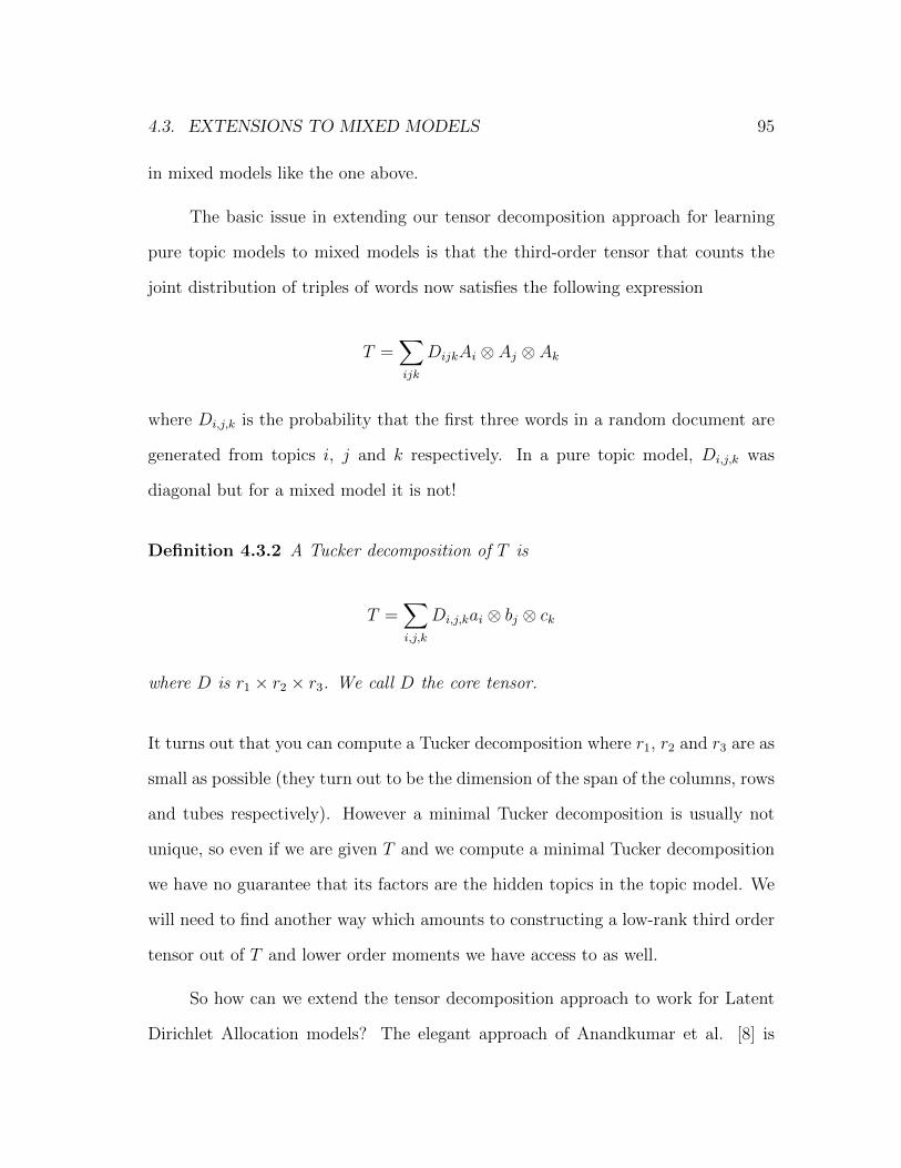
4.3. EXTENSIONS TO MIXED MODELS 95
in mixed models like the one above.
The basic issue in extending our tensor decomposition approach for learning
pure topic models to mixed models is that the third-order tensor that counts the
joint distribution of triples of words now satisfies the following expression
T =∑ijk
DijkAi ⊗ Aj ⊗ Ak
where Di,j,k is the probability that the first three words in a random document are
generated from topics i, j and k respectively. In a pure topic model, Di,j,k was
diagonal but for a mixed model it is not!
Definition 4.3.2 A Tucker decomposition of T is
T =∑i,j,k
Di,j,kai ⊗ bj ⊗ ck
where D is r1 × r2 × r3. We call D the core tensor.
It turns out that you can compute a Tucker decomposition where r1, r2 and r3 are as
small as possible (they turn out to be the dimension of the span of the columns, rows
and tubes respectively). However a minimal Tucker decomposition is usually not
unique, so even if we are given T and we compute a minimal Tucker decomposition
we have no guarantee that its factors are the hidden topics in the topic model. We
will need to find another way which amounts to constructing a low-rank third order
tensor out of T and lower order moments we have access to as well.
So how can we extend the tensor decomposition approach to work for Latent
Dirichlet Allocation models? The elegant approach of Anandkumar et al. [8] is

96 CHAPTER 4. TENSOR DECOMPOSITIONS: APPLICATIONS
based on the following idea:
Lemma 4.3.3
T =∑ijk
DijkAi ⊗ Aj ⊗ Ak
S =∑ijk
DijkAi ⊗ Aj ⊗ Ak
=⇒ T − S =∑ijk
(Dijk − Dijk)Ai ⊗ Aj ⊗ Ak
Proof: The proof is a simple exercise in multilinear algebra.
Hence if we have access to other tensors S which can be written using the same
factors Aii in its Tucker decomposition, we can subtract T and S and hope to
make the core tensor diagonal. We can think of D as being the third order moments
of a Dirichlet distribution in our setting. What other tensors do we have access to?
Other Tensors
We described the tensor T based on the following experiment: Let Ta,b,c be the
probability that the first three words in a random document are a, b and c respec-
tively. But we could just as well consider alternative experiments. The two other
experiments we will need in order to given a tensor spectral algorithm for LDA are:
(a) Choose three documents at random, and look at the first word of each docu-
ment

4.3. EXTENSIONS TO MIXED MODELS 97
(b) Choose two documents at random, and look at the first two words of the first
document and the first word of the second document
These two new experiments combined with the old experiment result in three tensors
whose Tucker decompositions use the same factors but whose core tensors differ.
Definition 4.3.4 Let µ, M and D be the first, second and third order moments of
the Dirichlet distribution.
More precisely, let µi be the probability that the first word in a random document
was generated from topic i. Let Mi,j be the probability that the first and second
words in a random document are generated from topics i and j respectively. And as
before, let Di,j,k be the probability that the first three words in a random document
are generated from topics i, j and k respectively. Then let T 1, T 2 and T 3 be the
expectation of the first (choose three documents), second (choose two documents)
and third (choose one document) experiments respectively.
Lemma 4.3.5 (a) T 1 =∑
i,j,k[µ⊗ µ⊗ µ]i,j,kAi ⊗ Aj ⊗ Ak
(b) T 2 =∑
i,j,k[M ⊗ µ]i,j,kAi ⊗ Aj ⊗ Ak
(c) T 3 =∑
i,j,kDi,j,kAi ⊗ Aj ⊗ Ak
Proof: Let w1 denote the first word and let t1 denote the topic of w1 (and similarly
for the other words). We can expand P[w1 = a, w2 = b, w3 = c] as:
∑i,j,k
P[w1 = a, w2 = b, w3 = c|t1 = i, t2 = j, t3 = k]P[t1 = i, t2 = j, t3 = k]

98 CHAPTER 4. TENSOR DECOMPOSITIONS: APPLICATIONS
and the lemma is now immediate.
Note that T 2a,b,c 6= T 2
a,c,b because two of the words come from the same document.
Nevertheless, we can symmetrize T 2 in the natural way: Set S2a,b,c = T 2
a,b,c + T 2b,c,a +
T 2c,a,b. Hence S2
a,b,c = S2π(a),π(b),π(c) for any permutation π : a, b, c → a, b, c.
Our main goal is to prove the following identity:
α20D + 2(α0 + 1)(α0 + 2)µ⊗3 − α0(α0 + 2)M ⊗ µ(all three ways) = diag(pii)
where α0 =∑
i αi. Hence we have that
α20T
3 + 2(α0 + 1)(α0 + 2)T 1 − α0(α0 + 2)S2 =∑i
piAi ⊗ Ai ⊗ Ai
The important point is that we can estimate the terms on the left hand side from
our sample (if we assume we know α0) and we can apply Jennrich’s algorithm to
the tensor on the right hand side to recover the topic model, provided that A has
full column rank. In fact, we can compute α0 from our samples (see [8]) but we will
focus instead on proving the above identity.
Moments of the Dirichlet
The main identity that we would like to establish is just a statement about the
moments of a Dirichlet distribution. In fact, we can think about the Dirichlet as
instead being defined by the following combinatorial process:
(a) Initially, there are αi balls of each color i

4.3. EXTENSIONS TO MIXED MODELS 99
(b) Repeat C times: choose a ball at random, place it back with one more of its
own color
This process gives an alternative characterization of the Dirichlet distribution, from
which it is straightforward to calculate:
(a) µ = [α1
α0, α2
α0, ..., αr
α0]
(b) Mi,j =
αi(αi+1)α0(α0+1)
i = j
αiαj
α0(α0+1)otherwise
.
(c) Ti,j,k =
αi(αi+1)(αi+2)α0(α0+1)(α0+2)
i = j = k
αi(αi+1)αk
α0(α0+1)(α0+2)i = j 6= k
αiαjαk
α0(α0+1)(α0+2)i, j, k distinct
.
For example for Ti,i,k this is the probability that the first two balls are color i and
the third ball is color k. The probably that the first ball is color i is αi
α0and since
we place it back with one more of its own color, the probability that the second ball
is color i as well is αi+1α0+1
. And the probability that the third ball is color k is αk
α0+2.
It is easy to check the above formulas in the other cases too.
Note that it is much easier to think about only the numerators in the above
formulas. If we can prove that following relation for just the numerators
D + 2µ⊗3 −M ⊗ µ(all three ways) = diag(2αii)
it is easy to check that we would obtain our desired formula by multiplying through
by α30(α0 + 1)(α0 + 2).

100 CHAPTER 4. TENSOR DECOMPOSITIONS: APPLICATIONS
Definition 4.3.6 Let R = num(D) + num(2µ⊗3)− num(M ⊗ µ)(all three ways)
Then the main lemma is:
Lemma 4.3.7 R = diag(2αii)
We will establish this by a case analysis:
Claim 4.3.8 If i, j, k are distinct then Ri,j,k = 0
This is immediate since the i, j, k numerator of D, µ⊗3 and M ⊗ µ are all αiαjαk.
Claim 4.3.9 Ri,i,i = 2αi
This is also immediate since the i, i, i numerator of D is αi(αi + 1)(αi + 2) and
similarly the numerator of µ⊗3 is α3i . Finally, the i, i, i numerator of M ⊗ µ is
α2i (αi + 1). The case that requires some care is:
Claim 4.3.10 If i 6= k, Ri,i,k = 0
The reason this case is tricky is because the terms M ⊗ µ(all three ways) do not
all count the same. If we think of µ along the third dimension of the tensor then
the ith topic occurs twice in the same document, but if instead we think of µ as
along either the first or second dimension of the tensor, even though the ith topic
occurs twice it does not occur twice in the same document. Hence the numerator
of M ⊗ µ(all three ways) is αi(αi + 1)αk + 2α2iαk. Also, the numerator of D is
αi(αi + 1)αk and the numerator of µ⊗3 is again α2iαk.

4.3. EXTENSIONS TO MIXED MODELS 101
These three claims together establish the above lemma. Even though the
tensor T 3 that we could immediately decompose in a pure topic model no longer
has a diagonal core tensor in a mixed model, at least in the case of LDA we can
still find a formula (each of whose terms we can estimate from our samples) that
diagonalizes the core tensor. This yields:
Theorem 4.3.11 [8] There is a polynomial time algorithm to learn a topic matrix
A whose columns are ε-close in Euclidean distance to the columns of A in a Latent
Dirichlet Allocation model, provided we are given at least poly(m, 1/ε, 1/σr, 1/αmin)
documents of length at least thee, where m is the size of the vocabulary and σr is the
smallest singular value of A and αmin is the smallest αi.
Epilogue
The algorithm of Anandkumar et al. [9] for learning mixed membership stochastic
block models follows the same pattern. Once again, the Dirichlet distribution plays
a key role. Instead of each node belonging to just one community as in the usual
stochastic block model, each node is described by a distribution πu over communities
where πu is chosen from a Dirichlet distribution. The main idea is to count three
stars and to add and subtract off tensors constructed from lower order subgraph
counts to make the core tensor in the natural Tucker decomposition diagonal.
It is worth mentioning that these techniques seem specialized to Dirichlet dis-
tributions. As we have seen, conditionally independent random variables play a key
role in tensor decompositions. In mixed membership models, finding such random
variables is challenging. But how far is the Dirichlet distribution from being inde-
pendent? Even though the coordinates are not independent, it turns out that they

102 CHAPTER 4. TENSOR DECOMPOSITIONS: APPLICATIONS
almost are. You can instead sample from a Dirichlet distribution by sampling from
a beta distribution for each coordinate independently and then renormalizing the
vector so that it is in the r-dimensional simplex. An interesting conceptual ques-
tion going forward is: Are tensor decomposition methods fundamentally limited to
settings where there is some sort of independence?
4.4 Independent Component Analysis
We can think about the tensor methods we have developed as a way to use higher
order moments to learn the parameters of a distribution (e.g. for phylogenetic
trees, HMMs, LDA, community detection) through tensor decomposition. Here we
will give another style of using the method of moments through an application to
independent component analysis which was introduced by Comon [53].
This problem is simple to define: Suppose we are given samples of the form
y = Ax+ b
where we know that the variables xi are independent and the linear transformation
(A, b) is unknown. The goal is to learn A, b efficiently from a polynomial number
of samples. This problem has a long history, and the typical motivation for it is to
consider a hypothetical situation called the cocktail party problem
We have n microphones and n conversations going on in an room. Each
microphone hears a superposition of the conversations given by the cor-
responding rows of A. If we think of the conversations as independent

4.4. INDEPENDENT COMPONENT ANALYSIS 103
and memoryless, can we disentangle them?
Such problems are also often referred to as blind source separation. We will follow
an approach of Frieze, Jerrum and Kannan [74]. What’s really neat about their
approach is that it uses non-convex optimization.
A Canonical Form and Rotational Invariance
Let’s first put our problem into a more convenient canonical form. It turns out we
can assume we are given samples from
y = Ax+ b
but where for all i, E[xi] = 0,E[x2i ] = 1. The idea is if any variable xi were not
mean zero, we could make it mean zero and add a correction to b. And similarly
if xi were not variance one we could rescale both it and the corresponding column
of A to make its variance be one. These changes are just notational and they do
not affect the distribution on samples that we observe. So from here on out, let’s
assume that we are given samples in the above canonical form.
We will give an algorithm based on non-convex optimization for estimating A
and b. But first let’s discuss what assumptions we will need. We will make two
assumptions: (a) A is nonsingular and (b) every variable satisfies E[x4i ] 6= 3. You
should be used to nonsingularity assumptions by now (it’s what we needed every
time we used Jennrich’s algorithm). But what about the second assumption? Where
does it come from? It turns out that it is actually quite natural and is needed to
rule out a problematic case.

104 CHAPTER 4. TENSOR DECOMPOSITIONS: APPLICATIONS
Claim 4.4.1 If each xi is an independent standard Gaussian, then for any orthog-
onal transformation R, x and Rx and consequently
y = Ax+ b and y = ARx+ b
have identical distributions.
Proof: The standard n-dimensional Gaussian is rotationally invariant.
What this means is when our independent random variables are standard Gaus-
sians, it is information-theoretically impossible to distinguish between A and AR.
Actually the n-dimensional Gaussian is the only problematic case. There are other
rotationally invariant distributions such as the uniform distribution on Sn−1 but its
coordinates are not independent. The standard n-dimensional Gaussian is the only
rotationally invariant distribution whose coordinates are independent.
In light of this discussion, we can understand where our assumption about the
fourth moments comes from. For a standard Gaussian distribution, its mean is zero,
its variance is one and its fourth moment is three. So our assumption on the fourth
moment of each xi is just a way to say that it is noticeably non-Gaussian.
Whitening
As usual, we cannot hope to learn A from just the second moments. This is really the
same issue that arose when we discussed the rotation problem. In the case of tensor
decompositions, we went directly to the third order moment to learn the columns of
A through Jennrich’s algorithm. Here we will learn what we can from the first and

4.4. INDEPENDENT COMPONENT ANALYSIS 105
second moments, and then move on to the fourth moment. In particular we will use
the first and second moments to learn b and to learn A up to a rotation:
Lemma 4.4.2 E[y] = b and E[yyT ] = AAT
Proof: The first identity is obvious. For the second, we can compute
E[yyT ] = E[AxxTAT ] = AE[xxT ]AT = AAT
where the last equality follows from the condition that E[xi] = 0 and E[x2i ] = 1 and
that each xi is independent.
What this means is that we can estimate b and M = AAT to arbitrary precision
by taking enough samples. What I claim is that this determines A up to a rotation.
Since M 0 we can find B such that M = BBT using the Cholesky factorization.
But how are B and A related?
Lemma 4.4.3 There is an orthogonal transformation R so that BR = A
Proof: Recall that we assumed A is nonsingular and hence M = AAT and B are
also nonsingular. So we can write
BBT = AAT ⇒ B−1AAT (B−1)T = I
which implies that B−1A = R is orthogonal since whenever a square matrix times its
own transpose is the identity the matrix is by definition orthogonal. This completes
the proof.

106 CHAPTER 4. TENSOR DECOMPOSITIONS: APPLICATIONS
Now that we have learned A up to an unknown rotation, we can set out to
use higher moments to learn the unknown rotation. First we will apply an affine
transformation to our samples:
z = B−1(y − b) = B−1Ax = Rx
This is called whitening (think white noise) because it makes the first moments of
our distribution zero and the second moments all one (in every direction). The key
to our analysis is the following functional
F (u) = E[(uT z)4] = E[(uTRx)4]
We will want to minimize it over the unit sphere. As u ranges over the unit sphere,
so does vT = uTR. Hence our optimization problem is equivalent to minimizing
H(v) = E[(vTx)4]
over the unit sphere. This is a non-convex optimization problem. In general it is
NP -hard to find the minimum or maximum of a non-convex function. But it turns
out that it is possible to find a local minimum and that these are good enough to
learn R.
Lemma 4.4.4 If for all i, E[x4i ] < 3 then the only local minima of H(v) are at
v = ±ei where ei are the standard basis vectors.

4.4. INDEPENDENT COMPONENT ANALYSIS 107
Proof: We can compute
E[(vTx)4
]= E
[∑i
(vixi)4 + 6
∑i<j
(vixi)2(vjxj)
2
]=
∑i
v4i E(x4
i ) + 6∑i<j
v2i v
2j + 3
∑i
v4i − 3
∑i
v4i
=∑i
v4i
(E[x4i
]− 3)
+ 3
From this expression it is easy to check that the local minima of H(v) correspond
exactly to setting v = ±ei for some i.
Recall that vT = uTR and so this characterization implies that the local min-
ima of F (u) correspond to setting u to be a column of ±R. The algorithm proceeds
by using gradient descent (and a lower bound on the Hessian) to show that you can
find a local minima of F (u) quickly. The intuition is that if you keep following steep
gradients, you are decreasing the objective value. Eventually you must get stuck at
a point where the gradients are small which is an approximate local minima. Any
such u must be close to some column of ±R and we can then recurse on the orthog-
onal complement to the vector we have found to find the other columns of R. This
idea requires some care to show that the errors do not accumulate too badly, see
[74], [140], [17]. Note that when E[x4i ] 6= 3 instead of the stronger assumption that
E[x4i ] < 3, we can follow the same approach but we need to consider local minima
and local maxima of F (u). Also Vempala and Xiao [140] gave an algorithm that
works under weaker conditions, whenever there is an constant order moment that is
different from that of the standard Gaussian.
The strange expression we encountered above are actually called cumulants and
are an alternative basis for the moments of a distribution. Sometimes cumulants

108 CHAPTER 4. TENSOR DECOMPOSITIONS: APPLICATIONS
are easier to work with since they satisfy the appealing property that the k-order
cumulant of the sum of independent variables Xi and Xj is the sum of the k-order
cumulants of Xi and Xj. This fact actually gives another more intuitive way to solve
independent component analysis when combined with Jennrich’s algorithm, but it
involves a bit of a digression into higher dimensional cumulants. We leave this as
an exercise to the reader.
4.5 Exercises
Problem 4-1: Let uv denote the Khatri-Rao product between two vectors, where
if u ∈ Rm and v ∈ Rn then u v ∈ Rmn and corresponds to flattening the matrix
uvT into a vector, column by column. Also recall that the Kruskal rank k-rank of
a collection of vectors u1, u2, ..., um ∈ Rn is the largest k such that every set of k
vectors are linearly independent.
In this problem, we will explore properties of the Khatri-Rao product and use
it to design algorithms for decomposing higher-order tensors.
(a) Let ku and kv be the k-rank of u1, u2, ..., um and v1, v2, ..., vm respectively. Prove
that the k-rank of u1 v1, u2 v2, ..., um vm is at least min(ku + kv − 1,m).
(b) Construct a family of examples where the k-rank of u1u1, u2u2, ..., umum
is exactly 2ku− 1, and not any larger. To make this non-trivial, you must use
an example where m > 2ku − 1.
(c) Given an n× n× n× n× n fifth order tensor T =∑r
i=1 a⊗5i give an algorithm
for finding its factors that works for r = 2n− 1, under appropriate conditions

4.5. EXERCISES 109
on the factors a1, a2, ..., ar. Hint: Reduce to the third-order case.
In fact for random or perturbed vectors, the Khatri-Rao product has a much stronger
effect of multiplying their Kruskal rank. These types of properties can be used to
obtain algorithms for decomposing higher-order tensors in the highly overcomplete
case where r is some polynomial in n.
Problem 4-2: In Section 4.4 we saw how to solve independent component analysis
using non-convex optimization. In this problem we will see how to solve it using
tensor decomposition instead. Suppose we observe many samples of the form y = Ax
where A is an unknown non-singular square matrix and each coordinate of x is
independent and satisfies E[xj] = 0 and E[x4j ] 6= 3E[x2
j ]2. The distribution of xj is
unknown and might not be the same for all j.
(a) Write down expressions for E[y⊗4] and (E[y⊗2])⊗2
in terms of A and the mo-
ments of x. (You should not have any A’s inside the expectation.)
(b) Using part (a), show how to use the moments of y to produce a tensor of the
form∑
j cja⊗4j where aj denotes column j of A and the cj are nonzero scalars.
(c) Show how to recover the columns of A (up to permutation and scalar multiple)
using Jennrich’s algorithm.

110 CHAPTER 4. TENSOR DECOMPOSITIONS: APPLICATIONS

Chapter 5
Sparse Recovery
In this chapter, we will witness the power of sparsity for the first time. Let’s get
a sense of what it’s good for. Consider the problem of solving an underdetermined
linear system Ax = b. If we are given A and b there’s no chance to recover x uniquely
right? Well not if we know that x is sparse. In that case there are natural conditions
on A where we actually will be able to recover x even though the number of rows of
A is comparable to the sparsity of x rather than its dimension. Here we will cover
the theory of sparse recovery. And in case you’re curious it’s an area that not only
has some theoretical gems but has also had major practical impact.
5.1 Introduction
In signal processing (particularly imaging) we are often faced with the task of recov-
ering some unknown signal given linear measurements of it. Let’s fix our notation.
Throughout this chapter we will be interested in solving a linear system Ax = b
111

112 CHAPTER 5. SPARSE RECOVERY
where A is an m× n matrix, and x and b are n and m dimensional vectors respec-
tively. In our setup both A and b are known. You can think of A as representing
the input-output functionality of some measurement device we are using.
Now if m < n then we cannot hope to recover x uniquely. At best we could find
some solution y that satisfies Ay = b and we would have the promise that x = y+ z
where z belongs to the kernel of A. This tells us that if we want to recover an n
dimensional signal we need at least n linear measurements. This is quite natural.
Sometimes you will hear this referred to as the Shannon-Nyquist rate, although I
find that a rather opaque way to describe what is going on. The amazing idea that
will save us is that if x is sparse — i.e. b is a linear combination of only a few
columns of A — then we really will be able to get away with many fewer linear
measurements and still be able to reconstruct x exactly.
What I want to do in this section is explain why you actually should not be
surprised by it. If you ignore algorithms (which we won’t do later on), it’s actually
quite simple. It turns out that assuming that x is sparse isn’t enough by itself. We
will always have to make some structural assumption about A as well. Let’s consider
the following notion:
Definition 5.1.1 The Kruskal rank of a set of vectors Aii is the maximum r such
that all subsets of at most r vectors are linearly independent.
If you are given a collection of n vectors in n dimensions, they can all be linearly
independent in which case their Kruskal rank is n. But if you have n vectors in m
dimensions — like when we take the columns of our sensing matrix A – and m is
smaller than n, the vectors can’t be all linearly independent but they can still have
Kruskal rank m. In fact this is the common case:

5.1. INTRODUCTION 113
Claim 5.1.2 If A1, A2, . . . , An are chosen uniformly at random from Sm−1 then
almost surely their Kruskal rank is m.
Now let’s prove our first main result about sparse recovery. Let ‖x‖0 be the
number of non-zero entries of x. We will be interested in the following highly non-
convex optimization problem:
(P0) min ‖w‖0 s.t. Aw = b
Let’s show that if we could solve (P0) we could find x from much fewer than n linear
measurements:
Lemma 5.1.3 Let A be an m×n matrix whose columns have Kruskal rank at least
r. Let x be an r/2-sparse vector and let Ax = b. Then the unique optimal solution
to (P0) is x.
Proof: We know that x is a solution toAx = b which has objective value ‖x‖0 = r/2.
Now suppose there were any other solution y which satisfies Ay = b.
Consider the difference between these solutions z = x − y. We know that z
is in the kernel of A. However ‖z‖0 ≥ r + 1 because by assumption every set of at
most r columns of A is linearly independent. Finally we have
‖y‖0 ≥ ‖z‖0 − ‖x‖0 ≥ r/2 + 1
which implies that y has larger objective value than x. This completes the proof.
So if we choose the columns of our sensing matrix to be random m dimensional

114 CHAPTER 5. SPARSE RECOVERY
vectors, then from just m linear measurements we can in principle recover any m/2-
sparse vector uniquely. But there is a huge catch. Solving (P0) — i.e. finding the
sparsest solution to a system of linear equations is NP -hard. In fact this is a simple
and important reduction that is worth seeing. Following Khachiyan [97], let’s start
from the subset sum problem which is a standard NP -hard problem:
Problem 1 Given distinct values α1, . . . , αn ∈ R, does there exist a set I ⊆ [n] so
that |I| = m and∑
i∈I αi = 0?
We will embed an instance of this problem into the problem of finding the
sparsest non-zero vector in a given subspace. We will make use of the following
mapping which is called the weird moment curve:
Γ′(αi) = [1, αi, α2i , . . . , α
m−2i , αmi ]
The difference between this and the standard moment curve is in the last term where
we have αmi instead of αm−1i .
Lemma 5.1.4 A set I with |I| = m has∑
i∈I αi = 0 if and only if the vectors
Γ′(αi)i∈I are linearly dependent.
Proof: Consider the determinant of the matrix whose columns are Γ′(αi)i∈I .
Then the proof is based on the following observations:
(a) The determinant is a polynomial in the variables αi with total degree(m2
)+ 1,
which can be seen by writing the determinant in terms of its Laplace expansion
(see e.g. [88]).

5.1. INTRODUCTION 115
(b) Moreover the determinant is divisible by∏
i<j αi − αj, since the determinant
is zero if any αi = αj.
Hence we can write the determinant as
( ∏i<ji,j∈I
(αi − αj))(∑
i∈I
αi
)
We have assumed that the αi’s are distinct, and consequently the determinant is
zero if and only if the sum of αi = 0.
We can now prove a double-whammy. Not only is solving (P0) NP -hard but
so is computing the Kruskal rank:
Theorem 5.1.5 Both computing the Kruskal rank and finding the sparsest solution
to a system of linear equations are NP -hard.
Proof: First let’s prove that computing the Kruskal rank is NP -hard. Consider the
vectors Γ′(αi)i. It follows from Lemma 5.1.4 that if there is a set I with |I| = m
that satisfies∑
i∈I αi = 0 then Kruskal rank of Γ′(αi)i is at most m − 1, and
otherwise is their Kruskal rank is exactly m. Since subset sum is NP -hard, so too
is deciding if the Kruskal rank is m or at most m− 1.
Now let’s move on to showing that finding the sparsest solution to a linear
system is NP -hard. We will use a one-to-many reduction. For each j, consider the
following optimization problem:
(Pj) min ‖w‖0 s.t.[Γ′(α1), . . . ,Γ′(αj−1),Γ′(αj+1), . . . ,Γ′(αn)
]w = Γ′(αj)

116 CHAPTER 5. SPARSE RECOVERY
It is easy to see that the Kruskal rank of Γ′(αi)i is at most m − 1 if and only if
there is some j so that (Pj) has a solution whose objective value is at most m− 2.
Thus (P0) is also NP -hard.
In the rest of this chapter, we will focus on algorithms. We will give simple
greedy methods as well as ones based on convex programming relaxations. These
algorithms will work under more stringent assumptions on the sensing matrix A than
just that its columns have large Kruskal rank. Nevertheless all of the assumptions
we make will still be met by a randomly chosen A as well as many others. The
algorithms we give will even come with stronger guarantees that are meaningful in
the presence of noise.
5.2 Incoherence and Uncertainty Principles
In 1965, Logan [107] discovered a striking phenomenon. If you take a band-limited
signal and corrupt it at a sparse set of locations, it is possible to uniquely recover
the original signal. This turns out to be a sparse recovery problem in disguise. Let’s
formalize this:
Example 1 The spikes-and-sines matrix A is a n× 2n matrix
A = [I,D]
where I is the identity matrix and D is the discrete Fourier transform matrix, i.e.
Da,b =ω(a−1)(b−1)
√n

5.2. INCOHERENCE AND UNCERTAINTY PRINCIPLES 117
and ω = e2πi/n is the nth root of unity.
Let x be a sparse 2n-dimensional vector. The nonzeros in the first n coordinates
represent the locations of the corruptions. The nonzeros in the last n coordinates
represent the frequencies present in the original signal. Thus we know A and b and
are promised that there is a solution x to Ax = b where x is sparse. It took a
number of years until the work of Donoho and Stark [64] who realized that this
phenomenon wasn’t limited to just the spike-and-sines matrix. It’s actually a quite
a general phenomenon. The key is the notion of incoherence:
Definition 5.2.1 The columns of A ∈ Rn×m are µ-incoherent if for all i 6= j:
|〈Ai, Aj〉| ≤ µ‖Ai‖ · ‖Aj‖
Throughout this section, we will focus on just the case when the columns of
A are unit vectors. Hence a matrix is µ-incoherent if for all i 6= j, |〈Ai, Aj〉| ≤ µ.
However all of the results we derive here can be extended to general A when the
columns are not necessarily unit vectors. As we did for the Kruskal rank, let’s show
that random vectors are incoherent:
Claim 5.2.2 If A1, A2, . . . , Am are chosen uniformly at random from Sn−1 then with
high probability they will be µ-incoherent for
µ = O(√ logm
n
).
You can also check that the spike-and-sines matrix is µ-incoherent with µ =
1/√n. In that way, the results we derive here will contain Logan’s phenomenon as

118 CHAPTER 5. SPARSE RECOVERY
a special case. Anyways let’s now show that if A is incoherent and if x is sparse
enough then it will be the uniquely sparsest solution to Ax = b.
Lemma 5.2.3 Let A be an n ×m matrix that is µ-incoherent and whose columns
are unit norm. If Ax = b and ‖x‖0 <1
2µ, then x is the uniquely sparsest solution to
the linear system.
Proof: Suppose for the sake of contradiction that we have another solution y that
satisfies Ay = b and ‖y‖0 <1
2µ. Then we can look at the difference between these
solutions z = x− y which satisfies ‖z‖0 <1µ
and consider the expression
zTATAz = 0.
If we let S denote the support of z — i.e. the locations where it is nonzero — we
have that ATA restricted to the rows and columns in S is singular. Let this matrix
be B. Then B has ones along the diagonal and the entries off the diagonal are
bounded by µ in absolute value. But by Gershgorin’s disk theorem we know that
all the eigenvalues of B are contained in a disk in the complex plane centered at one
with radius µ|S| < 1. Thus B is nonsingular and we have a contradiction.
Actually we can prove a stronger uniqueness result when A is the union of two
orthonormal bases, as is the case for the spikes-and-sines matrix. Let’s first prove
the following result, which we will mysteriously call an uncertainty principle:
Lemma 5.2.4 Let A = [U, V ] be a n× 2n matrix that is µ-incoherent where U and
V are n× n orthogonal matrices. If b = Uα = V β, then ‖α‖0 + ‖β‖0 ≥ 2µ
.

5.2. INCOHERENCE AND UNCERTAINTY PRINCIPLES 119
Proof: Since U and V are orthonormal we have that ‖b‖2 = ‖α‖2 = ‖β‖2. We
can rewrite b as either Uα or V β and hence ‖b‖22 = |βT (V TU)α|. Because A is
incoherent, we can conclude that each entry of V TU has absolute value at most
µ(A) and so |βT (V TU)α| ≤ µ(A)‖α‖1‖β‖1. Using Cauchy-Schwarz it follows that
‖α‖1 ≤√‖α‖0‖α‖2 and thus
‖b‖22 ≤ µ(A)
√‖α‖0‖β‖0‖α‖2‖β‖2
Rearranging, we have 1µ(A)≤√‖α‖0‖β‖0. Finally, applying the AM-GM inequality
we get 2µ≤ ‖α‖0 + ‖β‖0 and this completes the proof.
This proof was short and simple. Perhaps the only confusing part is why we
called it an uncertainty principle. Let’s give an application of Lemma 5.2.4 to clarify
this point. If we set A to be the spikes-and-sines matrix, we get that any non-zero
signal must have at least√n non-zeros in the standard basis or in the Fourier basis.
What this means is that no signal can be sparse in both the time and frequency
domains simultaneously! It’s worth taking a step back. If we had just proven
this result you would have naturally associated it with the Heisenberg uncertainty
principle. But it turns out that what’s really driving it is just the incoherence of the
time and frequency bases for our signal, and it applies equally well to many other
pairs of bases.
Let’s use our uncertainty principle to prove an even stronger uniqueness result:
Claim 5.2.5 Let A = [U, V ] be a n × 2n matrix that is µ-incoherent where U and
V are n × n orthogonal matrices. If Ax = b and ‖x‖0 <1µ
, then x is the uniquely
sparsest solution to the linear system.

120 CHAPTER 5. SPARSE RECOVERY
Proof: Consider any alternative solution Ax = b. Set y = x− x in which case y ∈
ker(A). Write y as y = [αy, βy]T and since Ay = 0, we have that Uαy = −V βy. We
can now apply the uncertainty principle and conclude that ‖y‖0 = ‖αy‖0+‖βy‖0 ≥ 2µ.
It is easy to see that ‖x‖0 ≥ ‖y‖0 − ‖x‖0 >1µ
and so x has strictly more non-zeros
than x does, and this completes the proof.
We can connect incoherence back to our original discussion about Kruskal
rank. It turns out that having a matrix whose columns are incoherent is just one
easy-to-check way to certify a lower bound on the Kruskal rank. The proof of the
following claim is essentially the same as the proof of Lemma 5.2.3. We leave it as
an exercise to the reader.
Claim 5.2.6 If A is µ-incoherent then the Kruskal rank of the columns of A is at
least 1/µ.
In the next section we will give a simple greedy algorithm for solving sparse
recovery problems on incoherent matrices. The way that the algorithm will certify
that it is making progress and is finding the right non-zero locations of x as it goes
along will revolve around the same ideas that underly the uniqueness results we just
proved.
5.3 Pursuit Algorithms
There is an important class of algorithms for sparse recovery problems called pursuit
algorithms. These algorithms are greedy and iterative. They work with incoherent
matrices and look for the column in A that explains as much of the observed vector b

5.3. PURSUIT ALGORITHMS 121
as possible. They subtract off a multiple that column and continue on the remainder.
The first such algorithm was introduced in an influential paper of Mallat and Zhang
[111] and was called matching pursuit. In this section, we will analyze a variant of it
called orthogonal matching pursuit. What’s particularly convenient about the latter
is that the algorithm will maintain the invariant that the remainder is orthogonal
to all of the columns of A we have selected so far. This is more expensive in each
step, but is easier to analyze and understand the intuition behind.
Throughout this section let A be an n×m matrix that is µ-incoherent. Let x
be k-sparse with k < 1/(2µ) and let Ax = b. Finally we will use T to denote the
support of x — i.e. the locations of the non-zeros in x. Now let’s formally define
orthogonal matching pursuit:
Orthogonal Matching Pursuit
Input: matrix A ∈ Rn×m, vector b ∈ Rn, desired number of nonzero entries k ∈ N.
Output: solution x with at most k nonzero entries.
Initialize: x0 = 0, r0 = Ax0 − b, S = ∅.
For ` = 1, 2, . . . , k
Choose column j that maximizes|〈Aj ,r
`−1〉|‖Aj‖22
.
Add j to S.
Set r` = projU⊥(b), where U = span(AS).
If r` = 0, break.
End
Solve for xS: ASxS = b. Set xS = 0.

122 CHAPTER 5. SPARSE RECOVERY
Our anlaysis will focus on establishing the following two invariants:
(a) Each index j the algorithm selects is in T .
(b) Each index j gets chosen at most once.
These two properties immediately imply that orthogonal matching pursuit
recovers the true solution x, because the residual error r` will be non-zero until
S = T , and moreover the linear system ATxT = b has a unique solution (which we
know from the previous section).
Property (b) is straightforward, because once j ∈ S at every subsequent step
in the algorithm we will have that r` ⊥ U , where U = span(AS), so 〈r`, Aj〉 = 0 if
j ∈ S. Our main goal is to establish property (a), which we will prove inductively.
The main lemma is:
Lemma 5.3.1 If S ⊆ T at the start of a stage, then orthogonal matching pursuit
selects j ∈ T .
We will first prove a helper lemma:
Lemma 5.3.2 If r`−1 is supported in T at the start of a stage, then orthogonal
matching pursuit selects j ∈ T .
Proof: Let r`−1 =∑
i∈T yiAi. Then we can reorder the columns of A so that the
first k′ columns correspond to the k′ nonzero entries of y, in decreasing order of
magnitude:
|y1| ≥ |y2| ≥ · · · ≥ |yk′ | > 0︸ ︷︷ ︸corresponds to first k′ columns of A
, |yk′+1| = 0, |yk′+2| = 0, . . . , |ym| = 0.

5.3. PURSUIT ALGORITHMS 123
where k′ ≤ k. Hence supp(y) = 1, 2, . . . , k′ ⊆ T . Then to ensure that we pick
j ∈ T , a sufficient condition is that
(5.1) |〈A1, r`−1〉| > |〈Ai, r`−1〉| for all i ≥ k′ + 1.
We can lower-bound the left-hand side of (5.1):
|〈r`−1, A1〉| =∣∣∣∣⟨ k′∑
`=1
y`A`, A1
⟩∣∣∣∣ ≥ |y1|−k′∑`=2
|y`||〈A`, A1〉| ≥ |y1|−|y1|(k′−1)µ ≥ |y1|(1−k′µ+µ),
which, under the assumption that k′ ≤ k < 1/(2µ), is strictly lower-bounded by
|y1|(1/2 + µ).
We can then upper-bound the right-hand side of (5.1):
|〈r`−1, Ai〉| =∣∣∣∣⟨ k′∑
`=1
y`A`, Ai
⟩∣∣∣∣ ≤ |y1|k′∑`=1
|〈A`, Ai〉| ≤ |y1|k′µ,
which, under the assumption that k′ ≤ k < 1/(2µ), is strictly upper-bounded by
|y1|/2. Since |y1|(1/2 + µ) > |y1|/2, we conclude that condition (5.1) holds, guaran-
teeing that the algorithm selects j ∈ T and this completes the proof.
Now we can prove Lemma 5.3.1:
Proof: Suppose that S ⊆ T at the start of a stage. Then the residual r`−1 is
supported in T because we can write it as
r`−1 = b−∑i∈S
ziAi, where z = arg min ‖b− ASzS‖2
Applying the above lemma, we conclude that the algorithm selects j ∈ T .
124 CHAPTER 5. SPARSE RECOVERY
This establishes property (a) inductively, and completes the proof of correctness for
orthogonal matching pursuit, which we summarize below:
Theorem 5.3.3 Let A be an n×m matrix that is µ-incoherent and whose columns
are unit norm. If Ax = b and ‖x‖0 <1
2µ, then the output of orthogonal matching
pursuit is exactly x.
Note that this algorithm works up to exactly the threshold where we established
uniqueness. However in the case where A = [U, V ] and U and V are orthogonal, we
proved a uniqueness result that is better by a constant factor. There is no known
algorithm that matches the best known uniqueness bound there, although there are
better algorithms than the one above (see e.g. [67]).
It is also worth mentioning how other pursuit algorithms differ. For example,
in matching pursuit we do not recompute the coefficients xi for i ∈ S at the end of
each stage. We just keep whatever they are set to and hope that these coefficients
do not need to be adjusted much when we add a new index j to S. This is what
makes matching pursuit faster in practice, however the analysis is more cumbersome
because we need to keep track of how the error (due to not projecting b on the
orthogonal complement of the columns we’ve chosen so far) accumulates.
5.4 Prony’s Method
There is a widespread misconception that sparse recovery algorithms are a modern
invention. Actually sparse recovery dates back to 1795 to an algorithm called Prony’s
method. It will give us almost everything we want. We will have an explicit 2k× n

5.4. PRONY’S METHOD 125
sensing matrix A for which we will be able to recover any k-sparse signal exactly
and with an efficient algorithm. It even has the benefit that we can compute the
matrix-vector product Ax in O(n log n) time using the fast Fourier transform.
The caveat to this method is that it is very unstable since involves inverting
a Vandermonde matrix which can be very ill-conditioned. So when you hear about
compressed sensing as breaking the Shannon-Nyquist barrier, you should remember
that Prony’s method already does that. What sets the algorithms we will study
later on apart is that they work in the presence of noise. That’s the crucial aspect
that makes them so practically relevant. Nevertheless Prony’s method is very useful
from a theoretical standpoint and the types of results you can get out of it have a
habit of being rediscovered under other names.
Properties of the Discrete Fourier Transform
Prony’s method will make crucial use of various properties of the discrete Fourier
transform. Recall that as a matrix, this transformation has entries
Fa,b =
(1√n
)exp
(i2π(a− 1)(b− 1)
n
)
As we did before, we will simplify the notation and write ω = ei2π/n for the nth root
of unity. With this notation, the entry in row a, column b is ω(a−1)(b−1).
The matrix F has a number of important properties, including:
(a) F is orthonormal: FHF = FFH , where FH is the Hermitian transpose of F
(b) F diagonalizes the convolution operator

126 CHAPTER 5. SPARSE RECOVERY
We haven’t defined convolution so let’s do that now. Actually let’s do that through
its corresponding linear transformation:
Definition 5.4.1 (Circulant matrix) For a vector c = [c1, c2, . . . , cn], let
M c =
cn cn−1 cn−2 . . . c1
c1 cn cn−1 . . . c2
......
cn−1 . . . . . . . . . cn
.
Then the matrix-vector product M cx is the vector we get out of convolving c and
x, which we will denote by c ∗ x. Intuitively if you think of c and x as representing
the probability distribution of discrete random variables, then c ∗ x represents the
distribution of the random variable you get by adding the two of them and wrapping
around n using modular arithmetic.
As we asserted above, we can diagonalize M c using F . More formally, we have
the following fact which we will use without proof:
Claim 5.4.2 M c = FHdiag(c)F , where c = Fc.
This tells us that we can think of convolution as coordinate-wise multiplication in
the Fourier representation. More precisely:
Corollary 5.4.3 Let z = c ∗ x; then z = c x, where indicates coordinate-wise
multiplication.
Proof: We can write z = M cx = FHdiag(c)Fx = FHdiag(c)x = FH(c x), and
this completes the proof.

5.4. PRONY’S METHOD 127
The Helper Polynomial
Prony’s method revolves around the following helper polynomial:
Definition 5.4.4 (Helper polynomial)
p(z) =∏
b∈supp(x)
ω−b(ωb − z)
= 1 + λ1z + . . .+ λkzk.
Claim 5.4.5 If we know p(z), we can find supp(x).
Proof: In fact, an index b is in the support of x if and only if p(ωb) = 0. So we can
evaluate p at powers of ω, and the exponents where p evaluates to a non-zero are
exactly the support of x.
The basic idea of Prony’s method is to use the first 2k values of the discrete Fourier
transform to find p, and hence the support of x. We can then solve a linear system
to actually find the values of x. Our first goal is to find the Helper polynomial. Let
v = [1, λ1, λ2, . . . , λk, 0, . . . , 0], and v = Fv
It is easy to see that the value of v at index b+ 1 is exactly p(ωb).
Claim 5.4.6 supp(v) = supp(x)
That is, the zeros of v correspond roots of p, and hence non-zeros of x. Conversely,
the non-zeros of v correspond to zeros of x. We conclude that x v = 0, and so:

128 CHAPTER 5. SPARSE RECOVERY
Corollary 5.4.7 M xv = 0
Proof: We can apply Claim 5.4.2 to rewrite x v = 0 as x ∗ v = 0 = 0, and this
implies the corollary.
Let us write out this linear system explicitly:
M x =
xn xn−1 . . . xn−k . . . x1
x1 xn . . . xn−k+1 . . . x2
......
......
......
xk+1 xk . . . x1 . . . xk+2
......
......
......
x2k x2k−1 . . . xk . . . x2k+1
......
......
......
Recall, we do not have access to all of the entries of this matrix since we are only
given the first 2k values of the DFT of x. However consider the k× k+ 1 submatrix
whose top left value is xk+1 and whose bottom right value is xk. This matrix only
involves the values that we do know!
Consider
xk xk−1 . . . x1
...
x2k−1 x2k−1 . . . xk
λ1
λ2
...
λk
= −
xk+1
...
...
x2k
It turns out that this linear system is full rank, so λ is the unique solution to the

5.5. COMPRESSED SENSING 129
linear system (the proof is left to the reader1). The entries in λ are the coefficients
of p, so once we have solved for λ we can evaluate the helper polynomial on ωb to
find the support of x. All that remains is to find the values of x. Indeed, let M be
the restriction of F to the columns in S and its first 2k rows. M is a Vandermonde
matrix, so again MxS = x1,2,...2k has a unique solution, and we can solve this linear
system to find the non-zero values of x.
The guarantees of Prony’s method are summarized in the following theorem:
Theorem 5.4.8 Let A be the 2k × n matrix obtained from taking the first 2k rows
of the discrete Fourier transform matrix F . Then for any k-sparse signal x, Prony’s
method recovers x exactly from Ax.
In case you’re curious, this is yet another topic in sparse recovery that we can relate
back to Kruskal rank. It is easy to show that the columns of A have Kruskal rank
equal to 2k. In fact this is true regardless of which 2k rows of F we choose. Moreover
it turns out that there are settings where Prony’s method and related methods can
be shown to work in the presence of noise, but only under some separation conditions
on the non-zero locations in x. See Moitra [113] for further details.
5.5 Compressed Sensing
In this section we will introduce a powerful new assumption about our sensing matrix
A, called the restricted isometry property. You can think of it as a robust analogue
of the Kruskal rank where not only do we want every set of (say) 2k columns of A
to be linearly independent, we also want them to be well-conditioned. We will show

130 CHAPTER 5. SPARSE RECOVERY
that a simple convex programming relaxation is amazingly effective. With a good
choice for A, we will be able to recover a k-sparse signal from O(k log(n/k)) linear
measurements. The algorithm runs in polynomial time and moreover it is robust to
noise in the sense that even if x is not k-sparse we will still be able to approximately
recover its k largest coordinates. This is a much stronger type of guarantee. After all
natural signals aren’t k-sparse. But being able to recover their k largest coordinates
is often good enough.
Now let’s define the restricted isometry property:
Definition 5.5.1 A matrix A satisfies the (k, δ)-restricted isometry property if for
all k-sparse vectors x we have:
(1− δ)‖x‖22 ≤ ‖Ax‖2
2 ≤ (1 + δ)‖x‖22
As with the other assumptions we have considered, the restricted isometry property
holds on randomly chosen sensing matrices with high probability:
Lemma 5.5.2 Let A be an m× n matrix where each entry is an independent stan-
dard Gaussian random variable. Provided that m ≥ 10k log n/k then with high
probability A satisfies the (k, 1/3)-restricted isometry property.
Next let’s work towards formalizing what we mean by approximately recovering
the k largest coordinates of x. Our goal will be formulated in terms of the following
function:
Definition 5.5.3 γk(x) = minw s.t. ‖w‖0≤k ‖x− w‖1

5.5. COMPRESSED SENSING 131
To put this in more plain terms, γk(x) is the sum of the absolute values of all but
the k largest magnitude entries of x. And if x really is k-sparse then γk(x) = 0.
Our goal is to find a w that approximates x almost as well as any k-sparse
vector does. More formally we want to find a w that satisfies ‖x−w‖1 ≤ Cγk(x) and
we want to do so using as few linear measurements as possible. This learning goal
already subsumes our other exact recovery results from previous sections, because
when x is k-sparse then as we discussed γk(x) is zero so we have no choice but to
recover w = x.
In this section, our approach will be based on a convex programming relax-
ation. Instead of trying to solve the NP -hard optimization problem (P0) we will
consider the now famous `1-relaxation:
(P1) min ‖w‖1 s.t. Aw = b
Let’s first state some of the well-known results about using (P1) for sparse recovery:
Theorem 5.5.4 [43] If δ2k + δ3k < 1 then if ‖x‖0 ≤ k we have w = x.
Theorem 5.5.5 [42] If δ3k + 3δ4k < 2 then
‖x− w‖2 ≤C√kγk(x)
The guarantees above are a bit different (and often stronger) than the others because
the bound is in terms of the `2 norm of the error x− w.

132 CHAPTER 5. SPARSE RECOVERY
Theorem 5.5.6 [51] If δ2k < 1/3 then
‖x− w‖1 ≤2 + 2δ2k
1− 3δ2k
γk(x)
We won’t prove exactly these results. But we will prove something similar
following the approach of Kashin and Temlyakov [96] that (to my taste) greatly
stream-lined these analyses. But before we get to analyzing (P1), we need to intro-
duce a notion from functional analysis called an almost Euclidean subsection.
Almost Euclidean Subsections
Informally, an almost Euclidean subsection is a subspace where the `1 and `2 norms
are almost equivalent after rescaling. We will just assert the fact that a random
subspace is an almost Euclidean subsection with high probability. Instead we will
spend most of our time establishing various geometric properties about them that
we will use when we return to compressed sensing. The crucial definition is the
following:
Definition 5.5.7 A subspace Γ ⊆ Rn is a C-almost Euclidean subsection if for all
v ∈ Γ,
1√n‖v‖1 ≤ ‖v‖2 ≤
C√n‖v‖1
Actually the first inequality is trivial. For any vector, it’s always true that 1√n‖v‖1 ≤
‖v‖2. The action is all happening in the second inequality. The first time you see
them, it’s not obvious that such subspaces exist. Indeed Garnaev and Gluskin [75]
proved that there are plenty of almost Euclidean subsections:

5.5. COMPRESSED SENSING 133
Theorem 5.5.8 If Γ is a subspace chosen uniformly at random with dim(Γ) = n−m
then for
C = O(√ n
mlog
n
m
)we have that Γ will be a C-almost Euclidean subsection with high probability.
Let’s end with a nice picture to keep in mind. Consider the unit ball for the `1
norm. It’s sometimes called the cross polytope and to visualize it you can think of
it as the convex hull of the vectors ±eii where ei are the standard basis vectors.
Then a subspace Γ is almost Euclidean if when we intersect it and the cross polytope
we get a convex body that is almost spherical.
Geometric Properties of Γ
Here we will establish some important geometric properties of C-almost Euclidean
subsections. Throughout this section, let S = n/C2. First we show that Γ cannot
contain any sparse, non-zero vectors:
Claim 5.5.9 Let v ∈ Γ, then either v = 0 or |supp(v)| ≥ S.
Proof: From Cauchy-Schwartz and the C-almost Euclidean property, we have:
‖v‖1 =∑
j∈supp(v)
|vj| ≤√|supp(v)| · ‖v‖2 ≤
√|supp(v)| C√
n‖v‖1
The proof now follows from rearranging terms.
It’s worth noting that there is a nice analogy with linear error correcting codes,
which are also subspaces of large dimension (but over GF2) where we want every

134 CHAPTER 5. SPARSE RECOVERY
non-zero vector to have at least a constant fraction of its coordinates be non-zero.
In any case, let’s move on to some
Let’s move on to some even stronger properties of almost Euclidean subsec-
tions, which have to do with how well the `1 norm is spread out. First let’s give a
useful piece of notation:
Definition 5.5.10 For Λ ⊆ [n], let vΛ denote the restriction of v to coordinates in
Λ. Similarly let vΛ denote the restriction of v to Λ.
With this notation in hand, let’s prove the following:
Claim 5.5.11 Suppose v ∈ Γ and Λ ⊆ [n] and |Λ| < S/16. Then
‖vΛ‖1 <‖v‖1
4
Proof: The proof is almost identical to that of Claim 5.5.9. Again using Cauchy-
Schwartz and the C-almost Euclidean property, we have:
‖vΛ‖1 ≤√|Λ|‖vΛ‖2 ≤
√|Λ|‖v‖2 ≤
√|Λ| C√
n‖v‖1
which plugging in terms, completes the proof.
And now we have all the tools we need to give our first results about (P1):
Lemma 5.5.12 Let w = x+ v and v ∈ Γ where ‖x‖0 ≤ S/16. Then ‖w‖1 > ‖x‖1.

5.5. COMPRESSED SENSING 135
Proof: Set Λ = supp(x). Then
‖w‖1 = ‖(x+ v)Λ‖1 + ‖(x+ v)Λ‖1 = ‖(x+ v)Λ‖1 + ‖vΛ‖1
Now we can invoke triangle inequality:
‖w‖1 ≥ ‖xΛ‖1 − ‖vΛ‖1 + ‖vΛ‖1 = ‖x‖1 − ‖vΛ‖1 + ‖vΛ‖1 = xΛ‖1 − 2‖vΛ‖1 + ‖v‖1
However ‖v‖1− 2‖vΛ‖1 ≥ ‖v‖1/2 > 0 using Claim 5.5.11. This completes the proof.
Plugging in the bounds from Theorem 5.5.8 we have shown that we can recover a
k-sparse vector x of dimension n with
k ≤ S/16 = Ω(n/C2) = Ω( m
log n/m
)
from m linear measurements.
Next we will consider stable recovery. Our main theorem is:
Theorem 5.5.13 Let Γ = ker(A) be a C-almost Euclidean subsection. Let S = nC2 .
If Ax = Aw = b and ‖w‖1 ≤ ‖x‖1 we have
‖x− w‖1 ≤ 4σ S16
(x) .
Proof: Let Λ ⊆ [n] be the set of S/16 coordinates maximizing ‖xΛ‖1. We want
to upper bound ‖x − w‖1. By the repeated application of the triangle inequality,

136 CHAPTER 5. SPARSE RECOVERY
‖w‖1 = ‖wΛ‖1 + ‖wΛ‖1 ≤ ‖x‖1 and the definition of σt(·), it follows that
‖x− w‖1 = ‖(x− w)Λ‖1 + ‖(x− w)Λ‖1
≤ ‖(x− w)Λ‖1 + ‖xΛ‖1 + ‖wΛ‖1
≤ ‖(x− w)Λ‖1 + ‖xΛ‖1 + ‖x‖1 − ‖wΛ‖1
≤ 2‖(x− w)Λ‖1 + 2‖xΛ‖1
≤ 2‖(x− w)Λ‖1 + 2σ S16
(x) .
Since (x − w) ∈ Γ, we can apply Claim 5.5.11 to conclude that ‖(x − w)Λ‖1 ≤14‖x− w‖1. Hence
‖x− w‖1 ≤1
2‖x− w‖1 + 2σ S
16(x) .
This completes the proof.
Epilogue
Finally, we will end with one of the main open questions in compressed sensing,
which is to give a deterministic construction of matrices that satisfy the restricted
isometry property:
Question 4 (Open) Is there deterministic algorithm to construct a matrix with
the restricted isometry property? Alternatively is there a deterministic algorithm to
construct an almost Euclidean subsection Γ?
Avi Wigderson likes to refer to these types of problems as “finding hay in a haystack”.
We know that a randomly chosen A satisfies the restricted isometry property with

5.6. EXERCISES 137
high probability. It’s kernel is also an almost Euclidean subspace with high probabil-
ity. But can we remove the randomness? The best known deterministic construction
is due to Guruswami, Lee and Razborov [82]:
Theorem 5.5.14 [82] There is a polynomial time deterministic algorithm for con-
structing an almost Euclidean subspace Γ with parameter C ∼ (log n)log log logn
This has got to be too strange a bound to be the best we can do, right?
5.6 Exercises
Problem 5-1: In this question, we will explore uniqueness conditions for sparse
recovery, and conditions under which `1-minimization provable works.
(a) Let Ax = b and suppose A has n columns. Further suppose 2k ≤ m. Prove
that for every x with ‖x‖0 ≤ k, x is the uniquely sparsest solution to the linear
system if and only if the k-rank of the columns of A is at least 2k.
(b) Let U = kernel(A), and that U ⊂ Rn. Suppose that for each non-zero x ∈ U ,
and for any set S ⊂ [n] with |S| ≤ k that
‖xS‖1 <1
2‖x‖1
where xS denotes the restriction of x to the coordinates in S. Prove that
(P1) min ‖x‖1 s.t. Ax = b
recovers x = x, provided that Ax = b and ‖x‖0 ≤ k.

138 CHAPTER 5. SPARSE RECOVERY
(c) Challenge: Can you construct a subspace U ⊂ Rn of dimension Ω(n) that has
the property that every non-zero x ∈ U has at least Ω(n) non-zero coordinates?
Hint: Use an expander.
Problem 5-2: Let x be a k-sparse vector in n-dimensions. Let ω be the nth root of
unity. Suppose we are given v` =∑n
j=1 xjω`j for ` = 0, 1, ..., 2k−1. Let A,B ∈ Rk×k
be defined so that Ai,j = vi+j−2 and Bi,j = vi+j−1.
(a) Express both A and B in the form A = V DAVT and B = V DBV
T where V
is a Vandermonde matrix, and DA, DB are diagonal.
(b) Prove that the solutions to the generalized eigenvalue problem Ax = λBx can
be used to recover the locations of the non-zeros in x.
(c) Given the locations of the non-zeros in x, and v0, v1, ..., vk−1, given an algorithm
to recover the values of the non-zero coefficients in x.
This is called the matrix pencil method. If you squint, it looks like Prony’s method
(Section 5.4) and has similar guarantees. Both are (somewhat) robust to noise if and
only if the Vandermonde matrix is well-conditioned, and when exactly that happens
is a longer story. See Moitra [113].

Chapter 6
Sparse Coding
Many types of signals turn out to be sparse either in their natural basis or in a hand-
designed basis (e.g. a family of wavelets). But if we are given a collection of signals
and we don’t know the basis in which they are sparse, can we automatically learn
it? This problem goes by various names including sparse coding and dictionary
learning. It was introduced in the context of neuroscience where it was used to
explain how neurons get the types of activation patterns that they have. It also
has applications to compression and deep learning. In this chapter, we will give
algorithms for sparse coding that leverage convex programming relaxations as well as
iterative algorithms where we will prove that greedy methods successfully minimize
a non-convex function in an appropriate stochastic model.
139

140 CHAPTER 6. SPARSE CODING
6.1 Introduction
Sparse coding was introduced by Olshausen and Field [117] who were neuroscientists
interested in understanding properties of the mammalian visual cortex. They were
able to measure the receptive field of neurons — essentially how neurons respond
to various types of stimuli. But what they found surprised them. The response
patterns were always:
(a) spatially localized which means that each neuron was sensitive only to light in
a particular region of the image
(b) bandpass in the sense that adding high-frequency components had a negligible
effect on the response
(c) oriented in that rotating images with sharp edges produced responses only
when the edge was within some range of angles
What’s surprising is that if you took a collection of natural images and compressed
them by finding a k-dimensional subspace to project them onto using principal
component analysis, the directions you find won’t have any of these properties. So
how are neurons learning the basis they are using to represent images?
What Olshausen and Field [117] proposed was revolutionary. First, what is
better about the basis that neurons are using is that they produce sparse activation
patterns. Or in our language, they are representing the set of natural images in
a basis in which they are sparse. Second, they proposed that there are natural
and biologically plausible rules for learning such a basis. They introduced a simple
update rule whereby neurons that fire together strengthen their connections to each

6.1. INTRODUCTION 141
other. This is called a Hebbian learning rule. And empirically they showed that
their iterative algorithm, when run on natural images, recovered a basis that met
the above three properties. Thus algorithms can explain the emergence of certain
biological properties of the visual cortex.
Since then sparse coding and dictionary learning have become important prob-
lems in signal processing and machine learning. We will assume that we are given
a collection of examples b(1), b(2), . . . , b(p) which are sparse in a common basis. In
particular there is a matrix A and a set of representations x(1), x(2), . . . , x(p) where
Ax(i) = b(i) and each x(i) is sparse. Let’s discuss two popular approaches called the
method of optimal directions and k-SVD.

142 CHAPTER 6. SPARSE CODING
Method of Optimal Directions [68]
Input: Matrix B whose columns can be jointly sparsely represented
Output: A basis A and representation X
Guess A
Repeat until convergence:
Given A, compute a column sparse X so that AX ≈ B (using e.g. matching
pursuit [111] or basis pursuit [50])
Given X, compute the A that minimizes ‖AX −B‖F
End
To simplify our notation, we have organized the observations b(i) as columns
in a matrix B and will use the matrix X to represent our estimated sparse repre-
sentations. Another popular approach is the following:

6.1. INTRODUCTION 143
K-SVD [5]
Input: Matrix B whose columns can be jointly sparsely represented
Output: A basis A and representation X
Guess A
Repeat until convergence:
Given A, compute a column sparse X so that AX ≈ B (using e.g. matching
pursuit [111] or basis pursuit [50])
For each column Aj:
Group all samples b(i) where x(i) has a non-zero at index j. Subtract
off components in the other directions
b(i) −∑j′ 6=j
Aj′x(i)j′
Organize these vectors into a residual matrix and compute the top
singular vector v and update the column Aj to v
End
You should think about these algorithms as variants of the alternating minimization
algorithm we gave for nonnegative matrix factorization. They follow the same style

144 CHAPTER 6. SPARSE CODING
of heuristic. The difference is that k-SVD is more clever about how it corrects for the
contribution of the other columns in our basis A when performing an update, which
makes it the heuristic of choice in practice. Empirically both of these algorithms
are sensitive to their initialization but work well aside from this issue.
We want algorithms with provable guarantees. Then it is natural to focus on
the case where A is a basis for which we know how to solve sparse recovery problems.
Thus we could both consider the undercomplete case where A has full column rank
and also the overcomplete case where there are more columns than rows and A
is either incoherent or has the restricted isometry property. That’s exactly what
we’ll do in this chapter. We’ll also assume a stochastic model for how the x(i)’s are
generated which helps prevent lots of pathologies that can arise (e.g. a column in A
is never represented).
6.2 The Undercomplete Case
In this section, we will give an algorithm for sparse coding when A has full column
rank. Our approach will be based on a convex programming relaxation and many of
the insights that we developed in the previous chapter. We will find our matrix X
of sparse representations using the insight that its rows are the sparsest vectors in
the row space of our matrix B of samples. More formally, the algorithm of Spielman
et al. [131] works under the following natural generative model:
(a) There is an unknown dictionary A that is an n×m matrix and has full column
rank
(b) Each sample x has independent coordinates, which are non-zero with prob-

6.2. THE UNDERCOMPLETE CASE 145
ability θ. If a coordinate is non-zero, its value is sample from a standard
Gaussian
(c) We observe b where Ax = b.
Thus all of our samples are sparse in an unknown basis. So we would like to find A,
or equivalently find its left pseudoinverse A+ which is a linear transformation that
makes all of our samples sparse. The parameter θ governs the average sparsity of
each representation x and it is required to be neither too big nor too small. More
formally we assume:
1
n≤ θ
1
n1/2 log n
Spielman et al. [131] gave a polynomial time algorithm to recover A exactly. This
is a stronger guarantee than the algorithms which we will see later, which merely
recover A approximately or to arbitrarily good precision, but require more and more
samples to do so. However the later algorithms will work in the overcomplete case
and in the presence of noise. It’s also important to note that strictly speaking if
the coordinates of xi were independent we could recover A using algorithms for
independent component analysis [74]. However those algorithms are very sensitive
to the independence assumption, and everything we do here will work even under
weaker conditions (that are a mouthful to properly spell out).
We will make the simplifying assumption that A is invertible. This doesn’t
really cost us anything but let’s leave that as an exercise to the reader. In any case
the main insight that underlies the algorithm is contained in the following claims:
Claim 6.2.1 The row span of B and the row span of A−1B = X are the same

146 CHAPTER 6. SPARSE CODING
Proof: The proof follows by observing that for any vector u,
uTB = (uTA)A−1B = vTX
So we can represent any linear combination of the rows of B with a corresponding
linear combination of the rows of X. We can obviously go in the reverse direction
as well.
We will state the second claim informally for now:
Claim 6.2.2 Given enough samples, with high probability the sparsest vectors in
the row span of X are the rows of X
Hopefully this claim is intuitively obvious. Each of the rows of X are independent
random vectors whose average sparsity is θ. For our choice of θ, we will have few
collisions which means the sparsity of any two rows of X should be about twice the
sparsity of one row.
Now we come to the need for a convex programming relaxation. We can’t hope
to directly find the sparsest vector in an arbitrary subspace. We proved that that
problem is NP -hard in Theorem 5.1.5. But let’s leverage our insights from sparse
recovery, and use a convex programming relaxation instead. Consider the following
optimization problem:
(P1) min ‖wTB‖1 s.t. rTw = 1
This is the usual trick of replacing the sparsity of a vector with its `1 norm. The
constraint rTw = 1 is needed just to fix a normalization, to prevent us from returning

6.2. THE UNDERCOMPLETE CASE 147
the all zero vector as a solution. We will choose r to be a column in B for reasons
that will become clear later. Our goal is to show that the optimal solution to (P1) is
a scaled row of X. In fact we can transform the above linear program into a simpler
one that will be easier to analyze:
(Q1) min ‖zTX‖1 s.t. cT z = 1
Lemma 6.2.3 Let c = A−1r. Then there is a bijection between the solutions of (P1)
and the solutions of (Q1) that preserves the objective value.
Proof: Given a solution w to (P1) we can set z = ATw. The objective values are
the same because
wTB = wTAX = zTX
and the linear constraint is met because again
1 = rTw = rT (AT )−1z = rT (A−1)T z = cT z
and it is easy to check that you can go from a solution to (Q1) to a solution to (P1)
in the analogous way.
The Minimizers are Somewhat Sparse
Here we will establish a key step in the analysis. We will show that any optimal
solution z∗ has its support contained in the support of c. Remember we chose r to

148 CHAPTER 6. SPARSE CODING
be a column of B. We promised to give an explanation later, so now we can ask:
Why did we do this? The point is if r is a column of B then the way that our
bijection between solutions to (P1) and (Q1) worked was we set c = A−1r and so c
is a column of X. In our model, c is sparse so if we show that the support of z∗ is
contained in the support of c we’ll have proven that z∗ is sparse too.
Now let’s state and prove the main lemma in this subsection. In what follows,
we will assert that certain things happen with high probability but will not dwell on
the number of samples needed to make these things be true. Instead we will give a
heuristic argument why the concentration bounds ought to work out that way, and
instead will focus on the analogy to sparse recovery. For full details see Spielman et
al. [131].
Lemma 6.2.4 With high probability, any optimal solution z∗ to (Q1) satisfies supp(z∗) ⊆
supp(c)
Proof: Let’s decompose z∗ into two parts. Set J = supp(c) and write z∗ = z0 + z1
where z0 is supported in J and z1 is supported in J . Then we have cT z0 = cT z∗.
What this means is that since z∗ is a feasible solution to (Q1), then z0 is too. Our
goal is to show that z0 is a strictly better solution to (Q1) than z∗ is. More formally
we want to show:
‖zT0 X‖1 < ‖zT∗X‖1
Let S be the set of columns of X that have a non-zero entry in J . That is
S = j|XJj 6= ~0

6.2. THE UNDERCOMPLETE CASE 149
We now compute:
‖zT∗X‖1 = ‖zT∗XS‖1 + ‖zT∗XS‖1
≥ ‖zT0 XS‖1 − ‖zT1 XS‖1 + ‖zT1 XS‖1
≥ ‖zT0 X‖1 − 2‖zT1 XS‖1 + ‖zT1 X‖1
For now, let’s assume the following claim:
Claim 6.2.5 With high probability, for any non-zero z1 we have ‖zT1 X‖1 > 2‖zT1 XS‖1.
With this claim, we have
‖zT∗X‖1 > ‖zT0 X‖1
which completes the proof.
Now lets prove Claim 6.2.5:
Proof: For now let’s cheat and assume that z1 is fixed and is a unit vector. Then
S is a random set and if we take p samples from the model we have:
E[‖zT1 XS‖1] =|S|p
E[‖zT1 X‖1]
The expected size of S is p×E[|supp(xi)|]× θ = θ2np = o(p). Together, these imply
that
E[‖zT1 X‖1 − 2‖zT1 XS‖1] =
(1− 2E[|S|]
p
)E[‖zT1 X‖1]

150 CHAPTER 6. SPARSE CODING
is bounded away from zero, and thus proving our desired bound
‖zT1 X‖1 − 2‖zT1 XS‖1 > 0
holds with high probability for any fixed z1. We can take a union bound over an
ε-net of all possible unit vectors z1 and conclude by rescaling that the bound holds
for all non-zero z1’s.
The Minimizers are Rows of X
Now we know that the solutions to (Q1) are somewhat sparse because their support
is contained in the support of c. But even sparse linear combinations of the rows of
X will have few collisions and so we should expect the `1 norm to be approximately
preserved. More precisely:
Lemma 6.2.6 With high probability, for any vector z supported in a set J of size
at most 10θn log n we have
‖zTJXJ‖1 = (1± o(1))Cp
|J |‖zJ‖1
where C is the expected absolute value of a non-zero in X.
We will not prove this lemma here. See Spielman et al. [131] for full details. However
the intuition is easy. We should expect most of the columns of XJ to have at most
one non-zero element. It is straightforward to analyze the expected contribution
of these columns, and the remaining columns have only lower order contributions.

6.2. THE UNDERCOMPLETE CASE 151
What this means for us is that instead of (Q1) we can consider:
(R1) min ‖z‖1 s.t. cT z = 1
Because the feasible regions of (Q1) and (R1) are the same, and their objective value
is nearly the same after rescaling. The final step is the following:
Lemma 6.2.7 If c has a unique coordinate of maximum value ci, then the unique
optimal solution to (R1) satisfies zi = 1/ci and zj = 0 for all other coordinates j.
Now we can state the main theorem:
Theorem 6.2.8 [131] Suppose A is an n×m matrix with full column rank and we
are given a polynomial number of samples from the generative model. There is a
polynomial time algorithm to recover A exactly (up to a permutation and rescaling
of its columns) that succeeds with high probability.
Proof: The theorem follows by putting together Lemma 6.2.4, Lemma 6.2.6 and
Lemma 6.2.7. Using these and the bijection in Lemma 6.2.3, we conclude that for
any optimal solution to (P1), the vector that appears in the objective function is
wTB = zTX
where the only the ith coordinate of z is non-zero. Hence it is a scaled copy of the
ith row of X. Now since the generative model chooses the non-zero entries of x from
a standard Gaussian, we have that almost surely there is a coordinate that is the
strictly largest in absolute value.

152 CHAPTER 6. SPARSE CODING
In fact, even more is true. For any fixed coordinate i, with high probability it
will be the strictly largest coordinate in absolute value for some column of X. This
means that if we repeatedly solve (P1) by setting r to be different columns of B,
then with high probability every row of X will show up. Now once we know the
rows of X we can solve for A as follows. With high probability if we take enough
samples then X will have a left pseudo-inverse and we can compute A = BX+ which
will recover A up to a permutation and rescaling of its columns. This completes the
proof.
6.3 Gradient Descent
Gradient descent and its relatives are some of the most ubiquitous algorithms in
machine learning. Traditionally, we are faced with the task of minimizing a convex
function f : Rn → R either over all of space (the unconstrained case) or over some
convex body K. The simplest possible algorithm you could think of — follow the
direction of steepest descent — works. Actually there are all sorts of convergence
guarantees out there depending on what you know about your function. Is it at
least twice differentiable? Do its gradients smoothly vary? Can you fit a quadratic
function under it? There are even accelerated methods that get faster rates by
leveraging connections to physics like momentum. You could write an entire book
on iterative methods. And indeed there are many terrific sources such as Nesterov
[116] or Rockefellar [127].
In this section we will prove some basic results about gradient descent in the
simplest setting where f is twice differentiable, β-smooth and α-strongly convex.

6.3. GRADIENT DESCENT 153
We will show that the difference between the current value of our objective and the
optimal value decays exponentially. Ultimately, our interest in gradient descent will
be in applying it to non-convex problems. Some of the most interesting problems
— like fitting parameters in a deep network — are non-convex. When faced with a
non-convex function f , you just run gradient descent anyways.
It is very challenging to prove guarantees about non-convex optimization (ex-
cept for things like being able to reach a local minimum). Nevertheless our approach
for overcomplete sparse coding will be based on an abstraction of the analysis of gra-
dient descent. What is really going on under the hood is that the gradient always
points you somewhat in the direction of the globally minimal solution. In non-convex
settings we will still be able to get some mileage out of this intuition, by showing
that under the appropriate stochastic assumptions, even simple update rules make
progress in a similar manner. In any case let’s now define gradient descent:
Gradient Descent
Given: a convex, differentiable function f : Rn → R
Output: a point xT that is an approximate minimizer of f
For t = 1 to T
xt+1 = xt − η∇f(xt)
End
The parameter η is called the learning rate. You want to make it large but not so
large that you overshoot. Our analysis of gradient descent will hinge on multivari-

154 CHAPTER 6. SPARSE CODING
able calculus. A useful ingredient for us will be the following multivariate Taylor’s
theorem:
Theorem 6.3.1 Let f : Rn → R be a convex, differentiable function. Then
f(y) = f(x) + (∇f(x))T (y − x) +1
2(y − x)T∇2f(x)(y − x) + o(‖y − x‖2)
Now let’s precisely define the conditions on f that we will impose. First we
need that the gradient does not change too quickly:
Definition 6.3.2 We will say that f is β-smooth if for all x and y we have
‖∇f(y)−∇f(x)‖ ≤ β‖y − x‖
Alternatively if f is twice differentiable, the condition above is equivalent to ‖∇2f(x)‖ ≤
β. for all x.
Next we need that we can fit a quadratic function underneath f . The reason
we need a condition like this is to preclude the case where f is essentially flat for a
long time, but we need to move far to reach the global minimum. If you can fit a
quadratic function underneath f , then you know that the global minimum cannot
be too far away from where you currently are.
Definition 6.3.3 We will say that a convex function f is α-strongly convex if for
all x and y we have
(y − x)T∇2f(x)(y − x) ≥ α‖y − x‖2

6.3. GRADIENT DESCENT 155
Or equivalently for all x and y, f satisfies
f(y) ≥ f(x) + (∇f(x))T (y − x) +α
2‖y − x‖2
Now let’s state the main result we will prove in this section:
Theorem 6.3.4 Let f be twice differentiable, β-smooth and α-strongly convex. Let
x∗ be the minimizer of f and η ≤ 1β
. Then gradient descent starting from x1 satisfies
f(xt)− f(x∗) ≤ β(
1− ηα
2
)t−1
‖x1 − x∗‖2
We will make use of the following helper lemma:
Lemma 6.3.5 If f is twice differentiable, β-smooth and α-strongly convex, then
∇f(xt)T (xt − x∗) ≥
α
4‖xt − x∗‖2 +
1
2β‖∇f(xt)‖2
Let’s come back to its proof. Let’s now see how it can be used to establish
Theorem 6.3.4:
Proof: Let α′ = α4
and β′ = 12β
. Then we have
‖xt+1 − x∗‖2 = ‖xt − x∗ − η∇f(xt)‖2
= ‖xt − x∗‖2 − 2η∇f(xt)T (xt − x∗) + η2‖∇f(xt)‖2
≤ ‖xt − x∗‖2 − 2η(α′‖xt − x∗‖2 + β′‖∇f(xt)‖)
= (1− 2ηα′)‖xt − x∗‖2 + (η2 − 2ηβ′)‖∇f(xt)‖2
≤ (1− 2ηα′)‖xt − x∗‖2

156 CHAPTER 6. SPARSE CODING
The first equality follows from the definition of gradient descent. The first inequality
follows from Lemma 6.3.5 and the last inequality from the bound on the learning
rate η. To complete the proof note that
f(xt) +∇f(xt)T (x∗ − xt) ≤ f(x∗)
Rearranging this inequality and invoking β-smoothness we have
f(xt)− f(x∗) ≤ ∇f(xt)T (xt − x∗) ≤ β‖xt − x∗‖2
And putting it all together we have
f(xt)− f(x∗) ≤ β(
1− 2ηα′)‖xt − x∗‖2
which completes the proof.
Now let’s tie up our loose ends and prove Lemma 6.3.5:
Proof: First by strong convexity we have
f(x∗) ≥ f(x) +∇f(x)T (x∗ − x) +α
2‖x− x∗‖2
Using the fact that f(x) ≥ f(x∗) and rearranging we get
∇f(x)T (x− x∗) ≥ α
2‖x− x∗‖2
This is half of the lemma. Now let’s relate the left hand side to the norm of the
gradient. Actually we need a more convenient form of Theorem 6.3.1 that has

6.3. GRADIENT DESCENT 157
Largrange remainder:
Theorem 6.3.6 Let f : Rn → R be a twice differentiable function. Then for some
some t ∈ [0, 1] and x′ = ty + (1− t)x we have
∇f(x) = ∇f(y) +∇2f(x′)(x− y)
This can be proven using a multivariate intermediate value theorem. In any case by
setting y = x∗ and observing that ∇f(x∗) = 0 we get
∇f(x) = ∇2f(x′)(x− x∗)
from which we get
∇f(x)T (∇2f(x′))−1∇f(x) = ∇f(x)T (x− x∗)
for some x′ = tx + (1 − t)x∗. Now β-smoothness implies that (∇2f(x′))−1 ≥1β‖∇f(x′)‖2 which gives us that
‖∇f(x)T (x− x∗)‖ ≥ 1
β
Taking the average of the two main inequalities completes the proof.
Actually our proof works even when the direction you move in is just an
approximation to the gradient. This is an important shortcut (for example) when f
is a loss function that depends on a very large number of training examples. Instead
of computing the gradient of f , you can sample some training examples, compute

158 CHAPTER 6. SPARSE CODING
your loss function on just those and follow its gradient. This is called stochastic
gradient descent. The direction it moves in is a random variable whose expectation
is the gradient of f . The beauty of it is that the usual proofs of convergence for
gradient descent carry over straightforwardly (provided your sample is large enough).
There is an even further abstraction we can make. What if the direction you
move in isn’t a stochastic approximation of the gradient, but is just some direction
that satisfies the conditions shown in Lemma 6.3.5? Let’s call this abstract gradient
descent, just to give it a name:
Abstract Gradient Descent
Given: a function f : Rn → R
Output: a point xT that is close to x∗
For t = 1 to T
xt+1 = xt − ηgt
End
Let’s introduce the following key definition:
Definition 6.3.7 We say that gt is (α′, β′, εt)-correlated with a point x∗ if for all t
we have
gTt (xt − x∗) ≥ α′‖xt − x∗‖2 + β′‖gt‖2 − εt
We have already proven that if f is twice differentiable, β-smooth and α-strongly
convex then the gradient is (α4, 1
2β, 0)-correlated with the optimal solution x∗. It

6.4. THE OVERCOMPLETE CASE 159
turns out that the proof we gave of Theorem 6.3.4 generalizes immediately to this
more abstract setting:
Theorem 6.3.8 Suppose that gt is (α′, β′, εt)-correlated with a point x∗ and more-
over η ≤ 2β′. Then abstract gradient descent starting from x1 satisfies
‖xt − x∗‖2 ≤(
1− ηα′
2
)t−1
‖x1 − x∗‖2 +maxt εtα′
Now we have the tools we need for overcomplete sparse coding. We’ll prove
convergence bounds for iterative methods in spite of the fact that the underlying
function they are attempting to minimize is non-convex. The key is using the above
framework and exploiting the stochastic properties of our model.
6.4 The Overcomplete Case
In this section, we will give an algorithm for sparse coding that works for overcom-
plete dictionaries. As usual, we will work in a stochastic model. More formally, x is
a random k-sparse vector generated according to the following procedure:
(a) The support of x is chosen uniformly at random from all size k subsets of [m]
(b) If the jth coordinate is non-zero, then its value is independently chosen to be
+1 or −1 (with equal probability)
And we observe just the right hand side of Ax = b. Our goal is to learn the columns
of A given enough samples from the model. Actually we’ve made some simplifying

160 CHAPTER 6. SPARSE CODING
assumptions in the above model, that we won’t actually need. We don’t really need
that the support of x is chosen uniformly at random, or that the coordinates are
independent. In fact our algorithms will even be able to tolerate additive noise.
Nevertheless our model is easier to think about, so let’s stick with it.
Now we come to the main conceptual insight. Usually we think of iterative
algorithms as performing alternating minimization on a non-convex objective func-
tion. For example, a popular energy function in the context of sparse coding is the
following:
E(A, X) =
p∑i=1
‖b(i) − Ax(i)‖2 +
p∑i=1
L(x(i))
where Ax(i) = b(i) are our observed samples. Moreover L is a loss function that
penalizes for vectors x(i) that are not k-sparse. You can think of this as being a
hard penalty function that is infinite when x has more than k non-zero coordinates
and is zero otherwise. It could also be your favorite sparsity-inducing soft penalty
function.
Many iterative algorithms attempt to minimize an energy function like the one
above that balances how well your basis explains each sample and how sparse each
representation is. The trouble is that the function is non-convex so if you want to
give provable guarantees, you would have to figure out all kinds of things like why it
doesn’t get stuck in a local minimum or why it doesn’t spend too much time moving
slowly around saddle points.
Question 5 Instead of viewing iterative methods as attempting to minimize a known,
non-convex function, can we view them as minimizing an unknown, convex function?
What we mean is: What if instead of the x’s, we plug in the true sparse

6.4. THE OVERCOMPLETE CASE 161
representations x? Our energy function becomes:
E(A,X) =
p∑i=1
‖b(i) − Ax(i)‖2
which is convex because only the basis A is unknown. Moreover it’s natural to
expect that in our stochastic model (and probably many others), the minimizer of
E(A,X) converges to the true basis A. So now we have a convex function where
there is a path from our initial solution to the optimal solution via gradient descent.
The trouble is that we cannot evaluate or compute gradients of the function E(A,X)
because X is unknown.
The path we will follow in this section is to show that simple, iterative algo-
rithms for sparse coding move in a direction that is an approximation to the gradient
of E(A,X). More precisely, we will show that under our stochastic model, that the
direction our update rule moves in meets the conditions in Definition 6.3.7. That’s
our plan of action. We will study the following iterative algorithm:

162 CHAPTER 6. SPARSE CODING
Hebbian Rule for Sparse Coding
Input: Samples b = Ax and an estimate A
Output: An improved estimate A
For t = 0 to T
Decode using the current dictionary:
x(i) = threshold1/2(AT b(i))
Update the dictionary:
A← A+ η
q(t+1)∑i=qt+1
(b(i) − Ax(i)) sign(x(i))T
End
We have used the following notation:
Definition 6.4.1 Let sign denote the entry-wise operation that sets positive coordi-
nates to +1, negative coordinates to −1 and zero to zero. Also let thresholdC denote
the entry-wise operation that zeros out coordinates whose absolute value is less than
C/2 and keeps the rest of the coordinates the same.
The update rule is also natural in another sense. In the context of neuroscience, the
dictionary A often represents the connection weights between two adjacent layers of
neurons. Then the update rule has the property that it strengthens the connections
between pairs of neurons that fire together, when you set up a neural network that
computes the sparse representation. Recall, these are called Hebbian rules.

6.4. THE OVERCOMPLETE CASE 163
Now let’s define the metric we will use for measuring how close our estimate
A is to the true dictionary A. As usual, we cannot hope to recover which column is
which or the correct sign, so we need to take this into account:
Definition 6.4.2 We will say that two n×m matrices A and A whose columns are
unit vectors are (δ, κ)-close if there is a permutation and sign flip of the columns of
A that results in a matrix B that satisifes
‖Bi − Ai‖ ≤ δ
for all i, and furthermore ‖B − A‖ ≤ κ‖A‖.
First let’s analyze the decoding step of the algorithm:
Lemma 6.4.3 Suppose that A an n×m matrix that is µ-incoherent and that Ax = b
is generated from the stochastic model. Further suppose that
k ≤ 1
10µ log n
and A is (1/ log n, 2)-close to A. Then decoding succeeds — i.e.
sign(threshold1/2(AT b)) = sign(x)
with high probability.
We will not prove this lemma here. The idea is that for any j, we can write:
(AT b)j = ATj Ajxj + (Aj − Aj)TAjxj + ATj∑
i∈S\j
Aixi

164 CHAPTER 6. SPARSE CODING
where S = supp(x). The first term is xj. The second term is at most 1/ log n in
absolute value. And the third term is a random variable whose variance can be
appropriately bounded. For the full details see Arora et al. [16]. Keep in mind that
for incoherent dictionaries, we think of µ = 1/√n.
Let γ denote any vector whose norm is negligible (say n−ω(1)). We will use
γ to collect various sorts of error terms that are small, without having to worry
about what the final expression looks like. Consider the expected direction that our
Hebbian update moves in when restricted to some column j. We have
gj = E[(b− Ax) sign(xj)]
where the expectation is over a sample Ax = b from our model. This is a priori a
complicated expression to analyze because b is a random variable of our model and
x is a random variable that arises from our decoding rule. Our main lemma is the
following:
Lemma 6.4.4 Suppose that A and A are (1/ log n, 2)-close. Then
gj = pjqj(I − AjATj )Aj + pjA−jQAT−jAj ± γ
where qj = P[j ∈ S], qi,j = P[i, j ∈ S] and pj = E[xjsign(xj)|j ∈ S]. Moreover
Q = diag(qi,ji).
Proof: Using the fact that the decoding step recovers the correct signs of x with
high probability, we can play various tricks with the indicator variable for whether
the decoding succeeds or not to replace x’s with x’s. For now let’s state the following

6.4. THE OVERCOMPLETE CASE 165
claim, which we will prove later:
Claim 6.4.5 gj = E[(I − ASATS )Ax sign(xj))]± γ
Now let S = supp(x). We will imagine first sampling the support of x then
choosing the values of its non-zero entries. Thus we can rewrite the expectation
using subconditioning as:
gj = ES
[ExS
[(I − ASATS )Ax sign(xj))]|S]± γ
= ES
[ExS
[(I − ASATS )Ajxj sign(xj))]|S]± γ
= pj ES
[(I − ASATS )Aj]± γ
= pjqj(I − AjATj )Aj + pjA−jQAT−jAj ± γ
The second equality uses the fact that the coordinates are uncorrelated, conditioned
on the support S. The third equality uses the definition of pj. The fourth equality
follows from separating the contribution from j from all the other coordinates, where
A−j denotes the matrix we obtain by deleting the jth column. This now completes
the proof of the main lemma.
So why does this lemma tell us that our update rule meets the conditions in
Definition 6.3.7? When A and A are close, you should think of the expression as
follows:
gj = pjqj(I − AjATj )Aj︸ ︷︷ ︸≈pjqj(Aj−Aj)
+ pjA−jQAT−jAj︸ ︷︷ ︸
systemic error
±γ
And so the expected direction that the update rule moves in is almost the

166 CHAPTER 6. SPARSE CODING
ideal direction Aj− Aj pointing towards the true solution. What this tells us is that
sometimes the way to get around non-convexity is to have a reasonable stochastic
model. Even though in a worst-case sense you can still get stuck in a local minimum,
in the average case you often make progress with each step you take. We have not
discussed the issue of how to initialize it. But it turns out that there are simple
spectral algorithms to find a good initialization. See Arora et al. [16] for the full
details, as well as the guarantees of the overall algorithm.
Let’s conclude by proving Claim 6.4.5:
Proof: Let F denote the event that decoding recovers the correct signs of x. From
Lemma 6.4.3 we know that F holds with high probability. First let’s use the indicator
variable for event F to replace the x inside the sign function with x at the expense
of adding a negligible error term:
gj = E[(b− Ax) sign(xj)1F ] + E[(b− Ax) sign(xj)1F ]
= E[(b− Ax) sign(xj)1F ]± γ
The equality uses the fact that sign(xj) = sign(xj) when event F occurs. Now let’s
substitute in for x:
gj = E[(b− A threshold1/2(AT b)) sign(xj)1F ]± γ
= E[(b− ASATSb) sign(xj)1F ]± γ
= E[(I − ASATS )b sign(xj)1F ]± γ
Here we have used that fact that threshold1/2(AT b) keeps all coordinates in S the
same and zeros out the rest when event F occurs. Now we can play some more

6.5. EXERCISES 167
tricks with the indicator variable to get rid of it:
gj = E[(I − ASATS )b sign(xj)]− E[(I − ASATS )b sign(xj)1F ]± γ
= E[(I − ASATS )b sign(xj)]± γ
which completes the proof of the claim. Line-by-line, the manipulations are trivial,
but yield a useful expression for the update rule.
There are other, earlier algorithms for overcomplete sparse coding. Arora et al.
[15] gave an algorithm based on overlapping clustering that works for incoherent dic-
tionaries almost up to the threshold where the sparse recovery problem has a unique
solution a la Lemma 5.2.3. Agarwal et al. [2], [3] gave algorithms for overcomplete,
incoherent dictionaries that work up to thresholds that are worse by a polynomial
factor. Barak et al. [25] gave algorithms based on the sum-of-squares hierarchy that
work with nearly linear sparsity but where the degree of the polynomial depends on
the desired accuracy.
6.5 Exercises
Problem 6-1: Consider the sparse coding model y = Ax where A is a fixed n× n
matrix with orthonormal columns ai, and x has i.i.d. coordinates drawn from the
distribution
xi =
+1 with probability α/2,
−1 with probability α/2,
0 with probability 1− α.
168 CHAPTER 6. SPARSE CODING
The goal is to recover the columns of A (up to sign and permutation) given many
independent samples y. Construct the matrix
M = Ey[〈y(1), y〉〈y(2), y〉yyT
]
where y(1) = Ax(1) and y(2) = Ax(2) are two fixed samples from the sparse coding
model, and the expectation is over a third sample y from the sparse coding model.
Let z be the (unit-norm) eigenvector of M corresponding to the largest (in absolute
value) eigenvalue.
(a) Write an expression for M in terms of α, x(1), x(2), ai.
(b) Assume for simplicity that x(1) and x(2) each have support size exactly αn and
that their supports intersect at a single coordinate i∗. Show that 〈z, ai∗〉2 ≥
1−O(α2n) in the limit α→ 0.
This method can be used to find a good starting point for alternating minimization.
Chapter 7
Gaussian Mixture Models
Many natural statistics — such as the distribution of people’s heights — can be
modeled as a mixture of Gaussians. The components of the mixture represent the
parts of the distribution coming from different subpopulations. But if we don’t know
about the subpopulations in advance, can we figure out what they are and learn their
parameters? And can we then classify samples based on which subpopulation they
are likely to have come from? In this chapter we will give the first algorithms for
learning the parameters of a mixture of Gaussians at an inverse polynomial rate. The
one-dimensional case was introduced by Karl Pearson who was one of the founders
of statistics. We will show the first provable guarantees for his method. Building
on this, we will solve the high-dimensional learning problem too. Along the way, we
will develop insights about systems of polynomial equations and how they can be
used for parameter learning.
169

170 CHAPTER 7. GAUSSIAN MIXTURE MODELS
7.1 Introduction
Karl Pearson was one of the luminaries of statistics and helped to lay its foundations.
He introduced revolutionary new ideas and methods such as:
(a) p-values which are now the defacto way to measure statistical significance
(b) the chi-squared test which measures goodness-of-fit to a Gaussian distribution
(c) Pearson’s correlation coefficient
(d) the method of moments for estimating the parameters of a distribution
(e) mixture models for modeling the presence of subpopulations
Believe it or not, the last two were introduced in the same influential study from
1894 which represented Pearson’s first foray into biometrics [120]. Let’s understand
what led Pearson down this road. While on vacation, his colleague Walter Weldon
and his wife had meticulously collected one thousand Naples crabs and measured 23
different physical attributes of each of them. But there was a surprise lurking in the
data. All but one of these statistics was approximately Gaussian. So why weren’t
they all Gaussian?
Everyone was quite puzzled until Pearson offered an explanation: Maybe the
Naples crab is not one species but rather two species? Then it is natural to model
the observed distribution as a mixture of two Gaussians, rather than just one. Let’s
be more formal. Recall that the density function of a one-dimensional Gaussian
7.1. INTRODUCTION 171
with mean µ and variance σ2 is:
N (µ, σ2, x) =1√
2πσ2exp
−(x− µ)2
2σ2
And for a mixture of two Gaussians it is:
F (x) = w1N (µ1, σ21, x)︸ ︷︷ ︸
F1(x)
+(1− w1)N (µ2, σ22, x)︸ ︷︷ ︸
F2(x)
We will use F1 and F2 to denote the two Gaussians in the mixture. You can also
think of it in terms of how you’d generate a sample from it: Take a biased coin that
is heads with probability w1 and tails with the remaining probability 1− w1. Then
for each sample you flip the coin — i.e. decide which subpopulation your sample
comes from — and if it’s heads you output a sample from the first Gaussian and
otherwise you output a sample from the second one.
This is already a powerful and flexible statistical model. But Pearson didn’t
stop there. He wanted to find the parameters of a mixture of two Gaussians that best
fit the observed data to test out his hypothesis. When it’s just one Gaussian, it’s
easy because you can set µ and σ2 to be the empirical mean and empirical variance
respectively. But what should you do when there are five unknown parameters and
for each sample there is a hidden variable representing which subpopulation it came
from? Pearson used the method of moments, which we will explain in the next
subsection. The parameters he found seemed to be a good fit, but there were still a
lot of unanswered questions, like, does the method of moments always find a good
solution if there is one?

172 CHAPTER 7. GAUSSIAN MIXTURE MODELS
0.58 0.60 0.62 0.64 0.66 0.68 0.70
05
1015
20
Figure 7.1: A fit of a mixture of two univariate Gaussians to the Pearson’s data onNaples crabs, created by Peter Macdonald using R
Method of Moments
Here we will explain how Pearson used the method of moments to find the unknown
parameters. The key observation is that the moments of a mixture of Gaussians
are themselves a polynomial in the unknown parameters. Let’s denote the rth raw
moments of a Gaussian by Mr:
Ex←F1(x)
[xr] = Mr(µ, σ)
It is easy to compute M1(µ, σ) = µ and M2(µ, σ) = µ2 + σ2 etc. and check that Mr
is a degree r polynomial in µ and σ. Now we have
Ex←F (x)
[xr] = w1Mr(µ1, σ1) + (1− w1)Mr(µ2, σ2) = Pr(w1, µ1, σ1, µ2, σ2)

7.1. INTRODUCTION 173
And so the rth raw moment of a mixture of two Gaussians is itself a degree r + 1
polynomial — which we denote by Pr — in the parameters we would like to learn.
Pearson’s Sixth Moment Test: We can estimate Ex←F [xr] from random sam-
ples: Let S be our set of samples. Then we can compute:
Mr =1
|S|∑x∈S
xr
And given a polynomial number of samples (for any r = O(1)), Mr will be additively
close to Ex←F (x) [xr]. Pearson’s approach was:
• Set up a system of polynomial equations
Pr(w1, µ1, σ1, µ2, σ2) = Mr
, r = 1, 2, . . . , 5
• Solve this system. Each solution is a setting of all five parameters that explains
the first five empirical moments.
Pearson solved the above system of polynomial equations by hand, and he
found a number of candidate solutions. Each solution corresponds to a way to set
all five unknown parameters so that the moments of the mixture match the empirical
moments. But how can we choose among these candidate solutions? Some of the
solutions were clearly not right; some had negative values for the variance, or a value
for the mixing weight that was not between zero and one. But even after eliminating
these solutions, Pearson was still left with more than one candidate solution. His
approach was to choose the candidate whose prediction is closest to the empirical

174 CHAPTER 7. GAUSSIAN MIXTURE MODELS
sixth moment M6. This is called the sixth moment test.
Expectation Maximization
The workhorse in modern statistics is the maximum likelihood estimator, which sets
the parameters so as to maximize the probability that the mixture would gener-
ate the observed samples. This estimator has lots of wonderful properties. Under
certain technical conditions, it is asymptotically efficient meaning that no other es-
timator can achieve asymptotically smaller variance as function of the number of
samples. Even the law of its distribution can be characterized and is known to be
normally distributed with a variance related to what’s called the Fisher information.
Unfortunately for most of the problems we will be interested in, it is NP -hard to
compute [19].
The popular alternative is known as expectation-maximization and was intro-
duced in an influential paper of Dempster, Laird, Rubin [61]. It is important to
realize that this is just a heuristic for computing the maximum likelihood estimator
and does not inherent any of its statistical guarantees. Expectation maximization
is a general approach for dealing with latent variables where we alternate between
estimating the latent variables given our current set of parameters, and updating
our parameters. In the case of mixtures of two Gaussians, it repeats the following
until convergence
• For each x ∈ S, calculate the posterior probability:
w1(x) =w1F1(x)
w1F1(x) + (1− w1)F2(x)

7.2. CLUSTERING-BASED ALGORITHMS 175
• Update the mixing weights:
w1 ←∑
x∈S w1(x)
|S|
• Re-estimate the parameters:
µi ←∑
x∈S wi(x)x∑x∈S wi(x)
, Σi ←∑
x∈S wi(x)(x− µi)(x− µi)T∑x∈S wi(x)
In practice, it seems to work well. But it can get stuck in local maxima of the
likelihood function. Even worse it can be quite sensitive to how it is initialized (see
e.g. [125]).
7.2 Clustering-Based Algorithms
Our basic goal will be to give algorithms that provably compute the true parame-
ters of a mixture of Gaussians, given a polynomial number of random samples. This
question was introduced in the seminal paper of Dasgupta [56], and the first gen-
eration of algorithms focused on the high-dimensional case where the components
are far enough apart that they have essentially no overlap. The next generation
algorithms are based on algebraic insights and avoid clustering altogether.
The High-Dimensional Geometry of Gaussians
Before we proceed, we will discuss some of the counter-intuitive properties of high-
dimensional Gaussians. First, the density of a multidimensional Gaussian in Rn is

176 CHAPTER 7. GAUSSIAN MIXTURE MODELS
given by:
N (µ,Σ) =1
(2π)n/2det(Σ)1/2exp
−(x− µ)>Σ−1(x− µ)
2
Here Σ is the covariance matrix. If Σ = σ2In and µ = ~0 then the distribution is just:
N (0, σ2)×N (0, σ2)× ...×N (0, σ2) and we call it a spherical Gaussian because the
density function is rotationally invariant.
Fact 7.2.1 The maximum value of the density function is at x = µ.
Fact 7.2.2 For a spherical Gaussian, almost all of the weight of the density function
has ‖x− µ‖22 = σ2n± σ2
√n log n
At first, these facts might seem to be inconsistent. The first one tells us that the
most probable value of a sample is at zero. The second one tells us that almost
all of the samples are far from zero. It’s easiest to think about what’s happening
in spherical coordinates. The maximum of the density function is when the radius
R = 0. But the rate at which the surface area of the sphere increases is much
faster than the rate that the density function decreases, until we reach a radius of
R = σ√n. Really, we should think about a high-dimensional spherical Gaussian as
being essentially a thin spherical shell.
The Cluster-then-Learn Paradigm
Clustering based algorithms are all based on the following strategy:
• Cluster all of the samples S into two sets S1 and S2 depending on whether
they were generated by the first or second component.

7.2. CLUSTERING-BASED ALGORITHMS 177
• Output the empirical mean and covariance of each Si along with the empirical
mixing weight |S1||S| .
The details of how we will implement the first step and what types of conditions
we need to impose will vary from algorithm to algorithm. But first let’s see that
if we could design a clustering algorithm that succeeds with high probability, the
parameters we find would be provably good estimates for the true ones. This is
captured by the following lemmas. Let |S| = m be the number of samples.
Lemma 7.2.3 If m ≥ C log 1/δε2
and clustering succeeds then
|w1 − w1| ≤ ε
with probability at least 1− δ.
Now let wmin = min(w1, 1− w1). Then
Lemma 7.2.4 If m ≥ C n log 1/δwminε2
and clustering succeeds then
‖µi − µi‖2 ≤ ε
for each i, with probability at least 1− δ.
Finally let’s show that the empirical covariance is close too:
Lemma 7.2.5 If m ≥ C n log 1/δwminε2
and clustering succeeds then
‖Σi − Σi‖ ≤ ε

178 CHAPTER 7. GAUSSIAN MIXTURE MODELS
for each i, with probability at least 1− δ.
All of these lemmas can be proven via standard concentration bounds. The first
two follow from concentration bounds for scalar random variables, and the third
requires more high-powered matrix concentration bounds. However it is easy to
prove a version of this that has a worse but still polynomial dependence on n by
proving that each entry of Σi and Σi are close and using the union bound. What
these lemmas together tell us is that if we really could solve clustering, then we
would indeed be able to provable estimate the unknown parameters.
Dasgupta [56] – Ω(√n) Separation
Dasgupta gave the first provable algorithms for learning mixtures of Gaussians, and
required that ‖µi− µj‖2 ≥ Ω(√nσmax) where σmax is the maximum variance of any
Gaussian in any direction (e.g. if the components are not spherical). Note that the
constant in the separation depends on wmin, and we assume we know this parameter
(or a lower bound on it).
The basic idea behind the algorithm is to project the mixture onto log k di-
mensions uniformly at random. This projection will preserve distances between each
pair of centers µi and µj with high probability, but will contract distances between
samples from the same component and make each component closer to spherical,
thus making it easier to cluster. Informally, we can think of this separation condi-
tion as: if we think of each Gaussian as a spherical ball, then if the components are
far enough apart then these balls will be disjoint.

7.2. CLUSTERING-BASED ALGORITHMS 179
Arora and Kannan [19], Dasgupta and Schulman [64] – Ω(n1/4) Separation
We will describe the approach in [19] in detail. The basic question is, if√n separa-
tion is the threshold when we can think of the components as disjoint, then how can
we learn when the components are much closer? In fact, even if the components are
only Ω(n1/4) separated then it is still true that every pair of samples from the same
component is closer than every pair of samples from different components. How can
this be? The explanation is that even though the balls representing each component
are no longer disjoint, we are still very unlikely to sample from their overlap region.
Consider x, x′ ← F1 and y ← F2.
Claim 7.2.6 All of the vectors x−µ1, x′−µ1, µ1−µ2, y−µ2 are nearly orthogonal
(whp)
This claim is immediate since the vectors x−µ1, x′−µ1, y−µ2 are uniform from a
sphere, and µ1 − µ2 is the only fixed vector. In fact, any set of vectors in which all
but one is uniformly random from a sphere are nearly orthogonal.
Now we can compute:
‖x− x′‖2 ≈ ‖x− µ1‖2 + ‖µ1 − x′‖2
≈ 2nσ2 ± 2σ2√n log n
And similarly:
‖x− y‖2 ≈ ‖x− µ1‖2 + ‖µ1 − µ2‖2 + ‖µ2 − y‖2
≈ 2nσ2 + ‖µ1 − µ2‖2 ± 2σ2√n log n

180 CHAPTER 7. GAUSSIAN MIXTURE MODELS
Hence if ‖µ1−µ2‖ = Ω(n1/4, σ) then ‖µ1−µ2‖2 is larger than the error term and each
pair of samples from the same component will be closer than each pair from different
components. Indeed we can find the right threshold τ and correctly cluster all of
the samples. Again, we can output the empirical mean, empirical covariance and
relative size of each cluster and these will be good estimates of the true parameters.
Vempala and Wang [141] – Ω(k1/4) Separation
Vempala and Wang [141] removed the dependence on n, and replaced it with a
separation condition that depends on k – the number of components. The idea is
that if we could project the mixture into the subspace T spanned by µ1, . . . , µk,
we would preserve the separation between each pair of components but reduce the
ambient dimension.
So how can we find T , the subspace spanned by the means? We will restrict
our discussion to a mixture of spherical Gaussians with a common variance σ2I. Let
x ∼ F be a random sample from the mixture, then we can write x = c + z where
z ∼ N(0, σ2In) and c is a random vector that takes the value µi with probability wi
for each i ∈ [k]. So:
E[xxT ] = E[ccT ] + E[zzT ] =k∑i=1
wiµiµ>i + σ2In
Hence the top left singular vectors of E[xxT ] whose singular value is strictly larger
than σ2 exactly span T . We can then estimate E[xxT ] from sufficiently many random
samples, compute its singular value decomposition and project the mixture onto T
and invoke the algorithm of [19].

7.3. DISCUSSION OF DENSITY ESTIMATION 181
Brubaker and Vempala [40] – Separating Hyperplane
What if the largest variance of any component is much larger than the separation
between the components? Brubaker and Vempala [40] observed that none of the
existing algorithms succeed for a mixture that looks like a pair of parallel pancakes.
In this example, there is a hyperplane that separates the mixture so that almost all
of one component is on one side, and almost all of the other component is on the
other side. [40] gave an algorithm that succeeds, provided that such a separating
hyperplane exists, however the conditions are more complex to state for mixtures of
three or more Gaussians. With three components, it is easy to construct mixtures
that we can hope to learn, but where there are no hyperplanes that separate one
component from the others.
7.3 Discussion of Density Estimation
The algorithms we have discussed so far all rely on clustering. But there are
some cases where this strategy just won’t work because clustering is information-
theoretically impossible. More precisely, we will show below that if dTV (F1, F2) =
1/2 then we will quickly encounter a sample which we cannot figure out which
component generated it, even if we knew the true parameters.
Let’s formalize this through the notion of a coupling:
Definition 7.3.1 A coupling between F and G is a distribution on pairs (x, y) so
that the marginal distribution on x is F and the marginal distribution on y is G.
The error is the probability that x 6= y.

182 CHAPTER 7. GAUSSIAN MIXTURE MODELS
So what is the error of the best coupling? It is easy to see that it is exactly
the total variation distance:
Claim 7.3.2 There is a coupling with error ε between F and G if and only if
dTV (F,G) ≤ ε.
In fact this is a nice way to think about the total variation distance. Operationally
upper bounding the total variation distance tells us there is a good coupling. In a
similar manner you can interpret the KL-divergence as the penalty you pay (in terms
of expected coding length) when you optimally encode samples from one distribution
using the best code for the other.
Returning to the problem of clustering the samples from a mixture of two
Gaussians, suppose we have dTV (F1, F2) = 1/2 and that
F (x) + 1/2F1(x) + 1/2F2(x)
Using the above claim we know that there is a coupling between F1 and F2 that agrees
with probability 1/2. Hence instead of thinking about sampling from a mixture of
two Gaussians in the usual way (choose which component, then choose a random
sample from it) we can alternatively sample as follows:
1. Choose (x, y) from the best coupling between F1 and F2
2. If x = y, output x with probability 1/2, and otherwise output y
3. Else output x with probability 1/2, and otherwise output y
This procedure generates a random sample from F just as before. What’s important
is if you reach the second step, the value you output doesn’t depend on which

7.3. DISCUSSION OF DENSITY ESTIMATION 183
component the sample came from. So you can’t predict it better than randomly
guessing. This is a useful way to think about the assumptions that clustering-based
algorithms made. Some were stronger than others, but at the very least they needed
to take at least n samples and cluster all of them correctly. In order for this to be
possible, we must have
dTV (F1, F2) ≥ 1− 1/n
But who says that algorithms for learning must first cluster? Can we hope to learn
the parameters even when the components almost entirely overlap, such as when
dTV (F1, F2) = 1/n?
Now is a good time to discuss the types of goals we could aim for and how
they relate to each other:
(a) Improper Density Estimation
This is the weakest learning goal. If we’re given samples from some distribution F
in some class C (e.g. C could be all mixtures of two Gaussians), then we want to
find any other distribution F that satisfies dTV (F, F ) ≤ ε. We do not require F to
be in the class C too. What’s important to know about improper density estimation
is that in one-dimension it’s easy. You can solve it using a kernel density estimate
provided that F is smooth.
Here’s how kernel density estimates work. First you take many samples and
construct an empirical point mass distribution G. Now G is not close to F . It’s
not even smooth so how can it be? But you can fix this by convolving with a
Gaussian with small variance. In particular if you set F = G ∗ N (0, σ2) and choose
the parameters and number of samples appropriately, what you get will satisfy

184 CHAPTER 7. GAUSSIAN MIXTURE MODELS
dTV (F, F ) ≤ ε with high probability. This scheme doesn’t use much about the
distribution F but it pays the price in high-dimensions. The issue is you just won’t
get enough samples that are close to each other. In general, kernel density estimates
need the number of samples to be exponential in the dimension in order to work.
(b) Proper Density Estimation
Proper density estimation is the same but stronger in that it requires F ∈ C. Some-
times you can interpolate between improper and proper density estimation by con-
straining F to be in some larger class that contains C. It’s also worth noting that
sometimes you can just take a kernel density estimate or anything else that solves
the improper density estimation problem and look for the F ∈ C that is closest to
your improper estimate. This would definitely work, but the trouble is algorithmi-
cally it’s usually not clear how to find the closest distribution in some class to some
other unwieldy target distribution. Finally we reach the strongest type of goal:
(c) Parameter Learning
Here we require not only that dTV (F, F ) ≤ ε and that F ∈ C, but we want F to be
a good estimate for F on a component-by-component basis. For example, our goal
specialized to the case of mixtures of two Gaussians is:
Definition 7.3.3 We will say that a mixture F = w1F1 + w2F2 is ε-close (on a
component-by-component basis) to F if there is a permutation π : 1, 2 → 1, 2 so
that for all i ∈ 1, 2: ∣∣∣wi − wπ(i)
∣∣∣, dTV (Fi, Fπ(i)) ≤ ε

7.3. DISCUSSION OF DENSITY ESTIMATION 185
Note that F and F must necessarily be close as mixtures too: dTV (F, F ) ≤ 4ε.
However we can have mixtures F and F that are both mixtures of k Gaussians, are
close as distributions but are not close on a component-by-component basis. So why
should we aim for such a challenging goal? It turns out that if F is ε-close to F ,
then given a typical sample we can estimate the posterior accurately [94]. What this
means is even if you can’t cluster all of your samples into which component they
came from, you can still figure out which ones it’s possible to be confident about.
This is one of the main advantages of parameter learning over some of the weaker
learning goals.
It’s good to achieve the strongest types of learning goals you can hope for,
but you should also remember that lower bounds for these strong learning goals
(e.g. parameter learning) do not imply lower bounds for weaker problems (e.g.
proper density estimation). We will give algorithms for learning the parameters of
a mixture of k Gaussians which run in polynomial time for any k = O(1), but have
an exponential dependence on k. But this is necessary in that there are pairs of
mixtures of k Gaussians F and F that are not close on a component-by-component
basis but have dTV (F, F ) ≤ 2−k [114]. So any algorithm for parameter learning
would be able to tell them apart, but that takes at least 2k samples again by a
coupling argument. But maybe for proper density estimation it’s possible to get an
algorithm that is polynomial in all of the parameters:
Open Question 1 Is there a poly(n, k, 1/ε) time algorithm for proper density esti-
mation for mixtures of k Gaussians in n dimensions? What about in one dimension?
186 CHAPTER 7. GAUSSIAN MIXTURE MODELS
7.4 Clustering-Free Algorithms
Our goal is to learn F that is ε-close to F . Let’s first generalize the definition to
mixtures of k Gaussians:
Definition 7.4.1 We will say that a mixture F =∑k
i=1 wiFi is ε-close (on a
component-by-component basis) to F if there is a permutation π : 1, 2, . . . , k →
1, 2, . . . , k so that for all i ∈ 1, 2, . . . , k:
∣∣∣wi − wπ(i)
∣∣∣, dTV (Fi, Fπ(i)) ≤ ε
When can we hope to learn an ε close estimate in poly(n, 1/ε) samples? There
are two situations where it just isn’t possible. Eventually our algorithm will show
that these are the only things that go wrong:
(a) If wi = 0, we can never learn Fi that is close to Fi because we never get any
samples from Fi.
In fact, we need a quantitative lower bound on each wi, say wi ≥ ε so that if we
take a reasonable number of samples we will get at least one sample from each
component.
(b) If dTV (Fi, Fj) = 0 we can never learn wi or wj because Fi and Fj entirely
overlap.
Again, we need a quantitive lower bound on dTV (Fi, Fj), say dTV (Fi, Fj) ≥ ε for
each i 6= j so that if we take a reasonable number of samples we will get at least
one sample from the non-overlap region between various pairs of components.

7.4. CLUSTERING-FREE ALGORITHMS 187
Theorem 7.4.2 [94], [114] If wi ≥ ε for each i and dTV (Fi, Fj) ≥ ε for each
i 6= j, then there is an efficient algorithm that learns an ε-close estimate F to F
whose running time and sample complexity are poly(n, 1/ε, log 1/δ) and succeeds
with probability 1− δ.
Note that the degree of the polynomial depends polynomially on k. Kalai, Moitra
and Valiant [94] gave the first algorithm for learning mixtures of two Gaussians with
no separation conditions. Subsequently Moitra and Valiant [114] gave an algorithm
for mixtures of k Gaussians, again with no separation conditions.
In independent and concurrent work, Belkin and Sinha [28] gave a polynomial
time algorithm for mixtures of k Gaussians too, however there is no explicit bound
given on the running time as a function of k (since their work depends on Hilbert’s
basis theorem which is fundamentally ineffective). Also, the goal in [94] and [114] is
to learn F so that its components are close in total variation distance to those of F ,
which is in general a stronger goal than requiring that the parameters be additively
close which is the goal in [28]. The benefit is that the algorithm in [28] works for
more general learning problems in the one-dimensional setting, and we will explain
the ideas of their algorithm at the end of this chapter.
Throughout this section we will focus on the k = 2 case since this algorithm is
conceptually much simpler. In fact, we will aim for a weaker learning goal: We will
say that F is additively ε-close to F if |wi− wπ(i)|, ‖µi− µπ(i)‖, ‖Σi− Σπ(i)‖F ≤ ε for
all i. We want to find such an F . It turns out that we will be able to assume that
F is normalized in the following sense:
Definition 7.4.3 A distribution F is in isotropic position if

188 CHAPTER 7. GAUSSIAN MIXTURE MODELS
(a) Ex←F [x] = 0
(b) Ex←F [xxT ] = I
The second condition means that the variance is one in every direction. Actually it’s
easy to put a distribution in isotropic position, provided that there’s no direction
where the variance is zero. More precisely:
Claim 7.4.4 If Ex←F [xxT ] is full-rank, then there is an affine transformation that
places F in isotropic position
Proof: Let µ = Ex←F [x]. Then
Ex←F [(x− µ)(x− µ)T ] = M = BBT
which follows because M and hence has a Cholesky decomposition. By assumption
M has full rank and hence B does too. Now if we set
y = B−1(x− µ)
it is easy to see that E[y] = 0 and E[yyT ] = B−1M(B−1)T = I as desired.
Our goal is to learn an additive ε approximation to F , and we will assume that F
has been pre-processed so that it is in isotropic position.
Outline
We can now describe the basic outline of the algorithm, although there will be many
details to fill:

7.4. CLUSTERING-FREE ALGORITHMS 189
(a) Consider a series of projections down to one dimension
(b) Run a univariate learning algorithm
(c) Set up a system of linear equations on the high-dimensional parameters, and
back solve
Isotropic Projection Lemma
We will need to overcome a number of obstacles to realize this plan, but let’s work
through the details of this outline. First let’s understand what happens to the
parameters of a Gaussian when we project it along some direction r:
Claim 7.4.5 projr[N (µ,Σ)] = N (rTµ, rTΣr)
This simple claim already tells us something important: Suppose we want to learn
the parameters µ and Σ of a high-dimensional Gaussian. If we project it onto
direction r and learn the parameters of the resulting one-dimensional Gaussian,
then what we’ve really learned are linear constraints on µ and Σ. If we do this many
times for many different directions r, we could hope to get enough linear constraints
on µ and Σ that we could simply solve for them. More its natural to hope we need
about n2 directions because there are that many parameters of Σ. But now we’re
coming up to the first problem we’ll need to find a way around. Let’s introduce
some notation:
Definition 7.4.6 dp(N (µ1, σ21),N (µ2, σ
22)) = |µ1 − µ2|+ |σ2
1 − σ22|
We will refer to this as the parameter distance. Ultimately, we will give a univariate
algorithm for learning mixtures of Gaussians and we would like to run it on projr[F ].

190 CHAPTER 7. GAUSSIAN MIXTURE MODELS
Problem 2 But what if dp(projr[F1], projr[F2]) is exponentially small?
This would be a problem since we would need to run our univariate algorithm with
exponentially fine precision just to see that there are two components and not one!
How can we get around this issue? We’ll prove that this problem essentially never
arises when F is in isotropic position. For intuition, consider two cases:
(a) Suppose ‖µ1 − µ2‖ ≥ poly(1/n, ε).
You can think of this condition as just saying that ‖µ1 − µ2‖ is not exponentially
small. In any case we know that projecting a vector onto a random direction typically
reduces its norm by a factor of√n and that its projected length is concentrated
around this value. This tells us that with high probability ‖rTµ1 − rTµ2‖ is at
least poly(1/n, ε) too. Hence projr[F1] and projr[F2] will have noticeably different
parameters just due to the difference in their means.
(b) Otherwise ‖µ1 − µ2‖ ≤ poly(1/n, ε).
The key idea is if dTV (F1, F2) ≥ ε and their means are exponentially close, then
their covariances Σ1 and Σ2 must be noticeably different when projected on a ran-
dom direction r. In this case, projr[F1] and projr[F2] will have noticeably different
parameters due to the difference in their variances. This is the intuition behind the
following lemma:
Lemma 7.4.7 If F is in isotropic position and wi ≥ ε and dTV (F1, F2) ≥ ε, then
with high probability for a direction r chosen uniformly at random
dp(projr[F1], projr[F2]) ≥ ε3 = poly(1/n, ε)

7.4. CLUSTERING-FREE ALGORITHMS 191
This lemma is false when F is not in isotropic position (e.g. consider the parallel
pancakes example)! It also fails when generalizing to mixtures of k > 2 Gaussians
even when the mixture is in isotropic position. What goes wrong is that there
are examples where projecting onto almost all directions r essentially results in a
mixture with strictly fewer components! (The approach in [114] is to learn a mixture
of fewer Gaussians as a proxy for the true mixture, and later on find a direction that
can be used to separate out pairs of components that have been merged).
Pairing Lemma
Next we will encounter the second problem: Suppose we project onto direction r
and s and learn F r = 12F r
1 + 12F r
2 and F s = 12F s
1 + 12F s
2 respectively. Then the mean
and variance of F r1 yield a linear constraint on one of the two high-dimensional
Gaussians, and similarly for F s1 .
Problem 3 How do we know that they yield constraints on the same high-dimensional
component?
Ultimately we want to set up a system of linear constraints to solve for the
parameters of F1, but when we project F onto different directions (say, r and s)
we need to pair up the components from these two directions. The key observation
is that as we vary r to s the parameters of the mixture vary continuously. See
Figure 7.2. Hence when we project onto r, we know from the isotropic projection
lemma that the two components will either have noticeably different means or vari-
ances. Suppose their means are different by ε3; then if r and s are close (compared
to ε1) the parameters of each component in the mixture do not change much and
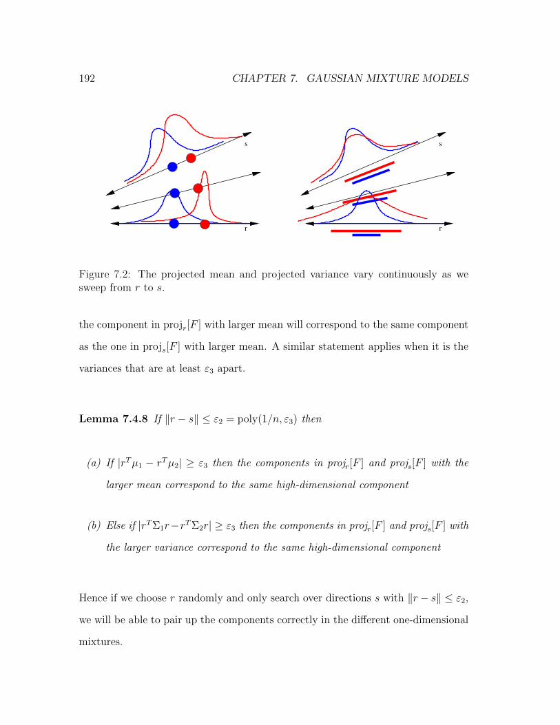
192 CHAPTER 7. GAUSSIAN MIXTURE MODELS
s
r
s
r
Figure 7.2: The projected mean and projected variance vary continuously as wesweep from r to s.
the component in projr[F ] with larger mean will correspond to the same component
as the one in projs[F ] with larger mean. A similar statement applies when it is the
variances that are at least ε3 apart.
Lemma 7.4.8 If ‖r − s‖ ≤ ε2 = poly(1/n, ε3) then
(a) If |rTµ1 − rTµ2| ≥ ε3 then the components in projr[F ] and projs[F ] with the
larger mean correspond to the same high-dimensional component
(b) Else if |rTΣ1r−rTΣ2r| ≥ ε3 then the components in projr[F ] and projs[F ] with
the larger variance correspond to the same high-dimensional component
Hence if we choose r randomly and only search over directions s with ‖r− s‖ ≤ ε2,
we will be able to pair up the components correctly in the different one-dimensional
mixtures.

7.4. CLUSTERING-FREE ALGORITHMS 193
Condition Number Lemma
Now we encounter the final problem in the high-dimensional case: Suppose we choose
r randomly and for s1, s2, . . . ., sp we learn the parameters of the projection of F onto
these directions and pair up the components correctly. We can only hope to learn the
parameters on these projection up to some additive accuracy ε1 (and our univariate
learning algorithm will have running time and sample complexity poly(1/ε1)).
Problem 4 How do these errors in our univariate estimates translate to errors in
our high dimensional estimates for µ1,Σ1, µ2,Σ2?
Recall that the condition number controls this. The final lemma we need in the
high-dimensional case is:
Lemma 7.4.9 The condition number of the linear system to solve for µ1,Σ1 is
poly(1/ε2, n) where all pairs of directions are ε2 apart.
Intuitively, as r and s1, s2, . . . ., sp are closer together then the condition number of
the system will be worse (because the linear constraints are closer to redundant),
but the key fact is that the condition number is bounded by a fixed polynomial
in 1/ε2 and n, and hence if we choose ε1 = poly(ε2, n)ε then our estimates to the
high-dimensional parameters will be within an additive ε. Note that each parameter
ε, ε3, ε2, ε1 is a fixed polynomial in the earlier parameters (and 1/n) and hence we
need only run our univariate learning algorithm with inverse polynomial precision
on a polynomial number of mixtures to learn an ε-close estimate F !
But we still need to design a univariate algorithm, and next we return to
Pearson’s original problem!

194 CHAPTER 7. GAUSSIAN MIXTURE MODELS
7.5 A Univariate Algorithm
Here we will give a univariate algorithm to learning the parameters of a mixture of
two Gaussians up to additive accuracy ε whose running time and sample complexity
is poly(1/ε). Our first observation is that all of the parameters are bounded:
Claim 7.5.1 Let F = w1F1+w2F2 be a mixture of two Gaussians that is in isotropic
position. Suppose that w1, w2 ≥ ε. Then
(a) µ1, µ2 ∈ [−1/√ε, 1/√ε]
(b) σ21, σ
22 ∈ [0, 1/ε]
The idea is that if either of the conditions is violated it would imply that the
mixture has variance strictly larger than one. Once we know that the parameters
are bounded, the natural approach is to try a grid search:
Grid Search
Input: samples from F (Θ)
Output: parameters Θ = (w1, µ1, σ21, µ2, σ
22)
For all valid Θ where the parameters are multiples of εC
Test Θ using the samples, if it passes output Θ
End
There are many ways we could think about testing the closeness of our estimate
with the true parameters of the model. For example, we could empirically estiamte

7.5. A UNIVARIATE ALGORITHM 195
the first six moments of F (Θ) from our samples, and pass Θ if its first six moments
are each within some additive tolerance τ of the empirical moments. (This is really
a variant on Pearson’s sixth moment test). It is easy to see that if we take enough
samples and set τ appropriately, then if we round the true parameters Θ to any
valid grid point whose parameters are multiples of εC , then the resulting Θ will with
high probability pass our test. This is called the completeness. The much more
challenging part is establishing the soundness; after all why is there no other set of
parameters Θ except for ones close to Θ that pass our test?
Alternatively, we want to prove that any two mixtures F and F whose param-
eters do not match within an additive ε must have one of their first six moments
noticeably different. The main lemma is:
Lemma 7.5.2 (Six Moments Suffice) For any F and F that are not ε-close in
parameters, there is an r ∈ 1, 2, . . . , 6 where
∣∣∣Mr(Θ)−Mr(Θ)∣∣∣ ≥ εO(1)
where Θ and Θ are the parameters of F and F respectively, and Mr is the rth raw
moment.
Let Mr be the empirical moments. Then
∣∣∣Mr(Θ)−Mr(Θ)∣∣∣ ≤ ∣∣∣Mr(Θ)− Mr
∣∣∣︸ ︷︷ ︸≤τ
+∣∣∣Mr −Mr(Θ)
∣∣∣︸ ︷︷ ︸≤τ
≤ 2τ
where the first term is at most τ because the test passes and the second term is
small because we can take enough samples (but still poly(1/τ)) so that the empirical

196 CHAPTER 7. GAUSSIAN MIXTURE MODELS
moments and the true moments are close. Hence we can apply the above lemma in
the contrapositive, and conclude that if the grid search outputs Θ then Θ and Θ
must be ε-close in parameters, which gives us an efficient univariate algorithm!
So our main goal is to prove that if F and F that are not ε-close, then one
of their first six moments is noticeably different. In fact, even the case of ε = 0 is
challenging: If F and F are different mixtures of two Gaussians, why is one of their
first six moments necessarily different? Our main goal is to prove this statement,
using the heat equation.
In fact, let us consider the following thought experiment. Let f(x) = F (x)−
F (x) be the point-wise difference between the density functions F and F . Then,
the heart of the problem is: Can we prove that f(x) crosses the x-axis at most six
times? See Figure 7.3.
Lemma 7.5.3 If f(x) crosses the x-axis at most six times, then one of the first six
moments of F and F are different
Proof: In fact, we can construct a (non-zero) degree at most six polynomial p(x)
that agrees with the sign of f(x) – i.e. p(x)f(x) ≥ 0 for all x. Then
0 <∣∣∣ ∫
x
p(x)f(x)dx∣∣∣ =
∣∣∣ ∫x
6∑r=1
prxrf(x)dx
∣∣∣≤
6∑r=1
|pr|∣∣∣Mr(Θ)−Mr(Θ)
∣∣∣And if the first six moments of F and F match exactly, the right hand side is zero
which is a contradiction.

7.5. A UNIVARIATE ALGORITHM 197
1
p(x)
f(x) = F(x) − F(x)^
F (x)
F (x)
F (x)
F (x)
^^
2
1
2
Figure 7.3: If f(x) has at most six zero crossings, we can find at most degree sixpolynomial that agrees with its sign

198 CHAPTER 7. GAUSSIAN MIXTURE MODELS
So all we need to prove is that F (x)− F (x) has at most six zero crossings. Let
us prove a stronger lemma by induction:
Lemma 7.5.4 Let f(x) =∑k
i=1 αiN (µi, σ2i , x) be a linear combination of k Gaus-
sians (αi can be negative). Then if f(x) is not identically zero, f(x) has at most
2k − 2 zero crossings.
We will rely on the following tools:
Theorem 7.5.5 Given f(x) : R→ R, that is analytic and has n zero crossings, then
for any σ2 > 0, the function g(x) = f(x) ∗ N (0, σ2) has at most n zero crossings.
This theorem has a physical interpretation. If we think of f(x) as the heat profile
of an infinite one-dimensional rod, then what does the heat profile look like at some
later time? In fact it is precisely g(x) = f(x) ∗N (0, σ2) for an appropriately chosen
σ2. Alternatively, the Gaussian is the Green’s function of the heat equation. And
hence many of our physical intuitions for diffusion have consequences for convolution
– convolving a function by a Gaussian has the effect of smoothing it, and it cannot
create a new local maxima (and relatedly it cannot create new zero crossings).
Finally we recall the elementary fact:
Fact 7.5.6 N (0, σ21) ∗ N (0, σ2
2) = N (0, σ21 + σ2
2)
Now we are ready to prove the above lemma and conclude that if we knew the
first six moments of a mixture of two Gaussians exactly, then we would know its
parameters exactly too. Let us prove the above lemma by induction, and assume
that for any linear combination of k = 3 Gaussians, the number of zero crossings is

7.5. A UNIVARIATE ALGORITHM 199
(a) (b)
(d) (c)
Figure 7.4: (a) linear combination of four Gaussians (b) subtracting σ2 from eachvariance (c) adding back in the delta function (d) convolving by N (0, σ2) to recoverthe original linear combination
at most four. Now consider an arbitrary linear combination of four Gaussians, and
let σ2 be the smallest variance of any component. See Figure 7.4(a). We can consider
a related mixture where we subtract σ2 from the variance of each component. See
Figure 7.4(b).
Now if we ignore the delta function, we have a linear combination of three
Gaussians and by induction we know that it has at most four zero crossings. But
how many zero crossings can we add when we add back in the delta function? We

200 CHAPTER 7. GAUSSIAN MIXTURE MODELS
can add at most two, one on the way up and one on the way down (here we are
ignoring some real analysis complications of working with delta functions for ease of
presentation). See Figure 7.4(c). And now we can convolve the function by N (0, σ2)
to recover the original linear combination of four Gaussians, but this last step does
not increase the number of zero crossings! See Figure 7.4(d).
This proves that
Mr(Θ) = Mr(Θ)
, r = 1, 2, . . . , 6
has only two solutions (the true parameters and we can also interchange which is
component is which). In fact, this system of polynomial equations is also stable and
there is an analogue of condition numbers for systems of polynomial equations that
implies a quantitative version of what we have just proved: if F and F that are not
ε-close, then one of their first six moments is noticeably different. This gives us our
univariate algorithm.
7.6 A View from Algebraic Geometry
Here we will present an alternative univariate learning algorithm of Belkin and Sinha
[28] that also makes use of the method of moments, but gives a much more general
analysis using tools from algebraic geometry.
Polynomial Families
We will analyze the method of moments for the following class of distributions:

7.6. A VIEW FROM ALGEBRAIC GEOMETRY 201
Definition 7.6.1 A class of distributions F (Θ) is called a polynomial family if
∀r, EX∈F (Θ) [Xr] = Mr(Θ)
where Mr(Θ) is a polynomial in Θ = (θ1, θ2, . . . ., θk).
This definition captures a broad class of distributions such as mixtures models whose
components are uniform, exponential, Poisson, Gaussian or gamma functions. We
will need another (tame) condition on the distribution which guarantees that it is
characterized by all of its moments.
Definition 7.6.2 The moment generating function (mgf) of a random variable X
is defined as
f(t) =∞∑n=0
E [Xn]tn
n!
Fact 7.6.3 If the moment generating function of X converges in a neighborhood of
zero, it uniquely determines the probability distribution, i.e.
∀r, Mr(Θ) = Mr(Θ) =⇒ F (Θ) = F (Θ).
Our goal is to show that for any polynomial family, a finite number of its moments
suffice. First we introduce the relevant definitions:
Definition 7.6.4 Given a ring R, an ideal I generated by g1, g2, · · · , gn ∈ R denoted
by I = 〈g1, g2, · · · , gn〉 is defined as
I =
∑i
rigi where ri ∈ R
.

202 CHAPTER 7. GAUSSIAN MIXTURE MODELS
Definition 7.6.5 A Noetherian ring is a ring such that for any sequence of ideals
I1 ⊆ I2 ⊆ I3 ⊆ · · · ,
there is N such that IN = IN+1 = IN+2 = · · · .
Theorem 7.6.6 [Hilbert’s Basis Theorem] If R is a Noetherian ring, then R[X] is
also a Noetherian ring.
It is easy to see that R is a Noetherian ring, and hence we know that R[x] is also
Noetherian. Now we can prove that for any polynomial family, a finite number of
moments suffice to uniquely identify any distribution in the family:
Theorem 7.6.7 Let F (Θ) be a polynomial family. If the moment generating func-
tion converges in a neighborhood of zero, there exists N such that
F (Θ) = F (Θ) if and only if Mr(Θ) = Mr(Θ) ∀r ∈ 1, 2, · · · , N
Proof: Let Qr(Θ, Θ) = Mr(Θ) − Mr(Θ). Let I1 = 〈Q1〉 , I2 = 〈Q1, Q2〉 , · · · .
This is our ascending chain of ideals in R[Θ, Θ]. We can invoke Hilbert’s basis
theorem and conclude that R[X] is a Noetherian ring and hence, there is N such
that IN = IN+1 = · · · . So for all N + j, we have
QN+j(Θ, Θ) =N∑i=1
pij(Θ, Θ)Qi(Θ, Θ)
for some polynomial pij ∈ R[Θ, Θ]. Thus, if Mr(Θ) = Mr(Θ) for all r ∈ 1, 2, · · · , N ,
then Mr(Θ) = Mr(Θ) for all r and from Fact 7.6.3 we conclude that F (Θ) = F (Θ).

7.6. A VIEW FROM ALGEBRAIC GEOMETRY 203
The other side of the theorem is obvious.
The theorem above does not give any finite bound on N , since the basis theorem
does not either. This is because the basis theorem is proved by contradiction, but
more fundamentally it is not possible to give a bound on N that depends only on
the choice of the ring. Consider the following example
Example 2 Consider the Noetherian ring R[x]. Let Ii =⟨xN−i
⟩for i = 0, · · · , N .
It is a strictly ascending chain of ideals for i = 0, · · · , N . Therefore, even if the ring
R[x] is fixed, there is no universal bound on N .
Bounds such as those in Theorem 7.6.7 are often referred to as ineffective. Consider
an application of the above result to mixtures of Gaussians: from the above theorem,
we have that any two mixtures F and F of k Gaussians are identical if and only if
these mixtures agree on their first N moments. Here N is a function of k, and N is
finite but we cannot write down any explicit bound on N as a function of k using the
above tools. Nevertheless, these tools apply much more broadly than the specialized
ones based on the heat equation that we used to prove that 4k − 2 moments suffice
for mixtures of k Gaussians in the previous section.
Systems of Polynomial Inequalities
In general, we do not have exact access to the moments of a distribution but only
noisy approximations. Our main goal is to prove a quantitive version of the previous
result which shows that any two distributions F and F that are close on their first
N moments are close in their parameters too. The key fact is that we can bound

204 CHAPTER 7. GAUSSIAN MIXTURE MODELS
the condition number of systems of polynomial inequalities; there are a number of
ways to do this but we will use quantifier elimination. Recall:
Definition 7.6.8 A set S is semi-algebraic if there exist multivariate polynomials
p1, . . . , pn such that
S = x1, . . . , xr|pi(x1, . . . , xr) ≥ 0
or if S is a finite union or intersection of such sets.
When a set can be defined through polynomial equalities, we call it algebraic
Theorem 7.6.9 [Tarski] The projection of a semi-algebraic set is semi-algebraic.
Interestingly the projection of an algebraic set is not necessarily algebraic. Can
you come up with an example? A projection corresponds to defining a set not just
through polynomial inequalities but also a ∃ operator. It turns out that you can
even take a sequence of ∃ and ∀ operators and the resulting set is still semi-algebraic.
With this tool in hand, we define the following helper set:
H(ε, δ) =∀(Θ, Θ) : |Mr(Θ)−Mr(Θ)| ≤ δ for r = 1, 2, . . . N =⇒ dp(Θ, Θ) ≤ ε
.
Here dp(Θ, Θ) is some parameter distance between Θ and Θ. It is not important
what exactly we choose, just that it can be expressed through polynomials in the
parameters and that it treats parameters that produce the same distribution as the
same — e.g. by taking the minimum over all matchings of components in F (Θ) to
components in F (Θ) and summing the component-wise parameter distances.

7.6. A VIEW FROM ALGEBRAIC GEOMETRY 205
Now let ε(δ) be the smallest ε as a function of δ. Using Tarski’s theorem, we
can prove the following stability bound for the method of moments:
Theorem 7.6.10 There are fixed constants C1, C2, s such that if δ ≤ 1/C1 then
ε(δ) ≤ C2δ1/s.
Proof: It is easy to see that we can define H(ε, δ) as the projection of a semi-
algebraic set, and hence using Tarski’s theorem we conclude that H(ε, δ) is also
semi-algebraic. The crucial observation is that because H(ε, δ) is semi-algebraic,
the smallest that we can choose ε to be as a function of δ is itself a polynomial
function of δ. There are some caveats here, because we need to prove that for a
fixed δ we can choose ε to be strictly greater than zero and moreover the polynomial
relationship between ε and δ only holds if δ is sufficiently small. However these
technical issues can be resolved without much more work, see [28].
Now we arrive at the main result:
Corollary 7.6.11 If |Mr(Θ)−Mr(Θ)| ≤(
εC2
)sthen dp(Θ, Θ) ≤ ε.
Hence there is a polynomial time algorithm to learn the parameters of any uni-
variate polynomial family (whose mgf converges in a neighborhood of zero) within
an additive accuracy of ε whose running time and sample complexity is poly(1/ε);
we can take enough samples to estimate the first N moments within εs and search
over a grid of the parameters, and any set of parameters that matches each of the
moments is necessarily close in parameter distance to the true parameters.

206 CHAPTER 7. GAUSSIAN MIXTURE MODELS
7.7 Exercises
Problem 7-1: Suppose we are given a mixture of two Gaussians where the variances
of each component are equal — i.e.
F (x) = w1N (µ1, σ2, x) + (1− w1)N (µ2, σ
2, x)
Show that four moments suffice to uniquely determine the parameters of the mixture.
Problem 7-2: Suppose we are given access to an oracle that for any direction r
returns the projected means and variances — i.e. rTµ1 and rTΣ1r for one component
and rTµ2 and rTΣ2r. The trouble is you do not know which parameters correspond
to which component.
(a) Design an algorithm to recover µ1 and µ2 (up to permuting which component is
which) that makes at most O(d2) queries to the oracle where d is the dimension.
Hint: Recover the entries of (µ1 − µ2)(µ1 − µ2)T .
(b) Challenge: Design an algorithm to recover Σ1 and Σ2 (up to permuting which
component is which) that makes O(1) queries to the oracle when d = 2.
Note that here we are not assuming anything about how far apart the projected
means or variances are on some direction r.

Chapter 8
Matrix Completion
In earlier chapters, we saw the power of sparsity. It’s possible to recover a sparse
vector from many fewer measurements than its dimension. And if we don’t know
the basis where our vectors are sparse, with enough examples we can learn it. But
sparsity is just the beginning. There are many other ways to make the objects
we are working with be low-complexity. In this chapter, we will study the matrix
completion problem where the goal is to reconstruct a matrix even when we observe
just a few of its entries. Without any assumptions on the matrix, this is impossible
because there are just too many degrees of freedom. But when the matrix is low-
rank and incoherent, it turns out that there are simple convex programs that work.
You can take these ideas much further and study all sorts of structured recovery
problems via convex programs, such as decomposing a matrix into the sum of a
sparse matrix and a low-rank matrix. We won’t get to these here but will give
pointers to the literature.
207

208 CHAPTER 8. MATRIX COMPLETION
8.1 Introduction
In 2006, Netflix issued a grand challenge to the machine learning community: Beat
our prediction algorithms for recommending movies to users by more than ten per-
cent, and we’ll give you a million dollars. It took a few years, but eventually the
challenge was won and Netflix paid out. During that time, we all learned a lot about
how to build good recommendation systems. In this chapter, we will cover one of
the main ingredients which is called the matrix completion problem.
The starting point is to model our problem of predicting movie ratings as
the problem of predicting the unobserved entries of a matrix from the ones we do
observe. More precisely, if user i rates movie j (between one and five stars) we set
Mi,j to be the numerical score. Our goal is to use the entries Mi,j that we observe to
predict the ones that we don’t know. If we could predict these accurately, it would
give us a way to suggest movies to users in a way that we are suggesting movies that
we think they may like. A priori there’s no reason to believe you can do this. If we
think about the entire matrix M that we would get by coercing every user to rate
every movie (and in the Netflix data set there are 480, 189 users and 17, 770 movies)
then in principle the entries Mi,j that we observe might tell us nothing about the
unobserved entries.
We’re in the same conundrum we were in when we talked about compressed
sensing. A priori there is no reason to believe you can take fewer linear measure-
ments of a vector x than its dimension and reconstruct x. What we need is some
assumption about the structure. In compressed sensing, we assumed that x is sparse
or approximately sparse. In matrix completion, we will assume that M is low-rank
or approximately low rank. It’s important to think about where this assumption

8.1. INTRODUCTION 209
comes from. If M were low-rank we could write it as
M = u(1)(v(1))T + u(2)(v(2))T . . . u(r)(v(r))T
The hope is that each of these rank one terms represents some category of movies.
For example, the first term might represent the category drama and the entries in
u(1) might represent for every user, to what extent do they like drama movies? Then
each entry in v(1) would represent for every movie, to what extent would it appeal
to someone who likes drama? This is where the low-rank assumption comes from.
What we’re hoping is that there are some categories underlying our data that make
it possible to fill in missing entries. When I have ratings for a user for movies in
each of the categories, I could then recommend other movies in the category that
he likes by leveraging the data I have from other users.
The Model and Main Results
Now let’s be formal. Suppose there are n users and m movies so that M is an n×m
matrix. Let Ω ⊆ [n]× [m] be the indices where we observe the value Mi,j. Our goal
is, under the assumption that M is low-rank or approximately low-rank, to fill in
the missing entries. The trouble is that in this level of generality, finding the matrix
M of lowest rank that agrees with our observations is NP -hard. However there are
some by now standard assumptions under which we will be able to give efficient
algorithms for recovering M exactly:
(a) the entries we observe are chosen uniformly random from [n]× [m]
(b) M has rank r

210 CHAPTER 8. MATRIX COMPLETION
(c) The singular vectors of M are uncorrelated with the standard basis (such a
matrix is called incoherent and we define this later)
In this chapter, our main result is that there are efficient algorithms for recovering
M exactly if m ≈ mr logm where m ≥ n and rank(M) ≤ r. This is similar
to compressed sensing, where we were able to recover a k-sparse signal x from
O(k log n/k) linear measurements, which is much smaller than the dimension of x.
Here too we can recover a low-rank matrix M from a number of observations that
is much smaller than the dimension of M .
Let us examine the assumptions above. The assumption that should give us
pause is that Ω is uniformly random. This is somewhat unnatural since it would
be more believable if the probability we observe Mi,j depends on the value itself.
Alternatively, a user should be more likely to rate a movie if he actually liked it.
We already discussed the second assumption. In order to understand the third
assumption, suppose our observations are indeed uniformly random. Consider
M = Π
Ir 0
0 0
ΠT
where Π is a uniformly random permutation matrix. M is low-rank, but unless we
observe all of the ones along the diagonal, we will not be able to recover M uniquely.
Indeed, the top singular vectors of M are standard basis vectors; but if we were to
assume that the singular vectors of M are incoherent with respect to the standard
basis, we would avoid this snag because the vectors in our low-rank decomposition
of M are spread out over many rows and columns.

8.1. INTRODUCTION 211
Definition 8.1.1 The coherence µ of a subspace U ⊆ Rn of dimension dim(u) = r
is
n
rmaxi‖PUei‖2,
where PU denotes the orthogonal projection onto U , and ei is the standard basis
element.
It is easy to see that if we choose U uniformly at random, then µ(U) = O(1). Also
we have that 1 ≤ µ(U) ≤ n/r and the upper bound is attained if U contains any ei.
We can now see that if we set U to be the top singular vectors of the above example,
then U has high coherence. We will need the following conditions on M :
(a) Let M = UΣV T , then µ(U), µ(V ) ≤ µ0.
(b) ‖UV T‖∞ ≤ µ1√r√
nm, where || · ||∞ denotes the maximum absolute value of any
entry.
The main result of this chapter is:
Theorem 8.1.2 Suppose Ω is chosen uniformly at random. Then there is a poly-
nomial time algorithm to recover M exactly that succeeds with high probability if
|Ω| ≥ C max(µ21, µ0)r(n+m) log2(n+m)
The algorithm in the theorem above is based on a convex relaxation for the rank
of a matrix called the nuclear norm. We will introduce this in the next section,
and establish some of its properties but one can think of it as an analogue to the
`1 minimization approach that we used in compressed sensing. This approach was

212 CHAPTER 8. MATRIX COMPLETION
first introduced in Fazel’s thesis [70], and Recht, Fazel and Parrilo [124] proved that
this approach exactly recovers M in the setting of matrix sensing, which is related
to the problem we consider here.
In a landmark paper, Candes and Recht [41] proved that the relaxation based
on nuclear norm also succeeds for matrix completion and introduced the assumptions
above in order to prove that their algorithm works. There has since been a long line
of work improving the requirements on m, and the theorem above and our exposition
will follow a recent paper of Recht [123] that greatly simplifies the analysis by making
use of matrix analogues of the Bernstein bound and using these in a procedure now
called quantum golfing that was first introduced by Gross [80].
Remark 8.1.3 We will restrict to M ∈ Rn×n and assume µ0, µ1 = O(1) in our
analysis, which will reduce the number of parameters we need to keep track of.
8.2 Nuclear Norm
Here we introduce the nuclear norm, which will be the basis for our algorithms for
matrix completion. We will follow a parallel outline to that of compressed sensing.
In particular, a natural starting point is the optimization problem:
(P0) min rank(X) s.t. Xi,j = Mi,j for all (i, j) ∈ Ω
This optimization problem is NP -hard. If σ(X) is the vector of singular values of
X then we can think of the rank of X equivalently as the sparsity of σ(X). Recall,
in compressed sensing we faced a similar obstacle: finding the sparsest solution

8.2. NUCLEAR NORM 213
to a system of linear equations is also NP -hard, but we instead considered the
`1 relaxation and proved that under various conditions this optimization problem
recovers the sparsest solution. Similarly it is natural to consider the `1-norm of σ(X)
which is called the nuclear norm:
Definition 8.2.1 The nuclear norm of X denoted by ‖X‖∗ is ‖σ(X)‖1.
We will instead solve the convex program:
(P1) min ‖X‖∗ s.t. Xi,j = Mi,j for all (i, j) ∈ Ω
and our goal is to prove conditions under which the solution to (P1) is exactly M .
Note that this is a convex program because ‖X‖∗ is a norm, and there are a variety
of efficient algorithms to solve the above program.
In fact, for our purposes a crucial notion is that of a dual norm. We will not
need this concept in full-generality, so we state it for the specific case of the nuclear
norm. This concept gives us a method to lower bound the nuclear norm of a matrix:
Definition 8.2.2 Let 〈X,B〉 =∑
i,j Xi,jBi,j = trace(XTB) denote the matrix inner-
product.
Lemma 8.2.3 ‖X‖∗ = max‖B‖≤1〈X,B〉.
To get a feel for this, consider the special case where we restrict X and B to be
diagonal. Moreover let X = diag(x) and B = diag(b). Then ‖X‖∗ = ‖x‖1 and
the constraint ‖B‖ ≤ 1 (the spectral norm of B is at most one) is equivalent to

214 CHAPTER 8. MATRIX COMPLETION
‖b‖∞ ≤ 1. So we can recover a more familiar characterization of vector norms in
the special case of diagonal matrices:
‖x‖1 = max‖b‖∞≤1
bTx
Proof: We will only prove one direction of the above lemma. What B should we
use to certify the nuclear norm of X. Let X = UXΣXVTX , then we will choose
B = UXVTX . Then
〈X,B〉 = trace(BTX) = trace(VXUTXUXΣXV
TX ) = trace(VXΣXV
TX ) = trace(ΣX) = ‖X‖∗
where we have used the basic fact that trace(ABC) = trace(BCA). Hence this
proves ‖X‖∗ ≤ max‖B‖≤1〈X,B〉, and the other direction is not much more difficult
(see e.g. [88]).
How can we show that the solution to (P1) is M? Our basic approach will be
a proof by contradiction. Suppose not, then the solution is M + Z for some Z that
is supported in Ω. Our goal will be to construct a matrix B of spectral norm at
most one for which
‖M + Z‖∗ ≥ 〈M + Z,B〉 > ‖M‖∗
Hence M +Z would not be the optimal solution to (P1). This strategy is similar to
the one in compressed sensing, where we hypothesized some other solution w that
differs from x by a vector y in the kernel of the sensing matrix A. Back then our
strategy was to use geometric properties of ker(A) to prove that w has strictly larger
`1 norm than x. The proof here will be in the same spirit but considerably more

8.2. NUCLEAR NORM 215
technical and involved.
Let us introduce some basic projection operators that will be crucial in our
proof. Recall, M = UΣV T , let u1, . . . , ur be columns of U and let v1, . . . , vr be
columns of V . Choose ur+1, . . . , un so that u1, . . . , un form an orthonormal basis
for all of Rn – i.e. ur+1, . . . , un is an arbitrary orthonormal basis of U⊥. Similarly
choose vr+1, . . . , vn so that v1, . . . , vn form an orthonormal basis for all of Rn. We
will be interested in the following linear spaces over matrices:
Definition 8.2.4 T = spanuivTj | 1 ≤ i ≤ r or 1 ≤ j ≤ r or both.
Then T⊥ = spanuivTj s.t. r+ 1 ≤ i, j ≤ n.. We have dim(T ) = r2 + 2(n− r)r and
dim(T⊥) = (n− r)2. Moreover we can define the linear operators that project into
T and T⊥ respectively:
PT⊥ [Z] =n∑
i=r+1
n∑j=r+1
〈Z, uivTj 〉 · uivTj = PU⊥ZPV ⊥ .
And similarly
PT [Z] =∑
(i,j)∈[n]×[n]−[r+1,n]×[r+1,n]
〈Z, uivTj 〉 · uivTj = PUZ + ZPV − PUZPV .
We are now ready to describe the outline of the proof of Theorem 8.1.2. The
proof will be based on:
(a) We will assume that a certain helper matrix Y exists, and show that this is
enough to imply ‖M + Z‖∗ > ‖M‖∗ for any Z supported in Ω
(b) We will construct such a Y using quantum golfing [80].

216 CHAPTER 8. MATRIX COMPLETION
Conditions for Exact Recovery
Here we will state the conditions we need on the helper matrix Y and prove that if
such a Y exists, then M is the solution to (P1). We require that Y is supported in
Ω and
(a) ‖PT (Y )− UV T‖F ≤√r/8n
(b) ‖PT⊥(Y )‖ ≤ 1/2.
We want to prove that for any Z supported in Ω, ‖M + Z‖∗ > ‖M‖∗. Recall,
we want to find a matrix B of spectral norm at most one so that 〈M+Z,B〉 > ‖M‖∗.
Let U⊥ and V⊥ be singular vectors of PT⊥ [Z]. Then consider
B =
[U U⊥
]·
V T
V T⊥
= UV T + U⊥VT⊥ .
Claim 8.2.5 ‖B‖ ≤ 1
Proof: By construction UTU⊥ = 0 and V TV⊥ = 0 and hence the above expression
for B is its singular value decomposition, and the claim now follows.
Hence we can plug in our choice for B and simplify:
‖M + Z‖∗ ≥ 〈M + Z,B〉
= 〈M + Z,UV T + U⊥VT⊥ 〉
= 〈M,UV T 〉︸ ︷︷ ︸‖M‖∗
+〈Z,UV T + U⊥VT⊥ 〉

8.2. NUCLEAR NORM 217
where in the last line we used the fact that M is orthogonal to U⊥VT⊥ . Now using
the fact that Y and Z have disjoint supports we can conclude:
‖M + Z‖∗ ≥ ‖M‖∗ + 〈Z,UV T + U⊥VT⊥ − Y 〉
Therefore in order to prove the main result in this section it suffices to prove that
〈Z,UV T + U⊥VT⊥ − Y 〉 > 0. We can expand this quantity in terms of its projection
onto T and T⊥ and simplify as follows:
‖M + Z‖∗ − ‖M‖∗ ≥ 〈PT (Z), PT (UV T + U⊥VT⊥ − Y )〉+ 〈PT⊥(Z), PT⊥(UV T + U⊥V
T⊥ − Y )〉
≥ 〈PT (Z), UV T − PT (Y )〉+ 〈PT⊥(Z), U⊥VT⊥ − PT⊥(Y )〉
≥ 〈PT (Z), UV T − PT (Y )〉+ ‖PT⊥(Z)‖∗ − 〈PT⊥(Z), PT⊥(Y )〉
where in the last line we used the fact that U⊥ and V⊥ are the singular vectors of
PT⊥ [Z] and hence 〈U⊥V T⊥ , PT⊥ [Z]〉 = ‖PT⊥ [Z]‖∗.
Now we can invoke the properties of Y that we have assumed in this section,
to prove a lower bound on the right hand side. By property (a) of Y , we have that
‖PT (Y ) − UV T‖F ≤√
r2n
. Therefore, we know that the first term 〈PT (Z), UV T −
PT (Y )〉 ≥ −√
r8n‖PT (Z)‖F . By property (b) of Y , we know the operator norm
of P⊥T (Y ) is at most 1/2. Therefore the third term 〈PT⊥(Z), PT⊥(Y )〉 is at most
12‖PT⊥(Z)‖∗. Hence
‖M + Z‖∗ − ‖M‖∗ ≥ −√
r
8n‖PT (Z)‖F +
1
2‖PT⊥(Z)‖∗
?> 0
We will show that with high probability over the choice of Ω that the inequality

218 CHAPTER 8. MATRIX COMPLETION
does indeed hold. We defer the proof of this last fact, since it and the construction
of the helper matrix Y will both make use of the matrix Bernstein inequality which
we present in the next section.
8.3 Quantum Golfing
What remains is to construct a helper matrix Y and prove that with high probability
over Ω, for any matrix Z supported in Ω that ‖PT⊥(Z)‖∗ >√
r2n‖PT (Z)‖F to
complete the proof we started in the previous section. We will make use of an
approach introduced by Gross [80] and we will follow the proof of Recht in [123]
where the strategy is to construct Y iteratively. In each phase, we will invoke
concentration results for matrix valued random variables to prove that the error
part of Y decreases geometrically and we make rapid progress in constructing a
good helper matrix.
First we will introduce the key concentration result that we will apply in several
settings. The following matrix valued Bernstein inequality first appeared in the work
of Ahlswede and Winter related to quantum information theory [6].
Theorem 8.3.1 [Non-commutative Bernstein Inequality] Let X1 . . . Xl be indepen-
dent mean 0 matrices of size d × d. Let ρ2k = max‖E[XkX
Tk ]‖, ‖E[XT
k Xk]‖ and
suppose ‖Xk‖ ≤M almost surely. Then for τ > 0,
Pr
[∥∥∥ l∑k=1
Xk
∥∥∥ > τ
]≤ 2d exp
−τ 2/2∑
k ρ2k +Mτ/3
If d = 1 this is the standard Bernstein inequality. If d > 1 and the matrices Xk are

8.3. QUANTUM GOLFING 219
diagonal then this inequality can be obtained from the union bound and the standard
Bernstein inequality again. However to build intuition, consider the following toy
problem. Let uk be a random unit vector in Rd and let Xk = ukuTk . Then it is easy
to see that ρ2k = 1/d. How many trials do we need so that
∑kXk is close to the
identity (after scaling)? We should expect to need Θ(d log d) trials; this is even true
if uk is drawn uniformly at random from the standard basis vectors e1 . . . ed due to
the coupon collector problem. Indeed, the above bound corroborates our intuition
that Θ(d log d) is necessary and sufficient.
Now we will apply the above inequality to build up the tools we will need to
finish the proof.
Definition 8.3.2 Let RΩ be the operator that zeros out all the entries of a matrix
except those in Ω.
Lemma 8.3.3 If Ω is chosen uniformly at random and m ≥ nr log n then with high
probability
n2
m
∥∥∥PTRΩPT −m
n2PT
∥∥∥ < 1
2
Remark 8.3.4 Here we are interested in bounding the operator norm of a linear
operator on matrices. Let T be such an operator, then ‖T‖ is defined as
max‖Z‖F≤1
‖T (Z)‖F
We will explain how this bound fits into the framework of the matrix Bernstein
inequality, but for a full proof see [123]. Note that E[PTRΩPT ] = PT E[RΩ]PT =
mn2PT and so we just need to show that PTRΩPT does not deviate too far from its

220 CHAPTER 8. MATRIX COMPLETION
expectation. Let e1, e2, . . . , ed be the standard basis vectors. Then we can expand:
PT (Z) =∑a,b
〈PT (Z), eaeTb 〉eaeTb
=∑a,b
〈Z, PT (eaeTb )〉eaeTb
Hence RΩPT (Z) =∑
(a,b)∈Ω
⟨Z, PT (eae
Tb )⟩eae
Tb and finally we conclude that
PTRΩPT (Z) =∑
(a,b)∈Ω
⟨Z, PT (eae
Tb )⟩PT (eae
Tb )
We can think of PTRΩPT as the sum of random operators of the form τa,b : Z →⟨Z, PT (eae
Tb )⟩PT (eae
Tb ), and the lemma follows by applying the matrix Bernstein
inequality to the random operator∑
(a,b)∈Ω τa,b.
We can now complete the deferred proof of part (a):
Lemma 8.3.5 If Ω is chosen uniformly at random and m ≥ nr log n then with high
probability for any Z supported in Ω we have
‖PT⊥(Z)‖∗ >√
r
2n‖PT (Z)‖F
Proof: Using Lemma 8.3.3 and the definition of the operator norm (see the remark)
we have ⟨Z, PTRΩPTZ −
m
n2PTZ
⟩≥ − m
2n2‖Z‖2
F

8.3. QUANTUM GOLFING 221
Furthermore we can upper bound the left hand side as:
〈Z, PTRΩPTZ〉 = 〈Z, PTR2ΩPTZ〉 = ‖RΩ(Z − PT⊥(Z))‖2
F
= ‖RΩ(PT⊥(Z))‖2F ≤ ‖PT⊥(Z)‖2
F
where in the last line we used that Z is supported in Ω and so RΩ(Z) = 0. Hence
we have that
‖PT⊥(Z)‖2F ≥
m
n2‖PT (Z)‖2
F −m
2n2‖Z‖2
F
We can use the fact that ‖Z‖2F = ‖PT⊥(Z)‖2
F+‖PT (Z)‖2F and conclude ‖PT⊥(Z)‖2
F ≥m
4n2‖PT (Z)‖2F . Now
‖PT⊥(Z)‖2∗ ≥ ‖PT⊥(Z)‖2
F ≥m
4n2‖PT (Z)‖2
F
>r
2n‖PT (Z)‖2
F
which completes the proof of the lemma.
All that remains is to prove that the helper matrix Y that we made use of
actually does exists (with high probability). Recall that we require that Y is sup-
ported in Ω and ‖PT (Y )− UV T‖F ≤√r/8n and ‖PT⊥(Y )‖ ≤ 1/2. The basic idea
is to break up Ω into disjoint sets Ω1,Ω2, . . .Ωp, where p = log n and use each set
of observations to make progress on the remained PT (Y ) − UV T . More precisely,
initialize Y0 = 0 in which case the remainder is W0 = UV T . Then set
Yi+1 = Yi +n2
mRΩi+1
(Wi)

222 CHAPTER 8. MATRIX COMPLETION
and update Wi+1 = UV T − PT (Yi+1). It is easy to see that E[n2
mRΩi+1
] = I. Intu-
itively this means that at each step Yi+1−Yi is an unbiased estimator for Wi and so
we should expect the remainder to decrease quickly (here we will rely on the concen-
tration bounds we derived from the non-commutative Bernstein inequality). Now
we can explain the nomenclature quantum golfing; at each step, we hit our golf ball
in the direction of the hole but here our target is to approximate the matrix UV T
which for various reasons is the type of question that arises in quantum mechanics.
It is easy to see that Y =∑
i Yi is supported in Ω and that PT (Wi) = Wi for
all i. Hence we can compute
‖PT (Yi)− UV T‖F =
∥∥∥∥PT n2
mRΩi
Wi−1 −Wi−1
∥∥∥∥F
=
∥∥∥∥PT n2
mRΩi
PTWi−1 − PTWi−1
∥∥∥∥F
=n2
m
∥∥∥PTRΩPT −m
n2PT
∥∥∥ ≤ 1
2‖Wi−1‖F
where the last inequality follows from Lemma 8.3.3. Therefore the Frobenius norm
of the remainder decreases geometrically and it is easy to guarantee that Y satisfies
condition (a).
The more technically involved part is showing that Y also satisfies condition
(b). However the intuition is that ‖PT⊥(Y1)‖ is itself not too large, and since the
norm of the remainder Wi decreases geometrically we should expect that ‖PT⊥(Yi)‖
does too and so most of the contribution to
‖PT⊥(Y )‖ ≤∑i
‖PT⊥(Yi)‖
comes from the first term. For the full details see [123]. This completes the proof
that computing the solution to the convex program indeed finds M exactly, provided

8.3. QUANTUM GOLFING 223
that M is incoherent and |Ω| ≥ max(µ21, µ0)r(n+m) log2(n+m).
Further Remarks
There are many other approaches to matrix completion. What makes the above ar-
gument so technically involved is that we wanted to solve exact matrix completion.
When our goal is to recover an approximation to M it becomes much easier to show
bounds on the performance of (P1). Srebro and Shraibman [132] used Rademacher
complexity and matrix concentration bounds to show that (P1) recovers a solution
that is close to M . Moreover their argument extends straightforwardly to the ar-
guably more practically relevant case when M is only entry-wise close to being low
rank. Jain et al. [93] and Hardt [83] gave provable guarantees for alternating mini-
mization. These guarantees are worse in terms of their dependence on the coherence,
rank and condition number of M but alternating minimization has much better run-
ning time and space complexity and is the most popular approach in practice. Barak
and Moitra [26] studied noisy tensor completion and showed that it is possible to
complete tensors better than naively flattening them into matrices and showed lower
bounds based on the hardness of refuting random constraint satisfaction problems.
Following the work on matrix completion, convex programs have proven to be
useful in many other related problems such as separating a matrix into the sum of a
low-rank and sparse part [44]. Chandrasekaran et al. [46] gave a general framework
for analyzing convex programs for linear inverse problems and applied it in many
settings. An interesting direction is to use reductions and convex programming
hierarchies as a framework for exploring computational vs. statistical tradeoffs [29,
45, 24].

224 CHAPTER 8. MATRIX COMPLETION

Bibliography
[1] D. Achlioptas and F. McSherry. On spectral learning of mixtures of distribu-
tions. In COLT, pages 458–469, 2005.
[2] A. Agarwal, A. Anandkumar, P. Jain, P. Netrapalli, R. Tandon Learn-
ing sparsely used overcomplete dictionaries via alternating minimization
arXiv:1310.7991, 2013
[3] A. Agarwal, A. Anandkumar, P. Netrapalli Exact recovery of sparsely used
overcomplete dictionaries arXiv:1309.1952, 2013
[4] M. Aharon. Overcomplete Dictionaries for Sparse Representation of Signals.
PhD Thesis, 2006.
[5] M. Aharon, M. Elad and A. Bruckstein. K-SVD: An algorithm for designing
overcomplete dictionaries for sparse representation. IEEE Trans. on Signal
Processing, 54(11):4311–4322, 2006.
[6] R. Ahlswede and A. Winter. Strong converse for identification via quantum
channels. IEEE Trans. Inf. Theory 48(3):569–579, 2002.
[7] Noga Alon. Tools from Higher Algebra. In Handbook of Combinatorics, pages
1749–1783, 1996.
225

226 BIBLIOGRAPHY
[8] A. Anandkumar, D. Foster, D. Hsu, S. Kakade, Y. Liu. A spectral algorithm
for latent dirichlet allocation. In NIPS, pages 926–934, 2012.
[9] A. Anandkumar, R. Ge, D. Hsu and S. Kakade. A tensor spectral approach
to learning mixed membership community models. In COLT, pages 867–881,
2013.
[10] A. Anandkumar, D. Hsu and S. Kakade. A method of moments for hidden
markov models and multi-view mixture models. In COLT, pages 33.1–33.34,
2012.
[11] J. Anderson, M. Belkin, N. Goyal, L Rademacher and J. Voss. The more the
merrier: the blessing of dimensionality for learning large Gaussian mixtures.
arXiv:1311.2891, 2013.
[12] S. Arora, R. Ge, Y. Halpern, D. Mimno, A. Moitra, D. Sontag, Y. Wu and
M. Zhu. A practical algorithm for topic modeling with provable guarantees. In
ICML, pages 280–288, 2013.
[13] S. Arora, R. Ge, R. Kannan and A. Moitra. Computing a nonnegative matrix
factorization – provably In STOC, pages 145–162, 2012.
[14] S. Arora, R. Ge and A. Moitra. Learning topic models - going beyond SVD. In
FOCS, pages 1–10, 2012.
[15] S. Arora, R. Ge and A. Moitra. New algorithms for learning incoherent and
overcomplete dictionaries. arXiv:1308.6273, 2013
[16] S. Arora, R. Ge, T. Ma and A. Moitra. Simple, efficient, and neural algorithms
for sparse coding In COLT, pages 113–149, 2015

BIBLIOGRAPHY 227
[17] S. Arora, R. Ge, A. Moitra and S. Sachdeva. Provable ICA with unknown
gaussian noise, and implications for gaussian mixtures and autoencoders. In
NIPS, pages 2384–2392, 2012.
[18] S. Arora, R. Ge, S. Sachdeva and G. Schoenebeck. Finding overlapping com-
munities in social networks: Towards a rigorous approach. In EC, 2012.
[19] S. Arora and R. Kannan. Learning mixtures of separated nonspherical gaus-
sians. Annals of Applied Probability, pages 69-92, 2005.
[20] M. Balcan, A. Blum and A. Gupta. Clustering under approximation stability.
Journal of the ACM, 2013.
[21] M. Balcan, A. Blum and N. Srebro. On a theory of learning with similarity
functions. Machine Learning, pages 89–112, 2008.
[22] M. Balcan, C. Borgs, M. Braverman, J. Chayes and S-H Teng. Finding endoge-
nously formed communities. In SODA, 2013.
[23] A. Bandeira, P. Rigollet and J. Weed. Optimal rates of estimation for multi-
reference alignment. arXiv:1702.08546, 2017.
[24] B. Barak, S. Hopkins, J. Kelner, P. Kothari, A. Moitra and A. Potechin. A
nearly tight sum-of-squares lower bound for the planted clique problem. In
FOCS, pages 428–437, 2016.
[25] B. Barak, J. Kelner and D. Steurer. Dictionary learning and tensor decompo-
sition via the sum-of-squares method. In STOC, pages 143–151, 2015.
[26] B. Barak and A. Moitra. Noisy tensor completion via the sum-of-squares hier-
archy. In COLT, pages 417–445, 2016.

228 BIBLIOGRAPHY
[27] M. Belkin and K. Sinha. Toward learning gaussian mixtures with arbitrary
separation. In COLT, pages 407–419, 2010.
[28] M. Belkin and K. Sinha. Polynomial learning of distribution families. In FOCS,
pages 103–112, 2010.
[29] Q. Berthet and P. Rigollet. Complexity theoretic lower bounds for sparse prin-
cipal component detection. In COLT, pages 1046–1066, 2013.
[30] A. Bhaskara, M. Charikar and A. Vijayaraghavan. Uniqueness of tensor de-
compositions with applications to polynomial identifiability. In COLT, pages
742–778, 2014.
[31] A. Bhaskara, M. Charikar, A. Moitra and A. Vijayaraghavan. Smoothed anal-
ysis of tensor decompositions. In STOC, pages 594–603, 2014.
[32] Y. Bilu and N. Linial. Are stable instances easy? In Combinatorics, Probability
and Computing, 21(5):643–660, 2012.
[33] V. Bittorf, B. Recht, C. Re, and J. Tropp. Factoring nonnegative matrices with
linear programs. In NIPS, 2012.
[34] D. Blei. Introduction to probabilistic topic models. Communications of the
ACM, pages 77–84, 2012.
[35] D. Blei and J. Lafferty. A correlated topic model of Science. Annals of Applied
Statistics, pp. 17–35, 2007.
[36] D. Blei, A. Ng and M. Jordan. Latent dirichlet allocation. Journal of Machine
Learning Research, pages 993–1022, 2003.

BIBLIOGRAPHY 229
[37] A. Blum, A. Kalai and H. Wasserman. Noise-tolerant learning, the parity
problem, and the statistical query model. Journal of the ACM 50: 506-519,
2003.
[38] A. Blum and J. Spencer. Coloring random and semi-random k-colorable graphs.
In Journal of Algorithms, 19(2):204–234, 1995.
[39] K. Borgwardt. The Simplex Method: a probabilistic analysis Springer, 2012.
[40] S. C. Brubaker and S. Vempala. Isotropic PCA and affine-invariant clustering.
In FOCS, pages 551–560, 2008.
[41] E. Candes and B. Recht. Exact matrix completion via convex optimization.
Foundations of Computational Math., pages 717–772, 2008.
[42] E. Candes, J. Romberg and T. Tao. Stable signal recovery from incomplete
and inaccurate measurements. Communications of Pure and Applied Math.,
pp. 1207–1223, 2006.
[43] E. Candes and T. Tao. Decoding by linear programming. IEEE Trans. on
Information Theory, 51(12):4203–4215, 2005.
[44] E. Candes, X. Li, Y. Ma and J. Wright. Robust principal component analysis?
Journal of the ACM, 58(3):1–37, 2011.
[45] V. Chandrasekaran and M. Jordan. Computational and statistical trade-
offs via convex relaxation. Proceedings of the National Academy of Sciences,
110(13)E1181–E1190, 2013.

230 BIBLIOGRAPHY
[46] V. Chandrasekaran, B. Recht, P. Parrilo and A. Willsky. The convex geometry
of linear inverse problems. Foundations of Computational Math., 12(6)805–849,
2012.
[47] J. Chang. Full reconstruction of markov models on evolutionary trees: identi-
fiability and consistency. Mathematical Biosciences, 137(1):51–73, 1996.
[48] K. Chaudhuri and S. Rao. Learning mixtures of product distributions using
correlations and independence. In COLT, pages 9–20, 2008.
[49] K. Chaudhuri and S. Rao. Beyond Gaussians: Spectral methods for learning
mixtures of heavy-tailed distributions. In COLT, pages 21–32, 2008.
[50] S. Chen, D. Donoho and M. Saunders. Atomic decomposition by basis pursuit.
SIAM J. on Scientific Computing, 20(1):33–61, 1998.
[51] A. Cohen, W. Dahmen and R. DeVore. Compressed sensing and best k-term
approximation. Journal of the AMS, pages 211–231, 2009.
[52] J. Cohen and U. Rothblum. Nonnegative ranks, decompositions and factor-
izations of nonnegative matrices. Linear Algebra and its Applications, pages
149–168, 1993.
[53] P. Comon. Independent component analysis: A new concept? Signal Process-
ing, pages 287–314, 1994.
[54] A. Dasgupta. Asymptotic Theory of Statistics and Probability. Springer, 2008.
[55] A. Dasgupta, J. Hopcroft, J. Kleinberg, and M. Sandler. On learning mixtures
of heavy-tailed distributions. In FOCS, pages 491–500, 2005.

BIBLIOGRAPHY 231
[56] S. Dasgupta. Learning mixtures of gaussians. In FOCS, pages 634–644, 1999.
[57] S. Dasgupta and L. J. Schulman. A two-round variant of EM for gaussian
mixtures. In UAI, pages 152–159, 2000.
[58] G. Davis, S. Mallat and M. Avellaneda. Greedy adaptive approximations. J.
of Constructive Approximation, 13:57–98, 1997.
[59] L. De Lathauwer, J Castaing and J. Cardoso. Fourth-order Cumulant-based
Blind Identification of Underdetermined Mixtures. IEEE Trans. on Signal Pro-
cessing, 55(6):2965–2973, 2007.
[60] S. Deerwester, S. Dumais, T. Landauer, G. Furnas and R. Harshman. Indexing
by latent semantic analysis. JASIS, pages 391–407, 1990.
[61] A.P. Dempster, N.M. Laird, and D.B. Rubin. Maximum likelihood from in-
complete data via the EM algorithm. Journal of the Royal Statistical Society
Series B, pages 1–38, 1977.
[62] D. Donoho and M. Elad. Optimally sparse representation in general (non-
orthogonal) dictionaries via `1-minimization. PNAS, 100(5):2197–2202, 2003.
[63] D. Donoho and X. Huo. Uncertainty principles and ideal atomic decomposition.
IEEE Trans. on IT, 47(7):2845–2862, 1999.
[64] D. Donoho and P. Stark. Uncertainty principles and signal recovery. SIAM J.
on Appl. Math., 49(3):906–931, 1989.
[65] D. Donoho and V. Stodden. When does nonnegative matrix factorization give
the correct decomposition into parts? In NIPS, 2003.

232 BIBLIOGRAPHY
[66] R. Downey and M. Fellows. Parameterized complexity Springer, 2012.
[67] M. Elad. Sparse and Redundant Representations. Springer, 2010.
[68] K. Engan, S. Aase and J. Hakon-Husoy. Method of optimal directions for frame
design. ICASSP, 5:2443–2446, 1999.
[69] P. Erdos, M. Steel, L. Szekely and T. Warnow. A few logs suffice to build
(almost) all trees. I. Random Structures and Algorithms 14:153-184, 1997.
[70] M. Fazel. Matrix Rank Minimization with Applications. PhD thesis, Stanford
University, 2002.
[71] U. Feige and J. Kilian. Heuristics for semi random graph problems. JCSS,
pages 639–671, 2001.
[72] U. Feige and R. Krauthgamer. Finding and certifying a large hidden clique in a
semirandom graph. Random Structures and Algorithms, pages 195–208, 2009.
[73] J. Feldman, R. A. Servedio, and R. O’Donnell. PAC learning axis-aligned
mixtures of gaussians with no separation assumption. In COLT, pages 20–34,
2006.
[74] A. Frieze, M. Jerrum, R. Kannan. Learning linear transformations. In FOCS,
pages 359–368, 1996.
[75] A. Garnaev and E. Gluskin. The widths of a Euclidean ball. Sovieth Math.
Dokl., pages 200–204, 1984.
[76] R. Ge and T. Ma. Decomposing overcomplete 3rd order tensors using sum-of-
squares algorithms. In RANDOM, pages 829–849, 2015.

BIBLIOGRAPHY 233
[77] A. Gilbert, S. Muthukrishnan and M. Strauss. Approximation of functions over
redundant dictionaries using coherence. In SODA, 2003.
[78] N. Gillis. Robustness analysis of hotttopixx, a linear programming model for
factoring nonnegative matrices. arXiv:1211.6687, 2012.
[79] N. Goyal, S. Vempala and Y. Xiao. Fourier PCA. In STOC, 2014.
[80] D. Gross. Recovering low-rank matrices from few coefficients in any basis.
arXiv:0910.1879, 2009.
[81] D. Gross, Y-K Liu, S. Flammia, S. Becker and J. Eisert. Quantum state to-
mography via compressed sensing. Physical Review Letters, 105(15), 2010.
[82] V. Guruswami, J. Lee, and A. Razborov. Almost euclidean subspaces of `n1 via
expander codes. Combinatorica, 30(1):47–68, 2010.
[83] M. Hardt. Understanding alternating minimization for matrix completion.
FOCS, pages 651–660, 2014.
[84] R. Harshman. Foundations of the PARFAC procedure: model and conditions
for an ‘explanatory’ multi-mode factor analysis. UCLA Working Papers in
Phonetics, pages 1–84, 1970.
[85] J. Hastad. Tensor rank is NP -complete. Journal of Algorithms, 11(4):644-654,
1990.
[86] C. Hillar and L-H. Lim. Most tensor problems areNP -hard. arXiv:0911.1393v4,
2013

234 BIBLIOGRAPHY
[87] T. Hofmann. Probabilistic latent semantic analysis. In UAI , pages 289–296,
1999.
[88] R. Horn and C. Johnson. Matrix Analysis. Cambridge University Press, 1990.
[89] D. Hsu and S. Kakade. Learning mixtures of spherical gaussians: Moment
methods and spectral decompositions. In ITCS, pages 11–20, 2013.
[90] P. J. Huber. Projection pursuit. Annals of Statistics 13:435–475, 1985.
[91] R. A. Hummel and B. C. Gidas. Zero crossings and the heat equation. Courant
Institute of Mathematical Sciences TR-111, 1984.
[92] R. Impagliazzo and R. Paturi. On the complexity of k-SAT. J. Computer and
System Sciences 62(2):pp. 367–375, 2001.
[93] P. Jain, P. Netrapalli and S. Sanghavi. Low rank matrix completion using
alternating minimization. STOC, pages 665–674, 2013.
[94] A. T. Kalai, A. Moitra, and G. Valiant. Efficiently learning mixtures of two
gaussians. In STOC, pages 553-562, 2010.
[95] R. Karp. Probabilistic analysis of some combinatorial search problems. In
Algorithms and Complexity: New Directions and Recent Results, pages 1–19,
1976.
[96] B. Kashin and V. Temlyakov. A remark on compressed sensing. Manuscript,
2007.
[97] L. Khachiyan. On the complexity of approximating extremal determinants in
matrices. Journal of Complexity, pages 138–153, 1995.

BIBLIOGRAPHY 235
[98] D. Koller and N. Friedman. Probabilistic Graphical Models. MIT Press, 2009.
[99] J. Kruskal. Three-way arrays: Rank and uniqueness of trilinear decompositions
with applications to arithmetic complexity and statistics. Linear Algebra and
its Applications, pages 95–138, 1997.
[100] A. Kumar, V. Sindhwani and P. Kambadur. Fast conical hull algorithms for
near-separable non-negative matrix factorization. In ICML, pages 231–239,
2013.
[101] D. Lee and H. Seung. Learning the parts of objects by non-negative matrix
factorization. Nature, pages 788-791, 1999.
[102] D. Lee and H. Seung. Algorithms for non-negative matrix factorization. In
NIPS, pages 556–562, 2000.
[103] S. Leurgans, R. Ross and R. Abel. A decomposition for three-way arrays.
SIAM Journal on Matrix Analysis and Applications, 14(4):1064–1083, 1993.
[104] M. Lewicki and T. Sejnowski. Learning overcomplete representations. Neural
Computation, 12:337–365, 2000.
[105] W. Li and A. McCallum. Pachinko allocation: DAG-structured mixture mod-
els of topic correlations. ICML, pp. 633-640, 2007.
[106] B. Lindsay. Mixture Models: Theory, Geometry and Applications. Institute
for Mathematical Statistics, 1995.
[107] B. F. Logan. Properties of High-Pass Signals. PhD thesis, Columbia Univer-
sity, 1965.

236 BIBLIOGRAPHY
[108] L. Lovasz and M. Saks. Communication complexity and combinatorial lattice
theory. Journal of Computer and System Sciences, pp. 322–349, 1993.
[109] F. McSherry. Spectral partitioning of random graphs. In FOCS, pages 529–
537, 2001.
[110] S. Mallat. A Wavelet Tour of Signal Processing. Academic-Press, 1998.
[111] S. Mallat and Z. Zhang. Matching pursuits with time-frequency dictionaries.
IEEE Trans. on Signal Processing, 41(12):3397–3415, 1993.
[112] A. Moitra. An almost optimal algorithm for computing nonnegative rank. In
SODA, pages 1454–1464, 2013.
[113] A. Moitra. Super-resolution, extremal functions and the condition number of
Vandermonde matrices In STOC, pages 821–830, 2015.
[114] A. Moitra and G. Valiant. Setting the polynomial learnability of mixtures of
gaussians. In FOCS, pages 93–102, 2010.
[115] E. Mossel and S. Roch. Learning nonsingular phylogenies and hidden markov
models. In STOC, pages 366–375, 2005.
[116] Y. Nesterov. Introductory Lectures on Convex Optimization: A Basic Course.
Springer, 2004.
[117] B. Olshausen and B. Field. Sparse coding with an overcomplete basis set: A
strategy employed by V1? Vision Research, 37(23):331–3325, 1997.
[118] C. Papadimitriou, P. Raghavan, H. Tamaki and S. Vempala. Latent semantic
indexing: A probabilistic analysis. JCSS, pages 217–235, 2000.
BIBLIOGRAPHY 237
[119] Y. Pati, R. Rezaiifar, P. Krishnaprasad. Orthogonal matching pursuit: recur-
sive function approximation with applications to wavelet decomposition. Asilo-
mar Conference on Signals, Systems and Computers, pages 40–44, 1993.
[120] K. Pearson. Contributions to the mathematical theory of evolution. Philo-
sophical Transactions of the Royal Society A, 1894.
[121] Y. Rabani, L. Schulman and C. Swamy. Learning mixtures of arbitrary dis-
tributions over large discrete domains. . In ITCS 2014.
[122] R. Raz. Tensor-rank and lower bounds for arithmetic formulas. In STOC,
pages 659–666, 2010.
[123] B. Recht. A simpler approach to matrix completion. Journal of Machine
Learning Research, pages 3413–3430, 2011.
[124] B. Recht, M. Fazel and P. Parrilo. Guaranteed minimum rank solutions of
matrix equations via nuclear norm minimization. SIAM Review, pages 471–
501, 2010.
[125] R. A. Redner and H. F. Walker. Mixture densities, maximum likelihood and
the EM algorithm. SIAM Review, 26(2):195-239, 1984.
[126] J. Renegar. On the computational complexity and geometry of the first-order
theory of the reals. Journal of Symbolic Computation, pages 255-352, 1991.
[127] T. Rockefellar. Convex Analysis. Princeton University Press, 1996.
[128] A. Seidenberg. A new decision method for elementary algebra. Annals of
Math, pages 365–374, 1954.

238 BIBLIOGRAPHY
[129] V. de Silva and L-H Lim. Tensor rank and the ill-posedness of the best low rank
approximation problem. SIAM Journal on Matrix Analysis and Applications,
30(3):1084–1127, 2008.
[130] D. Spielman and S-H Teng. Smoothed analysis of algorithms: Why the simplex
algorithm usually takes polynomial time. In Journal of the ACM, 51(3):385–
463, 2004.
[131] D. Spielman, H. Wang and J. Wright. Exact recovery of sparsely-used dictio-
naries. Journal of Machine Learning Research, 2012.
[132] N. Srebro and A. Shraibman. Rank, trace-norm and max-norm. In COLT,
pages 545–560, 2005.
[133] M. Steel. Recovering a tree from the leaf colourations it generates under a
Markov model. Appl. Math. Lett. 7:19-24, 1994.
[134] A. Tarski. A decision method for elementary algebra and geometry. University
of California Press, 1951.
[135] H. Teicher. Identifiability of mixtures. Annals of Mathematical Statistics,
pages 244–248, 1961.
[136] J. Tropp. Greed is good: Algorithmic results for sparse approximation. IEEE
Trans. on IT, 50(10):2231–2242, 2004.
[137] J. Tropp, A. Gilbert, S. Muthukrishnan and M. Strauss. Improved sparse
approximation over quasi-incoherent dictionaries. IEEE International Conf. on
Image Processing, 2003.
[138] L. Valiant. A theory of the learnable. Comm. ACM, 27(11):1134–1142, 1984.

BIBLIOGRAPHY 239
[139] S. Vavasis. On the complexity of nonnegative matrix factorization. SIAM
Journal on Optimization, pages 1364-1377, 2009.
[140] S. Vempala, Y. Xiao. Structure from local optima: Learning subspace juntas
via higher order PCA. arXiv:abs/1108.3329, 2011.
[141] S. Vempala and G. Wang. A spectral algorithm for learning mixture models.
Journal of Computer and System Sciences, pages 841–860, 2004.
[142] M. Wainwright and M. Jordan. Graphical Models, Exponential Families, and
Variational Inference. Foundations and Trends in Machine Learning, pages
1–305, 2008.
[143] P. Wedin. Perturbation bounds in connection with singular value decomposi-
tions. BIT, 12:99–111, 1972.
[144] M. Yannakakis. Expressing combinatorial optimization problems by linear
programs. Journal of Computer and System Sciences, pp. 441–466, 1991.

240 BIBLIOGRAPHY

Index
abstract gradient descent, 156
accelerated gradient descent, 150
almost euclidean subspace, 130
alternating minimization, 14
anchor words algorithm, 30
border rank, 51
chi-squared test, 168
Cholesky factorization, 103
circulant matrix, 124
clustering, 176
combinatorial rectangle, 17
condition number, 61
cone, 24
convolution, 124
correlated topic model, 35
coupling, 179
cumulants, 105
d-SUM problem, 29
dirichlet distribution, 96
discrete fourier transform, 125
Eckart-Young Theorem, 8
expectation maximization, 172
extended formulation, 23
extension complexity, 23
factor analysis, 44
Frobenius norm, 7
Gershgorin’s Disk Theorem, 63
gradient descent, 150
gram matrix, 36
Green’s function, 196
grid search, 192
heat equation, 196
Hebbian rule, 160
hidden markov model, 80
Hilbert’s Basis Theorem, 200
ideal, 199
improper density estimation, 181
incoherence, 115
241

242 INDEX
incoherence of a subspace, 208
independent component analysis, 100
ineffective bounds, 201
intermediate cone problem, 28
intermediate simplex problem, 25
isotropic position, 185
Jennrich’s algorithm, 54
k-SVD, 139
kernel density estimate, 181
Khatri-Rao product, 106
Kruskal rank, 110
latent dirichlet allocation model, 35, 92
latent semantic indexing, 10
Log-Rank Conjecture, 23
matching pursuit, 122
matrix bernstein inequality, 216
matrix completion, 206
matrix inner-product, 211
matrix sensing, 210
maximum likelihood estimator, 172
method of moments, 170
method of optimal directions, 139
mixture of two Gaussians, 169
moment generating function, 199
multivariate taylor series, 152
Netflix prize, 206
Noetherian ring, 200
noisy parity problem, 81
nonnegative matrix factorization, 13
nonnegative rank, 13
nuclear norm, 211
orthogonal matching pursuit, 119
overcomplete, 142
overlapping community detection, 99
p-value, 168
pachinko allocation model, 35
parallel pancakes, 179
parameter distance, 187
parameter learning, 182
Pearson’s correlation coefficient, 168
Pearson’s sixth moment test, 171
phylogenetic trees, 74
polynomial family, 198
Prony’s method, 122
proper density estimation, 182
quantifier elimination, 202
quantum golfing, 216
quartet test, 77

INDEX 243
random projection, 176
Renegar’s algorithm, 19
restricted isometry property, 128
semi-algebraic, 202
semi-random models, 89
separability, 30
simplicial factorization problem, 25
singular value decomposition, 6
six moments suffice, 193
smooth, 152
Spearman’s Hypothesis, 44
spectral norm, 8
spectral partitioning, 85
spherical gaussian, 174
spikes-and-sines matrix, 114
stable recovery, 133
Steel’s evolutionary distance, 76
stochastic block model, 84
strongly convex, 152
subset sum problem, 112
sum-of-squares hierarchy, 165
tensor rank, 47
term-by-document matrix, 10
topic model, 33
uncertainty principle, 116
undercomplete, 142
vandermonde matrix, 123
visual cortex, 138
whitening, 103
zero crossings, 196