algorithmic applications to social networks, …
TRANSCRIPT

ALGORITHMIC APPLICATIONS TO SOCIALNETWORKS, SECRETARY PROBLEMS AND
DIFFERENTIAL PRIVACY
BY Mangesh Gupte
A dissertation submitted to the
Graduate School—New Brunswick
Rutgers, The State University of New Jersey
in partial fulfillment of the requirements
for the degree of
Doctor of Philosophy
Graduate Program in Computer Science
Written under the direction of
Michael Saks
and approved by
New Brunswick, New Jersey
October, 2011

c© 2011
Mangesh Gupte
ALL RIGHTS RESERVED

ABSTRACT OF THE DISSERTATION
Algorithmic Applications to Social Networks, Secretary
Problems and Differential Privacy
by Mangesh Gupte
Dissertation Director: Michael Saks
This dissertation is a study in the applications of algorithmic techniques to four specific
problems in the domains of social networks, online algorithms and differential privacy.
We start by looking at the structure of directed networks. In [Gupte, Shankar, Li,
Muthukrishnan, and Iftode, 2011] we define a measure of hierarchy in directed online
social networks, and using primal-dual techniques, present an efficient algorithm to
compute this measure. Our experiments on different online social networks show how
hierarchy emerges as we increase the size of the network.
We study the dynamics of information propagation in online social networks in [Gupte,
Hajiaghayi, Han, Iftode, Shankar, and Ursu, 2009]. For a suitable random graph model
of a social network, we prove that news propagation follows a threshold phenomenon,
hence, high-quality information provably spreads throughout the network assuming
users are greedy. Starting from a sample of the Twitter graph, we show through simu-
lations that the threshold phenomenon is exhibited by both the greedy and courteous
user models.
In chapter 4, we turn our attention from social networks to online algorithms. The
ii

specific problem we tackle is to select a large independent set from a general indepen-
dence set systems when elements arrive online and we are in the random permutation
model. Using a random sampling oracle, we give an algorithm which outputs a set of
size Ω
(s
log n log log n
), where s is size of the largest set. This gives a O (log n log log n)
approximation algorithm, which matches the lower bound within log logn factors.
The last problem we discuss is a scheme for the private release of aggregate informa-
tion [Gupte and Sundararajan, 2010]. Such a scheme must resolve the trade-off between
utility to information consumers and privacy of the database participants. Differential
privacy [Dwork, McSherry, Nissim, and Smith, 2006] is a well-established definition of
privacy. In this work, we present a universal treatment of utility based on the standard
minimax rule from decision theory. Under the assumption of rational behavior, we show
that for every fixed count query, a certain geometric mechanism is universally optimal
for all minimax information consumers. Additionally, our solution makes it possible to
release query results at multiple levels of privacy in a collusion-resistant manner.
iii

Acknowledgements
This thesis has been the culmination of work done over the last six years and so a lot
of people contributed to making it happen. A lot of the early work did not make it into
the thesis, however, it did shape the kind of problems I later worked on and that are
present in the thesis. I would like to thank everyone who helped me throughout this
journey.
Most of all, I would like to thank my adviser, Mike Saks, who has been a support
throughout. His patience with me as I wandered around trying out different problems
and areas has been remarkable. I have particularly enjoyed exploring problems with
him. I have also had the pleasure of working with S. Muthukrishnan, Rebecca Wright
and Liviu Iftode. The breadth of topics I could work on which contributed greatly
to my enjoyment in the program. I would also like to thank Michael Littman, Tina
Eliassi-Rad and Martin Farach-Colton whom I worked with at different stages of the
Ph.D.
I would like to thank my committee members Mike, Muthu, Rebecca and Vahab
for taking time read and give helpful comments on the thesis. The quality improved
significantly and it would have been much poorer without their efforts.
Concentrating on work and fun was possible because of the great work by the
staff in my department. I would especially like to thank our graduate secretary Carol
DiFrancesco who took care of the all the day to day administrative issues I faced and
Aneta Unrat who took the payroll, insurance and other issues out of my way.
Working in the Computer Science department has been a pleasure due to my col-
leagues working in theory. The engaging discussions with Rajat, Fengming, Nikos,
iv

Devendra, Darakshan, Alex, Arzoo and Alantha were a constant source of problems
and new directions. My office mates Pavel and Edi made staying in office fun.
Over the years, I ended up having a long list great of housemates: Sankar, Datla,
Vardhan, Siddharth, Pinakin, Rajesh and Shivesh. A notable feature of my stay were
the long lunches and the variety of discussion topics in the Busch Campus Center, where
I spent countless hours, working and otherwise. A lot of friends kept me company there
and I would especially like to mention to mention Rajat who was the prime organizer
of lunches in BCC and Praveen, Hari, Gayatree, Rekha and Devendra who made the
lunches and discussions fun. Work cannot happen without an equal dose of fun and
the most fun I have had was during the numerous parties and game nights. Thank you
Shruti, Shivesh, Gayatree, Pallavi, Vikas, Madhur, Shiva and Rajesh for showing how
easy it is to keep awake for the whole night when you have something worthwhile to do!
Sagar, Mukund, Anubhav and Sangeeta have always been around since my pre-Rutgers
days to discuss course problems, startup dreams, life expectations, jobs, internships and
everything else under the sun.
Family is what kept me going throughout my stay here. Shweta has been supporting
me (both emotionally and financially!) for many years now without too much of a
grumble :-) Meeting her and being with her here at Rutgers has been the highlight of
the Ph.D. Aai, Baba and Poornima tai all been pushing me to always do better and to
complete faster. Their belief in me and their support has been invaluable. Of course,
my twin nephews Aditya and Pranav, who arrived during the Ph.D. adding spice to
life, making it more hectic and interesting and also very entertaining.
v

Dedication
To my wife Shweta
and to my parents.
To friends in the noisy booths of BCC
and the delicious lunches of Faculty Dining.
To long nights of getting high
on board games
and in parties
and especially on enchanting new ideas.
To hard problems
and technical proofs
and clumsy errors
and aimless exploration.
To the six years of work
and enjoyment
and fun
and growth.
To new beginnings ...
vi
Table of Contents
Abstract . . . . . . . . . . . . . . . . . . . . . . . . . . . . . . . . . . . . . . . . ii
Acknowledgements . . . . . . . . . . . . . . . . . . . . . . . . . . . . . . . . . iv
Dedication . . . . . . . . . . . . . . . . . . . . . . . . . . . . . . . . . . . . . . . vi
List of Tables . . . . . . . . . . . . . . . . . . . . . . . . . . . . . . . . . . . . . x
List of Figures . . . . . . . . . . . . . . . . . . . . . . . . . . . . . . . . . . . . xi
1. Introduction . . . . . . . . . . . . . . . . . . . . . . . . . . . . . . . . . . . 1
2. Hierarchy in Social Networks . . . . . . . . . . . . . . . . . . . . . . . . . 7
2.1. Introduction . . . . . . . . . . . . . . . . . . . . . . . . . . . . . . . . . . 7
2.2. Hierarchy in Directed Social Networks . . . . . . . . . . . . . . . . . . . 9
2.2.1. Examples . . . . . . . . . . . . . . . . . . . . . . . . . . . . . . . 11
2.3. Efficiently Measuring Hierarchy . . . . . . . . . . . . . . . . . . . . . . . 13
2.3.1. Algorithm . . . . . . . . . . . . . . . . . . . . . . . . . . . . . . . 13
2.4. Proofs . . . . . . . . . . . . . . . . . . . . . . . . . . . . . . . . . . . . . 18
2.5. Experiments . . . . . . . . . . . . . . . . . . . . . . . . . . . . . . . . . . 22
2.5.1. Validation of the Hierarchy Measure . . . . . . . . . . . . . . . . 24
2.5.2. Importance of Edge Direction . . . . . . . . . . . . . . . . . . . . 25
2.5.3. Hierarchy in Online Social Networks vs Random Graphs . . . . . 27
2.5.4. Effect of Scaling on Social Hierarchy . . . . . . . . . . . . . . . . 29
2.6. Related Work . . . . . . . . . . . . . . . . . . . . . . . . . . . . . . . . . 34
vii

2.7. Conclusions and Future Directions . . . . . . . . . . . . . . . . . . . . . 35
3. News Propagation in Social Networks . . . . . . . . . . . . . . . . . . . 36
3.1. Introduction . . . . . . . . . . . . . . . . . . . . . . . . . . . . . . . . . . 36
3.2. Strategic User Model . . . . . . . . . . . . . . . . . . . . . . . . . . . . . 38
3.3. Random Graph Models of Social Networks . . . . . . . . . . . . . . . . 40
3.3.1. Connectivity of stochastic Kronecker graphs . . . . . . . . . . . . 42
3.4. Analysis of a Model of Strategic User Behavior . . . . . . . . . . . . . . 43
3.4.1. The Connectedness of G[R] . . . . . . . . . . . . . . . . . . . . . 45
3.5. Simulation Results . . . . . . . . . . . . . . . . . . . . . . . . . . . . . . 50
3.6. Conclusion and Future Work . . . . . . . . . . . . . . . . . . . . . . . . 52
4. Secretary Problems on Independence Set Systems . . . . . . . . . . . 57
4.1. Introduction . . . . . . . . . . . . . . . . . . . . . . . . . . . . . . . . . . 57
Online Algorithms . . . . . . . . . . . . . . . . . . . . . . . . . . 57
4.1.1. The Random Permutation Model . . . . . . . . . . . . . . . . . . 58
4.1.2. Independence Set Systems . . . . . . . . . . . . . . . . . . . . . . 59
4.1.3. The Secretary Problem on Independence Set Systems . . . . . . 60
4.1.4. Related Work . . . . . . . . . . . . . . . . . . . . . . . . . . . . . 61
4.1.5. Bipartite Graph representation of Independence Set Systems . . 63
4.2. Oracles and Problem Variants . . . . . . . . . . . . . . . . . . . . . . . . 63
4.3. Algorithm . . . . . . . . . . . . . . . . . . . . . . . . . . . . . . . . . . . 65
4.4. Weighted Elements . . . . . . . . . . . . . . . . . . . . . . . . . . . . . . 70
4.5. Future direction using the Oracle O2 . . . . . . . . . . . . . . . . . . . . 71
4.5.1. Approximating the offline oracle . . . . . . . . . . . . . . . . . . 71
4.5.2. A labeling game . . . . . . . . . . . . . . . . . . . . . . . . . . . 73
4.6. Conclusion . . . . . . . . . . . . . . . . . . . . . . . . . . . . . . . . . . 76
viii
5. Differential Privacy . . . . . . . . . . . . . . . . . . . . . . . . . . . . . . . 79
5.1. Introduction . . . . . . . . . . . . . . . . . . . . . . . . . . . . . . . . . . 79
5.2. Model and Results . . . . . . . . . . . . . . . . . . . . . . . . . . . . . . 82
5.2.1. Privacy Mechanisms and Differential Privacy . . . . . . . . . . . 82
5.2.2. Oblivious Mechanisms . . . . . . . . . . . . . . . . . . . . . . . . 84
5.2.3. Minimax Information Consumers . . . . . . . . . . . . . . . . . . 85
5.2.4. Interactions of Information Consumers with Mechanisms . . . . . 86
Motivation . . . . . . . . . . . . . . . . . . . . . . . . . . . . . . 86
Feasible Interactions . . . . . . . . . . . . . . . . . . . . . . . . . 86
Optimal Interactions . . . . . . . . . . . . . . . . . . . . . . . . . 87
5.2.5. Optimal Mechanism for a Single Known Information Consumer . 88
5.2.6. Optimal Mechanism for Multiple Unknown Information Consumers 89
5.2.7. Comparison with Bayesian Information Consumers . . . . . . . . 92
5.2.8. Related Work . . . . . . . . . . . . . . . . . . . . . . . . . . . . . 93
5.3. Characterizing Mechanisms Derivable from the Geometric Mechanism . 94
5.4. Applications of the Characterization . . . . . . . . . . . . . . . . . . . . 98
5.4.1. Information-Consumers at Different Privacy Levels . . . . . . . . 98
5.4.2. Universal Utility Maximizing Mechanisms . . . . . . . . . . . . . 100
5.5. There always exists an Optimal Mechanism that is Oblivious . . . . . . 105
5.6. A Differentially Private Mechanism that is not derivable from the Geo-
metric Mechanism . . . . . . . . . . . . . . . . . . . . . . . . . . . . . . 108
5.7. Conclusion . . . . . . . . . . . . . . . . . . . . . . . . . . . . . . . . . . 108
ix

List of Tables
5.1. The optimal mechanism for consumer c characterized by loss-function
l(i, r) = |i− r| and side-information S = 0, 1, 2, 3. n = 3, α = 1/4. . . 90
5.2. The Range Restricted Geometric Mechanism . . . . . . . . . . . . . . . 95
x
List of Figures
2.1. Graphs with perfect hierarchy. h(G) = 1 for each of these
graphs. Nodes labels indicate levels. All edges have agony 0. . 11
2.2. Graphs with some hierarchy. All unlabeled edges have agony 0. 12
2.3. Graphs with no hierarchy. h(G) = 0 for each of these graphs.
All edges have agony 1. . . . . . . . . . . . . . . . . . . . . . . . . . 12
2.4. Correlation of hierarchy with popular metrics. . . . . . . . . . . . 23
2.5. Correlation with Wikipedia notability score. . . . . . . . . . . . 25
2.6. Hierarchy in the College Football network. . . . . . . . . . . . . . 26
2.7. Hierarchy in random graphs. . . . . . . . . . . . . . . . . . . . . . . 27
2.8. Hierarchy in social network among famous people. . . . . . . . . 30
2.9. Effect of network size on hierarchy. . . . . . . . . . . . . . . . . . . 31
2.10. Distribution of ranks among nodes. . . . . . . . . . . . . . . . . . . 31
2.11. Distribution of ranks among nodes. . . . . . . . . . . . . . . . . . . 32
2.12. Effect of directed edges. . . . . . . . . . . . . . . . . . . . . . . . . . 33
3.1. Coverage of greedy and courteous strategies over the crawled
graph. q is the probability with which each user likes the link.
t is the threshold for the greedy strategy. c is the threshold for
the courteous strategy. . . . . . . . . . . . . . . . . . . . . . . . . . . 51
4.1. Modeling knapsack constraints as an independence set system 60
4.2. Independence set systems as a bipartite graph . . . . . . . . . . . 63
4.3. Bucketing the independent sets . . . . . . . . . . . . . . . . . . . . 68
xi

5.1. The probability distribution on outputs given by the Geometric
Mechanism for α = 0.2 and query result 5. . . . . . . . . . . . . . . 83
xii
1
Chapter 1
Introduction
The computer science landscape of changed drastically over the last few years. Online
social networks exploded on the scene in the second half of the last decade, touching
not just areas within Computer Science itself, but also the lives of people outside the
field. Sites like Facebook and Twitter have become household names. Facebook has
more than 750 million active users, half of whom log on any given day. Online social
networks have become an increasingly popular medium for sharing information such as
links, news and multimedia among users. For example, during the recent Iran elections,
traditional news media acknowledged the power and influence of social networks such
as Twitter. In this scenario, understanding the structure of social networks and the
dynamics of sharing in networks is a fundamental challenge. Graph theory gives us the
necessary tools to embark on this. We analyze the structure of directed social networks
in chapter 2 and the dynamics of the process of news propagation in social networks
in 3.
The advent of social networks has been fueled by the immense amount of data
that people share in these networks. With the rising popularity of social networks and
in an age of information sharing, privacy concerns have become paramount. Initial
attempts at privacy were based on syntactic definitions like like k-anonymity [Sweeney,
2002]. The break in privacy of seemingly anonymous datasets like the one released by
Netflix as part of their programming challenge [Narayanan and Shmatikov, 2008] have
shown the need for refined definitions of privacy. Differential privacy [Dwork, McSherry,
Nissim, and Smith, 2006] gives a semantic definition of privacy and places privacy on

2
sound theoretical foundations. Mechanisms guarantee differential privacy by perturbing
results – they add random noise to the query result, and guarantee protection against
all attackers, whatever their side-information or intent. We discuss a universal privacy
preserving mechanism in chapter 5.
Finally, we study online algorithms in chapter 4. We look at the problem of selecting
a large independent set of elements in the secretary setting.
Underlying the study of all these problems is a common set of algorithmic techniques
like linear programming and duality, the theory of random graphs and concentration
bounds. These techniques help us analyze and understand modern phenomena like
online social networks. This dissertation is a study in the applications of algorithmic and
combinatorial techniques to different domains. We shall look at four specific problems
in the domains of social networking, online algorithms and differential privacy. The
modus operandi is to look at real world problems, construct simplified models of the
phenomenon under consideration, analyze the simplified models and apply the findings
back to the problem we started out with.
We start with the work in [Gupte, Shankar, Li, Muthukrishnan, and Iftode, 2011]
that looks at the structure of directed networks. Social hierarchy and stratification
among humans is a well studied concept in sociology. The popularity of online social
networks presents an opportunity to study social hierarchy for different types of net-
works and at different scales. We adopt the premise that people form connections in a
social network based on the perceived social hierarchy; as a result, the edge directions
in directed social networks can be leveraged to infer hierarchy. We define a measure
of hierarchy in a directed online social network, and present an efficient algorithm to
compute this measure. The main challenge is to define a measure that captures the
intuitive meaning of hierarchy while also being efficiently computable. We use primal-
dual linear programming techniques to come up with a polynomial time combinatorial
algorithm to compute this measure. We validate that our measure corresponds with

3
hierarchy as observed by people, by using ground truth including the Wikipedia nota-
bility score. We then use the measure to study hierarchy in several directed online social
networks including Twitter, Delicious, YouTube, Flickr, LiveJournal, and curated lists
of several categories of people based on different occupations, and different organiza-
tions. Our experiments on different online social networks show how hierarchy emerges
as we increase the size of the network. This is in contrast to random graphs, where the
hierarchy decreases as the network size increases. Further, we show that the degree of
stratification in a network increases very slowly as we increase the size of the graph.
In [Gupte, Hajiaghayi, Han, Iftode, Shankar, and Ursu, 2009], we look at the dy-
namics of information propagation in online social networks. We argue that users in
social networks are strategic in how they post and propagate information. We pro-
pose two models of user behavior — the greedy and the courteous model — and study
information propagation both analytically and through simulations. We model social
networks as random graphs and use properties of random graphs to prove how news
propagates over social networks. We model news using a single parameter q that denote
the quality. This parameter intuitively corresponds to the fraction of the population
that finds the particular news piece interesting. We also give two plausible models
of user behavior: greedy and courteous. For suitable random graph models of social
networks, we prove that news propagation follows a threshold phenomenon, hence,
high-quality information provably spreads throughout the network assuming users are
greedy. Starting from a sample of the Twitter graph, we show through simulations that
the threshold phenomenon is exhibited by both the greedy and courteous user models.
The next problem we tackle deals with online algorithms. The specific problem
we tackle is to select a large independent set from a general independence set systems
when elements arrive online. In the worst case (adversarial) setting, we cannot hope
to select more than one element. But in the random permutation model, also called
the secretary setting, we give an algorithm which outputs a set of size Ω
(s
log n
)with
4
probability O
(1
log log n
), where s is size of the largest set and n is the total number
of elements in the set system. This gives a O (log n log log n) approximation algorithm,
which matches the lower bound within O(
(log log n)2)
factor.
Last, we turn our attention to the problem of privacy. We need a scheme to re-
lease aggregates of private information that are also useful [Gupte and Sundararajan,
2010]. A scheme that publishes aggregate information about sensitive data must re-
solve the trade-off between utility to information consumers and privacy of the database
participants. Differential privacy [Dwork, McSherry, Nissim, and Smith, 2006] is a
well-established definition of privacy—this is a universal guarantee against all attack-
ers, whatever their side-information or intent. In this work, we present a universal
treatment of utility based on the standard minimax rule from decision theory. In our
model, information consumers are minimax (risk-averse) agents, each possessing some
side-information about the query, and each endowed with a loss-function which models
their tolerance to inaccuracies. Further, information consumers are rational in the sense
that they actively combine information from the mechanism with their side-information
in a way that minimizes their loss. Under the assumption of rational behavior, we show
that for every fixed count query, a certain geometric mechanism is universally optimal
for all minimax information consumers. Additionally, our solution makes it possible to
release query results at multiple levels of privacy in a collusion-resistant manner. We
use linear algebraic and linear programming techniques to solve this problem.

5
Social Networks

7
Chapter 2
Hierarchy in Social Networks
2.1 Introduction
Social stratification refers to the hierarchical arrangement of individuals in a society into
divisions based on various factors such as power, wealth, knowledge and importance 1.
Stratification existed among humans since the very beginning of human society and
continues to exist in modern society. In some settings, such as within an organization,
the hierarchy is well known, whereas in other settings, such as conferences and meetings
between a group of people, the hierarchy is implicit but discernible.
The popularity of online social networks has created an opportunity to study soci-
ological phenomenon at a scale that were earlier unfathomable. Phenomenon such as
small diameter in social networks [Travers and Milgram, 1969] and strength of weak
ties [Granovetter, 1973] have been revisited in light of the large data now available about
people and their connections [Albert, Jeong, and Barabasi, 1990, Watts and Strogatz,
1998, Barabasi, 2005]. Online social networks present an opportunity to study how
social hierarchy emerges.
Scientists have observed dominance hierarchies within primates. Schjelderup-Ebbe
[1975] showed a pecking order among hens where each hen is aware of its place among
the hierarchy and there have been various papers that investigate the importance of
such a hierarchy [Frank and Goyal, 2003, Fama and French, 2002]. However, data from
experimental studies indicates that the dominance graph contains cycles and hence,
1http://www.answers.com/topic/social-stratification-1

8
does not represent true hierarchy. There has been a lot of work on extracting a chain
given this dominance graph [de Vries, 1995, 1998, Appleby, 1983].
Stratification is manifested among humans in the form of a social hierarchy, where
people higher up in the hierarchy have higher social status than people lower in the
hierarchy. With the wide adoption of online social networks, we can observe the net-
work and can leverage the links between nodes to infer social hierarchy. Most of the
popular online social networks today, such as Twitter, Flickr, YouTube, Delicious and
LiveJournal contain directed edges.2 Our central premise is that there is a global social
rank that every person enjoys, and that individuals are aware of their rank as well as
the rank of people they connect to.
Given a social graph, we cannot directly observe the ranks of people in the network,
we can only observe the links. We premise that the existence of a link indicates a
social rank recommendation; a link u → v (u is a follower of v) indicates a social
recommendation of v from u. If there is no reverse link from v to u, it might indicate
that v is higher up in the hierarchy than u. We assume that in social networks, when
people connect to other people who are lower in the hierarchy, this causes them social
agony. To infer the ranks of the nodes in the network, we find the best possible ranking,
i.e. the ranking that gives the least social agony.
In this chapter, we define a measure that indicates how close the given graph is to
a true hierarchy. We also give a polynomial time algorithm to evaluate this measure
on general directed graphs and to find ranks of nodes in the network that achieve this
measure.
We use our algorithm to measure hierarchy in different online social networks, in-
cluding Twitter, Delicious, Flickr, YouTube, LiveJournal, and curated lists of people
based on categories like different occupations, and different organizations.
We experimentally find, using a college football dataset, that the edge directions
2Facebook is an exception with undirected edges.

9
encodes hierarchy information. The social strata of people in online social networks,
measured using our metric, shows strong correlation with human-observed ground truth
such as Wikipedia notability, as well as other well-known metrics such as page rank and
friend-follower ratio. Our experiments show that hierarchy emerges as the size of an
online social network grows. This is in contrast to random graphs, where the hierarchy
decreases as the network size increases. Finally, we show that hierarchy in online social
networks does not grow indefinitely; instead, there are a small number of levels (strata)
that users are assigned to and this number does not grow significantly as the size of the
network increases.
The key contributions that we see in this chapter are:
1. We define a measure of hierarchy for general directed networks.
2. We give a polynomial time algorithm to find the largest hierarchy in a directed
network.
3. We show how hierarchy emerges as the size of the networks increases for different
online social networks.
4. We show that, as we increase the size of the graph in our experiments, the degree
of stratification in a network does not increase significantly.
2.2 Hierarchy in Directed Social Networks
One of the most popular ways to organize various positions within an organization is
as a tree. A general definition of hierarchy is a (strict) partially ordered set. This
definition includes chains (Figure 2.1a) and trees (Figure 2.1b) as special cases. We can
view a partially ordered set as a graph, where each element of the set is a node and the
partial ordering (u > v) gives an edge from u to v. The fact that the graph represents
a partial order implies that the graph is a Directed Acyclic Graph (DAG). From now

10
on, we use DAGs as examples of perfect hierarchy. Figure 2.1c shows an example of a
DAG.
Let us define a measure of hierarchy for directed graphs that might contain cycles.
Consider a network G = (V,E) where each node v has a rank r(v). Formally, the rank
is a function r : V → N that gives an integer score to each vertex of the graph. Different
vertices can have the same score.
In social networks, where nodes are aware of their ranks, we expect that higher
rank nodes are less likely to connect to lower rank nodes. Hence, directed edges that
go from lower rank nodes to higher rank nodes are more prevalent than edges that go
in the other direction. In particular, if r(u) < r(v) the edge u → v is expected and
does not cause any agony to u. However, if r(u) ≥ r(v), then edge u → v causes
agony to the user u and the amount of agony depends on the difference between their
ranks. We shall assume that the agony caused to u by each such reverse edge is equal
to r(u)− r(v) + 1.3 4 Hence, the agony to u caused by edge (u, v) relative to a ranking
r is max(r(u)− r(v) + 1, 0).
We define the agony in the network relative to the ranking r as the sum of the agony
on each edge:
A(G, r) =∑
(u,v)∈E
max(r(u)− r(v) + 1, 0)
We defined agony in terms of a ranking, but in online social networks, we can only
observe the graph G and cannot observe the rankings. Hence, we need to infer the
rankings from the graph itself. Since nodes typically minimize their agony, we shall
find a ranking r that minimizes the total agony in the graph. We define the agony of
3Note that r(u) − r(v) does not work, since it gives rise to trivial solutions like r = 1 for all nodes.The +1 effectively penalizes such degenerate solutions. Using any positive constant threshold c otherthan 1 does not change the optimal ranking, the minimum agony value gets scaled by a factor of c.
4An interesting direction for future work is to investigate a different measure of agony, in particular,a non-linear function like log(r(u) − r(v) + 1).
11
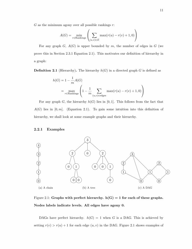
G as the minimum agony over all possible rankings r:
A(G) = minr∈Rankings
∑(u,v)∈E
max(r(u)− r(v) + 1, 0)
For any graph G, A(G) is upper bounded by m, the number of edges in G (we
prove this in Section 2.3.1 Equation 2.1). This motivates our definition of hierarchy in
a graph:
Definition 2.1 (Hierarchy). The hierarchy h(G) in a directed graph G is defined as
h(G) = 1− 1
mA(G)
= maxr∈Rankings
1− 1
m
∑(u,v)∈edges
max(r(u)− r(v) + 1, 0)
For any graph G, the hierarchy h(G) lies in [0, 1]. This follows from the fact that
A(G) lies in [0,m]. (Equation 2.1). To gain some intuition into this definition of
hierarchy, we shall look at some example graphs and their hierarchy.
2.2.1 Examples
0
1
2
3
4
(a) A chain
3
2
0 1
0 0
0 2
0 0 1
0
(b) A tree
0 0
1 1 1
2 2
3
(c) A DAG
Figure 2.1: Graphs with perfect hierarchy. h(G) = 1 for each of these graphs.
Nodes labels indicate levels. All edges have agony 0.
DAGs have perfect hierarchy. h(G) = 1 when G is a DAG. This is achieved by
setting r(v) > r(u) + 1 for each edge (u, v) in the DAG. Figure 2.1 shows examples of

12
graphs with perfect hierarchy. Nodes are labeled with levels. For this assignment, note
that the agony on each edge is 0.
3,r
2,l1 2
0 1
0, l2
2
(a) h(G) =2
3
3,r
2,l1 2
0 1
0, l2
4
(b) h(G) =1
3
Figure 2.2: Graphs with some hierarchy. All unlabeled edges have agony 0.
Consider the graph in Figure 2.2a. The hierarchy of this graph is 1− 1
6× 2 =
2
3. If
instead of the edge (r, l1), the “deeper” edge (r, l2) is present, as shown in Figure 2.2b,
then the hierarchy of the new graph becomes 1 − 1
6× 4 =
1
3. This illustrates how
hierarchy changes in a very simple setting. We shall explore this more in Section 2.5.
1
11
1
1 1
(a) A Simple Cycle
1
11
1
1 1
1 1
1
1
(b) A collection of cycles
Figure 2.3: Graphs with no hierarchy. h(G) = 0 for each of these graphs. All
edges have agony 1.
Directed cycles have no hierarchy. h(G) = 0 when G is a collection of edge disjoint

13
directed cycles. We prove in Section 2.3.1 that for any assignment of labels to nodes,
the agony is at least m. Figure 2.3 shows examples of graphs with 0 hierarchy. If each
node is labeled the same, say 1, this is achieved.
2.3 Efficiently Measuring Hierarchy
To find the hierarchy h(G) for a given graph G, we need to search over all rankings and
find the best one. Since the number of rankings r is exponentially large, we need an
efficient way to search among them. In Section 2.3.1, we present an efficient algorithm
that given a directed graph G as input, finds as output a ranking of the vertices of G
that gives the highest hierarchy for the input graph G.5
2.3.1 Algorithm
In this section, we describe an algorithm that finds the optimal hierarchy for a given
directed graph G = (V,E). For notational convenience, we shall denote n = |V | and
m = |E|. For a scoring function r : V → N, the hierarchy relative to r is:
h(G, r) = 1− 1
m
∑(i,j)∈E
max(r(i)− r(j) + 1, 0)
The task is to find an r such that h(G, r) is maximized over all scoring functions.
But maximizing h is the same as minimizing the total agony A(G, r). We formulate
minimizing agony as the following integer program:
5This ranking may not be unique. In fact, if G is a DAG, then any ordering that gives a topologicalsort of G gives an optimal ranking.

14
min∑
(i,j)∈E
x(i, j)
x(i, j) ≥ r(i)− r(j) + 1 ∀(i, j) ∈ E
x(i, j) ≥ 0 ∀(i, j) ∈ E
r(i) ≥ 0 ∀i ∈ V
x(i, j), r(i) ∈ Z
We can interpret the variables in the linear program as follows: the x(i, j) are defined
for each pair (i, j) ∈ E and represents the agony on each edge. The variables r(i) give
the rank of each node. We see that any feasible solution to this linear program gives
a ranking and the value of the linear program measures the total agony. We now see
a simple upper bound on the minimum value of the integer program. Consider the
solution:
r(i) = 0 : ∀i ∈ V
x(i, j) = 1 : ∀(i, j) ∈ E (2.1)
This is clearly feasible and the objective value for this is m. This gives a simple upper
bound of m on the objective value of the above integer program and hence on the
maximum agony in any graph.
To get insight into this problem, we look at the linear relaxation of this integer
program and then form the dual linear program. The dual is:
max∑
(i,j)∈E
z(i, j)
z(i, j) ≤ 1 ∀(i, j) ∈ E∑j∈V
z(k, j) ≤∑i∈V
z(i, k) ∀k ∈ V (node-degree)
z(i, j) ≥ 0 ∀(i, j) ∈ E

15
We can strengthen the node-degree constraints without affecting the solution of the
linear program by requiring equality, since if we sum over all k, we get:
∑k∈V
∑j∈V
z(k, j) ≤∑k∈V
∑i∈V
z(i, k)
Since both sides count the total number of edges in the graph, they are equal. Hence,
equality must hold for each individual constraint as well. So, we can rewrite the node-
degree condition as:
∑j∈V
z(k, j) =∑i∈V
z(i, k) ∀k ∈ V (node-degree)
Suppose we restrict the dual variables to be 0 or 1 instead of in the range [0, 1],
then we can think of the variables z(i, j) as being indicator variables for the edge (i, j).
The constraint∑j∈V
z(k, j) =∑i∈V
z(i, k) ∀k ∈ V , then says that at each vertex k, the
number of incoming edges must be equal to the number of outgoing edges. Hence, the
dual program is finding the maximum (in terms of number of edges) Eulerian subgraph
of the original graph.6
The reinterpretation gives us insight into the primal solution. By weak duality,
the value of the primal is lower bounded by the value of any feasible dual solution.
Hence, the primal value cannot become smaller than the size of the maximum Eulerian
subgraph.
If the original graph G is Eulerian, this gives a lower bound of m. Equation 2.1
demonstrates a way to get m as the primal solution. Hence, the optimal primal value
for Eulerian graphs is in fact m. This proves the observation that, for graphs that are
a collection of directed cycles, the agony is m and hence, the hierarchy is 0.
We can directly solve the LP to get the best ranking when we do not restrict the
rank of the node to be an integer. We shall prove that the linear program has an integral
optimal solution. In fact, we give a combinatorial algorithm that finds the best ranking.
6We say that a subgraph is Eulerian if the indegree of each vertex is equal to its outdegree. We donot impose the requirement that the subgraph be connected.

16
We first use Algorithm 1 to construct an integral solution to the dual. Algorithm 2
uses the dual solution to come up with a integral primal solution. We show that the
primal and dual solutions have the same objective value which, by LP duality, proves
that both are optimal.
Algorithm 1 constructs a maximum Eulerian subgraph of G. Theorem 2.2 proves
the correctness of Algorithm 1; that the subgraph is Eulerian and also that it has the
maximum number of edges among such subgraphs. We leave the proofs of Theorems 2.2
and 2.3 to Section 2.4.
Theorem 2.2. Let H be the subgraph of G that contains the reverse of all (and
only those) edges labeled +1 by Algorithm 1. Then, for each vertex v : indegH(v) =
outdegH(v). Also, for every subgraph T of G such that indegT (v) = outdegT (v) : ∀v ∈
T , the number of edges in H is greater than the number of edges in T .
To find the optimal value of hierarchy in the graph G, we need to assign a score r to
the nodes and calculate the agony x(i, j) value on each edge (i, j). Algorithm 2 gives a
labeling for each node, from the ±1 edge labels given by Algorithm 1. The input graph
to Algorithm 2 is the one output by Algorithm 1.
Even though the graph output by Algorithm 1 has negative edges, it does not have
any negative cycles and Lemma 2.7 proves that the algorithm terminates. Theorem 2.3
proves that the labels produced by this algorithm are optimal labels for the primal, and
hence, produce the optimal hierarchy.
Theorem 2.3. The output x, l of Algorithm 2 is a feasible solution to the primal. The
output z of Algorithm 1 is a feasible solution to the dual problem. Further,
∑(u.v)∈E
x(u, v) =∑
(u,v)∈E
z(u, v)
Hence, (x, l; z) give optimal solutions to the primal and dual linear programs respec-
tively.

17
Algorithm 1: Finding a Maximum Eulerian Subgraph
Input: Graph G = (V,E)
Output:
1. A subgraph H of G such that H is Eulerian and has the maximum number of
edges.
2. A DAG such that H ∪DAG = G
Set the weight of each edge in G as w(u, v)← −1
Set G0 = G,H0 = φ and s = 0. We shall successively form graphs G0, . . . , GS
and graphs H0, . . . ,HS
while ∃ a negative cycle C in Gs do
Gs+1 ← Gs
for edge (u, v) ∈ C do
w(u, v)← −w(u, v)
Reverse the direction of the edge
Gs+1 ← Gs+1 − (u, v) + (v, u)
end
Hs+1 ← reverse of all edges in Gs+1 labeled +1
Set s→ s+ 1
end
DAG ← All edges labeled -1
H ← HS (H is Eulerian)
z(u, v)← 0, for edge (u, v) ∈ DAG
z(u, v)← 1, for edge (u, v) ∈ H

18
Algorithm 2: Label the graph given as a decomposition of the Eulerian graph
and a DAGInput: A Graph G = (V,H ∪DAG) output by Algorithm 1. Edges in the
Eulerian graph H are labeled +1 and edges in DAG are labeled -1.
Output: A labeling l of all vertices of G, such that the agony measure on G with
the given labels: A(G, l), is equal to the size of the Eulerian graph H.
Set label l(v)← 0, for each vertex v ∈ V
while ∃ edge (u, v) such that l(v) < l(u)− w(u, v) do
l(v)← l(u)− w(u, v)
end
x(u, v)← 0, for edge (u, v) ∈ DAG
x(u, v)← l(u)− l(v) + 1, for edge (u, v) ∈ H
This shows that the value of the primal solution is equal to the value of a dual
solution, which shows that both are optimal. We present the proof in Section 2.4.
2.4 Proofs
We shall now prove Theorem 2.2 and 2.3. We start with proving that Algorithm 1
produces a feasible dual solution.
Lemma 2.4. Let H be the subgraph of G that contains the reverse of all (and only those)
edges labeled +1 by Algorithm 1. Then, for each vertex v : indegH(v) = outdegH(v)
Proof. LetH be the subgraph ofG consisting of all the +1 edges. We track the evolution
of H through steps s = 0, . . . , S. Initially, H0 is the empty graph. We establish the
following loop invariants.
• All edges with label -1 belong to G. The reverse of all edges labeled +1 belong to
G.
• ∀v ∈ V,∀s ∈ 0, . . . , S : indegHs(v) = outdegHs(v).

19
These are true at the start when s = 0. If we prove these for each iteration of the loop,
they will imply the lemma.
The first assertion is true, since we initialize the label all edges to −1 and whenever
we reverse an edge, we also change its sign.
We prove the second assertion by induction on s. Suppose the assertion is true at
some middle state Hs. Algorithm 1 finds a directed cycle C in Gs. Then Hs+1 is formed
from Hs by removing edges in C with label +1 adding edges with label -1 to Hs+1.
For any vertex v, the edges e1, e2 adjoining it in C can have any of the four ±1 label
combinations. When they have labels +1,+1, indegreeHs+1(v) = indegreeHs(v) − 1
and outdegreeHs+1(v) = outdegreeHs(v)− 1.
When they have labels -1,-1, indegreeHs+1(v) = indegreeHs(v)+1 and outdegreeHs+1(v) =
outdegreeHs(v) + 1.
When the labels are -1,+1, we remove edge e2, which was pointing into v and
add edge e1, which now points into v. Hence, indegreeHs+1(v) = indegreeHs(v) and
outdegreeHs+1(v) = outdegreeHs(v). Similarly, if the labels were +1,-1 then we remove
edge e2, which was pointing out of v in H and add edge e1, which now points out of v.
So, indegreeHs+1(v) = indegreeHs(v) and outdegreeHs+1(v) = outdegreeHs(v).
Since, by induction hypothesis indegreeHs(v) = outdegreeHs(v), we have shown
that indegreeHs+1(v) = outdegreeHs+1(v). This proves the second assertion and com-
pletes the proof of the lemma.
Lemma 2.5. H is a maximum Eulerian subgraph.
Proof. Let T be another subgraph, such that number of edges of T is greater than
number of edges of H. Let rev(H) be the graph with edges of H reversed. Consider the
graph P obtained by taking the disjoint union of edges of rev(H) and T and removing
cycles of length two with one edge from H and the other from T . Set the label of edges
in rev(H \ T ) to 1, and the label of edges in T \H to −1. The edges in T ∩H become

20
cycles of length two in rev(H)∪ T and are removed from P . Observe that P occurs as
a subgraph (along with the correct ±1 labels) of GS at the termination of Algorithm 1.
P is Eulerian since both rev(H) and T are Eulerian and we only remove cycles from
their disjoint union. Hence, we can construct a cycle cover of the edges of P . But
the total number of negative edges of P is greater than the number of positive edges.
Hence, there exists a negative cycle in this cover. Since P is a subgraph of G, this also
implies that there exists a negative cycle in G at the end of the Algorithm 1, which is
a contradiction.
Lemma 2.6. Algorithm 1 terminates in O(m2n
)time.
Proof. In each iteration of the loop, the number of edges with label +1 increases by at
least 1. The total number of edges is upper bounded by m. Hence, there are at most
m iterations. Each iteration calculates a negative cycle detection algorithm, which can
be done by Bellman-Ford and takes time O (mn) [Cormen, Leiserson, and Rivest, 2001,
Section 24.1]. Hence, the total time is at most O(m2n
).
Hence, we have proved Theorem 2.2. Theorem 2.2 shows that Algorithm 1 calculates
the optimal integral dual solution. We now prove properties of Algorithm 2. First we
prove that Algorithm 2 terminates.
Lemma 2.7. If the input graph to Algorithm 2 does not contain negative cycles, then
Algorithm 2 terminates.
Proof. All nodes have label 0 at the start of the algorithm. Consider the shortest paths
between all pairs of vertices. Since there are no negative cycles, these are well defined.
If the graph has no negative edges, then it cannot have negative cycles. Hence, let us
consider the case when it does have negative edges. Let p be the minimum path length
among all shortest paths. Since there exist negative edges, p will be negative. We claim
that −p is an upper bound on the label that any vertex can get. If any vertex gets a

21
higher label, we can trace the set of edges that were used to get to that label, and these
would give a shorter path (path with greater number of negative edges) than p, which
is a contradiction.
The next lemma helps us prove Theorem 2.3.
Lemma 2.8. For each edge (u, v) ∈ DAG, l(v) ≥ l(u) + 1. For each edge (u, v) ∈ the
Eulerian subgraph H, l(u)− l(v) + 1 ≥ 0
Proof. Suppose (u, v) ∈ DAG. Then, w(u, v) = −1. Hence, at the end of Algorithm 2,
the condition l(v) ≥ l(u)− (−1) is satisfied. Similarly, for edge (u, v) in H, w(v, u) = 1.
Hence, at the end of Algorithm 2, the condition l(u) ≥ l(v)− 1 is satisfied.
The above lemma shows setting the primal variables x(u, v) = 0 for an edge (u, v) in
the DAG, and x(u, v) = l(u)− l(v) + 1 ≥ 0 for an edge (u, v) in the Eulerian subgraph
results in a feasible primal solution by Lemma 2.8.
Theorem 2.3. The output x, l of Algorithm 2 is a feasible solution to the primal. The
output z of Algorithm 1 is a feasible solution to the dual problem. Further,
∑(u.v)∈E
x(u, v) =∑
(u,v)∈E
z(u, v)
Hence, (x, l; z) give optimal solutions to the primal and dual linear programs respec-
tively.
Proof. Lemma 2.8 proves that x, l is a feasible primal solution. Theorem 2.2 shows that
z is a feasible dual solution. Now, we show that the value of the primal solution is equal

22
to the value of a dual solution, which shows that both are optimal.
Value of the primal solution =∑
(u,v)∈E
x(u, v)
=∑
(u,v)∈E
max0, l(u)− l(v) + 1
=∑
(u,v)∈DAG
max0, l(u)− l(v) + 1+
∑(u,v)∈H
max0, l(u)− l(v) + 1
= 0 +∑
(u,v)∈H
l(u)− l(v) + 1 (By Lemmas 2.8)
=∑C∈C
∑(u,v)∈C
l(u)− l(v) + 1
(where C is some cycle cover of the Eulerian subgraph)
=∑C∈C|C|
For any cycle C,∑
(u,v)∈C
l(v)− l(u) + 1 = |C|
= number of edges in the Eulerian subgraph
=∑
(u,v)∈E
z(i, j)
= Value of the dual solution
This proves that x, l is an optimal primal solution and that z is an optimal dual
solution.
This shows that the linear program has an integral optimal solution and that Al-
gorithms 1 and 2 calculate the optimal solution to the integer program we started out
with.
2.5 Experiments
In this section, we present the results of our experiments, which have the following
goals:
23
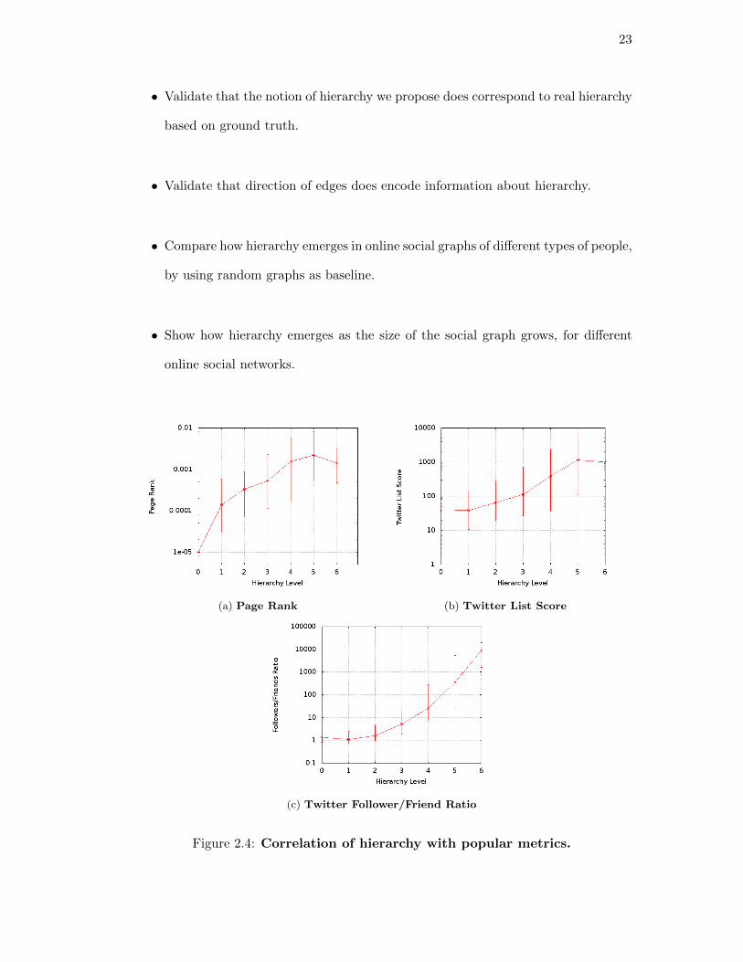
• Validate that the notion of hierarchy we propose does correspond to real hierarchy
based on ground truth.
• Validate that direction of edges does encode information about hierarchy.
• Compare how hierarchy emerges in online social graphs of different types of people,
by using random graphs as baseline.
• Show how hierarchy emerges as the size of the social graph grows, for different
online social networks.
(a) Page Rank (b) Twitter List Score
(c) Twitter Follower/Friend Ratio
Figure 2.4: Correlation of hierarchy with popular metrics.

24
2.5.1 Validation of the Hierarchy Measure
In this section, we want to validate that our measure of hierarchy corresponds with real
hierarchy observed by humans. Towards this aim, we designed the following experiment.
We collected a curated list of 961 journalists on Twitter and computed the hierarchy
on the graph generated by these journalists among themselves. We also looked at how
different measures of noteworthiness of node correlate with the level of that node in the
optimal hierarchy. We now present the results.
The computed hierarchy measure is 0.38. This indicates that there is a medium
hierarchy in this graph. There are seven levels (strata) that users are assigned to in the
optimal hierarchy. A higher level indicates people who enjoy higher social status.
Wikipedia notability: To confirm that our computed hierarchy corresponds to a real
hierarchy, we make use of Wikipedia to derive ground truth. Each node(journalist)
is assigned a Wikipedia notability score, which is either No Entry (the person does
not have an entry in Wikipedia), Small, Medium or Large (depending on the size of
the Wikipedia entry). Figure 2.5 shows how our hierarchy measure compares with
the ground truth obtained from Wikipedia. The figure shows that nodes with a low
hierarchy level do not have a Wikipedia entry, and nodes higher up in the computed
hierarchy are more likely to be noteworthy according to Wikipedia. This result lends
credence to our measure of hierarchy.
Correlation with well known measures: To get more insight into the factors that
contribute to a node’s hierarchy level, we measure the correlation of our computed
hierarchy level for the journalists graph with well known measures of social networks:
pagerank, friend-follower ratio, and Twitter list score.
Figure 2.4a plots the median page rank (along with the 10th and the 90th percentile
value) for each hierarchy level. The figure shows that people with a high page rank
tend to be higher up in the social hierarchy level computed by our measure.
Figure 2.4b plots the correlation of hierarchy level with the Twitter list score, which

25
Figure 2.5: Correlation with Wikipedia notability score.
corresponds to the number of user-generated Twitter lists for which that the node is a
member. Presence in a large number of user-generated Twitter lists indicates the user’s
popularity among Twitter users. The figure shows a high correlation of our computed
node hierarchy with this measure of Twitter user popularity.
Finally, we measure the correlation with a popular twitter measure, Follower/Friend
ratio, in Figure 2.4c. Popular users in Twitter tend to have an order of magnitude more
followers than friends. We once again see a strong correlation between this measure
and our computed hierarchy level.
2.5.2 Importance of Edge Direction
We now perform an experiment to validate that edge directions encode hierarchy infor-
mation. For this, we use the college football dataset.
College Football Dataset: This dataset is constructed by looking at all
(American) Football games played by College teams in Division 1 FBS (the highest
division, formerly called 1-A) during five year period 2005-2009. The number of teams

26
Figure 2.6: Hierarchy in the College Football network.
varies each year, but is between 150 and 200 for all five years. For each year, we consider
the win-loss record of these teams. In the graph, each team is a node, and we place an
edge from u → v if v played and defeated u during the season. We only consider the
win-loss records and do not consider the margin of victory.7 We also do not consider
other factors like home advantage, though these would lead to better predictions. We
end up with a directed unweighted graph representing win-loss record for a full season.
For each season, we find the optimal hierarchy. There is a lot of variation between
the quality of college football teams and we expect to see high hierarchy as observed in
Figure 2.6.
Random redirection: Since the complete schedule is fixed before any games are
played, we can compare the hierarchy we observe in the directed graph to the hierarchy
if all games were decided by a random coin toss. In terms of the graph, this amounts to
redirecting each edge in the network randomly. This technique allows us to observe the
7The margin of victory is not considered even in the official BCS computer rankings, since “runningup the scoreboard” is considered bad form and is discouraged.

27
effect of the directions on hierarchy once the undirected graph is fixed. This random
redirection would eliminate any quality difference between the nodes, and we now expect
to see a much smaller hierarchy in the redirected graph. To observe the variance of the
random redirection, we repeat this experiment five times. The hierarchy for these
randomly redirected graphs is also shown in Figure 2.6.
We see that the five randomly redirected graphs have very similar hierarchy, which
is significantly lower than the real graph, showing that directions encode important
information about hierarchy.
2.5.3 Hierarchy in Online Social Networks vs Random Graphs
To better understand how hierarchy emerges in a directed graph, we look at the behavior
of hierarchy in random graphs to establish a baseline. We generate a random directed
graph using the standard Erdos and Renyi [1960] random graph model as follows. We fix
a probability p that will decide the density of the graph. For each ordered pair of vertices
(u, v), we put an edges from u to v with probability p. The outdegree distribution of
nodes in this graph is a binomial distribution where each node has expected degree np.
(a) Effect of network size on hierarchy (b) Effect of network density on hierarchy
Figure 2.7: Hierarchy in random graphs.
Figure 2.7a shows that, for random graphs, the hierarchy starts out being large,
and monotonically decreases as the size of the graph increases. We can also see that

28
for small graph sizes, the variance is high, but as the graph size increases, the variance
become very small.
We also conduct this experiment for different values of density, p. Figure 2.7b shows
the outcome of the experiment with three different values of p. We see that for the same
graph size n, hierarchy decreases with density. Hence, for random graphs, sparse graphs
have higher hierarchy.
A plausible explanation for this phenomenon is that for sparse graphs, the random-
ness does not “cancel out” , but as the size of the graph and the density increases, the
randomness “cancels out” and we get a low measure of hierarchy. It is not clear, that
for a given the size of the graph n and the density p, what the hierarchy will be and
whether it will go to 0 as either n or p tends to infinity. We leave these questions as
open directions for future research.
Curated Lists on Twitter: We now measure hierarchy for different online
social networks. For this experiment, we collect curated lists on Twitter that correspond
to different types of users.
Famous people by field: Similar to the journalists dataset described earlier, we
collect curated lists of famous people in the fields of Technology, Journalism, Politics,
Anthropology, Finance and Sports. The smallest collection is Anthropology with fifty
nine people and the largest is Technology with almost three thousand people.
Organizations: We also look at lists of employees of different organizations that
have a team presence on Twitter. These include forrst, tweetdeck, ReadWriteWeb,
wikia, techcrunch, Mashable, nytimes and Twitter. The smallest graph, forrst, has just
seven employees. The largest is Twitter with two hundred and eighty two employees.
For each of these lists, we reconstruct the Twitter graph restricted to just these
nodes, i.e. the nodes in the restricted graph are all the people on a particular list and
there is an edge between two nodes if there is an edge between them on Twitter. For

29
all these graphs, we calculate the hierarchy. Figure 2.8 shows a plot of hierarchy with
respect to network size. We see that, among the fields, Sports has the highest hierarchy
while Finance has the lowest one, and among organizations, the TODAYshow has the
highest hierarchy while TweetDeck and ReadWriteWeb have the lowest one. Another
trend that is observed is that, as the network size becomes larger, the hierarchy also
increases. This is in contrast to random graphs, where the hierarchy decreases as the
network size increases.
Wikipedia administrator voting dataset: Leskovec, Huttenlocher, and Kleinberg
[2010b,a] collected and analyzed votes for electing administrators in Wikipedia. We
use the wiki-vote dataset they collected and observe a very strong hierarchy in this
dataset. This is consistent with the finding in [Leskovec, Huttenlocher, and Kleinberg,
2010a] that status governs these votes more than balance.
2.5.4 Effect of Scaling on Social Hierarchy
So far, we looked at small and medium sized graphs to get insight on how the measure of
hierarchy works. We noticed that the hierarchy increases as the network size increases.
Now, we shall consider large graphs to see the effect of scale on hierarchy in social
networks.
For this experiment, we sample four popular directed social networks: Delicious,
YouTube, LiveJournal and Flickr. The nodes are users and the edges indicate a follower
relationship. We start from a single node and crawl nodes in the graph in a breadth
first traversal. We plot hierarchy for different sizes of the graph. This is shown in
Figure 2.9a.
We observe that, as a online social network grows in size, the hierarchy either stays
the same or increases. This is in contrast with random graphs, where the hierarchy
decreases as the graph grows in size. This suggests that, within small groups, social
rank does not play an important role while forming connections but, as the group size

30
Figure 2.8: Hierarchy in social network among famous people.
increases, social rank becomes important to people while forming links.
This result corresponds with the intuition that, in social networks, people form
connections with others based on their perceived level in the social hierarchy.
Further, we see that different social networks have different amount of hierarchy:
YouTube has the lowest hierarchy, Flickr and LiveJournal have medium hierarchy, and
Delicious has the highest hierarchy.
Number of strata: Figure 2.9b plots the number of social strata in these four social
networks, as we increase the graph size. We see that the number of strata stabilizes
around seven for LiveJournal and around five for Flickr. YouTube has the lowest
number of levels, and it also has the lowest hierarchy, while Delicious has the largest
number of levels and also has the highest hierarchy. Compared to the number of nodes
(100,000), the number of strata (< 15) is very low.
Rank distribution: Figure 2.10a plots the frequency distribution of people belonging
to different social strata in a network, i.e., how many nodes belong to each stratum.
We see that, in all the networks, most nodes have a low rank in the hierarchy (between

31
one and three). A very small fraction of the nodes have ranks above four.
(a) Effect of network size on value and
variance of hierarchy
(b) Effect of network size on number of
strata in the hierarchy
Figure 2.9: Effect of network size on hierarchy.
The exception to this is Delicious, which has a wider distribution of ranks. We
show the exact probability distribution of the Delicious nodes in Figure 2.10b. The
plot shows that a lot of delicious nodes have medium ranks in the hierarchy. But, even
in Delicious, very few nodes belong to the highest stratum.
(a) Cumulative distribution of ranks (b) Probability distribution for the Deli-
cious graph
Figure 2.10: Distribution of ranks among nodes.
Agony distribution: Our measure of hierarchy is based on the intuition that people
prefer to connect to other people who are in the same stratum or higher up. People who
connect to others lower in the hierarchy incur agony. Figure 2.11a plots the distribution
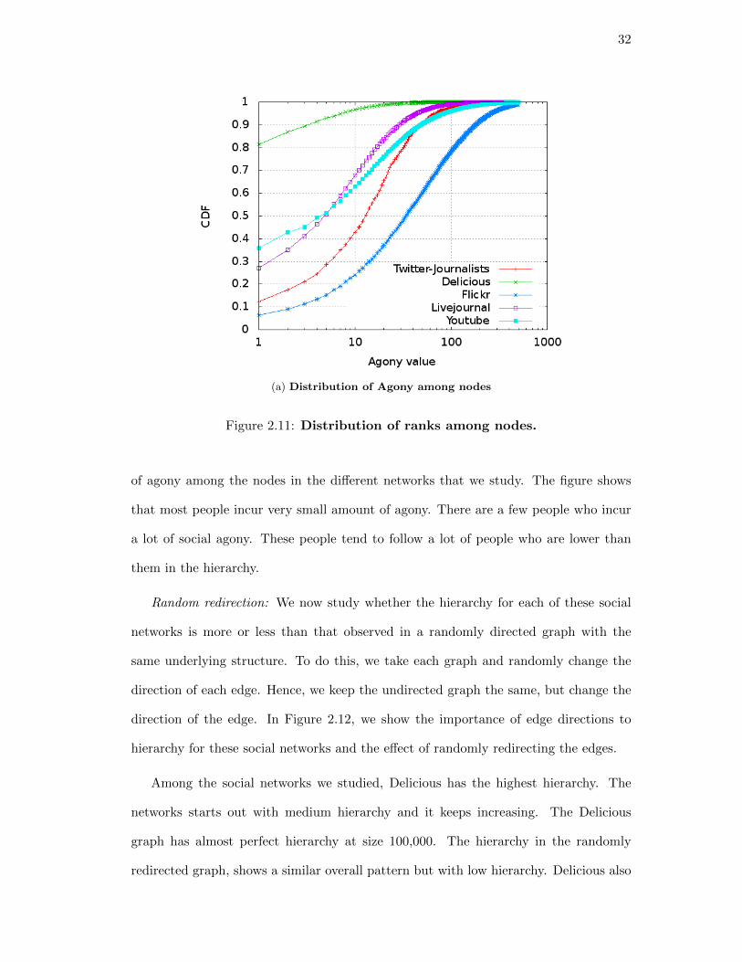
32
(a) Distribution of Agony among nodes
Figure 2.11: Distribution of ranks among nodes.
of agony among the nodes in the different networks that we study. The figure shows
that most people incur very small amount of agony. There are a few people who incur
a lot of social agony. These people tend to follow a lot of people who are lower than
them in the hierarchy.
Random redirection: We now study whether the hierarchy for each of these social
networks is more or less than that observed in a randomly directed graph with the
same underlying structure. To do this, we take each graph and randomly change the
direction of each edge. Hence, we keep the undirected graph the same, but change the
direction of the edge. In Figure 2.12, we show the importance of edge directions to
hierarchy for these social networks and the effect of randomly redirecting the edges.
Among the social networks we studied, Delicious has the highest hierarchy. The
networks starts out with medium hierarchy and it keeps increasing. The Delicious
graph has almost perfect hierarchy at size 100,000. The hierarchy in the randomly
redirected graph, shows a similar overall pattern but with low hierarchy. Delicious also

33
(a) Delicious (b) YouTube
(c) LiveJournal (d) Flickr
Figure 2.12: Effect of directed edges.
has the most number of levels in the hierarchy. YouTube, on the other hand, has the
lowest hierarchy, which is even lower than the hierarchy observed if the edges were
randomly oriented. The likely reason for this is that YouTube has a good search index
and the preferred way of getting to videos is through search. Hence, social connections
become less important and people do not connect to each other based on rank. In Flickr,
the hierarchy largely remains the same even as the graph becomes large. However, the
hierarchy in the redirected graph decreases sharply. In LiveJournal, the hierarchy starts
out being very low and increases slowly with graph size. The randomly redirected graph
on the other hand shows exactly the opposite behavior, consistent with the behavior of
random graphs that we saw earlier.

34
2.6 Related Work
Early efforts to find the hierarchy underlying social interactions followed from obser-
vations of dominance relationships among animals. Landau [1951] and Kendall [1962]
devised statistical tests of hierarchy for a society, but with the necessary assumption
that there exists a strict dominance relation between all pairs of individuals, and that
the relations are transitive (i.e. no cycles). Although de Vries [1995, 1998] expanded the
Landau and Kendall measures by allowing ties or missing relationships, his algorithms
are feasible only on small graphs.
The hierarchy underlying a social network can be used in recommending friends
(the link prediction problem [Liben-Nowell and Kleinberg, 2003]) and in providing bet-
ter query results [Kleinberg, 1999]. There exist link-based methods of ranking web
pages [Getoor and Diehl, 2005]. Maiya and Berger-Wolf [2009] begin from the assump-
tion that social interactions are guided by the underlying hierarchy, and they present
a maximum likelihood approach to find the best interaction model out of a range of
models defined by the authors. In the same vein, Clauset, Moore, and Newman [2006]
use Markov Chain Monte Carlo sampling to estimate the hierarchical structure in a
network. Rowe, Creamer, Hershkop, and Stolfo [2007] defined a weighted centrality
measure for email networks based on factors such as response time and total num-
ber of messages, and tested their algorithm on the Enron email corpus. Leskovec,
Huttenlocher, and Kleinberg [2010b,a] recently brought attention to signed network
relationships (e.g. friend or foe in the Epinions online social network) and presented a
way to predict whether a link in a signed social network is positive or negative.
The closest to our problem in the computer science literature is the minimum feed-
back arc set problem. In the minimum feedback arc set problem, we are given a directed
graph G and we want to find the smallest set of edges whose removal make the remain-
ing graph acyclic. This is a well known NP-hard problem and is in fact NP-hard to

35
approximate beyond 1.36 [Kann, 1992]. Poly-logarithmic approximation algorithms are
known for this problem [Even, Naor, Schieber, and Sudan, 1995].
2.7 Conclusions and Future Directions
In this chapter, we introduced a measure of hierarchy in directed social networks. We
gave an efficient algorithm to find the optimal hierarchy given just the network. We
also showed the emergence of hierarchy in multiple online social networks: in contrast
to random networks, social networks have low hierarchy when they are small and the
hierarchy increases as the network grows. We showed that there are a small number of
strata, and this number does not grow significantly as the network grows.
We now give directions for future research. Our experiments in section 2.5.3 indicate
that the measure of hierarchy is well behaved for random graphs. We leave open the
question of finding closed form expression for hierarchy in random graphs. Another
question we leave open is to find an algorithm that minimizes agony for sub-linear
functions like f(u, v) = log(r(u) − r(v) + 1). A different direction that we did not
touch upon in this chapter is to study the emergence of hierarchy over time in a given
social network. Finally, we could use this as a new signal and improve existing ranking
algorithms.
This chapter dealt with the structure of social networks, and in particular exploiting
the structure to obtain a measure of hierarchy. In the next chapter, we turn our
attention to the dynamics of information flow over an underlying social network.

36
Chapter 3
News Propagation in Social Networks
3.1 Introduction
Online social networks have become an increasingly popular medium for sharing infor-
mation such as links, news and multimedia among users. The average Facebook user
has 120 friends, and more than 30 million users update their status at least once each
day. 1 More than 5 billion minutes are spent on Facebook each day (worldwide). As a
direct consequence of these trends, social networks are fast overtaking traditional web
as the preferred source of information. 2
In the early days of social networks, users tended to post predominantly personal
information. Such information typically did not spread more than one hop, since only
immediate friends were interested in it. Over time, online social networks have meta-
morphosed into a forum where people post information such as news that they deem to
be of common interest. For example, during the recent Iran elections, traditional news
media acknowledged the power and influence of social networks such as Twitter.3 4
Prior work has studied various aspects of information sharing on social networks.
Domingos and Richardson [2002, 2001] study the question of determining the set of
1http://www.facebook.com/press/info.php?statistics
2http://siteanalytics.compete.com/facebook.com+google.com/?metric=uv
3The New York Times, Journalism Rules Are Bent in News Coverage From Iran,http://www.nytimes.com/2009/06/29/business/media/29coverage.html
4CNN, Twitter Revolution in Iran , http://money.cnn.com/video/news/2009/06/22/n twitter revo-lution Iran pentagon.cnnmoney/

37
nodes in a network that will most efficiently spread a piece of information for market-
ing purposes. Kempe, Kleinberg, and Tardos [2003] proposed a discrete optimization
formulation for this. Several recent studies focused on gathering intuition about in-
fluence spread from real-world data. Leskovec, Singh, and Kleinberg [2006] study the
patterns of cascading recommendations in social networks by looking at how individ-
uals recommend the products they buy in an online-retailer recommendation system.
Leskovec, Backstrom, and Kleinberg [2009] develop a framework for the dynamics of
news propagation across the web. Morris [2000] studied games where each player in-
teracts with a small set of neighbors. He proved conditions under which the behavior
adopted by a small set of users will spread to a large fraction of the network.
An aspect that has been overlooked so far is the question as to why users post
information such as news or links on social networks. Unlike personal information,
news typically propagates more than one hop, being received either from friends or from
external sources, and reposted when found interesting. We argue that on receiving a
news item, users behave strategically when weighting in various factors (such as how
interested their friends will be in this news) to decide whether to further propagate that
item by (re)posting it.
In this chapter, we posit that users in a social network have transitioned from being
passive entities to strategic users. This trend leads to several interesting questions, such
as: What factors do users consider when deciding whether to post an item? How does
information diffuse over the social network based on different strategies used by the
users? Furthermore, we envisage an advertising system where strategic users propagate
ads to their friends on social networks. This is in contrast to the current model of ad
dissemination on social networks where marketeers are given access to the social graph.
We believe that a better understanding of user strategies in a social network is a key
step towards such a system.
We use random graphs to formally model social networks. The formal definitions

38
of random graphs and the conditions under which they are connected are discussed
in section 3.3. In section 3.5 we show that if we restrict attention to people who are
interested in some particular news, then the induced subgraph retains the connectedness
properties of the original graph. We prove our main result in proposition 3.10 which
states that assuming strategic users, the spread of news over an online social network
exhibits a threshold behavior. The news spreads to a significant fraction of the network
if its quality is higher than a certain threshold that depends on how aggressive users
are about posting news. If the quality is smaller than this threshold, only a sub-linear
number of nodes in the network see the news.
The key contributions made in this chapter are:
1. We initiate the study of information propagation in social networks assuming
strategic users.
2. We propose two models for strategic user behavior, greedy and courteous.
3. Assuming social networks can be modeled as certain random graphs, we prove that
there is a threshold behavior when greedy users fully disseminate information.
4. We present a simulation study based on a real graph crawled from the Twitter
social network, and show the threshold phenomenon holds in both strategic models
of user behavior.
In what follows, we provide a detailed description of our results. We start by defining
the user model.
3.2 Strategic User Model
We propose a simple game to model the behavior of users posting news on online social
networks like Twitter and Facebook. For a particular user u in the network, whenever
u first sees a previously unseen news item, she has the option of either posting it or not

39
posting it. Her utility is 0 if she does not post it. If she does, then her utility depends
on (i) The set Iu = Neighbors who are interested in the news and (ii) The set Su =
Neighbors who, u knows, have already seen the news before. 5 Let Nu denote the set
of all u’s neighbors. We propose two particular forms for her utility:
1. Greedy Strategy: The utility is additive and for every neighbor who likes the
news (irrespective of whether the neighbor has seen it before or not), she gets
utility +a and for every neighbor who does not, she gets utility −b. In this case,
her decision to post only depends on a,b and fu =|Iu||Nu|
. User u posts only if
her utility is positive, that is, the fraction fu of users who like the news satisfies
afua+ b
− b(1− fu)
a+ b> 0 ⇐⇒ fu >
b
a+ b. Let us define t =
b
a+ b. In Section 3.4,
we analyze this behavior and show that it depends critically on t.
2. Courteous Strategy: If a user does not post an item, then her utility is 0. The
main difference from the greedy strategy is that the user does not want to spam
her friends. We model this by saying that if more than a c fraction of her friends
have already seen the news before, she gets a large negative utility, when she posts
the item. In case the fraction|Su||Nu|
≤ c, then her utility is the same as in the
greedy case. In particular, she gets utility +a for every neighbor who likes the
news and has not seen it before (the set Iu \Su), and she gets utility −b for every
neighbor who does not like it (the set Icu \ Su). Hence, her strategy in this case
is to post if the fraction of neighbors who have seen the newsSuNu≤ c and if the
fraction fu of neighbors in Scu who are interested in the news is ≥ t. Note that,
in this utility function, if a larger number of the user’s neighbors have posted the
news, she is less likely to post it. In section 3.5, we show simulation results for
this behavior on a small sample of the Twitter Graph.
5u might not know the true set of neighbors who have seen the news. She knows that a friend hasseen the news only if a mutual friend posted it. This also means that we assume that every user knowswhich of her friends are themselves friends.

40
3.3 Random Graph Models of Social Networks
Erdos and Renyi [1960] started the study of random graphs. They consider a single
parameter family of random graphs. The parameter p corresponds to the density of the
edges in the graph.
Definition 3.1 (Erdos Renyi random graph model). Given n the number of vertices
and a parameter 0 ≤ p ≤ 1, a graph in this model is generated by adding an edge (u, v)
between vertices u and v, independently at random with probability p. This process
generates a probability distribution over all graphs which we denote by G(n, p).
Initially, Erdos and Renyi random graphs were used as a model of real-world net-
works. With the advent of computational tools it became feasible to experimentally
study large graphs and various properties about real-world networks were discovered.
Travers and Milgram [1969] and Watts and Strogatz [1998] show the small-world effect
in real-world networks which states that the diameter of the graphs is small. Barabasi
[2005] shows that the degree distribution of real-world networks follows a power law and
hence has a heavy tail unlike for Erdos and Renyi random graphs. These properties
made it clear that the Erdos and Renyi random graph model was not suitable as a
model of real-world social networks.
Various models like small-world networks [Watts and Strogatz, 1998] and preferential
attachment [Barabasi and Albert, 1999] were proposed as models of social networks to
overcoming the shortcomings of the Erdos and Renyi model. We focus on the stochastic
Kronecker graph model proposed by Leskovec and Faloutsos. Leskovec and Faloutsos
[2007] model social networks using stochastic Kronecker graphs and show that these
graphs have various properties like a power law degree distribution, small diameter,
densification power law (E α Nk) [Leskovec, Kleinberg, and Faloutsos, 2005] and
shrinking diameter over time. We shall see the details of this model in 3.3.1.
G(n, P ) is a generalization of the well-studied model G(n, p) [Erdos and Renyi, 1960]

41
as well as of stochastic Kronecker graphs [Leskovec and Faloutsos, 2007, Mahdian and
Xu, 2007]. We can recover the G(n, p) model as well as the Kronecker graph model by
putting conditions on the matrix P . We shall prove our main results in section 3.4 in
the general model G(n, P ) of random graphs. We start with the formal definition of
G(n, P ).
Definition 3.2 (Random Graph G(n, P )). Given a real symmetric matrix P with
0 ≤ pi,j ≤ 1, denote by G(n, P ) a random graph where edge (i, j) exists with probability
pi,j .
Definition 3.3 (Weighted Projection of a Random Graph). Given a real symmetric
matrix P with 0 ≤ pi,j ≤ 1, we shall denote by W (P ) = (V,E(P )) the weighted graph
with P as its adjacency matrix. Note that pi,j gives the weight of edge (i, j) in W (P ).
Lemma 3.4 gives conditions on the matrix P that ensure that the graph G sampled
from the distribution G(n, P ) is connected.
Lemma 3.4 ( [Mahdian and Xu, 2007]). For a large enough constant c, if the weight of
the min-cut in W (P ) is at least c log n, then, with high probability6, the sampled graph
G ∼ G(n, P ) is connected.
Definition 3.5 (Induced Subgraph). Given a graph G = (V,E) and U ⊆ V, we shall
denote the subgraph of G induced by U as G[U ] and the subgraph of W (P ) induced
by U as W (P )[U ].
Before we begin, let us review the statement of the popular Chernoff Bounds. We
use this a lot in the next sections. Proof of the bounds can be found in [Chung and Lu,
2006, Theorem 3.2].
Theorem 3.6 (Chernoff Bounds). Let X1, X2, . . . , Xn be independent random variables
with
Pr [Xi = 1] = pi, P r [Xi = 0] = 1− pi
6Throughout this chapter, with high probability means with probability 1 − o(1).

42
Consider the random variable X that is defined as the sum of these random variables.
X =n∑i=1
Xi. The expectation of X is given by E[X] =∑i
pi. Then,
Pr [X ≤ E[X]− λ] ≤ e−λ2
2E[X]
Pr [X ≥ E[X] + λ] ≤ e−λ2
2(E[X]+λ/3)
3.3.1 Connectivity of stochastic Kronecker graphs
We shall prove our main results in section 3.4 in the general model G(n, P ) of ran-
dom graphs. Stochastic Kronecker graphs are a good model of social networks. Since
stochastic Kronecker graphs are a subset of the G(n, P ) model of random graphs, the
results that we prove in section 3.4 apply directly stochastic Kronecker graphs as well.
While the parameters that we obtain in the general case are not tight, we shall show
that when we apply them to the stochastic Kronecker graphs, they become tight. In
this section, we prove results that allow us to transfer results from the general model
to stochastic Kronecker graphs. We begin with a definition of Kronecker multiplication
of two matrices.
Definition 3.7 (Kronecker product). Given two matrices A,B, the Kronecker product
or tensor product of A and B is defined as
An×m ⊗Bk×l = Cnk×ml =
a1,1B a1,2B . . . a1,mB
a2,1B a2,2B . . . a2,mB
......
. . ....
an,1B an,2B . . . an,mB
Definition 3.8 (stochastic Kronecker graphs). Given an initiator matrix A, where
each element of ai,j ∈ [0, 1]. Consider the matrix P = A⊗k = A⊗A · · · ⊗ A︸ ︷︷ ︸k times
. Then the
random graph G(n, P ) is called a stochastic Kronecker graph. We shall denote such a
graph by K(A, k).

43
[Leskovec and Faloutsos, 2007] model social networks using Kronecker graphs. They
show that the graphs exhibit various real-world properties like a heavy-tail degree dis-
tribution, small diameter, densification power law (E α Nk) [Leskovec, Kleinberg, and
Faloutsos, 2005] as well as shrinking diameter over time. They show that Autonomous
Systems on the Internet, the citation graph for high energy physics from arXiv and
the U.S. Patent citation database can be modeled well using G(n, P ) where P = A⊗k
for particular 2× 2 initiator matrices A of the form[ γ ββ α
]and α ≥ β ≥ γ and a given
integer k.7 [Mahdian and Xu, 2007] give tight conditions on the connectivity of K(A, k)
in terms of properties of the initiator matrix A. Lemma 3.9 states these conditions.
Lemma 3.9. For fixed constants α ≥ β ≥ γ, the necessary and sufficient conditions
for the Kronecker graph K(A, k) to be connected with high probability is β + γ > 1 or
α = β = 1, γ = 0.
In fact, given a constant c, as n becomes large enough, if β + γ > 1, the size of the
min-cut is > ck(= c log n).
In the next section, we shall prove results on the spread of news when the underlying
random graph G is sampled from G(n, P ) and P satisfies some special characteristics.
Lemma 3.9 allows us to transfer results that we prove for graphs G(n, P ) where min-cut
of W (P ) > c log n to connected Kronecker graphs.
3.4 Analysis of a Model of Strategic User Behavior
In this section we analyze the spread of news in a social network. We start with a
high level description of the proof that news propagation in social networks follows
a threshold behavior. We prove our results in the G(n, P ) model of social networks
defined in section 3.3. Lemma 3.4 gives a condition on the matrix P , in terms of the
min-cut of W (P ), under which a random graph G, sampled from G(n, P ), is connected.
7In this chapter, A will always be a 2× 2 matrix of the form[γ ββ α
]where α, β, γ are fixed constants
and α ≥ β ≥ γ.

44
We assume that users follow the greedy strategy defined in section 3.2. A user
playing the greedy strategy posts only if the fraction of interested neighbors is larger
than the threshold t. The greedy strategy is monotone in the set of neighbors who
are interested and have posted the news. This means that the probability of posting
increases with the set of friends who have posted the news. Hence, to analyze the set
of users who post the news under the greedy strategy we do not need to analyze the
dynamic sequence of users that post the news but we only need to analyze the static
subgraph of users interested in the news and who initially receive the news.
We assume that for a given news, each user in the network likes it with probability
q, which is independent of everything else.8 The probability q is just a number ∈ [0, 1]
that could model the quality of the news item or the inherent interest the subject
generates. If we restrict attention to the subgraph of users that are interested in the
news, then the induced subgraph is a random sample of the vertices of the graph G.
Lemma 3.12 shows that the min-cut condition is preserved for a subgraph induced by a
random sample of the vertices. Hence, the same connectedness properties hold for the
induced subgraph. Finally, in proposition 3.10 we show that if the quality q of the news
is larger than the threshold t, then all users interested in the news also post it, if the
news reaches them. Hence, the induced subgraph is connected with high probability
and the news spreads across the network.
We start with some definitions. Color nodes in G not interested in the news blue
and the ones interested in the news yellow. Call the set of blue vertices B and yellow
vertices Y . A yellow node is responsive if more than a t fraction of its neighbors are
interested in the news. Responsive nodes are precisely the ones in the graph that will
repost the news if they receive it. Color responsive nodes red and call this set of nodes
R. Hence, we have the following set of nodes:
8It is an interesting question to relax this assumption, since in a typical social network we mightexpect nodes with similar interests to be clustered together.

45
B : The subset of nodes of G that are not interested in the news.
Y : The subset of nodes of G that are interested in the news.
R : The subset of nodes of G that are interested in the news and will post is if they
receive the news. Note that R ⊆ Y .
Recall that for a subset S ⊆ V , G[S] denotes the subgraph of G induced by the
vertex set S. We are interested in the structure of the graph G[R]. Throughout, we
assume that q and t are constants that do not depend on the number of nodes n. We
prove the following results in the next two sub-sections:
Proposition 3.10. Suppose P is a matrix such that the min-cut of the weighted graph
W (P ) had weight ≥ c log n, for a large enough constant c. Suppose G is a random graph
sampled from the distribution G(n, P ) and that log n random nodes in the G initially
see the news.
If q > t, then, with high probability, almost all nodes interested in the news will see
it. On the other hand, if q < t then only a sub-linear number of the vertices will post
the news.
3.4.1 The Connectedness of G[R]
We prove Proposition 3.10 in this subsection. We first show that G[R] is connected
and that its size is a constant fraction of the size of G. Then, we show that, if the
news is randomly received by a non-negligible number (log n) of users in G, someone in
G[R] will get it and hence it will spread to all nodes in G[R]. Let ρ be a large enough
constant that satisfies the condition of lemma 3.4.
Throughout this section, we shall assume that P is such that the min-cut of W (P )
has weight ≥ c log n, where c = max
16ρ
q2,
8q
(t− q)2
.
We have two sources of randomness here: For every edge (i, j) in G we have a coin
which decides whether edge (i, j) ∈ G. We call this set of coins CE . Also, for every

46
vertex v ∈ V , we have a coin toss that decides if v ∈ Y . We call this set of coins CV .
The probability space we have is over the union of the coins CE ∪ CV .
The next two lemmas show that the min-cut in the sampled graph G[Y ] remains
high.
Lemma 3.11. All nodes in the graph G have degree at leastc
2log n, with high probability
over coin tosses CE.
Lemma 3.11. Define the random variable Xuv to take value 1 with probability puv and
0 with probability 1 − puv. For a given vertex v, the degree of v in G is given by
Xv =∑u
Xuv. Using Chernoff Bounds, we can see that, for every constant δ,
Pr [Xv ≤ (1− δ)E[Xv]] ≤ 2 exp(−E[Xv] δ2/2)
≤ 2 exp(−c log n · δ2/2)
= n−cδ2/2
The above result is true for all δ. We choose δ =1
2.
Pr
[Xv ≤
1
2E[Xv]
]≤ n−c/8
≤ n−2 (Since c ≥ 16)
Apply union bound to get that for all vertices in G, with probability > 1 − 1/n, the
degree of each vertex is > (1− δ)c log n =c
2log n
The next lemma shows that if we sample nodes independently from the weighted
graph W (P ), then the weight of the min-cut in the induced subgraph W (P )[Y ] is large.
Lemma 3.12. The weight of the min-cut in W (P )[Y ] is at least ρ log n, with high
probability over the coin tosses CV .
Lemma 3.12. To prove this lemma, we use Chernoff bounds to upper bound the proba-
bility that the cut (S, V \S) in the induced subgraph is small. Then we use union bound

47
over all cuts. However, we cannot apply the union bound directly. We partition all cuts
depending on the weight of the cut. The Chernoff bound in weaker for cuts of small
weight, but the number of cuts of small weight is also small. Hence, we partition all
cuts depending on their weight, and then apply Chernoff bound to limit the probability
that there is a small min-cut in W (P )[Y ] due a cut of a particular weight in W (P ).
Call a cut α-minimal if the size of that cut is within an α factor of the size of the
min-cut. We use the theorem [Karger and Stein, 1996, Theorem 8.4] that bounds the
number of weighted α-minimal cuts: In any weighted graph, the number of α-minimal
cuts is O((2n)2α
). Let the weight of the min-cut in W (P ) be m. We partition all cuts
depending on their size. For a integer k, all cuts with weight in [mk,m(k + 1)] belong
to the same partition. All these cuts are (k + 1)-minimal, hence, there are at most
O(
(2n)2(k+1))
of them.
Consider any cut (S, V \S) having weight t ∈ [mk,m(k+ 1)]. Let X be the random
variable which gives the weight of the cut in W (P )[Y ]. Each edge of W (P ) is also
an edge of W (P )[Y ] with probability at least q2, hence E[X] ≥ tq2. By Chernoff
Bounds, for all δ ≥ 0, Pr[X ≤ (1− δ)tq2
]≤ exp (−δ2tq2/2) ≤ exp (−δ2q2km/2) ≤
exp (−δ2q2kc log n/2) = n−δ2q2kc/2.
Now, applying the union bound over all cuts, we get that with probability p =
1 −∑k
n(−δ2q2c/2)k(2nq2)2k+2 all cuts in the subgraph W (P )[Y ] have min-cut of size
≥ (1− δ)q2Size of min-cut in W (P ) = (1− δ)q2c log n with high probability.
Choose δ =1
2. By assumption, c ≥ 16ρ
q2=
4ρ
δ2q2.
Substituting these values, we get that the size of the min-cut in W (P )[U ] is > ρ log n
with high probability.
Suppose we toss all coins in CV ∪CE , but do not reveal them all. First we reveal only
the coins in CV . Lemma 3.12 shows that W (P )[Y ] has a min-cut of size ρ log n with high
probability. Now, we reveal coins in CE . Lemma 3.4 shows that, conditioned on CE and

48
that W (P )[Y ] has a min-cut of size ρ log n the graph GY sampled from G(|Y |,W (P )[Y ])
is connected. Now, applying union bound, we get that G[Y ] is connected, with high
probability over CE ∪ CV .
We shall now prove the main theorem of this section. We prove that G[R] is con-
nected by using the fact that the min-cut of G is large.
Theorem 3.13. If q > t then, with high probability, every vertex in Y also belongs to
R and so G[R] is connected. On the other hand, if q < t, then G[R] only contains o(n)
vertices, with high probability.
Proof. To prove this, we first reveal the coin tosses CE . That gives us a graph G
sampled from the distribution G(n, P ). Lemma 3.11 shows all nodes in G have degree
≥ c
2log n with high probability over CE . We assume for the rest of the proof that G is
a fixed graph with these properties.
Now, we reveal the coins CY . This corresponds to a random process of coloring
nodes of G yellow with probability q. Let Yq be a random variable that takes value 1
with probability q and 0 with probability 1− q. For a node v, let d(v) denote its degree
in G. We analyze two cases.
q > t :
Pr [v /∈ R] = Pr
d(v)∑i=1
Yq < t · d(v)
= Pr
d(v)∑i=1
Yq < qd(v)− (q − t)d(v)
≤ exp−((q − t)d(v))2
2qd(v)
≤ n−(t−q)2
4qc
The third inequality follows from Chernoff Bounds, since Yq are independent and
E[Yq] = q. The last is true since d(v) ≥ c
2log n. We apply the union bound to get

49
that with probability ≥ 1 − n · n−(t−q)2
4qc ≥ 1 − 1
n(since c >
8q
(t− q)2), all nodes
in Y also belong to R.
Now, we apply union bound to get that Y = R, with high probability over the
event CE ∪ CV .
Since, we proved that G[Y ] is connected with high probability over CE ∪ CV , we
get that G[R] is connected with high probability over the event CE ∪ CV .
q < t :
Pr [v ∈ R] = Pr
d(v)∑i=1
Yq ≥ t · d(v)
= Pr
d(v)∑i=1
Yq ≥ qd(v) + (t− q)d(v)
≤ exp− ((q − t)d(v))2
2(qd(v) + (q − t)d(v)/3)
≤ n−(t−q)24q−t
32c
Hence, E[|R|] ≤ |Y |n−(t−q)24q−t
32c ∈ o(n). So, R only contains a sub-linear number of
nodes of G.
Proposition 3.14. Suppose P is a matrix such that the min-cut of the weighted graph
W (P ) had weight ≥ c log n, for a large enough constant c. Suppose G is a random graph
sampled from the distribution G(n, P ) and that log n random nodes in the G initially
see the news.
If q > t, then, with high probability, almost all nodes interested in the news will see
it. On the other hand, if q < t then only a sub-linear number of the vertices will post
the news.
Proof. If q < t then the proposition follows directly from theorem 3.13. When q > t,
theorem 3.13 tells us that G[R] is connected. If any node in R receives the news it will

50
be propagated to all the nodes. But, the probability that none of the nodes in R get
the news is ≤ (1− q)logn = O(n−q) = o(1). Hence, with high probability, almost all the
nodes interested in the news actually receive it.
In the next section, we shall look at a real-world graph and simulate the greedy and
courteous behavior on this graph.
3.5 Simulation Results
In this section, we present results from the simulation of our two strategic user models
over a partial crawl of the Twitter social network.9
Dataset :
The dataset is obtained by means of a partial crawl of the Twitter social network.
Since we are interested in link postings by typical users, we remove hubs (users with
more than 500 friends) from our graph. The resulting graph we use in our experiments
consists of 5978 users with 110152 directed friendship edges. Each simulation starts
with a set of seed nodes (of size log n), and in each round, nodes decide whether to post
the link using one of the two models described earlier in the chapter.
Results:
We define coverage as the fraction of interested users who get to see the news item.
Figure 3.1 plots how the coverage varies for the greedy and courteous strategies. For
the courteous strategy we fixed q = 0.5. Each simulation was repeated 10 times, and
the standard deviations are indicated in the form of error bars.
9All the data was obtained in accordance with Twitter’s terms of use.
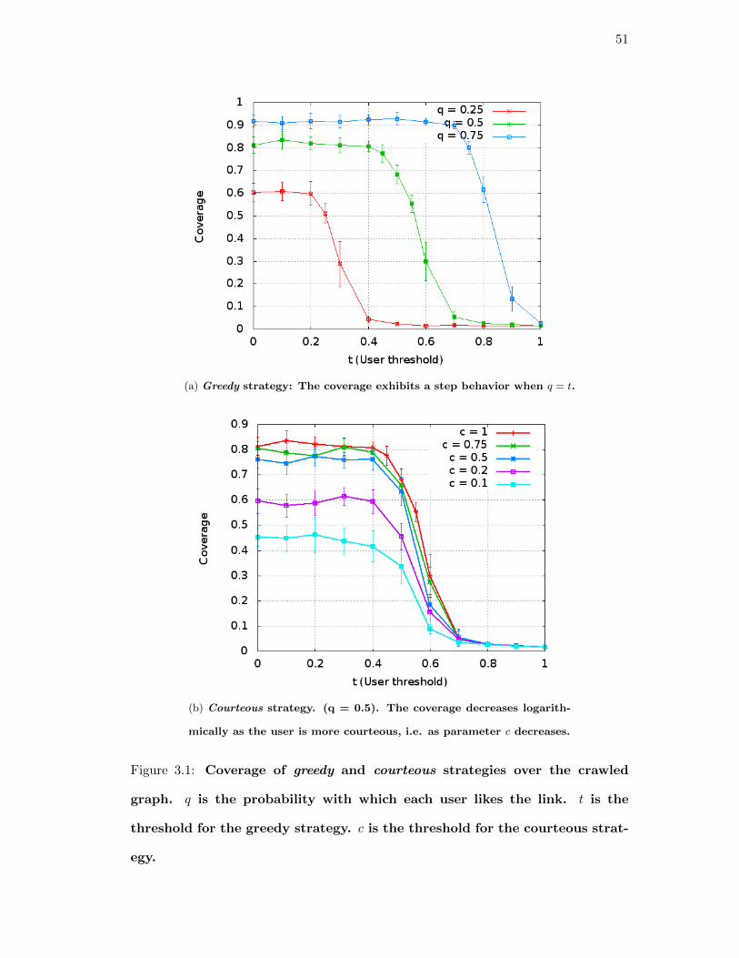
51
(a) Greedy strategy: The coverage exhibits a step behavior when q = t.
(b) Courteous strategy. (q = 0.5). The coverage decreases logarith-
mically as the user is more courteous, i.e. as parameter c decreases.
Figure 3.1: Coverage of greedy and courteous strategies over the crawled
graph. q is the probability with which each user likes the link. t is the
threshold for the greedy strategy. c is the threshold for the courteous strat-
egy.

52
Greedy Strategy: Figure 3.1a shows that, for all values of q, the coverage exhibits
a step behavior and the step happens around q = t. For different values of q, the per-
centage of coverage decreases with q. This is true even when t = 0, which means that
the size of the connected components drops when we sample the graph. The densifi-
cation power law (E α Nk) [Leskovec, Kleinberg, and Faloutsos, 2005] that has been
observed in other social networks would predict this behavior.
Courteous Strategy: Figure 3.1b shows the effect of the courteous strategy on the
coverage. The parameter c indicates the threshold of neighbors that have already seen
the link. A courteous user posts the link only if less than c fraction of neighbors have
already seen the link. The figure shows that the coverage decreases logarithmically as
the user is more courteous. This result shows that even when the users are courteous
if q > t then, news can still reach a reasonable fraction of the graph.
3.6 Conclusion and Future Work
We proposed the model of strategic user behavior in online social networks for news
posting, defined two user models (greedy and courteous), presented formal analysis of
the greedy model and simulated both models on the data set we collected from Twitter.
We propose the following directions:
Mine the Twitter data set: Search for patterns in the way users post news links
in order to validate the model and provide further insights about user strategies over
social networks.
Analyze the Courteous Strategy and Multiple Strategies: We leave open a formal
proof that the courteous strategy also exhibits threshold behavior. Further, we want
to test whether similar results hold in a social network in the presence of multiple user
strategies.

53
Design a framework for advertisement on online social networks of strategic users:
We believe that the strategic user model has applications in advertising and marketing.
We plan to investigate incentive schemes for marketeers to encourage strategic users to
advertise products over social networks.


Secretary Problems


57
Chapter 4
Secretary Problems on Independence Set Systems
4.1 Introduction
Consider the following problem: We want to hire one secretary for a job. Secretaries
come in one by one and we can interview them. Assume that there is a strict linear
ordering among all secretaries that is they are all comparable to each other and there
are no ties. We want to select the best secretary. This is trivial in the offline setting.
However, in the online setting where we are restricted to either make a job offer or
reject the secretary when a secretary comes in, the problem become challenging. If we
reject the secretary, the person never comes back.
It is clear that we cannot always select the best secretary in the online setting. In
fact, if we adopt the worst case adversarial analysis typically used for online algorithms,
we can always make up the input such that the any algorithm will always select the
worst secretary! Surprisingly, Dynkin [1963] showed that, if we assume that the order
in which the secretaries come is random, we can actually select the best secretary with
constant probability =1
e.
Online Algorithms
Online algorithms are defined as algorithms where the entire input is not available to
the algorithm at the start. In this chapter, we look at the problem where we are given
a set of elements, and we need to select a subset that maximizes an objective function.
In this setting, elements appears one after the other and the algorithm needs to make

58
irrevocable decisions about whether to accept the element or not.
Not knowing future input is a handicap, and so, in general online algorithms can-
not choose a solution which is as good as that found by an offline algorithm. The
performance of online algorithms is commonly measured in terms of the competitive
ratio which measures how the performance of the online algorithm compares with the
solution of the optimal offline algorithm. The competitive ratio of an algorithm A is
defined as the worst case ratio of the performance of the algorithm relative to the opti-
mal offline algorithm OPT . If v(A, i) is a value function which measures how good an
input i is for algorithm A, then the competitive ratio is given by:
maxi∈inputs
v(OPT, i)
v(A, i)
Note that according to this definition, the best competitive ratio an algorithm can
achieve is 1, which occurs when the online algorithm always selects the best possible
result. Typically, the competitive ratio is strictly greater than one. We say that an algo-
rithm A is constant competitive if there exists a constant c such that A has competitive
ratio less than or equal to c.
4.1.1 The Random Permutation Model
There are different models of how input is presented to an online algorithm. The
strictest one is adversarial, where the input is chosen adaptively by the adversary based
on the choices made by the algorithm so far. Assuming a powerful adversary often leads
to unreasonably pessimistic conclusions about online algorithms. Another shortcoming
of looking only at the worst case behavior is that, even if two algorithms have the same
worst case behavior, one might have much better performance for most inputs, which
the other might exhibit the same behavior on all inputs and the analysis wont be able
to distinguish between the two.

59
A much more benign assumption is that the input comes is sampled from a distribu-
tion. Distributional assumptions lead to better algorithms, however, these are generally
too strong for most practical scenarios as most real world data does not satisfy these
assumptions.
The random permutation model walks a fine line between these two. In this model,
the input is still assumed to be the worst case input. However, the order in which it
is presented to the algorithm is random. Hence, the worst case input is adversarially
decided, then a random permutation on this is generated and the input is presented
to the algorithm in the resulting order. We shall use this random permutation model
in this chapter. This setting has come to be known as the secretary setting due to
the problem discussed in a nice survey by Ferguson [1989] that we saw earlier. In this
chapter, we generalize the secretary problem to Independence Set Systems. We start
by looking at the definition of Independence Set Systems.
4.1.2 Independence Set Systems
An independence set system H = (V, I) is an ordered pair where V is the set of vertices
and I is a set of subsets of V such that
1. φ ∈ I
2. ∀S′, S where S′ ⊆ S : S ∈ I =⇒ S′ ∈ I
Members of I are called independent subsets of H. Property 2 is called the hereditary
property or down-monotonicity and so, these systems are also called hereditary set
systems or down monotone set systems.
Independence Set Systems are a generalization of various structures like graphs,
matroids, knapsacks, etc. Figure 4.1 shows an example of encoding the knapsack con-
straints as an independence set system.

60
Capacity = 8
1
2
7
4
e1
e2
e3
e4
I1
I2 I3 I4
I5 I6 I7
e1e4
e2
e3
Figure 4.1: Modeling knapsack constraints as an independence set system
4.1.3 The Secretary Problem on Independence Set Systems
We consider the problem of selecting a maximum independent set of vertices from
an independence set system. In this section, we consider the setting where elements
of V do not have any weight. We shall extend it to the setting of elements with
weight in Section 4.4. Formally, the problem is described as follows. We are given an
independence set system H = (V, I). A random permutation σ : [n] → V is generated
and elements of V are presented one by one in the order σ(1), σ(2), . . . , σ(n). At time
step i, we are presented with a vertex v = σ(i) and we need to make a decision whether
to select v or reject v. Once a vertex is selected, it cannot later be dropped. Conversely,
if v is rejected, then we cannot come back and select it. Hence, the decision to select or
reject is irrevocable. The task is to select the maximum number of elements such that
they are all independent in H.
Let n be the number of elements |V |. Babaioff, Immorlica, and Kleinberg [2007b]
gave an example of an independence set system showing that it is not possible to get

61
a o
(log n
log log n
)approximation algorithm to solve this problem even ignoring compu-
tational considerations. The set system is constructed by randomly throwing n balls
into n bins. The independence set system is obtained by treating the bins as maximal
independent sets.
Theorem 4.1. [Babaioff, Immorlica, and Kleinberg, 2007b] The expected size of the
maximum set in I is Ω
(log n
log logn
). Suppose the elements of V are presented in random
order. For any online randomized algorithm A, the expected number of elements selected
by A is at most two.
Given the lower bound we explore the question of obtaining an approximation al-
gorithm which matches this.
4.1.4 Related Work
The secretary problem was introduced into the computer science community though
its applications to auctions [Kleinberg, 2005, Hajiaghayi, Kleinberg, and Parkes, 2004,
Babaioff, Immorlica, Kempe, and Kleinberg, 2008].
Babaioff, Immorlica, and Kleinberg [2007b] introduce the Matroid Secretary Prob-
lem. In this setting, we are given a set of elements that form a matroid. Elements
have weights, and we want to select an independent set of elements that has the maxi-
mum weight. This encompasses problems like finding the maximum weight forest in a
q weighted undirected graph. They give a O (log n) approximation to the general prob-
lem. They also give constant factor approximation algorithms for various special cases
including graphical matroids (maximum weight forest). Dimitrov and Plaxton [2008]
give a constant factor approximation for transversal matroids. Later, Korula and Pal
[2009] gave a simpler algorithm and also improved the approximation ratio. Sato [2011],
Gharan and Vondrak [2011] gave a constant-factor competitive algorithms for general
matroids in the random assignment model where the weights are assigned randomly to

62
the elements of a matroid, and then the elements arrive on-line in an adversarial order.
Babaioff, Dinitz, Gupta, Immorlica, and Talwar [2009] consider the secretary prob-
lem with time discounting. Babaioff, Immorlica, Kempe, and Kleinberg [2007a] give a
constant factor approximation for the case when elements have a weight and a value,
and they must satisfy knapsack constraints. Kumar, Lattanzi, Vassilvitskii, and Vat-
tani [2011] consider the problem of selecting a maximal element when there is only a
partial order among the elements.
Variants where we want to maximize not just the number of sum of weights of the
set of selected secretaries, but some general submodular function of the set of selected
secretaries have also been studied [Feldman, Naor, and Schwartz, 2011, Bateni, Ha-
jiaghayi, and Zadimoghaddam, 2010, Gupta, Roth, Schoenebeck, and Talwar, 2010].
Feldman, Naor, and Schwartz [2011] give constant factor approximation for maximiz-
ing general submodular functions for the case of uniform and partition matroids and
under knapsack constraints. Bateni, Hajiaghayi, and Zadimoghaddam [2010] give a
constant competitive algorithm for uniform matroids where the submodular function
can be non-monotone. They also give a O(l log2 r
)-competitive algorithm for select-
ing under l matroid constrains where r is the maximum rank of the matroids. They
also give an O (l)-approximation algorithm when the feasible sets must satisfy l knap-
sack constraints. Gupta, Roth, Schoenebeck, and Talwar [2010] give a polynomial time
algorithm for the offline problem of maximizing non-monotone submodular functions
on p-independence set systems. They specialize their algorithms for maximizing non-
monotone submodular functions on matroids to obtain a constant factor approximation
algorithm for uniform and partition matroids and a O (log k) algorithm for general ma-
troids of rank k.
Since, Independence Set Systems are generalizations of structures like graphs, knap-
sack constraints, matroids, the secretary problem on these structures can be treated as
special cases of the problem we solve. The approximation ratio of most of the special

63
cases is in general better. In this chapter, we only consider maximizing the number of
elements and the weighted sum of selected elements. We do not consider more general
functions, on the selected set of elements.
4.1.5 Bipartite Graph representation of Independence Set Systems
1
2
3
4
5
a
b
c
a
b
c
L R
1 2
3
4
5
Figure 4.2: Independence set systems as a bipartite graph
One way to represent an independence set system is as a bipartite graph G =
(L ∪ R,E). The elements in the left set L are called points and represent the vertices
V from the set system and the right elements from the right set R are called blocks
and these represent subsets of the vertices V that are elements of I. We want to select
a large subset of points in L such that they share a common neighbor in R i.e. we
want to select a large independent set in V . Figure 4.2 shows a simple independence
set system and its representation as a bipartite graph.
4.2 Oracles and Problem Variants
Our algorithm takes an independence set system as input. However, the number of
independent sets in general set systems can be exponential in the number of vertices.
Just specifying the set system can take exponential time. Hence, we assume oracle
access to the set system. When a new vertex is presented the set system induced by all
vertices seen so far is revealed, through some kind of an oracle. Starting from a very

64
simple oracle we now describe successively stronger oracles that we will use to solve the
problem. The oracles can only process subsets of vertices that have arrived. (Also see
Section 4.5).
O0: This is the simplest oracle. Given a set of vertices O0 tells if they are inde-
pendent or not. In terms of the bipartite graph, given a set of left points, O0 returns
a right block that all the left points have in common if one exists otherwise return
that no such block exists. With this oracle even the offline case of selecting a largest
independent set is NP-hard. Moreover, it is even hard to approximate as seen by the
special case of selecting an independent set of vertices from a graph.
O1: To get over this and not restrict ourselves to a particular problem, we need
access to an oracle which will give us the optimal solution to the offline problem. The
simplest oracle is the one that solves the offline problem. It takes as input a set of
elements S, and returns a maximum independent subset T of S. If there are multiple
maximum independent subsets, it arbitrarily chooses one. In terms of the bipartite
graph, given a set S of points in L, O1 returns a block r ∈ R with the maximum
number of neighbors in S. If there are multiple elements in R it arbitrarily chooses
one. Note that access to O1 only allows us to solve the offline problem. Using this to
solve the online problem is not obvious. In fact, this oracle is still too weak to solve the
problem. We propose a slightly stronger version of this next.
O2: It takes as input two sets of elements S, T such that S ⊂ T and S ∈ I. The
oracle O2 returns a maximum independent subset W such that S ⊂ W ⊂ T . O2
ensures that we select all the elements of S and among all independent subsets of
T which also include S, we choose the largest one. If there are multiple maximum
independent subsets, it arbitrarily chooses one. In terms of the bipartite graph, given
a set of points S, T such that there is a block r ∈ R adjacent to all points in S, O2
returns a block p ∈ R with the maximum number of neighbors in T among all blocks
such that all elements in S are adjacent to p. If there are multiple such blocks, O2

65
arbitrarily chooses one.
O3: We need an even stronger oracle which we state now. We state this only in
terms of the bipartite graph representation of an independence set system. Given this
bipartite graph the oracle O3 takes as input a subset T of L and a threshold t and
returns a right block r ∈ R uniformly at random from all right blocks in R that connect
to all points in T and have degree ≥ t.
It is easy to show that for i ∈ 0, 1, 2, oracle Oi can be simulated by at most
O (log n), calls to oracle Oi+1. Hence, we assume that if we are given O1, then we are
also given O0. If we are given O2, then we are also given both O1 and O0. If we are
given O3, then we are also given O2, O1 and O0. We solve the secretary problem on
independence set systems using the oracle O3. We give an algorithm which outputs
a set of size Ω
(s
log n log log n
), where s is the size of the largest independent set
(largest right degree in R). This gives a O (log n log logn) approximation algorithm,
which matches the lower bound within O((log log n)2
)factors. We leave the problem
of finding a large independent set using the simpler oracle O2 open. A few directions
exploring this oracle further are presented in Section 4.5.
4.3 Algorithm
In this section we shall describe the actual algorithm for the unweighted case. The
algorithm starts by selecting a random sample of the points( elements of L) of size half
the total number of points. Its possible to do this since the input comes in a random
order. This happens in step 2 of the algorithm. The random sample of points is used to
select a threshold size such that we reject all sets smaller than that size. This is done
is step 3. Finally, O3 is used to select an independent set from the sample (a block
from R). This is selected such that the number of neighbors of the block in the sample
is large enough, but also that it has enough “space” left for new points. For each new
point, it is selected if and only if it belongs to the selected block. This is done in step 4.

66
We now formally describe the algorithm.
Input : A graph G = (L ∪ R,E) where access to E is given by the edge oracle E
which takes as input a subset T of L and returns true if all vertices in T share a com-
mon neighbor. We also assume we have access to the oracle O3(along with O2, O1 and
O0) mentioned before. Points in L are seen one by one in random order.
Output : A set S ⊂ L of selected points that all have a common right block as a com-
mon neighbor.
Algorithm :
1. Set S ← φ.
2. Sample an integer from the binomial distribution. k ∼ Binom(n, 1/2). Look at
the first k points and don’t select any. Call this set of points F (first half). This
is the random sample.
3. Among the points seen so far (F ), use the oracle O, to find the largest degree
of a right block using O2. Call this number s. Choose i ∈ [0, 8 log log n] and
α ∈
5
2,5
2
(5
7
),5
2
(5
7
)2
,5
2
(5
7
)3
uniformly at random. Set threshold t =
αs
2i
(= α
s
s
s
2i
).
4. Use the oracle O3 to get a right block r = O3(F, t). For every new point v, if v
is connected to r, S ← S ∪ v
We begin with a lemma that explains the choice of the set that α belongs to in
step 3.
Lemma 4.2. Let two intervals [a, b] and [c, d] such that a < b and c < d. Then the set
S = ca
( cd
)i0≤i≤m is such that for any k ∈ [a, b], there exists an element s ∈ S such
that k · s ∈ [c, d]. The size of S is at most
⌈log b
a
log dc
⌉.

67
Proof. Consider the partition of [a, b] into sub-intervals [a,ad
c]∪ [
ad
c,ad2
c2]∪ [
ad2
c2,ad3
c3]∪
[ad3
c3,ad4
c4] ∪ [
ad4
c4,ad5
c5] ∪ . . . ∪ [
adm−1
cm−1,adm
cm]. For a given i, the ith sub-interval given
by [adi
ci,adi+1
ci+1] maps into the interval [c, d] for s = si (where si =
c
a
( cd
)i).
Hence, we have shown that each element of [a, b] belongs to some interval I in C.
Also, for every interval I in C, there exists an element s ∈ S that maps I to [c, d].
The size m of S is such that b ≤ a
(d
c
)m. Hence, for m ≥
log ba
log dc
, the lemma holds
true.
We apply the lemma for parameters a =2
8, b =
8
8, c =
5
8and d =
7
8. This shows
that for every element e ∈ [a, b] the set
5
2,5
2
(5
7
),5
2
(5
7
)2
,5
2
(5
7
)3
contains an
element α such that αe ∈ [c, d]. We shall use this lemma in the proof of the next
theorem. The next theorem proves the correctness of the algorithm and also bounds
the approximation ratio obtained.
Theorem 4.3. The set of selected points S ∈ I. Also, |S| ∈ Ω
(s
log n
), with probability
≥ 1
8 log log n, where s is the size of the maximum independent set in I.
Proof. S ∈ I follows directly from the fact that we only add an point v to S if v is
connected to a specific right block r (obtained in step 4). Hence all elements in S share
r as a neighbor and are independent.
We now prove the bound on the size of S. Let r be a block in R. Denote the
neighbors of r by N(r). For a given first half F generated by a permutation σ, we say
that a right block r is badly sampled if |N(r)∩F | ≥ 3
4|N(r)| or |N(r)∩F | ≤ 1
4|N(r)|.
If r is not badly sampled we call it well-sampled. If the algorithm selects a well-sampled
block r (in step 4), then |S| ≥ N(r)
4.
We shall now prove that the algorithm picks a block of degree at leasts
256 log n
with probability at least1
8 log log n. Lemma 4.4 proves that any particular right block
is well-sampled with high probability.

68
Lemma 4.4. For a block r ∈ R the probability that it is badly sampled is ≤ 2−|N(r)|
16 .
Proof. Let N(r) = v1, . . . , vk ∈ L. Since elements of L are seen in random order, the
probability that a particular block vi ∈ F =1
2.
Define a random variable Xr = |N(r)∩F | which depends on the random sample F .
E[Xr] =1
2|N(r)|. Using Chernoff Bounds (for example Chung and Lu [2006]), we see
that Pr [|Xr − E[Xr] | ≥ λ] ≤ 2e− λ2
2(E[X]+λ/3) ≤ 2e− λ2
N(r)+ 23λ .
Choose λ =1
4|N(r)|.
Pr
[|Xr − E[Xr] | ≥
1
4|N(r)|
]≤ 2
− |N(r)|2/16|N(r)|+2/3|N(r)| < 2−
|N(r)|16 .
s s/2 s/4 s/8
B_1 B_2 B_3
Figure 4.3: Bucketing the independent sets
The algorithm needs to make sure that it selects a high degree block. This is
achieved by selecting a large threshold in step 3. Applying Lemma 4.4 to the high-
est degree block gives that it is well-sampled with high probability. Since s is the
highest degree, the block will have at leasts
4points in F with high probability.
Hence, the highest degree block in F has degree s ∈ [s, s/4] with high probability.
Lemma 4.2 shows that there exists an α ∈
5
2,5
2
(5
7
),5
2
(5
7
)2
,5
2
(5
7
)3
such that
t = αs/2i ∈[(
3
4− 1
8
)s
2i,
(3
4+
1
8
)s
2i
]. This happens with probability
1
4since α is
chosen uniformly at random . We classify right blocks into bins B1, . . . , B256 logn ac-
cording to their degree in the original hypergraph. Bi contains all blocks r ∈ R which
have degree d ∈[ s
2i−1,s
2i
).
We shall now prove that the oracle actually picks a well-sampled block. While any

69
particular block is well-sampled with high probability (Lemma 4.4), the number of
blocks is large. Hence, we cannot directly apply the union bound. We divide the proof
into two cases:
Case 1: |B1|+ |B2| < 2s
128
The algorithm chooses j = 1 with probability1
8 log log n. Hence with probability
1
32 log log n, t ∈
[5
8
s
2,7
8
s
2
]. None of the blocks in bins B>2 will be selected since they
cannot pass this threshold. Let q be a block in B1 ∪B2. By lemma 4.4, the probability
that q is badly sampled ≤ 2−|N(q)|/16 ≤ 2−s/64. Using the union bound, the probability
that there is a block in B1 ∪B2 that is badly sampled ≤ 2s/128 · 2−s/64 = 2−s/128.
This means the algorithm selects a well-sampled block r of degree at leasts
4and will
select at leasts
16elements with probability
1
32 log log n. This gives us a O (log log n)
approximation.
Case 2: |B1|+ |B2| ≥ 2s/128
This is the harder case. We start with a lemma that states the existence of consecutive
bins, such that the bins with the larger sets contain more blocks than the bins with the
smaller sets.
Lemma 4.5. There exists and index l ∈ [0, 8 dlog log ne] such that |Bl| + |Bl+1| ≥
|Bl+2|+ |Bl+3|.
Proof. Recall
(n
k
)≤ nk. For k =
s
256 log n, the equation becomes :
(ns
256 logn
)≤ n
s256 logn =
(n
1logn
) s256
= 2s
256
|B8dlog logne|+ |B8dlog logne+1| ≤ 2
(ns
256 logn
)≤ 2 ·2
s256 ≤ |B1|+ |B2|. Hence, there exists
an index l ∈ [0, 8 dlog logne] such that |Bl|+ |Bl+1| ≥ |Bl+2|+ |Bl+3|.
Consider the event t ∈[
5
8
s
2l+3,7
8
s
2l+3
]. It occurs if the algorithm chooses i = l+ 3

70
(in step 3) and α such that αs
s∈[
5
8,7
8
]. Lemma 4.2 shows that there always exists
such an α. The correct α is chosen with probability at least1
4. This happens with
probability at least1
8 log log n× 1
4=
1
32 log log n.
Let Yl be the random variable that denotes the number of badly sampled blocks in
bucket Bl. Lemma 4.4 says that any given block in B≤i is well-sampled with probability
at least 1 − 2−s
2i i.e. E[Yl] ≤ |Bl|2−s
2i . By Markov’s Inequality, Pr
[Yl ≥
|Bl|4
]≤
4 · 2−s
2i .
We show that the ratio of well-sampled blocks to badly sampled blocks is large.
None of the blocks in bins B>(i+3) can pass the threshold. Even if all the blocks in
bins Bi+2 and Bi+3 are badly sampled, with probability at least 1− 4 · 2−s
2i , the total
number of badly sampled blocks ≤∑m≤i
|Bm|4
+Bi+2+Bi+3 ≤∑
m≤i+1
|Bm|4
+Bi+Bi+1 ≤
5
4
∑m≤i+1
|Bm| =5
3
∑m≤i+1
3
4|Bm| ≤
5
3E[ # of well-sampled vertices] . Hence, the oracle
chooses a well-sampled block with probability at least3
8.
Also, i < 8 dlog log ne implies the size of any block in bin Bi is at leasts
256 log n.
Hence |S| ∈ Ω
(s
log n log logn
)and we get a O (log n log logn) approximation.
This completes the proof of the theorem.
4.4 Weighted Elements
Until now, we assumed that the elements did not have weights. Now we shall see an
algorithm when each element can have an unknown weight, that we get to know when
we actually see the element.
Let W be the largest weight among all elements in V . We split elements into
log n partition depending on their weight. Elements of weight w ∈[W
2j,W
2j+1
]fall in
partition j. We ignore all elements of weight <W
n, since they collectively have weight
smaller than W . Hence, we have log n partitions. Consider the partition which has the

71
largest weight independent set.
We add a preprocessing step to the algorithm presented in the previous section. The
preprocessing algorithm selects a partition uniformly at random from all partitions and
selects elements only from this partition. The probability that we select the heaviest
partition is1
log n.
Note that if we have an α approximation algorithm for selecting the largest indepen-
dent set for elements in the partition with the largest size, then the algorithm with the
preprocessing step gives a α log n approximation algorithm for the original independent
set. But all elements in a partition have weight within a factor 2 of each other. Hence,
if we ignore all the weights of elements in a partition, then we lose at most a factor 2
in the approximation guarantee. Coupled with the algorithm in the previous section,
this gives a O(log2 n log logn
)approximation algorithm for the general problem where
elements have weights.
4.5 Future direction using the Oracle O2
We shall now discuss the problem of selecting a maximum independent set of unweighted
vertices, given only the weaker oracle O2. Recall that given two sets of elements S, T
such that S ⊆ T and S ∈ I, the oracle O2 returns a maximum independent subset W
such that S ⊆ W ⊆ T . O2 ensures that we select all the elements of S and among
all independent subsets of T which also include S, we choose the largest one. If there
are multiple maximum independent subsets, it arbitrarily chooses one. We do not have
concrete results in this case and so we sketch two directions for further research that
seem fruitful in sections 4.5.1 and 4.5.2.
4.5.1 Approximating the offline oracle
Let H = (V, I) be a hypergraph. Consider the counting version of the offline ora-
cle function O2, given by Ooffline : 2V × 2V → N. Given two sets, green and red,

72
Ooffline(G,R) returns the maximum number of elements of V \ R that can be added
to G such that the resulting set is independent.
Hypothetically, suppose that the online algorithm has access to the offline ora-
cle Ooffline. We could use this to select a large independent set: Set G = R = φ.
Ooffline(φ, φ) tells us the size of the maximum independent set s. Look at elements
one by one. If the element x is such that Ooffline(G ∪ x,R) = s, add x to G else add
it to R. Clearly, this chooses a maximum independent set. Of course, since we want to
construct an online algorithm, the oracle O does not have access to elements that have
not arrived yet. The approach we take is to approximate the behavior of the offline
oracle Ooffline. We now give a candidate oracle that does not have access to future
elements, but that approximates the offline version of the oracle Ooffline.
The Mean Oracle
Let V be all the elements in the hypergraph. Consider a function fS of the following
type: Given sets green and red, (G,R) and a fixed subset S ⊆ V −(G∪R), the function
fS outputs the size of the largest set I ⊆ S such that I∪G is independent and I∩R = φ.
We define the mean oracle as the weighted average over all sets S, of the size output
by the above function fS . We define the mean oracle as follows
fmean(G,R) =∑
S⊆V−(G∪R)
2−|S|fS(G,R)
We call this the mean oracle since it gives, for any two sets G of selected elements
and R of rejected elements, the mean number of remaining elements that can be added
to G, such that the resulting set is independent. We shall now define a smoothness
property that we want the mean oracle to follow.
1) fmean(G ∪ x,R) ≥ fmean(G,R)− log n
2) fmean(G,R ∪ x) ≥ fmean(G,R)− 1
n

73
The initial value of the mean oracle is at least s, the size of the largest independent
set.
Suppose we can show that ∀x ∈ V −(G∪R), either 1 or 2 holds. (Its OK if both hold
too). For each new element, the smoothness properties ensure that either we increase
the size of the selected independent set (if option (1) holds), or if we reject the element,
then there are still enough elements left that we can use to extend the current set of
selected elements. That would give us a way to construct an online algorithm which
uses this mean oracle and gives a log n competitive ratio.
4.5.2 A labeling game
In this section, we consider a general strategy to solve the secretary problem. Given a
set R and an independent set S, let N(R,S) = Number of independent sets in R that
contain S. Consider the following strategy:
1. Look at half the elements in random order. Don’t select any element. Call
these elements red. The remaining are blue. Calculate N(R,φ) = Number of
independent sets in R.
2. Set S ← φ
3. For each element e, calculate pe =N(R,S ∪ e)N(R,S)
. Accept e with probability pe and
set S ← S ∪ e.
We want to show that this strategy does actually give us a log n approximation
algorithm. We start by stating some lemmas.
Lemma 4.6. If we randomly color each element R or B with probability1
2, then
N(R) ≥ 2s
100 with probability ≥ 1
2.
Lemma 4.7. We do not accept any element e for which pe <1
n2, with probability
≥(
1− 1
n
).

74
Proof. Since there are n elements, using union bound, we get that the probability that
we do select some element for which pe ≤1
n2is ≤
∑e:pe< 1
n2
pe <1
n.
Hence, if S is the set we have accepted so far, then ∀i :N(R,Si)
N(R,Si−1)≥ 1
n2.
Lemma 4.8. The number of accepting steps before N(R,S) becomes smaller than 2s
200
is at leasts
400 log n
Proof. At each step,
N(R,Sk) = N(R,φ) · N(R,S1)
N(R,φ)· · · N(R,Sk)
N(R,Sk−1)
≥ 2s/1001
n2k
= 2s/100−2k logn
For k ≤ s
400 log n, N(R,Sk) ≥ 2s/100−s/200 ≥ 2s/200
To show that the algorithm actually works as intended, we need another lemma
which proves that we can continue accepting elements with high probability. The proof
of this rests on the following equation
∑e∈B
N(R,Si ∪ e) ≥s
4 log nN(R,Si) (4.1)
Conjecture 4.9. We accept an element at each step i with high probability
Sketch. At step i, we know that N(R,Si) ≥ 2s/100−i logn. Suppose we can show that
the remaining elements also satisfy the property that N(B,Si) ≥ 2s/100−i logn. Then,
let pe =N(B,Si ∪ e)N(B,Si)
. The probability that we accept no element is equal to p =∏e∈B
(1− pe) ≤ exp
(−∑e∈B
pe
)= exp
(−∑
e∈B N(R,Si ∪ e)N(R,Si)
)≤ exp
(− s
4 log n
)The last deduction hinges on the assumption that we can prove 4.1
To prove equation 4.1, we construct the following game.

75
The Game
Consider the following single player game:
1. Start with n elements. Each element has weight 1. Color all the elements blue.
2. Repeat the next two stepsn
2times.
3. An element e is chosen, uniformly at random, from the set of blue elements. Color
it red. Fix its label to its current weight w(e).
4. The player can now select any set of blue elements B and increase their weight.
We imagine an adversary playing this game, and use it to model the moves made by
the adversary. At the end of the game, each element has a label, giving its weight. We
want to show that the adversary cannot make the weight of red elements much larger
than those of the blue elements. In particular we want to prove that, not matter what
strategy the adversary uses,
S =∑e∈B
w(e) ≥ 3
4
∑e∈R
w(e) with probability ≥ (1− 2−s/10) (4.2)
The correspondence of the game to the algorithm given in the previous section is
as follow: The weight of an element corresponds to the number of sets it belongs to.
The random move corresponds to a new element arriving. And selecting an element
corresponds to adding the element to the set of selected elements. The player in the
game corresponds to the structure of the hypergraph. This also now gives us ways to
constrain the move the player can make.
Equation 4.2 is not true unless we impose some constraints on the adversary. What
are the minimal conditions that we need to impose such that the above assertion be-
comes true? Here are two natural conditions that we can impose on the adversary. We
get these from the motivation that this game reflects selecting elements in an indepen-
dence set system.

76
1. The weight of elements in B cannot be more than doubled.
2. If the element e′ is selected in Step 3, then the weight of each e ∈ B can go up
by at most w(e′).
If we use the game to prove that the fraction of blue elements that can be added to
the selected elements is at least1
log ni.e.
∑e∈B
N(R, e)
N(R,φ)≥ s
2 log n, then this will give us
the online approximation algorithm.
Below we discuss some example strategies that the adversary can use :
1. Serial Increase : Keep one element in mind and keep increasing its weight by 1,
till it is selected. Once it is selected, choose another element and keep doing this.
This does not seem too good, but it leads to the next strategy.
2. Parallel Increase : Keep a set T in mind. Whenever any element is selected by
the algorithm, increase the weight of all elements in T by the maximum that is
allowed by the constraints. Note that the adversary wins with probability 2−T .
Is this the best the adversary can do, or is there a better strategy ?
4.6 Conclusion
In this chapter, we looked at the secretary problem for general independence set systems.
We saw that there was a lower bound of Ω
(log n
log log n
)on the competitive ratio of any
online algorithm. In Section 4.3, using a strong random sampling oracle, we gave a
O (log n log logn) approximation algorithm for unweighted elements. We also saw a
O(log2 n log log n
)approximation for weighted elements in Section 4.4. While we leave
the problem of solving the problem using the weaker oracle open, we looked some
directions for further research in Section 4.5.

Differential Privacy

79
Chapter 5
Differential Privacy
5.1 Introduction
Privacy Mechanisms: Agencies such as medical establishments, survey agencies, gov-
ernments use and publish aggregate statistics about individuals; this can have privacy
implications. Consider the query: Q: How many adults from San Diego contracted the
flu this October? The government can use the query result to track the spread of flu,
and drug companies can use it to plan production of vaccines. However, knowledge that
a specific person contracted the flu could be used to deny her health insurance based
on the rationale that she is susceptible to disease. As discussed by Sweeney [2002], and
as is exemplified by the AOL search data scandal1 and the breach of the Netflix chal-
lenge dataset [Narayanan and Shmatikov, 2008], seemingly benign data publications
can have privacy implications. Thus, it is important to think rigorously about privacy.
The framework of differential privacy [Dwork, 2006] does this, and is applicable widely
(see Section 5.2.8).
Mechanisms guarantee differential privacy by perturbing results – they add random
noise to the query result, and guarantee protection against all attackers, whatever their
side-information or intent (see Section 5.2.1 for a formal definition).
Our Utility Model: The addition of noise increases privacy but intuitively reduces
utility of the query result. To understand this privacy-utility trade-off, we propose a
formal decision-theoretic model of utility. Decision-theory is a widely applied field that
1http://en.wikipedia.org/wiki/AOL search data scandal
80
provides mathematical foundations for dealing with preferences under uncertainty. The
use of decision theory in this context is appropriate because, as we discussed above,
mechanisms guarantee differential privacy by introducing uncertainty.
In our model of utility (see Section 5.2.3 for details), the user of information, i.e. the
information consumer has side-information – for instance, knowledge of the population
of San Diego is an upper bound on the result of the query Q. It has a loss-function
that expresses it’s tolerance to inaccuracy. It is rational in the sense that it combines
information from the mechanism with its side-information optimally with respect to
its personal loss-function. It is risk-averse in the sense that it would like to minimize
worst-case loss over all scenarios.2
Given the privacy parameter, the loss-function and the side-information of an infor-
mation consumer it is possible to identify an optimal mechanism – a mechanism that is
differentially private and that maximizes its utility. See Section 5.2.4 for an algorithm
to find such a mechanism.
Non-Interactive Settings: Very often aggregate statistics, like answers to Q,
are published in mass media as opposed to following a query-response form( e.g.the
California Department of Public Health, H1N1 Flu–Data Tables 3). In such cases
neither the information consumer nor it’s loss-function and side-information are known
in advance. Thus it seems hard to identify the optimal mechanism for a information
consumer.
Nevertheless, we show that it is possible to deploy an optimal mechanism with-
out knowledge of the information consumer’s parameters. Furthermore, this mecha-
nism is universally optimal for all information consumers, no matter what their side-
information or loss-function.
2Ghosh, Roughgarden, and Sundararajan [2009] propose a model with most of these features, butassumes that information consumers are Bayesian and have a prior over the query-result.
3http://www.cdph.ca.gov/HealthInfo/discond/Documents/H1N1-Data-Table-CA-Cases-by-County-102409.pdf

81
How can we identify the optimal mechanism without knowledge of the information
consumer’s parameters? The apparent paradox is resolved by relying on the infor-
mation consumers’ rationality, i.e., each information consumer uses its personal loss-
function and side-information to actively transform the output of the deployed mecha-
nism. For a certain class of queries called count queries, when the deployed mechanism
is a certain geometric mechanism, this transformation is effective enough to result in
the optimal mechanism for the information consumer—a fact that we will establish via
linear-algebraic proof techniques.
Multiple Levels of Privacy: We also show how to simultaneously release the
query result at different levels of privacy to different information consumers. This
is useful, for instance, when we want to construct two versions of the report on flu
statistics, one which prioritizes utility for the eyes of government executives, and a
publicly available Internet version that prioritizes privacy.
A naive solution is to perturb the query results differently, independently adding
differing amounts of noise each time. The drawback is that consumers at different levels
of privacy can collude and combine their results to cancel the noise (as in Chernoff
bounds). An alternate way is to correlate the noise added to different outputs. We give
an algorithm to achieve this that makes the data release collusion-resistant.
In this chapter we focus on a single query; the complexity comes from a rich model
of consumer preferences, where we consider different utility functions for each consumer
and optimize for each of them. Blum, Ligett, and Roth [2008], Hay, Rastogi, Miklau,
and Suciu [2010], Hardt and Talwar [2010] exploit similarities between the queries to
obtain extension to multiple queries with good utility guarantees. However, they do
not consider a rich consumer preference model. Our results could be used as a building
block while answering multiple queries.

82
5.2 Model and Results
We gave a informal description of our model and results in the Introduction. In this
section, we formally define our model and discuss the main results. The proofs of the
results are presented in Sections 5.3, 5.4.
5.2.1 Privacy Mechanisms and Differential Privacy
A database is a collection of rows, one per individual. Each row is drawn from an
arbitrary domain D; for instance, in our running example, a row of the database has
the name, age, address and medical records of a single individual. A database with n
rows is thus drawn from the domain Dn.
We will focus on a class of queries, called count queries, that frequently occur in
surveys: Given a predicate p : D → True, False, the result of a count query is the
number of rows that satisfy this predicate, a number between 0 and the database size,
n. Q is an example of a count query with the predicate: individual is an adult residing
in in San Diego, who contracted flu this October. Though simple in form, count queries
are expressive because varying the predicate naturally yields a rich space of queries.
We guarantee differential privacy to protect information of individual database par-
ticipants. Differential privacy is a standard, well-accepted definition of privacy [Dwork,
2006] that has been applied to query privacy [Dwork and Nissim, 2004, Dwork, Mc-
Sherry, Nissim, and Smith, 2006, Nissim, Raskhodnikova, and Smith, 2007], privacy
preserving machine learning [Blum, Ligett, and Roth, 2008, Kasiviswanathan, Lee,
Nissim, Raskhodnikova, and Smith, 2008] and economic mechanism design [McSherry
and Talwar, 2007]. A fixed count query maps the database d to a number which belongs
to the set N . A privacy mechanism M for a fixed count query is a probabilistic function
that maps a database d ∈ Dn to the elements of the set N = 0 . . . n. These can be
represented, for each d ∈ Dn, by md,rr∈N , which gives for each database d ∈ Dn the

83
probability that M outputs r. For the database d, the mechanism releases a perturbed
result by sampling from the distribution md,rr∈N .
The Geometric Mechanism [Ghosh, Roughgarden, and Sundararajan, 2009] is a sim-
ple example of a privacy mechanism. It is a discrete version of the Laplace Mechanism
from [Dwork, McSherry, Nissim, and Smith, 2006].
Definition 5.1 (α-Geometric Mechanism). When the true query result is f(d), the
mechanism outputs f(d) + Z. Z is a random variable distributed as a two-sided geo-
metric distribution: Pr[Z = z] =1− α1 + α
α|z| for every integer z.
0
0.2
0.4
0.6
0.8
1
-20 -15 -10 -5 0 5 10 15 20
Figure 5.1: The probability distribution on outputs given by the Geometric
Mechanism for α = 0.2 and query result 5.
Informally, a mechanism satisfies differential privacy if it induces similar output
distributions for every two databases that differ only in a single individual’s data,
thereby ensuring that the output is not sensitive to any one individual’s data4. Formally,
differential privacy is defined as follows [Dwork, McSherry, Nissim, and Smith, 2006]:
4Thus any attack on an individual’s privacy that can be constructed using the perturbed queryresult with this individual present in the database can also be constructed, with a similar success rate,without this individual present in the database. See See [Dwork, McSherry, Nissim, and Smith, 2006,Kasiviswanathan and Smith, 2008] for details of such semantics of differential privacy.

84
Given a privacy parameter α ∈ [0, 1] and two database d1, d2 ∈ Dn that differ in at
most one individual’s data, a mechanism M is α-differentially private, if for all elements
r in the range of the mechanism :1
α· xd1,r ≥ xd2,r ≥ α · xd1,r.
The parameter α can be varied in the interval [0, 1] to vary the strength of the
privacy guarantee—when α = 0, the above definition is vacuous and there is no privacy,
whereas when α = 1, we effectively insist on absolute privacy– the query result cannot
depend on the database because we require distributions over perturbed results to be
identical for neighboring databases.
5.2.2 Oblivious Mechanisms
We will focus in this chapter on a class of privacy mechanisms that are oblivious. A
mechanism is oblivious if it sets up an identical distribution over outputs for every two
databases that have the same unperturbed query result. Naturally, an implementation
of an oblivious mechanism need only have access to the true query result—the input—
and can be oblivious to the database itself. An oblivious mechanism for count queries
can be expressed by the set of probability masses for every i ∈ N : xi,rr∈N , where xi,r
is the probability that the mechanism outputs r when the true result is i. Appendix 5.5
shows that this restriction to oblivious mechanisms is without loss of generality. The
geometric mechanism (Definition 5.1) only depends on the query result f(d) and not
on the database d itself; so it is a oblivious mechanism.
The query result for a count query can change by at most one when we change
any one row of the database, so we can rewrite the definition of differential privacy as
follows:
Definition 5.2 (Differential Privacy for Count Queries). An oblivious mechanism for
count queries for α ∈ [0, 1] is α-differentially private if for all i ∈ 0 . . . n− 1, r ∈ N :
1
αxi,r ≥ xi+1,r ≥ αxi,r.

85
Observe that the geometric mechanism is α-differentially private because for two
adjacent inputs i, i+ 1 ∈ N , and any output r ∈ N, xi,rxi+1,r
∈ [α, 1/α].
5.2.3 Minimax Information Consumers
We now discuss our model of an information consumer’s utility. The loss-function
l(i, r) : N×N → R specifies the loss of the information consumer, given the mechanism
outputs r when the true result is i. We only assume that the loss-function is monotone
non-decreasing in |i− r|, for every i. That is, the consumer becomes unhappier as the
returned answer is further away from the true result.
Consider some examples of valid loss-functions: The loss-function l(i, r) = |i − r|
quantifies the mean error—for our query Q, this loss-function may be a reasonable
one for the government who want to keep track of the rise of flu. The loss-function
l(i, r) = (i− r)2 quantifies the variance in the error—this may be reasonable for a drug
company who wants to ensure that they don’t over-produce or under-produce the flu
drug. The loss-function l(i, r) =
0 if i = r
1 if i 6= r
, measures the frequency of error.
Additionally, we will assume that the information consumer has side information
S ⊆ N , i.e., the information consumer knows that the query result cannot fall outside
the set S. For instance, knowledge of the population of San Diego yields an upper-bound
on the query result. The drug company may also know how many people bought its flu
drug this month, yielding a lower bound on the query result.
For any specific input i, the loss-function l allows us to evaluate the information
consumer’s dis-utility as the expected loss over the coin tosses of the mechanism:∑r∈N
l(i, r) · xi,r. To quantify the overall loss, we follow the minimax decision rule,
i.e., we take the worst-case loss over all inputs in the set S [Loomes and Sugden, 1982].
This amounts to the information consumers being risk-averse. Hence, the dis-utility of

86
the mechanism x to the consumer c is :
L(x) = maxi∈S
∑r∈N
l(i, r) · xi,r (5.1)
5.2.4 Interactions of Information Consumers with Mechanisms
As mentioned in the Introduction, information consumers actively interact with the
mechanism to induce a new mechanism; we now discuss the mechanics of this interac-
tion.
Motivation
The following example argues why a rational information consumer will not accept the
mechanism’s output at face value.
Example 1. Recall the query Q defined in the Introduction. Suppose that the infor-
mation consumer is a drug company, who knows that l individuals in San Diego bought
its flu drug in the month of October. Thus the query result Q must be at least l; the
information consumer cannot conclude that the query result is exactly l because some
individuals with flu may have bought a competitors drug, or bought no drug at all. Thus
it has side-information S = l . . . n.
Suppose we deploy the geometric mechanism for the query Q. This mechanism
returns with non-zero probability outputs outside the set l . . . n. Such outputs are
evidently incorrect to the information consumer, and naturally it makes sense for the
information consumer to map these results within the set l . . . n. Though it is not
clear what the best way of doing so is, a reasonable rule may be to re-interpret results
less than l as l, and results larger than n as n.
Feasible Interactions
Before we discuss the optimal way for an information consumer to interact with the
mechanism, we describe the space of feasible interactions. On receiving a query result

87
r from the mechanism, the consumer can reinterpret it as a different output. This
reinterpretation can be probabilistic and can be represented by a set of probability
masses Tr,r′ : r′ ∈ N which gives for each result r, the probability that the consumer
will reinterpret it as the output r′. Such an interaction induces a new mechanism for the
user. Suppose the deployed mechanism is represented by the set of probability masses
yi,r : i, r ∈ N, and the induced mechanism as the probability masses xi,r′ : i, r ∈ N,
then xi,r′ =∑r∈N
yi,r · Tr,r′ . We formalize this in a definition.
Definition 5.3 (Derivability). Given two mechanism x and y, we say that mechanism
x can be derived from y if and only if, for every r ∈ N , there exists a set of probability
masses Tr,r′ : r′ ∈ N such that for every i, r′ ∈ N : xi,r′ =∑r∈N
yi,r · Tr,r′ .
Optimal Interactions
Given a deployed mechanism y, the optimal interaction T ∗ is one that minimizes the
information consumer’s maximum loss on the induced mechanism. The optimal inter-
action can be computed using a simple linear program. There are n2 variables: one for
each T ∗r,r′∈N . The objective function is obtained by minimizing the loss to the consumer
if it uses interaction T ∗. The constraints are obtained from the fact for each r, the en-
tries T ∗r,r′ form a probability distribution and hence sum up to 1 and that all entries of
T ∗ are positive. The actual linear program is given as :
minimize maxi∈S
∑r∈N
xi,r · l(i, r)
xi,r =∑r∈N
yi,r · T ∗r,r′ ∀i ∈ N, ∀r ∈ N
∑r′∈N
T ∗r,r′ = 1 ∀r ∈ N
T ∗r,r′ ≥ 0 ∀r ∈ N, ∀r′ ∈ N

88
5.2.5 Optimal Mechanism for a Single Known Information Consumer
Identifying the optimal mechanism for a specific consumer reduces to the following:
Identify a level of privacy α with which to release the result. Find the consumer’s
loss-function and side-information. Identify an α-differentially private mechanism such
that the mechanism induced by the consumer’s optimal interaction (as described in the
previous section), has the best possible utility.
In the case of a single information consumer, we can obviate the need for the infor-
mation consumer to reinterpret the deployed mechanism’s output: Suppose there is a
mechanism y with post-processing T that induces a mechanism x. Clearly, presenting
x directly to the information consumer yields at least as much utility for it. All we have
to ensure is that x is α-differentially private, and a simple proof (omitted) shows that
this is indeed so.
Thus, to identify the optimal mechanism for a specific information user, it suffices
to search over α-differential mechanisms. For a given consumer c with loss-function
L(l, S) = maxi∈S
∑r∈N
xi,r · l(i, r)
and privacy parameter α, the optimal differentially private mechanismMc is the solution
to a simple linear program. Like in the previous section, there are n2 variables one for
each matrix entry of the mechanism x. The objective is to minimize the user’s loss
function. The constraints are obtained by the facts that
1. x is differentially private. So the variables xi,r must satisfy Definition 5.2
2. For each input i, elements xi,r form a probability distribution and hence sum up
to 1.
3. All elements xi,r are positive
Writing this as an optimization problem we get:

89
minimize maxi∈S
∑r∈N
xi,r · l(i, r)
xi,r − α · xi+1,r ≥ 0 ∀i ∈ N \ n,∀r ∈ N
α · xi,r − xi+1,r ≤ 0 ∀i ∈ N \ n,∀r ∈ N∑r∈N
xi,r = 1 ∀i ∈ N
xi,r ≥ 0 ∀i ∈ N, ∀r ∈ N
We can convert it into a Linear Program, the solution of which gives us x∗.
minimize d
d−∑r∈N
xi,r · l(i, r) ≥ 0 ∀i ∈ S
xi,r − α · xi+1,r ≥ 0 ∀i ∈ N \ n,∀r ∈ N
α · xi,r − xi+1,r ≤ 0 ∀i ∈ N \ n,∀r ∈ N∑r∈N
xi,r = 1 ∀i ∈ N
xi,r ≥ 0 ∀i ∈ N, ∀r ∈ N
To deploy this mechanism x∗, we first compute the true query result, say i, then
sample the perturbed result r from the distribution x∗i,r : ∀r ∈ N, and release the
sampled result. Table 5.1(a) gives an example of a optimal mechanism for a particular
information consumer.
5.2.6 Optimal Mechanism for Multiple Unknown Information Con-
sumers
How can we extend the results of the previous section to multiple consumers? The
naive solution is to identify and separately deploy the optimal mechanism for each
information consumer as described in the previous section.

90
2/3 5/17 1/25 1/98
1/6 7/11 7/44 2/49
2/49 7/44 7/11 1/6
1/98 1/25 5/17 2/3
=
4/3 1/4 1/16 1/48
1/3 1 1/4 1/12
1/12 1/4 1 1/3
1/48 1/16 1/4 4/3
×
9
11
2
110 0
0 1 0 0
0 0 1 0
0 02
11
9
11
(a)The Optimal Mechanism (b)G3, 1
4(c)Consumer Interaction
Table 5.1: The optimal mechanism for consumer c characterized by loss-function
l(i, r) = |i− r| and side-information S = 0, 1, 2, 3. n = 3, α = 1/4.
There are two reasons why this is undesirable. First, the naive solution results
in the release of several re-randomizations of the query result—this allows colluding
consumers to combine their results and cancel out the noise leading to a degradation
in privacy; see [McSherry and Talwar, 2007] for a discussion,
Second, solving the linear program that identifies the optimal mechanism for a
user requires the knowledge of the consumer’s parameters; knowledge that is often
unavailable when the decision of which mechanism to deploy is made. Consider a
report published on the Internet. It is not clear who the information consumers are
going to be.
Our main result works around these issues successfully.
Theorem 5.4. Consider a database d, count query q, k consumers and privacy levels
α1 < . . . < αk. There exists a mechanism M that constructs k results r1 . . . rk, and
releases result ri to the ith information consumer, such that:
1. (Collusion-Resistance) Mechanism M is αi′-differentially private for any set I of
colluding information consumers who combine their results. Here, C ⊆ 1 . . . k
and i′ = minj : j ∈ C.
2. (Simultaneous Utility Maximization) Suppose that the ith consumer is rational and

91
interacts optimally with the mechanism (as described in Section 5.2.4), then its
utility is equal to that of the differentially private mechanism tailored specifically
for it (the mechanism from Section 5.2.5).
We now describe the release mechanism M . The ith stage of the mechanism Mi is
just the αi-geometric mechanism. We shall prove in Lemma 5.10, that for any α > β,
the α-geometric mechanism can be derived from the β-geometric mechanism: that is
there is an implementable mechanism Tα,β such that if we use Tα,β to reinterpret results
given by the β-geometric mechanism, we get the α-geometric mechanism. The query
results ri are not generated independently of each other, they are obtained by succes-
sive perturbations: the result ri of mechanism Mi is given as input to the mechanism
Ti = Tαi,αi+1 . Hence, the (i + 1)th stage mechanism Mi+1 is just the αi+1-geometric
mechanism. This specifies how the noise added to the query results is correlated. We
describe the mechanism formally in Algorithm 3. In Section 5.4.1 we show that it is
collusion-resistant.
Consumer i interacts optimally with the published query result ri to get a result
tailored specifically for it. In Section 5.4.2, we prove that the interaction yields optimal
utility for the consumer. The main idea is that the optimal mechanism can be factored
into two parts – The first is a database specific mechanism which has access to the
database but not to the user parameters. In our case this is the αi-geometric mechanism.
The second is the user specific mechanism, which has access to the user loss-function
and side-information and the perturbed query result (given by the first mechanism), but
not to the database itself. Table 5.1 shows these two factors of the optimal mechanism
discussed in Section 5.2.5.
We briefly discuss proof techniques: Section 5.3 completely characterizes mecha-
nisms derivable from the geometric mechanism using linear algebraic techniques. Sec-
tion 5.4 applies this characterization twice: the first application shows that a α-
geometric mechanism can be derived by re-randomizing the output of a β-geometric

92
mechanism so long as α > β. The second application shows that the mechanism induced
by the interaction of a rational information consumer with the geometric mechanism is
an optimal solution to the linear program mentioned in Section 5.2.5.
5.2.7 Comparison with Bayesian Information Consumers
An alternative to the Minimax decision rule is the Bayesian decision rule. Ghosh,
Roughgarden, and Sundararajan [2009] prove an analogous result to Theorem 5.4 for
all Bayesian information consumers. We briefly compare the models and the proof
techniques.
The main distinction between the two models is their treatment of side-information.
The Bayesian model requires agents to have a prior over all possible scenarios (true
query results). Often, in practice, agents do not behave consistent with the preferences
of the Bayesian model, perhaps because they find it hard to come up with meaningful
priors [Mas-Colell, Whinston, and Green, 1995, Example 6.B.2,6.B.3], or are genuinely
risk-averse [Mas-Colell, Whinston, and Green, 1995, Section 6.3].
As discussed by Ghosh, Roughgarden, and Sundararajan [2009], Bayesian informa-
tion consumers employ deterministic post-processing, unlike minimax information con-
sumers which employ randomized post-processing (For example, see Table 5.1). Han-
dling this extra complexity requires us to construct a broader characterization of mech-
anisms derivable from the geometric mechanism—Section 5.3 presents a complete char-
acterization in terms of a simple condition on the probability masses xi−1,j , xi,j , xi+1,j .
Our proof avoids the LP based techniques and counting arguments of Ghosh, Rough-
garden, and Sundararajan [2009], and consequentially strictly generalizes and gives a
simpler proof of the main result of that chapter. In addition, our characterization
enables us to release data at multiple levels of privacy in a collusion-resistant manner.

93
5.2.8 Related Work
A recent thorough survey of the state of the field of differential privacy is given by Dwork
[2008]. Dinur and Nissim [2003], Dwork, McSherry, and Talwar [2007] establish upper-
bounds on the number of queries that can be answered with reasonable accuracy. Most
of the differential privacy literature circumvents these impossibility results by focusing
on interactive models where a mechanism supplies answers to only a sub-linear (in n)
number of queries. Count queries (e.g. [Dinur and Nissim, 2003, Dwork and Nissim,
2004]) and more general queries (e.g. [Dwork, McSherry, Nissim, and Smith, 2006,
Nissim, Raskhodnikova, and Smith, 2007]) have been studied from this perspective.
Hardt and Talwar [2010] give tight upper and lower bounds on the amount of
noise needed to ensure differential privacy for d non-adaptive linear queries, where
the database is a vector in Rn. Hay, Rastogi, Miklau, and Suciu [2010] give a way to
increase accuracy of answering multiple related queries while ensuring that the query
results follow consistency constraints.
Blum, Ligett, and Roth [2008] focus attention to count queries that lie in a re-
stricted class; they obtain non-interactive mechanisms that provide simultaneous good
accuracy (in terms of worst-case error) for all count queries from a class with polyno-
mial VC dimension. Kasiviswanathan, Lee, Nissim, Raskhodnikova, and Smith [2008]
give further results for privately learning hypotheses from a given class.
The use of abstract utility functions in McSherry and Talwar [2007] has a similar
flavor to our use of loss-functions, though the motivations and goals of their work
and ours are unrelated. Motivated by pricing problems, McSherry and Talwar [2007]
design differentially private mechanisms for queries that can have very different values
on neighboring databases (unlike count queries); they do not consider users with side
information and do not formulate a notion of mechanism optimality (simultaneous or
otherwise).
Our formulation of the multiple privacy levels is similar to Xiao, Tao, and Chen

94
[2009]. However, they use random output perturbations for preserving privacy, and do
not give formal guarantees about differential privacy.
5.3 Characterizing Mechanisms Derivable from the Geometric Mech-
anism
In this section we give a characterization of all mechanisms that can be derived from
the geometric mechanism. Recall that differential privacy imposes conditions on every
two consecutive entries (x1, x2) of every column: x1 ≥ αx2 (and x2 ≥ αx1). Our
characterization imposes syntactically similar conditions on every three consecutive
entries (x1, x2, x3) in a column: (x2−α ·x3) ≥ α(x1−α ·x2). Neither condition implies
the other. This characterization is both necessary and sufficient for any differentially
private mechanism to be derivable from the geometric mechanism.
We defined feasible consumer interactions in Section 5.2.4. A slightly different way
of representing these is to arrange the probability masses in a n×n matrix (Tr,r′)r,r′∈N .
We say that a matrix is (row) stochastic if the sum of elements in each row is 1 and
all elements are non-negative. We say that a matrix is a generalized (row) stochastic
matrix if the sum of elements in each row is 1, but with no condition on individual
entries. If the deployed mechanism is given by the matrix y, and the reinterpretation
by the matrix T , then the new mechanism is given by the matrix x = y · T .
We define a version of the Geometric Mechanism whose range is restricted to
0, . . . , n, which will be easier to work with since it can be easily represented as a
matrix.
Definition 5.5 (Range-Restricted Geometric Mechanism). For a given privacy param-
eter α, when the true query result is k ∈ [0, n], the mechanism outputs Z(k) where

95
Z(k) is a random variable with the following distribution for each integer z:
Pr[Z(k) = z] =
1
1 + α· α|z−k| if z ∈ 0, n
1− α1 + α
· α|z−k| if 0 < z < n
0 otherwise.
This mechanism is equivalent to the geometric mechanism in the sense that we can
derive this from the geometric mechanism and derive the geometric mechanism from
its range-restricted version. We shall refer to both as the Geometric Mechanism and
denote the matrix by Gn,α. (Table 5.2).
For ease of notation, we shall denote by G′n,α the matrix obtained by multiplying
the columns 1 and n of Gn,α by (1 +α) and all other entries by1 + α
1− α. Table 5.2 shows
the matrices of Gn,α and G′n,α. We are now ready to state the characterization.
1− α1 + α
1
1− α· 1 α α2 . . .
1
1− α· αn−1
1
1− α· α 1 α . . .
1
1− α· αn−2
1
1− α· α2 α 1 . . .
.... . .
1
1− α· αn−1 αn−2 . . .
1
1− α· 1
1 α α2 . . . αn−1
α 1 α . . . αn−2
α2 α 1 . . .
.... . .
αn−1 αn−2 . . . 1
Gn,α G′n,α
Table 5.2: The Range Restricted Geometric Mechanism
Theorem 5.6. Suppose M is any oblivious differentially private mechanism. Then
M can be derived from the geometric mechanism if and only if every three consecutive
entries x1, x2, x3 in any column of M satisfy (x2 − αx1) ≥ α(x3 − αx2).
The key insight is to think of each column in M and in Gn,α as a vector. Looking
at the problem through this linear algebraic lens, we see that deriving M from Gn,α
amounts to proving that each column of M lies in the convex hull of the (vectors which

96
form the) columns of Gn,α. In Lemma 5.7, we show that Gn,α is non-singular, hence
each column of M can be represented as a linear combination of columns of Gn,α.
Lemma 5.7. det(Gn,α) > 0.
Proof. Since G′n,α can be obtained by multiplying each entry in the first and last
column of Gn,α by (1 + α) and entries in all other columns by1 + α
1− α, detG′n,α =
(1+α)2(1 + α
1− α)n−2 detGn,α. Hence, we only need to prove that detG′n,α > 0. We prove
this by induction on n. For n = 2, an explicit calculation yields G′2,α = (1 − α2). For
the general case, perform the column transformation C1 ← C1−αC2 on G′n,α. Expand-
ing on the first column gives us detG′n,α = (1 − α2) detG′n−1,α. Hence, by induction,
detG′n,α = (1− α2)n−1.
We need to show that each column of M is actually a convex combination of columns
of G. We can write M = Gn,α · T for some matrix T . Hence, T = G−1n,α ·M . Note
that Gn,α and M are both generalized stochastic matrices. Since the set of all non-
singular generalized stochastic matrices forms a group [Poole, 1995], G−1n,α is a gener-
alized stochastic matrix. And since generalized stochastic matrices are closed under
multiplication, T is also a generalized stochastic matrix and is uniquely defined. All we
need to prove is that all entries in T are non-negative. We shall use Cramer’s Rule to
calculate the entries of T and complete the proof.
Given a n× n matrix G and a vector x = (x1, . . . , xn)t, define G(i, x) as the matrix
where the ith column of G has been replaced by x.
Let tj be the jth column of T . ti,j denotes the i, j entry in T . Observe that,
Gn,α · tj = mj . By Cramer’s Rule, we get that ti,j =detGn,α(i,mj)
detGn,α. To calculate this,
we shall explicitly calculate the value of detGn,α(i,mj).
Lemma 5.8. Given Gn,α and a vector x = (x1, . . . , xn)t:
1. detGn,α(1, x) > 0 iff x1 > αx2

97
2. detGn,α(n, x) > 0 iff xn > αxn−1
3. For 2 ≤ i ≤ n− 1 : detGn,α(i, x) ≥ 0 if and only if (x2 − αx1) ≥ α(x3 − αx2)
Since M is a differentially-private mechanism, every column of M satisfies x1 > αx2
and xn > αxn−1. Hence, when M satisfies the condition that for every three consecutive
entries x1, x2, x3 in any column (x2−αx1) ≥ α(x3−αx2), then si,j ≥ 0 for all i, j. This
proves that M can be derived from the geometric mechanism.
To prove the converse, suppose that there is a column c and row i of M such that
((1 + α2)mi,j − α(mi−1,j +mi+1,j)) < 0, then si,c = detG(i,mc)/ detG < 0. This says
that M cannot be derived from G. This completes the proof of Theorem 5.6.
We now prove Lemma 5.8, using similar column transformations as we used in
Lemma 5.7 to calculate detGn,α(i, x) for an arbitrary vector x.
Lemma 5.9. Given Gn,α and a vector x = (x1, . . . , xn)t:
1. detGn,α(1, x) > 0 iff x1 > αx2
2. detGn,α(n, x) > 0 iff xn > αxn−1
3. For 2 ≤ i ≤ n− 1 : detGn,α(i, x) ≥ 0 if and only if (x2 − αx1) ≥ α(x3 − αx2)
Proof. We will prove the above properties for G′n,α. Since, G′n,α is obtained from Gn,α
by multiplying columns with positive reals, the properties above will continue to hold
for Gn,α. We divide the proof into cases depending on the value of i :
1. i = 1 : For j from n down to 3 do the column transformation Cj ← Cj − αCj−1
to get that detG′n,α(1, x) = (1−α2)n−2
∣∣∣∣∣∣∣x1 α
x2 1
∣∣∣∣∣∣∣ = (1−α2)n−2(x1 −αx2). Hence,
detG′n,α(1, x) > 0 ⇐⇒ (x1 > αx2).

98
2. i = n : Similarly, for j from 1 to n − 3, do the column transformation Cj ←
Cj−αCj+1 to get that detG′n,α(n, x) = (1−α2)n−2
∣∣∣∣∣∣∣1 xn−1
α xn
∣∣∣∣∣∣∣ = (1−α2)n−2(xn−
αxn−1). Hence, detG′n,α(n, x) > 0 ⇐⇒ (xn > αxn−1).
3. 2 ≤ i ≤ n− 1 : Similarly, for the general case, j from 1 to i− 2 , we perform the
transformations Cj ← Cj − αCj+1 and for for j from n down to i + 2 set Cj ←
Cj −αCj−1. From this we get that detG′n,α(i, x) = (1−α2)n−3
∣∣∣∣∣∣∣∣∣∣∣1 xi−1 α2
α xi α
α2 xi+1 1
∣∣∣∣∣∣∣∣∣∣∣=
(1 − α2)n−2((1 + α2)xi − α(xi−1 + xi+1)). Hence, detG′n,α(i, x) > 0 ⇐⇒ (x2 −
αx1) ≥ α(x3 − αx2).
5.4 Applications of the Characterization
We show two applications of the characterization result of Theorem 5.6. The first one
gives us a way to simultaneously release data to consumers at different levels of privacy.
As a second application we show how to obtain a optimal mechanism for an information
consumer without knowing its parameters.
5.4.1 Information-Consumers at Different Privacy Levels
Suppose we want to release the answer of the query to different information consumers.
We represent the level of privacy of a consumer c by the privacy parameter αc. Given
true result r, we will release rc to consumer c such that the mechanism is αc-differentially
private. We expect that consumers at different levels of privacy do not share query
results with each other which is enforced via, say, non-disclosure agreements. Even
when they do share data, we want our mechanism to be collusion-resistant and not leak
privacy– the colluding group should not get any more information about the database

99
than the consumer with access to the least private result i.e., the one with the smallest
α .
We now describe a mechanism that achieves this. The next lemma gives us a way
to “add” more privacy to an existing geometric mechanism.
Lemma 5.10. For two privacy parameters α ≤ β, the geometric mechanism Gn,β can
be derived from the mechanism Gn,α i.e., there exists a stochastic matrix Tα,β such that
Gn,β = Gn,α · Tα,β.
Proof. Theorem 5.6 states that Gn,β can be derived from Gn,α if and only if for every
three consecutive entries x1, x2, x3 in any column of Gn,β, (x2 − αx1) ≥ α(x3 − αx2).
We check this condition for each of the three forms that consecutive entries in each row
of Gβ,n can have:
1. (βi, βi+1, βi+2) : (1 + α2)βi+1 − α(βi + βi+2) = βi(β + α2β − α− αβ2) = βi(β −
α)(1− αβ) > 0.
2. (β, 1, β) : (1 + α2)1− α(β + β) = 1 + α2 − 2αβ > (1− α)2 > 0.
3. (βi+2, βi+1, βi) : (1 + α2)βi+1 − α(βi + βi+2) = βi(β + α2β − α− αβ2) = βi(β −
α)(1− αβ) > 0.
This shows that Tα,β = G−1n,α ·Gn,β is a stochastic matrix.
The release mechanism is given in Algorithm 3. We conclude the section by proving
that Algorithm 3 is collusion-resistant.
Lemma 5.11. Any subset C = c1 < · · · < ct ⊆ 1, . . . , k of colluding information
consumers who have access to query results R(C) = rc1 . . . rck, released at privacy
levels αc1 , . . . , αck , respectively, can only reconstruct as much information about the
database d by combining their results as c1 can working alone.

100
Algorithm 3: Releasing Query Result to Consumers at Multiple Levels of Trust.
Input: True Query Result r. k privacy levels given by parameters
α1 < α2 < . . . < αk.
Output: Query Results r1, r2, . . . , rk to be released.
Define T1 = Gα1,n.
for 1 ≤ i ≤ k do
Compute post-processing matrix Ti+1 such that Gαi+1,n = Gαi,n · Ti+1.
end
By Lemma 5.10, each Ti is a stochastic matrix. Hence, we can think of Ti as a
mechanism – Given any input k we sample from the probability distribution
given by the kth row of Ti which we represent by Ti(k)
Let r0 = r.
for 1 ≤ i ≤ k do
ri = Ti(ri−1) is obtained by treating ri−1 as the true query output and
applying mechanism Ti to it.
end
Release the query results r1, r2, . . . , rk to consumers at privacy levels α1, . . . , αk.
Proof. The matrix Gn,α1 and post-processing matrices Tαci ,αci+1can be calculated by
anyone. Hence, given the random coin tosses made by the algorithm, Lemma 5.10
shows that rcj can be obtained from rci for cj > ci. Given rc1 , having access to R(C)
can at most reveal information about these coin tosses that Algorithm 3 made. Since,
these coin tosses do not depend on the database, any information about the database
that is reconstructed from R(C) can also be reconstructed by consumer c1 (who has
access to result rc1) alone.
5.4.2 Universal Utility Maximizing Mechanisms
We now prove that if we deploy the geometric mechanism (Definition 5.5), then the
interaction of every information consumer will yield a mechanism that is optimal for

101
that consumer. Since, the geometric mechanism is not dependent on any information
consumer’s loss-function or side information, it is simultaneously optimal for all of them.
Our result proves that all optimal mechanisms can be derived from the geometric
mechanism. However, there do exist differentially private mechanisms (which are not
optimal for any information consumer) that cannot be derived from the geometric
mechanism. We give an example of such a mechanism in Appendix 5.6.
The first part of the proof shows that every two adjacent rows of every optimal
mechanism must satisfy certain condition; if it does not, we can perturb the mechanism
in a way to yield a differentially private mechanism with strictly better utility. The
second part of the proof leverages this lemma and the characterization from Theorem 5.6
to complete the proof of Theorem 5.4.
Lemma 5.12. For every monotone loss-function L(l, S) = maxi∈S
∑r∈N
l(i, r) · xi,r, there
exists an optimal mechanism x such that for every two adjacent rows i, i + 1 of this
mechanism, there exist column indices c1 and c2 such that:
1. ∀j ∈ 1...c1 : αxi,j = xi+1,j
2. ∀j ∈ c2...n : xi,j = αxi+1,j
3. Either c2 = c1 + 1 or c2 = c1 + 2.
Proof. We define the function L′ : M → R given by L′(x) =∑i∈N
∑r∈N
xi,r ·|i−r|. Consider
the total order on R2 given by (a, b) (c, d) ⇐⇒ (a > c) or (a = c and b > d).
Let x be an optimal mechanism for the loss-function (L,L′) according to the order
defined above. The idea here is that there are multiple mechanisms that optimize
L and using L′ we isolate the ones with the property that we want. We prove by
contradiction that x satisfies the constraints given above.
Assume otherwise. Then there exist rows i, i+ 1 and columns j, k; k > j such that
αxi,j < xi+1,j and αxi+1,k < xi,k. We shall construct a differentially private mechanism

102
y for which (Ly, L′y) is strictly smaller than (Lx, L
′x) which is a contradiction since we
assumed that x minimized (L,L′).
We divide the proof into two cases : i ≤ (j+k)/2 and i > (j+k)/2. Consider the case
i ≤ (j+k)/2 first. For i′ ∈ 1 . . . i set yi′,j ← xi′,j+δxi′,k and yi′,k ← (1−δ)xi′,k. For all
other values set yl,m = xl,m. We first show that y is a differentially private mechanism.
Let the set of changed elements C = yl,m : m ∈ j, k and l ≤ i. The set of unchanged
elements U is all the remaining yl,m. All privacy constraints involving elements only
from U are satisfied since they were satisfied in M . The privacy constraints involving
only elements in C continue to hold since they are the same linear combinations of
corresponding elements from M . We only need to check that the privacy constraints
are satisfied when one element is from C and another from U . But this only happens
for yi,j , yi+1,j and yi,k, yi+1,k. By assumption, αxi,j < xi+1,j and αxi+1,k < xi,k. We can
choose a small enough δ such that αyi,j = α(xi,j + δxi,k) < xi+1,j = yi+1,j and αyi,k =
α(1 − δ)xi,k < xi+1,k = yi+1,k. Also, for m ∈ j, k, yi,m > xi,m > αxi+1,m = yi+1,m .
This proves that y satisfies differential privacy.
Now, we shall prove that y has strictly smaller loss than x. For any row r ∈
1, . . . , i, the change in loss due to row r is
∑i∈N
l(r, i)xr,i −∑i∈N
l(r, i)yr,i
= (l(r, j)xr,j + l(r, k)xr,k)− (l(r, j)yr,j + l(r, k)yr,k)
= (l(r, j)xr,j + l(r, k)xr,k)
− (l(r, j)(xr,j + δxr,k) + l(r, k)(xr,k − δxr,k)
= δxr,k(l(r, k)− l(r, j))
≥ 0 since l(i, j) is monotonic in |i− j|.
The total loss L = maxr∈S
∑i∈N
l(i, r) · xi,r and since so Lx ≥ Ly. Also∑i
∑r
xi,r · |i− r| >∑i
∑r
yi,r · |i − r|. This means that (Lx, L′x) (Ly, L
′y). But x was an optimal

103
mechanism with respect to . This gives us a contradiction.
The proof for the case i > (j + k)/2 is similar. For i ≥ i′ set yi′,k ← xi′,k + δxi′,j
and yi′,j ← (1− δ)xi′,j . The same arguments as above now hold for this definition of y
as well.
We are now ready to prove Theorem 5.4. We state it again for convenience.
Theorem 5.4. Consider a database d, count query q, k consumers and privacy levels
α1 < . . . < αk. There exists a mechanism M that constructs k results r1 . . . rk, and
releases result ri to the ith information consumer, such that:
1. (Collusion-Resistance) Mechanism M is αi′-differentially private for any set I of
colluding information consumers who combine their results. Here, C ⊆ 1 . . . k
and i′ = minj : j ∈ C.
2. (Simultaneous Utility Maximization) Suppose that the ith consumer is rational and
interacts optimally with the mechanism (as described in Section 5.2.4), then its
utility is equal to that of the differentially private mechanism tailored specifically
for it (the mechanism from Section 5.2.5).
Proof. Algorithm 3 is used to deploy geometric mechanism at different levels of privacy.
Lemma 5.10 shows that it is always possible to deploy geometric mechanism this way.
This proves that the deployed mechanisms are differentially private. Lemma 5.11 proves
that the release is αci′ -differentially private even for any set C of colluding consumers,
where i′ = minj : j ∈ C. This completes the proof of part 1.
To prove part 2, we concentrate on a single trust level with privacy parameter α.
We prove the result by contradiction. Assume there is an information consumer c with
loss-function l and side-information S, whose interaction with Gn,α does not optimize
its loss. Let M be an optimal differentially private mechanism for c that satisfies
Lemma 5.12. Since, c cannot optimize its loss by interacting with Gn,α, M cannot be

104
derived from the geometric mechanism. We prove that this implies that M is infeasible
which is a contradiction.
We know from Theorem 5.6 that there exists a column j of M and rows i, i+1, i+2,
such that the three entries xi,j , xi+1,j , xi+2,j satisfy
(1 + α2)xi+1,j − α(xi,j + xi+2,j) < 0. (5.2)
Recall the pattern of every pair of adjacent rows of M from Lemma 5.12. Let k
be the unique column that satisfies αxi,k < xi+1,k and αxi+1,k < xi,k, or if there is
no such column, let it be the last column such that αxi,j = xi+1,j . Let a =∑l<k
xi,l,
b = xi,k, b′ = xi+1,k, b
′′ = xi+2,k and c =∑l>k
xi,l. Rewrite Equation (5.2) to get:
0 ≤ xi+1,j − αxi+2,j < α(xi,j − αxi+1,j) =⇒ xi,j > αxi+1,j Thus, by Lemma 5.12,
k ≥ j. We now claim that:
(1 + α2)b′ − α(b+ b′′) < 0 (5.3)
This is true from Equation (5.2) if k = j. Otherwise rewrite Equation (5.2) to get
0 ≤ xi+1,j − αxi,j < α(xi+2,j − αxi+1,j) =⇒ xi+2,j > αxi+1,j . Thus, by Lemma 5.12,
it must be that α · b′′ = b, Further, by privacy b ≥ αb′ and so, b > α2b′. This proves
the claim.
Because M is a generalized stochastic matrix,∑l
xi,l =∑l
xi+1,l = 1. Thus,
a+ b+ c = 1 and α · a+ b′ + c/α = 1. Using these equations, we have:
a =1− b− α+ b′α
1− α2and c =
α− α2 + bα2 − b′α1− α2
(5.4)

105
We now prove that M is not feasible.∑l
xi+2,l ≥ α2 · a+ b′′ + c/α2
=α3 − bα3 − α4 + b′α4 + b′′α− b′′α3 + 1− α− b′ + bα
α(1− α2)
=1− α+ α2
α+
(b+ b′′)α− b′(1 + α2)
α
> 1
The first step is from Equation (5.2) and Lemma 5.12, the second is by Equa-
tion (5.4), the third is by rearranging and the fourth holds because the first summand
is always at least 1 and the second is strictly positive by Equation (5.3).
5.5 There always exists an Optimal Mechanism that is Oblivious
In Section 5.2 we restricted attention to oblivious mechanisms. While natural mech-
anisms (such as the Laplace mechanism from [Dwork, McSherry, Nissim, and Smith,
2006]) are usually oblivious, we now justify this restriction from first principles. Specif-
ically, we show that for every information consumer with a loss-function over databases
and side information over query results, there exists a oblivious loss-function5 and side-
information, such that the optimal utility with the oblivious loss-function is no more
than the optimal utility with the loss-function that depends on the database.
Consider a non-oblivious mechanism x. For the minimax information consumer with
loss-function l over databases and side information S ⊆ 0, 1, . . . , n, the utility of this
mechanism is given by
maxd∈S⊆Dn
∑r∈N
xd,r · l(f(d), r) (5.5)
The following lemma proves that obliviousness is without loss of generality i.e. there
always exists an oblivious mechanism whose loss is lower than or equal to the loss of
the best non-oblivious mechanism.
5We say a loss-function is oblivious if it depends only on output given by the mechanism and on thetrue query output and not on the database

106
Lemma 5.13. Fix a database size n ≥ 1 and privacy level α. For every minimax
information consumer with loss-function l and side information S ⊆ 0, 1, . . . , n, there
is an α-differentially private mechanism that minimizes the objective function (5.5) and
is also oblivious.
Proof. We shall now construct a differentially privacy mechanism x′ that is oblivious
and whose loss is not greater than the loss of x. This will prove our assertion.
We construct a partition E of all the databases, according to the query output. All
databases that have the same query output belong to the same subset of the partition.
For a database d, let E(d) = d′ : q(d) = q(d′). For r ∈ N and d ∈ Dn, define
x′E(d),r = avgd′∈E(d) xd′,r. It is clear that x′ is an oblivious mechanism.
First we show that x′ is α-differentially private. Fix two databases d1, d2 ∈ Dn such
that d1 and d2 differ in exactly one row; We need to show that αx′E(d1),r≤ x′E(d2),r
.
Assume f(d1) 6= f(d2), otherwise the proof is trivial.
For any database of E(d1), we can generate all its neighbors (databases that differ
in exactly one row) in E(d2) by enumerating all the ways in which we can change
the query result by exactly 1. For instance when f(d1) = f(d2) + 1, pick one of the
n− f(d1) rows that satisfy the predicate in d1 and change its value to one of those that
violates the predicate. This process is identical for all databases of E(d1), and so for
all d ∈ E(d1), the number of neighbors of d that belong to the set E(d2) is the same
(does not vary with d). Similarly, for all d ∈ E(d2), the number of neighbors of d that
belong to the set E(d1) is the same.
Consider the following set of inequalities that hold because x is α-differentially pri-
vate: d ∈ E(d1), d′ ∈ E(d2), where d1 and d2 are neighbors, αxdr ≤ xd′r. By the
argument in the above paragraph, all the databases in E(d1) appear equally frequently,
say kd1 in the left-hand-side of the above inequality and all the databases in E(d2) ap-
pear equally frequently, say kd2 times, in the right-hand-side. Summing the inequalities

107
we get
∑d∈E(d1)
α · kd1 · xd,r ≤∑
d′∈E(d2)
kd2 · xd′,r
=⇒ kd1 |E(d1)|α avgd∈E(d1) xd,r ≤ kd2 |E(d2)| avgd′∈E(d2) xd′,r
But kd1 |E(d1)| = kd2 |E(d2)|. To see this consider the bipartite graph between E(d1), E(d2)
obtained by looking at each database as a vertex, with an edge connecting two databases
if the they are neighbors. Then both the quantities count the number of edges in this
bipartite graph.
=⇒ α avgd∈E(d1) xd,r ≤ avgd′∈E(d2) xd′,r
=⇒ αxE(d1),r ≤ xE(d2),r
This completes the proof of privacy.
Now we show that x′ does not incur more loss than x. The loss for x′ is given by
maxd∈S⊆Dn
∑r∈N
x′E(d),r · l(f(d), r). Suppose the worst loss for x′ occurs for the partition
E(d1).
L(x′) =∑r∈N
x′E(d1,r)· l(f(d1), r)
=∑r∈N
avgd∈E(d1)(xd,r) · l(f(d), r)
≤ maxd∈E(d1)
∑r∈N
xd,r · l(f(d), r)
≤ maxd∈S⊆Dn
∑r∈N
xd,r · l(f(d), r) = L(x).
This completes the proof.

108
5.6 A Differentially Private Mechanism that is not derivable from the
Geometric Mechanism
Consider the mechanism M given by the following matrix. M(i, j) gives the probability
of returning j when the true query result is i. We can verify that M is1
2-differentially
private.
M =
1/9 2/9 4/9 2/9
2/9 1/9 2/9 4/9
4/9 2/9 1/9 2/9
13/18 1/9 1/18 1/9
We claim that M cannot be derived from the geometric mechanism. We can explicitly
calculate G−13, 1
2
·M to see that M is not derivable from the geometric. Instead we shall use
the characterization from Theorem 5.6. If we look at elements M(0, 1),M(1, 1),M(2, 1)
, then (1 +α2)M(1, 1)−α(M(0, 1) +M(2, 1)) = 1.25× 1
9− 1
2× (
2
9+
2
9) =−0.75
9. This
proves that M cannot be derived from G3, 12.
5.7 Conclusion
In this chapter, we give a minimax model of utility for information consumers that is
prescribed by decision theory. We show that for any particular count query, the geomet-
ric mechanism is simultaneously optimal for all consumers, assuming that consumers
interact rationally with the output of the mechanism. This is particularly useful in
publishing aggregate statistics, like the number of flu infections in a given region, to a
wide unknown audience, say on the Internet.
Followup work by Brenner and Nissim [2010] shows that it is impossible to obtain
a universally optimal mechanism for sum queries with non-binary individual values,
histograms, and two (or more) count queries. An open question is to investigate whether
we can get around the impossibility result, for example by providing multiple answers,
depending on a parametrization of the class of consumers.

109
Bibliography
Reka Albert, Hawoong Jeong, and Albert-Laszlo Barabasi. The diameter of the world
wide web. Nature, 401:130–131, 1990.
Michael Appleby. The probability of linearity in hierarchies. Animal Behavior, 31(2):
600–608, May 1983.
Moshe Babaioff, Nicole Immorlica, David Kempe, and Robert Kleinberg. A knapsack
secretary problem with applications. In APPROX-RANDOM, pages 16–28, 2007a.
Moshe Babaioff, Nicole Immorlica, and Robert Kleinberg. Matroids, secretary problems,
and online mechanisms. In Proceedings of the Symposium on Discrete Algorithms,
SODA, pages 434–443, 2007b.
Moshe Babaioff, Nicole Immorlica, David Kempe, and Robert Kleinberg. Online auc-
tions and generalized secretary problems. SIGecom Exchanges, 7:7:1–7:11, June 2008.
Moshe Babaioff, Michael Dinitz, Anupam Gupta, Nicole Immorlica, and Kunal Talwar.
Secretary problems: weights and discounts. In Proceedings of the Symposium on
Discrete Algorithms, SODA, pages 1245–1254, 2009.
Albert-Laszlo Barabasi. The origin of bursts and heavy tails in humans dynamics.
Nature 435, 207, 2005.
Albert-Laszlo Barabasi and Reka Albert. Emergence of scaling in random networks.
Science, 286(5439):509–512, 1999.
110
MohammadHossein Bateni, MohammadTaghi Hajiaghayi, and Morteza Zadimoghad-
dam. Submodular secretary problem and extensions. In APPROX-RANDOM, pages
39–52, 2010.
Avrim Blum, Katrina Ligett, and Aaron Roth. A learning theory approach to non-
interactive database privacy. In Proceedings of the 40th Annual ACM Symposium on
Theory of Computing (STOC), pages 609–618, 2008.
Hai Brenner and Kobbi Nissim. Impossibility of differentially private universally optimal
mechanisms. In 51st Annual Symposium on Foundations of Computer Science, FOCS,
pages 71–80, 2010.
Fan Chung and Linyuan Lu. Concentration inequalities and martingale inequalities :
A survey. Internet Mathematics, 3(1):79–127, 2006.
Aaron Clauset, Cristopher Moore, and Mark Newman. Structural inference of hierar-
chies in networks. In Workshop on Social Network Analysis, June 2006.
Thomas Cormen, Charles Leiserson, and Ronald Rivest. Introduction to Algorithms.
MIT Press and McGraw-Hill, second edition, 2001.
Han de Vries. An improved test of linearity in dominance hierarchies containing un-
known or tied relationships. Animal Behavior, 50:1375–1389, 1995.
Han de Vries. Finding a dominance order most consistent with a linear hierarchy: A
new procedure and review. Animal Behavior, 55(4):827–843, 1998.
Nedialko Dimitrov and C. Greg Plaxton. Competitive weighted matching in transversal
matroids. In Automata, Languages and Programming, volume 5125 of Lecture Notes
in Computer Science, pages 397–408, 2008.

111
Irit Dinur and Kobbi Nissim. Revealing information while preserving privacy. In Pro-
ceedings of the 22nd Symposium on Principles of Database Systems (PODS), pages
202–210, 2003.
Pedro Domingos and Matthew Richardson. Mining the network value of customers.
Proceedings 7th ACM SIGKDD International Conference on Knowledge Discovery
and Data Mining, 2001.
Pedro Domingos and Matthew Richardson. Mining knowledge-sharing sites for viral
marketing. Proceedings 8th ACM SIGKDD International Conference on Knowledge
Discovery and Data Mining, 2002.
Cynthia Dwork. Differential privacy. In Proceedings of the 33rd Annual International
Colloquium on Automata, Languages, and Programming (ICALP), volume 4051 of
Lecture Notes in Computer Science, pages 1–12, 2006.
Cynthia Dwork. Differential privacy: A survey of results. In 5th International Confer-
ence on Theory and Applications of Models of Computation (TAMC), volume 4978
of Lecture Notes in Computer Science, pages 1–19, 2008.
Cynthia Dwork and Kobbi Nissim. Privacy-preserving datamining on vertically parti-
tioned databases. In 24th Annual International Cryptology Conference (CRYPTO),
volume 3152 of Lecture Notes in Computer Science, pages 528–544, 2004.
Cynthia Dwork, Frank McSherry, Kobbi Nissim, and Adam Smith. Calibrating noise
to sensitivity in private data analysis. In Theory of Cryptography Conference (TCC),
volume 3876 of Lecture Notes in Computer Science, pages 265–284, 2006.
Cynthia Dwork, Frank McSherry, and Kunal Talwar. The price of privacy and the limits
of LP decoding. In Proceedings of the 39th Annual ACM Symposium on Theory of
Computing (STOC), pages 85–94, 2007.

112
Eugene B. Dynkin. Optimal choice of the stopping moment of a markov process. Dok-
lady Akademii Nauk SSSR, 150, 1963.
Paul Erdos and Alfred Renyi. On the evolution of random graphs. Publ. Math. Inst.
Hung. Acad. Sci, 5, 1960.
Guy Even, Joseph (Seffi) Naor, Baruch Schieber, and Madhu Sudan. Approximating
minimum feedback sets and multi-cuts in directed graphs, extended summary. Integer
Programming and Combinatorial Optimization, pages 14–28, 1995.
Eugene Fama and Kenneth French. Testing trade-off and pecking order predictions
about dividends and debt. Review of Financial Studies, 2002.
Moran Feldman, Joseph Seffi Naor, and Roy Schwartz. Improved competitive ratios for
submodular secretary problems. In APPROX-RANDOM, pages 218–229, 2011.
Thomas Ferguson. Who solved the secretary problem? Statistical Science, 4(3):282–
289, 1989.
Murray Frank and Vidhan Goyal. Testing the pecking order theory of capital structure.
Journal of Financial Economics, 2003.
Lise Getoor and Christopher Diehl. Link mining: A survey. ACM SIGKDD Explorations
Newsletter, 7(2):3–12, December 2005.
Shayan Oveis Gharan and Jan Vondrak. On variants of the matroid secretary problem.
http://arxiv.org/abs/1104.4081, 2011.
Arpita Ghosh, Tim Roughgarden, and Mukund Sundararajan. Universally utility-
maximizing privacy mechanisms. In Proceedings of the 41st Annual ACM Symposium
on Theory of Computing (STOC), pages 351–360, 2009.
Mark Granovetter. The strength of weak ties. American Journal of Sociology, 78:
1360–1380, 1973.

113
Anupam Gupta, Aaron Roth, Grant Schoenebeck, and Kunal Talwar. Constrained non-
monotone submodular maximization: Offline and secretary algorithms. In Internet
and Network Economics, volume 6484 of Lecture Notes in Computer Science, pages
246–257, 2010.
Mangesh Gupte and Mukund Sundararajan. Universally optimal privacy mechanisms
for minimax agents. In Proceedings of the 29th Symposium on Principles of Database
Systems (PODS), pages 135–146, 2010.
Mangesh Gupte, MohammadTaghi Hajiaghayi, Lu Han, Liviu Iftode, Pravin Shankar,
and Raluca M. Ursu. News posting by strategic users in a social network. In Proceed-
ings of the 5th International Workshop on Internet and Network Economics, WINE,
pages 632–639, 2009.
Mangesh Gupte, Pravin Shankar, Jing Li, S. Muthukrishnan, and Liviu Iftode. Finding
hierarchy in directed online social networks. In Proceedings of International Confer-
ence on World Wide Web, WWW, pages 557–566, 2011.
MohammadTaghi Hajiaghayi, Robert Kleinberg, and David Parkes. Adaptive limited-
supply online auctions. In Proceedings of the 5th ACM conference on Electronic
commerce, EC, pages 71–80, 2004.
Moritz Hardt and Kunal Talwar. The geometry of differential privacy. In 42nd Annual
ACM Symposium on Theory of Computing, STOC, pages 705–714, 2010.
Michael Hay, Vibhor Rastogi, Gerome Miklau, and Dan Suciu. Boosting the accuracy
of differentially-private queries through consistency. In 36th International Conference
on Very Large Databases (VLDB), 2010.
Vigo Kann. On the approximability of NP-complete optimization problems. PhD the-
sis, Department of Numerical Analysis and Computing Science, Royal Institute of
Technology, Stockholm, May 1992.

114
David Karger and Clifford Stein. A new approach to the minimum cut problem. Journal
of the ACM, 43(4), 1996.
Shiva Kasiviswanathan and Adam Smith. A note on differential privacy: Defining
resistance to arbitrary side information. http://arxiv.org/abs/0803.3946v1, 2008.
Shiva Kasiviswanathan, Homin Lee, Kobbi Nissim, Sofya Raskhodnikova, and Adam
Smith. What can we learn privately? In Proceedings of the 49th Annual IEEE
Symposium on Foundations of Computer Science (FOCS), pages 531–540, 2008.
David Kempe, Jon Kleinberg, and Eva Tardos. Maximizing the spread of influence
through a social network. Proceedings 9th ACM SIGKDD International Conference
on Knowledge Discovery and Data Mining, 2003.
Maurice Kendall. Rank correlation methods. Charles Griffin, London, 1962.
Jon Kleinberg. Authoritative sources in a hyperlinked environment. Journal of the
ACM, 46, 1999.
Robert Kleinberg. A multiple-choice secretary algorithm with applications to online
auctions. In Proceedings of the Symposium on Discrete Algorithms, SODA, pages
630–631, 2005.
Nitish Korula and Martin Pal. Algorithms for secretary problems on graphs and hyper-
graphs. In Automata, Languages and Programming, volume 5556 of Lecture Notes in
Computer Science, pages 508–520, 2009.
Ravi Kumar, Silvio Lattanzi, Sergei Vassilvitskii, and Andrea Vattani. Hiring a secre-
tary from a poset. In Proceedings of the 12th ACM conference on Electronic com-
merce, EC, 2011.
H. G. Landau. On dominance relations and the structure of animal societies: I. effect
of inherent characteristics. Bulletin of Mathematical Biophysics, 13(1):1–19, 1951.

115
Jure Leskovec and Christos Faloutsos. Scalable modeling of real graphs using kro-
necker multiplication. In Proceedings of the 24th International Conference on Ma-
chine Learning, ICML, 2007.
Jure Leskovec, Jon Kleinberg, and Christos Faloutsos. Graphs over time: Densification
laws, shrinking diameters and possible explanations. ACM SIGKDD International
Conference on Knowledge Discovery and Data Mining (KDD), 67, 2005.
Jure Leskovec, Ajit Singh, and Jon Kleinberg. Patterns of influence in a recommen-
dation network. Proceedings Pacific-Asia Conference on Knowledge Discovery and
Data Mining (PAKDD), 2006.
Jure Leskovec, Lars Backstrom, and Jon Kleinberg. Meme-tracking and the dynamics
of the news cycle. In Proceedings of the International Conference on Knowledge
Discovery and Data Mining, KDD, 2009.
Jure Leskovec, Daniel Huttenlocher, and Jon Kleinberg. Signed networks in social
media. In ACM SIGCHI Conference on Human factors in computing systems, 2010a.
Jure Leskovec, Daniel Huttenlocher, and Jon Kleinberg. Predicting positive and nega-
tive links in online social networks. In International Conference on World Wide Web
(WWW), 2010b.
David Liben-Nowell and Jon Kleinberg. The link prediction problem for social networks.
In Proceedings of the 12th International Conference on Information and Knowledge
Management, 2003.
Graham Loomes and Robert Sugden. Regret theory: An alternative theory of rational
choice under uncertainty. Economic Journal, 92(368):805–24, December 1982.
Mohammad Mahdian and Ying Xu. Stochastic kronecker graphs. In Proceedings of the
5th Workshop on Algorithms and Models for the Web-Graph, 2007.
116
Arun Maiya and Tanya Berger-Wolf. Inferring the maximum likelihood hierarchy in so-
cial networks. In Proceedings 12th IEEE International Conference on Computational
Science and Engineering, August 2009.
Andreu Mas-Colell, Michael D. Whinston, and Jerry R. Green. Microeconomic Theory.
Oxford University Press, New York, 1995.
Frank McSherry and Kunal Talwar. Mechanism design via differential privacy. In Pro-
ceedings of the 48th Annual IEEE Symposium on Foundations of Computer Science
(FOCS), pages 94–103, 2007.
Stephen Morris. Contagion. Review of Economic Studies, 67, 2000.
Arvind Narayanan and Vitaly Shmatikov. Robust de-anonymization of large sparse
datasets. In Proceedings of the 2008 IEEE Symposium on Security and Privacy (SP),
pages 111–125, 2008.
Kobbi Nissim, Sofya Raskhodnikova, and Adam Smith. Smooth sensitivity and sam-
pling in private data analysis. In Proceedings of the 39th Annual ACM Symposium
on Theory of Computing (STOC), pages 75–84, 2007.
David G. Poole. The stochastic group. American Mathematical Monthly, 102(798-801),
1995.
Ryan Rowe, German Creamer, Shlomo Hershkop, and Salvatore Stolfo. Automated
social hierarchy detection through email network analysis. In Joint 9th WEBKDD
and 1st SNA-KDD Workshop, 2007.
Jose Sato. Matroid secretary problem in the random assignment model. In Proceedings
of the Symposium on Discrete Algorithms, SODA, 2011.
Thorleif Schjelderup-Ebbe. Contributions to the social psychology of the domestic

117
chicken. Reprinted from Zeitschrift fuer Psychologie, 1922, 88:225-252. [Schleidt M.
Schleidt WM, translators], 1975.
Latanya Sweeney. k-anonymity: a model for protecting privacy. International Journal
on Uncertainty, Fuzziness and Knowledge-based Systems, 10(5):557–570, 2002.
Jeffrey Travers and Stanley Milgram. An experimental study of the small world prob-
lem. Sociometry, 32:425–443, 1969.
Duncan Watts and Steven Strogatz. Collective dynamics of small-world networks. Na-
ture 393, 440-442, 1998.
Xiaokui Xiao, Yufei Tao, and Minghua Chen. Optimal random perturbation at multiple
privacy levels. In 35th International Conference on Very Large Data Bases (VLDB),
pages 814–825, 2009.