algorithm efficiency big-o notation searching algorithms...

Algorithm Efficiency & Sorting

• Algorithm efficiency

• Big-O notation

• Searching algorithms

• Sorting algorithms

EECS 268 Programming II 1

Overview

• Writing programs to solve problem consists of a large number of decisions – how to represent aspects of the problem for solution

– which of several approaches to a given solution component to use

• If several algorithms are available for solving a given problem, the developer must choose among them

• If several ADTs can be used to represent a given set of problem data – which ADT should be used?

– how will ADT choice affect algorithm choice?

2 EECS 268 Programming II

Overview – 2

• If a given ADT (i.e. stack or queue) is attractive as part of a solution

• How will the ADT implemention affect the program's: – correctness and performance?

• Several goals must be balanced by a developer in producing a solution to a problem – correctness, clarity, and efficient use of computer

resources to produce the best performance

• How is solution performance best measured? – time and space


Overview – 3

• The order of importance is, generally, – correctness

– efficiency

– clarity

• Clarity of expression is qualitative and somewhat dependent on perception by the reader – developer salary costs dominate many software projects

– time efficiency of understanding code written by others can thus have a significant monetary implication

• Focus of this chapter is execution efficiency – mostly, run-time (some times, memory space)


Measuring Algorithmic Efficiency

• Analysis of algorithms – provides tools for contrasting the efficiency of different

methods of solution

• Comparison of algorithms – should focus on significant differences in efficiency

– should not consider reductions in computing costs due to clever coding tricks

• Difficult to compare programs instead of algorithms – how are the algorithms coded?

– what computer should you use?

– what data should the programs use?


Analyzing Algorithmic Cost


Analyzing Algorithmic Cost – 2



• Do not attempt to accumulate a precise prediction for program execution time, because – far too many complicating factors: compiler

instructions output, variation with specific data sets, target hardware speed

• Provide an approximation, an order of magnitude estimate, that permits fair comparison of one algorithm's behavior against that of another



• Various behavior bounds are of interest – best case, average case, worst case

• Worst-case analysis – A determination of the maximum amount of time that

an algorithm requires to solve problems of size n

• Average-case analysis – A determination of the average amount of time that


• Best-case analysis – A determination of the minimum amount of time that




• Complexity measures can be calculated in terms of – T(n): time complexity and S(n): space complexity

• Basic model of computation used – sequential computer (one statement at a time)

– all data require same amount of storage in memory

– each datum in memory can be accessed in constant time

– each basic operation can be executed in constant time

• Note that all of these assumptions are incorrect! – good for this purpose

• Calculations we want are order of magnitude


Example – Linked List Traversal

• Assumptions C1 = cost of assign. C2 = cost of compare C3 = cost of write • Consider the number of operations for n items T(n) = (n+1)C1 + (n+1)C2 + nC3

= (C1+C2+C3)n + (C1+C2) = K1n + K2

• Says, algorithm is of linear complexity – work done grows linearly with n but also involves

constants

11

Node *cur = head; // assignment op

while (cur != NULL) // comparisons op

cout << cur→item

<< endl; // write op

cur→next; // assignment op

}

EECS 268 Programming II

Example – Sequential Search

• Number of comparisons

TB(n) = 1

Tw(n) = n

TA(n) = (n+1)/2

• In general, what developers worry about the most is that this is O(n) algorithm – more precise analysis is

nice but rarely influences algorithmic decision

12

Seq_Search(A: array, key: integer);

i = 1;

while i ≤ n and A[i] ≠ key do

i = i + 1

endwhile;

if i ≤ n

then return(i)

else return(0)

endif;

end Sequential_Search;


Bounding Functions


Asymptotic Upper Bound


Asymptotic Upper Bound – 2


Algorithm Growth Rates

• An algorithm’s time requirements can be measured as a function of the problem size

– Number of nodes in a linked list

– Size of an array

– Number of items in a stack

– Number of disks in the Towers of Hanoi problem


Algorithm Growth Rates – 2

17

•Algorithm A requires time proportional to n2

•Algorithm B requires time proportional to n

Algorithm Growth Rates – 3

• An algorithm’s growth rate enables comparison of one algorithm with another

• Example – if, algorithm A requires time proportional to n2, and

algorithm B requires time proportional to n

– algorithm B is faster than algorithm A – n2 and n are growth-rate functions – Algorithm A is O(n2) - order n2 – Algorithm B is O(n) - order n

• Growth-rate function f(n) – mathematical function used to specify an algorithm’s

order in terms of the size of the problem


Order-of-Magnitude Analysis and Big O Notation

19

Figure 9-3a A comparison of growth-rate functions: (a) in tabular form



20

Figure 9-3b A comparison of growth-rate functions: (b) in graphical form



• Order of growth of some common functions

– O(C) < O(log(n)) < O(n) < O(n * log(n)) < O(n2) < O(n3) < O(2n) < O(3n) < O(n!) < O(nn)

• Properties of growth-rate functions

– O(n3 + 3n) is O(n3): ignore low-order terms

– O(5 f(n)) = O(f(n)): ignore multiplicative constant in the high-order term

– O(f(n)) + O(g(n)) = O(f(n) + g(n))


Keeping Your Perspective

• Only significant differences in efficiency are interesting

• Frequency of operations

– when choosing an ADT’s implementation, consider how frequently particular ADT operations occur in a given application

– however, some seldom-used but critical operations must be efficient


Keeping Your Perspective

• If the problem size is always small, you can probably ignore an algorithm’s efficiency – order-of-magnitude analysis focuses on large

problems

• Weigh the trade-offs between an algorithm’s time requirements and its memory requirements

• Compare algorithms for both style and efficiency


Sequential Search

• Sequential search – look at each item in the data collection in turn – stop when the desired item is found, or the end of the

data is reached

24

int search(const int a[ ], int number_used, int target) {

int index = 0; bool found = false;

while ((!found) && (index < number_used)) {

if (target == a[index])

found = true;

else

Index++;

}

if (found) return index;

else return -1;

} EECS 268 Programming II

Efficiency of Sequential Search

• Worst case: O(n)

– key value not present, we search the entire list to prove failure

• Average case: O(n)

– all positions for the key being equally likely

• Best case: O(1)

– key value happens to be first


The Efficiency of Searching Algorithms

• Binary search of a sorted array – Strategy

• Repeatedly divide the array in half

• Determine which half could contain the item, and discard the other half

– Efficiency • Worst case: O(log2n)

• For large arrays, the binary search has an enormous advantage over a sequential search

– At most 20 comparisons to search an array of one million items


Sorting Algorithms and Their Efficiency

• Sorting – A process that organizes a collection of data into

either ascending or descending order

– The sort key is the data item that we consider when sorting a data collection

• Sorting algorithm types – comparison based

• bubble sort, insertion sort, quick sort, etc.

– address calculation • radix sort


Sorting Algorithms and Their Efficiency

• Categories of sorting algorithms

– An internal sort

• Requires that the collection of data fit entirely in the computer’s main memory

– An external sort

• The collection of data will not fit in the computer’s main memory all at once, but must reside in secondary storage


for index=0 to size-2 {

select min/max element from among A[index], …, A[size-1];

swap(A[index], min);

}

Selection Sort

• Strategy – Place the largest (or smallest) item in its correct place – Place the next largest (or next smallest) item in its correct

place, and so on

• Algorithm • Analysis

– worst case: O(n2), average case: O(n2) – does not depend on the initial arrangement of the data


Selection Sort

30

Figure 9-4 A selection sort of an array of five integers


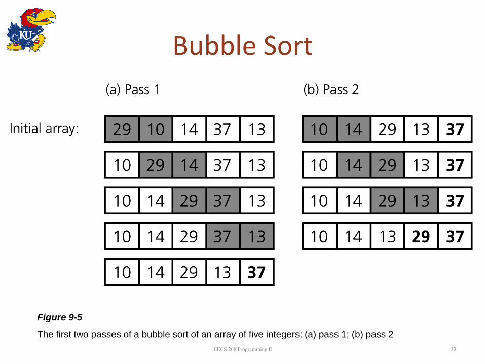
Bubble Sort

• Strategy

– compare adjacent elements and exchange them if they are out of order

• moves the largest (or smallest) elements to the end of the array

– repeat this process

• eventually sorts the array into ascending (or descending) order

• Analysis: worst case: O(n2), best case: O(n)


Bubble Sort – algorithm

for i = 1 to size - 1 do

for index = 1 to size - i do

if A[index] < A[index-1]

swap(A[index], A[index-1]);

endfor;

endfor;


Bubble Sort

33

Figure 9-5

The first two passes of a bubble sort of an array of five integers: (a) pass 1; (b) pass 2


Insertion Sort

• Strategy – Partition array in two regions: sorted and unsorted

• initially, entire array is in unsorted region

• take each item from the unsorted region and insert it into its correct position in the sorted region

• each pass shrinks unsorted region by 1 and grows sorted region by 1

• Analysis – Worst case: O(n2)

• Appropriate for small arrays due to its simplicity

• Prohibitively inefficient for large arrays


Insertion Sort

35

Figure 9-7 An insertion sort of an array of five integers.


Mergesort

• A recursive sorting algorithm

• Performance is independent of the initial order of the array items

• Strategy

– divide an array into halves

– sort each half

– merge the sorted halves into one sorted array

– divide-and-conquer approach


Mergesort – Algorithm

mergeSort(A,first,last) {

if (first < last) {

mid = (first + last)/2;

mergeSort(A, first, mid);

mergeSort(A, mid+1, last);

merge(A, first, mid, last)

}

}


Mergesort


Mergesort – Properties

• Needs a temporary array into which to copy elements during merging – doubles space requirement

• Mergesort is stable – items with equal key values appear in the same

order in the output array as in the input

• Advantage – mergesort is an extremely fast algorithm

• Analysis: worst / average case: O(n * log2n)


Quicksort

• A recursive divide-and-conquer algorithm – given a linear data structure A with n records

– divide A into sub-structures S1 and S2

– sort S1 and S2 recursively

• Algorithm – Base case: if |S|==1, S is already sorted

– Recursive case: • divide A around a pivot value P into S1 and S2 , such that

all elements of S1<=P and all elements of S2>=P

• recursively sort S1 and S2 in place


Quicksort

• Partition() – (a) scans array, (b) chooses a pivot, (c) divides A

around pivot, (d) returns pivot index – Invariant: items in S1 are all less than pivot, and items

in S2 are all greater than or equal to pivot

• Quicksort() – partitions A, sorts S1 and S2 recursively


Quicksort – Pivot Partitioning

• Pivot selection and array partition are fundamental work of algorithm

• Pivot selection

– perfect value: median of A[ ]

• sort required to determine median (oops!)

• approximation: If |A| > N, N==3 or N==5, use median of N

– Heuristic approaches used instead

• Choose A[first] OR A[last] OR A[mid] (mid = (first+last)/2) OR Random element

• heuristics equivalent if contents of A[ ] randomly arranged


Quicksort – Pivot Partitioning Example

• A= [5,8,3,7,4,2,1,6], first =0, last =7

• A[first]: pivot = 5, A[last]: pivot = 6,

• A[mid]: mid =(0+7)/2=3, pivot = 7

• A[random()]: any key might be chosen

• A[medianof3]: median(A[first], A[mid], A[last]) is median(5,7,6) = 6 • a sort of a fixed number of items is only O(1)

• Good pivot selection • computed in O(1) time and partitions A into roughly

equal parts S1 and S2


Quicksort – Pivot Partitioning • Middle element is pivot

• lastS1: index of last element of S1 partition

• firstUnknown: first element needing classification – if <p, then add to first

partition by incrementing last S1 and swapping

– incrementing firstUnknown expands partitioned sets either way

• Partitioning is an O(n) operation over A[ ]

int partition(A,first,last) {

middle = (first+last)/2;

pivot = A[middle];

swap(A[middle],A[first]);

lastS1 = first;

firstUnknown = first+1;

while( firstUnknown <= last ) {

if (A[firstUnknown] < pivot) {

lastS1++;

swap(A[firstUnknown],A[lastS1]);

}

firstUnknown++;

}

swap(A[first],A[lastS1]);

pivotIndex = lastS1;

return(pivotIndex);

} 45 EECS 268 Programming II

Quicksort – Pivot Partitioning

46

5 8 3 7 4 2 8 6

7 8 3 5 4 2 8 6 7 3 5 4 8 2 8 6

7 8 3 5 4 2 8 6 7 3 5 4 2 8 8 6

7 3 8 5 4 2 8 6 7 3 5 4 2 8 8 6

7 3 5 8 4 2 8 6 7 3 5 4 2 6 8 8

6 3 5 4 2 7 8 8

first last

mid

lastS1

firstUnknown

pivotIndex = 5

S1 = A[0..4]

S2 = A[6..7] EECS 268 Programming II

Quicksort – Analysis

• Best case – perfect partition at each level, log2n levels – O(n log n) total

• Average case – roughly equal partition – O(n log n)

• Worst case – S1 or S2 always empty – When the array is already sorted and the smallest

item is chosen as the pivot – O(n2 ), n levels, rare as long is input is in random order


Quicksort – Analysis

• Partitioning and recursive call overhead is such that for |A| < 10 or so it is faster to simply use insertion sort

– precise tipping point will vary with architecture

– but, Quicksort is usually extremely fast in practice

• Not stable like Mergesort, but sorts in place

• Even if the worst case occurs, quicksort’s performance is acceptable for moderately large arrays


Radix Sort

• Radix sort is a special kind of distribution sort that can efficiently sort data items using integer or other t element keys (atat-1...a0)m in a given radix (base) m – character string keys work as well; total order of all

characters required

• Strategy – Treats each data element as a character string

– Repeatedly organizes the data into groups according to the ith character in each element


Radix Sort

• Basic idea – each key consists of t places, each holding one of m

possible values – use m buckets and iterate the basic algorithm t times, each

time using a different element of the key for sorting – iterate from least significant to most significant key

position – 12345 – Five digit key, iterated over 100, 101, 102, 103, 104

using buckets 0-9 each time – FRED – Four character keys using capitol letters, iterated

from right to left using 26 buckets A-Z each time

• Analysis: Radix sort is O(n)


Radix Sort

51

Figure 9-21 A radix sort of eight integers

A Comparison of Sorting Algorithms

52

Figure 9-22 Approximate growth rates of time required for eight sorting algorithms


Heapsort

Summary

• Order-of-magnitude analysis and Big O notation measure an algorithm’s time requirement as a function of the problem size by using a growth-rate function

• To compare the efficiency of algorithms

– examine growth-rate functions when problems are large

– consider only significant differences in growth-rate functions


Summary

• Worst-case and average-case analyses

– worst-case analysis considers the maximum amount of work an algorithm will require on a problem of a given size

– average-case analysis considers the expected amount of work that an algorithm will require on a problem of a given size


Summary

• Worst case complexity of sorting algorithms

55

Imput in Sorted Order

Input in Reverse Sorted Order

Bubble Sort O(n) O(n2)

Insertion Sort O(n) O(n2)

Selection Sort O(n2) O(n2)

Merge Sort O(n log n) O(n log n)

Quick Sort O(n2) O(n2)

Radix Sort O(n) O(n)


Summary

• Complexity of sorting algorithms for random data, most common case

56

TB(n) TW(n) TA(n)

Bubble O(n) O(n2) O(n2)

Insertion O(n) O(n2) O(n2)

Selection O(n2) O(n2) O(n2)

Merge O(n log n) O(n log n) O(n log n)

Quiksort O(n log n) O(n2) O(n log n)

Radix O(n) O(n) O(n)


Summary

• Stability of sorting algorithms

– stable sort preserves the input order of data items with identical keys

– Thus, if input items x and y have identical keys, and x precedes y in the input data set, x will precede y in the output sorted data set

– bubble, insertion, selection, merge, and radix are stable sorting algorithms


algorithm efficiency big-o notation searching algorithms...

Documents