ALGEBRAIC SYSTEMS BIOLOGY:A CASE STUDY FOR THE WNT PATHWAY

ELIZABETH GROSS, HEATHER A. HARRINGTON, ZVI ROSEN, AND BERND STURMFELS

Abstract. Steady state analysis of dynamical systems for biological networks give rise toalgebraic varieties in high-dimensional spaces whose study is of interest in their own right.We demonstrate this for the shuttle model of the Wnt signaling pathway. Here the varietyis described by a polynomial system in 19 unknowns and 36 parameters. Current methodsfrom computational algebraic geometry and combinatorics are applied to analyze this model.

1. Introduction

The theory of biochemical reaction networks is fundamental for systems biology [13, 27].It is based on a wide range of mathematical fields, including dynamical systems, numericalanalysis, optimization, combinatorics, probability, and, last but not least, algebraic geometry.There are numerous articles that use algebraic geometry in the study of biochemical reactionnetworks, especially those arising from mass action kinetics. A tiny selection is [4,7,12,22,25].

We here perform a detailed analysis of one specific system, namely the shuttle model for theWnt signaling pathway, introduced recently by MacLean, Rosen, Byrne, and Harrington [17].Our aim is twofold: to demonstrate how biology can lead to interesting questions in algebraicgeometry and to apply state-of-the-art techniques from computational algebra to biology.

The dynamical system we study consists of the following 19 ordinary differential equations.Their derivation and the relevant background from biology will be presented in Section 2.

(1)

x1 = −k1x1 + k2x2x2 = k1x1 − (k2 + k26)x2 + k27x3 − k3x2x4 + (k4 + k5)x14x3 = k26x2 − k27x3 − k14x3x6 + (k15 + k16)x15x4 = −k3x2x4 − k9x4x10 + k4x14 + k8x16 + (k10 + k11)x18x5 = −k28x5 + k29x7 − k6x5x8 + k5x14 + k7x16x6 = −k14x3x6 − k20x6x11 + k15x15 + k19x17 + (k21 + k22)x19x7 = k28x5 − k29x7 − k17x7x9 + k16x15 + k18x17

x8 = −x16 = −k6x5x8 + (k7 + k8)x16x9 = −x17 = −k17x7x9 + (k18 + k19)x17

x10 = k12 − (k13 + k30)x10 − k9x4x10 + k31x11 + k10x18x11 = −k23x11 + k30x10 − k31x11 − k20x6x11 − k24x11x12 + k25x13 + k21x19

x12 = −x13 = −k24x11x12 + k25x13x14 = k3x2x4 − (k4 + k5)x14x15 = k14x3x6 − (k15 + k16)x15x18 = k9x4x10 − (k10 + k11)x18x19 = k20x6x11 − (k21 + k22)x19

1

arX

iv:1

502.

0318

8v1

[q-

bio.

MN

] 1

1 Fe

b 20

15

The quantity xi is a differentiable function of an unknown t, representing time, and xi(t) isthe derivative of that function. This dynamical system has five linear conservation laws:

(2)

0 = (x1 + x2 + x3 + x14 + x15)− c10 = (x4 + x5 + x6 + x7 + x14 + x15 + x16 + x17 + x18 + x19)− c20 = (x8 + x16)− c30 = (x9 + x17)− c40 = (x12 + x13)− c5

The 31 quantities ki are the rate constants of the chemical reactions, and the five ci are theconserved quantities. Both of these are regarded as parameters, so we have 36 parametersin total. Our object of interest is the steady state variety, which is the common zero set ofthe right hand sides of (1) and (2). This variety lives in K19, where K is an algebraicallyclosed field that contains the rational numbers Q as well as the 36 parameters ki and ci. Ifthese parameters are fixed to be particular real numbers then we can take K = C, the fieldof complex numbers. If it is preferable to regard k = (k1, . . . , k31) and c = (c1, . . . , c5) as

vectors of unknowns, then K = Q(k, c) is the algebraic closure of the rational function field.In this latter setting, when all parameters are generic, we shall derive the following result:

Theorem 1.1. The polynomials in (1)–(2) have 9 distinct zeros in K19 when K = Q(k, c).

By analyzing the steady state variety, we can better understand the model, which is non-linear, and thus the biological system. The aim is to predict the system’s behavior, offerbiological insight, and determine what data are required to verify or reject the model. Hereis a list of questions one might ask about our model from the perspective of systems biology.

Biological Problems. These are labeled according to the section that will address them.

4. For what real positive rate parameters and conserved quantities does the system exhibitmultistationarity? This question is commonly asked when using a dynamical systemfor modeling a real-world phenomenon. When modeling a process that experimentallyappears to have more than one stable equilibrium, multistationary models are preferred.

5. Suppose we can measure only a subset of the species concentrations. Which subsets canlead to model rejection? If all species are measurable at steady state, then we can substi-tute data into the system (1), and check that all expressions xi are close to zero. If onlysome xi are known, we still want to be able to evaluate models with the available data.

6. Give a complete description of the stoichiometric compatibility classes for the chemicalreaction network. A stoichiometric compatibility class is the set of all points accessiblefrom a given state via the reactions in the system. This question relates more closely tothe dynamics of the system, but also has ramifications for the set of all steady states.

7. What information does species concentration data give us for parameter estimation?In particular, are the parameters identifiable? Identifiability means that having manymeasurements of the concentrations x can determine the reaction rate constants k. If notidentifiable, we will explore algebraic constraints imposed by the species concentrationdata. This question is relevant for complete and partial steady-state data (usually noisy).

These questions are open challenges for medium to large models in systems biology andmedicine [13, 27]. The book chapter [16] illustrates standard mathematical and statistical

2

methods for addressing these questions, with Wnt signaling as a case study. Here, we examinethese questions from the perspective of algebraic geometry. The aim is to provide insight intoglobal behavior by applying tools from nonlinear algebra to synthetic and systems biology.Below are the algebraic problems underlying the four biological problems listed above.

Algebraic Problems.

4. Describe the set of points (k, c) ∈ R31>0 ×R5

>0 such that the polynomials (1)-(2) have twoor more positive zeros x ∈ R19

>0. When is there only one? Identify the discriminant.

5. Which projections of the variety defined by (1) into coordinate subspaces of K19 aresurjective? Equivalently, describe the algebraic matroid on the ground set {x1, . . . , x19}.

6. The conservation relations (2) specify a linear map χ : R19 → R5, x 7→ c. Describe all theconvex polyhedra χ−1(c) ∩ R19

≥0 where c runs over the points in the open orthant R5>0.

7. a. Complete data: Describe the matroid on the ground set {k1, k2, . . . , k31} that is definedby the linear forms on the right hand sides of (1), for fixed steady-state concentrations.

b. Partial steady-state data without noise: Repeat the analysis after eliminating some ofthe x-coordinates.

c. Partial steady-state data with noise: For the remaining x-coordinates, suppose that wehave data which are approximately on the projected steady state variety. Determine aparameter vector (k, c) that best fits the data.

In this paper we shall address these questions, and several related ones, after explaining thevarious ingredients. A particular focus is the exchange between the algebraic formulationand its biological counterpart. Our presentation is organized as follows.

In Section 2 we review the basics on the Wnt signaling pathway, we recall the shuttle modelof MacLean et al. [17], and we derive the dynamical system (1)–(2). In Section 3 we establishTheorem 1.1, and we examine the set of all steady states. This is here regarded as a complexalgebraic variety in an affine space of dimension 55 = 19 + 31 + 5 with coordinates (x,k, c).

In Sections 4, 5, 6, and 7 we address the four problems stated above. The numbers ofthe problems refer to the respective sections. Each section starts out with an explanationof how the biological problem and the algebraic problem are related. The rationale behindSection 4 is likely to be familiar to most of our readers, given that multistationarity has beendiscussed widely in the literature; see e.g. [4,22]. On the other hand, in Section 5 we employthe language of matroid theory. This may be unfamiliar to many readers, especially whenit comes to the algebraic matroid associated with an irreducible algebraic variety. Section 6characterizes the polyhedral geometry encoded in the conservation relations (2). This is acase study in the spirit of [25, Figure 1]. Section 7 addresses the problems of parameteridentifiability and parameter estimation. Finally, in Section 8 we return to the biology, andwe discuss what our findings might imply for the study of Wnt signaling and other systems.

3

2. From Biology to Algebra

Cellular decisions such as cell division, specialization and cell death are governed by a richrepertoire of complex signals that are produced by other cells and/or stimuli. In order fora cell to come to an appropriate decision, it must sense its external environment, communi-cate this information to the nucleus, and respond by regulating genes and producing relevantproteins. Signaling molecules called ligands, external to the cell, can bind to proteins calledreceptors, initializing the propagation of information within the cell by molecular interactionsand modifications (e.g. phosphorylation). This signal may be relayed from the cytoplasminto the nucleus via molecules and the cell responds by activation or deactivation of gene(s)that control, for example, cell fate. The complex interplay of molecules involved in this in-formation transmission is called a signaling transduction pathway. Although many signalingpathways have been defined biochemically, much is still not understood about them or how asignal results in a particular cellular response. Mathematical models constructed at differentscales of molecular complexity may help unravel the central mechanisms that govern cellulardecisions, and their analysis may inform and guide testable hypotheses and therapies.

In this paper, we focus on the canonical Wnt signaling pathway, which is involved in cel-lular processes, both during development and in adult tissues. This includes stem cells.Dysfunction of this pathway has been linked to neurodegenerative diseases and cancer. Con-sequently, Wnt signaling has been widely studied in various organisms, including amphibiansand mammals. Researchers are interested in how the extracellular ligand Wnt affects theprotein β-catenin, which plays a pivotal role in turning genes on and off in the nucleus.

The molecular interactions within the Wnt signaling pathway are not yet fully understood.This has led to the development and analysis of many mathematical models. The Wntshuttle model [17] includes an abstraction of the signal transduction pathway (via activa-tion/inactivation of molecules) described above. The model also takes into account moleculesthat exist, interact and move between different compartments in the cell (e.g., cytoplasmand nucleus). Biologists understand the Wnt system as either Wnt off or Wnt on. How-ever, such a scenario is rarely binary (i.e., different concentration levels of Wnt may exist)and inherently depends on spatial movement of molecules. The Wnt shuttle model includescomplex interactions with nonlinearities arising in the equations. In particular, it includesboth the Wnt off and Wnt on scenarios, by adjusting initial conditions or parameter values.The biology needed to understand the model can be described as follows. See also Table 1.

Wnt off: When cells do not sense the extracellular ligand Wnt, β-catenin is degraded (bro-ken down). The degradation of β-catenin is partially dependent on a group of molecules(Axin, APC and GSK-3) that form the destruction complex. Crucially, the break down ofβ-catenin occurs when the destruction complex is in an active state; modification to thedestruction complex by proteins, called phosphatases, changes it from inactive to active.Additionally, β-catenin can degrade independent of the destruction complex. Synthesis ofβ-catenin occurs at a constant rate.

Wnt on: When receptors on the surface of a cell bind to Wnt, the Wnt signaling transduc-tion pathway is initiated. This enables β-catenin to move into the nucleus where it bindswith transcription factors that regulate genes. This signal propagation is mediated by thefollowing molecular interactions. After Wnt stimulus, the protein Dishevelled is activated

4

near the membrane. This in turn inactivates the destruction complex, thereby preventingthe destruction of β-catenin, allowing it to accumulate in the cytoplasm through naturalsynthesis. Throughout the molecular interactions in the signaling pathway, intermediatecomplexes can form (e.g., β-catenin bound with Dishevelled).

Space: The location of molecules plays a pivotal role: β-catenin moves between the cytoplasmand the nucleus (to reach target genes and regulate them). Dishevelled and molecules thatform the destruction complex shuttle between the nucleus and the cytoplasm. However, itis assumed that only the inactive destruction complex can shuttle (since in the cytoplasm itwould be bound to β-catenin). Phosphatases exist in both the nucleus and the cytoplasmbut the movement across compartments is not included in the model. Symmetry of reactionsis assumed if the species exist in both compartments. Intermediate complexes are assumedto be short-lived, or not large enough for movement across compartments.

The Wnt shuttle model of [17] has 19 species whose interactions can be framed as biochemicalreactions. These species correspond to variables x1, . . . , x19 in our dynamical system (1).Namely, xi represents the concentration of the species that is listed in the ith row in Table 1.

Variable Species SymbolDishevelled D

x1 Dishevelled in cytoplasm (inactive) Di

x2 Dishevelled in cytoplasm (active) Da

x3 Dishevelled in nucleus (active) Dan

Destruction complex (APC/Axin/GSK3β) Yx4 Destruction complex in cytoplasm (active) Yax5 Destruction complex in cytoplasm (inactive) Yix6 Destruction complex in nucleus (active) Yanx7 Destruction complex in nucleus (inactive) Yin

Phosphatase Px8 Phosphatase in cytoplasm Px9 Phosphatase in nucleus Pn

β−catenin xx10 β-catenin in cytoplasm xx11 β-catenin in nucleus xn

Transcription Factor Tx12 TCF (gene transcription in nucleus) T

Intermediate complex Cx13 Transcription complex, β-catenin: TCF in nucleus CxT

x14 Intermediate complex, β-catenin: dishevelled in cytoplasm CY D

x15 Intermediate complex, destruction complex: dishevelled in nucleus CY Dn

x16 Intermediate complex, destruction complex: phosphatase in cytoplasm CY P

x17 Intermediate complex, destruction complex: phosphatase in nucleus CY Pn

x18 Intermediate complex, β-catenin: destruction complex in cytoplasm CxY

x19 Intermediate complex, β-catenin: destruction complex in nucleus CxY n

Table 1: The 19 species in the Wnt shuttle model.

5

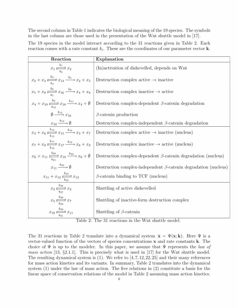
The second column in Table 1 indicates the biological meaning of the 19 species. The symbolsin the last column are those used in the presentation of the Wnt shuttle model in [17].

The 19 species in the model interact according to the 31 reactions given in Table 2. Eachreaction comes with a rate constant ki. These are the coordinates of our parameter vector k.

Reaction Explanation

x1k1// x2

k2

oo (In)activation of dishevelled, depends on Wnt

x2 + x4k3// x14

k4

ook5// x2 + x5 Destruction complex active → inactive

x5 + x8k6// x16

k7

ook8// x4 + x8 Destruction complex inactive → active

x4 + x10k9// x18

k10

ook11// x4 + ∅ Destruction complex-dependent β-catenin degradation

∅ k12// x10 β-catenin production

x10k13

// ∅ Destruction complex-independent β-catenin degradation

x3 + x6k14// x15

k15

ook16// x3 + x7 Destruction complex active → inactive (nucleus)

x7 + x9k17// x17

k18

ook19// x6 + x9 Destruction complex inactive → active (nucleus)

x6 + x11k20// x19

k21

ook22// x6 + ∅ Destruction complex-dependent β-catenin degradation (nucleus)

x11k23

// ∅ Destruction complex-independent β-catenin degradation (nucleus)

x11 + x12k24// x13

k25

oo β-catenin binding to TCF (nucleus)

x2k26// x3

k27

oo Shuttling of active dishevelled

x5k28// x7

k29

oo Shuttling of inactive-form destruction complex

x10k30// x11

k31

oo Shuttling of β-catenin

Table 2: The 31 reactions in the Wnt shuttle model.

The 31 reactions in Table 2 translate into a dynamical system x = Ψ(x; k). Here Ψ is avector-valued function of the vectors of species concentrations x and rate constants k. Thechoice of Ψ is up to the modeler. In this paper, we assume that Ψ represents the law ofmass action [13, §2.1.1]. This is precisely what is used in [17] for the Wnt shuttle model.The resulting dynamical system is (1). We refer to [4,7,12,22,25] and their many referencesfor mass action kinetics and its variants. In summary, Table 2 translates into the dynamicalsystem (1) under the law of mass action. The five relations in (2) constitute a basis for thelinear space of conservation relations of the model in Table 2 assuming mass action kinetics.

6

We refer to x1, . . . , x19 as the species concentrations, k1, . . . , k31 as the rate parameters,and c1, . . . , c5 as the conserved quantities. We write x, k and c for the vectors with thesecoordinates. As is customary in algebraic geometry, we take the coordinates in the complexnumbers C, or possibly in some other algebraically closed field K containing the rationals Q.

Our aim is to understand the relationships between x,k and c in the Wnt shuttle model. Tothis end, we introduce the steady state variety S ⊂ C55. This is the set of all points (x,k, c)that satisfy the equations x1 = . . . = x19 = 0 in (1) along with the five conservation lawsin (2). We write our ambient affine space as C55 = C19

x × C31k × C5

c. This emphasizes thedistinction between the species concentrations, rate parameters, and conserved quantities.

3. Ideals, Varieties, and Nine Points

We write I for the ideal in the polynomial ring Q[x,k] = Q[x1, . . . x19, k1, . . . k31] that isgenerated by the 19 polynomials xi on the right hand side of (1). Five of these generatorsare redundant. Indeed, the conservation relations (2) give the following identities modulo I:

x1 + x2 + x3 + x14 + x15 = x8 + x16 = x9 + x17 = x12 + x13 =x4 + x5 + x6 + x7 + x14 + x15 + x16 + x17 + x18 + x19 = 0.

For instance, the polynomials x13, x15, x16, x17 and x19 are redundant because they can beexpressed as negated sums of other generators of I. Hence I is generated by 14 polynomials.The variety V (I) lives in the 50-dimensional affine space C19

x × C31k , and it is isomorphic to

the steady state variety S ⊂ C55. A direct computation using the computer algebra packageMacaulay2 [11] shows that V (I) has dimension 36. Hence the affine ideal I is a completeintersection in Q[x,k]. Furthermore, using Macaulay2 we can verify the following lemma.

Lemma 3.1. The ideal I admits the non-trivial decomposition I = Im∩Ie, where Ie = I : 〈x1〉and Im = I + 〈x1〉, both of these components have codimension 14, and Ie is a prime ideal.

The ideal Im is called the main component, while Ie is called the extinction component, sinceit reflects those steady states where a number of the reactants “run out.” Both of these idealslive in Q[x,k], and we now present explicit generators. The extinction component equals

Ie = 〈x1, x2, x3, x5, x7, x14, x15, x16, x17, k30x10 − (k23 + k31)x11 − k22x19,k13x10 + k23x11 + k11x18 + k22x19 − k12, k24x11x12 − k25x13,

k20x6x11 − (k21 + k22)x19, k9x4x10 − (k10 + k11)x18〉.

The ideal Ie is found to be prime in Q[x,k]. The main component equals

Im = 〈k16x15 − k19x17, k5x14 − k8x16, k30x10 − (k23 + k31)x11 − k22x19,k13x10 + k23x11 + k11x18 + k22x19 − k12, k28x5 − k29x7, k26x2 − k27x3,

k1x1 − k2x2, k24x11x12 − k25x13, k20x6x11 − (k21 + k22)x19,k9x4x10 − (k10 + k11)x18, k17x7x9 − (k18 + k19)x17, k6x5x8 − (k7 + k8)x16,

k14x3x6 − k15x15 − k19x17, k3x2x4 − k4x14 − k8x16,(k4k6k8k14k16k18k26k29 + k5k6k8k14k16k18k26k29+

k4k6k8k14k16k19k26k29 + k5k6k8k14k16k19k26k29)k1x6x8−(k3k5k7k15k17k19k27k28 + k3k5k8k15k17k19k27k28

+k3k5k7k16k17k19k27k28 + k3k5k8k16k17k19k27k28)k1x4x9〉.7

This ideal is not prime in Q[x,k]. For instance, the variable k1 is a zerodivisor modulo Im,as seen from the last generator. Removing the factor k1 from the last generator yields thequotient ideal Im : 〈k1〉. However, even that ideal still has several associated primes. All ofthese prime ideals, except for one, contain some of the rate constants ki.

That special component is characterized in the following proposition. Given any ideal J ⊂Q[x,k], we write J = Q(k)[x]J for its extension to the polynomial ring Q(k)[x] in theunknowns x1, . . . , x19 over the field of rational functions in the parameters k1, . . . , k31.

Proposition 3.2. The ideal Jm = Im ∩Q[x,k] is prime. Its irreducible variety V (Jm) ⊂ C50

has dimension 36; it is the unique component of V (Im) that maps dominantly onto C31k .

Proof. The ideal Im has the same generators as Im but now regarded as polynomials in x with

coefficients in Q(k). Symbolic computation in the ring Q(k)[x] reveals that Im is a primeideal. This implies that Jm is a prime ideal in Q[x,k], and hence V (Jm) is irreducible. Thedimension statement follows from the result of Lemma 3.1 that Im is a complete intersection.This ensures that V (Im) has no lower-dimensional components, by Krull’s Principal IdealTheorem. Finally, V (Jm) maps dominantly onto C31

k because Jm ∩ Q[k] = {0}. �

Corollary 3.3. The ideal I is radical, and it is the intersection of two primes in Q(k)[x]:

(3) I = Ie ∩ Im.

Proof. This follows directly from Proposition 3.2 and the primality of Ie in Lemma 3.1. �

The decomposition has the following geometric interpretation. We now work over the field

K = Q(k). All rate constants are taken to be generic. Then V (I) is the 5-dimensionalvariety of all steady states in K19. This variety is the union of two irreducible components,

V (I) = V (Ie) ∪ V (Im),

where each component is 5-dimensional. The first component lies inside the 10-dimensionalcoordinate subspace V (x1, x2, x3, x5, x7, x14, x15, x16, x17). Hence it is disjoint from the hy-perplane defined by the first conservation relation x1 + x2 + x3 + x14 + x15 = c1. In other

words, V (Ie) is mapped into a coordinate hyperplane under the map χ : K19 → K5,x 7→ c.

On the other hand, the second component V (Im) maps dominantly onto K5 under χ. The-orem 1.1 states that the generic fiber of this map consists of 9 reduced points. Equivalently,

(4) χ−1(c) ∩ V (I) = χ−1(c) ∩ V (Im)

is a set of nine points in K19. We are now prepared to argue that this is indeed the case.

Computational Proof of Theorem 1.1. We consider the ideal of the variety (4) in the polyno-mial ring Q(k, c)[x]. This polynomial ring has 19 variables, and all 36 parameters are nowscalars in the coefficient field. This ideal is generated by the right hand sides of (1) and (2).Performing a Grobner basis computation in this polynomial ring verifies that our ideal iszero-dimensional and has length 9. Hence (4) is a reduced affine scheme of length 9 in K19.

Fast numerical verification of this result is obtained by replacing the coordinates of k and cwith generic (random rational) values. In Macaulay2 one finds, with probability 1, that the

8

resulting ideals in Q[x] are radical of length 9. We also verified this result via numericalalgebraic geometry, using the two software packages Bertini [1] and PHCpack [26]. �

4. Multistationarity and its Discriminant

This section centers around Question 4 from the Introduction: For what real positive rateparameters and conserved quantities does the system exhibit multistationarity? This is com-monly asked about biochemical reaction networks and about dynamical systems in general.

Mathematically, this is a problem of real algebraic geometry. Writing S for the steady statevariety in C55, we are interested in the fibers of the map πk,c : S ∩ R55

>0 → R31>0,k × R5

>0,c.

According to Theorem 1.1, the general fiber consists of 9 complex points x ∈ C19x , when the

map πk,c is taken over C. But here we take it over the reals R or over the positive reals R>0.

In our application to biology, we only care about concentration vectors x whose coordinatesare real and positive. Thus we wish to stratify R31

>0,k ×R5>0,c according to the cardinality of

(5) π−1k,c(k, c) ={

(x,k′, c′) ∈ S ∩ R55>0 : k′ = k and c′ = c

}.

This stratification comes from a decomposition of the 36-dimensional orthant R31>0,k ×R5

>0,c

into connected open semialgebraic subsets. The walls in this decomposition are given by thediscriminant ∆, a giant polynomial in the 36 unknowns (k, c) that is to be defined later.

We begin with the following result on what is possible with regard to real positive solutions.

Theorem 4.1. Consider the polynomial system in (1)–(2) where all parameters ki and cjare positive real numbers. The set (5) of positive real solutions can have 1, 2, or 3 elements.

Proof. For random choices of (k, c) = (k1, . . . , k31, c1, . . . , c5) in the orthant R36>0, our polyno-

mial system has 9 complex solutions, by Theorem 1.1. For the following two special choicesof the 36 parameter values, all 9 solutions are real. First, take (k, c) to be the vector

(1.7182818, 53.2659, 3.4134082, 0.61409879, 0.61409879, 3.4134082, 0.98168436, 0.98168436,92.331732, 0.86466471, 79.9512906, 97.932525, 1, 3.2654672, 0.61699064, 0.61699064,37.913879, 0.86466471, 0.86466471, 4.7267833, 0.17182818, 0.68292191, 1, 0.55950727,

1.0117639, 1.7182818, 1.7182818, 0.99326205, 0.99326205, 5.9744464, 1, 4.9951026,16.4733784, 1.6006340000000001, 1.2089126, 2.7756596399999998).

The resulting system has three positive solutions x ∈ R19>0. Next, let (k′, c′) be the vector

(0.948166, 7.45086, 5.72974, 3.96947, 7.21145, 7.8761, 1.87614, 8.11372, 6.21862, 5.24801,3.10707, 1.08146, 5.22133, 5.84158, .911392, 4.28788, 4.81201, 9.67849, 1.34452, 7.38597,6.64451, 7.10229, 8.57942, 5.79076, 6.33244, 1.53916, 1.39658, 0.81673, 5.8434, 3.86223,

7.22696, 1.45438, 3.36482, 6.06453, 4.82045, 3.6014).

Here, one solution to our system is positive. By connecting the two parameter points abovewith a general curve in R36

>0, and by examining in-between points (k′′, c′′), we can construct asystem with two positive solutions. All computations were carried out using Bertini [1]. �

Remark 4.2. At present, we do not know whether the number of real positive solutions canbe larger than three. We suspect that this is impossible, but we currently cannot prove it.

9

The difficulty lies in the fact that the stratification of R36>0 is extremely complicated. In

computer algebra, the derivation of such stratifications is known as the problem of real rootclassification. For a sample of recent studies in this direction see [3, 6, 23]. Real root classi-fication is challenging even when the number of parameters is 3 or 4; clearly, 36 parametersis out of the question. The stratification of R36

>0 by behavior of (5) has way too many cells.

While symbolic techniques for real root classification are infeasible for our system, we can usenumerical algebraic geometry [9] to gain insight into the stratification of R36

>0. Coefficient-parameter homotopies [19] can solve the steady state polynomial system (1)-(2) for multiplechoices of (k, c) quickly. For our computations we use Bertini.m2. This is the Bertini

interface for Macaulay2, as described in [2]. Each system has 19 equations in 19 unknownsand, for random (k, c), each system has 9 complex solutions. Such a system can be solvedin less than one second using the bertiniParameterHomotopy function from Bertini.m2.

Below we describe the following experiment. We sample 10, 000 parameter vectors (k, c)from two different probability distributions on R36

>0. In each case we report the observedfrequencies for the number of real solutions and number of positive solutions. We then followthese experiments with a specialized sampling scheme for testing numerical robustness.

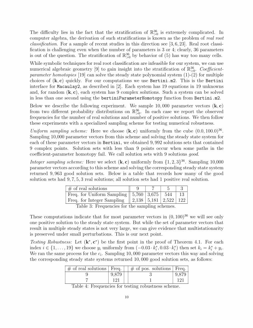
Uniform sampling scheme: Here we choose (k, c) uniformly from the cube (0.0, 100.0)36.Sampling 10,000 parameter vectors from this scheme and solving the steady state system foreach of these parameter vectors in Bertini, we obtained 9, 992 solutions sets that contained9 complex points. Solution sets with less than 9 points occur when some paths in thecoefficient-parameter homotopy fail. We call solution sets with 9 solutions good.

Integer sampling scheme: Here we select (k, c) uniformly from {1, 2, 3}36. Sampling 10,000parameter vectors according to this scheme and solving the corresponding steady state systemreturned 9, 963 good solution sets. Below is a table that records how many of the goodsolution sets had 9, 7, 5, 3 real solutions; all solution sets had 1 positive real solution.

# of real solutions 9 7 5 3Freq. for Uniform Sampling 5,760 3,675 544 13Freq. for Integer Sampling 2,138 5,181 2,522 122

Table 3: Frequencies for the sampling schemes.

These computations indicate that for most parameter vectors in (0, 100)36 we will see onlyone positive solution to the steady state system. But while the set of parameter vectors thatresult in multiple steady states is not very large, we can give evidence that multistationarityis preserved under small perturbations. This is our next point.

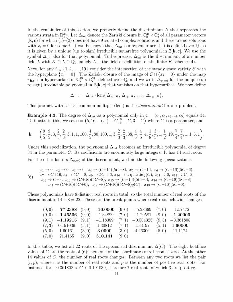
Testing Robustness: Let (k∗, c∗) be the first point in the proof of Theorem 4.1. For eachindex i ∈ {1, . . . , 19} we choose yi uniformly from (−0.03 · k∗i , 0.03 · k∗i ) then set ki = k∗i + yi.We ran the same process for the ci. Sampling 10, 000 parameter vectors this way and solvingthe corresponding steady state systems returned 10, 000 good solution sets, as follows:

# of real solutions Freq. # of pos. solutions Freq.9 9,879 3 9,8797 121 1 121

Table 4: Frequencies for testing robustness scheme.

10

In the remainder of this section, we properly define the discriminant ∆ that separates thevarious strata in R36

>0. Let ∆int denote the Zariski closure in C31k ×C5

c of all parameter vectors(k, c) for which (1)–(2) does not have 9 isolated complex solutions and there are no solutionswith xi = 0 for some i. It can be shown that ∆int is a hypersurface that is defined over Q, soit is given by a unique (up to sign) irreducible squarefree polynomial in Z[k, c]. We use thesymbol ∆int also for that polynomial. To be precise, ∆int is the discriminant of a numberfield L with K ⊃ L ⊃ Q, namely L is the field of definition of the finite K-scheme (4).

Next, for any i ∈ {1, 2, . . . , 19} consider the intersection of the steady state variety S withthe hyperplane {xi = 0}. The Zariski closure of the image of S ∩ {xi = 0} under the mapπk,c is a hypersurface in C19

k × C31c , defined over Q, and we write ∆xi=0 for the unique (up

to sign) irreducible polynomial in Z[k, c] that vanishes on that hypersurface. We now define

∆ := ∆int · lcm(

∆x1=0 , ∆x2=0 , . . . , ∆x19=0

).

This product with a least common multiple (lcm) is the discriminant for our problem.

Example 4.3. The degree of ∆int as a polynomial only in c = (c1, c2, c3, c4, c5) equals 34.To illustrate this, we set c =

(5, 16 + C, 8

5− C, 6

5+ C, 3− C

)where C is a parameter, and

k =

(9

5,9

5, 3,

2

3,2

3, 3, 1, 1, 100,

4

5, 80, 100, 1, 3,

2

3,2

3, 38,

4

5,4

5, 4,

1

8,3

5, 1,

1

2, 19,

7

4,7

4, 1, 1, 5, 1

).

Under this specialization, the polynomial ∆int becomes an irreducible polynomial of degree34 in the parameter C. Its coefficients are enormously large integers. It has 14 real roots.

For the other factors ∆xi=0 of the discriminant, we find the following specializations:

(6)

x1 → 0, x2 → 0, x3 → 0, x4 → (C+16)(5C−8), x5 → C+16, x6 → (C+16)(5C+6),x7 → C+16, x8 → 5C − 8, x9 → 5C + 6, x10 → a quartic q(C), x11 → 0, x12 → C−3,x13 → C−3, x14 → (C+16)(5C−8), x15 → (C+16)(5C+6), x16 → (C+16)(5C−8),

x17 → (C+16)(5C+6), x18 → (C+16)(5C−8)q(C), x19 → (C+16)(5C+6).

These polynomials have 8 distinct real roots in total, so the total number of real roots of thediscriminant is 14 + 8 = 22. These are the break points where real root behavior changes:

(9, 0) −77.2388 (9, 0) −16.0000 (9, 0) −5.28669 (7, 0) −1.57472(9, 0) −1.46506 (9, 0) −1.34899 (7, 0) −1.29581 (9, 0) −1.20000(9, 1) −1.19215 (9, 1) −1.18389 (7, 1) −0.584325 (9, 3) −0.361808(7, 3) 0.191039 (5, 1) 1.30812 (7, 1) 1.33197 (5, 1) 1.60000(5, 0) 1.60161 (3, 0) 3.0000 (3, 0) 4.26306 (5, 0) 11.1174(7, 0) 21.4165 (9, 0) 310.141 (9, 0)

In this table, we list all 22 roots of the specialized discriminant ∆(C). The eight boldfacevalues of C are the roots of (6): here one of the coordinates of x becomes zero. At the other14 values of C, the number of real roots changes. Between any two roots we list the pair(r, p), where r is the number of real roots and p is the number of positive real roots. Forinstance, for −0.361808 < C < 0.191039, there are 7 real roots of which 3 are positive.

11

5. Algebraic Matroids and Parametrizations

Question 5 asks: Suppose we can measure only a subset of the species concentrations. Whichsubsets can lead to model rejection? This issue is important for the Wnt shuttle modelbecause, in the laboratory, only some of the species are measurable by existing techniques.

We shall address Question 5 using algebraic matroids. Matroid theory allows us to analyzethe structure of relationships among the 19 species in Table 1. This first appeared in [17].We here present an in-depth study of the matroids that govern the Wnt shuttle model.

An introduction to (algebraic) matroids can be found in [21]; they have been applied in[14,15] to problems involving the completion of partial information. General algorithms forcomputing algebraic matroids are derived in [24]. We briefly review basic notions.

Definition 5.1. A matroid is an ordered pair (X, I), where X is a finite set, here regarded asunknowns, and I is a subset of the power set ofX. These satisfy certain independence axioms.For an algebraic matroid, we are given a prime ideal P in the polynomial ring K[X] generatedby X, and I consists of subsets of X whose images in K[X]/P are algebraically independentover K. Thus, the collection of independent sets is I =

{Y ⊆ X : P ∩K[Y ] = {0}

}.

1. Bases are maximal independent sets, i.e. subsets in I that have maximal cardinality.

2. Rank is a function ρ from the power set of X to the natural numbers, which takes as inputa set Y ⊂ X and returns the cardinality of the largest subset of Y in I.

3. Closure is a function from the power set 2X to itself. The input is a set Y and the outputis the largest set containing Y with the same rank.

4. Flats are the elements in 2X that lie in the image of the closure map.

5. Circuits are the sets of minimal cardinality not contained in I.

We are here interested in the matroid that is defined by the prime ideal P = Im in Q(k)[x]. Its

ground set X is the set of species concentrations {x1, . . . , x19}. Since V (Im) is 5-dimensional,each basis consists of five elements in X. In our application, bases are the maximal subsets ofX that can be specified independently at steady state; they are also the minimal-cardinalitysets that can be measured to learn all species concentrations. The rank of a set Y indicatesthe number of measurements required to learn the concentrations for every element of Y .Flats are the full subsets that are specified by any given collection of measurements.

Circuits furnish our answer to Question 5: they are minimal sets of species that can be usedto test compatibility of the data with the model. For each circuit Y there is a unique-up-

to-scalars relation in Im ∩Q(k)[Y ], called the circuit polynomial of Y . If the measurementsindicate that this relation is not satisfied, then the model and data are not compatible.

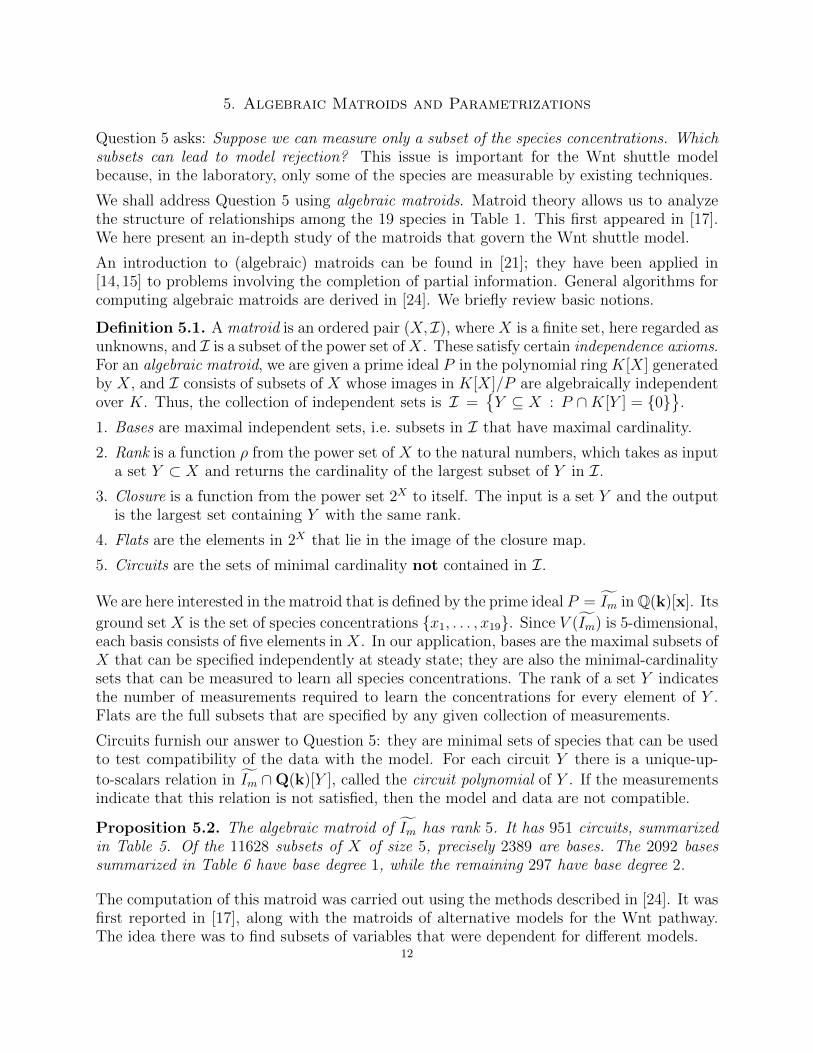
Proposition 5.2. The algebraic matroid of Im has rank 5. It has 951 circuits, summarizedin Table 5. Of the 11628 subsets of X of size 5, precisely 2389 are bases. The 2092 basessummarized in Table 6 have base degree 1, while the remaining 297 have base degree 2.

The computation of this matroid was carried out using the methods described in [24]. It wasfirst reported in [17], along with the matroids of alternative models for the Wnt pathway.The idea there was to find subsets of variables that were dependent for different models.

12

Our matroid analysis here goes beyond [17] in several ways:

1. We keep track of the parameters k. We take our circuit polynomials to have (relativelyprime) coefficients in Z[k]. This gives us a new tool for model rejection, e.g. in situationswhere only one data point is known but some parameter values are available.

2. We show how circuits can be used in parameter estimation; this will be done in Section 8.

3. We use the degree-1 bases to derive rational parametrizations of the variety V (Im).

We now explain Table 5. A circuit polynomial has type (i, j) if it contains i species concen-trations (x-variables) and j rate parameters (k-variables). The entry in row i and column jin Table 5 is the number of circuits of type (i, j). Zero values are omitted for clarity.

2 3 4 5 62 5 13 64 1 55 6 16 7 57 5 38 1 11 19 6 12 310 11 111 4 7 11 1

2 3 4 5 612 13 1013 13 15 214 19 16 115 17 21 416 15 11 217 16 32 918 4 6 219 26 36 1120 44 1 121 26 27 9

2 3 4 5 622 8 5823 4 56 524 54 1425 53 1526 8 1627 12 56 1628 2 229 29 143031 6

Table 5. The 951 circuit polynomials, by numbers of unknowns xi and kj.

Example 5.3. There are five circuits of type (2, 2). One of them is x1 = −k1x1+k2x2. Most

of the 951 circuit polynomials in Im are more complicated. In particular, they are non-linearin both x and y. For instance, the unique circuit polynomial of type (6, 11) equals

(−k15k17k19k20k25 − k16k17k19k20k25)x7x9x13+(k14k16k18k21k24 + k14k16k19k21k24 + k14k16k18k22k24 + k14k16k19k22k24)x3x12x19.

In Section 7, we will consider the role of these nonlinear functions in parameter estimation.

Given a basis Y of an algebraic matroid, its base degree is the length of the generic fiber ofthe projection of V (P ) onto the Y -coordinates (cf. [24]). Bases with degree 1 are desirable:

Proposition 5.4. Let P ⊂ K[X] be a prime ideal, Y a basis of its algebraic matroid,|X| = n, and |Y | = r. If Y has base degree 1 then V (P ) is a rational variety, and the basiccircuits of Y specify a birational map ϕY : Kr 99K Kn whose image is Zariski dense in V (P )

Proof. For each coordinate xi in X\Y there exists a circuit containing Y ∪ {xi}; this is thebasic circuit of (Y, xi). Since Y has base degree 1, the generic fiber of the map V (P )→ Kr

consists of a unique point. Therefore the circuit polynomial is linear in xi. It has the form

pi(Y ) · xi + qi(Y ), where pi, qi ∈ K[Y ].

The i-coordinate of the rational map ϕY equals xi if xi ∈ Y and −qi(Y )/pi(Y ) if xi /∈ Y . �13

From Propositions 5.2 and 5.4, we obtain 2092 rational parametrizations of the variety V (Im).These are the maps ϕY : K5 99K K19, where Y runs over all bases of base degree 1. Usingthese ϕY , we obtain 2092 representations of the steady state variety (4) as a subset of K5,where now K = Q(k, c). Namely, we consider the preimages of the five hyperplanes definedby (2). These are hypersurfaces in K5 whose intersection represents the nine points in (4).We performed the following computation for all 2092 bases Y = {y1, . . . , y5} of base degree 1:

1. Substitute x = ϕY (y1, . . . , y5) into the five linear equations (2).

2. Clear the denominators d1, . . . , d5 in each equation to get polynomials h1, . . . , h5 in Y .

3. The saturation ideal JY = 〈h1, . . . , h5〉 : 〈d1d2 · · · d5〉∞ represents the preimage of (4).

Given such a wealth of parametrizations, we seek one where JY has desirable properties.We use the following criterion: consider subsets of five of the generators of JY , compute themixed volume of their Newton polytopes, and fix a subset minimizing that mixed volume. Inthe census of 2092 bases in Table 6, that minimum is referred to as the mixed volume of Y .

Mixed Volume 5 9 10 11 12 13 14 15 16 20 23 24 25 30 35 42 45Frequency 2 416 6 73 50 167 563 751 10 12 6 1 11 12 4 4 4

Table 6. Reducing the steady state equations to the 2092 bases of base degree 1

By Bernstein’s Theorem, the mixed volume is the number of solutions to a generic systemwith the five given Newton polytopes. We seek bases Y where this matches the number ninefrom Theorem 1.1. We see that the mixed volume is nine for 416 of the bases in Table 6.

Example 5.5. The basis Y = {x1, x4, x6, x8, x13} has base degree 1 and mixed volume 9.The remaining variables can be expressed in terms of Y as follows. For brevity, we set

r(x4, x6) = k9k11k20k22x4x6 + k9k11(k21 + k22)(k23 + k31)x4+ k20k22(k10 + k11)(k13 + k30)x6 + (k10 + k11)(k21 + k22)(k13k23 + k23k30 + k13k31).

x2 =k1k2x1 x12 = r(x4,x6)

k12k30(k10+k11)(k21+k22)

k25k24

x13

x3 =k1k26k2k27

x1 x14 =k1k3

k2(k4 + k5)x1x4

x5 =k1k3k5(k7 + k8)

k2k6k8(k4 + k5)

x1x4x8

x15 =k1k14k26

k2k27(k15 + k16)x1x6

x7 =k1k3k5k28(k7 + k8)

k2k6k8k29(k4 + k5)

x1x4x8

x16 =k1k3k5

k2k8(k4 + k5)x1x4

x9 = k6k8k14k16k26k29(k4+k5)(k18+k19)k3k4k5k17k19k27k28(k7+k8)(k15+k16)

x6x8x4

x17 =k1k14k16k26

k2k19k27(k15 + k16)x1x6

x10 = k12(k10+k11)(k20k22x6+(k21+k22)(k23+k31))r(x4,x6)

x18 = k9k12(k20k22x6+(k21+k22)(k23+k31))r(x4,x6)

x4

x11 =k12k30(k10 + k11)(k21 + k22)

r(x4, x6)x19 =

k12k20k30(k10 + k11)

r(x4, x6)x6

14

This map ϕY is substituted into (2), and then we saturate. The resulting ideal JY equals

〈α1x6x8 + α2x4 + α3x6, α4x1x6 + α5x1 + α6x8 + α7,α8x1x4 + α9x8 + α10, α11x4x6x13 + α12x4x13 + α13x6x13 + α14x13 + α15,

α16x4x26 + α17x

36 + α18x4x6+ α19x

26 + α20x

28 + α21x1 + α22x4 + α23x6 + α24x8 + α25〉,

where the α1, . . . , α25 are certain explicit rational functions in the k-parameters.

6. Polyhedral Geometry

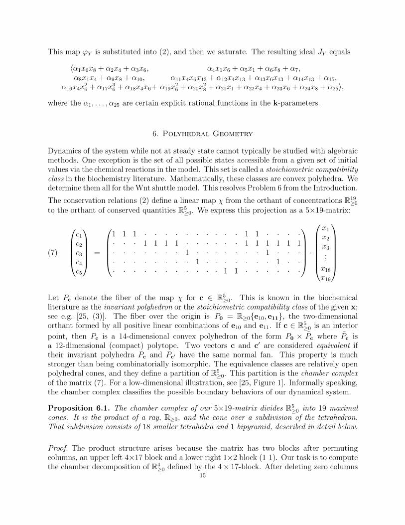
Dynamics of the system while not at steady state cannot typically be studied with algebraicmethods. One exception is the set of all possible states accessible from a given set of initialvalues via the chemical reactions in the model. This set is called a stoichiometric compatibilityclass in the biochemistry literature. Mathematically, these classes are convex polyhedra. Wedetermine them all for the Wnt shuttle model. This resolves Problem 6 from the Introduction.

The conservation relations (2) define a linear map χ from the orthant of concentrations R19≥0

to the orthant of conserved quantities R5≥0. We express this projection as a 5×19-matrix:

(7)

c1c2c3c4c5

=

1 1 1 · · · · · · · · · · 1 1 · · · ·· · · 1 1 1 1 · · · · · · 1 1 1 1 1 1· · · · · · · 1 · · · · · · · 1 · · ·· · · · · · · · 1 · · · · · · · 1 · ·· · · · · · · · · · · 1 1 · · · · · ·

·

x1x2x3...x18x19

Let Pc denote the fiber of the map χ for c ∈ R5

≥0. This is known in the biochemicalliterature as the invariant polyhedron or the stoichiometric compatibility class of the given x;see e.g. [25, (3)]. The fiber over the origin is P0 = R≥0{e10, e11}, the two-dimensionalorthant formed by all positive linear combinations of e10 and e11. If c ∈ R5

≥0 is an interior

point, then Pc is a 14-dimensional convex polyhedron of the form P0 × Pc where Pc isa 12-dimensional (compact) polytope. Two vectors c and c′ are considered equivalent iftheir invariant polyhedra Pc and Pc′ have the same normal fan. This property is muchstronger than being combinatorially isomorphic. The equivalence classes are relatively openpolyhedral cones, and they define a partition of R5

≥0. This partition is the chamber complexof the matrix (7). For a low-dimensional illustration, see [25, Figure 1]. Informally speaking,the chamber complex classifies the possible boundary behaviors of our dynamical system.

Proposition 6.1. The chamber complex of our 5×19-matrix divides R5≥0 into 19 maximal

cones. It is the product of a ray, R≥0, and the cone over a subdivision of the tetrahedron.That subdivision consists of 18 smaller tetrahedra and 1 bipyramid, described in detail below.

Proof. The product structure arises because the matrix has two blocks after permutingcolumns, an upper left 4×17 block and a lower right 1×2 block (1 1). Our task is to computethe chamber decomposition of R4

≥0 defined by the 4× 17-block. After deleting zero columns15

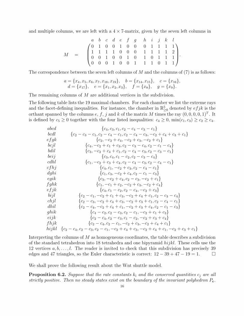
and multiple columns, we are left with a 4× 7-matrix, given by the seven left columns in

M =

a b c d e f g h i j k l

0 1 0 0 1 0 0 0 1 1 1 11 1 1 1 0 0 0 1 1 1 1 20 0 1 0 0 1 0 1 0 1 1 10 0 0 1 0 0 1 1 1 0 1 1

.The correspondence between the seven left columns of M and the columns of (7) is as follows:

a = {x4, x5, x6, x7, x18, x19}, b = {x14, x15}, c = {x16},d = {x17}, e = {x1, x2, x3}, f = {x8}, g = {x9}.

The remaining columns of M are additional vertices in the subdivision.

The following table lists the 19 maximal chambers. For each chamber we list the extreme raysand the facet-defining inequalities. For instance, the chamber in R5

≥0 denoted by efjk is the

orthant spanned by the columns e, f , j and k of the matrix M times the ray (0, 0, 0, 0, 1)T . Itis defined by c5 ≥ 0 together with the four listed inequalities: c4 ≥ 0, min(c1, c3) ≥ c2 ≥ c4.

abcd {c4, c3, c1, c2 − c4 − c3 − c1}bcdl {c2 − c3 − c1, c2 − c4 − c1, c2 − c4 − c3,−c2 + c4 + c3 + c1}efgk {c2,−c2 + c4,−c2 + c3,−c2 + c1}bcjl {c4,−c2 + c1 + c3, c2 − c3 − c4, c2 − c1 − c4}bdil {c3,−c2 + c4 + c1, c2 − c4 − c3, c2 − c3 − c1}beij {c3, c4, c1 − c2, c2 − c3 − c4}cdhl {c1,−c2 + c3 + c4, c2 − c4 − c3, c2 − c4 − c1}cfhj {c4, c1,−c2 + c3, c2 − c4 − c1}dghi {c1, c3,−c2 + c4, c2 − c1 − c3}egik {c3,−c2 + c4, c2 − c3,−c2 + c1}fghk {c1,−c1 + c2,−c2 + c3,−c2 + c4}efjk {c4, c1 − c2, c2 − c4,−c2 + c3}bijl {c2 − c1,−c2 + c1 + c3,−c2 + c4 + c1, c2 − c3 − c4}chjl {c2 − c3,−c2 + c4 + c3,−c2 + c3 + c1, c2 − c4 − c1}dhil {c2 − c4,−c2 + c4 + c1,−c2 + c3 + c4, c2 − c1 − c3}ghik {c4 − c2, c2 − c3, c2 − c1,−c2 + c1 + c3}eijk {c2 − c4, c2 − c3, c1 − c2,−c2 + c3 + c4}fhjk {c2 − c4, c2 − c1,−c2 + c3,−c2 + c4 + c1}hijkl {c2 − c4, c2 − c3, c2 − c1,−c2 + c4 + c3,−c2 + c4 + c1,−c2 + c3 + c1}

Interpreting the columns of M as homogeneous coordinates, the table describes a subdivisionof the standard tetrahedron into 18 tetrahedra and one bipyramid hijkl. These cells use the12 vertices a, b, . . . , l. The reader is invited to check that this subdivision has precisely 39edges and 47 triangles, so the Euler characteristic is correct: 12− 39 + 47− 19 = 1. �

We shall prove the following result about the Wnt shuttle model.

Proposition 6.2. Suppose that the rate constants ki and the conserved quantities cj are allstrictly positive. Then no steady states exist on the boundary of the invariant polyhedron Pc.

16

Proof. Consider the two components Im and Ie of the steady state ideal I given in Lemma 3.1.We intersect each of the two varieties with the affine-linear space defined by the conservationrelations (2) for some c ∈ R5

>0. We claim that all solutions x satisfy xi 6= 0 for i = 1, 2, . . . , 19.

For the main component V (Im), we prove this assertion with the help of the parametrizationϕY from Example 5.5. If the values of x1, x4, x6, x8, x13 and of the expression r(x4, x6) arenonzero, then each coordinate of ϕY is nonzero. We next observe that r(x4, x6) > 0 for anyk > 0 and x ≥ 0. A case analysis, using binomial relations in the ideal Im, reveals that ifany of x1, x4, x6, x8, x13 are zero, some coordinate of c is forced to zero as well:

x1 = 0 ⇒ x2, x3, x14, x15 = 0 ⇒ c1 = 0,x13 = 0 ⇒ x12 = 0 ⇒ c5 = 0,x4 = 0 ⇒ x5, x6, x7, x14, x15, x16, x17, x18, x19 = 0 ⇒ c2 = 0,

or x8, x16 = 0 ⇒ c3 = 0,x6 = 0 ⇒ x9, x17 = 0 ⇒ c4 = 0,

or x4 = 0 ⇒ c2 or c3 = 0,x8 = 0 ⇒ x16 = 0 ⇒ c3 = 0.

It remains to consider the extinction component. Its ideal Ie contains the set b ∪ l ={x1, x2, x3, x14, x15}. The corresponding columns of the matrix in (7) are the only columnswith a nonzero entry in the fourth row. This implies that c4 = 0 holds for every steady state inV (Ie). We conclude that there are no steady states on the boundary of the polyhedron Pc. �

Remark 6.3. In this proof we did not need the detailed description of the chamber complex,because of the special combinatorial structure in the Wnt shuttle model. In general, whenstudying chemical reaction networks that arise in systems biology, an analysis like Proposition6.1 is requisite for gaining information about possible zero coordinates in the steady states.

7. Parameter Estimation

Question 7 asks: What information does species concentration data give us for parameterestimation? This question is of particular importance to experimentalists, as species concen-trations depend on initial conditions, whereas parameter values are intrinsic to the biologicalprocess being modeled. Identifiability of parameters has been studied in many contexts, no-tably in statistics [8] and in biological modeling [19]. Sometimes, as in [19], parameters aredetermined from complete time-course data of the dynamical system, making a differentialalgebra approach desirable. In the present paper we focus on the steady state variety, so weconsider data collection only at steady state. We assume that there is a true but unknownparameter vector k∗ ∈ R31 of rate constants, and our data are sampled from the positivereal points x on the variety in R19 that is defined by the 19 polynomials in (1).

7.1. Complete Species Information. The first algebraic question we answer: To whatextent is the true parameter vector k∗ determined by points on its steady state variety?

To address this question, we form the polynomial matrix F (x) of format 19 × 31 whoseentries are the coefficients of the right-hand sides of (1), regarded as linear forms in k. Withthis notation, our dynamical system (1) can be written in matrix-vector product form as

x = F (x) · k.17

Our data points are sampled from

(8){

x ∈ R19>0 : F (x) · k∗ = 0

}.

Let x1,x2,x3, . . . denote generic data points in (8). The set of all parameter vectors k thatare compatible with these data is a linear subspace of R31, namely it is the intersection

(9) kernel(F (x1)) ∩ kernel(F (x2)) ∩ kernel(F (x3)) ∩ · · ·The best we can hope to recover from sampling data is the following subspace containing k∗:

(10)⋂

x in (8)

kernel(F (x)) ⊂ R31.

We refer to (10) as the space of parameters compatible with k∗. A direct computation reveals:

Proposition 7.1. The space of all parameters compatible with k∗ is a 14-dimensional sub-space of R31. If x is generic then the kernel of F (x) is a 17-dimensional subspace of R31.

This has the following noteworthy consequence for our biological application:

Corollary 7.2. The parameters of the Wnt shuttle model are not identifiable from steadystate data, but there are 14 degrees of freedom in recovering the true parameter vector k∗.

Our next step is to gain a more precise understanding of the subspaces in Proposition 7.1.To do this, we shall return to the combinatorial setting of matroid theory. We introduce twomatroids on the 31 reactions in Table 2. The common ground set is K = {k1, k2, . . . , k31}.The one-point matroid Mone is the rank 17 matroid on K defined by the linear subspacekernel(F (x)) of R31 where x ∈ R19 is generic. The parameter matroid Mpar is the rank 14matroid on K defined by the space (10) of all parameters compatible with a generic k∗. Thefollowing result, obtained by calculations, reflects the block structure of the matrix F (x).

11, 12, 31

13

22, 30

2321

20

9

10

9

10

12

11

1320

21

23

30

31

22

24

25

1

2

26

27

28

29

3

54

86

714

1615

1918

17

a) Single Data Point b) Multiple Data Points

Figure 1. Graphic representation of the one-point matroidMone of rank 17.The rank 4 component of the rank 14 parameter matroidMpar is not graphic.

Proposition 7.3. The one-point matroidMone is the graphic matroid of the graph shown inFigure 1 a). Its seven connected components are matroids of ranks 3, 3, 7, 1, 1, 1, 1. The rank14 parameter matroid Mpar is obtained from Mone by specializing the rank 7 component tothe rank 4 matroid on 11 elements whose affine representation is shown in Figure 1 b).

18

This characterizes the combinatorial constraints imposed on the parameters k by measuringthe species concentrations at steady state. For a single measurement x, the result on Mone

tells us that the 19× 31-matrix F (x) has rank 14 = 31− rank(Mone). After row operations,it block-decomposes into two matrices of format 3× 6, one matrix of format 4× 11, and fourmatrices of format 1 × 2. Each of these seven matrices is row-equivalent to the node-edgecycle matrix of a directed graph, with underlying undirected graph as in Figure 1 (a).

Consider the graph with edges 9, 10, 11, 12, 13, 20, 21, 22, 23, 30, 31. The cycle {22, 23, 30, 31}reveals that our measurement x imposes one linear constraint on k22, k23, k30, k31. If we takefurther measurements, as in (9), then six of the seven blocks of F (x) remain unchanged. Onlythe 4× 11-block of F (x) must be enlarged, to a 7× 11-matrix. The rows of that new matrixspecify the affine-linear dependencies among 11 points in R3. That point configurationis depicted in Figure 1 (b). For instance, the points {9, 10, 11} are collinear, the points{20, 21, 22} are collinear, but these two lines are skew in R3. From the other line we see thatthat repeated measurements at steady state impose two linear constraints on k22, k23, k30, k31.

7.2. Circuit Data. The second question we address in this section: Given partial speciesconcentration data, is any information about parameters available? In Section 7.1, all 19concentrations xi were available for a steady state. In what follows, we suppose that xi canonly be measured for indices i in a subset of the species, say C ⊂ {1, . . . , 19}. In our analysis,it will be useful to take advantage of the rank 5 algebraic matroid in Proposition 5.2, sincethat matroid governs dependencies among the coordinates x1, . . . , x19 at steady states.

We here focus on the special case when C is one of the 951 circuits of the algebraic matroid

of Im. Let fC be the corresponding circuit polynomial, as in Table 5. We regard fC as apolynomial in x whose coefficients are polynomials in Q[k]. Suppose that fC has r monomialsxa1 , . . . ,xar . We write FC ∈ Q[k]r for the vector of coefficients, so our circuit polynomial isthe dot product fC(k,x) = FC(k)·(xa1 , . . . ,xar). We write VC ⊂ Rr for the algebraic varietyparametrized by FC(k). Thus VC is the Zariski closure in Rr of the set {FC(k′) : k′ ∈ R31}.Our idea for parameter recovery is this: rather than looking for k compatible with the trueparameter k∗, we seek a point y = FC(k) in VC that is compatible with FC(k∗). And, onlylater do we compute a preimage of y under the map R31 → Rr given by FC . Most interestingis the case when VC is a proper subvariety of Rr. Direct computations yield the following:

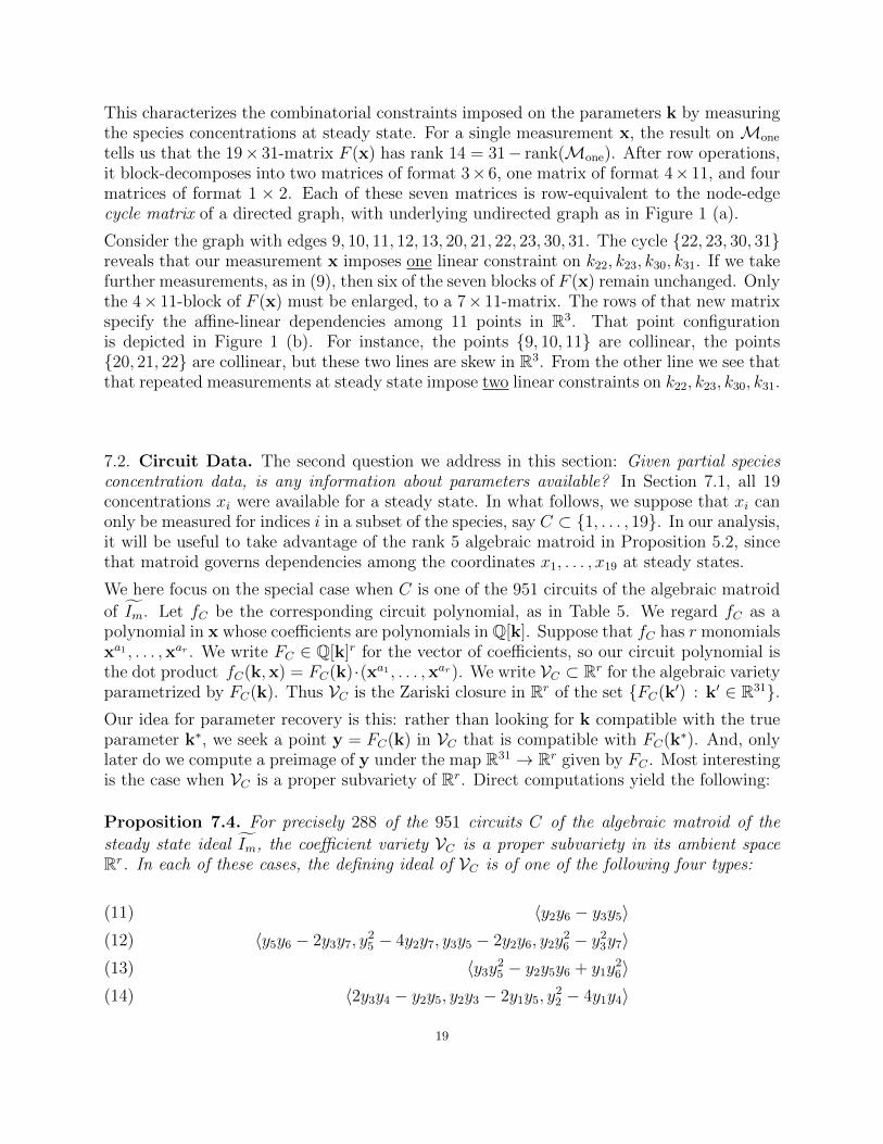
Proposition 7.4. For precisely 288 of the 951 circuits C of the algebraic matroid of the

steady state ideal Im, the coefficient variety VC is a proper subvariety in its ambient spaceRr. In each of these cases, the defining ideal of VC is of one of the following four types:

〈y2y6 − y3y5〉(11)

〈y5y6 − 2y3y7, y25 − 4y2y7, y3y5 − 2y2y6, y2y

26 − y23y7〉(12)

〈y3y25 − y2y5y6 + y1y26〉(13)

〈2y3y4 − y2y5, y2y3 − 2y1y5, y22 − 4y1y4〉(14)

19

Example 7.5. Consider the circuit C = {6, 10, 18}. The circuit polynomial fC equals

(k13k20k22 + k20k22k30) · x6x10 + k11k20k22 · x6x18 − k12k20k22 · x6+(k13k21k23 + k13k22k23 + k21k23k30 + k22k23k30 + k13k21k31 + k13k22k31) · x10

+(k11k21k23 + k11k22k23 + k11k21k31 + k11k22k31) · x18− (k12k21k23 + k12k22k23 + k12k21k31 + k12k22k31).

Here r = 6 and we write FC(k) = (y1, y2, y3, y4, y5, y6) for the vector of coefficient polynomi-als. The variety VC is the hypersurface in R5 defined by the equation y2y6 = y3y5.

We now sample data points xi from the model with the true (but unknown) parameter vectork∗. Each such point defines a hyperplane {y ∈ Rr : y · (xa1

1 , . . . ,xarr ) = 0}. The parameter

estimation problem is to find the intersection of these data hyperplanes with the variety VC .That intersection contains the point y∗ = FC(k∗), which is what we now aim to recover.

7.3. Noisy Circuit Data. The final question we consider in this section is: Given partialspecies concentration data with noise, is any information about parameters available?

As in Section 7.2, we fix a circuit C of the algebraic matroid in Section 5, and we assumethat we can only measure the concentrations xj where j ∈ C. Each measurement xi ∈ RC

still defines a hyperplane y · (xa1i , . . . ,x

ari ) = 0 in the space Rr. But now the true vector

y∗ = FC(k∗) is not exactly on that hyperplane, but only close to it. Hence, if we take srepeated measurements, with s > r, the intersection of these hyperplanes should be empty.

We propose to find the best fit by solving the following least squares optimization problem:

(15) Minimizes∑

i=1

(y · (xa1

i , . . . ,xari ))2

subject to y ∈ VC ∩ Sr−1,

where Sr−1 = {y ∈ Rr : y21 + y22 + · · · + y2r = 1} denotes the unit sphere. When the varietyVC is the full ambient space Rr, this is a familiar regression problem, namely, to find thehyperplane through the origin that best approximates s given points in Rr. Here “best”means that the sum of the squared distances of the s points to the hyperplane is minimized.This happens for 663 of the 951 circuits C, and in that case we can apply standard techniques.

However, for the 288 circuits C identified in Proposition 7.4, the problem is more interesting.Here the hyperplanes under consideration are constrained to live in a proper subvariety. Inthat case we need some algebraic geometry to reliably find the global optimum in (15).

Our problem is to minimize a quadratic function over the real affine variety VC ∩ Sr−1. Thequadratic objective function is generic because the xi are sampled with noise. The intrinsicalgebraic complexity of our optimization problem was studied by Draisma et al. in [5]. Thatcomplexity measure is the ED degree of VC ∩ Sr−1, which is the number of solutions in Cr

to the critical equations of (15). Here, by ED degree we mean the ED degree of VC ∩ Sr−1,when considered in generic coordinates. This was called the generic ED degree in [20].

We illustrate our algebraic approach by working out the first instance (11) in Proposition 7.4.

Example 7.6. Suppose we are given s noisy measurements of the concentrations x6, x10, x18.In order to find the best fit for the parameters k, we employ the circuit polynomial fC in

20

Example 7.5. We compute y ∈ R6 by solving the corresponding optimization problem (16).This problem is to minimize a random quadratic form subject to two quadratic constraints

(16) y2y6 − y3y5 = y21 + y22 + y23 + y24 + y25 + y26 − 1 = 0.

We solve this problem using the method of Lagrange multipliers. This leads to a system ofpolynomial equations in y. Using saturation, we remove the singular locus of (16), which isthe circle {y ∈ R6 : y21 + y24 − 1 = y2 = y3 = y5 = y6 = 0}. The resulting ideal has precisely40 zeros in C6. In the language of [5,20], the generic ED degree of the variety (16) equals 40.

8. From Algebra to Biology

The aims of this paper are: (1) to demonstrate how biology can lead to interesting ques-tions in algebraic geometry, and (2) to apply new techniques from computational algebrain biology. So far, our tour through (numerical) algebraic geometry, polyhedral geometryand combinatorics has demonstrated the range of mathematical questions to explore. Inthis section, we will focus on translating our analysis into applicable considerations for theresearch cycle in systems biology, which is illustrated in Figure 2. In what follows we discusssome concrete applications and results pertaining to the steps (a), (b) and (c) in Figure 2.

Im

ReTheorem I

xi + xj xi + xl k

Discriminant, Ex. 4.3Prop. 6.2, Ex. 8.1 Matroids

Prop. 5.2, Ex. 8.2

Model rejection via CircuitsEx 5.3, Ex. 8.3

Parameter estimation, Cor. 7.2, Ex. 8.4

Biologicalhypothesis

Model construction

Wnt Signal

Response?

Model f(x,k) Steady states f = 0

(a) Model analysis (b) Experimental design

(c) Model and data compatibility

Experiments Model variety

Data pointBiologicalinsight

Figure 2. Systems biology cycle informed by algebraic geometry and com-binatorics. (a) Model analysis. See Sections 1, 3, 4. (b) Experimental design.See Sections 5 and 6. (c) Model and data compatibility. See Sections 5 and 7.

Analysis of the Model: Before any experiments are performed, our techniques inform themodeler of the global steady-state properties of the model. The number of real solutions tosystem (1)–(2), stated in Theorem 1.1, governs the number of observable steady states. Var-ious sampling schemes demonstrated that most parameter values lead to only one observablesteady state. We produced a set of parameter values and conserved quantities with threereal solutions, and two solutions are also attainable. If the “true” parameters k∗ and c∗

admit multiple real solutions, then multistationarity of the system is theoretically possible.

If multiple states are observed experimentally, then the model must be capable of multista-tionarity. In the Wnt shuttle model, the system is capable of multiple steady states; however,based on parameter sampling, the frequency of this occurrence is low, and parameters in this

21

regime are somewhat stable under perturbation. The discriminant of the system is a poly-nomial of degree 34 in c, and our analysis along a single line in c-space illustrates the highdegree of complexity inherent in the full stratification of the 36-dimensional parameter space.

Experimental Design: In Section 6, the combinatorial structure of the various stoichiomet-ric compatibility classes was fully characterized. As the conserved quantities c = (c1, . . . , c5)range over all positive real values, the set of all compatible species-concentration vectors xwill take one of 19 polyhedral shapes Pc. This may find application in identifying multiplesteady state solutions for specific rate constants k. A natural choice for initial conditionswhen performing experiments is on or near the vertices of the 14-dimensional polyhedron Pc.

Example 8.1. Suppose the conserved quantities vector lies in the bipyramid, e.g. c =(1, 2, 2, 2, 3). The preimage of c in x-space is a product of the orthant R≥0{e10, e11} anda 12-dimensional polytope with 400 vertices: (1, 0, 0, 2, 0, 0, 0, 2, 2, 0, 0, 3, 0, 0, 0, 0, 0, 0, 0, 0),and 399 of its permutations. This product is the polyhedron Pc. If we have control over initialconditions, beginning near the vertices positions us to find interesting systems behavior.

In the laboratory, the experimentalist makes choices of what to measure and what not tomeasure. For instance, measuring a particular xi may be infeasible, or there may be asituation in which measuring concentration xi can preclude measuring concentration xj.

For every strategy, we fix a cost vector, listing the costs of making each measurement. We usethe symbol N to indicate infeasible measurements. Suppose there are two different ways torun the experiment; then we have a 2×19 cost matrix P , whose rows are cost vectors for eachexperiment. We multiply P by the 0-1-incidence matrix for the 951 circuits of Proposition5.2. That matrix has a 1 in row i and column j if circuit j contains species i, and 0 otherwise.The product is a matrix of size 2× 951. For N →∞, the 2× 951 matrix has a finite entryin position (i, j) precisely when the strategy i can measure the circuit j. Minimizing overthose finite cost entries selects the most cost-effective experiment to measure a circuit.

Example 8.2. Suppose that none of the intermediate complexes x13, . . . , x19 are measurable,and that we are able to measure only one Phosphatase concentration (x4 or x8) in eachexperimental setup. A corresponding cost matrix might look like

P =

[1 1 1 N 1 1 1 1 1 1 1 1 N N N N N N N1 1 1 1 1 1 1 N 1 1 1 1 N N N N N N N

]Multiplying by the circuit support matrix of size 19 × 951 reveals 82 feasible experiments:50 using the first row of P , and 32 using the second. With more refined cost assignment,this would decide not only feasibility but also optimal cost. In this way, the matroid allowsus to choose cost-minimal experiments to obtain meaningful information for the model.

Model and data compatibility: After an experiment is performed, the task of the modeleris to test the data with the model. One possible outcome is model rejection. If the data arecompatible, then another outcome is parameter estimation. Both may provide insights forbiology. The role of algebraic geometry is seen in [9,10] and shown in the next two examples.

Example 8.3 (Model Rejection). Suppose that rate parameters ki are all known to be 1,and that we have collected data for variables x1, x4, x14. The circuit polynomial is k1k3x1x4+(−k2k4−k2k5)x14, which specializes to x1x4−2x14. If the evaluation of the positive quantity|x1x4−2x14| lies above a threshold ε, then we can reject the model as not matching the data.

22

Every circuit polynomial of the matroid is a steady state invariant; depending on whichexperiment was performed, the collection of measured variables must contain some circuit.Even if one can measure all 19 species at steady state, it is not possible to recover all 31 kineticrate constants, but we do have relationships that must be satisfied among parameters [16].

Example 8.4 (Parameter Estimation). Suppose that rate parameters are unknown, and thatwe have collected data for x6, x10, x18. The corresponding circuit polynomial fC is shown inExample 7.5. We know that the coefficients of fC satisfy the constraint y2y6 = y3y5. Supposeour experiments lead to the following ten measurements for the vector (x6, x10, x18):

{(.715335, 4.06778, 14.6806), (.390982, 4.83152, 6.08251), (.706539, 4.98107, 3.83617),(.14316, 4.30851, 12.5809), (.995583, 4.01222, 15), (.413817, 4.08114, 14.902), (.232206, 3.38274, 23.3162),

(.219045, 5.06008, 3.67175), (.704106, 3.52804, 21.1037), (.648732, 3.6505, 19.7008)}

The data lead us to the following function to optimize in (15):

57.2345y21 + 376.181y1y2 + 801.672y22 − 27.5625y1y3 − 96.4429y2y3+3.36521y23 + 179.49y1y4 + 564.034y2y4 − 42.729y3y4 + 178.839y24 + 564.034y1y5

+2424.31y2y5 − 144.7y3y5 + 1054.49y4y5 + 2263.2y25 − 42.729y1y6−144.7y2y6 + 10.339y3y6 − 83.8072y4y6 − 269.749y5y6 + 10y26

The global minimum of this quadratic form on the codimension 2 variety (16) has coordinates

y1 = 0.183472, y2 = 0.152416, y3 = 0.959232, y4 = 0.038042, y5 = 0.00335267, y6 = 0.211.

Given these values, one now has three degrees of freedom in estimating the nine parameterski that appear in the circuit polynomial fC . The other ten coordinates of k are unspecified.

Acknowledgements

This project was supported by UK Royal Society International Exchange Award 2014/R1IE140219. EG, BS and HAH initiated discussions at an American Institute of Mathematicsworkshop in Palo Alto. Part of the work was carried out at the Simons Institute for Theoryof Computing in Berkeley. HAH gratefully acknowledges EPSRC Fellowship EP/K041096/1.EG, ZR and BS were also supported by the US National Science Foundation, through grantsDMS-1304167, DMS-0943745 and DMS-1419018 respectively. Thanks to Helen Byrne andReinhard Laubenbacher for comments on early drafts of the paper.

References

[1] D. Bates, J. Hauenstein, A. Sommese and C. Wampler: Numerically Solving Polynomial Systems withBertini, Software, Environments, and Tools, Vol. 25, SIAM, Philadelphia, 2013.

[2] D. Bates, E. Gross, A. Leykin and J. Rodriguez: Bertini for Macaulay2, arXiv:1310.3297.[3] C. Chen, J. Davenport, M. Moreno Maza, B. Xia and R. Xiao: Computing with semi-algebraic sets:

Relaxation techniques and effective boundaries, J. Symbolic Computation 52 (2013), 72–96.[4] G. Craciun and M. Feinberg: Multiple equilibria in complex chemical reaction networks. I. The injectivity

property, SIAM J. Appl. Math. 65 (2005) 1526–1546.[5] J. Draisma, E. Horobet, G. Ottaviani, B. Sturmfels and R.R. Thomas: The Euclidean distance degree

of an algebraic variety, Foundations of Computational Mathematics, to appear, arXiv:1309.0049.23

[6] J-C. Faugere, G. Moroz, F. Rouillier and M. Safey El Din: Classification of the perspective-three-pointproblem, discriminant variety and real solving polynomial systems of inequalities, ISSAC 2008, 79–86,ACM, New York, 2008.

[7] E. Feliu and C. Wiuf: Variable elimination in chemical reaction networks with mass-action kinetics,SIAM J. Appl. Math 72 (2012) 959–981.

[8] L. Garcia-Puente, S. Petrovic and S. Sullivant: Graphical models, J. Softw. Algebra Geom. 5 (2013) 1–7.[9] E. Gross, B. Davis, K. Ho, D. Bates and H. Harrington: Model selection using numerical algebraic

geometry, in preparation.[10] H. Harrington, K. Ho, T. Thorne and M. Stumpf: Parameter-free model discrimination criterion based

on steady-state coplanarity, Proc. Natl. Acad. Sci. 109 (2012) 15746–15751.[11] D. Grayson and M. Stillman: Macaulay2, a software system for research in algebraic geometry, available

at www.math.uiuc.edu/Macaulay2/.[12] R. Karp, M. Perez Millan, T. Desgupta, A. Dickenstein and J. Gunawardena: Complex-linear invariants

of biochemical networks, J. Theoret. Biol. 311 (2012) 130–138.[13] E. Klipp, W. Liebermeister, C. Wierling, A. Kowald, H. Lehrach and R. Herwig: Systems Biology, John

Wiley & Sons, 2009.[14] F. Kiraly, Z. Rosen and L. Theran: Algebraic matroids with graph symmetry, arXiv:1312.3777.[15] F. Kiraly, L. Theran, R. Tomioka: The algebraic combinatorial approach for low-rank matrix completion,

to appear in Journal of Machine Learning Research, arXiv:1211.4116.[16] A. MacLean, H. Harrington, M. Stumpf and H. Byrne: Mathematical and statistical techniques for

systems medicine: The Wnt signaling pathway as a case study, in Systems Biology for Medicine, toappear the series “Methods in Molecular Biology”, Springer, New York.

[17] A. MacLean, Z. Rosen, H. Byrne and H. Harrington: Parameter-free methods distinguish Wnt pathwaymodels and guide design of experiments, Proc. Natl. Acad. Sci, to appear, arXiv:1409.0269.

[18] N. Meshkat and S. Sullivant: Identifiable reparametrizations of linear compartment models, J. SymbolicComput. 63 (2014) 46–67.

[19] A. Morgan and A. Sommese: Coefficient-parameter polynomial continuation, Appl. Math. Comput. 29(1989) 123–160.

[20] G. Ottaviani, P-J. Spaenlehauer and B. Sturmfels: Exact solutions in structured low-rank approximation,SIAM J. Matrix Anal. Appl. 35 (2014) 1521–1542.

[21] J. Oxley: Matroid Theory, Oxford University Press, 2011.[22] M. Perez Millan, A. Dickenstein, A. Shiu and C. Conradi: Chemical reaction systems with toric steady

states, Bull. Math. Biol. 74 (2012) 1027–1065.[23] J. Rodriguez and X. Tang: Data-discriminants of likelihood equations, arXiv:1501.00334.[24] Z. Rosen: Computing algebraic matroids, arXiv:1403.8148.[25] A. Shiu and B. Sturmfels: Siphons in chemical reaction networks, Bull. Math. Biol. 72 (2010) 1448–1463.[26] J. Verschelde: Algorithm 795: PHCpack: A general-purpose solver for polynomial systems by homotopy

continuation, ACM Trans. Math. Softw. 25 (1999) 251–276.[27] E. Voit: A First Course in Systems Biology, Garland Science, 2012.

Elizabeth Gross: San Jose State University, elizabeth.gross@sjsu.eduHeather A. Harrington: University of Oxford, harrington@maths.ox.ac.ukZvi Rosen: University of California at Berkeley, zhrosen@berkeley.eduBernd Sturmfels: University of California at Berkeley, bernd@berkeley.edu

24