Newcastle University ePrints - eprint.ncl.ac.uk

Mokhov A. Algebraic Graphs with Class (functional pearl). In: Haskell

Symposium 2017 (part of Proceedings of the 10th ACM SIGPLAN International

Symposium on Haskell). 2017, Oxford: ACM.

Copyright:

© Author 2017. This is the author's version of the work. It is posted here for your personal use. Not for

redistribution. The definitive Version of Record was published in Proceedings of the 10th ACM SIGPLAN

International Haskell Symposium, September 7-8, 2017, https://doi.org/10.1145/3122955.3122956.

DOI link to paper:

https://doi.org/10.1145/3122955.3122956

Date deposited:

05/09/2017

Algebraic Graphs with Class (Functional Pearl)Andrey Mokhov

Newcastle University, United Kingdom

AbstractThe paper presents a minimalistic and elegant approach to workingwith graphs in Haskell. It is built on a rigorous mathematical foun-dation — an algebra of graphs — that allows us to apply equationalreasoning for proving the correctness of graph transformation al-gorithms. Algebraic graphs let us avoid partial functions typicallycaused by ‘malformed graphs’ that contain an edge referring to anon-existent vertex. This helps to liberate APIs of existing graphlibraries from partial functions.

The algebra of graphs can represent directed, undirected, reflex-ive and transitive graphs, as well as hypergraphs, by appropriatelychoosing the set of underlying axioms. The flexibility of the ap-proach is demonstrated by developing a library for constructingand transforming polymorphic graphs.

CCS Concepts • Mathematics of computing;

Keywords Haskell, algebra, graph theoryACM Reference Format:Andrey Mokhov. 2017. Algebraic Graphs with Class (Functional Pearl). InProceedings of 10th ACM SIGPLAN International Haskell Symposium, Oxford,UK, September 7-8, 2017 (Haskell’17), 12 pages.https://doi.org/10.1145/3122955.3122956

1 IntroductionGraphs are ubiquitous in computing, yet working with graphs oftenrequires painfully low-level fiddling with sets of vertices and edges.Building high-level abstractions is difficult, because the commonlyused foundation – the pair (V ,E) of vertex set V and edge setE ⊆ V ×V – is a source of partial functions. We can represent thepair (V ,E) by the following simple data type1:

data G a = G { vertices :: [a], edges :: [(a,a)] }

Now G [1,2,3] [(1,2),(2,3)] is the graph with three verticesV = {1, 2, 3} and two edges E = {(1, 2), (2, 3)}. The consistencyinvariant E ⊆ V ×V holds. But what is G [1] [(1,2)]? The edgerefers to the non-existent vertex 2, breaking the invariant, and thereis no easy way to reflect this in types. Perhaps, our data type is justtoo simplistic; let us look at state-of-the-art graph libraries instead.

The containers library is designed for performance and powersGHC itself. It represents graphs by adjacency arrays [King andLaunchbury 1995] whose consistency invariant is not staticallychecked, which can lead to runtime usage errors such as ‘indexout of range’. Another popular library fgl uses the inductive graphrepresentation [Erwig 2001], but its API also has partial functions,e.g. inserting an edge can fail with the ‘edge from non-existent

1Although in this paper we exclusively use Haskell, the problem we solve is generaland the proposed approach can be readily adapted to other programming languages.

Haskell’17, September 7-8, 2017, Oxford, UK© 2017 Copyright held by the owner/author(s). Publication rights licensed to Associa-tion for Computing Machinery.This is the author’s version of the work. It is posted here for your personal use.Not for redistribution. The definitive Version of Record was published in Proceed-ings of 10th ACM SIGPLAN International Haskell Symposium, September 7-8, 2017 ,https://doi.org/10.1145/3122955.3122956.

vertex’ error. Both containers and fgl are treasure troves of graphalgorithms, but it is easy to make an error when using them. Isthere a safe graph construction interface we can build on top?

In this paper we present algebraic graphs — a new interfacefor constructing and transforming graphs (more precisely, graphswith labelled vertices and unlabelled edges). We abstract awayfrom graph representation details and characterise graphs by a setof axioms, much like numbers are algebraically characterised byrings [Mac Lane and Birkhoff 1999]. Our approach is based on thealgebra of parameterised graphs, a mathematical formalism usedin digital circuit design [Mokhov and Khomenko 2014], which wesimplify and adapt to the context of functional programming.

Algebraic graphs have a safe and minimalistic core of four graphconstruction primitives, as captured by the following data type:

data Graph a = Empty| Vertex a| Overlay (Graph a) (Graph a)| Connect (Graph a) (Graph a)

Here Empty and Vertex construct the empty and single-vertexgraphs, respectively; Overlay composes two graphs by takingthe union of their vertices and edges, and Connect is similar toOverlay but also creates edges between vertices of the two graphs,see Fig. 1 for examples. The overlay and connect operations havetwo important properties: (i) they are closed on the set of graphs,i.e. are total functions, and (ii) they can be used to construct anygraph starting from the empty and single-vertex graphs. For exam-ple, Connect (Vertex 1) (Vertex 2) is the graph with two ver-tices {1, 2} and a single edge (1, 2). Malformed graphs, such asG [1] [(1,2)], cannot be expressed in this core language.

The main goal of this paper is to demonstrate that this core isa safe, flexible and elegant foundation for working with graphs thathave no edge labels. Our specific contributions are:• Compared to existing libraries, algebraic graphs have a smallercore (just four graph construction primitives), are more com-positional (hence greater code reuse), and have no partialfunctions (hence fewer opportunities for usage errors). Wepresent the core and justify these claims in §2.• The core has a simple mathematical structure fully charac-terised by a set of axioms (§3). This makes the proposedinterface easier for testing and formal verification. We showthat the core is complete, i.e. any graph can be constructed,and sound, i.e. malformed graphs cannot be constructed.• Under the basic set of axioms, algebraic graphs correspond todirected graphs. As we show in §4, by extending the algebrawith additional axioms, we can represent undirected, reflex-ive, transitive graphs, their combinations, and hypergraphs.Importantly, the core remains unchanged, which allows usto define highly reusable polymorphic functions on graphs.• We develop a library2 for constructing and transformingalgebraic graphs and demonstrate its flexibility in §5.

2The library is on Hackage: http://hackage.haskell.org/package/algebraic-graphs.

Haskell’17, September 7-8, 2017, Oxford, UK Andrey Mokhov

1 21 2+ =

(a) 1 + 2

1 2 = 1 2

(b) 1→ 2

1 =3

2

+ 13

2

(c) 1→ (2 + 3)

=1 1 1

(d) 1→ 1 (e) 1→ 2 + 2→ 3

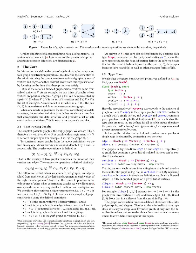
Figure 1. Examples of graph construction. The overlay and connect operations are denoted by + and→, respectively.

Graphs and functional programming have a long history. Wereview related work in §6. Limitations of the presented approachand future research directions are discussed in §7.

2 The CoreIn this section we define the core of algebraic graphs comprisingfour graph construction primitives. We describe the semantics ofthe primitives using the common representation of graphs by sets ofvertices and edges, and then abstract away from this representationby focusing on the laws that these primitives satisfy.

LetG be the set of all directed graphs whose vertices come froma fixed universe V. As an example, we can think of graphs whosevertices are positive integers. A graph д ∈ G can be represented bya pair (V ,E) whereV ⊆ V is the set of its vertices and E ⊆ V ×V isthe set of its edges. As mentioned in §1, when E * V ×V the pair(V ,E) is inconsistent and does not correspond to a graph.

When one needs to guarantee the internal consistency of a datastructure, the standard solution is to define an abstract interfacethat encapsulates the data structure and provides a set of safeconstruction primitives. This is exactly the approach we take.

2.1 Constructing GraphsThe simplest possible graph is the empty graph. We denote it by ε ,therefore ε = (∅,∅) and ε ∈ G. A graph with a single vertex v ∈ Vis denoted simply by v . For example, 1 ∈ G is the graph (1,∅).

To construct larger graphs from the above primitives we de-fine binary operations overlay and connect, denoted by + and→,respectively. The overlay operation + is defined as

(V1,E1) + (V2,E2)def= (V1 ∪V2,E1 ∪ E2).

That is, the overlay of two graphs comprises the union of theirvertices and edges. The connect→ operation is defined similarly:

(V1,E1) → (V2,E2)def= (V1 ∪V2,E1 ∪ E2 ∪V1 ×V2).

The difference is that when we connect two graphs, an edge isadded from each vertex of the left-hand argument to each vertex ofthe right-hand argument3. Note that the connect operation is theonly source of edges when constructing graphs. As we will see in §3,overlay and connect are very similar to addition and multiplication.We therefore give connect a higher precedence, i.e. 1 + 2 → 3 isinterpreted as 1+ (2→ 3). Fig. 1 illustrates a few examples of graphconstruction using the defined primitives:• 1 + 2 is the graph with two isolated vertices 1 and 2.• 1→ 2 is the graph with an edge between vertices 1 and 2.• 1→ (2+3) comprises vertices {1, 2, 3} and edges {(1, 2), (1, 3)}.• 1→ 1 is the graph with vertex 1 and the self-loop.• 1→ 2 + 2→ 3 is the path graph on vertices {1, 2, 3}.

3Our definitions of overlay and connect coincide with those of graph union and join,respectively, e.g see Harary [1969], however the arguments of union and join aretypically assumed to have disjoint sets of vertices. We make no such assumptions,hence our definitions are total: any graphs can be composed using overlay and connect.

As shown in §1, the core can be represented by a simple datatype Graph, parameterised by the type of vertices a. To make thecore more reusable, the next subsection defines the core type classthat has the usual inhabitants, such as the pair (V ,E), data typesfrom containers and fgl, as well as other, stranger forms of life.

2.2 Type ClassWe abstract the graph construction primitives defined in §2.1 asthe type class Graph4:class Graph g where

type Vertex gempty :: gvertex :: Vertex g -> goverlay :: g -> g -> gconnect :: g -> g -> g

Here the associated type5 Vertex g corresponds to the universe ofgraph vertices V, empty is the empty graph ε , vertex constructsa graph with a single vertex, and overlay and connect composegiven graphs according to the definitions in §2.1. All methods of thetype class are total, i.e. are defined for all possible inputs, therefore,the presented API allows fewer opportunities for usage errors andgreater opportunities for reuse.

Let us put the interface to the test and construct some graphs. Asingle edge is obtained by connecting two vertices:edge :: Graph g => Vertex g -> Vertex g -> gedge x y = connect (vertex x) (vertex y)

The graphs in Fig. 1(b,d) are edge 1 2 and edge 1 1, respectively.A graph that contains a given list of isolated vertices can be con-structed as follows:vertices :: Graph g => [Vertex g] -> gvertices = foldr overlay empty . map vertex

That is, we turn each vertex into a singleton graph and overlaythe results. The graph in Fig. 1(a) is vertices [1,2]. By replacingoverlaywith connect in the above definition, we obtain a directedclique – a fully connected graph on a given list of vertices:clique :: Graph g => [Vertex g] -> gclique = foldr connect empty . map vertex

For example, clique [1,2,3] expands to 1→ 2→ 3→ ε , i.e. thegraph with three vertices {1, 2, 3} and three edges (1, 2), (1, 3) and(2, 3). Note that it is different from the graph in Fig. 1(e).

The graph construction functions defined above are total, fullypolymorphic, and elegant. Thanks to the minimalistic core typeclass, it is easy to wrap your favourite graph library into the de-scribed interface, and reuse the above functions, as well as manyothers that we define throughout this paper.

4The name collision (data Graph and class Graph) is not a problem in practice,because the data type and type class are not used together and live in separate modules.5Associated types [Chakravarty et al. 2005] require the TypeFamilies GHC extension.

Algebraic Graphs with Class (Functional Pearl) Haskell’17, September 7-8, 2017, Oxford, UK

1 =3

2

+ 13

2 1 2

+1 3

=

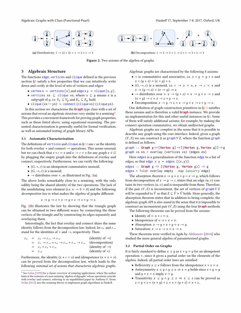
(a) Distributivity: 1→ (2 + 3) = 1→ 2 + 1→ 3

=

1 3

2

1 2 3

1

2+

1 3 3

2

=

(b) Decomposition: 1→ 2→ 3 = 1→ 2 + 1→ 3 + 2→ 3

Figure 2. Two axioms of the algebra of graphs.

3 Algebraic StructureThe functions edge, vertices and clique defined in the previoussection §2 satisfy a few properties that we can intuitively writedown and verify at the level of sets of vertices and edges:• vertex x = vertices [x] and edge x y = clique [x,y].• vertices xs ⊆ clique xs, where x ⊆ y means x is asubgraph of y, i.e. Vx ⊆ Vy and Ex ⊆ Ey hold.• clique (xs ++ ys) = connect (clique xs) (clique ys).

In this section we characterise the Graph type class with a set ofaxioms that reveal an algebraic structure very similar to a semiring6.This provides a convenient framework for proving graph properties,such as those listed above, using equational reasoning. The pre-sented characterisation is generally useful for formal verification,as well as automated testing of graph library APIs.

3.1 Axiomatic CharacterisationThe definitions of vertices and clique in §2.2 use ε as the identityfor both overlay + and connect→ operations. This seems unusual,but we can check that x +ε = x and x → ε = x for any graph x ∈ Gby plugging the empty graph into the definitions of overlay andconnect, respectively. Furthermore, we can verify the following:• (G,+, ε ) is an idempotent commutative monoid.• (G,→, ε ) is a monoid.• → distributes over +, as illustrated in Fig. 2(a).

The above looks remarkably close to a semiring, with the onlyoddity being the shared identity of the two operations. The lack ofthe annihilating zero element (i.e. x → 0 = 0) and the followingdecomposition law is what makes the algebra of graphs different:

x → y → z = x → y + x → z + y → z.

Fig. 2(b) illustrates the law by showing that the triangle graphcan be obtained in two different ways: by connecting the threevertices of the triangle and by constructing its edges separately andoverlaying them.

Interestingly, the fact that overlay and connect share the sameidentity follows from the decomposition law. Indeed, let ε+ and ε→stand for the identities of + and→, respectively. Then:

ε+ = ε+ → ε→ → ε→ (identity of→)= ε+ → ε→ + ε+ → ε→ + ε→ → ε→ (decomposition)= ε+ + ε+ + ε→ (identity of→)= ε→ (identity of +)

Furthermore, the identity (x + ε = x ) and idempotence (x + x = x )can be proved from the decomposition law, which leads to thefollowing minimal set of axioms that characterise algebraic graphs.

6 See Golan [1999] for a classic overview of semiring applications, where the authorhints at the existence of a non-semiring ‘algebra of digraphs’ whose operations coincidewith overlay and connect, referring to an unpublished paper by Anthony P. Stone.Dolan [2013] uses the semiring theory to implement graph algorithms in Haskell.

Algebraic graphs are characterised by the following 8 axioms:• + is commutative and associative, i.e. x + y = y + x andx + (y + z) = (x + y) + z.• (G,→, ε ) is a monoid, i.e. ε → x = x , x → ε = x andx → (y → z) = (x → y) → z.• → distributes over +: x → (y + z) = x → y + x → z and(x + y) → z = x → z + y → z.• Decomposition: x → y → z = x → y + x → z + y → z.

Our definition of graph construction primitives in §2.1 satisfiesthese axioms and is therefore a valid Graph instance. We providean implementation for this and other useful instances in §4. Someof them will satisfy additional axioms; for example, by making theconnect operation commutative, we obtain undirected graphs.

Algebraic graphs are complete in the sense that it is possible todescribe any graph using the core interface. Indeed, given a graph(V ,E) we can construct it as graphV E, where the function graphis defined as follows.graph :: Graph g => [Vertex g] -> [(Vertex g, Vertex g)] -> ggraph vs es = overlay (vertices vs) (edges es)

Here edges is a generalisation of the function edge to a list ofedges, so that edge x y = edges [(x,y)]:edges :: Graph g => [(Vertex g, Vertex g)] -> gedges = foldr overlay empty . map (uncurry edge)

The absorption theorem x → y + x + y = x → y, which followsfrom decomposition of x → y → ε , states that an edge (u,v ) con-tains its two vertices {u,v} and is inseparable from them. Therefore,if the pair (V ,E) is inconsistent, the set of vertices of graphV Ewill be expanded to V̂ so that E ⊆ V̂ × V̂ holds. More generally, theabsorption theorem states that in addition to being complete, thealgebraic graph API is also sound in the sense that it is impossible toconstruct an inconsistent pair (V ,E) using the four Graphmethods.

The following theorems can be proved from the axioms:• Identity of +: x + ε = x .• Idempotence of +: x + x = x .• Absorption: x → y + x + y = x → y.• Saturation: x → x → x = x → x .

These theorems were verified in Agda by Alekseyev [2014] whostudied the more general algebra of parameterised graphs.

3.2 Partial Order on GraphsIt is fairly standard to define x ≼ y as x + y = y for an idempotentoperation +, since it gives a partial order on the elements of thealgebra. Indeed, all partial order laws are satisfied:• Reflexivity x ≼ x follows from the idempotence x + x = x .• Antisymmetry x ≼ y ∧y ≼ x ⇒ x = y holds since x +y = yand y + x = x imply x = y.• Transitivity x ≼ y ∧ y ≼ z ⇒ x ≼ z can be proved asz = y + z = (x + y) + z = x + (y + z) = x + z.

Haskell’17, September 7-8, 2017, Oxford, UK Andrey Mokhov

vertices (h:t) = foldr overlay empty (map vertex (h:t)) (definition of vertices)= foldr overlay empty (vertex h : map vertex t) (definition of map)= overlay (vertex h) (vertices t) (definition of foldr)⊆ overlay (vertex h) (clique t) (monotony and the inductive hypothesis)⊆ connect (vertex h) (clique t) (overlay-connect order)= foldr connect empty (vertex h : map vertex t) (definition of foldr)= foldr connect empty (map vertex (h:t)) (definition of map)= clique (h:t) (definition of clique)

Figure 3. Equational reasoning with algebraic graphs.

It turns out that this definition corresponds to the subgraph relation,i.e. we can define:

x ⊆ ydef= x + y = y.

Indeed, expanding x +y = y to (Vx ,Ex ) + (Vy ,Ey ) = (Vy ,Ey ) givesusVx ∪Vy = Vy and Ex ∪ Ey = Ey , which is equivalent toVx ⊆ Vyand Ex ⊆ Ey , as desired.

Therefore, we can check if a graph is a subgraph of another oneif we know how to compare graphs for equality:isSubgraphOf :: (Graph g, Eq g) => g -> g -> BoolisSubgraphOf x y = overlay x y == y

The following theorems about the partial order on graphs canbe proved:• Least element: ε ⊆ x .• Overlay order: x ⊆ x + y.• Overlay-connect order: x + y ⊆ x → y.• Monotony: x ⊆ y ⇒(x + z ⊆ y + z) ∧ (x → z ⊆ y → z) ∧ (z → x ⊆ z → y).

3.3 Equational ReasoningIn this subsection we show how to use equational reasoning andthe laws of the algebra to prove properties of functions on graphs.For example, to prove that vertex x = vertices [x] we rewritethe right-hand side using the function definitions and x + ε = x :

vertices [x] = foldr overlay empty (map vertex [x])= foldr overlay empty [vertex x]= overlay (vertex x) empty= vertex x

Proving that vertices xs ⊆ clique xs requires more work.We start with the casewhen xs is the empty list [], which is straight-forward: vertices [] = ε ⊆ ε = clique [], as follows from thedefinition of foldr. If xs is non-empty, i.e. xs = h:t, we make theinductive hypothesis that vertices t ⊆ clique t and proceedas shown in Fig. 3.

We formally proved all properties and theorems discussed inthis paper in Agda7.

4 Graphs à la CarteIn this section we define several useful Graph instances, and showthat the algebra presented in the previous section §3 is not restrictedto directed graphs, but can be extended to axiomatically representundirected (§4.3), reflexive (§4.4) and transitive (§4.5) graphs, theirvarious combinations (§4.6), and even hypergraphs (§4.7).

7The proofs are available at https://github.com/snowleopard/alga-theory.

4.1 Binary RelationWe start by a direct encoding of the graph construction primitivesdefined in §2.1 into the abstract data type Relation isomorphic to apair of sets (V ,E), see Fig. 4. As we have seen, this implementationsatisfies the axioms of the graph algebra. Furthermore, it is a freegraph in the sense that it does not satisfy any other laws. Thisfollows from the fact that any algebraic graph expression д can berewritten in the following canonical form:

д =( ∑v ∈Vд

v)+

( ∑(u,v )∈Eд

u → v),

where Vд is the set of vertices that appear in д, and (u,v ) ∈ Eдif vertices u and v appear in the left-hand and right-hand argu-ments of the connect operation→ at least once (and should thusbe connected by an edge). The canonical form of an expression дcan be represented as R Vд Eд , and any additional law on Relationwould therefore violate the canonicity property. The existence ofthe canonical form was proved by Mokhov and Khomenko [2014]for an extended version of the algebra. The proof fundamentallybuilds on the decomposition axiom: one can apply it repeatedlyto an expression, breaking up connect sequences x → y → z intopairs x → y until the decomposition can no longer be applied. Wecan then open parentheses, such as x → (y + z), using the distribu-tivity axiom and rearrange terms into the canonical form by thecommutativity and idempotence of overlay +.

It is convenient to make Relation an instance of the Num typeclass to use the standard + and ∗ operators as shortcuts for overlayand connect, respectively:instance (Ord a, Num a) => Num (Relation a) where

fromInteger = vertex . fromInteger(+) = overlay(*) = connectsignum = const emptyabs = idnegate = id

Note that the Num law abs x * signum x == x is satisfied by theabove definition since x → ε = x . Any Graph instance can be madea Num instance if need be, using a definition similar to the above.

We can now experiment with graphs and binary relations usingthe interactive GHC:

λ> 1 * (2 + 3) :: Relation IntR {domain = fromList [1,2,3], relation = fromList [(1,2),(1,3)]}λ> 1 * (2 + 3) + 2 * 3 == (clique [1..3] :: Relation Int)Trueλ> 1 * 2 == (2 * 1 :: Relation Int)False

Algebraic Graphs with Class (Functional Pearl) Haskell’17, September 7-8, 2017, Oxford, UK

import Data.Set (Set, singleton, union, elems, fromAscList)import qualified Data.Set as Set (empty)

data Relation a = R { domain :: Set a, relation :: Set (a, a) } deriving Eq

instance Ord a => Graph (Relation a) wheretype Vertex (Relation a) = aempty = R Set.empty Set.emptyvertex x = R (singleton x) Set.emptyoverlay x y = R (domain x `union` domain y) (relation x `union` relation y)connect x y = R (domain x `union` domain y) (relation x `union` relation y `union`

fromAscList [ (a, b) | a <- elems (domain x), b <- elems (domain y) ])

Figure 4. Implementing the Graph type class by a binary relation and the core graph construction primitives defined in §2.1.

λ> :t clique "abc"clique "abc" :: (Graph g, Vertex g ∼ Char) => gλ> relation (clique "abc")fromList [(’a’,’b’),(’a’,’c’),(’b’,’c’)]

The last example highlights the fact that the Relation a instanceallows vertices of any type a that satisfies the Ord a constraint.

4.2 Deep EmbeddingWe can embed the core graph construction primitives into a simpledata type (excuse and ignore the name clash with the type class):data Graph a = Empty

| Vertex a| Overlay (Graph a) (Graph a)| Connect (Graph a) (Graph a)

The instance definition is a direct mapping from the shallowembedding of the core primitives, represented by the type class,into the corresponding deep embedding, represented by the datatype. It is known, e.g. see Gibbons and Wu [2014], that by foldingthe data type one can always obtain the inverse mapping:fold :: Graph g => Graph (Vertex g) -> gfold Empty = emptyfold (Vertex x ) = vertex xfold (Overlay x y) = overlay (fold x) (fold y)fold (Connect x y) = connect (fold x) (fold y)

We cannot use the derived Eq instance of the Graph data type,because it would clearly violate the axioms of the algebra, e.g.Overlay Empty Empty is structurally different from Empty, but theymust be equal according to the axioms. One way to implement acustom law-abiding Eq instance is to reinterpret the graph expres-sion as a binary relation, thereby gaining access to the canonicalgraph representation:instance Ord a => Eq (Graph a) where

x == y = fold x == (fold y :: Relation a)

An interesting feature of this graph instance is that it allows usto represent densely connected graphs more compactly. For exam-ple, clique [1..n] :: Graph Int has a linear-size representa-tion in memory, while clique [1..n] :: Relation Int storeseach edge separately and therefore requiresO (n2) memory. Exploit-ing the compact graph representation for deriving algorithms thatare asymptotically faster on dense graphs, compared to conven-tional algorithms operating on ‘uncompressed’ graph representa-tions isomorphic to (V ,E), is outside the scope of this paper, but isan interesting direction of future research.

4.3 Undirected GraphsAs hinted at in §3.1, to switch from directed to undirected graphsit is sufficient to add the axiom of commutativity for the connectoperation. For undirected graphs we can denote connect by↔:• ↔ is commutative: x ↔ y = y ↔ x .

Curiously, with the introduction of this axiom, the associativityof↔ follows from the left-associated version of the decompositionaxiom and the commutativity of +:

(x ↔ y) ↔ z = x ↔ y + x ↔ z + y ↔ z (decomposition)= y ↔ z + y ↔ x + z ↔ x (commutativity)= (y ↔ z) ↔ x (decomposition)= x ↔ (y ↔ z) (commutativity)

Therefore, the minimal algebraic characterisation of undirectedgraphs comprises only 6 axioms:• + is commutative and associative, i.e. x + y = y + x andx + (y + z) = (x + y) + z.• ↔ is commutative x ↔ y = y ↔ x and has ε is the identity:x ↔ ε = x .• Left distributivity: x ↔ (y + z) = x ↔ y + x ↔ z.• Left decomposition: (x ↔ y) ↔ z = x ↔ y +x ↔ z +y ↔ z.

Commutativity of the connect operator forces graph expressionsthat differ only in the direction of edges into the same equiva-lence class. One can implement this by the symmetric closure of theunderlying binary relation:newtype Symmetric a = S (Relation a) deriving (Graph, Num)

instance Ord a => Eq (Symmetric a) whereS x == S y = symmetricClosure x == symmetricClosure y

Note that algebraic expressions of undirected graphs have thecanonical form where all edges are directed in a canonical order,e.g. according to some total order on vertices.

Let’s test that the custom equality works as desired:

λ> clique "abcd" == (clique "dcba" :: Relation Char)False

λ> clique "abcd" == (clique "dcba" :: Symmetric Char)True

As you can see, polymorphic graph construction functions, suchas clique, can be reused when working with undirected graphs.We can define a subclass class Graph g => UndirectedGraph gand use the UndirectedGraph g constraint for functions that relyon the commutativity of the connect method.

Haskell’17, September 7-8, 2017, Oxford, UK Andrey Mokhov

2

3

4

1

2

3

1

2 4

1

3

4

1

2

3

4= + + +

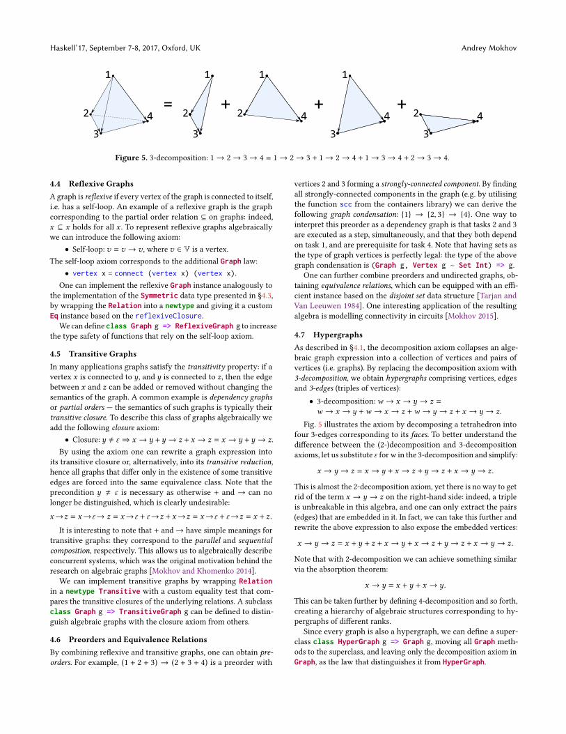
Figure 5. 3-decomposition: 1→ 2→ 3→ 4 = 1→ 2→ 3 + 1→ 2→ 4 + 1→ 3→ 4 + 2→ 3→ 4.

4.4 Reflexive GraphsA graph is reflexive if every vertex of the graph is connected to itself,i.e. has a self-loop. An example of a reflexive graph is the graphcorresponding to the partial order relation ⊆ on graphs: indeed,x ⊆ x holds for all x . To represent reflexive graphs algebraicallywe can introduce the following axiom:• Self-loop: v = v → v , where v ∈ V is a vertex.

The self-loop axiom corresponds to the additional Graph law:• vertex x = connect (vertex x) (vertex x).

One can implement the reflexive Graph instance analogously tothe implementation of the Symmetric data type presented in §4.3,by wrapping the Relation into a newtype and giving it a customEq instance based on the reflexiveClosure.

We can define class Graph g => ReflexiveGraph g to increasethe type safety of functions that rely on the self-loop axiom.

4.5 Transitive GraphsIn many applications graphs satisfy the transitivity property: if avertex x is connected to y, and y is connected to z, then the edgebetween x and z can be added or removed without changing thesemantics of the graph. A common example is dependency graphsor partial orders — the semantics of such graphs is typically theirtransitive closure. To describe this class of graphs algebraically weadd the following closure axiom:• Closure: y , ε ⇒ x → y +y → z + x → z = x → y +y → z.

By using the axiom one can rewrite a graph expression intoits transitive closure or, alternatively, into its transitive reduction,hence all graphs that differ only in the existence of some transitiveedges are forced into the same equivalence class. Note that theprecondition y , ε is necessary as otherwise + and → can nolonger be distinguished, which is clearly undesirable:

x→z = x→ε→ z = x→ε + ε→z + x→z = x→ε + ε→z = x + z.

It is interesting to note that + and→ have simple meanings fortransitive graphs: they correspond to the parallel and sequentialcomposition, respectively. This allows us to algebraically describeconcurrent systems, which was the original motivation behind theresearch on algebraic graphs [Mokhov and Khomenko 2014].

We can implement transitive graphs by wrapping Relationin a newtype Transitive with a custom equality test that com-pares the transitive closures of the underlying relations. A subclassclass Graph g => TransitiveGraph g can be defined to distin-guish algebraic graphs with the closure axiom from others.

4.6 Preorders and Equivalence RelationsBy combining reflexive and transitive graphs, one can obtain pre-orders. For example, (1 + 2 + 3) → (2 + 3 + 4) is a preorder with

vertices 2 and 3 forming a strongly-connected component. By findingall strongly-connected components in the graph (e.g. by utilisingthe function scc from the containers library) we can derive thefollowing graph condensation: {1} → {2, 3} → {4}. One way tointerpret this preorder as a dependency graph is that tasks 2 and 3are executed as a step, simultaneously, and that they both dependon task 1, and are prerequisite for task 4. Note that having sets asthe type of graph vertices is perfectly legal: the type of the abovegraph condensation is (Graph g, Vertex g ∼ Set Int) => g.

One can further combine preorders and undirected graphs, ob-taining equivalence relations, which can be equipped with an effi-cient instance based on the disjoint set data structure [Tarjan andVan Leeuwen 1984]. One interesting application of the resultingalgebra is modelling connectivity in circuits [Mokhov 2015].

4.7 HypergraphsAs described in §4.1, the decomposition axiom collapses an alge-braic graph expression into a collection of vertices and pairs ofvertices (i.e. graphs). By replacing the decomposition axiom with3-decomposition, we obtain hypergraphs comprising vertices, edgesand 3-edges (triples of vertices):• 3-decomposition:w → x → y → z =w → x → y +w → x → z +w → y → z + x → y → z.

Fig. 5 illustrates the axiom by decomposing a tetrahedron intofour 3-edges corresponding to its faces. To better understand thedifference between the (2-)decomposition and 3-decompositionaxioms, let us substitute ε forw in the 3-decomposition and simplify:

x → y → z = x → y + x → z + y → z + x → y → z.

This is almost the 2-decomposition axiom, yet there is no way to getrid of the term x → y → z on the right-hand side: indeed, a tripleis unbreakable in this algebra, and one can only extract the pairs(edges) that are embedded in it. In fact, we can take this further andrewrite the above expression to also expose the embedded vertices:

x → y → z = x + y + z + x → y + x → z + y → z + x → y → z.

Note that with 2-decomposition we can achieve something similarvia the absorption theorem:

x → y = x + y + x → y.

This can be taken further by defining 4-decomposition and so forth,creating a hierarchy of algebraic structures corresponding to hy-pergraphs of different ranks.

Since every graph is also a hypergraph, we can define a super-class class HyperGraph g => Graph g, moving all Graph meth-ods to the superclass, and leaving only the decomposition axiom inGraph, as the law that distinguishes it from HyperGraph.

Algebraic Graphs with Class (Functional Pearl) Haskell’17, September 7-8, 2017, Oxford, UK

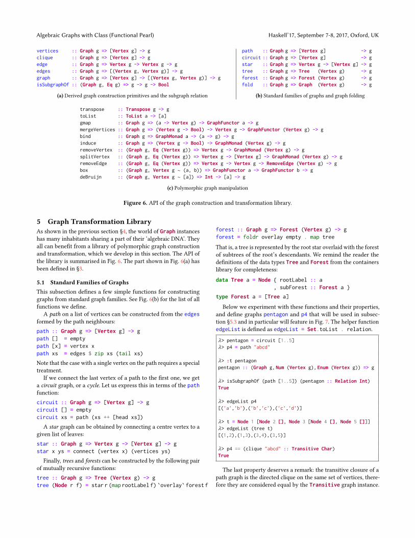
vertices :: Graph g => [Vertex g] -> gclique :: Graph g => [Vertex g] -> gedge :: Graph g => Vertex g -> Vertex g -> gedges :: Graph g => [(Vertex g, Vertex g)] -> ggraph :: Graph g => [Vertex g] -> [(Vertex g, Vertex g)] -> gisSubgraphOf :: (Graph g, Eq g) => g -> g -> Bool

(a) Derived graph construction primitives and the subgraph relation

path :: Graph g => [Vertex g] -> gcircuit :: Graph g => [Vertex g] -> gstar :: Graph g => Vertex g -> [Vertex g] -> gtree :: Graph g => Tree (Vertex g) -> gforest :: Graph g => Forest (Vertex g) -> gfold :: Graph g => Graph (Vertex g) -> g

(b) Standard families of graphs and graph folding

transpose :: Transpose g -> gtoList :: ToList a -> [a]gmap :: Graph g => (a -> Vertex g) -> GraphFunctor a -> gmergeVertices :: Graph g => (Vertex g -> Bool) -> Vertex g -> GraphFunctor (Vertex g) -> gbind :: Graph g => GraphMonad a -> (a -> g) -> ginduce :: Graph g => (Vertex g -> Bool) -> GraphMonad (Vertex g) -> gremoveVertex :: (Graph g, Eq (Vertex g)) => Vertex g -> GraphMonad (Vertex g) -> gsplitVertex :: (Graph g, Eq (Vertex g)) => Vertex g -> [Vertex g] -> GraphMonad (Vertex g) -> gremoveEdge :: (Graph g, Eq (Vertex g)) => Vertex g -> Vertex g -> RemoveEdge (Vertex g) -> gbox :: (Graph g, Vertex g ∼ (a, b)) => GraphFunctor a -> GraphFunctor b -> gdeBruijn :: (Graph g, Vertex g ∼ [a]) => Int -> [a] -> g

(c) Polymorphic graph manipulation

Figure 6. API of the graph construction and transformation library.

5 Graph Transformation LibraryAs shown in the previous section §4, the world of Graph instanceshas many inhabitants sharing a part of their ‘algebraic DNA’. Theyall can benefit from a library of polymorphic graph constructionand transformation, which we develop in this section. The API ofthe library is summarised in Fig. 6. The part shown in Fig. 6(a) hasbeen defined in §3.

5.1 Standard Families of GraphsThis subsection defines a few simple functions for constructinggraphs from standard graph families. See Fig. 6(b) for the list of allfunctions we define.

A path on a list of vertices can be constructed from the edgesformed by the path neighbours:path :: Graph g => [Vertex g] -> gpath [] = emptypath [x] = vertex xpath xs = edges $ zip xs (tail xs)

Note that the case with a single vertex on the path requires a specialtreatment.

If we connect the last vertex of a path to the first one, we geta circuit graph, or a cycle. Let us express this in terms of the pathfunction:circuit :: Graph g => [Vertex g] -> gcircuit [] = emptycircuit xs = path (xs ++ [head xs])

A star graph can be obtained by connecting a centre vertex to agiven list of leaves:star :: Graph g => Vertex g -> [Vertex g] -> gstar x ys = connect (vertex x) (vertices ys)

Finally, trees and forests can be constructed by the following pairof mutually recursive functions:tree :: Graph g => Tree (Vertex g) -> gtree (Node r f) = star r (map rootLabel f) `overlay` forest f

forest :: Graph g => Forest (Vertex g) -> gforest = foldr overlay empty . map tree

That is, a tree is represented by the root star overlaid with the forestof subtrees of the root’s descendants. We remind the reader thedefinitions of the data types Tree and Forest from the containerslibrary for completeness:

data Tree a = Node { rootLabel :: a, subForest :: Forest a }

type Forest a = [Tree a]

Below we experiment with these functions and their properties,and define graphs pentagon and p4 that will be used in subsec-tion §5.3 and in particular will feature in Fig. 7. The helper functionedgeList is defined as edgeList = Set.toList . relation.

λ> pentagon = circuit [1..5]λ> p4 = path "abcd"

λ> :t pentagonpentagon :: (Graph g, Num (Vertex g), Enum (Vertex g)) => g

λ> isSubgraphOf (path [1..5]) (pentagon :: Relation Int)True

λ> edgeList p4[(’a’,’b’),(’b’,’c’),(’c’,’d’)]

λ> t = Node 1 [Node 2 [], Node 3 [Node 4 [], Node 5 []]]λ> edgeList (tree t)[(1,2),(1,3),(3,4),(3,5)]

λ> p4 == (clique "abcd" :: Transitive Char)True

The last property deserves a remark: the transitive closure of apath graph is the directed clique on the same set of vertices, there-fore they are considered equal by the Transitive graph instance.

Haskell’17, September 7-8, 2017, Oxford, UK Andrey Mokhov

5.2 Graph TransposeIn the rest of this section we present a toolbox for transformingpolymorphic graph expressions. The functions in the presentedtoolbox are listed in Fig. 6(c).

One of the simplest transformations one can apply to a graph isto flip the direction of all of its edges. Transpose is usually straight-forward to implement but whichever data structure you use torepresent graphs, you will spend at leastO (1) time to modify it (say,by flipping the treatAsTransposed flag); much more often youwill have to traverse the data structure and flip every edge, resultingin O ( |V | + |E |) time complexity. However, by working with poly-morphic graphs, i.e. graphs of type forall g. Graph g => g, andusing Haskell’s zero-cost newtype wrappers, we can implementtranspose that takes zero time.

Consider the following Graph instance:newtype Transpose g = T { transpose :: g } deriving Eq

instance Graph g => Graph (Transpose g) wheretype Vertex (Transpose g) = Vertex gempty = T emptyvertex = T . vertexoverlay x y = T $ overlay (transpose x) (transpose y)connect x y = T $ connect (transpose y) (transpose x)

That is, we wrap a graph in a newtype flipping the order of connectarguments. Let us check if this works:

λ> edgeList $ 1 * (2 + 3) * 4[(1,2),(1,3),(1,4),(2,4),(3,4)]

λ> edgeList $ transpose $ 1 * (2 + 3) * 4[(2,1),(3,1),(4,1),(4,2),(4,3)]

The transpose has zero runtime cost, because all we do is wrap-ping and unwrapping the newtype, which is guaranteed to be freeor, to be more precise, is handled by GHC at compile time.

To make sure transpose is only applied to polymorphic graphs,we do not export the constructor T, therefore the only way to calltranspose is to give it a polymorphic argument and let the typeinference interpret it as a value of type Transpose.

5.3 Graph FunctorWe now implement a function gmap that given a function a -> b anda polymorphic graph whose vertices are of type a will produce apolymorphic graph with vertices of type b by applying the functionto each vertex. This is almost a Functor but it does not have theusual type signature, because Graph is not a higher-kinded type8:

newtype GraphFunctor a =F { gfor :: forall g. Graph g => (a -> Vertex g) -> g }

instance Graph (GraphFunctor a) wheretype Vertex (GraphFunctor a) = aempty = F $ \_ -> emptyvertex x = F $ \f -> vertex (f x)overlay x y = F $ \f -> overlay (gmap f x) (gmap f y)connect x y = F $ \f -> connect (gmap f x) (gmap f y)

gmap :: Graph g => (a -> Vertex g) -> GraphFunctor a -> ggmap = flip gfor

8It is possible to define a higher-kinded version of Graph, but it has fewer instances.

Essentially, we are defining another newtype wrapper, whichpushes the given function all the way towards the vertices of agiven graph expression. This has no runtime cost, just as before,although the actual evaluation of the given function at each vertexwill not be free, of course. Here is gmap in action:

λ> edgeList $ 1 * 2 * 3 + 4 * 5[(1,2),(1,3),(2,3),(4,5)]

λ> edgeList $ gmap (+1) $ 1 * 2 * 3 + 4 * 5[(2,3),(2,4),(3,4),(5,6)]

As you can see, we can increment the value of each vertex by map-ping the function (+1) over the graph. The resulting expression is apolymorphic graph, as desired. Note that gmap satisfies the functorlaws gmap id = id and gmap f . gmap g = gmap (f . g), be-cause it does not change the structure of the given expression andonly pushes the given function down to its leaves – the vertices.

An alert reader might wonder: what happens if the functionmaps two different vertices into the same one? They will be merged.Merging graph vertices is a useful graph transformation, so let usdefine it in terms of gmap:

mergeVertices :: Graph g => (Vertex g -> Bool)-> Vertex g -> GraphFunctor (Vertex g) -> g

mergeVertices p v = gmap $ \u -> if p u then v else u

λ> edgeList $ mergeVertices odd 3 $ 1 * 2 * 3 + 4 * 5[(2,3),(3,2),(3,3),(4,3)]

The function takes a predicate on graph vertices and a target vertexandmaps all vertices satisfying the predicate into the target, therebymerging them. In our example the odd vertices {1, 3, 5} are mergedinto 3, in particular creating the self-loop 3 → 3. Note: it takeslinear time O ( |д |) for mergeVertices to traverse the graph andapply the predicate to each vertex (where |д | is the size of the graphexpression д), which may be much more efficient than mergingvertices in a concrete data structure. For example, if the graph isrepresented by an adjacency matrix, it will likely be necessary torebuild the resulting matrix from scratch, which takesO ( |V |2) time.Since for many graphs we have |д | = O ( |V |), our mergeVerticesmay be quadratically faster than the matrix-based one.

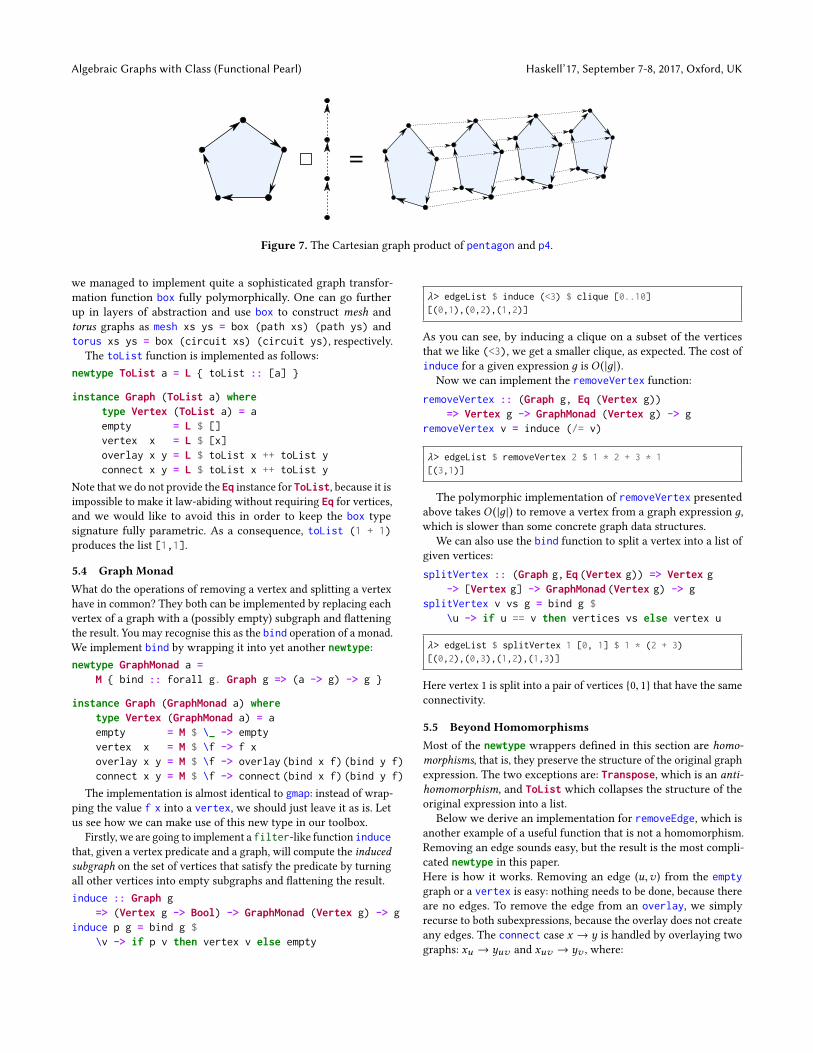
As another application of gmap, we implement the Cartesiangraph product operation box, orG � H , where the resulting vertexset is VG × VH and vertex (x ,y) is connected to vertex (x ′,y′) ifeither x = x ′ and (y,y′) ∈ EH , or y = y′ and (x ,x ′) ∈ EG . Anexample of the Cartesian product of graphs pentagon and p4 isshown in Fig. 7.

box :: (Graph g, Vertex g ∼ (a, b))=> GraphFunctor a -> GraphFunctor b -> g

box x y = foldr overlay empty $ xs ++ yswhere

xs = map (\b -> gmap (,b) x) . toList $ gmap id yys = map (\a -> gmap (a,) y) . toList $ gmap id x

The Cartesian product G � H is assembled by creating |VH |copies of graph G and overlaying them with |VG | copies of graphH . We get access to the list of graph vertices using toList andturn vertices of original graphs into pairs of vertices by gmap. Notethat we need to reinterpret the input of type GraphFunctor as apolymorphic graph by gmap id before passing it to the toListfunction, which expects inputs of type ToList. As you can see,

Algebraic Graphs with Class (Functional Pearl) Haskell’17, September 7-8, 2017, Oxford, UK

=

Figure 7. The Cartesian graph product of pentagon and p4.

we managed to implement quite a sophisticated graph transfor-mation function box fully polymorphically. One can go furtherup in layers of abstraction and use box to construct mesh andtorus graphs as mesh xs ys = box (path xs) (path ys) andtorus xs ys = box (circuit xs) (circuit ys), respectively.

The toList function is implemented as follows:newtype ToList a = L { toList :: [a] }

instance Graph (ToList a) wheretype Vertex (ToList a) = aempty = L $ []vertex x = L $ [x]overlay x y = L $ toList x ++ toList yconnect x y = L $ toList x ++ toList y

Note that we do not provide the Eq instance for ToList, because it isimpossible to make it law-abiding without requiring Eq for vertices,and we would like to avoid this in order to keep the box typesignature fully parametric. As a consequence, toList (1 + 1)produces the list [1,1].

5.4 Graph MonadWhat do the operations of removing a vertex and splitting a vertexhave in common? They both can be implemented by replacing eachvertex of a graph with a (possibly empty) subgraph and flatteningthe result. You may recognise this as the bind operation of a monad.We implement bind by wrapping it into yet another newtype:newtype GraphMonad a =

M { bind :: forall g. Graph g => (a -> g) -> g }

instance Graph (GraphMonad a) wheretype Vertex (GraphMonad a) = aempty = M $ \_ -> emptyvertex x = M $ \f -> f xoverlay x y = M $ \f -> overlay (bind x f) (bind y f)connect x y = M $ \f -> connect (bind x f) (bind y f)

The implementation is almost identical to gmap: instead of wrap-ping the value f x into a vertex, we should just leave it as is. Letus see how we can make use of this new type in our toolbox.

Firstly, we are going to implement a filter-like function inducethat, given a vertex predicate and a graph, will compute the inducedsubgraph on the set of vertices that satisfy the predicate by turningall other vertices into empty subgraphs and flattening the result.induce :: Graph g

=> (Vertex g -> Bool) -> GraphMonad (Vertex g) -> ginduce p g = bind g $

\v -> if p v then vertex v else empty

λ> edgeList $ induce (<3) $ clique [0..10][(0,1),(0,2),(1,2)]

As you can see, by inducing a clique on a subset of the verticesthat we like (<3), we get a smaller clique, as expected. The cost ofinduce for a given expression д is O ( |д |).

Now we can implement the removeVertex function:removeVertex :: (Graph g, Eq (Vertex g))

=> Vertex g -> GraphMonad (Vertex g) -> gremoveVertex v = induce (/= v)

λ> edgeList $ removeVertex 2 $ 1 * 2 + 3 * 1[(3,1)]

The polymorphic implementation of removeVertex presentedabove takes O ( |д |) to remove a vertex from a graph expression д,which is slower than some concrete graph data structures.

We can also use the bind function to split a vertex into a list ofgiven vertices:splitVertex :: (Graph g, Eq (Vertex g)) => Vertex g

-> [Vertex g] -> GraphMonad (Vertex g) -> gsplitVertex v vs g = bind g $

\u -> if u == v then vertices vs else vertex u

λ> edgeList $ splitVertex 1 [0, 1] $ 1 * (2 + 3)[(0,2),(0,3),(1,2),(1,3)]

Here vertex 1 is split into a pair of vertices {0, 1} that have the sameconnectivity.

5.5 Beyond HomomorphismsMost of the newtype wrappers defined in this section are homo-morphisms, that is, they preserve the structure of the original graphexpression. The two exceptions are: Transpose, which is an anti-homomorphism, and ToList which collapses the structure of theoriginal expression into a list.

Below we derive an implementation for removeEdge, which isanother example of a useful function that is not a homomorphism.Removing an edge sounds easy, but the result is the most compli-cated newtype in this paper.Here is how it works. Removing an edge (u,v ) from the emptygraph or a vertex is easy: nothing needs to be done, because thereare no edges. To remove the edge from an overlay, we simplyrecurse to both subexpressions, because the overlay does not createany edges. The connect case x → y is handled by overlaying twographs: xu → yuv and xuv → yv , where:

Haskell’17, September 7-8, 2017, Oxford, UK Andrey Mokhov

newtype RemoveEdge a = RE { re :: forall g. (Vertex g ∼ a, Graph g) => a -> a -> g }

instance Eq a => Graph (RemoveEdge a) wheretype Vertex (RemoveEdge a) = aempty = RE $ \_ _ -> emptyvertex x = RE $ \_ _ -> vertex xoverlay x y = RE $ \u v -> overlay (re x u v) (re y u v)connect x y = RE $ \u v -> connect (removeVertex u $ re x u u) (re y u v) `overlay`

connect (re x u v) (removeVertex v $ re y v v)

removeEdge :: (Eq (Vertex g), Graph g) => Vertex g -> Vertex g -> RemoveEdge (Vertex g) -> gremoveEdge u v g = re g u v

Figure 8. Removing an edge from a polymorphic graph.

• xu = removeVertex u x and yuv = removeEdge u v y, thusxu → yuv definitely does not contain the edge (u,v ) at thecost of losing the vertex u in the left-hand side xu .• yv = removeVertex v y and xuv = removeEdge u v x , thusxuv → yv definitely does not contain the edge (u,v ) at thecost of losing the vertex v in the right-hand side yv .

The overlay xu → yuv + xuv → yv contains the vertices u and v ,because at least one copy of each vertex has been preserved, butthe edge (u,v ) is removed in both subexpressions as intended.

We demonstrate removeEdge on two simple examples:

λ> edgeList $ path "Hello"[(’H’,’e’),(’e’,’l’),(’l’,’l’),(’l’,’o’)]

λ> edgeList $ removeEdge ’H’ ’e’ $ path "Hello"[(’e’,’l’),(’l’,’l’),(’l’,’o’)]

λ> edgeList $ removeEdge ’l’ ’l’ $ path "Hello"[(’H’,’e’),(’e’,’l’),(’l’,’o’)]

The removeEdge function is expensive: given an expression of size|д | it may produce a transformed expression of the quadratic sizeO ( |д |2). Many concrete Graph instances provide much faster equiv-alents of removeEdge.

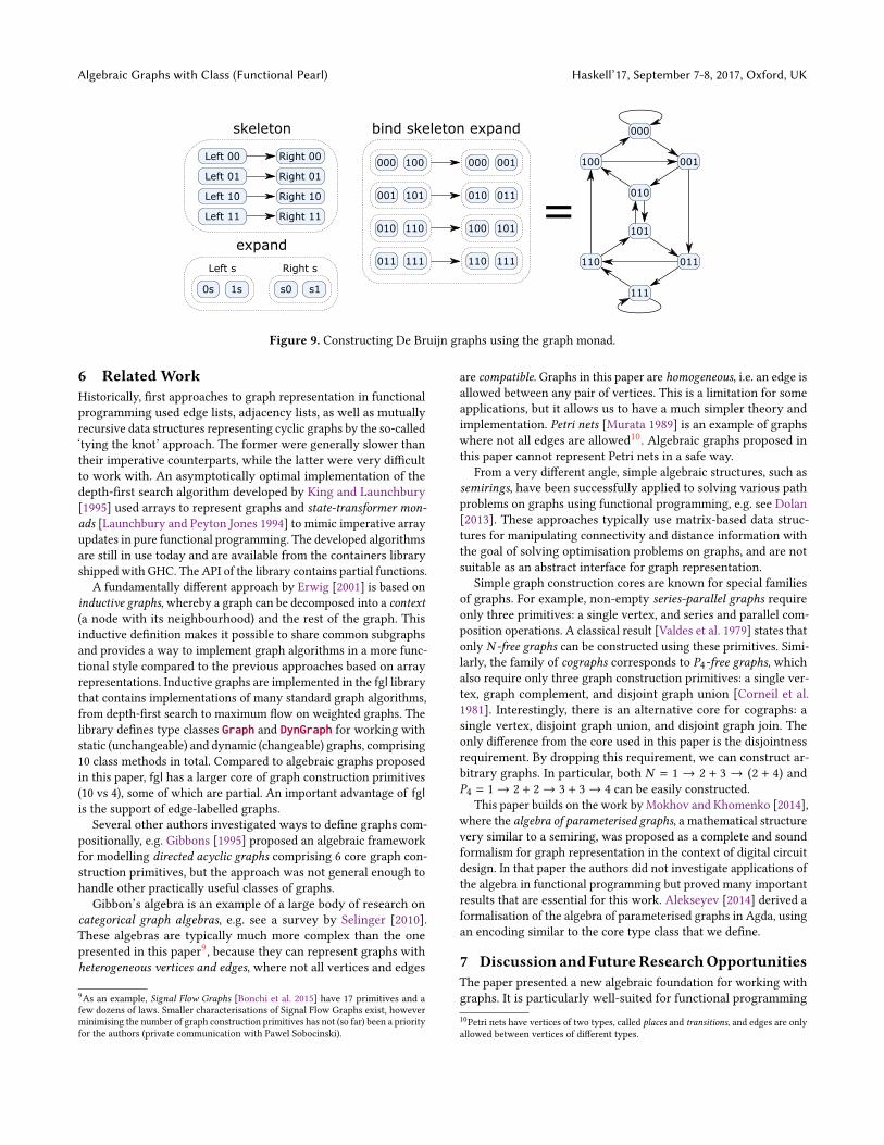
5.6 De Bruijn GraphsTo demonstrate that one can easily construct sophisticated graphsusing the presented library, let us try it on De Bruijn graphs, aninteresting combinatorial object that frequently shows up in com-puter engineering and bioinformatics. The implementation is veryshort, but requires some explanation:deBruijn :: (Graph g, Vertex g ∼ [a]) => Int -> [a] -> gdeBruijn len alphabet = bind skeleton expandwhere

overlaps = mapM (const alphabet) [2..len]skeleton = edges [ (Left s, Right s) | s <- overlaps ]expand v = vertices

[ either ([a]++) (++[a]) v | a <- alphabet ]

The function builds a De Bruijn graph of dimension len fromsymbols of the given alphabet. The vertices of the graph are allpossible words of length len containing symbols of the alphabet,and two words are connected x → y whenever x and y matchafter we remove the first symbol of x and the last symbol of y(equivalently, when x = az and y = zb for some symbols a and b).The process of construction of a 3-dimensional De Bruijn graph on

the alphabet {0, 1} is illustrated in Fig. 9. Here are all the ingredientsof the solution:

• overlaps contains all possible words of length len-1 thatcorrespond to overlaps of connected vertices.• skeleton contains one edge per overlap, with Left andRight vertices acting as temporary placeholders.• We replace a vertex Left s with a subgraph of two vertices{0s, 1s}, i.e. the vertices whose suffix is s . Symmetrically,Right s is replaced by vertices {s0, s1}. This is captured bythe function expand.• The result is obtained by computing bind skeleton expand.

Below we construct the De Bruijn graph shown in Fig. 9.

λ> edgeList $ deBruijn 3 "01"[("000","000"),("000","001"),("001","010"),("001","011"),("010","100"),("010","101"),("011","110"),("011","111"),("100","000"),("100","001"),("101","010"),("101","011"),("110","100"),("110","101"),("111","110"),("111","111")]

λ> g = deBruijn 9 "abc"λ> all (\(x,y) -> drop 1 x == dropEnd 1 y) $ edgeList gTrue

λ> Set.size $ domain g19683 -- i.e. 3^9

λ> Set.size $ relation g59049 -- i.e. 3^10

Note that a De Bruijn graph of dimension len on the alphabet has|alphabet|len vertices and |alphabet|len+1 edges.

5.7 SummaryWe have presented a library of polymorphic graph construction andtransformation functions that provide a flexible and elegant wayto manipulate graph expressions polymorphically. Polymorphicgraphs are highly reusable and composable, and can be interpretedusing any of the Graph instances defined in §4, as well as otherinstances provided by the algebraic-graphs library that is availableon Hackage. The library is written in the vanilla functional pro-gramming style and has no dependencies apart from core GHClibraries. Many of the presented graph transformation algorithmsare expressed using familiar functional programming abstractions,such as functors and monads.

Algebraic Graphs with Class (Functional Pearl) Haskell’17, September 7-8, 2017, Oxford, UK

000

100 001

010

101

011

111

110

skeleton

Left 10 Right 10

Left 01 Right 01

Left 11 Right 11

Left 00 Right 00

Left s

1s0s

Right s

s1s0

expand

bind skeleton expand

100000 001000

101001 011010

110010 101100

111011 111110

=

Figure 9. Constructing De Bruijn graphs using the graph monad.

6 Related WorkHistorically, first approaches to graph representation in functionalprogramming used edge lists, adjacency lists, as well as mutuallyrecursive data structures representing cyclic graphs by the so-called‘tying the knot’ approach. The former were generally slower thantheir imperative counterparts, while the latter were very difficultto work with. An asymptotically optimal implementation of thedepth-first search algorithm developed by King and Launchbury[1995] used arrays to represent graphs and state-transformer mon-ads [Launchbury and Peyton Jones 1994] to mimic imperative arrayupdates in pure functional programming. The developed algorithmsare still in use today and are available from the containers libraryshipped with GHC. The API of the library contains partial functions.

A fundamentally different approach by Erwig [2001] is based oninductive graphs, whereby a graph can be decomposed into a context(a node with its neighbourhood) and the rest of the graph. Thisinductive definition makes it possible to share common subgraphsand provides a way to implement graph algorithms in a more func-tional style compared to the previous approaches based on arrayrepresentations. Inductive graphs are implemented in the fgl librarythat contains implementations of many standard graph algorithms,from depth-first search to maximum flow on weighted graphs. Thelibrary defines type classes Graph and DynGraph for working withstatic (unchangeable) and dynamic (changeable) graphs, comprising10 class methods in total. Compared to algebraic graphs proposedin this paper, fgl has a larger core of graph construction primitives(10 vs 4), some of which are partial. An important advantage of fglis the support of edge-labelled graphs.

Several other authors investigated ways to define graphs com-positionally, e.g. Gibbons [1995] proposed an algebraic frameworkfor modelling directed acyclic graphs comprising 6 core graph con-struction primitives, but the approach was not general enough tohandle other practically useful classes of graphs.

Gibbon’s algebra is an example of a large body of research oncategorical graph algebras, e.g. see a survey by Selinger [2010].These algebras are typically much more complex than the onepresented in this paper9, because they can represent graphs withheterogeneous vertices and edges, where not all vertices and edges

9As an example, Signal Flow Graphs [Bonchi et al. 2015] have 17 primitives and afew dozens of laws. Smaller characterisations of Signal Flow Graphs exist, howeverminimising the number of graph construction primitives has not (so far) been a priorityfor the authors (private communication with Pawel Sobocinski).

are compatible. Graphs in this paper are homogeneous, i.e. an edge isallowed between any pair of vertices. This is a limitation for someapplications, but it allows us to have a much simpler theory andimplementation. Petri nets [Murata 1989] is an example of graphswhere not all edges are allowed10. Algebraic graphs proposed inthis paper cannot represent Petri nets in a safe way.

From a very different angle, simple algebraic structures, such assemirings, have been successfully applied to solving various pathproblems on graphs using functional programming, e.g. see Dolan[2013]. These approaches typically use matrix-based data struc-tures for manipulating connectivity and distance information withthe goal of solving optimisation problems on graphs, and are notsuitable as an abstract interface for graph representation.

Simple graph construction cores are known for special familiesof graphs. For example, non-empty series-parallel graphs requireonly three primitives: a single vertex, and series and parallel com-position operations. A classical result [Valdes et al. 1979] states thatonly N -free graphs can be constructed using these primitives. Simi-larly, the family of cographs corresponds to P4-free graphs, whichalso require only three graph construction primitives: a single ver-tex, graph complement, and disjoint graph union [Corneil et al.1981]. Interestingly, there is an alternative core for cographs: asingle vertex, disjoint graph union, and disjoint graph join. Theonly difference from the core used in this paper is the disjointnessrequirement. By dropping this requirement, we can construct ar-bitrary graphs. In particular, both N = 1 → 2 + 3 → (2 + 4) andP4 = 1→ 2 + 2→ 3 + 3→ 4 can be easily constructed.

This paper builds on the work by Mokhov and Khomenko [2014],where the algebra of parameterised graphs, a mathematical structurevery similar to a semiring, was proposed as a complete and soundformalism for graph representation in the context of digital circuitdesign. In that paper the authors did not investigate applications ofthe algebra in functional programming but proved many importantresults that are essential for this work. Alekseyev [2014] derived aformalisation of the algebra of parameterised graphs in Agda, usingan encoding similar to the core type class that we define.

7 Discussion and FutureResearchOpportunitiesThe paper presented a new algebraic foundation for working withgraphs. It is particularly well-suited for functional programming10Petri nets have vertices of two types, called places and transitions, and edges are onlyallowed between vertices of different types.

Haskell’17, September 7-8, 2017, Oxford, UK Andrey Mokhov

languages and benefits from functional programming abstractions,such as functors and monads. Compared to the state-of-the-art,algebraic graphs are easier to use and reuse, more compositional,and have a smaller core of only four graph construction primitives,fully characterised by an elegant algebra of graphs.

We demonstrated the flexibility of algebraic graphs by severalexamples and developed a Haskell library for constructing andtransforming polymorphic graphs.

The presented approach has a few important limitations:• This paper has not addressed edge-labelled graphs. In partic-ular, there is no known extension of the presented algebracharacterising graphs with arbitrary vertex and edge labels.However, Mokhov and Khomenko [2014] give an algebraiccharacterisation for graphs labelled with Boolean functions,which can be generalised to labels that form a semiring.We found that one can represent edge-labelled graphs byfunctions from labels to graphs. For example, a finite automa-ton can be thought of as a collection of graphs, one for eachsymbol of the alphabet:

type Automaton a s = a -> Relation s

Here a and s stand for the alphabet and the set of states ofthe automaton, respectively. This representation of labelledgraphs is supported by the following graph instance:

instance Graph g => Graph (a -> g) wheretype Vertex (a -> g) = Vertex gempty = pure emptyvertex = pure . vertexoverlay x y = overlay <$> x <*> yconnect x y = connect <$> x <*> y

Therefore, Automaton a s is a valid Graph instance.• As mentioned in §6, the presented approach is designed forhomogeneous graphs, where an edge is allowed betweenany pair of vertices. It is an open research question whetherit is possible to extend algebraic graphs for modelling het-erogeneous graphs, such as Petri nets, without sacrificingthe simplicity of the algebraic core.• Many graph instances, e.g. Relation, incur a logarithmicoverhead during graph construction, and may therefore beunsuitable for high-performance applications. One possiblesolution is to operate on deeply-embedded algebraic graphs(such as data Graph), and perform conversions to moreconventional representations only when necessary.• There are no known efficient implementations of fundamen-tal graph algorithms, such as depth-first search, that workdirectly on the algebraic core. Therefore, we need to trans-late core expressions to conventional graph representations,such as adjacency lists, and utilise existing graph libraries,which may be suboptimal for certain algorithmic problems.

Despite these limitations, algebraic graphs have been success-fully used in the design of processor microcontrollers [Mokhov andKhomenko 2014] and asynchronous circuits [Beaumont et al. 2015].

Our future research will focus on addressing the above limita-tions, and on the exploration of the following topics:• Algebraic graph expressions can be minimised via themodu-lar decomposition of graphs [McConnell and De Montgolfier2005], thereby reducing their memory footprint, as well as

speeding up their processing. Modular decomposition is acanonical graph representation, which can therefore be usedto efficiently compare algebraic graph expressions for equal-ity. Exploiting the compactness of algebraic graphs in algo-rithms is a promising research direction.• By using the algebraic approach to graph representationone can formulate graph algorithms in the form of solvingsystems of algebraic equations with unknowns. This maypotentially open way to the discovery of novel graph algo-rithms.

AcknowledgmentsI would like to thank Arseniy Alekseyev and Neil Mitchell fornumerous discussions on algebraic graphs, their advice, criticismand encouragement. Without their help this work would have likelyremained an unfinished toy project. Simon Peyton Jones, BrentYorgey, Danil Sokolov, Ben Lippmeier, Ulan Degenbaev and severalanonymous reviewers provided constructive feedback on an earlierdraft of this paper, helping to substantially improve it. Last but notleast, I’m very grateful to Victor Khomenko for his contribution tothe algebra of parameterised graphs that forms the mathematicalfoundation of this work.

ReferencesArseniy Alekseyev. 2014. Compositional approach to design of digital circuits. Ph.D.

Dissertation. Newcastle University.Jonathan Beaumont, Andrey Mokhov, Danil Sokolov, and Alex Yakovlev. 2015. Compo-

sitional design of asynchronous circuits from behavioural concepts. In ACM/IEEEInternational Conference on Formal Methods and Models for Codesign (MEMOCODE).IEEE, 118–127.

Filippo Bonchi, Pawel Sobocinski, and Fabio Zanasi. 2015. Full abstraction for signalflow graphs. In ACM SIGPLAN Notices, Vol. 50. ACM, 515–526.

Manuel Chakravarty, Gabriele Keller, and Simon Peyton Jones. 2005. Associated typesynonyms. In ACM SIGPLAN Notices, Vol. 40. ACM, 241–253.

Derek G Corneil, H Lerchs, and L Stewart Burlingham. 1981. Complement reduciblegraphs. Discrete Applied Mathematics 3, 3 (1981), 163–174.

Stephen Dolan. 2013. Fun with semirings: a functional pearl on the abuse of linearalgebra. In ACM SIGPLAN Notices, Vol. 48. ACM, 101–110.

Martin Erwig. 2001. Inductive graphs and functional graph algorithms. Journal ofFunctional Programming 11, 05 (2001), 467–492.

Jeremy Gibbons. 1995. An initial-algebra approach to directed acyclic graphs. InInternational Conference on Mathematics of Program Construction. Springer, 282–303.

Jeremy Gibbons and Nicolas Wu. 2014. Folding domain-specific languages: Deep andshallow embeddings (functional pearl). In ACM SIGPLAN Notices, Vol. 49. ACM,339–347.

Jonathan S Golan. 1999. Semirings and their Applications. Springer Science & BusinessMedia.

Frank Harary. 1969. Graph theory. Addison-Wesley.David J King and John Launchbury. 1995. Structuring depth-first search algorithms in

Haskell. In Proceedings of the 22nd ACM SIGPLAN-SIGACT symposium on Principlesof programming languages. ACM, 344–354.

John Launchbury and Simon L Peyton Jones. 1994. Lazy functional state threads. InACM SIGPLAN Notices, Vol. 29. ACM, 24–35.

Saunders Mac Lane and Garrett Birkhoff. 1999. Algebra. Chelsea Publishing Company.Ross M McConnell and Fabien De Montgolfier. 2005. Linear-time modular decomposi-

tion of directed graphs. Discrete Applied Mathematics 145, 2 (2005), 198–209.Andrey Mokhov. 2015. Algebra of switching networks. IET Computers & Digital

Techniques (2015).Andrey Mokhov and Victor Khomenko. 2014. Algebra of Parameterised Graphs. ACM

Transactions on Embedded Computing Systems 13, 4s (2014), 1–22.Tadao Murata. 1989. Petri nets: Properties, analysis and applications. Proc. IEEE 77, 4

(1989), 541–580.Peter Selinger. 2010. A survey of graphical languages for monoidal categories. In New

structures for physics. Springer, 289–355.Robert E Tarjan and Jan Van Leeuwen. 1984. Worst-case analysis of set union algo-

rithms. Journal of the ACM (JACM) 31, 2 (1984), 245–281.Jacobo Valdes, Robert E Tarjan, and Eugene L Lawler. 1979. The recognition of series

parallel digraphs. In Proceedings of the eleventh annual ACM symposium on Theoryof computing. ACM, 1–12.