alexander g. schwing - fields institute · deep learning meets structured prediction alexander g....
TRANSCRIPT
Deep Learning meets Structured Prediction
Alexander G. Schwing
in collaboration with T. Hazan, M. Pollefeys and R. Urtasunin collaboration with L.-C. Chen, A. L. Yuille and R. Urtasun
University of Toronto
A. G. Schwing (University of Toronto) Structured Prediction & Deep Learning 2014 1 / 40

Big Data and Statistical Machine Learning
Large scale problems according to the program:input dimensionalitynumber of training samplesnumber of categories
A. G. Schwing (University of Toronto) Structured Prediction & Deep Learning 2014 2 / 40

Scene understanding
Tutoring systems Tag prediction
S1 S1
S2 S2
S4 S4
S3 S3
t = 1 t = 2
x = image
x = responses x = image
s ∈ S : room layout
s ∈ S : student skills s ∈ S : tags
Large scale problems• input dimensionality x is large• number of training samples |D| = |{(x , s)}| is large• number of categories |S| is large
A. G. Schwing (University of Toronto) Structured Prediction & Deep Learning 2014 3 / 40

Scene understanding Tutoring systems
Tag prediction
S1 S1
S2 S2
S4 S4
S3 S3
t = 1 t = 2
x = image x = responses
x = image
s ∈ S : room layout s ∈ S : student skills
s ∈ S : tags
Large scale problems• input dimensionality x is large• number of training samples |D| = |{(x , s)}| is large• number of categories |S| is large
A. G. Schwing (University of Toronto) Structured Prediction & Deep Learning 2014 3 / 40

Scene understanding Tutoring systems Tag prediction
S1 S1
S2 S2
S4 S4
S3 S3
t = 1 t = 2
x = image x = responses x = image
s ∈ S : room layout s ∈ S : student skills s ∈ S : tags
Large scale problems• input dimensionality x is large• number of training samples |D| = |{(x , s)}| is large• number of categories |S| is large
A. G. Schwing (University of Toronto) Structured Prediction & Deep Learning 2014 3 / 40

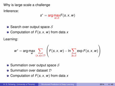
Why is large scale a challenge
Inference:s∗ = arg max
s∈SF (s, x ,w)
Search over output space SComputation of F (s, x ,w) from data x
Learning:
w∗ = arg maxw
∑(x ,s)∈D
F (s, x ,w)− ln∑s∈S
exp F (s, x ,w)
Summation over output space SSummation over dataset DComputation of F (s, x ,w) from data x
A. G. Schwing (University of Toronto) Structured Prediction & Deep Learning 2014 4 / 40
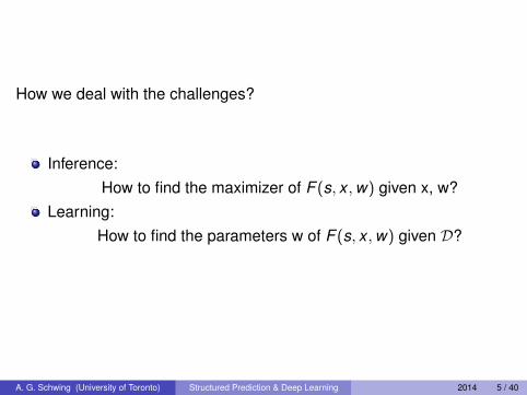
How we deal with the challenges?
Inference:How to find the maximizer of F (s, x ,w) given x, w?
Learning:How to find the parameters w of F (s, x ,w) given D?
A. G. Schwing (University of Toronto) Structured Prediction & Deep Learning 2014 5 / 40

Inference
s∗ = arg maxs∈S
F (s, x ,w)
The domain size |S| is potentially largeImageNet challenge: |S| = 1000Layout prediction: |S| = 504
Tutoring systems: |S| = 2Number of modeled skills
Tag prediction: |S| = 2Number of tags
Computation of F (s, x ,w) for all possible s ∈ S in general oftenintractable.
But: Interest in jointly predicting multiple variables s = (s1, . . . , sn)
A. G. Schwing (University of Toronto) Structured Prediction & Deep Learning 2014 6 / 40
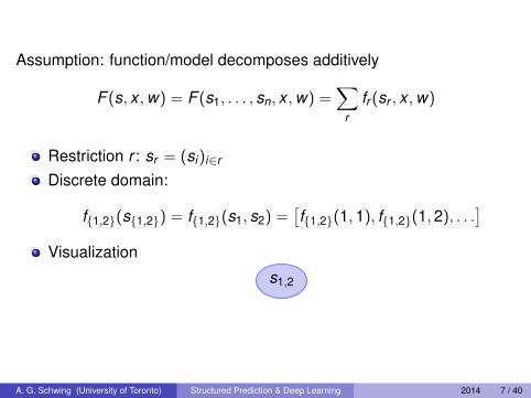
Assumption: function/model decomposes additively
F (s, x ,w) = F (s1, . . . , sn, x ,w) =∑
r
fr (sr , x ,w)
Restriction r : sr = (si)i∈r
Discrete domain:
f{1,2}(s{1,2}) = f{1,2}(s1, s2) =[f{1,2}(1,1), f{1,2}(1,2), . . .
]Visualization
s1,2
A. G. Schwing (University of Toronto) Structured Prediction & Deep Learning 2014 7 / 40

[Werner‘07; Koller&Friedman‘09]
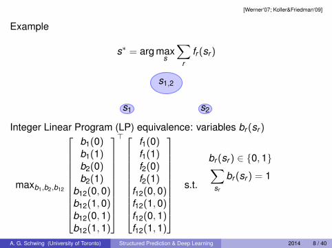
Example
s∗ = arg maxs
∑r
fr (sr )
s1 s2
s1,2
Integer Linear Program (LP) equivalence: variables br (sr )
maxb1,b2,b12
b1(0)b1(1)b2(0)b2(1)
b12(0,0)b12(1,0)b12(0,1)b12(1,1)
>
f1(0)f1(1)f2(0)f2(1)
f12(0,0)f12(1,0)f12(0,1)f12(1,1)
s.t.
br (sr ) ∈ {0,1}∑sr
br (sr ) = 1∑sp\sr
bp(sp) = br (sr )
A. G. Schwing (University of Toronto) Structured Prediction & Deep Learning 2014 8 / 40

[Werner‘07; Koller&Friedman‘09]
Example
s∗ = arg maxs
∑r
fr (sr )
s1 s2
s1,2
Integer Linear Program (LP) equivalence: variables br (sr )
maxb1,b2,b12
b1(0)b1(1)b2(0)b2(1)
b12(0,0)b12(1,0)b12(0,1)b12(1,1)
>
f1(0)f1(1)f2(0)f2(1)
f12(0,0)f12(1,0)f12(0,1)f12(1,1)
s.t.
br (sr ) ∈ {0,1}
∑sr
br (sr ) = 1∑sp\sr
bp(sp) = br (sr )
A. G. Schwing (University of Toronto) Structured Prediction & Deep Learning 2014 8 / 40
[Werner‘07; Koller&Friedman‘09]
Example
s∗ = arg maxs
∑r
fr (sr )
s1 s2
s1,2
Integer Linear Program (LP) equivalence: variables br (sr )
maxb1,b2,b12
b1(0)b1(1)b2(0)b2(1)
b12(0,0)b12(1,0)b12(0,1)b12(1,1)
>
f1(0)f1(1)f2(0)f2(1)
f12(0,0)f12(1,0)f12(0,1)f12(1,1)
s.t.
br (sr ) ∈ {0,1}∑sr
br (sr ) = 1
∑sp\sr
bp(sp) = br (sr )
A. G. Schwing (University of Toronto) Structured Prediction & Deep Learning 2014 8 / 40

[Werner‘07; Koller&Friedman‘09]
Example
s∗ = arg maxs
∑r
fr (sr )
s1 s2
s1,2
Integer Linear Program (LP) equivalence: variables br (sr )
maxb1,b2,b12
b1(0)b1(1)b2(0)b2(1)
b12(0,0)b12(1,0)b12(0,1)b12(1,1)
>
f1(0)f1(1)f2(0)f2(1)
f12(0,0)f12(1,0)f12(0,1)f12(1,1)
s.t.
br (sr ) ∈ {0,1}∑sr
br (sr ) = 1∑sp\sr
bp(sp) = br (sr )
A. G. Schwing (University of Toronto) Structured Prediction & Deep Learning 2014 8 / 40

[Werner‘07; Koller&Friedman‘09]
s = arg maxs
∑r
fr (sr )
Integer linear program:
maxb1,b2,b12
b1(1)b1(2)b2(1)b2(2)
b12(1,1)b12(2,1)b12(1,2)b12(2,2)
>
f1(1)f1(2)f2(1)f2(2)
f12(1,1)f12(2,1)f12(1,2)f12(2,2)
s.t.
br (sr ) ∈ {0,1}br (sr ) ≥ 0∑sr
br (sr ) = 1∑sp\sr
bp(sp) = br (sr )
Standard LP solvers are slow because of many variables andconstraints. Specifically tailored algorithms...
A. G. Schwing (University of Toronto) Structured Prediction & Deep Learning 2014 9 / 40

[Werner‘07; Koller&Friedman‘09]
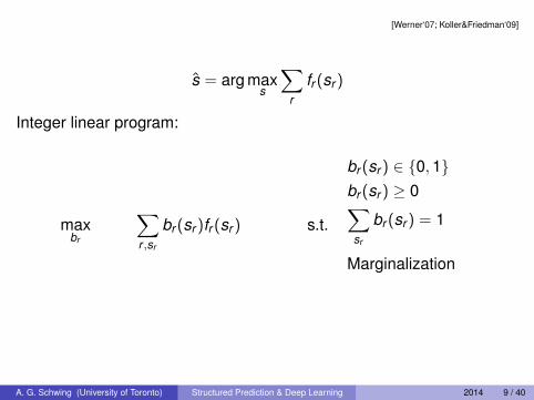
s = arg maxs
∑r
fr (sr )
Integer linear program:
maxbr
∑r ,sr
br (sr )fr (sr ) s.t.
br (sr ) ∈ {0,1}br (sr ) ≥ 0∑sr
br (sr ) = 1∑sp\sr
bp(sp) = br (sr )
Standard LP solvers are slow because of many variables andconstraints. Specifically tailored algorithms...
A. G. Schwing (University of Toronto) Structured Prediction & Deep Learning 2014 9 / 40
[Werner‘07; Koller&Friedman‘09]
s = arg maxs
∑r
fr (sr )
Integer linear program:
maxbr
∑r ,sr
br (sr )fr (sr ) s.t.
br (sr ) ∈ {0,1}br (sr ) ≥ 0∑sr
br (sr ) = 1
Marginalization
Standard LP solvers are slow because of many variables andconstraints. Specifically tailored algorithms...
A. G. Schwing (University of Toronto) Structured Prediction & Deep Learning 2014 9 / 40

[Werner‘07; Koller&Friedman‘09]
s = arg maxs
∑r
fr (sr )
Integer linear program:
maxbr
∑r ,sr
br (sr )fr (sr ) s.t.
br (sr ) ∈ {0,1}
Local probability br
Marginalization
Standard LP solvers are slow because of many variables andconstraints. Specifically tailored algorithms...
A. G. Schwing (University of Toronto) Structured Prediction & Deep Learning 2014 9 / 40

[Werner‘07; Koller&Friedman‘09]
s = arg maxs
∑r
fr (sr )
LP relaxation:
maxbr
∑r ,sr
br (sr )fr (sr ) s.t.
((((((((hhhhhhhhbr (sr ) ∈ {0,1}
Local probability br
Marginalization
Standard LP solvers are slow because of many variables andconstraints. Specifically tailored algorithms...
A. G. Schwing (University of Toronto) Structured Prediction & Deep Learning 2014 9 / 40

[Weiss et al.‘07, Globerson&Jaakkola‘07, Johnson‘08,Jojic et al.‘10, Hazan&Shashua‘10, Savchynskyy et al.‘12,
Ravikumar et al.‘10, Martins et al.‘11, Meshi&Globerson‘11,Komodakis et al.‘10‘12, Schwing et al.‘11‘12‘14]
Graph structure defined via marginalization constraints
s1 s2
s1,2
Message passing solversAdvantage: Efficient due to analytically computable sub-problemsProblem: Special care required to find global optimum
Subgradient methodsAdvantage: Guaranteed globally convergentProblem: Special care required to find fast algorithms
A. G. Schwing (University of Toronto) Structured Prediction & Deep Learning 2014 10 / 40

Block-coordinate ascent/message passing solvers[Weiss et al.‘07, Globerson&Jaakkola‘07, Johnson‘08,
Jojic et al.‘10, Hazan&Shashua‘10, Savchynskyy et al.‘12,Ravikumar et al.‘10, Martins et al.‘11, Meshi&Globerson‘11]
Optimize w.r.t. subset of variables
Advantage: Efficient due to analytically computable sub-problemsProblem: Getting stuck in corners
Smoothing, proximal updates, augmented Lagrangian methodsA. G. Schwing (University of Toronto) Structured Prediction & Deep Learning 2014 11 / 40
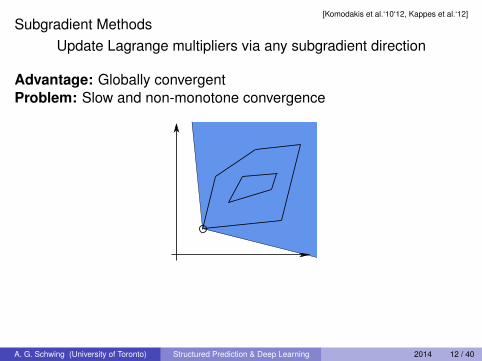
Subgradient Methods[Komodakis et al.‘10‘12, Kappes et al.‘12]
Update Lagrange multipliers via any subgradient direction
Advantage: Globally convergentProblem: Slow and non-monotone convergence
What we like: steepest subgradient ascent direction
A. G. Schwing (University of Toronto) Structured Prediction & Deep Learning 2014 12 / 40

Distributed Inference for Graphical Models
Goal:Optimize the LP relaxation objectiveLeverage the problem structureDistribute memory and computation requirementsMaintain convergence and optimality guarantees
Dual decomposition extension of LP relaxation solvers via partitioningof variables.
A. G. Schwing (University of Toronto) Structured Prediction & Deep Learning 2014 13 / 40

Dual decomposition intuition:
s1 s2 s3 s4
s5 s6 s7 s8
s1,2 s2,3 s3,4
s5,6 s6,7 s7,8
s1,5 s2,6 s3,7 s4,8
Unique set of variables:bκr (sr )
Marginalization constraints and local beliefs ∀κConsistency constraints:
bκr (sr ) = br (sr )
A. G. Schwing (University of Toronto) Structured Prediction & Deep Learning 2014 14 / 40

Dual decomposition intuition:
s1 s2 s3 s4
s5 s6 s7 s8
Unique set of variables:bκr (sr )
Marginalization constraints and local beliefs ∀κConsistency constraints:
bκr (sr ) = br (sr )
A. G. Schwing (University of Toronto) Structured Prediction & Deep Learning 2014 14 / 40

Dual decomposition intuition:
1 2 3 4
5 6 7 8
κ1 κ2
Unique set of variables:bκr (sr )
Marginalization constraints and local beliefs ∀κConsistency constraints:
bκr (sr ) = br (sr )
A. G. Schwing (University of Toronto) Structured Prediction & Deep Learning 2014 14 / 40

Dual decomposition intuition:
1 2 3 4
5 6 7 8
κ1 κ2
Unique set of variables:bκr (sr )
Marginalization constraints and local beliefs ∀κConsistency constraints:
bκr (sr ) = br (sr )
A. G. Schwing (University of Toronto) Structured Prediction & Deep Learning 2014 14 / 40

1 2 3 4
5 6 7 8
κ1 κ2
Distributed LP Relaxation
maxb
∑κ
( ∑r∈κ,sr
bκr (sr )fr (sr )
)
s.t.∀κ Local probabilities bκr∀κ Marginalization constraints∀κ Consistency
A. G. Schwing (University of Toronto) Structured Prediction & Deep Learning 2014 15 / 40

Algorithm:Some message passing iterations in parallel ∀κ
1 2 3 4
5 6 7 8
κ1 κ2Exchange of information between different κ
1 2 3 4
5 6 7 8
κ1 κ2
A. G. Schwing (University of Toronto) Structured Prediction & Deep Learning 2014 16 / 40
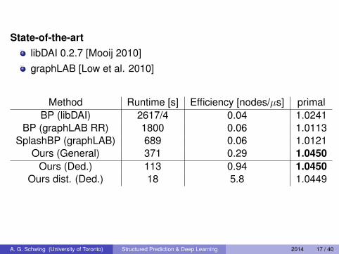
State-of-the-artlibDAI 0.2.7 [Mooij 2010]graphLAB [Low et al. 2010]
Method Runtime [s] Efficiency [nodes/µs] primalBP (libDAI) 2617/4 0.04 1.0241
BP (graphLAB RR) 1800 0.06 1.0113SplashBP (graphLAB) 689 0.06 1.0121
Ours (General) 371 0.29 1.0450Ours (Ded.) 113 0.94 1.0450
Ours dist. (Ded.) 18 5.8 1.0449
A. G. Schwing (University of Toronto) Structured Prediction & Deep Learning 2014 17 / 40

Inter-machine communication
200 400 600 800 10004.815
4.82
4.825
4.83
4.835
4.84x 10
6
Iterations
Dua
l Ene
rgy
15102050100
102
4.815
4.82
4.825
4.83
4.835
4.84x 10
6
Time [s]
Dua
l Ene
rgy
15102050100
A. G. Schwing (University of Toronto) Structured Prediction & Deep Learning 2014 18 / 40

Large-scale setting
x is large (> 12 MPixel image)|S| is large (28012,000,000)sr is large (> 12 million regions with 280 states)sr is large (> 24 million regions with 80k states)
Sources publicly available on http://alexander-schwing.de
A. G. Schwing (University of Toronto) Structured Prediction & Deep Learning 2014 19 / 40

How we deal with the challenges?
Inference:How to find the maximizer of F (s, x ,w) given x, w?
Learning:How to find the parameters w of F (s, x ,w) given D?
A. G. Schwing (University of Toronto) Structured Prediction & Deep Learning 2014 20 / 40

Learning
good parameters from annotated examples
D = {(x , s)}
Log-linear models (CRFs, structured SVMs):
F (s, x ,w) = w>F (s, x)
Non-linear models, e.g., CNNs (this talk):
F (s, x ,w)
A. G. Schwing (University of Toronto) Structured Prediction & Deep Learning 2014 21 / 40
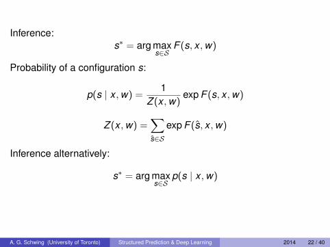
Inference:s∗ = arg max
s∈SF (s, x ,w)
Probability of a configuration s:
p(s | x ,w) =1
Z (x ,w)exp F (s, x ,w)
Z (x ,w) =∑s∈S
exp F (s, x ,w)
Inference alternatively:
s∗ = arg maxs∈S
p(s | x ,w)
A. G. Schwing (University of Toronto) Structured Prediction & Deep Learning 2014 22 / 40

Probability of a configuration s:
p(s | x ,w) =1
Z (x ,w)exp F (s, x ,w)
Z (x ,w) =∑s∈S
exp F (s, x ,w)
Maximize the likelihood of training data via
w∗ = arg maxw
∏(x ,s)∈D
p(s|x ,w)
= arg maxw
∑(x ,s)∈D
F (s, x ,w)− ln∑s∈S
exp F (s, x ,w)
A. G. Schwing (University of Toronto) Structured Prediction & Deep Learning 2014 23 / 40

Maximum likelihood is equivalent to maximizing cross-entropy:Target distribution: p(x ,s),tg(s) = δ(s = s)Cross-Entropy:
maxw
∑(x ,s)∈D,s
p(x ,s),tg(s) ln p(s | x ;w)
= maxw
∑(x ,s)∈D
ln p(s | x ;w)
= maxw
ln∏
(x ,s)∈D
p(s | x ;w)
A. G. Schwing (University of Toronto) Structured Prediction & Deep Learning 2014 24 / 40

Program of interest:
maxw
∑(x ,s)∈D,s
p(x ,s),tg(s) ln p(s | x ;w)
Optimize via gradient ascent
∂
∂w
∑(x ,s)∈D,s
p(x ,s),tg(s) ln p(s | x ;w)
=∑
(x ,s)∈D,s
(p(x ,s),tg(s)− p(s | x ;w)
) ∂
∂wF (s, x ,w)
Compute predicted distribution p(s | x ;w)
Use chain rule to pass back difference between prediction andobservation
A. G. Schwing (University of Toronto) Structured Prediction & Deep Learning 2014 25 / 40

Algorithm: Deep Learning
Repeat until stopping criteria
1 Forward pass to compute F (s, x ,w)
2 Compute p(s | x ,w)
3 Backward pass via chain rule to obtaingradient
4 Update parameters w
Why is large scale data a challenge?
How do we even represent F (s, x ,w) if S is large?How do we compute p(s | x ,w)?
A. G. Schwing (University of Toronto) Structured Prediction & Deep Learning 2014 26 / 40
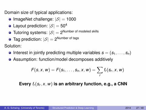
Domain size of typical applications:ImageNet challenge: |S| = 1000Layout prediction: |S| = 504
Tutoring systems: |S| = 2Number of modeled skills
Tag prediction: |S| = 2Number of tags
Solution:Interest in jointly predicting multiple variables s = (s1, . . . , sn)
Assumption: function/model decomposes additively
F (s, x ,w) = F (s1, . . . , sn, x ,w) =∑
r
fr (sr , x ,w)
Every fr (sr , x ,w) is an arbitrary function, e.g., a CNN
A. G. Schwing (University of Toronto) Structured Prediction & Deep Learning 2014 27 / 40
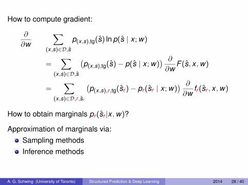
How to compute gradient:
∂
∂w
∑(x ,s)∈D,s
p(x ,s),tg(s) ln p(s | x ;w)
=∑
(x ,s)∈D,s
(p(x ,s),tg(s)− p(s | x ;w)
) ∂
∂wF (s, x ,w)
=∑
(x ,s)∈D,r ,sr
(p(x ,s),r ,tg(sr )− pr (sr | x ;w)
) ∂
∂wfr (sr , x ,w)
How to obtain marginals pr (sr |x ,w)?
Approximation of marginals via:Sampling methodsInference methods
A. G. Schwing (University of Toronto) Structured Prediction & Deep Learning 2014 28 / 40

Inference approximations:
maxb∈L
∑r ,sr
br (sr | x ,w)fr (sr , x ,w)︸ ︷︷ ︸Inference
+∑
r
cr H(br )
s1 s2
s1,2
A. G. Schwing (University of Toronto) Structured Prediction & Deep Learning 2014 29 / 40

Typically employed variational algorithms:Convex Belief Propagation (distributed)Tree-reweighted message passing(Generalized) Loopy Belief Propagation(Generalized) double loop Loopy Belief Propagation
A. G. Schwing (University of Toronto) Structured Prediction & Deep Learning 2014 30 / 40

Approximated Deep Structured Learning
Repeat until stopping criteria
1 CNN Forward pass to compute fr (sr , x ,w) ∀r2 Compute approximate beliefs br (sr | x ,w)
3 Backward pass via chain rule to obtaingradient g
4 Update parameters w
g =∑
(x ,s)∈D,r ,sr
(p(x ,s),r ,tg(sr )− br (sr | x ,w)
) ∂
∂wfr (sr , x ,w)
A. G. Schwing (University of Toronto) Structured Prediction & Deep Learning 2014 31 / 40
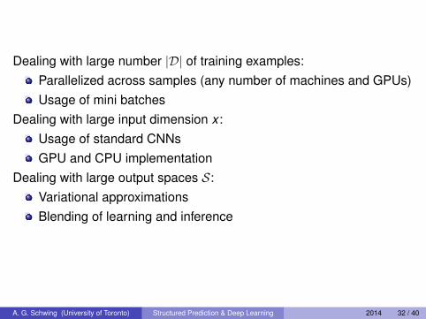
Dealing with large number |D| of training examples:Parallelized across samples (any number of machines and GPUs)Usage of mini batches
Dealing with large input dimension x :Usage of standard CNNsGPU and CPU implementation
Dealing with large output spaces S:Variational approximationsBlending of learning and inference
A. G. Schwing (University of Toronto) Structured Prediction & Deep Learning 2014 32 / 40

ImageNet dataset|S| = 10001.2 million training examples50,000 validation examples
Model Validation set error [%]AlexNet 19.95
DeepNet16 10.29DeepNet19 10.37
Different from reported results because of missing averaging, differentimage crops, etc.
A. G. Schwing (University of Toronto) Structured Prediction & Deep Learning 2014 33 / 40

Layout datasetGiven a single image x , predict a 3D parametric box that bestdescribes the observed room layout
|S| = 504
Linear model205 training examples104 test examples
A. G. Schwing (University of Toronto) Structured Prediction & Deep Learning 2014 34 / 40
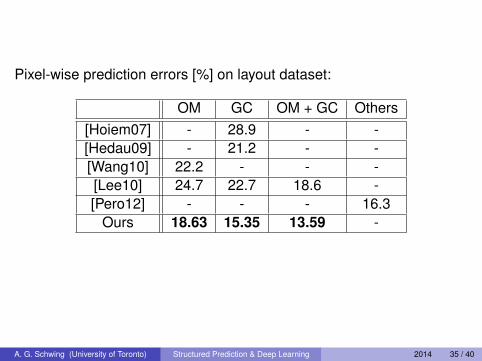
Pixel-wise prediction errors [%] on layout dataset:
OM GC OM + GC Others[Hoiem07] - 28.9 - -[Hedau09] - 21.2 - -[Wang10] 22.2 - - -[Lee10] 24.7 22.7 18.6 -[Pero12] - - - 16.3
Ours 18.63 15.35 13.59 -
A. G. Schwing (University of Toronto) Structured Prediction & Deep Learning 2014 35 / 40
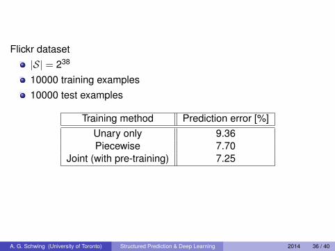
Flickr dataset|S| = 238
10000 training examples10000 test examples
Training method Prediction error [%]Unary only 9.36Piecewise 7.70
Joint (with pre-training) 7.25
A. G. Schwing (University of Toronto) Structured Prediction & Deep Learning 2014 36 / 40

Visual results
female/indoor/portrait sky/plant life/tree water/animals/seafemale/indoor/portrait sky/plant life/tree water/animals/sky
animals/dog/indoor indoor/flower/plant lifeanimals/dog ∅
A. G. Schwing (University of Toronto) Structured Prediction & Deep Learning 2014 37 / 40
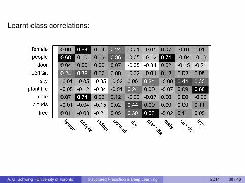
Learnt class correlations:
A. G. Schwing (University of Toronto) Structured Prediction & Deep Learning 2014 38 / 40

Distributed InferenceMaintaining convergence guaranteesParallelized across computers
Deep Nonlinear Structured PredictionNonlinearity, e.g., via CNNs in every factorUnifying structured prediction
A. G. Schwing (University of Toronto) Structured Prediction & Deep Learning 2014 39 / 40

Future directionsApplicationsEffects of approximationsLatent variable modelsCan we include the optimization of the model hyper-parametersTime series data
A. G. Schwing (University of Toronto) Structured Prediction & Deep Learning 2014 40 / 40