albrecht böttcher daniel potts peter stollmann david
TRANSCRIPT

Operator TheoryAdvances and Applications
268
Albrecht BöttcherDaniel PottsPeter StollmannDavid WenzelEditors
The Diversity and Beauty of Applied Operator Theory


Subseries Linear Operators and Linear Systems
Subseries editors: Daniel Alpay (Orange, CA, USA) Birgit Jacob (Wuppertal, Germany) André C.M. Ran (Amsterdam, The Netherlands)
Subseries Advances in Partial Differential Equations
Subseries editors: Bert-Wolfgang Schulze (Potsdam, Germany) Michael Demuth (Clausthal, Germany) Jerome A. Goldstein (Memphis, TN, USA) Nobuyuki Tose (Yokohama, Japan) Ingo Witt (Göttingen, Germany)
More information about this series at http://www.springer.com/series/4850
Operator Theory: Advances and Applications Volume 26
Founded in 1979 by Israel Gohberg
Editors: Joseph A. Ball (Blacksburg, VA, USA)
Heinz Langer (Wien, Austria) Christiane Tretter (Bern, Switzerland)
Associate Editors: Vadim Adamyan (Odessa, Ukraine) Wolfgang Arendt (Ulm, Germany)
Harry Dym (Rehovot, Israel)
B. Malcolm Brown (Cardiff, UK) Raul Curto (Iowa, IA, USA) Kenneth R. Davidson (Waterloo, ON, Canada) Fritz Gesztesy (Waco, TX, USA) Pavel Kurasov (Stockholm, Sweden) Vern Paulsen (Houston, TX, USA) Mihai Putinar (Santa Barbara, CA, USA) Ilya Spitkovsky (Abu Dhabi, UAE)
Albrecht Böttcher (Chemnitz, Germany)
Honorary and Advisory Editorial Board: Lewis A. Coburn (Buffalo, NY, USA) Ciprian Foias (College Station, TX, USA) J.William Helton (San Diego, CA, USA) Marinus A. Kaashoek (Amsterdam, NL)
Peter Lancaster (Calgary, Canada) Peter D. Lax (New York, NY, USA) Bernd Silbermann (Chemnitz, Germany) Harold Widom (Santa Cruz, CA, USA)
Thomas Kailath (Stanford, CA, USA)
8

Albrecht Böttcher • Daniel Potts • Peter StollmannDavid WenzelEditors
The Diversity and Beauty of Applied Operator Theory

ISSN 0255-0156 ISSN 2296-4878 (electronic) Operator Theory: Advances and Applications ISBN 978-3-319-75995-1 ISBN 978-3-319-75996-8 (eBook)https://doi.org/10.1007/978-3-319-75996-8
Mathematics Subject Classification (2010): 47-06, 15B05, 15B52, 42A16, 42C15, 47A10, 47B15, 47B35, 47F05, 47G30, 47L15, 58J40, 81U20, 93C55 © Springer International Publishing AG, part of Springer Nature 2018 This work is subject to copyright. All rights are reserved by the Publisher, whether the whole or part of the material is concerned, specifically the rights of translation, reprinting, reuse of illustrations, recitation, broadcasting, reproduction on microfilms or in any other physical way, and transmission or information storage and retrieval, electronic adaptation, computer software, or by similar or dissimilar methodology now known or hereafter developed. The use of general descriptive names, registered names, trademarks, service marks, etc. in this publication does not imply, even in the absence of a specific statement, that such names are exempt from the relevant protective laws and regulations and therefore free for general use. The publisher, the authors and the editors are safe to assume that the advice and information in this book are believed to be true and accurate at the date of publication. Neither the publisher nor the authors or the editors give a warranty, express or implied, with respect to the material contained herein or for any errors or omissions that may have been made. The publisher remains neutral with regard to jurisdictional claims in published maps and institutional affiliations. Printed on acid-free paper
company Springer International Publishing AG part of Springer Nature. The registered company address is: Gewerbestrasse 11, 6330 Cham, Switzerland
Library of Congress Control Number: 2018938795
This book is published under the imprint Birkhäuser, www.birkhauser-science.com by the registered
Editors Albrecht Böttcher Daniel Potts
Peter Stollmann David Wenzel Fakultät für Mathematik Fakultät für Mathematik TU Chemnitz TU Chemnitz Chemnitz, Germany Chemnitz, Germany
Fakultät für Mathematik TU Chemnitz Chemnitz, Germany
Fakultät für Mathematik TU Chemnitz Chemnitz, Germany

Contents
Preface . . . . . . . . . . . . . . . . . . . . . . . . . . . . . . . . . . . . . . . . . . . . . . . . . . . . . . . . . . . . . . . . . . ix
Participants . . . . . . . . . . . . . . . . . . . . . . . . . . . . . . . . . . . . . . . . . . . . . . . . . . . . . . . . . . . . .xii
J.A. Ball, G.J. Groenewald and S. ter HorstStandard versus strict Bounded Real Lemma withinfinite-dimensional state space II: The storage function approach . . . 1
M. Barrera, A. Bottcher, S.M. Grudsky and E.A. MaximenkoEigenvalues of even very nice Toeplitz matrices can beunexpectedly erratic . . . . . . . . . . . . . . . . . . . . . . . . . . . . . . . . . . . . . . . . . . . . . . . 51
H. Bart, T. Ehrhardt and B. SilbermannSpectral regularity of a C∗-algebra generated bytwo-dimensional singular integral operators . . . . . . . . . . . . . . . . . . . . . . . . 79
J. Behrndt, F. Gesztesy and S. NakamuraA spectral shift function for Schrodinger operators with singularinteractions . . . . . . . . . . . . . . . . . . . . . . . . . . . . . . . . . . . . . . . . . . . . . . . . . . . . . . . 89
I.V. Blinova and I.Y. PopovQuantum graph with the Dirac operator and resonance statescompleteness . . . . . . . . . . . . . . . . . . . . . . . . . . . . . . . . . . . . . . . . . . . . . . . . . . . . . 111
A. Bottcher and I.M. SpitkovskyRobert Sheckley’s Answerer for two orthogonal projections . . . . . . . 125
M.C. Camara and J.R. PartingtonToeplitz kernels and model spaces . . . . . . . . . . . . . . . . . . . . . . . . . . . . . . . . 139
O. Christensen and M. HasannasabFrames, operator representations, and open problems . . . . . . . . . . . . . 155
R. CorsoA survey on solvable sesquilinear forms . . . . . . . . . . . . . . . . . . . . . . . . . . . 167
L.R.Ya. DoktorskiAn application of limiting interpolation to Fourier series theory . . .179
I. Doust and S. Al-shakarchiIsomorphisms of AC(σ) spaces for countable sets . . . . . . . . . . . . . . . . . 193
T. Ehrhardt and K. RostRestricted inversion of split-Bezoutians . . . . . . . . . . . . . . . . . . . . . . . . . . . 207
v

vi Contents
S. Gefter and A. GoncharukGeneralized backward shift operators on the ring Z[[x]],Cramer’s rule for infinite linear systems, and p-adic integers . . . . . . 247
T. HartungFeynman path integral regularization using Fourier IntegralOperator ζ-functions . . . . . . . . . . . . . . . . . . . . . . . . . . . . . . . . . . . . . . . . . . . . . 261
T. Hartung, K. Jansen, H. Leovey and J. VolmerImproving Monte Carlo integration by symmetrization . . . . . . . . . . . .291
A. Karlovich and E. ShargorodskyMore on the density of analytic polynomials in abstract Hardyspaces . . . . . . . . . . . . . . . . . . . . . . . . . . . . . . . . . . . . . . . . . . . . . . . . . . . . . . . . . . . .319
Yu.I. KarlovichPseudodifferential Operators with compound non-regularsymbols . . . . . . . . . . . . . . . . . . . . . . . . . . . . . . . . . . . . . . . . . . . . . . . . . . . . . . . . . . 331
H. LangenauAsymptotically sharp inequalities for polynomials involvingmixed Hermite norms . . . . . . . . . . . . . . . . . . . . . . . . . . . . . . . . . . . . . . . . . . . . 355
M. Levitin and H.M. OzturkA two-parameter eigenvalue problem for a class ofblock-operator matrices . . . . . . . . . . . . . . . . . . . . . . . . . . . . . . . . . . . . . . . . . . 367
M. Lindner and H. SodingFinite sections of the Fibonacci Hamiltonian . . . . . . . . . . . . . . . . . . . . . 381
A. PushnitskiSpectral asymptotics for Toeplitz operators and an applicationto banded matrices . . . . . . . . . . . . . . . . . . . . . . . . . . . . . . . . . . . . . . . . . . . . . . . 397
S. RochBeyond fractality: piecewise fractal and quasifractal algebras . . . . . 413
K. SchmudgenUnbounded operators on Hilbert C∗-modules and C∗-algebras . . . . 429
Z. Sebestyen, Zs. Tarcsay and T. TitkosA characterization of positive normal functionals on the fulloperator algebra . . . . . . . . . . . . . . . . . . . . . . . . . . . . . . . . . . . . . . . . . . . . . . . . . 443
C. SeifertThe linearised Korteweg–de Vries equation on general metricgraphs . . . . . . . . . . . . . . . . . . . . . . . . . . . . . . . . . . . . . . . . . . . . . . . . . . . . . . . . . . . 449

Contents vii
N. ThornBounded multiplicative Toeplitz operators on sequence spaces . . . . 459
S. Trostorff and M. WaurickOn higher index differential-algebraic equations in infinitedimensions . . . . . . . . . . . . . . . . . . . . . . . . . . . . . . . . . . . . . . . . . . . . . . . . . . . . . . . 477
D. VirosztekCharacterizations of centrality by local convexity of certainfunctions on C∗-algebras . . . . . . . . . . . . . . . . . . . . . . . . . . . . . . . . . . . . . . . . . 487
J.A. VirtanenDouble-scaling limits of Toeplitz determinants andFisher–Hartwig singularities . . . . . . . . . . . . . . . . . . . . . . . . . . . . . . . . . . . . . . 495

Preface
These are the proceedings of the International Workshop on Operator Theoryand its Applications (IWOTA) that was held in Chemnitz in 2017. It was the28th iteration of the event since its initiation in 1981.
The fact that our university was chosen as the venue is a sign of thegreat appreciation for the longstanding tradition of our work in the field.Operator theory was established in Chemnitz by Siegfried Proßdorf in the1960s and later advanced by Bernd Silbermann and Georg Heinig. Today itis driven by various research groups, including those of the local organizingcommittee’s members.
Born about a century ago, operator theory now is one of the mathe-matical keys for the latest progress in science and technology. The methodsthat operator theory developed and continues to advance are used every dayby many people who work in the known application fields of mathematics,engineering, and physics. The aspect of applicability is also reflected in theensemble of that year’s main speakers:
Harm Bart,
Mark Embree,
Fritz Gesztesy,
Frances Kuo,
Christiane Tretter.
They all have made important contributions to both: development of operatortheory and concrete practical applications of new conceptual insights.
The list of invited speakers was completed by a healthy mix of youngand well-established researchers:
Marcel Hansmann,Bill Helton,Rien Kaashoek,Alexei Karlovich,Greg Knese,Marko Lindner,Alejandra Maestripieri,Jonathan Partington,
Stefanie Petermichl,Alexander Pushnitski,Konrad Schmudgen,Carola-Bibiane Schonlieb,Bernd Silbermann,Ilya Spitkovsky,Sanne ter Horst.
We managed to ensure undivided attention for all of them. Moreover, referringto them as “semi plenary speakers” is actually an understatement; since eachone had a 45 minutes talk, “semi-sesqui plenaries” would be a more precise,better fitting term.
ix

x Preface
Traditionally, the IWOTA conferences provide a platform for discussionand exchange of ideas via short talks. This time, they were scheduled in up toonly four parallel sessions, and many of these sessions were arranged within amini symposium. We are happy that especially early career scientists took theopportunity and approached us with well-fitting topics. In summary, sevenmini symposia were held:
Functional calculus(Markus Haase, Christian Le Merdy),
Riemann–Hilbert problems and applications in random matrix theory(Jani Virtanen),
Structured matrices and operators — in memory of Georg Heinig(Karla Rost),
New approaches for high-dim. integration in light of physics applications(Karl Jansen, Frances Kuo),
Semigroups and evolution equations(Andras Batkai, Christian Seifert),
Toeplitz and related operators(Santeri Miihkinen, Jani Virtanen),
The Rien Kaashoek mini symposium(Harm Bart, Andre Ran).
In addition to the thematically more closed symposia, several contributedtalks were accepted for presentation. They clearly demonstrate how big op-erator theory has become, extending over a wide range of topics:
General operator theory,Differential operators,Matrix norms and pseudospectra,Algebras and order relations,Functional analysis,Concrete operator theory.
Summing up, 157 participants from almost 40 countries enjoyed a total of126 talks given at the conference from August 14th to 18th. Many of thetalks can be found on the web site
https://www.tu-chemnitz.de/mathematik/iwota2017/
preserved for eternity. We are greatly indebted to the Deutsche Forschungs-gemeinschaft (DFG), the president and the chancellor of the TU Chemnitz,and the dean of the Department of Mathematics for their financial support.
We sincerely hope you will also enjoy the 29 articles in this volume ofOperator Theory: Advances and Applications. We are very thankful that thepublisher kindly raised the page number limit. Nevertheless, even more goodmanuscripts were submitted, and we could not include all of them. So weselected the most beautiful works representing the one or other of the diverseaspects of operator theory.
ChemnitzJanuary 2018
Albrecht Bottcher, Daniel PottsPeter Stollmann, David Wenzel


xii Participants
Participants
Abadias, Luciano(Zaragoza, Spain)
Adamo, Maria Stella(Palermo, Italy)
Amenta, Alex(Delft, Netherlands)
Banert, Michaela(Chemnitz, Germany)
Bart, Harm(Rotterdam, Netherlands)
Barta, Tomas(Praha, Czech Republic)
Batkai, Andras(Feldkirch, Austria)
Batty, Charles(Oxford, United Kingdom)
Bello-Burguet, Glenier L.(Madrid, Spain)
Beric, Tomislav(Zagreb, Croatia)
Blinova, Irina(St. Petersburg, Russian Fedn.)
Blower, Gordon(Lancaster, United Kingdom)
Bombach, Clemens(Chemnitz, Germany)
Bottcher, Albrecht(Chemnitz, Germany)
Bowkun, Jakob(Chemnitz, Germany)
Budde, Christian(Wuppertal, Germany)
Charlier, Christophe(Bruxelles, Belgium)
Chen, Jinwen(Beijing, China)
Cho, Muneo(Hiratsuka, Japan)
Choda, Marie(Osaka, Japan)
Christensen, Ole(Lyngby, Denmark)
Corso, Rosario(Palermo, Italy)
Dhara, Kousik(Chennai, India)
Didenko, Viktor(Odessa, Ukraine)
Djikic, Marko(Nis, Serbia)
Doeraene, Antoine(Louvain, Belgium)
Dogga, Venku naidu(Sangareddy, India)
Doktorski, Leo(Ettlingen, Germany)
Doust, Ian(Sydney, Australia)
Dragicevic, Oliver(Ljubljana, Slovenia)
Dritschel, Michael(Newcastle, United Kingdom)
Duduchava, Rolandi(Tbilisi, Georgia)
Ehrhardt, Torsten(Santa Cruz, United States)
Embree, Mark(Blacksburg/VA, United States)
Flemming, Katharina(Chemnitz, Germany)
Frazho, Arthur(West Lafayette/IN, Utd. States)
Frymark, Dale(Waco, United States)
Fulsche, Robert(Hannover, Germany)
Geher, Gyorgy Pal(Reading, United Kingdom)
Gesztesy, Fritz(Waco, United States)
Gohm, Rolf(Aberystwyth, United Kingdom)
Golla, Ramesh(Sangareddy, India)

Participants xiii
Goncalves, Helena(Jena, Germany)
Goncharuk, Anna(Kharkiv, Ukraine)
Grossmann, Christian(Dresden, Germany)
Grudsky, Sergei(Ciudad de Mexico, Mexico)
Guediri, Hocine(Riyadh, Saudi Arabia)
Gunatillake, Gajath(Sharjah, Utd. Arab Emirates)
Haase, Markus(Kiel, Germany)
Hagger, Raffael(Hannover, Germany)
Hansmann, Marcel(Chemnitz, Germany)
Hartung, Tobias(London, United Kingdom)
Hedenmalm, Hakan(Stockholm, Sweden)
Helton, J. William(San Diego, United States)
Jaftha, Jacob(Cape Town, South Africa)
Janse van Rensburg, Dawid(Potchefstroom, South Africa)
Jansen, Karl(Zeuthen, Germany)
Jardon Sanchez, Hector(Gijon/Xixon, Spain)
Junghanns, Peter(Chemnitz, Germany)
Kaashoek, Marinus A.(Amsterdam, Netherlands)
Kaiser, Robert(Chemnitz, Germany)
Kalmes, Thomas(Chemnitz, Germany)
Kammerer, Lutz(Chemnitz, Germany)
Kapanadze, David(Tbilisi, Georgia)
Karlovich, Alexei(Lisboa, Portugal)
Karlovich, Yuri(Cuernavaca, Mexico)
Kazashi, Yoshihito(Sydney, Australia)
Kerner, Joachim(Hagen, Germany)
Kitson, Derek(Lancaster, United Kingdom)
Kircheis, Melanie(Chemnitz, Germany)
Klaja, Hubert(Lille, France)
Knese, Greg(St. Louis, United States)
Koca, Beyaz Basak(Istanbul, Turkey)
Kozlowska, Katarzyna(Reading, United Kingdom)
Kreuter, Marcel(Ulm, Germany)
Kriegler, Christoph(Aubiere, France)
Kumar, V. B. Kiran(Cochin, India)
Kuo, Frances(Sydney, Australia)
Langenau, Holger(Chemnitz, Germany)
Lanucha, Bartosz(Lublin, Poland)
Le Merdy, Christian(Besancon, France)
Lee, Ji Eun(Seoul, Korea)
Lee, Mee-Jung(Seoul, Korea)
Lee, Young Joo(Gwangju, Korea)
Leiterer, Jurgen(Berlin, Germany)
Leka, Zoltan(London, United Kingdom)

xiv Participants
Leovey, Hernan(Villingen-Schwenn., Germany)
Lindner, Marko(Hamburg, Germany)
Lindstrom, Mikael(Turku, Finland)
Madler, Conrad(Leipzig, Germany)
Maestripieri, Alejandra(Buenos Aires, Argentina)
Marchenko, Vitalii(Kiev, Ukraine)
Mascarenhas, Helena(Lisboa, Portugal)
Maximenko, Egor(Ciudad de Mexico, Mexico)
Michael, Isaac(Waco, United States)
Michalska, Ma lgorzata(Lublin, Poland)
Miheisi, Nazar(London, United Kingdom)
Miihkinen, Santeri(Joensuu, Finland)
Nakic, Ivica(Zagreb, Croatia)
Nasdala, Robert(Chemnitz, Germany)
Nuyens, Dirk(Leuven, Belgium)
Ozturk, Hasen(Reading, United Kingdom)
Pannasch, Florian(Kiel, Germany)
Partington, Jonathan(Leeds, United Kingdom)
Peruzzetto, Marco(Kiel, Germany)
Petermichl, Stefanie(Toulouse, France)
Pietrzycki, Pawe l(Cracow, Poland)
Pik, Derk(Amsterdam, Netherlands)
Popov, Igor(St. Petersburg, Russian Fedn.)
Potts, Daniel(Chemnitz, Germany)
Pushnitski, Alexander(London, United Kingdom)
Quellmalz, Michael(Chemnitz, Germany)
Ran, Andre(Amsterdam, Netherlands)
Rebs, Christian(Chemnitz, Germany)
Roch, Steffen(Darmstadt, Germany)
Rocha, Jamilly(Recife, Brazil)
Rose, Christian(Chemnitz, Germany)
Rost, Karla(Chemnitz, Germany)
Sau, Haripada(Mumbai, India)
Schmudgen, Konrad(Leipzig, Germany)
Schonlieb, Carola-Bibiane(Cambridge, United Kingdom)
Schwenninger, Felix(Hamburg, Germany)
Seidel, Markus(Zwickau, Germany)
Seifert, Christian(Hamburg, Germany)
Seiler, Jorg(Torino, Italy)
Semrl, Peter(Ljubljana, Slovenia)
Shukur, Ali(Minsk, Belarus)
Silbermann, Bernd(Chemnitz, Germany)
Singh, Uaday(Roorkee, India)
Speck, Frank-Olme(Lisboa, Portugal)

Participants xv
Spitkovsky, Ilya(Abu Dhabi, Utd. Arab Emirates)
Stahn, Reinhard(Dresden, Germany)
Stollmann, Peter(Chemnitz, Germany)
Tanahashi, Kotaro(Sendai, Japan)
Taskinen, Jari(Helsinki, Finland)
Tautenhahn, Martin(Chemnitz, Germany)
ter Horst, Sanne(Potchefstroom, South Africa)
Thorn, Nicola(Reading, United Kingdom)
Titkos, Tams(Budapest, Hungary)
Tomilov, Yuri(Warsaw, Poland)
Trapani, Camillo(Palermo, Italy)
Tretter, Christiane(Bern, Switzerland)
Trostorff, Sascha(Dresden, Germany)
Trunk, Carsten(Ilmenau, Germany)
Uhlig, Sven(Mannheim, Germany)
Undrakh, Batzorig(Newcastle u. Tyne, Utd. Kingd.)
van Schagen, Frederik(Amsterdam, Netherlands)
Virosztek, Dniel(Budapest, Hungary)
Virtanen, Jani(Reading, United Kingdom)
Volkmer, Toni(Chemnitz, Germany)
Volmer, Julia(Zeuthen, Germany)
Wang, Qin(Shanghai, China)
Waurick, Marcus(Glasgow, United Kingdom)
Wegert, Elias(Freiberg, Germany)
Wenzel, David(Chemnitz, Germany)
Wintermayr, Jens(Wuppertal, Germany)
Yakubovich, Dmitry(Madrid, Spain)

Standard versus strict Bounded Real Lemmawith infinite-dimensional state space II:The storage function approach
J.A. Ball, G.J. Groenewald and S. ter Horst
Abstract. For discrete-time causal linear input/state/output systems,the Bounded Real Lemma explains (under suitable hypotheses) the con-tractivity of the values of the transfer function over the unit disk forsuch a system in terms of the existence of a positive-definite solutionof a certain Linear Matrix Inequality (the Kalman–Yakubovich–Popov(KYP) inequality). Recent work has extended this result to the set-ting of infinite-dimensional state space and associated non-rationalityof the transfer function, where at least in some cases unbounded solu-tions of the generalized KYP-inequality are required. This paper is thesecond installment in a series of papers on the Bounded Real Lemmaand the KYP-inequality. We adapt Willems’ storage-function approachto the infinite-dimensional linear setting, and in this way reprove vari-ous results presented in the first installment, where they were obtainedas applications of infinite-dimensional State-Space-Similarity theorems,rather than via explicit computation of storage functions.
Mathematics Subject Classification (2010). Primary 47A63; Secondary47A48, 93B20, 93C55, 47A56.
Keywords. KYP-inequality, storage function, bounded real lemma, infi-nite-dimensional linear system, minimal system.
1. Introduction
This paper is the second installment, following [11], on the infinite-dimen-sional bounded real lemma for discrete-time systems and the discrete-timeKalman–Yakubovich–Popov (KYP) inequality. In this context, we consider
This work is based on the research supported in part by the National Research Foundationof South Africa (Grant Numbers 93039, 90670, and 93406).
© Springer International Publishing AG, part of Springer Nature 2018
Theory: Advances and Applications 268, https://doi.org/10.1007/978-3-319-75996-8_1
1A. Böttcher et al. (eds.), The Diversity and Beauty of Applied Operator Theory, Operator

2 J.A. Ball, G.J. Groenewald and S. ter Horst
the discrete-time linear system
Σ :=
x(n+ 1) = Ax(n) +Bu(n),
y(n) = Cx(n) +Du(n),(n ∈ Z) (1.1)
where A : X → X , B : U → X , C : X → Y and D : U → Y are boundedlinear Hilbert space operators, i.e., X , U and Y are Hilbert spaces and thesystem matrix associated with Σ takes the form
M =
[A BC D
]:
[XU
]→[XY
]. (1.2)
We refer to the pair (C,A) as the output pair and to the pair (A,B) as theinput pair. In this case input sequences u = (u(n))n∈Z, with u(n) ∈ U , aremapped to output sequences y = (y(n))n∈Z, with y(n) ∈ Y, through thestate sequence x = (x(n))n∈Z, with x(n) ∈ X . A system trajectory of thesystem Σ is then any triple (u(n),x(n),y(n))n∈Z of input, state and outputsequences that satisfy the system equations (1.1).
With the system Σ we associate the transfer function given by
FΣ(λ) = D + λC(I − λA)−1B. (1.3)
Since A is bounded, FΣ is defined and analytic on a neighborhood of 0 inC. We are interested in the case where FΣ admits an analytic continuationto the open unit disk D such that the supremum norm ‖FΣ‖∞ of FΣ over Dis at most one, i.e., FΣ has analytic continuation to a function in the Schurclass
S(U ,Y) =
F : D 7→
holoL(U ,Y) : ‖F (λ)‖ ≤ 1 for all z ∈ D
.
Sometimes we also consider system trajectories (u(n),x(n),y(n))n≥n0
of the system Σ that are initiated at a certain time n0 ∈ Z, in which case theinput, state and output at time n < n0 are set equal to zero, and we onlyrequire that the system equations (1.1) are satisfied for n ≥ n0. Althoughtechnically such trajectories are not system trajectories for Σ, but rathercorrespond to trajectories of the corresponding singly-infinite forward-timesystem rather than the bi-infinite system Σ, the transfer function of thissingly-infinite forward-time system coincides with the transfer function FΣ ofΣ. Hence for the sake of the objective, determining whether FΣ ∈ S(U ,Y),there is no problem with considering such singly-infinite system trajectories.
Before turning to the infinite-dimensional setting, we first discuss thecase where U , X , Y are all finite-dimensional. If in this case one considers theparallel situation in continuous time rather than in discrete time, these ideashave origins in circuit theory, specifically conservative or passive circuits.An important question in this context is to identify which rational matrixfunctions, analytic on the left half-plane (rather than the unit disk D), arisefrom a lossless or dissipative circuit in this way (see, e.g., Belevitch [12]).
According to Willems [28, 29], a linear system Σ as in (1.1) is dissipative(with respect to supply rate s(u, y) = ‖u‖2−‖y‖2) if it has a storage functionS : X → R+, where S(x) is to be interpreted as a measure of the energy stored

Infinite-dimensional Bounded Real Lemma II 3
by the system when it is in state x. Such a storage function S is assumed tosatisfy the dissipation inequality
S(x(n+ 1))− S(x(n)) ≤ ‖u(n)‖2 − ‖y(n)‖2 (1.4)
over all trajectories (u(n),x(n),y(n))n∈Z of the system Σ as well as the ad-ditional normalization condition that S(0) = 0. The dissipation inequalitycan be interpreted as saying that for the given system trajectory, the energystored in the system (S(x(n+ 1))− S(x(n))) when going from state x(n) tox(n+ 1) can be no more than the difference between the energy that entersthe system (‖u(n)‖2) and the energy that leaves the system (‖y(n)‖2) attime n.
For our discussion here we shall only be concerned with the so-calledscattering supply rate s(u, y) = ‖u‖2 − ‖y‖2. It is not hard to see that aconsequence of the dissipation inequality (1.4) on system trajectories is thatthe transfer function FΣ is in the Schur class S(U ,Y). The results extend tononlinear systems as well (see [28]), where one talks about the system havingL2-gain at most 1 rather the system having transfer function in the Schurclass.
In case the system Σ is finite-dimensional and minimal (as defined inthe statement of Theorem 1.1 below), one can show that the smallest storagefunction, the available storage Sa, and the largest storage function, the re-quired supply Sr, are quadratic, provided storage functions for Σ exist. ThatSa and Sr are quadratic means that there are positive-definite matrices Ha
and Hr so that Sa and Sr have the quadratic form
Sa(x) = 〈Hax, x〉, Sr(x) = 〈Hrx, x〉with Ha and Hr actually being positive-definite. For a general quadraticstorage function SH(x) = 〈Hx, x〉 for a positive-definite matrix H, it is nothard to see that the dissipation inequality (1.4) assumes the form of a linearmatrix inequality (LMI):[
A BC D
]∗ [H 00 IY
] [A BC D
][H 00 IU
]. (1.5)
This is what we shall call the Kalman–Yakubovich–Popov or KYP inequality(with solution H for given system matrix M = [A B
C D ]).Conversely, if one starts with a finite-dimensional, minimal, linear sys-
tem Σ as in (1.1) for which the transfer function FΣ is in the Schur class, itis possible to show that there exist quadratic storage functions SH for thesystem satisfying the coercivity condition SH(x) ≥ δ‖x‖2 for some δ > 0 (i.e.,with H strictly positive-definite). This is the storage-function interpretationbehind the following result, known as the Kalman–Yakubovich–Popov lemma.
Theorem 1.1 (Standard Bounded Real Lemma (see [1])). Let Σ be a discrete-time linear system as in (1.1) with X , U and Y finite-dimensional, sayU = Cr, Y = Cs, X = Cn, so that the system matrix M has the form
M =
[A BC D
]:
[CnCr]→[CnCs]
(1.6)

4 J.A. Ball, G.J. Groenewald and S. ter Horst
and the transfer function FΣ is equal to a rational matrix function of sizes × r. Assume that the realization (A,B,C,D) is minimal, i.e., the outputpair (C,A) is observable and the input pair (A,B) is controllable:
n⋂k=0
KerCAk = 0 and spank=0,1,...,n−1
ImAkB = X = Cn. (1.7)
Then FΣ is in the Schur class S(Cr,Cs) if and only if there is an n × npositive-definite matrix H satisfying the KYP-inequality (1.5).
There is also a strict version of the Bounded Real Lemma. The asso-ciated storage function required is a strict storage function, i.e., a functionS : X → R+ for which there is a number δ > 0 so that
S(x(n+ 1))− S(x(n)) + δ‖x(n)‖2 ≤ (1− δ)‖u(n)‖2 − ‖y(n)‖2 (1.8)
holds over all system trajectories (u(n),x(n),y(n))n∈Z, in addition to thenormalization condition S(0) = 0. If SH(x) = 〈Hx, x〉 is a quadratic strictstorage function, then the associated linear matrix inequality is the strictKYP-inequality [
A BC D
]∗ [H 00 IY
] [A BC D
]≺[H 00 IU
]. (1.9)
In this case, one also arrives at a stronger condition on the transfer functionFΣ, namely that it has an analytic continuation to a function in the strictSchur class
So(U ,Y) =
F : D 7→
holoL(U ,Y) : sup
z∈D‖F (z)‖ ≤ ρ for some ρ < 1
.
Note, however, that the strict KYP-inequality implies that A is stable, so thatin case (1.9) holds, FΣ is in fact analytic on D. This is the storage-functioninterpretation of the following strict Bounded Real Lemma, in which onereplaces the minimality condition with a stability condition.
Theorem 1.2 (Strict Bounded Real Lemma (see [24])). Suppose that the dis-crete-time linear system Σ is as in (1.1) with X , U and Y finite-dimensional,say U = Cr, Y = Cs, X = Cn, i.e., the system matrix M is as in (1.6).Assume that A is stable, i.e., all eigenvalues of A are inside the open unitdisk D, so that rspec(A) < 1 and the transfer function FΣ(z) is analytic on
a neighborhood of D. Then FΣ(z) is in the strict Schur class So(Cr,Cs) ifand only if there is a positive-definite matrix H ∈ Cn×n so that the strictKYP-inequality (1.9) holds.
We now turn to the general case, where the state space X and the inputspace U and the output space Y are allowed to be infinite-dimensional. Inthis case, the results are more recent, depending on the precise hypotheses.
For generalizations of Theorem 1.1, much depends on what is meant byminimality of Σ, and hence by the corresponding notions of controllable andobservable. Here are the three possibilities for controllability of an input pair(A,B) which we shall consider. The third notion involves the controllability

Infinite-dimensional Bounded Real Lemma II 5
operator Wc associated with the pair (A,B) tailored to the Hilbert spacesetup which in general is a closed, possibly unbounded operator with domainD(Wc) dense in X mapping into the Hilbert space `2U (Z−) of Y-valued se-quences supported on the negative integers Z− = −1,−2,−3, . . . , as wellas the observability operator Wo associated with the pair (C,A), which hassimilar properties. We postpone precise definitions and properties of theseoperators to Section 2.
For an input pair (A,B) we define the following notions of controllabil-ity:
• (A,B) is (approximately) controllable if the reachability space
Rea(A|B) = spanImAkB : k = 0, 1, 2, . . . (1.10)
is dense in X .• (A,B) is exactly controllable if the reachability space Rea(A|B) is equal
to X , i.e., each state vector x ∈ X has a representation as a finite
linear combination x =∑Kk=0A
kBuk for a choice of finitely many inputvectors u0, u1, . . . , uK (also known as every x is a finite-time reachablestate (see [22, Definition 3.3]).• (A,B) is `2-exactly controllable if the `2-adapted controllability operatorWc has range equal to all of X : WcD(Wc) = X .
If (C,A) is an output pair, we have the dual notions of observability:
• (C,A) is (approximately) observable if the input pair (A∗, C∗) is (ap-proximately) controllable, i.e., if the observability space
Obs(C|A) = spanImA∗kC∗ : k = 0, 1, 2, . . . (1.11)
is dense in X , or equivalently, if ∩∞k=0 kerCAk = 0.• (C,A) is exactly observable if the observability subspace Obs(C|A) is
the whole space X .• (C,A) is `2-exactly observable if the adjoint input pair (A∗, C∗) is `2-
exactly controllable, i.e., if the adjoint W∗o of the `2-adapted observ-
ability operator Wo has full range: W∗o D(W∗
o) = X .
Then we say that the system Σ ∼ (A,B,C,D) is
• minimal if (A,B) is controllable and (C,A) is observable,• exactly minimal if both (A,B) is exactly controllable and (C,A) is ex-
actly observable, and• `2-exactly minimal if both (A,B) is `2-exactly controllable and (C,A)
is `2-exactly observable.
Despite the fact that the operators A, B, C and D associated withthe system Σ are all bounded, in the infinite-dimensional analogue of theKYP-inequality (1.5) unbounded solutions H may appear. We therefore haveto be more precise concerning the notion of positive-definiteness we employ.Suppose that H is a (possibly unbounded) selfadjoint operator H on a Hilbertspace X with domain D(H) dense in X ; we refer to [26] for background anddetails on this class and other classes of unbounded operators. Then we shallsay:

6 J.A. Ball, G.J. Groenewald and S. ter Horst
• H is strictly positive-definite (written H 0) if there is a δ > 0 so that〈Hx, x〉 ≥ δ‖x‖2 for all x ∈ D(H);• H is positive-definite if 〈Hx, x〉 > 0 for all nonzero x ∈ D(H);• H is positive-semidefinite (written H 0) if 〈Hx, x〉 ≥ 0 for x ∈ D(H).
We also note that any (possibly unbounded) positive-semidefinite operator
H has a positive-semidefinite square root H12 ; as H = H
12 ·H 1
2 , we have
D(H) = x ∈ D(H12 ) : H
12x ∈ D(H
12 ) ⊂ D(H
12 ).
See, e.g., [26] for details.Since solutions H to the corresponding KYP-inequality may be un-
bounded, the KYP-inequality cannot necessarily be written in the LMI form(1.5), but rather, we require a spatial form of (1.5) on the appropriate domain:For a (possibly unbounded) positive-definite operator H on X satisfying
AD(H12 ) ⊂ D(H
12 ), BU ⊂ D(H
12 ), (1.12)
the spatial form of the KYP-inequality takes the form∥∥∥∥[H 12 0
0 IU
] [xu
]∥∥∥∥2
−∥∥∥∥[H 1
2 00 IY
] [A BC D
] [xu
]∥∥∥∥2
≥ 0 (1.13)
(x ∈ D(H12 ), u ∈ U).
The corresponding notion of a storage function will then be allowed to assume+∞ as a value; this will be made precise in Section 3.
With all these definitions out of the way, we can state the following threedistinct generalizations of Theorem 1.1 to the infinite-dimensional situation.
Theorem 1.3 (Infinite-dimensional standard Bounded Real Lemma). Let Σbe a discrete-time linear system as in (1.1) with system matrix M as in (1.2)and transfer function FΣ defined by (1.3).
(1) Suppose that the system Σ is minimal, i.e., the input pair (A,B) iscontrollable and the output pair (C,A) is observable. Then the transferfunction FΣ has an analytic continuation to a function in the Schurclass S(U ,Y) if and only if there exists a positive-definite solution Hof the KYP-inequality in the following generalized sense: H is a closed,possibly unbounded, densely defined, positive-definite (and hence injec-
tive) operator on X such that D(H12 ) satisfies (1.12) and H solves the
spatial KYP-inequality (1.13).(2) Suppose that Σ is exactly minimal. Then the transfer function FΣ has
an analytic continuation to a function in the Schur class S(U ,Y) if andonly if there exists a bounded, strictly positive-definite solution H of theKYP-inequality (1.5). In this case A has a spectral radius of at mostone, and hence FΣ is in fact analytic on D.
(3) Statement (2) above continues to hold if the “exactly minimal” hypoth-esis is replaced by the hypothesis that Σ be “`2-exactly minimal.”
We shall refer to a closed, densely defined, positive-definite solution H of(1.12)–(1.13) as a positive-definite solution of the generalized KYP-inequality.

Infinite-dimensional Bounded Real Lemma II 7
The paper of Arov–Kaashoek–Pik [6] gives a penetrating treatment ofitem (1) in Theorem 1.3, including examples to illustrate various subtletiessurrounding this result—e.g., the fact that the result can fail if one insistson classical bounded and boundedly invertible selfadjoint solutions of theKYP-inequality. We believe that items (2) and (3) appeared for the firsttime in [11], where also a sketch of the proof of item (1) is given. The ideabehind the proofs of items (1)–(3) in [11] is to combine the result that aSchur-class function S always has a contractive realization (i.e., such an Scan be realized as S = FΣ for a system Σ as in (1.1) with system matrix Min (1.2) a contraction operator) with variations of the State-Space-SimilarityTheorem (see [11, Theorem 1.5]) for the infinite-dimensional situation underthe conditions that hold in items (1)–(3); roughly speaking, under appropriatehypothesis, a State-Space-Similarity Theorem says that two systems Σ andΣ′ whose transfer functions coincide on a neighborhood of zero, necessarilycan be transformed (in an appropriate sense) from one to other via a changeof state-space coordinates.
In the present paper we revisit these three results from a differentpoint of view: we adapt Willems’ variational formulas to the infinite-dimen-sional setting, and in this context present the available storage Sa and re-quired supply Sr, as well as an `2-regularized version Sr of the requiredsupply. It is shown, under appropriate hypothesis, that these are storagefunctions, with Sa and Sr being quadratic storage functions, i.e., Sa agrees
with SHa(x) = ‖H12a x‖2 and Sr(x) = SHr (x) = ‖H
12r x‖2 for x in a suitably
large subspace of X , where Ha and Hr are possibly unbounded, positive-definite density operators, which turn out to be positive-definite solutionsto the generalized KYP-inequality. In this way we will arrive at a proof ofitem (1). Further analysis of the behavior of Ha and Hr, under additionalrestrictions on Σ, lead to proofs of items (2) and (3), as well as the followingversion of the strict Bounded Real Lemma for infinite-dimensional systems,which is a much more straightforward generalization of the result in thefinite-dimensional case (Theorem 1.2).
Theorem 1.4 (Infinite-dimensional strict Bounded Real Lemma). Let Σ bea discrete-time linear system as in (1.1) with system matrix M as in (1.2)and transfer function FΣ defined by (1.3). Assume that A is exponentiallystable, i.e., rspec(A) < 1. Then the transfer function FΣ is in the strict Schurclass So(U ,Y) if and only if there exists a bounded strictly positive-definitesolution H of the strict KYP-inequality (1.9).
Theorem 1.2 was proved by Petersen–Anderson–Jonkheere [24] for thecontinuous-time finite-dimensional setting by using what we shall call an ε-re-gularization procedure to reduce the result to the standard case Theorem 1.1.In [11] we show how this same idea can be used in the infinite-dimensionalsetting to reduce the hard direction of Theorem 1.4 to the result of either ofitem (2) or item (3) in Theorem 1.3. For the more general nonlinear setting,Willems [28] was primarily interested in what storage functions look likeassuming that they exist, while in [29] for the finite-dimensional linear setting

8 J.A. Ball, G.J. Groenewald and S. ter Horst
he reduced the existence problem to the existence theory for Riccati matrixequations. Here we solve the existence problem for the more general infinite-dimensional linear setting by converting Willems’ variational formulation ofthe available storage Sa and an `2-regularized version Sr of his requiredsupply Sr to an operator-theoretic formulation amenable to explicit analysis.
This paper presents a more unified approach to the different variationsof the Bounded Real Lemma, in the sense that we present a pair of con-cretely defined, unbounded, positive-definite operators Ha and Hr that, un-der the appropriate conditions, form positive-definite solutions to the gener-alized KYP-inequality, and that have the required additional features underthe additional conditions in items (2) and (3) of Theorem 1.3 as well as The-orem 1.4. We also make substantial use of connections with correspondingobjects for the adjoint system Σ∗ (see (5.1)) to complete the analysis andarrive at some order properties for the set of all solutions of the generalizedKYP-inequality which are complementary to those in [6].
The paper is organized as follows. Besides the current introduction,the paper consists of seven sections. In Section 2 we give the definitionsof the observability operator Wo and controllability operator Wc associ-ated with the system Σ in (1.1) and recall some of their basic properties. InSection 3 we define what is meant by a storage function in the context ofinfinite-dimensional discrete-time linear systems Σ of the form (1.1) as wellas strict and quadratic storage functions, and we clarify the relations be-tween quadratic (strict) storage functions and solutions to the (generalized)KYP-inequality. Section 4 is devoted to the available storage Sa and requiredsupply Sr, two examples of storage functions, in case the transfer function ofΣ has an analytic continuation to a Schur-class function. It is shown that Saand an `2-regularized version Sr of Sr in fact agree with quadratic storagefunctions on suitably large domain via explicit constructions of two closed,densely defined, positive-definite operators Ha and Hr that exhibit Sa andSr as quadratic storage functions SHa and SHr . In Section 5 we make explicitthe theory for the adjoint system Σ∗ and the duality connections between Σand Σ∗. In Section 6 we study the order properties of a class of solutions ofthe generalized KYP-inequality, and obtain the conditions under which Ha
and Hr are bounded and/or boundedly invertible and thereby solutions ofthe classical KYP-inequality. These results are then used in Section 7 to giveproofs of Theorems 1.3 and 1.4 via the storage function approach.
2. Review: minimality, controllability, observability
In this section we recall the definitions of the observability operator Wo andcontrollability operator Wc associated with the discrete-time linear systemΣ given by (1.1) and various of their basic properties which will be neededin the sequel. Detailed proofs of most of these results as well as additionalproperties can be found in [11, Section 2].

Infinite-dimensional Bounded Real Lemma II 9
For the case of a general system Σ, following [11, Section 2], we define theobservability operator Wo associated with Σ to be the possibly unboundedoperator with domain D(Wo) in X given by
D(Wo) =x ∈ X : CAnxn≥0 ∈ `2Y(Z+)
(2.1)
with action given by
Wox = CAnxn≥0 for x ∈ D(Wo). (2.2)
Dually, we define the adjoint controllability operator W∗c associated with Σ
to have domain
D(W∗c ) =
x ∈ X : B∗A∗(−n−1)xn≤−1 ∈ `2U (Z−)
(2.3)
with action given by
W∗cx = B∗A∗(−n−1)xn≤−1 for x ∈ D(W∗
c ). (2.4)
It is directly clear from the definitions of Wo and W∗c that
kerWo = Obs(C|A)⊥ and kerW∗c = Rea(A|B)⊥. (2.5)
We next summarize the basic properties of Wc and Wo.
Proposition 2.1 (Proposition 2.1 in [11]). Let Σ be a system as in (1.1)with observability operator Wo and adjoint controllability operator W∗
c asin (2.1)–(2.4). Basic properties of the controllability operator Wc are:
(1) It is always the case that Wo is a closed operator on its domain (2.1).(2) If D(Wo) is dense in X , then the adjoint W∗
o of Wo is a closed anddensely defined operator, by a general property of adjoints of closed oper-ators with dense domain. Concretely for the case here, D(W∗
o) containsthe dense linear manifold `fin,Y(Z+) consisting of finitely supported se-quences in `2Y(Z+). In general, one can characterize D(W∗
o) explicitly
as the set of all y ∈ `2Y(Z+) such that there exists a vector xo ∈ X suchthat the limit
limK→∞
⟨x,
K∑k=0
A∗kC∗y(k)⟩X
exists for each x ∈ D(Wo) and is given by
limK→∞
⟨x,
K∑k=0
A∗kC∗y(k)⟩X
= 〈x, xo〉X , (2.6)
with action of Wc then given by
W∗oy = xo (2.7)
where xo is as in (2.6). In particular, `fin,Y(Z+) is contained in D(W∗o)
and the observability space defined in (1.11) is given by
Obs(C|A) = W∗o`fin,Y(Z+).
Thus, if in addition (C,A) is observable, then W∗o has dense range.
Dual properties of the controllability operator W∗c are:
(3) It is always the case that the adjoint controllability operator W∗c is closed
on its domain (2.3).

10 J.A. Ball, G.J. Groenewald and S. ter Horst
(4) If D(W∗c ) is dense in X , then the controllability operator Wc = (W∗
c )∗
is closed and densely defined by a general property of the adjoint of aclosed and densely defined operator. Concretely for the case here, D(Wc)contains the dense linear manifold `fin,U (Z−) of finitely supported se-quences in `2U (Z−). In general, one can characterize D(Wc) explicitlyas the set of all u ∈ `2U (Z−) such that there exists a vector xc ∈ X sothat
limK→∞
⟨x,
−1∑k=−K
A−k−1Bu(k)⟩X
exists for each x ∈ D(W∗c ) and is given by
limK→∞
⟨x,
−1∑k=−K
A−k−1Bu(k)⟩X
= 〈x, xc〉X , (2.8)
and action of Wc then given by
Wcu = xc (2.9)
where xc is as in (2.8). In particular, the reachability space Rea(A|B) isequal to Wc`fin,U (Z−). Thus, if in addition (A,B) is controllable, thenWc has dense range.
For systems Σ as in (1.1), without additional conditions, it can happenthat Wo and/or W∗
c are not densely defined, and therefore the adjoints W∗o
and Wc are at best linear relations and difficult to work with. However,our interest here is the case where the transfer function FΣ has analyticcontinuation to a bounded function on the unit disk (or even in the Schurclass, i.e., norm-bounded by 1 on the unit disk). In this case the multiplicationoperator
MFΣ: f(λ) 7→ FΣ(λ)f(λ) (2.10)
is a bounded operator from L2U (T) to L2
Y(T) and hence also its compressionto a map “from past to future”
HFΣ = PH2Y(D)MFΣ |H2
U (D)⊥ , (2.11)
often called the Hankel operator with symbol FΣ, is also bounded (by ‖MFΣ‖).If we take inverse Z-transform to represent L2(T) as `2(Z), H2(D) as `2(Z+)and H2(D)⊥ as `2(Z−), then the frequency-domain Hankel operator
HFΣ : H2U (D)⊥ → H2
Y(D)
given by (2.11) transforms via inverse Z-transform to the time-domain Hankeloperator HFΣ
with matrix representation
HFΣ= [CAi−j−1B]i≥0,j<0 : `2U (Z−)→ `2Y(Z+). (2.12)
We conclude that the Hankel matrix HFΣ is bounded as an operator from`2U (Z−) to `2Y(Z+) whenever FΣ has analytic continuation to an H∞ function.From the matrix representation (2.12) we see that the Hankel matrix formallyhas a factorization
HFΣ = col[CAi]i≥0 · row[A−j−1B]j<0 = Wo ·Wc. (2.13)

Infinite-dimensional Bounded Real Lemma II 11
It can happen that HFΣis bounded while Wo and Wc are unbounded. Nev-
ertheless, from the fact that HFΣ is bounded one can see that Rea(A|B) is inD(Wo) and
HFΣu = Wo
( −1∑k=K
A−1−kBu(k)
)∈ `2Y(Z+).
for each finitely supported input string u(K), . . . ,u(−1). If we assume that(A,B) is controllable, we conclude that Wo is densely defined. Similarly, byworking with boundedness of H∗FΣ
one can show that boundedness of FΣ onD leads to D(W∗
c ) containing the observability space Obs(C|A); hence if weassume that (C,A) is observable, we get that W∗
c is densely defined. Withthese observations in hand, the following precise version of the formal factor-ization (2.13) for the case where Wo and Wc may be unbounded becomesplausible.
Proposition 2.2 (Corollary 2.4 and Proposition 2.6 in [11]). Suppose that thesystem Σ given by (1.1) has transfer function FΣ with analytic continuationto an H∞-function on the unit disk D.
(1) Assume that D(W∗c ) is dense in X (as is the case if (C,A) is observable).
Then D(Wo) contains ImWc = WcD(Wc) and
HFΣ |D(Wc) = WoWc. (2.14)
In particular, as `fin,U (Z−) ⊂ D(Wc) and Wc`fin,U (Z−) = Rea(A|B)(from Proposition 2.1 (4)), it follows that Rea(A|B) ⊂ D(Wo).
(2) Assume that D(Wo) is dense in X (as is the case if (A,B) is control-lable). Then D(W∗
c ) contains ImW∗o = W∗
oD(W∗o) and
H∗FΣ|D(W∗
o) = W∗cW
∗o. (2.15)
In particular, as `fin,Y(Z) ⊂ D(W∗o) and W∗
o`fin,Y(Z+) = Obs(C|A)(from Proposition 2.1 (2)), it follows that Obs(C|A) ⊂ D(W∗
c ).(3) In case the system matrix M = [A B
C D ] is contractive, then Wo and Wc
also are bounded contraction operators and we have the bounded-operatorfactorizations
HFΣ = WoWc, (HFΣ)∗ = W∗cW
∗o. (2.16)
The following result from [11] describes the implications of `2-exactcontrollability and `2-exact observability on the operators Wo and Wc
Proposition 2.3 (Corollary 2.5 in [11]). Let Σ be a discrete-time linear sys-tem as in (1.1) with system matrix M as in (1.2). Assume that the transferfunction FΣ defined by (1.3) has an analytic continuation to an H∞-functionon D.
(1) If Σ is `2-exactly controllable, then Wo is bounded.(2) If Σ is `2-exactly observable, then Wc is bounded.(3) Σ is `2-exactly minimal, i.e., both `2-exactly controllable and `2-exactly
observable, then Wo and W∗c are both bounded and bounded below.
12 J.A. Ball, G.J. Groenewald and S. ter Horst
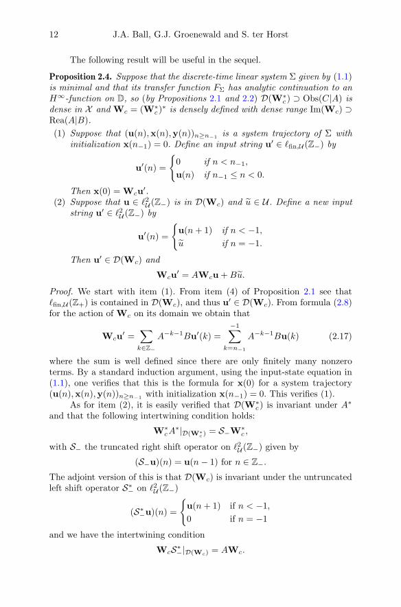
The following result will be useful in the sequel.
Proposition 2.4. Suppose that the discrete-time linear system Σ given by (1.1)is minimal and that its transfer function FΣ has analytic continuation to anH∞-function on D, so (by Propositions 2.1 and 2.2) D(W∗
c ) ⊃ Obs(C|A) isdense in X and Wc = (W∗
c )∗ is densely defined with dense range Im(Wc) ⊃
Rea(A|B).
(1) Suppose that (u(n),x(n),y(n))n≥n−1is a system trajectory of Σ with
initialization x(n−1) = 0. Define an input string u′ ∈ `fin,U (Z−) by
u′(n) =
0 if n < n−1,
u(n) if n−1 ≤ n < 0.
Then x(0) = Wcu′.
(2) Suppose that u ∈ `2U (Z−) is in D(Wc) and u ∈ U . Define a new inputstring u′ ∈ `2U (Z−) by
u′(n) =
u(n+ 1) if n < −1,
u if n = −1.
Then u′ ∈ D(Wc) and
Wcu′ = AWcu +Bu.
Proof. We start with item (1). From item (4) of Proposition 2.1 see that`fin,U (Z+) is contained in D(Wc), and thus u′ ∈ D(Wc). From formula (2.8)for the action of Wc on its domain we obtain that
Wcu′ =
∑k∈Z−
A−k−1Bu′(k) =
−1∑k=n−1
A−k−1Bu(k) (2.17)
where the sum is well defined since there are only finitely many nonzeroterms. By a standard induction argument, using the input-state equation in(1.1), one verifies that this is the formula for x(0) for a system trajectory(u(n),x(n),y(n))n≥n−1 with initialization x(n−1) = 0. This verifies (1).
As for item (2), it is easily verified that D(W∗c ) is invariant under A∗
and that the following intertwining condition holds:
W∗cA∗|D(W∗
c ) = S−W∗c ,
with S− the truncated right shift operator on `2U (Z−) given by
(S−u)(n) = u(n− 1) for n ∈ Z−.The adjoint version of this is that D(Wc) is invariant under the untruncatedleft shift operator S∗− on `2U (Z−)
(S∗−u)(n) =
u(n+ 1) if n < −1,
0 if n = −1
and we have the intertwining condition
WcS∗−|D(Wc) = AWc.

Infinite-dimensional Bounded Real Lemma II 13
Next note that S∗−u = u′−Π−1u, with Π−1 : U → `2U (Z−) the embedding ofU into the −1-th entry of `2U (Z−). This implies that
u′ = S∗−u + Π−1u ∈ S∗−D(Wc) + `fin,U (Z−) ⊂ D(Wc),
and
AWcu = WcS∗−|D(Wc)u = Wc(u′ −Π−1u) = Wcu
′ −Bu, (2.18)
which provides the desired identity.
Remark 2.5. It is of interest to consider the shift W(1)c of the controllability
operator Wc to the interval (−∞, 0] in place of Z− = (−∞, 0), i.e.,
W(1)c = Wcτ
−1
where the map τ transforms sequences u supported on Z− = (−∞, 0) tosequences u′ supported on (−∞, 0] according to the action
(τu)(n) = u(n+ 1) for n < 0
with inverse given by
(τ−1v)(n) = v(n− 1) for n ≤ 0.
For all u ∈ `2U (Z−) and u ∈ U , define a sequence (u, u) ∈ `2U ((−∞, 0]) by
(u, u)(n) =
u(n) if n ∈ Z−,u if n = 0.
The result of item (2) in Proposition 2.4 can be interpreted as saying: givenu ∈ `2U (Z−) and u ∈ U we have
(u, u) ∈ D(W(1)c ) ⇐⇒ u ∈ D(Wc)
and in that case W(1)c (u, u) = AWcu +Bu.
3. Storage functions
In the case of systems with an infinite-dimensional state space we allow stor-age functions to also attain +∞ as a value. Set [0,∞] := R+ ∪ +∞. Then,given a discrete-time linear system Σ as in (1.1), we say that a functionS : X → [0,∞] is a storage function for the system Σ if the dissipation in-equality
S(x(n+ 1)) ≤ S(x(n)) + ‖u(n)‖2U − ‖y(n)‖2Y for n ≥ N0 (3.1)
holds along all system trajectories (u(n),x(n),y(n))n≥N0with state initial-
ization x(N0) = x0 for some x0 ∈ X at some N0 ∈ Z, and S is normalized tosatisfy
S(0) = 0. (3.2)
As a first result we show that existence of a storage function for Σ is asufficient condition for the transfer function to have an analytic continuationto a Schur-class function.

14 J.A. Ball, G.J. Groenewald and S. ter Horst
Proposition 3.1. Suppose that the system Σ in (1.1) has a storage functionS. Then the transfer function FΣ of Σ defined in (1.3) has an analytic con-tinuation to a function in the Schur class S(U ,Y).
The proof of Proposition 3.1 relies on the following observation, whichwill also be of use in the sequel.
Lemma 3.2. Suppose that the system Σ in (1.1) has a storage function S. Foreach system trajectory (u(n),x(n),y(n))n∈Z and N0 ∈ Z so that x(N0) = 0,the following inequalities hold for all N ∈ Z+:
S(x(N0 +N + 1)) ≤N0+N∑n=N0
‖u(n)‖2U −N0+N∑n=N0
‖y(n)‖2Y ; (3.3)
N0+N∑n=N0
‖y(n)‖2Y ≤N0+N∑n=N0
‖u(n)‖2U . (3.4)
Proof. By the translation invariance of the system Σ we may assume withoutloss of generality that N0 = 0, i.e., x(0) = 0. From (3.1) and (3.2) we get
S(x(1)) ≤ ‖u(0)‖2 − ‖y(0)‖2 + S(0) = ‖u(0)‖2 − ‖y(0)‖2 <∞.Inductively, suppose that S(x(n)) <∞. Then (3.1) gives us
S(x(n+ 1)) ≤ ‖u(n)‖2U − ‖y(n)‖2Y + S(x(n)) <∞.We may now rearrange the dissipation inequality for n ∈ Z+ in the form
S(x(n+ 1))− S(x(n)) ≤ ‖u(n)‖2 − ‖y(n)‖2 (n ∈ Z+). (3.5)
Summing from n = 0 to n = N gives
0 ≤ S(x(N + 1)) ≤N∑n=0
‖u(n)‖2U −N∑n=0
‖y(n)‖2Y ,
which leads toN∑n=0
‖y(n)‖2Y ≤N∑n=0
‖u(n)‖2U for all N ∈ Z+.
These inequalities prove (3.3) and (3.4) for N0 = 0. As observed above, thecase of N0 6= 0 is then obtained by translation of the system trajectory.
Proof of Proposition 3.1. Let u ∈ `2U (Z+) and run the system Σ with inputsequence u and initial condition x(0) = 0. From Lemma 3.2, with N0 = 0,we obtain that for each N ∈ Z+ we have
N∑n=0
‖y(n)‖2Y ≤N∑n=0
‖u(n)‖2U for all N ∈ Z+.
Letting N → ∞, we conclude that u ∈ `2U (Z+) implies that the outputsequence y is in `2Y(Z+) with ‖y‖2
`2Y(Z+)≤ ‖u‖2
`2U (Z+).
Write u and y for the Z-transforms of u and y, respectively, i.e., de-note u(z) =
∑∞n=0 u(n)zn and y(z) =
∑∞n=0 y(n)zn. Since we have imposed

Infinite-dimensional Bounded Real Lemma II 15
zero-initial condition on the state, it now follows that y(z) = FΣ(z)u(z)in a neighborhood of 0. Since u was chosen arbitrarily in `2U (Z+), we seethat u is an arbitrary element of H2
U (D). Thus, the multiplication operatorMFΣ
: u 7→ FΣ · u maps H2U (D) into H2
Y(D). In particular, taking u ∈ H2U (D)
constant, it follows that FΣ has an analytic continuation to D. Furthermore,the inequality
‖FΣu‖H2Y(D) = ‖y‖H2
Y(D) = ‖y‖2`2Z+(Y) ≤ ‖u‖
2`2Z+
(U) = ‖u‖2H2U (D),
implies that the operator norm of the multiplication operator MFΣfrom
H2U (D) to H2
Y(D) is at most 1. It is well known that the operator norm ofMFΣ is the same as the supremum norm ‖FΣ‖∞ = supz∈D ‖FΣ(z)‖. Hence weobtain that the analytic continuation of FΣ is in the Schur class S(U ,Y).
We shall see below (see Proposition 4.2) that conversely, if the transferfunction FΣ admits an analytic continuation to a Schur-class function, thena storage function for Σ exists.
Quadratic storage functions. The class of storage functions associated withsolutions to the generalized KYP-inequality (1.12)–(1.13) are the so-calledquadratic storage functions described next. We shall say that a storage func-tion S is quadratic in case there is a positive-semidefinite operator H on thestate space X so that S has the form
S(x) = SH(x) =
‖H 1
2x‖2 for x ∈ D(H12 ),
+∞ otherwise.(3.6)
If in addition to FΣ having an analytic continuation to a Schur-classfunction it is assumed that Σ is minimal, it can in fact be shown (see The-orem 4.9 below) that quadratic storage functions for Σ exist; for the finite-dimensional case see [29].
Proposition 3.3. Suppose that the function S : X → [0,∞] has the form (3.6)for a (possibly) unbounded positive-semidefinite operator H on X . Then SH isa storage function for Σ if and only if H is a positive-semidefinite solution ofthe generalized KYP-inequality (1.12)–(1.13). Moreover, S is nondegeneratein the sense that SH(x) > 0 for all nonzero x in X if and only if H ispositive-definite.
Proof. Suppose thatH solves (1.12)–(1.13). It is clear that S(0) = ‖H 12 0‖2 = 0,
so in order to conclude that S is a storage function it remains to verify thedissipation inequality (3.1). Let (u(n),x(n),y(n))n≥N0
be a system trajectorywith state initialization x(n0) = x0 for some x0 ∈ X and N0 ∈ Z. Fix
n ≥ N0. If x(n) /∈ D(H12 ), then SH(x(n)) =∞ and the dissipation inequality
(3.1) is automatically satisfied. If x(n) ∈ D(H12 ), then (1.12) implies that
x(n+ 1) = Ax(n) +Bu(n) ∈ D(H12 ). Thus SH(x(n+ 1)) <∞. Replacing x
by x(n) and u by u(n) in (1.13) and applying (1.1) we obtain that∥∥∥∥[ H12 0
0 IU
] [x(n)u(n)
]∥∥∥∥2
−∥∥∥∥[ H
12 0
0 IY
] [x(n+ 1)y(n)
]∥∥∥∥2
≥ 0.

16 J.A. Ball, G.J. Groenewald and S. ter Horst
This can be rephrased in terms of SH as
SH(x(n)) + ‖u(n)‖2 − SH(x(n+ 1))− ‖y(n)‖2 ≥ 0,
so that (3.1) appears after adding SH(x(n+ 1)) on both sides.
Conversely, suppose that SH is a storage function. Take x ∈ X andu ∈ U arbitrarily. Let (u(n),x(n),y(n))n≥0 be any system trajectory withinitialization x(0) = x and with u(0) = u. Then the dissipation inequality(3.1) with n = 0 gives us
SH(Ax+Bu) ≤ SH(x) + ‖u‖2 − ‖y‖2, with y = Cx+Du. (3.7)
In particular, SH(x) < ∞ implies that SH(Ax + Bu) < ∞ (equivalently,
x ∈ D(H12 ) implies Ax + Bu ∈ D(H
12 )). Specifying u = 0 shows that
AD(H12 ) ⊂ D(H
12 ) and specifying x = 0 shows BU ⊂ D(H
12 ). Thus (1.12)
holds. Bringing ‖y‖2 in (3.7) to the other side and writing out SH gives
‖H 12 (Ax+Bu)‖2 + ‖Cx+Du‖2 ≤ ‖H 1
2x‖2 + ‖u‖2,
which provides (1.13).
We say that a function S : X → R+ = [0,∞) is a strict storage functionfor the system Σ in (1.1) if the strict dissipation inequality (1.8) holds, i.e.,if there exists a δ > 0 so that
S(x(n+1))−S(x(n))+δ‖x(n)‖2 ≤ (1−δ)‖u(n)‖2−‖y(n)‖2 (n ≥ N0) (3.8)
holds for all system trajectories u(n),x(n),y(n)n≥N0, initiated at some
N0 ∈ Z. Note that strict storage functions are not allowed to attain +∞as a value. The significance of the existence of a strict storage function fora system Σ is that it guarantees that the transfer function FΣ has analyticcontinuation to a H∞-function with H∞-norm strictly less than 1 as wellas a coercivity condition on S, i.e., we have the following strict version ofProposition 3.1.
Proposition 3.4. Suppose that the system Σ in (1.1) has a strict storage func-tion S. Then
(1) the transfer function FΣ has analytic continuation to a function in H∞
on the unit disk D with H∞-norm strictly less than 1, and(2) S satisfies a coercivity condition, i.e., there is a δ > 0 so that
S(x) ≥ δ‖x‖2 (x ∈ X ). (3.9)
Proof. Assume that S : X → [0,∞) is a strict storage function for Σ. Thenfor each system trajectory (u(n),x(n),y(n)))n≥0 with initialization x(0) = 0,the strict dissipation inequality (3.8) gives that there is a δ > 0 so that forn ≥ 0 we have
S(x(n+ 1))− S(x(n)) ≤ −δ‖x‖2 + (1− δ)‖u(n)‖2 − ‖y(n)‖2
≤ (1− δ)‖u(n)‖2 − ‖y(n)‖2.

Infinite-dimensional Bounded Real Lemma II 17
Summing up over n = 0, 1, 2, . . . , N for some N ∈ N for a system trajectory(u(n),x(n),y(n))n≥0 subject to initialization x(0) = 0 then gives
0 ≤ S(x(N+1)) = S(x(N+1))−S(x(0)) ≤ (1−δ)N∑n=0
‖u(n)‖2−N∑n=0
‖y(n)‖2.
By restricting to input sequences u ∈ `2U (Z+), it follows that the correspond-ing output sequences satisfy y ∈ `2Y(Z+) and ‖y‖2
`2U (Z+)≤ (1 − δ)‖u‖2
`2Y(Z+).
Taking Z-transform and using the Plancherel theorem then gives
‖MFΣu‖2H2
Y(D) = ‖y‖2H2Y(D) ≤ (1− δ)‖u‖2H2
U (D).
Thus ‖MFΣ‖ ≤√
1− δ < 1. This implies FΣ has analytic continuation to anL(U ,Y)-valued H∞ function with H∞-norm at most ‖MFσ‖ ≤
√1− δ < 1.
To this point we have not made use of the presence of the term δ‖x(n)‖2in the strict dissipation inequality (3.8). We now show how the presence ofthis term leads to the validity of the coercivity condition (3.9) on S. Let x0 beany state in X and let (u(n),x(n),y(n))n≥0 be any system trajectory withinitialization x(0) = x0 and u(0) = 0. Then the strict dissipation inequality(3.8) with n = 0 gives us
δ‖x0‖2 = δ‖x(0)‖2 ≤ S(x(1)) + δ‖x(0)‖2 + ‖y(0)‖2 ≤ S(x(0)) = S(x0),
i.e., S(x0) ≥ δ‖x0‖2 for each x0 ∈ X , verifying the validity of (3.9).
The following result classifies which quadratic storage functions SH arestrict storage functions.
Proposition 3.5. Suppose that S = SH is a quadratic storage function for thesystem Σ in (1.1). Then SH is a strict storage function for Σ if and onlyif H is a bounded positive-semidefinite solution of the strict KYP-inequality(1.9). Any such solution is in fact strictly positive-definite.
Proof. Suppose that SH is a strict storage function for Σ. Then by definitionSH(x) <∞ for all x ∈ X . Hence D(H) = X . By the Closed Graph Theorem,it follows that H is bounded. As a consequence of Proposition 3.4, SH is coer-cive and hence H is strictly positive-definite. The strict dissipation inequality(3.8) expressed in terms of H and the system matrix [A B
C D ] becomes
‖H 12 (Ax+Bu)‖2 − ‖H 1
2x‖2 + δ‖x‖2 ≤ (1− δ)‖u‖2 − ‖Cx+Du‖2
for all x ∈ X and u ∈ U . This can be expressed more succinctly as⟨[H 00 I
] [A BC D
] [xu
],
[A BC D
] [xu
]⟩−⟨[H 00 I
] [xu
],
[xu
]⟩≤ −δ
⟨[xu
],
[xu
]⟩for all x ∈ X and u ∈ U , for some δ > 0. This is just the spatial ver-sion of (1.9), so H is a strictly positive-definite solution of the strict KYP-inequality (1.9). By reversing the steps one sees that H 0 being a solutionof the strict KYP-inequality (1.9) implies that SH is a strict storage function.

18 J.A. Ball, G.J. Groenewald and S. ter Horst
As a consequence of Proposition 3.4 we see that then SH satisfies a coercivitycondition (3.9), so necessarily H is strictly positive-definite.
4. The available storage and required supply
In Proposition 3.1 we showed that the existence of a storage function (which isallowed to attain the value +∞) for a discrete-time linear system Σ impliesthat the transfer function FΣ associated with Σ is equal to a Schur-classfunction on a neighborhood of 0. In this section we investigate the conversedirection. Specifically, we give explicit variational formulas for three storagefunctions, referred to as the available storage function Sa (defined in (4.1)) therequired supply function Sr (defined in (4.2)) and the “regularized” versionSr of the required supply (defined in (4.18)). Let U denote the space of allfunctions n 7→ u(n) from the integers Z into the input space U . Then Sa isgiven by
Sa(x0) = supu∈U , n1≥0
n1∑n=0
(‖y(n)‖2 − ‖u(n)‖2
)(4.1)
with the supremum taken over all system trajectories (u(n),x(n),y(n))n≥0
with initialization x(0) = x0, while Sr is given by
Sr(x0) = infu∈U , n−1<0
−1∑n=n−1
(‖u(n)‖2 − ‖y(n)‖2
)(4.2)
with the infimum taken over all system trajectories (u(n),x(n),y(n))n≥n−1
subject to the initialization condition x(n−1) = 0 and the condition x(0) =x0.
The proof that Sa and Sr are storage functions whenever FΣ is in theSchur class requires the following preparatory lemma. We shall use the fol-lowing notation. For an arbitrary Hilbert space Z, write P+ and P− forthe orthogonal projections onto `2Z(Z+) and `2Z(Z−), respectively, acting on`2Z(Z). For integers m ≤ n, we write P[m,n] for the orthogonal projection on
the subspace of sequences in `2Z(Z) with support on the coordinate positionsm,m+ 1, . . . , n.
Lemma 4.1. Let Σ be as in (1.1) and suppose that its transfer function FΣ
is in the Schur class. Then, for each system trajectory (u(n),x(n),y(n))n≥0
with initialization x(0) = 0, the inequality
N∑n=0
‖y(n)‖2 ≤N∑n=0
‖u(n)‖2 (4.3)
holds for all N ∈ Z+.
Proof. As we have already observed, the fact that FΣ is in the Schur classS(U ,Y) implies that the multiplication operatorMFΣ (2.10) has norm at most1 as an operator from L2
U (T) to L2Y(T). If we apply the inverse Z-transform

Infinite-dimensional Bounded Real Lemma II 19
to the full operator MFΣ, not just to the compression HFΣ
as was done toarrive at the Hankel operator HFΣ in (2.12), we get the Laurent operator
LFΣ=
. . .. . .
. . .. . .
. . .. . .
. . . F0 0 0 0. . .
. . . F1 F0 0 0. . .
. . . F2 F1 F0 0. . .
. . . F3 F2 F1 F0. . .
. . .. . .
. . .. . .
. . .. . .
: `2U (Z)→ `2Y(Z), (4.4)
where F0, F1, F2, . . . are the Taylor coefficients of FΣ:
Fn =
D if n = 0,
CAn−1B if n ≥ 1.(4.5)
It is convenient to write LFΣ as a 2×2-block matrix with respect to the decom-
position `2U (Z) =[`2U (Z−)
`2U (Z+)
]of the domain and the analogous decomposition
`2Y(Z) =[`2Y(Z−)
`2Y(Z+)
]of the range; the result is
LFΣ=
[TFΣ
0HFΣ TFΣ
]:
[`2U (Z−)`2U (Z+)
]→[`2Y(Z−)`2Y(Z+)
]. (4.6)
Here HFΣ : `2−(U)→ `2+(Y) denotes the Hankel operator associated with FΣ
already introduced in (2.12), TFΣ : `2+(U) → `2+(Y) the Toeplitz operator
associated with FΣ, and TFΣthe Toeplitz operator acting from `2U (Z−) to
`2Y(Z−) associated with FΣ. From the assumption that FΣ is in the Schurclass S(U ,Y), it follows that MFΣ
is contractive, and hence also each of theoperators TFΣ
, HFΣ, and TFΣ
is contractive. From the lower triangular formof TFΣ
we see in addition that TFΣhas the causality property :
P[0,N ]TFΣ = P[0,N ]TFΣP[0,N ] (N ≥ 0). (4.7)
Now suppose that (u(n),x(n),y(n))n≥0 is a system trajectory on Z+ withinitialization x(0) = 0. In this case the infinite matrix identity y = TFΣuholds formally. For N ∈ Z+ we have P[0,N ]u ∈ `2U (Z+), and by the causalityproperty,
P[0,N ]TFΣP[0,N ]u = P[0,N ]TFΣ
u = P[0,N ]y.
Since TFΣis contractive, so is P[0,N ]TFΣ
P[0,N ] and thus the above identityshows that ‖P[0,N ]y‖ ≤ ‖P[0,N ]u‖, or, equivalently,
N∑n=0
‖y(n)‖2 ≤N∑n=0
‖u(n)‖2 (4.8)
holds for each system trajectory (u(n),x(n),y(n))n≥0 with x(0) = 0.

20 J.A. Ball, G.J. Groenewald and S. ter Horst
The proof of the following result is an adaptation of the proofs of The-orems 1 and 2 for the continuous-time setting in [28].
Proposition 4.2. Assume that the discrete-time linear system Σ has a transferfunction FΣ which has an analytic continuation to a function in the Schurclass S(U ,Y). Define Sa and Sr by (4.1) and (4.2). Then
(1) Sa is a storage function,(2) Sr is a storage function, and(3) for each storage function S for Σ we have
Sa(x0) ≤ S(x0) ≤ Sr(x0) for all x0 ∈ X .
Proof. The proof consists of three parts, corresponding to the three assertionsof the proposition.
(1) To see that Sa(x0) ≥ 0 for all x0 ∈ X , choose x(0) = x0 andu(n) = 0 for n ≥ 0 to generate a system trajectory (u(n),x(n),y(n))n≥0
such that∑n1
n=0(‖y(n)‖2 − ‖u(n)‖2) =∑n1
n=0 ‖y(n)‖2 ≥ 0 for all n1 ≥ 0.From the definition (4.1), we see that Sa(x0) ≥ 0.
By Lemma 4.1, each system trajectory (u(n),x(n),y(n))n≥0 with ini-tialization x(0) = 0 satisfies the inequality
n1∑n=0
‖y(n)‖2Y ≤n1∑n=0
‖u(n)‖2U (n1 ∈ Z+).
This observation leads to the conclusion that Sa(0) ≤ 0. Hence Sa(0) = 0and thus Sa satisfies the normalization (3.2).
Now let u(n), x(n), y(n)n≥N0 be any system trajectory initiated atsome N0 ∈ Z. We wish to show that this trajectory satisfies the dissipationinequality (3.1). It is convenient to rewrite this condition in the form
‖y(n)‖2Y − ‖u(n)‖2U + Sa(x(n+ 1)) ≤ Sa(x(n)) (n ∈ Z).
By translation invariance of the system equations (1.1), without loss of gen-erality we may take n = 0, so we need to show
‖y(0)‖2Y − ‖u(0)‖2U + Sa(x(1)) ≤ Sa(x(0)). (4.9)
We rewrite the definition (4.1) for Sa(x(1)) in the form
Sa(x(1)) = supu∈U ,n1≥0
n1∑n=0
(‖y(n)‖2Y − ‖u(n)‖2U
),
where the system trajectory (u(n),x(n),y(n))n≥0 is subject to the initializa-tion x(0) = x(1). Again making use of the translation invariance of the systemequations, we may rewrite this in the form
Sa(x(1)) = supu∈U ,n1≥1
n1∑n=1
(‖y(n)‖2Y − ‖u(n)‖2U
),
where (u(n),x(n),y(n))n≥0 is a system trajectory with initialization nowgiven by x(1) = x(1). Substituting this expression for S(x(1)), the left-hand

Infinite-dimensional Bounded Real Lemma II 21
side of (4.9) reads
‖y(0)‖2Y − ‖u(0)‖2U + supu∈U ,n1≥1
n1∑n=1
(‖y(n)‖2Y − ‖u(n)‖2U
).
This quantity indeed is bounded above by
Sa(x(0)) = supu∈U ,n1≥0
n1∑n=0
(‖y(n)‖2Y − ‖u(n)‖2U
),
with (u(n),x(n),y(n))n≥0 a system trajectory subject to the initializationx(0) = x(0). Hence the inequality (4.9) follows as required, and Sa is astorage function for Σ.
(2) Let (u(n),x(n),y(n))n≥n−1 be a system trajectory with zero-initial-ization of the state at n−1 < 0, subject also to x(0) = x0. Applying theresult of Lemma 4.1 to this system trajectory, using the translation invarianceproperty of Σ to get a sum in (4.3) starting at n−1 and ending at 0, itfollows that Sr(x0) ≥ 0 for all x0 in Rea(A|B). In case x0 6∈ Rea(A|B),i.e., x0 is not reachable in finitely many steps via some input signal u(n)(n−1 ≤ n < 0) with x(n−1) = 0, then the definition of Sr in (4.2) givesus Sr(x) = +∞ ≥ 0. By choosing n−1 = −1 with u(−1) = 0, we see thatSr(0) ≤ 0. Since Sr(x0) ≥ 0 for each x0 ∈ X , it follows that Sr also satisfiesthe normalization (3.2).
An argument similar to that used in part (1) of the proof shows thatSr satisfies (3.1). Indeed, note that it suffices to show that for each systemtrajectory u(n), x(n), y(n)n≥0 we have
Sr(x(1)) ≤ ‖u(0)‖2U − ‖y(0)‖2Y + Sr(x(0)) (4.10)
= infu∈U , n−1<0
‖u(0)‖2U − ‖y(0)‖2Y +−1∑
n=n−1
(‖u(n)‖2U − ‖y(n)‖2Y
)where (u(n),x(n),y(n))n≥n−1 is a system trajectory subject to the initialcondition x(n−1) = 0 and the terminal condition x(0) = x(0). Rewrite thedefinition of Sr(x(1)) as
Sr(x(1)) = infu∈U , n−1<1
0∑n=n−1
(‖u(n)‖2U − ‖y(n)‖2Y
),
with the system trajectory (u(n),x(n),y(n))n∈Z subject to the initial andterminal conditions x(n−1) = 0 and x(1) = x(1). Now recognize the argumentof the inf in the right-hand side of (4.10) as part of the competition in theinfimum defining Sr(x(1)) to deduce the inequality (4.10).
(3) Let S be any storage function for Σ and (u(n),x(n),y(n))n≥0 anysystem trajectory with initialization x(0) = x0. Iteration of the dissipationinequality (3.1) for S along the system trajectory (u(n),x(n),y(n))n≥0 as in

22 J.A. Ball, G.J. Groenewald and S. ter Horst
the proof of Lemma 3.2 yields
0 ≤ S(n1 + 1) ≤ S(x0) +
n1∑n=0
(‖u(n)‖2 − ‖y(n)‖2
)or
n1∑n=0
(‖y(n)‖2 − ‖u(n)‖2
)≤ S(x0).
Taking the supremum in the left-hand side of the above inequality over allsuch system trajectories (u(n),x(n),y(n))n≥0 and over all n1 ≥ 0 yieldsSa(x0) ≤ S(x0), and the first part of (3) is verified.
Next let x0 ∈ X be arbitrary. If (u(n),x(n),y(n))n≥n−1is any sys-
tem trajectory with state-initialization x(n−1) = 0 and x(0) = x0, applyingLemma 3.2 with N0 = n−1 and N = −1− n−1 gives us that
S(x0) ≤−1∑
n=n−1
(‖u(n)‖2U − ‖y(n)‖2Y
). (4.11)
Taking the infimum of the right-hand side over all such system trajec-tories gives us S(x0) ≤ Sr(x0). Here we implicitly assumed that the statex0 ∈ X is reachable. If x0 is not reachable, there are no such system trajec-tories, and taking the infimum over an empty set leads to Sr(x0) = ∞, inwhich case S(x0) ≤ Sr(x0) is also valid. Hence S(x0) ≤ Sr(x0) holds for allpossible x0 ∈ X . This completes the verification of the second part of (3).
Combining Proposition 4.2 with Proposition 3.1 leads to the following.
Corollary 4.3. A discrete-time linear system Σ in (1.1) has a transfer functionFΣ with an analytic continuation in the Schur class if and only if Σ has astorage function S.
Proof. The sufficiency is Proposition 3.1. For the necessity direction, byProposition 4.2 we may choose S equal to either Sa or Sr.
We next impose a minimality assumption on Σ and in addition assumethat FΣ has an analytic continuation in the Schur class S(U ,Y), i.e., we makethe following assumptions:
Σ is minimal, i.e., (C,A) is observable and (A,B) is controllable,and FΣ has an analytic continuation to a function in S(U ,Y).
(4.12)
Our next goal is to understand storage functions from a more operator-theoretic point of view. We first need some preliminaries.

Infinite-dimensional Bounded Real Lemma II 23
Recall the Laurent operator LFΣin (4.4). From the 2×2-block form for
LFΣ in (4.6), we see that
I − LFΣL∗FΣ
=
D2T∗FΣ
−TFΣH∗FΣ
−HFΣT∗FΣ
D2T∗FΣ
− HFΣH∗FΣ
;
I − L∗FΣLFΣ
=
[D2
TFΣ
− H∗FΣHFΣ
−H∗FΣTFΣ
−T∗FΣHFΣ
D2TFΣ
].
(4.13)
where in general the notation DX for the defect operator DX = (I −X∗X)12
of a contraction operator X is used. Since FΣ is assumed to be a Schur-class
function, TFΣ and TFΣ are contractions, and hence DTFΣ, DT∗FΣ
, DTFΣand
DT∗FΣ
are well defined.
Lemma 4.4. Let the discrete-time linear system Σ in (1.1) satisfy the assump-tions (4.12). The available storage function Sa and required supply functionSr can then be written in operator form as
Sa(x0) = supu∈`2U (Z+)
‖Wox0 + TFΣu‖2`2Y(Z+)−‖u‖
2`2U (Z+) (x0 ∈ D(Wo)), (4.14)
Sr(x0) = infu∈`fin,U (Z−) : x0=Wcu
‖DTFΣu‖2 (x0 ∈ X ), (4.15)
and Sa(x0) = +∞ for x0 6∈ D(Wo). Here Wo and Wc are the observ-ability and controllability operators defined via (2.1)–(2.4) and `fin,U (Z−) isthe linear manifold of finitely supported sequences in `2U (Z−). In particular,Sr(x0) <∞ if and only if x0 ∈ Rea(A|B).
Proof. We shall use the notation P± and P[m,n] as introduced in the discus-sion immediately preceding the statement of Lemma 4.1.
We start with Sa. For each system trajectory (u(n),x(n),y(n))n≥0 withinitialization x(0) = x0 and with u ∈ `2U (Z+) by linearity we have
y = Wox0 + TFΣu.
Now note that, for each system trajectory (u(n),x(n),y(n))n≥0 with initial-ization x(0) = x0 but with u not necessarily in `2U (Z+) and with n1 ≥ 0, bythe causality property (4.7), as in the proof of Lemma 4.1 we see that we canreplace u with P[0,n1]u ∈ `fin,U (Z+) ⊂ `2U (Z+) within the supremum in (4.1)without changing the value. Therefore, the value of Sa at x0 can be rewrittenin operator form as
Sa(x0) = supu∈`fin,U (Z+)
n1≥0
‖P[0,n1](Wox0 +TFΣu)‖2`2Y(Z+)−‖P[0,n1]u‖2`2U (Z+) (4.16)
where we use the notation `fin,U (Z+) for U-valued sequences on Z+ of finitesupport.
If x0 /∈ D(Wo) so that Wox0 /∈ `2Y(Z+), the above formulas are to beinterpreted algebraically, and we may choose u = 0 and take the limit asn1 →∞ to see that Wo(x0) = +∞.

24 J.A. Ball, G.J. Groenewald and S. ter Horst
Now assume x0 ∈ D(Wo). Fix u ∈ `fin,U (Z+) and take the limit asn1 → +∞ in the right-hand side of (4.16) to see that an equivalent expressionfor Sa(x0) is
Sa(x0) = supu∈`fin,U (Z+)
‖Wox0 + TFΣu‖2 − ‖u‖2.
Since `fin,U (Z+) is dense in `2U (Z+) and TFΣis a bounded operator, we see
that another equivalent expression for Sa(x0) is (4.14). This completes theverification of (4.14).
We next look at Sr. Let (u(n),x(n),y(n))n≥n−1be any system trajec-
tory with initialization x(n−1) = 0 for some n−1 < 0. Let us identify u withan element u ∈ `fin,U (Z−) by ignoring the values of u on Z+ and definingu(n) = 0 for n < n−1. Then, as a consequence of item (1) in Proposi-tion 2.4, the constraint x(0) = x0 in (4.2) can be written in operator form asWcu = x0. Furthermore, since (u(n),x(n),y(n))n≥n−1
is a system trajectorywith zero state initialization at n−1, it follows that
y|Z− = TFΣu.
We conclude that a formula for Sr equivalent to (4.2) is
Sr(x0) = infu∈`2fin,U (Z−) : Wcu=x0
‖u‖2 − ‖TFΣu‖2
which in turn has the more succinct formulation (4.15). If x0 ∈ Rea(A|B),then the infimum in (4.15) is taken over a nonempty set, so that Sr(x0) <∞.On the other hand, if x0 6∈ Rea(A|B), then the infimum is taken over anempty set, so that Sr(x0) =∞.
To compute storage functions more explicitly for the case where as-sumptions (4.12) are in place, it will be convenient to restrict to what weshall call `2-regular storage functions S, namely, storage functions S whichassume finite values on ImWc:
x0 = Wcu where u ∈ D(Wc)⇒ S(x0) <∞. (4.17)
We shall see in the next result that Sa is `2-regular. However, unless ifRea(A|B) is equal to the range of Wc, the required supply Sr will not be`2-regular (by the last assertion of Lemma 4.4).
To remedy this situation, we introduce the following modification Sr ofthe required supply Sr, which we shall call the `2-regularized required supply :
Sr(x0) = infu∈D(Wc) : Wcu=x0
−1∑n=−∞
(‖u(n)‖2 − ‖y(n)‖2
)(4.18)
where u ∈ `2U (Z−) determines y ∈ `2Y(Z−) via the system input/output map:
y = TFΣu. Thus formula (4.18) can be written more succinctly in operator
Infinite-dimensional Bounded Real Lemma II 25
form as
Sr(x0) = infu∈D(Wc) : Wcu=x0
‖u‖2`2U (Z−) − ‖TFΣu‖2`2Y(Z−)
= infu∈D(Wc) : Wcu=x0
‖DTFΣu‖2`2Y(Z−) for x0 ∈ ImWc. (4.19)
It is clear that Sr(x0) <∞ if and only if x0 ∈ ImWc. Since the objective inthe infimum defining Sr in (4.19) is the same as the objective in the infimumdefining Sr in (4.15) but the former infimum is taken over an a priori largerset, it follows directly that Sr(x0) ≥ Sr(x0) for all x0 ∈ X , as can also beseen as a consequence of Proposition 4.2 once we show that Sr is a storagefunction for Σ. From either of the formulas we see that 0 ≤ Sr(x0) and thatSr(x0) <∞ exactly when x0 is in the range of Wc. Hence once we show thatSr is a storage function, it follows that Sr is an `2-regular storage functionand is a candidate to be the largest such. However at this stage we have onlypartial results in this direction, as laid out in the next result.
Proposition 4.5. Assume that Σ is a system satisfying the assumptions (4.12)and let the function Sr : ImWc → R+ be given by (4.19). Then:
(1) Sa and Sr are `2-regular storage functions.(2) Sr is “almost” the largest `2-regular storage function in the following
sense: if S is another `2-regular storage function such that either(a) S is D(W∗
c )-weakly continuous in the sense that: given a sequencexn ⊂ ImWc and xc ∈ ImWc such that
limn→∞
〈x, xn〉X = 〈x, xc〉X for all x ∈ D(W∗c ),
then limn→∞ S(xn) = S(x0), or(b) Wc is bounded and S is continuous on X (with respect to the norm
topology on X ),then S(x0) ≤ Sr(x0) for all x0 ∈ X .
Proof. We first prove item (1), starting with the claim for Sa. Since by as-sumption Σ is minimal and FΣ has an analytic continuation to a Schur-classfunction, by item (1) of Proposition 2.2, ImWc ⊂ D(Wo). So on ImWc,the available storage Sa is given by (4.14). It remains to show that forx0 ∈ ImWc the formula for Sa(x0) in (4.14) gives a finite value. So as-sume x0 ∈ ImWc, say x0 = Wcu− for a u− ∈ `2U (Z−). Choose u+ ∈ `2U (Z+)arbitrarily and define u ∈ `2U (Z) by setting P−u = u− and P+u = u+. ThenWox0 = WoWcu− = HFΣu−. Thus, using the decomposition of LFΣ in (4.6)and the fact that ‖LFΣ‖ ≤ 1, we find that
‖Wox0 + TFΣu+‖2 − ‖u+‖2 = ‖HFΣu− + TFΣu+‖2 − ‖u+‖2
= ‖P+LFΣu‖2 − ‖P+u‖2 = ‖P−u‖2 + ‖P+LFΣ
u‖2 − ‖u‖2
≤ ‖P−u‖2 = ‖u−‖2.
Since the upper bound ‖u−‖2 is independent of the choice of u+ ∈ `2U (Z+),we can take the supremum over all u+ ∈ `2U (Z+) to arrive at the inequalitySa(x0) ≤ ‖u−‖2 <∞.

26 J.A. Ball, G.J. Groenewald and S. ter Horst
Next we prove the statement of item (1) concerning Sr. By the dis-cussion immediately preceding the statement of the proposition, it followsthat Sr is an `2-regular storage function once we show that Sr is a storagefunction, that is, Sr(0) = 0 and that Sr satisfies the dissipation inequality(3.1).
If x0 = 0, we can choose u = 0 as the argument in the right-hand side of(4.19) to conclude that Sr(0) ≤ 0. As we have already seen that Sr(x0) ≥ 0for all x0, we conclude that Sr(0) = 0.
To complete the proof of item (1), it remains to show that Sr satisfies thedissipation inequality (3.1). By shift invariance we may take n = N0 = 0 in(3.1). If x(0) /∈ ImWc, then Sr(x0) = ∞ and (3.1) holds trivially.We therefore assume that (u(n), x(n), y(n))n≥0 is a system trajectory withinitialization x(0) = x0 = Wcu− for some u− ∈ D(Wo) and the problem isto show
Sr(x(1)) ≤ ‖u(0)‖2 − ‖y(0)‖2 + Sr(x(0)) (4.20)
= infu∈D(Wc)Wcu=x(0)
[‖u(0)‖2 − ‖y(0)‖2 +
−1∑n=−∞
(‖u(n)‖2 − ‖y(n)‖2
)],
where y = TFΣu. As (u(n), x(n), y(n))n≥0 is a system trajectory initiated at
0, we know that x(1) = Ax(0) + Bu(0) and y(0) = Cx(0) + Du(0). On theother hand, by translation-invariance of the system equations (1.1) we mayrewrite the formula (4.18) for Sr(x(1)) as
Sr(x(1)) = infu′∈D(W
(1)c ) : W
(1)c u=x(1)
0∑n=−∞
(‖u′(n)‖2 − ‖y′(n)‖2
), (4.21)
where W(1)c is the shifted observability operator discussed in Remark 2.5
and where y′ = T(1)FΣ
u′; here now u′ is supported on (−∞, 0] rather than on
Z− = (−∞, 0) and T(1)FΣ
is the shift of TFΣ from the interval Z− to the interval
(−∞, 0]. Let us write sequences u′ ∈ `2U ((−∞, 0]) in the form u′ = (v′, v′) as
in Remark 2.5 where v′ ∈ `2U (Z−) and v′ ∈ U . As observed in Remark 2.5,
W(1)c (v′, v) = AWcv
′ +Bv′.
Furthermore, from the structure of the Laurent operator LFΣ(4.6) we read
off that
T(1)FΣ
(v′, v′) =
(TFΣv
′,−1∑
k=−∞
CA−k−1Bv′(k) +Dv′
)(4.22)
where the series converges at least in the weak topology of Y. For v′ ∈ D(Wc),we know from Proposition 2.1 that Wcv
′ is given by
Wcv′ =
−1∑k=−∞
A−k−1Bv′(k) (4.23)

Infinite-dimensional Bounded Real Lemma II 27
where the series converges D(W∗c )-weakly. We also know under our standing
assumption (4.12) that Obs(C|A) ⊂ D(W∗c ) (see Proposition 2.2 (2)), and
hence in particular C∗y ∈ D(W∗c ) for all y ∈ Y. This observation combined
with the formula (4.23) implies that
CWcv′ =
−1∑k=−∞
CA−k−1Bv′(k)
where the series converges weakly in Y. This combined with (4.22) gives us
T(1)FΣ
(v′, u) =(TFΣ
v′, CWcv′ +Dv′
).
Thus the formula (4.21) for Sr(x(1)) can be written out in more detail as
Sr(x(1)) = inf(v′,v′)∈T ′
(‖v′‖2 − ‖TFΣ
v′‖2) + ‖u‖2 − ‖CWcv′ +Du‖2
(4.24)
whereT ′ := v′ ∈ D(Wc), v
′ ∈ U : AWcv′ +Bv′ = x(1). (4.25)
Note that the infimum (4.20) can be identified with the infimum (4.24) if werestrict the free parameter (v′, v′) to lie in the subset
T = (v′, v′) ∈ T ′ : Wcv′ = x(0), v′ = u(0).
As the infimum of an objective function over a given set T is always boundedabove by the infimum of the same objective function over a smaller setT ′ ⊂ T , the inequality (4.20) now follows as wanted.
It remains to address item (2), i.e., to show that S(x0) ≤ Sr(x0) for anyother storage function S satisfying appropriate hypotheses. If x0 /∈ ImWc,Sr(x0) = ∞ and the desired inequality holds trivially, so we assume thatx0 = Wcu for some u ∈ D(Wc). Let us approximate u by elements of`fin,U (Z−) in the natural way:
uK(n) =
u(n) for −K ≤ n ≤ −1,
0 for n < −K
for K = 1, 2, . . . , and set xK = WcuK . We let (u(n),x(n),y(n))n≥−K bea system trajectory with u(n) = uK(n) and with the state initializationx(−K) = 0. Then, as x(0) will then be equal to xK , iteration of the dissipa-tion inequality (3.1) gives us
S(xK) ≤−1∑
n=−K
(‖uK(n)‖2 − ‖TFΣ
uK(n)‖2). (4.26)
We seek to let K → ∞ in this inequality. As uK → u in the norm topology
of `2U (Z−) and ‖TFΣ‖ ≤ 1 since F is in the Schur class by assumption, it is
clear that the right-hand side of (4.26) converges to
‖u‖2`2U (Z−) − ‖TFΣu‖2`2U (Z−) = ‖DTFΣu‖2`2U (Z−)
as K →∞. On the other hand, as a consequence of the characterization (2.8)of the action of Wc, it follows that xK = WcuK converges to x0 = Wcu

28 J.A. Ball, G.J. Groenewald and S. ter Horst
in the D(W∗c )-weak sense. Hence, if S is continuous with respect to the
D(W∗c )-weak topology as described in the statement of item (a), we see that
S(xK)→ S(x0) as K →∞ and we arrive at the limiting version of inequality(4.26):
S(x0) ≤ ‖u‖2 − ‖TFΣu‖2 = ‖DTFΣ
u‖2`2U (Z−). (4.27)
We may now take the infimum over all u ∈ D(Wc) with Wcu = x0 to arriveat the desired inequality S(x0) ≤ Sr(x0). This proves item (a) of (2). If Wc
is bounded, then xK = WcuK converges in norm to Wcu = x0. If S iscontinuous with respect to the norm topology on X , then S(xK) → S(x0)and we again arrive at the limit inequality (4.27), from which the desiredinequality S(x0) ≤ Sr(x0) again follows. This completes the verification ofitem (2) in Proposition 4.5.
Remark 4.6. Note that the fact that Sa is `2-regular can alternatively beseen from the fact that Sr is an `2-regular storage function combined withthe first inequality in item (3) of Proposition 4.2.
Collecting some of the observations on the boundedness of Sa and Srfrom the above results we obtain the following corollary. The inequalities in(4.28) follow directly from (4.14) and (4.19).
Corollary 4.7. Assume Σ as in (1.1) is a system satisfying the assumptions(4.12). Define Sa by (4.1) and Sr by (4.18). For x0 ∈ ImWo we have
‖Wox0‖2 ≤ Sa(x0) ≤ Sr(x0) ≤ ‖u−‖2 (4.28)
for all u− ∈ D(Wc) with x0 = Wcu−, with the last inequality being vacuousif x0 6∈ ImWc, in which case Sr(x0) =∞. Hence
Sr(x0) <∞ ⇐⇒ x0 ∈ ImWc,
x0 ∈ ImWc =⇒ Sa(x0) <∞ =⇒ x0 ∈ D(Wo).
In particular, Sr is finite-valued if and only if ImWc = X , that is, Σ is `2-exactly controllable, and Sa is finite-valued in case Σ is `2-exactly controllable.
Since FΣ is assumed to be a Schur-class function, LFΣ is a contraction,so that I − LFΣ
L∗FΣand I − L∗FΣ
LFΣare positive-semidefinite operators. We
can thus read off from the (2, 2)-entry in the right-hand side of the firstidentity and the (1, 1)-entry in the right-hand side of the second identity of(4.13) that
D2T∗FΣ
HFΣH∗FΣ
and D2TFΣ
H∗FΣHFΣ . (4.29)
The observability and controllability assumptions of (4.12) imply that theobservability operator Wo : D(Wo) → `2Y(Z+) and the controllability oper-ator Wc : D(Wc)→ X are closed densely defined operators that satisfy theproperties listed in Propositions 2.1 and 2.2. As spelled out in Proposition 2.2,the Hankel operator HFΣ
admits the factorizations
HFΣ |D(Wc) = WoWc and H∗FΣ|D(W∗
o) = W∗cW
∗o. (4.30)

Infinite-dimensional Bounded Real Lemma II 29
Using the Douglas factorization lemma [16] together with the factor-izations (4.30), we arrive at the following result. The proof also requires useof the Moore–Penrose generalized inverse X† of a densely defined closed lin-ear Hilbert-space operator X : D(X) → H2, with D(X) ⊂ H1: we defineX† : D(X†) = (ImX ⊕ (ImX)⊥)→ H1 by
X†(Xh1) = P(KerX)⊥h1,
X†|(ImX)⊥ = 0.(4.31)
Then X† is also closed and has the properties
X†X = P(KerX)⊥ |D(X), XX† = PImX |ImX⊕(ImX)⊥ .
In particular, if X is bounded and surjective, then X† is a bounded rightinverse of X, and, if X is bounded, bounded below and injective, then X† isa bounded left inverse of X.
Lemma 4.8. Let the discrete-time linear system Σ in (1.1) satisfy the assump-tions in (4.12). Then:
(1) There exists a unique closable operator Xa with domain ImWc mappinginto (KerDT∗FΣ
)⊥ ⊂ `2Y(Z+) so that we have the factorization
Wo|ImWc= DT∗FΣ
Xa. (4.32)
Moreover, if we let Xa denote the closure of Xa, then Xa is injective.(2) There exists a unique closable operator Xr with domain ImW∗
o mappinginto (KerDTFΣ
)⊥ ⊂ `2U (Z−) so that we have the factorization
W∗c |ImW∗
o= DTFΣ
Xr. (4.33)
Moreover, if we let Xr denote the closure of Xr, then Xr is injective.
Proof. As statement (2) is just a dual version of statement (1), we only discussthe proof of (1) in detail.
Apply the Douglas factorization lemma to the first of the inequalitiesin (4.29) to get the existence of a unique contraction operator
Ya : `2U (Z−)→ (KerDT∗FΣ)⊥ ⊂ `2Y(Z+)
such that
DT∗FΣYa = HFΣ
, so that, by (4.30), DT∗FΣYa|D(Wc) = WoWc.
If we let W†c be the Moore–Penrose generalized inverse (4.31) of Wc, then
W†c(x) = arg min ‖u‖2`2U (Z−) : u ∈ D(Wc), x = Wcu (x ∈ ImWc).
Since Wc is closed, KerWc is a closed subspace of `2U (Z−) and for all u ∈D(Wc) with x = Wcu we have W†
c(x) = u − PKerWcu. We next defineXa : ImWc → `2Y(Z+) by
Xa = YaW†c.

30 J.A. Ball, G.J. Groenewald and S. ter Horst
Then Xa is a well-defined, possibly unbounded, operator on the dense domainD(Xa) = ImWc. Moreover we have
DT∗FΣXa = DT∗FΣ
YaW†c = HFΣ
W†c = WoWcW
†c = Wo|ImWc
.
Hence Xa provides the factorization (4.32). Furthermore, Xa = YaW†c implies
that ImXa ⊂ ImYa, so that ImXa ⊂ (KerDT∗FΣ)⊥. Moreover, from the
factorization (4.32) we see that this property makes the choice of Xa unique.
We now check thatXa so constructed is closable. Suppose that x(k)0 k≥0
is a sequence of vectors in ImWc such that limk→∞ x(k)0 = 0 in X -norm, while
limk→∞Xax(k)0 = y in `2Y(Z+)-norm. As DT∗FΣ
is bounded, it follows that
limk→∞
Wox(k)0 = lim
k→∞DT∗FΣ
Xax(k)0 = DT∗FΣ
y in `2Y(Z+)-norm.
Since Wo is a closed operator and we have x(k)0 → 0 in X -norm, it follows
that DT∗FΣy = 0. As ImXa ⊂ (KerDT∗FΣ
)⊥ and Xax(k)0 → y, we also have
that y ∈ (KerDT∗FΣ)⊥. It follows that y = 0, and hence Xa is closable.
Let Xa be the closure of Xa. We check that Xa is injective as fol-
lows. The vector x0 being in D(Xa) means that there is a sequence of
vectors x(k)0 k≥1 contained in D(Xa) with limk→∞ x
(k)0 = x0 in X and
limk→∞Xax(k)0 = y for some y ∈ `2Y(Z+). The condition that Xax = 0
means that in addition y = 0. Since DT∗FΣis bounded, it then follows that
limk→∞DT∗FΣXax
(k)0 = 0, or, by (4.32)
limk→∞
Wox(k)0 = 0.
As we also have limk→∞ x(k)0 = x0 in X and Wo is a closed operator, it
follows that x0 ∈ D(Wo) and Wox0 = 0. As Wo is injective, it follows thatx0 = 0. We conclude that Xa is injective as claimed.
Using the closed operators Xa and Xr defined in Lemma 4.8 we nowdefine (possibly unbounded) positive-definite operators Ha and Hr so thatthe storage functions Sa and Sr have the quadratic forms Sa = SHa andSr = SHr as in (3.6).
We start with Ha. Since Xa is closed, there is a good polar factorization
Xa = Ua|Xa|
(see [26, Theorem VIII.32]); in detail, X∗aXa is selfadjoint with positive self-
adjoint square-root |Xa| = (X∗aXa)
12 satisfying D(|Xa|) = D(Xa), Ua is a
partial isometry with initial space equal to (KerXa)⊥ and final space equalto ImXa so that we have the factorization Xa = Ua|Xa|.
Now set
Ha = X∗aXa, H
12a = |Xa|. (4.34)
As noted in Lemma 4.8, Xa is injective, and thus Ha and H12a are injective
as well, and as a result Ua is an isometry.

Infinite-dimensional Bounded Real Lemma II 31
We proceed with the definition of Hr. As the properties of Xr parallelthose of Xa, also Xr has a good polar decomposition Xr = Ur|Xr| with |Xr|and Ur having similar properties as |Xa| and Ua, in particular, X
∗rXr and
|Xr| are injective and Ur is an isometry. We then define
Hr =(X∗rXr
)−1
, H12r = |Xr|−1. (4.35)
We shall also need a modification of the factorization (4.33). For u ∈ D(Wc)and x ∈ ImW∗
o, let us note that
〈Wcu, x〉X = 〈u,W∗cx〉`2U (Z−) = 〈u, DTFΣ
Xrx〉`2U (Z−) (by (4.33))
= 〈DTFΣu, Xrx〉`2U (Z−).
The end result is that then DTFΣu is in D(X∗r ) and X∗rDTFΣ
u = Wcu. In
summary we have the following adjoint version of the factorization (4.33):
Wc = X∗rDTFΣ|D(Wc). (4.36)
In the following statement we use the notion of a core of a closed,densely defined operator Γ between two Hilbert spaces H and K (see [26]or [20]), namely: a dense linear submanifold D is said to be a core for theclosed, densely defined operator X with domain D(X) in H mapping into Kif, given any x ∈ D(X), there is a sequence xnn≥1 of points in D such thatlimn→∞ xn = x and also limn→∞Xxn = Xx.
Theorem 4.9. Let the discrete-time linear system Σ in (1.1) satisfy the as-sumptions in (4.12). Define Xa, Xa, Xr, Xr as in Lemma 4.8 and the closedoperators Ha and Hr as in the preceding discussion. Then the available stor-age function Sa and required supply function Sr are given by
Sa(x0) = ‖Xax0‖2 = ‖H12a x0‖2 (x0 ∈ ImWc), (4.37)
Sr(x0) = ‖|Xr|−1x0‖2 = ‖H12r x0‖2 (x0 ∈ ImWc). (4.38)
In particular, the available storage Sa and `2-regularized required supply Sragree with quadratic storage functions on ImWc.
Moreover, ImWc is a core for H12a and ImW∗
o is a core for H− 1
2r .
Proof. By Lemma 4.8, in the operator form of Sa derived in Lemma 4.4 wecan replace Wox0 by DT∗FΣ
Xax0, leading to
Sa(x0) = supu∈`2U (Z+)
‖DT∗FΣXax0 + TFΣu‖2`2Y(Z+) − ‖u‖
2`2U (Z+). (4.39)

32 J.A. Ball, G.J. Groenewald and S. ter Horst
For x0 ∈ ImWc and each u ∈ `2U (Z+) we have
‖DT∗FΣXax0 + TFΣ
u‖2 − ‖u‖2 =
= ‖DT∗FΣXax0‖2 + 2 Re 〈DT∗FΣ
Xax0,TFΣu〉+ ‖TFΣ
u‖2 − ‖u‖2
= ‖DT∗FΣXax0‖2 + 2 Re 〈DT∗FΣ
Xax0,TFΣu〉 − ‖DTFΣ
u‖2
= ‖DT∗FΣXax0‖2 + 2 Re 〈Xax0, DT∗FΣ
TFΣu〉 − ‖DTFΣu‖2
= ‖DT∗FΣXax0‖2 + 2 Re 〈Xax0,TFΣDTFΣ
u〉 − ‖DTFΣu‖2
= ‖DT∗FΣXax0‖2 + 2 Re 〈T∗FΣ
Xax0, DTFΣu〉 − ‖DTFΣ
u‖2
= ‖DT∗FΣXax0‖2 + ‖T∗FΣ
Xax0‖2 − ‖T∗FΣXax0 −DTFΣ
u‖2
= ‖Xax0‖2 − ‖T∗FΣXax0 −DTFΣ
u‖2.
By construction, we have ImXa ⊂ (KerDT∗FΣ)⊥ = ImDT∗FΣ
. Using that
T∗FΣDT∗FΣ
= DTFΣT∗FΣ
, we obtain
T∗FΣImDT∗FΣ
⊂ ImDTFΣ.
Thus ImT∗FΣXa ⊂ ImDTFΣ
. Hence there is a sequence uk of input signals in
`2U (Z+) so that ‖T∗FΣXax0 −DTFΣ
uk‖ → 0 as k →∞. We conclude that for
x0 ∈ ImWc the supremum in (4.39) is given by
Sa(x0) = ‖Xax0‖2 = ‖Xax0‖2 = ‖H12a x0‖2.
Let x0 ∈ ImWc. Given a u ∈ D(Wc), by the factorization (4.36) wesee that Wcu = x0 if and only if X∗rDTFΣ
u = x0. Therefore, we have
Sr(x0) = infu∈D(Wc), X∗rDTFΣ
u=x0
‖DTFΣu‖2 = inf
v∈DTFΣD(Wc), X∗rv=x0
‖v‖2.
A general property of operator closures is X∗r = X∗r . Hence
Sr(x0) = infv∈D
TFΣD(Wc), X
∗rv=x0
‖v‖2. (4.40)
As x0 ∈ ImWc by assumption, the factorization (4.36) gives us a u0 ∈ D(Wc)so that
x0 = X∗rDTFΣ
u0. (4.41)
In particular, x0 has the form x0 = X∗rv0 with v0 ∈ DTFΣ
D(Wc). From
(4.41) we see that the general solution v ∈ D(X∗r) of x0 = X
∗rv is
v = DTFΣu0 + k where k ∈ KerX
∗r . (4.42)
By construction the target space for Xr (and Xr) is(KerDTFΣ
)⊥so the
domain space for X∗r is (KerDTFΣ
)⊥ and KerX∗r ⊂ ImDTFΣ
. Hence the infi-
mum in (4.40) remains unchanged if we relax the constraint v ∈ DTFΣD(Wc)
Infinite-dimensional Bounded Real Lemma II 33
to just v ∈ D(X∗r), i.e.,
Sr(x0) = infv∈D(X
∗r), X
∗rv=x0
‖v‖2. (4.43)
In terms of the polar decomposition Xr = Ur|Xr| for Xr, we have
X∗r = |Xr|U∗r
with
D(X∗r) = u ∈ ImDTFΣ
: U∗r u ∈ D(|Xr|) = D(Xr).
Since |Xr| is injective and Ur is an isometry with range equal to (KerX∗r)⊥,
the constraint |Xr|U∗r v = X∗rv = x0 is equivalent to
P(KerX∗r)⊥v = UrU
∗r v = Ur|Xr|−1x0.
As we want to minimize ‖v‖2 with P(KerX∗r)⊥v equal to Ur|X
∗r |−1x0 ∈ D(Xr),
it is clear that this is achieved at vopt = Ur|X∗r |−1x0, so that
Sr(x0) = ‖vopt‖2 = ‖Ur|Xr|−1x0‖2 = ‖|Xr|−1x0‖2 = ‖H12r x0‖2,
as claimed.
It remains to verify the last assertion concerning the core properties
of ImWc and ImW∗o. By definition H
12a = |Xa| where Xa is defined to be
the closure of the Xa = Xa|ImWc . Hence ImWc by definition is a core for
Xa from which it immediately follows that ImWc is a core for H12a = |Xa|.
That ImW∗o is a core for H
− 12
r = |Xr| follows in the same way via a dual
analysis.
5. The dual system Σ∗
In this section we develop a parallel theory for the dual system Σ∗ of Σ, whichis the system with system matrix equal to the adjoint of (1.2) evolving inbackwards time.
5.1. Controllability, observability, minimality and transfer function for thedual system
With the discrete-time linear system Σ given by (1.1) with system ma-trix M = [A B
C D ] we will associate the dual system Σ∗ with system matrix
M∗ =[A∗ C∗
B∗ D∗]
:[XY]→[XU]. It will be convenient for our formalism here to
let the dual system evolve in backwards time; we therefore define the systemΣ∗ to be given by the system input/state/output equations
Σ∗ : =
x∗(n− 1) = A∗x∗(n) + C∗u∗(n),
y∗(n) = B∗x∗(n) +D∗u∗(n).(5.1)

34 J.A. Ball, G.J. Groenewald and S. ter Horst
If we impose a final condition x∗(−1) = x0 and feed in an input-sequenceu(n)n∈Z− , one can solve recursively to get, for n ≤ −1,
x∗(n) = A∗−n−1x0 +−1∑
j=n+1
A∗−n+jC∗u∗(j),
y∗(n) = B∗A∗−n−1x0 +−1∑
j=n+1
B∗A∗−n+j−1C∗u∗(j) +D∗u∗(n).
Alternatively, the Z-transform x∗(n)n∈Z− 7→ x∗(λ) =∑−1n=−∞ x∗(n)λn
may be applied directly to the system equations (5.1). Combining this withthe observation that
−1∑n=−∞
x∗(n− 1)λn = λ
( −1∑n=−∞
x∗(n− 1)λn−1
)= λ
( −2∑n=−∞
x∗(n)λn
)= λ
(x∗(λ)− x0λ
−1)
= λx∗(λ)− x0,
converts the first system equation in (5.1) to
λx∗(λ)− x0 = A∗x∗(λ) + C∗u∗(λ),
leading to the Z-transformed version of the whole system:x∗(λ) = (λI −A∗)−1x0 + (λI −A∗)−1C∗u∗(λ),
y∗(λ) = B∗(λI −A∗)−1x0 + FΣ∗(λ)u∗(λ),
where the transfer function FΣ∗(λ) for the system Σ∗ is then given by
FΣ∗(λ) = D∗ +B∗(λI −A∗)−1C∗
= D∗ + λ−1(I − λ−1A∗)−1C∗ = FΣ(1/λ)∗ (5.2)
which is an analytic function on a neighborhood of the point at ∞ in thecomplex plane. Moreover, FΣ∗ has analytic continuation to a function analyticon the exterior of the unit disk De := λ ∈ C : |λ| > 1 ∪ ∞ exactly whenFΣ has analytic continuation to a function analytic on the unit disk D withequality of corresponding ∞-norms:
‖FΣ∗‖∞,De := supλ∈De
‖FΣ∗(λ)‖ = supλ∈D‖FΣ(λ)‖ =: ‖FΣ‖∞,D.
All the analysis done up to this point for the system Σ has a dual ana-logue for the system Σ∗. In particular, the observability operator W∗o forthe dual system is obtained by running the system (5.1) with final conditionx∗(−1) = x0 and input string u∗(n) = 0 for n ≤ −1, resulting in the out-put string B∗A∗(−n−1)x0n∈Z− . Since we are interested in a setting withoperators on `2, we define the observability operator W∗o for Σ∗ to havedomain
D(W)∗o = x0 ∈ X : B∗A∗(−n−1)x0n∈Z− ∈ `2U (Z−)with action given by
W∗ox0 = B∗A∗(−n−1)x0n∈Z− for x0 ∈ D(W∗o).

Infinite-dimensional Bounded Real Lemma II 35
Note that W∗o so defined is exactly the same as the adjoint controllabilityoperator W∗
c for the original system (2.3)–(2.4), and in fact viewing this oper-ator as W∗o gives a better control-theoretic interpretation for this operator.Similarly it is natural to define the adjoint controllability operator for theadjoint system (W∗c)
∗ by
D((W∗c)∗) = x0 ∈ X : CAnx0n∈Z+
∈ `2Y(Z+) = D(Wo)
with action given by
W∗∗cx0 = CAnx0n∈Z+
= Wox0.
In view of the equalities
W∗o = W∗c , (W∗c)
∗ = Wo, (W∗o)∗ = Wc, W∗c = W∗
o, (5.3)
one can work out the dual analogue of Proposition 2.1, either by redoing theoriginal proof with the backward-time system Σ∗ in place of the forward-timesystem Σ, or simply by making the substitutions (5.3) in the statement ofthe results.
Let us now assume that FΣ has analytic continuation to a boundedanalytic L(U ,Y)-valued function on the unit disk, or equivalently, FΣ∗ hasanalytic continuation to a bounded analytic L(Y,U)-valued function on theexterior of the unit disk De. Then FΣ and FΣ∗ can be identified via strongnontangential boundary-value limits with L∞-functions on the unit circle T;the relation between these boundary-value functions is simply
FΣ∗(λ) = FΣ(λ)∗ (a.e. λ ∈ T)
with the consequence that the associated multiplication operators
MFΣ : L2U (T)→ L2
Y(T), MFΣ∗ : L2Y(T)→ L2
U (T)
given by
MFΣ: u(λ) 7→ FΣ(λ) · u(λ), MFΣ∗ : u∗(λ) 7→ FΣ∗(λ) · u∗(λ)
are adjoints of each other:
(MFΣ)∗ = MFΣ∗ .
Notice also that MFΣmaps H2
U (D) into H2Y(D), while MFΣ∗ = M∗FΣ
maps
(H2Y)⊥ :=L2
Y(T)H2Y(D)∼=H2
Y(De) into (H2U )⊥ :=L2
U (T)H2U (D)∼=H2
U (De).It is natural to define the frequency-domain Hankel operator HFΣ∗ for
the adjoint system as the operator from H2Y(De)⊥ = H2
Y(D) (the past from
the point of view of the backward-time system Σ∗) to H2U (De) = H2
U (D)⊥
(the future from the point of view of Σ∗) by
HFΣ∗ = PH2U (D)⊥MFΣ∗ |H2
Y(D) = (HFΣ)∗. (5.4)
After application of the inverse Z-transform, we see that the time-domainversion HFΣ∗ of the Hankel operator for Σ∗ is just the adjoint (HFΣ
)∗ of thetime-domain version of the Hankel operator for Σ, namely
HFΣ∗ = [B∗A∗(−i+j−1)C∗]i<0,j≥0 : `2Y(Z+)→ `2U (Z−),

36 J.A. Ball, G.J. Groenewald and S. ter Horst
from which we see immediately the formal factorization
HFΣ∗ = coli<0[B∗A∗(−i−1)] · rowj≥0[A∗jC∗] = W∗oW∗c = W∗cW
∗o. (5.5)
With all these observations in place, it is straightforward to formulate thedual version of Proposition 2.2, again, either by redoing the proof of Propo-sition 2.2 with the backward-time system Σ∗ in place of the forward-timesystem Σ, or by simply substituting the identifications (5.3) and (5.4).
Note next that an immediate consequence of the identifications (5.3) isthat `2-exact controllability for Σ is the same as `2-exact observability forΣ∗ and `2-exact observability for Σ is the same as `2-exact controllabilityfor Σ∗. With this observation in hand, the dual version of Proposition 2.3 isimmediate.
5.2. Storage functions for the adjoint system
Let S∗ be a function from X to [0,∞]. In parallel with what is done in Sec-tion 3, we define S∗ to be a storage function for the system Σ∗ if
S∗(x∗(n− 1))) ≤ S∗(x∗(n)) + ‖u∗(n)‖2 − ‖y∗(n)‖2Y for n ≤ N0 (5.6)
holds over all system trajectories (u∗(n),x∗(n),y∗(n))n≤N0 of the systemΣ∗ in (5.1) with state initialization x∗(N0) = x0 for some x0 ∈ X at someN0 ∈ Z, and S∗ is normalized to satisfy
S∗(0) = 0. (5.7)
Then by redoing the proof of Proposition 3.1 with the backward-time systemΣ∗ in place of the forward-time system Σ, we arrive at the following dualversion of Proposition 3.1.
Proposition 5.1. Suppose that the system Σ∗ in (5.1) has a storage functionS∗ as in (5.6) and (5.7). Then the transfer function FΣ∗ of Σ∗ defined by(5.2) has an analytic continuation to the exterior unit disk De in the Schurclass SDe(Y,U).
Note that by the duality considerations already discussed above, anequivalent conclusion is that FΣ has analytic continuation to the unit disk inthe Schur class S(U ,Y) over the unit disk.
We say that S∗ is a quadratic storage function for Σ∗ if S∗ is a storagefunction of the form
S∗(x) = SH∗(x) =
‖H
12∗ x‖2 for x ∈ D(H
12∗ ),
+∞ otherwise,(5.8)
where H∗ is a (possibly) unbounded positive-semidefinite operator on X . Toanalyze quadratic storage functions for Σ∗, we introduce the adjoint KYP-inequality: we say that the bounded selfadjoint operator H on X satisfies theadjoint KYP-inequality if[
A BC D
] [H∗ 00 IU
] [A BC D
]∗[H∗ 00 IU
]. (5.9)

Infinite-dimensional Bounded Real Lemma II 37
More generally, for a (possibly) unbounded positive-semidefinite operatorH∗ on X , we say that H∗ satisfies the generalized KYP-inequality if, for
all x ∈ D(H12∗ ) we have
A∗D(H12∗ ) ⊂ D(H
12∗ ), C∗Y ⊂ D(H
12∗ ), (5.10)
and for all x∗ ∈ D(H12∗ ) and u∗ ∈ Y we have∥∥∥∥∥
[H
12∗ 0
0 IY
] [x∗u∗
]∥∥∥∥∥2
−
∥∥∥∥∥[H
12∗ 0
0 IU
] [A∗ C∗
B∗ D∗
] [x∗u∗
]∥∥∥∥∥2
≥ 0. (5.11)
Then the dual version of Proposition 3.3 is straightforward.
Proposition 5.2. Suppose that the function S∗ has the form (5.8) for a (possi-bly) unbounded positive-semidefinite operator H∗ on X . Then S∗ is a storagefunction for Σ∗ if and only if H∗ is a solution of the generalized adjoint-KYP-inequality (5.10)–(5.11). In particular, S∗ is a finite-valued storage functionfor Σ∗ if and only if H is a bounded positive-semidefinite operator satisfyingthe adjoint KYP-inequality (5.9).
We next discuss a direct connection between positive-definite solutionsH of the KYP-inequality (1.5) and positive-definite solutions H∗ of the ad-joint KYP-inequality (5.9). First let us suppose that H is a bounded strictlypositive-definite solution of the KYP-inequality (1.5). Set
Q =
[H
12 0
0 IY
] [A BC D
] [H−
12 0
0 IU
].
Then the KYP-inequality (1.5) is equivalent to Q∗Q I, i.e., the fact thatthe operator Q :
[XU]→[XY]
is a contraction operator. But then the adjointQ∗ of Q is also a contraction operator, i.e., QQ∗ I. Writing out
Q∗ =
[H−
12 0
0 IU
] [A∗ C∗
B∗ D∗
] [H
12 0
0 IY
]and rearranging gives[
A BC D
] [H−1 0
0 IU
] [A∗ C∗
B∗ D∗
][H−1 0
0 IY
],
i.e., H∗ := H−1 is a solution of the adjoint KYP-inequality (5.9) for theadjoint system Σ∗. Conversely, by flipping the roles of Σ and Σ∗ and usingthat Σ∗∗ = Σ, we see that ifH∗ is a bounded, strictly positive-definite solutionof the adjoint KYP-inequality (5.9), then H := H−1
∗ is a bounded, strictlypositive-definite solution of the KYP-inequality (1.5).
The same correspondence between solutions of the generalized KYP-inequality (1.12)–(1.13) for Σ and solutions of the generalized KYP-inequalityfor the adjoint system (5.10)–(5.11) continues to hold, but the details are moredelicate, as explained in the following proposition. For an alternative proofsee Proposition 4.6 in [6].

38 J.A. Ball, G.J. Groenewald and S. ter Horst
Proposition 5.3. Suppose Σ in (1.1) is a linear system with system ma-trix M = [A B
C D ] while Σ∗ is the adjoint system (5.1) with system matrix
M∗ =[A∗ C∗
B∗ D∗]. Then the (possibly unbounded) positive-definite operator H
is a solution of the generalized KYP-inequality (1.12)–(1.13) for Σ if andonly if H−1 is a positive-definite solution of the generalized KYP-inequality(5.10)–(1.13) for Σ∗.
Proof. Suppose that the positive-definite operator H with dense domain
D(H) in X solves the generalized KYP-inequality (1.12)–(1.13). Define an
operator Q :[
ImH12
U
]→[
ImH12
Y
]by
Q :
[H
12 0
0 IU
] [xu
]7→[H
12 0
0 IY
] [A BC D
] [xu
]for x ∈ D(H
12 ) and u ∈ U . We can write the formula for Q more explicitly
in terms of x′ = H12x ∈ ImH
12 as
Q :
[x′
u
]7→[H
12 0
0 IY
] [A BC D
] [H−
12 0
0 IU
] [x′
u
]for x′ ∈ ImH
12 and u ∈ U . The content of the generalized KYP-inequality
(1.12)–(1.13) is that Q is a well-defined contraction operator from[
ImH12
U
]into
[XY]
and hence has a uniquely determined contractive extension to a
contraction operator from[XU]
to[XY]. Let us now choose arbitrary vectors
x ∈ D(H12 ), x∗ ∈ D(H−
12 ) = ImH
12 , u ∈ U , u∗ ∈ Y and set x′ = H
12x,
x′∗ = H−12x∗. Then we compute on the one hand⟨[
A BC D
] [xu
],
[x∗u∗
]⟩=
⟨[A BC D
] [H−
12 0
0 I
] [x′
u
],
[H
12x′∗u∗
]⟩=
⟨[H
12 0
0 I
] [A BC D
] [H−
12 0
0 I
] [x′
u
],
[x′∗u∗
]⟩=
⟨Q
[x′
u
],
[x′∗u∗
]⟩=
⟨[x′
u
], Q∗
[x′∗u∗
]⟩=
⟨[H
12xu
], Q∗
[H−
12x∗u∗
]⟩while on the other hand⟨[
A BC D
] [xu
],
[x∗u∗
]⟩=
⟨[xu
],
[A∗ C∗
B∗ D∗
] [x∗u∗
]⟩.
We thus conclude that⟨[H
12 0
0 I
] [xu
], Q∗
[H−
12x∗u∗
]⟩=
⟨[xu
],
[A∗ C∗
B∗ D∗
] [x∗u∗
]⟩

Infinite-dimensional Bounded Real Lemma II 39
for all
[xu
]in D
([H
12 0
0 I
]). Hence
Q∗[H−
12x∗u∗
]∈ D
([H
12 0
0 I
]∗)= D
([H
12 0
0 I
])(5.12)
and [H
12 0
0 I
]Q∗[H−
12x∗u∗
]=
[A∗ C∗
B∗ D∗
] [x∗u∗
](5.13)
where x∗ ∈ D(H−12 ) and u∗ ∈ Y are arbitrary. From the formula (5.13) we see
that A∗ : D(H−12 ) → ImH
12 = D(H−
12 ) and C∗ : Y → ImH
12 = D(H−
12 ),
i.e., condition (5.10) holds with H∗ = H−1. Let us now rewrite equation(5.13) in the form
Q∗[H−
12x∗u∗
]=
[H−
12 0
0 I
] [A∗ C∗
B∗ D∗
] [x∗y∗
].
Using that Q∗ is a contraction operator now gives us the spatial KYP-inequality (5.11) with H∗ = H−1. This completes the proof of Proposi-tion 5.3.
We next pursue the dual versions of the results of Section 4 concerningthe available storage and required supply as well as the `2-regularized requiredsupply.
First of all let us note that the Laurent operator LFΣ∗ of FΣ∗ , i.e., theinverse Z-transform version of the multiplication operator MFΣ∗ = (MFΣ)∗,is just the adjoint of the Laurent operator LFΣ given by (4.4). We can rewriteLFΣ∗ in the convenient block form
LFΣ∗ =
[TFΣ∗ HFΣ∗
0 TFΣ∗
]=
[(TFΣ
)∗ (HFΣ)∗
0 (TFΣ)∗
](5.14)
where the Toeplitz operators associated with the adjoint system Σ∗ are givenby
TFΣ∗ = (LFΣ)∗|`2Y(Z−) = (TFΣ
)∗,
TFΣ∗ = P`2U (Z+)(LFΣ)∗|`2Y(Z+) = (TFΣ
)∗
and where the Hankel operator for the adjoint system (already introducedas the inverse Z-transform version of the frequency-domain Hankel operatorHFΣ∗ given by (5.4)) has the explicit representation in terms of the Laurentoperator LFΣ∗ = (LFΣ
)∗:
HFΣ∗ = P`2U (Z−)(LFΣ)∗|`2U (Z+).
Let U∗ be the space of all functions n 7→ u∗(n) from the integers Z intothe input space Y for the adjoint system Σ∗. We define the available storagefor the adjoint system S∗a by
S∗a(x0) = supu∈U∗,n−1<0
n=−1∑n=n−1
(‖y∗(n)‖2 − ‖u∗(n)‖2) (5.15)

40 J.A. Ball, G.J. Groenewald and S. ter Horst
where the supremum is taken over all adjoint-system trajectories
(u∗(n),x∗(n),y∗(n))n≤−1
(specified by the adjoint-system equations (5.1) running in backwards time)with final condition x∗(−1) = x0. Similarly, the dual required supply S∗r isgiven by
S∗r(x0) = infu∈U , n1≥0
n1∑n=0
(‖u∗(n)‖2 − ‖y∗(n)‖2) (5.16)
where the infimum is taken over system trajectories (u∗(n),x∗(n),y∗(n))n≤n1
subject to the boundary conditions x∗(n1) = 0 and x(−1) = x0. Then oneapplies the analysis behind the proof of Proposition 4.2 to the backward-timesystem Σ∗ in place of the forward-time system Σ to see that S∗a and S∗r areboth storage functions for Σ∗ and furthermore S∗a(x0) ≤ S∗(x0) ≤ S∗r(x0),x0 ∈ X , for any other Σ∗-storage function S∗. We shall however be primarilyinterested in the `2-regularized dual required supply S∗r, rather than in S∗r,defined by
S∗r(x0) = infu∈D(W∗c) : W∗cu=x0
∞∑n=0
(‖u∗(n)‖2 − ‖y∗(n)‖2
). (5.17)
Furthermore, by working out the backward-time analogues of the analysisin Section 4, one can see that S∗r is also a storage function for Σ∗, andthat the definitions of S∗a and S∗r can be reformulated in a more convenientoperator-theoretic form:
S∗a(x0) = supu∗∈`2Y(Z−)
‖W∗ox0 + TFΣ∗u∗‖2`2U (Z−) − ‖u∗‖
2`2Y(Z−)
= supu∗∈`2Y(Z−)
‖W∗cx0 + T∗FΣ
u∗‖2`2U (Z−) − ‖u∗‖2`2Y(Z−) (5.18)
for x0 ∈ D(W∗c ), with S∗a(x0) = +∞ if x0 /∈ D(W∗
c ), while
S∗r(x0) = infu∗∈D(W∗c) : W∗cu∗=x0
‖u∗‖2`2Y(Z+) − ‖TFΣ∗u∗‖2`2U (Z+)
= infu∗∈D(W∗
o) : W∗ou∗=x0
‖u∗‖2`2Y(Z+) − ‖T∗FΣ
u∗‖2`2U (Z+)
= infu∗∈D(W∗
o),W∗ou∗=x0
‖DT∗FΣu∗‖2. (5.19)
By notational adjustments to the arguments in the proof of Theorem 4.9,we arrive at the following formulas for S∗a and S∗r on ImW∗
o.
Theorem 5.4. Let the operators Xa, Xr be as in Lemma 4.8 and define oper-ators Ha and Hr as in (4.34) and (4.35). Then the dual available storage S∗aand the dual `2-regularized required supply are given (on a suitably restricteddomain) by
S∗a(x0) = ‖Xrx0‖2 = ‖H−12
r x0‖2 for x0 ∈ ImW∗o, (5.20)
S∗r(x0) = ‖|Xa|−1x0‖2 = ‖H−12
a x0‖2 for x0 ∈ ImW∗o. (5.21)

Infinite-dimensional Bounded Real Lemma II 41
Let us associate extended-real-valued functions SHa , SHr , SH−1r
, SH−1a
with the positive-definite operators Ha, Hr, H−1r , H−1
a as in (3.6). Theo-rems 4.9 and 5.4 give us the close relationship between these functions andthe functions Sa, Sr (storage functions for Σ) and S∗a, S∗r (storage functionsfor Σ∗), namely:
Sa(x) = SHa(x), Sr(x) = SHr (x) for x ∈ ImWc,
S∗a(x) = SH−1r
(x), S∗r(x) = SH−1a
(x) for x ∈ ImW∗o. (5.22)
In general we do not assert that equality holds in any of the four equalities in(5.22) for all x ∈ X . Nevertheless it is the case that SHa and SHr are storagefunctions for Σ and SH−1
rand SH−1
aare storage functions for Σ∗, as we now
explain.
Proposition 5.5. Let Ha, Hr, H−1r , H−1
a be the positive-definite operators asin Theorems 4.9 and 5.4. Then the following hold:
(1) SHa and SHr are nondegenerate storage functions for Σ, or equiva-lently, Ha and Hr are positive-definite solutions of the generalized KYP-inequality (1.12)–(1.13) for Σ.
(2) SH−1r
and SH−1a
are storage functions for Σ∗, or equivalently, H−1r and
H−1a are positive-definite solutions of the generalized KYP-inequality
(5.10)–(5.11) for Σ∗.
Proof. The fact that SH is a nondegenerate storage function for Σ (respec-tively Σ∗) if and only if H is a positive-definite solution of the generalizedKYP-inequality for Σ (respectively Σ∗) is a consequence of Proposition 3.3and its dual Proposition 5.2. We shall use these formulations interchangeably.
We know that SHa(x) = Sa(x) for x ∈ ImWc. Furthermore as a conse-quence of (2.18) with u = 0 and of (2.17) with n−1 = −1, we see that ImWc
is invariant under A and contains ImB. Thus condition (1.12) holds with
ImWc in place of D(H12 ). The facts that SHa agrees with Sa on ImWc and
that Sa is a storage function for Σ imply that the inequality (1.13) holds forx ∈ ImWc and u ∈ U :∥∥∥∥∥
[H
12a 0
0 IU
] [xu
]∥∥∥∥∥2
−
∥∥∥∥∥[H
12a 0
0 IY
] [A BC D
] [xu
]∥∥∥∥∥2
≥ 0. (5.23)
As noted at the end of Theorem 4.9, ImWc is a core for H12a ; hence, given
x ∈ D(Ha), there is a sequence of points xnn≥1 contained in ImWc such
that limn→∞ xn = x and limn→∞H12xn = H
12x. As each xn ∈ ImWc, we
know that the inequality (5.23) holds with xn in place of x for all n = 1, 2, . . . .We may now take limits in this inequality to see that the inequality continues
to hold with x = limn→∞ xn ∈ D(H12a ), i.e., condition (1.13) holds with Ha
in place of H. Thus H is a solution of the generalized KYP-inequality forΣ. That H−1
r is a solution of the generalized KYP-inequality for Σ∗ nowfollows by applying the same analysis to Σ∗ rather than to Σ. Finally, the factthat Ha (respectively, H−1
r ) is a positive-definite solution of the generalized

42 J.A. Ball, G.J. Groenewald and S. ter Horst
KYP-inequality for Σ (respectively for Σ∗) implies that H−1a (respectively,
Hr) is a positive-definite solution of the generalized KYP-inequality for Σ∗
(respectively, Σ) as a consequence of Proposition 5.3.
6. Order properties of solutions of the generalizedKYP-inequality and finer results for special cases
We have implicitly been using an order relation on storage functions, namely:we say that S1 ≤ S2 if S1(x0) ≤ S2(x0) for all x0 ∈ X . For the case ofquadratic storage functions SH1
and SH2where H1 and H2 are two positive-
semidefinite solutions of the generalized KYP-inequality (1.12)–(1.13), theinduced ordering ≤ on positive-semidefinite (possibly unbounded) operatorscan be defined as follows: given two positive-semidefinite operators H1 withdense domain D(H1) and H2 with dense domain D(H2) in X , we say that
H1 ≤ H2 if D(H122 ) ⊂ D(H
121 ) and
‖H121 x‖2 ≤ ‖H
122 x‖2 for all x ∈ D(H
122 ). (6.1)
In case H1 and H2 are bounded positive-semidefinite operators, one can seethat H1 ≤ H2 is equivalent to H1 H2 in the sense of the inequality be-tween quadratic forms: 〈H1x, x〉 ≤ 〈H2x, x〉, i.e., in the Loewner partial order:H2−H1 0. This ordering ≤ on (possibly unbounded) positive-semidefiniteoperators has appeared in the more general context of closed quadratic formsSH (not necessarily storage functions for some dissipative system Σ) and as-sociated semibounded selfadjoint operators H (not necessarily solving somegeneralized KYP-inequality); see formula (2.17) and the subsequent remark inthe book of Kato [20]. This order has been studied in the setting of solutionsof a generalized KYP-inequality in the paper of Arov–Kaashoek–Pik [6]. Herewe offer a few additional such order properties which follow from the resultsdeveloped here. Recall that the notion of a core of a closed, densely definedlinear operator was introduced in the paragraph preceding Theorem 4.9.
Theorem 6.1. Assume that the system Σ in (1.1) satisfies the standing as-sumption (4.12) and Ha and Hr are defined by (4.34) and (4.35). Let H beany positive-definite solution of the generalized KYP-inequality (1.12)–(1.13).
(1) Assume that ImWc is a core for H12 . Then we have the operator in-
equality
Ha ≤ H (6.2)
and furthermore ImW∗o ⊂ D(H−
12 ).
(2) Assume that ImW∗o is a core for H−
12 . Then we have the operator
inequality
H ≤ Hr (6.3)
and furthermore ImWc ⊂ D(H12 ).

Infinite-dimensional Bounded Real Lemma II 43
Proof. We deal with (1) and (2) in turn.
(1) Suppose that H is a positive-definite solution of the generalized
KYP-inequality such that ImWc is a core for H12 . From Theorem 4.9, we
know that Sa(x) = ‖H12a x‖ for x ∈ ImWc. Since Sa is the smallest storage
function (see Proposition 4.2) and SH is a storage function, it follows that
‖H12a x‖2 = Sa(x) ≤ SH(x) = ‖H 1
2x‖2 for x ∈ ImWc. (6.4)
Let now x be an arbitrary point of D(H12 ). Since ImWc is a core for H
12 ,
we can find a sequence xnn≥1 of points in ImWc such that xn → x and
H12xn → H
12x. In particular H
12xn is a Cauchy sequence and the inequality
‖H12a xn −H
12a xm‖2 = ‖H
12a (xn − xm)‖2
≤ ‖H 12 (xn − xm)‖2 = ‖H 1
2xn −H12xm‖2
implies that H12a xnn≥1 is Cauchy as well, so converges to some y ∈ X . As
Ha is closed, we get that x ∈ D(Ha) and y = H12a x. We may then take limits
in the inequality ‖H12a xn‖2 ≤ ‖H
12xn‖2 holding for all n (a consequence of
(6.4)) to conclude that ‖H12a x‖2 ≤ ‖H
12x‖2, i.e., Ha ≤ H, i.e., (6.2) holds.
Recall next from Corollary 4.7 that ‖Wox0‖2 ≤ Sa(x0), where we now
also know from Theorem 4.9 that Sa(x0) = ‖H 12x0‖2 for x0 ∈ ImWc. We
thus have the chain of operator inequalities
W∗oWo ≤ Ha ≤ H.
By Proposition 3.4 in [5], we may equivalently write
H−1 ≤ H−1a ≤ (W∗
oWo)−1.
In particular D(|Wo|−1) ⊂ D(H−12 ). If we introduce the polar decomposition
Wo = Uo|Wo| for Wo, we see that W∗o = |Wo|U∗o and ImW∗
o = Im |Wo|.Thus
D(|Wo|−1) = Im |Wo| = ImW∗o
and it follows that ImW∗o ⊂ D(H−
12 ) and the verification of (1) is complete.
(2) We now suppose that H is a positive-definite solution of the gener-
alized KYP-inequality such that ImW∗o is a core for H−
12 . By applying the
result of part (1) to the adjoint system Σ∗, we see that H−1r ≤ H−1 and that
ImWc ⊂ H12 . If we apply the result of Proposition 3.4 in [5], we see that
H−1r ≤ H−1 implies that (or is actually equivalent to) H ≤ Hr, completing
the verification of (2).
Remark 6.2. By the last assertion in Theorem 4.9, we know that ImWc is
a core for H12a and that ImW∗
o is a core for H− 1
2r . Also by Proposition 5.5
we know that Ha and Hr are positive-definite solutions of the generalizedKYP-inequality for Σ. Thus item (1) in Theorem 6.1 may be rephrased asfollows:

44 J.A. Ball, G.J. Groenewald and S. ter Horst
• The set GSc consisting of all positive-definite solutions H of the gen-eralized KYP-inequality (1.12)–(1.13) for Σ such that ImWc is a core
for H12 has the solution Ha as a minimal element with respect to the
ordering ≤.
Similarly item (2) in Theorem 6.1 may be rephrased as:
• The set GSo consisting of all positive-definite solutions H of the gener-alized KYP-inequality (1.12)–(1.13) such that ImW∗
o is a core for H−12
has the solution Hr as a maximal element with respect to the ordering ≤.
It would be tempting to say:
• The set GS consisting of all positive-definite solutions H of the gener-alized KYP-inequality (1.12)–(1.13) such that ImWc is a core for H
12
and ImW∗o is a core for H−
12 has Ha as a minimal element and Hr as
a maximal element with respect to the ordering ≤.
However, while the above results imply that ImWc ⊂ D(H12r ) and that
ImW∗o ⊂ D(H
− 12
a ), we have not been able to show in general that ImWc
is a core for H12r or that ImW∗
o is a core for H− 1
2a . Such a more satisfying
symmetric statement does hold in the pseudo-similarity framework for theanalysis of solutions of generalized KYP-inequalities (see Proposition 5.8 in
[6]).
We now consider the case that Σ is not only controllable and/or observ-able, but has the stronger `2-exact controllability or `2-exact observabilitycondition, or both, i.e., `2-exact minimality. We first consider the implica-tions on Ha and Hr.
Proposition 6.3. Let Σ be a system as in (1.1) such that assumption (4.12)holds.
(1) If Σ is `2-exactly controllable, then Ha and Hr are bounded.(2) If Σ is `2-exactly observable, then Ha and Hr are boundedly invertible.(3) Σ is `2-exactly minimal, i.e., both `2-exactly controllable and `2-exactly
observable, then Ha and Hr are both bounded and boundedly invertible.
Proof. We discuss each of (1), (2), (3) in turn.(1) Item (1) follows directly from the fact that ImWc is contained in
both D(Ha) and D(Hr) together with the Closed Graph Theorem.(2) From the last assertion in Theorem 4.9, we know that ImWc is a
core for H12a . Then item (1) in Theorem 6.1 implies that ImW∗
o ⊂ D(H− 1
2a ). If
ImW∗o = X , the Closed Graph Theorem then gives us that H
− 12
a is bounded.Also part of the last assertion of Theorem 4.9 is the statement that W∗
o
is a core for H− 1
2r , so in particular ImW∗
o ⊂ D(H− 1
2r ). Then again the Closed
Graph Theorem implies that H− 1
2r is bounded.
(3) Simply combine the results of items (1) and (2).
Next we consider general positive-definite solutions to the generalizedKYP-inequality.

Infinite-dimensional Bounded Real Lemma II 45
Proposition 6.4. Suppose that Σ is a system as in (1.1) such that assumption(4.12) holds and that H is any positive-definite solution of the generalizedKYP-inequality.
(1) Suppose that Σ is `2-exactly controllable and that ImWc ⊂ D(H12 ) (as
is the case, e.g., if ImW∗o is a core for H−
12 ). Then H is bounded and
furthermore
Ha ≤ H.(2) Suppose that Σ is `2-exactly observable and that ImW∗
o ⊂ D(H−12 ) (as
is the case, e.g., if ImWc is a core for H12 ). Then H−1 is bounded and
furthermore
H ≤ Hr.
(3) Suppose that Σ is both `2-exactly controllable and `2-exactly observable
and that either (a) ImWc ⊂ D(H12 ) or (b) ImW∗
o ⊂ D(H−12 ). Then
H is bounded and boundedly invertible and we have the inequality chain
Ha ≤ H ≤ Hr. (6.5)
Proof. First note that the fact that the parenthetical hypotheses in items (1)and (2) are stronger than the given hypotheses is a consequence of the finalassertions in parts (1) and (2) of Theorem 6.1. We now deal with the rest of(1), (2), (3).
(1) If we assume that X = ImWc ⊂ D(H12 ), then H
12 (and hence also
H) is bounded by the Closed Graph Theorem. Moreover, as ImWc = D(H12 ),
in particular ImWc is a core for H12 and the inequality Ha ≤ H follows from
Theorem 6.1 (1).
(2) Similarly, if we assume X = ImW∗o ⊂ D(H−
12 ), then H−
12 is
bounded by the Closed Graph Theorem. As ImW∗o = D(H−
12 ), in partic-
ular ImW∗o is a core for H−
12 and H ≤ Hr follows as a consequence of
Theorem 6.1 (2).
(3) If X = ImWc ⊂ D(H12 ), then in fact ImWc = D(H
12 ) so ImWc
is a core for H12 . By Theorem 6.1, it follows that ImW∗
o ⊂ D(H−12 ) and
hence hypothesis (b) is a consequence of hypothesis (a) when combined withall the other hypotheses in (3). Similarly hypothesis (a) is a consequence ofhypothesis (b). Hence there is no loss of generality in assuming that both (a)and (b) hold. Then the verification of (3) is completed by simply combiningthe results of (1) and (2).
7. Proofs of Bounded Real Lemmas
We now put all the pieces together to give a storage-function proof of Theo-rem 1.3.
Proof of Theorem 1.3. We are given a minimal system Σ as in (1.1) withtransfer function FΣ in the Schur class S(U ,Y).

46 J.A. Ball, G.J. Groenewald and S. ter Horst
Proof of sufficiency. For the sufficiency direction, we assume either that thereexists a positive-definite solution H of the generalized KYP-inequality (1.12)–(1.13) (statement (1)) or a bounded and boundedly invertible solution Hof the KYP-inequality (1.5) (statements (2) and (3)). As the latter case isa particular version of the former case, it suffices to assume that we havea positive-definite solution of the generalized KYP-inequality (1.12)–(1.13).We are to show that then FΣ is in the Schur class S(U ,Y).
Given such a generalized solution of the KYP-inequality, Proposition 3.3guarantees us that SH is an (even quadratic) storage function for Σ. ThenFΣ has analytic continuation to a Schur-class function by Proposition 3.1.
Proof of necessity in statement (1). We assume that Σ is minimal and thatFΣ has analytic continuation to a Schur-class function, i.e., assumption (4.12)holds. Then Proposition 5.5 gives us two choices Ha and Hr of positive-definite solutions of the generalized KYP-inequality (1.12)–(1.13).
Proof of necessity in statement (2). We assume that Σ is exactly controllableand exactly observable with transfer function FΣ having analytic continu-ation to the Schur class. From Proposition 2.2 (1) we see that ImWc ⊃Rea(A|B) = X and that D(Wo) ⊃ Rea(A|B) = X while from item (2)in the same proposition we see that ImW∗
o ⊃ Obs(C|A) = X and thatD(W∗
c ) ⊃ Obs(C|A) = X . Hence by the Closed Graph Theorem, in factWc and W∗
o are bounded in addition to being surjective. In particular Σ is`2-exactly controllable and `2-exactly observable, so this case actually fallsunder item (3) of Theorem 1.3, which we will prove next.
Proof of necessity in statement (3). We now assume that Σ is `2-exactly con-trollable and `2-exactly observable with FΣ having analytic continuation toa function in the Schur class S(U ,Y) and we want to produce a bounded andboundedly invertible solution H of the KYP-inequality (1.5). In particular,Σ is minimal (controllable and observable), so Proposition 5.5 gives us twosolutions Ha and Hr of the generalized KYP-inequality. But any solution Hof the generalized KYP-inequality becomes a solution of the standard KYP-inequality (1.5) if it happens to be the case that H is bounded. By the resultof item (3) in Proposition 6.3, both Ha and Hr are bounded and boundedlyinvertible under our `2-minimality assumptions. Thus in this case Ha andHr serve as two choices for bounded, strictly positive-definite solutions of theKYP-inequality, as needed.
We are now ready also for a storage-function proof of Theorem 1.4.
Proof of Theorem 1.4. The standing assumption for both directions is thatΣ is a linear system as in (1.1) with exponentially stable state operator A.
Proof of necessity. Assume that there exists a bounded strictly positive-definite solution H of the strict KYP-inequality. By Proposition 3.5, SHis a strict storage function for Σ. Then by Proposition 3.4, FΣ has analyticcontinuation to an L(U ,Y)-valued H∞-function with H∞-norm strictly lessthan 1 as wanted. The fact that A is exponentially stable implies that FΣ hasanalytic continuation to a slightly larger disk beyond D, and the fact that

Infinite-dimensional Bounded Real Lemma II 47
H is strictly positive-definite implies that SH has the additional coercivityproperty SH(x) ≥ ε0‖x‖2 for some ε0 > 0.
Proof of sufficiency. We are assuming that Σ has state operator A expo-nentially stable and with transfer function FΣ in the strict Schur class. Theexponential stability of A (i.e., A has spectral radius rspec(A) < 1) meansthat the series
W∗oy =
∞∑k=0
A∗kC∗y(k) (y ∈ `2Y(Z+)), Wcu =∞∑k=0
AkBu(k) (u ∈ `2U (Z−))
are norm-convergent (not just in the weak sense as in Proposition 2.1), andhence Wc and Wo are bounded. However it need not be the case that Wc orW∗
o be surjective, so we are not in a position to apply part (3) of Theorem 1.3to the system Σ. The adjustment for handling this difficulty which also ul-timately produces bounded and boundedly invertible solutions of the strictKYP-inequality (1.9) is what we shall call ε-regularization reduction. It goesback at least to Petersen–Anderson–Jonkheere [24] for the finite-dimensionalcase, and was extended to the infinite-dimensional case in our previous paper[11]. We recall the procedure here for completeness and because we refer toit in a subsequent remark.
Since rspec(A) < 1, the resolvent expression (I − λA)−1 is uniformlybounded for all λ in the unit disk D. Since we are now assuming that FΣ isin the strict Schur class, it follows that we can choose ε > 0 sufficiently smallso that the augmented matrix function
Fε(λ) :=
F (λ) ελC(I − λA)−1
ελ(I − λA)−1B ε2λ(I − λA)−1
εIU 0
(7.1)
is in the strict Schur class So(U ⊕ X ,Y ⊕ X ⊕ U). Note that
Fε(λ) =
D 00 0εIU 0
+ λ
CεIX0
(I − λA)−1[B εIX
]and hence
Mε =
[A BC D
]:=
A B εIXC D 0εIX 0 00 εIU 0
(7.2)
is a realization for Fε(λ). Suppose that we can find a bounded and boundedlyinvertible positive-definite operator H satisfying the KYP-inequality (1.5)associated with the system Σε:[
A∗ C∗
B∗ D∗
] [H 00 IY⊕X⊕U
] [A BC D
][H 00 IU⊕X
]. (7.3)

48 J.A. Ball, G.J. Groenewald and S. ter Horst
Spelling this out givesA∗HA+ C∗C + ε2IX A∗HB + C∗D εA∗HB∗HA+D∗C B∗HB +D∗D + ε2IU εB∗H
εHA εHB ε2H
H 0 0
0 IU 00 0 IX
.By crossing off the third row and third column, we get the inequality[
A∗HA+ C∗C + ε2IX A∗HB + C∗DB∗HA+D∗C B∗HB +D∗D + ε2IU
][H 00 IU
]or [
A∗ C∗
B∗ D∗
] [H 00 IY
] [A BC D
]+ ε2
[IX 00 IU
][H 00 IU
]leading us to the strict KYP-inequality (1.9) for the original system Σ aswanted.
It remains only to see why there is a bounded and boundedly invert-ible solution H of (7.3). It is easily checked that the system Σε is exactlycontrollable and exactly minimal, since B and C∗ are both already surjec-tive; as observed in the proof of necessity in item (2) of Theorem 1.3, sinceFΣε is in the Schur class it then follows that Σε is `2-exactly controllableand `2-exactly observable as well. Hence we can appeal to either items (2)or (3) of Theorem 1.3 to conclude that indeed the KYP-inequality (7.3) hasa bounded and boundedly invertible positive-definite solution. This is whatis done in [11], where the State-Space-Similarity approach is used to proveitems (2) and (3) in Theorem 1.3 rather the storage-function approach as isdone here.
Remark 7.1. Let Σ and FΣ satisfy the conditions of the strict Bounded RealLemma (Theorem 1.4). Define the ε-augmented system Σε as in (7.2). We thenobtain bounded, strictly positive-definite solutions Ha,ε and Hr,ε of the strictKYP-inequality (1.9), and consequently, by Proposition 6.4 (3) all boundedor bounded below solutions H to the generalized KYP-inequality (1.12)–(1.13) for Σε satisfy Ha,ε ≤ H ≤ Hr,ε and hence are in fact bounded, strictlypositive-definite solutions to the KYP-inequality (1.5) for the original systemΣ. An application of Theorem 6.1 together with the observation that D beinga core for the bounded operator X on X is the same as D being dense inX leads to the conclusion that the operators Ha and Hr associated with theoriginal system satisfy Ha ≤ Ha,ε and H−1
r ≤ H−1r,ε and hence are bounded.
However, this by itself is not enough to conclude that Ha and H−1r are also
bounded below.
Acknowledgements. This work is based on the research supported in partby the National Research Foundation of South Africa. Any opinion, findingand conclusion or recommendation expressed in this material is that of theauthors, and the NRF does not accept any liability in this regard.
It is a pleasure to thank Olof Staffans for enlightening discussion (bothverbal and written) and Mikael Kurula for his useful comments while visitingthe first author in July 2017.

Infinite-dimensional Bounded Real Lemma II 49
References
[1] B.D.O. Anderson and S. Vongpanitlerd, Network Analysis and Synthesis: AModern Systems Theory Approach, Prentice-Hall, Englewood Cliffs, 1973.
[2] D.Z. Arov, Scattering theory with dissipation of energy, Dokl. Akad. NaukSSSR, 216(1974), 713–716 [Russian]; English (with addenda): Sov. Math. Dokl.,15 (1974), 149–162.
[3] D.Z. Arov, Stable dissipative linear stationary dynamical scattering systems,J. Operator Theory, 1 (1979), 95–126 [Russian]; English translation in: Interpo-lation Theory, Systems Theory and Related Topics: The Harry Dym Anniver-sary Volume, pp. 99–136, Oper. Theory Adv. Appl. 134, Birkhauser, Basel, 2002.
[4] D.Z. Arov, M.A. Kaashoek, and D.R. Pik, Minimal and optimal linear discretetime-invariant dissipative scattering systems, Integr. Equ. Oper. Theory, 29(1997), 127–154.
[5] D.Z. Arov, M.A. Kaashoek, and D.R. Pik, Minimal representations of a con-tractive operator as a product of two bounded operators, Acta Sci. Math.(Szeged), 71 (2005), 313–336.
[6] D.Z. Arov, M.A. Kaashoek, and D.R. Pik, The Kalman-Yakubovich-Popovinequality for discrete time systems of infinite dimension, J. Operator Theory,55 (2006), 393–438.
[7] D.Z. Arov, M.A. Kaashoek, and D.R. Pik, Generalized solutions of Riccatiequalities and inequalities, Methods Funct. Anal. Topology, 22 (2016), 95–116.
[8] D.Z. Arov and O.J. Staffans,The infinite-dimensional continuous time Kalman-Yakubovich-Popov inequality, in: The Extended Field of Operator Theory, pp.37–72, Oper. Theory Adv. Appl. 171, Birkhauser, Basel, 2007.
[9] J.A. Ball and N. Cohen, De Branges-Rovnyak operator models and systemstheory: a survey, in: Topics in Matrix and Operator Theory, Oper. TheoryAdv. Appl. 50, Birkhauser, Basel, 1991, 93–136.
[10] J.A. Ball, G. Groenewald, and T. Malakorn, Bounded real lemma for struc-tured noncommutative multidimensional linear systems and robust control,Multidimens. Syst. Signal Process., 17 (2006), 119–150.
[11] J.A. Ball, G. Groenewald, and S. ter Horst, Standard versus strict boundedreal lemma with infinite-dimensional state space I: The state-space-similarityapproach, J. Operator Theory, to appear.
[12] V. Belevitch, Classical Network Theory, Holden-Day, San Francisco, Calif.-Cambridge-Amsterdam, 1968.
[13] A. Ben-Artzi, I. Gohberg, and M.A. Kaashoek, Discrete nonstationary boundedreal lemma in indefinite metrics, the strict contractive case, in: Operator Theoryand Boundary Eigenvalue Problems (Vienna, 1993), Oper. Theory Adv. Appl.80, Birkhauser, Basel, 1995, 49–78.
[14] A.N. Chakhchoukh and M.R. Opmeer, The state space isomorphism theoremfor discrete-time infinite-dimensional systems, Integr. Equ. Oper. Theory, 84(2016), 105–120.
[15] G.E. Dullerud and S. Lall, A new approach for analysis and synthesis of time-varying systems, IEEE Trans. Automat. Control, 44 (1999), 1486–1497.
[16] R.G. Douglas, On majorization, factorization, and range inclusion of operatorsin Hilbert space, Proc. Amer. Math. Soc., 17 (1966), 413–415.

50 J.A. Ball, G.J. Groenewald and S. ter Horst
[17] C. Foias, A.E. Frazho, I. Gohberg, and M.A. Kaashoek, Metric ConstrainedInterpolation, Commutant Lifting and Systems, Oper. Theory Adv. Appl. 100,Birkhauser, Basel. 1998.
[18] A. Halanay and V. Ionescu, Time-Varying Discrete Linear Systems, BirkhauserVerlag, Basel, 1994.
[19] J.W. Helton, Discrete time systems, operator models, and scattering theory, J.Functional Analysis, 16 (1974), 15–38.
[20] T. Kato, Perturbation Theory for Linear Operators, Grundlehren Math. Wiss.132, Springer Verlag, Berlin-Heidelberg, 1980.
[21] B. Sz.-Nagy, C. Foias, H. Bercovici, and L. Kerchy, Harmonic Analysis of Op-erators on Hilbert Space. Revised and enlarged edition, Universitext, Springer,New York, 2010.
[22] M.R. Opmeer and O.J. Staffans, Optimal state feedback input-output stabi-lization of infinite-dimensional discrete time-invariant linear systems, Compl.Anal. Oper. Theory, 2 (2008), 479–510.
[23] M.R. Opmeer and O.J. Staffans, Optimal input-output stabilization of infinite-dimensional discrete time-invariant linear systems by output injection, SIAMJ. Control Optim., 48 (2010), 5084–5107.
[24] I.R. Petersen, B.D.O. Anderson, and E.A. Jonckheere, A first principles solu-tion to the non-singular H∞ control problem, Internat. J. Robust NonlinearControl, 1 (1991), 171–185.
[25] A. Rantzer, On the Kalman-Yakubovich-Popov lemma, Systems & ControlLetters, 28 (1996), 7–10.
[26] M. Reed and B. Simon, Methods of Mathematical Physics I: Functional Anal-ysis Academic Press, San Diego, 1980.
[27] O.J. Staffans, Quadratic optimal control of well-posed linear systems, SIAMJ. Control Optim., 37 (1998), 131–164.
[28] J.C. Willems, Dissipative dynamical systems Part I: General theory, Arch.Rational Mech. Anal., 45 (1972), 321–351.
[29] J.C. Willems, Dissipative dynamical systems Part II: Linear systems with qua-dratic supply rates, Arch. Rational Mech. Anal., 45 (1972), 352–393.
[30] V.A. Yakubovich, The frequency theorem for the case in which the state spaceand the control space are Hilbert spaces, and its application in certain problemsin the synthesis of optimal control. I, Sibirsk. Mat. Z., 15 (1974), 639–668[Russian]; translation in: Sib. Math. J., 15 (1974), 457–476 (1975).
[31] V.A. Yakubovich, The frequency theorem for the case in which the state spaceand the control space are Hilbert spaces, and its application in certain problemsin the synthesis of optimal control. II, Sibirsk. Mat. Z., 16 (1975), 1081–1102[Russian]; translation in: Sib. Math. J. 16 (1974), 828–845 (1976).
J.A. BallDepartment of Mathematics, Virginia Tech, Blacksburg, VA 24061-0123, USAe-mail: [email protected]
G.J. Groenewald and S. ter HorstDepartment of Mathematics, Unit for BMI, North-West UniversityPotchefstroom 2531, South Africae-mail: [email protected]

Eigenvalues of even very nice Toeplitzmatrices can be unexpectedly erratic
Mauricio Barrera, Albrecht Bottcher,Sergei M. Grudsky and Egor A. Maximenko
Abstract. It was shown in a series of recent publications that the eigen-values of n × n Toeplitz matrices generated by so-called simple-loopsymbols admit certain regular asymptotic expansions into negative pow-ers of n + 1. On the other hand, recently two of the authors con-sidered the pentadiagonal Toeplitz matrices generated by the symbolg(x) = (2 sin(x/2))4, which does not satisfy the simple-loop conditions,and derived asymptotic expansions of a more complicated form. Herewe use these results to show that the eigenvalues of the pentadiagonalToeplitz matrices do not admit the expected regular asymptotic expan-sion. This also delivers a counter-example to a conjecture by Ekstrom,Garoni, and Serra-Capizzano and reveals that the simple-loop conditionis essential for the existence of the regular asymptotic expansion.
Mathematics Subject Classification (2010). Primary 15B05; Secondary15A18, 41A60, 47B35, 65F15.
Keywords. Toeplitz matrix, eigenvalue, spectral asymptotics.
1. Main results
This paper is on the eigenvalues of the n× n analog Tn(g) of the symmetricpentadiagonal Toeplitz matrix
T6(g) =
6 −4 1−4 6 −4 1
1 −4 6 −4 11 −4 6 −4 1
1 −4 6 −41 −4 6
.
Research of the first author is partially supported by CONACYT scholarship.
Research of the third author is partially supported by CONACYT grant 238630.Research of the fourth author is partially supported by IPN-SIP projects.
© Springer International Publishing AG, part of Springer Nature 2018 51
Theory: Advances and Applications 268, https://doi.org/10.1007/978-3-319-75996-8_2A. Böttcher et al. (eds.), The Diversity and Beauty of Applied Operator Theory, Operator

52 M. Barrera, A. Bottcher, S.M. Grudsky and E.A. Maximenko
These matrices are generated by the Fourier coefficients of the function
g(x) = e−2ix − 4e−ix + 6− 4eix + e2ix
= (2− e−ix − eix)2 = (2− 2 cosx)2 =(
2 sinx
2
)4. (1.1)
Previous results, and we will say more about them below, raise the expecta-tion that, given any natural number p, the eigenvalues λn,1 < · · · < λn,n ofTn(g) admit an asymptotic expansion
λn,j =
p∑k=0
fk(jπn+1
)(n+ 1)k
+O
(1
(n+ 1)p+1
)as n→∞ (1.2)
with the error term being uniform in 1 ≤ j ≤ n and with continuous functionsf0, . . . , fp : [0, π]→ R. The following theorem, which is the main result of thepresent paper, shows that this is surprisingly false for p = 4.
Theorem 1.1. Let g and Tn(g) be as above. There do not exist continuousfunctions f0, . . . , f4 : [0, π]→ R and numbers C > 0, N ∈ N such that∣∣∣∣∣λn,j −
4∑k=0
fk(jπn+1
)(n+ 1)k
∣∣∣∣∣ ≤ C
(n+ 1)5(1.3)
for every n ≥ N and every j ∈ 1, . . . , n.
Unfortunately, we are confronted with an unpleasant complication. Wecall it the n, n+1, n+2 problem. In (1.2) and (1.3) we used the denominatorn + 1. This denominator is very convenient when tackling simple-loop sym-bols. However, when dealing with the symbol (1.1), the denominator n + 2is naturally emerging. See Remark 6.6. Therefore we decided to work mostlywith n+ 2 in this paper. We will denote the coefficient functions by fk if thedenominator is n + 1 and by dk in case it is n + 2. To avoid any confusion,let us state the n+ 2 result we will prove.
Theorem 1.2. Let g and Tn(g) be as above and let p ≥ 0 be an integer.
(a) There exist continuous functions d0, . . . , dp : [0, π] → R and a numberDp > 0 such that ∣∣∣∣∣λn,j −
p∑k=0
dk(jπn+2
)(n+ 2)k
∣∣∣∣∣ ≤ Dp
(n+ 2)p+1(1.4)
whenever n ≥ 1 and p2 log(n + 2) ≤ j ≤ n. These functions d0, . . . , dp are
uniquely determined.
(b) There is a constant C > 0 such that∣∣∣∣∣λn,j −3∑k=0
dk(jπn+2
)(n+ 2)k
∣∣∣∣∣ ≤ C
(n+ 2)4(1.5)
for all n ≥ 1 and all j ∈ 1, . . . , n.

Erratic eigenvalue behavior of Toeplitz Matrices 53
(c) However, there do not exist numbers C > 0 and N ∈ N such that∣∣∣∣∣λn,j −4∑k=0
dk(jπn+2
)(n+ 2)k
∣∣∣∣∣ ≤ C
(n+ 2)5(1.6)
for all n ≥ N and all j ∈ 1, . . . , n.
In the final section of the paper we will pass from n + 2 to n + 1 andprove Theorem 1.1.
Part (b) of Theorem 1.2 might suggest that all eigenvalues λn,j aremoderately well approximated by the sums
∑3k=0 dk
(jπn+2
)/(n+ 2)k. In fact,
as we will show in Remark 7.4, this approximation is extremely bad for thefirst eigenvalues, in the sense that the corresponding relative errors do notconverge to zero. However, as Theorem 1.2 (a) shows, asymptotic expansionsof the form (1.2) for p = 2, 3, 4, . . . can be used outside a small neighborhoodof the point at which the symbol has a zero of order greater than 2.
It is well known that λn,j = g(jπ/n)+O(1/n), uniformly in j, implyingthat (1.2) and (1.4) hold for p = 0 with f0 = d0 = g. Figure 1 shows theplot of the symbol g (from 0 to π) and the eigenvalues of T64(g) as the points(jπ/65, λ64,j) and (jπ/66, λ64,j) with n+1 = 65 and n+2 = 66, respectively.Notice that the approximation of λn,j by g(jπ/(n+ 2)) is not very good forlarge values of j. It is seen that the approximation of λn,j by g(jπ/(n + 1))is better.
We will compute the functions d1, . . . , d4 of Theorem 1.2. Knowledgeof these functions allows us to illustrate the higher-order asymptotics of theeigenvalues and to depict the expected behavior for p = 0, 1, 2, 3 and theerratic behavior for p = 4. Put
Ωp+1,n,j := (n+ 2)p+1
(λn,j −
p∑k=0
dk(jπn+2
)(n+ 2)k
).
In Figure 2, we see a perfect matching between Ωp,64,j and dp(jπ/66) forp = 1, 2, 3, 4, except for p = 4 and j = 1, 2. The gap between d4(π/66) andΩ4,64,1 shows that the asymptotics of λn,1 does not obey the regular rule withthe functions d0, d1, d2, d3, d4.
Of course, the erratic behavior of the first two eigenvalues in subplot (d)of Figure 2 might be caused by the circumstance that n = 64 is not yetlarge enough. Figure 3 reveals that this behavior persists when passing tolarger n. In that figure we see the first piece of the graph of d4 and thepoints (jπ/(n+ 2),Ω4,n,j) for 1 ≤ j ≤ 64 and n = 1024. Now the first threeeigenvalues show distinct irregularity.
Figures 4 and 5 show what happens for p = 5 and for the matrix dimensionsn = 64 and n = 1024.

54 M. Barrera, A. Bottcher, S.M. Grudsky and E.A. Maximenko
00 π
16
00 π
16
Figure 1. Above is the plot of the function g and the points(jπ/65, λ64,j) for 1 ≤ j ≤ 64. Below we see the plot of g andthe points (jπ/66, λ64,j) for 1 ≤ j ≤ 64.
2. Prehistory
It was the previous papers [6, 9, 2, 5] that were devoted to regular as-ymptotic expansions for the eigenvalues of Toeplitz matrices with so-calledsimple-loop symbols. We recall that, in a more general context, the start-ing point is a 2π-periodic bounded function g : R → R with Fourier seriesg(x) ∼
∑∞k=−∞ gke
ikx. The n×n Toeplitz matrix generated by g is the matrixTn(g) = (gj−k)nj,k=1. The function g is referred to as the symbol of the matrix
sequence Tn(g)∞n=1. Examples of simple-loop symbols are even 2π-periodicC∞ functions g : R→ R satisfying g′(x) > 0 for every x in (0, π), g′(0) = 0,g′′(0) > 0, g′(π) = 0, g′′(π) < 0. The requirement that g be a real-valued andeven function implies that the matrices Tn(g) are real and symmetric.
In the beginning of Section 7 of [2], we also noted that the mere ex-istence of such regular asymptotic expansions already helps to approximate

Erratic eigenvalue behavior of Toeplitz Matrices 55
0π
25.7
(a) d1 and Ω1,64,j
0π
−71.6
(b) d2 and Ω2,64,j
0π
−128
(c) d3 and Ω3,64,j
0π
−144
(d) d4 and Ω4,64,j
Figure 2. In subplot (a), we see the graph of d1 and thevalues of Ω1,64,j , shown as the points (jπ/66,Ω1,64,j). Onsubplot (b), we see d2 and Ω2,64,j , etc.
the eigenvalues of large matrices by using the eigenvalues of small matricesand some sort of extrapolation.
Ekstrom, Garoni, and Serra-Capizzano [10] worked out the idea of suchextrapolation in detail. They also emphasized that the symbols of interest inconnection with the discretization of differential equations are of the form
gm(x) = (2− 2 cosx)m =(
2 sinx
2
)2m. (2.1)
In the simplest case m = 1, the matrices Tn(g1) are the n× n analogs of thetridiagonal Toeplitz matrix
T4(g1) =
2 −1−1 2 −1
−1 2 −1−1 2
.
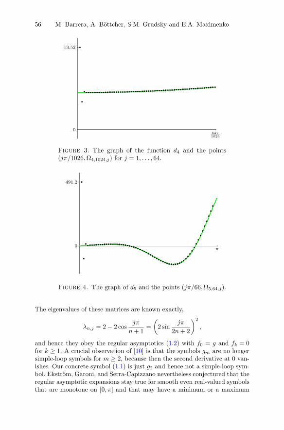
56 M. Barrera, A. Bottcher, S.M. Grudsky and E.A. Maximenko
064π1026
13.52
Figure 3. The graph of the function d4 and the points(jπ/1026,Ω4,1024,j) for j = 1, . . . , 64.
0π
491.2
Figure 4. The graph of d5 and the points (jπ/66,Ω5,64,j).
The eigenvalues of these matrices are known exactly,
λn,j = 2− 2 cosjπ
n+ 1=
(2 sin
jπ
2n+ 2
)2
,
and hence they obey the regular asymptotics (1.2) with f0 = g and fk = 0for k ≥ 1. A crucial observation of [10] is that the symbols gm are no longersimple-loop symbols for m ≥ 2, because then the second derivative at 0 van-ishes. Our concrete symbol (1.1) is just g2 and hence not a simple-loop sym-bol. Ekstrom, Garoni, and Serra-Capizzano nevertheless conjectured that theregular asymptotic expansions stay true for smooth even real-valued symbolsthat are monotone on [0, π] and that may have a minimum or a maximum

Erratic eigenvalue behavior of Toeplitz Matrices 57
064π1026
7623.7
Figure 5. The first piece of the graph of d5 (green) and thepoints (jπ/1026,Ω5,1024,j) for j = 1, . . . , 64. The plot of d5cannot be distinguished from the abscissa axis.
of higher order. They verified this conjecture numerically for some examplesand for small values of p. This conjecture has attracted a lot of attention.
Independently and at the same time, two of us [1] considered just thesymbol (1.1) and derived exact equations and asymptotic expansions for theeigenvalues of Tn(g). Later, when paper [10] came to our attention, we realizedto our surprise that the results of [1] imply that for the symbol (1.1) theeigenvalues do not admit a regular asymptotic expansion of the form (1.2)with p = 4. This is what Theorem 1.1 says and this is a counter-example tothe conjecture by Ekstrom, Garoni, and Serra-Capizzano.
The rest of the paper is organized as follows. In Sections 3 and 4 weprovide some general facts about regular asymptotic expansions. In Section 5,using formulas and ideas from [1], we show that an analog of (1.3) is true forthe eigenvalues that are not too close to the minimum of the symbol, namely,for 2 log(n + 2) ≤ j ≤ n, and provide recipes to compute the correspondingcoefficients. On the other hand, in Section 6 we deduce an asymptotic formulafor the first eigenvalue. In Section 8 we prove that the asymptotics fromSections 5 and 6 cannot be joined.
3. Regular expansions of the eigenvalues
In this and the following sections, we work in abstract settings and use thedenominator n + s, where s is an arbitrary positive constant (“shift”). Thisallows us to unify the situations with n + 1 and n + 2 and to simplify thesubsequent references in the last sections of the paper.
We first introduce some notation and recall some facts. Given a 2π-periodic bounded real-valued function g on the real line, we denote by
λn,1, . . . , λn,n

58 M. Barrera, A. Bottcher, S.M. Grudsky and E.A. Maximenko
the eigenvalues of the corresponding Toeplitz matrices Tn(g), ordered in theascending order: λn,1 ≤ · · · ≤ λn,n. Using the first Szego limit theorem andcriteria for weak convergence of probability measures, we proved in [4, 3]that if the essential range of g is a segment of the real line, then λn,j can beuniformly approximated by the values of the quantile function Q (associatedto g) at the points j/(n+ s):
max1≤j≤n
∣∣∣∣λn,j −Q( j
n+ s
)∣∣∣∣ = o(1) as n→∞. (3.1)
If g is continuous, even, and strictly increasing on [0, π], then Q(x) is justg(πx). Denote by un,j the points of the uniform mesh jπ/(n + s), wherej ∈ 1, . . . , n. Then (3.1) can be rewritten in the form
max1≤j≤n
|λn,j − g(un,j)| = o(1) as n→∞. (3.2)
Trench proved [14] that for this class of symbols the eigenvalues are all dis-tinct:
g(0) < λn,1 < · · · < λn,n < g(π).
Thus, there exist real numbers ϕn,1, . . . , ϕn,n such that
0 < ϕn,1 < . . . < ϕn,n < π
and λn,j = g(ϕn,j). Taking into account (3.2), we can try to use un,j as aninitial approximation for ϕn,j . This approximation can be very inaccurate,but it is better than nothing.
Now let J be an arbitrary set of integer pairs (n, j) such that 1 ≤ j ≤ nfor every (n, j) in J . Suppose that for each (n, j) in J the number ϕn,j is theunique solution of the equation
x = un,j +η(x)
n+ s+ ρn,j(x), (3.3)
where η is an infinitely smooth real-valued function on [0, π] and ρn,j(n,j)∈Jis a family of infinitely smooth real-valued functions on [0, π] such that
sup0≤x≤π
supj:(n,j)∈J
|ρn,j(x)| = O
(1
(n+ s)p
)(3.4)
for some p in N.
In the simple-loop case, the function ρn did not depend on j, and J wasof the form (n, j) : n ≥ N, 1 ≤ j ≤ n for some N .
Let us show how to derive asymptotic expansions of ϕn,j and λn,j fromequation (3.3).
Proposition 3.1. Let η be an infinitely smooth real-valued function on [0, π],and ρn,j(n,j)∈J be a family of real-valued functions on [0, π] satisfying (3.4)for some natural number p. Suppose that for all (n, j) in J equation (3.3) hasa unique solution ϕn,j. Then there exists a sequence of real-valued infinitely

Erratic eigenvalue behavior of Toeplitz Matrices 59
smooth functions c0, c1, c2, . . . defined on [0, π] such that there is a numberrp > 0 ensuring that, for all (n, j) in J ,∣∣∣∣∣ϕn,j −
p∑k=0
ck(un,j)
(n+ s)k
∣∣∣∣∣ ≤ rp(n+ s)p+1
. (3.5)
Furthermore, if g is an infinitely smooth 2π-periodic real-valued even functionon R, strictly increasing on [0, π], then there exists a sequence of real-valuedinfinitely smooth functions d0, d1, d2, . . . defined on [0, π] such that the num-bers λn,j := g(ϕn,j) can be approximated as follows: there exists an Rp suchthat, for all (n, j) in J ,∣∣∣∣∣λn,j −
p∑k=0
dk(un,j)
(n+ s)k
∣∣∣∣∣ ≤ Rp(n+ s)p+1
. (3.6)
Proof. This proposition was essentially proved in [2, 5], with a slightly dif-ferent notation and reasoning, including a justification of the fixed-pointmethod. Here we propose a simpler proof. Our goal is to show that (3.5)and (3.6) are direct and trivial consequences of the main equation (3.3).
In order to simplify notation, we denote by O(1/(n+s)p) any expressionthat may depend on n and j but can be estimated from above by C/(n+ s)p
with C independent of n or j. Then (3.3) implies that
ϕn,j = un,j +O
(1
n+ s
).
Substitute this expression into (3.3) and expand η by Taylor’s formula aroundthe point un,j :
ϕn,j = un,j +η(un,j +O
(1
n+s
))n+ s
+O
(1
(n+ s)2
)= un,j +
η(un,j)
n+ s+O
(1
(n+ s)2
).
Substituting the last expression into (3.3) and expanding η by Taylor’s for-mula around un,j we get
ϕn,j = un,j +η(un,j +
η(un,j)n+s +O
(1
(n+s)2
))n+ s
+O
(1
(n+ s)3
)= un,j +
η(un,j)
n+ s+η(un,j)η
′(un,j)(n+ s)2
+O
(1
(n+ s)3
).
This “Munchhausen trick” can be applied again and again (we refer to thestory when Baron von Munchhausen saved himself from being drowned in aswamp by pulling on his own hair), yielding an asymptotic expansion of theform (3.5) of any desired order p.

60 M. Barrera, A. Bottcher, S.M. Grudsky and E.A. Maximenko
The first of the functions ck are
c0(x) = x, c1(x) = η(x), c2(x) = η(x)η′(x),
c3 = η(η′)2 +1
2η2η′′, c4 = η(η′)3 +
3
2η2η′η′′ +
1
6η3η′′′,
c5 = η(η′)4 + 3η2(η′2)η′′ +1
2η3(η′′)2 +
2
3η3η′η′′′ +
1
24η4η(4).
(3.7)
By induction on p it is straightforward to show that ck is a uniquely deter-mined polynomial in η, η′, . . . , η(k−1) also for k ≥ 6.
Once we have the asymptotic formulas for ϕn,j , we can use the formulaλn,j = g(ϕn,j) and expand the function g by Taylor’s formula around thepoint un,j to get
λn,j = g
(un,j +
p∑k=1
ck(un,j)
(n+ s)k+O
(1
(n+ s)p+1
))
=
p∑m=0
g(m)(un,j)
m!
(p∑k=1
ck(un,j)
(n+ s)k+O
(1
(n+ s)p+1
))m+O((ϕn,j − un,j)p+1).
Expanding the powers, regrouping the summands, and writing ϕn,j −un,j asO(1/(n+ s)), we obtain a regular asymptotic formula for λn,j :
λn,j =
p∑k=0
dk(un,j)
(n+ s)k+O
(1
(n+ s)p+1
). (3.8)
The first of the functions d0, d1, d2, . . . can be computed by the formulas
d0 = g, d1 = g′c1, d2 = g′c2 +1
2g′′c21,
d3 = g′c3 + g′′c1c2 +1
6g′′′c31,
d4 = g′c4 + g′′(c1c3 +
1
2c22
)+
1
2g′′′c21c2 +
1
24g(4)c41,
d5 = g′c5 + g′′(c2c3 + c1c4) +1
2g′′′(c21c3 + c1c
22) +
1
6g(4)c31c2 +
1
120g(5)c51.
(3.9)
It can again be proved by induction on p that the functions c0, c1, c2, . . . arepolynomials in η, η′, η′′, . . . and that the functions d0, d1, d2, . . . are polyno-mials in c0, c1, c2, . . . and g, g′, g′′, . . .. As a consequence, all the functions ckand dk are infinitely smooth.
Remark 3.2. The expressions (3.7) and (3.9) can be easily derived with var-ious computer algebra systems. For example, in SageMath we used the fol-lowing commands (the expression 1/n is denoted by h):
var(’u, h, c1, c2, c3, c4, c5’); (eta, g) = function(’eta, g’)
phiexpansion1 = u + h * eta(u)
phiexpansion2 = u + h * taylor(eta(phiexpansion1), h, 0, 2)
phiexpansion3 = u + h * taylor(eta(phiexpansion2), h, 0, 3)

Erratic eigenvalue behavior of Toeplitz Matrices 61
phiexpansion4 = u + h * taylor(eta(phiexpansion3), h, 0, 4)
phiexpansion5 = u + h * taylor(eta(phiexpansion4), h, 0, 5)
print(phiexpansion5.coefficients(h))
phiformal5 = u + c1*h + c2*h^2 + c3*h^3 + c4*h^4 + c5*h^5
lambdaexpansion5 = taylor(g(phiformal5), h, 0, 5)
print(lambdaexpansion5.coefficients(h))
We also performed similar computations in Wolfram Mathematica, startingwith
phiexpansion0 = u + O[h]
phiexpansion1 = Series[u + h * eta[phiexpansion0], h, 0, 1]
Remark 3.3. If the functions d0, d1, . . . are infinitely smooth, then one cantransform an asymptotic expansion into negative powers of n + s1 into anasymptotic expansion in negative powers of n+ s2. For example, suppose wehave
λn,j =
p∑k=0
dk(un,j)
(n+ 2)k+O
(1
(n+ 2)p+1
),
and we want
λn,j =
p∑k=0
fk(un,j)
(n+ 1)k+O
(1
(n+ 1)p+1
).
For k = 0, 1, we have
dk
(jπ
n+ 2
)= dk
jπ
(n+ 1)(
1 + 1n+1
)
= dk
(jπ
n+ 1− jπ
(n+ 1)2+O
(1
(n+ 1)2
))= dk
(jπ
n+ 1
)− d′k
(jπ
n+ 1
)jπ
n+ 1
1
n+ 1+O
(1
(n+ 1)2
),
and thus
d0
(jπ
n+ 2
)+ d1
(jπ
n+ 2
)1
n+ 2+O
(1
(n+ 2)2
)= d0
(jπ
n+ 1
)− d′0
(jπ
n+ 1
)jπ
n+ 1
1
n+ 1
+ d1
(jπ
n+ 1
)1
n+ 1+O
(1
(n+ 1)2
),
resulting in the equalities f0(x) = d0(x) and f1(x) = d1(x)− xd′0(x).
Remark 3.4. The hard part of the work in [2, 5] was to derive equation(3.3) and an explicit formula for η, to verify that η is sufficiently smooth, toestablish upper bounds for the functions ρn, and to prove that (3.3) has aunique solution for every n large enough and for every j. Moreover, all thiswork was done under the assumption that g has some sort of smoothness ofa finite order. In Proposition 3.1 we just require all these properties.

62 M. Barrera, A. Bottcher, S.M. Grudsky and E.A. Maximenko
4. Uniqueness of the regular asymptotic expansion
As in the previous section, we fix some s > 0.If there exists an asymptotic expansion of the form (3.8), then the func-
tions d0, d1, d2, . . . are uniquely determined. Let us state and prove this factformally. Instead of requiring (3.8) for all n and j, we assume it holds for aset of pairs (n, j) such that the quotients un,j := jπ/(n+ s) “asymptoticallyfill” [0, π]. Here is the corresponding technical definition.
Definition 4.1. Let J be a subset of N2. We say that J asymptotically fills[0, π] by quotients if for every x in [0, π], every N in N, and every δ > 0 thereis a pair of numbers (n, j) in J such that n ≥ N , 1 ≤ j ≤ n, and |un,j−x| ≤ δ.
It is easy to see that J asymptotically fills [0, π] by quotients if and onlyif the set un,j : (n, j) ∈ J is dense in [0, π].
Proposition 4.2. Let p ≥ 0 be an integer, let d0, d1, . . . , dp and d0, d1, . . . , dpbe continuous functions on [0, π], let C > 0, and let J be a subset of N2
such that J asymptotically fills [0, π] by quotients. Suppose that for every pair(n, j) in J the inequalities∣∣∣∣∣λn,j −
p∑k=0
dk(un,j)
(n+ s)k
∣∣∣∣∣ ≤ C
(n+ s)p+1,
∣∣∣∣∣λn,j −p∑k=0
dk(un,j)
(n+ s)k
∣∣∣∣∣ ≤ C
(n+ s)p+1
hold. Then dk(x) = dk(x) for every k ∈ 0, . . . , p and every x ∈ [0, π].
Proof. Denote the function dp− dp by hp. It is clear that h0 = 0. Proceedingby mathematical induction on p, we assume that hk is the zero constant forevery k with k < p, and we have to show that hp is the zero constant.
Let x ∈ [0, π] and ε > 0. Using the continuity of hp at the point x,choose δ > 0 such that |y − x| ≤ δ implies
|hp(y)− hp(x)| ≤ ε
2.
Take N such that2C
N + s≤ ε
2.
After that, pick n and j such that (n, j) ∈ J , n ≥ N , and |un,j − x| ≤ δ.Then ∣∣∣∣∣dp(un,j)(n+ s)p
− dp(un,j)
(n+ s)p
∣∣∣∣∣ ≤ 2C
(n+ s)p+1,
which implies
|hp(un,j)| ≤2C
n+ s≤ 2C
N + s≤ ε
2.
Finally,
|hp(x)| ≤ |hp(x)− hp(un,j)|+ |hp(un,j)| ≤ε
2+ε
2= ε.
As ε > 0 can be chosen arbitrarily, it follows that hp is identically zero.

Erratic eigenvalue behavior of Toeplitz Matrices 63
5. An example with a minimum of the fourth order
We now consider the pentadiagonal Toeplitz matrices generated by the trigo-nometric polynomial
g(x) =(
2 sinx
2
)4. (5.1)
The function g takes real values, is even, and strictly increases on [0, π].Nevertheless, g does not belong to the simple-loop class, because g has aminimum of the fourth order: g(0) = g′(0) = g′′(0) = g′′′(0) = 0, g(4)(0) > 0.
The purpose of this section is to recall some results of [1] and to derivesome new corollaries. We begin by introducing some auxiliary functions:
β(x) := 2 arcsinh(
sinx
2
)= 2 ln
(sin
x
2+
√1 +
(sin
x
2
)2),
f(x) := β′(x) =cos x2√
1 +(sin x
2
)2 ,ηoddn (x) := 2 arctan
(1
f(x)coth
(n+ 2)β(x)
2
),
ηevenn (x) := 2 arctan
(1
f(x)tanh
(n+ 2)β(x)
2
),
ηn,j(x) :=
ηoddn (x), if j is odd,
ηevenn (x), if j is even.
As previously, we denote by ϕn,j the points in (0, π) such that λn,j = g(ϕn,j).In this example, we let un,j stand for jπ/(n+ 2).
In [1, Theorems 2.1 and 2.3], two of us used Elouafi’s formulas [11] forthe determinants of Toeplitz matrices and derived exact equations for theeigenvalues of Tn(g). Namely, it was proved that there exists an N0 such thatif n ≥ N0 and j ∈ 1, . . . , n, then ϕn,j is the unique solution in the interval(un,j , un,j+1) of the equation
x = un,j +ηn,j(x)
n+ 2. (5.2)
The corresponding equation in [1] is written in a slightly different (but equiv-alent) form, without joining the cases of odd and even values of j.
Equation (5.2) is hard to derive but easy to verify numerically. We com-puted the eigenvalues by general numerical methods in Wolfram Mathemat-ica, using high-precision arithmetic with 100 decimal digits after the floatingpoint, and obtained coincidence in (5.2) up to 99 decimal digits for each nfrom 10 to 100 and for each j from 1 to n.
Equation (5.2) is more complicated than (3.3), in the sense that nowinstead of one function η we have a family of functions, depending on n andon the parity of j.
Note that if x is not too close to zero, then β(x) is away from zero. Thus,when n is large enough, the product n+2
2 β(x) is large and the expressions
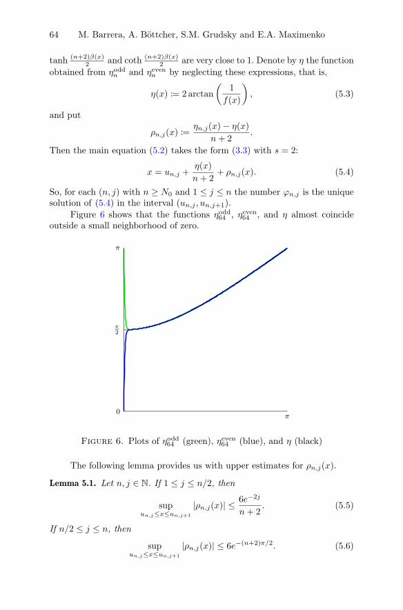
64 M. Barrera, A. Bottcher, S.M. Grudsky and E.A. Maximenko
tanh (n+2)β(x)2 and coth (n+2)β(x)
2 are very close to 1. Denote by η the function
obtained from ηoddn and ηevenn by neglecting these expressions, that is,
η(x) := 2 arctan
(1
f(x)
), (5.3)
and put
ρn,j(x) :=ηn,j(x)− η(x)
n+ 2.
Then the main equation (5.2) takes the form (3.3) with s = 2:
x = un,j +η(x)
n+ 2+ ρn,j(x). (5.4)
So, for each (n, j) with n ≥ N0 and 1 ≤ j ≤ n the number ϕn,j is the uniquesolution of (5.4) in the interval (un,j , un,j+1).
Figure 6 shows that the functions ηodd64 , ηeven64 , and η almost coincideoutside a small neighborhood of zero.
0π
π2
π
Figure 6. Plots of ηodd64 (green), ηeven64 (blue), and η (black)
The following lemma provides us with upper estimates for ρn,j(x).
Lemma 5.1. Let n, j ∈ N. If 1 ≤ j ≤ n/2, then
supun,j≤x≤un,j+1
|ρn,j(x)| ≤ 6e−2j
n+ 2. (5.5)
If n/2 ≤ j ≤ n, then
supun,j≤x≤un,j+1
|ρn,j(x)| ≤ 6e−(n+2)π/2. (5.6)

Erratic eigenvalue behavior of Toeplitz Matrices 65
Proof. First suppose that 1 ≤ j ≤ n/2 and un,j ≤ x ≤ un,j+1. Then
jπ
n+ 2≤ x ≤ (j + 1)π
n+ 2≤ π
2.
It is readily verified that β(x) ≥ 2x/π for every x in [0, π/2]. Consequently,
(n+ 2)β(x)
2≥ j.
It is also easy to see that 0 ≤ 1−tanh(y) ≤ 2e−2y and 0 ≤ coth(y)−1 ≤ 3e−2y
for y ≥ 1, f(x) > 1/2 for x in [0, π/2], and that arctan is Lipschitz continuouswith coefficient 1. Thus
|ηn,j(x)− η(x)| ≤ 6e−2j ,
which yields (5.5).Now consider the case n/2 ≤ j ≤ n. Here we use the two estimates
β(x) ≥ x/2 and f(x) > 1/(n+ 2) to obtain
(n+ 2)β(x)
2≥ (n+ 2)π
4,
|ηn,j(x)− η(x)| ≤ 6(n+ 2)e−(n+2)π/2,
which results in (5.6).
The next proposition is similar to Theorem 2.3 from [1], but here we jointhe cases of odd and even values of j and get rid of the additional requirementthat n ≥ N0. We rely on [1] for the existence of the solution but use a simplerargument to prove the uniqueness.
Proposition 5.2. For all n ≥ 1 and all j ∈ 1, . . . , n, the number ϕn,j is theunique solution of the equation (5.2) on the interval (un,j , un,j+1).
Proof. Let n ≥ 1. For each j ∈ 1, . . . , n, the main equation (5.2) can bewritten in the form
(n+ 2)x− ηn,j(x) = jπ. (5.7)
By Theorem 2.1 from [1], if x belongs to (0, π) and satisfies (5.7) for someinteger j, then the number g(x) is an eigenvalue of Tn(g).
Notice that f(x) > 0 and β(x) > 0 for every x ∈ (0, π). Using thedefinitions of tanh, coth, and arctan, we conclude that 0 < ηn,j(x) < πfor each x ∈ (0, π); see also Figure 6. Denote the left-hand side of (5.7) byFn,j(x). Then
Fn,j(un,j) = jπ − ηn,j(un,j) < jπ,
Fn,j(un,j+1) = (j + 1)π − ηn,j(un,j+1) > jπ.
Hence, by the intermediate value theorem, equation (5.7) has at least onesolution in the interval (un,j , un,j+1). At this moment we do not know whetherthis solution is unique. So let us, for each j, denote by ψn,j one of the solutionsof (5.7) on (un,j , un,j+1).

66 M. Barrera, A. Bottcher, S.M. Grudsky and E.A. Maximenko
Contrary to what we want, assume that for some j ∈ 1, . . . , n equa-tion (5.7) has another solution x belonging to (un,j , un,j+1). The n+ 1 num-bers ψn,1, . . . , ψn,n, x are different. Since g is strictly increasing on [0, π], thecorresponding eigenvalues g(ψn,1), . . . , g(ψn,n), g(x) are different, too. Thiscontradicts the fact that the matrix Tn(g) has only n eigenvalues.
We conclude that for each j equation (5.7) has only one solution ψn,j in(un,j , un,j+1). The numbers ψn,j satisfy ψn,1 < . . . < ψn,n, and their imagesunder g are eigenvalues of Tn(g), so g(ψn,j) = λn,j and ψn,j = ϕn,j for all jin 1, . . . , n.
The next proposition gives asymptotic formulas for the eigenvalues λn,jprovided j is “not too small”. It mimics Theorem 2.6 from [1], the noveltybeing that we here join the cases of odd and even values of j and state theresult for an arbitrary order p.
Proposition 5.3. For every p ∈ N, the functions ρn,j admit the asymptoticupper estimate
max(p/2) log(n+2)≤j≤n
supx∈[un,j ,un,j+1]
|ρn,j(x)| = O
(1
np+1
). (5.8)
Moreover, for every p ∈ N, every n ∈ N, and every j satisfying
p
2log(n+ 2) ≤ j ≤ n, (5.9)
the numbers ϕn,j and λn,j have asymptotic expansions of the form
ϕn,j =
p∑k=0
ck(un,j)
(n+ 2)k+O
(1
(n+ 2)p+1
), (5.10)
λn,j =
p∑k=0
dk(un,j)
(n+ 2)k+O
(1
(n+ 2)p+1
), (5.11)
where the upper estimates of the residue terms are uniform in j, the functionsck and dk are infinitely smooth and can be expressed in terms of η and g bythe formulas shown in the proof of Proposition 3.1.
Proof. We have to verify the upper bound (5.8). The other statements thenfollow from Proposition 3.1. Let p, n ∈ N and j satisfy (5.9). If j ≤ n/2, then(5.5) gives
6e−2j
n+ 2≤ 6e−p log(n+2)
n+ 2=
6
(n+ 2)p+1,
while if j > n/2, we obtain from (5.6) that
e−(n+2)π/2 = O
(1
np+1
).
Joining these two cases we arrive at (5.8).

Erratic eigenvalue behavior of Toeplitz Matrices 67
In Proposition 3.1 we expressed the first of the coefficients ck and dkin terms of the first derivatives of g and η. Here are explicit formulas forg′, . . . , g(5):
g′(x) = 23 cosx
2
(sin
x
2
)3, g′′(x) = 16(1 + 2 cos(x))
(sin
x
2
)2,
g′′′(x) = −8 sin(x) + 16 sin(2x), g(4)(x) = −8 cos(x) + 32 cos(2x),
g(5)(x) = 8 sin(x)− 64 sin(2x). (5.12)
For η′, . . . , η(4) we have
η′(x) =sin x
2(1 +
(sin x
2
)2)1/2 , η′′(x) =
√2 cos x2
(3− cos(x))3/2
, (5.13)
η′′′(x) = −5 sin x
2 + sin 3x2√
2(3− cos(x))5/2, η(4)(x) =
−4 cos x2 + 19 cos 3x2 + cos 5x
2
2√
2(3− cos(x))7/2.
Numerical test 5.4. In order to test (5.11) numerically for p = 4, we com-puted g′, . . . , g(4) by (5.12), η, η′, . . . , η(3) by (5.3) and (5.13), c0, c1, . . . , c4by (3.7) and d0, d1, . . . , d4 by (3.9). The exact eigenvalues were computed bysimple iteration in equation (5.4) and independently by general eigenvaluealgorithms (for n ≤ 1024). All computations were made in high-precisionarithmetic with 100 decimal digits after the floating point, in SageMath andindependently in Wolfram Mathematica. Denote by En,4 the maximal errorin (5.11), with p = 4:
En,4 := max2 log(n+2)≤j≤n
∣∣∣∣∣λn,j −4∑k=0
dk(un,j)
(n+ 2)k
∣∣∣∣∣ .The following table shows En,4 and (n+ 2)5En,4 for various values of n.
n = 64 n = 256 n = 1024 n = 4096 n = 16384
En,4 2.4 · 10−7 3.1 · 10−10 3.2 · 10−13 3.2 · 10−16 3.1 · 10−19
(n+ 2)5En,4 306.72 354.87 366.61 369.52 370.25
We see that the numbers En,4 really behave like O(1/(n+ 2)5).
6. An asymptotic formula for the first eigenvalues in theexample
In this section we study the asymptotic behavior of λn,j as n tends to ∞,considering j as a fixed parameter.
Using the definition of arctan and the formula for tan(x+jπ/2), we canrewrite equation (5.2) in the equivalent form
f(x)(−1)j+1
tanh(n+ 2)β(x)
2= (−1)j tan
(n+ 2)x
2. (6.1)

68 M. Barrera, A. Bottcher, S.M. Grudsky and E.A. Maximenko
The first factor on the left-hand side of (6.1) is just f(x) for odd values of jand 1/f(x) for even values of j. We know that
jπ
n+ 2≤ ϕn,j ≤
(j + 1)π
n+ 2,
and it is natural to expect that the product (n+ 2)ϕn,j has a finite limit αjas n tends to infinity and j is fixed. Assuming this and taking into accountthat
f(x)→ 1, β(x) ∼ x, as x→ 0,
we can pass to the limit in (6.1) to obtain a simple transcendental equationfor αj . This is an informal motivation of the following formal reasoning.
For each j in N, denote by αj the unique real number that belongs tothe interval (jπ, (j + 1)π) and satisfies
tanhαj2
= (−1)j tanαj2. (6.2)
Figure 7 shows both sides of (6.2) for j = 1, 2, 3.
0π 2π 3π 4πα1 α2 α3
1
Figure 7. The left-hand side (black) and the right-handside (blue) of (6.2), for j = 1 on (π, 2π), for j = 2 on (2π, 3π)and for j = 3 on (3π, 4π).
For each j, the transcendental equation (6.2) is easy to solve by numer-ical methods. Approximately,
α1 ≈ 4.73004, α2 ≈ 7.85320, α3 ≈ 10.99561.
It follows from (6.2) that αj >(2j+1)π
2 if j is odd and αj <(2j+1)π
2 if j iseven. In particular,
α1 >3π
2, α2 <
5π
2, α3 >
7π
2.
We remark that differences between αj and (2j+ 1)π/2 are extremely small:
α1 −3π
2≈ 1.8 · 10−2, α2 −
5π
2≈ −7.8 · 10−4, α3 −
7π
2≈ 3.3 · 10−5.
Contrary to the general agreement of this paper, the upper estimatesof the residual terms in the following proposition are not uniform in j. Thuswe use the notation Oj instead of O.

Erratic eigenvalue behavior of Toeplitz Matrices 69
Proposition 6.1. Let g be the function defined by (5.1) and define ϕn,j ∈ (0, π)by λn,j = g(ϕn,j). Then for each fixed j in N, ϕn,j and λn,j satisfy theasymptotic formulas
ϕn,j =αjn+ 2
+Oj
(1
(n+ 2)3
), (6.3)
λn,j =
(αjn+ 2
)4
+Oj
(1
(n+ 2)6
). (6.4)
Proof. Fix j in N. We are going to treat (6.1) by asymptotic methods, as ntends to infinity. Put
δn,j := (n+ 2)ϕn,j − αj ,i.e., represent the product (n+ 2)ϕn,j in the form
(n+ 2)ϕn,j = αj + δn,j .
It is easy to verify that, as x→ 0,
f(x) = 1 +O(x2), β(x) = x+O(x3).
Moreover, we know that jπn+2 ≤ ϕn,j ≤
(j+1)πn+2 and thus ϕn,j = Oj(1/(n+2)).
Therefore
f(ϕn,j) = 1 +Oj
(1
(n+ 2)2
),
1
f(ϕn,j)= 1 +Oj
(1
(n+ 2)2
),
(n+ 2)
2β(ϕn,j) =
αj + δn,j2
+Oj
(1
(n+ 2)2
),
tanh(n+ 2)
2β(ϕn,j) = tanh
αj + δn,j2
+Oj
(1
(n+ 2)2
).
By the mean value theorem, there exist some numbers ξ1,n,j and ξ2,n,j be-tween αj/2 and (αj + δn,j)/2 such that
tanhαj + δn,j
2− tanh
αj2
= tanh′(ξ1,n,j)δn,j2
and
tanαj + δn,j
2− tan
αj2
= tan′(ξ2,n,j)δn,j2.
After replacing x by ϕn,j , equation (6.1) takes the form
tanhαj2
+ tanh′(ξ1,n,j)δn,j2
+Oj
(1
(n+ 2)2
)= (−1)j
(tan
αj2
+ tan′(ξ2,n,j)δn,j2
+Oj
(1
(n+ 2)2
)).
Using the definition of αj , this can be simplified to(tan′(ξ2,n,j) + (−1)j−1 tanh′(ξ1,n,j)
)δn,j = Oj
(1
(n+ 2)2
).

70 M. Barrera, A. Bottcher, S.M. Grudsky and E.A. Maximenko
The coefficient before δn,j is strictly positive and bounded away from zero.Indeed, for all x from the considered domain (jπ/2, (j + 1)π/2) we havetan′(x) > 1 and
tanh′(x) =1
1 + x2<
1
1 + π2
4
<1
2,
thus
tan′(ξ2,n,j) + (−1)j−1 tanh′(ξ1,n,j) >1
2.
Therefore δn,j = Oj(1/(n+ 2)2), which is equivalent to (6.3). The function ghas the following asymptotic expansion near the point 0:
g(x) = x4 +O(x6). (6.5)
Using the formula λn,j = g(ϕn,j) and combining (6.3) with (6.5), we arriveat (6.4).
Numerical test 6.2. Denote by εn,j the absolute value of the residue in (6.4):
εn,j :=
∣∣∣∣∣λn,j −(
αjn+ 2
)4∣∣∣∣∣ .
Similarly to Numerical test 5.4, the exact eigenvalues λn,j and the coefficientsαj are computed in high-precision arithmetic with 100 decimal digits afterthe floating point. The next table shows εn,j and (n+ 2)6εn,j correspondingto j = 1, 2 and to various values of n.
n = 64 n = 256 n = 1024 n = 4096 n = 16384
εn,1 6.3 · 10−9 1.8 · 10−11 4.5 · 10−16 1.1 · 10−19 2.7 · 10−23
(n+ 2)6εn,1 523.37 524.39 524.46 524.46 524.46
εn,2 1.1 · 10−7 3.1 · 10−11 7.9 · 10−15 2.0 · 10−18 4.9 · 10−22
(n+ 2)6εn,2 9315.7 9266.9 9263.7 9263.5 9263.4
Moreover, numerical experiments show that
max1≤n≤100000
((n+ 2)6εn,1) < 524.47.
Remark 6.3. Notice that formula (2.7) from [1] does not have the form (6.3)because the numerator u1,j in this formula depends on n in a complicatedmanner.
Remark 6.4. Proposition 6.1 has trivial corollaries about the norm of theinverse matrix and the condition number:
‖T−1n (g)‖2 ∼(n+ 2
α1
)4
, cond2(Tn(g)) ∼ 16
(n+ 2
α1
)4
, as n→∞.

Erratic eigenvalue behavior of Toeplitz Matrices 71
Remark 6.5. Proposition 6.1 is not really new. Parter [12, 13] showed that ifgm is given by (2.1), then the corresponding eigenvalues satisfy
λn,j =γj(m)
(n+ 2)2m+ o
(1
(n+ 2)2m
)as n→∞ (6.6)
with some constant γj(m) for each fixed j. Our proposition identifies γ1(2)as α4
1 and improves the o(1/(n + 2)4) to O(1/(n + 2)6). Parter also had ex-plicit formulas for γj(2) in terms of the solutions of certain transcendentalequations. Widom [15, 16] derived results like (6.6) by replacing matrices byintegral operators with piecewise constant kernels and subsequently provingthe convergence of the appropriately scaled integral operators. Widom’s ap-proach delivered the constants γj(m) as the reciprocals of the eigenvalues ofcertain integral operators. More about these pioneering works can be foundin [7, pp. 256–259] and in [8]. The proof of Proposition 6.1 given above isdifferent from the ones by Parter and Widom.
Remark 6.6. If we pass to the denominator n + 1 in formula (6.4), then itbecomes more complicated:
λn,j =α4j
(n+ 1)4−
4α4j
(n+ 1)5+Oj
(1
(n+ 2)6
).
This reveals that the denominator n + 2 is more convenient when studyingthe asymptotic behavior of the first eigenvalues in the example (1.1).
7. The regular four term asymptotic expansion for theexample
Lemma 7.1. Let g(x) =(2 sin x
2
)4and let d0, . . . , d4 be the same functions as
in Proposition 5.3. Then, as n→∞, we have the asymptotic expansions
3∑k=0
dk(jπn+2
)(n+ 2)k
=(jπ + η(0))4 − η(0)4
(n+ 2)4+O
(j4
(n+ 2)5
), (7.1)
4∑k=0
dk(jπn+2
)(n+ 2)k
=
(jπ + η(0)
n+ 2
)4
+O
(j4
(n+ 2)5
), (7.2)
uniformly in j.
Proof. By (5.12), the function g and its derivatives admit the following as-ymptotic expansions near the point 0:
g(x) = x4 +O(x6), g′(x) = 4x3 +O(x5), g′′(x) = 12x2 +O(x4),
g′′′(x) = 24x+O(x3), g(4)(x) = 24 +O(x2) (x→ 0).(7.3)
Applying (5.13) and taking into account that η is smooth, we see that
c0(x) = x, c1(x) = η(x) = η(0) +O(x) (x→ 0) (7.4)

72 M. Barrera, A. Bottcher, S.M. Grudsky and E.A. Maximenko
and that the functions c2, c3, c4 are bounded. Substituting (7.3) and (7.4)into the formulas (3.9), we get the following expansions of d0(x), . . . , d4(x),as x→ 0:
d0(x) = x4 +O(x6), d1(x) = g′(x)c1(x) = 4x3η(0) +O(x4),
d2(x) =1
2g′′(x)c21(x) +O(x3) = 6x2η2(0) +O(x3),
d3(x) =1
6g′′′(x)c31(x) +O(x2) = 4xη3(0) +O(x2),
d4(x) =1
24g(4)(x)c41(x) +O(x) = η4(0) +O(x).
Using these formulas and the binomial theorem, we arrive at (7.2). Movingin (7.2) the summand with k = 4 to the right-hand side we obtain (7.1).
The following proposition proves Theorem 1.2 (b).
Proposition 7.2. Let g(x) =(2 sin x
2
)4and d0, . . . , d3 : [0, π]→ R be the func-
tions from the proof of Proposition 5.3. Then there exists a C > 0 such that∣∣∣∣∣λn,j −3∑k=0
dk(jπn+2
)(n+ 2)k
∣∣∣∣∣ ≤ C
(n+ 2)4(7.5)
for all n ∈ N and all j ∈ 1, . . . , n.
Proof. Thanks to Proposition 5.3 we are left with the case j < 2 log(n+ 2).Using (5.4), the upper estimate (5.5), and the smoothness of η, we concludethat
ϕn,j =jπ + η(0)
n+ 2+O
(j
(n+ 2)2
)+O
(e−2j
n+ 2
). (7.6)
From (6.5) we therefore obtain that
λn,j = g(ϕn,j) = ϕ4n,j +O
((log(n+ 2))6
(n+ 2)6
)= ϕ4
n,j +O
(1
(n+ 2)4
).
Expanding ϕ4n,j by the multinomial theorem and separating the main term,
we get
ϕ4n,j =
(jπ + η(0)
n+ 2
)4
+∑
p,q,r≥0p+q+r=4p<4
O
((jπ + η(0))pjq e−2jr
(n+ 2)p+2q+r
).
The sum over p, q, r can be divided into the part with q > 0 and the partwith q = 0 and estimated by∑p,q,r≥0p+q+r=4q>0
O
((jπ + η(0))pjq
(n+ 2)4+q
)+∑p,r≥0p+r=4r>0
O
((jπ + η(0))pe−2jr
(n+ 2)4
)= O
(1
(n+ 2)4
).

Erratic eigenvalue behavior of Toeplitz Matrices 73
Consequently, the true asymptotic expansion of λn,j under the conditionj < 2 log(n+ 2) is
λn,j =
(jπ + η(0)
n+ 2
)4
+O
(1
(n+ 2)4
). (7.7)
On the other hand, using (7.1) and the fact that j4 = O(n+ 2), we get
3∑k=0
dk(un,j)
(n+ 2)k=
(jπ + η(0)
n+ 2
)4
+O
(1
(n+ 2)4
). (7.8)
Comparing (7.7) and (7.8), we obtain the required result.
Numerical test 7.3. Denote by ∆n the maximal error in (7.5):
∆n := max1≤j≤n
∣∣∣∣∣λn,j −3∑k=0
dk(un,j)
(n+ 2)k
∣∣∣∣∣ .The following table shows ∆n and (n+ 2)4∆n for various values of n.
n = 64 n = 256 n = 1024 n = 4096 n = 16384
∆n 7.6 · 10−6 3.2 · 10−8 1.3 · 10−10 5.1 · 10−13 2.0 · 10−15
(n+ 2)4∆n 143.97 143.05 142.81 142.75 142.74
According to this table, the numbers ∆n really behave like O(1/(n+ 2)4).
Remark 7.4. Let us again embark on the case p = 3 and thus on Theo-
rem 1.2 (b) and the previous Numerical test 7.3. This test suggests that wecould be satisfied by an error of 10−15 for n = 16 384. However, as the firsteigenvalues are also of order 10−15 we obtain nothing but an upper bound
for them. In other words, the approximation of the first eigenvalues λn,j by∑3k=0
dk(un,j)(n+2)k
is bad in the sense that the absolute error of this approxima-
tion is of the same order Oj(1/(n + 2)4) as the eigenvalue λn,j which we
want to approximate! To state it in yet different terms, for each fixed j, theresidues
ωn,j := λn,j −3∑k=0
dk( jπn+2 )
(n+ 2)k
decay at the same rate Oj(1/(n+2)4) as the eigenvalues λn,j and the distancesbetween them, and the corresponding relative errors do not tend to zero:
ωn,jλn,j
→α4j + η(0)4 − (jπ + η(0))4
α4j
6= 0,
ωn,jλn,j+1 − λn,j
→α4j + η(0)4 − (jπ + η(0))4
α4j+1 − α4
j
6= 0.
Compared to this, the residues of the asymptotic expansions for simple-loop
symbols (see [2, 5]) can be bounded by o( j (n+1−j)
n21np
), where p is related
with the smoothness of the symbols, and the expression j (n+1−j)n2 is in the

74 M. Barrera, A. Bottcher, S.M. Grudsky and E.A. Maximenko
simple-loop case always comparable with the distance λn,j+1 − λn,j betweenthe consecutive eigenvalues, i.e., there exist C1 > 0 and C2 > 0 such that
C1j (n+ 1− j)
n2≤ λn,j+1 − λn,j ≤ C2
j (n+ 1− j)n2
.
Clearly, the quotient|ωn,j |
λn,j+1−λn,jis a more adequate measure of the quality
of the approximation than just the absolute error |ωn,j |.
8. There is no regular five term asymptotic expansion for theexample
As said, Ekstrom, Garoni, and Serra-Capizzano [10] conjectured that for ev-ery infinitely smooth 2π-periodic real-valued even function g, strictly increas-ing on [0, π], the eigenvalues λn,j of the corresponding Toeplitz matrices admitan asymptotic expansion of the regular form (1.2) for every order p.
We now show that for the symbol g(x) =(2 sin x
2
)4an asymptotic ex-
pansion of the form (1.2) cannot be true for p = 4. This disproves Conjecture 1from [10].
We remark that the following proposition is actually stronger than thethird part of Theorem 1.2. Namely, Theorem 1.2(c) states that (1.6) cannothold with the functions d1, . . . , d4 appearing in (1.4). The following proposi-tion tells us that (1.6) is also impossible for any other choice of continuousfunctions d1, . . . , d4. The reason is of course Proposition 4.2.
Proposition 8.1. Let g(x) =(2 sin x
2
)4. Denote by λn,1, . . . , λn,n the eigen-
values of the Toeplitz matrices Tn(g), written in the ascending order. Thenthere do not exist continuous functions d0, . . . , d4 : [0, π] → R and numbersC > 0, N ∈ N, such that for every n ≥ N and every j ∈ 1, . . . , n∣∣∣∣∣λn,j −
4∑k=0
dk(jπn+2
)(n+ 2)k
∣∣∣∣∣ ≤ C
(n+ 2)5. (8.1)
Proof. Reasoning by contradiction, assume there exist functions d0, . . . , d4and numbers C and N with the required properties. Put
J =
(n, j) ∈ N2 : n ≥ N, 2 log(n+ 2) ≤ j ≤ n.
Clearly, this set J asymptotically fills [0, π] by quotients.So, by Proposition 4.2, the functions d0, . . . , d4 from (8.1) must be the
same as the functions d0, . . . , d4 from Proposition 5.3. In other words, theasymptotic expansion (5.11) from Proposition 5.3 holds for every pair (n, j)with n large enough and j in 1, . . . , n, that is, without the restrictionj ≥ 2 log(n+ 2).
Combining (8.1) with (7.2), we see that for each fixed j the eigenvalueλn,j must have the asymptotic behavior
λn,j =
(jπ + η(0)
n+ 2
)4
+Oj
(1
(n+ 2)5
). (8.2)

Erratic eigenvalue behavior of Toeplitz Matrices 75
Since η(0) = 2 arctan(1) = π2 , we obtain for j = 1 that
λn,1 =
(3π/2
n+ 2
)4
+O
(1
(n+ 2)5
), (8.3)
which contradicts Proposition 6.1 because 3π/2 6= α1.
Remark 8.2. Here is an alternative way to finish the proof of Proposition 8.1.After having formula (8.2), we obtain the following hypothetical asymptoticrelation between the two first eigenvalues:
limn→∞
((n+ 2)
(λ1/4n,2 − λ
1/4n,1
))= (2π + η(0))− (π + η(0)) = π.
But this contradicts Proposition 6.1, according to which
limn→∞
((n+ 2)
(λ1/4n,2 − λ
1/4n,1
))= α2 − α1 < π.
In this reasoning we do not use the value η(0).
Proof of Theorem 1.2. The existence of the asymptotic expansions (1.4) fol-lows from Proposition 5.3, its uniqueness is a consequence of Proposition 4.2,formula (1.5) was established in Proposition 7.2, and the impossibility of (1.6)is just Proposition 8.1.
Proof of Theorem 1.1. The functions d0, d1, . . . from Proposition 5.3 are in-finitely smooth on [0, π], and thus, by Remark 3.3, the expansion (5.11) withp = 4 can be rewritten in the form (1.3) with some infinitely smooth functionsf0, . . . , f4. So, (1.3) is true for all (n, j) satisfying 2 log(n+ 2) ≤ j ≤ n.
Contrary to what we want, assume that there are f0, . . . , f4, C, and Nas in the statement of Theorem 1.1. Then, by Proposition 4.2, the functionsf0, . . . , f4 are the same as those in the previous paragraph. In particular,f0, . . . , f4 must be infinitely smooth. In this case, the asymptotic expansion(1.3) can be rewritten in powers of 1/(n+ 2) and is true for all n and j withn ≥ N and 1 ≤ j ≤ n. This contradicts Proposition 8.1.
We conclude with a conjecture about the eigenvalues of Toeplitz matri-ces generated by (2.1).
Conjecture 8.3. Let gm(x) =(2 sin x
2
)2mwith an integer m ≥ 3. If p ≤ 2m−1,
there are Np ∈ N and Dp > 0 such that∣∣∣∣∣λn,j −p∑k=0
dk(jπn+2
)(n+ 2)k
∣∣∣∣∣ ≤ Dp
(n+ 2)p+1(8.4)
for all n ≥ Np and all j in 1, . . . , n. For p = 2m, inequality (8.4) doesnot hold for all sufficiently large n and all 1 ≤ j ≤ n, but it holds for for allsufficiently large n and all j not too close to 1, say, for (log(n+2))2 ≤ j ≤ n.

76 M. Barrera, A. Bottcher, S.M. Grudsky and E.A. Maximenko
References
[1] M. Barrera and S.M. Grudsky, Asymptotics of eigenvalues for pentadiagonalsymmetric Toeplitz matrices, Operator Theory: Adv. and Appl. 259, Birkhauser,2017, 51–77. DOI: 10.1007/978-3-319-49182-0 7
[2] J.M. Bogoya, A. Bottcher, S.M. Grudsky, and E.A. Maximenko, Eigenvaluesof Hermitian Toeplitz matrices with smooth simple-loop symbols, J. Math.Analysis Appl. 422 (2015), 1308–1334. DOI: 10.1016/j.jmaa.2014.09.057
[3] J.M. Bogoya, A. Bottcher, S.M. Grudsky, and E.A. Maximenko, Maximumnorm versions of the Szego and Avram–Parter theorems for Toeplitz matrices,J. Approx. Theory 196 (2015), 79–100. DOI: 10.1016/j.jat.2015.03.003
[4] J.M. Bogoya, A. Bottcher, and E.A. Maximenko, From convergence in distri-bution to uniform convergence, Boletın de la Sociedad Matematica Mexicana22 (2016), no. 2, 695–710. DOI: 10.1007/s40590-016-0105-y
[5] J.M. Bogoya, S.M. Grudsky, and E.A. Maximenko, Eigenvalues of Hermit-ian Toeplitz matrices generated by simple-loop symbols with relaxed smooth-ness, Operator Theory: Adv. and Appl. 259, Birkhauser, 2017, 179–212. DOI:10.1007/978-3-319-49182-0 11
[6] A. Bottcher, S.M. Grudsky, and E.A. Maksimenko, Inside the eigenvalues ofcertain Hermitian Toeplitz band matrices, J. Comput. Appl. Math. 233 (2010),2245–2264. DOI: 10.1016/j.cam.2009.10.010
[7] A. Bottcher and S.M. Grudsky, Spectral Properties of Banded Toeplitz Matrices,SIAM, Philadelphia, 2005. DOI: 10.1137/1.9780898717853
[8] A. Bottcher and H. Widom, From Toeplitz eigenvalues through Green’s ker-nels to higher-order Wirtinger-Sobolev inequalities, Operator Theory: Adv. andAppl. 171, Birkhauser, 2006, 73–87. DOI: 10.1007/978-3-7643-7980-3 4
[9] P. Deift, A. Its, and I. Krasovsky, Eigenvalues of Toeplitz matrices in the bulkof the spectrum, Bull. Inst. Math. Acad. Sin. (N.S.) 7 (2012), 437–461. URL:http://web.math.sinica.edu.tw/bulletin ns/20124/2012401.pdf
[10] S.-E. Ekstrom, C. Garoni, and S. Serra-Capizzano, Are the eigenvalues ofbanded symmetric Toeplitz matrices known in almost closed form? Experi-mental Mathematics, 10 pp., 2017. DOI: 10.1080/10586458.2017.1320241
[11] M. Elouafi, On a relationship between Chebyshev polynomials and Toeplitzdeterminants, Applied Mathematics and Computation 229 (2014), 27–33. DOI:10.1016/j.amc.2013.12.029
[12] S.V. Parter, Extreme eigenvalues of Toeplitz forms and applications to ellip-tic difference equations, Trans. Amer. Math. Soc. 99 (1961), 153–192. DOI:10.2307/1993449
[13] S.V. Parter, On the extreme eigenvalues of truncated Toeplitz matrices, Bull.Amer. Math. Soc. 67 (1961), 191–196. DOI: 10.1090/S0002-9904-1961-10563-6
[14] W.F. Trench, Interlacement of the even and odd spectra of real symmetricToeplitz matrices, Linear Alg. Appl. 195 (1993), 59–68. DOI: 10.1016/0024-3795(93)90256-N
[15] H. Widom, Extreme eigenvalues of translation kernels, Trans. Amer. Math.Soc. 88 (1958), 491–522. DOI: 10.1090/S0002-9947-1961-0138980-4
[16] H. Widom, Extreme eigenvalues of N -dimensional convolution operators,Trans. Amer. Math. Soc. 106 (1963), 391–414. DOI: 10.2307/1993750

Erratic eigenvalue behavior of Toeplitz Matrices 77
Mauricio BarreraCINVESTAVDepartamento de MatematicasApartado Postal 07360Ciudad de MexicoMexicoe-mail: [email protected]
Albrecht BottcherTechnische Universitat ChemnitzFakultat fur Mathematik09107 ChemnitzGermanye-mail: [email protected]
Sergei M. GrudskyCINVESTAVDepartamento de MatematicasApartado Postal 07360Ciudad de MexicoMexicoe-mail: [email protected]
Egor A. MaximenkoInstituto Politecnico NacionalEscuela Superior de Fısica y MatematicasApartado Postal 07730Ciudad de MexicoMexicoe-mail: [email protected]

Spectral regularity of a C∗-algebragenerated by two-dimensional singularintegral operators
Harm Bart, Torsten Ehrhardt and Bernd Silbermann
Abstract. Given a bounded simply connected domain U ⊂ C having aLyapunov curve as its boundary, let L(L2(U)) stand for the C∗-algebraof all bounded linear operators acting on the Hilbert space L2(U) withLebesgue area measure. We show that the smallest C∗-subalgebra A ofL(L2(U)) containing the singular integral operator
(SUf)(z) = − 1
π
∫U
f(w)
(z − w)2dA(w),
along with its adjoint
(S∗Uf) (z) = − 1
π
∫U
f(w)
(z − w)2dA(w),
all multiplication operators aI, a ∈ C(U), and all compact operatorson L2(U), is spectrally regular. Roughly speaking the latter means thefollowing: if the contour integral of the logarithmic derivative of an an-alytic A-valued function f is vanishing (or is quasi-nilpotent), then ftakes invertible values on the inner domain of the contour in question.
Mathematics Subject Classification (2010). Primary: 45E05, Secondary:30G30, 47A53, 47L10.
Keywords. Analytic vector-valued function, logarithmic residue, spectralregularity, two-dimensional singular integral operator, C∗-algebra.
In memory of Georg Heinig
1. Introduction
Let B be a complex unital Banach algebra and let ∆ be a bounded Cauchydomain in C (see [13, 19]). The positively oriented boundary of ∆ will bedenoted by ∂∆. Let A∂(∆,B) stand for the set of all B-valued functions fwhich are defined and analytic on an open neighborhood of ∆ = ∂∆ ∪ ∆
© Springer International Publishing AG, part of Springer Nature 2018 79
Theory: Advances and Applications 268, https://doi.org/10.1007/978-3-319-75996-8_3A. Böttcher et al. (eds.), The Diversity and Beauty of Applied Operator Theory, Operator

80 H. Bart, T. Ehrhardt and B. Silbermann
and which take invertible values on all of ∂∆. For f ∈ A∂(∆,B) the contourintegral
LR(f ; ∆) =1
2πi
∫∂∆
f ′(λ)f(λ)−1 dλ , (1.1)
is well defined and called the logarithmic residue of f with respect to ∆.
In the scalar case B = C, the logarithmic residue is equal to the numberof zeros of f in ∆, multiplicities taken into account. Thus, in this situation,the integral (1.1) vanishes if and only if f takes non-zero values, not only on∂∆ (which has been assumed via the invertibility requirement in order to let(1.1) make sense) but on all of ∆.
This leads to the following question: Given a unital Banach algebraB and a function f ∈ A∂(∆,B) with LR(f ; ∆) = 0, does it follow that ftakes invertible values on all of ∆? In general the answer to this questionis negative. The Banach algebra B = L(`2) of all bounded linear operatorsacting on `2 together with a suitably defined analytic function f providesa counterexample (see [2]). More counterexamples are presented in [8]. Onthe other hand, it turns out that for several classes of Banach algebras Bthe above conclusion is true for all functions f ∈ A∂(∆,B) and all Cauchydomains ∆. Early results of this character can be found in [1, 3, 4]. Theybecame the starting point for a quest for more Banach algebras of the typein question.
A thorough investigation from a general point of view was carried outin [5]. It was recognized there that for all Banach algebras for which we wereable to show that the above implication is true, also a stronger statementis true in which the assumption LR(f ; ∆) = 0 is replaced by the weakerassumption that LR(f ; ∆) is a quasi-nilpotent element in B. Recall that anelement in a Banach algebra is quasi-nilpotent if its spectrum equals 0. Inline with this, the following notion of spectral regularity of a Banach algebrawas defined. A unital complex Banach algebra B is called spectrally regularif for every Cauchy domain ∆ and every function f ∈ A∂(∆,B) the propertythat LR(f ; ∆) is quasi-nilpotent implies that f takes invertible values on allof ∆.
We do not know whether the notion of spectral regularity and thatin its weaker form, in which LR(f ; ∆) being quasi-nilpotent is replaced byLR(f ; ∆) = 0, are always the same.
Among the spectrally regular Banach algebras are the commutative Ba-nach algebras [1], the matrix algebras [4], the polynomial identity algebras[3], the approximately finite-dimensional Banach algebras [9], and the Banachalgebras of quasi-triangular operators [11]. Additional classes, also relevantfor the considerations in this papers can be found in [7, Sect. 8]).
Notice that expression (1.1) defines the left logarithmic residue. Thereis also a right version obtained by replacing the left logarithmic derivativef ′(λ)f(λ)−1 by the right logarithmic derivative f(λ)−1f ′(λ). As far as theissues considered in the present paper are concerned, the results that can
Spectral regularity of a C∗-algebra 81
be obtained for the left and the right version of the logarithmic residue areanalogous. Therefore we will only consider the left version.
The purpose of this paper is to prove that a certain Banach algebrathat can be associated with two-dimensional singular operators is spectrallyregular. Here is the description of the algebra in question.
Given a bounded simply connected domain U ⊂ C whose boundary ∂Uis a Lyapunov curve, let SU stand for the singular integral operator actingon the Hilbert space L2(U),
(SUf)(z) = − 1
π
∫U
f(w)
(z − w)2dA(w). (1.2)
Here dA = dx dy denotes the area measure. Note that the adjoint of SU isgiven by
(S∗Uf) (z) = − 1
π
∫U
f(w)
(z − w)2dA(w). (1.3)
Finally, multiplication operators cI with c ∈ C(U) are defined by
cI : f(z) ∈ L2(U) 7→ c(z)f(z) ∈ L2(U). (1.4)
Note that these are bounded linear operators acting on L2(U).In the following,A stands for the smallest closed subalgebra of L(L2(U))
which contains SU , its adjoint S∗U , all multiplication operators cI with
c ∈ C(U), and all compact operators on L2(U). It is the aim of this noteto prove that the C∗-algebra A is spectrally regular.
Acknowledgement. The authors thank the anonymous referee for a helpfulcomment leading to an improvement of the paper.
2. Preliminaries
The verification of the spectral regularity of A is a nice application of a gen-eral principle developed in [5]. This principle allows us to prove the spectralregularity of a Banach algebra by establishing the existence of a family ofassociated Banach algebras for which spectral regularity has already beenverified. These associated Banach algebras reflect in some way the structureof the given Banach algebra and are usually easier to analyze.
The general principle meant above is formulated in [5, Theorem 3.1].However, for our purposes a simpler version (Corollary 3.3 of [5]) is sufficient.
Proposition 2.1. Let B be a unital Banach algebra. For ω in a (non-empty)index set Ω, let Bω be a spectrally regular Banach algebra, and let φω : B → Bωbe a Banach algebra homomorphism. Suppose⋂
ω∈Ω
Kerφω ⊆ R(B), (2.1)
where R(B) stands for the radical of B. Then B is spectrally regular.

82 H. Bart, T. Ehrhardt and B. Silbermann
A family φω : B → Bωω∈Ω of Banach algebra homomorphisms forwhich (2.1) holds will be called radical-separating. If, in fact, the intersectionsof the kernels equals 0, then the family is called separating. Notice that inthe case of a C∗-algebra B both notions coincide since the radical is trivial.
Another notion is of importance. A family φω : B → Bωω∈Ω of unitalBanach algebra homomorphisms is called sufficient if for every b ∈ B, theelement b is invertible in B if (and only if) for every ω ∈ Ω the element φω(b)is invertible in Bω.
It is easy to verify that a sufficient family is automatically radical-separating (see [5, Proposition 3.4]), although the converse does not hold. Forthis as well as related notions characterizing families of homomorphisms see[6]. In any case, we can draw the following conclusion (see [5, Corollary 3.5]).
Corollary 2.2. Let B be a unital Banach algebra, and let φω : B → Bωω∈Ω bea sufficient family of homomorphisms into spectrally regular Banach algebrasBω. Then B is spectrally regular, too.
We will need another consequence of [5, Theorem 3.1], which is statedas [5, Corollary 4.13]. The expression K(X) is used to denote the set of allcompact operators on a Banach space X.
Proposition 2.3. Let X be an infinite-dimensional Banach space, and let Bbe a unital Banach subalgebra of L(X). If the quotient algebra B/(K(X)∩B)is spectrally regular, then so is B.
3. C∗-algebras generated by isometries and partial isometries
Before we turn our attention to the C∗-algebra A we need to show the spec-tral regularity of certain auxiliary C∗-algebras. The results in question werealready presented in [7, Sect. 8]. For the convenience of the reader we recallthem here, in fact with simplified arguments.
Let B be a C∗-algebra with unit element e. We say that B is generatedby a non-unitary isometry v if v∗v = e 6= vv∗ and B coincides with thesmallest C∗-subalgebra of B containing e, v, and v∗. Algebras of this typeare universal, i.e., any two C∗-algebras generated by non-unitary isometriesare isomorphic to each other as C∗-algebras (cf. [10, 12], [20, Sect. 4.23 toSect. 4.25], or [14, Sect. XXXII.1]). A concrete example is the Toeplitz algebraT (C) ⊆ L(`2) which is generated by the forward shift
V : xn∞n=0 ∈ `2 7→ 0, x0, x1, x2, . . . ∈ `2.
The following theorem is taken from [7, Sect. 8]. The reasoning giventhere relies on the quite complicated Fredholm theory for C∗-algebras. Herewe present the result with a more direct proof.
Theorem 3.1. Any C∗-algebra B generated by a non-unitary isometry is spec-trally regular.

Spectral regularity of a C∗-algebra 83
Proof. Because of universality we can assume without loss of generality thatB is the Toeplitz algebra T (C). It is known that the Toeplitz algebra con-tains the ideal K(`2) of all compact operators, and that the quotient algebraBπ = T (C)/K(`2) is commutative. In fact, it is isomorphic to the C∗-algebraC(T) of all continuous complex functions on the unit circle T. Since commu-tative Banach algebras are spectrally regular, we conclude by using Corol-lary 2.3 that B is spectrally regular as well. The spectral regularity of commu-tative Banach algebras can be derived from Proposition 2.1 or Corollary 2.2by using Gelfand theory (cf. [1]).
Next let us consider a special instance of a C∗-algebra B which is gen-erated by a partial isometry. We do not know if every C∗-algebra generatedby a partial isometry is spectrally regular.
Let B1 and B2 be two C∗-algebras with unit elements e1 and e2 gen-erated by non-unitary isometries v1 ∈ B1 and v2 ∈ B2, respectively. Con-sider the C∗-algebra B1 × B2 with component-wise algebraic operations andmaximum norm. The unit element is (e1, e2). Now let B be the smallestC∗-subalgebra of B1×B2 containing the unit element, the element w =(v1, v
∗2)
and its adjoint w∗ = (v∗1 , v2).Note that w (as well as w∗) is a partial isometry because ww∗w = w
and w∗ww∗ = w∗. Thus B is a C∗-algebra generated by a partial isometry.The choice of the partial isometries is quite special, however. The C∗-algebraB can be described as a proper subalgebra of B1 ×B2 in a relatively explicitway (see [7, Theorem 8.4]). From the description given there it is clear that itis universal, i.e., up to isomorphy, it does not depend on the particular choiceof v1 and v2. Spectral regularity was already observed in [7]. Here, again, wegive a simpler argument.
Proposition 3.2. The C∗-algebra B constructed above is spectrally regular.
Proof. Consider the ∗-homomorphisms
φi : (x1, x2) ∈ B 7→ xi ∈ Bi, i = 1, 2,
and apply Proposition 2.1. Notice that the family φ1, φ2 is separating.
In [7, Sect. 8], two concrete realizations of such a C∗-algebra were given.One was related to sequences of finite sections of Toeplitz operators. Theother is of interest to us. Details and background for what follows in theremainder of this section can be found in [22, Theorems 2.1 and 3.5], or [17,Sect. 2] (see also [7, Example 8.5]).
Let Π stand for the upper half plane in C. We consider the two-dimen-sional singular integral operators SΠ and its adjoint S∗Π, which are definedas in (1.2) and (1.3). These are bounded linear operators acting on L2(Π).
It is known that L2(Π) is the orthogonal sum of two subspaces H and Hsuch that both SΠ and S∗Π have these two spaces as invariant subspaces, SΠ
restricted on H is a non-unitary isometry on H, and S∗Π restricted to H is a
non-unitary isometry on H.

84 H. Bart, T. Ehrhardt and B. Silbermann
Under the identification of L2(Π) with H u H, the operators SΠ andS∗Π take the form
SΠ =
(SΠ|H 0
0 SΠ|H
), S∗Π =
(S∗Π|H 0
0 S∗Π|H
).
In other words, SΠ = (v1, v∗2) and S∗Π = (v∗1 , v2), where v1 = SΠ|H ∈ L(H)
and v2 = S∗Π|H ∈ L(H) are both non-unitary isometries. Therefore, the
smallest closed unital subalgebra of L(L2(Π)) containing SΠ and its adjointis a C∗-algebra B of the type constructed above.
Corollary 3.3. The C∗-algebra BΠ generated by SΠ, S∗Π and the identity op-erator is spectrally regular.
4. The spectral regularity of AIn this section we will reach our goal: proving that the C∗-algebra A is spec-trally regular. For this we need to draw on the Fredholm theory for operatorsin A, which was developed originally by Vasilevski [21]. It can also be foundin the paper [15], to which we refer for details. The Fredholm theory allowsus to gain some insight into the structure of the Calkin algebra A/K. Here,and it what follows, K = K(L2(U)) denotes the ideal of all compact linearoperators acting on L2(U).
The paper [15] has defined the algebra A without explicitly including allcompact operators. The results mentioned below remain valid since includingK does not change the Fredholm theory (see also Section 5 below).
Let SR2 and S∗R2 stand for the singular integral operators on R2 ∼= C,which are also defined by (1.2) and (1.3) with U = C. It is known (see, e.g.,[18, Chapter X, p. 249] or [16, Sect. 2.3]) that
SR2 = F−1 ψ(ξ)F ,
where F is the two-dimensional Fourier transform on R2 ∼= C and ψ(ξ) = ξ/ξ.In particular, SR2 is a unitary operator with spectrum equal to the unit circle.Clearly, the singular integral operator SU on a domain U contained in C canbe thought of as the compression of SR2 onto U , i.e., SU = χUSR2χU andS∗U = χUS
∗R2χU .
The following auxiliary result is stated in [15] as Lemma 5.2. It is aconsequence of that fact that SU and S∗U commute with the multiplication
operator cI, c ∈ C(U), modulo compact operators. This, on the other hand,follows from the fact that SR2 and S∗R2 commute with cI, c ∈ C(R2), modulocompact operators. The latter has been proved in [20, Chapter X, Theo-rem 7.1].
Lemma 4.1. The commutator cIA − AcI belongs to K for every functionc ∈ C(U) and every A ∈ A.

Spectral regularity of a C∗-algebra 85
We will denote the Calkin algebra A/K by Aπ. It is a C∗-subalgebra ofL(L2(U))/K. Writing Aπ for the coset A+K in A/K, we have that
π : A ∈ A 7→ Aπ ∈ Aπ
is the canonical homomorphism from A onto Aπ.
Lemma 4.2. The set Zπ = (cI)π : c ∈ C(U) is a central C∗-subalgebra ofAπ, which is isomorphic to C(U). Consequently, the maximal ideal space ofZπ is homeomorphic to U , and for each t ∈ U , the corresponding maximalideal of Zπ is given by mt = (cI)π : c ∈ C(U), c(t) = 0.
The isomorphy of Zπ with C(U) can be obtained from [15]. Althoughis not explicitly shown there, it can be easily derived using an argumentinvolving the strong limits considered in the proof of [15, Theorem 5.5].
For each t ∈ U , let Jπt stand for the smallest closed ideal of Aπ whichcontains mt. Note that Jπt is ∗-ideal of Aπ. Furthermore, let πt : Aπ → Aπtbe the canonical homomorphism onto the quotient algebra Aπt = Aπ/Jπt .
As a consequence of the local principle of Allan–Douglas, the followingresult is obtained in [15, Theorem 5.4].
Theorem 4.3. Let Aπ ∈ Aπ. Then Aπ is invertible in Aπ if and only if forevery t ∈ U the coset Aπt = Aπ + Jπt is invertible in Aπt .
The next step, the identification of the local algebras Aπt , has also beenaccomplished in [15, Theorem 5.5].
For a subset T of a Banach algebra B, let alg BT stand for the smallestclosed subalgebra of B containing T .
Theorem 4.4. Let U be a bounded simply connected domain in C with Lya-punov boundary ∂U . Then the following statements hold:
(i) for t ∈ U , the local algebra Aπt is *-isomorphic to
alg L(L2(R2))I, SR2 , S∗R2
where the ∗-isomorphism is given by
(cI)πt 7→ c(t)I, (SU )πt 7→ SR2 , (S∗U )πt 7→ S∗R2 ;
(ii) for t ∈ ∂U , the local algebra Aπt is *-isomorphic to
alg L(L2(Π))I, SΠ, S∗Π
where the ∗-isomorphism is given by
(cI)πt 7→ c(t)I, (SU )πt 7→ SΠ, (S∗U )πt 7→ S∗Π .
Now we are able to address the issue of spectral regularity.
Theorem 4.5. For a bounded simply connected domain U in C with Lyapunovboundary, the algebras A and Aπ are spectrally regular.

86 H. Bart, T. Ehrhardt and B. Silbermann
Proof. Note that alg L(L2(Π))I, SΠ, S∗Π = BΠ is spectrally regular by Corol-
lary 3.3. On the other hand, as stated before, SR2 is unitary. Therefore, theC∗-algebra alg L(L2(R2))I, SR2 , S∗R2 is commutative, hence spectrally regu-
lar. As spectral regularity (obviously) is a notion which is invariant underBanach algebra isomorphisms, we conclude from Theorem 4.4 that all localalgebras Aπt (t ∈ U) are spectrally regular.
The family of homomorphisms πt : Aπ → Aπt t∈U is a sufficient familyby Theorem 4.3. It follows from Corollary 2.2 that Aπ is spectrally regular.Finally, we use Proposition 2.3 in order to conclude that A is spectrallyregular, too.
Theorem 4.4 is formulated under the assumption that U is a simplyconnected domain with Lyapunov boundary. This means in particular that Uis homeomorphic to the unit disk. The authors conjecture that the assumptionof simple connectedness is due to the method of proof in [15] and couldprobably be removed. We are able to establish the following modest extensionof Theorem 4.5.
Theorem 4.6. Let U be the finite union of bounded simply connected domainsU1, . . . , UN with Lyapunov boundaries such that U j ∩Uk = ∅ for j 6= k. Thenthe algebras A and Aπ are spectrally regular.
Here A is defined in the same way as before but with the simple con-nectedness requirement on U removed.
Proof. We rely on the decomposition L2(U) = L2(U1)uL2(U2)u· · ·uL2(UN ).Under this decomposition operators on L2(U) can be identified with blockoperators. In fact, for c ∈ C(U), the multiplication operator cI can be iden-tified with diag (c1I, c2I, . . . , cNI) where c1, . . . , cN are the restrictions of cto Uk, respectively. Because the integral operators with kernel 1/(z − w)2
and 1/(z − w)2, thought of as acting from L2(Uj) to L2(Uk), are compactfor j 6= k, it follows that SU can be identified with diag (SU1
, SU2, . . . , SUN
)modulo a compact operator. Therefore, the operators in A are of block formwith compact off-diagonal entries, while the entry on the k-th position on thediagonal belongs to A[Uk] given by
A[Uk] = alg L(L2(Uk))
SUk
, S∗Uk, ckI : ck ∈ C(Uk)
∪ K(L2(Uk)).
Passing to the quotients with respect to the compact operators, we seethat Aπ is isomorphic as a C∗-algebra to the finite direct product of theC∗-algebras A[Uk]π = A[Uk]/K(L2(Uk)). The latter algebras are spectrallyregular by Theorem 4.5. Invoking Proposition 2.1 we conclude that Aπ isspectrally regular. As before, this implies spectral regularity of A by Propo-sition 2.3.
5. Concluding remarks
Let A0 be the smallest closed subalgebra of L(L2(U)) containing SU , S∗U ,
and all multiplication operators cI with c ∈ C(U). Clearly, then A is the

Spectral regularity of a C∗-algebra 87
smallest closed subalgebra of L(L2(U)) which contains A0 and the ideal Kof all compact operators. If U is a disk or a half-plane, then results of [16](namely, Lemma 2.6 and statements made in the proof of Proposition 2.4)imply that K ⊂ A0 (and thus A0 = A). For other domains U , the questionwhether K ⊂ A0 seems to be open.
Putting this issue aside, we observe that A0 is a C∗-subalgebra of A.Now spectral regularity is a hereditary property which carries over to subal-gebras. This was mentioned in [5] as a consequence of Corollary 4.1 there. (Itcan also be obtained from Proposition 2.1 above with the single homomor-phism φ0 : A0 → A being the embedding map.) We conclude that the spectralregularity of A implies that of A0. Therefore, for those domains considered inthe previous two theorems, the spectral regularity of A0 is established, too.
References
[1] H. Bart, Spectral properties of locally holomorphic vector-valued functions,Pacific J. Math. 52 (1974), 321–329.
[2] H. Bart, T. Ehrhardt, and B. Silbermann, Zero sums of idempotents in Banachalgebras, Integral Equations Operator Theory 19 (1994), 125–134.
[3] H. Bart, T. Ehrhardt, and B. Silbermann, Logarithmic residues in Banachalgebras, Integral Equations Operator Theory 19 (1994), 135–152.
[4] H. Bart, T. Ehrhardt, and B. Silbermann, Logarithmic residues of Fredholmoperator-valued functions and sums of finite rank operators, Operator Theory:Advances and Applications 130, Birkhauser, Basel, 2001, 83–106.
[5] H. Bart, T. Ehrhardt, and B. Silbermann, Spectral regularity of Banach al-gebras and non-commutative Gelfand theory, Operator Theory: Advances andApplications 218, Birkhauser, Basel, 2012, 123–153.
[6] H. Bart, T. Ehrhardt, and B. Silbermann, Families of homomorphisms in non-commutative Gelfand theory: comparisons and examples, Operator Theory:Advances and Applications 221, Birkhauser, Basel, 2012, 131–159.
[7] H. Bart, T. Ehrhardt, and B. Silbermann, Logarithmic residues, Rouche’s theo-rem, and spectral regularity: The C∗-algebra case, Indagationes Mathematicae23 (2012), 816–847.
[8] H. Bart, T. Ehrhardt, and B. Silbermann, Zero sums of idempotents and Ba-nach algebras failing to be spectrally regular, Operator Theory: Advances andApplications 237, Birkhauser, Basel, 2013, 41–78.
[9] H. Bart, T. Ehrhardt, and B. Silbermann, Approximately finite-dimensionalBanach algebras are spectrally regular, Linear Algebra Appl. 470 (2015), 185–199.
[10] L.A. Coburn, The C∗-algebra generated by an isometry, Bull. Amer. Math.Soc. 73 (1967), 722–726.
[11] T. Ehrhardt and B. Silbermann, Banach algebras of quasi-triangular operatorsare spectrally regular, Linear Algebra Appl. 439 (2013), 577–583.
[12] I. Gohberg, An application of the theory of normed rings to singular integralequations, Uspeki Mat. Nauk (N.S.) 7 (2(48)) (1952), 149–156 (in Russian).

88 H. Bart, T. Ehrhardt and B. Silbermann
[13] I. Gohberg, S. Goldberg, and M.A. Kaashoek, Classes of Linear Operators,Vol. I, Operator Theory: Advances and Applications 49, Birkhauser, Basel,1990.
[14] I. Gohberg, S. Goldberg, and M.A. Kaashoek, Classes of Linear Operators,Vol. II, Operator Theory: Advances and Applications 63, Birkhauser, Basel,1993.
[15] Y.I. Karlovich and V.A. Mozel, On nonlocal C∗-algebras of two-dimensionalsingular integral operators, Operator Theory: Advances and Applications 220,Birkhauser, Basel, 2012, 115–135.
[16] Y.I. Karlovich and L. Pessoa, Algebras generated by Bergman and anti-Bergman projections and by multiplications with piecewise continuous coef-ficients, Integral Equations Operator Theory 52 (2005), 219–270.
[17] Y.I. Karlovich and L. Pessoa, C∗-algebras of Bergman type operators withpiecewise continuous coefficients, Integral Equations Operator Theory 57(2007), 521–565.
[18] S.G. Michlin and S. Prossdorf, Singular Integral Operators, Springer-Verlag,Berlin, 1986.
[19] A.E. Taylor and D.C. Lay, Introduction to Functional Analysis, 2nd edition,Wiley, New York, 1980.
[20] S. Prossdorf and B. Silbermann, Numerical Analysis for Integral and Re-lated Operator Equations, Operator Theory: Advances and Applications 52,Birkhauser, Basel, 1991.
[21] N.L. Vasilevski, Multidimensional Singular Integral Operators with Discontin-uous Classical Symbols, Doctoral thesis, Odessa, 1985.
[22] N.L. Vasilevski, Poly-Bergman spaces and two-dimensional singular integraloperators. Operator Theory: Advances and Applications 171, Birkhauser, Basel,2007, 349–359.
Harm BartEconometric InstituteErasmus University Rotterdam3000 DR RotterdamThe Netherlandse-mail: [email protected]
Torsten EhrhardtMathematics DepartmentUniversity of CaliforniaSanta Cruz, CA-95064USAe-mail: [email protected]
Bernd SilbermannFakultat fur MathematikTechnische Universitat Chemnitz09107 ChemnitzGermanye-mail: [email protected]

A spectral shift function for Schrodingeroperators with singular interactions
Jussi Behrndt, Fritz Gesztesy and Shu Nakamura
Abstract. For the pair (−∆,−∆−αδC) of self-adjoint Schrodinger oper-ators in L2(Rn) a spectral shift function is determined in an explicit formwith the help of (energy parameter dependent) Dirichlet-to-Neumannmaps. Here δC denotes a singular δ-potential which is supported on asmooth compact hypersurface C ⊂ Rn and α is a real-valued functionon C.Mathematics Subject Classification (2010). Primary 35J10; Secondary47A40, 47A55, 47B25, 81Q10.
Keywords. δ-potential, singular interaction, boundary triple, trace for-mula, Weyl–Titchmarsh function, Dirichlet-to-Neumann map.
1. Introduction
The goal of this paper is to determine a spectral shift function for the pair(H,Hδ,α), where H = −∆ is the usual self-adjoint Laplacian in L2(Rn), andHδ,α = −∆−αδC is a singular perturbation of H by a δ-potential of variablereal-valued strength α ∈ C1(C) supported on some smooth, compact hyper-surface C that splits Rn, n ≥ 2, into a bounded interior and an unboundedexterior domain. Schrodinger operators with δ-interactions are often usedas idealized models of physical systems with short-range potentials; in thesimplest case point interactions are considered, but in the last decades alsointeractions supported on curves and hypersurfaces have attracted a lot ofattention, see the monographs [2, 4, 26], the review [22], and, for instance,[3, 5, 9, 12, 13, 18, 23, 24, 25, 27, 35] for a small selection of papers in thisarea.
It is known from [9] (see also [12]) that for an integer m > (n/2)−1 them-th power of the resolvents of H and Hδ,α differs by a trace class operator,[
(Hδ,α − zIL2(Rn))−m − (H − zIL2(Rn))
−m] ∈ S1(L2(Rn)). (1.1)
Since H and Hδ,α are bounded from below, [38, Theorem 8.9.1, p. 306–307]applies (upon replacing the pair (H,Hδ,α) by (H+CIL2(Rn), Hδ,α+CIL2(Rn))
© Springer International Publishing AG, part of Springer Nature 2018 89
Theory: Advances and Applications 268, https://doi.org/10.1007/978-3-319-75996-8_4A. Böttcher et al. (eds.), The Diversity and Beauty of Applied Operator Theory, Operator

90 J. Behrndt, F. Gesztesy and S. Nakamura
such that H + CIL2(Rn) ≥ IL2(Rn) and Hδ,α + CIL2(Rn) ≥ IL2(Rn) for some
C > 0) and there exists a real-valued function ξ ∈ L1loc(R) satisfying∫
R
|ξ(λ)| dλ(1 + |λ|)m+1
<∞
such that the trace formula
trL2(Rn)
((Hδ,α − zIL2(Rn))
−m − (H − zIL2(Rn))−m) = −m
∫R
ξ(λ) dλ
(λ− z)m+1
is valid for all z ∈ ρ(Hδ,α) ∩ ρ(H). The function ξ in the integrand on theright-hand side is called a spectral shift function of the pair (H,Hδ,α). Formore details, the history and developments of the spectral shift function werefer the reader to the survey papers [14, 16, 17], the standard monographs[38, 40], the paper [39], and the original works [33, 34] by I. M. Lifshitz and[31, 32] by M. G. Krein.
Our approach in this note is based on techniques from extension theoryof symmetric operators and relies on a recent representation result of thespectral shift function in terms of an abstract Weyl–Titchmarsh m-functionfrom [6], which we recall in Section 3 for the convenience of the reader. Inour situation this abstract Weyl–Titchmarsh m-function will turn out to bea combination of energy dependent Dirichlet-to-Neumann maps Di(z) andDe(z) associated to −∆ on the interior and exterior domain, respectively.More precisely, we shall interpret H and Hδ,α as self-adjoint extensions ofthe densely defined closed symmetric operator
Sf = −∆f, dom(S) =f ∈ H2(Rn)
∣∣ f C= 0,
and make use of the concept of so-called quasi boundary triples and theirWeyl functions (see [7, 8]). It will then turn out in Theorem 4.5 that thetrace class condition (1.1) is satisfied, and in the special case α(x) < 0,x ∈ C, the function
ξ(λ) =∑j∈J
limε↓0
1
π
×((
Im(log((Di(λ+ iε) +De(λ+ iε)
)−1 − α−1)))
ϕj , ϕj
)L2(C)
for a.e. λ ∈ R, is a spectral shift function for the pair (H,Hδ,α) such thatξ(λ) = 0 for λ < 0; here (ϕj)j∈J is an orthonormal basis in L2(C). For thecase that no sign condition on the function α is assumed, a slightly moreinvolved formula for the spectral shift function is provided in Theorem 4.3and in Corollary 4.4.
Next, we briefly summarize the basic notation used in this paper. LetG, H, etc., be separable complex Hilbert spaces, (·, ·)H the scalar productin H (linear in the first factor), and IH the identity operator in H. If T is alinear operator mapping (a subspace of ) a Hilbert space into another, dom(T )denotes the domain and ran(T ) is the range of T . The closure of a closableoperator S is denoted by S. The spectrum and resolvent set of a closed linearoperator in H will be denoted by σ(·) and ρ(·), respectively. The Banach space

Spectral shift function for Schrodinger operators 91
of bounded linear operators in H is denoted by L(H); in the context of twoHilbert spaces, Hj , j = 1, 2, we use the analogous abbreviation L(H1,H2).The p-th Schatten–von Neumann ideal consists of compact operators withsingular values in `p, p > 0, and is denoted by Sp(H) and Sp(H1,H2). ForΩ ⊆ Rn nonempty, n ∈ N, we suppress the n-dimensional Lebesgue measurednx and use the shorthand notation L2(Ω) := L2(Ω; dnx); similarly, if ∂Ωis sufficiently regular we write L2(∂Ω) := L2(∂Ω; dn−1σ), with dn−1σ thesurface measure on ∂Ω. We also abbreviate C± := z ∈ C | Im(z) ≷ 0 andN0 = N ∪ 0.
2. Quasi boundary triples and their Weyl functions
In this preliminary section we briefly recall the concept of quasi boundarytriples and their Weyl functions from extension theory of symmetric opera-tors, which will be used in the next sections. We refer to [7, 8] for more detailson quasi boundary triples and to [19, 20, 21, 29, 37] for the closely relatedconcepts of generalized and ordinary boundary triples.
Throughout this section let H be a separable Hilbert space and let S bea densely defined closed symmetric operator in H.
Definition 2.1. Let T ⊂ S∗ be a linear operator in H such that T = S∗. Atriple G,Γ0,Γ1 is said to be a quasi boundary triple for T ⊂ S∗ if G is aHilbert space and Γ0,Γ1 : dom(T ) → G are linear mappings such that thefollowing conditions (i)–(iii) are satisfied:
(i) The abstract Green’s identity
(Tf, g)H − (f, Tg)H = (Γ1f,Γ0g)G − (Γ0f,Γ1g)G
holds for all f, g ∈ dom(T ).(ii) The range of the map (Γ0,Γ1)> : dom(T )→ G × G is dense.
(iii) The operator A0 := T ker(Γ0) is self-adjoint in H.
The next theorem from [7, 8] contains a sufficient condition for a tripleG,Γ0,Γ1 to be a quasi boundary triple. It will be used in the proof ofTheorem 4.3.
Theorem 2.2. Let H and G be separable Hilbert spaces and let T be a linearoperator in H. Assume that Γ0,Γ1 : dom(T ) → G are linear mappings suchthat the following conditions (i)–(iii) hold:
(i) The abstract Green’s identity
(Tf, g)H − (f, Tg)H = (Γ1f,Γ0g)G − (Γ0f,Γ1g)G
holds for all f, g ∈ dom(T ).(ii) The range of (Γ0,Γ1)> : dom(T )→ G×G is dense and ker(Γ0)∩ker(Γ1)
is dense in H.(iii) T ker(Γ0) is an extension of a self-adjoint operator A0.

92 J. Behrndt, F. Gesztesy and S. Nakamura
Then
S := T (ker(Γ0) ∩ ker(Γ1)
)is a densely defined closed symmetric operator in H such that T = S∗ holdsand G,Γ0,Γ1 is a quasi boundary triple for S∗ with A0 = T ker(Γ0).
Next, we recall the definition of the γ-field γ and Weyl function M asso-ciated to a quasi boundary triple, which is formally the same as in [20, 21] forthe case of ordinary or generalized boundary triples. For this let G,Γ0,Γ1be a quasi boundary triple for T ⊂ S∗ with A0 = T ker(Γ0). We note thatthe direct sum decomposition
dom(T ) = dom(A0) + ker(T − zIH) = ker(Γ0) + ker(T − zIH)
of dom(T ) holds for all z ∈ ρ(A0), and hence the mapping Γ0 ker(T − zIH)is injective for all z ∈ ρ(A0) and its range coincides with ran(Γ0).
Definition 2.3. Let T ⊂ S∗ be a linear operator in H such that T = S∗ andlet G,Γ0,Γ1 be a quasi boundary triple for T ⊂ S∗ with A0 = T ker(Γ0).The γ-field γ and the Weyl function M corresponding to G,Γ0,Γ1 areoperator-valued functions on ρ(A0) which are defined by
z 7→ γ(z) :=(Γ0 ker(T − zIH)
)−1and z 7→M(z) := Γ1
(Γ0 ker(T − zIH)
)−1.
Various useful properties of the γ-field and Weyl function associated toa quasi boundary triple were provided in [7, 8, 11], see also [19, 20, 21, 37]for the special cases of ordinary and generalized boundary triples. In thefollowing we only recall some properties important for our purposes. We firstnote that the values γ(z), z ∈ ρ(A0), of the γ-field are operators defined onthe dense subspace ran(Γ0) ⊂ G which map onto ker(T − zIH) ⊂ H. Theoperators γ(z), z ∈ ρ(A0), are bounded and admit continuous extensionsγ(z) ∈ L(G,H), the function z 7→ γ(z) is analytic on ρ(A0), and one has
dk
dzkγ(z) = k! (A0 − zIH)−kγ(z), k ∈ N0, z ∈ ρ(A0).
For the adjoint operators γ(z)∗ ∈ L(H,G), z ∈ ρ(A0), it follows from theabstract Green’s identity in Definition 2.1 (i) that
γ(z)∗ = Γ1(A0 − zIH)−1, z ∈ ρ(A0), (2.1)
and one has
dk
dzkγ(z)∗ = k! γ(z)∗(A0 − zIH)−k, k ∈ N0, z ∈ ρ(A0). (2.2)
The values M(z), z ∈ ρ(A0), of the Weyl function M associated to aquasi boundary triple are operators in G with dom(M(z)) = ran(Γ0) andran(M(z)) ⊆ ran(Γ1) for all z ∈ ρ(A0). In general, M(z) may be an un-bounded operator, which is not necessarily closed, but closable. One canshow that z 7→M(z)ϕ is holomorphic on ρ(A0) for all ϕ ∈ ran(Γ0) and in the

Spectral shift function for Schrodinger operators 93
case where the values M(z) are densely defined bounded operators for someand hence for all z ∈ ρ(A0), one has
dk
dzkM(z) = k! γ(z)∗(A0 − zIH)−(k−1)γ(z), k ∈ N, z ∈ ρ(A0). (2.3)
3. A representation formula for the spectral shift function
Let A and B be self-adjoint operators in a separable Hilbert space H andassume that the closed symmetric operator S = A ∩B, that is,
Sf = Af = Bf, dom(S) =f ∈ dom(A) ∩ dom(B) |Af = Bf
, (3.1)
is densely defined. According to [6, Proposition 2.4] there exists a quasiboundary triple G,Γ0,Γ1 with γ-field γ and Weyl function M such that
A = T ker(Γ0) and B = T ker(Γ1), (3.2)
and
(B − zIH)−1 − (A− zIH)−1 = −γ(z)M(z)−1γ(z)∗, z ∈ ρ(A)∩ ρ(B). (3.3)
Next we recall the main result in the abstract part of [6], in which anexplicit expression for a spectral shift function of the pair (A,B) in termsof the Weyl function M is found. We refer the reader to [6, Section 4] for adetailed discussion and the proof of Theorem 3.1. We shall use the logarithmof a boundedly invertible dissipative operator in the formula for the spectralshift function below. Here we define for K ∈ L(G) with Im(K) ≥ 0 and0 ∈ ρ(K) the logarithm as
log(K) := −i∫ ∞
0
[(K + iλIG)−1 − (1 + iλ)−1IG
]dλ;
cf. [28, Section 2] for more details. We only mention that log(K) ∈ L(G) by[28, Lemma 2.6].
Theorem 3.1. Let A and B be self-adjoint operators in a separable Hilbertspace H and assume that for some ζ0 ∈ ρ(A) ∩ ρ(B) ∩ R the sign condition
(A− ζ0IH)−1 ≥ (B − ζ0IH)−1 (3.4)
holds. Let the closed symmetric operator S = A ∩ B in (3.1) be denselydefined and let G,Γ0,Γ1 be a quasi boundary triple with γ-field γ and Weylfunction M such that (3.2), and hence also (3.3), hold. Assume that M(z1),M(z2)−1 are bounded (not necessarily everywhere defined ) operators in G forsome z1, z2 ∈ ρ(A) ∩ ρ(B) and that for some k ∈ N0, all p, q ∈ N0, and allz ∈ ρ(A) ∩ ρ(B),(
dp
dzpγ(z)
)dq
dzq(M(z)−1γ(z)∗
)∈ S1(H), p+ q = 2k,(
dq
dzq(M(z)−1γ(z)∗
)) dp
dzpγ(z) ∈ S1(G), p+ q = 2k,
94 J. Behrndt, F. Gesztesy and S. Nakamura
anddj
dzjM(z) ∈ S(2k+1)/j(G), j = 1, . . . , 2k + 1.
Then the following assertions (i) and (ii) hold:
(i) The difference of the (2k + 1)-th power of the resolvents of A and B isa trace class operator, that is,[
(B − zIH)−(2k+1) − (A− zIH)−(2k+1)]∈ S1(H)
holds for all z ∈ ρ(A) ∩ ρ(B).(ii) For any orthonormal basis ϕjj∈J in G the function
ξ(λ) =∑j∈J
limε↓0
1
π
(Im(
log(M(λ+ iε)
))ϕj , ϕj
)G for a.e. λ ∈ R
is a spectral shift function for the pair (A,B) such that ξ(λ) = 0 in anopen neighborhood of ζ0; the function ξ does not depend on the choiceof the orthonormal basis (ϕj)j∈J . In particular, the trace formula
trH((B − zIH)−(2k+1) − (A− zIH)−(2k+1)
)= −(2k + 1)
∫R
ξ(λ) dλ
(λ− z)2k+2, z ∈ ρ(A) ∩ ρ(B),
holds.
In the special case k = 0 Theorem 3.1 can be reformulated and slightlyimproved; cf. [6, Corollary 4.2]. Here the essential feature is that the limit
Im(log(M(λ+ i0))) exists in S1(G) for a.e. λ ∈ R.
Corollary 3.2. Let A and B be self-adjoint operators in a separable Hilbertspace H and assume that for some ζ0 ∈ ρ(A) ∩ ρ(B) ∩ R the sign condition
(A− ζ0IH)−1 ≥ (B − ζ0IH)−1
holds. Assume that the closed symmetric operator S = A ∩ B in (3.1) isdensely defined and let G,Γ0,Γ1 be a quasi boundary triple with γ-field γand Weyl function M such that (3.2), and hence also (3.3), hold. Assume thatM(z1), M(z2)−1 are bounded (not necessarily everywhere defined ) operatorsin G for some z1, z2 ∈ ρ(A) and that γ(z0) ∈ S2(G,H) for some z0 ∈ ρ(A).Then the following assertions (i)–(iii) hold:
(i) The difference of the resolvents of A and B is a trace class operator,that is, [
(B − zIH)−1 − (A− zIH)−1]∈ S1(H)
holds for all z ∈ ρ(A) ∩ ρ(B).
(ii) Im(log(M(z))) ∈ S1(G) for all z ∈ C\R and the limit
Im(
log(M(λ+ i0)
)):= lim
ε↓0Im(
log(M(λ+ iε)
))exists for a.e. λ ∈ R in S1(G).

Spectral shift function for Schrodinger operators 95
(iii) The function
ξ(λ) =1
πtrG(Im(
log(M(λ+ i0)
)))for a.e. λ ∈ R
is a spectral shift function for the pair (A,B) such that ξ(λ) = 0 in anopen neighborhood of ζ0 and the trace formula
trH((B − zIH)−1 − (A− zIH)−1
)= −
∫R
ξ(λ) dλ
(λ− z)2
is valid for all z ∈ ρ(A) ∩ ρ(B).
We also recall from [6, Section 4] how the sign condition (3.4) in theassumptions in Theorem 3.1 can be replaced by some weaker comparabilitycondition, which is satisfied in our main application in the next section. Again,let A and B be self-adjoint operators in a separable Hilbert space H andassume that there exists a self-adjoint operator C in H such that
(C − ζAIH)−1 ≥ (A− ζAIH)−1 and (C − ζBIH)−1 ≥ (B − ζBIH)−1
for some ζA ∈ ρ(A)∩ ρ(C)∩R and some ζB ∈ ρ(B)∩ ρ(C)∩R, respectively.Assume that the closed symmetric operators SA = A ∩ C and SB = B ∩ Care both densely defined and choose quasi boundary triples GA,ΓA0 ,ΓA1 andGB ,ΓB0 ,ΓB1 with γ-fields γA, γB and Weyl functions MA, MB for
TA = S∗A (dom(A) + dom(C)
)and TB = S∗B
(dom(B) + dom(C)
)such that
C = TA ker(ΓA0 ) = TB ker(ΓB0 )
and
A = TA ker(ΓA1 ) and B = TB ker(ΓB1 )
(cf. [6, Proposition 2.4]). Next, assume that for some k ∈ N0, the conditionsin Theorem 3.1 are satisfied for the γ-fields γA, γB and the Weyl functionsMA, MB . Then the difference of the (2k+ 1)-th power of the resolvents of Aand C, and the difference of the (2k+ 1)-th power of the resolvents of B andC are trace class operators, and for orthonormal bases (ϕj)j∈J in GA and(ψ`)`∈L in GB (J, L ⊆ N appropriate index sets),
ξA(λ) =∑j∈J
limε↓0
1
π
(Im(
log(MA(λ+ iε)
))ϕj , ϕj
)GA
for a.e. λ ∈ R
and
ξB(λ) =∑`∈L
limε↓0
1
π
(Im(
log(MB(λ+ iε)
))ψ`, ψ`
)GB
for a.e. λ ∈ R
are spectral shift functions for the pairs (C,A) and (C,B), respectively.

96 J. Behrndt, F. Gesztesy and S. Nakamura
It follows for z ∈ ρ(A) ∩ ρ(B) ∩ ρ(C) that
trH((B − zIH)−(2k+1) − (A− zIH)−(2k+1)
)= trH
((B − zIH)−(2k+1) − (C − zIH)−(2k+1)
)− trH
((A− zIH)−(2k+1) − (C − zIH)−(2k+1)
)= −(2k + 1)
∫R
[ξB(λ)− ξA(λ)] dλ
(λ− z)2k+2
and ∫R
|ξB(λ)− ξA(λ)| dλ(1 + |λ|)2m+2
<∞.
Therefore,
ξ(λ) = ξB(λ)− ξA(λ) for a.e. λ ∈ R (3.5)
is a spectral shift function for the pair (A,B), and in the special case whereGA = GB := G and (ϕj)j∈J is an orthonormal basis in G, one infers that
ξ(λ) =∑j∈J
limε↓0
1
π
((Im(log(MB(λ+ iε)
)− log
(MA(λ+ iε)
))ϕj , ϕj
)G
(3.6)
for a.e. λ ∈ R. We emphasize that in contrast to the spectral shift functionin Theorem 3.1, here the spectral shift function ξ in (3.5) and (3.6) is notnecessarily nonnegative.
4. Schrodinger operators with δ-potentials supported onhypersurfaces
The aim of this section is to determine a spectral shift function for the pair(H,Hδ,α), where H = −∆ is the usual self-adjoint Laplacian in L2(Rn), andHδ,α = −∆ − αδC is a self-adjoint Schrodinger operator with δ-potential ofstrength α supported on a compact hypersurface C in Rn which splits Rn ina bounded interior domain and an unbounded exterior domain. Throughoutthis section we shall assume that the following hypothesis holds.
Hypothesis 4.1. Let n ∈ N, n ≥ 2, and Ωi be a nonempty, open, boundedinterior domain in Rn with a smooth boundary ∂Ωi and let Ωe = Rn\Ωi be thecorresponding exterior domain. The common boundary of the interior domainΩi and exterior domain Ωe will be denoted by C = ∂Ωe = ∂Ωi. Furthermore,let α ∈ C1(C) be a real-valued function on the boundary C.
We consider the self-adjoint operators in L2(Rn) given by
Hf = −∆f, dom(H) = H2(Rn),
and
Hδ,αf = −∆f,
dom(Hδ,α) =
f =
(fi
fe
)∈ H2(Ωi)×H2(Ωe)
∣∣∣∣∣ γiDfi = γe
Dfe,
αγiDfi = γi
Nfi + γeNfe
.

Spectral shift function for Schrodinger operators 97
Here fi and fe denote the restrictions of a function f on Rn onto Ωi andΩe, and γi
D, γeD and γi
N , γeN are the Dirichlet and Neumann trace operators
on H2(Ωi) and H2(Ωe), respectively. We note that Hδ,α coincides with theself-adjoint operator associated to the quadratic form
hδ,α[f, g] = (∇f,∇g)(L2(Rn))n −∫Cα(x)f(x)g(x) dσ(x), f, g ∈ H1(Rn),
see [9, Proposition 3.7] and [18] for more details. For c ∈ R we shall also makeuse of the self-adjoint operator
Hδ,cf = −∆f,
dom(Hδ,c) =
f =
(fi
fe
)∈ H2(Ωi)×H2(Ωe)
∣∣∣∣∣ γiDfi = γe
Dfe,
cγiDfi = γi
Nfi + γeNfe
.
The following lemma will be useful for the Sp-estimates in the proof ofTheorem 4.3 (cf. [10, Lemma 4.7]).
Lemma 4.2. Let X ∈ L(L2(Rn), Ht(C)), and assume that ran(X) ⊆ Hs(C)for some s > t ≥ 0. Then X is compact and
X ∈ Sr
(L2(Rn), Ht(C)
)for all r > (n− 1)/(s− t).
Next we define interior and exterior Dirichlet-to-Neumann maps Di(z)and De(ζ) as operators in L2(C) for all z, ζ ∈ C\[0,∞) = ρ(H). One notesthat for ϕ,ψ ∈ H1(C) and z, ζ ∈ C\[0,∞), the boundary value problems
−∆fi,z = zfi,z, γiDfi,z = ϕ, (4.1)
and−∆fe,ζ = ζfe,ζ , γe
Dfe,ζ = ψ, (4.2)
admit unique solutions fi,z ∈ H3/2(Ωi) and fe,ζ ∈ H3/2(Ωe), respectively.The corresponding solution operators are denoted by
Pi(z) : L2(C)→ L2(Ωi), ϕ 7→ fi,z,
andPe(ζ) : L2(C)→ L2(Ωe), ψ 7→ fe,ζ .
The interior Dirichlet-to-Neumann map in L2(C),Di(z) : H1(C)→ L2(C), ϕ 7→ γi
NPi(z)ϕ, (4.3)
maps Dirichlet boundary values γiDfi,z of the solutions fi,z ∈ H3/2(Ωi) of
(4.1) to the corresponding Neumann boundary values γiNfi,z, and the exterior
Dirichlet-to-Neumann map in L2(C),De(ζ) : H1(C)→ L2(C), ψ 7→ γe
NPe(ζ)ψ, (4.4)
maps Dirichlet boundary values γeDfe,ζ of the solutions fe,ζ ∈ H3/2(Ωe) of
(4.2) to the corresponding Neumann boundary values γeNfe,ζ . The interior and
exterior Dirichlet-to-Neumann maps are both closed unbounded operators inL2(C).
In the next theorem a spectral shift function for the pair (H,Hδ,α) is ex-pressed in terms of the limits of the sum of the interior and exterior Dirichlet-to-Neumann map Di(z) and De(z) and the function α. It will turn out that

98 J. Behrndt, F. Gesztesy and S. Nakamura
the operators Di(z)+De(z) are boundedly invertible for all z ∈ C\[0,∞) andfor our purposes it is convenient to work with the function
z 7→ E(z) =(Di(z) +De(z)
)−1, z ∈ C\[0,∞). (4.5)
It was shown in [9, Proposition 3.2 (iii) and Remark 3.3] that E(z) is acompact operator in L2(C) which extends the acoustic single layer potentialfor the Helmholtz equation, that is,
(E(z)ϕ)(x) =
∫CG(z, x, y)ϕ(y)dσ(y), x ∈ C, ϕ ∈ C∞(C),
where G(z, · , · ), z ∈ C\[0,∞), represents the integral kernel of the resolventof H (cf. [36, Chapter 6] and [9, Remark 3.3]). Explicitly,
G(z, x, y) = (i/4)(2πz−1/2|x− y|
)(2−n)/2H
(1)(n−2)/2
(z1/2|x− y|
),
z ∈ C\[0,∞), Im(z1/2
)> 0, x, y ∈ Rn, x 6= y, n > 2.
Here H(1)ν ( · ) denotes the Hankel function of the first kind with index ν ≥ 0
(cf. [1, Sect. 9.1]).We mention that for the difference of the (2k + 1)-th power of the re-
solvents in the next theorem the trace class property is known from [9] (seealso [12]).
Theorem 4.3. Assume Hypothesis 4.1, let E(z) be defined as in (4.5), letα ∈ C1(C) be a real-valued function and fix c > 0 such that α(x) < c for allx ∈ C. Then the following assertions (i) and (ii) hold for k ∈ N0 such thatk ≥ (n− 3)/4:
(i) The difference of the (2k+ 1)-th power of the resolvents of H and Hδ,α
is a trace class operator, that is,[(Hδ,α − zIL2(Rn))
−(2k+1) − (H − zIL2(Rn))−(2k+1)
]∈ S1
(L2(Rn)
)holds for all z ∈ ρ(Hδ,α) = ρ(H) ∩ ρ(Hδ,α).
(ii) For any orthonormal basis (ϕj)j∈J in L2(C) the function
ξ(λ) =∑j∈J
limε↓0
1
π
((Im(log(Mα(λ+ iε))− log(M0(λ+ iε))
))ϕj , ϕj
)L2(C)
for a.e. λ ∈ R with
M0(z) = −c−1(cE(z)− IL2(C)
)−1, (4.6)
Mα(z) = (c− α)−1(αE(z)− IL2(C)
)(cE(z)− IL2(C)
)−1, (4.7)
for z ∈ C\R, is a spectral shift function for the pair (H,Hδ,α) such thatξ(λ) = 0 for λ < inf(σ(Hδ,c)) and the trace formula
trL2(Rn)
((Hδ,α − zIL2(Rn))
−(2k+1) − (H − zIL2(Rn))−(2k+1)
)= −(2k + 1)
∫R
ξ(λ) dλ
(λ− z)2k+2
is valid for all z ∈ ρ(Hδ,α) = ρ(H) ∩ ρ(Hδ,α).

Spectral shift function for Schrodinger operators 99
Proof. The structure and underlying idea of the proof of Theorem 4.3 is asfollows. In the first two steps a suitable quasi boundary triple and its Weylfunction are constructed. In the third step it is shown that the assumptionsin Theorem 3.1 are satisfied.
Step 1. Since c−α(x) 6= 0 for all x ∈ C by assumption, the closed symmetricoperator S = Hδ,c ∩Hδ,α is given by
Sf = −∆f, dom(S) =f ∈ H2(Rn)
∣∣ γiDfi = γe
Dfe = 0.
In this step we show that the operator
T = −∆, dom(T ) =
f =
(fi
fe
)∈ H2(Ωi)×H2(Ωe)
∣∣∣∣ γiDfi = γe
Dfe
,
satisfies T = S∗ and that L2(C),Γ0,Γ1, where
Γ0f = cγiDfi − (γi
Nfi + γeNfe), dom(Γ0) = dom(T ), (4.8)
and
Γ1f =1
c− α(αγi
Dfi − (γiNfi + γe
Nfe)), dom(Γ1) = dom(T ), (4.9)
is a quasi boundary triple for T ⊂ S∗ such that
Hδ,c = T ker(Γ0) and Hδ,α = T ker(Γ1). (4.10)
For the proof of this fact we make use of Theorem 2.2 and verify nextthat assumptions (i)–(iii) in Theorem 2.2 are satisfied with the above choiceof S, T and boundary maps Γ0 and Γ1. For f, g ∈ dom(T ) one computes
(Γ1f,Γ0g)L2(C) − (Γ0f,Γ1g)L2(C)
=(
1c−α
(αγi
Dfi − (γiNfi + γe
Nfe)), cγi
Dgi − (γiNgi + γe
Nge))L2(C)
−(cγiDfi − (γi
Nfi + γeNfe), 1
c−α(αγi
Dgi − (γiNgi + γe
Nge)))L2(C)
= −(
αc−αγ
iDfi, γ
iNgi + γe
Nge
)L2(C) −
(γiNfi + γe
Nfe,c
c−αγiDgi
)L2(C)
+(
cc−αγ
iDfi, γ
iNgi + γe
Nge
)L2(C) +
(γiNfi + γe
Nfe,αc−αγ
iDgi
)L2(C)
=(γiDfi, γ
iNgi + γe
Nge
)L2(C) −
(γiNfi + γe
Nfe, γiDgi
)L2(C),
and on the other hand, Green’s identity and γiDfi = γe
Dfe and γiDgi = γe
Dge
yield
(Tf, g)L2(Rn) − (f, Tg)L2(Rn)
= (−∆fi, gi)L2(Ωi) − (fi,−∆gi)L2(Ωi)
+ (−∆fe, ge)L2(Ωe) − (fe,−∆ge)L2(Ωe)
= (γiDfi, γ
iNgi)L2(C) − (γi
Nfi, γiDgi)L2(C)
+ (γeDfe, γ
eNge)L2(C) − (γe
Nfe, γeDge)L2(C)
=(γiDfi, γ
iNgi + γe
Nge
)L2(C) −
(γiNfi + γe
Nfe, γiDgi
)L2(C),

100 J. Behrndt, F. Gesztesy and S. Nakamura
and hence condition (i) in Theorem 2.2 holds. Next, in order to show thatran(Γ0,Γ1)> is dense in L2(C) we recall that(
γiD
γiN
): H2(Ωi)→ H3/2(C)×H1/2(C)
and (γeD
γeN
): H2(Ωe)→ H3/2(C)×H1/2(C)
are surjective mappings. It follows that also the mapping(γiD
γiN + γe
N
): dom(T )→ H3/2(C)×H1/2(C) (4.11)
is surjective, and since the 2× 2-block operator matrix
Θ :=
(cIL2(C) −IL2(C)αc−αIL2(C) − 1
c−αIL2(C)
)is an isomorphism in L2(C)×L2(C), it follows that the range of the mapping(
Γ0
Γ1
)= Θ
(γiD
γiN + γe
N
): dom(T )→ L2(C)× L2(C),
is dense. Furthermore, as C∞0 (Ωi)×C∞0 (Ωe) is contained in ker(Γ0)∩ker(Γ1),it is clear that ker(Γ0)∩ker(Γ1) is dense in L2(Rn). Hence one concludes thatcondition (ii) in Theorem 2.2 is satisfied. Condition (iii) in Theorem 2.2 issatisfied since (4.10) holds by construction and Hδ,c is self-adjoint. Thus,Theorem 2.2 implies that the closed symmetric operator
T (ker(Γ0) ∩ ker(Γ1)
)= Hδ,c ∩Hδ,α = S
is densely defined, its adjoint coincides with T , and L2(C),Γ0,Γ1 is a quasiboundary triple for T ⊂ S∗ such that (4.10) holds.
Step 2. In this step we prove that for z ∈ ρ(Hδ,c) ∩ ρ(H) the Weyl functioncorresponding to the quasi boundary triple L2(C),Γ0,Γ1 is given by
M(z) =1
c− α(αE1/2(z)− IL2(C)
)(cE1/2(z)− IL2(C)
)−1,
dom(M(z)) = H1/2(C),(4.12)
where E1/2(z) denotes the restriction of the operator E(z) in (4.5) onto
H1/2(C). Furthermore, we verify that M(z1) and M(z2)−1 are bounded forsome z1, z2 ∈ C\R, and we conclude that the closures of the operators M(z),z ∈ C\R, in L2(C) are given by the operators Mα(z) in (4.6), (4.7).
It will first be shown that the operator E(z) and its restriction E1/2(z)are well-defined for all z ∈ ρ(H) = C\[0,∞). For this fix z ∈ C\[0,∞), andlet
fz =
(fi,z
fe,z
)∈ H3/2(Ωi)×H3/2(Ωe) (4.13)

Spectral shift function for Schrodinger operators 101
be such that γiDfi,z = γe
Dfe,z, and
−∆fi,z = zfi,z and −∆fe,z = zfe,z.
From the definition of Di(z) and De(z) in (4.3) and (4.4) one concludes that(Di(z) +De(z)
)γiDfi,z = Di(z)γ
iDfi,z +De(z)γe
Dfe,z
= γiNfi,z + γe
Nfe,z.(4.14)
This also proves that Di(z) + De(z) is injective for z ∈ C\[0,∞). In fact,otherwise there would exist a function fz = (fi,z, fe,z)
> 6= 0 as in (4.13)which would satisfy both conditions
γiDfi,z = γe
Dfe,z and γiNfi,z + γe
Nfe,z = 0, (4.15)
and hence for all h ∈ dom(H) = H2(Rn), Green’s identity together with theconditions (4.15) would imply
(Hh, fz)L2(Rn) − (h, zfz)L2(Rn)
= (−∆hi, fi,z)L2(Ωi) − (hi,−∆fi,z)L2(Ωi)
+ (−∆he, fe,z)L2(Ωe) − (he,−∆fe,z)L2(Ωe)
= (γiDhi, γ
iNfi,z)L2(C) − (γi
Nhi, γiDfi,z)L2(C)
+ (γeDhe, γ
eNfe,z)L2(C) − (γe
Nhe, γeDfe,z)L2(C)
= 0,
(4.16)
that is, fz ∈ dom(H) and Hfz = zfz; a contradiction since z ∈ ρ(H). Hence,
ker(Di(z) +De(z)
)= 0, z ∈ C\[0,∞),
and if we denote the restrictions of Di(z) and De(z) onto H3/2(C) by Di,3/2(z)and De,3/2(z), respectively, then also ker(Di,3/2(z) + De,3/2(z)) = 0 forz ∈ C\[0,∞). Thus, we have shown that E(z) and its restriction E1/2(z) arewell-defined for all z ∈ ρ(H) = C\[0,∞).
Furthermore, if the function fz in (4.13) belongs to H2(Ωi) ×H2(Ωe),that is, fz ∈ ker(T − zIL2(Rn)), then γi
Dfi,z = γeDfe,z ∈ H3/2(C) and hence
besides (4.14) one also has(Di,3/2(z) +De,3/2(z)
)γiDfi,z = γi
Nfi,z + γeNfe,z ∈ H1/2(C). (4.17)
One concludes from (4.17) that
E1/2(z)(γiNfi,z + γe
Nfe,z
)= γi
Dfi,z,
and from (4.8) one then obtains(cE1/2(z)− IL2(C)
)(γiNfi,z + γe
Nfe,z
)= cγi
Dfi,z −(γiNfi,z + γe
Nfe,z
)= Γ0fz,
(4.18)
and(αE1/2(z)− IL2(C)
)(γiNfi,z + γe
Nfe,z
)= αγi
Dfi,z −(γiNfi,z + γe
Nfe,z
). (4.19)

102 J. Behrndt, F. Gesztesy and S. Nakamura
For z ∈ ρ(Hδ,c)∩ρ(H) one verifies ker(cE1/2(z)− IL2(C)) = 0 with the helpof (4.18). Then (4.8) and (4.11) yield
ran(cE1/2(z)− IL2(C)
)= ran(Γ0) = H1/2(C).
Thus, it follows from (4.18), (4.19), and (4.9) that
1
c− α(αE1/2(z)− IL2(C)
)(cE1/2(z)− IL2(C)
)−1Γ0fz
=1
c− α(αE1/2(z)− IL2(C)
)(γiNfi,z + γe
Nfe,z
)=
1
c− α
(αγi
Dfi,z −(γiNfi,z + γe
Nfe,z
))= Γ1fz
holds for all z ∈ ρ(Hδ,c) ∩ ρ(H). This proves that the Weyl function corre-sponding to the quasi boundary triple (4.8)–(4.9) is given by (4.12).
Next it will be shown that M(z) and M(z)−1 are bounded for z ∈ C\R.For this it suffices to check that the operators
αE1/2(z)− IL2(C) and cE1/2(z)− IL2(C) (4.20)
are bounded and have bounded inverses. The argument is the same for bothoperators in (4.20) and hence we discuss αE1/2(z) − IL2(C) only. One recallsthat
Di(z) +De(z), z ∈ C\R,maps onto L2(C), is boundedly invertible, and its inverse E(z) in (4.5) isa compact operator in L2(C) with ran(E(z)) = H1(C) (see [9, Proposi-tion 3.2 (iii)]). Hence also the restriction E1/2(z) of E(z) onto H1/2(C) is
bounded in L2(C). It follows that αE1/2(z) − IL2(C) is bounded, and its clo-sure is given by
αE1/2(z)− IL2(C) = αE(z)− IL2(C) ∈ L(L2(C)
), z ∈ C\R. (4.21)
In order to show that the inverse (αE1/2(z) − IL2(C))−1 exists and is
bounded for z ∈ C\R we first check that
ker(αE(z)− IL2(C)
)= 0, z ∈ C\R. (4.22)
In fact, assume that z ∈ C\R and ϕ ∈ L2(C) are such that αE(z)ϕ = ϕ.It follows from dom(E(z)) = ran(Di(z) + De(z)) = L2(C) that there existsψ ∈ H1(C) such that
ϕ =(Di(z) +De(z)
)ψ, (4.23)
and from (4.1)–(4.2) one concludes that there exists a unique
fz =
(fi,z
fe,z
)∈ H3/2(Ωi)×H3/2(Ωe)
such thatγiDfi,z = γe
Dfe,z = ψ, (4.24)
and−∆fi,z = zfi,z and −∆fe,z = zfe,z.

Spectral shift function for Schrodinger operators 103
Since ϕ = αE(z)ϕ = αψ by (4.23), one obtains from (4.14), (4.24), and (4.23)that
γiNfi,z + γe
Nfe,z =(Di(z) +De(z)
)γiDfi,z
=(Di(z) +De(z)
)ψ
= ϕ
= αψ
= αγiDfi,z.
(4.25)
For h = (hi, he)> ∈ dom(Hδ,α) one has
γiDhi = γe
Dhe and γiNhi + γe
Nhe = αγiDhi, (4.26)
and in a similar way as in (4.16), Green’s identity together with (4.24), (4.25),and (4.26) imply
(Hδ,αh, fz)L2(Rn) − (h, zfz)L2(Rn)
= (−∆hi, fi,z)L2(Ωi) − (hi,−∆fi,z)L2(Ωi)
+ (−∆he, fe,z)L2(Ωe) − (he,−∆fe,z)L2(Ωe)
= (γiDhi, γ
iNfi,z)L2(C) − (γi
Nhi, γiDfi,z)L2(C)
+ (γeDhe, γ
eNfe,z)L2(C) − (γe
Nhe, γeDfe,z)L2(C)
=(γiDhi, γ
iNfi,z + γe
Nfe,z
)L2(C) −
(γiNhi + γe
Nhe, γiDfi,z
)L2(C)
=(γiDhi, αγ
iDfi,z
)L2(C) −
(αγi
Dhi, γiDfi,z
)L2(C)
= 0.
As Hδ,α is self-adjoint one concludes that fz ∈ dom(Hδ,α) and
fz ∈ ker(Hδ,α − zIL2(Rn)).
Since z ∈ C\R, this yields fz = 0 and therefore, ψ = γiDfi,z = 0 and hence
ϕ = 0 by (4.23), implying (4.22).Since E(z) is a compact operator in L2(C) (see [9, Proposition 3.2 (iii)])
also αE(z) is compact and together with (4.22) one concludes that
(αE(z)− IL2(C))−1 ∈ L
(L2(C)
). (4.27)
Hence also the restriction (αE1/2(z)− IL2(C)
)−1
is a bounded operator in L2(C). Summing up, we have shown that the oper-ators in (4.20) are bounded and have bounded inverses for all z ∈ C\R, andhence the values M(z) of the Weyl function in (4.12) are bounded and havebounded inverses for all z ∈ C\R. From (4.12), (4.21) and (4.27) it followsthat that the closures of the operators M(z), z ∈ C\R, in L2(C) are given bythe operators Mα(z) in (4.6), (4.7).
Step 3. Now we check that the operators Hδ,c, Hδ,α and the Weyl functioncorresponding to the quasi boundary triple L2(C),Γ0,Γ1 in Step 1 satisfythe assumptions of Theorem 3.1 for n ∈ N, n ≥ 2, and all k ≥ (n− 3)/4.

104 J. Behrndt, F. Gesztesy and S. Nakamura
In fact, the sign condition (3.4) follows from the assumption α(x) < cand the fact that the closed quadratic forms hδ,α and hδ,c associated toHδ,α and Hδ,c satisfy the inequality hδ,c ≤ hδ,α. More precisely, the in-equality for the quadratic forms yields inf(σ(Hδ,c)) ≤ inf(σ(Hδ,α)), and forζ < inf(σ(Hδ,c)) the forms hδ,c− ζ and hδ,α− ζ are both nonnegative, satisfythe inequality hδ,c− ζ ≤ hδ,α− ζ, and hence the resolvents of the correspond-ing nonnegative self-adjoint operators Hδ,c − ζIL2(Rn) and Hδ,α − ζIL2(Rn)
satisfy the inequality
(Hδ,c − ζIL2(Rn))−1 ≥ (Hδ,α − ζIL2(Rn))
−1, ζ < inf(σ(Hδ,c))
(see, e.g., [30, Chapter VI, § 2.6] or [15, Chapter 10, §2, Theorem 6]). Thusthe sign condition (3.4) in the assumptions of Theorem 3.1 holds.
In order to verify the Sp-conditions
γ(z)(p)(
M(z)−1γ(z)∗)(q) ∈ S1
(L2(Rn)
), p+ q = 2k, (4.28)(
M(z)−1γ(z)∗)(q)
γ(z)(p)∈ S1
(L2(C)
), p+ q = 2k, (4.29)
anddj
dzjM(z) ∈ S(2k+1)/j
(L2(C)
), j = 1, . . . , 2k + 1, (4.30)
for all z ∈ ρ(Hδ,c) ∩ ρ(Hδ,α) in the assumptions of Theorem 3.1, one firstrecalls the smoothing property
(Hδ,c − zIL2(Rn))−1f ∈ Hk+2(Ωi)×Hk+2(Ωe) (4.31)
for f ∈ Hk(Ωi) ×Hk(Ωe) and k ∈ N0, which follows, for instance, from [36,Theorem 4.20]. Next one observes that (2.1), (4.9), and the definition of Hδ,c
imply
γ(z)∗f = Γ1(Hδ,c − zIL2(Rn))−1f
= (c− α)−1(αγi
D − (γiN + γe
N ))(Hδ,c − zIL2(Rn))
−1f
= (c− α)−1(cγiD − (γi
N + γeN ) + (α− c)γi
D
)(Hδ,c − zIL2(Rn))
−1f,
which yields
γ(z)∗f = −γiD(Hδ,c − zIL2(Rn))
−1f, f ∈ L2(Rn). (4.32)
Hence (2.2), (4.31), and Lemma 4.2 imply(γ(z)∗
)(q)= −q! γi
D(Hδ,c − zIL2(Rn))−(q+1) ∈ Sr
(L2(Rn), L2(C)
)(4.33)
for r > (n− 1)/[2q + (3/2)], z ∈ ρ(Hδ,c) and q ∈ N0 (cf. [12, Lemma 3.1] forthe case c = 0). One also has
γ(z)(p)∈ Sr
(L2(C), L2(Rn)
), r > (n− 1)/[2p+ (3/2)], (4.34)
for all z ∈ ρ(Hδ,c) and p ∈ N0. Furthermore,
dj
dzjM(z) = j! γ(z)∗(Hδ,c − zIL2(Rn))
−(j−1)γ(z) (4.35)

Spectral shift function for Schrodinger operators 105
by (2.3) and with the help of (4.32) it follows that
γ(z)∗(Hδ,c−zIL2(Rn))−(j−1) =−γi
D(Hδ,c−zIL2(Rn))−j ∈ Sx
(L2(Rn), L2(C)
)for x > (n−1)/[2j− (1/2)]. Moreover, we have γ(z) ∈ Sy(L2(C), L2(Rn)) fory > 2(n−1)/3 by (4.34) and hence it follows from (4.35) and the well-knownproperty PQ ∈ Sw for P ∈ Sx, Q ∈ Sy, and x−1 + y−1 = w−1, that
dj
dzjM(z) ∈ Sw
(L2(C)
), w > (n− 1)/(2j + 1), z ∈ ρ(Hδ,c), j ∈ N. (4.36)
One observes that
d
dz
[M(z)
]−1= −
[M(z)
]−1(d
dzM(z)
)[M(z)
]−1, z ∈ ρ(Hδ,c) ∩ ρ(Hδ,α),
that[M(z)
]−1is bounded, and by (4.36) that for j ∈ N also
dj
dzj[M(z)
]−1 ∈ Sw
(L2(C)
), w > (n− 1)/(2j + 1),
z ∈ ρ(Hδ,c) ∩ ρ(Hδ,α);(4.37)
we leave the formal induction step to the reader. Therefore,(M(z)−1γ(z)∗
)(q)=([M(z)
]−1γ(z)∗
)(q)=
∑p+m=qp,m>0
(qp
)([M(z)
]−1)(p)(γ(z)∗
)(m)
=[M(z)
]−1(γ(z)∗
)(q)+∑
p+m=qp>0,m≥0
(qp
)([M(z)
]−1)(p)(γ(z)∗
)(m),
(4.38)
and one has [M(z)
]−1(γ(z)∗)(q) ∈ Sr
(L2(Rn), L2(C)
)for r > (n − 1)/[2q + (3/2)] by (4.33) and each summand (and hence alsothe finite sum) on the right-hand side in (4.38) is in Sr(L
2(Rn), L2(C)) forr > (n− 1)/[2p+ 1 + 2m+ (3/2)] = (n− 1)/[2q + (5/2)], which follows from(4.37) and (4.33). Hence one has(
M(z)−1γ(z)∗)(q) ∈ Sr
(L2(Rn), L2(C)
)(4.39)
for r > (n−1)/[2q+(3/2)] and z ∈ ρ(Hδ,c)∩ρ(Hδ,α). From (4.34) and (4.39)one then concludes
γ(z)(p)(
M(z)−1γ(z)∗)(q) ∈ Sr
(L2(Rn)
)for r > (n− 1)/[2(p+ q) + 3] = (n− 1)/(4k+ 3), and since k ≥ (n− 3)/4, onehas 1 > (n− 1)/(4k + 3), that is, the trace class condition (4.28) is satisfied.The same argument shows that (4.29) is satisfied. Finally, (4.30) follows from(4.36) and the fact that k ≥ (n− 3)/4 implies
2k + 1
j≥ n− 1
2j>
n− 1
2j + 1, j = 1, . . . , 2k + 1.

106 J. Behrndt, F. Gesztesy and S. Nakamura
Hence the assumptions in Theorem 3.1 are satisfied with S in Step 1,the quasi boundary triple in (4.8)–(4.9), the corresponding γ-field, and Weylfunction in (4.12). Therefore, Theorem 3.1 yields assertion (i) in Theorem 4.3with H replaced by Hδ,c. In addition, for any orthonormal basis ϕjj∈J inL2(C), the function
ξα(λ) =∑j∈J
limε↓0
1
π
(Im(log(Mα(λ+ iε))
)ϕj , ϕj
)L2(C) for a.e. λ ∈ R
is a spectral shift function for the pair (Hδ,c, Hδ,α) such that ξα(λ) = 0 forλ < inf(σ(Hδ,c)) ≤ inf(σ(Hδ,α)) and the trace formula
trL2(Rn)
((Hδ,α − zIL2(Rn))
−(2k+1) − (Hδ,c − zIL2(Rn))−(2k+1)
)= −(2k + 1)
∫R
ξα(λ) dλ
(λ− z)2k+2, z ∈ ρ(Hδ,c) ∩ ρ(Hδ,α),
holds.The above considerations remain valid in the special case α = 0 which
corresponds to the pair (Hδ,c, H) and yields an analogous representation fora spectral shift function ξ0. Finally it follows from the considerations in theend of Section 3 (see (3.5)) that
ξ(λ) = ξα(λ)− ξ0(λ)
=∑j∈J
limε↓0
1
π
((Im(log(Mα(λ+ iε))− log(M0(λ+ iε))
))ϕj , ϕj
)L2(C)
for a.e. λ ∈ R is a spectral shift function for the pair (H,Hδ,α) such thatξ(λ) = 0 for λ < inf(σ(Hδ,c)) ≤ infσ(H), σ(Hδ,α). This completes theproof of Theorem 4.3.
In space dimensions n = 2 and n = 3 one can choose k = 0 in Theo-rem 4.3 and together with Corollary 3.2 one obtains the following result.
Corollary 4.4. Let the assumptions and Mα and M0 be as in Theorem 4.3,and suppose that n = 2 or n = 3. Then the following assertions (i)–(iii) hold:
(i) The difference of the resolvents of H and Hδ,α is a trace class operator,that is, for all z ∈ ρ(Hδ,α) = ρ(H) ∩ ρ(Hδ,α),[
(Hδ,α − zIL2(Rn))−1 − (H − zIL2(Rn))
−1]∈ S1
(L2(Rn)
).
(ii) Im(log(Mα(z))) ∈ S1(L2(C)) and Im(log(M0(z))) ∈ S1(L2(C)) for allz ∈ C\R, and the limits
Im(log(Mα(λ+ i0))
):= lim
ε↓0Im(log(Mα(λ+ iε))
)and
Im(log(M0(λ+ i0))
):= lim
ε↓0Im(log(M0(λ+ iε))
)exist for a.e. λ ∈ R in S1(L2(C)).

Spectral shift function for Schrodinger operators 107
(iii) The function defined by
ξ(λ) =1
πtrL2(C)
(Im(
log(Mα(λ+ i0))− log(M0(λ+ i0))))
for a.e. λ ∈ R is a spectral shift function for the pair (H,Hδ,α) suchthat ξ(λ) = 0 for λ < inf(σ(Hδ,c)) and the trace formula
trL2(Rn)
((Hδ,α − zIL2(Rn))
−1 − (H − zIL2(Rn))−1)
= −∫R
ξ(λ) dλ
(λ− z)2
is valid for all z ∈ ρ(Hδ,α) = ρ(H) ∩ ρ(Hδ,α).
In the special case α < 0, Theorem 4.3 simplifies slightly since in thatcase the sign condition (3.4) in Theorem 3.1 is satisfied by the pair (H,Hδ,α).Hence it is not necessary to introduce the operator Hδ,c as a comparisonoperator in the proof of Theorem 4.3. Instead, one considers the operators Sand T in Step 1 of the proof of Theorem 4.3, and defines the boundary mapsby
Γ0f = −γiNfi − γe
Nfe, dom(Γ0) = dom(T ),
and
Γ1f = −γiDfi +
1
α(γiNfi + γe
Nfe)), dom(Γ1) = dom(T ).
In this case the corresponding Weyl function is given by
M(z) = E1/2(z)− α−1IL2(C), z ∈ C\R,and hence the next statement follows in the same way as Theorem 4.3 fromour abstract result Theorem 3.1.
Theorem 4.5. Assume Hypothesis 4.1, let E(z) be defined as in (4.5), and letα ∈ C1(C) be a real-valued function such that α(x) < 0 for all x ∈ C. Thenthe following assertions (i) and (ii) hold for k ∈ N0 such that k ≥ (n− 3)/4:
(i) The difference of the (2k+ 1)-th power of the resolvents of H and Hδ,α
is a trace class operator, that is,[(Hδ,α − zIL2(Rn))
−(2k+1) − (H − zIL2(Rn))−(2k+1)
]∈ S1
(L2(Rn)
)holds for all z ∈ ρ(Hδ,α) = ρ(H) ∩ ρ(Hδ,α).
(ii) For any orthonormal basis (ϕj)j∈J in L2(C) the function defined by
ξ(λ) =∑j∈J
limε↓0
1
π
(Im(log(E(t+ iε)− α−1IL2(C))
)ϕj , ϕj
)L2(C)
for a.e. λ ∈ R is a spectral shift function for the pair (H,Hδ,α) suchthat ξ(λ) = 0 for λ < 0 and the trace formula
trL2(Rn)
((Hδ,α − zIL2(Rn))
−(2k+1) − (H − zIL2(Rn))−(2k+1)
)= −(2k + 1)
∫R
ξ(λ) dλ
(λ− z)2k+2
is valid for all z ∈ C\[0,∞).
The analog of Corollary 4.4 again holds in the special cases n = 2 andn = 3; we omit further details.

108 J. Behrndt, F. Gesztesy and S. Nakamura
Acknowledgments. J.B. is most grateful for the stimulating research stayand the hospitality at the Graduate School of Mathematical Sciences of theUniversity of Tokyo from April to July 2016, where parts of this paper werewritten. F.G. is indebted to all organizers of the IWOTA 2017 Conferencefor creating such a stimulating atmosphere and for the great hospitality inChemnitz, Germany, August 14–18, 2017. The authors also wish to thankHagen Neidhardt for fruitful discussions and helpful remarks. Finally, wethank the anonymous referee and Albrecht Bottcher for a careful reading ofour manuscript and for very helpful comments.
This work is supported by International Relations and Mobility Pro-grams of the TU Graz and the Austrian Science Fund (FWF), projectP-25162-N26.
References
[1] M. Abramowitz and I.A. Stegun, Handbook of Mathematical Functions, Dover,New York, 1972.
[2] S. Albeverio, F. Gesztesy, R. Høegh-Krohn, and H. Holden, Solvable Modelsin Quantum Mechanics, 2nd edition. With an appendix by Pavel Exner. AMSChelsea Publishing, Providence, RI, 2005.
[3] S. Albeverio, A. Kostenko, M.M. Malamud, and H. Neidhardt, SphericalSchrodinger operators with δ-type interactions, J. Math. Phys. 54 (2013),052103.
[4] S. Albeverio and P. Kurasov, Singular Perturbations of Differential Operators,London Mathematical Society Lecture Note Series, Vol. 271, Cambridge Uni-versity Press, Cambridge, 2000.
[5] J.-P. Antoine, F. Gesztesy, and J. Shabani, Exactly solvable models of sphereinteractions in quantum mechanics, J. Phys. A 20 (1987), 3687–3712.
[6] J. Behrndt, F. Gesztesy, and S. Nakamura, Spectral shift functions andDirichlet-to-Neumann maps, Math. Ann., DOI 10.1007/s00208-017-1593-4.
[7] J. Behrndt and M. Langer, Boundary value problems for elliptic partial differ-ential operators on bounded domains, J. Funct. Anal. 243 (2007), 536–565.
[8] J. Behrndt and M. Langer, Elliptic operators, Dirichlet-to-Neumann maps andquasi boundary triples, in: Operator Methods for Boundary Value Problems,London Math. Soc. Lecture Note Series, Vol. 404, 2012, pp. 121–160.
[9] J. Behrndt, M. Langer, and V. Lotoreichik, Schrodinger operators with δ andδ′-potentials supported on hypersurfaces, Ann. Henri Poincare 14 (2013), 385–423.
[10] J. Behrndt, M. Langer, and V. Lotoreichik, Spectral estimates for resolventdifferences of self-adjoint elliptic operators, Integral Equations Operator Theory77 (2013), 1–37.
[11] J. Behrndt, M. Langer, and V. Lotoreichik, Trace formulae and singular valuesof resolvent power differences of self-adjoint elliptic operators, J. London Math.Soc. 88 (2013), 319–337.

Spectral shift function for Schrodinger operators 109
[12] J. Behrndt, M. Langer, and V. Lotoreichik, Trace formulae for Schrodinger op-erators with singular interactions, in: Functional Analysis and Operator Theoryfor Quantum Physics, J. Dittrich, H. Kovarik, and A. Laptev (eds.), EMS Pub-lishing House, EMS, ETH–Zurich, Switzerland, 2017, 129–152.
[13] J. Behrndt, M.M. Malamud, and H. Neidhardt, Scattering matrices andDirichlet-to-Neumann maps, J. Funct. Anal. 273 (2017), 1970–2025.
[14] M.Sh. Birman and A.B. Pushnitski, Spectral shift function, amazing and mul-tifaceted, Integral Equations Operator Theory 30 (1998), 191–199.
[15] M.Sh. Birman and M.Z. Solomjak, Spectral Theory of Self-Adjoint Operatorsin Hilbert Spaces, D. Reidel Publishing Co., Dordrecht, 1987.
[16] M.Sh. Birman and D.R. Yafaev, The spectral shift function. The papers ofM.G. Krein and their further development, Algebra i Analiz 4 (1992), no. 5,1–44; translation in St. Petersburg Math. J. 4 (1993), no. 5, 833–870.
[17] M.Sh. Birman and D.R. Yafaev, Spectral properties of the scattering matrix,Algebra i Analiz 4 (1992), no. 6, 1–27; translation in St. Petersburg Math. J. 4(1993), no. 6, 1055–1079.
[18] J.F. Brasche, P. Exner, Yu.A. Kuperin, and P. Seba, Schrodinger operatorswith singular interactions, J. Math. Anal. Appl. 184 (1994), 112–139.
[19] J. Bruning, V. Geyler, and K. Pankrashkin, Spectra of self-adjoint extensionsand applications to solvable Schrodinger operators, Rev. Math. Phys. 20 (2008),1–70.
[20] V.A. Derkach and M.M. Malamud, Generalized resolvents and the boundaryvalue problems for Hermitian operators with gaps, J. Funct. Anal. 95 (1991),1–95.
[21] V.A. Derkach and M.M. Malamud, The extension theory of Hermitian opera-tors and the moment problem, J. Math. Sci. (NY) 73 (1995), 141–242.
[22] P. Exner, Leaky quantum graphs: a review, Proc. Symp. Pure Math. 77 (2008),523–564.
[23] P. Exner and T. Ichinose, Geometrically induced spectrum in curved leakywires, J. Phys. A 34 (2001), 1439–1450.
[24] P. Exner and S. Kondej, Bound states due to a strong δ interaction supportedby a curved surface, J. Phys. A 36 (2003), 443–457.
[25] P. Exner and S. Kondej, Scattering by local deformations of a straight leakywire, J. Phys. A 38 (2005), 4865–4874.
[26] P. Exner and H. Kovarık, Quantum Waveguides, Springer, Cham, 2015.
[27] P. Exner and K. Yoshitomi, Asymptotics of eigenvalues of the Schrodingeroperator with a strong δ-interaction on a loop, J. Geom. Phys. 41 (2002), 344–358.
[28] F. Gesztesy, K.A. Makarov, and S.N. Naboko, The spectral shift operator,Operator Theory Advances Applications 108, Birkhauser, 1999, 59–90.
[29] V.I. Gorbachuk and M.L. Gorbachuk, Boundary Value Problems for OperatorDifferential Equations, Kluwer Academic Publishers, Dordrecht, 1991.
[30] T. Kato, Perturbation Theory for Linear Operators, Grundlehren der math-ematischen Wissenschaften, Vol. 132, corr. printing of the 2nd ed., Springer,Berlin, 1980.

110 J. Behrndt, F. Gesztesy and S. Nakamura
[31] M.G. Krein, On the trace formula in perturbation theory, Mat. Sbornik 33(1953), 597–626.
[32] M.G. Krein, On perturbation determinants and a trace formula for unitary andself-adjoint operators, Dokl. Akad. Nauk SSSR 144 (1962), 268–271.
[33] I.M. Lifshits, On a problem of the theory of perturbations connected withquantum statistics, Uspehi Matem. Nauk 7 (1952), 171–180.
[34] I.M. Lifsic, Some problems of the dynamic theory of nonideal crystal lattices,Nuovo Cimento Suppl. 3 (Ser. X) (1956), 716–734.
[35] A. Mantile, A. Posilicano, and M. Sini, Self-adjoint elliptic operators withboundary conditions on not closed hypersurfaces, J. Diff. Eq. 261 (2016), 1–55.
[36] W. McLean, Strongly Elliptic Systems and Boundary Integral Equations, Cam-bridge University Press, Cambridge, 2000.
[37] K. Schmudgen, Unbounded Self-Adjoint Operators on Hilbert Space, Springer,Dordrecht, 2012.
[38] D. R. Yafaev, Mathematical Scattering Theory. General Theory, Translations ofMathematical Monographs, Vol. 105. Amer. Math. Soc., Providence, RI, 1992.
[39] D.R. Yafaev, A trace formula for the Dirac operator, Bull. London Math. Soc.37 (2005), 908–918.
[40] D.R. Yafaev, Mathematical Scattering Theory. Analytic Theory, MathematicalSurveys and Monographs, Vol. 158, Amer. Math. Soc., Providence, RI, 2010.
Jussi BehrndtInstitut fur Angewandte Mathematik, Technische Universitat GrazSteyrergasse 30, 8010 Graz, Austriae-mail: [email protected]: http://www.math.tugraz.at/~behrndt/
Fritz GesztesyDepartment of Mathematics Baylor UniversityOne Bear Place #97328, Waco, TX 76798-7328, USAe-mail: [email protected]: http://www.baylor.edu/math/index.php?id=935340
Shu NakamuraGraduate School of Mathematical Sciences, University of Tokyo3-8-1, Komaba, Meguro-ku, Tokyo, Japan 153-8914e-mail: [email protected]: http://www.ms.u-tokyo.ac.jp/~shu/

Quantum graph with the Dirac operator andresonance states completeness
Irina V. Blinova and Igor Y. Popov
Abstract. Quantum graphs with the Dirac operator at the edges are con-sidered. Resonances (quasi-eigenvalues) and resonance states are foundfor certain star-like graphs and graphs with loops. Completeness of theresonance states on finite subgraphs is studied. Due to use of a functionalmodel, the problem reduces to factorization of the characteristic matrix-function. The result is compared with the corresponding completenesstheorem for the Schrodinger quantum graph.
Mathematics Subject Classification (2010). Primary 81U20; Secondary46N50.
Keywords. Spectrum, resonance, completeness.
1. Introduction
The problems of resonances and resonance states have a long history. Theoldest one in the field is the problem of resonance state description forthe Helmholtz resonator posed by Rayleigh a century ago. The complete-ness problem is a part of this general task. Let us briefly describe it forthe Helmholtz resonator. Consider a closed resonator. The Neumann (orDirichlet) Laplacian for this domain has purely discrete spectrum with com-plete system of eigenfunctions. If we consider the analogous operator forthe resonator coupled to the external domain through a small opening, thesituation changes. Eigenvalues transform to quasi-eigenvalues (resonances)[1, 2, 3, 4]. Correspondingly, a natural question appears: is the system ofquasi-eigenstates complete? This problem is related to the Sz.-Nagy func-tional model [5, 6, 7]. Starting with work [8], it is known that the scatteringmatrix is the same as the characteristic function from the functional model.
This work was partially financially supported by the Government of the Russian Feder-
ation (grant 074-U01), DFG Grant NE 1439/3-1, grant 16-11-10330 of Russian ScienceFoundation.
© Springer International Publishing AG, part of Springer Nature 2018 111
Theory: Advances and Applications 268, https://doi.org/10.1007/978-3-319-75996-8_5A. Böttcher et al. (eds.), The Diversity and Beauty of Applied Operator Theory, Operator

112 I.V. Blinova and I.Y. Popov
This observation allowed the establishment of many interesting relations inscattering theory. In particular, root vectors in the functional model corre-spond to resonance states in scattering theory. The problem of completenessof the system of root vectors is related to the factorization problem for thecharacteristic function. Correspondingly, one can study completeness usingfactorization. Particularly, for the finite-dimensional case, this approach givesone an effective completeness criterion [6].
The simplest model for an open resonator is based on a quantum graph.As for quantum mechanics, this problem is related to a particle in a quantumdot. If one assumes the Schrodinger operator at the graph edges then themodel corresponds to a non-relativistic particle. If one deals with a relativisticparticle, the operator should be replaced by the Dirac one (see, e.g., [9, 10]and references in [11]). The problem is finite-dimensional and we can usethe above mentioned completeness criterion. In the present paper, we dealwith quantum graphs with the Dirac operator at the edges. The followinggraphs are studied: 1) a segment attached to a line; 2) a loop attached tosemi-infinite lines at two points; 3) a loop attached to a line at one point;4) a loop attached to a line through a segment. We study the completeness ofresonance states on the finite subgraphs for these systems. The correspondingnon-relativistic case was considered in [12, 13, 14]
2. Model construction
2.1. Dirac operator
We consider the Dirac operator at the edges of a metric graph Γ (E is the setof edges, V is the set of vertices). The Dirac operator on the graph is definedin the conventional way (see, e.g., [15]).
Definition 2.1. The Dirac operator H on L2(Γ) ⊗ C2, where Γ is a metricgraph, acts as follows:
H = i~cd
dx⊗ σ1 +mc2 ⊗ σ3
where σ1 =(
0 11 0
)and σ3 =
(1 00 −1
)are the Pauli matrices, ~ is the Planck
constant, c is the speed of light, m is the particle mass. The domain is
D(H) =
ψ =
(ψ1
ψ2
), ψ ∈W 1
2 (Γ \ V )⊗ C2, ψ1 ∈ ACloc(Γ),
ψ2 ∈ ACloc(Γ \ V ),∑j
±ψj2(v) =iα
cψj1(v), v ∈ V
, (2.1)
where the summation is over all edges including the vertex v, sign “plus” ischosen for outgoing edges, sign “minus” for incoming edges, α ∈ R character-izes the strength of the point-like potential at the vertex v, ACloc(Γ) is thespace of absolutely continuous functions, and W 1
2 is the Sobolev space.

Resonance states completeness 113
The spectral problem reduces to the equation(mc2 −i~c ddx−i~c ddx −mc2
)(ψ1
ψ2
)= λ
(ψ1
ψ2
)at the edges and the matching conditions (see (2.1)) at the graph vertices.The solution of the equation has the form
ψ1 = C1eikx + C2e
−ikx,
ψ2 = β(C1eikx − C2e
−ikx).(2.2)
Here and throughout below in the text, k =√λ2−m2c4
~c is the wave number
and β = sign(λ+mc2)√
λ−mc2λ+mc2 .
2.2. Lax–Phillips approach and functional model
For our purposes, it is convenient to consider the scattering in the frameworkof the Lax–Phillips approach [16]. Let us briefly describe the method for thecase of the simplest graph structure shown in Fig. 1.
•0
1 32
A,B C,D
ML
Figure 1. Graph structure: vertical segment as a modelof a resonator. The arrows show the orientation of edges,the notations A,B,C,D,M,L will be explained below in thenext section.
Consider the Cauchy problem for the time-dependent Dirac equation:i~u′t = Hu,
u(x, 0) = u0(x), x ∈ Γ.(2.3)
Here u(x, t) =
(u1(x, t)u2(x, t)
). Let E be the Hilbert space of two-component
functions u on the graph Γ with the norm∥∥∥∥(u1(x, t)u2(x, t)
)∥∥∥∥2
E=
∫Γ
(|u1(x, t)|2 + |u2(x, t)|2)dx.
The solution for problem (2.3) is given by a continuous, one parameter, evo-lution unitary group U(t)|t∈R of operators in E :
U(t)
(u1(x, 0)u2(x, 0)
)=
(u1(x, t)u2(x, t)
).
It is important for the Lax–Phillips scattering theory that there exist twoorthogonal subspaces D− and D+ in E , called, correspondingly, the incomingand outgoing subspaces, with the properties listed in the following definition.

114 I.V. Blinova and I.Y. Popov
Definition 2.2. The outgoing subspace D+ is a subspace of E having thefollowing properties:
(a) U(t)D+ ⊂ D+ for t > 0,
(b) ∩t>0U(t)D+ = 0,(c) ∪t<0U(t)D+ = E .
Remark 2.3. D− is defined analogously (with the natural replacement t < 0instead of t > 0). The subspace D− corresponds to incoming waves which donot interact with the target (scatterer) prior to t = 0 while the subspace D+
corresponds to outgoing waves which do not interact with the target aftert = 0.
Let P− be the orthogonal projection of E onto the orthogonal comple-ment of D− and P+ be the orthogonal projection of E onto the orthogonalcomplement of D+. Consider the family Z(t)|t≥0 of operators on E (knownas the Lax–Phillips semigroup) defined by
Z(t) = P+U(t)P−, t ≥ 0.
Lax and Phillips proved the following theorem [16].
Theorem 2.4. The operators Z(t)|t≥0 annihilate D+ and D−, map the or-thogonal complement subspace K = E (D− ⊕ D+) into itself and form astrongly continuous semigroup (i.e., Z(t1)Z(t2) = Z(t1 + t2) for t1, t2 ≥ 0)of contraction operators on K. Furthermore, we have s-limt→∞ Z(t) = 0.
The following theorem was proved in [17].
Theorem 2.5. If D+ is an outgoing subspace with respect to the unitary groupU(t)t∈R defined on a Hilbert space E, then E can be represented isomet-rically as the Hilbert space of functions L2(R, N) for some Hilbert space N(called the auxiliary Hilbert space) in such a way that U(t) goes to translationto the right by t units and D+ is mapped onto L2(R+, N). This representationis unique up to an isomorphism of N .
Such a representation is called an outgoing translation representation.Analogously, one can obtain an incoming translation representation, i.e., ifD− is an incoming subspace with respect to the group U(t)t∈R then thereis a representation in which E is mapped isometrically onto L2(R, N), U(t)goes to translation to the right by t units and D− is mapped onto L2(R−, N).
The Lax–Phillips scattering operator S is defined as follows. SupposeW+ : E → L2(R, N) and W− : E → L2(R, N) are the mappings of E ontothe outgoing and incoming translation representations, respectively. The mapS : L2(R, N)→ L2(R, N) is defined by the formula
S = W+(W−)−1.
Lax and Phillips proved that this definition is equivalent to the standard def-inition of the scattering operator. For most purposes it is more convenient towork with the Fourier transforms of the incoming and outgoing translationrepresentations, respectively, called the incoming spectral representation and

Resonance states completeness 115
outgoing spectral representation. According to the Paley–Wiener theorem[18], in the incoming spectral representation, D− is represented by H2
+(R, N),i.e., by the space of boundary values on R of functions in the Hardy spaceH2(C+, N) of vector-valued functions (with values in N) defined in the upperhalf-plane C+. Correspondingly, the same theorem gives one a symmetric re-sult: in the outgoing spectral representation, D+ is represented by H2
−(R, N)where H2
−(R, N) is the space of boundary values on R of functions in theHardy space H2(C−, N) of vector-valued functions (with values in N) de-
fined in the lower half-plane C−. Accordingly, the scattering operator S inthe spectral representation is transformed to
S = FSF−1,
where F is the Fourier transform operator. The operator S is realized inthe spectral representation as the operator of multiplication by the operator-valued function S(·) : R → B(N), where B(N) is the space of all boundedlinear operators on N . S(·) is called the Lax–Phillips S-matrix. The followingtheorem ([16]) presents the main properties of S.
Theorem 2.6. (a) S(·) is the boundary value on R of an operator-valuedfunction S(·) : C+ → B(N) analytic in C+.
(b) ‖S(z)‖ ≤ 1 for every z ∈ C+.(c) S(E), E ∈ R, is, pointwise, a unitary operator on N .
The analytic continuation of S(·) from the upper half-plane to the lowerhalf-plane is constructed in a conventional manner:
S(z) = (S∗(z))−1, =z < 0.
Thus, S(·) is a meromorphic operator-valued function on the whole complexplane. Let B be the generator of the semigroup Z(t) : Z(t) = exp iBt, t > 0.The eigenvalues of B are called resonances and the corresponding eigenvectorsare the resonance states. There is a relation between the eigenvalues of B andthe poles of the S-matrix. It is described in the following theorem from [16].
Theorem 2.7. If =k < 0, then k belongs to the point spectrum of B if andonly if S∗(k) has a non-trivial null space.
Remark 2.8. The theorem shows that a pole of the Lax–Phillips S-matrix ata point k in the lower half-plane is associated with an eigenvalue k of the gen-erator of the Lax–Phillips semigroup. In other words, resonance poles of theLax–Phillips S-matrix correspond to eigenvalues of the Lax–Phillips semi-group with well defined eigenvectors belonging to the so-called the resonancesubspace K = E (D− ⊕D+).
Let us return to the problem of the Dirac quantum graph. In this case,analogously to the Schrodinger graph, one can construct D± and the spec-tral representations explicitly. Accordingly, the following lemmas take placeanalogously to the corresponding lemmas in [12].

116 I.V. Blinova and I.Y. Popov
Lemma 2.9. There is a pair of isometric maps T± : E → L2(R,C2) (the out-going and incoming spectral representations) having the following properties:
T±U(t) = eiktT±, T+D+ = H2+(C2), T−D− = H2
−(C2),
where H2± is the Hardy space of the upper (lower) half-plane.
Lemma 2.10. We have
T−D− = H2−(C2), T−D+ = SH2
+(C2), T−U(t) = eiktT−,
the matrix-function S is an inner function in C+, and
K− = T−K = H2+ SH2
+, T−Z(t)|K = PK−eiktT−|K− .
As an inner function, S can be represented in the form S = ΠΘ, whereΠ is a Blaschke–Potapov product and Θ is a singular inner function [5, 6, 7].We are interested in the completeness of the system of resonance states. It isrelated to the factorization of the scattering matrix. The next theorem showsthis relation (we use here the notations described above).
Theorem 2.11 (Completeness criterion from [6]). The following statementsare equivalent:
1. The operator B is complete;2. The operator B∗ is complete;3. S is a Blaschke–Potapov product.
Remark 2.12. The auxiliary space N in our case is C2. The operator is saidto be complete if it has a complete set of the root vectors.
There is a simple criterion for the absence of the singular inner factorin the case dimN <∞ (in the general operator case there is no such simplecriterion).
Theorem 2.13 ([6]). Let dimN <∞. The following statements are equivalent:
1. S is a Blaschke–Potapov product;2. we have
limr→1
∫Cr
ln |detS(k)| 2i
(k + i)2dk = 0, (2.4)
where Cr is the image of |ζ| = r under the inverse Cayley transform.
The integration curve can be parameterized as Cr = R(r)eit + iC(r) |t ∈ [0, 2π) (see (2.6) below). For brevity, we define
s(k) = |detS(k)| ,and after throwing away constants which are irrelevant for convergence, weobtain the final form of the criterion (2.4), which is convenient for us and willbe used afterwards:
limr→1
2π∫0
R(r) ln(s(R(r)eit + iC(r)))
(R(r)eit + iC(r) + i)2dt = 0, (2.5)

Resonance states completeness 117
where
C(r) =1 + r2
1− r2, R(r) =
2r
1− r2. (2.6)
It should be noted that R→∞ corresponds to r → 1.
2.3. Scattering matrix
Let us return to the Dirac operator and consider a system consisting of asubgraph playing the role of the resonator and two semi-infinite wires Ωj ,
Ωk. The wave functions for Ωj are denoted by ψ(j)1 and ψ
(j)2 with the corre-
sponding coefficients A and B, while the wave functions for Ωk are denotedby ψ
(k)1 and ψ
(k)2 with the corresponding coefficients C and D. The matrix S
gives us the following relation between A, B, C, D:(BC
)= S
(AD
).
Let A = 1, D = 0. Then B = R, C = T . The scattering matrix has the form
S =
(R TT R
).
3. Resonance states completeness for graphs of differentstructures
3.1. A line with attached segment
Consider a segment as a model of a resonator (Fig. 1). The wave function ateach edge has the form
ψ(1)1 = Aeikx +Be−ikx, ψ
(1)2 = β(Aeikx −Be−ikx),
ψ(2)1 = iM sin kx, ψ
(2)2 = βM cos kx,
ψ(3)1 = Ceikx +De−ikx, ψ
(3)2 = β(Ceikx −De−ikx),
k =
√λ2 −m2c4
~c.
(3.1)
The boundary condition at the internal vertex is as follows:ψ
(1)1 (0) = ψ
(2)1 (L) = ψ
(3)1 (0),
−ψ(1)2 (0)− ψ(2)
2 (L) + ψ(3)2 (0) = iα
c ψ(1)1 (0).
(3.2)
Using (3.1) and (3.2) for the case A = 1, B = R, C = T , D = 0, one obtainsR =
γ − i cot kL
2− γ + i cot kL,
T =2
2− γ + i cot kL.

118 I.V. Blinova and I.Y. Popov
Here and below in the text γ = iαcβ . Correspondingly, one has the following
expression for s(k):
s(k) = |R2 − T 2| =∣∣∣∣2 + γ − i cot kL
2− γ + i cot kL
∣∣∣∣ .If γ = 0, then s(k) =
∣∣−2 sin kL+i cos kL2 sin kL+i cos kL
∣∣.Let us prove the completeness using the criterion (2.5). We have to
estimate the integral
2π∫0
F (t)dt =
2π∫0
R(r) ln(s(R(r)eit + iC(r)))
(R(r)eit + iC(r) + i)2dt.
Here C,R are given by (2.6), s is the function
s(k) =
∣∣∣∣ (3 + γ)eixe−y − (1 + γ)e−ixey
(3− γ)eixe−y − (1− γ)e−ixey
∣∣∣∣ ,where k = x + iy, L = 1, x = R cos t, y = R sin t + C. The integration curveis divided into several parts. The first part is that inside a strip 0 < y < δ.Taking into account that at the real axis (y = 0) one has s(k) = 1, oneobtains | ln s(Reit + Ci)| < δ. The length of the corresponding part of thecircle is of order
√2Rδ. As a result, the integral over this part of the curve is
o(1/√R) and tends to zero if R→∞.
The second part of the integral is related to the singularities of F , i.e.,the roots of s(k) (resonances). These values are roots of an analytic function.Correspondingly, the number of roots at the integration curve is finite. Lett0 be the value of a parameter corresponding to a resonance. Let us take avicinity (t0 − δ′1, t0 + δ1) such that outside it we have
| ln s(Reit + Ci)| < c1. (3.3)
One can find such δ′1, δ1, because if e2y > 3+γ1+γ then s(k) has no roots. Let us
take δ′1, δ1 such that e2y > 4 3+γ1+γ outside the interval and, correspondingly,
|s(k)| ≤ c3.Inside the interval, we have
|F | ≤ c2R−1 ln t.
The corresponding integral is estimated as
I2 =
∣∣∣∣∣∫ t0+δ1
t0−δ′1F (t)dt
∣∣∣∣∣ ≤ c2R−1δ1 ln δ1.
On the remaining part of the integration curve we have |F | ≤ c1R−1, and thelength of the integration interval is not greater than 2π.
Thus, the procedure of estimation is as follows. Choose δ′1, δ1 to separatethe root (or roots) of s(k). If t0 − δ1 > 0 then consider (0, t0 − δ1] separately(for the second semi-circle π ≤ t < 2π the consideration is analogous). Forthis part of the curve with small t (i.e. small y), the estimate of the integral is
O(1/√R). For the part of the curve outside these intervals, the estimate of the

Resonance states completeness 119
integral is O(1/R). Consequently, the full integral is estimated as O(1/√R),
i.e., the integral tends to zero if R→∞. In accordance with the completenesscriterion we come to the following theorem.
Theorem 3.1. The system of resonance states is complete in L2(Ω2).
3.2. A loop with two semi-infinite lines attached
Consider another graph-type model of a resonator - a loop with two edges oflengths L2, L3 with L2 < L3, and two semi-infinite wires attached (Fig. 2).
1 4
2
3
A,B C,DM,N
E,F
L2
L3
• •0 0
Figure 2. Graph structure: A loop with two semi-infinitelines attached. L2, L3 are the lengths of the correspondingedges, the coefficients A,B,C,D,E, F,M,N are explainedin the text.
The wave function at each edge is as follows:
ψ(1)1 = Aeikx +Be−ikx, ψ
(1)2 = β(Aeikx −Be−ikx),
ψ(2)1 = Meikx +Ne−ikx, ψ
(2)2 = β(Meikx −Ne−ikx),
ψ(3)1 = Eeikx + Fe−ikx, ψ
(3)2 = β(Eeikx − Fe−ikx)
ψ(4)1 = Ceikx +De−ikx, ψ
(4)2 = β(Ceikx −De−ikx),
k =
√λ2 −m2c4
~c.
The boundary condition at two vertices are given byψ
(1)1 (0) = ψ
(2)1 (0) = ψ
(3)1 (0),
−ψ(1)2 (0) + ψ
(2)2 (0) + ψ
(3)2 (0) = iα
c ψ(1)1 (0),
ψ(2)1 (L2) = ψ
(3)1 (L3) = ψ
(4)1 (0),
−ψ(2)2 (L2)− ψ(3)
2 (L3) + ψ(4)2 (0) = iα
c ψ(4)1 (0).
The reflection and the transmission coefficients areR = −1− 2β1
β22 − β2
1
,
T =2β2
β22 − β2
1
,

120 I.V. Blinova and I.Y. Popov
where β1 = i cot kL2 + i cot kL3 + 1− γ, β2 = 1i sin kL2
+ 1i sin kL3
. Correspond-ingly, the absolute value of the determinant of the matrix S is
s(k) = |R2 − T 2| =∣∣∣∣1 +
4(β1 − 1)
β22 − β2
1
∣∣∣∣ .Thus, we arrive at the final expression
s(k) =
∣∣∣∣−3− 2γ − γ2 − β3 + 2i(1 + γ)(cot kL2 + cot kL3)
−3 + 2γ − γ2 − β3 − 2i(1− γ)(cot kL2 + cot kL3)
∣∣∣∣ ,β3 = tan
kL2
2cot
kL3
2+ tan
kL3
2cot
kL2
2.
If γ = 0, then
s(k) =
∣∣∣∣∣−3− tan kL2
2 cot kL3
2 − tan kL3
2 cot kL2
2 + 2i(cot kL2 + cot kL3)
−3− tan kL2
2 cot kL3
2 − tan kL3
2 cot kL2
2 − 2i(cot kL2 + cot kL3)
∣∣∣∣∣ .For equal edges L2 = L3 = L, one has
s(k) =
∣∣∣∣−5 + 4i cot kL
−5− 4i cot kL
∣∣∣∣ =
∣∣∣∣ 4i cos kL− 5 sin kL
−4i cos kL− 5 sin kL
∣∣∣∣ .The investigation of the integral from the completeness criterion is analogousto the previous section. The result is presented in the following theorem.
Theorem 3.2. The system of resonance states is complete in L2(Ω2 ∪ Ω3).
3.3. A loop touched by a line
Consider a loop coupled to a line at one point (Fig. 3).
1 3
2
A,B C,D
M,NL
•0
Figure 3. Graph structure: Loop of length L coupled to aline at one point.
The wave function at the edges has the form
ψ(1)1 = Aeikx +Be−ikx, ψ
(1)2 = β(Aeikx −Be−ikx),
ψ(2)1 = Meikx +Ne−ikx, ψ
(2)2 = β(Meikx −Ne−ikx),
ψ(3)1 = Ceikx +De−ikx, ψ
(3)2 = β(Ceikx −De−ikx),
k =
√λ2 −m2c4
~c.

Resonance states completeness 121
The conditions at the vertex are as follows:ψ
(1)1 (0) = ψ
(2)1 (0) = ψ
(2)1 (L) = ψ
(3)1 (0),
−ψ(1)2 (0) + ψ
(2)2 (0)− ψ(2)
2 (L) + ψ(3)2 (0) = iα
c ψ(1)1 (0).
This yields the transmission and reflection coefficientsR =
2eikL − 2 + γ(1 + eikL)
4− γ(1 + eikL),
T =2(1 + eikL)
4− γ(1 + eikL).
The S-matrix determinant for this case takes the form
s(k) =
∣∣∣∣4eikL + γ(1 + eikL)
4− γ(1 + eikL)
∣∣∣∣ .If γ 6= 0, then the integral estimation is similar to the previous section. Ifγ = 0, then s(k) = |eikL|. In this case, the result differs from the previousone. It is clear that ln s(k) has linear growth in the upper half-plane, andthe corresponding integral does not tend to zero for R → ∞ (moreover, thepresence of the singular inner factor is clear directly from the expression fors(k)). We so come to the following theorem.
Theorem 3.3. If γ 6= 0, then the system of resonance states is complete inthe space L2(Ω2), whereas if γ = 0, then the system of resonance states isnot complete in L2(Ω2).
3.4. A loop coupled to a line through a segment
To study the completeness/incompleteness situation in more detail, let usconsider a small perturbation of the system: a graph with a connectionthrough a segment (may be, arbitrarily small) between a loop and a line(Fig. 4).
•0
1 42
A,B C,D
M,NL2
•0
L3
3E,F
Figure 4. Graph structure: A loop coupled to a linethrough a segment.

122 I.V. Blinova and I.Y. Popov
The wave functions are
ψ(1)1 = Aeikx +Be−ikx, ψ
(1)2 = β(Aeikx −Be−ikx),
ψ(2)1 = Meikx +Ne−ikx, ψ
(2)2 = β(Meikx −Ne−ikx),
ψ(3)1 = Eeikx + Fe−ikx, ψ
(3)2 = β(Eeikx − Fe−ikx),
ψ(4)1 = Ceikx +De−ikx, ψ
(4)2 = β(Ceikx −De−ikx),
k =
√λ2 −m2c4
~cand the boundary conditions at the two graph vertices read
ψ(1)1 (0) = ψ
(2)1 (0) = ψ
(4)1 (0),
−ψ(1)2 (0) + ψ
(2)2 (0) + ψ
(4)2 (0) = iα
c ψ(1)1 (0),
ψ(2)1 (L2) = ψ
(3)1 (0) = ψ
(3)1 (L3),
−ψ(2)2 (L2) + ψ
(3)2 (0)− ψ(3)
2 (L3) = iαc ψ
(3)1 (0).
This leads to the following expressions for the reflection and transmissioncoefficients:
T = 2−eikL2(β6 − 1) + e−ikL2(β6 + 1)
eikL2(γ − 1)(β6 − 1) + e−ikL2(3− γ)(β6 + 1), R = T − 1,
where β6 = 2 1−eikL3
1+eikL3− γ. Correspondingly,
s(k) =
∣∣∣∣eikL2(γ + 3)β4 − e−ikL2(γ + 1)β5
eikL2(γ − 1)β4 + e−ikL2(3− γ)β5
∣∣∣∣with β4 = 1−3eikL3 −γ(1+eikL3) and β5 = 3−eikL3 −γ(1+eikL3). If γ = 0then
s(k) =
∣∣∣∣ 3eikL2(1− 3eikL3)− e−ikL2(3− eikL3)
−eikL2(1− 3eikL3) + 3e−ikL2(3− eikL3)
∣∣∣∣ .If L2 = 0 then one has the natural answer s(k) = |eikL3 | as in the previoussection.
The integral estimation is analogous to the cases considered above. Wehave completeness of the resonance states in L2(Ω3). Thus, only the caseL2 = 0, γ = 0 leads to incompleteness. Any perturbation (small couplingsegment or point-like potential at the vertex, i.e., γ 6= 0) restores the com-pleteness. This is summarized in the following theorem.
Theorem 3.4. If γ 6= 0 or L2 6= 0, then the system of resonance states iscomplete in L2(Ω3). If L2 = 0 and γ = 0, then the system of resonance statesis not complete in L2(Ω3).
Remark 3.5. The results obtained in Theorems 3.1 – 3.4 can be comparedwith those for Schrodinger quantum graphs [13, 14]. For each of the graphsconsidered, there is no difference between the completeness of the resonancestates in the Dirac and Schrodinger cases.
Resonance states completeness 123
References
[1] P. Exner, V. Lotoreichik, and M. Tater, On resonances and bound states ofSmilansky Hamiltonian, Nanosystems: Phys. Chem. Math. 7 (2016), 789–802.
[2] A. Aslanyan, L. Parnovski, and D. Vassiliev, Complex resonances in acousticwaveguides, Q. J. Mech. Appl. Math. 53 (2000), 429–447.
[3] P. Duclos, P. Exner, and B. Meller, Open quantum dots: Resonances fromperturbed symmetry and bound states in strong magnetic fields, Rep. Math.Phys. 47 (2001), 253–267.
[4] J. Edward, On the resonances of the Laplacian on waveguides, J. Math. Anal.Appl. 272 (2002), 89–116.
[5] B. Sz.-Nagy, C. Foias, H. Bercovici, and L. Kerchy, Harmonic Analysis of Op-erators on Hilbert Space, 2nd ed., Springer, Berlin, 2010.
[6] N. Nikol’skii, Treatise on the Shift Operator: Spectral Function Theory, SpringerScience & Business Media, Berlin, 2012.
[7] S.V. Khrushchev, N.K. Nikol’skii, and B.S. Pavlov, Unconditional bases of ex-ponentials and of reproducing kernels, Complex Analysis and Spectral Theory(Leningrad, 1979/1980), Lecture Notes in Math. 864, 214-335, Springer, 1981.
[8] V.M. Adamyan and D.Z. Arov, On a class of scattering operators and charac-teristic operator-functions of contractions, Dokl. Akad. Nauk SSSR 160 (1965),9–12 (in Russian).
[9] F. Gesztesy and P. Seba, New analytically solvable models of relativistic pointinteractions, Lett. Math. Phys. 13 (1987), 345–358.
[10] S. Benvegnu and L. Dabrowski, Relativistic point interaction, Lett. Math. Phys.30 (1994), 159–167.
[11] I.Y. Popov, P.A. Kurasov, S.N. Naboko, A.A. Kiselev, A.E. Ryzhkov, A.M.Yafyasov, G.P. Miroshnichenko, Yu.E. Karpeshina, V.I. Kruglov, T.F. Pankra-tova, and A.I. Popov, A distinguished mathematical physicist Boris S. Pavlov,Nanosystems: Phys. Chem. Math. 7 (2016), 782–788.
[12] I.Y. Popov and A.I. Popov, Quantum dot with attached wires: Resonant statescompleteness, Rep. on Math. Phys. 80 (2017), 1–10.
[13] D.A. Gerasimov and I.Y. Popov, Completeness of resonance states for quantumgraph with two semi-infinite edges, Complex Variables and Elliptic Equations62 (2017). DOI: 10.1080/17476933.2017.1289517.
[14] I.Y. Popov and A.I. Popov, Line with attached segment as a model of Helmholtzresonator: Resonant states completeness, Journal of King Saud University -Science 29 (2017), 133–136.
[15] G. Berkolaiko and P. Kuchment, Introduction to Quantum Graphs, AMS, Prov-idence, 2012.
[16] P.D. Lax and R.S. Phillips, Scattering Theory, Academic Press, New York,1967.
[17] I.P. Cornfield, S.V. Fomin and Ya.G. Sinai, Ergodic Theory, Springer, Berlin,1982.
[18] R.E.A.C. Paley and N. Wiener, Fourier Transforms in the Complex Domain,Amer. Math. Soc. Colloq. Pub. 19, New York, 1934.

124 I.V. Blinova and I.Y. Popov
Irina V. Blinova and Igor Y. PopovITMO UniversityKronverkskiy, 49St. Petersburg, 197101Russiae-mail: [email protected]

Robert Sheckley’s Answererfor two orthogonal projections
Albrecht Bottcher and Ilya M. Spitkovsky
Abstract. The meta theorem of this paper is that Halmos’ two projec-tions theorem is something like Robert Sheckley’s Answerer: no questionabout the W ∗- and C∗-algebras generated by two orthogonal projectionswill go unanswered, provided the question is not foolish. An alternativeapproach to questions about two orthogonal projections makes use ofthe supersymmetry equality introduced by Avron, Seiler, and Simon.A noteworthy insight of the paper reveals that the supersymmetric ap-proach is nothing but Halmos in different language and hence an equiv-alent Answerer.
Mathematics Subject Classification (2010). Primary 47L15; Secondary47A53, 47A60, 47B15, 47C15.
Keywords. Orthogonal projection, C∗-algebra, W ∗-algebra, Drazin in-verse, Fredholm operator, trace-class operator.
1. Introduction
One of the books which had a great influence on us when we just startedstudying Functional Analysis was Glazman and Lyubich’s [12]. In particu-lar, we always remembered Glazman’s famous “And how does this look inthe two-dimensional case?” question when someone was describing to himan elaborate infinite-dimensional construction, and the claim that “quite fre-quently this shocking question helped to better understand the gist of thematter”. The topic of this paper is a striking example of the validity of Glaz-man’s approach.
So, let us start with a pair of orthogonal projections P,Q acting onC2. If one of them, say P , is the zero or the identity operator, we maydiagonalize Q by a unitary similarity to diag[0, 0], diag[1, 0], or diag[1, 1],while P remains equal to diag[0, 0] or diag[1, 1] under this unitary similarity.
The second author was supported in part by Faculty Research funding from the Divisionof Science and Mathematics, New York University Abu Dhabi.
© Springer International Publishing AG, part of Springer Nature 2018
Theory: Advances and Applications 268, https://doi.org/10.1007/978-3-319-75996-8_6
125A. Böttcher et al. (eds.), The Diversity and Beauty of Applied Operator Theory, Operator

126 A. Bottcher and I.M. Spitkovsky
Thus suppose P,Q both have rank one. A unitary similarity can then be usedto put P in the diagonal form diag[1, 0]. The matrix of Q in the respectivebasis is Hermitian, with zero determinant and the trace equal to one. Anadditional (diagonal) unitary similarity, while leaving the representation ofP unchanged, allows us to make the off-diagonal entries of this matrix equaland non-negative, without changing its diagonal entries. It is thus bound toequal [
x√x(1− x)√
x(1− x) 1− x
]with x ∈ (0, 1) (the values x = 0, 1 are excluded because otherwise Q wouldcommute with P ).
2. Canonical representation
This picture extends to the general Hilbert space setting in the most naturaland direct way. Namely, according to Halmos’ paper [13], for a pair of or-thogonal projections acting on a Hilbert space H there exists an orthogonaldecomposition
H =M00 ⊕M01 ⊕M10 ⊕M11 ⊕ (M⊕M′) , (1)
with respect to which
P = I ⊕ I ⊕ 0⊕ 0 ⊕W ∗[I 00 0
]W ,
Q = I ⊕ 0⊕ I ⊕ 0 ⊕W ∗[
H√H(I −H)√
H(I −H) I −H
]W ,
(2)
where
W =
[I 00 W
],
W : M′ −→M is unitary, and H is the compression of Q toM. The operatorH is selfadjoint with spectrum σ(H) ⊂ [0, 1] and 0, 1 not being its eigenvalues.We refer to [6, 16] for more on the history of this representation before andafter Halmos, for full proofs, and for related topics. One more proof will begiven in Section 12.
Of course,
M00 = ImP ∩ ImQ, M01 = ImP ∩KerQ,
M10 = KerP ∩ ImQ, M11 = KerP ∩KerQ,
and soM = ImP (M00 ⊕M01) , (3)
whileM′ = KerP (M10 ⊕M11) .
It is an implicit consequence of (2) that dimM′ = dimM. In what follows,for simplicity of notation we will identify M′ with M via their isomorphismW . In other words, we will drop the factors W ,W ∗ in (2).

Robert Sheckley’s Answerer for two orthogonal projections 127
The operators P and Q commute if and only if the last summand in (2)is missing, that is, M(= M′) = 0. This P,Q configuration is of coursenot very interesting, though should be accounted for. Another extreme isMij = 0 for all i, j = 0, 1. If this is the case, P and Q are said to be in thegeneric position.
3. Algebras
Based on (2), a description of the von Neumann algebra A(P,Q) generated byP and Q was obtained in [11]. The elements of A(P,Q) are all the operatorsof the form (⊕
aijIMij
)⊕[φ00(H) φ01(H)φ10(H) φ11(H)
], (4)
where aij ∈ C, the direct sum in the parentheses is taken with respect toi, j = 0, 1 for which Mij 6= 0 and the functions φij are Borel-measurableand essentially (with respect to the spectral measure of H) bounded on [0, 1].
With the notation Φ =
[φ00 φ01φ10 φ11
], we can (and sometimes will) abbre-
viate (4) to (⊕aijIMij
)⊕ Φ(H). (5)
Invoking the spectral representation
H =
∫σ(H)
λ dE(λ)
of H, we can also rewrite (4) as(⊕aijIMij
)⊕∫σ(H)
Φ(λ)dE(λ).
The elements of the C∗-algebra B(P,Q) generated by P and Q aredistinguished among those of the form (4) by the following [15, 21] additionalproperties1:
(i) The functions φij are continuous on [0, 1], not just measurable;(ii) If 0 ∈ σ(H), then φ01(0) = φ10(0) = 0, a00 = φ11(0), a11 = φ00(0);(iii) If 1 ∈ σ(H), then φ01(1) = φ10(1) = 0, a01 = φ11(1), a10 = φ00(1).
In the finite-dimensional setting the algebras A(P,Q) and B(P,Q) ofcourse coincide, and their elements are (up to a unitary similarity which weagreed to ignore) of the form
(⊕aijIMij
)⊕
⊕λj∈σ(H)
Φ(λj)
. (6)
1Of course, conditions on aij below are meaningful only if the respective subspaces Mij
are non-zero.

128 A. Bottcher and I.M. Spitkovsky
4. The Answerer
Independently of whether H is finite- or infinite-dimensional, the representa-tions (4)–(6) allow us to settle any meaningful question about operators fromthe algebras generated by the pair P,Q. The real challenge is to ask the rightquestions, and this brings us to Robert Sheckley’s famous short story “Aska foolish question”, written in 1953.
In that story, we encounter an Answerer, a machine built a long timeago by a race and left back on a planet after the race disappeared. “He [theAnswerer] knew the nature of things, and why things are as they are, and whatthey are, and what it all means. Answerer could answer anything, providedit was a legitimate question.” For example, he could not give an answer tothe question “Is the universe expanding?” What he replied was “ ‘Expansion’is a term inapplicable to the situation. Universe, as the Questioner views it,is an illusory concept.” Another drastic passage in the story says ”Imaginea bushman walking up to a physicist and asking him why he can’t shoothis arrow into the sun. The scientist can explain it only in his own terms.What would happen?” – ”The scientist wouldn’t even attempt it, ... he wouldknow the limitations of the questioner.” – ”How do you explain the earth’srotation to a bushman? Or better, how do you explain relativity to him,maintaining scientific rigor in your explanation at all times, of course.” –“We’re bushmen. But the gap is much greater here. Worm and super-man,perhaps. The worm desires to know the nature of dirt, and why there’s somuch of it.” The quintessence of the story is that
“In order to ask a question you must already know most of the answer.”
In what follows we embark on some questions about two orthogonalprojections we consider as meaningful and will show what kind of answerHalmos’ theorem will give.
5. Routine
Some necessary bookkeeping was performed in [18]. An explicit, though some-what cumbersome, description was provided there for the kernels and rangesof operators A ∈ A(P,Q). Based on those, Fredholmness and invertibilitycriteria, formulas for spectra and essential spectra, norms, and the Moore–Penrose inverse A† (when it exists) were derived.
To give a taste of these results, here is the description of KerA for Agiven by (4). Let M(r) be the spectral subspace of H corresponding to thesubset ∆r of σ(H) on which Φ(t) has rank r ∈ 0, 1, 2. Let also
φ =∑
i,j=0,1
|φij |2 , χi =
√|φ0i|2 + |φ1i|2
φ, i = 0, 1,
and
u = exp(i arg(φ01φ00 + φ11φ10)
).

Robert Sheckley’s Answerer for two orthogonal projections 129
Then
KerA =
⊕aij=0
Mij
⊕ (M(0) ⊕M(0))⊕[u(H)χ1(H)−χ0(H)
](M(1)). (7)
For example, let A = I −Q. In its representation (4) we then have
a00 = a10 = 0, a01 = a11 = 1, (8)
φ00(t) = 1− t, φ11(t) = t, φ01(t) = φ10(t) = −√t(1− t).
Consequently,
φ = 1, u = −1, χ1(t) =√t, χ0(t) =
√1− t. (9)
Plugging (8), (9) into (7) we see that
ImQ (= Ker(I −Q)) =M00 ⊕M10 ⊕[ √
H√I −H
](M). (10)
Since A∗ belongs to A(P,Q) along with A, the description of KerA∗
follows from (7) via a simple change of notation. The closures of ImA∗ andImA can then be obtained as the respective orthogonal complements. Notehowever that [18] provides the description of these ranges themselves, notjust their closures. In particular, ImA and ImA∗ are closed if and only if
det Φ and φ are separated from 0 on ∆2 and ∆1 respectively, (11)
so (11) is also a criterion for A† to exist. In its turn, A is invertible if andonly if det Φ is separated from zero on the whole ∆ and, in addition, aij 6= 0whenever Mij 6= 0.
Example. Consider A = P −Q. Its representation (5) has the form
0M00 ⊕ IM01 ⊕ (−I)M10 ⊕ 0M11 ⊕[
I −H −√H(I −H)
−√H(I −H) H − I
], (12)
and so the respective matrix Φ is
ΦP−Q(t) =
[1− t −
√t(1− t)
−√t(1− t) t− 1
](13)
with the characteristic polynomial λ2 + t− 1. It immediately follows that
σ(P −Q) =±√
1− t : t ∈ σ(H), (14)
which is a subset of [−1, 1] that is symmetric about the origin, with theadditional eigenvalues 1,−1 or 0 materializing if and only if the respectivesubspace M01, M10, or M00 ⊕M11 is non-trivial.

130 A. Bottcher and I.M. Spitkovsky
6. Anticommutators
To provide yet another example of how easily the considerations of Section 5generate some nice formulas, we turn to the anticommutator PQ + QP ofP,Q. For simplicity, take P and Q in generic position. Then
PQ+QP − λI =
[2H − λI
√H(I −H)√
H(I −H) −λI
]. (15)
Since the entries of the operator matrix on the right-hand side of (15) com-mute pairwise, according to [14, Problem 70] it is invertible only simultane-ously with its formal determinant
λ2I − 2λH −H +H2 = (λI −H)2 −H
= (λI −H +√H)(λI −H −
√H).
Consequently,
σ(PQ+QP ) = λ±√λ : λ ∈ σ(H).
In particular, PQ+QP is invertible if and only if 0, 1 /∈ σ(H). Note that thisis always the case if dimH <∞.
On the other hand, in our setting H is simply the operator PQP consid-ered on ImP , and thus σ(H)∪0 = σ(PQP ). We therefore conclude that thespectrum of the anticommutator PQ+QP is the set λ±
√λ : λ ∈ σ(PQP )
from which the origin should be removed if 0, 1 /∈ σ(H). This covers the resultof [9].
Moreover, since PQ+QP is a positive semi-definite operator, its normcoincides with the maximum of its spectrum. Therefore,
‖PQ+QP‖ = maxλ+√λ : λ ∈ σ(PQP ) = ‖PQP‖+‖PQP‖1/2 . (16)
In its turn, ‖PQP‖ = ‖PQ(PQ)∗‖ = ‖PQ‖2, and (16) can be rewritten as
‖PQ+QP‖ = ‖PQ‖2 + ‖PQ‖ .
The latter formula was the main subject of Walters’ [22].
7. Drazin invertibility
Recall that an operator A acting on a Hilbert (or even a Banach) spaceis Drazin invertible if and only if the sequences ImAj and KerAj stabi-lize. If this is the case, and k is the smallest non-negative integer for whichKerAk = KerAk+1 and ImAk = ImAk+1, the Drazin inverse X of A isdefined uniquely by the properties
Ak+1X = Ak, XAX = X, AX = XA.
A criterion for Drazin invertibility of operators A ∈ A(P,Q) and a formulafor their Drazin inverse AD was found in [5]. Setting ∆11 := t ∈ ∆1 :trace Φ(t) 6= 0, we have that A is Drazin invertible if and only if
det Φ|∆2 and trace Φ|∆11 are separated from 0. (17)

Robert Sheckley’s Answerer for two orthogonal projections 131
Note that the first parts of conditions (11), (17) are the same, while the secondrequirement of (17) implies that φ is separated from zero on ∆11 though notnecessarily on the whole ∆1. So, if ∆10 := ∆1 \∆11 6= ∅, a Drazin invertibleoperator A may or may not have closed range and thus be Moore–Penroseinvertible or not (and, even if it is, AD 6= A†). This is exactly the case whenk = 2. On the other hand, if ∆10 = ∅, then condition (17) implies (11). So,A is Moore–Penrose invertible with AD = A† and k is either zero (in whichcase A is invertible in the usual sense) or k = 1.
If A is a polynomial in P and Q, the functions det Φ, trace Φ are alsopolynomial. This allows us to simplify (17) accordingly. To illustrate things,consider a linear combination A = aP + bQ. In that case
Φ(t) =
[a+ bt b
√t(1− t)
b√t(1− t) b(1− t)
],
implying det Φ(t) = ab(1 − t) and trace Φ(t) = a + b. So, this particularA is Drazin invertible if and only if a = 0 or b = 0 or 1 /∈ σ(H). Indeed,if a = b = 0, then A = 0 is Drazin invertible. If a = 0 and b is differentfrom 0, then ∆2 is empty and the trace is separated from zero, so (17) holds.Analogously for b = 0 and a different from zero. Finally, if ab is different fromzero, then ∆2 is the whole spectrum with 1 deleted, and in order for det Φ tobe separated from zero on it it is necessary and sufficient that the spectrumis separated from the point 1. But this is exactly the condition that 1 is notin σ(H). Note that in all these cases, A is also Moore–Penrose invertible. Weremark that the differences P −Q, along with some other simple polynomialsin P,Q, were treated by Deng [7], prompting the considerations of [5].
8. Compatible ranges
As in [8], we will say that an operator A acting on H has the compatible range(CoR) property if A and A∗ coincide on (KerA+ KerA∗)⊥. It is easy to see(and was also observed in [8]) that all the products P, PQ,PQP, . . . have thisproperty. Those containing an odd number of factors are Hermitian, whichof course implies CoR. On the other hand, the product of n = 2k interlacingP s and Qs is A = (PQ)k. So, KerA ⊃ KerQ, KerA∗ ⊃ KerP , and in thenotation of (2) we have (KerA+KerA∗)⊥ =M00. It remains to observe thatthe restrictions of both A and A∗ to this subspace are equal to the identityoperator.
A somewhat tedious but straightforward computation of
(KerA+ KerA∗)⊥
with the use of (7) and its analogue for A∗ leads to the CoR criterion forarbitrary A ∈ A(P,Q) obtained in [19]. Namely:
The operator (4) has the CoR property if and only if aij ∈ R whenMij 6= 0 and for (almost) every t ∈ ∆ the matrix Φ(t) is either (i) Her-mitian or (ii) singular but not normal.

132 A. Bottcher and I.M. Spitkovsky
9. A distance formula
Along with P,Q, let us introduce the involution U = 2Q − I. If R is anorthogonal projection, then, following [23], UR is called the symmetry ofR (with respect to U) and R is said to be orthogonal to its symmetry ifRUR = 0. Denote by QU the set of all orthogonal projections R satisfyingthe orthogonality equation RUR = 0.
It was shown in [23] that if P is “nearly orthogonal to its symmetry”(quantitatively, x := ‖PUP‖ < ξ ≈ 0.455), then
dist(P,QU ) ≤ 1
2x+ 4x2. (18)
In fact, concentrating onQ0U := QU∩A(P,Q) and computing the norms along
the lines of Section 5 we arrive at the following result established in [20]: ifM00 =M01 = 0 in (1), then
dist(P,Q0U ) =
√1
2
(1−
√1− x2
)=
1
2x+
1
16x3 + · · · , (19)
and dist(P,Q0U ) = 1 otherwise. Note that the latter case is only possible if
‖PUP‖ = 1 and note also that there are no a priori restrictions on ‖PUP‖in order for (19) to hold.
The distance (19) is actually attained and, if ‖PUP‖ < 1, the respectiveelement of Q0
U lies in B(P,Q).
10. Index and trace
According to [3], (P,Q) is a Fredholm pair if the operator
C := QP : ImP −→ ImQ (20)
is Fredholm, and the index ind(P,Q) of the pair (P,Q) is by definition theindex of C. Using (3) and (10), we can rewrite (20) in a more detailed form:
C : M00 ⊕M01 ⊕M −→M00 ⊕M10 ⊕N ,
where N =
[ √H√
I −H
](M).
Now observe that C acts as the identity onM00, the zero onM01, whileits action on M is the composition of the unitary operator[ √
H√I −H]
]: M→N
with diag[√H,√H]. We conclude that KerC = M01 while ImC is the or-
thogonal sum ofM00 with a dense subspace of N which is closed if and onlyif the operator H is invertible. In particular, (ImC)⊥ =M10.
So, the pair (P,Q) is Fredholm if and only if M01,M10 are finite-dimensional and H is invertible. Moreover, if these conditions hold, then
ind(P,Q) = dimM01 − dimM10.

Robert Sheckley’s Answerer for two orthogonal projections 133
This result can be recast in terms of the difference P−Q. Namely, the operatorH is invertible if and only if ±1 are at most isolated points of σ(P −Q) (seeformula (14) and the explanations following it), while M01 and M10 aresimply the eigenspaces of P −Q corresponding to ±1, due to (12). We thusarrive at Proposition 3.1 of [3], which says that the pair (P,Q) is Fredholmif and only if ±1 are (at most) isolated points of σ(P − Q) having finitemultiplicity and that under these conditions
ind(P,Q) = dim Ker(P −Q− I)− dim Ker(P −Q+ I). (21)
Because σ(P − Q) ⊂ [−1, 1], we see in particular that if P,Q are in genericposition, then the pair is Fredholm if and only if
‖P −Q‖ < 1, (22)
and then ind(P,Q) = 0. This was pointed out in [1].
Let us now consider powers of P −Q. Since (13) may be rewritten as
ΦP−Q =√
1− t[√
1− t −√t
−√t −
√1− t
],
with the matrix factor on the right-hand side being an involution, it is easyto see that (12) implies that, for every even k = 2n,
(P −Q)k = 0M00⊕ IM01
⊕ IM10⊕ 0M11
⊕ diag[(I −H)n, (I −H)n].
Consequently, for odd powers k = 2n+ 1,
(P −Q)k = 0M00⊕ IM01
⊕ (−I)M10⊕ 0M11
⊕ (I −H)n+1/2
[√I −H −
√H
−√H −
√I −H
]. (23)
Suppose now that for some m the m-th power of P − Q is a trace classoperator. Then M01,M10 are finite-dimensional, and for every k ≥ m thelast direct summand in (23) is a zero-trace operator. We thus have
trace(P −Q)k = dim Ker(P −Q− I)− dim Ker(P −Q+ I) (24)
independently of k.
Note also that (P −Q)k being a trace class operator implies that P −Q,and therefore I −H, is compact. Then H, as a Fredholm operator with zeroindex and (by its construction) satisfying KerH = 0 is in fact invertible.As stated above, the pair (P,Q) is thus Fredholm, and (21) holds. Comparing(21) with (24), we arrive at the formula
trace(P −Q)k = ind(P,Q)
valid for any odd k ≥ m provided that (P − Q)m is trace class. This is [3,Theorem 4.1]. In relation to their physics applications, the results of thissection are also treated in [2].

134 A. Bottcher and I.M. Spitkovsky
11. Intertwining
In the early 1950s, Kato (unpublished) found a unitary operator U satisfyingUP = QU provided that (22) holds. In [3] it was established that, under thesame condition (22), the unitary U can be constructed to satisfy the twoequations
UP = QU and UQ = PU ; (25)
we will say that such a U intertwines P with Q.A necessary and sufficient condition for such U to exist is that in (1)
dimM01 = dimM10, (26)
see [24, Theorem 6]. Note that (22) implies
M01 =M10 = 0, (27)
so that (26) holds in a trivial way.A description of all U satisfying (25) was provided in [10]. In the notation
(2) it looks as follows [4]:
U = U0 ⊕[
0 U10
U01 0
]⊕U1 ⊕W∗
[V 00 V
] [ √H
√I −H√
I −H −√H
]W. (28)
Here Uj , Uij are arbitrary unitary operators acting on Mjj and from Mji
onto Mij , respectively, and V is an arbitrary unitary operator acting on Mand commuting with H.
Invoking (4), it was also observed in [4] that operators U intertwining Pand Q can be chosen in A(P,Q) only if instead of (26) the stronger condition(27) is imposed. All such operators U are then given by
U = a0IM00⊕a1IM11
⊕W∗[φ(H) 0
0 φ(H)
][ √H
√I −H√
I −H −√H
]W, (29)
where |a0| = |a1| = 1 and φ is a Borel-measurable unimodular function on[0, 1].
In its turn, such U lie in B(P,Q) if and only if the unimodular functionφ is continuous on [0, 1], not just measurable. Finally, if the pair P,Q isin generic position and the spectrum of PQP is simple, then all operatorssatisfying (25) lie in A(P,Q).
12. The supersymmetric approach
The pertinent results of Sections 10 and 11 were obtained in [2, 3] solelybased on the simple (and directly verifiable) observation that for any twoorthogonal projections P,Q the (selfadjoint) operators
A = P −Q, B = I − P −Q (30)
satisfyA2 +B2 = I, AB +BA = 0. (31)
Because of the second formula in (31), it is natural to speak of the supersym-metric approach.

Robert Sheckley’s Answerer for two orthogonal projections 135
The approach of [1, 9, 10] and [24] was geometrical, using either (2) or itsequivalents. In [17] a point was made to derive the existence criterion for theintertwining unitary U via the supersymmetric approach. For the descriptionof all such U , this was done in [4, Section 4]. Here we would like to show howthe reasoning of the latter, with some modifications, can be used to deriveHalmos’ canonical representation (1),(2) for
P =1
2(I +A−B), Q =
1
2(I −A−B) (32)
directly from (31).
The first of the formulas (31) implies that the restriction of B to theeigenspaces of A corresponding to the eigenvalues ±1 equals zero. Denotethese eigenspaces by M01 and M10, respectively, and let 〈·, ·〉 be the scalarproduct in H. Then for a unit vector x ∈ M01 we have 〈(P − Q)x, x〉 = 1.But both 〈Px, x〉 and 〈Qx, x〉 take their values in [0, 1], leaving us with theonly option 〈Px, x〉 = 1, 〈Qx, x〉 = 0. This in turn implies Px = x andQx = 0, i.e., P |M01 = I, Q|M01 = 0. Similarly, P |M10 = 0, Q|M10 = I.This agrees with (2) and allows us to consider now the restrictions of A,Bto the orthogonal complement H′ of M01 ⊕M10.
Representing H′ as the orthogonal sum of KerA and the spectral sub-spaces of A corresponding to the positive (resp., negative) parts of its spec-trum, we can write A|H′ and B|H′ as A′ = diag[0, A+,−A−] and
B′ =
B00 B01 B02
B∗01 B11 B12
B∗02 B∗12 B22
,with A± being positive definite operators.
Since formulas (31) carry over to A′, B′, we have in particular
A+B11 +B11A+ = 0.
Thus, the operator A+B11 has zero Hermitian part, and so its spectrum ispurely imaginary. Since for any two operators X,Y we have σ(XY ) ∪ 0and σ(Y X) ∪ 0 being equal, the spectrum of A
1/2+ B11A
1/2 also is purelyimaginary. On the other hand, the latter operator is selfadjoint, and henceits spectrum is real. Combining these two observations we conclude that theselfadjoint operator A
1/2+ B11A
1/2 has zero spectrum and thus itself is zero.From the injectivity of A+ we conclude that B11 = 0. Similarly,
A−B22 +B22A− = 0
implies that B22 = 0.
With these simplifications in mind, the second part of (31) is now equiv-alent to
B01A+ = 0, B02A− = 0, (33)
and
A+B12 = B12A−. (34)

136 A. Bottcher and I.M. Spitkovsky
Invoking the injectivity of A± again, we see from (33) that the blocks B01, B02
are also equal to zero, and so B′ takes the form
B00 ⊕[
0 B12
B∗12 0
].
In particular, KerA is an invariant subspace of B. According to the firstformula in (31), the restriction B00 of B to KerA is a (selfadjoint) involution.Consequently, KerA splits into the orthogonal sum of the eigenspaces of Bcorresponding to the eigenvalues ±1. Denoting them by M00 and M11 andusing (32), we find ourselves in agreement with (2) again.
With a slight abuse of notation, we are now left with the following. LetA,B be given by
A =
[A+ 00 −A−
], B =
[0 B12
B∗12 0
],
with A± positive definite and not having 1 as an eigenvalue. Let also (34)hold and suppose
A2+ +B12B
∗12 = I, A2
− +B∗12B12 = I. (35)
Our task is to show that then the pair (32) is in generic position and admitsthe respective representation (2).
Of course, (35) is simply the first condition in (31) written block-wise.
Since 1 is not an eigenvalue of A±, equalities (35) imply that B12 haszero kernel and dense range. In its polar representation
B12 = CV, C =√B∗12B12
the operator V is an isometry between the domains of A±, implying in par-ticular that these domains have equal dimensions. The unitary similaritydiag[I, V ] allows us to replace the pair (A,B) by[
A+ 00 −V A−V ∗
], B =
[0 CC 0
],
for which (35) turns into A2+ + C2 = (V A−V
∗)2 + C2 = I.
But A+ and V A−V∗ are both positive definite. So, the latter equality
defines them uniquely as
A+ = V A−V∗ =
√I − C2 := S.
We have thus found a unitary similarity under which P,Q become
P =1
2
[I + S −C−C I − S
], Q =
1
2
[I − S −C−C I + S
]. (36)
A side note: the representation (36), being more “balanced”, has some ad-vantages over the generic portion of (2). In particular, the existence of anintertwining U becomes obvious: the permutation
[0 II 0
]does the job.

Robert Sheckley’s Answerer for two orthogonal projections 137
For the task at hand, however, one more unitary similarity is needed,one which reduces P from (36) to the form diag[I, 0]. To this end, let usintroduce the selfadjoint involution
J =
√2
2(I + S)−1/2
[C −(I + S)
−(I + S) −C
].
A direct computation shows that then indeed JPJ = diag[I, 0], while
JQJ =
[S2 CSCS C2
].
It remains to relabel C2 = H.
So, it is not surprising that any result pertinent to pairs of orthogonalprojections can be derived from scratch just by using the purely algebraicrelations (31). The supersymmetric approach is an Answerer that can rivalwith Halmos’ theorem.
References
[1] W.O. Amrein and K.B. Sinha, On pairs of projections in a Hilbert space, LinearAlgebra Appl. 208/209 (1994), 425–435.
[2] J.E. Avron, R. Seiler, and B. Simon, Charge deficency, charge transport andcomparison of dimensions, Comm. Math. Phys. 159 (1994), 399–422.
[3] J.E. Avron, R. Seiler, and B. Simon, The index of a pair of projections, J.Functional Analysis 120 (1994), 220–237.
[4] A. Bottcher, B. Simon, and I. Spitkovsky, Similarity between two projections,Integral Equations and Operator Theory 89 (2017), 507–518.
[5] A. Bottcher and I. Spitkovsky, Drazin inversion in the von Neumann algebragenerated by two orthogonal projections, J. Math. Anal. Appl. 358 (2009),403–409.
[6] A. Bottcher and I. M. Spitkovsky, A gentle guide to the basics of two projectionstheory, Linear Algebra Appl. 432 (2010), 1412–1459.
[7] C.Y. Deng, The Drazin inverses of products and differences of orthogonal pro-jections, J. Math. Anal. Appl. 335 (2007), 64–171.
[8] M.S. Djikic, Operators with compatible ranges, Filomat 31 (2017), 4579–4585.
[9] Y.-N. Dou, H.-K. Du, and Y.Q. Wang, Spectra of anticommutator for twoorthogonal projections, arXiv.math.SP/1705.05866v1, 1–5, 2017.
[10] Y.-N. Dou, W.-J. Shi, M.-M. Cui, and H.-K. Du, General explicit descriptionsfor intertwining operators and direct rotations of two orthogonal projections,Linear Algebra Appl. 531 (2017), 575–591.
[11] R. Giles and H. Kummer, A matrix representation of a pair of projections ina Hilbert space, Canad. Math. Bull. 14 (1971), 35–44.
[12] I.M. Glazman and Yu.I. Lyubich, Finite-Dimensional Analysis in Problems (inRussian), Nauka, Moscow, 1969.
[13] P.R. Halmos, Two subspaces, Trans. Amer. Math. Soc. 144 (1969), 381–389.

138 A. Bottcher and I.M. Spitkovsky
[14] P.R. Halmos, A Hilbert Space Problem Book, 2nd ed., Graduate Texts in Math-ematics 19, Encyclopedia of Mathematics and its Applications 17, Springer-Verlag, New York and Berlin, 1982.
[15] G.K. Pedersen, Measure theory for C∗-algebras. II, Math. Scand. 22 (1968),63–74.
[16] S. Roch, P.A. Santos, and B. Silbermann, Non-Commutative Gelfand Theories,Springer-Verlag, London, 2011.
[17] B. Simon, Unitaries permuting two orthogonal projections, Linear AlgebraAppl. 528 (2017), 436–441.
[18] I.M. Spitkovsky, Once more on algebras generated by two projections, LinearAlgebra Appl. 208/209 (1994), 377–395.
[19] I.M. Spitkovsky, Operators with compatible ranges in an algebra generated bytwo orthogonal projections, Advances in Operator Theory 3 (2018), 117–122.
[20] I.M. Spitkovsky, A distance formula related to a family of projections orthog-onal to their symmetries, Operator Theory: Advances and Applications (toappear).
[21] N. Vasilevsky and I. Spitkovsky, On the algebra generated by two projections(in Russian), Doklady Akad. Nauk Ukrain. SSR, Ser. A 8 (1981), 10–13.
[22] S. Walters, Anticommutator norm formula for projection operators, arXiv.math.FA/1604.00699v1, 1–9, 2016.
[23] S. Walters, Projection operators nearly orthogonal to their symmetries, J.Math. Anal. Appl. 446 (2017), 1356–1361.
[24] Y.Q. Wang, H.K. Du, and Y.N. Dou, On the index of Fredholm pairs of idem-potents, Acta Math. Sin. (Engl. Ser.) 25 (2009), 679–686.
Albrecht BottcherFakultat fur MathematikTU ChemnitzD-09107 ChemnitzGermanye-mail: [email protected]
Ilya M. SpitkovskyDivision of ScienceNew York University Abu Dhabi (NYUAD)Saadiyat IslandP.O. Box 129188 Abu DhabiUAEe-mail: [email protected], [email protected]

Toeplitz kernels and model spaces
M. Cristina Camara and Jonathan R. Partington
Abstract. We review some classical and more recent results concern-ing kernels of Toeplitz operators and their relations with model spaces,which are themselves Toeplitz kernels of a special kind. We highlight thefundamental role played by the existence of maximal vectors for everynontrivial Toeplitz kernel.
Mathematics Subject Classification (2010). Primary 47B35; Secondary30H10.
Keywords. Toeplitz kernel, model space, nearly-invariant subspace,minimal kernel, multiplier, Carleson measure.
1. Introduction
We shall mostly be discussing Toeplitz operators on the familiar Hardy spaceH2 = H2(D) of the unit disc D, which embeds isometrically as a closed sub-space of L2(T), where T is the unit circle, by means of non-tangential limits.These are standard facts that can be found in many places, such as [14, 30].
For a symbol g ∈ L∞(T) the Toeplitz operator Tg : H2 → H2 is definedby
Tgf = PH2(g · f) (f ∈ H2),
where PH2 denotes the orthogonal projection from L2(T) onto H2.Similarly we may define Toeplitz operators on the Hardy space H2(C+)
of the upper half-plane, which embeds as a closed subspace of L2(R), and weshall use the same notation, since the context should always be clear, writing
Tgf = PH2(C+)(g · f) (f ∈ H2(C+)),
where PH2(C+) is the orthogonal projection from L2(R) onto H2(C+).The kernels of such operators have been a subject of serious study for
at least fifty years, and one particular example here is the class of modelspaces. Let θ ∈ H∞ = H∞(D) be an inner function, that is |θ(t)| = 1 almost
This work was partially supported by FCT/Portugal through the grantUID/MAT/04459/2013.
© Springer International Publishing AG, part of Springer Nature 2018
Theory: Advances and Applications 268, https://doi.org/10.1007/978-3-319-75996-8_7
139A. Böttcher et al. (eds.), The Diversity and Beauty of Applied Operator Theory, Operator

140 M.C. Camara and J.R. Partington
everywhere on T, and consider the Toeplitz operator Tθ. It is easily verifiedthat its kernel is the space
Kθ := H2 θH2 = H2 ∩ θH20 ,
where H20 denotes the orthogonal complement of H2 in L2(R). It follows from
Beurling’s theorem that these spaces Kθ are the nontrivial closed invariantsubspaces of the backward shift operator S∗ = Tz, defined by
S∗f(z) =f(z)− f(0)
z(f ∈ H2, z ∈ D).
They include the spaces of polynomials of degree at most n for n = 0, 1, 2, . . .(take θ(z) = zn+1), as well as the finite-dimensional spaces consisting ofrational functions (each such n-dimensional space corresponds to taking θ tobe a Blaschke product of degree n). For a good recent book on model spaces,see [19].
Another example, which has applications in systems and control theory,is the space corresponding to the inner function θT (s) = eisT in H∞(C+),for a fixed T > 0. For by the Paley–Wiener theorem, the Fourier transformestablishes a canonical isometric isomorphism between L2(0,∞) andH2(C+),mapping the subspace L2(0, T ) onto KθT .
As we shall now see, the class of Toeplitz kernels, which includes theclass of model spaces, can itself be described in terms of model spaces. Mostof the results we present are valid (with suitable modifications) in Hp for1 < p < ∞, as well as in Hardy spaces on the half-plane. The interestedreader may refer back to the original sources.
We recall first one classical result of Coburn [10], that for g ∈ L∞(T)not almost everywhere 0, either kerTg = 0 or kerT ∗g = 0 (note thatT ∗g = Tg). This was proved as an intermediate step towards showing that theWeyl spectrum of a Toeplitz operator coincides with its essential spectrum.
2. Background results
2.1. The 1980s
The papers of Nakazi [29], Hayashi [22, 23], Hitt [25], and Sarason [31] wereall published within a short space of time.
Nakazi’s paper is mostly concerned with finite-dimensional Toeplitz ker-nels, but does explore the role of rigid functions in the context of Toeplitzkernels. He uses the term p-strong for an outer function f ∈ Hp with theproperty that if kf ∈ Hp for some measurable k with k ≥ 0 a.e., then k isconstant, although nowadays the term rigid is generally adopted. He thenshows that dim kerTg = n, a non-zero integer, if and only if kerTg = uPn−1,where u ∈ H2 with u2 rigid, and Pn−1 is the space of polynomials of degree atmost n−1. Nakazi’s work also bears on extremal problems and the propertiesof Hankel operators.
In fact, a function f ∈ H1 with ‖f‖ = 1 is rigid if and only if it is anexposed point of the ball of H1; that is, if and only if there is a functional

Toeplitz kernels and model spaces 141
φ ∈ (H1)∗ such that φ(f) = ‖φ‖ = ‖f‖ = 1, and such that if φ(g) = 1for some g with ‖g‖ = 1, then g = f . Chapter 6 of [18] contains a usefuldiscussion of this result.
Meanwhile, Hayashi [23] showed that the kernel of a Toeplitz operatorTg can be written as uKθ, where u is outer and θ is inner with θ(0) = 0,and u multiplies the model space Kθ isometrically onto kerTg. Every closedsubspace M of H2 possesses a reproducing kernel kw ∈ M (where w ∈ D),such that 〈f, kw〉 = f(w) for f ∈ M , and, as an application of his mainresult, Hayashi gave an expression for the reproducing kernel correspondingto a Toeplitz kernel, namely,
kw(z) = u(w)u(z)1− θ(w)θ(z)
1− wz,
for w, z ∈ D, where kerTg = uKθ. Hayashi also noted in [22] that everynontrivial Toeplitz kernel Tg is equal to kerTh/h for some outer function h, a
significant simplification in the analysis of Toeplitz kernels. Moreover, in therepresentation uKθ, we have that u2 is rigid.
Hitt’s work was mostly concerned with the Hardy space H2(A) of theannulus A = z ∈ C : 1 < |z| < R for some R > 1, and in classifyingthose closed subspaces of H2(A) invariant under Sf(z) = zf(z). To do thishe made a study of subspaces M of H2(D) that are nearly invariant underthe backwards shift S∗, i.e., f ∈ M and f(0) = 0 implies that S∗f ∈ M .(Again, his original terminology, weakly invariant, has been superseded.)
It is easy to see that a Toeplitz kernel is nearly S∗-invariant, for iff ∈ kerTg with f(0) = 0, then gf ∈ H2
0 and so g(zf) ∈ H20 also, with
zf ∈ H2, which means that zf ∈ kerTg too. Indeed, a similar argumentshows that we may divide out each inner factor while remaining in the kernel.
Thus Hitt proved the following result.
Theorem 2.1. The nearly S∗-invariant subspaces have the form M = uK,with u ∈ M of unit norm, u(0) > 0, and u orthogonal to all elements ofM vanishing at the origin, K an S∗-invariant subspace, and the operator ofmultiplication by u is isometric from K into H2.
Note that K may be H2 itself, as for example θH2 is nearly S∗-invariantif θ is an inner function with θ(0) 6= 0. This case is often overlooked, butthese spaces θH2 are not Toeplitz kernels, since they are not invariant underdividing by θ. The case we are most interested in is K = Kθ, with θ inner.
The link with H2(A) is that if M is an invariant subspace of H2(A),then under the change of variable s = 1/z, the subspace M ∩ H2(C \ D)corresponds to a nearly S∗-invariant subspace.
Sarason gave a new proof of Hitt’s theorem using the de Branges–Rovnyak spaces studied in [12]. He further showed that the inner function θin the representation kerTg = uKθ divides (F − 1)/(F + 1), where F is theHerglotz integral of |u|2.

142 M.C. Camara and J.R. Partington
2.2. The 1990s
Hayashi [24] and Sarason [32] continued to examine the nearly S∗-invariantsubspaces which are kernels of Toeplitz operators.
Hayashi gave a complete characterization of such uKθ, as follows. Letu ∈ H2 be outer with u(0) > 0, let F be the Herglotz integral of |u|2, andb = (F − 1)/(F + 1). Let a be the outer function with a(0) > 0 such thata.e. |a|2 + |b|2 = 1. We have a = 2f/(F + 1) and f = a/(1− b), and we writeuθ = a/(1− θb).
Theorem 2.2. Let M = uKθ as in Theorem 2.1. Then M is the kernel of aToeplitz operator if and only if u is outer and a/(1 − zθb))2 is an exposedpoint of the unit ball of H1.
Another way of writing this is to say that as follows.
Theorem 2.3. The nontrivial kernels of Toeplitz operators are the subspacesof the form M = uθKzθ, where θ is inner and u ∈ H2 is outer with u(0) > 0and u2 an exposed point of the unit ball of H1.
Sarason gave an alternative proof of Hayashi’s result, and a furtherdiscussion of rigid functions (for example the 1-dimensional Toeplitz kernelsare spanned by functions u with u2 rigid, and an outer function u is rigid ifand only if kerTu/u = 0) .
2.3. The 2000s and 2010s
Dyakonov [15] took an alternative approach to Toeplitz kernels, using Bour-gain’s factorization for a unimodular function ψ [1, 5], namely that there is atriple (B, b, g) such that ψ = bg/(Bg), where b and B are Blaschke productsand g is an invertible element in H∞.
As a result he showed the following result (in fact he showed a similarresult in Hp for p > 1).
Theorem 2.4. For every ψ ∈ L∞ \0, there exists a triple (B, b, g) such thatkerTψ = gb−1(KB ∩ bH2).
Then Makarov and Poltoratski [27], working in the upper half-plane C+,considered uniqueness sets. A Blaschke set Λ ⊂ C+ is said to be a uniquenessset for Kθ if every function in Kθ that vanishes on Λ vanishes identically.This property is equivalent to the injectivity property for Toeplitz operators,i.e., kerTΘB = 0, where B is the Blaschke product with zero set Λ. Usingthese ideas they gave a necessary and sufficient condition for the injectivityof a Toeplitz operator with the symbol U = eiγ where γ is a real-analyticreal function.
Before describing more recent work, we mention the survey article ofHartmann and Mitkovski [21] and the book of Fricain and Mashreghi [18],which give good treatments of the material we have discussed above. Thenthe theory of model spaces and their operators (including composition opera-tors, multipliers, restricted shifts and indeed more general truncated Toeplitzoperators) forms the subject of a monograph [19].

Toeplitz kernels and model spaces 143
3. Near invariance and minimal kernels
Toeplitz kernels form one of the most important classes of nearly S∗-invariantsubspaces. One may look at this property as meaning that if there is anelement of a Toeplitz kernelK of the form zf+ with f+ ∈ H2, then f+ ∈ K. Inparticular, one cannot have a one-dimensional Toeplitz kernel whose elementsall vanish at 0. It is easy to see that an analogous property holds when z isreplaced by the inverse of a function η ∈ H∞, as, for instance, an innerfunction. More generally, if η is a complex-valued function defined a.e. on T,we say that a proper closed subspace E of H2 is nearly η-invariant if, forall f+ ∈ E , ηf+ ∈ H2 implies that ηf+ ∈ E . Thus, saying that E is nearlyS∗-invariant is equivalent to saying that E is nearly z-invariant.
It can be shown [6] that if η ∈ H∞ and η is not constant, then nofinite-dimensional kernel is nearly η-invariant. However, one can characterizea vast class of functions η, besides those in H∞, for which all Toeplitz kernelsare nearly η-invariant. Let N2 denote the class of all such functions. We havethe following.
Theorem 3.1 ([6]). If η : X → C, measurable and defined on a set X ⊂ Tsuch that T \X has measure zero, satisfies
L2(T) ∩ ηH20 ⊂ H2
0 ,
then every Toeplitz kernel is nearly η-invariant, i.e., η ∈ N2.
Note that the class described in this theorem is rather large, includ-ing various well-known classes of functions, not necessarily bounded [6], inparticular all rational functions whose poles are in the closed disc D and allfunctions belonging to H2
0 , as for instance those in θKθ = zKθ for some in-ner function θ. We conclude therefore that if kerTg 6= 0 (with g ∈ L∞(T)),then, for each η in that class, all H2 functions that can be obtained fromf+ ∈ kerTg by factoring out η−1 must also belong to kerTg. This establishessome sort of “lower bound” for the Toeplitz kernel. For example, we have thefollowing.
Theorem 3.2 ([6]). A Toeplitz kernel that contains an element of the formφ+ = Rf+, where f+ ∈ H2 and R ∈ H∞ is a rational function of theform R = p1/p2, with p1 and p2 polynomials with no common zeroes, anddeg p1 ≤ deg p2, has dimension at least d := P − Z + 1, where P is thenumber of poles of R, and Z is the number of zeroes of R in the exterior ofD (including ∞).
As another example, we have that if an inner function θ belongs to aToeplitz kernel K, then K ⊃ Kθ [6]. Thus, if θ is a singular inner function,then K must be infinite-dimensional.
These lower bounds imply that, if f+ ∈ H2 has a non-constant innerfactor, then spanf+ cannot be a Toeplitz kernel. On the other hand, it iseasy to see that there always exists a Toeplitz kernel containing f+, namelykerTzf+/f+ , where the symbol is unimodular. We are thus led to the question

144 M.C. Camara and J.R. Partington
whether there is some “smaller” Toeplitz kernel containing f+. Or, in finite-dimensional language, is there a minimum dimension for a Toeplitz kernelcontaining f+? And can there be two different Toeplitz kernels with thatminimum dimension, such that f+ is contained in both? The answer to thefirst question is affirmative, while the second question has a negative answer.We have the following result.
Theorem 3.3 ([6]). Let f+ ∈ H2\0 and let f+ = IO+ be its inner–outer fac-torization. Then there exists a minimal Toeplitz kernel containing spanf+,written Kmin(f+), such that every Toeplitz kernel K with f+ ∈ K containsKmin(f+), and we have
Kmin(f+) = kerTzIO+/O+. (3.1)
For example, given an inner function θ, every kernel containing θ mustcontain Kθ, as mentioned before; the minimum kernel for θ is
Kmin(θ) = kerTzθ = Kθ ⊕ spanθ = Kθ ⊕ θKz.
If a Toeplitz kernel is the minimal kernel for f+ ∈ H2, we say that f+ is amaximal function or maximal vector for K. Since every Toeplitz kernel is thekernel of an operator TzIO+/O+
for some inner function I and outer function
O+ ∈ H2 [32] we conclude the following.
Corollary 3.4. Every Toeplitz kernel has a maximal function.
Note that this implies that every Toeplitz kernel K contains an outerfunction, since, with the notation above, if IO+ ∈ K, then O+ ∈ K by nearinvariance.
One may ask when Kmin(f+) = spanf+, i.e., it is one-dimensional.There is a close connection between one-dimensional Toeplitz kernels in H2
and rigid functions in H2. It is easy to see that every rigid function is outer,and every rigid function in H1 is the square of an outer function in H2. Wehave the following.
Theorem 3.5 ([32]). If f+ ∈ H2 \0, then E = spanf+ is a Toeplitz kernelif and only if f+ is outer and f2
+ is rigid in H2. In that case E = kerTzf+/f+ .
4. Maximal functions in model spaces
The maximal vectors for a given Toeplitz kernel can be characterized asfollows.
Theorem 4.1 ([8]). Let g ∈ L∞ \ 0 be such that kerTg is nontrivial. Thenk+ is a maximal vector for kerTg if and only if k+ ∈ H2 and k+ = g−1zp+,where p+ ∈ H2 is outer.
Since model spaces are Toeplitz kernels (Kθ = kerTθ), the maximalvectors are the functions k+ ∈ H2 of the form
k+ = θzp+ (p+ ∈ H2, outer),
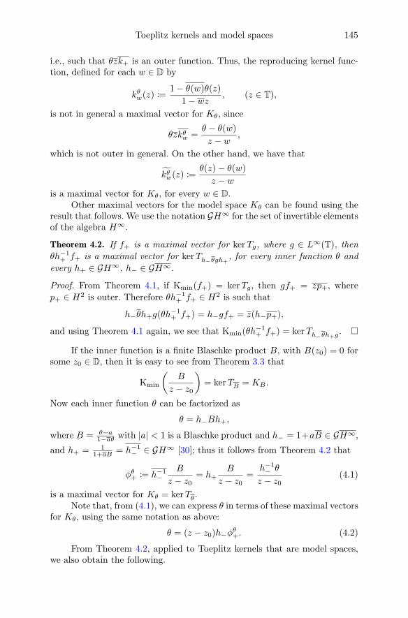
Toeplitz kernels and model spaces 145
i.e., such that θzk+ is an outer function. Thus, the reproducing kernel func-tion, defined for each w ∈ D by
kθw(z) :=1− θ(w)θ(z)
1− wz, (z ∈ T),
is not in general a maximal vector for Kθ, since
θzkθw =θ − θ(w)
z − w,
which is not outer in general. On the other hand, we have that
kθw(z) :=θ(z)− θ(w)
z − wis a maximal vector for Kθ, for every w ∈ D.
Other maximal vectors for the model space Kθ can be found using theresult that follows. We use the notation GH∞ for the set of invertible elementsof the algebra H∞.
Theorem 4.2. If f+ is a maximal vector for kerTg, where g ∈ L∞(T), then
θh−1+ f+ is a maximal vector for kerTh−θgh+
, for every inner function θ and
every h+ ∈ GH∞, h− ∈ GH∞.
Proof. From Theorem 4.1, if Kmin(f+) = kerTg, then gf+ = zp+, where
p+ ∈ H2 is outer. Therefore θh−1+ f+ ∈ H2 is such that
h−θh+g(θh−1+ f+) = h−gf+ = z(h−p+),
and using Theorem 4.1 again, we see that Kmin(θh−1+ f+) = kerTh−θh+g
.
If the inner function is a finite Blaschke product B, with B(z0) = 0 forsome z0 ∈ D, then it is easy to see from Theorem 3.3 that
Kmin
(B
z − z0
)= kerTB = KB .
Now each inner function θ can be factorized as
θ = h−Bh+,
where B = θ−a1−aθ with |a| < 1 is a Blaschke product and h− = 1+aB ∈ GH∞,
and h+ = 11+aB = h−1
− ∈ GH∞ [30]; thus it follows from Theorem 4.2 that
φθ+ := h−1−
B
z − z0= h+
B
z − z0=
h−1− θ
z − z0(4.1)
is a maximal vector for Kθ = kerTθ.Note that, from (4.1), we can express θ in terms of these maximal vectors
for Kθ, using the same notation as above:
θ = (z − z0)h−φθ+. (4.2)
From Theorem 4.2, applied to Toeplitz kernels that are model spaces,we also obtain the following.

146 M.C. Camara and J.R. Partington
Theorem 4.3 ([9]). Let θ and θ1 be inner functions. If k1+ is a maximal vectorfor Kθ1 , then θk1+ is a maximal vector for Kθθ1 = Kθ1 ⊕ θ1Kθ.
Thus if Kmin(k1+) is a model space Kθ1 , then Kmin(θk1+) is also a modelspace, Kθθ1 for all inner functions θ.
More generally, one can consider the minimal kernel containing a givenset of functions. In particular, when these functions are maximal vectors formodel spaces, we obtain the following generalization of the previous result.
Theorem 4.4 ([9]). Let k1+, k2+, . . . , kn+∈ H2 be maximal vectors for the
spaces Kθ1 ,Kθ2 , . . . ,Kθn , respectively, where every θj is an inner function,for j = 1, 2, . . . , n. Then there exists a minimal kernel containing the vectorskj+ : j = 1, 2, . . . , n, and for θ = LCM(θ1, θ2, . . . , θn) we have
K = Kθ = closH2(Kθ1 +Kθ2 + · · ·+Kθn) = Kθj ⊕ θjKθθj,
for each j = 1, 2, . . . , n.
5. On the relations between ker Tg and ker Tθg
Direct sum decompositions of the form Kθθ1 = Kθ1 ⊕ θ1Kθ can also beexpressed in terms of maximal functions, using (4.2) with θ replaced by θ1:
Kθθ1 = Kθ1 ⊕ (z − z0)h−φθ1+Kθ. (5.1)
For g = θθ1 the identity (5.1) is equivalent to
kerTg = kerTθg ⊕ (z − z0)h−φθg+ Kθ, (5.2)
where φθg+ is a maximal vector for kerTθg and h− = 1 if θ is a Blaschkeproduct with θ(z0) = 0. This relation can be extended for general g ∈ L∞(T)when θ is a finite Blaschke product, in terms of maximal functions and modelspaces.
Indeed for every g ∈ L∞(T) and every non-constant inner function θ,we have
kerTθg ( kerTg,
whenever kerTg 6= 0.If θ is not a finite Blaschke product and dim kerTg <∞, then actually
kerTθg = 0; while, if kerTg is infinite-dimensional, then kerTθg may or maynot be finite-dimensional, and in particular it can be 0— as it happens, forinstance, when g is an inner function dividing θ, or in the case of the followingexample.
Example ([8, 9]). For θ(z) = exp(z+1z−1
)and ψ(z) = exp
(z−1z+1
), we have
kerTzθψ = 0.
For finite Blaschke products θ we have the following.

Toeplitz kernels and model spaces 147
Theorem 5.1 ([9]). If g ∈ L∞(T) and θ is a finite Blaschke product, then
dim kerTg <∞ if and only if dim kerTθg <∞,
and kerTg is finite-dimensional if and only if there exists a k0 ∈ Z suchthat kerTzk0g = 0; in that case dim kerTg ≤ max0, k0. Moreover, ifdim kerTg <∞, we have
dim kerTθg = max0,dim kerTg − k, (5.3)
where k is the number of zeroes of θ counting their multiplicity.
Thus, in particular, if dim kerTg = d < ∞ and θ is a finite Blaschkeproduct such that dimKθ = k ≤ d, then
dim kerTθg = dim kerTg − k. (5.4)
Of course, when kerTg is infinite-dimensional and the same happens withkerTθg, it is not possible to relate their dimension as in (5.4). We can, how-ever, use maximal functions to present an alternative relation, analogous to(5.2), which not only generalizes Theorem 5.1 but moreover sheds new lighton the meaning of (5.3) when k < dim kerTg <∞.
Theorem 5.2 ([9]). Let g ∈ L∞(T) and let B be a finite Blaschke product ofdegree k. If dim kerTg ≤ k, then kerTBg = 0; if dim kerTg > k, then
kerTg = kerTBg ⊕ (z − z0)φ+KB ,
where z0 is a zero of B and φ+ is a maximal function for kerTBg.
6. Injective Toeplitz operators
Clearly, the existence of maximal functions and the results of the previoussection are closely connected with the question of injectivity of Toeplitz op-erators, which in turn is equivalent to the question whether the Riemann–Hilbert problem gf+ = f−, with f+ ∈ H2 and f− ∈ H2
0 , has a nontrivialsolution.
It is well known that various properties of a Toeplitz operator, and inparticular of its kernel, can be described in terms of an appropriate factor-ization of its symbol ([4, 13, 20, 26, 28]). For instance, the so-called L2-factorization is a representation of the symbol g ∈ L∞(T) as a product
g = g−dg−1+ , (6.1)
where g±1+ ∈ H2, g±1
− ∈ H2 and d(z) = zk for some k ∈ Z. If g is invertible
in L∞(T) and admits an L2-factorization, then dim kerTg = |k| if k ≤ 0,and dim kerT ∗g = k if k > 0. The factorization (6.1) is called a bounded
factorization when g±1+ , g±1
− ∈ H∞. In various subalgebras of L∞(T), everyinvertible element admits a factorization of the form (6.1), where the middlefactor d is an inner function. This is the case in the Wiener algebra on T andin the analogous algebra APW of almost-periodic functions on the real line R.

148 M.C. Camara and J.R. Partington
In the latter case d may be a singular inner function, d(ξ) = exp(−iλξ) withλ ∈ R, and we have that if g ∈ APW is invertible in L∞(R) then kerTg iseither trivial or isomorphic to an infinite-dimensional model space Kθ withθ(ξ) = exp(iλξ), depending on whether λ ≤ 0 or λ > 0. For more details see[8] and [3, Sec. 8.3].
For g1, g2 ∈ L∞(T), we say that g1 ∼ g2 if and only if there are functionsh+ ∈ GH∞, h− ∈ GH∞ such that g1 = h−g2h+, and in that case we havekerTg1 = h−1
+ kerTg2 (which we write as kerTg1 ∼ kerTg2). Thus if (6.1) is
a bounded factorization, we have g ∼ zk and kerTg = 0 if k ≥ 0, andkerTg ∼ Kz|k| if k < 0.
L2 factorizations are a particular case of factorizations of the form
g = g−θ−Ng−1
+ , g− ∈ H2, g+ ∈ H2, (6.2)
where θ is an inner function and N ∈ Z. We have the following.
Theorem 6.1 ([7, 8]). If g ∈ L∞(T) admits a factorization (6.2), where g−and g+ are outer functions in H2, with g2
+ rigid in H1, then
kerTg 6= 0 if and only if N > 0.
If N > 0 and θ is a finite Blaschke product of degree k, then dim kerTg = kN ;if θ is not a finite Blaschke product, then dim kerTg =∞.
We also have the following.
Theorem 6.2 ([7, 29]). For g ∈ L∞(T), kerTg is nontrivial of finite dimension
if and only if, for some N ∈ N, g admits a factorization g = g−z−Ng−1
+ , whereg− ∈ H2
0 is outer, and g+ ∈ H2 is outer with g2+ rigid in H1. In that case
kerTg = kerTz−Ng+/g+ , and dim kerTg = N .
Some other results regarding conditions for injectivity or non-injectivityof Toeplitz operators will be mentioned in the next section.
7. Multipliers between Toeplitz kernels
The existence of maximal vectors for every non-zero Toeplitz kernel alsoprovides test functions for various properties of these spaces.
In [11] Crofoot characterized the multipliers from a model space ontoanother. Partly motivated by that work, Fricain, Hartmann and Ross ad-dressed in [17] the question of which holomorphic functions w multiply amodel space Kθ into another model space Kφ. Their main result shows thatw multiplies Kθ into Kφ (written w ∈M(Kθ,Kφ)) if and only if
(i) w multiplies the function S∗θ = kθ0 into Kφ, and(ii) w multiplies Kθ into H2, which can be expressed by saying that |w|2 dm
is a Carleson measure for Kθ.
Model spaces being a particular type of Toeplitz kernel, that questionmay be posed more generally for the latter. We may also ask whether moregeneral test functions can be used, other than S∗θ.

Toeplitz kernels and model spaces 149
In this more general setting, one immediately notices that, unlike mul-tipliers between model spaces, multipliers between general Toeplitz kernelsneed not lie in H2. In fact, for model spaces, we must have w ∈ H2 if w ∈M(Kθ,Kφ), because we must then have wkθ0 ∈ Kφ ⊂ H2, and 1/kθ0 ∈ H∞;
but the function w(z) = (z− 1)−1/2 multiplies kerTg, with g(z) = z−3/2 andarg z ∈ [0, 2π) for z ∈ T, onto the model space Kz = kerTz consisting of theconstant functions, even though w 6∈ H2.
One can characterize all multipliers from one Toeplitz kernel into an-other as follows. We denote by C(kerTg) the class of all w such that |w|2 dm isa Carleson measure for kerTg, i.e., w kerTg ⊂ L2(T), and by N+ the Smirnovclass.
Theorem 7.1 ([8]). Let g, h ∈ L∞(T) \ 0 be such that kerTg and kerTh arenontrivial. Then the following are equivalent:
(i) w ∈M(kerTg, kerTh);(ii) w ∈ C(kerTg) and wk+ ∈ kerTh for some (and hence all) maximal
vectors k+ of kerTg;
(iii) w ∈ C(kerTg) and hg−1w ∈ N+.
Note that if k+ is not a maximal vector for kerTg, then k+ cannot beused as a test function; for example, the function w = 1 is not a multiplierfrom kerTg into Kmin(k+), even though wk+ ∈ Kmin(k+).
Corollary 7.2 ([8]). With the same assumptions as in Theorem 7.1, and as-suming moreover that hg−1 ∈ L∞(T), one has
w ∈M(kerTg, kerTh) if and only if w ∈ C(kerTg) ∩ kerTzgh−1 .
By considering the special case g = θ, where θ is inner, we obtain thefollowing result.
Corollary 7.3 ([8, 17]). Let θ be inner and let h ∈ L∞(T) \ 0 be such thatkerTh is nontrivial. Then the following are equivalent:
(i) w ∈M(Kθ, kerTh);(ii) w ∈ C(Kθ) and wS∗θ ∈ kerTh;
(iii) w ∈ C(Kθ) ∩ kerTzθh.
The last two corollaries also bring out a close connection between theexistence of non-zero multipliers in L2(T) and their description, on the onehand, and the question of injectivity of an associated Toeplitz operator andthe characterization of its kernel (discussed in Sections 5 and 6), on the otherhand. Thus, for instance, the result of Example 5 implies that, since Tzθψ is
injective in that case, we have M(Kθ,Kφ) = 0. Another example is thefollowing.
Example. Let θ, φ be two inner functions with φ θ, i.e., Kφ ⊂ Kθ. Then
dim kerTzθφ ≤ 1, as θφ ∈ H∞ and kerTθφ = 0 ([2]). We have kerTzθφ = Cif φ = aθ with a ∈ C, |a| = 1, and we have kerTzθφ = 0 if φ ≺ θ; therefore
M(Kθ,Kφ) 6= 0 if and only if Kθ = Kφ, in which case M(Kθ,Kφ) = C.
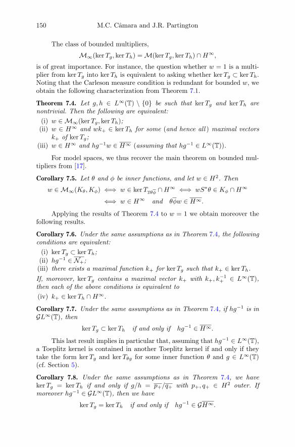
150 M.C. Camara and J.R. Partington
The class of bounded multipliers,
M∞(kerTg, kerTh) =M(kerTg, kerTh) ∩H∞,is of great importance. For instance, the question whether w = 1 is a multi-plier from kerTg into kerTh is equivalent to asking whether kerTg ⊂ kerTh.Noting that the Carleson measure condition is redundant for bounded w, weobtain the following characterization from Theorem 7.1.
Theorem 7.4. Let g, h ∈ L∞(T) \ 0 be such that kerTg and kerTh arenontrivial. Then the following are equivalent:
(i) w ∈M∞(kerTg, kerTh);(ii) w ∈ H∞ and wk+ ∈ kerTh for some (and hence all ) maximal vectors
k+ of kerTg;
(iii) w ∈ H∞ and hg−1w ∈ H∞ (assuming that hg−1 ∈ L∞(T)).
For model spaces, we thus recover the main theorem on bounded mul-tipliers from [17].
Corollary 7.5. Let θ and φ be inner functions, and let w ∈ H2. Then
w ∈M∞(Kθ,Kφ) ⇐⇒ w ∈ kerTzθφ ∩H∞ ⇐⇒ wS∗θ ∈ Kφ ∩H∞
⇐⇒ w ∈ H∞ and θφw ∈ H∞.
Applying the results of Theorem 7.4 to w = 1 we obtain moreover thefollowing results.
Corollary 7.6. Under the same assumptions as in Theorem 7.4, the followingconditions are equivalent:
(i) kerTg ⊂ kerTh;
(ii) hg−1 ∈ N+;(iii) there exists a maximal function k+ for kerTg such that k+ ∈ kerTh.
If, moreover, kerTg contains a maximal vector k+ with k+, k−1+ ∈ L∞(T),
then each of the above conditions is equivalent to
(iv) k+ ∈ kerTh ∩H∞.
Corollary 7.7. Under the same assumptions as in Theorem 7.4, if hg−1 is inGL∞(T), then
kerTg ⊂ kerTh if and only if hg−1 ∈ H∞.
This last result implies in particular that, assuming that hg−1 ∈ L∞(T),a Toeplitz kernel is contained in another Toeplitz kernel if and only if theytake the form kerTg and kerTθg for some inner function θ and g ∈ L∞(T)(cf. Section 5).
Corollary 7.8. Under the same assumptions as in Theorem 7.4, we havekerTg = kerTh if and only if g/h = p+/q+ with p+, q+ ∈ H2 outer. Ifmoreover hg−1 ∈ GL∞(T), then we have
kerTg = kerTh if and only if hg−1 ∈ GH∞.

Toeplitz kernels and model spaces 151
We can draw several interesting conclusions from these results:
1. First, we can characterize the Toeplitz kernels that are contained in agiven model space Kθ (kerTg = kerTθα, with α inner), and those that contain
Kθ (kerTg with g ∈ θH∞), assuming that the symbols are in GL∞(T).
2. Second, while (3.1) provides an expression for a (unimodular) symbolg such that kerTg is the minimal kernel for a given function with inner–outerfactorization φ+ = IO+, it is not claimed that all Toeplitz operators withthat kernel have the same symbol. Indeed, from Corollary 7.8, we have thatif kerTg = Kmin(φ+) with φ+ = IO+, then
g =p+
q+
IO+
O+with p+, q+ ∈ H2 outer;
if, moreover, g ∈ GL∞(T), then g = h−IO+/O+, with h− ∈ GH∞.
3. Clearly, a Toeplitz operator with unimodular symbol u is non-injectiveif and only if it has a maximal vector, i.e., there exist an inner function I andan outer function O+ ∈ H2 such that kerTu = Kmin(IO+) = kerTIO+/O+
,
which is equivalent, as shown in point 2, to having
u = zIO+
O+h−, with h− ∈ GH∞.
Since |h−| = 1 a.e. on T, we conclude that h− must be a unimodular constant,and therefore Tu is non-injective if and only if
u = zIO+/O+,
thus recovering a result by Makarov and Poltoratski [27, Lem. 3.2].
4. Since there are different maximal functions for each Toeplitz kernelwith dimension greater than 1, one may ask how they can be related. Again,from Corollary 7.8, we see that if Kmin(f1+) = Kmin(f2+), where f1+ = I1O1+
and f2+ = I2O2+ with I1, I2 inner and O1+, O2+ ∈ H2 outer, then
I1O1+
O1+=I2O2+
O2+h−,
where h− ∈ GH∞, |h−| = 1, and so h− is constant. Thus, finally f1+ andf2+ are related by
f2+ = f1+O2+
O1+
.
References
[1] S. Barclay, A solution to the Douglas-Rudin problem for matrix-valued func-tions, Proc. Lond. Math. Soc. (3) 99 (2009), no. 3, 757–786.
[2] C. Benhida, M.C. Camara, and C. Diogo, Some properties of the kernel andthe cokernel of Toeplitz operators with matrix symbols, Linear Algebra Appl.432 (2010), no. 1, 307–317.

152 M.C. Camara and J.R. Partington
[3] A. Bottcher, Y.I. Karlovich, and I.M. Spitkovsky, Convolution Operators andFactorization of Almost Periodic Matrix Functions, Operator Theory: Ad-vances and Applications 131, Birkhauser Verlag, Basel, 2002.
[4] A. Bottcher and B. Silbermann, Analysis of Toeplitz Operators, Springer-Verlag, Berlin, 1990.
[5] J. Bourgain, A problem of Douglas and Rudin on factorization, Pacific J. Math.121 (1986), no. 1, 47–50.
[6] M.C. Camara and J.R. Partington, Near invariance and kernels of Toeplitzoperators, J. Anal. Math. 124 (2014), 235–260.
[7] M.C. Camara and J.R. Partington, Finite-dimensional Toeplitz kernels andnearly-invariant subspaces, J. Operator Theory 75 (2016), no. 1, 75–90.
[8] M.C. Camara and J.R. Partington, Multipliers and equivalences betweenToeplitz kernels, https://arxiv.org/abs/1611.08429
[9] M.C. Camara, M.T. Malheiro, and J.R. Partington, Model spaces and Toeplitzkernels in reflexive Hardy space, Oper. Matrices 10 (2016), no. 1, 127–148.
[10] L.A. Coburn, Weyl’s theorem for nonnormal operators. Michigan Math. J. 13(1966), 285–288.
[11] R.B. Crofoot, Multipliers between invariant subspaces of the backward shift,Pacific J. Math. 166 (1994), no. 2, 225–246.
[12] L. de Branges and J. Rovnyak, Square Summable Power Series, Holt, Rinehartand Winston, New York–Toronto–London, 1966.
[13] R. Duduchava, Integral Equations in Convolution with Discontinuous Presym-bols. Singular Integral Equations with Fixed Singularities, and their Applica-tions to some Problems of Mechanics, Teubner-Texte zur Mathematik, Leipzig,1979.
[14] P.L. Duren, Theory of Hp Spaces, Dover, New York, 2000.
[15] K.M. Dyakonov, Kernels of Toeplitz operators via Bourgain’s factorizationtheorem. J. Funct. Anal. 170 (2000), no. 1, 93–106.
[16] I.A. Feldman and I.C. Gohberg, Wiener-Hopf integro-difference equations.Dokl. Akad. Nauk SSSR 183 (1968), 25–28. English translation: Soviet Math.Dokl. 9 (1968), 1312–1316.
[17] E. Fricain, A. Hartmann and W.T. Ross, Multipliers between model spaces,Studia Math., to appear. http://arxiv.org/abs/1605.07418.
[18] E. Fricain and J. Mashreghi, The Theory of H(b) Spaces, Vol. 1, New Mathe-matical Monographs 20, Cambridge University Press, Cambridge, 2016.
[19] S.R. Garcia, J. Mashreghi, and W.T. Ross, Introduction to Model Spaces andtheir Operators, Cambridge Studies in Advanced Mathematics 148, CambridgeUniversity Press, Cambridge, 2016.
[20] I. Gohberg and N. Krupnik, One-dimensional Linear Singular Integral Equa-tions, Vols. I and II, Birkhauser Verlag, Basel, 1992.
[21] A. Hartmann and M. Mitkovski, Kernels of Toeplitz operators, Recent progresson operator theory and approximation in spaces of analytic functions, 147–177,Contemp. Math. 679, Amer. Math. Soc., Providence, RI, 2016.
[22] E. Hayashi, The solution sets of extremal problems in H1, Proc. Amer. Math.Soc. 93 (1985), no. 4, 690–696.

Toeplitz kernels and model spaces 153
[23] E. Hayashi, The kernel of a Toeplitz operator, Integral Equations OperatorTheory 9 (1986), no. 4, 588–591.
[24] E. Hayashi, Classification of nearly invariant subspaces of the backward shift.Proc. Amer. Math. Soc. 110 (1990), no. 2, 441–448.
[25] D. Hitt, Invariant subspaces of H2 of an annulus, Pacific J. Math. 134 (1988),no. 1, 101–120.
[26] G.S. Litvinchuk and I.M. Spitkovsky, Factorization of Measurable Matrix Func-tions, Birkhauser Verlag, Basel and Boston, 1987.
[27] N. Makarov and A. Poltoratski, Meromorphic inner functions, Toeplitz kernelsand the uncertainty principle, Perspectives in analysis, 185–252, Math. Phys.Stud. 27, Springer, Berlin, 2005.
[28] S.G. Mikhlin and S. Prossdorf, Singular Integral Operators, Translated fromthe German by Albrecht Bottcher and Reinhard Lehmann, Springer-Verlag,Berlin, 1986.
[29] T. Nakazi, Kernels of Toeplitz operators, J. Math. Soc. Japan 38 (1986), no.4, 607–616.
[30] N.K. Nikolski, Operators, Functions, and Systems: an Easy Reading, Vol. 1,Hardy, Hankel, and Toeplitz, Translated from the French by Andreas Hart-mann, Mathematical Surveys and Monographs 92, American MathematicalSociety, Providence, RI, 2002.
[31] D. Sarason, Nearly invariant subspaces of the backward shift, Contributions tooperator theory and its applications (Mesa, AZ, 1987), 481–493, Oper. TheoryAdv. Appl. 35, Birkhauser, Basel, 1988.
[32] D. Sarason, Kernels of Toeplitz operators, Toeplitz operators and related topics(Santa Cruz, CA, 1992), 153–164, Oper. Theory Adv. Appl. 71, Birkhauser,Basel, 1994.
M. Cristina CamaraCenter for Mathematical AnalysisGeometry and Dynamical SystemsInstituto Superior Tecnico, Universidade de LisboaAv. Rovisco Pais, 1049-001 LisboaPortugal.e-mail: [email protected]
Jonathan R. PartingtonSchool of MathematicsUniversity of LeedsLeeds LS2 9JTU.K.e-mail: [email protected]

Frames, operator representations, andopen problems
Ole Christensen and Marzieh Hasannasab
Abstract. A frame in a Hilbert space H is a countable collection of el-ements in H that allows each f ∈ H to be expanded as an (infinite)linear combination of the frame elements. Frames generalize the well-known orthonormal bases, but provide much more flexibility and canoften be constructed with properties that are not possible for orthonor-mal bases. We will present the basic facts in frame theory with focus ontheir operator theoretical characterizations and discuss open problemsconcerning representations of frames in terms of iterations of a fixed op-erator. These problems come up in the context of dynamical sampling, atopic that has recently attracted considerably interest within harmonicanalysis. The goal of the paper is twofold, namely, that experts in oper-ator theory will explore the potential of frames, and that frame theorywill benefit from insight provided by the operator theory community.
Mathematics Subject Classification (2010). 42C15.
Keywords. Frames, dual frames, dynamical sampling, operator theory.
1. Introduction and motivation
A coherent state is a (typically overcomplete) system of vectors in a Hilbertspace H. In general it is given by the action of a class of linear operatorson a single element in the underlying Hilbert space. In particular, it couldbe given by iterated action of a fixed operator on a single element, i.e., asTnϕ∞n=0 for some ϕ ∈ H and a linear operator T : H → H. Coherent statesplay an important role in mathematical physics [20, 22], operator theory, andmodern applied harmonic analysis [14, 7]. In particular, a Gabor system (seethe definition below) is a coherent state.
Systems of vectors on the form Tnϕ∞n=0 also appear in the more recentcontext of dynamical sampling [1, 2, 3, 23]. Key questions in this context arewhether Tnϕ∞n=0 can form a basis or a frame when the operator T belongsto a certain class of operators, e.g., normal operators or self-adjoint operators.
© Springer International Publishing AG, part of Springer Nature 2018
Theory: Advances and Applications 268, https://doi.org/10.1007/978-3-319-75996-8_8
155A. Böttcher et al. (eds.), The Diversity and Beauty of Applied Operator Theory, Operator

156 O. Christensen and M. Hasannasab
We will postpone the formal definition of a frame to Section 2 and justmention that a frame is a collection of vectors in H that allows each f ∈ Hto be expanded as an (infinite) linear combination of the frame elements.Frames are getting increasingly popular in applied harmonic analysis andsignal processing, mainly due to the fact that they are much more flexible andeasier to construct with prescribed properties than the classical orthonormalbases.
A different approach was taken in the papers [9, 10, 12]: here, the start-ing point is a frame and the question is when and how it has a representationof the form
Tnϕ∞n=0 for some ϕ ∈ H and a bounded linear operator T : H → H. (1.1)
We will give a short survey of some of the most important results con-cerning frame representations of the form (1.1). As inspiration for the readerwe will also state a number of open problems.
The above questions will also be analyzed with a different indexing, i.e.,considering systems on the form Tnϕ∞n=−∞ instead of Tnϕ∞n=0. The in-dexing in terms of Z is natural for several well-known classes of frames, andthe theoretical conditions for a frame having such a representation with abounded operator T are similar to the ones for systems indexed by N0. Thechange in indexing gives an interesting twist on the problem. For example,a shift-invariant system (see Section 4 for the definition) always has a rep-resentation Tnϕ∞n=−∞ with a bounded operator T, but it does not have arepresentation with the indexing in (1.1). This observation indeed leads toone of the open problems, stated for the so-called Gabor frames in L2(R).
The paper is organized as follows. In Section 2 we will provide a veryshort survey on frame theory with focus on operator theoretical characteri-zations. Section 3 discusses representations of frames via iterated systems ofoperators acting on a single element in the underlying Hilbert space. Finally,in Section 4 we consider concrete classes of frames, namely, shift-invariantframes and Gabor frames, and discuss a number of open problems related tooperator representations.
2. Frame theory
Let H denote a separable Hilbert space. A sequence fk∞k=1 in H is a framefor H if there exist constants A,B > 0 such that
A ||f ||2 ≤∞∑k=1
|〈f, fk〉|2 ≤ B ||f ||2 ∀f ∈ H;
it is a frame sequence if the stated inequalities hold for all f ∈ spanfk∞k=1.The sequence fk∞k=1 is a Bessel sequence if at least the upper frame con-dition holds. Also, fk∞k=1 is called a Riesz sequence if there exist constantsA,B > 0 such that
A∑|ck|2 ≤
∣∣∣∣∣∣∑ ckfk
∣∣∣∣∣∣2 ≤ B∑ |ck|2

Frames, operator representations, and open problems 157
for all finite scalar sequences ck∞k=1. A Riesz basis is a Riesz sequencefk∞k=1 for which spanfk∞k=1 = H.
It is well-known that the above concepts have operator theoretical char-acterizations, see, e.g., [7].
Theorem 2.1. Consider a sequence fk∞k=1 in a separable Hilbert space H.Then the followings hold:
(i) fk∞k=1 is a Bessel sequence if and only if U : ck∞k=1 7→∑∞k=1 ckfk
is a well-defined mapping from `2(N) to H, i.e., the infinite series isconvergent for all ck∞k=1 ∈ `2(N); in the affirmative case the operatorU is linear and bounded.
(ii) fk∞k=1 is a frame if and only if the mapping ck∞k=1 7→∑∞k=1 ckfk is
well-defined from `2(N) to H and surjective.(iii) fk∞k=1 is a Riesz basis if and only if the mapping ck∞k=1 7→
∑∞k=1 ckfk
is well-defined from `2(N) to H and bijective.
Theorem 2.1 tells us that if fk∞k=1 is a Bessel sequence, then thesynthesis operator defined by
U : `2(N)→ H, Uck∞k=1 :=∞∑k=1
ckfk (2.1)
is well-defined and bounded. A central role will be played by the kernel ofthe operator U, i.e., the subset of `2(N) given by
NU =
ck∞k=1 ∈ `2(N)
∣∣∣∣ ∞∑k=1
ckfk = 0
. (2.2)
We will now state one more characterization of frames, in terms of a conditionthat is very similar to the Riesz basis condition, except that it only takes placeon sequences in the orthogonal complement of the kernel of the operator U .
Lemma 2.2. A sequence fk∞k=1 in H is a frame for H with bounds A,B ifand only if the following conditions are satisfied:
(i) fk∞k=1 is complete in H.(ii) The synthesis operator U is well defined on `2(N) and
A∞∑k=1
|ck|2 ≤ ||Uck∞k=1||2 ≤ B∞∑k=1
|ck|2 ∀ck∞k=1 ∈ N⊥U . (2.3)
The excess of a frame is the number of elements that can be removedyet leaving a frame. It is well-known that the excess equals dim(NU ); see [4].
Given a Bessel sequence fk∞k=1, the frame operator is defined by
S : H → H, Sf := UU∗f =∞∑k=1
〈f, fk〉fk.

158 O. Christensen and M. Hasannasab
For a frame fk∞k=1, the frame operator is bounded, bijective, and self-adjoint; these properties immediately lead to the important frame decom-position
f = SS−1f =∞∑k=1
〈f, S−1fk〉fk ∀f ∈ H. (2.4)
The sequence S−1fk∞k=1 is also a frame; it is called the canonical dual frame.
One of the most striking properties of frames is that they can be over-complete; the intuitive interpretation of this is that a frame might consistof more elements than necessary to span the Hilbert space. In practice,this means that if fk∞k=1 is a frame but not a basis, then there existsgk∞k=1 6= S−1fk∞k=1 such that
f =∞∑k=1
〈f, gk〉fk ∀f ∈ H. (2.5)
Any frame gk∞k=1 satisfying (2.5) for a given frame fk∞k=1 is called adual frame of fk∞k=1. Note that if fk∞k=1 and gk∞k=1 are Bessel sequenceswith synthesis operators U, V, respectively, then (2.5) means precisely that
UV ∗ = I.
We refer to [7] and [18] for more information about frames and Rieszbases.
3. Operator representations of frames
Formulated in purely mathematical terms, dynamical sampling in a Hilbertspace H deals with frame properties of sequences in H of the form Tnϕ∞n=0,where ϕ ∈ H and T : H → H is a linear operator. The purpose of this sectionis to give an introduction to the topic that allows to discuss a number ofimportant open problems as well.
Considering a class A of operators T : H → H, typical questions indynamical sampling are as follows:
• Can Tnϕ∞n=0 be a basis for H for some T ∈ A, ϕ ∈ H?• Can Tnϕ∞n=0 be a frame for H for some T ∈ A, ϕ ∈ H?
Unfortunately, the theory of dynamical sampling is full of no-go results. Letus state some of them here.
Theorem 3.1. Consider a bounded operator T : H → H, and let ϕ ∈ H. Thenthe followings hold:
(i) If T is normal, then Tnϕ∞n=0 can not be a basis [2];(ii) If T is unitary, then Tnϕ∞n=0 can not be a frame [3];(iii) If T is compact, then Tnϕ∞n=0 can not be a frame [12].

Frames, operator representations, and open problems 159
The first construction of a frame of the form Tnϕ∞n=0 was obtained in[1] and further discussed in [2, 3]. Since it deals with a class of diagonalizableoperators it is natural to formulate it for the Hilbert space `2(N), where theoperator T can be considered as a matrix.
Theorem 3.2. Consider a diagonal matrix T = [ajk]j,k∈N given by akk = λk,ajk = 0, j 6= k, and a sequence ϕ = ϕ(k)k∈N ∈ `2(N). Then the systemTnϕ∞n=0 is a frame for `2(N) if and only if
(i) |λk| < 1 for all k ∈ N;(ii) |λk| → 1 as k →∞;
(iii) The sequence λk∞k=1 satisfies the Carleson condition, i.e.,
infn
∏n6=k
|λk − λn||1− λkλn|
> 0; (3.1)
(iv) ϕ(k) = mk
√1− |λk|2 for a scalar-sequence mk∞k=1 that is bounded
below away from zero and above.
In the affirmative case Tnϕ∞n=0 is overcomplete, i.e., not a basis.
The fact that the Carleson condition comes in as the key conditionin Theorem 3.2 indicates that the result is based on deep results concerninginterpolation theory in spaces of analytic functions. Note that a self-containedproof (just based on a single result in [24] and standard frame theory) wasgiven later in [13].
The construction in Theorem 3.2 can be extended to diagonalizablematrices, but very little is known in the literature about how and when onecan construct frames for general matrices. Let us formulate this as an openproblem.
Problem 1. Identify a class of non-diagonalizable matrices T = [ajk]j,k∈N forwhich
(i) T is a bounded operator on `2(N);(ii) Tnϕ∞n=0 is a frame for `2(N) for some ϕ ∈ `2(N).
The class of frames that are known to be representable on the formTnϕ∞n=0 for a bounded operator T is indeed limited: except for the con-struction in Theorem 3.2, such a representation has only been obtained fornon-redundant frames, i.e., Riesz bases [9].
Note that the way the key questions in dynamical sampling are formu-lated in the introduction puts the operator in the central spot: we start withan operator and ask for frame properties of the associated iterated system.The opposite approach was taken in the papers [9, 10, 12], where we consid-ered a given frame fk∞k=1 and ask for the existence of a representation ofthe form
fk∞k=1 = Tnf1∞n=0, (3.2)
where T : spanfk∞k=1 → H is a bounded linear operator.

160 O. Christensen and M. Hasannasab
The following result collects a generalization of results from the papers[9, 10, 12]. Indeed, for reasons that will become clear in Section 4, we willgeneralize (3.2) and ask for representations of the form
fk∞k=1 = anTnf1∞n=0, (3.3)
for some scalars an 6= 0 with supn | anan+1| <∞ and a bounded linear operator
T : spanfk∞k=1 → H. We will see in the subsequent example that thetechnical condition on the scalars an is necessary. Define the weighted right-
shift operator on `2(N0) by
Tω : `2(N0)→ `2(N0), Tω(c0, c1, · · · ) =
(0,a0a1c0,
a1a2c1, · · ·
). (3.4)
Theorem 3.3. Consider a frame fk∞k=1 for an infinite-dimensional Hilbertspace H, and a sequence of non-zero scalars an∞n=0 with supn | anan+1
| <∞.
Then the followings hold:
(i) fk∞k=1 is linearly independent if and only if there exists a linear oper-ator T : spanfk∞k=1 → H such that (3.3) is satisfied.
(ii) Assume that fk∞k=1 is linearly independent. Then the operator T in(3.3) is bounded if and only if the kernel NU of the synthesis operatoris invariant under weighted right-shifts given as in (3.4); in particularT is bounded if fk∞k=1 is a Riesz basis.
(iii) Assume that fk∞k=1 is linearly independent and overcomplete. If theoperator T in (3.3) is bounded, then fk∞k=1 has infinite excess.
Proof. The proof of (i) is similar to the proof of the non-weighted case givenin [9]. In order to prove (ii), consider now the representation (3.3). Let uswrite the synthesis operator for the frame anTnf1∞n=0 as
U : `2(N0)→ H, Ucn∞n=0 =∞∑n=0
cnanTnf1.
Now, assume first that T is bounded and cn∞n=0 ∈ NU . Then
UTωcn∞n=0 =∞∑n=1
an−1an
cn−1anTnf1 =
∞∑n=0
cnanTn+1f1
= T
∞∑n=0
cnanTnf1 = 0.
Therefore Tωcn∞n=0 ∈ NU . Conversely, assume that NU is invariant underthe weighted right-shift operator. We want to prove that T is bounded. Con-sider an element f ∈ H that has a finite expansion in terms of the frame
anTnf1∞n=0, i.e., f =∑Nn=0 cnanT
nf1 for some N ∈ N, cn ∈ C. Lettingcn = 0 for n > N , we consider cn∞n=0 as a sequence in `2(N0). Choosedn∞n=0 ∈ NU and rn∞n=0 ∈ N⊥U such that cn∞n=0 = dn∞n=0 + rn∞n=0.
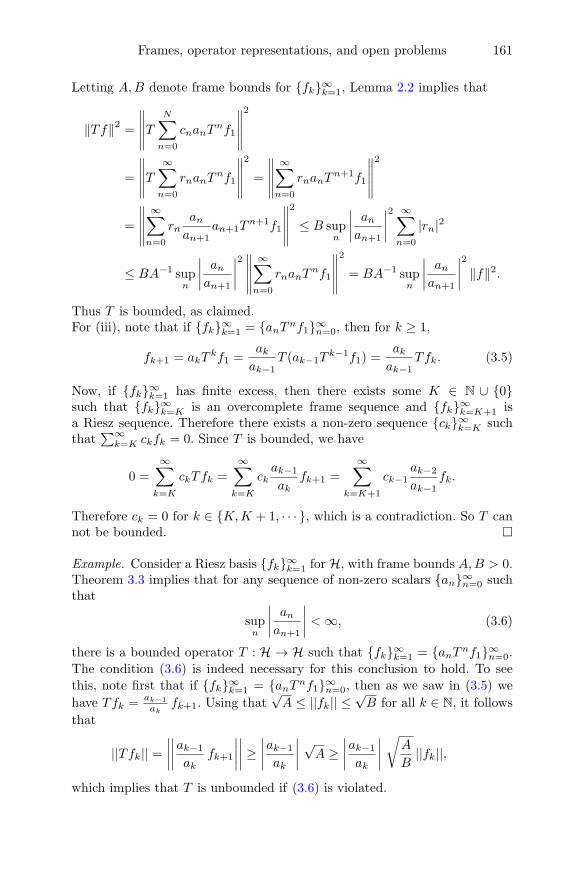
Frames, operator representations, and open problems 161
Letting A,B denote frame bounds for fk∞k=1, Lemma 2.2 implies that
‖Tf‖2 =
∥∥∥∥∥TN∑n=0
cnanTnf1
∥∥∥∥∥2
=
∥∥∥∥∥T∞∑n=0
rnanTnf1
∥∥∥∥∥2
=
∥∥∥∥∥∞∑n=0
rnanTn+1f1
∥∥∥∥∥2
=
∥∥∥∥∥∞∑n=0
rnanan+1
an+1Tn+1f1
∥∥∥∥∥2
≤ B supn
∣∣∣∣ anan+1
∣∣∣∣2 ∞∑n=0
|rn|2
≤ BA−1 supn
∣∣∣∣ anan+1
∣∣∣∣2∥∥∥∥∥∞∑n=0
rnanTnf1
∥∥∥∥∥2
= BA−1 supn
∣∣∣∣ anan+1
∣∣∣∣2 ‖f‖2.Thus T is bounded, as claimed.For (iii), note that if fk∞k=1 = anTnf1∞n=0, then for k ≥ 1,
fk+1 = akTkf1 =
akak−1
T (ak−1Tk−1f1) =
akak−1
Tfk. (3.5)
Now, if fk∞k=1 has finite excess, then there exists some K ∈ N ∪ 0such that fk∞k=K is an overcomplete frame sequence and fk∞k=K+1 isa Riesz sequence. Therefore there exists a non-zero sequence ck∞k=K suchthat
∑∞k=K ckfk = 0. Since T is bounded, we have
0 =∞∑k=K
ckTfk =∞∑k=K
ckak−1ak
fk+1 =∞∑
k=K+1
ck−1ak−2ak−1
fk.
Therefore ck = 0 for k ∈ K,K + 1, · · · , which is a contradiction. So T cannot be bounded.
Example. Consider a Riesz basis fk∞k=1 for H, with frame bounds A,B > 0.Theorem 3.3 implies that for any sequence of non-zero scalars an∞n=0 suchthat
supn
∣∣∣∣ anan+1
∣∣∣∣ <∞, (3.6)
there is a bounded operator T : H → H such that fk∞k=1 = anTnf1∞n=0.
The condition (3.6) is indeed necessary for this conclusion to hold. To seethis, note first that if fk∞k=1 = anTnf1∞n=0, then as we saw in (3.5) we
have Tfk = ak 1
akfk+1. Using that
√A ≤ ||fk|| ≤
√B for all k ∈ N, it follows
that
||Tfk|| =∣∣∣∣∣∣∣∣ak−1ak
fk+1
∣∣∣∣∣∣∣∣ ≥ ∣∣∣∣ak−1ak
∣∣∣∣ √A ≥ ∣∣∣∣ak−1ak
∣∣∣∣√A
B||fk||,
which implies that T is unbounded if (3.6) is violated.
−

162 O. Christensen and M. Hasannasab
Cyclic vectors and hypercyclic vectors
We would like to point out that the frame condition on an iterated systemTnϕ∞n=0 is indeed very different from the conditions that are typically con-sidered in operator theory for such systems. First, consider a linear operatorT : H → H and recall that a vector ϕ ∈ H is said to be cyclic with respect toT if spanTnϕ∞n=0 = H. By (2.4) this condition is satisfied if Tnϕ∞n=0 is aframe for H. However, the frame condition is significantly stronger than thecondition of ϕ being cyclic. In order to illustrate this, let ek∞k=1 denote anorthonormal basis for H and consider the family fk∞k=1 := ek + ek+1∞k=1.Define the operator T by Tek := ek+1; then T can be extended to a boundedlinear operator on H and fk∞k=1 = Tn(e1 + e2)∞n=0. It is known (seeExample 5.4.6 in [7]) that spanfk∞k=1 = H, which implies that the vectorϕ := e1 + e2 is cyclic with respect to the operator T ; however, the sameexample in [7] shows that Tn(e1 + e2)∞n=0 is not a frame.
Recall also that a vector ϕ ∈ H is hypercyclic with respect to the op-erator T if Tnϕ∞n=0 is dense in H. This condition is way too strong in thecontext of frames, as it implies that Tnϕ∞n=0 does not satisfy the Besselcondition.
4. Shift-invariant systems and Gabor frames
In this section we will consider some classes of explicitly given frames in theHilbert space L2(R) and open problems related to dynamical sampling. Forour purpose the central class of frames is the so-called Gabor frames, but itis natural also to consider shift-invariant systems. Both systems are definedin terms of certain classes of operators on L2(R).
For a ∈ R, define the translation operator
Ta : L2(R)→ L2(R), Taf(x) := f(x− a)
and the modulation operator
Ea : L2(R)→ L2(R), Eaf(x) := e2πiaxf(x).
The translation operators and the modulation operators are unitary. We de-fine the Fourier transform of f ∈ L1(R) by
f(γ) = Ff(γ) =
∫ ∞−∞
f(x)e−2πiγxdx
and extend it in the standard way to a unitary operator on L2(R).Given a function ϕ ∈ L2(R) and some b > 0, the associated shift-
invariant system is given by Tkbϕk∈Z. The frame properties of such systemsare well understood. The following proposition collects some of the mainresults. Given ϕ ∈ L2(R) and some b > 0, consider the function
Φ(γ) :=∑k∈Z
∣∣∣∣ϕ(γ + k
b
)∣∣∣∣2 , γ ∈ R. (4.1)

Frames, operator representations, and open problems 163
Proposition 4.1. Let ϕ ∈ L2(R)\0 and b > 0 be given. Then the followingshold:
(i) Tkbϕk∈Z is linearly independent.(ii) Tkbϕk∈Z is a Riesz basis if and only if there exist A,B > 0 such that
A ≤ Φ(γ) ≤ B for almost all γ ∈ [0, 1].(iii) Tkbϕk∈Z is a frame sequence if and only if there exist A,B > 0 such
that A ≤ Φ(γ) ≤ B for almost all γ ∈ [0, 1] \ γ ∈ [0, 1]∣∣ Φ(γ) = 0.
(iv) Tkbϕk∈Z can at most be a frame for a proper subspace of L2(R).(v) If Tkbϕk∈Z is an overcomplete frame sequence, it has infinite excess.(vi) Tkbϕk∈Z = (Tb)kϕk∈Z, i.e., the system Tkbϕk∈Z has the form of
an iterated system indexed by Z.
The result in (i) is well-known, and (ii) & (iii) are proved in [5]; (iv) isproved in [8], (v) is proved in [4, 10], and (vi) is clear.
Note that the representation of a shift-invariant system as an iteratedsystem in Proposition 4.1 (v) differs from the ones appearing in Section 3 interms of the index set Z. It was recently shown in [11] that even though ashift-invariant frame Tkbϕk∈Z can be re-indexed and be represented in theform (1.1) for a linear operator T : spanTkbϕk∈Z → L2(R), the operator Tcan only be bounded if Tkbϕk∈Z is a basis.
Let us now introduce the Gabor systems. Given some a, b > 0 and afunction g ∈ L2(R), the associated Gabor system is the collection of functionsgiven by
EmbTnagm,n∈Z =e2πimbxg(x− na)
m,n∈Z.
Gabor systems play an important role in time-frequency analysis; we will juststate the properties that are necessary for the flow of the current paper, andrefer to [17, 15, 16, 7] for much more information.
Proposition 4.2. Let g ∈ L2(R) \ 0. Then the followings hold:
(i) EmbTnagm,n∈Z is linearly independent.(ii) If EmbTnagm,n∈Z is a frame for L2(R), then ab ≤ 1.
(iii) If EmbTnagm,n∈Z is a frame for L2(R), then EmbTnagm,n∈Z is aRiesz basis if and only if ab = 1.
(iv) If EmbTnagm,n∈Z is an overcomplete frame for L2(R), then it hasinfinite excess.
The result in (i) was proved in [21] (hereby confirming a conjecturestated in [19]); (ii) & (iii) are classical results [17, 7], and (iv) is proved in [4].
Note that since a Gabor frame EmbTnagm,n∈Z is linearly independentby Proposition 4.2 (i), Proposition 3.3 shows that any reordering fk∞k=1
can be represented on the form Tnϕ∞n=0 for T : L2(R) → L2(R) somelinear operator and some ϕ ∈ L2(R). However, it was recently shown in[11] that the operator T always is unbounded, except in the case wherethe Gabor frame is a Riesz basis, i.e., if ab = 1. This is indeed the rea-son that we considered the more general representations (3.3) in Section 3:

164 O. Christensen and M. Hasannasab
the hope is that the possibility of choosing appropriate coefficients an allowsto find a bounded operator T. Let us formulate the key question as an openproblem.
Problem 2. Do there exist overcomplete Gabor frames EmbTnagm,n∈Z suchthat an appropriate ordering fk∞k=1 of the frame elements has a represen-tation
fk∞k=1 = anTnϕ∞n=0, (4.2)
for some scalars an 6= 0, a bounded operator T : L2(R) → L2(R), and someϕ ∈ L2(R)?
Note that if the Gabor frame EmbTnagm,n∈Z is generated by a func-tion g for which ||g|| = 1 and we assume that an > 0 for all n ∈ N0, therepresentation (4.2) implies that an = ||Tnϕ||−1, and thus the representationtakes the form
fk∞k=1 =
Tnϕ
||Tnϕ||
∞n=0
. (4.3)
For shift-invariant frames Tkbϕk∈Z, we just saw that they are indeed“born” having the structure of an iterated system, indexed by Z. Thus, it isnatural to ask whether such a representation is possible for Gabor frames aswell. Let us formulate this as the final problem.
Problem 3. Do there exist overcomplete Gabor frames EmbTnagm,n∈Z suchthat an appropriate ordering fk∞k=−∞ of the frame elements has a repre-sentation
fk∞k=−∞ = Tnϕ∞n=−∞,for some bounded operator T : L2(R)→ L2(R) and some ϕ ∈ L2(R)?
Acknowledgment. The authors would like to thank Albrecht Bottcher formany useful comments to the manuscript.
References
[1] A. Aldroubi, C. Cabrelli, U. Molter, and S. Tang, Dynamical sampling, Appl.Harm. Anal. Appl. 42 (2017), no. 3, 378–401.
[2] A. Aldroubi, C. Cabrelli, A.F. Cakmak, U. Molter, and A. Petrosyan, Iterativeactions of normal operators, J. Funct. Anal. 272 (2017), no. 3, 1121–1146.
[3] A. Aldroubi, and A. Petrosyan, Dynamical sampling and systems from iterativeactions of operators, in: Frames and Other Bases in Abstract and FunctionSpaces, eds. H. Mhaskar, I. Pesenson, D.X. Zhou, Q.T. Le Gia, and A. Mayeli,Birkhauser, Boston, 2017.
[4] R. Balan, P. Casazza, C. Heil, and Z. Landau, Deficits and excesses of frames,Adv. Comp. Math. 18 (2002), 93–116.
[5] J. Benedetto and S. Li, The theory of multiresolution analysis frames andapplications to filter banks, Appl. Comp. Harm. Anal. 5 (1998), 389–427.

Frames, operator representations, and open problems 165
[6] C. Cabrelli, U. Molter, V. Paternostro, and F. Philipp, Dynamical samplingon finite index sets, Preprint, 2017.
[7] O. Christensen, An introduction to frames and Riesz bases, 2nd expanded ed.,Birkhauser, Boston, 2016.
[8] O. Christensen, B. Deng, and C. Heil, Density of Gabor frames, Appl. Comp.Harm. Anal. 7 (1999), 292–304.
[9] O. Christensen, and M. Hasannasab, Frame properties of systems arising viaiterative actions of operators, To appear in Appl. Comp. Harm. Anal..
[10] O. Christensen, and M. Hasannasab, Operator representations of frames:boundedness, duality, and stability, Integral Equations and Operator Theory88 (2017), no. 4, 483–499.
[11] O. Christensen, M. Hasannasab, and F. Philipp, Frame properties of operatororbits, Submitted, 2018.
[12] O. Christensen, M. Hasannasab, and E. Rashidi, Dynamical sampling andframe representations with bounded operators, Preprint, 2017.
[13] O. Christensen, M. Hasannasab, and D.T. Stoeva, Operator representations ofsequences and dynamical sampling, Preprint, 2017.
[14] I. Daubechies, The wavelet transformation, time-frequency localization andsignal analysis, IEEE Trans. Inform. Theory 36 (1990), 961–1005.
[15] H.G. Feichtinger and T. Strohmer (eds.), Gabor Analysis and Algorithms: The-ory and Applications, Birkhauser, Boston, 1998.
[16] H.G. Feichtinger and T. Strohmer (eds.), Advances in Gabor Analysis,Birkhauser, Boston, 2002.
[17] K. Grochenig, Foundations of time-frequency analysis, Birkhauser, Boston,2000.
[18] C. Heil, A basis theory primer, Expanded ed., Applied and Numerical HarmonicAnalysis, Birkhauser, New York, 2011.
[19] C. Heil, J. Ramanathan, and P. Topiwala, Linear independence of time-frequency translates, Proc. Amer. Math. Soc. 124 (1996), 2787–2795.
[20] J. Klauder and B. Skagerstam, Coherent states. Applications in physics andmathematical physics, World Scientific, Singapore, 1985.
[21] P. Linnell, Von Neumann algebras and linear independence of translates, Proc.Amer. Math. Soc. 127 (1999), no. 11, 3269–3277.
[22] A. Perelomov, Generalized coherent states and their applications, Springer, NewYork, 2012.
[23] F. Philipp, Bessel orbits of normal operators, J. Math. Anal. Appl. 448 (2017),767–785.
[24] H.S. Shapiro and A.L. Shields, On some interpolation problems for analyticfunctions, American Journal of Mathematics 83 (1961), no. 3, 513–532.
Ole Christensen and Marzieh HasannasabTechnical University of DenmarkDTU Compute, Building 303, 2800 LyngbyDenmarke-mail: [email protected]

A survey on solvable sesquilinear forms
Rosario Corso
Abstract. The aim of this paper is to present a unified theory of manyKato type representation theorems in terms of solvable forms on aHilbert space (H, 〈·, ·〉). In particular, for some sesquilinear forms Ω ona dense domain D ⊆ H one looks for a representation Ω(ξ, η) = 〈Tξ, η〉(ξ ∈ D(T ), η ∈ D), where T is a densely defined closed operator withdomain D(T ) ⊆ D. There are two characteristic aspects of a solvableform on H. One is that the domain of the form can be turned into areflexive Banach space that need not be a Hilbert space. The secondone is that representation theorems hold after perturbing the form by abounded form that is not necessarily a multiple of the inner product ofH.
Mathematics Subject Classification (2010). Primary 47A07; Secondary47A10, 47A12.
Keywords. Kato’s representation theorems, q-closed and solvable sesqui-linear forms.
1. Introduction
Let H be a Hilbert space with inner product 〈·, ·〉. Bounded linear operatorsand bounded sesquilinear forms are related by the formula
Ω(ξ, η) = 〈Tξ, η〉 ∀ξ, η ∈ H,
which holds for every bounded sesquilinear form Ω and for some boundedlinear operator T by Riesz’s classical representation theorem. The situationin the unbounded case is more complicated. One of the earliest results onthis topic is formulated by Kato in [8].
Kato’s first representation theorem. Let Ω be a densely defined closed secto-rial form with domain D ⊆ H. Then there exists a unique m-sectorial operatorT , with domain D(T ) ⊆ D, such that
Ω(ξ, η) = 〈Tξ, η〉 ∀ξ ∈ D(T ), η ∈ D. (1.1)
© Springer International Publishing AG, part of Springer Nature 2018
Theory: Advances and Applications 268, https://doi.org/10.1007/978-3-319-75996-8_9
167A. Böttcher et al. (eds.), The Diversity and Beauty of Applied Operator Theory, Operator

168 R. Corso
Here there are some differences compared to the bounded case. For ex-ample, representation (1.1) does not necessarily hold on the whole D becausein general D(T ) is smaller than D. However, D(T ) is not a ‘small’ subspacesince it is dense in H. It is worth mentioning that a representation like (1.1)can be given for any sesquilinear form Ω considering the operator defined by
D(T ) = ξ ∈ D : ∃χ ∈ H, Ω(ξ, η) = 〈χ, η〉 ∀η ∈ D (1.2)
and Tξ = χ for all ξ ∈ D(T ) and χ as in (1.2). Note that this T , the operatorassociated to Ω, is the maximal operator that satisfies (1.1). However, usuallyone is looking for operators T satisfying some additional requirements, suchas closedness or properties of the resolvent set, like in Kato’s theorem.
A bijection between densely defined closed sectorial forms and theirassociated operators (i.e. m-sectorial operators) is valid. But this bijection isnot preserved when we consider a larger class of sesquilinear forms. Indeed,there exist many sesquilinear forms with the same associated operator (seeProposition 4.2 of [6]). Although in the unbounded case the representationon the whole domain and the correspondence between forms and operatorsare lost, we have the following strong result (see [8]).
Kato’s second representation theorem. Let Ω be a densely defined closed non-negative sesquilinear form with domain D and let T be its positive self-adjointassociated operator. Then D = D(T
12 ) and
Ω(ξ, η) = 〈T 12 ξ, T
12 η〉 ∀ξ, η ∈ D. (1.3)
We stress that in (1.3) the representation is well-defined in D, whichis also the domain of a positive self-adjoint operator. Nevertheless, this lasttheorem does not have direct generalizations without the condition of posi-tivity. Indeed, Example 2.11, Proposition 4.2 of [6], and Example 5.4 of [4]show sesquilinear forms that satisfy the first type of representation but notthe second.
Kato’s theorems lead to several applications. These include, for instance,a way to define the Friedrichs extension of densely defined sectorial operators[8, Ch. VI.2.3], a proof of von Neumann’s theorem about the operator T ∗Twhen T is densely defined and closed [8, Example VI.2.13], and a way toprove that some operators are m-sectorial or self-adjoint (see [8, Ch. VI] andalso [5] for some generalizations). There are cases in which it is simpler tohandle forms rather than operators. Indeed, the sum of two operators mightbe defined in a small subspace, but with closed forms one can define a specialsum that has a dense domain (see [13] for the concrete example of the so-calledform sum of the operators Af = −f ′′ and δf = f(0) with f ∈ C∞0 (R)).
Recently, the first representation theorem has been generalized to thecontext of q-closed and solvable forms in [1] and, successively, in [2] (seeTheorem 2.3 below). The second one has been extended to solvable formsin [3] (see Theorem 2.5 below). Solvable forms constitute a unified theory ofmany representation theorems (for example [4, 6, 9, 10, 11, 14, 15]).
The new aspects of solvable forms, compared to the ones in the worksmentioned above, are the following (see Definitions 2.1 and 2.2). First, the

A survey on solvable sesquilinear forms 169
structure of a reflexive Banach space on the domain of the form need not bethe structure of a Hilbert space. Secondly, representation theorems hold forperturbations of the form by a bounded form instead by a multiple of the innerproduct of the Hilbert space. These conditions are stressed in Example 7.3of [2] and Example 2.9 in Section 2, respectively.
This paper is organized as follows. In Section 2 we give the definition ofsolvable forms and their representation theorems. We show in Section 3 someproperties of these forms in terms of the numerical range. Section 4 providesan exposition of particular cases of solvable forms known in the literature. Inthe final section we discuss another representation, the Radon–Nikodym-likerepresentation.
2. The representation theorems
Throughout this paper we will use the following notations. H is a Hilbertspace with inner product 〈·, ·〉 and norm ‖ · ‖, D is a dense subspace of H,D(T ), R(T ), and ρ(T ) are the domain, range, and resolvent set of an operatorT on H, respectively, B(H) is the set of bounded linear operators definedeverywhere onH, <B and =B are the real and imaginary parts of an operatorB ∈ B(H), respectively,
nT := 〈Tξ, ξ〉 : ξ ∈ D(T ), ‖ξ‖ = 1
is the numerical range of T , and lp with p > 1 is the classic Banach spacewith the usual norm.
We will consider sesquilinear forms defined on D, i.e., maps D×D → Cwhich are linear in the first component and anti-linear in the second one. IfΩ is a sesquilinear form defined on D, then the adjoint form Ω∗ of Ω is givenby Ω∗(ξ, η) = Ω(η, ξ) for ξ, η ∈ D. The real and imaginary parts <Ω and=Ω are <Ω = 1
2 (Ω + Ω∗) and =Ω = 12i (Ω− Ω∗), respectively. The numerical
range of Ω is
nΩ := Ω(ξ, ξ) : ξ ∈ D, ‖ξ‖ = 1.Ω is said to be symmetric if Ω = Ω∗ (i.e., nΩ ⊆ R) and, in particular,Ω is non-negative if nΩ ⊆ [0,+∞). We will denote by ι the sesquilinearform ι(ξ, η) = 〈ξ, η〉 (ξ, η ∈ H) and by ϑ the null form on H. The followingdefinition of q-closed forms is taken from [2, Proposition 3.2].
Definition 2.1. A sesquilinear form Ω on D is called q-closed with respect toa norm on D which is denoted by ‖ · ‖Ω if
1. EΩ := D[‖ · ‖Ω] is a reflexive Banach space;2. the embedding EΩ → H is continuous;3. there exists a β ≥ 0 such that |Ω(ξ, η)| ≤ β‖ξ‖Ω‖η‖Ω for all ξ, η ∈ D;
i.e., Ω is bounded on EΩ.
If EΩ is a Hilbert space, then Ω is called q-closed with respect to the innerproduct of EΩ.

170 R. Corso
Let Ω be a q-closed sesquilinear form on D w.r.t. ‖ · ‖Ω. We denote byE×Ω the conjugate dual space of EΩ := D[‖ · ‖Ω] and by 〈Λ, ξ〉 the action of the
conjugate linear functional Λ ∈ E×Ω on an element ξ ∈ D. The reason why we
use the symbol 〈·, ·〉 also here is that H is continuously embedded into E×Ωand the action of elements of E×Ω is an extension of the inner product of H(see [2, Sect. 4]). Let P(Ω) be the set of bounded sesquilinear forms Υ on Hsuch that
1. if (Ω + Υ)(ξ, η) = 0 for all η ∈ D, then ξ = 0;2. for all Λ ∈ E×Ω there exists a ξ ∈ D such that 〈Λ, η〉 = (Ω + Υ)(ξ, η) for
all η ∈ D.
Definition 2.2. If the set P(Ω) is not empty, then Ω is said to be solvablew.r.t. ‖ · ‖Ω (if moreover ‖ · ‖Ω is a Hilbert norm, then Ω is also said to besolvable w.r.t. the inner product induced by ‖ · ‖Ω).
Solvable forms are q-closed forms characterized by the existence of abounded sesquilinear form Υ onH such that the operatorXΥ : EΩ → E×Ω is bi-jective, where 〈XΥξ, η〉 = Ω(ξ, η)+Υ(ξ, η) for all η ∈ EΩ (see [1, Lemma 5.6]).Therefore, the set P(Ω) denotes perturbations of Ω with bounded forms whichinduce a bijection of EΩ onto E×Ω . Equivalent characterizations of solvableforms are provided by [2, Lemma 5.1].
The next theorem generalizes Kato’s first representation theorem tosolvable forms (for a proof see [2, Theorem 4.6] and also [3, Theorem 2.7]).
Theorem 2.3. Let Ω be a solvable sesquilinear form on D w.r.t. a norm ‖·‖Ω.Then there exists a closed operator T , with dense domain D(T ) ⊆ D in H,such that the following statements hold.
1. Ω(ξ, η) = 〈Tξ, η〉 for all ξ ∈ D(T ), η ∈ D.2. D(T ) is dense in D[‖ · ‖Ω].3. A bounded form Υ(·, ·) = 〈B·, ·〉 belongs to P(Ω) if and only if 0 is inρ(T +B). In particular, if Υ = −λι, with λ ∈ C, then Υ ∈ P(Ω) if andonly if λ ∈ ρ(T ).
The operator T is uniquely determined by the following condition. Let ξ, χ bein H. Then ξ ∈ D(T ) and Tξ = χ if and only if ξ ∈ D and Ω(ξ, η) = 〈χ, η〉for all η belonging to a dense subset of D[‖ · ‖Ω].
Kato’s second theorem is generalized in Theorem 2.5 below for thespecial class of hyper-solvable forms defined in the following way (see [3,Lemma 4.14, Theorem 4.17]).
Definition 2.4. A solvable sesquilinear form on D with associated operator Tis said to be hyper-solvable if D = D(|T | 12 ).
Theorem 2.5. Let Ω be a hyper-solvable sesquilinear form on D w.r.t. a norm‖ · ‖Ω and with associated operator T . Then D = D(|T ∗| 12 ) and
Ω(ξ, η) = 〈U |T | 12 ξ, |T ∗| 12 η〉 ∀ξ, η ∈ D,
Ω(ξ, η) = 〈|T ∗| 12Uξ, |T ∗| 12 η〉 ∀ξ, η ∈ D,

A survey on solvable sesquilinear forms 171
where T = U |T | = |T ∗|U is the polar decomposition of T , and ‖ · ‖Ω is
equivalent to the graph norms of |T | 12 and of |T ∗| 12 .
Remark 2.6. According to Theorem 2.3 and since the resolvent set of a closedoperator is open we obtain the following property: if Ω is a solvable sesquilin-ear form and Υ ∈ P(Ω), then there exists a δ > 0 such that (Υ+µι) ∈ P(Ω),for all |µ| < δ.
We mention some other features of a q-closed and solvable form Ω w.r.t. ‖·‖Ω:
• the same property of being q-closed or solvable holds for the adjointΩ∗ ([2, Theorem 4.11]) (this implies also that <Ω and =Ω are q-closedforms);• the operators associated to Ω and to Ω∗ are the adjoints of each other
([2, Theorem 4.11]);• the peculiarity of symmetric solvable forms to have self-adjoint associ-
ated operators ([2, Corollary 4.14]);• all norms w.r.t. which Ω is q-closed or solvable are equivalent to ‖ · ‖Ω
([2, Theorems 3.8 and 4.4]);• different hyper-solvable forms have different associated operators ([3,
Theorem 5.3]).
Remark 2.7. Let Ω1,Ω2 be two q-closed sesquilinear forms on D w.r.t. ‖ · ‖1and ‖ · ‖2, respectively, and let c ∈ C. Then the two norms are equivalent by[2, Theorem 2.5] and the sesquilinear forms cΩ1,Ω
∗1,<Ω1,=Ω1,Ω1 + Ω2 are
q-closed w.r.t. both ‖ · ‖1 and ‖ · ‖2.
We conclude this section by presenting some examples of solvable forms(cf. [2, Example 4.16] and [3, Example 4.5]).
Example 2.8. Let α := αn be a sequence of complex numbers and
Ωα(ξn, ηn) =∞∑n=1
αnξnηn
with domain D = ξn ∈ l2 :∑∞n=1 |αn||ξn|2 <∞. The form Ωα is hyper-
solvable w.r.t. the norm given by
‖ξn‖Ωα=
( ∞∑n=1
|ξn|2 +∞∑n=1
|αn||ξn|2) 1
2
.
Moreover,
1. if αn : n ∈ N 6= C, then −λι ∈ P(Ωα) for all λ /∈ αn : n ∈ N;2. if in the general case1 we define the sequence β = βn by βn = −αn+1
for |αn| ≤ 1 and βn = 0 for |αn| > 1, then the form Ωβ is bounded and
0 /∈ αn + βn : n ∈ N, and, by the previous case, Ωα + Ωβ is solvable,
and Ωβ ∈ P(Ωα).
1The case αn : n ∈ N = C is not considered in [1, 2].

172 R. Corso
The operator associated to Ωα is the operator Mα of multiplication by αwith domain
D(Mα) =
ξn ∈ l2 :
∞∑n=1
|αn|2|ξn|2 <∞
,
which is given by Mαξn = αnξn for ξn ∈ D(Mα).
The next is a new example of a solvable sesquilinear form.
Example 2.9. Let 1 < p < 2 and q be such that 1p + 1
q = 1. For convenience
we denote by ξ = ξn the generic element of the space lr with r > 1. Letmoreover D = lp ⊕ lq, which is a reflexive Banach space if it is endowed withthe norm ‖(ξ, η)‖D = ‖ξ‖p + ‖η‖q (as usual, ‖ · ‖p and ‖ · ‖q are the classical
norms on lp and lq, respectively). The Banach space D[‖ ·‖D] will be denoted
by E . Observe that E is isomorphic to its conjugate dual space E×. Indeed,we have the isomorphism (we identify E× with lq ⊕ lp)
X : E → E×
(ξ, η) 7→ (η, ξ).
The action of X is given by
〈X(ξ, η), (ξ′, η′)〉 =∞∑n=1
(ηnξ′n + ξnη′n) (2.1)
for all (ξ, η), (ξ′, η′) ∈ E . Now we define a sesquilinear form Ω on D exactlyby (2.1); i.e., for (ξ, η), (ξ′, η′) ∈ E ,
Ω((ξ, η), (ξ′, η′)) :=∞∑n=1
(ηnξ′n + ξnη′n).
Then Ω is bounded on E . Indeed, an easy computation shows that∣∣∣Ω((ξ, η), (ξ′, η′))∣∣∣ ≤ ∣∣∣∣∣
∞∑n=1
ηnξ′n
∣∣∣∣∣+
∣∣∣∣∣∞∑n=1
ξnη′n
∣∣∣∣∣≤ ‖ξ′‖p‖η‖q + ‖ξ‖p‖η′‖q ≤ ‖(ξ, η)‖D‖(ξ′, η′)‖D.
Our goal is to show that Ω is solvable w.r.t. ‖ · ‖E . The first thing we need isa Hilbert space in which E can be continuously embedded with dense range.To this end, we list the following observations:
• lp is continuously embedded in the Hilbert space H1 := l2 with denserange.• An inner product on lq can be given by
[η, η′] =
∞∑n=1
2−nηnη′n, η, η′ ∈ lq.
This is well defined since
|[η, η′]| ≤∞∑n=1
2−n|ηn||η′n| ≤∞∑m=1
2−m‖η‖q‖η′‖q = ‖η‖q‖η′‖q. (2.2)

A survey on solvable sesquilinear forms 173
Let (H2, [·, ·]) be the completion of the pre-Hilbert space (lq, [·, ·]). More-over, by (2.2) we obtain [η, η]
12 ≤ ‖η‖q for every η ∈ lq. Hence, lq is
continuously embedded into H2, and of course the range is dense.• E is continuously embedded into H := H1 ⊕H2 and the range is dense.
These observations prove that Ω is q-closed w.r.t. ‖ · ‖D. Moreover, by [1,Lemma 5.6] Ω is solvable w.r.t. ‖ · ‖D (in fact the operator Xϑ coincides withX, which is bijective).
However, Ω is not solvable w.r.t. any inner product. Indeed, presumingthe contrary, D would be a Hilbert space with the same topology as that of Eby [2, Theorem 3.8]. The subspace lp ⊕ 0 is closed in E , therefore lp wouldbe a Hilbert space with the same topology as the one induced by ‖ · ‖p. Butwe know that lp is not isomorphic to a Hilbert space (for example, it is aconsequence of [12]).
Moreover, this form is not hyper-solvable by [3, Corollary 4.4].
3. Numerical range
The purpose of this short section is to show that the numerical range of aq-closed form plays a special role for the property of being solvable.
Lemma 3.1.2 Let Ω be a solvable sesquilinear form and let nΩ 6= C be itsnumerical range. Assume that m is a connected component of nΩ
c, the com-plementary set of the closure of nΩ. Then the following statements are equiv-alent:
1. −λι ∈ P(Ω) for some λ ∈ m;2. −µι ∈ P(Ω) for all µ ∈ m.
Proof. This is an immediate consequence of statement 3 of Theorem 2.3 andof the fact that the defect numbers of the associated operator are constanton m (see [8, Theorem V.3.2]).
Let Ω be a q-closed sesquilinear form on D w.r.t. a norm ‖ · ‖Ω withnumerical range nΩ 6= C. Let Υ be a bounded form such that nΩ ∩ n−Υ = ∅,where n−Υ is the numerical range of −Υ (we may in particular take Υ = −λιwith λ /∈ nΩ). Theorem 5.2 of [2] gives an equivalent condition for Υ to be inP(Ω), and Theorem 5.4 of [2] contains a sufficient condition. By statement 2of Corollary 5.3 of [2], Υ ∈ P(Ω) if and only if the map
ξ 7→ sup‖η‖Ω=1
|(Ω + Υ)(ξ, η)|
defines a norm on D that is equivalent to ‖ · ‖Ω.We also mention that the numerical range of the operator associated to
a solvable sesquilinear form is a dense subset of the numerical range of theform ([2, Proposition 4.13]).
2A particular case of this result for symmetric forms is [3, Corollary 2.8].

174 R. Corso
4. Special cases
Many representation theorems in the literature for sesquilinear forms areparticular cases of Theorem 2.3. The following list witnesses this assertion.
Lemma 4.1. Let Ω be a sesquilinear form on D.
1. Ω satisfies [4, Theorem 3.3] if and only if Ω is solvable w.r.t. an innerproduct, nΩ ⊆ R and −λι ∈ P(Ω) for some λ ∈ R.
2. Ω satisfies [6, Theorem 2.3] if and only if Ω is solvable w.r.t. an innerproduct, nΩ ⊆ R and ϑ ∈ P(Ω).
3. Ω is symmetric and satisfies Kato’s first theorem if and only if Ω issolvable and nΩ is contained in the half-line [ω,+∞) for some ω ∈ R.
4. Ω satisfies Kato’s first theorem if and only if Ω is solvable, nΩ is con-tained in a sector S := λ ∈ C : arg(λ − γ) ≤ θ, where γ ∈ R and0 ≤ θ < π
2 , and −λι ∈ P(Ω) for some λ /∈ Sc.5. Ω satisfies [10, Theorem 3.1] if and only if Ω is solvable w.r.t. an inner
product, nΩ is contained in the half-plane λ ∈ C : <λ ≥ 0, and−iι ∈ P(Ω).
6. Ω satisfies [11, Proposition 2.1] if and only if Ω is solvable w.r.t. aninner product and −λι ∈ P(Ω) for some λ ∈ C.
7. If Ω satisfies [14, Theorem 2.3], then Ω is solvable w.r.t. an inner prod-uct, nΩ ⊆ R, and P(Ω) contains a bounded form which may not be amultiple of the inner product 〈·, ·〉.
8. If Ω satisfies [15, Theorem 11.3], then Ω is solvable w.r.t. an innerproduct, nΩ is contained in a half-plane which excludes 0, and ϑ ∈ P(Ω).
Proof. Item 3 is proved in [3, Proposition 2.9]. Item 4 is a consequence of[2, Proposition 7.1] and Lemma 3.1. The other results are contained in [2,Section 7]. Note that if Ω satisfies [15, Theorem 11.3] (see also [9]), then|Ω(ξ, ξ)| ≥ ω‖ξ‖2 for all ξ ∈ D and some constant ω > 0. Therefore, 0 /∈ nΩ,and since nΩ is convex, it is contained in a half-plane which excludes 0.
Remark 4.2. The sesquilinear forms in Example 2.8 with αn : n ∈ N = C,in Example 2.9, and in Example 7.3 of [2] satisfy Theorem 2.3. But therepresentation theorems listed in Lemma 4.1 cannot be used for these forms.
As for Kato’s second representation theorem, Theorem 2.5 generalizesalso Theorem 4.2 of [4], Theorem 2.10 of [6], and Theorem 3.1 of [14].
5. Radon–Nikodym-like representation
Theorem 3.8 of [3] provides another representation of sesquilinear forms, onewith weaker hypothesis. In particular, a sesquilinear form Ω on D is q-closedw.r.t. an inner product if and only if
Ω(ξ, η) = 〈QHξ,Hη〉 ∀ξ, η ∈ D, (5.1)
where H is a positive self-adjoint operator with domain D(H) = D and0 ∈ ρ(H), and Q ∈ B(H).

A survey on solvable sesquilinear forms 175
We call a representation as in (5.1) a Radon–Nikodym-like representationof Ω. It is never unique (since we can act on Q,H by multiplication withscalars) and Lemma 3.7 of [3] gives a way to obtain this type of representation.
Remark 5.1. (a) Actually, Theorem 3.8 of [3] is another generalization ofKato’s second theorem. Indeed, (1.3) is equal to (5.1), with Q being theidentity operator and H = T
12 .
(b) If Ω is a closed sectorial form with vertex 0 then a Radon–Nikodym-likerepresentation is given by formula (3.5) of [8, Chapter VI].
(c) In [6, 19] the authors dealt with sesquilinear forms like (5.1). In partic-ular, in [6] the operator Q is symmetric and 0 ∈ ρ(Q).
(d) The motivation for the name ‘Radon–Nikodym-like’ comes from a moregeneral context (see Theorem 3.6 and Example 6.2 of [1]). Previousworks on Radon–Nikodym style theorems, in the non-negative case, are[16, 18], which concern the Lebesgue decomposition of non-negativeforms (see also [17]). We mention that Theorem 2.2 of [18] and The-orem 3 of [16], with the so-called singular part null, are Kato’s secondversion theorems in a framework with two non-negative sesquilinearforms. However, in this paper by ‘Radon–Nikodym-like representation’we mean also that D(H) = D in (5.1).
Let S be the family of all q-closed sesquilinear forms on D w.r.t. to someinner product and let F be the family of all positive self-adjoint operators Hwith D(H) = D and 0 ∈ ρ(H). By [3, Lemma 3.7] we can define a map usingthe Radon–Nikodym-like representation as
b : S × F → B(H), b(Ω, H) = Q,
where Q is the operator in (5.1). For a fixed H ∈ F we can also define a mapby
bH : S → B(H), bH(Ω) = b(Ω, H) = Q.
The following proposition is an immediate consequence of [3, Lemma 3.7,Theorem 3.8, and Proposition 3.12].
Proposition 5.2. For every H ∈ F , bH establishes an isomorphism betweenthe vector spaces S and B(H). Moreover, for every Ω ∈ S,
bH(Ω∗) = bH(Ω)∗, bH(<Ω) = <bH(Ω), bH(=Ω) = =bH(Ω).
Remark 5.3. Let n be one of the sets (0,+∞), [0,+∞), R, λ ∈ C : <λ ≥ 0,or λ ∈ C : arg(λ) ≤ θ with 0 ≤ θ < π
2 . Clearly, nQ ⊆ n if, and only if,nΩ ⊆ n.
Corollary 5.4. Suppose that Ω is a q-closed sesquilinear form on D withRadon–Nikodym-like representation (5.1).
1. If 0 /∈ nQ, then Ω is solvable and ϑ ∈ P(Ω).2. If n<Q ⊆ [γ,+∞) with γ > 0, then Ω is a closed sectorial form in Kato’s
sense.

176 R. Corso
Proof. Suppose 0 /∈ nQ. Then 0 ∈ ρ(Q) (see [7, Problem 214]) and Ω issolvable with ϑ ∈ P(Ω) by [3, Theorem 3.8]. In particular, if n<Q ⊆ [γ,+∞)with γ > 0, then Ω is solvable with ϑ ∈ P(<Ω). Moreover, taking into accountthat nQ is a bounded subset, we conclude that nQ is contained in a sectorS = λ ∈ C : arg(λ) ≤ θ with 0 ≤ θ < π
2 . As mentioned in Remark 5.3, Ωhas numerical range in S, and there exists a λ < 0 such that −λι ∈ P(<Ω) byRemark 2.6. Finally, Theorem 4.1 implies that Ω is sectorial closed in Kato’ssense.
Acknowledgements
The author gratefully acknowledges the helpful remarks and suggestions ofthe referees. This work was supported by the Gruppo Nazionale per l’AnalisiMatematica, la Probabilita e le loro Applicazioni (GNAMPA) of the IstitutoNazionale di Alta Matematica (INdAM) (project ‘Problemi spettrali e dirappresentazione in quasi *-algebre di operatori’ 2017).
References
[1] S. Di Bella and C. Trapani, Some representation theorems for sesquilinearforms, J. Math. Anal. Appl. 451 (2017), 64–83.
[2] R. Corso and C. Trapani, Representation theorems for solvable sesquilinearforms, Integral Equ. Oper. Theory 89 (2017), 43–68.
[3] R. Corso, A Kato’s second type representation theorem for solvable sesquilin-ear forms, arXiv:1707.05073v2, math.FA, 2017; to appear in J. Math. Anal.Appl., DOI 10.1016/j.jmaa.2017.12.058.
[4] A. Fleige, S. Hassi, and H.S.V. de Snoo, A Krein space approach to rep-resentation theorems and generalized Friedrichs extensions, Acta Sci. Math.(Szeged) 66 (2000), 633–650.
[5] A. Fleige, S. Hassi, H.S.V. de Snoo, and H. Winkler, Sesquilinear forms cor-responding to a non-semibounded Sturm-Liouville operator, Proc. Roy. Soc.Edinburgh 140A (2010), 291–318.
[6] L. Grubisic, V. Kostrykin, K.A. Makarov, and K. Veselic, Representationtheorems for indefinite quadratic forms revisited, Mathematika 59, (2013),169—189.
[7] P.R. Halmos, A Hilbert Space Problem Book, 2nd ed., Springer, New York,1982.
[8] T. Kato, Perturbation Theory for Linear Operators, Springer, Berlin, 1966.
[9] J.L. Lions, Equations differentielles operationnelles et problemes aux limites,Springer, Berlin, Gottingen, Heidelberg, 1961.
[10] A. McIntosh, Representation of bilinear forms in Hilbert space by linear op-erators, Trans. Amer. Math. Soc. 131 (1968), 365–377.
[11] A. McIntosh, Hermitian bilinear forms which are not semibounded, Bull.Amer. Math. Soc. 76 (1970), 732—737.
[12] F.J. Murray, On complementary manifolds and projections in spaces Lp andlp, Trans. Amer. Math. Soc. 41 (1937), 138–152.

A survey on solvable sesquilinear forms 177
[13] M. Reed and B. Simon, Methods of Modern Mathematical Physics I. Func-tional Analysis, Academic Press, New York, 1972.
[14] S. Schmitz, Representation theorems for indefinite quadratic forms withoutspectral gap, Integral Equ. Oper. Theory 83 (2015), 73—94.
[15] K. Schmudgen, Unbounded Self-adjoint Operators on Hilbert Space, Springer,Dordrecht, 2012.
[16] Z. Sebestyen and T. Titkos, A Radon–Nikodym type theorem for forms, Pos-itivity 17 (2013), 863—873.
[17] B. Simon, A canonical decomposition for quadratic forms with applicationsto monotone convergence theorems, J. Funct. Anal. 28 (1978), 371—385.
[18] Zs. Tarcsay, Radon-Nikodym theorems for nonnegative forms, measures andrepresentable functionals, Complex Anal. Oper. Theory 10 (2016), 479—494.
[19] K. Veselic, Spectral perturbation bounds for sefadjoint operators. I, Oper.Matrices 2 (2008), 307—339.
Rosario CorsoDipartimento di Matematica e InformaticaUniversita degli Studi di PalermoVia Archirafi 34I-90123 PalermoItalye-mail: [email protected]

An application of limiting interpolation toFourier series theory
Leo R.Ya. Doktorski
Abstract. The limiting real interpolation method is applied to describethe behavior of the Fourier coefficients of functions that belong to spaceswhich are “very close” to L2. The Fourier coefficients are taken withrespect to bounded orthonormal systems.
Mathematics Subject Classification (2010). Primary 42A16; Secondary42A24, 43A15, 46B70.
Keywords. Orthonormal bounded system, Fourier coefficients, Real in-terpolation method, Limiting reiteration theorems.
1. Introduction
For simplicity, we consider (equivalence classes of) complex-valued measur-able functions on (0, 1). Let ϕn (n ∈ N or n ∈ Z) be an orthonormal systemin L2 bounded in L∞,
sup ||ϕn||L∞(0,1) = M (<∞) . (1.1)
Everywhere below we denote by cn (f) the Fourier coefficients of a functionf with respect to the system ϕn,
cn ≡ cn (f) :=
∫ 1
0
f (x)ϕn (x) dx.
We write F for the Fourier series map assigning the sequence of Fouriercoefficients to a function f , i.e., F (f) = cn (f). It is known [35, 39] that Fis a bounded linear operator from L2 to l2 and from L1 to l∞ with the normsequal to 1 and M , respectively:
‖F|L2 → l2‖ = 1, (1.2)
‖F|L1 → l∞‖ = M. (1.3)
The results of Hausdorff, Young, and Paley describe the behavior ofthe Fourier coefficients of functions that belong to the Lebesgue spaces Lp(1 < p < 2). For further information about classical results dealing with the
© Springer International Publishing AG, part of Springer Nature 2018
Theory: Advances and Applications 268, https://doi.org/10.1007/978-3-319-75996-8_10
179A. Böttcher et al. (eds.), The Diversity and Beauty of Applied Operator Theory, Operator

180 L.R.Ya. Doktorski
Fourier series map, we refer to [2, 3, 27, 28, 39]. Interpolation between (1.2)and (1.3) by the classical real interpolation method (∗, ∗)θ,q (0 < θ < 1)
provides such a description for the Lorentz spaces Lp,q [1, 35], namely,
‖F|Lp,q → lr,q‖ ≤ Cp,qM2p−1.
Application of the real interpolation functor (∗, ∗)θ,q,α (0 < θ < 1, α ∈ R)involving a logarithmic factor shows that
F : Lp,q (logL)α → lr,q (logL)α
holds for the Lorentz–Zygmund spaces Lp,q (logL)α [2, 14, 15]. In both for-mulas 1 < p < 2, 1
r = 1− 1p , 0 < q ≤ ∞. Note that in the scale Lp,q (logL)α
this result is optimal (see [34, Theorem 5.3]). Similar results were obtainedfor p = 1 in [1, 7, 14]. For 1 < p < 2, other approaches can be found in[26, 33, 34].
But for spaces which are “very close” to L2, all these methods do notwork. Instead, two other approaches can be applied. One of them is a “directway” based on estimates of a K-functional [5, 6, 29, 30, 32]. The other oneis based on limiting real interpolation methods [7, 11, 14, 36].
Comparable results are also known for the inverse transformation
F−1 : cn 7→∑
cnϕn (x) ,
applied to complex sequences cn. It is known [35, 39] that∥∥F−1|l2 → L2
∥∥ = 1, (1.4)∥∥F−1|l1 → L∞∥∥ ≤M. (1.5)
Interpolation between (1.4) and (1.5) by the real interpolation methods
(∗, ∗)θ,q or (∗, ∗)θ,q,α (0 < θ < 1)
leads also to results for Lorentz and Lorentz–Zygmund sequence spaces withmain parameter between 1 and 2 [14, 15, 35]. However, for the spaces whichare “very close” to l2 all these methods do not work either.
The main objective of this work is to study the Fourier series map andits inverse for the spaces which are “very close” to L2 or l2 via limitinginterpolation methods as well as to estimate the norms of these operators.To be more precise, we prove the following assertions.
Theorem 1.1. Let 0 < q ≤ ∞ and α < − 1q . Then ∞∑
k=1
(1 + log k)α
(k∑i=1
c∗2i (f)
) 12
q
1
k
1q
≤ C min(M, (1 + logM)
|α|)
×
∫ 1
0
((1− log t)
α
(∫ 1
t
f∗2 (u) du
) 12
)qdt
t
1q

Application of limiting interpolation to Fourier series theory 181
for some constant C which depends only on q and α. (As usual, here and belowthe integral and the sum should be replaced by the supremum when q = ∞.Moreover, f∗ and c∗k (k ∈ N) are the non-increasing rearrangements of thefunction |f | and the sequence |cn|, respectively.)
Theorem 1.2. Let 0 < q ≤ ∞ and α > − 1q . Then for any ε > 0,∫ 1
0
((1− log t)
α
(∫ t
0
f∗2 (u) du
) 12
)qdt
t
1q
≤ C min(M, (1 + logM)
|α|+ε+ 1q
)×
∞∑k=1
(1 + log k)α
( ∞∑i=k
c∗2i (f)
) 12
q
1
k
1q
with some constant C which depends only on q, α, and ε. In particular, thismeans that if the expression on the right-hand side of the estimate aboveexists, then the series
∑cnϕn (x) converges in the (quasi-) norm determined
by the expression on the left-hand side.
Remark 1.3. (i) The orthonormality of the system ϕn and (1.1) imply thatalways M ≥ 1.
(ii) Theorems 1.1 and 1.2 remain true for systems ϕn that are boundedin LQ for some Q ∈ (2,∞] [28]. The estimates do not depend on Q.
This paper is organized as follows. Section 2 contains necessary nota-tions, definitions, and auxiliary results. Theorems 1.1 and 1.2 will be provedand discussed in Sections 3 and 4, respectively.
2. Notations, definitions, and auxiliary results
If X is a (quasi-) Banach space and x ∈ X, then its (quasi-) norm is denotedby ‖x‖X . We write X ∼= Y if the spaces X and Y are isomorphic. Throughoutthe paper, Lp (a, b) (0 < p ≤ ∞,−∞ ≤ a < b ≤ ∞) is the usual quasinormedLebesgue space Lp on the interval (a, b). For p ≥ 1, it is a Banach space.By C we designate different positive constants which are independent on allsignificant arguments. If f and g are positive functions, we will write f ≺ gif f ≤ Cg and f ' g if f ≺ g and g ≺ f .
2.1. Interpolation spaces
Let X ≡ (X0, X1) be a compatible couple of (quasi-) Banach spaces. ThePeetre K-functional is defined by
K (t, x) ≡ K(t, x;X
):= inf
x=x0+x1;xi∈Xi(‖x0‖X0
+ t‖x1‖X1) (x ∈ X0 +X1, t > 0) .

182 L.R.Ya. Doktorski
For further information about properties of the K-functional and the real
interpolation method we refer to [3, 4, 27, 38]. For our purposes, it is enough
to consider only ordered couples X0 ⊃ X1 with the norm of the embedding
equal to 1. This will be denoted as X0
1⊃ X. In this case K (t, x) ' ‖x‖X0 for
t > 1; see [4].
Definition 2.1. Let X0
1⊃ X1, 0 ≤ θ ≤ 1, 0 < q ≤ ∞, and α ∈ R. We define
the (quasi-) Banach space Xθ,q,α ≡ (X0, X1)θ,q,α asx ∈ X0 +X1 | ‖x‖Xθ,q,α :=
∥∥∥t−θ− 1q (1 + | log t|)αK (t, x)
∥∥∥Lq(0,1)
<∞.
It makes only sense to consider the spaces Xθ,q,α on the set(θ, q, α) ∈ [0, 1]× (0,∞]× R | 0 < θ < 1, or θ = 0, q ≤ ∞, α ≥ −1
q,
or θ = 1, q ≤ ∞, α < −1
q, or θ = 1, q =∞, α = 0
.
Note that the functors (X0, X1)0,q,α and (X0, X1)1,q,α produce spaceswhich are “very close” to X0 and X1 respectively. This definition can be foundin a lot of papers (see, e.g., [10, 12, 15, 16, 17, 19, 21, 36]). Different versionsof the next lemma can be found in the literature, see [12, Theorem 2.5],[8, Theorem 4.9], [9, Eq. (2.3) and (2.4)], [18], and [22, Theorem 3.5].
Lemma 2.2. Let X0
1⊃ X1 and Y0
1⊃ Y1 be (quasi-) Banach spaces and let
T be a (quasi-) linear bounded operator, T : Xj → Yj with norms Mj :=‖T |Xj → Yj‖ > 0 (j = 0, 1). Additionally suppose that 0 < q ≤ ∞.
(a) If M0 ≥M1 and α < − 1q , then T is bounded from X1,q,α to Y 1,q,α and
∥∥T |X1,q,α → Y 1,q,α
∥∥ ≤ min
(M0,
(1 + log
(M0
M1
)|α|)M1
).
(b) If M0 ≤M1 and α ≥ − 1q , then T is bounded from X0,q,α to Y 0,q,α and
for every ε > 0,∥∥T |X0,q,α → Y 0,q,α
∥∥ ≺ min
(M1,
(1 + log
(M1
M0
))|α|+ε+ 1q
M0
).
Proof. First, notice that if x ∈ X0 +X1 , then
K(t, Tx;Y
)≤ max (M0,M1)K
(t, x;X
). (2.1)
Moreover,
K(t, Tx;Y
)≤M0K
(M1
M0t, x;X
). (2.2)
We begin with the assertion (a). It is not difficult to show that
(1 + |log (uv)|)α ≤ (1 + |log (u)|)α (1 + |log (v)|)|α| (u, v > 0) .

Application of limiting interpolation to Fourier series theory 183
By means of this inequality and of (2.2), because M1
M0≤ 1, and using the
change of variable u = M1
M0t, we obtain
‖Tx‖Y 1,q,α≤M0
∥∥∥∥t−1− 1q (1 + |log t|)αK
(M1
M0t, x;X
)∥∥∥∥Lq(0,1)
= M1
∥∥∥∥u−1− 1q
(1 +
∣∣∣∣log
(M0
M1u
)∣∣∣∣)αK (u, x;X)∥∥∥∥Lq
(0,M1M0
)
≤M1
(1 + log
(M0
M1
))|α| ∥∥∥u−1− 1q (1 + |log u|)αK
(u, x;X
)∥∥∥Lq(0,1)
= M1
(1 + log
(M0
M1
))|α|‖x‖X1,q,α
.
Combining this with (2.1) we get assertion (a).Next we consider the case (b). For real numbers α0 und α∞ we put, as
usual,
l(α0,α∞) (t) :=
(1− log t)
α0 , if 0 < t ≤ 1,
(1 + log t)α∞ , if 1 < t <∞.
Now we show that for every ε > 0,∥∥∥t− 1q (1 + | log t|)αK
(t, x;X
)∥∥∥Lq(0,1)
'∥∥∥t− 1
q l(α,−ε−1q ) (t)K
(t, x;X
)∥∥∥Lq(0,∞)
. (2.3)
It is enough to check that∥∥∥t− 1q (1 + | log t|)−(ε+ 1
q )K(t, x;X
)∥∥∥Lq(1,∞)
≺∥∥∥t− 1
q (1 + | log t|)αK(t, x;X
)∥∥∥Lq(0,1)
.
Observe first that∥∥∥t1− 1
q (1 + | log t|)α∥∥∥Lq(0,1)
<∞ and if ε > 0, then∥∥∥t− 1q (1 + | log t|)−(ε+ 1
q )∥∥∥Lq(1,∞)
<∞.
Using that t−1K(t, x;X
)is non-increasing and K
(t, x;X
)' K
(1, x;X
)for
t > 1, we obtain∥∥∥t− 1q (1 + | log t|)−(ε+ 1
q )K(t, x;X
)∥∥∥Lq(1,∞)
' K(1, x;X
) ∥∥∥t− 1q (1 + | log t|)−(ε+ 1
q )∥∥∥Lq(1,∞)
' K(1, x;X
)' K
(1, x;X
) ∥∥∥t1− 1q (1 + | log t|)α
∥∥∥Lq(0,1)
≤∥∥∥t− 1
q (1 + | log t|)αK(t, x;X
)∥∥∥Lq(0,1)
.

184 L.R.Ya. Doktorski
So, (2.3) is proved. It can be shown that (cf. [9], p. 169.)
l(α0,α∞) (uv) ≤ l(α0,α∞) (u) (1 + |log v|)|α0|+|α∞| (u, v > 0) .
Therefore,
l(α,−ε−1q ) (uv) ≤ l(α,−ε−
1q ) (u) (1 + |log v|)|α|+ε+
1q .
Since M0 ≤M1, using (2.2) and (2.3), and by means of the change of variableu = M1
M0t, we obtain
‖Tx‖Y 0,q,α'∥∥∥t− 1
q l(α,−ε−1q ) (t)K
(t, Tx;Y
)∥∥∥Lq(0,∞)
≤M0
∥∥∥∥t− 1q l(α,−ε−
1q ) (t)K
(M1
M0t, x;X
)∥∥∥∥Lq(0,∞)
= M0
∥∥∥∥u− 1q l(α,−ε−
1q )(M0
M1u
)K(u, x;X
)∥∥∥∥Lq(0,∞)
≺M0
(1 + log
(M1
M0
))|α|+ε+ 1q ∥∥∥u− 1
q l(α,−ε−1q ) (u)K
(u, x;X
)∥∥∥Lq(0,∞)
'M0
(1 + log
(M1
M0
))|α|+ε+ 1q ∥∥∥u− 1
q (1− log u)αK(u, x;X
)∥∥∥Lq(0,1)
= M0
(1 + log
(M1
M0
))|α|+ε+ 1q
‖x‖X0,q,α.
Combining this with (2.1), we complete the proof.
Remark 2.3. Due to Lemma 2.2, we have in Theorems 1.1 and 1.2 an expres-sion of the form
G (M,γ) := min (M, (1 + logM)γ)
with M ≥ 1 and γ ≥ 0. It is clear that
G (M,γ) =
(1 + logM)
γif γ ≤ logM/ log (1 + logM) ,
M otherwise.
In particular, G (M,γ) = (1 + logM)γ
if γ ≤ 1.
Next we consider the following limiting interpolation spaces. Thesespaces allow us to formulate reiteration theorems in the limiting cases θ = 0and θ = 1. In more general form, these spaces were introduced and investi-gated in [14, 16, 19, 23, 25].
Definition 2.4. Let X0
1⊃ X1, 0 < q, r ≤ ∞, and α ∈ R. We denote by
XLθ,q,α,r (0 ≤ θ < 1) and X
Rθ,q,α,r (0 < θ ≤ 1) the sets of elements x ∈ X0 for
which the expressions
‖x‖X
Lθ,q,α,r
:=
∥∥∥∥t− 1q (1 + | log t|)α
∥∥∥u−θ−1/rK (u, x)∥∥∥Lr(0,t)
∥∥∥∥Lq(0,1)

Application of limiting interpolation to Fourier series theory 185
and
‖x‖X
Rθ,q,α,r
:=
∥∥∥∥t− 1q (1 + | log t|)α
∥∥∥u−θ−1/rK (u, x)∥∥∥Lr(t,1)
∥∥∥∥Lq(0,1)
,
respectively, are finite.
The next lemma follows from [14, Lemma 6.2] and [16, Lemma 4]; seealso [19].
Lemma 2.5. Let 0 < q, r ≤ ∞. Additionally suppose that 0 ≤ θ < 1 andα > − 1
q (or 0 < θ ≤ 1 and α < − 1q ). Then
Xθ,q,α+ 1min(r,q)
⊂ XLθ,q,α,r (or XRθ,q,α,r respectively)
⊂ Xθ,q,α+ 1max(r,q)
∩Xθ,max(r,q),α+ 1q.
2.2. Function spaces
In this section, we give the necessary definitions of function and sequencespaces. We consider (equivalence classes of) complex-valued measurable func-tions on (0, 1) and bounded complex-valued sequences cn. As usual, f∗ andc∗k (k ∈ N) are the non-increasing rearrangements of a function |f | and ofa sequence |cn|, respectively. The Lorentz–Zygmund spaces can be definedas follows.
Definition 2.6. Let 0 < p, q ≤ ∞ and α ∈ R. Put
Lp,q (logL)α :=f | ‖f‖Lp,q(logL)α :=
∥∥∥t 1p−
1q (1 + |log t|)α f∗ (t)
∥∥∥Lq(0,1)
<∞.
Analogously
lp,q (log l)α :=ck | ‖ck‖lp,q(log l)α :=
∥∥∥k 1p−
1q (1 + log k)
αc∗k
∥∥∥lq<∞
.
These spaces are studied in [2, 13, 15, 16, 17, 19, 20, 21, 31]. See also[3] and [25]. Note that Lp,q = Lp,q (logL)0, Lp = Lp,p, lp,q = lp,q (log l)0, andlp = lp,p. Concerning the next definition, we refer to [14, 19, 25].
Definition 2.7. Let 0 < q ≤ ∞ and α ∈ R. Put
LL2,q,α,2 :=f | ‖f‖LL
2,q,α,2:=∥∥∥t− 1
q (1 + |log t|)α ‖f∗ (u)‖L2(0,t)
∥∥∥Lq(0,1)
<∞,
LR2,q,α,2 :=f | ‖f‖LR
2,q,α,2:=∥∥∥t− 1
q (1 + |log t|)α ‖f∗ (u)‖L2(t,1)
∥∥∥Lq(0,1)
<∞.

186 L.R.Ya. Doktorski
Analogously,
lL2,q,α,2 :=ck | ‖ck‖lL2,q,α,2 :=
∞∑k=1
(1 + log k)α
(k∑i=1
c∗2i
) 12
q
1
k
1q
<∞
,
lR2,q,α,2 :=ck | ‖ck‖lR2,q,α,2 :=
∞∑k=1
(1 + log k)α
( ∞∑i=k
c∗2i
) 12
q
1
k
1q
<∞
.
Note that in the terminology of [24], LR2,∞,α,2 is the generalized grand
Lorentz space L2),2(1+|log t|)α and lL2,∞,α,2 is the generalized grand Lorentz space
of sequences l2),2(1+|log t|)α . The following result is a consequence of [14, Corol-
laries 7.3 and 7.9], [19, Theorem 8.9], and [25, Theorem 5.7].
Lemma 2.8. Let 0 < q ≤ ∞. If α < − 1q , then
(L1, L2)1,q,α∼= LR2,q,α,2, (l∞, l2)1,q,α
∼= lL2,q,α,2.
If α > − 1q , then
(L2, L∞)0,q,α∼= LL2,q,α,2, (l2, l1)0,q,α
∼= lR2,q,α,2.
By Lemmas 2.5 and 2.8, we get the following embeddings (cf. [14, Corol-laries 7.4 and 7.8]).
Lemma 2.9. Let 0 < q ≤ ∞. If α < − 1q (or α > − 1
q ), then
L2,q (logL)α+ 1min(q,2)
⊂ LR2,q,α,2 (or LL2,q,α,2 respectively)
⊂ L2,q (logL)α+ 1max(q,2)
∩ L2,max(q,2) (logL)α+ 1q, (2.4)
l2,q (log l)α+ 1min(q,2)
⊂ lL2,q,α,2 (or lR2,q,α,2 respectively)
⊂ l2,q (log l)α+ 1max(q,2)
∩ l2,max(q,2) (log l)α+ 1q. (2.5)
Remark 2.10. For 0 < q < 2, the spaces L2,q (logL)α+ 12
and L2,2 (logL)α+ 1q
are incomparable [37].
Corollary 2.11. If α < − 12 (or α > − 1
2 ), we have the isomorphisms
LR2,2,α,2 (or LL2,2,α,2 respectively) ∼= L2,2 (logL)α+ 12,
lL2,2,α,2 (or lR2,2,α,2 respectively) ∼= l2,2 (log l)α+ 12. (2.6)
For the scale lL2,q,α,2, we also need the following inclusion.
Lemma 2.12. If 0 < q <∞ and α < − 1q , then l
L2,q,α,2 ⊂ lL2,∞,α+ 1
q ,2.

Application of limiting interpolation to Fourier series theory 187
Proof. Let ck ∈ lL2,q,α,2. The sequence bk :=(∑k
i=1 c∗2i
)q/2is non-
negative and non-decreasing. Because 0 < q < ∞ and qα < −1, we obtainfor m ≥ 1 that
(1 + logm)1+qα '
∫ ∞m
(1 + log x)1+qα dx
x'∞∑k=m
(1 + log k)qα 1
k.
Therefore,
(1 + logm)1+qα
bm ' bm∞∑k=m
(1 + log k)qα 1
k≤∞∑k=m
(1 + log k)qαbk
1
k.
Thus, for all m ≥ 1, we have
(1 + logm)α+ 1
q
(m∑i=1
c∗2i
) 12
≺
∞∑k=m
(1 + log k)α
(k∑i=1
c∗2i
) 12
q
1
k
1q
≤ ‖ck‖lL2,q,α,2 ,
and finally
‖ck‖lL2,∞,α+1
q,2
= supm≥1
(1 + logm)α+ 1
q
(m∑i=1
c∗2i
) 12
≺ ‖ck‖lL2,q,α,2 .
3. Proof of Theorem 1.1, corollaries, and remarks
Proof of Theorem 1.1. The assertion of Theorem 1.1 can be reformulated asfollows: if 0 < q ≤ ∞ and α < − 1
q , then the Fourier series map F is bounded
from LR2,q,α,2 to lL2,q,α,2 and∥∥F | LR2,q,α,2 → lL2,q,α,2∥∥ ≺ min
(M, (1 + logM)
|α|). (3.1)
By Lemma 2.8, we have (L1, L2)1,q,α∼= LR2,q,α,2 and (l∞, l2)1,q,α
∼= lL2,q,α,2.
Now due to (1.2) and (1.3), it only remains to apply Lemma 2.2.
Remark 3.1. Theorem 8.2 (b) in [14] is a special case of Theorem 1.1 for thesystem
ei2πnx
.
Using the isomorphisms (2.6), we get the following corollary.
Corollary 3.2. If α < − 12 , then∥∥∥F | L2,2 (logL)α+ 12→ l2,2 (logL)α+ 1
2
∥∥∥ ≺ min(M, (1 + logM)
|α|).
Remark 3.3. Writing down Corollary 3.2 in the special case ϕn(x) = ei2πnx
and α = −1, we obtain [11, Theorem 8.5] (see also [36, Theorem 3.25]).
The following result is a consequence of (3.1) and the first of the inclu-sions (2.4).

188 L.R.Ya. Doktorski
Corollary 3.4. If 2 ≤ q ≤ ∞ and α < 12 −
1q , then∥∥∥F | L2,q (logL)α → lL2,q,α− 1
2 ,2
∥∥∥ ≺ min(M, (1 + logM)|α−
12 |).
In particular, due to Remark 2.3, if 2 < q ≤ ∞, then∥∥∥F | L2,q → lL2,q,− 12 ,2
∥∥∥ ≺ (1 + logM)12 .
Remark 3.5. S. V. Bochkarev [5, 6] proved the following estimate (see also[29]): ∥∥∥F | L2,q → lL2,∞, 1q−
12 ,2
∥∥∥ ≺M (2 < q ≤ ∞). (3.2)
Note that in the case q = ∞, (3.2) was proved in [32]. In [30], Bochkarev’sinequality was improved in Lorentz–Zygmund spaces, namely,∥∥∥F | L2,q (logL)α → lL2,∞,α+ 1
q−12 ,2
∥∥∥ ≺M (2 < q ≤ ∞, α < 1
2−1q
). (3.3)
Due to Lemma 2.12, if 2 < q < ∞ and α < 12 −
1q , we have the inclusion
lL2,q,α− 1
2 ,2⊂ lL
2,∞,α+ 1q−
12 ,2
. So, Corollary 3.4 improves both inequalities (3.2)
and (3.3).
Corollary 3.6. Let 0 < q ≤ ∞ and α < − 1q . Then∥∥∥F | L2,q (logL)α+ 1
min(q,2)→ l2,q (log l)α+ 1
max(q,2)∩ l2,max(q,2) (log l)α+ 1
q
∥∥∥≺ min
(M, (1 + logM)
|α|).
Remark 3.7. In the special case ϕn(x) =ei2πnx
, Corollary 3.6 yields [7,
Theorem 5.3].
4. Proof of Theorem 1.2, corollaries, and remarks
Proof of Theorem 1.2. The assertion of Theorem 1.2 can be restated as fol-lows: if 0 < q ≤ ∞ and α > − 1
q , then the operator F−1 is bounded from
lR2,q,α,2 to LL2,q,α,2 and, for every ε > 0,∥∥F−1 | lR2,q,α,2 → LL2,q,α,2∥∥ ≺ min
(M, (1 + logM)
|α|+ 1q+ε). (4.1)
By Lemma 2.8, we have (l2, l1)0,q,α∼= lR2,q,α,2 and (L2, L∞)0,q,α
∼= LL2,q,α,2.
Thus, due to (1.4) and (1.5), the assertion follows from Lemma 2.2.
The following result is a consequence of (4.1) and the first of the inclu-sions (2.5).
Corollary 4.1. If 0 < q ≤ ∞ and α > − 1q , then, for every ε > 0,∥∥∥F−1 | l2,q (logL)α+ 1
min(q,2)→ LL2,q,α,2
∥∥∥ ≺ min(M, (1 + logM)
|α|+ 1q+ε).
Applying Lemma 2.9 to both spaces in (4.1), we get the next corollary.

Application of limiting interpolation to Fourier series theory 189
Corollary 4.2. Suppose 0 < q ≤ ∞ and α > − 1q . Then, for every ε > 0,∥∥∥F−1 | l2,q (logL)α+ 1
min(q,2)→ L2,q (logL)α+ 1
max(q,2)∩ L2,max(q,2) (logL)α+ 1
q
∥∥∥≺ min
(M, (1 + logM)
|α|+ 1q+ε).
Remark 4.3. Writing down Theorem 1.2 and Corollary 4.2 in the specialcase of the system
ei2πnx
, we obtain [14, Theorem 8.2 (g) and Lemma 8.4],
respectively.
References
[1] C. Bennett, Banach function spaces and interpolation methods III. Hausdorff-Young estimates, J. Approx. Theory 13 (1975), 267–275.
[2] C. Bennett and K. Rudnick, On Lorentz-Zygmund spaces, Diss. Math. 175(1980), 5–67.
[3] C. Bennett and R. Sharpley, Interpolation of Operators, Academic Press,Boston, 1988.
[4] J. Bergh and J. Lofstrom, Interpolation Spaces. An Introduction, Springer,Berlin, 1976.
[5] S.V. Bochkarev, The Hausdorff-Young-Riesz theorem in Lorentz spaces andmultiplicative inequalities, Proc. Steklov Inst. Math. 219 (1997), 103–114.
[6] S.V. Bochkarev, Estimation of the Fourier coefficients of functions from Lorentzspaces, Soviet Math. Dokl. 57 (1998), no. 3, 454–457.
[7] F. Cobos and O. Domıngues, Approximation spaces, limiting interpolation andBesov spaces, J. Approx. Theory 189 (2015), 43–66.
[8] F. Cobos, L.M. Fernandez-Cabrera, Th. Kuhn, and T. Ullrich, On an extremeclass of real interpolation spaces, J. Func. Anal. 256 (2009), 2321–2366.
[9] F. Cobos, L.M. Fernandez-Cabrera, and A. Martınez, On a paper of Edmundsand Opic on limiting interpolation of compact operators between Lp spaces,Math. Nachr. 288 (2015), 167–175.
[10] F. Cobos and Th. Kuhn, Equivalence of K- and J-methods for limiting realinterpolation spaces, J. Func. Anal. 261 (2011), no. 12, 3696–3722.
[11] F. Cobos and A. Segurado, Limiting real interpolation methods for arbitraryBanach couples, Studia Math. 213 (2012), no. 3, 243–273.
[12] R.Ya. Doktorskii, A multiparametric real interpolation method I. Multipara-metric interpolation functors (Russian), Manuscript No. 6120-B88, depositedat VINITI (1988).
[13] R.Ya. Doktorskii, A multiparametric real interpolation method III. Lorentz-Zygmund spaces (Russian), Manuscript No. 6070-B88, deposited at VINITI(1988).
[14] R.Ya. Doktorskii, A multiparametric real interpolation method IV. Reiterationrelations for “limiting” cases η = 0 and η = 1, application to the Fourier seriestheory (Russian), Manuscript No. 4637-B89, deposited at VINITI (1989).
190 L.R.Ya. Doktorski
[15] R.Ya. Doktorskii, Description of the scale of the Lorentz-Zygmund spaces viaa multiparametric modification of the real interpolation method (Russian), in:Differential and integral equations and their applications, Kalmytsk. Gos. Univ,Elista, 1990, 38–48.
[16] R.Ya. Doktorskii, Reiteration relations of the real interpolation method, Soviet.Math. Dokl. 44 (1992), no. 3, 665–669.
[17] L.R.Ya. Doktorski, Limiting reiteration for real interpolation with logarithmicfunctions, Bol. Soc. Mat. Mex. 22 (2016), no. 2, 679–693.
[18] D.E. Edmunds and B. Opic, Limiting variants of Krasnosel’skii’s compact in-terpolation theorem, J. Funct. Anal. 266 (2014), 3265–3285.
[19] W.D. Evans and B. Opic, Real interpolation with logarithmic functors andreiteration, Canad. J. Math. 52 (2000), no. 5, 920–960.
[20] W.D. Evans, B. Opic, and L. Pick, Interpolation of operators on scales ofgeneralized Lorentz-Zygmund spaces, Math. Nachr. 182 (1996), 127–181.
[21] W.D. Evans, B. Opic, and L. Pick, Real interpolation with logarithmic functors,J. of Inequal. & Appl. 7 (2002), no. 2, 187–269.
[22] P. Fernandez-Martınez, A. Segurado, and T. Signes, Compactness results fora class of limiting interpolation methods, Mediterr. J. Math. 13 (2016), no. 5,2959–2979.
[23] P. Fernandez-Martınez, and T. Signes, Limit cases of reiteration theorems,Math. Nachr. 288 (2015), no. 1, 25–47.
[24] A. Fiorenza and G.E. Karadzhov, Grand and small Lebesgue spaces and theiranalogs, J. Anal. Appl. 23 (2004), no. 4, 657–681.
[25] A. Gogatishvili, B. Opic, and W. Trebels, Limiting reiteration for real interpo-lation with slowly varying functions, Math. Nachr. 278 (2005), no. 1–2, 86–107.
[26] A. Kopezhanova and L.-E. Persson, On summability of the Fourier coefficientsin bounded orthonormal systems for functions from some Lorentz type spaces,Eurasian Mathematical Journal 1 (2010), no. 2, 76–85.
[27] S.G. Krein, Ju.I. Petunin, and E.M. Semenov, Interpolation of Linear Opera-tors, Transl. Math. Monogr. 54, Amer. Math. Soc., Providence, RI, 1982.
[28] J. Marcinkiewicz and A. Zygmund, Some theorems on orthogonal systems,Fund. math. 28 (1937), 309–335.
[29] G.K. Mussabayeva, Inequality type Bochkarev, KazNU Bull. Math., Mech.,Comp. Science Series 3 (2014), no. 82, 12–17.
[30] H. Oba, E. Sato, and Y. Sato, A note on Lorentz-Zygmund spaces, GeorgianMath. J. 18 (2011), 533–548.
[31] B. Opic and L. Pick, On generalized Lorentz-Zygmund spaces, Math. Inequal.& Appl. 2 (1999), no. 3, 391–467.
[32] V.I. Ovchinnikov, V.D. Raspopova, and V.A. Rodin, Sharp estimates of theFourier coefficients of summable functions and K-functionals, Math. Notes 32(1982), no. 3, 627–631.
[33] L.-E. Persson, Relations between summability of functions and their Fourierseries, Acta Math. Acad. Sci. Hungar 27 (1976), 267–280.
[34] J. Rastegari and G. Sinnamon, Fourier series in weigted Lorentz spaces, J.Fourier Anal. Appl. 22 (2016), no. 5, 1192–1223.

Application of limiting interpolation to Fourier series theory 191
[35] Y. Sagher, Interpolation of r-Banach spaces, Stud. Math. 41 (1972), no. 1,45–70.
[36] A. Segurado, Limiting interpolation methods, Ph.D. Thesis, Madrid, 2015.
[37] R. Sharpley, Counterexamples for classical operators in Lorentz-Zygmundspaces, Studia Math. 68 (1980), 141–158.
[38] H. Triebel, Interpolation Theory, Function Spaces, Differential Operators,North-Holland, Amsterdam, 1978.
[39] A. Zygmund, Trigonometric Series, 2nd ed., Cambridge Univ. Press, New York,1968.
Leo R.Ya. DoktorskiDepartment Object RecognitionFraunhofer Institute of Optronics
System Technologiesand Image Exploitation IOSB
Gutleuthausstr. 176275 EttlingenGermanye-mail: [email protected]

Isomorphisms of AC(σ) spacesfor countable sets
Ian Doust and Shaymaa Al-shakarchi
Abstract. It is known that the classical Banach–Stone theorem does notextend to the class of AC(σ) spaces of absolutely continuous functionsdefined on compact subsets of the complex plane. On the other hand, ifσ is restricted to the set of compact polygons, then all the correspondingAC(σ) spaces are isomorphic (as algebras). In this paper we examinethe case where σ is the spectrum of a compact operator, and show thatin this case one can obtain an infinite family of homeomorphic sets forwhich the corresponding function spaces are not isomorphic.
Mathematics Subject Classification (2010). Primary: 46J10; Secondary:46J35, 47B40, 26B30.
Keywords. AC(σ) spaces, functions of bounded variation, compact op-erators.
1. Introduction
Well-bounded operators are one generalization of self-adjoint operators tothe Banach space setting. A bounded linear operator T on a Banach spaceis said to be well-bounded if there is a compact interval [a, b] ⊆ R suchthat T admits a bounded AC[a, b] functional calculus. At least on reflexivespaces such operators possess a type of spectral decomposition theory similarto that for self-adjoint operators, but one which allows conditionally ratherthan unconditionally convergent spectral expansions.
Even on a general Banach space, every compact well-bounded operatoradmits a diagonal representation of the form
T =∞∑j=1
λjPj , (1.1)
where λj is the set of nonzero eigenvalues of T and Pj is the correspond-ing set of Riesz projections onto the eigenspaces. Conversely, under suitableconditions on λj and Pj, any operator formed in this way is compact and
© Springer International Publishing AG, part of Springer Nature 2018
Theory: Advances and Applications 268, https://doi.org/10.1007/978-3-319-75996-8_11
193A. Böttcher et al. (eds.), The Diversity and Beauty of Applied Operator Theory, Operator

194 I. Doust and S. Al-shakarchi
well-bounded [7]. For example, if Qj∞j=0 are the projections associated witha Schauder decomposition of the space X and Pj = Qj −Qj−1, j = 1, 2, . . . ,then
∑∞j=1 λjPj is compact and well-bounded for any decreasing sequence
λj of positive reals converging to zero.
An obstruction to extending this theory to provide an analogue of nor-mal operators was the lack of a good replacement for the function algebraAC[a, b]. Ideally the functional calculus for an operator T should only dependon the values of the function on σ(T ), and so one would like a suitable alge-bra AC(σ) where σ is any nonempty compact subset of C. Over the years anumber of papers addressed this problem (see for example, [10, 5, 6]) withoutproviding a fully satisfactory theory.
For use in spectral theory, any proposed definition of a Banach algebraAC(σ) of ‘absolutely continuous functions’ on a compact set σ ⊆ C shouldhave the properties that:
1. it should agree with the usual definition if σ is an interval in R;2. AC(σ) should contain all sufficiently well-behaved functions;3. if α, β ∈ C with α 6= 0, then the space AC(ασ + β) should be isometri-
cally isomorphic to AC(σ).
The final condition is capturing the fact that the spectral decomposition andfunctional calculus for αT + β should essentially match that of T .
Since none of the existing concepts of absolute continuity for functionsdefined on subsets of the plane satisfied these conditions, a new definition(which does satisfy properties 1, 2, and 3) was introduced in [1], and theseare the spaces AC(σ) which we consider in this paper. We briefly outline theappropriate definitions in Section 2.
An AC(σ) operator is defined to be one which admits a bounded AC(σ)functional calculus. This class includes not only all normal Hilbert space op-erators, but also the classes of scalar-type spectral operators, well-boundedoperators, and trigonometrically well-bounded operators acting on any Ba-nach space [2]. Compact AC(σ) operators admit a spectral decompositionas a possibly conditionally convergent sum of the form (1.1) (see [3]). Con-versely, Theorem 5.1 of [3] shows how to construct large families of compactAC(σ) operators on a Banach space X from conditional decompositions ofX. In particular, αT is a compact AC(ασ(T )) operator whenever α ∈ C andT ∈ B(X) is compact and well-bounded.
For a normal operator T on a Hilbert space, the C∗-algebra C∗(T ) gen-erated by T is isometrically isomorphic to C(σ(T )). The Banach–Stone andGelfand–Kolmogorov theorems say that if Ω1 and Ω2 are compact Hausdorffspaces then the following conditions are equivalent:
1. Ω1 and Ω2 are homeomorphic,2. C(Ω1) and C(Ω2) are linearly isometric as Banach spaces,3. C(Ω1) and C(Ω2) are isomorphic as algebras (or as C∗-algebras).
This greatly limits the structure of the algebras C∗(T ) for compact normaloperators.

Isomorphisms of AC(σ) spaces for countable sets 195
The link between the Banach algebra
BT = clf(T ) : f ∈ AC(σ)generated by an AC(σ) operator and the function algebra AC(σ) is less direct(even in the case that σ = σ(T )). Nonetheless, it is natural to ask about theextent to which a Banach–Stone type theorem might apply in this setting. Inparticular, we are predominantly interested in determining conditions underwhich two such spaces AC(σ1), AC(σ2) are isomorphic as Banach algebras.
To be definite, if A and B are algebras, we shall say that A is isomorphicas an algebra to B if there exists an algebra isomorphism (that is, a linearand multiplicative bijection) Φ : A → B. If A and B are Banach algebras,then we shall say that they are isomorphic as Banach algebras, and writeA ' B if there is an algebra isomorphism Φ : A → B such that Φ and Φ−1
are continuous. Since this will generally be the context in this paper, unlessotherwise specified, the term isomorphic should be taken to mean isomorphicas Banach algebras.
In [9] it was shown that if AC(σ1) and AC(σ2) are isomorphic as alge-bras, then any algebra isomorphism is necessarily bicontinuous and hence thespaces are in fact isomorphic as Banach algebras. However, unlike the casefor the C(Ω) spaces, the algebra isomorphisms need not be isometric.
One could also consider the question as to when AC(σ1) and AC(σ2)are isomorphic as Banach spaces. Although we will not pursue this here, wewill see in Section 6 that it is easy to construct examples where two of thesespaces are linearly isomorphic, but not isomorphic as algebras.
One direction of the Gelfand–Kolmogorov theorem carries over to thecurrent setting. If AC(σ1) and AC(σ2) are isomorphic as algebras, then thesets σ1 and σ2 must be homeomorphic subsets of C (see [9, Theorem 2.6]). Theconverse direction was shown to fail since the spaces of absolutely continuousfunctions on the closed disc and the closed square are not isomorphic. Ina positive direction, the spaces for any two closed polygons are necessarilyisomorphic Banach algebras. (Indeed, this result can be extended to a moregeneral class of sets consisting of polygonal regions with polygonal holes.)
The aim of this paper is to examine the situation where σ is the spectrumof a compact operator, and more particularly where σ is a compact countablesubset of the plane with a single limit point. All sets in this latter categoryare of course homeomorphic, but we shall show that one can get infinitelymany non-isomorphic AC(σ) spaces from such sets. On the other hand, ifwe require that these sets are subsets of R, then there are exactly two suchspaces up to isomorphism.
The AC(σ) spaces are defined as subalgebras of spaces of functions ofbounded variation, denoted by BV (σ). For general sets σ the isomorphismsbetween BV (σ) spaces have been much less studied. Certainly isomorphismsof such spaces need not be associated with homeomorphisms of the domainsof the function spaces (see Example 3.4). On the other hand, for the limitedrange of sets we are working with here, BV (σ) is not much bigger than AC(σ)and many proofs can be adapted to give a result about these larger spaces.

196 I. Doust and S. Al-shakarchi
2. Preliminaries
In this section we shall briefly outline the definition of the spaces AC(σ) andBV (σ). Throughout, σ, σ1 and σ2 will denote nonempty compact subsets ofthe plane, which, for notational convenience, we shall often identify as R2.We shall work throughout with algebras of complex-valued functions.
Suppose that f : σ → C. Let S =[x0,x1, . . . ,xn
]be a finite ordered
list of elements of σ, where, for the moment, we shall assume that n ≥ 1. LetγS denote the piecewise linear curve joining the points of S in order. Notethat the elements of such a list do not need to be distinct.
The curve variation of f on the set S is defined to be
cvar(f, S) =
n∑i=1
|f(xi)− f(xi−1)| . (2.1)
Unless f is constant, this quantity can be made arbitrarily large by taking Sto consist of a repeating sequence of points on which f differs. To deal withthis we associate to each list S a variation factor vf(S). Loosely speaking,this is the greatest number of times that γS crosses any line in the plane. Tomake this more precise we need the concept of a crossing segment.
Definition 2.1. Suppose that ` is a line in the plane. We say that xi xi+1, theline segment joining xi to xi+1, is a crossing segment of S =
[x0,x1, . . . ,xn
]on ` if any one of the following holds:
(i) xi and xi+1 lie on (strictly) opposite sides of `.(ii) i = 0 and xi ∈ `.(iii) i > 0, xi ∈ ` and xi−1 6∈ `.(iv) i = n− 1, xi 6∈ ` and xi+1 ∈ `.In this case we shall write xi xi+1 ∈ X(S, `).
Definition 2.2. Let vf(S, `) denote the number of crossing segments of S on`. The variation factor of S is defined to be
vf(S) = max`
vf(S, `).
Clearly 1 ≤ vf(S) ≤ n. For completeness, in the case that S =[x0
]we
set cvar(f,[x0
]) = 0 and let vf(
[x0
], `) = 1 whenever x0 ∈ `.
Definition 2.3. The two-dimensional variation of a function f : σ → C isdefined to be
var(f, σ) = supS
cvar(f, S)
vf(S), (2.2)
where the supremum is taken over all finite ordered lists of elements of σ.
The variation norm of such a function is
‖f‖BV (σ) = ‖f‖∞ + var(f, σ),
and the set of functions of bounded variation on σ is
BV (σ) = f : σ → C : ‖f‖BV (σ) <∞.

Isomorphisms of AC(σ) spaces for countable sets 197
The space BV (σ) is a Banach algebra under pointwise operations [1, Theo-rem 3.8]. If σ = [a, b] ⊆ R then the above definition is equivalent to the moreclassical one.
Let P2 denote the space of polynomials in two real variables of the formp(x, y) =
∑n,m cnmx
nym, and let P2(σ) denote the restrictions of elementson P2 to σ. The algebra P2(σ) is always a subalgebra of BV (σ) [1, Corol-lary 3.14].
Definition 2.4. The set of absolutely continuous functions on σ, denoted byAC(σ), is the closure of P2(σ) in BV (σ).
The set AC(σ) forms a closed subalgebra of BV (σ) and hence is aBanach algebra. Again, if σ = [a, b], this definition reduces to the classicaldefinition.
More generally, we always have that C1(σ) ⊆ AC(σ) ⊆ C(σ), whereone interprets C1(σ) as consisting of all functions for which there is a C1
extension to an open neighbourhood of σ (see [8]).
3. Locally piecewise affine maps
It is essentially a consequence of the classical Banach–Stone theorem thatany algebra isomorphism between two AC(σ) spaces must take the form ofa composition operator determined by a homeomorphism. (Note that this isnot true for the BV (σ) spaces.)
Theorem 3.1 ([9, Theorem 2.6]). Suppose that σ1 and σ2 are nonempty com-pact subsets of the plane. If Φ : AC(σ1) → AC(σ2) is an isomorphism, thenthere exists a homeomorphism h : σ1 → σ2 such that Φ(f) = f h−1 for allf ∈ AC(σ1).
Not all homeomorphisms h : σ1 → σ2 produce algebra isomorphisms,but a large class of suitable maps can be obtained by taking compositions ofwhat are known as locally piecewise affine maps.
Let α : R2 → R2 be an invertible affine map, and let C be a convexn-gon. Then α(C) is also a convex n-gon. Denote the sides of C by s1, . . . , sn.Suppose that x0 ∈ int(C). The point x0 determines a triangulation T1, . . . , Tnof C, where Tj is the (closed) triangle with side sj and vertex x0. A pointy0 ∈ int(α(C)) determines a similar triangularization T1, . . . , Tn of α(C),where the numbering is such that α(sj) ⊆ Tj .
Lemma 3.2. With the notation as above, there is a unique map h : R2 → R2
such that
1. h(x) = α(x) for x 6∈ int(C);
2. h maps Tj onto Tj, for 1 ≤ j ≤ n;3. αj = h|Tj is affine, for 1 ≤ j ≤ n;4. h(x0) = y0.

198 I. Doust and S. Al-shakarchi
We shall say that h is the locally piecewise affine map determined by(C,α,x0,y0).
The important property of locally piecewise affine maps is that theypreserve the isomorphism class of AC(σ) spaces. (Explicit bounds on thenorms of the isomorphisms are given in [9], but we shall not need these here.In any case, the known bounds are unlikely to be sharp.)
Theorem 3.3 ([3, Theorem 5.5]). Suppose that σ is a nonempty compact subsetof the plane, and that h is a locally piecewise affine map. Then we haveBV (σ) ' BV (h(σ)) and AC(σ) ' AC(h(σ)).
σ1
x
y Ch
σ1
C
x
y
Figure 1. A locally piecewise affine map h moving x to y.
For most applications it suffices to restrict one’s attention to locallypiecewise affine maps where the map α is the identity. This allows you to movecertain parts of σ while leaving other parts fixed. In particular, if σ1 is a com-pact set and x and y are points in the complement of σ1 which can be joinedby a polygonal path which avoids σ1, then BV (σ1 ∪ x) ' BV (σ1 ∪ y)and AC(σ1∪x) ' AC(σ1∪y) (see Figure 1). This would be sufficient toprove our main theorem in Section 5, but in the next section we shall provea more general result which removes the requirement that there be a pathfrom x to y.
The following example shows that there are isomorphisms of BV (σ)spaces which are not induced by homeomorphisms of the domains σ1 and σ2.
Example 3.4. Let σ1 = σ2 = 0 ∪ 1n∞n=1. Define h : σ1 → σ2 by
h(x) =
1, x = 0,
0, x = 1,
x, otherwise.
and for f ∈ BV (σ1) let Φ(f) : σ2 → C be Φ(f) = fh−1. A simple calculationshows that 1
3 var(f, σ1) ≤ var(Φ(f), σ2) ≤ 3 var(f, σ1), and so Φ is a Banachalgebra isomorphism from BV (σ1) to BV (σ2). The map h is of course not ahomeomorphism.

Isomorphisms of AC(σ) spaces for countable sets 199
On the other hand, as in the example, all isomorphisms of BV (σ) spacesdo come from composition with a bijection of the two domains.
Theorem 3.5. Suppose that σ1 and σ2 are nonempty compact subsets of theplane. If Φ : BV (σ1) → BV (σ2) is an isomorphism, then there exists abijection h : σ1 → σ2 such that Φ(f) = f h−1 for all f ∈ BV (σ1).
Proof. Since Φ is an algebra isomorphism, it must map idempotents to idem-potents. Note that for all z ∈ σ1, the function fz = χz lies in BV (σ1)and hence gz = Φ(fz) is an idempotent in BV (σ2). Since Φ is one-to-one,gz is not the zero function and hence the support of gz is a nonempty setτ ⊆ σ2. If τ is more than a singleton then we can choose w ∈ τ and writegz = χw + χSτ\w as a sum of two nonzero idempotents in BV (σ2). But
then fz = Φ−1(χw) + Φ−1(χS\w) is the sum of two nonzero idempotentsin BV (σ1) which is impossible. It follows that gz is the characteristic func-tion of a singleton set, and this clearly induces a map h : σ1 → σ2 so thatΦ(fz) = χh(z). Indeed, by considering Φ−1 it is clear that h must be abijection between the two sets.
4. Isolated points
In general, calculating ‖f‖BV (σ), or indeed checking that a function f is in
AC(σ) can be challenging. One way to simplify things is to break σ into
smaller pieces and then deal with the restrictions of f to these pieces. Ifσ1 is a compact subset of σ and f ∈ AC(σ), then it is easy to check thatf |σ1 ∈ AC(σ1) and ‖f |σ1‖BV (σ1)
≤ ‖f‖BV (σ). However there are simple ex-
amples (see, e.g., [8, Example 3.3]) where σ = σ1 ∪ σ2, f |σ1 ∈ AC(σ1),f |σ2 ∈ AC(σ2), but f 6∈ BV (σ).
If one has disjoint sets σ1 and σ2, then the situation is rather better.Writing σ = σ1 ∪ σ2 one essentially has that AC(σ) = AC(σ1) ⊕ AC(σ2);see [8, Corollary 5.3]. To formally make sense of this one needs to identifyAC(σ1) with the set f ∈ AC(σ) : supp(f) ⊆ σ1. This requires that if oneextends a function g ∈ AC(σ1) to all of σ by making it zero on σ2, thenthe extended function is absolutely continuous. While this is indeed alwaystrue, the constant Cσ1,σ2
such that ‖f‖BV (σ) ≤ Cσ1,σ2‖f |σ1‖BV (σ1)
depends
on the geometric configuration of the two sets, and is not bounded by anyuniversal constant.
For what we need later in the paper, we shall just need to consider thespecial case where σ2 is an isolated singleton point. For the remainder of thissection then assume that σ1 is a nonempty compact subset of C, that z 6∈ σ1and that σ = σ1 ∪ z. It is worth noting (using Proposition 4.4 of [1] forexample) that χz is always an element of AC(σ).
For f ∈ BV (σ) let
‖f‖D = ‖f‖D(σ1,z)= ‖f |σ1‖BV (σ1)
+ |f(z)|.

200 I. Doust and S. Al-shakarchi
(To prevent the notation from becoming too cumbersome we will usuallyjust write ‖f‖BV (σ1)
rather than ‖f |σ1‖BV (σ1)unless there is some risk of
confusion.)
Proposition 4.1. The norm ‖·‖D is equivalent to the usual norm ‖·‖BV (σ) on
BV (σ).
Proof. We first remark that it is clear that ‖·‖D is a norm on BV (σ). Also,noting the above remarks, ‖f‖D ≤ 2 ‖f‖BV (σ) so we just need to find a
suitable lower bound for ‖f‖D.Suppose then that f ∈ BV (σ). Let S = [x0,x1, . . . ,xn] be an ordered
list of points in σ and let S′ = [y0, . . . ,ym] be the list S with those pointsequal to z omitted. Our aim is to compare cvar(f, S) with cvar(f, S′). Incalculating cvar(f, S) we may assume that no two consecutive points in thislist are both equal to z, and that S′ is nonempty. Let N be the number oftimes that the point z occurs in the list S.
Now if xk = z for some 0 < k < n, then
|f(xk)− f(xk−1)|+ |f(xk+1)− f(xk)|≤ 2 ‖f |σ1‖∞ + 2|f(z)|≤ |f(xk+1)− f(xk−1)|+ 2 ‖f |σ1‖∞ + 2|f(z)|.
If x0 = z, then |f(x1) − f(x0)| ≤ ‖f |σ1‖∞ + |f(z)|, and a similar estimateapplies if xn = z. Putting these together shows that
cvar(f, S) =n∑k=1
|f(xk)− f(xk−1)|
≤m∑k=1
|f(yk)− f(yk−1)|+ 2N(‖f |σ1‖∞ + |f(z)|).
Let ` be any line through z which doesn’t intersect any other points of S.Checking Definition 2.1, one sees that we get a crossing segment of S on ` foreach time that xk = z and so vf(S) ≥ vf(S, `) ≥ N . By [8, Proposition 3.5]we also have that vf(S) ≥ vf(S′). Thus
cvar(f, S)
vf(S)≤
cvar(f, S′) + 2N(‖f |σ1‖∞ + |f(z)|)vf(S)
≤ cvar(f, S′)
vf(S′)+
2N(‖f |σ1‖∞ + |f(z)|)N
≤ var(f, σ1) + 2(‖f |σ1‖∞ + |f(z)|)≤ 2 ‖f‖D .
Taking the supremum over all lists S then shows that var(f, σ) ≤ 2 ‖f‖D andhence that
‖f‖BV (σ) = ‖f‖∞ + var(f, σ) ≤ 3 ‖f‖D ,which completes the proof.

Isomorphisms of AC(σ) spaces for countable sets 201
The constants obtained in the proof of Proposition 4.1 are in fact sharp.
Suppose that σ1 = −1, 1, z = 0 and σ = σ1∪z. Then∥∥χ0∥∥D = 1 while∥∥χ0∥∥BV (σ)
= 3. On the other hand, if f is the constant function 1, then
‖f‖D = 2 while ‖f‖BV (σ) = 1.
Proposition 4.2. f ∈ AC(σ) if and only if f |σ1 ∈ AC(σ1).
Proof. Rather than using the heavy machinery of [8, Section 5], we give a
more direct proof using the definition of absolute continuity. As noted above,one just needs to show that if f |σ1 ∈ AC(σ1), then f ∈ AC(σ). Suppose thenthat f |σ1 ∈ AC(σ1). Given ε > 0, there exists a polynomial p ∈ P2 such that‖f − p‖BV (σ1)
< ε/3. Define g : σ → C by g = p + (f(z) − p(z))χz. Then
we have g ∈ AC(σ) and ‖f − g‖BV (σ) ≤ 3 ‖f − g‖D = 3 ‖f − p‖BV (σ1)< ε
since χz ∈ AC(σ). As AC(σ) is closed, this shows that f ∈ AC(σ).
Corollary 4.3. Suppose that σ1 is a nonempty compact subset of C and that xand y are points in the complement of σ1. Then BV (σ1∪x) ' BV (σ1∪y)and AC(σ1 ∪ x) ' AC(σ1 ∪ y).
Proof. Let h : σ1 ∪ x → σ1 ∪ y be the natural homeomorphism, whichis the identity on σ1 and which maps x to y, and for f ∈ BV (σ1 ∪ x) letΦ(f) = f h−1. Then Φ is an algebra isomorphism of BV (σ1 ∪ x) ontoBV (σ1 ∪ y) which is isometric under the norms ‖·‖D(σ1,x)
and ‖·‖D(σ1,y),
and hence it is certainly bicontinuous under the respective BV norms.It follows immediately from Proposition 4.2 that Φ preserves absolute
continuity as well.
More generally of course, this result says that one can move any finitenumber of isolated points around the complex plane without altering theisomorphism class of these spaces.
5. C-sets
The spectrum of a compact operator is either finite or else a countable setwith limit point 0. If σ has n elements, then AC(σ) is an n-dimensionalalgebra and consequently for finite sets, one has a trivial Banach–Stone typetheorem: AC(σ1) ' AC(σ2) if and only if σ1 and σ2 have the same numberof elements. (Of course the same result is also true for the BV (σ) spaces.)
The case where σ is a countable set is more complicated however.
Definition 5.1. We shall say that a subset σ ⊆ C is a C-set if it is a countablyinfinite compact set with unique limit point 0. If further σ ⊆ R, we shall saythat σ is a real C-set.
Any two C-sets are homeomorphic, but as we shall see, they can producean infinite number of non-isomorphic spaces of absolutely continuous func-tions. In most of what follows, it is not particularly important that the limitpoint of the set is 0 since one can apply a simple translation of the domain σ

202 I. Doust and S. Al-shakarchi
to achieve this and any such translation induces an isometric isomorphism ofthe corresponding function spaces.
The easiest C-sets to deal with are what were called spoke sets in [3],that is, sets which are contained in a finite number of rays emanating fromthe origin. To state our main theorem, we shall need a slight variant of thisconcept. For θ ∈ [0, 2π) let Rθ denote the ray teiθ : t ≥ 0.
Definition 5.2. Suppose that k is a positive integer. We shall say that a C-setσ is a k-ray set if there are k distinct rays Rθ1 , . . . , Rθk such that
1. σj := σ ∩Rθj is infinite for each j,2. σ0 := σ \ (σ1 ∪ · · · ∪ σk) is finite.
If σ0 is empty, then we shall say that σ is a strict k-ray set.
Although in general the calculation of norms in BV (σ) can be difficult,if σ is a strict k-ray set, then we can pass to a much more tractable equivalentnorm, called the spoke norm in [3].
Definition 5.3. Suppose that σ is a strict k-ray set. The k-spoke norm onBV (σ) is (using the notation of Definition 5.2)
‖f‖Sp(k) = |f(0)|+k∑j=1
‖f − f(0)‖BV (σj).
Since each of the subsets σj is contained in a straight line, the calculationof the variation over these is straightforward. If we write σj = 0∪λj,i∞i=1
with |λj,1| > |λj,2| > · · · , then
‖f − f(0)‖BV (σj)= sup
i|f(λj,i)− f(0)|+
∞∑i=1
|f(λj,i)− f(λj,i+1)|.
Proposition 5.4 ([3, Proposition 4.3]). Suppose that σ is a strict k-ray set.Then for all f ∈ BV (σ),
1
2k + 1‖f‖Sp(k) ≤ ‖f‖BV (σ) ≤ 3 ‖f‖Sp(k) .
One property which significantly simplifies the analysis for such spacesis that for a k-ray set σ, one always has AC(σ) = BV (σ)∩C(σ). In particulara function of bounded variation on such a set σ is absolutely continuous ifand only if it is continuous at the origin.
Proposition 5.5. If σ is a k-ray set then AC(σ) = BV (σ) ∩ C(σ).
Proof. Since AC(σ) is always a subset of BV (σ)∩C(σ) we just need to provethe reverse inclusion.
Suppose first that σ is a strict k-ray set and f ∈ BV (σ) ∩ C(σ). Forn = 1, 2, . . . , define gn : σ → C by
gn(z) =
f(z), if |z| ≥ 1
n ,
f(0), if |z| < 1n
= f(0) +
∑|z|≥1/n
(f(z)− f(0))χz.

Isomorphisms of AC(σ) spaces for countable sets 203
Since χz ∈ AC(σ) for all nonzero points in σ, clearly gn ∈ AC(σ). Now
‖f − gn‖Sp(k) =k∑j=1
‖f − gn‖BV (σj). (5.1)
Fix j and label the elements of σj as above. Then, for all n there exists anindex Ij,n such that |λj,i| < 1
n if and only if i ≥ Ij,n. Thus
‖f − gn‖BV (σj)
= supi≥Ij,n
|f(λj,i)−f(0)|+∑i≥Ij,n
|f(λj,i)−f(λj,i+1)|+ |f(λj,Ij,n −f(0)|.
The first and last of these terms converge to zero since f ∈ C(σ). The middleterm also converges to zero since it is the tail of a convergent sum.
Since we can make each of the k terms in (5.1) as small as we like,‖f − gn‖Sp(k) → 0 and hence gn → f in BV (σ). Thus f ∈ AC(σ).
Suppose finally that σ is not a strict k-ray set, that is σ0 6= ∅. Letσ′ = σ \σ0. If f ∈ BV (σ)∩C(σ), then f |σ′ ∈ BV (σ′)∩C(σ′). By the above,f |σ′ ∈ AC(σ′). Repeated use of Proposition 4.2 then shows f ∈ AC(σ).
It would be interesting to know whether Theorem 5.5 holds for moregeneral C-sets.
Corollary 5.6. Suppose that σ is a strict k-ray set and that f : σ → C. Forj = 1, . . . , k, let fj denote the restriction of f to σj. Then f ∈ AC(σ) if andonly if fj ∈ AC(σj) for all j.
Proof. By Lemma 4.5 of [1], if f ∈ AC(σ), then the restriction of f to anycompact subset is also absolutely continuous. If each fj ∈ AC(σj), thencertainly f ∈ C(σ). Furthermore ‖f‖Sp(k) is finite and hence f ∈ BV (σ).
Thus, by Proposition 5.5, f ∈ AC(σ).
Theorem 5.7. Suppose that σ is a k-ray set and that τ is an `-ray set. ThenAC(σ) ' AC(τ) if and only if k = `.
Proof. Write σ = ∪kj=0σj and τ = ∪`j=0τj as in Definition 5.2. It follows fromCorollary 4.3 that by moving the finite number of points in σ0 onto one ofthe rays containing a set σj , that AC(σ) is isomorphic to AC(σ′) for somestrict k-ray set. To prove the theorem then, it suffices therefore to assumethat σ and τ are strict k and `-ray sets.
Suppose first that k > ` and that there is a Banach algebra isomor-phism Φ from AC(σ) to AC(τ). By Theorem 3.1, Φ(f) = f h−1 for somehomeomorphism h : σ → τ .
By the pigeonhole principle there exists L ∈ 1, . . . , ` so that h(σj)∩τLis infinite for (at least) two distinct sets values of j. Without loss of generalitywe will assume that this is true for j = 1 and j = 2. Indeed, since rotationsproduce isometric isomorphisms of these spaces, we may also assume thatτL ⊂ [0,∞). Let σj = 0 ∪ λj,i∞i=1, where the points are labelled so

204 I. Doust and S. Al-shakarchi
that |λj,1| > |λj,2| > · · · . There must then be two increasing sequencesi1 < i2 < · · · and k1 < k2 < · · · such that
h(λ1,i1) > h(λ2,k1) > h(λ1,i2) > h(λ2,k2) > · · · .
For n = 1, 2, . . . define fn ∈ AC(σ) by
fn(z) =
1, z ∈ λ1,1, . . . , λ1,n,0, otherwise.
Then ‖fn‖Sp(k) = 2 for all n, but ‖Φ(fn)‖Sp(`) ≥ 2n. Using Proposition 5.4,
this means that Φ must be unbounded, which is impossible. Hence no suchisomorphism can exist.
Finally, suppose that k = `. For each j = 1, 2, . . . , k order the elementsof σj and τj by decreasing modulus and let hj be the unique homeomorphismfrom σj to τj which preserves this ordering. Let h be the homeomorphismwhose restriction to each σj is hj and let Φ(f) = f h−1. Then Φ is an iso-metric isomorphism from (BV (σ), ‖·‖Sp(k)) to (BV (τ), ‖·‖Sp(k)), and hence
is a Banach algebra isomorphism between these spaces under their usual BVnorms. Since Φ is also an isomorphism from C(σ) to C(τ), the result nowfollows from Proposition 5.5.
Corollary 5.8. There are infinitely many mutually non-isomorphic AC(σ)spaces with σ a C-set.
Clearly, any real C-set is either a 1-ray set, or a 2-ray set.
Corollary 5.9. There are exactly two isomorphism classes of AC(σ) spaceswith σ a real C-set.
We should point out at this point that Theorem 5.7 is far from a char-acterization of the sets τ for which AC(τ) is isomorphic to AC(σ) where σis some k-ray set.
Example 5.10. Let τ = 0∪
1j + i
j2
∞j=1
and let σ = 0∪
1j
∞j=1
. Clearly,τ is not a k-ray set for any k.
For f ∈ BV (σ) let Φ(f)(t + it2) = f(t), t ∈ σ. It follows from [1,
Lemma 3.12] that ‖Φ(f)‖BV (τ) ≤ ‖f‖BV (σ). For the other direction, suppose
that λ0 ≤ λ1 ≤ · · · ≤ λn are points in σ and let S = [λ0 + iλ20, . . . , λn + iλ2n]
be the corresponding list of points in τ . It is easy to see that vf(S) is 2 ifn > 1 (and is 1 if n = 1). Then
n∑j=1
|f(λj))− f(λj−1)| =n∑j=1
∣∣Φ(f)(λj + iλ2j ))− Φ(f)(λj−1 + iλ2j )∣∣
≤ 2cvar(Φ(f), S)
vf(S)
≤ 2 var(Φ(f), τ).

Isomorphisms of AC(σ) spaces for countable sets 205
Since the variation of f is given by the supremum of such sums over allsuch ordered subsets of σ, we have var(f, σ) ≤ 2 var(Φ(f), τ) and hence‖f‖BV (σ) ≤ 2 ‖Φ(f)‖BV (τ). This shows that BV (σ) ' BV (τ).
Proposition 4.4 of [1] ensures that if f ∈ AC(σ), then Φ(f) ∈ AC(τ).Conversely, if g = Φ(f) ∈ AC(τ), then certainly g ∈ C(τ) and consequentlyf ∈ C(σ). By the previous paragraph f ∈ BV (σ) too and hence, by Propo-sition 5.5, f ∈ AC(σ). Thus AC(σ) ' AC(τ).
Example 5.11. Let σ = 0 ∪ei/m
n : n,m ∈ Z+∪
1n : n ∈ Z+
(where
Z+ denotes the set of positive integers) and let τ be an `-ray set. Repeatingthe proof of Theorem 5.7, one sees that there can be no Banach algebraisomorphism from AC(σ) to AC(τ), so even among C-sets there are moreisomorphism classes than those captured by Theorem 5.7.
The corresponding result for the BV (σ) spaces also holds.
Corollary 5.12. Suppose that σ is a k-ray set and that τ is an `-ray set. ThenBV (σ) ' BV (τ) if and only if k = `.
Proof. The proof is more or less identical to that of Theorem 5.7. In showingthat AC(σ) 6' AC(τ) for k 6= ` we used the fact that any isomorphismbetween these spaces is of the form Φ(f) = f h−1. In showing that sucha map cannot be bounded, the continuity of h was not used, only the factthat h must be a bijection, and so one may use Theorem 3.5 in place ofTheorem 3.1 in this case.
The fact that BV (σ) ' BV (τ) for k = ` is already noted in the aboveproof.
6. Operator algebras
If σ = 0 ∪
1n
∞n=1
, the map Ψ : AC(σ)→ `1,
Ψ(f) =(f(1), f( 1
2 )− f(1), f( 13 )− f( 1
2 ), . . .)
is a Banach space isomorphism. Indeed it is not hard to see that Proposi-tion 5.4 implies that if σ is a strict k-ray set, then, as Banach spaces, AC(σ)is isomorphic to ⊕kj=1`
1, which in turn is isomorphic to `1, and consequentlyall such AC(σ) spaces are Banach space isomorphic.
Given any nonempty compact set σ ⊆ C, the operator Tg(z) = zg(z)acting on AC(σ) is an AC(σ) operator. Indeed the functional calculus forT is given by f(T )g = fg for f ∈ AC(σ), from which one can deduce that‖f(T )‖ = ‖f‖BV (σ), and therefore the Banach algebra generated by the func-
tional calculus for T is isomorphic to AC(σ). Proposition 6.1 of [3] shows thatif σ is a C-set, then any such operator T is a compact AC(σ) operator.
Combining these observations, together with Corollary 5.8, shows thaton `1 there are infinitely many non-isomorphic Banach subalgebras of B(`1)which are generated by (non-finite rank) compact AC(σ) operators on `1,so things are rather different to the known situation for compact normaloperators on `2.

206 I. Doust and S. Al-shakarchi
References
[1] B. Ashton and I. Doust, Functions of bounded variation on compact subsetsof the plane, Studia Math. 169 (2005), 163–188.
[2] B. Ashton and I. Doust, A comparison of algebras of functions of boundedvariation, Proc. Edin. Math. Soc. 49 (2006), 575–591.
[3] B. Ashton and I. Doust, Compact AC(σ) operators, Integral Equations Oper-ator Theory 63 (2009), 459–472.
[4] B. Ashton and I. Doust, AC(σ) operators, J. Operator Theory 65 (2011), 255–279.
[5] E. Berkson and T.A. Gillespie, Absolutely continuous functions of two variablesand well-bounded operators, J. London Math. Soc. (2) 30 (1984), 305–321.
[6] E. Berkson and T.A. Gillespie, AC functions on the circle and spectral families,J. Operator Theory 13 (1985), 33–47.
[7] Q. Cheng and I. Doust, Compact well-bounded operators, Glasg. Math. J. 43(2001), 467–475.
[8] I. Doust and M. Leinert, Approximation in AC(σ), arXiv:1312.1806v1, 2013.
[9] I. Doust and M. Leinert, Isomorphisms of AC(σ) spaces, Studia Math. 228(2015), 7–31.
[10] J.R. Ringrose, On well-bounded operators II, Proc. London. Math. Soc. (3) 13(1963), 613–638.
Ian Doust and Shaymaa Al-shakarchiSchool of Mathematics and StatisticsUniversity of New South WalesUNSW Sydney 2052Australiae-mail: [email protected]

Restricted inversion of split-Bezoutians
Torsten Ehrhardt and Karla Rost
In memory of Georg Heinig
Abstract. The main aim of the present paper is to compute inverses ofsplit-Bezoutians considered as linear operators restricted to subspaces ofsymmetric or skewsymmetric vectors. Such results are important, e.g.,for the inversion of nonsingular, centrosymmetric or centroskewsymmet-ric Toeplitz-plus-Hankel Bezoutians B of order n. To realize this inver-sion we present algorithms with O(n2) computational complexity, whichinvolves an explicit representation of B 1 as a sum of a Toeplitz anda Hankel matrix. Based on different ideas such inversion formulas havealready been proved in previous papers by the authors. Here we focuson the occurring splitting parts since they are of interest also in a moregeneral context. The main key is the solution of the converse problem:the inversion of Toeplitz-plus-Hankel matrices. An advantage of this ap-proach is that all appearing special cases can be dealt with in the same,relatively straightforward way without any additional assumptions.
Mathematics Subject Classification (2010). Primary 15A09; Secondary15B05, 65F05.
Keywords. Bezoutian matrix, Toeplitz matrix, Hankel matrix, Toeplitz-plus-Hankel matrix, matrix inversion.
1. Introduction
In the present paper we deal with special types of structured matrices, theso-called split-Bezoutians. The entries of all vectors and matrices consideredhere belong to a field F with characteristic not equal to 2. The subject ofsplit-Bezoutians is inspired by a series of papers dedicated to the inversion ofToeplitz-plus-Hankel Bezoutians. The starting point was [2], where inversionalgorithms for Toeplitz Bezoutians and Hankel Bezoutians were established.They relied on the result of [1] that the nullspace of generalized resultantmatrices can be described by means of solutions of Bezout equations. In [3],[4], and [5] the inversion of Toeplitz-plus-Hankel Bezoutians was discussedfor the first time.
© Springer International Publishing AG, part of Springer Nature 2018
Theory: Advances and Applications 268, https://doi.org/10.1007/978-3-319-75996-8_12
207A. Böttcher et al. (eds.), The Diversity and Beauty of Applied Operator Theory, Operator
−

208 T. Ehrhardt and K. Rost
Let us recall some underlying notions. A matrix B = [bij ]n−1i,j=0 is called
a Toeplitz-plus-Hankel Bezoutian (briefly, T +H-Bezoutian) if in polynomiallanguage
B(t, s) :=n−1∑i,j=0
bijtisj =
4∑i=1
fi(t)gi(s)
(t− s)(1− ts)
for certain polynomials fi(t),gi(t), i = 1, . . . , 4. In the papers [3], [4], and [5],the T +H-Bezoutians are assumed to be centrosymmetric or centroskewsym-metric. Recall that an n×n matrix A is called centrosymmetric if JnAJn = Aand centroskewsymmetric if JnAJn = −A, where Jn denotes the flip matrixof order n,
Jn :=
0 1. .
.
1 0
. (1.1)
In both cases a splitting of the T + H-Bezoutian into two special matri-ces, called split-Bezoutians, is possible. In fact, four kinds of split-Bezoutiansoccur. For centrosymmetric T +H-Bezoutians we have a splitting
B = B++ +B−− ,
while in the centroskewsymmtric case we have
B = B+− +B−+ .
The split-Bezoutians B±± can be thought of as acting between the spaces Fn±of symmetric or skewsymmetric vectors (i.e., vectors satisfying x = ±Jnx).The type of the split-Bezoutians is indicated by ‘±’-signs. Split-Bezoutianshave a structure which is simpler than that of general T + H-Bezoutians.They are given by a pair of vectors f , g. For instance, split-Bezoutians of(++)type are of the form
B++(t, s) =f(t)g(s)− g(t)f(s)
(t− s)(1− ts)
with polynomials f(t) and g(t) whose coefficients are the entries of symmetricvectors f and g.
In the centrosymmetric case these splittings were discovered in Section 8of [12] (see also Section 5 of [13] for the centro(skew)symmetric cases and moredetails).
A few words about the history. Bezoutians were considered first in con-nection with elimination theory by Euler in 1748, Bezout in 1764 and Cayleyin 1857 (see, e.g., [18]). Much later, in 1974, their importance for the inver-sion of Hankel and Toeplitz matrices was discovered by Lander [15]. He ob-served that the inverse of a nonsingular Hankel (Toeplitz) matrix is a Hankel(Toeplitz) Bezoutian and vice versa. In 1988 Heinig and Rost [11] discoveredthat inverses of T +H-Bezoutians are Toeplitz-plus-Hankel matrices (briefly,T +H matrices), i.e., matrices Tn(a)+Hn(s) which are the sum of a Toeplitz

Split-Bezoutians 209
matrix Tn(a) = [ ai−j ]n−1i,j=0 and a Hankel matrix Hn(s) = [ si+j ]n−1i,j=0. Theconverse is also true.
Let us mention that there is a vast literature dedicated to the inversionof Toeplitz, Hankel, and also Toeplitz-plus-Hankel matrices, which startedwith the papers [17], [6], [16], and [10]. On the other hand, the converseproblem – the inversion of Bezoutians – has received little attention in thepast (see [9], [8], [7]).
The main aim of the present paper is to investigate the invertibility ofsplit-Bezoutians of order n (> 2) in more detail. These matrices are alwayssingular, but, under certain assumptions, restrictedly invertible. By this wemean the following. For example, if B is an n×n split-Bezoutian of (++)type,then it maps Fn+ into itself. We call B restrictedly invertible if this map fromFn+ to Fn+ is bijective. The inverse map is called the restricted inverse and
denoted by B(−1).
It turns out that the restricted inverse of a split-Bezoutian is a (partic-ular) T + H matrix. Generally, it is given by only one vector. For instance,the restricted inverse of a split-Bezoutian of (++)type is a T +H matrix ofthe form
Tn(c)(I + Jn), (1.2)
where c is a symmetric vector called symbol of the Toeplitz matrix Tn(c).Note that Tn(c)Jn is a Hankel matrix.
Our task will be the following. Given a pair of vectors f , g whichdetermines a split-Bezoutian B, and assuming that the split-Bezoutian isrestrictedly invertible, compute the vector c which describes the restrictedinverse of B, a T +H matrix (1.2).
Our considerations are based on the results of [13] concerning the in-version of centro(skew)symmetric Toeplitz-plus-Hankel matrices by meansof four special solutions of (pure) Toeplitz equations. These solutions allowan explicit description of the Toeplitz-plus-Hankel matrix inverses, which areT+H-Bezoutians and which decompose into split-Bezoutians. In other words,the solutions of certain Toeplitz systems give rise to split-Bezoutians, whichin our case are given. So we have to reinterpret these linear systems. Theentries of the Toeplitz matrices are now the unknowns, whereas the formersolution vectors are given. The reinterpretation leads to inhomogeneous re-sultant equations the solutions of which are just the symbols of the T + Hmatrices we are looking for.
The paper is organized as follows. In Section 2 we introduce notationalconventions. The notion of splitting and the restricted invertibility of generalcentro(skew)symmetric matrices is discussed in Section 3. In Section 4 somebasic properties of centro(skew)symmetric T + H matrices are considered.Section 5 is dedicated to T +H-Bezoutians and split-Bezoutians of differenttypes denoted by (++), (−−), (+−), and (−+). In particular, criteria fortheir restricted invertibility are established, the reduction of split-Bezoutiansof (−−), (+−), and (−+)type to split-Bezoutians of (++)type is presented,and examples are discussed.

210 T. Ehrhardt and K. Rost
In Section 6 the results of [13] on inversion of T +H matrices by specialsolutions of related Toeplitz equations are presented. Morever, their connec-tion to split-Bezoutians is revealed. A first step towards the afore-mentionedreinterpretation is done in that the restricted invertibility of (special) T +Hmatrices is examined. Their restricted inverses are the split-Bezoutians.
In Section 7 the second step of the reinterpretation is realized. Hereinhomogeneous resultant equations occur, which are solvable if and only ifthe corresponding split-Bezoutians are restrictedly invertible. The solutionof these resultant equations determines the symbol of the T + H matricesconnected with restricted inverses of the different types of split-Bezoutians.To summarize, at this point, we have reduced the problem of inverting split-Bezoutians of order n to the problem of solving inhomogeneous resultantequations. The kernels of the corresponding resultant matrices are also de-termined.
The next step is the construction of particular solutions to these re-sultant equations. Here the consideration of six cases is necessary. This isbecause in the (±±) cases we have to distinguish between n even and n odd.In the (±∓) cases only n even is of interest. This is done in Section 8. Theresultant equations are interpreted as polynomial equations, and solutionsare constructed by solving Bezout equations. Note that generalized resultantequations and Bezout equations already occurred in connection with the in-version of Toeplitz (or Hankel) Bezoutians [2].
Section 9 is the extract of the previous considerations and presents themain results, the restricted inversion of the split-Bezoutians in all six cases.The resulting algorithms use only the extended Euclidian algorithm (in or-der to solve Bezout equations) and polynomial multiplications. Hence theircomputational complexity is O(n2). Finally, in Section 10, we illustrate thealgorithms with some simple examples.
The results obtained here can be applied to the inversion of centro-(skew)symmetric T +H-Bezoutians. They confirm the results of [4] and [5].Notice that the proof of the results of [5] required an artificial extra-condition,which is now shown to be unnecessary. Moreover, the approach presented hereis unified and simpler than that one of [5].
2. Preliminaries
Throughout this paper we consider vectors or matrices whose entries belongto a field F with a characteristic not equal to 2. By Fn we denote the linearspace of all vectors of length n, In denotes the identity matrix in Fn×n andJn denotes the flip matrix introduced in (1.1).
In what follows we often use polynomial language. We associate with amatrix A = [ aij ]n−1i,j=0 ∈ Fn×n the bivariate polynomial
A(t, s) :=n−1∑i,j=0
aij tisj , (2.1)
and call it the generating polynomial of A.
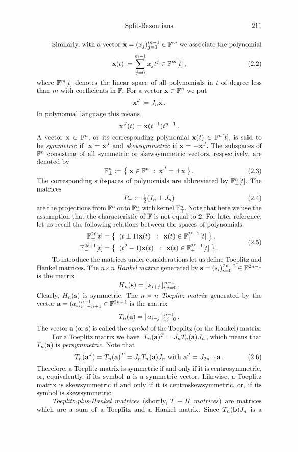
Split-Bezoutians 211
Similarly, with a vector x = (xj)m−1j=0 ∈ Fm we associate the polynomial
x(t) :=
m−1∑j=0
xjtj ∈ Fm[t] , (2.2)
where Fm[t] denotes the linear space of all polynomials in t of degree lessthan m with coefficients in F. For a vector x ∈ Fn we put
xJ := Jnx .
In polynomial language this means
xJ(t) = x(t−1)tn−1 .
A vector x ∈ Fn, or its corresponding polynomial x(t) ∈ Fn[t], is said tobe symmetric if x = xJ and skewsymmetric if x = −xJ . The subspaces ofFn consisting of all symmetric or skewsymmetric vectors, respectively, aredenoted by
Fn± :=
x ∈ Fn : xJ = ±x. (2.3)
The corresponding subspaces of polynomials are abbreviated by Fn±[t]. Thematrices
P± := 12 (In ± Jn) (2.4)
are the projections from Fn onto Fn± with kernel Fn∓. Note that here we use theassumption that the characteristic of F is not equal to 2. For later reference,let us recall the following relations between the spaces of polynomials:
F2`± [t] =
(t± 1)x(t) : x(t) ∈ F2`−1
+ [t],
F2`+1− [t] =
(t2 − 1)x(t) : x(t) ∈ F2`−1
+ [t].
(2.5)
To introduce the matrices under considerations let us define Toeplitz andHankel matrices. The n×n Hankel matrix generated by s = (si)
2n−2i=0 ∈ F2n−1
is the matrix
Hn(s) = [ si+j ]n−1i,j=0 .
Clearly, Hn(s) is symmetric. The n × n Toeplitz matrix generated by thevector a = (ai)
n−1i=−n+1 ∈ F2n−1 is the matrix
Tn(a) = [ ai−j ]n−1i,j=0 .
The vector a (or s) is called the symbol of the Toeplitz (or the Hankel) matrix.For a Toeplitz matrix we have Tn(a)T = JnTn(a)Jn , which means that
Tn(a) is persymmetric. Note that
Tn(aJ) = Tn(a)T = JnTn(a)Jn with aJ = J2n−1a . (2.6)
Therefore, a Toeplitz matrix is symmetric if and only if it is centrosymmetric,or, equivalently, if its symbol a is a symmetric vector. Likewise, a Toeplitzmatrix is skewsymmetric if and only if it is centroskewsymmetric, or, if itssymbol is skewsymmetric.
Toeplitz-plus-Hankel matrices (shortly, T + H matrices) are matriceswhich are a sum of a Toeplitz and a Hankel matrix. Since Tn(b)Jn is a

212 T. Ehrhardt and K. Rost
Hankel matrix it is possible to represent any T +H matrix by means of twoToeplitz matrices,
Rn = Tn(a) + Tn(b)Jn (a,b ∈ F2n−1). (2.7)
Related to this representation is another one, using the projections (2.4) andthe symbols c = a + b and d = a− b, namely
Rn = Tn(c)P+ + Tn(d)P− . (2.8)
3. Centro(skew)symmetric matrices: splitting and restrictedinvertibility
We are now going to discuss some very basic concepts, which facilitates thepresentation of the results in the subsequent sections.
As before, let F stand for a field of characteristic different from two, andlet A ∈ Fn×n. Recall that A is called centrosymmetric if A = JnAJn, and Ais called centroskewsymmetric if A = −JnAJn. Alternative characterizationscan be given in terms of P+ and P−. Indeed, A is centrosymmetric if andonly if
P−AP+ = P+AP− = 0, (3.1)
and A is centroskewsymmetric if and only if
P−AP− = P+AP+ = 0. (3.2)
We also note that A is centrosymmetric if and only if A has both Fn+ andFn− as invariant subspaces, while A is centroskewsymmetric if and only ifA maps Fn+ into Fn− and maps Fn− into Fn+. Hence AP± = P±AP± if A iscentrosymmetric, and AP± = P∓AP± if A is centroskewsymmetric.
We will observe in a few moments that centro(skew)symmetric matricesallow a unique splitting into two matrices of a more particular structure, andthis splitting allows us to reduce the inversion of such matrices to two otherinvertibility problems.
We need to prepare with the following definitions. A matrix A said tobe a matrix of (++)type or of (−−)type if
A = P+AP+ or A = P−AP−,
respectively. Furthermore, a matrix A is said to be of (+−)type or (−+)typeif
A = P+AP− or A = P−AP+,
respectively. Note that, for instance, a matrix of (+−)type has symmetriccolumns and skewsymmetric rows, and similar statements hold for matricesof the other types as well. Furthermore, matrices of (++)type or (−−)type arecentrosymmetric, and matrices of (+−)type or (+−)type are centroskewsym-metric.
Let s1, s2 ∈ +,−, and let A be a matrix of (s1s2)type. We can viewsuch a matrix as a linear map for Fns2 into Fns1 . If this map is invertible, we callthe matrix A restrictedly invertible and denote the corresponding inverse by

Split-Bezoutians 213
A(−1). The restricted inverse is a map from Fns1 to Fns2 and can be identifiedwith a matrix of (s2s1)type. More specifically, if A is a matrix of (s1s2)type,then its restricted inverse A(−1) is a matrix of (s2s1)type such that
A(−1)A = Ps2 and AA(−1) = Ps1 .
The relationship between centro(skew)symmetric matrices and the ma-trices of the four types is now clarified in the following proposition.
Proposition 3.1.
(a) Each centrosymmetric matrix A admits a unique splitting
A = A++ +A−−
into matrices of (++)type and (−−)type. Moreover, A is invertible ifand only if both A++ and A−− are restrictedly invertible. In this case,
A−1 = A(−1)++ +A
(−1)−−
and A(−1)++ = P+A
−1P+ and A(−1)−− = P−A
−1P−.
(b) Each centroskewsymmetric matrix A admits a unique splitting
A = A−+ +A+−
into matrices of (−+)type and (+−)type. Moreover, A is invertible ifand only if both A−+ and A+− are restrictedly invertible. In this case,
A−1 = A(−1)−+ +A
(−1)+−
and A(−1)−+ = P+A
−1P− and A(−1)+− = P−A
−1P+.
Indeed, the splitting parts of A can be obtained by A±± = P±AP± andA±∓ = P±AP∓, respectively (see also (3.1) and (3.2)).
We note that in the centroskewsymmetric case invertibility and re-stricted invertibility can only occur if n is even. Indeed, only for even nthe dimensions of Fn+ and Fn− are the same.
4. Centro(skew)symmetric T+H matrices
The goal of this section is to recall how centrosymmetric and centroskewsym-metric T +H matrices can be represented. Furthermore, the connection withT +H matrices of (++), (−−), (+−), and (−+)type is made.
Let us start with the observation, already mentioned above, that a gen-eral T +H matrix can be written in the form
Tn(c)P+ + Tn(d)P− .
The choice of c and d is in general not unique. The reason is that there existmatrices of “checkerboard” structure which are both Toeplitz and Hankel(see [13, Sect. 2]).

214 T. Ehrhardt and K. Rost
The following basic result shows under which conditions a T + H ma-trix is centrosymmetric or centroskewsymmetric. It also addresses the non-uniqueness of the symbol. For the details of the proof we refer to [3, Prop. 3.3]and [4, Prop. 3.1].
Proposition 4.1.
(a) A T +H matrix
Rn = Tn(c)P+ + Tn(d)P− (4.1)
is centrosymmetric if and only if c and d both are symmetric, i.e.,c,d ∈ F2n−1
+ .
(b) We have Tn(c)P+ + Tn(d)P− = 0 if and only if
c =
0 if n is odd,
eα,−α if n is even,d =
eα,β if n is odd,eα,α if n is even,
(4.2)
where eα,β = (α, β, α, β, . . . , β, α)T ∈ F2n−1+ .
(c) An n×n matrix Rn is a centroskewsymmetric T +H matrix if and onlyif it can be written in the form
Rn = Tn(c)P+ + Tn(d)P− (4.3)
with skewsymmetric c,d ∈ F2n−1− . The choice of these vectors is unique.
Concerning general T + H matrices, (b) tells us that the choice of thesymbols c and d is not unique. This is equally true in the centrosymmet-ric case. In the centroskewsymmetric case, non-uniqueness can also occur,but only if one allows for non-skewsymmetric vectors. As stated in (c), therestriction to skewsymmetric vectors makes the choice of the symbols unique.
Parts (a) and (c) of the previous proposition imply that centrosymmetricT +H matrices can also be written as
Rn = P+Tn(c)P+ + P−Tn(d)P−
with symmetric c,d ∈ F2n−1+ , while centroskewsymmetric T + H matrices
can be written as
Rn = P−Tn(c)P+ + P+Tn(d)P−
with skewsymmetric c,d ∈ F2n−1− . Indeed, to see this recall (3.1) and (3.2)
and take the remarks made after formula (2.6) into account. These two for-mulas represent the splitting of centro(skew)symmetric T +H matrices intoT +H matrices of (++), (−−), (−+), and (+−)type, respectively.
In particular, we can characterize T + H matrices of the four types.Firstly, a T +H matrix of (++)type or (−−)type is given by
P+Tn(c)P+ and P−Tn(d)P− ,
respectively, with symmetric c,d ∈ F2n−1+ . The symbols are not necessarily
unique, but the only modifications are those described in (4.2). Secondly, aT +H matrix of (−+)type or (+−)type is given by
P−Tn(c)P+ and P+Tn(d)P− ,

Split-Bezoutians 215
respectively, with skewsymmetric symbol c,d ∈ F2n−1− . Within the class of
skewsymmetric vectors, these symbols are unique.
At this point let us mention that there is a relationship between therestricted invertibility of the T + H matrices of the various types and theinvertibility of a Toeplitz matrix.
Proposition 4.2. Let c ∈ F2n−1− . Then the following are equivalent:
(a) Tn(c) is invertible;(b) P+Tn(c)P− is restrictedly invertible;(c) P−Tn(c)P+ is restrictedly invertible.
Proof. Note that we have P+Tn(c)P+ = P−Tn(c)P− = 0 and thereforeTn(c) = P+Tn(c)P− + P−Tn(c)P+. The equivalence of (a) with (b) and (c)follows from Proposition 3.1.
The equivalence of (b) with (c) becomes clear by passing to the trans-pose, (P+Tn(c)P−)T = P−Tn(cJ)P+ = −P−Tn(c)P+.
Proposition 4.3. Let c ∈ F2n−1+ . Then Tn(c) is invertible if and only if both
matrices P+Tn(c)P+ and P−Tn(c)P− are restrictedly invertible.
Proof. It suffices to note that P+Tn(c)P− = P−Tn(c)P+ = 0 and henceTn(c) = P+Tn(c)P+ + P−Tn(c)P−. Proposition 3.1 gives the assertion.
Note that the restricted invertibility of P+Tn(c)P+ is not equivalent tothe restricted invertibility of P−Tn(c)P−. For example, if c = (0, 1, 0, 1, 0)T ,then P+T3(c)P+ is restrictedly invertible, but P−T3(c)P− = 0 is not. Onthe other hand, if we take d = (−1, 0, 1, 0,−1)T , then P+T3(d)P+ is notrestrictedly invertible, while P−T3(d)P− is. Clearly, T3(c) and T3(d) are notinvertible.
5. Centro(skew)symmetric T+H-Bezoutians andsplit-Bezoutians
Recall that a T + H-Bezoutian is an n × n matrix B for which there existeight vectors fi,gi ∈ Fn+2 (i = 1, 2, 3, 4) such that, in polynomial language,
B(t, s) =
∑4i=1 gi(t)fi(s)
(t− s)(1− ts).
The relationship between T +H-Bezoutians and T +H matrices is shown inthe following important theorem, which was established in [11].
Theorem 5.1. The inverse of an invertible T +H-Bezoutian is an invertibleT +H matrix and vice versa.
We will see in a few moments that if an invertible T + H-Bezoutianis centrosymmetric or centroskewsymmetric, then it admits a decompositioninto a sum of two particular T +H-Bezoutians, called split-Bezoutians. Thedefinition of these two split-Bezoutians is different in the centrosymmetricand the centroskewsymmetric case.
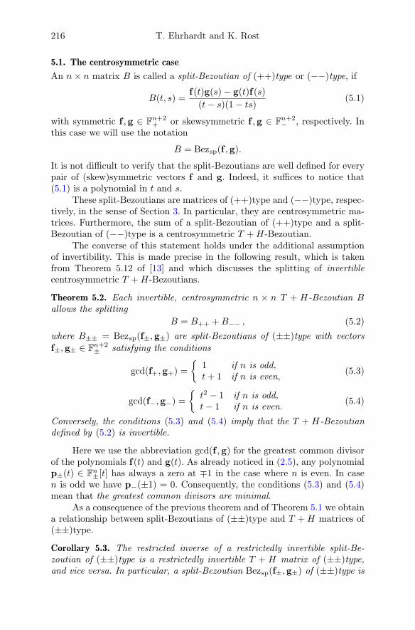
216 T. Ehrhardt and K. Rost
5.1. The centrosymmetric case
An n× n matrix B is called a split-Bezoutian of (++)type or (−−)type, if
B(t, s) =f(t)g(s)− g(t)f(s)
(t− s)(1− ts)(5.1)
with symmetric f ,g ∈ Fn+2+ or skewsymmetric f ,g ∈ Fn+2
− , respectively. Inthis case we will use the notation
B = Bezsp(f ,g).
It is not difficult to verify that the split-Bezoutians are well defined for everypair of (skew)symmetric vectors f and g. Indeed, it suffices to notice that(5.1) is a polynomial in t and s.
These split-Bezoutians are matrices of (++)type and (−−)type, respec-tively, in the sense of Section 3. In particular, they are centrosymmetric ma-trices. Furthermore, the sum of a split-Bezoutian of (++)type and a split-Bezoutian of (−−)type is a centrosymmetric T +H-Bezoutian.
The converse of this statement holds under the additional assumptionof invertibility. This is made precise in the following result, which is takenfrom Theorem 5.12 of [13] and which discusses the splitting of invertiblecentrosymmetric T +H-Bezoutians.
Theorem 5.2. Each invertible, centrosymmetric n × n T + H-Bezoutian Ballows the splitting
B = B++ +B−− , (5.2)
where B±± = Bezsp(f±,g±) are split-Bezoutians of (±±)type with vectors
f±,g± ∈ Fn+2± satisfying the conditions
gcd(f+,g+) =
1 if n is odd,t+ 1 if n is even,
(5.3)
gcd(f−,g−) =
t2 − 1 if n is odd,t− 1 if n is even.
(5.4)
Conversely, the conditions (5.3) and (5.4) imply that the T + H-Bezoutiandefined by (5.2) is invertible.
Here we use the abbreviation gcd(f ,g) for the greatest common divisorof the polynomials f(t) and g(t). As already noticed in (2.5), any polynomialp±(t) ∈ Fn±[t] has always a zero at ∓1 in the case where n is even. In casen is odd we have p−(±1) = 0. Consequently, the conditions (5.3) and (5.4)mean that the greatest common divisors are minimal.
As a consequence of the previous theorem and of Theorem 5.1 we obtaina relationship between split-Bezoutians of (±±)type and T +H matrices of(±±)type.
Corollary 5.3. The restricted inverse of a restrictedly invertible split-Be-zoutian of (±±)type is a restrictedly invertible T + H matrix of (±±)type,and vice versa. In particular, a split-Bezoutian Bezsp(f±,g±) of (±±)type is

Split-Bezoutians 217
restrictedly invertible if and only if the condition (5.3) or (5.4), respectively,is satisfied.
Proof. We first need to establish the rather simple fact that there exist re-strictedly invertible split-Bezoutians and T + H matrices of both (++) and(−−)type in every dimension n. Indeed, we can consider the identity matrixIn, which is a centrosymmetric T +H matrix and a centrosymmetric T +H-Bezoutian, and has the corresponding splitting In = P+ +P−. Therefore, P+
and P− are split-Bezoutians as well as T+H matrices of (++) and (−−)type,respectively. Since they are projections, they are their own restricted inverses.
More specifically, P± = Bezsp(f(0)± ,g
(0)± ) with
f(0)± (t) = −1
2
(tn+1 ± 1
), g
(0)± (t) = tn ± t ,
and it can be verified by direct computation that f (0)± ,g(0)± satisfy (5.3) and
(5.4), respectively. Note that this also follows from the splitting In = P++P−by applying Theorem 5.2.
Now let B++ be a split-Bezoutian of (++)type. Then
B = B++ + P−
is a centrosymmetric T+H-Bezoutian. Because of Proposition 3.1 the matrixB is invertible if and only if B++ is restrictedly invertible. Using the previoustheorem we see that this is the case precisely if f+(t),g+(t) satisfies thecondition (5.3).
Let us proceed to show that the restricted inverse of a split-Bezoutianis a T + H matrix of corresponding type and vice versa. First assume thatB++ is restrictedly invertible, i.e., B is invertible. Then, by Theorem 5.1, theinverse of B is a (centrosymmetric) T +H matrix. Again, by Proposition 3.1,the restricted inverse is given by
B(−1)++ = P+B
−1P+ .
In view of (4.1) it is a T +H matrix of (++)type.Now let us show the converse. Assume that A++ is a restrictedly in-
vertible T + H matrix of (++)type. Consider A = A++ + P−, which is aninvertible centrosymmetric T + H matrix. By Theorem 5.1, its inverse is acentrosymmetric T + H-Bezoutian B = A−1, which can be split into a sumB++ +B−−. Now, by Proposition 3.1 we have
A(−1)++ = P+A
−1P+ = B++.
Hence the restricted inverse of a T+H matrix of (++)type is a split-Bezoutianof (++)type.
Finally, remark that the case of split-Bezoutians and T +H matrices of(−−)type can be proved similarly by changing the roles of P+ and P−.
We proceed with the observation that the two kinds of split-Bezoutiansconsidered here can be reduced to split-Bezoutians of (++)type and of oddorder. This was shown in [13, Thm. 5.12]. It is a simple consequence of the fact

218 T. Ehrhardt and K. Rost
that depending on whether n is even or odd and whether the split-Bezoutianis of (++) or (−−)type, the polynomials f(t) and g(t) may have commonfactors (t− 1) or (t+ 1) (see Theorem 5.2 and formulas (2.5)), which one canpull out in the representation (5.1).
To that aim let us introduce the n × (n − 1) matrices M t±1n−1 and the
n× (n− 2) matrix M t2−1n−2 ,
M t±1n−1 =
±1 0
1 ±1
1. . .
. . . ±1
0 1
, M t2−1
n−2 =
−1 0
0 −1
1 0. . .
1. . . −1. . . 0
0 1
. (5.5)
These are matrices of multiplication operators (in the corresponding polyno-mial spaces with respect to the canonical bases) with the polynomials beingindicated in their superscripts.
Finally, taking Theorem 5.2 and Corollary 5.3 into account we obtainthe following.
Theorem 5.4. Let B++ and B−− be n × n split-Bezoutians of (++) and(−−)type, respectively.
(a) If n is even, then there exist fi,gi ∈ Fn+1+ , i = 1, 2, such that
B++ = M t+1n−1Bezsp(f1,g1)(M t+1
n−1)T ,
B−− = M t−1n−1Bezsp(f2,g2)(M t−1
n−1)T .(5.6)
Moreover, the split-Bezoutians are restrictedly invertible if and only ifthe pair f1(t),g1(t) or f2(t),g2(t), respectively, is coprime.
(b) If n is odd, then there exist f1,g1 ∈ Fn+2+ and f2,g2 ∈ Fn+ such that
B++ = Bezsp(f1,g1),
B−− = M t2−1n−2 Bezsp(f2,g2)(M t2−1
n−2 )T .(5.7)
Moreover, the split-Bezoutians are restrictedly invertible if and only ifthe pair f1(t),g1(t) or f2(t),g2(t), respectively, is coprime.
The formulas (5.6) and (5.7) can be expressed in polynomial language.Then they read
B++(t, s) = (t+ 1)f1(t)g1(s)− g1(t)f1(s)
(t− s)(1− ts)(s+ 1),
B−−(t, s) = (t− 1)f2(t)g2(s)− g2(t)f2(s)
(t− s)(1− ts)(s− 1)
(5.8)

Split-Bezoutians 219
for n even, while
B++(t, s) =f1(t)g1(s)− g1(t)f1(s)
(t− s)(1− ts),
B−−(t, s) = (t2 − 1)f2(t)g2(s)− g2(t)f2(s)
(t− s)(1− ts)(s2 − 1)
(5.9)
for n odd. Note that in all cases of (5.6) and (5.7) the terms in the middle,Bezsp(fi,gi), are split-Bezoutians of odd order and (++)type.
5.2. The centroskewsymmetric case
Let us now consider centroskewsymmetric T +H-Bezoutians. We will assumethat the order n is even since centroskewsymmetric matrices of odd order aresingular.
We start with the following splitting theorem about centroskewsymmet-ric T +H-Bezoutians, which was proved in [13, Thm. 5.13].
Theorem 5.5. Each invertible, centroskewsymmetric T + H-Bezoutian B ofeven order n allows the splitting B = B+− +B−+ with
B+−(t, s) = (t+ 1)f1(t)g1(s)− g1(t)f1(s)
(t− s)(1− ts)(s− 1), (5.10)
B−+(t, s) = (t− 1)f2(t)g2(s)− g2(t)f2(s)
(t− s)(1− ts)(s+ 1), (5.11)
where fi,gi ∈ Fn+1+ are such that fi(t),gi(t) are coprime (i = 1, 2). Con-
versely, each centroskewsymmetric T + H-Bezoutian B defined in this waywith coprime fi(t),gi(t), i = 1, 2, is invertible.
In matrix form, the formulas (5.10) and (5.11) read
B+− = M t+1n−1Bezsp(f1,g1)(M t−1
n−1)T , (5.12)
B−+ = M t−1n−1Bezsp(f2,g2)(M t+1
n−1)T . (5.13)
Again, as before, the terms in the middle, Bezsp(fi,gi), are split-Bezoutiansof (++)type and odd order n− 1.
We will refer to matrices of the kind (5.10) and (5.11) as split-Bezoutiansof (+−)type and of (−+)type, respectively. These split-Bezoutians are ma-trices of (+−)type and (−+)type, respectively, in the sense of Section 3.Hence they are centroskewsymmetric T + H-Bezoutians. In fact, a sum ofa split-Bezoutian of (+−)type and a split-Bezoutian of (−+)type is a cen-troskewsymmetric T +H-Bezoutian.
In contrast to the centrosymmetric case, the factors on the left and theright hand side in (5.10) and (5.11) are different, so that these representationscannot be brought into a simpler form (5.1) involving only two polynomials.

220 T. Ehrhardt and K. Rost
However, one can obtain three equivalent representations by means of simplesubstitutions. Given f1,g1, f2,g2 ∈ Fn+1
+ , introduce f±,g±, f±, g± ∈ Fn+2± by
f1(t) =f+(t)
t+ 1=
f−(t)
t− 1, g1(t) =
g+(t)
t+ 1=
g−(t)
t− 1,
f2(t) =f−(t)
t− 1=
f+(t)
t+ 1, g2(t) =
g−(t)
t− 1=
g+(t)
t+ 1.
Then we obtain the following representations:
B±∓(t, s) =
(f±(t)g±(s)− g±(t)f±(s)
(t− s)(1− ts)
)s∓ 1
s± 1
=t± 1
t∓ 1
(f∓(t)g∓(s)− g∓(t)f∓(s)
(t− s)(1− ts)
)
=f±(t)g∓(s)− g±(t)f∓(s)
(t− s)(1− ts).
Notice that the last representation comes closest to resembling (5.1), but itinvolves four polynomials. The other two representations are ‘adjoint’ to eachother. One of them was already used in [13].
From the previous theorem it is possible to derive the following result,which examines the restricted invertibility of split-Bezoutians of (±∓)typeand its relationship to T +H matrices of (∓±)type.
Corollary 5.6. Let n be even. The restricted inverse of a restrictedly invert-ible split-Bezoutian of (±∓)type is a restrictedly invertible T + H matrix of(∓±)type, and vice versa. In particular, a split-Bezoutian B±∓ of (±∓)typegiven by (5.10)–(5.11) (or (5.12)–(5.13)) is restrictedly invertible if and onlyif the pair of polynomials f1(t),g1(t) or f2(t),g2(t), respectively, is co-prime.
Proof. As before, we need to show that there exist restrictedly invertiblesplit-Bezoutians of (±∓)type in even dimension n. Let
C+− = M t+1n−1P+(M t−1
n−1)T , C−+ = M t−1n−1P+(M t+1
n−1)T ,
where P+ is of order n − 1. Since P+ = Bezsp(f ,g) with two polynomialsf(t) = − 1
2 (tn + 1), g(t) = tn−1 + t, which are coprime, it follows from theprevious theorem that C = C+−+C−+ is an invertible T+H-Bezoutian. Con-sequently, the splitting parts C±∓ are restrictedly invertible split-Bezoutiansof (±∓)type.
Now we can proceed similarly as in the proof of Corollary 5.3. For in-stance, given a split-Bezoutian B+− of (+−)type, we define a centroskewsym-metric T +H-Bezoutian B = B+−+C−+. For the converse, if we are given a
T +H matrix A−+ of (−+)type, we are going to consider A = A−+ +C(−1)−+ ,
which is a centroskewsymmetric T + H matrix. We leave the details to thereader.

Split-Bezoutians 221
5.3. The uniqueness of the split-Bezoutians
In the last two subsections, we obtained six different kinds of representationsfor the split-Bezoutians of the various types, namely (5.6), (5.7), (5.12), and(5.13). Note that one has corresponding polynomial representations (5.8),(5.9), (5.10), and (5.11). In these polynomial representations, only the termson the left and on the right are different, but the term in the middle,
f(t)g(s)− g(t)f(s)
(t− s)(1− st),
is always of the same form.Later we need the following simple fact about split-Bezoutians. It is
known for Hankel- and Toeplitz-Bezoutians (see Corollaries 2.3 and 2.10 in[14]) and split-Bezoutians of (++)type (see Remark 4.3 in [5]), but holds forsplit-Bezoutians of (−−) or (±∓)type as well.
Lemma 5.7. Two nonzero split-Bezoutians (of (±±)type or (±∓)type) givenby pairs of vectors f ,g and u,v, respectively, are equal if and only ifthere is Φ ∈ F2×2 with det Φ = 1 such that
[ u,v ] = [ f ,g ] Φ . (5.14)
Proof. In view of the polynomial representations of the two Bezoutians, wecan cancel possible factors on the left and the right as well as remove thedenominator in the middle term in order to get
f(t)g(s)− g(t)f(s) = u(t)v(s)− v(t)u(s) .
Translated into matrix language this means that
[ f , g ]
[0 −11 0
] [fT
gT
]= [ u, v ]
[0 −11 0
] [uT
vT
].
Note that [f , g] has rank two because otherwise the two vectors are linearlydependent, which would imply that the Bezoutian vanishes. The same holdsfor [u, v]. It follows that there exists an invertible Φ such that (5.14) holds.Now plug this relation into the above formula in order to conclude thatdet Φ = 1.
5.4. Split-Bezoutians versus T+H-Bezoutians
Let us make some further comments on the relationship between the split-Be-zoutians of the various types and centro(skew)symmetric T +H-Bezoutians.These remarks are added for illustration, but are not needed subsequently.
Clearly, each split-Bezoutian of (±±)type is a (centrosymmetric) T+H-Bezoutian of (±±)type. However, not every T +H-Bezoutian of (±±)type isa split-Bezoutian. For example, let B1 and B2 be two n× n split-Bezoutiansof (++)type given by
Bi(t, s) =fi(t)gi(s)− gi(t)fi(s)
(t− s)(1− ts), (i = 1, 2),
where fi,gi ∈ Fn+2+ . Then, clearly, B = B1+B2 is a T+H-Bezoutian and it is
a matrix of (++)type. But, for general choices of f1, f2,g1,g2 and if n ≥ 3,

222 T. Ehrhardt and K. Rost
the matrix B is not a split-Bezoutian. The same construction works in thecase of split-Bezoutians of (−−)type if n ≥ 4.
Now we are going to provide examples of T+H-Bezoutians of (±±)typewhich are not split-Bezoutians. Note that each such matrix is a non-invertiblecentrosymmetric T +H-Bezoutian which cannot be written as the sum of asplit-Bezoutian of (++)type and a split-Bezoutian of (−−)type. Hence thestatement of Theorem 5.2 is not true without the invertibility assumption.
Example 5.8. The following matrices B+ and B− describe two n × n cen-trosymmetric T + H-Bezoutians of (++)type and (−−)type. Assume thatthe order is n ≥ 3 and n ≥ 4, respectively.
B+ =
1 1 1 11 1
1 1
.
.
.
. . ..
.
.
1 11 1
1 1 1 1
, B−=
1 1 −1 −11 −1
1 −1
.
.
.
. . ..
.
.
−1 1−1 1
−1 −1 1 1
.
It can be verified straightforwardly that both are restrictedly invertible. Onthe other hand, neither of them is a split-Bezoutian.
In the case of centroskewsymmetric T + H-Bezoutians of (±∓)type,similar statements hold, and corresponding examples can be given as well.
6. Inversion results for T+H matrices
In this section we consider the invertibility of centrosymmetric and cen-troskewsymmetric T +H matrices. In [13] necessary and sufficient conditionsfor the invertibility of centro(skew)symmetric T + H matrices were given.Using these results we derive necessary and sufficient conditions for the re-stricted invertibility of T +H matrices of (±±) and (±∓)type. These resultsare used later on for studying the (restricted) invertibility of split-Bezoutiansof the various types.
To begin with, recall from Section 4 that T +H matrices can be writtenin the form
Rn = Tn(c)P+ + Tn(d)P−
where the symbols c and d are both symmetric or skewsymmetric vectors ifthe matrix Rn is centrosymmetric or centroskewsymmetric, respectively.
6.1. The centrosymmetric case
We first start with the issue of invertibility of a centrosymmetric T+H matrixRn. As it will turn out, it is related to the solvability of two systems of linearequations being of Toeplitz form, which we are going to state now.

Split-Bezoutians 223
For given symmetric c,d ∈ F2n−1+ , we consider the systems
Tn(c)(u+j )nj=1 = 2P+e1 , Tn(c)(v+j )nj=1 = −2P+(cj)nj=1 , (6.1)
Tn(d)(u−j )nj=1 = 2P−e1 , Tn(d)(v−j )nj=1 = −2P−(dj)nj=1 . (6.2)
Here we choose arbitrary constants cn = c−n , and dn = d−n . The solvabilityof these systems is independent of the choice of these constants. Indeed, ifthe systems have solutions (u±j ), (v±j ) for some specific choice of c±n or d±n,
then for another choice a solution is given by (u±j ), (v±j ) + λ± · (u±j ) , where
λ± ∈ F is a constant depending on the new (and the old) choices.Furthermore, if these systems have a solution, then they also have a
solution where the vectors (u±j )nj=1 and (v±j )nj=1 belong to Fn±. In fact, using
that c and d are symmetric, one can replace (u±j ) by P±(u±j ) and (v±j ) by
P±(v±j ) . Henceforth we will only be interested in symmetric and skewsym-metric solutions.
From the solutions of (6.1) and (6.2) we will pass to augmented vectors,
u± =
0
u±1...
u±n0
∈ Fn+2± , v± =
1
v±1...
v±n±1
∈ Fn+2± . (6.3)
In terms of the augmented vectors, the systems (6.1) and (6.2) are equivalentto c1 c0 c1 . . . cn
.... . .
. . .. . .
...cn . . . c1 c0 c1
[ u+, v+ ] = [ 2P+e1 , 0 ] (6.4)
and d1 d0 d1 . . . dn...
. . .. . .
. . ....
dn . . . d1 d0 d1
[ u−, v− ] = [ 2P−e1 , 0 ] , (6.5)
respectively.The following theorem was proved in [13, Thm. 3.3].
Theorem 6.1. Let c,d ∈ F2n−1+ and Rn = P+Tn(c)P+ + P−Tn(d)P−. Then
Rn is invertible if and only if the Toeplitz equations (6.1) and (6.2) have(symmetric respectively skewsymmetric) solutions. In this case, the inverse ofRn is given by the corresponding augmented vectors (6.3) of these solutions,
R−1n =1
2
(B++ +B−−
), (6.6)
where B±± = Bezsp(u±,v±), i.e.,
B±±(t, s) =u±(t)v±(s)− v±(t)u±(s)
(t− s)(1− ts). (6.7)

224 T. Ehrhardt and K. Rost
Note that the invertibility of the Toeplitz matrices Tn(c) or Tn(d) is, ofcourse, sufficient for the (unique) solvability of the systems (6.1) and (6.2),while it is not always necessary. Therefore, in the case of invertible Rn given asin Theorem 6.1, the solutions to (6.1) and (6.2) need not be unique. However,one can show that the solutions are unique within the set of symmetric andskewsymmetric vectors.
Using the same kind of argument as in the proof of Corollary 5.3 one canderive from the previous theorem a corresponding result for T +H matricesof (±±)type.
Corollary 6.2.
(a) Let c ∈ F2n−1+ . Then P+Tn(c)P+ is restrictedly invertible if and only if
the Toeplitz equations (6.1) have symmetric solutions. In this case
(P+Tn(c)P+)(−1) =1
2Bezsp(u+,v+),
where u+,v+ are defined in (6.3).(b) Let d ∈ F2n−1
+ . Then P−Tn(d)P− is restrictedly invertible if and only ifthe Toeplitz equations (6.2) have skewsymmetric solutions. In this case
(P−Tn(d)P−)(−1) =1
2Bezsp(u−,v−),
where u−,v− are defined in (6.3).
The example of vectors c and d given at the end of Section 4 showthat it is possible that P+Tn(c)P+ is restrictedly invertible, but Tn(c) is notinvertible. Likewise, P−Tn(d)P− is restrictedly invertible whereas Tn(d) isnot invertible. While the systems (6.1) and (6.2) have solutions, we see thatin these cases the solutions are not unique. However, as already mentionedabove, if we restrict ourselves to symmetric or skewsymmetric solutions, re-spectively, then uniqueness is guaranteed.
6.2. The centroskewsymmetric case
In this subsection we consider centroskewsymmetric T +H matrices. We willassume that the order n is even because this is a necessary condition for theinvertibility of any centroskewsymmetric matrix. We start again from therepresentation (2.8) of general T +H matrices.
The invertibility of centroskewsymmetric T + H matrices Rn is againconnected with systems of Toeplitz form. For given c,d ∈ F2n−1
− consider
Tn(c)(u+j )nj=1 = 2P−e1, Tn(c)(v+j )nj=1 = −2P−(cj)nj=1, (6.8)
Tn(d)(u−j )nj=1 = 2P+e1, Tn(d)(v−j )nj=1 = −2P+(dj)nj=1, (6.9)
where we choose arbitrary constants cn = −c−n , dn = −d−n. As before, thesolvability of (6.8) or (6.9), respectively, is independent of the choice of theseconstants. This can be seen in the same way as in the centrosymmetric case.
As before, if these systems have a solution, then there is also a solution inwhich (u±j )nj=1 and (v±j )nj=1 belong to Fn±. Furthermore, given these solutions

Split-Bezoutians 225
we will pass to augmented vectors (6.3) as we did in the centrosymmetriccase.
In terms of the augmented vectors, the system (6.8) is equivalent to c1 0 −c1 . . . −cn...
. . .. . .
. . ....
cn . . . c1 0 −c1
[ u+, v+ ] = [ 2P−e1 , 0 ] , (6.10)
and the system (6.9) is equivalent to d1 0 −d1 . . . −dn...
. . .. . .
. . ....
dn . . . d1 0 −d1
[ u−, v− ] = [ 2P+e1 , 0 ] . (6.11)
The following theorem was proved in [13, Thm. 3.6].
Theorem 6.3. Let c,d ∈ F2n−1− and let Rn = P−Tn(c)P+ + P+Tn(d)P−
with n being even. Then Rn is invertible if and only if the Toeplitz equations(6.8) and (6.9) have (symmetric respectively skewsymmetric) solutions. Inthis case, the inverse of Rn is given by the corresponding augmented vectors(6.3) of these solutions,
R−1n =1
2
(B+− +B−+
),
where
B±∓(t, s) =u±(t)v±(s)− v±(t)u±(s)
(t− s)(1− ts)s∓ 1
s± 1. (6.12)
Contrary to the centrosymmetric case, it is known that in the cen-troskewsymmetric case Rn = P−Tn(c)P+ + P+Tn(d)P− is invertible if andonly if both Tn(c) and Tn(d) are invertible. Indeed, this follows from Propo-sitions 3.1 and 4.2 (see also [13, Corollary 3.7]). As a consequence, if theToeplitz equations (6.8) or (6.9) have a solution, then the solution is uniqueand it is necessarily symmetric or skewsymmetric, respectively.
Finally, as in the symmetric case, we are able to conclude a correspond-ing restricted invertibility result for T +H matrices of (±∓)type.
Corollary 6.4.
(a) Let c ∈ F2n−1− . Then P−Tn(c)P+ is restrictedly invertible if and only if
the Toeplitz equations (6.8) have (symmetric) solutions. In this case
(P−Tn(c)P+)(−1) = B+−,
where B+− is defined in (6.12) with the augmented vectors of the solu-tions.
(b) Let d ∈ F2n−1− . Then P+Tn(d)P− is restrictedly invertible if and only
if the Toeplitz equations (6.9) have (skewsymmetric) solutions. In thiscase
(P+Tn(d)P−)(−1) = B−+,
where B−+ is defined in (6.12) with the augmented vectors of the solu-tions.

226 T. Ehrhardt and K. Rost
Note that by Proposition 4.2, P−Tn(c)P+ is restrictedly invertible if andonly if Tn(c) is invertible. Likewise, P+Tn(d)P− is restrictedly invertible ifand only if Tn(d) is invertible. In this case, the solutions to (6.8) and (6.9),respectively, are unique.
7. Resultant equations
In the previous section we arrived at the equations (6.1) and (6.2) in thecentrosymmetric case, which are equivalent to equations (6.4) and (6.5). Inthe centroskewsymmetric case we obtained the equations (6.8) and (6.9),which are equivalent to (6.10) and (6.11).
Our goal is now to express these equations as resultant equations. Atthe same time, we relate these equations to the restricted invertibility of thesplit-Bezoutians of the various types rather than the restricted invertibilityof T +H matrices.
7.1. Resultant matrices
Hereafter we need the following m× (m+ k) matrix which is associated witha vector w = (wi)
ki=0 ∈ Fk+1 ,
Dm,m+k(w) =
w0 w1 . . . wk 0
w0 w1 . . . wk. . .
. . .. . .
0 w0 w1 . . . wk
. (7.1)
The equation Dm,m+k(w)x = y can be interpreted in the language ofrational functions as follows:
w(t−1)x(t) ≡ y(t) mod . . . , t−2, t−1, tm, tm+1, . . . . (7.2)
Indeed, write
w(t−1) = w0+w1t−1+· · ·+wkt−k and x(t) = x0+x1t+· · ·+xm+k−1t
m+k−1.
The coefficients of the powers 1, t, . . . , tm−1 in the product w(t−1)x(t) haveto coincide with those of the polynomial y(t) = y0 + y1t+ · · ·+ ym−1t
m−1.
Let u ∈ Fm1+1,v ∈ Fm2+1 be nonzero vectors, p < minm1,m2, allow-ing p to be negative, and let m1,m2 ≥ 0. We introduce the resultant matrixResp(u,v) of u and v,
Resp(u,v) =
[Dm2−p,m1+m2−p(u)
Dm1−p,m1+m2−p(v)
], (7.3)

Split-Bezoutians 227
i.e.,
Resp(u,v) =
u0 u1 . . . um10
u0 u1 . . . um1
. . .. . .
. . .
0 u0 u1 . . . um1
v0 v1 . . . vm20
v0 v1 . . . vm2
. . .. . .
. . .
0 v0 v1 . . . vm2
m2 − p
m1 − p
.
︸ ︷︷ ︸m1 +m2 − p
In the square case p = 0 we have the classical Sylvester resultant matrix.Define
ν = deg gcd(u(t),v(t)) + ν∞
where ν∞ = minm1 − deg u(t),m2 − deg v(t). More specifically (see [1,Sect. 3]) it can be shown that the dimension of the nullspace of the transposeof Resp(u,v) is
dim ker(Resp(u,v))T = max0, ν − p,
and thus
dim ker Resp(u,v) = maxp, ν. (7.4)
7.2. The centrosymmetric case
In the centrosymmetric case (see Corollary 6.2), we arrive at the equations(6.4) and (6.5) with u±,v± ∈ Fn+2
± given in augmented form (6.3). We canequivalently rewrite these equations in the following way. Equation (6.4) isequivalent to
0 u+1 . . . u+n 0 0
0 u+1 . . . u+n 0
. . .. . .
. . .. . .
0 0 u+1 . . . u+n 0
1 v+1 . . . v+n 1 0
1 v+1 . . . v+n 1
. . .. . .
. . .. . .
0 1 v+1 . . . v+n 1
cn
...
c1
c0
c1
...
cn
=
1
0...0
1
0
...
0
,

228 T. Ehrhardt and K. Rost
and equation (6.5) is equivalent to
0 u−1 . . . u−n 0 0
0 u−1 . . . u−n 0
. . .. . .
. . .. . .
0 0 u−1 . . . u−n 0
1 v−1 . . . v−n −1 0
1 v−1 . . . v−n −1
. . .. . .
. . .. . .
0 1 v−1 . . . v−n −1
dn
...
d1
d0
d1
...
dn
=
−1
0...0
1
0
...
0
.
Therein the underlying matrices are of size 2n × (2n + 1), where we have nrows containing the u±j and n rows containing the v±j .
Note that each of the variables cn and dn, respectively, occurs only intwo equations, and these two equations are the same because we assume that(v+j )nj=1 is symmetric and (v−j )nj=1 is skewsymmetric. The equations read
cn + v+1 cn−1 + . . . v+n c0 + c1 = 0
and
dn + v−1 dn−1 + . . . v−n d0 − d1 = 0,
respectively. This means we can eliminate cn and dn from the systems bydeleting the first and the last equation of the subsystems of equations in-volving the v±j . After this, the variables cn and dn are annihilated by matrix-vector multiplication, and therefore we can delete the first and the last columnof the matrix.
As a result, we obtain systems with the following underlying matrices:
u±1 u±2 . . . u±n−1 u±n 0
u±1 u±2 . . . u±n−1 u±n
. . .. . .
. . .. . .
u±1 u±2 . . . u±n−1 u±n
0 u±1 u±2 . . . u±n−1 u±n
1 v±1 v±2 . . . v±n−1 v±n ±1 0
. . .. . .
. . .. . .
. . .. . .
0 1 v±1 v±2 . . . v±n−1 v±n ±1
n
n− 2
︸ ︷︷ ︸2n− 1

Split-Bezoutians 229
These are the resultant matrices Res1(u± , v±). Here
u± = (u±j )nj=1 (7.5)
denote the reduced vectors, which are associated with the vectors u± in aug-mented form (6.3). As a consequence, we obtain the following lemma.
Lemma 7.1. Let c,d ∈ F2n−1+ , let u±,v± ∈ Fn+2
± be of the augmented form(6.3), and let u± ∈ Fn± the reduced vectors (7.5) associated with u±.
(a) There exists cn = c−n ∈ F such that (6.4) is true if and only if
Res1(u+ , v+) c =
[2P+e1
0
]. (7.6)
(b) There exists dn = d−n ∈ F such that (6.5) is true if and only if
Res1(u− , v−) d =
[−2P−e1
0
]. (7.7)
Theorem 7.2. Let u±,v± ∈ Fn+2± be of the form (6.3), and let
B±± = Bezsp(u±,v±).
(a) B++ is restrictedly invertible if and only if equation (7.6) has a solutionc ∈ F2n+1
+ . In this case,
B(−1)++ =
1
2P+Tn(c)P+.
(b) B−− is restrictedly invertible if and only if equation (7.7) has a solutiond ∈ F2n+1
− . In this case,
B(−1)−− =
1
2P−Tn(d)P−.
Proof. ⇐: Let us first assume that the systems (7.6) or (7.7), respectively,have a solution. We are going to show that B±± are restrictedly invertibleand that their restricted inverses are given as above.
Since u±,v± with the corresponding reduced vector u± satisfy the sys-tems (7.6) or (7.7), Lemma 7.1 implies that there exist cn = c−n and dn = d−nsuch that the Toeplitz systems (6.4) or (6.5) are satisfied. These Toeplitz sys-tems are in turn equivalent to the systems (6.1) or (6.2). Hence the system(6.1) or (6.2) is solvable, and the pair of vectors u±,v± represents a solu-tion.
Now Corollary 6.2 implies that
R+ := P+Tn(c)P+ or R− := P−Tn(d)P−
is restrictedly invertible and that
R(−1)± =
1
2B±±
with the split-Bezoutian B±± = Bezsp(u±,v±). Hence B±± is restrictedlyinvertible, and the above formula is true.
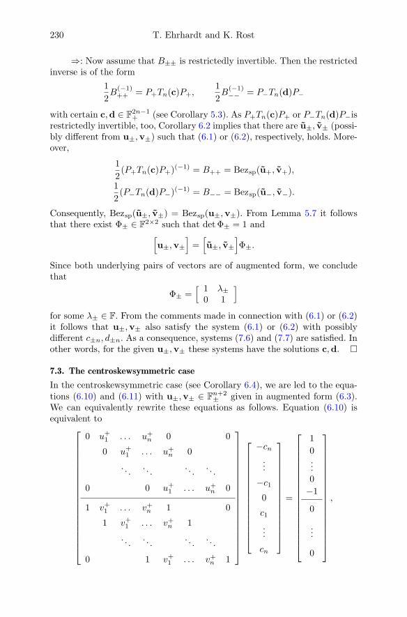
230 T. Ehrhardt and K. Rost
⇒: Now assume that B±± is restrictedly invertible. Then the restrictedinverse is of the form
1
2B
(−1)++ = P+Tn(c)P+,
1
2B
(−1)−− = P−Tn(d)P−
with certain c,d ∈ F2n−1+ (see Corollary 5.3). As P+Tn(c)P+ or P−Tn(d)P−is
restrictedly invertible, too, Corollary 6.2 implies that there are u±, v± (possi-bly different from u±,v±) such that (6.1) or (6.2), respectively, holds. More-over,
1
2(P+Tn(c)P+)(−1) = B++ = Bezsp(u+, v+),
1
2(P−Tn(d)P−)(−1) = B−− = Bezsp(u−, v−).
Consequently, Bezsp(u±, v±) = Bezsp(u±,v±). From Lemma 5.7 it followsthat there exist Φ± ∈ F2×2 such that det Φ± = 1 and[
u±,v±
]=[u±, v±
]Φ±.
Since both underlying pairs of vectors are of augmented form, we concludethat
Φ± =[
1 λ±0 1
]for some λ± ∈ F. From the comments made in connection with (6.1) or (6.2)it follows that u±,v± also satisfy the system (6.1) or (6.2) with possiblydifferent c±n, d±n. As a consequence, systems (7.6) and (7.7) are satisfied. Inother words, for the given u±,v± these systems have the solutions c,d.
7.3. The centroskewsymmetric case
In the centroskewsymmetric case (see Corollary 6.4), we are led to the equa-tions (6.10) and (6.11) with u±,v± ∈ Fn+2
± given in augmented form (6.3).We can equivalently rewrite these equations as follows. Equation (6.10) isequivalent to
0 u+1 . . . u+n 0 0
0 u+1 . . . u+n 0
. . .. . .
. . .. . .
0 0 u+1 . . . u+n 0
1 v+1 . . . v+n 1 0
1 v+1 . . . v+n 1
. . .. . .
. . .. . .
0 1 v+1 . . . v+n 1
−cn...
−c10
c1
...
cn
=
1
0...0
−1
0
...
0
,

Split-Bezoutians 231
and equation (6.11) is equivalent to
0 u−1 . . . u−n 0 0
0 u−1 . . . u−n 0
. . .. . .
. . .. . .
0 0 u−1 . . . u−n 0
1 v−1 . . . v−n −1 0
1 v−1 . . . v−n −1
. . .. . .
. . .. . .
0 1 v−1 . . . v−n −1
−dn...
−d10
d1
...
dn
=
−1
0...0
−1
0
...
0
.
As before, the underlying matrices are of size 2n × (2n + 1), where we haven rows containing the u±j and n rows containing the v±j .
We can also eliminate cn = −c−n and dn = −d−n in the same way asin Subsection 7.2. This leads to the following lemma.
Lemma 7.3. Let c,d ∈ F2n−1− , let u±,v± ∈ Fn+2
± be of the augmented form(6.3), let u± ∈ Fn± be the reduced vector (7.5) associated with u±.
(a) There exists cn = −c−n ∈ F such that (6.10) is true if and only if
Res1(u+ , v+) c =
[2P−e1
0
]. (7.8)
(b) There exists dn = −d−n ∈ F such that (6.11) is true if and only if
Res1(u− , v−) d =
[−2P+e1
0
]. (7.9)
The proof of the following theorem is completely analogous to that ofTheorem 7.2.
Theorem 7.4. Let u±,v± ∈ Fn+2± be of the form (6.3), and let B+− and B−+
be given by (6.12).
(a) B+− is restrictedly invertible if and only if equation (7.8) has a solutionc ∈ F2n+1
+ . In this case,
B(−1)+− =
1
2P−Tn(c)P+.
(b) B−+ is restrictedly invertible if and only if equation (7.9) has a solutiond ∈ F2n+1
+ . In this case,
B(−1)−+ =
1
2P+Tn(d)P−.

232 T. Ehrhardt and K. Rost
7.4. Kernels of resultant matrices
Theorems 7.2 and 7.4 tell us that if we want to invert split-Bezoutians of thevarious types, we are led to linear systems, namely (7.6), (7.7), (7.8), and(7.9), whose coefficient matrices are the (2n−2)× (2n−1) resultant matricesRes1(u±,v±). Here u±,v± ∈ Fn+2
± are of the augmented form (6.3), andu± ∈ Fn± are the reduced vectors (7.5). Note that in terms of the notation ofSection 7.1, we are in the setting of
p = 1, m1 = n− 1, m2 = n+ 1.
The afore-mentioned systems are inhomogeneous, and their solution vectorsc and d are sought in F2n−1
+ (in the centrosymmetric case) or in F2n−1− (in
the centroskewsymmetric case).It is worthwhile to look at the kernels of these resultant matrices, which
are non-trivial. According to Theorems 7.2 and 7.4, any solution to the afore-mentioned systems should give rise to the same inverse of the split-Bezoutianeven though c and d may not be unique. To see this directly, we need thefollowing lemma.
Lemma 7.5.
(a) Let n be even, u+,v+ ∈ Fn+2+ and assume that gcd(u+,v+) = t + 1.
Then
ker Res1(u+,v+) = lin
(1,−1, 1, . . . , 1,−1, 1)T.
(b) Let n be even, u−,v− ∈ Fn+2− and assume that gcd(u−,v−) = t − 1.
Then
ker Res1(u−,v−) = lin
(1, 1, 1, . . . , 1, 1, 1)T.
(c) Let n be odd, u+,v+ ∈ Fn+2+ and assume that gcd(u+,v+) = 1. Then
ker Res1(u+,v+) = lin q ,
where
q(t) = α(t)βJ(t)− β(t)αJ(t) ∈ F2n−1−
with u+(t)α(t) + v+(t)β(t) = 1, α ∈ Fn+1, and β ∈ Fn−1.
(d) Let n be odd, u−,v− ∈ Fn+2− and assume that gcd(u−,v−) = t2 − 1.
Then
ker Res1(u−,v−)
= lin
(1,−1, 1, . . . , 1,−1, 1)T , (1, 1, 1, . . . , 1, 1, 1)T.
Proof. Since v±(t) has no zero at t = 0 and at t = ∞ (the latter meansthat the polynomial v±(t) has the maximal degree n + 1) it follows thatgcd(u±,v±) = gcd(u±,v±). Furthermore, with the notation of Section 7.1,ν∞ = 0 in all cases. Hence, we have
ν = 1, ν = 1, ν = 0, ν = 2

Split-Bezoutians 233
in the cases (a), (b), (c), (d), respectively. As p = 1 in all cases, we get thatthe dimension of the kernel equals 1 in the cases (a), (b), (c), and 2 in thecase (d) (see formula (7.4)).
In the cases (a), (b), (d) the form of the kernel can be found by directinspection.
In the case (c) the kernel can be obtained as follows (see [1, Thm. 3.3]).Solve the Bezout equations
u+(t)α(t) + v+(t)β(t) = 1, uJ+(t)γJ(t) + vJ+(t)δJ(t) = 1,
with α,γ ∈ Fn+1and β, δ ∈ Fn−1, and put q(t) = α(t)δ(t) − β(t)γ(t).Since u+(t) and v+(t) are generalized coprime, the Bezout equations haveunique solutions, and because u+ and v+ are symmetric, it follows that
α = γJ and β = δJ . Then the one-dimensional kernel is spanned by thevector q ∈ F2n−1
− .
Note that in case (c) the kernel is spanned by a skewsymmetric vector,while in cases (a), (b), (d), the kernel consists of symmetric vectors.
To justify the above claim that two different solutions to the systemsconsidered in Theorems 7.2 and 7.4 lead to the same T +H matrices (of thevarious kinds), it suffices to consider the intersections of the correspondingkernels with the spaces of symmetric and skewsymmetric vectors, respectively,and compare them with Proposition 4.1. With the notation of Proposition 4.1we have
ker Res1(u±,v±) ∩ F2n−1+ = eα,±α : α ∈ F
in the case n even, and
ker Res1(u±,v±) ∩ F2n−1+ =
0 in the + case,eα,β : α, β ∈ F in the − case,
in the case n odd. Furthermore,
ker Res1(u±,v±) ∩ F2n−1− = 0
in the case n even.
8. Solution of the resultant equations
The goal of this section is to find solutions to the equations (7.6), (7.7), (7.8),and (7.9). In the centrosymmetric case, we have to distinguish between n evenand odd, while in the centroskewsymmetric case we only consider n even.
The basic observation is that these equations can be written in thelanguage of polynomials (in t and t−1). Observe that u±,v± are given inaugmented form (6.3), and that the corresponding reduced vector is given byu±(t) = 1
tu±(t). Using (7.2) we can reformulate (7.6) in the form
tu+( 1t )c(t) ≡ 1 + tn−1 mod . . . , t−3, t−2, t−1, tn, tn+1, tn+2, . . . ,
v+( 1t )c(t) ≡ 0 mod . . . , t−3, t−2, t−1, tn−2, tn−1, tn, . . . ,
(8.1)

234 T. Ehrhardt and K. Rost
while the resultant equation (7.7) is equivalent to
tu−( 1t )d(t) ≡ −1 + tn−1 mod . . . , t−3, t−2, t−1, tn, tn+1, tn+2, . . . ,
v−( 1t )d(t) ≡ 0 mod . . . , t−3, t−2, t−1, tn−2, tn−1, tn, . . . .
(8.2)
Regarding the centroskewsymmetric cases, the resultant equation (7.8) isequivalent to
tu+( 1t )c(t) ≡ 1− tn−1 mod . . . , t−3, t−2, t−1, tn, tn+1, tn+2, . . . ,
v+( 1t )c(t) ≡ 0 mod . . . , t−3, t−2, t−1, tn−2, tn−1, tn, . . . ,
(8.3)
and the resultant equation (7.9) is equivalent to
tu−( 1t )d(t) ≡ −1− tn−1 mod . . . , t−3, t−2, t−1, tn, tn+1, tn+2, . . . ,
v−( 1t )d(t) ≡ 0 mod . . . , t−3, t−2, t−1, tn−2, tn−1, tn, . . . .
(8.4)
8.1. The centrosymmetric case
We start with considering the systems (8.1) and (8.2), the solution of whichrelates to the restricted inverses of split-Bezoutians B±± (see Theorem 7.2).
Note that the restricted invertibility of these split-Bezoutians requiresthat the g.c.d. of u±(t) and v±(t) is minimal (see Corollary 5.3 and formu-las (5.3) and (5.4)). Hence it is natural to assume here the correspondingconditions of coprimeness.
As we have to distinguish between n even and odd, we end up with fourcases to consider. The proofs are similar to each other in certain respects.Hence we will give the most detailed arguments in the first case, while weconfine ourselves to the differences in the other cases.
Let us start with finding the solution of (8.1) in the case n is odd.Suppose u+,v+ ∈ Fn+2
+ are of the form (6.3) and assume gcd(u+,v+) = 1.Then the Bezout equation
u+(t)α0(t) + v+(t)β0(t) = 1 (8.5)
has unique solutions α0,β0 ∈ Fn+1. Recall that the solution c of (8.1) isrelated to the restricted inverse of the split-Bezoutian B++ = Bezsp(u+,v+)of size n× n.
Theorem 8.1. Let z(t) be the polynomial
z(t) = α0(t)βJ0 (t)− β0(t)αJ0 (t) ∈ F2n+1− [t], (8.6)
and let y(t) = (t2 − 1)z(t) ∈ F2n+3+ [t]. Then
c =
0 0 1 0 0 0...
.... . .
......
0 0 0 1 0 0
y ∈ F2n−1+
is a solution of (8.1).
Note that the vector c is obtained from the vector y by dropping thefirst and the last two entries.

Split-Bezoutians 235
Proof. We first notice that z = (zi)2ni=0 ∈ F2n+1
− , and therefore we can writez(t) = z0 + z1t+ · · · − z1t2n−1 − z0t2n. It follows that the polynomial y(t) isgiven by
y(t) = −z0 − z1t+ · · · − z1t2n+1 − z0t2n+2 ,
where we note only the first and last two coefficients. The vector c is obtainedfrom y by dropping these coefficients, i.e.,
c(t) = t−2(y(t) + z0t
2n+2 + z1t2n+1 + z1t+ z0
)=(
1− 1
t2
)z(t) + z0t
2n + z1t2n−1 + z1
1
t+ z0
1
t2.
Let us now verify the first equation in (8.1). Taking into account thatu+(0) = 0 and deg u+(t) ≤ n (see (6.3)) we get
tu+
(1
t
)c(t) = u+
(1
t
)((t− 1
t
)z(t) + z0t
2n+1 + z1t2n + z1 + z0
1
t
)≡ u+
(1
t
)(t− 1
t
)z(t).
Note that here “≡” signals that equality holds up to linear combinations oftk with k < 0 or k ≥ n. In what follows we are going to apply formulas (8.5)and (8.6), and use the symmetry of u+,v+ ∈ Fn+2, i.e.,
u+(t) = tn+1u+
(1
t
)and v+(t) = tn+1v+
(1
t
).
Furthermore, note that αJ0 (t) = tnα0(t−1) and βJ0 (t) = tnβ0(t−1). It followsthat
tu+
(1
t
)c(t)
≡ u+
(1
t
)(t− 1
t
)(α0(t)tnβ0
(1
t
)− β0(t)tnα0
(1
t
))=(t− 1
t
)(1
tα0(t)u+(t)β0
(1
t
)− tnα0
(1
t
)u+
(1
t
)β0(t)
)=(t− 1
t
)(1
t
(1− β0(t)v+(t)
)β0
(1
t
)− tn
(1− β0
(1
t
)v+
(1
t
))β0(t)
)=(t− 1
t
)(1
tβ0
(1
t
)− tnβ0(t)
)≡ β0
(1
t
)+ tn−1β0(t).
Now consider equation (8.5) and use that u+(0) = 0 and v+(0) = 1 (see(6.3)). We conclude that β0(0) = 1. From this it follows that
β0
(1
t
)+ tn−1β0(t) ≡ 1 + tn−1 .
Hence the first equation in (8.1) is satisfied.

236 T. Ehrhardt and K. Rost
Now let us verify the second equation in (8.1). Proceeding similar asbefore, but with deg v+(t) ≤ n+ 1, we obtain first
v+
(1
t
)c(t) = v+
(1
t
)((1− 1
t2
)z(t) + z0t
2n + z1t2n−1 + z1
1
t+ z0
1
t2
)≡ v+
(1
t
)(1− 1
t2
)z(t).
Here “≡” signals that equality holds up to linear combinations of tk withk < 0 or k ≥ n− 2. Furthermore,
v+
(1
t
)c(t)
≡ v+
(1
t
)(1− 1
t2
)(α0(t)tnβ0
(1
t
)− β0(t)tnα0
(1
t
))=(
1− 1
t2
)(tnα0(t)v+
(1
t
)β0
(1
t
)− 1
tα0
(1
t
)v+(t)β0(t)
)=(
1− 1
t2
)(tnα0(t)
(1− u+
(1
t
)α0
(1
t
))− 1
tα0
(1
t
)(1− u+(t)α0(t)
))=(
1− 1
t2
)(tnα0(t)− 1
tα0
(1
t
))≡ 0.
Hence the second equation in (8.1) is satisfied, too.
Next, let us find the solution of (8.2) in the case n is odd. This so-lution d corresponds to the restricted inverse of a split-Bezoutian, namelyB−− = Bezsp(u−,v−), where u−,v− ∈ Fn+2
− are of the form (6.3). Due to(2.5) we can always write
u−(t) = (1− t2)u0(t), v−(t) = (1− t2)v0(t),
where u0,v0 ∈ Fn+. It is natural to assume that gcd(u−,v−) is minimal(see (5.4)), and therefore we require that gcd(u0,v0) = 1. Then the Bezoutequation
u0(t)α0(t) + v0(t)β0(t) = 1 (8.7)
has unique solutions α0,β0 ∈ Fn−1.
Theorem 8.2. Let z(t) be the polynomial
z(t) = α0(t)βJ0 (t)− β0(t)αJ0 (t) ∈ F2n−3− [t]. (8.8)
Then
d(t) =t2
1− t2z(t) ∈ F2n−1
+ [t]
is a solution of (8.2).
Note that the vector d is obtained by adding two zeros at the beginningand two zeros at the end of the vector y where y(t) := 1
1−t2 z(t) ∈ F2n−5+ [t].
We remark that y is well defined due to (2.5).

Split-Bezoutians 237
Proof. We start with observing that u0(0) = 0,v0(0) = 1, and
t2
t2 − 1u−
(1
t
)= u0
(1
t
)= t−(n−1)u0(t).
A corresponding formula holds for v− and v0 as well.Let us consider the first equation in (8.2). Taking (8.7) and (8.8) into
account, we get
tu−
(1
t
)d(t) = u−
(1
t
) t3
1− t2
(α0(t)tn−2β0
(1
t
)− β0(t)tn−2α0
(1
t
))= −α0(t)u0(t)β0
(1
t
)+ tn−1α0
(1
t
)u0
(1
t
)β0(t)
= −(1− β0(t)v0(t)
)β0
(1
t
)+ tn−1
(1− β0
(1
t
)v0
(1
t
))β0(t)
= −β0
(1
t
)+ tn−1β0(t) ≡ −1 + tn−1.
Here β0(0) = 1. Along the same lines we obtain for the second equation in(8.2),
v−
(1
t
)d(t) = v−
(1
t
) t2
1− t2
(α0(t)tn−2β0
(1
t
)− β0(t)tn−2α0(
1
t)
)= −tn−2α0(t)v0
(1
t
)β0
(1
t
)+
1
tα0
(1
t
)v0(t)β0(t)
= −tn−2α0(t)
(1− u0
(1
t
)α0
(1
t
))+
1
tα0
(1
t
)(1− u0(t)α0(t)
)= −tn−2α0(t) +
1
tα0
(1
t
)≡ 0,
which completes the proof.
Now we turn to the case of n even. We first want to find a solution ofequation (8.1). Note that the solution c is related to the restricted inverse ofa split-Bezoutian of (++)type B++ = Bezsp(u+,v+) with u+,v+ ∈ Fn+2
+ ofthe form (6.3). Using (2.5) we can write
u+(t) = (1 + t)u0(t), v+(t) = (1 + t)v0(t).
with u0,v0 ∈ Fn+1+ . The natural assumption is that gcd(u+,v+) = 1 + t. In
other words, we will assume gcd(u0,v0) = 1. Then the Bezout equation
u0(t)α0(t) + v0(t)β0(t) = 1 (8.9)
has unique solutions α0,β0 ∈ Fn.
Theorem 8.3. Let z(t) be the polynomial
z(t) = α0(t)βJ0 (t)− β0(t)αJ0 (t) ∈ F2n−1− [t]. (8.10)
Then
c(t) =t− 1
t+ 1z(t) ∈ F2n−1
+ [t]
is a solution of (8.1).

238 T. Ehrhardt and K. Rost
Proof. First note that u0(0) = 1,v0(0) = 1, and
t
t+ 1u+
(1
t
)= u0
(1
t
)= t−nu0(t) .
For the first equation in (8.1) we obtain using (8.9),
tu+
(1
t
)c(t) = u+
(1
t
) t− 1
t+ 1
(α0(t)tnβ0
(1
t
)− β0(t)tnα0
(1
t
))=t− 1
t
(u0(t)α0(t)β0
(1
t
)− tnu0
(1
t
)α0
(1
t
)β0(t)
)=(
1− 1
t
)(β0
(1
t
)− tnβ0(t)
)≡ β0
(1
t
)+ tn−1β0(t) ≡ 1 + tn−1.
Here β0(0) = 1. For the second equation in (8.1) we have
v+
(1
t
)c(t) = v+
(1
t
) t− 1
t+ 1
(α0(t)tn−1β0
(1
t
)−α0
(1
t
)tn−1β0(t)
)=t− 1
t2
(tnv0
(1
t
)β0
(1
t
)α0(t)− v0(t)β0(t)α0
(1
t
))=t− 1
t2
(tnα0(t)−α0
(1
t
))≡ 0.
Hence the second equation in (8.1) is fulfilled.
It remains to find the solution of equation (8.2) in the case n is even.Here the solution d corresponds to a split-Bezoutian B−− = Bezsp(u−,v−)
of (−−)type with u−,v− ∈ Fn+2− of the form (6.3). The natural assumption
that gcd(u−,v−) = 1− t implies that we can write
u−(t) = (1− t)u0(t), v−(t) = (1− t)v0(t)
with gcd(u0,v0) = 1 and u0,v0 ∈ Fn+1+ . Then the Bezout equation
u0(t)α0(t) + v0(t)β0(t) = 1 (8.11)
has unique solutions α0,β0 ∈ Fn.
Theorem 8.4. Let z(t) be the polynomial
z(t) = α0(t)βJ0 (t)− β0(t)αJ0 (t) ∈ F2n−1− [t]. (8.12)
Then
d(t) =1 + t
1− tz(t) ∈ F2n−1
+ [t]
is a solution of (8.2).
Proof. Ast
t− 1u−
(1
t
)= u0
(1
t
)= t−nu0(t)

Split-Bezoutians 239
we obtain for the first equation
tu−
(1
t
)d(t) = u−
(1
t
)1 + t
1− t
(α0(t)tnβ0
(1
t
)− β0(t)tnα0
(1
t
))= −1 + t
t
(u0(t)α0(t)β0
(1
t
)− tnu0
(1
t
)α0
(1
t
)β0(t)
)= −
(1 +
1
t
)(β0
(1
t
)− tnβ0(t)
)≡ −β0
(1
t
)+ tn−1β0(t) ≡ −1 + tn−1
as β0(0) = 1. The verification of the second equation is analogous.
8.2. The centroskewsymmetric case
Let us now discuss the cases related to the split-Bezoutians of (±∓)type (seeTheorem 7.4). Here n is even, and our goal is to find solutions to the equations(8.3) and (8.4).
We start with equation (8.3), the solution of which corresponds to the re-stricted inverse of a split-BezoutianB+− defined in (6.12) with u+,v+ ∈ Fn+2
+
of the form (6.3). Due to (2.5) we can write
u+(t) = (1 + t)u0(t), v+(t) = (1 + t)v0(t)
with u0,v0 ∈ Fn+1+ . The results of Section 5.2 (see Corollary 5.6 and the
various representations of the split-Bezoutians) imply that B+− is restrictedlyinvertible if and only if gcd(u0,v0) = 1, which we will therefore assume. Thenthe Bezout equation
u0(t)α0(t) + v0(t)β0(t) = 1 (8.13)
has unique solutions α0,β0 ∈ Fn.
Theorem 8.5. Let c(t) be the polynomial
c(t) = α0(t)βJ0 (t)− β0(t)αJ0 (t) ∈ F2n−1− [t]. (8.14)
Then c is a solution of (8.3).
Proof. For the first equation in (8.3) we obtain
tu+
(1
t
)c(t) = (1 + t)u0
(1
t
)(α0(t)tn−1β0
(1
t
)− β0(t)tn−1α0
(1
t
))= (1 + t)
(1
tu0(t)α0(t)β0
(1
t
)− tn−1u0
(1
t
)α0
(1
t
)β0(t)
)= (1 + t)
(1
tβ0
(1
t
)− tn−1β0(t)
)≡ β0
(1
t
)− tn−1β0(t) ≡ 1− tn−1.

240 T. Ehrhardt and K. Rost
Here β0(0) = 1 since u+(0) = 0 and v+(0) = 1. For the second equation wehave
v+
(1
t
)c(t) =
(1 +
1
t
)v0
(1
t
)(α0(t)tn−1β0
(1
t
)− β0(t)tn−1α0
(1
t
))=(
1 +1
t
)(tn−1v0
(1
t
)β0
(1
t
)α0(t)− 1
tv0(t)β0(t)α0
(1
t
))=(
1 +1
t
)(tn−1α0(t)− 1
tα0
(1
t
))≡ 0.
Hence the second equation in (8.3) is fulfilled.
It remains to consider equation (8.4), whose solution corresponds to asplit-Bezoutian B−+ defined in (6.12) with u−,v− ∈ Fn+2
− being of the form(6.3). Here we can write
u−(t) = (1− t)u0(t), v−(t) = (1− t)v0(t)
with u0,v0 ∈ Fn+1+ . We will assume gcd(u0,v0) = 1. Then the Bezout equa-
tion
u0(t)α0(t) + v0(t)β0(t) = 1 (8.15)
has unique solutions α0,β0 ∈ Fn.
Theorem 8.6. Let d(t) be the polynomial
d(t) = −(α0(t)βJ0 (t)− β0(t)αJ0 (t)
)∈ F2n−1− [t]. (8.16)
Then d is a solution of (8.4).
Proof. For the first equation of (8.4) we obtain
tu−
(1
t
)d(t) = (1− t)u0
(1
t
)(α0(t)tn−1β0
(1
t
)− β0(t)tn−1α0
(1
t
))= (1− t)
(1
tu0(t)α0(t)β0
(1
t
)− tn−1u0
(1
t
)α0
(1
t
)β0(t)
)= (1− t)
(1
tβ0
(1
t
)− tn−1β0(t)
)≡ −β0
(1
t
)− tn−1β0(t)
≡ −1− tn−1.
Here β0(0) = 1. This proves the first equation. The verification of the secondequation is analogous.
9. Restricted inversion of split-Bezoutians
Using the results of the previous section and of Section 7 (Theorems 7.2and 7.4), we can establish the following results concerning the restrictedinvertibility of split-Bezoutians. For sake of presentation we split the results

Split-Bezoutians 241
into the cases n even and odd, and consider the different types of split-Bezoutians as subcases therein.
For all cases we rely on the following preparatory constructions. Givenf ,g ∈ Fn+1+i
+ with i ∈ −1, 0, 1, assume that the pair f(t),g(t) is coprime.
We are going to define z ∈ F2n−1+2i− as follows. First determine the (unique)
solutions of the Bezout equation
f(t)α(t) + g(t)β(t) = 1
with α,β ∈ Fn+i, and then define
z(t) = α(t)βJ(t)− β(t)αJ(t) ∈ F2n−1+2i− [t] . (9.1)
Theorem 9.1. Let n be even and f ,g ∈ Fn+1+ be such that f(t),g(t) is
coprime. Define z ∈ F2n−1− by (9.1).
(a) Then B++ = M t+1n−1Bezsp(f ,g)(M t+1
n−1)T is restrictedly invertible and
B(−1)++ =
1
2P+Tn(c)P+
with c(t) = t−1t+1z(t) ∈ F2n−1
+ [t].
(b) Then B−− = M t−1n−1Bezsp(f ,g)(M t−1
n−1)T is restrictedly invertible and
B(−1)−− =
1
2P−Tn(d)P−
with d(t) = 1+t1−tz(t) ∈ F2n−1
+ [t].
(c) Then B+− = M t+1n−1Bezsp(f ,g)(M t−1
n−1)T is restrictedly invertible and
B(−1)+− =
1
2P−Tn(c)P+
with c(t) = z(t) ∈ F2n−1− [t].
(d) Then B−+ = M t−1n−1Bezsp(f ,g)(M t+1
n−1)T is restrictedly invertible and
B(−1)−+ =
1
2P+Tn(d)P−
with d(t) = −z(t) ∈ F2n−1− [t].
Proof. For sake of definiteness, consider the case (a). The treatment of theother cases is analogous.
Let B++ = M t+1n−1Bezsp(f ,g)(M t+1
n−1)T be given with coprime polyno-mials f(t),g(t). Using the symmetry of these polynomials and that theycannot have a common zero (otherwise they are not coprime), it follows thatthere exists a Φ ∈ F2×2 with det Φ = 1 such that the vectors u0,v0 definedby
[ u0, v0 ] := [ f , g ] Φ
are in augmented form (6.3). So Bezsp(f ,g) = Bezsp(u0,v0) by Lemma 5.7,
and we obtain B++ = M t+1n−1Bezsp(u0,v0)(M t+1
n−1)T , where u0(t),v0(t) arecoprime as well. Define u+ and v+ by
u+(t) = (t+ 1)u0(t), v+(t) = (t+ 1)v0(t).

242 T. Ehrhardt and K. Rost
Then u+ and v+ are also in augmented form, and B++ = Bezsp(u+,v+).Now use Theorem 8.3 to see that the vector c defined there is a solution of(8.1). To distinguish that vector there from the vector c considered in thistheorem denote it by c.
Let us show that c = c. Indeed, recalling the definitions we have
c(t) =t− 1
t+ 1z(t), c(t) =
t− 1
t+ 1z(t)
with
z(t) = α0(t)βJ0 (t)− β0(t)αJ0 (t), z(t) = α(t)βJ(t)− β(t)αJ(t),
andu0(t)α0(t) + v0(t)β0(t) = 1, f(t)α(t) + g(t)β(t) = 1.
Since [u0, v0] = [f , g, ]Φ the uniqueness of the Bezout equations implies that
[α0, β0 ] = [α, β] Φ−T ,
where Φ−T stands for the inverse of the transpose matrix. Since
ΦT[
0 −11 0
]Φ =
[0 −11 0
]as det Φ = 1, it follows that z = z via straightforward considerations (com-pare the proof of Theorem 8.1 of [5]). Therefore c = c as desired.
It follows that the vector c defined in the present theorem satisfies (8.1).As noted at the beginning of Section 8, this means it satisfies (7.6).
Now recall Theorem 7.2 (a) to conclude that B++ is restrictedly invert-ible and that
B(−1)++ =
1
2P+Tn(c)P+.
This proves statement (a).For the remaining statements notice that we use Theorem 8.4 in case (b).
In cases (c) and (d) we take Theorems 8.5 and 8.6 into account. Furthermore,we utilize Theorem 7.2 (b) in case (b) and Theorem 7.4 in cases (c) and(d).
The proof of the result for the odd case is also completely analogousto the previous proof. Here we employ Theorems 8.1 and 8.2 together withTheorem 7.2 (a), (b).
Theorem 9.2. Let n be odd.
(a) Let f ,g ∈ Fn+2+ be such that f(t),g(t) is coprime. Define z ∈ F2n+1
−by (9.1). Then B++ = Bezsp(f ,g) is restrictedly invertible and
B(−1)++ =
1
2P+Tn(c)P+ ,
where
c =
0 0 1 0 0 0...
.... . .
......
0 0 0 1 0 0
y ∈ F2n−1+
with y(t) = (t2 − 1)z(t) ∈ F2n+3+ [t].

Split-Bezoutians 243
(b) Let f ,g ∈ Fn+ be such that f(t),g(t) is coprime. Define z ∈ F2n−3− by
(9.1). Then B−− = M t2−1n−2 Bezsp(f ,g)(M t2−1
n−2 )T is restrictedly invertibleand
B(−1)−− =
1
2P−Tn(d)P− ,
where
d(t) =t2
1− t2z(t) ∈ F2n−1
+ [t].
The algorithms resulting from Theorems 9.1 and 9.2 have a computa-tional complexity of O(n2). They require to apply the extended Euclidianalgorithm to solve Bezout equations and polynomial multiplications. Thepolynomial division by factors (t±1) can be done with linear complexity. Formore details see Remark 9.7 of [5].
By Proposition 3.1 the formulas in Theorems 9.1 and 9.2 lead to in-version formulas for centro(skew)symmetric T +H-Bezoutians. For instance,let n be even, and B be a centrosymmetric T + H-Bezoutian of order ngiven by its splitting B = B++ +B−−, where B±± are defined in (5.6) withfi(t),gi(t) coprime polynomials (i = 1, 2). Then
B−1 = B(−1)++ +B
(−1)−−
where B(−1)±± can be computed as in Theorem 9.1, part (a) with f1,g1 and
part (b) with f2,g2.In case n is odd, we use Theorem 9.2. For centroskewsymmetric T +H-
Bezoutians we apply Theorem 9.1 (c) and (d).
The formulas of Theorems 9.1 and 9.2 coincide with the formulas es-tablished in Section 9 of [5] (centrosymmetric case) and Section 6 of [4] (cen-troskewsymmetric case). In fact, we have shown here that they are true evenwithout the additional assumptions required in [5].
10. Examples
We are going to illustrate the algorithms obtained in the previous sectionwith some simple examples. We first focus on the four cases considered inTheorem 9.1 with n = 4. In all four cases we choose the vectors f ,g ∈ F5
+
given by
f(t) = t+ t2 + t3, g(t) = 1 + 2t2 + t4.
According to the definition (5.1) we get
Bezsp(f ,g) =
1 1 11 0 11 1 1
.

244 T. Ehrhardt and K. Rost
The four split-Bezoutians considered in Theorem 9.1 evaluate now to
B++ =
1 2 2 12 3 3 32 3 3 31 2 2 1
, B−− =
1 0 0 −10 −1 1 00 1 −1 0−1 0 0 1
,
B+− =
−1 0 0 1−2 1 −1 2−2 1 −1 2−1 0 0 1
, B−+ =
−1 −2 −2 −10 1 1 00 −1 −1 01 2 2 1
.To obtain the restricted inverses of these matrices, solve the Bezout equationf(t)α(t) + g(t)β(t) = 1, α,β ∈ F4 to get α(t) = −2 − t − t2 − t3 andβ(t) = 1+2t+t2. Then by (9.1) we obtain z(t) = 1+t−t2+t4−t5−t6 ∈ F7
−[t].For the centrosymmetric cases it follows that
c(t) =t− 1
t+ 1z(t) = −1 + t+ t2 − t3 + t4 + t5 − t6,
d(t) =1 + t
1− tz(t) = 1 + 3t+ 3t2 + 2t3 + 3t4 + 4t5 + t6,
and thus B(−1)++ = 1
4Tn(c)(I + Jn) and B(−1)−− = 1
4Tn(d)(I − Jn) evaluate to
B(−1)++ =
1
4
−3 2 2 −32 −1 −1 22 −1 −1 2−3 2 2 −3
, B(−1)−− =
1
4
1 0 0 −10 −1 1 00 1 −1 0−1 0 0 1
.For the centroskewsymmetric cases we have c = z and d = −z. Here then
B(−1)+− = 1
4Tn(c)(I + Jn) and B(−1)−+ = 1
4Tn(d)(I − Jn) evaluate to
B(−1)+− =
1
4
−1 0 0 −1−2 1 1 −22 −1 −1 21 0 0 1
, B(−1)−+ =
1
4
−1 −2 2 10 1 −1 00 1 −1 0−1 −2 2 1
.It can be verified straightforwardly that these are indeed the restricted in-verses.
Let us now illustrate Theorem 9.2. We consider n = 5 and start withcase (b), where we use the same f ,g ∈ F5 as before. Then the split-Bezoutianof (−−)type is
B−− =
1 1 0 −1 −11 0 0 0 −10 0 0 0 0−1 0 0 0 1−1 −1 0 1 1
.The polynomial z(t) is the same as above, and
z(t)
1− t2= 1 + t+ t3 + t4 ∈ F7
+[t],

Split-Bezoutians 245
which gives the vector d = (0, 0, 1, 1, 0, 1, 1, 0, 0) ∈ F9+ by adding zeros. The
corresponding restricted inverse is 14Tn(d)(I − Jn), i.e.,
B(−1)−− =
1
4
0 1 0 −1 01 −1 0 1 −10 0 0 0 0−1 1 0 −1 10 −1 0 1 0
.For the case (a) consider the following f ,g ∈ F7
+,
f(t) = t+ t2 + t3 + t4 + t5, g(t) = 1 + 3t2 + 3t4 + t6.
The Bezoutian B++ = Bezsp(f ,g) of (++)type is
B++ =
1 1 1 1 11 −1 2 −1 11 2 0 2 11 −1 2 −1 11 1 1 1 1
.The solutions α,β ∈ F6 of the Bezout equation are now
α(t) = −3− 4t− 5t2 − 4t3 − 2t4 − t5, β(t) = 1 + 3t+ 4t2 + 3t3 + t4.
It follows that
z(t) = 1 + 2t+ t2 − t3 − 2t4 + 2t6 + t7 − t8 − 2t9 − t10 ∈ F11− [t],
y(t) = −1− 2t+ 3t3 + 3t4 − t5 − t6 − t7 + 3t8 + 3t9 − 2t11 − t12 ∈ F13+ [t],
since y(t) = (t2 − 1)z(t). Thus c = (0, 3, 3,−1 − 4,−1, 3, 3, 0) ∈ F9+ by
chopping off four entries of y. The corresponding restricted inverse is
B(−1)++ =
1
4
−4 2 6 2 −42 −1 −2 −1 26 −2 −8 −2 62 −1 −2 −1 2−4 2 6 2 −4
,which is obtained from 1
4Tn(c)(I + Jn).
References
[1] T. Ehrhardt and K. Rost, On the kernel structure of generalized resultantmatrices, Indagationes Mathematicae 23 (2012), 1053–1069.
[2] T. Ehrhardt and K. Rost, Resultant matrices and inversion of Bezoutians,Linear Algebra Appl. 439 (2013), 621–639.
[3] T. Ehrhardt and K. Rost, Inversion of centrosymmetric Toeplitz-plus-HankelBezoutians, Electron. Trans. Numer. Anal. 42 (2014), 106–135.
[4] T. Ehrhardt and K. Rost, Inversion of centroskewsymmetric Toeplitz-plus-Hankel Bezoutians, Electron. J. Linear Algebra 30 (2015), 336–359.

246 T. Ehrhardt and K. Rost
[5] T. Ehrhardt and K. Rost, Fast inversion of centrosymmetric Toeplitz-plus-Hankel Bezoutians, Oper. Theory Adv. Appl. 259, 267–300, Birkhauser, 2017.
[6] I.C. Gohberg and A.A. Semencul, The inversion of finite Toeplitz matricesand their continuous analogues (in Russian), Mat. Issled. 7 (1972), no. 2(24),201–223, 290.
[7] M.C. Gouveia, Group and Moore-Penrose invertibility of Bezoutians, LinearAlgebra Appl. 197/198 (1994), 495–509.
[8] G. Heinig and U. Jungnickel, Hankel matrices generated by the Markov pa-rameters of rational functions, Linear Algebra Appl. 76 (1986), 121–135.
[9] G. Heinig and K. Rost, Algebraic methods for Toeplitz-like matrices and op-erators, Operator Theory: Advances and Applications 13, Birkhauser Verlag,Basel, 1984.
[10] G. Heinig and K. Rost, Fast inversion of Toeplitz-plus-Hankel matrices, Wiss.Z. Tech. Hochsch. Karl-Marx-Stadt 27 (1985), no. 1, 66–71.
[11] G. Heinig and K. Rost, On the inverses of Toeplitz-plus-Hankel matrices, Lin-ear Algebra Appl. 106 (1988), 39–52.
[12] G. Heinig and K. Rost, Hartley transform representations of inverses of realToeplitz-plus-Hankel matrices, In: Proceedings of the International Conferenceon Fourier Analysis and Applications (Kuwait, 1998), Numer. Funct. Anal.Optim. 21 (2000), 175–189.
[13] G. Heinig and K. Rost, Centrosymmetric and centro-skewsymmetric Toeplitz-plus-Hankel matrices and Bezoutians, Linear Algebra Appl. 366 (2003), 257–281.
[14] G. Heinig and K. Rost, Introduction to Bezoutians, Oper. Theory Adv. Appl.199, 25–118, Birkhauser, 2010.
[15] F.I. Lander, The Bezoutian and the inversion of Hankel and Toeplitz matrices(in Russian), Mat. Issled. 9 (1974), no. 2(32), 69–87, 249–250.
[16] A.B. Nersesyan and A.A. Papoyan, Construction of a matrix inverse to thesum of Toeplitz and Hankel matrices (in Russian), Izv. Akad. Nauk Armyan.SSR Ser. Mat. 18(2) (1983), 150–160.
[17] W.F. Trench, An algorithm for the inversion of finite Toeplitz matrices, J. Soc.Indust. Appl. Math. 12 (1964), 515–522.
[18] H.K. Wimmer, On the history of the Bezoutian and the resultant matrix,Linear Algebra Appl. 128 (1990), 27–34.
Torsten EhrhardtMathematics Department, University of CaliforniaSanta CruzCA-95064, U.S.A.e-mail: [email protected]
Karla RostFaculty of Mathematics, Technische Universitat ChemnitzReichenhainer Straße 39D-09126 Chemnitz, Germanye-mail: [email protected]

Generalized backward shift operators on thering [[x]], Cramer’s rule for infinite linearsystems, and p-adic integers
Sergey Gefter and Anna Goncharuk
Abstract. Let A be a generalized backward shift operator on Z[[x]] andf(x) be a formal power series with integer coefficients. A criterion forthe existence of a solution of the linear equation (Ay)(x) + f(x) = y(x)in Z[[x]] is obtained. An explicit formula for its unique solution in Z[[x]]is found as well. The main results are based on using the p-adic topologyon Z and on using a formal version of Cramer’s rule for solving infinitelinear systems.
Mathematics Subject Classification (2010). Primary 13J05; Secondary35C10, 35E05, 44A35.
Keywords. Formal power series, generalized backward shift operator,Cramer’s rule, p-adic integers, convolution.
1. Introduction
Let a = (a1, a2, a3, . . .) be a sequence of positive integers, such that thefollowing conditions hold:
1. infinitely many of ai are greater than 1;2. for each prime p, either p does not divide any of the numbers ai or p
divides an infinite number of the numbers ai.
We define the operator A on the ring of formal power series with integercoefficients by
A(y0 + y1x+ y2x2 + · · · ) = a1y1 + a2y2x+ a3y3x
2 + · · ·and consider the equation
(Ay)(x) + f(x) = y(x), (1.1)
where f(x) = f0 + f1x+ f2x2 + · · · ∈ Z[[x]].
This work was completed with the support by the Akhiezer Fond.
© Springer International Publishing AG, part of Springer Nature 2018
Theory: Advances and Applications 268, https://doi.org/10.1007/978-3-319-75996-8_13
247A. Böttcher et al. (eds.), The Diversity and Beauty of Applied Operator Theory, Operator

248 S. Gefter and A. Goncharuk
It will be shown that this equation has at most one solution, however,it may have no solutions (see the examples in Section 2). We also obtain acriterion for the existence of a solution and find an explicit formula for thissolution (see Theorem 4.2 and formula (4.1)).
Moreover we study the relation of equation (1.1) with an infinite linearsystem, which naturally arises from this equation. Infinite linear systems arestudied in numerous works (see, for example, [1]–[3]).
We show that if a solution exists, then it can be found using Cramer’srule, where, in order to introduce determinants of infinite matrices, we useconvergence in the p-adic and related topologies and on the integers Z (seeSections 3 and 4).
Notice, that if a = (1, 2, 3, 4, . . .), then conditions 1 and 2 hold and A isthe differentiation operator. Then equation (1.1) becomes y′(x)+f(x) = y(x).In the general case, the operator A can be regarded as an analogue of theGelfond–Leontjev generalized differentiation operator (see [4], [5]).
Besides, if a = (b, b, b, b, . . .), b 6= 1, then conditions 1 and 2 hold aswell and A = b · S∗, where S∗ is the backward shift operator. This operatoris widely used in the theory of functions, the theory of operators, and thealgebraic analysis (see, for example, [6]–[8]).
In Section 5 we introduce a special convolution generalizing the con-struction of the Hurwitz product for Laurent series (see [9, §1, Section 1.5]and [10]). Using this convolution we rewrite the solution of equation (1.1) ina form which is close to the usual one in linear differential equation theory(see Theorem 5.12). We can consider this result as an algebraic analogue ofTheorem 4.4 and Corollary 4.5 from [11]. In Section 5 we also consider someconcrete examples of equation (1.1).
2. Linear equations with a generalized backward shift operator
Lemma 2.1. Equation (1.1) has at most one solution in Z[[x]].
Proof. It suffices to prove that the homogeneous equation Ay = y has onlythe trivial solution. Let y(x) = y0 + y1x+ y2x
2 + · · · be its solution. Then
a1y1 + a2y2x+ a3y3x2 + · · · = y0 + y1x+ y2x
2 + · · · .We have yn = an+1yn+1 for all n. Thus, yn = y0
a1a2···an . Recall that all
the coefficients of the formal series y(x) are integers. Therefore, yn = 0, soy(x) = 0.
Remark 2.2. There are infinitely many solutions of (1.1) in Z[[x]] if an = 1
for all n greater than some n0. Actually, solving the homogeneous equation
we obtain yn = y0a1a2···an = y0
a1a2···an0for all n ≥ n0. So, we get different
solutions for all y0 divisible by a1a2 · · · an0. That is, condition 1 is essential
for uniqueness.
The next result is on a simple situation where the solution of the inho-mogeneous equation is unique.

Generalized backward shift operators 249
Lemma 2.3. Equation (1.1) with f(x) = f0 + f1x+ · · ·+ fnxn ∈ Z[x] being a
polynomial has exactly one solution in Z[x].
Proof. It is not difficult to check that the polynomial
f(x) + (Af)(x) + (A2f)(x) + (A3f)(x) + · · · .
is a solution.
From Lemmas 2.1 and 2.3 we obtain the following statement.
Theorem 2.4. The set of formal power series f(x) with integer coefficientssuch that equation (1.1) has a solution with integer coefficients is uncountable.Moreover, it is a dense submodule of the space of formal power series withinteger coefficients equipped with the Krull topology.
Proof. For the Krull topology, see [12, Ch. 1, §3, Sec. 4]. Actually, we canconstruct the inhomogeneity if we know a solution: f(x) = y(x)−(Ay)(x), andwe have an uncountable set of the power series with integer coefficients whichcould be a solution. There is a solution for all polynomial inhomogeneities,and as the set of polynomials is dense in Z[[x]], so the set of formal powerseries with integer coefficients f(x) such that equation (1.1) has a solutionwith integer coefficients is dense in the Krull topology.
Example. Consider (1.1) with a = (2, 2, . . .) and f(x) = 1+x+x2 +x3 + · · · ,that is,
2(S∗y)(x) + 1 + x+ x2 + x3 + · · · = y(x). (2.1)
It is easy to verify that this equation has y(x) = −1 − x − x2 − x3 − · · · asthe unique solution from Z[[x]].
The next examples show that equation (1.1) not necessarily has a solu-tion from Z[[x]].
Example. Consider (1.1) with a = (3, 3, . . .) and f(x) = 1+x+x2 +x3 + · · · ,that is, the equation
3(S∗y)(x) + 1 + x+ x2 + x3 + · · · = y(x). (2.2)
Let us prove that there are no solutions in Z[[x]]. If y(x) = y0+y1x+y2x2+· · ·
is a solution, then the following equality holds:
3y1 + 3y2x+ 3y3x2 + · · ·+ 1 + x+ x2 + x3 + · · · = y0 + y1x+ y2x
2 + · · · .
Therefore, there is a sequence yn ⊂ Z so that the equalities 3yn+1 +1 = ynhold for all n. Notice, that the sequence yn+1 also satisfies these equalities.As the solution is unique the sequences yn and yn+1 coincide. Becauseyn = yn+1 for all n, then yn = − 1
2 , so there is no integer solution of thisequation.
Example. Consider equation (1.1) where we choose a = (1, 2, 3, 4, . . .) andf(x) = 1 + x+ x2 + x3 + · · · , that is,
y′(x) + 1 + x+ x2 + x3 + · · · = y(x). (2.3)

250 S. Gefter and A. Goncharuk
Let us prove that there are no solutions in Z[[x]]. If y(x) = y0+y1x+y2x2+· · ·
is a solution, we have
y1 +2y2x+3y3x2 +4y4x
3 + · · ·+1+x+x2 +x3 + · · · = y0 +y1x+y2x2 + · · · .
Therefore, there is a sequence yn, yn ∈ Z such that for all n the equalitiesnyn + 1 = yn−1 hold. Then, yn+1 = yn−1
n+1 .
If y0 = 0, then y1 = −1, y2 = −1, y3 = − 23 . But we supposed the
coefficients to be integers. Obviously, if yn = 0, then yn+1 = − 1n+1 , which is
not an integer if n ≥ 1. Now suppose that yn 6= 0 for all n. Considering |yn|if n > 2 we get
|yn| ≤1
n(|yn−1|+ 1) =
1
n|yn−1|+
1
n<
1
n|yn−1|+
n− 1
n|yn−1| = |yn−1|.
Here we used that yn ∈ Z and yn 6= 0, so |yn−1| > 1n−1 if n > 2 and
n−1n |yn−1| >
1n . So, we get |yn| < |yn−1| for all n. This is impossible for the
integer coefficients.
Remark 2.5. There are infinitely many solutions of (1.1) in the ring Q[[x]]: wecan find a unique solution of this equation for each initial condition y(0) ∈ Q.
3. Cramer’s rule
As we saw in Section 2, equation (1.1) has at most one solution in Z[[x]], butit may have no solution. Let us try to find the solution of (1.1) assuming thatit exists.
Substituting the solution y(x) = y0 + y1x+ y2x2 + · · · into the equation
Ay + f(x) = y we get
a1y1+a2y2x+a3y3x2+· · ·+f0+f1x+f2x
2+f3x3+· · · = y0+y1x+y2x
2+· · · ,
which leads to a recurrence formula for the coefficients of y(x), namelyan+1yn+1 + fn = yn. It can be rewritten as an infinite system of linearequations:
By = f, where B =
1 −a1 0 0 · · ·0 1 −a2 0 · · ·0 0 1 −a3 · · ·0 0 0 1 · · ·...
......
.... . .
, f =
f0f1f2f3...
. (3.1)
Let us try to solve this system using the “formal” Cramer rule. Let Bibe the matrix formed by replacing the i-th column of B by f . Then
B0 =
f0 −a1 0 0 · · ·f1 1 −a2 0 · · ·f2 0 1 −a3 · · ·f3 0 0 1 · · ·...
......
.... . .
, B1 =
1 f0 0 0 · · ·0 f1 −a2 0 · · ·0 f2 1 −a3 · · ·0 f3 0 1 · · ·...
......
.... . .
, . . . .

Generalized backward shift operators 251
By the formal Cramer rule, the “solution” of the system (3.1) is the sequenceyn given by yn = detBn
detB . We are going to give meaning to the expressionsdetBn and detB. At first, let us denote the principal minor of order k of amatrix M as detM (k). In Section 4 we will show that detBn and detB canbe regarded as certain limits: detBn = lim
k→∞detB(k)
n , detB = limk→∞
detB(k).
Let us find explicit expressions for detB(k)n . Obviously,
detB(n+1)n = det
1 −a1 0 · · · f00 1 −a2 · · · f10 0 1 · · · f20 0 0 · · · f3...
......
. . ....
0 0 0 · · · fn
= fn.
If k > n, then
detB(k+1)n = det
1 −a1 · · · f0 0 · · · 00 1 · · · f1 0 · · · 0...
......
......
. . ....
0 0 · · · fn 0 · · · 0...
.... . .
......
. . ....
0 0 · · · fk−1 0 · · · −ak0 0 · · · fk 0 · · · 1
= detB(k)
n + fkan+1an+2 · · · ak.
Hence, detB(k)n = fn +
∑ks=n+1 fsan+1 · · · as =
∑ks=n fsan+1an+2 · · · as.
Thus, we have the formal equalities
detB = 1 and (3.2)
yn =detBndetB
=∞∑j=0
fn+jan+1an+2 · · · an+j . (3.3)
In the next section these equalities will be justified.
Remark 3.1. Let us solve system (3.1) finding the inverse matrix of B. Wecan construct it “algebraically” as the adjugate matrix of B. This gives
B−1 =
1 a1 a1a2 a1a2a3 a1a2a3a4 · · ·0 1 a2 a2a3 a2a3a4 · · ·0 0 1 a3 a3a4 · · ·0 0 0 1 a4 · · ·0 0 0 0 1 · · ·...
.... . .
......
. . .
.
Now the infinite sums (3.3) of integers appear when multiplying this matrixby the vector f .

252 S. Gefter and A. Goncharuk
4. Using p-adic and related topologies
We denote by a the sequence obtained from a = (a1, a2, a3, . . .) by deleting allak which are equal to 1. By condition 1 of Section 1, a is an infinite sequenceof integers (all greater than 1). Let Za be the ring of a-adic integers with thestandard topology (see [13, Chapter 2, §10]). For example, if p is a prime anda = (p, p, p, . . .), then Za is the ring of p-adic integers Zp (see [14, §3]). Belowwe use the following fact: the series
∑∞n=0 xn with xn ∈ Za converges in Za
if and only if xn → 0 in Za.We first consider the question about the solvability of Ay+ f(x) = y in
the ring Za[[x]].
Theorem 4.1. Let f ∈ Z[[x]]. Equation (1.1) has the following unique solutionin Za[[x]] :
y(x) = f(x) + (Af)(x) + (A2f)(x) + (A3f)(x) + · · · , (4.1)
where the sum on the right hand side converges in Za[[x]] in the topology ofcoefficientwise convergence.
Proof. First we prove the uniqueness. Solving the homogeneous equation, weobtain the recurrence formula yn = an+1yn+1. Hence y0 = a1 · · · anyn. Noticethat the sequence a1 · · · an tends to zero in Za. So y0 = 0. Similarly, we obtainthat yn = 0 for n ≥ 1. Thus, y = 0.
Let f(x) = f0 + f1x+ f2x2 + · · · ∈ Z[[x]]. Consider the formal sum
f(x) + (Af)(x) + (A2f)(x) + (A3f)(x) + · · · .Notice that every formal power series g(x) may be expressed in the followingway:
g(x) = g(0) +(Ag)(0)
a1x+
(A2g)(0)
a1a2x2 +
(A3g)(0)
a1a2a3x3 + · · · .
It is a certain analogue of the Taylor series expansion. We expand each termof the series in the similar way and regroup terms, obtaining
f(x) + (Af)(x) + (A2f)(x) + (A3f)(x) + · · ·
=
(f(0) +
Af(0)
a1x+
A2f(0)
a1a2x2 + · · ·
)+
(Af(0) +
A2f(0)
a1x+
A3f(0)
a1a2x2 + · · ·
)+
(A2f(0) +
A3f(0)
a1x+
A4f(0)
a1a2x2 + · · ·
)+ · · ·
= (f(0) +Af(0) +A2f(0) + · · · )
+
(Af(0)
a1+A2f(0)
a1+A3f(0)
a1+ · · ·
)x
+
(A2f(0)
a1a2+A3f(0)
a1a2+A4f(0)
a1a2+ · · ·
)x2 + · · · .

Generalized backward shift operators 253
We first show that each of the series that occurs as the coefficient of a powerof x converges in Za. Indeed, the n-th term in the coefficient of xm has theform
(Am+nf)(0)
a1 · · · am= am+1 · · · am+nfm+n.
Therefore it tends to zero in Za as n → ∞ (actually, for all j there exist nsuch that am+1 · · · am+n is divisible by aj , because each prime divisor of ajdivides an infinite number of ai due to condition 2 from Section 1). Since eachterm tends to zero, the series converges. Thus the coefficient of xm belongsto Za for every m. So, the series in the right-hand side of (4.1) is well definedas an element of Za[[x]]. It is easy to check that this series is a solution of(1.1).
The next theorem is a criterion for equation (1.1) to have a solution inthe ring Z[[x]].
Theorem 4.2. Let f ∈ Z[[x]], f(x) = f0 + f1x + f2x2 + · · · . The following
statements are equivalent:
(1) f0 + a1f1 + a1a2f2 + a1a2a3f3 + a1a2a3a4f4 + · · · ∈ Z in Za.(2) The equation Ay + f(x) = y has a solution in Z[[x]].
Proof. By Theorem 4.1, the unique solution of our equation is of the form(4.1). Let us prove that, if the statement (1) holds, then it belongs to Z[[x]].In other words, let us prove that the coefficient of xn is an integer for everyn. The proof is by induction. For y0, note that
y0 = f0 + a1f1 + a1a2f2 + a1a2a3f3 + · · · .
This is an integer due to our assumption. Now suppose that the k-th coeffi-cient
yk = fk + ak+1fk+1 + ak+1ak+2fk+2 + · · ·
is an integer. We need to prove that the k + 1-st coefficient
yk+1 = fk+1 + ak+2fk+2 + ak+2ak+3fk+3 + · · ·
is an integer as well. We have yk+1 = yk−fkak+1
. Since fk ∈ Z we conclude that
ak+1fk+1 + ak+1ak+2fk+2 + ak+1ak+2ak+3fk+3 + · · · is an integer. We provethat the sum of this series is divisible by ak+1. To this end, we make use ofthe following lemma.
Lemma 4.3. Let rn be a sequence from Z. If akrn → l in Za as n → ∞,then ak|l.
Proof. Since akrn → l, it follows that σ(akrn, l)a → 0, where σ is the stan-dard metric on Za (see [13, Chapter 2, §10]). Then there exists an n0 suchthat akrn − l is divisible by ak for all n > n0. Thus, l is divisible by ak, andrn → l
ak.

254 S. Gefter and A. Goncharuk
Therefore, if each term of a series, considered over Za, is divisible by ak,then the sum of the series is also divisible by ak. Moreover, if
∑∞n=1 akrn = l,
then∑∞n=1 rn = l
ak.
Let us now return to the proof of the theorem. We have that all terms ofthe series ak+1fk+1 + ak+1ak+2fk+2 + ak+1ak+2ak+3fk+3 + · · · , whose sumis equal to yk − fk, are divisible by ak+1. Using the lemma, we get thatthe sum of the series is also divisible by ak+1. Thus, the sum of the series
fk+1 + ak+2fk+2 + ak+2ak+3fk+3 + · · · = yk−fkak+1
is an integer.
Now we can give meaning to the formal designs from Section 3.
Corollary 4.4. If equation (1.1) has a solution in Z[[x]], then it is uniqueand its coefficients may be found, using Cramer’s rule, as yk = detBk
detB , wherethe determinants of B, Bn are the limits of the principal minors of thesematrices in Za, i.e.,
detB = limk→∞
B(k), detBn = limk→∞
B(k)n .
5. Some particular cases
5.1. Differential equations
If a = (b, 2b, 3b, 4b, 5b, . . .), then (1.1) is the differential equation
by′(x) + f(x) = y(x). (5.1)
By Theorem 4.2 the solution of this equation can be written as
y(x) = f(x) + bf ′(x) + b2f ′′(x) + b3f ′′′(x) + · · · (5.2)
in Za[[x]], and the equation has the solution in Z[[x]] if and only if
f0 + bf1 + 2!b2f2 + 3!b3f3 + 4!b4f4 + · · · ∈ Z.
Besides, in this case we can formulate another condition for the existence ofa solution of this equation. To this end let us prove the following lemma.
Lemma 5.1. Suppose c ∈ Z and rn is a sequence from Z. Then the followingstatements are equivalent:
(1) rn → c in Za, where a = (b, 2b, 3b, 4b, . . .).(2) rn → c in Zp for all prime p.
Proof. The statement (1) means that σ(rn, c)a → 0. Then for each m thereexists an n0 such that rn−c is divisible by a0a1a2 · · · am = m!bm+1 if n > n0.So for every power pk of a prime p there exists an n0 such that rn−c is divisibleby pk if n > n0. Therefore, ||rn − c||p → 0, where || · ||p is the standard normin Zp. The reverse can be proved similarly, because m!bm+1 can be writtenas a product of primes.
Using this lemma and Theorem 4.2, we get the following theorem.

Generalized backward shift operators 255
Theorem 5.2. The following statements are equivalent:
(1) There exist c ∈ Z such that f0 + 1!bf1 + 2!b2f2 + · · · = c in Zp for allprimes p.
(2) The equation by′ + f(x) = y has a solution from Z[[x]].
Example. Let us return to the example from Section 2 and consider theequation (2.3).
Using the previous theorem we obtain, that this equation has a solutionif and only if 1 + 1! + 2! + 3! + 4! + · · · is integer in Zp for all p. As the sum ofthe factorials is not integer in Zp, we conclude once more that this equationhas no solution in Z[[x]].
Example. Consider the equation y′(x) + x+ 2x2 + 3x3 + · · · = y(x).One easily proves 1 ·1!+2 ·2!+3 ·3!+4 ·4!+ · · ·+n ·n! = (n+1)!−1. In
Zp the sequence (n+ 1)! tends to zero, so (n+ 1)!−1 tends to −1. Therefore,1 · 1! + 2 · 2! + 3 · 3! + 4 · 4! + · · · = −1 is in Zp for all p. Consequently, thisequation has a solution. It is not difficult to check that the following series isits solution: y(x) = −1− x− x2 − x3 − · · · .
Now we are going to rewrite the solution (5.2) of equation (5.1) in theform that is usual in the theory of linear differential equations, namely, as aconvolution of a fundamental solution with the inhomogeneity. So, we needto introduce the notion of a special convolution of an element from 1
xZ[[ 1x ]]and an element from Z[[x]].
First let us consider the convolution of a formal Laurent series with onlynegative powers on Z and a polynomial on Z (see [15, Section 3]).
Definition 5.3. Suppose Q(x) = q1x + q2
x2 + q3x3 + · · · ∈ 1
xZ[[ 1x ]] and f(x) ∈ Z[x].By definition, put
(Q ∗ f)(x) = Resy(Q(y)f(x− y)), (5.3)
where Resy is the formal residue (see [16, Section 2.1]).
Here we consider f(x− y) as an element of Z[x][y], i.e., as a polynomialin y the coefficients of which are polynomials in x,
f(x− y) = f(x)− f ′(x)
1!y +
f ′′(x)
2!y2 − f ′′′(x)
3!y3 +
f (4)(x)
4!y4 − · · · .
This is well defined; all the coefficients of f (k)(x) are divisible by k!.The product Q(y)f(x−y) is an element from Z[x][[y, 1y ]], i.e., a two-sided
formal Laurent series in the variable y with coefficients in Z[x].From the definition of this convolution we obtain an explicit formula for
the convolution:
(Q∗f)(x) = q1f(x)− q21!f ′(x)+
q32!f ′′(x)− q4
3!f ′′′(x)+
q54!f (4)(x)−· · · . (5.4)
If we try to define the convolution of an element from 1xZ[[ 1x ]] and an
element from Z[[x]] similarly using the formula (5.3), we will obtain sums ofan infinite number of integers. Actually, if f(x) =
∑∞k=0 fkx
k ∈ Z[[x]], thenf(x − y) is a power series in y with coefficients which are power series in x.

256 S. Gefter and A. Goncharuk
Then the formal product Q(y)f(x− y) has infinite sums of integers as “coef-ficients”, and these do not necessarily exist in a p-adic sense.
The “coefficient” of yn in (5.3) is for all n > 0 given by
∞∑k=1
(−1)n+kqkf(n+k)(x)
(n+ k)!. (5.5)
Then the “coefficient” of xm in the “series” (5.5) is, again for all n > 0, equalto
∞∑k=1
(−1)n+k(n+m+ k)!
(n+ k)!m!fn+m+kqk. (5.6)
For all n > 0, the “coefficient” in (5.3) of 1yn is
∞∑k=0
(−1)kqn+kf
(k)(x)
k!. (5.7)
Then, again for all n > 0, the “coefficient” of xm in the “series” (5.7) equals
∞∑k=0
(−1)k(m+ k)!
m!k!fm+kqn+k. (5.8)
Lemma 5.4. Let Q(x) = q1x + q2
x2 + · · · + qnxn + · · · be from 1
xZ[[ 1x ]] and let
f(x) =∑∞i=0 fkx
k be from Z[[x]], and suppose qi tends to zero in Zp as
i → ∞. Then the sequences (n+m+i)!(n+i)!m! fn+m+iqi and (m+i)!
m!i! fm+iqn+i tend to
zero in Zp as i→∞, so the series (5.6) and (5.8) converge in Zp. Therefore,
Q(y)f(x− y) ∈ Zp[[x]][[y, 1y ]].
Using Lemma 5.4 we can define a convolution of the two, Q ∈ 1xZ[[ 1x ]]
and f ∈ Z[[x]].
Definition 5.5. Let qi → 0 in Zp, Q =∑∞k=1
qkxk ∈ 1
xZ[[ 1x ]], and f ∈ Z[[x]]. Bydefinition, put
(Q ∗ f)(x) = Resy(Q(y)f(x− y)), (5.9)
where Resy is the formal residue.
As a result of the convolution we get an element in Zp[[x]] and it canbe represented by the formula (5.4).
From Theorem 4.2 we now obtain the following.
Theorem 5.6. Suppose (5.1) has a solution in Z[[x]]. Then this solution has
the form of the convolution Eb ∗ f , where Eb(x) = 1x −
1!bx2 + 2!b2
x3 − 3!b3
x4 + · · ·is the Euler series.
That means we can regard the Euler series as a fundamental solution ofequation (5.1) (see [17, Section 4.4]).

Generalized backward shift operators 257
5.2. The backward shift operator
Let b ∈ N and a = (b, b, b, b, . . .). Then A = bS∗ where S∗ is the backwardshift operator, and equation (1.1) can be written as
b(S∗y)(x) + f(x) = y(x). (5.10)
Notice that in the case b = 1 equation (5.10) has an infinite numberof solutions in Z[[x]], while in all other cases it has at most one solution. Inwhat follows we assume that b > 1, since otherwise condition 1 of Section 1is violated. Then a matches with a, so Za = Za.
By Theorem 4.2 the equation has a solution from Z[[x]] if and only iff0 + bf1 + b2f2 + b3f3 + · · · ∈ Z in Za, and the solution can then be writtenas
y(x) = f(x) + bS∗(f)(x) + b2(S∗)2(f)(x) + b3(S∗)3(f)(x) + · · · .In this case we can reformulate Theorem 4.2 using the next lemma.
Lemma 5.7. Suppose c ∈ Z and rn is a sequence from Z. Then the followingstatements are equivalent:
(1) rn → c in Za, where a = (b, b, b, . . .).(2) rn → c in Zp for all prime divisors of b.
Proof. The statement (1) means that σ(rn, c)a → 0. Then for each m thereexists an n0 such that rn − c is divisible by a0a1a2 · · · am = bm if n > n0. Ifp is a divisor of b, then rn − c is divisible by pm. So for every power pk ofa prime p|b there exists an n0 such that rn − c is divisible by pk if n > n0.Therefore, ||rn − c||p → 0. The reverse can be proved similarly, because bm
can be written as the product of the prime divisors of b.
From this we get the following theorem.
Theorem 5.8. The following statements are equivalent:
(1) There exists a c ∈ Z such that f0 + bf1 + b2f2 + b3f3 + · · · = c in Zp forall prime divisors of b.
(2) The equation b(S∗y) + f(x) = y has a solution in Z[[x]].
Example. Let us consider the equation (2.1). In this case
f0 + bf1 + b2f2 + b3f3 + · · · = 1 + 2 + 22 + 23 + · · · .Note that 1 + 2 + 22 + 23 + · · ·+ 2k = 2k+1 − 1→ −1 when k →∞, so thissum is equal to −1.
Example. Now consider (2.2). In this case f0+bf1+b2f2+b3f3+ · · · becomes
1+3+32+33+· · · /∈ Z in Z3. Note that 1+3+32+33+· · ·+3k = 3k+1−12 → − 1
2
as k → ∞, so this sum is equal to − 12 in Z3. So we once more see that this
equation has no solution in Z[[x]].
Now we are going to rewrite the solution of equation (5.10) in the formof a convolution of a fundamental solution with the inhomogeneity. We needto introduce a convolution of an element from 1
xZ[[ 1x ]] and an element fromZ[[x]] for equation (5.10) similarly to formula (5.4).

258 S. Gefter and A. Goncharuk
Definition 5.9. Let p be a prime. Suppose Q(x) = q1x + q2
x2 + q3x3 + · · · , where
qi tends to zero in Zp and f(x) = f0 + f1x+ f2x2 + · · · . By definition, put
(Q ∗ f)(x) = q1f(x)− q2S∗f(x) + q3(S∗)2f(x)− q4(S∗)3f(x) + · · · . (5.11)
The coefficient of xn in (5.11) is q1fn− q2fn+1 + q3fn+2− q4fn+3 + · · · .Obviously qi+1fn+i tends to zero as i → ∞ in Zp. Then the series (5.11)converges, so the convolution is well defined and its result is included in Zp.
Similarly to Theorem 5.6, we obtain the following statement.
Theorem 5.10. Suppose there exists a solution of equation (5.10) that belongsto Z[[x]]. Then this solution has the form of the convolution ∆b ∗ f , where
∆b(x) = 1x −
bx2 + b2
x3 − b3
x4 + · · · .
5.3. A convolution over Za
To define the convolution of a Laurent series Q(x) = q1x + q2
x2 + q3x3· · · ∈ 1
xZ[[ 1x ]]
with a power series f(x) = f0 + f1x + f2x2 + · · · ∈ Z[[x]] over Za, we need
conditions that are stronger than those in the previous cases: suppose qi is
divisible by a1a2 · · · ai−1.
Definition 5.11. Similarly to the formula (5.4), put, by definition,
(Q ∗ f)A = q1f −q2A(f)
a1+q3A
2(f)
a1a2− q4A
3(f)
a1a2a3+ · · · . (5.12)
The coefficient of xn in (5.12) is
q1fn −q2an+1fn+1
a1+q3an+1an+2fn+2
a1a2− q4an+1an+2an+3fn+3
a1a2a3+ · · · .
Because qia1···ai 1
is an integer and an+1an+2 · · · an+i−1 tends to zero in Zaas i → ∞, this series converges in Za. Therefore the convolution belongs toZa[[x]].
From Theorem 4.2 we obtain the following result.
Theorem 5.12. Suppose there exists a solution of equation (1.1) belonging toZ[[x]]. Then this solution has the form of the convolution E ∗ f , where wehave E(x) = 1
x −a1x2 + a1a2
x3 − a1a2a3x4 + · · · .
Then we can regard the series E(x) = 1x −
a1x2 + a1a2
x3 − a1a2a3x4 + · · · as a
fundamental solution of the equation (Ay)(x) + f(x) = y(x).
References
[1] J. Combes, Sur la resolution de certains systemes infinis d’equations lineaires,Annales de la Faculte des sciences de Toulouse: Mathematiques 28 (1964), no.1, 149–159.
[2] R.G. Cooke, Infinite Matrices and Sequence Spaces, Dover, 1955.
[3] P.N. Shivakumar and K.C. Shivakumar, A rewiew of infinite matrices and theirapplications, Linear Algebra and its Applications 430 (2009), 976–998.
−
Generalized backward shift operators 259
[4] A.O. Gel’fond and A.F. Leont’ev, On a generalization of Fourier series, Mat.Sb. (N.S.) 29(71) (1951), no. 3, 477–500.
[5] Ju.F. Korobeinik, Compound operator equations in generalized derivatives andtheir applications to Appell sequences, Mathematics of the USSR-Sbornik 31(1977), no. 4, 425–443.
[6] R.G. Douglas, H.S. Shapiro, and A.L. Shields, On cyclic vectors of the backwardshift, Bull. Amer. Math. Soc. 73 (1967), no. 1, 156–159.
[7] N.K. Nikol’skii, Treatise on the Shift Operator. Spectral Function Theory,Spinger-Verlag, 1986.
[8] D. Przeworska-Rolewicz, Logarithms and Antilogarithms. An Algebraic Analy-sis Approach, Kluwer Academic Publishers, 1998.
[9] L. Bieberbach, Analytische Fortsetzung, Springer, 1955.
[10] A. Hurwitz, Sur un theoreme de M. Hadamard, C.R. Acad. Sci. 128 (1899),350–353.
[11] S. Gefter and T. Stulova, On some vector differential operators of infinite order,Operator Theory: Advances and Applications 236, 193–203, Birkhauser, 2014.
[12] H. Grauert and R. Remmert, Analytische Stellenalgebren, Springer-Verlag,1971.
[13] E. Hewitt and K.A. Ross, Abstract Harmonic Analysis: Volume I, Structureof Topological Groups Integration Theory Group Representations, Springer-Verlag, 1963.
[14] Z.I. Borevich and I.R. Shafarevich, Number Theory, Academic Press Inc.,1966.
[15] S. Gefter and A. Goncharuk, Fundamental solution of an implicit linear inho-mogeneous first order differential equation over an arbitrary ring, Journal ofMathematical Sciences 219 (2016), no. 6, 922–935.
[16] V.G. Kac, Vertex Algebras for Beginners, 2nd ed., University Lecture Series10, American Mathematical Society, 1998.
[17] L. Hormander, The Analysis of Linear Partial Differential Operators I: Distri-bution Theory and Fourier Analysis, Springer-Verlag, 1983.
Sergey Gefter and Anna GoncharukV.N. Karazin Kharkiv National UniversitySchool of Mathematics and Computer Sciences4 sq. Svoboda61022 KharkivUkrainee-mail: [email protected]

Feynman path integral regularization usingFourier Integral Operator ζ-functions
Tobias Hartung
Abstract. We will have a closer look at a regularized path integral defini-tion based on Fourier Integral Operator ζ-functions and the generalizedKontsevich–Vishik trace, as well as physical examples.
Using Feynman’s path integral formulation of quantum mechanics,it is possible to formally write partition functions and expectations ofobservables in terms of operator traces. More precisely, Let U be thewave propagator (a Fourier Integral Operator of order 0) and Ω anobservable (a pseudo-differential operator), then the expectation 〈Ω〉can formally be expressed as 〈Ω〉 = tr(UΩ)
trU. Unfortunately, the operators
U and UΩ are not of trace-class in general. Hence, “regularizing the pathintegral” can be understood as “defining these traces.” In particular, thetraces should extend the classical trace on trace-class operators.
We therefore consider the generalized Kontsevich–Vishik trace(i.e., Fourier Integral Operator ζ-functions) since its restriction to pseu-do-differential operators (obtained through Wick rotations if they arepossible) is the unique extension of the classical trace. Applying theconstruction of the generalized Kontsevich–Vishik trace yields a newdefinition of the Feynman path integral whose predictions coincide witha number of well-known physical examples.
Mathematics Subject Classification (2010). Primary 58J40; Secondary81Q30, 46F10.
Keywords. Feynman path integral, operator ζ-functions, Fourier IntegralOperators.
Introduction
Quantum mechanics and Quantum Field Theories (QFTs) have had quitea unique history. Not many theories can claim to have been developed in-dependently from two very different points of view; yet quantum mechanicshas Schrodinger’s differential equation and Heisenberg’s matrix algebra for-malism. As these two mathematical descriptions seem to be very distinct,
© Springer International Publishing AG, part of Springer Nature 2018
Theory: Advances and Applications 268, https://doi.org/10.1007/978-3-319-75996-8_14
261A. Böttcher et al. (eds.), The Diversity and Beauty of Applied Operator Theory, Operator

262 T. Hartung
Dirac’s transformation theory indeed proved their equivalence. Dirac [5] alsointroduced the first QFT that he called “Quantum Electrodynamics” (QED),however emerging infinities rendered progress of developing the theoreticalframeworks of QFTs rather slow.
Based on some of Dirac’s observations about the classical action in quan-tum mechanics, Feynman [7] added a third important mathematical formula-tion of quantum mechanics—the Feynman path integral—which could handlethese infinities through means of a process called renormalization. In memoryof the two independent formulations of quantum mechanics, Schwinger inde-pendently introduced an operator based formalism of renormalization, whichwas also independently developed by Tomonaga. Finally, Dyson showed thatthese formalisms of QFT are, in fact, equivalent and could be described in afield-theoretical framework.
In this paper, we will consider Feynman’s formulation of a path in-tegral. In particular, we want to address the problem of the path integralbeing a notoriously elusive object. In fact, only for quantum mechanics ananalytically well-defined path integral construction is known. In most othercases, the path integral can merely be evaluated “formally”, e.g., by meansof a formal power series in the physical variables [18]. These developmentsgave rise to perturbation theoretical approaches to QFT. On the other hand,the quantum mechanical path integral formalism (as described in Section 1)can be defined by means of an inductive limit of the discretized system [35].Wilson [37] further developed this idea for QFTs since the path integralof a quantum mechanical system in discretized space-time is always well-defined. Wilson’s approach (Lattice QFT; LQFT) is, thus, non-perturbativeand can describe physics beyond perturbation theory of QFTs. In order tostudy path integrals in LQFTs computationally, an additional transforma-tion (Wick rotation) from Minkowski space-time to Euclidean space-time isintroduced [4, 9, 21, 22, 23, 26].
Furthermore, this Wick rotation allows us to study non-discretized pathintegrals in Euclidean space-time within the framework of classical pseudo-differential operators and their traces and determinants [29]. Using operatorζ-functions (Section 2) these traces and determinants can be defined in termsof the Kontsevich–Vishik trace [19, 20]. Long before the Kontsevich–Vishiktrace was developed, however, Hawking [16] studied the path integral witha curved space-time background applying spectral ζ-functions on the qua-dratic term of the power series expansion of the physical action. Gibbons,Hawking, and Perry [10] then studied convergence properties of the one-loopapproximation of the path integral in this ζ-regularized setting.
Recent developments [14, 15] (Section 3) in the field of Fourier IntegralOperator ζ-functions enable us to consider that path integral (discretizedand non-discretized) in Minkowski space-time. This option is particularlyinteresting for LQFT as some observables, e.g., parton distribution functionsof a nucleon, require light-cone dynamics [36] and, hence, are not directlyaccessible on a Euclidean lattice.

Feynman path integral regularization using FIO ζ-functions 263
Using the path integral formulation obtained by the operator ζ-functionsetting (Section 4), we will consider a number of physical examples (Sec-tions 6–10), as well as its application to LQFT (Section 11).
Our results are originally reported in [13]. The main focus of this paper isto have a more in-depth look at the operator theory underlying the approachto regularize Feynman’s path integral. From this regularization, we obtain anew definition of the path integral. This definition will be given in Section 5,but we anticipate it already here.
Definition 5.1 Let H be the Hamiltonian, (G(T, z))T∈R>0,z∈C a gauged fam-ily of operators with
∀T ∈ R>0 : G(T, 0) = exp
(−i~
∫ T
0
H(s)ds
),
and Ω an observable. Then we define the ζ-regularized expectation value 〈Ω〉Gof Ω with respect to G as
〈Ω〉G := limT→∞
limz→0
ζ (G(T, ·)Ω) (z)
ζ (G(T, ·)) (z)
= limT→∞
limz→0
(C<(·)0 3 s 7→ tr (G(T, s)Ω) ∈ C
)∣∣∣mer.
(z)(C<(·)0 3 s 7→ trG(T, s) ∈ C
)∣∣∣mer.
(z),
where f |mer. denotes the meromorphic extension of a function f with maximalopen and connected domain (provided f has open and connected domain).
Thus, we want to shine a light onto the mathematical background of thisdefinition and discuss why this is a definition to consider. Finally, we quicklyconsider examples (Sections 6–10) and application to LQFT (Section 11)—which can both be found in more detail in [13]—to show that the resultsobtained using this new definition of the path integral coincide with physics.
1. The Feynman path integral
Feynman’s path integral is a reformulation of quantum mechanics from a“particle point of view.” To illustrate this, let us consider a particle movingthrough a double slit:
According to Feynman’s interpretation of quantum mechanics, we shouldinterpret physics in the sense that the particle moves not through one butboth slits at the same time. To do this, we attribute a so-called quantummechanical amplitude Φ1 to the event of the particle moving through thetop slit, and a quantum mechanical amplitude Φ2 to the event of the particle

264 T. Hartung
moving through the bottom slit. Using the superposition principle, the overallprobability density of detecting the particle on the right is then given byP = |Φ1 + Φ2|2.
While computing such an example with a few multi-slits is seldom moredifficult than cumbersome, this approach becomes rapidly unfeasible as the
number of slits grows, since the number of possible paths, and hence ampli-
tudes Φp in P =∣∣∑
p∈paths Φp∣∣2 that need to be computed after quantization,
grows even more rapidly:
It is precisely this point at which Dirac’s observations about the classicalaction before and after quantization are crucial. Feynman realized that
∀p ∈ paths : Φp = exp
(i
~Scl(p)
),
where Scl is the classical action, renders the computation of the limit “denseset of infinitesimal slits” possible. In order to compute this limit, we need toassume that the classical action can be evaluated at a given path. Thus, weneed to assume that paths are continuous and have at least some regularitywith respect to (weak) derivatives. Therefore, the set of paths is usuallymodeled as a set of sections of some vector bundle over the given space-time. Taking the inductive limit, Feynman formally replaced the “sum overall paths” by an “integral over all paths” to denote that the inductive limithas taken place and obtained the so-called Feynman propagator
K(t1, x1; t0, x0) =
∫p∈paths((t0,x0)→(t1,x1))
exp
(i
~Scl(p)
)Dp,
which is the probability density of a particle measured at (t0, x0) to moveto (t1, x1). While this formulation is well-defined in quantum mechanics andsome very simple QFTs by means of this inductive limits of the discretizedsystem, i.e., the multi-slit picture, this formula cannot be interpreted in gen-eral as no measure Dp is known to exist (in fact, the “canonical choices” areknown not to exist).
Perturbation theory: Since certain classes of free theories allow the in-ductive limit to be performed, the first methods of studying the Feynmanpropagator were based on perturbation theory. In more precise terms, physi-cists applied stationary phase approximation to the propagator which gaverise to Feynman diagrams. Considering Quantum Chromodynamics (QCD)for instance, these perturbation theoretical methods excel in high energy sit-uations (e.g., quark-gluon plasma) or at length scales that are significantlysmaller than 1 fm. However, they cannot produce effects like instantons,and, hence, they cannot accurately describe physics at the 1 fm scale or above(e.g., if you want to capture a proton in your theory).

Feynman path integral regularization using FIO ζ-functions 265
Lattice QFT and non-perturbative methods: In order to study physicsat length scales not reachable by perturbation theory, a number of non-perturbative methods were developed. Most notably, in Lattice QFT theFeynman propagator is still a well-defined object as we still live in the dis-cretized multi-slit picture. Thus, the unknown inductive limit can be com-puted through extrapolation of discretized computations.
Probably the most prominent non-perturbative method (that does notrequire extrapolation of a family of discretized QFTs) is topological QFT(TQFT). A TQFT is a QFT that computes topological invariants and isclosely related to knot theory, algebraic topology, and algebraic geometry.While a TQFT is inherently a non-perturbative description of physics, mostmethods known to compute interesting quantities are unfortunately based onperturbative frameworks.
ζ-functions: As such, a non-perturbative understanding of the Feynmanpropagator in the continuum is still an open problem that we want to ad-dress using operator ζ-functions. However, before we can do that, we need toreformulate the Feynman propagator in terms that are well-defined.
Axiomatically, it has to be possible to construct a Hilbert space H, ele-ments δx ∈ H, and operators U(t, t′) onH such that the Feynman propagatorhas the representation
K(t1, x1; t0, x0) = 〈δx1, U(t1, t0)δx0
〉H .
The family U is the time-evolution semigroup (also known as the wave prop-agator) and satisfies the “Schrodinger equation”
∂t1K(t1, x1; t0, x0) =
⟨δx1 ,−i~H(t1)U(t1, t0)δx0
⟩H,
where the family H is called the Hamiltonian. This, in turn, induces theHamiltonian formulation of our QFT,
ψ(t1) = U(t1, t0)ψ(t0) = exp
(− i~
∫ t1
t0
H(t)dt
)ψ(t0),
where ψ is the state vector of the “universe” and exp is the time-orderedexponential if the H(t) don’t commute.
Following Feynman’s approach [7] (cf. “Some Remarks on MathematicalRigor” in chapter 4-3 [8] and [3], as well), we will change the physics slightlyand introduce a (flat) time torus of length T , i.e.,
ψ(T ) = exp
(− i~
∫ T
0
H(t)dt
)ψ(0) = ψ(0).
Locality of physical theories implies that the limit T →∞ lets us recover theQFT we started out with. On the other hand, the time torus allows us tointroduce the partition function
ZT “=” tr exp
(− i~
∫ T
0
H(t)dt
),

266 T. Hartung
which captures the statistical properties of the thermal equilibrium of theuniverse. Given an observable Ω, we define its expectation value 〈Ω〉T on thetime torus as
〈Ω〉T “=”tr exp
(− i
~∫ T
0H(t)dt
)Ω
ZT=
tr exp(− i
~∫ T
0H(t)dt
)Ω
tr exp(− i
~∫ T
0H(t)dt
) ,
and we recover the actual expectation value 〈Ω〉 in our QFT through thethermal limit
〈Ω〉 := limT→∞
〈Ω〉T .
In this reformulation, we can clearly see why the path integral is ill-defined;the operators whose traces we need to compute are not of trace-class, ingeneral. Thus, these traces need to be constructed.
2. Operator ζ-functions
Operator ζ-functions were introduced by Ray and Singer [30, 31] as a traceconstruction. Given an operator A with purely discrete spectrum, Ray andSinger introduced the spectral ζ-function of A as
ζσ(A)(z) :=∑
λ∈σ(A)\0
µλλz,
where µλ denotes the multiplicity of the eigenvalue λ. If ζσ(A) exists in someopen subset of C and extends analytically to a neighborhood of 1, then theidea is to interpret ζσ(A)(1) as a generalized trace of A; very much in the sameway that
∑n∈N n
2 can be interpreted as ζR(−2) where ζR is the Riemannζ-function. This is precisely the notion of ζ-regularization Hawking [16] usedin his work on path integrals with a curved space-time background.
If the operator A allows for the construction of complex powers (e.g., ifit has a spectral cut) and the complex powers Az are of trace-class in someopen subset of C, then the spectral ζ-function can be written as the analyticextension of
ζσ(A)(z) = trAz.
Such complex powers of operators and spectral ζ-functions were extensivelystudied based on pioneering work by Seeley [33]; in particular, with respectto classical pseudo-differential operators.
In the context of classical pseudo-differential operators, it is natural toconsider a more general version of the ζ-function since taking complex powersis not always possible. Hence, rather than studying the holomorphic familyAz, one considers a more general holomorphic family of classical pseudo-differential operators (A(z))z∈C where each symbol σ(z) of A(z) has an as-ymptotic expansion
∑j∈N0
am+qz−j(z) with am+qz−j(z) being homogeneous
of degree m+ qz − j and q 6= 0.

Feynman path integral regularization using FIO ζ-functions 267
Given a classical pseudo-differential operator A0, a common construc-tion is A(z) := A0Q
z where Q is a classical pseudo-differential operator whosecomplex powers exist (e.g., a Laplacian), and q is the order of Q. Then it canbe shown that A(z) is of trace-class if <(z) is sufficiently small (that is,sufficiently negative) and the map
ζ(A0, Q)(z) := trA0Qz
has a meromorphic extension to C with at most isolated first-order poles.Furthermore, the Laurent expansion of ζ(A0, Q) near zero is given by
ζ(A0, Q)(z) =resA0
qz+∑k∈N0
ck(A0, Q)zk,
where resA0 is the Wodzicki residue [38, 39]. The Wodzicki residue is indepen-dent of Q, in fact it only depends on the term with homogeneity−dimM , andis, in general, the projectively unique continuous trace on the algebra of clas-sical pseudo-differential operators on a compact Riemannian C∞-manifoldM without boundary. Hence, any ζ-function ζ(A0, Q) is holomorphic in aneighborhood of zero if A0 has no term with homogeneity −dimM in itsasymptotic expansion of the symbol (e.g., for all non-integer-order classicalpseudo-differential operators). Therefore, the degree −dimM is called the“critical degree of homogeneity.”
If we are given an operator A0 that has no critical degree of homogeneity,then the constant Laurent coefficient c0(A0, Q) is independent of Q and tra-cial.1 This (unbounded) trace is called the Kontsevich–Vishik trace [19, 20],and it can be shown [25] that the Kontsevich–Vishik trace is the only traceon the algebra of classical pseudo-differential operators that coincides withthe canonical trace of trace-class operators in L(L2(M)).
While the operator traces we would like to construct are not traces ofclassical pseudo-differential operators, they are very closely related to FourierIntegral Operators, which contain pseudo-differential operators as a specialcase. Since the Kontsevich–Vishik trace has been generalized to Fourier In-tegral Operators [14, 15], this generalized version of the Kontsevich–Vishiktrace is a natural starting point for our trace construction in the path integralcase. However, we will have to consider a slightly more generalized notion ofζ-functions.
Definition 2.1. Let A be an algebra of operators (usually containing manyunbounded operators),A0 ⊆ A a subalgebra, τ : A0 → C tracial, A : C → Aholomorphic, and Ω ⊆ C open and connected such that ∀z ∈ Ω : A(z) ∈ A0.We then define the (generalized) ζ-function ζ(A) of the family A with respectto τ as the maximal holomorphic extension of τ A with open and connecteddomain Ω′ ⊇ Ω.
1A functional τ on an algebra A is called tracial if and only if ∀x, y ∈ A : (xy, yz ∈ D(τ) ⇒τ(xy) = τ(yx)).

268 T. Hartung
Given such a (generalized) ζ-function ζ(A), we want to consider ζ(A)(0)as a regularized notion of τ(A(0)). However, in order to do this, there area number of questions to be answered. First and foremost, does the domainΩ′ of ζ(A) contain zero for all suitable families A with A(0) = A0 for agiven A0? If so, does ζ(A)(0) only depend on A(0), or will different fami-lies A and B with A(0) = B(0) = A0 yield ζ(A)(0) 6= ζ(B)(0)? Finally, ifA0 7→ (A(z))z∈C 7→ ζ(A)(0) =: τ reg(A0) is well-defined, is it tracial?
While the former two questions necessarily need to have a positiveanswer, it should be noted that traciality of τ reg is not absolutely crucial.Though the physical interpretation of an anomalous trace might be difficult,trace anomalies can be very informative and useful. For instance, trace anom-alies determine the energy momentum tensor of a two-dimensional black holein a box and, for a four-dimensional black hole, it determines the energymomentum tensor up to a function of position [2].
3. Fourier Integral Operator ζ-functions
In order to answer these questions, we need to study our class of operatorsin more detail. More precisely, we will reduce the trace construction for thepath integral to a trace construction problem for Fourier Integral Operators.Hence, in this section, we will give an overview of Fourier Integral Operatorsand their ζ-functions. For more details, please refer to [14, 15].
Throughout this section, we will consider a compact, orientable, con-nected, finite-dimensional Riemannian C∞-manifold X without boundaryand a closed conic Lagrangian submanifold Λ of T ∗X2 \ 0, where 0 denotesthe zero-section of T ∗X2. Then X and Λ define classes of Fourier IntegralOperators.
Definition 3.1. Let E be a (complex) vector bundle over X and Y a C∞ sub-manifold of X without boundary. Then the space Im(X,Y ;E) of distributionsections of E that are conormal to Y and of order less than or equal to m isthe set of all distributions u ∈ C∞c (X,E)′ such that
L1 . . . LNu ∈ B−m− dimX
4
2,∞,loc (X,E)
for all N ∈ N0 and all first-order differential operators Lj between distribu-tion sections of E whose coefficients are C∞ tangential to Y.
In the definition above, Bsp,q(Rn) denotes the usual Besov space, and,
for U ⊆ Rn open, we define Bsp,q,loc(U) as the set of distributions u ∈ C∞c (U)′
such that ∀ϕ ∈ C∞c (U) : ϕu ∈ Bsp,q(Rn). This definition can then be liftedto manifolds in the usual manner. Furthermore, the definition of conormalitycan be extended to pseudo-differential operators from E to E whose principalsymbol vanishes on Y . This lift and extension to pseudo-differential operatorsallows us to define Lagrangian distributions and Fourier Integral Operatorsin the sense of Hormander (cf. Chapter 25 in [17]).

Feynman path integral regularization using FIO ζ-functions 269
Definition 3.2. (i) Let E be a (complex) vector bundle over X. Then thespace Im(X,Λ;E) of Lagrangian distribution sections of E of order less
than or equal to m is the set of all distributions u ∈ C∞c (X,E)′ such that
L1 . . . LNu ∈ B−m− dimX
4
2,∞,loc (X,E) for all N ∈ N0 and all properly supported
first-order pseudo-differential operators Lj ∈ Ψ1(X;E,E) whose principalsymbols vanish on Λ.
(ii) An integral operator A : C∞c (X,E)→ C∞c (X,E)′ is called Fourier Inte-gral Operator of order m if and only if its kernel is an element of the spaceIm(X2,Λ;E) for some Λ.
While Λ is geometrically the object defining classes of Fourier IntegralOperators, it is often algebraically useful to introduce a “twist” and considerthe canonical relation Γ ⊆ (T ∗X \ 0)
2(cf., e.g., Chapter 1 in [14]) which
satisfies
Λ = Γ′ :=
((x, ξ), (y, η)) ∈ (T ∗X \ 0)2
; ((x, ξ), (y,−η)) ∈ Γ.
Γ is the object that describes whether or not the composition of given FourierIntegral Operators makes sense. In particular, for a homogeneous canonicalrelation Γ (cf., e.g., Chapter 1 in [14], Theorem 2.4.1 in [6], and Example 1in [12]), the set of operators AΓ with kernels in
⋃m∈R I
m(X2; Γ′) is an as-sociative operator algebra which has non-trivial intersection with the set oftrace-class operators in L(L2(X)) (cf. Lemmata 1.12 and 1.13 in [14]). In fact,if the kernel k is in Im(X2; Γ′) with m sufficiently small, then the associatedFourier Integral Operator A is of trace-class and
trA =
∫X
k(x, x)dvolX(x).
As we are interested in extending this trace to non-trace-class elementsof AΓ, we need to consider holomorphic families A ∈ Cω (C,AΓ) with kernels
k ∈ Cω(C, Im(X2; Γ′)
)such that ∀z ∈ C : k(z) ∈ Im+<(z)(X; Γ′). We then
define ζ(A) to be the maximal meromorphic extension of
ζ(A)(z) := trA(z) =
∫X
k(z)(x, x)dvolX(x),
which is well-defined for <(z) sufficiently small, that is, <(z) 0.
In order to show existence of a meromorphic extension to C, we need toconsider special cases of such families. The holomorphic families we will utilizeto regularize the path integral are called “gauged Fourier Integral Operatorswith log-polyhomogeneous amplitudes.” Gauged Fourier Integral Operatorsare holomorphic families of Fourier Integral Operators whose kernels canlocally be written as
∀z ∈ C ∀x, y ∈ X : k(z)(x, y) =
∫RN
eiϑ(x,y,ξ)a(z)(x, y, ξ)dξ, (1)
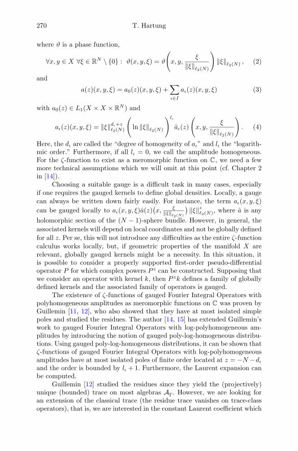
270 T. Hartung
where ϑ is a phase function,
∀x, y ∈ X ∀ξ ∈ RN \ 0 : ϑ(x, y, ξ) = ϑ
(x, y,
ξ
‖ξ‖`2(N)
)‖ξ‖`2(N) , (2)
and
a(z)(x, y, ξ) = a0(z)(x, y, ξ) +∑ι∈I
aι(z)(x, y, ξ) (3)
with a0(z) ∈ L1(X ×X × RN ) and
aι(z)(x, y, ξ) = ‖ξ‖dι+z`2(N)
(ln ‖ξ‖`2(N)
)lιaι(z)
(x, y,
ξ
‖ξ‖`2(N)
). (4)
Here, the dι are called the “degree of homogeneity of aι” and lι the “logarith-mic order.” Furthermore, if all lι = 0, we call the amplitude homogeneous.For the ζ-function to exist as a meromorphic function on C, we need a fewmore technical assumptions which we will omit at this point (cf. Chapter 2in [14]).
Choosing a suitable gauge is a difficult task in many cases, especiallyif one requires the gauged kernels to define global densities. Locally, a gauge
can always be written down fairly easily. For instance, the term aι(x, y, ξ)
can be gauged locally to aι(x, y, ξ)a(z)(x, ξ‖ξ‖`2(N)
)‖ξ‖z`2(N), where a is any
holomorphic section of the (N − 1)-sphere bundle. However, in general, the
associated kernels will depend on local coordinates and not be globally defined
for all z. Per se, this will not introduce any difficulties as the entire ζ-function
calculus works locally, but, if geometric properties of the manifold X arerelevant, globally gauged kernels might be a necessity. In this situation, itis possible to consider a properly supported first-order pseudo-differentialoperator P for which complex powers P z can be constructed. Supposing thatwe consider an operator with kernel k, then P zk defines a family of globallydefined kernels and the associated family of operators is gauged.
The existence of ζ-functions of gauged Fourier Integral Operators withpolyhomogeneous amplitudes as meromorphic functions on C was proven byGuillemin [11, 12], who also showed that they have at most isolated simplepoles and studied the residues. The author [14, 15] has extended Guillemin’swork to gauged Fourier Integral Operators with log-polyhomogeneous am-plitudes by introducing the notion of gauged poly-log-homogeneous distribu-tions. Using gauged poly-log-homogeneous distributions, it can be shown thatζ-functions of gauged Fourier Integral Operators with log-polyhomogeneousamplitudes have at most isolated poles of finite order located at z = −N −dιand the order is bounded by lι + 1. Furthermore, the Laurent expansion canbe computed.
Guillemin [12] studied the residues since they yield the (projectively)unique (bounded) trace on most algebras AΓ. However, we are looking foran extension of the classical trace (the residue trace vanishes on trace-classoperators), that is, we are interested in the constant Laurent coefficient which

Feynman path integral regularization using FIO ζ-functions 271
is ζ(A)(0) if ∀ι ∈ I : dι 6= −N (the non-critical case). In fact, in the non-critical case, ζ(A) is holomorphic in a neighborhood of zero and ζ(A)(0)depends only on A(0). This can be used to prove that
A0 ∈ AΓ A ∈ Cω(C,AΓ) gauged with A(0) = A0 ζ(A)(0) ∈ C
defines an unbounded tracial functional on AΓ (cf. Chapter 7 in [14]); thegeneralized Kontsevich–Vishik trace.
To be more precise, let us consider a gauged Fourier Integral Operator Awith kernel k as described in equations (1)–(4). Using Theorem 25.1.3 in [17](cf. Chapter 4 [14] or [11]), it is possible to show that the distributionaltrace
∫Xk(z)(x, x)dvolX(x) can locally be written as a sum of a holomorphic
function τ and a gauged poly-log-homogeneous distribution∫R≥1×∂BRN
α(z)(r, ξ)dvolR≥1×∂BRN
(r, ξ).
The family α has an expansion α = α0 +∑ι∈I αι where I ⊆ N, ∀z ∈ Ω0 :
α0(z) ∈ L1(R≥1 × ∂BRN ) and each αι(z) is log-homogeneous with degreeof homogeneity dι + z and logarithmic order lι ∈ N0, i.e., there exists anαι ∈ C∞(C, L1(∂BRN )) such that
∀r ∈ R≥1 ∀ξ ∈ ∂BRN : αι(z)(r, ξ) = rdι+z(ln r)lι αι(z)(ξ).
Furthermore, we assume the following.
• The family (<(dι))ι∈I is bounded from above. (Note, we do not require<(dι)→ −∞. In fact, ∀ι ∈ I : <(dι) = 42 is entirely possible.)• The map I 3 ι 7→ (dι, lι) ∈ C × N0 is injective.• There are only finitely many ι satisfying dι = d for any given d ∈ C.• The family ((dι − δ)−1)ι∈I is in `2(I) for any δ ∈ C \ dι; ι ∈ I.• Each
∑ι∈I αι(z) converges unconditionally in L1(∂BRN ).2
Note that I is finite if a is a classical symbol, i.e., all the assumptions above aresatisfied and Ω0 can be chosen to be CR(·)<R for any R ∈ R>0. Furthermore,
if A is a gauged pseudo-differential operator with symbol a, then (locally)
α(z)(r, ξ) =
∫X
a(z)(x, rξ)dvolX(x).
Under the conditions above, we obtain
ζ(α)(z) :=
∫R≥1×∂BRN
α(z)dvolR≥1×∂BRN
=
∫R≥1×∂BRN
α0(z)dvolR≥1×∂BRN︸ ︷︷ ︸
=:τ0(z)
+∑ι∈I
∫R≥1×∂BRN
αι(z)dvolR≥1×∂B
2Unconditional convergence of∑ι∈I αι(z) in L1(M) may also be replaced by the slightly
weaker, though more artificial, condition∑ι∈I ‖αι(z)‖
2L1(M) < ∞. However, we need at
least conditional convergence or∑ι∈I αι would not make sense, and having only condi-
tional convergence (rather than unconditional convergence) would give rise to complications
as we want to split off critical terms and treat them separately.

272 T. Hartung
= τ0(z) +∑ι∈I
∫R≥1
∫∂BRN
rdι+z+N−1(ln r)lι αι(z)(ξ)dvol∂BRN(ξ)dr
= τ0(z) +∑ι∈I
(−1)lι+1lι!∫∂BRN
αι(z)dvol∂BRN
(N + dι + z)lι+1,
where∑ι∈I (−1)lι+1lι!
∫∂BRN
αι(z)dvol∂BRN/(N + dι + z)lι+1 is absolutely
convergent (Lemma 2.2 in [14]). It is then possible to compute the Lau-
rent expansion of ζ(α) and transform back to the Fourier Integral Operator
picture which yields the generalized Kontsevich–Vishik trace
ζ(A)(0) =
∫X
∫BRN (0,1)
eiϑ(x,x,ξ)a(0)(x, x, ξ) dξ dvolX(x)
+
∫R≥1×∂BRN
∫X
eiϑ(x,x,ξ)a0(0)(x, x, ξ) dvolX(x) dvolR≥1×∂B(ξ)
+∑ι∈I
(−1)lι+1lι!∫X×∂BRN
eiϑ(x,x,ξ)aι(0)(x, x, ξ) dvolX×∂B(x, ξ)
(N + dι)lι+1
provided that none of the dι are −N . Furthermore, by construction the gen-eralized Kontsevich–Vishik trace coincides with the trace tr on trace-classoperators.
It should also be noted that the (classical) Kontsevich–Vishik trace (thatis the case of AΓ being the algebra of classical pseudo-differential operatorsΨcl) is the only trace on Ψcl that extends tr in L(L2(X)) [25].
4. The path integral in the ζ-regularized setting
Recall that we are trying to make sense of the equality
〈Ω〉T “=”tr exp
(− i
~∫ T
0H(t)dt
)Ω
ZT=
tr exp(− i
~∫ T
0H(t)dt
)Ω
tr exp(− i
~∫ T
0H(t)dt
) .
In order to use Fourier Integral Operator ζ-functions, we need to examinethe operators in questions a little more closely.
The operator H is the Hamiltonian of our QFT. Thus, we may assumethat H is a pseudo-differential operator with symbol (amplitude)
σH(t, x, rξ) := h2(t, x, ξ)r2 + h1(t, x, ξ)r + h0(t, x, r, ξ),
where ‖ξ‖`2 = 1, the hj are continuous, and h0(t, x, r, ξ) has an asymptotic ex-
pansion∑j∈N0
r−ja−j(t, x, ξ). Thus, exp(−i
~∫ T
0H(s)ds
)is an operator with
kernel
1
(2π)dimX
∫RdimX
ei〈x−y,ξ〉`2(dimX)σexp(−i~∫ T0H(s)ds)(x, ξ)dξ.

Feynman path integral regularization using FIO ζ-functions 273
If the symbol of H is independent of x, then the symbol σexp(−i~∫ T0H(s)ds)
satisfies
σexp(−i~∫ T0H(s)ds) = eiH2eiH1e
−i~∫ T0h0(s,·)ds
with
H2(rξ) :=−1
~r2
∫ T
0
h2(s, ξ)ds
and
H1(rξ) :=−1
~r
∫ T
0
h1(s, ξ)ds.
Since h0(t, r, ξ) has an asymptotic expansion∑j∈N0
r−ja−j(t, ξ), we obtain
e−i~∫ T0h0(s,r,ξ)ds =
∑k∈N0
(− i
~)k
k!
(∫ T
0
h0(s, r, ξ)ds
)k
∼∑k∈N0
(− i
~)k
k!
∑j∈N0
r−j∫ T
0
a−j(s, ξ)ds
k
,
and, using ∑k∈N0
akXk
n
=∑m∈N0
cmXm
with c0 = an0 and cm = 1ma0
∑mk=1(kn − m + k)akcm−k, we conclude that
e−i~∫ T0h0(s,r,ξ)ds has an asymptotic expansion
e−i~∫ T0h0(s,r,ξ)ds = b(rξ) ∼
∑j∈N0
r−jb−j (ξ) .
These formulae are more complicated if the symbol of H depends on x, but
we still obtain a symbol of the form σexp(−i~∫ T0H(s)ds) = eiH2eiH1eiH0 with
H2 and H1 homogeneous of degrees 2 and 1, and eiH0 having an asymptotic
expansion.
This shows that the denominator is very closely related to Fourier In-tegral Operators as discussed in Section 3 if it weren’t for the second-orderphase function. However, before we address this fact, let us consider the nu-
merator exp(−i
~∫ T
0H(s)ds
)Ω. Using the Fourier transform F , we observe for
all u, ϕ ∈ C∞c (X)
〈FΩϕ,Fu〉 = 〈ϕ,Ω∗u〉
=
∫RN
ϕ(x)
(∫RN
ei〈x,ξ〉σΩ∗(x, ξ)Fu(ξ)dξ
)∗dx
=
∫RN
∫RN
ϕ(x)e−i〈x,ξ〉σΩ∗(x, ξ)∗Fu(ξ)∗dξdx,

274 T. Hartung
which implies
FΩϕ(ξ) =
∫RN
e−i〈x,ξ〉σΩ∗(x, ξ)∗ϕ(x)dx
and, thus,
exp
(−i~
∫ T
0
H(s)ds
)Ωϕ(x)
=
∫RN
eiH2(x,ξ)eiH1(x,ξ)b(x, ξ)ei〈x,ξ〉FΩϕ(ξ)dξ
=
∫RN
∫RN
eiH2(x,ξ)eiH1(x,ξ)b(x, ξ)ei〈x,ξ〉e−i〈y,ξ〉σΩ∗(y, ξ)∗ϕ(y)dydξ
=
∫RN
∫RN
eiH2(x,ξ)eiH1(x,ξ)b(x, ξ)ei〈x,ξ〉e−i〈y,ξ〉σΩ(y, ξ)ϕ(y)dydξ,
where we used the identity σA∗(x, y, ξ) = σA(y, x, ξ)∗ which holds for anypseudo-differential operator A. In other words,
σexp(−i~∫ T0H(s)ds)Ω(x, y, ξ) = eiH2(x,ξ)eiH1(x,ξ)b(x, ξ)σΩ(y, ξ).
Hence, both numerator and denominator have kernels of the form∫RN
ei〈x−y,ξ〉eiH2(x,ξ)eiH1(x,ξ)a(x, ξ)dξ,
where a is poly-(log)-homogeneous provided that h0 and σΩ are poly-(log)-homogeneous.
For the ζ-function regularization, we now need to gauge these integrals.The choice of a reasonable gauge usually depends a lot on the specific opera-tors. However, it is often convenient to choose anM-gauge (or Mellin-gauge;cf. Definition 2.10 in [14])∫
RNei〈x−y,ξ〉eiH2(x,ξ)eiH1(x,ξ)a(x, ξ) ‖ξ‖z`2(N) dξ.
Theorem 4.1. Let X be a compact, orientable, N -dimensional RiemannianC∞-manifold without boundary, σΩ polyhomogeneous, and
Z =
∫X
∫RN
e−iσH(x,ξ)σΩ(x, ξ) dξ dvolX(x)
with
∀(x, r, η) ∈ X×R≥0×∂BRN : σH(x, rη) = h2(x, η)r2 +h1(x, η)r+h0(x, rη),
where h2, h1 ∈ C(X × ∂BRN ), h0 polyhomogeneous, and
(i) either h2 = 0 and ϑ(x, ξ) := h1
(x, ξ‖ξ‖`2
)‖ξ‖`2 is a non-degenerate phase
function(ii) or ∀x ∈ X ∀η ∈ ∂BRN : |h2(x, η)| > 0.
Then Z can be regularized using Fourier Integral Operator ζ-functions.

Feynman path integral regularization using FIO ζ-functions 275
Proof. We can absorb eih0 into the amplitude σ, and obtain
Z =
∫X
∫∂BRN
∫R>0
e−i(h2(x,η)r2+h1(x,η)r)σ(x, rη) dr dvol∂BRN(η) dvolX(x).
For (i), suppose h2 = 0 and ϑ(x, ξ) := h1
(x, ξ‖ξ‖`2(N)
)‖ξ‖`2(N) is non-
degenerate. Then Z is a Fourier Integral Operator trace already and theentire known theory (Section 3) is applicable.
For (ii), suppose ∀x ∈ X ∀η ∈ ∂BRN : |h2(x, η)| > 0 and
R := 1 + max
∣∣∣∣ h1(x, η)
2h2(x, η)
∣∣∣∣ ∈ R; (x, η) ∈ X × ∂BRN
.
Then we can split Z into two parts
Z1 :=
∫X×∂BRN×[0,R]
e−i(h2(x,η)r2+h1(x,η)r)σ(x, rη) dvolX×∂BRN×[0,R](x, η, r)
and
Z2 :=
∫X×∂BRN×R≥R
e−i(h2(x,η)r2+h1(x,η)r)σ(x, rη) dvolX×∂BRN×R≥R(x, η, r).
Regarding Z1, we observe that X × ∂BRN × [0, R] is compact. Hence, Z1 iswell-defined and will yield a holomorphic function after gauging.
Regarding Z2, we recall the assumption |h2| > 0 and obtain
h2(x, η)r2 + h1(x, η)r = h2(x, η)
(r +
h1(x, η)
2h2(x, η)
)2
− h1(x, η)2
4h2(x, η).
Absorbing eih1(x,η)2
4h2(x,η) into σ and setting σ1(x, s, η) = σ(x, s− h1(x,η)
2h2(x,η) , η)
yields
Z2 =
∫X×∂BRN
∫R≥R
e−ih2(x,η)
(r+
h1(x,η)
2h2(x,η)
)2
σ(x, rη) dr dvolX×∂BRN(x, η)
=
∫X×∂BRN
∫R
≥R+h1(x,η)2h2(x,η)
e−ih2(x,η)s2σ1(x, s, η) ds dvolX×∂BRN(x, η))
=
∫X×∂BRN
∫R
≥(R+
h1(x,η)2h2(x,η)
)2e−ih2(x,η)tσ1
(x,√t, η) dt
2√tdvolX×∂B(x, η).
This shows there exists a Fourier Integral Operator with polyhomogeneousamplitude whose trace coincides with Z2 (up to another term similar to Z1)and gauging Z2 gauges the Fourier Integral Operator, as well. In other words,existence of the ζ-function of that gauged Fourier Integral Operator impliesthat Z can be gauged, exists for <(z) sufficiently small, and has a meromor-phic extension to C.
Theorem 4.1 implies that we can write
〈Ω〉T (z) =N(T, z)
D(T, z),

276 T. Hartung
where both N(T, ·) and D(T, ·) are ζ-functions of gauged traces, i.e., mero-morphic. Hence, point evaluation at z = 0 might not be possible. Further-more, gauge dependence of 〈Ω〉T (0) needs to be addressed provided the pointevaluation is possible.
Let us first assume that both N(T, ·) and D(T, ·) have no critical degreeof homogeneity (that is −N in the h2 = 0 case and 1 − 2N in the |H2| > 0case) and at most one of them has a zero in zero. Then gauge independence ofthe constant Laurent coefficient of the Fourier Integral Operator ζ-function(cf. Lemma 2.6 in [14]) implies that both N(T, 0) and D(T, 0) are gaugeindependent, as well. In particular, evaluation of 〈Ω〉T (0) is possible if andonly if D(T, 0) 6= 0. Furthermore, if D(T, 0) 6= 0, then 〈Ω〉T (0) is independentof the gauges chosen in N(T, ·) and D(T, ·). Unfortunately, there is no reasonto assume D(T, 0) 6= 0 in general; in fact, the free relativistic fermion asdescribed in Section 8 is an example of N(T, 0) = D(T, 0) = 0.
In the case N(T, 0) = D(T, 0) = 0, evaluation of 〈Ω〉T (0) depends on thefirst non-zero Laurent coefficient, and we obtain the same situation as abovebut with some higher-order Laurent coefficient. Supposing we can evaluate〈Ω〉T (0), it is important to note that the higher-order Laurent coefficients aregauge dependent and, thus, so is 〈Ω〉T (0). In other words, we have to chooseour gauges in a physically meaningful way (cf. Section 5).
On the other hand, if critical degrees of homogeneity are present, thenwe have to expect N(T, ·) and D(T, ·) to have first-order poles in zero. If atleast one of the residues does not vanish, then we are in exactly the samesituation as in the non-critical case with at least one of the constant Laurentcoefficients not vanishing; namely, evaluation of 〈Ω〉T (0) is possible if and onlyif res0D(T, ·) 6= 0 and both res0D(T, ·) and res0N(T, ·) are independent ofthe chosen gauges (cf. Lemma 2.5 in [14]). Hence, existence of 〈Ω〉T (0) impliesgauge independence in the critical case. Similarly, if both residues vanish, wehave a quotient of higher-order Laurent coefficients which depend on thegauge (the constant Laurent coefficient is gauge dependent in the criticalcase), and the choice of gauge becomes important again.
5. Physical choices of gauges
At the end of the last section, we have noticed that the expectation value〈Ω〉T of an observable Ω on the time torus may depend on the gauges chosenfor the numerator and denominator.
Recall that we have obtained the denominator D(T, ·) by meromorphicextension of a function trG(T, ·) where G(T, ·) is a gauged family of operatorssuch that G(T, z) is of trace-class for <(z) 0 and G(T, 0) coincides with the
time-evolution operator exp(−i
~∫ T
0H(s)ds
)of the QFT we want to study.
Thus, we may interpret G(T, ·) as the holomorphic family time-evolutionoperators of a “holomorphic family Q of QFTs.” In that sense, trG(T, z)is precisely the partition function of Q(z) given <(z) 0. However, sincethe path integral in Q(z) with <(z) 0 is well-defined, there is only one

Feynman path integral regularization using FIO ζ-functions 277
reasonable choice of gauge for the numerator, since Feynman’s constructionin Q(z) implies that the expectation 〈Ω〉Q(z) of Ω in Q(z) satisfies
∀z ∈ C<(·)0 : 〈Ω〉T (z) = 〈Ω〉Q(z) =tr (G(T, z)Ω)
trG(T, z).
These observations lead to the following definition of a ζ-regularized expec-tation of Ω.
Definition 5.1. Let H be the Hamiltonian, (G(T, z))T∈R>0,z∈C a gauged fam-ily of operators with
∀T ∈ R>0 : G(T, 0) = exp
(−i~
∫ T
0
H(s)ds
),
and Ω an observable. Then we define the ζ-regularized expectation value 〈Ω〉Gof Ω with respect to G as
〈Ω〉G := limT→∞
limz→0
ζ (G(T, ·)Ω) (z)
ζ (G(T, ·)) (z)
= limT→∞
limz→0
(C<(·)0 3 s 7→ tr (G(T, s)Ω) ∈ C
)∣∣∣mer.
(z)(C<(·)0 3 s 7→ trG(T, s) ∈ C
)∣∣∣mer.
(z),
where f |mer. denotes the meromorphic extension of a function f with maximalopen and connected domain (provided f has open and connected domain).
Given that this definition is rather esoteric, we will proceed with anumber of physical examples to convince ourselves that this new way ofinterpreting the path integral is physically useful. It should be noted thatthe ζ-regularized expectation coincides with Feynman’s definition wheneverFeynman’s notion is well-defined in the Hamiltonian formulation (i.e., theoperators are of trace-class). As such, the ζ-definition is an extension of Feyn-man’s definition and, since going forward we will not always explicitly definethe time-evolution family G, we will drop the index G from 〈Ω〉G in theupcoming examples.
6. The topological oscillator
The first example we would like to consider is the topological oscillator (a.k.a.quantum rotor). It describes a particle of mass M moving on a circle withradius R. Parametrizing the circle as (x, y) = (R cosϕ,R sinϕ) with freecoordinate ϕ, we obtain the Lagrangian
L =M
2(x2 + y2) =
J
2ϕ2,
where J = MR2 is the moment of inertia. This yields the generalized mo-mentum
p = ∂ϕL = Jϕ

278 T. Hartung
and Hamiltonian
H = ϕp− L =p2
J− p2
2J=p2
2J.
In other words, the symbol σH of H is
σH(x, rξ) =r2
2J.
As an observable, we will consider the topological charge
Q =1
2π
∫ T
0
ϕ(t)dt =1
2π
∫ T
0
p(t)
Jdt ⇒ σQ(x, rξ) =
1
2π
∫ T
0
rξ
Jdt =
Trξ
2πJ,
which is the winding number of the path of the particle “over the entirelifetime of the universe.” The topological charge is interesting since it allowsus to compute the topological charge χtop of the system
χtop = limT→∞
⟨Q2
−iT
⟩T
which is related to the energy gap
∆E = 2π2χtop
between the ground state and first excited state of the particle. Using thePython 2.7 implementation [13], we obtain the physically correct values (innatural units c = ~ = 1)
χtop =1
4π2Jand ∆E =
1
2J.
7. The free massive Schwinger model
Our next example is the free massive Schwinger model [32]. The massiveSchwinger model is a theory of quantum electrodynamics (QED) in two space-time dimensions with Hamiltonian (in the zero-momentum frame; cf., e.g.,equation (2.2) in [1])
Hm =
(mc2 −i∂−i∂ mc2
)= mc2 +
(0 −i∂−i∂ 0
)︸ ︷︷ ︸
=:H0
.
Thus,
σH0(x, rξ) =
(0 −rξ−rξ 0
)implies σH2k
0(x, rξ) = r2k = (rξ)2k, σH2k−1
0(x, rξ) =
(0 (rξ)2k−1
(rξ)2k−1 0
),
and
σexp(−i~ H0T)(x, rξ) =
(cos(T~ rξ
)−i sin
(T~ rξ
)−i sin
(T~ rξ
)cos(T~ rξ
) ) .

Feynman path integral regularization using FIO ζ-functions 279
Since mc2 and H0 commute, e−i~ HmT = e
−i~ mc
2T e−i~ H0T yields
σexp(−i~ HmT)(x, rξ) = e
−i~ mc
2T
(cos(T~ rξ
)−i sin
(T~ rξ
)−i sin
(T~ rξ
)cos(T~ rξ
) )and
σexp(−i~ HmT)Hm(x, rξ)
= e−i~ mc
2T
(mc2 cos
(T~ rξ
)− iξ sin
(T~ rξ
)ξ cos
(T~ rξ
)− imc2 sin
(T~ rξ
)ξ cos
(T~ rξ
)− imc2 sin
(T~ rξ
)mc2 cos
(T~ rξ
)− iξ sin
(T~ rξ
)).We can gauge these using an M-gauge, i.e., σ(x, rξ) σ(x, rξ)rz. Further-more, we need to introduce a cut-off function 1B(0,X) ≤ χ ≤ 1B(0,X+1) tocompactify the spacial domain. Then the ground state energy of the systemis given by (replacing rξ by ξ ∈ R)
〈Hm〉 = limX,T→∞
limz→0
12π
∫R∫R χ(x) trσexp(−i
~ HmT)Hm(ξ) |ξ|z dξdx1
2π
∫R∫R χ(x) trσexp(−i
~ HmT)(ξ) |ξ|z dξdx.
Replacing cosx and sinx by eix+e−ix
2 and eix−e−ix2i , we obtain the known
gauged Fourier Integral Operator form, and Theorem 8.7 in [14] implies thatthese are distributional trace integrals of Hilbert–Schmidt operators withcontinuous kernels. Computing the traces by hand or using the Python 2.7implementation supplied in [13] yields the physically correct ground stateenergy
〈Hm〉 = E = mc2
for the free massive Schwinger model.
8. Free relativistic Fermions
Moving on to four space-time dimensions, we need to add Pauli matricesto the Hamiltonian (now in natural units and using Einstein summationconvention to ease notation)
Hm =
(m −iσk∂k
−iσk∂k m
),
and replacing rξ by ξ ∈ R3 we obtain
σe−iHmT (x, ξ) = e−imT
(cos(T ‖ξ‖`2
)−i sin
(T ‖ξ‖`2
)‖ξ‖`2
(0 σkξk
σkξk 0
))and
σexp(−iHmT )Hm(x, ξ)
= e−imT(
cos(T ‖ξ‖`2(3)
)( m σkξkσkξk m
)− i ‖ξ‖`2(3) sin
(T ‖ξ‖`2(3)
)).

280 T. Hartung
Then we can compute the ground state energy (by hand this time and havingalready canceled the volX(X) terms from the integration over the spatialvariable x and taken the limit X → R3 similar to the one-dimensional case):
〈Hm〉 = limT→∞
limz→0
∫R3
(4m cos
(T ‖ξ‖`2
)− 4i ‖ξ‖`2 sin
(T ‖ξ‖`2
))‖ξ‖z`2 dξ∫
R3 4 cos(T ‖ξ‖`2
)‖ξ‖z`2 dξ
= m+ limT→∞
limz→0
∫R3 ‖ξ‖z+1
`2(3)
(eiT‖ξ‖`2(3) − e−iT‖ξ‖`2(3)
)dξ∫
R3 ‖ξ‖z`2(3)
(eiT‖ξ‖`2(3) + e−iT‖ξ‖`2(3)
)dξ
= m+ limT→∞
limz→0
vol (∂BR3)∫R>0
rz+3(eiTr − e−iTr
)dr
vol (∂BR3)∫R>0
rz+2 (eiTr + e−iTr) dr(∗)
= m+ limT→∞
limz→0
(−e−i
π(z+3)2 − e−3i
π(z+3)2
)Γ(z + 4)T−z−4(
−e−iπ(z+2)
2 + e−3iπ(z+2)
2
)Γ(z + 3)T−z−3
= m+ limT→∞
limz→0
(−e−i
π(z+3)2 − e−i
π(z+3)2 e−iπ(z+3)
)Γ(z + 4)T−z−4(
−e−iπ(z+2)
2 + e−iπ(z+2)
2 e−iπ(z+2))
Γ(z + 3)T−z−3
= m+ limT→∞
limz→0
e−iπ(z+3)
2
(−1− e−iπ(z+2)e−iπ
)(z + 3)Γ(z + 3)T−z−4
e−iπ(z+2)
2
(e−iπ(z+2) − 1
)Γ(z + 3)T−z−3
= m+ limT→∞
limz→0
e−iπ(z+2)
2 e−iπ2 (z + 3)
e−iπ(z+2)
2 T
= m+ limT→∞
limz→0
−i(z + 3)
T= m.
In other words, we have correctly computed E = mc2 again.
Remark. This example highlights a number of properties. These will becomevery important in the case of the massive Schwinger model (Section 9). The“observable” m of the first summand depends on none of the variables. Thisleads to cancelations just like the results of the integration over X canceled.In the massive Schwinger model this will be paramount since the part of themodel that is not analytically solvable will vanish in one such cancelation.
The latter summand exhibits the other important property; namely,these integrals can be written as Laplace transforms of homogeneous distri-butions and the time extent T of the time-torus is part of the point evaluationof the Laplace transform. Thus, the limit T → ∞ depends primarily on theasymptotic expansion of the observable. In particular, this allows us to de-termine many terms that will vanish in the limit T → ∞ simply by lookingat the asymptotic expansion of the observable.

Feynman path integral regularization using FIO ζ-functions 281
Remark. Note that (∗) can be implemented directly since the Laplace trans-form satisfies
L(r 7→ rq)(s) =Γ(q + 1)
sq+1
for <(s) > 0 and <(q) > −1, and hence for s ∈ C \ 0 and q ∈ C \ (−N) byanalytic extension. In particular,∫
R>0
rzeiTrdr =−ie−iπz2 Γ(z + 1)
T z+1
and ∫R>0
rze−iTrdr =ie−3iπz2 Γ(z + 1)
T z+1.
Furthermore, using stationary phase approximation (cf. Chapter 8 in [14]) onthe results of Theorem 4.1, we obtain that the regularization is given solely interms of such Laplace transforms. In other words, computing 〈Ω〉T (z) reducesto the numerical problem of computing integrals over ∂BRN and possiblycomputing the limits z → 0 and T →∞.
Here, the integrals over ∂BRN are trivial and a Python 2.7 implemen-tation is given in [13] which, too, outputs <H_m>=m.
9. Gauge boson mass in the Schwinger model
Let us now return to the two-dimensional Schwinger model. With the additionof an Abelian gauge field, the model is fully interacting and has non-trivialdynamics which lead to confinement of charges and bound states. This modelis no longer analytically solvable, but as we are going to consider the gaugeboson mass as our observable, non-integrable parts of the system will cancelin the quotient, allowing us to compute the gauge boson mass analytically.
The Hamiltonian (in the temporal gauge and using natural units) iscomprised of two parts: the fermionic Hamiltonian
HF =
(m −i∂1 − eA
−i∂1 − eA m
)and the Hamiltonian describing the self-interaction of the gauge field
HS = −1
4FµνF
µν =1
2E2,
where Fµν = ∂µAν − ∂νAµ, A = A1 (A0 = 0 is the temporal gauge), andE = −∂0A.
At this point, we should recall the nature of the path integral being aformal inductive limit of discretized space-time. As such, it is convenient toconsider the family ((A(x), E(x)))x∈X as canonical coordinates on a space-torus X (recall that the ζ-regularization needs a compact manifold) whiletime dependence of the gauge fields is implicit.

282 T. Hartung
As the limit X → R3 will be trivial, we will suppress it in the followingcomputation. Then we observe
σe−i
∫T0 H = e−imT e−
i2TE
2
(cos(Tξ − e
∫ T0A)
−i sin(Tξ − e
∫ T0A)
−i sin(Tξ − e
∫ T0A)
cos(Tξ − e
∫ T0A) ) .
Schwinger [32] computed the observable Ω for the squared gauge boson massin terms of the Green’s function of the Abelian gauge field and we can extractthe symbol of the squared gauge boson mass to be
σΩ(E) = E2 +e2
π.
Hence, the gauge boson mass mg is given by (suppressing the differentialdξDAdEdx, as well as gauges for ξ, x, and A)
m2g = 〈Ω〉
= limT→∞z→0
∫e−imT−
i2TE
2(eiTξe−ie
∫ T0A + e−iTξeie
∫ T0A)(
E2 + e2
π
)|E|z∫
e−imT−i2TE
2(eiTξe−ie
∫ T0A + e−iTξeie
∫ T0A)|E|z
=e2
π+ limT→∞
limz→0
∫e−
i2TE
2(eiTξe−ie
∫ T0A + e−iTξeie
∫ T0A)|E|z+2∫
e−i2TE
2(eiTξe−ie
∫ T0A + e−iTξeie
∫ T0A)|E|z
=e2
π+ limT→∞
limz→0
∫e−
i2TE
2 |E|z+2dE∫
e−i2TE
2 |E|z dE
=e2
π+ limT→∞
limz→0
−ie− 3iπ2z+12 Γ
(z+3
2
) (2T
) z+32
−ie− 3iπ2z−12 Γ
(z+1
2
) (2T
) z+12︸ ︷︷ ︸
∝ 1T=
e2
π.
Remark. Again, we observe the cancelations and asymptotic properties asseen in Section 8. However, now they are vital to the computation since theintegrals with respect to A are not analytically solvable. Yet, the structureof the observable forced these integrals in the numerator and denominatorto coincide. Even more so, suppose they did not cancel, then the asymptoticbehavior in E still implies that the second term vanishes in the limit T →∞.
10. Spontaneous symmetry breaking and mass – the ϕ4 model
Spontaneous symmetry breaking is another very important showcase to con-sider. Physically, it is fundamental to the Higgs mechanism and, thus, ex-hibits fundamental physical behavior we want the ζ-regularized theory toreproduce. From a mathematical point of view it is interesting since it is our
first example that is not of the form 〈Ω〉 = limT→∞ limz→0N(T,z)D(T,z) .

Feynman path integral regularization using FIO ζ-functions 283
For simplicity, let us consider the simplest, non-trivial, relativistic ex-ample. Suppose we have scalar fields ϕ = (ϕ1, . . . , ϕk) and a Lagrangiandepending on ϕ. Then we obtain our ζ-regularized partition function ZT (ϕ)
which is the denominator D(T, 0) in 〈Ω〉 = limT→∞ limz→0N(T,z)D(T,z) . We now
consider ZT (ϕ) to be the partition function with respect to an effective po-tential (Lagrangian) V Te (ϕ), i.e.,
ZT (ϕ) = exp
(−i∫V Te (ϕ)d(t, x)
).
The vacuum expectation values ϕj0 of the ϕj are constant local minimizers ofV Te in the limit T → ∞, and the corresponding field masses are the squareroots of the eigenvalues of
(∂i∂jV
Te (ϕ0)
)i,j∈N≤k
in the limit T →∞.
As we are looking for constant solutions ϕj0, we can write
V Te (ϕ) =lnZT (ϕ)
−iTX,
where TX is the volume of our space time, and, if we assume k = 1 forsimplicity, we want to find ϕT0 ∈ R such that ∂V Te (ϕT0 ) = 0. Then limT→∞ ϕT0yields the vacuum expectation of ϕ and limT→∞
√∂2V Te (ϕT0 ) the field mass.
It should be noted that this is a particularly interesting and highly non-trivial behavior of QFTs. Usually, when someone writes down a QFT, theystart with a classical field theory that then will be quantized. However, if thisclassical field theory contains mass terms for the classical field, quantizationis impossible. Thus, considering a QFT as a classical field theory necessar-ily implies that all field masses vanish. Hence, non-zero field masses are anentirely quantum mechanical effect and they warrant that our ζ-regularizedtheory is quantized.
As an example for spontaneous symmetry breaking, we would like toconsider the one-dimensional ϕ4 model whose Hamiltonian is given by
H =
∫p2
2− 1
2ϕ∆ϕ− 1
2µ2ϕ2 +
λ
4!ϕ4dx.
Then we can ζ-regularize the partition function to obtain3
ZT (z, ϕ) =1
2π
∫Re−iTX
(p2
2 −µ2
2 ϕ2+ λ
4!ϕ4)|p|z dp.
Gauge independence of ZT (0, ϕ) implies that lnZT (z, ϕ) exists in a neigh-
borhood of z = 0 provided ZT (0, ϕ) 6= 0 and a suitable branch cut of ln is
chosen. As this is the case here, we may use the Python 2.7 implementation
from [13] and obtain the physically correct values of ±√
6λµ for the vacuum
expectation and√
2µ for the field mass.
3Note that the factor 12π
has to be included now. Previously, the (2π)− dim factors used
to cancel as they appeared in both numerator and denominator.

284 T. Hartung
Remark. We made a priori use of the fact that we are looking for (spatially)constant ϕ and therefore dropped the term ϕ∆ϕ. If we were to compute anobservable for instance, we would not be able to do this and the computationwill be a lot more complex. In such cases, it may be advantageous to writeϕ∆ϕ as −〈∇ϕ,∇ϕ〉, which can be combined with the p2 term as a space-time version of canonically conjugated momentum with respect to ϕ. Thebest choice will but depend on the specific problem at hand and even space-
discretization, i.e., replacing ϕ by a vector (ϕ(xj))j∈N≤n∈ Rn can be an
interesting option resulting in a path integral that is ζ-regularizable. In fact,
this idea is fundamental to Lattice QFT which we will discuss in Section 11.
11. Application to Lattice QFT
One of the most important frameworks in computational physics is calledLattice QFT. Lattice QFTs treat the discretized path integral. In other words,we are working with the path integral before taking the formal inductive limitto continuous space time:
Using the discretized Lagrangian L and an observable Ω, the aim is to com-pute quotients
〈Ω〉 =Z (Ω)
Z (1)(5)
where both numerator and denominator have the structure
Z (ω) =
∫Rnei~∫L(p)(t,x)dvol(t,x)aω(p)dp, (6)
aω is an amplitude depending on ω, and vol is a discrete measure dependingon the discretization. However, in general, these integrals are still not well-defined as the integrands are not in L1(Rn). Usually this problem is solvedusing a Wick rotation which turns Minkowski space-time into Euclideanspace-time and results in the integrands being integrable now. More pre-cisely, the Wick rotation replaces the time-evolution semigroup exp(−i
∫H)
with the “heat” semigroup exp(−∫H), which is trace-class on compact man-
ifolds. Hence, the Wick rotated path integral is well-defined. In fact, thisWick rotation plays such an important role in QFTs that Osterwalder andSchrader [27, 28] developed axioms that a Euclidean path integral has tosatisfy for it to be Wick rotated by analytic continuation to define a QFT inMinkowski space-time satisfying the Wightman axioms [34].
However, some physically interesting problems cannot be solved usingWick rotations on a lattice. Such an example would be the computation of

Feynman path integral regularization using FIO ζ-functions 285
parton distribution functions of a nucleon, i.e., the probability density of mea-suring a certain number of quarks of a certain type in a proton for instance.These are inaccessible on the lattice because the dynamics are localized onthe light cone and using a Wick rotation ds2 = 0 turns the light cone intoa single point (the origin). Thus, the Wick rotation destroys the physicallyinteresting properties. While parton distribution functions can still be re-covered using very sophisticated methods [36], no such methods are knownfor many other high energy situations (like the early universe). Hence, beingable to compute the objects in Minkowski space-time (or more precisely witha Lorentzian background) would be a great step forward. A ζ-regularizedLattice QFT might be able to fill this gap.
A “ζ-Lattice QFT” can be constructed on the background of the Hamil-tonian theory we have already described; although, in many cases it is advan-tageous to stay in the Lagrangian picture (which is the much more commonnotation for QFTs) rather than explicitly computing the Hamiltonian pic-ture. Of course, this is only possible since the discretized path integral isnotationally well-posed (up to the fact that the integrals don’t exist) and wecan rely on the fact that we are equivalent to the Hamiltonian picture at alltimes.
Hence, given the Lagrangian L of a Lattice QFT, we obtain a “ζ-LatticeQFT” as follows.
(i) Choose a gauge g, that is, a holomorphic family g such that ∀z ∈ C :g(z) ∈ C∞(Rn \ 0) and
∀z ∈ C ∀p ∈ Rn \ 0 : g(z)(p) = ‖p‖z`2(n) g(z)
(p
‖p‖`2(n)
).
Then we consider the family
Z (ω)(z) =
∫Rnei~∫L(p)(t,x)dvol(t,x)aω(p)g(z)(p)dp.
(ii) Construct a gauged Fourier Integral Operator Aω (according to theproof of Theorem 4.1) and a holomorphic function τω such that
∀z ∈ C : Z (ω)(z) is distributionally equivalent to τω(z) + trAω(z).
Thus, we obtain a representation
Z (ω)(z) = τω(z) +∑ι∈I
∫∂BRn
∫R>0
eirϑι(ξ)rdι+zαω,ι(z)(ξ)drdξ.
(iii) Now there are two possible cases.(a) If ϑι has no zeros on ∂BRn , analytically continuing the Laplace
transform yields the ζ-regularization of the inner integral; namely,
ϑι > 0 ⇒∫R>0
rdι+zeirϑι(ξ)dr =−ie−i
π(dι+z)2 Γ(dι + z + 1)
ϑι(ξ)dι+z+1

286 T. Hartung
and
ϑι < 0 ⇒∫R>0
rdι+zeirϑι(ξ)dr =ie−3i
π(dι+z)2 Γ(dι + z + 1)
|ϑι(ξ)|dι+z+1.
(b) If ϑι has zeros, the computation of these traces is more involved(see Chapters 4 and 8 of [14]).
(iv) At last, we need to take the limit z → 0 (assuming ϑ > 0 for notationalsimplicity), obtaining
Z (ω)(0) = τω(0)−∑ι∈I
ie−iπdι2 Γ(dι + 1)
∫∂BRn
αω,ι(0)(ξ)
ϑι(ξ)dι+1dξ.
It should be noted that this contains the entire regularization. The re-maining integrals are integrals of continuous functions over the sphere∂BRn . In particular, even though these still may be very difficult tocompute numerically, at least we are now left with a well-posed numer-ical problem (as opposed to trying to compute these integrals of thenon-integrable functions that we started out with).
Hence, ζ-regularization is a viable tool to study Lattice QFT without Wickrotations.
Conclusion
Having considered Feynman’s path integral in the light of some propertiesof axiomatic QFTs, we have seen that the ill-definedness of Feynman’s pathintegral can be expressed in terms of formal operator traces acting on opera-tors that are not of trace-class. From this point of view, the main obstacle tounderstanding the path integral is the construction of a suitable trace for theoccurring operators. Given the physically important methods and instancesfor which the path integral is well-defined (e.g., Wick rotations, lattice formu-lations, or trace-class operators), we proposed ζ-regularization since, for someof the special cases, it is known that ζ-regularization yields the unique traceextension (the Kontsevich–Vishik trace) we are looking for. Hence, we ap-plied the ζ-function calculus to Feynman’s path integral and obtained a newdefinition of ζ-regularized partition functions and ζ-regularized expectationvalues of observables (Definition 5.1).
In order to construct a ζ-regularization, we replaced the time-evolutionsemigroup T (t) := e−
i~∫ t0H(s)ds by a holomorphic family z 7→ G(t, z) sat-
isfying G(t, 0) = T (t). If G is suitably chosen (gauging), Feynman’s pathintegral with time-evolution t 7→ G(t, z) is well-defined for <(z) 0 and canbe extended meromorphically to C (Theorem 4.1). Hence, the ζ-regularizedpath integral is obtained evaluating this meromorphic extension at z = 0 pro-vided the meromorphic extension is holomorphic in a neighborhood of zero(Definition 5.1).

Feynman path integral regularization using FIO ζ-functions 287
Since there is no particular reason to assume that this constructionyields physically correct results, we considered a number of physical exam-ples. These specifically addressed three points. First and foremost, we agreewith physics (at least on these examples). Secondly, the regularization is com-putable and explicit in a way that allows for it to be used in computationalphysics since it reduces the numerical effort to evaluating integrals of contin-uous functions over compact manifolds (and possibly the limits z → 0 andphysical volume→∞). Thirdly, the ζ-regularized theory is a true extensionof Feynman’s path integral which allows for applications that were previouslyinaccessible (e.g., Lattice QFT with Lorentzian signatures).
An important question we had to address though was that of gaugedependence. Since the ζ-construction contains a large amount of choice, weneed to make sure that our choices don’t change the results. In many cases,we obtain gauge independence from the theory of Fourier Integral Opera-tor ζ-functions that we utilized behind the scenes. However, there are cases(e.g., the free massive Schwinger model in Section 7) in which gauge inde-pendence is not warranted. Here, we argued from physical intuition. Since weare working with quotients of Fourier Integral Operator ζ-functions, choosingdifferent gauges in numerator and denominator can lead to different resultsif the leading order Laurent coefficients in both numerator and denominatorvanish. However, gauging the denominator can be interpreted as the construc-tion of a holomorphic family of QFTs Q. In this interpretation, the choiceof gauge for the numerator is fixed and rather than considering numeratorand denominator separately, we can consider the quotient 〈Ω〉(z) = N(z)
D(z) to
be a function of Q rather than z. In other words, the idea is that physicallyreasonable results cannot be expected a priori, but should be obtained in thelimit 〈Ω〉(Q(z)) → 〈Ω〉(Q(0)); that is, to say that our QFT Q(0) is consis-tent with the holomorphic family Q of QFT it is embedded in, especiallysince some of these <(z) 0 have path integrals that are well-defined inFeynman’s sense.
References
[1] M.C. Banuls, K. Cichy, J.I. Cirac, and K. Jansen, The mass spectrum of theSchwinger model with matrix product states, Journal of High Energy Physics158 (2013).
[2] S.M. Christensen and S.A. Fulling, Trace anomalies and the Hawking effect,Physical Review D 15 (1977), 2088–2104.
[3] M. Creutz and B. Freedman, A statistical approach to Quantum Mechanics,Annals of Physics 132 (1981), 427–462.
[4] T. Degrand and C. Detar, Lattice methods for Quantum Chromodynamics,World Scientific, 2006.
[5] P.A.M. Dirac, The quantum theory of the emission and absorption of radiation,Proceedings of the Royal Society A 114 (1927), 243–265.
[6] J.J. Duistermaat, Fourier Integral Operators, Birkhauser, 1996.

288 T. Hartung
[7] R.P. Feynman, Space-time approach to non-relativistic Quantum Mechanics,Reviews of Modern Physics 20 (1948), 367–387.
[8] R.P. Feynman, A.R. Hibbs, and D.F. Styer, Quantum Mechanics and pathintegrals, Emended Edition, Dover Publications, Inc., 2005.
[9] C. Gattringer and C.B. Lang, Quantum Chromodynamics on the lattice,Springer, 2010.
[10] G.W. Gibbons, S.W. Hawking, and M.J. Perry, Path integrals and the indefi-niteness of the gravitational action, Nuclear Physics B138 (1978), 141–150.
[11] V. Guillemin, Gauged Lagrangian distributions, Advances in Mathematics 102(1993), 184–201.
[12] V. Guillemin, Residue traces for certain algebras of Fourier Integral Operators,Journal of Functional Analysis 115 (1993), 391–417.
[13] T. Hartung, Regularizing Feynman path integrals using the generalized Kon-tsevich-Vishik trace, Journal of Mathematical Physics 58 (2017), 1–19.
[14] T. Hartung, ζ-functions of Fourier Integral Operators, Ph.D. thesis, King’sCollege London, 2015.
[15] T. Hartung and S. Scott, A generalized Kontsevich-Vishik trace for FourierIntegral Operators and the Laurent expansion of ζ-functions,arXiv:1510.07324v2[math.AP], 2015.
[16] S.W. Hawking, Zeta function regularization of path integrals in curved space-time, Communications in Mathematical Physics 55 (1977), 133–148.
[17] L. Hormander, The analysis of linear partial differential operators I–IV,Springer, 1990.
[18] T. Johnson-Freyd, The formal path integral and quantum mechanics, Journalof Mathematical Physics 51 122103 (2010), 1–31.
[19] M. Kontsevich and S. Vishik, Determinants of elliptic pseudo-differential op-erators, Max Planck Preprint, arXiv:hep-th/9404046 (1994).
[20] M. Kontsevich and S. Vishik, Geometry of determinants of elliptic operators,in: Functional Analysis on the Eve of the XXI century, Vol. I, Progress inMathematics 131, 173–197, Birkhauser, 1994.
[21] N. Kumano-go, Phase space Feynman path integrals with smooth functionalderivatives by time slicing approximation, Bulletin des sciences mathematiques135 (2011), 936–987.
[22] N. Kumano-go and D. Fujiwara, Phase space Feynman path integrals via piece-wise bicharacteristic paths and their semiclassical approximations, Bulletin dessciences mathematiques 132 (2008), 313–357.
[23] N. Kumano-go and A.S. Vasudeva Murthy, Phase space Feynman path in-tegrals of higher order parabolic type with general functional as integrand,Bulletin des sciences mathematiques 139 (2015), 495–537.
[24] C.H. Lee, The exponential calculus of pseudodifferential operators of minimumtype. I, Proceedings of the Japan Academy 89 (A) (2013), 6–10.
[25] L. Maniccia, E. Schrohe, and J. Seiler, Uniqueness of the Kontsevich-Vishiktrace, Proceedings of the American Mathematical Society 136 (2) (2008), 747–752.
[26] I. Montvay and G. Munster, Quantum fields on a lattice, Cambridge UniversityPress, 1994.

Feynman path integral regularization using FIO ζ-functions 289
[27] K. Osterwalder and R. Schrader, Axioms for Euclidean Green’s functions, Com-munications in Mathematical Physics 31 (1973), 83–112.
[28] K. Osterwalder and R. Schrader, Axioms for Euclidean Green’s functions II,Communications in Mathematical Physics 42 (1975), 281–305.
[29] S. Paycha, Zeta-regularized traces versus the Wodzicki residue as tools in quan-tum field theory and infinite dimensional geometry, Proceedings of the Inter-national Conference on Stochastic Analysis and Applications, 2001, 69–84.
[30] D.B. Ray, Reidemeister torsion and the Laplacian on lense spaces, Advancesin Mathematics 4 (1970), 109–126.
[31] D.B. Ray and I.M. Singer, R-torsion and the Laplacian on Riemannian mani-folds, Advances in Mathematics 7 (1971), 145–210.
[32] J. Schwinger, Gauge invariance and mass II, Physical Review 128 (1962), 2425–2429.
[33] R.T. Seeley, Complex powers of an elliptic operator, Proceedings of Symposiain Pure Mathematics 10 (1967), 288–307.
[34] R.F. Streater and A.S. Wightman, PCT, spin and statistics, and all that, Ad-vanced Book Classics, Addison-Wesley, 1989.
[35] L.A. Takhtajan, Quantum Mechanics for mathematicians, American Mathe-matical Society, 2008.
[36] C. Wiese, Investigating new lattice approaches to the momentum and spin struc-ture of the nucleon, Ph.D. thesis, Humboldt-Universitat zu Berlin, 2016.
[37] K.G. Wilson, Confinement of quarks, Physical Review D 10 (1974), 2445.
[38] M. Wodzicki, Noncommutative residue. I. Fundamentals, in: K-theory, arith-metic and geometry (Moscow, 1984–1986), Lecture Notes in Mathematics 1289,Springer, 1987, 320–399.
[39] M. Wodzicki, Spectral asymmetry and noncommutative residue, Ph.D. thesis,Steklov Institute of Mathematics, 1984.
Tobias HartungDepartment of MathematicsKing’s College LondonStrandLondon WC2R 2LSUnited Kingdome-mail: [email protected]

Improving Monte Carlo integration bysymmetrization
Tobias Hartung, Karl Jansen, Hernan Leovey and Julia Volmer
Abstract. The error scaling for Markov chain Monte Carlo (MCMC)techniques with N samples behaves like 1/
√N . This scaling makes it
often very time intensive to reduce the error of calculated observables,in particular for applications in 4-dimensional lattice quantum chromo-dynamics as our theory of the interaction between quarks and gluons.Even more, for certain cases, where the infamous sign problem appears,MCMC methods fail to provide results with a reliable error estimate.It is therefore highly desirable to have alternative methods at handwhich show an improved error scaling and have the potential to over-come the sign problem. One candidate for such an alternative integra-tion technique we used is based on a new class of polynomially exactintegration rules on U(N) and SU(N) which are derived from polyno-mially exact rules on spheres. We applied these rules successfully to anon-trivial, zero-dimensional model with a sign problem and obtainedarbitrary precision results. In this article we test a possible way to applythe integration rules for spheres to the case of a one-dimensional U(1)model, the topological rotor, which already leads to a problem of veryhigh dimensionality.
Mathematics Subject Classification (2010). Primary 65C40; Secondary28C10; Tertiary 65Z05.
Keywords. Numerical sign-problem, Markov chain Monte Carlo, Haarmeasure, quantum mechanical oscillator, lattice systems.
1. Introduction
High-dimensional integration problems appear in vast areas of physics andmathematics. In the field of high energy physics (HEP), which aims at ex-ploring and understanding the fundamental interactions of elementary par-ticles, such problems occur when the underlying models are evaluated withFeynman’s path integrals [1]. Since the theories in high energy physics are
© Springer International Publishing AG, part of Springer Nature 2018
Theory: Advances and Applications 268, https://doi.org/10.1007/978-3-319-75996-8_15
291A. Böttcher et al. (eds.), The Diversity and Beauty of Applied Operator Theory, Operator

292 T. Hartung, K. Jansen, H. Leovey and J. Volmer
formulated in three space and one time dimensions, the number of degrees offreedom to be treated is very large leading to very high-dimensional integrals,which can easily reach O(108) dimensions.
By formulating the involved theoretical models on a space-time crystaland using Feynman’s path integral one arrives at a lattice field theory versionof systems in high energy physics, see e.g. [2] for an introduction to thisapproach. The 4-dimensional discrete formulation within lattice field theorygives the considered theories a conceptually clean meaning, since the resultingintegrals are well defined, although they are very high-dimensional.
For a number of physical questions these integrals are solvable by usingimportance sampling via Markov chain Monte Carlo (MCMC) methods. And,in fact, this approach has proven to be very successful: E.g., the low lyingbound state spectrum of hadrons (the proton and the neutron being promi-nent examples) could be determined from such ab-initio calculations [3], aresult that could not be computed analytically. Also, present MCMC sim-ulations in high energy physics are reaching fully physical conditions [4, 5],requiring, however, the evaluation of even higher-dimensional integrals. Infact, the dimensionality of the involved integrals become easily of the or-der of hundreds of millions, so that only state of the art supercomputerswith nowadays reaching hundreds of Petaflops [6] have to be employed. Still,typical projects run at the order of 1–2 years or even longer. Thus, findingmethods to improve and accelerate such calculations is highly desirable.
In addition, and more severely, there are certain problems, where MCMCcannot be applied straightforward. This is the case when a highly oscillatory,complex integrand describes the problem under consideration. In this case,the interpretation of a probability density, on which MCMC methods rely,is lost and MCMC calculations do not deliver meaningful results, leading tothe infamous sign problem [7]. It is important to note that this problem isnot academic in high energy physics but that such situations occur when wewant to understand the very early universe [8] or why there is more matterthan anti-matter in the universe [9]. These so far unexplained phenomenaaddress therefore our sheer existence and clearly need to be understood.
In this project, we have tried to solve the sign problem by employingfully symmetric and polynomially exact integration rules over integrationvariables from a compact group. In particular, we have considered Abeliangroups U(1) and also non-Abelian groups U(N) and SU(N) for N > 1, asthey are used in models of high energy physics. For a simple test model, theso-called 1-dimensional quantum chromodynamics (QCD)1, we could clearlydemonstrate that this fully symmetric integration rules work at (arbitrary)machine precision level, outperforming MCMC methods by far [10]. In partic-ular, we could demonstrate numerically that the polynomial exactness of thismethod also holds for the case when a phase factor appears in the integrand,i.e. when the sign problem occurs and when MCMC completely fails.2
1QCD is the theory of the strong interaction between quarks and gluons.2For a related approach see refs. [11, 12].

Improving Monte Carlo integration 293
However, for the model considered in [10] the complexity and the cor-responding dimensionality was very small. And, when the integration dimen-sion is increased, the complexity of the full symmetrization approach and theassociated computational cost fast becomes prohibitively large such that re-alistic models cannot be treated with this method. Still, the extremely highprecision we could reach in [10], owing to the polynomial exactness of theintegration rule, motivated us strongly to try to apply these integration rulesalso in higher physical dimensions.
The idea we follow in this article is to combine the symmetrized integra-tion rules with MCMC. We expected that we can sample sufficiently manysymmetrized integration points to achieve precise results, even in cases whena phase factor appears. In order to overcome the MCMC problem for a phasefactor, we included the phase factor into the physical quantity to be com-puted leading to a modified expectation value. The correct expectation valueof the observables of interest can then be reconstructed through a reweightingprocedure as described in this article.
The model we have analyzed is the so-called quantum mechanical rotordefined through integration variables from the compact, Abelian group U(1)and formulated on a 1-dimensional discrete time lattice [13]. We provide amathematical description of the model in the following section. The quan-tum mechanical rotor is still a very simple model with respect to realistictheories in high energy physics, but shows already some basic features ofthese models such as the use of compact integration variables and very simi-lar type of interactions. We remark that we used this model already to testsuccessfully a recursive numerical integration technique [13]. By applying apolynomially exact, full symmetrization rule to a very small system of onlyfour discrete time points, having thus a four-dimensional integration problem,we could achieve a very high precision in the evaluation of the model withand without a phase factor. However, combining MCMC with some particularsymmetrization schemes, as discussed in this article, did not lead to an im-provement compared to MCMC. By analyzing in detail the way how the fullsymmetrization reaches the observed accurate results, we were able to finda possible explanation of this failure as we discuss at the end of this article.For an alternative to solve high-dimensional integration problems presentedat the IWOTA 2017 we refer to [14]. An excellent introduction to the ap-proach of quasi Monte Carlo methods for solving high-dimensional integralshas been given in the plenary presentation by F. Kuo at this conference [15].
This article is organized as follows. In Section 2, we give an introductionto the quantum mechanical rotor. We then proceed in Section 3 to describethe used symmetrized integration rules applied to the quantum mechanicalrotor. Section 4 is devoted to numerical experiments combining MCMC and asymmetrization technique when no phase factor appears. Section 5 discussesthe case when a highly oscillatory, complex integrand is added. Section 6 aimsat an explanation of the failure we observe for the case of Section 5, and inSection 7 we formulate our conclusions.

294 T. Hartung, K. Jansen, H. Leovey and J. Volmer
2. The quantum mechanical rotor
Let us consider the coordinate x(t) ∈ R describing the trajectory of a par-ticle in time. In classical mechanics, the path of such a particle starting atx0 = x(0) and ending at x1 = x(T ) is given by the minimum of the actionS(x) (with respect to x(t)),
S(x) =
∫ T
0
L(x, t) dt ∈ R,
where the Lagrangian L(x, t) defines the model under consideration.In order to analyze a particular model, or, equivalently, a Lagrangian,
we will define the trajectory x(t) on an Euclidean, equidistant time latticewith spacing a. Hence, we replace the continuum trajectories x(t) by theirdiscretized counterparts:
t→ ti := i · a, i ∈ 0, 1, 2, . . . , d− 1,x(t)→ xi := x(ti), xi ∈ R,
(2.1)
with T = a · d, such that ∫ T
0
dt→ ad−1∑i=0
. (2.2)
The continuum limit is reached by sending a → 0 and d → ∞, keepinga · d fixed. We will use cyclic boundary conditions xd := xd( mod d) = x0
throughout this article.In quantum mechanics, the system does not follow a single path starting
at x0 = x(0) and ending at xT = x(T ) with a stationary action, but thebehavior of the system depends on all possible paths and the value of theiractions. Following Feynman [1], the quantum mechanical system is then givenby the (Euclidean) path integral∫
Dde−S[x]dx, (2.3)
where D is a domain in R. The performed time discretization of the quantummechanical system results in a well-defined integral (2.3). Note, however, thatalready for such a quantum mechanical system we may be faced with a highdimension d, which can easily reach several thousands.
Exactly the same prescription to quantize a system as described aboveis applied to models in high energy physics. There, in addition to discretizedtime, also three additional (discretized) space dimensions have to be takeninto account. With these additional internal degrees of freedom it becomesclear that for such models the dimensionality after lattice discretization isvery high. Typical space time lattices considered today involve mesh sizeslike 643 · 128, with 12 internal degrees of freedom at each space-time gridpoint, see e.g. [4].
Coming back to the quantum mechanical model considered in this study,a physical quantity, i.e. an expectation value 〈O[x]〉 of an observable

Improving Monte Carlo integration 295
O[x] = O(x0, x2, . . . , xd−1) can be calculated using the path integral for-malism
〈O[x]〉 =
∫Dd
O[x] e−S[x]dx∫Dd
e−S[x]dx. (2.4)
These observables are the objects which are of main interest in quantumphysics. For example such an observable could be the mass of a proton whichis the nucleus of a hydrogen atom.
The model
The particular model we are considering in this article is the topological oscil-lator or quantum mechanical rotor [16, 13]. It describes a particle with massM0 moving on a circle with radius R. Hence, its moment of inertia is given byI = M0R
2. As mentioned above, this model has already some characteristicfeatures of gauge theories (conjugacy classes) which are of prime importancein high energy physics.
The discretized action of the model is given by
S[φ] =I
a
L−1∑i=0
(1− cos (φi+1 − φi)) , (2.5)
where we take a periodic boundary condition, φL = φ0, L being the number ofdiscrete time points, i.e. the dimensionality of the problem. In the following wewill, if not stated otherwise, set the lattice spacing size to a = 1. This means inparticular that the continuum limit can be reached by taking T = L ·a→∞.
The action given in eq. (2.5) can be rewritten using variables from thecompact group U(1), Φl = eiφl as
S[Φ] =I
a
L∑l=1
<(1− Φ∗l Φl+1). (2.6)
In this form the model can be also generalized to variables Φi ∈ U(N) oreven Φi ∈ SU(N). The observable we consider in this work is the real partof the link variable
O = L =1
L
L∑l=1
Φ∗l Φl+1, (2.7)
and we will be interested in the expectation value <〈O〉 of this observable.
3. Symmetrization
In this section we introduce the concept of symmetrized integration. We willdistinguish two methods using the symmetrization idea. In the first approach,we apply a full symmetrization which has delivered very satisfactory resultsin a different 1-dimensional QCD model considered in [10]. We consider inthe second method a combination of symmetrization technique and MCMC,which we term locally full symmetrization. The name originates from the factthat not all lattice points are fully symmetrized globally, but only local pointsare symmetrized, see the following discussion.

296 T. Hartung, K. Jansen, H. Leovey and J. Volmer
0 10 20
0.6
0.5
0.4
L= 4L= 5
MC L= 6
g
<〈L 〉
0 10 20
100
10−5
10−15
MC
L= 4L= 5L= 6
g
∆<〈L 〉
Figure 1. The full symmetrization results compared to thecorresponding MCMC calculation results for three differentlattice sizes L ( Ia = 1). For g & 10 we always find consistentvalues (left). The error of the full symmetrization methodshrinks exponentially until it reaches a plateau which is or-ders of magnitude below the MCMC error.
As detailed below, we found that without an oscillating phase factorthe full symmetrization method produces right results on machine precisionfor fewer than ten lattice points and different values of I in eq. (2.5). Alsoadding a phase factor, the full symmetrization method can reach much higherprecision than MCMC when the number of symmetrization points is largeenough.
The one-variable symmetrization points, as applied by us to one-dimen-sional QCD [10], for U(1) are the g roots of unity
e( 2πikg ), k ∈ 1, . . . , g
= Gg. (3.1)
The variables Φi of eq. (2.6) at all lattice points i of the quantum mechanicalrotor are in U(1) as well, which motivates to use the symmetrization entriesGk ∈ Gg as sampling points for each variable. As a generalization of the one-dimensional QCD case we use a hyperrectangular rule to approximate themulti-dimensional integrals in (2.4) to
〈O〉 ≈1g
∑gk1=1 · · · 1
g
∑gkL=1O[Gk1 , . . . , GkL ]w[Gk1 , . . . , GkL ]
1g
∑gk1=1 · · · 1
g
∑gkL=1 w[Gk1 , . . . , GkL ]
, (3.2)
with w[Gk1 , . . . , GkL ] = e−S[Gk1 ,...,GkL ]. Note that the fully symmetrized formof (3.2) includes all possible combinations of the symmetrization samplingpoints in the sums and is therefore the product quadrature rule.
We applied the full symmetrization method to compute the expectationvalue of the link observable in eq. (2.7) following the prescription in eq. (3.2).Our results are shown in Fig. 1 as a function of the number of symmetrizationpoints g. There, we also show the corresponding truncation error which wetake to be the difference to the computed expectation value for g = 30.

Improving Monte Carlo integration 297
Although the symmetrized integration clearly outperforms the MCMCmethod as can be seen in the right graph of Fig. 1, from inspecting eq. (3.2)it is obviously unfeasible to apply this method when systems with a highdimension are considered since the scaling is proportional to Lg. For high-dimensional problems, still some kind of importance sampling would thereforebe required and, following this observation, we will combine in the followingsymmetrization with MCMC as our method of choice.
4. Applying locally full symmetrization in combination withMCMC
As we saw in the previous section, the method of full symmetrization givesmuch smaller error estimates than MCMC applied to the quantum mechani-cal rotor when the dimension, i.e. the number of time lattice points is small,L ≤ 10. Unfortunately, the computational cost prevents us to apply thismethod to higher-dimensional systems. On the other hand, MCMC is usuallyvery efficient when applied to high-dimensional integrals. It seems thereforea very natural idea to try to combine both methods. As a first step, in whichwe leave out a phase factor in the integrand, we used an MCMC algorithm ona symmetrized weight wsym[Φ] to compute the expectation value of a sym-metrized observable function Osym[Φ]. The concrete form of the symmetrizedweight and observable are given further below and here we denote them in ageneral form as
[〈Osym〉] ≡∫Osym wsym dΦ∫wsym dΦ
. (4.1)
The square brackets in [〈Osym〉] express that this is not the standard ex-pectation value with respect to the weight function w = e−S in (2.4), butthe modified symmetrized expectation value with respect to a symmetrizedweight. Our expectation has been that by using this form of the observablelarge cancelations would occur for each configuration generated in the MCMCprocess and therefore that a much better accuracy could be reached, as inthe case of full symmetrization discussed in Section 3.
To compute Osym and wsym we used the following particular form of alocally full symmetrization, which has been inspired by the work in [17]: Ateach lattice point i (that is for each variable Φi) our realization of a locallyfull symmetrization used a random permutation Pi to permute the sym-metrization entries G1, . . . , Gg to GPi(1), . . . , GPi(g). All first entries of thesepermuted symmetrizations at each lattice point are combined to form a sym-metrized lattice [GP (1)] = [GP1(1), GP2(1), . . . , GPL(1)]. This works similarlyfor all kth entries of the permuted symmetrizations, such that g symmetrizedlattices are created (see Fig. 2).

298 T. Hartung, K. Jansen, H. Leovey and J. Volmer
Φ1 Φ2 Φ3 ΦL
[GP (1)][GP (2)][GP (3)]
GP1 GP2 GP3 GP4
G2
G1
G3
G1
G2
G3
G3
G1
G2
G1
G3
G2
Figure 2. An example set in the locally full symmetriza-tion for L = 4 and g = 3: at each lattice point i all sym-metrization entries G1, G2, G3 are permuted using a ran-dom permutation Pi = (Pi(1), Pi(2), Pi(3)) to form GPi .The combinations of all kth entries of these permutations,k ∈ 1, 2, 3, are taken into account as the symmetrized lat-tices [GP (k)] = [GP1(k), GP2(k), GP3(k), GP4(k)].
The combination with MCMC consists in the step that at each latticepoint i the symmetrization entries GPi(k), k ∈ 1, . . . , g are multiplied withthe real dynamical degree of freedom Φi. The so generated symmetrized lat-tices are therefore of the form
[GP (k)Φ] = [GP1(k)Φ1, GP2(k)Φ2, . . . , G
PL(k)ΦL], k ∈ 1, . . . , g. (4.2)
We then perform a Metropolis test to either accept or reject these sym-metrized configurations at each lattice point separately. Note that the compu-tational effort of this combination of locally full symmetrization and MCMCscales only linearly with the number of variables used instead of exponentiallyin the case of full symmetrization.
We used these symmetrized lattices to compute the symmetrized ob-servable and weight separately,
Osym =
g∑k=1
O[GP (k)Φ], (4.3)
wsym =
g∑k=1
w[GP (k)Φ], (4.4)
with the weight function w ∈ R. We also developed formulae to retrievethe expectation value 〈O〉 from the symmetrized expectation value [〈Osym〉],given that the observable function is a polynomial in the lattice variables Φi,
O =
L∑t=1
Ot, with Ot =
L∏i=1
Φαtii , (4.5)
where αti is the ith component of the vectors αt ∈ ZL, one for each summandOt. Note that the expectation value of the quantity of interest, the link, is apolynomial in the Φi’s. Its αt’s are given by αtt = −1, αtt+1 = 1 and all otherαtk = 0. The desired expectation value of O is the sum of the expectation

Improving Monte Carlo integration 299
values of the Ot’s and they can be derived from the symmetrized expectationvalues [〈Osym,t〉]. Following the appendix, we find for the true expectationvalue
〈Ot〉 =1
ct[〈Osym,t〉], (4.6)
where the correction factor ct is given by
ct = 1 +1
g
∑i 6=j
(GPt(i)(GPt(j))∗
)∗(GPt+1(i)(GPt+1(j))∗
). (4.7)
Note that this correction factor is independent of the variables Φi, which isthe underlying reason to allow to relate the symmetrized expectation valueto the true one.
The concrete computation of the expectation value 〈O〉 is shown in Sec-tion 4.1 and results are presented in Section 4.3.
4.1. Computing the expectation value
Combining (4.5) with (4.6) to compute the expectation value of O results in
〈O〉 =
L∑t=1
〈Ot〉 =
L∑t=1
[〈Osym,t〉]ct
. (4.8)
In the following, one set is a given random permutation of the symmetrizationpoints, as written in (4.2). For one chosen set of symmetrized lattices we usedNMC MCMC steps to obtain an estimate for
[〈Osym,t〉] ≈1
NMC
NMC∑i=1
Osym,t i . (4.9)
We used Nsets different sets of symmetrized lattices to reduce the error onthe considered observable. Then the final observable is computed by
〈O〉average =1
Nsets
Nsets∑j=1
(1
NMC
NMC∑i=1
L∑t=1
Osym,t ij
ct
). (4.10)
In the following, this averaged observable is called 〈O〉 for simplicity. Theerror follows from the standard deviation of the mean observable over allsets.
The two important variables in equation (4.10), ct and Osym,t, are nowdiscussed further. First the distribution of the correction factor values isinvestigated and then the MCMC-step to compute Osym,t is explained.
Choice of a cut value for the correction factor
Before starting test simulations to compute Osym,t with MCMC, we neededto check that the correction factors ct in (4.7) are not becoming too small forthe sets of symmetrizations we are going to use, because there is no reason forct not to be very small. And, since it appears in the denominator in (4.10),it would afflict our sample by introducing unnaturally large contributions tothe targeted observable if ct becomes too small.

300 T. Hartung, K. Jansen, H. Leovey and J. Volmer
g = 1 10
10−5 10210−5
100 50
ct
normalized
ctdistrib.
100
Figure 3. At least 90% of the correction factor values ct, fort ∈ 1, 2, 3, 4, lie in the region ct ∈ [10−1, 101) for all testedg. For better visibility the binwidth and the distribution-axisscale exponentially.
We found that at least 90% of the computed values of the correctionfactor ct, t ∈ 1, . . . , T for T = 4, lie in [10−1, 101) for the tested g’s (Fig. 3).Most of the remaining ct values are smaller. Here we computed 10 times thecorrection factors of 10000 sets to get an error estimate. To avoid the smallct’s, we applied different lower bounds cmin on the correction factors and re-jected all sets which contained at least one ct value smaller than cmin. Foreach cmin we checked how many sets are rejected and how this affects thefinal link variable result. Of course, it is preferable to reject as few sets aspossible because this cut is not physically motivated but just computation-ally necessary. Additionally, a larger amount of rejected sets leads to longerruntimes because new sets have to be created and checked again. And thelarger amount of rejected sets could induce a systematic bias. Hence, ourcriterion for the final choice of the cut parameter cmin has been that only avery small amount of sets are to be rejected. In Fig. 4 we show the numberof rejected sets as a function of cmin.3 As can be seen, for cmin . 10−2 thenumber of rejected sets is very small for all numbers of symmetrizations gused. We also checked explicitly that for this value of cmin = 10−2 the resultof the link expectation value is compatible with the corresponding standard-MCMC value using the cluster algorithm of [18] and the error is comparable.We therefore will use a value of cmin = 10−2 for all our further experiments.
3The simulations ran until 100 sets were accepted. For each data point we repeated the
simulation 10 times to get an error estimate. Data points for all g > 1 are slightly shiftedfor better visibility.

Improving Monte Carlo integration 301
10−5 10−3 10−1
0
0.5
1
cmin
# rejected sets# accepted sets g = 1
g = 10g = 50g = 100
Figure 4. For large lower bounds cmin & 10−1 on the cor-rection factor ct, given by (4.7), a significant number of setsis rejected for g > 1. For all smaller lower bounds tested, lessthan 10% of the sets are rejected.
4.2. Metropolis algorithm
As explained above, it is our goal to combine the symmetrization with theMCMC method. For this purpose, we will use a very simple MCMC method,namely the Metropolis algorithm, although the same principle can be appliedto other MCMC algorithms as well. The Metropolis step in this algorithmconsists of three substeps:
a. At lattice point i we choose
Φnewi = Φold
i · eiπ·random(−1,1), (4.11)
with a uniform random number.b. Then we compute the Boltzmann factor of the old and new variable,
Boldi =
g∑k=1
e−S(GP1(k)Φ1,...,GPi(k)Φold
i ,...,GPL(k)ΦL), (4.12)
Bnewi =
g∑k=1
e−S(GP1(k)Φ1,...,GPi(k)Φnew
i ,...,GPL(k)ΦL). (4.13)
c. Finally we accept Φnewi if
Bnewi
Boldi
> random(0, 1) . (4.14)
Step b seems very time intensive. This is especially important becausethe Metropolis step is repeated very often in the simulation. But the fullBoltzmann factor does not need to be recomputed for every Φnew
i . The actionS[Φ] is a sum over local actions Si[Φi,Φi+1] and if one Φi changes, only twoterms, Si and Si−1, are changing. Therefore the new action can be computedfrom the old action and two local action changes
S[Φ]new = S[Φ]old − (Soldi + Sold
i−1) + (Snewi + Snew
i−1 ) . (4.15)

302 T. Hartung, K. Jansen, H. Leovey and J. Volmer
100 101 102
0.5050
0.5052MC
Sym.
g
<〈O〉
100 101 10210−5
10−4
MC
∝ √g
g
∆<〈O〉
Figure 5. The real link variable results of the combinedMCMC/symmetrization method (10 sets with 108 configu-rations each) as a function of g. We compare the results fromthis simulation to a conventional cluster algorithm simula-tion value (109 configurations) (left graph). The error growsproportional to
√g, necessitating significantly larger statis-
tics for increasing g to match the accuracy of the clusteralgorithm (right graph).
The same is true for the symmetrized actions S[GP (k)Φ]new. For all sym-metrization indices k we computed and saved S[GP (k)Φ]old once at the start.Then for each Metropolis step we computed S[GP (k)Φ]new with (4.15) forall k, saved them, and summed them up to get Bold
i and Bnewi . If Φnew
i isaccepted, all S[GP (k)Φ]old have to be overwritten by S[GP (k)Φ]new.
4.3. Results
In Fig. 5 we show our results from our combined MCMC/symmetrizationsimulation as a function of g, as well as the corresponding error. Althoughwe find a good agreement with the cluster algorithm result in general, weobserve that for larger values of g the expectation value fluctuates more.These results were obtained with 108 configurations times 10 permutationsets and compared to conventional MCMC using the cluster algorithm with109 configurations. The growing of the error suggests that still significantlylarger statistics are needed to reach the precision of the cluster algorithm. Theerror increase proportional to
√g is probably due to the fact that for larger
g more terms are added up to compute the link observable (4.3). Thereforethe variation of the sum grows with larger g, and the errors get larger.
5. The topological rotor with a phase factor
Besides the desire to find methods that can compute physical observables ina more efficient way than MCMC the main motivation of this work was totry to overcome the sign problem MCMC has to face when the integrandcontains a phase factor. In this section, we will address this question again

Improving Monte Carlo integration 303
for the two cases where we perform a full symmetrization and a locally fullsymmetrization by adding a phase factor to the integrand of the path integralof the quantum mechanical rotor.
5.1. Full symmetrization in presence of a phase factor
From our experience in the case of 1-dimensional QCD [10] we expect thatalso for a situation with a phase factor the full symmetrization method shouldoutperform MCMC. We recall that the expectation value of an observablefunction O[Φ] is generally an integral over two functions, the observable func-
tion O[Φ] and the normalized weight function w[Φ]∫w[Φ]dΦ
.
In case we have a phase factor, the weight function splits into two partsw[Φ] = wr[Φ]wp[Φ], the real weight function wr[Φ] and the complex phaseweight function wp[Φ]. In the previous sections, we have only considered thecase wp[Φ] = 1, where the weight function can be interpreted as a probabilitydistribution. The presence of a factor wp[Φ] ∈ C (and not in R) is responsiblefor the sign problem of standard MCMC methods, see e.g. [7] and referenceswithin.4 With this weight function the expectation value has the form
〈O〉 =
∫Owr wp dΦ∫wr wp dΦ
. (5.1)
The particular form of the phase factor wp we have chosen is given as
wp =L∏l=1
(Φl)θ. (5.2)
This term emulates the situation when a complex phase factor appears andprovides a suitable testbench for addressing the sign problem, in particularfor the physically most relevant cases of a chemical potential or a topologi-cal term in the action. We have evaluated the expectation value <〈L 〉 withthe method of full symmetrization using (3.2). In Fig. 6 we show the resultof this expectation value as a function of the parameter θ. As we can see,although the behavior of <〈L 〉 is rather irregular in θ, with this full sym-metrization approach the oscillating integral can be evaluated very well. Herethe oscillations cancel each other, such that the result is very accurate.
The behavior of the truncation error, i.e. the difference of the real partof the link expectation value compared to the value at Nsym = 100, is shownin Fig. 7 as a function of Nsym for various values of the parameter θ. Wesee that for larger θ the truncation error increases and reaches the value atNsym = 100 more slowly than for θ = 0. Still, the absolute error is very smalland outperforms the error from the cluster algorithm simulation, especiallyfor larger θ values not shown in Fig. 7, where the MCMC error is large.
4For readability the dependence of the mentioned functions on Φ in the following is onlyexplicitly written out when needed.

304 T. Hartung, K. Jansen, H. Leovey and J. Volmer
0 0.2 0.4 0.6 0.8 10
1
2
3
fullsymmetrization
θ / 2π
<〈L 〉
Figure 6. With full symmetrization (g = 80) the real partof the link observable is computed very accurately, such thatalso small fluctuations are resolved. The irregular behavioris due to the choice of the phase weight function (5.2).
0 50 100
100
10−6
10−12
θ = 10−1 · 2π
θ = 10−2 · 2πθ = 10−3 · 2πθ = 10−4 · 2πθ = 10−5 · 2π
θ = 0
MCMC θ = 0.01 · 2πMCMC θ = 0.1 · 2π
g
∆<〈L 〉
Figure 7. The error of the real part of the link variablechanges its behavior for θ > 0 and does not reach the ma-chine precision plateau as in the case of θ = 0. The greylines are the errors resulting from the MCMC calculationwith the cluster algorithm at θ = 0.01 · 2π and 0.1 · 2π for106 configurations.

Improving Monte Carlo integration 305
Given our experience from the 1-dimensional QCD model the very goodbehavior of the full symmetrization was, of course, expected. But, it is veryreassuring that full symmetrization works in this more complicated model ofthe quantum mechanical rotor with a phase factor, in particular, since theintegrand is non-polynomial. In addition, the accurate results for the linkexpectation value in Fig. 6 from the full symmetrization can serve to test thevalidity of the calculations where we combine MCMC with symmetrization,as we will discuss in the next section.
5.2. Results for combining MCMC with symmetrization in presence of aphase factor
With (5.1) we can evaluate the real expectation value of the link variable bytaking the phase factor wp of (5.2) as part of the observable. For a MCMCmethod, this means that we generate configurations of rotor variables witha positive weight wrdΦ/
∫wrdΦ and then compute the desired expectation
value with the help of (5.1), a procedure known as reweighting [19]. Note thatthe here described reweighting procedure can also be applied in a straight-forward way to the symmetrized observables and weights.
We first applied the reweighting procedure to a pure MCMC simulation.For a small value of θ = 0.01 · 2π, we found that the reweighting procedureworks well and we obtain <〈L 〉 = 0.49881(34). However, when we increase θ,the error increases steadily and for θ = 0.5·2π we find <〈L 〉 = 0.78(15). Thus,at this value of θ we cannot compute the link expectation value accuratelyanymore, which is just a manifestation of the sign problem in the MCMCapproach.
Proceeding with the combined MCMC/symmetrization method, we thenwanted to see whether this technique can improve this situation. Inserting(4.6) into (5.1) results in
〈O〉θ =
∑Lt=1[〈Osym,t wp〉]/at
[〈wp〉]/b(5.3)
with correction factors at and b. Here [〈. . .〉] is the symmetrized expectationvalue defined through the symmetrized weight wsym in (4.1). Note that here
wsym =∑gk=1 wr[G
P (k)Φ] depends only on the real part, wr, of w and henceis real itself (compare (4.4)). By inserting the specific forms of the link variableand the phase factor, the symmetrized expectation value of the numerator is
[〈Ot wp〉] =
[⟨ L∏k=1
Φαtkk
L∏l=1
φ−θt
⟩]=
[⟨ L∏k=1
Φαtk−θk
⟩]. (5.4)
This is a monomial of non-integer degree. Therefore the connection betweensymmetrized expectation value [〈. . .〉] and standard expectation value 〈. . .〉(derived in the appendix) is still valid, but the formula of the correction factor(4.7) has to be slightly modified for at and b. Comparing the observable in(5.4) with the observable (4.5) we find that we have to rescale αtk → αtk − θto compute at, and additionally, we need to rescale αtk → −θ to obtain b.

306 T. Hartung, K. Jansen, H. Leovey and J. Volmer
100 101 102
0.480
0.490
0.500 MC
Sym.
g
<〈L 〉
100 101 10210−4
10−3
10−2
MC
∝ √g
g
∆<〈L 〉
Figure 8. In the left graph we show the real link variableresults of the combined MCMC/symmetrization method asa function of g. Here we use θ = 0.01 ·2π. The data from thecombined method fluctuate around the MCMC value but areconsistent within the error. Here, the number of symmetriza-tion sets used is 104 with 100 configurations for each set. Inthe right graph we show the error of the combined method asfunction of g. This error grows with
√g and is clearly larger
than the MCMC error for 106 configurations.
Therefore the correction factors for the link observable are given explicitlyby
at = 1 +1
g
g∑k=1
∑m 6=k
(GPt(k)(GPt(m))∗
)∗(GPt+1(k)(GPt+1(m))∗
)·L∏l=1
(GPl(k)(GPl(m))∗
)−θ(5.5)
b = 1 +1
g
g∑k=1
∑m 6=k
L∏l=1
(GPl(k)(GPl(m))∗
)−θ. (5.6)
Hence, also when adding the θ-term, the correction factor remains indepen-dent of the rotor variables Φi.
In Fig. 8 we show our results from the combined method as a functionof g and compare them with the corresponding MCMC result for 106 config-urations. Here we choose θ = 0.01 · 2π. For the combined method, we used104 symmetrization sets and 100 configurations for each set. We see that thedata from the combined method are compatible with the MCMC result buthave significantly larger errors. In fact, the error resulting from the combinedmethod increases with
√g, as can be seen in the right graph of Fig. 8. We
have to conclude therefore that already for the here chosen small value ofθ = 0.01 · 2π the combined method cannot compete with a standard MCMCmethod for values of, say, g ∼ O(10).
When we increase the value of θ the situation becomes worse and, sim-ilarly to the case of the pure MCMC simulation, at θ = 0.5 · 2π we cannot

Improving Monte Carlo integration 307
reliably compute the expectation value of the real link variable, see also thediscussion in the next paragraph. Thus, as in the case of θ = 0, the combinedmethod is not able to beat MCMC or even solve the sign problem of MCMC.
6. A possible explanation
As we discussed above, the proposed method of locally full symmetrizationsin combination with MCMC does not improve the error estimates. Especiallyfor the case of a complex weight factor and, in particular, for larger θ-valueswe did not see any improvement over MCMC. In addition, we observed thatthe error grows with the number of symmetrizations used. In this section, weattempt to find an explanation for these findings.
In striking contrast to the combination of symmetrization and MCMC,the full symmetrization was always found to be superior to MCMC. We there-fore decided to have a more detailed look at the mechanism that leads tothis superior behavior of the full symmetrization. Let us recall that in thefull symmetrization approach the numerator and denominator are computedseparately by summing over all possible combinations of the symmetrizationsampling points (3.2).
To gain an insight into how the full symmetrization method producesthe very precise results we obtained, we concentrate here only on the denomi-nator, i.e. the partition function. However, we obtained similar, correspondingresults for the numerator, which includes the observable, too.
The partition function is given by the summation of all possible combi-nations of the symmetrization entries Gk (the denominator of (3.2)),
Z =1
g
g∑k1=1
· · · 1g
g∑kL=1
w[Gk1 , . . . , GkL ] (6.1)
=1
gL
gL∑k=1
w[Gk]. (6.2)
The second form renames the kth possible combination of symmetrizationentries Gk and sums over all these gL combinations.
In the following, we will investigate the distribution of the real andimaginary summands of this complex Z separately. We define the distributionof the real summands, F<(Z)(w), to be the number of summands in <(Z) withsummand entry w, divided by the number of all summands in <(Z),
F<(Z)(wi) =1
gL
gL∑k=1
δ(<(w[Gk])−<(wi)
). (6.3)
The imaginary summands’ distribution, F=(Z)(w), is computed accordingly.

308 T. Hartung, K. Jansen, H. Leovey and J. Volmer
0 0.5 1−0.2
−0.1
0
0.1
0.2
summand entry w
F<(Z)
θ/2π = 0.
0 0.5 1
0.03
0 0.5 1
0.5
(a) g = 5
0 0.5 1−0.3
−0.2
−0.1
0
0.1
0.2
0.3
summand entry w
F<(Z)
θ/2π = 0.
0 0.5 1
0.03
0 0.5 1
0.5
(b) g = 30
Figure 9. The distribution of summands in <(Z), F<(Z) ofeq. (6.3), in the full symmetrization method as a function ofthe summand entry w for different θ-values. Left plot: g = 5,right plot: g = 30. By increasing θ, more and more negativesummands arise in the sum to compute <(Z). Especially theleft plot for g = 5 shows that these negative summands ap-proximately cancel with some of the positive summands. Forg = 30 we find that many positive and negative summandentries between 0.5 and 1 occur in the sum of <(Z), whichcancel each other.
We show F<(Z) for g = 5, where Z has only few different summands, in theleft graph of Fig. 9 for a number of θ-values. For smaller values of θ there isa concentration of F<(Z) at small summand entries, and only small fractionsoccur at summand entries larger than 0.5. For θ = 0.5 there occur negativeentries which are basically canceled by the positive entries, leading thus toa stable result. For g = 30 (right graph of Fig. 9) more and more negativeentries occur for larger θ. Again we observe that at θ = 0.5 the positiveand negative summands are distributed very similarly, leading thus again tolarge cancelations. The distribution of the imaginary part of the summandsis similar for all values of θ > 0, see Fig. 10. For each θ > 0 the distribution ofthe positive entries is similar to the distribution of negative entries, leadingto large cancelations in the full symmetrization method. Of course, at θ = 0no imaginary part occurs.

Improving Monte Carlo integration 309
0 0.5 1
−1
−0.5
0
0.5
1
summand entry w
F=(Z)
θ/2π = 0.
0 0.5 1
0.03
0 0.5 1
0.5
Figure 10. The distribution of summands in =(Z), F=(Z),i.e. the corresponding expression similar to (6.3), in the fullsymmetrization method as a function of the summand entryw for different θ-values. Already for a small value θ = 0.03imaginary summands occur in the sum of the =(Z). Thepicture suggests that positive and negative entries occur withvery similar probability, thus canceling each other; g = 30 isused here.
The above findings indicate that for θ > 0 a lot of cancelations ofsummands occur in the full symmetrization method. To assure that all ofthese cancelations take place, all summands have to be taken into account.Although not shown here, we found a very similar behavior for the numeratorin (5.1). This hints already at the reason for the problem to obtain stableresults in the combined symmetrization and MCMC method (where we donot use all summands) if the sampled statistics are insufficient. Our results forthe combined symmetrization and MCMC method, discussed above, suggestthat the statistics required are, in fact, extremely large.
In order to better understand whether this conclusion makes sense, wecomputed the partition function by truncating the summands to some maxi-mal value. The idea is to test how the value of the partition function behaveswhen we vary this maximal value. The real part of the so truncated partitionfunction is the sum over all real summands smaller than some value wtrunc,
<(Ztrunc(wtrunc)) =1
gL
gL∑k=1
θ[<(w[Gk])−<(wtrunc)
]. (6.4)

310 T. Hartung, K. Jansen, H. Leovey and J. Volmer
Similarly, we computed the corresponding imaginary part of the truncatedpartition function as well as the real and imaginary part of the truncatednumerator Atrunc of the link observable, correspondingly. Finally, we thencalculated the truncated real part of the link,
Ltrunc =<(Atrunc) + =(Atrunc)
<(Ztrunc) + =(Ztrunc)= <(Ltrunc) + =(Ltrunc). (6.5)
In Fig. 11, top, we show the result for <(Ltrunc) as a function of the trun-cation parameter wtrunc. For the cases of θ = 0 and θ = 0.01 · 2π, <(Ltrunc)shows a similar behavior: the smaller the value of the truncation parame-ter is, the more <(Ltrunc) changes. Thus, the small summands contributemore to <(L ), and the contribution of summands larger than 0.8 appears tobe small. Therefore, <(L ) shows a saturation to the final value already atwtrunc ≈ 0.8.
On the other hand, the imaginary part of the corresponding truncatedlink for θ = 0.01 becomes non-zero, see Fig. 11, bottom, in contrast to the caseof θ = 0 where the imaginary part is zero. It appears that most contributionsto =(Ltrunc) for θ = 0.01 come from the small summands and that onlyfor a truncation parameter larger about 0.8 a cancelation of the imaginarypart occurs, giving finally a zero value for =(L ). This finding supports ourexplanation that a large number of summands have to be added to find astable result and this happens to be difficult already for θ = 0.01 with thecombined symmetrization/MCMC method.
Let us finally discuss the case for θ = 0.5. Inspecting Fig. 12, we see thatthe behavior of <(Ltrunc) and =(Ltrunc) is very irregular as a function of thetruncation parameter. There is no hierarchy visible between small and largesummands and Ltrunc can assume very different values, depending on wherethe sum is truncated, which is also a measure for how many summands areused. Only if all summands are used, the correct result of the link observableis obtained. Thus, basically all summands are needed to obtain a sufficientcancelation of the various contributions and eventually a stable result.
How can the above observations help to understand why the combina-tion of locally full symmetrizations and MCMC does not work? Initially, weexpected that in this combined method, large oscillations would cancel anda stable result with small errors could be obtained. In particular, we antic-ipated that the relevant contributions would be centered around the finalexpectation value with a not too large spread. But Figs. 5 and 8 show thatthis picture does not seem to be correct and that the desired cancelations donot happen.
In order to find an explanation for this observation, we went back tothe full symmetrization method. The way the final stable results are obtainedhere from the individual summands is very instructive to understand our ob-servations, despite the fact that the computation of observables differ betweenboth methods: the full symmetrization computes numerator and denomina-tor separately, whereas the combined method uses MCMC and hence calcu-lates an observable directly from a given probability density. Furthermore,

Improving Monte Carlo integration 311
Figure 11. Top: for θ = 0 and θ = 0.01 mostly the smallsummand entries are relevant for computing the real partof the link variable. Here we used g = 30. Bottom: For theparameter θ = 0.01 · 2π mostly the small summand entriesare relevant for computing the imaginary part of the linkvariable. Here we used g = 30.
in the combined method we summed the symmetrized observable (4.3) andthe symmetrized weight (4.4) over a number of combinations of symmetriza-tion entries, but not over all possible ones, as done in the full symmetrizationmethod. To improve the accuracy of our results, we additionally averagedthe result over different combinations of symmetrization sets, which are therandomly chosen permutation sets of (4.10). Therefore, by using more per-mutation sets, more summands are taken into account, leading to a resultwhich is closer to the full symmetrization result.
0 0.2 0.4 0.6 0.8 10
0.25
0.5
upper bound wtrunc on summand entries
(Ltrunc)
θ = 0.θ = 0.01 · 2π
0 0.2 0.4 0.6 0.8 1
−0.002
0
0.002
upper bound wtrunc on summand entries
(Ltrunc)

312 T. Hartung, K. Jansen, H. Leovey and J. Volmer
0 0.2 0.4 0.6 0.8 1−5
0
5
10
15
upper bound wtrunc on summand entries
Ltrunc <
=
Figure 12. For θ = 0.5 all real and imaginary summandentries contribute to the real and imaginary parts of the linkobservable. Only the sum of all real or imaginary entriesresult in the correct final real or imaginary link observable.Here we used g = 30.
With θ = 0 this gives valid results, as seen in Fig. 5, if we use enoughsets, because here it is possible to come close to the full symmetrizationresult. The full symmetrization result in Fig. 11, top, shows that if enough,but not too many summands are used, the result saturates to the final value.For a small value of θ = 0.01 · 2π there are already imaginary summandscontributing to the link observable, which means that we need more setsto compute the final link value than for θ = 0. And indeed, Fig. 8 showssignificantly larger errors than for θ = 0 even with an already increasednumber of permutation sets used. The fluctuations are then increasing withlarger values of θ since more and more summands are needed to eventuallyobtain stable results with small errors.
Finally, for θ = 0.5 · 2π Fig. 12 shows that here only all summands to-gether give the correct value. But with the combined method this situationcan only be achieved by using many more permutation sets, which is ineffi-cient to compute. Therefore we were not able to obtain results for θ = 0.5with statistically controlled errors.
7. Conclusion and summary
In this article we have investigated the quantum mechanical rotor in Feyn-man’s (Euclidean) path integral formulation with a special emphasis onadding a phase factor. Such a setup not only easily leads to the problemof a high dimensionality, but through the presence of the phase factor, it alsogives rise to the infamous sign problem appearing in MCMC methods.

Improving Monte Carlo integration 313
Although, through the use of importance sampling, MCMC is able toaddress the problem of a high dimensionality, it fails when a too strongly os-cillating phase factor is added. On the other hand, when we apply a polyno-mially exact full symmetrization method [10] to solve the corresponding pathintegral, for low-dimensional problems we can overcome the sign problem. Wedemonstrated this at the example of the quantum mechanical oscillator witha phase factor, and at the simpler model of 1-dimensional QCD [10]. However,for the latter method, the dimensionality problem strikes back and we canapply the full symmetrization method only to systems with small dimensions.
It is therefore a natural idea to try to combine the methods of MCMCand symmetrization, and in this article we tested this approach. The desiredcombination of both methods could be achieved by giving up on a full sym-metrization and, following ideas of [17], replacing it by only local symmetri-zations which were realized by sets of random permutations of the sym-metrization points. Going first to a situation where the phase factor is ab-sent, we found that the combined method gives fully compatible results withMCMC calculations. However, we could not find an improvement in the sta-tistical accuracy of the combined method over MCMC. In contrast, when wehave chosen a large number of symmetrization points, the error deterioratedand the combined method could not compete with pure MCMC.
Switching to the phase factor, again the combined method did not beatMCMC and, in particular, could not solve the sign problem. The errors ofthe combined method remained to be large and for the cases where the phasefactor showed large oscillations, expectation values could not be computedreliably anymore.
To find a possible explanation of this negative outcome of our investi-gations, we analyzed the full symmetrization method in more detail. To thisend, we looked which summands in the full symmetrization method are par-ticularly important to give the final result. We found that even if the phasefactor oscillates only little, that is at small θ, an imaginary part is buildingup, necessitating a significant number of summands to reach the final result.When the phase factor starts to oscillate strongly, we observed that basicallyall summands have to be taken into account to obtain the correct requiredexpectation value. Truncating the sum leads to highly irregular behavior inthe so computed expectation value with results that can be far away fromthe final value.
We suspect that it is this effect that made our combined method failing:in the local symmetrization approach we can simply not sample sufficientlymany relevant symmetrization points to reach a stable situation. Dependingon which sets of symmetrization we have chosen, the results of the individualsets can fluctuate strongly, leading to the large errors we observe. Thus,although the combined method as such is exact, it does not seem to solve theproblem of dimensionality or overcome the sign problem of standard MCMCmethods. Whether this shortcoming can be overcome by combining our ideawith other methods for solving high-dimensional problems, such as Quasi-Monte Carlo techniques, needs further investigations in the future.
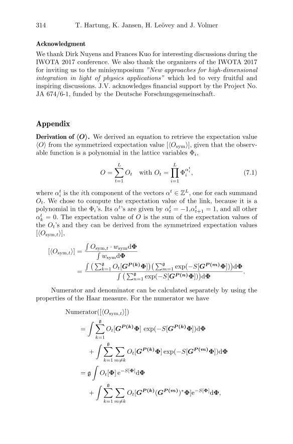
314 T. Hartung, K. Jansen, H. Leovey and J. Volmer
Acknowledgment
We thank Dirk Nuyens and Frances Kuo for interesting discussions during theIWOTA 2017 conference. We also thank the organizers of the IWOTA 2017for inviting us to the minisymposium ”New approaches for high-dimensionalintegration in light of physics applications” which led to very fruitful andinspiring discussions. J.V. acknowledges financial support by the Project No.JA 674/6-1, funded by the Deutsche Forschungsgemeinschaft.
Appendix
Derivation of 〈O〉. We derived an equation to retrieve the expectation value〈O〉 from the symmetrized expectation value [〈Osym〉], given that the observ-able function is a polynomial in the lattice variables Φi,
O =
L∑t=1
Ot with Ot =
L∏i=1
Φαtii , (7.1)
where αti is the ith component of the vectors αt ∈ ZL, one for each summandOt. We chose to compute the expectation value of the link, because it is apolynomial in the Φi’s. Its αt’s are given by αtt = −1,αtt+1 = 1, and all otherαtk = 0. The expectation value of O is the sum of the expectation values ofthe Ot’s and they can be derived from the symmetrized expectation values[〈Osym,t〉],
[〈Osym,t〉] =
∫Osym,t · wsymdΦ∫
wsymdΦ
=
∫ (∑gk=1Ot[G
P (k)Φ])(∑g
m=1 exp(−S[GP (m)Φ]))dΦ∫ (∑g
n=1 exp(−S[GP (n)Φ]))dΦ
.
Numerator and denominator can be calculated separately by using theproperties of the Haar measure. For the numerator we have
Numerator([〈Osym,t〉])
=
∫ g∑k=1
Ot[GP (k)Φ] exp(−S[GP (k)Φ])dΦ
+
∫ g∑k=1
∑m6=k
Ot[GP (k)Φ] exp(−S[GP (m)Φ])dΦ
= g
∫Ot[Φ] e−S[Φ]dΦ
+
∫ g∑k=1
∑m6=k
Ot[GP (k)(GP (m))∗Φ]e−S[Φ]dΦ,

Improving Monte Carlo integration 315
and the denominator is
Denominator([〈Osym,t〉])
= g
∫e−S[GP (m)Φ]dΦ.
Numerator and denominator combine to
[〈Osym,t〉] =
∫Ot[Φ] e−S[Φ]dΦ∫
e−S[Φ]dΦ
+1
g
g∑k=1
∑m 6=k
∫Ot[G
P (k)(GP (m))∗Φ]e−S[Φ]dΦ∫e−S[Φ]dΦ
.
The first term is 〈Ot〉. The second term needs the form of Ot from (7.1) togive
[〈Osym,t〉] = 〈Ot〉+1
g
g∑k=1
∑m 6=k
∫ ∏Ll=1
(GPl(k)(GPl(m))∗Φl
)αtl e−S[Φ]dΦ∫e−S[Φ]dΦ
= 〈Ot〉+1
g
g∑k=1
∑m 6=k
L∏l=1
(GPl(k)(GPl(m))∗
)αtl ∫ ∏Lp=1 Φ
αtpp e−S[Φ]dΦ∫
e−S[Φ]dΦ
= 〈Ot〉+1
g
g∑k=1
∑m 6=k
L∏l=1
(GPl(k)(GPl(m))∗
)αtl ∫ Ot[Φ]dΦ∫e−S[Φ]dΦ
= 〈Ot〉(
1 +1
g
g∑k=1
∑m 6=k
L∏l=1
(GPl(k)(GPl(m))∗
)αtl).If the correction factor
ct ≡ 1 +1
g
g∑k=1
∑m 6=k
L∏l=1
(GPl(k)(GPl(m))∗
)αtlis non-zero, the expectation value of Qt can be derived from the symmetrizedexpectation value [〈Qsym,t〉] via
〈Ot〉 =1
ct[〈Osym,t〉].
This formula is true because the correction factor is independent of the latticevalues Φi. With the proper αt’s for the link variable, the correction factor forthe link is
ct = 1 +1
g
∑i 6=j
(GPt(i)(GPt(j))∗
)∗(GPt+1(i)(GPt+1(j))∗
).
References
[1] R.P. Feynman, Space-time approach to nonrelativistic quantum mechanics,Rev. Mod. Phys. 20 (1948), 367–387.

316 T. Hartung, K. Jansen, H. Leovey and J. Volmer
[2] Christof Gattringer and Christian B. Lang, Quantum chromodynamics on thelattice, Lect. Notes Phys. 788 (2010), 1–343.
[3] S. Durr et al, Ab-Initio Determination of Light Hadron Masses, Science 322(2008), 1224–1227.
[4] A. Abdel-Rehim et al., Nucleon and pion structure with lattice QCD simula-tions at physical value of the pion mass, Phys. Rev., D92(11) (2015), 114513.[Erratum: Phys. Rev. D93(3) (2016), 039904].
[5] A. Abdel-Rehim et al., First physics results at the physical pion mass fromNf = 2 Wilson twisted mass fermions at maximal twist, Phys. Rev. D95(9)(2017), 094515.
[6] Haohuan Fu, Junfeng Liao, Jinzhe Yang, Lanning Wang, Zhenya Song, Xi-aomeng Huang, Chao Yang, Wei Xue, Fangfang Liu, Fangli Qiao, Wei Zhao,Xunqiang Yin, Chaofeng Hou, Chenglong Zhang, Wei Ge, Jian Zhang, Yan-gang Wang, Chunbo Zhou, and Guangwen Yang, The sunway taihulight super-computer: system and applications, Science China Information Sciences 59(7)(2016), 072001.
[7] Matthias Troyer and Uwe-Jens Wiese, Computational complexity and funda-mental limitations to fermionic quantum Monte Carlo simulations, Phys. Rev.Lett. 94 (2005), 170201.
[8] Christian Schmidt, Lattice QCD at finite density, PoS LAT2006:021 (2006).
[9] Andrew G. Cohen, D.B. Kaplan, and A.E. Nelson, Progress in electroweakbaryogenesis, Ann. Rev. Nucl. Part. Sci. 43 (1993), 27–70.
[10] A. Ammon, T. Hartung, K. Jansen, H. Levey, and J. Volmer, Overcoming thesign problem in one-dimensional QCD by new integration rules with polynomialexactness, Phys. Rev. D94(11) (2016), 114508.
[11] Jacques Bloch, Falk Bruckmann, and Tilo Wettig, Subset method for one-dimensional QCD, JHEP 10 (2013), 140.
[12] Jacques Bloch and Falk Bruckmann, Positivity of center subsets for QCD, Phys.Rev. D93(1) (2016), 014508. [Addendum: Phys. Rev. D93(3) (2016), 039907].
[13] A. Ammon, A. Genz, T. Hartung, K. Jansen, H. Levey, and J. Volmer, Onthe efficient numerical solution of lattice systems with low-order couplings,Comput. Phys. Commun. 198 (2016), 71–81.
[14] Tobias Hartung, Regularizing Feynman path integrals using the generalizedKontsevich-Vishik trace, J. Math. Phys. 58 (2017), 123505, 1–19.
[15] F Kuo, High dimensional integration: the Quasi-Monte Carlo (QMC) way,Plenary presentation, 28th IWOTA conference, August 14 to August 18, 2017,Technical University Chemnitz, Germany.
[16] W. Bietenholz, U. Gerber, M. Pepe, and U.-J. Wiese, Topological Lattice Ac-tions, JHEP 1012 (2010), 020.
[17] Kerstin Hesse, Frances Y. Kuo, and Ian H. Sloan, A component-by-componentapproach to efficient numerical integration over products of spheres, Journalof Complexity 23(1) (2007), 25–51.
[18] Ulli Wolff, Collective Monte Carlo Updating for Spin Systems, Phys. Rev. Lett.62 (1989), 361.
[19] A.M. Ferrenberg and R.H. Swendsen, New Monte Carlo Technique for StudyingPhase Transitions, Phys. Rev. Lett. 61 (1988), 2635–2638.

Improving Monte Carlo integration 317
Tobias HartungDepartment of MathematicsKing’s College LondonStrandLondon WC2R 2LSUnited Kingdome-mail: [email protected]
Karl JansenDESYJohn von Neumann Institute for ComputingPlatanenallee 615738 ZeuthenGermanye-mail: [email protected]
Hernan LeoveyStructured Energy ManagementAxpo TradingParkstrasse 235400 Baden, Germanye-mail: [email protected]
Julia VolmerDESYJohn von Neumann Institute for ComputingPlatanenallee 615738 ZeuthenGermanye-mail: [email protected]

More on the density of analyticpolynomials in abstract Hardy spaces
Alexei Karlovich and Eugene Shargorodsky
Abstract. Let Fn be the sequence of the Fejer kernels on the unitcircle T. The first author recently proved that if X is a separable Banachfunction space on T such that the Hardy–Littlewood maximal operatorM is bounded on its associate space X ′, then ‖f ∗ Fn − f‖X → 0 forevery f ∈ X as n→∞. This implies that the set of analytic polynomialsPA is dense in the abstract Hardy space H[X] built upon a separableBanach function space X such that M is bounded on X ′. In this notewe show that there exists a separable weighted L1 space X such thatthe sequence f ∗ Fn does not always converge to f ∈ X in the norm ofX. On the other hand, we prove that the set PA is dense in H[X] underthe assumption that X is merely separable.
Mathematics Subject Classification (2010). Primary 46E30, Secondary42A10.
Keywords. Banach function space, abstract Hardy space, analytic poly-nomial, Fejer kernel.
1. Preliminaries and the main results
For 0 < p ≤ ∞, let Lp := Lp(T) be the Lebesgue space on the unit circleT := z ∈ C : |z| = 1 in the complex plane C. For f ∈ L1, let
f(n) :=1
2π
∫ π
−πf(eiθ)e−inθ dθ, n ∈ Z,
be the sequence of the Fourier coefficients of f . Let X be a Banach spacecontinuously embedded in L1. Following [13, p. 877], we will consider theabstract Hardy space H[X] built upon the space X, which is defined by
H[X] :=f ∈ X : f(n) = 0 for all n < 0
.
This work was partially supported by the Fundacao para a Ciencia e a Tecnologia (Portu-
guese Foundation for Science and Technology) through the project UID/MAT/00297/2013(Centro de Matematica e Aplicacoes).
© Springer International Publishing AG, part of Springer Nature 2018
Theory: Advances and Applications 268, https://doi.org/10.1007/978-3-319-75996-8_16
319A. Böttcher et al. (eds.), The Diversity and Beauty of Applied Operator Theory, Operator

320 A. Karlovich and E. Shargorodsky
It is clear that if 1 ≤ p ≤ ∞, then H[Lp] is the classical Hardy space Hp.
A function of the form
q(t) =
n∑k=0
αktk, t ∈ T, α0, . . . , αn ∈ C,
is said to be an analytic polynomial on T. The set of all analytic polynomialsis denoted by PA. It is well known that the set PA is dense in Hp whenever1 ≤ p <∞ (see, e.g., [3, Chap. III, Corollary 1.7(a)]). The density of the setPA in the abstract Hardy spaces H[X] was studied by the first author [8] forthe case when X is a so-called Banach function space.
Let us recall the definition of a Banach function space. We equip Twith the normalized Lebesgue measure dm(t) = |dt|/(2π). Let L0 be thespace of all measurable complex-valued functions on T. As usual, we do notdistinguish functions which are equal almost everywhere (for the latter weuse the standard abbreviation a.e.). Let L0
+ be the subset of functions in L0
whose values lie in [0,∞]. The characteristic function of a measurable setE ⊂ T is denoted by χE .
Following [1, Chap. 1, Definition 1.1], a mapping ρ : L0+ → [0,∞] is
called a Banach function norm if, for all functions f, g, fn ∈ L0+ with n ∈ N,
for all constants a ≥ 0, and for all measurable subsets E of T, the followingproperties hold:
(A1) ρ(f) = 0⇔ f = 0 a.e., ρ(af) = aρ(f), ρ(f + g) ≤ ρ(f) + ρ(g),
(A2) 0 ≤ g ≤ f a.e. ⇒ ρ(g) ≤ ρ(f) (the lattice property),
(A3) 0 ≤ fn ↑ f a.e. ⇒ ρ(fn) ↑ ρ(f) (the Fatou property),
(A4) m(E) <∞ ⇒ ρ(χE) <∞,
(A5)
∫E
f(t) dm(t) ≤ CEρ(f)
with a constant CE ∈ (0,∞) that may depend on E and ρ, but is independentof f . When functions differing only on a set of measure zero are identified,the set X of all functions f ∈ L0 for which ρ(|f |) < ∞ is called a Banachfunction space. For each f ∈ X, the norm of f is defined by ‖f‖X := ρ(|f |).The set X under the natural linear space operations and under this normbecomes a Banach space (see [1, Chap. 1, Theorems 1.4 and 1.6]). If ρ is aBanach function norm, its associate norm ρ′ is defined on L0
+ by
ρ′(g) := sup
∫Tf(t)g(t) dm(t) : f ∈ L0
+, ρ(f) ≤ 1
, g ∈ L0
+.
It is a Banach function norm itself [1, Chap. 1, Theorem 2.2]. The Banachfunction space X ′ determined by the Banach function norm ρ′ is called theassociate space (Kothe dual) of X. The associate space X ′ can be viewed asa subspace of the (Banach) dual space X∗.

More on the density of analytic polynomials 321
Recall that L1 is a commutative Banach algebra under the convolutionmultiplication defined for f, g ∈ L1 by
(f ∗ g)(eiθ) =1
2π
∫ π
−πf(eiθ−iϕ)g(eiϕ) dϕ, eiθ ∈ T.
For n ∈ N, let
Fn(eiθ) :=n∑
k=−n
(1− |k|
n+ 1
)eiθk =
1
n+ 1
(sin n+1
2 θ
sin θ2
)2
, eiθ ∈ T,
be the n-th Fejer kernel. For f ∈ L1, the n-th Fejer mean of f is defined asthe convolution f ∗ Fn.
Given f ∈ L1, the Hardy–Littlewood maximal function is defined by
(Mf)(t) := supI3t
1
m(I)
∫I
|f(τ)| dm(τ), t ∈ T,
where the supremum is taken over all arcs I ⊂ T containing t ∈ T. Theoperator f 7→Mf is called the Hardy–Littlewood maximal operator.
Theorem 1.1 ([8, Theorem 3.3]). Suppose X is a separable Banach functionspace on T. If the Hardy–Littlewood maximal operator is bounded on the as-sociate space X ′, then for every f ∈ X,
limn→∞
‖f ∗ Fn − f‖X = 0. (1.1)
It is well known that for f ∈ L1 one has
(f ∗ Fn)(eiθ) =n∑
k=−n
f(k)
(1− |k|
n+ 1
)eiθk, eiθ ∈ T
(see, e.g., [9, Chap. I]). This implies that if f ∈ H[X] ⊂ H[L1] = H1, thenf ∗Fn ∈ PA. Combining this observation with Theorem 1.1, we arrive at thefollowing.
Corollary 1.2 ([8, Theorem 1.2]). Suppose X is a separable Banach functionspace on T. If the Hardy–Littlewood maximal operator M is bounded on itsassociate space X ′, then the set of analytic polynomials PA is dense in theabstract Hardy space H[X] built upon the space X.
Note that if a Banach function space X is, in addition, rearrangement-invariant, then the requirement of the boundedness of M on the space X ′
can be omitted in Corollary 1.2 (see [8, Theorem 1.1] or [11, Lemma 1.3(c)]).Lesnik [10] conjectured that the same fact should be true for arbitrary, notnecessarily rearrangement-invariant, Banach function spaces.
In this note, we first observe that Theorem 1.1 does not hold for arbi-trary separable Banach function spaces. For a function K ∈ L1, consider theconvolution operator CK with kernel K defined by
CKf = f ∗K, f ∈ L1.

322 A. Karlovich and E. Shargorodsky
It follows from [12, Theorem 2] that there exists a continuous functionp : T → [1,∞) such that the sequence of the convolution operators CFn isnot uniformly bounded in the variable Lebesgue space Lp(·) defined as theset of all f ∈ L0 such that∫
T|f(t)|p(t)dm(t) <∞.
It is well known (see, e.g., [4, Propostion 2.12, Theorem 2.78, Section 2.10.3])that if p : T→ [1,∞) is continuous, then Lp(·) is a separable Banach functionspace equipped with the norm
‖f‖Lp(·) = inf
λ > 0 :
∫T
∣∣∣∣f(t)
λ
∣∣∣∣p(t) dm(t) ≤ 1
.
Since the norms of the convolution operators CFn may not be uniformlybounded on Lp(·), the standard argument, based on the uniform boundednessprinciple, leads us to the following.
Theorem 1.3. There exist a separable Banach function space X on T and afunction f ∈ X such that (1.1) is not fulfilled.
We show that the separable Banach function space in Theorem 1.3 canbe chosen as a weighted L1 space, that is, the techniques of variable Lebesguespaces can be omitted.
Theorem 1.4 (Main result 1). There exist a nonnegative function w ∈ L1
such that w−1 ∈ L∞ and a function f in the separable Banach function space
X = L1(w) = f ∈ L0 : fw ∈ L1such that (1.1) is not fulfilled.
In spite of the observation made in Theorems 1.3 and 1.4, we show thatthe requirement of the boundedness of the Hardy–Littlewood maximal oper-ator M on the associate space X ′ of a separable Banach function space X inCorollary 1.2 can be omitted. Thus, Lesnik’s conjecture [10] is, indeed, true.
Theorem 1.5 (Main result 2). If X is a separable Banach function space onT, then the set of analytic polynomials PA is dense in the abstract Hardyspace H[X] built upon the space X.
The paper is organized as follows. In Section 2, we prove that a convolu-tion operator CK with a nonnegative symmetric kernel K ∈ L1 is bounded ona Banach function space X if and only if it is bounded on its associate spaceX ′. Further, we consider a special weight w ∈ L1 such that w−1 ∈ L∞. ThenX = L1(w) is a separable Banach function space with the associate spaceX ′ = L∞(w−1). We show that the sequence of convolution operators CKnwith nonnegative bounded symmetric kernels Kn, satisfying ‖Kn‖L1 = 1 anda natural localization property, is not uniformly bounded on X ′ = L∞(w−1),and therefore, on its associate space X ′′ = X = L1(w). Applying this resultto the sequence of the Fejer kernels Fn, we prove Theorem 1.4 with the aidof the uniform boundedness principle.

More on the density of analytic polynomials 323
In Section 3, we recall that the separability of a Banach function spaceXis equivalent to X∗ = X ′. Further, we collect some facts on the identificationof the Hardy spaces Hp on the unit circle and the Hardy spaces Hp(D) ofanalytic functions in the unit disk D. Finally, we give a proof of Theorem 1.5based on an application of the Hahn–Banach theorem, a corollary of theSmirnov theorem and properties of the identification of H1 with H1(D).
2. Proof of the first main result
2.1. Norms of convolution operators on X and on its associate space X′
The Banach space of all bounded linear operators on a Banach space E isdenoted by B(E).
Lemma 2.1. Let X be a Banach function space on T and K ∈ L1 be anonnegative function such that K(eiθ) = K(e−iθ) for almost all θ ∈ [−π, π].Then the convolution operator CK is bounded on the Banach function X ifand only if it is bounded on its associate space X ′. In that case
‖CK‖B(X′) = ‖CK‖B(X). (2.1)
Proof. Suppose CK is bounded on X ′. Fix f ∈ X \ 0. Since K ≥ 0, wehave |f ∗K| ≤ |f | ∗K. According to the Lorentz–Luxemburg theorem (see,e.g., [1, Chap. 1, Theorem 2.7]), X = X ′′ with equality of the norms. Hence
‖f ∗K‖X ≤ ‖ |f | ∗K‖X = ‖ |f | ∗K‖X′′
= sup
∫T(|f | ∗K)(t)|g(t)| dm(t) : g ∈ X ′, ‖g‖X′ ≤ 1
.
Then for every ε > 0 there exists a function h ∈ X ′ such that h ≥ 0,‖h‖X′ ≤ 1, and
‖f ∗K‖X ≤ (1 + ε)
∫T(|f | ∗K)(t)h(t) dm(t). (2.2)
Taking into account that K(eiθ) = K(e−iθ) for almost all θ ∈ R, by Fubini’stheorem, we get∫
T(|f | ∗K)(t)h(t) dm(t) =
∫T(h ∗K)(t)|f(t)| dm(t).
From this identity, Holder’s inequality for X (see, e.g., [1, Chap. 1, Theo-rem 2.4]), and the boundedness of CK on X ′, we obtain∫
T(|f | ∗K)(t)h(t) dm(t) ≤ ‖f‖X‖h ∗K‖X′ ≤ ‖f‖X‖CK‖B(X′). (2.3)
It follows from (2.2)–(2.3) that
‖CK‖B(X) = supf∈X,f 6=0
‖f ∗K‖X‖f‖X
≤ (1 + ε)‖CK‖B(X′)
for every ε > 0, which implies the boundedness of CK on X and the inequality
‖CK‖B(X) ≤ ‖CK‖B(X′). (2.4)

324 A. Karlovich and E. Shargorodsky
If CK is bounded on X, then using the Lorentz–Luxemburg theoremand (2.4) with X ′ in place of X, we obtain that CK is bounded on X ′ and
‖CK‖B(X′) ≤ ‖CK‖B(X′′) = ‖CK‖B(X). (2.5)
Combining (2.4)–(2.5), we arrive at (2.1).
2.2. Spaces L1(w) and L∞(w−1) with a special weight w
Lemma 2.2. Let
w(eiθ)
:=
√m, π
2m ≤ |θ| ≤π
2m−1 , m ∈ N,
1, π2m+1 < |θ| <
π2m , m ∈ N.
(2.6)
Then the spaces
L1(w) = f ∈ L0 : fw ∈ L1, L∞(w−1) = f ∈ L0 : fw−1 ∈ L∞are Banach function spaces on T with respect to the norms
‖f‖L1(w) = ‖fw‖L1 , ‖f‖L∞(w−1) = ‖fw−1‖L∞ ,
and (L1(w))′ = L∞(w−1). Moreover, the space L1(w) is separable.
Proof. It is clear that w−1 ∈ L∞ and, since
‖w‖L1 =1
2π
∫ π
−πw(eiθ) dθ
=∞∑m=1
(1
2m− 1
2m+ 1
)+∞∑m=1
√m
(1
2m− 1− 1
2m
)<∞, (2.7)
we also have w ∈ L1. Then it follows from [7, Lemma 2.5] that L1(w) andL∞(w−1) are Banach function spaces and (L1(w))′ = L∞(w−1). Finally,the separability of the space L1(w) follows from [7, Proposition 2.6] and [1,Chap. 1, Corollary 5.6].
2.3. Norms of convolution operators are not uniformly bounded on the spacesL1(w) and L∞(w−1) with the special weight w
Theorem 2.3. Let Kn be a sequence of bounded functions Kn : T→ C suchthat
Kn(eiθ) ≥ 0, Kn(eiθ) = Kn(e−iθ) a.e. on [−π, π], (2.8)
1
2π
∫ π
−πKn
(eiθ)dθ = 1, (2.9)
andlimn→∞
supε≤|θ|≤π
Kn
(eiθ)
= 0 for each ε > 0. (2.10)
If w is the weight given by (2.6), then the convolution operators CKn arebounded on L∞(w−1) and on L1(w) for all n ∈ N, however,
supn∈N‖CKn‖B(L∞(w−1)) =∞, (2.11)
supn∈N‖CKn‖B(L1(w)) =∞. (2.12)

More on the density of analytic polynomials 325
Proof. By (2.6)–(2.7), w ∈ L1 and w−1 ∈ L∞. Therefore, for every n ∈ N,
‖CKnf‖L1(w) ≤1
2π
∥∥∥∥∫ π
−πKn(ei(·−θ))
∣∣f (eiθ)∣∣ dθ∥∥∥∥L1(w)
≤ 1
2π
∫ π
−π
∥∥Kn(ei(·−θ))∥∥L1(w)
∣∣f (eiθ)∣∣ dθ≤ 1
2π‖Kn‖L∞‖w‖L1‖f‖L1
=1
2π‖Kn‖L∞‖w‖L1‖w−1fw‖L1
≤ 1
2π‖Kn‖L∞‖w‖L1‖w−1‖L∞‖f‖L1(w).
Hence
‖CKn‖B(L1(w)) ≤1
2π‖Kn‖L∞‖w‖L1‖w−1‖L∞ , n ∈ N.
It follows from (2.8) and Lemmas 2.1–2.2 that the operators CKn are boundedon L∞(w−1) for all n ∈ N. Moreover, (2.11) implies (2.12).
Let us prove (2.11). Consider the sequence
vm(eiθ)
:=
√m, π
2m ≤ θ ≤π
2m−1 ,
0, θ ∈ [−π, π] \[π2m ,
π2m−1
],
m ∈ N.
Then it follows from (2.6) that ‖vm‖L∞(w−1) = 1 for all m ∈ N.
Fix m ∈ N. According to (2.9) and the localization property (2.10),there exists n(m) ∈ N such that∫ 0
− π(2m)2
Kn
(eiθ)dθ =
1
2
∫ π(2m)2
− π(2m)2
Kn
(eiθ)dθ ≥ 1
3for all n ≥ n(m).
Since Kn ∈ L1, for every n ≥ n(m), there exists δn > 0 such that∫ −δn− π
(2m)2
Kn
(eiθ)dθ ≥ 1
4.
Therefore, for almost all ϑ ∈[π2m − δn,
π2m
], one gets
(CKnvm)(eiϑ)
=
√m
2π
∫ π2m−1
π2m
Kn
(eiϑ−iθ
)dθ
≥√m
2π
∫ π2m+ π
(2m)2
π2m
Kn
(eiϑ−iθ
)dθ
=
√m
2π
∫ ϑ− π2m
ϑ− π2m−
π(2m)2
Kn
(eiη)dη
≥√m
2π
∫ −δn− π
(2m)2
Kn
(eiη)dη ≥
√m
8π. (2.13)

326 A. Karlovich and E. Shargorodsky
In view of (2.6), w(eiϑ) = 1 for all ϑ ∈(
max
π2m − δn,
π2m+1
, π2m
). Hence,
it follows from (2.13) that
‖CKnvm‖L∞(w−1) ≥√m
8πfor all n ≥ n(m),
while ‖vm‖L∞(w−1) = 1. So,
‖CKn‖B(L∞(w−1)) ≥√m
8πfor all n ≥ n(m).
Since m ∈ N is arbitrary, the latter inequality immediately implies (2.11).
2.4. Proof of Theorem 1.4
Let X = L1(w), where w is the weight given by (2.6). By Lemma 2.2, X is aseparable Banach function space. It is well known (and not difficult to check)that the sequence Fn of the Fejer kernels is a sequence of bounded functionssatisfying (2.8)–(2.10). By Theorem 2.3, the operators CFn are bounded onX for every n ∈ N.
Assume that (1.1) is fulfilled for all f ∈ X. Then, for all f ∈ X, thesequence CFnf is bounded in X. Therefore, by the uniform boundednessprinciple, the sequence ‖CFn‖B(X) is bounded, but this contradicts (2.12).Thus, there exists a function f ∈ X such that (1.1) does not hold.
3. Proof of the second main result
3.1. Separable Banach function spaces X are spaces for which X∗ is isomet-rically isomorphic to X′
Combining [1, Chap. I, Corollaries 4.3 and 5.6] and observing that the mea-sure dm is separable (for the definition of a separable measure, see, e.g., [1,p. 27] or [6, Chap. I, Section 6.10]), we arrive at the following.
Theorem 3.1. Let X be a Banach function space on T. Then X is separableif and only if its dual space X∗ is isometrically isomorphic to the associatespace X ′.
3.2. Hardy spaces on the unit disk
Let D denote the open unit disk in the complex plane C. Recall that a functionF analytic in D is said to belong to the Hardy space Hp(D), 0 < p ≤ ∞, ifthe integral mean
Mp(r, F ) =
(1
2π
∫ π
−π
∣∣F (reiθ)∣∣p dθ)1/p
, 0 < p <∞,
M∞(r, F ) = max−π≤θ≤π
∣∣F (reiθ)∣∣,
remains bounded as r → 1. If F ∈ Hp(D), 0 < p ≤ ∞, then the nontangentiallimit
f(eiθ) = limr→1−0
F (reiθ)

More on the density of analytic polynomials 327
exists for almost all θ ∈ [−π, π] (see, e.g., [5, Theorem 2.2]) and the boundaryfunction f = f(eiθ) belongs to Lp.
The following lemma is an immediate consequence of the Smirnov the-orem (see, e.g., [5, Theorem 2.11]).
Lemma 3.2. If F ∈ Hp(D) for some p ∈ (0, 1) and its boundary function fbelongs to L1, then F ∈ H1(D).
Recall that if f ∈ H1 then its analytic extension F into D, given by thePoisson integral
F (reiθ) =1
2π
∫ π
−πP (r, θ − ϕ)f(eiϕ) dϕ, 0 ≤ r < 1, −π ≤ θ ≤ π,
where
P (r, θ) =1− r2
1− 2r cos θ + r2, 0 ≤ r < 1, −π ≤ θ ≤ π,
is the Poisson kernel, belongs to H1(D) and the boundary function of Fcoincides with f a.e. on T (see, e.g., [5, Theorem 3.1]).
It is important to note that the Taylor coefficients of F ∈ Hp(D) coincidewith the Fourier coefficients of its boundary function f ∈ Lp. More precisely,one has the following.
Theorem 3.3 ([5, Theorem 3.4]). Let F (z) =∑∞n=0 anz
n belong to H1(D) and
let f(n) be the sequence of the Fourier coefficients of its boundary function
f ∈ L1. Then f(n) = an for all n ≥ 0 and f(n) = 0 for n < 0.
3.3. Proof of Theorem 1.5
Suppose PA is not dense in H[X]. Take any function f ∈ H[X] that doesnot belong to the closure of PA with respect to the norm of X. Since X isseparable, it follows from Theorem 3.1 that X∗ is isometrically isomorphic toX ′. Then, by a corollary of the Hahn–Banach theorem (see, e.g., [2, Chap. 7,Theorem 4.1]), there exists a function g ∈ X ′ ⊂ L1 such that∫ π
−πf(eiθ)g(eiθ)dθ 6= 0 (3.1)
and ∫ π
−πp(eiθ)g(eiθ)dθ = 0 for all p ∈ PA.
In particular, if p(eiθ) = einθ with n = 0, 1, 2, . . . , then
g(−n) = 0 for all n = 0, 1, 2, . . . . (3.2)
Hence g ∈ H[X ′] ⊂ H1. For functions f ∈ H[X] ⊂ H1 and g ∈ H[X ′] ⊂ H1,let F and G denote their analytic extensions to the unit disk D by meansof their Poisson integrals. Then F,G ∈ H1(D). It follows from (3.2) andTheorem 3.3 that G(0) = 0. Since F,G ∈ H1(D), by Holder’s inequality,FG ∈ H1/2(D). On the other hand, since f ∈ X and g ∈ X ′, it followsfrom Holder’s inequality for Banach function spaces (see [1, Chap. 1, Theo-rem 2.4]) that fg ∈ L1. Then it follows from Lemma 3.2 that FG ∈ H1(D).

328 A. Karlovich and E. Shargorodsky
Since (FG)(0) = F (0)G(0) = 0, applying Theorem 3.3 to FG, we obtain
fg(0) = 0, that is, ∫ π
−πf(eiθ)g(eiθ)dθ = 0,
which contradicts (3.1).
Acknowledgment
We would like to thank the referee for the useful remarks.
References
[1] C. Bennett and R. Sharpley, Interpolation of Operators, Academic Press,Boston, 1988.
[2] Yu.M. Berezansky, Z.G. Sheftel, and G.F. Us, Functional Analysis, Vol. 1,Birkhauser, Basel, 1996.
[3] J.B. Conway, The Theory of Subnormal Operators, American MathematicalSociety, Providence, RI, 1991.
[4] D. Cruz-Uribe and A. Fiorenza, Variable Lebesgue Spaces, Birkhauser, Basel,2013.
[5] P.L. Duren, Theory of Hp Spaces, Academic Press, New York and London,1970.
[6] L.V. Kantorovich and G.P. Akilov, Functional Analysis, Pergamon Press, Ox-ford, 2nd ed., 1982.
[7] A. Karlovich, Fredholmness of singular integral operators with piecewise con-tinuous coefficients on weighted Banach function spaces, J. Integral EquationsAppl. 15 (2003), 263–320.
[8] A. Karlovich, Density of analytic polynomials in abstract Hardy spaces. Com-ment. Math., to appear. Preprint is available at arXiv:1710.10078 [math.CA](2017).
[9] Y. Katznelson, An Introduction to Harmonic Analysis, Dower Publications,Inc., New York, 1976.
[10] K. Lesnik, Personal communication to A. Karlovich, February 23, 2017.
[11] K. Lesnik, Toeplitz and Hankel operators between distinct Hardy spaces,arXiv:1708.00910 [math.FA] (2017).
[12] I.I. Sharapudinov, Uniform boundedness in Lp (p = p(x)) of some families ofconvolution operators, Math. Notes 59 (1996), 205–212.
[13] Q. Xu, Notes on interpolation of Hardy spaces, Ann. Inst. Fourier 42 (1992),875–889.

More on the density of analytic polynomials 329
Alexei KarlovichCentro de Matematica e Aplicacoes,Departamento de Matematica,Faculdade de Ciencias e Tecnologia,Universidade Nova de Lisboa,Quinta da Torre,2829–516 CaparicaPortugale-mail: [email protected]
Eugene ShargorodskyDepartment of MathematicsKing’s College LondonStrand, London WC2R 2LSUnited Kingdome-mail: [email protected]

Pseudodifferential operators withcompound non-regular symbols
Yuri I. Karlovich
Abstract. The boundedness and compactness of Fourier pseudodifferen-tial operators with compound symbols in subclasses of L∞(R2, L1(R))is studied on weighted Lebesgue spaces Lp(R, w) with p ∈ (1,∞) andMuckenhoupt weights w ∈ Ap(R) by applying the techniques of oscilla-tory integrals. The boundedness and compactness conditions are also ob-tained for Mellin pseudodifferential operators with compound symbolsin subclasses of L∞(R2
+, L1(R)), which act on the spaces Lp(R+, dµ),
where dµ(t) = dt/t for t ∈ R+. The latter results allow one to reducethe smoothness of slowly oscillating Carleson curves Γ and slowly oscil-lating Muckenhoupt weights w in the Fredholm study of singular integraloperators with shifts on weighted Lebesgue spaces Lp(Γ, w).
Mathematics Subject Classification (2010). Primary 47G30; Secondary45E05, 47G10.
Keywords. Fourier and Mellin pseudodifferential operators; compoundsymbol; oscillatory integral; singular integral operator; Lebesgue space;Muckenhoupt weight; boundedness; compactness.
1. Introduction
The paper is devoted to studying the Fourier and Mellin pseudodifferen-tial operators with compound non-regular symbols of limiting smoothness.Pseudodifferential operators with non-regular symbols are intensively stud-ied now (see, e.g., [5]–[7], [23], [28]–[31] and the references therein). Reduc-ing the smoothness of symbols, which expands the fields of applications ofpseudodifferential operators, is one of the main interests. Pseudodifferentialoperators of Mellin type with non-regular symbols are also actively studiedalong with Fourier pseudodifferential operators (see, e.g., [8], [22], and [23],and the references given there). Applications of pseudodifferential operatorsto the theory of singular integral operators with non-regular data are given,
The author was partially supported by the PFCE project (Mexico).
© Springer International Publishing AG, part of Springer Nature 2018
Theory: Advances and Applications 268, https://doi.org/10.1007/978-3-319-75996-8_17
331A. Böttcher et al. (eds.), The Diversity and Beauty of Applied Operator Theory, Operator

332 Yu.I. Karlovich
e.g., in [1]–[4], [15], [19], [23]. For applications of pseudodifferential opera-tors with non-regular symbols to singular integral operators with shifts andnon-regular data see, e.g., [9], [11]–[13], [18], [21].
Let Γ be an oriented locally rectifiable simple open arc in the complexplane, and let Lp(Γ, w) be the weighted Lebesgue space with the norm
‖f‖Lp(Γ,w) :=
(∫Γ
|f(τ)|p|w(τ)|p|dτ |)1/p
,
where p ∈ (1,∞) and w : Γ→ [0,∞] is a measurable function with pre-imagew−1(0,∞) of measure zero. As is known (see, e.g., [1]), the Cauchy singularintegral operator SΓ, given for f ∈ L1(Γ) and almost all t ∈ Γ by
(SΓf)(t) := limε→0
1
πi
∫Γ\Γ(t,ε)
f(τ)
τ − tdτ, Γ(t, ε) :=
τ ∈ Γ : |τ − t| < ε
, (1.1)
is bounded on the space Lp(Γ, w) if and only if w ∈ Ap(Γ), that is,
cp,w := supε>0
supt∈Γ
1
ε
(∫Γ(t,ε)
w(τ)p|dτ |)1/p(∫
Γ(t,ε)
w(τ)−q|dτ |)1/q
<∞, (1.2)
where 1/p+ 1/q = 1. If (1.2) holds, then the Holder inequality implies that
supε>0
supt∈Γ|Γ(t, ε)|/ε <∞, (1.3)
where |Γ(t, ε)| stands for the Lebesgue (length) measure of Γ(t, ε). Condition(1.2) is called the Muckenhoupt condition, and curves Γ satisfying (1.3) arenamed Carleson or Ahlfors–David curves (see [1]).
The present paper continues investigations started in [14]–[17] and [20],and deals with studying the boundedness and compactness of Fourier pseudo-differential operators with compound non-regular symbols on the weightedLebesgue spaces Lp(R, w) with p ∈ (1,∞) and Muckenhoupt weights w be-longing to Ap(R). The results obtained are applied to studying the bounded-ness and compactness of Mellin pseudodifferential operators with compoundnon-regular symbols on the Lebesgue spaces Lp(R+, dµ) with the invariantmeasure dµ(t) = dt/t. In contrast to the papers [15]–[17], we essentially re-duce the smoothness of the considered compound symbols with respect tospatial variables. This, in turn, leads to decreasing the smoothness of curvesand weights in the Fredholm theory of singular integral operators with shiftson weighted Lebesgue spaces.
The paper is organized as follows. Section 2 contains preliminaries: def-initions of oscillatory integrals, the Banach algebra V (R) of all absolutelycontinuous functions of bounded total variation on R, and the Banach al-gebras L∞
(Rn, V (R)
)(n = 1, 2) of bounded measurable V (R)-valued sym-
bols. In Section 3 we study the boundedness and compactness of Fourierpseudodifferential operators with compound non-regular symbols on weightedLebesgue spaces Lp(R, w), making use of the techniques of oscillatory in-tegrals (see, e.g., [27], [32]). In Section 4 these results are carried over tothe Mellin pseudodifferential operators with compound non-regular symbols

Pseudodifferential operators with compound non-regular symbols 333
on Lebesgue spaces Lp(R+, dµ). In Section 5 we illustrate an applicationof the results of Section 4 to Mellin pseudodifferential operators arising instudying singular integral operators on weighted Lebesgue spaces over slowlyoscillating Carleson curves with slowly oscillating Muckenhoupt weights.
2. Preliminaries
2.1. Oscillatory integrals
Let F and F−1 be the Fourier transform and its inverse defined on functionsf ∈ L2(R) by
(Ff)(x) =
∫Rf(t)e−ixtdt, (F−1f)(x) =
1
2π
∫Rf(t)eixtdt, x ∈ R. (2.1)
Let C∞0 (Rn) stand for the set of all infinitely differentiable complex-valuedfunctions of compact support on Rn, for n ∈ N.
Let χ ∈ C∞0 (R × R) and χ(y, η) = 1 in a neighborhood of the origin.Put χε(y, η) := χ(εy, εη) and consider a function a : R× R→ C. If the limit
limε→0
1
2π
∫∫R2
χε(y, η)a(y, η)e−iyηdydη
exists and does not depend on the choice of the cut-off function χ, then it iscalled the (double) oscillatory integral of a and is denoted by Os
[a(y, η)e−iyη
](see, e.g., [27, Chapter 1] or [32, Vol. 1, Chapter 1]).
Clearly, if a ∈ L1(R×R), then, by the Lebesgue dominated convergencetheorem (see, e.g., [24, Theorem I.11]), Os
[a(y, η)e−iyη
]exists and
Os[a(y, η)e−iyη
]=
1
2π
∫∫R2
a(y, η)e−iyηdydη. (2.2)
In what follows we will use the notation
〈y〉−2 = (1 + y2)−1, 〈Dη〉2 = I − ∂2η
and will apply the following regularization of oscillatory integrals, which isbased on the relation
〈y〉−2〈Dη〉2e−iyη = e−iyη, (2.3)
integrating by parts, and on the Lebesgue dominated convergence theorem.
Lemma 2.1. If the functions (y, η) 7→ ∂jηa(y, η) are in the space L∞(R, L1(R)
)for all j = 0, 1, 2, then the oscillatory integral Os
[a(y, η)e−iyη
]exists and is
given by
Os[a(y, η)e−iyη
]=
1
2π
∫∫R2
〈y〉−2〈Dη〉2a(y, η)
e−iyηdydη. (2.4)

334 Yu.I. Karlovich
Proof. Choosing a cut-off function χ ∈ C∞0 (R× R) and integrating by partsmaking use of (2.3), we obtain∫∫
R2
χε(y, η)a(y, η)e−iyηdydη
=
∫∫R2
χε(y, η)a(y, η)〈y〉−2〈Dη〉2
e−iyη
dydη (2.5)
=
∫∫R2
〈y〉−2〈Dη〉2χε(y, η)a(y, η)
e−iyηdydη.
As ∂jηχε(y, η)a(y, η)
∈ L∞
(R, L1(R)
)for all j = 0, 1, 2, and hence the func-
tion (y, η) 7→ 〈y〉−2〈Dη〉2χε(y, η)a(y, η)
belongs to L1(R×R), we conclude
that the last double integral in (2.5) exists.
Taking into account the facts that the function
(y, η) 7→ 〈y〉−2〈Dη〉2a(y, η)
e−iyη
belongs to L1(R×R) and, therefore, the double integral on the right of (2.4)exists, we proceed to prove the equality (2.4).
By definition of oscillatory integrals and by (2.5),
Os[a(y, η)e−iyη
]= limε→0
1
2π
∫∫R2
χε(y, η)a(y, η)e−iyηdydη
= limε→0
1
2π
∫∫R2
〈y〉−2〈Dη〉2χε(y, η)a(y, η)
e−iyηdydη.
(2.6)
Applying the Lebesgue dominated convergence theorem and taking into ac-count the fact that for j = 1, 2 the partial derivatives ∂jηχε(y, η) uniformlyconverge on R× R to zero as ε→ 0, we infer from (2.6) that
Os[a(y, η)e−iyη
]= limε→0
1
2π
∫∫R2
χε(y, η)〈y〉−2〈Dη〉2a(y, η)
e−iyηdydη
=1
2π
∫∫R2
〈y〉−2〈Dη〉2a(y, η)
e−iyηdydη.
Thus the oscillatory integral Os[a(y, η)e−iyη
]exists, equals the double in-
tegral in (2.4), and hence does not depend on the particular choice of thecut-off function χ.
2.2. Absolutely continuous functions of bounded total variation
Let a be an absolutely continuous function on R of bounded total variationV (a), where V (a) is given by
sup
n∑k=1
∣∣a(xk)− a(xk−1)∣∣ : −∞ < x0 < x1 < . . . < xn < +∞, n ∈ N
.
Hence (see, e.g., [10, Chapter 9]), there exist the finite limits
a(±∞) = limx→±∞
a(x),

Pseudodifferential operators with compound non-regular symbols 335
and therefore a is continuous on R := [−∞,+∞], and
a′ ∈ L1(R), V (a) =
∫R|a′(y)|dy.
The set V (R) of all absolutely continuous functions of bounded total variationon R is a Banach algebra equipped with the norm
∥∥a∥∥V
:=∥∥a∥∥
L∞(R)+V (a).
2.3. Bounded measurable V (R)-valued symbols
For every n = 1, 2, we denote by L∞(Rn, V (R)
)the set of all functions
a : Rn × R → C such that x 7→ a(x, ·) is a bounded measurable V (R)-valued function on Rn. Since the Banach space V (R) is separable, we concludeaccording to [26, Chapter IV, Theorem 232] that every measurable V (R)-valued function is a limit a.e. of a sequence of simple measurable functionsak : Rn → V (R) having only finite sets of values bi ∈ V (R), with measurablepre-images a−1
k (bi) of these values. This implies that, for all λ ∈ R, the
functions x 7→ a(x, λ) and the function x 7→∥∥a(x, ·)
∥∥V
are measurable on Rnas limits a.e. of suitable sequences of simple measurable functions. Therefore,a(·, λ) ∈ L∞(Rn) for every λ ∈ R, and the function x 7→
∥∥a(x, ·)∥∥V
, where∥∥a(x, ·)∥∥V
:= maxλ∈R|a(x, λ)|+
∫R|∂λa(x, λ)|dλ, (2.7)
belongs to L∞(Rn). Clearly, L∞(Rn, V (R)
)is a Banach algebra with the
norm ∥∥a∥∥L∞(Rn,V (R))
:= ess supx∈Rn
∥∥a(x, ·)∥∥V. (2.8)
3. The Fourier pseudodifferential operators
Lemma 3.1. If the function a(x, y, λ) belongs to the algebra L∞(R×R, V (R)
)and the function
a(x, y, λ) := a(x, y, λ)− a(x, x, λ), (3.1)
belongs to the space L∞(R × R, L1(R)
), then the Fourier pseudodifferential
operator A is well defined for every u ∈ C∞0 (R) by the iterated integral
(Au)(x) :=1
2π
∫Rdλ
∫Ra(x, y, λ)ei(x−y)λu(y)dy, x ∈ R. (3.2)
Proof. We need to prove that the iterated integral on the right of (3.2) con-verges for every u ∈ C∞0 (R) and almost all x ∈ R.
Since the function a(x, λ) := a(x, x, λ) belongs to L∞(R,V (R)
), we see
from [14, Theorem 3.1] that the Fourier pseudodifferential operator a(x,D)defined for functions u ∈ C∞0 (R) by the iterated integral
[a(x,D)u](x) :=1
2π
∫Rdλ
∫Ra(x, λ)ei(x−y)λu(y)dy, x ∈ R, (3.3)
extends to a bounded linear map on every Lebesgue space Lp(R), p∈(1,∞),

336 Yu.I. Karlovich
and therefore the iterated integral in (3.3) converges for almost all x ∈ R.Hence, by (3.1),
A = a(x,D) + A, (3.4)
where the Fourier pseudodifferential operator A for every u ∈ C∞0 (R) is de-fined by the iterated integral
(Au)(x) :=1
2π
∫Rdλ
∫Ra(x, y, λ)ei(x−y)λu(y)dy, x ∈ R. (3.5)
Since the functions a(x, y, λ) and u(y) belong to the spaces L∞(R×R, L1(R)
)and C∞0 (R), respectively, we conclude that the function
(y, λ) 7→ a(x, y, λ)u(y)ei(x−y)λ (3.6)
belongs to the space L1(R × R) for almost every x ∈ R, which implies theconvergence of the iterated integral on the right of (3.5) for almost all x ∈ Rby the Fubini theorem. This and the convergence of the iterated integral in(3.3) a.e. on R imply the convergence of the iterated integral in (3.2) foralmost all x ∈ R.
Lemma 3.2. Under the conditions of Lemma 3.1, the Fourier pseudodifferen-tial operator A defined for every u ∈ C∞0 (R) by the iterated integral (3.5) canbe represented in the form
(Au)(x) = Os[a(x, y, λ)u(x+ y)e−iyλ
], (3.7)
where the oscillatory integral depends on the parameter x ∈ R.
Proof. It follows from (3.5) that
(Au)(x) =1
2π
∫Rdλ
∫Ra(x, x+ y, λ)u(x+ y)e−iyλdy. (3.8)
Since the function
(y, λ) 7→ a(x, x+ y, λ)u(x+ y)e−iyλ
belongs to the space L1(R× R) for almost every x ∈ R along with (3.6), weinfer from (2.2) that
Os[a(x, x+ y, λ)u(x+ y)e−iyλ
]= limε→0
1
2π
∫∫R2
χε(y, λ)a(x, x+ y, λ)u(x+ y)e−iyλdydλ (3.9)
=1
2π
∫∫R2
a(x, x+ y, λ)u(x+ y) e−iyλdydλ
for any cut-off function χ ∈ C∞0 (R×R) and for almost every x ∈ R. Applyingthe Fubini theorem, we obtain
1
2π
∫∫R2
a(x, x+ y, λ)u(x+ y) e−iyλdy
=1
2π
∫Rdλ
∫Ra(x, x+ y, λ)u(x+ y)e−iyλdy,
which gives (3.7) in view of (3.8) and (3.9).

Pseudodifferential operators with compound non-regular symbols 337
Thus, under the conditions of Lemma 3.1, the pseudodifferential oper-
ator A with compound symbol a(x, y, λ) can be defined via the oscillatoryintegral (3.7) depending on the parameter x ∈ R. In this form the oper-
ator A can be extended to the functions u ∈ L∞(R) whenever the func-
tions (x, y, λ) 7→ ∂jλa(x, y, λ) belong to the space L∞(R × R, L1(R)
)for all
j = 0, 1, 2.Let B(X) denote the Banach algebra of all bounded linear operators
acting on a Banach space X.
Lemma 3.3. If the functions ∂jλa(x, y, λ) belong to the space L∞(R×R, L1(R)
)for all j = 0, 1, 2, then the pseudodifferential operator A given by (3.7) is
bounded on the space L∞(R) and∥∥A∥∥B(L∞(R))≤ ess sup
x∈R
1
2π
∫∫R2
〈y〉−2∣∣〈Dλ〉2
a(x, x+ y, λ)
∣∣dydλ. (3.10)
Proof. By the hypotheses of the lemma, for every u ∈ L∞(R), the functions
(x, y, λ) 7→ 〈y〉−2∂jλa(x, x+ y, λ)u(x+ y)
belong to the space L∞(R, L1(R×R)
)for all j = 0, 1, 2. Indeed, taking into
account the equality∫R〈y〉
−2dy = π, we obtain
ess supx∈R
∫∫R2
〈y〉−2∣∣∂jλa(x, x+ y, λ)
u(x+ y)
∣∣dydλ≤ ess sup
x∈R
∫∫R2
〈y − x〉−2∣∣∂jλa(x, y, λ)
u(y)
∣∣dydλ≤ ess sup
x∈R
∫R〈y − x〉−2
∥∥∂jλa(x, y, ·)∥∥
L1(R)‖u‖L∞(R)dy
≤ π ess supx,y∈R
∥∥∂jλa(x, y, ·)∥∥
L1(R)‖u‖L∞(R) <∞. (3.11)
Hence, (3.7) and Lemma 2.1 imply that
(Au)(x) = Os[a(x, x+ y, λ)u(x+ y)e−iyλ
]=
1
2π
∫∫R2
〈y〉−2〈Dλ〉2a(x, x+ y, λ)
u(x+ y) e−iyλdydλ, (3.12)
where the latter integral is a usual double integral of an L1(R×R) function foralmost every x ∈ R. Since the function (x, y, λ) 7→ 〈y〉−2〈Dλ〉2a(x, x+y, λ)belongs to the space L∞
(R, L1(R × R)
)as well (it suffices to take u = 1 in
(3.11)), we infer from (3.12) that∥∥(Au)∥∥L∞(R)
≤(
ess supx∈R
1
2π
∫∫R2
〈y〉−2∣∣〈Dλ〉2
a(x, x+y, λ)
∣∣dydλ)‖u‖L∞(R),
which gives (3.10) and completes the proof.
Given u ∈ C∞0 (R), we denote by u = Fu the Fourier transform of u(see (2.1)).

338 Yu.I. Karlovich
Lemma 3.4. If the functions ∂jλa(x, y, λ) belong to the space L∞(R×R, L1(R)
)for all j = 0, 1, 2, 3, and the functions ∂y∂
jλa(x, y, λ) and λ∂jλa(x, y, λ) belong
to the space L∞(R×R, L1(R)
)for all j = 1, 2, 3, then the pseudodifferential
operator A, given by (3.7) for all u ∈ C∞0 (R), can be represented in the form
[σA(x,D)u
](x) =
1
2π
∫Rdλ
∫RσA(x, λ)ei(x−y)λu(y)dy, x ∈ R, (3.13)
where the symbol σA(x, λ) is given by the oscillatory integral
σA(x, λ) = Os[a(x, x+ y, λ+ η)e−iyη
], (x, λ) ∈ R× R, (3.14)
and belongs to the space L∞(R, V (R)
).
Proof. By Lemmas 3.2 and 3.3,
(Au)(x) = Os[a(x, x+ y, η)u(x+ y)e−iyη
],
and the operator A is bounded on the space L∞(R). Therefore, if we takeu(x) = eiλx in L∞(R) and follow [29, Chapter 2, Theorem 3.8], we get
σA(x, λ) := e−ixλA(ei(·)λ) = Os[e−ixλa(x, x+ y, η)ei(x+y)λe−iyη
]= Os
[a(x, x+ y, η)e−iy(η−λ)
]= Os
[a(x, x+ y, λ+ η)e−iyη
],
(3.15)
which gives (3.14). Substituting the first equality of (3.15) into (3.13), weinfer for u ∈ C∞0 (R) that
[σA(x,D)u
](x) =
1
2π
∫Rdλ
∫RσA(x, λ)ei(x−y)λu(y)dy
=1
2π
∫ReixλσA(x, λ)u(λ)dλ =
1
2π
∫R
[A(ei(·)λ
)](x) u(λ)dλ
=
[A
(1
2π
∫Ru(λ)ei(·)λdλ
)](x) = (Au)(x),
which completes the proof of (3.13).
It remains to prove that the function (x, λ) 7→ ∂λσA(x, λ) belongs to
the space L∞(R, L1(R)
), which implies that σA ∈ L
∞(R, V (R)). Since the
functions ∂jλa(x, y, λ) belong to the space L∞(R×R, L1(R)
)for all j = 0, 1, 2,
it follows similarly to the proof of Lemma 3.3 that the function
(x, λ, y, η) 7→ 〈y〉−2〈Dη〉2a(x, x+ y, λ+ η)
e−iyη (3.16)
belongs to the space L∞(R × R, L1(R × R)
). Indeed, taking into account

Pseudodifferential operators with compound non-regular symbols 339
the equality∫R〈y〉
−2dy = π, we obtain
ess supx,λ∈R
1
2π
∫∫R2
〈y〉−2∣∣〈Dη〉2
a(x, x+ y, λ+ η)
∣∣dydη≤ ess sup
x∈R
1
2π
∫∫R2
〈y − x〉−2∣∣〈Dη〉2
a(x, y, η)
∣∣dydη≤ ess sup
x∈R
1
2π
∫R〈y − x〉−2
∥∥〈Dη〉2a(x, y, ·)
∥∥L1(R)
dy
≤ 1
2ess supx,y∈R
∥∥〈Dη〉2a(x, y, ·)
∥∥L1(R)
<∞. (3.17)
As the function (3.16) belongs to the space L∞(R × R, L1(R × R)
)in view
of (3.17), we deduce from (3.14) and (2.2) that
σA(x, λ) = Os[a(x, x+ y, λ+ η)e−iyη
]= Os
[〈y〉−2〈Dη〉2
a(x, x+ y, λ+ η)
e−iyη
]=
1
2π
∫∫R2
〈y〉−2〈Dη〉2a(x, x+ y, λ+ η)
e−iyηdydη. (3.18)
Hence, we conclude from (3.18) and (3.17) that
‖σA‖L∞(R×R) ≤ ess supx,λ∈R
1
2π
∫∫R2
〈y〉−2∣∣〈Dη〉2
a(x, x+ y, λ+ η)
∣∣dydη≤ 1
2ess supx,y∈R
∥∥〈Dη〉2a(x, y, ·)
∥∥L1(R)
<∞. (3.19)
On the other hand, under the conditions of the lemma, we infer from(3.18) for almost all x ∈ R and some M > 0 that
V [σA(x, ·)] =
∫R
∣∣∂λσA(x, λ)∣∣dλ
=1
2π
∫Rdλ
∣∣∣∣∫∫R2
〈y〉−2〈Dη〉2∂ηa(x, x+ y, λ+ η)
e−iyηdydη
∣∣∣∣= I1 + I2,
with
I1(x) :=1
2π
∫R\[−M,M ]
dλ
∣∣∣∣∫∫R2
〈y〉−2〈Dη〉2∂ηa(x, x+ y, λ+ η)
e−iyηdydη
∣∣∣∣,I2(x) :=
1
2π
∫ M
−Mdλ
∣∣∣∣∫∫R2
〈y〉−2〈Dη〉2∂ηa(x, x+ y, λ+ η)
e−iyηdydη
∣∣∣∣. (3.20)
Since the functions ∂jλa(x, y, λ) belong to the space L∞(R× R, L1(R)
)for all j = 1, 2, 3, it follows from (3.20) for almost all x ∈ R that we have

340 Yu.I. Karlovich
the estimate
I2(x) ≤ 1
2π
∫ M
−Mdλ
∫∫R2
〈y〉−2∣∣〈Dη〉2∂η
a(x, x+ y, λ+ η)
∣∣dydη=
1
2π
∑j=1,3
∫ M
−Mdλ
∫R〈y〉−2dy
∫R
∣∣∂jηa(x, x+ y, η)∣∣dη
=M
π
∑j=1,3
∫R〈y〉−2 ess sup
x,y∈R
∥∥∂jηa(x, x+ y, ·)∥∥
L1(R)dy
≤M∑j=1,3
∥∥∂jηa∥∥L∞(R×R,L1(R))<∞. (3.21)
On the other hand, as the functions
∂jλa(x, y, λ), λ∂jλa(x, y, λ), ∂y∂jλa(x, y, λ)
belong to the space L∞(R×R, L1(R)
)for all j = 1, 2, 3, from (3.20), we infer
for almost all x ∈ R that
I1(x) (3.22)
=
∫R\[−M,M ]
dλ
∣∣∣∣ 1
2π
∫∫R2
〈y〉−2〈Dη〉2∂ηa(x, x+ y, η)
e−iy(η−λ)dydη
∣∣∣∣=
∫R\[−M,M ]
dλ
∣∣∣∣ 1
2π
∫R〈y〉−2Fη→y
〈Dη〉2∂η
a(x, x+ y, η)
eiyλdy
∣∣∣∣=
∫R\[−M,M ]
dλ
∣∣∣∣ 1
2πiλ
∫R∂y
(〈y〉−2Fη→y
〈Dη〉2∂η
a(x, x+ y, η)
)eiyλdy
∣∣∣∣=
∫R\[−M,M ]
dλ
2π|λ|
∣∣∣∣∫R
−2y
(1 + y2)2
(Fη→y
〈Dη〉2∂η
a(x, x+ y, η)
)eiyλdy
∣∣∣∣+
∫R\[−M,M ]
dλ
2π|λ|
∣∣∣∣∫R〈y〉−2
(Fη→y
− iη〈Dη〉2∂η
a(x, x+ y, η)
)eiyλdy
∣∣∣∣+
∫R\[−M,M ]
dλ
2π|λ|
∣∣∣∣∫R〈y〉−2
(Fη→y
∂y〈Dη〉2∂η
a(x, x+ y, η)
)eiyλdy
∣∣∣∣.It is easily seen that the functions
f1 : (x, y) 7→ Fη→y〈Dη〉2∂η
a(x, x+ y, η)
,
f2 : (x, y) 7→ Fη→y− iη〈Dη〉2∂η
a(x, x+ y, η)
, (3.23)
f3 : (x, y) 7→ Fη→y∂y〈Dη〉2∂η
a(x, x+ y, η)
,
being the Fourier transforms with respect to the variable η of correspondingfunctions in L1(R), belong to the space L∞(R× R) and that∥∥f1
∥∥L∞(R×R)
≤ ess supx,y∈R
∫R
∣∣〈Dη〉2∂ηa(x, x+ y, η)
∣∣dη≤∑j=1,3
ess supx,y∈R
∫R
∣∣∂jηa(x, y, η)∣∣dη <∞,

Pseudodifferential operators with compound non-regular symbols 341
∥∥f2
∥∥L∞(R×R)
≤ ess supx,y∈R
∫R
∣∣η〈Dη〉2∂ηa(x, x+ y, η)
∣∣dη≤∑j=1,3
ess supx,y∈R
∫R
∣∣η∂jηa(x, y, η)∣∣dη <∞, (3.24)
∥∥f3
∥∥L∞(R×R)
≤ ess supx,y∈R
∫R
∣∣∂y〈Dη〉2∂ηa(x, x+ y, η)
∣∣dη≤∑j=1,3
ess supx,y∈R
∫R
∣∣∂y∂jηa(x, y, η)∣∣dη <∞.
Consequently, the functions
g1 : (x, y) 7→ −2y
(1 + y2)2
(Fη→y
〈Dη〉2∂η
a(x, x+ y, η)
),
g2 : (x, y) 7→ 〈y〉−2(Fη→y
− iη〈Dη〉2∂η
a(x, x+ y, η)
), (3.25)
g3 : (x, y) 7→ 〈y〉−2(Fη→y
∂y〈Dη〉2∂η
a(x, x+ y, η)
)belong to the space L∞
(R, L2(R)
)and, in view of (3.23),
∥∥g1
∥∥L∞(R,L2(R))
= ess supx∈R
(∫R
∣∣∣ −2y
(1 + y2)2
∣∣∣2∣∣f1(x, y)∣∣2dy)1/2
≤(∫
R
∣∣∣ 2y
(1 + y2)2
∣∣∣2dy)1/2∥∥f1
∥∥L∞(R×R)
<∞,
∥∥g2
∥∥L∞(R,L2(R))
= ess supx∈R
(∫R
∣∣〈y〉−2∣∣2∣∣f2(x, y)
∣∣2dy)1/2
≤(∫
R
∣∣〈y〉−2∣∣2dy)1/2∥∥f2
∥∥L∞(R×R)
<∞,
∥∥g3
∥∥L∞(R,L2(R))
= ess supx∈R
(∫R
∣∣〈y〉−2∣∣2∣∣f3(x, y)
∣∣2dy)1/2
≤(∫
R
∣∣〈y〉−2∣∣2dy)1/2∥∥f3
∥∥L∞(R×R)
<∞.
(3.26)
Therefore the functions
h1 : (x, λ) 7→ 1
2π
∫R
−2y
(1 + y2)2
(Fη→y
〈Dη〉2∂η
a(x, x+ y, η)
)eiyλdy,
h2 : (x, λ) 7→ 1
2π
∫R〈y〉−2
(Fη→y
− iη〈Dη〉2∂η
a(x, x+ y, η)
)eiyλdy, (3.27)
h3 : (x, λ) 7→ 1
2π
∫R〈y〉−2
(Fη→y
∂y〈Dη〉2∂η
a(x, x+ y, η)
)eiyλdy,
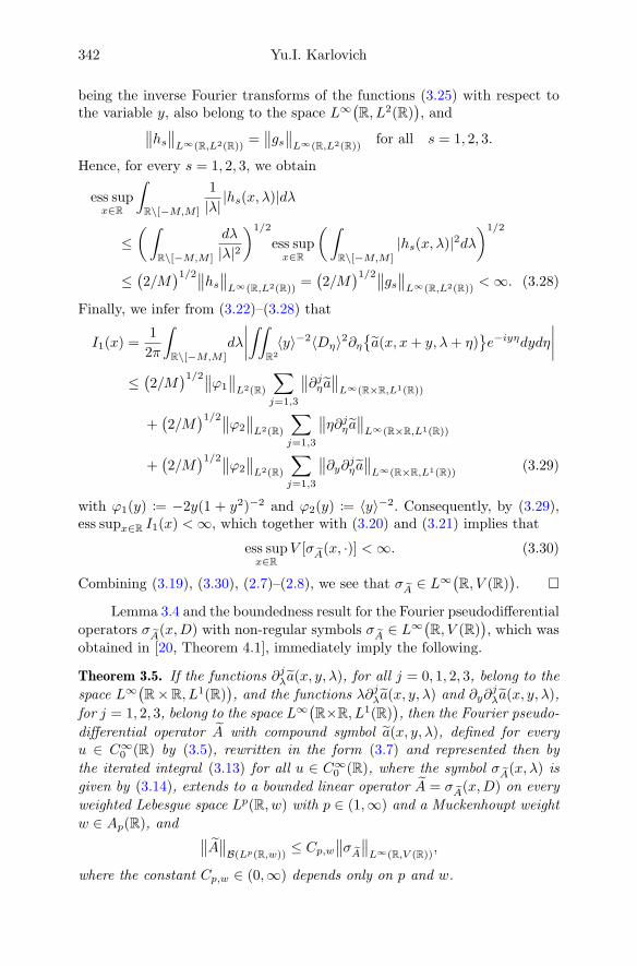
342 Yu.I. Karlovich
being the inverse Fourier transforms of the functions (3.25) with respect tothe variable y, also belong to the space L∞
(R, L2(R)
), and∥∥hs∥∥L∞(R,L2(R))
=∥∥gs∥∥L∞(R,L2(R))
for all s = 1, 2, 3.
Hence, for every s = 1, 2, 3, we obtain
ess supx∈R
∫R\[−M,M ]
1
|λ||hs(x, λ)|dλ
≤(∫
R\[−M,M ]
dλ
|λ|2
)1/2
ess supx∈R
(∫R\[−M,M ]
|hs(x, λ)|2dλ)1/2
≤(2/M
)1/2∥∥hs∥∥L∞(R,L2(R))=(2/M
)1/2∥∥gs∥∥L∞(R,L2(R))<∞. (3.28)
Finally, we infer from (3.22)–(3.28) that
I1(x) =1
2π
∫R\[−M,M ]
dλ
∣∣∣∣∫∫R2
〈y〉−2〈Dη〉2∂ηa(x, x+ y, λ+ η)
e−iyηdydη
∣∣∣∣≤(2/M
)1/2∥∥ϕ1
∥∥L2(R)
∑j=1,3
∥∥∂jηa∥∥L∞(R×R,L1(R))
+(2/M
)1/2∥∥ϕ2
∥∥L2(R)
∑j=1,3
∥∥η∂jηa∥∥L∞(R×R,L1(R))
+(2/M
)1/2∥∥ϕ2
∥∥L2(R)
∑j=1,3
∥∥∂y∂jηa∥∥L∞(R×R,L1(R))(3.29)
with ϕ1(y) := −2y(1 + y2)−2 and ϕ2(y) := 〈y〉−2. Consequently, by (3.29),ess supx∈R I1(x) <∞, which together with (3.20) and (3.21) implies that
ess supx∈R
V [σA(x, ·)] <∞. (3.30)
Combining (3.19), (3.30), (2.7)–(2.8), we see that σA ∈ L∞(R, V (R)
).
Lemma 3.4 and the boundedness result for the Fourier pseudodifferentialoperators σA(x,D) with non-regular symbols σA ∈ L
∞(R, V (R)), which was
obtained in [20, Theorem 4.1], immediately imply the following.
Theorem 3.5. If the functions ∂jλa(x, y, λ), for all j = 0, 1, 2, 3, belong to the
space L∞(R×R, L1(R)
), and the functions λ∂jλa(x, y, λ) and ∂y∂
jλa(x, y, λ),
for j = 1, 2, 3, belong to the space L∞(R×R, L1(R)
), then the Fourier pseudo-
differential operator A with compound symbol a(x, y, λ), defined for everyu ∈ C∞0 (R) by (3.5), rewritten in the form (3.7) and represented then by
the iterated integral (3.13) for all u ∈ C∞0 (R), where the symbol σA(x, λ) is
given by (3.14), extends to a bounded linear operator A = σA(x,D) on every
weighted Lebesgue space Lp(R, w) with p ∈ (1,∞) and a Muckenhoupt weight
w ∈ Ap(R), and ∥∥A∥∥B(Lp(R,w))≤ Cp,w
∥∥σA∥∥L∞(R,V (R)),
where the constant Cp,w ∈ (0,∞) depends only on p and w.

Pseudodifferential operators with compound non-regular symbols 343
Under the conditions of Lemma 3.1, the pseudodifferential operator Agiven by (3.2) is represented in the form (3.4), where a(x, λ) = a(x, x, λ) isa function belonging to the space L∞
(R, V (R)
). Combining then [20, Theo-
rem 4.1] and Theorem 3.5, we arrive at the following assertion.
Corollary 3.6. If the function a(x, y, λ) belongs to the space L∞(R×R, V (R)
)and the function a(x, y, λ) = a(x, y, λ)− a(x, x, λ) satisfies all the conditionsof Theorem 3.5, then the Fourier pseudodifferential operator A, defined forevery u ∈ C∞0 (R) by the iterated integral (3.2), extends to a bounded linearoperator on every weighted Lebesgue space Lp(R, w) with p ∈ (1,∞) andw ∈ Ap(R).
Lemma 3.7. If the functions ∂jλa(x, y, λ) belong to the space L∞(R×R, L1(R)
)for all j = 0, 1, 2, 3, the functions ∂y∂
jλa(x, y, λ) and λ∂jλa(x, y, λ) belong to
the space L∞(R× R, L1(R)
)for all j = 1, 2, 3 and, for every j = 1, 2, 3,
lim|x|→∞
∂jλa(x, x+ y, λ) = 0, lim|x|→∞
λ∂jλa(x, x+ y, λ) = 0,
and lim|x|→∞
∂y∂jλa(x, x+ y, λ) = 0
(3.31)
for all λ ∈ R and almost all y ∈ R, then
σA(x,±∞) = 0 for almost all x ∈ R, limx→±∞
V [σA(x, ·)] = 0, (3.32)
and for every N > 0,
limM→+∞
ess sup|x|≤N
(V −M−∞
[σA(x, ·)
]+ V +∞
M
[σA(x, ·)
])= 0. (3.33)
Proof. It follows from (3.18) that
σA(x, λ) =1
2π
∫∫R2
〈y〉−2〈Dη〉2a(x, x+ y, η)
e−iy(η−λ)dydη
=1
2π
∫R〈y〉−2
(Fη→y
〈Dη〉2
a(x, x+ y, η)
)eiyλdy. (3.34)
Since the function (x, y, η) 7→ 〈Dη〉2a(x, x + y, η)
belongs to the space
L∞(R× R, L1(R)
), we conclude that the function
f : (x, y) 7→ Fη→y〈Dη〉2
a(x, x+ y, η)
belongs to the space L∞(R× R), and therefore the function
g : (x, y) 7→ 〈y〉−2Fη→y〈Dη〉2
a(x, x+ y, η)
belongs to the space L∞
(R, L1(R)
). Hence the function
h : (x, λ) 7→ 1
2π
∫R〈y〉−2
(Fη→y
〈Dη〉2
a(x, x+ y, η)
)eiyλdy,
being the inverse Fourier transform of the function g with respect to thevariable y, belongs to the space L∞
(R, C0(R)
), where C0(R) is the C∗-
algebra of all continuous complex-valued functions on R that vanish at ∞.

344 Yu.I. Karlovich
This in view of (3.34) gives the first equality σA(x,±∞) = 0 in (3.32) foralmost all x ∈ R.
Let us prove the second equality in (3.32). Since the functions
(x, y, η) 7→∣∣∂jηa(x, y, η)
∣∣, (x, y, η) 7→∣∣η∂jηa(x, y, η)
∣∣,(x, y, η) 7→
∣∣∂y∂jηa(x, y, η)∣∣
belong to the space L∞(R×R, L1(R)
)for all j = 1, 2, 3, we infer from (3.24),
(3.31), and the Levi monotone convergence theorem that
0 ≤ lim|x|→∞
∣∣∣Fη→y〈Dη〉2∂ηa(x, x+ y, η)
∣∣∣≤ lim|x|→∞
∫R
∣∣〈Dη〉2∂ηa(x, x+ y, η)
∣∣dη=
∫R
lim|x|→∞
∣∣〈Dη〉2∂ηa(x, x+ y, η)
∣∣dη = 0.
Applying analogous reasonings to all functions (3.23), we conclude that
lim|x|→∞
Fη→y
〈Dη〉2∂η
a(x, x+ y, η)
= 0,
lim|x|→∞
Fη→y
− iη〈Dη〉2∂η
a(x, x+ y, η)
= 0, (3.35)
lim|x|→∞
Fη→y
∂y〈Dη〉2∂η
a(x, x+ y, η)
= 0
for almost all y ∈ R. Further, the functions
(x, y) 7→(2y(1 + y2)−2
)∣∣∣Fη→y〈Dη〉2∂ηa(x, x+ y, η)
∣∣∣,(x, y) 7→ 〈y〉−2
∣∣∣Fη→y− iη〈Dη〉2∂ηa(x, x+ y, η)
∣∣∣, (3.36)
(x, y) 7→ 〈y〉−2∣∣∣Fη→y∂y〈Dη〉2∂η
a(x, x+ y, η)
∣∣∣also belong to the space L∞
(R × R, L1(R)
), because their second factors
on the right are uniformly bounded according to (3.23) and (3.24). Then,applying the Levi monotone convergence theorem to the first function in(3.36), we deduce from (3.35) that
0 ≤ lim|x|→∞
∣∣∣∣ 1
2π
∫R
−2y
(1 + y2)2
(Fη→y
〈Dη〉2∂η
a(x, x+ y, η)
)eiyλdy
∣∣∣∣≤ lim|x|→∞
1
2π
∫R
2|y|(1 + y2)2
∣∣∣Fη→y〈Dη〉2∂ηa(x, x+ y, η)
∣∣∣dy=
1
2π
∫R
2|y|(1 + y2)2
lim|x|→∞
∣∣∣Fη→y〈Dη〉2∂ηa(x, x+ y, η)
∣∣∣dy = 0.

Pseudodifferential operators with compound non-regular symbols 345
Applying the same arguments to all functions (3.36), we obtain for almostall λ ∈ R the equalities
lim|x|→∞
1
2π
∫R
−2y
(1 + y2)2
(Fη→y
〈Dη〉2∂η
a(x, x+ y, η)
)eiyλdy = 0,
lim|x|→∞
1
2π
∫R〈y〉−2
(Fη→y
− iη〈Dη〉2∂η
a(x, x+ y, η)
)eiyλdy = 0, (3.37)
lim|x|→∞
1
2π
∫R〈y〉−2
(Fη→y
∂y〈Dη〉2∂η
a(x, x+ y, η)
)eiyλdy = 0.
By the proof of Lemma 3.4, the functions h1(x, λ), h2(x, λ), h3(x, λ) given by(3.27) belong to the space L∞
(R, L2(R)
), and therefore the functions
(x, λ) 7→ |hs(x, λ)|/|λ| (s = 1, 2, 3)
in view of (3.28) belong to the space L∞(R, L1(R)
). Applying then (3.27),
(3.37), and the Levi monotone convergence theorem, we infer that, abbrevi-ating G := R \ [−M,M ],
lim|x|→∞
∫G
dλ
2π|λ|
∣∣∣∣∫R
−2y
(1 + y2)2
(Fη→y
〈Dη〉2∂η
a(x, x+ y, η)
)eiyλdy
∣∣∣∣=
∫G
dλ
2π|λ|
∣∣∣∣ lim|x|→∞
∫R
−2y
(1 + y2)2
(Fη→y
〈Dη〉2∂η
a(x, x+ y, η)
)eiyλdy
∣∣∣∣= 0,
lim|x|→∞
∫G
dλ
2π|λ|
∣∣∣∣∫R〈y〉−2
(Fη→y
− iη〈Dη〉2∂η
a(x, x+ y, η)
)eiyλdy
∣∣∣∣=
∫G
dλ
2π|λ|
∣∣∣∣ lim|x|→∞
∫R〈y〉−2
(Fη→y
− iη〈Dη〉2∂η
a(x, x+ y, η)
)eiyλdy
∣∣∣∣= 0,
lim|x|→∞
∫G
dλ
2π|λ|
∣∣∣∣∫R〈y〉−2
(Fη→y
∂y〈Dη〉2∂η
a(x, x+ y, η)
)eiyλdy
∣∣∣∣=
∫G
dλ
2π|λ|
∣∣∣∣ lim|x|→∞
∫R〈y〉−2
(Fη→y
∂y〈Dη〉2∂η
a(x, x+ y, η)
)eiyλdy
∣∣∣∣= 0. (3.38)
Combining (3.38) and (3.22), we obtain
lim|x|→∞
1
2π
∫G
dλ
∣∣∣∣∫∫R2
〈y〉−2〈Dη〉2∂ηa(x, x+y, λ+η)
e−iyηdydη
∣∣∣∣ = 0. (3.39)
Similarly and even easier, one can prove from (3.21) by applying the Levimonotone convergence theorem that
lim|x|→∞
1
2π
∫ M
−Mdλ
∣∣∣∣∫∫R2
〈y〉−2〈Dη〉2∂ηa(x, x+y, λ+η)
e−iyηdydη
∣∣∣∣ = 0. (3.40)

346 Yu.I. Karlovich
Finally, combining (3.39) and (3.40), we infer from (3.20) that
lim|x|→∞
V [σA(x, ·)]
= lim|x|→∞
1
2π
∫Rdλ
∣∣∣∣∫∫R2
〈y〉−2〈Dη〉2∂ηa(x, x+ y, λ+ η)
e−iyηdydη
∣∣∣∣ = 0,
which gives the second equality in (3.32).It remains to prove (3.33). Applying (3.20) and (3.29), for every N > 0,
we obtain
ess sup|x|≤N
(V −M−∞
[σA(x, ·)
]+ V +∞
M
[σA(x, ·)
])= ess sup|x|≤N
1
2π
∫G
dλ
∣∣∣∣∫∫R2
〈y〉−2〈Dη〉2∂ηa(x, x+ y, λ+ η)
e−iyηdydη
∣∣∣∣≤ ess sup
x∈RI1(x) ≤ C
(2/M
)1/2, (3.41)
where the constant C ∈ (0,∞) is independent of M > 0. Passing to limitsas M → +∞ in (3.41), we immediately get (3.33), which completes theproof.
Lemma 3.7 and [20, Theorem 5.4] imply the following compactness resultfor the Fourier pseudodifferential operators with non-regular symbols.
Theorem 3.8. Under the conditions of Lemma 3.7, the Fourier pseudodifferen-
tial operator A with compound symbol a(x, y, λ), defined for every u ∈ C∞0 (R)
by (3.5) and represented in the form A = σA(x,D) with a symbol σA(x, λ)
in L∞(R, V (R)
), is a compact operator on every weighted Lebesgue space
Lp(R, w) with p ∈ (1,∞) and w ∈ Ap(R).
Corollary 3.6 and Theorem 3.8 imply the following.
Corollary 3.9. If the function a(x, y, λ) belongs to the space L∞(R×R, V (R)
)and the function a(x, y, λ) = a(x, y, λ)− a(x, x, λ) satisfies all the conditionsof Lemma 3.7, then the pseudodifferential operator A, defined for every u ∈C∞0 (R) by the iterated integral (3.2) and extended to a bounded linear operatoron every weighted Lebesgue space Lp(R, w) with p ∈ (1,∞) and w ∈ Ap(R),is represented in the form
A = a(x,D) +K, (3.42)
where the Fourier pseudodifferential operator a(x,D) with symbol a(x, λ) ∈L∞(R, V (R)) given by a(x, λ) = a(x, x, λ) is bounded on the space Lp(R, w)
and K = A is a compact operator on the space Lp(R, w).
4. The Mellin pseudodifferential operators
Let R+ := (0,∞) and let L∞(R+×R+, V (R)
)stand for the set of all functions
a : R+ × R+ × R → C such that (r, %) 7→ a(r, %, ·) is a bounded measurable

Pseudodifferential operators with compound non-regular symbols 347
V (R)-valued function on R+ × R+. The set L∞(R+ × R+, V (R)
)becomes a
Banach algebra if we equip it with the norm∥∥a∥∥L∞(R+×R+,V (R))
:= ess sup(r,%)∈R+×R+
∥∥a(r, %, ·)∥∥V<∞.
Theorem 4.1 ([15, Theorem 6.1]). If b ∈ L∞(R+, V (R)
), then the Mellin
pseudodifferential operator Op(b), defined for functions f ∈ C∞0 (R+) by the
iterated integral[Op(b)f
](r) =
1
2π
∫Rdλ
∫R+
b(r, λ)
(r
%
)iλf(%)
d%
%, r ∈ R+, (4.1)
extends to a bounded linear operator on every Lebesgue space Lp(R+, dµ) withp ∈ (1,∞) and the measure dµ = d%/%, and∥∥Op(b)
∥∥B(Lp(R+,dµ))
≤ Cp,1∥∥b∥∥
L∞(R+,V (R)),
where the constant Cp,1 for w = 1 is taken from Theorem 3.5.
Theorem 4.1 immediately follows from [14, Theorem 3.1] by applyingthe transform A 7→ EAE−1, where E is the isometric isomorphism
E : Lp(R+, dµ)→ Lp(R), (Ef)(x) = f(ex), x ∈ R, (4.2)
to the Mellin pseudodifferential operator Op(b) defined by (4.1), which gives
E Op(b)E−1 = a(x,D), (4.3)
where a(x, λ) := b(ex, λ), ‖a‖L∞(R,V (R)) = ‖b‖L∞(R+,V (R)), and a(x,D) is theFourier pseudodifferential operator defined for functions ϕ ∈ C∞0 (R) by
[a(x,D)ϕ](x) =1
2π
∫Rdλ
∫Ra(x, λ)ei(x−y)λϕ(y)dy, x ∈ R.
Let a(x, y, λ) ∈ L∞(R×R, V (R)
), let a(x, y, λ) ∈ L∞
(R×R, L1(R)
)be
given by (3.1), and let
b(r, %, λ) := a(log r, log %, λ), b(r, %, λ) := a(log r, log %, λ) (4.4)
for all (r, %, λ) ∈ R+ × R+ × R. Obviously, by (4.4), the conditions
∂jλa(x, y, λ) ∈ L∞(R× R, L1(R)
)for all j = 0, 1, 2, 3;
λ∂jλa(x, y, λ), ∂y∂jλa(x, y, λ) ∈ L∞
(R× R, L1(R)
)for all j = 1, 2, 3
are equivalent, respectively, to the conditions
∂jλb(r, %, λ) ∈ L∞(R+ × R+, L
1(R))
(j = 0, 1, 2, 3);
λ∂jλb(r, %, λ), (%∂%)∂jλb(r, %, λ) ∈ L∞
(R+ × R+, L
1(R))
(j = 1, 2, 3).(4.5)
Similarly to Theorem 4.1, applying (4.2)–(4.3) to the Mellin pseudo-differential operators with compound non-regular symbols and using Corol-lary 3.6 with w = 1, we easily obtain the following.
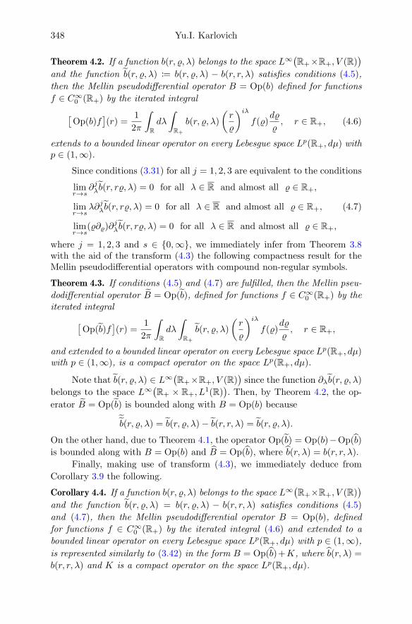
348 Yu.I. Karlovich
Theorem 4.2. If a function b(r, %, λ) belongs to the space L∞(R+×R+, V (R)
)and the function b(r, %, λ) := b(r, %, λ) − b(r, r, λ) satisfies conditions (4.5),
then the Mellin pseudodifferential operator B = Op(b) defined for functions
f ∈ C∞0 (R+) by the iterated integral[Op(b)f
](r) =
1
2π
∫Rdλ
∫R+
b(r, %, λ)
(r
%
)iλf(%)
d%
%, r ∈ R+, (4.6)
extends to a bounded linear operator on every Lebesgue space Lp(R+, dµ) withp ∈ (1,∞).
Since conditions (3.31) for all j = 1, 2, 3 are equivalent to the conditions
limr→s
∂jλb(r, r%, λ) = 0 for all λ ∈ R and almost all % ∈ R+,
limr→s
λ∂jλb(r, r%, λ) = 0 for all λ ∈ R and almost all % ∈ R+, (4.7)
limr→s
(%∂%)∂jλb(r, r%, λ) = 0 for all λ ∈ R and almost all % ∈ R+,
where j = 1, 2, 3 and s ∈ 0,∞, we immediately infer from Theorem 3.8with the aid of the transform (4.3) the following compactness result for theMellin pseudodifferential operators with compound non-regular symbols.
Theorem 4.3. If conditions (4.5) and (4.7) are fulfilled, then the Mellin pseu-
dodifferential operator B = Op(b), defined for functions f ∈ C∞0 (R+) by theiterated integral[
Op(b)f](r) =
1
2π
∫Rdλ
∫R+
b(r, %, λ)
(r
%
)iλf(%)
d%
%, r ∈ R+,
and extended to a bounded linear operator on every Lebesgue space Lp(R+, dµ)with p ∈ (1,∞), is a compact operator on the space Lp(R+, dµ).
Note that b(r, %, λ) ∈ L∞(R+×R+, V (R)
)since the function ∂λb(r, %, λ)
belongs to the space L∞(R+ × R+, L
1(R)). Then, by Theorem 4.2, the op-
erator B = Op(b) is bounded along with B = Op(b) because˜b(r, %, λ) = b(r, %, λ)− b(r, r, λ) = b(r, %, λ).
On the other hand, due to Theorem 4.1, the operator Op(b) = Op(b)−Op(b)
is bounded along with B = Op(b) and B = Op(b), where b(r, λ) = b(r, r, λ).
Finally, making use of transform (4.3), we immediately deduce from
Corollary 3.9 the following.
Corollary 4.4. If a function b(r, %, λ) belongs to the space L∞(R+×R+, V (R)
)and the function b(r, %, λ) = b(r, %, λ) − b(r, r, λ) satisfies conditions (4.5)
and (4.7), then the Mellin pseudodifferential operator B = Op(b), defined
for functions f ∈ C∞0 (R+) by the iterated integral (4.6) and extended to a
bounded linear operator on every Lebesgue space Lp(R+, dµ) with p ∈ (1,∞),
is represented similarly to (3.42) in the form B = Op(b)+K, where b(r, λ) =
b(r, r, λ) and K is a compact operator on the space Lp(R+, dµ).
Pseudodifferential operators with compound non-regular symbols 349
5. Applications
The results of Section 4 applied to Mellin pseudodifferential operators withcompound non-regular symbols, which are related to singular integral oper-ators on weighted Lebesgue spaces Lp(Γ, w), where Γ are slowly oscillatingCarleson curves and w are slowly oscillating Muckenhoupt weights (cf. [2]and [18]), allow one to reduce the smoothness of curves Γ and weights w,which is important for studying singular integral operators with shifts (see,e.g., [9], [11]–[13], and [21]).
Let Cb(R+) and C1(R+) denote, respectively, the set of bounded contin-uous functions a : R+ → C and the set of continuously differentiable functionsb : R+ → C. Given b ∈ C1(R+), let (rDr)b := rb′(r).
Let SO(R+) stand for the set of all functions a ∈ Cb(R+) that slowlyoscillate at 0 and ∞, that is (see, e.g., [25]), satisfy the condition
limr→s
max|a(x)− a(y)| : x, y ∈ [r, 2r]
= 0 for s ∈ 0,∞. (5.1)
We remark that (5.1) holds if and only if, for some λ > 1 (equivalently, forany λ > 1),
limr→s
max|a(r)− a(νr)| : ν ∈ [λ−1, λ]
= 0 for s ∈ 0,∞. (5.2)
Obviously, SO(R+) is a unital C∗-subalgebra of L∞(R+).Following [2], we define slowly oscillating curves and weights, where we
reduce their smoothness in comparison with [2] and [18].An unbounded oriented simple open arc Γ with the starting point t is
called a slowly oscillating curve (at t and ∞) if
Γ =τ = t+ reiθ(r) : r ∈ R+
(5.3)
where θ is a real-valued function in C1(R+), the function (rDr)θ = rθ′(r)belongs to SO(R+), and the function (rDr)
2θ belongs to L∞(R+). Note thatt,∞ /∈ Γ and that the function θ(r) can be unbounded as r → 0 or r → ∞.Obviously, Γ is a Carleson curve (see, e.g., [3]).
Let Γ be a slowly oscillating curve given by (5.3). We call a functionw : Γ→ (0,∞) a slowly oscillating weight (at t and ∞) if
w(t+ reiθ(r)
)= ev(r) for r ∈ R+, (5.4)
where v is a real-valued function in C1(R+), the function (rDr)v belongs toSO(R+), and the function (rDr)
2v belongs to L∞(R+). Let 1 < p <∞. Onecan show (cf. [1, Theorem 2.36]) that w ∈ Ap(Γ) if and only if
−1/p < lim infr→s
rv′(r) ≤ lim supr→s
rv′(r) < 1/q for s ∈ 0,∞.
Let ASOp denote the set of all pairs (Γ, w) such that Γ is a slowly oscillatingcurve and w is a slowly oscillating weight in Ap(Γ).
By [2] (see also [15]), studying singular integral operators on weightedLebesgue spaces Lp(Γ, w) over Carleson curves Γ given by (5.3) with slowlyoscillating Muckenhoupt weights w given by (5.4) is reduced to studyingMellin pseudodifferential operators with compound symbols on Lp(R+, dµ).

350 Yu.I. Karlovich
In particular, with the operator SΓ given by (1.1) and bounded on the spaceLp(Γ, w), one associates the compound symbol of the form
σ(r, %, λ) :=1 + i%θ′(%)
1 + imθ(r, %)coth
[πλ+ i(1/p+mv(r, %))
1 + imθ(r, %)
], (5.5)
where
mv(r, %) =v(r)− v(%)
log r − log %, mθ(r, %) =
θ(r)− θ(%)
log r − log %, (5.6)
and
0 <1
p+ infr,%∈R+
mv(r, %) ≤ 1
p+ supr,%∈R+
mv(r, %) < 1. (5.7)
Let us illustrate the results of Section 4 for Mellin pseudodifferentialoperators with compound and related to (5.5) symbols of the form
b(r, %, λ) = coth
[πλ+ i(1/p+mv(r, %))
1 + imθ(r, %)
]. (5.8)
Lemma 5.1. If the functions r 7→ rv′(r) and r 7→ rθ′(r) belong to the algebraSO(R+), then, for every % ∈ R+,
limr→s
[mv(r, r%)− rv′(r)] = 0, limr→s
[mθ(r, r%)− rθ′(r)] = 0, (5.9)
limr→s
(%∂%)mv(r, r%) = 0, limr→s
(%∂%)mθ(r, r%) = 0. (5.10)
Proof. Obviously, it suffices to prove the first equalities in (5.9) and (5.10).Since the function r 7→ rv′(r) belongs to the algebra SO(R+), we concludethat the function x 7→ exv′(ex) belongs to the algebra SO(R). Replacingr = ex and % = ey in (5.6), we obtain
mv(r, r%)− rv′(r) =v(ex+y)− v(ex)
y− exv′(ex)
=1
y
∫ y
0
[ex+tv′(ex+t)− exv′(ex)
]dt. (5.11)
As the function x 7→ exv′(ex) belongs to the algebra SO(R) and hence
limx→±∞
maxt,τ∈[x,x+h]
∣∣etv′(et)− eτv′(eτ )∣∣ = 0 for every h > 0
in view of (5.1) or (5.2), we infer from (5.11) that
limx→±∞
1
y
∫ y
0
[ex+tv′(ex+t)− exv′(ex)
]dt = 0 for every y ∈ R, (5.12)
which gives the first equality in (5.9). Similarly, we deduce that
(%∂%)mv(r, r%) = ∂y
(v(ex+y)− v(ex)
y
)=ex+yv′(ex+y)y −
(v(ex+y)− v(ex)
)y2
=
∫ 1
0
ex+yv′(ex+y)− ex+tyv′(ex+ty)
ydt,
Pseudodifferential operators with compound non-regular symbols 351
which implies by analogy with (5.12) that
limx→±∞
∫ 1
0
ex+yv′(ex+y)− ex+tyv′(ex+ty)
ydt = 0 for every y ∈ R.
This gives the first equality in (5.10) and completes the proof.
Applying Theorems 4.2 and 4.3, Corollary 4.4, and Lemma 5.1, we arriveat the following.
Theorem 5.2. Let p ∈ (1,∞) and let (Γ, w) ∈ ASOp be given by (5.3) and(5.4), respectively, where
(rDr)θ, (rDr)v ∈ SO(R+), (rDr)2θ, (rDr)
2v ∈ L∞(R+),
and (5.7) holds. Then the Mellin pseudodifferential operator Op(b) with com-pound symbol b given by (5.8) and (5.6) is bounded on the space Lp(R+, dµ),and Op(b) = Op(b) +K, where the function b(r, λ) ∈ Cb
(R+, V (R)
)is given
by
b(r, λ) := coth
[πλ+ i(1/p+ rv′(r))
1 + irθ′(r)
]and K is a compact operator on the space Lp(R+, dµ).
References
[1] A. Bottcher and Yu.I. Karlovich, Carleson Curves, Muckenhoupt Weights, andToeplitz Operators, Progress in Mathematics 154, Birkhauser, Basel, 1997.
[2] A. Bottcher, Yu.I. Karlovich, and V.S. Rabinovich, Mellin pseudodifferentialoperators with slowly varying symbols and singular integrals on Carleson curveswith Muckenhoupt weights, Manuscripta Math. 95 (1998), 363–376.
[3] A. Bottcher, Yu.I. Karlovich, and V.S. Rabinovich, The method of limit op-erators for one-dimensional singular integrals with slowly oscillating data, J.Operator Theory 43 (2000), 171–198.
[4] A. Bottcher, Yu.I. Karlovich, and V.S. Rabinovich, Singular integral operatorswith complex conjugation from the viewpoint of pseudodifferential operators,Operator Theory: Advances and Applications 121, Birkhauser, 2001, 36–59.
[5] A.P. Calderon and R. Vaillancourt, On the boundedness of pseudodifferentialoperators, J. Math. Soc. Japan 23 (1971), 374–378.
[6] R.R. Coifman and Y. Meyer, Au dela des operateurs pseudodifferentiels,Asterisque 57 (1978), 1–184.
[7] H.O. Cordes, On compactness of commutators of multiplications and convo-lutions, and boundedness of pseudodifferential operators, J. Funct. Anal. 18(1975), 115–131.
[8] H.O. Cordes, Elliptic Pseudo-Differential Operators – An Abstract Theory, Lec-ture Notes in Math. 756, Springer, Berlin, 1979.
[9] G. Fernandez-Torres and Yu.I. Karlovich, Fredholmness of nonlocal singularintegral operators with slowly oscillating data, In: Integral Methods in Scienceand Engineering, vol. 1, eds. C. Constanda et al., Birkhauser, Cham, 2017,pp. 95–105.

352 Yu.I. Karlovich
[10] N.B. Haaser and J.A. Sullivan, Real Analysis, Dover, New York, 1991.
[11] A.Yu. Karlovich, Yu.I. Karlovich, and A.B. Lebre, On a weighted singularintegral operator with shifts and slowly oscillating data, Complex Anal. Oper.Theory 10 (2016), 1101–1131.
[12] A.Yu. Karlovich, Yu.I. Karlovich, and A.B. Lebre, The index of weighted sin-gular integral operators with shifts and slowly oscillating data, J. Math. Anal.Appl. 450 (2017), 606–630.
[13] A.Yu. Karlovich, Yu.I. Karlovich, and A.B. Lebre, Necessary Fredholm condi-tions for weighted singular integral operators with shifts and slowly oscillatingdata, J. Integral Equ. Appl. 29 (2017), 365–399.
[14] Yu.I. Karlovich, An algebra of pseudodifferential operators with slowly oscil-lating symbols, Proc. London Math. Soc. 92 (2006), 713–761.
[15] Yu.I. Karlovich, Pseudodifferential operators with compound slowly oscillatingsymbols, Operator Theory: Advances and Applications 171, Birkhauser, 2007,189–224.
[16] Yu.I. Karlovich, Algebras of pseudodifferential operators with discontinuoussymbols, Operator Theory: Advances and Applications 172, Birkhauser, 2007,207–233.
[17] Yu.I. Karlovich, Pseudodifferential operators with compound non-regular sym-bols, Math. Nachr. 280 (2007), 1128–1144.
[18] Yu.I. Karlovich, Nonlocal singular integral operators with slowly oscillatingdata, Operator Theory: Advances and Applications 181, Birkhauser, 2008, 229–261.
[19] Yu.I. Karlovich, An algebra of shift-invariant singular integral operators withslowly oscillating data and its application to operators with a Carleman shift,Operator Theory: Advances and Applications 193, Birkhauser, 2009, 81–95.
[20] Yu.I. Karlovich, Boundedness and compactness of pseudodifferential operatorswith non-regular symbols on weighted Lebesgue spaces, Integr. Equ. Oper.Theory 73 (2012), 217–254.
[21] Yu.I. Karlovich, The Haseman boundary value problem with slowly oscillat-ing coefficients and shifts, Operator Theory: Advances and Applications 259,Birkhauser, 2017, 463–500.
[22] J.E. Lewis and C. Parenti, Pseudodifferential operators of Mellin type, Comm.Part. Diff. Equ. 8 (1983), 477–544.
[23] V.S. Rabinovich, S. Roch, and B. Silbermann, Limit Operators and Their Ap-plications in Operator Theory, Operator Theory: Advances and Applications150, Birkhauser, Basel, 2004.
[24] M. Reed and B. Simon, Methods of Modern Mathematical Physics. 1. Func-tional Analysis, Academic Press, New York, 1972.
[25] D. Sarason, Toeplitz operators with piecewise quasicontinuous symbols, Indi-ana Univ. Math. J. 26 (1977), 817–838.
[26] L. Schwartz, Analyse Mathematique, Vol. 1, Hermann, Paris, 1967.
[27] M.A. Shubin, Pseudodifferential Operators and Spectral Theory, Springer,Berlin, 1987; Russian original: Nauka, Moscow, 1978.
[28] E.M. Stein, Harmonic Analysis: Real-Variable Methods, Orthogonality, and Os-cillatory Integrals, Princeton Univ. Press, Princeton, NJ, 1993.

Pseudodifferential operators with compound non-regular symbols 353
[29] M.E. Taylor, Pseudodifferential Operators, Princeton Univ. Press, Princeton,NJ, 1981.
[30] M.E. Taylor, Pseudodifferential Operators and Nonlinear PDE, Birkhauser,Boston, 1991.
[31] M.E. Taylor, Tools for PDE. Pseudodifferential Operators, Paradifferential Op-erators, and Layer Potentials, American Math. Soc., Providence, RI, 2000.
[32] F. Treves, Introduction to Pseudodifferential and Fourier Integral Operators,Vols. 1, 2, Plenum Press, New York, 1982.
Yuri I. KarlovichCentro de Investigacion en CienciasUniversidad Autonoma del Estado de MorelosAv. Universidad 1001, Col. ChamilpaC.P. 62209 Cuernavaca, MorelosMexicoe-mail: [email protected]

Asymptotically sharp inequalities for poly-nomials involving mixed Hermite norms
Holger Langenau
Abstract. The paper concerns best constants in Markov-type inequal-ities between the norm of a higher derivative of a polynomial and thenorm of the polynomial itself. The norm of the polynomial and its de-
rivative is taken in L2 on the real axis with the weight |t|2αe t2 and
|t|2βe t2 , respectively. We determine the leading term of the asymp-totics of the constants as the degree of the polynomial goes to infinity.
Mathematics Subject Classification (2010). Primary 15A60; Secondary15A18, 26D10, 41A44.
Keywords. Markov inequality, Hermite weight, matrix norm.
1. Introduction and main result
A Markov-type inequality gives upper bounds on the norm of the νth deriv-ative of a polynomial in terms of the norm of the polynomial itself, that is,it is an inequality of the form
‖Dνfn‖β ≤ C(ν)n (α, β)‖fn‖α for all fn ∈ Pn, (1.1)
where Pn is the space of all algebraic polynomials with complex coefficientsof degree at most n and Dν denotes the operator that maps a polynomial toits νth derivative. In the following, the norms ‖ ·‖α are the weighted Hermitenorms
‖f‖2α =
∫ ∞−∞|f(t)|2|t|2αe−t
2
dt. (1.2)
The study of Markov-type inequalities goes back to the 1880s, whenAndrei Andreevich Markov proved that for a real polynomial p(t) of degreen with |p(t)| ≤ 1 on [−1, 1] the inequality |p′(t)| ≤ n2 holds, or equivalently,
‖Df‖∞ ≤ n2‖f‖∞ for all real f ∈ Pn,
where D is the differential operator and ‖ · ‖∞ denotes the maximum normon [−1, 1]. He also showed that n2 is best-possible [1, 2]. Not long after that,
© Springer International Publishing AG, part of Springer Nature 2018
Theory: Advances and Applications 268, https://doi.org/10.1007/978-3-319-75996-8_18
355A. Böttcher et al. (eds.), The Diversity and Beauty of Applied Operator Theory, Operator
−−

356 H. Langenau
his younger brother Vladimir Andreevich showed that
‖Dνf‖∞ ≤n2(n2 − 1)(n2 − 22) · · · (n2 − (ν − 1)2)
(2ν − 1)!!‖f‖∞ for all f ∈ Pn.
This is the best possible constant for higher derivatives in this case.
Starting in the 1940s Erhard Schmidt [14] was the first to consider suchinequalities with Hilbert space norms instead of the maximum norm. Hefound the best constants for the first derivative
λn ∼2
πn, γn ∼
1
πn2, ηn =
√2n,
in the Laguerre, Legendre, and Hermite case, respectively. Here, the expres-sion an ∼ bn means that the quotient an
bnconverges to 1 as n goes to infinity.
In the 1960s, Lawrence F. Shampine [15, 16] studied second order derivativesfor the Laguerre and Legendre norms. Peter Dorfler [7, 8] then was the first tostudy higher order derivatives and gave bounds for the Laguerre case. Afterthis, the development paused for almost two decades.
Shampine’s and Dorfler’s approach involved the study of matrices. Sincethis led to certain special Toeplitz matrices, Dorfler wrote a letter to AlbrechtBottcher and together they could prove asymptotic expressions for the con-stants in the Laguerre and Gegenbauer cases. They made use of an old (andthen already forgotten) trick used by Harold Widom in the 1960s in anothercontext [18, 19], which we will employ later, too. Not only could they showthat a limit for those constants exists, they could also treat the much moregeneral case of weighted Laguerre and Gegenbauer norms.
In 2009, Jurgen Prestin drew the attention of Bottcher and Dorfler tothe problem of using two different weights in the inequality. This concerns twodifferent norms, and as changes of norms may improve error estimates, thiscase could be useful in approximation theory and numerical analysis. This isnot an easy problem. However, they could give asymptotic expressions for theconstants under some restrictions on the differences between the parametersinvolved.
Subsequently, the author lifted most of these restrictions for the La-guerre [10] and Gegenbauer [12] cases. Since one part, already studied byBottcher and Dorfler, involved the Hilbert–Schmidt norm of integral opera-tors, a small gap in the parameter space remains. Bottcher, Widom, and theauthor made some preparatory studies to close this gap in [5].
The Hermite case has not been considered so far. In the unweightedcase this is a trivial question, as already noted by Schmidt [14]. However,inserting weights makes things much more complicated. We here determinethe best constant in (1.1) for almost all possible parameter pairs. We denotethis constant by η
(ν)n (α, β). Our main result is the following.
Theorem 1.1. Let α, β > −1/2 be real numbers and let ν be a positive integer.Then,
η(ν)n (α, β) ∼ Cν(α, β)n(|β−α|+ν)/2

Inequalities involving mixed Hermite norms 357
with
Cν(α, β) =
2(β−α+ν)/2, β − α ≥ 0,
2(β−α−ν)/2 ·max∥∥H(0)
ν,α,β
∥∥∞,
∥∥H(1)ν,α,β
∥∥∞
, β − α < − 1
2 ,
where H(0)ν,α,β and H
(1)ν,α,β are the integral operators on L2(0, 1) defined by
(H
(0)ν,α,βf
)(x) =
2νΓ(dν/2e+ 1
)Γ(α− β + dν/2e
) ∫ 1
x
xβ/2−1/4y−α/2+1/4+(bν/2c−dν/2e)/2
× (y − x)α−β+dν/2e−1
dν/2e∑`=0
(β
`
)(β − α− `dν/2e − `
)(x
y − x
)dν/2e−`f(y)dy
and(H
(1)ν,α,βf
)(x) =
2νΓ(bν/2c+ 1
)Γ(α− β + bν/2c
) ∫ 1
x
xβ/2+1/4y−α/2−1/4+(dν/2e−bν/2c)/2
× (y − x)α−β+bν/2c−1
bν/2c∑`=0
(β
`
)(β − α− `bν/2c − `
)(x
y − x
)bν/2c−`f(y)dy.
2. Matrix representation of the operator
As this was done for the Laguerre and Gegenbauer norms (see, e.g., [3, 4]), inorder to determine the best constant in inequality (1.1), we want to estimatethe spectral norm of the matrix representation of the differential operatorwith respect to appropriately chosen orthonormal bases.
For the norm (1.2) the polynomialsH0(·, α), H1(·, α), . . .
form an or-
thonormal basis. Hn(·, α) is the nth generalized Hermite polynomial, givenby
Hn(t, α) = 2nΓ(bn/2c+ 1
) bn/2c∑j=0
(α+ dn/2e − 1/2
j
)(−1)j
Γ(bn/2c − j + 1
) tn−2j .With the normalizing factor
wn(α) =
(2n√
Γ(bn/2c+ 1
)Γ(dn/2e+ α+ 1/2
))−1the nth normalized polynomial is given by
Hn(t, α) = wn(α)Hn(t, α) =√Γ(bn/2c+ 1
)Γ(dn/2e+ α+ 1/2
) bn/2c∑j=0
(α+ dn/2e − 1/2
j
)(−1)j
Γ(bn/2c − j + 1
) tn−2j .For α = 0 we get back the classical Hermite polynomials. As mentioned
above, the question for the best constant then is trivial. Due to the relation
H(ν)n (t, 0) = 2ν
(n− ν + 1
)νHn−ν(t, 0),

358 H. Langenau
the matrix representation of the operator is just a diagonal matrix. Theexpression
(x)n
stands for the rising factorial, or Pochhammer symbol,(x)n
= x(x+ 1) · · · (x+ n− 1) =Γ(x+ n
)Γ(x) .
Therefore, the norm and thus the smallest constant is the maximal absolutevalue on the diagonal. The corresponding entry is√
2νΓ(n+ 1
)Γ(n− ν + 1
) ∼ (2n)ν/2.
Hence, in that case, the constant
η(ν)n (0, 0) ∼ (2n)ν/2
is fully identified.
Theorem 2.1. Let Cn =(c(ν)jk (α, β)
)nj,k=0
be the matrix representation of the
differential operator Dν with respect to the orthonormal bases given by thegeneralized Hermite polynomials with the corresponding weight. The entries
c(ν)jk (α, β) are given by
c(ν)jk (α, β) =
2ν Γ(bν/2c+ νk + 1
)√Γ(dj/2e+ β + 1/2
)Γ(bj/2c+ 1
) Γ(bk/2c+ 1
)Γ(dk/2e+ α+ 1/2
)×(d(j + ν)/2e − 1/2
bν/2c+ νk
)(β − α− bν/2c − νk
(k − j − ν)/2
)× 3F2
(−bν/2c − νk, −(k − j − ν)/2, β + dj/2e+ 1/2
β − α− bν/2c − νk − (k − j − ν)/2 + 1, dj/2e+ 1/2; 1
) (2.1)
if 0 ≤ k − ν − j is even, and they are zero otherwise. Here, νk = 1 if k andν are odd, and νk = 0 if k or ν is even (i.e., νk = kν mod 2).
We note that the hypergeometric series occurring here is not defined ifβ − α − bν/2c − νk is a nonnegative integer smaller than (k − j − ν)/2. Butthen, the coefficient before this term is zero, and we define the whole term tobe zero. In the other cases, the series terminates naturally before a divisionby zero would happen. The proof can be done by a comparison of coefficients.See [11] for details.
3. The constant for integral β−α≥0
The matrix representation of the operator Dν has a chessboard structure
above the main diagonal. Since η(ν)n−1(α, β) ≤ η
(ν)n (α, β) ≤ η
(ν)n+1(α, β), we
assume that N = n−ν+1 is an even number. Then there is some permutationmatrix UN with
AN = UN
(EN 00 FN
)UN ,

Inequalities involving mixed Hermite norms 359
where EN = (ejk)N/2−1j,k=0 , FN = (fjk)
N/2−1j,k=0 are built from the entries
ejk = c(ν)2j,2k+ν(α, β), fjk = c
(ν)2j+1,2k+ν+1(α, β).
We will just investigate the matrix EN and point out that the matrix FNcan be treated likewise. First, assume β−α ≥ dν/2e is an integer. Due to the
term(β−α−bν/2c−νk
(k−j−ν)/2)
occurring in (2.1), the matrix is banded. We will employ
the same idea as in the Laguerre case in [3] and the Gegenbauer case in [4]:Consider the matrix as a sum of (shifted) diagonal matrices and make use ofthe fact that the norm of the sum is less than the sum of the norms of thesediagonals. To derive a lower estimate, we show that some scaled version ofthe matrix EN converges in the norm to a given Toeplitz operator.
Let m = β−α−dν/2e ∈ N0. Then, after some transformation, the entries
d(`)j of the `th diagonal in row j, ` = 0, . . . ,m, are given by
d(`)j = 2νΓ
(dν/2e+ 1
)√Γ(j + β + 1/2
)Γ(j + 1
) Γ(j + `+ bν/2c+ 1
)Γ(j + `+ dν/2e+ α+ 1/2
)×
mindν/2e,`∑τ=0
(j + dν/2e − 1/2
dν/2e − τ
)(β + j + τ − 1/2
τ
)(m
`− τ
).
Fixing `, we can show that d(`)j is increasing with j. So, the maximum along
each diagonal (and with this the norm of this particular diagonal matrix) isattained for j = N/2 − 1 − `. We get the following upper estimate for thenorm of EN :
‖EN‖∞ ≤ 2ν Γ(dν/2e+ 1
) m∑`=0
√Γ(N/2− `+ β − 1/2
)Γ(N/2 + bν/2c
)Γ(N/2− `
)Γ(N/2 + dν/2e+ α− 1/2
)×
mindν/2e,`∑τ=0
(N/2− `+ dν/2e − 3/2
dν/2e − τ
)(β +N/2− `+ τ − 3/2
τ
)(m
`− τ
).
Ignoring the constant factor for the moment, as well as the terms under thesquare root, which we will replace with the maximum over 0 ≤ ` ≤ m, thesum reduces to
m∑`=0
mindν/2e,`∑τ=0
(N/2− `+ dν/2e − 3/2
dν/2e − τ
)(β +N/2− `+ τ − 3/2
τ
)(m
`− τ
)
≤m∑`=0
mindν/2e,`∑τ=0
(N/2 + dν/2e − 1/2
dν/2e − τ
)(β +N/2 + dν/2e − 1/2
τ
)(m
`− τ
)
=
dν/2e∑τ=0
(N/2 + dν/2e − 1/2
dν/2e − τ
)(β +N/2 + dν/2e − 1/2
τ
)m−τ∑`=0
(m
`
)

360 H. Langenau
≤dν/2e∑τ=0
(N/2 + dν/2e − 1/2
dν/2e − τ
)(β +N/2 + dν/2e − 1/2
τ
) m∑`=0
(m
`
)
=Γ(β +N + 2dν/2e
)Γ(β +N + dν/2e
)Γ(dν/2e+ 1
) 2m.
Together with the other terms and by applying asymptotic formulas for allof them, we get the following upper bound for ‖EN‖∞:
‖EN‖∞ ≤ 2ν(N2
)(β−1/2)/2 (N2
)(−α+1/2+bν/2c−dν/2e)/2(3.1)
· 2β−α−dν/2eNdν/2e(1 +O(1/N)
)= 2(β−α+ν)/2N (β−α+ν)/2(1 +O(1/N)
). (3.2)
Now, let JN denote the (N × N)-matrix with ones on the counter-diagonal and zeros elsewhere. We set BN = JNENJN . Then obviously,‖EN‖∞ = ‖E∗N‖∞ = ‖BN‖∞. We quickly confirm that the entry at positionjk of BN equals the entry at position N/2 − 1 − j,N/2 − 1 − k from EN .Now, let πN be the projection
πN : `2 → `2, x0, x1, x2, . . . 7→ x0, x1, . . . , xN/2−1, 0, . . .
and consider the operators TN = 2(β−α−ν)/2N (α−β−ν)/2BNπN on `2. Wecan show that these operators converge strongly to the Toeplitz operatorT ∗((1 + z)β−α) on `2 that is given by the infinite Toeplitz matrix (ϕjk)∞j,k=0
with ϕjk = 0 for k > j and
ϕjk =
(β − αj − k
)for k ≤ j. (3.3)
From (3.1) we infer that ‖TN‖∞ ≤ 2β−α(1 +O(1/N)), that is, the operatorsTN are uniformly bounded. In order to prove TN → T ((1 + z)β−α) strongly,it is therefore enough to show that TNek converges to T ((1 + z)β−α)ek forevery k ≥ 0, where ek ∈ `2 has 1 at the kth position and zeros elsewhere.As all involved operators are banded with bandwidth m + 1 independent ofN , it suffices to verify that the jk entry of TN converges to the jk entry ofthe matrix T ((1 + z)β−α). But, the jk entry of TN is zero for k > j and fork < j −m, and if k ≤ j ≤ k + m, we can show that for N → ∞ it equalsϕjk. For details, we again refer to [11]. Together with the Banach–Steinhaustheorem we deduce
lim infN→∞
∥∥2(β−α−ν)/2N (α−β−ν)/2BN∥∥∞ ≥
∥∥T ((1 + z)β−α)∥∥∞.
By a well-known result on the norm of Toeplitz operators (see, e.g., [6, p. 10]),the latter is ∥∥T ((1 + z)β−α
)∥∥∞ = max
|z|=1|1 + z|β−α = 2β−α.
Thus,
lim infN→∞
N (α−β−ν)/2‖EN‖∞ ≥ 2(β−α+ν)/2. (3.4)
Inequalities involving mixed Hermite norms 361
Combining (3.1) and (3.4), we conclude that
‖EN‖∞ ∼ (2N)(β−α+ν)/2.
As above, one can show that
‖FN‖∞ ∼ (2N)(β−α+ν)/2.
Since ‖Cn‖∞ = max‖EN‖∞, ‖FN‖∞, we obtain for β − α ≥ dν/2e,β − α an integer, the following asymptotic behavior for n→∞:
η(ν)n (α, β) ∼ (2n)(β−α+ν)/2.
We need one more integer case. If β − α = 0 the matrix is in generalnot banded as in the above case. However, α = β = 0 has been disposed ofbefore. In this case this matrix is a diagonal matrix and it is known that
η(ν)n (0, 0) ∼ (2n)ν/2.
Now, assume α = β 6= 0. We will show that the asymptotic expressionsobtained above also hold in this case. A closer look at the matrix revealsthat, although it is no diagonal matrix, it is very close to one in the sensethat the entries along the diagonal are significantly bigger in their absolutevalues than the off-diagonal entries. Indeed, applying some estimates, the lastentry on the diagonal of the matrix EN is given by
eN/2−1,N/2−1 = 2ν(N2
)ν/2 (1 +O(1/N)
).
This is exactly what we want. Since
‖ENeN/2−1‖2 =
√√√√N/2−1∑j=0
e2j,N/2−1 ≥ eN/2−1,N/2−1,
this already provides a lower bound. An upper bound is harder to show. Theapproach we used for the banded matrices does not work here any longer.What we do instead is to use a corollary of the Gershgorin theorem [9, p. 344].The Gershgorin theorem provides disks in the complex plane containing theeigenvalues of a matrix. The closer such a matrix is to a diagonal matrix, themore precise the location can be given. Since we look for the singular values,we could apply the theorem to E∗NEN . Its eigenvalues all are nonnegative realnumbers, so the disks are in fact intervals. However, the matrix representationof E∗NEN is not easy to work with. The paper [13] uses the ideas of theGershgorin theorem directly with the matrix EN to provide intervals for thelocation of the singular values. Even more, it also provides a scaled versionof the theorem. Since the eigenvalues do not change if we multiply a matrixby an invertible matrix from the right and its inverse from the left, we maymodify the matrix entries slightly to get better bounds.
Since we are interested only in the largest singular value of the matrixEN , the combination of Theorem 2 and Theorem 4 of [13] yields
‖EN‖∞ ≤ max0≤i≤N/2−1
N/2−1∑j=0
djdi|eij |,
N/2−1∑j=0
djdi|eji|
,

362 H. Langenau
where d0, . . . , dN/2−1 are positive real numbers. We set dj =(√
j+1N
)εfor
0 ≤ j ≤ N/2− 2 and dN/2−1 = 1, with a small positive number ε > 0. Withthe help of these entries, we can show that the off-diagonal elements are oflower order than the ones on the diagonal. While this is not of immediateuse, it is sufficient for the asymptotic results. This is done in detail in [11]and we could show
η(ν)n (α, α) ∼ (2n)ν/2
as n goes to infinity.
4. The constant for non-integral β−α>0
In this section, we make use of the results shown above for integral differencesβ − α to show that the asymptotic behavior
η(ν)n (α, β) ∼ (2n)(β−α+ν)/2
holds for all β − α ≥ 0.First, we employ the interpolation theorem of Stein [17], or rather a
corollary thereof. With the help of this theorem, we can show that if
η(ν)n (α, βi) = C(ν)n (α, βi), i = 0, 1
and if
C(ν)n (α, (1− θ)β0 + θβ1) =
(C(ν)n (α, β0)
)1−θ(C(ν)n (α, β1)
)θfor all θ ∈ [0, 1], then
η(ν)n (α, (1− θ)β0 + θβ1) ≤ C(ν)n (α, (1− θ)β0 + θβ1)
for all θ ∈ [0, 1]. As one easily verifies, the constant
η(ν)n (α, β) = (2n)(β−α+ν)/2
satisfies this relation. With the appropriate choice of the parameter θ we haveproven an upper bound for the constant. The same approach was used in theLaguerre and Gegenbauer cases, although we have to take special care forthe gap between β = α and β = α+ dν/2e. For details we refer to [11].
A little more work has to be done for the lower bound. We will con-centrate on the matrix BN = JNENJN , where EN and JN are the matricesfrom above. The entries bjk of the matrix BN can be written as
bjk = 2νΓ(dν/2e+ 1
)×
√Γ(N/2− j + β − 1/2
)Γ(N/2− j
) √Γ(N/2− k + bν/2c
)Γ(N/2− k + dν/2e+ α− 1/2
)×(N/2− j + dν/2e − 3/2
dν/2e
)(β − α− dν/2e
j − k
)× 3F2
(−dν/2e, k − j, β +N/2− j − 1/2
β − α− dν/2e+ k − j + 1, N/2− j − 1/2; 1
).

Inequalities involving mixed Hermite norms 363
We define vectors v+ = (v+j )N/2−1j=0 and v− = (v−j )
N/2−1j=0 for
α+ dν/2e − bν/2c ≥ 1/2 and α+ dν/2e − bν/2c < 1/2,
respectively, by
v+j =
j∏`=1
√N/2− `+ bν/2c
N/2− `+ dν/2e+ α+ 1/2, 0 ≤ j ≤ µ− 1,
0, otherwise,
v−j =
j+µ−1∏`=j
√N/2− `+ dν/2e+ α− 3/2
N/2− `+ dν/2e − 1, 0 ≤ j ≤ µ− 1,
0, otherwise,
with the parameter µ = µ(N) ∈ N increasing with N while µ/N → 0 for N toinfinity. We will only investigate ‖BNv+‖2 and note that the norm ‖BNv−‖2can be estimated similarly. Analogously to the treatment of this norm in theLaguerre case [10], we have
µ−1∑j=0
ρj
(j∑
k=0
(β − αk
))2
≥ 2
⌊µ− dβ − αe
2
⌋22β−2α · min
0≤j≤µ−1ρj
for β−α ∈ (0,∞), µ ∈ N, µ > dβ−αe, and ρj > 0, j = 0, . . . , µ−1. Considerthe jth entry of BNv
+,
(BNv+)j = 2νΓ
(dν/2e+ 1
)×
√Γ(N/2− j + β − 1/2
)Γ(N/2− j
) √Γ(N/2 + bν/2c+ 1
)Γ(N/2 + dν/2e+ α+ 1/2
)×(N/2− j + dν/2e − 3/2
dν/2e
)(β − α− dν/2e
j − k
)× 3F2
(−dν/2e, k − j, β +N/2− j − 1/2
β − α− dν/2e+ k − j + 1, N/2− j − 1/2; 1
).
We are only interested in large values of N . Then, the last upper and lowerarguments in the hypergeometric series are almost the same and cancel outeach other. Hence, the 3F2 transforms to 2F1, and, by the Chu–Vandermondeidentity,
2F1
(−dν/2e, k − j
β − α− dν/2e+ k − j + 1; 1
)=
(β − α− dν/2e+ 1
)dν/2e(
β − α− dν/2e+ k − j + 1)dν/2e
.
Together with the coefficient(β−α−dν/2e
j−k), this turns into
(β−αj−k).
As can easily be seen, the vectors v+ and v− were chosen in such away that ‖v+‖22 ≤ µ and ‖v−‖22 ≤ µ for the values of α for which they willbe applied. Therefore, we can estimate the norm of BN together with the

364 H. Langenau
aforementioned relation for the hypergeometric series by
‖BN‖2∞ ≥‖BNv+‖22‖v+‖22
≥ 22νΓ(N/2 + bν/2c+ 1
)Γ(N/2 + dν/2e+ α+ 1/2
) µ−1∑j=0
Γ(N/2− j + β − 1/2
)Γ(N/2− j
)×[(N/2− j + dν/2e − 3/2
dν/2e
)]2( j∑k=0
(β − αj − k
))2
.
Applying the result from above, this is not smaller than
22νΓ(N/2 + bν/2c+ 1
)Γ(N/2 + dν/2e+ α+ 1/2
) · µ−1 · 2⌊µ− dβ − αe2
⌋22β−2α
× min0≤j≤µ−1
Γ(N/2− j + β − 1/2
)Γ(N/2− j
) Γ2(N/2− j + dν/2e − 1/2
)Γ2(N/2− j − 1/2
) .
Letting µ(N) go to infinity controlled byN−2µ∼N and µ−dβ−αe−dν/2e∼µ,this is asymptotically equal to
22β−2α+2ν(N2
)bν/2c−dν/2e−α+β+2dν/2e= (2N)β−α+ν .
In the same way we get the result for v− and the matrix FN . Together withthe upper estimate, we have shown
η(ν)n (α, β) ∼ (2n)(β−α+ν)/2
as n goes to infinity, for arbitrary β − α ≥ 0.
5. The constant for β−α<0
Finally, we turn to the case where β−α is a negative real number. In contrastto the cases above, the large entries are not on the diagonal anymore, butcan be found in the full upper triangle. Similar to the Laguerre and Gegen-bauer cases, we again employ a result by Harold Widom [18, 19], which wasindependently discovered by Lawrence Shampine [15, 16].
If AN is an (N × N)-matrix, we define kN (x, y) = (AN )bNxc,bNyc, a
simple function, and the integral operator KN on L2(0, 1) that is given by
(KNf)(x) =
∫ 1
0
kN (x, y)f(y)dy.
Then ‖AN‖∞ = N‖KN‖∞. Therefore, if we can show that the sequenceof appropriately scaled operators converges in the norm to some integraloperator, we have found an asymptotic expression for the matrix norm, which,in our case, is just the best constant in (1.1).
As in the Laguerre and Gegenbauer cases, we have to restrict ourselvesa little bit, this time to β − α < −1/2. The reason for this will be ex-plained soon. In contrast to the aforementioned cases, the sign between two

Inequalities involving mixed Hermite norms 365
entries of the matrix EN from above, which we will concentrate on, changesand we cannot immediately work with these. Instead, we consider the matrix
EN = SENS, with the diagonal matrix S = diag((−1)jN/2−1j=0
). Because
‖SAS‖ = ‖A‖ holds for any matrix A, this does not change our claim. Now
let KN be the integral operator from above, but insert EN as matrix (whichis an (N/2 × N/2)-matrix) defining the kernel. Then it can be proven thatthe scaled operators (N/2)(β−α−ν)/2+1KN converge in the Hilbert–Schmidt
norm (and thus in the operator norm) to the integral operator H(0)ν,α,β , on
L2(0, 1) given by
(H
(0)ν,α,βf
)(x) =
2νΓ(dν/2e+ 1
)Γ(α− β + dν/2e
) ∫ 1
x
xβ/2−1/4y−α/2+1/4+(bν/2c−dν/2e)/2
× (y − x)α−β+dν/2e−1
dν/2e∑`=0
(β
`
)(β − α− `dν/2e − `
)(x
y − x
)dν/2e−`f(y)dy,
provided that β−α < −1/2. That we handle the study of the convergence inthe Hilbert–Schmidt norm, which then yields the convergence in the operator
norm, is the reason for this restriction. If β −α ≥ −1/2, the operator H(0)ν,α,β
is no longer Hilbert–Schmidt.For the matrix FN we can do the same and find convergence to
(H
(1)ν,α,βf
)(x) =
2νΓ(bν/2c+ 1
)Γ(α− β + bν/2c
) ∫ 1
x
xβ/2+1/4y−α/2−1/4+(dν/2e−bν/2c)/2
× (y − x)α−β+bν/2c−1
bν/2c∑`=0
(β
`
)(β − α− `bν/2c − `
)(x
y − x
)bν/2c−`f(y)dy.
Putting all of the above together, we have proven our claim. In full detail,this is done in [11].
Moreover, since it seems that the restriction to β − α < −1/2 is due tothe technique used, we conjecture that
Cν(α, β) = 2(β−α−ν)/2 ·max∥∥H(0)
ν,α,β
∥∥∞,∥∥H(1)
ν,α,β
∥∥∞
for β − α < 0.
Acknowledgment
I thank Albrecht Bottcher for his support and the helpful discussions.
References
[1] R.P. Boas, Jr, Inequalities for the derivatives of polynomials, Math. Mag. 42(1969), 165–174.
[2] Albrecht Bottcher, Best constants for Markov type inequalities in Hilbert spacenorms, in: Recent Trends in Analysis, Proceedings of the Conference in Honorof Nikolai Nikolski, pp. 73–83, Theta, Bucharest, 2013.

366 H. Langenau
[3] Albrecht Bottcher and Peter Dorfler, On the best constants in Markov-typeinequalities involving Laguerre norms with different weights, Monatsh. Math.161 (2010), no. 4, 357–367.
[4] Albrecht Bottcher and Peter Dorfler, On the best constants in Markov-typeinequalities involving Gegenbauer norms with different weights, Oper. Matrices5 (2011), no. 2, 261–272.
[5] Albrecht Bottcher, Holger Langenau, and Harold Widom, Schatten class in-tegral operators occurring in Markov-type inequalities, Operator Theory: Ad-vances and Applications 255, Birkhauser, 2016, 91–104.
[6] Albrecht Bottcher and Bernd Silbermann, Introduction to large truncated Toep-litz matrices, Universitext, Springer, New York, 1999.
[7] P. Dorfler, New inequalities of Markov type, SIAM J. Math. Anal. 18 (1987),no. 2, 490–494.
[8] P. Dorfler, A Markov type inequality for higher derivatives of polynomials,Monatsh. Math. 109 (1990), no. 2, 113–122.
[9] Roger A. Horn and Charles R. Johnson, Matrix analysis, Cambridge UniversityPress, Cambridge, 1990. Corrected reprint of the 1985 original.
[10] Holger Langenau, Asymptotically sharp inequalities for polynomials involvingmixed Laguerre norms, Linear Algebra Appl. 458 (2014), 116–127.
[11] Holger Langenau, Best constants in Markov-type inequalities with mixedweights, Universitatsverlag Chemnitz, Chemnitz, 2016.
[12] Holger Langenau, Asymptotically sharp inequalities for polynomials involvingmixed Gegenbauer norms, Asymptot. Anal. 103 (2017), no. 4, 221–233.
[13] Li Qun Qi, Some simple estimates for singular values of a matrix, Linear Al-gebra Appl. 56 (1984), 105–119.
[14] Erhard Schmidt, Uber die nebst ihren Ableitungen orthogonalen Polynomen-systeme und das zugehorige Extremum, Math. Ann. 119 (1944), 165–204.
[15] Lawrence F. Shampine, Some L2 Markoff inequalities, J. Res. Nat. Bur. Stan-dards Sect. B 69B (1965), 155–158.
[16] Lawrence F. Shampine, An inequality of E. Schmidt, Duke Math. J. 33 (1966),145–150.
[17] Elias M. Stein, Interpolation of linear operators, Trans. Amer. Math. Soc. 83(1956), 482–492.
[18] Harold Widom, Rapidly increasing kernels, Proc. Amer. Math. Soc. 14 (1963),501–506.
[19] Harold Widom, Hankel matrices, Trans. Amer. Math. Soc. 121 (1966), 1–35.
Holger LangenauFakultat fur MathematikTechnische Universitat Chemnitz09107 ChemnitzGermanye-mail: [email protected]

A two-parameter eigenvalue problem for aclass of block-operator matrices
Michael Levitin and Hasen Mekki Ozturk
Abstract. We consider a symmetric block operator spectral problemwith two spectral parameters. Under some reasonable restrictions, westate localisation theorems for the pair-eigenvalues and discuss relationsto a class of non-self-adjoint spectral problems.
Mathematics Subject Classification (2010). Primary 15A18; Secondary47A25.
Keywords. Multiparametric spectral problems, eigenvalues, block-oper-ator matrices, non-self-adjoint problems.
1. Introduction
The Multiparameter Eigenvalue Problems (MEPs) are the generalisation ofthe one-parameter standard eigenvalue problem Mx = λx and the gener-alised one-parameter eigenvalue problem Mx = λV x. MEPs can be writtenin the following abstract form:
Mx =k∑i=1
λiVix, (1.1)
where λi ∈ C, i = 1, 2, . . . , k, are spectral parameters, and M and Vi are self-adjoint linear operators in some Hilbert space H. Then λ = (λ1, . . . , λk) iscalled a multi-parametric eigenvalue (or k-tuple, or eigentuple) if there existsan x ∈ H \ 0, called an eigenvector, such that (1.1) holds.
MEPs arise in numerous applications, in particular in mathematicalphysics when the method of separation of variables is used to solve boundaryvalue problems for partial differential equations. In the 1960s, an abstractalgebraic setting for MEPs was introduced by Atkinson [1, 2], see also [3, 5]and references therein.
In this paper, we consider a special class of two-parameter eigenvalueproblems in a block-operator setting.
© Springer International Publishing AG, part of Springer Nature 2018
Theory: Advances and Applications 268, https://doi.org/10.1007/978-3-319-75996-8_19
367A. Böttcher et al. (eds.), The Diversity and Beauty of Applied Operator Theory, Operator

368 M. Levitin and H.M. Ozturk
Let H1 and H2 be Hilbert spaces. Let in (1.1), with k = 2,
x =
(uv
)∈ H1 ⊕H2,
and
M =
(A CC∗ B
), V1 =
(I 00 0
), V2 =
(0 00 I
),
where A, B are self-adjoint operators in the Hilbert spaces H1, H2, respec-tively, and C is a linear operator from H2 to H1. Hence (1.1) becomes theequation
M(α, β)
(uv
)=
(A− α CC∗ B − β
)(uv
)= 0. (1.2)
In this paper, the operators A, B, and C are assumed to be bounded,with further restrictions imposed starting from Section 2. The case of un-bounded operators will be considered elsewhere.
Definition 1.1. We call (α, β) ∈ C2 a pair-eigenvalue of M if there exists anon-trivial solution
(uv
)∈ H of (1.2). We denote by Specp(M) the set of
all pair-eigenvalues of M . If both α, β ∈ R, then we will call (α, β) a realpair-eigenvalue of (1.2).
The equation (1.2) can be re-written as
(A− α)u = −Cv, (1.3)
(B − β)v = −C∗u. (1.4)
If α /∈ Spec(A), then (1.3) can be re-written as u = −(A − α)−1Cv, andsubstituting this into (1.4) yields(
B − C∗(A− α)−1C)v = βv. (1.5)
This also means that if α /∈ Spec(A) and β(α) is an eigenvalue of
B − C∗(A− α)−1C,
then (α, β(α)) ∈ Specp(M).
2. Basics and statements
2.1. Restrictions and notation
Suppose that H1 and H2 are finite-dimensional, and therefore we are dealingwith matrices. In addition, for simplicity, take H1 = H2 = H and dimH = n.Our main results (Theorem 2.5 and its special case Theorem 2.3) are statedbelow.
Remark 2.1. Most of our results transfer rather seamlessly to the cases whenH1 and H2 have either different finite dimensions, or are infinite-dimensional,but we exclude these from this paper for clarity.

A two-parameter eigenvalue problem 369
The eigenvalues of A and B will be denoted by
α1 ≤ . . . ≤ αn, β1 ≤ . . . ≤ βn,
respectively, and their corresponding eigenvectors will be denoted by ϕj andψj , j = 1, . . . , n.
In stating most of our results, we restrict our attention to the case whereC has rank one. Take C = κP , where κ ∈ R, and P is a projection onto aone-dimensional subspace Z = Spanz, ‖z‖ = 1. In the basis ϕj, P willhave the matrix representation (〈z,ϕk〉〈z,ϕj〉)nk,j=1. The equation (1.2) then
becomes (A− α κPκP B − β
)(uv
)= 0, (2.1)
and (1.5) becomes (B − κ2P (A− α)−1P
)v = βv. (2.2)
Thus, by (2.2), for every α ∈ C \ Spec(A), there are n complex values β(α),and the corresponding curves are continuous in α.
Let ΦX,λ denote the eigenspace of a self-adjoint operator X correspond-ing to an eigenvalue λ, simple or multiple. Further denote
ΓX :=λ ∈ Spec(X) | ∃ϕ ∈ ΦX,λ : ϕ 6= 0 and 〈z,ϕ〉 = 0
,
ΓX :=λ ∈ Spec(X) | 〈z,ϕ〉 = 0 ∀ϕ ∈ ΦX,λ
.
Note that ΓX ⊆ ΓX . If λ is a simple eigenvalue of X, then λ ∈ ΓX ⇔ λ ∈ ΓX .Also, ΓX contains all the multiple eigenvalues of X.
Let Q := I−P be the orthogonal projection onto Z⊥. For a self-adjointoperator X : H → H, denote
X‖,‖ = PX|Z : Z → Z, X⊥,‖ = PX|Z⊥ : Z⊥ → Z,
X‖,⊥ = QX|Z : Z → Z⊥, X⊥,⊥ = QX|Z⊥ : Z⊥ → Z⊥.
The eigenvalues of A⊥,⊥ and B⊥,⊥ will be denoted by
α1 ≤ . . . ≤ αn−1, β1 ≤ . . . ≤ βn−1,
respectively, and their corresponding eigenvectors will be denoted by ϕk and
ψk, k = 1, . . . , n− 1.
Remark 2.2. By the variational principle, the eigenvalues of A and A⊥,⊥interlace,
αk ≤ αk ≤ αk+1, (2.3)
and similarly the eigenvalues of B and B⊥,⊥ interlace,
βk ≤ βk ≤ βk+1.

370 M. Levitin and H.M. Ozturk
2.2. Statement of the simple Chess Board Theorem
Assume for the moment that ΓA = ΓB = ∅, which in particular implies thatall the eigenvalues of A and B are simple. Denote
x0 := −∞, x2n :=∞, x2j−1 := αj , x2k := αk,
and similarly for β,
y0 := −∞, y2n :=∞, y2j−1 := βj , y2k := βk,
where j = 1, . . . , n and k = 1, . . . , n−1. Then, the numbers x0, . . . , x2n dividethe α-line into 2n intervals, finite or infinite, and similarly for β. Combinationof these lines divides the (α, β)-plane into rectangles, some of them semi-infinite,
Rp,q := rp × rq, rp := (xp−1, xp), rq := (yq−1, yq), p, q = 1, . . . , 2n,
see Figure 1.
x1=α1 x2=α1 x3=α2 x4=α2 x5=α3
y1=β1
y2=β1
y3=β2
y4=β2
y5=β3
R1,1 R1,2 R1,3
R2,1 R2,2
R3,1
Figure 1. In the (α, β)-plane, black dotted and red dot-dashed lines in the vertical direction represent α = αj andα = αk, respectively; in the horizontal direction they repre-
sent β = βj and β = βk, respectively. Here n = 3, and therectangles Rp,q with even p+ q are shaded.
Theorem 2.3 (Simple Chess Board Theorem). Let ΓA = ΓB = ∅. Then allthe real pair-eigenvalues (α, β) of M lie on a family of curves (α, β(α)) withthe following properties:
(a) each curve may pass only through rectangles Rp,q with p+ q even;(b) each curve may cross from rectangle to rectangle only through the corner
points (xi, yj) with i+ j odd;(c) each curve β(α) is continuous in α except at eigenvalues of A; and
at each eigenvalue of A exactly one curve blows up in the sense thatβ(α)→ ±∞ as α→ αi ± 0, αi ∈ Spec(A);

A two-parameter eigenvalue problem 371
(d) each curve β(α) is monotone decreasing in α on its domain of continu-ity; more precisely, we have
dβ
dα= −κ2 〈(A− α)−2z, z〉(〈(B − β)−1z, z〉)2
〈(B − β)−2z, z〉< 0. (2.4)
Remark 2.4. As α and β are in fact interchangeable, Theorem 2.3 can beequivalently reformulated in terms of curves (α(β), β) with the only modifi-cation being that exactly one curve α(β) blows up at each eigenvalue of B inthe sense that α(β)→ ±∞ as β → βj ± 0, βj ∈ Spec(A).
2.3. Statement of the full Chess Board Theorem
In this section, we assume that either ΓA 6= ∅ or ΓB 6= ∅. Denote addition-ally, for X : H → H,
∆X :=λ ∈ Spec(X) |λ ∈ Spec(X) ∩ Spec(X⊥,⊥) and
dim(ΦX⊥,⊥,λ) > dim(ΦX,λ).
We will state formally an analogue of Theorem 2.3 below, but we start withsummarising the principle changes: first, we exclude from the dividing mesh
the points of ΓA \∆A and ΓB \∆B ; and secondly, the real pair-spectrum ofM will, in addition to the curves, contain the lines (ΓA × R) and (R× ΓB).
More precisely, let xi, i = 1, . . . , s, denote the points of((Spec(A) ∪ Spec(A⊥,⊥)
)\ ΓA
)∪∆A
enumerated in increasing order without account of multiplicities, and sim-ilarly yj , j = 1, . . . , t, denote the points of the analogue for B enumer-ated in increasing order without account of multiplicities. Set additionallyx0 = y0 = −∞, xs+1 = yt+1 = +∞, and
Rp,q = (xp−1, xp)× (yq−1, yq), p = 1, . . . , s+ 1, q = 1, . . . , t+ 1.
Theorem 2.5 (Full Chess Board Theorem). All the real pair-eigenvalues (α, β)of M lie either on the straight lines (ΓA × R) ∪ (R × ΓB) or on a family ofcurves (α, β(α)) with the following properties:
(a) each curve may pass only through rectangles Rp,q with p+ q even;(b) each curve may cross from rectangle to rectangle only through the corner
points (xi, yj) with i+ j odd;(c) each curve β(α) is continuous in α except at eigenvalues of A not be-
longing to ΓA; at each such eigenvalue of A exactly one curve blows up
in the sense that β(α)→ ±∞ as α→ αi ± 0, αi ∈ Spec(A);(d) each curve β(α) is monotone decreasing in α on its domain of continuity
with (2.4).
2.4. Limit cases
In this section, we show that when κ → 0, the components of the real pair-eigenvalues of (2.1) approach the eigenvalues of A and B, and when κ→∞,they approach the eigenvalues of A⊥,⊥ and B⊥,⊥. For brevity, we will workunder the restrictions of the simple Chess Board Theorem.

372 M. Levitin and H.M. Ozturk
Theorem 2.6. Suppose ΓA = ΓB = ∅. As κ → 0, the real pair-eigenvaluespectrum of M converges to (Spec(A) × R) ∪ (R × Spec(B)), and similarly,as κ→∞, the real pair-eigenvalue spectrum of M converges, but in this caseto (Spec(A⊥,⊥)× R) ∪ (R× Spec(B⊥,⊥)).
3. Auxiliary results
The statements in this section are for a single matrix, and mostly very ele-mentary. We shall use them later in the proof of the Chess Board Theorem.We shall frequently use the Fourier representation of the resolvent,
(A− α)−1f =∑j
〈f ,ϕj〉αj − α
ϕj , α 6∈ Spec(A). (3.1)
We also set
R(α) := 〈(A− α)−1z, z〉 =∑j
|〈z,ϕj〉|2
αj − α. (3.2)
Lemma 3.1. Let α /∈ Spec(A). Then R(α) = 0 if and only if α ∈ Spec(A⊥,⊥)and (A−α)−1z = cϕ, where ϕ is an eigenfunction of A⊥,⊥ corresponding toα and c 6= 0.
Proof. Set ζ = (A− α)−1z. Then
(A− α)ζ = z ⇔(A⊥,⊥ − α A‖,⊥A⊥,‖ A‖,‖ − α
)(qp
)=
(0z
), (3.3)
where q = Qζ and p = Pζ. Note that 〈ζ, z〉 = 0 iff p = Pζ = 0. Substitutingthis into (3.3) gives us
(A⊥,⊥ − α)q = 0,
A⊥,‖q = z.(3.4)
By the second equation, q is non-zero, and then α ∈ Spec(A⊥,⊥) and q = cϕ,with c 6= 0, by the first equation. Also, we have q = Qζ = (I −P )ζ = ζ, andso ζ = (A− α)−1z = cϕ.
Lemma 3.2. ΓA = ∅ if and only if Spec(A) ∩ Spec(A⊥,⊥) = ∅.
Proof. If there exits an α ∈ ΓA, then there is an eigenfunction ϕ ∈ ΦA,α suchthat 〈z,ϕ〉 = 0, and therefore Pϕ = 0 and so Qϕ = ϕ. Thus
A⊥,⊥ϕ = QAϕ = αQϕ = αϕ,
and so α ∈ Spec(A) ∩ Spec(A⊥,⊥).On the other hand, let α ∈ Spec(A) ∩ Spec(A⊥,⊥). Then
Aϕ = αϕ ⇒ 〈Aϕ, ϕ〉 = α〈ϕ, ϕ〉 = α〈Qϕ, ϕ〉. (3.5)
Also, since ϕ⊥z,
Aϕ = A(ϕ+ 0z) = A⊥,⊥ϕ+A⊥,‖ϕ, (3.6)

A two-parameter eigenvalue problem 373
therefore
〈Aϕ, ϕ〉 = 〈ϕ, Aϕ〉 = 〈ϕ, A⊥,⊥ϕ〉+ 〈ϕ, A⊥,‖ϕ〉= 〈Qϕ, A⊥,⊥ϕ〉+ 〈Pϕ, A⊥,‖ϕ〉= α〈Qϕ, ϕ〉+ 〈Pϕ, A⊥,‖ϕ〉,
which implies by (3.5) that 〈Pϕ, A⊥,‖ϕ〉 = 0. Now, if Pϕ = 0, then ϕ⊥z,and so α ∈ ΓA. If A⊥,‖ϕ = 0, then we have from (3.6) that Aϕ = αϕ, andtherefore ϕ is an eigenfunction of A such that z⊥ϕ, so again α ∈ ΓA.
Lemma 3.3. If α ∈ Spec(A) \ ΓA, then R(t) has a singularity at t = α. Thefunction R(t) changes sign when t passes through an αj, j = 1, . . . , n, or anαk, k = 1, . . . , n− 1.
If α ∈ ΓA, then (A − α)−1z exists, and R(t) is continuous at t = α. Itchanges sign at this α if and only if additionally α ∈ ∆A.
Proof. If αj ∈ Spec(A) \ ΓA, then there exits at least one ϕj ∈ ΦA,α suchthat 〈z,ϕj〉 6= 0, and it can be seen from (3.2) that R(t) goes to ±∞ asα → αj ∓ 0. Furthermore, since R(t) has zeros at α = αk by Lemma 3.1,and also is a continuous function except at the poles α = αj , it changes signevery time t passes through αj as well.
The second statement follows immediately from (3.2) and the fact thatz ⊥ ΦA,α, and the last statement can be shown by considering A|Φ⊥
A,αand
repeating the above argument.
4. Proofs of the main results
We now proceed to the proof of Theorem 2.5; Theorem 2.3 then follows fromTheorem 2.5 immediately as a special case.
We first derive the characteristic equation of (2.1).
Theorem 4.1. If α /∈ Spec(A) and β /∈ Spec(B), then the characteristic equa-tion of (2.1) for β(α) is
κ2〈(A− α)−1z, z〉〈(B − β)−1z, z〉 = 1. (4.1)
Proof. Re-writing the equation (2.2) as
(B − β)v = κ2P (A− α)−1Pv (4.2)
and then using the information that P is a projection, we obtain
(B − β)v = κ2〈v, z〉P (A− α)−1z = κ2〈v, z〉〈(A− α)−1z, z〉z,
which implies
v = κ2〈v, z〉〈(A− α)−1z, z〉(B − β)−1z.
Now since the term κ2〈v, z〉〈(A− α)−1z, z〉 is a constant, we can fix it as
κ2〈v, z〉〈(A− α)−1z, z〉 = 1 (4.3)
by setting v := (B−β)−1z. Substituting this into (4.3), we arrive at (4.1).

374 M. Levitin and H.M. Ozturk
The next lemma shows that (ΓA×C)∪ (C×ΓB) ⊂ Specp(M), strength-ening in fact the claim of Theorem 2.5.
Lemma 4.2. If α ∈ ΓA, then (α, β) ∈ Specp(M) for all β ∈ C. Similarly ifβ ∈ ΓB, then (α, β) ∈ Specp(M) for all α ∈ C.Proof. We prove the first of these statements, the second one is similar. Letα ∈ ΓA, and let ϕ ∈ ΦA,α such that 〈ϕ, z〉 = 0. An immediate check showsthat (
uv
)=
(ϕ0
)is a pair-eigenvector of (2.1) for a pair-eigenvalue (α, β) with an arbitraryβ ∈ C.
In Lemma 4.2 we show what happens when α ∈ ΓA or β ∈ ΓB ; our nextresult shows which points (α, β) may lie in Specp(M) when α is an eigenvalueof A outside of ΓA.
Lemma 4.3. Let α ∈ Spec(A) \ ΓA and β 6∈ ΓB. Then (α, β) ∈ Specp(M) if
and only if β = β ∈ Spec(B⊥,⊥). Similarly, if β ∈ Spec(B) \ΓB and α 6∈ ΓA,then (α, β) ∈ Specp(M) if and only if α = α ∈ Spec(A⊥,⊥).
Proof. Once more, we only prove the first statement. Let α ∈ Spec(A) \ ΓA.Let us re-write (1.3), (1.4) as
(A− α)u = −κ〈v, z〉z, (4.4)
κ〈u, z〉z + (B − β)v = 0. (4.5)
Multiplying (4.4) by ϕ ∈ ΦA,α, we get
〈(A− α)u,ϕ〉 = 〈u, (A− α)ϕ〉 = 0 = −κ〈v, z〉 〈z,ϕ〉.Since α 6∈ ΓA, we have 〈z,ϕ〉 6= 0, and so 〈v, z〉 = 0 (and so Pv = 0), and by(4.4), u = aϕ, where the constant a may or may not be zero.
Substituting now u = aϕ into (4.5), and applying the projections Qand P to the result, we obtain
B⊥,⊥v = βv, (4.6)
B⊥,‖v = −κa〈z,ϕ〉z. (4.7)
If β 6∈ Spec(B⊥,⊥), then by (4.6), v = 0, and thus a = 0, and so u = 0,
and (α, β) 6∈ Specp(M), proving the “only if” part of the statement.
If β = β ∈ Spec(B⊥,⊥), and ψ ∈ ΦB⊥,⊥,β, we choose v = bψ; we
claim that a, b with a2 + b2 6= 0 may be chosen now to satisfy (4.7). After
multiplying by z, it becomes
b〈B⊥,‖ψ, z〉 = −κa〈z,ϕ〉. (4.8)
The scalar product on the right-hand side is non-zero by our assumptionα 6∈ ΓA. The scalar product on the left-hand side is non-zero since otherwiseβ ∈ Spec(B), and therefore β ∈ ΓB by Lemma 3.2, again contradicting ourassumptions. Thus we can always choose a, b with a2 + b2 6= 0 in order tosatisfy (4.8).

A two-parameter eigenvalue problem 375
We can now prove our main result.
Proof of the full Chess Board Theorem. The eigenvalues that are inside of(ΓA × R) ∪ (R × ΓB) have been already accounted for by Lemma 4.2, sowe will be working outside this set.
Recall the characteristic equation (4.1). Since it needs to be satisfied,〈(A−α)−1z, z〉 and 〈(B− β)−1z, z〉 have to have the same sign for real pair-eigenvalues. It can be seen from (3.2) that 〈(A − α)−1z, z〉 is positive whenα < α1, and by Lemma 3.3, it only changes sign every time when α passesthrough xp, p = 1, . . . , s. Similarly, 〈(B − β)−1z, z〉 is positive when β < β1
and it only changes sign every time when β passes through yq, q = 1, . . . , t.Thus the only allowed regions for real α and β are when (α, β) ∈ Rp,q witheven p+ q, proving, with account of Lemma 4.3, the statements (a) and (b).
Statement (c) follows immediately from (4.1) and Lemma 3.3.To prove (d), we differentiate the characteristic equation (4.1) with re-
spect to α, arriving at
κ2〈(A−α)−2z, z〉〈(B−β)−1z, z〉+κ2〈(A−α)−1z, z〉〈(B−β)−2z, z〉dβdα
= 0,
so thatdβ
dα= −〈(A− α)−2z, z〉〈(B − β)−1z, z〉〈(A− α)−1z, z〉〈(B − β)−2z, z〉
,
and re-arranging with account of (4.1), we can re-write β′ as in (2.4).To see β′ < 0, we observe from (4.1) that 〈(A − α)−1z, z〉 6= 0 and
〈(B − β)−1z, z〉 6= 0. Also,
〈(A− α)−2z, z〉 = 〈(A− α)−1z, (A− α)−1z〉 = ‖(A− α)−1z‖,which is always positive by (3.1), and similarly 〈(B − β)−2z, z〉 > 0, andtherefore dβ/dα < 0.
Proof of Theorem 2.6. By the characteristic equation (4.1), we have that ei-ther 〈(A− ακ)−1z, z〉 → ∞ or 〈(B − βκ)−1z, z〉 → ∞ as κ→ 0, and the firststatement follows by Lemma 3.3 and standard perturbation techniques. Sim-ilarly, if κ → ∞, then either 〈(A − ακ)−1z, z〉 → 0 or 〈(B − βκ)−1z, z〉 → 0,and the result follows from Lemma 3.1.
5. Examples
5.1. Motivation and Example 1
The main motivation of this paper comes from the particular non-self-adjointproblem which was considered in [4], with corresponding change of notations.Consider the n× n matrices
A1 =
0 1
1 0. . .
. . .. . . 1
1 0
, P1 =
0
. . .
0
1
.

376 M. Levitin and H.M. Ozturk
We set A = B = A1 and C = κP1 (i.e. z = (0, . . . , 0, 1)T ). The eigenvaluesof A1 are given by
αj = 2 cos
(πj
n+ 1
), j = 1, . . . , n,
and the eigenvalues of (A1)⊥,⊥ are given by the same formula with n replacedby n− 1.
In fact, [4] studied the spectrum of a non-self-adjoint problem(A1 + γ P1
−P1 −A1 − γ
)(uv
)= λ
(uv
), (5.1)
where λ is a spectral parameter and γ ∈ R is fixed; the problem (5.1) relatesto (2.1) by setting κ = 1 and
α = λ− γ, β = −λ− γ. (5.2)
We shall return to the comparison of the two problems and especially tonon-real λ in Section 6.
Figure 2. A = B = A1 for n = 4. Left: Specp(M) withκ = 0.4 (magenta curves), κ = 1 (blue curves) and κ = 2(orange curves). Right: the superimposition of Specp(M) forthe values of κ from 0.001 to 10 with the step-size of 0.1.
Note that ΓA1= ∅ and the general spectral picture in the (α, β)-plane
including the rectangular mesh can be seen in Figures 2 and 5. We see thatthe results of the simple Chess Board Theorem hold.
5.2. Example 2
This example illustrates the case when Γ = ∅. We denote by diag(λ1, . . . , λn)
a diagonal matrix composed of the entries λ1, . . . , λn. Let A2 = diag(−1, 1)
and B1 = diag(1, 3). Set z =(
1√5, 2√
5
)T. Then ΓA2
= ΓB1= ∅. We also have
Spec((A2)⊥,⊥) =− 3
5
and Spec((B1)⊥,⊥) =
75
. The spectral picture can
be seen in the left of Fig. 3, and we see that the simple Chess Board Theorem
(Theorem 2.3) holds.

A two-parameter eigenvalue problem 377
Figure 3. Specp(M) for two cases. Left: with A = A2,B = B1, and κ = 2/3. Right: with A = A3, B = B1, andκ = 1/2.
5.3. Example 3
This example illustrates two cases; the case when Γ 6= ∅ and Γ = ∅, and
also the case when Γ = Γ 6= ∅. Consider A3 = diag(−1,−1) and B1. Setz = (1, 0)T . Then ΓA3
= −1, ΓA3= ∅, and ΓB1
= ΓB1= 3. Also
Spec((A3)⊥,⊥) = −1, Spec((B1)⊥,⊥) = 3. The spectral picture is shownin the right of Fig. 3. We see that Specp(M) has an additional vertical straightline at α = −1, and there is also a blow-up at α = −1. This line is included
in the mesh since z is orthogonal to one eigenvector but z 6⊥ ΦA3,−1. On theother hand, there is a horizontal straight line passing through β = 3 whichis not included in the mesh since B1 has simple eigenvalues and z ⊥ ΦB1,3.
5.4. Example 4
This example illustrates the case when Γ, Γ 6= ∅ and Γ 6= Γ. Take
A4 = diag(1, 1, 3, 3), B2 =
−2 1 0 01 −1 0 00 0 2 10 0 1 3
. (5.3)
Set z = (0, 0, 0, 1)T . Then we have Spec(B2) =− (3 ±
√5)/2, (5 ±
√5)/2
and ΓA4 = 1, 3, ΓA4 = 1, ΓB2 = ΓB2 =
− 1
2 (3±√
5)
. We also obtain
Spec((A4)⊥,⊥) = 1, 3, where the eigenvalue 1 has multiplicity two, and
Spec((B2)⊥,⊥) =
(−3 ±√
5)/2, 2
. The spectral picture is shown in the
left of Fig. 4. As expected, there are two additional vertical straight lines:at α = 1, where is no blow-up and the line is not included in the meshsince z ⊥ ΦA4,1; and at α = 3, where is a blow-up and the line is includedin the mesh since z 6⊥ ΦA4,3. On the other hand, there are two additional
horizontal lines at β = −(3±√
5)/2 which are not included in the mesh as zis orthogonal to the corresponding eigenspaces.

378 M. Levitin and H.M. Ozturk
Figure 4. Left: Specp(M) with A = A4, B = B2, andκ = 1. Right: Specp(M) with A = A5, B = B2, and κ = 1.
5.5. Example 5
This example illustrates the case when ∆ 6= ∅. Consider A5 = diag(1, 2, 2, 3),
and B2. Set z =(
1√2, 0, 0, 1√
2
)T. Then ΓA5
= ΓA5= 2 and ΓB2
= ΓB2= ∅.
Also Spec((A5)⊥,⊥) = 2, where the eigenvalue 2 has multiplicity three,
and Spec((B2)⊥,⊥) =
(1 ±√
13)/2, 1/2
. The spectral picture is shown on
the right side of Fig. 4. Since z ⊥ ΦA5,2, there is no blow-up at α = 2.
Nevertheless, this line is also included in the mesh as ∆A5 = 2, that is,
dim(Φ(A5)⊥,⊥,2) > dim(ΦA5,2).
6. Relation to a non-self-adjoint problem
We now return to the example studied in [4]. Generally speaking, there are ncomplex β(α) ∈ C for every α ∈ Spec(A)\C. We therefore limit our attentionto pair-eigenvalues subject to the additional restriction
Im(α+ β) = 0, (6.1)
which is equivalent to introducing the additional restriction γ ∈ R, see (5.2).
A general spectral picture of this non-self-adjoint problem in the (α, β)-plane is illustrated in Figure 5. Light blue curves depict the real parts ofnon-real pair-eigenvalues Re β(Re α) such that (6.1) holds, which keeps all(α, β) ∈ R2 in the picture (shown in dark blue) and also some non-real pair-eigenvalues. It is easily verified that the spectra are symmetric with respectto (α, β)↔ (β, α) and (α, β)↔ (−α,−β).
The real and non-real eigenvalue curves λ(γ) may collide, with two pos-sible types of collisions: those when two real eigenvalues collide and producea complex conjugate pair, called Type-A, and those when a pair of complexconjugate eigenvalues collide and become real, called Type-B, see Fig. 6 forequivalents in the (α, β)-plane.
Lemma 6.1. The collisions happen at the points where dβdα = −1.

A two-parameter eigenvalue problem 379
Figure 5. Specp(M) with A = B = A1 and C = P1 for n = 5.
Figure 6. Left: the collisions in the (Re(λ), Im(λ))-plane.Right: the collisions in the (α, β)-plane.
Proof. Consider (A− λ+ γ C
C∗ B + λ+ γ
)(uv
)= 0.
Considering the curves γ(λ) instead of λ(γ) and differentiating with respectto λ we arrive at(
−1 + γ′
1 + γ′
)(uv
)= −
(A− λ+ γ C
C∗ B + λ+ γ
)(u′
v′
), (6.2)
which is solvable if and only if the right hand side of (6.2) is perpendicularto(uv
). Therefore multiplying by
(uv
)we obtain
(−1 + γ′)‖u‖2 + (1 + γ′)‖v‖2 = 0 ⇔ γ′(‖u‖2 + ‖v‖2) = ‖u‖2 − ‖v‖2
⇔ γ′ = 0,
and since at critical points dγdλ = 0, using (5.2) we obtain
dγ
dλ=
dγdαdλdα
=− 1
2 −12β
′
12 −
12β
′ = 0 ⇔ β′
= −1.

380 M. Levitin and H.M. Ozturk
Acknowledgments
We are grateful to E. Brian Davies for useful suggestions. The second authoracknowledges the financial support by the Ministry of National Education ofthe Republic of Turkey.
References
[1] F.V. Atkinson, Multiparameter spectral theory, Bull. Amer. Math. Soc. 74(1968), no. 1, 1–27.
[2] F.V. Atkinson, Multiparameters eigenvalue problems, Academic Press, NewYork–London, 1972.
[3] F.V. Atkinson and A.B. Mingarelli, Multiparameter eigenvalue problems:Sturm–Liouville theory, CRC Press, Boca Raton, FL, 2011.
[4] E.B. Davies and M. Levitin, Spectra of a class of non-self-adjoint matrices,Linear Algebra Appl. 448 (2014), 55–84.
[5] B.D. Sleeman, Multiparameter spectral theory in Hilbert space, J. Math. Anal.Appl. 65 (1978), no. 3, 511–530.
Michael Levitin and Hasen Mekki OzturkDepartment of Mathematics and StatisticsUniversity of ReadingWhiteknights, PO Box 220Reading RG6 6AXUKe-mail: [email protected]
Finite sections of the Fibonacci Hamiltonian
Marko Lindner and Hagen Soding
Abstract. We study finite but growing principal square submatrices An
of the one- or two-sided infinite Fibonacci Hamiltonian A. Our resultsshow that such a sequence (An), no matter how the points of trunca-tion are chosen, is always stable – implying that An is invertible forsufficiently large n and A 1
n → A 1 pointwise.
Mathematics Subject Classification (2010). Primary 65J10, Secondary47A35, 47B36.
Keywords. Finite section method, Fibonacci Hamiltonian, Jacobi oper-ator, limit operators.
1. Introduction
The 1D Schrodinger operator −∆ + b· with a bounded potential b ∈ L∞(R)can be discretized, via finite differences on a uniform grid on R, by the secondorder difference operator
(Ax)n = xn−1 + vnxn + xn+1, n ∈ Z, (1)
acting on a sequence space like `p(Z). The discrete potential v = (vn) ∈ `∞(Z)corresponds to evaluations of the potential b on the grid (subtracted by a twothat comes from the discretization of the Laplace operator). A is commonlyreferred to as a discrete 1D Schrodinger operator.
A particularly beautiful example, the so-called Fibonacci Hamiltonian,arises when the discrete potential v is given by the formula
vn = χ[1−α,1)(nα mod 1), n ∈ Z, (2)
where α =√5−12 is the golden ratio and χI is the characteristic function of
an interval I.
The sequence v from (2) is not periodic (as α is irrational); it dis-plays a so-called quasiperiodic pattern. Here are its values v1, . . . , v55 and
© Springer International Publishing AG, part of Springer Nature 2018
Theory: Advances and Applications 268, https://doi.org/10.1007/978-3-319-75996-8_20
381A. Böttcher et al. (eds.), The Diversity and Beauty of Applied Operator Theory, Operator
− −

382 M. Lindner and H. Soding
three attempts to identify basic building blocks of the sequence (one withnormal/bold face, one with separation by minus signs and one with un-der/overlines):
10110-10110-110-10110-10110-110-10110-110-10110-10110-110-10110-101.
The global pattern of these building blocks (on each scale) is the same as thepattern formed by 1 and 0 on the finest scale. The Fibonacci potential showsself-similarity on many levels.
The Fibonacci Hamiltonian is the standard model in 1D for physicalproperties of so-called quasicrystals and is therefore heavily studied in math-ematical physics. Most of the research deals with the spectrum of A, whichis a Cantor set of measure zero without any eigenvalues (purely singularcontinuous spectrum).
Our focus is different. The operator (1) acts via multiplication with atwo-sided infinite tridiagonal matrix (aij)i,j∈Z. The main diagonal carries thesequence v, the first sub- and super-diagonal are constant to one, and the restis zero. We study the applicability of the so-called finite section method tothat infinite matrix.
The finite section method (FSM ) looks at finite submatrices
An = (aij)rni,j=ln
, n ∈ N
of an infinite matrix A = (aij)i,j∈Z with integer cut-off points
ln → −∞ and rn → +∞and asks whether
a) the matrices An are invertible for all sufficiently large n andb) their inverses (after embedding them into an infinite matrix again) con-
verge pointwise in `p(Z) to the inverse of A.
Assuming invertibility of A on `p(Z), property b) is equivalent to the uniformboundedness of the inverses A−1n .
As a consequence, one can solve an infinite systemAx = b approximatelyby solving large but finite systems Anxn = bn. For one-sided infinite matricesA = (aij)i,j∈N, all of the above remains true but ln should be fixed at 1.
Our result. For the Fibonacci Hamiltonian A from (1) with potential (2) aswell as for its one-sided infinite submatrix AN := (aij)i,j∈N, we first show thatboth operators are invertible on every space `p(Z), resp. `p(N), with p ∈ [1,∞]before proving that the FSM with arbitrary cut-off points is applicable for Aas well as for AN.
Historic remarks. Quasicrystals are materials that show features of periodic-ity (so-called Bragg peaks in diffraction experiments) and aperiodicity (sym-metries that rule out periodicity) at the same time – so-called quasiperiod-icity. They have first been observed by D. Shechtman in 1982 in his labora-tory [29] but are meanwhile also found to be occurring in nature. Physicistsand mathematicians quickly developed an interest in this topic. In partic-ular the spectrum of the corresponding Hamiltonian is of huge interest for

Finite sections of the Fibonacci Hamiltonian 383
the understanding of electrical properties of the material [1, 13, 30]. Themost famous quasiperiodic ensemble in 2D is the Penrose tiling [4]. The un-derstanding of the corresponding spectrum seems however currently out ofreach, so that one resorts to 1D ensembles, the most common of which is theFibonacci sequence (2). A detailed history and the current state of the art onthe extensively studied spectral analysis of the Fibonacci Hamiltonian canbe found in [9].
The idea of the FSM is so natural that it is difficult to give a historicalstarting point. First rigorous treatments are from Baxter [2] and Gohberg &Feldman [12] on Wiener–Hopf and convolution operators in dimension N = 1in the early 1960’s. For convolution equations in higher dimensions N ≥ 2,the FSM goes back to Kozak & Simonenko [14, 15], and for general band-dominated operators with scalar [23] and operator-valued [24, 25] coefficients,most results are due to Rabinovich, Roch & Silbermann. For the state of theart see, e.g., [3, 27, 20, 28].
2. The finite section method
As usual, for an index set I ⊂ Z, let `p(I) denote the set of all complexsequences (xk)k∈I with
∑k∈I |xk|p < ∞ for p ∈ [1,∞), and `∞(I) be the set
of all bounded complex sequences over I.Let A = (aij)i,j∈Z be a band matrix (i.e., a matrix with only finitely
many nonzero diagonals) with uniformly bounded complex entries. Then Aacts, via matrix-vector multiplication, as a bounded linear operator on allspaces `p(Z) with p ∈ [1,∞]. Denote that operator again by A.
For integer cut-off points l1, l2, . . . and r1, r2, . . . with
ln → −∞ and rn → +∞,we look at the finite submatrices
An = (aij)rni,j=ln
, n ∈ N, (3)
of A and call the sequence (An)n∈N stable if there exists an n0 ∈ N such thatAn is invertible for all n ≥ n0 and supn≥n0
‖A−1n ‖ <∞.Invertibility of A and stability of (An) together are sufficient and nec-
essary for the applicability of (An), that is, for the pointwise convergence(i.e., column-wise convergence of the matrices) A−1n → A−1, when A−1n isextended to an infinite matrix again. This approximation of A−1 can be usedfor solving equations Ax = b approximately via the solutions of growing finitesystems.
We see that it is crucial to know about the stability of (An). This sta-bility is closely connected to a family of one-sided infinite matrices that areassociated to A and to the cut-off sequences (ln) and (rn). Those associatedone-sided infinite matrices are partial limits of the upper left and the lowerright corner of the finite matrix An as n → ∞. Precisely, the associatedmatrices are the entrywise limits
(ai+l′n,j+l′n)∞i,j=0 → B+ and (ai+r′n,j+r′n)0i,j=−∞ → C− as n→∞ (4)

384 M. Lindner and H. Soding
of one-sided infinite submatrices of A, where (l′n)∞n=1 and (r′n)∞n=1 are subse-quences of (ln)∞n=1 and (rn)∞n=1, respectively, such that the limits (4) exist.The boundedness of the diagonals of A ensures (by Bolzano–Weierstrass anda Cantor diagonal argument) the existence of such subsequences and thecorresponding limits (4). Here is the result.
Lemma 2.1. [Lemma 1.2 of [7]] For a band matrix A = (aij)i,j∈Z and twocut-off sequences (ln)∞n=1 and (rn)∞n=1 in Z with ln → −∞ and rn → +∞,the following are equivalent:
(i) the FSM (An)∞n=1 with An from (3) is applicable to A,(ii) the FSM (An)∞n=1 with An from (3) is stable,(iii) A and the limits B+ and C− from (4) are invertible for all subsequences
(l′n) of (ln) and (r′n) of (rn).
So by the choice of the cut-off sequences (ln) and (rn), one can controlthe selection of associated matrices B+ and C− and hence control the stabilityand applicability of the FSM.
The construction of the B+ and C− brings us to the notion of a limitoperator [23, 26, 19].
Definition 2.2. Let I be either Z or N. For a bounded one- or two-sided infiniteband matrix A = (aij)i,j∈I and a sequence h1, h2, ... in I with |hn| → ∞ wesay that B = (bij)i,j∈Z is a limit operator of A if, for all i, j ∈ Z,
ai+hn,j+hn→ bij as n→∞. (5)
We write Ah instead of B.
Note that limit operators are always given by a two-sided infinite matrix,no matter if the matrix A to start with is one- or two-sided infinite.
So in this language, our associated matricesB+ and C− from (4) are one-sided truncations of limit operators of A: each B+ = (bij)
∞i,j=0 is a submatrix
of a limit operator B = (bij)i,j∈Z of A w.r.t. a subsequence h of (ln), andeach C− = (cij)
0i,j=−∞ is a submatrix of a limit operator C = (cij)i,j∈Z of
A w.r.t. a subsequence h of (rn). To be able to rephrase Lemma 2.1 in thatlanguage, we introduce the following notations.
Definition 2.3. a) For a bounded one- or two-sided infinite band matrix A =(aij)i,j∈I with I ∈ Z,N and a sequence g1, g2, ... in I with |gn| → ∞ we writeLimg(A) for the set of all limit operators Ah with respect to a subsequenceh of g, and we write Lim(A) for the set of all limit operators of A. Moreover,put
Lim+(A) := Lim(1,2,3,... )(A) and Lim−(A) := Lim(−1,−2,−3,... )(A).
b) For a two-sided infinite matrix A = (aij)i,j∈Z, write
A± := (aij)i,j∈Z± ,
respectively, where Z− := . . . ,−2,−1, 0 and Z+ := 0, 1, 2, . . . .
Note that A+ and A− overlap in a00. Here is the announced reformula-tion of Lemma 2.1.

Finite sections of the Fibonacci Hamiltonian 385
Corollary 2.4. For a bounded band matrix A = (aij)i,j∈Z and two cut-offsequences l = (ln)∞n=1 and r = (rn)∞n=1 in Z with ln → −∞ and rn → +∞,the following are equivalent:
(i) the FSM (An)∞n=1 with An from (3) is applicable to A,(ii) the FSM (An)∞n=1 with An from (3) is stable,
(iii) A and all operators B+ and C− with B ∈ Liml(A) and C ∈ Limr(A)are invertible.
If stability holds for l = (−1,−2,−3, . . . ) and r = (1, 2, 3, . . . ) then itholds for arbitrary cut-off sequences (ln) and (rn).
Corollary 2.5. For a bounded band matrix A = (aij)i,j∈Z, the following areequivalent:
(i) the FSM (An)∞n=1 with An from (3) is applicable for arbitrary cut-offs(ln) and (rn),
(ii) the FSM (An)∞n=1 with An from (3) is stable for arbitrary cut-offs (ln)and (rn),
(iii) A and all operators B+ and C− with B ∈ Lim−(A) and C ∈ Lim+(A)are invertible.
The one-sided infinite case, in which A = (aij)i,j∈N, only requires min-imal changes to what was written above: The sequence (ln) is then constantat 1 and therefore the operators B+ do not appear in (iii) of Lemma 2.1 andCorollary 2.4.
Limit operators are not only good for detecting stability1 of the FSM.Their primary purpose is to characterize the coset A + K(X) of A modulothe ideal of all compact operators K(X), where we abbreviate `p(I) =: X.
Recall that a bounded linear operator A on X, we write A ∈ L(X), is aFredholm operator if its coset A+ K(X) is invertible in the so-called Calkinalgebra L(X)/K(X), which holds iff the nullspace of A has finite dimensionand the range of A has finite codimension in X.
Lemma 2.6. For a bounded band matrix A = (aij)i,j∈I with I ∈ Z,N andX = `p(I) with any p ∈ [1,∞], the following are equivalent:
(i) A is a Fredholm operator on X,(ii) all limit operators of A are invertible on `p(Z) [23, 21],(iii) all limit operators of A are injective on `∞(Z) [5, 6].
3. The Fibonacci word
Recall the infinite sequence v = (vn)n∈Z of zeros and ones from (2). In thissection we interpret v as an infinite word over the alphabet Σ = 0, 1. Letus recall some basic notions on words. For a detailed discussion, including onthe Fibonacci word, see e.g. [22].
1They only come into play here because the stability of the sequence (An) is equivalent to
the operator D := Diag(A1, A2, . . . ) being a Fredholm operator. Then Lemma 2.6 belowis applied to D.

386 M. Lindner and H. Soding
3.1. Some words on words
An alphabet is a nonempty set Σ. A finite vector w = (w1, . . . , wn) ∈ Σn
is called a word of length n over Σ. We write |w| = n for its length. Se-quences (w1, w2, . . . ) and (. . . , w−2, w−1) are one-sided infinite words over Σand (. . . , w−2, w−1, w0, w1, w2, . . . ) is a two-sided infinite word over Σ whenwi ∈ Σ for all i. The word of length zero is denoted by ε and is called theempty word.
Let Σ∗ := ∪∞n=0Σn denote the set of all finite words over Σ. Moreover,for an infinite index set I ∈ Z,N,−N,Z+,Z−, let ΣI denote the set of allinfinite words (wn)n∈I over Σ.
The word (w1, w2, . . . , wn) is often simply written as w1w2 . . . wn. Sim-ilarly for infinite words. For two words u = u1 . . . um and v = v1 . . . vn, theword u1 . . . umv1 . . . vn is denoted by u v or just uv. This operation, calledconcatenation, is associative on Σ∗, with ε as the neutral element of Σ∗. Con-catenation is also defined between two oppositely directed one-sided infinitewords (at their finite endpoints) and between finite and one-sided infinitewords in the natural way.
A word w is called a subword (or factor) of a word u if u can be writtenas xwy with (possibly empty) words x and y. We write w ≺ u if w is a subwordof u. Then ε ≺ u holds for all words u. The reversed word of u = u1 . . . umand w = w1w2 . . . is uR := um . . . u1 and wR := . . . w2w1, respectively.
3.2. Finite Fibonacci words: substitution, recursion, and limit
Let Σ = 0, 1 and ϕ : Σ∗ → Σ∗ be the homomorphism (w.r.t. concatena-tion ) with ϕ : 0 7→ 1 and ϕ : 1 7→ 10. Then put f1 := 1, f2 := ϕ(f1),f3 := ϕ(f2), etc. In particular, we get
f1 = ϕ(0) = 1,f2 = ϕ(1) = 10,f3 = ϕ(10) = ϕ(1)ϕ(0) = 101,f4 = ϕ(101) = ϕ(10)ϕ(1) = 10110,f5 = ϕ(10110) = ϕ(101)ϕ(10) = 10110101,f6 = ϕ(10110101) = ϕ(10110)ϕ(101) = 1011010110110,
...
This leads to the list of finite Fibonacci words f1, f2, . . .. It is easy to see (byinduction) that
fn+1 = fnfn−1 (6)
holds for n ≥ 2, so that the length of fn is the n-th Fibonacci number; let usdenote it by Fn.
The pointwise limit of this sequence (fn) is the one-sided infinite Fi-bonacci word v+ = (vn)n∈N with each vn from (2). More precisely, equip Σwith the discrete topology, ΣN with the product topology and extend eachfn (by anything) to the right to a word in ΣN; then (fn) converges, by (6),and the limit is v+ = 1011010110110101101011011010110110 . . ..
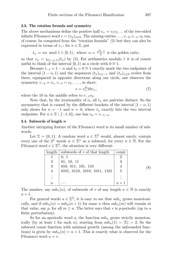
Finite sections of the Fibonacci Hamiltonian 387
3.3. The rotation formula and symmetry
The above mechanisms define the positive half v+ = v1v2 . . . of the two-sidedinfinite Fibonacci word v = (vn)n∈Z. The missing entries . . . , v−2, v−1, v0 can,of course, be computed from the “rotation formula” (2) but they can also beexpressed in terms of v+: for n ∈ Z, put
tn := nα mod 1 ∈ [0, 1), where α =√5−12 is the golden ratio,
so that vn = χ[1−α,1)(tn) by (2). For arithmetics modulo 1 it is of courseuseful to think of the interval [0, 1) as a circle with 0 ∼= 1.
Because t−1 = 1− α and t0 = 0 ∼= 1 exactly mark the two endpoints ofthe interval [1 − α, 1) and the sequences (tn)n≤−1 and (tn)n≥0 evolve fromthere, equispaced in opposite directions along our circle, one observes thesymmetry v−2 = v1, v−3 = v2, . . . , in short:
v = vR+10v+, (7)
where the 10 in the middle refers to v−1v0.Note that, by the irrationality of α, all tn are pairwise distinct. So the
asymmetry that is caused by the different brackets of the interval [1 − α, 1)only shows for n = −1 and n = 0, where tn exactly hits the two intervalendpoints. For n ∈ Z \ −1, 0, one has vn = v−1−n.
3.4. Subwords of length n
Another intriguing feature of the Fibonacci word is its small number of sub-words.
Let Σ = 0, 1. A random word u ∈ ΣZ would, almost surely, containevery one of the 2n words w ∈ Σn as a subword, for every n ∈ N. For theFibonacci word v ∈ ΣZ, the situation is very different:
length subwords of v of that length count1 0, 1 22 01, 10, 11 33 010, 011, 101, 110 44 0101, 0110, 1010, 1011, 1101 5...
...n · · · n+ 1
(8)
The number, say subv(n), of subwords of v of any length n ∈ N is exactlyn+ 1.
For general words u ∈ ΣZ, it is easy to see that subu grows monotoni-cally, and if subu(n) = subu(n + 1) for some n then subu(m) will remain atthat value, say p, for all m ≥ n. The latter says that v is p-periodic (up to afinite perturbation).
So for an aperiodic word u, the function subu grows strictly monoton-ically (by at least 1 for each n), starting from subu(1) = |Σ| = 2. So thesubword count function with minimal growth (among the unbounded func-tions) is given by subu(n) = n + 1. This is exactly what is observed for theFibonacci word u = v.

388 M. Lindner and H. Soding
4. Finite sections of the Fibonacci Hamiltonian
Let v = (vn)n∈Z be the Fibonacci sequence (2) and let
A := S−1 +Mv + S1 : `p(Z)→ `p(Z) (9)
be the Fibonacci Hamiltonian (1), where
Sk : `p(Z)→ `p(Z), (Skx)n+k = xn, n ∈ Z
denotes the shift by k ∈ Z components and
Mb : `p(Z)→ `p(Z), (Mbx)n = bnxn, n ∈ N
denotes the operator of pointwise multiplication by b = (bn)n∈Z ∈ `∞(Z).We identify A with its two-sided infinite matrix (aij)i,j∈Z with ann = vn
and an,n±1 = 1 for all n ∈ Z and zeros everywhere else. Corollary 2.5 connectsthe FSM of A with the limit operators of A. So we need to get a hand onthese limit operators.
4.1. Limit operators of the Fibonacci Hamiltonian
Let h = (h1, h2, . . . ) be a sequence in Z with hk → ±∞, so that the limitoperator Ah of the Fibonacci Hamiltonian A from (9) exists. Then
Ah = (S−1)h + (Mv)h + (S1)h =: S−1 +Mvh + S1
with a new potential
vh := limk→∞
S−hkv,
where the limit is taken w.r.t. pointwise convergence on ΣZ for Σ = 0, 1.The set F of all such potentials vh is translation invariant (translations
of limit operators of A are limit operators of translations of A) and closedunder pointwise convergence. F is the so-called Fibonacci subshift. By ourdefinition of F ,
Lim(A) = S−1 +Mvh + S1 : vh ∈ F.
The set F is explicitly known (see, e.g., Theorem 2.14 in [8] and the appendixof [11]):
F = vθ, wθ : θ ∈ [0, 1), (10)
where
vθn := χ[1−α,1)(θ + nα mod 1), wθn := χ(1−α,1](θ + nα mod 1), n ∈ Z.
In particular,
A ∈ Lim(A), (11)
since v = v0 ∈ F . In fact, we do not need this explicit description (10) of F .The following lemma is sufficient (and much more handy) for us. It expressesthe well-known minimality of the Fibonacci subshift.
Lemma 4.1. Every vh ∈ F has the same list (8) of subwords as v. So forevery w ∈ Σ∗ and every vh ∈ F it holds that
w ≺ v ⇐⇒ w ≺ vh.

Finite sections of the Fibonacci Hamiltonian 389
Proof. Take arbitrary w ∈ Σ∗ and vh ∈ F . So there exists a sequenceh = (h1, h2, . . . ) in Z with hk → ±∞ and vh = limk→∞ S−hk
v, pointwise.⇐ If w ≺ vh then w ≺ S−hk
v for large k (strict topology on Σ), sothat w ≺ v.
⇒ Now let w ≺ v. W.l.o.g. assume w ≺ v+. Choose n ∈ N so that wappears in the first Fn letters of v+, i.e., w ≺ fn ≺ fn+1 (recall the notationsfrom §3.2).
By (6), we have fn+2 = fn+1fn and fn+3 = fn+2fn+1 = fn+1fnfn+1. Byinduction, every fm with m ≥ n, and hence v+, is composed of fn and fn+1.Since w appears as a subword in fn and fn+1, it appears infinitely often inv+, where two appearances of w are at most |fn+1| = Fn+1 letters away fromeach other. So every translate S−hk
v of v contains w in an Fn+1-neighborhoodof zero. Hence, every limit vh ∈ F contains w (in an Fn+1-neighborhood ofzero).
4.2. Main results
Now we are ready to state and prove our two main results.
Theorem 4.2. The FSM of the two-sided infinite Fibonacci Hamiltonian (9) isstable for any choice of cut-off points and in every space `p(Z) with p ∈ [1,∞].
The compression AN of A from (9) to `p(N) is called one-sided infiniteFibonacci Hamiltonian. Its matrix (aij)i,j∈N is the submatrix of A consistingof all rows and columns with i, j ∈ N.
Theorem 4.3. The FSM of the one-sided infinite Fibonacci Hamiltonian AN isstable for any choice of cut-off points and in every space `p(N) with p ∈ [1,∞].
The rest of this paper is devoted to the proof of these two theorems.The main ingredient, besides Corollary 2.5 and Lemma 2.6, is the followinglemma.
Lemma 4.4. For the Fibonacci Hamiltonian A from (9), the following state-ments hold:
a) All B ∈ Lim(A) are injective on `∞(Z).b) For all B ∈ Lim+(A), the compression B− is injective on `∞(Z−).c) For all B ∈ Lim−(A), the compression B+ is injective on `∞(Z+).
Here we use the notations B± and Z± from Definition 2.3 b). We nowshow how this lemma implies Theorems 4.2 and 4.3 before we come to itsproof (in Section 4.3).
Proof of Theorem 4.2. Let p ∈ [1,∞]. By Corollary 2.5, we have to show that
1) A is invertible on `p(Z),2) for all B ∈ Lim+(A), the compression B− is invertible on `p(Z−), and3) for all B ∈ Lim−(A), the compression B+ is invertible on `p(Z+).
It is sufficient to study the case p = 2 as A and all B+ and B− are bandmatrices, and so their invertibility is independent of p ∈ [1,∞] (see e.g. [16,§5.2.7]).

390 M. Lindner and H. Soding
Property a) of Lemma 4.4 implies the invertibility of all B ∈ Lim(A),by Lemma 2.6. Since A ∈ Lim(A), by (11), also B = A is invertible. So 1) isshown.
To show 2), take an arbitrary B ∈ Lim+(A) and look at B− as anoperator on `2(Z−). Since B− is injective on `∞(Z−), by Lemma 4.4 b), itis also injective on the subset `2(Z−) of `∞(Z−). Its adjoint is also injec-tive on `2(Z−) since B− is self-adjoint (by A = A∗). So it remains to showthat the range of B− is closed: From 1) it follows that A is Fredholm. ByLemma 2.6, B is invertible, hence Fredholm. By Lemma 2.6 again, all oper-ators in Lim(B) ⊃ Lim(B−) are invertible, whence also B− is Fredholm (byLemma 2.6 again) and hence has a closed range.
3) follows from Lemma 4.4 c) and Lemma 2.6 in the very same way.
Proof of Theorem 4.3. This time we have to show that
4) AN is invertible on `p(Z),5) for all B ∈ Lim+(AN), the compression B− is invertible on `p(Z−).
Statement 4) follows from 3) because AN = B+ for B = S−1AS1 ∈ Lim−(A).Statement 5) follows from 2) because Lim+(AN) = Lim+(A), by the con-struction of AN.
Let us point out that the presence of (iii) in Lemma 2.6 is vital here.With only (i) and (ii) at hand, we would be stuck in a vicious circle. Thestudy of the invertibility of A can be reduced to the following, presumablyeasier, problems: injectivity of A, injectivity of A∗, Fredholmness of A. Thelatter again splits into many, presumably easier, problems: invertibility ofall limit operators B of A, by Lemma 2.6 (ii). But now A is one of thoseoperators B, by (11), which brings us back to the original problem! So it isgood to have – and use – Lemma 2.6 (iii) instead of (ii) here.
Now all that remains to be done is the proof of Lemma 4.4.
4.3. Proof of Lemma 4.4
First notice that one can restrict consideration to real sequences in both theone- and two-sided infinite case. Since B (and the compressions B+ and B−)correspond to real matrices, it holds
Bx = 0 ⇐⇒ 0 = Re(Bx) = B(Re(x)) and 0 = Im(Bx) = B(Im(x))
with Re(·) and Im(·) denoting the real and imaginary part of a sequence.So the injectivity of B on the space of real bounded sequences implies theinjectivity on the space `∞(I) of complex bounded sequences. One is left withproving Bx = 0 ⇒ x = 0 for all bounded real sequences. The idea is mosttransparent in the one-sided infinite case. So let us start with the proof of c).
To show that an operator B+ is injective on `∞(Z+), derive the entriesx1, x2, . . . of a solution x = (xn)n∈Z+
of the homogeneous equation B+x = 0,starting from a nonzero initial entry x0, and prove that some entry xn willeventually exceed (in modulus) any previously given bound r > 0. Because,for every r > 0, this computation will only take finitely many steps x1, . . . , xn,

Finite sections of the Fibonacci Hamiltonian 391
it is enough to know about finite subwords of the potential of B+. (Our proofdoes not use the explicit formula (10).)
Identify B+ with its matrix (bij)i,j∈Z+ . Because of the tridiagonal struc-ture, the value of x0 is sufficient to calculate the whole solution vector x.More precisely, x1 = −b00 x0 and xn+1 = −bnn xn − xn−1 for n ∈ N. Asusual, rewrite this recurrence with transfer matrices:
Tbnn
(xn−1xn
)=
(xnxn+1
), where Tbnn
=
(0 1−1 −bnn
)with bnn ∈ 0, 1.
W.l.o.g. we can assume x0 = 1. Here is an example computation for a certaindiagonal (bnn):
n 0 1 2 3 4 5 6 7 8 9 10 11 12 13 14bnn 1 0 1 1 0 1 0 1 1 0 1 1 0 1 0
xn 1 −1 −1 2 −1 −2 3 2 −5 3 5 −8 3 8 −11
In this example, with a bit of optimism, we seem to observe that
• the diagonal (bnn) of B is composed of blocks “101” and “01”, and• the entries xn at the beginning of each block grow unboundedly in
modulus.
We will prove that this is always the case. The following lemma is a specialcase of a partition of general Sturmian words as introduced in [17] (also see[10, 18]).
Lemma 4.5. The diagonal b := (bnn)n∈Z+of B+ with B ∈ Lim−(A) is of the
form
b = pw1 w2 w3 . . . with p ∈ ε, 1 and wi ∈ 101, 01 for all i ∈ N.
Proof. By Lemma 4.1 and (8), b contains neither 00 nor 111 as a subword.So 0 is always followed by 1, and 1 is always followed by 101 or 01.
So we are particularly interested in the patterns “101” and “01” andtheir corresponding transfer matrices
T101 := T1T0T1 =
(0 −11 2
)and T01 := T1T0 =
(−1 01 −1
). (12)
Let us say that a vector( y1y2
)∈ R2 has property C if y1 · y2 < 0 and
|y1| < |y2|.
Lemma 4.6. Both T101 and T01 preserve property C. More precisely, if( y1y2
)in R2 has property C then
(z1z2
):= Tw
( y1y2
)with w ∈ 101, 01 has properties
A) |z2| > |y2| with |z2| − |y2| ≥ min|y1 + y2|, |y1| > 0,B) |z1 + z2| ≥ |y1 + y2| and |z1| ≥ |y1|, andC) z1 · z2 < 0 and |z1| < |z2|.
Proof. This is a straightforward computation using
T101
(y1y2
)=
(−y2
y2 + (y1 + y2)
)and T01
(y1y2
)=
(−y1
y1 − y2
).

392 M. Lindner and H. Soding
Property A shows a growth (in modulus) of the second vector componentafter applying T101 or T01. By property B, the amount of growth is non-decreasing when applying T101 or T01 again. The fact that property C ispreserved keeps the argument working for the next application of T101 or T01,leading to unbounded growth of the second vector component, by induction.
So all what we need is one first occurrence of property C for a vector( xnxn+1
)in our computation of a sequence x = (x0, x1, x2, . . . ) that solves
B+x = 0.We start with the case p = ε. Besides x0 = 1 (see above), we put
x−1 := 0 to start our recurrence and account for the non-existence of columnnumber −1 in the matrix B+. Depending on which of T101 and T01 from (12)we apply to
( x−1x0
)=(01
), we get
T01
(01
)=
(0−1
)or T101
(01
)=
(−12
).
So repeated application of T01 leads to ±(01
)but after the first applica-
tion of T101, which will eventually happen since b is not periodic, one gets( xnxn+1
)= ±
(−12
)for some n ∈ N. This vector has property C. From our
arguments above it follows that the sequence x is unbounded.If the prefix p of b is 1, it follows from x0 = 1 that x1 = −1, so that our
recurrence starts with(x0x1
)=(
1−1). The application of the transfer matrices
from (12) yields
T01
(1−1
)=
(−12
)and T101
(1−1
)=
(1−1
).
So repeated application of T101 leads to(
1−1)
but after the first applica-tion of T01, which will eventually happen since b is not periodic, one gets( xnxn+1
)=(−1
2
)for some n ∈ N. This vector has property C. From our argu-
ments above it follows that the sequence x is unbounded.For both possibilities of the prefix b ∈ ε, 1 and all possibilities of the
following blocks wi ∈ 101, 01 (recall Lemma 4.5), we have shown that allnontrivial solutions x of the homogenous system B+x = 0 are unbounded, sothat every B+ with B ∈ Lim−(A) is injective on `∞(Z+). Thus, c) is proved.
To see b), consider the three flip operators
J← : `∞(Z+)→ `∞(Z−), J→ : `∞(Z−)→ `∞(Z+), and J↔ : `(Z)→ `(Z),
all three acting by the rule x 7→ y with yn = x−n for n in Z−, Z+ and Z,respectively.
The formula v = vR+10v+ from (7) implies that Lim+(A) exactly consistsof the reflections C = J↔BJ↔ of operators B ∈ Lim−(A), so that
C− : C ∈ Lim+(A) = (J↔BJ↔︸ ︷︷ ︸C
)+ = J←B+J→ : B ∈ Lim−(A).
So, clearly, b) follows from c).
Finally, we are going to prove a). To do this, we will use a two-sidedversion of the proof of c).

Finite sections of the Fibonacci Hamiltonian 393
Let B ∈ Lim(A) and again let b ∈ 0, 1Z be the diagonal of B. Let xbe a nontrivial solution of the homogeneous equation Bx = 0. We will provethat the sequence x grows unboundedly in at least one direction, left or right.The growth to the right is studied as in the proof of c) above – growth to theleft by symmetric arguments. Here is the analogue of Lemma 4.5.
Lemma 4.7. The diagonal b := (bnn)n∈Z of B ∈ Lim(A) is of the form
b = · · · w−4 w−3 101︸︷︷︸w−2
101︸︷︷︸w−1
01︸︷︷︸w0
101︸︷︷︸w1
101︸︷︷︸w2
w3 w4 · · · (13)
with w−i ∈ 101, 10 and wi ∈ 101, 01 for all i ∈ N.
Proof. The word 101 101 01 101 101 is contained in the Fibonacci word v (asv−6 · · · v7) and therefore, by Lemma 4.1, also in b. By Lemma 4.1 and (8), bcontains neither 00 nor 111 as a subword. So, as argued in Lemma 4.5, 0 isalways followed by 1, and 1 is always followed by 101 or 01. Moreover, 0 isalways preceded by 1, and 1 is always preceded by 101 or 10.
So besides T101 and T01, we now also have to look at the transfer matrixT10 := T0T1. Note that, when we study the asymptotics of x towards −∞(going backward in “time”), we will have to look at inverses of the transfermatrices.
Therefore, let us say that a vector( y1y2
)∈ R2 has property F if y1 ·y2 < 0
and |y1| > |y2|. Here is the “leftward” analogue of Lemma 4.6.
Lemma 4.8. Both T−1101 and T−110 preserve property F. More precisely, if( y1y2
)in R2 has property F then
(z1z2
):= T−1w
( y1y2
)with w ∈ 101, 10 has properties
D) |z1| > |y1| with |z1| − |y1| ≥ min|y1 + y2|, |y2| > 0,E) |z1 + z2| ≥ |y1 + y2| and |z2| ≥ |y2|, andF) z1 · z2 < 0 and |z1| > |z2|.
Proof. This is again a straightforward computation using
T−1101
(y1y2
)=
(y1 + y2 + y1−y1
)and T−110
(y1y2
)=
(−y1 + y2−y2
).
As before, property D states a growth (in modulus) of the first compo-nent. Property E ensures that the amount of this growth is non-decreasingin further applications of T−1w with w ∈ 101, 10, and the fact that propertyF is preserved makes sure that the same argument keeps working for furtherapplications of T−1w , leading to unbounded growth.
So again, we just need a first occurrence of property F for a vector( xnxn+1
)with n < 0 or a first occurrence of property C for a vector
( xnxn+1
)with
n ≥ 0 in our computation of a sequence x = (. . . , x−2, x−1, x0, x1, x2, . . . )
that solves Bx = 0. Then x will be unbounded.This time, one entry, say x0, does not determine the whole sequence x,
but two entries do. Let the two entries of x that are associated to the entries 0and 1 of w0 in (13) be equal to α and β, respectively, with arbitrary α, β ∈ R.W.l.o.g label them as x0 and x1.

394 M. Lindner and H. Soding
Using the adjacent entries of w0 = 01 in b, see (13), the correspondingentries x−4, . . . , x5 in x turn out to be as follows:
x−4 x−3 x−2 x−1 x0 x1 x2 x3 x4 x5α− 2β β −α+ β −β α β −α− β α α+ β −2α− β
With respect to α and β, we have to distinguish the following cases:
1. If α = β = 0 then x = 0 follows.2. If α = 0 and β 6= 0 then
( x−4x−3
)=(−2β
β
)has property F.
3. If α 6= 0 and β = 0 then(x4x5
)=(
α−2α
)has property C.
4. If α 6= 0 and β 6= 0 we have to look at two more cases:(a) If α · β > 0 then
(x1x2
)=( β−α−β
)has property C.
(b) If α · β < 0 then( x−4x−3
)=( α−2β
β
)has property F.
This completes the study of all cases. Each nontrivial solution of the ho-mogenous equation Bx = 0 is unbounded, thus B is injective on `∞(Z). Thiscompletes the proof of a) and thus of Lemma 4.4.
Acknowledgements. The first author thanks Albrecht Bottcher, Daniel Potts,Peter Stollmann and David Wenzel for organizing a wonderful IWOTA con-ference 2017 in Chemnitz with many inspiring talks and countless other pleas-ant moments.
References
[1] M. Baake and U. Grimm, Aperiodic Order. Vol. 1. A Mathematical Invitation,Encyclopedia of Mathematics and its Applications 149, Cambridge UniversityPress, Cambridge, 2013.
[2] G. Baxter, A norm inequality for a ‘finite-section’ Wiener-Hopf equation, Illi-nois J. Math. 7 (1963), 97–103.
[3] A. Bottcher and S.M. Grudsky, Spectral Properties of Banded Toeplitz Matrices,SIAM, Philadelphia, 2005.
[4] N.G. de Bruijn, Algebraic theory of Penrose’s non-periodic tilings of the plane.I, Nederl. Akad. Wetensch. Indag. Math. 43 (1981), 39–52.
[5] S.N. Chandler-Wilde and M. Lindner, Sufficiency of Favard’s condition for aclass of band-dominated operators on the axis, J. Funct. Anal. 254 (2008),1146–1159.
[6] S.N. Chandler-Wilde and M. Lindner, Limit Operators, Collective Compact-ness, and the Spectral Theory of Infinite Matrices, Memoirs of the AMS 210,no. 989, Amer. Math. Soc., Providence, 2011.
[7] S.N. Chandler-Wilde and M. Lindner, Coburn’s lemma and the finite sectionmethod for random Jacobi operators, J. Funct. Anal. 270 (2016), 802–841.
[8] D. Damanik, Strictly ergodic subshifts and associated operators, Proceedingsof Symposia in Pure Math. (Festschrift for Barry Simon’s 60th birthday), 505–538, Amer. Math. Soc., Prividence, 2007.
[9] D. Damanik, M. Embree and A. Gorodetski, Spectral properties of Schrodingeroperators arising in the study of quasicrystals, Mathematics of Aperiodic Order,Progress in Mathematics 309, Birkhauser, 2015, 307–370.

Finite sections of the Fibonacci Hamiltonian 395
[10] D. Damanik and D. Lenz, Uniform spectral properties of one-dimensional qua-sicrystals. I. Absence of eigenvalues, Comm. Math. Phys. 207 (1999), 687–696.
[11] D. Damanik and D. Lenz, Half-line eigenfunction estimates and purely singularcontinuous spectrum of zero Lebesgue measure, Forum Math. 16 (2004), 109–128.
[12] I. Gohberg and I.A. Feldman, Convolution Equations and Projection Methodsfor their Solution, Transl. of Math. Monographs, 41, AMS, Providence, R.I.,1974 [Russian original: Nauka, Moscow, 1971].
[13] J. Kellendonk, D. Lenz and J. Savinien (eds.), Mathematics of Aperiodic Order,Progress in Mathematics 309, Birkhauser, Basel, 2015.
[14] A.V. Kozak, A local principle in the theory of projection methods (Russian),Dokl. Akad. Nauk SSSR 212 (1973), 1287–1289; English transl. Soviet Math.Dokl. 14 (1974), 1580–1583.
[15] A.V. Kozak and I.V. Simonenko, Projection methods for solving multidimen-sional discrete convolution equations (Russian), Sib. Mat. Zh. 21 (1980), 119–127.
[16] V.G. Kurbatov, Functional Differential Operators and Equations, Kluwer Aca-demic Publishers, Dordrecht, Boston, London, 1999.
[17] D. Lenz, Aperiodische Ordnung und gleichmaßige spektrale Eigenschaften vonQuasikristallen, PhD thesis, Frankfurt, Logos Verlag, Berlin, 2000.
[18] D. Lenz, Hierarchical structures in Sturmian dynamical systems, Theoret.Comput. Sci. 303 (2003), 463–490.
[19] M. Lindner, Infinite Matrices and their Finite Sections: An Introduction to theLimit Operator Method, Frontiers in Mathematics, Birkhauser, Basel, 2006.
[20] M. Lindner, Fredholm Theory and Stable Approximation of Band Operatorsand Generalisations, Habilitation thesis, TU Chemnitz, 2009.
[21] M. Lindner and M. Seidel, An affirmative answer to a core issue on limitoperators, J. Funct. Anal. 267 (2014), 901–917.
[22] M. Lothaire, Algebraic Combinatorics on Words, Cambridge Univ. Press, Cam-bridge, 2002.
[23] V.S. Rabinovich, S. Roch and B. Silbermann, Fredholm theory and finite sec-tion method for band-dominated operators, Integral Equations Operator The-ory 30 (1998), 452–495.
[24] V.S. Rabinovich, S. Roch and B. Silbermann, Band-dominated operators withoperator-valued coefficients, their Fredholm properties and finite sections, In-tegral Equations Operator Theory 40 (2001), no. 3, 342–381.
[25] V.S. Rabinovich, S. Roch and B. Silbermann, Algebras of approximation se-quences: Finite sections of band-dominated operators, Acta Appl. Math. 65(2001), 315–332.
[26] V.S. Rabinovich, S. Roch and B. Silbermann, Limit Operators and Their Ap-plications in Operator Theory, Birkhauser, Basel, Boston, Berlin, 2004.
[27] S. Roch, Finite Sections of Band-dominated Operators, Memoirs of the AMS191, no. 895, Amer. Math. Soc., Providence, 2008.
[28] M. Seidel, On Some Banach Algebra Tools in Operator Theory, PhD thesis,TU Chemnitz, 2012.

396 M. Lindner and H. Soding
[29] P.J. Steinhardt, Quasicrystals: a brief history of the impossible, Rend. Fis. Acc.Lincei 24 (2013), 85–91.
[30] P. Stollmann, Caught by Disorder. Bound states in random media, Progress inMathematical Physics 20, Birkhauser, Boston, 2001.
Marko LindnerHamburg University of Technology (TUHH)Institute of Mathematics21073 HamburgGermanye-mail: [email protected]
Hagen SodingStudent of Technomathematicsat Hamburg University and TUHHe-mail: [email protected]

Spectral asymptotics for Toeplitz operatorsand an application to banded matrices
Alexander Pushnitski
Abstract. We consider a class of compact Toeplitz operators on theBergman space on the unit disc. The symbols of the operators in ourclass are assumed to have a sufficiently regular power-like behaviour nearthe boundary of the disc. We compute the asymptotics of the singularvalues of Toeplitz operators in this class. We use this result to obtainthe asymptotics of the singular values for a class of compact bandedmatrices.
Mathematics Subject Classification (2010). Primary 47B32; Secondary47B36.
Keywords. Toeplitz operators, Bergman space, banded matrix, spectralasymptotics.
1. Introduction and main results
1.1. Introduction
Let D be the unit disc in the complex plane, and let L2(D) be the Hilbert spaceof all square integrable functions with respect to the normalised Lebesgue areameasure on D. Next, let B2(D) be the Bergman space, i.e., the closure of thelinear span of the functions zn∞n=0 in L2(D). Denote by P : L2(D)→ B2(D)the Bergman projection, i.e., the orthogonal projection in L2 onto B2. For asymbol ϕ ∈ L∞(D), the Toeplitz operator T (ϕ) in B2(D) is defined by
T (ϕ)f = P (ϕ · f), f ∈ B2(D).
It is well known that if ϕ(z)→ 0 as |z| → 1, then T (ϕ) is compact. Moreover,roughly speaking, the rate of convergence of ϕ(z)→ 0 as |z| → 1 determinesthe rate of convergence of the sequence of singular values sn(T (ϕ)) → 0as n → ∞. For radial symbols ϕ(z) = ϕ(|z|) it is very easy to make thisstatement precise. Indeed, in this case the Toeplitz operator T (ϕ) is diag-onal in the standard orthonormal basis
√n+ 1zn∞n=0 of B2(D), and so
© Springer International Publishing AG, part of Springer Nature 2018
Theory: Advances and Applications 268, https://doi.org/10.1007/978-3-319-75996-8_21
397A. Böttcher et al. (eds.), The Diversity and Beauty of Applied Operator Theory, Operator

398 A. Pushnitski
the sequence of the singular values of T (ϕ) is given by
sn(T (ϕ)) = (n+ 1)∣∣(T (ϕ)zn, zn)L2(D)
∣∣ = 2(n+ 1)
∣∣∣∣∫ 1
0
r2nϕ(r)rdr
∣∣∣∣ .Specialising to the power behaviour ϕ(r) = (1− r)γ , γ > 0, by an elementarycalculation one obtains
sn(T (ϕ)) = 2−γΓ(γ + 1)n−γ +O(n−1−γ), n→∞. (1.1)
The purpose of this paper is
(i) to present a method that allows one to extend this calculation to symbolsϕ that have some sufficiently regular angular dependence;
(ii) to give an application to the spectral analysis of banded matrices.
1.2. Spectral asymptotics for Toeplitz operators
Theorem 1.1. Let ϕ ∈ L∞(D), and let γ > 0. Assume that for some contin-uous function ϕ∞ on the unit circle one has
sup0<θ≤2π
|(1− r)−γϕ(reiθ)− ϕ∞(eiθ)| → 0, r → 1.
Then the singular values of T (ϕ) satisfy
sn(T (ϕ)) = Cγ(ϕ∞)n−γ + o(n−γ), n→∞,where
Cγ(ϕ∞) = 2−γΓ(γ + 1)
(∫ 2π
0
|ϕ∞(eiθ)|1/γ dθ2π
)γ.
As will be clear from the proof, the requirement of the continuity ofϕ∞ can be considerably relaxed. For example, any Riemann integrable ϕ∞is admissible.
If ϕ is real-valued, then it is evident that T (ϕ) is self-adjoint. In thiscase, let us denote by λ+n (T (ϕ))∞n=0 the sequence of positive eigenvalues ofT (ϕ) and set a+ = maxa, 0 for a ∈ R. We have an analogous result foreigenvalues.
Theorem 1.2. Assume the hypothesis of Theorem 1.1 and let ϕ be real-valued.Then the positive eigenvalues of T (ϕ) satisfy
λ+n (T (ϕ)) = C+γ (ϕ∞)n−γ + o(n−γ), n→∞, (1.2)
where
C+γ (ϕ∞) = 2−γΓ(γ + 1)
(∫ 2π
0
ϕ+∞(eiθ)1/γ
dθ
2π
)γ.
Of course, a similar result holds true for the negative eigenvalues.By using conformal mapping, it is possible to extend Theorems 1.1 and
1.2 to other domains. However, we prefer to focus on the simplest case, asour aim is to emphasise the method rather than the result.
A result similar to Theorem 1.2 is known in the context of Toeplitzoperators on the Fock space. In this case, the symbol ϕ(z) depends on z ∈ C,and the rate of convergence of the eigenvalues of the corresponding Toeplitzoperator to zero depends on the rate of convergence of ϕ(z)→ 0 as |z| → ∞.

Spectral asymptotics for Toeplitz operators 399
In [6], symbols that behave as |z|−γϕ∞(eiθ) when |z| → ∞ are consideredand a spectral asymptotics of the type (1.2) is proved. The proof is achievedthrough a reduction to a pseudodifferential operator in L2(R).
Another closely related recent result is [3], where the authors considerharmonic Toeplitz operators in a bounded domain in Rd with symbols thathave a power decay near the boundary. They obtain asymptotics of eigenval-ues very similar to (1.2). The method of proof of [3] is quite different fromthe one in this paper and consists in a reduction to a pseudodifferential op-erator on the boundary. The same method can probably be applied to givean alternative proof of Theorems 1.1 and 1.2.
1.3. Application: spectral asymptotics for banded matrices
Let A be the operator on `2 corresponding to an infinite matrix aj,k∞j,k=0
of the following form. Our first assumption is that the operator A is banded,i.e., for some M ∈ N, we have
aj,j+m = 0 if |m| > M .
Our second assumption is that for each m with |m| ≤ M , the sequence ofentries aj,j+m has a power asymptotics as j →∞. More precisely, we fix anexponent γ > 0 and complex numbers bm, m = −M, . . . ,M , and assume that
aj,j+m = bmj−γ + o(j−γ), j →∞, |m| ≤M.
It is easy to see that under these assumptions the matrix A is compact. It isalso not difficult to see that sn(A) = O(n−γ). The theorem below gives theasymptotic behaviour of the singular values.
Theorem 1.3. Under the above assumptions, the singular values of A satisfy
sn(A) =
(∫ π
−π|b(eiθ)|1/γ dθ
2π
)γn−γ + o(n−γ), n→∞,
where
b(eiθ) =M∑
k=−M
bkeikθ, −π < θ ≤ π. (1.3)
If A is self-adjoint, then b is necessarily real-valued. In this case one hasa similar asymptotic formula for the positive eigenvalues of A.
Theorem 1.4. Assume the hypothesis of Theorem 1.3 and suppose that A isself-adjoint. Then the positive eigenvalues of A satisfy
λ+n (A) =
(∫ π
−πb+(eiθ)1/γ
dθ
2π
)γn−γ + o(n−γ), n→∞,
where b is given by (1.3) and b+ = maxb, 0.
Again, a similar result holds for the negative eigenvalues of A.

400 A. Pushnitski
Example 1.5. Lommel polynomials (see e.g. [7, Section 3] and referencestherein) are orthogonal polynomials associated with the Jacobi matrix (i.e.,the tridiagonal matrix) which in our notation corresponds to M = 1, aj,j = 0,and
aj,j+1 = aj+1,j =1
2√
(j + ν + 1)(j + ν), j ≥ 0
(here ν > 0 is a parameter). Since the entries on the main diagonal areidentically zero, the spectrum of this Jacobi matrix is symmetric with respectto reflection around zero. Further, it is known that its eigenvalues are givenby 1/jk,ν−1, k ∈ Z, where jk,ν−1 are the zeros of the Bessel function Jν−1.These zeros have the asymptotic behaviour jk,ν−1 ∼ πk as |k| → ∞, and sothe positive eigenvalues of our Jacobi matrix satisfy
λ+n (A) =1
πn+ o
(1
n
), n→∞.
This agrees with Theorem 1.4, which gives b(eiθ) = cos θ, γ = 1, and∫ π
−πb+(eiθ)
dθ
2π=
∫ π/2
−π/2cos θ
dθ
2π=
1
π.
Example 1.6. Tricomi–Carlitz polynomials (see [7, Section 3]) are orthogonalpolynomials associated with the Jacobi matrix with M = 1, aj,j = 0, and
aj,j+1 = aj+1,j =
√j + 1√
(j + α+ 1)(j + α), j ≥ 0
(α is a real parameter). Again, the spectrum of this Jacobi matrix is symmet-ric with respect to reflection around zero, and it is known that its eigenvaluesare given by ±1/
√n+ α, n ≥ 0. This agrees with Theorem 1.4, which gives
b(eiθ) = 2 cos θ, γ = 1/2, and(∫ π
−πb+(eiθ)2
dθ
2π
)1/2
=
∫ π/2
−π/24(cos θ)2
dθ
2π= 1.
1.4. Key ideas of the proof and the structure of the paper
We focus on the case of the singular value asymptotics, i.e., on Theorems 1.1and 1.3; the eigenvalue asymptotics is considered in a similar fashion. It willbe convenient to work with the singular value counting function:
n(s;T ) = #n : sn(T ) > s, s > 0. (1.4)
We recall that for a compact operator T , the relations
sn(T ) =C
nγ+o(n−γ), n→∞, and n(s;T ) =
C1/γ
s1/γ+o(s−1/γ), s→ 0, (1.5)
are equivalent.The main issue is to prove Theorem 1.1 for symbols of the form
ϕ(reiθ) = (1− r)γϕ∞(eiθ).

Spectral asymptotics for Toeplitz operators 401
For such symbols, we shall write Tγ(ϕ∞) instead of T (ϕ). By a limitingargument, the problem reduces to replacing the continuous function ϕ∞ bystep functions that are constant on each arc
δ` =eiθ : 2π`
L < θ < 2π(`+1)L
,
where L ∈ N is fixed. Let us denote by 1δ` the characteristic function of δ`and write
ϕ∞ =
L∑`=1
c`1δ` (1.6)
with some coefficients c`. Then
Tγ(ϕ∞) =L∑`=1
c`Tγ(1δ`). (1.7)
Our main observation is that the terms in the sum (1.7) are asymptoticallyorthogonal in the sense that the products Tγ(1δ`)Tγ(1δm), ` 6= m, satisfy cer-tain Schatten class properties. An operator theoretic lemma from [2] (Theo-rem 2.2) then shows that the leading term coefficient in the spectral asymp-totics is additive for the sum (1.7). This means that the relation
n(s;Tγ(ϕ∞)) =L∑`=1
n(s; c`Tγ(1δ`)) + o(s−1/γ), s→ 0,
holds true. Using this fact, it is not difficult to derive the required spectralasymptotics for piecewise constant functions ϕ∞ of the form (1.6) from thesame asymptotics for characteristic functions ϕ∞.
We note that this construction is almost purely operator theoretic anduses very little specific features of the problem, apart from rotational symme-try and asymptotic orthogonality. Thus, it can be used in other contexts, forexample for Toeplitz operators associated with multi-dimensional domainswith spherical symmetry. This method of proof, based on asymptotic orthog-onality, was developed in [4, 5] for a different purpose.
Let us explain the key idea of the proof of Theorem 1.3. Consider asymbol of the form
ϕ(reiθ) = (1− r)γeimθ,where m ∈ Z. Then the matrix of T (ϕ) in the standard orthonormal basis√
k + 1zk∞k=0
of the Bergman space is
aj,k =√j + 1
√k + 1(ϕzj , zk)L2(D).
It is easy to see that aj,k 6= 0 only if k = j +m and
aj,j+m = 2−γΓ(γ + 1)j−γ + o(j−γ)
as j →∞. This corresponds to a matrix A as in Theorem 1.3 with only onenon-zero diagonal. Taking a finite linear combination of such matrices givesthe case of a general banded matrix. Thus, the proof of Theorem 1.3 reducesto Theorem 1.1.

402 A. Pushnitski
In Section 2 we recall some background facts concerning singular valueand eigenvalue asymptotics for compact operators and state the result from[2] on asymptotically orthogonal operators. In Section 3 we prove Theo-rems 1.1 and 1.2 and in Section 4 we prove Theorems 1.3 and 1.4.
Acknowledgements
The author is grateful to P. Honore and M. Reguera for useful discussionsat the early stage of this work, to the organisers of IWOTA 2017 for theencouragement, and to G. Raikov and L. Golinskii for valuable remarks onthe text of the paper.
2. Operator theoretic tools
Here we collect some general operator theoretic tools related to the singularvalue and eigenvalue estimates and asymptotics for compact operators.
2.1. Definitions
For a compact operator T in a Hilbert space, we denote by sn(T )∞n=0 thenon-increasing sequence of singular values of T , enumerated with multiplic-ities taken into account. Recall that sn(T ) is defined as the n’th eigenvalue
of the positive semi-definite self-adjoint operator |T | =√T ∗T . We will work
with the singular value counting function (1.4). For p > 0, the standardSchatten class Sp is defined by the condition
∞∑n=0
sn(T )p <∞.
In terms of the counting function n(s;T ) this can be equivalently rewrittenas ∫ ∞
0
n(s;T )sp−1ds <∞.
The weak Schatten class Sp,∞ is defined by the condition
n(s;T ) = O(s−p), s→ 0.
The quantity
‖T‖Sp,∞ = sups>0
sn(s;T )1/p
is a quasi-norm on Sp,∞, and we will be considering Sp,∞ with respect to thetopology given by this quasi-norm. The subclass S0
p,∞ ⊂ Sp,∞ is defined bythe condition
n(s;T ) = o(s−p), s→ 0;
it can be characterised as the closure of all operators of finite rank in Sp,∞.In order to work with the singular value asymptotics, it will be conve-
nient to use the following functionals in Sp,∞:
∆p(T ) := lim sups→0
spn(s;T ), δp(T ) := lim infs→0
spn(s;T ). (2.1)

Spectral asymptotics for Toeplitz operators 403
In applications, one usually has ∆p(T ) = δp(T ), but it is technically conve-nient to treat the upper and lower limits separately. The functionals ∆p andδp are continuous in Sp,∞.
We will denote S0 = ∩p>0Sp. In other words, S0 consists of compactoperators T such that for all C > 0, one has
sn(T ) = O(n−C), n→∞.
2.2. Additive and multiplicative estimates
Below we recall some estimates for singular values of sums and products ofcompact operators.
The following fundamental result is known as the Ky Fan lemma; seee.g. [1].
Lemma 2.1. Let A ∈ Sp,∞ and B ∈ S0p,∞ for some p > 0. Then
∆p(A+B) = ∆p(A), δp(A+B) = δp(A).
In Section 3 we will also need more advanced information about thequantities ∆p and δp. One has the following additive esimates, see e.g. [1,formulas (11.6.12), (11.6.14), (11.6.15)]:
∆p(A1 +A2)1/(p+1) ≤ ∆p(A1)1/(p+1) + ∆p(A2)1/(p+1), (2.2)
|∆p(A1)1/(p+1) −∆p(A2)1/(p+1)| ≤ (∆p(A1 −A2))1/(p+1), (2.3)
|δp(A1)1/(p+1) − δp(A2)1/(p+1)| ≤ (∆p(A1 −A2))1/(p+1). (2.4)
We will also need some multiplicative estimates. One has (see [1, (11.1.19),(11.1.12)])
n(s1s2;A1A2) ≤ n(s1;A1) + n(s2;A2), s1 > 0, s2 > 0, (2.5)
n(s;A1A2) ≤ n(s; ‖A1‖A2), s > 0. (2.6)
From (2.5) it is not difficult to obtain (see [1, (11.6.18)]) the bound
∆p/2(A1A2) ≤ 2∆p(A1)∆p(A2). (2.7)
2.3. Asymptotically orthogonal operators
The theorem below is the key operator theoretic ingredient of our construc-tion. It has first appeared (under slightly more restrictive assumptions) in [2,Theorem 3]. Here we follow the presentation of [4, Theorem 2.2].
Theorem 2.2. [2, 4] Let p > 0. Assume that A1, . . . , AL ∈ S∞ and
A∗`Aj ∈ S0p/2,∞, A`A
∗j ∈ S0
p/2,∞ for all ` 6= j. (2.8)
Then for A = A1 + · · ·+AL, we have
∆p(A) = lim sups→0
spL∑`=1
n(s,A`),
δp(A) = lim infs→0
spL∑`=1
n(s,A`).

404 A. Pushnitski
Proof. Put
HL = H⊕ · · · ⊕ H︸ ︷︷ ︸L terms
and let A0 = diagA1, . . . , AL in HL, i.e.,
A0(f1, . . . , fL) = (A1f1, . . . , ALfL).
Since
A∗0A0 = diagA∗1A1, . . . , A∗LAL,
we see that
n(s;A0) =L∑`=1
n(s;A`).
Thus, we need to prove the relations
∆p(A) = ∆p(A0), δp(A) = δp(A0).
We will focus on the functionals ∆p; the functionals δp are considered in thesame way.
Next, let J : HL → H be the operator given by
J(f1, . . . , fL) = f1 + · · ·+ fL so that J∗f = (f, . . . , f).
Then
JA0(f1, . . . , fL) = A1f1 + · · ·+ALfL
and
(JA0)∗f = (A∗1f, . . . , A∗Lf).
It follows that
(JA0)(JA0)∗f = (A1A∗1 + · · ·+ALA
∗L)f (2.9)
and the operator (JA0)∗(JA0) is the “matrix” in HL given by
(JA0)∗(JA0) =
A∗1A1 A∗1A2 · · · A∗1ALA∗2A1 A∗2A2 · · · A∗2AL
......
. . ....
A∗LA1 A∗LA2 · · · A∗LAL
.
By our assumption (2.8), we have
(JA0)∗(JA0)−A∗0A0 ∈ S0p/2,∞. (2.10)
Indeed, the “matrix” of the operator in (2.10) has zeros on the diagonal, andits off-diagonal entries are given by A∗`Aj , ` 6= j. Now Lemma 2.1 impliesthat
∆p/2((JA0)∗(JA0)) = ∆p/2(A∗0A0)
or
∆p/2((JA0)(JA0)∗) = ∆p/2(A∗0A0), (2.11)
because for any compact operator T the non-zero singular values of T ∗T andTT ∗ coincide.

Spectral asymptotics for Toeplitz operators 405
Further, since AA∗ =∑L`,j=1A`A
∗j , it follows from (2.9) and the second
assumption (2.8) that
AA∗ − (JA0)(JA0)∗ =∑j 6=`
A`A∗j ∈ S0
p/2,∞.
Using Lemma 2.1 again, from here we obtain
∆p(A) = ∆p/2(AA∗) = ∆p/2((JA0)(JA0)∗).
Combining the last equality with (2.11), we see that
∆p(A) = ∆p/2(A∗0A0) = ∆p(A0).
The same reasoning also proves δp(A) = δp(A0).
Corollary 2.3. Under the hypothesis of the theorem above, assume in additionthat
n(s;A1) = n(s;A2) = · · · = n(s;AL), s > 0.
Then
∆p(A) = L∆p(A1), δp(A) = Lδp(A1).
Finally, we shall briefly discuss the corresponding result for the asymp-totics of the positive eigenvalues for compact self-adjoint operators. We letn+(s;T ) stand for the positive eigenvalue counting function for a compactself-adjoint operator T :
n+(s;T ) = #n : λ+n (T ) > s, s > 0.
Similarly to the quantities (2.1), we set
∆+p (T ) := lim sup
s→0spn+(s;T ), δ+p (T ) := lim inf
s→0spn+(s;T ).
Then we have the following theorem, which is proven in [5, Theorem 2.3].
Theorem 2.4. Let p > 0. Assume that A1, . . . , AL ∈ S∞ are self-adjointoperators such that
A`Aj ∈ S0p/2,∞, for all ` 6= j.
Then for A = A1 + · · ·+AL, we have
∆+p (A) = lim sup
s→0sp
L∑`=1
n+(s,A`),
δ+p (A) = lim infs→0
spL∑`=1
n+(s,A`).
In particular, if
n+(s;A1) = n+(s;A2) = · · · = n+(s;AL), s > 0,
then
∆+p (A) = L∆+
p (A1), δ+p (A) = Lδ+p (A1).

406 A. Pushnitski
3. Proof of Theorems 1.1 and 1.2
3.1. Preliminary remarks
By the equivalence (1.5), the statement of Theorem 1.1 can be equivalentlyrewritten in terms of the singular value counting function as
lims→0
s1/γn(s;T (ϕ)) =1
2Γ(γ + 1)1/γ
∫ 2π
0
|ϕ∞(eiθ)|1/γ dθ2π.
Throughout the proof, we use the shorthand notation κγ for the coefficientappearing on the right-hand side:
κγ :=1
2Γ(γ + 1)1/γ .
Using this notation and the functionals ∆p and δp defined in (2.1), one canrewrite the statement of Theorem 1.1 as
∆1/γ(T (ϕ)) = δ1/γ(T (ϕ)) = κγ
∫ 2π
0
|ϕ∞(eiθ)|1/γ dθ2π.
As in Section 1, for a symbol ϕ of the form
ϕ(reiθ) = (1− r)γg(eiθ), g ∈ L∞(T),
we will write Tγ(g) instead of T (ϕ). The case of a radially symmetric ϕcorresponds to the choice g = 1. In this case, the asymptotics of the singularvalues is given by (1.1). In terms of the asymptotic functionals ∆p, δp thiscan be rewritten as
∆1/γ(Tγ(1)) = δ1/γ(Tγ(1)) = κγ .
Finally, we need some notation: for a symbol ϕ we denote by M(ϕ) theoperator of multiplication by ϕ(z) in L2(D). Then the Toeplitz operator T (ϕ)can be written as
T (ϕ) = PM(ϕ)P ∗ in B2(D), (3.1)
where the orthogonal projection P is understood to act from L2(D) to B2(D),and P ∗ acts from B2(D) to L2(D).
3.2. Asymptotic orthogonality
The main analytic ingredient of our construction is the following lemma.
Lemma 3.1. Let g1, g2 ∈ L∞(T) be such that the distance between the supportsof g1 and g2 on T is positive. Then
Tγ(g1)Tγ(g2)∗ ∈ S0.
Proof. For j = 1, 2, denote
ϕj(reiθ) = (1− r)γgj(eiθ),
ψj(reiθ) = (1− r)γ1[1/2,1](r)gj(e
iθ),
where 1[1/2,1] is the characteristic function of the interval [1/2, 1]. Since thedifference ϕj − ψj is bounded and supported in the disc |z| ≤ 1/2, it is easyto conclude that
T (ϕj − ψj) ∈ S0, j = 1, 2.

Spectral asymptotics for Toeplitz operators 407
Thus, it suffices to prove the inclusion
T (ψ1)T (ψ2)∗ ∈ S0.
We have
T (ψ1)T (ψ2)∗ = PM(ψ1)P ∗PM(ψ2)P ∗,
and so it suffices to prove the inclusion
M(ψ1)P ∗PM(ψ2) ∈ S0.
Further, let ω1, ω2 ∈ C∞(D) be such that the distance between the supportssuppω1, suppω2 is positive and
ω1ψ1 = ψ1, ω2ψ2 = ψ2.
Such functions exist by our assumption on the supports of g1, g2. We have
M(ψ1)P ∗PM(ψ2) = M(ψ1)M(ω1)P ∗PM(ω2)M(ψ2).
So it suffices to prove that M(ω1)P ∗PM(ω2) ∈ S0. Clearly, P ∗P is the or-thogonal projection in L2(D) whose integral kernel is the Bergman kernel. Us-ing the explicit formula for the Bergman kernel, we see thatM(ω1)P ∗PM(ω2)is the integral operator in L2(D) with the kernel
ω1(z)ω2(ζ)
(1− zζ)2, z, ζ ∈ D.
Since ω1 and ω2 have disjoint supports, we see that this kernel is C∞-smooth.It is a well known fact that integral operators with C∞ kernels on compactdomains belong to S0 (it can be proven, for example, by approximating theintegral kernel by polynomials). Thus, the operator M(ω1)P ∗PM(ω2) is inthe class S0.
We would like to have an analogous statement where g1 and g2 arecharacteristic functions of disjoint (but possibly “touching”) open intervals.We will obtain it from Lemma 3.1 by an approximation argument. To thisend, in the next subsection we develop some rather crude estimates.
3.3. Auxiliary estimates
Lemma 3.2. If |g| ≤ g0, where g0 is a constant, then
∆1/γ(Tγ(g)) ≤ 2κγ |g0|1/γ .
Proof. Let us write our symbol ϕ as
ϕ = ϕ1/20 ϕ1ϕ
1/20 , where ϕ0(z) = |g0|(1− |z|)γ and |ϕ1(z)| ≤ 1.
Then by (3.1) we have
n(s;Tγ(g)) = n(s;T (ϕ)) = n(s;GM(ϕ1)G∗), G = PM(ϕ1/20 )
and
n(s; |g0|Tγ(1)) = n(s;T (ϕ0)) = n(s;PM(ϕ0)P ∗) = n(s;GG∗).

408 A. Pushnitski
Applying the estimates (2.5) and (2.6), we obtain
n(s;GM(ϕ1)G∗) ≤ n(√s;G) + n(
√s;M(ϕ1)G∗)
≤ n(√s;G) + n(
√s;G∗)
= 2n(√s;G) = 2n(s;GG∗) = 2n(s;T (ϕ0)).
Multiplying by s1/γ and taking lim sup yields
∆1/γ(Tγ(g)) ≤ 2∆1/γ(|g0|Tγ(1)) = 2|g0|1/γκγ ,
as required.
Lemma 3.3. Let δ ⊂ T be an arc with arclength |δ| < 2π. Then
∆1/γ(Tγ(1δ)) ≤ κγ |δ|.
Proof. Let L ∈ N be such that 2π/(L + 1) ≤ |δ| < 2π/L. For ` = 1, . . . , L,let δ` be the arc δ rotated by the angle 2π`/L:
δ` = e2πi`/Lδ`. (3.2)
In particular, δL = δ. Then the arcs δ1, . . . , δL are disjoint and so
g :=L∑`=1
1δ` ≤ 1.
By Lemma 3.2, it follows that
∆1/γ(Tγ(g)) ≤ 2κγ .
Further, it is easy to see that the operators Tγ(1δ`) are unitarily equivalentto each other by rotation. Thus,
n(s;Tγ(1δ`)) = n(s;Tγ(1δ)), s > 0,
for all `. Finally, we have
Tγ(1δ`)Tγ(1δj ) ∈ S0, ` 6= j,
by Lemma 3.1. Thus, we can apply Corollary 2.3 to A` = Tγ(1δ`) and toA = Tγ(g). This yields
∆1/γ(Tγ(1δ)) = ∆1/γ(Tγ(g))/L ≤ 2κγ/L ≤ 2πκγ/(L+ 1) ≤ κγ |δ|,
as claimed.
Lemma 3.4. Let δ and δ′ be two arcs in T such that the symmetric differenceδ4 δ′ has total length < ε. Then
∆1/γ(Tγ(1δ))− Tγ(1δ′)) ≤ 21+1/γκγε.
Proof. Let δ4 δ′ = δ1 ∪ δ2, where δ1, δ2 are intervals with |δ1| < ε, |δ2| < ε.Then
Tγ(1δ)− Tγ(1δ′) = ±Tγ(1δ1)± Tγ(1δ2),

Spectral asymptotics for Toeplitz operators 409
where the signs depend on the relative location of δ, δ′. Using the estimate(2.2), we get
∆1/γ(Tγ(1δ)− Tγ(1δ′))γ/(γ+1)
≤ ∆1/γ(Tγ(1δ1))γ/(γ+1) + ∆1/γ(Tγ(1δ2))γ/(γ+1),
and so, applying Lemma 3.3, we get
∆1/γ(Tγ(1δ)− Tγ(1δ′)) ≤ κγ(|δ1|γ/(γ+1) + |δ2|γ/(γ+1))1+1/γ ≤ εκγ21+1/γ ,
as required.
Now we can prove a refined version of Lemma 3.1, where the supportsof g1, g2 are allowed to “touch”.
Lemma 3.5. Let δ and δ′ be disjoint open arcs in T: δ ∩ δ′ = ∅. Then
Tγ(1δ)Tγ(1δ′) ∈ S01/2γ,∞.
Proof. Let us “shrink” δ a little: for ε > 0, let δε be an arc such that thedistance between δε and δ′ is positive and the symmetric difference δε 4 δhas a total length < ε. By Lemma 3.1, we have
Tγ(1δε)Tγ(1δ′) ∈ S0 ⊂ S01/2γ,∞.
By Lemma 2.1, it follows that
∆1/2γ(Tγ(1δ)Tγ(1δ′)) = ∆1/2γ
((Tγ(1δ)− Tγ(1δε))Tγ(1δ′)
).
Applying the estimate (2.7), we get
∆1/2γ
((Tγ(1δ)−Tγ(1δε))Tγ(1δ′)
)≤ ∆1/γ
(Tγ(1δ)−Tγ(1δε)
)∆1/γ(Tγ(1δ′)).
By Lemma 3.4, we get
∆1/2γ(Tγ(1δ)Tγ(1δ′)) ≤ Cγε.Since ε can be chosen arbitrarily small, we get
∆1/2γ(Tγ(1δ)Tγ(1δ′)) = 0,
which is exactly what is required.
3.4. Step functions g
Lemma 3.6. Let δ be an arc with |δ| = 2π/L, L ∈ N. Then
∆1/γ(Tγ(1δ)) = δ1/γ(Tγ(1δ)) = κγ/L.
Proof. Let δ` be as in (3.2). Then δj ∩ δ` = ∅ for j 6= ` and
1 =L∑`=1
1δ` a.e. on T.
Thus,
Tγ(1) =L∑`=1
Tγ(1δ`),
and by Lemma 3.5Tγ(1δ`)Tγ(1δj ) ∈ S0
1/2γ,∞.

410 A. Pushnitski
Consequently, we can apply Corollary 2.3, which yields
∆1/γ(Tγ(1δ)) = ∆1/γ(Tγ(1))/L,
and similarly for the lower limits δ1/γ .
Lemma 3.7. Let δ ⊂ T be an arc of length |δ| = 2π/L, L ∈ N, and let δ` beas in (3.2). Let
g =L∑`=1
c`1δ` (3.3)
for some coefficients c1, . . . , c` ∈ C. Then
∆1/γ(Tγ(g)) = δ1/γ(Tγ(g)) = κγ
∫ 2π
0
|g(eiθ)|1/γ dθ2π. (3.4)
Proof. We have
Tγ(g) =L∑`=1
c`Tγ(1δ`),
andTγ(1δ`)Tγ(1δj ) ∈ S0
1/2γ,∞, j 6= `.
By Theorem 2.2, we get
∆1/γ(Tγ(g)) ≤L∑`=1
∆1/γ(c`Tγ(1δ`)) =L∑`=1
|c`|1/γ∆1/γ(Tγ(1δ`))
=1
L
L∑`=1
|c`|1/γ∆1/γ(Tγ(1)) = κγ
∫ 2π
0
|g(eiθ)|1/γ dθ2π
and similarly
δ1/γ(Tγ(g)) ≥ 1
L
L∑`=1
|c`|1/γδ1/γ(Tγ(1)) = κγ
∫ 2π
0
|g(eiθ)|1/γ dθ2π.
3.5. Concluding the proof
Lemma 3.8. Let g ∈ C(T). Then formula (3.4) holds true.
Proof. For any ε > 0, there exists a step function gε of the form (3.3) suchthat ‖g − gε‖∞ ≤ ε. By Lemma 3.7, the identity
∆1/γ(Tγ(gε)) = δ1/γ(Tγ(gε)) = κγ
∫ π
−π|gε(eiθ)|1/γ
dθ
2π(3.5)
holds true for all ε > 0; our task is to pass to the limit as ε→ 0. It is obviousthat one can pass to the limit on the right-hand side of (3.5). As for theleft-hand side, note first that by Lemma 3.2 we have
∆1/γ(Tγ(g − gε)) ≤ 2κγε1/γ .
Applying the estimate (2.3), we then get
|∆1/γ(Tγ(g))γ/(γ+1) −∆1/γ(Tγ(gε))γ/(γ+1)|
≤ ∆1/γ(Tγ(g − gε))γ/(γ+1) ≤ Cγε1/(γ+1).

Spectral asymptotics for Toeplitz operators 411
It follows that
limε→0
∆1/γ(Tγ(gε)) = ∆1/γ(Tγ(g)).
Similarly, using (2.4) instead of (2.3), we obtain
limε→0
δ1/γ(Tγ(gε)) = δ1/γ(Tγ(g)).
Now we can pass to the limit ε→ 0 in (3.5), which gives the desired result.
Proof of Theorem 1.1. Write ϕ = ϕ0 + ϕ1, where
ϕ0(reiθ) = (1− r)γg(eiθ),
and
ϕ1(z) = o((1− |z|)γ), |z| → 1.
By the previous step, we have that T (ϕ0) satisfies the required asymptotics.
It remains to prove that T (ϕ1) ∈ S01/γ,∞. In order to do this, for any ε > 0
write ϕ1 = ψε + ψε, where ψε is supported inside the smaller disc |z| < a,
a < 1, and ψε satisfies the estimate
|ψε(z)| ≤ ε(1− |z|)γ , |z| < 1.
It is easy to see that T (ψε) ∈ S0. On the other hand, by Lemma 3.2, we have
∆1/γ(T (ψε)) ≤ 2κγε1/γ .
By Lemma 2.1, we get
∆1/γ(T (ϕ1)) = ∆1/γ(T (ψε)) ≤ 2κγε1/γ .
Since ε is arbitrary, we get the equality ∆1/γ(T (ϕ1)) = 0, which means
T (ϕ1) ∈ S01/γ,∞.
The proof of Theorem 1.2 repeats the above proof verbatim. The onlydifferences are that (i) instead of using Corollary 2.3, we use Theorem 2.4;(ii) instead of working with the functionals ∆p, δp, we work with ∆+
p , δ+p ;(iii) all the symbols appearing in the proof are real-valued.
4. Proof of Theorems 1.3 and 1.4
Let ϕ(eiθ) = (1−|z|)γb(eiθ) with b as in (1.3) and consider the correspondingToeplitz operator T (ϕ) in B2(D). Let T = tn,m∞n,m=0 be the matrix of T (ϕ)
in the orthonormal basis √k + 1zk∞k=0:
tj,k =√j + 1
√k + 1(T (ϕ)zj , zk).
We have
tj,j+m = 0 if |m| > M .
Further, for |m| ≤M we have
tj,j+m = bm√j + 1
√j +m+ 1((1− |z|)γeimθzj , zj+m)
= 2−γΓ(γ + 1)bmj−γ + o(j−γ) as j →∞.

412 A. Pushnitski
This calculation shows that 2γ(Γ(γ+ 1))−1T = A+A′, where A′ is a bandedmatrix with a′j,j+m = o(j−γ) as j → ∞ for all |m| ≤ M . Considering A′
as a sum of 2M + 1 matrices, each of which has non-zero entries only onthe “off-diagonal” k = j + m, it is easy to see that A′ ∈ S0
1/γ,∞. Thus, byLemma 2.1,
∆1/γ(A) = ∆1/γ(2γ(Γ(γ + 1))−1T ) = 2(Γ(γ + 1))−1/γ∆1/γ(T ).
Finally, by Theorem 1.1,
∆1/γ(A) = 2(Γ(γ + 1))−1/γ∆1/γ(T ) =
∫ π
−π|b(eiθ)|1/γ dθ
2π.
The same calculation applies to δ1/γ(A). This completes the proof of Theo-rem 1.3.
To prove Theorem 1.4, one repeats the above arguments for the func-
tionals ∆+1/γ , δ+1/γ instead of ∆1/γ , δ1/γ , and uses Theorem 1.4 instead of
Theorem 1.3.
References
[1] M.Sh. Birman and M.Z. Solomyak, Spectral theory of self-adjoint operators inHilbert space, Reidel, Dordrecht, 1987.
[2] M.Sh. Birman and M. Z. Solomyak, Compact operators with power asymptoticbehavior of the singular numbers, J. Sov. Math. 27 (1984), 2442–2447.
[3] V. Bruneau and G. Raikov, Spectral properties of harmonic Toeplitz operatorsand applications to the perturbed Krein Laplacian, preprint, arXiv:1609.08229.
[4] A. Pushnitski and D. Yafaev, Localization principle for compact Hankel opera-tors, J. Funct. Anal. 270 (2016), 3591–3621.
[5] A. Pushnitski and D. Yafaev, Spectral asymptotics for compact self-adjoint Han-kel operators, J. Operator Theory 74 (2015), no. 2, 417–455.
[6] G.D. Raikov, Eigenvalue asymptotics for the Schrodinger operator, Commun.PDE 15 (1990), no. 3, 407–434.
[7] W. Van Assche, Compact Jacobi matrices: from Stieltjes to Krein and M(a, b),100 ans apres Th.-J. Stieltjes, Ann. Fac. Sci. Toulouse Math. 6 (1996), Specialissue, 195–215.
Alexander PushnitskiDepartment of MathematicsKing’s College LondonStrand, London WC2R 2LSUnited Kingdome-mail: [email protected]

Beyond fractality: piecewise fractal andquasifractal algebras
Steffen Roch
Abstract. Fractality is a property of C∗-algebras of approximation se-quences with several useful consequences: for example, if (An) is a se-quence in a fractal algebra, then the pseudospectra of the An convergein the Hausdorff metric. The fractality of a separable algebra of ap-proximation sequences can always be forced by a suitable restriction.This observation leads to the question to describe the possible fractalrestrictions of a given algebra. In this connection we define two classesof algebras beyond the class of fractal algebras (piecewise fractal andquasifractal algebras), give examples for algebras with these properties,and present some first results on the structure of quasifractal algebras(being continuous fields over the set of their fractal restrictions).
Mathematics Subject Classification (2010). Primary 47N40; Secondary65J10, 46L99.
Keywords. Finite sections discretization, block Toeplitz operators, frac-tal restriction, continuous fields.
1. Introduction
Fractality is a special property of algebras of approximation sequences whichtypically arise as follows.
Let H be a Hilbert space and P = (Pn)n≥1 a filtration on H, i.e.,a sequence of orthogonal projections of finite rank that converges stronglyto the identity operator on H. Let FP denote the set of all bounded se-quences (An)n≥1 of operators An ∈ L(imPn) and GP the set of all sequences(An) ∈ FP with ‖An‖ → 0. Provided with the operations
(An) + (Bn) := (An +Bn), (An)(Bn) := (AnBn), (An)∗ := (A∗n) (1.1)
and the norm ‖(An)‖ := sup ‖AnPn‖, FP becomes a unital C∗-algebra andGP a closed ideal of FP . The importance of the quotient algebra FP/GP innumerical analysis stems from the fact that a coset (An) + GP is invertiblein FP/GP if and only if the An are invertible for all sufficiently large n and
© Springer International Publishing AG, part of Springer Nature 2018
Theory: Advances and Applications 268, https://doi.org/10.1007/978-3-319-75996-8_22
413A. Böttcher et al. (eds.), The Diversity and Beauty of Applied Operator Theory, Operator
414 S. Roch
if the norms of the inverses are uniformly bounded, which is equivalent tosaying that (An) is a stable sequence.
With every non-empty subset A of L(H), we associate the smallestC∗-subalgebra SP(A) of FP that contains all sequences (PnAPn)n≥1 withA ∈ A. Algebras of this form are the prototypes of algebras of approximationsequences mentioned above.
To make this concrete, consider the algebra S(T(C)) of the finite sec-tions discretization (FSD) for Toeplitz operators with continuous generatingfunction. Here, H is the Hilbert space l2(Z+), Pn is the projection on H send-ing (x0, x1, . . .) to (x0, . . . , xn−1, 0, 0, . . .) (we agree to omit the superscriptP when the filtration is specified in this way), and A is the C∗-algebra T(C)generated by all Toeplitz operators T (a) with a a continuous function on thecomplex unit circle T. Recall that T (a) is given by the matrix representation(ai−j)i,j≥0 with respect to the standard basis of l2(Z+), where
ak :=1
2π
∫ 2π
0
a(eis)e−iks ds, k ∈ Z, (1.2)
denotes the kth Fourier coefficient of a. It is well known that the algebraT(C) has a nice description, as follows.
Theorem 1.1. T(C) =T (a) +K : a ∈ C(T) and K ∈ K(l2(Z+))
.
Here, K(l2(Z+)) is the ideal of the compact operators on l2(Z+).Similarly, the sequences in the algebra S(T(C)) are completely charac-
terized in the following theorem by Bottcher and Silbermann [2] (see also[3], [4, Section 1.4.2], and the pioneering paper [10]). Therein Rn standsfor the operator (x0, x1, . . .) 7→ (xn−1, . . . , x0, 0, 0, . . .) on l2(Z+). It is nothard to see that for each sequence A = (An) ∈ S(T(C)), the strong lim-
its W (A) := s-limAnPn and W (A) := s-limRnAnRnPn exist and that W
and W are unital ∗-homomorphisms from S(T(C)) to L(l2(Z+)) (actually, toT(C)).
Theorem 1.2. (a) The algebra S(T(C)) consists of all sequences (An)n≥1 ofthe form
(An) = (PnT (a)Pn + PnKPn +RnLRn +Gn) (1.3)
where a ∈ C(T), K and L are compact operators on l2(Z+), and (Gn) ∈ G.The representation of a sequence (An) ∈ S(T(C)) in this form is unique.
(b) For every sequence A ∈ S(T(C)), the coset A + G is invertible in thequotient algebra S(T(C))/G (equivalently, A + G is invertible in F/G or,
again equivalently, A is stable) if and only if the operators W (A) and W (A)
are invertible.
The algebra S(T(C)) of the FSD of the Toeplitz operators gives a firstexample of a fractal algebra. The idea behind the notion of a fractal algebracomes from a remarkable property of the algebra S(T(C))/G: the structure
of this algebra is determined by the two representations W and W . Theserepresentations are defined by certain strong limits, hence, the operators

Beyond fractality: piecewise fractal and quasifractal algebras 415
W (A) and W (A) can be determined from each subsequence of the sequenceA ∈ S(T(C)). This observation implies that whenever a subsequence of a
sequence A ∈ S(T(C)) is stable, then the operators W (A) and W (A) arealready invertible and, hence, the full sequence A is stable by Theorem 1.2.
One can state this observation in a slightly different way: every sequencein S(T(C)) can be rediscovered from each of its (infinite) subsequences up to asequence tending to zero in the norm. In that sense, the essential informationon a sequence in S(T(C)) is stored in each of its subsequences. Subalgebrasof F with this property were called fractal in [9] (see also [6]) in order toemphasize this self-similarity aspect. We will recall some basic properties offractal algebras that will be needed in what follows and start with the officialdefinition of a fractal algebra. We will state this definition in the slightlymore general context where C = (Cn)n∈N is a sequence of unital C∗-algebrasand FC is the set of all bounded sequences (An) with An ∈ Cn. With theoperations as in (1.1) and with the supremum norm, FC becomes a unitalC∗-algebra and the set GC of all sequences in FC tending to zero in the normforms a closed ideal of FC . Again, we will often simply write F and G in placeof FC and GC . Note in that connection that
‖(An) + G‖F/G = lim supn→∞
‖An‖Cn (1.4)
for every sequence (An) ∈ F .
The sequences in G are often called zero sequences. Thus, (Gn) ∈ F isa zero sequence if limn→∞ ‖Gn‖ = 0. We call a sequence (Gn) ∈ F a partialzero sequence if lim infn→∞ ‖Gn‖ = 0. The perhaps simplest way to definefractal algebras is the following (which is equivalent to the original definitionin [9]).
Definition 1.3. A C∗-subalgebra A of F is called fractal if every partial zerosequence in A is a zero sequence.
The fractality of the algebra S(T(C)) can be seen as follows. SupposeA := (PnT (a)Pn + PnKPn + RnLRn + Gn) is a partial zero sequence in
S(T(C)). Then, necessarily, W (A) = T (a)+K = 0 and W (A) = T (a)+L = 0with a(t) := a(t−1). Hence, A ∈ G.
Here are some facts which illustrate the importance of the notion offractality.
(F1) For a sequence (An) in a fractal subalgebra A of F , the sets of thesingular values (the pseudospectra, the numerical ranges) of the Anconverge with respect to the Hausdorff metric to the set of the singularvalues (the pseudospectrum, the numerical range) of the coset (An) +G(see [4], Chapter 3).
(F2) The ideal of the compact sequences in a fractal algebra has a nice struc-ture: it is a dual subalgebra of A/G as shown in [7] (see the part beforeCorollary 4.10 for the definition of a compact sequence and the result).

416 S. Roch
(F3) If (An) is a sequence in a fractal algebra, then limn→∞ ‖An‖ exists(compare this fact with (1.4), which holds for an arbitrary sequence inthe algebra F).
Property (F3) is crucial for the present paper. It follows easily from thedefinition of a fractal algebra and, conversely, the existence of limn→∞ ‖An‖for every sequence (An) in A implies that A is fractal.
It is certainly not true that every subalgebra of F is fractal (F itself isnot fractal), but it is a remarkable consequence of (F3) that every separableC∗-subalgebra of F has a fractal restriction. To state this precisely, we needsome more notation. Let η : N→ N be a strictly increasing sequence. By Fηwe denote the set of all subsequences (Aη(n)) of sequences (An) in F . Onecan make Fη to a C∗-algebra in a natural way. The mapping Rη : F → Fη,(An) 7→ (Aη(n)) is called the restriction of F onto Fη. For every subset Sof F , we abbreviate RηS by Sη. It is easy to see that Gη coincides withthe ideal of the sequences in Fη which tend to zero in the norm. Since thestrictly increasing sequences η : N → N are in one-to-one correspondence tothe infinite subsets M := η(N) of N, we will also use the notation A|M in placeof RηA = Aη. With these notations, we can formulate the following result of[6] (a shorter proof is in [8]).
Theorem 1.4 (Fractal restriction theorem). If A is a separable C∗-subalgebraof F , then there is a strictly increasing sequence η : N → N such that therestricted algebra Aη is fractal.
One cannot expect that Theorem 1.4 holds for arbitrary C∗-subalgebrasof F ; for example it is certainly not true for the algebra F . On the other hand,non-separable fractal algebras exist: the algebra of the FSD for Toeplitz oper-ators with piecewise continuous generating function can serve as an example.
The goal of this paper is to present some first steps into the world be-yond fractal algebras. Repeated use of the fractal restriction theorem will leadus to the fractal exhaustion theorem, which then will give rise to single outtwo classes of non-fractal algebras, the piecewise fractal and the quasifrac-tal algebras. For both classes, we present typical examples and study someproperties. For piecewise fractal algebras, this will be quite simple: they arejust constituted by a finite number of fractal algebras, and (F1) – (F3) holdfor each of the finite restrictions separately. For quasifractal algebras, it isour first goal to get an overview of the possible fractal restrictions. In par-ticular, we will define a topology on the set of all (equivalence classes of)fractal restrictions which makes this set to a compact Hausdorff space. Thenwe show that every quasifractal algebra can be considered as a continuousfield of C∗-algebras over this space.
2. Fractal exhaustion of C∗-subalgebras of FThe restriction process in Theorem 1.4 can be iterated to yield a completedecomposition of a separable subalgebra of F into fractal restrictions.

Beyond fractality: piecewise fractal and quasifractal algebras 417
Theorem 2.1 (Fractal exhaustion theorem). Let A be a separable C∗-subal-gebra of F . Then there exist a (finite or infinite) number of infinite subsetsM1, M2, . . . of N with
Mi ∩Mj = ∅ for i 6= j and ∪i Mi = N
such that every restriction A|Miis a fractal subalgebra of F|Mi
.
Proof. With Theorem 1.4, we find an infinite subset M1 of N such that A|M1
is fractal. Without loss of generality we may assume that 1 ∈M1 (otherwisewe include 1 into M1). If N\M1 is a finite set, we include these finitely manypoints into M1. The algebra A|M1
is still fractal, and we are done.If N \ M1 is an infinite set, we apply Theorem 1.4 to the restriction
A|N\M1and get an infinite subset M2 of N \M1 such that A|M2
is fractal.Without loss we may assume that the smallest number in N \M1 belongs toM2. If now N \ (M1 ∪M2) is finite, we include these finitely many points intoM2 and are done.
If N \ (M1 ∪M2) is infinite, we proceed in this way and obtain a finite(in case one of the sets N \ (M1 ∪ . . . ∪ Mk) is finite) or infinite sequenceA|M1 , A|M2 , . . . of fractal restrictions of A. It follows from our constructionthat the Mi are pairwise disjoint, and the inclusion of the smallest numberof N \ (M1 ∪ . . . ∪Mk) into Mk+1 guaranties that k ∈ M1 ∪ . . . ∪Mk, whichgives the exhausting property.
If the number of restrictions in Theorem 2.1 is infinite, then the relationbetween the algebra A and its restrictions may be quite loose. For example,there could be a sequence A in A such that every restriction A|Mk
tendsto zero in the norm, but A does not belong to G (consider a sequence therestriction of which to Mk is (P1, 0, . . .) for every k). This cannot happen ifthe number of restrictions is finite, which leads to the following definition.
Definition 2.2. A C∗-subalgebra A of F is called piecewise fractal if there arefinitely many infinite subsets M1, . . . , Mk of N with
Mi ∩Mj = ∅ for i 6= j and ∪ki=1 Mi = N (2.1)
such that every restriction A|Miis a fractal subalgebra of F|Mi
.
A typical example of a piecewise fractal algebra (in fact, a close relativeof the algebra of the FSD for Toeplitz operators) will be examined in thefollowing section. It is clear that, in piecewise fractal algebras, properties(F1) – (F3) hold separately on each of the finitely many fractal restrictions.
It turns out that several important properties of a sequence A in F canbe expressed in terms of the family of all fractal restrictions of A. To explainthis observation, we introduce a class of subalgebras of F which is still smallenough to own a useful fractality property, but which is also large enough tocover all separable subalgebras of F .
Definition 2.3. A C∗-subalgebra A of F is called quasifractal if every restric-tion of A has a fractal restriction.

418 S. Roch
Lemma 2.4. (a) Piecewise fractal C∗-subalgebras of F are quasifractal.
(b) Separable C∗-subalgebras of F are quasifractal.
Proof. Let A be piecewise fractal and let M be an infinite subset of N. Thenthere is an infinite subset Mi of N as in (2.1) such that the intersectionM ∩Mi =: K is infinite. Then K defines a fractal restriction of A|M, whichproves (a). Assertion (b) is a direct consequence of the fractal restrictiontheorem.
Proposition 2.5. Let A be a quasifractal C∗-subalgebra of F . Then a sequenceA ∈ A is a zero sequence (is stable) if and only if every fractal restriction ofA goes to zero (is stable, respectively).
Proof. If A is a zero sequence, then every restriction of A goes to zero aswell. If A = (An) is not in G, there are a restriction η and a positive constantC such that ‖Aη(n)‖ ≥ C for all n ∈ N. Due to the quasifractality of A, thereis a fractal restriction µ of η. The restricted sequence (Aµ(n)) does not tendto zero. The argument for stability is similar.
In particular, this result holds when A is a sequence in F and A isthe smallest C∗-subalgebra of F which contains A. Since A is separable, itis quasifractal. Note also that the fractal exhaustion theorem (Theorem 2.1)holds for general quasifractal algebras (in place of separable algebras) as well.
3. The FSD for block Toeplitz operators
We are now going to extend the results cited in the introduction to the FSDfor Toeplitz operators with matrix-valued generating functions, which willprovide us with an archetypal example of a piecewise fractal algebra.
3.1. Block Toeplitz operators
Throughout this section, N denotes a fixed positive integer. For a C∗-subal-gebra B of L∞(T), we write BN×N for the C∗-algebra of all N ×N -matriceswith entries in B. The elements of BN×N are considered as functions on Twith values in CN×N .
Let a ∈ L∞(T)N×N . The kth Fourier coefficient ak of a is given as in(1.2). We define the Toeplitz operator T (a) and the Hankel operator H(a)with generating function a via their matrix representations (ai−j)i,j≥0 and(ai+j+1)i,j≥0 with respect to the standard basis of l2(Z+) in verbatim thesame way as for N = 1, having in mind that in the present setting, the akare N ×N -matrices. To emphasize the latter fact, T (a) and H(a) are usuallyreferred to as block Toeplitz and block Hankel operators. For B as above,we write T(BN×N ) for the smallest closed subalgebra of L(l2(Z+)) whichcontains all Toeplitz operators T (a) with a ∈ BN×N .
Every Toeplitz operator T (a) generated by a (scalar-valued) functiona ∈ L∞(T) can also be viewed as an N × N -block Toeplitz operator gen-erated by a certain function a〈N〉 ∈ L∞(T)N×N . In particular, if a is a

Beyond fractality: piecewise fractal and quasifractal algebras 419
trigonometric polynomial a, then a〈N〉 has only finitely many non-vanishing
Fourier coefficients and is, hence, a function in CN×N := C(T)N×N . Sincethe trigonometric polynomials are dense in C(T) we obtain the following.
Proposition 3.1. T(B) ⊆ T(BN×N ) for B = C(T), L∞(T).
This inclusion holds for other function classes as well, e.g., for B = PC,the algebra of the piecewise continuous functions. We will not need theseresults in the present paper.
The analogue of Theorem 1.1 reads as follows.
Theorem 3.2. T(CN×N ) =T (a)+K : a ∈ C(T)N×N and K ∈ K(l2(Z+))
.
Proof. As in the case N = 1 one can show that the right-hand side is a C∗-subalgebra of L(l2(Z+)). Since this algebra contains all Toeplitz operatorsT (a) with a ∈ C(T)N×N , the inclusion ⊆ follows. For the reverse inclusion, wehave to show K(l2(Z+)) ⊆ T(CN×N ). This follows from K(l2(Z+)) ⊆ T(C)by Theorem 1.1 and T(C) ⊆ T(CN×N ) by Proposition 3.1.
3.2. An adapted FSD for block Toeplitz operators
Let the filtration P = (Pn) and the reflection operators Rn on l2(Z+) be asin Theorem 1.2, and let a ∈ C(T)N×N . In contrast to the case N = 1, whereevery finite section PnT (a)Pn is a finite Toeplitz matrix again, the blockToeplitz structure of the PnT (a)Pn gets lost when N > 1 and n is not divis-ible by N . It is therefore only natural to consider the adapted or restrictedsequence (PnNT (a)PnN )n≥1 instead of the full sequence (PnT (a)Pn)n≥1 ofall finite sections of T (a). Accordingly, we set PN := (PnN )n≥1 and writeSNN(T(CN×N )) for the smallest closed subalgebra of FPN which contains allsequences (PnNT (a)PnN )n≥1 with a ∈ CN×N . The algebra S(T(CN×N )) ofthe full FSD for block Toeplitz operators, which is generated by the sequences(PnT (a)Pn)n≥1, will be the subject of the following section.
A common basis both for the adapted and the full FSD is provided bythe following lemma.
Lemma 3.3. Let 0 ≤ i < N . The strong limits
W (A) := s-limn→∞
AnPn, Wi(A) := s-limn→∞
RnN+iAnN+iRnN+i
exist for every sequence A = (An) ∈ S(T(CN×N )). In particular, if A is
(PnT (a)Pn) with a ∈ C(T)N×N , then W (A) = T (a) and Wi(A) = T (ai)with
ai(t) :=
RN a(t−1) RN if i = 0,(
Ri 00 tRN−i
)a(t−1)
(Ri 00 t−1RN−i
)if i > 0.
(3.1)
The operators Rk in (3.1) are understood as k × k matrices.
Proof. The existence of the strong limits is either evident or follows from(3.1), which on its hand rests on the equality
RnN+iT (a)RnN+i = PnN+iT (ai)PnN+i, (3.2)

420 S. Roch
holding for general a ∈ L∞(T)N×N . Note that it is clear that (3.2) holds witha certain function ai. The concrete form of these functions, as shown in (3.1),follows by straightforward, but somewhat tedious, calculations showing thatthe kth Fourier coefficient of ai coincides with the kth Fourier coefficient ofthe function on the right-hand side of the equality (3.1).
Theorem 3.4. (a) The algebra SNN(T(CN×N )) of the adapted FSD coincideswith the set of all sequences
(PnNT (a)PnN + PnNKPnN +RnNLRnN +GnN )n≥1 (3.3)
where a ∈ C(T)N×N , K, L ∈ K(l2(Z+)), and (Gn) ∈ GP .
(b) The sequence (3.3) is stable if and only if the operators T (a) + Kand T (a0) + L are invertible.
Proof. Let S denote the set of all sequences (3.3). Proceeding as in the proofof Theorem 1.2 (a) and using Lemma 3.3, which we need here for i = 0
only, we obtain that S is a C∗-subalgebra of F and that W and W0 are∗-homomorphisms on S. Since S contains all sequences (PnNT (a)PnN ) witha ∈ C(T)N×N , we conclude that SNN(T(CN×N )) ⊆ S.
For the reverse inclusion we have to show that all sequences
(PnNKPnN +RnNLRnN +GnN )n≥1
with K, L ∈ K(l2(Z+)) and (Gn) ∈ G belong to the algebra SNN(T(CN×N )).From Theorem 1.2 (a) and Lemma 3.1 we know that
(PnKPn +RnLRn +Gn)n≥1 ∈ S(T(C)) ⊆ S(T(CN×N )),
hence the restriction of that sequence to NN belongs to SNN(T(CN×N )).This settles the proof of (a). Assertion (b) follows as in the proof of Theo-rem 1.2 (b).
As a by-product we obtain that the algebra SNN(T(CN×N )) of theadapted FSD can also be characterized as the smallest closed subalgebraof FPN which contains all sequences (PnNAPnN )n≥1 with A ∈ T(CN×N ).
3.3. The full FSD for block Toeplitz operators
Now we turn our attention to the algebra S(T(CN×N )) of the full FSD forblock Toeplitz operators. In analogy with Theorems 1.2 (b) and 3.4, we willderive a complete description of that algebra. For that goal, we define theremainder function κ : N→ 0, 1, . . . , N − 1 such that N divides n− κ(n).
Theorem 3.5. (a) The algebra S(T(CN×N )) of the full FSD coincides withthe set of all sequences
(PnT (a)Pn + PnKPn +RnLκ(n)Rn +Gn)n≥1 (3.4)
where a ∈ C(T)N×N , K, L0, L1, . . . , LN−1 ∈ K(l2(Z+)), and (Gn) ∈ GP .
(b) The sequence (3.4) is stable if and only if the operators T (a) + Kand T (ai) + Li are invertible for every 0 ≤ i < N .

Beyond fractality: piecewise fractal and quasifractal algebras 421
Proof. (a) Let again S denote the set of all sequences (3.4). The inclu-sion S(T(CN×N )) ⊆ S follows as in the proof of Theorem 3.4, using nowLemma 3.3 in its general form. The more interesting part of the proof is thereverse inclusion S ⊆ S(T(CN×N )).
The sequences (PnT (a)Pn) with a ∈ C(T)N×N belong to S(T(CN×N ))by definition. From Proposition 3.1 we infer that S(T(C)) ⊆ S(T(CN×N ));hence, the sequences (PnKPn) with K ∈ K(l2(Z+)) and the sequences inGP belong to S(T(CN×N )) by Theorem 1.2 (a). It remains to show that thesequences
(0, . . . , 0, RjLRj , 0, . . . , 0, Rj+NLRj+N , 0, . . .)
(starting with a block of j−1 zeros; all subsequent blocks of zeros have lengthN−1) belong to S(T(CN×N )) for every 1 ≤ j ≤ N and L ∈ K(l2(Z+)). Sincethe algebra S(T(CN×N )) is closed, it is sufficient to show that all sequences
(0, . . . , 0, RjPkLPkRj , 0, . . . , 0, Rj+NPkLPkRj+N , 0, . . .)
with k ∈ N belong to S(T(CN×N )). This sequence is the product of thesequence (RnPkLPkRn)n≥1, which is in S(T(C)) by Theorem 1.2 (a) andhence also in S(T(CN×N )), with the sequence
(0, . . . , 0, RjPkRj , 0, . . . , 0, Rj+NPkRj+N , 0, . . .). (3.5)
So it remains to show that these sequences are in S(T(CN×N )) for everyk ∈ N. This task can be further reduced to showing that the sequence
(0, . . . , 0, RjP1Rj , 0, . . . , 0, Rj+NP1Rj+N , 0, . . .) (3.6)
is in S(T(CN×N )) for every 1 ≤ j ≤ N . Indeed, with the shift operators V±1defined on L2(Z+) by
V1 : (x0, x1, . . .) 7→ (0, x0, x1, . . .), V−1 : (x0, x1, . . .) 7→ (x1, x2, . . .),
we have (PnV±1Pn)n≥1 ∈ S(T(C)) and
PnV−1Pn ·RnP1Rn · PnV1Pn = Rn(P2 − P1)Rn.
Thus, if the sequence (3.6) is in S(T(CN×N )), then the sequence
(0, . . . , 0, Rj(P2 − P1)Rj , 0, . . . , 0, Rj+N (P2 − P1)Rj+N , 0, . . .),
obtained by multiplying (3.6) by (PnV−1Pn) from the left and by (PnV1Pn)from the right, is in S(T(CN×N )); hence, the sequence (3.5) is in S(T(CN×N ))when k = 2. Repeating this argument we get the assertion for general k.
So we are left with verifying that (3.6) is in S(T(CN×N )). Now for1 ≤ j ≤ N , let Bj = (bkl)
Nk,l=1 and Dj = (dkl)
Nk,l=1 be the N × N -matrices
with bj1 = djj = 1 and with all other entries being zero, and set
Aj :=
0 Bj 0 00 0 Bj 00 0 0 Bj
. . .
, Cj :=
Cj 0 00 Cj 00 0 Cj
. . .
.

422 S. Roch
These are block Toeplitz operators with polynomial generating function,hence the sequences (PnAjPn) and (PnCjPn) belong to S(T(CN×N )). Astraightforward computation gives
PnCjPn − PnAjPnA∗jPn
=
diag (0, . . . , 0) if 1 ≤ n < j,diag (0, . . . , 0, 1, 0, . . . , 0) if j ≤ n ≤ N,diag (0, . . . , 0) if N + 1 ≤ n < N + j,diag (0, . . . , 0, 1, 0, . . . , 0) if N + j ≤ n ≤ 2N,diag (0, . . . , 0) if 2N + 1 ≤ n < 2N + j,diag (0, . . . , 0, 1, 0, . . . , 0) if 2N + j ≤ n ≤ 3N
and so on, with the ones standing at the jth, (N + j)th and (2N + j)thposition in lines 2, 4 and 6, respectively. For j = N we conclude that thesequence (ENn )∞n=1 with
ENn :=
diag (0, . . . , 0, 1) if n = kN,diag (0, . . . , 0) else
belongs to S(T(CN×N )). Similarly, for j = N−1 and j = N−2, the sequences(Ejn) with
EN−1n :=
diag (0, . . . , 0, 1) if n = kN − 1,diag (0, . . . , 0, 1, 0) if n = kN,diag (0, . . . , 0) else
and
EN−2n :=
diag (0, . . . , 0, 1) if n = kN − 2,diag (0, . . . , 0, 1, 0) if n = kN − 1,diag (0, . . . , 0, 1, 0, 0) if n = kN,diag (0, . . . , 0) else
are elements of S(T(CN×N )). Employing a shift argument as before we con-clude that with (ENn ) also the sequence (EN,1n )∞n=1 with
EN,1n :=
diag (0, . . . , 0, 1, 0) if n = kN,diag (0, . . . , 0) else
and hence the sequence (FN−1n ) := (EN−1n )− (EN,1n ) with
FN−1n :=
diag (0, . . . , 0, 1) if n = kN − 1,diag (0, . . . , 0) else
belongs to S(T(CN×N )). Similarly, with (ENn ) and (FN−1n ), also the shiftedsequences (EN,2n ) and (FN−1,1n ) with
EN,2n :=
diag (0, . . . , 0, 1, 0, 0) if n = kN,diag (0, . . . , 0) else
and
FN−1,1n :=
diag (0, . . . , 0, 1, 0) if n = kN − 1,diag (0, . . . , 0) else

Beyond fractality: piecewise fractal and quasifractal algebras 423
belong to S(T(CN×N )). Then also the sequence
(FN−2n ) := (EN−2n )− (EN,2n )− (FN−1,1n )
with
FN−2n :=
diag (0, . . . , 0, 1) if n = kN − 2,diag (0, . . . , 0) else
lies in S(T(CN×N )). So we have found that the sequences (FNn ) := (ENn ),(FN−1n ), and (FN−2n ), i.e., the sequences (3.6) with j = N , j = N − 1, andj = N − 2, are in S(T(CN×N )). Continuing in this way, we get the assertionfor general j. This finishes the proof of assertion (a); assertion (b) followsagain as in the proof of Theorem 1.2 (b).
Corollary 3.6. The algebra S(T(CN×N ))/G is ∗-isomorphic to the C∗-algebra
of all (N+1)-tuples (W (A), W0(A), . . . , WN−1(A)) with A ∈ S(T(CN×N )).
4. Quasifractal algebras
4.1. An example
We start with a concrete example of a quasifractal algebra which we willobtain by a discretization of continuous functions of Toeplitz operators. LetX = [0, 1] (or another compact metric, hence separable, space) and (ξn)n≥1a dense sequence in X. Let S(X, T(C)) stand for the smallest C∗-subalgebraof F which contains all sequences (PnA(ξn)Pn) where A : X → T(C) is acontinuous function. If we apply this discretization to a constant functionA : X → T(C), we just get the usual FSD for A. In this sense, we haveS(T(C)) ⊆ S(X, T(C)).
Theorem 4.1. The algebra S(X, T(C)) is quasifractal.
Proof. Consider an arbitrary restriction of S(X, T(C)) given by a strictly in-creasing sequence η. By compactness, the sequence (ξη(n)) has a convergentsubsequence (ξµ(n)) with limit µ∗ ∈ X. Let A : X → T(C) be continuous.Then ‖A(µ(n))−A(µ∗)‖ → 0. Hence, the sequence (Pµ(n)A(µ(n))Pµ(n)) dif-fers from the sequence (Pµ(n)A(µ∗)Pµ(n)) ∈ S(T(C))µ by a zero sequence.This shows that S(X, T(C))µ = S(T(C))µ. Since S(T(C)) is fractal, thisimplies the fractality of the restriction S(X, T(C))µ. Since η was arbitrary,the algebra S(X, T(C)) is quasifractal.
4.2. The fractal variety of an algebra
Let C be a sequence of unital C∗-algebras and A be a C∗-subalgebra of thealgebra FC . By frA we denote the set of all infinite subsets M of N suchthat the restriction A|M is fractal. We say that M1, M2 ∈ frA are equivalentif M1 ∪M2 ∈ frA. This relation is reflexive and symmetric. The followinglemma implies that it is also transitive and, hence, an equivalence relation.
Lemma 4.2. If M1, M2 ∈ frA and M1 ∩M2 is infinite, then M1 ∪M2 ∈ frA.

424 S. Roch
Proof. Let M be an infinite subset of M1 ∪M2, and let A ∈ A be a sequencefor which A|M is a zero sequence. We show that then A|M1∪M2 is a zerosequence, whence the fractality of A|M1∪M2 by definition.
One of the sets M∩M1, M∩M2 is infinite; say M∩M1. Then A|M∩M1
is a zero subsequence of A|M1∈ A|M1
. Since A|M1is fractal, A|M1
is a zerosequence. But then A|M1∩M2 is a zero subsequence of A|M2 ∈ A|M2 . SinceA|M2 is fractal, we conclude that A|M2 is a zero sequence. Thus, A|M1∪M2 isa zero sequence.
We write M1 ∼M2 if M1, M2 ∈ frA are equivalent, denote the set of allequivalence classes of the relation ∼ by (frA)∼, and call (frA)∼ the fractalvariety of A. If A is fractal, then (frA)∼ is a singleton, consisting of theequivalence class of N.
Our goal is to define a topology on (frA)∼ which makes (frA)∼ to acompact Hausdorff space. For A as above, let L(A) denote the smallest closedcomplex subalgebra of l∞ := l∞(N) which contains all sequences (‖An‖)where (An) is a sequence in A. Clearly, L(A) is a commutative C∗-algebra,and L(A) is unital if A is unital.
For a C∗-subalgebra L of l∞, we let crL stand for the set of all infinitesubsets M of N such that all sequences in the restriction L|M converge. Thealgebra L is called quasiconvergent if every infinite subset of N has an infinitesubset in crL.
Proposition 4.3. If A is a C∗-subalgebra of F , then frA = crL(A).
Proof. If M ∈ frA, then the sequence (‖An‖)n∈M converges for every se-quence (An) ∈ A by Fact (F3) in the introduction; hence, M ∈ crL(A).Conversely, let M ∈ crL(A), and let (An)n∈M be a partial zero sequence inA|M. Then the sequence (‖An‖) is in L(A); hence the sequence (‖An‖)n∈Mconverges. The limit of this sequence is necessarily equal to 0; hence (An)n∈Mis a zero sequence, and A|M is fractal by definition.
Corollary 4.4. A C∗-subalgebra A of F is quasifractal if and only if the as-sociated C∗-subalgebra L(A) of l∞ is quasiconvergent.
4.3. Quasiconvergent algebras
Let c and c0 denote the algebras of the convergent sequences and of the zerosequences on N, respectively. The restrictions of l∞, c, and c0 to an infinitesubset M of N can be identified with l∞(M), c(M), and c0(M).
Let L be a C∗-subalgebra of l∞ and M be an infinite subset of N. Therestriction L|M is called non-degenerated if L|M is not contained in c0(M).The algebra L is called non-degenerated if no restriction of L to an infinitesubset of N is degenerated. Every unital algebra L is non-degenerated.
For every M ∈ crL, the mapping
ϕM : L → C, a 7→ lim(a|M) (4.1)

Beyond fractality: piecewise fractal and quasifractal algebras 425
is a continuous linear functional on L which is a character if M is non-degen-erated. Since L∩c0 is in the kernel of the mapping (4.1), the quotient mapping
ϕM : L/(L ∩ c0)→ C, a+ (L ∩ c0) 7→ lim(a|M) (4.2)
is well defined. This mapping is a character of L/(L ∩ c0) if M is non-degenerated.
Proposition 4.5. Let L be a unital and quasiconvergent C∗-subalgebra of l∞.Then the set ϕM : M ∈ crL is strictly spectral for L/(L ∩ c0), i.e., ifb ∈ L/(L ∩ c0) and ϕM(b) is invertible for all M ∈ crL, then b is invertible.
Proof. Suppose that a+ (L∩ c0) is not invertible in L/(L∩ c0). Then a+ c0is not invertible in L/c0; hence, a is a partial zero sequence. Let M′ be aninfinite subset of N such that a|M′ → 0. Since L is quasiconvergent, there isan infinite subset M of M′ which belongs to crL. The character associatedwith M satisfies ϕM(a) = 0. Conversely, if a ∈ L and ϕM(a) 6= 0 for allM ∈ crL, then a + (L ∩ c0) is invertible in L/(L ∩ c0). This is the strictspectral property.
To conclude that ϕM : M ∈ crL is all of the maximal ideal spaceMax (L/(L ∩ c0)) we need a further property of L: separability.
Proposition 4.6. Let L be a unital, separable, and quasiconvergent C∗-subalge-bra of l∞. Then ϕM : M ∈ crL = Max (L/(L ∩ c0)).
Proof. The assertion is a consequence of an observation by Nistor and Prud-hon: since L/(L∩c0) is separable, every strictly spectral family for L/(L∩c0)is exhaustive (see [5] for the terminology and a proof). A short direct proof ofthe proposition goes as follows. Let ϕ be a character of L/(L∩c0). We extendϕ to a character on L by ϕ : a 7→ ϕ(a + (L ∩ c0)). Since L is separable, thekernel of ϕ is separable. Let (jn)n∈N be a sequence which is dense in kerϕ.Then the element
j :=∞∑j=1
1
2nj∗njn‖jn‖2
belongs to kerϕ, implying that j + c0 is not invertible in L/c0. By Proposi-tion 4.5, there is a set M ∈ crL such that ϕM(j) = 0. Since characters arepositive, we conclude that ϕM(j∗njn) = 0, hence ϕM(jn) = 0 for all n ∈ N.The continuity of ϕM and the density of (jn) in kerϕ imply that ϕM vanisheson kerϕ. Thus, the characters ϕ and ϕM coincide.
To make the equality established in the previous proposition to a bijec-tion between (cosets of) crL and Max (L/(L ∩ c0)), we need to understandwhich sets M ∈ crL generate the same character ϕM. Proceeding similarly asin the previous section, we call M1, M2 ∈ crL equivalent if M1 ∪M2 ∈ crL.The so-defined relation ∼ is an equivalence relation, and M1 ∼ M2 if andonly if ϕM1
= ϕM2. We denote the equivalence class of M ∈ crL by M∼ and
write (crL)∼ for the set of all equivalence classes. Then, by construction, themapping
(crL)∼ → ϕM : M ∈ crL, M∼ 7→ ϕM

426 S. Roch
is a (well defined) bijection. Combining this observation with the result ofProposition 4.6 we obtain the following.
Corollary 4.7. Let L be a unital, separable, and quasiconvergent C∗-subalgebraof l∞. Then M∼ 7→ ϕM is a bijection from (crL)∼ onto Max (L/(L ∩ c0)).
4.4. Quasifractal algebras as continuous fields
Recall from Proposition 4.3 that frA = crL(A) for every C∗-subalgebra Aof F . If A is quasifractal, then L(A) is quasiconvergent by Corollary 4.4,and the relations ∼ on frA and crL(A) are compatible in the sense that(frA)∼ = (crL(A))∼. Thus, if A is unital and quasifractal and L(A) isseparable, then there is a (well defined) bijection
(frA)∼ → Max (L(A)/(L(A) ∩ c0)), M∼ 7→ ϕM. (4.3)
This bijection transfers the Gelfand topology of Max (L(A)/(L(A)∩c0)) onto(frA)∼, thus making the latter to a compact Hausdorff space.
We claim that the algebra A/(A ∩ G) is ∗-isomorphic to a continuousfield of C∗-algebras over the base space (frA)∼ in the following sense1.
Definition 4.8. Let X be a compact Hausdorff space and let B be the directproduct of a family Bxx∈X of C∗-algebras, labeled by X. A continuous fieldof C∗-algebras over X is a C∗-subalgebra C of B with the following properties:
(a) C is maximal, i.e., Bx = c(x) : c ∈ C for every x ∈ X,(b) the function X → C, x 7→ ‖c(x)‖ is continuous for every c ∈ C.
The algebras Bx are called the fibers of A, and X is the base space.
Set X = (frA)∼, for M ∈ frA define BM as A|M/(A|M ∩ G|M) (notethat these algebras depend on the equivalence class M∼ of M only), and letB be the direct product of the family BMM∈frA. Every sequence A ∈ Adetermines a function in B via
M 7→ A|M + (A|M ∩ G|M) ∈ A|M/(A|M ∩ G|M). (4.4)
Let C be the set of all functions (4.4) with A ∈ A.
Theorem 4.9. Let A be a unital and quasifractal C∗-subalgebra of F for whichL(A) is separable. Then
(a) C is a continuous field of C∗-algebras over (frA)∼,(b) the mapping which sends A + (A ∩ G) to the function (4.4) is a ∗-
isomorphism from A/(A ∩ G) onto C.
Proof. (a) Evidently, C is maximal. Let A = (An) ∈ A. Then
‖A|M + (A|M ∩ G|M)‖ = limn∈M‖An‖ = ϕM(a + (L(A) ∩ c0));
where a := (‖An‖) ∈ L. Since M 7→ ϕM(a + (L(A) ∩ c0)) is a continuousfunction, it follows that condition (b) of Definition 4.8 is also satisfied.
1Note that one usually adds a third condition to the definition of a continuous field, namelythat C is a C(X)-algebra.

Beyond fractality: piecewise fractal and quasifractal algebras 427
(b) It is evident that this mapping is a surjective ∗-homomorphism. If A ∈ Aand A|M ∈ G|M for every M ∈ frA, then A ∈ G by Proposition 2.5. Thus,the mapping in assertion (b) is also injective.
To state our last result, we need some more notation. For F as in thesetting of the FSD for Toeplitz operators, let K denote the smallest closedideal of F which contains all sequences (Kn) with sup rankKn < ∞. Thesequences in K are called compact. Further, a C∗-algebra is called elementaryif it is ∗-isomorphic to an algebra K(H), the compact operators on a certainHilbert space H, and a C∗-algebra is called dual if it is ∗-isomorphic to adirect sum of elementary algebras. See [1] for more on dual algebras.
For example, the compact sequences in S(T(C)) are just the sequences
(An) = (PnKPn +RnLRn +Gn)
where K and L are compact operators on l2(Z+) and (Gn) ∈ G, and thealgebra (S(T(C)) ∩ K)/G is isomorphic to the algebra of all pairs (K, L),hence, to the direct sum of two copies of K(l2(Z+)).
A basic observation in [7] states that (A∩K)/G is a dual algebra when-ever A is fractal. Combining this observation with Theorem 4.9 we obtainthe following.
Corollary 4.10. Let A be a unital and quasifractal C∗-subalgebra of F forwhich L(A) is separable. Then A/(A ∩ K) is ∗-isomorphic to a continuousfield of dual algebras over (frA)∼.
References
[1] M.C.F. Berglund, Ideal C∗-algebras, Duke Math. J. 40 (1973), 241–257.
[2] A. Bottcher and B. Silbermann, The finite section method for Toeplitz oper-ators on the quarter-plane with piecewise continuous symbols, Math. Nachr.110 (1983), 279–291.
[3] A. Bottcher and B. Silbermann, Introduction to Large Truncated Toeplitz Ma-trices, Springer, New York 1999.
[4] R. Hagen, S. Roch, and B. Silbermann, C∗-Algebras and Numerical Analysis,Marcel Dekker, Inc., New York, 2001.
[5] V. Nistor and N. Prudhon, Exhausting families of representations and spectraof pseudodifferential operators,http://front.math.ucdavis.edu/1411.7921.
[6] S. Roch, Algebras of approximation sequences: Fractality, in: Problems andMethods in Mathematical Physics, Oper. Theory: Adv. Appl. 121, Birkhauser,Basel, 2001, 471–497.
[7] S. Roch, Algebras of approximation sequences: Fredholm theory in fractal al-gebras, Studia Math. 150 (2002), no. 1, 53–77.
[8] S. Roch, Extension-restriction theorems for algebras of approximation se-quences, In Proc. WOAT 2016, Lisbon (to appear).
[9] S. Roch and B. Silbermann, C∗-algebra techniques in numerical analysis, J.Oper. Theory 35 (1996), no. 2, 241–280.

428 S. Roch
[10] B. Silbermann, Lokale Theorie des Reduktionsverfahrens fur Toeplitzopera-toren, Math. Nachr. 104 (1981), 137 – 146.
Steffen RochTechnische Universitat DarmstadtFachbereich MathematikSchlossgartenstrasse 764289 DarmstadtGermanye-mail: [email protected]

Unbounded operators onHilbert C∗-modules and C∗-algebras
Konrad Schmudgen
Abstract. Hilbert C∗-modules are generalizations of Hilbert spacesequipped with scalar products taking values in C∗-algebras. The fail-ure of the projection theorem leads to new difficulties for the operatortheory on Hilbert C∗-modules compared to the Hilbert space setting. Inthis paper we discuss two classes of unbounded operators (regular oper-ators, graph regular operators) on Hilbert C∗-modules and C∗-algebras.
Mathematics Subject Classification (2010). Primary 46L08, Secondary47C15.
Keywords. Hilbert C∗-module, unbounded operator, regular operator,affiliated operator.
1. Why operators on Hilbert C∗-modules?
Unbounded operators on Hilbert C∗-modules play an important role in sev-eral fields of mathematics and mathematical physics. They appear as un-bounded Fredholm modules or Kasparov modules in K-theory of C∗-algebrasand as Dirac operators in noncommutative geometry. In the C∗-approach toquantum field theory (Haag–Kastler axioms) observables (for instance, thefield operators) can be considered as operators on the local C∗-algebras.
The main driving force for developing a theory of “well-behaved” (thatis, regular) unbounded operators on C∗-modules was the theory of noncom-pact quantum groups. In the C∗-approach pioneered by S.L. Woronowicz,the coordinate functions act as (in general, unbounded) operators on thecorresponding C∗-algebra. We briefly explain this for the quantum (ax+ b)-group. Let q be a complex number of modulus one. The coordinate algebraof the quantum (ax+ b)-group is the unital ∗-algebra X with two Hermitiangenerators a, b satisfying the relation
ab = qba. (1.1)
In addition, this algebra is equipped with the structure of a Hopf ∗-algebra,but we will not carry out this here. Suppose that q2 6= 1. In this case, all
© Springer International Publishing AG, part of Springer Nature 2018
Theory: Advances and Applications 268, https://doi.org/10.1007/978-3-319-75996-8_23
429A. Böttcher et al. (eds.), The Diversity and Beauty of Applied Operator Theory, Operator

430 K. Schmudgen
self-adjoint operators a and b satisfying (1.1) are unbounded and a class of“good” representations of (1.1) has to be selected. Then a C∗-algebra A isconstructed which carries the Hopf ∗-algebra structure such that these self-adjoint operators act as regular operators on A. Since a large part of thealgebraic quantum group theory is encoded in the coordinate algebra X, aclose relationship between the operators a, b and the C∗-algebra A is required.Details can be found in [23]. For noncompact quantum groups unboundedoperators on C∗-algebras are crucial and advanced results of their theory arereally needed.
Apart from the class of regular operators, unbounded operator theory onC∗-algebras, more generally on Hilbert C∗-modules, is still at the very begin-ning and it has not (yet) obtained much attention among operator theorists.In this article I will give a short introduction into this subject addressed alsoto non-experts. I will put the main emphasis on operator-theoretic aspects,not on C∗-algebras! I will avoid technicalities as far as possible and pointout the difference to ordinary Hilbert space theory. Among others, I will dis-cuss a new class of unbounded operators (graph regular operators) inventedin a recent joint paper [6] of the author with R. Gebhardt, see also [7] formore details. In my opinion, graph regular operators are an important classof operators beyond regular operators. An elaboration of this concept (forinstance, its relations to representation theory) and the search for furtherimportant and useful classes of operators should be the next steps towardsan operator theory on Hilbert C∗-modules.
Regular (unbounded) operators on Hilbert C∗-modules were introducedby S. Baaj [1] and in a different setting (as affiliated operators on C∗-algebras)by S.L. Woronowicz [21]. Fundamental results on affiliated operators on C∗-algebras were obtained in [22]. Regular operators are treated in Chapters9 and 10 of C. Lance’s book [13]. A slightly larger class of densely definedoperators are the semiregular operators invented by A. Pal [16]. Operators onHilbert C∗-modules have been studied in [2], [8], [11], [12], [16], [17], [4], [9],[6], [15], and others. A comprehensive overview on the literature concerningHilbert C∗-modules and related topics was compiled by M. Frank [5].
Proofs of results and facts stated with no explicit reference can be foundin [13] for regular operators and in [6] for graph regular operators.
Throughout this paper, A denotes a (not necessarily unital) C∗-algebraand E,F,G are Hilbert C∗-modules over A.
The author would like to thank R. Gebhardt for useful discussions onthe subject of this paper.
2. Hilbert C∗-modules
Roughly speaking, a Hilbert C∗-module over A is a right A-module which isequipped with an A-valued scalar product and complete in the correspondingnorm. The precise definition is the following.

Unbounded operators on Hilbert C∗-modules 431
Definition 2.1. A pre-Hilbert C∗-module E over the C∗-algebra A is a complexvector space E which is also right A-module, together with a sesquilinear map〈·, ·〉E : E × E → A, such that for x, y, z ∈ E and a ∈ A:
〈x, ya〉E = 〈x, y〉E a,
〈x, y〉E = (〈y, x〉E)∗,
〈x, x〉E ≥ 0 and 〈x, x〉E = 0 =⇒ x = 0.
If (E, ‖.‖E) is complete, where ‖.‖E is the norm
‖x‖E := ‖〈x, x〉E‖1/2A , x ∈ E,then E is called a Hilbert C∗-module over A, briefly a Hilbert A-module.
If no confusion can arise we write 〈·, ·〉 instead of 〈·, ·〉E . In the caseA = C, Hilbert A-modules are just “ordinary” complex Hilbert spaces.
Example 1. First standard example: E = A.
Clearly, E := A is a Hilbert A-module with multiplication as right action andA-valued scalar product
〈a, b〉 := a∗b, a, b ∈ E.In this case, ‖a‖E = ‖a‖A for a ∈ A.
Example 2. Second standard example: E = l2(A).
l2(A) :=
(xn)∞n=1 : xn ∈ A,
∞∑n=1
x∗nxn converges in A
is a Hilbert A-module with pointwise operations and
〈(xn), (yn)〉 :=
∞∑n=1
x∗nyn, (xn), (yn) ∈ l2(A).
If the C∗-algebra A is infinite-dimensional, then l2(A) is different from
H1 :=
(xn)∞n=1 :
∞∑n=1
‖xn‖2 <∞⊂ l2(A).
Definition 2.2. The orthogonal complement of a subset M of E is
M⊥ := x ∈ E : 〈x, y〉 = 0 for y ∈M .
Obviously, M⊥ is a closed submodule of E and hence itself a HilbertA-module.
Definition 2.3. A submodule G of E is called• orthogonally closed if G = G⊥⊥,
• orthogonally complemented if G⊕G⊥ = E,
• essential if G⊥ = 0.
Each orthogonally closed submodule is closed, but the converse is nottrue.

432 K. Schmudgen
Example 3. A proper closed submodule which is essential.
Let E = A = C([0, 1]). Then G = f ∈ E : f(0) = 0 is a closed submoduleof E such that G 6= E and G⊥ = 0. In particular, G⊕G⊥ 6= E.
The preceding example shows that a projection theorem does not holdfor Hilbert C∗-modules! From the technical side, this failure is the main rea-son for most of the difficulties and pathologies in operator theory on HilbertC∗-modules.
3. Operators on Hilbert C∗-modules
Definition 3.1. An operator t : E → F is a C-linear A-linear map of E intoF defined on a right submodule D(t) of E, that is,
t(λx) = λt(x) and t(xa) = t(x)a for λ ∈ C, x ∈ D(t), a ∈ A.
Note that the A-linearity t(xa) = t(x)a is a very strong requirement.
Suppose that t : E → F is an essentially defined operator, that is,D(t)⊥ = 0. Set
D(t∗) := y ∈ F |∃ z ∈ E : 〈tx, y〉F = 〈x, z〉E for x ∈ D(t).
Since D(t)⊥ = 0, z is uniquely determined by y. Define t∗y := z. It is easilyverified that t∗ : F → E is an operator, called the adjoint of t, and
〈tx, y〉F = 〈x, t∗y〉E for x ∈ D(t), y ∈ D(t∗).
Definition 3.2. An essentially defined operator t : E → E is called symmetricif t ⊆ t∗ and self-adjoint if t = t∗.
These definitions are very similar to the corresponding definitions ofoperators on Hilbert spaces. However, in contrast to ordinary Hilbert spacetheory there are two crucial differences:
• Self-adjoint operators are not necessarily densely defined!
• Self-adjoint operators are not necessarily “good” operators!(For instance, (t+ i)E and (t2 + 1)E are not dense in general!)
In order to remedy these drawbacks, regularity conditions are needed,see Definition 4.1 below.
Definition 3.3. An operator t : E → F is called orthogonally closed if itsgraph G(t) := (x, tx) : x ∈ D(t) satisfies G(t)⊥⊥ = G(t).
An orthogonally closed operator is closed, the converse does not hold.
It seems that the notion of an “orthogonally closed operator” is moreimportant than that of a “closed operator”, because the former is betteradapted to the A-valued scalar products.

Unbounded operators on Hilbert C∗-modules 433
4. Regular operators
The following definition introduces the first fundamental notion of this paper.
Definition 4.1. A closed operator t : E → F is called regular if
D(t) is dense in E, D(t∗) is dense in F, and (1 + t∗t)E is dense in E.
The set of regular operators of E into F is denoted by Reg(E,F ).
Regular operators have been invented by S. Baaj [1]. In the special caseE = F = A (see Example 2) the regular operators t : E → F are preciselythe affiliated operators of A in the sense of S.L. Woronowicz [21].
The next theorem contains basic results on regular operators.
Theorem 4.2. Suppose that t : E → F is a closed operator such that t and t∗
are densely defined. Then the following are equivalent:
(i) t ∈ Reg(E,F ).(ii) G(t) is orthogonally complemented: G(t)⊕ G(t)⊥ = E ⊕ F .
(iii) (1 + t∗t)E = E.
If t ∈ Reg(E,F ), then t∗ ∈ Reg(F,E), t = t∗∗, and (1 + tt∗)F is dense in F .
As noted in [16], t∗ ∈ Reg(F,E) does not imply that t ∈ Reg(E,F ).(The corresponding implication of [13, Corollary 9.6] does not hold.) However,if t is densely defined and orthogonally closed, then t = t∗∗ and hence, by thelast statement of Theorem 4.2, t∗ ∈ Reg(F,E) implies t ∈ Reg(E,F ).
The following theorem (proved in [18]) gives a regularity criterion bymeans of resolvents. For this we assume that the C∗-algebra A is realized ona Hilbert space H and that E = A. The multiplier algebra of A is (isomorphicto) the C∗-algebra
M(A) = a ∈ B(H) : aA ⊆ A, Aa ⊆ A. (4.1)
Theorem 4.3. Let T be a closed operator on H with non-empty resolvent setρ(T ) and let λ ∈ ρ(T ). Then T is a regular operator on E = A if and onlyif (T − λI)−1 ∈ M(A) and the ranges (T − λI)−1A and (T ∗ − λI)−1A aredense in A.
Since Theorem 4.3 is formulated in terms of resolvents, it is betteradapted to standard operator theory. In general, the criteria in Theorems 4.2and 4.3 are difficult to verify. In Theorem 4.3 the denseness of the ranges(T − λI)−1A and (T ∗ − λI)−1A in A is crucial. It can be shown that theseranges are dense in A (with respect to the norm of A!) if for each (irreducible)representation of A their images are dense in the image of A in the corre-sponding Hilbert space norm. The latter denseness condition is much easierto deal with.
In the next example A is the C∗-algebra K(H) of compact operators ona Hilbert space H.
Example 4. A = K(H).
Obviously, M(A) = B(H). Then each densely defined closed operator T onH acts as a regular operator on E = A = K(H).

434 K. Schmudgen
That is, operator theory on an ordinary Hilbert space H is just thetheory of regular operators on the C∗-algebra of compact operators on H.
In the seminal paper [22], K. Napiorkowski and S.L. Woronowicz havedeveloped the basics of an operator theory for regular operators on E = A.It includes the following results (the last one was proved in [6]):
• polar decomposition;• functional calculus of normal operators;• self-adjoint extension theory of symmetric operators via Cayley transform;• existence of self-adjoint extensions of positive symmetric operators;• Nelson’s integrability theorem of Lie algebra representations;• Stone’s theorem;• Kato–Rellich theorem for relatively bounded symmetric operators.
5. Graph regular operators
The second main concept of this paper is the following notion. It was intro-duced and studied in [6].
Definition 5.1. An orthogonally closed operator t : E → F is graph regular if
D(t)⊥ = 0, (1 + t∗t)E is dense in E, and (1 + tt∗)F is dense in F.
Let Reggr(E,F ) denote the set of graph regular operators of E into F .
It is not difficult to show that if t : E → F is orthogonally closedand D(t)⊥ = 0, then also D(t∗)⊥ = 0. However, in contrast to regularoperators, both denseness conditions in Definition 5.1 are needed.
The following theorems are the counter-part of Theorem 4.2 for graphregular operators.
Theorem 5.2. Let t : E → F be an operator such that D(t)⊥ = 0 andD(t∗)⊥ = 0. Then the following conditions are equivalent:
(i) t ∈ Reggr(E,F ).(ii) G(t) is orthogonally complemented: G(t)⊕ G(t)⊥ = E ⊕ F .(iii) (1 + t∗t)E = E and (1 + tt∗)F = F .
Theorem 5.3. Let t : E → F be an orthogonally closed operator such thatD(t)⊥ = 0. Then t ∈ Reggr(E,F ) if and only if t∗ ∈ Reggr(F,E).
Comparing conditions (ii) in Theorems 4.2 and 5.2 yields the following.
Corollary 5.4. Each regular operator is graph regular.
There is no such nice theory as for regular operators and many patholo-gies can occur (see e.g. the multiplication operator tm in Example 6 below).
As indicated above, there exist densely defined self-adjoint operators onHilbert C∗-modules which are not regular. The first example of this kind wasconstructed by M. Hilsum [8]; this phenomenon was further elaborated in [9].(The corresponding example in [13, pp. 103–104] is not correct.)

Unbounded operators on Hilbert C∗-modules 435
6. Some Examples
Because of the A-linearity condition in Definition 3.1, it is not completelyobvious how to get examples of unbounded graph regular or regular operators.Each densely defined closed operator on a Hilbert space is a quotient of twobounded operators. Hence the first guess might be to look for a similar resulton Hilbert modules.
Definition 6.1. An adjointable operator is an operator of
L(E,F ) := t : E → F with D(t) = E, D(t∗) = F.
Adjointable operators are always bounded, but a bounded operator de-fined on E is not necessarily adjointable.
Example 5. Quotients “ba−1” for a ∈ L(G,E), b ∈ L(G,F ).
Let a ∈ L(G,E), b ∈ L(G,F ). Suppose ker(a) ⊆ ker(b), ker(a∗) = 0. Define
D(t) = aG, t(ax) = bx, x ∈ G.
If t is closed, then t : E → F is graph regular and t∗ = (a∗)−1b∗. In particular,if a ∈ L(F,E) and ker(a) = ker(a∗) = 0, then a−1 : E → F is graphregular.
Important examples of regular operators are provided by the next the-orem; it follows from [22, Theorem 2.1].
Theorem 6.2. Let G be a Lie group. Then each element of the Lie algebra ofG acts as a regular operator on the C∗-algebra E = C∗(G).
Let X be a locally compact topological Hausdorff space and E the C∗-algebra A = C0(X) of continuous functions on X vanishing at infinity. Forany function m : X → C the multiplication operator tm on E is defined by
D(tm) := f ∈ C0(X) : m · f ∈ C0(X), tmf := m · f, f ∈ D(tm).
The following fact is proved in [21].
Proposition 6.3. For each continuous function m ∈ C(X) the operator tm isregular on E. Each regular operator on E is of the form tm with m ∈ C(X).
In sharp contrast, multiplication operators with discontinuous functionscan be graph regular on E. We illustrate this with three examples on X = R.
Example 6.
m(x) :=
x−1exp(ix−1), x 6= 0,
0, x = 0.
The operator tm is graph regular on E. Moreover, t∗mtm = tmt∗m, that is, tm
is normal, but D(tm) 6= D(t∗m).
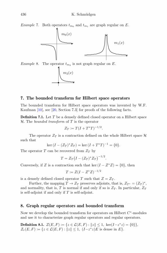
436 K. Schmudgen
Example 7. Both operators tm0and tm1
are graph regular on E.
m0(x)
m1(x)
Example 8. The operator tm2is not graph regular on E.
m2(x)
7. The bounded transform for Hilbert space operators
The bounded transform for Hilbert space operators was invented by W.F.Kaufman [10], see [20, Section 7.3] for proofs of the following facts.
Definition 7.1. Let T be a densely defined closed operator on a Hilbert spaceH. The bounded transform of T is the operator
ZT := T (I + T ∗T )−1/2.
The operator ZT is a contraction defined on the whole Hilbert space Hsuch that
ker (I − (ZT )∗ZT ) = ker (I + T ∗T )−1 = 0.The operator T can be recovered from ZT by
T = ZT(I − (ZT )∗ZT
)−1/2.
Conversely, if Z is a contraction such that ker (I − Z∗Z) = 0, then
T := Z(I − Z∗Z)−1/2
is a densely defined closed operator T such that Z = ZT .Further, the mapping T → ZT preserves adjoints, that is, ZT∗ = (ZT )∗,
and normality, that is, T is normal if and only if so is ZT . In particular, ZTis self-adjoint if and only if T is self-adjoint.
8. Graph regular operators and bounded transform
Now we develop the bounded transform for operators on Hilbert C∗-modulesand use it to characterize graph regular operators and regular operators.
Definition 8.1. Z(E,F ) := z ∈ L(E,F ) : ‖z‖ ≤ 1, ker(I−z∗z) = 0,Zr(E,F ) := z ∈ L(E,F ) : ‖z‖ ≤ 1, (I−z∗z)E is dense in E.

Unbounded operators on Hilbert C∗-modules 437
It is easily seen that Zr(E,F ) is a (in general proper) subset of Z(E,F ).For z ∈ Z(E,F ), we set
tz := z(I − z∗z)−1/2.
The operator I−z∗z belongs to the C∗-algebra L(E,E). Since z ∈ Z(E,F ),it is nonnegative and has trivial kernel, so the inverse (I − z∗z)−1/2 of itssquare root (I − z∗z)1/2 is a well-defined operator on the Hilbert C∗-moduleE with domain (I − z∗z)1/2E.
Conversely, for t ∈ Reggr(E,F ) we define
Et := D(t∗t), Ft∗ := D(tt∗), zt := t(I + t∗t)−1/2 Et .
The operator zt is called the bounded transform of t. It can be shown thatD(t∗t) is essential in E and that D(tt∗) is essential in F.
The following theorems are the main results concerning the boundedtransform.
Theorem 8.2. The map z 7→ tz is a bijection of Zr(E,F ) onto Reg(E,F ).In particular, z = tz(I + t∗ztz)
−1/2 for z ∈ Zr(E,F ).
Theorem 8.3. The map z 7→ tz is an injection of Z(E,F ) into Reggr(E,F ).If t ∈ Reggr(E,F ), then tzt : Et → Ft∗ is a regular operator, called theregular part of the graph regular operator t.
For the next theorem we assume that E = A. Then L(E,E) is themultiplier algebra M(A). One may think of A as being realized on a Hilbertspace H; then M(A) is given by (4.1). Recall from C∗-algebra theory thateach ∗-representation of A extends uniquely to a ∗-representation of M(A).Therefore, if t ∈ Reg(E), then zt ∈ M(A), so π(zt) is well-defined. Thefollowing basic result was proved in [21].
Theorem 8.4. Let E = A and t ∈ Reg(E). For each ∗-representation π ofA there is a unique densely defined closed operator π(t) on the Hilbert spaceH(π) such that Zπ(t) = π(zt), that is, the bounded transform of π(t) is equalto π(zt). Moreover,
π(t)(π((I − (zt)∗zt)
1/2a)ϕ) = π(zta)ϕ, a ∈ A, ϕ ∈ H(π). (8.1)
Theorem 8.4 says that a regular operator can be “mapped” to a denselydefined closed operator (defined by (8.1)) in each representation of A. Incontrast, graph regular operators can be “transported” to densely definedHilbert space operators only in certain representations. For instance, for thegraph regular operator tm in Example 6 the point evaluation at 0 cannot bedefined.

438 K. Schmudgen
9. Further examples
9.1. Lie algebra of the Heisenberg group
Let H be the 3-dimensional Heisenberg group, that is, H is the Lie group ofmatrices 1 a c
0 1 b0 0 1
, where a, b, c ∈ R.
The Lie algebra of H has a basis X,Y, Z with the commutation relations
[X,Y ] = Z, [X,Z] = [Y, Z] = 0.
The family of irreducible unitary representations U of H consists of a seriesUλ, λ ∈ R×, of infinite-dimensional representations acting on L2(R) and ofa series Ua, a ∈ R2, of one-dimensional representations. The correspondingactions of the Lie algebra generators are given by the formulas
λ 6= 0 : dUλ(X) = −iλx, dUλ(Y ) =d
dx, dUλ(Z) = iλ·I,
λ = 0 : dUa(X) = ia1, dUa(Y ) = ia2, dUa(Z) = 0, a = (a1, a2) ∈ R2.
The C∗-algebra C∗(H) of H is completely described in [14, Theorem 2.16].It consists of operator fields F = (F (λ);λ ∈ R) such that F (λ), λ 6= 0, is acompact operator on L2(R), F (0) ∈ C0(R2), and
limλ→0
‖F (λ)− νλ(F (0))‖ = 0, (9.1)
where νλ is a linear map of C0(R2) into L2(R). Then we have the following.
Proposition 9.1. (iZ)−1 is a graph regular self-adjoint operator on E =C∗(H).
Note that the operator (iZ)−1 is not regular, because dUa(iZ) = 0 fora ∈ R2 and hence (iZ)−1 is not densely defined.
9.2. Unbounded Toeplitz operators
For φ ∈ L∞(T) let Tφ denote the corresponding Toeplitz operator on H2(T).The C∗-algebra generated by the unilateral shift S = Tz is the Toeplitzalgebra:
T := Tφ : φ ∈ C(T)uK(H2(T)).
Let p, q ∈ C[z] be relatively prime polynomials such that q 6= 0 in D. TheToeplitz operator Tp/q is defined by
D(Tp/q) := f ∈ H2(T) : (p/q)f ∈ H2(T), Tp/qf := (p/q)f, f ∈ D(Tp/q).
Proposition 9.2. If q has a zero on T, then the operator Tp/q on E = T isgraph regular, but not regular.
For instance, the operator (S − I)−1 is graph regular, but not regular.

Unbounded operators on Hilbert C∗-modules 439
9.3. A fraction algebra related to the canonical commutation relations
Let Q = x and P = −i ddx be the position and momentum operators, respec-
tively, on L2(R). Then the bounded operators
a := (Q− iI)−1 and b := (P − iI)−1. (9.2)
satisfy the commutation relations
a− a∗ = 2ia∗a = 2iaa∗, b− b∗ = 2ib∗b = 2ibb∗, (9.3)
ab− ba = −iab2a = −iba2b, ab∗ − b∗a = −ia(b∗)2a = −ib∗a2b∗. (9.4)
Let A denote the universal unital C∗-algebra with generators a and b anddefining relations (9.3) and (9.4). This algebra appeared in [19] and inde-pendently in the paper [3] of D. Buchholz and H. Grundling. In [19] it wasused as a tool for proving a noncommutative Positivstellensatz for the Weylalgebra.
The set of irreducible representations of A consists of a single infinite-dimensional representation on L2(R) given by the operators (9.2) and of seriesof one-dimensional representations given by the points of the circles
K1 := (a, 0) ∈ C2 : a− a = 2i|a|2, K2 := (0, b) ∈ C2 : b− b = 2i|b|2.Suggested by equation (9.2) we define operators q and p on E = A by
q := iI + a−1, D(q) := aA, and p := i + b−1, D(p) := bA.
Proposition 9.3. q and p are graph regular self-adjoint operators on E := A.
Looking at the one-dimensional representations it follows that the do-mains aA and bA are not dense in A. Hence q and p are not regular.
The C∗-algebra A contains the compacts K(L2(R)) as an essential idealand the restrictions of q and p are regular operators for K(L2(R)). In fact,these restrictions are the regular parts of q and p.
10. Why graph regular operators?
In complex function theory isolated singularities of holomorphic functionssuch as
f1(z) = z−1, f2(z) = exp(z−1)
are studied by the behavior of the functions in a neighborhood of the singu-larity.
Many C∗-algebras consist of operator fields z → a(z) ∈ Az, where Az isa C∗-algebra on a Hilbert space Hz. For such a C∗-algebra let us consider anoperator field z → t(z) such that t(z), z 6= z0, is a regular operator for the C∗-algebra Az. In general, t(z0) is not defined. Often graph regular operators areof this form; for instance, the multiplication operator tm0 with m0(x) = x−1
for A = C0(R) in Example 7, the operator (iZ)−1 for the C∗-algebra C∗(H)in Example 9.1, and the operator (S−I)−1 for the Toeplitz algebra in Exam-ple 9.2. Because of these examples, it is hoped that graph regular operatorsbecome useful tools for the study of operator fields with isolated singularities.

440 K. Schmudgen
References
[1] S. Baaj, Multiplicateurs non bornes, Thesis, Universite Pierre et Marie Curie,Paris, 1981.
[2] S. Baaj and P. Julg, Theorie bivariante de Kasparov et operateurs non bornesdans les C*-modules hilbertiens, C.R. Acad. Sci. Paris Ser. I Math. 296 (1983),875–878.
[3] D. Buchholz and H. Grundling, The resolvent algebras: a new approach tocanonical quantum systems, J. Funct. Anal. 254 (2010), 2725–2779.
[4] M. Frank and K. Sharifi, Generalized inverses and polar decomposition ofunbounded regular operators on Hilbert C∗-modules, J. Operator Theory 64(2010), 377–386.
[5] M. Frank, Hilbert C∗-modules and related subjects – a guided referenceoverview, HTWK Leipzig, 89 pages, last update 31.3.2017.
[6] R. Gebhardt and K. Schmudgen, Unbounded operators on Hilbert C∗-modules,Intern. J. Math. 26 (2015), 197–255.
[7] R. Gebhardt, Unbounded operators on Hilbert C∗-modules: graph regular oper-ators, Thesis, University of Leipzig, 2016.
[8] M. Hilsum, Fonctorialite en K-theorie bivariante pour les varietes lipschitzi-ennes, K-Theory 3 (1987), 401–440.
[9] J. Kaad and M. Lesch, A local global principle for regular operators in HilbertC∗-modules, J. Funct. Anal. 262 (2012), 4540–4569.
[10] W.F. Kaufman, Representing a closed operator as a quotient of continuousoperators, Proc. Amer. Math. Soc. 72 (1978), 531–534.
[11] D. Kucerovsky, The KK-product of unbounded modules, K-Theory 11 (1997),17–34.
[12] D. Kucerovsky, Functional calculus and representations of C0(X) on a Hilbertmodule, Quart. J. Math. 53 (2002), 467–477.
[13] E.C. Lance, Hilbert C∗-modules, Cambridge Univ. Press, 1995.
[14] J. Ludwig and L. Turowska, The C∗-algebras of the Heisenberg group and ofthread-like Lie groups, Math. Z. 268 (2011), 897–930.
[15] R. Meyer, Representations by unbounded operators, C∗-hulls, local-global prin-ciple, and induction, Preprint, University of Gottingen, 2016.
[16] A. Pal, Regular operators on Hilbert C∗-modules, J. Operator Theory 42(1999), 331–350.
[17] F. Pierrot, Operateurs reguliers dans les C∗-modules et structure des C∗-algebres de groups de Lie semisimples complexes simplement connexes, J. LieTheory 16 (2006), 651–689.
[18] K. Schmudgen, Unbounded operators affiliated with C∗-algebras, Preprint,University of Leipzig, 2005.
[19] K. Schmudgen, Algebras of fractions and strict Positivstellensatze for ∗-alge-bras, J. reine angew. Math. 647 (2010), 57–88.
[20] K. Schmudgen, Unbounded self-adjoint operators on Hilbert space, GraduateTexts, Springer-Verlag, Dordrecht, 2012.
[21] S.L. Woronowicz, Unbounded elements affiliated with C∗-algebras and non-compact quantum groups, Commun. Math. Phys. 136 (1991), 399–432.

Unbounded operators on Hilbert C∗-modules 441
[22] S.L. Woronowicz and K. Napiorkowski, Operator theory in the C∗-algebraframework, Reports Math. Phys. 31 (1992), 353–371.
[23] S.L. Woronowicz and S. Zakrewski, Quantum ax + b group, Rev. Math. Phys.14 (2002), 797–828.
Konrad SchmudgenUniversitat LeipzigMathematisches InstitutAugustusplatz 10/1104109 LeipzigGermanye-mail: [email protected]
A characterization of positive normalfunctionals on the full operator algebra
Zoltan Sebestyen, Zsigmond Tarcsay and Tamas Titkos
Abstract. Using the recent theory of Krein–von Neumann extensions forpositive functionals we present several simple criteria to decide whethera given positive functional on the full operator algebra B(H) is normal.We also characterize those functionals defined on the left ideal of finiterank operators that have a normal extension.
Mathematics Subject Classification (2010). Primary 46K10, Secondary46A22.
Keywords. Krein–von Neumann extension, normal functionals, trace.
The aim of this short note is to present a theoretical application of thegeneralized Krein–von Neumann extension, namely to offer a characterizationof positive normal functionals on the full operator algebra. To begin with, letus fix our notations. Given a complex Hilbert space H, denote by B(H) thefull operator algebra, i.e., the C∗-algebra of continuous linear operators on H.The symbols BF (H), B1(H), B2(H) are referring to the ideals of continuousfinite rank operators, trace class operators, and Hilbert–Schmidt operators,respectively. Recall that B2(H) is a complete Hilbert algebra with respect tothe inner product
(X |Y )2 = Tr(Y ∗X) =∑e∈E
(Xe |Y e), X, Y ∈ B2(H).
Here Tr refers to the the trace functional and E is an arbitrary orthonormalbasis in H. Recall also that B1(H) is a Banach ∗-algebra under the norm‖X‖1 := Tr(|X|), and that BF (H) is dense in both B1(H) and B2(H), withrespect to the norms ‖ · ‖1 and ‖ · ‖2, respectively. It is also known thatX ∈ B1(H) holds if and only if X is the product of two elements of B2(H).For the proofs and further basic properties of Hilbert–Schmidt and trace classoperators we refer the reader to [1, 2, 6].
Zsigmond Tarcsay was supported by the Hungarian Ministry of Human Capacities, NTP-NFTO-17. Corresponding author: Tamas Titkos.
© Springer International Publishing AG, part of Springer Nature 2018
Theory: Advances and Applications 268, https://doi.org/10.1007/978-3-319-75996-8_24
443A. Böttcher et al. (eds.), The Diversity and Beauty of Applied Operator Theory, Operator
444 Z. Sebestyen, Zs. Tarcsay and T. Titkos
Before dealing with normal functionals, we recall the notion of a rep-resentable functional. Let B be a complex ∗-algebra. A linear functionalg : B → C is called representable if there exist a complex Hilbert space Hg
with inner product (· | ·)g, a ∗-representation πg : B → B(Hg), and a cyclicvector ζg ∈ Hg such that
g(b) = (πg(b)ζg | ζg)gholds for all b ∈ B. We refer the reader to [5] for more details about repre-sentable functionals.
Let A be a von Neumann algebra, that is, a strongly closed ∗-subalgebraof B(H) containing the identity. A continuous linear functional f : A → Cis called normal if it is continuous in the ultraweak topology, that is, if fbelongs to the predual of A . It is well known that the predual of B(H) isB1(H), hence every normal functional can be represented by a trace classoperator. We will use this property as the definition.
Definition. A linear functional f : B(H)→ C is called a normal functional ifthere exists a trace class operator F such that
f(X) := Tr(XF ) = Tr(FX), X ∈ B(H).
We remark that such a functional is always continuous due to the inequality
|Tr(XF )| ≤ ‖F‖1 · ‖X‖.Our main tool is a canonical extension theorem for linear functionals
which is analogous to the well-known operator extension theorem named afterthe pioneers of the 20th century operator theory, M.G. Krein [3] and J. vonNeumann [4]. For the details see Section 5 in [8], especially Theorem 5.6 andthe subsequent comments.
Next, we recall the cited theorem.
A Krein–von Neumann type extension. Let I be a left ideal of a complexBanach ∗-algebra A , and consider a linear functional ϕ : I → C. Thefollowing statements are equivalent:
(a) There is a representable positive functional ϕ• : A → C extending ϕwhich is minimal in the sense that
ϕ•(x∗x) ≤ ϕ(x∗x) holds for all x ∈ A
whenever ϕ : A → C is a representable extension of ϕ.(b) There is a constant C ≥ 0 such that |ϕ(a)|2 ≤ C ·ϕ(a∗a) for all a ∈ I .
We remark that the construction used in the proof of the above theoremis closely related to the one developed in [7] for Hilbert space operators. Themain advantage of that construction is that we can compute the values ofthe smallest extension ϕ• on positive elements, namely
ϕ•(x∗x) = sup|ϕ(x∗a)|2
∣∣ a ∈ I , ϕ(a∗a) ≤ 1
for all x ∈ A . (∗)The minimal extension ϕ• is called the Krein–von Neumann extension of ϕ.

A characterization of positive normal functionals on B(H) 445
The characterization we are going to prove is as follows.
Main Theorem. For a given positive functional f : B(H) → C the followingstatements are equivalent:
(i) f is normal.(ii) There exists a normal positive functional g such that f ≤ g.
(iii) f ≤ g holds for every positive functional g that agrees with f on BF (H).(iv) For every X ∈ B(H) we have
f(X∗X) = sup|f(X∗A)|2 |A ∈ BF (H), f(A∗A) ≤ 1. (∗∗)
(v) f(I) ≤ sup|f(A)|2 |A ∈ BF (H), f(A∗A) ≤ 1.
Proof. The proof is divided into three claims, which might be interesting ontheir own right. Before doing that, we make some observations. For a giventrace class operator S let us denote by fS the normal functional defined by
fS(X) := Tr(XS), X ∈ B(H).
The map S 7→ fS is order preserving between positive trace class operatorsand normal positive functionals. Indeed, if S ≥ 0, then
fS(A∗A) = Tr(A∗AS) = ‖AS1/2‖22 ≥ 0.
Conversely, if fS is a positive functional and P〈h〉 denotes the orthogonalprojection onto the subspace spanned by h ∈ H, we obtain S ≥ 0 by
(Sh |h) = Tr(P〈h〉S) = fS(P ∗〈h〉P〈h〉) ≥ 0 for all h ∈ H.
Our first two claims will prove that (i) and (iv) are equivalent.
Claim 1. Let f be a normal positive functional and set ϕ := f |BF (H). Thenf is the smallest positive extension of ϕ, i.e., ϕ• = f .
Proof of Claim 1. Since f ≥ 0 is normal, there is a positive S ∈ B1(H) suchthat f = fS . By assumption ϕ has a positive extension (namely f itself isone), thus there exists also the Krein–von Neumann extension denoted byϕ•. As fS −ϕ• is a positive functional due to the minimality of ϕ•, its normis attained at the identity I. Therefore it is enough to show that
ϕ•(I) ≥ fS(I) = Tr(S).
We know from (∗) that
ϕ•(X∗X) = sup|ϕ(X∗A)|2 |A ∈ BF (H), ϕ(A∗A) ≤ 1for any X ∈ B(H). Choosing A = Tr(S)−1/2P for a projection P with finiterank, we see that ϕ(A∗A) = Tr(S)−1 Tr(PS) ≤ 1, whence
ϕ•(I) ≥ |ϕ(A)|2 =Tr(PS)2
Tr(S).
Taking the supremum over P on the right-hand side we obtain ϕ•(I) ≥ Tr(S),which proves the claim.
Claim 2. The smallest positive extension of ϕ, i.e. (f |BF (H))• is normal.

446 Z. Sebestyen, Zs. Tarcsay and T. Titkos
Proof of Claim 2. First observe that the restriction of f to B2(H) defines acontinuous linear functional on B2(H) with respect to the norm ‖ ·‖2. Due tothe Riesz representation theorem, there exists a unique representing operatorS ∈ B2(H) such that
f(A) = (A |S)2 = Tr(S∗A) for all A ∈ B2(H). (∗ ∗ ∗)
We are going to show that S ∈ B1(H). Indeed, let E be an orthonormal basisin H and let F be any non-empty finite subset of E . Denoting by PF theorthogonal projection onto the subspace spanned by F we get∑
e∈F(Se | e) = (PF |S)2 = f(PF ) ≤ f(I).
Taking the supremum over F we obtain that S is in the trace class. ByClaim 1, the smallest positive extension ϕ• of ϕ equals fS , which is normal.This proves Claim 2.
Now, we are going to prove (ii)⇒(i).
Claim 3. If there exists a normal positive functional g such that f ≤ g holds,then f is normal as well.
Proof of Claim 3. Let g be a normal positive functional dominating f , andlet T be a trace class operator such that g = fT . According to Claim 2 it isenough to prove that f = ϕ•. Since h := f − ϕ• is positive, this will followby showing that h(I) = 0. We see from (∗ ∗ ∗) that h(A) = 0 for every finiterank operator A. Consequently, as h ≤ f ≤ fT , it follows that
h(I) = h(I − P ) ≤ fT (I − P ) = Tr(T )− Tr(TP )
for every finite rank projection P . Taking the infimum over P we obtainh(I) = 0, and therefore Claim 3 is established.
To complete the proof we mention all the missing trivial implications.Taking g := f , we see that (i) implies (ii). As (∗∗) means that ϕ• = f , theequivalence of (iii) and (iv) follows from the minimality of the Krein–vonNeumann extension. Replacing X with I in (∗∗) we obtain that (iv) implies(v). Conversely, (v) implies (iv) as ϕ• ≤ f and f −ϕ• attains its norm at theidentity I.
Finally, we remark that the above proof contains a characterization ofthe property of having a normal extension for a functional defined on BF (H).
Corollary. Let ϕ : BF (H) → C be a linear functional. The following state-ments are equivalent to the existence of a normal positive extension:
(a) There is a C ≥ 0 such that |ϕ(A)|2 ≤ C · ϕ(A∗A) for all A ∈ BF (H).(b) There is a positive functional f such that f |BF (H) = ϕ.(c) There is a positive operator F ∈ B1(H) such that ϕ(A) = Tr(FA) for
all A ∈ BF (H).

A characterization of positive normal functionals on B(H) 447
References
[1] I.C. Gohberg and M.G. Krein, Introduction to the Theory of Linear Non-selfadjoint Operators, Translations of Mathematical Monographs 18, Amer.Math. Soc., Providence, RI, 1969.
[2] R.V. Kadison and J.R. Ringrose, Fundamentals of the theory of operator alge-bras I., Academic Press, New York, 1983.
[3] M.G. Krein, The theory of self-adjoint extensions of semi-bounded Hermitiantransformations and its applications, I–II, Mat. Sbornik 20 (1947), 431–495,Mat. Sbornik 21 (1947), 365–404 (Russian).
[4] J. von Neumann, Allgemeine Eigenwerttheorie Hermitescher Funktionalopera-toren, Math. Ann. 102 (1930), 49–131.
[5] T.W. Palmer, Banach Algebras and the General Theory of ∗-Algebras II, Cam-bridge University Press, Cambridge, 2001.
[6] R. Schatten, Norm Ideals of Completely Continuous Operators, Ergebnisse derMathematik und ihrer Grenzgebiete 27, Springer, Berlin, 1960.
[7] Z. Sebestyen, Operator extensions on Hilbert space, Acta Sci. Math. (Szeged)57 (1993), 233–248.
[8] Z. Sebestyen, Zs. Szucs, and Zs. Tarcsay, Extensions of positive operators andfunctionals, Linear Algebra Appl. 472 (2015), 54–80.
Zoltan Sebestyen and Zsigmond TarcsayDepartment of Applied AnalysisEotvos Lorand UniversityPazmany Peter setany 1/cBudapest H-1117Hungarye-mail: [email protected]
Tamas TitkosAlfred Renyi Institute of MathematicsHungarian Academy of SciencesRealtanoda utca 13–15Budapest H-1053HungaryandBBS University of Applied SciencesAlkotmany u. 9Budapest H-1054Hungarye-mail: [email protected]

The linearised Korteweg–de Vries equationon general metric graphs
Christian Seifert
Abstract. We consider the linearised Korteweg–de Vries equation, some-times called Airy equation, on general metric graphs with edge lengthsbounded away from zero. We show that properties of the induced dy-namics can be obtained by studying boundary operators in the cor-responding boundary space induced by the vertices of the graph. Inparticular, we characterise unitary dynamics and contractive dynamics.We demonstrate our results on various special graphs, including thoserecently treated in the literature.
Mathematics Subject Classification (2010). Primary 35Q53; Secondary47B25, 81Q35.
Keywords. metric graphs, linearised KdV-equation, generators of C0-semigroups.
1. Introduction
The Korteweg–de Vries equation [4, 3]
∂u
∂t=
3
2
√g
`
(σ
3
∂3u
∂x3+
2a
3
∂u
∂x+
1
2
∂u2
∂x
)models shallow water waves in channels, where u describes the elevation ofthe water w.r.t. the average water depth and g, ` , σ, and a are constants.Due to the last term on the right-hand side it becomes non-linear. Assumingonly small elevations u (i.e. u is close to zero) and/or long waves (i.e. ∂u
∂x isclose to zero), the linear approximation neglecting the non-linearity (whichis the linearisation around the stationary solution u = 0) yields an equationof the form
∂u
∂t= α
∂3u
∂x3+ β
∂u
∂x(1)
with appropriate constants α and β. In this paper we are going to study theevolution equation on general networks, i.e. metric graphs, from a functionalanalytic point of view.
© Springer International Publishing AG, part of Springer Nature 2018
Theory: Advances and Applications 268, https://doi.org/10.1007/978-3-319-75996-8_25
449A. Böttcher et al. (eds.), The Diversity and Beauty of Applied Operator Theory, Operator

450 C. Seifert
Evolution equations (or, more generally, differential operators) on metricgraphs have been intensively studied during the last two decades. However,the focus was put on Schrodinger type operators and the corresponding heatand Schrodinger evolution equations, see [1] and references therein. Recently,also KdV-type equations on star graphs have gained interest, see [2, 9, 7, 8, 5].Such star graphs give rise to model either singular interactions at one point,i.e. interface conditions, but can also be interpreted as models for junctionsof channels. The drawback of star graphs is that one only has exactly onevertex (i.e. junction), and the channels are modelled by halflines.
In this paper, we consider the linearised KdV-equation (1) on generalmetric graphs, i.e., we model a whole network, including channels of finitelength. We will describe the evolution equation in a functional analytic setup,namely in the framework of strongly continuous semigroups. Thus, we are leftto study the spacial operator describing the right-hand side of (1). The aim isto obtain a “reasonable” dynamics in an L2-setting, meaning either unitaryC0-semigroups or contractive C0-semigroups (which resembles the fact thatthe spacial derivatives appear only in odd order). In order to do that we willemploy the framework of boundary systems developed in [6].
In Section 2 we introduce the metric graph and the operator setupfor the spacial derivatives. Section 3 summarises notions from Krein spacetheory which we will need to describe the right boundary conditions at thevertices. We then focus on unitary and contractive dynamics in Section 4.In Section 5 we specialise our framework (which does not take the concretegraph structure into account) to the graph structure setting. We end thispaper by briefly listing some examples in Section 6, where we refer to thecorresponding literature, but also explaining new examples which have notbeen dealt with before.
2. Notation and model
Let Γ = (V,E, a, b, γl, γr) be a metric graph, i.e., V is the set of vertices of Γ,and E is the set of edges of Γ. Moreover, a, b : E → [−∞,∞] are such thatae < be for all e ∈ E, and each edge e ∈ E is identified with the interval(ae, be) ⊆ R. Let El := e ∈ E; ae > −∞ and Er := e ∈ E; be < ∞ bethe sets of edges with finite starting and termination point, respectively, andlet γl : El → V , γr : Er → V assign to each e ∈ El or e ∈ Er the startingvertex γl(e) and the termination vertex γr(e), respectively. Note that we donot assume V or E to be finite or countable.
We assume to have a positive lower bound on the edge lengths, that is,
` := infe∈E
(be − ae) > 0. (2)
For k ∈ 0, 1, 2 we define the mappings trkl :⊕
e∈EWk+12 (ae, be) → `2(El)
and trkr :⊕
e∈EWk+12 (ae, be)→ `2(Er) by
(trkl u)(e) := u(k)e (ae+) (e ∈ El), (trkr u)(e) := u(k)
e (be−) (e ∈ Er).

The linearised Korteweg–de Vries equation on metric graphs 451
Furthermore, define the trace maps Trl :⊕
e∈EW32 (ae, be) → `2(El)
3 and
Trr :⊕
e∈EW32 (ae, be)→ `2(Er)
3 by
Trl u := (tr0l u, tr
1l u, tr
2l u), Trr u := (tr0
r u, tr1r u, tr
2r u).
Let HΓ :=⊕
e∈E L2(ae, be) be the Hilbert space we are going to con-sider. Let (αe)e∈E in (0,∞) be bounded and bounded away from zero, let(be)e∈E be bounded, and also abbreviate αl := (αe)e∈El
, αr := (αe)e∈Er ,βl := (βe)e∈El
, and βr := (βe)e∈Er. By the same symbol we will denote the
corresponding multiplication operators in `2(El) and `2(Er), respectively.
Remark 2.1. One could choose αe ∈ R \ 0. However, for edges e ∈ E withαe < 0 we can just change the orientation of the edge (by setting αe := −αe,βe := −βe, and u := u(−·)). Thus, w.l.o.g. we may (and will) assume αe > 0for all e ∈ E. Moreover, by scaling the variables appropriately, it would sufficeto deal with the case βe = 0 for all e ∈ E. In order to do this uniformly for alledges, one only needs boundedness of (βe) and
(1αe
). However, we will keep
the βe’s possibly non-zero.
Definition. We define the minimal operator A0 in HΓ by
D(A0) :=⊕e∈E
C∞c (ae, be),
(A0u)e := αe∂3ue + βe∂ue (e ∈ E, u ∈ D(A0)).
And we define the maximal operator A in HΓ by
D(A) :=⊕e∈E
W 32 (ae, be),
(Au)e := αe∂3ue + βe∂ue (e ∈ E, u ∈ D(A)).
Applying integration by parts we obtain the following lemma.
Lemma 2.2. We have −A∗0 = A.
Define F : G(A)→ `2(Er)3 ⊕ `2(El)
3 by
F (u, Au) := (Trr u,Trl u).
Lemma 2.3. F is linear and surjective.
Proof. Linearity of F is clear. In order to show that F is surjective first notethat there exists ϕ ∈ C∞c [0, `), where ` is as in (2), such that ϕ equals 1in a neighbourhood of 0 and ϕ(x) = 0 for x > `
2 . For (t0, t1, t2) ∈ C3 let
u(x) := (t0 + t1x + 12 t
2x2)ϕ(x) for x ∈ (0, `). Then there exists a c > 0
(independent of (t0, t1, t2)) such that
‖u‖2L2(0,`) + ‖u′‖2L2(0,`) + ‖u′′′‖2L2(0,`) 6 c∥∥(t0, t1, t2)
∥∥2
2.
Since (αe) and (βe) are bounded, as a consequence, F is surjective.

452 C. Seifert
For u, v ∈ D(A) we obtain by integration by parts
(u∣∣∣ Av)+
(Au∣∣∣ v) =−
−βr 0 −αr
0 αr 0−αr 0 0
Trr u
∣∣∣∣∣∣Trr v
+
−βl 0 −αl
0 αl 0−αl 0 0
Trl u
∣∣∣∣∣∣Trl v
. (3)
Let us define Ω: G(A)×G(A)→ C by
Ω((u, Au), (v, Av)
):=
((0 11 0
)(u
Au
) ∣∣∣∣ ( v
Av
)),
and ω :(`2(Er)
3 ⊕ `2(El)3)×(`2(Er)
3 ⊕ `2(El)3)→ C by
ω((x, y), (u, v)
):=
((−Br 0
0 Bl
)(xy
) ∣∣∣∣ (uv))
,
abbreviating
Bl :=
−βl 0 −αl
0 αl 0−αl 0 0
, Br :=
−βr 0 −αr
0 αr 0−αr 0 0
.
By rewriting (3) we obtain
Ω((u, Au), (v, Av)
)= ω
(F (u, Au), F (v, Av)
)(4)
for all (u, Au), (v, Av) ∈ G(A).Let L be a densely defined linear operator from `2(Er)
3 to `2(El)3. Then
A0 ⊆ AL ⊆ A = −A∗0 is defined by
D(AL) :=u ∈ D(A); Trr u ∈ D(L), LTrr u = Trl u
,
that is, G(AL) = F−1(G(L)).
3. Operators in Krein spaces
Remark 3.1. Let K be a vector space and 〈· | ·〉 an (indefinite) inner producton K such that (K, 〈· | ·〉) is a Krein space. Then (· | ·) := 〈J · | ·〉, where Jis the fundamental symmetry of K, defines an inner product on K such that(K, (· | ·)) is a Hilbert space. Notions such as closedness or continuity are thendefined by the underlying Hilbert space structure.
Definition. Let K−, K+ be Krein spaces and ω :(K−⊕K+
)×(K−⊕K+
)→ C
be sesquilinear.(a) Let X ⊆ K− ⊕K+ be a subspace. Then X is called ω-self-orthogonal if
X = X⊥ω , where
X⊥ω :=
(x, y) ∈ K− ⊕K+; ω((x, y), (u, v)) = 0 for all (u, v) ∈ X.

The linearised Korteweg–de Vries equation on metric graphs 453
(b) Let L be a densely defined linear operator from K− to K+. Then its(K−,K+)-adjoint L] is defined by
D(L]) :=y ∈ K+; ∃z ∈ K− : 〈Lx | y〉+ = 〈x | z〉− for all x ∈ D(L)
,
L]y := z.
Clearly, L] is then a linear operator from K+ to K−.(c) Let L be a linear operator from K− to K+. Then L is called a (K−,K+)-
contraction if
〈Lx |Lx〉+ 6 〈x |x〉− for all x ∈ D(L).
(d) Let L be a linear operator from K− to K+. Then L is called (K−,K+)-unitary if D(L) and R(L) are dense, L is injective, and finally L] = L−1.
If K−, K+ are Hilbert spaces, then obviously (K−,K+)-adjoint (-contraction,-unitary) operators are the usual objects of Hilbert space operator theory.
Remark 3.2. Let K± be Krein spaces. Let L be (K−,K+)-unitary. Then
〈Lx |Ly〉+ = 〈x | y〉− for all x, y ∈ D(L). (5)
However, L may not be bounded.
Note that `2(El)3 equipped with 〈· | ·〉l : `2(El)
3 × `2(El)3 → C,⟨
(x0, x1, x2)∣∣ (y0, y1, y2)
⟩l:=(Bl(x
0, x1, x2)∣∣ (y0, y1, y2)
)`2(El)3
yields a Krein space Kl := (`2(El)3, 〈· | ·〉l). Analogously, `2(Er)
3 equippedwith 〈· | ·〉r : `2(Er)
3 × `2(Er)3 → C,⟨
(x0, x1, x2)∣∣ (y0, y1, y2)
⟩r
:=(Br(x
0, x1, x2)∣∣ (y0, y1, y2)
)`2(Er)3
yields a Krein space Kr := (`2(Er)3, 〈· | ·〉r).
4. Dynamics
Let us study different types of dynamics for the equation.
Generating unitary groups
We are now interested in generators of unitary groups. By Stone’s theoremthis is equivalent to looking for skew-self-adjoint realisations of AL.
Theorem 4.1. Let L be a linear operator from `2(Er)3 to `2(El)
3 such thatD(L) and R(L) are dense. Then AL is skew-self-adjoint if and only if L is(Kr,Kl)-unitary.
Proof. By [6, Corollary 2.3 and Example 2.7 (b)], see also [5, Theorem 3.7],we have to show that G(AL) is Ω-self-orthogonal if and only if G(L) is ω-self-orthogonal. But this is an easy consequence of (4) and the definition ofthe operator AL.
454 C. Seifert
Generating contraction semigroups
Instead of unitary dynamics let us characterise generators of contraction semi-groups.
Theorem 4.2. Let L be a densely defined closed linear operator from `2(Er)3
to `2(El)3. Then AL is the generator of a semigroup of contractions if and
only if L is(Kr,Kl
)-contractive and L] is
(Kl,Kr
)-contractive.
Proof. Note that since L is closed, also AL is closed. First, it is easy to seethat A∗L is given by
D(A∗L) =u ∈ D(A∗0); Trl u ∈ D(L]), L] Trl u = Trr u
,
A∗Lu = A∗0u.
For u ∈ D(AL) we compute
2 Re (ALu |u) = Ω((u,ALu), (u,ALu)
)= ω
(F (u,ALu), F (u,ALu)
)= ω
((Trr u, LTrr u), (Trr u, LTrr u)
)= −〈Trr u |Trr u〉r + 〈LTrr u |LTrr u〉l .
Hence, AL is dissipative, i.e. Re (ALu |u) 6 0 for all u ∈ D(AL), if andonly if L is
(Kr,Kl
)-contractive. Similarly, A∗L is dissipative if and only if L]
is(Kl,Kr
)-contractive. Thus, the Lumer–Phillips theorem in Hilbert spaces
yields the assertion.
5. Local boundary conditions
So far, we did not take into account the graph structure. Now, we ask forboundary conditions at each vertex v ∈ V separately. For v ∈ V let
El,v := e ∈ El; γl(e) = v, Er,v := e ∈ Er; γr(e) = v.
Then `2(El,v) equipped with 〈· | ·〉l,v := 〈· | ·〉l |`2(El,v)3×`2(El,v)3 and `2(Er,v)
equipped with 〈· | ·〉r,v := 〈· | ·〉r |`2(Er,v)3×`2(Er,v)3 yield Krein spaces Kl,v andKr,v, respectively, such that
〈· | ·〉l =∑v∈V〈· | ·〉l,v
and analogously for 〈· | ·〉r.For v ∈ V let Lv be a densely defined linear operator from `2(Er,v)
3 to
`2(El,v)3, and define A0 ⊆ A(Lv)v∈V
⊆ A = −A∗0 by
D(AL) :=u ∈ D(A); ∀ v ∈ V : (Trr u)|Er,v
∈ D(Lv),
Lv((Trr u)|Er,v
)= Trl u|El,v
.
For the case of unitary dynamics we obtain the following corollary.

The linearised Korteweg–de Vries equation on metric graphs 455
Corollary 5.1. For v ∈ V let Lv be a densely defined linear operator from`2(Er,v)
3 to `2(El,v)3. Then A(Lv)v∈V
is the generator of a unitary group ifand only if Lv is (Kr,v,Kl,v)-unitary for all v ∈ V .
Proof. We show that (Lv) is (Kr,Kl)-unitary if and only if Lv is (Kr,v,Kl,v)-unitary for all v ∈ V . Then the result follows from Theorem 4.1. Notethat (Lv) acts as a block-diagonal operator with block Lv from `2(Er,v)
3
to `2(El,v)3 for all v ∈ V . Hence, clearly, (Lv) is densely defined with dense
range if and only if Lv is densely defined with dense range for all v ∈ V .Moreover, (Lv) is injective if and only if Lv is injective for all v ∈ V . Since(Lv)
] = (L]v) we also obtain (Lv)] = (Lv)
−1 if and only if L]v = L−1v for all
v ∈ V .
Analogously, in the case of contractive dynamics we have the following result.
Corollary 5.2. For v ∈ V let Lv be a densely defined linear operator from`2(Er,v)
3 to `2(El,v)3 such that L := (Lv)v∈V is closed. Then A(Lv)v∈V
isthe generator of a semigroup of contractions if and only if Lv is (Kr,v,Kl,v)-contractive and L]v is (Kl,v,Kr,v)-contractive for all v ∈ V .
Proof. We show that (Lv) is (Kr,Kl)-contractive and (Lv)] is (Kl,Kr)-con-
tractive if and only if Lv is (Kr,v,Kl,v)-contractive and L]v is (Kl,v,Kr,v)-con-tractive for all v ∈ V . Then the result follows from Theorem 4.2. Again, (Lv)acts as a block-diagonal operator with block Lv from `2(Er,v)
3 to `2(El,v)3 for
all v ∈ V . Hence, (Lv) is (Kr,Kl)-contractive if and only if Lv is (Kr,v,Kl,v)-contractive for all v ∈ V . Since (Lv)
] = (L]v), we have that (Lv)] is (Kl,Kr)-
contractive if and only if L]v is (Kl,v,Kr,v)-contractive for all v ∈ V .
6. Examples
In this section we will specialise to particular examples of graphs. For thosespecial cases already treated in the literature we just explain the setup. Weask the reader to go to the corresponding references for more details in thesecases.
Two semi-infinite edges
Let us consider two semi-infinite edges attached to one vertex v, and let thetwo edges correspond to the intervals (−∞, 0] and [0,∞):
v
If the coefficients (αe) and (βe) are constant, we can interpret the equation asthe linearised KdV-equation on the real line with a generalised point interac-tion at 0 (which corresponds to the vertex v). This situation was consideredin [2].

456 C. Seifert
As a particular example, if αe = 1 and βe = 0 for all e, then
L :=
1 0 0√2 1 0
1√
2 1
yields a unitary dynamics, since L : Kr → Kl is (Kr,Kl)-unitary, i.e., L isbijective and
〈Lx |Ly〉l = 〈x | y〉r (x, y ∈ Kr).
An example yielding contractive (but not unitary) dynamics in the caseαe = 1 and βe = 0 for all e is given by
L :=
2 0 10 2 01 0 2
.
Star graphs
The special case of star graphs was considered in [7, 8, 9, 5]. Here, we haveone vertex v, each edge is described by a semi-infinite interval, say (−∞, 0]or [0,∞), and each edge is adjacent to v with its endpoint corresponding tothe value 0 for the interval:
v
Star graphs generalise graphs with two semi-infinite edges to more than twoedges. For those graphs, there is a necessary condition on the graph for ex-istence of unitary dynamics, namely |El| = |Er|, where |·| denotes the cardi-nality for sets.
A Loop
Let Γ be a loop, i.e., |V | = |E| = 1, and the edge corresponds to the interval[0, 1], and both endpoints of the edge are attached to the vertex v:
v

The linearised Korteweg–de Vries equation on metric graphs 457
Here, we can model generalised periodic boundary conditions. Indeed, con-sider L to be represented by the identity matrix in the usual basis. Then thisresults in periodic boundary conditions
u(k)(0+) = u(k)(1−) (k ∈ 0, 1, 2).
Moreover, L becomes Krein space unitary in this case, so the dynamics isunitary.
Graphs with more than one vertex
We will now consider graphs with more than one vertex. By the results ofSection 5 we can study the dynamics for the linearised KdV-equation on ageneral graph by studying the ‘local’ behaviour at each vertex. Since locallyaround each vertex a graph looks like a (local part of a) star graph, thisbrings us back to studying boundary couplings for star graphs.
As an example, let us consider the following graph, where the edgelengths are all equal to 1 for simplicity:
v1 v2
v3v4
v5
e1
e2
e3
e4e5
e6 e7
e8
Since |El,vk | = |Er,vk | for k ∈ 1, . . . , 5, by defining suitable boundary cou-pling operators Lvk (k ∈ 1, . . . , 5), we can obtain unitary or contractivedynamics. Let us assume that αek = 1 and βek = 0 for all k ∈ 1, . . . , 8.Then, as an example for unitary dynamics we can choose
Lv1 = Lv5 :=
1 0 0√2 1 0
1√
2 1
and
Lv2 = Lv3 = Lv4 :=
1 0 0 0 0 00 1 0 0 0 0√2 0 1 0 0 0
0 0 0 1 0 0
1 0√
2 0 1 00 0 0 0 0 1
.
Acknowledgment
The author thanks Delio Mugnolo and Diego Noja for many useful discussionson the linearised KdV-equation.

458 C. Seifert
References
[1] G. Berkolaiko and P. Kuchment, Introduction to Quantum Graphs, Mathemat-ical Surveys and Monographs 186, Amer. Math. Soc., Providemce, 2013.
[2] B. Deconinck, N.E. Sheils, and D.A. Smith, The linear KdV equation with aninterface, Comm. Math. Phys. 347 (2016), no. 2, 489–509.
[3] D. Lannes, The Water Waves Problem: Mathematical Analysis and Asymp-totics, Mathematical Surveys and Monographs 188, Amer. Math. Soc., Provi-dence, 2013.
[4] D.J. Korteweg and G. de Vries, On the change of form of long waves advancingin a rectangular canal, and on a new type of long stationary waves, The London,Edinburgh, and Dublin Phil. Mag. and Journal of Sci. 39 (1895), 422–443.
[5] D. Mugnolo, D. Noja, and C. Seifert, Airy-type evolutuion equations of stargraphs, submitted. arXiv-Preprint 1608.01461.
[6] C. Schubert, C. Seifert, J. Voigt, and M. Waurick, Boundary systems and(skew-)self-adjoint operators on infinite metric graphs. Math. Nachr. 288(2015), 1776–1785.
[7] Z.A. Sobirov, M.I. Akhmedov, and H. Uecker, Cauchy problem for the lin-earized KdV equation on general metric star graph. Nanosystems 6 (2015),198–204.
[8] Z.A. Sobirov, M.I. Akhmedov, and H. Uecker, Exact solution of the Cauchyproblem for the linearized KdV equation on metric star graph. Uzbek. Math.J. 3 (2015), 143–154.
[9] Z.A. Sobirov, M.I. Akhmedov, O.V. Karpova, and B. Jabbarova, LinearizedKdV equation on a metric graph. Nanosystems 6 (2015), 757–761.
Christian SeifertTechnische Universitat HamburgInsitut fur MathematikAm Schwarzenberg-Campus 3 (E)21073 HamburgGermanye-mail: [email protected]

Bounded multiplicative Toeplitz operatorson sequence spaces
Nicola Thorn
Abstract. In this paper, we study the linear mapping which sends thesequence x = (xn)n∈N to y = (yn)n∈N where yn =
∑∞k=1 f(n/k)xk for
f : Q+ → C. This operator is the multiplicative analogue of the classicalToeplitz operator, and as such we denote the mapping by Mf . We showthat for 1 ≤ p ≤ q ≤ ∞, if f ∈ `r(Q+), then Mf : `p → `q is boundedwhere 1
r= 1 − 1
p+ 1
q. Moreover, for the cases when p = 1 with any
q, p = q, and q = ∞ with any p, we find that the operator norm is
given by ‖Mf‖p,q = ‖f‖r,Q+ when f ≥ 0. Finding a necessary conditionand the operator norm for the remaining cases highlights an interestingconnection between the operator norm of Mf and elements in `p thathave a multiplicative structure, when considering f : N → C. We alsoprovide an argument suggesting that f ∈ `r may not be a necessarycondition for boundedness when 1 < p < q <∞.
Mathematics Subject Classification (2010). Primary 47B37; Secondary47B35, 11N99.
Keywords. Bounded multiplicative Toeplitz operators, multiplicative se-quences, sequence spaces.
1. Introduction
In this paper, we study the multiplicative Toeplitz operator, denoted by Mf ,which sends a sequence (xn)n∈N to (yn)n∈N where
yn =∞∑k=1
f(nk
)xk, (1.1)
and f is a function defined from the positive rationals, Q+, to C. We can thinkof Mf as being given by the infinite matrix Af whose entries are ai,j = f(i/j)for i, j ∈ N:
© Springer International Publishing AG, part of Springer Nature 2018
Theory: Advances and Applications 268, https://doi.org/10.1007/978-3-319-75996-8_26
459A. Böttcher et al. (eds.), The Diversity and Beauty of Applied Operator Theory, Operator

460 N. Thorn
Af =
f(1) f(1/2) f(1/3) f(1/4) · · ·f(2) f(1) f(2/3) f(1/2) · · ·f(3) f(3/2) f(1) f(3/4) · · ·f(4) f(2) f(4/3) f(1) · · ·f(5) f(5/2) f(5/3) f(5/4) · · ·
......
......
. . .
.
Characterised by matrices with constants on skewed diagonals, these map-pings are the “multiplicative” analogue of the vastly studied classical Toeplitzoperators on sequence spaces. The topic of multiplicative analogues of Toep-litz operators, discussed in [1], [2] and [3] for example, has grown in recentyears, with the study of other multiplicative constructions; for example, [4]and [5] investigate the multiplicative Hankel matrix, otherwise known as Hel-son matrices.
Toeplitz operators, Tφ, are most often studied via the function φ, whichis referred to as the symbol. In a similar manner, we shall be considering Mf
in terms of the function f and asking for which f do certain properties hold1.By taking f supported only on N, we have yn =
∑d|n f
(nd
)xd = (f ∗ x) (n),
where ∗ is the Dirichlet convolution [6]. In this case, Af becomes a lowertriangular matrix given by
Af =
f(1) 0 0 0 · · ·f(2) f(1) 0 0 · · ·f(3) 0 f(1) 0 · · ·f(4) f(2) 0 f(1) · · ·f(5) 0 0 0 · · ·
......
......
. . .
.
We shall denote the mapping induced by this matrix by Df .Interesting connections to analytic number theory and many open ques-
tions have fuelled recent research. For example, in [1] the author illustrates aconnection between these operators and the Riemann zeta function. Namely,by choosing f to be supported on N where f(n) = 1
nα (denoted by Dα), we
have that Dα : `2 → `2 is bounded iff α > 1, in which case ‖Dα‖2,2 = ζ(α).Thus when α ≤ 1, then Dα is unbounded. By restricting the range of themapping when α ∈
(12 , 1]
and considering
Yα(N) = sup‖x‖2=1
(N∑n=1
|yn|2) 1
2
,
it can be shown that Yα(N) is a lower bound for the maximal order of theRiemann zeta function. Specifically, for α ∈
(12 , 1),
Zα(T ) = maxt∈[0,T ]
|ζ(α+ it)| ≥ Yα(T 2/3(α−1/2)−ε
),
1The symbol of Mf would be given by F (t) =∑
q∈Q f(q)qit where t ∈ R.

Bounded multiplicative Toeplitz operators 461
for sufficiently large T . Moreover, an estimate for Yα(N) leads to
logZα(T ) (log T )1−α
log log T,
a known estimate for the maximal order of ζ. There have since been someimprovements upon this estimate, and new estimates for the case when α = 1
2have been found, which interestingly utilise a similar method [7], [8]. For otherliterature on the connections to the Riemann zeta function see also [9], [2].
The authors of [3] also highlight an application of analytic number the-ory to these operators, by using the properties of smooth numbers to ascertain‖Dfx‖p,p = ‖f‖1 when f is expressible in terms of completely multiplicativeand non-negative functions (see the preliminaries for the definitions).
One can also consider the matrix properties of these mappings. Forexample, [10] considers the determinants of multiplicative Toeplitz matrices.By taking an N × N truncation, denoted by Af (N), the author is able toshow that if f is multiplicative, then the determinant of Af (N) can be givenas a product over the primes up to N , of determinants of Toeplitz matrices.
In Section 2, we generalise results on the boundedness of Df containedin [1] and [3], giving a partial criterion for Mf to be bounded as a mappingfrom `p → `q. In an attempt to find a full criterion, we present a relationshipbetween the sets of multiplicative sequences and the operator norm ‖Df‖p,q inSection 3. By considering Df acting upon these subsets, we are able to givea further boundedness result which, due to this connection, indicates thatthe extension of the partial criterion may not hold. As such, we speculatewhether the result can be generalised to Mf acting on `p spaces, which isthen followed by a discussion on the existence of a possible counterexample tothis generalisation. We end the paper with a summary of the open problemsthat arise within this paper, and also some unanswered questions which areconcerned with other operator properties of multiplicative Toeplitz operatorssuch as the spectral points of Mf .
Preliminaries and notation
Sequences and arithmetic functions. We use the terms “sequences” (realor complex valued) and “functions” interchangeably, as we can write anyarithmetical function f(n) as a sequence indexed by the natural numbersf = (fn)n∈N.
Multiplicative functions. First, we say that f (not identically zero) is mul-tiplicative if f(nm) = f(n)f(m) for every n,m ∈ N such that (n,m) = 1.Secondly, we say f is completely multiplicative if this holds for all n,m ∈ N.Finally, if g(n) = cf(n) where f is multiplicative, we call g constant multi-plicative.
Euler products. If f is multiplicative such that∑n∈N |f(n)| <∞, then
∞∑n=1
f(n) =∏t∈P
∞∑k=1
f(tk),

462 N. Thorn
where P is the set of prime numbers. If f is completely multiplicative, we canwrite
∞∑n=1
f(n) =∏t∈P
1
1− f(t).
GCD and LCM. We use (n,m) and [n,m] to denote the greatest commondivisor and least common multiple of n and m in N, respectively. We let d(n)stand for the number of divisors of n, including 1 and n itself.
O-notation. We say that f is of the order of g and write f = O(g) if, forsome constant, |f(n)| ≤ C |g(n)| as n → ∞. We also write f g to meanf = O(g).
Sequence spaces. For p ∈ [1,∞], let `p denote the usual space of sequencesx = (xn)n∈N for which the norm ‖x‖p := (
∑∞n=1 |xn|
p)1/p converges or
‖x‖∞ = supn∈N |xn| exists (if p ∈ [1,∞) or p = ∞ respectively). Analo-gously, we define `p(Q+) to be the space of sequences x = (xs)s∈Q+ for which
‖x‖p,Q+ = (∑s∈Q+ |xs|p)1/p converges or ‖x‖∞,Q+ = sups∈Q+ |xs| exists. For
the case when p = 2, we also have that 〈x, y〉 =∑n∈N xnyn.
Operator norm. Given a bounded linear operator L, we use the usual nota-tion ‖L‖p,q to denote the operator norm of L : `p → `q which is given by‖L‖p,q = sup‖x‖p=1 ‖Lx‖q.
2. Partial criterion for boundedness
The following results extend theorems contained in [1] and [3].
Theorem 2.1. For 1 ≤ p ≤ q ≤ ∞, define r ∈ [1,∞] by
1
r= 1− 1
p+
1
q
where 1∞ = 0. If f ∈ `r(Q+), then Mf : `p → `q is bounded. More precisely,
we have
‖Mfx‖q ≤ ‖x‖p‖f‖r,Q+ .
Theorem 2.1 gives a partial criterion for boundedness between `p and `q;partial in the sense that f ∈ `r(Q+) is a sufficient condition. It is natural toask whether this is also a necessary condition, i.e., does Mf : `p → `q boundedimply that f ∈ `r? Moreover, can we find the operator norm, ‖Mf‖p,q? Forf positive, both of these questions can be answered by Theorem 2.2 for thecases where p = q, p = 1 with any q, and q = ∞ with any p. We refer tothese as the “edge” cases.
Theorem 2.2. Let us define r as in Theorem 2.1. For p = q, p = 1 (any q),q =∞ (any p) with f ∈ `r(Q+) positive, we have
‖Mf‖p,q = ‖f‖r,Q+ .

Bounded multiplicative Toeplitz operators 463
Proof of Theorem 2.1. Let yn be given by (1.1). The proof proceeds by con-sidering the cases separately.
• 1 ≤ p ≤ q <∞By Holder’s inequality,
|yn| ≤∞∑k=1
∣∣∣f (nk
)xk
∣∣∣ =∞∑k=1
∣∣∣f (nk
)∣∣∣r(1− 1p ) ∣∣∣f (n
k
)∣∣∣ rq |xk| pq |xk|1− pq≤
( ∞∑k=1
∣∣∣f (nk
)∣∣∣r)(1− 1p )( ∞∑
k=1
|xk|p) 1p−
1q( ∞∑k=1
∣∣∣f (nk
)∣∣∣r |xk|p)1q
≤ ‖f‖r(1−1p )
r,Q+ ‖x‖1−pq
p
( ∞∑k=1
∣∣∣f (nk
)∣∣∣r |xk|p)1q
.
Hence,
∞∑n=1
|yn|q ≤ ‖f‖rq(1− 1
p )r,Q+ ‖x‖q−pp
∞∑n=1
∞∑k=1
∣∣∣f (nk
)∣∣∣r |xk|p .Considering only the summation on the RHS above,
∞∑n=1
∞∑k=1
∣∣∣f (nk
)∣∣∣r |xk|p ≤ ∑s∈Q+
|f(s)|r∞∑k=1
|xk|p = ‖f‖rr,Q+‖x‖pp.
Therefore,
‖Mfx‖qq =
∞∑n=1
|yn|q ≤ ‖f‖qr(1− 1
p )+rr,Q+ ‖x‖q−p+pp = ‖f‖qr,Q+‖x‖qp.
• p = 1 and q =∞ (so r =∞)
By the triangle inequality,
|yn| ≤∞∑k=1
∣∣∣f (nd
)xk
∣∣∣ ≤ ‖f‖∞,Q+
∞∑k=1
|xk| ≤ ‖f‖∞,Q+‖x‖1.
Hence, ‖Mfx‖∞ ≤ ‖f‖∞,Q+‖x‖1.
• q =∞ with 1 < p <∞ (so r = pp−1 )
By Holder’s inequality, we have
|yn| ≤∞∑k=1
∣∣∣f (nk
)xk
∣∣∣ ≤ ( ∞∑k=1
∣∣∣f (nk
)∣∣∣r) 1r( ∞∑k=1
|xk|p) 1p
≤ ‖f‖r,Q+‖x‖p.
Thus, ‖Mfx‖∞ ≤ ‖f‖r,Q+‖x‖p.
• p = q =∞ (so r = 1)
We now have |yn| ≤ ‖x‖∞∑∞k=1
∣∣f (nk )∣∣ ≤ ‖x‖∞‖f‖1,Q+ , which gives thedesired inequality ‖Mfx‖∞ ≤ ‖x‖∞‖f‖1,Q+ .

464 N. Thorn
Proof of Theorem 2.2. We consider each edge case separately.
1. We first embark on the case when p = 1 with any q.
• Let q ∈ [1,∞), so that r = q.
Fix c ∈ N, and let xn = 1 if n = c and 0 otherwise. Then ‖x‖1 = 1, and so
|yn|q =
∣∣∣∣∣∞∑k=1
f(nk
)xk
∣∣∣∣∣q
=∣∣∣f (n
c
)∣∣∣q .Therefore,
‖Mfx‖qq =
∞∑n=1
|yn|q =
∞∑n=1
∣∣∣f (nc
)∣∣∣q =∑d|c
∞∑n=1
(n,c)=d
∣∣∣f (nc
)∣∣∣q
=∑d|c
∞∑m=1
(m, cd )=1
∣∣∣∣f (mdc)∣∣∣∣q by writing n = md,
=∑d|c
∞∑m=1
(m,d)=1
∣∣∣f (md
)∣∣∣q by writingc
d7→ d. (2.1)
Note that we can write
‖f‖qq,Q+ =∑s∈Q+
|f (s)|q =∞∑v=1
∞∑u=1
(u,v)=1
∣∣∣f (uv
)∣∣∣q . (2.2)
By computing the difference between (2.2) and (2.1), we shall show that‖Mfx‖q can be made arbitrarily close to ‖f‖q,Q+ . We have
∞∑v=1
∞∑u=1
(u,v)=1
∣∣∣f (uv
)∣∣∣q −∑d|c
∞∑n=1
(n,c)=d
∣∣∣f (nc
)∣∣∣q =∑u,v∈N(u,v)=1v-c
∣∣∣f (uv
)∣∣∣q .Now, choose c = (2 · 3 · 5 · · ·T )k where k ∈ N and T is prime. Then v - cimplies v > T for k large enough. Therefore, for every ε > 0, we can chooseT such that
‖f‖qq,Q+ − ‖Mfx‖qq =∑u,v∈N(u,v)=1v-c
∣∣∣f (uv
)∣∣∣q < ε.
Hence, ‖Mf‖1,q = ‖f‖q,Q+ as required.
• Let q =∞, so r = q =∞.
Fix c ∈ N. Like before, choose xn = 1 if n = c and 0 otherwise. Again‖x‖1 = 1. Now,
‖Mfx‖∞ = supn∈N|yn| = sup
n∈N
∣∣∣f (nc
)∣∣∣ .

Bounded multiplicative Toeplitz operators 465
Note that there exist u, v ∈ N with (u, v) = 1 such that ‖f‖∞,Q+−ε <∣∣f (uv )∣∣.
Simply choose n = u and c = v. Then
‖f‖∞,Q+ − ‖Mfx‖∞ < ε.
2. Now consider the edge case where p = q.
• Let 1 < p = q <∞, so r = 1.
Fix c ∈ N. Choose xn = 1/d(c)1q if n | c and 0 otherwise. Hence, we have
‖x‖qq = 1d(c)
∑d|c 1 = 1. By Holder’s inequality,
∞∑n=1
xq−1n yn ≤
( ∞∑n=1
|xn|q)1− 1
q( ∞∑n−1
yqn
) 1q
=
( ∞∑n−1
yqn
) 1q
= ‖Mfx‖q.
Consequently, it suffices to show that∑∞n=1 x
q−1n yn can be made arbitrarily
close to ‖f‖1,Q+ . We have
∞∑n=1
xq−1n yn =1
d(c)q−1q
∑n|c
yn =1
d(c)q−1q
∑n|c
∑k|c
f(nk
)xk
=1
d(c)
∑n,k|c
f(nk
).
We now follow the argument given in [2] (page 87). For s = uv ∈ Q+,
1
d(c)
∑n,k|c
f(nk
)=
1
d(c)
∑s∈Q+
f(s)∑n,k|cs=n
k
1 =1
d(c)
∑u,v∈N
f(uv
) ∑n,k|cnv=uk
1,
where we used that nk = u
v if and only if nv = uk. Since (u, v) = 1 we haveu | n and v | k, and for any contribution to the summation on the RHS, wemust have u, v | c, that is, uv | c. Assume therefore, that uv | c. By writingn = lu and k = lv for some l ∈ N, we get
1
d(c)
∑uv|c
f(uv
) ∑n,k|cnv=uk
1 =1
d(c)
∑uv|c
f(uv
) ∑lu,lv|c
1
=1
d(c)
∑uv|c
f(uv
)∑l| cuv
1 =∑uv|c
f(uv
) d (c/uv)
d(c).
Now, by choosing c appropriately, we can show that d(c/uv)d(c) can be made
close to 1 for all u, v less than some large constant. Fix T ∈ P and choose cto be
c =∏t≤Tt∈P
tαt with αt =
[log T
log t
].

466 N. Thorn
If uv | c, then uv =∏t≤T t
βt where βt ∈ [0, αt], and hence
d(c/uv)
d(c)=∏t≤T
(αt − βt + 1
αt + 1
)=∏t≤T
(1− βt
αt + 1
).
If we take uv ≤√
log T , then tβt ≤√
log T for every prime divisor t of uv.Therefore, βt ≤ log log T
2 log t and βt = 0 if t >√
log T . It follows that
d(c/uv)
d(c)=
∏t≤√log T
(1− βt
αt + 1
)≥
∏t≤√log T
(1− log log T
2 log T
)
=
(1− log log T
2 log T
)π(√log T )
,
where π(x) is the prime counting function up to x. As π(x) xlog x , we have
for sufficiently large T ,
d(c/uv)
d(c)=
(1− log log T
2 log T
)π(√log T )
≥ 1− C√log T
,
for some constant C. Therefore,∑uv|c
f(uv
) d(c/uv)
d(c)>
∑uv≤√log T
f(s)
(1− C√
log T
)−
∑uv>√log T
f(q)
≥∑s∈Q+
f(s)− C1√log T
− 2∑
uv>√log T
f(s),
as f ∈ `1(Q+). By choosing T to be arbitrarily large, for every ε > 0, we have
‖f‖1,Q+ − ‖Mfx‖q ≤ ‖f‖1,Q+ −∞∑n=1
xq−1n yn < ε.
• We now consider the case where p = q =∞, and so r = 1.
Let xn = 1 for all n ∈ N, so that ‖x‖∞ = 1. Moreover, for a fixed c ∈ N, wehave
|yc| =∞∑k=1
f( ck
)xk =
∞∑k=1
f( ck
).
Again, by applying the same methods already shown, we conclude that yccan be arbitrarily close to ‖f‖1,Q+ . Hence, ‖Mf‖∞,∞ = ‖f‖1,Q+ .
3. Finally, we consider the case when q =∞ with any p.
We have already dealt with the case when p = 1 and p =∞. So let p ∈ (1,∞),giving r = p
p−1 . Fix c ∈ N, and let
xn = f( cn
) rp
F− 1p
c , where Fc =
∞∑n=1
f( cn
)rexists as f ∈ `r(Q+).

Bounded multiplicative Toeplitz operators 467
With this choice,
‖x‖p =1
Fc
∞∑n=1
f( cn
)r=FcFc
= 1.
Now consider just the term yc,
yc = F− 1p
c
∞∑k=1
f( ck
)f( ck
) rp
= F− 1p
c
∞∑k=1
f( ck
)r,
as 1 + rp = p−1+1
p−1 = r. Therefore,
yc = F1− 1
pc = F
1rc =
( ∞∑k=1
f( ck
)r) 1r
.
We can apply the same argument as before to show that for every ε > 0, wecan choose c = (2 · 3 · 5 · · ·T )k where T is prime such that yc can be madearbitrarily close to ‖f‖r,Q+ . Hence, ‖Mf‖p,∞ = ‖f‖r,Q+ .
Remark 2.3. In [2], the author showed that if f is any, not necessarily strictlypositive, sequence in `1(Q+), then Mf : `2 → `2 is bounded and the operatornorm is given by
‖Mf‖2,2 = supt∈R
∣∣∣∣∣ ∑q∈Q+
f(q)qit
∣∣∣∣∣.By assuming f positive, the supremum of the above is attained when t = 0,and as such ‖Mf‖2,2 = ‖f‖1,Q+ as given in Theorem 2.2. The differing op-erator norm when f is not positive, is echoed in the work of [3], where anexample is given showing that ‖Df‖p,p 6= ‖f‖1. Determining ‖Mf‖p,q for anyf and general p, q remains an open question, but is not, however, the focusof this paper.
3. Connection with multiplicative sequences
Generalising Theorem 2.2 to find a necessary condition and the operatornorm for all other p and q (which we will refer to as the interior cases) ischallenging and is the focus of the proceeding discussions.
We start by taking f supported on N, i.e., Mf = Df . To understand thebehaviour of the operator norm in the interior cases, we can consider where‖Dfx‖ attains its supremum value in the edge cases. First, setting c = 1 incase 1 of the proof of Theorem 2.2 yields the supremum of ‖Dfx‖q. This givesxn = 1 if n = 1 and 0 otherwise, and as such x is completely multiplicative.Secondly, for 1 < p = q <∞ in case 2, we choose xn = 1
d(c)1/pwhenever n | c
and 0 otherwise, which is a constant multiplicative sequence. Moreover, forp = q = ∞, the completely multiplicative sequence xn = 1 (for all n ∈ N)attains the operator norm. Finally, in case 3, for f multiplicative, x is againconstant multiplicative.

468 N. Thorn
It follows, for the edge cases, that Df is “largest” when acting on asequence x ∈ `p that has multiplicative structure. Why this is the case isunclear and leads to a surprising connection between the operator norm ofDf and the set of multiplicative elements in `p, which we denote by Mp.Moreover, we shall denote the set of completely multiplicative sequences in`p by Mp
c . It is interesting to ask therefore how Df acts on these sets for1 < p < q < ∞, as from this connection, we would expect Df : `p → `q toattain its supreme value here. Thus, we shall investigate the boundedness ofDf :Mp
c → `q for 1 < p < q < ∞, with the aim of giving some insight into‖Df‖p,q, its norm.2
From Theorem 2.1, it follows that Df :Mpc → `q is bounded if f ∈ `r.
We wish to know whether this is also a necessary condition. In Theorem 3.1,we show that for f completely multiplicative, the requirement that f beMr
c is not a necessary condition for Df : Mpc → M2 to be bounded3 when
p ∈ (1, 2) and q = 2. One can speculate therefore that f ∈ `r is not anecessary condition when considering Df : `p → `2.
Theorem 3.1. Let 1 < p < 2. If f ∈ M2c, the mapping Df : Mp
c → M2 isbounded.
To highlight the difference between this criterion and that shown in the
previous section, we consider the following example. Let f(n) = 1nα for α > 1
2
and p = 32 , giving 1
r = 1 − 23 + 1
2 = 56 . Theorem 2.1 states that if α > 5
6 ,
then Df :M3/2c → `2 is bounded. In contrast, Theorem 3.1 shows that only
α > 12 is required for boundedness. For the proof of Theorem 3.1, we will
require the following lemma, which will be proved below.
Lemma 3.2. Let f, g, h, j ∈M2c. Then,
〈f ∗ g, h ∗ j〉 =〈g, j〉〈f, h〉〈f, j〉〈g, h〉
〈fg, hj〉. (3.1)
Proof of Theorem 3.1. By taking h = f and g = j = x in (3.1), we have
‖Dfx‖2 =‖f‖2‖x‖2 |〈f, x〉|
‖fx‖2≤ ‖f‖2‖x‖2 |〈f, x〉| ,
as f and x are completely multiplicative, and as such we have x1 = 1 andf(1) = 1, giving
‖fx‖2 =∞∑n=1
|f(n)xn|2 ≥ 1.
2Mpc and Mp are subsets, not subspaces of `p. For example, they are not closed under
addition. Given X,Y which are subsets of some Banach space, we say L : X → Y is
bounded iff ‖Lx‖ ≤ C‖x‖ for all x ∈ X.3The convolutions of two multiplicative sequences is also multiplicative, so we can considery ∈M2.

Bounded multiplicative Toeplitz operators 469
Now,
‖Dfx‖2‖x‖p
≤ ‖f‖2‖x‖2 |〈f, x〉|‖x‖p
= ‖f‖2∏t∈P
(1− |xt|p
) 1p(
1− |xt|2) 1
2 (1− |xtf(t)|), (3.2)
where we made use of Euler products. Therefore, it remains to show that theproduct over primes is bounded independently of xt. As 0 ≤ |xt| < 1, we cansay that
|xt|2 < |xt|p =⇒ 1
1− |xt|2<
1
1− |xt|p.
Hence, the product of (3.2) is at most
∏t∈P
(1− |xt|p
) 1p(
1− |xt|p) 1
2 (1− |xtf(t)|)=∏t∈P
(1− |xt|p
) 2−p2p
(1− |xtf(t)|).
By taking logarithms, we arrive at the equality
log
∏t∈P
(1− |xt|p
) 2−p2p
(1− |xtf(t)|)
=∑t∈P
(log
1
1− |xtf(t)|− 2− p
2plog
1
1− |xt|p).
Note in general for a > 0, we have a ≤ log(
11−a)
= a+O(a2). Hence,
∑t∈P
log
(1
1− |xt|p)≥∑t∈P|xt|p ,
and moreover, ∑t∈P
log
(1
1− |xtf(t)|
)=∑t∈P|xtf(t)|+O(1),
where the O(1) term is independent of the sequence xt. Therefore, we obtain∑t∈P
(log
1
1− |xtf(t)|− 2− p
2plog
1
1− |xt|p)
<∑t∈P
(|xtf(t)| − 2− p
2p|xt|p
)+O(1).
Now, we consider the case when the terms of the above series are positive. Inother words, with β = 1
p−1 ,
|xtf(t)| ≥ 2− p2p|xt|p ⇐⇒
(2p
2− p|f(t)|
)β≥ |xt| .

470 N. Thorn
Hence, by only summing over the t which yield positive terms, we have∑t∈P
(|xtf(t)| − 2− p
2p|xt|p
)<
∑t s.t
|xt|≤( 2p2−p |f(t)|)
β
(|xtf(t)| − 2− p
2p|xt|p
)
≤∑t s.t
|xt|≤( 2p2−p |f(t)|)
β
|xtf(t)| ≤(
2p
2− p
)β∑t∈P|f(t)|β |f(t)| .
As β + 1 = pp−1 > 2, we see that∑
t∈P|f(t)|β+1 ≤
∑t∈P|f(t)|2 <∞,
since f ∈ M2c . Hence, the product in (3.2) is bounded, which implies that
the mapping Df :Mpc →M2 is bounded.
Proof of Lemma 3.2. We start by computing the LHS of (3.1):
〈f ∗ g, h ∗ j〉 =∑n≥1
(f ∗ g)(n)(h ∗ j)(n) =∑n≥1
∑c,d|n
f(c)g(nc
)h(d)j
(nd
)=∑c,d≥1
∑n≥1c,d|n
f(c)g(nc
)h(d)j
(nd
)=∑c,d≥1
∑n≥1[c,d]|n
f(c)g(nc
)h(d)j
(nd
),
since c, d|n⇔ [c, d]|n. Now, as [c, d]|n⇔ n = [c, d]m, the above is given by
∑c,d≥1
∑m≥1
f(c)g
(m[c, d]
c
)h(d)j
(m[c, d]
d
)
=∑m≥1
g(m)j(m)∑c,d≥1
f(c)g
([c, d]
c
)h(d)j
([c, d]
d
)
= 〈g, j〉∑c,d≥1
f(c)g
(d
(c, d)
)h(d)j
(c
(c, d)
)as [c, d](c, d) = cd,
= 〈g, j〉∑k≥1
∑c,d≥1(c,d)=k
f(c)g
(d
(c, d)
)h(d)j
(c
(c, d)
).
If (c, d) = k, then c = c′k, d = d′k where (c′, d′) = 1. Therefore,
〈f ∗ g, h ∗ j〉 = 〈g, j〉∑k≥1
∑c′,d′≥1(c′,d′)=1
f(c′k)g(d′)h(d′k)j(c′),

Bounded multiplicative Toeplitz operators 471
which is equal to
〈g, j〉∑k≥1
f(k)h(k)∑
c′,d′≥1(c′,d′)=1
f(c′)g(d′)h(d′)j(c′)
= 〈g, j〉〈f, h〉∑
c′,d′≥1(c′,d′)=1
f(c′)g(d′)h(d′)j(c′). (3.3)
We now compute the RHS of (3.1). We have
〈f, j〉〈g, h〉 =∑c,d≥1
f(c)j(c)g(d)h(d) =∑k≥1
∑c,d≥1(c,d)=k
f(c)j(c)g(d)h(d)
=∑k≥1
∑c′,d′≥1(c′,d′)=1
f(c′k)j(c′k)g(d′k)h(d′k)
=∑k≥1
f(k)j(k)g(k)h(k)∑
c′,d′≥1(c′,d′)=1
f(c′)j(c′)g(d′)h(d′)
= 〈fg, hj〉∑
c′,d′≥1(c′,d′)=1
f(c′)j(c′)g(d′)h(d′). (3.4)
Hence, by comparing (3.3) with (3.4) we obtain (3.1).
Naturally one can ask if Theorem 3.1 generalises to `p. In other words:is f ∈ `2 a sufficient condition for Df : `p → `2 to be bounded for every p in(1, 2)? Furthermore, Theorem 3.1 raises some interesting points of specula-tion regarding this question. It would perhaps be surprising if Theorem 3.1could not be generalised to Mf on `p as we know that in the edge cases,the operator norm is “largest” when acting on multiplicative sequences. Whythis would not also be true for the interior cases is unclear. In contrast, weknow from Theorem 2.2 that when p = 2, for boundedness, f ∈ `1 is needed.If a generalisation is possible, there would be a jump in the required value ofr. That is, by considering p = 2 − ε for any ε > 0, then f ∈ `2 is all that isrequired. Why the jump between f ∈ `1 to f ∈ `2 would occur is also unclear.Finding a generalisation of Theorem 3.1 has not been possible, and leads toan investigation of a possible counterexample to the question raised above.
A possible counterexample
We wish to know, given f ∈ `2, does there exist x ∈ `p, for p ∈ (1, 2), suchthat Dfx 6∈ `2? For simplicity, we choose f(n) = 1
nα with α > 12 .
Proposition 3.3. Let p ∈ (1, 2), q = 2, and α > 12 . If (xn) ∈ `p is a sequence
such that xn 1/d(n)1
2−p , then Dαx ∈ `2.
472 N. Thorn
Proof. By the Cauchy–Schwarz inequality, we have
y2n =
∑d|n
xn/d
dα
2
≤∑d|n
1∑d|n
x2n/d
d2α= d(n)
∑d|n
x2n/d
d2α.
So,
‖Dαx‖22 ≤∞∑n=1
d(n)∑d|n
x2n/d
d2α=∞∑d=1
∞∑m=1
d(md)x2md2α
by writing dm = n,
≤∞∑d=1
d(d)
d2α
∞∑m=1
d(m)x2m,
as d(mn) ≤ d(m)d(n). As α > 12 , the first series on the RHS is convergent
(and given by ζ(2α)2). Hence,
‖Dαx‖22 ∞∑m=1
d(m)x2m.
This is convergent if x2md(m) xpm (as x ∈ `p). By rearranging, this is
equivalent to xm 1/d(m)1
2−p as required.
From Proposition 3.3, we can conclude that any counterexample, say
x = (xn), must satisfy xn > 1/d(n)1
2−p for infinitely many n ∈ N. As suchwe define
S =n ∈ N : xn > 1/d(n)
12−p,
and we may assume that the support of x is contained within the set S, i.e.,xn = 0 if n /∈ S. However, some care must be taken in choosing S (if anexample is possible), as ∑
n∈S
1
d(n)p
2−p≤∑n∈S
xpn <∞ (3.5)
must be satisfied due to x ∈ `p. First, S must be a “sparse” set; considerthe function which counts number of n ∈ S below a c given, S(c) =
∑n≤cn∈S
1.Then
S(c) =∑n≤cn∈S
xpnxpn cε
∑n≤cn∈S
xpn cε for all ε > 0,
as 1/xpn ≤ d(n)p
2−p nε ≤ cε for all ε > 0. For example, choosing S = Nfails. Secondly, S must contain n with large numbers of divisors, otherwise1/d(n)
p2−p 6→ 0 as n → ∞, and so (3.5) will not be satisfied (S can not be
a subset of P, for example). However, the following example indicates thedifficulty of choosing S to yield Dα unbounded: define S =
2k : k ∈ N
.

Bounded multiplicative Toeplitz operators 473
We see that (3.5) is satisfied because
∑n∈S
1
d(n)p
2−p=
∞∑k=1
1
(k + 1)p
2−p<∞ as
p
2− p> 1 for p ∈ (1, 2).
Now,
yn =∑2k|n
2kα
nαxd.
Write n = 2lm where m is odd. Then
(y2lm)2
=
(l∑
k=0
x2k
(2l−km)α
)2
=1
m2α
(l∑
k=0
x2k
2(l−k)α
)2
=1
m2α
(l∑
k=0
x2l−k
2kα
)2
by writing k 7→ l − k,
=1
m2α
(l∑
k=0
x2l−k
2k(α−δ)1
2kδ
)2
≤ 1
m2α
l∑k=0
( x2l−k
2k(α−δ)
)2 l∑k=0
1
22kδ
1
m2α
l∑k=0
( x2l−k
2k(α−δ)
)2.
We now sum over all l and m,
∞∑l=1
∑m∈Nm odd
(y2lm)2
∞∑l=1
∑m∈Nm odd
1
m2α
l∑k=0
( x2l−k
2k(α−δ)
)2
≤ ζ(2α)
∞∑l=0
l∑k=0
( x2l−k
2k(α−δ)
)2
∞∑k=0
∞∑l=0
( x2l
2k(α−δ)
)2=∞∑k=0
1
22k(α−δ)
∞∑l=0
x22l ,
which is finite as x ∈ `p. The following Proposition suggests some furtherstructure of S.
Proposition 3.4. Let α > 12 and β = p
(2−p)(2α−1) . Let y = γ+µ where γ = (γn)
and µ = (µn) are given by
γn =∑d|nnd∈S
d≥d(n)β
xn/d
dαand µn =
∑d|nnd∈S
d<d(n)β
xn/d
dα.
Then γ ∈ `2.

474 N. Thorn
Proof. By the Cauchy–Schwarz inequality,
γ2n =
( ∑d|nnd∈S
d≥d(n)β
xn/d
dα
)2
=
( ∑d|nd∈S
d≤ n
d(n)β
xd
(d
n
)α)2
≤∑d|nd∈S
d≤ n
d(n)β
x2d∑d|nd∈S
d≤ n
d(n)β
(d
n
)2α
∑d|nd∈S
d≤ n
d(n)β
(d
n
)2α
,
as x ∈ `2. Therefore,∞∑n=1
γ2n ∞∑n=1
∑d|nd∈S
d≤ n
d(n)β
(d
n
)2α
≤∑d∈S
∑m≥1
d(dm)β<m
1
m2α
≤∑d∈S
∑d(d)β<m
1
m2α∑d∈S
1
d(d)β(2α−1),
as, for s > 1, ∑n>m
1
ns m1−s
(see [6], page 55). By assumption, we have
∑n∈S
1
d(n)β(2α−1)=∑n∈S
1
d(n)p
2−p≤∑n∈S
xpn <∞,
as required.
From Proposition 3.4, we can see that any counterexample must yieldµ 6∈ `2. This suggests that S must contain n ∈ N such that n has a largenumber of small divisors so that d < d(n)β is satisfied often and in turnensuring that many divisors contribute to the summation. The investigationof finding a suitable support set S has not yet yielded µ 6∈ `2, and this giveslittle indication of a successful counterexample. The lack of existence of eithera generalisation of Theorem 3.1 or a counterexample demonstrates perhapsthe challenging nature of this problem and leaves further open questionsregarding the boundedness of multiplicative Toeplitz operators.
Open questions
We conclude this paper by summarising the open problems that have risenfrom our discussion:
• Is f ∈ `r a necessary condition for Df : `p → `q to be bounded for anyp and q?• Can we generalise Theorem 3.1 from multiplicative subsets to the map-
ping Df : `p → `2? Or can we find a counterexample to this?
Bounded multiplicative Toeplitz operators 475
Finally, we give some further open questions regarding multiplicative Toeplitzoperators which we have not discussed in this paper:
• What is the operator norm when f can take negative values? Does itmimic that given in [2]?• Can we compute the spectrum of Mf? Does Mf have any eigenvalues
and, if so, what are they?• For which f is Mf Fredholm, and can we describe the essential spectrum
of Mf?
References
[1] T.W. Hilberdink, An arithmetical mapping and applications to Ω-results forthe Riemann zeta function, Acta Arithmetica 139 (2009), 341–367.
[2] T.W. Hilberdink, Multiplicative Toeplitz matrices and the Riemann zeta func-tion, in: Four Faces of Number Theory, EMS Series of Lectures in Mathematics,European Mathematical Society (EMS), Zurich, 2015, 77–121.
[3] P.K. Codeca and M. Nair, Smooth numbers and the norms of arithmeticDirichlet convolutions, Journal of Mathematical Analysis and Applications 347(2008), 400–406.
[4] O.F. Brevig, K.-M. Perfekt, K. Seip, A.G. Siskakis, and D. Vukotic, The mul-tiplicative Hilbert matrix, Advances in Mathematics 302 (2016), 410–432.
[5] K.-M. Perfekt and A. Pushnitski, On Helson matrices: moment problems, non-negativity, boundedness, and finite rank, arXiv:1611.03772v2 [math.FA], toappear in Proceedings of the London Mathematical Society.
[6] T.M. Apostol, Introduction to Analytic Number Theory, Springer, New York,Heidelberg, 1976.
[7] C. Aistleitner, Lower bounds for the maximum of the Riemann zeta functionalong vertical lines, Mathematische Annalen 365 (2016), 473–496.
[8] A. Bondarenko and K. Seip, Large greatest common divisor sums and extremevalues of the Riemann zeta function, Duke Mathematical Journal 166 (2017),1685–1701.
[9] T.W. Hilberdink, Quasi-norm of an arithmetical convolution operator and theorder of the Riemann Zeta function, Functiones et Approximatio 49 (2013),201–220.
[10] T.W. Hilberdink, Determinants of multiplicative Toeplitz matrices, Acta Arith-metica 125 (2006), 265–284.
Nicola ThornDepartment of MathematicsUniversity of ReadingWhiteknightsPO Box 22,Reading RG66AXUKe-mail: [email protected]

On higher index differential-algebraicequations in infinite dimensions
Sascha Trostorff and Marcus Waurick
Abstract. We consider initial value problems for differential-algebraicequations in a possibly infinite-dimensional Hilbert space. Assuming agrowth condition for the associated operator pencil, we prove existenceand uniqueness of solutions for arbitrary initial values in a distributionalsense. Moreover, we construct a nested sequence of subspaces for initialvalues in order to obtain classical solutions.
Mathematics Subject Classification (2010). Primary: 34A09, Secondary:34A12, 34A30, 34G10.
Keywords. Differential-algebraic equations, higher index, infinite-dimen-sional state space, consistent initial values, distributional solutions.
1. Introduction and main results
In this short note, we consider two solution concepts of differential-algebraicequations (DAEs) in infinite dimensions. For this, let E and A be boundedlinear operators in some possibly infinite-dimensional Hilbert space H.
We consider the implicit initial value problemEu′(t) +Au(t) = 0, t > 0,
u(0+) = u0(∗)
for some given u0 ∈ H. In order to talk about a well-defined problem in (∗),we assume that the pair (E,A) is regular, that is,
∃ν ∈ R : CRe>ν ⊆ ρ(E,A),
∃C ≥ 0, k ∈ N ∀s ∈ CRe>ν : ‖ (sE +A)−1 ‖ ≤ C|s|k,
where
ρ(E,A) := s ∈ C ; (sE +A)−1 ∈ L(H).We note that these two conditions are our replacements for regularity in
finite dimensions. Indeed, for H finite-dimensional, (E,A) is called regular,
© Springer International Publishing AG, part of Springer Nature 2018
Theory: Advances and Applications 268, https://doi.org/10.1007/978-3-319-75996-8_27
477A. Böttcher et al. (eds.), The Diversity and Beauty of Applied Operator Theory, Operator

478 S. Trostorff and M. Waurick
if det(sE + A) 6= 0 for some s ∈ C. Thus, s 7→ det(sE + A) is a polynomialof degree at most dimH, which is not identically zero. The growth conditionis a consequence of the Weierstrass or Jordan normal form theorem validfor finite spatial dimensions, see e.g. [1, 2, 4]. The smallest possible k ∈ Noccurring in the resolvent estimate is called the index of (E,A):
ind(E,A) := mink ∈ N ; ∃C ≥ 0∀s ∈ CRe>ν : ‖ (sE +A)
−1 ‖ ≤ C|s|k.
We shall also define a sequence of (initial value) spaces associated with (E,A):
IV0 := H and IVk+1 := x ∈ H;Ax ∈ E[IVk] (k ∈ N).
A first observation is the following.
Proposition 1.1. Let k = ind(E,A) and assume that E[IVk] ⊆ H is closed.Then IVk+1 = IVk+2.
Since the sequence of spaces (IVk)k is decreasing (see Lemma 3.1),Proposition 1.1 leads to the following question.
Problem 1.2. Assume that E[IVj ] ⊆ H is closed for each j ∈ N. Do we thenhave
mink ∈ N; IVk+1 = IVk+2 = ind(E,A)?
With the spaces (IVk)k at hand, we can present the main theorem ofthis article.
Theorem 1.3. Assume that E[IVind(E,A)] ⊆ H is closed, u0 ∈ IVind(E,A)+1.Then there exists a unique continuously differentiable function u : R>0 → Hwith u(0+) = u0 such that
Eu′(t) +Au(t) = 0 (t > 0).
With Proposition 1.1 and Theorem 1.3, it is possible to derive the fol-lowing consequence.
Corollary 1.4. Assume that E[IVj ] ⊆ H is closed for each j ∈ N, u0 ∈ H.Then there exists a continuously differentiable function u : R>0 → H withu(0+) = u0 and
Eu′(t) +Au(t) = 0 (t > 0),
if, and only if, u0 ∈ IVind(E,A)+1.
Corollary 1.4 suggests that the answer to Problem 1.2 is in the affirma-tive for H being finite-dimensional.
Also in our main result, there is room for improvement: In applica-tions, it is easier to show that R(E) ⊆ H is closed as the IV-spaces are notstraightforward to compute. Thus, we ask whether the latter theorem can beimproved in the following way.
Problem 1.5. Does R(E) ⊆ H closed imply that E[IVind(E,A)] ⊆ H is closedor even the closedness of E[IVj ] ⊆ H for all j ∈ N?
On higher index differential-algebraic equations in infinite dimensions 479
We shall briefly comment on the organization of this article. In the nextsection, we introduce the time-derivative operator in a suitably weightedvector-valued L2-space. This has been used intensively in the framework ofso-called ‘evolutionary equations’, see [6]. With this notion, it is possible toobtain a distributional solution of (∗) such that the differential algebraic equa-tion holds in an integrated sense, where the number of integrations neededcorresponds to the index of the DAE. We conclude this article with the proofsof Proposition 1.1, Theorem 1.3, and Corollary 1.4. We emphasize that we donot employ any Weierstrass or Jordan normal theory in the proofs of our mainresults. We address the case of unbounded A to future research. The case ofindex 0 is discussed in [8], where also exponential stability and dichotomiesare studied.
2. The time derivative and weak solutions of DAEs
Throughout this section, we assume that H is a Hilbert space and that E,A ∈L(H) with (E,A) regular. We start out with the definition of the space of(equivalence classes of) vector-valued L2 functions: Let ν ∈ R. Then we set
L2,ν(R;H) :=
f : R→ H ; f measurable,
∫R
|f(t)|2H exp(−2νt) dt <∞
,
see also [6, 3, 5]. Note that L2,0(R;H) = L2(R;H). We define H1ν (R;H) to be
the (H-valued) Sobolev space of L2,ν(R;H)-functions with weak derivativerepresentable as L2,ν(R;H)-function. With this, we can define the derivativeoperator
∂0,ν : H1ν (R;H) ⊆ L2,ν(R;H)→ L2,ν(R;H), φ 7→ φ′.
In the next theorem we recall some properties of the operator just defined.For this, the Fourier–Laplace transformation Lν : L2,ν(R;H) → L2(R;H) isintroduced as being the unitary extension of
Lνφ(t) :=1√2π
∫Rφ(s)e−(it+ν)sds (φ ∈ Cc(R;H), t ∈ R),
where Cc(R;H) denotes the space of compactly supported, continuous H-valued functions defined on R. Moreover, let
m: f ∈ L2(R;H); (t 7→ tf(t)) ∈ L2(R;H) ⊆ L2(R;H)→ L2(R;H),
f 7→ (t 7→ tf(t))
be the multiplication by the argument operator with maximal domain.
Theorem 2.1 ([3, Corollary 2.5]). Let ν ∈ R. Then
∂0,ν = L∗ν(i m + ν)Lν .
Remark 2.2. A direct consequence of Theorem 2.1 is the continuous invert-ibility of ∂0,ν if ν 6= 0.

480 S. Trostorff and M. Waurick
Corollary 2.3. Let ν > 0 be such that ρ(E,A) ⊇ CRe>ν and also such that
‖ (sE +A)−1 ‖ ≤ C|s|ind(E,A) for some C ≥ 0 and all s ∈ CRe>ν . Then
∂−k0,ν (∂0,νE +A)−1 ∈ L(L2,ν(R;H)),
where k = ind(E,A). Moreover, ∂−k0,ν (∂0,νE +A)−1
is causal, i.e., for each
f ∈ L2,ν(R;H) with spt f ⊆ R≥a for some a ∈ R it follows that
spt ∂−k0,ν (∂0,νE +A)−1f ⊆ R≥a.
Proof. By Theorem 2.1 and the unitarity of Lν , we obtain that the first claimis equivalent to
(i m + ν)−k (
(i m + ν)E +A)−1 ∈ L(L2(R;H)),
which, in turn, would be implied by the fact that the function
t 7→ (it+ ν)−k (
(it+ ν)E +A)−1
belongs to the space L∞(R;L(H)). This is, however, true by regularity of
(E,A). We now show the causality. As the operator ∂−k0,ν (∂0,νE +A)−1
com-mutes with translation in time, it suffices to prove the claim for a = 0. So letf ∈ L2,ν(R;H) with spt f ⊆ R≥0. By a Paley–Wiener type result (see e.g. [7,19.2 Theorem]), the latter is equivalent to(
CRe>ν 3 z 7→ (LRe zf) (Im z))∈ H2(CRe>ν ;H),
where H2(CRe>ν ;H) denotes the Hardy space of H-valued functions on thehalf-plane CRe>ν . As(
LRe z∂−k0,ν (∂0,νE +A)
−1f)(Im z) = z−k (zE +A)
−1(LRe zf) (Im z)
for each z ∈ CRe>ν , we infer that also(CRe>ν 3 z 7→
(LRe z∂
−k0,ν (∂0,νE +A)
−1f)(Im z)
)∈ H2(CRe>ν ;H),
due to the boundedness and analyticity of(CRe>ν 3 z 7→ z−k (zE +A)
−1 ∈ L(H)).
This proves the claim.
Corollary 2.3 states a particular boundedness property for the solutionoperator associated with (∗). This can be made more precise by introducinga scale of extrapolation spaces associated with ∂0,ν .
Definition 2.4. Let k ∈ N, ν > 0. Then we define Hkν (R;H) := D(∂k0,ν)
endowed with the scalar product 〈φ, ψ〉k := 〈∂k0,νφ, ∂k0,νψ〉0. Quite similarly,
we define H−kν (R;H) as the completion of L2,ν(R;H) with respect to the
inner product 〈φ, ψ〉−k := 〈∂−k0,νφ, ∂−k0,νψ〉0.
We observe that the spaces (Hkν (R;H))k∈Z are nested in the sense that
jk→` : Hkν (R;H) → H`
ν(R;H), x 7→ x, whenever k ≥ `.

On higher index differential-algebraic equations in infinite dimensions 481
Remark 2.5. The operator ∂`0,ν can be considered as a densely defined isome-
try from Hkν (R;H) to Hk−`
ν (R;H) with dense range for all k ∈ Z. The closureof this densely defined isometry will be given the same name. In this way, wecan state the boundedness property of the solution operator in Corollary 2.3equivalently as follows:
(∂0,νE +A)−1 ∈ L
(L2,ν(R;H), H−kν (R;H)
).
More generally, as (∂0,νE +A)−1
and ∂−10,ν commute, we obtain
(∂0,νE +A)−1 ∈ L
(Hjν(R;H), Hj−k
ν (R;H))
for each j ∈ Z.
Note that by the Sobolev embedding theorem (see e.g. [3, Lemma 5.2])the δ-distribution of point evaluation at 0 is an element of H−1ν (R;H); in factit is the derivative of χR≥0
∈ L2,ν(R;H) = H0ν (R;H). With these prepara-
tions at hand, we consider the following implementation of the initial valueproblem stated in (∗): Let u0 ∈ H. Find u ∈ H−kν (R;H) such that
(∂0,νE +A)u = δ · Eu0. (2.1)
Theorem 2.6. Let (E,A) be regular. Then for all u0 ∈ H there exists a uniqueu ∈ H−kν (R;H) such that (2.1) holds. Moreover, we have
u = χR≥0u0 − (∂0,νE +A)
−1χR≥0
Au0
and
spt ∂−k0,νu ⊆ R≥0.
Proof. Note that the unique solution is given by
u = (∂0,νE +A)−1δ · Eu0 ∈ H−k−1ν (R;H).
Hence,
u− χR≥0u0 = (∂0,νE +A)
−1 (δ · Eu0 − (∂0,νE +A)χR≥0
u0)
= − (∂0,νE +A)−1χR≥0
Au0,
which shows the desired formula. Since χR≥0u0 ∈ L2,ν(R;H) → H−kν (R;H)
and (∂0,νE +A)−1χR≥0
Au0 ∈ H−kν (R;H) by Corollary 2.3 we obtain the
asserted regularity for u. The support statement follows from the causalitystatement in Corollary 2.3.
In the concluding section, we will discuss the spaces IVk in connectionto (E,A) and will prove the main results of this paper mentioned in theintroduction.

482 S. Trostorff and M. Waurick
3. Proofs of the main results and initial value spaces
Again, we assume that H is a Hilbert space, and that E,A ∈ L(H) with(E,A) regular.
At first, we turn to the proof of Proposition 1.1. For this, we note someelementary consequences of the definition of IVk and of regularity.
Lemma 3.1. (a) For all k ∈ N, we have IVk ⊇ IVk+1.
(b) Let s ∈ C ∩ ρ(E,A). Then
E(sE +A)−1A = A(sE +A)−1E.
(c) Let k ∈ N, x ∈ IVk. Then for all s ∈ C ∩ ρ(E,A) we have
(sE +A)−1Ex ∈ IVk+1.
(d) Let s ∈ C ∩ ρ(E,A) \ 0. Then
(sE +A)−1E =1
s− 1
s(sE +A)−1A.
(e) Let k ∈ N, x ∈ IVk. Then for all s ∈ C ∩ ρ(E,A) \ 0 we have
(sE +A)−1Ex =1
sx+
k∑`=1
1
s`+1x` +
1
sk+1(sE +A)−1Aw.
for some w ∈ H, x1, . . . , xk ∈ H.
Proof. The proof of (a) is an induction argument. The claim is trivial fork = 0. For the inductive step, we see that the assertion follows using theinduction hypothesis by
IVk+1 = A−1[E[IVk]] ⊇ A−1[E[IVk+1]] = IVk+2.
Next, we prove (b). We compute
E(sE +A)−1A = E(sE +A)−1(sE +A− sE)
= E − E(sE +A)−1sE
= E − (sE +A−A) (sE +A)−1E
= A(sE +A)−1E.
We prove (c) by induction on k. For k = 0, we let x ∈ IV0 = H and put
y := (sE +A)−1Ex. Then, by (b), we get that
Ay = A (sE +A)−1Ex = E (sE +A)
−1Ax ∈ R(E) = E[IV0].
Hence, y ∈ IV1. For the inductive step, we assume that the assertion holdsfor some k ∈ N. Let x ∈ IVk+1. We need to show that y := (sE +A)
−1Ex
is in IVk+2. For this, note that there exists a w ∈ IVk such that Ax = Ew.

On higher index differential-algebraic equations in infinite dimensions 483
In particular, by the induction hypothesis, we have (sE +A)−1Ew ∈ IVk+1.
Then we compute, using (b) again,
Ay = A (sE +A)−1Ex
= E (sE +A)−1Ax
= E (sE +A)−1Ew ∈ E[IVk+1].
Hence, y ∈ IVk+2 and (c) is proved.For (d), it suffices to observe
(sE +A)−1E =1
s(sE +A)−1sE
=1
s(sE +A)−1(sE +A−A)
=1
s− 1
s(sE +A)−1A.
In order to prove part (e), we proceed by induction on k ∈ N. The case k = 0has been dealt with in part (d) by choosing w = −x. For the inductive step,we let x ∈ IVk+1. By definition of IVk+1, we find y ∈ IVk such that Ax = Ey.By the induction hypothesis, we find w ∈ H and x1, . . . , xk ∈ H such that
(sE +A)−1Ey =1
sy +
k∑`=1
1
s`+1x` +
1
sk+1(sE +A)−1Aw.
With this we compute using (d)
(sE +A)−1Ex =1
sx− 1
s(sE +A)−1Ax
=1
sx− 1
s(sE +A)−1Ey
=1
sx− 1
s
(1
sy +
k∑`=1
1
s`+1x` +
1
sk+1(sE +A)−1Aw
)
=1
sx+
k+1∑`=1
1
s`+1x` +
1
sk+2(sE +A)−1Aw,
with x1 = −y, x` = −x`−1 for ` ≥ 2 and w = −w.
With Lemma 3.1 (a), we obtain the following reformulation of Proposi-tion 1.1.
Proposition 3.2. Assume that E[IVind(E,A)] ⊆ H is closed. Then
IVind(E,A)+1 ⊆ IVind(E,A)+2.
Proof. Note that the closedness of E[IVind(E,A)] implies the same for thespace IVind(E,A)+1 since A is continuous. We set k := ind(E,A). Now letx ∈ IVk+1. Then we need to find y ∈ IVk+1 with Ax = Ey. By definitionthere exists an x0 ∈ IVk with the property Ax = Ex0. For n ∈ N largeenough we define yn := n (nE +A)
−1Ex0. Since x0 ∈ IVk, we deduce with

484 S. Trostorff and M. Waurick
the help of Lemma 3.1 (c) that yn ∈ IVk+1. Moreover, by Lemma 3.1 (e),(yn)n is bounded. Choosing a suitable subsequence, for which we use thesame name, we may assume that (yn)n is weakly convergent to some y ∈ H.The closedness of IVk+1 implies y ∈ IVk+1. Then, using Lemma 3.1 (e), wefind w ∈ H and x1, . . . , xk+1 ∈ H such that
(nE +A)−1Ex0 =
k∑`=0
1
n`+1x` +
1
nk+1(nE +A)−1Aw.
Hence, we obtain
Ey = w-limn→∞
Eyn
= w-limn→∞
E (nE +A)−1nEx0
= w-limn→∞
nE (nE +A)−1Ax
= w-limn→∞
(nE +A−A) (nE +A)−1Ax
= Ax− w-limn→∞
A (nE +A)−1Ex0
= Ax−Aw-limn→∞
(k∑`=0
1
n`+1x` +
1
nk+1(nE +A)−1Aw
)= Ax,
which yields the assertion.
With an idea similar to the one in the proof of Proposition 1.1 (Propo-sition 3.2), it is possible to show that E : IVk+1 → E[IVk] is an isomorphismif k = ind(E,A) and E[IVk] ⊆ H is closed. We will need this result also inthe proof of our main theorem.
Theorem 3.3. Let (E,A) be regular and assume that E[IVk] ⊆ H is closed,k = ind(E,A). Then
E : IVk+1 → E[IVk], x 7→ Ex
is a Banach space isomorphism.
Proof. Note that by the closed graph theorem, it suffices to show that theoperator under consideration is one-to-one and onto. So, for proving injectiv-ity, we let x ∈ IVk+1 such that Ex = 0. By definition, there exist y ∈ IVk
such that Ey = Ax = Ax+nEx for all n ∈ N. Hence, for n ∈ N large enough,we have x = (nE +A)
−1Ey. Thus, from y ∈ IVk we deduce with the help
of Lemma 3.1 (e) that there exist w, x1, . . . .xk ∈ H such that
x = (nE +A)−1Ey =
1
ny +
k∑`=1
1
n`+1x` +
1
nk+1(nE +A)−1Aw → 0
as n→∞, which shows that x = 0.Next, let y ∈ E[IVk]. For n ∈ N large enough, we put
wn := (nE +A)−1ny.

On higher index differential-algebraic equations in infinite dimensions 485
By Lemma 3.1 (c), we obtain that wn ∈ IVk+1. Let x ∈ IVk with Ex = y.Then, using Lemma 3.1 (e), we find w, x1, . . . , xk ∈ H such that
wn = (nE +A)−1ny
= (nE +A)−1nEx
= x+k∑`=1
1
n`x` +
1
nk(nE +A)−1Aw,
proving the boundedness of (wn)n. Without loss of generality, we may assumethat (wn)n weakly converges to z ∈ IVk+1 = A−1[E[IVk]]. Hence,
Ez = w-limn→∞
Ewn
= w-limn→∞
1
n(nE +A)wn
= w-limn→∞
1
n(nE +A) (nE +A)−1ny
= y.
Next, we come to the proof of our main result Theorem 1.3, which werestate here for convenience.
Theorem 3.4. Assume that E[IVind(E,A)] ⊆ H is closed, u0 ∈ IVind(E,A)+1.Then (2.1) has a unique continuously differentiable solution u : R>0 → H,satisfying u(0+) = u0 and
Eu′(t) +Au(t) = 0 (t > 0). (3.1)
Moreover, the solution coincides with the solution given in Theorem 2.6.
Proof. Let u0 ∈ IVind(E,A)+1. We denote E : IVk+1 → E[IVk], x 7→ Ex,where k = ind(E,A). By Theorem 3.3, we have that E is an isomorphism.
For t > 0, we define
u(t) := exp(−tE−1A
)u0.
Then u(0+) = u0. Moreover, u(t) is well-defined. Indeed, if u0 ∈ IVk+1, then
Au0 ∈ E[IVk]. Hence, E−1Au0 ∈ IVk+1 is well-defined. Since E[IVk] is closed
and A is continuous, we infer that IVk+1 is a Hilbert space. Thus, we deducethat u : R>0 → IVk+1 is continuously differentiable. In particular, we obtain
IVk+1 3 u′(t) = −E−1Au(t).
If we apply E to both sides of the equality, we obtain (3.1). If u : R>0 → His a continuously differentiable solution of (3.1) with u(0+) = u0, we inferthat u ∈ L2,ν(R;H) for some ν > 0 large enough, where we extend u to R<0
by zero. Hence,
∂0,νEu+Au = E∂0,νu+Au = Eu′ +Au+ δ · Eu(0+) = δ · Eu0,where we have used that u is differentiable on R<0 ∪ R>0 and jumps at 0.Thus, u is the solution given in Theorem 2.6, from which we also derive theuniqueness.

486 S. Trostorff and M. Waurick
We conclude with a comment on the proof of Corollary 1.4.
Remark 3.5. We note that the condition u0 ∈ IVind(E,A)+1 arises naturallyif we assume that IVj is closed for each j ∈ N. Indeed, if u : R>0 → H is acontinuously differentiable solution of (3.1), we infer that
Au(t) = −Eu′(t) (t > 0),
and thus u(t) ∈ IV1 for t > 0. Since IV1 is closed, we derive u′(t) ∈ IV1 and
hence, inductively u(t) ∈⋂j∈N IVj for each t > 0. Since
⋂j∈N IVj is equal to
IVind(E,A)+1 by Proposition 3.2, we get
u0 = u(0+) ∈ IVind(E,A)+1.
References
[1] T. Berger, A. Ilchmann, and S. Trenn, The quasi-Weierstraß form for regularmatrix pencils, Linear Algebra Appl. 436 (2012), no. 10, 4052–4069.
[2] L. Dai, Singular Control Systems, Springer, New York, 1989.
[3] A. Kalauch, R. Picard, S. Siegmund, S. Trostorff, and M. Waurick, A Hilbertspace perspective on ordinary differential equations with memory term, Journalof Dynamics and Differential Equations 26 (2014), no. 2, 369–399.
[4] P. Kunkel and V. Mehrmann, Differential-Algebraic Equations. Analysis andNumerical Solution, European Mathematical Society Publishing House, Zurich,2006.
[5] R. Picard, Hilbert Space Approach to Some Classical Transforms, Pitman Re-search Notes in Mathematics Series 196, Longman Scientific & Technical, Har-low; copublished in the U.S. with John Wiley & Sons, Inc., New York, 1989.
[6] R. Picard, A structural observation for linear material laws in classical mathe-matical physics. Mathematical Methods in the Applied Sciences 32 (2009), 1768–1803.
[7] W. Rudin, Real and Complex Analysis, Mathematics series, McGraw-Hill, 1987.
[8] S. Trostorff and M. Waurick, On differential-algebraic equations in infinite di-mensions, Technical report, TU Dresden, University of Strathclyde, 2017.
Sascha TrostorffInsitut fur AnalysisFakultat MathematikTechnische Universitat DresdenGermanye-mail: [email protected]
Marcus WaurickDepartment of Mathematics and StatisticsUniversity of StrathclydeGlasgowUnited Kingdome-mail: [email protected]

Characterizations of centrality by localconvexity of certain functions onC∗-algebras
Daniel Virosztek
Abstract. We provide a quite large function class which is useful to dis-tinguish central and non-central elements of a C∗-algebra in the follow-ing sense: for each element f of this function class, a self-adjoint elementa of a C∗-algebra is central if and only if the function f is locally convexat a.
Mathematics Subject Classification (2010). Primary: 46L05.
Keywords. C∗-algebra, centrality, convexity.
1. Introduction
1.1. Motivation
Connections between algebraic properties of C∗-algebras and some essentialproperties of functions defined on them by functional calculus have beeninvestigated widely.
The first results concern the relation between the commutativity of aC∗-algebra and the monotonicity (with respect to the order induced by posi-tivity) of certain functions defined on the positive cone of it. It was shown byOgasawara in 1955 that a C∗-algebra is commutative if and only if the mapa 7→ a2 is monotonic increasing on its positive cone [9]. Later on, Pedersenprovided a generalization of Ogasawara’s result for any power function a 7→ ap
with p > 1 [10]. More recently, Wu proved that the exponential function isalso useful to distinguish commutative and non-commutative C∗-algebras inthe above sense [13], and in 2003, Ji and Tomiyama described the class of allfunctions that can be used to decide whether a C∗-algebra is commutativeor not [5].
The author was partially supported by the Hungarian National Research, Developmentand Innovation Office – NKFIH (grant no. K124152).
© Springer International Publishing AG, part of Springer Nature 2018
Theory: Advances and Applications 268, https://doi.org/10.1007/978-3-319-75996-8_28
487A. Böttcher et al. (eds.), The Diversity and Beauty of Applied Operator Theory, Operator
488 D. Virosztek
Some “local” results were also obtained in this topic. First, Molnarshowed that a self-adjoint element a of a C∗-algebra is central if and only ifthe exponential function is locally monotone at a [8]. Later on, we managedto provide a quite large class of functions (containing all the power functionswith exponent greater than 1 and also the exponential function) which hasthe property that each element of this function class can distinguish centraland non-central elements via local monotonicity [12].
Investigating the connections between the commutativity of a C∗-algebra(or locally, the centrality of an element) and the global (or local) convexityproperty of some functions is of particular interest, as well.
In 2010, Silvestrov, Osaka and Tomiyama showed that a C∗-algebra Ais commutative if and only if there exists a convex function f defined on thepositive axis which is not convex of order 2 (that is, it is not convex on theC∗-algebra of the 2× 2 matrices) but convex on A [11, Thm. 4.].
Motivated by the above mentioned result in [11], the main aim of thispaper is to provide a large class of functions which have the property thatthey are locally convex only at central elements, that is, they characterizecentral elements by local convexity.
1.2. Basic notions, notation
Throughout this paper, C∗-algebras are always assumed to be unital. Thespectrum of an element a of the C∗-algebra A is denoted by σ(a). The symbolAs stands for the set of all self-adjoint elements of A. A self-adjoint elementof a C∗-algebra is called positive if its spectrum is contained in [0,∞). Theorder induced by positivity on the self-adjoint elements is defined as follows:a ≤ b if b − a is positive. In the sequel, the symbol H stands for a complexHilbert space and B(H) denotes the algebra of all bounded linear operators onH. The inner product on a Hilbert space is denoted by 〈·, ·〉 and the inducednorm is denoted by ‖·‖ . If u and v are elements of a Hilbert space, the symbolu⊗ v stands for the linear map z 7→ 〈z, v〉u.
2. The main theorem
In this section we provide the main result of this paper. In order to do so, wefirst need a definition.
Definition 1 (Local convexity). Let A be a C∗-algebra and let f be a continu-ous function defined on some open interval I ⊂ R. Let a ∈ As with σ(a) ⊂ I.We say that f is locally convex at the point a if for every b ∈ As such thatσ(a+ b) ∪ σ(a− b) ⊂ I we have
f(a) ≤ 1
2(f(a+ b) + f(a− b)) .
Remark 2. Note that in fact the above definition is the definition of themid-point convexity. However, in this paper every function is assumed tobe continuous, so there is no difference between mid-point convexity andconvexity.

Centrality and local convexity 489
Now we are in the position to present the main result of the paper.
Theorem 3. Let I ⊂ R be an open interval and let f be a convex function inC2(I) such that the second derivative f ′′ is strictly concave on I. Let A bea C∗-algebra and let a ∈ As be such that σ(a) ⊂ I. Then the followings areequivalent:
(1) The element a is central, that is, ab = ba for every b ∈ A.(2) The function f is locally convex at a.
Example. On the interval I = (0,∞) the functions f(x) = xp (2 < p < 3)satisfy the conditions given in Theorem 3. That is, these functions are usefulto distinguish central and non-central elements via local convexity.
3. Proof of the main theorem
This section is devoted to the proof of Theorem 3. We believe that some ofthe main ideas of the proof can be better understood if we provide the prooffirst only for the special case of the C∗-algebra of all 2× 2 matrices and thenturn to the proof of the general case.
3.1. The case of the algebra of 2×2 matrices
Let I ⊂ R be an open interval and f be a function defined on I that satisfiesthe conditions given in Theorem 3. Let A be the C∗-algebra of all 2 × 2complex matrices (which is denoted by M2(C)). Let A ∈ M2(C) be a self-adjoint matrix with σ(A) ⊂ I.
The proof of the direction (1)=⇒(2) is clear. If A is central, that is,A = λI2 (where I2 denotes the identity element of M2(C)) for some λ ∈ I,then f(A) ≤ 1
2 (f(A+B) + f(A−B)) holds for every self-adjointB ∈M2(C)(such that σ(A+B)∪σ(A−B) ⊂ I) because of the convexity of f as a scalarfunction.
The interesting part is the direction (2)=⇒(1). We will prove it bycontraposition, that is, we show that if A is not central, then f is not locallyconvex at the point A. So assume that the self-adjoint matrix A is not central,which means that it has two different eigenvalues, say, x and y in I.
Let us use the formula for the (higher order) Frechet derivatives ofmatrix valued functions defined by the functional calculus given by Hiai andPetz [4, Thm. 3.33]. This formula is essentially based on the prior works ofDaleckii and Krein [2], Bhatia [1], and Hiai [3].
This formula gives us that if A =[x 00 y
]and B =
[1 11 1
], then the second
order Frechet derivative of the function f (defined by the functional calculus)at the point A with arguments (B,B) is
∂2f(A)(B,B) = 2
[f [2][x, x, x] + f [2][x, x, y] f [2][x, x, y] + f [2][x, y, y]f [2][x, x, y] + f [2][x, y, y] f [2][x, y, y] + f [2][y, y, y]
],
where f [2][·, ·, ·] denotes the second divided difference with respect to f. (Forthe Frechet derivatives, we use the notation of Hiai and Petz [4].)

490 D. Virosztek
It is well-known that
∂2f(A)(B,B) =d2
dt2f(A+ tB)|t=0
= limt→0
1
t2(f(A+ tB)− 2f(A) + f(A− tB)) . (1)
Now we show that ∂2f(A)(B,B) is not positive semidefinite. Indeed, assumew = [1 − 1]>, then⟨
∂2f(A)(B,B)w,w⟩
= 2(f [2][x, x, x] + f [2][x, x, y]− f [2][x, x, y]− f [2][x, y, y]
−f [2][x, x, y]− f [2][x, y, y] + f [2][x, y, y] + f [2][y, y, y])
= 2(f [2][x, x, x]− f [2][x, x, y]− f [2][x, y, y] + f [2][y, y, y]
), (2)
where 〈·, ·〉 denotes the inner product on C2. Using the basic properties ofthe divided differences (which can be found e.g. in Section 3.4 of the book[4]) one can compute that the above expression (2) is equal to
f ′′(x)− 2f ′(x)− f(x)−f(y)
x−y
x− y− 2
f(x)−f(y)x−y − f ′(y)
x− y+ f ′′(y)
= f ′′(x)− 2f ′(x)− f ′(y)
x− y+ f ′′(y). (3)
And the expression (3) is negative by the strict concavity of the function f ′′
as one can see for example by the following calculation:
2
(1
2(f ′′(x) + f ′′(y))− f ′(x)− f ′(y)
x− y
)= 2
(∫ 1
0
tf ′′(x) + (1− t)f ′′(y)dt−∫ 1
0
f ′′ (tx+ (1− t)y) dt
)= 2
∫ 1
0
tf ′′(x) + (1− t)f ′′(y)− f ′′ (tx+ (1− t)y) dt. (4)
The integrand in (4) is continuous in t and is negative for every 0 < t < 1because x 6= y and f ′′ is strictly concave, hence the above integral (4) isnegative. So we deduced that
⟨∂2f(A)(B,B)w,w
⟩< 0. (It is fair to remark
that the above computation is essentially a possible proof of the well-knownHermite–Hadamard inequality.)
So, by (1), we have⟨limt→0
1
t2(f(A+ tB)− 2f(A) + f(A− tB))w,w
⟩< 0.
This means that
limt→0
1
t2⟨(f(A+ tB)− 2f(A) + f(A− tB))w,w
⟩< 0,

Centrality and local convexity 491
so there exists some t0 > 0 such that⟨(f(A+ t0B)− 2f(A) + f(A− t0B))w,w
⟩< 0. (5)
(For further use, let us denote the negative number in (5) by −δ.) So, weobtained that f(A+ t0B)− 2f(A) + f(A− t0B) is not positive semidefinite,i.e.,
0 f(A+ t0B)− 2f(A) + f(A− t0B),
in other words,
f(A) 1
2
(f(A+ t0B) + f(A− t0B)
).
This means that f is not locally convex at the point A. The proof is done.
3.2. The general case
The proof of Theorem 3 in the case of a general C∗-algebra is heavily basedon our arguments given in [12]. For the convenience of the reader, we repeatsome of the arguments of [12] here in this subsection instead of referring to[12] all the time.
Also in this general case, the proof of the direction (1)=⇒(2) is easy.As f is continuous and convex as a function of one real variable, the mapa 7→ f(a) is also convex on any set of commuting self-adjoint elements of aC∗-algebra (provided that the expression f(a) makes sense). So, centralityautomatically implies local convexity.
To prove the direction (2)=⇒(1), we use contraposition again. Assumethat a ∈ As, σ(a) ⊂ I and a is not central, that is, aa′ − a′a 6= 0 for somea′ ∈ A. Then, by [7, 10.2.4. Corollary], there exists an irreducible representa-tion π : A → B(H) such that π (aa′ − a′a) 6= 0, i.e., π(a)π (a′) 6= π (a′)π(a).Let us fix this irreducible representation π. So, π(a) is a non-central self-adjoint (and hence normal) element of B(H) with σ (π(a)) ⊂ I (as a rep-resentation does not increase the spectrum). By the non-centrality, σ (π(a))has at least two elements, and by the normality, every element of σ (π(a)) isan approximate eigenvalue [6, 3.2.13. Lemma]. Let x and y be two differentelements of σ (π(a)) , and let unn∈N ⊂ H and vnn∈N ⊂ H satisfy
limn→∞
(π(a)un − xun) = 0, limn→∞
(π(a)vn − yvn) = 0,
〈um, vn〉 = 0 for all m,n ∈ N.
(As x 6= y, the approximate eigenvectors can be chosen to be orthogonal.)Set Kn := spanun, vn and let En be the orthoprojection onto the closedsubspace K⊥n ⊂ H. Let
ψn(a) := xun ⊗ un + yvn ⊗ vn + Enπ(a)En.
We intend to show thatlimn→∞
ψn(a) = π(a)
in the operator norm topology. Let h be an arbitrary non-zero element of Hand consider the orthogonal decompositions h = h
(n)1 +h
(n)2 , where h
(n)1 ∈ Kn
and h(n)2 ∈ K⊥n for any n ∈ N. Let us further introduce the two symbols

492 D. Virosztek
εu,n := π(a)un−xun and εv,n := π(a)vn−yvn and recall that, in the standardtopology of the Hilbert spaceH, limn→∞ εu,n = 0 and limn→∞ εv,n = 0. Now,
1
‖h‖‖(π(a)− ψn(a))h‖
≤ 1
‖h‖
∥∥∥(π(a)− ψn(a))h(n)1
∥∥∥+1
‖h‖
∥∥∥(π(a)− ψn(a))h(n)2
∥∥∥ .Both the first and the second term of the right-hand side of the above in-equality are bounded by the term ‖εu,n‖+ ‖εv,n‖ because
1
‖h‖
∥∥∥(π(a)− ψn(a))h(n)1
∥∥∥ =1
‖h‖‖(π(a)− ψn(a)) (αnun + βnvn)‖
=1
‖h‖‖αnxun + αnεu,n − xαnun + βnyvn + βnεv,n − yβnvn‖
≤ |αn|‖h‖‖εu,n‖+
|βn|‖h‖‖εv,n‖ ≤ ‖εu,n‖+ ‖εv,n‖
as the sequences |αn| and |βn| are obviously bounded by ‖h‖ , and
1
‖h‖
∥∥∥(π(a)− ψn(a))h(n)2
∥∥∥ =1
‖h‖
∥∥∥(IH − En)π(a)h(n)2
∥∥∥=
1
‖h‖
∥∥∥(un ⊗ un + vn ⊗ vn)π(a)h(n)2
∥∥∥=
1
‖h‖
∥∥∥⟨π(a)h(n)2 , un
⟩un +
⟨π(a)h
(n)2 , vn
⟩vn
∥∥∥=
1
‖h‖
∥∥∥⟨h(n)2 , π(a)un⟩un +
⟨h(n)2 , π(a)vn
⟩vn
∥∥∥≤ 1
‖h‖
∣∣∣⟨h(n)2 , xun + εu,n⟩∣∣∣+
1
‖h‖
∣∣∣⟨h(n)2 , yvn + εv,n⟩∣∣∣
=1
‖h‖
∣∣∣⟨h(n)2 , εu,n⟩∣∣∣+
1
‖h‖
∣∣∣⟨h(n)2 , εv,n⟩∣∣∣
≤∥∥h(n)2
∥∥‖h‖
‖εu,n‖+
∥∥h(n)2
∥∥‖h‖
‖εv,n‖ ≤ ‖εu,n‖+ ‖εv,n‖ .
We used that a is self-adjoint and that hence so is π(a). So, we found that
sup
1
‖h‖‖(π(a)− ψn(a))h‖
∣∣∣∣h ∈ H \ 0 ≤ 2 (‖εu,n‖+ ‖εv,n‖)→ 0,
which means that ψn(a) tends to π(a) in the operator norm topology.Let us use the notation Bn := (un + vn)⊗ (un + vn) and wn := un− vn.
By the result of Subsection 3.1 (the proof for the case of A = M2(C)) wehave ⟨
(f (ψn(a) + t0Bn)− 2f (ψn(a)) + f (ψn(a)− t0Bn))wn, wn⟩
= −δ < 0, (6)
where t0 is the same as in (5) and −δ is the left-hand side of (5), for anyn ∈ N. That is, the left-hand side of (6) is independent of n.

Centrality and local convexity 493
The operator Bn is a self-adjoint element of B(H) and Kn is a finite-dimensional subspace ofH, hence by Kadison’s transitivity theorem [7, 10.2.1.Theorem], there exists a self-adjoint bn ∈ A such that
π (bn)|Kn= Bn|Kn
.
So, we can rewrite (6) as⟨(f (ψn(a) + t0π (bn))− 2f (ψn(a)) + f (ψn(a)− t0π (bn)))wn, wn
⟩= −δ < 0, (7)
A standard continuity argument which is based on the fact that ψn(a) tendsto π(a) in the operator norm topology shows that
limn→∞
‖f (ψn(a))− f (π(a))‖ = 0. (8)
Moreover, by Kadison’s transitivity theorem, the sequence π (bn) is bounded(for details, the reader should consult the proof of [6, 5.4.3. Theorem]), andhence
limn→∞
‖f (ψn(a)± t0π (bn))− f (π(a)± t0π (bn))‖ = 0 (9)
also holds. By (8) and (9), for any δ > 0 one can find n0 ∈ N such that forn > n0 we have
‖f (ψn(a))− f (π(a))‖ < 1
16δ
and
‖f (ψn(a)± t0π (bn))− f (π (a± t0bn))‖ < 1
16δ.
Therefore, by (7), for n > n0, the inequality⟨(f (π (a+ t0bn))− 2f (π(a)) + f (π (a− t0bn)))wn, wn
⟩< −δ/2 < 0,
holds. In other words,
f (π(a)) 1
2
(f (π (a+ t0bn)) + f (π (a− t0bn))
),
or equivalently (as functional calculus commutes with every representationof a C∗-algebra),
π (f(a)) π
(1
2
(f (a+ t0bn) + f (a− t0bn)
)).
Any representation of a C∗-algebra preserves the semidefinite order, hencethis means that
f(a) 1
2(f (a+ t0bn) + f (a− t0bn)) ,
which means that f is not locally convex at a. The proof is done.
Acknowledgement
The author is grateful to Lajos Molnar for proposing the problem discussedin this paper and for great conversations about this topic and about ear-lier versions of this paper. The author is grateful to Albrecht Bottcher forsuggestions that helped to improve the presentation of this paper.

494 D. Virosztek
References
[1] R. Bhatia, Matrix Analysis, Springer, New York, 1996.
[2] Ju.L. Daleckii and S.G. Krein, Integration and differentiation of functions ofHermitian operators and applications to the theory of perturbations, Amer.Math. Soc. Transl., Ser. 2 47 (1965), 1–30.
[3] F. Hiai, Matrix analysis: matrix monotone functions, matrix means, and ma-jorization, Interdisciplinary Information Sciences 16 (2010), 139–248.
[4] F. Hiai and D. Petz, Introduction to Matrix Analysis and Applications, Hin-dustan Book Agency, New Delhi and Springer, Heidelberg, 2014.
[5] G. Ji and J. Tomiyama, On characterizations of commutativity of C∗-algebras,Proc. Amer. Math. Soc. 131 (2003), 3845–3849.
[6] R.V. Kadison and J.R. Ringrose, Fundamentals of the Theory of Operator Al-gebras, Vol. I, Academic Press, Orlando, 1983.
[7] R.V. Kadison and J.R. Ringrose, Fundamentals of the Theory of Operator Al-gebras, Vol. II, Academic Press, Orlando, 1986.
[8] L. Molnar, A characterization of central elements in C∗-algebras, Bull. Austral.Math. Soc. 95 (2017), 138–143.
[9] T. Ogasawara, A theorem on operator algebras, J. Sci. Hiroshima Univ. Ser.A 18 (1955), 307–309.
[10] G.K. Pedersen, C∗-Algebras and Their Automorphism Groups, London Math-ematical Society Monographs 14, Academic Press, Inc., London–New York,1979.
[11] S. Silvestrov, H. Osaka and J. Tomiyama, Operator convex functions over C∗-algebras, Proc. Eston. Acad. Sci. 59 (2010), 48–52.
[12] D. Virosztek, Connections between centrality and local monotonicity of certainfunctions on C∗-algebras, J. Math. Anal. Appl. 453 (2017), 221–226.
[13] W. Wu, An order characterization of commutativity for C∗-algebras, Proc.Amer. Math. Soc. 129 (2001), 983–987.
Daniel VirosztekFunctional Analysis Research Group, Bolyai InstituteUniversity of SzegedH-6720 Szeged, Aradi vertanuk tere 1.Hungarye-mail: [email protected]

Double-scaling limits of Toeplitzdeterminants and Fisher–Hartwigsingularities
Jani A. Virtanen
Abstract. Double-scaling limits of Toeplitz determinants Dn(ft) gen-erated by a set of functions ft ∈ L1 are discussed as both n → ∞and t → 0 simultaneously, which is currently of great importance inmathematics and in physics. The main focus is on the cases where thenumber of Fisher–Hartwig singularities changes as t→ 0. All the resultson double-scaling limits are discussed in the context of applications inrandom matrix theory and in mathematical physics.
Mathematics Subject Classification (2010). Primary 47B35; Secondary15B05, 82B20.
Keywords. Toeplitz determinants, Szego asymptotics, Fisher–Hartwigsingularities, double-scaling limits.
1. Introduction
For a sequence (fk) of complex numbers, we define the (infinite) Toeplitzmatrix T (f) and the n× n Toeplitz matrix Tn(f) by setting
T (f) = (fj−k)j,k≥0 (1)
andTn(f) = (fj−k)0≤j,k≤n−1 (2)
where n ∈ N. Given a function f in L1 on the unit circle T, we can define aToeplitz matrix via the Fourier coefficients fk = 1
2π
∫f(eiθ)e−iθkdθ of f as
in (1) or (2). The function f is referred to as the symbol of the correspondingToeplitz matrix. It is well known that an infinite Toeplitz matrix generatesa bounded linear operator on `2 if and only if the symbol is in L∞(T). Formore information on Toeplitz operators and their spectral properties, we referto [5].
This work was supported by Engineering and Physical Sciences Research Council (EPSRC)grant EP/M024784/1.
© Springer International Publishing AG, part of Springer Nature 2018
Theory: Advances and Applications 268, https://doi.org/10.1007/978-3-319-75996-8_29
495A. Böttcher et al. (eds.), The Diversity and Beauty of Applied Operator Theory, Operator

496 J.A. Virtanen
The (spectral) properties of these matrices have been studied since theearly 1900s, and their importance in mathematics and in a variety of ap-plications continues to increase. Finite Toeplitz matrices play an importantrole in (numerical) linear algebra while the infinite ones have contributed toconsiderable advances and new concepts in operator theory and functionalanalysis. The juxtaposition of these two cases that we are interested in is theasymptotic study of Toeplitz matrices, and, in particular, the large n limits ofToeplitz determinants Dn(f) and their recent applications in mathematicalphysics.
In what follows we consider two types of symbols. We start with Szegosymbols, which are sufficiently smooth symbols with no winding or zeros. Bycontrast, Fisher–Hartwig symbols may possess zeros, discontinuities, (inte-grable) singularities, and nonzero winding numbers.
The study of the asymptotics of Toeplitz determinants with such sym-bols is a feast of beautiful mathematics with remarkable applications. In thefollowing two sections we briefly discuss the relevant results, symbol classesand selected references as much as is needed for double-scaling limits in Sec-tion 4.
2. Szego symbols
A function f ∈ L∞ is called Szego if it has no zeros and∑n∈Z|fn| <∞ (3)
and ∑n∈Z
(|n|+ 1)|fn|2 <∞ (4)
and wind f = 0, where wind f is the winding number of f defined by
wind f =1
2πi
∫f(T)
z−1dz. (5)
The set of all functions satisfying (3) is called the Wiener algebra and denotedby W . Observe that each function in W is continuous and that each Szegosymbol f has a logarithm log f ∈W with
∑n∈Z(|n|+ 1)|(log f)n|2 <∞ . We
will also need the fact that functions analytic in some annulus of T are in Wand satisfy (4).
In the rest of this section, we recall and formulate the two Szego limittheorems in a form suitable for our purposes. For an excellent introductionto this topic, see [4]. For a thorough treatment, see Chapter 10 of [5], whichincludes block Toeplitz matrices, and [19] for results on Toeplitz matriceswhose symbols are measures. In [1] the asymptotics are computed using theRiemann–Hilbert method—the main tool to deal with double-scaling limitsof Toeplitz determinants in Section 4.
More than a hundred years ago, at the age of nineteen, Szego provedthe following result.

Double-scaling limits of Toeplitz determinants 497
Theorem 1 (First Szego Limit Theorem). If f > 0 is continuous on T, then
limn→∞
1
nlogDn(f) = (log f)0 =
1
2π
∫ 2π
0
log f(eiθ)dθ, (6)
equivalently,
Dn(f) = exp(n(log f)0 + o(n)
)(7)
or
limn→∞
log λ(n)1 + · · ·+ log λ
(n)n
n= (log f)0, (8)
where λ(n)k > 0 are the eigenvalues of Tn(f).
This is one of the few results that we mention without direct applica-tion as its motivation. However, it would become clear a few decades laterthat one needs to know more about the error term o(n) in (7) and indeedthe motivation was no other than the exact computation of the 2D Isingmodel, which is covered in great detail in [23]. In 1925 Ising proved that theone-dimensional Ising model with nearest-neighbor forces exhibits no phasetransition; see [23, Chapter III].
The difference between the one-dimensional and two-dimensional Isingmodels is enormous. In one dimension both the free energy and the 2-spincorrelation function can be exactly computed in closed form in the presenceof a magnetic field h. By contrast, in two dimensions we need to rely on ap-proximations. Indeed, Onsager and Kaufman managed to express the 2-spincorrelation function of the 2D Ising model as a Toeplitz determinant, andworked on their asymptotics. The beautiful story surrounding these develop-ments is best told in [11].
More than three decades after his first theorem, Szego became aware ofOnsager and Kaufman’s work, and in 1952 he proved his strong limit theorem(for positive symbols in C1+ε with ε > 0) which finally provided the errorterm. Over the years, the result was generalized to complex-valued matrixsymbols in Krein algebras (see Section 10.4 of [4]) and to the case in whichsymbols are measures (see Chapter 6 of [19]). We formulate the result forSzego symbols. For the proofs, see Section 5.1 of [4], and, in the case ofanalytic symbols, Section 5.7 of [1] or [8], which employ Riemann–Hilbertmethods.
Theorem 2 (Strong Szego Limit Theorem). If f is Szego, then
Dn(f) = exp(n(log f)0 +
∞∑k=1
k(log f)k(log f)−k + o(1)). (9)
3. Fisher–Hartwig symbols
In 1968, motivated by applications to statistical mechanics, M. Fisher andR. Hartwig [13, 17] singled out a class of symbols of the form
f(z) = eV (z)zβ |z − z1|2αgz1,β(z)z−β1 , (10)

498 J.A. Virtanen
where V is analytic in an annulus of T, Reα > − 12 , β ∈ C, z1 = eiθ1 , and
gz1,β(z) =
eiπβ if 0 ≤ arg z < θ1
e−iπβ if θ1 ≤ arg z < 2π.(11)
The condition on α ensures that f ∈ L1. If β 6= 0, gz1,β has a jump at z1.Suppose now that β = 0. If Reα > 0, f has a zero at z1, and if Reα < 0,f has a pole at z1. Finally, if Reα = 0 and Imα 6= 0, then f has a disconti-nuity of oscillating type. Representing Fisher–Hartwig singularities this wayis more natural for Riemann–Hilbert analysis of the problem. For an alterna-tive (equivalent) definition of these symbols, more suitable for an operator-theoretic approach, see Section 5.7 of [5].
More generally, we say that f ∈ L1 is Fisher–Hartwig if
f(z) = eV (z)z∑n
k=0 βk
m∏k=0
|z − zk|2αkgzk,βk(z)z−βk
k , (12)
where m ≥ 0, Reαk > − 12 , βk ∈ C, zk = eiθk with 0 = θ0 < . . . < θn < 2π
and gzk,βkis defined in (11).
It took more than 40 years and considerable effort of many mathe-maticians before the asymptotic study of Toeplitz determinants with Fisher–Hartwig singularities was finally completed in full generality; see [10]. For acomprehensive account of this exciting story, see [3, 5, 11, 12]. For the purposeof this work, we consider only two major cases, which involves the conceptof the seminorm
‖β‖ = maxj,k|Reβj − Reβk|, (13)
where 1 ≤ j, k ≤ n if α0 = β0 = 0, and 0 ≤ j, k ≤ n otherwise, while ‖β‖ = 0if n = 0. The final result (in a sense) when ‖β‖ < 1 was obtained in [12].
Theorem 3 (Fisher–Hartwig conjecture). Let f be a Fisher–Hartwig symbolwith V ∈ C∞, ‖β‖ < 1 and αk ± βk /∈ Z− for k = 0, . . . ,m. Then
Dn(f) = exp
nV0 +
∞∑k=1
kVkV−k
m∏j=0
b+(zj)−(αj−βj)b−(zj)
−(αj+βj) (14)
× n∑m
j=0(α2j−β
2j )
∏0≤j<k≤m
|zj − zk|2(βjβk−αjαk)
(zkzjeiπ
)αjβk−αkβj
×m∏j=0
G(1 + αj + βj)G(1 + αj − βj)G(1 + 2αj)
(1 + o(1)),
where G is Barnes’ G-function and the product over j < k is set to 1 ifm = 0.
For important notes on this theorem, such as its validity for less smoothfunctions V , see the remarks to Theorem 1.1 of [10], and Notes and Com-ments 10.66–10.80 of [5], which gives a detailed history of the subject. We willnot discuss any of these notes here as the formulation of the theorem above is

Double-scaling limits of Toeplitz determinants 499
all we need. What we wish to emphasize is that the approach in [10] is basedon the Riemann–Hilbert method while earlier the conjecture had been veri-fied in several cases using operator-theoretic methods and (weighted) Hardyspace techniques.
We next consider the case ‖β‖ ≥ 1. In 1991 Basor and Tracy [2] observedthat the conjecture fails if f(eiθ) = 1 for 0 < θ < π and f(eiθ) = −1 forπ < θ < 2π, in which case ‖β‖ = 1. They conjectured the following result,which is proved in [10].
Theorem 4 (Basor–Tracy conjecture). Let f be a Fisher–Hartwig symbol andsuppose that M is nondegenerate (see Remark 5). Then
Dn(f) =∑(
m∏k=0
znk
k
)nR(f(z;n0, . . . , nm))(1 + o(1)),
where the sum is over all Fisher–Hartwig representations in M and eachR(f(z;n0, . . . , nm)) is obtained from the Fisher–Hartwig conjecture.
Remark 5. Let f be a Fisher–Hartwig symbol with parameters αk and βk;see (12). A Fisher–Hartwig symbol f(z;n0, . . . , nm) with parameters αk andβk is said to be a FH-representation of f if
βk =
βk + nk if βk 6= 0 or αk 6= 0,
βk otherwise(15)
for some nk ∈ Z with n0 + . . .+ nm = 0. Then
f(z) =
m∏k=0
znk
k × f(z;n0, . . . , nm). (16)
The set of FH-representations of f for which∑mk=0(Reβk + nk)2 is minimal
is denoted by M. Finally, we say that a FH-representation is degenerate ifαk + (βk + nk) ∈ Z− or αk − (βk + nk) ∈ Z− for some k. We call M non-degenerate if it contains no degenerate FH-representation. For further detailson FH-representations, see Lemma 1.12 and the preceding comments in [10].
4. Double-scaling limits
Let ft ∈ L1 for t ≥ 0. By a double-scaling limit of Toeplitz determinantsDn(ft) we mean an asymptotic expansion of Dn(ft) valid uniformly for0 ≤ t < t0 for some t0, as n → ∞. In general, double-scaling limits (of notnecessarily Toeplitz determinants) are of great interest in mathematics andin physics, and it can be argued, as in [9], that double-scaling limits mayexplain universal behavior that transcends the problem at hand. Anothertypical application is a system of size n that has an external parameter twith a critical value tc, and one needs to understand the transition t → tc.We have already seen how this is featured in the study of the 2D Ising model,and RMT provides yet another source of such situations, where the matrixdistribution may depend on some parameter t. Most problems of this kindremain open [9].

500 J.A. Virtanen
It appears that the first study of double-scaling limits of Toeplitz deter-minants was done in [25] in the context of the 2D Ising model, and the phasetransition was described in terms of a solution to the Painleve III equation. Inparticular, with ft(z) = (z−et)−1/2(z−e−t)1/2z−1/2ziπ/2 the double-scalinglimits of Dn(ft) were computed under the assumption that x = n(e2t − 1)remains fixed. This was later relaxed by Tracy et al. allowing for x→∞ andx → 0 and obtaining the right asymptotics up to a multiplicative constant,whose exact value was computed also for small x by Tracy [20] in 1991. Underadditional boundary conditions on the Ising model their study is a specialcase of Theorem 6 of [6] below, which actually provides uniform asymptoticsin x.
If f is Fisher–Hartwig, we denote the number of its singularities by#f = m; see (12). Given distinct nonnegative integers j and j0, we considerthe problem of finding double-scaling limits of Dn(ft) when #ft = j for t > 0and #f0 = j0. We concentrate on two model cases that result in the changein the number of singularities as t→ 0. The term
h+t (z;w) = (z − eteiθ0)α+β(z − e−teiθ0)−α+βz−α+βe−iπ(α+β) (17)
produces an additional singularity at w = eiθ0 ∈ T as t → 0, while, formoving singularities z1 = ei(θ0+t) and z2 = ei(θ0−t), the term
h−t (z;w) = zβ1+β2
2∏k=1
|z − zk|2αkgzk,βkz−βk
k (18)
reduces the number of singularities by one as t→ 0. Another way of describingthe actions of h±t (z;w) is that there is an emergence of a singularity at eiθ0
in (17) as t→ 0 while in (18) the two singularities coalesce at eiθ0 as t→ 0.
4.1. Transition from Szego to one Fisher–Hartwig singularity
Let w = 1 and consider the symbols
ft(z) = eV (z)h+t (z;w) = eV (z)(z−et)α+β(z−e−t)−α+βz−α+βe−iπ(α+β), (19)
where V is analytic in a neighborhood of T and α ± β /∈ Z−. When t > 0,ft is Szego and Theorem 2 provides the asymptotics of Dn(ft), while, fort = 0, the symbol is Fisher–Hartwig and we may apply Theorem 3. Thefollowing result provides asymptotics of Dn(ft) as n→∞ uniformly for all tsufficiently small.
Theorem 6 ([6]). Let α > − 12 and β ∈ iR. Then there is a t0 > 0 such that
uniformly for 0 < t < t0,
logDn(ft) = nV0 + (α+ β)nt
+∞∑k=1
k
(Vk − (α+ β)
e−tk
k
)(V−k − (α− β)
e−tk
k
)+ logGα+β,α−β + Ω(2nt) + o(1),
where Gα+β,α−β = G(1+α+β)G(1+α−β)G(1+2α) , Ω(2nt) =
∫ 2nt
0(σ(x)−α2+β2)x−1dx+
(α2 − β2) log 2nt and σ is described by a special Painleve V transcendent.

Double-scaling limits of Toeplitz determinants 501
For further (technical) details and generalizations, such as complex-valued α, see Theorem 1.4 of [6]. The motivation for Theorem 6 comes fromthe 2D Ising model and in particular it describes the transition of the 2-spincorrelation function for large n from temperature T < Tc to T = Tc, whereTc is the critical temperature of when the spontaneous magnetization occurs.For further details, see Section 1.1 of [6]. Another application of Theorem 6is the emptiness formation probability in a Heisenberg spin chain, which wediscuss in more detail in Section 4.3.
4.2. Transition from two Fisher–Hartwig singularities to one
Again let w = 1 and consider the symbols ft(z) = eV (z)h−t (z;w), whichhave two F-H singularities located at eit and ei(2π−t) when t > 0 whichmerge into one at 1 when t → 0. The double-scaling limits of Dn(ft) werecomputed in [7], and can be used to prove conjectures of Dyson (on the largestoccupation number in the ground state of a one-dimensional Bose gas) and ofFyodorov and Keating on the second moment of powers of the characteristicpolynomials of random matrices [15]). Unlike in Theorem 6, the study needsto be split into two cases depending on whether ‖β‖ < 1.
4.3. Transition from one Fisher–Hartwig singularities to two
Consider a symbol ft that has one fixed F-H singularity at T \ 1 withparameters α1, β1 and one emerging singularity at 1 with parameters α0, β0as in (19). For a given t ≥ 0, we may compute the asymptotics of Dn(ft) usingthe F-H conjecture. It is easy to see that these asymptotics are not uniformfor t. Double-scaling limits of these determinants were recently computedin [18]. As in Section 4.2, one needs to consider the two cases ‖β‖ < 1 and‖β‖ = 1. In the former case, with α0 ∈ R, α1 ∈ C, α0,Reα1 > −1/2, β0 ∈ iR,β1 ∈ C, uniformly for sufficiently small t, we get as n→∞,
Dn(t) = exp nV0 + nt(α0 + β0) exp
∞∑k=1
k [(log at)k][(log at)−k
]× exp −(α1 − β1) log at,+(z1) exp (α1 + β1) log at,−(z1)
× n(α21−β
21)Gα0+β0,α0−β0
Gα1+β1,α1−β1exp(Ω(2nt))(1 + o(1)), (20)
where Gαj+βj ,αj−βjand Ω are defined as in Theorem 6.
We finish this section with an application of these double-scaling limitsto a problem in quantum spin chains. In [14], the asymptotic behavior ofthe emptiness formation probability (EFP) for 1D anisotropic XY spin-1/2chain in a transverse magnetic field is studied. In a sense, the EFP can beviewed as the probability of formation of a ferromagnetic string of length nin the antiferromagnetic ground state of the chain. By expressing the EFPas a Toeplitz determinant with symbol σ, one can compute its asymptoticsas the number of spins goes to infinity using the SSLT and the F-H conjec-ture. As explained in [14], the values of the magnetic field h correspond tothree regions Σ± and Σ0, which are separated by critical regions Ω± and Ω0.The asymptotic behavior of the EFP in Σ− is governed by Szego symbols,

502 J.A. Virtanen
in Σ0 by σ with one F-H singularity, and Σ+ by σ with two F-H singularities.With Theorem 6, one can describe the transition from Σ− to Σ0, and using theresults of this section, we get a description of the transition from Σ0 to Σ+.
5. Open problems
The approach in [6, 7, 18] is based on the use of Riemann–Hilbert prob-lems, associated orthogonal polynomials, Painleve equations, special func-tions, such as hypergeometric functions, and overall requires heavy machineryand computations, which may seem unnecessarily long for those familiar withthe operator-theoretic approach to the asymptotics of Toeplitz determinants.It would be interesting to try to compute double-scaling limits (or verify theBasor–Tracy conjecture) without the use of the Riemann–Hilbert method.One idea involves expressing the Toeplitz determinant as a Fredholm deter-minant using the GCBO identity [16], after which one is faced with a problemof connecting to Painleve V (as in [6]), which depends on the structure of thekernel (see [21, 24]). These ideas combined with the deformation theory [22]may provide double-scaling limits at least in some (special) cases.
Another interesting problem is the computation of double-scaling limitsfor Toeplitz determinants with a mix of merging, emerging and fixed typesof F-H singularities; that is, combining the model cases in [6, 7, 18]. Besidesintrinsic interest, these types of results could be used to make the argumentsin [15] rigorous, and complete the program started in [7].
Acknowledgments. The author wishes to thank the American Institute ofMathematics (AIM) and the organizers of the AIM workshop on Fisher–Hartwig symbols for providing an excellent scientific environment for thiswork and for many opportunities for stimulating discussions.
References
[1] J. Baik, P. Deift, and T. Suidan, Combinatorics and random matrix theory,Amer. Math. Soc., Providence, RI, 2016.
[2] E. Basor and C.A. Tracy, The Fisher-Hartwig conjecture and generalizations.Phys. A 177 (1991), 167–173.
[3] A. Bottcher, The Onsager formula, the Fisher-Hartwig conjecture, and theirinfluence on research into Toeplitz operators. J. Statist. Physics (Lars OnsagerFestschrift) 78 (1995), 575–585.
[4] A. Bottcher and B. Silbermann, Introduction to large truncated Toeplitz ma-trices, Springer, New York, 1999.
[5] A. Bottcher and B. Silbermann, Analysis of Toeplitz operators, 2nd ed.,Springer-Verlag, Heidelberg, 2006.
[6] T. Claeys. A. Its and I. Krasovsky, Emergence of a singularity for Toeplitzdeterminants and Painleve V, Duke Math. J. 160 (2011), 207–262.
[7] T. Claeys and I. Krasovsky, Toeplitz determinants with merging singularities,Duke Math. J. 164 (2015), 2897–2987.

Double-scaling limits of Toeplitz determinants 503
[8] P. Deift, Integrable operators, In: Differential operators and spectral theory,69–84, Amer. Math. Soc. Transl. Ser. 2 189, Amer. Math. Soc., Providence,RI, 1999.
[9] P. Deift, Some open problems in random matrix theory and the theory ofintegrable systems. II, SIGMA Symmetry Integrability Geom. Methods Appl.13 (2017), paper no. 016, 23.
[10] P. Deift, A. Its and I. Krasovsky, Asymptotics of Toeplitz, Hankel, andToeplitz+Hankel determinants with Fisher-Hartwig singularities, Ann. ofMath. (2) 174 (2011), 1243–1299.
[11] P. Deift, A. Its and I. Krasovsky, Toeplitz matrices and Toeplitz determinantsunder the impetus of the Ising model: some history and some recent results,Comm. Pure Appl. Math. 66 (2013), 1360–1438.
[12] T. Ehrhardt, A status report on the asymptotic behavior of Toeplitz determi-nants with Fisher-Hartwig singularities, In Recent advances in operator theory(Groningen, 1998), Oper. Theory Adv. Appl. 124, Birkhauser, Basel, 2001,217–241.
[13] M.E. Fisher and R.E. Hartwig, Toeplitz determinants: some applications, the-orems, and conjectures, In Advances in Chemical Physics, John Wiley & Sons,Inc., 2007, 333–353.
[14] F. Franchini and A.G. Abanov, Asymptotics of Toeplitz determinants and theemptiness formation probability for the XY spin chain, J. Phys. A 38 (2005),5069–5095.
[15] Y.V. Fyodorov and J.P. Keating, Freezing transitions and extreme values: ran-dom matrix theory, and disordered landscapes, Philos. Trans. R. Soc. Lond.Ser. A Math. Phys. Eng. Sci. 372 (2007), 20120503, 32.
[16] J. Gravner, C.A. Tracy and H. Widom, Limit Theorems for Height Fluctuationsin a Class of Discrete Space and Time Growth Models, J. Statist. Phys. 102(2001), 1085–1132.
[17] R.E. Hartwig and M.E. Fisher, Asymptotic behavior of Toeplitz matrices anddeterminants, Arch. Rational Mech. Anal. 32 (1969), 190–225.
[18] K. Kozlowska and J.A. Virtanen, Transition asymptotics of Toeplitz determi-nants and emergence of Fisher-Hartwig representations, preprint.
[19] B. Simon, Orthogonal polynomials on the unit circle. Part 1, Amer. Math. Soc.,Providence, RI, 2005.
[20] C.A. Tracy, Asymptotics of a τ -function arising in the two-dimensional Isingmodel, Comm. Math. Phys. 142 (1991), 297–311.
[21] C.A. Tracy and H. Widom, Fredholm determinants, differential equations andmatrix models, Comm. Math. Phys. 163 (1994), 33–72.
[22] C.A. Tracy and H. Widom, Asymptotics in ASEP with step initial condition,Comm. Math. Phys. 290 (2009), 129–154.
[23] B.M. McCoy and T.T. Wu, The two-dimensional Ising model, Harvard Univer-sity Press, Cambridge, MA, 1973.
[24] H. Widom, On the solution of a Painleve III equation, Math. Phys. Anal.Geom. 3 (2000), 375–384.
[25] T.T. Wu, B.M. McCoy, C.A. Tracy, and E. Barouch, Spin-spin correlationfunctions for the two-dimensional Ising model: Exact theory in the scalingregion, Phys. Rev. B 13 (1976), 316–374.
504 J.A. Virtanen
Jani A. VirtanenDepartment of MathematicsUniversity of ReadingWhiteknightsReading RG6 6AXEnglande-mail: [email protected]