akari/irc near-infrared spectral atlas of galactic
TRANSCRIPT
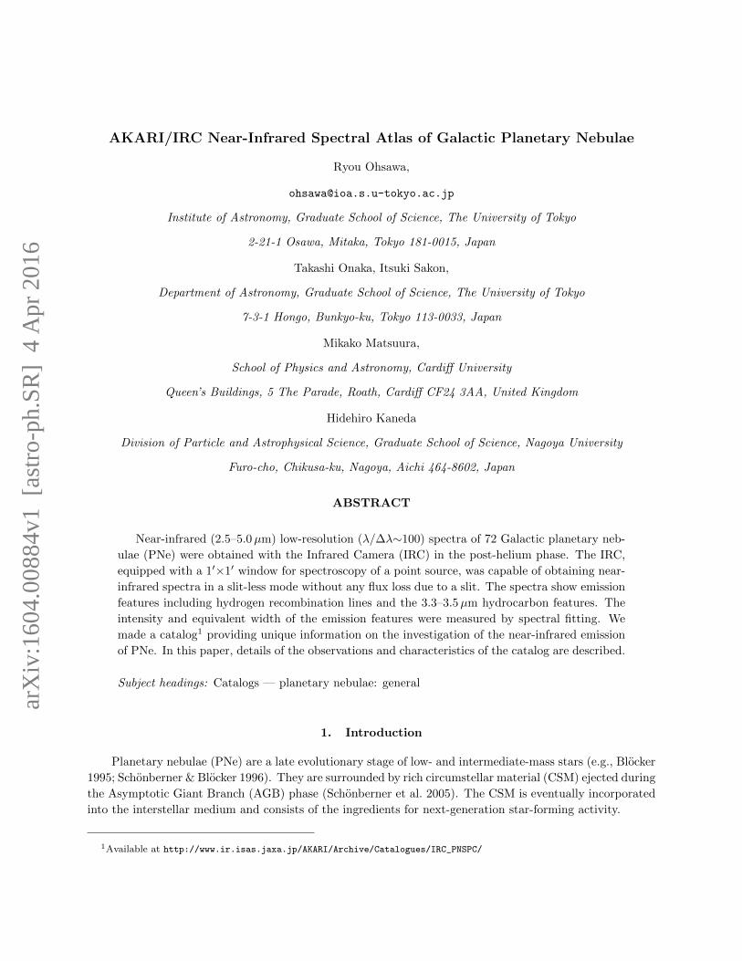
AKARI/IRC Near-Infrared Spectral Atlas of Galactic Planetary Nebulae
Ryou Ohsawa,
Institute of Astronomy, Graduate School of Science, The University of Tokyo
2-21-1 Osawa, Mitaka, Tokyo 181-0015, Japan
Takashi Onaka, Itsuki Sakon,
Department of Astronomy, Graduate School of Science, The University of Tokyo
7-3-1 Hongo, Bunkyo-ku, Tokyo 113-0033, Japan
Mikako Matsuura,
School of Physics and Astronomy, Cardiff University
Queen’s Buildings, 5 The Parade, Roath, Cardiff CF24 3AA, United Kingdom
Hidehiro Kaneda
Division of Particle and Astrophysical Science, Graduate School of Science, Nagoya University
Furo-cho, Chikusa-ku, Nagoya, Aichi 464-8602, Japan
ABSTRACT
Near-infrared (2.5–5.0µm) low-resolution (λ/∆λ∼100) spectra of 72 Galactic planetary neb-
ulae (PNe) were obtained with the Infrared Camera (IRC) in the post-helium phase. The IRC,
equipped with a 1′×1′ window for spectroscopy of a point source, was capable of obtaining near-
infrared spectra in a slit-less mode without any flux loss due to a slit. The spectra show emission
features including hydrogen recombination lines and the 3.3–3.5µm hydrocarbon features. The
intensity and equivalent width of the emission features were measured by spectral fitting. We
made a catalog1 providing unique information on the investigation of the near-infrared emission
of PNe. In this paper, details of the observations and characteristics of the catalog are described.
Subject headings: Catalogs — planetary nebulae: general
1. Introduction
Planetary nebulae (PNe) are a late evolutionary stage of low- and intermediate-mass stars (e.g., Blocker
1995; Schonberner & Blocker 1996). They are surrounded by rich circumstellar material (CSM) ejected during
the Asymptotic Giant Branch (AGB) phase (Schonberner et al. 2005). The CSM is eventually incorporated
into the interstellar medium and consists of the ingredients for next-generation star-forming activity.
1Available at http://www.ir.isas.jaxa.jp/AKARI/Archive/Catalogues/IRC_PNSPC/
arX
iv:1
604.
0088
4v1
[as
tro-
ph.S
R]
4 A
pr 2
016

– 2 –
Infrared spectra are rich in CSM emission features. These features can be used to investigate mass,
temperature and chemical properties of CSMs (e.g., Bernard-Salas & Tielens 2005; Phillips & Marquez-Lugo
2011; Pottasch & Bernard-Salas 2006; Pottasch et al. 1984). In some PNe, far-infrared emission is dominated
by that from dust grains, providing information about the temperature and the total mass of dust grains.
Spectroscopic observations in the mid-infrared (∼5–40µm) have been used to identify dust species (e.g.,
Stanghellini et al. 2012; Volk & Cohen 1990). Emission from stochastically heated dust grains also appears
in the mid-infrared (Draine & Li 2001; Dwek et al. 1997). The dust features commonly found are PAHs,
MgS, silicate, and some potential cases of SiC. Near-infrared (∼1–5µm) continuum emission in PNe involves
free-free emission, stellar continuum, and hot dust emission. Hydrogen recombination lines are prominent in
the near-infrared, such as Brackett-α at 4.051µm. The PAH emission feature appears at 3.3µm (Beintema
et al. 1996; Roche et al. 1996; Tokunaga et al. 1991), while there is also emission from aliphatic C H bonds
at around 3.4–3.5µm (Joblin et al. 1996; Sloan et al. 1997).
Infrared space telescopes have been instrumental for PNe observations despite limited spatial resolution.
Eliminating the effects of heavy terrestrial atmospheric absorption provides the critical advantage of con-
tinuous infrared spectroscopic coverage. Volk & Cohen (1990) investigated 7–23µm low-resolution spectra
of 170 Galactic PNe with the Infrared Astronomical Satellite (IRAS). The Short-Wave Spectrometer (SWS)
and the Long-Wave Spectrometer (LWS) on-board the Infrared Space Observatory (ISO) cover 2.5–45 and
45–197µm. A number of emission lines have been identified and the physical conditions of circumstellar
nebulae have been investigated (e.g., Bernard-Salas & Tielens 2005; Pottasch & Bernard-Salas 2006). The
Infrared Spectrograph (IRS) on-board the Spitzer space telescope covers 5.5–37µm. Stanghellini et al. (2012)
obtained 157 spectra of compact Galactic PNe and investigated their dust emission. Spectra of PNe in the
Magellanic Clouds were also obtained with the IRS (Bernard-Salas et al. 2009, 2008; Stanghellini & Haywood
2010) thanks to its high sensitivity. The ISO/SWS had obtained 2.5–5.0µm spectra of Galactic PNe. About
85 spectra of Galactic PNe are available in Sloan et al. (2003). However, only a few PNe have spectra with
a sufficient signal-to-noise ratio at 2.5–5.0µm to investigate weak features such as the 3.4–3.5µm aliphatic
emission. The Infrared Camera (IRC) on-board AKARI satellite, for the first time, provides near-infrared
(2.5–5.0µm) spectroscopy with a sensitivity of a few mJy (Onaka et al. 2007).
The present paper reports near-infrared spectroscopy with the AKARI /IRC. Observations were carried
out as part of an Open Time Program for the post-helium phase, “Near-Infrared Spectroscopy of Planetary
Nebulae” (PNSPC). Near-infrared spectra of 72 PNe were obtained. The data were compiled as a near-
infrared spectral catalog. In this paper, we describe details of the observations and the characteristics of the
catalog. Detailed information about the observations is given in Section 2. Section 3 describes the reduction
procedures and the method to extract the spectra. The characteristics of the retrieved spectra and the
format of the compiled catalog are presented in Section 4. The quality of the IRC spectra and the statistical
properties of the catalog are discussed in comparison with the observations by other facilities in Section 5.
We summarize the paper in Section 6.
2. Observations
2.1. Target Selection
The observed targets were selected from the Strasbourg-ESO Catalogue of Galactic Planetary Nebulae
(Acker et al. 1992), taking into account their NIR magnitude and angular size. The spectroscopic sensitivity
of the IRC is a few mJy in the range of 2–5µm, while the saturation limit is about 10 Jy. With these

– 3 –Lat
itu
de
(deg
)
Longitude (deg)
-40
-20
0
20
40
-180 -120 -60 0 60 120 180
Fig. 1.— Distribution of the observed planetary nebulae (the crosses) overlaid on an extinction map in the
Galactic coordinates created from the DSS (Dobashi et al. 2005a). The gray scale indicates extinction at
the V -band from 0.1 to 5 mag.
limits taken into account, objects whose K-band magnitude is between 5 and 13 were selected as targets
for this program. The observations were carried out with the 1′×1′ Np-window (see Section 2.2 and Onaka
et al. 2007) in the slit-less mode. Therefore, compact objects were preferred to avoid degrading the spectral
resolution. The candidate list was then narrowed to objects whose radius in the optical was smaller than 5′′,
comparable to the full width half maximum of the IRC point spread function (∼3′′), to exclude apparently
large objects. Finally, 72 objects were selected and their spectra were successfully obtained. Figure 1 shows
the distribution of the targets in the Galactic coordinates. The PNG ID, the AKARI observation ID, and
the coordinates of the PNSPC samples are listed in Table 1. Table 2 summarizes miscellaneous information
of the objects, including the optical (the V -band) and infrared (the 2MASS Ks-band) magnitudes.
The target selection method was independent of the chemistry and dust compositions of the circumstellar
nebula. The catalog is not considered to be biased, in terms of chemical abundance and the chemistry of
dust. However, the objects were selected based on their sizes. Since PNe expand as they evolve, the selection
could be biased toward young PNe. The potential biases of the PNSPC samples are discussed in detail in
Section 5.
2.2. Instruments
Although the AKARI /IRC has three channels (Onaka et al. 2007), only the NIR channel was available
during the post-helium phase. The field of view of the NIR channel consists of four parts: the N/Nc-window,
the Ns-slit, the Np-window, and the Nh-slit (see, Figure 3 in Onaka et al. 2007). The observations were
performed with the Np-window, which was designed for point source, slit-less spectroscopy. Spectroscopy
with the Np-window allows us to collect all of the flux from an object. The present spectroscopy was carried
out with the grism, providing 2.5–5.0µm spectra with the spectral resolution of λ/∆λ∼100, for point sources
(.3′′). The spectral resolution was degraded for extended objects.
The observations were carried out with the observation template IRCZ4. This mode consists of three
sequences: the first set is four spectroscopic images, the second set is a broad band image, and the final
set is another sequence of four spectroscopic images. Thus, each pointing observation involves eight frames
for spectroscopy and one frame for broad-band imaging. Every frame consists of short (4.58 sec) and long
(44.41 sec) exposure images. Due to the short integration time, the typical signal-to-noise ratio of the short

– 4 –
exposure images is worse than that of the long exposure images. In general, we used only the long exposure
images. The short exposure images were used only for cases when the long exposure image showed saturated
pixels.
Each object was observed either once, or twice. Thus, there were eight or sixteen frames for each object.
However, some frames were not usable due to cosmic rays or unstable pointing during the exposure. The
net integration time thus depends on the target, listed in the sixth column of Table 1.

– 5 –
Table 1. Summary of Observations
PN G Obs. ID RA (J2000) DEC (J2000) N (a) tint(b) FWHM Flags
hh:mm:ss dd:mm:ss sec. µm S(c) D(d) C(e)
000.3+12.2 3460107 17 : 01 : 33.6 −21 : 49 : 33.5 17 754.97 0.045 N N N
002.0−13.4 3460003 18 : 45 : 50.7 −33 : 20 : 35.0 16 710.56 0.040 N Y N
003.1+02.9 3460005 17 : 41 : 52.8 −24 : 42 : 07.7 9 399.69 0.045 N Y Y
011.0+05.8 3460012 17 : 48 : 19.8 −16 : 28 : 44.0 18 799.38 0.035 N N N
027.6−09.6 3460016 19 : 16 : 28.3 −09 : 02 : 37.0 9 399.69 0.040 N Y N
037.8−06.3 3460019 19 : 22 : 56.9 +01 : 30 : 48.0 17 754.97 0.035 N Y N
038.2+12.0 3460020 18 : 17 : 34.0 +10 : 09 : 05.0 9 399.69 0.040 N N N
043.1+03.8 3460093 18 : 56 : 33.6 +10 : 52 : 12.0 9 399.69 0.035 N Y Y
046.4−04.1 3460021 19 : 31 : 16.4 +10 : 03 : 21.7 9 399.69 0.040 N Y Y
051.4+09.6 3460022 18 : 49 : 47.6 +20 : 50 : 39.5 17 754.97 0.040 N N N
052.2−04.0 3460094 19 : 42 : 18.7 +15 : 09 : 09.0 18 799.38 0.035 N Y N
058.3−10.9 3460023 20 : 20 : 08.8 +16 : 43 : 54.0 18 799.38 0.040 N N N
060.1−07.7 3460024 20 : 12 : 42.9 +19 : 59 : 23.0 14 621.74 0.048 N Y N
060.5+01.8 3460025 19 : 38 : 08.4 +25 : 15 : 42.0 18 799.38 0.035 N Y N
064.7+05.0 3460026 19 : 34 : 45.3 +30 : 30 : 59.2 17 77.86 0.048 Y N N
071.6−02.3 3460027 20 : 21 : 03.8 +32 : 29 : 24.0 18 799.38 0.035 N N N
074.5+02.1 3460028 20 : 10 : 52.5 +37 : 24 : 41.0 18 799.38 0.040 N N N
082.1+07.0 3460029 20 : 10 : 23.7 +46 : 27 : 39.0 18 799.38 0.045 N Y N
082.5+11.3 3460030 19 : 49 : 46.6 +48 : 57 : 40.0 9 399.69 0.035 N Y N
086.5−08.8 3460114 21 : 33 : 08.3 +39 : 38 : 09.7 18 799.38 0.045 N Y N
089.3−02.2 3460031 21 : 19 : 07.2 +46 : 18 : 48.0 18 799.38 0.038 N Y N
089.8−05.1 3460032 21 : 32 : 31.0 +44 : 35 : 47.7 18 799.38 0.035 N N N
095.2+00.7 3460033 21 : 31 : 50.2 +52 : 33 : 52.0 18 799.38 0.042 N Y N
100.6−05.4 3460034 22 : 23 : 55.7 +50 : 58 : 00.0 18 799.38 0.035 N N N
111.8−02.8 3460035 23 : 26 : 14.9 +58 : 10 : 53.0 8 355.28 0.038 N N N
118.0−08.6 3460096 00 : 18 : 42.2 +53 : 52 : 20.0 16 710.56 0.035 N Y N
123.6+34.5 3460115 12 : 33 : 06.8 +82 : 33 : 50.1 18 799.38 0.065 N Y N
146.7+07.6 3460097 04 : 25 : 50.8 +60 : 07 : 12.7 18 799.38 0.035 N N N
159.0−15.1 3460098 03 : 47 : 33.0 +35 : 02 : 48.9 9 399.69 0.045 N Y N
166.1+10.4 3460116 05 : 56 : 23.9 +46 : 06 : 17.2 18 799.38 0.050 N N N
190.3−17.7 3460099 05 : 05 : 34.3 +10 : 42 : 23.8 9 399.69 0.045 N N N
194.2+02.5 3460117 06 : 25 : 57.2 +17 : 47 : 27.3 18 799.38 0.045 N N N
211.2−03.5 3460036 06 : 35 : 45.1 +00 : 05 : 38.0 16 710.56 0.035 N N N
221.3−12.3 3460118 06 : 21 : 42.7 −12 : 59 : 14.0 15 666.15 0.046 N N N
226.7+05.6 3460100 07 : 37 : 18.9 −09 : 38 : 50.0 17 754.97 0.040 N Y N
232.8−04.7 3460037 07 : 11 : 16.7 −19 : 51 : 04.0 14 621.74 0.035 N N N
235.3−03.9 3460038 07 : 19 : 21.5 −21 : 43 : 54.3 17 754.97 0.035 N N N
258.1−00.3 3460039 08 : 28 : 28.0 −39 : 23 : 40.0 17 754.97 0.042 N N N
264.4−12.7 3460040 07 : 47 : 20.0 −51 : 15 : 03.4 17 754.97 0.035 N Y N
268.4+02.4 3460042 09 : 16 : 09.6 −45 : 28 : 42.8 18 799.38 0.038 N N N
278.6−06.7 3460101 09 : 19 : 27.5 −59 : 12 : 00.3 18 799.38 0.040 N Y N

– 6 –
3. Data Reduction
3.1. Bias Subtraction and Flux Calibration
The basic data reduction procedure used here, includes subtraction of dark frames, linearity correction,
saturation masking, flat fielding, and subtraction of background emission. All steps were carried out with
the IRC Spectroscopy Toolkit for Phase 3 (Version 20111121)2. Pixels affected by cosmic rays were masked
by hand. Some pixels were saturated by bright objects in the long exposure images. The saturated pixels
were replaced by the corresponding pixels from the short exposure images. Objects whose spectra were
saturated in the long exposure images are marked in the eighth column of Table 1. Spectroscopic images
were aligned by maximizing the correlation among the images. Then, the images were combined by median
stacking, producing a two-dimensional spectrum. Frames that were affected by unstable pointing during the
exposure were excluded from stacking. The toolkit also produced a two-dimensional noise map, which was
given as a standard deviation of the stacked frames.
3.2. Extraction of One-Dimensional Spectrum
Some objects were extended with respect to the point spread function (PSF) of the IRC. To make a
homogeneous data reduction, we assumed that all the sources were extended. We used a sufficiently wide
aperture (>10 pixels) to extract a one-dimensional spectrum that included all of the fluxes from the object,
and did not apply any aperture correction. The standard error in the spectrum was calculated using the
noise map produced by the toolkit.
It was difficult to use a wide aperture for objects which were located in crowded regions. Noble et al.
(2013) invented a novel method to extract the spectrum of a certain object in a crowded region by profile
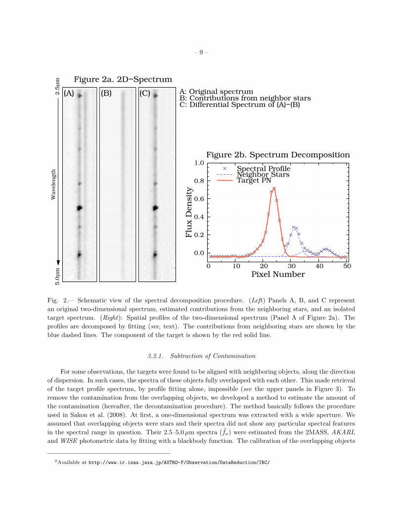
fitting. We used a similar method to remove the contribution from neighboring objects. Figure 2 shows
a schematic view of the method (hereafter, the spectral decomposition procedure). Panel A of Figure 2a
shows an example two-dimensional spectrum of a target in a crowded region. The horizontal and vertical axes
correspond to the position and wavelength. The spectrum of the target PN runs through the center of the
panel. The spectra of neighboring objects are located to the right side of the PN spectrum. Figure 2b shows
the spatial profiles of the spectra (Panel A). The spectra were decomposed by fitting with a combination of
Gaussian functions. The red solid line shows the PN profile, and the blue dashed lines show those of the
neighboring objects. The fitting was performed for every spectral element. The instrumental spatial profile
of a spectrum was not a Gaussian, rather a combination of Gaussian profiles provided the best fit to the
profile. Panel B of Figure 2a shows the estimated contribution from the neighboring objects. By subtracting
Panel B from Panel A, the two-dimensional spectrum of the target PN was extracted (Panel C). Finally, the
one-dimensional spectrum of the target PN was obtained from Panel C with a wide aperture, as mentioned
above. The uncertainty in the contamination-corrected spectrum was estimated by taking into account errors
in the spectral decomposition procedure. The targets which are in crowded regions are denoted in the ninth
column of Table 1.

– 7 –
Table 1—Continued
PN G Obs. ID RA (J2000) DEC (J2000) N (a) tint(b) FWHM Flags
hh:mm:ss dd:mm:ss sec. µm S(c) D(d) C(e)
283.8+02.2 3460044 10 : 31 : 33.4 −55 : 20 : 50.5 16 710.56 0.045 N Y N
285.4−05.3 3460120 10 : 09 : 20.8 −62 : 36 : 48.5 18 799.38 0.050 N Y N
285.6−02.7 3460045 10 : 23 : 09.1 −60 : 32 : 42.3 17 754.97 0.042 N Y N
285.7−14.9 3460121 09 : 07 : 06.3 −69 : 56 : 30.6 17 754.97 0.060 N N N
291.6−04.8 3460046 11 : 00 : 20.0 −65 : 14 : 57.8 18 799.38 0.038 N Y N
292.8+01.1 3460102 11 : 28 : 47.4 −60 : 06 : 37.3 18 799.38 0.042 N Y N
294.9−04.3 3460047 11 : 31 : 45.4 −65 : 58 : 13.7 18 799.38 0.035 N N N
296.3−03.0 3460048 11 : 48 : 38.2 −65 : 08 : 37.3 15 666.15 0.035 N N N
304.5−04.8 3460051 13 : 08 : 47.3 −67 : 38 : 37.6 16 710.56 0.038 N Y N
305.1+01.4 3460122 13 : 09 : 36.4 −61 : 19 : 35.6 18 82.44 0.050 Y N N
307.2−09.0 3460052 13 : 45 : 22.4 −71 : 28 : 55.7 18 799.38 0.035 N Y Y
307.5−04.9 3460053 13 : 39 : 35.1 −67 : 22 : 51.7 18 799.38 0.040 N Y Y
312.6−01.8 3460123 14 : 18 : 43.3 −63 : 07 : 10.1 16 710.56 0.056 N Y N
315.1−13.0 3460054 15 : 37 : 11.2 −71 : 54 : 52.9 18 82.44 0.042 Y N N
320.1−09.6 3460103 15 : 56 : 01.7 −66 : 09 : 09.2 16 710.56 0.045 N Y N
320.9+02.0 3460056 15 : 05 : 59.2 −55 : 59 : 16.5 9 399.69 0.042 N Y N
322.5−05.2 3460060 15 : 47 : 41.2 −61 : 13 : 05.6 16 710.56 0.092 N Y Y
323.9+02.4 3460061 15 : 22 : 19.4 −54 : 08 : 13.1 9 399.69 0.045 N Y N
324.8−01.1 3460062 15 : 41 : 58.8 −56 : 36 : 25.6 8 355.28 0.036 N Y Y
325.8−12.8 3460063 16 : 54 : 35.2 −64 : 14 : 28.4 16 710.56 0.035 N Y N
326.0−06.5 3460064 16 : 15 : 42.3 −59 : 54 : 01.0 14 621.74 0.035 N Y Y
327.1−01.8 3460065 15 : 58 : 08.1 −55 : 41 : 50.3 9 399.69 0.035 N Y Y
327.8−01.6 3460066 16 : 00 : 59.1 −55 : 05 : 39.7 8 355.28 0.038 N Y N
331.1−05.7 3460067 16 : 37 : 42.7 −55 : 42 : 26.5 17 754.97 0.035 N Y N
331.3+16.8 3460068 15 : 12 : 50.8 −38 : 07 : 32.0 16 710.56 0.048 N Y N
336.3−05.6 3460069 16 : 59 : 36.1 −51 : 42 : 08.4 18 799.38 0.035 N Y N
342.1+27.5 3460104 15 : 22 : 19.3 −23 : 37 : 32.0 18 799.38 0.050 N Y N
349.8+04.4 3460105 17 : 01 : 06.2 −34 : 49 : 38.0 9 399.69 0.040 N Y N
350.9+04.4 3460070 17 : 04 : 36.2 −33 : 59 : 18.0 18 799.38 0.038 N Y N
356.1+02.7 3460076 17 : 25 : 19.2 −30 : 40 : 41.0 18 799.38 0.035 N Y Y
357.6+02.6 3460082 17 : 29 : 42.7 −29 : 32 : 50.0 15 666.15 0.035 N Y N
Note. — (a) the number of exposures; (b) the net integration time; (c) the saturation flag, Y: the spectrum is
(partly) saturated in long-exposure spectral images; N: the spectrum is not saturated; (d) the decomposition flag,
Y: the spectral decomposition procedure was used; N: the spectrum was not affected by any neighbor object; (e)
the contamination flag, Y: the decontamination procedure was used; N: the spectrum was not affected by any
overlapping object.

– 8 –
Table 2. Miscellaneous Information of Objects
PN G V (a) K(b)s AV (Hβ) AV (fit.) Teff Refs. Teff
mag. mag. mag. mag. 103 K
000.3+12.2 13.9 11.4 0.90+0.03−0.03 0.98+0.15
−0.05 47 Ka76,Ph03
002.0−13.4 14.1 11.1 0.31+0.02−0.01 0.38+0.02
−0.04 60 PM89,PM91,Ph03
003.1+02.9 >17.0 11.6 3.31+0.03−0.03 3.4+0.6
−0.1 87 PM89,Ph03
011.0+05.8 · · · 11.8 1.81+0.04−0.04 1.79+0.06
−0.06 93 PM91,Ph03
027.6−09.6 15.2 11.9 1.04+0.06−0.05 1.0+0.9
−0.2 58 PM91,Ka76,KJ91,Ph03
037.8−06.3 · · · 9.47 1.4+0.1−0.1 1.41+0.08
−0.02 74 Ph03
038.2+12.0 12.5 11.1 0.82+0.05−0.05 0.93+0.07
−0.07 30 Ka78,Ph03
043.1+03.8 14.9 12.1 1.9+0.1−0.1 2.05+0.46
−0.05 28 Ph03
046.4−04.1 15.2 11.1 1.42+0.02−0.02 1.39+0.01
−0.01 68 Ka76,KJ91,Ph03
051.4+09.6 13.3 10.4 0.88+0.05−0.04 0.98+0.11
−0.08 37 Ka76,Ka78,Ph03
Note. — Table 2 is published in its entirety in the electronic edition of the Astrophysical
Journal. A portion is shown here for guidance regarding its form and content.
References. — (a)Acker et al. (1992); (b) Skrutskie et al. (2006); HF83: Harrington & Feibel-
man (1983), Ka76: Kaler (1976), Ka78: Kaler (1978), KJ91: Kaler & Jacoby (1991), Lu01:
Lumsden et al. (2001), Me88: Mendez et al. (1988), Ph03: Phillips (2003), PM89: Preite-
Martinez et al. (1989), PM91: Preite-Martinez et al. (1991).
– 9 –
A: Original spectrumB: Contributions from neighbor starsC: Differential Spectrum of (A)−(B)
Figure 2a. 2D−Spectrum
(A) (B) (C)
Wav
elen
gth
2.5
µm
5.0
µm
0.0
0.2
0.4
0.6
0.8
1.0
0 10 20 30 40 50
Flu
x D
ensi
ty
Pixel Number
Figure 2b. Spectrum Decomposition
Spectral ProfileNeighbor StarsTarget PN
Fig. 2.— Schematic view of the spectral decomposition procedure. (Left) Panels A, B, and C represent
an original two-dimensional spectrum, estimated contributions from the neighboring stars, and an isolated
target spectrum. (Right): Spatial profiles of the two-dimensional spectrum (Panel A of Figure 2a). The
profiles are decomposed by fitting (see, text). The contributions from neighboring stars are shown by the
blue dashed lines. The component of the target is shown by the red solid line.
3.2.1. Subtraction of Contamination
For some observations, the targets were found to be aligned with neighboring objects, along the direction
of dispersion. In such cases, the spectra of these objects fully overlapped with each other. This made retrieval
of the target profile spectrum, by profile fitting alone, impossible (see the upper panels in Figure 3). To
remove the contamination from the overlapping objects, we developed a method to estimate the amount of
the contamination (hereafter, the decontamination procedure). The method basically follows the procedure
used in Sakon et al. (2008). At first, a one-dimensional spectrum was extracted with a wide aperture. We
assumed that overlapping objects were stars and their spectra did not show any particular spectral features
in the spectral range in question. Their 2.5–5.0µm spectra (fν) were estimated from the 2MASS, AKARI,
and WISE photometric data by fitting with a blackbody function. The calibration of the overlapping objects
2Available at http://www.ir.isas.jaxa.jp/ASTRO-F/Observation/DataReduction/IRC/

– 10 –
PN
G 1
23.6
+34.5
A n
uis
ance
obj
ect
Imaging Spectroscopy
2.5 3.0 3.5 4.0 4.5 5.0
Flu
x D
ensi
ty F
λ
Wavelength (µm)
PNG 123.6+34.5(3460115)Estimated ContaminationDecontaminated Spectrum
Fig. 3.— Schematic view of the decontamination procedure. The upper left panel shows the locations of a PN
and an overlapping star, while the upper right panel shows the obtained spectrum with contamination from
the overlapping star. The contaminated spectrum is shown by the gray dotted line in the bottom panel.
The red dashed line shows the estimated contamination from the overlapping star. The decontaminated
spectrum of the PN is shown by the blue solid line.
required correction since the overlapping object was shifted along the direction of dispersion. The amount
of contamination f cν(λ) was converted from fν using the distance between the target and the overlapping
objects in the direction of the dispersion, d, in units of pixel and the spectral response function of the IRC,
R(λ), in units of ADU mJy−1. We defined δ as the pixel scale of the spectrum in units of µm pixel−1. The
amount of the contamination was estimated by
f cν(λ) =fν(λ−δd)R(λ−δd)
R(λ). (1)
We defined fobsν as the obtained spectrum, including the contamination. The decontaminated spectrum was
defined by fobjν = fobsν − f cν . A schematic view of the method is given in Figure 3. The upper left panel
shows the location of the target (PN G123.6+34.5) and overlapping object. The direction of dispersion is
horizontal. The spectrum with the contamination is shown in the upper right panel. The contaminated one-
dimensional spectrum is shown by the gray dotted line in the bottom panel. The estimated contamination
and decontaminated spectra are shown by the red dashed and blue solid lines. We assume that the spectrum
of the overlapping star does not have any significant features and that the decontamination procedure does
not affect the estimate of emission feature intensities (although continuum flux could be somewhat affected).
The targets with overlapping objects are flagged as contaminated objects in the tenth column of Table 1.
4. Results
4.1. Near-Infrared Spectroscopy of Planetary Nebulae Spectral Atlas
Details of the observations are summarized in Table 1, which includes the PNG ID, the observation
ID, the location, the number of exposures, the total integration time, the spectral PSF size, and the flags
– 11 –
0
400
800
1200
1600
2000
Flu
x D
ensi
ty (10
−15W
m−2µ
m−1)
Step−like continuum
PAH3.3µm
PAH3.4−3.5µm
HI recombination lines
HeI recombination lines
HeII recombination lines
PNG 064.7+05.0
0
40
80
120
160
2.5 3.0 3.5 4.0 4.5 5.0
[MgIV] [ArVI]
Wavelength (µm)
PNG 074.5+02.1
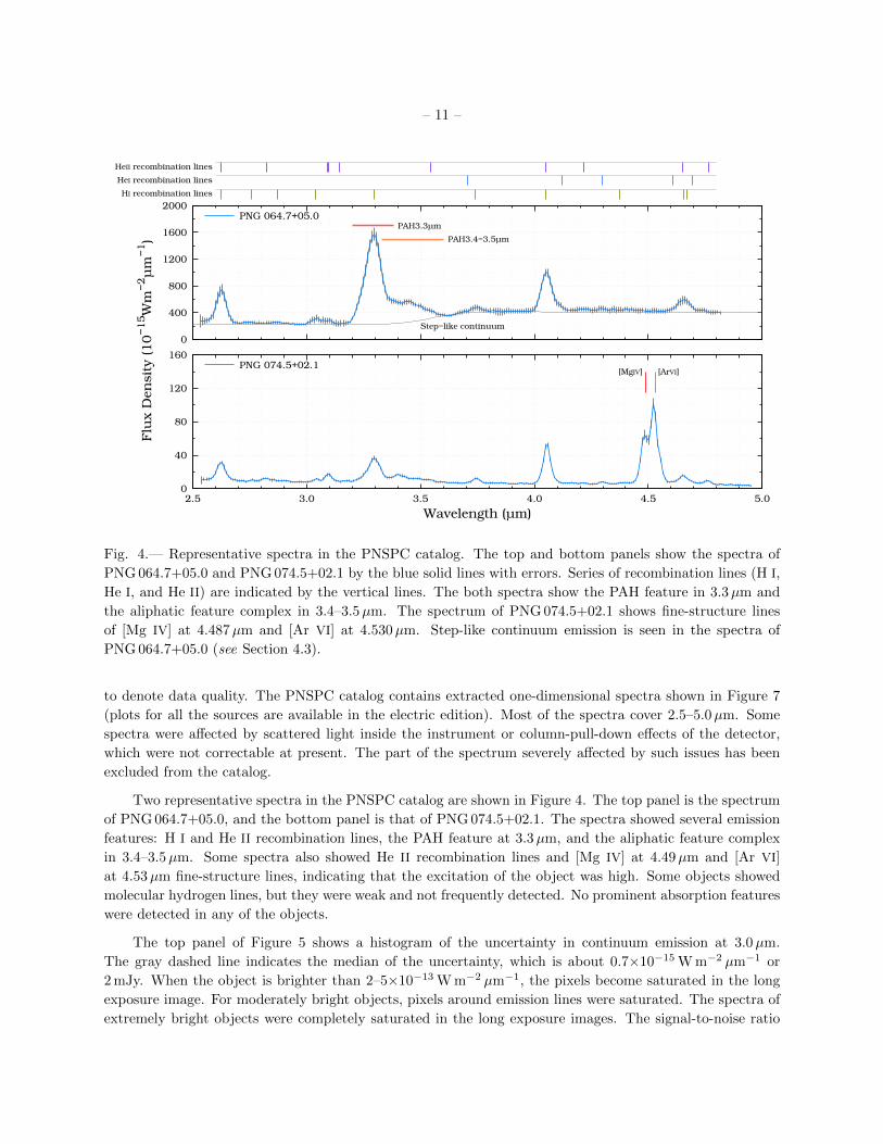
Fig. 4.— Representative spectra in the PNSPC catalog. The top and bottom panels show the spectra of
PNG 064.7+05.0 and PNG 074.5+02.1 by the blue solid lines with errors. Series of recombination lines (H I,
He I, and He II) are indicated by the vertical lines. The both spectra show the PAH feature in 3.3µm and
the aliphatic feature complex in 3.4–3.5µm. The spectrum of PNG 074.5+02.1 shows fine-structure lines
of [Mg IV] at 4.487µm and [Ar VI] at 4.530µm. Step-like continuum emission is seen in the spectra of
PNG 064.7+05.0 (see Section 4.3).
to denote data quality. The PNSPC catalog contains extracted one-dimensional spectra shown in Figure 7
(plots for all the sources are available in the electric edition). Most of the spectra cover 2.5–5.0µm. Some
spectra were affected by scattered light inside the instrument or column-pull-down effects of the detector,
which were not correctable at present. The part of the spectrum severely affected by such issues has been
excluded from the catalog.
Two representative spectra in the PNSPC catalog are shown in Figure 4. The top panel is the spectrum
of PNG 064.7+05.0, and the bottom panel is that of PNG 074.5+02.1. The spectra showed several emission
features: H I and He II recombination lines, the PAH feature at 3.3µm, and the aliphatic feature complex
in 3.4–3.5µm. Some spectra also showed He II recombination lines and [Mg IV] at 4.49µm and [Ar VI]
at 4.53µm fine-structure lines, indicating that the excitation of the object was high. Some objects showed
molecular hydrogen lines, but they were weak and not frequently detected. No prominent absorption features
were detected in any of the objects.
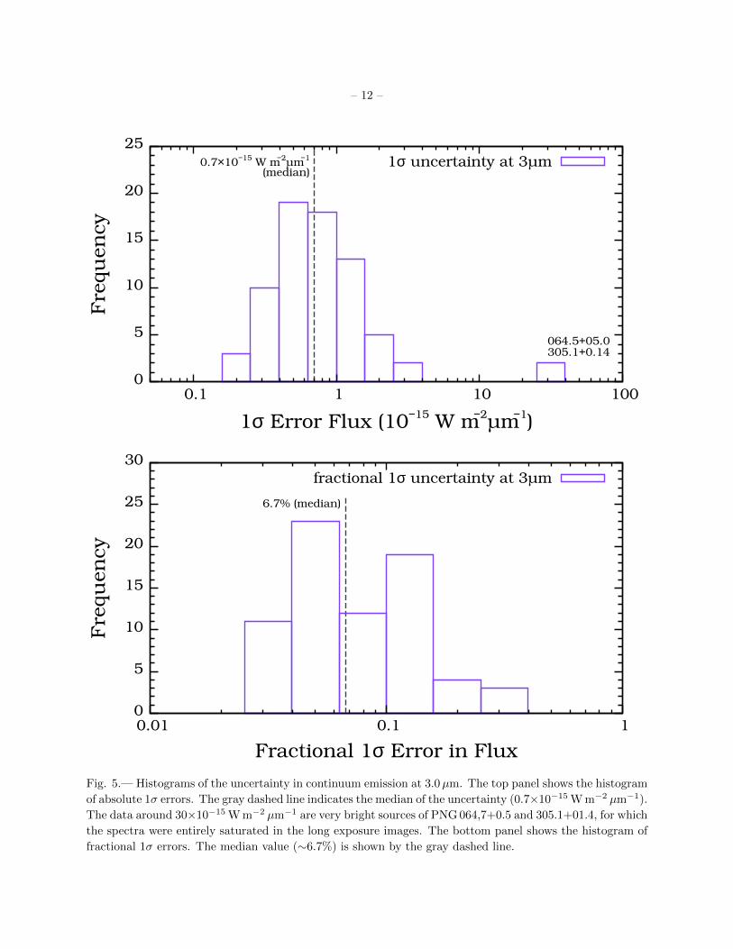
The top panel of Figure 5 shows a histogram of the uncertainty in continuum emission at 3.0µm.
The gray dashed line indicates the median of the uncertainty, which is about 0.7×10⁻¹⁵ W m−2 µm−1 or
2 mJy. When the object is brighter than 2–5×10⁻¹³ W m−2 µm−1, the pixels become saturated in the long
exposure image. For moderately bright objects, pixels around emission lines were saturated. The spectra of
extremely bright objects were completely saturated in the long exposure images. The signal-to-noise ratio
– 12 –
0.7×10⁻¹⁵ W m−2µm−1
(median)
064.5+05.0305.1+0.14
Fre
quen
cy
1σ Error Flux (10−15 W m−2µm−1)
1σ uncertainty at 3µm
0
5
10
15
20
25
0.1 1 10 100
6.7% (median)
Fre
quen
cy
Fractional 1σ Error in Flux
fractional 1σ uncertainty at 3µm
0
5
10
15
20
25
30
0.01 0.1 1
Fig. 5.— Histograms of the uncertainty in continuum emission at 3.0µm. The top panel shows the histogram
of absolute 1σ errors. The gray dashed line indicates the median of the uncertainty (0.7×10⁻¹⁵ W m−2 µm−1).
The data around 30×10−15 W m−2 µm−1 are very bright sources of PNG 064,7+0.5 and 305.1+01.4, for which
the spectra were entirely saturated in the long exposure images. The bottom panel shows the histogram of
fractional 1σ errors. The median value (∼6.7%) is shown by the gray dashed line.

– 13 –
of the spectrum depends on the fraction of saturated pixels. PNG 064.7+05.0 and 305.1+01.4 are extremely
bright, with their spectrum completely saturated in the long exposure images. Figure 5 (top) indicates that
their uncertainties at 3.0µm are about 50 times worse than the others. The fractional uncertainty at 3.0µm
is shown in the bottom panel of Figure 5. The median of the fractional uncertainty is about 6.4%, indicated
by the vertical dashed line. This means that, for half of the PNSPC samples, the continuum emission at
3.0µm was detected with a signal-to-noise ratio larger than about 15.
The full width half maximum (FWHM) of the spectral PSF of the IRC, equivalent to the FWHM of
an unresolved emission line, is about 0.035µm. Thus, the spectral resolution is about λ/∆λ ∼ 100. When
the object is extended for the IRC, the spectral resolution is degraded. The FWHM of the spectral PSF,
estimated from spectral fitting (see Section 4.3), is listed in the seventh column of Table 1. PN G322.5−05.2
is the most extended object in the PNSPC catalog and its spectral resolution was estimated to be about
λ/∆λ ∼ 40 at 4µm.
4.2. Extinction
Foreground extinction towards the objects was estimated based on an intensity ratio of Hβ to Brackett-α
(Brα). The intensities of Hβ were obtained from literature (Acker et al. 1992, and references therein). We
measured the intensities of Brα from the AKARI spectra by fitting with a Gaussian function. We defined
IHβ and IBrα as the intensities of Hβ and Brα. The observed intensity ratio follows the relation:
IobsHβ
IobsBrα
=I0Hβe−τHβ
I0Brαe−τBrα, (2)
where IobsX and I0X are the observed and intrinsic intensities of the line X, and τX is the extinction of the
line X. We assumed that the nebula was totally opaque for Lyman photons (Case B in Baker & Menzel
(1938)). Then, the intrinsic intensity ratio(I0Hβ/I
0Brα
)was assumed to be ∼12.853, given by the Case B line
ratio calculated for the electron density of 104 cm−3 and the electron temperature of 104 K from Storey &
Hummer (1995). We adopted the extinction curve given by Mathis (1990) and the extinction at the V -band
was derived as
AV (Hβ) = 2.39− 0.95 ln
(IobsHβ
IobsBrα
). (3)
The coefficients in Equation (3) depends on the assumed electron temperature and density. When the
assumed electron temperature increases to 2×10⁴ K, AV will increase by about 0.3. The effect of the electron
density on AV is much smaller than 0.3 for the range from 102 to 106 cm−3. The systematic uncertainty in
AV , chiefly attributable to the electron temperature uncertainty, was estimated to be less than 0.3 mag. The
estimated AV (Hβ) is listed in the fourth colunm of Table 2.
4.3. Spectral Fitting
The intensities of the spectral features were measured by spectral fitting. The fitted function was
assumed to be a linear combination of the spectral features as
Fλ(λ) =[f contλ (λ) + f lineλ (λ) + fdustλ (λ)
]e−τ(λ), (4)

– 14 –
where f contλ , f lineλ , and fdustλ were the components of continuum, emission lines, and dust features, and
τ(λ) was the optical depth at λ. The functional shape of τ(λ) was given by a cubic spline function that
interpolated the extinction curve of Mathis (1990) at every data point of the IRC spectrum. The amount of
the extinction at the V -band, AV = τ(V ), was included as a fitting parameter.
The continuum emission, f contλ , was given by a polynomial function, f contλ =∑Nl=0 clλ
l, where cl’s were
the fitting parameters. The order N was defined for each object, usually N = 2 or 3. This was sufficient
to represent the contributions from free-free and hot thermal dust emission. Some PNe showed a sudden
increase in the continuum emission around λ ∼ 3.6µm, for instance, PN G064.7+05.0 in Figure 4. The
existence of this emission was mentioned in Boulanger et al. (2011), but the carrier of this emission has not
been identified. It was difficult to fit this profile with such a low-order polynomial function. Thus, for those
objects with such an increase, we added a step-like function in the components of the continuum emission as
f contλ (λ) =
N∑l=0
clλl + c
[1
2+
1
2erf
(λ− 3.65µm
∆step
)], (5)
where c was the fitting parameter, erf(x) was the error function, and ∆step was the width of the step function,
which was tentatively fixed at 0.135µm. This component strongly appears in PNG 037.8−06.3, 064.7+050,
089.8−05.1, and 268.4+02.4.
The emission line profile was approximated by a Gaussian function. The line emission component, f lineλ ,
was approximated by a combination of Gaussian functions:
f lineλ (λ) =∑m
cm√2πσ
exp
[− (λ− λm0)2
2σ2
], (6)
where λm0 was the central wavelengths of the m-th emission line and cm’s were the parameters to indicate
the strength of the lines. The central wavelengths were fixed in the fitting. The line width of the Brα line
was measured by fitting with a Gaussian function prior to the fitting and the line widths of other emission
lines were assumed to be the same as Brα. The lines included in the fitting are listed in Table 3. The
assignment and central wavelength are shown in the first and second column. In the fitting, we did not
include the lines which were apparently not detected. Some of the H I and He II recombination lines appear
at the same wavelength and it was impossible to isolate them. Thus, the relative intensities of the H I and
He II recombination lines were fixed, assuming the Case B condition. The relative intensity was adopted
from Storey & Hummer (1995) for the electron temperature and the electron density of 104 K and 104 cm−2.
The variations in the relative intensity with the electron temperature and density were almost negligible
compared to the uncertainty in the observed spectra.
The intrinsic spectral profiles of the PAH emission and the aliphatic feature complex were assumed to
be given by a combination of Lorentzian functions which need to be convoluted with the resolution given by
the instrument. Thus, their spectral profiles were approximated by the Lorentzian function convoluted with
the spectral PSF of the IRC, which was approximated by a Gaussian. The component from dust emission,
fdustλ , was defined by
fdustλ (λ) =∑n
cn
π√
2πσ
∫dλ′e−
(λ−λ′)2
2σ2∆n
∆2n + (λ′ − λn0)2
, (7)
where ∆n and λn0 were the width and peak wavelength of the n-th dust emission and cn’s were the fitting
parameters. The adopted values of ∆n’s and λn0’s were listed in Table 4. The PAH feature at 3.3µm was

– 15 –
Table 3: List of Line Features
Name λ0 (µm)
Brakett-α† 4.051
Brakett-β† 2.625
Pfund-β† 4.653
Pfund-γ† 3.740
Pfund-δ† 3.296
Pfund-ε† 3.039
Pfund-ζ† 2.873
Pfund-η† 2.758
Humpleys-ε† 4.671
Humpleys-ζ† 4.376
He I(3Po-3D) 3.704
He I(1Po-1D) 4.123
He I(3S-3Po) 4.296
He I(1Po-1S) 4.607
He I(3Po-3S) 4.695
Name λ0 (µm)
He II(7-6)‡ 3.092
He II(9-7)‡ 2.826
He II(8-7)‡ 4.764
He II(12-8)‡ 2.625
He II(11-8)‡ 3.096
He II(10-8)‡ 4.051
He II(14-9)‡ 3.145
He II(13-9)‡ 3.544
He II(12-9)‡ 4.218
He II(14-10)‡ 4.652
H2(1-0) 2.802
H2(1-0) 3.003
H2(1-0) 3.234
H2(0-0) 3.836
H2(0-0) 4.181
[Mg IV] 4.487
[Ar VI] 4.530
Note. — †,‡: relative intensities of these lines are fixed assuming the Case B condition.
Table 4: List of Dust Features
Name λ0 (µm) ∆ (µm)
PAH 3.25† 3.248 0.005
PAH 3.30† 3.296 0.021
C Hal 3.41‡ 3.410 0.030
C Hal 3.46‡ 3.460 0.013
C Hal 3.51‡ 3.512 0.013
C Hal 3.56‡ 3.560 0.013
Note. — †: they belong to the PAH feature at 3.3µm. ‡: they belong to the aliphatic feature complex in 3.4–3.5µm.
mainly composed of the 3.30µm feature, but the 3.25µm feature was added to account for a slight change
in the spectral profile of the 3.3µm feature. For instance the 3.3µm feature of PNG 320.9+02.0 show an
extended blue component, which cannot be well-fitted without the 3.25µm component. Mori et al. (2012)
used a combination of four Lorentzian functions to describe the 3.4–3.5µm feature complex (C Hal) in
spectra obtained with the IRC. We used a combination of the four components to describe the C Hal
feature. The central wavelengths and widths were adopted from Mori et al. (2012).
Define F objλ (λ) and σλ(λ) as the observed flux and its uncertainty at λ. We assumed that the residual
∆λ(λ) = F objλ (λ)−Fλ(λ) followed a normal distribution with the variance of σ2
λ(λ). The likelihood function
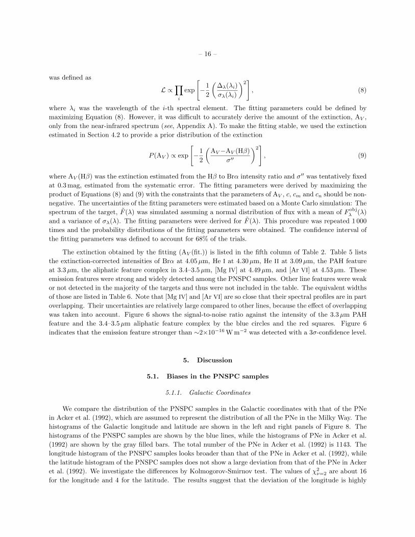
– 16 –
was defined as
L ∝∏i
exp
[−1
2
(∆λ(λi)
σλ(λi)
)2], (8)
where λi was the wavelength of the i-th spectral element. The fitting parameters could be defined by
maximizing Equation (8). However, it was difficult to accurately derive the amount of the extinction, AV ,
only from the near-infrared spectrum (see, Appendix A). To make the fitting stable, we used the extinction
estimated in Section 4.2 to provide a prior distribution of the extinction
P (AV ) ∝ exp
[−1
2
(AV−AV (Hβ)
σ′′
)2], (9)
where AV (Hβ) was the extinction estimated from the Hβ to Brα intensity ratio and σ′′ was tentatively fixed
at 0.3 mag, estimated from the systematic error. The fitting parameters were derived by maximizing the
product of Equations (8) and (9) with the constraints that the parameters of AV , c, cm and cn should be non-
negative. The uncertainties of the fitting parameters were estimated based on a Monte Carlo simulation: The
spectrum of the target, F (λ) was simulated assuming a normal distribution of flux with a mean of F objλ (λ)
and a variance of σλ(λ). The fitting parameters were derived for F (λ). This procedure was repeated 1 000
times and the probability distributions of the fitting parameters were obtained. The confidence interval of
the fitting parameters was defined to account for 68% of the trials.
The extinction obtained by the fitting (AV (fit.)) is listed in the fifth column of Table 2. Table 5 lists
the extinction-corrected intensities of Brα at 4.05µm, He I at 4.30µm, He II at 3.09µm, the PAH feature
at 3.3µm, the aliphatic feature complex in 3.4–3.5µm, [Mg IV] at 4.49µm, and [Ar VI] at 4.53µm. These
emission features were strong and widely detected among the PNSPC samples. Other line features were weak
or not detected in the majority of the targets and thus were not included in the table. The equivalent widths
of those are listed in Table 6. Note that [Mg IV] and [Ar VI] are so close that their spectral profiles are in part
overlapping. Their uncertainties are relatively large compared to other lines, because the effect of overlapping
was taken into account. Figure 6 shows the signal-to-noise ratio against the intensity of the 3.3µm PAH
feature and the 3.4–3.5µm aliphatic feature complex by the blue circles and the red squares. Figure 6
indicates that the emission feature stronger than ∼2×10⁻¹⁶ W m−2 was detected with a 3σ-confidence level.
5. Discussion
5.1. Biases in the PNSPC samples
5.1.1. Galactic Coordinates
We compare the distribution of the PNSPC samples in the Galactic coordinates with that of the PNe
in Acker et al. (1992), which are assumed to represent the distribution of all the PNe in the Milky Way. The
histograms of the Galactic longitude and latitude are shown in the left and right panels of Figure 8. The
histograms of the PNSPC samples are shown by the blue lines, while the histograms of PNe in Acker et al.
(1992) are shown by the gray filled bars. The total number of the PNe in Acker et al. (1992) is 1143. The
longitude histogram of the PNSPC samples looks broader than that of the PNe in Acker et al. (1992), while
the latitude histogram of the PNSPC samples does not show a large deviation from that of the PNe in Acker
et al. (1992). We investigate the differences by Kolmogorov-Smirnov test. The values of χ2ν=2 are about 16
for the longitude and 4 for the latitude. The results suggest that the deviation of the longitude is highly

– 17 –
1
10
100
0.01 0.1 1 10 100
S/N
rat
io
Intensity (10−15 W/m2 )
S/N ratio of the 3.3µm PAH featureS/N ratio of the 3.4−3.5µm complex feature
Fig. 6.— The signal-to-noise ratio (S/N) is plotted against the intensity of the emission features, indicating
a typical detection limit of emission features. The blue circles represent the S/N ratio of the 3.3µm PAH
feature, while the red squares show that of the 3.4–3.5µm aliphatic feature complex.

– 18 –
Tab
le5.
Exti
nct
ion
Corr
ecte
dL
ine
Inte
nsi
ty
PN
GB
rack
et-α
He
II(3.0
9µ
m)
He
I(4.3
0µ
m)
PA
H(3.3µ
m)
CH
al(
3.4
-3.5µ
m)
[Mg
IV](
4.4
9µ
m)
[Ar
VI]
(4.5
3µ
m)
10−
15
Wm−
210−
15
Wm−
210−
15
Wm−
210−
15
Wm−
210−
15
Wm−
210−
15
Wm−
210−
15
Wm−
2
000.3
+12.2
2.7
4+
0.0
5−
0.0
4···
0.1
4+
0.0
3−
0.0
3<
0.1
1···
···
···
002.0−
13.4
2.0
5+
0.0
4−
0.0
3···
0.3
1+
0.0
3−
0.0
20.2
5+
0.0
5−
0.0
5<
0.1
0···
···
003.1
+02.9
3.1
6+
0.0
4−
0.0
4<
0.5
30.4
3+
0.0
3−
0.0
40.9
4+
0.2
5−
0.1
60.4
9+
0.0
9−
0.0
80.3
5+
0.0
5−
0.0
4···
011.0
+05.8
1.0
9+
0.0
3−
0.0
40.1
3+
0.0
3−
0.0
3<
0.1
3···
···
1.1
1+
0.0
5−
0.0
80.2
0+
0.0
4−
0.0
5
027.6−
09.6
1.1
2+
0.0
4−
0.0
2···
0.1
0+
0.0
1−
0.0
1···
···
···
···
037.8−
06.3
4.6
1+
0.2
4−
0.1
0···
1.8
0+
0.1
3−
0.0
96.6
4+
0.4
0−
0.2
12.6
0+
0.2
1−
0.1
4···
···
038.2
+12.0
2.1
8+
0.0
4−
0.0
6···
<0.1
30.4
5+
0.0
4−
0.0
50.1
2+
0.0
3−
0.0
2···
···
043.1
+03.8
0.4
5+
0.0
1−
0.0
1···
···
<0.0
6<
0.0
1···
···
046.4−
04.1
2.4
3+
0.0
2−
0.0
10.1
1+
0.0
2−
0.0
20.3
2+
0.0
2−
0.0
10.4
0+
0.0
4−
0.0
5<
0.1
6···
···
051.4
+09.6
3.2
5+
0.0
6−
0.0
2···
0.5
2+
0.0
2−
0.0
20.9
7+
0.0
5−
0.0
70.2
3+
0.0
4−
0.0
5···
···
Note
.—
Table
5is
publish
edin
its
enti
rety
inth
eel
ectr
onic
edit
ion
of
the
Ast
rophysi
cal
Journ
al.
Ap
ort
ion
issh
own
her
efo
rguid
ance
regard
ing
its
form
and
conte
nt.
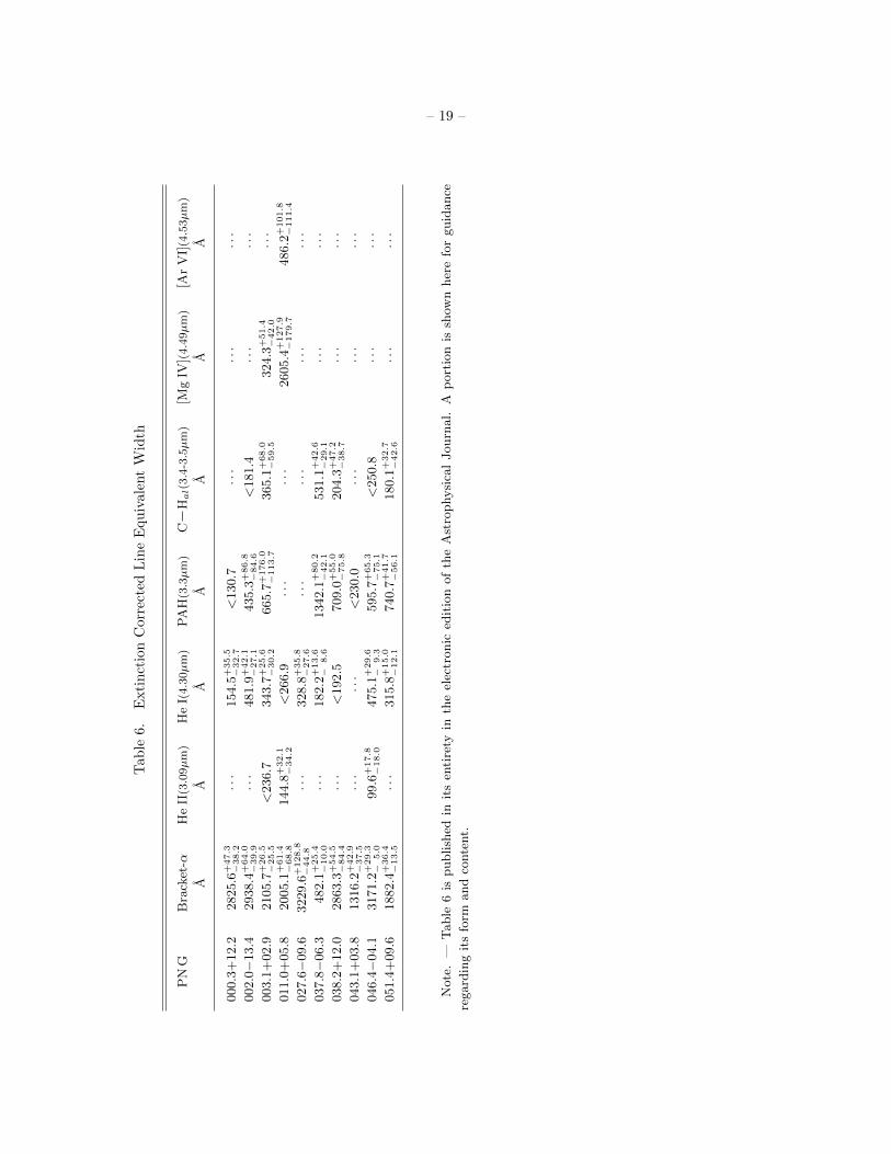
– 19 –
Tab
le6.
Exti
nct
ion
Corr
ecte
dL
ine
Equ
ivale
nt
Wid
th
PN
GB
rack
et-α
He
II(3.0
9µ
m)
He
I(4.3
0µ
m)
PA
H(3.3µ
m)
CH
al(
3.4
-3.5µ
m)
[Mg
IV](
4.4
9µ
m)
[Ar
VI]
(4.5
3µ
m)
AA
AA
AA
A
000.3
+12.2
2825.6
+47.3
−38.2
···
154.5
+35.5
−32.7
<130.7
···
···
···
002.0−
13.4
2938.4
+64.0
−39.9
···
481.9
+42.1
−27.1
435.3
+86.8
−84.6
<181.4
···
···
003.1
+02.9
2105.7
+26.5
−25.5
<236.7
343.7
+25.6
−30.2
665.7
+176.0
−113.7
365.1
+68.0
−59.5
324.3
+51.4
−42.0
···
011.0
+05.8
2005.1
+61.4
−68.8
144.8
+32.1
−34.2
<266.9
···
···
2605.4
+127.9
−179.7
486.2
+101.8
−111.4
027.6−
09.6
3229.6
+128.8
−44.8
···
328.8
+35.8
−27.6
···
···
···
···
037.8−
06.3
482.1
+25.4
−10.0
···
182.2
+13.6
−8.6
1342.1
+80.2
−42.1
531.1
+42.6
−29.1
···
···
038.2
+12.0
2863.3
+54.5
−84.4
···
<192.5
709.0
+55.0
−75.8
204.3
+47.2
−38.7
···
···
043.1
+03.8
1316.2
+42.9
−37.5
···
···
<230.0
···
···
···
046.4−
04.1
3171.2
+29.3
−5.0
99.6
+17.8
−18.0
475.1
+29.6
−9.3
595.7
+65.3
−75.1
<250.8
···
···
051.4
+09.6
1882.4
+36.4
−13.5
···
315.8
+15.0
−12.1
740.7
+41.7
−56.1
180.1
+32.7
−42.6
···
···
Note
.—
Table
6is
publish
edin
its
enti
rety
inth
eel
ectr
onic
edit
ion
of
the
Ast
rophysi
cal
Journ
al.
Ap
ort
ion
issh
own
her
efo
rguid
ance
regard
ing
its
form
and
conte
nt.

– 20 –
0
10
20
30
40
50
60
70
80
2.5 3.0 3.5 4.0 4.5 5.0
PNG 000.3+12.2 (3460107)
Flu
x D
ensi
ty (
10
−1
5W
m−
2µ
m−
1)
Wavelength (µm)
0
10
20
30
40
50
60
70
2.5 3.0 3.5 4.0 4.5 5.0
PNG 002.0−13.4 (3460003)
Flu
x D
ensi
ty (
10
−1
5W
m−
2µ
m−
1)
Wavelength (µm)
0
10
20
30
40
50
60
70
80
90
2.5 3.0 3.5 4.0 4.5 5.0
PNG 003.1+02.9 (3460005)
Flu
x D
ensi
ty (
10
−1
5W
m−
2µ
m−
1)
Wavelength (µm)
Fig. 7.— The AKARI /IRC 2.5–5.0µm spectra. Explanations of the lines are shown in the bottom of the
figures. Plots for all sources are available in the electronic edition of the journal.

– 21 –
0.0
0.1
0.2
-180 -120 -60 0 60 120 180
Fre
quen
cy
Galactic Longitude (deg)
Galactic PNePNSPC sample
0.0
0.1
0.2
0.3
0.4
-60 -30 0 30 60
Fre
quen
cy
Galactic Latitude (deg)
Galactic PNePNSPC sample
Fig. 8.— Histograms of PNe in the Galactic coordinates. The left panel shows the histogram of the Galactic
longitude, while the right panel shows that of the Galactic latitude. The histograms for the PNSPC objects
are shown by the blue boxes. The gray filled boxes represent the distribution of all the Galactic PNe in
Acker et al. (1992).
significant and that the PNSPC samples are biased toward PNe in the Galactic disk rather than those in the
bulge. Figure 9 shows the position of the PNSPC samples projected onto the Galactic plane. The distances
to the objects are taken from literature (Acker 1978; Acker et al. 1992; Amnuel et al. 1984; Cahn et al. 1992;
Gathier et al. 1986a,b; Maciel 1984; Pottasch 1983; Sabbadin 1986, and references therein). Figure 9 shows
that most of the PNSPC samples are within 5 kpc of the Sun, even when accounting for uncertainties in the
distance estimate. This also supports that the PNSPC samples mainly consist of PNe in the Galactic disk.
5.1.2. Effective Temperature and Age
The central star of a PN becomes hot as it evolves. The effective temperature of the PN can be used
as an indicator of the age of the PN. The timescale of the evolution depends on the mass of the central
star (e.g., Blocker 1995; Schonberner 1983). Although the individual age of the PN is difficult to accurately
derive from the effective temperature, the distribution of the effective temperature reflects the bias in the
age of the PNSPC samples. The effective temperatures were collected from literature. The temperature and
its references are listed in the sixth and seventh columns of Table 2. The effective temperature is estimated
with several different methods. The effective temperatures estimated based on a model atmosphere should
be the most reliable. The temperatures estimated in Mendez et al. (1988) and Harrington & Feibelman
(1983) are preferentially used, if available. The typical error for temperatures measured by this method is
about 10% (Mendez et al. 1988). Otherwise, the effective temperatures estimated with the Zanstra or the
Energy Balance methods are used. The Zanstra temperatures are estimated based on H I, He I, and He II
recombination lines. Since the radiation-bounded condition is assumed in the Zanstra method, the Zanstra
temperature estimated using the line with the highest ionization potential is most reliable. The Zanstra
temperatures are used with the preferential order of He II, He I, and H I. A typical uncertainty in the
Zanstra temperature is as large as 10,000 K in the worst case (Phillips 2003). Preite-Martinez et al. (1991)
reported that the typical uncertainty in the temperature with the Energy Balance method is no more than
20%. We assume that a typical uncertainty in these methods is about 20%. Finally, the effective temperature

– 22 –
0
5
10
15
-10 -5 0 5 10
Dis
tan
ce (kpc)
Distance (kpc)
8 kp
c
✧Galactic Center
SunPNSPC samples
Fig. 9.— Distribution of the PNSPC samples on the Galactic Plane. The red cross shows the locus of the
Sun. The purple circles show the positions of the PNSPC samples.

– 23 –
0.0
0.2
0.4
0.6
0.8
1.0
20 30 5010 100
Cu
mu
lati
ve H
isto
gram
Effective Temperature (103K)
Phillips (2003)PNSPC samples
Fig. 10.— Cumulative histogram of the effective temperature of Galactic PNe. The blue solid line shows
the histogram for the PNSPC samples. The gray dashed line represents the temperature distribution of all
the Galactic PNe in Phillips (2003).
was obtained for 67 of 72 objects in the catalog. When multiple references are available, the averaged value
is adopted.
Figure 10 shows the distribution of the effective temperature in the PNSPC samples. Phillips (2003)
collected the effective temperature of 373 Galactic PNe using the Zanstra method. Their samples were
widely collected from literature without any limitation. Thus, we assume that their samples are not biased
and that the temperature distribution of Phillips’ samples represents that of the whole Galactic PNe (gray
dashed line). The median of the effective temperature for the PNSPC samples is about 50 000 K, while
that for Phillips’ data is about 80 000 K. Figure 10 indicates that the PNSPC samples are biased toward
low-temperature or young PNe, possibly due to the target selection bias: the targets are limited by the
apparent size (∼3′′).

– 24 –
5.2. Accuracy of the Absolute Intensity
One of the major characteristics of the PNSPC catalog is slit-less spectroscopy in the Np-window, which
allows us to collect all of the flux from the target. Since the IRC spectrum totally covers the WISE W1 band,
the accuracy of the absolute flux density is evaluated by comparing the PNSPC spectra with the WISE W1
photometry from WISE All-Sky Release Catalog (Cutri et al. 2012). Define RW1 as the relative response
curve of the WISE W1 band (per photon; Wright et al. 2010). The flux in the W1 band estimated from the
IRC spectrum is defined as
F IRCν (W1) =
∫F objν (ν)RW1(ν)
dν
ν∫ (νisoν
)2RW1(ν)
dν
ν
, (10)
where νiso is the isophotal frequency of the W1 band (3.35µm) and F objν is the observed flux density in units
of Jy. Figure 11 shows the estimated flux density in the W1 band against the WISE W1 catalog data. It
confirms that the W1 flux density estimated from the IRC spectra, F IRCν (W1), is consistent with the WISE
W1 data in a wide range from about 0.01 to 5 Jy. The histogram of the AKARI to WISE W1 flux ratio is
shown in Figure 12. Errors in Figure 12 are calculated by a Monte Carlo simulation with the uncertainty
in the flux ratio. The ratios are distributed with the mean of 1.01±0.01 and the standard deviation of
0.21±0.02. Three PNe (PNG 285.7−14.9, 324.8−01.1, and 305.1+01.4) show significant deviations larger
than 50%. For PNG 285.7−14.9 and 305.1+01.4, their AKARI W1 fluxes are larger than those of WISE.
Both objects are apparently extended in WISE W1 images. The deviations may be attributed to the loss of
the flux in WISE photometry. Furthermore, PNG 305.1+01.4 is the brightest object in the PNSPC sample.
The WISE detector starts to saturate in the W1 band at ∼0.17 Jy (Wright et al. 2010). This may also cause
an error in WISE photometry of PNG 305.1+01.4. The AKARI W1 flux of PNG 324.8−01.1 is smaller than
the WISE W1 flux. PNG 324.8−01.1 is located in a crowded region, so that the IRC field of view may not
be wide enough to estimate background emission accurately. The loss of the AKARI W1 flux is attributable
to the error in the estimation of the background emission. Thus, although the absolute continuum intensity
of PNG 324.8−01.1 may be erroneous, the intensity of emission features is not affected by the estimation of
background emission. The absolute flux of the present catalog is concluded to be accurate within 20%.
5.3. Extinction within the Individual Nebula
The PNSPC spectra include Brackett-α (Brα), the hydrogen recombination line at 4.05µm, which
enables us to estimate the extinction towards the objects using the relative intensity of Hβ to Brα (the
intensity of Hβ is from Acker et al. (1992), see Section 4.2). The cumulative histogram of the total extinction
towards the PNSPC samples, AV (Hβ), is shown by the dotted line in Figure 13. The extinction toward the
PNSPC samples are less than 6 mag. at the V -band. About 70% of the PNSPC samples have AV(Hβ) <
2 mag., suggesting that most of the PNSPC samples are not heavily obscured. This is consistent with the
Galactic distribution of the PNSPC sample shown in Section 5.1.1.
The extinction values calculated in Section 4.2 include the contribution from their circumstellar envelope,
AV,PN, and the interstellar medium to the object, AV, ISM. The contribution from the interstellar medium,
AV, ISM, can be estimated using the extinction map based on the Digitized Sky Survey (Dobashi et al.
2005a,b). The extinction map is given in the resolution of 2′×2′. We calculate the averaged extinction
values within a 6′ radius around the object AV (DSS) and assumed them as AV, ISM. Dobashi et al. (2005a)
showed that a systematic error in AV (DSS) is typically less than 0.2 mag for AV (DSS) < 5 mag. We

– 25 –
10-3
10-2
10-1
100
101
10-3 10-2 10-1 100 101
FνIR
C(W
1): A
KA
RI
W1 flu
x (J
y)
FνWISE(W1): WISE W1 flux (Jy)
AKARI:WISE=1:1WISE W1 Flux
285.7-14.9
305.1+01.4
324.8-01.1
Fig. 11.— Flux comparison between the AKARI and WISE observations. The vertical axis shows the flux
in the WISE W1 filter estimated from the AKARI /IRC spectra, while the horizontal axis shows the flux in
the WISE All-Sky Release Catalog (Cutri et al. 2012). When the deviation between the AKARI and WISE
W1 fluxes is larger than 50%, the data point is labeled with the PNG ID.

– 26 –
0
5
10
15
20
25
0.0 0.5 1.0 1.5 2.0
Fre
quen
cy
FνIRC(W1)/Fν
WISE(W1) ratio
FνIRC(W1)/Fν
WISE(W1)
Fig. 12.— Distribution of the flux ratio: the flux in the WISE W1 filter estimated from the AKARI /IRC
spectra to that from the WISE All-Sky Release Catalog.

– 27 –
estimate the uncertainty in AV, ISM from the scatter of AV (DSS) within the 6′ circle taking into account
the systematic error. Note that the extinction AV, ISM estimated here may have a large uncertainty. The
extinction from the circumstellar envelope, defined by AV (Hβ) − AV (DSS), is shown by the solid line in
Figure 13. Some objects show negative extinction values (∼0.5 mag.), possibly due to the overestimation
of AV, ISM. Figure 14 shows the dependence of AV (Hβ) − AV (DSS) on the distance towards the PN. We
find that PNe with extinction >2 mag. frequently appear around 2 kpc. The name of the constellation is
added next to those PNe, indicating that most of them are in the regions around Cygnus and Norma as
indicated by the orange and green symbols. The extinction AV, ISM for these PNe may be underestimated or
have large local fluctuations, but this affects only about 10% of the PNSPC samples. Except for the objects
in the Cygnus and Norma regions, Figure 14 does not show any trend with the distance, suggesting that
the AV (Hβ)−AV (DSS) value is attributable to the extinction internal to the PN. Figure 13 indicates that
the median of the circumstellar extinction is about 0.8 mag. and about 40% of the PNe show extinction
larger than 1 mag. suggesting that the circumstellar envelope of a PN is generally optically thick in the UV.
Ohsawa et al. (2012) investigated the spatial distribution of mid-infrared dust emission of PN G095.2+00.7,
a young and UV-thick Galactic PN, and suggest that the evolution of a UV-thick circumstellar envelope may
have a significant impact on the appearance of the mid-infrared spectrum of the PN. The present results
suggest that PNe spectra should be investigated by taking into account the radiation transfer within the
nebula, and the gradient in the dust temperature.
5.4. Equivalent Width of Ionized Gas Emission Lines
The spectra in the PNSPC catalog contain several emission lines, including hydrogen and helium re-
combination lines and fine-structure lines of [Mg IV] at 4.49µm and [Ar VI] at 4.53µm. These emission
lines should reflect the characteristics of the radiation field of the circumstellar envelope. Figure 15 shows
the equivalent widths of Brα, He I at 4.30µm, He II at 3.09µm, and the summation of [Mg IV] and [Ar VI]
against the effective temperature of the central star. Since the [Mg IV] and [Ar VI] lines are close to each
other, the equivalent width of the summation of these lines is used. The data whose signal-to-noise ra-
tio of the equivalent width is less than three are replaced by 3-σ upper limits. When the emission is not
detected, the effective temperature is indicated by the crosses. The equivalent width of Brα is typically
about 1–3×10³ A and does not show a clear dependence on the effective temperature. The He I line is
seen from 20 000 to 150 000 K. Its equivalent width is almost constant at about 2×10² A. It shows a small
increase from 30 000–50 000 K, possibly explained by the increase in photons with enough energy to ionize He
with increasing effective temperature. When the effective temperature exceeds 50 000 K, the He I equivalent
width stops increasing and shows a small decrease. At the same time, the He II lines start to be detected,
suggesting that high-energy photons are in part used to ionize He+. The decrease in the He I equivalent
width is attributable to the ionization balance between He+ and He++. The He II, [Mg IV], and [Ar VI] lines
are not detected until the effective temperature exceeds about 50 000 K. The ionization potentials of He II,
Mg IV, and Ar VI are 54.41, 109.27, and 91.00 eV. Although the ionization potential of He II is about two
times lower than those of Mg IV, and Ar VI, the He II, [Mg IV], and [Ar VI] lines start to appear at almost
the same temperature in Figure 15. The equivalent width of the He II line is typically about 2×10² A, not
showing a clear trend with the effective temperature. The equivalent width of the [Mg IV]+[Ar VI] becomes
as large as 8×10³ A at a high temperature of about 100 000 K. Figure 16 shows the intensity ratio of the
[Mg IV]+[Ar VI] to Brα. The effective temperature of the PNe with the ratio larger than unity ranges about
500 000–150 000 K. The [Mg IV] and [Ar VI] lines are an indicator of high-temperature PNe as expected. But
note that some PNe with high effective temperature show a ratio less than unity. A ratio less than unity

– 28 –
0.0
0.2
0.4
0.6
0.8
1.0
−1 0 1 2 3 4 5 6
Cu
mu
lati
ve H
isto
gram
Av (mag.)
Av(Hβ)Av(Hβ)−Av(DSS)
Fig. 13.— Cumulative histogram of the extinction at the V -band. The dotted line shows the histogram
of the total extinction towards the PN. The solid line shows the histogram of the extinction without the
contribution from the interstellar medium.

– 29 –
0.0
1.0
2.0
3.0
4.0
5.0
0 2 4 6 8 10
Av(H
β)−A
v(D
SS
) (m
ag.)
Distance (kpc)
Av(Hβ)−Av(DSS)Cyg & Vul
Nor, Lup, & Cir
Vul
Cyg Cyg
Cyg
MonCMaVela
Cir
Lup
Nor
Nor
Nor
Cen
Fig. 14.— Net extinction at the V -band is plotted against a distance towards the PN. Errors in the distance
are assumed to be about 20%. The name of the constellation is added next to the symbols for the PN with
the net extinction >2.0 mag. The PNe in Cygnus and Vulpecula are indicated by the orange filled circles,
while the PNe in Norma, Lupus and Circinus are indicated by the green filled circles.

– 30 –
Equ
ival
ent
Wid
th (Å
)
Effective Temperature (103K)
Brackett−α
101
102
103
104
20 30 50 200100
Equ
ival
ent
Wid
th (Å
)
Effective Temperature (103K)
He I 4.30µm
↓↓
↓
↓
↓
↓↓ ↓↓
↓
↓↓
↓
↓
↓
×
101
102
103
104
20 30 50 200100
Equ
ival
ent
Wid
th (Å
)
Effective Temperature (103K)
He II 3.09µm
↓
× × ×× ××× ××××× × ××× × ××× ×××× ×× × × ×× ××× ×× ×× ×× ××
101
102
103
104
20 30 50 200100
Equ
ival
ent
Wid
th (Å
)
Effective Temperature (103K)
[MgIV] 4.49µm + [ArVI] 4.53µm
× × ×× ×××× ××××× × ××× × ××× ×××× ×× × × ×× ××× ×× ×× ×× ××
101
102
103
104
20 30 50 200100
Fig. 15.— Equivalent widths of Brackett-α at 4.05µm (upper left), He I at 4.30µm (upper right), He II
at 3.09µm (lower left), and [Mg IV] at 4.49µm + [Ar VI] at 4.53µm (lower right) against the effective
temperature. The downward arrows indicate a 3-σ upper limit. When the emission is not detected, the
effective temperature is indicated by the crosses.
does not necessarily indicate a PN with a low effective temperature.
5.5. PAH Features of Galactic PNe in the Near-Infrared
The PAH features appear both in the near- and mid-infrared, and the PAH features in the mid-infrared
are stronger than those in the near-infrared (e.g., Draine & Li 2001; Schutte et al. 1993). The PAH features
of PNe in the mid-infrared have been intensively investigated with Spitzer (e.g., Bernard-Salas et al. 2009;
Stanghellini et al. 2012, 2007). Surveys of the 3.3µm PAH feature in Galactic PNe were carried out by
Roche et al. (1996) and Smith & McLean (2008). Their samples were, however, biased towards carbon-rich
objects. The PNSPC samples are not selected based on their chemistry. The PNSPC catalog provides a
useful data set to investigate the near-infrared PAH features in Galactic PNe.
The type of dust features (carbon-rich or oxygen-rich) is thought to be closely related to the abundance
ratio of nebular gas. Several studies have suggested that the intensities of the PAH features increases with
the carbon-to-oxygen abundance (C/O) ratio (e.g., Cohen et al. 1986; Cohen & Barlow 2005; Roche et al.
1996; Smith & McLean 2008). However, PAH formation both in carbon-rich and oxygen-rich environments
has been suggested recently (Guzman-Ramirez et al. 2014, 2011). Delgado-Inglada & Rodrıguez (2014)
measured the C/O ratio of 51 Galactic PNe and confirmed that the PAH emission can be seen even in
PNe with C/O < 1. The C/O ratios of 11 PNe in the PNSPC catalog were measured by Delgado-Inglada
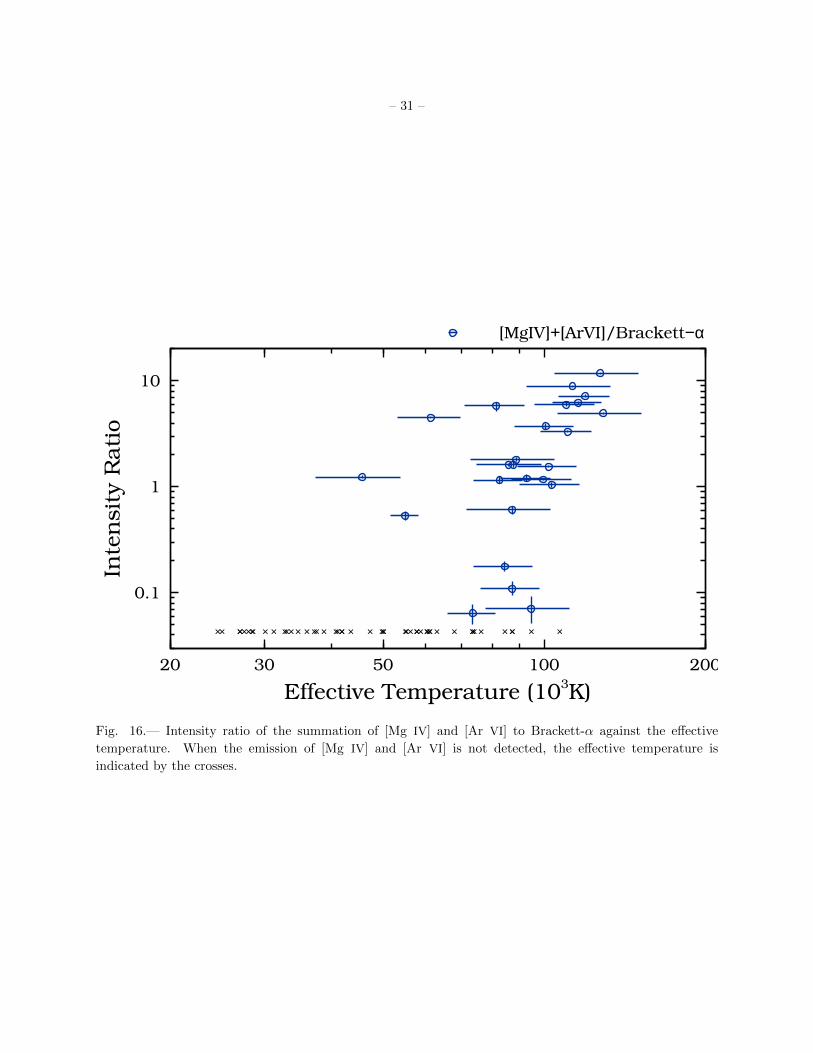
– 31 –In
ten
sity
Rat
io
Effective Temperature (103K)
[MgIV]+[ArVI]/Brackett−α
× ×× ×× ×× ×× ××× ×××× × ××× × ××× ×××× ×× × × ×× ××× × × ×× ×× ×× × ××
0.1
1
10
20 30 50 200100
Fig. 16.— Intensity ratio of the summation of [Mg IV] and [Ar VI] to Brackett-α against the effective
temperature. When the emission of [Mg IV] and [Ar VI] is not detected, the effective temperature is
indicated by the crosses.

– 32 –
& Rodrıguez (2014). Figure 17 shows the equivalent width of the 3.3µm PAH feature against the C/O
ratio. The C/O ratio measured by collisionally excited lines (CEL) is indicated by the blue circles, while
that measured by recombination lines (RL) is shown by the red squares. The downward arrows indicate
non-detection of the 3.3µm PAH features. Figure 17 shows that the 3.3µm PAH emission is detected even
in oxygen-rich environments, consistent with Delgado-Inglada & Rodrıguez (2014). Due to the small number
of samples, however, it is difficult to claim the correlation between the strength of the 3.3µm PAH feature
and the C/O ratio. Extensive measurements of the C/O ratio are encouraged.
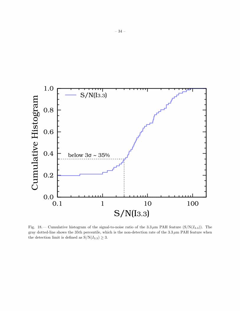
Figure 18 shows a cumulative histogram of the signal-to-noise ratio of the 3.3µm PAH feature (hereafter,
S/N(I3.3)). The gray dotted line shows the 35th percentile, which corresponds to S/N(I3.3) = 3. The result
suggests that about 65% of the PNSPC samples show band emission at 3.3µm. The 5–38µm spectra of
Galactic PNe with Spitzer/IRS are available in Stanghellini et al. (2012). We counted the number of PNe
with PAH features, obtaining 40% (60 of 150 PNe). Despite the intrinsic weakness of the near-infrared
PAH features, the PAH detection rate is as high in the near-infrared as in the mid-infrared. The 3.3µm
feature is thought to come from the smallest PAH populations, which are most fragile, and thus primarily
reflect environment variations (Allain et al. 1996a,b; Micelotta et al. 2010; Schutte et al. 1993). The PNSPC
catalog is useful to investigate the evolution of the PAH features and the processing of PAHs in circumstellar
environments.
6. Summary & Conclusion
Near-infrared (2.5–5.0µm) spectra of 72 Galactic PNe were obtained at high sensitivity using the
AKARI /IRC. The PNSPC program provided a set of near-infrared spectra that collected all of the flux
from the objects. The absolute flux of spectra provided by the PNSPC program is in agreement with the
WISE W1 photometry within ∼20%. These spectra were compiled into the PNSPC catalog. The intensity
and equivalent width of Brackett-α, He I at 4.30µm, He II at 3.09µm, the 3.3µm PAH feature, the 3.4–
3.5µm aliphatic feature complex, [Mg IV] at 4.49µm, and [Ar VI] at 4.53µm were measured. The detection
limit of the emission features was as faint as 2×10⁻¹⁶ W m−2. The PNSPC catalog is the largest data set
of near-infrared spectra of Galactic PNe. It provides unique information for the investigation of 2.5–5.0µm
emission of Galactic PNe.
The Galactic coordinates of the PNSPC samples suggest that the objects in the PNSPC catalog are
biased toward PNe in the Galactic disk rather than those in the Galactic bulge. The median of the effective
temperature of the PNSPC samples is lower than that of the whole Galactic PNe by about 30,000 K. This
indicates that the PNSPC catalog is biased toward young PNe. This bias possibly originates in the criterion
on the apparent size in the target selection.
The PNSPC catalog also provides the extinction toward the objects. Even after the contribution from
the interstellar medium is taken into account, Figure 13 suggests that 40% of PNe have extinction at the
V -band larger than unity, which is attributed to the extinction in the circumstellar envelope. The present
result suggests that for a large fraction of PNe a circumstellar envelope is optically thick in the UV.
The equivalent width of Brakett-α does not show a clear dependence on the effective temperature. The
variations in the He I and He II equivalent widths can be attributed to the ionization balance between
He+ and He++. The [Mg IV] at 4.49µm and [Ar VI] at 4.53µm lines are only detected when the effective
temperature becomes higher than 50 000 K. The [Mg IV] and [Ar VI] lines are good indicators of PNe with
a hot central star.

– 33 –
102
103
104
−0.6 −0.4 −0.2 0.0 0.2 0.4 0.6
3.3
µm
Equ
ival
ent
Wid
th (Å
)
log [C/O]CRL,RL
↓↓ ↓↓↓ ↓↓↓↓↓↓↓↓↓↓↓ ↓ ↓↓ ↓↓↓↓↓↓↓↓↓
[C/O]CEL [C/O]RL
Fig. 17.— Equivalent width of the 3.3µm PAH feature against the carbon-to-oxygen (C/O) ratio. The C/O
ratios are from Delgado-Inglada & Rodrıguez (2014). The C/O ratio measured by collisionally excited lines
(CEL) is shown by the blue circles, while the C/O ratio measured by recombination lines (RL) is by the red
squares. The arrows indicate the non-detection of the 3.3µm PAH feature.
– 34 –
0.0
0.2
0.4
0.6
0.8
1.0
0.1 1 10 100
below 3σ ~ 35%
Cu
mu
lati
ve H
isto
gram
S/N(I3.3)
S/N(I3.3)
Fig. 18.— Cumulative histogram of the signal-to-noise ratio of the 3.3µm PAH feature (S/N(I3.3)). The
gray dotted-line shows the 35th percentile, which is the non-detection rate of the 3.3µm PAH feature when
the detection limit is defined as S/N(I3.3) ≥ 3.

– 35 –
The 3.3µm PAH feature is detected in about 65% of the PNSPC samples. This detection rate is
comparable to that reported from mid-infrared observations (Stanghellini et al. 2012). The present result
suggests that the AKARI /IRC is as sensitive as the Spitzer/IRS in terms of detecting the PAH features.
The PNSPC catalog provides a suitable data set to investigate PAHs in circumstellar environments. The
near-infrared PAH features are attributed to small-sized PAHs, which are sensitive to harsh environments
and processed faster than larger ones. The processing and evolution of PAHs during the PN phase will be
discussed in the forth-coming paper.
The present results are based on observations with AKARI, a JAXA project with the participation of
ESA. We greatly appreciate all the people who worked in the operation and maintenance of those instruments.
This publication makes use of data products from the Wide-field Infrared Survey Explorer, which is a joint
project of the University of California, Los Angeles, and the Jet Propulsion Laboratory/California Institute
of Technology, funded by the National Aeronautics and Space Administration. This research has made use
of the SIMBAD database, operated at CDS, Strasbourg, France. This work is supported in part by Grant-
in-Aids for Scientific Research (25-8492, 23244021, and 26247074) by the Japan Society of Promotion of
Science (JSPS).
REFERENCES
Acker, A. 1978, Astronomy and Astrophysics Supplement Series, 33, 367
Acker, A., Marcout, J., Ochsenbein, F., Stenholm, B., & Tylenda, R. 1992, Strasbourg-ESO Catalogue of
Galactic Planetary Nebulae, Parts I, II (Garching, Germany: European Southern Observatory)
Allain, T., Leach, S., & Sedlmayr, E. 1996a, Astronomy and Astrophysics, 305, 602
—. 1996b, Astronomy and Astrophysics, 305, 616
Amnuel, P. R., Guseinov, O. K., Novruzova, K. I., & Rustamov, I. S. 1984, Astrophysics and Space Science,
107, 19
Baker, J. G., & Menzel, D. H. 1938, The Astrophysical Journal, 88, 52
Beintema, D. A., van den Ancker, M. E., Molster, F. J., et al. 1996, Astronomy and Astrophysics, 315, L369
Bernard-Salas, J., Peeters, E., Sloan, G. C., et al. 2009, The Astrophysical Journal, 699, 1541
Bernard-Salas, J., Pottasch, S. R., Gutenkunst, S., Morris, P. W., & Houck, J. R. 2008, The Astrophysical
Journal, 672, 274
Bernard-Salas, J., & Tielens, A. G. G. M. 2005, Astronomy and Astrophysics, 431, 523
Blocker, T. 1995, Astronomy and Astrophysics, 299, 755
Boulanger, F., Onaka, T., Pilleri, P., & Joblin, C. 2011, in EAS Publications Series, Vol. 46, PAHs and
the Universe: A Symposium to Celebrate the 25th Anniversary of the PAH Hypothesis (Toulouse,
France: EAS Publications Series), 399–405
Cahn, J. H., Kaler, J. B., & Stanghellini, L. 1992, Astronomy and Astrophysics Supplement Series, 94, 399
– 36 –
Cohen, M., Allamandola, L., Tielens, A. G. G. M., et al. 1986, The Astrophysical Journal, 302, 737
Cohen, M., & Barlow, M. J. 2005, Monthly Notices of the Royal Astronomical Society, 362, 1199
Cutri, R. M., Wright, E. L., Conrow, T., et al. 2012, VizieR Online Data Catalog, 2311
Delgado-Inglada, G., & Rodrıguez, M. 2014, The Astrophysical Journal, 784, 173
Dobashi, K., Uehara, H., Kandori, R., et al. 2005a, Publications of the Astronomical Society of Japan, 57, 1
—. 2005b, Publications of the Astronomical Society of Japan, 57, 417
Draine, B. T., & Li, A. 2001, The Astrophysical Journal, 551, 807
Dwek, E., Arendt, R. G., Fixsen, D. J., et al. 1997, The Astrophysical Journal, 475, 565
Gathier, R., Pottasch, S. R., & Goss, W. M. 1986a, Astronomy and Astrophysics, 157, 191
Gathier, R., Pottasch, S. R., & Pel, J. W. 1986b, Astronomy and Astrophysics, 157, 171
Guzman-Ramirez, L., Lagadec, E., Jones, D., Zijlstra, A. A., & Gesicki, K. 2014, Monthly Notices of the
Royal Astronomical Society, 441, 364
Guzman-Ramirez, L., Zijlstra, A. A., Nıchuimın, R., et al. 2011, Monthly Notices of the Royal Astronomical
Society, 414, 1667
Harrington, J. P., & Feibelman, W. A. 1983, The Astrophysical Journal, 265, 258
Joblin, C., Tielens, A. G. G. M., Allamandola, L. J., & Geballe, T. R. 1996, The Astrophysical Journal, 458,
610
Kaler, J. B. 1976, The Astrophysical Journal, 210, 843
—. 1978, The Astrophysical Journal, 220, 887
Kaler, J. B., & Jacoby, G. H. 1991, The Astrophysical Journal, 372, 215
Lumsden, S. L., Puxley, P. J., & Hoare, M. G. 2001, Monthly Notices of the Royal Astronomical Society,
320, 83
Maciel, W. J. 1984, Astronomy and Astrophysics Supplement Series, 55, 253
Mathis, J. S. 1990, Annual Review of Astronomy and Astrophysics, 28, 37
Mendez, R. H., Kudritzki, R. P., Herrero, A., Husfeld, D., & Groth, H. G. 1988, Astronomy and Astrophysics,
190, 113
Micelotta, E. R., Jones, A. P., & Tielens, A. G. G. M. 2010, Astronomy and Astrophysics, 510, 37
Mori, T. I., Sakon, I., Onaka, T., et al. 2012, The Astrophysical Journal, 744, 68
Noble, J. A., Fraser, H. J., Aikawa, Y., Pontoppidan, K. M., & Sakon, I. 2013, The Astrophysical Journal,
775, 85
Ohsawa, R., Onaka, T., Sakon, I., et al. 2012, The Astrophysical Journal Letters, 760, L34

– 37 –
Onaka, T., Matsuhara, H., Wada, T., et al. 2007, Publications of the Astronomical Society of Japan, 59, 401
Phillips, J. P. 2003, Monthly Notices of the Royal Astronomical Society, 344, 501
Phillips, J. P., & Marquez-Lugo, R. A. 2011, Revista Mexicana de Astronomia y Astrofisica, 47, 83
Pottasch, S. R. 1983, in IAU Symposium, Vol. 103, Planetary Nebulae (London, United Kingdom: Dordrecht,
D. Reidel Publishing Co.), 391–409
Pottasch, S. R., & Bernard-Salas, J. 2006, Astronomy and Astrophysics, 457, 189
Pottasch, S. R., Baud, B., Beintema, D., et al. 1984, Astronomy and Astrophysics, 138, 10
Preite-Martinez, A., Acker, A., Koppen, J., & Stenholm, B. 1989, Astronomy and Astrophysics Supplement
Series, 81, 309
—. 1991, Astronomy and Astrophysics Supplement Series, 88, 121
Roche, P. F., Lucas, P. W., Hoare, M. G., Aitken, D. K., & Smith, C. H. 1996, Monthly Notices of the Royal
Astronomical Society, 280, 924
Sabbadin, F. 1986, Astronomy and Astrophysics Supplement Series, 64, 579
Sakon, I., Onaka, T., Wada, T., et al. 2008, in Society of Photo-Optical Instrumentation Engineers (SPIE)
Conference Series, Vol. 7010, Space Telescopes and Instrumentation 2008: Optical, Infrared, and
Millimeter, 88
Schonberner, D. 1983, The Astrophysical Journal, 272, 708
Schonberner, D., & Blocker, T. 1996, Astrophysics and Space Science, 245, 201
Schonberner, D., Jacob, R., Steffen, M., et al. 2005, Astronomy and Astrophysics, 431, 963
Schutte, W. A., Tielens, A. G. G. M., & Allamandola, L. J. 1993, The Astrophysical Journal, 415, 397
Skrutskie, M. F., Cutri, R. M., Stiening, R., et al. 2006, The Astronomical Journal, 131, 1163
Sloan, G. C., Bregman, J. D., Geballe, T. R., Allamandola, L. J., & Woodward, C. E. 1997, The Astrophysical
Journal, 474, 735
Sloan, G. C., Kraemer, K. E., Price, S. D., & Shipman, R. F. 2003, The Astrophysical Journal Supplement
Series, 147, 379
Smith, E. C. D., & McLean, I. S. 2008, Astrophysical Journal, 676, 408
Stanghellini, L., Garcıa-Hernandez, D. A., Garcıa-Lario, P., et al. 2012, The Astrophysical Journal, 753, 172
Stanghellini, L., Garcıa-Lario, P., Garcıa-Hernandez, D. A., et al. 2007, The Astrophysical Journal, 671,
1669
Stanghellini, L., & Haywood, M. 2010, The Astrophysical Journal, 714, 1096
Storey, P. J., & Hummer, D. G. 1995, Monthly Notices of the Royal Astronomical Society, 272, 41
Tokunaga, A. T., Sellgren, K., Smith, R. G., et al. 1991, Astrophysical Journal, 380, 452

– 38 –
Volk, K., & Cohen, M. 1990, The Astronomical Journal, 100, 485
Wright, E. L., Eisenhardt, P. R. M., Mainzer, A. K., et al. 2010, The Astronomical Journal, 140, 1868
This preprint was prepared with the AAS LATEX macros v5.2.

– 39 –
Table 2. Miscellaneous Information of Objects
PN G V (a) K(b)s AV (Hβ) AV (fit.) Teff Refs. Teff
mag. mag. mag. mag. 103 K
000.3+12.2 13.9 11.4 0.90+0.03−0.03 0.98+0.15
−0.05 47 Ka76,Ph03
002.0−13.4 14.1 11.1 0.31+0.02−0.01 0.38+0.02
−0.04 60 PM89,PM91,Ph03
003.1+02.9 >17.0 11.6 3.31+0.03−0.03 3.4+0.6
−0.1 87 PM89,Ph03
011.0+05.8 · · · 11.8 1.81+0.04−0.04 1.79+0.06
−0.06 93 PM91,Ph03
027.6−09.6 15.2 11.9 1.04+0.06−0.05 1.0+0.9
−0.2 58 PM91,Ka76,KJ91,Ph03
037.8−06.3 · · · 9.47 1.4+0.1−0.1 1.41+0.08
−0.02 74 Ph03
038.2+12.0 12.5 11.1 0.82+0.05−0.05 0.93+0.07
−0.07 30 Ka78,Ph03
043.1+03.8 14.9 12.1 1.9+0.1−0.1 2.05+0.46
−0.05 28 Ph03
046.4−04.1 15.2 11.1 1.42+0.02−0.02 1.39+0.01
−0.01 68 Ka76,KJ91,Ph03
051.4+09.6 13.3 10.4 0.88+0.05−0.04 0.98+0.11
−0.08 37 Ka76,Ka78,Ph03
052.2−04.0 18.1 12.0 1.68+0.05−0.04 1.62+0.09
−0.09 61 Lu01,PM89,KJ91,Ph03
058.3−10.9 14.4 9.67 0.66+0.05−0.05 0.18+0.08
−0.04 50 PM89,Ka76,Ph03
060.1−07.7 18.0 11.5 1.19+0.02−0.02 1.28+0.03
−0.02 129 Ph03
060.5+01.8 · · · 11.8 4.1+0.2−0.2 3.5+0.5
−0.4 · · · · · ·064.7+05.0 12.5 8.11 1.44+0.04
−0.04 1.43+0.05−0.04 28 Lu01,Ka76,Ka78,Ph03
071.6−02.3 >15.7 10.1 4.4+0.1−0.1 5.1+1.3
−0.7 · · · · · ·074.5+02.1 18.4 11.0 3.43+0.07
−0.07 3.47+1.32−0.04 81 Ph03
082.1+07.0 >15.6 10.7 1.71+0.07−0.08 1.7+2.3
−0.1 87 Ph03
082.5+11.3 14.5 12.2 0.17+0.04−0.04 0.16+0.08
−0.05 63 Me88
086.5−08.8 17.3 12.5 0.60+0.03−0.03 0.52+0.03
−0.03 61 Lu01,Ph03
089.3−02.2 12.1 9.20 2.0+0.8−0.5 1.90+5.40
−0.01 · · · · · ·089.8−05.1 16.7 9.49 1.99+0.04
−0.04 2.02+0.02−0.01 83 Ka78,KJ91,Ph03
095.2+00.7 · · · 11.2 5.5+0.3−0.2 5.4+0.4
−0.1 58 Lu01
100.6−05.4 15.5 12.0 0.52+0.03−0.03 0.47+0.05
−0.07 74 Ka78,KJ91,Ph03
111.8−02.8 13.8 8.81 1.92+0.10−0.10 2.12+0.01
−0.76 41 Ka76,Ph03
118.0−08.6 14.2 12.9 0.41+0.10−0.10 0.32+0.02
−0.03 55 Lu01,Ka76,KJ91,Ph03
123.6+34.5 13.4 11.9 0.50+0.03−0.03 0.60+0.09
−0.03 50 HF83
146.7+07.6 14.0 11.2 1.55+0.09−0.09 1.56+0.29
−0.02 27 Ph03
159.0−15.1 15.8 12.6 0.44+0.04−0.04 0.40+0.02
−0.06 89 Ph03
166.1+10.4 11.6 10.6 0.63+0.02−0.02 0.64+0.02
−0.03 39 Ka76,Ka78,Ph03
190.3−17.7 14.4 13.2 0.34+0.03−0.03 0.36+0.10
−0.04 61 PM89,Ka76,KJ91,Ph03
194.2+02.5 17.8 10.6 1.40+0.06−0.06 1.41+0.04
−0.12 88 PM89,Ph03
211.2−03.5 15.8 10.6 3.5+0.2−0.2 3.49+0.03
−0.02 33 Lu01,PM89,Ph03
221.3−12.3 17.9 11.0 0.91+0.01−0.01 0.91+0.10
−0.02 111 PM91,Ph03
226.7+05.6 16.9 12.8 1.63+0.02−0.03 1.61+0.11
−0.05 46 Ph03
232.8−04.7 13.9 9.48 2.96+0.06−0.06 2.99+0.39
−0.09 25 Lu01,PM89,Ph03
235.3−03.9 14.1 10.6 1.6+0.2−0.2 1.62+0.01
−0.01 29 Lu01,PM89,Ph03
258.1−00.3 16.2 10.9 4.02+0.03−0.03 4.02+0.05
−0.04 60 PM91,Ph03
264.4−12.7 14.7 12.2 0.72+0.07−0.07 0.6+0.1
−0.1 56 PM91,KJ91
268.4+02.4 18.7 10.6 3.80+0.03−0.03 3.91+0.23
−0.05 110 PM91,Ph03

– 40 –
Table 2—Continued
PN G V (a) K(b)s AV (Hβ) AV (fit.) Teff Refs. Teff
mag. mag. mag. mag. 103 K
278.6−06.7 · · · 12.3 0.73+0.03−0.03 0.75+0.10
−0.05 84 PM91,Ph03
283.8+02.2 17.2 12.3 1.57+0.02−0.02 1.35+0.01
−0.01 113 Ph03
285.4−05.3 15.5 11.6 0.75+0.03−0.02 0.68+0.03
−0.01 100 PM91,Ph03
285.6−02.7 13.0 10.2 2.11+0.02−0.02 2.16+0.06
−0.05 34 PM89,Ph03
285.7−14.9 14.2 13.3 0.14+0.03−0.03 0.14+0.02
−0.03 55 Me88
291.6−04.8 15.4 10.5 1.80+0.02−0.02 1.79+0.13
−0.03 116 PM91,Ph03
292.8+01.1 · · · 12.5 2.03+0.02−0.03 2.16+0.19
−0.07 95 PM91
294.9−04.3 · · · 11.5 1.80+0.02−0.02 1.80+0.08
−0.05 41 PM89
296.3−03.0 16.1 11.6 2.32+0.05−0.05 2.38+0.35
−0.06 103 PM91,Ph03
304.5−04.8 16.4 10.8 1.34+0.04−0.04 1.34+0.05
−0.02 102 PM91,Ph03
305.1+01.4 15.6 7.93 3.5+0.1−0.1 3.50+0.02
−0.05 59 PM91,KJ91,Ph03
307.2−09.0 15.3 11.6 1.16+0.02−0.02 1.10+0.05
−0.03 50 PM89,KJ91,Ph03
307.5−04.9 · · · 10.8 1.6+0.2−0.1 1.64+0.07
−0.03 38 PM89,Ph03
312.6−01.8 15.1 11.9 3.17+0.03−0.03 3.35+0.47
−0.08 42 PM89,KJ91,Ph03
315.1−13.0 11.0 9.36 0.5+0.1−0.1 9+1
−5 27 PM89,Ka78,Ph03
320.1−09.6 10.9 10.1 0.72+0.08−0.07 0.63+3.31
−0.05 27 Me88
320.9+02.0 >17.9 10.2 4.96+0.09−0.09 7+2
−2 44 PM89
322.5−05.2 15.3 12.7 0.80+0.03−0.03 0.89+0.19
−0.04 127 Ph03
323.9+02.4 16.8 11.8 3.05+0.03−0.03 3.01+0.05
−0.22 42 PM89,Ph03
324.8−01.1 · · · 10.6 6.34+0.02−0.03 6.5+0.3
−0.2 · · · · · ·325.8−12.8 13.4 11.1 0.50+0.03
−0.03 0.9+0.5−0.1 36 Me88
326.0−06.5 13.1 11.8 1.23+0.07−0.07 1.16+0.04
−0.05 25 Me88
327.1−01.8 17.2 11.5 3.83+0.04−0.03 4.2+0.2
−0.3 35 PM89,Ph03
327.8−01.6 · · · 11.0 5.10+0.03−0.03 5.7+0.7
−0.5 · · · · · ·331.1−05.7 12.7 10.3 1.4+0.1
−0.1 1.36+3.35−0.03 31 PM89,Ph03
331.3+16.8 15.5 12.5 0.10+0.03−0.03 0.78+0.01
−0.46 86 PM89,Ph03
336.3−05.6 16.6 12.2 1.32+0.07−0.06 1.36+0.02
−0.03 101 PM91,Ph03
342.1+27.5 · · · 13.2 0.25+0.02−0.02 0.27+0.47
−0.04 119 PM89,Ph03
349.8+04.4 17.0 12.1 1.9+0.2−0.1 2.1+0.1
−0.1 76 PM89
350.9+04.4 13.3 10.3 1.83+0.07−0.08 1.83+2.23
−0.02 33 Me88
356.1+02.7 · · · 11.9 5.8+1.0−0.5 5.54+0.16
−0.01 73 PM89
357.6+02.6 · · · 12.2 4.7+1.8−0.6 4.71+0.06
−0.45 107 PM91
References. — (a)Acker et al. (1992); (b) Skrutskie et al. (2006); HF83: Harrington &
Feibelman (1983), Ka76: Kaler (1976), Ka78: Kaler (1978), KJ91: Kaler & Jacoby (1991),
Lu01: Lumsden et al. (2001), Me88: Mendez et al. (1988), Ph03: Phillips (2003), PM89:
Preite-Martinez et al. (1989), PM91: Preite-Martinez et al. (1991).

– 41 –
Tab
le5.
Exti
nct
ion
Corr
ecte
dL
ine
Inte
nsi
ty
PN
GB
rack
et-α
He
II(3.0
9µ
m)
He
I(4.3
0µ
m)
PA
H(3.3µ
m)
CH
al(
3.4
-3.5µ
m)
[Mg
IV](
4.4
9µ
m)
[Ar
VI]
(4.5
3µ
m)
10−
15
Wm−
210−
15
Wm−
210−
15
Wm−
210−
15
Wm−
210−
15
Wm−
210−
15
Wm−
210−
15
Wm−
2
000.3
+12.2
2.7
4+
0.0
5−
0.0
4···
0.1
4+
0.0
3−
0.0
3<
0.1
1···
···
···
002.0−
13.4
2.0
5+
0.0
4−
0.0
3···
0.3
1+
0.0
3−
0.0
20.2
5+
0.0
5−
0.0
5<
0.1
0···
···
003.1
+02.9
3.1
6+
0.0
4−
0.0
4<
0.5
30.4
3+
0.0
3−
0.0
40.9
4+
0.2
5−
0.1
60.4
9+
0.0
9−
0.0
80.3
5+
0.0
5−
0.0
4···
011.0
+05.8
1.0
9+
0.0
3−
0.0
40.1
3+
0.0
3−
0.0
3<
0.1
3···
···
1.1
1+
0.0
5−
0.0
80.2
0+
0.0
4−
0.0
5
027.6−
09.6
1.1
2+
0.0
4−
0.0
2···
0.1
0+
0.0
1−
0.0
1···
···
···
···
037.8−
06.3
4.6
1+
0.2
4−
0.1
0···
1.8
0+
0.1
3−
0.0
96.6
4+
0.4
0−
0.2
12.6
0+
0.2
1−
0.1
4···
···
038.2
+12.0
2.1
8+
0.0
4−
0.0
6···
<0.1
30.4
5+
0.0
4−
0.0
50.1
2+
0.0
3−
0.0
2···
···
043.1
+03.8
0.4
5+
0.0
1−
0.0
1···
···
<0.0
6<
0.0
1···
···
046.4−
04.1
2.4
3+
0.0
2−
0.0
10.1
1+
0.0
2−
0.0
20.3
2+
0.0
2−
0.0
10.4
0+
0.0
4−
0.0
5<
0.1
6···
···
051.4
+09.6
3.2
5+
0.0
6−
0.0
2···
0.5
2+
0.0
2−
0.0
20.9
7+
0.0
5−
0.0
70.2
3+
0.0
4−
0.0
5···
···
052.2−
04.0
0.8
7+
0.0
1−
0.0
1···
0.1
4+
0.0
1−
0.0
10.0
5+
0.0
1−
0.0
1<
0.0
3···
···
058.3−
10.9
4.6
2+
0.1
0−
0.0
7···
0.9
9+
0.0
7−
0.0
4<
0.5
5<
0.2
6···
···
060.1−
07.7
1.4
1+
0.0
2−
0.0
10.1
9+
0.0
1−
0.0
10.0
5+
0.0
1−
0.0
12.2
1+
0.0
3−
0.0
31.3
4+
0.0
3−
0.0
35.0
4+
0.0
6−
0.0
61.9
0+
0.0
4−
0.0
3
060.5
+01.8
1.1
2+
0.0
3−
0.0
1···
0.1
6+
0.0
1−
0.0
10.2
3+
0.0
2−
0.0
40.0
7+
0.0
1−
0.0
2···
···
064.7
+05.0
34.6
9+
1.4
9−
1.3
8···
5.1
7+
2.1
8−
1.3
8145.3
6+
4.7
7−
4.2
350.9
2+
2.8
7−
1.7
9···
···
071.6−
02.3
3.5
0+
0.2
2−
0.0
9···
0.7
5+
0.1
3−
0.0
97.1
3+
0.3
7−
0.5
82.0
7+
0.2
9−
0.4
4···
···
074.5
+02.1
1.8
2+
0.0
8−
0.0
60.4
1+
0.0
6−
0.0
30.1
2+
0.2
0−
0.0
42.8
6+
0.2
5−
0.2
21.6
8+
0.3
7−
0.1
04.4
3+
0.3
9−
0.2
56.1
8+
0.3
0−
0.3
4
082.1
+07.0
3.8
5+
0.4
0−
0.0
40.4
0+
0.0
8−
0.0
20.3
4+
0.0
6−
0.0
2···
···
2.2
5+
0.0
9−
0.0
60.1
0+
0.0
9−
0.0
2
082.5
+11.3
0.5
2+
0.0
2−
0.0
2···
0.1
0+
0.0
2−
0.0
2···
···
···
···
086.5−
08.8
0.9
2+
0.0
1−
0.0
10.4
9+
0.0
2−
0.0
1···
<0.0
8<
0.0
71.4
0+
0.0
3−
0.0
32.7
5+
0.0
5−
0.0
6
089.3−
02.2
0.7
9+
0.2
4−
0.0
7···
···
1.9
6+
0.6
2−
0.1
7<
0.4
8···
···
089.8−
05.1
2.9
2+
0.1
5−
0.0
30.2
3+
0.0
9−
0.0
40.9
2+
0.1
1−
0.0
614.7
5+
0.4
1−
0.1
94.8
6+
0.2
2−
0.0
92.9
1+
0.2
4−
0.0
50.4
3+
0.1
4−
0.0
6
095.2
+00.7
2.5
2+
0.0
7−
0.0
6···
0.5
3+
0.0
6−
0.0
20.5
6+
0.0
8−
0.0
6<
0.1
8···
···
100.6−
05.4
0.9
3+
0.0
1−
0.0
10.0
5+
0.0
1−
0.0
10.0
5+
0.0
1−
0.0
1···
···
0.0
6+
0.0
1−
0.0
1···
111.8−
02.8
6.1
8+
0.0
1−
0.4
7···
<2.6
2<
3.5
51.6
5+
0.3
8−
0.2
9···
···
118.0−
08.6
0.3
5+
0.0
2−
0.0
2···
<0.0
5···
···
···
···
123.6
+34.5
2.0
2+
0.0
5−
0.0
5···
<0.1
5<
0.1
8<
0.0
5···
···
146.7
+07.6
0.5
6+
0.0
4−
0.0
1···
0.1
0+
0.0
3−
0.0
24.2
3+
0.1
4−
0.1
00.7
9+
0.0
8−
0.0
4···
···
159.0−
15.1
0.4
8+
0.0
1−
0.0
10.1
1+
0.0
1−
0.0
1<
0.0
6···
···
0.8
6+
0.0
3−
0.0
3···
166.1
+10.4
4.3
4+
0.0
5−
0.0
6···
0.3
5+
0.0
6−
0.0
60.2
3+
0.2
5−
0.0
6<
0.1
6···
···

– 42 –
Tab
le5—
Conti
nu
ed
PN
GB
rack
et-α
He
II(3.0
9µ
m)
He
I(4.3
0µ
m)
PA
H(3.3µ
m)
CH
al(
3.4
-3.5µ
m)
[Mg
IV](
4.4
9µ
m)
[Ar
VI]
(4.5
3µ
m)
10−
15
Wm−
210−
15
Wm−
210−
15
Wm−
210−
15
Wm−
210−
15
Wm−
210−
15
Wm−
210−
15
Wm−
2
190.3−
17.7
0.4
6+
0.0
1−
0.0
1···
0.0
4+
0.0
1−
0.0
1<
0.0
4···
···
···
194.2
+02.5
1.7
2+
0.0
5−
0.0
80.4
1+
0.0
6−
0.0
4<
0.2
03.7
0+
0.2
5−
0.1
71.1
6+
0.1
7−
0.1
42.4
4+
0.1
1−
0.0
90.3
4+
0.1
1−
0.1
0
211.2−
03.5
1.8
2+
0.0
5−
0.0
4···
0.2
6+
0.0
5−
0.0
50.4
7+
0.2
3−
0.0
7<
0.2
4···
···
221.3−
12.3
2.6
3+
0.0
3−
0.0
30.7
0+
0.0
4−
0.0
40.1
8+
0.0
4−
0.0
3<
0.7
7<
0.3
06.5
6+
0.0
8−
0.0
92.1
7+
0.0
7−
0.0
7
226.7
+05.6
0.4
7+
0.0
1−
0.0
10.0
5+
0.0
1−
0.0
10.0
4+
0.0
1−
0.0
10.8
4+
0.0
5−
0.0
30.5
2+
0.0
2−
0.0
20.4
0+
0.0
1−
0.0
10.1
8+
0.0
1−
0.0
1
232.8−
04.7
2.8
8+
0.1
9−
0.1
4···
<0.5
98.8
7+
0.6
9−
0.6
12.4
9+
0.4
7−
0.2
3···
···
235.3−
03.9
1.1
2+
0.0
5−
0.0
5···
0.1
6+
0.0
6−
0.0
40.5
7+
0.0
8−
0.0
8<
0.2
1···
···
258.1−
00.3
3.7
0+
0.0
6−
0.0
5···
0.5
6+
0.0
5−
0.0
40.3
5+
0.1
5−
0.0
7<
0.0
9···
···
264.4−
12.7
0.7
0+
0.0
2−
0.0
1···
0.0
7+
0.0
1−
0.0
1<
0.0
6<
0.0
4···
···
268.4
+02.4
1.5
2+
0.0
4−
0.0
30.2
9+
0.0
5−
0.0
20.2
7+
0.0
6−
0.0
411.2
3+
0.3
8−
0.3
15.5
2+
0.1
9−
0.1
35.3
4+
0.1
4−
0.1
43.6
9+
0.1
5−
0.0
9
278.6−
06.7
0.5
9+
0.0
1−
0.0
10.0
3+
0.0
1−
0.0
10.0
9+
0.0
1−
0.0
10.1
0+
0.0
2−
0.0
1<
0.0
40.1
0+
0.0
1−
0.0
1···
283.8
+02.2
0.7
3+
0.0
1−
0.0
10.3
4+
0.0
1−
0.0
1<
0.0
1···
···
5.4
6+
0.0
6−
0.0
10.9
6+
0.0
1−
0.0
1
285.4−
05.3
2.6
8+
0.0
2−
0.0
10.4
2+
0.0
2−
0.0
20.1
8+
0.0
2−
0.0
20.2
1+
0.0
6−
0.0
6<
0.0
62.8
4+
0.0
2−
0.0
10.2
9+
0.0
2−
0.0
1
285.6−
02.7
4.9
2+
0.0
5−
0.0
4···
0.2
4+
0.0
2−
0.0
21.4
1+
0.0
6−
0.0
40.2
1+
0.0
7−
0.0
4···
···
285.7−
14.9
1.2
8+
0.0
3−
0.0
20.2
2+
0.0
3−
0.0
3<
0.1
2···
···
0.6
5+
0.0
5−
0.0
5<
0.0
8
291.6−
04.8
2.9
1+
0.0
8−
0.0
30.5
5+
0.0
9−
0.0
30.3
8+
0.0
6−
0.0
17.1
8+
0.2
4−
0.0
83.6
1+
0.1
8−
0.0
410.1
8+
0.4
0−
0.0
57.7
2+
0.3
8−
0.0
4
292.8
+01.1
0.7
8+
0.0
2−
0.0
20.0
8+
0.0
1−
0.0
10.0
7+
0.0
1−
0.0
10.4
3+
0.0
4−
0.0
30.2
3+
0.0
4−
0.0
30.0
6+
0.0
2−
0.0
1···
294.9−
04.3
0.9
2+
0.0
2−
0.0
2···
0.1
4+
0.0
3−
0.0
3<
0.2
4<
0.0
2···
···
296.3−
03.0
1.1
6+
0.0
3−
0.0
30.1
2+
0.0
2−
0.0
10.1
4+
0.0
2−
0.0
20.4
9+
0.0
4−
0.0
30.2
3+
0.0
4−
0.0
20.8
4+
0.0
4−
0.0
40.3
8+
0.0
3−
0.0
3
304.5−
04.8
3.4
7+
0.0
4−
0.0
20.3
1+
0.0
4−
0.0
40.4
8+
0.0
4−
0.0
31.3
2+
0.1
0−
0.2
70.4
9+
0.1
0−
0.0
94.4
9+
0.0
8−
0.0
30.8
5+
0.0
6−
0.0
3
305.1
+01.4
12.6
5+
1.4
2−
1.6
7···
···
7.4
3+
2.5
9−
1.6
410.7
8+
3.2
3−
1.4
0···
···
307.2−
09.0
0.9
8+
0.0
2−
0.0
1···
0.1
9+
0.0
1−
0.0
10.2
0+
0.0
5−
0.0
5<
0.0
6···
···
307.5−
04.9
2.6
7+
0.0
3−
0.0
3···
0.2
7+
0.0
4−
0.0
22.0
6+
0.1
8−
0.0
80.2
8+
0.1
2−
0.0
9···
···
312.6−
01.8
1.3
8+
0.0
3−
0.0
2···
0.1
1+
0.0
2−
0.0
20.1
1+
0.0
5−
0.0
3<
0.0
4···
···
315.1−
13.0
11.9
0+
1.0
5−
0.9
1···
0.7
8+
0.2
7−
0.2
05.1
5+
1.0
8−
1.0
21.4
8+
0.5
0−
0.4
5···
···
320.1−
09.6
3.2
6+
0.4
0−
0.0
4···
<0.1
33.5
8+
0.3
3−
0.0
80.8
1+
0.1
9−
0.0
6···
···
320.9
+02.0
5.9
9+
0.4
6−
0.2
7···
1.2
0+
0.3
1−
0.0
93.2
3+
0.1
2−
0.1
91.3
1+
0.1
6−
0.0
9···
···
322.5−
05.2
1.1
2+
0.0
2−
0.0
20.7
8+
0.0
4−
0.0
3<
0.1
6···
···
13.1
8+
0.1
4−
0.1
1···
323.9
+02.4
2.0
2+
0.0
4−
0.0
3···
0.2
5+
0.0
3−
0.0
22.2
0+
0.0
4−
0.0
90.9
5+
0.0
4−
0.0
3···
···
324.8−
01.1
4.1
1+
0.1
2−
0.0
8···
0.8
6+
0.0
7−
0.0
51.0
6+
0.1
4−
0.1
20.3
5+
0.1
1−
0.0
8···
···

– 43 –
Tab
le5—
Conti
nu
ed
PN
GB
rack
et-α
He
II(3.0
9µ
m)
He
I(4.3
0µ
m)
PA
H(3.3µ
m)
CH
al(
3.4
-3.5µ
m)
[Mg
IV](
4.4
9µ
m)
[Ar
VI]
(4.5
3µ
m)
10−
15
Wm−
210−
15
Wm−
210−
15
Wm−
210−
15
Wm−
210−
15
Wm−
210−
15
Wm−
210−
15
Wm−
2
325.8−
12.8
1.5
0+
0.0
6−
0.0
3···
0.1
7+
0.0
3−
0.0
1···
···
···
···
326.0−
06.5
0.3
6+
0.0
1−
0.0
1···
<0.0
10.0
7+
0.0
6−
0.0
1<
0.0
4···
···
327.1−
01.8
1.6
9+
0.0
7−
0.0
7···
0.1
7+
0.0
4−
0.0
11.2
0+
0.1
0−
0.1
60.6
0+
0.0
3−
0.0
2···
···
327.8−
01.6
1.9
7+
0.0
7−
0.0
30.3
6+
0.0
6−
0.0
30.2
8+
0.0
5−
0.0
32.2
4+
0.2
1−
0.3
51.3
3+
0.1
3−
0.1
13.1
2+
0.0
8−
0.1
43.6
8+
0.0
4−
0.2
8
331.1−
05.7
1.1
3+
0.2
2−
0.0
3···
0.2
9+
0.0
8−
0.0
2···
···
···
···
331.3
+16.8
0.7
4+
0.0
2−
0.0
20.2
1+
0.0
3−
0.0
2<
0.0
40.1
6+
0.0
4−
0.0
30.0
5+
0.0
3−
0.0
11.2
0+
0.0
2−
0.0
4···
336.3−
05.6
0.2
1+
0.0
1−
0.0
10.0
6+
0.0
1−
0.0
1<
0.0
30.4
3+
0.0
8−
0.0
30.2
3+
0.0
4−
0.0
20.3
9+
0.0
2−
0.0
20.4
1+
0.0
2−
0.0
2
342.1
+27.5
0.4
7+
0.0
1−
0.0
10.2
5+
0.0
2−
0.0
1<
0.0
3···
···
2.9
1+
0.0
5−
0.0
50.4
4+
0.0
3−
0.0
2
349.8
+04.4
0.8
7+
0.0
2−
0.0
2···
0.1
3+
0.0
1−
0.0
10.4
1+
0.0
3−
0.0
20.1
9+
0.0
4−
0.0
3···
···
350.9
+04.4
2.0
3+
0.2
1−
0.0
4···
0.1
4+
0.0
8−
0.0
3···
···
···
···
356.1
+02.7
0.7
4+
0.0
1−
0.0
4···
0.2
2+
0.0
1−
0.0
20.9
9+
0.0
3−
0.0
20.4
8+
0.0
8−
0.0
1···
···
357.6
+02.6
0.7
3+
0.0
5−
0.0
4···
0.1
6+
0.0
4−
0.0
40.5
4+
0.0
8−
0.0
70.1
5+
0.0
5−
0.0
1···
···
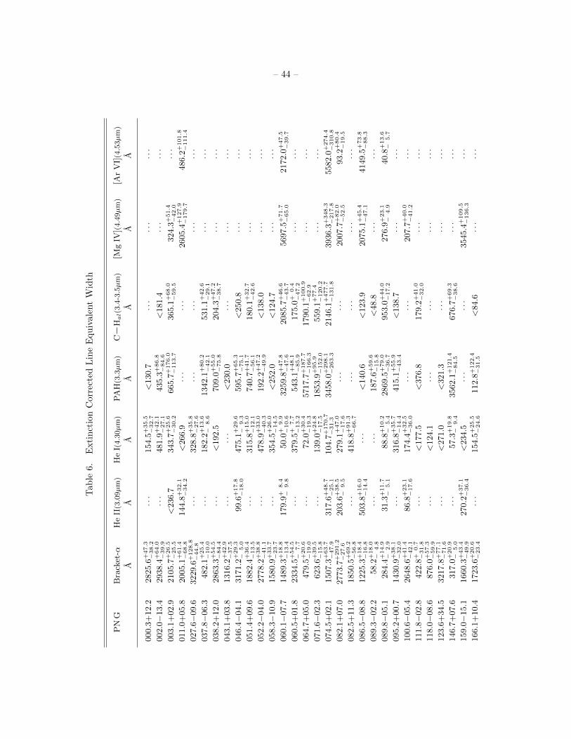
– 44 –
Tab
le6.
Exti
nct
ion
Corr
ecte
dL
ine
Equ
ivale
nt
Wid
th
PN
GB
rack
et-α
He
II(3.0
9µ
m)
He
I(4.3
0µ
m)
PA
H(3.3µ
m)
CH
al(
3.4
-3.5µ
m)
[Mg
IV](
4.4
9µ
m)
[Ar
VI]
(4.5
3µ
m)
AA
AA
AA
A
000.3
+12.2
2825.6
+47.3
−38.2
···
154.5
+35.5
−32.7
<130.7
···
···
···
002.0−
13.4
2938.4
+64.0
−39.9
···
481.9
+42.1
−27.1
435.3
+86.8
−84.6
<181.4
···
···
003.1
+02.9
2105.7
+26.5
−25.5
<236.7
343.7
+25.6
−30.2
665.7
+176.0
−113.7
365.1
+68.0
−59.5
324.3
+51.4
−42.0
···
011.0
+05.8
2005.1
+61.4
−68.8
144.8
+32.1
−34.2
<266.9
···
···
2605.4
+127.9
−179.7
486.2
+101.8
−111.4
027.6−
09.6
3229.6
+128.8
−44.8
···
328.8
+35.8
−27.6
···
···
···
···
037.8−
06.3
482.1
+25.4
−10.0
···
182.2
+13.6
−8.6
1342.1
+80.2
−42.1
531.1
+42.6
−29.1
···
···
038.2
+12.0
2863.3
+54.5
−84.4
···
<192.5
709.0
+55.0
−75.8
204.3
+47.2
−38.7
···
···
043.1
+03.8
1316.2
+42.9
−37.5
···
···
<230.0
···
···
···
046.4−
04.1
3171.2
+29.3
−5.0
99.6
+17.8
−18.0
475.1
+29.6
−9.3
595.7
+65.3
−75.1
<250.8
···
···
051.4
+09.6
1882.4
+36.4
−13.5
···
315.8
+15.0
−12.1
740.7
+41.7
−56.1
180.1
+32.7
−42.6
···
···
052.2−
04.0
2778.2
+38.8
−41.1
···
478.9
+33.0
−40.3
192.2
+47.2
−49.9
<138.0
···
···
058.3−
10.9
1580.9
+33.7
−23.7
···
354.5
+26.0
−14.5
<252.0
<124.7
···
···
060.1−
07.7
1489.3
+18.8
−13.4
179.9
+8.4
−9.8
50.0
+9.9
−10.6
3259.8
+47.8
−47.6
2085.7
+46.6
−43.7
5697.5
+71.7
−65.0
2172.0
+47.5
−39.7
060.5
+01.8
2334.5
+54.5
−7.7
···
379.5
+7.7
−13.2
543.1
+48.1
−85.9
175.0
+0.4
−47.2
···
···
064.7
+05.0
479.5
+20.6
−19.0
···
72.0
+30.4
−19.3
5717.7
+187.7
−166.3
1790.1
+100.9
−62.9
···
···
071.6−
02.3
623.6
+39.5
−15.8
···
139.0
+24.8
−17.5
1853.9
+95.9
−152.0
559.1
+77.4
−120.2
···
···
074.5
+02.1
1507.3
+63.7
−47.9
317.6
+48.7
−25.1
104.7
+170.7
−31.3
3458.0
+298.1
−263.3
2146.1
+477.7
−131.8
3936.3
+348.3
−217.8
5582.0
+274.4
−310.8
082.1
+07.0
2773.7
+291.2
−27.6
203.6
+38.5
−9.5
279.1
+47.0
−17.6
···
···
2007.7
+82.0
−52.5
93.2
+80.4
−19.5
082.5
+11.3
1850.5
+69.2
−56.8
···
418.8
+91.3
−66.7
···
···
···
···
086.5−
08.8
1225.3
+18.4
−16.8
503.8
+16.0
−14.4
···
<140.6
<123.9
2075.1
+45.4
−47.1
4149.5
+73.8
−88.3
089.3−
02.2
58.2
+18.0
−4.8
···
···
187.6
+59.6
−15.8
<48.8
···
···
089.8−
05.1
284.4
+14.9
−2.9
31.3
+11.7
−5.1
88.8
+10.2
−5.4
2869.5
+79.0
−36.7
953.0
+44.0
−17.2
276.9
+23.1
−4.9
40.8
+13.6
−5.7
095.2
+00.7
1430.9
+38.1
−32.0
···
316.8
+35.7
−14.4
415.1
+55.9
−43.4
<138.7
···
···
100.6−
05.4
2648.6
+41.4
−42.1
86.8
+23.1
−17.6
174.4
+32.5
−36.0
···
···
207.7
+40.0
−41.2
···
111.8−
02.8
422.8
+0.7
−31.8
···
<177.5
<376.8
179.2
+41.0
−32.0
···
···
118.0−
08.6
876.0
+57.3
−59.9
···
<124.1
···
···
···
···
123.6
+34.5
3217.8
+77.1
−71.6
···
<271.0
<321.3
···
···
···
146.7
+07.6
317.0
+20.9
−5.0
···
57.3
+19.8
−9.4
3562.1
+121.4
−84.5
676.7
+69.3
−38.6
···
···
159.0−
15.1
1660.3
+43.4
−49.9
270.2
+37.1
−36.4
<234.5
···
···
3545.4
+109.5
−136.3
···
166.1
+10.4
1723.6
+20.6
−23.4
···
154.5
+25.5
−24.6
112.8
+122.4
−31.5
<84.6
···
···

– 45 –
Tab
le6—
Conti
nu
ed
PN
GB
rack
et-α
He
II(3.0
9µ
m)
He
I(4.3
0µ
m)
PA
H(3.3µ
m)
CH
al(
3.4
-3.5µ
m)
[Mg
IV](
4.4
9µ
m)
[Ar
VI]
(4.5
3µ
m)
AA
AA
AA
A
190.3−
17.7
2110.9
+32.7
−27.2
···
215.4
+41.2
−44.8
<202.7
···
···
···
194.2
+02.5
372.3
+11.4
−17.7
85.0
+12.7
−9.3
<44.5
1157.9
+79.8
−53.9
379.3
+56.9
−46.7
585.6
+26.1
−21.7
82.2
+27.1
−23.5
211.2−
03.5
476.4
+12.3
−10.3
···
71.3
+12.4
−12.3
173.7
+84.5
−25.6
<95.3
···
···
221.3−
12.3
1873.6
+23.2
−18.8
371.5
+22.7
−21.0
148.6
+30.7
−28.1
<655.3
<273.5
5881.3
+74.2
−78.8
1983.8
+63.3
−62.0
226.7
+05.6
1578.7
+22.1
−19.0
142.7
+14.8
−13.3
147.0
+32.7
−20.4
3534.1
+206.2
−134.5
2311.3
+100.0
−98.9
1501.2
+45.9
−37.7
659.9
+42.4
−26.9
232.8−
04.7
191.3
+12.9
−9.0
···
<40.3
865.2
+67.6
−59.6
250.9
+47.1
−22.8
···
···
235.3−
03.9
339.2
+14.4
−15.4
···
50.9
+17.7
−11.2
243.1
+32.0
−35.8
<92.8
···
···
258.1−
00.3
1577.4
+23.8
−19.8
···
248.9
+21.1
−16.0
195.1
+81.7
−42.1
···
···
···
264.4−
12.7
2768.5
+62.1
−47.2
···
273.6
+54.6
−47.5
<289.7
<223.4
···
···
268.4
+02.4
354.8
+8.2
−7.8
86.7
+13.9
−6.4
64.2
+15.1
−9.2
4927.5
+166.2
−135.8
2485.7
+86.2
−57.7
1292.7
+34.2
−32.9
894.1
+37.5
−21.5
278.6−
06.7
2063.3
+39.5
−36.9
80.3
+26.9
−24.2
336.7
+31.8
−32.5
423.5
+82.9
−64.1
<167.5
433.0
+46.3
−38.6
···
283.8
+02.2
1568.7
+21.4
−9.8
581.3
+15.3
−12.8
···
···
···
14919.7
+154.9
−0.8
2690.9
+38.0
−2.4
285.4−
05.3
3817.1
+25.0
−13.1
411.9
+23.7
−17.5
308.6
+28.5
−27.2
325.8
+85.1
−85.8
···
5558.5
+33.6
−27.3
593.4
+46.2
−19.5
285.6−
02.7
2316.2
+22.3
−20.5
···
120.8
+9.4
−10.8
808.8
+33.0
−24.1
128.8
+41.1
−24.2
···
···
285.7−
14.9
1226.6
+33.5
−20.7
175.2
+22.9
−25.6
<121.2
···
···
696.6
+52.1
−57.0
<85.6
291.6−
04.8
1133.6
+32.8
−11.0
212.1
+36.5
−10.2
152.4
+24.2
−1.1
4125.6
+135.3
−43.9
2129.4
+105.9
−22.0
4046.0
+160.5
−18.4
3068.7
+150.2
−15.6
292.8
+01.1
2695.2
+73.5
−73.4
219.4
+37.6
−25.2
278.3
+54.5
−57.0
1736.0
+168.7
−129.6
1005.7
+164.8
−137.5
232.8
+64.1
−60.8
···
294.9−
04.3
1092.7
+26.7
−22.4
···
179.9
+40.2
−33.8
<349.8
···
···
···
296.3−
03.0
1920.9
+53.9
−45.3
148.3
+22.3
−15.0
255.0
+34.9
−31.2
958.8
+83.4
−68.0
489.3
+88.5
−49.1
1575.0
+77.2
−80.5
719.9
+48.8
−54.3
304.5−
04.8
2554.8
+25.8
−14.7
154.7
+20.4
−18.9
409.0
+33.5
−23.1
1051.8
+79.3
−213.0
415.2
+88.9
−76.7
4319.5
+72.4
−29.1
840.2
+61.8
−28.2
305.1
+01.4
60.5
+6.8
−8.0
···
···
76.2
+26.5
−16.8
103.7
+31.1
−13.4
···
···
307.2−
09.0
2398.0
+50.2
−20.1
···
518.9
+39.9
−16.9
634.2
+161.6
−159.4
<212.6
···
···
307.5−
04.9
2930.3
+35.5
−30.3
···
325.5
+48.3
−25.7
3231.1
+287.3
−123.0
450.4
+196.3
−141.3
···
···
312.6−
01.8
3717.1
+72.7
−56.8
···
334.5
+66.0
−57.3
310.7
+142.1
−86.5
<130.4
···
···
315.1−
13.0
2011.0
+176.7
−153.6
···
148.8
+50.3
−38.8
1027.3
+215.8
−202.8
318.9
+107.4
−96.5
···
···
320.1−
09.6
1647.3
+201.6
−22.0
···
<69.8
2336.5
+212.7
−50.0
566.8
+133.6
−43.7
···
···
320.9
+02.0
2469.2
+191.4
−111.9
···
530.5
+136.2
−38.2
1650.4
+61.4
−94.8
724.1
+87.9
−47.5
···
···
322.5−
05.2
3553.0
+70.9
−58.9
2671.8
+124.1
−88.3
<540.1
···
···
51038.3
+559.8
−417.1
···
323.9
+02.4
2326.6
+46.8
−29.6
···
298.4
+40.4
−27.3
3466.2
+63.6
−134.4
1567.2
+63.0
−56.4
···
···
324.8−
01.1
3142.8
+88.2
−63.1
···
697.5
+52.8
−43.7
1571.2
+206.2
−176.5
488.3
+158.1
−107.4
···
···

– 46 –
Tab
le6—
Conti
nu
ed
PN
GB
rack
et-α
He
II(3.0
9µ
m)
He
I(4.3
0µ
m)
PA
H(3.3µ
m)
CH
al(
3.4
-3.5µ
m)
[Mg
IV](
4.4
9µ
m)
[Ar
VI]
(4.5
3µ
m)
AA
AA
AA
A
325.8−
12.8
1794.9
+72.0
−31.8
···
228.1
+37.1
−15.1
···
···
···
···
326.0−
06.5
1304.5
+44.7
−38.8
···
<51.7
255.9
+205.4
−46.4
<154.9
···
···
327.1−
01.8
2261.4
+97.3
−87.8
···
264.9
+68.2
−21.1
1435.7
+121.8
−187.8
806.4
+40.5
−29.4
···
···
327.8−
01.6
1645.0
+54.4
−27.2
203.9
+35.8
−18.3
253.8
+41.9
−31.9
2054.3
+194.1
−319.2
1326.9
+129.8
−108.0
3042.7
+73.8
−139.6
3621.1
+36.6
−273.8
331.1−
05.7
812.3
+156.7
−22.4
···
222.7
+60.4
−16.4
···
···
···
···
331.3
+16.8
1783.6
+51.3
−45.2
419.0
+51.2
−33.0
<103.9
489.5
+140.0
−86.0
159.6
+103.3
−40.3
3389.7
+54.5
−108.1
···
336.3−
05.6
890.3
+54.9
−35.2
193.2
+28.6
−20.0
<128.2
2160.7
+418.2
−156.5
1279.7
+197.5
−132.8
1925.4
+102.4
−102.0
2132.4
+91.4
−124.6
342.1
+27.5
1960.9
+51.6
−60.0
720.0
+54.5
−41.6
<145.2
···
···
15844.8
+292.1
−282.7
2427.5
+145.3
−129.0
349.8
+04.4
2499.7
+61.3
−64.9
···
415.9
+49.1
−45.4
1403.2
+111.5
−79.1
721.8
+161.8
−99.5
···
···
350.9
+04.4
744.9
+76.0
−15.4
···
56.6
+32.5
−12.0
···
···
···
···
356.1
+02.7
831.7
+6.7
−42.4
···
243.8
+0.1
−23.0
1854.2
+59.7
−35.3
893.9
+141.8
−7.2
···
···
357.6
+02.6
1567.0
+97.8
−91.4
···
397.6
+89.1
−92.9
1177.0
+176.0
−149.0
383.6
+129.1
−37.1
···
···

– 47 –
0
10
20
30
40
50
60
70
80
2.5 3.0 3.5 4.0 4.5 5.0
PNG 000.3+12.2 (3460107)
Flu
x D
ensi
ty (
10
−1
5W
m−
2µ
m−
1)
Wavelength (µm)
0
10
20
30
40
50
60
70
2.5 3.0 3.5 4.0 4.5 5.0
PNG 002.0−13.4 (3460003)
Flu
x D
ensi
ty (
10
−1
5W
m−
2µ
m−
1)
Wavelength (µm)
0
10
20
30
40
50
60
70
80
90
2.5 3.0 3.5 4.0 4.5 5.0
PNG 003.1+02.9 (3460005)
Flu
x D
ensi
ty (
10
−1
5W
m−
2µ
m−
1)
Wavelength (µm)
Fig. 7.— The AKARI /IRC 2.5–5.0µm spectra. Explanations of the lines are shown in the bottom of the
figures.

– 48 –
0
5
10
15
20
25
30
35
40
2.5 3.0 3.5 4.0 4.5 5.0
PNG 011.0+05.8 (3460012)
Flu
x D
ensi
ty (
10
−1
5W
m−
2µ
m−
1)
Wavelength (µm)
0
5
10
15
20
25
30
35
40
2.5 3.0 3.5 4.0 4.5 5.0
PNG 027.6−09.6 (3460016)
Flu
x D
ensi
ty (
10
−1
5W
m−
2µ
m−
1)
Wavelength (µm)
0
50
100
150
200
2.5 3.0 3.5 4.0 4.5 5.0
PNG 037.8−06.3 (3460019)
Flu
x D
ensi
ty (
10
−1
5W
m−
2µ
m−
1)
Wavelength (µm)
Fig. 7.— Cont.—

– 49 –
0
10
20
30
40
50
60
70
2.5 3.0 3.5 4.0 4.5 5.0
PNG 038.2+12.0 (3460020)
Flu
x D
ensi
ty (
10
−1
5W
m−
2µ
m−
1)
Wavelength (µm)
0
5
10
15
20
2.5 3.0 3.5 4.0 4.5 5.0
PNG 043.1+03.8 (3460093)
Flu
x D
ensi
ty (
10
−1
5W
m−
2µ
m−
1)
Wavelength (µm)
0
10
20
30
40
50
60
70
80
2.5 3.0 3.5 4.0 4.5 5.0
PNG 046.4−04.1 (3460021)
Flu
x D
ensi
ty (
10
−1
5W
m−
2µ
m−
1)
Wavelength (µm)
Fig. 7.— Cont.—

– 50 –
0
20
40
60
80
100
2.5 3.0 3.5 4.0 4.5 5.0
PNG 051.4+09.6 (3460022)
Flu
x D
ensi
ty (
10
−1
5W
m−
2µ
m−
1)
Wavelength (µm)
0
5
10
15
20
25
30
2.5 3.0 3.5 4.0 4.5 5.0
PNG 052.2−04.0 (3460094)
Flu
x D
ensi
ty (
10
−1
5W
m−
2µ
m−
1)
Wavelength (µm)
0
20
40
60
80
100
120
140
160
2.5 3.0 3.5 4.0 4.5 5.0
PNG 058.3−10.9 (3460023)
Flu
x D
ensi
ty (
10
−1
5W
m−
2µ
m−
1)
Wavelength (µm)
Fig. 7.— Cont.—

– 51 –
0
10
20
30
40
50
60
70
80
2.5 3.0 3.5 4.0 4.5 5.0
PNG 060.1−07.7 (3460024)
Flu
x D
ensi
ty (
10
−1
5W
m−
2µ
m−
1)
Wavelength (µm)
0
5
10
15
20
25
30
35
40
2.5 3.0 3.5 4.0 4.5 5.0
PNG 060.5+01.8 (3460025)
Flu
x D
ensi
ty (
10
−1
5W
m−
2µ
m−
1)
Wavelength (µm)
0
200
400
600
800
1000
1200
1400
1600
1800
2.5 3.0 3.5 4.0 4.5 5.0
PNG 064.7+05.0 (3460026)
Flu
x D
ensi
ty (
10
−1
5W
m−
2µ
m−
1)
Wavelength (µm)
Fig. 7.— Cont.—

– 52 –
0
20
40
60
80
100
120
140
2.5 3.0 3.5 4.0 4.5 5.0
PNG 071.6−02.3 (3460027)
Flu
x D
ensi
ty (
10
−1
5W
m−
2µ
m−
1)
Wavelength (µm)
0
20
40
60
80
100
2.5 3.0 3.5 4.0 4.5 5.0
PNG 074.5+02.1 (3460028)
Flu
x D
ensi
ty (
10
−1
5W
m−
2µ
m−
1)
Wavelength (µm)
0
20
40
60
80
100
2.5 3.0 3.5 4.0 4.5 5.0
PNG 082.1+07.0 (3460029)
Flu
x D
ensi
ty (
10
−1
5W
m−
2µ
m−
1)
Wavelength (µm)
Fig. 7.— Cont.—

– 53 –
0
5
10
15
20
2.5 3.0 3.5 4.0 4.5 5.0
PNG 082.5+11.3 (3460030)
Flu
x D
ensi
ty (
10
−1
5W
m−
2µ
m−
1)
Wavelength (µm)
0
10
20
30
40
50
2.5 3.0 3.5 4.0 4.5 5.0
PNG 086.5−08.8 (3460114)
Flu
x D
ensi
ty (
10
−1
5W
m−
2µ
m−
1)
Wavelength (µm)
0
20
40
60
80
100
120
140
160
2.5 3.0 3.5 4.0 4.5 5.0
PNG 089.3−02.2 (3460031)
Flu
x D
ensi
ty (
10
−1
5W
m−
2µ
m−
1)
Wavelength (µm)
Fig. 7.— Cont.—

– 54 –
0
50
100
150
200
2.5 3.0 3.5 4.0 4.5 5.0
PNG 089.8−05.1 (3460032)
Flu
x D
ensi
ty (
10
−1
5W
m−
2µ
m−
1)
Wavelength (µm)
0
10
20
30
40
50
60
70
80
2.5 3.0 3.5 4.0 4.5 5.0
PNG 095.2+00.7 (3460033)
Flu
x D
ensi
ty (
10
−1
5W
m−
2µ
m−
1)
Wavelength (µm)
0
5
10
15
20
25
30
35
40
2.5 3.0 3.5 4.0 4.5 5.0
PNG 100.6−05.4 (3460034)
Flu
x D
ensi
ty (
10
−1
5W
m−
2µ
m−
1)
Wavelength (µm)
Fig. 7.— Cont.—

– 55 –
0
50
100
150
200
250
2.5 3.0 3.5 4.0 4.5 5.0
PNG 111.8−02.8 (3460035)
Flu
x D
ensi
ty (
10
−1
5W
m−
2µ
m−
1)
Wavelength (µm)
0
5
10
15
20
2.5 3.0 3.5 4.0 4.5 5.0
PNG 118.0−08.6 (3460096)
Flu
x D
ensi
ty (
10
−1
5W
m−
2µ
m−
1)
Wavelength (µm)
0
5
10
15
20
25
30
35
40
2.5 3.0 3.5 4.0 4.5 5.0
PNG 123.6+34.5 (3460115)
Flu
x D
ensi
ty (
10
−1
5W
m−
2µ
m−
1)
Wavelength (µm)
Fig. 7.— Cont.—

– 56 –
0
10
20
30
40
50
60
70
2.5 3.0 3.5 4.0 4.5 5.0
PNG 146.7+07.6 (3460097)
Flu
x D
ensi
ty (
10
−1
5W
m−
2µ
m−
1)
Wavelength (µm)
0
5
10
15
20
2.5 3.0 3.5 4.0 4.5 5.0
PNG 159.0−15.1 (3460098)
Flu
x D
ensi
ty (
10
−1
5W
m−
2µ
m−
1)
Wavelength (µm)
0
20
40
60
80
100
120
2.5 3.0 3.5 4.0 4.5 5.0
PNG 166.1+10.4 (3460116)
Flu
x D
ensi
ty (
10
−1
5W
m−
2µ
m−
1)
Wavelength (µm)
Fig. 7.— Cont.—

– 57 –
0
5
10
15
20
2.5 3.0 3.5 4.0 4.5 5.0
PNG 190.3−17.7 (3460099)
Flu
x D
ensi
ty (
10
−1
5W
m−
2µ
m−
1)
Wavelength (µm)
0
10
20
30
40
50
60
70
80
2.5 3.0 3.5 4.0 4.5 5.0
PNG 194.2+02.5 (3460117)
Flu
x D
ensi
ty (
10
−1
5W
m−
2µ
m−
1)
Wavelength (µm)
0
10
20
30
40
50
60
70
80
90
2.5 3.0 3.5 4.0 4.5 5.0
PNG 211.2−03.5 (3460036)
Flu
x D
ensi
ty (
10
−1
5W
m−
2µ
m−
1)
Wavelength (µm)
Fig. 7.— Cont.—

– 58 –
0
20
40
60
80
100
2.5 3.0 3.5 4.0 4.5 5.0
PNG 221.3−12.3 (3460118)
Flu
x D
ensi
ty (
10
−1
5W
m−
2µ
m−
1)
Wavelength (µm)
0
5
10
15
20
2.5 3.0 3.5 4.0 4.5 5.0
PNG 226.7+05.6 (3460100)
Flu
x D
ensi
ty (
10
−1
5W
m−
2µ
m−
1)
Wavelength (µm)
0
50
100
150
200
2.5 3.0 3.5 4.0 4.5 5.0
PNG 232.8−04.7 (3460037)
Flu
x D
ensi
ty (
10
−1
5W
m−
2µ
m−
1)
Wavelength (µm)
Fig. 7.— Cont.—

– 59 –
0
10
20
30
40
50
60
2.5 3.0 3.5 4.0 4.5 5.0
PNG 235.3−03.9 (3460038)
Flu
x D
ensi
ty (
10
−1
5W
m−
2µ
m−
1)
Wavelength (µm)
0
20
40
60
80
100
120
2.5 3.0 3.5 4.0 4.5 5.0
PNG 258.1−00.3 (3460039)
Flu
x D
ensi
ty (
10
−1
5W
m−
2µ
m−
1)
Wavelength (µm)
0
5
10
15
20
25
30
2.5 3.0 3.5 4.0 4.5 5.0
PNG 264.4−12.7 (3460040)
Flu
x D
ensi
ty (
10
−1
5W
m−
2µ
m−
1)
Wavelength (µm)
Fig. 7.— Cont.—

– 60 –
0
20
40
60
80
100
120
140
2.5 3.0 3.5 4.0 4.5 5.0
PNG 268.4+02.4 (3460042)
Flu
x D
ensi
ty (
10
−1
5W
m−
2µ
m−
1)
Wavelength (µm)
0
5
10
15
20
2.5 3.0 3.5 4.0 4.5 5.0
PNG 278.6−06.7 (3460101)
Flu
x D
ensi
ty (
10
−1
5W
m−
2µ
m−
1)
Wavelength (µm)
0
10
20
30
40
50
60
70
80
90
2.5 3.0 3.5 4.0 4.5 5.0
PNG 283.8+02.2 (3460044)
Flu
x D
ensi
ty (
10
−1
5W
m−
2µ
m−
1)
Wavelength (µm)
Fig. 7.— Cont.—

– 61 –
0
10
20
30
40
50
60
70
2.5 3.0 3.5 4.0 4.5 5.0
PNG 285.4−05.3 (3460120)
Flu
x D
ensi
ty (
10
−1
5W
m−
2µ
m−
1)
Wavelength (µm)
0
20
40
60
80
100
120
140
2.5 3.0 3.5 4.0 4.5 5.0
PNG 285.6−02.7 (3460045)
Flu
x D
ensi
ty (
10
−1
5W
m−
2µ
m−
1)
Wavelength (µm)
0
5
10
15
20
25
30
35
40
2.5 3.0 3.5 4.0 4.5 5.0
PNG 285.7−14.9 (3460121)
Flu
x D
ensi
ty (
10
−1
5W
m−
2µ
m−
1)
Wavelength (µm)
Fig. 7.— Cont.—

– 62 –
0
20
40
60
80
100
120
140
160
180
2.5 3.0 3.5 4.0 4.5 5.0
PNG 291.6−04.8 (3460046)
Flu
x D
ensi
ty (
10
−1
5W
m−
2µ
m−
1)
Wavelength (µm)
0
5
10
15
20
25
30
2.5 3.0 3.5 4.0 4.5 5.0
PNG 292.8+01.1 (3460102)
Flu
x D
ensi
ty (
10
−1
5W
m−
2µ
m−
1)
Wavelength (µm)
0
5
10
15
20
25
30
35
40
2.5 3.0 3.5 4.0 4.5 5.0
PNG 294.9−04.3 (3460047)
Flu
x D
ensi
ty (
10
−1
5W
m−
2µ
m−
1)
Wavelength (µm)
Fig. 7.— Cont.—

– 63 –
0
10
20
30
40
50
2.5 3.0 3.5 4.0 4.5 5.0
PNG 296.3−03.0 (3460048)
Flu
x D
ensi
ty (
10
−1
5W
m−
2µ
m−
1)
Wavelength (µm)
0
20
40
60
80
100
120
2.5 3.0 3.5 4.0 4.5 5.0
PNG 304.5−04.8 (3460051)
Flu
x D
ensi
ty (
10
−1
5W
m−
2µ
m−
1)
Wavelength (µm)
0
500
1000
1500
2000
2.5 3.0 3.5 4.0 4.5 5.0
PNG 305.1+01.4 (3460122)
Flu
x D
ensi
ty (
10
−1
5W
m−
2µ
m−
1)
Wavelength (µm)
Fig. 7.— Cont.—
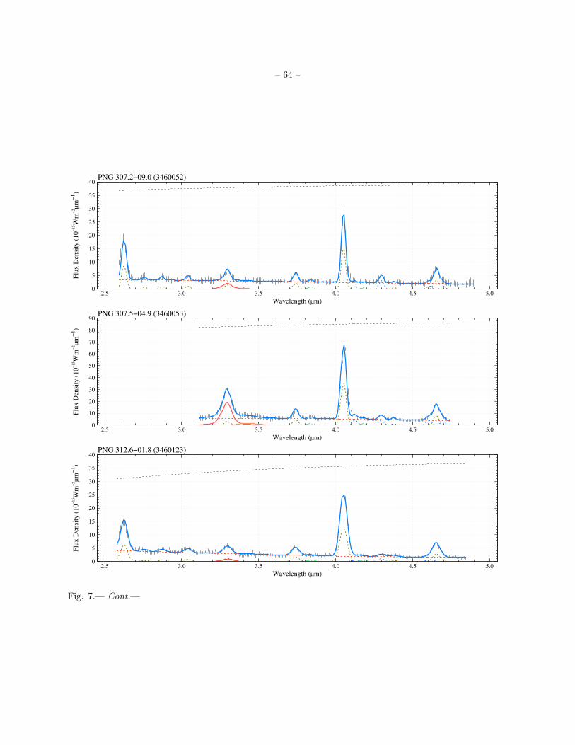
– 64 –
0
5
10
15
20
25
30
35
40
2.5 3.0 3.5 4.0 4.5 5.0
PNG 307.2−09.0 (3460052)
Flu
x D
ensi
ty (
10
−1
5W
m−
2µ
m−
1)
Wavelength (µm)
0
10
20
30
40
50
60
70
80
90
2.5 3.0 3.5 4.0 4.5 5.0
PNG 307.5−04.9 (3460053)
Flu
x D
ensi
ty (
10
−1
5W
m−
2µ
m−
1)
Wavelength (µm)
0
5
10
15
20
25
30
35
40
2.5 3.0 3.5 4.0 4.5 5.0
PNG 312.6−01.8 (3460123)
Flu
x D
ensi
ty (
10
−1
5W
m−
2µ
m−
1)
Wavelength (µm)
Fig. 7.— Cont.—

– 65 –
0
50
100
150
200
250
300
350
2.5 3.0 3.5 4.0 4.5 5.0
PNG 315.1−13.0 (3460054)
Flu
x D
ensi
ty (
10
−1
5W
m−
2µ
m−
1)
Wavelength (µm)
0
20
40
60
80
100
2.5 3.0 3.5 4.0 4.5 5.0
PNG 320.1−09.6 (3460103)
Flu
x D
ensi
ty (
10
−1
5W
m−
2µ
m−
1)
Wavelength (µm)
0
20
40
60
80
100
120
140
160
180
2.5 3.0 3.5 4.0 4.5 5.0
PNG 320.9+02.0 (3460056)
Flu
x D
ensi
ty (
10
−1
5W
m−
2µ
m−
1)
Wavelength (µm)
Fig. 7.— Cont.—

– 66 –
0
20
40
60
80
100
2.5 3.0 3.5 4.0 4.5 5.0
PNG 322.5−05.2 (3460060)
Flu
x D
ensi
ty (
10
−1
5W
m−
2µ
m−
1)
Wavelength (µm)
0
10
20
30
40
50
60
2.5 3.0 3.5 4.0 4.5 5.0
PNG 323.9+02.4 (3460061)
Flu
x D
ensi
ty (
10
−1
5W
m−
2µ
m−
1)
Wavelength (µm)
0
20
40
60
80
100
120
140
2.5 3.0 3.5 4.0 4.5 5.0
PNG 324.8−01.1 (3460062)
Flu
x D
ensi
ty (
10
−1
5W
m−
2µ
m−
1)
Wavelength (µm)
Fig. 7.— Cont.—

– 67 –
0
10
20
30
40
50
60
2.5 3.0 3.5 4.0 4.5 5.0
PNG 325.8−12.8 (3460063)
Flu
x D
ensi
ty (
10
−1
5W
m−
2µ
m−
1)
Wavelength (µm)
0
5
10
15
20
2.5 3.0 3.5 4.0 4.5 5.0
PNG 326.0−06.5 (3460064)
Flu
x D
ensi
ty (
10
−1
5W
m−
2µ
m−
1)
Wavelength (µm)
0
10
20
30
40
50
60
2.5 3.0 3.5 4.0 4.5 5.0
PNG 327.1−01.8 (3460065)
Flu
x D
ensi
ty (
10
−1
5W
m−
2µ
m−
1)
Wavelength (µm)
Fig. 7.— Cont.—
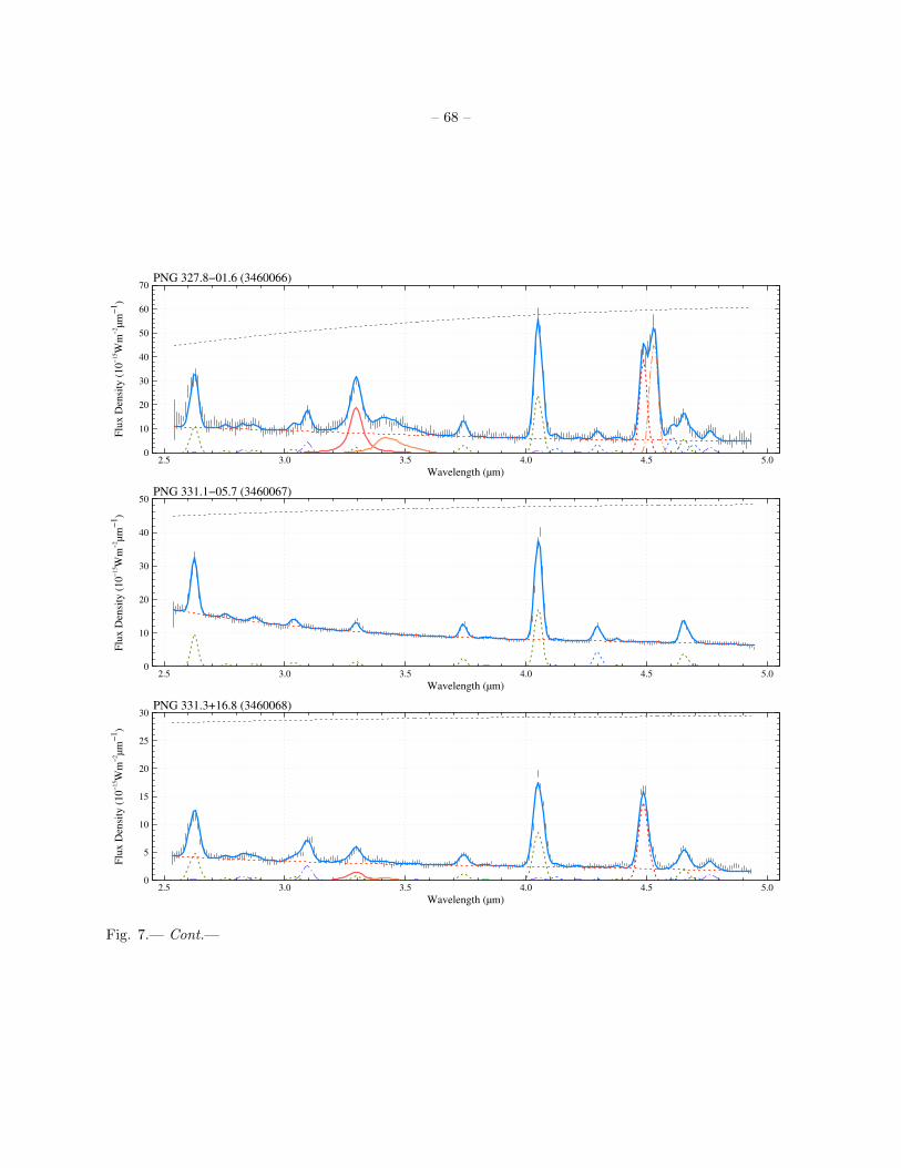
– 68 –
0
10
20
30
40
50
60
70
2.5 3.0 3.5 4.0 4.5 5.0
PNG 327.8−01.6 (3460066)
Flu
x D
ensi
ty (
10
−1
5W
m−
2µ
m−
1)
Wavelength (µm)
0
10
20
30
40
50
2.5 3.0 3.5 4.0 4.5 5.0
PNG 331.1−05.7 (3460067)
Flu
x D
ensi
ty (
10
−1
5W
m−
2µ
m−
1)
Wavelength (µm)
0
5
10
15
20
25
30
2.5 3.0 3.5 4.0 4.5 5.0
PNG 331.3+16.8 (3460068)
Flu
x D
ensi
ty (
10
−1
5W
m−
2µ
m−
1)
Wavelength (µm)
Fig. 7.— Cont.—

– 69 –
0
2
4
6
8
10
2.5 3.0 3.5 4.0 4.5 5.0
PNG 336.3−05.6 (3460069)
Flu
x D
ensi
ty (
10
−1
5W
m−
2µ
m−
1)
Wavelength (µm)
0
10
20
30
40
50
2.5 3.0 3.5 4.0 4.5 5.0
PNG 342.1+27.5 (3460104)
Flu
x D
ensi
ty (
10
−1
5W
m−
2µ
m−
1)
Wavelength (µm)
0
5
10
15
20
25
30
2.5 3.0 3.5 4.0 4.5 5.0
PNG 349.8+04.4 (3460105)
Flu
x D
ensi
ty (
10
−1
5W
m−
2µ
m−
1)
Wavelength (µm)
Fig. 7.— Cont.—

– 70 –
0
10
20
30
40
50
60
70
80
2.5 3.0 3.5 4.0 4.5 5.0
PNG 350.9+04.4 (3460070)
Flu
x D
ensi
ty (
10
−1
5W
m−
2µ
m−
1)
Wavelength (µm)
0
5
10
15
20
25
30
2.5 3.0 3.5 4.0 4.5 5.0
PNG 356.1+02.7 (3460076)
Flu
x D
ensi
ty (
10
−1
5W
m−
2µ
m−
1)
Wavelength (µm)
0
5
10
15
20
25
30
2.5 3.0 3.5 4.0 4.5 5.0
PNG 357.6+02.6 (3460082)
Flu
x D
ensi
ty (
10
−1
5W
m−
2µ
m−
1)
Wavelength (µm)
Fig. 7.— Cont.—

– 71 –E
stim
ated
Ext
inct
ion
Av
Observed Brβ/Brα ratio
1
10
0.3 0.4 0.5 0.6
S/N=10
3σ2σ1σ
median
1
10
0.3 0.4 0.5 0.6
S/N=50
3σ2σ1σ
median
Fig. 19.— Estimated extinction and uncertainty. The dashed, dotted, and dot-dashed contours show the
confidence intervals of the 1-, 2-, and 3-σ, respectively.
A. Uncertainty in AV
There are several hydrogen recombination lines in the 2.5–5.0µm spectrum. Extinction can be estimated
based on the intensity ratio of these lines. The accuracy of the estimated extinction heavily depends on the
signal-to-noise ratio (S/N) of the intensity ratio. This chapter describes the method to derive the extinction
based on the IRC spectrum and shows that a typical uncertainty in AV is ∼1 mag for the PNSPC samples.
The observed intensity of the line emission X is given by IobsX = IXe−τX , where IX is the intrinsic
intensity and τX is the extinction at the line X. The observed intensity ratio of the line X to Y is
IobsX
IobsY
=IXIY
exp (−α(X,Y )AV ) , (A1)
where α(X,Y ) is defined by (τX − τY )/AV , which is a constant value specific to the extinction curve. Thus,
the extinction is estimated by
AV =log xint − log xobs
α(X,Y ), (A2)
where xint is IX/IY and xobs is IobsX /IobsY . Given that the line X and Y are Brackett-α (Brα) and β (Brβ),
respectively, the intrinsic intensity ratio is about 0.57 assuming the Case-B condition (Baker & Menzel 1938)
with the electron density of 104 K and the electron density of 104 cm−3. The ratio is less sensitive to either
the electron temperature or density. We adopt the extinction curve given by Mathis (1990). The value of
α(Brβ,Brα) is about 0.041. The extinction estimated from the Brackett-β to α ratio is
AV (Brβ,Brα) ' −24.6 log xobs − 13.7. (A3)
The uncertainty in AV (Brβ,Brα) is investigated. The measured intensity ratio (xobs) includes a statis-
tical error. Define the error by σ. Assuming that the variation in xobs is given by a normal distribution, the

– 72 –
posterior probability distribution of the intensity ratio (xobs) is given by
prob(xobs|xobs, σ) ∝ 1√2πσ
exp
(− (xobs − xobs)2
2σ2
)prob(xobs), (A4)
where prob(xobs) is the prior distribution of xobs assumed to be a uniform distribution from 0 to x. From
Equations (A3) and (A4), the posterior distribution of AV (Brβ,Brα) is given by
prob(AV |xobs, σ) ∝ prob(xobs|xobs)prob(xobs). (A5)
The results for S/N = 10 and 50 are shown in Figure 19. The horizontal axis shows the observed intensity
ratio (xobs), while the vertical axis is the estimated AV value. The gray solid line indicates the median
extinction AV . The red dashed, orange dotted, and yellow dot-dashed contours show the 1-, 2-, and 3-σ
confidence intervals, respectively. The typical S/N for the PNSPC spectrum is about 50. Figure 19 suggests
that the extinction estimated from the Brα/Brβ ratio are quite uncertain when AV ∼ 1–3 mag. Figure 13
shows that the AV values are typically less than about 2 mag for the PNSPC samples. Thus, it is practically
impossible to precisely estimate the extinction of the PNSPC samples without using ancillary data such as
the intensity of the Hβ emission. The standard errors on AV derived from the Brβ/Brα and Hβ/Brα ratios
are estimated to be about 0.5 and 0.02 mag., respectively. The intrinsic line ratio may depend on the electron
temperature and density. The impact is much larger for the Hβ/Brα ratio, but the variations in them can
change AV at most by 0.3 mag. Even though these variations are taken into account, the extinction derived
from the Hβ/Brα ratio is much more reliable than that from the Brβ/Brα ratio.