AIRCC-Clim: a user-friendly tool for generating regional probabilistic climate change

scenarios and risk measures

Francisco Estrada1,2,3*, Oscar Calderón-Bustamante1, Wouter Botzen2,4, Julián A. Velasco1,

Richard S.J. Tol5,6,7,8,9

1Centro de Ciencias de la Atmosfera, Universidad Nacional Autónoma de México, CDMX, Mexico; 2Institute for

Environmental Studies, VU Amsterdam, Amsterdam, the Netherlands; 3Programa de Investigación en Cambio

Climático, Universidad Nacional Autónoma de México, CDMX, Mexico; 4Utrecht University School of Economics

(U.S.E.), Utrecht University, Utrecht, Netherlands; 5Department of Economics, University of Sussex, Falmer, UK; 6Department of Spatial Economics, Vrije Universiteit, Amsterdam, The Netherlands; 7Tinbergen Institute,

Amsterdam, The Netherlands; 8CESifo, Munich, Germany; 9Payne Institute for Public Policy, Colorado School of

Mines, Golden, CO, USA

*Corresponding autor: feporrua@atmosfera.unam.mx

Highlights

• A new tool for generating probabilistic regional climate change scenarios and risk

measures

• AIRCC-Clim is a standalone, user-friendly software designed for a variety of applications

including impact, vulnerability and adaptation assessments, integrated assessment

modelling,

• It includes a graphical interface that allows the quick evaluation of the consequences on

global and regional climate of user-defined experiments of international mitigation

policies.

Abstract

Complex physical models are the most advanced tools available for producing realistic simulations

of the climate system. However, such levels of realism imply high computational cost and

restrictions on their use for policymaking and risk assessment. Two central characteristics of

climate change are uncertainty and that it is a dynamic problem in which international actions can

significantly alter climate projections and information needs, including partial and full compliance

of global climate goals. Here we present AIRCC-Clim, a simple climate model emulator that

produces regional probabilistic climate change projections of monthly and annual temperature and

precipitation, as well as risk measures, based both on standard and user-defined emissions

scenarios for six greenhouse gases. AIRCC-Clim emulates 37 atmosphere-ocean coupled general

circulation models with low computational and technical requirements for the user. This

standalone, user-friendly software is designed for a variety of applications including impact

assessments, climate policy evaluation and integrated assessment modelling.

Keywords: Climate change scenarios; climate model emulator; impact, vulnerability and

adaptation assessment; stochastic simulation.

Software availability: AIRCC-Clim can be downloaded at no cost from

https://sites.google.com/view/aircc-lab-airccclim/aircc-clim

1. Introduction

Climate change projections are one of the main inputs for assessing the potential consequences of

different socioeconomic development pathways and international climate policy on natural and

human systems. Due to the complexity of the systems involved and their interactions, climate

projections are inherently uncertain (Curry and Webster, 2011; Gay and Estrada, 2010a; Knutti

and Sedláček, 2012). Moreover, computational and technical costs of state-of-the-art physical

models allow exploration of only a small fraction of the range of possible climate futures and

hinder assessing risk through probabilistic scenarios (Knutti et al., 2010; Sanderson et al., 2015).

For most decision-makers and researchers, these costs make it infeasible to explore how current

and hypothetical changes in international mitigation policy can influence future warming and its

consequences for society. In a time of proactive international mitigation policy, the dynamic nature

of projecting future climate becomes even more evident and decision-making requirements can go

beyond fixed illustrative emissions scenarios, such as the RCPs (Estrada and Botzen, 2021). For

example, Nationally Determined Contributions (NDCs) that represent greenhouse gas emission

reductions that countries promise as their contributions to the Paris Agreement are currently a key

focus of international climate policy. Moreover, due to the nonlinearity of most climate impacts,

even small deviations from a high-warming trajectory can produce large changes in the associated

impacts (Estrada and Botzen, 2021; Ignjacevic et al., 2021).

International efforts such as the Coupled Model Intercomparison Project (CMIP), which build and

host large databases of climate models’ simulations publicly available, have significantly

contributed to improving the accessibility and utilization of climate scenarios for the wider

research community and decision-makers (Knutti and Sedláček, 2012; Thomas F. Stocker et al.,

2013; Taylor et al., 2012). However, many users still face the problem of processing large datasets

for adapting them to their particular needs (e.g., temporal frequency and spatial domains). As such,

studies and decisions are commonly based on a few illustrative greenhouse gases emissions

trajectories and a handful of climate models’ simulations which are often selected due to their

availability and ease of use, such as WorldClim (Fick and Hijmans, 2017). Such a selection of

climate model runs can hardly provide a good representation of uncertainty and indicate if a

model’s projections for a given region may represent extreme realizations in comparison to the

majority of other models (Sanderson et al., 2015; Weigel et al., 2010). Even in cases when climate

models’ performance is assessed, the resulting selection of models does not guaranty that those

projections of future climate are reliable (Altamirano del Carmen et al., 2021). Climate model

selection remains an unresolved problem as commonly used metrics can be non-informative about

the models’ ability to reproduce the observed climate change signal and indicate much less about

their ability for projecting future climate (Knutti et al., 2010).

Uncertainty is a key characteristic of climate change and how it is understood and included in

climate impact assessments can have profound effects on the estimates of the consequences of this

phenomenon and on the design of policies to address these consequences (Gay and Estrada, 2010a;

IPCC-TGICA, 2007). The development of tools and methods for better uncertainty management

and for improving the usefulness of the large (thousands of terabytes) databases that are currently

available are increasingly relevant research topics. More efficient, simple, and flexible approaches

for taking advantage of the available databases can transform data into useful information and

knowledge for better assessments of impacts, risks, and climate policy options. Reduced

complexity models and emulators of more advanced models allow exploring –at low

computational and technical costs for the user– a wide range of possible futures and emissions

trajectories, parameterizations, as well as probabilistic assessment of risks for natural and human

systems (Blanc, 2017; Estrada et al., 2020; Meinshausen et al., 2011a). Integrated assessment

modelling benefits from such models and emulators to provide tools for supporting decision-

making and providing estimates for cases in which complex climate/impacts model runs are not

available.

A notable example of the usefulness of such models is the MAGICC software which has made

significant contributions to climate change research, particularly in impact, vulnerability and

adaptation (IVA) assessments, and integrated assessment modelling (Meinshausen et al., 2011a,

2011b; Wigley, 1995). The MAGICC software has been regularly used in the IPCC reports when

simulations produced by general circulation climate models are not available and also in the

national climate change assessments of several countries (Conde et al., 2011; IPCC, 2021, 2018).

Here we present AIRCC-Clim (Assessment of Impacts and Risks of Climate Change –

Probabilistic Climate Model Emulator), a simple and flexible climate model emulator for

producing probabilistic regional projections of monthly and annual temperature and precipitation,

as well as risk measures. AIRCC-Clim emulates the results from 37 atmosphere-ocean coupled

general circulation models included in the Fifth Assessment Report of the IPCC (Thomas F.

Stocker et al., 2013) with low computational and technical requirements on the user. It is a

standalone software for Windows and Linux operating systems that requires no programming or

advanced technical skills from the user and runs on computers with standard memory and

processing resources. AIRCC-Clim is designed for a variety of applications including IVA

assessments, integrated assessment modelling, and the quick evaluation of the consequences on

global and regional climate of user-defined experiments of international mitigation.

The remainder of this paper is structured as follows: Section 2 describes the AIRCC-Clim model

structure and describes in detail each of its modules in terms of data sources, modelling approaches

and methods, and their output. This section also describes the file options for exporting climate

projections and their characteristics. An application of the model is shown in Section 3 in which

the benefits of stringent international mitigation efforts are illustrated in terms of avoided warming,

changes in precipitation and risk reduction. Section 4 concludes and discusses model extensions

and integration with IVA models.

2. Model structure, data and methods

AIRCC-Clim is composed of four main modules: greenhouse gas emission scenario editor; global

climate models, a regional scenario generator; and a climate risk index generator (Figure 1). In the

following paragraphs each module is discussed, including detailed descriptions of the modelling

approaches, methods and data sources.

Figure 1. Schematic representation of AIRCC-Clim model structure. Calculation modules are

represented by rectangles while output is denoted by rectangles with rounded corners. The four

modules are: a) the emissions scenario editor; b) the climate module which produces annual global

temperature change estimates; c) the regional climate scenario generator which produces

probabilistic monthly and annual climate projections, and; d) the climate risk index generator that

calculates risk measures defined by the user.

2.1. Emissions scenario editor

AIRCC-Clim offers a graphic interface for constructing user-defined emissions scenarios for six

climate changing substances: Carbon dioxide (CO2 in MtC/yr), methane (CH4; in MtCH4/yr),

nitrous oxide (N2O; MtN2O-N/yr), chlorofluorocarbons (CFC11, CFC12 in kt/yr), and sulfur

hexafluoride (SF6 in kt/yr). Four RCP emissions trajectories are included by default and the user

can select one of them as starting point for editing. As shown in Figure 2 AIRCC-Clim has three

input options for emissions: 1) by means of editing the values displayed on a table; 2) by selecting

and plotting the substance of interest and modifying the emissions trajectories directly in a graph;

3) loading an Excel file (.xlsx) with user-defined emissions trajectories for each gas in a predefined

format (see the AIRCC-Clim user guide included in the SI). The modified emissions scenario is

saved in an Excel (.xlsx) file and used for generating the corresponding climate projections in

AIRCC-Clim.

Figure 2. AIRCC-Clim’s graphic emissions editor. Four RCP emissions trajectories can be loaded

and edited by the user by means of: 1) modifying the values in the editor’s table (upper part); 2)

by changing the trajectory in an interactive graph (lower part) and; 3) loading an Excel file with

user-defined emissions trajectories. In the lower part of the figure, the dashed blue line shows the

default values for the selected RCP scenario, while the continuous red line shows the trajectory

edited by the user.

2.2.Global climate projections

Global temperature projections in AIRCC-Clim can be generated by running a simple climate

model, as well as by using precalculated projections from two reduced complexity climate models.

As described in the following paragraphs, in all cases probabilistic projections are constructed by

means of stochastic simulation to represent uncertainty in the climate sensitivity (CS) parameter.

2.2.1. Modified Schneider-Thompson model

The Schneider-Thompson (ST) simple climate model (Schneider and Thompson, 1981) includes

three components that allows to calculate the atmospheric concentrations of greenhouse gases, the

corresponding change in radiative forcing and the resulting increase in global temperature. Due to

its flexibility and low computational cost, this climate model (and modified versions of it) is used

in some of the most popular integrated assessment models, such as FUND and RICE (Anthoff and

Tol, 2014; Nordhaus and Boyer, 2003).

The version of the ST model in AIRCC-Clim builds upon that used in the FUND integrated

assessment model (Tol and Fankhauser, 1998) which is available at http://www.fund-model.org/.

In this section, the ST model and the modifications that are introduced in AIRCC-Clim.

Calculation of atmospheric concentrations and radiative forcing

A five box-model (Tol, 2019) is used to convert annual emissions of CO2 (MtC) into atmospheric

concentrations (ppm). The initial value for CO2 concentrations is 278 ppm which represent

preindustrial times (circa 1750). The carbon cycle model is represented by the following equation:

𝐶𝑖,𝑡𝐶𝑂2 = (1 − 𝛼𝑖)𝐶𝑖,𝑡−1

𝐶𝑂2 + 𝛾𝑖𝛽𝐸𝑡𝐶𝑂2 (1)

𝐶𝑡𝐶𝑂2 = ∑ 𝐶𝑖,𝑡

𝐶𝑂25𝑖=1 (2)

where 𝐶𝑖,𝑡𝐶𝑂2 represents the atmospheric concentrations of CO2 in box i=1,..,5 at time t, 𝐸𝑡 are the

CO2 emissions at time t, 𝛼𝑖 determines how long CO2 remain in box i, while 𝛾𝑖 is the proportion

of emissions that enter box i, and 𝛽 is a scale parameter (𝛽 = 0.00045). These boxes are

characterized by different decay times that resemble the slow and fast components of the carbon

cycle. However, these boxes do not represent physical processes and are just simple mathematical

devices that allow to approximate the observed concentrations (Schneider and Thompson, 1981;

Tol, 2019). 𝐶𝑡𝐶𝑂2is the total concentration of CO2 in the atmosphere at time t. Parameter values are

reproduced in Table S1. The radiative forcing from CO2 is calculated as:

𝐹𝑡𝐶𝑂2 = 5.35𝑙𝑛 (

𝐶𝑖,𝑡𝐶𝑂2

𝐶𝑝𝑟𝑒𝐶𝑂2

) (3)

Where 𝐶𝑝𝑟𝑒𝐶𝑂2 = 278 represents the preindustrial atmospheric concentrations of CO2.

CH4 concentrations are calculated using the following equation:

𝐶𝑡𝐶𝐻4 = (1 − 𝑎1)𝐶𝑡−1

𝐶𝐻4 + 𝑎1𝐶𝑝𝑟𝑒 𝐶𝐻4 + 𝑏1𝐸𝑡

𝐶𝐻4 (4)

Where 𝐶𝑡𝐶𝐻4 are the atmospheric concentrations of CH4 at time t, 𝐶𝑝𝑟𝑒

𝐶𝐻4 = 721.89 is the

preindustrial concentrations of CH4, 𝐸𝑡𝐶𝐻4 are the emissions of CH4 at time t, 𝑎1 = 0.1057

represents the permanence of CH4 in the atmosphere and 𝑏1 = 0.3597 is a scaling factor.

The atmospheric concentrations of N2O are calculated using an equation similar to that of CH4:

𝐶𝑡𝑁2𝑂

= (1 − 𝑎2)𝐶𝑡−1𝑁2𝑂

+ 𝑎2𝐶𝑝𝑟𝑒 𝑁2𝑂

+ 𝑏2𝐸𝑡𝑁2𝑂

(5)

Where the emissions and atmospheric concentrations of N2O are denoted by 𝐸𝑡𝑁2𝑂

and 𝐶𝑡𝑁2𝑂

,

respectively, while 𝐶𝑝𝑟𝑒 𝑁2𝑂

= 272.96, 𝑎2 = 1 120⁄ and 𝑏2 = 0.1550.

Calculating the radiative forcing of CH4 and N2O involves an interaction term between these gases

to account for their overlap in the absorption bands as represented in the following equations:

𝐼𝑛𝑡𝑡𝐶𝐻4 = 𝑓(𝑀, 𝑁0) − 𝑓(𝑀0, 𝑁0) (6)

𝐼𝑛𝑡𝑡𝑁2𝑂

= 𝑓(𝑀0, 𝑁) − 𝑓(𝑀0, 𝑁0)′ (7)

Where these interaction functions are given by:

𝑓(𝑀, 𝑁0) = 𝑝1𝑙𝑛 [1 + 𝑝2(𝐶𝑡𝐶𝐻4𝐶𝑡=0

𝑁2𝑂)0.75

+ 𝑝3𝐶𝑡𝐶𝐻4(𝐶𝑡

𝐶𝐻4𝐶𝑡=0 𝑁2𝑂)

1.52] (8)

𝑓(𝑀0, 𝑁) = 𝑝1𝑙𝑛 [1 + 𝑝2(𝐶𝑡=0 𝐶𝐻4𝐶𝑡

𝑁2𝑂)0.75

+ 𝑝3𝐶𝑡𝐶𝐻4(𝐶𝑡=0

𝐶𝐻4𝐶𝑡𝑁2𝑂)

1.52] (9)

𝑓(𝑀0, 𝑁0) = 𝑝1𝑙𝑛 [1 + 𝑝2(𝐶𝑝𝑟𝑒 𝐶𝐻4𝐶𝑡=0

𝑁2𝑂)0.75

+ 𝑝3𝐶𝑝𝑟𝑒 𝐶𝐻4(𝐶𝑝𝑟𝑒

𝐶𝐻4𝐶𝑡=0 𝑁2𝑂)

1.52] (10)

𝑓(𝑀0, 𝑁0)′ = 𝑝1𝑙𝑛 [1 + 𝑝2(𝐶𝑡=0 𝐶𝐻4𝐶𝑝𝑟𝑒

𝑁2𝑂)

0.75+ 𝑝3𝐶𝑝𝑟𝑒

𝑁2𝑂(𝐶𝑡=0

𝐶𝐻4𝐶𝑝𝑟𝑒 𝑁2𝑂

)1.52

] (11)

With 𝑝1 = 0.47, 𝑝2 = 2.01 ∗ 10−5, 𝑝3 = 5.31 ∗ 10−15. The radiative forcing of CH4 and N20 is

calculated as:

𝐹𝑡𝐶𝐻4 = 0.036 [(𝐶𝑡

𝐶𝐻4)0.5

− (𝐶𝑝𝑟𝑒 𝐶𝐻4)

0.5] − 𝐼𝑛𝑡𝑡

𝐶𝐻4 (12)

𝐹𝑡𝑁2𝑂

= 0.12 [(𝐶𝑡𝑁2𝑂)

0.5− (𝐶𝑝𝑟𝑒

𝑁2𝑂)0.5

] − 𝐼𝑛𝑡𝑡𝑁2𝑂

(13)

CFC11 and CFC12 concentrations are calculated as follows:

𝐶𝑡𝐶𝐹𝐶11 = (1 − 𝑎3)𝐶𝑡−1

𝐶𝐹𝐶11 + 𝑏3𝐸𝑡𝐶𝐹𝐶11 (14)

𝐶𝑡𝐶𝐹𝐶12 = (1 − 𝑎4)𝐶𝑡−1

𝐶𝐹𝐶12 + 𝑏4𝐸𝑡𝐶𝐹𝐶12 (15)

In which 𝑎3 and 𝑎4 are equal to 1 45⁄ and 1 100⁄ while 𝑏3 = 0.0423 and 𝑏4 = 0.0481. The

radiative forcing from CFCs is calculated by multiplying it by a scaling factor equal to 0.25/1000

in the case of CFC11 and 0.32/1000 for CFC12.

Finally, the concentrations of 𝑆𝐹6 are obtained using the following equation:

𝐶𝑡𝑆𝐹6 = (1 − 𝑎5)𝐶𝑡−1

𝑆𝐹6 + 𝑎5𝐶𝑝𝑟𝑒 𝑆𝐹6 + 𝑏5𝐸𝑡

𝑆𝐹6 (16)

Where 𝑎5 = 1 3200⁄ and 𝑏5 = 0.0393. The radiative forcing of 𝑆𝐹6 is calculated as 𝐹𝑡𝑆𝐹6 =

0.00052 ∗ 𝐶𝑡𝑆𝐹6.

Calculation of global temperature change

The ST model uses the following two interlinked equations to produce annual mean global air and

ocean surface temperatures:

𝑇𝑡𝐴 = 𝑇𝑡−1

𝐴 + 𝜆1(𝜆2𝐹𝑡 − 𝑇𝑡−1𝐴 ) + 𝜆3(𝑇𝑡−1

𝑂 − 𝑇𝑡−1𝐴 ) (17)

𝑇𝑡𝑂 = 𝑇𝑡−1

𝑂 + 𝜆4(𝑇𝑡−1𝐴 − 𝑇𝑡−1

𝑂 ) (18)

Following Tol (2019) we use the following parameter values as the initial calibration: 𝜆1 =

0.0256, 𝜆2 = 1.14891, 𝜆3 = 0.00738, and 𝜆4 = 0.00568. The CS of this model is calculated as

𝜆2[5.35ln (2)] and it is the main parameter for calibrating the model to reproduce observed or

projected annual mean global air surface temperature. A limitation with this approach is that the

accuracy of its projections will depend on which temperature series is used for calibration. To

illustrate this, we use the projections obtained from the MAGICC6 model for the RCP8.5, RCP6,

RCP4.5 and RCP2.6 for the period 2005-2100. The calibration procedure used was to minimize

the sum of the squared residuals between the TS and the MAGICC6 projections using ordinary

least squares. The CS values that calculated for each scenario are 3.27 (RCP8.5), 2.70 (RCP6),

2.64 (RCP4.5) and 2.23 (RCP2.6). Choosing any single value of this parameter to project all the

RCP scenarios would lead to over- or underestimating future temperatures, particularly in the case

of extreme scenarios (RCP2.6 and RCP8.5). As such, this approach could have an impact on, for

example, the evaluation of the benefits of mitigation policies.

The level of warming is closely related to the total cumulative emissions of CO2 (TCRE). The

relationship between global temperature change and TCRE is relatively constant over time and

independent from the emissions scenario used, but it is dependent of the global climate model CS

and transient climate response (Collins et al., 2013). Figure 1 shows that in the case of MAGICC6

this assumption holds as the cumulative amount of CO2 is linearly related to the estimated CS.

Given this relationship, we propose a dynamic CS parameter for the ST model that is calculated

based on the cumulative CO2 emissions, which are dominant in any RCP, SRES or other realistic

emissions scenario. The CS is thus calculated prior to projecting global temperatures with the ST

model. The regression equation that relates the CS and the cumulative CO2 emissions is 𝐶𝑆 =

2.05 + 6.18 × 10−7 ∑ 𝐶𝑂2 (𝑅2 = 0.96; Figure 2). To get a better approximation for the lowest

and highest cumulative scenarios, we also fitted a line based on the CS values for RCP2.6 and the

RCP8.5. The results were compared to the projections in the IPCC Fifth Assessment Report (AR5)

and were optimized to reproduce the best estimates. The final extreme CS values are 2.1ºC and

3.3ºC for the RCP2.6 and RCP8.5 scenarios, respectively. The final equation relating CS and

cumulative CO2 emissions is

𝐶𝑆 = 1.85 + 7.51 × 10−7 ∑ 𝐶𝑂2 (19)

In which the CS values are restricted to the interval [2.1, 3.3]. Table 2 shows the projections of the

modified ST model and the best estimates and likely ranges in the AR5. For all four RCP emissions

scenarios and both short- and long-term horizons, the average difference is about 0.08ºC and the

maximum 0.23ºC. This illustrates that the modified ST model very closely resembles the IPCC

AR5 temperature projections.

Figure 2. Scatter plot between cumulative CO2 emissions and the climate sensitivity that

minimizes the sum of squared errors between the TS and the MAGICC6 projections.

Table 1. Comparison between the best estimates and likely ranges of annual mean global air

surface temperature reported in the IPCC’s AR5 and those obtained with the modified ST model.

2046-2065 2081-2100

Best estimate Likely range Best estimate Likely range

RCP2.6 IPCC ST*

1.61 1.56

1.01 – 2.21 1.06 – 2.10

1.61 1.67

0.91 – 2.31 1.10 – 2.31

RCP4.5 IPCC ST*

2.01 1.94

1.51 – 2.61 1.39 – 2.54

2.41 2.44

1.71 – 3.21 1.70 – 3.25

RCP6 IPCC ST*

1.91 2.15

1.41 – 2.41 1.59 – 2.75

2.81 3.01

2.01 – 3.71 2.17 – 3.92

RCP85 IPCC ST*

2.61 2.80

2.01 – 3.21 2.17 – 3.48

4.31 4.32

3.21 – 5.41 3.30 – 5.43

To extend the ST model to account for the uncertainty in CS values and to produce probabilistic

projections, we represent the model’s CS with a triangular distribution. In this distribution the most

likely value is given by equation 19 above, and the lower and upper limits are the calculated CS

value plus/minus some constants that are to be calibrated. The equations for the upper (𝐶𝑆ℎ𝑖𝑔ℎ)

and lower limits (𝐶𝑆𝑙𝑜𝑤) of the triangular distribution for CS are:

𝐶𝑆𝑙𝑜𝑤 = 𝐶𝑆 + ℎ1 (20)

𝐶𝑆ℎ𝑖𝑔ℎ = 𝐶𝑆 + ℎ2 (21)

The ℎ1 and ℎ2 constants are calibrated to match the likely ranges reported in the IPCC’s AR5.

Simulations of 10,000 realizations were used and the 5th and 95th percentiles were chosen to

construct the ST likely ranges. The parameter values that provided good fit for all RCPs are ℎ1 =

1.1 and ℎ2 = 1.5. Table 1 shows that the likely ranges of the modified ST model closely reproduce

those reported in the IPCC for both short- and long-term horizons, showing almost exact overlap

with differences in upper and lower limits typically smaller than 0.2ºC.

2.2.2. Generating probabilistic global temperature projections using precalculated runs from

MAGICC6 and the Thermodynamic Climate Model.

The MAGICC6 and the Thermodynamic Climate Model (TCM) are reduced-complexity climate

models that were designed for different objectives. MAGICC is composed of a set of coupled

models that include gas cycles and climate and ice-melt models designed to explore the effects of

anthropogenic emissions of greenhouse gas concentrations, radiative forcing, and changes in

global mean annual temperature and sea level (Meinshausen et al., 2011a, 2011b; Wigley, 1995).

The TCM was originally conceived as a weather forecast model for the northern hemisphere and

then extended to the global scale for studying the climate of Earth and of other planets in the Solar

System (Adem, 1991). In the case of MAGICC6, precalculated projections of global temperature

are included in AIRCC-Clim for the emissions scenarios RCP2.6, RCP4.5 RCP6 and RCP8.5,

while in the case of the TCM the precalculated that were available are the RCP4.5, RCP6 and

RCP8.5.

To account for the uncertainty in CS values and to produce probabilistic projections, we propose

a simple method based on linear regression and statistical simulation. Due to the availability of

climate models’ output we base our calculations on MAGICC6. Projections for each RCP scenario

were obtained using of MAGICC6 for three different CS values that represent medium CS (3.0ºC),

low CS (1.5ºC) and high CS (4.5ºC). To emulate MAGICC’s results for high and low climate

sensitivities, we propose the use of some scaling weights 𝑤 that would approximate them when

multiplied by the global temperature obtained using a medium CS value. Such weights can be

obtained by means of the following regression:

𝑇𝑡𝑠𝑒𝑛𝑠∗ = 𝜔𝑇𝑡

𝑚𝑒𝑑𝑖𝑢𝑚 + 𝜀𝑡 (22)

Where 𝑇𝑡𝑠𝑒𝑛𝑠∗ is the global temperature projection obtained with MAGICC6 using either low or

high CS, while 𝑇𝑡𝑚𝑒𝑑𝑖𝑢𝑚 corresponds to the global temperature projection obtained with medium

CS; 𝜔 is the slope parameter and 𝜀𝑡 are the regression residuals. In all cases, the 𝑅2 is higher than

0.99; note that the objective of these models is not to make inference about parameter values, but

just to produce a close fit of projections using different values of CS. The values of parameter 𝜔

for the different combinations of CS and for each RCP emissions scenario are provided in Table

2. The estimated parameter values are very similar for different RCPs with an average value of

1.34 and 0.57 for high and low CS values, respectively. As shown in Figure 3, these values allow

to closely approximate the simulations of MAGICC6 produced using high/low CS values by

scaling a simulation of the same model calculated with medium sensitivity. The approximation is

less precise when used on scenarios that lead to stabilization (Figure 3d), but the error is still very

small (0.17ºC for the high CS projection using the RCP2.6).

Table 2. Estimated slope parameter values of regression 𝑇𝑡𝑠𝑒𝑛𝑠∗ = 𝜔𝑇𝑡

𝑚𝑒𝑑𝑖𝑢𝑚 + 𝜀𝑡 for annual mean

air surface global temperature projections using MAGICC6.

Scenario 𝜔 (CS=4.5) 𝜔 (CS=1.5)

RCP8.5 1.3369 0.5762

RCP6 1.3345 0.5720

RCP4.5 1.3430 0.5652

RCP3PD 1.3510 0.5582

Mean 1.3414 0.5679

To produce probabilistic scenarios using the ST model, we use a triangular distribution to scale

the MAGICC6 runs obtained with a medium CS. The parameters of the triangular distribution are

1 for the mode or most likely value and, 0.5679 and 1.3414 for the lower and upper limits,

respectively (Table 2). These parameter values allow to emulate the projections that would be

obtained with MAGICC6 randomly choosing CS values contained in the interval 1.5ºC to 4.5ºC,

assigning a larger probability of occurrence to values that are closer to the medium sensitivity of

3ºC. CS is high uncertainty (Cox et al., 2018; Freeman et al., 2015; Friedrich et al., 2016; Knutti

et al., 2017; Lewis and Curry, 2015; Rogelj et al., 2014; Tan et al., 2016). However, the consensus

is that the CS is probably within the 1.5ºC to 4.5ºC interval with a central estimate of 3ºC (Bony

et al., 2013; Callendar, 1938; Freeman et al., 2015; Santer et al., 2019; Stocker et al., 2013). This

CS range encompasses the range produced by the state-of-the-art models included in the Coupled

Model Intercomparison Project 5 (CMIP5) (Jonko et al., 2018; Stocker et al., 2013).

Given that in the TCM the CS is not an explicit parameter as in MAGICC6, but an emerging

property of the model, there are no high/low CS projections that can be used to find the

corresponding parameters in Table 2. As such we apply the same scaling parameters we found for

MAGICC6 to represent uncertainty in CS values and to extend the TCM projections to be

probabilistic.

Figure 3. Actual MAGICC6 projections for different RCP scenarios and projections of high/low

CS approximated using the parameters in Table 2. M, H, L denote projections using medium, high,

and low CS values, while the symbol * indicates the projections are obtained using the average

scaling parameters in Table 2.

2.3. Regional climate projections

Pattern scaling is a technique for producing regional scenarios based on the robust finding

documented in the literature of stationarity in geographical patterns of change in some climate

variables, in particular temperature and precipitation (Collins et al., 2013; Santer et al., 1990;

Tebaldi and Arblaster, 2014). These patterns can be scaled by global temperature change to

produce regional climate change scenarios in a simple and computationally efficient manner that

provide a useful approximation to those produced by complex global climate models.

The performance of pattern scaling techniques has been evaluated in the literature in several

occasions (Cabré et al., 2010; Collins et al., 2013; Herger et al., 2015; Kravitz et al., 2017a;

Mitchell, 2003; Osborn et al., 2018; Tebaldi and Arblaster, 2014; Tebaldi and Knutti, 2018;

Zelazowski et al., 2018). These techniques produce adequate approximations for variables such as

annual/seasonal temperature and precipitation and other variables excluding extreme events and

time-scales in which natural variability is dominant. These patterns are also adequate for most of

-2

-1

0

1

2

3

4

5

6

7

1800 1850 1900 1950 2000 2050 2100

RCP85 M RCP85 H* RCP85 L*

RCP85 H RCP85 L

dT

(ºC

)

-2

-1

0

1

2

3

4

5

1800 1850 1900 1950 2000 2050 2100

RCP6 M RCP6 H* RCP6 L*

RCP6 H RCP6 L

dT

(ºC

)

-2

-1

0

1

2

3

4

1800 1850 1900 1950 2000 2050 2100

RCP4.5 M RCP4.5 H* RCP4.5 L*

RCP4.5 H RCP4.5 L

dT

(ºC

)

-1.2

-0.8

-0.4

0.0

0.4

0.8

1.2

1.6

2.0

2.4

1800 1850 1900 1950 2000 2050 2100

RCP2.6 M RCP2.6 H* RCP2.6 L*

RCP2.6 H RCP2.6 L

dT

(ºC

)

the emissions scenarios, including low-warming policy trajectories and most regions except where

local forcing is strong and time-varying (Collins et al., 2013; Estrada and Botzen, 2021).

The pattern scaling technique can be described as follows (Collins et al., 2013; Estrada and Botzen,

2021; Tebaldi and Arblaster, 2014):

𝑃(𝑖, 𝑗, 𝑡, 𝐸, 𝑦, 𝑠) = 𝑇(𝑡, 𝐸)𝑝(𝑖, 𝑗, 𝑦, 𝑠) + 𝜉(𝑖, 𝑗, 𝑡, 𝑠) (23)

where i, j denote longitude and latitude, respectively, and t is time. E represents the emissions

scenario, y is the climate variable of interest, s is the time of the year for which the scenarios is

constructed (annual, month, season) and 𝑇(𝑡) is the global annual mean temperature change at

time t under the emission scenario E. 𝑃(∙) is the projected field of change for variable y obtained

using a complex climate model, while 𝑝(∙) is the time/emissions scenario invariant spatial pattern

of change per 1ºC change in annual global mean temperature, for the climate variable y. 𝜉(𝑖, 𝑗, 𝑡, 𝑠)

represents is an error term due to both natural variability and the limitations of the pattern scaling

methodology (Collins et al., 2013; Estrada and Botzen, 2021).

The patterns 𝑝(𝑖, 𝑗, 𝑦, 𝑠) were calculated for monthly and annual air surface temperature and

precipitation using simulations from a battery of coupled ocean-atmosphere general circulation

models (Table S2) under the RCP8.5 emissions scenario and that are available at the CMIP5 data

portal (https://esgf-node.llnl.gov/search/cmip5/). All simulations were bilinearly interpolated into

a common grid with a spatial resolution of 2.5º x 2.5º. The Hodrick Prescott filter (Hodrick and

Prescott, 1997) was applied to the time series from each grid point from the climate models’

simulations to remove the effects of high frequency variability. Then, temperature/precipitation

time series from each grid cell were regressed on the global mean temperature and the slope

coefficients were stored as maps that represent the scaling patterns (Kravitz et al., 2017b; Lynch

et al., 2017). For producing the regional climate change scenarios, global mean temperature

projections from section 2.2 are used to scale the patterns produced in this section. The projections

are expressed in ºC for changes in temperatures and in percentage of change for precipitation, with

respect to preindustrial conditions (c. 1750). AIRCC-Clim allows the user to select the scaling

patters for any given climate model, as well as to generate probabilistic scenarios combining all of

them. This stochastic version of AIRCC-Clim uses a uniform distribution which assigns the same

probability to each of the climate models. A variety of approaches for assigning probabilities to

climate models’ output have been proposed in the literature (Knutti et al., 2010; Mendlik and

Gobiet, 2016; Xu et al., 2010) but there is no agreement on which would be the best way of doing

it (Deser et al., 2014; Knutti, 2010; Notz, 2015; Stephenson et al., 2012). The uniform distribution

follows the Principle of Insufficient Reason which is the maximum entropy distribution in absence

of any additional information (Gay and Estrada, 2010b; Jaynes and Bretthorst, 2003; Jaynes,

1957). Other probability distributions based on performance evaluation or model dependence

could be implemented, however these distributions may be as arbitrary as assigning equal

probabilities to each model and may lead to unjustified dismissal of uncertainty (Altamirano del

Carmen et al., 2021; Gay and Estrada, 2010b; Potter and Colman, 2003).

Climate change scenarios for temperature and precipitation can be exported as geotiff and netCDF

files for three time horizons: 2030 (2021-2040), 2050 (2041-2060) and 2070 (2061-2080). Maps

of changes in temperature and precipitation for any year between 2005-2100 can be exported as

high-quality PNG and as netCDF files.

2.4. Climate risk index generator

AIRCC-Clim uses the probabilistic nature of its projections to produce user-defined risk measures

based on thresholds. The current version of the model includes two types of risk metrics:

probabilities of exceedance and the dates when the selected threshold is exceeded. The threshold

values are selected by the user to reflect his perceptions of risk and information needs.

The calculation of the risks indices is done following the same procedure as CLIMRISK (Estrada

and Botzen, 2021). First, the indicator function is used to identify in which simulations and grid

cells the threshold is exceeded. In the case of changes in temperature T, we have:

𝐼𝑅𝑇𝑖,𝑗,𝑡,𝑠𝑖𝑚 = 𝐼(𝑇𝑖,𝑗,𝑡,𝑠𝑖𝑚 > 𝑇∗) 24

where 𝐼𝑅𝑇𝑖,𝑗,𝑡,𝑠𝑖𝑚 is a four-dimensional matrix in which 𝑖, 𝑗 are the longitude and the latitude that

define the location of the gird cell, 𝑡 is time, 𝑠𝑖𝑚 is the number that identifies each of the

realizations of the simulation experiment, and 𝑇∗ is the user-defined threshold in ºC. For cases in

which the threshold 𝑇∗ is exceeded the indicator function returns a value of 1 and zero otherwise.

In the case of the change in precipitation P, the threshold of interest 𝑃∗ can be positive or negative

and thus the indicator function is applied as follows:

𝐼𝑅𝑃𝑖,𝑗,𝑡,𝑠𝑖𝑚 = {𝐼(𝑃𝑖,𝑗,𝑡,𝑠𝑖𝑚 > 𝑃∗) 𝑖𝑓 𝑃∗ > 0

𝐼(𝑃𝑖,𝑗,𝑡,𝑠𝑖𝑚 < 𝑃∗) 𝑜𝑡ℎ𝑒𝑟𝑤𝑖𝑠𝑒 (25)

𝐼𝑅𝑃𝑖,𝑗,𝑡,𝑠𝑖𝑚 is a four-dimensional matrix defines as above in which the indicator function returns a

value of 1 if the threshold 𝑃∗ is exceeded and zero otherwise.

Estimates of the probabilities of exceeding the thresholds 𝑇∗ and 𝑃∗ can be obtained by summing

over the 𝑠𝑖𝑚 dimension:

𝑃𝐼𝑅𝑇𝑖,𝑗,𝑡 = 𝑃(𝑇𝑖,𝑗,𝑡 > 𝑇∗) =∑ 𝐼𝑅𝑇𝑖,𝑗,𝑡,𝑠𝑖𝑚

𝑛𝑠𝑖𝑚=1

𝑛 (26)

𝑃𝐼𝑅𝑃𝑖,𝑗,𝑡 = 𝑃(𝑃𝑖,𝑗,𝑡 > 𝑃∗) =∑ 𝐼𝑅𝑃𝑖,𝑗,𝑡,𝑠𝑖𝑚

𝑛𝑠𝑖𝑚=1

𝑛 𝑖𝑓 𝑃∗ > 0 (27a)

𝑃𝐼𝑅𝑃𝑖,𝑗,𝑡 = 𝑃(𝑃𝑖,𝑗,𝑡 < 𝑃∗) =∑ 𝐼𝑅𝑃𝑖,𝑗,𝑡,𝑠𝑖𝑚

𝑛𝑠𝑖𝑚=1

𝑛 𝑖𝑓 𝑃∗ ≤ 0 (27b)

Where 𝑃𝐼𝑅𝑇𝑖,𝑗,𝑡 and 𝑃𝐼𝑅𝑃𝑖,𝑗,𝑡, are three-dimensional matrices containing probability estimates.

The estimated probability maps can be exported as PNG and netCDF files for any year in the

period 2005-2100.

These probability estimates of exceeding critical thresholds are used to estimate the expected dates

when such thresholds would be attained. These dates can be computed as follows:

𝐼𝐷𝑇𝑖,𝑗,𝑡 = 𝐼(𝑃𝐼𝑅𝑇𝑖,𝑗,𝑡 ≥ 𝛾) (28)

𝐼𝐷𝑃𝑖,𝑗,𝑡 = 𝐼(𝑃𝐼𝑅𝑃𝑖,𝑗,𝑡 ≥ 𝛾) (29)

Where the parameter 𝛾 represents the percentage of simulations that is required by the user to

declare the threshold has been exceeded. 𝐼𝐷𝑇𝑖,𝑗,𝑡 and 𝐼𝐷𝑃𝑖,𝑗,𝑡 are matrices in which the entries take

the value 1 if the confidence level 𝛾 is attained or exceeded and zero otherwise. In AIRCC-Clim

and CLIMRISK, this value is called confidence level and can vary with the risk tolerance of

different users. The default value in AIRCC-Clim is 50%. The estimated dates for exceeding the

risk threshold are obtained by mapping into a year index the first occurrence of the value 1 in the

time dimension of all gird cells in 𝐼𝐷𝑇𝑖,𝑗,𝑡 and 𝐼𝐷𝑃𝑖,𝑗,𝑡. The maps of the dates of exceedance can

be exported as PNG and netCDF files.

3. Estimating the risks of delaying the implementation of deep mitigation efforts

In this section we provide an example application of AIRCC-Clim in which the effects on climate

from a high-emissions trajectory (RCP6.0) are compared to those of a deep mitigation scenario

(RCP2.6) consistent with the goals of the Paris Agreement and to those in which such mitigation

effort is delayed ten years.

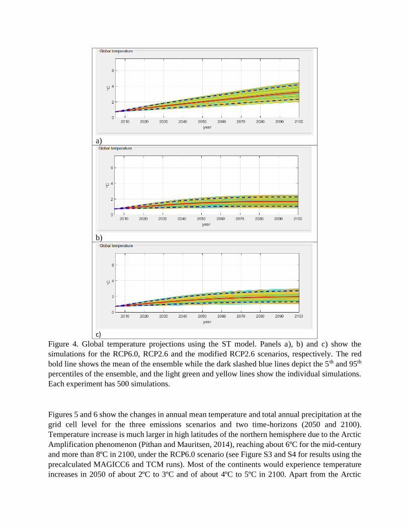
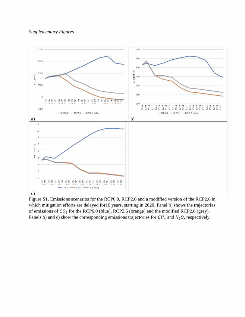
Figure S1 shows the trajectories of 𝐶𝑂2, 𝐶𝐻4 and 𝑁2𝑂 for the RCP6.0, RCP2.6 and the modified

version of the RCP2.6 scenarios in which mitigation is delayed for 10 years, starting in 2020. The

modified version of the RCP2.6 was edited in Excel and directly loaded to AIRCC-Clim using the

user-defined option for emissions scenarios. The RCP6.0 and the RCP2.6 scenarios produce

contrasting results in terms of their effects on climate. While the first produces a mean increase in

global temperature of about 3ºC at the end of this century, and up to 4ºC when the 95th percentile

is considered, the RCP2.6 limits warming below 2ºC for the ensemble mean (about 1.7ºC),

although this limit is exceeded for the 95th percentile (Figure 4). The MAGICC model produces

similar results, with a mean increase in global temperature of 3.1ºC and 1.6ºC for the end of the

century under the RCP6.0 and RCP2.6 scenarios, respectively (Figure S2). The TCM produces a

considerably larger mean increase for the RCP6.0 (3.9ºC), but that still lies within the likely range

of the CMIP5 experiment (Table 1). The ST simulations for the modified RCP2.6 in which the

mitigation effort is delayed for 10 years, show that the mean increase in global temperature reaches

2ºC in 2100, and up to 3ºC in the 95th percentile.

a)

b)

c)

Figure 4. Global temperature projections using the ST model. Panels a), b) and c) show the

simulations for the RCP6.0, RCP2.6 and the modified RCP2.6 scenarios, respectively. The red

bold line shows the mean of the ensemble while the dark slashed blue lines depict the 5th and 95th

percentiles of the ensemble, and the light green and yellow lines show the individual simulations.

Each experiment has 500 simulations.

Figures 5 and 6 show the changes in annual mean temperature and total annual precipitation at the

grid cell level for the three emissions scenarios and two time-horizons (2050 and 2100).

Temperature increase is much larger in high latitudes of the northern hemisphere due to the Arctic

Amplification phenomenon (Pithan and Mauritsen, 2014), reaching about 6ºC for the mid-century

and more than 8ºC in 2100, under the RCP6.0 scenario (see Figure S3 and S4 for results using the

precalculated MAGICC6 and TCM runs). Most of the continents would experience temperature

increases in 2050 of about 2ºC to 3ºC and of about 4ºC to 5ºC in 2100. Apart from the Arctic

region, midlatitudes in North America and in Eurasia would have the largest increases (5ºC-6ºC)

in temperature by the end of the present century, followed by Southern Asia and the Middle East,

North and South Africa, parts of the west coast of North America, Mexico and the Amazonian

region and the northern part of Brazil. Large changes are also expected in precipitation under the

RCP6.0 scenario, with large increases in high latitudes, the equatorial Pacific Ocean and some

parts of the Middle East, and large decreases in the Mediterranean, the Caribbean, Mexico, and the

southern part of the US, as well as in southern parts of Africa and America (Figure S3 and S4).

The implementation of a deep mitigation effort consistent with the goals of the Paris Agreement

would significantly limit these changes in climate. Under the RCP2.6 most of the Arctic would not

exceed a warming of 5ºC during this century, most continents would not exceed 3.5ºC, and

precipitation change would be notably smaller.

2050 2100

Figure 5. Annual temperature change projections (ºC) for different emissions scenarios estimated

by the modified ST model. The upper panel shows the changes in temperature under the RCP6.0

scenario for 2050 (left) and 2100 (right). The middle panel shows the changes in temperature under

the RCP2.6 scenario for 2050 (left) and 2100 (right). The lower panel shows the changes in

temperature under the delayed RCP2.6 scenario for 2050 (left) and 2100 (right).

2050 2100

Figure 6. Annual precipitation projections (%) for different emissions scenarios estimated by the

modified ST model. The upper panel shows the changes in precipitation under the RCP6.0 scenario

for 2050 (left) and 2100 (right). The middle panel shows the changes in precipitation under the

RCP2.6 scenario for 2050 (left) and 2100 (right). The lower panel shows the changes in

precipitation under the delayed RCP2.6 scenario for 2050 (left) and 2100 (right).

AIRCC-Clim portraits the risks of climate change, and the benefits of mitigation, in a clearer way

due to its probabilistic nature and its capacity to produce maps of probabilities and of dates of

exceedance. Figures 7 and 8 show the probabilities of exceeding a 2.5ºC increase in annual

temperatures and a decrease of 15% in annual precipitation in 2050 and 2100. Under the RCP6.0,

by 2050 the probabilities of exceeding 2.5ºC increase in annual temperatures are higher than 60%

for most of the continents, while the Arctic region and the high latitudes of the northern hemisphere

are virtually certain to exceed this threshold by mid-century (Figure S5). These simulations also

show that a 2.5ºC warming would be exceeded in all continents by 2100 and that there is a high

probability (above 60%) that this threshold would be crossed in all oceans, except for parts of the

southern hemisphere and the Atlantic. The probabilities of exceeding a decrease of 15% in total

annual precipitation in 2050 are higher than 50% for several areas of the world such as the

Mediterranean, parts of Northern, Western and Southern Africa, the Caribbean and Mexico (Figure

S5). For 2100, these probabilities increase to more than 60% in those regions and extend to parts

of South America and West Australia. If the emissions trajectory described in by the RCP2.6 is

achieved, by 2050 the probability of exceeding 2.5ºC would be lower than 40% over the continents,

except for the Arctic and parts of the midlatitudes in the northern hemisphere where the

probabilities range from 60% to 100% (Figure 7). Likewise, the probabilities of exceeding

decreases in precipitation of at least 15% are considerably smaller in comparison to the RCP6.0.

However, by the end of this century the probabilities of exceeding this threshold would be close

to 50% for the southern region of Spain, parts of North and West Africa (Morocco, Mauritania,

Mali, Senegal, Sierra Leone and Guinea), and about 40% for parts of the Caribbean, Central and

South America (Colombia and Venezuela; Figure 8).

2050 2100

Figure 7. Probabilities of exceeding increases of 2.5ºC in annual temperature for different

emissions scenarios estimated by the modified ST model. The upper panel shows the probabilities

of exceedance for the RCP6.0 scenario in 2050 (left) and 2100 (right). The middle panel shows

the probabilities of exceedance for the RCP2.6 scenario for 2050 (left) and 2100 (right). The lower

panel shows the probabilities of exceedance for the delayed RCP2.6 scenario for 2050 (left) and

2100 (right). Probabilities are expressed in percentages.

2050 2100

Figure 8. Probabilities of exceeding decreases of 15% in annual precipitation for different

emissions scenarios estimated by the modified ST model. The upper panel shows the probabilities

of exceedance for the RCP6.0 scenario in 2050 (left) and 2100 (right). The middle panel shows

the probabilities of exceedance for the RCP2.6 scenario for 2050 (left) and 2100 (right). The lower

panel shows the probabilities of exceedance for the delayed RCP2.6 scenario for 2050 (left) and

2100 (right). Probabilities are expressed in percentages.

Figure 9 shows the dates when the 2.5ºC threshold would be exceeded. The default confidence

level (𝛾 = 50) was used for the estimates presented in this section. The results show that under

the RCP6.0, most of the planet except for part of the southern oceans and part of the North Atlantic,

would exceed the 2.5ºC threshold during this century and that some parts of the world already

exceeded it (Figure S5). The date of exceedance for the Arctic occurred during the 2000s, while

for much of the high latitudes in the northern hemisphere, the Middle East, parts of South Asia,

and West and South Africa, the exceedance is expected to occur in the 2020s-2030s. The remainder

of the continents and the Antarctic region would go over this threshold during the period 2040-

2060 and most of the oceans above the 20ºS would exceed the 2.5ºC threshold during this century.

The regions in which reductions of at least 15% in annual precipitation is exceeded are fewer and

form well-defined geographical patterns that cover the Mediterranean, parts of North, West and

South Africa, Central America and the Caribbean, Mexico and Colombia and Venezuela in South

America, as well as the west part of Australia and part of the southern Pacific Ocean (Figures 9

and S5). The dates for exceedance on these regions are typically reached in the 2050-2060 decades,

although regions of Spain and West Africa could exceed this threshold as early as the 2040s.

Achieving RCP2.6 would prevent exceeding these thresholds for most of the world during this

century (Figure 9). However, as mentioned above, some regions such as the Arctic and the high

latitudes of the northern hemisphere already have exceeded the 2.5ºC temperature threshold or will

do so during the next decade, regardless of the emission scenario that is selected. For parts of the

midlatitudes, the RCP2.6 represents delaying reaching the 2.5ºC threshold for about 20 years,

which buys time for adapting to the projected changes and to reduce risks and damages. The

occurrence of this threshold would also be delayed until 2060 in some parts of the Sahara, South

Africa, the Middle East and India. Exceeding decreases in precipitation of more than 15% would

not occur during this century, with the exception of a few grid cells in Africa, Spain and Central

America.

AIRCC-Clim runs illustrate that delaying the deep mitigation efforts of the RCP2.6 by ten years

would significantly increase the risks of climate change during this century. The bottom rows of

Figures 7 and 8 show that, under delayed international action, the probabilities of exceeding 2.5ºC

in annual temperature and a decrease of at least -15% annual precipitation in 2100 are similar to

those obtained in 2050 for the RCP6.0 and much higher than those of the original RCP2.6. The

consequences of delaying for ten years the mitigation efforts described in the RCP2.6 are clearly

illustrated by Figure 9: North and South Africa, South America, the Middle East and Central Asia

would exceed a 2.5ºC increase in temperatures around 2060, when this threshold was not reached

during this century under the original RCP2.6 trajectory. Parts of Australia would exceed this

threshold at the end of the present century if mitigation efforts were postponed. In terms of

precipitation reductions, the Mediterranean region would be most affected, as the dates of

exceedance of decreases of at least 15% in precipitation would occur as soon as 2040-2050 for the

south of Spain and North Africa and at the end of this century for Greece. Western Africa would

go over this threshold in 2040, and parts of Central America and South Africa would see decreases

of more than 15% in the 2050-2060 period. However, it is important to note that this delayed action

scenario still provides important benefits in comparison with the RCP6.0, which is commonly used

to represent current international mitigation commitments. Some of the most affected regions due

to warming would buy time (about 2 decades) for adapting to a 2.5ºC under the delayed version of

the RCP2.6. This is not so clear with regard to exceeding -15% decrease in annual precipitation

for the most affected regions, as in comparison with the RCP6.0, the delayed version of the RCP2.6

would buy them only 5-10 years for implementing adaptation actions.

Figure 9. Dates of exceedance for increases of 2.5ºC in annual temperature and decreases of 15%

in annual precipitation for different emissions scenarios estimated by the modified ST model. The

upper panel shows the dates of exceedance for annual temperature (left) and annual precipitation

(right) under the RCP6.0 scenario. The middle panel shows the probabilities of exceedance for

annual temperature (left) and annual precipitation (right) under the RCP2.6 scenario. The lower

panel shows the probabilities of exceedance for annual temperature (left) and annual precipitation

(right) under the delayed RCP2.6 scenario.

Monthly estimates of changes in precipitation and temperature are commonly needed for assessing

the impacts of climate change in natural and human systems. AIRCC-Clim also generates

estimates of monthly temperature and precipitation change, as well as estimates of probabilities

and dates of exceedance for user-defined thresholds. Figure 10 illustrates this feature for the RCP6

emissions scenario and for the central month of winter and summer (i.e., February and July).

During the coldest months in the northern hemisphere’s winter, the threshold of 2.5ºC was

exceeded at the beginning of this century in the Arctic, while for parts of the midlatitudes it will

be exceeded during this decade of in the 2030s (Figure 10a). In most of the remaining parts of the

northern hemisphere the 2.5ºC threshold in temperatures during February would be exceeded in

the 2030-2050 decades. For parts of North and Central America, the driest months occur in winter

and precipitation in February in those areas would decrease at least 15% as soon as 2030. In the

case of regions in southern hemisphere, such as Australia, Central and South Africa, as well as

most of South America, the temperature threshold during one of the hottest months (February)

would occur before 2060 and, in some parts of these region, this threshold could be exceeded 20

years earlier.

The hottest months in the northern hemisphere occur during the boreal summer. As shown in

Figure 10c, exceeding the threshold a 2.5ºC increase in July would happen in this decade for

regions in the Mediterranean such as Spain, France, Italy, Greece, and parts of North Africa. In

these regions, exceeding this threshold in temperatures during July would be accompanied by

decreases of at least 15% in precipitation before 2050 in the same month, which is one of the driest

in the Mediterranean.

a)

b)

c)

d)

Figure 10. Estimates of dates of exceedance during February and July for 2.5ºC and -15%

thresholds in temperature and precipitation, respectively.

Moreover, due to its capabilities for exporting output, AIRCC-Clim can be easily combined with

other products to address the user’s specific information needs. Figure 11 combines population

count projections from the SSP3 scenario that were obtained from CLIMRISK (Estrada and

Botzen, 2021) with two risk measures produced with AIRCC-Clim to provide a first approximation

of risk and exposure. Climate and population projections show that by 2050 some regions of the

world will have high exposure and high probabilities of experiencing large changes in climate. In

the bivariate map shown in Figure 11a dark magenta color indicate regions for which large

population and high probabilities of exceeding 15% decrease in precipitation are projected. These

high-risk, high-exposure regions include large fractions of the Mediterranean, Central America

and parts of the Middle East and South Asia. Light yellow areas indicate regions characterized by

large population but low probabilities of decreases in precipitation of at least 15%. These include

high latitude regions in the northern hemisphere for which most climate models’ projections

suggest an increase in precipitation. This combination of population and precipitation change

would be found in parts of India, China, parts of central, northern and eastern Europe, northern US

and Canada. Light blue regions such as Australia, large parts of Noth Africa and South America,

are where decreases in precipitation of at least 15% are highly likely but where population counts

are low.

Figure 11b shows a bivariate map of population counts and the probability of exceeding 2.5ºC in

annual temperature change by year 2050. Regions such as the eastern part of the US, Central

America, most of Europe, India, China, the Middle East and parts of Africa are shown in dark

magenta color. These regions are characterized by high probabilities of exceeding 2.5ºC and large

population counts. Regions in light blue hue represent places where the probability of exceeding a

warming of at least 2.5ºC in 2050 are high, but population in those areas is not large. This is the

case of high latitudes in the northern hemisphere, Australia, the Amazon rainforest, the Sahara,

Namib and the Arabian deserts. Moreover, Figures 11 helps to identify risk hotspots in which

population counts will be high in the future and significantly dryer and hotter conditions will likely

occur. Such combination of factors has been associated with higher risks of human conflict and

migration (Barrios et al., 2006; Hodler and Raschky, 2014; Hsiang et al., 2013; Puente et al., 2016;

World Bank, 2016), as well as impacts on biomass production and more frequent wildfires (De

Dato et al., 2008; Stevens-Rumann et al., 2018).

a)

b)

Figure 11. Bivariate maps of population and probabilities of user-defined risk thresholds. Panel a)

shows a bivariate map of population counts in year and of the probabilities of decreases in annual

precipitation of at least 15% in year 2050. Panel b) shows a bivariate map of population counts

and of the probabilities of warming of at least 2.5ºC in year 2050.

4. Conclusions

Here we present AIRCC-Clim, an emulator of complex climate models included in the IPCC’s

Fifth Assessment Report that allows generating probabilistic climate change projections and risk

measures for RCP emissions scenarios, as well as for user-defined emissions scenarios. Global

temperature projections are produced using a modified version of the ST model and precalculated

runs of the MAGICC and TCM models. AIRCC-Clim has a spatial resolution of 2.5º x 2.5º and

produces monthly and annual temperature and precipitation scenarios. This is a user-friendly,

stand-alone software aimed for students, decision-makers, and researchers that allows for quick

estimates of changes in climate, as well as of the probabilities and dates of exceedance of user-

defined thresholds. The AIRCC-Clim model attempts to fill users’ needs for models that have low

technical and computing requirements, but that are able to emulate complex climate models’

output and produce spatially explicit, probabilistic projections and risk measures.

AIRCC-Clim extends the ST climate model to include a dynamic climate sensitivity that takes

advantage of the well-established approximately linear relationship between cumulative CO2

emissions and global temperature increase. This extension of the ST model, combined with

stochastic simulation, allows to closely approximate the best estimate and likely range included in

the Fifth Assessment Report of the IPCC. By means of a simple stochastic simulation procedure,

we account for the uncertainty in the climate sensitivity parameter and produce probabilistic

scenarios based on MAGICC and TCM precalculated runs. Extensions and future development of

this model include the integration with IVA and integrated assessment models, such as simple

agricultural emulators and climate-economy models (Estrada et al., 2020; Estrada and Botzen,

2021; Ignjacevic et al., 2021, 2020); the inclusion of additional climate variables (e.g., minimum

and maximum temperatures and bioclimatic indices), as well as complementary uni- and

multivariate risk measures.

Acknowledgements: Francisco Estrada acknowledges financial support from DGAPA-UNAM

through the projects PAPIIT IN110718 and IN111221 and from PINCC-UNAM.

References

Adem, J., 1991. Review of the development and applications of the Adem thermodynamic

climate model. Clim. Dyn. 5, 145–160. https://doi.org/10.1007/BF00251806

Altamirano del Carmen, M.A., Estrada, F., Gay-Garciá, C., 2021. A new method for assessing

the performance of general circulation models based on their ability to simulate the

response to observed forcing. J. Clim. 34, 5385–5402. https://doi.org/10.1175/JCLI-D-20-

0510.1

Anthoff, D., Tol, R.S.J., 2014. Climate policy under fat-tailed risk: an application of FUND.

Ann. Oper. Res. 220, 223–237. https://doi.org/10.1007/s10479-013-1343-2

Barrios, S., Bertinelli, L., Strobl, E., 2006. Climatic change and rural–urban migration: The case

of sub-Saharan Africa. J. Urban Econ. 60, 357–371.

https://doi.org/10.1016/J.JUE.2006.04.005

Blanc, É., 2017. Statistical emulators of maize, rice, soybean and wheat yields from global

gridded crop models. Agric. For. Meteorol. 236, 145–161.

https://doi.org/10.1016/j.agrformet.2016.12.022

Bony, S., Stevens, B., Held, I.H., Mitchell, J.F., Dufresne, J.-L., Emanuel, K.A., Friedlingstein,

P., Griffies, S., Senior, C., 2013. Carbon Dioxide and Climate: Perspectives on a Scientific

Assessment, in: Climate Science for Serving Society. pp. 391–413.

https://doi.org/10.1007/978-94-007-6692-1_14

Cabré, M.F., Solman, S.A., Nuñez, M.N., 2010. Creating regional climate change scenarios over

southern South America for the 2020’s and 2050’s using the pattern scaling technique:

validity and limitations. Clim. Change 98, 449–469. https://doi.org/10.1007/s10584-009-

9737-5

Callendar, G.S., 1938. The artificial production of carbon dioxide and its influence on

temperature. Q. J. R. Meteorol. Soc. 64, 223–240. https://doi.org/10.1002/qj.49706427503

Collins, M., Knutti, R., Arblaster, J., Dufresne, J.L., Fichefet, T., Friedlingstein, P., Gao, X.,

Gutowski, W.J., Johns, T., Krinner, G., Shongwe, M., 2013. Long-term climate change:

Projections, commitments and irreversibility, in: Climate Change 2013 the Physical Science

Basis: Working Group I Contribution to the Fifth Assessment Report of the

Intergovernmental Panel on Climate Change. pp. 1029–1136.

https://doi.org/10.1017/CBO9781107415324.024

Conde, C., Estrada, F., Martínez, B., Sánchez, O., Gay, C., 2011. Regional climate change

scenarios for México. Atmosfera 24, 125–140.

Cox, P.M., Huntingford, C., Williamson, M.S., 2018. Emergent constraint on equilibrium

climate sensitivity from global temperature variability. Nature 553, 319–322.

https://doi.org/10.1038/nature25450

Curry, J.A., Webster, P.J., 2011. Climate science and the uncertainty monster. Bull. Am.

Meteorol. Soc. https://doi.org/10.1175/2011BAMS3139.1

De Dato, G., Pellizzaro, G., Cesaraccio, C., Sirca, C., De Angelis, P., Duce, P., Spano, D.,

Scarascia Mugnozza, G., 2008. Effects of warmer and drier climate conditions on plant

composition and biomass production in a Mediterranean shrubland community.

http://iforest.sisef.org/ 1, 39. https://doi.org/10.3832/IFOR0418-0010039

Deser, C., Phillips, A.S., Alexander, M.A., Smoliak, B. V., 2014. Projecting North American

climate over the next 50 years: Uncertainty due to internal variability. J. Clim. 27, 2271–

2296. https://doi.org/10.1175/JCLI-D-13-00451.1

Estrada, F., Botzen, W.J.W., 2021. Economic impacts and risks of climate change under failure

and success of the Paris Agreement. Ann. N. Y. Acad. Sci. nyas.14652.

https://doi.org/10.1111/NYAS.14652

Estrada, F., Botzen, W.J.W., Calderon-Bustamante, O., 2020. The Assessment of Impacts and

Risks of Climate Change on Agriculture (AIRCCA) model: a tool for the rapid global risk

assessment for crop yields at a spatially explicit scale. Spat. Econ. Anal. 15, 262–279.

https://doi.org/10.1080/17421772.2020.1754448

Fick, S.E., Hijmans, R.J., 2017. WorldClim 2: new 1-km spatial resolution climate surfaces for

global land areas. Int. J. Climatol. 37, 4302–4315. https://doi.org/10.1002/joc.5086

Freeman, M.C., Wagner, G., Zeckhauser, R.J., 2015. Climate sensitivity uncertainty: When is

good news bad? Philos. Trans. R. Soc. A Math. Phys. Eng. Sci. 373, 20150092.

https://doi.org/10.1098/rsta.2015.0092

Friedrich, T., Timmermann, A., Tigchelaar, M., Timm, O.E., Ganopolski, A., 2016. Nonlinear

climate sensitivity and its implications for future greenhouse warming. Sci. Adv. 2,

e1501923. https://doi.org/10.1126/sciadv.1501923

Gay, C., Estrada, F., 2010a. Objective probabilities about future climate are a matter of opinion.

Clim. Change 99, 27–46.

Gay, C., Estrada, F., 2010b. Objective probabilities about future climate are a matter of opinion.

Clim. Change 99, 27–46. https://doi.org/10.1007/s10584-009-9681-4

Herger, N., Sanderson, B.M., Knutti, R., 2015. Improved pattern scaling approaches for the use

in climate impact studies. Geophys. Res. Lett. 42, 3486–3494.

https://doi.org/10.1002/2015GL063569

Hodler, R., Raschky, P.A., 2014. Economic shocks and civil conflict at the regional level. Econ.

Lett. 124, 530–533. https://doi.org/10.1016/J.ECONLET.2014.07.027

Hodrick, R.J., Prescott, E.C., 1997. Postwar U.S. Business Cycles: An Empirical Investigation. J.

Money, Credit Bank. 29, 1. https://doi.org/10.2307/2953682

Hsiang, S.M., Burke, M., Miguel, E., 2013. Quantifying the influence of climate on human

conflict. Science 341, 1235367. https://doi.org/10.1126/science.1235367

Ignjacevic, P., Botzen, W.J.W., Estrada, F., Kuik, O., Ward, P., Tiggeloven, T., 2020.

CLIMRISK-RIVER: Accounting for local river flood risk in estimating the economic cost

of climate change. Environ. Model. Softw. 132.

https://doi.org/10.1016/j.envsoft.2020.104784

Ignjacevic, P., Estrada, F., Botzen, W.J.W., 2021. Time of emergence of economic impacts of

climate change. Environ. Res. Lett. 16, 074039. https://doi.org/10.1088/1748-

9326/AC0D7A

IPCC-TGICA, 2007. General Guidelines on the Use of Scenario Data for climate impact and

adaptation assessment, IPCC. https://doi.org/10.1144/SP312.4

IPCC, 2021. Climate Change 2021: The Physical Science Basis. IPCC.

IPCC, 2018. Impacts of 1.5°C of Global Warming on Natural and Human Systems [WWW

Document]. Glob. Warm. 1.5°C. An IPCC Spec. Rep. impacts Glob. Warm. 1.5°C above

pre-industrial levels Relat. Glob. Greenh. gas Emiss. pathways, Context Strength. Glob.

response to Threat Clim. Chang.

Jaynes, E.T., 1957. Information Theory and Statistical Mechanics. Phys. Rev. 106, 620–630.

https://doi.org/10.1103/PhysRev.106.620

Jaynes, E.T. (Edwin T.., Bretthorst, G.L., 2003. Probability theory : the logic of science.

Cambridge University Press.

Jonko, A., Urban, N.M., Nadiga, B., 2018. Towards Bayesian hierarchical inference of

equilibrium climate sensitivity from a combination of CMIP5 climate models and

observational data. Clim. Change 149, 247–260. https://doi.org/10.1007/s10584-018-2232-0

Knutti, R., 2010. The end of model democracy? Clim. Change 102, 395–404.

https://doi.org/10.1007/s10584-010-9800-2

Knutti, R., Furrer, R., Tebaldi, C., Cermak, J., Meehl, G.A., 2010. Challenges in combining

projections from multiple climate models. J. Clim. 23, 2739–2758.

https://doi.org/10.1175/2009JCLI3361.1

Knutti, R., Rugenstein, M.A.A., Hegerl, G.C., 2017. Beyond equilibrium climate sensitivity. Nat.

Geosci. https://doi.org/10.1038/NGEO3017

Knutti, R., Sedláček, J., 2012. Robustness and uncertainties in the new CMIP5 climate model

projections. Nat. Clim. Chang. 3, 1–5. https://doi.org/10.1038/nclimate1716

Kravitz, B., Lynch, C., Hartin, C., Bond-Lamberty, B., 2017a. Exploring precipitation pattern

scaling methodologies and robustness among CMIP5 models. Geosci. Model Dev. 10,

1889–1902. https://doi.org/10.5194/gmd-10-1889-2017

Kravitz, B., Lynch, C., Hartin, C., Bond-Lamberty, B., 2017b. Exploring precipitation pattern

scaling methodologies and robustness among CMIP5 models. Geosci. Model Dev. 10,

1889–1902. https://doi.org/10.5194/gmd-10-1889-2017

Lewis, N., Curry, J.A., 2015. The implications for climate sensitivity of AR5 forcing and heat

uptake estimates. Clim. Dyn. 45, 1009–1023. https://doi.org/10.1007/s00382-014-2342-y

Lynch, C., Hartin, C., Bond-Lamberty, B., Kravitz, B., 2017. An open-access CMIP5 pattern

library for temperature and precipitation: description and methodology. Earth Syst. Sci.

Data 9, 281–292. https://doi.org/10.5194/essd-9-281-2017

Meinshausen, M., Raper, S.C.B., Wigley, T.M.L., 2011a. Emulating coupled atmosphere-ocean

and carbon cycle models with a simpler model, MAGICC6 – Part 1: Model description and

calibration. Atmos. Chem. Phys. 11, 1417–1456. https://doi.org/10.5194/acp-11-1417-2011

Meinshausen, M., Wigley, T.M.L., Raper, S.C.B., 2011b. Emulating atmosphere-ocean and

carbon cycle models with a simpler model, MAGICC6 - Part 2: Applications. Atmos.

Chem. Phys. https://doi.org/10.5194/acp-11-1457-2011

Mendlik, T., Gobiet, A., 2016. Selecting climate simulations for impact studies based on

multivariate patterns of climate change. Clim. Change 135, 381–393.

https://doi.org/10.1007/s10584-015-1582-0

Mitchell, T.D., 2003. Pattern Scaling: An Examination of the Accuracy of the Technique for

Describing Future Climates. Clim. Change 60, 217–242.

https://doi.org/10.1023/A:1026035305597

Nordhaus, W.D., Boyer, J., 2003. Warming the world: economic models of global warming. MIT

press.

Notz, D., 2015. How well must climate models agree with observations? Philos. Trans. R. Soc. A

Math. Phys. Eng. Sci. 373, 20140164. https://doi.org/10.1098/rsta.2014.0164

Osborn, T.J., Wallace, C.J., Lowea, J.A., Bernie, D., 2018. Performance of pattern-scaled climate

projections under high-end warming. Part I: Surface air temperature over land. J. Clim. 31,

5667–5680. https://doi.org/10.1175/JCLI-D-17-0780.1

Pithan, F., Mauritsen, T., 2014. Arctic amplification dominated by temperature feedbacks in

contemporary climate models. Nat. Geosci. 7, 181–184. https://doi.org/10.1038/ngeo2071

Potter, T.D., Colman, B.R., 2003. Handbook of weather, climate, and water : atmospheric

chemistry, hydrology, and societal impacts. Wiley-Interscience.

Puente, G.B., Perez, F., Gitter, R.J., 2016. The Effect of Rainfall on Migration from Mexico to

the United States. Int. Migr. Rev. 50, 890–909. https://doi.org/10.1111/imre.12116

Rogelj, J., Meinshausen, M., Sedláček, J., Knutti, R., 2014. Implications of potentially lower

climate sensitivity on climate projections and policy. Environ. Res. Lett. 9, 031003.

https://doi.org/10.1088/1748-9326/9/3/031003

Sanderson, B.M., Knutti, R., Caldwell, P., 2015. A representative democracy to reduce

interdependency in a multimodel ensemble. J. Clim. 28, 5171–5194.

https://doi.org/10.1175/JCLI-D-14-00362.1

Santer, B.D., Bonfils, C.J.W., Fu, Q., Fyfe, J.C., Hegerl, G.C., Mears, C., Painter, J.F., Po-

Chedley, S., Wentz, F.J., Zelinka, M.D., Zou, C.Z., 2019. Celebrating the anniversary of

three key events in climate change science. Nat. Clim. Chang.

https://doi.org/10.1038/s41558-019-0424-x

Santer, B.D., Wigley, T.M.L., Schlesinger, M.E., Mitchell, J.F.B., 1990. Developing climate

scenarios from equilibrium GCM results. Report/Max-Planck-Institut für Meteorol. 47.

Schneider, S.H., Thompson, S.L., 1981. Atmospheric CO 2 and climate: Importance of the

transient response. J. Geophys. Res. 86, 3135. https://doi.org/10.1029/JC086iC04p03135

Stephenson, D.B., Collins, M., Rougier, J.C., Chandler, R.E., 2012. Statistical problems in the

probabilistic prediction of climate change. Environmetrics 23, 364–372.

https://doi.org/10.1002/env.2153

Stevens-Rumann, C.S., Kemp, K.B., Higuera, P.E., Harvey, B.J., Rother, M.T., Donato, D.C.,

Morgan, P., Veblen, T.T., 2018. Evidence for declining forest resilience to wildfires under

climate change. Ecol. Lett. https://doi.org/10.1111/ele.12889

Stocker, T F, Qin, D., Plattner, G.K., Tignor, M., Allen, S.K., Boschung, J., Nauels, A., Xia, Y.,

Bex, B., Midgley, B.M., 2013. IPCC, 2013: Climate Change 2013: The Physical Science

Basis. Contribution of Working Group I to the Fifth Assessment Report of the

Intergovernmental Panel on Climate Change. Cambridge University Press.

Stocker, Thomas F., Qin, D., Plattner, G.K., Tignor, M.M.B., Allen, S.K., Boschung, J., Nauels,

A., Xia, Y., Bex, V., Midgley, P.M., 2013. Climate change 2013 the physical science basis:

Working Group I contribution to the fifth assessment report of the intergovernmental panel

on climate change, Climate Change 2013 the Physical Science Basis: Working Group I

Contribution to the Fifth Assessment Report of the Intergovernmental Panel on Climate

Change. https://doi.org/10.1017/CBO9781107415324

Tan, I., Storelvmo, T., Zelinka, M.D., 2016. Observational constraints on mixed-phase clouds

imply higher climate sensitivity. Science (80-. ). 352, 224–227.

https://doi.org/10.1126/science.aad5300

Taylor, K.E., Stouffer, R.J., Meehl, G.A., 2012. An overview of CMIP5 and the experiment

design. Bull. Am. Meteorol. Soc. https://doi.org/10.1175/BAMS-D-11-00094.1

Tebaldi, C., Arblaster, J.M., 2014. Pattern scaling: Its strengths and limitations, and an update on

the latest model simulations. Clim. Change 122, 459–471. https://doi.org/10.1007/s10584-

013-1032-9

Tebaldi, C., Knutti, R., 2018. Evaluating the accuracy of climate change pattern emulation for

low warming targets. Environ. Res. Lett. 13, 055006. https://doi.org/10.1088/1748-

9326/aabef2

Tol, R.S.J., 2019. Climate economics: economic analysis of climate, climate change and climate

policy, Second. ed. Edward Elgar Publishing. https://doi.org/10.5860/choice.188270

Tol, R.S.J., Fankhauser, S., 1998. On the representation of impact in integrated assessment

models of climate change. Environ. Model. Assess. 3, 63–74.

https://doi.org/10.1023/A:1019050503531

Weigel, A.P., Knutti, R., Liniger, M.A., Appenzeller, C., 2010. Risks of model weighting in

multimodel climate projections. J. Clim. 23, 4175–4191.

https://doi.org/10.1175/2010JCLI3594.1

Wigley, T.M.L., 1995. MAGICC and SCENGEN: Integrated models for estimating regional

climate change in response to anthropogenic emissions. Stud. Environ. Sci. 65, 93–94.

https://doi.org/10.1016/S0166-1116(06)80197-4

World Bank, 2016. High and Dry: Climate Change, Water, and the Economy, High and Dry:

Climate Change, Water, and the Economy. World Bank. https://doi.org/10.1596/k8517

Xu, Y., Gao, X., Giorgi, F., 2010. Upgrades to the reliability ensemble averaging method for

producing probabilistic climate-change projections. Clim. Res. 41, 61–81.

https://doi.org/10.3354/cr00835

Zelazowski, P., Huntingford, C., Mercado, L.M., Schaller, N., 2018. Climate pattern-scaling set

for an ensemble of 22 GCMs – adding uncertainty to the IMOGEN version 2.0 impact

system. Geosci. Model Dev. 11, 541–560. https://doi.org/10.5194/gmd-11-541-2018

Supplementary Figures

a)

b)

c)

Figure S1. Emissions scenarios for the RCP6.0, RCP2.6 and a modified version of the RCP2.6 in

which mitigation efforts are delayed for10 years, starting in 2020. Panel b) shows the trajectories

of emissions of 𝐶𝑂2 for the RCP6.0 (blue), RCP2.6 (orange) and the modified RCP2.6 (grey).

Panels b) and c) show the corresponding emissions trajectories for 𝐶𝐻4 and 𝑁2𝑂, respectively.

ST

MAGICC

TCM

Figure S2. Global temperature projections under the RCP6.0 and RCP2.6. The left and right

columns show the projections for the RCP6.0 and the RCP2.6, respectively. The upper row shows

the simulations of the ST model, while the middle and bottom rows show the projections based on

the MAGICC and TCM model runs, respectively.

2050 2100

a)

b)

c)

d)

e)

f)

g)

h)

Figure S3. Projections based on MAGICC6 runs for annual temperature and precipitation. Panel

a) and b) show the changes in annual temperature under the RCP6.0 for 2050 and 2100,

respectively. Panels c) and d) show the changes in annual precipitation under the RCP6.0 for 2050

and 2100, respectively. Panels e) and f) show the probabilities of exceeding 2.5ºC increase in

annual temperature under the RCP6.0 for 2050 and 2100, respectively. Panels g) and h) show the

probabilities of exceeding decreases of -15% in annual precipitation.

a)

b)

c)

d)

e)

f)

g)

h)

Figure S4. Projections based on TCM runs for annual temperature and precipitation. Panel a) and

b) show the changes in annual temperature under the RCP6.0 for 2050 and 2100, respectively.

Panels c) and d) show the changes in annual precipitation under the RCP6.0 for 2050 and 2100,

respectively. Panels e) and f) show the probabilities of exceeding 2.5ºC increase in annual

temperature under the RCP6.0 for 2050 and 2100, respectively. Panels g) and h) show the

probabilities of exceeding decreases of -15% in annual precipitation.

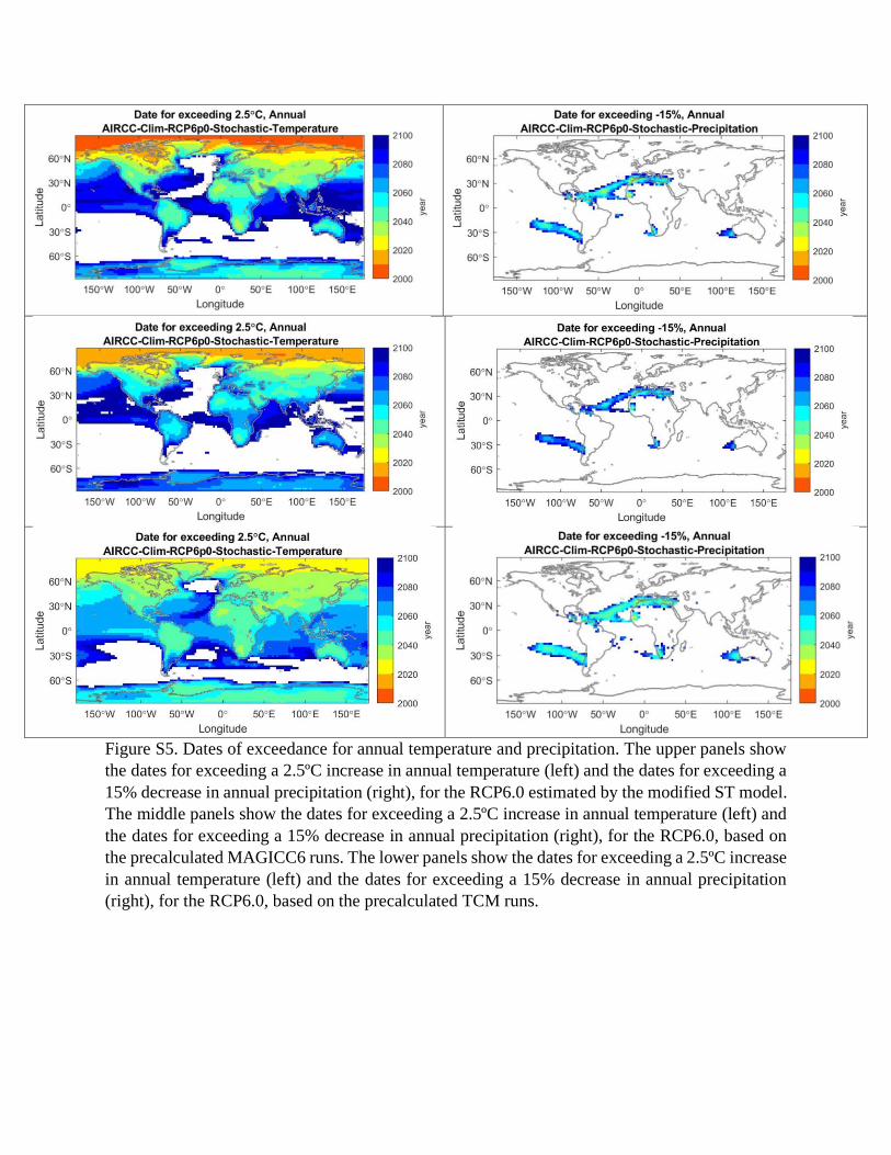
Figure S5. Dates of exceedance for annual temperature and precipitation. The upper panels show

the dates for exceeding a 2.5ºC increase in annual temperature (left) and the dates for exceeding a

15% decrease in annual precipitation (right), for the RCP6.0 estimated by the modified ST model.

The middle panels show the dates for exceeding a 2.5ºC increase in annual temperature (left) and

the dates for exceeding a 15% decrease in annual precipitation (right), for the RCP6.0, based on

the precalculated MAGICC6 runs. The lower panels show the dates for exceeding a 2.5ºC increase

in annual temperature (left) and the dates for exceeding a 15% decrease in annual precipitation

(right), for the RCP6.0, based on the precalculated TCM runs.

Supplementary Tables

Table S1. Parameter values of the five box carbon cycle model.

𝛼1 0 𝛾1 0.13

𝛼2 1 − 𝑒−1 363⁄ 𝛾2 0.2

𝛼3 1 − 𝑒−1 74⁄ 𝛾3 0.32

𝛼4 1 − 𝑒−1 17⁄ 𝛾4 0.25

𝛼5 1 − 𝑒−1 2⁄ 𝛾5 0.1

𝛽 0.00045

Table S2. List of climate models included in the CMIP5 experiment that are emulated in AIRCC-

Clim.

ACCESS1-0 CSIRO-Mk3-6-0 GISS-E2-R_p1 MIROC-ESM

ACCESS1-3 EC-EARTH GISS-E2-R_p2 MIROC-ESM-CHEM

BNU-ESM FGOALS-g2 GISS-E2-R_p3 MPI-ESM-LR

CanESM2 FIO-ESM HadGEM2-AO MPI-ESM-MR

CCSM4 GFDL-CM3 HadGEM2-CC MRI-CGCM3

CESM1-BGC GFDL-ESM2G HadGEM2-ES NorESM1-M

CESM1-CAM5 GFDL-ESM2M IPSL-CM5A-LR NorESM1-ME

CMCC-CM GISS-E2-H_p1 IPSL-CM5A-MR

CMCC-CMS GISS-E2-H_p2 IPSL-CM5B-LR

CNRM-CM5 GISS-E2-H_p3 MIROC5