airborne radar for high-resolution mapping of internal

AIRBORNE RADAR FOR HIGH-RESOLUTION MAPPING OF

INTERNAL LAYERS IN GLACIAL ICE TO ESTIMATE

ACCUMULATION RATE

by

Pannirselvam Kanagaratnam

B.S.E.E., University of Kansas, 1993

M.S.E.E. (With Honors), University of Kansas, 1995

Submitted to the Department of Electrical Engineering and Computer Science and the

Faculty of the Graduate School of The University of Kansas in partial fulfillment of

the requirements for the degree of Doctor of Philosophy.

Dissertation Committee:

______________________________ Sivaprasad Gogineni: Chairperson

______________________________ Christopher Allen

______________________________ Swapan Chakrabarti

______________________________ James Stiles

______________________________ David Braaten

Date Defended: February 27, 2002

ii

To my Gurus

iii

ACKNOWLEDGEMENTS

I am deeply indebted to my mentor, Dr. Sivaprasad Gogineni, for giving me

the opportunity to pursue a Ph.D. degree in electrical engineering. When I first started

my undergraduate study I did not even dream about pursuing graduate school, let

alone a doctorate. Because of his encouragement I was inspired to pursue a doctoral

degree. He not only looks after his students’ academic needs but also their well being

outside of the classroom.

I would like to thank Dr. Chris Allen, Dr. James Stiles, Dr. Swapan

Chakrabarti and Dr. David Braaten for serving on my committee. I would like to

thank Dr. Robert Thomas, Dr. Ken Jezek and Dr. Waleed Abdalati for their help and

encouragement during the course of my research. I am also grateful to Mr. William

Krabill, Mr. Doug Young and the rest of the support crew at the NASA flight facility

at Wallops Island for all of their help.

I am grateful to Mr. Niels Gundestrup and Mr. Lars Larsen for the enormous

support they provided during our surface-based experiments at the North Greenland

Ice core Camp (NGRIP). I would like to thank Dr. Justin Legarsky, Dr. Carl

Leuschen and Mr. Shane Haas for helping to conduct experiments at NGRIP Also I

am grateful to Sverrir Hilmarrson for the antenna mounts and to Björk Hardarsdottir

for going out of her way to prepare vegetarian meals for me.

iv

I would like to thank Torry Akins and Dilip Tammana for their help with the

digital system. They continued to help me even after they had left the university. I am

grateful to Donnis Graham for editing this dissertation and for all of her help over the

last nine years.

I would like to acknowledge Wes Ellison and Dan Depardo for helping me

with the radar assembly. I would like to thank Mr. Bharath Pharthasarathy for helping

me with the data processing and characterizing the components for the radar and

target simulator. I would like to thank Mr. Travis Plummer for simulating and

building the target simulator. Finally, I would like to everyone at ITTC for their help

and support.

v

TABLE OF CONTENTS

LIST OF FIGURES .................................................................................................. vii

LIST OF TABLES .................................................................................................... xii

ABSTRACT.............................................................................................................. xiii

Chapter 1 INTRODUCTION .....................................................................................1

1.1 Why Study Glacial Ice? ...............................................................................1 1.2 Raison d’etre for Remote Mapping of Internal Layers................................2 1.3 Objective and Approach ..............................................................................6 1.4 Organization.................................................................................................8

Chapter 2 BACKGROUND......................................................................................10

Chapter 3 ELECTROMAGNETIC PROPERTIES OF ICE SHEET..................13

3.1 Introduction................................................................................................13 3.2 Theory ........................................................................................................13 3.3 Density .......................................................................................................14 3.4 Conductivity...............................................................................................15 3.5 Crystal Orientation Fabrics ........................................................................17 3.6 Transmission Line Method ........................................................................19 3.7 Summary ....................................................................................................26

Chapter 4 SURFACE AND VOLUME CLUTTER ...............................................27

4.1 Introduction................................................................................................27 4.2 Problem......................................................................................................27 4.3 Area of Illumination...................................................................................29 4.4 Surface Scattering ......................................................................................32

4.4.1 Coherent Scattering ........................................................................33 4.4.2 Incoherent Scattering......................................................................36

4.5 Volume Scattering .....................................................................................41 4.6 Summary ....................................................................................................48

Chapter 5 SURFACE-BASED SYSTEM AND EXPERIMENTS ........................49

5.1 Theory of Linear FM-CW Radar ...............................................................49 5.2 System Description ....................................................................................53

5.2.1 System Specifications ......................................................................53 5.2.2 Transmitter......................................................................................60 5.2.3 Receiver...........................................................................................62 5.2.4 IF Section ........................................................................................63

5.3 Experiment.................................................................................................64

vi

5.4 Signal Processing .......................................................................................66 5.5 Results and Discussion ..............................................................................67

5.5.1 Computation of Accumulation Rate and Error Analysis ................76 5.5.2 Determination of Optimum Frequency for Airborne Radar ...........80

5.6 Summary ....................................................................................................85 Chapter 6 PROTOTYPE AIRBORNE SYSTEM ..................................................86

6.1 System Design ...........................................................................................86 6.1.1 Transmitter......................................................................................92 6.1.2 Receiver...........................................................................................94

6.2 Experiment.................................................................................................96 6.3 Signal Processing and Results ...................................................................98 6.4 Evaluation of Prototype System...............................................................105 6.5 Summary ..................................................................................................107

Chapter 7 AN IMPROVED AIRBORNE SYSTEM ............................................109

7.1 System Description ..................................................................................109 7.2 Design of an Optimum High-pass Filter..................................................111 7.3 System Simulation ...................................................................................115 7.4 Target Simulator ......................................................................................120 7.5 Isolation....................................................................................................124 7.6 Summary ..................................................................................................125

Chapter 8 SUMMARY AND RECOMMENDATIONS ......................................127

8.1 Digital Beamforming to Null Clutter.......................................................131 8.2 Model-Based Signal Processing ..............................................................133

REFERENCES.........................................................................................................135

vii

LIST OF FIGURES

Figure 1.1. Uncertainty in accumulation rate [Bales et al., 2001a]. ............................. 4

Figure 1.2. Change in elevation [Krabill et al., 2000]. ................................................. 4

Figure 1.3. Limitation of ice cores in sampling local variability in snow distribution. 5

Figure 3.1. Structure of an ice crystal. ........................................................................ 18

Figure 3.2. Transmission line model in EEsof®......................................................... 22

Figure 3.3. Setup on EEsof® to simulate pulse response to layered media. .............. 25

Figure 3.4. Reflection profile of EEsof® simulation. The pulse width of the second

reflection is about 1.4 times the reflection from the first interface..................... 25

Figure 4.1. Clutter problem in airborne systems. Off-angle surface clutter may mask

reflections from deeper layers............................................................................. 28

Figure 4.2. Illuminated area of first range cell............................................................ 30

Figure 4.3. Illuminated area of second range cell. ...................................................... 32

Figure 4.4. Nature of surface scattering...................................................................... 33

Figure 4.5. Coherent backscattering versus equivalent range to surface. ................... 36

Figure 4.6. Backscattering coefficient due to surface roughness................................ 39

Figure 4.7. Comparison between reflection coefficient of internal layers and surface

scattering. Frequency=600 MHz......................................................................... 40

Figure 4.8. Comparison between reflection coefficient of internal layers and surface

scattering. Frequency=900 MHz......................................................................... 40

Figure 4.9. Typical scattering pattern from within the firn. .......................................... 41

viii

Figure 4.10. Backscattering coefficient due to snow grains. ...................................... 47

Figure 5.1. Transmit and receive signals from a point target for an FM-CW radar. B is

the bandwidth of the signal, τ is the two-way travel time from the radar system

to the target, Tm is the modulation period and fb is the beat frequency. ............. 50

Figure 5.2. Propagation loss through the ice sheet for a distance of 150 m. .............. 57

Figure 5.3. Block diagram of the prototype wideband FM-CW radar system for

surface-based mapping of internal layers............................................................ 60

Figure 5.4. Horn antennas mounted on either side of the Trackmaster. ..................... 62

Figure 5.5. Location of the North Greenland Icecore Project (NGRIP) site (75.1o N,

42.3o W). ............................................................................................................. 65

Figure 5.6. Radar system (top) and data-acquisition computer (bottom) mounted in a

Hardigg box on the Trackmaster......................................................................... 66

Figure 5.7. Density and permittivity of firn at NGRIP. .............................................. 68

Figure 5.8. Speed of radio waves in the firn. .............................................................. 69

Figure 5.9. Internal layers observed along a 2 km transect in 1998 (0-45 m depth). . 71

Figure 5.10. Internal layers observed along a 10 km transect in 1999 (0-45 m depth).

............................................................................................................................. 71


............................................................................................................................. 72

Figure 5.12. Internal layers observed along a 10 km transect in 1999 (45-105 m

depth). ................................................................................................................. 72


depth). ................................................................................................................. 73

ix


depth). ................................................................................................................. 73


depth). ................................................................................................................. 74

Figure 5.16. Internal layers observed in 1998 (0-45 m depth) compared with

reflections due to density changes.. .................................................................... 74

Figure 5.17. Frequency response of reflection from layer located at about 115 m (top)

and 148 m (bottom)............................................................................................. 82

Figure 5.18. EEsof® setup to simulate the effects of finite layer thickness. .............. 83

Figure 5.19. Simulated frequency response of reflection from a 17 cm layer............ 83



Figure 6.1. Block diagram of the prototype wideband FM-CW radar system for

airborne mapping of internal layers. ................................................................... 92

Figure 6.2. Synthesizer output. ................................................................................... 94

Figure 6.3. Location of accumulation radar and antennas marked in green on NASA’s

P-3 (courtesy of Doug Young, NASA Wallops). ............................................... 97

Figure 6.4. Lines over which data were collected with the accumulation radar during

the May 2001 field season. ................................................................................. 98

Figure 6.5. Spectral data before (top) and after (bottom) gain compensation. ......... 100

Figure 6.6. Dry snow, percolation and wet snow zones of the Greenland icesheet

[Long and Drinkwater, 1994]. .......................................................................... 101

x

Figure 6.7. Internal layers observed at the GRIP camp, which is located in the dry

snow region of the icesheet............................................................................... 102

Figure 6.8. Internal layers observed at the percolation zone of the icesheet. ........... 103

Figure 6.9. Internal layers observed at the wet snow zone of the icesheet. .............. 104

Figure 7.1. Block diagram of improved airborne radar system. ............................... 110

Figure 7.2. Transmission parameter (S21) between the horn antennas. .................... 113

Figure 7.3. Comparison between measured and simulated response of Gaussian high-

pass filter. .......................................................................................................... 114

Figure 7.4. A zoom-in of the Gaussian filter’s attenuation at 500 kHz (left) and 10

MHz (right). ...................................................................................................... 114

Figure 7.5. Comparison between measured and simulated responses to a 0.2 V step

input. ................................................................................................................. 115

Figure 7.6. Illustration of 1 dB compression and third-order intercept points. ........ 117

Figure 7.7. FM-CW radar system setup in EEsof®.................................................. 118

Figure 7.8. Comparison between measured and simulated delay line response....... 119

Figure 7.9. Block diagram of target simulator and the effects that are being simulated.

........................................................................................................................... 121

Figure 7.10. Comparison between simulated and measured response of target

simulator. .......................................................................................................... 122

Figure 7.11. Results of FM-CW radar test with target simulator. ............................ 123

Figure 7.12. Isolating the transmit, receive and IF sections. .................................... 125

Figure 8.1. Bow-tie array to form beams digitally.................................................... 132

xi

Figure 8.2. Digital beamforming to null out undesired clutter. ................................ 133

Figure 8.3. Model-based signal processing............................................................... 134

xii

LIST OF TABLES

Table 1. Surface-based radar systems to map near-surface internal layers. ............... 12

Table 2. Gain and noise figure of components used in the front end of the receiver. 55

Table 3. Expected return from air/firn interface. ........................................................ 58

Table 4. Expected return from volcanic layer............................................................. 58

Table 5. Summary of radar parameters....................................................................... 64

Table 6. Depth error between radar data and core data. ............................................. 75

Table 7. Computed accumulation rate from 1998 radar data...................................... 80

Table 8. Computed accumulation rate from 1999 radar data...................................... 80

Table 9. Frequency of equipment aboard NASA’s P-3 aircraft.................................. 87

Table 10. Noise figures of the front end of the receiver. ............................................ 88

Table 11. Expected return from air/firn interface. ...................................................... 89

Table 12. Expected return from annual layer at a depth of 100m............................... 89

Table 13. Operating parameters of airborne system. .................................................. 95

Table 14. High-pass filter specifications. ................................................................. 113

xiii

ABSTRACT

Global climate change is currently a major environmental and political issue.

The rise in sea level has been strongly correlated with global climate change. Now

there is considerable uncertainty in the present-day and future roles played by polar

ice sheets in sea level rise. An accurate determination of the mass balance of polar ice

sheets is essential to quantify their role in sea level rise. Snow accumulation rate is an

important parameter in mass balance computation of polar ice sheets. Currently this is

determined by dating ice cores and analyzing stratigraphy of snow pits. Retrieving

and analyzing ice cores and digging snow pits are, however, time-consuming,

expensive and tedious. In addition, the sparse sampling of ice cores and snow pits has

resulted in uncertainty of about 24% in the accumulation rate maps. This dissertation

explores the possibility of conducting high-resolution mapping of near-surface

isochronous layers in the ice sheet with aircraft radar to estimate long-term

accumulation rate.

Our approach to the development of an operational airborne radar system was

five fold. We first obtained the physical and electrical properties of an ice core and

modeled it using the transmission line method. We performed a simple

electromagnetic simulation to determine the optimum radar parameters for a ground-

based system. Second, we developed an ultra-wideband Frequency-Modulated-

Continuous-Wave (FM-CW) radar to operate over the frequency range from 170 to

2000 MHz. We tested the radar at the North Greenland Ice Core Project (NGRIP)

xiv

camp and successfully mapped the internal layers for the top 300 m of the ice sheet.

We analyzed the frequency response of the internal reflections from these

measurements to determine the optimum frequency of operation for an airborne radar

system. Third, we used surface- and volume-scattering models to determine the

effects of clutter on the return from internal layers. Our modeling results indicated

that we should be able to detect the near-surface inter-annual layers from an aircraft.

We then developed a 600-900 MHz prototype airborne radar system and tested it over

the Greenland ice sheet. Our results show that it is indeed possible to map the internal

layers with high resolution from an aircraft. Finally, we addressed the problems

associated with the prototype system and used a CAD tool to optimize the radar

performance. We also developed a target simulator to test and calibrate the radar. The

system is now ready for routine measurement of internal layers over the polar ice

sheets.

1

Chapter 1

INTRODUCTION

1.1 Why Study Glacial Ice?

The rise of sea level has been proposed as a significant indicator of global

climate change [Etkins and Epstein, 1982]. Over the last century sea levels rose by

about 15 cm. The Intergovernmental Panel of Climate Change (IPCC) [2001] has

projected a sea level rise of 5 mm/yr over the next 100 years. This magnitude of sea

level rise would lead to a host of devastating problems such as dislocation of people

in coastal regions, coastal erosion, loss of land and property, increased risk of storm

surges, increased vulnerability of coastal ecosystems, saltwater intrusion into

freshwater resources, and high costs associated with adapting and responding to these

changes [IPCC, 2001]. The Institute of Electrical and Electronic Engineers recently

examined nine critical challenges facing the engineering community. One of the

challenges is the use of technology to anticipate and mitigate the effects of climate

change [Perry, 2002].

About 50% of the current sea level rise is attributed to thermal expansion of

the ocean and the melt of mountain glaciers [Dyurgerov and Meier, 1997]. The

increase in glacier melting has, in turn, been positively correlated with the increase in

land-surface temperature, especially in the Northern Hemisphere [IPCC, 2001]. There

is considerable uncertainty about the present and future roles played by polar ice

2

sheets in the rise of sea levels. An accurate determination of their role is essential to

quantify present and future contributions of polar ice sheets to sea level rise [Thomas,

1991; van der Veen, 2002].

To assess the role of the Antarctic and Greenland ice sheets in sea level rise,

an improved knowledge of the mass balance of these ice sheets is required. There are

two methods to determine the mass balance of an ice sheet [Patterson, 1998]. The first

is the flux method in which a comparison is made between the (net) long-term

average input (net accumulation) and the output (ice flow) fluxes. The second is the

volumetric method in which changes in surface elevation are measured. For the flux

method, ice velocities, ice thickness, surface temperature and topography, ablation

measurements, and an accurate knowledge of the accumulation rate are needed. For

the volumetric method, inter-annual variability of snowfall is needed to interpret

results. [van der Veen and Bolzan, 1999; McConnell et al., 2001; Davis et al., 2000].

1.2 Raison d’etre for Remote Mapping of Internal Layers

Accumulation information is currently determined from ice cores and pits

[Patterson, 1998]. For the Greenland ice sheet, Ohmura and Reeh [1991] generated an

accumulation map using data on 251 pits and cores and precipitation measurements

from 35 meteorological stations located in coastal regions. The accuracy of this map

is a function of the spatial location of the data points. Ohmura and Reeh [1991] also

reported that an inherent accumulation rate uncertainty of 20% in their map was due

to the inconsistency between meteorologically determined precipitation and

3

glaciologically determined accumulation. In addition, more than 75 different cores

from 50 distinct locations were obtained in the NASA PARCA (Program for Arctic

Regional Climate Assessment) program. Information from these cores was used to

generate an updated map of accumulation over the Greenland ice sheet. Bales et al.

[2001a, 2001b] report that the uncertainty in accumulation is in the order of 24% at

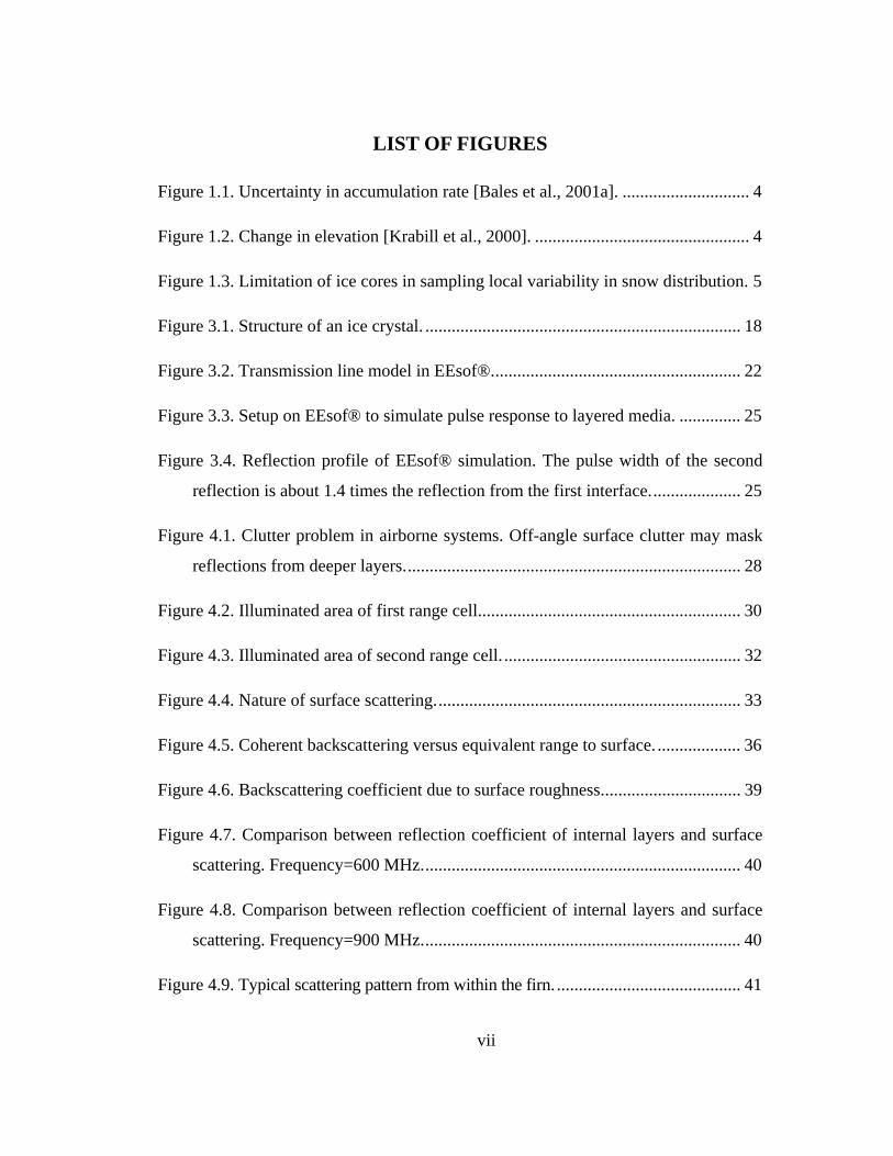
certain areas. Figure 1.1 shows the kriging variance in the current accumulation map.

The black spots on the map indicate the locations of the ice cores that were used to

create the accumulation map. The darker shades on the map indicate greater

uncertainty in the accumulation rate estimates. We can clearly see a correlation

between the core locations and the uncertainty in the map. Areas with a large number

of ice core samples have lower uncertainty in the accumulation rate estimates. Figure

1.2 shows the elevation change measured with a laser altimeter [Krabill et al., 2000].

The altimeter measurements indicate rapid thinning in areas close to the coast,

especially in the southwest region. The accumulation rate estimates in this region are,

however, highly uncertain due to the sparse sampling of ice cores here. To accurately

interpret the results we need a more accurate estimate of the accumulation rate. A

long-term history of the accumulation rate will indicate to us whether this is a recent

phenomenon or a historically high-melt area. Collecting icecores in this area is,

however, a daunting task since there are many deep crevasses in this region. The only

practical method of obtaining an accumulation profile in this region is by remote

sensing.

4

Figure 1.1. Uncertainty in accumulation rate [Bales et al., 2001a].

Figure 1.2. Change in elevation [Krabill et al., 2000].

5

Furthermore, the ice cores provide only point estimates. They do not account

for local variations that are known to occur within short distances. Figure 1.3

illustrates this point. Note how undulations are overlooked when the sampling is too

far apart.

Inter-annual layers

Ice cores Surface

Figure 1.3. Limitation of ice cores in sampling local variability in snow distribution.

To provide improved spatial and temporal coverage, the development of

remote sensing methods to estimate the accumulation rate is required. An accurate

estimate of the long-term accumulation rate can be obtained by mapping a continuous

profile of the dated layers in the ice sheet. The dated layers here refer to inter-annual

layers, volcanic and melt events. Annual accumulation and melt events register a

change in the density, whereas volcanic events are marked by a change in

conductivity [Hammer, 1980]. Reflection profiles from ice-sounding radar systems

6

show many internal ice reflections between the bedrock and the surface. The internal

layers observed over the first few hundred meters have been attributed to density

contrast between annual layers [Robin, et al., 1969; Paren & Robin, 1975], whereas

the reflections from deeper layers where there is no discernable density contrast are

attributed to changes in conductivity and crystal orientation [Hammer, 1980; Millar,

1981; Fujita et al., 2000]. By mapping shallow internal layers, we will be able to

identify the inter-annual layers and melt and volcanic events; this information,

combined with published data on density and thickness, can be used to estimate the

accumulation rate over periods of time. We can also reduce the errors due to local

variability and study the effect of such local variability by collecting data from the

near-surface layers over distances greater than several ice thicknesses.

There are several types of airborne radar systems that can measure the

thickness of the ice sheet. To the best of my knowledge, however, there is no airborne

system capable of achieving less than 1 m vertical resolution to 100 m depth. This is

needed to map the near-surface internal layers for accumulation estimation.

1.3 Objective and Approach

The primary objective of this project is to develop an airborne radar system to

map the internal layers in the Greenland ice sheet with a resolution of 1 m up to a

depth of 100 m. This corresponds to snow accumulations over the past 200 to 500

years, depending on location.

7

To determine optimum radar parameters, we performed simulations on an

electromagnetic model of the ice sheet. The electrical conductivity measurements of

ice cores and the published real value of permittivity were used to model the electrical

properties of the ice sheet. An electronic design automation software, EEsof®

[Agilent Technologies], was then used to model the ice sheet using the Transmission

Line Method [Cheng, 1989]. A simple simulation was then performed to determine

the optimum radar parameters by simulating the scattering response of the ice sheet

due to radar sounding. We then developed an ultra-wideband Frequency-Modulated-

Continuous-Wave (FM-CW) [Saunders, 1990; Stove, 1992] radar system to operate

over a frequency range of 170 to 2000 MHz to image the top 200 to 300 m of ice with

a high vertical resolution of about 0.5 m. Using this system we performed shallow

radar-sounding experiments at the North Greenland Ice core Project (NGRIP) site

(75.1o N, 42.3o W) during June and July of 1998, and in August of 1999. We

collected data over a 2-km and a 10-km traverse with the radar mounted on a tracked

vehicle. We successfully mapped the internal layers to within ± 2 m of that in an ice

core for the top 300 m of the ice sheet.

We analyzed the frequency response of the internal reflections from surface-

based measurements to determine the optimum frequency of operation for an airborne

radar system. Based on this analysis, and, taking into account the frequencies used for

communication on the aircraft, we developed a 600-900 MHz airborne prototype. We

tested this system during the May 2001 field season over the Greenland ice sheet. The

results from this experiment prove that it is indeed, possible to map the internal layers

8

remotely from an aircraft with a resolution of 1 m or better for the top 150 m of the

firn. The problems encountered with the system during the May 2001 field season

were identified to develop an improved system.

We developed an improved radar for routine measurements starting in the

2002 field season. We used EEsof® to optimize the system performance before

construction. We designed a Gaussian high-pass filter with fast settling time to

minimize ringing in the Intermediate Frequency (IF) section. We constructed boxes to

shield the transmit, receive and IF sections adequately. The front end of the

transmitter and receiver were placed in a second box close to the bomb bay to shorten

the path length between the two. This served to push the antenna feed-through signal

further into the stop band of the high-pass filter. In addition, we developed a target

simulator using Radio Frequency (RF)/optical transceivers and fiber optic delay lines

to optimize radar performance further. It simulates a signal coupled between the

transmit and receive antenna, strong reflection from air-snow interface and reflections

from internal layers that are spaced 50 cm apart. The target simulator is a useful tool

for laboratory characterization of the system. This is because it is difficult to test the

system outdoors due to interference from wireless communication devices that

operate in our frequency band of interest.

1.4 Organization

This dissertation is divided into 8 chapters. Chapter 2 presents a brief history

of glacial ice sounding and previous shallow snow sounding systems. Chapter 3

9

describes an electromagnetic model of the ice sheet model. The use of the

transmission line method to model the layers in the ice sheet is discussed in this

section. Chapter 4 describes the application of surface and volume scattering models

to compute the signal-to-clutter ratio and hence, to determine the possibility of

detecting internal layers from an aircraft. Chapter 5 describes the radar system

developed for the surface-based experiments at NGRIP and their results. The

optimum frequency for airborne operation is determined from these experiments.

Uncertainty in the accumulation rate computation is also presented in this section.

Chapter 6 describes the design and development of an airborne radar system and the

results of the field experiment. Chapter 7 provides details of further improvements in

the radar system for future airborne missions. Chapter 8 concludes this dissertation

with a summary and recommendations.

10

Chapter 2

BACKGROUND

Efforts to study the physical properties of snow using microwave techniques

began as early as the 1950s [Saxton, 1950; Cumming, 1952]. Theoretical

developments of radar methods in glaciology began with the express purpose of

measuring the thickness of glacial ice in 1955 [Bogorodsky et al., 1983]. The

capability of a Radar Echo Sounder (RES) in measuring ice thickness was first

demonstrated experimentally by Amory Waite in 1957, when he observed a return

from the bottom of the Ross Ice Shelf in Antarctica [Waite, 1959]. Since then, there

has been a rapid development of radar systems to map the thickness of ice sheets. A

short discussion on the evolution of RES can be found in Gogineni et al. [1998].

A brief summary of previous research on characterizing internal layers with

RES systems is given here. A more detailed discussion can be found in Robin [1983].

The detection of internal layers in glacial ice by RES was first reported by Bailey,

Evans and Robin [1964]. A number of researchers have since written papers on the

phenomena of layer reflections from within the ice sheet [Robin, et al., 1970;

Harrison, 1973; Gudmansen, 1975]. Researchers attributed the reflections from the

first few hundred meters to density contrast between depositional layers [Robin, et al.,

1969; Paren and Robin, 1975]. However, internal layering was also observed at

depths where the density difference is believed to be non-existent. Paren and Robin

11

[1975] suggested that changes in conductivity between layers could be contributing to

reflections from deeper depths. The conductivity was attributed to impurities in the

snowfall. However, Hammer (1977) showed that the impurities in the ice sheet are

due to acidity from major volcanic eruptions. A thorough discussion of the nature of

dielectric discontinuities in glacial ice and their implications to ice sounding can be

found in [Fujita et al., 2000]. Internally reflecting layers at large depths provide a

measure of the deformation undergone by the ice sheets and reveal information about

the ice flow dynamics.

Concerted efforts to sound the stratigraphy of snowpack began in the 1970s.

In 1972, Vickers and Rose [1972] made high-resolution measurement of snowpack

using a short-pulse radar to measure the thickness, density and stratigraphy. A FM-

CW system was used by Ellerbruch and Boyne [1980] to correlate radar signature

with density, hardness, stratigraphy and moisture content of the snowpack. These

parameters were then used to determine the water equivalence of the snowpack.

Sounding of shallow snow layers in the polar ice sheets to measure accumulation rate

was performed in 1982 by a Russian team [Bogorodsky et al., 1982; Lebedev et al.,

1990]. An X-band radar was developed at the University of Kansas in 1990 to

demonstrate that a less expensive and simpler FM-CW radar system could be used to

map the inter-annual layers [Forster et al., 1991]. Since then, a number of systems

have been developed to map the near-surface internal layer in the polar icesheet.

Table 1 summarizes some of the systems that have been used to map the thickness of

annual snow accumulation. However all these systems are ground based and do not

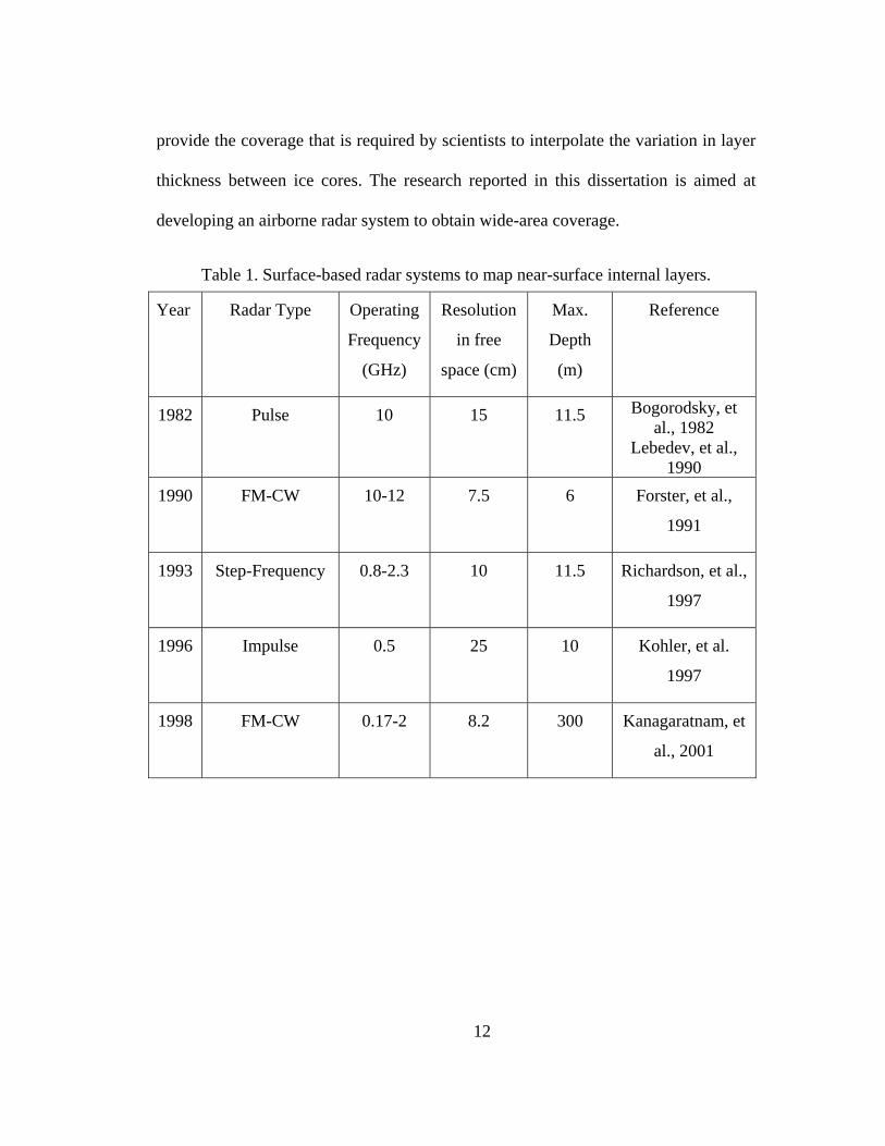
12

provide the coverage that is required by scientists to interpolate the variation in layer

thickness between ice cores. The research reported in this dissertation is aimed at

developing an airborne radar system to obtain wide-area coverage.

Table 1. Surface-based radar systems to map near-surface internal layers.

Year Radar Type Operating

Frequency

(GHz)

Resolution

in free

space (cm)

Max.

Depth

(m)

Reference

1982 Pulse 10 15 11.5 Bogorodsky, et al., 1982

Lebedev, et al., 1990

1990 FM-CW 10-12 7.5 6 Forster, et al.,

1991

1993 Step-Frequency 0.8-2.3 10 11.5 Richardson, et al.,

1997

1996 Impulse 0.5 25 10 Kohler, et al.

1997

1998 FM-CW 0.17-2 8.2 300 Kanagaratnam, et

al., 2001

13

Chapter 3

ELECTROMAGNETIC PROPERTIES OF ICE SHEET

3.1 Introduction

The internal layers seen in a radar echogram of an ice sheet are due to the

reflections from dielectric discontinuities within the ice. In this chapter, a brief review

of physical properties of firn that influence dielectric characteristics is provided. Use

of a transmission line method of modeling radar response is discussed and simulation

results obtained with a transmission line model of the ice sheet are presented.

3.2 Theory

A transmitted radar signal will reflect from the interfaces between layers of

differing permittivity. For a monochromatic wave, the reflection coefficient for a

three-layer media, Γ, at the firn-air interface of an embedded layer is given by [Paren

and Robin, 1975]:

λπ

ε+ε

ε−ε=Γ

m1r2r

1r2r l2sin2 (3.1)

where εr1 is the complex permittivity of layer 1 and layer 3, εr2 is the complex

permittivity of layer 2, l is the thickness of layer 2 and λm is the wavelength in layer

2. The magnitude of the reflection coefficient increases as the dielectric contrast

14

increases, but it is modulated by a sinusoidal term related to layer thickness and

wavelength. The maximum value of the reflection coefficient occurs whenever layer

thickness is an odd integer multiple of λm/4. The complex permittivity of the ice sheet

is a function of crystal orientation fabrics, density, impurities (acidity concentration),

and temperature [Fujita et al., 2000]. For the near-surface layer mapping, the three

factors that influence reflected signals are density, impurities and temperature.

3.3 Density

Density changes are caused by melt events that normally occur in the

percolation zone. The formation of a high-density melt layer occurs when a layer of

snow or near-surface firn melts during the summer and the drainage forms a layer that

subsequently refreezes. In between the winter and summer seasons a new layer of

snow accumulates over the melt layer. Hence, the melt layer is sandwiched between

two layers of low-density snow or firn. Density changes seen in the dry snow zone are

primarily due to the pressure exerted by accumulation of snow above a layer. Depth

hoar layers are also found in the dry snow region. Depth hoar layers are formed by

large crystals due to sublimation and subsequent deposition of water vapor. Although

depth hoar layers cause more abrupt change in density, their spatial continuity across

spatial scales greater > 100 m is unknown [Forster et al., 1999]. The real part of the

complex permittivity of firn, which consists of a mixture of air and ice, has been

described by Looyenga [1965] using the following equation:

( )[ ]3311

311

312r v ε+ε−ε=ε (3.2)

15

where ε2 is the dielectric constant of ice (i.e., 3.15), ε1 is the dielectric constant of air

(i.e., 1), and v is the volume fraction of ice in the firn given by:

v=ρs/ρi (3.3)

where ρs is the density of the firn and ρi is the density of pure ice (i.e., 918 kg/m3).

The reflection coefficient due to changes in the density can be computed by

substituting the permittivity computed in (3.2) into (3.1). The real part of the complex

permittivity does not vary as a function of frequency and has negligible temperature

dependence for temperatures less than –2.5oC [Fujita et al., 2000].

3.4 Conductivity

Variations in conductivity have also been shown to be sources of internal

reflections [Hammer, 1980; Fujita and Mae, 1994]. These variations are due to the

acidic impurities embedded in the ice during volcanic eruptions. We derive below the

reflection coefficient due to a change in conductivity.

The permittivity of the background and acidic layer can be expressed as:

"1

'11 rrr jεεε −= (3.4)

"2

'22 rrr jεεε −= (3.5)

where εr1 is the dielectric constant of the background and εr2 is the dielectric constant

of the acidic layer.

16

Let us assume that 1'

"

<<r

r

εε and '

2'1 rr εε =

The square-root of (3.5) is:

"2

'22 rrr jεεε −= (3.6)

Using the above assumptions allows us to expand (3.6) using the Taylor series

expansion:

'2

"2'

222 r

rrr

j

ε

εεε −≈ (3.7)

Similarly,

'1

"1'

112 r

rrr

jε

εεε −≈ (3.8)

Equation 3.1 can then be simplified to:

( )

−

≈Γmr

rr ljλππ

εεε 2sin2

2exp

4 '2

"2

"1 (3.9)

The equation above shows that the reflection coefficient due to a conductive

change can be approximated with an imaginary quantity. However, Fujita et al.

[2000] have shown that the phase delay of the reflection coefficient drops below π/2

with increasing frequency for temperatures above the eutectic point of the acid. Thus,

17

there is a contribution from the real part of the dielectric constant as well for

temperatures above the eutectic point. The contribution to the real part of the

reflection coefficient is probably due to the presence of liquid associated with

impurities in the volcanic layer [Fujita et al., 2000] that may be present at

temperatures above –40o C.

3.5 Crystal Orientation Fabrics

Discontinuities in the crystal orientation fabric are due to shear strain along

the isochrones. Robin and Millar [1982] suggest that acidic impurities in the ice may

change the mechanical properties in ice and thus cause an easy glide plane and,

hence, a different fabric from its enclosing layers. The discontinuity in the orientation

of the crystal fabric is quantified by the dielectric anisotropy of ice, which is the

difference between permittivity parallel, ε||c, and perpendicular, ε⊥c, to the c-axis,

which is perpendicular to the basal plane of the ice crystal. Figure 3.1 shows the ice

crystal structure. The circles in the figure are H2O molecules. The hexagonal plane

refers to the basal plane and the direction perpendicular to this plane is the c-axis.

18

Figure 3.1. Structure of an ice crystal.

The dielectric anisotropy, ∆ε’, was found to be [Fujita and Mae, 1994]:

007.0037.0' ±=ε∆ (3.10)

The dielectric permittivity tensor of polycrystalline ice was given as [Fujita

and Mae, 1994]:

ε' = ε'⊥c + ∆ε' Da (3.11)

where Da is a factor which accounts for the contribution of ∆ε’ to the dielectric

permittivity tensor and is given as

∑ θ==

N

1jja cos

N1D (3.12)

where N is the number of crystal grains and θj is the angle between the c-axis of the

jth grain and the incident wave. The orientations of the crystals are measured using

19

optical techniques, a description of which can be found in Paterson [1998]. The

reflection coefficient due to changes in the crystal orientation fabric is expressed as:

λπ

εδε∆

=Γm

'a

' l2sin24

D (3.13)

The amplitude of the reflection coefficient caused by changes in the crystal

orientation fabric is independent of ice temperature and frequency [Fujita et al.,

2000]. Reflections due to changes in the crystal orientation fabric have only been

found at depths where there are no density changes. In the analyses that are to follow,

the orientations of the crystal fabrics will not be considered as we are currently

interested in the near-surface reflections only.

3.6 Transmission Line Method

The density and conductivity data of an ice core can be used to model the ice

sheet using the transmission line method. The wave characteristics on a transmission

line are analogous to uniform plane waves in lossy media. The propagation of a plane

wave through a medium is given by:

E(z)=Eoexp(-γz) (3.14)

where Eo is the field strength of the transmitted signal, E(z) is the field strength at

distance z into the media, γ is the propagation constant given by:

cojj εµω=β+α=γ (3.15)

20

where α is the attenuation constant (Np/m), β is the phase constant (rad/m), ω is the

frequency of the signal, µo is the permeability constant in free space, εο is the

permittivity constant in free space and εc is the complex permittivity of the media in

which the wave is propagating. The complex permittivity, εc, is given by:

ϖσ

−εε=

ε−ε=ε

j

j

ro

"'c

(3.16)

where ε’ is the lossless part of the complex permittivity, εr is the relative permittivity,

ε” is the dielectric loss of the media, and σ is the conductivity.

The relationships between the physical parameters, density and electrical

conductivity, measured from the ice cores and the complex permittivity have been

approximated by equations. The relationship between the density and the permittivity

has been described by (3.2).

The conductivity of the ice sheet is determined using the dielectric profiling

(DEP) method [Moore and Paren, 1987]. The DEP system is used to measure the

capacitance and the conductance of ice. The capacitance of the ice determines the

relative permittivity of the ice whereas the conductance determines the imaginary part

of the ice. The conductivity is determined by the following equation [Gross et al.,

1980]:

air

iceofirn C

Gε=σ (3.17)

21

where Gice is the measured conductance of the firn and Cair is the measured

capacitance without the firn. The conductivity thus computed is substituted in (3.16)

to determine the imaginary part of the permittivity.

Several ice cores have been collected at the GRIP and NGRIP sites. The

density and conductivity for some of these ice cores have been determined. We can

divide these ice cores into layers of length h m and determine the impedance of each

layer from the complex permittivity profile of the ice core. In an electromagnetic

simulation this will be analogous to cascading transmission lines of length h and

characteristic impedances corresponding to the layers’ impedance. A similar

procedure was described by Moore [1988]. The relationship between the impedance

and the complex permittivity is given as:

γ

ϖµ= oj

Z (3.18)

( )"'o

o

jZ

ε−εεµ

= (3.19)

The transmission line model of the ice core can be used in an electromagnetic

simulator to observe the effects of changes in complex permittivity on the incident

wave. The concept will be illustrated using Agilent EEsof®’s Advanced Design

Systems (ADS) simulator [2001]. EEsof® is a powerful electromagnetic simulator

that has many features that will enable the radar designer to optimize the design

before construction. Some of the salient features of EEsof® are:

22

1) Seamless interface with test equipment. This feature allows the designer to

measure the S-Parameter of components using a network analyzer and use them for

simulations.

2) Integrated test environment. Circuits and system models can be easily

interfaced for simulations. The medium of propagation can be modeled using the

transmission line elements. The system and propagation models can thus be combined

and simulated to determine the radar response to a particular medium.

Figure 3.2 shows the transmission line model available in EEsof® to define

the complex permittivity of layers in the ice sheet.

TLINPTL1

TanD=2.64e-4F=fscK=2L=10 meterZ=35.0 Ohm

Figure 3.2. Transmission line model in EEsof®.

The various parameters of the transmission line shown above are described

herein. Z is the characteristic impedance of the transmission line. EEsof® will allow

23

one to specify only the real part of the impedance for the characteristic impedance, Z.

The imaginary part of the impedance will be factored in the TanD parameter. The

characteristic impedance will govern the reflection due to changes in the real part of

the complex permittivity. In our simulations, the characteristic impedances were

normalized with respect to a 50Ω system and not with the conventional 377Ω system

in free space. This was done to match the radar system’s components that were

included in the overall simulation. In practice, the 50Ω system was matched to the

free space impedance of 377Ω with a horn antenna. The parameter, L, defines the

layer thickness. K is the effective dielectric constant. The effective dielectric constant

reduces the free space velocity of waves in a particular layer by a factor of its square

root; i.e. K . It does not influence the computation of the reflection coefficient. The

parameter, F, is the frequency at which the loss tangent parameter, TanD, is

computed. The loss tangent is given as:

ϖεε

σ=

εε

=o

''

"

TanD (3.20)

The loss tangent governs the dielectric loss of the propagating wave in ice.

This parameter will allow us to model the changes in the imaginary part of the ice

sheet and observe its effect on the incident wave. A simple four-layer model is

presented first to illustrate the concept (Figure 3.3).

24

The first layer is 500 m of free space to simulate the height of the aircraft

above the ice sheet. The free space was modeled using a time delay of 1.67 µs. The

second and fourth layers form the ice sheet. A relative permittivity of 2 and a

conductivity of 17 µS/m were assumed for these layers. The third layer, a volcanic

ash layer embedded in the ice sheet, was modeled as a layer with a relative

permittivity of 2 and a conductivity of 40 µS/m at 10 m below the air-firn interface.

The relative permittivity values as well as the conductivity values were substituted in

(3.19) and (3.20) to compute the real part of the impedance and the loss tangent. A S-

parameter simulation was performed from 600 MHz to 900 MHz in steps of 187.5

kHz. This measurement is analogous to a step-frequency radar measurement using a

vector network analyzer whereby the inverse Fourier Transform (IFT) of the S11

measurement will yield the reflection profile.

Figure 3.4 shows the result of this simulation. The first reflection is about –15

dBm, which is the expected level for the given impedance mismatch. The second

reflection is about –79 dBm. It was also observed that the pulse width of the second

reflection is about 1.4 times the pulse width of the first reflection. The loss of

resolution is due to the greater attenuation of the high-frequency components as the

wave propagates through the lossy media.

25

S_ParamSP2

Step=187500Stop=900 MHzStart=600 MHz

S-PARAMETERSVARVAR1fsc=600e6

EqnVar

TermTerm1

Z=50 OhmNum=1

TLINPTL3


TLINPTL2

TanD=6.2e-4F=fscK=2L=0.5 meterZ=35.0 Ohm

TLINPTL1


TimeDelayTD1

ZRef=50. OhmDelay=1.67 usec

TermTerm2

Z=35 OhmNum=2

Figure 3.3. Setup on EEsof® to simulate pulse response to layered media.

3.30 3.32 3.34 3.36 3.38 3.40 3.42 3.44 3.46 3.48 3.503.28 3.52

-140

-120

-100

-80

-60

-40

-20

-160

0

Two-way travel time (usec)

Ref

lect

ed p

ower

(dB

m)

Figure 3.4. Reflection profile of EEsof® simulation. The pulse width of the second reflection is about 1.4 times the reflection from the first interface.

26

3.7 Summary

In this chapter we provided a brief review of the physical properties of firn

and showed how these physical properties can be used to construct an

electromagnetic model for simulating radar response using a CAD package. These

simulations are useful for studying the trade-off of radar characteristics when

mapping near-surface layers.

27

Chapter 4

SURFACE AND VOLUME CLUTTER

4.1 Introduction

Because of the finite beamwidth, reflections from internal layers may be

masked by off-nadir backscatter from the surface and volume scatter. A long antenna

can be synthesized by taking advantage of the forward aircraft motion to reduce

beamwidth in the along-track direction. It is possible to install a large-array antenna

to obtain narrow beamwidth in the cross-track direction under the wing of a P-3

aircraft. However, the hardpoints needed to install such an antenna are used for the

coherent radar depth sounder. Because the wideband accumulation radar antennas

have to be installed in the limited space available in the bomb bay of P-3 aircraft, we

used a TEM horn with an aperture of 1 meter with beamwidth of 45 degrees. In this

chapter, limitations resulting from off-nadir surface and volume clutter are

investigated.

4.2 Problem

The off-nadir clutter may mask some of the reflections from deeper layers as

illustrated in Figure 4.1. The effect of clutter on the received signal will be examined

in this section.

28

Firn/Internal Layer Interface

Air/Firn Interface

θ

Figure 4.1. Clutter problem in airborne systems. Off-angle surface clutter may mask reflections from deeper layers.

The return power, S, from a perfectly flat surface is given as:

( ) ( )22

222t

R24GP

Sπ

Γλ= (4.1)

where Pt is the transmitted power, λ is the wavelength, G is the antenna gain, Γ is the

reflection coefficient at the air/snow interface or between two internal layers and R is

the range to the interface.

The above equation can be used to approximate the received power from the

internal layers. The internal layers can be successfully detected only if their reflected

power is higher than that due to surface and volume scattering from the firn. The

return power, C, from a distributed target is given as

29

( ) 43

o22t

R4AGP

Cπ

σλ= (4.2)

where A is the illuminated area and σo is the backscattering coefficient of the incident

medium. To obtain signal-to-clutter ratio greater than one, the following inequality

needs to be satisfied:

S > C (4.3)

( ) ( ) ( ) 43

o22t

22

222t

R4AGP

R24GP

π

σλ>

π

Γλ (4.4)

2

o2

RA

πσ

>Γ (4.5)

The following sections will be devoted to the computation of the illuminated

area and the backscattering coefficient due to surface and volume scattering. This will

determine if the above inequality is satisfied for the dry snow region of the Greenland

ice sheet.

4.3 Area of Illumination

The horn antennas that are to be used in our experiments have beamwidths of

45o at 600 MHz and 30o at 900 MHz. The footprints covered by these beamwidths are

much larger than those due to the range resolution of the radar system. Therefore, the

illuminated area has to be computed for the pulse-limited case. The shaded areas in

Figure 4.2 and Figure 4.3 show the illuminated area for the pulse-limited case [Ridley

30

and Partington, 1988]. Figure 4.2 illustrates the illuminated area of the first range cell.

The illuminated areas for subsequent range cells are rings, as shown in Figure 4.3.

The diameter of the circle in Figure 4.2 is computed as follows:

( ) 222

1 HRH2d

−∆+=

(4.6)

( ) 221 HRH2d −∆+= (4.7)

The illuminated area is thus:

2

11 2

dAill

π= (4.8)

θ

∆RH

d1

Figure 4.2. Illuminated area of first range cell.

31

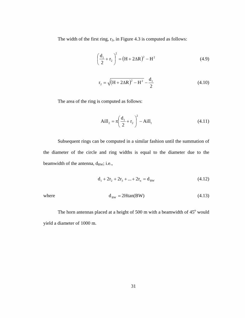
The width of the first ring, r2, in Figure 4.3 is computed as follows:

( ) 222

21 HR2Hr

2d

−∆+=

+ (4.9)

( )2dHR2Hr 122

2 −−∆+= (4.10)

The area of the ring is computed as follows:

1

2

21

2 Aillr2dAill −

+π= (4.11)

Subsequent rings can be computed in a similar fashion until the summation of

the diameter of the circle and ring widths is equal to the diameter due to the

beamwidth of the antenna, dBW; i.e.,

BWn321 dr2...r2r2d =++++ (4.12)

where =BWd 2Htan(BW) (4.13)

The horn antennas placed at a height of 500 m with a beamwidth of 45o would

yield a diameter of 1000 m.

32

∆R

θ H

d1 r2

Figure 4.3. Illuminated area of second range cell.

4.4 Surface Scattering

Figure 4.4 below illustrates the nature of surface scattering. When an

electromagnetic wave impinges on the boundary layer between two media of differing

permittivity, a portion of this wave's energy is reflected and the rest is transmitted into

the second medium. The reflection of an electromagnetic wave from a smooth surface is

called the specular or coherent component and the direction of reflection is called the

specular direction. As the roughness of the surface increases, the reflection in the

specular direction begins to decrease as the incident wave's energy is redistributed in

33

other directions. These scattered components are called the incoherent components.

Theoretically, a monostatic radar should not be able to receive the return power from a

smooth surface at incidence angles other than nadir. The primary component seen at

incidence angles greater than zero is the incoherent component, whose magnitude is

typically larger when the surface is rougher. However, incoherent components may also

be observed at nadir if the antenna beamwidth is large. These incoherent components

may fall at later range bins and mask the weaker coherent components from subsequent

interfaces. The roughness of a surface seen by the radar is dependent on the wavelength.

The smaller the wavelength, the rougher the surface seen by the radar.

Coherent component

Incident Wave

Incoherent components

Surface

εr2

εr1

θ1 θ1

θ2

Figure 4.4. Nature of surface scattering.

4.4.1 Coherent Scattering

The specular reflection from a small rms (root-mean-square) surface

roughness superimposed on a smooth surface is given as [Fung and Eom, 1983;

Fetterer et al., 1992]:

34

( )

βθ

−σ−βθΓ

=σ 2

222

2

2ocoh k4exp|| (4.14)

where Γ is the Fresnel reflection coefficient, β is the one-sided pulse-limited beam

width, k is the wavenumber and σ is the rms height of the surface. The one-sided

pulse-limited beam width is equivalent to θ in Figure 4.2. As such, we can determine

β as follows:

( )

( )

HRRH2h

HRRH2Hh

HRH

H2d

tan

2

222

22

1

∆+∆=

−∆+∆+=

−∆+=

=β

(4.15)

Since H >> ∆R, the above equation reduces to:

( )

HR2

HRH2tan

∆≈

∆≈β

(4.16)

For small angles, tan(β) ≈ β, thus:

H

R22 ∆≈β (4.17)

Substituting (4.17) into (4.14), we obtain:

35

( )

∆

θ−σ−

∆θΓ

=σR2Hk4exp

R2H|| 2

222

ocoh (4.18)

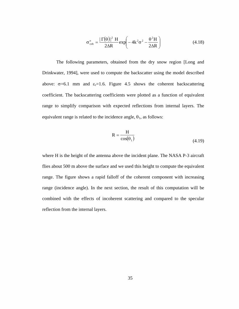
The following parameters, obtained from the dry snow region [Long and

Drinkwater, 1994], were used to compute the backscatter using the model described

above: σ=6.1 mm and εr=1.6. Figure 4.5 shows the coherent backscattering

coefficient. The backscattering coefficients were plotted as a function of equivalent

range to simplify comparison with expected reflections from internal layers. The

equivalent range is related to the incidence angle, θ1, as follows:

( )1cosHR

θ=

(4.19)

where H is the height of the antenna above the incident plane. The NASA P-3 aircraft

flies about 500 m above the surface and we used this height to compute the equivalent

range. The figure shows a rapid falloff of the coherent component with increasing

range (incidence angle). In the next section, the result of this computation will be

combined with the effects of incoherent scattering and compared to the specular

reflection from the internal layers.

36

500 502 504 506 508 510 512 514 516−80

−70

−60

−50

−40

−30

−20

−10

0

10

20σo (

dB)

Range (m)

Coherent Scattering. σ = 6.1 mm, εr=1.6

Figure 4.5. Coherent backscattering versus equivalent range to surface.

4.4.2 Incoherent Scattering

The Integral Equation Method (IEM) [Fung, A.K., 1994] was developed to

model the backscatter due to surface roughness. This model will be used to compute

the backscatter due to surface roughness in the dry snow region of the Greenland ice

sheet. A special case of the IEM was derived for surfaces of small and medium

roughness. For surfaces with a Gaussian correlation function, the required condition

was given as:

37

( )( ) r2.1kLk ε<σ (4.20)

where k is the wave number (2π/λ), σ is the rms height, L is the correlation length

and εr is the relative permittivity of the incident surface. A rms height of 6.1 mm and

correlation length of 9 cm are typical roughness parameters of the dry snow region in

Greenland [Long and Drinkwater, 1994]. The permittivity of the surface is given as

1.6. The highest frequency of our radar system is 900 MHz. Substituting these

parameters into (4.20) yields 0.1951 for the left side and 1.52 for the right side. The

inequality is thus satisfied and we can proceed to use the modified IEM, which is

given as:

( )∑ −σ−=σ

∞

=1n

x)n(

2npp

22z

2opp !n

)0,k2(W|I|k2exp2

k (4.21)

where kz=kcosθ1, kx=ksinθ1, θ1 is the incidence angle, and pp = vv or hh polarization,

( ) ( ) ( ) ( ) ( )[ ]2

0,kF0,kFkkexpfk2I xppxpp

nz22

zppn

znpp

+−σ+σ−σ= (4.22)

1

||vv cos

R2f

θ= (4.23)

( ) ( )( )

θεθε−θ−εµ

+

ε

−θ

Γ+θ=

+−

122

r

12

r12

rr

r1

2||1

2

xvvxvv

coscossin11

cos1sin2

0,kF0,kF

(4.24)

38

where Γ|| is the Fresnel reflection coefficient for the vertically polarized case and is

given as:

21r12r

21r12r|| coscos

coscosθε+θε

θε−θε=Γ (4.25)

where εr1 is the relative permittivity of the first medium and εr2 is the relative

permittivity of the second medium. The angles θ1 and θ2 are illustrated in Figure 4.4

and they satisfy Snell’s law:

k1sinθ1 = k2sinθ2 (4.26)

where k1 and k2 are the wave numbers of media one and two, respectively.

The roughness spectrum corresponding to a Gaussian correlation is:

−=

22

2KLexp

2L)K(W (4.27)

and the Fourier transform of the nth power of the correlation function is:

( ) ( )

−=

n4KLexp

n2L)K(W

22n (4.28)

The following parameters were used to compute the backscatter using the

IEM described above: σ=6.1 mm, L=9 cm, εr=1.6. Figure 4.6 shows the computed

backscattering coefficient for frequencies ranging from 600 MHz to 900 MHz.

39

500 520 540 560 580 600 620 640 660 680 700−45

−40

−35

−30

−25

−20

σo (dB

)

Range (m)

IEM. σ = 6.1 mm, L=9 cm, εr=1.6

600 MHz700 MHz800 MHz900 MHz

Figure 4.6. Backscattering coefficient due to surface roughness.

The coherent backscattering coefficient and incoherent backscattering at 600

MHz and 900 MHz were summed and substituted into (4.5) for comparison with the

power reflection coefficient computed from the ice core at NGRIP. Figure 4.7 and

Figure 4.8 show that the specular reflection beyond the first reflection is consistently

higher than the surface clutter by about 10 to 15 dB and 5 to 10 dB for the first 50 m

at 600 MHz and 900 MHz, respectively.

40

500 550 600 650 700 750 800−80

−70

−60

−50

−40

−30

−20

−10

Am

plitu

de (

dB)

Range (m)

σoA/(πR2)Γ2

Figure 4.7. Comparison between reflection coefficient of internal layers and surface scattering. Frequency=600 MHz.

500 550 600 650 700 750 800−80

−70

−60

−50

−40

−30

−20

−10

Am

plitu

de (

dB)

Range (m)

σoA/(πR2)Γ2

Figure 4.8. Comparison between reflection coefficient of internal layers and surface scattering. Frequency=900 MHz.

41

4.5 Volume Scattering

IncidentBeam

Ice particles in the firn

Surface

Figure 4.9. Typical scattering pattern from within the firn.

Figure 4.9 illustrates the nature of volume scattering wherein the ice particles

in the firn scatter the incident wave. The magnitude of the scattered energy is highly

dependent on the size of the ice particle relative to the wavelength of the incident

signal. The smaller the wavelength of the transmitted signal, the more energy is

scattered when incident upon an ice particle. The Rayleigh volume scattering model

introduced by Ulaby et al. [1986] and adapted by Forester et al. [1999] for modeling

the dry snow zone in Greenland will be used to determine the scattering from the firn.

The backscatter for a single annual layer from the firn is given by:

( ) ( ) ( )( )

θθσ

+θσθγ=σ2

22

os

2ods1

2olayer L

(4.29)

42

where γ is the transmitivity, θ is the incidence angle, osσ is the surface backscatter

from the interface between annual layers, and odsσ is the normalized radar cross

section from the dry snow volume given by:

( )( )

θ

−κ

θσ=σ '2

e

'bo

ds L11

2cosN (4.30)

where N is the number of scatterers per volume, eκ is the extinction coefficient, L is

the one-way loss factor given by:

( ) ( )[ ]'e

'2 sechexpL θκ=θ (4.31)

where h is the annual layer thickness, and bσ is the backscattering cross section for a

single snow grain given by:

2

bs

bs6e

4'bb 2r

38

ε+εε−ε

πκ=σ (4.32)

where 'bκ is the wave number in the background medium (air), εs is the permittivity of

the scatterer (ice), εb is the permittivity of the background (air), and re is the optically

equivalent snow grain radius given by:

( )rv2v2.1r 2e −+= (4.33)

where r is the physical radius of the grain and v is the volume fraction of the ice,

which is the ratio of the density of the firn, ρs, to the density of pure ice, ρi.

43

The extinction coefficient, κe, in (4.30) and (4.31) is the summation of both

the volume absorption (κa) and scattering coefficients (κs); i.e.,

ase κ+κ=κ (4.34)

The volume scattering coefficient is given as:

ss NQ=κ (4.35)

where Qs is the scattering cross section of the sphere of radius r, m2. The scattering

cross section is given as:

262

s |K|32Q χ

πλ

= (4.36)

where χ is given as:

bob

r2r2ε

λπ

=λπ

=χ (4.37)

and K is given as:

bs

bs

2K

ε+εε−ε

= (4.38)

The number of scatterers per volume is computed as:

πρ

ρ=

3i

s

r34

N (4.39)

44

The volume absorption coefficient is given as:

abaia κ+κ=κ (4.40)

where κai accounts for the absorption by the ice spheres whereas κab accounts for the

absorption by the background. κai is given by:

aai NQ=κ (4.41)

where Qa is the absorption cross section of the sphere of radius r, m2. The absorption

cross section is given as:

KImQ 32

a −χπλ

= (4.42)

The absorption coefficient due to the background is given as:

( ) boab Imv1k2 ε−=κ (4.43)

where ko is the wavenumber in free space.

The absorption coefficients are dependent on the imaginary component of the

dielectric constant. In the dry snow region this is very small and hence we can neglect

it for our computations. The absorption factor becomes significant only when one

moves to the percolation and wet snow zones where the wetness increases the

imaginary component of the dielectric constant.

45

The surface backscatter from the interface between the annual layers, osσ , in

(4.29) is assumed to be negligible since the surface characteristics for these layers

[Long and Drinkwater, 1994] are smooth relative to the wavelengths in the 600 MHz

to 900 MHz frequency range according to the Rayleigh criteria [Ulaby et al., 1986].

Equation 4.29 then reduces to:

( ) ( )'ods

2olayer θσθγ=σ (4.44)

The total backscatter from multiple annual-layers from the firn is given by:

( ) ( )

∑θσθγ

=σ= −

−M

1n2

)!1n(

'n

ods

'1n

2ofirn L

n (4.45)

where n is the annual layer number, M is the last layer contributing to the total

backscatter, θ'n is the refracted angle in the nth annual layer for n ≥ 1, and θ'

o is the

look angle when n = 1.

The thickness of the annual layers is required to determine the loss through

the medium. The depth of the annual layers for a region with a given accumulation

rate were computed using the firn-densification model developed by Heron and

Langway [1980]. They have showed that densification occurs in two distinct stages.

The first stage occurs for densities less than 0.55 x 106 g m-3. In this region the rate of

densification is proportional to accumulation rate times the difference between the

densities in this region and pure ice. The depth, h1, for a given density in this region is

given as:

46

( )

ρ−ρ

ρ−

ρ−ρ

ρρ

=ρoi

o

si

s

ois1 lnln

K1h (4.46)

where ρo is the zero depth density, Ko is the rate constant and is given as:

−=

GT160,10exp11K o (4.47)

where G is the gas constant (8.314 JK-1mol-1) and T is the temperature in Kelvins.

The age in years, t1, for this depth is:

( )

ρ−ρρ−ρ

=ρsi

oi

os1 ln

AK1t (4.48)

Thus we can solve for ρs for each annual layer and substitute the same in

(4.46) to determine its depth.

The second stage of firn densification occurs at densities greater than 0.55x106

g m-3. In this region the rate of densification differs from stage one in that it is now

dependent on the square root of the accumulation rate. The depth corresponding to a

given density in this region is:

( ) ( )55.0h55.0

55.0lnlnKAh 1

isi

s

1is2 +

−ρ

−

ρ−ρ

ρρ

=ρ (4.49)

where K1 is the rate constant in this stage and is given as:

47

−=

GT400,21exp575K1 (4.50)

The age of firn corresponding to densities at this depth is

( ) ( )55.0t55.0

lnAK

1t 1si

i

1s2 +

ρ−ρ

−ρ=ρ (4.51)

The annual layer depth is determined in a similar fashion to that of stage one.

500 520 540 560 580 600 620 640 660 680 700−60

−58

−56

−54

−52

−50

−48

−46

−44

−42

−40

σo (dB

)

Range (m)

Rayleigh Model. r = 0.3 mm, εr=1.6

600 MHz700 MHz800 MHz900 MHz

Figure 4.10. Backscattering coefficient due to snow grains.

48

The volume scattering contribution due to a snow grain size of 0.3 mm is

shown above. The backscattering coefficient due to the snow volume is more than 15

dB below that due to surface scattering at 900 MHz. These simulations show that the

volume scattering is negligible in computing the return power.

The modeling results indicate that only off-angle surface scattering has the

potential of masking returns from internal layers in areas where the surface roughness

is significantly larger. Rougher surfaces can be expected when one moves from the

dry snow regions to the percolation and wet snow regions. However, the dielectric

contrast between layers resulting from melt events is large, which compensates for

increased backscatter.

4.6 Summary

In this chapter, we examined the effects of clutter, due to surface and volume

scattering, on the return from internal layers. This is a problem particular to antennas

with large beamwidth since they have the potential of masking the returns from the

internal layers. We obtained the physical parameters of the ice sheet and computed

the surface and volume scattering coefficients and compared them to the specular

reflection due to density changes. Our results showed that the reflections from the

internal layer were about 10 to 15 dB and 5 to 10 dB above the surface clutter at 600

MHz and 900 MHz, respectively. The volume scattering was 15 dB below that due to

surface scattering and thus has little effect on the return from internal layers.

49

Chapter 5

SURFACE-BASED SYSTEM AND EXPERIMENTS

For high-resolution mapping of internal layers in the top 200 m of ice, we

developed an ultra-wideband Frequency-Modulated-Continuous-Wave (FM-CW)

radar system [Saunders, 1990; Stove, 1992] operating over the frequency range from

170 to 2000 MHz. Using this system we performed shallow radar-sounding

experiments at the North Greenland Ice core Project (NGRIP) site (75.1o N, 42.3o W)

during June and July of 1998, and in August of 1999. We used these experiments to

demonstrate that near-surface internal layers can be mapped with high resolution and

analyzed these data to determine optimum parameters for an airborne system.

This chapter presents the theory of FM-CW radar, the system description,

experiments conducted at NGRIP, signal processing and the discussion of results and

error analysis.

5.1 Theory of Linear FM-CW Radar

A simple FM-CW radar transmits a continuous waveform for which carrier

frequency increases linearly with time. The modulation bandwidth, which determines

range resolution, is the difference between the start and stop frequencies of the

transmitted signal. In a FM-CW radar a sample of transmitted signal is mixed with

the received signal to generate a beat signal. The frequency of transmit and received

50

signals will be different because of time delay, which is directly proportional to the

range, associated with signal propagation to the target and back. The beat signal

contains the range, amplitude and phase information of the target. Figure 5.1 shows a

typical transmit and receive signals from a point target.

Transmitted signal

Receivedsignal

Tm

B τ

fb

Figure 5.1. Transmit and receive signals from a point target for an FM-CW radar. B is the bandwidth of the signal, τ is the two-way travel time from the radar system to the target, Tm is the

modulation period and fb is the beat frequency.

The time, τ, for the signal to travel the two-way distance between the target

and the radar is:

cR2

=τ (5.1)

where R is the range to the target and c is the velocity of light in free space. From the

geometry of the transmit and receive waveforms a relationship can be derived

between the beat frequency, fb, and the range, R. For the triangular modulation the

beat frequency is:

51

c

RBf4Bf2f

m

mb

=

τ= (5.2)

where fm (1/Tm) is the modulation frequency.

For multiple targets, the beat signal will be a summation of several signals

with frequencies proportional to their range. By Fourier transforming the beat signal

to determine received signal frequencies, we can determine range to each target. The

minimum separation between targets, τmin, that can be seen by the radar is:

B1

min =τ (5.3)

Substituting (5.3) into (5.1) gives the range resolution, ∆R, for the radar:

B2cR =∆ (5.4)

In the derivation that follows, an expression for the beat signal will be

determined. The transmitted signal voltage, vt(t), is given as:

)tBf2tf2(cosA)t(v o2

mot θ+π+π= (5.5)

where fo is the initial sweep frequency, θo is the initial phase of the sweep source, and

t is time. A portion of the transmitted signal is reflected back when it impinges on a

dielectric interface. At the receive antenna, the reflected signal from a target located

at range with time delay of t s can be expressed as:

52

[ ] [ ] )t(f)t(Bf2)t(f2cos)t(fA)t(v o2

mo'

r φ+θ+τ−π+τ−πΓ= (5.6)

where |Γ[f(t)]| is the magnitude of the reflection coefficient at the dielectric interface

and φ[f(t)] is the phase of the reflection coefficient. The reflection coefficient is a

function of the transmit signal frequency, f(t), which, as indicated, is a function of

time.

The IF signal is obtained by mixing the received signal with a portion of the

transmit signal and filtering out the higher-order terms. This process results in the

following expression:

[ ] [ ] )t(f)t2(fB2f2cos)t(fA)t(v 2mo

'IF φ−τ−τπ+τπΓ= (5.7)

The above equation can be rewritten in terms of the beat frequency, fb.

Substituting (5.2) into (5.7) gives:

[ ] [ ] )t(fff2tf2cos)t(fA)t(v bob'

IF φ−τπ−τπ+πΓ= (5.8)

The amplitude and phase of the target’s reflection coefficient can be

determined by means of the Hilbert Transform (HT) of the IF signal above. The HT

of the IF signal will give us a complex signal in the following form:

[ ] [ ] ( ))t(fff2tf2jexp)t(fA)t(v bob'

IF φ−τπ−τπ+πΓ= (5.9)

We can obtain the phase response of the target by computing the phase term in

(5.9), removing the range contribution in the phase term and then calibrating it with a

53

target of known phase. The amplitude response can be similarly obtained by

computing the magnitude of the complex signal and calibrating it with a target of

known amplitude.

5.2 System Description

The current section is divided into several sub-sections dealing with the

specifications for the system, transmitter, receiver and IF sections of the radar system.

5.2.1 System Specifications

There are several parameters that need to be determined before deciding on

the transmit power level and receiver gain. These parameters include the A/D

dynamic range, noise figure of the system and the expected return power from the

target.

The A/D that is available for our use is a 12-bit digitizer [Akins, 1999]. It is

able to digitize signals with levels between –0.5 V and +0.5 V. The maximum signal-

to-noise ratio (SNR) of an A/D converter is given as:

2Q3SNR

2

= (5.10)

where Q is the number of quantization levels. For a N-bit digitizer, the number of

quantization levels is 2N. Thus the maximum SNR for a 12-bit A/D is 74 dB. The

maximum signal level that can be digitized with this A/D in a 50 Ω system is:

54

dBm4W0025.0502

5.0R2

VP

22p

max ≈=×

== (5.11)

The A/D noise floor is the difference between Pmax and the SNR. Hence the noise

floor of the A/D is –70 dBm.

The noise floor of the radar system, N, determines the minimum signal level

that can be detected. This is given as:

N=kTBF (5.12)

where k is the Boltzman constant (1.38 x 10-23 J/K), T is the room temperature (290

K), B is the bandwidth of a range bin in FM-CW radar systems and F is the noise

figure of the receiver.

The bandwidth of a range bin is simply the sampling rate divided by the

number of DFT (discrete Fourier transform) points before zero padding. The

sampling rate for our ground-based system is 1 MHz and the number of DFT points is

57500. The bandwidth is thus 17.4 Hz.

The noise figure, F, is given by the Friis formula:

( )

∑∏

−+=+

−+

−+=

=−

=

n

1i1i

0jj

i

21

3

1

21

G

1F1....GG

1FG

1FFF (5.13)

55

The subscript of F denotes the component number subsequent to the receive antenna.

G is the gain of the component. The table below lists the first three components of our

radar system and their respective noise figures and gains.

Table 2. Gain and noise figure of components used in the front end of the receiver.

Component Gain (dB)/(Linear) F (dB)/(Linear)

1. Attenuator -3 / 0.5 3 / 2

2. Amplifier 23 / 200 5.5 / 3.55

3. Attenuator -3 / 0.5 3 / 2

Substituting the above values into (5.13) yields a noise figure of 8.5 dB. The

minimum detectable signal from (5.12) is thus –153 dBm.

The simulations carried out in Chapter 3 on some typical parameters from the

ice sheet show that the power reflected for the air/firn interface is about 15 dB below

the transmit power of 0 dBm and for the volcanic layer embedded within the ice the

reflected power is about -80 dBm at 600 MHz. Substituting these parameters into the

radar equation in (4.1) we can compute the expected return power. Equation 4.1 can

be rewritten in logarithmic form as:

S = Pt + 2λ + 2G + 10log10|Γ|2 - 20log10(4π) - 20log10(2R) (5.14)

56

The above equation does not account for the scattering and absorption loss in

the ice sheet. To get a better estimate of the reflected power we shall also include the

losses due to scattering and absorption. The extinction coefficient given in (4.34)

describes the loss through the medium. The two-way loss through the medium, α, is

simply:

( )eR2exp κ−=α (5.15)

where R is the range to the target. Equation 5.14 then becomes

S=Pt+2λ+2G+10log10|Γ|2-20log10(4π)-20log10(2R)-20Rκelog10(exp(1)) (5.16)

A grain size of 0.3 mm, which is the value reported by Forester et al. [1999] in

the dry snow region, will be used for the computation of the scattering as well as

absorption loss. We used a dielectric of 3.15-j0.001 for the dielectric constant of the

snow particles. Figure 5.2 shows the attenuation through the ice sheet. The loss is

mainly due to absorption. This is expected at these frequencies since the wavelengths

are much larger than the particle size and, hence, a negligible amount of scattering

loss is expected.

As explained in Chapter 3, the power reflection coefficient (PRC) for the

volcanic layer will vary as a function of frequency, while the power reflection

coefficient from the air/firn interface will remain constant. The constants that will be

used in (5.14) are Pt = 0 dBm and R = 2 m for the air/firn interface and R = 150 m for

the volcanic layer. The expected return power for these two interfaces at various

57

frequencies are tabulated in tables 3 and 4. Table 3 shows the expected return power

from the air/firn interface and Table 4 shows the expected return power from the

volcanic layer.

200 400 600 800 1000 1200 1400 1600 1800 2000

−14

−12

−10

−8

−6

−4

−2

0

2

Loss

(dB

)

Frequency (MHz)

Absorption LossScattering Loss

Figure 5.2. Propagation loss through the ice sheet for a distance of 150 m.

58

Table 3. Expected return from air/firn interface.

Frequency (MHz)

λ (cm)/(dB)

Gain (dB)

PRC (dB) (air/firn)

S (dBm)

170 176.5 / 2.5 -0.4 -15 -79

500 60 / -2.2 7.5 -15 -73

1000 30 / -5.2 7.0 -15 -80

1500 20 / -7.0 8.4 -15 -80.5

2000 15 / -8.2 3.0 -15 -94

Table 4. Expected return from volcanic layer.

Frequency (MHz)

λ (cm)/(dB)

Gain (dB)

PRC (dB) (volcanic

layer)

α (dB) S (dBm)

170 176.5 / 2.5 -0.4 -70 -1 -135

500 60 / -2.2 7.5 -79 -3 -140

1000 30 / -5.2 7.0 -85 -6 -156

1500 20 / -7.0 8.4 -89 -9 -163

2000 15 / -8.2 3.0 -92 -13 -183

The expected return power from the volcanic layer can be detected by our

system for frequencies less than 1000 MHz if 0 dBm of power is transmitted. We

chose an amplifier with 23 dBm of output power. The effective transmit power is 20

dBm since we had a 3 dB pad at the output of the amplifier. This output level should

enable us to detect the volcanic layer for frequencies less than 1500 MHz. We did not

59

transmit additional power to detect the reflection at 2 GHz, since we felt it was not

economical for our purposes; viz., to test the concept and determine the optimum

frequency for airborne application. In airborne applications, we would need to

transmit more power at 2 GHz to overcome the additional free-space loss, making the

cost prohibitive.

Given the transmit power, A/D dynamic range and the noise figure of the

system, we should now be able to derive the gain required in the receiver. We want

the gain of the receiver such that there is greater than 10 dB signal-to-noise ratio at

the A/D after coherent integration. In terms of an equation this translates to:

S + Pt + Int. Gain + Grcvr > A/D noise floor + SNR (5.17)

-163 + 20 + 9 + Grcvr. > -70+10

Grcvr. > 74 dB

We used a 23 dB gain amplifier on the front end and a 63 dB IF amplifier to

obtain a gain of 86 dB. We chose a gain that is higher than 74 dB to offset the losses

due to the mixer (conversion loss), attenuators and filters (insertion loss). We

performed eight coherent integrations to obtain a 9 dB gain in signal-to-noise ratio.

This large receiver gain, however, will cause the A/D to saturate when stronger

reflections from the surface are received. To alleviate this problem we used a high-

pass filter to attenuate the stronger signals to less than the A/D’s maximum input of 4

dBm. The high-pass filter attenuates the surface reflection and the strong near-surface

60

reflections that occur at lower beat frequencies and passes the weaker reflections from

deeper within the ice that occur at higher beat frequencies.

5.2.2 Transmitter

BPF

4 GHzPLO

Op Amp

50 MHzTCXO

Data SystemClock

Receive

LO

Q-Channel

Power Amp

3 dB

Transmit

LPF

COMPUTER RF

3 dB

4-6 GHzYIG

RF detector

3 dB

HPFI-Channel

FMSweep

3 dB

VGA

LPF HPF

LPF

LPF

Figure 5.3. Block diagram of the prototype wideband FM-CW radar system for surface-based mapping of internal layers.

The wideband FM-CW radar system that we developed for mapping the near-

surface internal layers is shown in Figure 5.3. The triangular modulation waveform is

digitally generated and converted to an analog signal on a PCI card [Akins, 1999] in

the host computer. This voltage is applied at the control port of a YIG oscillator to

generate a transmit signal whose frequency is directly proportional to the input

voltage. As indicated, the YIG oscillator can produce a 4 to 6 GHz chirp. The

frequency of operation can be chosen within this bandwidth via the computer. Our

61

system was operated from 170 MHz to 2 GHz since the antenna’s cutoff frequency at

the lower end is 170 MHz. This frequency range is obtained by down converting the

4.17 to 6 GHz chirp using a 4 GHz signal at the LO (local oscillator) port of the mixer

and low-pass filtering the output of the mixer. The 4 GHz signal is generated with a

phase-locked oscillator (PLO), which is referenced to a stable 50 MHz temperature-

compensated crystal oscillator (TCXO). The 50 MHz clock also serves as a reference

for the data-acquisition and integration systems. This ensures that all the system

clocks are synchronized for coherent integration.

Before down converting the 4.17 to 6 GHz chirp, a portion of this signal is

sampled using a coupler to serve as a local oscillator for the receiver’s I/Q mixer. An

automatic gain control circuitry was designed to set the output power of the

transmitted signal to a constant level. The variable gain amplifier’s (VGA) output is

further amplified to 23 dBm by a power amplifier, and a portion of this signal is

coupled to a feedback loop to monitor the fluctuation in transmit power. A RF

detector is used in the feedback loop to detect the power level. The RF detector has a

linear relationship between the log of the input power and output voltage. The output

of the RF detector is amplified using an operational amplifier to provide the

appropriate voltage levels for the VGA and thus compensate for the fluctuations in

the power levels. The attenuator minimizes multiple reflections between the power

amplifier output and the low-pass filter. The low-pass filter suppresses any harmonics

produced by the amplifier and ensures only the desired frequencies are transmitted.

The transmit and receive antennas are horn antennas that could be operated from 170

62

MHz to 3 GHz. The mouth of the antenna measures 94 cm by 68.6 cm and the height

is 93.3 cm. The antennas are shown in Figure 5.4.

5.2.3 Receiver

The receive antenna collects the reflected signal from the target. This signal is

supplied to a mixer through an amplifier padded with attenuators both at the input and

output ports because the Voltage Standing Wave Ratio (VSWR) of the wideband

amplifier approaches values close to 2 at certain frequencies. The received signal is

Figure 5.4. Horn antennas mounted on either side of the Trackmaster.

63

upconverted to 4 GHz by taking the difference between the 4.17 to 6 GHz chirp and

the 0.17 to 2 GHz received signal. The 4 GHz signal is band-pass filtered to remove

the upper sideband. In the I/Q mixer, an IF signal whose frequency is proportional to

the range is obtained by mixing the 4 GHz signal with a sample of the 4 GHz signal

from the PLO.

5.2.4 IF Section

An I/Q mixer is not a requirement for FM-CW radar systems since the IF

signal has non-zero beat frequency. However, we developed the radar with the option

of operating it in the step-frequency radar [Izuka et al., 1984] mode as well. As such,

both I and Q channel sampling were required. In the FM-CW mode, only the I

channel was sampled. The IF signal was passed through a high-pass filter to suppress

the strong surface reflection. The antenna feed-through signal was not an issue in this

experiment as the Trackmaster (a tracked vehicle) provided a good isolation between

the transmit and receive antennas (see Figure 5.4). The IF signal was further

amplified and filtered with an anti-aliasing low-pass filter. The IF signal was sampled

at 1 MHz and digitized using a 12 bit A/D card [Akins, 1999]. An onboard integration

card [Akins, 1999] was used to coherently integrate the traces before storage into the

hard drive. The digitized signal was processed to generate a reflection profile as a

function of range (depth). Table 5 summarizes the system parameters.

64

Table 5. Summary of radar parameters.

Frequency 170 – 2000 MHz

Sweep Time 125 ms

Transmit Power 0.1 Watt

Number of Coherent Integrations 8

Antennas TEM Horn

A/D Dynamic Range 12-bit, 72 dB

Sampling Rate 1 MHz

5.3 Experiment

For mapping the near-surface internal layers of the Greenland icesheet at the

NGRIP camp, we conducted surface-based experiments during June and July of 1998,

and August of 1999. The NGRIP camp is located 3000 m above sea level in the

middle of the Greenland ice cap at 75.1o N, 42.3o W (Figure 5.5). We housed the

radar system and the computer in a Hardigg box (Figure 5.6) and mounted the box on

the Trackmaster. We powered the systems with a portable generator that was hoisted

on top of the Trackmaster and regulated generator output with an Uninterruptible

Power Supply (UPS). Figure 5.4 shows the antennas mounted on either sides of the

Trackmaster with their apertures about 2 m above the snow surface. We used our

system to collect data over several transects. The longest transect during the 1998

experiments was for a distance of 2 km, whereas in 1999 the transect was 10 km long.

We drove the Trackmaster at a speed of about 6.7 ms-1 (24 kph) during our

measurements. We integrated eight traces coherently before storing the data on hard

disk for further processing.

65

Figure 5.5. Location of the North Greenland Icecore Project (NGRIP) site (75.1o N, 42.3o W).

66

Figure 5.6. Radar system (top) and data-acquisition computer (bottom) mounted in a Hardigg box on the Trackmaster.

5.4 Signal Processing

The raw data from the field were processed to generate the reflection profiles.

The signal processing included removing the DC offset in the time series data,

applying a Hanning window to reduce the range sidelobes, and applying a Fourier

transform on the windowed data to obtain the spectral response. We then designed a

low-pass filter with a very low cut-off frequency for filtering the spectral data. The

67

low-pass filtered data give us an estimate of the amount of gain needed to correct for

the 1/r2 power falloff with range, as well as the response of the high-pass filter in the

IF section. The high-pass filter was used to attenuate the strong surface reflections to

match the dynamic range of the received signal to the A/D converter. The original

spectra were then multiplied with the inverse of the low-pass filter response to obtain

the gain-corrected spectra. The gain correction was applied from a depth of about 10

m since the transition band of the high-pass filter occurs after this range. The gain

correction could not be applied before this range since the stop band of the high-pass

filter had attenuated the signals considerably, resulting in levels too low to invert

accurately. All the spectra along the traverse were subsequently compiled to produce

a reflection profile for the transect. Median filtering was applied along the layers to

smooth the image.

5.5 Results and Discussion

Glacial ice and firn, particularly in the top 200 m, are stratified media. The

density, and therefore the velocity of propagation, varies with depth. To determine the

thickness of layers between two events from a measured range, we used the density

data that was measured up to a depth of 275 m at the NGRIP site [Larsen, 1999]. The

permittivity of the firn was computed using Looyenga’s model [1965], which was

given in Chapter 3, (3.6). We reproduce it here for convenience:

( )[ ]3311

311

312r v ε+ε−ε=ε (5.18)

68

where ε2 is the dielectric constant of ice (i.e., 3.15), ε1 is the dielectric constant of air

(i.e., 1), and v is the volume fraction of ice in the firn given by:

v=ρs/ρi (5.19)

where ρs is the density of the firn and ρi is the density of pure ice (i.e., 918 kg/m3).

Figure 5.7 shows the dielectric constant that was computed using (5.18), and

Figure 5.8 shows the resulting velocity of propagation as a function of depth. We

computed the range in the firn by integrating the velocity curve. The corresponding

range was divided by two since the time on the scale is the two-way time.

0 50 100 150 200 250 3000

200

400

600

800

1000

Depth (m)

Den

sity

(kg/

m3 )

0 50 100 150 200 250 3000

1

2

3

4

5

Per

mitt

ivity

Density Permittivity

Figure 5.7. Density and permittivity of firn at NGRIP.

69

Figure 5.8. Speed of radio waves in the firn.

Figures 5.9 to 5.16 show radar reflection profiles of internal layers recorded at

NGRIP. Figures 5.9, 5.11, 5.13 and 5.16 are for the 1998 field season, and figures

5.10, 5.12, 5.14 and 5.15 are for the 1999 field season. Data are plotted as a function

of depth into the ice and distance traversed from the camp. We placed the electrical

conductivity measurement (ECM) records to the right of the figures for comparison

with the layers detected by the radar. The depths for the 1998 and 1999 data were

plotted on the same scale for comparison. We currently do not have high-resolution

density data for comparison with the reflection profile; hence we are unable to

account for all the reflections. However, we do have a 1.7 m resolution density data

for a rough comparison. This is illustrated in Figure 5.16. Some of the weaker ECM

70

peaks do not have a corresponding radar horizon, but the change in conductivity may

be too low for the radar to detect. However, the multitude of radar horizons assures

that one will always correspond with a major ECM peak.

Figure 5.9 and Figure 5.10 show layers detected from the surface to a depth of

45 m. In these figures there are two layers detected by our system that match

impurities at 25 m deposited during the Katmai eruption in 1912, and a melt event in

1889 at 34 m. Figure 5.16 shows the comparison between the reflection due to density

changes and the measured data. A correlation can be observed between the measured

data and the profile on the right. The reflection at about 15 m and the melt layer at 34

m have a corresponding match in peak with the profile on the right. There is also a

strong reflection from a depth of 40 m but this layer has yet to be identified.

Figure 5.11 and Figure 5.12 show layers detected from depths of 45 m to 105

m. Here we have another two layers that have been identified as those resulting from

the Tambora volcanic event in 1816 at 55 m and the Laki volcanic event in 1783 at 60

m [Clausen, 1998].

Figure 5.13 and Figure 5.14 show layers at depths between 105 m and 165 m.

According to the density profile (Figure 5.7), this depth range and below is well

within the ice region where density contrasts should be minimal. These two layers we

believe are due to an unknown volcanic event in 1514 at 113 m and the Mt. St.

Helens volcanic event in 1479 at 118 m. Figure 5.15 shows layers that were detected

between 165 m and 290 m during the 1999 experiment.

71

Katmai (1912)

Melt Layer (1889)



72

Tambora (1816)

Laki (1783)



73

Mt. St. Helens(1479)

Unknown (1514)



74


Katmai (1912)

Melt Layer (1889)

Figure 5.16. Internal layers observed in 1998 (0-45 m depth) compared with reflections due to density changes..

75

Table 6 shows the error between the radar-measured depths of major events

and the depths determined from ice cores. This table shows that our errors are within

±2 m of the core-determined depths.

Table 6. Depth error between radar data and core data.

EventYear

CoreDepth(m)

Radar Depth1998 (m)

Error1998 (m)

Radar Depth1999 (m)

Error1999 (m)

1912 27 25 -2 25 -21889 34 34 0 35 11816 53 55 2 55 21783 59 60 1 61 21601 102 100 -2 102 01514 114 113 -1 115 11479 120 118 -2 120 01259 162 163 1 163 1

It has been reported in a previous study [Fujita et al., 1999] that the reflections

from the firn are due to the changes in the density. However in their study the data

were obtained with systems that have resolution of about tens of meters. With a

resolution of this magnitude it will be difficult to resolve the weak reflections due to

conductivity changes from the reflections due to density changes. However, we

believe we are able to resolve the reflections with our high-resolution system. We are

awaiting high-resolution permittivity data to verify this. In addition, signal-processing

techniques have been developed by Leuschen [2001] to recover weak reflections that

have been masked by sidelobes of stronger reflections.

76

5.5.1 Computation of Accumulation Rate and Error Analysis

The following subsection will describe the computation of the accumulation

rate based on the radar measurements and also derive the uncertainty associated with

the computation. As mentioned in the previous section, the layer depths measured

with our radar are within ± 2 m of the layers obtained from ice-core data. We did not

adjust the density profile to match radar-determined depths with core data. Using the

radar data from the 1998 and 1999 experiments and neglecting the effect of creep, we

computed the average accumulation rate, A, from radar-determined depths and

density data from the NGRIP core as:

water

layer

dtdRA

ρ

ρ= (5.20)

where dR/dt is the change in thickness over time, ρlayer is the average density between

the two layers and ρwater is the density of water.

To determine the error in our accumulation rate computation we will first have

to compute the uncertainty in our range computation. The range is computed using

the following equation:

ετ

2cR = (5.21)

The uncertainty in the range, σR, is related to the uncertainty in dielectric

constant, σε and is given by:

77

ε∂∂

σ=σ εR

R (5.22)

where ε−=

ε∂∂

2RR

(5.23)

The uncertainty in the dielectric constant is related to the uncertainty in the

density, σρ, and is given by:

ρ∂ε∂

σ=σ ρε (5.24)

where ( ) ( )

ρ

ε−ε

ε+

ρρ

ε−ε=ρ∂ε∂

i

3/11

3/12

23/1

1i

3/11

3/123 (5.25)

hence ( ) ( )

ρ

ε−ε

ε+

ρρ

ε−εσ=σ ρεi

3/11

3/12

23/1

1i

3/11

3/123 (5.26)

Substituting (5.25) and (5.26) into (5.22) we obtain the error expression for

our range computation as:

( )

( )

ε+

ρρ

ε−ε

ρ

ε−εσ−

=σρ

3/11

i

3/11

3/12

i

3/11

3/12

R

2

R3

(5.27)

In addition to the error in the range due to uncertainty in the density, the range

computation also depends on the resolution of the radar. Although we transmitted a 2

GHz-bandwidth signal, the frequency response of a typical reflection from the

78

internal layer (Figure 5.17) shows a 10 dB bandwidth of 500 MHz. This translates to

a ±30 cm uncertainty in the range. Hence the overall uncertainty in the range

computation would be

( )

( )3.0

2

R3

3/11

i

3/11

3/12

i

3/11

3/12

R m

ε+

ρρ

ε−ε

ρ

ε−εσ−

=σρ

(5.28)

where σρ, the uncertainty in the density measurement, is 5%. This result can then be

used to compute the uncertainty in the accumulation rate. The uncertainty in

accumulation rate, σA, is given by:

2

layer

2

RAA

RA

ρ∂∂

σ+

∂∂

σ=σ ρ (5.29)

where water

layer

tRA

ρ

ρ=

∂∂

(5.30)

and waterlayer tRA

ρ=

ρ∂∂

(5.31)

Equation 5.29 becomes:

2

water

2

water

layerRA t

Rt

ρ

σ+

ρ

ρσ=σ ρ (5.32)

79

Table 7 and Table 8 show the computed water-equivalent accumulation rate

per year along with its uncertainty, over the periods indicated in column one. The

average density was determined by averaging the density of firn over the indicated

period. The accumulation rate over this period is then calculated using (5.20). The

average accumulation rate between 1259 and 1997 was determined by taking a

weighted sum of the accumulation rate for each of the periods indicated in column

one and dividing it by the total number of years over this period. Equation 5.29 was

used to determine the uncertainty in the accumulation rate. The uncertainty over the

entire period was determined by taking the square root of the sum of the squares of

the uncertainty of the accumulation spanning this period; i.e.,

2A

2A

2AA layerN2layer1layer

... σ++σ+σ=σ (5.33)

The average yearly rate between 1259 and 1997 was computed to be 17.3

cm/yr with an uncertainty of about 4%. Dahl-Jensen et al. [1997] report that modeling

results indicate that the average snow accumulation rate is about 19 cm/yr. However

measurements at a location close to the NGRIP camp located at 75.0o N, 42.0o W,

indicate an accumulation rate of 17.1 cm/yr [Kipfstuhl, 1998].

80

Table 7. Computed accumulation rate from 1998 radar data.

Year

MeasuredThickness(

m)Avg. Density

(g/cm 3 ) cm/yr. % Error1912-1997 25 0.50 14.59 1.491889-1912 9 0.63 24.62 2.281816-1889 21 0.71 20.49 1.501783-1816 5 0.77 11.68 1.261601-1783 40 0.84 18.42 1.121514-1601 13 0.89 13.29 0.091479-1514 5 0.90 12.84 1.321259-1479 45 0.91 18.59 1.04

Mean= 17.3 ±4.01%

Table 8. Computed accumulation rate from 1999 radar data.

Year

MeasuredThickness

(m)Avg. Density

(g/cm 3 ) cm/yr. % Error1912-1997 25 0.50 14.59 1.491889-1912 10 0.63 27.49 2.471816-1889 20 0.71 19.59 1.431783-1816 6 0.77 14.05 1.351601-1783 41 0.84 18.96 1.141514-1601 13 0.89 13.33 0.871479-1514 5 0.90 12.87 1.321259-1479 43 0.91 17.76 0.99

Mean= 17.3 ±4.12%

5.5.2 Determination of Optimum Frequency for Airborne Radar

We analyzed the data to determine the frequency response of the signal

reflected by some of the layers. The frequency response of the layer was determined

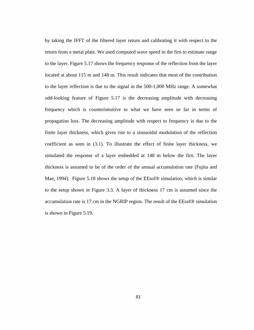
81

by taking the IFFT of the filtered layer return and calibrating it with respect to the

return from a metal plate. We used computed wave speed in the firn to estimate range

to the layer. Figure 5.17 shows the frequency response of the reflection from the layer

located at about 115 m and 148 m. This result indicates that most of the contribution

to the layer reflection is due to the signal in the 500-1,000 MHz range. A somewhat

odd-looking feature of Figure 5.17 is the decreasing amplitude with decreasing

frequency which is counterintuitive to what we have seen so far in terms of

propagation loss. The decreasing amplitude with respect to frequency is due to the

finite layer thickness, which gives rise to a sinusoidal modulation of the reflection

coefficient as seen in (3.1). To illustrate the effect of finite layer thickness, we

simulated the response of a layer embedded at 148 m below the firn. The layer

thickness is assumed to be of the order of the annual accumulation rate [Fujita and

Mae, 1994]. Figure 5.18 shows the setup of the EEsof® simulation, which is similar

to the setup shown in Figure 3.3. A layer of thickness 17 cm is assumed since the

accumulation rate is 17 cm in the NGRIP region. The result of the EEsof® simulation

is shown in Figure 5.19.

82

400 600 800 1000 1200 1400 1600 1800−100

−90

−80

−70

−60

−50

−40

−30

−20

Am

plitu

de (

dBm

)

Frequency (MHz)

Figure 5.17. Frequency response of reflection from layer located at about 115 m (top) and 148 m (bottom).

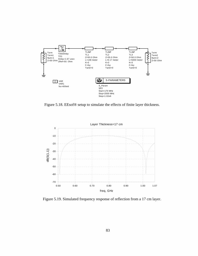
83

TLINPTL1

TanD=0F=fscK=3L=148 meterZ=50.0 Ohm

TLINPTL3

TanD=0F=fscK=3L=5000 meterZ=50.0 Ohm

TLINPTL2

TanD=0F=fscK=3L=0.17 meterZ=35.0 Ohm

S_ParamSP2

Step=1.02e6Stop=2000 MHzStart=170 MHz

S-PARAMETERS

TermTerm1

Z=50 OhmNum=1

VARVAR1fsc=600e6

EqnVar

TimeDelayTD1

ZRef=50. OhmDelay=1.67 usec

TermTerm2

Z=50 OhmNum=2

Figure 5.18. EEsof® setup to simulate the effects of finite layer thickness.

0.60 0.70 0.80 0.90 1.000.50 1.07

-60

-50

-40

-30

-20

-10

-70

0

freq, GHz

dB(S

(1,1

))

Layer Thickness=17 cm

Figure 5.19. Simulated frequency response of reflection from a 17 cm layer.

84

0.60 0.70 0.80 0.90 1.000.50 1.07

-60

-50

-40

-30

-20

-10

-70

0

freq, GHz

dB(S

(1,1

))



0.60 0.70 0.80 0.90 1.000.50 1.07

-60

-50

-40

-30

-20

-10

-70

0

freq, GHz

dB(S

(1,1

))



85

The simulation result does not exactly match our measured response as we did

not account for propagation and scattering losses. The general trend, however, can be

observed to be in good agreement with the reflection coefficient of the return from the

layer peaking between 600 and 1,000 MHz. We repeated the simulation for a layer

thickness of 10 cm and 30 cm and noted that the oscillation of the reflection

coefficient increases with increasing layer thickness. The sinusoidal property of the

reflection coefficient can be used to determine the thickness of a layer if the

resolution of the radar is greater than the annual accumulation rate.

5.6 Summary

In this chapter, we reviewed the concept of FM-CW radar and derived the

required specifications for a FM-CW radar to detect internal layers in the dry snow

region of the Greenland ice sheet. We described the system that was developed and

the experiments that were carried out at the NGRIP campsite during the summers of

1998 and 1999. We presented the results that were obtained with our system and

showed that the measurements were within ±2 m of the layers obtained from ice-core

data. We computed the uncertainty in the accumulation rate to be around 4% based on

the radar measurements. We also determined the optimum frequency range of the

measurements to be between 500 MHz to 1,000 MHz in the NGRIP area.

86

Chapter 6

PROTOTYPE AIRBORNE SYSTEM

Frequency analyses of the layer reflections from the surface-based experiment

described in the previous chapter reveal that the reflections are strongest at the 500-

1000 MHz frequency range. Based on this result and taking into consideration the

frequencies used for communication in the P-3 aircraft, we developed a 600-900 MHz

coherent airborne FM-CW radar for high-resolution mapping of the internal layers in

the Greenland ice sheet. Airborne measurements were made with the prototype

system over the Greenland ice sheet during the May 2001 field season. In this

chapter, we will present detailed design of the airborne radar and the results from

measurements made over the Greenland ice sheet.

6.1 System Design

The derivation of system specifications for the airborne system is similar to

the surface-based system described in the previous chapter. The goal is to develop a

system that can map internal layers in the upper 100 m of ice. This will be more than

adequate for our current purpose since most of the ice cores that have been collected

to create the latest accumulation map [Bales, et al., 2001a] were in the top 20 m of

ice. Also the frequency of operation for the system must be selected to avoid

interference with communication and navigation equipment aboard the NASA P-3

aircraft. Table 9 shows the frequency of instruments aboard the P-3.

87

Table 9. Frequency of equipment aboard NASA’s P-3 aircraft.

Equipment Frequency

ADF Receiver 190 – 2185 kHz

HF Comm. 2 – 30 MHz

Marker Beacon 75 MHz

VHF Nav. Receiver 108 – 118 MHz

VHF Comm. 30 – 88 MHz

VHF Comm. 118 – 174 MHz

UHF Comm. 225 – 400 MHz

DME/TACAN 960 – 1215 MHz

Transponder 1030 MHz

GPS Receiver 1575 MHz

Satcom Receiver 1525 – 1559 MHz

Satcom Transmitter 1626.5 – 1660.5 MHz

Radio Altimeter 4300 MHz

Weather Radar 9345 MHz

Based on the frequency analyses of layer data from surface-based

experiments, where the optimum frequency range is found to be between 500 and

1000 MHz, and the available range of 400-960 MHz on the P-3 aircraft, we chose the

frequency of operation of our system to be 600 – 900 MHz. This provides a range

resolution of 0.5 m in free space. To prevent any leakage and to minimize the use of

very high order filter a guard band of 100 MHz at the lower end and 60 MHz at the

higher end were used.

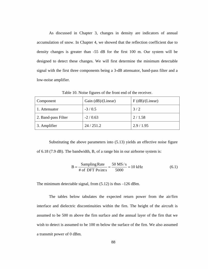
88

As discussed in Chapter 3, changes in density are indicators of annual

accumulation of snow. In Chapter 4, we showed that the reflection coefficient due to

density changes is greater than -55 dB for the first 100 m. Our system will be

designed to detect these changes. We will first determine the minimum detectable

signal with the first three components being a 3-dB attenuator, band-pass filter and a

low-noise amplifier.

Table 10. Noise figures of the front end of the receiver.

Component Gain (dB)/(Linear) F (dB)/(Linear)

1. Attenuator -3 / 0.5 3 / 2

2. Band-pass Filter -2 / 0.63 2 / 1.58

3. Amplifier 24 / 251.2 2.9 / 1.95

Substituting the above parameters into (5.13) yields an effective noise figure

of 6.18 (7.9 dB). The bandwidth, B, of a range bin in our airborne system is:

kHz105000

s/MS50sintPoDFTof#

RateSamplingB === (6.1)

The minimum detectable signal, from (5.12) is thus –126 dBm.

The tables below tabulates the expected return power from the air/firn

interface and dielectric discontinuities within the firn. The height of the aircraft is

assumed to be 500 m above the firn surface and the annual layer of the firn that we

wish to detect is assumed to be 100 m below the surface of the firn. We also assumed

a transmit power of 0 dBm.

89

Table 11. Expected return from air/firn interface.

Frequency (MHz)

λ (cm)/(dB)

Gain (dB)

PRC (dB) (air/firn)

S (dBm)

600 50 / -3.0 8.2 -15 -87

700 43 / -3.7 9.1 -15 -86

800 38 / -4.3 9.7 -15 -86

900 33 / -4.7 9.4 -15 -88

Table 12. Expected return from annual layer at a depth of 100m.

Frequency (MHz)

λ (cm)/(dB)

Gain (dB)

PRC (dB) (annual layer)

α (dB) S (dBm)

600 50 / -3.0 8.2 -55 -2.5 -131

700 43 / -3.7 9.1 -55 -2.9 -131

800 38 / -4.3 9.7 -55 -3.3 -131

900 33 / -4.7 9.4 -55 -3.8 -133

The expected returns from the annual layer are lower than the minimum

detectable signal for the given transmit power. We chose a transmit power of 30 dBm,

which will put the received signal power from the annual layers above the minimum

detectable signal level by more than 20 dB, assuming that the S/N ratio is limited by

thermal noise.

90

To determine the required number of coherent integrations, we first need to

compute the maximum distance over which integration can be performed. For

unfocused synthetic aperture radar, the maximum integration length, Lmax, is given as

[Wehner, 1995]:

λ= R5.0Lmax (6.2)

where R is the height of the aircraft above the firn and λ is the wavelength.

Obviously, the highest frequency of the system will determine the integration length

since the wavelength is the smallest at the highest frequency. For a platform height of

500 m and frequency of 900 MHz the integration length turns out to be 6.5 m. The

relationship between the integration length, PRF (pulse repetition frequency), number

of integrations, N, and velocity of the aircraft, v, is:

PRFvNLmax ≥ (6.3)

The aircraft travels at an average ground speed of 130 ms-1. Since the sweep time of

source is 100 µs, the maximum PRF for the system is 10 kHz. We were, however,

operating our system at only 2 kHz. We plan to operate it at a higher PRF during the

next field season in 2002. With these parameters, the number of coherent integrations

turns out to be 100. This will provide a 20 dB improvement in the SNR.

We now have all the required parameters to compute the receiver gain. We

want the gain of the receiver such that there is a greater than 20 dB signal-to-noise

91

ratio at the A/D. We note however that since the minimum signal level we want to

detect is 20 dB higher than the noise floor we are not going to gain any additional

SNR unless there are other sources of non-coherent noise picked up by the receiver.

As such, we modify (5.17) by omitting the integration gain term and express it as:

S + Pt + Grcvr > A/D noise floor + SNR (6.4)

-133 + 30 + Grcvr. > -70+20

Grcvr. > 53 dB

The receive chain was designed to have about 60 dB net gain to compensate for any

errors.

92

6.1.1 Transmitter

ChirpSynthesizer

BPF

BPF24 dB

1 GHzPLO

50 MHzTCXO

Data SystemClock

Receive

LO

IF

Power Amp

Transmit

BPF

COMPUTER

29 dB

BPFRF

3 dB

÷ 2BPF

LimiterBPF

BPF

31 dB

LPF

LPF

Figure 6.1. Block diagram of the prototype wideband FM-CW radar system for airborne mapping of internal layers.

Figure 6.1 shows the radar system we designed for airborne mapping of the

internal layers over the Greenland ice sheet. The signal source is the STEL-9949

programmable digital chirp synthesizer (DCS). It can be operated with a maximum

clock frequency of 1 GHz to generate a chirp signal between 1 MHz and 400 MHz. It

can also be programmed to generate a single carrier frequency in this range. The DCS

has a TTL level trigger input that is used to start the chirp and control its duration.

The pulse width of the trigger input controls the duration by driving a switch at the

output of the DCS. The switch is turned on when the trigger goes low. The pulse

width of the trigger signal was set equal to a sweep time of 100 µs. Figure 6.2 shows

93

the output from the synthesizer. Besides the main chirp from 100-400 MHz, there is

also a 600-900 MHz image signal and a 1 GHz clock signal. The image and clock

signals were filtered out using a low-pass filter with cutoff frequency at 440 MHz.

The 600 to 900 MHz chirp is generated by upconverting the 100 to 400 MHz chirp

using a 500 MHz phase-locked signal. The 500 MHz signal is obtained by dividing

the 1 GHz phase-locked oscillator (PLO) clock by 2. The 1 GHz PLO is referenced to

a 50 MHz temperature-compensated crystal oscillator (TCXO). A sample of the 50

MHz signal is used as the input clock for the timing system. This ensures that all the

signals are synchronized. The chirp signal is amplified and propagated through a

limiter that sets the output power to a constant level. The signal is finally amplified to

2 W by a 40-dB gain amplifier and is passed through a 3 dB attenuator, a band-pass

filter and coupled to a TEM horn antenna. The attenuator minimizes the effects of

mismatch between the amplifier and the transmit antenna. The band-pass filter is used

to suppress any spurious and harmonic signals. The TEM horn is the same as that

used during the surface-based experiment and is shown in Chapter 5.

94

0 100 200 300 400 500 600 700 800 900 1000−55

−50

−45

−40

−35

−30

−25

−20

−15

−10

−5

0

Am

plitu

de (

dBm

)

Frequency (MHz)

Figure 6.2. Synthesizer output.

6.1.2 Receiver

The signal is received with a TEM horn antenna and all out-of-band signals

are rejected with a band-pass filter before being amplified. The amplified signal is

mixed with a portion of the transmit signal to obtain the IF signal. This signal is high-

pass filtered to suppress the antenna feed-through signal. The beat frequency of the

signal from the firn surface is expected to be about 10 MHz since the aircraft is flying

about 500 m. The high-pass filter was designed with a cut-off frequency of 10 MHz.

We do not have to attenuate the surface return since our computations in Table 11 and

Table 12 show that the difference between the surface and internal returns is about 50

dB, which is less than the dynamic range of the A/D. We only need to consider the

95

antenna feed through, which we did not know at the time of this design. Hence, a

high-order band-pass filter was designed to ensure that the antenna feed through was

rejected. The amplifier that we used after the band-pass filter had a low-pass roll-off

after 900 MHz. This helped to further suppress the upper side-band signal that could

otherwise saturate the amplifier which had a fairly high-gain of 29 dB. We had

another amplifier with a gain of 31 dB to further amplify the IF signal. The IF signal

is finally low-pass filtered to prevent the LO leakage and other out-of-band signals

from being aliased into the IF band. One hundred traces were acquired and coherently

integrated before storing it onto a hard drive. The A/D that was used to digitize the

signal is the same one used during the surface-based experiment; i.e. 12 bits. The

traces, however, were sampled at 50 MHz instead of 1 MHz. The table below

summarizes the radar system’s parameters:

Table 13. Operating parameters of airborne system.

Frequency 600 – 900 MHz

Sweep Time 100 µs

PRF 2 kHz

Transmit Power 1 W

Number of Coherent Integrations 100

Antennas TEM Horn

A/D Dynamic Range 12 bit, 74 dB

Sampling Rate 50 MHz

96

6.2 Experiment

The University of Kansas, as a part of the NASA PARCA initiative, has been

performing measurements from the NASA P-3 aircraft over the Greenland ice sheet

for several years. We have been making ice thickness measurements using a coherent

radar [Gogineni et al., 1998], while the NASA team has been conducting surface

elevation measurements using a laser altimeter [Krabill et al., 1999]. During the May

2001 field mission we installed the wideband radar in the P-3 for mapping the internal

layers along with the other systems. The installation of our system in the aircraft is

shown in green in Figure 6.3. The radar system and computer were installed in a rack

by the wing of the aircraft. The horn antennas were installed in the bomb bay of the

aircraft. A low-loss RF cable was used to connect the transmitter and receiver to the

antennas.

The primary purpose of the test flights was to show that it is possible to map

the near-surface isochronous layers in the Greenland ice sheet using our high-

resolution radar. The test flights were also important in helping to evaluate the

performance of the radar system. Figure 6.4 shows the flight lines over which data

were collected using the wideband radar.

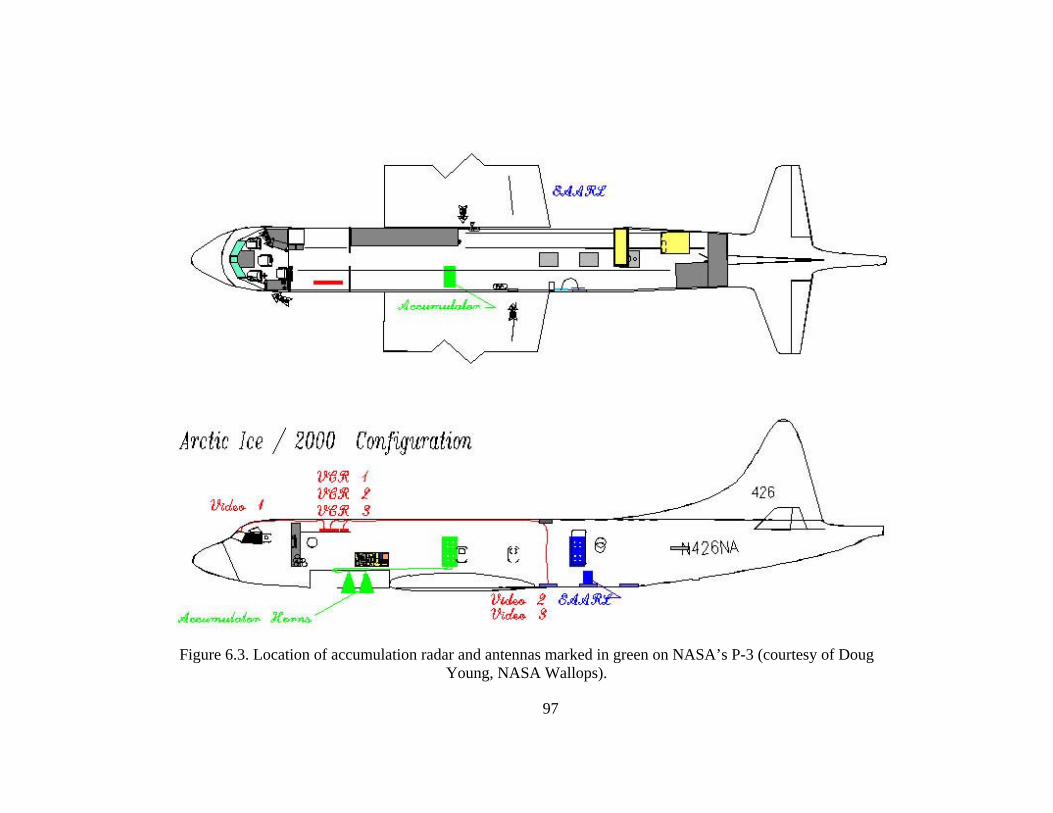
97

Figure 6.3. Location of accumulation radar and antennas marked in green on NASA’s P-3 (courtesy of Doug Young, NASA Wallops).

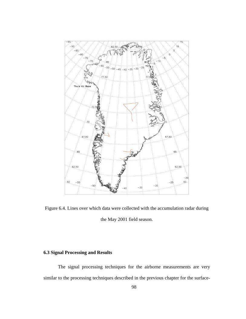
98

Figure 6.4. Lines over which data were collected with the accumulation radar during

the May 2001 field season.

6.3 Signal Processing and Results

The signal processing techniques for the airborne measurements are very

similar to the processing techniques described in the previous chapter for the surface-

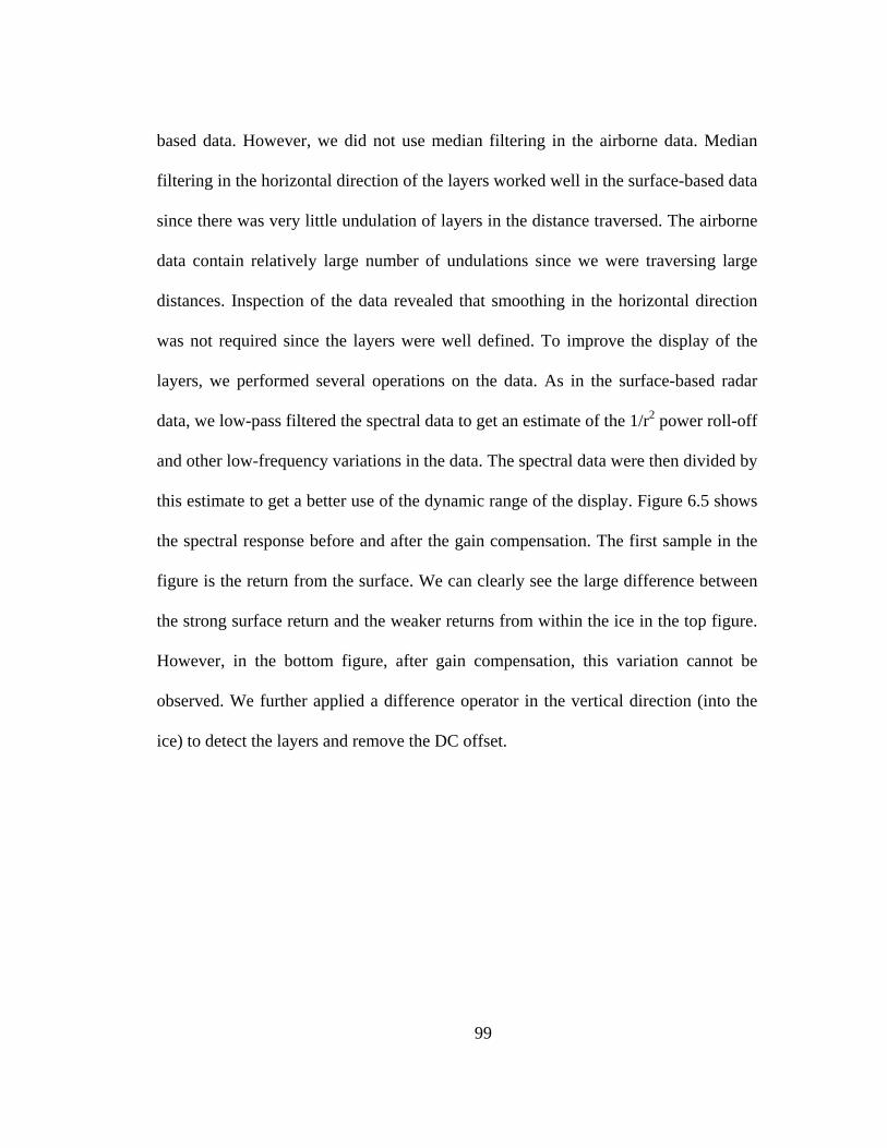
99

based data. However, we did not use median filtering in the airborne data. Median

filtering in the horizontal direction of the layers worked well in the surface-based data

since there was very little undulation of layers in the distance traversed. The airborne

data contain relatively large number of undulations since we were traversing large

distances. Inspection of the data revealed that smoothing in the horizontal direction

was not required since the layers were well defined. To improve the display of the

layers, we performed several operations on the data. As in the surface-based radar

data, we low-pass filtered the spectral data to get an estimate of the 1/r2 power roll-off

and other low-frequency variations in the data. The spectral data were then divided by

this estimate to get a better use of the dynamic range of the display. Figure 6.5 shows

the spectral response before and after the gain compensation. The first sample in the

figure is the return from the surface. We can clearly see the large difference between

the strong surface return and the weaker returns from within the ice in the top figure.

However, in the bottom figure, after gain compensation, this variation cannot be

observed. We further applied a difference operator in the vertical direction (into the

ice) to detect the layers and remove the DC offset.

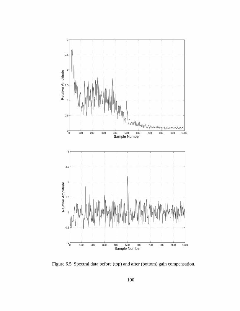
100

0 100 200 300 400 500 600 700 800 900 10000

0.5

1

1.5

2

2.5

3

Rel

ativ

e A

mpl

itude

Sample Number

0 100 200 300 400 500 600 700 800 900 10000

0.5

1

1.5

2

2.5

3

Rel

ativ

e A

mpl

itude

Sample Number

Figure 6.5. Spectral data before (top) and after (bottom) gain compensation.

101

Figure 6.6 shows the three major zones of the Greenland ice sheet: dry snow,

percolation and wet snow. We made measurements over these zones and the results

sare shown in Figures 6.7-6.9.

Figure 6.6. Dry snow, percolation and wet snow zones of the Greenland icesheet

[Long and Drinkwater, 1994].

102

Figure 6.7. Internal layers observed at the GRIP camp, which is located in the dry snow region of the icesheet.

103

Figure 6.7 shows a 208 km flight line over the GRIP camp. The GRIP camp is

located at 72o 35' N, 37o 38' W in the dry snow region of the ice sheet. The dry snow

zone is defined as the region where there is negligible melting or percolation [Benson,

1962]. The depth shown in the figure has been corrected for variation in the velocity

of the electromagnetic wave due to the non-uniform density. The layers in this region

are very well defined and can be observed up to a depth of 130 m, which is more than

our design goal of 100 m. We have enlarged a portion of the figure to show the

excellent delineation of the layers in the GRIP region. The resolution of our

measurements is less than a meter.

Dep

th (

m)

41.395W66.424N

125655.00 0.00

41.221W66.432N

125745.00 11.70

41.038W66.422N

125835.00 23.40

40.855W66.416N

125925.00 35.10

0 50 100 150 200 250 300

480

490

500

510

520

530

540

550

560

570

Figure 6.8. Internal layers observed at the percolation zone of the icesheet.

104

The layers that are observed in Figure 6.8 are from the percolation region of

the ice sheet. This area is characterized by meltwater percolating into the snowpack.

The depth shown on the figure is relative to the height of the aircraft, as we do not

have density data in this region to correct for the velocity of the wave. There are only

a few layers that can be observed here compared to the dry snow region. This is due

to the existence of meltwater, which makes the medium lossy. Also, the meltwater

often refreezes in the snowpack, creating a strong dielectric contrast and preventing

the transmission of signals further into the ice sheet. There are several strong

reflections that can be observed in the top 30 m. These reflections are probably due to

the refreezing of the meltwater when transitioning from the summer to winter

seasons.

Dep

th (

m)

47.384W70.754N

0.0047.309W70.735N

4.1647.228W70.715N

13.5247.144W70.692N

17.6847.053W70.669N

27.0446.959W70.643N

31.20

0 50 100 150 200 250 300 350 400 450 500

480

490

500

510

520

530

540

550

Figure 6.9. Internal layers observed at the wet snow zone of the icesheet.

105

Figure 6.9 shows the layers that were observed in the wet snow zone. The wet

snow zone is characterized by surfaces with wet or saturated snow at a temperature of

0o C. Again, the depths are plotted relative to aircraft height since density data are

unavailable in this region. As expected, there are very few layers that can be observed

since penetration of the waves is severely limited by the presence of wetness on the

surface. However, we do observe a strong reflection at about 35 m below the surface,

which could be from a dense ice firn. We are also able to observe layers to a depth of

about 50 m. However, they are not as clearly defined as those in the dry snow zone

because these data were collected when the system was not well tuned.

6.4 Evaluation of Prototype System

The results from our measurements show that it is indeed possible to map the

near-surface internal layers using an airborne radar system. We believe that the

quality of the data can be further improved by addressing some of the problems that

we discovered with the system during the test flights. The airborne system was

initially designed to operate in the step-pulse mode, where the received signal would

be digitized directly in two channels [Eakin, 2001]. One channel would have a high

gain for the weaker returns from within the ice, and the second channel would have a

low gain to receive the strong signals from the antenna feed-through and near-surface

reflections.

However, because the digital system failed two weeks before the experiment,

we had to redesign and reconfigure the entire system to operate in FM-CW mode.

106

The maximum sampling rate for digitizing the received signals from a maximum

range of 800 meters was 16 MHz. The existing digital system was capable of

sampling at 50 MHz rate, which was the reason for configuring the radar to operate in

FM-CW mode. Reconfiguring the system over a period of two weeks resulted in a

system that was less than optimum and needed frequent repairs and adjustments in the

field.

Leakage from the transmit antenna to the receive antenna was a severe

problem in FM-CW systems since it reduced the sensitivity of the radar. We used a

fourth-order band-pass filter [Wong, 2001] to suppress the antenna feed through. This

band-pass filter was not thoroughly evaluated, in particular its transient behavior,

before going to the field, and we discovered in the field that the filter’s large settling

time resulted in ringing that saturated the amplifiers. We constructed a simple high-

pass filter in the field and reduced amplifier gain to solve this problem. This reduced

radar sensitivity. In summary, the following problems were identified with our

prototype system:

1) Transient response of the band-pass filter following the mixer. The filter

transient response was not optimized to minimize ringing. The overshoot resulting

from filter ringing caused amplifier saturation.

2) Inadequate isolation between transmitter and receiver sections of the radar.

107

3) Insufficient receiver dynamic range. To minimize ringing we replaced the

four-pole band-pass filter with a single-pole high-pass filter, which resulted in

lowering the attenuation of the antenna feed-through signal.

4) Inadequate knowledge of the level of antenna feed-through signal. We did

not have the opportunity to determine the isolation between transmit and receive

antennas before the experiment in Greenland.

In the following chapter, we will show simulations of the band-pass filter

response and the improved filter design. During our return flight, we measured the S-

parameter of the antenna feed through using a network analyzer. This measurement is

used in our simulations so we can optimize the filter design to suppress the antenna

feed through. The packaging of the system is also improved to isolate the transmitter,

receiver and IF sections better.

6.5 Summary

This chapter described the design of a prototype airborne system to map the

near-surface internal layers of the Greenland ice sheet. We described the experiments

that were carried out during the May 2001 field season and showed results from three

distinct regions on the icesheet, namely the dry snow, percolation and wet snow

regions. The excellent delineation of the layers that were observed with our system

demonstrates that we can indeed map the near-surface internal layers with an airborne

108

radar system. We identified the problems with the system and these will be addressed

in the next chapter.

109

Chapter 7

AN IMPROVED AIRBORNE SYSTEM

In the previous chapter, we described some of the problems we had with the

airborne system during data collection in May 2001. In this chapter, we will describe

the system improvements made to solve these problems. We will show the results of

system simulations that were carried out on EEsof® and compare them with

laboratory measurements of the system. We could not test the system with antennas at

the University of Kansas due to interference from television stations that were

operating in the same frequency band. We developed a target simulator to enable us

to test the system under conditions similar to those of airborne measurements over the

ice sheet. The target simulator was designed with the aid of EEsof® and constructed

using optical and microwave delay lines to generate the effects of antenna feed

through, return from air-firn interface and returns from the internal layers.

7.1 System Description

Figure 7.1 shows the improved radar design. There were several changes

made to the system from the prototype design. The 1 GHz clock is now used directly

to upconvert the 100-400 MHz signal to 600-900 MHz. This is accomplished by

taking the lower sideband of the upconverted signal. We have eliminated the divide-

by-two circuitry needed to upconvert the chirp signal. Aside from reducing the

number of components that were used to generate the 600-900 MHz chirp, this did

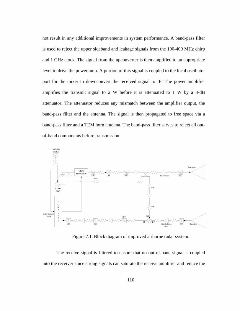
110

not result in any additional improvements in system performance. A band-pass filter

is used to reject the upper sideband and leakage signals from the 100-400 MHz chirp

and 1 GHz clock. The signal from the upconverter is then amplified to an appropriate

level to drive the power amp. A portion of this signal is coupled to the local oscillator

port for the mixer to downconvert the received signal to IF. The power amplifier

amplifies the transmit signal to 2 W before it is attenuated to 1 W by a 3-dB

attenuator. The attenuator reduces any mismatch between the amplifier output, the

band-pass filter and the antenna. The signal is then propagated to free space via a

band-pass filter and a TEM horn antenna. The band-pass filter serves to reject all out-

of-band components before transmission.

ChirpSynthesizer

BPF

BPFHigh-IsolationAmp

1 GHzPLO

50 MHzTCXO

Data SystemClock

Receive

LO

IF

Power Amp3 dB

Transmit

BPF

COMPUTER RF

3 dB

3 dB

LPF

LPFLPF

HPF

Figure 7.1. Block diagram of improved airborne radar system.

The receive signal is filtered to ensure that no out-of-band signal is coupled

into the receiver since strong signals can saturate the receive amplifier and reduce the

111

sensitivity of the system. A low-gain (10 dB), high-isolation amplifier, which has 50-

dB of reverse isolation, is used as the first-stage amplifier. We require a low gain at

this stage since the high feed-through signal from the transmit antenna will saturate

the mixer if higher gains are used. The high reverse isolation reduces the local

oscillator signal coupled into the RF port of the mixer being transmitted via the

receive antenna. The received signal is downconverted to IF. The IF signal is filtered

using a third-order Gaussian high-pass filter to attenuate the antenna feed through.

During last year’s field season we noted that the antenna feed-through signal

appeared at 500 kHz. The high-pass filter is designed to attenuate this leakage signal

by 60 dB with a fast settling time. An amplifier with a medium-high output power (20

dBm) is used to amplify the IF signal. We require a fairly high output to avoid

saturation by the upper sideband signal that is generated during the mixing process.

The signal is then low-pass filtered to reject the upper sideband signal and the LO

leakage signal. The IF signal is further amplified to use the full A/D dynamic range.

The signal is finally filtered with an anti-aliasing filter to keep the input noise from

folding over into the desired IF range.

7.2 Design of an Optimum High-pass Filter

During the last field season we noticed that the antenna feed-through signal

was saturating the IF amplifiers even though a fourth-order band-pass signal was

placed between the mixer and the first IF amplifier to suppress this signal. As

explained in the previous chapter, the filter’s large settling time caused excessive

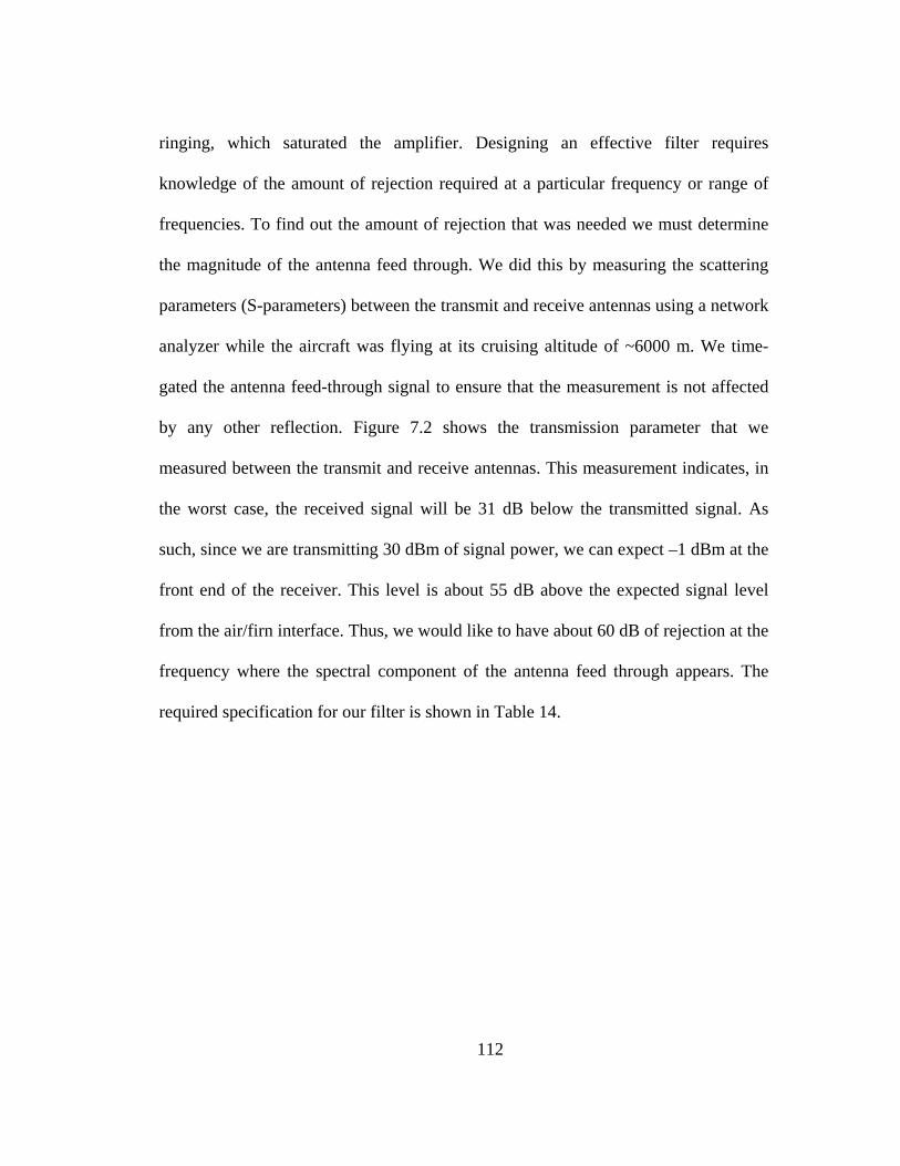
112

ringing, which saturated the amplifier. Designing an effective filter requires

knowledge of the amount of rejection required at a particular frequency or range of

frequencies. To find out the amount of rejection that was needed we must determine

the magnitude of the antenna feed through. We did this by measuring the scattering

parameters (S-parameters) between the transmit and receive antennas using a network

analyzer while the aircraft was flying at its cruising altitude of ~6000 m. We time-

gated the antenna feed-through signal to ensure that the measurement is not affected

by any other reflection. Figure 7.2 shows the transmission parameter that we

measured between the transmit and receive antennas. This measurement indicates, in

the worst case, the received signal will be 31 dB below the transmitted signal. As

such, since we are transmitting 30 dBm of signal power, we can expect –1 dBm at the

front end of the receiver. This level is about 55 dB above the expected signal level

from the air/firn interface. Thus, we would like to have about 60 dB of rejection at the

frequency where the spectral component of the antenna feed through appears. The

required specification for our filter is shown in Table 14.

113

600 650 700 750 800 850 900−55

−50

−45

−40

−35

−30

S21

(dB

)

Frequency (MHz)

Figure 7.2. Transmission parameter (S21) between the horn antennas.

Table 14. High-pass filter specifications.

Frequency (MHz) Attenuation (dB)

0.5 60

10 3

The high-pass filter that is desired is one that settles quickly and thus provides

a minimum overshoot. A class of filters known as the Gaussian filters has the ideal

time-domain response with no overshoots. However, an ideal Gaussian filter requires

an infinite number of elements and thus is impractical for physical realization [Dishal,

1959]. Dishal has given approximations to the Gaussian filter that can be used to

build these filters.

114

A third-order Gaussian filter was designed and fabricated in the laboratory

[Athial, 2001]. Figure 7.3 and Figure 7.4 show the comparison between the EEsof®

simulation and the measured response. The measured results do meet the

specifications in Table 14.

0 5 10 15 20 25 30−80

−70

−60

−50

−40

−30

−20

−10

0

S21

(dB

)

Frequency (MHz)

Measured Simulation

Figure 7.3. Comparison between measured and simulated response of Gaussian

high-pass filter.

0 0.1 0.2 0.3 0.4 0.5 0.6 0.7 0.8−80

−75

−70

−65

−60

−55

−50

S21

(dB

)

Frequency (MHz)

Measured Simulation

9.6 9.7 9.8 9.9 10 10.1 10.2 10.3 10.4−6

−5

−4

−3

−2

−1

0

S21

(dB

)

Frequency (MHz)

Measured Simulation

Figure 7.4. A zoom-in of the Gaussian filter’s attenuation at 500 kHz (left) and 10 MHz

(right).

115

The above figures clearly illustrate the versatility of EEsof® in simulating

circuits. The match at the 3 dB cutoff at 10 MHz is only off by 0.5 dB. At 500 kHz,

the frequency at which we expect the antenna leakage, we do have a 60 dB rejection.

The increased mismatch between the measured and simulated response can be

attributed to the uncertainty in the measurement of the signal level, since the signal-

to-noise ratio is low at these levels. Figure 7.5 shows the transient response of the

filter. An excellent match is again demonstrated between the simulated and measured

responses.

0 50 100 150 200 250−40

−20

0

20

40

60

80

100

Vol

tage

(m

V)

time (ns)

Measured Simulation

Figure 7.5. Comparison between measured and simulated responses to a 0.2 V step input.

7.3 System Simulation

To optimize the radar’s performance, we used EEsof® to simulate the system

response. Accurate simulations can be performed by incorporating the scattering

parameter models of components that are to be used in the radar. A number of

manufacturers of RF components provide S-parameter models of their parts on

116

websites. For components for which there were no models, we measured them in the

laboratory using a network analyzer. Since we were modifying an existing system, we

had most of the components we intend to use on hand. The S11, S21, S12 and S22

scattering parameters of the components were measured with a network analyzer,

which had been interfaced with EEsof®. The interface between EEsof® and the

network analyzer was accomplished using National Instrument’s general-purpose

interface bus (GPIB) card. The parameters are written to a file and stored on the hard

drive. The scattering parameters were measured over a 30 kHz to 2 GHz frequency

range. We used this wider frequency range instead of the 600-900 MHz range of our

system to enable EEsof® to obtain a more accurate impulse response of the

components. Further, these parameter files will be stored in a database that can be

accessed by students here for future radar design.

We also digitized the output of the STEL-9949 digital chirp synthesizer to be

used as the source during the simulation. The oscilloscope that was used to digitize

the chirp signal had a 8 bit A/D converter. Hence the dynamic range of our simulation

will be about 48 dB if the full dynamic range of the oscilloscope was used. Referring

to Figure 7.1, we measured the signal at the output of the amplifier that is just before

the coupler. We measured it at this point to get a better use of the oscilloscope’s

dynamic range.

EEsof® can model the non-linearities in the amplifiers and mixers by

allowing the designer to specify the 1 dB compression and the third-order intercept

117

(TOI) points. These points are usually specified with respect to the output power for

amplifiers and input power for mixers. The 1 dB compression point for a mixer is the

input power at which the output reduces by 1 dB from the linear relationship between

the input and output power levels (see Figure 7.6). The TOI point is the imaginary

point at which the output level of the third-order intermodulation products would be

equal to the desired output power if the device were linear. The 1 dB compression and

TOI points inform the radar designer of the power levels at which to operate a device

for a desired spurious free dynamic range. Further discussions and measurement

techniques of these parameters can be found in Henderson [1997] and Anritsu [2000].

Input Power (dBm)

Out

put P

ower

(dB

m)

TOI

1 dB

Spurious free dynamic range

Figure 7.6. Illustration of 1 dB compression and third-order intercept points.

The system shown in Figure 7.1 was simulated in EEsof® excluding the

power amplifier, which was not available at the time of simulation. Figure 7.7 shows

the simulation setup in EEsof®. The transmitter, receiver and IF sections have been

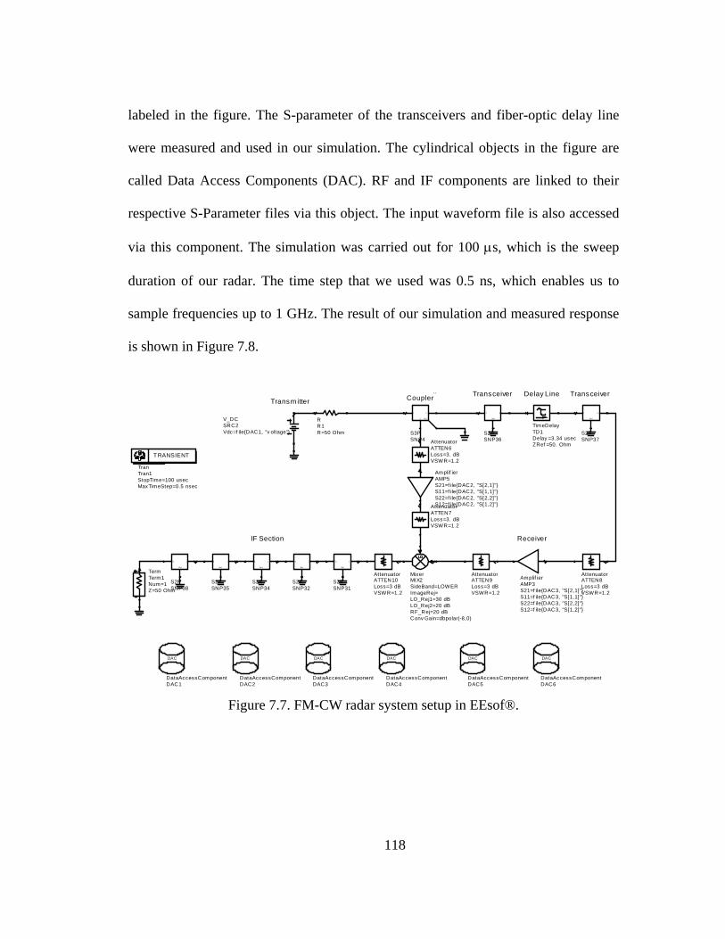
118

labeled in the figure. The S-parameter of the transceivers and fiber-optic delay line

were measured and used in our simulation. The cylindrical objects in the figure are

called Data Access Components (DAC). RF and IF components are linked to their

respective S-Parameter files via this object. The input waveform file is also accessed

via this component. The simulation was carried out for 100 µs, which is the sweep

duration of our radar. The time step that we used was 0.5 ns, which enables us to

sample frequencies up to 1 GHz. The result of our simulation and measured response

is shown in Figure 7.8.

TransceiverDelay LineTransceiverTransm itter Coupler``

ReceiverIF Section

``

S3PSNP4

2

3 Re f

1

MixerMIX2

Conv Gain=dbpolar(-8,0)RF_Rej=20 dBLO_Rej2=20 dBLO_Rej1=30 dBImageRej=SideBand=LOWER

DataAccessComponentDAC6

DAC


DAC


DAC


DAC


DAC


DAC

AttenuatorATTEN8

VSWR=1.2Loss=3 dB

S2PSNP36

21

Re f

S2PSNP37

21

Re f

TranTran1

MaxTimeStep=0.5 nsecStopTime=100 usec

T RANSIENT

V_DCSRC2Vdc=f ileDAC1, "v oltage"

TermTerm1

Z=50 OhmNum=1 S2P

SNP38

2 1

Re f

S2PSNP31

2 1

Re f

S2PSNP32

2 1

Re f

S2PSNP34

2 1

Re f

S2PSNP35

2 1

Re f

AttenuatorATTEN6

VSWR=1.2Loss=3. dB

Amplif ierAMP5

S12=f ileDAC2, "S[1,2]"S22=f ileDAC2, "S[2,2]"S11=f ileDAC2, "S[1,1]"S21=f ileDAC2, "S[2,1]"

TimeDelayTD1

ZRef =50. OhmDelay =3.34 usec

Amplif ierAMP3

S12=f ileDAC3, "S[1,2]"S22=f ileDAC3, "S[2,2]"S11=f ileDAC3, "S[1,1]"S21=f ileDAC3, "S[2,1]"

AttenuatorATTEN9

VSWR=1.2Loss=3 dB

AttenuatorATTEN10

VSWR=1.2Loss=3 dB

AttenuatorATTEN7

VSWR=1.2Loss=3. dB

RR1R=50 Ohm

Figure 7.7. FM-CW radar system setup in EEsof®.

119

10.26 10.28 10.3 10.32 10.34 10.36 10.38−60

−50

−40

−30

−20

−10

0

Beat Frequency (MHz)

Nor

mal

ized

Am

plitu

de (

dBm

)

Measured Simulation

Figure 7.8. Comparison between measured and simulated delay line response.

There is an excellent agreement between the measured and simulated data for

the main lobe, but there is slight disagreement between the two for sidelobes. These

mismatches can be attributed to the fact that not all the adapters and cables that were

used in the actual system were characterized on EEsof®. The excellent match in pulse

response between the measured and simulated response will enable us to develop

accurate system models and explore deconvolution techniques [Robinson and Treitel,

1980] to remove the system response from the received signal.

120

7.4 Target Simulator

Before the 2000 field season, we attempted to test our radar system outdoors

by pointing a UHF Yagi antenna at external targets such as buildings and trees.

However, interference from TV stations and cell phones operating in the UHF band

prevented us from doing so. Likewise, attempts to test the radar outdoors will cause

degradation in service for cell and cordless telephone users in the surrounding area. In

lieu of this problem and to provide a good calibration mechanism for the radar, a

target simulator was designed and developed as an undergraduate honors research

project [Plummer and Pharatasarathy, 2002].

The target simulator mimics the antenna feed-through path, reflection from

the air/firn interface and reflections from the internal layers. The simulator was first

designed using ideal components in EEsof®. Figure 7.9 shows the EEsof® simulation

setup along with an illustration of the aircraft and the various paths that are being

simulated. The color codes map the paths being simulated to the components that

simulate the path. The green path simulates the antenna feed-through signal. We used

a semi-rigid microwave delay line of 167 ns to match the actual path length. The blue

path simulates the 1000 m two way path length between the aircraft and the air/firn

interface. This was simulated using a fiber-optic delay line with optical/RF

transceivers to interface the RF and optical sections. Fiber-optic cables are ideal for

simulating large path lengths due to its low loss, small size and light weight. The

yellow path simulates the multitude of reflections from layers within the ice. This was

121

accomplished using a feedback loop. A short cable was used in this path to simulate

the 0.5 m spacing between the reflections from the internal layers.

Short cable Delay Line

Fibre Optic Delay Line

Layer Reflections

Transceiver

Transceiver

Reflection from air/snow interface

Antenna Feedthru

Port P1 Num=1

Attenuator ATTEN8 VSWR=1. Loss=45 dB

S2P

SNP1 2

1

Ref

S2P

SNP2 2

1

Ref

TimeDelay

TD7

ZRef=50. Ohm Delay=3.33 usec PwrSplit2

PWR8 S31=0.3162 S21=0.9487

TimeDelay

TD5 ZRef=50. Ohm

Delay=3.33 nsec

TimeDelay

TD6

ZRef=50. Ohm Delay=1.67e-7 sec

Amplifier

AMP1

S12=0 S22=polar(0,180)

S11=polar(0,0) S21=dbpolar(5.5,0)

Attenuator

ATTEN11

VSWR=1. Loss=3 dB

Attenuator ATTEN10 VSWR=1. Loss=3 dB

Port

P2

Num=2

PwrSplit2

PWR7

S31=0.707 S21=0.707

PwrSplit2 PWR6 S31=0.707 S21=0.707

PwrSplit2

PWR5 S31=0.707

S21=0.707

Ice Layers

Receiver

Transmitter

Figure 7.9. Block diagram of target simulator and the effects that are being simulated.

Once the component parameters were optimized, off-the-shelf components

were purchased. The scattering parameters of these components were measured using

a network analyzer and simulated in EEsof®. The simulator was constructed in the

122

laboratory and the overall response of the system was measured using a network

analyzer. The simulation result is compared with the measured response in Figure

7.10.

0 2 4 6 8 10 12 14−140

−120

−100

−80

−60

−40

−20

0N

orm

aliz

ed A

mpl

itude

(dB

m)


EESOF Simul.Measured

10.05 10.1 10.15 10.2 10.25

0

0.5

1

1.5

2

2.5

3

3.5

4

x 10−3

Nor

mal

ized

Am

plitu

de (

V)


EESOF Simul.Measured

Figure 7.10. Comparison between simulated and measured response of target simulator.

Air/firn interface

Internal Layers

123

The top figure shows the reflection profile for the entire path. The first signal

represents the antenna feed-through signal, which is about 40 dB above the air/firn

interface. The 40 dB difference can be easily adjusted to suit the field conditions by

changing the attenuator that is located just before the input transceiver. The signals

following the antenna feed through are the reflections from the air/firn interface and

from the internal layers. We clearly see the excellent match between the measured

response and the EEsof® simulation in the zoomed figure below.

The FM-CW radar system that we constructed was tested with the target

simulator and the results are shown in Figure 7.11.

0 5 10 15 20 25−80

−70

−60

−50

−40

−30

−20

−10

0

Nor

mal

ized

Am

plitu

de (

dBm

)

Beat Frequency (MHz)10.3 10.35 10.4 10.45 10.5 10.55 10.6 10.65

−40

−35

−30

−25

−20

−15

−10

−5

0

Nor

mal

ized

Am

plitu

de (

dBm

)


Figure 7.11. Results of FM-CW radar test with target simulator.

The results show excellent suppression of the antenna feed through. The

antenna feed through was 40 dB above the target response before the IF section. The

final output is 40 dB below the target response. The 80 dB suppression is due to the

Antenna Feed-through

Target

124

60 dB rejection by the Gaussian filter and an additional 20 dB suppression by the DC

blocks in the amplifiers. The bottom figure shows excellent resolution of the layering

that we are able to observe with the simulator.

7.5 Isolation

To provide better isolation between the transmitter, receiver and IF sections,

we constructed a box that partitions and shields these sections. We constructed two

boxes. Part of the transmitter and receiver were placed in the second box and will be

placed in a rack right above the horn antennas that are located in the bomb bay. This

will shorten the path length between the transmit and receive antenna and push the

antenna feed through further into the stop band. Low-loss cables are used to connect

the transmit and receiver sections mounted in the rack to the transmit and receive

antennas, respectively. Figure 7.12 shows how the various sections are isolated from

each other. Box 1 will be located at the rack mount and Box 2 will be located close to

the antennas above the bomb bay. We also replaced the low quality cables that were

used last year with high-isolation RF cables, which provide more than 100 dB of

isolation.

125

ChirpSynthesizer

LPF BPF

BPFHigh-IsolationAmp

1 GHzPLO

50 MHzTCXO

Data SystemClock

Receive

LO

IF

Power Amp3 dB

Transmit

BPF

COMPUTER

LPFHPFLPFRF

3 dB

3 dB

Box 2, Partition 1

Box 2, Partition 2

Box 1, Partition 1

Box 1, Partition 2

Figure 7.12. Isolating the transmit, receive and IF sections.

7.6 Summary

In this chapter, we described the improvements that were made to the

prototype system. We addressed the problem of filter ringing that was saturating the

amplifier during the last field season by designing a Gaussian high-pass filter with

very fast settling time and little overshoot. We addressed the lack of isolation by

building two boxes to shield transmit, receive and IF sections from each other. We

placed the front end of the transmitter and receiver near the antennas to reduce the

path length between the two and thus push the antenna feed through further into the

stop band. We performed EEsof® simulation on the system and showed an excellent

match between the measured and simulation response for a delay line test. We

constructed a target simulator, which mimics the antenna feed-through, air/firn

126

reflection and reflections from within the firn. The target simulator was also designed

with the aid of EEsof® and excellent match was again achieved between simulation

and measured responses. We tested our improved system with the target simulator,

and the results show that we are able to suppress the antenna feed through and obtain

excellent layering details. We believe our radar has been improved by an order of

magnitude and we expect the quality of the data from the upcoming field experiment

to be similarly superior to the results obtained from the previous year.

127

Chapter 8

SUMMARY AND RECOMMENDATIONS

Accumulation rate of the polar ice sheets is an important parameter that is

required for mass balance computation of the ice sheet. The present accumulation

map has relatively large uncertainty in many areas due to sparse sampling in these

regions. Accumulation rates are currently determined using ice cores and pits. Ice

core retrieval is an expensive, tedious and, at times, dangerous process. It is thus

prudent to seek remote sensing techniques to assist in the interpolation between ice

core data to reduce the uncertainty associated with the sparse sampling. The crux of

this dissertation was to explore the feasibility of employing a high-resolution airborne

radar to map the near-surface isochronous layers in the Greenland ice sheet. We have

shown that it is indeed possible to map the near-surface internal layers with high

resolution from an aircraft. We present below a summary of the work that was done

to arrive at an operational airborne radar that is ready for routine measurement of

internal layers over the polar ice sheets.

In Chapter 3, we looked at the factors that cause dielectric discontinuities

within the ice sheet. The primary cause of discontinuities at the near surface of the

firn is density changes. These density changes in the dry snow zone are due to

pressure exerted by annual accumulation of snow over the firn. Mapping of these

layers is the primary aim of this work. The other causes of dielectric discontinuities

128

are those due to changes in conductivity and crystal orientation. The conductivity

changes are usually due to acidic deposits from volcanic eruptions. Major volcanic

eruptions such as the Laki in 1783 and Tambora in 1815 are often used for absolute

dating of deeper ice cores. Changes in crystal orientation fabrics have been attributed

to shear strain along isochrones. They, however, occur at depths where there are no

density changes and hence are of little interest to our work since we are only

interested in the near-surface reflections. We used the transmission line model in the

CAD tool EEsof® to determine the reflection coefficients that can be expected for

discontinuities due to air/firn interface and those due to conductivity changes.

In Chapter 4, we applied surface and volume scattering models to observe the

off-nadir backscatter due to finite beamwidth of the horn antennas in the cross-track

direction. These backscatter signals have the potential for masking the reflections

from internal layers. We computed the reflection coefficient due to density changes

from an ice core record at the NGRIP site and compared it to that due to surface and

volume scattering. The physical parameters for the surface-scattering and volume-

scattering models were obtained from published data in the dry snow zone. Our

results showed that the reflections from the internal layer were about 10 to 15 dB and

5 to 10 dB above the surface clutter at 600 MHz and 900 MHz, respectively. The

volume scattering was 15 dB below that due to surface scattering and thus has little

effect on the return from internal layers.

129

Based on the results of simulations in Chapter 3, we described in Chapter 5

the design of a surface-based ultra-wideband FM-CW radar system that operates from

170 to 2,000 MHz. The purpose of the surface-based system was to determine the

optimum frequency range for mapping the internal layers. This system was tested

during the 1998 and 1999 field seasons at NGRIP. We showed that we were

successful in mapping internal layers up to a depth of almost 300 m. A number of the

layers were identified to within ±2 m of the layers obtained from ice-core data. We

computed the accumulation rate based on the radar mapping of the layers and

determined its uncertainty to be around 4%. We also analyzed the frequency content

of a signal reflected from a layer within the firn. The results showed that the optimum

frequency range for operating our radar is from 500 to 1,000 MHz.

In Chapter 6, we described the design of a 600-900 MHz airborne radar. The

frequency was selected such that it did not interfere with communication and

navigational equipments onboard the aircraft. Two TEM horns were installed

adjacent to each other in the bomb bay of the aircraft to serve as the transmit and

receive antennas. The system was initially designed to operate in the chirped and

stepped-frequency pulse modes to avoid the problem of antenna feed through. The

digital system that was being developed to accommodate these modes, however,

failed two weeks before the experiment and hence we reverted to a FM-CW operation

to use with the existing digital system. The band-pass filter used to suppress the

antenna feed through had a large settling time that resulted in ringing and saturation

of the IF amplifiers. We designed a single-pole high-pass filter in the field to avoid

130

the ringing and this, in turn, meant that we had to reduce the amplifier gain and thus

produced less sensitivity. During our return flight from the field, we measured the

isolation between the transmit and receive antenna with a network analyzer to aid us

in the design of a better IF filter for the new system. During the experiment we also

noted that there was inadequate isolation between the transmit and receive sections of

the radar.

Chapter 7 described the design of an improved FM-CW radar system for

routine mapping of internal layers over the Greenland ice sheet. The CAD tool

EEsof® was used to design and optimize the system performance before construction.

A third-order Gaussian high-pass filter was designed to provide the desired rejection

while minimizing the ringing effect. The entire system was simulated on EEsof® and

this performance was compared with delay-line measurements made with the actual

system. An excellent match was obtained between the two mainlobes and first

sidelobe. The slight mismatch in distance between the minor reflections can be

attributed to the fact that not all the adapters and cables that were used in the actual

system were characterized on EEsof®. During the last field season, we had

difficulties testing our system with antennas due to interference from communication

equipment operating in the UHF band. To enable us to test the radar system

effectively, a target simulator was designed as an undergraduate honors research

project. The simulator was constructed using RF and optical delay lines with a

RF/optical transceiver to interface the RF and optical sections. The target simulator

was designed to simulate the antenna feed-through signal and reflections from the

131

air/firn and internal layers. The multiple internal layers were generated by means of a

feedback loop using a short cable. We tested our new system with the target simulator

and obtained the desired suppression of the antenna feed through. The multiple layers

were observed to be very well defined. We constructed boxes with partitions to shield

the transmitter, receiver and IF sections adequately. The front end of the transmitter

and receiver were placed in a separate box to be positioned close to the bomb bay

where the antennas are located. This serves to shorten the path length between the

transmitter and receiver and hence push the antenna feed-through signal further into

the stopband of the high-pass filter.

Our system sensitivity improved by an order of magnitude and is ready for

routine mapping of internal layers over the polar ice sheets. The current system is

optimized for data collection over the dry snow region where the surface is not as

rough as in the percolation and wet snow zones where surface clutter could pose a

problem. We showed that we were able to map up to about 50 m in these regions even

with a sub-optimum system. However, if deeper layers need to be observed in these

regions or if weak reflections from volcanic layers need to be tracked, we will need to

implement a clutter cancellation scheme. There are a couple of ways this can be done.

The following section discusses some techniques that are worth considering.

8.1 Digital Beamforming to Null Clutter

To improve the resolution in the cross-track direction we recommend that the

TEM horn antennas be replaced with an array of bow-tie antennas as shown in Figure

132

8.1. In addition, the array could be implemented such that beamforming [Steyskal,

1987] can be performed to null out clutter that is masking reflection from a layer of

interest. Figure 8.2 shows how the null is placed to enable detection of the internal

layer.

In beamforming, the amplitude and phase of each stick of the bow tie will be

recorded. In traditional beam-steering arrays, only the phase is manipulated to steer

the beam. However, amplitude and phase control will enable us to better manage the

side lobe levels and steer the nulls. Each stick can be weighted appropriately with

complex weights (amplitude and phase) to produce a pattern that nulls out the clutter

that masks the desired return.

Receiver #-3 Receiver #-2 Receiver #-1 Receiver #0 Receiver #`1 Receiver #2 Receiver #3

Alo

ng T

rack

Figure 8.1. Bow-tie array to form beams digitally.

133

Internal Layer

Air/Snow Interface Null

Null

Figure 8.2. Digital beamforming to null out undesired clutter.

8.2 Model-Based Signal Processing

Model-based signal processing (MBP) has been used extensively in sonar for

detection of acoustic sources [Candy, 2000]. MBP uses noise, system and propagation

models to generate the expected signature from a target (Figure 8.3). The noise model

consists of the uncertainty in the model parameters, interference signal, etc. The

propagation model contains a priori information about the firn. We can use data from

ice cores to generate the propagation model. We can also include surface and volume

characteristics of the firn in this model to estimate the effects of clutter. We can

generate the system model using CAD tools such as EEsof® or by calibrating the

radar with known targets. It would be better to obtain an external target for calibration

134

so antenna effects are also included in the model. We can first compare the measured

surface return with that from the simulated response. The model parameters can then

be adjusted to fit the measured data. Once a match is achieved, we can subtract the

surface return from the measured data to reveal the internal layer data that can be seen

be our radar. We can then iteratively subtract each layer until the radar response for

all the layers that can be observed by the radar are obtained.

System Model

Noise Model

Firn Model

Raw Data

Estimate

Figure 8.3. Model-based signal processing.

135

REFERENCES

Agilent Technologies, Advanced Design System 2001, http://www.agilent.com/eesof-

eda/, 2001.

Akins, T., Design and Development of an Improved Data Acquisition System for the

Coherent Radar Depth Sounder, M.S. Thesis, Electrical Engineering and

Computer Science, The University of Kansas, Lawrence, KS, 1999.

Anritsu, Intermodulation Distortion (IMD) Measurements Using the 37300 Series

Vector Network Analyzer Application Note/GIP-G, Morgan Hill, California,

2000.

Athial, G., Private communication, Lawrence, KS, 2001.

Bailey, J. T., S. Evans, and G. de Q. Robin, Radio echo soundings of polar ice sheets,

Nature, vol. 204, pp. 420-421, 1964.

Bales, R. C., J. R. McConnell, E. Mosley-Thompson, and G. Lamorey, Accumulation

map for the Greenland ice sheet: 1971-1990, Geophysical Research Letters,

vol. 28, no. 15, pp. 2,967-2,970, 2001a.

Bales, R. C., J. R. McConnell, E. Mosley-Thompson, and B. Csthao, Accumulation

over the Greenland ice sheet from historical and recent records, Journal of

Geophysical Research, vol. 106, no. D24, pp. 33,813-33,826, 2001b.

Benson, C. S., Stratigraphic Studies in the Snow and Firn of the Greenland Ice Sheet,

Research Report 70, US Army Cold Regions Research and Engineering

Laboratory (CRREL), Hanover, NH, 1962.

Bogorodsky, V. V., V. I. Pozdnyak, G. V. Trepov, and A. M. Shremet’yev, Radar

sounding measurements of the thickness of annual snow strata in the

136

Antarctic, Doklady Akademii Nauk SSSR [Trans.: Doklady of the Academy of

Sciences of the U.S.S.R. Earth science sections.], vol. 264, no. 4, pp. 909-911,

1982.

Bogorodsky, V. V., C. R. Bentley, and P. E. Gudmandsen, Radioglaciology, D.

Reidel, Dordrecht, Holland, 1983.

Candy, J. V., Model-based signal processing in the ocean, Oceanic Engineering

Society Newsletter, vol. 35, no. 3, 2000.

Cheng, D. K., Field and Wave Electromagnetics, 2nd ed., Addison-Wesley, Reading,

MA, 1989.

Clausen, H. B., Private communication, NGRIP, Greenland, 1998.

Cumming, W. A., The dielectric properties of ice and snow at 3.2 centimeters,

Journal of Applied Physics, vol. 23, no. 7, 1952.

Dahl-Jensen, D., N. S. Gundestrup, K. Keller, S. J. Johnsen, S. P. Gogineni, C. T.

Allen, T.S. Chuah, H. Miller, S. Kipfstuhl, and E. D. Waddington, A search in

north Greenland for a new ice-core drill site, Journal of Glaciology, vol. 43,

no. 144, pp. 300-306, 1997.

Davis, C. H., C. A. Kluever, B. J. Haines, C. Perez, and Y. Yoon, Improved elevation

change measurement of the southern Greenland ice sheet from satellite radar

altimetry, IEEE Transactions on Geoscience and Remote Sensing, vol. 38, no.

3, pp. 1367-1378, 2000.

Dishal, M., Gaussian-response filter design, Electrical Communication, vol. 36, no. 1,

pp. 3-26, 1959.

Dyurgerov, M. B., and M. F. Meier, Year-to-year fluctuations of global mass balance

of small glaciers and their contribution to sea-level changes, Arctic and Alpine

Research, vol. 29, no. 4, pp. 392-402, 1997.

137

Eakin, R. K., Design and Development of a One Gigasample per Second Radar Data

Acquisition System, M.S. Thesis, Electrical Engineering and Computer

Science, The University of Kansas, Lawrence, KS, 2001.

Ellerbruch, D. A., and H. S. Boyne, Snow stratigraphy and water equivalence

measured with an active microwave system, Journal of Glaciology, vol. 26,

no. 94, pp. 225-233, 1980.

Etkins, R., and E. S. Epstein, The rise of global mean sea level as an indication of

climate change, Science, vol. 215, pp. 287-289, 15 January 1982.

Fetterer, F. M., M. R. Drinkwater, K. C. Jezek, S. W. C. Laxon, R.G. Onstott, and L.

M. H. Ulander, Sea ice altimetry, in Microwave Remote Sensing of Sea Ice,

ed., F.D. Carsey (Washington DC, American Geophysical Union),

Geophysical Monograph, vol. 68, pp. 111-135, 1992.

Forster, R. R., C. H. Davis, T. W. Rand, and R. K. Moore, Snow-stratification

investigation on an Antarctic ice stream with an X-band radar system, Journal

of Glaciology, vol. 37, no. 127, 1991.

Forster, R.R., K. C. Jezek, J. Bolzan, F. Baumgartner, and S. P. Gogineni,

Relationships between radar backscatter and accumulation rates on the

Greenland ice sheet, International Journal of Remote Sensing, vol. 20, no. 15,

pp. 3131-3147, 1999.

Fujita, S., and S. Mae, Causes and nature of ice-sheet radio-echo internal reflections

estimated from the dielectric properties of ice, Annals of Glaciology, vol. 20,

pp. 80-86, 1994.

Fujita, S., H. Maeno, S. Uratsuka, T. Furukawa, S. Mae, Y. Fujii, and O. Watanabe,

Nature of radio echo layering in the Antarctic ice sheet detected by a two-

frequency experiment, Journal of Geophysical Research, vol. 104, no. B6, pp.

13,013-13,024, 1999.

138

Fujita, S., T. Matsuoka, T. Ishida, K. Matsuoka, and S. Mae, A summary of the

complex dielectric permittivity of ice in the megahertz range and its

application for radar sounding of polar ice sheets, in Physics of Ice Core

Records, ed., by T. Hondoh, pp. 185-212, Hokkaido University Press,

Sapporo, Japan, 2000.

Fung, A. K., and H. J. Eom, Coherent scattering of a spherical wave from an irregular

surface, IEEE Transactions on Antennas and Propagation, vol. AP-31, no. 1,

pp. 68-72, 1983.

Fung, A. K., Microwave Scattering and Emission Models and Their Applications,

Artech House, Boston, 1994.

Gogineni, S., T. Chuah, C. Allen, K. Jezek, and R. K. Moore, An improved coherent

radar depth sounder, Journal of Glaciology, vol. 44, no. 148, 1998.

Gross, G.W., I. C. Hayslip, and R. N. Hoy, Dielectric relaxation spectrum of ice

measured with linear blocking electrodes, Geophysics, vol. 45, no. 5, pp. 914-

927, 1980.

Gudmandsen, P., Layer echoes in polar ice sheets, Journal of Glaciology, vol. 15, no.

73, 1975.

Hammer, C. U., Past volcanism revealed by Greenland ice sheet impurities, Nature,

vol. 270, pp. 482-486, 1977.

Hammer, C.U., Acidity of polar ice cores in relation to absolute dating, past

volcanism, and radio-echoes, Journal of Glaciology, vol. 25, no. 93, pp. 359-

372, 1980.

Harrison, C. H., Radio echo sounding of horizontal layers in ice, Journal of

Glaciology, vol. 12, no. 66, pp. 383-397, 1973.

139

Henderson, B. C., Mixers: Part 1, characteristics and performance, 97-98 RF and

Microwave Designer’s Handbook, pp. 469-475, Watkins-Johnson Company,

Palo Alto, CA, 1997.

Herron, M. M., and C. C. Langway, Jr., Firn densification: An empirical model,

Journal of Glaciology, vol. 25, no. 93, pp. 373-385, 1980.

Intergovernmental Panel on Climate Change (IPCC), Climate Change 2001: Impacts,

Adaptation, and Vulnerability (Summary for Policy Makers), Geneva,

Switzerland, February 13-16, 2001.

Izuka, K., A.P. Freundorfer, K.H. Wu, H. Mori, H. Ogura, and V.K. Nguyen, Step-

frequency radar, Journal of Applied Physics, vol. 56, no. 9, pp. 2572-2583,

1984.

Kanagaratnam, P., S. Gogineni, N. Gundestrup, and L. Larsen, High-resolution radar

mapping of internal layers at the North Greenland Ice Core Project, Journal of

Geophysical Research, vol. 106, no. D24, pp. 33,799-33,812, 2001.

Kipfstuhl, S., Private communication, NGRIP, Greenland, 1998.

Kohler, J., J. Moore, M. Kennett, R. Engeset, and H. Elvehøy, Using ground-

penetrating radar to image previous years’ summer surfaces for mass-balance

measurements, Annals of Glaciology, vol. 24, pp. 153-159, 1997.

Krabill, W., E. Frederick, S. Manizade, C. Martin, J. Sonntag, R. Swift, R. Thomas,

W. Wright and J. Yungel, Rapid thinning of parts of the southern Greenland

ice sheet, Science, vol. 283, pp. 1,522-1,524, 5 March 1999.

Krabill, W., W. Abdalati, E. Frederick, S. Manizade, C. Martin, J. Sonntag, R. Swift,

R. Thomas, W. Wright, and J. Yungel, Greenland ice sheet: High-elevation

balance and peripheral thinning, Science, vol. 289, pp. 428-430, 21 July 2000.

Larsen, L., Private communication, Lawrence, KS, 1999.

140

Lebedev, G. A., G. A., G. V. Trepov, and V. I. Poznyak, Results of radio-echo

soundings of annual snow layer depth in Antarctica, Proceedings of URSI

Commission F, Hyannisport, Massachusetts, 1990.

Leuschen, C., Surface-penetrating Radar for Mars Exploration, PhD. Dissertation,

Electrical Engineering and Computer Science, The University of Kansas,

Lawrence, KS, 2001.

Long, D. G., and M. R. Drinkwater, Greenland ice-sheet surface properties observed

by the Seasat-A scatterometer at enhanced resolution, Journal of Glaciology,

vol. 40, no. 135, pp. 213-230, 1994.

Looyenga, H., Dielectric constants of heterogeneous mixtures, Physica, vol. 31, pp.

401-406, 1965.

McConnell, J. R., G. Lamorey, E. Hanna, E. Mosley-Thompson, R. C. Bales, D.

Belle-Oudry, and J. D. Kyne, Annual net snow accumulation over southern

Greenland from 1975 to 1998, Journal of Geophysical Research, vol. 106, no.

D24, pp. 33,827-33,838, 2001.

Millar, D. H. M., Radio-echo layering in polar ice sheets and past volcanic activity,

Nature, vol. 292, 441-443, 1981.

Moore, J.C., and J. G. Paren, A new technique for dielectric logging of Antarctic ice

cores, Journal. de Physique., vol. 48, no. C1, pp. 155-160, 1987.

Moore, J. C., Dielectric variability of a 130 m Antarctic ice core: Implications for

radar sounding, Annals of Glaciology, vol. 11, pp. 95-99, 1988.

Ohmura, A., and N. Reeh, New precipitation and accumulation maps for Greenland,

Journal of Glaciology, vol. 37, no. 125, pp. 140-148, 1991.

Paren, J. G., and G. de Q. Robin, Internal Reflections in Polar Ice Sheets, Journal of

Glaciology, vol. 14, no. 71, pp. 251-259, 1975.

141

Paterson, W.S.B., The Physics of Glaciers, Butterworth-Heinemann, Oxford,

England, 1998.

Perry, T. S., Capturing climate change, IEEE Spectrum, vol. 39, no. 1, pp. 58-65,

2002.

Plummer, T. and B. Pharatasarathy, Target simulation for internal layers of Greenland

ice sheet, IEEE student paper contest, Electrical Engineering and Computer

Science, The University of Kansas, Lawrence, Kansas, 2002.

Richardson, C., E. Aarholt, S-E. Hamran, P. Holmlund, and E. Isaksson, Spatial

distribution of snow in western Dronning Maud Land, East Antarctica,

mapped by a ground-based snow radar, Journal of Geophysical Research, vol.

102, no. B9, pp. 20,343-20,353, 1997.

Ridley, J. K., and K. C. Partington, A model of satellite radar altimeter return from

ice sheets, International Journal of Remote Sensing, vol. 9, no. 4, pp. 601-624,

1988

Robin, G. de Q., S. Evans, and J. T. Bailey, Interpretation of radio echo sounding in

polar ice sheets, Philosophical Transactions of the Royal Society of London,

Series A, Mathematical and Physical Sciences, vol. 265, no. 1166, pp. 437-

505, 1969.

Robin, G. de Q., C. W. M. Swithinbank, and B. M. E. Smith, Radio echo exploration

of the Antarctic ice sheet, International Association of Scientific Hydrology,

no. 86, pp. 97-115, 1970.

Robin, G. de Q., and D. H. M. Millar, Flow of ice sheets in the vicinity of subglacial

peaks, Annals of Glaciology, vol. 3, pp. 290-294, 1982.

142

Robin, G. de Q., Radio-echo studies of internal layering of polar ice sheets, in The

Climatic Record in Polar Ice Sheets, ed., G. de Q. Robin, pp. 89-93,

Cambridge University Press, Cambridge, England, 1983.

Robinson, E. A., and S. Treitel, Geophysical Signal Analysis, Prentice Hall,

Englewood Cliffs, NJ, 1980.

Saunders, W. K., CW and FM radar, in Radar Handbook, 2nd ed., M. I. Skolnik, ch.

14, McGraw-Hill, New York, 1990.

Saxton, J. A., Reflection coefficient of snow and ice at V.H.F., Wireless Engineer,

vol. 27, no. 316, pp. 17-25, 1950.

Steyskal, H., Digital beamforming antennas, Microwave Journal, pp. 107-122,

January 1987.

Stove, A. G., Linear FMCW radar techniques, IEE Proceedings-F, vol. 139, no. 5, pp.

343-350, 1992.

Thomas, R. H., Polar Research from Satellites, Joint Oceanographic Institutions, Inc.,

Washington DC, 1991.

Ulaby, F.T., R. K. Moore, and A. K. Fung, Microwave Remote Sensing: Active and

Passive, vol. 2, Artech House, Norwood, MA, 1986.

van der Veen, C. J., and J.F. Bolzan, Interannual variability in net accumulation on

the Greenland Ice Sheet: Observations and implications for mass balance

measurements. Journal of Geophysical Research, vol. 104, no. D2, pp. 2009-

2014, 1999.

van der Veen, C.J., Polar ice sheets and global sea level: how well can we predict the

future?, in press, Global and Planetary Change, 2002.

143

Vickers, R. S., and G. C. Rose, High resolution measurements of snowpack

stratigraphy using a short pulse radar, Proceedings of the Eighth International

Symposium on Remote Sensing of Environment, vol. 1, pp. 261-267, Ann

Arbor, Michigan, October 2-6, 1972.

Waite, A. H., Ice depth soundings with ultra-high frequency radio waves in the Arctic

and Antarctic, and some observed over-ice altimeter errors, U.S. Army Signal

Research and Development Laboratory, Technical Report 2092, 1959.

Wehner, D. R., High-resolution Radar 2nd ed., Artech House, Norwood, MA, 1995.

Wong, W., Private communication, Lawrence, KS, 2001.

airborne radar for high-resolution mapping of internal

Documents