Airborne Measurements for estimating Methane Emissions in the Surat Basin, Australia

Stefan Schwietzke

Rebecca FisherDave LowryJames France

Thomas RockmannCarina van der Veen Malika Menoud

Bryce KellyXinyi Lu (Lexie)Stephen Harris

An intro and more details presented in this session by the project partners:Schwietzke et al., Konek et al., Kelly et al., and Lu et al.

Bruno Neininger Jorg Hacker and Wolfgang Lieff

Airborne Research AustraliaNon-Profit Research Institute

(Switzerland)

2

This presentation is about the airborne CH4 emission estimates over the Surat Basin

IN OUTIn a nutshell:

trying to measure in- and outflows ofan imaginary box, both by the mean flow,

and by turbulent fluxes

3

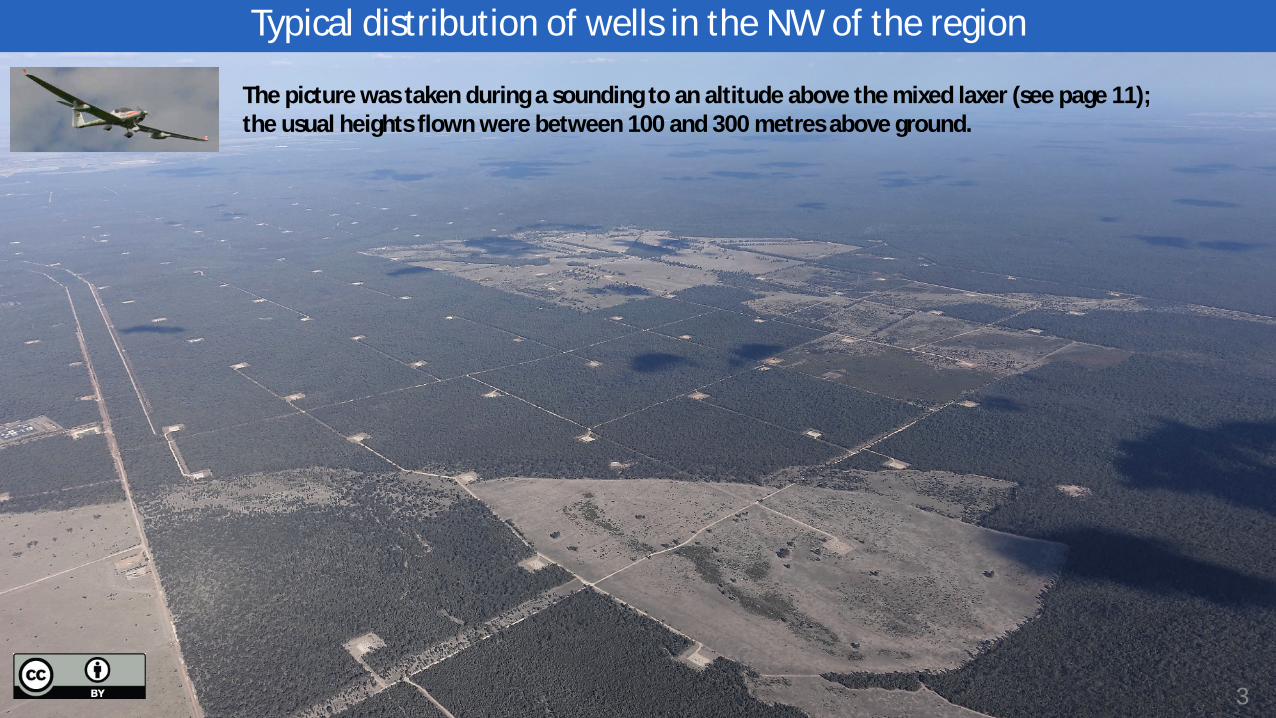
Typical distribution of wells in the NW of the region

The picture was taken during a sounding to an altitude above the mixed laxer (see page 11);the usual heights flown were between 100 and 300 metres above ground.

4

Surat Basin Topography

This landscape looks very flat, but it is not. It is an elongated basin.

5

Impressions (1/4): Typical Gas-Related Facilities

6

Impressions (2/4): Typical Gas-Related Facilities

7

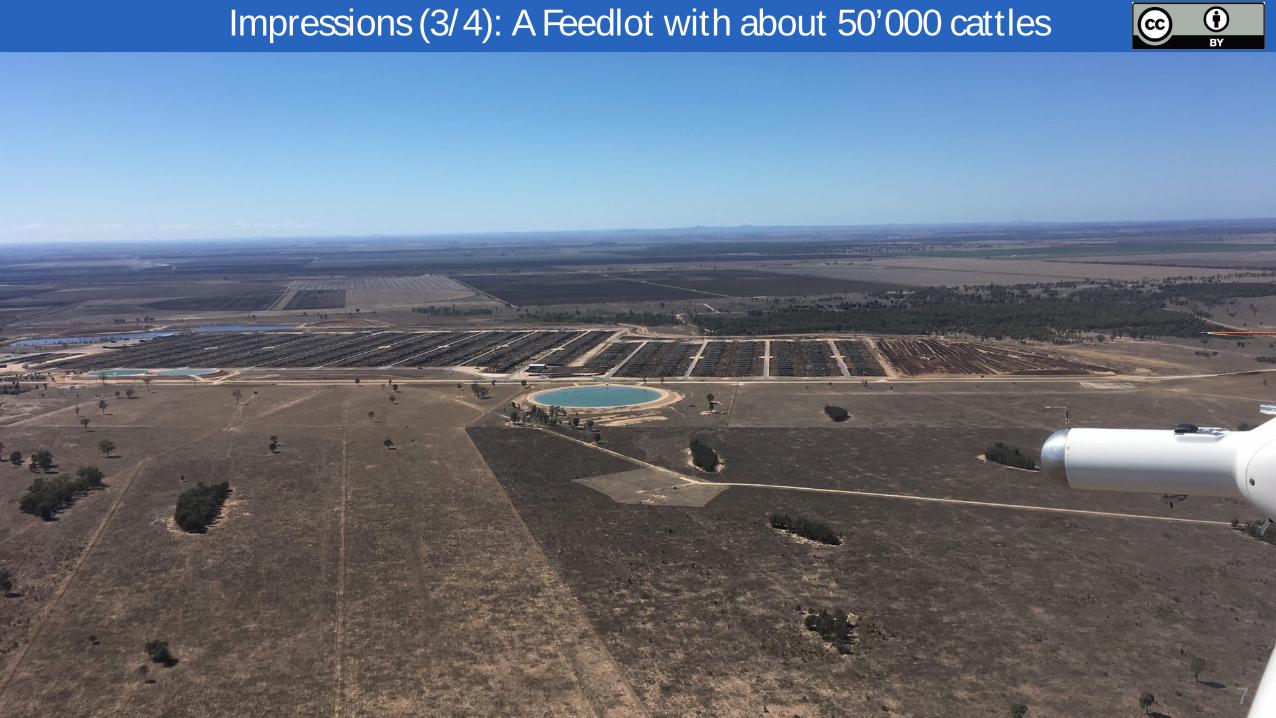
Impressions (3/4): A Feedlot with about 50’000 cattles

8

Impressions (4/4): All tracks and cockpit view

Real-time Data Display

Mission Scientist’s view in and out of the Cockpit

Known wells (yellow dots)All flight tracks flown (green lines)

9

The basic Concept (1/3): A 'balance sheet' of fluxes in and out of a box

IN OUT

all these contributions can be deduced from the measurements performed

secondary effect 2: convective exchange with the higher boundary layer

secondary effect 1: exchange with the surface (deposition)

10

Concept (2/3): Aerial Flux Quantification Method shown in 2-D

The basic principle of the emission estimates is quite simple: It's a 'balance sheet' of fluxes in and out of a box

Within such a virtual box, both the overall accumulation of CH4 and some point sources can be documented

Of course there are many subtleties that cannot be discussed with a few slides.

However, we can discuss right here,and more details will follow

in later publications.

11

Concept (3/3): A typical Flight Path

The basic principle of the emission estimates is quite simple: It's a 'balance sheet' of fluxes in and out of a box

Realization of this approach for an along-basin flow, and details with two heights of transects and soundings in between(important for knowing

the mixing height):

12

The instrumented airborne Platform (1/3)

All data was captured by sensors mounted on one of ARA’s small research aircraft (Diamond Aircraft HK 36 TTC-ECO; short name DIMO).

The ARA-DIMO is a highly modified special mission version of a motorglider featuring two under-wing pods and two additional pylons for sensing equipment.

The aircraft can carry two crew plus ~150kg of scientific instrumentation for flights of typically 5-6 hours over distances of up to ~800km and altitudes up to 7km.

All missions were flown from Toowoomba Airport with occasional intermediate refuelling stops at Dalby Airport.

The environmental footprint of the aircraft is minimal in terms of noise and CO2 emission (17 ltr/h unleaded car fuel).

11 science flights on 7 days over 15 day deployment period(plus 1 demo flight with some additional results for one source on another day)

13

The instrumented airborne Platform (2/3)

• RH underwing pod and pylon - meteorological instrumentation: • 10Hz air temperature, humidity, 3D-wind• 250Hz position, speed and attitudes (IMU/GPS)• laser altimeter for flying height above ground• air intake/pumps for bag samples• fast (20Hz) additional gas analyzer

(modified LiCor-7500) for CO2 and H2O• Aerosol/particle counter (MetOne)• Nadir-looking Canon 5D Mk4 RGB-camera

• Fuselage:• flight crew (pilot/scientist and mission scientist/systems operator)• data system with real-time data display• manual bag sampling

• LH underwing pod – main gas analyzer:• Los Gatos gas analyzer (high accuracy CH4, CO2 and H2O)

with external pump for achieving a temporal resolution of about 2 seconds

14

The instrumented airborne Platform (3/3)

ARA/Metair Flight Crew from right to left:

Jorg Hacker: Pilot and Chief Scientist of ARA

Shakti Chakravarty: Operator for the first flights

Bruno Neininger (MetAir): Operator for the remaining flights

15

Lagrangian Flight Planning

The basic principle of the emission estimates is quite simple: It's a 'balance sheet' of fluxes in and out of a box

Two cases of flight planning based on forecast trajectories (GFS grid data, own adjusted trajectory calculation)

a) Along valley flow: When the general wind regime is known (NW), suitable entry points were defined. The trajectories were then suggesting, where the 'walls' have to be flown after N hours (depending on the size of the box)

b) The same procedure for cross-valley flow from the NE, in this case turning to NNW during the planned flights.

air mass after 8 hours(two flights in sequence)

The suitable flight legs were then defined by observing additional aspects like airspaces, endurance, actual wind observations (leading to ad-hoc adjustments during flights), etc.Examples on previous and next slides.

16

Example of a Flight Track with grab samples (up to 25 bags/flight)

Flight track with 22 bag samples

Sampling bag

17

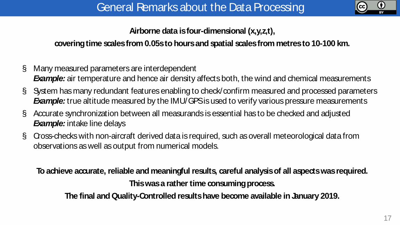
General Remarks about the Data Processing

Airborne data is four-dimensional (x,y,z,t),covering time scales from 0.05s to hours and spatial scales from metres to 10-100 km.

§ Many measured parameters are interdependentExample: air temperature and hence air density affects both, the wind and chemical measurements

§ System has many redundant features enabling to check/confirm measured and processed parameters Example: true altitude measured by the IMU/GPS is used to verify various pressure measurements

§ Accurate synchronization between all measurands is essential has to be checked and adjusted Example: intake line delays

§ Cross-checks with non-aircraft derived data is required, such as overall meteorological data from observations as well as output from numerical models.

To achieve accurate, reliable and meaningful results, careful analysis of all aspects was required.This was a rather time consuming process.

The final and Quality-Controlled results have become available in January 2019.

18

All tracks and First Results

Sept 10 in the SE Sept 12 in the NW Sept 15 along basin

Sept 16 across basin Sept 18 across valley Sept 19 along valley Sept 21 plume chasing in the NW

Wind

7 cases with different wind regimes; all with well mixed convective boundary layer

19

Two more detailed examples for along-valley flow

The basic principle of the emission estimates is quite simple: It's a 'balance sheet' of fluxes in and out of a box

The increasing concentrations are visible already now. However, for a quantitative assessment, all the fluxes in and out of the box will have to be calculated.

20

Example of an individual plume in about 20 km distance

The basic principle of the emission estimates is quite simple: It's a 'balance sheet' of fluxes in and out of a box

A preliminary calculationof the flux resulted in

about 750 g/sor 2.7 kg/h

21

Emission vs. concentrations airborne vs. near the source

Discussing the order of magnitude of concentration enhancements in a large region compared to near-source measurements near the ground (Kelly et al. by car):

Assuming a CH4 source of 16 g/s (1 mol/s, or 58 kg/h) somewhere.Case 1: Diluted in wind of 3 m/s (100 mol s-1 m-2) in a plume of 1’000 m2 cross-section

(red shaded ellipse below; 1 m3 of air is containing roughly 30 mol N2+O2)ð 100 kmol s-1 diluting air, resulting in a concentration enhancement of 10 ppm

Case 2: Diluted in Wind of 6 m/s (200 mol s-1 m-2) on an exit cross section of 50 km x 2’000 mð concentration enhancement of 0.05 ppb only!

Conclusion: Typical concentration enhancements of 10 ppb over the region are indicating emissions in the order of magnitude of 10 t/h(sum of very different sources including feedlots)

Typi

calc

onve

ctiv

em

ixin

gup

to2’

000

mAG

L

22

Four publications describing some related detailsFrom previous first work on CH4 in Switzerland:Hiller R.V., B. Neininger, D. Brunner, C. Gerbig, D. Bretscher, T. Künzle, N. Buchmann, W. Eugster,2014: Aircraft based CH4 flux estimates for validation of emissions from an agriculturally dominated area inSwitzerland. Journal of Geophysical Research: Atmospheres 03/2014; DOI:10.1002/2013JD020918.

From a previous project with a focus on one big rural CH4 source in Australia:Hacker, J.M., D. Chen, M. Bai, C. Ewenz, W. Junkermann, W. Lieff, B. McManus, B. Neininger, J. Sun,T. Coates, T. Denmead, T. Flesch, S. McGinn and J. Hill, 2016: Using airborne technology to quantify andapportion emissions of CH4 and NH3 from feedlots. Animal Production Science, 2016, 56, 190-203.

About a first feasibility study around other Oil & Gas fields near Groningen, NL:Yacovitch T.I., B. Neininger, S.C. Herndon, H.D. van der Gon, S. Jonkers, J. Hulskotte, J.R. Roscioli, D.Zavala-Araiza: Methane Emissions in the Netherlands, 2018: The Groningen Field. Elem Sci Anth, 6: 57. DOI: https://doi.org/10.1525/elementa.308.

About some special aspects of calculating horizontal and vertical fluxes from our airborne dataKrings T, Neininger B, Gerilowski K, Krautwurst S, Buchwitz M, et al. 2016. Airborne remote sensing and in-situ measurements of atmospheric CO2 to quantify point source emissions. Atmos Meas Tech Discuss 2016: 1-30. DOI:10.5194/amt-2016-362. https://www.atmos-meas-tech.net/11/721/2018/amt-11-721-2018.pdf