airborne lidar study of the vertical distribution of ... fileteaching and research institutions in...

HAL Id: hal-00318176https://hal.archives-ouvertes.fr/hal-00318176

Submitted on 20 Oct 2006

HAL is a multi-disciplinary open accessarchive for the deposit and dissemination of sci-entific research documents, whether they are pub-lished or not. The documents may come fromteaching and research institutions in France orabroad, or from public or private research centers.

L’archive ouverte pluridisciplinaire HAL, estdestinée au dépôt et à la diffusion de documentsscientifiques de niveau recherche, publiés ou non,émanant des établissements d’enseignement et derecherche français ou étrangers, des laboratoirespublics ou privés.

Airborne lidar study of the vertical distribution ofaerosols over Hyderabad, an urban site in central India,

and its implication for radiative forcing calculationsH. Gadhavi, A. Jayaraman

To cite this version:H. Gadhavi, A. Jayaraman. Airborne lidar study of the vertical distribution of aerosols over Hyder-abad, an urban site in central India, and its implication for radiative forcing calculations. AnnalesGeophysicae, European Geosciences Union, 2006, 24 (10), pp.2461-2470. �hal-00318176�

https://hal.archives-ouvertes.fr/hal-00318176

https://hal.archives-ouvertes.fr

Ann. Geophys., 24, 2461–2470, 2006www.ann-geophys.net/24/2461/2006/© European Geosciences Union 2006

AnnalesGeophysicae

Airborne lidar study of the vertical distribution of aerosols overHyderabad, an urban site in central India, and its implication forradiative forcing calculations

H. Gadhavi and A. Jayaraman

Physical Research Laboratory, Ahmedabad 380 009, India

Received: 13 March 2006 – Revised: 25 July 2006 – Accepted: 24 August 2006 – Published: 20 October 2006

Abstract. Use of a compact, low power commercial lidar on-board a small aircraft for aerosol studies is demonstrated. AMicro Pulse Lidar fitted upside down in a Beech Superkingaircraft is used to measure the vertical distribution of aerosolsin and around Hyderabad, an urban location in the centralIndia. Two sorties were made, one on 17 February 2004evening hours and the other on 18 February 2004 morninghours for a total flight duration of four hours. Three differentalgorithms, proposed by Klett (1985), Stephens et al. (2001)and Palm et al. (2002) for deriving the aerosol extinction co-efficient profile from lidar data are studied and is shown thatthe results obtained from the three methods compare within2%. The result obtained from the airborne lidar is shownmore useful to study the aerosol distribution in the free tro-posphere than that obtained by using the same lidar fromground. Using standard radiative transfer model the aerosolradiative forcing is calculated and is shown that knowledgeon the vertical distribution of aerosols is very important toget more realistic values than using model vertical profiles ofaerosols. We show that for the same aerosol optical depth,single scattering albedo and asymmetry parameter but fordifferent vertical profiles of aerosol extinction the computedforcing values differ with increasing altitude and improperselection of the vertical profile can even flip the sign of theforcing at tropopause level.

Keywords. Atmospheric composition and structure(Aerosols and particles; Instruments and techniques) – Me-teorology and atmospheric dynamics (Radiative processes)

1 Introduction

Aerosols play a major role in determining the regional scaleradiation budget of the earth’s atmosphere by directly scat-

Correspondence to:H. Gadhavi([email protected])

tering and absorbing the incoming and outgoing radiations aswell as through modifying cloud properties, such as the clouddroplet size distribution and cloud lifetime (e.g. Twomey,1974; Albrecht, 1989; Pincus and Baker, 1994; Haywoodand Boucher, 2000; Kaufman et al., 2005; Ramanathan elal., 2005). Nevertheless, measurements of aerosol proper-ties, particularly their vertical distribution are less and un-evenly distributed around the globe. Over India, knowledgeon the vertical distribution of aerosols has come mostly fromin situ probing using rocket and balloon-borne instrumen-tations (Jayaraman et al., 1987; Jayaraman and Subbaraya,1993; Ramachandran and Jayaraman, 2003), ground-basedlidar measurements (Devara et al., 1995; Jayaraman et al.,1995; Parameswaran et al., 1998) as well as from remote-sensing satellites (Kent et al., 1998; Spinhirne et al., 2005).Airborne lidars are gaining popularity in recent years as theyprovide useful information on the aerosol vertical profilesover a wider region such as during the INDOEX (Pelon etal., 2002), SAFARI-2000 (McGill et al., 2003), ACE-2 (Fla-mant et al., 2000) etc. Airborne laser remote sensing has ad-ditional advantage that it can measure aerosol profiles bothin vertical as well as horizontal directions in very short timeand can be a good tool to quantify the aerosol properties inthe three-dimensional space.

Under the Indian Space Research Organization’s (ISRO)Geosphere Biosphere Programme (GBP) a land campaignwas conducted in the central India during February 2004 (tobe referred henceforth as LC-1) to study the aerosol proper-ties and different trace gases concentrations. During LC-1,for the first time in India, airborne lidar measurements werecarried out over Hyderabad, one of the major industrializedcities located in the central India. Results obtained from thisairborne lidar experiment are discussed in the present paperin the context of their implication to radiative forcing calcu-lations. Section 2 of the paper describes instrumentation anddata reduction while Sect. 3 describes retrieval of aerosol ex-tinction profile and highlights the difference between three

Published by Copernicus GmbH on behalf of the European Geosciences Union.

2462 H. Gadhavi and A. Jayaraman: Airborne lidar study of the vertical distribution of aerosolsFigures

Hyderabad

Shaadh Nagar

Figure 1. Ground track of the airborne lidar measurements made on 17 February 2004 (Yellow line)

and 18 February 2004 (Green line). The background image is created from MODIS surface reflectance

data for the visible wavelength region.

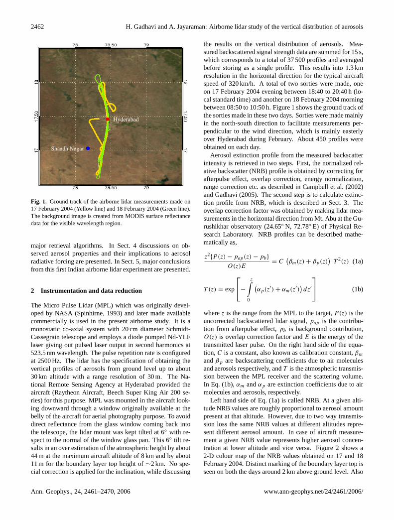
Fig. 1. Ground track of the airborne lidar measurements made on17 February 2004 (Yellow line) and 18 February 2004 (Green line).The background image is created from MODIS surface reflectancedata for the visible wavelength region.

major retrieval algorithms. In Sect. 4 discussions on ob-served aerosol properties and their implications to aerosolradiative forcing are presented. In Sect. 5, major conclusionsfrom this first Indian airborne lidar experiment are presented.

2 Instrumentation and data reduction

The Micro Pulse Lidar (MPL) which was originally devel-oped by NASA (Spinhirne, 1993) and later made availablecommercially is used in the present airborne study. It is amonostatic co-axial system with 20 cm diameter Schmidt-Cassegrain telescope and employs a diode pumped Nd-YLFlaser giving out pulsed laser output in second harmonics at523.5 nm wavelength. The pulse repetition rate is configuredat 2500 Hz. The lidar has the specification of obtaining thevertical profiles of aerosols from ground level up to about30 km altitude with a range resolution of 30 m. The Na-tional Remote Sensing Agency at Hyderabad provided theaircraft (Raytheon Aircraft, Beech Super King Air 200 se-ries) for this purpose. MPL was mounted in the aircraft look-ing downward through a window originally available at thebelly of the aircraft for aerial photography purpose. To avoiddirect reflectance from the glass window coming back intothe telescope, the lidar mount was kept tilted at 6◦ with re-spect to the normal of the window glass pan. This 6◦ tilt re-sults in an over estimation of the atmospheric height by about44 m at the maximum aircraft altitude of 8 km and by about11 m for the boundary layer top height of∼2 km. No spe-cial correction is applied for the inclination, while discussing

the results on the vertical distribution of aerosols. Mea-sured backscattered signal strength data are summed for 15 s,which corresponds to a total of 37 500 profiles and averagedbefore storing as a single profile. This results into 1.3 kmresolution in the horizontal direction for the typical aircraftspeed of 320 km/h. A total of two sorties were made, oneon 17 February 2004 evening between 18:40 to 20:40 h (lo-cal standard time) and another on 18 February 2004 morningbetween 08:50 to 10:50 h. Figure 1 shows the ground track ofthe sorties made in these two days. Sorties were made mainlyin the north-south direction to facilitate measurements per-pendicular to the wind direction, which is mainly easterlyover Hyderabad during February. About 450 profiles wereobtained on each day.

Aerosol extinction profile from the measured backscatterintensity is retrieved in two steps. First, the normalized rel-ative backscatter (NRB) profile is obtained by correcting forafterpulse effect, overlap correction, energy normalization,range correction etc. as described in Campbell et al. (2002)and Gadhavi (2005). The second step is to calculate extinc-tion profile from NRB, which is described in Sect. 3. Theoverlap correction factor was obtained by making lidar mea-surements in the horizontal direction from Mt. Abu at the Gu-rushikhar observatory (24.65◦ N, 72.78◦ E) of Physical Re-search Laboratory. NRB profiles can be described mathe-matically as,

z2{P (z) − pap(z) − pb}

O(z)E= C

(βm(z) + βp(z)

)T 2(z) (1a)

T (z) = exp

−

z∫0

(αp(z′) + αm(z′)

)dz′

(1b)

wherez is the range from the MPL to the target,P(z) is theuncorrected backscattered lidar signal,pap is the contribu-tion from afterpulse effect,pb is background contribution,O(z) is overlap correction factor andE is the energy of thetransmitted laser pulse. On the right hand side of the equa-tion, C is a constant, also known as calibration constant,βm

andβp are backscattering coefficients due to air moleculesand aerosols respectively, andT is the atmospheric transmis-sion between the MPL receiver and the scattering volume.In Eq. (1b),αm andαp are extinction coefficients due to airmolecules and aerosols, respectively.

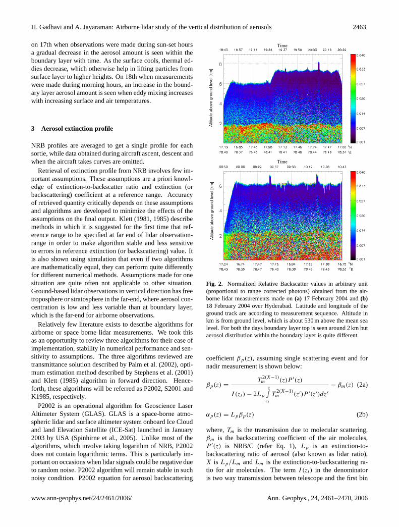
Left hand side of Eq. (1a) is called NRB. At a given alti-tude NRB values are roughly proportional to aerosol amountpresent at that altitude. However, due to two way transmis-sion loss the same NRB values at different altitudes repre-sent different aerosol amount. In case of aircraft measure-ment a given NRB value represents higher aerosol concen-tration at lower altitude and vice versa. Figure 2 shows a2-D colour map of the NRB values obtained on 17 and 18February 2004. Distinct marking of the boundary layer top isseen on both the days around 2 km above ground level. Also

Ann. Geophys., 24, 2461–2470, 2006 www.ann-geophys.net/24/2461/2006/

H. Gadhavi and A. Jayaraman: Airborne lidar study of the vertical distribution of aerosols 2463

on 17th when observations were made during sun-set hoursa gradual decrease in the aerosol amount is seen within theboundary layer with time. As the surface cools, thermal ed-dies decrease, which otherwise help in lifting particles fromsurface layer to higher heights. On 18th when measurementswere made during morning hours, an increase in the bound-ary layer aerosol amount is seen when eddy mixing increaseswith increasing surface and air temperatures.

3 Aerosol extinction profile

NRB profiles are averaged to get a single profile for eachsortie, while data obtained during aircraft ascent, descent andwhen the aircraft takes curves are omitted.

Retrieval of extinction profile from NRB involves few im-portant assumptions. These assumptions are a priori knowl-edge of extinction-to-backscatter ratio and extinction (orbackscattering) coefficient at a reference range. Accuracyof retrieved quantity critically depends on these assumptionsand algorithms are developed to minimize the effects of theassumptions on the final output. Klett (1981, 1985) describemethods in which it is suggested for the first time that ref-erence range to be specified at far end of lidar observation-range in order to make algorithm stable and less sensitiveto errors in reference extinction (or backscattering) value. Itis also shown using simulation that even if two algorithmsare mathematically equal, they can perform quite differentlyfor different numerical methods. Assumptions made for onesituation are quite often not applicable to other situation.Ground-based lidar observations in vertical direction has freetroposphere or stratosphere in the far-end, where aerosol con-centration is low and less variable than at boundary layer,which is the far-end for airborne observations.

Relatively few literature exists to describe algorithms forairborne or space borne lidar measurements. We took thisas an opportunity to review three algorithms for their ease ofimplementation, stability in numerical performance and sen-sitivity to assumptions. The three algorithms reviewed aretransmittance solution described by Palm et al. (2002), opti-mum estimation method described by Stephens et al. (2001)and Klett (1985) algorithm in forward direction. Hence-forth, these algorithms will be referred as P2002, S2001 andK1985, respectively.

P2002 is an operational algorithm for Geoscience LaserAltimeter System (GLAS). GLAS is a space-borne atmo-spheric lidar and surface altimeter system onboard Ice Cloudand land Elevation Satellite (ICE-Sat) launched in January2003 by USA (Spinhirne et al., 2005). Unlike most of thealgorithms, which involve taking logarithm of NRB, P2002does not contain logarithmic terms. This is particularly im-portant on occasions when lidar signals could be negative dueto random noise. P2002 algorithm will remain stable in suchnoisy condition. P2002 equation for aerosol backscattering

Time

Altit

ude

abov

e gr

ound

leve

l [km

]

0N 0E

Time

Altit

ude

abov

e gr

ound

leve

l [km

]

0E

0N

Figure 2. Normalized Relative Backscatter values in arbitrary unit (proportional to range corrected

photons) obtained from the airborne lidar measurements made on (a) 17 February 2004 and (b) 18

February 2004 over Hyderabad. Latitude and longitude of the ground track are according to

measurement sequence. Altitude in km is from ground level, which is about 530 meter above the mean

Fig. 2. Normalized Relative Backscatter values in arbitrary unit(proportional to range corrected photons) obtained from the air-borne lidar measurements made on(a) 17 February 2004 and(b)18 February 2004 over Hyderabad. Latitude and longitude of theground track are according to measurement sequence. Altitude inkm is from ground level, which is about 530 m above the mean sealevel. For both the days boundary layer top is seen around 2 km butaerosol distribution within the boundary layer is quite different.

coefficientβp(z), assuming single scattering event and fornadir measurement is shown below:

βp(z) =T

2(X−1)m (z)P ′(z)

I (zt ) − 2Lp

z∫zt

T2(X−1)m (z′)P ′(z′)dz′

− βm(z) (2a)

αp(z) = Lpβp(z) (2b)

where,Tm is the transmission due to molecular scattering,βm is the backscattering coefficient of the air molecules,P ′(z) is NRB/C (refer Eq. 1),Lp is an extinction-to-backscattering ratio of aerosol (also known as lidar ratio),X is Lp/Lm andLm is the extinction-to-backscattering ra-tio for air molecules. The termI (zt ) in the denominatoris two way transmission between telescope and the first bin

www.ann-geophys.net/24/2461/2006/ Ann. Geophys., 24, 2461–2470, 2006

2464 H. Gadhavi and A. Jayaraman: Airborne lidar study of the vertical distribution of aerosols

from where backscattering coefficients calculations are to bemade. When this distance is very small, as in the presentcase it will be very close to 1. In Eq. (2a),Lm is a knownquantity which is equal to 8π /3. Molecular transmissionTm can be calculated fairly accurate from temperature andpressure profiles. U.S. standard atmospheric temperature andpressure profiles (McClatchey et al., 1972) are scaled to theobserved surface level pressure and are used in the presentcase to calculateTm. Aerosol extinction coefficient (αp) canbe obtained fromβp by multiplying it with Lp as shown inEq. (2b).

The S2001 algorithm is based on the optimum estimationmethod, which is quite popular among satellite remote sens-ing community for retrieval of atmospheric temperature andcomposition from thermal radiation measurements (Rodger,1976, 1990, 2000). In this algorithm NRB profile is firstconstructed by lidar equation using climatological or crudeestimate of extinction values and the difference between ob-served and reconstructed NRB profile is minimized usingan iteration loop of the form shown in Eq. (3). This al-gorithm is mathematically vigorous and demands quite ahigh computer-memory and processing time in comparisonto other two algorithms. However, the very unique and im-portant advantage is that it retrieves simultaneously error es-timates of final result for various uncertainties in the inputvalues. A general equation for the optimum estimation algo-rithm can be written as,

xn+1

= Snx(S

−1a xa + KnT S−1

y [y − f + Knxn]) (3)

wherex is the resultant vector, the quantity to be retrievedand in the present case the extinction values at different alti-tudes.y is the measurement vector and in the present case itis a range corrected signal strength and aerosol optical depth.f is known as the forward function which relates the mea-surements to retrievable quantity, which essentially is a lidarequation.Sn

x is an error co-variance matrix fornth iteration.Sa andSy are error co-variance matrices for a priori knowl-edge of aerosol extinction and measurement errors.K is thesensitivity matrix. SuperscriptT denotes transpose of a ma-trix and n denotes number of iteration. Symbols in Eq. (3)are kept same as in S2001. More complete explanation ofthe symbols is available in Stephens et al. (2001).

Klett (1981) presents two solutions, one refers to solv-ing the lidar equation with reference value provided at nearend while other refers to solving lidar equation with refer-ence value provided at far end. Solution presented in Klett(1981) is further elaborated for separating Rayleigh contri-bution and range dependent lidar ratio in K1985. It shouldbe noted that focus of Klett (1981) is to show better stabil-ity of far-end solution in comparison to near-end solution.K1985 solution with near end reference value is not muchdifferent than previously existing lidar solutions such as Fer-nald et al. (1972). Following are equations for near end solu-

tion based on Klett’s (1985) solution for backscattering coef-ficient assuming a constant lidar ratio.

β(r) =exp(S′

− S′

0)[β−1

0 − 2Lp

r∫r0

exp(S′ − S′

0)dr ′

] (4a)

S′− S′

0 = S − S0 + 2Lm

r∫r0

βmdr ′− 2Lp

r∫r0

βmdr ′ (4b)

S(r) = log(NRB(r)) (4c)

where, β is the total backscattering by air molecules andaerosols. Subscriptm denotes molecular scattering andp

denotes particulate (aerosol) scattering.L is the lidar ratio asexplained in Eq. (2). Subscript 0 denotes the reference rangenear lidar telescope.

Poor stability in near end solution for ground based ver-tical observation of lidar is due to the denominator term inEq. (4a). It decreases rapidly with increasing range becauseof reduction in aerosol concentration and air density, whichmakes solution numerically unstable. However in case of air-borne or space-borne lidar observation aerosol concentrationand air density increases with range and hence near-end solu-tion is expected to be stable than compared to ground-basedobservation. Also for airborne observations reference rangeat far-end can not be guessed as reasonably as in the case ofground based observations and hence near-end solution be-comes a good choice for the airborne observations.

Calibration constant “C” and lidar-ratioLp are prerequi-site to compute extinction coefficient as evident from Eqs. (1)to (4). The calibration constant “C” can be calculated byknowing extinction (or backscattering) coefficient at refer-ence range. In case of high altitude airborne or space-bornemeasurements it can be obtained by comparing the NRBprofile with modelled Rayleigh backscattering profile for airmolecules in the stratosphere. But in the free tropical tropo-sphere significant amount of aerosol could be present. Ra-machandran and Jayaraman (2003) have reported a value of0.02 km−1 for aerosol extinction at the altitude of 5.5 km us-ing balloon borne sun-photometer over Hyderabad in April2001. However, Hart et al. (2005) report aerosol extinctionover the Indian Ocean region close to zero above 3 km usingGLAS observation. In the absence of independent measure-ments of aerosol extinction or backscattering coefficient dur-ing our experiment, we have carried out sensitivity analysisfor reference values used to estimate “C”. Aerosol backscat-tering coefficient at reference range is varied between 0 and6×10−4 km−1 sr−1 so as to cover observed extinction valuefor a wide range of lidar-ratios. Results of this sensitivityanalysis are discussed in the next few paragraphs.

A priori knowledge of lidar-ratio is necessary to derivethe extinction profile apart from knowing the backscatter-ing coefficient value at the reference range. In the present



Fig. 3. Sensitivity of aerosol extinction profile retrieved by algo-rithm described in Palm et al. (2002) to assumed values of aerosolbackscattering coefficient at a reference altitude of 6 km.

case, the lidar-ratio is obtained by an iterative process inwhich independently measured column AOD values usingsun-photometer are employed to constrain the extinctionvalues and the constrain is applied by adjusting the lidar-ratio. Ideally an extinction profile should be available upto top of the atmosphere in order to compare it with thecolumn AOD. During volcanically quiescent period thereis very less aerosol amount present at higher altitudes; forexample AOD above 6 km measured by SAGE-II on 28February 2004 over 19.3◦ N Latitude and 80.6◦ E Longi-tude is 0.015±0.004. Column AOD observations made froma nearby station (Shaadh Nagar, Fig. 1) are found to be0.4±0.05 on 17 February and 0.29±0.01 on 18 February dur-ing periods close to aircraft sorties. In the present case thehigher altitude aerosols are found to contribute only about3 to 5% to the total column AOD, which will result in 2to 3% error in extinction values. However, lidar-ratio ob-tained by constraining the extinction profile with AOD is sen-sitive to assumed value of backscattering coefficient at refer-ence range. For example, in case of “No Aerosol” above6 km (i.e.,βp=0 for altitude above 6 km) we get a lidar ratioof 45.2 sr, whereas forβp=6×10−4 km−1 sr−1 at 6 km, thelidar-ratio is 18.9 sr. Aerosol extinction profiles for three dif-ferent values of reference aerosol backscattering coefficient(viz., βp=0; 2×10−4 km−1 sr−1 and 6×10−4 km−1 sr−1 ataltitude around 6 km) using the P2002 algorithm are shownin Fig. 3. When retrieval of extinction profile is constrainedwith AOD, the effect is to shift the extinction profile in onedirection in free troposphere and in the opposite direction inboundary layer (Fig. 3). A 50% uncertainty in the total (Airmolecules + Aerosols) backscattering coefficient at reference

Fig. 4. Comparison of the performance of three algorithms de-scribed in Palm et al. (2002), Stephens et al. (2001) and Klett (1985)used for the retrieval of aerosol extinction coefficient profiles fromthe airborne lidar measurements.

range leads to approximately an error of 20% in the derivedaerosol extinction coefficient at lower altitudes. S2001 andK1985 algorithms have similar sensitivity to the assumedbackscattering coefficient values at the reference range.

Figure 4 shows the comparison between the results ob-tained using the three algorithms for 17 February data andassuming zero aerosol-backscattering at reference range.Lidar-ratios for P2002 and K1985 obtained from AOD mea-surements as explained earlier compare better than one deci-mal place and so is the extinction profiles. S2001 algorithmhas in-built constraint based on AOD and doesn’t require tosupply lidar-ratio explicitly. Results from these algorithmscompare within about 2% and no appreciable bias with alti-tude is observed in any particular algorithm.

The aerosol extinction profiles obtained from the airbornelidar measurements are compared with that obtained fromthe ground based observations made using the same lidarfrom Shaadh Nagar, located around 60 km south of Hyder-abad (see Fig. 1 for the location). The ground-based obser-vations are made between 19:30 to 20:30 h on 18 February2004. Same instrument settings are used in the ground basedobservation except that photon counts are summed for oneminute instead of 15 s as in the case of airborne observations.Kaestner (1986) algorithm is used to retrieve extinction pro-file for the ground-based measurements, which is similar toKlett’s (1985) algorithm but defines the solution directly interms of extinction coefficient. The aerosol extinction profileis derived by assuming zero aerosol content at far end (about6 km in the present case). Since ground-based observationswere made after sun-set, AOD data are not available for con-straining extinction in order to get the lidar-ratio. Hence,



Fig. 5. Comparison of the average aerosol extinction coefficientprofiles obtained from airborne lidar measurements made on 17and 18 Feb with that from ground based measurements made on18 evening at a nearby location using the same lidar instrument.

extinction profile for ground-based observation is retrievedusing lidar-ratio equal to 40 sr, which is in between the lidarratios obtained for airborne measurements made on the twodays. Figure 5 shows the ground-based observations alongside airborne observations of extinction profiles on 17 and18 February. Ground-based observations detect almost noaerosol above the boundary layer whereas significant aerosolextinction is seen in the free troposphere from airborne ob-servations on both days. Though the ground-based observa-tion is temporally and spatially separated from the airbornemeasurements, detection of no aerosol in the free tropospherefrom ground observations is due to poor signal-to-noise ratiofor the data obtained from free tropospheric altitudes. Partic-ularly over polluted urban locations, as in the present case, itis difficult to study aerosols from ground based lidar of mod-erate power, because of the weak backscattered signal fromhigher altitudes which is further attenuated by high amountof aerosols found within the boundary layer. From signal-to-noise ratio (S/N) point of view, airborne lidar is found morefavourable than the ground based measurements for the freetropospheric aerosol study, particularly over polluted urbanlocations.

4 Aerosol Radiative Forcing

The measured aerosol extinction profiles are used to calcu-late the aerosol radiative forcing (ARF), a parameter widelyused by modellers for the estimation of the role of aerosolsin inducing regional and global scale climate modifications.Radiative forcing is defined as difference in net radiative

0

5

10

15

20

25

30

1.E-05 1.E-04 1.E-03 1.E-02 1.E-01 1.E+00Aerosol Extinction (1/km)

Alti

tude

(km

)

Standard ProfileObserved Profile

Figure 6. Aerosol extinction profile with circle and dashed line is obtained by combining air-borne

lidar measurements on 17 Feb and SAGE data at altitudes above 6 km. Extinction profile with solid

line is the 'standard' model aerosols profile. Comparison of aerosol radiative forcing values computed

using these two profiles is shown in Figure 7.

Fig. 6. Aerosol extinction profile with circle and dashed line is ob-tained by combining air-borne lidar measurements on 17 Februaryand SAGE data at altitudes above 6 km. Extinction profile with solidline is the “standard” model aerosols profile. Comparison of aerosolradiative forcing values computed using these two profiles is shownin Fig. 7.

fluxes at given altitude between aerosol laden atmosphereand aerosol free atmosphere. Though this definition dif-fers with conventional definition of radiative forcing given inIPCC (2001) which defines aerosol radiative forcing for an-thropogenic aerosol, it serves the purpose of estimating influ-ence of aerosols (natural + anthropogenic) in radiation bud-get (Ramanathan et al., 2001). Atmospheric absorption dueto aerosols for a given layer is defined as difference betweenaerosol radiative forcing at top and bottom of the layer. Forthe sake of brevity, henceforth atmospheric absorption dueto aerosol will be mentioned as atmospheric absorption only.The objective of computing ARF in the present study is to ex-amine the sensitivity of the ARF computation to the aerosolvertical distribution. Calculations are carried out using SantaBarbara Discrete ordinate Atmospheric Radiative Transfer(SBDART) model developed by Ricchiazzi et al. (1998). Ac-curacy of SBDART is better than 3% in shortwave range.SBDART computes radiative fluxes assuming plane paral-lel atmosphere. Scattered fluxes are estimated using discreteordinate method (Stamnes et al., 1988) and molecular ab-sorption using LOWTRAN-7 atmospheric transmission bandmodel.

The different input parameters used in the ARF calcula-tions are summarized in Table 1. Aerosol extinction profilefrom ground to 40 km is constructed by combining the mea-sured profiles from the airborne lidar observations for thelower altitudes (0–6 km) and the smoothed extinction pro-file from SAGE-II (Ackerman et al., 1989) available for 28



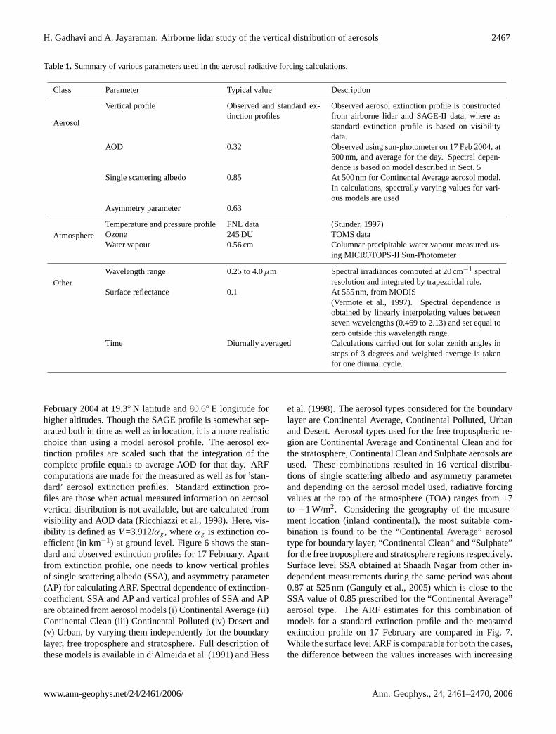
Table 1. Summary of various parameters used in the aerosol radiative forcing calculations.

Class Parameter Typical value Description

Aerosol

Vertical profile Observed and standard ex-tinction profiles

Observed aerosol extinction profile is constructedfrom airborne lidar and SAGE-II data, where asstandard extinction profile is based on visibilitydata.

AOD 0.32 Observed using sun-photometer on 17 Feb 2004, at500 nm, and average for the day. Spectral depen-dence is based on model described in Sect. 5

Single scattering albedo 0.85 At 500 nm for Continental Average aerosol model.In calculations, spectrally varying values for vari-ous models are used

Asymmetry parameter 0.63

AtmosphereTemperature and pressure profile FNL data (Stunder, 1997)Ozone 245 DU TOMS dataWater vapour 0.56 cm Columnar precipitable water vapour measured us-

ing MICROTOPS-II Sun-Photometer

OtherWavelength range 0.25 to 4.0µm Spectral irradiances computed at 20 cm−1 spectral

resolution and integrated by trapezoidal rule.Surface reflectance 0.1 At 555 nm, from MODIS

(Vermote et al., 1997). Spectral dependence isobtained by linearly interpolating values betweenseven wavelengths (0.469 to 2.13) and set equal tozero outside this wavelength range.

Time Diurnally averaged Calculations carried out for solar zenith angles insteps of 3 degrees and weighted average is takenfor one diurnal cycle.

February 2004 at 19.3◦ N latitude and 80.6◦ E longitude forhigher altitudes. Though the SAGE profile is somewhat sep-arated both in time as well as in location, it is a more realisticchoice than using a model aerosol profile. The aerosol ex-tinction profiles are scaled such that the integration of thecomplete profile equals to average AOD for that day. ARFcomputations are made for the measured as well as for ’stan-dard’ aerosol extinction profiles. Standard extinction pro-files are those when actual measured information on aerosolvertical distribution is not available, but are calculated fromvisibility and AOD data (Ricchiazzi et al., 1998). Here, vis-ibility is defined asV =3.912/αg, whereαg is extinction co-efficient (in km−1) at ground level. Figure 6 shows the stan-dard and observed extinction profiles for 17 February. Apartfrom extinction profile, one needs to know vertical profilesof single scattering albedo (SSA), and asymmetry parameter(AP) for calculating ARF. Spectral dependence of extinction-coefficient, SSA and AP and vertical profiles of SSA and APare obtained from aerosol models (i) Continental Average (ii)Continental Clean (iii) Continental Polluted (iv) Desert and(v) Urban, by varying them independently for the boundarylayer, free troposphere and stratosphere. Full description ofthese models is available in d’Almeida et al. (1991) and Hess

et al. (1998). The aerosol types considered for the boundarylayer are Continental Average, Continental Polluted, Urbanand Desert. Aerosol types used for the free tropospheric re-gion are Continental Average and Continental Clean and forthe stratosphere, Continental Clean and Sulphate aerosols areused. These combinations resulted in 16 vertical distribu-tions of single scattering albedo and asymmetry parameterand depending on the aerosol model used, radiative forcingvalues at the top of the atmosphere (TOA) ranges from +7to −1 W/m2. Considering the geography of the measure-ment location (inland continental), the most suitable com-bination is found to be the “Continental Average” aerosoltype for boundary layer, “Continental Clean” and “Sulphate”for the free troposphere and stratosphere regions respectively.Surface level SSA obtained at Shaadh Nagar from other in-dependent measurements during the same period was about0.87 at 525 nm (Ganguly et al., 2005) which is close to theSSA value of 0.85 prescribed for the “Continental Average”aerosol type. The ARF estimates for this combination ofmodels for a standard extinction profile and the measuredextinction profile on 17 February are compared in Fig. 7.While the surface level ARF is comparable for both the cases,the difference between the values increases with increasing



Standard Aerosol Profile

Observed Aerosol Profile

Surface -33.6 W/m2-31.7 W/m2

850 mbar -5.7W/m2-18.1 W/m2

100 mbar +0.4 W/m2-0.4 W/m2

Top of the atmosphere +0.7 W/m2+0.0 W/m2

Absorption +27.9 W/m2+13.6 W/m2 -14.3 W/m2

+11.6 W/m2

+0.1 W/m2

Difference

+6.1 W/m2+17.7 W/m2Absorption


Bou

ndar

yLa

yer

Free

Tro

posp

here

Stra

tosp

here



Surface -33.6 W/m2-31.7 W/m2

850 mbar -5.7W/m2-18.1 W/m2

100 mbar +0.4 W/m2-0.4 W/m2

Top of the atmosphere +0.7 W/m2+0.0 W/m2

Absorption +27.9 W/m2+13.6 W/m2





Surface -33.6 W/m2-31.7 W/m2Surface -33.6 W/m2-31.7 W/m2

850 mbar -5.7W/m2-18.1 W/m2850 mbar -5.7W/m2-18.1 W/m2

100 mbar +0.4 W/m2-0.4 W/m2100 mbar +0.4 W/m2-0.4 W/m2

Top of the atmosphere +0.7 W/m2+0.0 W/m2Top of the atmosphere +0.7 W/m2+0.0 W/m2

Absorption +27.9 W/m2+13.6 W/m2Absorption +27.9 W/m2+13.6 W/m2

+6.1 W/m2+17.7 W/m2Absorption +6.1 W/m2+17.7 W/m2Absorption

+0.3 W/m2+0.4 W/m2Absorption +0.3 W/m2+0.4 W/m2Absorption

Bou

ndar

yLa

yer

Free

Tro

posp

here

Stra

tosp

here

-14.3 W/m2

+11.6 W/m2

+0.1 W/m2

Difference

-14.3 W/m2-14.3 W/m2

+11.6 W/m2+11.6 W/m2

+0.1 W/m2+0.1 W/m2

Difference

Figure 7. Clear sky aerosol radiative forcing in the short wave region (0.25 to 4 µm) calculated for the

profiles shown in Figure 6 while the integrated column AOD and aerosol optical properties are kept

same. Large differences are seen in the forcing values at higher altitude and at the top of the

atmosphere. Values in regular font are aerosol radiative forcing at given altitude and values in bold font

are atmospheric absorption due to aerosols.

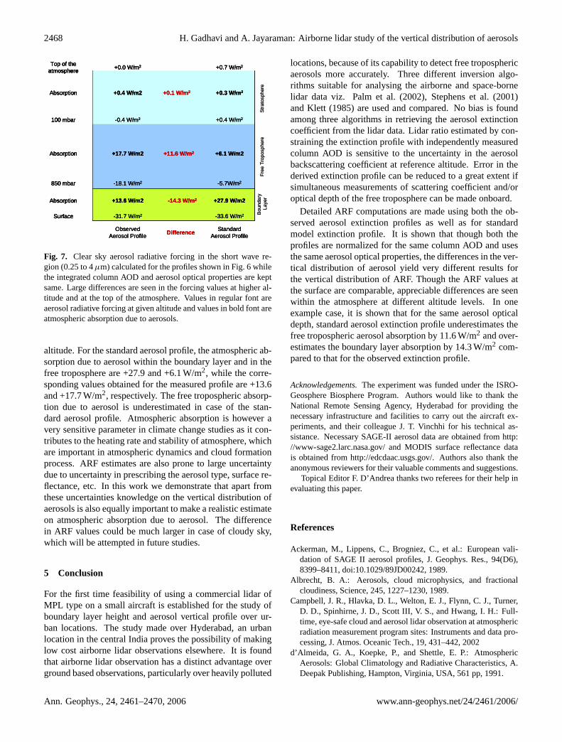
Fig. 7. Clear sky aerosol radiative forcing in the short wave re-gion (0.25 to 4µm) calculated for the profiles shown in Fig. 6 whilethe integrated column AOD and aerosol optical properties are keptsame. Large differences are seen in the forcing values at higher al-titude and at the top of the atmosphere. Values in regular font areaerosol radiative forcing at given altitude and values in bold font areatmospheric absorption due to aerosols.

altitude. For the standard aerosol profile, the atmospheric ab-sorption due to aerosol within the boundary layer and in thefree troposphere are +27.9 and +6.1 W/m2, while the corre-sponding values obtained for the measured profile are +13.6and +17.7 W/m2, respectively. The free tropospheric absorp-tion due to aerosol is underestimated in case of the stan-dard aerosol profile. Atmospheric absorption is however avery sensitive parameter in climate change studies as it con-tributes to the heating rate and stability of atmosphere, whichare important in atmospheric dynamics and cloud formationprocess. ARF estimates are also prone to large uncertaintydue to uncertainty in prescribing the aerosol type, surface re-flectance, etc. In this work we demonstrate that apart fromthese uncertainties knowledge on the vertical distribution ofaerosols is also equally important to make a realistic estimateon atmospheric absorption due to aerosol. The differencein ARF values could be much larger in case of cloudy sky,which will be attempted in future studies.

5 Conclusion

For the first time feasibility of using a commercial lidar ofMPL type on a small aircraft is established for the study ofboundary layer height and aerosol vertical profile over ur-ban locations. The study made over Hyderabad, an urbanlocation in the central India proves the possibility of makinglow cost airborne lidar observations elsewhere. It is foundthat airborne lidar observation has a distinct advantage overground based observations, particularly over heavily polluted

locations, because of its capability to detect free troposphericaerosols more accurately. Three different inversion algo-rithms suitable for analysing the airborne and space-bornelidar data viz. Palm et al. (2002), Stephens et al. (2001)and Klett (1985) are used and compared. No bias is foundamong three algorithms in retrieving the aerosol extinctioncoefficient from the lidar data. Lidar ratio estimated by con-straining the extinction profile with independently measuredcolumn AOD is sensitive to the uncertainty in the aerosolbackscattering coefficient at reference altitude. Error in thederived extinction profile can be reduced to a great extent ifsimultaneous measurements of scattering coefficient and/oroptical depth of the free troposphere can be made onboard.

Detailed ARF computations are made using both the ob-served aerosol extinction profiles as well as for standardmodel extinction profile. It is shown that though both theprofiles are normalized for the same column AOD and usesthe same aerosol optical properties, the differences in the ver-tical distribution of aerosol yield very different results forthe vertical distribution of ARF. Though the ARF values atthe surface are comparable, appreciable differences are seenwithin the atmosphere at different altitude levels. In oneexample case, it is shown that for the same aerosol opticaldepth, standard aerosol extinction profile underestimates thefree tropospheric aerosol absorption by 11.6 W/m2 and over-estimates the boundary layer absorption by 14.3 W/m2 com-pared to that for the observed extinction profile.

Acknowledgements.The experiment was funded under the ISRO-Geosphere Biosphere Program. Authors would like to thank theNational Remote Sensing Agency, Hyderabad for providing thenecessary infrastructure and facilities to carry out the aircraft ex-periments, and their colleague J. T. Vinchhi for his technical as-sistance. Necessary SAGE-II aerosol data are obtained fromhttp://www-sage2.larc.nasa.gov/and MODIS surface reflectance datais obtained fromhttp://edcdaac.usgs.gov/. Authors also thank theanonymous reviewers for their valuable comments and suggestions.

Topical Editor F. D’Andrea thanks two referees for their help inevaluating this paper.

References

Ackerman, M., Lippens, C., Brogniez, C., et al.: European vali-dation of SAGE II aerosol profiles, J. Geophys. Res., 94(D6),8399–8411, doi:10.1029/89JD00242, 1989.

Albrecht, B. A.: Aerosols, cloud microphysics, and fractionalcloudiness, Science, 245, 1227–1230, 1989.

Campbell, J. R., Hlavka, D. L., Welton, E. J., Flynn, C. J., Turner,D. D., Spinhirne, J. D., Scott III, V. S., and Hwang, I. H.: Full-time, eye-safe cloud and aerosol lidar observation at atmosphericradiation measurement program sites: Instruments and data pro-cessing, J. Atmos. Oceanic Tech., 19, 431–442, 2002

d’Almeida, G. A., Koepke, P., and Shettle, E. P.: AtmosphericAerosols: Global Climatology and Radiative Characteristics, A.Deepak Publishing, Hampton, Virginia, USA, 561 pp, 1991.


http://www-sage2.larc.nasa.gov/

http://www-sage2.larc.nasa.gov/

http://edcdaac.usgs.gov/


Devara, P. C. S., Raj, P. E., and Pandithurai, G.: Aerosol-profilemeasurements in the lower troposphere with four-wavelengthbistatic argon-ion lidar, Appl. Opt. 34(21), 4416–4425, 1995.

Fernald, F. G., Herman, B. M., and Reagan, J. A.: Determinationof aerosol height distributions by Lidar, J. Appl. Meteorol., 11,482–490, 1972.

Flamant C., Pelon, J., Chazette, P., Trouillet, V., Quinn, P. K.,Frouin, R., Bruneau, D., Leon, J.-F., Bates, T., Johnson, J., andLivingston, J.: Airborne lidar measurements of aerosol spatialdistribution and optical properties over the Atlantic Ocean duringan European pollution outbreak of ACE-2, Tellus, 52B, 662–677,2000.

Gadhavi, H.: Experimental investigation of aerosol properties andmodelling its impact on radiation budget, PhD Thesis, GujaratUniversity, Ahmedabad, India, 138 pp, 2005

Ganguly, D., Gadhavi, H., Jayaraman, A., Rajesh, T. A., and Misra,A.: Single scattering albedo of aerosols over the central India:Implications for the regional aerosol radiative forcing, Geophys.Res. Lett., 32, L18803, doi:10.1029/2005GL023903, 2005.

Hart, W. D., Spinhirne, J. D., Palm, S. P., and Hlavka, D. L.: Heightdistribution between cloud and aerosol layers from the GLASspaceborne lidar in the Indian Ocean region, Geophys. Res. Lett.,32, L22S06, doi:10.1029/2005GL023671, 2005.

Haywood, J. and Boucher, O.: Estimates of the direct and indirectradiative forcing due to tropospheric aerosols: A review, Rev.Geophys., 38(4), 513–543, doi:10.1029/1999RG000078, 2000.

Hess, M., Koepke, P., and Schult, I.: Optical properties of aerosolsand clouds: The software package OPAC, Bull. Am. Meteorol.Soc., 79, 831–844, 1998.

IPCC: Climate Change 2001: The Scientific Basis, Contribution ofWorking Group I to the Third Assessment Report of the Inter-governmental Panel on Climate Change, edited by: Houghton, J.T., Ding, Y., Griggs, D. J., et al., Cambridge University Press,New York, 881 pp, 2001.

Jayaraman, A., Subbaraya, B. H., and Acharya, Y. B.: The verti-cal distribution of aerosol concentration and their size distribu-tion function over the tropics and their role in radiation transfer,Physica Scripta, 36, 358–361, 1987.

Jayaraman, A. and Subbaraya, B. H.: In situ measurements ofaerosol extinction profiles and their spectral dependencies at tro-pospheric levels, Tellus, 45B, 473–478, 1993.

Jayaraman, A., Ramachandran, S., Acharya, Y. B., and Subbaraya,B. H.: Pinatubo volcanic aerosol layer decay observed at Ahmed-abad (23 N) India using Nd:YAG backscatter lidar, J. Geophys.Res., 100, 23 209–23 214, 1995.

Kaestner, M.: Lidar inversion with variable backscatter/extinctionratios: comment, Appl. Opt., 25(6), 833–835, 1986.

Kaufman, Y. J., Koren, I., Remer, L. A., Rosenfeld, D.,and Rudich, Y.: The effect of smoke, dust and pollu-tion aerosol on shallow cloud development over the AtlanticOcean, Proc. Nation. Acad. Sci. (USA), 102(32), 11 207–11 212,doi:10.1073/pnas.0505191102, 2005.

Kent, G. S., Trpte, C. R., and Lucker, P. L.: Long-term StratosphericAerosol and Gas Experiment I and II measurements of uppertropospheric aerosol extinction, J. Geophys. Res., 103, 28 863–28 874, 1998.

Klett, J. D.: Stable analytical inversion solution for processing lidarreturns, Appl. Opt., 20(2), 211–221, 1981.

Klett, J. D.: Lidar inversion with variable backscatter/extinction ra-

tios, Appl. Opt., 24(11), 1638–1643, 1985.McClatchey, R. A., Fenn, R. W., Selby, J. E. A., Volz, F. E., and Gar-

ing, J. S.: Optical properties of the atmosphere, 3rd ed. AFCRLEnviron. Res. Papers No. 411, 108 pp, 1972.

McGill, M. J., Hlavka, D. L., Hart, W. D., Welton, E. J., and Camp-bell, J. R.: Airborne lidar measurements of aerosol optical prop-erties during SAFARI-2000, J. Geophys. Res., 108(D13), 8493,doi:10.1029/2002JD002370, 2003.

Palm, S. P., Hart, W., Hlavka, D., et al.: GLAS atmospheric dataproducts, Algorithm Theor. Basis. Doc. ATBD-GLAS-01, ver-sion 4.2, Earth Obs. Syst. Proj. Off., Greenbelt, Md. (Availableat http://eospso.gsfc.nasa.gov/eoshomepage/forscientists/atbd/), 2002.

Parameswaran, K., Rajan, R., Vijayakumar, G., Rajeev, K., Moor-thy, K. K., Nair, P. R., and Satheesh, S. K.: Seasonal and longterm variations of aerosol content in the atmospheric mixing re-gion at a tropical station on the Arabian sea-coast, J. Atmos.Solar-Terrestrial Phys., 60(1), 17–25, 1998.

Pelon, J., Flamant, C., Chazette, P., Leon, J.-F., Tanre, D., Sicard,M., and Satheesh, S. K.: Characterization of aerosol spatial dis-tribution and optical properties over the Indian Ocean from air-borne LIDAR and radiometry during INDOEX’99, J. Geophys.Res., 107(D19), 8029, doi:10.1029/2001JD000402, 2002.

Pincus, R. and Baker, M.: Precipitation, solar absorption, andalbedo susceptibility in marine boundary layer clouds, Nature,372, 250–252, 1994.

Ramachandran, S. and Jayaraman, A.: Balloon-borne study of theupper tropospheric and stratospheric aerosols over a tropical sta-tion in India, Tellus, 55(3)B, 820–836, 2003.

Ramanathan, V., Chung, C., Kim, D., et al.: Atmospheric brownclouds: Impacts on south Asian climate and hydrological cycle,Proc. Nation. Acad. Sci. (USA), doi:10.1073/pnas.0500656102,2005.

Ramanathan, V., Crutzen, P. J., Lelieveld, J., et al.: Indian OceanExperiment: An integrated analysis of the climate forcing andeffects of the great Indo-Asian haze, J. Geophysic. Res., 106(22),28 371–28 398, doi:10.1029/2001JD900133, 2001.

Ricchiazzi, P., Yang, S., Gautier, C., and Sowle, D.: SBDART: Aresearch and teaching software tool for plane-parallel radiativetransfer in the Earth’s atmosphere, Bull. Am. Meteorol. Soc.,79(10), 2101–2114, 1998.

Rodger, C.: Retrieval of atmospheric temperature and compositionfrom remote measurements of thermal radiation, Rev. Geophys.,14, 609–624, 1976.

Rodger, C.: Characterization and error analysis of profiles re-trieved from remote sounding measurements, J. Geophys. Res.,95, 5587–5595, 1990.

Rodger, C.: Inverse methods for atmospheric sounding: Theory andPractice, World Scientific, 2, 238, 2000.

Spinhirne, J. D., Palm, S. P., Hart, W. D., Hlavka, D. L., andWelton, E. J.: Cloud and aerosol measurements from GLAS:Overview and initial results, Geophys. Res. Lett., 32, L22S03,doi:10.1029/2005GL023507, 2005.

Spinhirne, J.D.: Micro Pulse Lidar, IEEE Trans. Geosci. RemoteSens., 31, 48–55, 1993.

Stephens, G. L., Engelen, R. J., Vaughan, M., and Anderson, T.L.: Toward retrieving properties of the tenuous atmosphere usingspace-based lidar measurements, J. Geophys. Res., 106, 28 143–28 157, 2001.


http://eospso.gsfc.nasa.gov/eos_homepage/for_scientists/atbd/


Stunder, B.: NCEP Model Output – FNL Archive Data, References134, National Climate Data Center, NOAA – Air Resources Lab-oratory, USA, 1997.

Twomey, S.: Pollution and the planetary albedo, Atmos. Environ.,8, 1251–1256, 1974.

Vermote, E. F., El Saleous, N. Z., Justice, C. O., Kaufman, Y. J.,Privette, J., Remer, L. C., and Tanre, D.: Atmospheric correctionof visible to middle infrared EOS-MODIS data over land surface,background, operational algorithm and validation, J. Geophys.Res., 102(14), 17 131–17 142, doi:10.1029/97JD00201, 1997.


airborne lidar study of the vertical distribution of ... fileteaching and research institutions in...

Documents