Airbnb’s Role in Tourism Gentrification

Working Paper

Jake Schild∗

October 29, 2018

Abstract

Since its founding in 2008 Airbnb has spread to over 190 countries and has a total number of

listings greater than the top five major hotel brands combined. In this study I document how the

proliferation of Airbnb redistributes tourists within cities, and analyze how the redistribution

affects the development of firms in the service and entertainment sectors. This is the first study

to document the effects of Airbnb on firms outside of the hospitality and housing sectors. First a

model of intra-city trade is developed from which two conjectures are drawn. These conjectures

are then empirically tested using a novel dataset that combines data on Airbnb from Inside

Airbnb with U.S. Census data. The results of the analysis show an increase in Airbnb usage

leads to an increase in the number of entertainment sector firms within the area; however, no

statistically significant effect is found for the number of firms in the service sector.

JEL Code: L89, R12, Z32

Key Words: Airbnb, Tourism Gentrification

∗Indiana University Email: jjschild@indiana.edu

1 Introduction

Airbnb has quickly risen to become the industry leader in peer-to-peer accommodations and

is now operating in over 190 countries with over five million listings worldwide (Airbnb, 2018).

The reason Airbnb has been able to grow at such a rapid pace is that it allows tourists to rent

accommodations directly from local hosts. As a result tourists are redistributed from traditional

tourists districts into residential areas. By increasing the presence of tourists within residential

areas the local demand for businesses will change. In this paper, I show the presence of Airbnb

redistributes tourists within cities and document how their redistribution affects the development of

the service and entertainment sectors. This is the first study to analyze the effect of Airbnb outside

of the hospitality and housing sectors by examining the role Airbnb plays in tourism gentrification.

I develop a model of intra-city trade to examine firm location selection and empirically test two

conjectures using a novel dataset. The analysis shows an increase in Airbnb usage within residential

areas leads to an increase in the number of entertainment sector firms. In contrast, an increase in

Airbnb usage is shown to have no statistically significant effect on service sector firms.

First introduced in 2007 as a solution to two problems, founders Joe Gebbia and Brian Chesky

created Airbnb as a way to help pay their rent and resolve a shortage of accommodations for

attendants of a San Francisco design conference.1 Since then Airbnb has grown from a solution to

a market shortage to a viable and sought out alternative to conventional tourist accommodations.

As a result the hotel industry has experienced significant declines in revenues. Additionally by

utilizing residential housing, the proliferation of Airbnb has led to increased rents and housing

shortages. The effects have grown so large in some areas that cities, including San Francisco

(Brousseau et al., 2015) and New York (NY State AG, 2014), have conducted their own studies

documenting the effects Airbnb has had on rental availability and the cost of affordable housing.

While it is important to understand the effects Airbnb has had on these industries the effects are

not limited to the hospitality and housing sectors.

Airbnb has also impacted the flow of tourism, which is an important source of revenue for many

cities. Data from the World Tourism Organization (UNWTO) shows tourist arrivals have shown

virtually uninterrupted growth since 1980 (UNWTO, 2012). Furthermore, in their 2018 report

the World Travel and Tourism Council (WTTC) states within the U.S. tourism directly accounts

for 2.6% of total GDP, and is forecasted to rise by 3.4% in 2018 (WTTC, 2018). Consequently

cities have invested substantial funds in new infrastructure, refurbishing, and developing new brand

images (Judd, 1991). New infrastructure is typically centered around already established major

tourist attractions (e.g. sports stadiums, convention centers, etc.), which has resulted in the creation

of tourist districts.2 Accordingly, most traditional tourist accommodations are located in or around

these districts thus constricting tourists to locating in the tourist district as well. Because Airbnb

allows tourists to rent directly from local hosts, individuals who are looking for an alternative to

the traditional accommodation are able to stay in areas and city neighborhoods that were previous

less accessible.

1See The Airbnb Story: How Three Ordinary Guys Disrupted an Industry, Made Billions... and Created Plenty ofControversy for more details about the founding and subsequent rise of Airbnb.

2Getz (1993) defines tourist districts as areas with high concentrations of entertainment businesses and visitor-oriented attractions and services located in conjunction with central business districts.

1

By redistributing tourists, Airbnb is changing the aggregate demand for goods and services

within residential areas. Both tourists and residents patronize a variety of businesses, but tourists

have a preference for entertainment like bars, restaurants, and clubs, while residents have a stronger

preference for services like barbers, hardware stores, and grocers. The resulting change in the com-

position of demand stemming from the increased presence of tourists will alter the incentives for

firms to enter the residential area. More tourists in the area increases the demand for entertain-

ment, which can lead to an increase in the presence of entertainment firms. If left unchecked this

process can lead to tourism gentrification. Gotham (2005) defines “tourism gentrification” as the

“...transformation of a middle-class neighbourhood into a relatively affluent and exclusive enclave

marked by a proliferation of corporate entertainment and tourism venues.” He then goes on to

discuss how the introduction of tourism into New Orleans’ French Quarter resulted in tourism gen-

trification.3 The purpose of this paper is to examine the role Airbnb plays in one part of tourism

gentrification - the development of businesses within the entertainment sector.

To analyze the impact of Airbnb usage on firms in the entertainment and service sectors I adapt

Krugman’s (1980) model of international trade to address intra-city trade. The model shows an

increased presence of tourists within an area leads to an increase in the number of entertainment

sector firms and decreases the number of firms in the service sector. The incentive for entertainment

sector firms to enter the area increases in response to a rise in tourism due to the increase in local

demand. Conversely, the increased demand for retail space causes service sector firms to exit the

market due to fixed costs, such as rents, rising faster than local demand. These two conjectures are

empirically tested using a novel dataset that combines Airbnb data from Inside Airbnb with data

from the U.S. Census. Results of the empirical analysis show that an increase in Airbnb usage leads

to an increase in the number of entertainment sector firms within the area; however, no statistically

significant effect is found for the number of firms in the service sector.

The remainder of the paper is structured as follows. Section 2 provides a brief overview of the

relevant literature. Section 3 describes the theoretical model and conjectures. Section 4 details

the estimation strategy and describes the data. Section 5 presents the empirical results. Finally,

Section 6 concludes.

2 Literature Review

Airbnb’s rapid rise in popularity combined with the lack of regulation has led researchers to con-

sider it a disruptive innovation within both the hospitality and housing sector. Work by Guttentag

and Smith (2017) and Zervas et al. (2017) have shown the negative effect Airbnb has had on hotel

revenues. Additionally, Schafer and Braun (2016) and Lee (2016) study the impact Airbnb has had

on the availability of residential flats in the Berlin housing market and affordable housing in the

Los Angeles area, respectively. While it is important to understand the impact Airbnb has had on

these sectors, Airbnb has also been shown to have effects on industries outside the hospitality and

housing sectors.

3See Tourism and Gentrification in Contemporary Metropolises for more case studies of tourism gentrification anda discussion of the literature.

2

Alyakoob and Rahman (2018) argue the introduction of Airbnb has spillover effects on comple-

mentary local industries. They focus specifically on the restaurant industry, and show an increase in

the intensity of Airbnb activity has led to an increase in restaurant employment. Though Alyakoob

and Rahman do not explicitly address it, their work also suggests the intensity of Airbnb activity

effects the aggregate demand for goods and services within the area. For example, as more tourists

utilize Airbnb the demand for restaurants will increase, which will lead to an increase in employ-

ment within the restaurant industry as documented by Alyakoob and Rahman. Ioannides et al.

(2018) finds a similar result with respect to the Lombok neighborhood in the city of Utrecht.

Tourists, however, do not just have a demand for restaurants. Rather, an increase in tourism

will raise the demand for a broader set of entertainment firms including restaurants, bars, clubs, and

other tourist attractions. A more inclusive definition of the “entertainment” sector is used in this

paper to allow for these other types of entertainment firms. Under this more general definition,

the introduction of Airbnb into an area could lead to the growth of a thriving entertainment

district, further increasing the area’s appeal to tourists, and increase the incentive for firms in

the entertainment sector to enter. Underlying this theory is the idea that a firm’s entry decision

responds to changes in local demand, which depends on the demographics of the area. This idea is

closely related to the “home market” effect developed by Krugman (1980).4 Therefore, this paper

adapts Krugman’s model of international trade in a novel way to model intra-city trade.5

Using this model a theoretical foundation for the connection between Airbnb and tourism gen-

trification is developed. The conjectures are then tested empirically using data from multiple cities

within the U.S. Prior to this point the connection between Airbnb and tourism gentrification has

been limited to case studies (Cocola-Grant, 2018; Sans and Domınguez, 2016). These studies pro-

vide detailed analyses of the impact Airbnb has had on the local community, but the implications

of the results are limited to the particular case being studied. By analyzing data from multiple

cities this paper is able to extend prior work by showing a systematic connection between Airbnb

usage and the presence of entertainment and service sector firms.

3 Theoretical Model

A result of cities investing in the growth of their tourism industry has been the formation of

tourist districts. In his research, Getz (1993) discusses planning strategies for the creation of tourist

districts, mentioning zoning as a means to encourage the desired development within a controlled

area. In order to promote its growth as a tourist destination the downtown area is zoned primarily

for commercial use.6 Conversely, areas outside the downtown area are zoned for residential and

limited commercial use. As a result most tourist accommodations, and therefore tourists, are

located downtown where as most residents are located outside the downtown area in residential

districts or neighborhoods. Though residents and tourists reside in different districts within the city

they are able to travel between districts to consume the products produced in the other district.

4The “home market” effect states that a country will be a net exporter in the industry for which it has the largerhome market (local demand).

5The model developed in this paper is also closely aligned with the work of Fujita (1988).6It should be noted more recent city zoning policies have adopted mixed use zoning; zoning allowing both com-

mercial and residential use. This has mainly been in the downtown area and popular commercial districts.

3

The traveling between districts can be thought of as intra-city “trade.”

In this section I develop a model of intra-city trade comprised of two geographic districts, two

production sectors, and two types of consumers. The two districts are defined as district 1, the

downtown district, and district 2, the residential district. The two sectors of production are an

entertainment (E) sector and a service (S) sector. Both sectors are assumed to have a large variety

of differentiated goods, so many that the production space for each sector can be represented as

a continuum of products. Firms are able to occupy either district, and the distribution of firms

across the two districts will be determined endogenously.

The two types of consumers in the model are defined as tourists (T) and non-tourists (N).

Tourists are interpreted as consumers who do not reside in the city and are visiting for a short

period of time. Since tourists are not spending extended time within the city they have little

need for most of the products produced by the service sector and therefore predominantly consume

goods from the entertainment sector. Conversely, non-tourists are consumers who are residents of

the city or staying within the city for an extended period of time. As a result non-tourists have a

stronger preference for service sector products, though they still consume some goods produced by

the entertainment sector. The distribution of consumers across districts is determined exogenously.7

Tourists and non-tourists in district j have Cobb-Douglas preferences over the two sectors given by

the respective utility functions

UTj = CµEjC1−µSj UNj = CλEjC

1−λSj ,

where µ (λ) represents the expenditure share on entertainment goods by tourists (non-tourists),

µ > λ, and Cij represents a composite index of the consumption of sector i ∈ {E,S} available

to consumers in district j. The quantity index, Cij , is a sub-utility function defined over the

continuum of varieties available to consumers in district j. Let cijk(ω) denote the consumption

of each available variety of sector i good in district j from district k, and nik denote the range

or “number” of varieties available in sector i in district k. Assume Cij is defined by a constant

elasticity of substitution (CES) function

Cij =

[2∑

k=1

∫ nik

0cijk(ω)ρdω

] 1ρ

, 0 < ρ < 1,

where k ∈ 1, 2 represents the two districts in the economy: the downtown and the residential

district.

Consumers are able to purchase products in either location; however, if a consumer from district

j consumes a product from district k she will incur a transportation cost. The cost of transportation

from district j to district k will be represented as a markup over the price of the good in district

k. Therefore the price to a consumer in district j of consuming good i from district k will be the

7The exogeneity of the tourist distribution requires some additional assumptions. First, all tourists redistributedinto the residential district are able to be accommodated. Second, non-tourists do not earn income from hosting atourist. In reality, the movement of tourists is an endogenous process governed by the supply of and demand forAirbnb. However allowing the tourist distribution to be endogenous would necessitate the addition of a market forAirbnb, which would substantially complicate the model, and is left for future research.

4

price in district k times the transportation cost, pijk = pikτjk where τjk ≥ 1.8 When j = k τjk = 1.

3.1 Consumer Problem

Consumers receive an exogenous income Y . Given Y , pEk(ω) for each entertainment firm, and

pSk(ω) for each service firm the consumer’s problem is to maximize utility subject to the budget

constraint

Y =2∑

k=1

∫ nEk

0pEk(ω)τjkcEjk(ω)dω +

∫ nSk

0pSkτjk(ω)cSjk(ω)dω.

The consumer’s problem can be solved in two steps. First, given the value of the composite for

good i, Cij , each cijk(ω) needs to be chosen so as to minimize the cost of attaining Cij . Therefore,

consumers will solve the following cost minimization problem

min2∑

k=1

∫ nik

0pik(ω)τjkcijk(ω)dω s.t. Cij =

[2∑

k=1

∫ nik

0cijk(ω)ρdω

] 1ρ

.

For simplicity assume all firms producing good i in district k sell their good for the same price,

pik. Then the consumer’s problem can be written as

min2∑

k=1

nikpikτjkcijk s.t. Cij =

[2∑

k=1

nikcρijk

] 1ρ

.

First-order conditions to the expenditure minimization problem gives

cρ−1ijk

cρ−1ijl

=pikτjkpilτjl

.

Plugging this condition into the budget constraint and solving for cijl yields the compensated

demand function for a good in sector i produced in district l and consumed in district j,

cijl =(pilτjl)

1ρ−1[∑2

k=1 nik (pikτjk)ρρ−1

] 1ρ

Cij .

We can also derive an expression for the minimum cost of attaining Cij . Expenditure on a

single variety of sector i is pilτjlcijl, so using the above equation, summing over all varieties and

summing over districts l gives

2∑l=1

nilpilτjlcijl =

[2∑

k=1

nik (pikτjk)ρρ−1

] ρ−1ρ

Cij .

8The transportation cost used in this model is similar to Samuelson’s “iceberg” transportation costs. Consumersface higher prices as a result of having to travel to consume the product. However, unlike in the traditional applicationof iceberg costs, no physical product “melts away” or is lost in transport. Therefore, firms only have to produce whatis actually demanded. The “transportation” cost is intended to capture the additional cost incurred by consumersfor the inconvenience or time it take to travel to a different district.

5

The term multiplying Cij on the right-hand side of the expression can be defined as the price

index, so that the price index times the quantity composite is equal to expenditure. Denote the

price index for sector i in district j as Pij which gives

Pij =

[2∑

k=1

nik (pikτjk)ρρ−1

] ρ−1ρ

=

[2∑

k=1

nik (pikτjk)1−σ

] 11−σ

where ρ ≡ σ−1σ . The price index, Pij , measures the minimum cost of purchasing a unit of the

composite index Cij of sector i. Demand for cijk can now be written more compactly as

cijk =

(pikτjkPij

) 1ρ−1

Cij =

(pikτjkPij

)−σCij . (1)

The upper-level step of the consumer’s problem is to divide total income between entertainment

and service sector goods in aggregate, that is, to choose CEj and CSj so as to

max U = CµEjC1−µSj s.t. Y = PEjCEj + PSjCSj .

Since tourists and non-tourists have comparable problems the analysis conducted for the remain-

der of this subsection will focus on tourists, but a similar strategy can be applied to the non-tourist’s

problem. The results of the first-order conditions from the problem above are CEj = µ YPEj and

CSj = (1 − µ) YPSj . Plugging these solutions into (1) gives the following uncompensated demand

functions for products produced in district k and consumed in district j

cEjk = µY(pEkτjk)

−σ

P−(σ−1)Ej

cSjk = (1− µ)Y(pSkτjk)

−σ

P−(σ−1)Sj

.

Summing across all locations in which the product is sold, total sales to tourists for a single

location variety k, denoted qTik, is given by

qTEk = µY2∑j=1

sTj(pEkτjk)

−σ

P−(σ−1)Ej

qTSk = (1− µ)Y2∑j=1

sTj(pSkτjk)

−σ

P−(σ−1)Sj

, (2)

where sTj represents the share of the total population that is tourists in district j. The indirect

utility function is able to be obtained by plugging the solutions from (2) into the utility function,

UTj = µµ(1− µ)1−µY P−µEj P

−(1−µ)Sj .

The term P−µEj P

−(1−µ)Sj can be interpreted as the cost-of-living index for district j.

3.2 Firm Problem

Firms’ profits from producing a specific variety of sector i good in district j is given by

πij = pijQij − cQij − F,

where Qij is the total demand by tourists and non-tourists, Qij = qTij + qNij , with qTij and qNij are

6

defined by (2), pij is the price the firm charges in district j for the sector i good, c is the constant

marginal cost of production, and F is the fixed cost of production. The fixed cost should be thought

of as rent paid by the firm. For now fixed costs are assumed to be independent of the number of

firms in the district, but this assumption will be relaxed in the next section. Each firm is assumed

to choose its price taking the price index, Pij , as given. Entertainment and service firms have

symmetric problems so this analysis will focus on entertainment firms for the remainder of this

subsection. Profit maximization implies

p∗Ej =

(σ

σ − 1

)c

for all varieties produced in location j.9 Firms are allowed to freely enter and exit the market in

response to profits or losses. Given the pricing rule derived above, the profits of a firm in district

j are

πEj =cQEjσ − 1

− F.

Imposing the zero-profit condition implies the equilibrium output of any active firm will be

Q∗Ej =

F (σ − 1)

c.

The equations for p∗Ej and Q∗Ej reveal the size of the market will not affect the markup of

price over marginal cost nor the quantity at which individual goods are produced. Therefore, all

market effects will work through changes in the number of varieties that are available. This result

is an artifact of assuming demand has constant-elasticity of substitution along with assuming firms

behave non-strategically, i.e. take the price index as given.10

To determine the optimal number of firms substitute the zero-profit quantity, Q∗Ej , the optimal

price, p∗Ej , and the equation for the price index into the equation for QEj to get

Fσ =µY sT1 + λY sN1nE1 + nE2τ1−σ

+

(µY sT2 + λY sN2

)τ−σ

nE1τ1−σ + nE2

for district 1 and

Fσ =

(µY sT1 + λY sN1

)τ−σ

nE1 + nE2τ1−σ+µY sT2 + λY sN2nE1τ1−σ + nE2

for district 2. Setting these two equations equal to each other and solving yields

n∗E1 =µY sT1 + λY sN1

Fσ(

1 + (ψτ1−σ−1)(τ1−σ−ψ) τ

1−σ) +

(µY sT2 + λY sN2

)τ−σ

Fσ(τ1−σ + (ψτ1−σ−1)

(τ1−σ−ψ)

) (3)

n∗E2 =µY sT1 + λY sN1

Fσ(

(τ1−σ−ψ)(ψτ1−σ−1)

+ τ1−σ) +

(µY sT2 + λY sN2

)τ−σ

Fσ(

(τ1−σ−ψ)(ψτ1−σ−1)

τ1−σ + 1) , (4)

9Derivation of the profit maximizing price can be found in the Appendix.10Relaxing either of these assumptions would allow the market size to have pro-competitive effects. As more firms

enter the market the price-cost margin would decrease implying firms would need to operate at a higher quantity inorder to break even (Fujita et al., 2001). This extension is left for future research.

7

where ψ =µY sT1 +λY sN1µY sT2 +λY sN2

. A similar solution method can be used to find the optimal number of

service firms for district 1, n∗S1, and district 2, n∗S2. To ensure the number of firms in all locations

is non-negative, n∗i1 ≥ 0 and n∗i2 ≥ 0,

τ1−σ < ψ < τσ−1

and

τ1−σ < φ < τσ−1

where φ =(1−µ)Y sT1 +(1−λ)Y sN1(1−µ)Y sT2 +(1−λ)Y sN2

.

3.3 Numerical Analysis

The purpose of this section is to better understand the relationship between the number of

firms and the distribution of tourists by conducting a numerical analysis. Figure 1 plots equations

(3) and (4) and the corresponding equations for the number of service firms as a function of the

proportion of tourists in district one (downtown), sT1 .11 Assume there is a unit mass of consumers

equally split between tourists and non-tourists, sT = 0.5 and sN = 0.5. Before Airbnb is introduced

all the tourists reside downtown so sT1 = 0.5 and sT2 = 0. Figure 1a shows at this initial point all

entertainment firms choose to locate downtown. As tourists start utilizing Airbnb sT1 will decrease

and sT2 will increase. Consequently, the number of entertainment firms downtown will decrease

while the number of entertainment firms in the residential district will increase. This result is

consistent with the home market effect.

Conjecture 1. Increasing the proportion of tourists within a district will lead to an increase in the

number of entertainment sector firms.

Figure 1

(a) Entertainment Sector (b) Service Sector

11Other parameters are assumed to be sN1 = sN2 = 0.25, µ = 0.75, λ = 0.25, t = 1.5, σ = 3.5, F = 1, and Y = 2.

8

Figure 1b shows the effect redistributing tourists has on the number of service firms. As the

fraction of tourists downtown decreases the number of service firms downtown also decreases. Con-

versely, the number of service firms in the residential district increases in response to an increase

in the fraction of tourists. Although tourists do not primarily consume service sector products,

the model assumes tourists consume some service sector products. When combining the additional

demand from redistributed tourists with the existing demand from non-tourists in the district the

aggregate local demand for service sector firms increases. The subsequent increase in the num-

ber of service sector firms is consistent with the home market effect. However, this result does not

agree with the observations about tourism gentrification made by Gotham (2005) and Cocola-Grant

(2018). For the model to exhibit tourism gentrification the number of service firms in the residential

district would need to decline as the presence of tourists and, thus, entertainment firms increased.

The reason the model does not exhibit tourism gentrification is because it does not incorporate

the effects of congestion, land scarcity, and rising rents. By holding fixed costs constant the model

assumes a district is able to accommodate an infinite number of firms at no additional cost, which

is not realistic. Land rents rise with demand (Fujita, 1988; Sivitanidou and Wheaton, 1992; Anas

and Xu, 1999). Therefore, as the number of firms in a district increases, and with it demand for

retail space, the fixed cost of locating in the region will also increase. The next section extends the

model to allow fixed costs to be a function of the number of firms and analyzes how the change

impacts the results.

3.4 Endogenous Fixed Costs

Following the literature on urban economics, fixed costs for district j are assumed to be an

increasing function of the number of firms within the district, Fj(nEj , nSj). For simplicity, the

function for fixed costs is assumed to be linear, Fj = nEj +nSj . Figure 2 plots the number of firms

for each district as a function of the number of tourists in district one (downtown), sT1 . The mass

of consumers is again assumed to be one and equally split between tourists and non-tourists.

The plot of entertainment firms in Figure 2a tells a similar story to what was seen in Figure

1a. When tourists reside in only the downtown district all entertainment firms choose to locate

downtown. Then as tourists are redistributed to the residential district the number of entertainment

firms in the residential district (nE2) increases, while the number of entertainment firms downtown

(nE1) decreases. The results in Figure 2a are consistent with the home market effect. As the local

demand for entertainment firms increases or decreases the number of entertainment firms increases

or decreases, respectively.

9

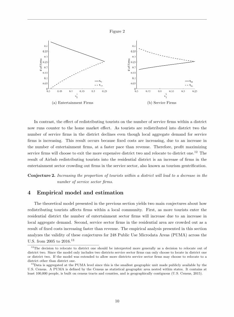
Figure 2

(a) Entertainment Firms (b) Service Firms

In contrast, the effect of redistributing tourists on the number of service firms within a district

now runs counter to the home market effect. As tourists are redistributed into district two the

number of service firms in the district declines even though local aggregate demand for service

firms is increasing. This result occurs because fixed costs are increasing, due to an increase in

the number of entertainment firms, at a faster pace than revenue. Therefore, profit maximizing

service firms will choose to exit the more expensive district two and relocate to district one.12 The

result of Airbnb redistributing tourists into the residential district is an increase of firms in the

entertainment sector crowding out firms in the service sector, also known as tourism gentrification.

Conjecture 2. Increasing the proportion of tourists within a district will lead to a decrease in the

number of service sector firms.

4 Empirical model and estimation

The theoretical model presented in the previous section yields two main conjectures about how

redistributing tourists affects firms within a local community. First, as more tourists enter the

residential district the number of entertainment sector firms will increase due to an increase in

local aggregate demand. Second, service sector firms in the residential area are crowded out as a

result of fixed costs increasing faster than revenue. The empirical analysis presented in this section

analyzes the validity of these conjectures for 248 Public Use Microdata Areas (PUMA) across the

U.S. from 2005 to 2016.13

12The decision to relocate to district one should be interpreted more generally as a decision to relocate out ofdistrict two. Since the model only includes two districts service sector firms can only choose to locate in district oneor district two. If the model was extended to allow more districts service sector firms may choose to relocate to adistrict other than district one.

13Data is aggregated at the PUMA level since this is the smallest geographic unit made publicly available by theU.S. Census. A PUMA is defined by the Census as statistical geographic area nested within states. It contains atleast 100,000 people, is built on census tracts and counties, and is geographically contiguous (U.S. Census, 2015).

10

4.1 Empirical Model

To investigate the questions proposed by the theoretical model, the following reduced-form

specification for the number of firms within a PUMA is developed:

nijt = µij + β1isjt−1 + β2iXjt−1 + εijt, (5)

where i denotes the business sector, i ∈ {E,S}, j denotes the PUMA, and t denotes time in years.

The variable nijt denotes the number of businesses in sector i within PUMA j at time t, while

sjt−1 denotes the measure of tourists within a PUMA from the previous year. Tourism data is

routinely available at the city level; however, tourism data at a more disaggregated level is not

as common. Therefore instead of using explicit measures of tourism at the PUMA level, data on

Airbnb usage is employed as a proxy. Whenever an Airbnb listing is rented a tourist(s) is residing

at the listing during the rental period. Therefore, by measuring the number of Airbnb listings

rented within a PUMA during the year the model is able to approximate the number of tourists

that were redistributed into the PUMA.

Of course, Airbnb is not the only way for tourists to reside outside of a city’s downtown district;

hotels can exist outside a city’s central business district or downtown as well.14 The empirical model

attempts to separate the effects of tourists using Airbnb from those using hotels by including a count

of the number of hotels.15 This variable along with the total population and median income are

included in Xjt−1, a vector of PUMA specific time-varying controls. Finally, µij denotes PUMA

fixed effects for sector i, the β’s are the parameters to be estimated, and εijt is the idiosyncratic

error.

Lagged measures of the independent variables are used because firm’s entry decision is inherently

a slow moving process. It takes time for a firm to find a location and acquire the necessary inputs.

Consequently, a firm deciding that market conditions are right for entry at time t−1 will likely not

be observed entering the market until time t. For this reason lag, rather than contemporaneous,

measures of the independent variables are included in the reduced form model.

4.2 Estimation strategy

Standard fixed effects methodology can be implemented to estimate (5), which allows the model

to control for unobserved heterogeneity across PUMAs. Additionally using fixed effects allows the

unobserved heterogeneity to be correlated with the regressors. For example, median income and

total population are likely correlated with unobserved attributes of the PUMA, such as the quality

of the area. Not accounting for this relationship would bias the estimates.16 By including fixed

14Tourists are not confined to the immediate area around their accommodation. They are able to travel throughouta city, which means the economic impact of a tourist may not be limited to the area immediately around theiraccommodation. Though without detailed data on tourist flows within a city it is not possible tract their economicimpact. Additionally, research by Versichele et al. (2014) and Shoval et al. (2011) show tourists typically spend mostof their time and money around the area of their accommodation, which suggests a majority of the economic impactof tourists will occur around where their accommodation is located.

15A count of hotel room rentals would be a more accurate measure of the number of tourists brought into the areaby hotels, but the data on rental rates and room counts are not available at the PUMA level.

16Results of the Hausman test suggest a fixed effects specification is preferred to random effects, which supportsthe claim observed regressors are correlated with unobserved heterogeneity.

11

effects the model accounts for endogeneity caused by the unobserved heterogeneity; however it does

not control for other sources of endogeneity.

The types of firms within an area depend on where tourists choose to locate. Additionally, it

is likely where tourists choose to locate will be, at least partially, determined by the types of firms

within the area. The cyclical nature of this problem leaves the model open to endogeneity bias

that is not removed by the inclusion of fixed effects. Let Airbnb usage in district j at time t (sjt)

be represented by the following reduced form equation

sjt = νj + β3nEjt + β4nSjt + β5Zjt + γjt, (6)

where nEjt is the number of entertainment sector firms and nSjt is the number of service sector

firms within PUMA j at time t, Zjt is a vector of PUMA level observable characteristics, νj

represents PUMA fixed effects, and γjt represents the error term. Unlike (5), the measure of

Airbnb usage, sjt, depends on contemporaneous regressors. A survey conducted by Gitelson and

Crompton (1983) shows over 70% of individuals plan a vacation less than three months in advance,

which suggests current, rather than lagged, characteristics of an area will influence their location

decision. Therefore, the reduced form model states Airbnb usage at time t depends on PUMA level

characteristics and sector firm counts at time t.

While estimating (6) is not the focus of this paper, the equation can be used to provide conditions

for the exogeneity of sjt, E[εijtsjt−1] = 0. Substituting (6) into the equation of strict exogeneity of

sjt−1 yields

E[εijt(νj + β3nijt−1 + β4Zjt−1 + γjt−1)] = 0,

which will hold as long as (i) the errors in the two equations are independent, E[εijtγjt−1)] =

0, (ii) the error εijt is independent of PUMA fixed effects, E[εijtνj ] = 0, (iii) the error εijt is

independent of the explanatory variables in Zjt−1, E[εijtZjt−1] = 0, and (iv) the errors do not

exhibit autocorrelation, E[εijtεijt−1] = 0.17 Results of both the Arellano and Bond (1991) and

Wooldridge (2010) test for serial correlation reject the null hypothesis of no autocorrelation. The

strict exogeneity assumption on sjt−1 fails.

A common method for addressing endogeneity is to estimate the model using an instrumental

variable (IV) approach. The percentage of households with internet will be used as an instrument for

Airbnb usage. To host an accommodation an individual needs to have access to Airbnb’s website. If

an individual has access to internet within the home it is more convenient for the individual to post

a listing. As a result it is more likely the individual will choose to list their property. Furthermore,

as the number of listings within an area increases so too will Airbnb usage.18 Therefore, household

internet penetration is positively correlated with Airbnb usage.

Conversely, a firm’s entry decision does not depend on household internet penetration. The

types of firms being studied in this paper are those that provide a good or service that must

be consumed in person. An individual cannot go to a restaurant or bar online. Additionally,

17The final condition was obtained by substituting a lagged version of (5) into E[εijtnijt−1] = 0.18Though more listings within an area does not necessitate higher levels of Airbnb activity, based on the Airbnb

data collected the correlation coefficient between the number of listings and number of reviews, a proxy for usage,within a PUMA is R = 0.8710.

12

traditional brick-and-mortar retailers as well as service providers like barbers and lawyers still

require individuals to visit a physical location in order to consume their product. Thus, the entry

decision for these firms will depend on the fixed cost and demographics of the PUMA, which are

independent of internet accessibility.

There does exist a subset of firms whose entry decision is likely to be dependent on internet

accessibility. Firms providing a good or service that can be consumed online, for example online

retailers and service providers like Amazon and Google. Since their products can be consumed

or purchased online, these firms do not need to be in the immediate vicinity of their consumers.

Accordingly, any changes in local demand, such as from an increase in tourism, will have no effect

on the location decision of online retailers. For this reason these firms are not included in either

the entertainment or service sector count of firms.19

A potential criticism of using internet penetration as an instrument for Airbnb usage is that it

is a weak instrument, and, therefore, any estimates will suffer from weak instrument bias. Though

the Kleibergen-Paap Wald rk F statistic rejects the weak instrument hypothesis, the correlation

between the Airbnb usage and internet penetration is low, R = 0.15. Moreover, data on internet

penetration is only available from 2013 to 2016. Therefore estimates using this shortened time

series will measure the effect for only the last four years. Ideally an alternative instrument would

be used to check the robustness of the results, but a strong external instrument is difficult to find.

A natural next step is to look within the dataset to generate instruments via lags of the endogenous

regressors; however, by demeaning the data lagged values of Airbnb usage become embedded in the

transformed error and, therefore, are invalid instruments.

Alternatively, first differences can be used to transform the data that will remove the fixed

effects and avoid making lagged values of Airbnb usage endogenous.20 Though, first differencing

does result in the differenced error, ∆εijt, no longer being i.i.d. Consequently, using 2SLS results

in distorted estimates. Following the work of Arellano and Bond (1991) and Arellano and Bover

(1995)/Blundell and Bond (1998), more efficient, better behaving estimates can be achieved using

system Generalized Method of Moments (GMM).

System GMM utilizes moment conditions based on lagged levels, E(sjt−L∆εijt) = 0 for t ≥ 3

and L ≥ 2, as well as lagged first differences, E(∆sjt−1εijt) = 0 for t ≥ 3. Including both sets of

moment conditions improves the estimates by taking advantage of more information, but also opens

up the model to possibly over fitting endogenous variables. The Hansen test can be employed to

diagnose any over fitting. Following the work of Roodman (2009), if the Hansen test has a p-val of

at least 0.25 then it can be concluded the endogenous variables are not being over fit.21

19Online retailers have a unique NAICS code, 454110, which allows them to be separately identified from brick-and-mortar retailers.

20The two most common transformations used when instrumenting with lags in the presence of fixed effects are firstdifferencing and forward orthogonal projections (Arellano and Bover, 1995). Arellano and Bover show with balancedpanels any two transformations of full row rank will yield numerically identical estimators, holding the instrumentset fixed. The panel used in this paper is unbalanced, but only for one PUMA, PUMA 2400 in New Orleans that ismissing two years of data. Results are robust to the use of the forward orthogonal transformation.

21If the model does suffer from over fitting, Hansen test p-val of less than 0.25, then the lag length will be restrictedin order to reduce the number of moment conditions.

13

4.3 Variable construction and data

This section discusses the construction of the variables used to estimate the effects of Airbnb

usage on the number of firms (5) as well as the data sources. A summary of the variable descriptions

as well as summary statistics are provided in Table 1 at the end of this section.

4.3.1 Dependent variable

The annual counts and percentages of entertainment and service sector firms within a PUMA

were constructed using data collected from the Census County Business Patterns (CPB) database.

Data was collected from 2005 to 2016 for sixteen major U.S. cities.22 The annual datasets pulled

from the CPB report the number of businesses within a ZIP Code by six-digit NAICS code.

The data was converted from ZIP Code level to PUMA level using a crosswalk file obtained

from the Missouri Census Data Center.23 The crosswalk file reported the proportion of each ZIP

Code that was contained within the relevant PUMAs. For example, 6% of ZIP Code 10003 (New

York) falls within PUMA 3807, 24% falls within PUMA 3808, 44% falls within PUMA 3809, and

25% falls within PUMA 3810. These proportions are multiplied by the ZIP Code business counts

and then totaled by PUMA.

This methodology implicitly assumes businesses within an NAICS are uniformly distributed

across a ZIP Code, which is not the case. As this paper has already pointed out, businesses tend

to cluster by sector as a result of zoning and agglomeration effects. Ideally, each business would

be able to be assigned to a PUMA based on its geographic location, but this is not possible with

publicly available data.24

After the data was converted to the PUMA level businesses were classified into the entertainment

sector, service sector, or neither using their six-digit NAICS code. The general definition of an

“entertainment sector” firm is a firm producing a good or service that is consumed by both tourists

and residents. Examples of entertainment firms include bars, movie theaters, restaurants, and

retail clothing stores. The general definition of a “service sector” firm is a firm producing a good or

service consumed primarily by residents. Examples of service firms include auto mechanics, grocery

stores, retail furniture stores, and tutoring services. Table 5 in the Appendix provides a detailed

list of how every NAICS code was classified. After assigning each NAICS code to a sector the data

was aggregated by year, PUMA, and sector to create an annual count of the number of firms in

each sector by PUMA. Percentages were calculated by dividing the count for each sector by the

total number of firms within the PUMA.

22The cities include in the dataset are: Asheville, NC; Austin, TX; Boston, MA; Chicago, IL; Denver, CO; LosAngeles, CA; Nashville, TN; New Orleans, LA; New York, NY; Oakland, CA; Portland, OR; San Diego, CA; SanFrancisco, CA; Santa Cruz, CA; Seattle, WA; and Washington, DC. These cities correspond to the cities available onInside Airbnb, and were the only U.S. cities for which data was made available.

23See http://mcdc.missouri.edu.24Alternatively, the Department of Housing and Urban Development has crosswalk files available for ZIP Codes

to census tract, which can then be converted to PUMAs, that reports proportions based on business addresses.The proportion is the ratio of business addresses within the overlapping ZIP Code-tract part to the total numberof businesses within the ZIP Code. Though the proportions are still assumed to be uniform across NAICS codes,weighting the proportions by business addresses more accurately represents how businesses are distributed. However,these crosswalk files are only made available starting in 2010. Therefore, for the entire dataset to be included in theanalysis the Missouri Census Data Center crosswalk files must be used.

14

Every NAICS code was classified by manually going through the list of codes and classifying

them based on the previously stated definitions. Although this procedure is somewhat ad hoc, the

literature on tourism gentrification and urban economics provides no operational definitions for

the “entertainment” or “service” sector on which to base the classification. Most of the literature

on tourism gentrification discusses these sectors as abstract concepts, not seeking to quantify the

effect of tourism gentrification, and thus have not had a reason to provide an operational definition.

Therefore the classification system defined in Table 5 should be thought of as a first attempt at

providing the literature with a operational definition of the entertainment and service sectors for

the purpose of analyzing tourism gentrification.

4.3.2 Airbnb Usage

Data on Airbnb was collected from Inside Airbnb, an independent data collection project that

compiles information about Airbnb listings for public use. The project scrapes Airbnb’s website

across various major U.S. and international cities for host level data.25 The raw data files include

information about when the host joined Airbnb, geographic coordinates for the listing, the listing

availability over the next year, when the listing received reviews, as well detailed information about

the listing’s amenities.

Since Inside Airbnb collects data by scraping Airbnb’s website the data includes only those

hosts who are active at the time of the scrape. Additionally, Airbnb does not provide a record of

hosts that have since removed their listing from the website. Therefore, hosts who have removed

their listing before the time of the scrape will not be included in the dataset. Without access to a

database of historical data, the snapshot provided by Inside Airbnb is the best available option for

measuring the intensity of Airbnb usage.

With the data provided a count of all listings available in an area can be created, but would

overstate Airbnb usage. Just because a property is listed does not mean that it is being rented.

Furthermore, Airbnb listings in and of themselves do not cause tourism gentrification. Rather,

tourism gentrification is a result of an increase in tourism, which occurs when more tourists are

brought into the area. Therefore only those listings that are rented should be included in the

measure. By exploiting data on listing reviews a more accurate measure of Airbnb usage can be

generated.

Inside Airbnb provides a record of all reviews a listing receives as well as the date the review

was posted.26 Utilizing this record, an annual count of the number of reviews a listing receives is

generated. It should be noted, guests are not required to submit a review after renting. As a result

a listing maybe more active than what is reflected by the number of reviews. In addition, only an

individual who has rented the listing is able to post a review. Therefore, the measure of Airbnb

usage generated using review data should be thought of as a lower bound of Airbnb usage. It is

25Though tourism gentrification can effect any city this paper chooses to focus on U.S. cities for two reasons. First,demographic controls and business count data are easier to acquire for U.S. cities. Second, many cities outside theU.S. do not have as restrictive zoning laws. Rather than having separate zoning for residential and commerical areas,cities outside the U.S. more commonly implement mixed use zoning or allow for land-owners to apply to change theland use type. As a result it is more difficult to define distinct “residential” and “tourist” zones within a city.

26Guests have fourteen days to post a review after checking out. So even though the date does not correspond tothe exact date of rental it is a close approximation.

15

also assumed the incentive to provide a review is consistent across time and PUMA since there is

no explicit benefit to the renter for providing a review.

Using the geographic coordinates reported for each listing and boundary shape files obtained

from the Census website each listing was assigned to a PUMA. The count of reviews was then

aggregated by PUMA year. The resulting variable should be thought of as a lower bound estimate

of the number of times Airbnb was rented within a PUMA during the year. More aptly this variable

can be interpreted as the minimum number of tourists brought into the PUMA by Airbnb since at

least one tourist will accompany every rental. Of course, it is possible for more than one tourist to

stay in an Airbnb, and in fact many of the listings allow two or more people to stay. However, the

review data does not identify how many individuals stayed during the rental period. Therefore, to

be conservative, and not over estimate the effect, the minimum number of individuals that could

have used Airbnb during the year is implemented as the measure of Airbnb usage.

4.3.3 Other controls

Controls for total population, median household income, and the number of hotels are also

included in the model. Data on total population and median household income were collected

from the American Community Survey (ACS) and were available at the PUMA level. Data on the

number of hotels was collected from the CBP database. All businesses with the four-digit NAICS

code 7211 (Traveler Accommodations) are included in the hotel count. The same methodology to

convert business sector counts from ZIP Code level to PUMA level was applied to the ZIP Code

level hotel counts.

The instrumental variable, percentage of households with internet, was also collected from the

ACS. However, the ACS did not start collecting data on internet usage until 2013. Therefore, all

IV estimates are calculated using only data from 2013 to 2016.27

27The Consumer Population Survey provides data on internet usage prior to 2013, but not at a level of disaggregationuseful for this study.

16

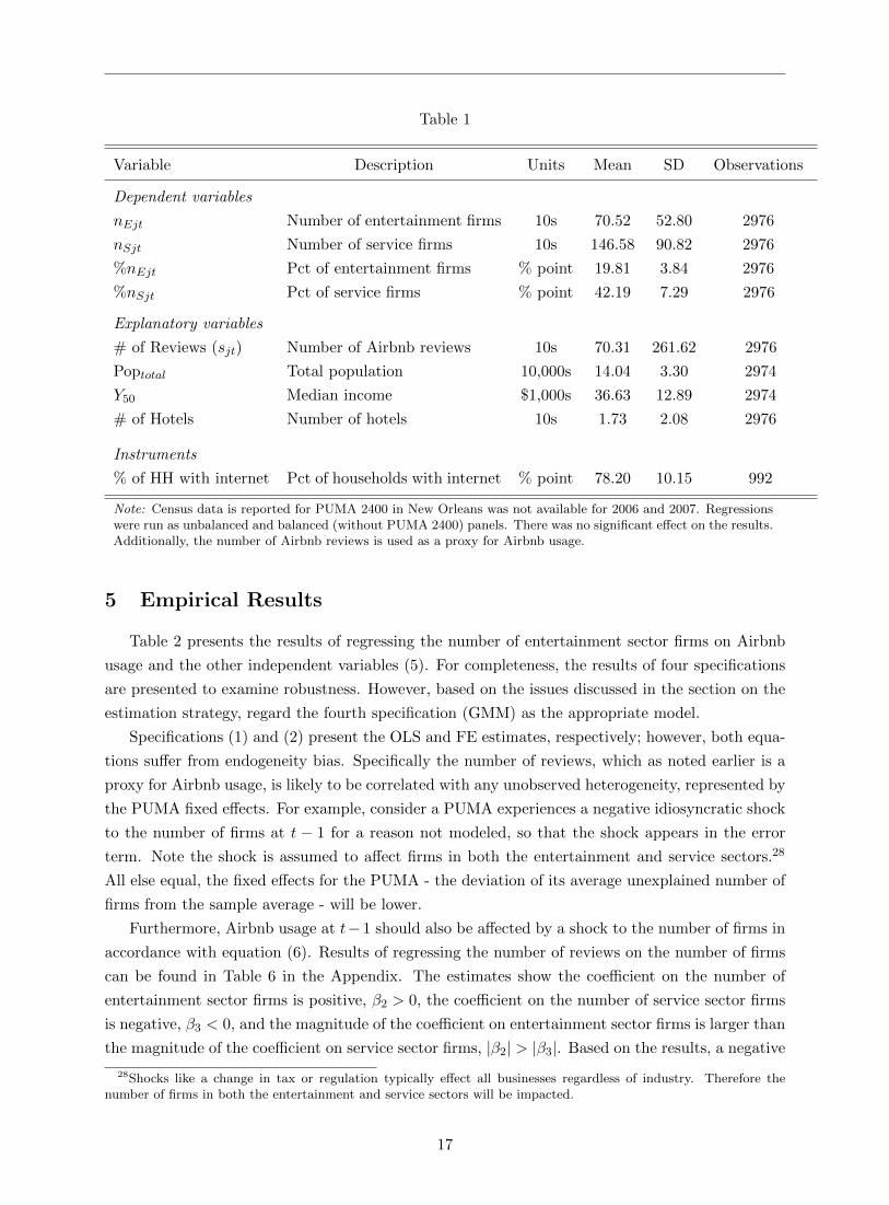
Table 1

Variable Description Units Mean SD Observations

Dependent variables

nEjt Number of entertainment firms 10s 70.52 52.80 2976

nSjt Number of service firms 10s 146.58 90.82 2976

%nEjt Pct of entertainment firms % point 19.81 3.84 2976

%nSjt Pct of service firms % point 42.19 7.29 2976

Explanatory variables

# of Reviews (sjt) Number of Airbnb reviews 10s 70.31 261.62 2976

Poptotal Total population 10,000s 14.04 3.30 2974

Y50 Median income $1,000s 36.63 12.89 2974

# of Hotels Number of hotels 10s 1.73 2.08 2976

Instruments

% of HH with internet Pct of households with internet % point 78.20 10.15 992

Note: Census data is reported for PUMA 2400 in New Orleans was not available for 2006 and 2007. Regressionswere run as unbalanced and balanced (without PUMA 2400) panels. There was no significant effect on the results.Additionally, the number of Airbnb reviews is used as a proxy for Airbnb usage.

5 Empirical Results

Table 2 presents the results of regressing the number of entertainment sector firms on Airbnb

usage and the other independent variables (5). For completeness, the results of four specifications

are presented to examine robustness. However, based on the issues discussed in the section on the

estimation strategy, regard the fourth specification (GMM) as the appropriate model.

Specifications (1) and (2) present the OLS and FE estimates, respectively; however, both equa-

tions suffer from endogeneity bias. Specifically the number of reviews, which as noted earlier is a

proxy for Airbnb usage, is likely to be correlated with any unobserved heterogeneity, represented by

the PUMA fixed effects. For example, consider a PUMA experiences a negative idiosyncratic shock

to the number of firms at t − 1 for a reason not modeled, so that the shock appears in the error

term. Note the shock is assumed to affect firms in both the entertainment and service sectors.28

All else equal, the fixed effects for the PUMA - the deviation of its average unexplained number of

firms from the sample average - will be lower.

Furthermore, Airbnb usage at t−1 should also be affected by a shock to the number of firms in

accordance with equation (6). Results of regressing the number of reviews on the number of firms

can be found in Table 6 in the Appendix. The estimates show the coefficient on the number of

entertainment sector firms is positive, β2 > 0, the coefficient on the number of service sector firms

is negative, β3 < 0, and the magnitude of the coefficient on entertainment sector firms is larger than

the magnitude of the coefficient on service sector firms, |β2| > |β3|. Based on the results, a negative

28Shocks like a change in tax or regulation typically effect all businesses regardless of industry. Therefore thenumber of firms in both the entertainment and service sectors will be impacted.

17

shock to the number of firms should result in a decrease in the number of reviews. Therefore, both

the number of reviews at t− 1 and the fixed effects are lower as a result of the shock. The positive

correlation between lagged number of reviews (sjt−1) and the error (eijt) results in an inflated

estimate of the OLS coefficient on the number of reviews.

Table 2

# of EntertainmentFirms(nEjt)

(1) (2) (3) (4)

OLS FE IV GMM

# of Reviews(sjt−1)

0.0547∗∗∗ 0.0251∗∗∗ 0.0203∗∗∗ 0.0258∗

(0.0056) (0.0082) (0.0046) (0.0153)

Poptotal 2.5611∗∗∗ 0.4183 -0.3412 4.3003∗∗∗

(0.2081) (0.5829) (0.3636) (1.2385)

Y50 1.1723∗∗∗ 0.4519∗∗ -0.2766∗ -1.6373∗

(0.0568) (0.2268) (0.1513) (0.9075)

# of Hotels 13.7920∗∗∗ 17.3385∗∗∗ -0.7442 12.4061∗∗

(0.3582) (1.9554) (1.5270) (4.9642)

PUMA FE No Yes Yes YesYear FE Yes Yes No YesF Stat 258.0035 21.7182 11.5635AR(2) 0.5622Hansen Test p-val 0.5789Instruments 1 33Years 2005-2016 2005-2016 2014-2016 2005-2016N Obs 2726 2726 744 2726∗ p < 0.10, ∗∗ p < 0.05, ∗∗∗ p < 0.01 Robust standard errors clustered at thePUMA level are reported in parentheses.

Including PUMA fixed effects in the estimation draws the unobserved heterogeneity out of

the error term, and removes the endogeneity bias caused by the correlation between the number

of reviews and the fixed effects. In spite of that, the number of reviews is still correlated with

the error due to the presence of autocorrelation. Under the within group transformation the lag

of the number of reviews becomes s∗jt−1 = sjt−1 − 1T−1 (sj2 + ...+ sjT ) while the error becomes

ε∗ijt = εijt − 1T−1 (εij2 + ...+ εijt). Assume again a negative shock to the number of firms at time

t − 1. The shock causes the transformed error at time t to increase, and sjt−1 will decline for the

same arguments as before. The transformed error (ε∗ijt) and the transformed number of reviews

(s∗jt−1) are negatively correlated. As a result estimation using FE is likely to underestimate the

true effect of Airbnb usage.

Specification (3) attempts to correct for the endogeneity in the FE model by utilizing the

percentage of households with internet as an instrument for Airbnb usage. The coefficient on the

number of reviews is similar to the FE estimate, but given FE is predicted to underestimate the

true effect the IV estimate is lower than expected. However, this outcome is not unexpected for a

couple of reasons. First the percentage of households with internet is weakly correlated with the

18

number of reviews, which can lead to weak instrument bias. Second, the estimation only utilizes

data from 2013 to 2016; a period well after Airbnb was established and widely adopted. By not

including the variation in the number of firms during the years prior to and shortly after the start

of Airbnb the IV regression is estimating something slight different than if it were to utilize the full

time series.

The final specification (4) is GMM with lags used as instruments for the endogenous regressors.

The p-value for the Hansen test is above the threshold of 0.25, and thus cannot reject the null

hypothesis of joint validity of the instruments. Furthermore, the coefficient on the number of

reviews is significant at the 10% level. The results of the empirical analysis displayed in Table 2

suggest as Airbnb usage within a PUMA increases more entertainment firms will choose to enter

the area, which supports the conjecture made by the theoretical model.

Result 1. Increasing Airbnb usage within a PUMA leads to an increase in the number of firms

in the entertainment sector.

Now we turn to analyzing the effect Airbnb usage has on the number of firms in the service

sector, nSjt. Table 3 presents the regression results. Again for completeness, the results of four

specifications are presented to examine robustness; however, the fourth specification (GMM) should

be regarded as the appropriate model.

The OLS estimate for the coefficient on the number of reviews, presented in the second column

of the table, is an overestimate of the true effect due to the positive correlation between the error

term and Airbnb usage.29 Similarly, the FE estimate, presented in column three, underestimates

the true effect due to the negative correlation between the transformed number of reviews (s∗jt−1)

and transformed error (e∗ijt). Furthermore, the effect is insignificant at the 10% level. The IV

estimate presented in the fourth column of the table is significant at the 1% level, but is larger

than the OLS estimate, which is expected to overestimate the true effect. The inconsistency of the

estimate is likely occurring because of weak instrument bias and constricted time series.

Specification (4) of the table presents the results of the GMM estimation. The Hansen test is

found to be insignificant, so the instruments can be regarded as jointly valid. Furthermore, the

estimate on Airbnb usage is similar to the OLS and FE estimates. While there is support for the

validity of the estimation strategy the coefficient on the number of reviews is insignificant at the

10% level. Thus the empirical results are unable to conclude Airbnb usage has any effect on the

number of service sector firms within a PUMA.

Result 2. Airbnb usage does not have a statistically significant effect on the number of service

sector firms within a PUMA.

The absence of a statistically significant effect by Airbnb usage on the number of service firms

does not support Conjecture 2 - increasing the proportion of tourists within a district will lead to a

decrease in the number of service sector firms when the increase in fixed costs outweighs the increase

in revenue. However a null effect could occur if the net effect of an increase in fixed costs and an

29Though the results of regressing the number of reviews on the number of firms shows the coefficient on the numberof service sector firms is negative, it is smaller in magnitude than the coefficient on the number of entertainmentsector firms. Therefore, the net effect of a positive shock to the number of firms will be an increase in number ofreviews.

19

Table 3

# of ServiceFirms(nSjt)

(1) (2) (3) (4)

OLS FE IV GMM

# of Reviews(sjt−1)

0.0365∗∗∗ 0.0076 0.0383∗∗∗ 0.0142(0.0099) (0.0104) (0.0101) (0.0102)

Poptotal 5.7987∗∗∗ 1.6292 -0.2382 9.3962∗∗∗

(0.3658) (1.0689) (0.7505) (2.9535)

Y50 2.4193∗∗∗ 0.6874∗∗ -0.5258 -3.2946(0.0999) (0.3116) (0.3313) (2.6584)

# of Hotels 21.2947∗∗∗ 31.1340∗∗∗ -1.7606 16.0910∗

(0.6297) (7.3553) (2.9777) (9.1277)

PUMA FE No Yes Yes YesYear FE Yes Yes No YesF Stat 233.4746 31.2784 8.4620AR(2) 0.9902Hansen Test 0.6407Instruments 1 21Years 2005-2016 2005-2016 2014-2016 2005-2016N Obs 2726 2726 744 2726∗ p < 0.10, ∗∗ p < 0.05, ∗∗∗ p < 0.01 Robust standard errors clustered atthe PUMA level are reported in parentheses.

increase in revenue was zero, which would happen with slight modifications to the assumptions of

the theoretical model. The model assumes the utility of tourists depends on products produced

in the service sector, which is not necessarily the case. Tourists typically visit a city or place

for a short period of time, and as a result will primarily consume the products produced by the

entertainment sector. Only those individuals staying within an area for an extended period of time

typically consume the goods and services provided by the service sector. Therefore in an extreme

case the utility of tourists can be assumed to put no weight on the consumption of service sector

products.

In this extreme case tourists will not consume any products produced by the service sector.

Therefore as Airbnb usage increases and tourists are redistributed into the residential area, the

local aggregate demand for service sector firms will not change, and new service sector firms will

have no incentive to enter the market. On the other hand, firms in the entertainment sector will still

experience an increase in local aggregate demand, and thus have an incentive to enter the residential

area. If the resulting increase in the number of entertainment sector firms does not affect the fixed

cost of production then service sector firms will have no incentive to exit the market. The number

of firms in the service sector will not change. However, if the increase entertainment sector firms

does lead to an increase in fixed costs firms in the service sector will have an incentive to exit the

market. When fixed costs increase without a sufficient increase in revenue an increase in Airbnb

usage will lead to a decline in the number of service firms.

20

Therefore for the number of service sector firms to remain unchanged when fixed costs increase

there must also be an increase in local aggregate demand, which will occur if the utility of tourists

places a positive weight on products produced in the service sector. As more tourists enter the

residential area aggregate demand for service sector firms increases resulting in an increase in

revenue for the firms already in the market. At the same time fixed costs are also increasing as a

result of higher demand for retail space. The net of these two forces will determine whether there

is an increase, decrease, or no effect on the number of service firms.

In the numerical analysis conducted earlier the effect of rising fixed costs was assumed to

dominate the increase in demand resulting in a net outflow of service sector firms as more tourists

enter the residential area. If instead, the marginal effect firms have on fixed cost is reduced the

resulting outflow of service firms will also diminish. Moreover, if the marginal effect is small enough

such that the increase in fixed costs is exactly offset by an increase in revenue the outflow of service

firms will cease. The result in this case is an increase in Airbnb usage leads to no observable change

in the number of service sector firms.

An additional test of the empirical results can be conducted by estimating the effect of Airbnb

usage on firms (5) using the percentage of entertainment/service sector firms as the dependent

variable. Based on the results of Tables 2 and 3 the number of reviews is expected to have a positive

effect on the percentage of entertainment sector firms and a negative effect on the percentage of

service sector firms. Results 1 and 2 state the number of entertainment sector firms increases in

response to an increase in Airbnb usage while the number of firms in the service sector remains

unchanged. Therefore, the proportion of firms within a PUMA in the entertainment sector should

increase as Airbnb usage increases. Conversely, the proportion of service sector firms in a PUMA

should decrease. Table 4 presents the FE and GMM estimates using the percentage of firms as the

dependent variable.30

30A linear probability model is assumed to be a good approximation since the dependent variables are not closeto the bounds, %nEjt,%nSjt ∈ [0, 1]. The min and max of the percentage of entertainment sector firms ,%nEjt, are8.61% and 33.19%, respectively, and the min and max of the percentage of service sector firms ,%nSjt, are 14.32%64.39%, respectively.

21

Table 4

% of EntertainmentFirms

(%nEjt)

% of ServiceFirms

(%nSjt)

FE GMM FE GMM

# of Reviews(sjt−1)

0.0013∗∗∗ 0.0003∗∗ -0.0019∗∗∗ -0.0028∗∗

(0.0004) (0.0001) (0.0005) (0.0013)

Poptotal 0.0384 0.0129 0.0405 0.1430(0.0457) (0.0533) (0.0534) (0.0911)

Y50 0.0072 -0.0038 0.0017 0.0210(0.0193) (0.0176) (0.0192) (0.0344)

# of Hotels 0.1211 -0.0224 -0.0967 -1.0197∗∗∗

(0.1740) (0.1285) (0.1998) (0.1747)

PUMA FE Yes Yes Yes YesYear FE Yes Yes Yes YesF Stat 17.5491 18.7799AR(2) 0.8059 0.8186Hansen Test 0.5013 0.3206Instruments 29 78Years 2005-2016 2005-2016 2005-2016 2005-2016N Obs 2726 2726 2726 2726∗ p < 0.10, ∗∗ p < 0.05, ∗∗∗ p < 0.01 Robust standard errors clustered atthe PUMA level are reported in parentheses.

Columns two and three present the results for the entertainment sector, and columns four and

five present the results for the service sector. The coefficient on the number of reviews is positive

and statistically significant for both sets of regressions. The result suggests an increase in Airbnb

usage leads to an increase in the concentration of firms in the entertainment sector. When the

percentage of firms in the service sector is the dependent variable the coefficient on the number of

reviews is negative, which suggests increasing Airbnb usage leads to a decline in the concentration

of firms in the service sector.

The regression results presented in Table 4 provide support for Results 1 and 2. If the number

of firms in the entertainment sector increased in response to an increase in Airbnb usage while

the number of firms in the service sector remained unchanged then the percentage of firms in the

entertainment sector should increase. The results in column two and three of Table 4 support

this claim. Furthermore, if the number of firms in the service sector remains unchanged while the

number of firms in the entertainment sector increase in response to an increase in Airbnb usage

then the percentage of firms belonging to the service sector should decline. Column four and five

of Table 4 support this claim.

22

6 Conclusion

An overlooked consequence of the introduction and proliferation of Airbnb has been the redis-

tribution of tourists into parts of cities that previously have had little exposure to tourism. This

paper examines, both theoretically and empirically, the effects redistributing tourists has had on

the development of the entertainment and services sectors within city neighborhoods. To investi-

gate this question theoretically a model of intra-city trade based on work by Krugman (1980) was

developed. Two conjectures were drawn from the model. When tourists, entertainment centric

consumers, are concentrated in the downtown area, as they have historically been, firms in the

entertainment sector choose to agglomerate downtown. As tourists are redistributed into the resi-

dential district, as they are with Airbnb, the number of entertainment sector firms in the residential

district increases. Furthermore, the number of service sector firms in the residential district will

decrease if fixed costs (rents) increase, due to an increased demand for retail space, more than

revenue increases.

An empirical analysis was then conducted to test the validity of the conjectures. A novel dataset

was created by combining data from Inside Airbnb and a variety of U.S. Census Data sources. Data

was collected from 2005-2016 at the PUMA level. The empirical results suggest Airbnb usage does

have an effect on the development of businesses within a PUMA, which led to two primary results.

First, an increase in Airbnb usage results in an increase in the number of entertainment sector firms.

Second, the data does not provide sufficient evidence to suggest Airbnb usage has a statistically

significant effect on number of service sector firms. A result that can be explained theoretically by

the increase in local aggregate demand exactly offsetting the increase in fixed costs, which means

there is no incentive for service sector firms to enter or exit the market. Thus there will be no

observable effect on the number of firms in the service sector.

There are several ways in which the analysis of this paper can be extended. First, alternative

definitions of the “entertainment” and “service” sectors could be tested. The definitions provided

in this paper are a first pass, and more rigorous definitions should still be pursued. Second, the

theoretical model could be modified to include a second residential district that does not have any

tourists redistributed into it. By including this third district the model would be able to explore

what effect, if any, Airbnb usage has on districts not directly affected by the redistribution of

tourists. Additionally, the theoretical model could be extended to include a market for Airbnb.

This extension would allow the distribution of tourists to be endogenous as well as allow the model

to analyze how the additional income residents receive from hosting affects the location decision of

firms.

Nevertheless, the results of this paper still have implications that bridge the empirical literature

on Airbnb and tourism gentrification. Prior to this paper the research on Airbnb has been largely

limited to analyzing the effects Airbnb has had on the hospitality and housing sectors, but this paper

suggests Airbnb may also impact the development of a district’s entertainment and service sectors.

Specifically, an increase in Airbnb usage leads to an increase in the presence of entertainment sector

firms. A characteristic the literature commonly associates with tourism gentrification. Cocola-

Grant (2016; 2018) provides anecdotal evidence and motivation for the connection between the

growth of Airbnb and tourism gentrification, but is limited to a case study of Barcelona. By

23

focusing in on a singular aspect of tourism gentrification, the presence of entertainment sector

firms, the results of this paper support and extend the work of Cocola-Grant by providing evidence

of a systematic link between the increase in Airbnb usage and an increase in entertainment sector

firms. However, this paper is not able to definitively conclude the use of Airbnb within an area will

lead to tourism gentrification.

There are other aspects of tourism gentrification not explored within this paper that are needed

to conclude a causal link exists. Similar to gentrification in general, tourism gentrification can

lead to the displacement of residents as a result of higher rents as well as displacement resulting

from long-term residential accommodations being converted to short-term tourist accommodations.

Some states have begun addressing the latter issue by implementing policies restricting Airbnb hosts

to listing only their primary residence or requiring hosts obtain a short-term rental license.31 While

these types of policies may help prevent the decline in availability of residential accommodations

the potential issue of rising rents is still largely unaddressed. Additionally, congestion and the

replacement of locally own firms with national chains are characteristics frequently associated with

tourism gentrification that are not explored in this paper. Though no causal link between Airbnb

usage and tourism gentrification is shown to exist, the results of this paper do show a connection

between Airbnb usage and the presence of entertainment sector firms, which provides motivation

for further research into the role Airbnb plays in tourism gentrification.

31Airbnb provides detailed information on its site about regulations in various cities. Additionally, Cohen (2018),Honan (2018), and Loudenback (2018) discuss various regulations being imposed by states.

24

References

Airbnb (2018). Fast facts. https://press.airbnb.com/fast-facts/.

Alyakoob, M. and Rahman, M. S. (2018). Shared prosperity (of lack thereof) in the sharingeconomy.

Anas, A. and Xu, R. (1999). Congestion, land use, and job dispersion: A general equilibriummodel. Journal of Urban Economics, 45.

Arellano, M. and Bond, S. (1991). Some tests of specification for panel data: Monte Carlo evidenceand an application to employment equations. The Review of Economic Studies, 58(2).

Arellano, M. and Bover, O. (1995). Another look at the instrumental variable estiamtion of error-component models. Journal of Econometrics, 68(1).

Blundell, R. and Bond, S. (1998). Initial conditions and moment restrictions in dynamic panel datamodels. Journal of Econometrics, 87(1).

Brousseau, F., Metcalf, J., and Yu, M. (2015). Analysis of the impact of short-term rentals onhousing. Technical report, City and County of San Francisco, San Francisco, CA.

Cocola-Grant, A. (2016). Holiday rentals: The new gentrification battlefront. Sociological ResearchOnline, 21(3).

Cocola-Grant, A. (2018). Struggling with the leisure class: Tourism, gentrification and displacement.PhD thesis, Cardiff University.

Cohen, J. (2018). Boston moves to regulate short-term rentals like Airbnb.https://nextcity.org/daily/entry/boston-moves-to-regulate-airbnb.

Fujita, M. (1988). A monopolistic competition model of spatial agglomeration: Differentiatedproduct approach. Regional Science and Urban Economics, 18(1).

Fujita, M., Krugman, P., and Venables, A. J. (2001). The Spatial Economy. MIT Press.

Getz, D. (1993). Planning for tourism business districts. Annals of Tourism Research, 20.

Gitelson, R. J. and Crompton, J. L. (1983). The planning horizons and sources of information usedby pleasure vacationers. Journal of Travel Research, 21(3).

Gotham, K. F. (2005). Tourism gentrification: The case of New Orleans’ Vieux Carra (FrenchQuarter). Urban Studies, 42(7).

Graviari-Barbas, M. and Guinand, S., editors (2017). Tourism and Gentrification in ContemporaryMetropolises. Routledge.

Guttentag, D. A. and Smith, S. L. (2017). Assessing Airbnb as a distruptive innovation relativeto hotels: Substitution and comparative performance expectations. International Journal ofHospitality Management, 64.

Honan, K. (2018). New York city council passes bill to regulate Airbnb.https://www.wsj.com/articles/new-york-city-council-passes-bill-to-regulate-airbnb-1531952763.

Ioannides, D., Roslmaier, M., and van der Zee, E. (2018). Airbnb as an instigator of ‘tourismbubble’ expansion in Utrecht’s Lombok neighbourhood. Tourism Geographies.

25

Judd, D. R. (1991). Promoting tourism in U.S. cities. Tourism Management, 16(3).

Krugman, P. (1980). Scale economies, product differentiation, and the pattern of trade. TheAmerican Economic Review, 70(5).

Lee, D. (2016). How Airbnb short-term rentals exacerbate Los Angeles’s affordable housing crisis:Analysis and policy recommendations. Havard Law and Policy Review, 10.

Loudenback, T. (2018). Los Angeles just took a big step toward regulating Airbnbstays — here’s what new short-term rental laws could mean for hosts and travel-ers. https://www.businessinsider.com/airbnb-vrbo-regulations-los-angeles-what-it-means-for-hosts-renters-2018-5.

New York State Attorney General (2014). Airbnb in the City. Technical report, New York StateAttorney General, New York, NY.

Organization, W. T. (2012). Global report on city tourism. Technical Report 6th.

Roodman, D. (2009). A note on the theme of too many instruments. Oxford Bulletin of Economicsand Statistics, 71(1).

Sans, A. A. and Domınguez, A. Q. (2016). Unravelling Airbnb: Urban perspectives from Barcelona.In Russo, A. P. and Richards, G., editors, Reinventing the Local in Tourism: Producing, Con-suming and Negotiating Place. Channel View.

Schafer, P. and Braun, N. (2016). Misuse through short-term rentals on Berlin housing market.International Journal of Housing Markets and Analysis, 9(2).

Shoval, N., McKercher, B., Ng, E., and Birenboim, A. (2011). Hotel location and tourist activityin cities. Annals of Tourism Research, 38(4).

Sivitanidou, R. and Wheaton, W. C. (1992). Wage and rent capitalization in the commercial realestate market. Journal of Urban Economics, 31.

Travel, W. and Council, T. (2018). Travel and Tourism Economic Impact 2018 United States.Technical report.

U.S. Census (2015). Public Use Micro Data Areas (PUMAs).https://www.census.gov/geo/reference/puma.html.

Versichele, M., de Groote, L., Bouuaert, M. C., Neutens, T., Moerman, I., and de Weghe, N. V.(2014). Pattern mining in tourist attraction visits through association rule learning on Bluetoothtracking data: A case study of Ghent, Belgium. Tourism Management, 44.

Wooldridge, J. (2010). Econometric Analysis of Cross Section and Panel Data. MIT Press.

Zervas, G., Proserpio, D., and Byers, J. W. (2017). The rise of the sharing economy: Estimatingthe impact of Airbnb on the hotel industry. Journal of Marketing Research, 54(5).

26

Appendix

Derive compensated demand

Using the FOC from the consumer’s expenditure minimization problem the following equationfor the marginal rate of substitution can be obtained

cρ−1ijk

cρ−1ijl

=pikτjkpilτjl

.

cijk = cijl

(pilτjlpikτjk

) 11−ρ

Plugging the above equation into the budget constraint yields

Cij =

[2∑

k=1

nik

(cijl

(pilτjlpikτjk

) 11−ρ)ρ] 1

ρ

Cij = cijl(pilτjl)1

1−ρ

[2∑

k=1

nik

(1

pikτjk

) ρ1−ρ

dω

] 1ρ

Solve for cijl

cijl =(pilτjl)

1ρ−1[∑2

k=1 nik (pikτjk)ρρ−1

] 1ρ

Cij

Solve for entertainment sector profit maximizing price

Taking the derivative of the profit function with respect to pEj yields

∂πEj∂pEj

= QEj + (pEj − c)∂QEj∂pEj

= 0.

Substitute in the definition of QEj

qTEj + qNEj = (c− pEj)

(∂qTEj∂pEj

+∂qNEj∂pEj

).

Calculate the derivate of qTEj and qNEj with respect to pEj

∂qTEj∂pEj

= µY (−σ)p−1Ej

2∑k=1

sTk(pEjτkj)

−σ

P−(σ−1)Ej

∂qNEj∂pEj

= λY (−σ)p−1Ej

2∑k=1

sNk(pEjτkj)

−σ

P−(σ−1)Ej

Plug the equations for qTEj and qNEj as well as the equations for∂qTEj∂pEj

and∂qNEj∂pEj

into the FOC of the

27

firm’s profit function.

µY

2∑k=1

sTk(pEjτkj)

−σ

P−(σ−1)Ej

+ λY

2∑k=1

sNk(pEjτkj)

−σ

P−(σ−1)Ej

= (c− pEj)

µY (−σ)p−1Ej

2∑k=1

sTk(pEjτkj)

−σ

P−(σ−1)Ej

+ λY (−σ)p−1Ej

2∑k=1

sNk(pEjτkj)

−σ

P−(σ−1)Ej

Solve the above equation for pEj .

pEj = (pEjσ − cσ)

pEj(1− σ) = −cσ

p∗Ej =

(σ

σ − 1

)c

Solve for optimal number of entertainment sector firms

Plug the equations for QEj , qTEj , and qNEj into the market clearing condition for the entertain-

ment sector.QEj = qTEj + qNEj

F (σ − 1)

c= µY

2∑k=1

sTk(pEjτkj)

−σ

P−(σ−1)Ek

+ λY

2∑k=1

sNk(pEjτkj)

−σ

P−(σ−1)Ek

Expand the summations.

F (σ − 1)

c= µY

(sT1

(pEjτ1j)−σ

P−(σ−1)E1

+ sT2(pEjτ2j)

−σ

P−(σ−1)E2

)+ λY

(sN1

(pEjτ1j)−σ

P−(σ−1)E1

+ sN2(pEjτ2j)

−σ

P−(σ−1)E2

)

F (σ − 1)

c= (µY sT1 + λY sN1 )

(pEjτ1j)−σ

P−(σ−1)E1

+ (µY sT2 + λY sN2 )(pEjτ2j)

−σ

P−(σ−1)E2

F (σ − 1)

c= (µY sT1 + λY sN1 )(pEjτ1j)

−σPσ−1E1 + (µY sT2 + λY sN2 )(pEjτ2j)

−σPσ−1E2

Substitute in the equation for the optimal price, p∗Ej .

F (σ − 1)

c=

(σ

σ − 1c

)−σ(µY sT1 + λY sN1 )τ−σ1j Pσ−1

E1 + (µY sT2 + λY sN2 )τ−σ2j Pσ−1E2

Substitute in the definition of the price index, PEj .

F (σ − 1)

c=

(σ

σ − 1c

)−σ[ (µY sT1 + λY sN1

)τ−σ1j

([nE1(pE1τ11)

1−σ + nE2(pE2τ12)1−σ] 1

1−σ)σ−1

+(µY sT2 + λY sN2

)τ−σ2j

([nE1(pE1τ21)

1−σ + nE2(pE2τ22)1−σ] 1

1−σ)σ−1

]

28

F (σ − 1)

c=

(σ

σ − 1c

)−σ[ (µY sT1 + λY sN1

)τ−σ1j

(nE1(pE1)

1−σ + nE2(pE2τ12)1−σ)−1

+(µY sT2 + λY sN2

)τ−σ2j

(nE1(pE1τ21)

1−σ + nE2(pE2)1−σ)−1

]

The profit maximizing price is independent of location, p∗E1 = p∗E2 = p.

F (σ − 1)

c=

(σ

σ − 1c

)−σpσ−1

[ (µY sT1 + λY sN1

)τ−σ1j

(nE1 + nE2τ

1−σ12

)−1

+(µY sT2 + λY sN2

)τ−σ2j

(nE1τ

1−σ21 + nE2

)−1

]

F (σ − 1)

c=

(σ

σ − 1c

)−1[(µY sT1 + λY sN1

)τ−σ1j

nE1 + nE2τ1−σ12

+

(µY sT2 + λY sN2

)τ−σ2j

nE1τ1−σ21 + nE2

]

Fσ =

(µY sT1 + λY sN1

)τ−σ1j

nE1 + nE2τ1−σ12

+

(µY sT2 + λY sN2

)τ−σ2j

nE1τ1−σ21 + nE2

The equation for district 1 is

Fσ =µY sT1 + λY sN1nE1 + nE2τ

1−σ12

+

(µY sT2 + λY sN2

)τ−σ21

nE1τ1−σ21 + nE2

,

and the equation for district 2 is

Fσ =

(µY sT1 + λY sN1

)τ−σ12

nE1 + nE2τ1−σ12

+µY sT2 + λY sN2nE1τ

1−σ21 + nE2

.

The transportation cost from district 1 to district 2 is equal to the transportation cost from district2 to district 1, τ12 = τ21 = τ .

Fσ =µY sT1 + λY sN1nE1 + nE2τ1−σ

+

(µY sT2 + λY sN2

)τ−σ

nE1τ1−σ + nE2Fσ =

(µY sT1 + λY sN1

)τ−σ

nE1 + nE2τ1−σ+µY sT2 + λY sN2nE1τ1−σ + nE2

Set the two equations above equal to each other.

µY sT1 + λY sN1nE1 + nE2τ1−σ

+

(µY sT2 + λY sN2

)τ−σ

nE1τ1−σ + nE2=

(µY sT1 + λY sN1

)τ−σ

nE1 + nE2τ1−σ+µY sT2 + λY sN2nE1τ1−σ + nE2

µY sT1 +λY sN1 +(µY sT2 + λY sN2

)τ−σ

nE1 + nE2τ1−σ

nE1τ1−σ + nE2=(µY sT1 + λY sN1

)τ−σ+µY sT2 +λY sN2

nE1 + nE2τ1−σ

nE1τ1−σ + nE2

(µY sT1 + λY sN1 )(1− τ−σ) = (µY sT2 + λY sN2 )(1− τ−σ)nE1 + nE2τ

1−σ

nE1τ1−σ + nE2

µY sT1 + λY sN1µY sT2 + λY sN2

=nE1 + nE2τ

1−σ

nE1τ1−σ + nE2

29

ψ =nE1 + nE2τ

1−σ

nE1τ1−σ + nE2

ψ(nE1τ1−σ + nE2) = nE1 + nE2τ

1−σ

nE1(ψτ1−σ − 1) = nE2(τ

1−σ − ψ)

nE1 = nE2(τ1−σ − ψ)

(ψτ1−σ − 1)

Fσ =µY sT1 + λY sN1

nE2(τ1−σ−ψ)(ψτ1−σ−1)

+ nE2τ1−σ+

(µY sT2 + λY sN2

)τ−σ

nE2(τ1−σ−ψ)(ψτ1−σ−1)

τ1−σ + nE2

n∗E2 =µY sT1 + λY sN1

Fσ(

(τ1−σ−ψ)(ψτ1−σ−1)

+ τ1−σ) +

(µY sT2 + λY sN2

)τ−σ

Fσ(

(τ1−σ−ψ)(ψτ1−σ−1)

τ1−σ + 1)

Fσ =µY sT1 + λY sN1

nE1 + nE1(ψτ1−σ−1)(τ1−σ−ψ) τ

1−σ+

(µY sT2 + λY sN2

)τ−σ

nE1τ1−σ + nE1(ψτ1−σ−1)(τ1−σ−ψ)

n∗E1 =µY sT1 + λY sN1

Fσ(

1 + (ψτ1−σ−1)(τ1−σ−ψ) τ

1−σ) +

(µY sT2 + λY sN2

)τ−σ

Fσ(τ1−σ + (ψτ1−σ−1)

(τ1−σ−ψ)

)An equivalent solution method can be used to solve for the optimal number of service sector firms,n∗S1 and n∗S2.

30

Table 5

2-digitNAICS

Description6-digitNAICS

Classification

11Agriculture, Forestry, Fishing andHunting

Neither

21 Mining Neither

22 Utilities Neither

23 Construction

236117, 236118, 237110, 237120,238160, 238170, 238190, 238210,238220, 238310, 238320, 238330,238340, 238350, 238390, 238990

Service

31-33 Manufacturing 312120, 312130, 312140 Entertainment

42 Wholesale Trade Neither

44-45 Retail Trade

445120, 445291, 445292, 445299,445310, 446110, 446120, 446130,446191, 446199, 447110, 447190,448110, 448120, 448130, 448140,448150, 448190, 448210, 448310,448320, 451110, 451120, 451130,451140, 451211, 451212, 451220,452111, 452112, 452910, 452990,453110, 453210, 453220, 453310,453910, 453920, 453930, 453991,453998, 454210, 454310, 454311,

454312, 454319, 454390

Entertainment

441110, 441120, 441210, 441221,441222, 441228, 441229, 441310,441320, 442110, 442210, 442291,442299, 443111, 443112, 443120,443130, 443141, 443142, 444110,444120, 444130, 444190, 444210,444220, 445110, 445120, 445210,445220, 445230, 454310, 454311,

454312, 454319

Service

48-49 Transportation and Warehousing 487110, 487210, 487990 Entertainment

51 Information 512120, 512131, 512132, 519120 Entertainment

52 Finance and Insurance522120, 522130, 522190, 522210,522220, 522291, 522292, 523910,

523930Service

53 Real Estate Rental and Leasing

532292, 532299 Entertainment

531110, 531130, 531190, 531210,531311, 531312, 531320, 532111,532120, 532210, 532220, 532230,

532291

Service

Note: Any codes not listed in the table are classified as “Neither.”

31

2-digitNAICS

Description6-digitNAICS

Classification

54Professional, Scientific, and Tech-nical Services

541110, 541120, 541211, 541213,541921, 541940

Service

55Management of Companies andEnterprises

Neither

56Administrative and Support andWaste Management andRemediation Services

561510, 561520 Entertainment

561622, 561710, 561740, 561790 Service

61 Educational Services

611110, 611210, 611410, 611420,611430, 611511, 611512, 611513,611519, 611610, 611620, 611630,

611691, 611692, 611699

Service

62 Health Care and Social Assistance

621111, 621112, 621210, 621310,621320, 621330, 621340, 621391,621399, 621410, 621491, 621492,621498, 621511, 621512, 621610,621910, 621999, 622110, 622210,622310, 623110, 623210, 623311,623312 ,623990, 624110, 624120,624190, 624210, 624221, 624229,

624310, 624410

Service

71Arts, Entertainment, and Recre-ation

711110, 711120, 711130, 711190,711211, 711212, 711219, 711510,712110, 712120, 712130, 712190,713110, 713120, 713210, 713290,713910, 713920, 713930, 713950,

713990

Entertainment

713940 Service

72Accommodation and Food Ser-vices

721110, 721120, 721191, 721199,721211, 721214, 721310, 722110,722211, 722212, 722213, 722310,722320, 722330, 722410, 722511,

722513, 722514, 722515

Entertainment

81Other Services (except PublicAdministration)

812199, 812990 Entertainment

811111, 811112, 811113, 811118,811121, 811122, 811191, 811192,811198, 811211, 811411, 811412,811420, 811430, 811490, 812111,812112, 812113, 812191, 812199,812210, 812220, 812310, 812320,812910, 812922, 812930, 812990,813110, 813211, 813212, 813219,813311, 813312, 813319, 813410

Service

92 Public Administration Neither

Note: Any codes not listed in the table are classified as “Neither.”

32

Table 6

# of Reviews(sjt)

(1) (2)

OLS FE

# of Service Firms(nSjt)

-0.9620∗∗∗ -2.3556∗∗∗

(0.2678) (0.9008)

# of Entertainment Firms(nEjt)

2.7863∗∗∗ 5.2002∗∗∗

(0.5164) (1.4708)

Y50 -0.2466 3.38856∗∗

(0.5924) (1.5901)

# of Occupied Houses 0.8169∗ 2.5091(0.4904) (2.0784)

PUMA FE No YesYear FE Yes YesAdjusted R2 0.3420 0.3671F 13.72 12.53N Obs 2974 2974

33