air quality analysis - co.shasta.ca.us

AIR QUALITY ANALYSIS For The

PANORAMA PLANNED DEVELOPMENT PROJECT

Prepared By

1940 E. Deere Avenue, Suite 200

Santa Ana, CA 92705 www.tteci.com

April 1, 2008

1

Air Quality

Environmental Setting

Shasta County is located at the northern end of the Sacramento Valley Air Basin (SVAB). The

SVAB consists of a total of all or part of eleven counties. The SVAB is bounded on the north and

west by the Coastal Range and on the east by the southern end of the Cascade Range and the

northern end of the Sierra Nevada Range. These mountain ranges represent a substantial physical

barrier to locally created pollution as well as that transported northward on prevailing winds from the

Sacramento Metropolitan areaa,d

. The proposed Panorama Development Project (the Project), is

located in Shasta County, north of the city of Cottonwood, California. Project location maps are

presented elsewhere in the EIR.

Regional Climate and Meteorology

The climate of the Sacramento Valley Air Basin, as with all of Central California, is dominated by

the strength and location of a semi-permanent, subtropical high-pressure cell over the

northeastern Pacific Ocean. Climate is also affected by the temperature moderating effects of the

nearby oceanic heat reservoir. Warm summers, cool winters, rainfall, daytime onshore breezes,

and moderate humidity characterize regional climatic conditions. In summer when the high-pressure

cell is strongest, temperatures are very warm and humidity is low. The daily incursion of the sea

breeze into the Central Valley, however, creates persistent breezes that moderate the summer heat.

In winter, when the high-pressure cell is weakest, conditions are characterized by occasional

rainstorms interspersed with stagnant conditions and occasional heavy fog. Airflow patterns in the

basin can be characterized by one of sixteen directional types or wind sectors, the most frequent being

northwesterly. The northwesterly flow is predominant in spring and summer, but seasonal variations

do occur. Calm conditions dominate the winter monthsa,d

. Figure 1 shows the wind rose data for

the Redding Airport reporting station. Figures 2 through 5 show the seasonal wind flow regimes

for the northern Sacramento Valley area (including the project site).

The valley is frequently subjected to inversions that, coupled with geographic barriers and high

summer temperatures, create a high potential for air pollution problems. Generally, areas below

1000 ft. in elevation within Shasta County experience a moderate to poor capability to disperse

pollutants in both the horizontal and vertical wind fields. This is, in large measure, due to

relatively stable atmospheric conditions which acts to suppress vertical air movement. Extremely

stable atmospheric conditions referred to as "inversions" act as barriers to pollutants. In valley

locations, at or below 1,000 feet elevation, such as the Redding-Anderson-Cottonwood areas and

the project area, they create a "lid" under which pollutants are trapped. Dust and other pollutants

can be trapped within these inversion layers and will not disperse until atmospheric conditions

become unstable. This situation creates concentrations of pollutants at or near the ground surface

and as a result poses significant health risks for plants, animals, and peoplea,d

. Summary climate

statistics for the Redding Airport (Redding WSO #047304), which lies to the north of the project

site, are presented in Table 1.

2

Table 1 Summary Climate Statistics1

Mean Maximum Temperature, F 75.3

Highest Mean Maximum Temperature, F 103.4

Lowest Mean Maximum Temperature, F 48.9

Mean Minimum Temperature, F 47.9

Highest Mean Minimum Temperature, F 68.7

Lowest Mean Minimum Temperature, F 26.9

Mean Annual Precipitation, in. 33.52

Predominate Wind Direction2 N to NW

Annual Average Wind Speed, mph2 7.1

% of Calm Conditions2 15.55

1 NCDC 1971-2000 Monthly Normal Data, Western Regional Climatic Center

2 Redding airport wind data for 1988-1991

Terrain features can create various microclimates. The existence of mountains and hills within the

basin is responsible, in large part, for the wide variations of rainfall, temperatures, and localized

winds that occur throughout the region. Temperature variations have an important influence on

basin wind flow, dispersion along mountain ridges, vertical mixing and photochemistry. Because

the temperature moderating marine influence decreases with distance, monthly and annual

temperature variations are greater inland than along the coasta,d

.

Precipitation is highly variable seasonally. Summer months are often dry, averaging less than

one inch in total precipitation per month. Rainfall is most abundant during the winter months and

increases with elevation. Annual rainfall is lowest in the inland valleys, higher in the coastal and

inland foothills, and highest in the mountainsa,d

.

Regional airflow patterns have an effect on air quality patterns by directing pollutants downwind

of sources. Localized meteorological conditions, such as light winds and shallow vertical mixing, as

well as topographical features, such as surrounding mountain ranges, create areas of high pollutant

concentrations by hindering dispersal. An inversion layer is produced when a layer of warm air traps

cooler air close to the ground. Such temperature inversions hamper dispersion by stratifying

contaminated air near the grounda,d

.

Existing Air Quality

Air quality in Shasta County is generally good to excellent. Table 2 presents data on the current

attainment status of the region for the various air pollutants.

Table 2 Air Quality Attainment Status

Pollutant State Standards Federal Standards

Ozone Moderate-NA Unclassified/Attainment

Nitrogen Dioxide Attainment Unclassified/Attainment

Sulfur Dioxide Attainment Unclassified

3

Table 2 Air Quality Attainment Status

Pollutant State Standards Federal Standards

Carbon Monoxide Unclassified UNC/ATT

PM10 NA Unclassified

PM2.5 Unclassified Unclassified/Attainment

Sulfates Attainment No standard

CARB 2006 Air Quality Designation Maps

In 1970, the United States Congress instructed EPA to establish standards for air pollutants

which were of nationwide concern. This directive resulted from the concern of the effects of air

pollutants on the health and welfare of the public. The resulting Clean Air Act (CAA) set forth

air quality standards to protect the health and welfare of the public. Two levels of standards

were promulgated--primary standards and secondary standards. Primary national ambient air

quality standards (NAAQS) are "those which, in the judgment of the administrator (of the EPA),

based on air quality criteria and allowing an adequate margin of safety, are requisite to protect

the public health (state of general health of community or population)." The secondary NAAQS

are "those which in the judgment of the administrator (of the EPA), based on air quality criteria,

are requisite to protect the public welfare and ecosystems associated with the presence of air

pollutants in the ambient air." To date, NAAQS have been established for seven contaminants

termed "criteria pollutants" as follows: sulfur dioxide (SO2), carbon monoxide (CO), ozone (O3),

nitrogen dioxide (NO2), sub 10-micron particulate matter (PM10), sub 2.5-micron particulate

matter (PM2.5), and lead (Pb). The criteria pollutants are those that have been demonstrated

historically to be widespread and have a potential for adverse health impacts. EPA developed

comprehensive documents detailing the basis of, or criteria for, the standards that limit the

ambient concentrations of these pollutants. The State of California has also established ambient

air quality standards that further limit the allowable concentrations of certain criteria pollutants.

Review of the established air quality standards are undertaken by both EPA and the State of

California on a periodic basis. As a result of the periodic reviews, the standards have been

updated, i.e., amended, additions, and deletions, over the ensuing years to the present.

Each federal or state ambient air quality standard is comprised of two basic elements; (1) a

numerical limit expressed as an allowable concentration, and (2) an averaging time which

specifies the period over which the concentration value is to be measured. Table 3 presents the

current federal and state ambient quality standards.

Table 3 Ambient Air Quality Standards.

Pollutant Averaging Time California Standards

Concentration

National Standards

Concentration

Ozone 1 hour 0.09 ppm (180 µg/m3) -

8 hours 0.07 ppm (137 µg/m3) 0.075 ppm (147 µg/m3)

(3-year average of annual 4th-highest daily maximum)

Carbon Monoxide 8 hours 9.0 ppm (10000 ug/m3) 9 ppm (10000 ug/m3)

1 hour 20 ppm (23000 ug/m3) 35 ppm (40000 ug/m3)

4

Table 3 Ambient Air Quality Standards.

Pollutant Averaging Time California Standards

Concentration

National Standards

Concentration

Nitrogen Dioxide Annual Average 0.03 ppm (57 ug/m3) 0.053 ppm (100 µg/m3)

1 hour 0.18 ppm (338 µg/m3) -

Sulfur Dioxide Annual Average - 0.03 ppm (80 µg/m3)

24 hours 0.04 ppm (105 µg/m3) 0.14 ppm (365 µg/m3)

3 hours - 0.5 ppm (1300 µg/m3)

1 hour 0.25 ppm (655 µg/m3) -

PM10 24 hours 50 µg/m3 150 µg/m3

Annual Arithmetic Mean 20 µg/m3 -

PM2.5 Annual Arithmetic Mean 12 µg/m3 15 µg/m3 (3-year average)

24 hours - 35 µg/m3 (3-year average of 98th

percentiles)

Sulfates 24 hours 25 µg/m3 -

Lead 30 days 1.5 µg/m3 -

Calendar Quarter - 1.5 µg/m3

ppm = parts per million µg/m3 = micrograms per cubic meter

Brief descriptions of health effects for the main criteria pollutants are as follows.

Ozone

Ozone is a reactive pollutant, which is not emitted directly into the atmosphere, but is a

secondary air pollutant produced in the atmosphere through a complex series of photochemical

reactions involving reactive organic gases (ROG) and oxides of nitrogen (NOx). ROG and NOx

are known as precursor compounds for ozone. Significant ozone production generally requires

ozone precursors to be present in a stable atmosphere with strong sunlight for approximately

three hours. Ozone is a regional air pollutant because it is not emitted directly by sources, but is

formed downwind of sources of ROG and NOx under the influence of wind and sunlight. Short-

term exposure to ozone can irritate the eyes and cause constriction of the airways. Besides

causing shortness of breath, ozone can aggravate existing respiratory diseases such as asthma,

bronchitis and emphysema.

Carbon Monoxide

Carbon monoxide is a non-reactive pollutant that is a product of incomplete combustion.

Ambient carbon monoxide concentrations generally follow the spatial and temporal distributions

of vehicular traffic and are also influenced by meteorological factors such as wind speed and

atmospheric mixing. Under inversion conditions, carbon monoxide concentrations may be

distributed more uniformly over an area out to some distance from vehicular sources. When

inhaled at high concentrations, carbon monoxide combines with hemoglobin in the blood and

reduces the oxygen-carrying capacity of the blood. This results in reduced oxygen reaching the

brain, heart, and other body tissues. This condition is especially critical for people with

cardiovascular diseases, chronic lung disease or anemia, as well as fetuses.

5

Particulate Matter (PM-10 and PM-2.5)

PM-10 consists of particulate matter that is 10 microns or less in diameter (a micron is one-

millionth of a meter), and PM-2.5 consists of particulate matter 2.5 microns or less in diameter.

Both PM-10 and PM-2.5 represent fractions of particulate matter, which can be inhaled into the

air passages and the lungs and can cause adverse health effects. Particulate matter in the

atmosphere results from many kinds of dust- and fume-producing industrial and agricultural

operations, combustion, and atmospheric photochemical reactions. Some of these operations,

such as demolition and construction activities, contribute to increases in local PM-10

concentrations, while others, such as vehicular traffic, affect regional PM-10 concentrations.

National ambient air quality standards for particulate matter were first established in 1971. The

standards covered total suspended particulate matter (TSP), or particles that are 30 microns or

smaller in diameter. In 1987, EPA changed the standards from TSP to PM-10 as the new

indicator. The new standards were based on a comprehensive study of information on the health

effects from inhaling particulate matter. In December 1994, EPA began a long review process to

determine if the PM-10 standards set in 1987 provide a reasonable margin of safety, and if a new

standard should be established for finer particles.

Based on numerous epidemiological studies and other health and engineering related

information, EPA established new standards for fine particulate matter (PM-2.5) in 1997. Before

establishing the new PM-2.5 standards, discussions were conducted with the Clean Air Scientific

Advisory Committee (CASAC). CASAC is a group of nationally recognized experts in the fields

related to air pollution, environmental health, and engineering. CASAC reviewed and

commented on the information generated by EPA regarding proposed particulate matter

standards.

Subsequent to these discussions and reviews, EPA established PM-2.5 standards of 65

micrograms per cubic meter, 24-hr average concentration, and 15 micrograms per cubic meter,

annual average concentration. EPA also confirmed the national PM-10 standards of 150

micrograms per cubic meter, 24-hr average, and 50 micrograms per cubic meter, annual average,

as providing an adequate margin of safety for limiting exposure to larger particles. The

recommendations for new PM-2.5 standards and for maintaining the PM-10 standards were

released in a staff report that presents the conclusions of the Agency and of the review

committee, CASAC.

Several studies that EPA relied on for their staff report have shown an association between

exposure to particulate matter, both PM-10 and PM-2.5, and respiratory ailments or

cardiovascular disease. Other studies have related particulate matter to increases in asthma

attacks. In general, these studies have shown that short-term and long-term exposure to

particulate matter can cause acute and chronic health effects. Fine particulate matter (PM-2.5),

which can penetrate deep into the lungs, causes more serious respiratory ailments. These studies,

along with information provided by EPA in the 1996 staff report, were used as the basis for

evaluating the impacts of the proposed facility emissions of PM-10 and PM-2.5, on public

health.

6

Nitrogen Dioxide and Sulfur Dioxide

Nitrogen dioxide and sulfur dioxide are two gaseous compounds within a larger group of

compounds, NOx and sulfur oxides (SOx), respectively, which are products of the combustion of

fuel. NOx and SOx emission sources can elevate local NO2 and SO2 concentrations, and both

are regional precursor compounds to particulate matter. As described above, NOx is also an

ozone precursor compound and can affect regional visibility. (Nitrogen dioxide is the "whiskey

brown" colored gas readily visible during periods of heavy air pollution.) Elevated

concentrations of these compounds are associated with increased risk of acute and chronic

respiratory disease. Sulfur dioxide and nitrogen oxides emissions can be oxidized in the

atmosphere to eventually form sulfates and nitrates, which contribute to acid rain.

Lead

Gasoline-powered automobile engines used to be the major source of airborne lead in urban

areas. Excessive exposure to lead concentrations can result in gastrointestinal disturbances,

anemia, kidney disease, and in severe cases of neuromuscular and neurologic dysfunction. The

use of lead additives in motor vehicle fuel has been eliminated in California, and lead

concentrations have declined substantially as a result.

Hydrogen Sulfide

Hydrogen sulfide (H2S) is a naturally occurring gas contained in geothermal waters and steam.

H2S has a "rotten egg" odor at concentration levels as low as 0.005 parts per million (ppm). The

state 1-hour standard of 0.03 ppm is set to reduce the potential for substantial odor complaints.

At concentrations of approximately 10 ppm, exposure to H2S can lead to health effects such as

eye irritation.

Toxic Air Contaminants

"Toxic air contaminants" are air pollutants that are believed to have carcinogenic or adverse non-

carcinogenic effects but do not have a corresponding ambient air quality standard. There are

hundreds of different types of toxic air contaminants, with varying degrees of toxicity. Sources

of toxic air contaminants include industrial processes such as petroleum refining, electric utility

and chrome plating operations, commercial operations such as gasoline stations and dry cleaners,

and motor vehicle exhaust.

Toxic air contaminants are regulated under both state and federal laws. Federal laws use the term

"Hazardous Air Pollutants" (HAPs) to refer to the same types of compounds referred to as

"Toxic Air Contaminants" (TACs) under State law. Both terms encompass essentially the same

compounds. For the sake of simplicity, this section will use TACs when referring to these

compounds rather than HAPs. Under the 1990 Clean Air Act Amendments, approximately 190

substances are regulated under a two-phase strategy. The first phase involves requiring facilities

to install Maximum Achievable Control Technology (MACT); EPA has established MACT

standards for a wide variety industries that emit toxic air contaminants and will develop MACT

standards for others over the next several years. Even if MACT is established for a given source

category, a facility in that category is subject to MACT only if the TAC emissions are 10 tons

per year or more for any substance or 25 tons per year or more for any combination of TACs.

7

The second phase of control involves determining the residual health risk represented by TAC

emissions sources after implementation of MACT standards. EPA will determine residual risks

within eight years after MACT standards for a source category are set. Results of this analysis

will be used to determine if the residual risks allow for a reasonable margin of safety for public

health.

With respect to State law, in 1983 the State legislature adopted Assembly Bill 1807 (AB 1807),

which established a process for identifying toxic air contaminants and provided the authority for

developing retrofit air toxics control measures on a statewide basis. In 1992, the State legislature

adopted Assembly Bill 2728 to provide a legal framework for the integration of the existing State

air toxics programs, including those developed under AB 1807, with the new federal program

discussed above. Air toxics in California may also be regulated because of another state law, the

Air Toxics "Hot Spots" Information and Assessment Act of 1987, Assembly Bill 2588

(AB 2588). Under AB 2588, toxic air contaminant emissions from individual facilities are

required to be quantified by the facility and reported to the local air pollution control agency.

The facilities are prioritized by the local agencies based on the quantity and toxicity of these

emissions, and their proximity to areas where the public may be exposed. High priority facilities

are required to perform a health risk assessment, and if specific risk thresholds are exceeded,

they are required to communicate the results to the public in the form of notices and public

meetings. Depending on the health risk levels, emitting facilities can be required to implement

varying levels of risk reduction measures.

The nearest criteria pollutant air quality monitoring sites to the proposed project site would be

the stations located in the areas as follows, i.e., Redding and Anderson. Ambient monitoring data

for these sites for the most recent three (3) year period is summarized in Table 4. Table 5

presents a summary of historical air quality data for the air basin for the period 1985 through

2004.

Table 4 Air Quality Summary for Most Recent 3 Years

Pollutant Site Avg. Time 2004 2005 2006

Ozone, ppm Redding 8 Hr

(4th

High)

.077 .084 .08

Anderson .083 .08 .073

PM10, ug/m3 Redding 24 Hr

76.0 30.0 54.0

Anderson 49.0 47.0 53.0

PM10, ug/m3 Redding Annual AM 16.7 14.9 17.5

Anderson 23.5 22.3 23.3

PM2.5,

ug/m3

Redding 24 Hr 26.0 20.0 31.0

PM2.5,

ug/m3

Redding Annual AM 7.2 7.3 8.7

CO, ppm - 8 Hr nd nd nd

CO, ppm - 1 Hr nd nd nd

NO2, ppm - 1 Hr nd nd nd

NO2, ppm - Annual nd nd nd

8

Table 4 Air Quality Summary for Most Recent 3 Years

Pollutant Site Avg. Time 2004 2005 2006

SO2, ppm - Annual nd nd nd

SO2, ppm - 24 Hr nd nd nd

Sulfate,

ug/m3

- 24 Hr nd nd nd

9

Table 5 Historic Air Quality Summary for Shasta Countyc

10

Table 6 shows the background air quality values based upon the data presented in Table 4. The

background values represent the average of all the highest values reported for all sites during the

most recent 3 year period.

Table 6 Background Air Quality Values

Pollutant and Averaging Time Background Value, ug/m3

Ozone – 8 Hour 157

PM10 – 24 Hour 52

PM10 – Annual 19.7

PM2.5 – 24 Hour 25.7

PM2.5 – Annual 7.7

CO – 8 Hour nd

CO – 1 Hour nd

NO2 – 1 Hour nd

NO2 – Annual nd

SO2 – 1 Hour nd

SO2 – 3 Hour nd

SO2 – 24 Hour nd

SO2 - Annual nd

Air quality in Shasta County is influenced by two primary mechanisms, i.e., localized emissions

and pollutant transport.

Pollutant Transport

Transport of pollutants from other areas or regions can have a significant effect on localized air

quality. Such transport is especially important with respect ozone impacts. The northern portion

of the SVAB is a recognized transport “couplet”, as defined by the State Air Resources Board.

The ARB reportb identifies the transport “couplet” between the broader Sacramento area to the

Upper Sacramento Valley as both “overwhelming and significant.”

Localized Emissions

Table 7 presents a summary of the most current emissions inventory for Shasta County.

Table 7 2006 Emissions Inventory Data for Shasta County

Source Category TOG ROG CO NOx SOx PM10 PM2.5

Total Stationary Sources 3.82 2.01 24.97 7.88 0.28 2.15 1.56

Total Area Sources 23.41 8.46 90.85 1.04 0.15 29.1 10.99

Total Mobile Sources 15.32 14.12 99.41 30.61 0.39 1.59 1.32

Total Natural Sources 177.76 166.89 49.47 1.65 0.51 5.09 4.32

County Total 220.3 191.5 264.7 41.2 1.3 37.9 18.2

Source: CARB 2006

11

Regulatory Setting

At the federal level, the U.S. Environmental Protection Agency (EPA) has been charged with

implementing national air quality programs. The U.S. EPA air quality mandates are derived from

the federal Clean Air Act (CAA), which was signed into law in 1970. Congress amended the CAA in

1977 and again in 1990 a,d

.

The CAA required EPA to establish the national ambient air quality standards (NAAQS), and to

also establish deadlines for their attainment. Two types of NAAQS have been established:

primary standards, which protect public health, and secondary standards, which protect public

welfare from non-health-related adverse effects, i.e., such as visibility impact limitations. a,d

The CAA Amendments of 1990 made major changes in deadlines for attaining NAAQS and in the

actions required of areas of the nation that exceed these standards. Under the CAA, state and local

agencies in areas that exceed the NAAQS are required to develop and implement air pollution control

plans designed to achieve and maintain the NAAQS established by EPA. States may also

establish their own standards, provided that state standards are at least as stringent as the

NAAQS. California has established California ambient air quality standards (CAAQS) pursuant to

California Health and Safety Code a,d

.

The CAA requires states to develop an air quality control plan referred to as the State

Implementation Plan (SIP). The SIP contains the strategies and control measures that California

will use to attain the NAAQS. EPA approved the California SIP in September 1996. The SIP

became effective on February 7, 1997. Pursuant to the recently adopted SIP, the State of California

will strive for compliance with federal ozone standards by the year 2010. This will be accomplished

using a combination of performance standards and market-based programs that will speed the

introduction of cleaner technology and expand compliance flexibility a,d

.

The California Air Resources Board (ARB) is the agency responsible for coordination and oversight

of state and local air pollution control programs and for implementing the California Clean Air

Act (CCAA) of 1988. The CCAA requires that all air districts in the state endeavor to achieve and

maintain CAAQS by the earliest practical date. The CCAA mandates that districts focus particular

attention on reducing emissions from transportation and area-wide emission sources, and the act

provides districts with new authority to regulate indirect sources. Each district plan is to achieve a 5

percent annual reduction, averaged over consecutive 3-year periods, in district-wide

emissions of each nonattainment pollutant or its precursors. Air districts in violation of CAAQS

are required to prepare an Air Quality Attainment Plan (AQAP) that includes measures for

attaining the CCAA mandatesa.

The project site is located in the jurisdiction of the Shasta County Air Quality Management District

(AQMD). The AQMD is designated by law to adopt and enforce regulations to achieve and

maintain ambient air quality standards. The AQMD, along with other air districts in the

Sacramento Valley Air Basin (SVAB), have committed to jointly prepare the SVAB Air Quality

Attainment Plan for the purpose of achieving and maintaining healthful air quality throughout the

air basin. The Plan was initially adopted in 1994 and updated on a triennial basis. The most recent

update occurred in 2003 and was formally adopted in March of 2004. The triennial updates of the

12

SVAB Air Quality Attainment Plan address the progress made in implementing the AQAP and

propose modifications to the strategies necessary to attain the California ambient air quality

standard for the 1-hour ozone standard at the earliest practicable date. Like previous updates of

the Air Quality Attainment Plan, the 2003 AQAP focuses on adoption and implementation of

control measures for stationary sources, area wide sources, indirect sources, and addresses public

education and information programs. The 2003 AQAP also addresses the effect that pollutant

transport has on the north valley area’s ability to meet and attain the State standards. Specific

AQMD rules or programs applicable to the proposed project are as followsa,d

:

Rule 3:16 – Fugitive, Indirect, or Non-Traditional Sources

Protocol for Review-Land Use Permitting Activities

Environmental Review Guidelines-Procedures for Implementing CEQA

The Shasta County General Plan also includes various air quality related objectives and policies.

These objectives and policies are intended to help protect and improve the County’s air quality

and to help the County attain and maintain federal and state ambient air quality standards a,d

. The

objectives and policies most applicable to the proposed project are summarized as follows:

PUBLIC HEALTH

Objective

AQ- 1 To protect and improve the County's air quality in accordance with Federal and

State clean air laws in order to: (1) safeguard human health, and (2) minimize crop,

plant, and property damage.

Policies

AQ-1a The County shall require builders/developers to limit fireplace installations in new

development to low-emitting fireplaces conforming to a maximum emission limit of

7.5 grams per hour of total particulate matter by being equipped with a EPA-certified

insert or by being individually certified to meet the above emission standard.

AQ-1b The County will encourage the development of local programs to minimize

emissions from residential wood burning.

AQ- 1c The County will work with the AQMD to develop standards to minimize

exposure of the public to toxic air pollutant emissions and noxious odors from

industrial, manufacturing, and processing facilities.

AQ-1d The County shall require residential development projects and projects

categorized as sensitive receptors to be located an adequate distance from existing

and potential sources of toxic emissions such as freeways, major arterial, industrial

sites, and hazardous material locations.

AQ-1e The County shall require new air pollution point sources such as, but not limited to,

industrial, manufacturing, and processing facilities to be located an adequate

distance from residential areas and other sensitive receptors.

REGULATORY ACKNOWLEDGMENT/ENVIRONMENTAL ASSESSMENT

Objective

AQ-2 To meet the requirements of the: (1) Federal Clean Air Act, and (2) the California

Clean Air Act as soon as feasible.

13

Policies

AQ-2a The County will cooperate with the AQMD, the California Air Resources

Board, and the Regional Transportation Planning Agency in implementing

programs designed to comply with provisions of Federal and State Clean Air Acts

and the County's Air Quality Attainment Plan.

AQ-2b The County will work to accurately determine and fairly mitigate the local

and regional air quality impacts of projects proposed in the unincorporated portions

of Shasta County.

AQ-2c Land use decisions, where feasible, should contribute to the improvement of air

quality. New projects shall be required to reduce their respective air quality

impacts to below levels of significance, or proceed as indicated in Policy AQ-2e.

AQ-2d Shasta County shall ensure that air quality impacts identified during CEQA review

are: (1) consistently and fairly mitigated, and (2) mitigation measures are feasible.

AQ-2e Shasta County will cooperate with the AQMD in assuring that new projects with

stationary sources of emissions of non-attainment pollutants or their precursors that

exceed 25 tons per year shall provide appropriate emission offsets. A comparable

program which offsets indirect emissions of these pollutants exceeding 25 tons per

year from development projects shall also be utilized to mitigate air pollution

impacts. An Environmental Impact Report will be required for all projects that have

unmitigated emissions of non-attainment pollutants exceeding 25 tons per year.

AQ-2f Shasta County shall require appropriate Standard Mitigation Measures and Best

Available Mitigation Measures on all discretionary land use applications as

recommended by the AQMD in order to mitigate both direct and indirect

emissions of non-attainment pollutants.

AQ-2g Significance thresholds as proposed by the AQMD for emissions shall be

utilized when appropriate for: (1) Reactive Organic Gases (ROG) and

Oxides of Nitrogen (NOx), both of which are precursors of ozone, and (2)

inhalable particulate matter (PM10) in determining mitigation of air quality

impacts.

AQ-2h Shasta County shall evaluate AQMD data annually to determine if the air

quality impacts of development projects that may be insignificant by

themselves are cumulatively significant.

AQ-2i The County, in cooperation with the Cities of Redding, Anderson, and Shasta

Lake and the AQMD, should develop an air quality impact analysis

program to annually monitor and report the cumulative emissions from

all new discretionary permits. This process will aid decision-makers

in implementing effective and equitable mitigation measures.

AQ-2j The County shall work toward measures to reduce particulate emissions from

construction, grading, excavation, and demolition to the maximum extent feasible.

LAND USE/TRANSPORTATION/AIR QUALITY

Objective

AQ-3 To integrate air quality, land use, housing, transportation, and energy planning

efforts to achieve the most efficient use of public resources and to create a healthier

and more livable environment through reductions in air pollution contaminants.

14

Policies

AQ-3a The County shall consider potential air quality impacts when planning the land uses

and transportation systems needed to accommodate expected growth.

AQ-3b The County shall work towards creating a land use pattern that encourages people to

walk, bicycle, or use public transit for a significant number of their daily trips.

AQ-3c The County shall encourage projects proposing pedestrian- or transit-oriented designs

at suitable locations.

AQ-3d The County shall work to preserve and enhance existing neighborhood and

commercial districts having transit-oriented and pedestrian-oriented designs.

AQ-3e The County shall encourage the development of pedestrian-oriented shopping areas

within walking distance of residential neighborhoods.

AQ-3f Existing town centers and rural community centers should be recognized

among the primary pedestrian-oriented commercial and service centers as major

contributors in promoting air quality goals in the unincorporated portions of the

County.

AQ-3g The County will encourage mixed use developments at appropriate locations

that provide commercial services such as day care centers, restaurants, banks and

stores near employment centers.

AQ-3h The County will encourage higher residential densities in areas served by the full

range of urban services.

AQ-3i The County will encourage infill of vacant parcels in town centers and rural

community centers through promotion of such concepts as mixed land use and

planned developments particularly where they have the potential to contribute to

reducing significant adverse air quality impacts and not adversely affect existing

development.

AQ-3j The County will encourage infill and redevelopment projects within urban

and suburban areas that will improve the effectiveness of the transit system and not

adversely affect existing development.

TRANSIT

Objective

AQ-4 To reduce traffic congestion, vehicle trips, vehicle miles traveled, and

increase average vehicle ridership through more efficient use of infrastructure and

support for trip reduction programs.

Policies

AQ-4a All County proposals and programs for transportation improvement projects to

be included in regional transportation plans shall be consistent with the air quality

objectives and policies of the General Plan.

AQ-4b The County's development standards shall require the paving of roads as a

part of new development permits to the extent necessary to meet access and air

quality objectives. These requirements shall be designed to help mitigate potentially

significant adverse air quality impacts created by particulate emissions on both an

individual and cumulative basis.

AQ-4c The County will encourage and publicize the use of public transit;

ridesharing and van pooling; shortened and combined motor vehicle trips for work,

15

shopping and services; use of bicycles; "pedestrian friendly" design criteria and

walking.

AQ-4d The County will work with local transit providers and Caltrans to plan park and ride

lots at suitable locations servicing long distance and local commuters.

AQ-4e The County should work toward development of plans for multi-modal

transfer sites that incorporate auto parking areas, bike parking, transit, pedestrian

and bicycle paths, and park and ride pick-up points.

AQ-4f The County shall consult as appropriate with transit providers to

determine potentially significant project impacts on long-range transit plans to

ensure that impacts are adequately mitigated.

AQ-4g The County will work with Caltrans and the Regional Transportation

Planning Agency to minimize the air quality, mobility, and social impacts of large

scale transportation projects on existing neighborhoods and communities.

COORDINATION and COOPERATION

Objective

AQ-5 To coordinate the County's air quality program with regional programs as well as

those of other local agencies.

Policies

AQ-5a Shasta County will work together with its incorporated cities plus other

affected agencies to coordinate air quality programs and implementation measures to

address mutual air quality and transportation related issues of local and/or regional

significance.

AQ-5b The SCDRM will consult with the AQMD, where appropriate, when conducting

CEQA reviews for all discretionary development applications.

SITE DESIGN

Objective

AQ-6 To promote site designs that encourage walking, cycling, and transit use.

Policies

AQ-6a The County shall encourage project sites designed to increase the convenience,

safety, and comfort of people using transit, walking, or cycling.

AQ-6b The County shall review all subdivision street and lot designs, commercial site

plans and multi-family site plans to identify design changes that can improve access

by transit, bicycle, or walking.

PUBLIC EDUCATION

Objective

AQ-7 To educate the public on the impact of individual transportation, lifestyle, and land

use decisions on air quality.

Policy

AQ-7a The County shall work to improve the public's understanding of the interrelationships

between land use, transportation, and air quality.

ENERGY

16

Objective

AQ-8 To reduce emissions related to energy consumption and area sources.

Policies

AQ-8a The County will encourage new development projects to reduce air quality impacts

from area sources and energy consumption requirements for heating and cooling.

AQ-8b The County will encourage use of energy conservation features and low-emission

equipment for all new residential and commercial development.

Environmental Impacts

Air quality impacts from the proposed residential subdivision project can be categorized as

follows:

Temporary impacts during the construction phases from exhaust emissions from

construction related equipment, and fugitive dust due to grading, trenching, surface

preparation activities, and road paving activities.

Traffic related emissions resulting from vehicle uses as the project phases are sold and

occupancy is established.

Occupancy related emissions from fuel use, most notably natural gas use, fireplace and

wood stove uses, etc.

Generally, these emissions activities are not subject to the permitting regulations of the AQMD,

but are subject to the CEQA review guidelines, and indirect source review provisions of the

AQMD rules, as noted above.

Shasta County (Air Quality Management District) has established the following significance

levels applicable to CEQA review.

Table 8 Significance Levels, lbs/day

Level NOx ROG PM10

A 25 25 80

B 137 137 137 Table Footnotes:

Apply Standard Mitigation Measures (SMM) to all projects based on potential air quality impacts.

Apply SMM and appropriate Best Available Mitigation Measures (BAMM) when a project exceeds Level "A" thresholds. The

appropriate type and number of BAMM applied to a project will be based on the unique characteristics of the project. BAMM will

be selected from a list of measures kept updated by the Shasta County Planning Division (SCPD) and the Shasta County Air

Quality Management District (AQMD).

Apply SMM, BAMM, and special BAMM (when project exceeds Level "B" thresholds) based on their emission reduction

potential to lower project emissions below Level "B" thresholds. The AQMD will advise the SCPD of the efficiency of proposed

emission measures as part of the effort to reduce project emissions below Level "B" thresholds.

If application of the above procedures results in reducing project emissions below Level "B" thresholds, the project can

proceed with an environmental determination of a Mitigated Negative Declaration assuming other project impacts do not require

more extensive environmental review.

If project emissions cannot be reduced to below Level "B" thresholds, emission offsets will be required. The SCPD may seek

the assistance of the AQMD regarding other efforts and measures that could be used to reduce unmitigated emissions exceeding the

137 lbs. per day. If, after applying the emissions offsets, the project emissions still exceed the Level "B" threshold, an EIR will be

required before the project can be considered for action by the reviewing authority.

17

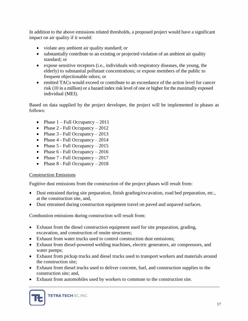
In addition to the above emissions related thresholds, a proposed project would have a significant

impact on air quality if it would:

violate any ambient air quality standard; or

substantially contribute to an existing or projected violation of an ambient air quality

standard; or

expose sensitive receptors (i.e., individuals with respiratory diseases, the young, the

elderly) to substantial pollutant concentrations; or expose members of the public to

frequent objectionable odors; or

emitted TACs would exceed or contribute to an exceedance of the action level for cancer

risk (10 in a million) or a hazard index risk level of one or higher for the maximally exposed

individual (MEI).

Based on data supplied by the project developer, the project will be implemented in phases as

follows:

Phase 1 – Full Occupancy – 2011

Phase 2 - Full Occupancy – 2012







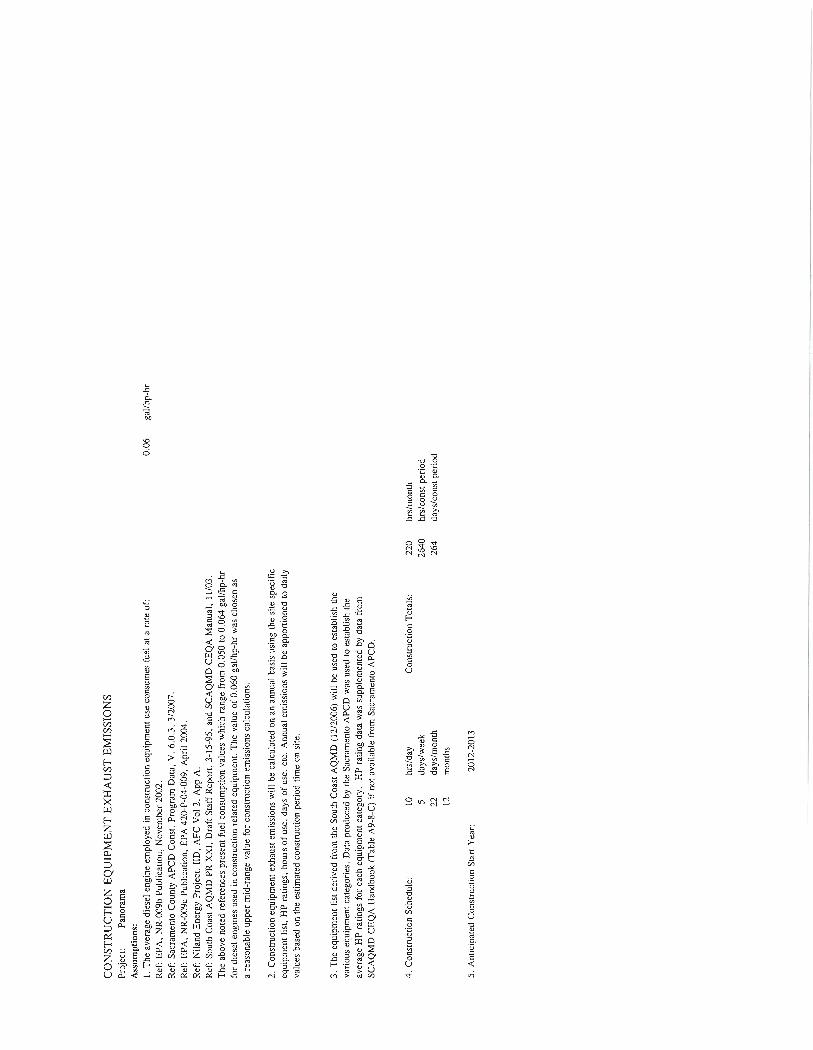
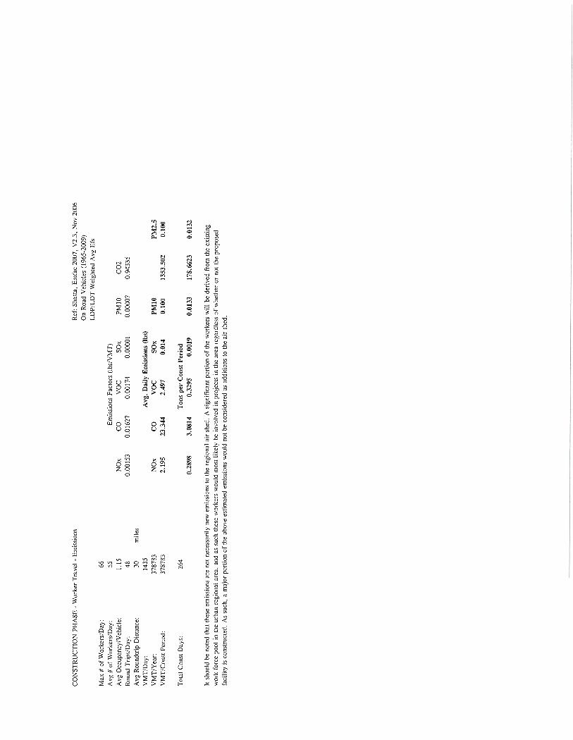
Construction Emissions

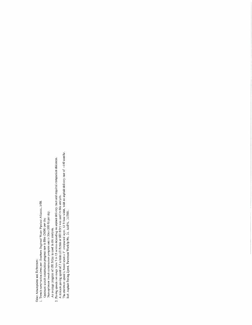
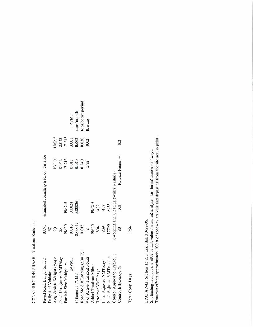
Fugitive dust emissions from the construction of the project phases will result from:

Dust entrained during site preparation, finish grading/excavation, road bed preparation, etc.,

at the construction site, and,

Dust entrained during construction equipment travel on paved and unpaved surfaces.

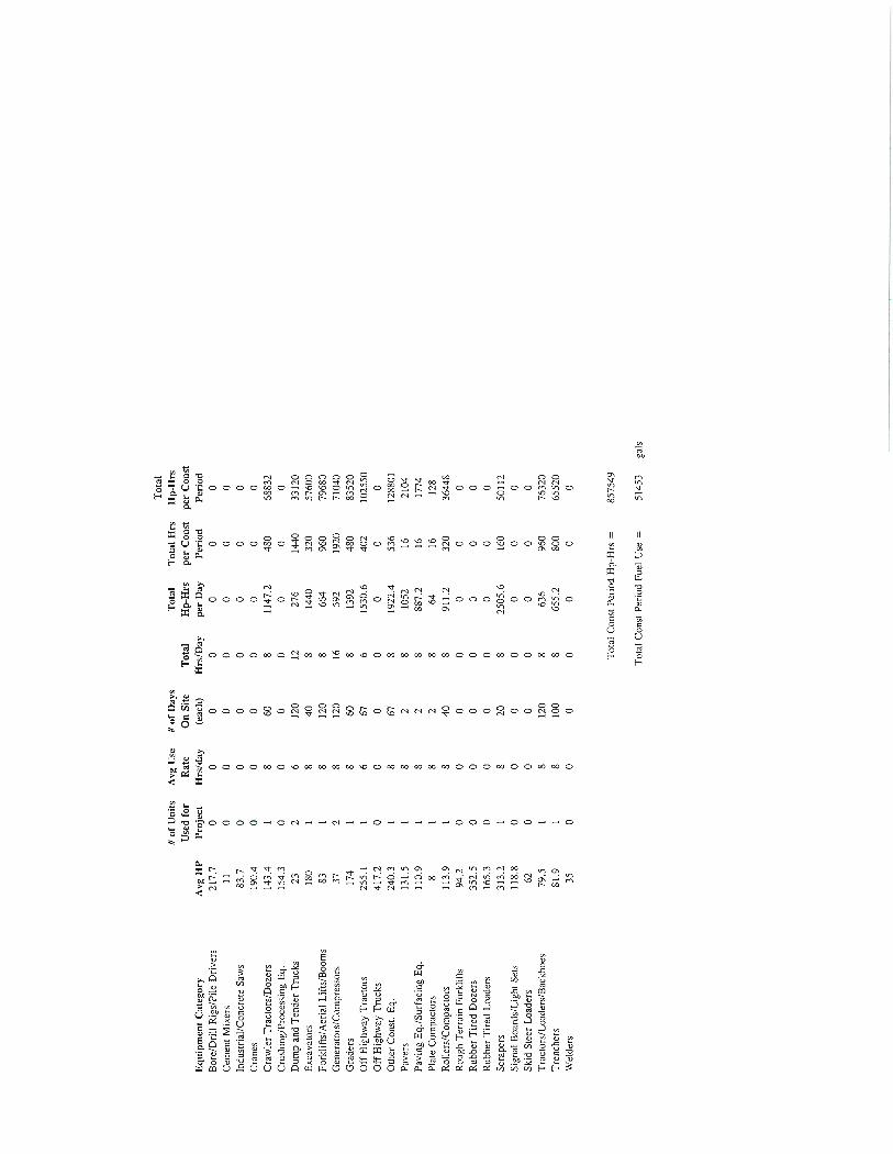
Combustion emissions during construction will result from:

Exhaust from the diesel construction equipment used for site preparation, grading,

excavation, and construction of onsite structures;

Exhaust from water trucks used to control construction dust emissions;

Exhaust from diesel-powered welding machines, electric generators, air compressors, and

water pumps;

Exhaust from pickup trucks and diesel trucks used to transport workers and materials around

the construction site;

Exhaust from diesel trucks used to deliver concrete, fuel, and construction supplies to the

construction site; and,

Exhaust from automobiles used by workers to commute to the construction site.

18

Construction of the phases will be ongoing over the following period:

Start of Construction – 2009

End of Construction – 2018

Table 9 presents data on the specific phases and the areas of disturbance, etc.

Table 9 Phase Data

Phase # # Home Sites Total Acres Open Space Acres Disturbed Acres

1 36 13.35 1.3 12.05

2 59 15.17 0.38 14.79

3 139 47.05 15.13 31.92

4 59 63.12 14.49 48.63

5 73 113.91 26.2 87.71

6 16 18.62 11.81 6.81

7 17 16.24 10.94 5.3

8 31 19.95 10.79 9.16

The project has an approximate total area of 307.4 acres, a net buildable area of 287.6 acres, and

a net open/common space area of 138.5 acres.

Soils in the project area are generally described as followsh:

1. Churn-Perkins-Tehama association: nearly level to moderately steep, well drained to

moderately well drained clay loams and silty clay loams.

2. Reiff-Cobbly alluvial land: nearly level to gently sloping, moderately well drained to

excessively drained loamy fine sands to loams, and frequently flooded cobbly land on valley

bottoms and flood plains.

There are no indications that any characteristics of these soils would exempt them from a

fugitive dust analysis per the MRI Reporto. As such, fugitive dust emissions will be estimated

using the MRI Level 2 Analysis approach.

Table 10 presents the estimated data on project construction times.

Table 10 Construction Phase Time Frames

Phase Estimated Construction Time, months

1 18

2 12

3 12

4 12

5 12

6 12

7 12

8 12

19

Table 11 presents the results of the construction emissions analysis for each phase in terms of

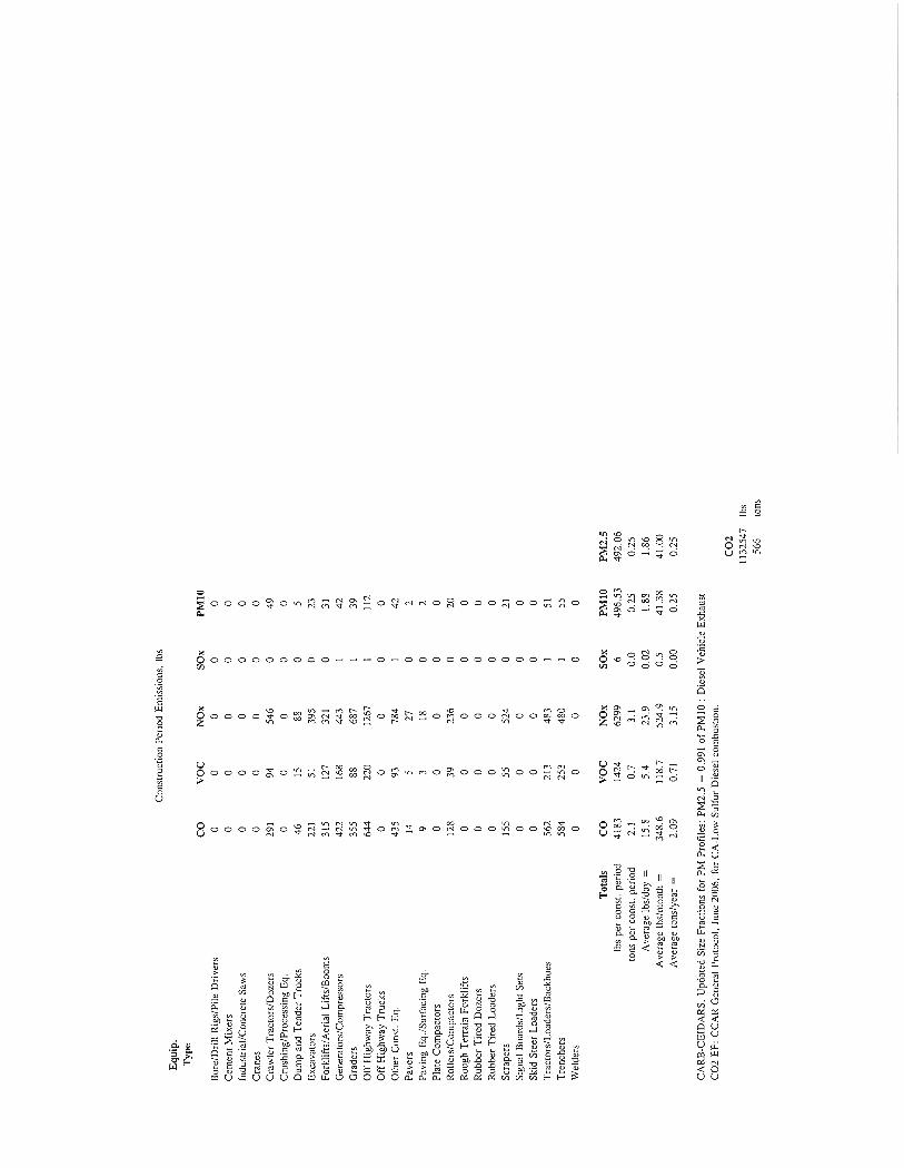
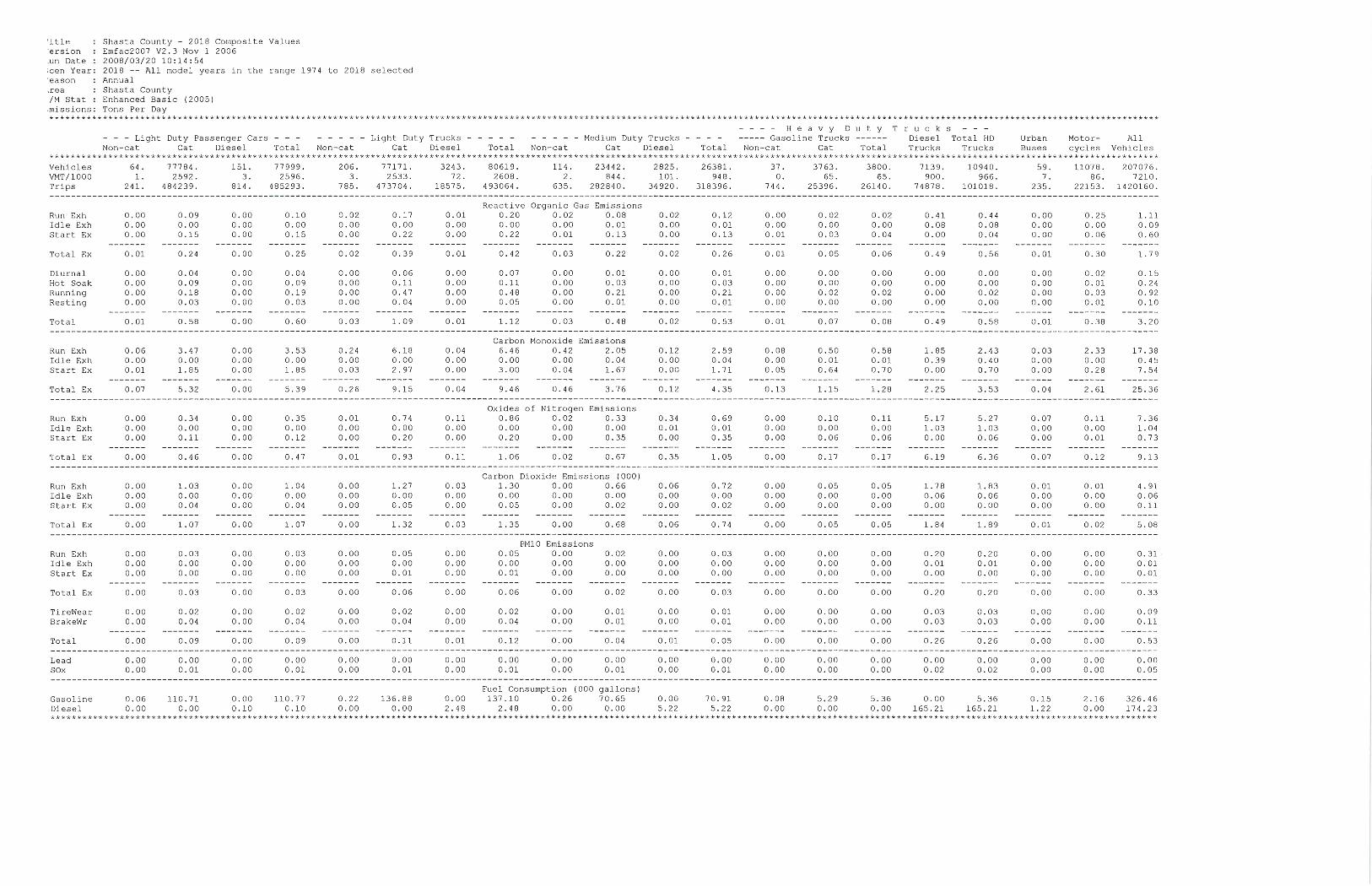
lbs/day (per Table 9). CO2 data is presented in units of tons for each construction phase.

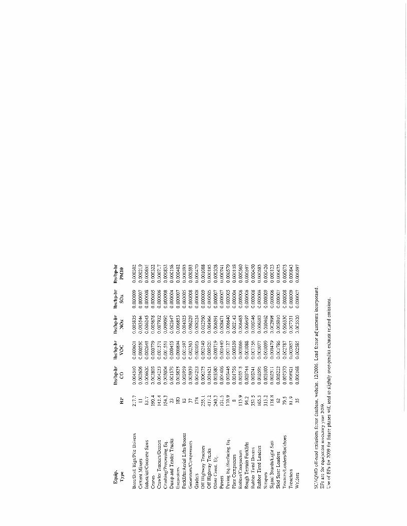
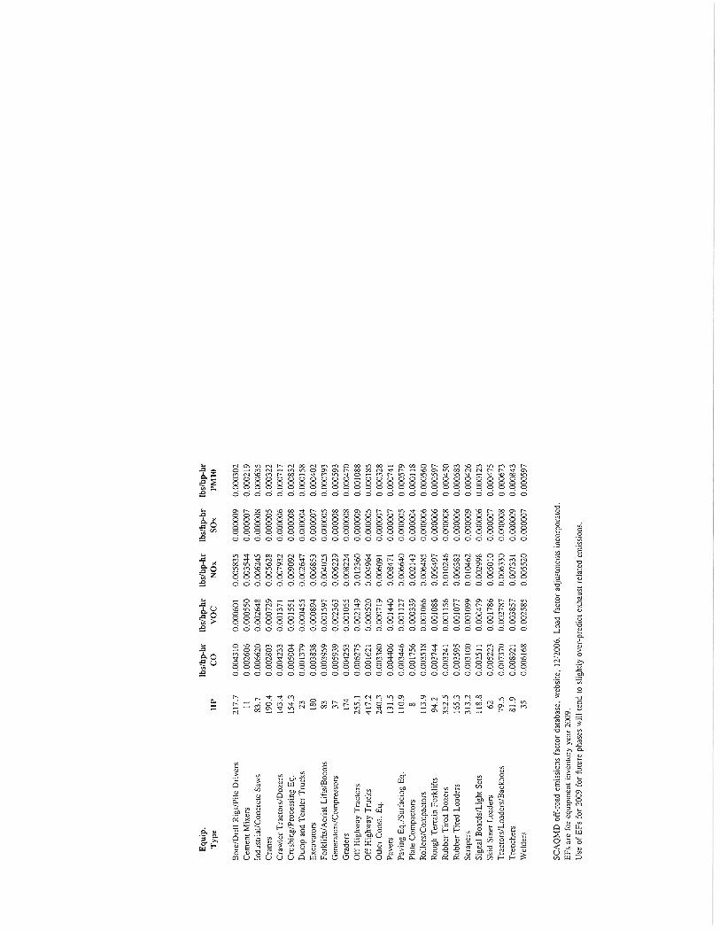
Appendix A contains detailed emissions calculations and the support data and assumptions for

each phase.

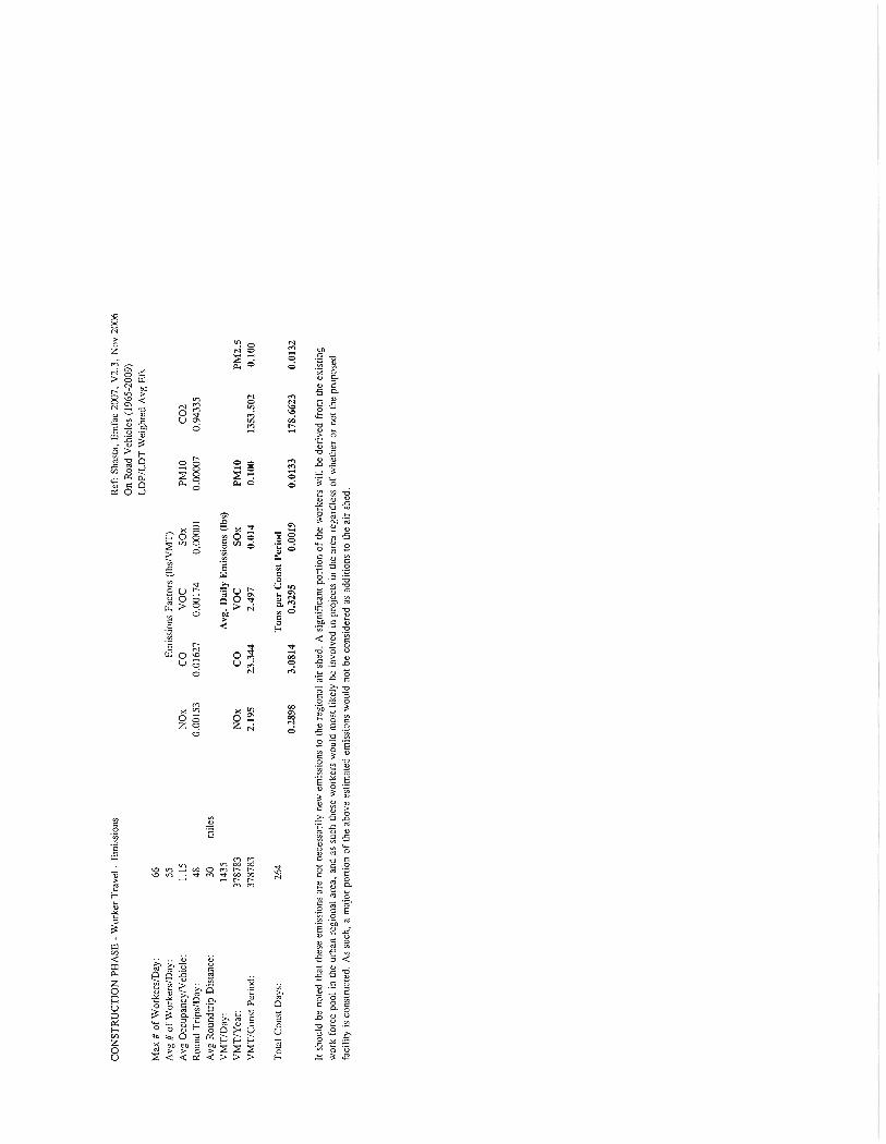
Table 11 Construction Emissions Summary

Phase NOx,

lbs/day

CO,

lbs/day

VOC,

lbs/day

SOx,

lbs/day

PM10,

lbs/day

PM2.5,

lbs/day

CO2, tons

per Const

Period

1 31.6 41 22.5 0.04 2.2/3.1 2.18/0.5 1240.4

2 31.7 41.0 22.5 0.04 2.2/3.6 2.17/0.6 829

3 31.7 41.1 24.6 0.04 2.21/8.4 2.18/1.4 830.1

4 31.65 41.1 24.3 0.04 2.2/9.0 2.18/1.7 829

5 31.65 41.1 25.0 0.04 2.2/15.4 2.18/2.9 829

6 31.6 41.1 21.9 0.04 2.2/2.1 2.18/0.25 828

7 31.6 41.1 21.7 0.04 2.2/1.9 2.18/0.21 828

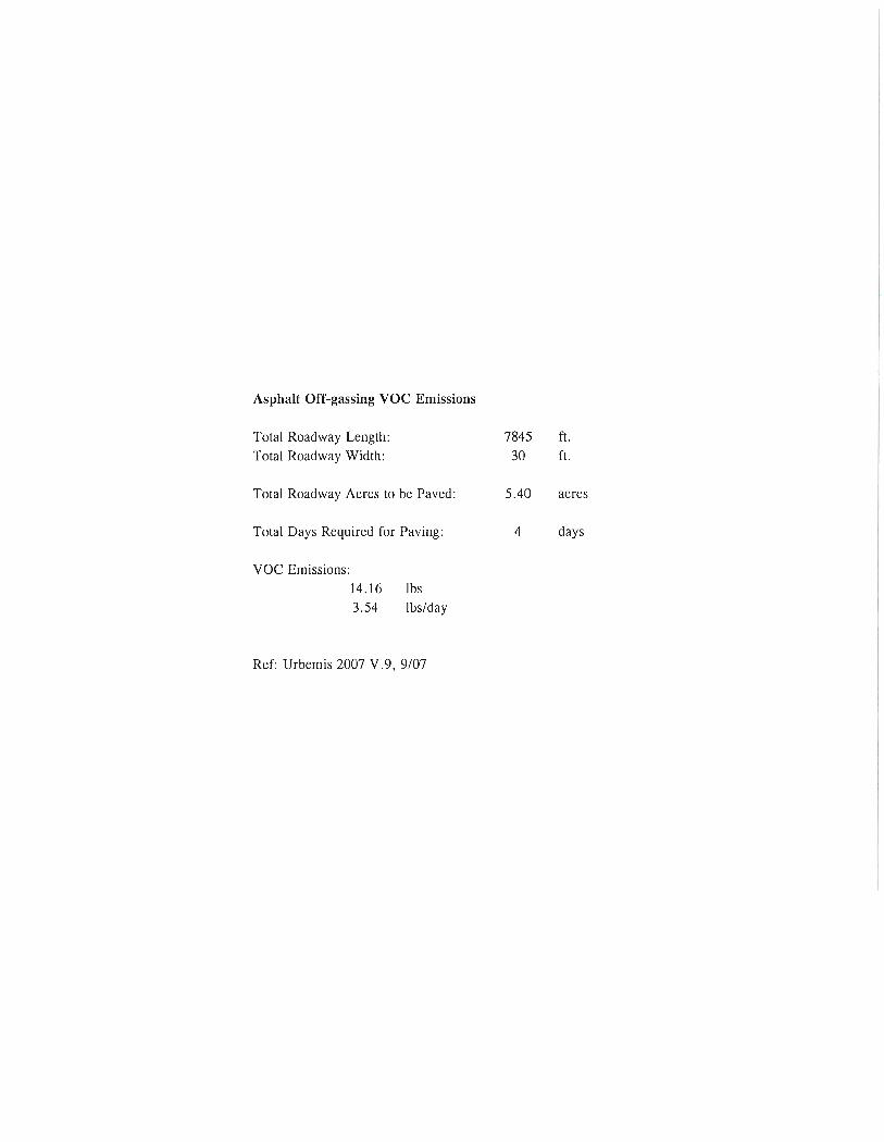
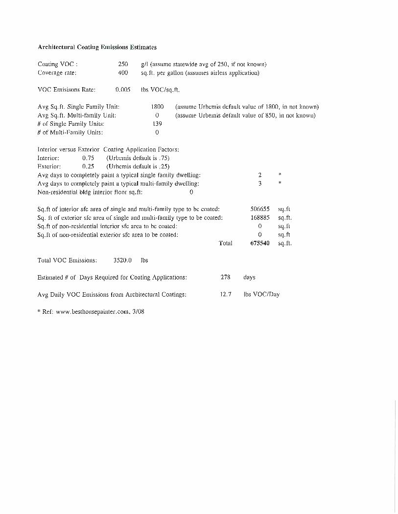
8 31.6 41.1 22.0 0.04 2.2/3.6 2.18/0.34 828 1 For PM10 and PM2.5 two values are presented as V1/V2. V1 is PM from equipment exhaust, while V2 is PM from

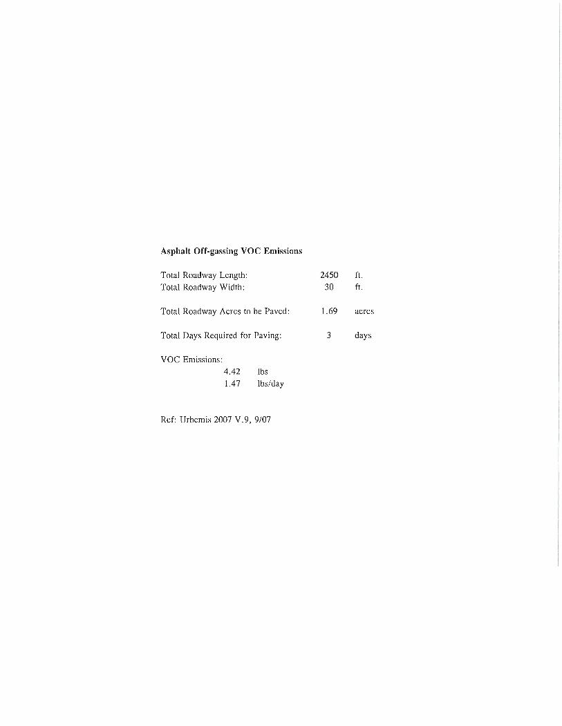
fugitive dust sources. 2 VOC includes asphalt off-gassing and structure coating VOC losses.

Comparison to Significance Criteria

For the construction phases, only NOx exceeds the Level “A” significance thresholds, but the

following should be noted:

It is highly unlikely that all of the predicted construction equipment will be used each

and every day, nor will all of the equipment listed be used for the listed hourly rates each

day.

It is highly unlikely that all of the workers will be on site each and every day, nor will

this occur on a supposed “worst case” day.

It is highly unlikely that all delivery and support traffic emissions will occur each and

every day, nor will all of this activity occur on a supposed “worst case” day.

The following mitigation measures are proposed to control exhaust emissions from the Diesel

heavy equipment used during construction of the project phases:

Operational measures, such as limiting time spent with the engine idling by shutting down

equipment when not in use;

Regular preventive maintenance to prevent emission increases due to engine problems;

Use of low sulfur and low aromatic fuel meeting California standards for motor vehicle

Diesel fuel; and

Use of low-emitting gas and diesel engines meeting state and federal emissions standards

(Tier I, II, III) for construction equipment.

20

As such, the emissions of NOx will most likely be below the Level “A” threshold value of 25

lbs/day.

The following mitigation measures are proposed to control fugitive dust emissions during

construction of the project phases:

Use either water application or chemical dust suppressant application to control dust

emissions from active construction areas (including onsite roads);

Use vacuum sweeping and/or water flushing of paved road surfaces to remove buildup of

loose material to control dust emissions from travel on the paved access road (including

adjacent public streets impacted by construction activities) and paved parking areas;

Cover all trucks hauling soil, sand, and other loose materials or require all trucks to maintain

at least two feet of freeboard;

Limit traffic speeds on all unpaved or active site construction areas to 5 mph;

Install sandbags or other erosion control measures to prevent silt runoff to roadways;

Replant vegetation in disturbed areas as quickly as possible;

Use wheel washers or wash off tires of all trucks exiting construction site; and

Mitigate fugitive dust emissions from wind erosion of areas disturbed from construction

activities (including storage piles) by application of either water or chemical dust

suppressant.

These measures will result in fugitive dust emission well below the Level “A” significance

thresholds for PM10.

The following mitigation measures are proposed to control other miscellaneous emissions during

construction of the project phases:

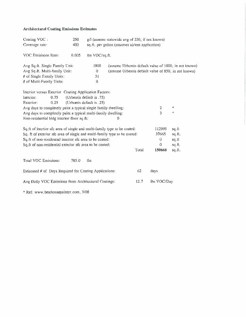
Use of low VOC coatings for the architectural coating phase of construction. All coatings

will meet the VOC limits per AQMD Rule 3-31.

Use of asphalt mixtures appropriate for the time of year of application, while maintaining

compliance with County road design and construction standards.

Construction emissions, with appropriate mitigations applied are not expected to result in any

short or long term violations of any current ambient air quality standard. In addition, the State

Implementation Plan for Shasta County incorporates an emissions allowance for construction

projects. This project will be included in the emissions allowance, as will other similar projects

within the AQMD boundaries.

Vehicular Emissions

Vehicular emissions resulting from project generated trips are based upon the following

assumptions:

21

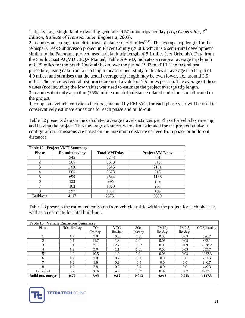
1. the average single family dwelling generates 9.57 roundtrips per day (Trip Generation, 7th

Edition, Institute of Transportation Engineers, 2003).

2. assumes an average roundtrip travel distance of 6.5 milesk,l,m

. The average trip length for the

Whisper Creek Subdivision project in Placer County (2006), which is a semi-rural development

similar to the Panorama project, used a default trip length of 5.1 miles (per Urbemis). Data from

the South Coast AQMD CEQA Manual, Table A9-5-D, indicates a regional average trip length

of 8.25 miles for the South Coast air basin over the period 1987 to 2010. The federal test

procedure, using data from a trip length measurement study, indicates an average trip length of

4.9 miles, and surmises that the actual average trip length may be even lower, i.e., around 2.5

miles. The previous federal test procedure used a value of 7.5 miles per trip. The average of these

values (not including the low value) was used to estimate the project average trip length.

3. assumes that only a portion (25%) of the roundtrip distance related emissions are allocated to

the project.

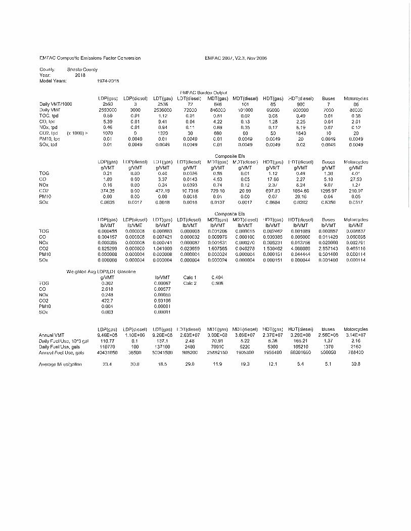
4. composite vehicle emissions factors generated by EMFAC, for each phase year will be used to

conservatively estimate emissions for each phase and build-out.

Table 12 presents data on the calculated average travel distances per Phase for vehicles entering

and leaving the project. These average distances were also estimated for the project build-out

configuration. Emissions are based on the maximum distance derived from phase or build-out

distances.

Table 12 Project VMT Summary

Phase Roundtrips/day Total VMT/day Project VMT/day

1 345 2243 561

2 565 3673 918

3 1330 8645 2161

4 565 3673 918

5 699 4544 1136

6 153 995 249

7 163 1060 265

8 297 1931 483

Build-out 4117 26761 6690

Table 13 presents the estimated emission from vehicle traffic within the project for each phase as

well as an estimate for total build-out.

Table 13 Vehicle Emissions Summary

Phase NOx, lbs/day CO,

lbs/day

VOC,

lbs/day

SOx,

lbs/day

PM10,

lbs/day

PM2.5,

lbs/day1

CO2, lbs/day

1 0.7 7.8 0.8 0.01 0.03 0.03 526.7

2 1.1 11.7 1.3 0.01 0.05 0.05 862.1

3 2.4 25.1 2.7 0.02 0.09 0.09 2028.2

4 0.9 9.6 1.1 0.01 0.03 0.03 859.7

5 1.0 10.5 1.2 0.01 0.03 0.03 1062.3

6 0.2 2.0 0.2 0.0 0.0 0.0 232.5

7 0.2 1.8 0.2 0.0 0.0 0.0 246.7

8 0.3 2.8 0.3 0.0 0.0 0.0 449.3

Build-out 3.7 38.6 4.5 0.07 0.07 0.07 6232.1

Build-out, tons/yr 0.70 7.05 0.82 0.013 0.013 0.013 1137.3

22

1 CARB-CEIDARS Updated PM2.5 fraction inventory indicates that PM2.5 is 0.998 of PM10 for gasoline fuel

vehicles.

Vehicle related emissions do not exceed the Level “A” significance levels on a phase or

build-out basis.

Operational Emissions

Emissions from the use of natural gas for home heating and food preparation are based on the

following assumptions:

1. Energy Information Administration, 2007 report on Higher Natural Gas Prices Impacts

on Local Distribution and Residential Customers. This report indicates that the average

US residence used approximately 75500 scf of natural gas per year during the latest

reporting cycle, i.e., 2005.

2. 75500 scf of gas (0.0755 mmscf) is equivalent to 77,387,500 btu’s/year (assuming gas at

1025 btu/scf HHV). At 100,000 btu’s per therm, the average US residence consumes

approximately 773.9 therms per year.

3. Emissions factors derived from South Coast AQMD CEQA Manual, Appendix A9, Table

A9-12-B were used to estimate emissions for each phase and total build-out. This data is

presented in Table 9. These factors were supplemented by EPA AP-42 factors for CO2,

Section 1.4, 7/98. Annual emissions were converted to daily values using 365 days/year.

Table 14 presents a summary of estimated emissions from residential natural gas use.

Table 14 Residential Natural Gas Emissions Summary

EF,

lbs/mmscf

80 20 5.3 0.6 0.2 0.2 120,000

Phase NOx,

lbs/day

CO,

lbs/day

VOC,

lbs/day

SOx,

lbs/day

PM10,

lbs/day

PM2.5,

lbs/day

CO2,

lbs/day

1 0.596 0.149 0.04 0.0045 0.00149 0.00149 894

2 0.98 0.24 0.065 0.0073 0.00244 0.00244 1465

3 2.3 0.58 0.152 0.029 0.0058 0.0058 3452

4 0.98 0.24 0.065 0.0073 0.00244 0.00244 1465

5 1.21 0.30 0.08 0.0091 0.003 0.003 1812

6 0.27 0.066 0.018 0.00199 0.00066 0.00066 398

7 0.28 0.07 0.019 0.0021 0.0007 0.0007 422

8 0.513 0.128 0.034 0.00385 0.00128 0.00128 797

Build-out 7.12 1.78 0.472 0.0534 0.0178 0.0178 10678

Build-out,

tons/yr

1.3 0.325 0.086 0.00975 0.00325 0.00325 1949

The emissions noted in Table 13 assume the use of currently approved energy saving home

heating and cooking systems. Emissions for future phases may be lower due to changes in the

design and emissions signatures of such devices.

23

Emissions from the use of natural gas do not exceed the Level “A” significance

thresholds on a phase or build-out basis.

It is potentially possible that a percentage of the homes proposed will supplement their annual

heating needs by installing wood stoves or utilizing built in fireplaces. For purposes of gaining

an estimate of potential emissions from such a scenario, it was assumed that 45% of the homes

would supplement heating with wood stoves/fireplaces, using up to 1.48 cords of wood per year

each (Urbemis 9.2.4). A standard cord of wood is approximately equal to 3850 lbs (dry weight),

for wood species in the local area (cedar, pine, fir, oak). Wood stoves installed were assumed to

meet EPA emissions standards. Total estimated fuel consumed annually would be approximately

287 cords/year, or 553 tons of wood fuel. Emissions factors for wood stove/fireplace use were

derived from EPA, AP-42 Section 1.9 and 1.10 (each dated 10/96). The emissions factors for

each category of device were averaged to account for a potential equal mix of devices. Table 15

presents a summary of the estimated emissions from residential wood combustion sources for

purposes of home heating.

Table 15 Residential Wood Stove/Fireplace Emissions Summary

Phase NOx,

lbs/day

CO,

lbs/day

VOC,

lbs/day

SOx,

lbs/day

PM10,

lbs/day

PM2.5,

lbs/day

CO2,

lbs/day

1 0.35 20.89 7.89 0.05 2.89 2.6 0

2 0.57 34.24 12.93 0.08 4.74 4.3 0

3 1.34 80.66 30.46 0.19 11.17 10.1 0

4 0.57 34.24 12.93 0.08 4.74 4.3 0

5 0.70 42.36 16.0 0.10 5.87 5.3 0

6 0.15 9.28 3.51 0.02 1.29 1.2 0

7 0.16 9.87 3.73 0.02 1.37 1.2 0

8 0.30 17.99 6.79 0.04 2.49 2.2 0

Build-out 4.15 249.53 94.24 0.60 34.55 31.1 0

Build-out,

tons/yr

0.76 45.54 17.20 0.11 6.39 5.75 0

1 CO2 emissions are carbon neutral for this source category, i.e., carbon uptake in the fuel equals carbon release

upon combustion. 2 PM2.5 is 90% of PM10, per CARB-CEIDARS fractionation listing.

VOC emissions exceed the Level “A” significance threshold during Phase 3, as well as on a final

build-out basis. The VOC emissions for all phases and build-out are significantly influenced by

the use of fireplaces, which account for only 22% of the residential wood combustion, while

woodstoves account for 78% of the wood combustion. Mitigation measures which should be

considered are as follows:

Withhold approval of any residential design which includes the use of fireplaces or other

similar in-efficient wood or biomass combustion devices for home heating purposes.

If woodstoves are offered as an integral part of the residential design or accessory

package, such stoves should be required to meet the current EPA Phase II emissions

certification standards.

Require any post-construction installation of fireplaces or woodstoves to meet the

minimum EPA Phase specific emissions certification standards existing on the date of

installation. Compliance to be verified at the time of building permit issuance.

24

Estimates of emissions from residential landscaping equipment use are presented in Table 16.

Table 16 Residential Landscaping Equipment Emissions Summary

Phase NOx,

lbs/day

CO,

lbs/day

VOC,

lbs/day

SOx,

lbs/day

PM10,

lbs/day

PM2.5,

lbs/day

CO2,

lbs/day

1 0.02 1.61 0.29 0.0001 0.004 0.004 2.58

2 0.03 2.63 0.48 0.0001 0.007 0.007 4.23

3 0.07 6.20 1.12 0.0003 0.016 0.016 9.96

4 0.03 2.63 0.48 0.0001 0.007 0.007 4.23

5 0.04 3.26 0.59 0.0001 0.009 0.009 5.23

6 0.01 0.71 0.13 0.0 0.002 0.002 1.15

7 0.01 0.76 0.14 0.0 0.002 0.002 1.22

8 0.02 1.38 0.25 0.0001 0.004 0.004 2.22

Build-out 0.22 19.20 3.48 0.0009 0.051 0.050 30.82

Build-out,

tons/yr

0.039 3.5 0.635 0.0002 0.009 0.009 5.625

1 PM2.5 fraction is 0.998 of PM10, per CARB-CEIDARS fractionation listing.

Emissions from residential landscape equipment use do not exceed the Level “A”

significance thresholds.

Estimated emissions for VOCs from the use of consumer products are presented in Table 17.

Table 17 Summary of Project Related Consumer VOC Emissions

Phase lbs/day tons/yr

1 1.76 0.32

2 2.89 0.53

3 6.8 1.24

4 2.89 0.53

5 3.57 0.65

6 0.78 0.14

7 0.83 0.15

8 1.52 0.28

Build-out 20.04 3.84

Emissions from residential/consumer product use do not exceed the Level “A”

significance thresholds for VOCs.

Pre-Existing Odor Issues in the Area

The following summarizes information concerning pre-existing odor sources which may impact

the project area.

Shasta-Signal Energy Facility – The energy facility is a biomass energy production

facility rated at approximately 50 Mw. The primary fuels are biomass wood wastes and

mill wood wastes. Fuel is stored outside and is rotated into the energy production

(combustion) process on schedule which matches fuel needs with fuel storage times, etc.

Odors from outside storage of biomass fuels are rare, with the typical odor resembling

that of recently cut wood, sawdust, or wood chips. Fuel management practices rarely

25

result in fuel being kept on site for a duration of time where rotting or malodor

production can occur, thus odors from the facility are not anticipated to result in a

significant impact on the proposed development.

Cottonwood Livestock/Auction Yard – Livestock are only kept on a small portion of the

overall site (NW corner). This location is approximately 1500 ft or greater from the

closest development lot. The auction yard is only used intermittently throughout the year,

with livestock brought on site for sale and transport. It is highly unlikely that odors from

the site will result in any impacts to the proposed site development.

Table 18 presents a summary of the estimated operational emissions (including vehicle

emissions), for the build-out scenario.

Table 18 Operational Emissions Summary

Phase NOx,

lbs/day

CO,

lbs/day

VOC,

lbs/day

SOx,

lbs/day

PM10,

lbs/day

PM2.5,

lbs/day

CO2,

lbs/day

Build-out 15.2 309.1 122.7 0.72 34.7 31.2 16941

As noted above, in the woodstove emissions section, VOC is the only pollutant which exceeds

the Level “A” threshold criteria. No pollutant exceeds the Level “B” significance thresholds. The

VOC emissions are primarily influenced by the following emissions categories:

Woodstove/fireplace emissions

Consumer product use

Although the estimated VOC emissions from the operational phase of the project (at buildout)

will be above the Level “A”, but below the Level “B” significance criteria, the following should

be noted.

1. Rural and semi-rural areas such as Shasta County (including the small Redding-Anderson

urban area) are generally considered to be “NOx” limited regions, i.e., regions where the

concentrations of ozone depend on the amount of NOx in the atmosphere. This occurs

when there is a lack of nitrogen dioxides thus inhibiting ozone titration when oxygen

mixes with VOCs. In NOx limited regions, controlling NOx is the preferred strategy to

reduce ozone concentrations.

2. The lower elevations of Shasta County, are probably the most impacted by transport, as

noted above, from the lower Sacramento Valley areas, most notably the Sacramento

metropolitan area. The Sacramento metropolitan area, like most large urbanized areas, is

a VOC limited area, i.e., an area in which the concentrations of ozone depend upon the

amount of VOCs in the atmosphere. Consequently, controlling VOCs in these areas

would reduce ozone. In all likelihood, transport from the Sacramento metropolitan area is

highly enriched with VOCs, which when mixed with the local contribution of VOCs,

results in much more NOx limited environment.

In light of the above, a balanced strategy of controlling both NOx and VOCs would most likely

the best approach for Shasta County, with an emphasis placed on NOx reduction strategies.

26

Exposure of Sensitive Receptors to Air Toxic Pollutants

The property surrounding the proposed development is sparsely populated. The small town of

Cottonwood lies to the south of the project. The main I-5 north-south corridor lies due west of

the project site. To the north, over the existing ridge area lies the south Anderson industrial area.

It is highly unlikely that any significant exposures of air toxic pollutants would be generated

from the Cottonwood town center or the I-5 corridor to the west that would impact the proposed

development area. Emissions of both criteria and toxic pollutants can come from a wide range of

sources located in the Anderson industrial area. These pollutants can be generated from sources

such as biomass power generation sources, sand and gravel processing operations, lumber

processing operations, metal fabricating sources, etc. Presently, there is no evidence that any

single source or group of sources would product exposures to toxic pollutants that would result

in impacts to the project residents that would be above the normal exposures seen elsewhere in

the lower elevation areas of Shasta County.

Localized Carbon Monoxide Impacts

Carbon monoxide concentrations in Shasta County (Redding-Anderson-Cottonwood region)

have historically been very low, and well within compliance with both state and federal ambient

air quality standards. Historical CO data over the period 1985-1994 showed that the average

annual 1 hour CO concentration in the Redding urban (downtown) area was 3.75 ppm which is

19% and 11% of the state and federal CO standards respectively. The 8 hour average

concentration during the same period was 2.1 ppm, which represents 23% of the current state and

federal CO standards respectively. Over the ensuing years, a number of industries in the south

county area that were significant CO sources have closed and ceased operations. These closures

have most probably been offset by increases in traffic related CO emissions. But the overall

effect in the County is that CO concentrations remain relatively low, and it is not anticipated that

CO from project traffic would generate a CO “hotspot”. The following qualitative analysis is

presented to support the conclusion that CO impacts from the project are highly unlikely to result

in a CO “hotspot” or a violation of any CO ambient air quality standard.

The base analysis was prepared by the South Coast Air Quality Management District regarding

the emissions and impacts from a number of roadways and intersections for inclusion into the

State Implementation Plan. The analysis, conducted by AQMD staff, was intended to be used as

a comparative planning and analysis tool for other projects to gauge significance with respect to

traffic impacts. Caltrans has recommended using this analysis approach for a number of projects.

This approach has used on the proposed Interstate 10-Tippecanoe interchange improvements in

San Bernardino County, as well as in the follow-on analysis for the Stillwater Business Park

(City of Redding) regarding air quality and traffic related air quality issues posed by the FAA.

The analysis is as follows:

South Coast AQMD SIP Analysis Summary

CO concentrations were modeled at three of the most congested intersections with the highest

traffic volumes in Los Angeles, in addition to an intersection (Long Beach – Imperial) near the

Lynwood air monitoring stations that consistently records the highest 8-hour CO concentrations

27

in the air basin each year. Table 19 identifies each of the intersections modeled and their

associated maximum AM and PM traffic volumes.

Table 19 CO Attainment Plan Intersections (Traffic Counts)*

Eastbound Westbound Southbound Northbound Total

Intersection AM PM AM PM AM PM AM PM AM PM

Wilshire-Veteran 4,951 2,069 1,830 3,317 721 1,400 560 933 8,062 7,719

Sunset-Highland 1,417 1,764 1,342 1,540 2,340 1,832 1,551 2,238 6,650 7,374

La Cienega-Century 2,540 2,243 1,890 2,728 1,348 2,029 821 1,674 6,599 8,674

Long Beach-Imperial 1,217 2,020 1,760 1,400 479 944 756 1,150 4,212 5,514

Source: Transportation Project-Level Carbon Monoxide Protocol User Workbook (U.C. Davis, 1998)

* Mainline counts only.

The localized CO impact (hot spot) modeling in the South Coast AQMD CO attainment

demonstration was conducted using the CAL3QHC air quality model. Additionally, results from

the regional, area-wide, CO modeling conducted for the attainment demonstration were

combined with the hot spot modeling results to identify the combined maximum 8-hour CO

concentration at each intersection. The highest 1-hour CO concentrations calculated using the

CAL3QHC model at each of the intersections evaluated are summarized in Table 20.

Table 20 Year 2002 Intersection Maximum1-Hour CO Modeling

Concentrations (ppm)

Location Morning * Afternoon+

Wilshire-Veteran 4.6 3.5

Sunset-Highland 4.0 4.5

La Cienega-Century 3.7 3.1

Long Beach-Imperial 3.0 3.1

Source: SCAQMD 2003 AQMP Appendix V

* Morning: 7-8 a.m. for La Cienega-Century, 8-9 a.m. for Wilshire-Veteran, 7-8

a.m. for Long Beach-Imperial, and 8-9 a.m. for Sunset-Highland.

+ Afternoon: 3-4 p.m. for Sunset-Highland, 5-6 p.m. for Wilshire-Veteran, 4-5 p.m.

for Long Beach-Imperial, and 6-7 p.m. for La Cienega-Century.

The results of the 8-hour CO modeling for each of the four intersections evaluated are shown in

Table 21.

Table 21 Projected 8-hour Carbon Monoxide Concentrations (ppm) at Various Intersections Located in

the South Coast Air Basin

28

Year Maximum

Areawide

Maximum

Hot Spot

Time of

Maximum

Hot Spot

Time of

Maximum

Areawide

"Hot Spot" at

time of

Maximum

Areawide

Maximum Areawide

and Hot Spot at

time of Maximum

Areawide

Wilshire Blvd. and Veteran Ave. located in Westwood

1997 2.3 5.8

1400 PST 1100 PST

4.6 6.9

2002 1.6 3.4 2.9 4.5

2003 1.5 3.2 2.7 4.2

2004 1.4 3.0 2.6 4.0

2005 1.3 2.8 2.4 3.7

Sunset Blvd. and Highland Ave. located in Hollywood

1997 3.3 6.6 1400 PST 0300 PST 3.5 6.8

2002 2.1 3.8 2.0 4.1

2003 2.0 3.6 1.9 3.9

2004 1.9 3.4 1.8 3.7

2005 1.8 3.2 1.7 3.5

La Cienega Blvd. And Century Blvd. located in Inglewood

1997 8.0 4.5

1200 PST 0800 PST

3.0 11.0

2002 4.5 2.6 1.7 6.2

2003 4.2 2.5 1.6 5.8

2004 4.0 2.3 1.5 5.5

2005 3.8 2.2 1.4 5.2

Long Beach Blvd. and Imperial Hwy. located in Lynwood

1997 14.5 4.2

1300 PST 0600 PST

1.5 16.0

2002 9.2 2.3 0.8 10.0

2003 8.6 2.2 0.7 9.3

2004 8.1 2.0 0.7 8.8

2005 7.7 1.9 0.7 8.4

Source: 2003 SCAQMP, Appendix V

As shown in Tables 20 and 21 the projected 1-hour and 8-hour CO concentrations are less than

the NAAQS CO thresholds of 20 ppm for 1-hour average and 9.0 ppm for an 8-hour average CO

concentrations.

A simple comparison of the South Coast study intersections and traffic volumes versus the

project road service intersections and traffic volumes in the project area indicates that the

predicted build-out and/or the 2025 traffic volumes in the areas are well below the values used in

the South Coast SIP analysis, and as such, modeling of the traffic emissions for the subdivision

project area and surrounding services road network is not warranted.

Residual Impacts

The residual impacts from the construction phases of the proposed project are not expected to be

significant since the emissions are below the Level “A” thresholds, and the mitigations proposed

29

are anticipated to result in offsite impacts well below and state and federal ambient air quality

standard.

The residual impacts from long term occupancy of the housing project will be in the areas of

traffic related emissions, use of woodstoves/fireplaces for supplemental home heating, and the

use of consumer products by the residents of the project. Impacts in these categories are

dominated by woodstove/fireplace emissions, which can be mitigated by requirements to use

EPA Phase II certified devices, and discouraging the use of fireplace and other similar in-

efficient supplemental home heating methods.

As stated earlier, the County emissions inventory as well as the SIP emissions inventory include

current and future year emissions estimates or growth allowance emissions for construction and

operation of the proposed subdivision (based on population growth, etc.). Therefore, these

emissions are accounted for in the normal growth cycle of the County.

30

References:

a Shasta Ranch Mining and Reclamation Plan, DEIR, July 2006, Pacific Municipal Consultants.

b The Assessment of the Impacts of Transported Pollutants on Ozone Concentrations in

California, March 2001.

c The California Almanac of Emissions and Air Quality, 2006 Edition, CARB, Planning and

Technical Support Division.

d Shasta County General Plan, Section 6.5, Air Quality, as Amended through 2004.

e Environmental Review Guidelines-Procedures for Implementing CEQA, Shasta County

AQMD, November 2003.

f Protocol for Review-Land Use Permitting Activities, Shasta County AQMD, November 2003.

g Standard Mitigation Measures Applicable to All Projects, Attachments 1, 2, and 3, Shasta

County AQMD, 9-20-07.

h Soil Survey of Shasta County, USDA-SCS, August 1974.

i A Workforce Needs Assessment of the Arizona Construction Trades Industry, State or Arizona,

Dept. of Commerce, February 2005.

j Craft Labor Supply Outlook: 2005-2015, Construction Labor Research Council, 2005.

k USDOT, Bureau of Transportation Statistics, FHWA, January 2003.

l National Household Travel Survey, USDOT-FHWA, August 2007.

m

Federal Test Procedure Review Project, Preliminary Technical Report, EPA-420-R-93-007,

May 1993.

n Shasta County Ozone Transport Study, STI, March 1996-97.

o Improvement of Specific Emission Factors-BACM Project No.1-Final Report, Midwest

Research Institute, March 1996, South Coast AQMD Contract # 95040.

APPENDIX A ____________________________

Construction and Operational Phase Emmissions

APPENDIX B ____________________________

Construction Staffing Estimate

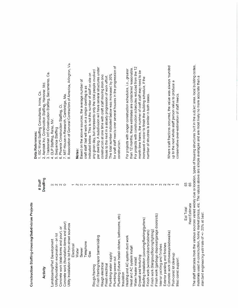
Panorama Planned Development Construction Staffing Estimate Based on the referenced sources, the average number of craft staff that will work on a single dwelling is as indicated below. This is not the number of staff on site on any given day, but represents only the total people involved per dwelling. A subdivision will typically have several structures under construction at one time, with craft staff moving from one house to the next in a steady progression of work effort. The total number indicated below was increased by 20% for craft staff needs over several houses in the progression of construction. For projects with longer construction schedules, i.e., greater than 12 months, these estimates are considered reasonable. For projects with construction schedules reduced from the 12-month time frame, the number of craft staff may need to be increased in order to finish the building schedule, if the number of structures is similar in both cases. Where staff fractions occurred, the value was always rounded up to the next whole staff person value to produce a conservative over-estimation of staff needs. The staff estimates from the various sources varied widely due to location, types of housing structures built in the subject area, local building codes, materials used in construction, home market prices, etc. The values included are simple averages and are most likely no more accurate than a standard engineering estimate of ±20% at best.

Construction Staffing-Housing/Subdivision Projects Activity # Staff/Dwelling

Landclearing/Pad Development 2 Utility/foundation excavation - on lot 2 Concrete work (slab forms and pour), or 2 Concrete work (foundation forms and pour) 0 Utility installation to lot from street sources

Electrical 1 Water 2 Sewer 2 Telephone 1 Gas 1

Rough framing 3 Finish framing/vapor barrier/siding 3 Rough electrical 2 Finish electrical 2 Plumbing water supply 1 Plumbing sewer out 1 Plumbing (fixture install-kitchen, bathrooms, etc) 2 Insulation 2 Heating and AC system duct work 2 Heat and AC system install 2 Water heater install 1 Drywall and texturing 3 Roofing installation (covering/flashing/gutters) 3 Finish work (windows/doors/cabinets) 2 Finish work (tile/grout/flooring/lighting) 2

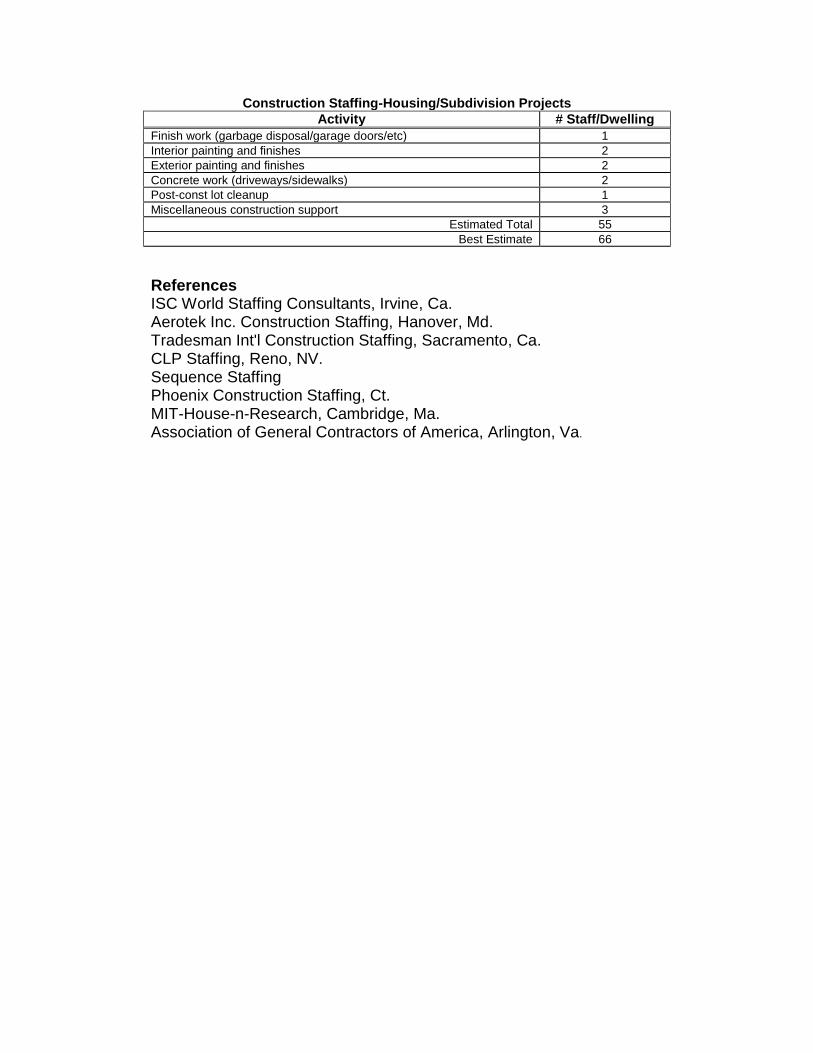
Construction Staffing-Housing/Subdivision Projects Activity # Staff/Dwelling

Finish work (garbage disposal/garage doors/etc) 1 Interior painting and finishes 2 Exterior painting and finishes 2 Concrete work (driveways/sidewalks) 2 Post-const lot cleanup 1 Miscellaneous construction support 3

Estimated Total 55 Best Estimate 66

References ISC World Staffing Consultants, Irvine, Ca. Aerotek Inc. Construction Staffing, Hanover, Md. Tradesman Int'l Construction Staffing, Sacramento, Ca. CLP Staffing, Reno, NV. Sequence Staffing Phoenix Construction Staffing, Ct. MIT-House-n-Research, Cambridge, Ma. Association of General Contractors of America, Arlington, Va.

",.."..

i\-:.'rH

CALIFORNIA

PREDOMINANT SURF ACE

WIND FLOW PATTERNS,~.. PLATEAU

WINTER (DEC. -.JAN. -FED.)

Legend-SACRAMENTOVALLEY

-.~ COASTAL WATERS

MOUNT AINCOUNTIES

MOUNTAINOUSZONES

TAHOE

"0.

SAN JOAQUIN V ALLEY

BASIN V ALLEYS, ,

w

NORTH..-

M~

SOUTH

"..

w E~

~

0 20 .0 60 80 100I , I , I , I , I , I

Sc.I. In ..II..

HEAVY LINES DELINEATE THE

1. CALIFORNIA AIR BASINS

TCALIFORNIA AIR RESOURCES BOARO

AEROf-IETRIC DATA OIVISION 4/84

"...

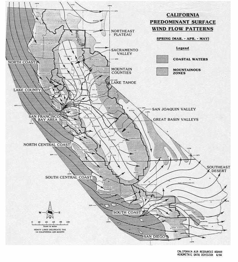
CALIFORNIA


WIND FLOW PATTERNS

..~

SPRING (MAR. -APR. -MAY)

Legend

COASTAL WATERS

MOUNTAINOUSZONES

.-SAN JOAQUIN V ALLEY

BASIN VALLEYS

NORTH",.

~~

SOUTH

~

w E

'P(VS"'\

o 20 .0 00 00 100I , I , I , I , I , I

Sc.l. I. ..II..

HEAVY LINES DELINEATE THEI. CALIFORNIA AIR BASINS

CALIFORNIA AIR RESOURCES BOARD

AEROI1ETRIC DATA DIVISION 4/84

",..""W

.,.w

I-.r.

CALIFORNIA


WIND FLOW PATTERNS.-00 0. ~

PLATEAU

SUMMER (JUN. .JUL. -AUG.)-.

-SACRAMENTOVALLEY

-0-

LegeD~

COASTAL WATERS

MOUNT AINCOUNTIES MOUNTAINOUS

ZONES

TAHOE

"..

...SAN JOAQUIN V ALLEY00.0

BASIN V ALLEYS

~

NORTH

,

SOUTH

~

A","

W-~-E

~

0 20 .0 60 10 100I , I , I , , , , , ,

Scal. In mil.,

HEAVY LINES DELINEATE THE

,. CALIFORNIA AIR BASINS

~

.,;..

CALIFORNIA AIR RESOURCES BOARO

AERO~IETRIC DATA OIVISION 4/84

~~~~..-

.-I-0...

CALIFORNIA


WIND FLOW PATTERNS.~.. PLATEAU

FALL (SEP. .OCT. .NOV.)

Legend-SACRAMENTOVALLEY

COASTAL WATERS

MOUNT AINCOUNTIES

MOUNTAINOUSZONES

TAHOE

~

.r.SAN JOAQUIN V ALLEY.0.0

BASIN V ALLEYS.,O-W

NORTH

SOUTH

,

w-~M

o 10 .0 .0 10 100I , I , I , I , I , I

6c.lo in ..110.

,"...

";."

CALIFORNIA AIR RESOURCES BOARD

AEROHETRIC DATA DIVISION 4184

air quality analysis - co.shasta.ca.us

Documents