Air Pollution in Hamilton – Health Effects and Sources

November 22, 2006

McMaster Centre for Spatial Analysis

Clean Air Hamilton Strategy

Risk Management Approach Applied to Community Wide Actions

• Identify Problem• Measure/Evaluate• Prioritize Risks • Inform Community• Cooperative Actions

www.cleanair.hamilton.ca

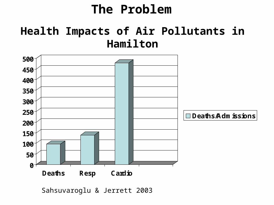
The Problem

0

50

100

150

200

250

300

350

400

450

500

Deaths Resp Cardio

Deaths/Admissions

Sahsuvaroglu & Jerrett 2003

Health Impacts of Air Pollutants in Hamilton

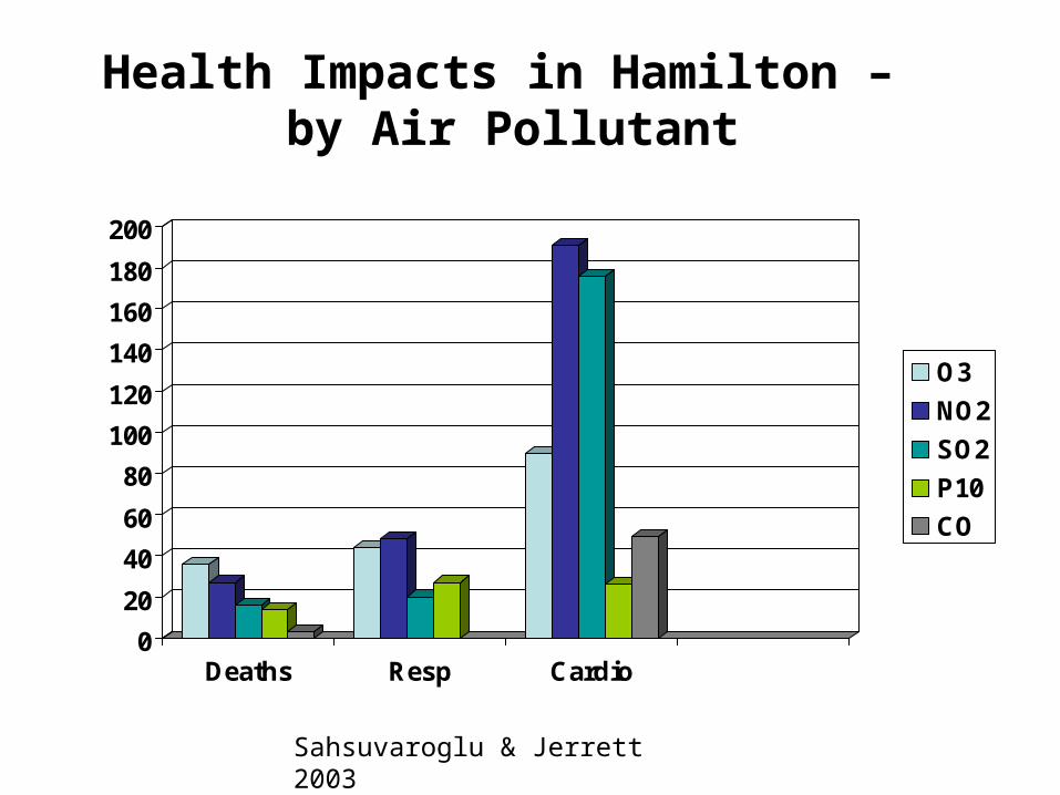
Health Impacts in Hamilton – by Air Pollutant

0

20

40

60

80

100

120

140

160

180

200

Deaths Resp Cardio

O3

NO2

SO2

P10

CO

Sahsuvaroglu & Jerrett 2003

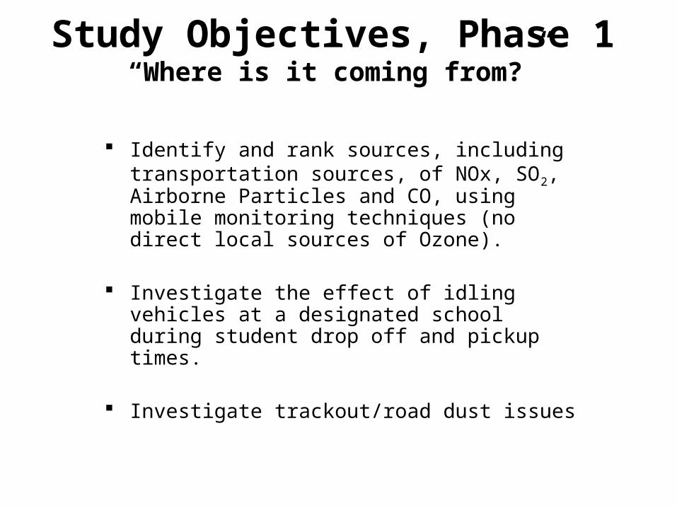
Study Objectives, Phase 1“Where is it coming from?”

Identify and rank sources, including transportation sources, of NOx, SO2, Airborne Particles and CO, using mobile monitoring techniques (no direct local sources of Ozone).

Investigate the effect of idling vehicles at a designated school during student drop off and pickup times.

Investigate trackout/road dust issues

National Pollutant Release Inventory – Hamilton Point Sources

• PM1056 Sources

• CO 14 Sources

• NOx 13 Sources

• SO2 9 Sources

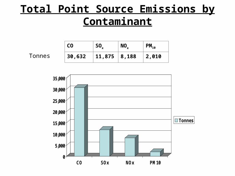
Total Point Source Emissions by Contaminant

0

5,000

10,000

15,000

20,000

25,000

30,000

35,000

CO SOx NOx PM10

Tonnes

CO SOx NOx PM10

30,632 11,875 8,188 2,010Tonnes

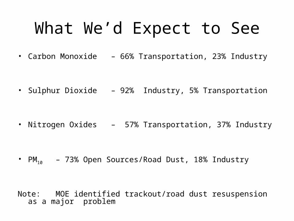
What We’d Expect to See

• Carbon Monoxide – 66% Transportation, 23% Industry

• Sulphur Dioxide – 92% Industry, 5% Transportation

• Nitrogen Oxides – 57% Transportation, 37% Industry

• PM10 – 73% Open Sources/Road Dust, 18% Industry

Note: MOE identified trackout/road dust resuspension as a major problem

Emission Sources by Regions in Hamilton

Flamborough/Waterdown

East Mtn

NE Ind

Stny Crk

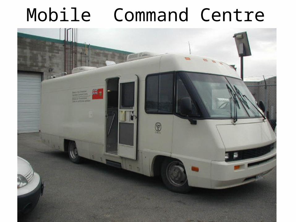
Mobile Command Centre

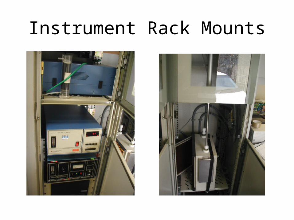
Instrument Rack Mounts

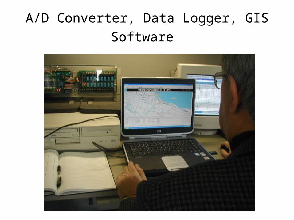
A/D Converter, Data Logger, GIS Software

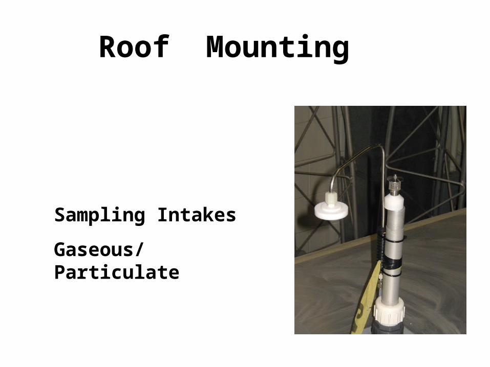
Roof Mounting

Sampling Intakes

Gaseous/Particulate

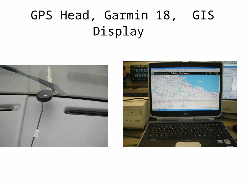
GPS Head, Garmin 18, GIS Display

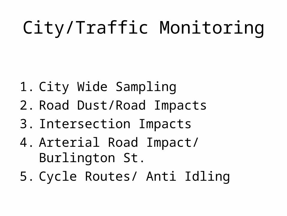
City/Traffic Monitoring

1. City Wide Sampling

2. Road Dust/Road Impacts

3. Intersection Impacts

4. Arterial Road Impact/ Burlington St.

5. Cycle Routes/ Anti Idling

Sampling Track, City Wide Scan

City Wide Sampling

11:0

7

11:1

7

11:2

7

11:3

7

11:4

7

11:5

7

12:0

7

12:1

7

12:2

7

12:3

7

12:4

7

12:5

7

13:0

7

13:1

7

13:2

7

13:3

7

13:4

7

13:5

7

14:0

7

14:1

7

14:2

7

14:3

7

14:4

7

14:5

7

15:0

7

15:1

7

15:2

7

15:3

7

15:4

7

15:5

7

16:0

7

16:1

7

16:2

7

16:3

7

16:4

7

16:5

7

SO2

CO

NO

P10

Road Dust

BartonSt

Road Dust

###

#

###

#

#

##

### ###########

###

##

#

##

#####

#########

#

##

###

#

##

#

##

#

##

###########

##

########

#

#

#########

##

###

#########

##

#

#

##

#

########### #

#

# ###

##

########

####################################

#

#

#

#

#

##

##

#

##

########

##

##

########

###

#

###

###########

###########

#

##

#

##

#

#

##

###############

##

#

##

#

#

#

#

## #

### #

#

#

##

##

#

#

#

##

####

##

###

###

##

#####

### ###

No

December 8, 2005

1 0 1 2 Kilometers

Wind

NO ppb

###

#

###

#

#

##

### ###########

###

##

#

##

#####

#########

#

##

###

#

##

#

##

#

##

###########

##

########

#

#

#########

##

###

#########

##

#

#

##

#

########### #

#

# ###

##

########

###################################

##

#

#

#

#

##

##

#

##

########

##

##

########

###

#

##

###########

############

#

##

#

##

#

#

##

###############

#

#

#

##

#

#

#

#

## #

### #

#

#

##

##

#

#

#

##

####

##

##

###

#

##

#####

### ###

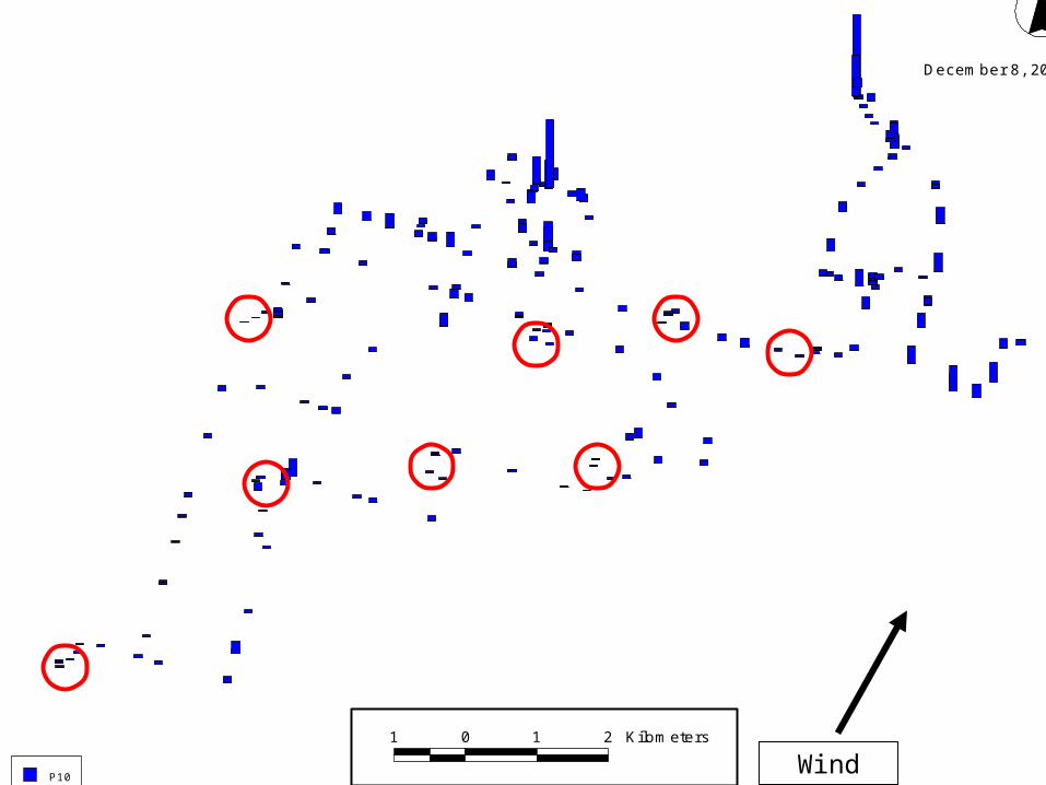
P10

1 0 1 2 Kilometers

December 8, 2005

Wind

0

5

10

15

20

25

30

35

40

45

50

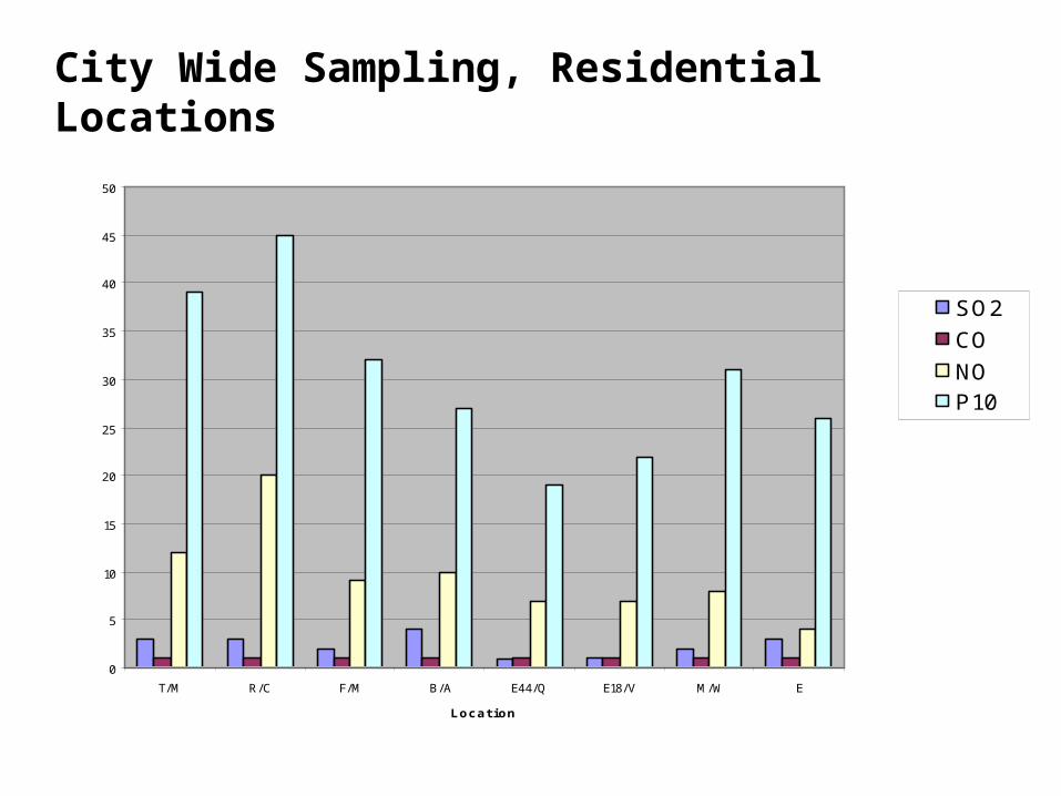
T/M R/C F/M B/A E44/Q E18/V M/W E

Location

SO2

CO

NOP10

City Wide Sampling, Residential Locations

0

20

40

60

80

100

120

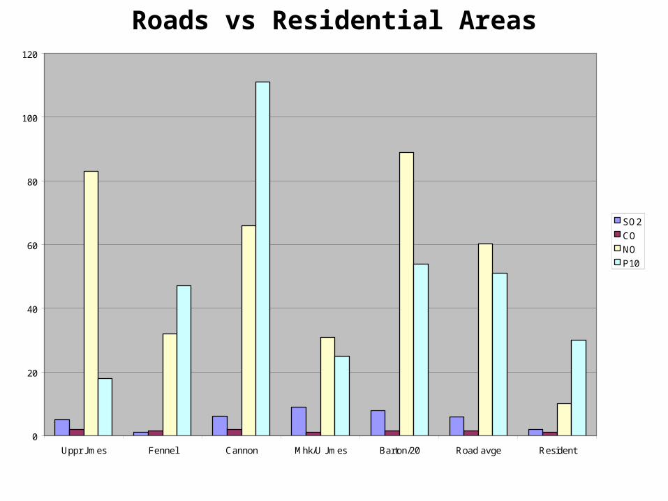
Uppr Jmes Fennel Cannon Mhk/U Jmes Barton/20 Road avge Resident

SO2

CO

NO

P10

Roads vs Residential Areas

0

20

40

60

80

100

120

140

160

180

Time

P10

ug/

m3

NO

ppb SO2

CO

NO

PM10Mohawk and Upper James

Barton and Centennial Pkwy

= idling impact

--NO Residential

--PM10 Residential

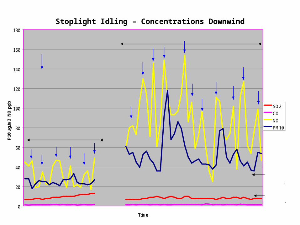
Stoplight Idling – Concentrations Downwind

Burlington St. Upwind Downwind

10:5

210

:54

10:5

610

:58

11:0

011

:02

11:0

411

:06

11:0

811

:10

11:1

211

:14

11:1

611

:18

11:3

011

:32

11:3

411

:36

11:3

8

NO

NO2

P2.5

P10

Downwind

Upwind

Burlington St Contribution(Approx. 600 Trucks/Hr)

0

10

20

30

40

50

60

70

80

90

P10 P2.5 P1 NO NO2 SO2 CO

Difference

CARS

Vehicle Idling outside Schools

“Natural Experiment”

0

5

10

15

20

25

30

35

8:59

9:05

9:11

14:0

0

14:0

6

14:1

2

14:1

8

14:2

4

14:3

0

14:3

6

14:4

2

14:4

8

14:5

4

15:0

0

15:0

6

15:1

2

15:1

8

15:2

4

15:3

0

15:3

6

15:4

2

15:4

8

15:5

4

NO (ppb)

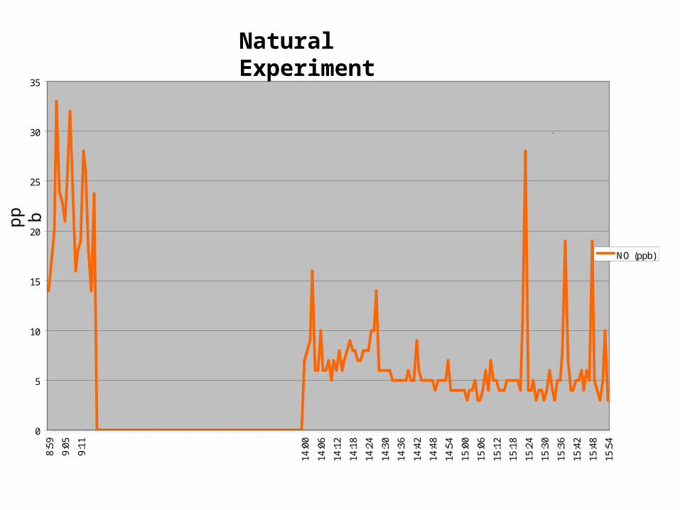
MorningStudent Dropoff

AfternoonStudentPickup

Natural Experimentpp b

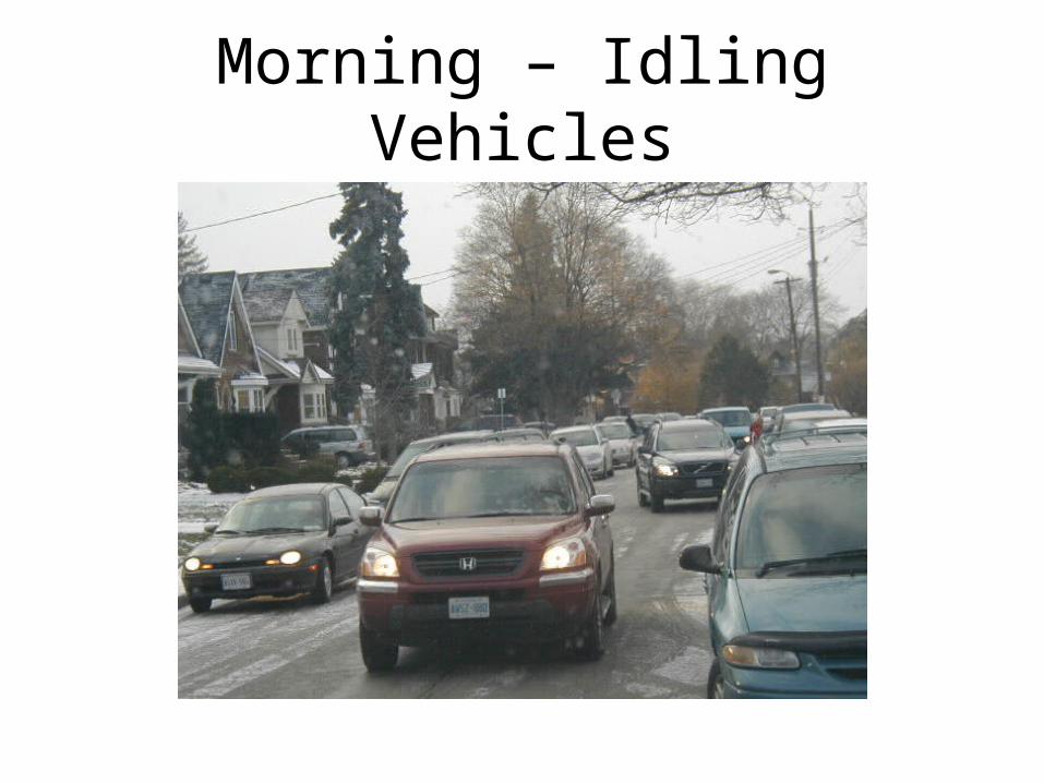
Morning – Idling Vehicles

Trackout/Diesel Trucks

1. PM2.5, PM1 Components

2. Photos

3. Sample Trace

4. Consolidated PM10 Data

5. Comparison Previous Data

Road Dust , Covariance 20xPM1, 10xPM2.5, PM10

0

500

1000

1500

2000

2500

3000

3500

1 4 7 10 13 16 19 22 25 28 31 34 37 40 43 46 49 52 55 58 61 64 67 70 73 76 79 82

20xP1

10xP2.5

P10

P2.5/P10 R2 = 0.7

P2.5/P1 R2 = 0.98

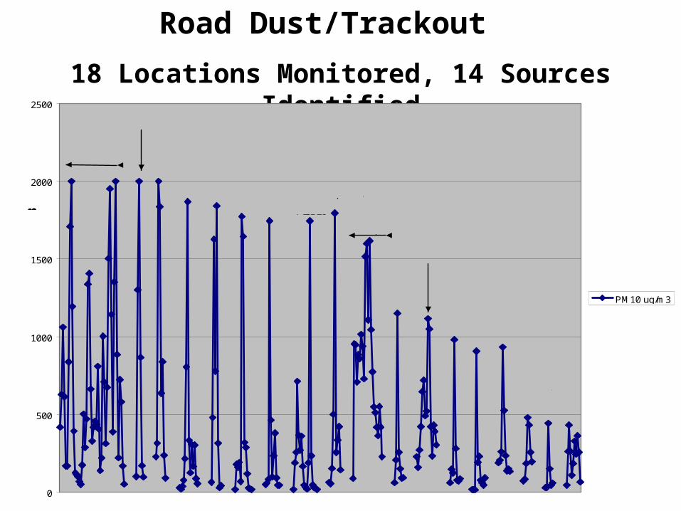
Road Dust/Trackout

18 Locations Monitored, 14 Sources Identified

0

500

1000

1500

2000

2500

PM10 ug/m3

Strathearne

Kenilworth N

Depew

Vict. NPortAuth

Nebo

Hwy 20Goder

Brampton

Pier 25

Imperial

Brant

BurlSher/Burl

Burl/Parkdale

Sherman

ChathamFrid

Parkdale

McKeil

ug

/m3

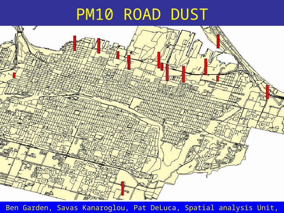
PM10 ROAD DUST

Ben Garden, Savas Kanaroglou, Pat DeLuca, Spatial analysis Unit, McMaster University

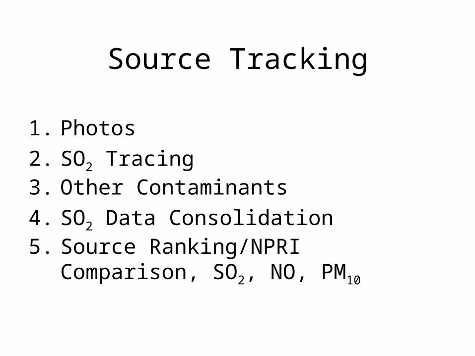
Source Tracking

1. Photos

2. SO2 Tracing3. Other Contaminants

4. SO2 Data Consolidation

5. Source Ranking/NPRI Comparison, SO2, NO, PM10

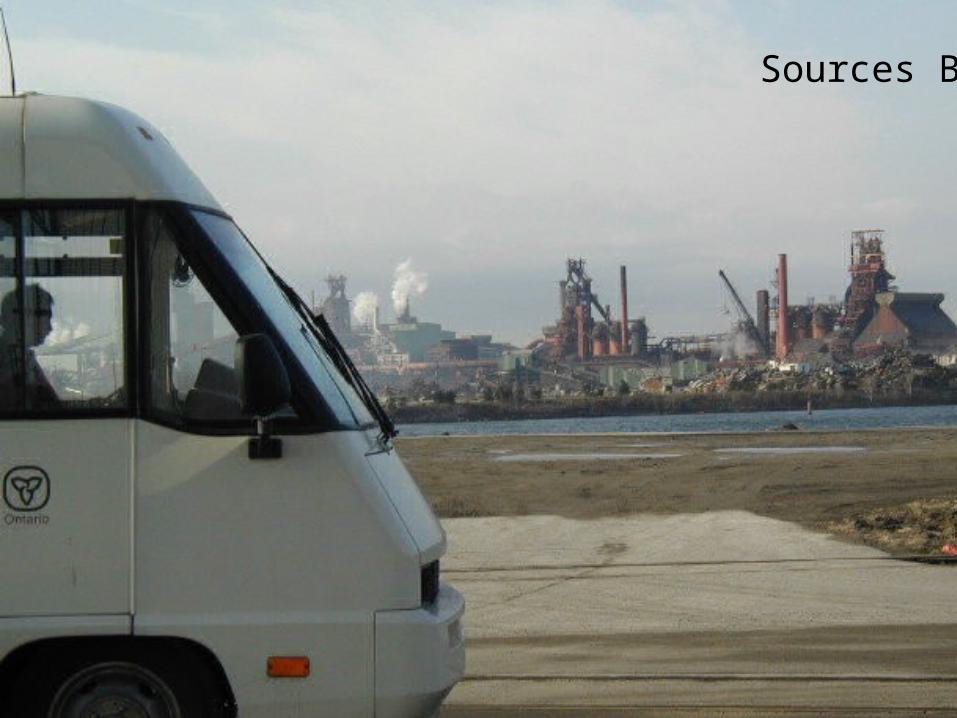
B

Sources B

Source AY

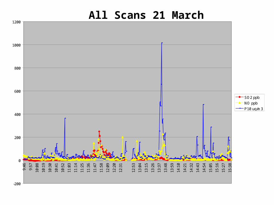
All Scans 21 March

-200

0

200

400

600

800

1000

12009:

46

9:57

10:0

8

10:1

9

10:3

0

10:4

1

10:5

2

11:0

3

11:1

4

11:2

5

11:3

6

11:4

7

11:5

8

12:0

9

12:2

0

12:3

1

12:5

3

13:0

4

13:1

5

13:2

6

13:3

7

13:4

8

13:5

9

14:1

0

14:2

1

14:3

2

14:4

3

14:5

4

15:0

5

15:1

6

15:2

7

15:3

8

SO2 ppb

NO ppb

P10 ug/m3

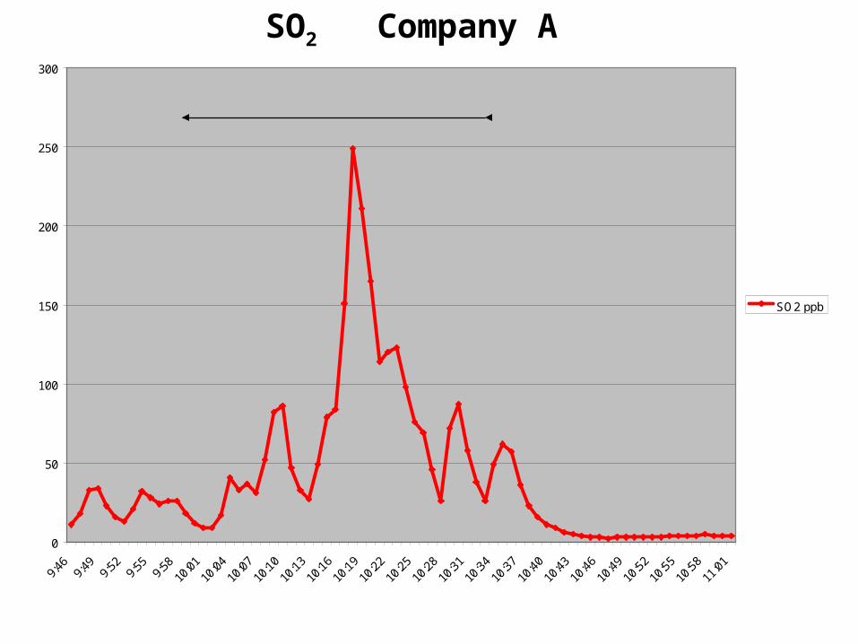
SO2 Company A

0

50

100

150

200

250

300

9:46

9:49

9:52

9:55

9:58

10:0

110

:04

10:0

710

:10

10:1

310

:16

10:1

910

:22

10:2

510

:28

10:3

110

:34

10:3

710

:40

10:4

310

:46

10:4

910

:52

10:5

510

:58

11:0

1

SO2 ppb

pp

b

Company A

Source

Plume

Back Tracking

Impact

Source

SO2 Company A

0

50

100

150

200

250

300

9:46

9:49

9:52

9:55

9:58

10:0

110

:04

10:0

710

:10

10:1

310

:16

10:1

910

:22

10:2

510

:28

10:3

110

:34

10:3

710

:40

10:4

310

:46

10:4

910

:52

10:5

510

:58

11:0

1

SO2 ppb

pp

b

Company A

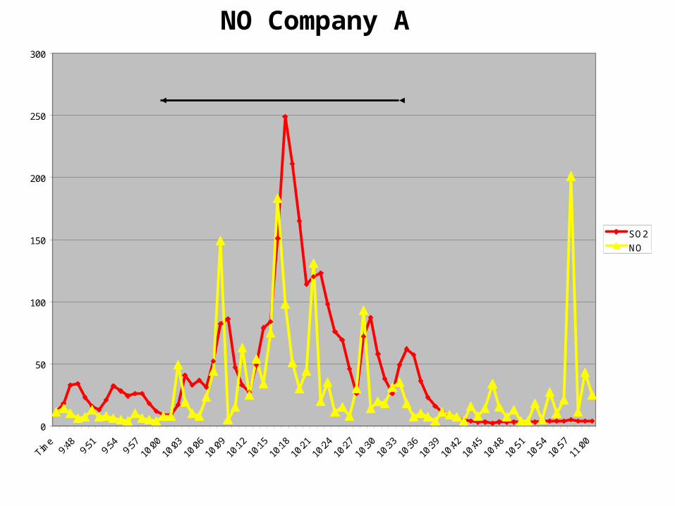
NO Company A

0

50

100

150

200

250

300

Time

9:48

9:51

9:54

9:57

10:0

010

:03

10:0

610

:09

10:1

210

:15

10:1

810

:21

10:2

410

:27

10:3

010

:33

10:3

610

:39

10:4

210

:45

10:4

810

:51

10:5

410

:57

11:0

0

SO2

NO

Company A

SO2

NOpp

b

19 Jan SO2

0

10

20

30

40

50

60

70

80

90

10:0

210

:1410

:2610

:3810

:5011

:0211

:1411

:2611

:3811

:5012

:0212

:1412

:2612

:3812

:5013

:0213

:1413

:2613

:3813

:5014

:0214

:1414

:2614

:3814

:5015

:0215

:1415

:2615

:3815

:5016

:0216

:1416

:26

SO2

C

Eastport

B

Burning rubber

D

A

B

pp

b

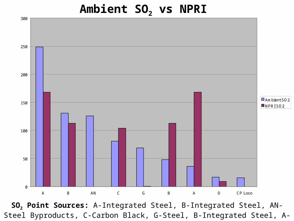
Ambient SO2 vs NPRI

0

50

100

150

200

250

300

A B AN C G B A D CP Loco

Ambient SO2

NPRI SO2BAN

C

G

AB

D CP

1.1km

.09

1.1

.25

3.5

3.2

.2 .02

0.8km

A

SO2 Point Sources: A-Integrated Steel, B-Integrated Steel, AN- Steel Byproducts, C-Carbon Black, G-Steel, B-Integrated Steel, A-Integrated Steel, D-Lime, CP-Rail Yard.

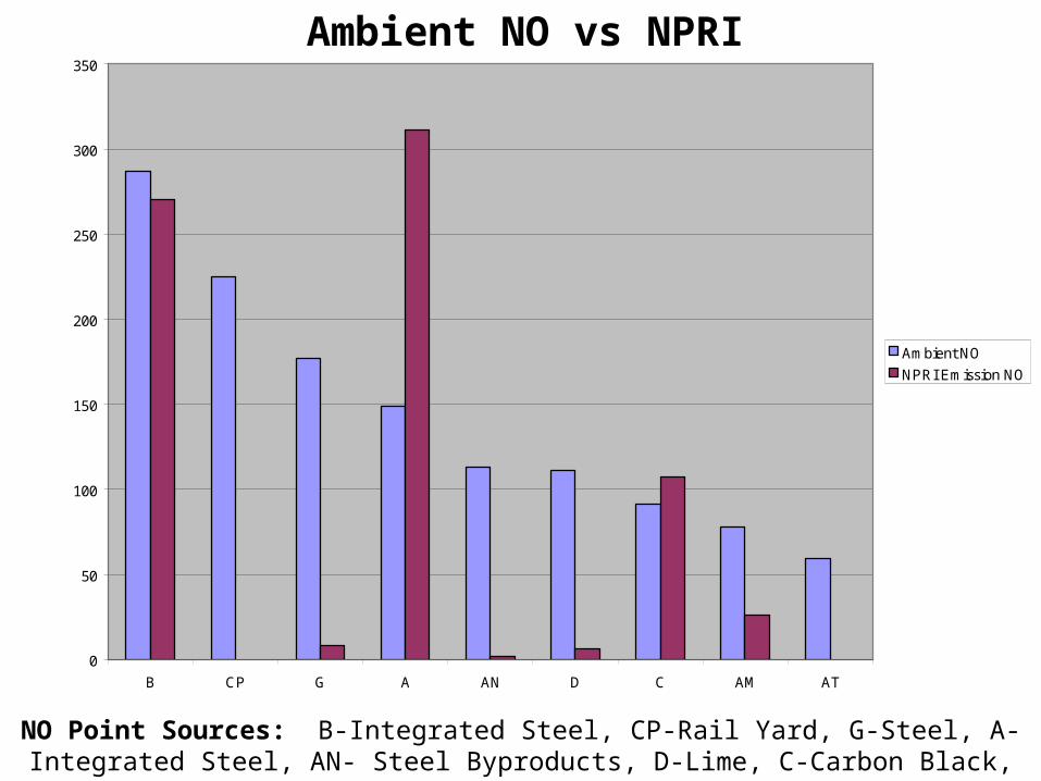
Ambient NO vs NPRI

0

50

100

150

200

250

300

350

B CP G A AN D C AM AT

Ambient NO

NPRI Emission NO

0.8

0.2

0.3

0.03

0.25

G

0.1

AN

0.32.3

CD

AM

AT

CP1.5km

B

A

NO Point Sources: B-Integrated Steel, CP-Rail Yard, G-Steel, A-Integrated Steel, AN- Steel Byproducts, D-Lime, C-Carbon Black, AM-Cogeneration, AT-Chemical.

Ambient PM10 vs NPRI

0

200

400

600

800

1000

1200

1400

1600

1800

2000

B ABP AY AG AU AT M G CP A AM C

Ambient P10

NPRI P10

1.5km

0.3

0.2

0.25CP

0.02 1

0.2

0.1 2.3

B

ABP

AT

G

A

M

AM

C

AY

0.1

AG

0.2 0.3

AU

PM10 Point Sources: B-Integrated Steel, ABP-Recycling, AY-Agricultural Product Handling, AG-Aggregate or AZ-Steel Handling, AU-Recycling, AT-Chemical, M-Foundry, G-Steel, CP-Rail Yard,

A-Integrated Steel, AM-Natural Gas Cogeneration Facility, C-Carbon Black.

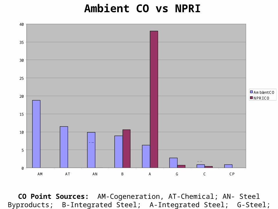
Ambient CO vs NPRI

0

5

10

15

20

25

30

35

40

AM AT AN B A G C CP

Ambient CO

NPRI CO

AM

AT

AN B

A

GC

CP

0.2km

0.10.1

2.5

0.251.1

0.03

3.6

CO Point Sources: AM-Cogeneration, AT-Chemical; AN- Steel Byproducts; B-Integrated Steel; A-Integrated Steel; G-Steel; C-Carbon Black; CP-Rail Yard.

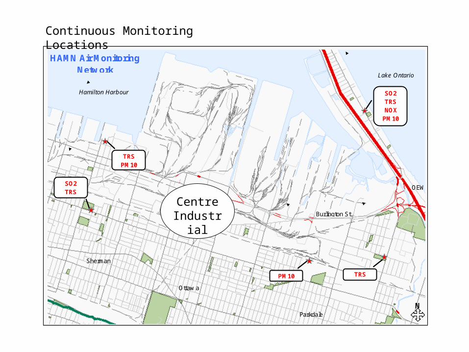
Lake Ontario

Hamilton Harbour

HAMN Air MonitoringNetwork

N

SO2TRS

TRSPM10

PM10 TRS

Parkdale

Ottaw a

Sherman

Burlington St.

QEW

SO2TRSNOX

PM10

Continuous Monitoring Locations

Centre Industrial

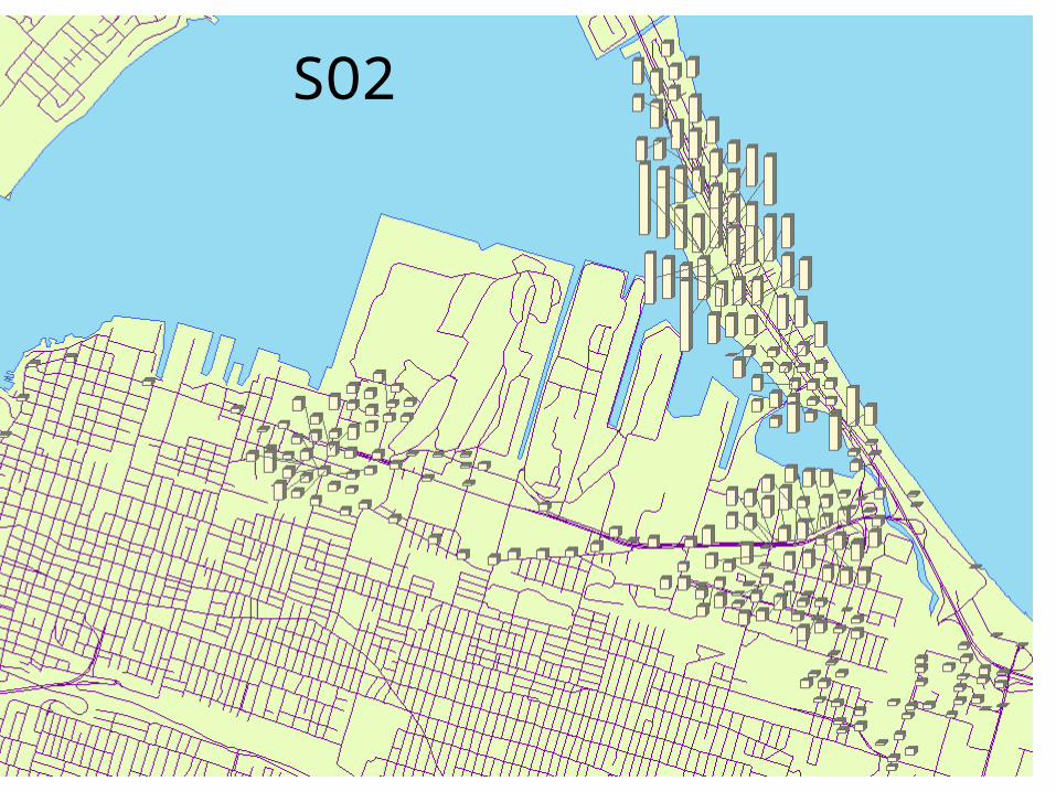
SO2

SO2

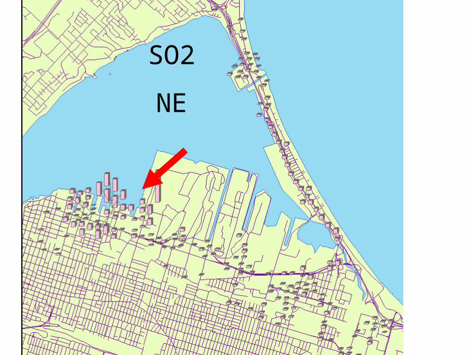
SO2

NE

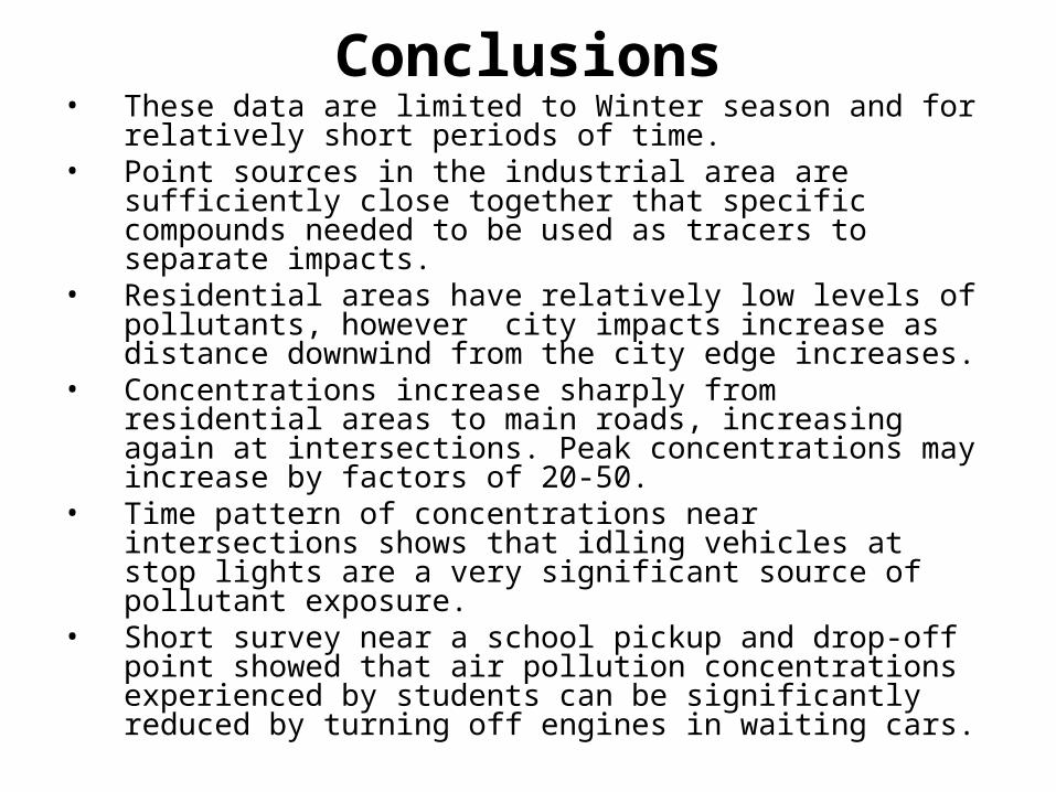
Conclusions• These data are limited to Winter season and for

relatively short periods of time.• Point sources in the industrial area are sufficiently

close together that specific compounds needed to be used as tracers to separate impacts.

• Residential areas have relatively low levels of pollutants, however city impacts increase as distance downwind from the city edge increases.

• Concentrations increase sharply from residential areas to main roads, increasing again at intersections. Peak concentrations may increase by factors of 20-50.

• Time pattern of concentrations near intersections shows that idling vehicles at stop lights are a very significant source of pollutant exposure.

• Short survey near a school pickup and drop-off point showed that air pollution concentrations experienced by students can be significantly reduced by turning off engines in waiting cars.

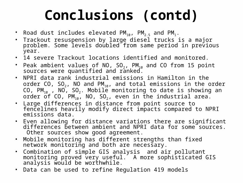
Conclusions (contd)• Road dust includes elevated PM10, PM2.5 and PM1.• Trackout resuspension by large diesel trucks is a major problem. Some

levels doubled from same period in previous year.• 14 severe Trackout locations identified and monitored.• Peak ambient values of NO, SO2, PM10 and CO from 15 point sources were

quantified and ranked.• NPRI data rank industrial emissions in Hamilton in the order CO, SO2, NO

and PM10, and total emissions in the order CO, PM10 , NO, SO2. Mobile monitoring to date is showing an order of CO, PM10, NO, SO2, even in the industrial area.

• Large differences in distance from point source to fencelines heavily modify direct impacts compared to NPRI emissions data.

• Even allowing for distance variations there are significant differences between ambient and NPRI data for some sources. Other sources show good agreement.

• Mobile monitoring has different strengths than fixed network monitoring and both are necessary.

• Combination of simple GIS analysis and air pollutant monitoring proved very useful. A more sophisticated GIS analysis would be worthwhile.

• Data can be used to refine Regulation 419 models

Recommendations• Move cycle lanes off main roads, innovative signage.• Reduce idling emissions, including at school dropoff locations (enlist parent teacher

groups).• Monitor school bus idling.• Prioritize trackout reduction - paving, wheel washing, front gate dust monitoring.• Reinstate/enhance targeted road cleaning in industrial areas.• Reduce large diesel truck trips, it’s the combination of heavy trucks and dirty roads

that is a problem.• Gateway monitoring of diesel exhaust at city entry/exit points, industrial arterials.• Continue reducing point source remissions of SOx, NOx and PM10 (both ambient and

NPRI data) in order to improve/reduce health impacts.• Review existing fixed network stations and locations to refocus on adverse health

causing pollutants, e.g. NOx, monitoring gaps.• Compare mobile data to MOE STAC data, more detailed GIS analysis.• Review NPRI data variances with ambient.• Extend mobile monitoring to other seasons for more definitive source separation in

complex areas and documenting different met regime impacts, particularly inversions.• Extend mobile monitoring to other communities.• Use mobile data to refine local source inputs to Regulation 419 models.Disclaimer:- All recommendations and opinions are the sole responsibility of D. Corr and do not necessarily represent the policy or position of

funding agencies or others.

Phase 2 Proposal• Perform a more sophisticated and comprehensive GIS analysis

of existing data to develop traffic impact and source impact mapping visualization

• Re equip instrumentation and modify the data collection system in the Mobile Unit for consolidated air pollution/GPS data collection.

• Meet with stakeholders to finalize monitoring targets and locations.

• Support the MOE and City of Hamilton Fugitive Emission Control Initiative through monitoring of control activities for effectiveness.

• Test existing models of city wide distribution of air pollution and extend mobile monitoring to fill data gaps across the City, e.g. Dundas, Stoney Creek.

• Perform Smog day/Inversion day monitoring, upwind of City and across City to identify Regional and Transboundary impacts and compare to City impacts.

Phase 2 Proposal• Perform sampling on major arterial roads, at intersections

and drive thrus.• Monitor downwind impacts of roads and intersections on

residential areas.• Perform more intensive monitoring of NPRI and other point

sources identified in Phase 1 in consultation with MOE staff.• Utilize McMaster University advanced spatial analysis

capabilities for pollution source visualization and in depth data analyses.

• Provide monitoring data to modelling initiatives for ongoing model calibration, e.g., GTA/Hamilton modelling exercise (Phase 2.

• Generate recommendations for air quality improvements. • Develop and give presentations on findings and

recommendations.