air force institute of technologyafit/ge/eng/96d-06 application of a finite-volume time-domain...

APPLICATION OF AFINITE-VOLUME TIME-DOMAINMAXWELL EQUATION SOLVER

TO THREE-DIMENSIONAL OBJECTS

THESIS

Frederick G. Harmon, Captain, USAF

-AHITGE/ENG/96D-06I !XTRIBOCW 'ATEMH AAppmwed tar pu~ miso

Dbr1budm Un~wte.d

DEPARTMENT OF THE AIR FORCEAIR UNIVERSITYU

AIR FORCE INSTITUTE OF TECHNOLOGY

Wright-Patterson Air Force Base, Ohio

DTIC QUALMT ~ ~wW.

AFIT/GE/ENG/96D-06



THESIS


AFIT/GE/ENG/96D-06

Approved for public release, distribution unlimited

The views expressed in this thesis are those of the authorand do not reflect the official policy or position of the

Department of Defense or the U.S. government

AFIT/GE/ENG/96D-06



THESIS

Presented to the faculty of the Graduate School of Engineering

of the Air Force Institute of Technology

Air University in Partial Fulfillment of the

Requirements for the Degree of

Master of Science in Electrical Engineering

Frederick G. Harmon, B.S.E.E.

Captain, USAF

December, 1996

Approved for public release, distribution unlimited

Acknowledgments

I dedicate this thesis to my Lord and Savior, Jesus Christ, my wife, Marie, and my dog,

Hannah. Jesus gave me the determination to complete this research and was faithful in

answering prayer throughout the thesis effort. Marie, who completed her graduate education

simultaneously with me, supported me throughout the thesis research and proofed the thesis

drafts numerous times. As my best friend, she was understanding, helpful, and instrumental in

the completion of the thesis. Hannah was patient during the many hours that I "ignored" her

while I was on the computer. We have all completed this together and grown as a family.

For guidance, encouragement, and assistance, I want to thank my thesis advisor, Dr.

Andrew Terzuoli, and the members of my thesis committee, Dr. William Baker, Major Tom

Buter, and Major Gerald Gerace. Dr. Naishadham, from Wright State University, and Captain

Doug Blake, a Ph.D. candidate at AFIT, also provided invaluable assistance.

Further, I want to thank my sponsors, Dr. J.S. Shang and Dr. Kueichien Hill, from

Wright Laboratory. Their guidance and insight kept me focused on the work that needed to be

accomplished. Dr. Hill was also very helpful in providing Moment Method results.

To my classmate, Jim Taylor, the AFIT experience has been tough but worthwhile and

enjoyable. Thanks for the friendship and the memories.

Dr. Vijaya Shankar from Rockwell and Ken Wurztler from Wright Laboratory deserve

recognition for generating the complicated grids. Also, this thesis research was supported in part

by a grant of high performance computing (HPC) time from the DoD HPC Centers, CEWES

(Cray 90) and Maui (SP-2). The personnel at these HPC centers generously provided computer

support for the Cray 90 and SP-2 used throughout this research effort.

Frederick G. Harmon

ii

Table of Contents

Page

A cknow ledgm ents.......................................................11........i

Table of Contents ...................................................................................... 1ii

List of Figures ............................................................................................. vi

List of Tables.............................................................................................. ix

List of Abbreviations and Variables ..................................................................... x

Abstract ................................................................................................ xii

1 Introduction .............................................................................................. 1

1.1 Background .................................................................................... 21.2 Problem Statement .............................................................................. 41.3 Summary of Current Knowledge .............................................................. 51.4 Assumptions ................................................................................... 71.5 Scope ............................................................................................. 71.6 Thesis Organization............................................................................. 8

2 Literature Review..................................................................................... 9

2.1 Overview......................................................................................... 92.2 Grid Generation of Finite-Volume Cells...................................................... 92.3 Maxwell's Equations .......................................................................... 102.4 Maxwell's Equations in Conservation Form ................................................ 112.5 Coordinate Transformation ................................................................... 122.6 Finite-Volume Formulation................................................................... 132.7 Boundary Conditions .......................................................................... 142.8 Flux Evaluation and Time Integration ....................................................... 152.9 Green' s-Function-Based Near-to-Far Field Transformation............................... 162. 10 Applications................................................................................. 172.11 Summary .................................................................................... 18

3 Methodology............................................................................................ 19

3.1 Overview........................................................................................ 193.2 FVTD FORTRAN Code Modifications ..................................................... 21

3.2.1 Geometry: Ogive...................................................................... 213.2.2 Geometry: Cone-sphere .............................................................. 233.2.3 Grid Files............................................................................... 243.2.4 Grid Modifications .................................................................... 27

Wi

3.2.5 Direction and Polarization of the Incident W ave ............................................ 283.2.6 Incident W ave Type ....................................................................................... 293.2.7 Scattered-Field Checks ................................................................................... 323.2.8 Bistatic-to-M onostatic Approxim ation .......................................................... 33

3.3 FVTD Computational Issues ...................................................................................... 343.3.1 Scattered-Field Formulation ............................................................................. 343.3.2 Stability ............................................................................................................... 353.3.3 Numerical Dispersion ...................................................................................... 363.3.4 Transient W aves ............................................................................................ 363.3.5 Creeping W aves and Traveling W aves .......................................................... 373.3.6 Diffraction ....................................................................................................... 37

3.4 Comparisons/Benchmarks ......................................................................................... 383.4.1 M ethod of M oments ........................................................................................ 383.4.2 Empirical Data ................................................................................................. 393.4.3 Error Calculations and M etrics ....................................................................... 39

3.5 Computer Support ..................................................................................................... 403.5.1 AFIT's Sparc 20 ............................................................................................ 413.5.2 AFIT's DEC Alpha ....................................................................................... 413.5.3 CEW ES HPCC's Cray 90 .............................................................................. 413.5.4 M aui HPCC's IBM SP-2 ................................................................................. 41

3.6 Summ ary ......................................................................................................................... 42

4 Applications, Results, and Comparisons ............................................................................... 43

4.1 Overview ......................................................................................................................... 434.2 Ogive Electrom agnetic Scattering Results ................................................................. 44

4.2.1 Ogive Bistatic RCS Results for 1.18 GHz, Sinusoid Incident Wave ............. 484.2.2 Ogive Bistatic RCS Results for 1.18 GHz, Gaussian Pulse Incident Wave ........ 564.2.3 Ogive M onostatic RCS Results for 1.18 GHz ................................................. 584.2.4 Ogive Bistatic RCS Results for 9.0 GHz ....................................................... 614.2.5 Ogive Bistatic RCS Results for the Gaussian Pulse Incident Wave ............... 63

4.3 Cone-Sphere Electrom agnetic Scattering Results ..................................................... 744.3.1 Cone-sphere Bistatic RCS Results for 0.869 GHz, Sphere-Cap Incidence ......... 774.3.2 Cone-Sphere Bistatic RCS Results for 0.869 GHz, Tip-On Incidence ........... 814.3.3 Cone-sphere M onostatic RCS Results for 0.869 GHz ................................... 834.3.4 Cone-sphere Bistatic RCS Results for 3.0 GHz ............................................. 85

4.4 Summary ......................................................................................................................... 87

5 Conclusions and Recommendations ..................................................................................... 89

5.1 Conclusions ..................................................................................................................... 895.1.1 Ogive RCS Results .......................................................................................... 905.1.2 Cone-Sphere RCS Results ............................................................................... 925.1.3 FVTD Computational Issues .......................................................................... 93

5.2 Suggested Areas for Further Research ........................................................................ 955.2.1 Surface Boundary Condition .......................................................................... 965.2.2 Radiation Boundary Condition ........................................................................ 965.2.3 M aterial Interfaces ......................................................................................... 965.2.4 Dielectric M aterials ........................................................................................ 97

iv

5.2.5 Frequency-Dependent and Time-Dependent Materials............................ 975.2.6 Anisotropic Materials ................................................................. 975.2.7 Multi-zoning for Complicated Objects.............................................. 985.2.8 Hybrid Techniques .................................................................... 985.2.9 Multi-discipline Applications......................................................... 985.2. 10 Code Optimization................................................................... 995.2.11 Summary............................................................................... 99

Appendix A: FVTD Formulation and Numerical Algorithm....................................... 100

A.1I Maxwell's Equations ....................................................................... 100A.2 Maxwell's Equations in Conservation Form ............................................. 101A.3 Coordinate Transformation................................................................. 102A.4 Finite-Volume Formulation................................................................ 104A.5 Eigenvalues and Eigenvectors ............................................................. 107A.6 Flux Evaluation using a Local Orthogonal Coordinate System........................ 110A.7 Time Integration............................................................................. 112A.8 Incident Wave ............................................................................... 113A.9 Boundary Conditions ....................................................................... 114

A.9. 1 Scatterer Surface Boundary Conditions .......................................... 114A.9.2 Radiation Boundary Condition .................................................... 114

A. 10 Fourier Transform ......................................................................... 115A. 11 Near-to-Far Field Transformation........................................................ 115

A. 11.1 Surface Equivalence Theorem.................................................... 116A. 11.2 Transformation .................................................................... 117

A. 12 RCS Calculations.......................................................................... 118A.13 Summary .................................................................................. 119

Appendix B: Finite-Volume Time-Domain FORTRAN Code..................................... 120

B. 1 FVTD FORTRAN Code Outline .......................................................... 120B.2 FVTD Code Listings of Modifications.................................................... 122

B.2.1 Input File............................................................................. 122B.2.2 Ogive Grid Modifications .......................................................... 128B.2.3 Incident Field........................................................................ 132B.2.4 RCS Convergence Check........................................................... 135B.2.5 Scattered-Field Threshold Check.................................................. 138B .2.6 Bistatic-to-Monostatic Approximation............................................ 140

B.3 Additional Codes ............................................................................ 142B.3.1 Error Calculations and Metrics .................................................... 142B.3.2 Scattered Electric Field Movie .................................................... 144

B.4 FVTD FORTRAN Code.................................................................... 147

Bibliography............................................................................................. 148

Vita ................................................................................................... 153

V

List of Figures

Page

Figure 1: FVTD Thesis Research Block Diagram .................................................................. 19

Figure 2: M esh Plot of EM CC-Defined Ogive ........................................................................ 22

Figure 3: Mesh Plot of EMCC-Defined Cone-Sphere ............................................................ 23

Figure 4: Slice of the Ogive Grid (10-121-30) in the yz Plane .............................................. 25

Figure 5: Slice of the Ogive Grid (10-121-30) in the xy Plane .............................................. 25

Figure 6: Slice of the Cone-Sphere Grid (50-73-45) in the xz Plane ....................................... 26

Figure 7: Slice of the Cone-Sphere Grid (50-73-45) in the xy Plane ..................................... 26

Figure 8: Incident W ave Specification ..................................................................................... 28

Figure 9: Gaussian Pulses with Different Bandwidths ............................................................ 31

Figure 10: Frequency Spectrum of Gaussian Pulses Shown in Figure 9 ................................ 31

Figure 11: Flowchart for RCS Convergence and Threshold Checks ....................................... 32

Figure 12: Ogive Bistatic RCS, 1.18 GHz, VV, Number of Cells Varied in R Direction ..... 49

Figure 13: Ogive Bistatic RCS, 1.18 GHz, VV, Number of Cells Varied in 0 Direction ........ 49

Figure 14: Ogive Bistatic RCS, 1.18 GHz, VV, Number of Cells Varied in Direction ...... 50

Figure 15: Ogive Bistatic RCS, 1.18 GHz, VV, Fine (71-125-55 ) vs. Coarse (71-43-25) Grid. 51

Figure 16: Ogive Bistatic RCS, 1.18 GHz, VV, Difference Between FVTD and MoM RCS ..... 51

Figure 17: Ogive Bistatic RCS, 1.18 GHz, VV, Cross-Correlation of FVTD and MoM RCS .... 52

Figure 18: Ogive Bistatic RCS, 1.18 GHz, VV, Fourier Transform of FVTD and MoM RCS... 53

Figure 19: Ogive Bistatic RCS, 1.18 GHz, HH, Fine (71-125-55) vs. Coarse (71-43-25) Grid.. 54

Figure 20: Ogive Bistatic RCS, 1.18 GHz, HH ........................................................................ 55

Figure 21: Ogive Bistatic RCS, 1.18 GHz, HH, Difference Between FVTD and MoM RCS ..... 55

vi

Figure 22: Ogive Bistatic RCS, 1.18 GHz, VV, Gaussian Pulse Incident Wave .................... 57

Figure 23: Ogive Bistatic RCS, 1.18 GHz, HH, Gaussian Pulse Incident Wave .................... 57

Figure 24: Ogive M onostatic RCS, 1.18 GHz, HH ................................................................. 59

Figure 25: Ogive Monostatic RCS, 1.18 GHz, HH, Error Between RCS Results ................... 59

Figure 26: Ogive M onostatic RCS, 1.18 GHz, VV ................................................................. 60

Figure 27: Ogive Bistatic RCS, 9.0 GHz, HH .......................................................................... 62

Figure 28: Ogive Bistatic RCS, 9.0 GHz, VV .......................................................................... 62

Figure 29: Ogive Bistatic RCS, 1.0 GHz, HH, Gaussian Pulse vs. Sinusoid Incident Wave ...... 65

Figure 30: Ogive Bistatic RCS, 1.0 GHz, VV, Gaussian Pulse vs. Sinusoid Incident Wave ...... 65






Figure 36: Ogive Bistatic RCS, 4.0 GHz, HH, Difference Between RCS Results .................. 70

Figure 37: Ogive Bistatic RCS, 4.0 GHz, HH, Cross-Correlation of FVTD and MoM RCS ...... 71


Figure 39: Ogive Bistatic Results, 4.0 GHz, Electric Field Contour Plot ............................... 72

Figure 40: Cone-Sphere Bistatic RCS, 0.869 GHz, VV, Sphere-Cap Incidence, Coarse Grid .... 78

Figure 41: Cone-Sphere Bistatic RCS, 0.869 GHz, VV, Sphere-Cap Incidence, Fine Grid ........ 78

Figure 42: Cone-Sphere Bistatic RCS, 0.869 GHz, VV, Difference Between RCS Results ....... 80

Figure 43: Cone-Sphere Bistatic RCS, 0.869 GHz, VV, Cross-Correlation of RCS Data .......... 80

Figure 44: Cone-Sphere Bistatic RCS, 0.869 GHz, HH, Sphere-Cap Incidence, Fine Grid ........ 81

Figure 45: Cone-Sphere Bistatic RCS, 0.869 GHz, HH, Tip-On Incidence ............................ 82

vii

Figure 46: Cone-Sphere Bistatic RCS, 0.869 GHz, VV, Tip-On Incidence ............................ 82

Figure 47: Cone-Sphere Monostatic RCS, 0.869 GHz, HH .......................................... 83

Figure 48: Cone-Sphere Monostatic RCS, 0.869 GHz, VV .................................................. 84

Figure 49: Cone-Sphere Bistatic RCS, 3.0 GHz, HH, Sphere-Cap Incidence ......................... 85

Figure 50: Cone-Sphere Bistatic RCS, 3.0 GHz, VV, Tip-On Incidence ................................ 86

Figure A .1: Finite-V olum e C ell ................................................................................................. 106

Figure A.2: Virtual Surface and Far-Field Sketch ..................................................................... 118

Figure B .1 : FV TD .F Flow chart .................................................................................................. 121

viii

List of Tables

Page

Table 1: O give Test M atrix .................................................................................................. 44

Table 2: Stability and Time Data for the Ogive Tests .......................................................... 46

Table 3: Grid Point Densities for the Ogive Tests ............................................................... 47

Table 4: MSE and Comparisons for the Ogive Tests .............................................................. 73

Table 5: Cone-Sphere Test Matrix .......................................................................................... 75

Table 6: Stability and Time Data for the Cone-Sphere Tests ................................................ 76

Table 7: Grid Point Densities for the Cone-Sphere Tests ....................................................... 76

Table 8: MSE and Comparisons for the Cone-Sphere Tests .............................................. 87

Table B.1: Gaussian Pulse Parameters for a Specified Bandwidth ............................................ 126

ix

List of Abbreviations and Variables

BC boundary condition

BOR body-of-revolution

c velocity of electromagnetic waves in free space (m/s)

CAD computer-aided design

CEM computational electromagnetics

CFD computational fluid dynamics

CFL Courant-Friedrichs-Lewy stability value

E electric field strength vector (V/m)

Eo, E, components of the incident E field vector

D electric flux density vector (C/m 2)

B magnetic flux density vector (Wb/m 2 or Tesla)

EMCC Electromagnetic Code Consortium

F, G, H flux vectors

F, G, H flux vectors in transformed curvilinear coordinates

FDTD finite-difference time-domain

FVTD finite-volume time-domain

GPD grid point density (cells/L?)

GTD geometrical theory of diffraction

H magnetic field strength vector (A/m)

HH polarization, transmit horizontal and receive horizontal

HPCC high performance computing center

i, j, k indices of a discretized finite-volume cell

x

k propagation vector of incident wave

J electric current density vector (A/m2)

MoM method of moments

MSE mean-square error

MUSCL monotone upstream-centered scheme for conservation laws

n time index

PEC perfect electric conductor

R, 0, q spherical coordinates

RAM radar absorbing material

t time variable (s)

U vector containing dependent variables, Cartesian components of B and D

UTD uniform theory of diffraction

V Jacobian of coordinate transformation, finite volume

VV polarization, transmit vertical and receive vertical

x, y, z Cartesian coordinates

6 electric permittivity (F/m)

A diagonal matrix containing the eigenvalues of the coefficient matrices

X wavelength (m)

pt magnetic permeability (H/m)

, 11, general curvilinear coordinates

P electric charge density (C/m3)

Gradar cross section (dBsm)

(0 radian frequency (rad/s)

xi

Abstract

Concurrent engineering approaches for the disciplines of computational fluid dynamics

(CFD) and electromagnetics (CEM) are necessary for designing future high-performance, low-

observable aircraft. A characteristic-based finite-volume time-domain (FVTD) computational

algorithm developed for CFD and herein applied to CEM is implemented to analyze the radar

cross section (RCS) of two three-dimensional objects, the ogive and cone-sphere, by utilizing a

scattered-field formulation of the time-dependent Maxwell equations. The FVTD formulation

uses a van Leer's kappa scheme for the flux evaluation and a Runge-Kutta multi-stage scheme

for the time integration. The RCS results are obtained from the electromagnetic fields

subsequent to a Fourier transform and a near-to-far field transformation.

Developmental work for the thesis focused on modifying the original code to analyze

scattering and obtain RCS data for closed-surface perfect electric conductor (PEC) 3-D objects

using either a Gaussian pulse or sinusoid incident wave. Specification of the direction and

polarization of the incident wave provides monostatic and bistatic results for various

polarizations. A RCS convergence check, used with a sinusoid, ends the simulation after the

transients diminish and the bistatic RCS values are within 0.1 dB of the RCS values calculated

during the previous period. A threshold check, used with a Gaussian pulse, ends the simulation

once the amplitude of the scattered field is 140 dB below the peak of the Gaussian pulse. A

bistatic-to-monostatic RCS approximation saves computer run time by a factor of nearly 40.

The FVTD code and algorithm are validated for electromagnetic scattering problems by

comparing FVTD code RCS results to data obtained from the Moment Method (MoM) code,

CICERO, and empirical RCS data published by the Electromagnetic Code Consortium (EMCC).

The FVTD RCS results for the ogive and cone-sphere are within 3.0 dB of the bistatic MoM

results and 3.1 dB of the monostatic empirical RCS data. Accurate FVTD computations of

diffraction, traveling waves, and creeping waves require a surface grid point density of 15-30

cells/X and a PEC boundary condition grid density of 200-400 cells/, dependent on frequency.

xii

APPLICATION OF A FINITE-VOLUME TIME-DOMAIN MAXWELL EQUATION SOLVER TO

THREE-DIMENSIONAL OBJECTS

1 Introduction

When designing low-observable, high-performance military aircraft, engineers must

consider both a low radar cross section (RCS) and excellent aerodynamic performance.

However, an optimum electromagnetic design may not be an optimum aerodynamic design. The

efficient design of future military aircraft requires concurrent multi-disciplinary approaches for

the electromagnetic and fluid dynamic disciplines. One computational design tool, the finite-

volume time-domain (FVTD) technique, can potentially consider optimum electromagnetic and

aerodynamic designs concurrently, benefiting the design process of low-observable, high-

performance aircraft [47]. Researchers have used FVTD successfully in the computational fluid

dynamics (CFD) discipline since the early 1980's [48] to analyze the airflow about an aircraft,

and recently, Shang, Shankar, Blake, Bishop, Huh, Noack, and others have applied the technique

to the computational electromagnetics (CEM) discipline [5, 6-7, 15, 22, 29-47]. The application

of the FVTD technique to the time-domain Maxwell equations of electromagnetics is relatively

new compared to other CEM techniques but is proving to be successful.

FVTD requires application to complicated three-dimensional (3-D) benchmark objects

for researchers to consider it a feasible computational tool for electromagnetic scattering

problems. In this thesis research, the comparison of FVTD scattering results for the three-

dimensional objects, the ogive and cone-sphere, to Method of Moments (MoM) and empirical

RCS data validates the FVTD technique in the area of electromagnetics. The MoM calculations,

obtained from the code CICERO, and the empirical RCS data, published by the Electromagnetic

Code Consortium (EMCC), serve as benchmarks for the FVTD RCS computations.

1.1 Background

FVTD is a logical choice for simulations in both computational fluid dynamics and

computational electromagnetics. Fluid dynamics utilizes FVTD to solve the Euler equations by

calculating the fluxes, such as energy or mass, through finite-volume cells of a discretized space

[8]. The Maxwell equations, which model electromagnetic phenomena, are hyperbolic like the

Euler equations; that is, both systems of partial differential equations have real eigenvalues

(characteristic values). Their similar mathematical form permits the use of the same algorithm to

numerically solve each set of equations. Thus, hyperbolic equation solvers developed for CFD,

such as FVTD, can potentially be applied to Maxwell's equations of CEM.

In addition to multi-discipline applications, FVTD has other potential advantages

including [18, 51]

" the direct solution of Maxwell's two curl partial differential equations

" the analysis of electromagnetic propagation through frequency-dependent, time-

dependent, and anisotropic materials

* the ability to obtain multiple frequency results with a single simulation

Specifically, the direct solution of Maxwell's time-dependent equations is robust and potentially

as accurate as the Method of Moments [18, 51]. The finite-difference time-domain (FDTD)

technique, which also directly solves Maxwell's partial differential equations, provides highly

2

accurate simulations for free space electromagnetic scattering problems [51]. The Helmholtz

equations, the time-harmonic wave equations derived from the Maxwell equations, are not used;

therefore, the propagation of electromagnetic waves through frequency-dependent and time-

dependent materials can be calculated. FVTD also permits the analysis of anisotropic materials,

such as radar absorbing materials (RAM) found in filled honeycomb structures [42].

Additionally, the time-domain algorithm allows the solution of a problem for more than one

frequency. Broadband incident waves, such as Gaussian pulses, can be used to obtain multiple

frequency results.

The two most prominent FVTD researchers in the area of CEM are Dr. Vijaya Shankar

of the Rockwell International Science Center [42-47] and Dr. Joe Shang of the Air Force's

Wright Laboratory [29-41]. Both have written characteristic-based FVTD codes for analyzing

the electromagnetic scattering from objects. The two codes differ in several significant areas:

mathematical algorithm, order of accuracy, and capability. Shang has implemented a spatially

third-order accurate algorithm and a temporal fourth-order accurate scheme in the FVTD code,

while Shankar has implemented a second-order accurate algorithm. The higher-order accurate

code can potentially reduce the required number of grid points per wavelength permitting the

computation of the electromagnetic scattering from electrically larger objects and reducing the

computer simulation time [36, 40]. The differences between the algorithms and the accuracy of

the codes are discussed in more detail in Chapter 2.

The Rockwell FVTD code currently has more capability than the Wright Laboratory

FVTD code. The Rockwell FVTD code has the ability to analyze the scattering from

complicated objects and surfaces such as airfoils, inlets, and edges, while the Wright Lab FVTD

code, prior to this research, was limited to calculating the scattering from a sphere [39, 41, 44,

46]. The Rockwell code can also calculate the electromagnetic scattering from layered dielectric

3

surfaces such as those found on low-observable aircraft. The Wright Lab FVTD requires

modification to calculate the electromagnetic scattering from complicated 3-D objects and

dielectric surfaces. After first modifying the Wright Lab FVTD code for this thesis research, an

analysis of the electromagnetic scattering is performed for the complicated perfect electric

conductor (PEC) objects: ogive and cone-sphere. The code has yet to be modified for dielectric

surfaces.

1.2 Problem Statement

The objectives of this research are to

" modify the Wright Lab FVTD code to analyze the electromagnetic scattering from

complicated perfect electric conductor (PEC) three-dimensional (3-D) objects

" validate the characteristic-based FVTD formulation by using the modified code to

analyze the scattering from the 3-D objects, ogive and cone-sphere, and compare the

FVTD RCS results to MoM results and empirical data published by the EMCC.

Prior to the thesis research, the Wright Lab FVTD code required modification to analyze

the electromagnetic scattering from complicated three-dimensional objects such as an ogive and

cone-sphere or other closed-surface, single-zone objects. The original FVTD code was limited to

calculating the RCS from a sphere and required modification for closed-surface three-

dimensional objects. A modification changing the spherical coordinate system dependency to a

curvilinear grid system which is applicable for closed-surface objects permits the code to be

applied to complicated 3-D geometries. Code modifications also include the ability to add grid

points near tips of objects to ensure accuracy. The incident wave specification in the original

FVTD code also required modification. The original code limited the specification of the

incident wave to a sinusoid with one polarization and one direction of propagation.

4

Modifications permit an incident wave with options for specifying the direction, polarization,

and type, either a sinusoid or broadband Gaussian pulse. The incident wave modifications permit

the calculation of monostatic and bistatic RCS results for different polarizations. The Gaussian

pulse provides scattering results for multiple frequencies with one simulation. A bistatic-to-

monostatic approximation reduces computer simulation times for monostatic RCS calculations.

An analysis of the effectiveness of using FVTD to compute the electromagnetic

scattering from complicated objects is a requirement before the Wright Lab FVTD code and

algorithm can be considered a feasible computational design tool. The comparison of FVTD

RCS calculations to a historically proven CEM method such as the Method of Moments and to

empirical RCS data validates its capability and accuracy. This validation is completed for the

EMCC-defined ogive and cone-sphere in this thesis research.

1.3 Summary of Current Knowledge

The FVTD formulation is characteristic-based. Chapter 2 gives an overview of the

characteristic-based schemes used by different researchers. Dr. Shang's specific FVTD

formulation and characteristic-based numerical algorithm are described in detail in Appendix A.

Reportedly, the advantages of characteristic-based computational algorithms are [30]

" a naturally enforced well-posedness condition for specifying initial values

" a windward spatial discretization based on the direction of wave propagation

" a radiation boundary condition (BC) based on a compatibility condition

Specifically, the windward spatial discretization imitates the physics of the electromagnetic

scattering. For instance, it imitates the direction of wave propagation. The sign of the

eigenvalue corresponds to the direction of propagation. Forward differencing is used with the

5

negative eigenvalues and backward differencing with the positive eigenvalues. The compatibility

condition minimizes erroneous numerical reflections from the outer boundary of the grid.

The process of applying the characteristic-based FVTD formulation to electromagnetics

problems is sequential and follows a logical procedure. First, the physical space surrounding the

object of interest, such as an aircraft, is discretized into finite-volume cells. The space grid refers

to the computational space containing the cells [51]. The frequency of interest and the electrical

length of the object determines the number of cells required in the space grid [47]. The finite

truncated space of a computational domain will generate numerical reflections in the space and

produce erroneous computations [37]. Radiation boundary conditions, such as the compatibility

condition which sets the incoming flux component equal to zero, are implemented at the edges of

the truncated space and reduce the numerical reflections in the grid space.

Second, for use in the FVTD algorithm, the time-domain Maxwell partial differential

equations are placed in conservation form (See Chapter 2 or Appendix A) [47]. Maxwell's

equations comprise a hyperbolic system of partial differential equations which can be solved

using characteristic-based analysis. The Maxwell equations in conservation form are applied to

every finite-volume cell in the grid and solved numerically in the spatial and temporal domains

using one of several techniques. The spatial techniques, or flux evaluation methods, are broadly

categorized as implicit or explicit (See Chapter 2) [37]. For the time integration, Maxwell's

equations in FVTD form are integrated using one of several techniques.

For the implementation of the FVTD technique, the scattered-field formulation is used as

opposed to the total-field formulation. Only the scattered electric and magnetic fields and not the

total fields propagate through the space grid. The scattered-field formulation is implemented for

a PEC object by setting the tangential electric field on the scatterer surface equal to the negative

of the tangential incident field. The incident field never appears in the FVTD calculations.

6

Finally, the far-field RCS is computed. The scattered fields computed by FVTD give

calculations in the near-field and in the time-domain. A Fourier transform permits frequency

data to be obtained from the time-domain data. A Green' s-function-based transformation allows

the far-field RCS to be easily calculated from the near-field frequency data [51].

1.4 Assumptions

To modify the Wright Lab FVTD code for complicated objects, several assumptions

were made. First, the radiation boundary condition, or compatibility condition, implemented by

Shang was assumed to be sufficient. The compatibility condition sets the incoming flux

component equal to zero. The boundary condition is only accurate if the scattered

electromagnetic wave is parallel to one of the transformed coordinates [30, 38]. Numerical

errors introduced because the propagating wave is not parallel to a coordinate axis were not

addressed. The first-order surface boundary condition for a PEC surface was also assumed to be

sufficient for the purposes of this thesis research.

Second, the mathematical algorithm used by Shang, van Leer's kappa scheme, was

assumed to be the most adequate method for the flux evaluation in Maxwell's equations. Shang

has studied numerous FVTD numerical techniques for solving Maxwell's equations and the

current flux evaluation technique is assumed to be the most efficient and accurate [29-41].

1.5 Scope

The focus of this thesis research was to modify the Wright Lab FVTD code to compute

the scattering from the ogive and cone-sphere and validate the FVTD code by comparing FVTD

RCS results to MoM and empirical RCS data.

7

Perfect electric conductor (PEC) surfaces are used for the complicated three-dimensional

objects. Dielectric surfaces were not studied; therefore, multi-zoning which requires generating

different grids for each dielectric surface or layer, is not implemented in the FVTD code.

FVTD codes potentially require massive amounts of computational time and memory.

Modifying the code for speed optimization or parallel computing was not emphasized because

other researchers such as Blake are optimizing the code for parallel computing [6, 7].

1.6 Thesis Organization

With Chapter 1 serving as the basic foundation for FVTD and the research which needs

to be completed in the area of CEM, Chapter 2 discusses the FVTD formulation and the

numerical techniques used by various researchers such as Shang and Shankar to solve

electromagnetic scattering problems. Chapter 3 discusses the methodology used in completing

the research and the code modifications that were required to thoroughly analyze the scattering

from the ogive and cone-sphere using FVTD. The FVTD RCS results for the ogive and cone-

sphere using the modified Wright Lab FVTD code are presented in Chapter 4 along with a

discussion of the results. Also in Chapter 4, FVTD results are compared to MoM results and

empirical RCS data. Chapter 5 contains conclusions on the FVTD research and includes

proposed areas of future FVTD research. The two appendices contain supplemental data on the

FVTD formulation and code development. In Appendix A, the FVTD formulation and numerical

algorithm implemented by Dr. Shang in the Wright Lab FVTD code are discussed. Appendix B

contains code listings and descriptions of the FVTD code modifications.

8

2 Literature Review

2.1 Overview

The FVTD computational technique is capable of concurrently solving the Euler

equations of fluid dynamics and the Maxwell equations of electromagnetics. CFD has used the

FVTD technique since the early 1980's [48] to analyze the airflow about an aircraft or airfoil and

the technique has recently been applied to CEM. Several engineers, Blake, Shang, Shankar,

Bishop, Huh, and Noack, are exploring and advancing the application of the FVTD technique to

the Maxwell equations of electromagnetics [5, 6-7, 15, 22, 29-41, 42-47].

The FVTD technique follows a logical procedure from grid generation and formulating

the Maxwell equations in FVTD form to evaluating the fields or fluxes through each cell of the

grid. The computed scattered-field results are then transformed from the near-field to the far-

field. From the far-field calculations, RCS results are obtained. The following sections discuss

the FVTD procedures for applying FVTD to electromagnetic scattering problems and the

characteristic-based FVTD formulations and numerical algorithms implemented by Shang and

Shankar. Appendix A describes in detail one specific formulation and numerical algorithm used

by Shang and implemented in the FORTRAN code in this thesis research.

2.2 Grid Generation of Finite-Volume Cells

Computer simulations require that 3-D geometries in a physical space be accurately

represented in a computational domain [47]. To use FVTD, the physical space surrounding an

object of interest, such as the ogive and cone-sphere used in this thesis, must be discretized into

volumetric cells. The space containing the finite-volume cells is referred to as the space grid

9

[51]. The frequency of interest and the electrical length of the object determines the number of

cells in the grid [47]. The grid can take on several forms, either structured or unstructured.

A structured grid is defined by clearly distinguishable coordinate directions [7]. Simple

shapes or surfaces which can align with the axes of the three-dimensional coordinate system use

the structured grid. In contrast to the structured grid, an unstructured grid contains undefinable

coordinate directions [7]. An advantage of the unstructured grid is its ability to conform the grid

to the surfaces of irregular objects.

For characteristic-based FVTD formulations, a structured grid using curvilinear

coordinates is used so the wave propagation is aligned closely with one of the coordinate axes

[34]. The compatibility condition used for the radiation boundary condition is exact if the wave

propagation parallels a coordinate axis. In addition, the curvilinear coordinates permit higher

accuracy in the computation of the electric and magnetic scattered fields. The fields at the

centers of the cells and the fluxes at the faces of the cell are calculated using the metrics of the

cell and the curvilinear coordinates better represent the geometric features of the object resulting

in higher accuracy of the scattered field computations.

2.3 Maxwell's Equations

The time-domain Maxwell equations, in differential form, are shown below and will be

used in the development of the electromagnetic FVTD equations:

Faraday's Law: V x E =-- (1)at

OJDAmpere's Law: V x H =- + J (2)at

Gauss's Electric Law: V . D = p (3)

Conservation of Magnetic Charge: V. B = 0 (4)

10

where E: Electric field strength vector (V/m)

D: Electric flux density vector (C/m 2)

H: Magnetic field strength vector (A/m)

B: Magnetic flux density vector (Wb/m 2 or T)

J: Electric current density vector (A/m2)

P: Electric charge density (C/m 3)

The constitutive parameters relate the field strength vectors and the flux density vectors.

The constitutive parameters, the electric permittivity and the magnetic permeability, are normally

expressed as tensors. However, if the material is linear and isotropic, the constitutive parameters

are scalars and the constitutive relations become

D = eE and B =gH (5)

where F: Electric permittivity (F/m)

g: Magnetic permeability (H/m)

The four Maxwell equations are interdependent. The two divergence equations can be

derived from the two curl equations using the conservation of charge relationship

V- J = - ap / at assuming the material is linear and isotropic. The FVTD calculations do not

use the two divergence equations, but the equations can be used as a check on the predicted field

response [18].

2.4 Maxwell's Equations in Conservation Form

For use in FVTD, the two curl Maxwell equations are cast in conservation form [37].

The solution of Maxwell's equations do not require the conservation form; however, the form is

required by the Euler equations to conserve physical properties such as energy, mass, and

momentum [8]. The Maxwell equations are also cast in conservation form to take advantage of

11

the same computational technique used to solve the Euler equations. To place the two curl

Maxwell equations in conservation form, the curl operations are carried out and the constitutive

parameters are implemented. The result is given by [37]

U aF aG aH- +-y+- =-J (6)

at ax y az

where

Bx 0 Dz Dy 0

By -Dz 0 Dx 0

U= B F Dy e G -D/ H= 0 j 0

Dx 0 -Bz/ By Jx

Dy Bz/ 0 -Bx / g Jy

.Dz -- By [ .Bx ] g .0 .JZ.

Equation (6) is a system of six linear equations. U is the independent variable and the F, G, and

H flux vectors are the dependent variables. The equations are not linearly independent;

therefore, a characteristic-based technique is needed to uncouple the six equations.

2.5 Coordinate Transformation

To analyze the scattering of various objects, including the ogive and cone-sphere

analyzed in this thesis, a curvilinear coordinate transformation is required [37]. A curvilinear

structured grid minimizes the errors introduced in the cell metrics and the flux calculations. The

order of accuracy will be below the formal order of accuracy if a poor curvilinear grid is

generated [34]. The coordinate transformation converts the Cartesian coordinates to curvilinear

coordinates. The transformation defines a one-to-one relationship between two sets of temporal

and spatially dependent variables. The variables used are , 11, and and are all functions of x, y,

and z. Equation (6), after a coordinate transformation, becomes [37, 38]

12

M aG atHt) +T 6 - =-j (7)dt D" iDa

where =UV

jV

ax ay ) V

G; (= q F +F + G+ H 1aDx ay az 9V

(ax ay az )V

V is the Jacobian of the coordinate transformation and is equal to [34]

ax ay az ax ax ax

V=al 0 O_ Q K- -T (8)ax ay az ay ay ayat, at a a , 0_1 Kax ay az az az az

A coordinate transformation closely aligns the direction of propagation of the scattered

electric and magnetic fields to the coordinate directions [37]. The radiation boundary condition

produces fewer numerical reflections if the coordinate axis closely parallels the direction of

propagation of the scattered fields.

2.6 Finite-Volume Formulation

Equation (7) is applied to every finite-volume cell in the grid. An integration is

performed over each finite-volume cell:

13

aJJ -dV + JJJ y- + ad +aiiJ dV=- JJjdV (9)ffdV-- at~ dVf f

The divergence theorem is then applied to the second integral:

f JJudV +s(F + G + H). n dS =-f JdV (10)

where n: Unit vector normal to the surface ( , il, and ; for F, G, and H, respectively)

S: Closed surface bounding the finite volume (m2)

Equation (10) is the expression for a generic FVTD formulation. The unknown

components of the & vector are the magnetic and electric flux densities. The vectors

P, G, and H are the flux vectors and can be expressed in terms of the magnetic and flux

densities. A multitude of techniques are used to solve Equation (10) and differentiate the myriad

of FVTD numerical algorithms.

2.7 Boundary Conditions

Realistically, radar waves scattered from an object travel away from the object and are

not reflected back to the target. However, the truncated space of a computational domain will

generate numerical reflections in the space and produce erroneous computations [45].

Implementing a radiation boundary condition (BC) reduces the numerical reflections in the grid

space.

Shankar and Shang use a first-order accurate radiation BC [30, 45]. For precise

calculations, first-order accuracy is not acceptable and higher-order BCs would ensure higher

accuracy. Shang and Shankar use a compatibility condition in which the incoming flux

component is set to zero at the boundary [37]. For the compatibility condition, the fields

traveling perpendicular to the boundary are not reflected. For example, in the case of the

14

propagation of a wave from a dipole, the BC is exact since the wave travels along the radial

coordinate direction. However, numerical errors can result if the wave is not traveling

perpendicular to the boundary. The coordinate transformation discussed previously increases the

component of the wave traveling perpendicular to the outer boundary [37].

A surface boundary condition is implemented on the surface of PEC scatterers. The BC

sets the tangential electric field equal to zero and the normal component of the magnetic flux

density equal to zero [7]. Details for the PEC BCs implemented for this thesis research can be

found in Appendix A. Boundary conditions are also required for dielectric interfaces and details

for these BCs can be found in the Shankar references [42-47].

2.8 Flux Evaluation and Time Integration

The flux vectors in Equation (10) can be evaluated numerically using one of several

techniques which can be broadly categorized as explicit or implicit [30, 47]. Explicit numerical

expressions place the independent and dependent variables on different sides of the equation.

Implicit expressions are recognized by the intermixing of the dependent and independent

variables on each side of the equation.

The techniques implemented by Shang and Shankar are explicit characteristic-based

schemes. The objective of the characteristic-based numerical procedures is to achieve the

Riemann approximation to a three-dimensional problem in each spatial dimension [30]. The

three-dimensional Maxwell equations can then be solved in each dimension sequentially.

Shang has studied and applied several characteristic-based implicit and explicit

techniques. He is presently using an explicit van Leer's kappa scheme in which the flux on a

surface of a cell is extrapolated from data of adjacent cell centers [34]. The scheme is referred

to as a Monotone Upstream-Centered Scheme for Conservation Laws (MUSCL) and is a

15

windward approach that considers the direction of wave propagation. The MUSCL approach

produces various orders of accuracy. The approach used in this thesis research produces results

which are third-order accurate. The details of van Leer's kappa scheme are discussed in

Appendix A.

A flux-vector splitting algorithm developed by Steger and Warming [48] is used to

calculate the fluxes from the independent variable U. The incoming and outgoing

electromagnetic waves are split based on the positive and negative sign of the characteristic,

hence, the name split-flux vectors.

Shankar uses an explicit Lax-Wendroff upwind scheme that is characteristic-based. The

scheme uses a predictor and a corrector step. The predictor step results in a first-order accurate

solution. The corrector step increases the accuracy of the solution to second-order [42].

Equation (10), in the temporal or time-stepping domain, can be solved using several

techniques, just as in the spatial domain. Shankar uses the same second-order Lax-Wendroff

upwind scheme. Shang uses a Runge-Kutta family of single-step multi-stage procedures [32, 38]

which gives varying degrees of accuracy. For example, with van Leer's kappa scheme for the

flux evaluation, he uses either a two-stage or four-stage Runge-Kutta method that produces

second-order accuracy and fourth-order accuracy, respectively [34].

The higher-order accurate Wright Lab code can potentially reduce the required number

of grid points per wavelength permitting the computation of the electromagnetic scattering from

electrically larger objects and reducing the computer simulation time [36, 40].

2.9 Green's-Function-Based Near-to-Far Field Transformation

The spatial and time integration of Equation (10) gives results in the near-field. Various

calculations, such as the RCS, are far-field results. The FVTD grid is in the near field; however,

16

Green' s-function-based transformations allow the scattered fields in the far-field to be easily

calculated from the near-field results subsequent to a Fourier transform [51]. The near-to-far

field transformation permits the FVTD grid to be truncated in the near-field and does not have to

extend out to the far-field to obtain the RCS data.

The far-field results are obtained by creating a virtual surface around the object. This

surface does not have to conform to the object. An imaginary surface in the FVTD grid space

can serve as a virtual surface. The surface equivalence theorem is applied to the surface to

obtain the equivalent time-harmonic electric and magnetic currents and charges. The currents

and charges on the virtual surface are then weighted by a free-space Green's function to obtain

the far-field E and H fields [51]. The far-field results, such as the RCS, are easily calculated

from the far-field scattered E and H fields.

2.10 Applications

As mentioned previously, FVTD is relatively new to CEM. Shankar, Shang, Blake, and

others have applied the FVTD codes to analyzing the electromagnetic scattering from various

objects. Shankar has analyzed a two-dimensional PEC and dielectric circular cylinder [44]. Also

in 2-D, Shankar has analyzed a simple engine inlet, ogive, and airfoil [44]. In addition, Shankar

has completed extensive 3-D research in which he has analyzed a PEC sphere and missile. He

has also worked with frequency-dependent materials [44]. Other applications can be found in

Shankar's contract report [42].

Shang has used his various FVTD codes to analyze the scattering from a sphere,

propagation from a dipole, and the propagation of a wave through a waveguide. Blake has

rewritten Shang's FVTD vectorized code for parallel computing machines and has used his

17

modified code to study the propagation of an electromagnetic wave in a waveguide and the

scattering from a single sphere and dual spheres [6, 7].

2.11 Summary

Computational techniques which permit simultaneous trade-offs between the

electromagnetic and aerodynamic disciplines would greatly improve the efficiency of the

engineering design process for low-observable aircraft. The FVTD computational technique is

capable of solving the Euler equations of fluid dynamics and the Maxwell equations of

electromagnetics. The FVTD technique, historically proven for fluid dynamics, has excellent

potential in computational electromagnetics. Several engineers, such as Shang, Shankar, and

Blake, are advancing the application of the FVTD technique to solving the Maxwell equations of

electromagnetics.

The FVTD technique follows a logical process for calculating electromagnetic data for a

scattering object. A curvilinear grid is generated about an object to ensure accurate results from

the FVTD formulation. The Maxwell equations are placed in conservation form and then solved

in the spatial and temporal domains using a technique dependent on the desired accuracy.

Numerical reflections in the domain are reduced by implementing outer boundary conditions.

Depending on the desired results, transformations can be applied to the computational results.

18

3 Methodology

3.1 Overview

For the thesis research, a disciplined approach was taken to modify the code and validate

the FVTD formulation by studying the electromagnetic scattering from an ogive and cone-sphere.

Figure 1 illustrates the basic approach used to complete the FVTD research. By performing

several tasks concurrently, more research was completed successfully and efficiently. The

columns in the block diagram correspond to the tasks which were performed in parallel and

include the broad areas of FVTD code, comparisons/benchmarks, and computer support.

FVTD

Thesis Research

IFVT,,oode Comparisons/ I Computer IS Benchmarks Support

Grid/BCNalidation CEM Code Results Sparc 20/DEC AlphaI ICode Moment Method: EMCC H

Modifications CICERO Empirical Data Cray 90/IBM SP-2

Figure 1: FVTD Thesis Research Block Diagram

The first task, FVTD code, was the focus of the thesis research. The FVTD code was

first used to solve for the scattering of a PEC sphere to become familiar with the software, the

FVTD formulation, grid generation, and boundary conditions. Analytical solutions for the

19

scattering of a sphere were used as benchmarks and for verifying code modifications to ensure

accurate changes. Shang has published results for the sphere using the original FVTD code [38].

The reference includes comparisons to analytical solutions.

After becoming familiar with the code, it was modified to obtain electromagnetic

scattering results from the PEC surfaces of an ogive and cone-sphere. The modified code can be

used for other closed-surface perfect electric conductor (PEC) 3-D objects if an appropriate grid

is generated. Appendix B contains the detailed requirements for the grid. The Rockwell

International Science Center generated the grid for the ogive and the Flight Dynamics Directorate

of Wright Labs generated the grid for the cone-sphere. In addition to modifying the code for a

generic 3-D object, the option of specifying the direction, polarization, and type of the incident

wave was programmed. Also programmed was an RCS convergence check used with a sinusoid

incident wave which ends the simulation after the transients diminish. A threshold check, used

with a Gaussian pulse incident wave, ends the simulation once the scattered field is below a pre-

determined threshold. A bistatic-to-monostatic approximation saves computer simulation time

for monostatic computations.

To complete the research, another CEM technique and experimental measurements were

used as benchmarks. Column two in Figure 1 corresponds to the code and experimental results

used as comparisons. The Method of Moments, considered as a very accurate CEM code, is used

as a benchmark. The body-of-revolution Moment Method code, CICERO [55], was used to

obtain bistatic and monostatic RCS results for the ogive and cone-sphere. Experimental

measurements published by the Electromagnetic Code Consortium (EMCC) are benchmarks for

the monostatic calculations [55]. The empirical results are excellent data to use as benchmarks

and validate developmental CEM codes such as the FVTD code.

20

The third task, computer support, was critical in the completion of the research. The Air

Force Institute of Technology (AFIT) machines, the SUN Sparc 20 and DEC Alpha machines,

were used to assess code modifications. A Cray 90 at the USAE Waterways Experiment Station

(CEWES) high performance computing center (HPCC) in Vicksburg, Mississippi was used to

complete the majority of the computer simulations for the ogive. The SP-2 at the Maui HPCC in

Maui, Hawaii, was used to complete the monostatic tests for the cone-sphere. The Cray 90 and

SP-2 were invaluable in completing the research.

3.2 FVTD FORTRAN Code Modifications

The original FVTD FORTRAN code calculated the electromagnetic scattering from a

sphere. The code modifications permit the calculation of the scattering from other closed-

surface, single-zone, 3-D objects. The capability was added to read grid files generated by

computer-aided design (CAD) software programs. Options for changing the size of the grid,

such as the addition of grid points at diffraction points, were implemented to improve accuracy

of the scattered-field computations. The original code specified the incident wave to propagate

from only one direction with one polarization. The direction and type of incident wave was

added along with an RCS convergence check and a threshold check for the scattered field. A

bistatic-to-monostatic approximation obtains monostatic results from bistatic results. Appendix

B contains the code and subroutines written for the code modifications and related functions.

3.2.1 Geometry: Ogive

The ogive is a very common test body for code validation and is a classic low-observable

shaped body. The ogive is a body-of-revolution formed by rotating a convex arc around a chord

[27]. No analytical solution for the electromagnetic scattering from an ogive is available;

21

therefore, MoM results and experimental data are used as benchmarks. The EMCC-defined

ogive is 10 inches (0.254 m) long, has a maximum radius of 1 inch (0.0254 m), and a half-angle

of 22.62 degrees [55]. The single ogive with a metallic surface is described mathematically as

f(z) = - cos(22.62 °) + 1- - sin(22.62 °) (11)

f(z) cos s(

x = (22.62 0 (12)1 - cos(22.62 °)

f (z) sin A ( 31 - cos(22.62*)

for -5.0 < z < 5.0 inches

-7t < P < r radians

X

0).030

-0.020

O0

-OOi 0 MC

y (m)

Figure 2: Mesh Plot of EMCC-Defined Ogive

22

Figure 2 is a mesh plot of the single ogive. Note that the ogive is approximately one wavelength

long at 1.18 GHz [55]. The units in the plot are in meters.

3.2.2 Geometry: Cone-sphere

The cone-sphere is another common RCS test body which is also a body-of-revolution.

The EMCC-defined cone-sphere has a half-angle of 7.0 degrees, radius of 2.947 inches (0.07485

x z

0.08

0.04

x(m)()(( 0.00la

-0-080

OD 0

y (in)

Figure 3: Mesh Plot of EMCC-Defined Cone-Sphere

n), and length of 27.127 inches (0.6890 m) [55]. The metallic surface of the cone portion of the

cone-sphere is described mathematically as

23

x = 0.12279cos(xV)(z + 23.821) (14)

y = 0.12279sin(i)(z + 23.821) (15)

for -23.821 < z < 0.0 inches

-7t < TI< 7t radians

The surface of the sphere portion of the cone-sphere is described mathematically as

x = 2.947cos(V ) 1 ( z0.359 y (16)

IF 2.9 4 7

y= 2.947sin(Nf) 1 - (z- 0.359 2 (17)2.947 )(7

for 0.0 < z < 3.306 inches

-7c < T < iT radians

Figure 3 is a mesh plot of the cone-sphere. The cone-sphere is approximately two wavelengths

long at 0.869 GHz [55]. The units in the plot are in meters.

3.2.3 Grid Files

A grid file for the ogive was obtained from NASA but was originally generated by the

Rockwell International Science Center. Slices of the ogive grid are shown in Figures 4 and 5.

The dimensions of the ogive equal the size of the EMCC-defined ogive. Figure 4 is a slice of the

grid in the yz plane. The original grid size is (10-121-30) in spherical coordinates (R,0,0). As

seen, the radial lines of the grid are approximately perpendicular to the surface of the ogive. This

characteristic will produce more accurate results from the first-order surface boundary condition

(See Appendix A). The spacing of the cells in the radial direction also increases with an increase

in R. The larger grid spacing with an increases in R minimizes the computer simulation time due

to the fewer number of cells but retains the numerical accuracy of a finer grid near the surface.

24

0.10-

0.05

y(in) 0.00

-0.05-

-0.10-

o o 0

z (in)

Figure 4: Slice of the Ogive Grid (10-121-30) in the yz Plane

Y

Lx

0.10-

0.05

y (M) 0.00

-0.05

-0.10

0 0 0

x (M)

Figure 5: Slice of the 0 give Grid (10-121-30) in the xy Plane

25

x

1.0 L z

0.5

x (M) 0.0

-0.5

-1.0

7 7 6 6

z (in)

Figure 6: Slice of the Cone-Sphere Grid (50-73 -45) in the xz Plane

Y

1.0 -L x

0.5

y (M) 0.0

-0.5

-1.0

7 9 0 0

x (in)

Figure 7: Slice of the Cone-Sphere Grid (50-73 -45) in the xy Plane

26

The original cone-sphere grid was generated by the Flight Dynamics directorate of

Wright Laboratory using GRIDGEN, a common CFD CAD package. The size of the original

grid is (50-73-45) in spherical coordinates (R,0,0). The grid has the same characteristics as the

ogive grid such as the increase in the spacing of the cells in the radial direction and tightly

packed cells at the surface. A hyperbolic tangent distribution was used to generate the grid

spacing in the radial direction. The radial lines are also approximately perpendicular to the

surface, similar to the ogive grid. Slices of the cone-sphere grid are shown in Figures 6 and 7.

Figure 6 is a slice of the grid in the xz plane and Figure 7 is a slice in the xy plane. The

dimensions, in meters, of the cone-sphere match the size of the EMCC-defined cone-sphere.

3.2.4 Grid Modifications

Simple calculations included in the code change the size of the original grid, grid

spacing, and the distance of the outer boundary from the scatterer. For the ogive and cone-sphere

grids, the number of grid points in the phi direction are changed by finding the length of the

radial. Then the desired spacing is calculated and (x, y) coordinates are generated based on the

same radial distance, desired spacing, and number of grid points.

For each grid, to change the number of grid points in the radial direction and distance to

the outer boundary, the following method is used:

R = (1 -o)R o + cR i (18)

where R: Distance to the new coordinate

R.: Distance to outer radial coordinate at the edge of grid

Ri: Distance to inner radial coordinate at the surface of the scatterer

cc: Scaling factor or increment

27

The sizes and densities of the grids were changed to analyze the effects of grid size and

the number of grid points per wavelength. Grid points are added by averaging the grid

coordinates of the surrounding points. Grid points can also be removed. A listing of the code

containing the methods for changing the grid sizes for the ogive and cone-sphere is given in

Appendix B.

3.2.5 Direction and Polarization of the Incident Wave

The incident wave's direction of propagation and polarization are specified as shown in

Figure 8. The direction of the incident wave, r, is specified by the spherical coordinates, 0 and d.

IncidentField Eo

k

- r R D

rD

S- Scatterer

X I

Figure 8: Incident Wave Specification

The direction is specified using the angle from which the incident field is propagating. This

angle should not be confused with the angle of the propagation vector, k. The polarization is

specified with E0 and EO [18]. The magnitude of the polarization components is unity and the

28

amplitude of the wave is specified separately. The displacement unit vector, rD, is used to define

the relative spatial delay for each component of the incident field. The vector, R', is used to

calculate the value of the incident field at each location on the surface of the scatterer. Appendix

B contains more details on specifying the incident field.

3.2.6 Incident Wave Type

3.2.6.1 Sinusoid

The sinusoid incident wave, sin((t+(R'-rD)/c)), is specified easily at one frequency.

The sinusoidal wave provides bistatic RCS results for one frequency. At the beginning of each

time step for the scattered-field formulation, the tangential scattered electric field is specified as

the negative of the sinusoid at the scatterer surface. The amplitude of the sinusoid at one time

step will depend on the location of the grid point on the surface. The spatial delay is found by

taking the dot product of R' and the displacement unit vector, ri. The initial application of the

sinusoidal wave at the surface generates transients which must attenuate before accurate

frequency data can be obtained. The time for the transients to die out is discussed in Chapter 4.

The frequency data for the near-to-field transformation are taken after the transients diminish.

3.2.6.2 Gaussian Pulse

An advantage of the time-domain analysis is the capability to obtain multiple frequency

results simultaneously. A Gaussian pulse is ideal to use as an incident wave for multiple

frequency analysis. The Gaussian pulse is specified as [18]

g(t) = exp[ t+(RrD)/C -tD -t°)2 1 (19)

29

where c: Velocity of the incident wave in free space

g(t): Gaussian pulse with an amplitude of unity

to: Center of Gaussian pulse, mean

tD: Delay of Gaussian pulse due to maximum spatial delay in the direction of the

incident wave (IRDI/c)

T: Duration of the Gaussian pulse

The parameters, T and to, of the Gaussian pulse can be specified to obtain accurate

results for a desired bandwidth of frequencies [18]. T is the duration of the pulse. The

parameter to determines the delay of the center of the pulse and the amplitude of the pulse at

truncation. The pulses used for the thesis research are truncated 140 dB from the peak of the

pulse [18]. The location of the truncation point is approximately 5.7 standard deviations from

the center of the pulse. Two Gaussian pulses are illustrated in Figure 9. The wider pulse has a

duration of 0.1278 nsec, delay of 0.5111 nsec, and a bandwidth (BW) of 10 GHz. The narrower

pulse has a width of 0.07099 nsec, delay of 0.2840 nsec, and a BW of 18 GHz. The frequency

spectra of the same pulses are shown in Figure 10. The useful range of frequencies is taken to be

roughly one-third of the bandwidth shown [18]. As seen in Figure 10, sufficient amplitude is

available for that range of frequencies. Appendix B contains a reference for specifying the

parameters for a Gaussian pulse incident wave.

The use of either a Gaussian pulse or a sinusoid wave for the incident field is dependent

on the results desired. The simulation for a Gaussian pulse is usually longer due to the time that

it takes the pulse to travel through the computational space and for the scattered field to diminish.

Therefore, the Gaussian pulse is advantageous only if the time required for the simulation is less

than the total time required to complete tests for individual sinusoid cases.

30

0

," Gaussian Pulse

,R ' (10 GHz BW)

S',Gaussian Pulse

(18 GHz BW)a) %E I

<

o

0.0 0.1 0.2 0.3 0.4 0.5 0.6 0.7 0.8 0.9 1.0t (nanoseconds)

Figure 9: Gaussian Pulses with Different Bandwidths

------ Frequency Magnitudeo _(10 GHz BW at -140 dB)

Frequency Magnitude(18 GHz BW at -140 dB)

CO

..... ........................

CI.0.0 5.0 10.0 15.0 20.0 25.0 30.0 35.0 40.0 45.0 50.0

Frequency (GHz)

Figure 10: Frequency Spectrum of Gaussian Pulses Shown in Figure 9

31

3.2.7 Scattered-Field Checks

Figure 11 shows the decision flowchart for the scattered-field checks added to the FVTD

code. The checks ensure that accurate frequency data is taken before the simulation ends. The

checks occur at the end of a time step or a period. If the checks result in a "Yes," the simulation

ends and the RCS values are calculated. If the result is "No", the time loop is entered again to

calculate the fluxes for another time step. If the checks are not enabled, the Fourier transform

parameters included in the input file end the simulation (See Appendix B).

SInitial Parameters

Time Loop

YesYes

Calculate RCS

Figure 11: Flowchart for RCS Convergence and Threshold Checks

32

3.2.7.1 RCS Convergence

When initially specified, the sinusoid incident wave generates transients that must die

out before accurate results can be obtained. To ensure convergence for the RCS values when a

sinusoidal incident wave is implemented, a convergence check was programmed in the code.

The check calculates the RCS value at ten different viewing angles. If the RCS values are within

0.1 dB of the RCS values from the previous time step, convergence has been reached. The

bistatic RCS values are calculated from the frequency data taken for one period after

convergence. Appendix B contains the code listing for the RCS convergence check.

3.2.7.2 Threshold Check

A threshold check for the scattered field resulting from a Gaussian pulse incident wave

was added to the code. The check ends the simulation if the amplitude of the scattered field is

less than 140 dB of the maximum amplitude of the incident wave. The check is performed by

sampling the scattered field one cell away from the scatterer surface. The virtual surface which

is used to calculate equivalent currents and the far-field RCS results is also located one cell away

from the target surface. Sampling scattered-field amplitudes on the virtual surface ensures that

the frequency data is accurate for the RCS calculations.

3.2.8 Bistatic-to-Monostatic Approximation

One simulation of the FVTD code gives bistatic data at 721 receiving locations. The

angles are spaced 0.250 degrees apart, providing a 1800 sweep of bistatic RCS values. A

monostatic calculation is obtained for only one location. To obtain monostatic results for the

entire 180' sweep, a monostatic FVTD test must be performed for every viewing location which

would require 721 computer simulations. Obviously, this would require an enormous amount of

33

computer time and effort. A bistatic-to-monostatic approximation provides the entire monostatic

sweep and decreases the number of monostatic tests required [28].

The bistatic-to-monostatic approximation is expressed as

RCSM(0.5. x) = RCSB(a) (20)

where RCSB: Calculated bistatic RCS value

RCSM: Approximate monostatic RCS value

(X: Angle at which bistatic value is calculated

The approximation originated when researchers at RCS test ranges observed that experimental

monostatic RCS values are equal to bistatic values at twice the receiving angle [28]. The angle

must be small, usually less than or equal to 5'.

The monostatic calculations in Chapter 4 are obtained by performing monostatic

simulations every 100. The bistatic-to-monostatic approximation uses the bistatic data at angles

on each side of the incident angle to obtain the monostatic data. For example, the bistatic data

from 0.50' to 100 is used to calculate the monostatic data from 0.25' to 5' . As will be seen in the

monostatic plots, the approximation is sufficient for obtaining reasonable RCS results.

3.3 FVTD Computational Issues

3.3.1 Scattered-Field Formulation

The FVTD code uses a scattered-field formulation in which only the scattered field

propagates through the computational space. The scattered-field formulation, as opposed to the

total-field/scattered field formulation, avoids the numerical dispersion and dissipation of the

incident wave as it propagates through the grid [52]. Also, the scattered field is analytically

specified at the scatterer surface. A disadvantage of the scattered-field formulation is that it

34

requires the calculation of the scattered field at every time step at every point on the surface of

the scatterer.

The scattered-field formulation is implemented for a PEC object by specifying the

scattered tangential electric field as the negative of the incident field at the surface. The total

tangential electric field is zero at the surface of the PEC object: ET = E + Es = 0. Therefore,

the tangential scattered electric field is equal to the negative of the incident electric field at the

surface: E' = - Ei .

The scattered field is specified at the boundary of the scatterer. Because of the unknown

electric and magnetic fields required at the scatterer surface for the FVTD formulation, an

extrapolated boundary condition is used for the magnetic field. See Appendix A for the details

on the extrapolated boundary condition.

3.3.2 Stability

The stability of the explicit FVTD formulation is based on the relationship between the

spatial discretization and the time step. The time step is directly proportional to the smallest grid

spacing and is inversely proportional to the wave velocity. The Courant-Friedrichs-Lewy (CFL)

number determines the stability of the algorithm [38]. For example, for a three-dimensional

problem, the CFL number has a maximum of 1.74. The stability condition is [51]

At / c (21)S1 1 1

(-FA) (Ay) 2 + (Az) 2

where CFL: Courant-Friedrichs-Lewy number

At: Time step

Ax, Ay, Az: Spatial increments

35

The stability of a system is also related to the eigenvalues of the system of equations. An

advantage of the characteristic-based formulation is that it addresses the fundamental issues of

well-posedness and numerical stability of a system of hyperbolic differential equations.

Several disadvantages of the explicit FVTD formulation are due to the stability criteria.

First, surface characteristics such as tips and edges produce converging grid lines resulting in

extremely small cells. The small cell sizes result in a very small time step which increases

simulation times. Also, for higher frequencies, the wavelength decreases and the grid spacing

decreases to maintain the same number of cells/X increasing the computation time.

3.3.3 Numerical Dispersion

The discretized space causes unwanted dispersion of the scattered field. Numerical

dispersion varies with the direction of propagation, frequency, and variation of the cell size [52].

The amount of dispersion increases as the electrical size of the object increases. To minimize the

effects of the numerical dispersion on the RCS results, the virtual surface used for calculating

equivalent currents is located close to the scatterer, usually one cell away from the surface.

3.3.4 Transient Waves

Several issues arise with the use of either a sinusoid or Gaussian incident wave. The

introduction of the sinusoid wave at the surface of the scatterer produces transient waves in the

computational space. The frequency data for the RCS calculations cannot be taken until the

transients diminish. The electrical size of the target determines the time required for the

transients to diminish. Taflove reports that the minimum time is four times the longest electrical

length of the object [52]. The required time may be shorter or longer, as will be seen in Chapter

4, to obtain converged solutions.

36

3.3.5 Creeping Waves and Traveling Waves

Creeping waves and traveling waves are electromagnetic phenomena that can

significantly affect the RCS results. Knott defines creeping waves as the phenomenon associated

with smooth bodies such as a sphere or cylinder which are not large with respect to X,. The wave

is launched at the shadow boundary and travels around on the shadow side of the object and

emerges at the other shadow boundary [17]. Because the amplitude of the creeping wave

attenuates exponentially, creeping waves are usually negligible for bodies which are larger than

7X [27]. Since the cone-sphere and ogive bodies used for this thesis research are less than 72,,

creeping waves contribute to the scattering results [17].

Surface traveling waves are an electromagnetic phenomenon similar to creeping waves

except the wave is launched along smooth surfaces when the grazing incidence is small. The

traveling wave occurs on the "illuminated" side of the object, as opposed to the creeping wave

which occurs on the shadow side of an object. The E field must be parallel to the surface and a

surface discontinuity must exist to reflect the wave back along the surface.

FVTD will accurately calculate creeping and surface traveling waves if the grid is

correctly generated and the grid density at the surface is relatively high. The waves travel close

to the surface, and thus, the grid must be dense to accurately predict the propagation of waves

near the surface. The exact grid density required will be discussed in more detail in Chapter 4.

3.3.6 Diffraction

The correct prediction of diffraction, another electromagnetic phenomenon, is critical for

the accurate calculation of scattering results. Diffraction occurs at the tips or edges of an object.

The grid requirements for correctly predicting diffraction are similar to the grid requirements for

creeping and traveling waves. The requirements for the grid will be discussed in Chapter 4.

37

The terms, traveling waves, creeping waves, and diffraction, originated with the use of

high frequency techniques which do not necessarily account for these interactions. The terms

refer to electromagnetic phenomena that have to be accounted for by using other methods or

correction terms. FVTD's direct solution of Maxwell's equations account for all of these

phenomena because the wave physics and interactions are inherent in the governing equations.

The traditional high frequency terms are used in the discussion to easily refer to the phenomena.

3.4 Comparisons/Benchmarks

3.4.1 Method of Moments

Analytical solutions do not exist for objects such as the ogive and cone-sphere. A low

frequency CEM method commonly used for validation purposes is the Method of Moments

(MoM). The accuracy of the MoM permits it to be used for validation. The MoM requires the

surface of the PEC scatterer to be discretized; whereas, for FVTD, a volume discretization is

required.

The MoM solves for the equivalent current density induced on the surface of the

scatterer. The method produces a system of linear equations which can be written in matrix form

as

V=Z.I (22)

where I: Current Vector

V: Voltage Vector

Z: Impedance Matrix

The known variables are the voltage vector and the entries of the impedance matrix. The current

vector is the unknown; therefore, the left-hand inverse of Z is required to solve for I. The Z

38

matrix is usually dense and can become very large for electrically large objects, limiting the size

of the scatterer that can be studied. The inversion of the Z matrix required to solve for the

equivalent currents can be computationally extensive limiting the size of the usable matrix [51].

The traditional radiation integral uses the equivalent currents to calculate the scattered fields.

3.4.2 Empirical Data

The EMCC has published empirical results for the ogive and cone-sphere discussed

previously. The FVTD computational results are compared to the monostatic RCS experimental

data. The Volakis reference contains the details on the measurement methods for the validation

objects [55].

3.4.3 Error Calculations and Metrics

The FVTD results are compared to MoM and empirical RCS data. Metrics are

established to compare the FVTD results to MoM results and empirical results. Only theoretical

solutions are known for a few simple shapes such as the sphere. The MoM code results and the

empirical data for the ogive and cone-sphere will not be considered "exact," but as very accurate

RCS results which can be used as benchmarks.

Four methods are used to analytically determine the difference between the FVTD and

MoM or empirical results. The various methods include the

* difference, in dB, after considering phase by calculating the minimum error between

the FVTD RCS result at one angle and several surrounding (+1-5 degrees) MoM RCS

results

e Mean-Square Error (MSE) using FVTD and MoM results (square meters). The phase

is taken into account in the same way as for the previous method

39

* Cross-Correlation between FVTD and MoM results (square meters)

" FFT of the FVTD and MoM results (square meters)

The first two methods are common ways to calculate the difference or error. As will be seen in

several plots in Chapter 4, a small phase shift of one or two degrees will result in a greater error

if the phase shift is not considered. The phase shift is considered for the first two methods by

calculating the minimum difference between the FVTD RCS result at one point and the MoM

RCS result at surrounding points (+/-5 degrees). The expression for the MSE is

IN

MSE = (Xf - Xm) 2 (23)

where xf: FVTD RCS value at a bistatic or monostatic angle

xm: MoM RCS value at a bistatic or monostatic angle

The last two methods are mathematically more rigorous techniques to compare the

FVTD and MoM results. The cross-correlation gives the similarity between two plots and

locates the point of maximum correlation. The absolute value of the Fourier Transform

eliminates the phase shift by transforming the data (in degrees) to a non-physical quantity in

units of I/degrees. A MATLAB program which calculates the difference in dB, MSE, and the

data for the cross-correlation and Fourier transform plots is listed in Appendix B.

3.5 Computer Support

The FVTD code, written in FORTRAN 77, was run on Air Force Institute of Technology

(AFIT) machines, such as the SUN Sparc 20 and Digital Electric Corporation (DEC) Alpha, to

obtain familiarization with the code. After modifications were made to the code, accounts were

created on high performance supercomputers managed by high performance computing centers

(HPCC).

40

3.5.1 AFIT's Sparc 20

AFIT's Sparc 20s use the UNIX operating system. The Sparcs were useful for short

FVTD tests because of the relatively quick turn around time and accessibility. For tests requiring

longer simulation times and more memory, other computing machines were more useful.

3.5.2 AFIT's DEC Alpha

The Digital Electric Corporation (DEC) Alpha machines use an AXP central processing

unit (CPU). The CPU uses a 21064 chip, a 64-bit reduced instruction set chip (RISC) processor,

which operates at 190 MHz. The DEC Alpha machines utilize the OpenVMS version 6.2

operating system. The DEC Alpha machines were useful for short tests for the 3-D objects.

3.5.3 CEWES HPCC's Cray 90

The Cray 90, located at USAE Waterways Experiment Station (CEWES) HPCC in

Vicksburg, Mississippi, is a 16 processor high performance vector machine. The Cray 90, or

C90, uses the UNICOS 9.0 operating system. The peak performance for each processor is one

Gigaflop. The FVTD code, optimized for a vector machine, has a faster run time on the Cray 90

than any other computing machine.

3.5.4 Maui HPCC's IBM SP-2

The IBM SP-2 is a scalable parallel machine with 400 RS/6000 processors which operate

at 66.7 MHz each. The SP-2 is a high performance computing machine with a peak throughput

of 266 Mflops per processor. The IBM SP-2 used in this thesis research is located in Maui,

Hawaii, at the Maui HPC. Although the FVTD code is optimized for a vector machine, shorter

simulations were completed on one processor of the parallel SP-2 machine.

41

3.6 Summary

The successful code modifications permit the analysis of the electromagnetic scattering

from an ogive and cone-sphere. The modified code can be applied to other closed-surface

perfect electric conductor (PEC) 3-D objects if an appropriate grid is generated. In addition to

modifying the code for a generic 3-D object, the option of specifying the direction and

polarization of the incident wave was programmed. Other options, such as convergence checks,

ensure accurate RCS data is computed.

In the next chapter, the options programmed into the code are used to perform computer

simulations for the ogive and cone-sphere for different grid sizes, frequencies, types of incident

waves, etc. The option added to specify the direction and polarization of the incident wave

permits the completion of monostatic tests. The monostatic results are compared to MoM and

empirical data. The different computational issues discussed in this chapter serve as a

foundation for explaining the results and the differences between the FVTD and MoM or

empirical RCS data. The ogive and cone-sphere RCS results in the next chapter validate the

FVTD code and algorithm for CEM.

42

4 Applications, Results, and Comparisons

4.1 Overview

The electromagnetic scattering and RCS results for the EMCC-defined RCS test bodies

ogive and cone-sphere are presented in this chapter. Bistatic and monostatic RCS results are

presented for each PEC test body. The bistatic results are compared to MoM results and the

monostatic results are compared to empirical data and MoM data to validate the FVTD algorithm

and code for CEM. Sinusoid incident wave results for the ogive are compared to Gaussian pulse

incident wave results to illustrate the trade-offs between the two types of incident waves. The

metrics established in Chapter 3 depict the differences between the FVTD RCS results and MoM

and empirical RCS data.

To analyze the scattering from the ogive, the size of the grid is varied in each coordinate

direction (R,0,0) to perform a grid convergent study and to obtain the optimum grid point density

(GPD) for each coordinate direction. The grid for the cone-sphere was then generated using

these optimal GPDs. The RCS results for the cone-sphere confirm the grid requirements

obtained for the ogive and validate the FVTD algorithm for another PEC test body.

Several different computing platforms were used (See Chapter 3) to complete the FVTD

tests for each scattering object. Several test simulations were completed on each platform to

ensure the results were independent of the platform. Platform differences such as compiler

optimization and floating point accuracy can affect the results. For example, the Cray 90 has a

floating point accuracy of 14 digits as compared to the 7 digit accuracy of the DEC Alpha and

SP-2 computing machines. Compiler options were used on the DEC Alpha and SP-2 machines to

increase the floating point accuracy to that comparable to the Cray 90.

43

4.2 Ogive Electromagnetic Scattering Results

Table 1 is the test matrix listing the computer simulations completed for the ogive. The

five ogive tests include several subtests. "OG" in the test number refers to a test for the ogive,

and the number in the test designator refers to the test number. The last letter in each test

number refers to the subtest. The subtests are groups of tests that use a specific incident wave,

frequency, or grid size. In the discussion, a designator such as OG1X refers to the entire group

of subtests. The tests are easily referenced in the discussion with the use of the test numbers.

Table 1: Ogive Test Matrix

Test Incident Wave Frequency Angle of Grid SizeNumber Type (GHz) Incidence (R,0,0)

OGla Sinusoid 1.18 0.0 36-74-45OGlb .. .. 71-43-45OGlc ..... 71-74-25OGld ... 71-125-55OGle ..... 71-43-25OG1fl ..... 71-74-45OG2a Gaussian 1.18 0.0 71-74-45OG2b .. .....

OG3a' Sinusoid 1.18 10.0 71-74-45OG3b 1 ... 20.0 "

OG3c' ... 30.0OG3d' . 40.0OG3e' ... 50.0OG3f' .. 60.0OG3g 1 .70.0OG3h 1 ... 80.0 "OG3i' . 90.0 "OG4a Sinusoid 9.0 0.0 61-125-95OG5a Gaussian 1.0-7.0, Af=0.5 0.0 76-125-75OG5b Sinusoid 1.0 0.0 83-74-35OG5c " 2.0 "_ 70-74-35OG5d " 3.0 " 69-74-45OG5e " 4.0 " 76-125-75

'Separate tests were completed for HH (transmit horizontal, receive horizontal)and VV (transmit vertical, receive vertical) polarization. The grid size for HHpolarization is (71-74-45). For VV, the grid size is (71-43-25).

44

The RCS results for the ogive for each test is compared to MoM RCS results and

experimental data for VV and HH polarization. The first ogive tests, OGiX, are simulations

which analyze the variation of the number of cells in each coordinate direction (R,0,0) using a

sinusoid incident wave at 1.18 GHz. The ogive is one wavelength long at 1.18 GHz. Tests

OG2X are two tests at 1.18 GHz using a Gaussian pulse for the incident wave with the frequency

of interest near the center of the pulse and near the edge of the pulse. Tests OG3X are tests for

monostatic calculations at 1.18 GHz. The bistatic RCS for the ogive at 9.0 GHz is test OG4a.

The final tests, OG5X, compare results using sinusoid incident waves for various frequencies to

the results from a Gaussian pulse incident wave test to illustrate the trade-offs between the use of

each incident wave. For all of the bistatic tests, the angle of incidence is tip-on at 00.

The data in Table 2 lists the stability and time data for each computer simulation such as

the CFL value, time step, number of time steps per period, total number of periods, total number

of time steps, and total CPU time. The CFL value used for the majority of the tests is 1.5. The

maximum CFL value to enforce stability is 1.74; however, a smaller CFL value provides greater

accuracy. A value of 1.5 provides reasonable accuracy and a time step close to the maximum.

The time steps are normalized to the wave velocity of the medium. The time steps, if not

normalized, are in the picosecond range. As discussed in the thesis scope in Chapter 1, this

thesis research did not focus on speed optimization. Due to the structure of the grids and the tips

of the ogive, the cell size can be very small relative to 2. and the resulting time step is very small

(i.e. 2.3221E-5 or 0.07740 picoseconds for test OG4a). The total number of periods required for

the test is related to the electrical size of the object. Normally, the computer test must be, in

periods, two to four times the electrical length of the object. The computer simulation times for

several tests are large (e.g. OG4a) for the higher frequencies due to the electrical length of the

object and the small time step.

45

Table 2: Stability and Time Data for the Ogive Tests

Test CFL At Time Steps/ Total Total Time CPU Time1

Number (Seconds(c)) Period Periods Steps (seconds)OGla 1.5 1.5030E-4 1692 7 11844 13194OGlb " 1.1674E-4 2178 _ 15246 18137OGlc " 2.0210E-4 1258 " 8806 8831

OGld " 9.5292E-4 2668 " 18676 66744OGle " 2.0210E-4 1258 _ 8806 N/A

OGlf " 1.1674E-4 2178 " 15246 27773OG2a " 2.0210E-4 N/A N/A 14263 N/AOG2b " 2.0210E-4 N/A N/A 14263 N/A

OG3X-HH " 1.1674E-4 2178 7 15246 27851

OG3X-VV 1.7 2.2904E-4 979 5 4895 3156

OG4a2 1.7 5.1749E-5 644 22 14168 79922OG5a 1.5 5.8723E-5 N/A N/A 17020 117396

OG5b "_ 1.4938E-4 2009 7 14063 22831

OG5c2 1.3159E-4 1140 8 18240 25902

OG5d2 " 9.71272-5 1030 13 13390 24190

OG5e 2 " 5.8723E-5 1277 14 17878 104909

'Cray 90 CPU time2lhe RCS convergence check was used for these FVTD tests

The grid point densities (GPD) in each coordinate direction (R,0,0) for each ogive test

are shown in Table 3. The grid point density is defined as the number of finite-volume cells per

wavelength, X, and is significant when generating a grid for an object to ensure accuracy. In the

radial direction, as explained in Chapter 3, the spacing of the cells increases as the distance

increases from the surface of the scatterer. Therefore, the grid point density is much larger at the

surface of the scatterer as compared to the outer edge of the grid. As can be seen in the table, the

GPD varies from 200 to 602 cells/k at the surface and from 8.2 to 24.7 cells/k at the outer edge

of the grid. The spacing required at the surface is due to the object's small electrical size and the

tips which requires the correct calculation of the electromagnetic phenomena occurring at the

surface such as creeping waves, traveling waves, and diffraction. In the radial direction, the

outer edge of the grid is three wavelengths from the surface of the scatterer for every test.

46

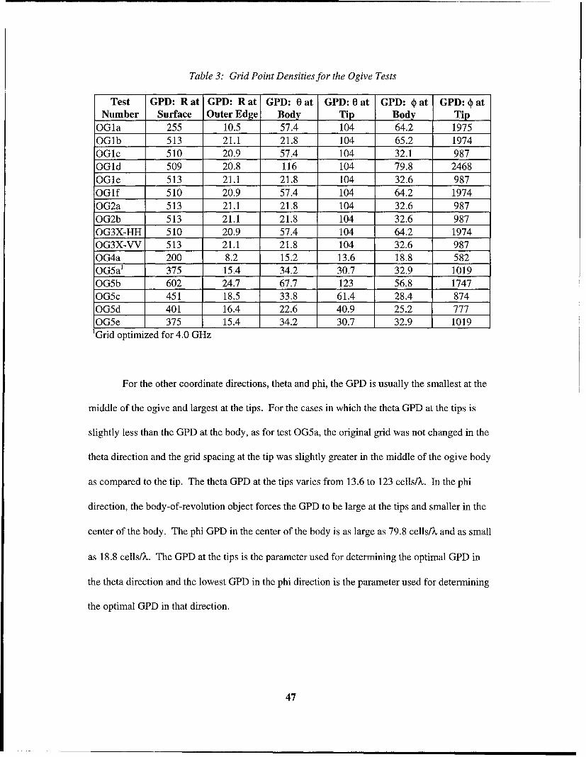
Table 3: Grid Point Densities for the Ogive Tests

Test GPD: R at GPD: R at GPD: 0 at GPD: 0 at GPD: at GPD: 0 atNumber Surface Outer Edge Body Tip Body Tip

OGla 255 10.5 57.4 104 64.2 1975OGlb 513 21.1 21.8 104 65.2 1974OGIc 510 20.9 57.4 104 32.1 987OGId 509 20.8 116 104 79.8 2468OGle 513 21.1 21.8 104 32.6 987OG1f 510 20.9 57.4 104 64.2 1974OG2a 513 21.1 21.8 104 32.6 987OG2b 513 21.1 21.8 104 32.6 987OG3X-HH 510 20.9 57.4 104 64.2 1974OG3X-VV 513 21.1 21.8 104 32.6 987OG4a 200 8.2 15.2 13.6 18.8 582OG5al 375 15.4 34.2 30.7 32.9 1019OG5b 602 24.7 67.7 123 56.8 1747OG5c 451 18.5 33.8 61.4 28.4 874OG5d 401 16.4 22.6 40.9 25.2 777OG5e 375 15.4 34.2 30.7 32.9 1019

'Grid optimized for 4.0 GHz

For the other coordinate directions, theta and phi, the GPD is usually the smallest at the

middle of the ogive and largest at the tips. For the cases in which the theta GPD at the tips is

slightly less than the GPD at the body, as for test OG5a, the original grid was not changed in the

theta direction and the grid spacing at the tip was slightly greater in the middle of the ogive body

as compared to the tip. The theta GPD at the tips varies from 13.6 to 123 cells/X. In the phi

direction, the body-of-revolution object forces the GPD to be large at the tips and smaller in the

center of the body. The phi GPD in the center of the body is as large as 79.8 cells/X and as small

as 18.8 cells/X. The GPD at the tips is the parameter used for determining the optimal GPD in

the theta direction and the lowest GPD in the phi direction is the parameter used for determining

the optimal GPD in that direction.

47

4.2.1 Ogive Bistatic RCS Results for 1.18 GHz, Sinusoid Incident Wave

The first set of tests, OGIX, study the scattering from the ogive at 1.18 GHz using a

sinusoid incident wave. The incident wave is incident at 00, or tip-on. Figures 12 through 15 are

plots of the nose-on bistatic scattering from the ogive for VV polarization. Figures 12, 13, and

14 show the results as the grid point density is varied in the radial, theta, and phi directions,

respectively (i.e. tests OGla, OGlb, and OGlc). Test OGlf is considered the acceptable FVTD

result after a grid convergence study was completed. The original size of the grid limited the

grid sizes which could be generated. The number of grid points have to be a multiple of the

original grid size.

As can be seen in Figure 12, the largest errors occur when the number of cells is

decreased in the radial direction. The primary reason for the change is due to the first-order

surface boundary condition which does not accurately predict diffraction and traveling waves

unless the grid points are tightly packed at the surface. The GPD for OGla as shown in Figure

12 is 255 cells/k in the radial direction and does not produce good results. To maintain accuracy,

the first two cells in the radial direction must be small relative to the wavelength. For the ogive

tests, OGlb through OGlf, the grid point density (GPD) at the surface in the radial direction is

513 cells/k. If the object is electrically larger, the GPD at the surface in the radial direction does

not have to be as large, as will be seen for test OG4a, because the electromagnetic phenomena

can be considered local.

In the theta and phi directions, the density can be decreased to 21.8-32.6 cells/k from 80-

110 cells/X as can be seen in Figure 15 to obtain accurate results. As the grid point density

decreases, the errors in the RCS occur first in the backscatter and forward scattering directions as

would be expected because of the diffraction at the tips of the ogive.

48

0

- -- FVTD1-OGla (36-74-45)

o - - -FVTD2-OGlf (71-74-45)

-Moment Method (CICERO)

0

C)(0

0 20 40 60 80 100 120 140 160 180Theta (Degrees)

Figure 12: Ogive Bistatic RCS, 1.18 GHz, VV, Number of Cells Varied in R Direction

0

-...FVTD1 -OG 1b (71 -43-45)

o- - - FVTD2-OGlf (71-74-45)


0

T~0 0 4 0 80 10 10 14 6 8

Tht Dges

Fiue1:OieBsai CS .1 2,VNme f el aidi ieto

C49

In each plot for the ogive at 1.18 GHz, VV, the FVTD results are plotted against MoM

results. A surface grid with 31 points along the arc was used to obtain the MoM results. Figure

16 shows the difference or error between the FVTD results for test OGif and the CICERO MoM

---- FV'TD1-OGlc (71-74-25)o - FVTD2-OGlf (71-74-45)


E0' o /,U)

0

C?

0 20 40 60 80 100 120 140 160 180

Theta (Degrees)

Figure 14: Ogive Bistatic RCS, 1.18 GHz, VV, Number of Cells Varied in t Direction

results. The difference is no more than 0.71 dB if the phase difference is considered as described

in Chapter 3. The largest difference occurs in the forward scattering region. Figure 17 illustrates

the cross-correlation between the FVTD results from test OGlf, VV polarization, and MoM

results. The plot clearly shows the FVTD and MoM results have a high correlation but the phase

of the FVTD result is one or two degrees to the left of the MoM results. If the null in Figure 15

occurred at the same bistatic angle, the maximum correlation would occur at 180 degrees.

Another representation of the accuracy of the FVTD results is shown in Figure 18 where

50

0

- -- FVTD 1-OGl1d (71-125-55)

o- - - FVTD2-OGl1e (71 -43-25)


C,E

0Cr0 ______

0

0 20 40 60 80 100 120 140 160 180Theta (Degrees)

Figure 15: Ogive Bistatic RCS, 1. 18 GHz, VV, Fine (71-125-55) vs. Coarse (71-43-25) Grid

0co

-Difference Between FVTD (OGi1f)and MoM Results

CD

6A

C

0

CDJ

0 20 40 60 80 100 120 140 160 180Theta (Degrees)

Figure 16: 0 give Bistatic RCS, 1. 18 GHz, VV, Difference Between FVTD and MoM RCS

51

0

O

C;0._o

0o

0

o -Cross-Correlation Between FVTD (OGlf)6 and MoM Results

LO

170 175 180 185 190

Theta (Degrees)

Figure 17: Ogive Bistatic RCS, 1.18 GHz, VV, Cross-Correlation of FVTD and MoM RCS

the Fourier transform of each plot is taken. The x axis has units of l/degrees which has no

physical meaning. The maximum magnitude corresponds to the large 140 degree arc in the

bistatic plot. Before the Fourier transform was taken, the data was windowed with a Hamming

window. If the FVTD and MoM results are not windowed first, the truncation of the data in the

FT sequence produces unwanted oscillations in the curve. The metrics displayed in Figures 15-

17 illustrate the small difference and high correlation between the FVTD and MoM RCS results.

The frequency data for tests OGla to OGIf was taken from the fifth to the seventh

periods to calculate the RCS data. Subsequent tests using the RCS convergence check showed

the same results could be acquired if the data was taken from the fourth to the fifth periods.

These tests revealed that for 1.18 GHz, the transients introduced with the sinusoid incident wave

require at least four periods to diminish before frequency data can be taken for the RCS

52

calculations. Taflove recommends that at least four times the electrical length, in periods, are

required [51]. The ogive results show that this approximation is appropriate for this frequency;

however, fewer periods can be used for higher frequencies to obtain accurate data.

Similar results were obtained for HH polarization. The same grid sizes were tested and

the results were similar. Figure 19 compares the coarse grid (OGle) to the fine grid (OGld).

Figure 20 is the plot of the accepted result (OGif) and the MoM results. Again, the results for

CO

------ FT of FVTD (OGif) Results

FT of MoM Results0

I'-

U-

0

Ca

CMJ

0

0.000 0.005 0.010 0.015 0.020 0.025 0.030 0.035 0.040 0.045 0.0501/Theta (1/Degrees)

Figure 18: Ogive Bistatic RCS, 1.18 GHz, VV, Fourier Transform of FVTD and MoM RCS

OGld are accurate within several dB, but for comparison, the slightly more accurate results from

test OGlf are used to compare to the MoM results.

Figure 21 is the difference, in dB, between the FVTD and MoM results for HH

polarization. The phase shift in the null was accounted for or the difference, in dB, would be

much greater if taken point by point. The largest difference of approximately 2.0 dB occurs at

53

151'. The null in the FVTD solution at that location is not as deep as in the MoM solution. If

the nulls are not considered, the greatest difference is approximately 0.7 dB. The cross-

correlation was computed for the FVTD and MoM RCS results and the FVTD results were

highly correlated with the MoM results, except the shift of the FVTD data was to the right by one

or two degrees. This shift of two degrees can be seen visually in Figure 20. The Fourier

transforms of the curves were taken and were very similar just as for the VV RCS results.

The FVTD results for the ogive at 1.18 GHz using a sinusoid incident wave were

excellent when compared to MoM results. The results illustrated that for electrically small

objects, the FVTD algorithm correctly computes diffraction and traveling waves. The small

electrical size also allowed a relatively large time step resulting in a reasonable simulation time.

For test OGle, the Cray 90 CPU time was approximately 3200 seconds. For higher frequencies,

as shown in Table 2, the computer simulation times are much longer.

...... FVTD1-OG1 d (71-125-55)

- - - FVTD2-OGle (71-43-25)

o - Moment Method (CICERO)C..

EmCf,

0r

To

0 20 40 60 80 100 120 140 160 180

Theta (Degrees)

Figure 19: Ogive Bistatic RCS, 1.18 GHz, HH, Fine (71-125-55) vs. Coarse (71-43-25) Grid

54

- - - FVTD-OGlf (71 -74-45)


(0

C)

o(0

(0

0 20 40 60 80 100 120 140 160 180Theta (Degrees)

~~~~~Figure 20: Ogive Bistatic RCS, 1. 18 GHz, HH, ifrneBtenFT n o C

05

4.2.2 Ogive Bistatic RCS Results for 1.18 GHz, Gaussian Pulse Incident Wave

The accuracy of the Gaussian pulse incident wave is illustrated in Figures 22 and 23.

One-third of the bandwidth of the pulse is considered to be adequate to take frequency data. This

is illustrated in the plots for tests OG2a and OG2b. Test OG2a placed the frequency of interest,

1.18 GHz, near the center of the pulse bandwidth. A Gaussian pulse with a duration of 0.017831,

normalized to c, and a radian frequency delta of 12.35693 rad/s was used to place the frequency

near the center of the pulse. The test, OG2b, placed the frequency near the edge of the usable

bandwidth by using a Gaussian pulse with a duration of 0.100000 and a radian frequency delta of

2.471386 rad/s. The results are almost identical. Appendix B contains detailed data for

specifying the parameters for the Gaussian pulse incident wave.

The vertical polarization case is plotted in Figure 22. The Gaussian pulse RCS results,

OG2X, are compared to MoM RCS results. The horizontal polarization case is shown in Figure

23. The Gaussian pulse RCS results, OG2X, match the RCS calculations of test OGle which

also used the coarse grid size of (71-43-25). The results for the grid size of (71-43-25) are nearly

as accurate as the results for the grid size of (71-74-45) to permit use of the smaller grid. The

savings in computer time also justifies the use of the smaller grid.

The comparison of tests OG1X and OG2X illustrate the accurate results which can be

obtained with either a Gaussian pulse or sinusoid incident wave. The computer run times for the

Gaussian pulse tests, OG2X, are greater than the times for the sinusoid (approximately 9600

seconds vs. 3200 seconds). This factor of three will not always be the relationship between run

times. The electrical length of the object and the grid size will affect the computer run times.

The sinusoid incident wave is clearly the correct incident wave to use if the RCS is desired for a

single frequency. The Gaussian pulse is used when the simulation time is less than the total time

required for the individual sinusoid tests. Test OG5X looks at these trade-offs in more detail.

56

0---FT1OGa(14-5

--- FVTD1-OG2a (71-43-25)


U)

0 20 40 6 8 00 12 40 10 8

Theta (Degrees)

Figure 22: 0 give Bistatic RCS, 1. 18 GHz, VV, Gaussian Pulse Incident Wave

0- -- ______ 714325

- FVTD1-OG2a (71-43-25)

o -Moment Method_(CICERO)

EC,)

0co

0 20 40 60 80 100 120 140 160 180Theta (Degrees)

Figure 23: Ogive Bistatic RCS, 1.18 GHz, HH, Gaussian Pulse Incident Wave

57

4.2.3 Ogive Monostatic RCS Results for 1.18 GHz

In addition to bistatic results, the FVTD code can also obtain monostatic data. Multiple

simulations have to be completed to obtain monostatic data for one frequency as compared to one

test for bistatic data. One simulation produces a bistatic plot for 00 to 1800. The simulation

produces a monostatic result for one angle, the angle of incidence. To obtain a full monostatic

sweep, a bistatic-to-monostatic approximation is used (See Chapter 3). The approximation

requires tests to be completed every 10' and bistatic data completes the monostatic

approximation. Tests OG3X are monostatic calculations for the ogive at 1.18 GHz. A test was

completed for an angle of incidence every 100 from 00 to 900. The ogive is symmetric about the

xy plane resulting in a symmetric monostatic plot about 0=900.

The monostatic approximation for HH polarization is plotted in Figure 24. The HH

monostatic test used a grid size of (71-74-45), and frequency data was taken from the fifth to the

seventh period. The FVTD results are plotted against MoM RCS results and empirical RCS data.

As can be seen in the plot, the MoM and FVTD results are almost identical and differ from the

empirical data by nearly the same value. In Figure 25, the difference between the FVTD, MoM,

and empirical results is plotted. The FVTD results differ from the MoM results by no more than

2.5 dB. If the large fluctuations are ignored in the empirical data, the FVTD results are within

3.1 dB of the empirical data. The FVTD results differ from the empirical data by 2.8 dB at the

tips (0=00 and 0=1800) and 2.5 dB at broadside incidence (0=90').

The VV polarization results for the monostatic calculations are shown in Figure 26. For

this group of tests, a grid size of (71-43-25) was used. Again, the FVTD results are excellent

when plotted against MoM and experimental RCS data. The FVTD results, however, do not

agree well at the nulls at 300 and 1500. The difference between the FVTD results and the other

data, shown in the figure, can be as large as 8-10 dB in the nulls.

58

00

C')

C')cc 0

- -- RdTD-OG33X (71-74-45)

0 ~Experimental Results (EMACC)

......... Ml~ment Method (CICERO)

0

0 20 40 60 80 100 120 140 160 180Theta (Degrees)

Figure 24: Ogive Monostatic RCS, 1. 18 GHz, HH

0

0

.... FVTD vs. MoM (CICERO)

-FVTD vs. Experimental Results

960 20 40 60 80 100 120 140 160 180

Theta (Degrees)

Figure 25: 0 give Monostatic RCS, 1. 18 GHz, HH, Error Between RCS Results

59

The accuracy and limitations of the bistatic-to-monostatic approximation can be

determined by close observation of the FVTD monostatic plots. The data at 10' increments, such

as 00, 100, 200, etc., are the true monostatic FVTD RCS results and are in agreement with the

MoM RCS results. However, the data at the angles 50 , 150,250,350,450, etc. are at the junction of

the approximation data from each monostatic test. Slight discontinuities can be seen at these

angles. For example, the monostatic data for 25°-35' degrees is obtained from the bistatic test

0

0

, - - - FVTD-OG3X (71-43-25)

-Experimental Results (EMCC)

...... Moment Method (CICERO)

0 20 40 60 80 100 120 140 160 180

Theta (Degrees)

Figure 26: Ogive Monostatic RCS, 1. 18 GHz, VV

at 30' . The monostatic data for 35°-45' is taken from the 40' bistatic test. A small discontinuity

can be seen at 35*. The approximation is only good for small angles, 5' or less. If the

discontinuity is great, the approximation is not poor, but more monostatic tests have to be made

for more angles so the approximation is used for smaller angles. A large number of oscillations

in the plot can require a greater number of monostatic tests (i.e. higher frequencies).

60

cc|

4.2.4 Ogive Bistatic RCS Results for 9.0 GHz

The ogive tests completed previously were at one frequency, 1.18 GHz. Further analysis

is completed for the ogive using FVTD by running a test, OG4a, for the ogive at 9.0 GHz. The

ogive is approximately 7.6 wavelengths long at this frequency. The grid size required for this

frequency is much larger along with an increased simulation time. The wavelength is smaller at

9.0 GHz, but the time step is much smaller due to the fine grid resulting in a large simulation

time (i.e. 79,922 seconds) as seen in Table 2.

The ogive results for 9.0 GHz, HH polarization, are shown in Figure 27. The FVTD

results for 9.0 GHz, VV, are shown in Figure 28. The FVTD results are plotted against MoM

RCS data. The results are excellent, except there are small discrepancies for the backscatter and

forward scattering regions. The grid densities for these tests are smaller than for 1.18 GHz. The

GPDs in the theta and phi directions are 15.2 cells/k and 18.8 cells/k, respectively. The results

for the ogive at 1.18 GHz showed that a GPD of approximately 22-32 cells/X gives the best data.

These results depict the dependence of the required GPD on the electrical size of the object. The

GPD can be smaller, 15-20 cells/k, as the electrical length of the object gets larger.

The 9.0 GHz results for the ogive illustrate the dependence of the length of simulation

time, in periods, to the length of the object. At 1.18 GHz, the test had to be at least four times, in

periods, the length of the object. The same factor would require a simulation time of 30 periods

for 9.0 GHz. This is not required because, at 9.0 GHz, the ogive is in the optical region. As a

rule of thumb, the optical region is encountered for an object greater than approximately 7X [27].

At 9.0 GHz, the diffraction and the traveling waves can be considered to be more of a local

phenomena than for 1.18 GHz. This reduces the simulation time for the test to approximately

three times the length of the object, in periods, instead of four.

61

0 Vol '00

Co 0 0 4 0 8 0 2 4 6 8

Tht (eres

Fiue20 gv ittcRS . ~,H

0VD1-Ga 6-2-5

MoetMtod(IEO

0 ORIN

- ~ ~ ~ ht (Degrees)(1-2595

FiMome Metho (ICERO)atcRS,90G ,V

06

The results for the ogive at 9.0 GHz begin to show the limitations of the explicit FVTD

algorithm and available computing resources. The stability of the explicit time-domain algorithm

is related to the cell size which is small for this grid at 9.0 GHz. The grid size is large to meet

the GPD requirements and the fineness of the grid at the tips forces the time step to be small.

The small time step, the large grid size, and the number of periods required to obtain accurate

frequency data results in a long simulation time (i.e. 79,922 seconds). Accuracy in the

backscatter and forward scattering regions is sacrificed for a faster run time and smaller grid.

4.2.5 Ogive Bistatic RCS Results for the Gaussian Pulse Incident Wave

The option of specifying either a sinusoid or Gaussian pulse for the incident wave gives

the user flexibility in obtaining FVTD RCS data for one frequency or multiple frequencies,

respectively, depending on the results desired. The Gaussian pulse provides RCS data for

multiple frequencies but normally requires a longer run time (See Table 2); therefore, a sinusoid

is ideal for single frequency RCS data. Included in this section are results for several frequencies

using a Gaussian pulse. The Gaussian pulse RCS data are compared to sinusoid incident wave

RCS data and the results for one frequency, 4.0 GHz, are also compared to MoM RCS results.

The Gaussian pulse used for test OG5a was optimized for 4.0 GHz. The grid used, (76-

125-75), was also optimized for that frequency. The bistatic RCS results for frequencies less

than 4.0 GHz are excellent and will be shown. The GPDs due to the grid size for frequencies

below 4.0 GHz are sufficient to provide excellent results. The Gaussian pulse for test OG5a had

a width of 0.0182556 (See Appendix B) with a radian frequency delta of 10.471975 rad/s (0.5

GHz). The Gaussian pulse width had a bandwidth of 21.0 GHz and a usable BW of 7.0 GHz for

these parameters. The grid was optimized for 4.0 GHZ so results for higher frequencies are not

discussed.

63

The FVTD results for 1.0 GHz using the Gaussian pulse (OG5a) and a sinusoid (OG5b)

are shown in Figure 29, HH, and Figure 30, VV. The RCS convergence check was not used for

test OG5b. The results are identical except for a negligible small difference in the forward

scattering region which could be due to a different grid size, numerical dispersion, or reflections

from the outer boundary. Slight differences were seen previously for different grid sizes. The

longer run time for the Gaussian pulse test can introduce numerical dispersion which

accumulates during the test. Also, the longer simulation for the Gaussian pulse may allow the

reflections from the outer boundary to affect the results more than for the sinusoid test.

The Gaussian pulse incident wave also provided RCS data for 2.0 GHz. The HH

polarization results are shown in Figure 31. As can be seen in the figure, the data for the

Gaussian pulse (OG5a) and sinusoid incident wave (OG5c) are almost identical. A small

difference exists between the results in the forward scatter direction. The RCS convergence

check was used for test OG5c. The VV polarization result is shown in Figure 32. The results are

identical except for a slight difference in the forward scatter region.

The results comparing Gaussian pulse RCS data to sinusoid data reveal several important

computational issues requiring attention when obtaining FVTD results. The Gaussian pulse

results accurately predict the backscatter and forward scatter regions. Results from a sinusoid

incident wave will not if the transients have not diminished. The convergence check for the

sinusoid was programmed to take data for one period, sample the RCS values, take data for

another period, and sample again. Other FVTD tests showed that more accurate results can be

obtained from sampling data over a two to three period span. A convergence check designed to

sample every two or three periods would provide a more robust and accurate method of ensuring

accurate results from a sinusoid incident wave, especially for higher frequencies. At higher

frequencies, the enormous run times require methods which ensure accurate results with one test.

64

-- - -- FVTD1 -OG5a (76-125-75)

FVTD2-OG5b (83-74-35)

0l)

C,

0

0 20 40 60 80 100 120 140 160 180Theta (Degrees)

Figure 29: Ogive Bistatic RCS, 1.0 GHz, HH, Gaussian Pulse vs. Sinusoid Incident Wave

0)

.--- FVTD1 -OG5a (76-125-75)

FVTD2-OG5b (83-74-35)

C)m

E20n

0 20 40 60 80 100 120 140 160 180Theta (Degrees)

Figure 30: Ogive Bistatic RCS, 1.0 GHz, VV, Gaussian Pulse vs. Sinusoid Incident Wave

65

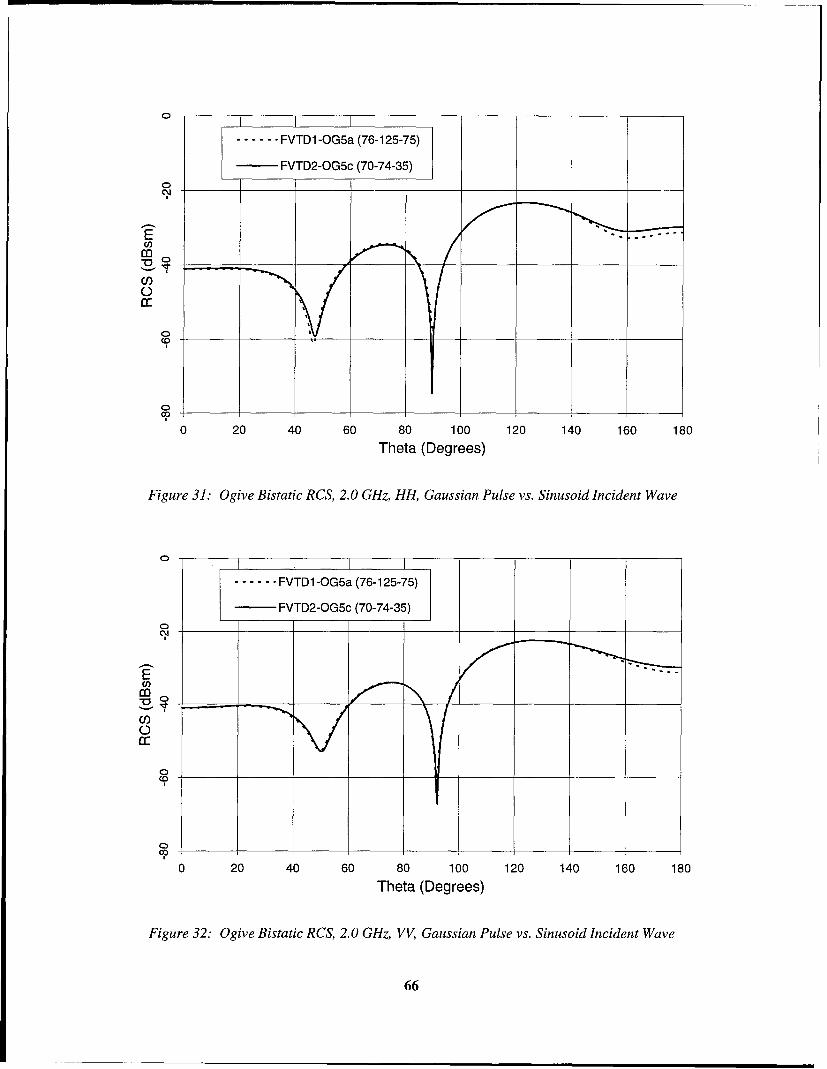
- -- FVTD1 -OG5a (76-125-75)

FVTD2-OG5c (70-74-35)

C,)

(0

(0

C0 2 10 4 0 6 .0 80 100 120 140 160 180Theta (Degrees)

Figure 31: 0 give Bistatic RCS, 2.0 GHz, HH, Gaussian Pulse vs. Sinusoid Incident Wave

- -- FVTD1 -OG5a (76-125-75)

FVTD2-OG5c (70-74-35)0

0

0)0

0 20 40 60 80 100 120 140 160 180Theta (Degrees)


66

Another computational issue which arises with the use of the Gaussian pulse is the

location of the outer boundary for each frequency. The grid, when using a Gaussian pulse, is

optimized for a specific frequency with the location of the outer boundary three wavelengths

from the scatterer. The test gives results for lower frequencies, but the outer boundary for the

lower frequencies is less than three wavelengths away from the scatterer surface. For example,

the outer edge of the grid for 2.0 GHz in test OG5a is 1.5 wavelengths from the surface of the

scatterer. As the frequency decreases, the reflections from the outer boundary will increase the

errors for those particular frequencies. The slight errors in the forward scatter regions for 1.0

and 2.0 GHz are most likely due to the reflections from the outer boundary as opposed to

numerical dispersion in the Gaussian pulse test.

In Figure 33, the accurate results for 3.0 GHz, HH, is illustrated using a Gaussian pulse

(OG5a) and a sinusoid (OG5d). The VV polarization case is shown in Figure 34. The grid sizes

for each test are different, but the results are almost identical. No errors in the forward scatter

region reveal that numerical reflections are causing the slight errors in the forward scatter area

for the lower frequencies of 1.0 and 2.0 GHz.

Test OGld ran for thirteen periods, although convergence was almost reached at 10

periods (within 0.12 dB as compared to 0.1 dB for the RCS convergence check). At 10 periods,

the simulation time is approximately four times the electrical length of the ogive. The

electromagnetic phenomena, including diffraction at the tips and traveling waves along the

surface of the body, require time to stabilize. These frequencies dictate that the electromagnetic

scattering cannot be considered local phenomena. Multiple diffractions from the tips due to

traveling waves require time to establish and stabilize. As the electrical size of the object gets

larger, as for the case of 9.0 GHz, the multiple diffractions are not as prominent and less time is

required to establish the stabilized fields.

67

-- --FVTD1 -OG5a (76-125-75)

FVTD2-OG5d (69-74-45)

0

U)

CI)0V

0 20 40 60 80 100 120 140 160 180Theta (Degrees)


0) -

-- --FVTD1 -OG5a (76-125-75)

FVTD2-OG5d (69-74-45)

C,,

C/)

0 20 40 60 80 100 120 140 160 180Theta (Degrees)


68

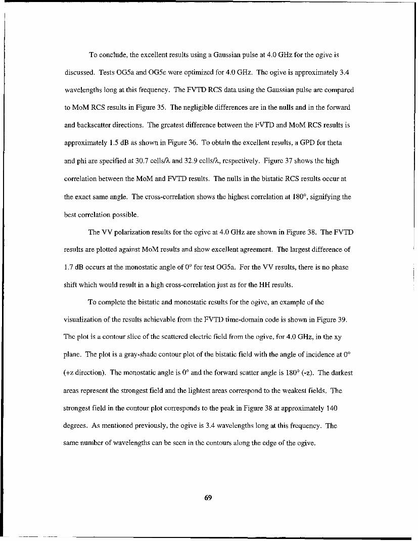
To conclude, the excellent results using a Gaussian pulse at 4.0 GHz for the ogive is

discussed. Tests OG5a and OG5e were optimized for 4.0 GHz. The ogive is approximately 3.4

wavelengths long at this frequency. The FVTD RCS data using the Gaussian pulse are compared

to MoM RCS results in Figure 35. The negligible differences are in the nulls and in the forward

and backscatter directions. The greatest difference between the FVTD and MoM RCS results is

approximately 1.5 dB as shown in Figure 36. To obtain the excellent results, a GPD for theta

and phi are specified at 30.7 cells/ and 32.9 cells/?, respectively. Figure 37 shows the high

correlation between the MoM and FVTD results. The nulls in the bistatic RCS results occur at

the exact same angle. The cross-correlation shows the highest correlation at 1800, signifying the

best correlation possible.

The VV polarization results for the ogive at 4.0 GHz are shown in Figure 38. The FVTD

results are plotted against MoM results and show excellent agreement. The largest difference of

1.7 dB occurs at the monostatic angle of 00 for test OG5a. For the VV results, there is no phase

shift which would result in a high cross-correlation just as for the HH results.

To complete the bistatic and monostatic results for the ogive, an example of the

visualization of the results achievable from the FVTD time-domain code is shown in Figure 39.

The plot is a contour slice of the scattered electric field from the ogive, for 4.0 GHz, in the xy

plane. The plot is a gray-shade contour plot of the bistatic field with the angle of incidence at 00

(+z direction). The monostatic angle is 00 and the forward scatter angle is 1800 (-z). The darkest

areas represent the strongest field and the lightest areas correspond to the weakest fields. The

strongest field in the contour plot corresponds to the peak in Figure 38 at approximately 140

degrees. As mentioned previously, the ogive is 3.4 wavelengths long at this frequency. The

same number of wavelengths can be seen in the contours along the edge of the ogive.

69

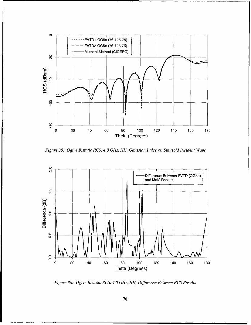
-- -FVTD1 -OG5a (76-1 25-75)- - - FVTD2-OG5e (76-125-75)

-Moment Method_(CICERO)

C)

Co

CECDA

U)

0

Cr

0 20 40 60 80 100 120 140 160 180Theta (Degrees)


0~

- Difference Between FVTD (OG5a)

LO and MoM Results

700

a)

0 C

0 20 40 60 80 100 120 140 160 180Theta (Degrees)

Figure 36: Ogive Bistatic RCS, 4.0 GHz, HH, Difference Between RCS Results

70

0

00

O

o) ._ _ _ _ _ _

(00

0

cli - Cross-Correlation Between FVTD (OG5a)0 and MoM Results

175.0 177.5 180.0 182.5 185.0

Theta (Degrees)

Figure 37: Ogive Bistatic RCS, 4.0 GHz, HH, Cross-Correlation of FVTD and MoM RCS

Several important observations can be obtained from the contour plot of the electric field

in Figure 39. The perfect symmetry of the contours about the z axis validates the computational

accuracy for the scattered electric field. The fields in each half of the plot about the z axis are

calculated separately. Any errors in the code, especially overlap regions in the grid, would create

errors in the symmetry of the contour plot. The symmetry confirms the accuracy of the code.

The diffraction of the electromagnetic wave can also be seen at the tips of the ogive. In

the backscatter region, 0', a strong field exists. The grid must be accurately generated for the

FVTD algorithm to correctly predict the diffraction at the tip. The incident field and the

scattered electric and magnetic fields are implemented at cell centers and not cell faces or cell

grid points. The grid points of the cells define the tip of the ogive, but if only the cell centers are

viewed, the tip of the ogive appears to have a small blunt tip. This characteristic of the grid and

71

-- -- FV D I~ (7 -2 -5

- FVTD1-OG5a (76-125-75)

-MomentMethod_(CICERO)

0

Cl)

0

0

C0

0 20 40 60 80 100 120 140 160 180

Theta (Degrees)

Figure 38: 0 give Bistatic RCS, 4.0 GHz, VV, Gaussian Pulse vs. Sinusoid Incident Wave

x

z

-0.20

Ci N q- 04 Ci)9 9 9 0 0

z (in)

Figure 39: 0give Bistatic Results, 4.0 GHz, Electric Field Contour Plot

72

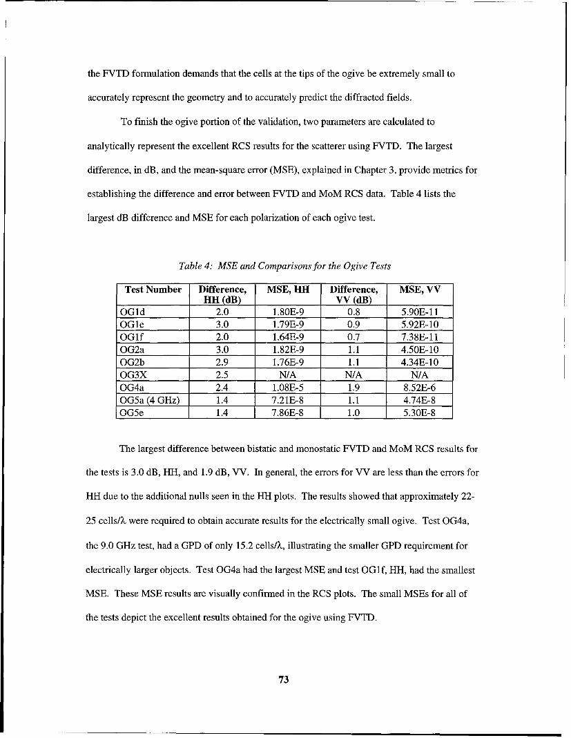
the FVTD formulation demands that the cells at the tips of the ogive be extremely small to

accurately represent the geometry and to accurately predict the diffracted fields.

To finish the ogive portion of the validation, two parameters are calculated to

analytically represent the excellent RCS results for the scatterer using FVTD. The largest

difference, in dB, and the mean-square error (MSE), explained in Chapter 3, provide metrics for

establishing the difference and error between FVTD and MoM RCS data. Table 4 lists the

largest dB difference and MSE for each polarization of each ogive test.

Table 4: MSE and Comparisons for the Ogive Tests

Test Number Difference, MSE, HH Difference, MSE, VHH (dB) VV (dB)

OGid 2.0 1.80E-9 0.8 5.90E-11OGle 3.0 1.79E-9 0.9 5.92E-10OGlf 2.0 1.64E-9 0.7 7.38E-11OG2a 3.0 1.82E-9 1.1 4.50E-10OG2b 2.9 1.76E-9 1.1 4.34E-10OG3X 2.5 N/A N/A N/AOG4a 2.4 1.08E-5 1.9 8.52E-6OG5a (4 GHz) 1.4 7.21E-8 1.1 4.74E-8OG5e 1.4 7.86E-8 1.0 5.30E-8

The largest difference between bistatic and monostatic FVTD and MoM RCS results for

the tests is 3.0 dB, HH, and 1.9 dB, VV. In general, the errors for VV are less than the errors for

HH due to the additional nulls seen in the HH plots. The results showed that approximately 22-

25 cells/?, were required to obtain accurate results for the electrically small ogive. Test OG4a,

the 9.0 GHz test, had a GPD of only 15.2 cells/X, illustrating the smaller GPD requirement for

electrically larger objects. Test OG4a had the largest MSE and test OGIf, HH, had the smallest

MSE. These MSE results are visually confirmed in the RCS plots. The small MSEs for all of

the tests depict the excellent results obtained for the ogive using FVTD.

73

4.3 Cone-Sphere Electromagnetic Scattering Results

The RCS calculations for the cone-sphere provide further validation of the FVTD code

and algorithm. The cone-sphere is a common RCS test body but the narrow cone portion and the

sphere cap provide a unique body for analysis. At smaller frequencies, the scattering from the

cone-sphere is a result of traveling waves along the narrow cone, creeping waves around the

sphere cap, and diffraction from the tip. Excellent RCS results for the cone-sphere validate the

FVTD code and algorithm for predicting complicated electromagnetic phenomena.

The test matrix for the cone-sphere computer simulations is shown in Table 5. Five tests

were completed which include several subtests. The test numbers are constructed in the same

method as the ogive test numbers. "CS" is used instead of "OG" to refer to the cone-sphere. The

test numbers are used in the discussion of the results to easily reference the tests.

The electromagnetic scattering results for the cone-sphere are compared to MoM RCS

results and experimental data for VV and HH polarization. The first cone-sphere tests, CS 1X,

are bistatic RCS results which analyze several grid sizes at 0.869 GHz using a sinusoid incident

wave incident on the sphere section of the cone-sphere. The cone-sphere is two wavelengths

long at 0.869 GHz. An incident angle of 00 corresponds to incidence on the cone-sphere along

the axis of symmetry directly onto the sphere-cap. Tests CS2X are bistatic tests at 0.869 GHz

with a sinusoid incident wave at 1800 or tip-on incidence. Tests CS3X are tests for the

monostatic calculations at 0.869 GHz. The monostatic RCS is computed every 100 from 0' to

1800 and bistatic data completes the monostatic plot. The cone-sphere is not symmetric about

the xy plane and therefore monostatic tests cannot be completed for only 0' to 90' as for the

ogive. CS4a and CS5a are bistatic simulations for the cone-sphere at 3.0 GHz using a sinusoid

incident wave at sphere-cap (0=0 °) and tip-on incidence (0=1800), respectively.

74

Table 5: Cone-Sphere Test Matrix

Test Number Incident Wave Frequency Angle of Grid SizeType (GHz) Incidence

CS la1 Sinusoid 0.869 0.0 50-73-45CS lb1 It 50-39-35CSlc 50-73-45CSld 50-39-35CS2a' Sinusoid 0.869 180.0 50-39-35CS2b ...... 50-39-35CS3a Sinusoid 0.869 10.0 50-39-35CS3b It 20.0 "

CS3c 30.0CS3d 40.0CS3e 50.0CS3f 60.0CS3g 70.0CS3h 80.0 "CS3i 90.0 "CS3j 100.0 "CS3k 110.0CS31 120.0 "CS3m 130.0 "CS3n 140.0 "CS3o 150.0 "CS3p 160.0CS3q 170.0 "CS4a' 3.0 0.0 73-141-81CS5a' 3.0 180.0 73-141-65

'The grid spacing at the surface (R direction) for these tests is approximately 200 cells/X.The surface grid spacing for all other tests is 400 cells/X.

The data in Table 6 contains the stability and time data for each cone-sphere test such as

the CFL value, time step, number of time steps per period, total number of periods, total number

of time steps, and total CPU time. The grid is structured to produce the largest time step as

possible. For example, the tip GPD in the theta direction is 22.0 cells/,. Greater accuracy could

be obtained with a larger GPD, but the trade-off between run time and accuracy justifies the

spacing. As will be seen in the discussion, the results are excellent despite the larger spacing at

75

the tip of the cone-sphere. Due to the larger time step as compared to the ogive, the majority of

the tests for the cone-sphere were completed on the DEC Alpha and SP-2 computing machines.

Table 6: Stability and Time Data for the Cone-Sphere Tests

Test CFL At Time Steps/ Total Total Time CPU Time'Number (Seconds(c)) Period Periods Steps (seconds)

CSla2 1.5 1.9553E-4 1766 4 7064 9797CS lb2 " 3.9937E-4 864 4 3456 2246CSlc 2 1.7304E-4 3990 4 15960 22900CSld 2 " 2.9814E-4 1158 4 4632 3010CS2a2 " 3.9937E-4 864 4 3456 2248CS2b 2 " 2.9814E-4 1158 4 4632 3072CS3X 2 " 3.3789E-2 1158 43 4632 2697CS4a2 " 4.8238E-5 2073 9 18657 126612CS5a2 " 5.3004E-5 1887 10 18870 102190

1Cray 90 CPU time2The RCS convergence check was used for these FVTD simulations3Several monostatic tests required five periods to reach convergence

Table 7: Grid Point Densities for the Cone-Sphere Tests

Test GPD: R at GPD: R at GPD: 0 at GPD: 0 at GPD: 0 at GPD: 0 atNumber Surface Outer Edge Body Tip Body Tip

CSla 201 3.67 51.8 45.3 29.6 2367CSlb 200 3.65 26.0 22.0 22.0 862CS1c 402 2.64 51.8 45.3 29.6 2367CSld 401 2.56 25.9 22.0 22.0 862CS2a 200 3.65 26.0 22.0 22.0 862CS2b 401 2.56 25.9 22.0 22.0 862CS3X 401 2.56 25.9 22.0 22.0 862CS4a 233 9.3 30.0 26.2 16.3 2605CS5a 233 9.3 30.0 26.2 14.0 2056

Table 7 shows the grid point densities (GPD) in each direction for each cone-sphere test.

Again, the GPD is defined as the number of finite-volume cells per wavelength, X, and must be

considered when generating a grid for a scatterer. As explained in Chapter 3, the spacing of the

76

cells in the radial direction increases as the distance from the surface of the scatterer increases.

Therefore, the grid point density is much larger at the surface as compared to the outer edge of

the grid. As can be seen in the table, the GPD varies from 200 to 401 cells/k at the surface and

from 2.56 to 9.3 cells/k at the outer edge of the grid for the cone-sphere grid. The outer edge of

the grid is three wavelengths from the surface of the scatterer for every simulation. The GPD in

the 0 direction is approximately the same at the sphere/cone junction and the cone tip. The GPD

for the tests in the 4) direction is the smallest at the sphere/cone junction and the largest at the tip,

just as for the ogive.

4.3.1 Cone-sphere Bistatic RCS Results for 0.869 GHz, Sphere-Cap Incidence

Two bistatic tests at 0.869 GHz are discussed for the cone-sphere. For the first group of

tests, CS 1X, the sinusoid incident wave is incident at 0', or sphere-cap incidence. The second

group of tests, CS2X, is for an incident wave tip-on. Two different grids were generated for the

cone-sphere. The grid size, (50-73-45), is identical for both grids, but the grid spacing in the

radial direction is different at the surface. For the first grid, the spacing is 200 cells/X at the

surface and for the second grid, the spacing is 400 cells/k at the surface.

For the group of tests with sphere-cap incidence, both grids were tested along with two

different grid sizes. In Figure 40, the results using a coarse grid with 200 cells/k spacing is

shown. Figure 40 shows that the forward scattering from the tip is not accurate. This proves that

this grid spacing at this frequency is not sufficient. The diffraction from the tip is not correctly

computed with this grid spacing. A finer grid in the theta and phi directions also does not

improve the results in the forward scattering direction as shown with test CS 1 a. An increase in

the spacing in the radial direction, tests CS Ic and CS Id, as shown in Figure 41 greatly improves

77

0

------------------------FVTD1 -CS1 a (50-73-45)

U? ~- -- FVTD2-CS1 b (50-39-35)

Moment Method (CICERO)

E 0(n .

C\J

0 20 40 60 80 100 120 140 160 180Theta (Degrees)

Figure 40: Cone-Sphere Bistatic RCS, 0.869 GHz, VV, Sphere-Cap Incidence, Coarse Grid

- -- FVTD 1-CS1 c (50-73-45)

u?- FVTD2-CS 1d (50-39-35)


-)

Co

0 20 40 60 80 100 120 140 160 180Theta (Degrees)

Figure 41: Cone-Sphere Bistatic RCS, 0.869 GHz, VV, Sphere-Cap Incidence, Fine Grid

78

the forward scattering region. The surface GPD can be decreased to 22.0 cells/A, but the GPD at

the surface in the radial direction needs to be high at this frequency (400 cells/k). The results for

test CSlc are slightly closer (<0.5 dB) to the MoM results than the CSld results. The small

difference can be considered negligible; therefore, grid convergence can be assumed for the

smaller grid due to the computer run time saved. The computer run time saved with the smaller

grid is approximately a factor of seven (22900 seconds (CSlc) vs. 3010 seconds (CSId)). Due to

the time step increase and the lower run time, test CS 1 d is considered sufficient and provides a

very close computation to that obtained with the finer grid and to the MoM RCS results.

In Figure 42, the difference between test CS Ic and the MoM RCS results are shown after

the phase is taken into account as discussed in Chapter 3. A difference of approximately 0.1 dB

is shown for the first 40 degrees in the backscatter direction. This difference is considered

negligible in the calculations of RCS data. The phase difference for this bistatic data is not as

critical as for the ogive RCS data. No deep nulls, which can provide erroneous error

calculations, occur in the results. As can be seen in the plot, no more than 0.98 dB separates the

FVTD RCS results from the MoM RCS results. The greatest difference occurs in the forward

scatter region from the tip. Again, the tip is the most difficult geometric characteristic of the

cone-sphere to accurately compute RCS data. For the ogive, the most significant errors occurred

at the tips. The same trend is seen here with the cone-sphere.

The cross-correlation between the FVTD (CS lc) and MoM RCS results is shown in

Figure 43. The maximum correlation occurs at 1800 which illustrates the excellent correlation

between the two sets of data. The steep slope of the cross-correlation curve signifies that no

phase shift exists. Phase shifts tend to level the curve at the peak or shift the peak to either side

of 180'. The Fourier transforms of both RCS curves illustrate the excellent agreement between

the FVTD and MoM RCS results.

79

(0 Difference Between FVTD (OSi c)0 6 and MoM Results

a)

C!

0

0 20 40 60 80 100 120 140 160 180Theta (Degrees)

Figure 42: Cone-Sphere Bistatic RCS, 0.869 GHz, VV, Difference Between RCS Results

0

0C;

q (0I

0

Fiue4:CoeShr -Crss-i C,0.6 ,VV rs-Correlation Betee FVTD Data

08

. ...... FVTD1-CSlc (50-73-45)

-?- ---- FVTD2-CS1d (50-43-35)


0

U)E

co

m,

0 LC'.

U) _ _ _

C'.

0 20 40 60 80 100 120 140 160 180Theta (Degrees)

Figure 44: Cone-Sphere Bistatic RCS, 0.869 GHz, HH, Sphere-Cap Incidence, Fine Grid

Similar results were obtained for the cone-sphere for 0.869 GHz for HH polarization.

Figure 44 plots the FVTD results for HH against MoM RCS data. The greatest difference of 2.5

dB occurs in the null at 1430. The FVTD results for HH miss the nulls by several dB for some

bistatic plots. The same result was seen for the ogive at 1.18 GHz for HH in Figure 19.

4.3.2 Cone-Sphere Bistatic RCS Results for 0.869 GHz, Tip-On Incidence

FVTD RCS data for tip-on incidence were obtained in test OG2X. The incidence wave

propagates toward the cone-sphere from 1800. The accuracy of the bistatic results is dependent

on the correct calculation of creeping and traveling waves and diffraction at the tip. The

creeping waves travel behind the sphere and the creeping waves travel along the smooth surface

of the cone. The VV and HH polarization cases are shown in Figures 45 and 46, respectively.

81

-------------------------- FVTD1 -CS2a (50-39-35)

L9 ~- -- FVTD2-CS2b (50-39-35)

Moment Method (CICERO)0

cc 0

C'.

Co

0 20 40 60 80 100 120 140 160 180Theta (Degrees)

Figure 46: Cone-Sphere Bistatic RCS, 0.869 GHz, HH, Tip-On Incidence

L9 ......-FVTD1 -CS2a (50-39-35)- - - FVTD2-CS2b (50-39-35)

0 - Moment Method (CICERO)E

0

LC)

C'J

0 20 40 60 80 100 120 140 160 180Theta (Degrees)

Figure 45: Cone-Sphere Bistatic RCS, 0.869 GHz, VV, Tip-On Incidence

82

The finer grid, CS2b, produces much better results than the grid with the coarser spacing

(CS2a) at the surface. The forward scatter results (0=0 °) are only accurate if the fine grid is used

(CS2b). Recall that the fine grid has a spacing of 400 cells/X at the surface. The forward scatter

region is dependent on the accurate calculation of creeping waves as shown in the plot.

4.3.3 Cone-sphere Monostatic RCS Results for 0.869 GHz

The monostatic RCS data for the cone-sphere, HH polarization, is plotted in Figure 47.

The FVTD and MoM RCS results match each other much closer than they match the empirical

data. The author of reference [55] states that errors exist in the experimental data, especially in

the forward scatter area (120'-1800). The MoM and FVTD results are almost identical for every

location except for several of the bistatic-to-monostatic approximation junctions. The agreement

between the techniques suggest that the empirical data is not correct from 120'- 1800.

Cn,

--.--- FVTD-CS3X (50-39-35)o Experimental Results (EMCC)

- - - Moment Method (CICERO)

L9

0 20 40 60 80 100 120 140 160 180

Theta (Degrees)

Figure 47: Cone-Sphere Monostatic RCS, 0.869 GHz, HH

83

co

Cl)

0

...... FVTD-CS3X (50-39-35)0- Experimental Results (EMCC)

- - - Moment Method (CICERO)

0 20 40 60 80 100 120 140 160 180

Theta (Degrees)

Figure 48: Cone-Sphere Monostatic RCS, 0.869 GHz, VV

Monostatic RCS results for VV polarization for the cone-sphere are shown in Figure 48.

The FVTD results closely match the experimental and MoM RCS results. For certain regions,

the FVTD results are closer to the MoM results than the experimental results. The small

fluctuation in the FVTD curve at 1350 shows the limitation of the bistatic-to-monostatic

approximation. As the monostatic curve obtains more oscillations, as for higher frequencies, the

monostatic simulations every 100 may not be sufficient. The simulations may have to be

performed every 50 to accurately obtain the oscillations in the curve.

The FVTD results for the cone-sphere at 0.869 GHz using a sinusoid incident wave were

excellent when compared to MoM results. The results illustrate that for electrically small

objects, the FVTD algorithm correctly predicts diffraction, creeping waves, and traveling waves.

The following results are for a higher frequency, 3.0 GHz.

84

4.3.4 Cone-sphere Bistatic RCS Results for 3.0 GHz

In this section, the bistatic RCS results for the cone-sphere for 3.0 GHz are presented.

Test CS4a and CS5a are the sphere-cap and tip-on incidence tests, respectively. The length of

the cone-sphere is 6.9 wavelengths at this specific frequency. The cone-sphere at this frequency

is in the optical region, just as the ogive was for 9.0 GHz. The electromagnetic phenomena, such

as diffraction, creeping waves, and traveling waves, are local and the test time, in periods, is not

as long as for lower frequencies.

0/o7 /

//

C\1i(I)m

-- - FVTD-CS4a (73-141-81)


0 2

20 40 60 80 100 120 140 160 180

Theta (Degrees)

Figure 49: Cone-Sphere Bistatic RCS, 3.0 GHz, HH, Sphere-Cap Incidence

The HH polarization case for test CS4a is shown in Figure 49. The FVTD RCS results

are plotted against MoM CICERO data. The accuracy of the VV polarization results was almost

identical. The MoM and FVTD RCS data differ by no more than 1.4 dB. The largest difference

occurs in the forward scatter direction at the tip (0=1800) and in the nulls.

85

-- - - FVTD-CS5a (73-141-65)


E

m,

C)

0 20 40 60 80 100 120 140 160 180

Theta (Degrees)

Figure 50: Cone-Sphere Bistatic RCS, 3.0 GHz, VV, Tip-On Incidence

Figure 50 is the VV polarization result for tip-on incidence (CS5a). The FVTD results

are almost identical to the MoM RCS results. Small differences of less than 1.2 dB occur in

several of the oscillations but are negligible. The FVTD RCS data for the forward scatter region,

from the sphere-cap (0=0°), differ by 1.0 dB from the MoM data. The FVTD data for the

backscatter region (0= 1800) from the tip differ by 1.2 dB from the MoM RCS results. As seen

with the ogive, errors in the FVTD RCS calculations first occur at the tips. An increase in the

GPD will better the RCS results but the computer run time will be longer. The amount of error

permissible determines the shortest run time and GPD required for the tip of a scattering object.

To complete the analysis of the cone-sphere, the same metrics are calculated for the

cone-sphere as for the ogive to illustrate the excellent RCS results obtained using FVTD. The

largest difference, in dB, and the mean-square error (MSE) are metrics for presenting the

86

difference and error between FVTD and MoM RCS results. Table 8 lists the largest dB

difference and MSE for each polarization of each cone-sphere test.

Table 8: MSE and Comparisons for the Cone-Sphere Tests

Test Number Difference, MSE, 1H Difference, MSE, VVHH (dB) VV (dB)

CS1a 3.0 3.11E-5 2.3 2.36E-5CS lb 3.2 3.77E-5 2.4 2.76E-5CS lc 1.2 2.80E-6 1.0 2.16E-6CS Id 1.6 5.54E-6 1.2 4.14E-6CS2a 2.4 2.99E-5 2.0 3.09E-5CS2b 1.3 5.27E-5 1.0 4.53E-6CS3X 0.5 N/A N/A N/ACS4a 1.4 3.54E-4 N/A N/ACS5a N/A N/A 2.1 2.40E-4

The largest difference, in dB, between bistatic FVTD and MoM results for tests CS 1X-

CS2X is 3.2 but this was for the grid with the coarse spacing (200 cells/X) at the surface. For the

results using the finer grid at the surface (400 cells/X), the greatest error is 1.6 dB. For the

monostatic results, the largest difference for HH is 0.5 dB. The greatest error for the 3.0 GHz

tests is 2.1 dB. The errors for VV are less than for HH just as for the ogive RCS results. Test

CSlb had the largest MSE and test CSlc had the smallest MSE. Based on the plots, test CS4a

visually had the smallest error and the MSE data confirm this observation. The metrics listed in

the table illustrate the excellent FVTD results obtained for the cone-sphere.

4.4 Summary

The electromagnetic scattering and RCS results for the EMCC-defined RCS test bodies,

ogive and cone-sphere, were presented. Bistatic and monostatic RCS results were compared to

87

MoM and empirical RCS results. Grid convergent tests were completed which analyzed the

variation of the size of the grid in each coordinate direction (R,0,6). Grid point densities (GPD)

were studied to arrive at an optimum GPD in each direction.

For the ogive, the bistatic results at 1.18 GHz required a grid spacing of 510 cells/X at

the surface in the radial direction. The surface spacing in the theta and phi directions had to be at

least 22 cells/X. The bistatic-to-monostatic approximation gave monostatic results for the ogive

that differed from MoM RCS data by no more than 2.5 dB for HH polarization. The FVTD RCS

results for VV were similar when compared to MoM and experimental RCS data.

The ogive bistatic RCS for 9.0 GHz differed by no more than 2.4 dB. The largest

differences occurred in the forward and backscatter regions. The electrically larger ogive at this

frequency required a lower PEC surface boundary condition GPD of 200 cells/X and a surface

GPD of 15.2-18.8 cells/X. The simulation time was longer but the number of periods required

for convergence was less than for lower frequencies.

A Gaussian pulse and sinusoid incident wave produced almost identical results for 1.0,

2.0, 3.0, and 4.0 GHz. Computational issues such as numerical dispersion and the distance of the

outer boundary from the scatterer for different frequencies were critical when using the Gaussian

pulse incident wave. The Gaussian pulse incident wave provides results for multiple frequencies

but the simulation time is longer than for a test using a sinusoid incident wave.

The bistatic and monostatic cone-sphere results confirmed the accuracy and grid

requirements for the ogive. For 0.869 GHz, the surface grid spacing required was 22-25 cells/X.

The spacing in the radial direction had to be 400 cells/X to accurately compute diffraction and

traveling and creeping waves. The results differed by no more than 1.6 dB from the MoM results

and 0.5 dB from the empirical results. The bistatic RCS for 3.0 GHz differed by no more than

2.1 dB from the MoM results.

88

5 Conclusions and Recommendations

5.1 Conclusions

The objectives of this research were to

" modify the Wright Lab FVTD code to analyze the electromagnetic scattering from

PEC three-dimensional objects

* validate the characteristic-based FVTD formulation by using the modified code to

analyze the electromagnetic scattering from the three-dimensional objects, ogive and

cone-sphere, and compare the FVTD results to MoM results and empirical data

published by the EMCC.

Both objectives were met. The original code was modified to analyze scattering from closed-

surface perfect electric conductor (PEC) 3-D objects using either a Gaussian pulse or a sinusoid

incident wave. The specification of the direction and polarization of the incident wave was

added to give monostatic and bistatic results. An RCS convergence check was also programmed,

used with a sinusoid, which ends the simulation after the transients diminish and the bistatic RCS

values are within 0.1 dB of the RCS values calculated during the previous period. A threshold

check used with a Gaussian pulse was programmed to end the simulation once the scattered field

is 140 dB below the peak of the Gaussian pulse. A bistatic-to-monostatic RCS approximation

saves computer simulation time by a factor of nearly 40 for computing monostatic data.

Using the FVTD algorithm, the bistatic and monostatic RCS were calculated and

compared to MoM and empirical results in this research. A meticulous grid study was performed

for the ogive to determine the grid parameters required to obtain accurate results. The

conclusions drawn from the ogive grid were applied to the generation of the grid for the cone-

89

sphere to obtain accurate results. The modified code can be used to analyze the scattering from

other closed-surface, single-zone, 3-D objects if an appropriate grid is generated.

5.1.1 Ogive RCS Results

The FVTD results for the ogive were excellent when compared to MoM results and

empirical data. Several bistatic and monostatic tests were completed for the ogive at 1.18 GHz.

The bistatic tests showed that a grid point density (GPD) on the surface of approximately 22-32

cells/. produced the best results. Shankar reports a GPD requirement of 30-50 cells/, for objects

with edges or tips, like the ogive, for his second-order accurate algorithm [42]. The lower GPD

requirement for Shang's Wright Lab fourth-order accurate FVTD code is consistent with the

order of accuracy of the algorithms. It was critical for the spacing in the radial direction to be

close to 400-510 cells/k to obtain accurate results for lower frequencies but could be reduced to

200 cells/, for higher frequencies (9.0 GHz). The bistatic tests for 1.18 GHz differed from the

MoM results by no more than 3.0 dB for HH polarization and 1.1 dB for VV polarization. The

FVTD calculations for the monostatic tests were compared to empirical results in addition to

MoM results. The FVTD results are within 2.5 dB of the MoM monostatic values and within 3.1

dB of the empirical results.

The ogive is one wavelength long at 1.18 GHz. The small electrical size of the ogive at

this frequency dictates that electromagnetic phenomenon such as traveling waves have to be

calculated accurately ( 3.0 dB). Diffraction from the tip of the ogive also contributes to the

RCS. The small spacing in the radial direction (approximately 400-510 cells/k) is required to

accurately compute the electromagnetic scattering due to these interactions. As the GPD

decreases, the errors in the RCS occur first in the backscatter and forward scatter direction as

would be expected because of the diffraction at the tips of the ogive.

90

Two additional tests were completed for the ogive at 1.18 GHz. The Gaussian pulse

incident wave used for the two tests placed the frequency of interest near the center of the pulse

BW and near the edge of the usable BW of the pulse. Both tests showed that the entire usable

BW of the pulse will provide results almost identical to those of the sinusoid incident wave.

The RCS was calculated for the ogive at 9.0 GHz. For the 9.0 GHz test, the surface grid

spacing was decreased to 15-19 cells/,. The results were excellent and the forward and

backscatter RCS values differed from MoM RCS results by no more than 2.4 dB. The grid

spacing in the radial direction was 200 cells/,. As the electrical size of the object increases,

traveling waves and diffraction contribute less to the RCS. These phenomena become local and

the spacing does not have to be as large to accurately compute the propagation of the wave.

The relatively large GPD required at the surface in the radial direction as compared to

the theta and phi directions is due to the geometry in addition to the calculation of specific

electromagnetic phenomena. The curves and the tips of the ogive are defined by the surfaces of

the finite-volume cells. For the FVTD formulation, the tangential scattered electric field based

on the incident field is implemented at the cell centers and not on the cell faces or cell vertices.

The tip of the ogive appears to have a small blunt tip if only the cell centers are viewed. This

characteristic of the grid and FVTD formulation requires the cell size at the tips of the ogive to

be extremely small to accurately represent the geometry. The geometry must be accurately

represented to correctly calculate the diffraction occurring at the tips.

The tests for the ogive at several different frequencies show the length of time required

to obtain accurate RCS data for an object using a sinusoid incident wave. Sufficient time,

approximately two-four periods times the electrical length of the object, is required for the

transients to diminish due to the turn-on of the incident wave. At lower frequencies, such as 1.18

GHz, convergence was not reached until four periods. For a higher frequency, 9.0 GHz, accurate

91

data was obtained for a length of time, in periods, equal to approximately three times the

electrical length of the object.

The RCS of the ogive was obtained using a sinusoid and a Gaussian pulse incident wave.

The Gaussian pulse is advantageous if multiple frequencies are desired and the simulation time is

less than the total time for the individual sinusoid tests. Excellent results were obtained using the

Gaussian pulse for 4.0 GHz and below. Simulation times and grid sizes limited the largest

frequency which could be studied using a Gaussian pulse. The range of frequencies is limited for

the Gaussian pulse due to the location of the outer edge of the grid for each frequency. Errors

were identified for the 1.0 and 2.0 GHz in the forward scatter region due to the location of the

outer edge of the grid (0.75X and 1.5X for 1.0 GHz and 2.0 GHz, respectively). The outer edge

must be 2X-3X to minimize the numerical reflections from the outer edge of the grid.

The metrics established to compare FVTD RCS results to MoM and empirical RCS data

revealed excellent correlation. The greatest difference, in dB, between the FVTD and MoM RCS

data was 3.0 dB and between empirical and FVTD data, 3.1 dB. The errors for VV were less

than for HH due to the additional nulls in the HH curves. High correlation between FVTD and

MoM RCS results were computed, but any phase shifts showed up as a shift of one or two

degrees in the cross-correlation curve. The low MSEs (i.e. 5.90E-11 to 1.08E-5) also depicted

the excellent results.

5.1.2 Cone-Sphere RCS Results

The cone-sphere results helped to confirm the ogive results. The cone-sphere, two

wavelengths long at 0.869 GHz, is electrically small. Accurate results were obtained for a

surface grid spacing of 22-26 cells/?,, but the radial spacing for the PEC surface boundary

92

condition must be 400 cells/X to accurately consider diffraction, traveling waves, and creeping

waves.

The bistatic FVTD results do not differ by more than 1.6 dB from the MoM results. The

largest errors occurred at the tip of the cone-sphere. The results could be improved slightly with

a finer grid, but the time step would be decreased resulting in a longer simulation time. The

slight error is acceptable and justifiable if the simulation time is decreased. Excellent monostatic

results were obtained using FVTD and differ by no more than 0.5 dB from the MoM results.

The bistatic RCS data was also obtained for the cone-sphere at 3.0 GHz using FVTD.

Accurate data was obtained after 9 or 10 periods for the 6.9 wavelength object. The FVTD RCS

calculations were within 2.1 dB of the MoM RCS data. Accurate results required a surface grid

spacing of 14-26 cells/X and a radial spacing of 200 cells/X to accurately consider diffraction,

traveling waves, and creeping waves. These grid point density requirements confirm the ogive

conclusion that a lower grid point density is needed for electrically larger objects since

diffraction, traveling waves, and creeping waves contribute less to the RCS.

5.1.3 FVTD Computational Issues

The experience gained using FVTD to solve electromagnetic scattering problems

revealed that several important computational issues need to be considered to obtain accurate

data. The issues arise because of the FVTD technique and numerical algorithm, boundary

conditions, type of incident wave, and the electromagnetic scattering phenomena occurring at the

surface of the object.

The numerical algorithm used for the flux evaluation, van Leer's kappa scheme (MUSCL

approach), is third-order accurate. The Runge-Kutta technique used for the time integration is

fourth-order accurate. These techniques give the code a potential high order of accuracy but the

93

accuracy is degraded if the grid is poorly constructed. A grid which is highly distorted or

incongruent will produce computational errors. The grids incorporated grid stretching, such as

hyperbolic tangent stretching, but extreme stretching will degrade the flux calculations. Further

work could be done to calculate the minimum number of cells required in the radial direction.

For this research, 50-83 cells were used in the radial direction but as few as 15-20 cells may be

sufficient if the grid is properly constructed. This improvement would improve simulation times

by a factor of two or three.

The grid must be properly constructed to obtain the best results from the first-order

surface boundary condition. The radial lines at the surface of the scatterer should be

approximately perpendicular to the surface. Several attempts were made to construct grids

analytically but the grid lines were not perpendicular to the surface. These attempts produced

poor results.

Another computational issue which is critical for the completion of the computer tests is

the time step. The stability of the system of differential equations is related to the smallest cell

size. The ogive and cone-sphere geometries produce converging grid lines at the tips resulting in

extremely small cells. This characteristic for these geometries revealed a limitation of the

explicit FVTD algorithm and available computing resources. The small time step, the large grid

size, and the number of periods required to obtain accurate frequency data results in a longer

simulation time. Accuracy in the backscatter and forward scattering regions must be sacrificed

for a faster simulation time and smaller grid. If a large number of periods required for the test is

large, such as 20-25 periods, the resulting computer simulation time is large on the Cray (i.e. 25-

35 hours).

If the first-order boundary condition was improved, the size of the smallest grid cell

could be increased and the resulting simulation time would decrease. The time step is dependent

94

on the cell size. Any research efforts that will permit larger cells relative to the wavelength will

greatly increase the flexibility of the explicit algorithm and potential applications.

The initial transients produced from the sinusoid incident wave require that frequency

data cannot be taken for several periods after the beginning of the test. The length of time is

dependent on the electrical size of the object. The time required was found to be, in periods, two

to four times the electrical length of the object. As the object increases in electrical size, the

electromagnetic phenomena becomes more localized and less time, in periods, is required.

The electromagnetic phenomena which occurs from the surfaces of an ogive and cone-

sphere provide validation for many computational codes. The smooth curved surfaces, tips, and

diffraction points are surface characteristics which can pose difficulties for computing accurate

scattering results. Based on the FVTD results for the ogive and cone-sphere, the electrical size

of the object is critical when determining grid size and spacing. For a small object, 1-2X, the grid

spacing can be 22-25 cells/X on the surface. The spacing in the radial direction must be 400-500

cells/X. For an object which is electrically larger (7k-8x), the surface grid spacing may be

reduced to 15-19 cells/X, and the radial grid spacing can be decreased to approximately 200

cells/X. These findings are critical for the expansion of the code to studying electrically larger

objects such as airfoils and aircraft shaped bodies. A grid must be generated which will

incorporate these features for a particular frequency.

5.2 Suggested Areas for Further Research

The application of FVTD to the area of CEM is relatively new. The potential areas of

future research are numerous and several areas are briefly discussed below.

95

5.2.1 Surface Boundary Condition

The first-order accurate boundary condition by Shang necessitates a very dense grid near

the surface of the object. The third-order accurate Van Leer's kappa scheme used to calculate

the fluxes through the faces of the cells and the fourth-order accurate Runge-Kutta scheme used

for the time integration requires a grid density of approximately 15-30 cells/?,. The first-order

accurate surface boundary condition requires a grid density of at least 200 cells/k for objects

containing tips such as the ogive and cone-sphere. An improvement in the surface boundary

condition would greatly decrease the grid density required at the surface of the PEC object.

5.2.2 Radiation Boundary Condition

For the purpose of this thesis research, the compatibility condition implemented by

Shang at the outer boundary of the computational domain was considered to be sufficient. The

compatibility condition is not exact and the outer boundary must be placed at approximately

three wavelengths from the surface of the object to prevent erroneous numerical reflections from

significantly affecting the scattered field results. A more accurate radiation boundary condition

similar to the perfectly matched layer (PML) boundary condition developed for FDTD would

greatly reduce the number of cells in the computational space. The PML developed by Berenger

[4] cannot be directly implemented in a characteristic-based FVTD formulation; however,

several researchers have developed generalized PML theories which could possibly be

implemented in the FVTD formulation [57].

5.2.3 Material Interfaces

For multi-layer dielectric surfaces to be analyzed, the boundary conditions at the

interface between the two materials must be enforced. This boundary condition corresponds to a

96

jump in the characteristic, or eigenvalue, across the interface. Further research needs to be

completed in this area.

5.2.4 Dielectric Materials

Dielectric materials are used as radar absorbing materials on wings and the fuselages of

aircraft. The code requires further modification to analyze lossy dielectric materials.

5.2.5 Frequency-Dependent and Time-Dependent Materials

As stated in the first chapter, a potential advantage of FVTD is the ability to solve the

electromagnetic wave propagation through frequency-dependent or dispersive materials and also

time-dependent materials. A low-frequency or high-frequency CEM code cannot analyze these

particular types of materials. Future research with these materials would provide an advantage

for the FVTD code over other traditional CEM codes and techniques.

5.2.6 Anisotropic Materials

Code modifications for anisotropic materials could also be considered for further

research. The constitutive parameters currently can only be specified as scalars. The

constitutive parameters for anisotropic materials are tensors and the code requires modification

for these types of materials. The generalized PML theories require the use of anisotropic

materials in the PML. Development in this area would be a step toward implementing a PML for

the radiation boundary condition.

RAM structures, such as honeycomb-filled structures, can exhibit anisotropic behavior

[42]. Development work and advancement of the code for these materials would greatly improve

the flexibility and capability of the code.

97

5.2.7 Multi-zoning for Complicated Objects

Objects coated with dielectric materials or frequency-dependent materials would require

different grid structures for each material. A zone is required for each material or layer.

Complicated objects may also require multi-zones for the accurate generation of the grid.

Research needs to be conducted to expand the code for multi-zones.

5.2.8 Hybrid Techniques

As discussed previously, the small time step results in large computation time due to the

tips of the ogive and cone-sphere. Shankar has considered using high-frequency techniques at

edges and tips where the diffraction of the fields can be accurately computed. For electrically

large objects, the diffraction can be considered a local phenomenon. Hybrid techniques could be

researched to include techniques such as the geometrical theory of diffraction (GTD) or the

uniform theory of diffraction (UTD) to compute the diffracted fields at tips and edges [3]. The

time step would be increased and the resulting computation time would decrease dramatically.

5.2.9 Multi-discipline Applications

Multi-discipline applications could be studied utilizing the FVTD code after appropriate

modifications. As discussed previously, the Euler equations of CFD and the Maxwell equations

of CEM are both hyperbolic in nature. The body of the code which calculates the fluxes is

practically identical for each application. The difference in the code between the two disciplines

lies in the boundary conditions, pre-processing, and post-processing. CFD applications require

the calculation of density and pressure values of the flow field around the airfoil and drag and

pitching moment coefficient data [8]. With appropriate additions to the code, the aerodynamics

98

of an airfoil could be analyzed along with the electromagnetic scattering from the airfoil. The

trade-offs between the two disciplines could be studied using the FVTD algorithm.

5.2.10 Code Optimization

The code is optimized for a vectorized machine, such as the Cray 90. Simulation times

could be decreased if the code was optimized for a parallel machine such as the IBM SP-2 or

Cray YMP. At higher frequencies, the grid size required and the multi-zones for dielectric-

layered materials will require a parallel code for reasonable simulation times. Research is

currently being performed to optimize the code for parallel computing machines [6,7], but further

research has yet to be completed.

5.2.11 Summary

In conclusion, the FVTD code modifications completed in this thesis research permitted

the FVTD algorithm and code to calculate the RCS of the ogive and cone-sphere. The FVTD

code results were excellent as compared to RCS data obtained from the Moment Method (MoM)

code, CICERO, and empirical results published by the Electromagnetic Code Consortium

(EMCC). The comparisons validate the characteristic-based FVTD formulation and code for

electromagnetic scattering problems.

99

Appendix A: FVTD Formulation and Numerical Algorithm

The finite-volume time-domain method is relatively new to computational

electromagnetics (CEM). As discussed in the literature review, Shang and Shankar have

performed the majority of the finite-volume time-domain (FVTD) effort in CEM. Included in

this appendix is a summary of the characteristic-based FVTD formulation and numerical

algorithm implemented by Shang in the FORTRAN code used for this thesis research. The

FVTD formulation is a generic finite-volume scheme; however, the numerical technique is one of

many schemes. The references by Shang and Shankar include numerous other numerical

techniques, used with the generic finite-volume algorithm, to solve the Maxwell equations in the

time domain. This summary is intended to aide the reader, without referencing numerous papers,

in understanding the FVTD formulation and one specific numerical technique and how they are

implemented to solve the Maxwell equations. It will also be helpful to others who desire to

perform subsequent FVTD efforts with application to CEM. Several equations and paragraphs

from Chapter 2 are repeated for convenience and readability.

A.1 Maxwell's Equations

The time-domain Maxwell equations, in differential form, are shown below and will be

used in the development of the electromagnetic FVTD equations:

Faraday's Law: V x E =-- (A.1)at

3DAmpere's Law: VxH= - + J (A.2)

Gauss's Electric Law: V. D = p (A.3)

Conservation of Magnetic Charge: V. B = 0 (A.4)

100

where E: Electric field strength vector (V/m)

D: Electric flux density vector (C/m 2)

H: Magnetic field strength vector (A/m)

B: Magnetic flux density vector (Wb/m 2 or Tesla)

J: Electric current density vector (A/m2)

P: Electric charge density (C/m3)

The field strength vectors and the flux density vectors are related by the constitutive

parameters. The constitutive parameters, the electric permittivity and magnetic permeability, are

normally expressed as tensors. However, if the material is linear and isotropic the constitutive

parameters are scalars and the constitutive relations become

D = eE and B =H (A.5)

where e: Electric permittivity (F/m)

t: Magnetic permeability (H/m)

The four Maxwell equations are not independent of each other. The two divergence

equations can be derived from the two curl equations using the conservation of charge

relationship V .J = - ap / at assuming that the material is linear and isotropic. The two

divergence equations are not used in the FVTD calculations but can be used as a check on the

predicted field response [18].

A.2 Maxwell's Equations in Conservation Form

For use in FVTD, the two curl Maxwell equations are cast in conservation form [37].

The conservation form is not required for the Maxwell equations but is required for the Euler

equations of fluid dynamics. For the Euler equations, the conservation form conserves physical

properties such as energy, mass, and momentum [8]. To take advantage of the same

101

computational tool, the Maxwell equations are also cast in conservation form. To place the two

curl Maxwell equations in conservation form, the curl operations are carried out, the constitutive

relations are implemented, and the result is given by [37]

aU aF aG 3H+ + +--y -t x(A.6)

at ax ay Jz

where

Bx 0 Dz -Dr 0

By -Dz [E 0 Dx / E 0

U Bz F Dy G -Dx H 0 j 0Dx 0 -Bz ] i Byl [A~tJ

Dy Bz/ 0 -Bx / g Jp_Dz. -- By [ . Bx ] t 0 _JZ_

Equation (A.6) is a system of six linear equations with six unknowns (U vector). The equations

are linearly dependent; therefore, a characteristic-based scheme is developed to uncouple the six

equations. The system constitutes a hyperbolic system of partial differential equations and an

initial value problem [34]. The hyperbolic system possesses real eigenvalues and independent

eigenvectors.

A.3 Coordinate Transformation

To analyze the scattering of various shapes including the ogive and cone-sphere analyzed

in this thesis, a curvilinear coordinate transformation is required [37]. The transformation

defines a one-to-one relationship between two sets of temporal and spatially dependent variables.

The variables , rl, and are used and are all functions of x, y, and z. Equation (A.6) after a

coordinate transformation becomes [37, 38]

at +--4-+--a (A.7)

102

where UV

j=JV

( ax ay az ) V

=0 F+ 2iG+ IiH 1

ax ay az Jv

(a a az 9vV is the Jacobian of the coordinate transformation and is given by [34]

a a at! a on1 4ax ay az ax ax ax

v = afl OM a, = a 0I a(A.8)ax ay az ay ay aya D a a -o Ktax ay az az az Dz

For example, F is transformed to F and is equal to [34]

00 0 0EV az EV ay

00 0 0 - BxEV az -V x

1 a4 1a4 By

= 1ay V aX D (A.9)

RtV z .V ay Dy

0 1 a 00 0 DzRV az tV ax""

1 4- 1 D 0 0 0 0jtV ay tVt ax

C and ]I are the same as F, except t is replaced with rl and , respectively. F, G, and H are

the flux vectors and represent the electric and magnetic flux densities at the faces of each finite-

103

volume cell of the discretized space in transformed curvilinear coordinates. The finite-volume

formulation of Equation (A.7) and the calculation of the flux at each cell face will be discussed

next.

A.4 Finite-Volume Formulation

Equation (A.7) is applied to every finite-volume cell in the grid. An integration is

performed over each finite-volume cell:

au+ v fff ( af+ad f

-- dV JJJa -t _ -+-'-) dV=- fJJJ dV (A.1O)

The divergence theorem is then applied to the second integral:

J (dV (+ +H).ndS =-fJdV (A.11)

where n: Unit vector normal to the surface ( , 1, and for F, G, and H, respectively)

S: Closed surface bounding the finite volume (m)

If the size of the cell is invariant with time and a finite-volume discretization is applied

to the closed surface integral, then Equation (A. 11) becomes [7]

30 6au V (A +6m+ + V (A.12)

m=1

where F'm Magnitude of the F flux vector through face m in the 4 direction

Gmn" Magnitude of the G flux vector through face m in the 11 direction

Hn: Magnitude of the H flux vector through face m in the direction

m: Index for the sides of the cell

V: Volume of cell, equal to the Jacobian of the coordinate transformation

104

Equation (A. 12) is applied to every volumetric cell in the grid. The equation is the

generic FVTD formulation. The components of U are physically located at the center of the cell.

The fluxes, F, G, and H, are located on the surfaces of the cell and represent the tangential

components of the electric and magnetic fields [8].

To evaluate the magnitude of the flux components through each face, the magnitude of

the flux density in each coordinate direction is multiplied by the area of the face. The area of

each face is evaluated by taking the dot product of the normal and the surface area vector,

essentially the magnitude of the surface area vector [8]:

1 m = F!(ndSm*.) (A.13)

Gmrn = G(ndSm • ii) (A. 14)

H/.. = /H ( n d ~m ") (A.lS5)

A representation of a finite-volume cell is shown in Figure A. 1. The surface area vectors

required in Equations (A. 13-A. 15) to calculate the magnitude of the fluxes through each face are

calculated as follows, using face 2 as an example:

1ndS2 = 7'dS2 =(R63 x R 7 2 ) (A.16)

2

where rl: Unit vector normal to face 2

R63: Vector joining cell vertices 6 and 3

R72: Vector joining cell vertices 7 and 2

R 63 and R 72 are found using the vertices of face 2:

R63 = (X 6 - x 3 )i + (Y6 -Y 3 )J + (Z6 -z 3 )k (A.17)

R72 = (x 7 - x 2 )i + (Y7 - Y2)J + (z7 - z2 )k (A.18)

105

(i- 1/2,j - 1/2, k+ 1/2)

(il2,-/,kl2 8 i12j12,+/) X

2 (- l2,jl/2-+1/2,+/

/-1/2,j-1/2,k-l/2), (ij,k)s

Sd

, ndS 2' (i-1/2,j+l/2,k-1/2)

(i4/2j-1/2,k-1/2) '"4

(i+l/2,j+l/2,k-1/2)

Figure A.: Finite-Volume Cell

The magnitudes of each flux component in Equations (A. 13)-(A. 15) are calculated using

a flux-splitting method. The split fluxes correspond to the magnitude of the flux associated with

the positive and negative eigenvalues. The magnitude of the flux is the sum of the individual

split fluxes. The details for the flux-splitting will be discussed in Section A.6.

Equation (A. 12) is a generic finite-volume formulation. One of numerous techniques can

be used to calculate the fluxes and to perform the time integration. Shang uses a Monotone

Upstream-Centered Scheme for Conservation Laws (MUSCL) to calculate the fluxes on the

surfaces of the cells and a multi-stage Runge-Kutta method to solve it in the temporal domain

[37]. The methods used to solve it are characteristic-based; therefore, a brief review of

applicable linear algebra will be given to provide a foundation for the discussion of the

characteristic-based scheme.

106

A.5 Eigenvalues and Eigenvectors

As review, a system of linear equations can be solved using linear algebra. The Maxwell

equations in conservation form are a complete set of six linear equations. The system of

equations can be solved using eigenvalue and eigenvector, or characteristic, analysis. The

eigenvalues and eigenvectors of a linear system of equations satisfy the equation [49]

(D-XI)x = 0 (A.19)

where D: Coefficient matrix

X: Eigenvalue

I: Identity matrix

x: Eigenvector corresponding to an eigenvalue

The eigenvalues and eigenvectors of the coefficient matrices in transformed coordinates

is not required for the present FVTD formulation [37]. Only the eigenvalues and eigenvectors of

the coefficient matrices of F, G, and H in Cartesian coordinates are required because of the local

orthogonal coordinate system developed and discussed later. The flux vectors F, G, and H, can

be represented as F=AU, G=BU, and H=CU, respectively, if the constitutive parameters are

scalars. U is the same vector as used in Equation (A.6). The coefficient matrices A, B, and C

are shown below [29]:

0 0 0 0 0 0

0 0 0 0 0 0

0 0 0 0 0AEF (A.20)0 0 0_1 0 0 0

0- 0 000

107

0 0 0 0 0 - - -

E0 0 0 0 0 00 0 0 - 0 0

B (A.21)0 0- 0 0 0

t0 10 0 0 0 0

S0 0 0 0 0

00 0 0 - 0

0 0 0 0 0

C 0 0 10 0 0 0 (A.22)0 0 0 0 0

1 0 0 0 0 0

0 0 0 0 0 0

The eigenvalues of A, B, and C are [29]

A = Diagonal -, , 1 O, (A.23)

The eigenvalues are equal to the speed of the electromagnetic wave in the medium. In free

space, the eigenvalues are equal to the speed of light. The signs indicate the direction of

propagation of the wave. The eigenvalues are repeated and contain multiplicities, but linearly

independent eigenvectors can still be found [34].

The coefficient matrices A, B, and C can be transformed using similarity matrices. The

transformation uncouples the six equations in the system of linear equations, Equation (A.6), so

that each can be solved independently. The transformation has the form [49]

A = S-1 DS (A.24)

where A: Diagonal matrix containing the eigenvalues of D along the diagonal

108

For the FVTD formulation, split fluxes are calculated [37]. The flux-splitting procedure

splits the fluxes according to the direction of propagation [34]. The split fluxes are calculated

using the similarity matrices and the corresponding positive or negative eigenvalue. Forward

differencing is used for the negative eigenvalue and backward differencing is used for the

positive eigenvalue [30]. The calculation of the split fluxes is facilitated with the use of a local

orthogonal system.

A.6 Flux Evaluation using a Local Orthogonal Coordinate System

In Cartesian coordinates, the split flux vectors can be calculated by [37]

F+ = SA+S- 1U+ 1 (A.28)i+- i+-

2 2

F-1 = SA-S-'U" 1 (A.29)i+- i+-

2 2

where A+: Diagonal matrix containing the positive eigenvalues which correspond to the

flux flowing in the positive direction through the face with index i+1/2

A-: Diagonal matrix containing the negative eigenvalues which correspond to the

flux flowing in the negative direction through the face with index i+1/2

The calculation of the flux in the characteristic-based FVTD formulation in transformed

coordinates is greatly facilitated with the use of a local orthogonal system in the transformed

space (i.e. , 1'1, and space). The local orthogonal system is established for each face of a cell

and includes the normal to the face and two unit vectors lying in the face. Diagonalization of the

coefficient matrices in the curvilinear coordinate system is not required [37]. The transformation

between two orthogonal systems is well known and permits easy calculation of the fluxes:

P± = M-IM& + = M-1F - (A.30)

110

I=M-( 'A+ U + +S'A-SU )= + (A.31)i

l i+ 1i +- +-

2 2 2 2 2

where M': Transpose of the matrix containing the metrics of the coordinate transformation

M: Matrix containing the metrics of the coordinate transformation between the

Cartesian coordinate system and the local orthogonal coordinate system

M : Matrix containing the metrics of the coordinate transformation between the

Cartesian coordinate system and the curvilinear coordinate system

,P: Positive and negative split flux through the face where the local orthogonal

system has been established

P ±: Positive and negative flux through a face, expressed in curvilinear coordinates

.+1 : Positive split flux expressed in curvilinear coordinates through the (i+1/2) face2

V 1: Negative split flux expressed in curvilinear coordinates through the (i+1/2) facei+-

2

F : Sum of the positive and negative flux expressed in curvilinear coordinatesi+-

2

through the (i+ 1/2) face

S: Matrix containing the eigenvectors of the local orthogonal system, same as SA in

Equation (A.26)

The flux which is evaluated using Equation (A.31) is used in Equation (A.13). Note that

the flux is evaluated at the face and the values of the U vector on the face must be calculated

from the cell centers. The numerical accuracy of the numerical algorithm is dependent on the

extrapolation procedure used to calculate the fluxes from the values of the fields at the cell

centers. The accuracy is also dependent on the metrics of the cells (i.e. surface area vector) [34].

The same flux-splitting procedure is used to calculate the G and 1 flux vectors.

111

The values of the U vector on the cell interfaces are calculated using a high-order

accurate extrapolation scheme developed by van Leer [53]. The Monotone Upstream-Centered

Scheme for Conservation Laws (MUSCL) is used to create a third-order accurate solution for the

Maxwell's equations. The fluxes in Equation (A.32) and the 0 and H fluxes are calculated

based on piece-wise data from the centers of adjacent cells (U vector) from the previous time

step. Values of the U vector are required at the cell face to calculate the split-flux vectors. The

fields for one side of the cell, such as i = 1/2, are

U+1= Ui -- [(1 -K)(U i - U i 11 ) + (1 +K)(Ui+1 - U i )] (A.32)i+l"4

2

U- I = Ui+1 - [(1 + K)(Ui+1 - U) + (1- )(Ui+ 2 - Ui+1)] (A.33)i+- "4

2

where ic and 0 are parameters which control the accuracy of the approximation. To obtain third-

order accuracy from van Leer's kappa scheme, ic = 1/3 and 0 = 1. The subscripts correspond to

the cell center locations referenced to the current cell.

A.7 Time Integration

For the time integration of Equation (A.12), a multi-stage Runge-Kutta scheme is used

[38]. A fourth-order, four-stage scheme is calculated as follows:

U° = U° (t, Un ) (A.34)

U1 = U(t + At /2,U" + At /2. U) (A.35)

U2 = U2(t + At /2,U n + At /2. U) (A.36)

U3 = U3(t + At, Un + At. U2) (A.37)

Un + l

= Un + At / 6. (U° + 2U' + 2U 2 + U3) (A.38)

where Um: Value of the electric and magnetic flux densities at the cell centers at stage m

112

For other orders of accuracy, refer to [26]. The intermediate steps between Un and Un+1

have no physical meaning. The values of U are physically located at the cell center. U is found

by adding the split fluxes and dividing by the cell volume as in Equation (A. 12).

A.8 Incident Wave

To obtain the scattered field from an object, an incident field must be generated in the

computational grid. Various waveforms can be used to analyze the scattering from an object. A

sinusoid, sin(0ot), can be used to analyze the scattering for a single frequency. However, an

advantage of the time-domain analysis is that multiple frequencies can be analyzed

simultaneously with one computer simulation. A Gaussian pulse is ideal to use as an incident

wave for multiple-frequency analysis. The Gaussian pulse contains multiple frequencies and has

the form [18]

g(t) = exp[..{t T - 2] (A.39)

where g(t): Gaussian pulse with an amplitude of unity

to: Center of Gaussian pulse

T: Period/duration of the Gaussian pulse

The Gaussian pulse and the parameters for the incident wave are described in detail in

Chapter 3. A trade-off exists between a sinusoid incident wave and a Gaussian pulse. A

Gaussian pulse will give results for multiple frequencies, but the duration of the simulation can

be several times longer than the test with the sinusoid incident wave. The particular incident

wave can be selected depending on the results desired.

113

A.9 Boundary Conditions

A.9.1 Scatterer Surface Boundary Conditions

For perfect electric conductor (PEC) objects, surface boundary conditions state that the

tangential components of the total electric field are equal to zero and the normal components of

the total magnetic flux density are zero:

nxE=0 (A.40)

n.B=O (A.41)

In the FVTD formulation, the electric and magnetic fields are both calculated on the surface of

the scatterer. Therefore, extrapolated boundary conditions are needed to solve for the unknowns.

The extrapolated boundary conditions which are introduced to solve for the total fields at the

surface of the scatterer are given by [38]

n. V(In x (H - H2)I) = 0 (A.42)

n.V(n.(D 1 -D 2)) = 0 (A.43)

where n x (HI - H2): J, - electric current density with finite jump of constant value [38]

n. (D1 - D2): p - electric charge density with finite jump of constant value [38]

The current and charge densities are assumed to be finite jumps and piece-wise continuous.

A.9.2 Radiation Boundary Condition

In a computational space, the truncated space will produce erroneous errors. The

truncated space produces reflections which propagate through the grid. Shang uses a

compatibility condition which sets the incoming flux component equal to zero at the outer edge

of the computational grid.

114

Ideally, the one-dimensional characteristic boundary condition is exact for wave motion

in one coordinate direction. For multiple dimensions, the boundary condition reduces to first-

order accuracy depending on the wave direction. Because of the low order of accuracy, the outer

edge of the grid must be placed two to three wavelengths from the scatterer surface to minimize

the reflections which contaminate the scattering computations.

A.10 Fourier Transform

A Fourier Transform (FT) can be used to obtain frequency data from the time-domain

scattered field results. The FT takes the following form [23]:

X(O) I -1 x(n)e - jconAt (A.44)

where n: Index for time increments

N: Maximum time increment for the FT

CO: Radian frequency

x(n): Total field component calculated at time n

X(Co): Amplitude of the scattered electric or magnetic field for radian frequency co

The FT results are used in the near-to-far field transformation. The transformation

requires sinusoidal or phasor values for the total fields. The summation in Equation (A.45) is

performed for each frequency at the end of each time step as an accumulating sum.

A.11 Near-to-Far Field Transformation

To obtain far-field parameters, such as the radar cross section (RCS), a near-field to far-

field transformation is required. The transformation requires equivalent electric and magnetic

currents and charges on a virtual surface surrounding the object of interest. A review of the

115

surface equivalence theorem will be given, and then the near-field to far-field transformation will

be discussed in detail.

A.11.1 Surface Equivalence Theorem

The surface equivalence theorem, or Huygen's principle, places a virtual surface around

an object or sources and replaces the electric and magnetic fields on the boundary of the virtual

surface with equivalent electric or magnetic currents and charges which satisfy the boundary

conditions [3]. The currents are selected so that the fields inside the surface are zero and the

fields outside are equivalent to the fields produced by the sources on the surface or equivalent to

the scattered fields. The currents are calculated from the tangential fields over the virtual surface

and the equivalent charges are calculated from the normal fields at the surface [51]:

J nx H (A.45)

M, =-nxE (A.46)

Pes = n, H (A.47)

Pims = n. E (A.48)

where n: Outward normal of the virtual surface

E, H: Phasor representations of the total electric and magnetic fields

J: Equivalent electric current density tangential to virtual surface

M,: Equivalent magnetic current density tangential to virtual surface

Pes: Equivalent electric charge on the virtual surface

p": Equivalent magnetic charge on the virtual surface

The equivalent currents and charges are used in the near-field to far-field transformation.

116

A.11.2 Transformation

The equivalent currents and charges are used to find the far fields; however, the

transformation requires time-harmonic quantities. The equivalent phasor currents and charges

are calculated from the scattered fields by using a FT and the equivalence theorem as discussed

in the previous section [51]. Once the currents and charges are found, the following

transformation computes the far-field quantities [12] for the scattered field:

ESexp(jkR) jk [ 2( H) nEx -n.r

Es (n ex H) - (n x E) x r - (n E)rexp(-jkr. R' )dS' (A.49)R 47c fs' (E

Hs = exp(jkR) jk 2 (n x E) + (n x H) x r + (n. )r exp(-jkr R' )dS' (A.50)R 4c s t

where ES,HS: Far-field scattered electric and magnetic fields

k: Wave number

n: Unit vector normal to the virtual surface

r: Unit vector in the direction of the far-field observation point

R: Vector from the origin to the observation point

R': Vector from the origin to a point on the virtual surface

S': Closed virtual surface over which the equivalent surface charges and currents are

integrated

The primed coordinates refer to an integration over the virtual surface or a point on the

virtual surface as shown in Figure A.2. The observation point is in the far field and the various

vectors describing the location of the scatterer and observation point are shown in the

illustration.

117

ObservationPoint

z

R

SS: Virtual

x

Figure A.2: Virtual Surface and Far-Field Sketch

A.12 RCS Calculations

The RCS can be obtained for the backscatter direction or the bistatic direction. The RCS

is calculated by using

2Es 12

73-D = lir 4R 2 E (A.51)R-- IEil 2

where E': Incident electric field (sinusoid or Gaussian pulse)

Es: Scattered electric field

R: Distance to the observation point (Magnitude of R in Equation (A.50))

118

The magnitude of the scattered electric field is calculated using Equation (A.50). The RCS can

also be determined from the scattered magnetic field in the same way using Equation (A.5 1) and

the equivalent equation of (A.52) for the magnetic field.

A.13 Summary

The FVTD formulation calculates the scattering and the RCS from PEC objects using a

scattered-field formulation of the time-dependent Maxwell equations. A characteristic-based

FVTD formulation is used to solve the Maxwell equations. The FVTD formulation uses a van

Leer's kappa scheme for the flux evaluation and a Runge-Kutta multi-stage scheme for the time

integration. The far-field scattering results such as the RCS are obtained from the

electromagnetic fields subsequent to a Fourier transform and a near-to-far field transformation.

119

Appendix B: Finite-Volume Time-Domain FORTRAN Code

This appendix contains the code listings and descriptions of the FORTRAN finite-

volume time-domain (FVTD) code modifications. Also included in this appendix is a MATLAB

code for comparing FVTD results to Moment Method results and a MATLAB code for

generating a movie of contour slices of the scattered electric field from a cone-sphere.

B.1 FVTD FORTRAN Code Outline

The basic structure of the FORTRAN 77 code is shown in Figure B. 1. The code closely

follows the outline in Appendix A which describes the procedures required to solve an

electromagnetic scattering problem using FVTD. Apart from the time loop and the loops

required to calculate the fluxes, the code follows a sequential process to solve for the RCS of a 3-

D object.

At the beginning of the code, the input data and the grid data are read. Initial parameters

for the incident wave and metrics of the finite-volume cells are computed. The time loop is then

entered and for each time step, the F, G, and H flux vectors are calculated in separate

subroutines. Boundary conditions are implemented at the beginning of each time step. The

fluxes are computed for the faces of the finite-volume cells as described in Appendix A. The U

vector, physically located at the center of the cells, is computed from the fluxes at the end of

each time step. Once the time loop is completed, the Fourier transform and near-to far field

transformation are calculated, and the RCS values are computed from the field data.

As shown in Figure B. 1, the Runge-Kutta loop is completed four times for every time

step. The fourth-order accurate code requires the fluxes (electric and magnetic fields) to be

computed four times for every time step to obtain the fourth-order accuracy. The extra

120

Read Input Parameters(FVTD.DAT) and Geometry Dat

(i.e. OGIVE.GRD, etc.)

ICalculatwe Incident Wave

Parameters: Propagatio n Vector,Time Delay, Frequency Values

Compute Metrics of Cell Coordinates, Sur7lace aV.lu:e

Transformed Coordinates Vectors, JacobianV.lu:e

Using Subroutine METRICS Maximum Time Step

Initialize Variables:Flux Vectors, BC's, Fourier

Transform Variables

Time Loop

Boundary Coiliiiiiiiiiiiiiiiiiiiiiiiiiiiiiiiiii 111111111111111111111111111111 G enerate the Incident Ficed; atG neraure the Incident FieldDetermineUsing Subroutine BC Using Subroutine SOURCE face of the Scatterer

-W.-Usci or Gaussian Pulse)

Runge-Kutta Loop(Four Stages)

Calculate F Flux Vector Local Orthogonal System, SplitI in jTransformed gCoordinates Fluxes, = Transfom Fluxes to

Usin Subroutine FXI Curvilinear Spa)ZyTo ttal Flux

Calculate G Flux Vector -ZL-o7c-a.-Orth-.g.-.a -Sy- t m-, -Sp-1171in Transformed Coordinates Fluxes, Transfomn Fluxes to

Using Subroutine GETA 4-1 Curvilinear Space, Total Flux

Calculate H Flux e tor Local Orthogonal System, Splitin Transformed Co a s Fluxes, Transform, Fluxes to

-- mateUsin Subroutine Z Curvilinear Space, Total Flux

dhonCalculate Values of U Vector Calculate Intermedia c

'Cat Center of Cells by Summing Boundary Con Values]4 Generate the Incident Field using

Fluxes Using Subroutine SUM Using Subroutine BC Sub

NoEnd of Loop9

Y sYes

Calculate the Fourier Trmsfomof the Time-Domain Data

for Each Desired Frequency

End of Loop?

Yes

at_Complete the FT, Calculate the Calculate Equivalent Cu r"ents,

RCS Using the Subroutine RCS Surface Integrations for Far_Field Transformation, 7RSC,

Y s 6

Output the Data:Grid, Scattered Fields, RCS

FigureB.1: FVTD.FFlowchart

121

computational time required would be excessive except the higher-order accurate code permits a

much larger CFL value resulting in a larger time step as compared to a lower-order accurate

code.

B.2 FVTD Code Listings of Modifications

The original code contained approximately 1450 lines of code and the modified code

contains approximately 2350 lines of code. The modifications include the following subtopics:

" input file (FVTD.DAT) for specifying grid size, geometry type, incident wave type,

material parameters, stability parameters, and Fourier transform variables

" input grid file with the option to add or delete grid points depending on the

frequency of the incident wave and the desired accuracy

" incident wave type, polarization, and direction

* RCS convergence check and threshold check used in conjunction with a sinusoid and

Gaussian pulse incident wave, respectively

* bistatic-to-monostatic approximation to obtain monostatic values from bistatic

calculations

The code modifications are described and listed below.

B.2.1 Input File

The input file, FVTD.DAT, for the FVTD.F code is listed below. The input parameters

are described in the file. Parameters for the grid size, geometry, incident wave, material,

stability, and Fourier transform can be specified in the input file. Most of the variables are self-

explanatory but several clarifications are required.

122

FVTD.DAT: INPUT FILE FOR FVTD.F *INPUT VARIABLES:GRID VARIABLES:

IL: MAX X/XI INDEX, CORRESPONDS TO NUMBER OF GRID POINTSJL: MAX Y/ETA INDEX, CORRESPONDS TO NUMBER OF GRID POINTSKL: MAX Z/ZETA INDEX, CORRESPONDS TO NUMBER OF GRID POINTS

GEOMETRY VARIABLESIGEO: INDICATOR FOR TYPE OF GEOMETRY

"0": SPHERE (GRID GENERATED IN FVTD CODE)"1": OGIVE (GRID FILE, OGIVE.GRD, REQUIRED)"2": CONE-SPHERE (GRID FILE, CONESPH.GRD, REQUIRED)"3": MISCELLANEOUS GEOMETRY (GRID FILE REQUIRED)

RO: DISTANCE OF OUTER BOUNDARY BEYOND SCATTERER SURFACE(IN TERMS OF WAVELENGTHS)

NGPD: TIP GRID POINT DENSITY IF REQUIRED (POINTS/WAVELENGTH)INCIDENT WAVE VARIABLES:AMP: PEAK AMPLITUDE OF THE INCIDENT WAVEPHI: PHI DIRECTION OF INCIDENT WAVE (SPHERICAL COORDINATES)THI: THETA DIRECTION OF INCIDENT WAVE (SPHERICAL COORDINATES)EPHI: E FIELD COMPONENT (POLARIZATION) IN THE PHI DIRECTIONETHI: E FIELD COMPONENT (POLARIZATION) IN THE THETA DIRECTION

NOTE: SQRT(EPHI**2 + ETHI**2) SHOULD BE EQUAL TO ONEISRC: INDICATOR FOR TYPE OF INCIDENT WAVE

"0": SINUSOID (SPECIFY W)"1": GAUSSIAN PULSE (SPECIFY GPT, GPD, AND WD)

W: SINUSOID RADIAN FREQUENCYGPT: GAUSSIAN PULSE PERIOD (NORMALIZED: (T*C))GPD: GAUSSIAN PULSE TIME DELAY (CENTER OF PULSE, IN TERMS OF GPT)WD: GAUSSIAN PULSE RADIAN FREQUENCY DELTA (FREQUENCY INCREMENT)

MATERIAL VARIABLES:REP: RELATIVE EPSILON, ELECTRIC PERMITTIVITYRMU: RELATIVE MU, MAGNETIC PERMEABILITY

STABILITY VARIABLES:CFL: COURANT-FRIEDRICHS-LEWY NUMBER, CONTROLS STABILITY

FOURIER TRANSFORM VARIABLES:ICON: CONVERGENCE INDICATOR FOR SINUSOID INCIDENT WAVE

"0": DO NOT USE CONVERGENCE CHECK"1": USE CONVERGENCE CHECK (NBS,NES,AND NEND ARE NOT USED)

NBS: TIME BEGINNING POINT FOR THE FT (NUMBER OF PERIODS)NES: TIME ENDPOINT FOR THE FT (NUMBER OF PERIODS)NEND: TIME ENDPOINT FOR THE FVTD CODE (NUMBER OF PERIODS)*********** * ******* ****** ****** ****** * ******************* *****

INPUT PARAMETERS:

IL 71JL 74KL 45IGEO 1RO 3.0NGPD 30AMP 1.0PHI 0.0THI 0.0EPHI 0.0ETHI 1.0ISRC 0W 24.17386GPT 0.0182556GPD 4.0WD 10.4719755

123

REP 1.0RMU 1.0CFL 1.5ICON 0NBS 5NES 7NEND 7

Miscellaneous closed-surface 3-D geometries can be read in under the option of "3" for

the variable "IGEO". This will permit easy expansion of the code for analyzing other closed-

surface, single-zone PEC geometries other than a sphere, ogive, and cone-sphere. Possible

geometries include the EMCC-defined double ogive, cone-sphere with gap, or almond. The grid

generated for the geometry must incorporate several important features. First, the value for "KL"

must be odd. Several sections of the code assume that KL is odd to correctly generate grid

overlap areas and to fill in voids in the calculation of the fluxes. The values of "IL" and "KL"

can be odd or even. Second, the code assumes that the PEC surface of the geometry is the first

cell in the radial direction (spherical coordinates). The PEC surface boundary conditions are

imposed at the first cell in the radial direction. Third, the FVTD code assumes the z axis is the

line of singularity, or rotation (4), for the grid. For example, the tips of the ogive in the ogive

grid are located on the line of singularity. The geometry doesn't necessarily have to be a body-

of-revolution (BOR) for an appropriate grid to be generated correctly for the code. A grid could

be generated for the NASA almond which is not a BOR [55]. If the z axis is not the line of

singularity, the grid coordinates must be rotated. These three grid requirements are necessary for

the correct use of the FVTD code.

The constitutive parameters, REP and RMU, can be specified only for real values.

Currently the code cannot incorporate complex values for the permittivity and permeability

although this would be a relatively simple modification.

124

The specification of the Fourier transform variables require clarification. For use with a

sinusoid incident wave without the RCS convergence check, the "NBS" and "NES" variables

specify the value of the periods in which the Fourier data will be taken which is usually for two

to three periods after the transients diminish. If a sinusoid incident wave is used with the RCS

convergence check, the variables "NBS" and "NES" are specified in the same way except the

Fourier transform data is taken for only one period. "NBS"can begin after one or two periods

and the simulation will not end until convergence has been reached. "NES" and "NEND" can be

used to "override" the convergence check and end the simulation. For a Gaussian pulse, "NBS"

is not used since the Fourier transform data is taken beginning with the first time step. "NES"

and "NEND" are specified to "override" the threshold check. The simulation ends if the

amplitude of the scattered field is less than 140 dB below the peak of the incident field; however,

if the "NES" value is reached before this point, the simulation ends. The override gives the user

a method to end the test and obtain data without running out of computer queue time.

If a Gaussian pulse is used for the incident wave, several parameters must be specified.

Table B. 1 is included as a reference for specifying the Gaussian pulse parameters. First, the

bandwidth of the pulse is required. Typically, only one-third of the bandwidth of the pulse is

used [ 18]. Therefore, a pulse must be specified which has three times the bandwidth of the

desired bandwidth. For example, if the RCS values are required for 6 GHz, the parameters for a

pulse with a bandwidth of 18 GHz (f) must be specified. The code was modified to incorporate

up to 15 different frequencies; therefore, "WD" must be specified accordingly as to not exceed

the limit of 15 frequencies within the specified bandwidth. "GPD" is always specified as 4.0 so

the Gaussian pulse is truncated at 140 dB down from the peak. "GPD" refers to the Gaussian

pulse delay and should not be confused with GPD used in Chapter 4. The transients produced at

this truncation level are negligible. The value of t , computed in the code, will be the value as

125

shown in the table.. The value of "W" should be specified for the frequency in which the grid is

optimized. The values in the table are normalized to the velocity of a wave in the medium and

are specified in the same way in the input file. The parameters in the FVTD code are also

normalized to the velocity of the medium (i.e. velocity of an electromagnetic wave in free space).

Table B.I : Gaussian Pulse Parameters for a Specified Bandwidth

f (GHz) f (Normalized) W (Normalized) GPT (Normalized) t. (Normalized)0.1 0.333333 2.0943953 3.833790719 15.335162880.2 0.666666 4.1887906 1.916835138 7.6673405540.3 1.000000 6.2831860 1.277890092 5.1115603690.4 1.333333 8.3775813 0.958417569 3.8336702770.5 1.666666 10.4719766 0.766734055 3.0669362210.6 2.000000 12.5663720 0.638945046 2.5557801850.7 2.333333 14.6607673 0.547667182 2.1906687300.8 2.666666 16.7551626 0.479208785 1.9168351380.9 3.000000 18.8495580 0.425963364 1.7038534561.0 3.333333 20.9439533 0.383367028 1.5334681111.5 5.000000 31.4159300 0.255578018 1.0223120742.0 6.666666 41.8879066 0.191683514 0.7667340552.5 8.333333 52.3598833 0.153346811 0.6133872443.0 10.000000 62.8318600 0.127789009 0.5111560373.5 11.666666 73.3038366 0.109533436 0.4381337464.0 13.333333 83.7758133 0.095841757 0.3833670284.5 15.000000 94.2477900 0.085192673 0.3407706915.0 16.666666 104.7197667 0.076673406 0.3066936225.5 18.333333 115.1917433 0.069703096 0.2788123846.0 20.000000 125.6637200 0.063894505 0.2555780186.5 21.666666 136.1356967 0.058979543 0.2359181717.0 23.333333 146.6076733 0.054766718 0.2190668737.5 25.000000 157.0796500 0.051115604 0.2044624158.0 26.666666 167.5516267 0.047920878 0.1916835148.5 28.333333 178.0236033 0.045102003 0.1804080139.0 30.000000 188.4955800 0.042596336 0.1703853469.5 31.666666 198.9675567 0.040354424 0.161417696

10.0 33.333333 209.4395333 0.038336703 0.15334681110.5 35.000000 219.9115100 0.036511145 0.14604458211.0 36.666666 230.3834867 0.034851548 0.13940619211.5 38.333333 240.8554633 0.033336263 0.13334505312.0 40.000000 251.3274400 0.031947252 0.12778900912.5 41.666666 261.7994167 0.030669362 0.12267744913.0 43.333333 272.2713933 0.029489771 0.11795908513.5 45.000000 282.7433700 0.028397558 0.11359023014.0 46.666666 293.2153467 0.027383359 0.10953343614.5 48.333333 303.6873233 0.026439105 0.10575642115.0 50.000000 314.1593000 0.025557802 0.102231207

126

f (GHz) f (Normalized) W (Normalized) GPT (Normalized) t. (Normalized)15.5 51.666666 324.6312767 0.024733357 0.09893342616.0 53.333333 335.1032533 0.023960439 0.09584175716.5 55.000000 345.5752300 0.023234365 0.09293746117.0 56.666666 356.0472067 0.022551002 0.09020400717.5 58.333333 366.5191833 0.021906687 0.08762674918.0 60.000000 376.9911600 0.021298168 0.08519267318.5 61.666666 387.4631367 0.020722542 0.08289016819.0 63.333333 397.9351133 0.020177212 0.08070884819.5 65.000000 408.4070900 0.019659848 0.07863939020.0 66.666666 418.8790667 0.019168351 0.07667340620.5 68.333333 429.3510433 0.018700831 0.07480332221.0 70.000000 439.8230200 0.018255573 0.07302229121.5 71.666666 450.2949967 0.017831025 0.07132409822.0 73.333333 460.7669733 0.017425774 0.06970309622.5 75.000000 471.2389500 0.017038535 0.06815413823.0 76.666666 481.7109267 0.016668132 0.06667252723.5 78.333333 492.1829033 0.016313491 0.06525396224.0 80.000000 502.6548800 0.015973626 0.06389450524.5 81.666666 513.1268567 0.015647634 0.06259053525.0 83.333333 523.5988333 0.015334681 0.06133872425.5 85.000000 534.0708100 0.015034001 0.06013600426.0 86.666666 544.5427867 0.014744886 0.05897954326.5 88.333333 555.0147633 0.014466680 0.05786672127.0 90.000000 565.4867400 0.014198779 0.05679511527.5 91.666666 575.9587167 0.013940619 0.05576247728.0 93.333333 586.4306933 0.013691680 0.05476671828.5 95.000000 596.9026700 0.013451475 0.05380589929.0 96.666666 607.3746467 0.013219553 0.05287821129.5 98.333333 617.8466233 0.012995492 0.05198197030.0 100.00000 628.3186000 0.012778901 0.05111560430.5 101.66666 638.7905767 0.012569411 0.05027764331.0 103.33333 649.2625533 0.012366678 0.04946671331.5 105.00000 659.7345300 0.012170382 0.04868152732.0 106.66666 670.2065067 0.011980220 0.04792087832.5 108.33333 680.6784833 0.011795909 0.04718363433.0 110.00000 691.1504600 0.011617183 0.04646873133.5 111.66666 701.6224367 0.011443792 0.04577516734.0 113.33333 712.0944133 0.011275501 0.04510200334.5 115.00000 722.5663900 0.011112088 0.04444835135.0 116.66666 733.0383667 0.010953344 0.04381337535.5 118.33333 743.5103433 0.010799071 0.04319628536.0 120.00000 753.9823200 0.010649084 0.04259633636.5 121.66666 764.4542967 0.010503206 0.04201282537.0 123.33333 774.9262733 0.010361271 0.04144508437.5 125.00000 785.3982500 0.010223121 0.04089248338.0 126.66666 795.8702267 0.010088606 0.04035442438.5 128.33333 806.3422033 0.009957585 0.03983034139.0 130.00000 816.8141800 0.009829924 0.03931969539.5 131.66666 827.2861567 0.009705494 0.03882197740.0 133.33333 837.7581333 0.009584176 0.03833670340.5 135.00000 848.2301100 0.009465853 0.037863410

127

f (GHz) f (Normalized) W (Normalized) GPT (Normalized) t. (Normalized)41.0 136.66666 858.7020867 0.009350415 0.03740166141.5 138.33333 869.1740633 0.009237760 0.03695103942.0 140.00000 879.6460400 0.009127786 0.03651114542.5 141.66666 890.1180167 0.009020401 0.03608160343.0 143.33333 900.5899933 0.008915512 0.03566204943.5 145.00000 911.0619700 0.008813035 0.03525214044.0 146.66666 921.5339467 0.008712887 0.03485154844.5 148.33333 932.0059233 0.008614989 0.03445995845.0 150.00000 942.4779000 0.008519267 0.03407706945.5 151.66666 952.9498767 0.008425649 0.03370259646.0 153.33333 963.4218533 0.008334066 0.03333626346.5 155.00000 973.8938300 0.008244452 0.03297780947.0 156.66666 984.3658067 0.008156745 0.03262698147.5 158.33333 994.8377833 0.008070885 0.03228353948.0 160.00000 1005.3097600 0.007986813 0.03194725248.5 161.66666 1015.7817370 0.007904475 0.03161789949.0 163.33333 1026.2537130 0.007823817 0.03129526849.5 165.00000 1036.7256900 0.007744788 0.03097915450.0 166.66666 1047.1976670 0.007667341 0.030669362

B.2.2 Ogive Grid Modifications

The majority of the simulations were performed for the ogive. A detailed grid resolution

study was performed. Addition and deletion of grid points increases the accuracy and the ability

to obtain grid resolution requirements for the tips of the ogive. The subroutine for the ogive grid

is listed below. A similar but shorter subroutine was used for the cone-sphere grid.

CSUBROUTINE OGIVE(NGPD)PARAMETER(ID=75,JD=125,KD=45,KF=15,PI=3.14159265359)COMMON /CO/ SXI(ID,JD,KD,3),SET(ID,JD,KD,3),SZT(ID,JD,KD,3),1 V(ID,JD,KD),X(ID,JD,KD),Y(ID,JD,KD),Z(ID,JD,KD)COMMON /IN/ AMPX,AMPY,AMPZ,DEL,GPD,GPT,ISRC,W,WG(KF),XDIS,YDIS,

1 ZDIS,XK,YK,ZKCOMMON /PR/ AMP,CFL,DT,EPS,IB,ILJL,KL,ILM,JLM,KLM,KWM,REP,RMU,

1 RK,RO,RP,SS,TDIMENSION XG(ID,JD,KD),YG(ID,JD,KD),ZG(ID,JD,KD)CHARACTER *72 HEADER

CC VARIABLES USED ONLY IN THE OGIVE SUBROUTINE:C DJ: DISTANCE IN THE J DIRECTIONC DPH: ANGLE INCREMENT IN THE PHI DIRECTIONC GPD'S: GRID POINT DENSITIES IN EACH DIRECTIONC I,J,KG: SIZE OF ORIGINAL GRIDC IRI: FACTOR TO INCREASE NUMBER OF POINTS IN RADIAL DIRECTION

128

C Ii,Jl: I AND J INDICES DURING AN INTERMEDIATE CALCULATIONC JTD: THETA INDEX TO WHICH TIP DENSITY WILL BE INCREASEDC JTHD: FACTOR TO DECREASE NUMBER OF POINTS IN THETA DIRECTIONC JTHI: FACTOR TO INCREASE NUMBER OF POINTS IN THETA DIRECTIONC NGPD: NUMBER OF POINTS REQUIRED FOR OGIVE TIPSC NR: EXTRA NUMBER OF GRID POINTS ADDED IN RADIAL DIRECTIONC R,D: DISTANCE TO A GRID POINT OR BETWEEN GRID POINTSC ROE: EXTENSION OF OUTER BOUNDARY IN THE RADIAL DIRECTIONC WL: WAVELENGTHC X,Y,ZG: GRID POINTS AT AN INTERMEDIATE CALCULATIONCC SPECIFY VARIOUS FORMATS FOR FILES100 FORMAT(EI3.6,1X,E13.6,1X,E13.6)101 FORMAT(A72)102 FORMAT(EII.4,1X,E1I.4,1X,EII.4)

CIG=10JG=121KG=30WL=2.0*PI/WRO=RO*WLROE=RO-0.08JL4=JL-4KL4=KL-4DPH=2.0*PI/FLOAT(KL-5)

CC INPUT THE OGIVE GRID (UNITS ARE IN METERS)

OPEN(UNIT=2,FILE='ogive.grd',STATUS='OLD')READ(2,101) HEADERREAD(2,101) HEADERREAD(2,101) HEADERDO 1 K=I,KG

DO 1 J=I,JGDO 1 I=1,IG

READ(2,100) X(I,J,K),Y(I,J,K),Z(I,J,K)1 CONTINUE

CLOSE(2)CC ADJUST GRID TO DESIRED DIMENSIONSC CHANGE NUMBER OF PHI GRID POINTS (K)

DO 2 I=1,IGDO 2 J=1,JG

R=0.0D=0.0DO 2 K=1,KG

R=R+SQRT(X(I,J,K)**2+Y(I,J,K)**2)D=D+Z(I,J,K)IF(K.EQ.KG) THEN

R=R/FLOAT (KG)D=D/FLOAT(KG)DO 3 KOG=1,KL4

PH=FLOAT(KOG-1)*DPHXG(I,J,KOG)=R*COS(PH)YG(I,J,KOG)=R*SIN(PH)ZG(I,J,KOG)=D

3 CONTINUEEND IF

2 CONTINUECC CHANGE NUMBER OF R GRID POINTS (I)

129

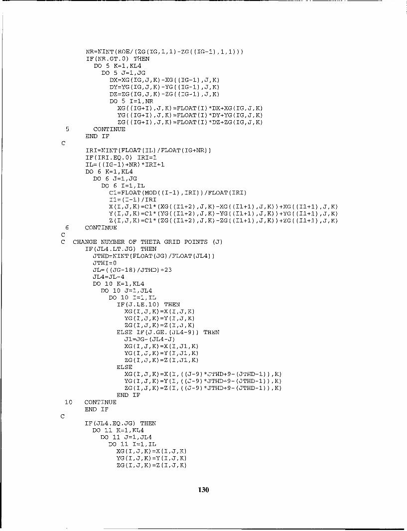
NR=NINT(ROE/ (ZG(IG, 1,1) -ZG( (IG-1) ,1,1)))IF(NR.GT.0) THENDO 5 K=1,KL4

DO 5 J=1,JGDX=XG(IG,J,K) -XG( (IG-1) ,J,K)DY=YG(IG,J,K) -YG( (IG-1) ,J,K)DZ=ZG(IG,J,K) -ZG( (IG-1) ,J,K)DO 5 I=1,NRXG((IG+I),J,K)=FLOAT(I)*DX+XG(IG,J,K)YG((IG+I),J,K)=FLOAT(I)*DY+YG(IG,J,K)ZG((IG+I),J,K)VFLOAT(I)*DZ+ZG(IG,J,K)

5 CONTINUEEND IF

CIRI=NINT (FLOAT (IL) /FLOAT (IG+NR))IFCIRI.EQ.0) IRI=1IL= ((IG-1) +NR) *IRI+1DO 6 K=1,KL4

DO 6 J=1,JGDO 6 I=1,IL

C1=FLOAT(MOD( (I-i) ,IRI) )/FLOAT(IRI)

6 CONTINUECC CHANGE NUMBER OF THETA GRID POINTS (J)

IF(JL4.LT.JG) THENJTHD=NINT(FLOAT(JG) /FLOAT(JL4))JTHI=0JL= ((JG-18) /JTHD) +23JL4=JL-4DO 10 K=1,KL4

DO 10 J=1,JL4DO 10 I=1,IL

IF(J.LE.10) THENXG(I,J,K) =X(I,J,K)YG(I,J,K) =Y(I,J,K)

ELSE IF(J.GE.(JL4-9)) THENJ1=JG- (JL4-J)XG(I,J,K) =X(I,J1,K)YG(I,J,K) =Y(I,J1,K)ZG(I,J,K)=Z(I,J1,K)

ELSEXG(I,J,K)=X(I,C(J-9)*JTHD+9-(JTHD-1)),K)YG(I,J,K)=Y(I,((J-9)*JTHD 9-(JTHD-1)),K)ZG(I,J,K)=Z(I,(CJ-~9)*JTHD+9-(JTHD-1)),K)

END IF10 CONTINUE

END IFC

IF(JL4.EQ.JG) THENDO 11 K=1,KL4


XG(I,J,K) =X(I,J,K)YG(I,J,K) =Y(I,J,K)ZG (I,,K) =Z (I,J, K)

130

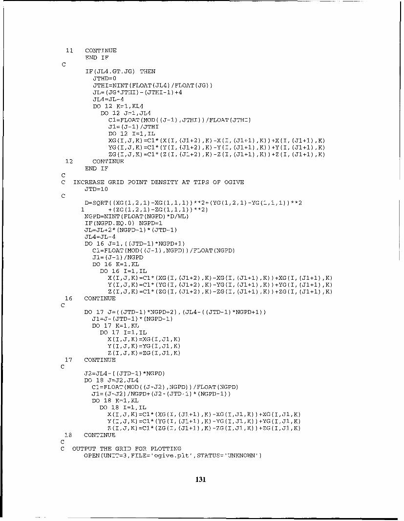
11 CONTINUEEND IF

CIF(JL4.GT.JG) THENJTHD=0JTHI=NINT(FLOAT(JL4) /FLOAT(JG))JL= (JG*JTHI) -(JTHI-1) +4JL4=JL-4DO 12 K=1,KL4

DO 12 J=1,JL4C1=FLOAT(MOD( (J-1) ,JTHI) )/FLOAT(JTHI)J1= (J-1) /JTHIDO 12 I=1,IL

12 CONTINUEEND IF

CC INCREASE GRID POINT DENSITY AT TIPS OF OGIVE

JTD= 10C

1 (ZG(1,2,1)-ZG(1,1,1) )**2)NGPD=NINT (FLOAT (NGPD) *D/WL)IF(NGPD.EQ.0) NGPD=1JL=JL+2* (NGPD-1) *(JTD-1)JL4=JL-4DO 16 J=1,C(JTD-1)*NGPD+1)C1=FLOAT(MOD( (J-1) ,NGPD) )/FLOAT(NGPD)Jl=(J-1) /NGPDDO 16 K=1,KL

DO 16 I=1,IL

Y(I,J,K)=C1*(YG(I, (J1+2) ,K)-YG(I, (J1+1) ,K) )+YG(I, (J1+1) ,K)

16 CONTINUEC

DO 17 J=((JTD-1)*NGPD+2), (JL4-((JTD-1)*NGPD+1))J1=J- (JTD-1) *(NGPD-1)DO 17 K=1,KL

DO 17 I=1,ILX(I,J,K)=XG(I,J1,K)Y(I,J,K)=YG(I,J1,K)Z(I,J,K)=ZG(I,J1,K)

17 CONTINUEC

J2=JL4- ((JTD-1) *NGPD)DO 18 J=J2,JL4

C1=FLOAT(MOD( (J-J2) ,NGPD) )/FLOAT(NGPD)J1=(J-j2) /NGPD+(J2- (JTD-1) *(NGPD-1))DO 18 K=1,KL

DO 18 I=1,ILX(I,J,K)=C1*(XG(I, (J1+1) ,K)-XG(I,J1,K))+XG(I,J1,K)Y(I,J,K)=C1*(YG(I, (J1+1) ,K)-YG(I,J1,K) )+YG(I,J1,K)Z(I,J,K)=C1* (ZG(I,CJ1+1) ,K) -ZG(I,J1,K) )+ZG(I,J1,K)

18 CONTINUECC OUTPUT THE GRID FOR PLOTTING

OPEN(UNIT=3,FILE='ogive.plt' ,STATUS='UNKNOWN')

131

WRITE(3, *) 'TITLE=OGIVE'WRITE(3,*) 'VARIABLES=X,Y,Z'WRITE(3,*) 'ZONE T="GRID", I=',IL,', J=',JL4,', K=',KL4DO 20 K=1,KL4


WRITE(3,102) X(I,J,K),Y(I,J,K),Z(IJ,K)20 CONTINUE

CLOSE (3)CC CALCULATE GRID POINT DENSITIES

J=JL/2+1KL5=KL-5GPDKB=KL5/ (W*X(1,J,1))GPDKT=KL5/ (W*X(1,2,1))

CGPDII=WL/(X(2,(JL/2+1),1)-X(1,(JL/2+1),1))GPDIO=WL/ (X(IL, (JL/2+1).1) -X( (IL-i) ,(JL/2+1), 1))

CD=0 .0DO 30 J=((JTD-.1)*NGPD+2), (JL4-(JTD-.1)*NGPD)

30 CONTINUEGPDJB=WL*FLOAT( (JL4- (JTD-1) *NGPD) -( (JTD-1) *NGPD+2) )/D

CD=0 .0DO 31 J=2,((JTD-1)*NGPD+1)

31 CONTINUEGPDJT=WL*FLOAT ((JTD-1) *NGPD-1)/AMAX1 (D, SS)

CC CALCULATE SURFACE LENGTH IN J DIRECTION

DJ=0 .0DO 32 J=2,JL4

J1=J-1

32 CONTINUEC

PRINT *,'OGIVE: RO,ROE,NR,IRI,IL ',RO,ROE,NR,IRI,ILPRINT *, 'OGIVE: JTHD,JTHI,JTD,NGPD,JL ',JTHD,JTHI,JTD,NGPD,JLPRINT *, 'OGIVE: GPD=KB,KT,IIIO,JB,JT ', OPDKB,GPDKT,GPDII,

1 GPDIO,GPDJB,GPDJTPRINT *,'L,PRX,DJ ',Z(1,1,1)-Z(1,JL4,1),X(1,(JL/2+1),1),DJ

CRETURNEND

C

B.2.3 Incident Field

The initial parameters for the incident field are calculated prior to the time loop. The

components of the E field vector, displacement vector, and the propagation unit vector are

132

calculated from the input parameters. The frequencies are also calculated if the Gaussian pulse

incident wave is specified. If a Gaussian pulse is used, a delay is introduced so the truncated

edge of the pulse is initially located at the point on the surface of the object farthest away from

the origin in the direction of the incident wave. The origin is located inside of the PEC scatterer.

The section of the code which calculates the initial incident field parameters is shown below.

C CALCULATE INCIDENT FIELD PARAMETERSC CONVERT ANGLES FROM DEGREES TO RADIANS

COSPH=COS(PHI*PI/180.0)SINPH=SIN(PHI*PI/180.0)COSTH=COS(THI*PI/180.0)SINTH=SIN(THI*PI/180.0)

CC FIND THE COMPONENTS OF THE E FIELD VECTOR

AMPX=AMP*(ETHI*COSTH*COSPH-EPHI*SINPH)AMPY=AMP*(ETHI*COSTH*SINPH+EPHI*COSPH)AMPZ=AMP*(-ETHI*SINTH)

CC FIND THE COMPONENTS OF THE DISPLACEMENT UNIT VECTOR FOR DELAY

XDIS=SINTH*COSPHYDIS=SINTH*SINPHZDIS=COSTH

CC CALCULATE THE ANGLES AND COMPONENTS OF K (PROPAGATION) UNIT VECTOR

PHK=PHI-180.0THK=-THI+180.0XK=SIN(THK*PI/180.0)*COS(PHK*PI/180.0)YK=SIN(THK*PI/180.0)*SIN(PHK*PI/180.0)ZK=COS(THK*PI/180.0)

CC INITIALIZE THE FREQUENCIES

DO 4 KW=I,KFWG(KW)=0.0

4 CONTINUECC ASSIGN THE FREQUENCY OF THE SINUSOID

KWM=1WG (1) =W

CC CALCULATE THE PARAMETERS/FREQUENCIES FOR THE GAUSSIAN PULSE

IF (ISRC.EQ.1) THENGTH=1.OE-8WM=2*PI*(1.0/3.0)*(I/(PI*GPT))*SQRT(-LOG(1.0E-7))KWM=INT(1.0/WD*WM)+1PRINT *,'W,WD,KWM ARE: ',W,WD,KWMDO 5 KW=1,KWMWG(KW)=FLOAT(KW-I)*WD

5 CONTINUEEND IF

CC CALCULATE DELAY SO INCIDENT WAVE, IF GAUSSIAN, PROPAGATES CORRECTLY

DEL=0.0

133

IF (ISRC.EQ.1) THENDO 6 K=1,KLM

DO 6 J=1,JLMD=XC1(J,K)*XDIS+YC1(J,K)*YDIS+ZC1(J,K)*ZDISIF (D.GT.O.0) THENDEL=AMAX1(DEL,D)

END IF6 CONTINUE

END IF

The values of the incident field, either from a sinusoid or Gaussian pulse incident wave,

at the surface of the scatterer are calculated in the subroutine SOURCE. The code listing for the

SOURCE subroutine is shown below.

CSUBROUTINE SOURCE(BIX1,BIX2,BIYI,BIY2,BIZ1,BIZ2,DIXI,DIX2,DIY1,

1 DIY2,DIZI,DIZ2,J,K,TF)PARAMETER(ID=75,JD=125,KD=45,KF=15)COMMON /CC/ XC1(JD,KD),XC2(JD,KD),YCI(JD,KD),YC2(JD,KD),1 ZC1(JD,KD),ZC2(JD,KD)COMMON /IN/ AMPX,AMPY,AMPZ,DEL,GPD,GPT,ISRC,W,WG(KF),XDIS,YDIS,1 ZDIS,XK,YK,ZKCOMMON /PR/ AMP,CFL,DT,EPS,IB,IL,JL,KL,ILM,JLM,KLM,KWM,REP,RMU,1 RK,RO,RP,SS,T

CC VARIABLES USED ONLY IN THE SOURCE SUBROUTINE:C BIX1,2: X COMPONENTS OF INCIDENT B FIELD AT CELL CENTERS 1,2C BIY1,2: Y COMPONENTS OF INCIDENT B FIELD AT CELL CENTERS 1,2C BIZ1,2: Z COMPONENTS OF INCIDENT B FIELD AT CELL CENTERS 1,2C DIS1,2: SPATIAL DELAY AT A CELL WITH CENTER OF I=1,2C DIX1,2: X COMPONENTS OF INCIDENT B FIELD AT CELL CENTERS 1,2C DIYI,2: Y COMPONENTS OF INCIDENT B FIELD AT CELL CENTERS 1,2C DIZ1,2: Z COMPONENTS OF INCIDENT B FIELD AT CELL CENTERS 1,2C GAUS1,2: INCIDENT FIELD AS A FCT OF W,GPT,GPD,DEL, AND DIS1,2C SINW1,2: INCIDENT FIELD AS A FCT OF W,T, AND DIS1,2C

C1=SQRT(RMU/REP)CC CALCULATE SPATIAL DELAY

DIS1=XC1(J,K)*XDIS+YCI(J,K)*YDIS+ZCI(J,K)*ZDISDIS2=XC2(J,K)*XDIS+YC2(J,K)*YDIS+ZC2(J,K)*ZDIS

CC CALCULATE D FIELD IF A SINUSOID IS REQUIRED

IF (ISRC.EQ.0) THENSINW1=SIN(W*(TF+DIS1))SINW2=SIN(W*(TF+DIS2))DIX1=REP*AMPX*SINWIDIX2=REP*AMPX*SINW2DIY1=REP*AMPY*SINWIDIY2=REP*AMPY*SINW2DIZ1=REP*AMPZ*SINW1DIZ2=REP*AMPZ*SINW2

CC CALCULATE D FIELD IF A GAUSSIAN PULSE IS REQUIRED

134

ELSERGPT=1. 0/GPTGP=GPD*GPTGAUS1=EXP(-((TF+DIS1-DEL-GP) *RGPT) **2)GAUS2=EXP(-((TF+DIS2-DEL-GP) *RGPT) **2)DIX1=REP*AMPX*GAUS 1DIX2 =REP*AMPX*GAUS2DIYI=REP *AMPY*GAUS1

DIY2 =REP*AMPY*GAUS2DIZI=REP*AMPZ*GAUSIDIZ2=REP*AMPZ*GAUS2

END IFCC CALCULATE THE COMPONENTS OF THE B FIELD

BIX1=C* (YK*DIZ1-ZK*DIY1)BIX2=C* (YK*DIZ2-ZK*DIY2)BIY1=C* (ZK*DIX1-XK*DIZ1)BIY2=C* (ZK*DIX2-XK*DIZ2)BIZI=C1* XK*DIYI-YK*DIX1)BIZ2=C* (XK*DIY2-YK*DIX2)

CRETURNEND

C

As can be seen in the code, the spatial and time delay is taken into account for the

sinusoid and Gaussian pulse incident wave. The location of the grid point on the surface of the

scatterer is accounted for in the calculation of the sinusoid incident wave. For the Gaussian

pulse, the time delay for the center of the pulse, the time delay due to the length of the object,

and the time delay due to the location of the grid point on the surface of the scatterer are used in

calculating the amplitude of the pulse.

B.2.4 RCS Convergence Check

The RCS convergence check is used to end the time loop when the RCS values have

converged to within a certain value when using a sinusoid incident wave. The RCS values are

sampled every 10 degrees every period. If the values are with 0.1 dB of the previously sampled

values, convergence has been reached and the time loop ends. The frequency data for the

scattered fields are set to zero prior to each period.

135

C

SUBROUTINE RCSCONV(FS,FU,N,NEND,NES,NP,RCSEC,RI)PARAMETER(ID=75,JD=125,KD=45,PI=3.14159265359,KF=15)COMMON ICC! XC1(JD,KD),XC2(JD,KD) ,YC1(JD,KD) ,YC2(JD,KD),1 ZC1 (JD, KD) ,ZC2 (JD, KD)COMMON /CO/ SXI(ID,JD,KD,3),SET(ID,JD,KD,3),SZT(ID,JD,KD,3),1 V(ID,JD,KD),X(ID,JD,KD),Y(ID,JD,KD),Z(ID,JD,KD)COMMON /IN/ AMPX,AMPY,AMPZ,DEL,GPD,GPT,ISRC,W,WG(KF) ,XDIS,YDIS,1 ZDIS,XK,YK,ZKCOMMON /PR/ AMP,CFL,DT,EPS, IB,IL,JL,KL, ILM,JLM,KLM,KWM,REP,RMU,1 RK,RO,RP,SS,TCOMPLEX AX,AY,AZ,CX,CY,CZ,DE,FS(JD,KD,6,KF) ,FU(JD,KD,6,KF),

1 FUEC (JD, KD, 6) ,RI, SUMEKi, SUMEK2 ,SUMEK3 ,SUMEJK1, SUMEJK2,2 SUMEJK3

DIMENSION RCSEC (19)CC VARIABLES USED ONLY IN THE RCSCONV SUBROUTINE:C SEE MAIN PROGRAM AND RCS SUBROUTINE FOR MOST VARIABLE DESCRIPTIONSC FUEC: FREQUENCY DATA USED FOR CONVERGENCE CHECKC RCSCH: RATIO OF CURRENT RCS VALUES TO PREVIOUS RCS VALUESC RCSCHI: INTERMEDIATE VALUE FOR RCSCHC

SME=SQRT (RMU/REP)C1=1 .0/REPC2=1 .0/RMU

CC CALCULATE INTEGRATION LIMITS

JLM1=JLM-1KLM4=KLM-4

CC NORMALIZE SCATTERED FIELD DATA TO INCIDENT FIELD

DO 5 K=1,KLDO 5 J=1,JL

RFSB=SQRT(CABS(FS(J,K,1,1))**2+CABS(FS(J,K,2,1))**21 +CABS(FS(J,K,3,1) )**2)

DO 6 L=1,3FUEC(J,K,L)=FU(J,K,L,1)/RFSB

6 CONTINUERFSD=SQRT(CABS(FS(J,K,4,1))**2+CABS(FS(J,K,5,1))**2

1 +CABS(FS(J,K,6,1))**2)DO 7 L=4,6

FUEC (J,K,L) =FU(J,K,L, 1) /RFSD7 CONTINUE5 CONTINUE

CC GENERATE THE BISTATIC RADAR CROSS SECTIONC

PHO=0 .0SINPO=SIN(PHO)COSPO=COS (PHO)

CC CHECK FOR CONVERGENCE OF RCS VALUES

RCSCH=0 .0DO 10 JO=1,19

THO= (PI*FLOAT (JO-i) *10.0)/180.0SINTO=SIN (THO)COSTO=COS (THO)

136

CC CALCULATE CARTESIAN COMPONENTS OF THE R (OBSERVATION) UNIT VECTOR

BX=SINTO*COSPOBY=SINTO*SINPOBZ=COSTO

CC PERFORM THE SURFACE INTEGAL (FREE SPACE GREEN'S FUNCTION)C SET INITIAL VALUES FOR THE SURFACE INTEGRAL,J & K LOOPS

SUI4EJK1= (0.0, 0. 0)SUMEJK2= (0. 0,0. 0)SUMEJK3= (0 .0,0. 0)

CDO 20 J=3,JLM1

CC SET INITIAL VALUES FOR THE SURFACE INTEGRAL, K LOOP

SUMEK1= (0.0,0.0)SUMEK2= (0.0,0.0)SUMEK3= (0 .0,0. 0)

CDO 30 K=1,KLM4

CC CALCULATE THE DOT PRODUCT OF R' AND R

PV=BX*XC2 (J, K) +BY*YC2 (J, K) +BZ*ZC2 (J,K)WP=WG(1) *PV

CC GENERATE SURFACE INTEGRAL SCALE & METRICS OF OUTWARD NORMAL

DS=SQRT((0.5*(SXI(IB,J,K,1)+SXI(IB-1,J,K,1)))**21 +(0.5* (SXI(IB,J,K,2)+SXI(IB-1,J,K,2) ) )**22 +(0.5* (SXI(IB,J,K,3)+SXI(IB-1,J,K,3) ) )**2)

SUMX=AMAX1 (DS, SS)RSUMX=1 .0/SUMXXIX=SXI (IB,J,K,1) *RStJJXXIY=SXI(IB,J,K,2) *RSUM XXIZ=SXI(IB,J,K,3) *RSUMX

CC GENERATE THE CROSS PRODUCTS OF THE ELECTROMAGNETIC FIELDC THE SURFACE ELECTRIC & MAGNETIC CURRENT DENSITIESC FOR THE EQUIVALENCE THEOREM

AX=C1*(XIY*FUEC(J,K,6)-XIZ*FUEC(J,K,5))AY=Cl*(XIZ*FUECCJ,K,4)-XIX*FUEC(J,K,6))AZ=C1*(XIX*FUEC(J,K,5)-XIY*FUEC(J,K,4))CX=C2*(XIY*FUEC(J,K,3)-XIZ*FUEC(J,K,2))CY=C2*(XIZ*FUEC(J,K,1)-XIX*FUEC(J,K,3))CZ=C2*CXIX*FUEC(J,K,2)-XIY*FUEC(J,K,1))DE=Cl*(XIX*FUEC(J,K,4)+XIY*FUEC(J,K,5)+XIZ*FUEC(J,K,6))

CIF((J.EQ.3).OR.(J.EQ.JLM1)) THENAX=AX/2 .0AY=AY/2 .0AZ=AZ/2 .0CX=CX/2 .0CY=CY/2 .0CZ=CZ/2 .0DE=DE/2 .0

END IFCC PERFORM THE SURFACE INTEGRATIONS FOR NEAR TO FAR FIELD TRANSFORM

SUMEK1=SUMEK1+WG(1) *(DE*BX+(AY*BZ-~AZ*BY) -SME*CX)1 *CEXP (-(RI*WP) )*DS

SUNEK2=SUMEK2+WG(1) *(DE*BY+ (AZ*BX-AX*BZ) -SME*CY)

137

1 *CEXP(-(RI*WP))*DSSUMEK3=SUMEK3+WG(1)*(DE*BZ+(AX*BY-AY*BX)-SME*CZ)

1 *CEXP(-(RI*WP))*DSC30 CONTINUE

CSUMEJK1=SUMEJK1+SUMEKISUMEJK2=SUMEJK2+SUMEK2SUMEJK3=SUMEJK3+SUMEK3

C20 CONTINUE

CC CALCULATE THE RCS: 4*PI*(R**2)*IEsI**2/IEiI**2C NOTE: NORMALIZATION WRT THE INCIDENT FIELD WAS DONE DURING FT

RCSE=RCSEC(JO)RCSEC(JO)=(CABS(SUMEJKI)**2+CABS(SUMEJK2)**2+CABS(SUMEJK3)**2)

1 /(4.0*PI)CC CHECK FOR CONVERGENCE, CONTINUE OR END TIME LOOP

RCSE=AMAXI(RCSE,SS)RCSCHI=RCSEC(JO)/RCSEIF(RCSCHI.LT.1.0) RCSCHI=1.0/RCSCHIRCSCH=AMAX1(RCSCHI,RCSCH)

10 CONTINUECC IF ALL RCS VALUES ARE WITHIN 0.1 DB OF PREVIOUS VALUES,C CONVERGENCE HAS BEEN REACHED

IF(RCSCH.LT.I.0233) THENNEND=NNES=NEND

C RESET THE INITIAL VALUES FOR ALL FOURIER TRANSFORM VARIABLESELSEDO 40 L=1,6

DO 40 K=1,KLDO 40 J=1,JL

FU(J,K,L,1)=(0.0,0.0)FS(J,K,L,1)=(0.0,0.0)

40 CONTINUEEND IFPRINT *,'N,RCSCH: ',N,RCSCH

CRETURNEND

B.2.5 Scattered-Field Threshold Check

The time loop ends if the amplitude of the scattered field is below a predetermined

threshold when a Gaussian pulse is used for the incident wave. The amplitude of the scattered

field on the virtual surface (I=IB) is checked every time step to determine the maximum

138

amplitude of the scattered field. The time loop which contains the threshold check is listed

below.

C PERFORM THE SOLVING SEQUENCEN=1DO WHILE(N.LE.NEND)

T=FLOAT(N-I)*DTMR=0M=1

CCALL BC(M,MR)

CC

DO 11 MR=1,4C

CALL FXICALL GETACALL HZETACALL SUM(MR)

C11 CONTINUE

CIF((N.GT.NES).OR.(N.LT.NBS)) GOTO 10

C PERFORM FOURIER TRANSFORMTF=T+DTRU=0.0DO 12 KW=I,KWM

WT=WG (KW) * (TF)DO 12 K=1,KL

DO 12 J=I,JLC

CALL SOURCE(BIX1,SN(1),BIYI,SN(2),BIZI,SN(3),DIX1,SN(4),DIY1,SN(5),DIZ1,SN(6),J,K,TF)

CCC IF GAUSSIAN SOURCE, CHECK AMPLITUDE OF SCATTERED FIELD, END TIME LOOPC IF BELOW THRESHOLD

IF(ISRC.EQ.1) THENRUL=SQRT(U(1,IB,J,K,4)**2+U(1,IB,J,K,5)**2

1 +U(1, IB,J,K, 6) **2)RU=AMAX1(RU,RUL)

END IFDO 12 L=1,6FU(J,K,L,KW)=FU(J,K,L,KW)+(U(1,IB,J,K,L)+SN(L))

1 *CEXP(RI*WT)FS(J,K,L,KW)=FS(J,K,L,KW)+SN(L)*CEXP(RI*WT)

12 CONTINUEIF((ISRC.EQ.1).AND.(N.GE.100)) THENIF(RU.LE.GTH) NEND=NNES=NEND

END IFCC IF SINUSOID SOURCE, RUN CONVERGENCE CHECK ON RCS VALUES

IF((ISRC.EQ.0).AND.(ICON.EQ.1)) THENIF(MOD(N,NP).EQ.0) THEN

C

139

CALL RCSCONV(FS,FU,N,NEND,NES,NP,RCSEC,RI)C

END IFEND IF

C10 N=N+I

END DOC END OF TIME LOOP

B.2.6 Bistatic-to-Monostatic Approximation

A description of the bistatic-to-monostatic approximation is given in Chapter 3. The

code is not a subroutine for the FVTD code but is an independent program. The RCS values

from the "rcsmO.plt" files are used for the HH polarization approximation. The incident wave

must be specified with ETH polarization to obtain HH polarization results. To obtain RCS

results for the VV polarization, the "rcseO.plt" files are used. The incident wave must be

specified with EPH polarization to obtain VV polarization results. The code listed below is for

obtaining a monostatic sweep for the ogive for HH polarization. A similar file is used for VV

polarization and to obtain the monostatic results for the cone-sphere.

C THIS FORTRAN CODE USES CONTINUOUS BISTATIC VALUES AND SEVERALC MONOSTATIC VALUES TO APPROXIMATE A CONTINUOUS MONOSTATICC SOLUTION FOR THE OGIVECC SOURCE: THE MONOSTATIC/BISTATIC APPROXIMATIONC MICHAEL SCHUH, ALEX WOO, MICHAEL SIMONC IEEE ANTENNAS AND PROPAGATION MAGAZINEC VOL. 36, NO. 4, AUGUST 1994, PAGES 76-78CC VARIABLE DESCRIPTIONSC DEG: ANGLE AT WHICH MONOSTATIC VALUE IS APPROXIMATEDC NB: INDEX FOR BISTATIC RCS VALUEC NU: INDEX FOR FILE UNIT WHICH IS CURRENTLY BEING USEDC RCSE: MONOSTATIC AND BISTATIC RCS VALUES READ FROM FILEC RCSMON: CALCULATED MONOSTATIC RCS VALUESC W: FREQUENCY IN RADIANS/SECC

PROGRAM RCSCONVDIMENSION RCSE(721),RCSMON(721),A(15)

CC SPECIFY VARIOUS FORMATS FOR FILE INPUTS/OUTPUTS100 FORMAT(F6.2,1X,E13.6)

C

140

OPEN(UNIT=50,FILE='rcsmon-v.plt' ,STATUS='UNKNOWN')C

DO 10 N=1,361NU= (N+19) /40+11OPEN(UNIT=11,FILE='rcsmO-O.plt' ,STATUS='OLD')OPEN(UNIT=12,FILE='rcsmO-l0.plt' ,STATUS='OLD')OPEN(UNIT=13,FILE='rcsmn020.plt' ,STATUS='OLD')OPEN(TJNIT=14,FILE='rcsnO-3O.plt' ,STATUS='OLD')OPEN(UNIT=15,FILE='rcsmn040.plt' ,STATUS='OLD')OPEN(UNIT=16,FILE='rcsmO-50.plt' ,STATUS='OLD')OPEN(UNIT=17,FILE='rcsm06o0.plt ,STATUS='OLD')OPEN(UNIT=18,FILE='rcsm07o0.plt' ,STATUS='OLD')OPEN(UNIT=19,FILE='rcsmO-80.plt ,STATUS='OLD')OPEN(UNIT=20,FILE='rcsmO-90.plt ,STATUS='OLD')

CREAD(NU,*) FILL,WDO 20 I=1,721

READ(NU,*) DEGREE,RCSE(I)20 CONTINUE

CIF(NU.EQ.11) THEN

NB= (2* (N-i) +1)RCSMON(N) =RCSE (NB)

ELSE IF(NU.EQ.20) THENNB=-2* (361-N) +361RCSMON (N) =RCSE (NB)

ELSENB=2* (N- ((NU-11) *40+1) )+ (NU-11) *40+1RCSMON (N) =RCSE (NB)

END IFC

CLOSE (11)CLOSE (12)CLOSE (13)CLOSE (14)CLOSE (15)CLOSE (16)CLOSE (17)CLOSE (18)CLOSE (19)CLOSE (20)

C10 CONTINUE

CWRITE(50,100) FILL,WDO 50 I=1,361

DEG=FLOAT(I-1) *0.25WRITE(50,100) DEG,RCSMON(I)

50 CONTINUEC

DO 51 I=362,721DEG=FLOAT(I-1) *0.25WRITE(50,100) DEG,RCSMON(722-I)

51 CONTINUEC

CLOSE (50)STOPEND

141

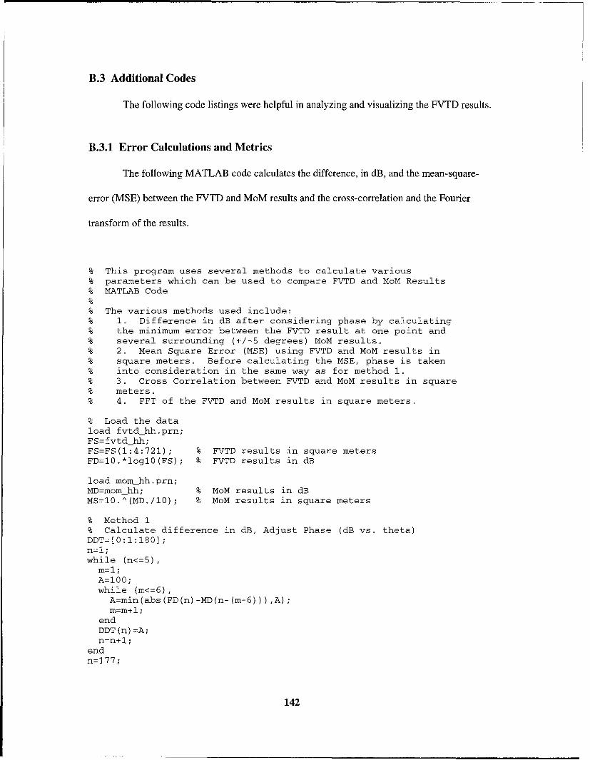
B.3 Additional Codes

The following code listings were helpful in analyzing and visualizing the FVTD results.

B.3.1 Error Calculations and Metrics

The following MATLAB code calculates the difference, in dB, and the mean-square-

error (MSE) between the FVTD and MoM results and the cross-correlation and the Fourier

transform of the results.

% This program uses several methods to calculate various% parameters which can be used to compare FVTD and MoM Results% MATLAB Code

% The various methods used include:% 1. Difference in dB after considering phase by calculating% the minimum error between the FVTD result at one point and% several surrounding (+/-5 degrees) MoM results.% 2. Mean Square Error (MSE) using FVTD and MoM results in% square meters. Before calculating the MSE, phase is taken% into consideration in the same way as for method 1.% 3. Cross Correlation between FVTD and MoM results in square% meters.% 4. FFT of the FVTD and MoM results in square meters.

% Load the dataload fvtd-hh.prn;FS=fvtdhh;FS=FS(I:4:721); % FVTD results in square metersFD=I0.*loglO(FS); % FVTD results in dB

load momhh.prn;MD=mom hh; % MoM results in dBMS=I0.^(MD./10); % MoM results in square meters

% Method 1% Calculate difference in dB, Adjust Phase (dB vs. theta)DDT=[0:1:180];n=l;while (n<=5),

m=l;A=100;while (m<=6),A=min(abs(FD(n)-MD(n-(m-6))),A);m=m+l;

endDDT (n) =A;n=n+l;

endn=177;

142

while (n<=181),m=6;A=100;while (m<=ll),

A=min(abs (FD(n) -MD(n- (m-6) )) ,A);m=m+l;

endDDT(n)=A;n=n+l;

end

n=6;while (n<=176),

m=l;A=100;while (m<=ll),

A=min(abs(FD(n)-MD(n-(m-6))) ,A);m=m+l;

endDDT(n)=A;n=n+l;

endDD=max(DDT)DDT=rot90(DDT,3);save diffhh DDT -ascii % Save difference values in dB to a file

% Method 2% Calculate MSE, Adjust Phase if Incorrect (square meters).^2MSE=0;n=l;while (n<=5),

MSE=MSE+(FS(n)-MS(n)) .^2;n~n+l;

endn=177;while (n<=181),

MSE=MSE+(FS(n)-MS(n)) .^2;n=n+l;

end

n=6;while (n<=176),

m=l;A=100;while (m<=ll),A=min(abs(FS(n)-MS(n-(m-6))),A);m=m+l;

endMSE:MSE+A.^2;n=n+l;

endMSE=(I./181).*MSE

% Method 3% Compute cross-correlation (square meters)XC=xcor(MS,FS, 'coeff');

% Plot the cross-correlationtheta=[0:l:(2*length(FS)-2)];plot(theta,XC)

143

title('Cross-Correlation Between FVTD and MoM results, HH')xlabel('Theta (Degrees)')ylabel('XCORR')axis([170 190 0.95 1]);save xcorrhh XC -ascii % Save cross-correlation values to a file

% Method 4% Calculate FFT of FVTD and Mom results (square meters)% Remove DC value firstn=l;FST=0;while (n<=181),

FST=FS(n)+FST;n=n+l;

endFST=FST./181;FS=FS-FST;n=l;MST=0;while (n<=181),MST=MS(n)+MST;n=n+l;

endMST=MST./181;MS=MS-MST;

% Use Hamming windowFS=ham(181).*FS;MS=ham(181).*MS;

% Calculate FFTFF=abs(fft(FS,1024));MF=abs(fft(MS,1024));

% Plot the fft'sfigurethetai=(l./1024).*[0:1023];plot(thetai,FF)hold onplot(thetai,MF, '--')

title('FFT of FVTD vs. MoM Results, HH')xlabel('Cycles/Theta')ylabel('FFT')axis([0 0.1 0 0.06]);save fftfhh FF -ascii % Save FVTD fft values to a filesave fftmhh MF -ascii % Save MoM fft values to a file

B.3.2 Scattered Electric Field Movie

The listed MATLAB code generates a movie of the scattered field for the cone-sphere.

The plots are contour plots of the scattered electric field.

% Movie of Electromagnetic Scattering from 3-D Object (Cone-Sphere)

144

% Movie displays contours of the scattered electric field% MATLAB Code% As the scattered field data is loaded and displayed at each of N time% steps, snapshots of the graphics window are saved in a large matrix.% The total storage required is proportional to the area of the% graphics window.% Load the gridI=49;J=36;nframes=40;fid = fopen('x.grd','r')[x,Count] = fscanf(fid, '%13e', [I,J]);fid = fopen('y.grd',' r');[y,Count] = fscanf(fid, '%13e', [I,J]);

% Set up movie framefid = fopen('plot5O.dat','r');[El,Countl = fscanf~fid,'%lle',[I,J]);% Plot the contourpcolor Cx, -y, El)shading(C'interp')colormap (let)axis([-l.l 1.1 -1.1 1.7]);axis ('square')caxis([0.0 0.3]);title('Cone-Sphere Scattered Electric Field Contours (0.869 GHz)')xlabel('x (in)')ylabelC'y (m)')hold onpcolor(-x,-y,El);shading(C'interp')M=moviein (nframes);

% Record the Moviefor j=1:nframes

if l==lfid=fopen( 'plot50.dat', 'r');

endif j==2

fid=fopenC 'plot5l.dat', 'r');endif j==3

fid=fopenC 'plot52.dat', 'r');endif j==4

fid=fopen C'plot53 .dat', 'r');endif j==5



fid=fopen('plot56.dat','r');endif j==8

fid=fopenC'plot57.dat', 'r');endif j==9

145

fid=fopen( 'plot58.dat', 'r');endif j==1O

fid=fopen( 'plot59.datl, r');endif j==11

fid=fopen( 'plot6O.dat', 'r');endif j==12

fid=fopen( 'plot6l.dat', 'r');endif j==13

fid=fopen C plot62 .dat','r');endif j==14

fid=fopen('plot63.dat' ,'r');endif j==15

fid=fopen( 'plot64.dat', 'r');endif j==16

fid=fopenC 'plot65.dat' ,'r');endif j==17


fid=fopen ('plot67 .dat', r');endif j==19


fid=fopen ('plot69 .dat' ,'r');endif j==21

fid=fopen( 'plot7O.dat', 'r');endif j==22

fid=fopen( 'plot7l.dat', 'r');endif j==23



fid~fopen( 'plot74.dat', 'r');endif j==26

fid=fopen( 'plot75.dat' ,'r');endif j==27


fid=fopen ('plot77 .dat', 'r');endif j==29

146



fidz~fopen( 'plot8O.dat','r');endif j==32

fid=fopen('plot8l.dat', 'r');endif j==3 3

fid=fopen('plot82.dat', r');endif j==34

fid=fopen ( plot83 .dat ,r );endif j== 3 5

fid=fopen( 'plotS4.dat' ,'r')

endif j==36

fid=fopen( 'plot85.dat','r');endif j==?37

fid=fopen( 'plot86.dat', r')endif j==3 8


fid=fopen( 'plot88.datI, 'r');endif j==40

fid=fopen('plot89.dat','r');end[El,Count] = fscanf(fid,'%llel,[I,J]);% Plot the contourpcolor Cx, -y, El)shading ('interpl)axis([-l.l 1.1 -1.1 1.7]);axis ( square')caxis([0.0 0.3]);title('Cone-Sphere Scattered Electric Field Contours (0.869 GHz) ')xlabel('x (in))

ylabel('y (mn)')pcolor(-x,-y,El);shading(C'interp')M(:,1) =getfrane;

end% Play Moviemovie (M, 5,4)

B.4 FVTD FORTRAN Code

The entire code can be obtained from Dr. J.S. Shang of Wright Laboratory or the author.

147

Bibliography

1. M.J. Aftosmis, "Two Compact Cell-Vertex Methods for Computational Electromagnetics,"AIAA Paper 91-1504. 22nd AIAA Fluid Dynamics, Plasmadynamics, and LasersConference, Honolulu HI, June 1991.

2. W. Kyle Anderson and James L. Thomas, "Comparison of Finite Volume Flux VectorSplittings for the Euler Equations," AIAA Journal, vol. 24, no. 9, pp. 1453-1460, Sept. 1986.

3. Constantine A. Balanis, Advanced Engineering Electromagnetics. New York: John Wiley& Sons, 1989.

4. Jean-Pierre Berenger, "A Perfectly Matched Layer for the Absorption of ElectromagneticWaves," Journal of Computational Physics, vol. 114, no. 2, pp. 185-200, Oct. 1994.

5. David G. Bishop and Dale A. Anderson, "A Comparison of Finite-Volume Time-DomainSchemes for the Maxwell Equations," AIAA Paper 92-0456. 30th Aerospace SciencesMeeting and Exhibit, Reno NV, Jan. 1992.

6. D.C. Blake and T.A. Buter, "Domain Decomposition Strategies for Solving HyperbolicSystems on Distributed Parallel Architectures," AIAA Paper 96-0834. 34th AerospaceSciences Meeting and Exhibit, Reno NV, Jan. 1996.

7. D.C. Blake and T.A. Buter, "Overset Grid Methods Applied to a Finite-Volume Time-Domain Maxwell Equation Solver," AIAA Paper 96-0834. 27th Fluid Dynamics,Plasmadynamics and Lasers Conference, New Orleans LA, June 1996.

8. Douglas C. Blake, A Numerical Study of High-Speed Missile Configurations Using a Block-Structured Parallel Algorithm. MS thesis, AFIT/GAE/ENY/93D-4. Graduate School ofEngineering, Air Force Institute of Technology (AU), Wright-Patterson AFB, OH, Dec.1993.

9. Mary L. Boas, Mathematical Methods in the Physical Sciences. New York: John Wiley &Sons, 1983.

10. Richard C. Booton, Jr., Computational Methods for Electromagnetics and Microwaves.New York: John Wiley & Sons, 1992.

11. David K. Cheng, Field and Wave Electromagnetics (Second Edition). Reading: Addison-Wesley Publishing Company, 1992.

12. J.W. Crispin, Jr. and K.M. Siegel, Methods of Radar Cross Section Analysis. New York:Academic Press, 1968.

13. Bjorn Engquist and Andrew Majda, "Absorbing Boundary Conditions for the NumericalSimulation of Waves," Mathematics of Computation, vol. 31, no. 139, pp. 629-65 1, July1977.

148

14. N.T. Frink, P. Parikh, and S. Pirzadeh, "A Fast Upwind Solver for the Euler Equations onThree-Dimensional Unstructured Meshes," AIAA Paper 91-0102. 29th Aerospace SciencesMeeting, Reno NV, Jan. 1991.

15. K.S. Huh, M. Shu, and R.K. Agarwal, "A Compact High-Order Finite-Volume Time-Domain/Frequency-Domain Method for Electromagnetic Scattering," AIAA Paper 92-0453.30th Aerospace Sciences Meeting and Exhibit, Reno NV, Jan. 1992.

16. Elliot B. Koffman and Frank L. Friedman, FORTRAN with Engineering Applications (FifthEdition). Reading: Addison-Wesley Publishing Company, 1993.

17. Eugene F. Knott, John F. Shaeffer, and Michael T. Tuley, Radar Cross Section. Dedham:Artech, 1985.

18. Karl S. Kunz and Raymond J. Luebbers, The Finite Difference Time Domain Method forElectromagnetics. Boca Raton: CRC Press, 1993.

19. Yen Liu, "Fourier Analysis of Numerical Algorithms for the Maxwell Equations," AIAAPaper 93-0368. 31 st Aerospace Sciences Meeting and Exhibit, Reno NV, Jan. 1993.

20. A. H. Mohammadian, V. Shankar, and W.F. Hall, "Application of Time-Domain Finite-Volume Method to Some Radiating Problems in Two and Three Dimensions," IEEETransactions on Magnetics, vol. 27, no. 5, pp. 3841-3844, Sept. 1991.

21. Gerrit Mur, "Absorbing Boundary Conditions for the Finite Difference Approximation ofthe Time-Domain Electromagnetic-Field Equations," IEEE Transactions onElectromagnetic Compatibility, vol. EMC-23, no. 4, pp. 377-382, Nov. 1981.

22. Ralph W. Noack and Dale A. Anderson, "Time-Domain Solutions of Maxwell's EquationsUsing a Finite-Volume Formulation," AIAA Paper 92-0451. 30th Aerospace SciencesMeeting and Exhibit, Reno NV, Jan. 1992.

23. Alan V. Oppenheim and Ronald W. Schafer, Discrete-Time Signal Processing. EnglewoodCliffs, New Jersey: Prentice-Hall, 1989.

24. P.L. Roe, "Approximate Riemann Solvers, Parameter Vectors, and Difference Schemes,"Journal of Computational Physics, vol. 43, pp. 357-372, 1981.

25. Alfred Rosenblatt and George F. Watson, "Concurrent Engineering," IEEE Spectrum, pp.22-37, July 1991.

26. Shepley L. Ross, Introduction to Ordinary Differential Equations (Fourth Edition). NewYork: John Wiley & Sons, 1989.

27. George T. Ruck, Donald E. Barrick, William D. Stuart, and Clarence K. Krichbaum, RadarCross Section Handbook. New York: Plenum Press, 1970.

149

28. Schuh, Michael J., Alex C. Woo, and Michael P. Simon, "The Monostatic/BistaticApproximation," IEEE Antennas and Propagation Magazine, vol. 36, no. 4, pp. 76-78, Aug.1994.

29. J.S. Shang, "A Characteristic-Based Algorithm for Solving 3-D, Time-Domain MaxwellEquations," AIAA Paper 92-0452. 30th Aerospace Sciences Meeting and Exhibit, RenoNV, Jan. 1992.

30. J.S. Shang, "Characteristic-Based Algorithms for Solving Maxwell's Equations in the Time-Domain," IEEE Antennas and Propagation Magazine, vol. 37, no. 3, pp. 15-25, June 1995.

31. J.S. Shang, "Characteristic-Based Methods for the Time-Domain Maxwell Equations,"AIAA Paper 91-0606. 29th Aerospace Sciences Meeting, Reno NV, Jan. 1991.

32. J.S. Shang, "A Fractional-Step Method for Solving 3-D Time-Domain Maxwell Equations,"AIAA Paper 93-0461. 31 st Aerospace Sciences Meeting and Exhibit, Reno NV, Jan. 1991.

33. J.S. Shang, "A Fractional-Step Method for Solving 3-D Time-Domain Maxwell Equations,"Journal of Computational Physics, vol. 118, pp. 109-119, 1995.

34. J.S. Shang and Robert M. Fithen, "A Comparative Study of Numerical Algorithms forComputational Electromagnetics," AIAA Paper 94-2410. 25th AIAA Plasmadynamics andLasers Conference, Colorado Springs CO, June 1994.

35. J.S. Shang, K.C. Hill, and D. Calahan, "Performance of a Characteristic-Based, 3-D, Time-Domain Maxwell Equations Solver on a Massively Parallel Computer," AIAA Paper 93-3179. 24th AIAA Plasmadynamics and Lasers Conference, Orlando FL, July 1993.

36. J.S. Shang, D.A. Calahan, and B. Vikstrom, "Performance of a Finite Volume CEM Codeon Multicomputers," AIAA Paper 94-0236. 32nd Aerospace Sciences Meeting and Exhibit,Reno NV, Jan. 1994.

37. J.S. Shang and D. Gaitonde, "Characteristic-Based Time-Dependent Maxwell EquationsSolvers on a General Curvilinear Frame," AIAA Paper 93-3178. 24th AIAAPlasmadynamics and Laser Conference, Orlando FL, July 1993.

38. J.S. Shang and D. Gaitonde, "On High Resolution Schemes for Time-Dependent MaxwellEquations," AIAA Paper 96-0832. 34th Aerospace Sciences Meeting and Exhibit, RenoNV, Jan. 1996.

39. J.S. Shang and D. Gaitonde, "Scattered Electromagnetic Field of a Reentry Vehicle," AIAAPaper 94-0231. 32nd Aerospace Sciences Meeting and Exhibit, Reno NV, Jan. 1996.

40. J.S. Shang and S.J. Scherr, "Time-Domain Electromagnetic Scattering Simulations onMulticomputers," AIAA Paper 95-1966. 26th AIAA Plasmadynamics and LasersConference, San Diego CA, June 1995.

150

41. J.S. Shang and C.C. Shang, "Concurrent Computation of Electromagnetic Phenomena onthe Paragon," AIAA Paper 95-0592. 33rd Aerospace Sciences Meeting and Exhibit, RenoNV, Jan. 1995.

42. Vijaya Shankar, "Computational Electromagnetics (CEM) - Development of a Finite-Volume, Time-Domain Solver for Maxwell's Equations," Report NAWCADWAR-93052-60, Contract N62269-90-C-0257, Thousand Oaks, CA: Rockwell International ScienceCenter, 1993.

43. Vijaya Shankar, "Research to Application - Supercomputing Trends for the 90's,Opportunities for Interdisciplinary Computations," AIAA Paper 91-0002. 29th AerospaceSciences Meeting, Reno NV, Jan. 1991.

44. Vijaya Shankar, W.F. Hall, and A.H. Mohammadian, "A CFD-based Finite-VolumeProcedure for Computational Electromagnetics - Interdisciplinary Applications of CFDMethods," AIAA Paper 89-1987. 9th AIAA Computational Fluid Dynamics Conference,Buffalo NY, June 1989.

45. Vijaya Shankar, W.F. Hall, and A.H. Mohammadian, "A Time-Domain, Finite-VolumeTreatment for the Maxwell Equations," Electromagnetics, vol. 10, pp. 127-145, 1990.

46. Vijaya Shankar, W.F. Hall, A.H. Mohammadian, and R. Erickson, "CFD Spinoff -Computational Electromagnetics for Radar Cross Section (RCS) Studies," AIAA Paper 90-3055. 8th AIAA Applied Aerodynamics Conference, Portland OR, Aug. 1990.

47. Vijaya Shankar, W.F. Hall, A.H. Mohammadian, and C. Rowell, "Algorithmic Aspects andSupercomputing Trends in Computational Electromagnetics," AIAA Paper 93-0367. 31stAerospace Sciences Meeting, Reno NV, Jan. 1993.

48. Joseph L. Steger and R.F. Warming, "Flux Vector Splitting of the Inviscid GasdynamicEquations with Application to Finite-Difference Methods," Journal of ComputationalPhysics, vol. 40, pp. 263-293, 1981.

49. Gilbert Strang, Linear Algebra and its Applications (Third Edition). Fort Worth: SaundersCollege Publishing, 1988.

50. Julius Adams Stratton, Electromagnetic Theory. New York: McGraw-Hill, 1941.

51. Allen Taflove, Computational Electrodynamics: The Finite-Difference Time-DomainMethod. Boston: Artech House, 1995.

52. Allen Taflove, "Re-inventing Electromagnetics: Supercomputing Solution of Maxwell'sEquations via Direct Time Integration on Space Grids," AIAA Paper 92-0333, 30thAerospace Sciences Meeting, Reno NV, Jan. 1992.

53. Brain van Leer, "Flux-Vector Splitting For the Euler Equations," Eighth InternationalConference on Numerical Methods in Fluid Dynamics, Berlin: Springer-Verlag, pp. 507-512, 1982.

151

54. John L. Volakis and Leo C. Kempel, "Electromagnetics: Computational Methods andConsiderations," IEEE Computational Science and Engineering, pp. 42-57, Spring 1995.

55. John L. Volakis, Alex C. Woo, Helen T.G. Wang, Michael J. Schuh, and Michael L.Sanders, "Benchmark Radar Targets for the Validation of Computational ElectromagneticsPrograms," IEEE Antennas and Propagation Magazine, vol. 35, no. 1, pp. 84-89, Feb. 1993.

56. Kane S. Yee, "Numerical Solution of Initial Boundary Value Problems Involving Maxwell'sEquations in Isotropic Media," IEEE Transactions on Antennas and Propagation, vol. AP-14, no. 3, pp. 302-307, May 1966.

57. Li Zhao and Andreas C. Cangellaris, "A General Approach for the Development of Unsplit-Field Time-Domain Implementation of Perfectly Matched Layers for FDTD GridTruncation," IEEE Microwave and Guided Wave Letters, vol. 6, no. 5, pp. 209-211, May1996.

152

Vita

Captain Frederick G. Harmon

- n He graduated as valedictorian from Sweet Grass

County High School in Big Timber, Montana in 1987.

lie joined the Air Force Reserve Officer Training Corps (ROTC) detachment at Embry-

Riddle Aeronautical University in Prescott, AZ in 1987. He received his Bachelor of Science

degree in Electrical Engineering, graduated Magna Cur Laude, and was commissioned as a

second lieutenant in April 1992.

His initial assignment was at the National Air Intelligence Center (NAIC) at Wright-

Patterson AFB, OH where he analyzed foreign electronic warfare equipment such as airborne

radar jammers, radar warning receivers, and ground-based radar jammers. He was the technical

nmanager for the exploitation of a foreign radar jammer and received the Air Force

Commendation Medal for his performance at NAIC. Upon completion of this assignment, he

entered the AiriForce Institute of Technology to pursue a Master of Science degree in Electrical

Engineering specializing in electromagnetic scattering, antennas, and communication and radar

systems.

153

Form ApprovedREPORT DOCUMENTATION PAGE OMB No. 0704-0188

Public reporting burden for this collection of information is estimated to average 1 hour per response, including the time for reviewing instructions, searching existing data sources,gathering and maintaining the data needed, and completing and reviewing the collection of information. Send comments regarding this burden estimate or any other aspect of thiscollection of information, including suggestions for reducing this burden, to Washington Headquarters Services, Directorate for Information Operations and Reports, 1215 JeffersonDavis Highway, Suite 1204, Arlington, VA 22202-4302, and to the Office of Management and Budget, Paperwork Reduction Project (0704-0188), Washington, DC 20503.

1. AGENCY USE ONLY (Leave blank) 2. REPORT DATE 3. REPORT TYPE AND DATES COVEREDDecember 1996 Master's Thesis

4. TITLE AND SUBTITLE 5. FUNDING NUMBERS

APPLICATION OF A FINITE-VOLUME TIME-DOMAINMAXWELL EQUATION SOLVER TO THREE-DIMENSIONAL OBJECTS

6. AUTHOR(S)


7. PERFORMING ORGANIZATION NAME(S) AND ADDRESS(ES) 8. PERFORMING ORGANIZATIONREPORT NUMBER

Air Force Institute of Technology, WPAFB, OH 45433-6583 AFIT/GE/ENG/96D-06

9. SPONSORING/MONITORING AGENCY NAME(S) AND ADDRESS(ES) 10. SPONSORING/MONITORING

Dr. J.S. Shang Dr. Kueichien Hill AGENCY REPORT NUMBER

Wright Laboratory, WL/FIM Wright Laboratory, WL/XPN, Bldg 2542645 Fifth St, Ste 6 2591 K StWPAFB, OH 45433-7912 WPAFB, OH 45433-7602

11. SUPPLEMENTARY NOTES

12a. DISTRIBUTION /AVAILABILITY STATEMENT 12b. DISTRIBUTION CODE

13. ABSTRACT (Maximum 200 words)

Concurrent engineering approaches for the disciplines of computational fluid dynamics (CFD) andelectromagnetics (CEM) are necessary for designing future high-performance, low-observable aircraft. Acharacteristic-based finite-volume time-domain (FVTD) computational algorithm, developed for CFD and nowapplied to CEM, is implemented to analyze the radar cross section (RCS) of two three-dimensional objects, theogive and cone-sphere. The FVTD formulation implements a Monotone Upstream-Centered Scheme forConservation Laws (MUSCL) algorithm for the flux evaluation and a Runge-Kutta multi-stage scheme for thetime integration. Developmental FVTD work for the thesis focused on algorithm development to analyzescattering and obtain RCS data for closed-surface perfect electric conductor (PEC) 3-D objects using either aGaussian pulse or sinusoid incident wave. In addition, specification of the direction and polarization of theincident wave gives monostatic and bistatic RCS results. Convergence and threshold checks end the simulationrun to ensure accurate computation of the RCS. Validation of the characteristic-based FVTD formulation and

code for electromagnetic scattering problems is completed by comparing RCS results obtained from the FVTDcode to Moment Method and empirical RCS data. The FVTD results for the ogive and cone-sphere are within

3.0 dB of the MoM results and 3.1 dB of the empirical RCS results. Accurate FVTD computations of diffraction,traveling waves, and creeping waves require a surface grid point density of 15-30 cells/,.

14. SUBJECT TERMS 15. NUMBER OF PAGES168

electromagnetic scattering, radar cross section, RCS, finite-volume 16. PRICE CODEtime-domain, FVTD, computational fluid dynamics

17. SECURITY CLASSIFICATION 18. SECURITY CLASSIFICATION 19. SECURITY CLASSIFICATION 20. LIMITATION OF ABSTRACTOF REPORT OF THIS PAGE OF ABSTRACT

UNCLASSIFIED UNCLASSIFIED UNCLASSIFIED ULNSN 7540-01-280-5500 Standard Form 298 (Rev. 2-89)

Prescribed by ANSI Std. Z39-18298-102

GENERAL INSTRUCTIONS FOR COMPLETING SF 298

The Report Documentation Page (RDP) is used in announcing and cataloging reports. It is importantthat this information be consistent with the rest of the report, particularly the cover and title page.Instructions for filling in each block of the form follow. It is important to stay within the lines to meetoptical scanning requirements.

Block 1. Agency Use Only(Leave blank). Block 12a. Distribution/Availability Statement.Denotes public availability or limitations. Cite any

Block 2. Report Date. Full publication date availability to the public. Enter additionalincluding day, month, and year, if available (e.g. 1 limitations or special markings in all capitals (e.g.Jan88). Mustciteatleasttheyear. NOFORN, REL, ITAR).

Block 3. Type of Report and Dates Covered. DOD - See DoDD 5230.24, "DistributionState whether report is interim, final, etc. If S e e o n Technicalapplicable, enter inclusive report dates (e.g. 10 Statements on TechnicalJun8730Ju88).Documents."~Jun 87 -30 Jun 88). DOE - See authorities.Block 4. Title and Subtitle. A title is taken from NASA - See Handbook NHB 2200.2.the part of the report that provides the most NTIS - Leave blank.meaningful and complete information. When areport is prepared in more than one volume, Block 12b. Distribution Code.repeat the primarytitle, add volume number, andinclude subtitle for the specific volume. Onclassified documents enter the title classificationin parentheses. DOE - Enter DOE distribution categories

from the Standard Distribution forBlock 5. Funding Numbers. To include contract Unclassified Scientific and Technicaland grant numbers; may include program Reports.element number(s), project number(s), task NASA - Leave blank.number(s), and work unit number(s). Use the NTiS - Leave blank.following labels:

C - Contract PR - Project Block 13. Abstract. Include a brief (MaximumG - Grant TA - Task 200 words) factual summary of the mostPE - Program WU - Work Unit significant information contained in the report.

Element Accession No.

Block 6. Author(s). Name(s) of person(s) Block 14. Subiect Terms. Keywords or phrasesresponsible for writing the report, performing identifying major subjects in the report.the research, or credited with the content of thereport. If editor or compiler, this should followthe name(s). Block 15. Number of Pages. Enter the total

number of pages.Block 7. Performing Organization Name(s) andAddress(es). Self-explanatory. Block 16. Price Code. Enter appropriate price

Block 8. Performing Organization Report code (NTIS only).Number. Enter the unique alphanumeric reportnumber(s) assigned by the organizationperforming the report. Blocks 17. -19. Security Classifications. Self-

explanatory. Enter U.S. Security Classification in

Block g. Sponsoring/Monitoring Agency Name(s) accordance with U.S. Security Regulations (i.e.,and Address(es). Self-explanatory. UNCLASSIFIED). If form contains classified

information, stamp classification on the top andBlock 10. Sponsoring/Monitoring Agency bottom of the page.Report Number. (If known)

Block 11. Supplementary Notes. Enter Block 20. Limitation of Abstract. This block mustinformation not included elsewhere such as: be completed to assign a limitation tothePrepared in cooperation with...; Trans. of...; To be abstract. Enter either UL (unlimited) or SAR (samepublished in.... When a report is revised, include as report). An entry in this block is necessary ifa statement whether the new report supersedes the abstract is to be limited. If blank, the abstractor supplements the older report. is assumed to be unlimited.

*U.S.GPO:1993-0-336-043 Standard Form 298 Back (Rev. 2-89)