air force aerospace medical research lab e …
TRANSCRIPT

-A122 579 CONJOINT MEASUREMENT AND CONJOINT SCALING: A USERS / \GUIDE(U) AIR FORCE AEROSPACE MEDICAL RESEARCH LABNRIGNT-PRTTERSON AFB OH T E NYGREN APR 82
UNCLASSIFIED FAMRL-TR-82-22 F/G 2/1 N
omommohhmilEhhhhhmhhmhhlo

E
III
I I ~ DII12.21 L
!W
MICROCOPY RESOLUTION TEST CHARTNATIONAL BUREAU OF STANDARDS-1963-A
jj

AFAMRL-TR-82-22
CONJOINT MEASUREMENT AND CONJOINT SCALING:A USERS GUIDE
APRIL 1982
Approved for public release*, distribution unlimited
DTIC1928Sd% EC T--
L D-4
"- AIR FORCE AEROSPACE MEDICAL RESEARCH LABORATORYAEROSPACE MEDICAL DIVISIONAIR FORCE SYSTEMS COMMANDWRIGHT-PATTERSON AIR FORCE BASE. OHIO 45433
82 !2 17 054

NOTICES
When US Government drawings, specifications, or other data are used for any purpose other than adefinitely related Government procurement operation, the Government thereby incurs no responsibilitynor any obligation whatsoever, and the fact that the Government may have formulated, furnished, orin any way supplied the said drawings, specifications, or other data, is not to be regarded byimplication or otherwise, as in any manner licensing the holder or any other person or corporation, orconveying any rights or permission to manufacture, use, or sell any patented invention that may in anyway be related thereto.
Please (1o not request copies of this report from Air Force Aerospace Medical Research ILaboratory.
Additional copies may be purchased from:
National Technical Information Service5285 Port Royal RoadSpringfield, Virginia 22161
Federal Government agencies and their contractors registered with )efense Technical Information('enter should direct requests for copies of this report to:
Defense Technical Information CenterCameron StationAlexandria, Virginia 22314
TECHNICAL REVIEW AND APPROVAL
AFAMRL-TR- '2-22
This report has been reviewed by the Office of Public Affairs (PA) and is releasable to the NationalTechnical Information Service (NTIS). At NTIS, it will be available to the general public, includingforeign nations.
This technical report has been reviewed and is approved for publication.
FOR THE COMMANI)ER
AC [ES BARES, ,;R.
ChiefHuman Engineering l)ivisionAir Force Aerospace Medical Research ILaborat(ry
AIR FORCE/56780/2 July 1982- 300

SECURITY CLASSIFICATION OF THIS PAGE (If hen I tF, teted)S READ INSTRUCTIONS
REPORT DOCUMENTATION PAGE BEFORE COMPLETING FORM
AFAMRL-TR-32-22 t~j~ wo NSCTLGN~E
4. TITLE (and Sbttle) 5. TYPE OF REPORT & PERIOD COVERED
Technical Report
CONJOINT MEASUREMENT AND CONJOINT SCALING: A June 1981 - August 1981USERS GUIDE 6. PERFORMING 0'G. REPORT NUMBER
8. CONTRACT OR GRANT NUMBER,')
9 P rn- l' . nCtPAJI17ATION NJAME AND ADDRESS 10. PROGRAM ELEMENT. PROJECT, TASKAREA & WORK UNIT NUMBERS
Air Force Aerospace Medical Research Laboratory
Aerospace Medical Division, AFSC,WriQht-Patterson Air Force Base, Ohio 45433 62202F; 7184-14-07
I. CONTROLLING OFFICE NAME AND ADDRESS 12. REPORT DATE
April 198213. NUMBER OF PAGES
136
14. MONITORING AGENCY NAME & ADDRESS(i diferent from Contollinrg Office) 15. SECURITY CLASS. (of this report)
Air Force Aerospace Medical Research LaboratoryAerospace Medical Division UnclassifiedWright-Patterson AFB OH 45433 Isa. DECLASSIFICATION DOWNZRADING
SCHEDULE
16. DISTRIBUTION STATEMENT tot this Report)
Approved for public release; distribution unlimited.
17. DISTRIBUTION STATEMENT (of the abstract entered in flock 20. it different from Report)
lB.SUPPLEMENTARY NOTES
*Participant in the 1981 USAF - SCEEE Summer Research Program, sponsored by
Air Force Office of Scientific Research, Bolling AFB, DC. Dr. Nygrenis fromOhio State University, Department of Psychology, Columbus, Ohio 43210.
19. K EY WORDS (Continoe on eve, - sde if nece-fry and identlfy by block nutmbe')
conjoint measurementconjoint scalingmultiple dimensional scaling
a2t ABSTRACT (Contitrwe on reverse fide If necessary and identify by block ntiher)
"AConjoint measurement methodology offers a new and potentially useful approachfor obtaining psychological scale values for components of multidimensionalattributes. This report describes the mathematical foundations of thismethodology. Six computer based algorithms that can be used to performspecific kinds of conjoint analysis have been generalized and documented forapplication as subjective assessment techniques. The six programs (CONJOINT,PCJM2, NONMETRG, MONANOVA, DISTRIB, and DUALDIST) are each summarized withrespect to their function as conjoint analysis techniques. Additionally,
F CRM
DD .JAN 73 1473 EJITION OF I NOV AS IS OBSOLETE
SECURITY CLASSIFICATION OF THIS PAGE (*len f)ofa E,,t.,ed)

SECURITY CLASSIFICATION OF THIS PAGE(Wh" Data Entered)
Block 20. Abstract (continued)
the appendix provides a step-by-step explanation of data deck arrangementsfor the programs described.
I
I
SECURITI' CLASSIrICATION OF L, PAGk( When Del. Fnfered)

PREFACE
This report describes the foundations of conjoint measurement and the
ordinal properties associated with the more widely used polynomial
conjoint measurement models. The principles behind several widely used
conjoint testing and conjoint scaling computer programs are explained.
Additionally, Appendix I provides a detailed explanation of how to set
up data decks for using the six programs described. This report was one
of the products produced by Dr. Thomas E. Nygren while participating in
the 1981 USAF-SCEEE Summer Faculty Research. The work was performed in support
of AFSC Project 7184, Man-Machine Integration Technology for the Air
Force, Air Force Aerospace Medical Research Laboratory (AFAMRL), Human
Engineering Division (HE), Wright-Patterson AFB, Ohio 45433.
The author would like to thank the Air Force Office of Scientific
Research for making possible the Productive Summer at the Human
Engineering Division. In particular collaboration with Col Robert
O'Donnell, Mr. Gary Reid and Dr. Clark Shingledecker was an essential
ingredient to the success of this project.
Accession For
NTIS GRA&IDTIC TABUnannounced lJustification_-
Distribution/
Availability Codes Sr
Avail and/orDisti Special

cTABLE OF CONTENTS
Section Page
I INTRODUCTION 5MULTIDIMENSIONAL PHENOMENA 5COMPOSITION RULES 6
2 FOUNDATIONS OF CONJOINT MEASUREMENT 7TWO FACTOR ADDITIVE MODELS 7THREE FACTOR SIMPLE POLYNOMIAL MODELS 12
3 AXIOM TESTING PROGRAMS 21CONJOINT 22PCJM 2 30
4 ADDITIVE CONJOINT SCALING PROGRAMS 38NONMETRG 39MONANOVA 53
5 ADDITIONAL CONJOINT SCALING PROGRAMS 66DISTRIB 66DUALDIST 66
APPENDIX 1 70
REFERENCES 128
2*

LIST OF TABLES
Table Page
1 RANKINS OF RISKINESS FROM CONJOINT 4x4x3 DESIGN 21
2 RESULST OF TESTS OF SIMPLE INDEPENDENCE FROM CONJOINT 23ANALYSIS
3 RESULTS OF TEST OF JOINT INDEPENDENCE FROM CONJOINT 24ANALYSIS
4 RESULTS OF TESTS OF DOUBLE CANCELLATION FROM CONJOINT 26ANALYSIS
5 RESULTS OF TESTS OF DISTRIBUTIVE CANCELLATION FROM 28CONJOINT ANALYSIS
6 RANKED RISK RATINGS FROM PCJM2 ANALYSIS FOR A 4x4x3 30DESIGN
7 RESULTS OF TESTS OF SIMPLE INDEPENDENCE FROM PCJM2 32ANALYSIS
8 DISTRIBUTION OF FAILURES IN SIMPLE INDEPENDENCE FOR 33EACH CELL OF THE DATA MATRIX
9 RESULTS OF TESTS OF JOINT INDEPENDENCE FROM PCJM2 34ANALYSIS
10 DISTRIBUTION OF FAILURES OF JOINT INDEPENDENCE FOR EACH 35CELL OF THE DATA MATRIX FROM PCJM ANALYSIS
11 RESULTS OF TESTS OF DOUBLE CANCELLATION AND DISTRIBUTION 37CANCELLATION FROM PCJM2 ANALYSIS
12 DISTRIBUTION OF FAILURES OF DISTRIBUTIVE CANCELLATION 38FOR EACH CELL OF THE DATA MATRIX FROM THE PCJM2 ANALYSIS
13 INPUT MATRIX FROM RISKINESS DATA USED IN THE NONMETRG 41ANALYSIS
14 HISTORY OF COMPUTATION AND FINAL CONFIGURATION FROM 44NONMETRG ANALYSIS OF THE RISKINESS DATA
15 ADDITIVE SCALE VALUES FOR THE 43 TAMBLES IN THE NONMETRG 47ANALYSIS OF THE RISKINESS DATA
16 COMPARISON OF ORIGINAL DATA AND FINAL SCALE VALUES OF 50STIMULI IN BLOCK I FOR RISKINESS DATA
3

LIST OF TABLES (cont.)
Table Page
17 HISTORY OF COMPUTATION FROM MONANOVA ANALYSIS OF 54RISKINESS DATA
18 FINAL CONFIGURATION AND STIMULUS SCALE VALUES FOR 56MONANOVA ANALYSIS OF RISKINESS DATA
19 HISTORY OF COMPUTATION FROM DISTRIB ANALYSIS OF 58RISKINESS DATA: Ax(B+C)
20 FINAL CONFIGURATION AND STIMULUS SCALE VALUES FOR 60DISTRIB ANALYSIS OF RISKINESS DATA: Ax(B+C)
21 REANALYSIS OF RISKINESS DATA FOR NEW DISTRIB MODEL 62WITH FACTOR C AS THE OUTSIDE FACTOR
22 FINAL CONFIGURATION AND STIMULUS SCALE VALUES FROM NEW 67DISTRIB ANALYSIS OF RISKINESS DATA: Cx(B+A)
23 FINAL CONFIGURATION AND STIMULUS SCALE VALUES FOR 68DUALDIST ANALYSIS OF RISKINESS DATA: A+(BxC)
4

. INTRODUCTION
Subjective scaling techniques are an integral part of much of
social science research. In many situations it is assumed that
the variable of interest is a complex phenomenon that is
multidimensional in nature. That is, it is recGgnized that the
* ordering of scores produced by an individual on this variable may
be based on the joint effects of two or more independent
variables. The multidimensionality of the phenomenon, of itself,
poses no real problem to the research since in many cases,
standard statistical procedures like analysis of variance or
multiple regression techniques may be used. These procedures,
however, are primarily used to assess the predictive ability of
the independent variables rather than to estimate psycholoqical
scale values.
Often the researcher may be interested in one or both of the
following more basic issues. First, can the composition rule by
which the independent variables combine to produce the joint
effect on the dependent variable be established empirically? In
addition, it may not be possible to obtain initial measurements
for the independent variables themselves, but only for their
resultant joint effects. Secondly, then, can the independent and
dependent variables be scaled simultaneously according to some
specified composition rule in a way that preserves the order of
the joint effects in the data? This question, as Tversky 11967)
points out, is the cojoint measurement problem, and the
composition rule is the 2 measurement model.

There are, of course, pany composition rules tuat miqht be
hypothesized in psychological theories. The simplest such rule is
an additive one which sugqests that the independent variables
combine in an independent additive fashion to produce the joint
effect. For example, let a be a level of factor N1 , a2 be a
level of factor A., and as be a level of factor A3 . We miqht
hypothesize that the joint effects of these three factors could be
described as
f (a, a 2 , a = 1(a1 f (a 2 + f 3 (a) (1)
where f, fi" f,, and f3 are separate and identifiable numerical
functions. Additive models like the three-factor model
illustrated in Equation 1 have been and continue to De an
important part of many psychological theories. Until recently,
however, even for this simple model, there has not been a
satisfactory means by which one could simultaneously estimate all
four functions f,, far f., and f. Conjoint measurement theory
provides a means to do this and herein lies its power. Just as
important, however, is the result of the theory (to be described
below) which indicates that only ordinal relations are required
among the data points in order to produce resultant scales unique
up to an affine transformation. The implications of this result
will become more apparent following the presentation of the basic
theory of conjoint measurement.
6Il

11. FOUNDATIONS OF CONJOINT MEASUREMENT
Prior to an introduction to the mathematical foundations of
conjoint measurement it might be useful to review two terms that
are generally distinguished in the literature (Emery and Barron,
1979; Green and Rao, 1971; Green and Srinivasan, 1978). First, we
define conjoint measurement as the procedure whereby we specify
for a given combination rule, the conditions under which there
exist measurement scales for the dependent and independent
variables, such that the order of the joint effects of the
independent variables in the data are preserved by the numerical
composition rule. We then define conjoint analysis (sometimes
referred to as numerical conjoint measurement) as the procedure
whereby the actual numerical scale values for the joint effects
and the levels of the independent variables are obtained. Thus,
there are effectively two separate and independent processes in
the conjoint measurement methodology. First, one attempts to find
the appropriate combination rule and then, assuming the rule is
valid, finds numerical functions that "best" fit the observed
order of the joint effects in the data according to the specified
rule.
We begin the discussion of the foundations of conjoint
measurement with the definition of a decomposable structure.
Defi ition 1. Given:
(1) the set A = A1 x A& x...x Anwhere each ot the Al are
non-empty sets, (2) a binary relation > on A = * A
(where 0" might be a relation like "is prefered to",
"is larger than", "is greater in workload than", etc.),
and (3) a real-valued function F in n real variables,
7
-------------------------------------

then we say that <A,, A1, ... A"> is decomposable if we
can construct real-valued functions A on A and on
the A;, such that for a = (a,, a2, ... a.) and b =(b,
bap ... , b,)
(i) a > b if and only if 0(a) > '(b)d
) [/I (aI) 6 (a 2 )" (a)
where F gives the composition rule for the n factors. The
q measurement question at this point is whether we can find the set
of axioms or empirical laws that are necessary and/or sutticient
to ensure decomposability for the specific function F. If F is an
additive composition rule, then we have a specific decomposable
structure, an additive conjoint structure.
Decomposability, while certainly necessary for dduitive
conjoint measurement, is not sufficient. To obtain a set of
sufficient conditions we must rely on a theorem first proved by
Holder (1901). Thus, the foundations of conjoint measurement have
been established for some time, although it was not until Luce and
Tukey (1964), Krantz (1964), and Tversky (1967) established
iI conditions for additive and polynomial conjoint measurement, that
interest in the measurement technique began to increase.
Luce and Tukey (1964) restricted their initial discussion to
establishing the sufficient conditions for additive conjoint
measurement in two factors. Krantz (1964) later added some
extensions to their work as did Tversky (1967) in his presentation
of a general theory of polynomial conjoint measurement. In the
Luce-Tukey axiomatization we begin by defining A = A, x A to be a
set of objects that can be constructed from independent components
3

of the non-empty sets A0 and A2. We again define > ds a binary
relation on A. We can now present the set of axioms.
Axiom 1. Let > be a weak order on A such that > satisfies
the following two properties:
(i) either a > b or b > a and
(ii) if a > b and b > c, then a > c.
These two properties make > a meaningful empirical relation.
Property (i) above insures that all elements in A can be compared
with respect to '. This is sometimes referred to as the propertyof connectedness. In addition, a weak order must exhibit property
(ii) above, transitivity. Although transitivity Seems at first
glance to be a very innocuous and trivial axiom, it is not. There
are many examples in the psychological literature that show
subjects consistently violating transitivity, (cf. Tversky, 1969).
We now come to our first "technical" axiom. It is an axiom
that states that we can solve inequalities in our system. Hence,
the axiom in its many torms is referred to as solvability.
Formally, we have
Axiom 2. Let a = (a,a2) A, b f_ A , then there exists
a b 2 A such that a -(b1 ,b . A comparable statement
can be made for Factor A2e
Very simply, solvability means that any change in one factor
(increase or decrease) can be exactly compensated for by a change(incLease or decrease) in the second factor, producing an
. . ... . . . " uu~vl' --nfmm"'-' ,,-,,,bn unm • ndm -h mm lmm mu lnnu mu mnnl um~uumu nammn llnlln
'rq

windifference" or Opsychological equalityn relation between any
two elements (a1 .2) and (b!,b%).
It is important to note that the solvability axiom in this
unrestricted form cannot, unlike transitivity, be directly tested
empirically. Since our experimental design utilizes factors that
would necessarily require finite levels, it would most likely not
be possible to empirically solve inequalities exactly. This would
not, of course, imply rejection of the axiom since other levels of
the factors, not included in the study, might lead to solvability.
The third axiom is a cancellation axiom that is stated
formally as
Axiom 3. Given (a , a2), (b , b2)" and (c , c ) 6 A,
if (a , b ) > (b c ) and1 2 #% 1 2
(b 1 , a2) > (Cl, b then this implies1 0%0 1 2
(a , a 2 1 > (c , c 2 )1 2 P. 1 2
Given an additive representation on factors A, and A2 , it is clear
that this axiom must hold. If we were to add the two antecedent
inequality conditions, the b I and b terms would cancel leavinq
the relation between (a,, a ) and (c, c.). Hence, the property
has become known as double cancellation.
Axiom 4 is another technical axiom that is common to many
measurement systems because it is a fundamental property of the
real number system. before presenting this Archimedean axioa wc
first define a dual standard sequence (dss). Formally, we have
10

Axiom 4. £(aj,a) i,j 0, +1, +2, ....3 in A is1i j
called a dss it (a ,a ) (a ,a2) if and only ifii 2j 1k 21
14 ) k~l.
If (a i,a 2j) is a dss, then for any af A, there exist
integers a and n such that (aln,a )> a > (ai, ).in 2n ' ~~13am
Axiom 4 indicates that no element in the set is either infinitely
greater trhan or infinitely smaller than any other element in the
set. Clearly, since this holds in the real number system (i.e.,
no number is infinitely bigger or smaller than any other number),
it must hold in our empirical system if we hope to obtain
numerical measurement scales.
Given this set of four axioms, Luce and Tukey (1964) were
able to prove the following fundamental theorem of additive
conjoint measurement.
TUEORLEM: If <A , A , > ) is an empirical relational system
--1 2 O%
which satisfies Axioms 1-4, then, there exist real-valued
functions j on A, X on A , and / on A such that for1 2 2
all (a a . and (b ib in A
(i) (a ,a ) >(b ,b iff '(a, a) /(b, b )1 2 ' 1 2 1 2 1 2
(ii) j (a 1 a ) 1fi (a) 1 ;2 (a),
(iii) if ', jd'S, and /' are any other functions which
satisfy (i) and (ii) above, then there exist real num.
11i

bers K > 0, P1 and P2 such that
c*2+ 02' -tnd
It is important to recoqnize the power inherent in this
theorem. Given four simple axioms that require only ordinal
properties in the data for the binary relation >, we arrive dt a
theorem which guarantees the existence of functions /, i.nd A
such that numerical scale values can be assigned to the stimulus
4 objects in such a way that (1) the order amonq objects is
preserved, (2) the levels of the factors on which the stimuli vary
combine in an independent and additive fashion, and (3) the
numerical scales have interval properties. Note that in (iii)
above we are free to set the zero point of each scale, but the
same unit value is applied to j, jI, and We will show later
how some mathematical psychologists have developed procedures for
actually constructing the scales /, !, and /a on the basis of
only the ordinal relationships among the stimuli in a given set of
data.
Given the above presentation of the foundations of the two
factor additive model, we can now proceed with a discussion of tne
more interesting three factor simple polynomial models as
discussed by Krantz and Tversky (1971). There are four simple
models that will be discussed. They are the familiar aiditive
model
12
4

(a a 2a 3) 1 (aI + 2 (a 2 + 3 (a 3 ), (2)
the multiplicative model
S(a , a2, a) =)(a,) * (a) * (a) (3)
the distributive model
0 (a I, a 2, a 3) 1 (a) I D (a) 2 3(aJ1 (d4)
and the dual-distributive model
(a1, a2, a3)= SI(a )+ 2 (a) * 3(a3. (5)
Krantz and Tversky (1971) have previously discussed a number
of ordinal properties that are necessary though not sufficient for
these four models to hold. Since these properties form the basis
of two computer programs that are used as diagnostic methods, they
will be briefly summarized here. The intent of the Krantz and
Tversky (1971) paper was not to ptesent an axiomatization for each
of the four models in Equations 2-5, but rather to describe a set
of ordinal properties that may be used as diagnostic tools in
differentiating among these four models as viable composition
rules.
We begin with the fundamental property of indepndence which
can be checked separately for each of the three factors. We say
that
A is independent of A and A whenever,.1 2 .3
(a ,a2,a3) > (b ,a2,a ) if and only if1 2 3 P. 1 23
(a ,b ,b ) > (b ,b ,b ). (6)
13

1 2 3 1 2 3
Thus independence of A, asserts that if a > bi for some
combination of levels of factors A. and A3., then this relation
will hold for any other combination of levels of AL and As. Every
test of independence of A, with A2 and A3 requires a 2x2x4 mratrix
with two levels of factor A, and two combinations of AZ x A3.
Thus the total number of possible tests of the property in this
case would then be
T n 1) n 2* n 37T= ( 1) (2* 3)()2 2
where n is the number of levels of Factor i.i
Although this property is clearly necessary for an additive
model, it need not hold for any of the three models in Equations 3
- 5. This is because these latter models have multiplicative
factors which might not preserve the order if negative or zero
scale values are allowed. If all scale values for multiplicative
factors are positive, however, the ordering of the stimuli cannot
be reversed without violating the property. If a zero value is
permitted for a multiplicative factor, then a deqenerate case is
produced regardless of the levels of the other factor(s). It
negative values are permitted then a legitimate order reversal may
occur. Hence, it only positive values are permitted, the
independence property is necessary for all tour models. If zero
or negative values are permitted then we must define a more
general property labelled sign d1ependence by Krantz and TvArsky
(1971)
A is said to satisfy §iq dependence if the other tactois
14

1
A and A can be jointly partitioned into three sets2 3
A2 xk3 , so I 2 x A31 and S IA 2 x A3 such that
3M (a a ( Ia if and 2nl 3'
( 1b > (b Jb b (8)
(i) a1, a 3, 1 , 1' 2J
(ii) (a l a 2 , a 3 1 ) > (blj a2 ) if and only it
* I j
1i b 3J ) 0% 2'a ~ 3J
(ii) (al1i a, I (b, a"a ) a ()( 11 b2, 3 1 ) > ( 1 J b29 31 (9
4 + I+
In other words, if we restrict our comparisons in Equation 6 tocb o wa th p > ( S , and S (i .e. ,
combinations of A x Al with the same "sign"), then independenceshould hold for all of our models. Equation 6 is then a special
case of sign dependence when So is empty and only one of either S+
or S" is nonempty.
A second form of independence can also be examined in our
three-factor models. The property, known as Joint independence,
states that
15

A Iand A are jointly independent of A whenever
(a ,a2,a 3 ) > (b ,b ,a_) if and only if1 2 3 ~ 123J
(a ,a ,b )> (b,b2,b3 ). (12)1 23 12 3
Joint independence of A, and At with respect to A. indicates that
if one combination of A, and A. is greater than another at a fixed
level of A3 , (i.e., (al,ad) > (bl,bl) at a3), then the orderina
should be preserved for any other level of the third tactor (b 3) .
If joint independence holds for all pairs of tactors, then this
implies that independence holds for a single factor. However, the
converse is not necessarily true. If simple independence holds
for all factors, this does not imply that joint independence will
be satisfied for all pairs of factors.
We can, of course, state two other forms to the joint
independence property for A, and A3 of AL , and At and A3 ot AI .
If we again restrict our scale values for all factors to be
positive, then it is clear that joint independence must hold in
all three forms for the additive and multiplicative models.
However, for the distributive model of the form A,*(A. + A3) only
A. and A3 must be jointly independent of A,. For any qiven set of
finite observations, it is important to note that all three forms
of joint independence may hold even if the model is, in fact,
distributive. However, the larger the design, the more likely it
is that only the one appropriate form will hold if the model is
truely distributive.
It should be clear that we again are faced with the same
potential problem discussed above for single factor independence
-- namely, that zero or negative values will affect the orderinas
16

of the stimuli in the joint independence property. We again must
generalize the property by partitioning in this case the third
factor A3 into three sets = A , So = A , and S- A- of the
same "sign.*
Joint ign dependence of A and A with A is stated as1 2 3
+ 4(i) (aaa) > (b,b, a) if and only if
1 2 3~ 12 3* 4
(a ,a ,b > (b ,b , b - (13)1 2 3~ 1 23
(ii) (a ,a2,a ) > (b ,a a ) if and only if1 2 3v 12 3
(a~a2,b3 > (b ~b, b3 ( 14)1 2 3 O 12 3
4(iii) (a ,a ,a3) > (b ,b ,a3 ) if and only if
1 2 3 ~ 1 23
(a ,a ,b ) > (b ,b 2b . 15 )
1 2 3~ 12 3
0 0(iv) (a ,a2,a3 1 = (b ,b2,a3). (16)
1 23 12 3
Thus, the property of joint independence is a special case of sign
dependence where only S or S" is nonempty.
The third property examined by Krantz and Tversky (1971) is
one that has already been discussed with respect to the Luce-
Tukey axiomatization for the two-factor additive model. This is
the property usually referred to as double cancellation or Luce-
Tukel cancellation and is stated for factors A, and AL as
17

If (a ,b ,a) > (b c a and1 2 3 b 1 2 3
(b a a > (c ,b a then,^.0a3 1"b1 2 3~ 12 3
(a ,a ,a > (Clc2,a ) - (17)1 2 3 N 1 23
Note that double cancellation requires at least three levels of
each of factors A, and A7. , and deals with only two such factors
at a time. Hence, it must be satisfied for all pairs of factors
for any of the four models listed in Equations 2-5 when the scale
values are all positive, if Factors A, and A. have n, and nLlevels respectively, then there will be
n nT (1) * (2) (18)
3 3
possible tests of double cancellation for these two factors.
Like independence and joint independence, douole cancellation
need not hold in the signed case. Althouqh it will not be
presented in detail here, it can be shown (cf., Krantz and
Tversky, 1971) that double cancellation will hold when subsets of
the factors are established according to their "sign" as was done
above for independence and joint independence.
Up to this point we have not presented a ateans of
distinguishing between the distributive and dual-distributive
models. The final two properties attempt to do this. We first
describe a property known as distributive cancellation.
Distributive cancellation is satisfied if and only if
13

(a b a > (d c c1a 2 3 N 1 2 3
(b ,a 2 ,a 3 ) > (C ,d c and12 3N 12 3
(d ,dc 3 ) > (b ,b pa then1 2 3~ 12 3
(a ,a ,a > (C ,c 2c3). (19)1 2 3~ 12 3
It can be shown that this property is a necessary condition
for the distributive model to hold. However, distributive
cancellation also holds in an additive representatior. Hence,
although this property can be used to support a distributive
representation, it cannot be used to reject additivity. It is not
necessary for a dual-distributive representation, however, and can
be used as a means to differentiate between these two models.
The final property to be discussed for our three-factor
models is dual-distributive cancellation. Formally, we say that
If A and A are sign dependent on one another, then
1 2
dual-distributive cancellation is satisfied if and only if
(a ,c ,c) > (c ,d b12 3 1 2 3
(a ,e2,e3) > (d ,b 2e 3 ),1 2 3 0 12 3
(d a2,a 3 ) > (b ,e ,d 3 ) 41 2 3 1% 12 3
(d ,c ,d3) > (e ,d2,a3), and1 2 3 N 1 23
(c ,e ,e3) > (e ,b ,e3), then1 2 3~ 12 3
(a 1 ,a ,b 3 ) > (b b 2,c3). (20)1 2 3 1 23
19

Dual-distributive cancellation is comparable to distributive
cancellation in that it is necessary for both dual-distributive and
additive representations. Hence, again it cannot be used to reject
additivity. Since it is not necessary for a distributive
representation, however, it can be used as a means of possibly
distinguishing between a distributive and dual-distributive model.
Note, however, that this property is extremely complex. It
requires that five antecedent conditions from a 5x5x5 desiqn be
met in order for a test to even be possible. Hence, this property
suffers from being empirically very difficult to evaluate.
Given this set of conditions it should be possible to
evaluate each of the four polynomial models in Equations 2-5 for a
* set of observations obtained from a factorial design. In each of
the axiom conditions only ordinal information is required in order
to adequately test these properties. Thus it is sufficient to
require each subject to merely present rank order judgments for
each of the stimulus combinations generated by combining levels of
the factors. As was discussed earlier, in most applications of
conjoint measurement methodology it is the additive representation
with restriction to the positive case that is of interest.
However, even for an additive model as small as 3x3x3, both the
testing procedures for the properties ientioned above and the
actual scaling procedure tor obtaining the numerical scale values
become extremely impractical without the aid of a computer Dased
* algorithm. In the next two sections we will discuss several ot
the computer programs that were designed to do the testing and the
scaling. We begin with a discussion of CONJOINT and PC1IM, two
programs designed to test the properties in Equations 6-20.
20

III. AXIOM TESTING PROGRAMS: CONJOINT AND PCJM2
One attempt to develop a general diagnostic proqram for
testing the conjoint measurement axioms was made by Holt and
Wallsten (1974). Their program, CONJOINT, was designed to test
each of the axioms mentioned above except for dual-distributive
cancellation. CONJOINT was written in PL/i and has been modified
to run on an IBM 370 or Amdahl 470 operating system. Jllrich and
Cummins (1973) developed two other programs, PCJM and PCJN2,
*written in FORTRAN to do essentially the same thing as CONJOINT.
There are, however, several differences between the programs which
make both useful as diagnostic tools. In the following sections,
both CONJOINT and PCJM2 will be discussed with respect to their
*. input and output.
Table 1
I Rankinqs of Riskiness from CONJOINT
for a 4x4x3 Design
C A 1 2 3 4 (B)
1 1 47.0 42.5 36.5 29.01 2 42.5 29.0 14.5 10.01 3 36.5 14.5 7.5 4.51 4 29.0 10.0 4.0 3.5
2 1 47.0 42.5 36.5 29.02 2 42.5 29.0 22.5 18.t2 3 36.5 22.5 13.5 5.52 4 29.0 14.0 4.0 3.5
3 1 46.5 42.5 36.5 29.03 2 43.0 29.0 22.5 18.53 3 36.5 22.5 16.5 12.53 4 29.0 18.5 12.5 3.5
21

The data shown in Table 1 will be used to illustrate theU applications of the programs discussed in the remaining sections
of this report. The values in the table are rankinqs formed by the
CONJOINT program. These data came from one subject's rdtings of
"riskiness" for each of 48 gambles from a 4x4x3x1 design (where A
is "Amount to Lose", B is "Probability of Losing", C is
OProbability of Winning", and "Amount to win" is held constant).
The original data from which these ranks were formed can be found
on pages 7-8 of the CPSCAL manual.
Throughout the discussion of the toundations of conjoint
measurement we have used the notation A, # AL, and As to represent
our factors. Two different ways to denote the factors will now be
6 introduced. Although it may at first seem confusing to introduce
this additional notation, it is necessary since these notational
changes are used rather extensively in the CONJOINT and PCJM2
programs. CONJOINT uses the Roman letters A, B, and C to
represent the factors (Tables 1-5) whereas PCJM2 uses the letters
A, P, and U to represent the corresponding three factors (Tables
6-12).
CONJOINT
Bot n CONJOINT and PCJM2 allow one to test for independence
among the factors, although the approach taken by each is somewhat
* different. CONJOINT tests tor independence of factors by
considerina them two at a time. independence for A of B qouli be
checked by comparing the rank order of the cells for the levels of
Factor A at each level of Factor B. Similarly, a check can be
* made for the independence of b at each level of A.
6P

Table 2
Results of Tests of Simple Independence
from CONJOINT Analysis
FACTOR A IS THE OUTSIDE FACTOR.1 2 3 4
B of C 1.00 1.00 1.00 1.00C of B 0.25 0.58 0.70 0.Q6
FACTOR B IS THE OUTSIDE FACTOh.1 2 3 4
A of C 1.00 1.00 1.00 1.00C of A 0.J0 0.46 0.63 0.46
FACTOR C IS THE OUTSIDE FACTOR.1 2 3
A of 8 1.00 1.00 1.00B of A 1.00 1.00 1.00
To illustrate the property of independence, let us look at
the A x B matrix at fixed Level 1 of Factor C. Note that in
comparing the rank orders of the tour rows of this matrix, there
is perfect agreement. Hence, we say "B is independent v.r A" at
Level I of Factor C. It is also the case, however, that "B is
independent of Am at Levels i and 3 of C (the second and third
matrices) , and we can say simply that "B is independent of AN. In
a comparable manner we can look at the ranks of the columns for
the A x B matrix at each level of C. Again, we find perfect rank
order agreement. Hence, we also say "A is independent of 5". It
is important to recognize that "A independent of B" does not imply
nor is implied by "B independent of A". To illustrate this,
suppose that the data value iii cell (4,3,1) had been 2.0 Lather
than 4.0. Then, although independence of A from B would hold,
independence of B from A would be violated. A second point to
recognize is that we are only looking at independence for two
factors at a time at this point.
23
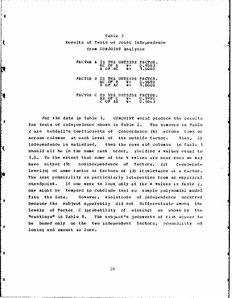
Table 3
Results of Tests of Joint Independence
from CONJOINT Analysis
FACTOR A IS THE OUTSIDE FACTOR.BC OF A W= 0.9583A OF BC W= 1.0000
FACTOR B IS THE OUTSfDE FACTOR.AC OF B W= 0.9680B OP AC W= 1.0000
FACTOR C IS THE OUTSIDE FACTOR.AB OF C W= 0.9990C OF AB W= 0.3063
For the data in Table 1, CONJOINT would produce the resu1ts
for tests of independence shown in Table 2. The numbers in Table
2 are Kendall's Coefficients of Concordance (W) across rows or
across columns at each level ot the outside factor. Thus, if
independence is satisfied, then the rows and columns in Table I
should all be in the same Lank order, yielding W values equal to
1.0. To the extent that some of the W values are near zero we may
have either (1) nonindependence of factors, (2) degenerate
level(s) of some factor or factors or (3) irrelevance o1 a factor.The last possibility is particularly interestinq from an empirical
standpoint. If one were to look only at the w values in rable 2,
one might be tempted to conclude that no simple polynomial model
fits the data. However, violations of independence occurred
because the subject apparently did not differentiate amonq the
levels of Factor C (probability of winning) as shown by the"rankings" in Table 1. The subject's judgments of risk appear to
be based only on the two independent factors, :)roability ot
losing and amount to lose.
24

Table 3 presents similar results for joint independence. The
W values are all very near 1.0, except for the test of OC of AB."
To understand the implications of the tests of independence (Table
2) and joint independence (Table 3), it is important to follow how
the W-values were computed. First, we will illustate simple
independence with the value of W .56 from Table 2. This value
was obtained from the check of independence for C of B at level hz
- It was obtained by comparing the rank orders of the following
four sets (BI-Bq) of three numbers (C -C5 ):
(1 42.5, 42.5, 43.02 29:0: 29.0 29.0
14.5, 22.5, 22.541 1 18.5, 18.5
In a comparable manner independence for B of C at level A where W
= 1.00 was obtained by comparing the rank orders of the three sets
(C 1 -C 3 ) of four numbers (BI-8q)
4.5, 29.0, 14.5, 10.02 42.5, 29.0, 22.5, 18.5
43.0, 29.0, 22.5, 18.5
The joint inlependence value of W = .3063 from Table 3 for "C of
ABO was obtained by comparing the rank orders of the followinq 16sets (A1 ,B I ; A,BK; ... ; Aq,B ) of three numbers (CI-C):
47 470, 46.5542 42.5, 42.5
36.5, 36.5, 36.5
15 40, 4.0, 12.516 3:5: 3.5, 3.5
Finally, W .9990 for "AB of Ca was found from the ranks of
three sets of 16 numbers:
25

47.0, 42.5 36. 29.5, .. ,0.0 4.0, 3.53 46.5, 42.5 36.5 29.0, .. ,18.5, 12.5# 3.5
In addition to the independence tests, CONJOINT allows one to
test both Luce-Tukey or double cancellation and distributive
cancellation. Tests of these properties are illustrated for the
risk data in Tables 4 and 5. Double cancellation is checked for
each pair of factors at each level of the third ("outside")
factor. Table 4 illustrates one such test -- Factors A and B at
each level of Factor C. At each level of C there will be 16
possible tests. Recall that each test of double cancellation
requires a 3x3 submatrix. With n = 4 levels of Factor A and n = 4
levels of Factor B, there will be 16 possible tests.
Table 4
Results of Tests of Double Cancellation from CONJOINT
Analysis: Factors A and B at Edch Level of Factor C
L-T CANCELLATIONFACTOR C IS THE OUTSIDE FACTOR.
LEVEL C 1 2 VIOLATIONS.0 TESTS NOT POSSIBLE.
14 SUCCESSFUL TESTS.
LEVEL C 2 2 VIOLATIONS.0 TESTS NOT POSSIBLE.
14 SUCCESSFUL TESTS.IJ
LEVEL C 3 2 VIOLATIONS.0 TESTS NOT POSSIBLE.
14 SUCCESSFUL TESTS.
For the data in Table 4 all 16 tests at each level of Factox
C were possible. The "Tests Not Possible" counter would have bee-n
'?3

nonzero only if the antecedent conditions in Equation 17 had not
been met for one or more of the 3x3 submatrices. Given that a
test was possible in each submatrix, the program then checked for
violations. A violation occurs whenever either or both of the
antecedent conditions in Equation 17 produce a strict inequality
in one direction, but the consequence in an equality oi strict
inequality in the opposite direction. As an example, let us find
one of the two violations for Factors A and B at Level C . One
violation occurs in the 3x3 submatrix below with Levels A l-Aqand b,
-B4. Note that (abZ)-v(a,,b3) and (a+,b3 ) < (a.?b ),
B2 b3 B4A2 29.0 14.5 10.0k3 14.5 7.5 4.5A4 10.0 4.0 3.5
but that (a,b 2 ) e-(aj,bq). The consequence cannot be an equality
because one of the antecedent conditions was a strict inequality.
It is important to recognize from this example that there are
several (in fact, there are nine) ways to distinctly permute the
rows and columns of this specific (or any) 3x3 submatrix in order
to test for double cancellation. CONJOINT automatically does
this. Note that there is a second test that is actually satisfiedby the data in this matrix; it is (a.,bL) > (abb) and (a1 ,b3 ) >
(a ,b4) imply (ax, bL) > (a 1 1 bq). However, this check of the
matrix is not counted as a "successful' testj CONJOINT still counts
this 3x3 matrix as producing a violation since one (or more) of
the nine possible tests has failed.
Table 5 illustrates the results of tests of distributive
cancellation for Factors A and B at pairs of levels of Factor C.
21

Table 5
Results of Tests of Distributive Cancellation from CONJOINT
Analysis: Factors A and B At Each Level of C
DISTRIBUTIVE CANCELLATIONFACTOR C IS THE OUTSIDE FACTOR.
LEVELS 1 VS. 218 VIOLATIONS88 TESTS NOT POSSIBLE
1190 SUCCESSFUL TESTS
LEVELS 1 VS. 3bb VIOLATIONS41 TESTS NOT POSSIBLE
1187 SUCCESSFdL TESTS
LEVELS 2 VS. 365 VIOLATIONS75 TESTS NOT POSSIBLE
1156 SUCCESSFUL TESTS
Comparable tests were done for Factors A and C for pairs of levels
of Factor B and for B and C for pairs of levels of A. From
Equation 19 it is clear that to test this axiom we need a 2x2
matrix in the AB plane at two different levels of Factor C. holt
and Wallsten (1974) have shown that there are 16 permutations of
the pair of 2x2 matrices that define distributive cancellation.
For each pair of these 2x2 matrices CONJOINT will test all 16
permutations if necessary. in a manner comparable to that of
double cancellation, the proqram will record a failure for the 2x2
matrix if any one of the 1b tests fails. If the antecedent
conditions are not met in any of the 16 tests, then the "Tests Not
Possible" counter is incremented.
Since all 2x2 matrices for A and B are checked at any two
4 levels of C, there will be
n n n n
4
28

T = (21) * (2) * ( 1) * (22) (21)
or 36 x 36 = 1296 such tests for the risk rating data for each
level of C1 vs. C2, C1 vs. C3, and C2 vs. C3. The actual number
of violations, tests not possible, and successful tests for the
risk data are shown in Table 5. CONJOINT would also print the
results of comparable tests for A and C with B as the outside
factor and for B and C with A as the outside factor. In this way
one could check the feasibility of each of the distributive
models A*(B+C), B*(A+C), and C*(A+B). In addition, even it the
data were proposed to fit an additive model, these tests would
still be very useful since distributive cancellation would have to
hold in all three forms for an additive representation.
There is one final note worth mentioning about distributive
cancellation. It appears from extended tests of the distributive
cancellation axiom across many data sets that this axiom is not
very powerful as a diagnostic tool. That is, it appears that even
for data that have a high degree of error variance associated with
them, distributive cancellation will be supported most of the time.
CONJOINT does print one additional piece of information that may
be useful to the researcher, however. After printing the results
of the tests of distributive cancellation, the program prints a
matrix indicating the number of times each cell was involved in a
violation. An illustration of this matrix will be shown when the
comparable PCJM2 procedure is discussed. Sometimes systematic
violations may aid in identifying particular problem levels of the
factors.
29

Table 6
Ranked Risk Ratings from PCJM2 Analysis
for a 4x4x3 Design
DATA MATRIX BEING CHECKED FOR INDEPENDENCE:MATRIX ID NO. = 1 U=1A =1 2 3 4
P = 1 2.00 6.50 12.50 20.00P = 5 6.50 20.00 34.50 39.00P = 9 12.50 34.50 41.50 45.00P =13 20.00 39.00 44.50 45.50
MATRIX ID NO. = 1 U =17A =1 2 3 4
P = 1 2.00 6.50 12.50 20.00P = 5 6.50 A0.00 26.50 34.50P = 9 12.50 26.50 35.50 45.00P =13 20.00 30.50 43.50 45.50
MATRIX ID NO. = 1 U =33A 1 2 3 4
P = 1 2.50 6.00 12.50 20.00P = 5 6.50 20.00 26.50 30.50P 9 12.50 26.50 32.50 36.50P =13 20.00 30.50 36.50 45.50
PCJM 2
Let us now examine the same riskiness data using the PZJM2
program. The rankings of the 48 data cells in the 4x4x. desiqn
are presented aqain in Table 6. Notice that the values in this
table are the complements of the rankings of 1 to 48 from Table 1.
In general, PCJM2 ranks the data in the opposite ,irection of
CONJOINT when there are multiple observations per cell. In the
illustrative data used here there were three entries in each ot
the 48 data cells. That is, the subject gave three ratinqs of
riskiness to each of the 48 gambles. In situations such as this
with multiple observations in each cell, we could proceed in
either of two ways to obtain ranks for the cells. One method
would be to simply average the observatioDs in each cell and then
31

rank these averaqes. A more statistically useful method was used
by Holt and Wallsten (1974). If there are three or more
observations per cell then CONJOINT proceeds as follows. Each
cell is compared with every other cell via a Mann-Whitney U-test.
If the U-value for a comparison is greater than the critical value
at the .05 significance level, then the two cells are considered
unequal in rank. If the a-value is not significant, the two cells
are considered equal. A counter is employed to keep a record of
all cells that a particular cell exceeds. The rank for the cell
is given by the number of cells that it has exceeded plus one-half
the number of cells it has tied. Exactly the same procedure is
used by PCJM2 except that the rank of a cell is equal to the
number of cells that it is smaller than plus one-half the number
it has tied. Thus the values in Table 6 are equal to 48 minus the
corresponding value in Table 1, plus one.
It should not be surprising that a number of the tied cells
were formed from the present data set. With only three
observations in each cell, it can be shown that only when all
three values of one cell exceed the values from another cell that
a significant U-value at the .05 level of significance can be
obtained. dith only two observations in each cell, a significant
U-value could not be obtained at the .05 level. Hence, both
CONJOINT and PCJM2 use this Mann-Whitney U-test only when the
number of replications in the cells is equal to or greater than
three. If there are only two observations in each cell, the
researcher must first alter the data to obtain the ranks. Perhaps
here a simple averaging procedure would be best. When there is
only one observation per cell, neither program makes any
31

Table 7
Results of Tests of Simple Independence
from PCJM2 Analysis
TEST FAILURE u= I AND v=33 ARE REVERSED AT a=1 p=1 AND b=2 o= 9TEST FAILURE u= 1 AND v=33 ARE REVERSED AT a=1 p=1 AND b=2 q=13TEST FAILURE u= 1 AND v=33 ARE REVERSED AT a= p=1 AND b=3 q= 5TEST FAILURE u= I AND v=33 ARE REVERSED AT a=1 p1 AND b=3 = 9TEST FAILURE u=17 AND v=33 ARE REVERSED AT a=1 p=1 AND b=3 q= 9TEST FAILURi u= I AND v=33 AHE REVERSED AT a=1 p=1 AND b=3 q=13TEST FAILURE u=17 AND v=33 ARE REVERSED AT a=1 p=1 AND b=3 g=13TEST FAILURE u= 1 AND v=33 ARE REVERSED AT a=1 p=1 AND b=4 q= 5TEST FAILURE u=17 AND v=33 ARE REVERSED AT a=1 p=1 AND b=4 q= 5TEST FAILURE u= 1 AND v=33 ARE REVERSED AT a=1 p=1 AND b=4 q= 9ETC.
TEST SUMMARY STATISTICS:TOTAL POSSIBLE TESTS ("NUMBER TESTS"), NON-TESTS IN THE DATA(NINMBER EQUALS )_AND TOTAL ERRORS (-NUMBER FAILS")
NUMBER TESTS A INDEPT P X U 3961JPBER EQUALS A INDEPT P X U 0NUMBER FAILS A INDEPT P X U 0AVLRAGE TAU A INDEPT P X U 1.000
NUMBER TESTS P INDEPT U X A 396NUMBER EQUALS P INDEPT U X A 1NUMBER FAILS P INDEPT U X A 0AVERhGE TAU P 1NDEPT U X A 0.997
NUMBER TESTS 0 INDEPT A X P 360NUMBER EQUALS U INDEPT A X P 296NUMBER FAILS U INDEPT A X P 11AVERAGE TAU U INDEPT A X P 0.117
modification to the data since only the ordinal relations among
the values are used. Finally, PCJM2 and CONJOINT do not require
every data cell to be non-empty (or to have three or more
obse-vations in every cell in the case of multiple entry data).
Both programs will handle missing data designs, although CONJOINT
will not run if 10% or more of the cells are empty.
32

Table 8
Distribution of Failures in Simple Independence
for Each Cell of the Data Matrix
MATRIX ID NO. = 1 U =A = 1 2 3 4
P = 1 7.00 0.0 0.0 0.0P = 5 0.0 0.0 1.00 1.00P = 9 0.0 1.00 1.00 1.00P = 13 0.0 1.00 1.00 0.0
MATRIX ID NO. 1 =17A 1 2 3 4
P = 1 4.00 0.0 0.0 0.0P = 5 0.0 0.0 0.0 1.00P = 9 0.0 0.0 1.00 1.00P =13 0.0 0.0 1.00 0.0
MATRIX ID NO. = 1 U =33A = 1 2 3 4
P = 1 11.00 0.0 0.0 0.0P = 5 0.0 0.0 1.00 2.00P = 9 0.0 1.00 2.00 2.00P =13 0.0 1.00 2.00 0. 3
Tables 7 and 8 present the results of the PCJM2 analysis of
the riskiness data for tests of independence. As was mentioned
earlier, PCJM2 actually tests for independence in the manner
suggested by Krantz and Tversky (1971) and stated in Equation 6.From Equation 7 it is clear that for the riskiness data there
should be 6x66 = 396 tests of independence for each of Factors A
and P, and 3x120 = 360 tests for Factor U. Let us look at the 360
possible tests of "U independent of A and P." Notice that here
296 of the tests could not be done ("NUMBER EQUALS" = 296). A
non-test of independence is counted by PCJM2 when one of the two
conditions in Equatio 6 is an equality. An error is counted when
one condition has an inequality in one direction anJ the second
has an inequality in the other direction. Table 7 is again
indicating that Factor U was apparently irrelevant to the subject
in making riskiness ratings. Hence, while violations of tne axiom
33
4
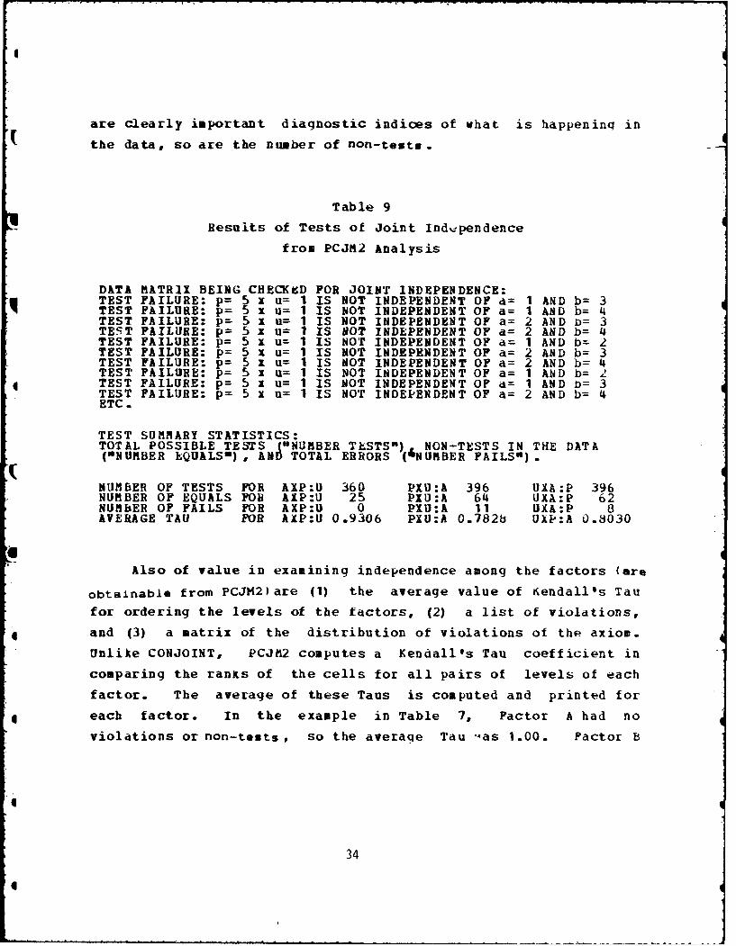
are clearly important diagnostic indices of what is happeninq in
the data, so are the number of non-tests.
Table 9
Results of Tests of Joint Independence
from PCJM2 Analysis
DATA MATRIX BEING CHECKED FOR JOINT INDEPENDENCE:TEST FAILURE: p= 5 x u= I IS NOT INDEPENDENT OF a= 1 AND b= 3TEST FAILURE: p= 5 x u= I IS NOT INDEPENDENT OF a= I AND b= 4TEST FAILURE: p= 5 x u= 1 IS NOT INDEPENDENT OF a= 2 AND 0= 3TEST FAILURE: p= 5 x u= I IS NOT INDEPENDENT OF a= 2 AND b= 4TEST FAILURE: p= 5 x u= 1 IS NOT INDEPENDENT OF a= 1 AND b= 2TEST FAILURE: p= 5 x u= I IS NOT INDEPENDENT OF a= 2 AND b= 3TEST FAILURE: = 5 x u= 1 IS NOT INDEPENDENT OF a= 2 AND b= 4TEST FAILURE: p= 5 x u= I IS NOT INDEPENDENT OF a= 1 AND b= 2TEST FAILURE: p= 5 x u= I IS NOT INDEPENDENT OF d= 1 AND b= 3TEST FAILURE: p= 5 x u= I IS NOT INDEPENDENT OF a= 2 AND b= 4ETC .
TEST SUMMARY STATISTICS:TOTAL POSSIBLE TESTS ("NUMBER TESTS") NON-TESTS IN THE DATA("NUMBER EQUALS) , AND TOTAL ERRORS (&NUMBER FAILS")
NUMBER OF TESTS FOR AXP:U 360 PXU:A 396 UXA:P 396NUMBER OF EQUALS FOR AXP:U 25 PXU:A 64 UXA:P 62NUMBER OF FAILS FOR AXP:U 0 PXU:A 11 UXA:P 8AVERAGE TAU FOR AXP:U 0.9306 PXU:A 0.7828 UXP:A 0.8030
Also of value in examining independence among the factors (are
obtainable from PCJM2)are (1) the average value of Kendall's Tau
for ordering the levels of the factors, (2) a list of violations,
4 and (3) a matrix of the distribution of violations of the axiom.
Unlike CONJOINT, PCJM2 computes a Kendall's Tau coefficient in
comparing the ranks of the cells for all pairs of levels of each
factor. The average of these Taus is computed and printed for
4 each factor. In the example in Table 7, Factor A had no
violations or non-tests, so the average Tau -as 1.00. Factor B
34
I

has an average Tau of slightly less then 1.00 (Tau = .997) since
there was only one non-test (i.e. 1 one tied rank) iu the data.
Factor U had a low average Tau because of the number of violations
and non-tests in the data for tbst tactor.
One may specify when using the PCJ92 program that a number of
the violations are to be printed. In this example the request was
to list up to ten violations for each axiom. If more than the
requested number of violations to be printed have actually
occurred, the program indicates this by writing "ETC.* following
the last printed violation.
Table 10
Distribution ot Failures of Joint Independence
for Each Cell of the Data Matrix from the PCJM2 Analysis
MATRIX ID NO. = 1 U =IA =1 2 3 4
P = 1 0.0 2.00 2.00 0.0P = 5 2.00 4.00 4.00 2.00
= 9 3.00 7.00 5.00 3.00P =13 0.0 2.00 2.00 0.0
MATRIX ID NO. = 1 0 =17A = 2 3 4
P = 1 0.0 0.0 0.0 0.0P -5 0.0 0.0 0.0 0.0P = 9 0.0 0.0 0.0 0.0P =13 2.00 4.00 0.0 0.0
MATRIX ID NO. = 1 9 =33A 1 2 3 4
P 1 0.0 0.0 4.00 4.00P 5 0.o 0.0 4.00 2.00P 9 4.80 4.00 0.0 2.00P =13 4.00 2.00 2.00 0.0
Using the PCJM2 notation of a,b,c..., poq,r.... and u,v,W...
35

to denote the levels of the factors, we can illustrate the fi-st
violation of independence listed in Table 7. We have (1,1,1) <
(1,1,33) but (2,9,1) > (2,9,33). That is, from the rankings:
2.00 < 2.50 but 34.5 > 26.5. The other violations can be
interpreted in a comparable manner. Finally, the summary matrix
in Table 8 shows how many times each AxPxU cell was involved in, d
violation.
Tables 9, 10, 11, and 12 illustrate the PCJM2 analysis of the
riskiness data for the joint independence, double cancellation,
and distributive cancellation properties. Although the proqram
can test for dual-distributive cancellation, the illustrative .Iata
set used here is not large enough for appropriate tests of this
axiom. Tables 9 and 10 show for joint independence the
information concerninq tests and violations ot the axioms as
presented in Equation 12. The program will list (1) as many
violations of the axiom as indicated by the user, (2) the nuinber
of possible tests, errors, and non-tests, and (3) the averaae Tau
value for each pair of factors. Table 10 indicates the number of
violations associated with each cell of the matrix. Tables 11 and
12 illustrate double and distributive cancellation. For both or
these cancellation axioms, PCJM2 will summarize the number of
violations, the actual tailur* locations, and the summary matrix
* of cells involved in violations. Since there were no violations
of double cancellatirn in this data, however, only the summary
statistics were presented.
366m
36!
6I

Table 11
Results of Tests of Double Cancellation and Distributive
Cancv.llation from the PCJM2 Analysis
DATA MATRIX BEING CHECKED FOR DOUBLE CANCELLATION:TEST SUMMARY STATISTICS:NUMBER OF TESTS FOR DBL CAN IN AXP = 38 PXU = 16 AXU = 16NUMBER OF FAILS FOR DBL CAN IN AXP = 0 PXJ = 0 AXU = 0
DATA MATRIX BEING CHECKED FOR DISTRIBUTIVE CANCELLATION:FACTOR 1 IS THE OUTSIDE FACTOR.TEST SUMMARY STATISTICS:
NUMBER OF TESTS = 503 NUMBER OF FAILURES = 19
DATA MATRIX BEING CHECKED FOR DISTRIBUTIVE CANCELLATION:FACTOR 2 IS THE OUTSIDE FACTOR.TEST SUMMARY STATISTICS:
NUMBER OF TESTS = 503 NUMBER OF FAILURES = 25
DATA MATRIX BEING CHECKED FOR DISTRIBUTIVE CANCELLATION:FACTOR 3 IS THE OUTSIDE FACTOR.TEST FAILURE AT RECTANGLESa= 1 b= 2 p= 1 q= 9 AT u= 1 AND c= 1 d= 2 r= 1 s=13 AT v=17a= 3 b= 2 p= 1q= 9 AT u= 1 AND c= 3 d= 2 r= I s=13 AT v=17a= 4 b= 2 p= I = 9 AT u= 1 AND c= 4 d= 2 r= 1 s=13 AT v=17a= 1 b= 2 p= 5 q= 9 AT u= 1 AND c= 2 d= 4 r= 1 s= 5 AT v=17a= 1 b= 2 p= 5 q= 9 AT u= 1 AND c= 1 d= 2 r= 5 s=13 AT v=17a= 3 b= 2 p= 5 = 9 AT u= I AND c= 3 d= 2 r= 5 s=13 AT v=17a= 3 b= 1 p= 5q= 1 AT u= I AND c= 4 d= I r= 5 s= 1 AT v=17a= 3 b= 1 p= 5 q= 9 AT u= I AND c= 4 d= 1 r= 5 s= 9 AT v=17a= 3 b= p= 5 q=13 AT u= 1 AND c= 4 d= 1 r = 5 s= 9 AT v=17a= 3 b= I p 5 g=13 AT u= I AND c= 4 d= I r= 5 s=13 AT v=17ETC.
TEST SUMMARY STATISTICS:NUMBER OF TESTS = 2723 NUMBER OF FAILURES = 166
3/

Table 12
Distribution of Failures of Distributive Cancellation
for Each Cell of the Data Matrix from the PCJM2 Analysis
MATRIX ID NO. = 1 U = IA 1 2 3 4
P = 1 12.00 38.00 25.00 23.00P = 5 38.00 97.00 46.00 41.00P = 9 21.00 42.00 19.00 20.00P =13 25.00 41.00 24.00 24.00
MATRIX ID NO. = 1 U =17A 1 2 3 4
P = 1 17.00 32.00 16.00 21.00P = 5 23.00 40.00 17.00 38.00P = 9 11.00 17.00 9.00 19.00P =13 19.00 35.00 14.00 24.00
MATRIX ID NO. I U =33A = 1 2 3 4
4P = 1 11.00 40.00 18.00 31.00P = 5 25.00 42.00 24.00 39.00P = 9 12.00 25.00 12.00 25.00P =13 26.00 33.00 26.00 51.00
IV. ADDITIV CONJOINT SCAL.NG PROGRAMS: NONMETRG AND MONANOVA
Let us assume that we have used the CONJOINT and PCJM2
programs with our data set and have found that an adlitive model
appears to be supported. We may now want to obtain a scalinq
solution for the data such that the numerical values associated
with the levels of the independent variables combine additively to
form scale values for the stimulus combinations. In all but the
simplest situations it is virtually impossible to attempt to
simultaneously scale the independent and dependent variables using
an additive (or any other) composition rule without the aid of a
computer program. With the advent of computer-based algorithms
originally intended for non-metric multidimensional scaling of
similarities data (cf. Shepard, 1962a,1962b; Kruskal, 1964a,1964b;
Johnson, 1973), it became possible to obtain conjoint scalin
33
II

solutions for even complex data sets. A number of algorithms are
now available for obtaining these scaling solutions for either an
additive, multiplicative, distributive or dual-distributive model.
Four of these programs will be discussed here. The first two will
deal with an additive Lepresentation; the latter two will be used
with the distributive and dual-distributive models, respectively.
ONIt ETRG
NONnETRG is a modified version of a scaling procedure
originally proposed by Johnson (1973). As the name of the program
implies, MONMETRG is a nnn-matrac scaling procedure. By that we
mean that it attempts to find interval-scaled values for the
levels of the independent variables based only on the ordinal
relationships exhibited in the data. The objective of the
program, as with all non-metric programs is simple: to use the
ordinal constraints imposed on the data to find an effectively
unique solution (i.e., unique up to an affine transformation). In
a metric procedure we assume that the data are related to the final
distance scale values by
d a * d 4 b (22)
where d3 is the original response judgment for stimulus j, d' is
the rescaled distance value, and a > 0 and b are constants. In a
non-metric procedure, the function need only be monotonic. That
is,
- md. f (d) (23)
J J
39

NONAETRG is different from most non-metric programs in that it
does not directly attempt to find the monotonic transformation in
Equation 23. The procedure employed by the program is a one-step
pairwise method. This procedure will now be summarized.
NONMETRG, like many non-metric proqrams is an iterative
technique. By this we mean that the program continues to search
for a set of scale values that will "best" reproduce the ordinal
relationships among the stimuli according to specified composition
rule (e.g., an additive rule in our example). The search or
iterative procedure continues until a cutoff criterion is dchieved
or until no practical improvements can be found. Hence, to negin
the scaling process hONMETRG needs three sets of values. First,
the program needs a set of parameters that describe the
independent factors and the data to be rescaled. Next, the aata
is read in the form of an nx(n*1) matrix where n represents the
number of stimuli and m represents the total number of levels of
all of the factors. In the illustrative risk-takinq example, m
would equal 4,43 = 11. The first x values i. each row of the
matrix are coded as 0's or 1's. A zero indicates the absence of
the corresponding level of a factor and a one represents its
presence. The last value in each row is the actual response
judgment. Before doing the actual scaling, NONMETRG will print
this input matrix so that the user may check for errors. Table 13
illustrates this printed input matrix for the riskiness data.
Ignoring the first two indexing columns of this matrix for
now, we can see that there are m+1 = 12 columns remaining. The
stimuli in this example are in the natural order; that is,
40
J

Table 13
Input Matrix from Riskiness Data
Used in the NONMETRG Analysis
TITLE: CONJOINT SCALING: RISKINESS DATA.TITLE: 48 STIMULI. 1X4X4X3 DESIGN.TITLE: FACTORS ARE:TITLE: AMOUNT TO LOSE, 4 LEVELS. -10 -20, -30, AND -40 CENTS.TITLE: PROBABILITY OF LOSING 4 LEVEL. 1/8 2/8 3/8, AND 4/8.TITLE: PROBABILITY OF WINNING 3 LEVELS. 2/A 3/A AND 4/8.TITLE: DATA ARE THREE RISKINESS RATINGS FOR EACH Of 48 GAMBLES.TITLE: SCALE RANGES FROM i10 TO '100'.TITLE: STIMULI ARE IN THE NATURAL ORDER.
DATA MATRIX: SUBJECT/REPLICATION NO. 1BLOCK STIM LEVELS OF FACTORS1 1 1.0 0.0 0.0 0.0 1.0 0.0 0.0 0.0 1.0 0.0 0.0 3.01 2 1.0 0.0 0.0 0.0 1.0 0.0 0.0 0.0 0.0 1.0 0.0 4.01 3 1.0 0.0 0.0 0.0 1.0 0.0 0.0 0.0 0.0 0.0 1.0 4.01 4 1.0 0.0 0.0 0.0 0.0 1.0 0.0 0.0 1.0 0.0 0.0 9.01 5 1.0 0.0 0.0 0.0 0.0 1.0 0.0 0.0 0.0 1.0 0.0 '.01 6 1.0 0.0 0.0 0.0 0.0 1.0 0.0 0.0 0.0 0.0 1.0 -3.01 7 1.0 0.0 0.0 0.0 0.0 0.0 1.0 0.0 1.0 0.0 0.0 14.01 8 1.0 0.0 0.0 0.0 0.0 0.0 1.0 0.0 0.0 1.0 0.0 15.01 9 1.0 0.0 0.0 0.0 0.0 0.0 1.0 0.0 0.0 0.0 1.0 15.01 10 1.0 0.0 0.0 0.0 0.0 0.0 0.0 1.0 1.0 0.0 0.0 19.01 11 1.0 0.0 0.0 0.0 0.0 0.0 0.0 1.0 0.0 1.0 0.0 19.01 12 1.0 0.0 0.0 0.0 0.0 0.0 0.0 1.0 0.0 0.0 1.0 19.01 13 0.0 1.0 0.0 0.0 1.0 0.0 0.0 0.0 1.0 0.0 0.0 9.01 14 0.0 1.0 0.0 0.0 1.0 0.0 0.0 0.0 0.0 1.0 0.0 9.01 15 0.0 1.0 0.0 0.0 1.0 0.0 0.0 0.0 0.0 0.0 1.0 6.01 16 0.0 1.0 0.0 0.0 0.0 1.0 0.0 0.0 1.0 0.0 0.0 19.01 17 0.0 1.0 0.0 0.0 0.0 1.0 0.0 0.0 0.0 1.0 0.0 18.01 18 0.0 1.0 0.0 0.0 0.0 1.0 0.0 0.0 0.0 0.0 1.0 19.01 19 0.0 1.0 0.0 0.0 0.0 0.0 1.0 0.0 1.0 0.0 0.0 52.01 20 0.0 1.0 0.0 0.0 0.0 0.0 1.0 0.0 0.0 1.0 0.0 29.01 21 0.0 1.0 0.0 0.0 0.0 0.0 1.0 0.0 0.0 0.0 1.0 29.01 22 0.0 1.0 0.0 0.0 0.0 0.0 0.0 1.0 1.0 0.0 0.0 89.01 23 0.0 1.0 0.0 0.0 0.0 0.0 0.0 1.0 0.0 1.0 0.0 38.01 24 0.0 1.0 0.0 0.0 0.0 0.0 0.0 1.0 0.0 0.0 1.0 39.01 25 0.0 0.0 1.0 0.0 1.0 0.0 0.0 0.0 1.0 0.0 0.0 15.01 26 0.0 0.0 1.0 0.0 1.0 0.0 0.0 0.0 0.0 1.0 0.0 15.01 27 0.0 0.0 1.0 0.0 1.0 0.0 0.0 0.0 0.0 0.0 1.0 14.01 28 0.0 0.0 1.0 0.0 0.0 1.0 0.0 0.0 1.0 0.0 0.0 51.01 29 0.0 0.0 1.0 0.0 0.0 1.0 0.0 0.0 0.0 1.0 0.0 29.01 30 0.0 0.0 1.0 0.0 0.0 1.0 0.0 0.0 0.0 0.0 1.0 29.01 31 0.0 0.0 1.0 0.0 0.0 0.0 1.0 0.0 1.0 0.0 0.0 92.01 32 0.0 0.0 1.0 0.0 0.0 0.0 1.0 0.0 0.0 1.0 0.0 61.01 33 0.0 0.0 1.0 0.0 0.0 0.0 1.0 0.0 0.0 0.0 1.0 46.01 34 0.0 0.0 1.0 0.0 0.0 0.0 0.0 1.0 1.0 0.0 0.0 96.01 35 0.0 0.0 1.0 0.0 0.0 0.0 0.0 1.0 0.0 1.0 0.0 95.01 36 0.0 0.0 1.0 0.0 0.0 0.0 0.0 1.0 0.0 0.0 1.0 59.01 37 0.0 0.0 0.0 1.0 1.0 0.0 0.0 0.0 1.0 0.0 0.0 19.01 38 0.0 0.0 0.0 1.0 1.0 0.0 0.0 0.0 0.0 1.0 0.0 19.01 39 0.0 0.0 0.0 1.0 1.0 0.0 0.0 0.0 0.0 0.0 1.0 19.0
414

1 40 0.0 0.0 (.O 1.0 0.0 1.0 0.0 0.0 1.0 0.0 6.0 88.01 41 0.0 0.0 0.0 1.0 0.0 1.0 0.0 0.0 0.0 1.0 0.0 39.01 42 0.0 0.0 0.0 1.0 0.0 1.0 0.0 0.0 0.0 0.0 1.0 39.01 13 0.0 0.0 0.0 1.0 0.0 0.0 1.0 0.0 1.0 0.0 0.0 94.01 44 0.0 0.0 0.0 1.0 0.0 0.0 1.0 0.0 0.0 1.0 0.0 96.01 45 0.0 0.0 0.0 1.0 0.0 0.0 1.0 0.0 0.0 1.0 1.0 59.01 46 0.0 0.0 0.0 1.0 0.0 0.0 0.0 1.0 1.0 0.0 0.0 98.01 46 0.0 0.0 0.0 1.0 0.0 0.0 0.0 1.0 0.0 1.0 0.0 97.01 48 0.0 0.0 0.0 1.0 0.0 0.0 0.0 1.0 0.0 1.0 1.0 98.02 1 1.0 0.0 0.0 0.0 1.0 0.0 0.0 0.0 0.0 0.0 0.0 5.02 2 1.0 0.0 0.0 0.0 1.0 0.0 0.0 0.0 0.0 0.0 0.0 5.02 3 1.0 0.0 0.0 0.0 1.0 0.0 0.0 0.0 0.0 0.0 1.0 5.02 4 1.0 0.0 0.0 0.0 0.0 1.0 0.0 0.0 1.0 O.0 0.0 9.02 5 1.0 0.0 0.0 0.0 0.0 1.0 0.0 0.0 0.0 1.0 0.0 9.02 6 1.0 0.0 0.0 0.0 0.0 1.0 0.0 0.0 0.0 0.0 1.0 9.02 7 1.0 0.0 0.0 0.0 0.0 0.0 1.0 0.0 1.0 0.0 0.0 15.02 8 1.0 0.0 0.0 0.0 0.0 0.0 1.0 0.0 0.0 1.0 0.0 15.02 9 1.0 0.0 0.0 0.0 0.0 0.0 1.0 0.0 0.0 1.0 1.0 15.02 10 1.0 0.0 0.0 0.0 0.0 0.0 o.0 1.0 1.0 0.0 0.0 19.02 11 1.0 0.0 0.0 0.0 0.0 0.0 0.0 1.0 0.0 0.0 1.0 19.02 12 1.0 0.0 0.0 0.0 0.0 0.0 0.0 1.0 0.0 0.0 1.0 19.02 13 0.0 1.0 0.0 0.0 1.0 0.0 0.0 0.0 1.0 0.0 0.0 9.02 13 0.0 1.0 0.0 0.0 1.0 0.0 0.0 0.0 0.0 1.0 0.0 9.02 15 0.0 1.0 0.0 0.0 1.0 0.0 0.0 0.0 0.0 0.0 1.0 9.02 16 0.0 1.0 0.0 0.0 0.0 1.0 0.0 0.0 1.0 0.0 0.0 19.02 17 0.0 1.0 0.0 0.0 0.0 1.0 0.0 0.0 0.0 1.0 0.0 19.02 18 0.0 1.0 0.0 0.0 0.0 1.0 0.0 0.0 0.0 0.0 1.0 19.02 19 0.0 1.0 0.0 0.0 0.0 0.0 1.0 0.0 1.0 0.0 0.0 52.02 20 0.0 1.0 0.0 0.0 0.0 0.0 1.0 0.0 1.0 1.0 0.0 29.02 21 0.0 1.0 0.0 0.0 0.0 0.0 1.0 0.0 0.0 0.0 1.0 28.02 22 0.0 1.0 0.0 0.0 0.0 0.0 0.0 1.0 1.0 0.0 0.0 89.0
2 22 0.0 1.0 0.0 0.0 0.0 0.0 0.0 1.0 1.0 0.0 0.0 89.02 23 0.0 1.0 0.0 0.0 0.0 0.0 0.0 1.0 0.0 1.0 1.0 39.02 25 0.0 0.0 1.0 0.0 1.0 0.0 0.0 0.0 1.0 0.0 0.0 15.U2 26 0.0 0.0 1.0 0.0 1.0 0.0 O.0 0.0 0.0 1.0 U.0 14.02 27 0.0 0.0 1.0 0.0 1.0 0.0 0.0 0.0 0.0 0.0 1.0 14.02 28 0.0 0.0 1.0 0.0 0.0 1.0 0.0 0.0 1.0 0.0 0.0 52.02 29 0.0 0.0 1.0 0.0 0.0 1.0 0.0 0.0 0.0 1.0 0.0 29.02 30 0.0 0.0 1.0 0.0 0.0 1.0 0.0 0.0 0.0 0.0 1.0 29.02 31 0.0 0.0 1.0 0.0 0.0 0.0 1.0 0.0 1.0 0.0 0.0 41.02 32 0.0 0.0 1.0 0.0 0.0 0.0 1.0 0.0 0.0 1.0 0.0 51.0
42 33 0.0 0.0 1.0 0.0 0.0 0.0 1.0 0.0 0.0 0.0 1.0 45.02 34 0.0 0.0 1.0 0.0 0.0 0.0 0.0 1.0 1.0 0.0 0.0 96.02 35 0.0 0.0 1.0 0.0 0.0 0.0 0.0 1 .0 0.0 1.0 0.0 94.02 36 0.0 0.0 1.0 0.0 0.0 0.0 0.0 1.0 0.0 0.0 1.0 59.02 37 0.0 0.0 0.0 1.0 1.0 0.0 0.0 0.0 1.0 0.0 0.0 19.02 38 0.0 0.0 0.0 1.0 1.0 0.0 0.0 0.0 0.0 1.0 0.0 19.02 39 0.0 0.0 0.0 1.0 1.0 0.0 0.0 0.0 0.0 o.0 1.0 19.02 40 0.0 0.0 0.0 1.0 0.0 1.0 0.0 0.0 1.0 0.0u 0.0 89.02 41 0.0 0.0 0.0 1.0 0.0 1.0 0.0 0.0 0.0 1.0 0.0 39.02 42 0.0 0.0 0.0 1.0 0.0 1.0 0.0 0.0 0.0 0.0 1.0 39.02 43 0.0 0.0 0.0 1.0 0.0 0.0 1.0 0.0 1.0 0.0 0.0 96.02 44 0.0 0.0 0.0 1.0 0.0 0.0 1.0 0.0 0.0 1.0 0.0 93.045 0.0 0.0 0.0 1.0 0.0 0).0 1.0( 0.0 0.0 0.0A 1.0 59.03
2 46 0.0 0.0 0.0 1.0 0.0 0.0 0.0 1.0 1.0 0.0 0.0 99.02 47 0.0 0.0 0.0 1.0 0.0 0.0 0.0 1.0 0. 0 1.0 0.0 98.02 48 0.0 0.0 0.0 1.0 0.0 0.0 0.0 1.0 0.0 0.0 1.0 97.03 1 1.0 0.0 0.0 0.0 1.0 0.0 0.0 0.0 1.0 0.0 0).0 5.03 2 1.0 0.0 0.0 0.0 1.0 0.0 0.0 0.0 0).( 1. U0.0 5.03 3 1.0 0.0 0.0 0.0 1.0 0.0 0.0 0.0 0.0 0.0 1.0 (3.03 4 1.0 0.0 0 .0 0.0 0.0 1.0 0.0 0 .0 1.0 J.0 0.0 9.0
o~o~o .oo~ oo~ ,. o~o ~o ,o o4',.o~ o~o,.oo~o ~o ~o ,o oo o~ o~ ,.oo .

3 5 1.0 0.0 0.0 0.0 0.0 1.0 0.0 0.0 0.0 1.0 0.0 9.03 6 1.0 0.0 0.0 0.0 0.0 1.0 0.0 0.0 0.0 0.0 1.0 9.03 7 1.0 0.0 O.0 0.0 0.0 0.0 1.0 0.0 1.0 0.0 0.0 15.03 8 1.0 0.0 0.0 0.0 0.0 0.0 1.0 0.0 0.0 1.0 0.0 15.03 9 1.0 0.0 0.0 0.0 0.0 0.0 1.0 0.0 0.0 0.0 1.0 15.03 10 1.0 0.0 0.0 0.0 0.0 0.0 0.0 1.0 1.0 0.0 0.0 19.03 11 1.0 0.0 0.0 0.0 0.0 0.0 0.0 1.0 0.0 1.0 0.0 19.03 12 1.0 0.0 0.0 0.0 0.0 0.0 0.0 1.0 0.0 0.0 1.0 19.03 13 0.0 1.0 0.0 0.0 1.0 0.0 0.0 0.0 1.0 0.0 0.0 9.03 13 0.0 1.0 0.0 0.0 1.0 0.0 0.0 0.0 0.0 1.0 0.0 9.03 15 0.0 1.0 0.0 0.0 1.0 0.0 0.0 0.0 0.0 0.0 1.0 9.03 16 0.0 1.0 0.0 0.0 0.0 1.0 0.0 0.0 1.0 0.0 0.0 19.03 17 0.0 1.0 0.0 0.0 0.0 1.0 0.0 0.0 0.0 1.0 0.0 19.03 18 0.0 1.0 0.0 0.0 0.0 1.0 0.0 0.0 0.0 0.0 1.0 19.03 19 0.0 1.0 0.0 0.0 0.0 0.0 1.0 0.0 1.0 0.0 0.0 51.03 20 0.0 1.0 0.0 0.0 0.0 0.0 1.0 0.0 0.0 1.0 0.0 29.03 21 0.0 1.0 0.0 0.0 0.0 0.0 1.0 0.0 0.0 0.0 1.0 29.03 22 0.0 1.0 0.0 0.0 0.0 0.0 0.0 1.0 1.0 0.0 0.0 89.03 23 0.0 1.0 0.0 0.0 0.0 0.0 0.0 1.0 0.0 1.0 0.0 39.03 23 0.0 1.0 0.0 0.0 0.0 0.0 0.0 1.0 0.0 0.0 1.0 39.03 25 0.0 1.0 1.0 0.0 1.0 0.0 0.0 0.0 1.0 0.0 0.0 16.03 26 0.0 0.0 1.0 0.0 1.0 0.0 0.0 0.0 0.0 1.0 0.0 15.03 27 0.0 0.0 1.0 0.0 1.0 0.0 0.0 0.0 0.0 1.0 1.0 15.03 28 0.0 0.0 1.0 0.0 0.0 1.0 0.0 0.0 1.0 0.0 0.0 51.03 29 0.0 0.0 1.0 0.0 0.0 1.0 0.0 0.0 0.0 1.0 0.0 29.03 30 0.0 0.0 1.0 0.0 0.0 1.0 0.0 0.0 0.0 0.0 1.0 29.03 31 0.0 0.0 1.0 0.0 0.0 0.0 1.0 0.0 1.0 0.0 0.0 91.03 32 0.0 0.0 1.0 0.0 0.0 0.0 1.0 0.0 0.0 0.0 0.0 52.03 33 0.0 0.0 1.0 0.0 0.0 0.0 1.0 0.0 0.0 0.0 1.0 45.03 33 0.0 0.0 1.0 0.0 0.0 0.0 0.0 1.0 1.0 0.0 0.0 92.03 35 0.0 0.0 1.0 0.0 0.0 0.0 0.0 1.0 0.0 1.0 0.0 94.03 35 0.0 0.0 1.0 0.0 0.0 0.0 0.0 1.0 0.0 0.0 1.0 59.03 37 0.0 0.0 0.0 1.0 1.0 0.0 0.0 0.0 1.0 0.0 0.0 19.03 38 0.0 0.0 0.0 1.0 1.0 0.0 0.0 0.0 0.0 1.0 0.0 19.03 39 0.0 0.0 0.0 1.0 1.0 0.0 0.0 0.0 0.0 0.0 1.0 19.03 39 0.0 0.0 0.0 1.0 0.0 1.0 0.0 0.0 1.0 0.0 0.0 89.03 41 0.0 0.0 0.0 1.0 0.0 1.0 0.0 0.0 0.0 1.0 0.0 89.03 42 0.0 0.0 0.0 1.0 0.0 1.0 0.0 0.0 0.0 1.0 1.0 39.03 43 0.0 0.0 0.0 1.0 0.0 0.0 1.0 0.0 1.0 0.0 0.0 95.03 '43 0.0 0.0 0.0 1.0 0.0 0.0 1.0 0.0 0.0 1.0 0.0 95.03 45 0.0 0.0 0.0 1.0 0.0 0.0 1.0 0.0 0.0 0.0 1.0 59.03 46 0.0 0.0 0.0 1.0 0.0 0.0 0.0 1.0 1.0 0.0 0.0 96.03 47 0.0 0.0 0.0 1.0 0.0 0.0 0.0 1.0 0.0 1.0 0.0 96.03 48 0.0 0.0 0.0 1.0 0.0 0.0 0.0 1.0 0.0 0.0 1.0 96.0
(1,1,1), (1,1,2), (1,1,3), ... , (4,4,3). Thus the first cell
(1,1,1) is represented by the first row of the matrix as
1.0 0.0 0.0 0.0 1.0 0.0 0.0 0.0 1.0 0.0 0.0 3.0
indicating Level 1 of Factor A, Level 1 of Factor 8, and Level 1of Factor C are present, and the response value is 3.0.
43

Note that there are 144 rows in this matrix -- three blocks
(Column 1) of 48 rows each (Column 2). This is because of the
fact that the subject had given three responses to each stimulus
combination. NONMETRG, then, can handle replications of stimulus
combinations either within or among subjects.
Table 14
History of Computation and Final Configuration
q| from NONMETRG Analysis of the Riskiness Data
ITERATION THETA TAU1 0.84485 -0.350472 0.23613 0.596933 0.05461 0.806744 0.07670 0.763005 0.06918 0.b04966 0.06906 0.76300
VARIABLE ADDITIVE ADDITIVE MJLTIP FROM ITERATIONRESCALED NUMBER 6
1 IL=-.10 0.66792 88.54173 1.950172 L=-.20 0.20749 42.49893 1.230583 L=-.30 0.00154 21.90387 1.001544 $L=-.40 -0.21750 0.0 0.804535 PL=I/8 0.61410 83.15974 1.847996 PL=2/8 0.22083 43.83362 1.247127 PL=3/8 0.03066 24.81602 1.031138 PL=4/8 -0.08626 13.12417 0.917369 PW=2/8 0.05189 26.93941 1.05326
10 PW=3/8 0.16813 38.56279 1.1830911 PW=4/8 0.25957 47.70709 1.29637
Given the appropriate initial parameter values and the data
matrix as shown in Table 13, NONBETRG needs one additional matrix
of values to begin the scaling procedure. This matrix is actually
a vector of m initial scale values to be used by the program as an
initial estimate of the stimulus coordinates (i.e., the scale
44
iJ
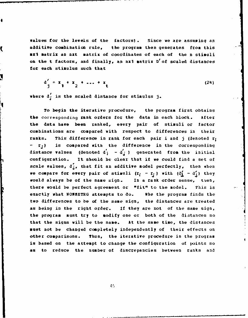
values for the levels of the factors). Since we are assuming an
additive combination rule, the program then generates from this
mx matrix an nit matrix of coordinates of each of the n stimuli
on the t factors, and finally, an nxl matrix D'of scaled distances
for each stimulus such that
d' =x 1 x 2 x.. x (24)
where d is the scaled distance for stimulus j.
To begin the iterative procedure, the program first obtains
the corresponding rank orders for the data in each block. After
the data have been ranked, every pair of stimuli or factor
combinations are c~mpared with respect to differences in their
ranks. This difference in rank for each pair i and j (denoted r
- rj) is compared with the difference in the corresponding
distance values (denoted d'; - d'j ) generated from the initial
configuration. It should be clear that if we could find a set of
scale values, d , that fit an additive model perfectly, then when
we compare for every pair of stimuli (r, . - rj ) with (dj - d3) they
would always be of the same sign. In a rank order sense, tuen,
there would be perfect agreement or *fit" to the model. This is -
exactly what NONMETRG attempts to do. Whe the program finds the
two differences to be of the same sign, the distances are treated
* as being in the right order. If they are not of the same sign,
the program must try to modify one or both of the distances so
that the signs will be the same. At the same time, the distances
must not be changed completely independently of their effects on
other comparisons. Thus, the iterative procedure in the program
is based on the attempt to change the confiquration of points so
as to reduce the number of discrepancies between ranks and
45

distances as illustrated above for all pairs of stimulus points.
To accomplish this, Johnson (1973) suggested the following
procedure.
We begin by defining a measure of the goodness-of-fit of the
data to the model. The measure is THETA (,0) and is defined as
j=1 i<j d1 d (25)
ij=l ilj
where a=O if sign (d. - d5 sign(V -() and a=1 otherwise.I j
* THETA would be zero, indicating a perfect fit, only if the signs
matched across all n*(n-1)/2 pairs of stimuli. In the worst
situation THETA could theoretically equal a maximum of one. What
we have is a suitably normalized measure of qoodness-of-fit based
on the sum of squared differences in the distances amonq the
stimulus combinations. The numerator can be thought of as a sum
of squared departures from monotonicity. It ranges in value from
zero to the value of the denominator.
Table 14 presents the results of the scaling of the riskiness
data to an additive model. Previous research (Nygen, 1979)
suggests that a good fit should be expected for the additive
model. Looking first at the history 2f computation, we find that
on the first iteration THETA was very poor -- .84485. This is to
* be expected for the first iteration since the initial stimulus
configuration in this example was based on random numbers. One
6J
44J
6]

Table 15
Additive Scale Values for the 48 Gambles in the
NONMETRG Analysis of the Riskiness Data
STIMULUS: LEVELS ADDITIVE RESCALEDADDITIVE
1 1 1 1 1.33390 0.02 1 1 2 1.45014 11.623383 1 1 3 1.54158 20.767684 1 2 1 0.94064 -39.326025 1 2 2 1.05688 -27.702716 1 2 3 1.14832 -18.558407 1 3 1 0.75047 -58.343618 1 3 2 0.86670 -46.720219 1 3 3 0.95814 -37.57591
10 1 4 1 0.63355 -70.0354611 1 4 2 0.74978 -58.. 120612 1 4 3 0.84123 -49.2677813 2 1 1 0.87348 -46.0426914 2 1 2 0.98971 -34.4193015 2 1 3 1.08115 -25.2750416 2 2 1 0.48021 -85.3689417 2 2 2 0.59645 -73.7454418 2 2 3 0.68789 -64.6011419 2 3 1 0.29004 -104.3863220 2 3 2 0.40627 -92.7630221 2 3 3 0.49772 -83.6187122 2 4 1 0.17312 -116.0782823 2 4 2 0.28935 -104.4548024 2 4 3 0.38080 -95.3105825 3 1 1 0.66753 -66.6377426 3 1 2 0.78376 -55.0143627 3 1 3 0.87520 -45.8700628 3 2 1 0.27426 -105.9637929 3 2 2 0.39050 -94.3404830 3 2 3 0.48194 -85.1961831 3 3 1 0.08409 -124.9814032 3 3 2 0.20032 -113.3580233 3 3 3 0.29177 -104.2137134 3 4 1 -0.03283 -136.6732535 3 4 2 0.08340 -125.0498736 3 4 3 0.17485 -115.9055637 4 1 1 0.44849 -88.5416338 4 1 2 0.56472 -76.9182439 4 1 3 0.65616 -67.7739440 4 2 1 0.05523 -127.8676941 4 2 2 0.17146 -116.2443142 4 2 3 0.26290 -107.1000143 4 3 1 -0.13495 -146.8853044 4 3 2 -0.01872 -135.2619245 4 3 3 0.07273 -126.1176046 4 4 1 -0.25187 -158.5771547 4 4 2 -0.13563 -146.9537748 4 4 3 -0.04419 -137.80946
47

could, of course, use a good appioximation of the contiouiation
obtained via some previous analysis as a means of improving the
efficiency of the iterative process. Notice, however, that on
Iteration 2 the THETA value is reduced to .23613. The program was
able in one iteration to move the dj 's considerably closer to
monotonicity. This is also reflected in the TAU value printed in
the table. TAU is simply a Kendall's Tau coefficient computed
between the rank order of the oriqinal data with the rank order of
the rescaled distances. As THkTA decreases TAJ will necessarily
increase.
There are several other things to notice from the history
section of this table. First, the program stopped after Iteration
6. We could let the program continue to iterate much lonqer.
However, there is generally a practical stopping point for any
given analysis. As with virtually all non-metric iterative
scaling programs, the procedure is stopped in either of two ways.
First, the iterative process will stop if a maximum number ot
iterations is reached. Usually 20 to 30 iterations is set as the
default stopping point. In our example, the program converged
very quickly, with only six iterations. This is not uncommon tor
data with a small amount of error. If the program requires more
than 30 iterations to converge, it generally means that there is a
significant amount of error in the data or that the proqram is
vascillating back and forth between several equally good (or bail)
solutions, or both. The second stopping criterion is based on a
measure of improvement in fit from one iteration to another.
Generally, an efficient iterative algorithm will, except ti
occasional minor fluctuations in the iterative process, continue
to minimize the goodness-of-fit measure. Theoretically, one
should be able to continually iterate to find a proqressively
4

better solution. In practice, however, if the THETA values on
Iterations n and n+1 differ by a value of .001 or less, there will
be no appreciable differences in the final scale values for each.
Hence, the program will have found for all practical purposes, the
minimum value of THETA, and the iterative process should be
stopped. The user can then specify a cutoff criterion for
differences in THETA to allow the program to stop after a
practical ObestO solution has been found. This is what happened
on Iteration 6 in the analysis in Table 14.
Notice that Iteration 6 produced neither the lowest THETA nor
the highest TAU. These two measures are not perfectly linearly
related to one another, since we are dealing with only ordinal
relationships here. The program allows the user to specify
whether the solution from the iteration with the lowest THETW
should be used in the final scaling or whether the solution from
the last iteration should be used. Usually there is little
practical significance to this option, since the last iteration
will generally produce the lowest THETA. Using the last iteration
is generally recommended, since it has been the author's
experience with moderate-sized data sets (e.g., 4x4x3 or smaller)
tkat a more interpretable solution will be obtained from the last
or next to lait iteration even if it has a slightly higher THETA
value than some previous early iteration.
How does NONNETEG or any other iterative procedure find the
"best" solution? Generally, the procedure is conceptually
straightforward, although mathematically and computationally it
can become quite involved. Essentially, an attempt is made to
49

Table 16
Comparison of Original Data and Final Scale Values
of Stimuli in Block 1 for Riskiness Data
DEPENDENT & PREDICTIONS SORTED BY DEPENDENT. BLOCK NO. 1.
98.000 -0.04498.000 -0.25297.000 -0.13696.000 -0.01996.000 -0.03395.000 0.08394.000 -0.13592.000 0.08489.000 0.17388.000 0.05561.000 0.20059.000 0.07359.000 0.17552.000 0.29051.000 0.27446.000 0.29239.000 0.26339.000 0.17139.000 0.38138.000 0.28929.000 0.48229.000 0.39029.000 0.49829.000 0.40619.000 0.65619.000 0.56519.000 0.44819.000 0.68819.000 0.48019.000 0.84119.000 0.75019.000 0.63418.000 0.59615.000 0.78415.000 0.66815.000 0.95815.000 0.86714.000 0.87514.000 0.7509.000 0.9909.000 0.8739.000 1.1489.000 0.9418.000 1.0576.000 1.0814.000 1.5424.000 1.4503.000 1.334
PREDICTIV5 CAPABILITY = 4.521286 PERCENTOR = 95.41 8714 IF DATA ARE IN REVERSE ORDER.
I5

minimize the goodness-of-fit measure. In the case of NONAETRG
this means minimizing THETA. Let W represent the vector
containing the n, + n. 4 ... * n, = m scale values for the levels
of the t factors, let U represent the numerator of Equation 25,
and let V represent the denominator of Equation 25. Then we have
= U/. We can use a standard mathematical procedure for
minimizing 0 by finding the gradient for the partial derivatives
of with respect to W. That is, we find
0 1 L Uv --1= -- * ( V*-- - U*-- ) (26)VIow v 0W ow
Thus we need to find the partial derivatives of U and V with
respect to W, where U and V are as defined in Equation 24 to be
functions of (d' - d') . The procedure is simplified somewhat
since the partial of the sum of squared differences is equal to
the sum of the partials of each of the terms being summed.
On any given iteration we proceed as follows. Since we have
the matrix W (a set of random or user supplied values on Iteration
1) we can easily compute X, the stimulus coordinates. We will
normalize X to have a sum of squares equal to a convenient
constant value (usually a value of one). We then compute the
gradient, G, and normalize it to have a sum of squaLes of one
also. On the first iteration we have W. and X6 , and compute 4from them. We find G as indicated in Equation 26 and modify Wo,
the initial set of scale values by
WI = W0 -(0 0 G ) (27)
In general, we have
I
51

W =W -(0 *G ) (2)i i-i i-i i-i
In the minimization process we are attempting to locate the paint
in "configuration space" where G, will be exactly zero and no
change in W will occur. In practice, the iterative procedure will
actually stop when G is hopetully very close to zero.
The remaining information presented in Table 14 indicates the
final solution for riskiness data based on Iteration 6. The tinal
scale values for the m=11 levels are presented for an additive
model and a multiplicative model. Recall that it was shown
earlier that in the positive case the multiplicative and additive
models are mathematically equivalent. That is, the additive scale
values are merely the logarithms of the multiplicative values.
Hence, both are presented in the NONMETRG procedure. In addition,
the additive values are conveniently rescaled in such a way that
cell (1,1,...,1) is set to zero and each new value is multiplied
by 100. Finally, the additive scale values for all stimulus
combinations are presented both in the original and rescaled forms
in the program. The scale values for the riskiness data are
presented in Table 15. Notice that the greatest perceived risk is
associatei with the smallest scale values. That is, the original
data and the final scale values are negatively correlated. since
this ordering is somewhat arbitrary, the NONMETRG program has as
an option a means of simply reversing the data values so that
large observations are associated with large scale values.
Sometimes it is useful to look at the transformation that has
been applied to the data to form the stimulus scale values.
NONMLTRG provides several additional pieces of information that
may aid in this analysis. First, the program prints ior each
32

block of data (in our example a block represents one complete
replication or set of scores for the subject), each original data
value and its corresponding rescaled value from the additive model
-- sorted by the data values. Table 16 illustrates this
information for the first block (replication) of observations in
the risk study. A useful statistic is presented following the
presentation of these values. It is a component of the Kendallts
Tau value that could be computed between the two sets of scores.
It is the proportion of pairs of final scale values that are in
the same order as their corresponding data values. In the case of
the riskiness data, this value is quite high, 95.48%. Finally,NONMETRG presents a plot of the corresponding data values and
additive scale values within each block. This allows the user to
obtain a good estimate of the degree of linearity or nonlinearity
in the function relating data and rescaled values. An excellent
fit of the data to the model would be indicated by a smooth curve
(not necessarily linear) running through all of the pairs of
points. This plot for Block 1 in the risk study is presented inFigure 1.
MOl I&NOVA
A second program that is capable of scaling data to fit an
additive model is Kruskal's (1965) KONAMOVA program. As the name
of the program sugqests, it too is a non-metric procedure that
attempts to find amonotonic transformation of the data such that
stimulus combinations are obtained by applying an additive
combination rule to the levels of the independent factors. This
is equivalent to finding no interactions in an analysis of
variance of the transformed data. Hence, the program is referred
53

to as BONANOVA (tonotonic Analysis Of Variance).
Table 17
History of Computation from MONANOVA
Analysis of Riskiness Data
IT STRESS SRAT SRTAVG CAGRGL COSAY ACSAV GRMAG GRMULT STEP0 0.221 1.2000 1.2000 0.0 0.0 0.067 0.21191 5.5219 1.170171 0.200 1.1054 1.1676 -0.734 -0.490 0.512 0.24620 2.6406 0.650142 0.124 1.6156 1.3011 -0.961 -0.804 0.811 0.08954 3.0046 0.269053 0.126 0.9806 1.1841 -0.993 -0.930 0.932 0.10638 0.7722 0.082154 0.120 1.0540 1.1390 0.999 0.356 0.977 0.04940 1.5106 0.074625 0.118 1.0133 1.0955 -0.983 -0.537 0.981 0.00775 2.3781 0.018436 0.118 1.0001 1.0627 -0.997 -0.844 0.992 0.00659 0.4307 0.002847 0.118 1.0001 1.0414 1.000 0.385 0.997 0.00438 0.4903 0.002158 0.118 1.0001 1.0274 1.000 0.795 0.999 0.00270 1.0275 0.002789 0.118 1.0000 1.0182 0.996 0.929 0.997 0.00054 8.2718 0.00448
10 0.118 1.0000 1.0121 -0.999 -0.357 0.999 0.00293 0.3847 0.001134 11 0.118 1.0000 1.0081 1.000 0.548 1.000 0.00206 0.4792 0.00099
12 0.118 1.0000 1.0054 1.000 0.849 1.000 0.00129 1.0057 0.0013013 0.118 1.0000 1.0036 0.996 0.947 0.997 0.00028 7.3671 0.0021014 0.118 1.0000 1.0024 -0.999 -0.350 0.999 0.00134 0.3896 0.0005215 0.118 1.0000 1.0016 1.000 0.550 0.999 0.00093 0.4811 0.0004516 0.118 1.0000 1.0011 1.000 0.850 1.000 0.00059 1.0006 0.0005917 0.118 1.0000 1.0007 0.996 0.947 0.997 0.00013 7.1704 0.00095IT STRESS SRAT SRTAVG CAGRGL COSAY ACSAV GRfAG GRMULT STEP
APPROXIMATE MINIMUM WAS REACHED. FINAL CONFIGURATION HAS STRESSor 0.1180
Conceptually, NONMETRG and MONANOVA are quite similar in that
both seek to find scale values for the factor levels with respect
to an additive model. The specific algorithms associated with the
two programs are quite different, however, since MONANOVA
minimizes a different goodness-of-fit measure. The FONANOVA4 algorithm is based on Kruskal's earlier extensions of Shepard's
original non-metric multidimensional scaling procedure for the
analysis of similarities data (cf. Kruskal, 1964a, 1964b; Shepard,
1962a, 1962b). Kruskal showed how it was possible to obtain amatrix of interval-scaled distances that was a least squares
5
54

estimate to a matrix of monotonically transformed data values.
That is, the procedure finds and applies a monotonic
transformation to the original data such that a set of distances
can be estimated for the stimuli with the constraint that the
distances Obest" fit the monotonically transformed data in a least
squares sense. This suggests a new coodness-of-fit measure which
Kruskal (1965) called STRESS>. To define this measure, however, we
must first describe the monotonically transformed data matrixA
which we will call disparities, and will denote as di. If we letA
S represent our original data matrix, D be the disparities matrix,
D P be the distances matrix, and X be the final configuration then
the procedure can be illustrated as
*A 0'S D = D = g(X) (30)
Here S = D indicates that a monotonic transformation is applied to
the data in such a way that a set of disparities are formed,
subject to the constraint that
I I
(i) if s > s., then d > d andi ji- j
(ii) if s = s., then d = di. (31)i ) 1 j
Bquation 31 is often referred to as weak monotonicity. It is animportant concept and its practical significance will be discussed
later in the CPSCAL manual. The portion of Equation 30 written asA .D D indicates that a least squares procedure is used to fit
distances to the disparity values, subject to the constraint that
the d'0 s satisfy the standard distance properties and D" = q(1)
where 9(X) is defined in the case of the additive model to be
55

d = f (x j) + 2(x j2) + + ft (x jt) (32)
and x is the level of Stimulus j on Factor i.
Table 18
Final Configuration and Stimulus Scale Values for
MONANOVA Analysis of Riskiness Data
ACB DESIGN. 4X4X3 DESIGN. SL, PL, PW.1 -1.7999 -0.1881 0.6659 1.32222 -1.8258 -0.1436 0.6668 1.30273 0.1477 -0.0245 -0.1232
ADDITIVE SCALE 'VLUES FOR 46 STIMULI.STIMULUS: LEVELS kDDITIVE RESCALED
1 1 1 1 -3.47809 0.02 1 1 2 -3.65023 -17.213623 1 1 3 -3.74894 -27.085114 1 2 1 -1.79589 168.219655 1 2 2 -iJ96803 151.006036 1 2 3 -2.06674 141.13454
1o
43 4 3 1 2.13659 561.4677744 4 3 2 1.96445 544.2541545 4 3 3 1.86574 534.3825746 4 4 1 2.77251 625.0598147 4 4 2 2.60037 607.8461948 4 4 3 2 50166 597.97461
PREDICTIVE CAPABILITY = 90.763397 PERCENTOR = 9.236603 IF DATA ARE IN REVERSE ORDER.
As with NOAMETRG we need several pieces of information to
begin the MONANOVA program. First, we need the parameter values
that describe the input data and the independent factors. Next,
we need the original data values in the matrix S. Finally, we
need a starting configuration, X, consisting of an initial set of
scale values for the levels of the factors. This last matrix is
56

important since a Ogoodu starting configuration may lead to
convergence to an optimal solution very quickly, reducing computer
time as well as possibly reducing the likelihood of the program
stopping at a non optional or Olocal minimum" solution.
In HONAOUVA, this initial configuration can either be
supplied by the user or be created in the program. When generated
by the program the initial configuration is created in a rather
arbitrary way and-generally produces a poor fit of the model to
the data. Regardless of how this initial configuration is
generated, it is then normalized. By this we mean that the mean
of the scale values of the m levels of the factors is 0.0 and the
sum of squares of the scale values is a. This normalization
procedure will in no way hinder the iterative procedure, since as
we shall see when the STRESS measure is defined, it is totally
invariant to both translation and uniform stretching of the
stimulus space.
Once the initial configuration, 1, has been generated, it is
easy to compute the df's in the distance matrix, Do. by using the
additive composition rule. We now have the ingredients for
Kruskal's goodness-of-fit measure. If a monotonic transformation
of the data (i.e., the S matrix) could be found such that when thet ,A
sjs are transformed into the disparities, d, these d.'s could be
treated exactly as distances, d , satisfying the additive model
perfectly, then we would have a d. for evey stimulus J. This
suggests that a measure of goodness-of-fit might be the sum across
all stimuli of a function of the discrepancies between the
disparity and distance values. This is exactly what STRESS is.
57

Table 19
r. History of Computation from DISTRIB
Analysis of Riskiness Data: A*(B.C)
IT STRESS SRAT SRTAYG CkGRGL COSAV ACSAV GRMAG GRMULT STEP0 0.3465 1.2000 1.2000 0.0 0.0 0.067 0.1450 8.6618 1.25651 0.1748 1.9819 1.4184 0.848 0.565 0.588 0.0938 39.9433 3.74392 0.6962 0.2511 0.7965 -0.726 -0.295 0.680 0.1673 5.1330 0.85893 0.5426 1.2830 0.9336 0.9 7 0.553 0.878 0.1876 5.6952 1.06844 0.34 1 1.5633 1.1087 0.962 0.825 0.934 0.1724 15.7342 2.71325 0.2570 1.3504 1.1840 -0.810 -0.265 0.851 0.1107 12.5933 1.39496 0.1727 1.4885 1.2779 -0.730 -0.575 0.771 0.0467 15.1527 0.70827 0.1785 0.9676 1.1647 -0.812 -0.733 0.798 0.0745 3.6369 0.27118 0.1640 1.0879 1.1385 0.925 0.372 0.883 0.0313 9.9091 0.31049 0.1625 1.0092 1.0937 -0.713 -0.351 0.770 0.0331 4.4277 0.1468
10 0.1598 1.0170 1.0675 0.309 0.089 0.463 0.0117 12.3183 0.144411 0.1583 1.00941 1.0478 0.718 0.508 0.633 0.0122 21.0217 0.256612 0.1574 1.0060 1.0337 -0.182 0.048 0.332 0.0305 7.5817 0.231513 0.1572 1.0011 1.0227 -0.820 -0.531 0.657 0.0354 2.5933 0.091914 0.1551 1.0139 1.0197 0.830 0.377 0.773 0.0134 7.6772 0.103415 0.1544 1.0044 1.0146 -0.035 0.102 0.281 0.0155 6.3229 0.098016 0.1538 1.0041 1.0111 -0.187 -0.090 0.218 0.0154 4.6057 0.07091 0.1531 1.0040 1.0087 0.153 0.071 0.174 0.0113 5.6230 0.063918 0.1526 1.0036 1.0070 0.524 0.373 0.408 0.0109 7.9875 0.087219 0.1519 1.00414 1.0061 0.336 0.348 0.360 0.0129 8.8537 0.114820 0.1515 1.0028 1.0050 -0.280 -0.071 0.307 0.0207 4.0009 0.083021 0.1507 1.0050 1.0050 -0.238 -0.182 0.261 0.0122 4.2b40 0.052122 0.1503 1.0029 1.0043 0.414 0.215 0.363 0.0102 5.4874 0.05642 0.1498 1.0031 1.0039 0.6. 0.483 0.533 0.0103 8.6424 0.089024 0.1492 1.0041 1.0040 0.2.-1 0.319 0.335 0.0140 7.9926 0.112025 0.1491 1.0009 1.0029 -0.486 -0.217 0.436 0.0246 2.6493 0.065326 0.14 B 1.0059 1.0039 0.219 0.073 0.291 0.0090 6.3729 0.057627 0.1471 1.0034 1.0038 0.932 0.646 0.719 0.0091 12.4162 0.113028 0.1468 1.0060 1.0045 0.520 0.562 0.586 0.0124 16.0709 0.199329 0.1489 0.9860 0.9983 -0.619 -0.226 0.608 0.0550 1.8776 0.103330 0.1455 1.0233 1.0066 0.811 0.466 0.744 0.0123 11.3779 0.1404IT STRESS SRAT SRTAVG CAGRGL COSAV ACSAV GEMAG GRMULT STEP
SXZIMUM NUMBER OF ITERATIONS WAS USED.FINAL CONFIGURATION HAS STRESS = 0.14552
Formally, we define it ac
Z (d -d.)= j=1 j jS j= - (33)
f (d 2
j=1 3
Avhere n is th, number of stimulus combinations, d and d are

defined as before, and d is the mean distance value. Oriqinally,
Kruskal had suggested that STRESS be defined by simply using the
sum of squares of the distances in the denominator. However, he
found that in some situations the likelihood of degenerate or non-
optimal solutions could be avoided if the denominator were
actually the sum of squared deviations from the mean of thedistances. Other measures of goodness-of-fit related to STRESS
have been proposed, including one in which the mean distance, d,
in the denominator of Equation 33 is replaced by T, the meandisparity value. Regardless of how STRESS is defined, it is clear
that a perfect solution will be found when the original data can
be monotonically transformed into disparities that fit the
distance model perfectly. This leads to a STRESS of zero. The
goal of the MONANOVA program is then to find distances that will
minimize STRESS. To accomplish the minimization process, MONANOVA
uses basically the same means that was used in NONMETRG. That is,
the numerical method of gradients or L descent is used to
find the minimal value of STRESS (or more accurately, the minimal
value of the square of the STRESS value, S )
Before the minimization process can be done, however, a
method for computing the disparities must be constructed. There
are several methods for doing this, although Kruskal's (1964)
monotonicity principle is most often used. In the monotonic
regression procedure devised by Kruskal we attempt to find values
of d from the given values of 5j under the constraints of
montonicity as defined in Equation 31. On the first iteration the
given values of the d 's come from the user-supplied or program-
generated initial configuration. The procedure to be described
59~

Table 20
Final Configuration and Stimulus Scale Values for
DISTRIB Analysis of Riskiness Data: A*(B*C)
FINAL ITERATION CONFIGURATION:1 J.1563 3.7007 4.6566 5.58322 0.2069 2.8841 4.4955 6.01033 3.8372 3.3831 3.0611
FINAL STRESS AND MINIBUS STRESS ARE EQUAL.THE PREDICTED DISTRIBUTIVE SCALE VALUES FOR 48 STIMULI:FINAL ITERATION CONFIGURATION:SEQ. NO. DATA SUBSCRIPTS
1 8.72031 1 1 12 7.74130 1 1 23 7.04681 1 1 34 14.49306 1 2 15 13.51405 1 2 26 12.81956 1 2 3
43 46.52243 4 3 144 43.98755 4 3 245 42.118938 4 3 346 54.97975 4 4 147 52.44485 4 4 248 50.64668 4 4 3
PRECAP VALUE FOR FINAL ITERATION CONFIGURATION.PREDICTIVE CAPABILITY = 90.637131 PERCENT
below, although it is not identical to Kruskal*s monotone
regression procedure as actually programmed in BONAAOVA, it is
very similar to this method, it is easier to understand
intuitively, and produces final disparity values that are
identical to those obtained from the actual method. For these
reasons, this modified procedure devised by Young (1973) will be
described.
We begin by ordering the data values from smallest to
60

largest. From this point on we will need only this rank ordering
of the data and not the data values themselves. Again, this is
because the procedure is nonsetric. We begin by assigning theA% A
first and second disparities, d, and dL , the values of the
distances from the initial configuration that correspond to our
smallest and second smallest data values. That is, d = d, andA A
dt. If do < d., then they are in the correct order and are what
Kruskal referred to as being down-satisfied. If this ordering is
correct, then we go on and set d3 = d3. If, however, d. > do ,A
then each is replaced by d1i, the average of the two. In this
way, the "new" d, and dLwill be weakly monotonic with the original
data, and we will have a block of two equal disparities. The
process continues with d3 being set equal to d It is thenAA
compared with d L G: with the block consisting of do and d1 if theyA A
are equal. If the ordering here is correct (d. < ds) then we goA A A , aon to d . If not, then dtand d 3 (or if d i I, , d., and a5 )
are set equal to their average, a, 3 (or T1z 3} The process iscontinued until all observations have been ordered. In this
procedure we are always making comparisons in the down-satisfied
direction. In Kruskal's procedure there is actually an
alternating process whereby each block is compared with the next
smaller block as well as the next larqer block. Thus, a
particular block is also being made up-satisfied. However, when
we have completed the process described above, all blocks will, in
fact, be both up-and down-satifed, yielding final disparities
that are identical to those that would be obtained using Kruskal's
method.
Given the disparities and distances, STRESS can now be
computed for Iteration 1. Since our initial confiquration may be
very poor, we miqht expect large discrepancies between the .S• eS1
1

I
and the d-Is. This would produce a high initial STRESS value. Wenext compute the partial derivatives (i.e., the gradients) of S
with respect to the configuration coordinates, X. The negative
gradient is then calculated. This allows us to move the
configuration in a direction where S will be decreasing most
rapidly (i.e., steepest descent). In the MONkXOVA program this
allows us to compute a parameter called the step size which then
leads to the creation of a new configuration. This new
configuration should be much better than the initial one used on
Iteration 1.
Table 21
0 Reanalysis of Riskiness Data for New DISTRIB
Model with Factor C as the Outside Factor
DISTRIBUTIVE MODEL ANALYSIS FOR C*(BA) DESIGN.SEQ. NO. DATA SUBSCRIPTS
C B A1 3.00000 1 1 12 5.00000 1 1 13 5.00000 1 1 14 9.00000 1 1 25 9.00000 1 1 26 9.00000 1 1 2
Sm
139 59.00000 3 4 3140 59.00000 3 4 3141 59.00000 3 4 3142 98.00000 3 4 4143 97.00000 3 4 4144 96.00000 3 4 4
We can now begin Iteration 2, repetition of Iteration 1
beginning with the normalization of the new configuration found on
the last iteration. As the iterative process continues, the
62
mmm mm m#4,Jm,~mml mm mumm ~ mmm mmmmm ~ n~nrnw . . .. . . . .. .

IJ
STRESS value should continue to decrease until there is no
practical improvement in this fit measure and, consequently, in
the final configuration. As with NONMETRG there needs to be a
stopping criterion in MONANOVA. There are two such criteria that
are directly comparable to those found in NONHETRG. First, the
user may specify a maximum number of iterations. Usually, 30 is
sufficient to insure convergence. Secondly, there is an
improvement criterion associated with the change in STRESS from
Iteration n to Iteration n+1. Usually this criterion is set at a
value between .001 and .0001.
Table 17 presents the history of computation from the
MONAMOVA analysis of the riskiness data used in the previousanalyses. This history provides several useful pieces of
information not directly related to the final scaling solution.The columns represent the values on each iteration of the
parameters used in the iterative process. Aside from the STRESSvalue, the other parameter that might be of value is the STEP
size. The STEP size indicates the "movement" in the configurationvalues from one iteration to the next. Note that in our example
the STRESS value had stabilized and the STEP size was very close
to zero. This indicates little improvement in the last eleven
iterations. As it does in most cases with low or moderately low
amounts of error in the data, the MONANOVA program converged veryrapidly to a final additive configuration.
The final configuration and the scale values for 12 of the 48
stimuli are presented in Table 18. As was mentioned in the
discussion of the normalization process, the mean of the scale
values in the configuration is zero and the sum of squares of
these values adds to eleven. This normalization is arbitrary, of
63

course, since the scales are interval. It is important to
recognize, however, that the scale values for the levels of tue
different factors can be compared. In this example, the scale
values for Amount to Lose ($L) ranged from -1.7999 to 1.3222. For
Probability of Losing (PL) the range was about the same, being
-1.8258 to 1.3027. For the Probability of Winning factor (PW),
the range was only 0.1477 to -0.1232. These scale values are in
agreement with what was suggested earlier in the CONJOINT and
PCJ82 analyses of this subject's riskiness ratings. Both Amount
to Lose and Probability of Losing were very important in
determining risk for this subject. In fact, they appear to be
about equally weighted because their ranges are comparable.
Probability of Winning had virtually no effect on perceived risk.
In this example, the levels of Probability of Winning were 2/8,
3/8, and 4/8. For this subject, then, the MONANOVA results
indicate that peroeived risk would be essentially unaffected if
the Probability of Winning were doubled from 2/8 to 4/8, assuming
that the other factors were held constant.
A final piece of useful information provided by the MONANOVA
program is a plot of the monotonic transformation applied to the
data values. Just as with NONMETRG, this plot should indicate a
nice, smooth curve if the data are being fit perfectly by the
model. The plot for the riskiness data is found in Figure 2.
This plot is monotonic am wam expected from the results in
Tables 17 and 18. The STRESS value was low (0.1180) and the
Predictive Capability value was high (90.76%). The Predictive
Capability measure is interpreted in the same way as it was with
NOURDTRG. It is the percentage of data values and final distances
4 that is in the right order in a pairwise comparison sense. In
the case of the risk analysis 90.761 of the (48*47)/2 = 1128
64

conpazzisons were in the sane order for the original data and the( final distances.
65

i4
1. jDITIOUkL CONJOINT SCAL.NG PROGRAMS: DISTRIB AND DUALDIST
There are a number of other programs that will also do
additive conjoint scaling (cf. Carroll's (1972) HDPBEF, Young's
(1972, 1980) POLYCON and ADDALS, and Srinivasan and Shocker's
(1973) LINBAP. There are, however, two other programs that are
currently available for doing a conjoint analysis via a
distributive or dual-distributive model. Both of these programs
were adapted from ROVANOVA by Emery (1977a, 1977b). These
programs were called DIST and DULDIST respectively. They have
been further revised in a manner to be described below into the
DISTRIB and DUALDIST programs in the CPSCAL manual.
There is no need to describe in detail the non-metric
iterative procedure employed by the DISTRIB and DUALDIST programs
since they are virtually identical to that of MONANOVA. In fact,
Emery's original DIST and DULDIST Fortran programs are identical
to the HONANOVA program except for about ten of the 1000 programstatements. All that is changed in these two programs are
statements allowing for the computation of the distances from a
distributive or dual-distributive model rather than an additive
model, and appropriate modifications to the minimization
subroutine.
The primary change made to the DIST and DULDIST proqrams by
the author for the CPSCAL manual was an extension to allow for the
testing of more than one form of the models. In an additive
66
6 4
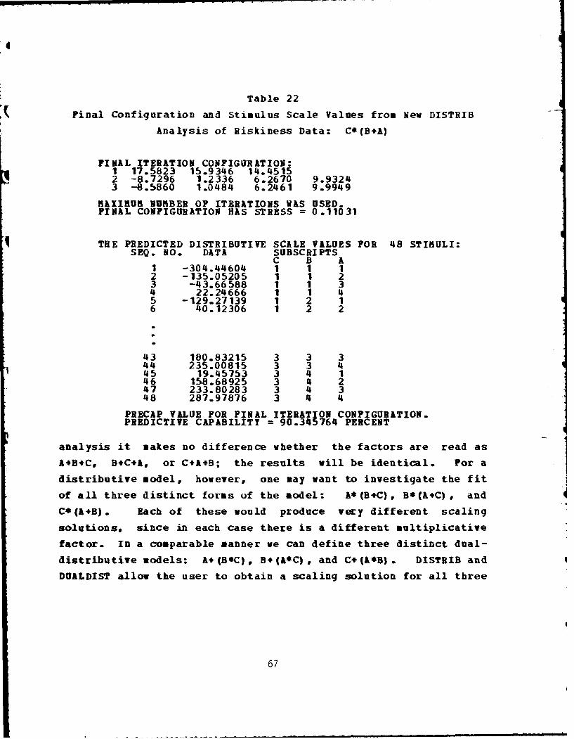
Table 22
Final Configuration and Stimulus Scale Values from New DISTRIB
Analysis of Riskiness Data: C*(B+A)
FINAL ITERATION CONFIGURATION:1 17.5823 15.9346 14.45152 -8.7296 1.2336 6.2670 9.93243 -8.5860 1.0484 6.2461 9.9949
MAXIMUM NUMBER OF ITERATIONS WAS USED.FINAL CONFIGURATION HAS STRESS = 0.11031
THE PREDICTED DISTRIBUTIVE SCALE VALUES FOR 48 STIMULI:SEQ. NO. DATA SUBSCRIPTS
C B A1 -304.44604 1 1 12 -135.05205 1 1 23 -43.66588 1 1 34 22.24666 1 1 45 -129.27139 1 2 16 40.12306 1 2 2
43 180.83215 3 3 344 235.00815 3 3 445 19.45753 3 4 146 158.68925 3 4 247 233.80283 3 4 348 287.97876 3 4 4
PRECAP VALUE FOR FINAL ITERATION CONFIGURATION.PREDICTIVE CAPABILITY = 90.345764 PERCENT
analysis it makes no difference whether the factors are read as
A4B4C, B*C*A, or C*A*B; the results will be identical. For a
distributive model, however, one may want to investigate the fit
of all three distinct forms of the model: A* (B*C), Bs(&+C), and
C*(A+B). Each of these would produce very different scaling
solutions, since in each case there is a different multiplicative
factor. In a comparable manner we can define three distinct dual-
distributive models: A+ (B*C), B+(&*C), and C+(A*B). DISTRIB and
DUALDIST allow the user to obtain a scaling solution for all three
67

4
Table 23
Final Configuration and Stimulus Scale Values for
DUALDIST Analysis of Riskiness Data: A4(B*C)
FINAL ITERATION CONFIGURATION.1 -1.2534 2.8208 5.0111 6.68302 1.3106 2.9658 3.7756 4.40773 2.6976 2.5455 2.4608
APPROXIMATE MINIMUM WAS REACHED.MAXIMUM NUMBER OF ITERATIONS WAS USED.FINAL CONFIGURATION HAS STRESS = 0.11354THE PREDICTED DUAL-DISTRIBUTIVE SCALE VALUESFOR 48 STIMULI:
SEQ. NO. DATA SUBSCRIPTSA B C
1 2.28201 1 1 12 2.08268 1 1 23 1.97169 1 1 34 6.74721 1 2 15 6.29612 1 2 26 6.04496 1 2 3
43 16.86804 4 3 144 16.29378 4 3 245 15.97406 4 3 346 18.57320 4 4 147 17.90279 4 4 248 17.52953 4 4 3
PRECAP VALUE FOR FINAL ITERATION CONFIGURATION.PREDICTIVE CAPABILITY = 90.773102 PERCENT
forms of the models in one analysis. This is not only potentially
interesting in terms of the data, but it is also convenient, since
the data need only be stored in one form.
* Tables 19 and 20 present the results of the DISTRIB analysis
of the riskiness data assuming a model of the form A*(B+C) or
specifically, SL*(PL*PW). Again, since the programs are very
simple extensions of MONANOVA, the values in Tables 19 and 20 are
• interpreted in the same manner as were Tables 17 and 18. Tables
21 and 22 show the results of the reanalysis of the risk data to
68
t"8
fit the distributive model C*(B.A). Table 21 merely indicates how
the data have been internally rearranged to be in the appropriate
sequence for the C* (B+A) model. Table 22 shows the final
configuration and final scale values for 12 of the 48 stimuli for
this model. Finally, Table 23 illustrates the final solution for
the data as it was fit by DUALDIST according to the A+(B*C) model.
It should be apparent from looking at the STRESS values and
the Predictive Capability values from the MONANOVA analysis, the
two DISTRIB analyses, and the DUALDIST analysis of the same
riskiness data that there are only small differences in the fit of
the models. This seems quite surprising since the models are
conceptually and mathematically very different. However, recent
research by Emery and Barron (1979) and others suggests that the
goodness-of-fit measures like STRESS may not be very powerful in
many situations in differentiating among the four models discussed
in this manual. Clearly, a great deal of research needs to be
done in order for investigators to make the greatest use of these
scaling techniques.
69

APPENDIX 1
THIS APPENDIX PROVIDES STEP-BY-STEPINSTRUCTIONS FOR SETTING UP AND RUNNING SIX DIFFERENTCONJOINT TESTING AND SCALING PROGRAMS. IN EACH OFTHE DESCRIPTIONS OF THE PROGRAMS THERE IS A SMALLSECTION SET OFF BY *6S. THIS SECTION DESCRIBES THENECESSARY JCL CARDS FOR RUNNING THE SOURCE DECK VERSIONOF THE PROGRAMS. IN EACH CASE CARDS 1-4 ARE UNIQUETO THE AMDAHL 470 SYSTEM AT OHIO STATE UNIVERSITY.USERS OF CPSCAL WILL HAVE TO MODIFY THESE CARDS TOFIT THE REQUIREMENTS OF THEIR OWN INSTALLATIONS.
AN EFFORT HAS BEEN MADE TO FIND ALL TYPOGRAPHICALERRORS AND INACCURACIES IN THIS MANUAL. NEVERTHELESS,SOME MINOR PROBLEMS MAY STILL EXIST. IF INACCURACIESARE FOUND PLEASE REPORT THEM TO THE AUTHOR.
70
• iIa m n ~ m ~ ~ m i n ul i us -n u nl m nnnmnnn m, " m

I!
C 0 N J 0 N T
* C 0 N J 0 I N T *
* INSTRUCTIONS FOR USING CONJOINT.OPT2 *
* *[
* CONJOINT IS A COMPUTER PROGRAM FOR EVALUATING *, CERTAIN CONJOINT-MEASUREMENT AXIOMS. IT WAS *
WRITTEN BY JAMES 0. HOLT III AND THOMAS S. ** WALLSTEN.
* *
* THE PROGRAM HAS BEEN MODIFIED AND ADAPTED FOR ** USE ON THE AMDAHL 470 OPERATING SYSTEM AT ** THE OHIO STATE UNIVERSITY BY: *
* DR. THOMAS E. NYGREN* DEPT. OF PSYCHOLOGY ** OHIO STATE UNIVERSITY
* *
* TO CALL THIS PROGRAM FOR THE SOURCE DECK FORM FROM ** THE TAPE NCPSCAL", USE THE FOLLOWING JCL CARDS: *4[ *
* 1) YOUR ID CARD* 2) // TIME=2,REGION=300K ** 3) /*JOBPARM LINES=10000,DISKIO=400,TPEIO=4O0 * 4) /*SETP UNIT=TAPE9,ID=(CPSCAL,XXXX,READ) *
* 5) // EXEC PLIXGTIME.GO=2,REGION.GO=300K ** 6) //GO.SYSLIN DD UNIT=3400,VOL=SER=CPSCAL, ** 7) // DISP=(OLD,PASS),DSN=CONJOINT, *
* 8) /, LABEL= (1,SL), * 9) // DCB=(RECFM=FB,LRECL=80,BLKSIZE=1600) *
* 10) //GO.SYSIN DD * *
* 11) INPOT DECK AS DESCRIBED BELOW ( CONTROL AND *4[ DATA CARDS GO HERE.) ** *
* 12) /* **13) // *
71

SIN P U T DECK A R R A N GE M E N T* *
CARD 1. THE wTASK" CARD.
THIS CARD IS USED TO SET UP THE PARAMETERS OF CONJOINT.wTASK" MUST BE PUNCHED IN COLUMNS 1-4. COLUMN 5 IS BLANK. THEN,ALL OF THE FOLLOWING MOST APPEAR IN ORDER AND SEPERATED BYONE OR MORE SPACES:
NUMBER OF DATA SETS TO BE ANALYZED (UNLIMITED)NUMBER OF LEVELS OF FACTOR A (FROM 1 TO 6) .NUMBER OF LEVELS OF FACTOR B (FROM 1 TO 6) .NURSER OF LEVELS OF FACTOR C (FROM I TO 6) .READIN METHOD.
= 0, IF MORE THAN ONE OBSERVATION PER CELL ANDDATA CELLS ARE TO BE RANK ORDERED USINGTHE MANN-WHITNEY U-TEST PROCEDURE.
= 1, IF THERE IS ONE OBSERVATION PER CELL AJD NORANKING IS REQUIRED.
= 2, IF MORE THAN ONE OBSERVATION PER CELL AS INOPTION "0 AND THE DATA CELLS ARE TO BERANK ORDERED. THIS OPTION DIFFERS FROMOPTION 0 ABOVE IN THAT THE DATA AREASSUMED TO BE IN A PRESPECIFIED ORDER FORREADIN PURPOSES. THIS SPECIAL READIN ORDERIS DESCRIBED BELOW.
DISTRIBUTIVE CANCELLATION PRINTING OPTION.= 0, IF THE LISTING OF THE SUBMATRICES VIOLATING
DISTRIBUTIVE CANCELLATION IS TO BE SUPPRESSED.= 1, IF THE LISTING IS TO BE PROVIDED.
DOUBLE CANCELLATION PRINTING OPTION.= 0, IF THE LISTING OF THE SUBMATRICES VIOLATING
DOUBLE CANCELLATION IS TO BE SUPPRESSED.= 1, IF THE LISTING IS TO BE PROVIDED.
CARD 2. THE NTITLEN CARD.
THIS IS AN OPTIONAL CARD AND IS USED TO PROVIDE A TITLEFOR THE OUTPUT. "TITL" MUST BE PUNCHED IN COLUMNS 1-4. COLUMN5 IS BLANK. ANY STRING OP TO 73 CHARACTERS, AND ENCLOSED BYSINGLE QUOTES, CAN BE USED.
7?
...*.....

CARD(S) 3. THE OTESTO CARDS.
ONE TEST CARD IS NECESSARY FOR EACH OF THE SIXTESTS DESIRED. THE TESTS ARE IDENTIFIED BY THE NUMBERS 1 - 6.IN EACH CASE THE WORD OTESTO APPEARS IN COLUMNS 1-4, AND COLUMNIS BLANK. THEN THE FOLLOWING MUST APPEAR IN ORDER ANDSEPARATED BY ONE OR MORE SPACES:
TEST NUMBER. (ONE OF THE FOLLOWING MUST APPEAR.)= 1, IF DOUBLE CANCELLATION IS TO BE TESTED.= 2, IF SIMPLE INDEPENDENCE IS TO BE TESTED.- 3, IF SIGN DEPENDENCE IS TO BE TESTED.= 4, IF DISTRIBUTIVE CANCELLATION IS TO BE TESTED.= 5, IF JOINT INDEPENDENCE IS TO BE TESTED.= 6, IF JOINT SIGN DEPENDENCE IS TO BE TESTED.
NUMBER OF OUTSIDE FACTORS.- 1, 2, OR 3. IN EACH OF THE TESTS ABOVE ONE
FACTOR SERVES AS THE 'OUTSIDE FACTOR" EACHTIME. FOR EXAMPLE, WHEN CHECKING DOUBLECANCELLATION ONE MIGHT LOOK AT FACTORS A AND B,A AND C, OR B AND C. THE OUTSIDE FACTOR INEACH OF THESE CASES WOULD BE FACTORS C, B, ANDA RESPECTIVELY. HENCE, IF ONE WANTED TOCHECK DOUBLE CANCELLATION IN ALL THREE OFTHESE CASES, ONE WOULD INDICATE THAT THEREARE N30 OUTSIDE FACTORS. THE NEXT PARAMETERINDICATES WHICH OF THE FACTORS ARE TO BECONSIDERED THE OUTSIDE FACTOR(S).
DESIGNATION OF OUTSIDE FACTOR (S).THIS PARAMETER INDICATES WHICH FACTORS ARE TOBE CONSIDERED THE OUTSIDE FACTOR(S). THELETTERS A, B, AND C, PLACED IN SINGLE QUOTES ANDSEPARATED BY ONE OR MORE SPACES ARE USED (E.G.,GAS GBG GCs). THE NUMBER OF LETTERS PLACED INQUOTES MUST MATCH THE NUMBER OF OUTSIDE FACTORSAS INDICATED BY THE PARAMETER ABOVE.
CARD 4. THE LABEL CARD FOR FACTOR A - wALBLn.
THIS CARD PROVIDES A LABEL ON THE COMPUTER PRINTOUT OUTPUT FORFACTOR A. THE WORD uALBL" APPEARS IN COLUMNS 1-4, ANDCOLON 5 IS BLANK. COLUMNS 6 - 8 CONTAIN *A*. ANY STRING OFUP TO 25 CHARACTERS MAY BE USED FOR THE LABEL. THIS STRINGMOST BE ENCLOSED IN SINGLE QUOTES, BEGINNING IN COLUMN 10.
CARD(S) 5. LABEL CARDS FOR FACTORS B AND C.
THESE CARDS CORRESPOND TO THE "ALBL" CARD ABOVE, EXCEPTTHAT NBLBL" AND "CLBL" APPEAR IN COLUMNS I - 4, RESPECTIVELY.
73

CARD(S) 6. THE DATA CARDS.
THE DATA CARDS ARE SET UP DIFFERENTLY DEPENDING ON THE READINMETHOD INDICATED ON CARD 1.
IF READIN 0, THE FORMAT IS:COLUMN MEANING1 -2 DATA SET ID, FROM 01 TO 98.4 INDEX ON FACTOR A.6 INDEX ON FACTOR B.8 INDEX ON FACTOR C.33 - 41 DATA VALUE IN F9.5 FORMAT.
45 INCLUSION FLAG.= BLANK OR 0 OR 1, IF THE CARD IS TO BEINCLUDED IN THE DATA SET.= 2 OR 3, IF THE CARD IS NOT TO BE INCLUDED.
READIN = 0 IMPLIES THAT THERE ARE 3 OR MORE REPLICATIONS OF EACHJUDGMENT IN EACH DATA SET. THE ENTIRE CARD IS SKIPPED IFCOLUMNS 1 AND 2 ARE EMPTY. THE NUMBER OF CARDS, OR DATAENTRIES PER CELL CANNOT BE LESS THAN 3 NOR EXCEED 50, ANDTHE ENTIRE NUMBER OF CARDS PER DATA SET CANNOT EXCEED 2000.IT IS NOT NECESSARY TO INCLUDE BLANK CARDS FOR EMPTY CELLS,NOR IS IT NECESSARY TO ARRANGE THE CARDS IN A PARTICULARORDER.EACH DATA SET MUST BE FOLLOWED BY A CARD WITH "990 IN COLUMNSI AND 2. THIS SIGNALS THE END OF THE DATA SET AND INITIATESTHE ANALYSIS. THE NUMBER OF DISTINCT DATA SETS MUST EQUAL THENUMBER INDICATED ON THE TASK CARD.
IF READIN 1, THE FORMAT IS:COLUMN MEANINGI - 2 DATA SET ID, FROM 01 TO 98.4 INDEX ON A VARIABLE.6 INDEX ON B VARIABLE.8 INDEX ON C VARIABLE.
* 10 - 11 THE NUMBER OF OBSERVATIONS ON WHICH THE CELLENTRY (DATUM) IS BASED. (IF THIS IS LEFT BLANK,THE CELL WILL BE TREATED AS EMPTY.)
33 - 41 THE DATA VALUE IN F9.5 FORMAT.
READIN = I IMPLIES ONLY ONE REPLICATION OF EACH JUDGMENT INEACH DATA SET. THE 'ITIRE CARD IS SKIPPED IF COLUMNS 1 AND 2ARE EMPTY. THE NUMBth OF CARDS CANNOT EXCEED ONE PER CELL,AND RONE ARE NEEDED FOR EMPTY CELLS. THE CARDS WITHIN A DATASET NEED NOT BE IN ORDER.
74

4
EACH DATA SET MOST BE FOLLOWED BY A CARD WITH "990 IN COLUMNSI AND 2 TO SIGNAL THE END OF THE DATA SET AND TO INITIATETHE ANALYSIS. THE NUMBER OF DISTINCT DATA SETS MUST EQUAL THENUMBER INDICATED ON THE TASK CARD.
IF READIN = 2, THEN PROCEED AS FOLLOWS FOR READING IN THE DATA:COLUMN MEANING1 - 2 DATA SET ID, FROM 01 TO 98.4 NUMBER OF REPLICATIONS OF EACH JUDGMENT
APPEARING ON EACH DATA CARD.
THIS PARAMETER CARD APPEARS BEFORE THE DATA CARDS. NOTETHAT FOR READIN = 2 IF IT ASSURED THAT THE NUMBER OFREPLICATIONS OF EACH JUODGMENT IN THE DATA SET IS THE SAME.THE PARAMETER CARD IS FOLLOWED BY THE DATA CARDS. ALLREPLICATIONS OF EACH JUDGMENT ARE ON THE SAME CARD.OBSERVATIONS CAN BE PUNCHED FORMAT-FREE, EACH BEING SEPERATEDBY AT LEAST ONE BLANK.
WHEN USING THIS SPECIAL READIN METHOD, HOWEVER, THECARDS WITHIN EACH DATA SET MOST BE IN THE SAME SPECIALORDER. INDICES ON VARIABLES A, 8, AND C NEED NOT BE PUNCHED.IN THIS INPUT MODE IT IS ASSUMED THAT THE DATA CARDS ARE INTHE FOLLOWING ORDER:(1,1,1) , (1,1,2),.. ., (1, 1,Z) , (1,2, 1), (1,2,2),.
(1,2,Z) , (1,3, 1)},..., (1,YZ),., (X,Y,.),
WHERE 1, Y, AND Z ARE THE IJMBER OF LEVELS OFFACTORS A, B, AND C.
CARD 7. END OF DATA CARD.
A bLANK CARD FOLLOWS THE LAST DATA SET. THIS CARDSIGNALS THE END OF THE ANALYSIS.
75

* C ON JOIN T .E X A PL E
THE FOLLOWING CARDS ARE A SAMPLE DATA DECK FOR A wCONJOINT"ANALYSIS. IN THE EXAMPLE, "CONJOINTu IS USED TO CHECK ALL SIXTESTS (I.E., DOUBLE CANCELLATION) FOR THE DATA FROM ONE SUBJECT.THE STIMULUS DESIGN IS A THREE-FACTOR 4X3X4 DESIGN. THERE ARETHREE REPLICATIONS OF EACH OF THE 48 STIMULI. SPECIAL READ INMETHOD READIN=2 WAS USED. NOTE THAT INDICES FOR THE FACTORLEVELS ARE NOT PUNCH/ED ON THE DATA CARDS. THE DATA ARE ASSUMEDTO BE IN THE ORDER DESCRIBED IN THE SECTION ABOVE.
TASK 2 4 4 3 2 0 0TITL ATTRACTIVENESS & RISK DATA, 1 SUB. lX4X3XQ DESIGN.'TEST 1 3 'A' 'B' 'C'TEST 2 3 'A' 'Bs sC'TEST 3 3 'A' 'oB' 'C'TEST 4 3 'A' 'B' 'C'
TEST 5 3 IA' 'B' 'C'TEST 6 3 'A' 'B' 'COALBL 'A' 'AMOUNT TO LOSE'BLBL 'B' 'PROBABILITY OF LOSING'CLBL 'C' 'PROBABILITY OF WINNING'1 3
58 67 6877 78 7486 94 9156 57 6474 75 7785 89 9154 55 5964 71 7351 86 8879 89 8991 93 9448 69 6756 62 6968 ,73 7276 87 8681 49 4952 59 6576 78 7738 41 3252 52 5359 64 69
76

77 79 8388 91 9359 59 6151 49 4855 64 6564 72 7651 35 3649 49 4857 63 5942 21 2136 34 3679 49 4859 78 7785 88 8855 54 5739 41 4161 54 5461 67 6935 22 2336 38 3552 47 48
9 9 821 25 1939 32 2969 72 7152 86 8758 76 75
2 33 5 54 5 54 5 69 9 98 9 99 9 9
14 15 1515 15 1515 15 1519 19 1919 19 1919 19 19
9 9 99 9 96 9 9
19 19 1918 19 1919 19 1952 52 5129 29 2929 28 29
77

89 89 8938 39 3939 39 3915 15 1615 14 1514 14 1.5"51 52 5129 29 2929 29 2992 91 9161 51 5246 45 4596 96 9295 94 9459 59 5919 19 1919 19 1919 19 1988 89 8939 39 8939 39 3994 96 9596 93 9459 59 5998 99 9697 98 9698 97 96
I
I
73

D I s T I B
D I S T R I B
* INSTRUCTIONS FOR USING DISTRIB *
* *
*THE PROGRAM HAS BEEN MODIFIED AND ADAPTED FOR* SE ON THE AMIDAHL 470 OPERATING SYSTEM AT* THE OHIO STATE UNIVERSITY B!: ** DR. THOMAS E. NYGREN ** DEPT. OP PSYCHOLOGY ** OHIO STATE UNIVERSITY *
* TO CALL THIS PROGRAM FOR THE SOURCE DECK FORN FROM ** THE TAPE "CPSCAL", USE THE FOLLOWING JCL CARDS: *
* 1) YOUR ID CARD ** 2) // TIdE=2,REGION=400K ** 3) /*JOBPARM LINES= 10000, DISKIO=500,TAPEIO=500 ** 4) /*SETUP UNIT=TAPE9,ID=(CPSCAL,XXXX,READ) ** 5) // EXEC FORTHCLGTIME.GO=2,REGION.GO=400K ** 6) //FORT.SYSIN DD UNIT=3400,VOL=SER=CPSCAL, ** 7) // DISP=(OLD,PASS) ,DSN=DISTRIB,* 8) // LABEL=(2,SL),* 9) // DCB=(kECFM=FBLRECL=80,BLKSIZE=1600) ** 10) //GO.FT02F001 DD UNIT=SYSDA,SPACE=(CYL,(1,1)), ** 11) // DCB=(RECFK=VBS,BLKSIZE=13030),s 12) // DSP=(NEW,DELETs) ** 13) //GO.SYSIN DD * *
* 14) INPUT DECK AS DESCRIBED BELOV (CONTROL AND ** DATA CARDS GO HERE.) *
* 15) /$ ** 16) /I *
79

0
INPUT DECK ARRANGEM ENT
CARD(S) A. (JCL CARDS- SEE ABOVE CARDS I THROUGH 13.)
CARD B. TITLE CARD IDENTIFIER.THIS IS A CARD USED TO PROVIDE A TITLE TO THE OUTPUT.NTITLN MUST BE PUNCHED IN COLUMNS 1-4.
CARD C. TITLE CARD. (FORMAT IS 18A4.) ANY INFORMATIONMAY bE TYPED IN COLUMNS 1-72.
* CARD(S) D. ADDITIONAL INFORMATION CARDS.ANY OF THE FOLLOWING STATEMENT PHRASES MAY BE TYPED ONONE OR MORE CARDS. THESE PHRASES CONTROL A NUMBER OFINPUT, OUTPUT, AND CONTROL PARAMETERS WITHIN THEDISTRIB PROGRAM. LEFT JUSTIFY EACH CARD BY BEGINNINGIN COLUMN 1. THE PHRASES ARE:
PHRAa EANING
PRINT INPUT INPUT DATA WILL BE PRINTED BACK OUT.PRINT NOINPUT INPUT DATA WILL NOT BE PRINTED OUT.
THIS IS THE DEFAULT OPTION. IF THE"PRINT" STATEMENT IS OMITTED, THEDATA WILL NOT BE PRINTED OUT.
COTOFF= X.X I.1 IS A DECIMAL NUMBER WHICH INDICATESTHAT ALL DATA VALUES LESS THAN OR EQUALTO IT WILL BE TREATED AS MISSING DATA.THIS VALUE IS SET TO -1.23 X 10**20 IFTHIS CONTROL PHRASE IS OMITTED. SETTHIS PARAMETER TO 0.0 IF ZEROS, BLANKS,AND/OR NEGATIVE NUMBERS ARE TO BE TREATEDAS MISSING DATA.
NOCARDS THE FINAL CONFIGURATION WILL NOT BEPUNCHED ON CARDS. THIS IS THE DEFAULT.THAT IS, IF THIS PHRASE IS OMITTED, NOCARDS WILL BE PUNCHED.
CARDS THE FINAL CONFIGURATION WILL BE PUNCHED.ITERATIONS= I THE PROGRAM WILL USE A MAXIMUM OF "X"
ITERATIONS TO ACHIEVE A FINALCONFIGURATION WITH MINIMUM STRESS.
mno

TIES PRIMARY IF THERE ARE TIES IN THE DATA, THEPROGRAM CAN PERFORM TWO DIFFERENTMONOTONE REGRESSION PROCEDURES. WHEN THEPRIMARY APPROACH IS SPECIFIED, THEMONOTONE REGRESSION PROCEDURE IS NOTFORCED TO LEAVE TIES IN THE ORIGINAL DATAAS TIES IN THE FINAL SCALE VALUES. THATIS, ALTHOUGH THE ORIGINAL DATA MAY HAVEEQUAL VALUES, THE FINAL SCALE VALUES NEEDNOT BE EQUAL. THIS IS THE DEFAULT.
TIES SECONDARY IF THERE ARE TWO OR MORE DATA VALUES THATARE TIED, THE MONOTONE REGRESSIONPROCEDURE VILL KEEP THEIR CORRESPONDINGFINAL SCALE VALUES TIED OR EQUAL. IFNEITHER OF THE NTIESN STATEMENTS AREPRESENT, "TIES PRIMARY" IS ASSURED. FORSMALL DESIGNS IT IS STRONGLY RECOMMENDEDTHAT *TIES SECONDARY= BE USED IN ORDER TOREDUCE THE PROBABILITY OF GETTING A LOCALMINIMUM SOLUTION.
* AAAAAAAAAAA ANY CARD BEGINNING WITH A 0*0 IN COLUMNI SERVES AS A COMMENT CARD. THERE ISNO LIMIT AS TO THE NUMBER OF SUCH CARDSTHAT CAN BE USED. THE COMMENT CAN GO UPTHROUGH COLUMN 72. ON CARDS FOR WHICH THEm*0 DOES NOT OCCUR IN COLUMN 1, ALLINFORMATION FROM THE POINT OF OCCURENCE OFTHE "*m IS TREATED AS A COMMENT.
(CARD E.) INITIAL CONFIGURATION CARD. THIS CARD ISOPTIONAL. IT IS ONLY PRESENT IS AN INITIAL STIMULUSCONFIGURATION IS TO BE READ IN BY THE USER. IF SO,THE WORD "CONFIGURATIONN SHOULD BE TYPED IN COLUMNS1-13.
(CARD F.) PARAMETER CARD FOR INITIAL CONFIGURATION.THIS CARD IS OPTIONAL AND IS PRESENT ONLY IFCARD E IS PRESENT. THIS CARD DESCRIBES THELEVELS OF THE FACTORS IN THE INITIAL CONFIGURATION.FORMAT IS 414.
COL. PARKHMU MEnING
1- 4 KK NUMBER OF FACTORS. THIS VALUE MUST BE 3.5- 8 II(1) NUMBER OF LEVELS OF FACTOR 1.9-12 11(2) NUMBER OF LEVELS OF FACTOR 2.
13-16 11(3) NUMBER OF LEVELS OF FACTOR 3.
31

(CARD G.) FORMAT FOR INITIAL CONFIGURATION. THISCARD IS ALSO OPTIONAL AND IS PRESENT ONLY IF CARD E ISPRESENT. THIS CARD INDICATES THE FORMAT FOR READING INTHE INITIAL VALUES OF THE LEVELS OF EACH OF THE FACTORS.EACH SET OF VALUES FOR THE FACTORS IS ASSUMED TO START ONA NEW CARD. THE FORMAT STATEMENT CAN BE UP TO 80CHARACTERS IN LENGTH AND SHOULD BEGIN AND END WITH PARENTHESES. FOR EXAMPLE, (5F8.4).
(CARD (S) H.) INITIAL CONFIGURATION.THESE CARDS ARE PRESENT ONLY IF CARD E IS PRESENT. CARDSH ARE THE INITIAL CONFIGURATION PUNCHED AS SPECIFIED ONCARD G.
CARD I. DATA CONTROL CARD.THE WORD NDATAN IS PUNCHED IN COLUMNS 1-4 TO INDICATE THATTHE PARAMETER, FORMAT AND ACTUAL DATA CARDS WILL FOLLOW.
CARD J. PARAMETER CARD. FORMAT IS 914.
COL. PARAMETER MEANING
1- 4 KK NUMBER OF FACTORS. THIS VALUE MUST BE 3.5- 8 11(1) NUMBER OF LEVELS OF FACTOR 1.9-12 11(2) NUMBER OF LEVELS OF FACTOR 2.13-16 11(3) NUMBER OF LEVELS OF FACTOR 3.17-20 LREPLI NUMBER OF REPLICATIONS OF EACH
OBSERVATION IN THE DATA SET.21-24 NREVL =0, IF THE INPUT DATA WILL BE GIVEN
VALUES OF THE OPPOSITE SIGN. THAT IS,THE DATA WILL BE REVERSED.=1, IF THE INPUT DATA WILL BE LEFT AS IS.
25-28 JUNIT --0, INPUT DATA VALUES ARE ON PUNCHEDCARDS.=N, INPUT DATA VALUES ARE ON LOGICALUNIT NUMBER INI.
3 2

CARD K. FORMAT FOR READING IN THE DATA.THIS CARD INDICATES THE FORMAT FOR READING IN THEDATA. THE DATA ARE ASSUMED TO BE IN THE NATURALORDER. FOR EXAMPLE, IN A THREE FACTOR DESIGN THISWOULD IMPLY THAT ALL REPLICATIONS OF CELL (1.1,1)WOULD BE READ FIRST, FOLLOWED BY (1,1,2), (1,1,3)AND SO ON. THUS, FACTOR 3 VARIES FASTEST, FOLLOWEDBY FACTORS 2 AND 1. THE ACTUAL FORMAT IS FLEXIBLE.THERE MAY BE ONE OBSERVATION PER CARD, ALLREPLICATIONS OF A CELL ON A CARD, OR ALL OBSERVATIONSSTRUNG OUT ON THE CARD(S).
CARD(S) L. DATA CARD(S) IN THE FORMAT SPECIFIED INCARD K.
CARD M. COMPOTE CARD.THE WORD "COMPUTEN IS PUNCHED IN COLUMNS 1 - 7 TOINDICATE THAT THE NECESSARY INFORMATION HAS BEENPROVIDED TO BEGIN THE COMPUTATION. EACH TIME ACOMPUTE CARD IS ENCOUNTERED A NEW ANALYSIS IS BEGUN.
CARD N. STOP CARD.THE WORD NSTOP" IS PUNCHED IN COLUMNS 1 - 4 TO INDICATETHE END OF ALL ANALYSES. MULTIPLE ANALYSES CAN BEDONE IN EACH COMPUTER RUN. ONLY THE LAST ANALYSISSHOULD BE CONCLUDED WITH A STOP CARD.
I
83

D I STRI B .E X A PLE
THE FOLLOWING DATA CARDS ILLUSTRATE FOUR EXAMPLESOF USING THE DISTRIB PROGRAM. THE DATA IN EXAMPLES 2 AND 3 AREEXACTLY THE SAME AS THOSE USED IN MONANOVA.
TITLELISTRIBUTIVE MODELPRINT INPUTTIES SECONDARY*EXAMPLE NO. 1.*
*EXAMPLE OF DISTRIBUTIVE MODEL*GAMBLING DATA*4 13 DESIGN. ATTRACTIVENESS DATA FOR SUBJECT 1.STRIIN=0 .0001ITERATIONS=30DATA
3 4 4 3 3 0 0(3F6.0)
58 67 6877 78 7486 94 9156 57 6474 75 7785 89 9154 55 5964 71 7351 86 8879 89 8991 93 Q448 69 6756 62 6968 73 7276 87 8681 49 4952 59 6576 78 77
4 38 41 3252 52 5359 64 6977 79 8388 91 9359 59 61
51 4 48
84

55 64 6564 72 7651 35 3649 49 4857 63 5942 21 2136 34 3679 49 4859 78 7785 88 8855 54 5739 41 4161 54 5461 67 6935 22 2336 38 3552 47 489 9 8
21 25 1939 32 2969 72 7152 86 8758 76 75
COMPUTETITLEDISTRIBUTIVE MODELPRINT INPUTTIES SECONDARY*EXAMPLE NO. 2.
*EXAMPLE OF DISTRIBUTIVE MODEL*GAMBLING DATA*414X3 DESIGN. RISKINESS DATA FOR SUBJECT 1.STRMIN=O .0001ITERATIONS=30DATA
3 4 4 3 3 0 0(3F6.0)
3 5 54 5 54 5 69 9 98 9 99 9 9
14 15 1515 15 1515 15 1519 19 19
35

19 19 1919 19 199 9 99 9 96 9 9
19 19 1918 19 1919 19 1952 52 5129 29 2929 28 2989 89 8938 39 3939 39 3915 15 1615 14 1514 14 1551 52 5129 29 2929 29 2992 91 9161 51 5246 45 4596 96 9295 94 94
59 59 5919 19 1919 19 1919 19 1988 89 8939 39 8939 39 3994 96 9596 93 9459 59 5998 99 96
* 97 98 9698 97 96
COMPUTET ITLEDISTRIBUTIVE MODELPRINT INPUTTIES SECONDARY*EXAMPLE NO. 3.
* PERFECT DISTRIBUTIVE DATA.* 4I312 DESIGN.STRMIN=0 .000 1ITERATIONS=30
86
6]

DATA3 4 3 2 1 0 0
(1074 .0)3 4 5 6 7 8 9 12 15 18
21 24 15 20 25 30 35 40 21 2835 42 49 56
COMPUTETITLEDISTRIBUTIVE MODEL, MISSING DATAPRINT INPUTTIES SECONDARY*EXAMPLE NO. 4.
" PERFECT DISTRIBUTIVE DATA, KISSING OBSERVATIONS.* 4X3X2 DESIGN.STRBIN=O.0001ITERATIONS=30DATA
3 4 3 2 1 0 0(1074 .0)
3 4 5 6 -7 8 9 12 15 1821 24 15 20 25 30 35 -40 21 2835 42 49 56
COMPUTESTOP
0
37

D U A L D
* D U A L D I S T *
* INSTRUCTIONS FOR USING DUALDIST *
** ****** **** **.* *** ** *****$*$****** ** ************
* THE PROGRAM HAS BEEN MODIFIED AND ADAPTED FOR ** USE ON THE AMDAHL 470 OPERATING SYSTEM AT ** THE OHIO STATE UNIVERSITY BY: *
* DR. THOMAS E. NYGREN* DEPT. OF PSYCHOLOGY l* OHIO STATE UNIVERSITY i
* TO CALL THIS PROGRAM FOR THE SOURCE DECK FORM FROM *
* THE TAPE wCPSCAL", USE THE FOLLOWING JCL CARDS: *
* 1) YOUR ID CARD ** 2) // TIME=2,REGION=400K ** 3) /*JOBPARM LINES=10000,DISKIO=500,TAPEIO=500 ** 4) /*SETUP UNIT=TAPE9,ID=CPSCAL,XXXX,READ) *
5) // EXEC FORTHCLG,TIME.GO=2,REGION.GO=400K* 6) //FORT.SISIN DD UNIT=3400,VOL=SER=CPSCAL, ** ') // D.ISP=(OLD,PASS),DSN=DUALDIST, ** 8) // LABEL=(3,SL),* 9) // DCB=(IEC~ft=FB,LRECL=80,BLKSIZE=1600) ** 10) //GO.FT02F001 DD UNIT=SYSDA,SPACE=(CfL,(I,1)), ** 11) // DCB=(RECF=VBS,BLKSIZE=13030), *
* 12) // DISP= (NEW,DELETE) ** 13) //GO.S5SIN DD * *
* 14) INPUT DECK AS DESCRIBED BELOW (CONTROL AND ** DATA CARDS GO HERE.) *
* 15) /4 ** 16) // *
88

* I NPUT DECK A RR A N GE MENT
CARD(S) A. (JCL CARDS- SEE ABOVE CARDS 1 THROUGH 13.)
CARD B. TITLE CARD IDENTIFIER.THIS IS A CARD USED TO PROVIDE A TITLE TO THE OUTPUT.NTITLn BUST BE PUNCHED IN COLUMNS 1-4.
CARD C. TITLE CARD. (FORMAT IS 18A4.) ANY INFORMATIONMAY BE TYPED IN COLUMNS 1-72.
CARD(S) D. ADDITIONAL INFORMATION CARDS.ANY OF THE FOLLOWING STATEMENT PHRASES MAY BE TYPED ONONE OR MORE CARDS. THESE PHRASES CONTROL A NUMBER OFINPUT, OUTPUT, AND CONTROL PARAMETERS WITHIN THEDISTRIB PROGRAM. LEFT JUSTIFY EACH CARD BY BEGINNINGIN COLUMN 1. THE PHRASES ARE:
PHRASE MEANING
PRINT INPUT INPUT DATA WILL BE PRINTED BACK OUT.PRINT NOINPUT INPUT DATA WILL NOT BE PRINTED OUT.
THIS IS THE DEFAULT OPTION. IF THE"PRINT" STATEMENT IS OMITTED, THEDATA WILL NOT BE PRINTED OUT.-
CUTOFF= X.X X.X IS A DECIMAL NUMBER WHICH INDICATESTHAT ALL DATA VALUES LESS THAN OR EQUALTO IT WILL BE TREATED AS MISSING DATA.THIS VALUE IS SET TO -1.23 X 10*020 IFTHIS CONTROL PHRASE IS OMITTED. SETTHIS PARAMETER TO 0.0 IF ZEROS, BLANKS,AND/OR NEGATIVE NUMBERS ARE TO BE TREATEDAS MISSING DATA.
NOCARDS THE FINAL CONFIGURATION WILL NOT BEPUNCHED ON CARDS. THIS IS THE DEFAULT.THAT IS, IF THIS PHRASE IS OMITTED, NOCARDS WILL BE PUNCHED.
CAkDS THE FINAL CONFIGURATION WILL BE PUNCHED.ITERATIONS= X THE PROGRAM WILL USE A MAXIMUM OF "NXN
ITERATIONS TO ACHIEVE A FINALCONFIGURATION WITH MINIMUM STRESS.
89

TIES PRIMARY IF THERE ARE TIES IN THE DATA, THEPROGRAM CAN PERFORM TWO DIFFERENTMONOTONE REGRESSION PROCEDURES. WHEN THEPRIMARY APPROACH IS SPECIFIED, THEMONOTONE REGRESSION PROCEDURE IS NOTFORCED TO LEAVE TIES IN THE ORIGINAL DATAAS TIES IN THE FINAL SCALE VALUES. THATIS, ALTHOUGH THE ORIGINAL DATA MAY HAVEEQUAL VALUES, THE FINAL SCALE VALUES NEEDNOT BE EQUAL. THIS IS THE DEFAULT.
TIES SECONDARY IF THERE ARE TWO OR MORE DATA VALUES THATARE TIED, THE MONOTONE REGRESSIONPROCEDURE WILL KEEP THEIR CORRESPONDINGFINAL SCALE VALUES TIED OR LQUAL. IFNEITHER OF THE NTIES" STATEMENTS AREPRESENT, TIES PRIMARY" IS ASSUMED. FORSMALL DESIGNS IT IS STRONGLY RECOMMENDEDTHAT "TIES SECONDARYO BE USED IN ORDER TOREDUCE THE PROBABILITY OF GETTING A LOCALMINIMUM SOLUTION.
* AAAAAAAAAAA ANY CARD BEGINNING WITH A *U IN COLUMN1 SERVe'-" AS A COMMENT CARD. THERE ISNO LIMIT AS TO THE NUMBER OF SUCH CARDSTHAT CAN BE USED. THE COMMENT CAN GO UPTHROUGH COLUMN 72. ON CARDS FOR WHICH THE0*U DOES NOT OCCUR IN COLUMN 1, ALLINFORMATION FROM THE POINT OF OCCURENCE OFTHE *U IS TREATED AS A COMMENT.
(CARD E.) INITIAL CDNFIGURATION CARD. THIS CARD ISOPTIONAL. IT IS ONLY PRESENT IS AN INITIAL STIMULUSCONFIGURATION IS TO BE READ IN BY THE USER. IF SO,THE WORD "CONFIGURATION" SHOULD BE TYPED IN COLUMNS1-13.
(CARD F.) PARAMETER CARD FOR INITIAL CONFIGURATION.THIS CARD IS OPTIONAL AND IS PRESENT ONLY IFCARD E IS PRESENT. THIS CARD DESCRIBES THELEVELS OF THE FACTORS IN THE INITIAL CONFIGURATION.FORMAT IS 414.
COL. kARAMETER MEANINjG
1- 4 KK NUMBER OF FACTORS. THIS VALUE MUST BE 3.
5- 8 If(1) NUMBER OF LEVELS OP FACTOR 1.9-12 11(2) NUMBER OF LEVELS OF FACTOR 2.13-16 11(3) NUMBER OF LEVELS OF FACTOR 3.
9o
.4

(CARD G.) FORMAT FOR INITIAL CONFIGURATION. THIS
CARD IS ALSO OPTIONAL AND IS PRESENT ONLY IF CARD E ISPRESENT. THIS CARD INDICATES THE FORMAT FOR READING INTHE INITIAL VALUES OF THE LEVELS OF EACH OF THE FACTORS.EACH SET OF VALUES FOR THE FACTORS IS ASSUMED TO START ONA NEW CARD. THE FORMAT STATEMENT CAN BE UP TO 80CHARACTERS IN LENGTH AND SHOULD BEGIN AND END WITH PARENTHESES. FOR EXAMPLE, (5F8.4).
(CARD (S) H.) INITIAL CONFIGURATION.THESE. CARDS ARE PRESENT ONLY IF CARD E IS PRESENT. CARDSH ARE THE INITIAL CONFIGURATION PUNCHEL AS SPECIFIED ONCARD G.
CARD I. DATA CONTROL CARD.THE %ORD "DATA" IS PUNCHED IN COLUMNS 1-4 TO INDICATE THATTHE PARAMETER, FORMAT AND ACTUAL DATA CARDS WILL FOLLOW.
CARD J. PARAMETER CARD. FORMAT IS 914.
COL. PAR AM ET ER MEANING
1- 4 KK NUMBER OF FACTORS. THIS VALUE MUST BE 3.5- 8 II(1) NUMBER OF LEVELS OF FACTOR I.9-12 11(2) NUMBER OF LEVELS OF FACTOR 2.13-16 11(3) NUMBER OF LEVELS OF FACTOR 3.17-20 LREPLI NUMBER OF REPLICATIONS OF EACH
OBSERVATION IN THE DATA SET.21-24 NREVL =0, IF THE INPUT DATA WILL BE GIVEN
VALUES OF THE OPPOSITE SIGN. THAT IS,THE DATA WILL BE REVERSED.=1, IF THE INPUT DATA WILL BE LEFT AS IS.
25-28 JUNIT =0, INPUT DATA VALUES ARE ON PUNCHEDCARDS.=N, INPUT DATA VALUES ARE ON LOGICALUNIT NiUMBER 'NO.

CARD K. FORMAT FOR READING IN THE DATA.THIS CARD INDICATES THE FORMAT FOR READING IN THEDATA. THE DATA ARE ASSUMED TO BE IN THE NATURALORDER. FOR EXAMPLE, IN A THREE FACTOR DESIGN THISWOULD IMPLY THAT ALL REPLICATIONS OF CELL (1,1,I)WOULD BE READ FIRST, FOLLOWED BY (1,1,2), (1,1,3)AND SO ON. THUS, FACTOR 3 VARIES FASTEST, FOLLOWEDBY FACTORS 2 AND 1. THE ACTUAL FORMAT IS FLEXIBLE.THERE MAY BE ONE OBSERVATION PER CARD, ALLREPLICATIONS OF A CELL ON A CARD, OR ALL OBSERVATIONSSTRUNG OUT ON THE CARD(S).
q CARD(S) L. DATA CARD(S) IN THE FORMAT SPECIFIED INCARD K.
CARD M. COMPOTE CIRD.THE WORD "COMPUTER IS PUNCHED IN COLUMNS I - 7 TOINDICATE THAT THE NECESSARY INFORMATION HAS BEEN
PROVIDED TO BEGIN THE COMPUTATION. EACH TIME ACOMPUTE CARD IS ENCOUNTERED A NEW ANALYSIS IS BEGUN.
I CARD N. STOP CARD.THE WORD OSTOP" IS PUNCHED IN COLUMNS I - 4 TO INDICATETHE END OF ALL ANALYSES. MULTIPLE ANALYSES CAN BEDONE IN EACH COMPUTER RON. ONLY THE LAST ANALYSISSHOULD BE CONCLUDED WITH A STOP CARD.
I

AD-R122 579 CONJOINT MEASUREMENT AND CONJOINT SCALING: A USERS 2/2GUIDE(U) AIR FORCE AEROSPACE MEDICAL RESEARCH LABWRIGHT-PRTTERSON AFB ON T E NYGREN APR 82
UNCLASSIFIED AFRMRL-TR-82-22 F/G 12/1 i
* 1 2 111 1 .5
IIIL2 340 1111 1.
MICROCOPY RESOLUTION TEST CHARTNATIONAL BUREAU OF STANDARDS 1963 A
IL

* *
* DUALDI ST .EXAMPLE ,
THE FOLLOWING DATA CARDS INDICATE FOUR EXAMPLESOF USING THE DUILDIST PROGRA.B THE DATA IN EXAMPLES1 AND 2 ARE EXACTLY THE SANE AS THOSE USED IN BONANOVA.
TITLEDUAL DISTRIBUTIVE MODELPRINT INPUTTIES SECONDARY*EXAMPLE NO. 1.
*EXAMPLE OF DUAL DISTRIBUTIVE MODEL*GAMBLING DATA*414X3 DESIGN. ATTRACTIVENESS DATA FOR SUBJECT 1.STRNIN=0.0001ITERATIONS=30DATA
3 4 4 3 3 0 0(3F6.0)
58 67 6877 78 7486 94 9156 57 6474 75 7785 89 9154 55 5964 71 7351 86 8879 89 8991 93 9448 69 6756 62 6968 73 7276 87 8681 49 4952 59 6576 78 7738 41 3252 52 5359 64 6977 79 8388 91 9359 59 6151 49 48
93

55 64 6564 72 7651 35 3649 49 4857 63 5942 21 2136 34 3679 49 4859 78 7785 88 8855 54 5739 41 4161 54 5461 67 6935 22 2336 38 3552 47 489 9 8
21 25 1939 32 2969 72 7152 86 8758 76 75
CONPUTETITLEDUAL DISTRIBUTIVE BODELPRINT INPUTTIES SECONDARY*EXABPLE 9O. 2.
*GAMBLING DATA*4X4X3 DESIGN. RISKINESS DATA FOR SUBJECT 1.STRNIN=0.0001ITBRATIONS=30DATA
3 4 4 3 3 0 0(3F6.O)
3 5 54 5 54 5 69 9 98 9 99 9 9
14 15 1515 15 1515 15 1519 19 1919 19 1919 19 19
94

4
9 9 9!..9 9 9
6 9 919 19 1918 19 1919 19 1952 52 5129 29 2929 28 2989 89 8938 39 3939 39 3915 15 1615 14 1514 14 1551 52 5129 29 2929 29 2992 91 9161 51 5246 45 4596 96 9295 94 9459 59 5919 19 1919 19 1919 19 1988 89 8939 39 8939 39 3994 96 9596 93 9459 59 5998 99 9697 98 9698 97 96
COM PU TETITLEDUAL DISTRIBUTIVE BODELPRINT INPUTTIES SECONDARY*EXAMPLE 10. 3.
* PERFECT DUAL DISTRIBUTIVE DATA.* 4X312 DESIGN.STRMIN=0.0001ITRRATIONS=30DATA
95
95

3 4 3 2 1 0 0(10F4 .0)
3 5 5 9 7 13 5 7 7 119 15 7 9 9 13 11 17 9 11
11 15 13 19COMPUTETITLEDUAL-DISTRIBUTIVE MODEL, MISSING DATAPRINT INPUTTIES SECONDARY*EXABPLE NO. 4.
* PERFECT DUAL-DISTRIBUTIVE DATA, MISSING OBSERVATIONS.S 4X3X2 DESIGN.STRMIN=0.0001ITERATIONS=30DATA
3 4 3 2 1 0 0(10F4.0)
3 5 5 9 -7 13 5 7 7 119 15 7 9 9 13 -11 17 9 11
11 15 13 19COMPUTESTOP
96

C_ o i_ A Q_ o I_
M f 0 N A N 0 V A
* INSTRUCTIONS FOR USING MONANOVA
* THE PROGRAM HAS BEEN MODIFIED AND ADAPTED FOR ** USE ON THE AMDAHL 470 OPERATING SYSTEM AT ,* THE OHIO STATE UNIVERSITY BY:
DR. THOMAS E. NYGREN* DEPT. OF PSYCWLOGY* OHIO STATE UNIVERSITY *
• *
• TO CALL THIS PROGRAM FOR THE SOURCE DECK FORM FROM *• THE TAPE "CPSCALm , USE THE FOLLOWING JCL CARDS:
* 1) YOUR ID CARD* 2) // TIN E=2, REGION =400K ** 3) /*JOBPARN LINES=10000,DISKIO=500,TAPEIO=500 ,
4 5) /*SET8P UNIT=TAPE9,ID=(CPSCAL,ZXII,READ)* 5) // EXEC FORTHCLGTIME.GO=2,REGION.GO=O00K ** 6) //FORT.SYSIN DD UNIT=-3400,VOL=SER=CPSCAL, *• 7) // DISP= (OLD,PASS) ,DSN=MONkNOVA,• 8) // LABEL=(4,SL), ** 9) // DCB=(RECFM=FB,LEECL=80BLKSIZE=1600) ** 10) //GO.FTO2F001 DD UIIT=SYSDASPACE=(CYL,(I, 1)),* 11) // DCB=(RBCFM=VBSBLKSIZE=13030), ** 12) // DISP= (NEV,DELETE) •* 13) //GO.SYSIN DD * ** *
1 4l) INPUT DECK AS DESCRIBED BELO (CONTROL AND ** DATA CARDS GO HERE.) •
* 15) /* *
* 16) // *
97
. . . . . .. . .. . .- d ~ ad~ ma m m ~ m m %mdm ~ m % m m~mml '--; i am~m~s~ " m'I

* INPUT DECK A R RAN GE MENT *
CARD(S) A. (JCL CARDS- SEE ABOVE CARDS I THROUGH 13.)
CARD B. TITLE CARD IDENTIFIER.THIS IS A CARD USED TO PROVIDE A TITLE TO THE OUTPUT.wTITLw MOST BE PUNCHED IN COLUMNS 1-4.
CARD C. TITLE CARD. (FORMAT IS 18A4.) ANY INFORMATIONMAY BE TYPED IN COLUMNS 1-72.
CARD(S) D. ADDITIONAL INFORMATION CARDS.AN! OF THE FOLLOWING STATEMENT PHRASES BAY BE TYPED ONONE OR MORE CARDS. THESE PHRASES CONTROL A NUMBER OFINPUT, OUTPUT, AND CONTROL PARAMETERS WITHIN THEMONANOVA PROGRAN. LEFT JUSTIFY EACH CARD BY BEGINNINGIN COLUMN 1. THE PHRASES ARE:
PHRASE
PRINT INPUT INPUT DATA WILL BE PRINTED BACK OUT.PRINT NOINPUT INPUT DATA WILL NOT BE PRINTED OUT.
THIS IS THE DEFAULT OPTION. IF THE*PRINTs STATEMENT IS OMITTED, THEDATA WILL NOT BE PRINTED OUT.
CUTOFF= XI. X.. IS A DECIMAL NUMBER WHICH INDICATESTHAT ALL DATA VALUES LESS THAN OR EQUALTO IT WILL BE TREATED AS MISSING DATA.THIS VALUE IS SET TO -1.23 X 10**20 IFTHIS CONTROL PHRASE IS OMITTED. SETTHIS PARAMETER TO 0.0 IF ZEROS, BLANKS,AND/OR NEGATIVE NUMBERS ARE TO BE TREATEDAS MISSING DATA.
NOCARDS THE FINAL CONFIGURATION WILL NOT BEPUNCHED ON CARDS. THIS IS THE DEFAULT.THAT IS, IF THIS PHRASE IS OMITTED, NOCARDS WILL BE PUNCHED.
CARDS THE FINAL CONFIGURATION WILL BE PUNCHED.ITERATIONS= X THE PROGRAM WILL USE A MAXIMUM OF nXw
ITERATIONS TO ACHIEVE A FINALCONFIGURATION WITH MINIMUM STRESS.
93
- aIm m~nlm S uummu lmdn m~ n -,m bammnm mn

TIES PRIMARY IF THERE ARE TIES IN THE DATA, THEPROGRAM CAN PERFORM TWO DIFFERENTMONOTONE REGRESSION PROCEDURES. WHEN THEPRIMARY APPROACH IS SPECIFIED, THEMONOTONE REGRESSION PROCEDURE IS NOTFORCED TO LEAVE TIES IN THE ORIGINAL DATAAS TIES IN THE FINAL SCALE VALUES. THATIS, ALTHOUGH THE ORIGINAL DATA MAY HAVEEQUAL VALUES, THE FINAL SCALE VALUES NEEDNOT BE EQUAL. THIS IS THE DEFAULT.
TIES SECONDARY IF THERE ARE TWO OR MORE DATA VALUES THATARE TIED, THE MONOTONE REGRESSIONPROCEDURE WILL KEEP THEIR CORRESPONDINGFINAL SCALE VALUES TIED OR EQUAL. IFNEITHER OF THE "TIES* STATEMENTS AREPRESENT, OTIES PRIMARYO IS ASSUMED. FORSMALL DESIGNS IT IS STRONGLY RECOMMENDEDTHAT OTIES SECONDARY" BE USED IN ORDER TOREDUCE THE PROBABILITY OF GETTING A LOCALMINIMUM SOLUTION.
* AAAAAAAAAAA ANT CARD BEGINNING WITH A =*" IN COLUMN
1 SERVES AS A COMMENT CARD. THERE ISNO LIMIT AS TO THE NUMBER OF SUCH CARDSTHAT CAN BE USED. THE COMMENT CAN GO UPTHROUGH COLUMN 72. 01 CARDS FOR WHICH THE"*0 DOES NOT OCCUR IN COLUMN 1, ALLINFORMATION FROM THE POINT OF OCCURENCE OFTHE w** IS TREATED AS A COMMENT.
(CARD E.) INITIAL CONFIGURATION CARD. THIS CARD ISOPTIONAL. IT IS ONLY PRESENT IS AN INITIAL STIMULUSCONFIGURATION IS TO BE READ IN BY THE USER. IF SO,THE WORD NCONFIGURATIONO SHOULD BE TYPED IN COLUMNS1-13.
1
99

6
((CARD F.) PARAMETER CARD FOR INITIAL CONFIGURATION.THIS CARD IS OPTIONAL AND IS PRESENT ONLY IFCARD E IS PRESENT. THIS CARD DESCRIBES THELEVELS OF THE FACTORS IN THE INITIAL CONFIGURATION.FORMAT IS 614.
COL. PARAMETER MEANING
1-4 L KK NUMBER OF FACTORS. MAX=5.5- 8 11(1) NUMBER OF LEVELS OF FACTOR 1.9-12 11(2) NUMBER OF LEVELS OF FACTOR 2.13-16 11(3) NUMBER OF LEVELS OF FACTOR 3.17-20 11(4) NUMBER OF LEVELS OF FACTOR 4.21-24 11(5) NUMBER OF LEVELS OF FACTOR 5.
WHEN THE NUMBER OF FACTORS IS < 5,THE NUMBER OF LEVELS OF THE HIGHERFACTORS SHOULD BE TYPED AS 1IN IN THEAPPROPRIATE COLUMN (S).
(CARD G.) FORMAT FOR INITIAL CONFIGURATION. THISCARD IS ALSO OPTIONAL AND IS PRESENT ONLY IF CARD E ISPRESENT. THIS CARD INDICATES THE FORMAT FOR READING INTHE INITIAL VALUES OF THE LEVELS OF EACH OF THE FACTORS.EACH SET OF VALUES FOR THE FACTORS IS ASSUMED TO START ONA BEV CARD. THE FORMAT STATEMENT CAN BE UP TO 80CHARACTERS IN LENGTH AND SHOULD BEGIN AND END WITH PARENTHESES. FOR EXAMPLE, (5F8.4).
(CARD(S) H.) INITIAL CONFIGURATION.THESE CARDS ARE PRESENT ONLY IF CARD E IS PRESENT. CARDSH ARE THE INITIAL CONFIGURATION PUNCHED AS SPECIFIED ONCARD G.
CARD I. DATA CONTROL CARD.* THE WORD *DATA m IS PUNCHED IN COLUMNS 1-4 TO INDICATE THAT
THE PARAMETER, FORMAT AND ACTUAL DATA CARDS VILL FOLLOW.
CARD J. PARAMETER CARD. ( FORMAT IS 914.)
C21 . PARAMETE BRAYING
1- 4 KK NUMBER OF FACTORS. MAX=5.5- 8 11(1) NUMBER OF LEVELS OF FACTOR 1.9-12 11(2) NUMBER OF LEVELS OF FACTOR 2.13-16 11(3) NUMBER OF LEVELS OF FACTOR 3.
a 17-20 11(4) NUMBER OF LEVELS OF FACTOR 4.
109
6 ~ . ; l l u i l J J . ... .

21-24 11(5) NUMBER OF LEVELS OF FACTOR 5.WHEN THE NUMBER OF FACTORS IS < 5,THE NUMBER OF LEVELS OF THE HIGHERFACTORS SHOULD BE TYPED AS 010 IN THEAPPROPRIATE COLUMN (S).
25-28 LREPLI NUMBER OF REPLICATIONS OF EACHOBSERVATION IN THE DATA SET.
29-32 NREVL =0, IF THE INPUT DATA WILL BE GIVENVALUES OF THE OPPOSITE SIGN. THAT IS,THE DATA WILL BE REVERSED.=1, IF THE INPUT DATA WILL BE LEFT AS IS.
33-36 JUNIT =0, INPUT DATA VALUES ARE ON PUNCHEDCARDS.=N, INPUT DATA VALUES ARE ON LOGICALUNIT NUMBER 'N'.
CARD K. FORMAT FOR READING IN THE DATA.THIS CARD INDICATES THE FORMAT FOR READING IN THEDATA. THE DATA ARE ASSUMED TO BE IN THE NATURALORDER. FOR EXAMPLE, IN A THREE FACTOR DESIGN THISWOULD IMPLY THAT ALL REPLICATIONS OF CELL (1,1,1)WOULD BE READ FIRST, FOLLOWED BY (1,1,2), (1,1,3)AND SO ON. THUS, FACTOR 3 VAhIES FASTFST, FOLLOWEDBY FACTORS 2 AND 1. THE ACTUAL FORMAT IS FLEXIBLE.THERE MA! BE ONE OBSERVATION PER CARD, ALLREPLICATIONS OF A CELL ON A CARD, OR ALL OBSERVATIONSSTRONG OUT ON THE CARD(S).
CARD(S) L. DATA CARD(S) IN THE FORMAT SPECIFIED IN
1 1

CARD 5. COMPTE CARD.THE WORD wCOEPUTEw IS PUNCHED IN COLUMNS 1 - 7 TOINDICATE THAT THE NECESSARY IMFORMATION HAS BEENPROVIDED TO BEGIN THE COMPUTATION. EACH TIRE ACOMPUTE CARD IS ENCOUNTERED A NEW ANALYSIS IS BEGUN.
CARD N. STOP CARD.THE WORD NSTOP0 IS PUNCHED IN COLUMNS 1 - 4 TO INDICATE2HE END OF ALL ANALYSES. MULTIPLE ANALYSES CAD BEDONE IN EACH COMPUTER RUN. ONLY THE LAST ANALYSISSHOULD BE CONCLUDED WITH A STOP CARD.
102

* MON A NO VA . X A M PLE ** *
THE FOLLOWING DATA CARDS ILLUSTRATE SEVERAL EXAMPLESOF USING MONANOVA TO OBTAIN AN ADDITIVE CONJOINTSCALING SOLOTION.
TITLEACB DESIGN. 41413 DESIGN. $L, PL, PW.PRINT=INPUT,ITERATIONS=25TIES SECONDARY
EXAMPLE NO. 1.
* SAMPLE DATA, SUBJECT 1, ATTRACTIVENESS.DATA
3 4 4 3 1 1 3 1 0(3F6.0)
58 67 6877 78 7486 94 9156 57 64714 75 7785 89 9151 55 5964 71 7351 86 88 _
79 89 89
91 93 9448 69 6756 62 6968 73 72 .76 87 8b81 49 4952 59 6576 78 7738 41 32
52 52 5359 64 6977 79 8388 91 9359 59 6151 49 4855 64 6564 72 76
103
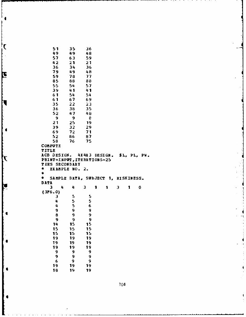
4
: 51 35 3649 49 4857 63 5942 21 2136 34 3679 49 4859 78 7785 88 8855 54 5739 41 4161 54 5461 67 6935 22 2336 38 3552 47 48
9 9 821 25 1939 32 2969 72 7152 86 8758 76 75
COMPUTETITLEACB DESIGN. 4X43 DESIGN. SL, PL, PW.PRINT=INPUT,ITERATIONS=25TIES SECONDARY* EXAMPLE NO. 2.
SAMPLE DATA, SUBJECT 1, RISKINESS.
DATA3 4 4 3 1 1 3 1 0
(3F6.0)3 5 54 5 54 5 69 9 98 9 99 9 9
14 15 1515 15 1515 15 1519 19 1919 19 1919 19 19
9 9 99 9 96 9 9
19 19 19l 18 19 19
104

Li
19 19 1952 52 5129 29 2929 28 2989 89 8938 39 3939 39 3915 15 1615 14 1514 14 1551 52 5129 29 2929 29 2992 91 9161 51 5246 45 4596 96 9295 94 9459 59 5919 19 1919 19 1919 19 1988 89 8939 39 8939 39 3994 96 9596 93 9459 59 5998 99 9697 98 9698 97 96
COMPUTET ITLEKRUSKALOS SQUARE, MOKANOVA EXAMPLE.PRINT =N POT, ITE RATION S=25TIES SECONDARY* EXAMPLE NO. 3.
SAMPLE DATA, SQOARED SCALE VALUESDATA
2 3 3 1 1 1 1 1 0(3F4.o)
1 4 94 9 169 16 25
COM PU TESTOP
105

mm~ _ _ _T _a G
* 1 0 N a E T R G *
* INSTRUCTIONS FOR USING NONETRG •
* NONMETRG IS A CONJOINT ANALYSIS PROGRAM ** DESIGNED TO USE A YONBETRIC REGRESSION** PROCEDURE FOR OBTAINING AN ADDITIVE CONJOINT ** SCALING OF A SET OF BULTI-ATTRIBUTE STIMULI. •* THE PROGRAM WAS ORIGINALLY WRITTEN BY •* RICHARD f. JOHNSON AND WAS MODIFIED,• EXTENDED, AND ADAPTED FOR USE ON THE AMDAHL ** 470 SYSTEM AT THE OHIO STATE UNIVERSITY BY: ** DR. THOMAS E. NYGREN ** DEPT. OF PSYCHOLOGY ** OHIO STATE UNIVERSITY *
******* **********************************************
• TO CALL THIS PROGRAM FOR THE SOURCE DECK FORK FROM ** THE TAPE CPSCALN, USE THE FOLLOWING JCL CARDS: *
•1) YOUR ID CARD *• 2) // TIME=2, REGION=550K *• 3) /*JOBPARM LINES=10000,DISKIO=200,TAPEIO=200 *
4 1) /*SETUP UNIT--TAPE9,ID=(CPSCAL,XIX,READ) ** 5) // EXEC FORTHCLG,TIRE.GO=2,REGION.GO=550K ** 6) //FORT.SYSIN DD UNIT=3400,VOL=SER=CPSCAL, ** 7) // DISP=(OLDPASS),DSNK=ONMETRG.VER2, ** 8) // LABEL=(6,SL), *• 9) // DCB=(RECFM=FB,LRECL=80,BLKSIZE=1600) ** 10) //GO.SYSIN DD * *
11) INPUT DECK AS DESCRIBED BELOW (CONTROL ANDDATA CARDS GO HERE.) *
12 ) /• 13) // *• *
106

* *
I N P U T DE C K A R R A N G E M E N T* *
CARD(S) A. (JCL CARDS- SEE ABOVE CARDS I THROUGH 10.)
CARD B. PARAMETER CARD. (FORMAT IS 14I4.)
COL. PARAMETER MEANING
1- 4 NF NUMBER OF FACTrCOd{. MAX=S.5- 8 m TOTAL NUMBER OF LEVELS OF ALL FACTORS.
MAX:3b FOR VER2. MAX=24 FOR VERI.
9-12 NBLKS NUMBER OF "ALOCKS OR TRADE-OFF MATRICESPRESENT IN THE DATA. MAX=10 FOR VER2.MAX=6 FOR VERI. THE MAXIMUM NUMBER OFSTIMULI IN EACH BLOCK IS 260 FOR VER2AND IS 150 FOR VERi.
13-16 ITRLIM NUMBER OF ITERATIONS ALLOWED TO REACHOPTIMAL SCALING CRITERION. (THE'DEFAULT VALUE IS 30; MAX=50.)
17-20 ICOT =0, NO WEIGHTING IS DESIRED.=1, WEIGHTING IS DESIRED.
21-24 ITIES =0, IF TIES IN THE DATA ARE TO BE LEFTAS TIES IN THE SCALING SOLUTION.=1, IF TIES APE NOT TO BE FORCED INTHE SCALING SOLUTION. NONMETRG WILLBREAK TIES AS NECESSARY TO IMPROVE THEFIT OF THE SCALING SOLUTION.
25-28 LABEL =0, NO LABELS ARE PROVIDED FORDESCRIBING LEVELS OF FACTORS. FACTORLEVELS WILL BE NUMBERED FROM '1' TO
=1, LABELS ARE PROVIDED BY THE USER.29-32 NPUN =0, DO NOT PUNCH SCALING SOLUTION ON
CARDS.=1, SCALING SOLUTION WILL BE PUNCHED
33-36 NREP NUMBER OF DATA MATrICES(SUBJECTS,REPLICATIONS) TO BE INDEPENDENTLYRESCALED.
37-40 LASTIT =0, USE THE SOLUTION FOR THE ITERATIONWITH THE LOWEST ITHETA' VALUE.=1, USE THE SOLUTION FROM TUE LASTITERATION.
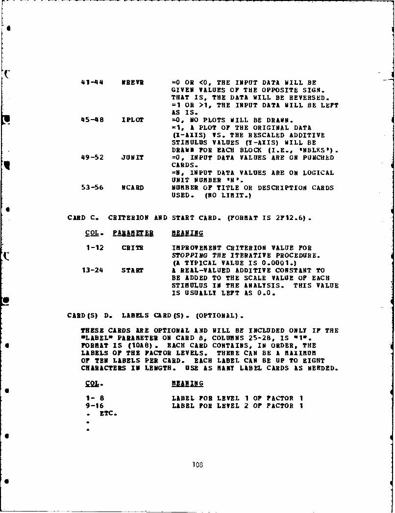
41-44 NREVR =0 OR <0, THE INPUT DATA WILL BEGIVEN VALUES OF THE OPPOSITE SIGN.THAT IS, THE DATA WILL BE REVERSED.=1 OR >1, THE INPUT DATA WILL BE LEFTAS IS.
45-48 IPLOT --0, N PLOTS WILL BE DRAWN.
=1, A PLOT OF THE ORIGINAL DATA(I-AXIS) VS. THE RESCALED ADDITIVESTIMULUS VALUES (Y-AXIS) WILL BEDRAWN FOR EACH BLOCK (I.E., ONBLKSO)
49-52 JUNIT --0, INPUT DATA VALUES ARE ON PUNCHEDCARDS.=N, INPUT DATA VALUES ARE ON LOGICALUNIT NUMBER rNe.
53-56 NCARD NUMBER OF TITLE OR DESCRIPTION CARDSUSED. (NO LIMIT.)
CARD C. CRITERION AND START CARD. (FORMAT IS 2F12.6).
COL. PARAMZ MEANING
1-12 CRITR IMPROVEMENT CRITERION VALUE FORSTOPPING THE ITERATIVE PROCEDURE.(A TYPICAL VALUE IS 0.0001.)
13-24 START A REAL-VALUED ADDITIVE CONSTANT TOBE ADDED TO THE SCALE VALUE OF EACHSTIMULUS IN THE ANALYSIS. THIS VALUEIS USUALLY LEFT AS 0.0.
CARD (S) D. LABELS CARD (S). (OPTIONAL).
THESE CARDS ARE OPTIONAL AND VILL BE INCLUDED ONLY IF THE*LABEL" PARAMETER ON CARD B, COLUMNS 25-28, IS "1".FORMAT IS (10A8). EACH CARD CONTAINS, IN ORDER, THELABELS OF THE FACTOR LEVELS. THERE CAN BE A MAXIMUMOF TEN LABELS PER CARD. EACH LABEL CAN BE UP TO EIGHTCHARACTERS IN LENGTH. USE AS MANY LABEL CARDS AS NEEDED.
£2L.-MANING
1- 8 LABEL FOR LEVEL I OF FACTOR 19-16 LABEL FOE LEVEL 2 0F FACTOR 1. ETC.
108

CARD(S) Z. TITLE CARD(S). (FORMAT IS 20A4).
USE AS MANY CARDS AS ARE SPECIFIED BY THE PARAMETER 9NCARD9ON CARD B, COLUMNS 53-56.
CARD F. STIMULI (OR DATA CELLS) PER BLOCK CARD (FORMAT IS 1614.)
COL. PARAMETER MEANING
1- 4 NV(1) NUMBER OF STIMULI OR DATA CELLS INBLOCK 1.
5- 8 1V(2) NUMBER OF STIMULI OR DATA CELLS INBLOCK 2.
o ETC.
CARD G. LEVELS OF FACTOR CARD. (FORMAT IS 1614).
cQj. PARAMETER MEANING
1- 4 MV(1) NUMBER OF LEVELS OF FACTOR 1.5- 1 MV(2) NUMBER OF LEVELS OF FACTOR 2.* TrC.
CARD H. FORMAT FOR READING IN THS INITIAL RANDOM VECTOR.(FORMAT IS 20A4.)
CARD I. INITIAL RANDOM VECTOR.
CARD I MUST CONTAIN *M VALUES. THESE VALUES ARE USED TOGENERATE THE INITIAL SCALING OF THE DATA AND TO BEGIN THEITERATIVE PROCEDURE.RANDOM START DATA MUST BE REAL-VALUED.
CARD J. FORMAT FOR READING IN THE DATA. (FORMAT IS 20A4.)DATA BUST BE REAL-VALUED NUMBERS.
109

CARD K. DATA MATRICES.
ALL ONREP' DATA MATRICES WILL BE PLACED HERE, ONE BEHINDTHE OTHER. FORMAT RUST CONFORM WITH CARD J. EACH CARDCONTAINS INFORMATION FOR ONE DATA POINT. THERE ARE M.+19VALUES. THE FIRS? A VALUES ARE POS AND 0'S, SIGNIFYINGTHE PRESENCE 0 ABSENCE OF EACH OF THE OKI LEVELS OF THEFACTORS IN DEFINING THE CELL LOCATION OF THE DATA POINT.THE 8*I1"ST VALUE IS THE ACTUAL DATA VALUE.
CARD L. END OF ANALYSIS CARD.
A BLANK CARD TO SIGNIFY THE END OF THE ANALYSIS. IFADDITIONAL ANALYSES ARE INCLUDED, REPEAT CARDS A THROUGHK. THE BLANK CARD IS THE LAST CARD IN THE DECK.
110

9 ON N ET RG. E X A P LE
THE FOLLOWING DATA CARDS ILLUSTRATE THREE DIFFERENT EXAMPLESUSING THE NONMETRG PROGRAM. EXAMPLE I CONSISTS OF ANANALYSIS OF A 4X3X4 COMPLETE DESIGN. EXAMPLE 2 CONSISTSOF A 3X3X3 DESIGN IN WHICH THE DATA WERE OBTAINED FROBTHREE SEPARATE 3X3 TRADE-OFF MATRICES. EXAMPLE 3 USESKRUSKALIS TWO-FACTOR PERFECT SQUARES DATA PRESENTED IN A3X3 DESIGN.
3 11 1 30 0 0 1 0 1 1 1 1 0 150.001000 0.000000
$L=-.10 $L=-.20 SL=-.30 $L=-.40 P1=2/8 P1f=3/8 PV=4/8 PL=1/8 PL=2/8PL=4/8
EXAMPLE NO. 1. NONKETRG.
CONJOINT SCALING: ATTRACTIVENESS DATA.
1 SUBJECT.£8 STIMULI. 1X4X3X4 DESIGN.
FACTORS ARE:AMOUNT TO LOSE, 4 LEVELS. -10, -20, -30, AND -40 CENTS.PROBABILITY OF VINNING, 3 LEVELS. 2/8, 3/8, AND 4/8.PROBABILITY OF LOSING, 4 LEVELS. 1/8, 2/8, 3/8, AND 4/8.
DATA ARE MEAN ATTRACTIVENESS RATINGS FOR THE 48 GAMBLES.SCALE RANGES FROM I19 TO 11001.STIBULI ARE IN THE NATURAL ORDER.
484 3 4
(11F1.0)35687946655(1IZ, 11F 1.0 ,F8.3)
1 1 10001001000 81.3331 2 10001000100 70.0001 3 10001000010 67.0001 4 10001000001 67.6671 5 10000101000 79.6671 6 10000100100 71.0001 7 10000100010 72.3331 8 10000100001 75.0001 9 10000011000 93.000
111

1 1 1 8.333
1 10 10000010100 86.3331 11 10000010010 81.333
1 12 10000010001 74.6671 13 01001001000 60.6671 14 01001000100 69.0001 15 01001000010 37.0001 116 0100 100000 1 24&. 333
1 17 01000101000 79.333 /
1 18 01000100100 61.3331 19 01000100010 61.3331 20 01000100001 48.0001 21 01000011000 86.3331 22 01000010100 74.3331 23 01000010010 68.6671 24 01000010001 66.3331 25 00101001000 70.0001 26 00101000100 51.3331 27 00101000010 31.0001 28 00101000001 24.3331 29 00100101000 82.6671 30 00100100100 58.6671 31 00100100010 47.0001 32 00100100001 29.6671 33 00100011000 80.6671 34 00100010100 76.3331 35 00100010010 64.0001 36 00100010001 52.0001 37 00011001000 67.6671 38 00011000100 37.3331 39 00011000010 29.0001 40 00011000001 25.0001 41 00010101000 83.0001 42 00010100100 61.3331 43 00010100010 33.0001 44 00010100001 38.0001 45 00010011000 77.0001 46 00010010100 66.0001 47 00010010010 57.6671 48 00010010001 32.333
112

3 9 3 20 0 0 1 0 1 1 1 1 0 100.00 1000 0.000000
GAS15-24GAS25-34GAS35-44 LON-DEP NED-DEP HI-DEPSTYLE-FSTYLE-AVSTILE-NDEXABPLE NO. 2. NOMBETRG.
CONJOINT EXAMPLE: CAR ATTRIBUTE UTILITIES. (RANKS)
3 FACTORS.3 LEVELS OF EACH FACTOR.3 BLOCKS. EACH BLOCK IS k 313 RANKING OF 9 COMBINATIONS.9 TOTAL ATTRIBUTE LEVELS TO SCALE.
DATA ARE RANKS.9 9 93 3 3
(9p1.0)9832657541(gFl.0,PF.0)100100000 9.0010100000 8.0001100000 6.0100010000 7.0010010000 4.0001010000 3.0100001000 5.0010001000 2.0001001000 1.0100000100 9.0010000100 6.0001000100 3.0100000010 8.0010000010 5.0001000010 2.0100000001 7.0010000001 4.0001000001 1.0000100100 9.0000010100 6.0000001100 3.0000100010 8.0000010010 5.0000001010 2.0000100001 7.0000010001 4.0000001001 1.0
113

2 6 1 30 0 0 0 0 1 1 1 1 0 40.000100 0.000000
EXAMPLE NO. 3. VOYMETRG.
KRISKALOS KOIAiOVA EXAMPLE.DATA ARE SQUARES Ii A 3 X 3 DESIGN.
93 3
(6P4 .0)3 8 9 4 1 7
(6?1. 0,F6.0)100100 1100010 4100001 9010100 4010010 9010001 16001100 9001010 16001001 25
11
I
II

** 4******* ** ** ** * ,4** ****** *** ** * * **•
* *
* P C J M 2 *
* INSTRUCTIONS FOR USING PCJR2* *
******q*** **.* ~ * *******************$ *******
* *
* THE PROGRAM HAS BEEN MODIFIED AND ADAPTED FOR ** USE ON THE AMDAHL 470 OPERATING SYSTEM AT *
* THE OHIO STATE UNIVERSITY BY: ** DR. THOMAS E. NYGREN *$ DEPT. OF PSYCHOLOGY ** OHIO STATE UNIVERSITY *
** *•*4***.**•****,*********** ***.*.*****•*.*.*
* TO CALL THIS PROGRAM FOR THE SOURCE DECK FORM FROM ** THE TAPE NCPSCAL", USE THE POLLOVING JCL CARDS: *
S1) YOUR ID CARD ** 2) // TIME= 1, REGION=30OK ** 3) /*JOBPARS LINES=10O00,DISKIO=500,TAPEIO=500 ** 4) /*SETUP ONIT=TAPE9,ID=(CPSCALXiXXREAD) *
S5) // EXEC FORTHCLG,TIME.GO=I,REGION.GO=300K *S6) //FORT.SYSIN DD UNIT=3400,VOL=SZR=CPSCAL, •
* 7) / DISP= (OLD,PASS) ,DSN=PCJK, ,* 8) / LABEL=(7,SL), 0* 9) // DCB=(RZCP=FB,LRECL=8O,BLKSIZE=1600) *
* 10) //GO.SYSIN DD * •
* 11) INPUT DECK AS DESCRIBED BELOV (CONTROL AND* DATA CARDS GO HERE.) *
* 12* 12 /* *
* 13*
115

*I N PU T DECK A R R A N GE M E NT
CARD(S) A. (JCL CARDS- SEE ABOVE CARDS I THROUGH 10.)
CARD B. PARAMETER CARD.
COL~. PARMEER EAIN
1- 4 ID AN IDENTIFICATION NUMBER TO IDENTIFYTHE SUBJECTIS DATA SET.
5- 8 D111 NUMBER OF LEVELS OF THL FIRST FACTOR.(MAX = 6.)
4 9-12 DIM2 NUMBER OF LEVELS OF THE SECOND FACTOR.(MAX = 6.)
13-16 DIM3 NUMBER OF LEVELS OF THE THIRD FACTOR.(MAX = 6.)
17-20 PRINT = 0, IF NONE OF THE VIOLATIONS OF THEAXIOMS ARE TO BE LISTED. THAT IS,THE USER HAS THE OPTION OF HAVING THEPROGRAM LIST ALL OR PART OF THESET OF VIOLATIONS OF EACH AXIOM. IF0 IS SPECIFIED, THE VIOLATIONS WILLNOT BE PRINTED.= N, IF IN" VIOLATIONS OF EACH AXIOMS ARETO BE PRINTED. THE USER IS CAUTIONEDTO CHOSE ONLY A MODERATE VALUE OF "N"SINCE AN EXTENSIVE AMOUNT OF PRINTEDLINES COULD RESULT.
21-24 SUBCAL() 0, IF INDEPENDENCE AMONG THE FACTORSIS NOT TO BE TESTED.= 1, IF INDEPENDENCE IS TO BE TESTEDFOR THE ORIGINAL FULL MATRIX ONLY.= 2, IF INDEPENDENCE IS TO BE TESTEDFOR THE ORIGINAL FULL MATRIX AND ANYSPECIFIED SUBMATRIX.
25-28 SOBCAL(2) 0, 1 OR 2 AS FOR SUBCAL(1) ABOVE.SOBCAL(2) IS THE INDICATOR FORDOUBLE CANCELLATION.
29-32 SUBCAL(3) 0 0, 1 OR 2 AS FOR SUBCAL(1) ABOVE.SUBCAL(3) IS THE INDICATOR FORJOINT INDEPENDENCE.
33-36 SDBCAL(4) -0, 1 OR 2 AS FOR SUBCAL(1) ABOVE.SUBCAL(4) IS THE INDICATOR FOR
* DISTRIBUTIVE CANCELLATION.
116

37-40 SOBCAL(S) = 0, 1 OR 2 AS FOR SUBCAL(1) ABOVE.SUBCAL(5) IS THE INDICATOR FORDUAL-DISTRIBUTIVE CANCELLATION.
I41-44 FLAG = 0, IF DATA CONSIST OF ONE OBSERVATIONPER CELL.= 1, IF DATA CONSIST OF THREE OR MOREOBSERVATIONS PER CELL. TWO OBSERVATIONSPER CELL IS NOT PERMITTED.
45-48 ISUB 0, 1, 2, 3, 4 OR 5. NSUB INDICATESTHE NUMBER OF SOBMATRICES TO BEANALYZED. IF NSUB IS SET TO 0, THENONLY THE FULL MATRIX WILL BE ANALYZED.
49-52 INTYP IF EQUAL TO -1, -2 OR -3, IT INDICATESONE DATA POINT PER CELL.
-1, IF DATA ARE IN A RANDOM ORNON-NATURAL ORDER, ONE OBSERVATION PERCARD.= -2, IF THE DATA ARE IN THE NATURALORDER, STRUNG OUT OR ONE PER CARD.= -3, IF DATA ARE IN THE REVERSE NATURALORDER, STRUNG OUT OR ONE PER CARD.IN THE REVERSE NATURAL ORDER, FACTOR 1CHANGES INDICES FASTEST, FOLLOWED BYFACTORS 2 AND 3.IF EQUAL TO 1, 2, 3, 4, 5 OR 6, ITINDICATES MULTIPLE OBSERVATIONS PER CELL.
1, IF DATA ARE IN A RANDOM OR NONNATURAL ORDER, ONE REPLICATION PER CARD.= 2, IF DATA ARE IN THE NATURAL ORDERWITH ONE REPLICATION PER CAkD.= 3, IF DATA ARE IN THE REVERSE NATURALORDER WITH ONE REPLICATION PER CARD.= 4, IF DATA ARE IN A RANDOM OR NONNATURAL ORDER, ALL REPLICATIONS PER CARD.= 5, IF DATA ARE IN THE NATURAL ORDERWITH ALL REPLICATIONS ON A CARD.= 6, IF DATA ARE IN THE REVERSE NATURALORDER WITH ALL REPLICATIONS ON A CARD.IF EQUAL TO 1 OR 4 , THE NUMBER OFREPLICATIONS NEED NOT BE THE SAMEIN EACH CELL. IF EQUAL TO 2, 3, 5OR 6, THE NUMBER OF REPLICATIONS ISASSURED TO BE EQUA. FOR ALL CELLS.
117

53-56 JUNIT = 0, IF INPUT DATA ARE ON PUNCHED CARDS.= N, IF INPUT DATA ARE ON LOGICALOMIT NUMBER "N".
57-60 NCARD NUMBER OF TITLE OR DESCRIPTION CARDSUSED. (NO LIMIT.)
CARD C. OUTSIDE FACTOR CARD. (FORMAT IS 614.)
THESE CARDS APPLY TO TESTS OF DISTRIBUTIVE AND DUAL -
DISTRIBUTIVE CANCELLATION. FOR BOTH OF THESE AXIOMS, ONEFACTOR IS CONSIDERED THE OOTSIDEn FACTOR. FOR EXAMPLE, FORDISTRIBUTIVE CANCELLATION WE COULD HAVE THE MODELS:
(A 4 B) C, WHERE C IS THE OUTSIDE FACTOR;(A + C) B, WHERE B IS THE OUTSIDE FACTOR;(B 4 C) A, WHERE A IS THE OUTSIDE FACTOR.
COL. PAAMTE MEANING
1- 4 INDIC1(1) = 1, IF DISTRIBUTIVE CANCELLATIONWITH FACTOR A AS THE OUTSIDE FACTORIS TO BE TESTED.= 0, IF TEST IS NOT TO BE DONE.
5- 8 INDICt(2) = 1, IF DISTRIBUTIVE CANCELLATIONWITH FACTOR B AS THE OUTSIDE FACTORIS TO BE TESTED.= 0, IF TEST IS NOT TO BE DONE.
9-12 INDICt(3) = 1, IF DISTRIBUTIVE CANCELLATIONWITH FACTOR C AS THE OUTSIDE FACTORIS TO BE TESTED.= 0, IF TEST IS NOT TO BE DONE.
13-16 INDIC2(1) = 1, IF DUAL-DISTRIBUTIVE CANCELLATIONWITH FACTOR A AS THE OUTSIDE FACTORIS TO BE TESTED.= 0, IF TEST IS NOT TO BE DONE.
17-20 INDIC2(2' = 1, IF DUAL-DISTRIBUTIVE CANCELLATIONWITH FACTOR B AS THE OUTSIDE FACTORIS TO BE TESTED.= 0, IF TEST IS NOT TO BE DONE.
21-24 INDIC2(3) = 1, IF DUAL-DISTRIBUTIVE CANCELLATIONWITH FACTOR C AS THE OUTSIDE FACTORIS TO BE TESTED.= 0, IF TEST IS NOT TO BE DONE.
113

CARD D. MISSING DATA INDICATOR. (FORMAT IS F4.0.)
COL. PARAMETER MEANING
1- 4 EMPTY A REAL-VALUED NUMBER INDICATIN NG THECUTOFF FOR DATA TO BE TREATED ASMISSING. ALL OBSERVATIONS EQUAL TO01 LESS THAN "EMPTY" WILL BE IGNORED.
CARD E. FORMAT FOR READING IN THE DATA. (FORMAT IS 20A4.)
CARD(S) F. TITLE CARDS.USE AS MANY CARDS AS SPECIFIED BY THE PARAMETER ONCARD."
CARD(S) G. SOBMATRICES CARDS. (FORMAT IS 614.)
THESE CARDS ARE PRESENT ONLY IF THE PARAMETER nNSUBw ISGREATER THAN ZERO. THERE WILL BE AS MANY CARDS AS INDICATEDBY THE ONSUB" PARAMETER. THE CARDS INDICATE FOR EACHSUBRATRIX TO BE TESTED THE STARTING AND ENDING LEVELS OFFACTORS A, B, AND C.
COL. PARAMETER MEANING
1- 4 STRTA(I) INDICATES THE STARTING LEVEL OFFACTOR A FOR SOBMATRIX I.
5- 8 ENDA(I) INDICATES THE ENDING LEVEL OF FACTORA FOR SUBRATRIX I.
9-12 STRTP(I) INDICATES THE STARTING LEVEL OFFACTOR B FOR SUBMATRIX I.
13-16 ENDP(I) INDICATES THE ENDING LEVEL OF FACTORB FOR SUBMATRIX I.
17-20 STRT0(I) INDICATES THE STARTING LEVEL OF4 FACTOR C FOR SUBMATRIX I.
21-24 ENDU(I) INDICATES THE ENDING LEVEL OF FACTORC FOR SUBMATRIX I.
9
4
119

CARD(S) H. DATA CARDS.THESE CARDS WILL BE DIFFERENT DEPENDING ON THE VALUE OFTHE PARARETER NITYPE".
IF ITYPE = -1, THEN PROCEED AS FOLLOWS:FOR EACH DATA CARD THERE SHOULD BE FOUR NUMBERS ONTHE CARD PUNCHED IN THE FORMAT SPECIFIED ABOVE.A THE LEVEL OF FACTOR A.B THE LEVEL OF FACTOR B.C THE LEVEL OF FACTOR C.ENTRY THE ACTUAL DATA VALUE. A, B, C, AND
ENTRY ARE ASSUMED TO BE INTEGERS.
IF ITYPE = -2, THEN PROCEED AS FOLLOWS:DATA SHOULD BE STRUNG OUT IN NATURAL ORDER. DATACAN BE ONE OBSERVATION PER CARD OR MULTI OBSERVATIONSPER CARD.
IF ITYPE = -3, THEN PROCEED AS FOLLOWS:DATA SHOULD BE STRUNG OUT IN REVERSE NATURAL ORDER.
IF ITYPE = 1, PROCEED AS WITH ITYPE = -1. THERE SHOULDBE ONE CARD FOR EACH REPLICATION OF EACH OBSERVATION.THE LAST DATA CARD SHOULD HAVE A = 999.
IF ITYPE = 2, THEN PROCEED AS FOLLOWS:CARD H1. THE DATA CARDS SHOULD BE PRECEDED BY A
CARD THAT HAS THE NUMBER OF REPLICATIONSFOR EACH OBSERVATION PUNCHED IN COLUMNSI - 4.
THE DATA CARDS SHOULD HAVE ONE REPLICATION OF EACHOBSERVATION PUNCHED ON THEM.
IF ITYPE = 3, PROCEED AS WITH ITYPE = 2. THE DATA AREASSURED TO BE IN THE REVERSE NATURAL ORDER.
IF ITYPE = 4, THEN PROCEED AS FOLLOWS:EACH DATA CARD SBOULD HAVE THE FOLLOWING ENTRIESPUNCHED ON THEN:A LEVEL OF FACTOR A.B LEVEL OF FACTOR B.
0 C LEVEL OF FACTOR C.NE NUMBER OF REPLICATIONS OF THIS OBSERVATION.ENTR(i) - "NE* ACTUAL DATA VALUES.ENTR(NE)ENTR(NE) A, B, C, NE, AND ENTR ARE ASSURED TO
BE INTEGERS.
1200!

IF ITYPE - 5, THEN PROCEED AS WHEN ITYPE 2, EXCEPT THATALL REPLICATIONS OF EACH OBSERVATION ARE ON THESAME CARD. DATA ARE ASSURED TO BE IN THE NATURALORDER.
IF ITYPE = 6, THEN PROCEED AS WHEN ITYPE = 2, EXCEPT THATALL REPLICATIONS OF BACH OBSERVATION ARE ON THESANE CARD. DATA ARE ASSURED TO BE IN THE REVERSENATURAL ORDER.
CARD I. END OF DATA DECK CARD.A BLANK CARD IS INSERTED TO INDICATE THE END OF ALL ANALYSES.IF ADDITIONAL ANALYSES ARE TO BE DONE BEGIN AGAIN WITHCARD B.
121

4
PCJK2 . EX AfPLE
1 4 4 3 10 1 1 1 1 1 1 0 5 0 51 1 1 10
(376.0)EXAMPLE 1O. 1.PCJH ANALYSIS OF ATTRACTIVENESS RATINGS.THREE REPLICATIONS OF EACH JODGMENT.4 X 4 X 3 DESIGN, REARRANGED. A X C I B.TEST ALL AXIOMS.
358 67 68
a 77 78 7486 94 9156 57 6474 75 7785 89 9154 55 5964 71 7351 86 8879 89 8991 93 9448 69 6756 62 6968 73 7276 87 8681 49 4952 59 6576 78 7738 41 32
* 52 52 5359 64 6977 79 8388 91 9359 59 6151 49 48
* 55 64 6564 72 7651 35 3649 49 4857 63 5942 21 21
6 36 34 36
122

79 49 4859 78 7785 88 8855 54 5739 41 4161 54 5461 67 6935 22 2336 38 3552 47 489 9 8
21 25 1939 32 2969 72 7152 86 8758 76 751 4 4 3 10 1 1 1 1 0 5 0 51 1 1 10
(3F6.0)EXANPLE NO. 2.PCJd ANALYSIS OF RISKINESS RATINGS.THREE REPLICATIONS o EACH JUDGRENT.4X 4 X 3 DESIGN, REARRANGED. A I C X B.TEST ALL AXIOBS.
33 5 54 5 54 5 69 9 98 9 99 9 9
14 15 1515 15 1515 15 1519 19 1919 19 1919 19 19
9 9 99 9 96 9 9
19 19 1918 19 1919 19 1952 52 5129 29 2929 28 29
123

89 89 8938 39 3939 39 3915 15 1615 14 1514 14 1551 52 5129 29 2929 29 2992 91 9161 51 5246 45 4596 96 9295 94 9459 59 5919 19 1919 19 1919 19 1988 89 8939 39 8939 39 3994 96 9596 93 9459 59 5998 99 9697 98 9698 97 96
1 4 Ii 3 10 1 1 1 1 1 0 0 -2 0 51 1 1 1 1 1
0* (F6.0)
EXAMPLE NO. 3.ONE REPLICATION OF EACH JUDGMENT. NATURAL ORDER.PCJM ANALYSIS OF ATTRACTIVENESS RATINGS.
I X 4 X 3 DESIGN, REARRANGED. A X C I B.TEST ALL AXIOMS.
4 587786567485
4 546451799148
124
I

Ii
566876815276385259778859515564514957423679598555396161353652
921396952581 4 4 3 10 1 1 1 1 1 0 0 -2 0 51 1 1 1 1 10
(F6.0)EXIABPLE NO. 4.PCJK ANALYSIS OF RISKINESS RATINGS.ONE REPLICATION OF EACH JBDGRENT. NATURAL ORDER.4 I 4 X 3 DESIGN. REARRANGED. A I C I B.TEST ALL AXIOMS.
125

4
3
9
14
15191919996
191819
4 522929893839151514512929
* 926146969559
4 1919
4
126

19
949659989798
127

REFERENCES
Beals, R., Krantz, D.H., and Tversky, A. Foundations of multi
dimensional scaling. Psychologica1 Review, 1968, 75,
127-142.
Carroll, J.D. Individual differences and multidimensional
scaling. In R. Shepard, A. K. Romney, and S. Nerlove (Eds.),
ltidisensional scaling: Theory and applications in the
Behavioral sciences, Vol. 1. New York: Seminar Press,
1972, Pp. 105-155.
Emery, D.R. DIST: A numerical conjoint measurement program
designed to scale data to a distributive model in three
dimensions. Journal of arketing Resea rc, 1977, _4,413-414.
Emery, D.R. DLDIST: A numerical conjoint measurement program
designed to scale data to a dual-distributive model in three
dimensions. Journal of Barketing Research, 1977, 14,
558-559.
Emery, D.R., and Barron, F. H. Axiomatic and numerical conjoint
measurement: An evaluation of diagnostic efficacy.
!fichometrika, 1979, 44, 195-210.
Green, P.E. and Rao, V. Conjoint measurement for quantifying
judgmental data. Journal of Marketing Research, 1971, 8,
355-363.
128

Green, P.E. and Srinivasan, V. Conjoint analysis in consumer
research: Issues and outlook. Journal of Consumer Research,
1978, 5, 103-123.
Holder, 0. Die axiome der Quantitat und die Lehre woe Bass.
c uber die Lerhandlugen der Konialich Sachsischen
Gesellenschf~j fx Wissenschaften 12 Leipzig, Hatheatisch
Physische Clas, 190 1, 53, 1-64.
Holt, J.O. and Vaflsten, T.S. A userls manual for CONJOINT: A
computer program for evaluating certain conjoint-measurement
axioms. Technical Report No. 42, University of North
Carolina, L. L. Thurstone Psychometric Laboratory, October,
1974.
Johnson, R.N. Pairvise nonmetric multidimensional scaling.
Psyvh2!e.ka, 1973, 38, 11-18.
Krantz, D.H. Conjoint measurement: The Luce-Tukey
axioaatization and some extensions. Jou of Mathematical
e_ ho, 1964, 1, 248-277.
Krantz, D.K. A survey of measurement theory. In G. B. Dantzig
and A. F. Veinott, Jr. (Eds.), athlatics 2t the decision
sjences, f J. Providence: American Nathemtical
Society, Lectures in Applied Mathematics, 1968, 12.
Pp. 314-350.
Krantz, D.H., Luce, R.D., Suppes, P., and Tversky, A. Foundations
o measureent, Vol. 1. New York: Academic Press, 1971.
129

KZrantz, D.I., and Tversky, A. Conjoint measurement analysis of
composition rules in psychology. Psychological Review,
1971, 78, 151-169.
Kruskal, J.B. Rultidimensional scaling by optimizing goodness
of-fit to a nonmetric hypothesis. kPychoetrika, 1964, 29,
1-27.
Kruskal, J.B. Uonmetric multidimensional scaling: A numericalmethod. Psychometri~ka, 1964, 29, 115-129.
Kruskal, J.B. Analysis of factorial experiments by estimating
monotone transformations of the data. Journal of the Royal
Ljtistical S , Series_ , 1965, 27, 251-263.
Luce, R.D. and Tukey, J.V. Simultaneous conjoint measurement: A
new type of fundamental measurement, Journal of Mathematical
kslcholoqy, 1964, 1, 1-27.
lygren, T.E. A theoretical framework for testing the additive
difference model for dissimilarities data: Representing
gambles as multidimensional stimuli. Journal of
lathematical Psychology, 1979, 20, 53-77.
uygren, T.E. Limitiations of additive conjoint scaling
procedures: Detecting additivity when additivity is known to
be violated. Aweid Psycholoqical Measurement, 1980, !,
367-383.
130

Shepard, R.N. The analysis of proximities: Multidimensional
scaling with an unknown distance function, I.
Pychometrika, 1962, 27, 125-140.
Shepard, R.N. The analysis of proximities: Multidimensional
scaling with an unknown distance function, II.
P schometrika, 1962, 27, 219-246.
Srinivasan, V. and Shocker, A.D. Linear programming techniques
for multidimensional analysis of preferences. Psychoeetrika,
1973, 38, 337-369.
Srinivasan, V. and Shocker, A.D. Estimating the weights for
multiple attributes in a composite criterion using pairwise
judgments. Psycholetrika, 1973, 38, 473-493.
Takane, Y., Young, F.W., and deLeeuw, J. An individual
differences additive model: An alternating least squares
method with optimal scaling features. Psychometrika, 1980,45, 183-210°.
Tversky, A. A general theory of polynomial conjoint measurement.
Journal g_ Hathematical Psvck.2g., 1967, !j, 1-20.
Twersky, A. Intransitivity of preferences. Psycholoiical
Review, 1969, Z6k, 31-48.
Ullrich, J.R. and Cummins, D.E. PCJH: A program for conjointmeasurement analysis of polynomial composition rules.
Bhajioral S , 1973, 18, 226-227.
131

Nallsten, T.S. Using conjoint measurement models to investigate
a theory about probabilistic information processing.
Journal of Hathenatical Psychology, 1976, !4, 144-185.
Young, F.W. A model for polynomial conjoint analysis algorithms.
In R. Shepard, A. K. Romney, and S. Nerlove (Eds.), Multi
dimensional scali: Theory and applications in the
behavioral sciences, Vol. 1. New York: Seminar Press,
1972, Pp. 69-104.
132*U.S.Government Printing Office: 1982 - 559-007/6041

FIM D
lm8