aim national aquatic monitoring framework: field protocol
TRANSCRIPT
AIM National Aquatic Monitoring Framework:Field Protocol for Wadeable Lotic SystemsTechnical Reference 1735-2, Version 2
February 2021

Production services were provided by the BLM National Operations Center’s Information and Publishing Services Section in Denver, Colorado.
Suggested citation:Bureau of Land Management. 2021. AIM National Aquatic Monitoring
Framework: Field Protocol for Wadeable Lotic Systems. Tech Ref 1735-2, Version 2. U.S. Department of the Interior, Bureau of Land Management, National Operations Center, Denver, CO.
BLM/OC/ST-17/002+1735+REV21
AIM NATIONAL AQUATIC MONITORING FRAMEWORK • Technical Reference 1735-2FIELD PROTOCOL FOR W
ADEABLE LOTIC SYSTEMS – FEBRUARY 2021
i
AIM National Aquatic Monitoring Framework: Field Protocol for Wadeable Lotic Systems
Technical Reference 1735-2, Version 2
February 2021
Compiled by:
Scott W. Miller – BLM Lotic AIM Lead, National Operations Center, Denver, Colorado; and Co-Director, BLM/Utah State University (USU) National Aquatic Monitoring Center, Logan, Utah
Colin Brady – BLM Fisheries Biologist, Alaska State Office, Anchorage, Alaska
Nicole Cappuccio – BLM Aquatic Analyst, National Operations Center, Denver, Colorado
Jennifer Courtwright – USU Aquatic Ecologist, BLM/Utah State University National Aquatic Monitoring Center, Logan, Utah
Technical guidance provided by:
Bryce Bohn – BLM Aquatic Habitat Management Program Lead, Idaho State Office, Boise, Idaho (now retired)
Dan Dammann – BLM Hydrologist, Swiftwater Field Office, Roseburg, Oregon
Melissa Dickard – BLM AIM Section Chief, National Operations Center, Denver, Colorado
Mark Gonzalez – BLM Riparian/Wetland Ecologist and Soil Scientist, National Riparian Service Team, National Operations Center, Denver, Colorado
Justin Jimenez – BLM Riparian and Fisheries Lead for the Aquatic Habitat Management Program, Utah State Office, Salt Lake City, Utah
Ed Rumbold – BLM Water Lead for the Aquatic Habitat Management Program, Colorado State Office, Lakewood, Colorado
Steve Smith – BLM Riparian Ecologist, National Riparian Service Team Leader, National Operations Center, Denver, Colorado
Gordon Toevs – BLM Division Chief for Resource Services, National Operations Center, Denver, Colorado
Matthew Varner – BLM Riparian and Fisheries Lead for the Aquatic Habitat Management Program, Alaska State Office, Anchorage, Alaska

AIM NATIONAL AQUATIC MONITORING FRAMEWORK • Technical Reference 1735-2FI
ELD
PROT
OCOL
FOR
WAD
EABL
E LOT
IC SY
STEM
S – FE
BRUA
RY 2
021
ii
Acknowledgments
The compilation and completion of this protocol would not have been possible without the technical assistance of the Bureau of Land Management’s (BLM’s) partners—in particular, the U.S. Forest Service’s PACFISH/INFISH Biological Opinion and Aquatic and Riparian Effectiveness Monitoring Programs and the Environmental Protection Agency’s National Aquatic Resource Surveys. The developers of these protocols offered sage methodological advice based on their many years of experience and were very generous with their time. We are also grateful to the numerous National Aquatic Monitoring Center and BLM staff that field tested and contributed to the refinement of the protocol. Lastly, Tammie Adams and Janine Koselak at the National Operations Center did their best work with technical editing and layout. Many thanks to all for making this possible.

AIM NATIONAL AQUATIC MONITORING FRAMEWORK • Technical Reference 1735-2FIELD PROTOCOL FOR W
ADEABLE LOTIC SYSTEMS – FEBRUARY 2021
iii
Table of Contents
1. Introduction . . . . . . . . . . . . . . . . . . . . . . . . . . . . . . . . . . . . . . . . . . . . . . . . . . . . . . . . . . . . 1 1.1 Reach Selection and Method Precision . . . . . . . . . . . . . . . . . . . . . . . . . . . . . . 5 1.2 Timing of Field Data Collection. . . . . . . . . . . . . . . . . . . . . . . . . . . . . . . . . . . . . . 7
2. How to Use This Protocol . . . . . . . . . . . . . . . . . . . . . . . . . . . . . . . . . . . . . . . . . . . . . . . . 8 2.1 Protocol Overview. . . . . . . . . . . . . . . . . . . . . . . . . . . . . . . . . . . . . . . . . . . . . . . . . . 8 2.2 Critical Concepts . . . . . . . . . . . . . . . . . . . . . . . . . . . . . . . . . . . . . . . . . . . . . . . . . . . 9 2.2.1 Identifying Bankfull . . . . . . . . . . . . . . . . . . . . . . . . . . . . . . . . . . . . . . . . . . . . 9 2.2.2 Identifying Benches . . . . . . . . . . . . . . . . . . . . . . . . . . . . . . . . . . . . . . . . . . 11 2.2.3 Identifying Scour Line . . . . . . . . . . . . . . . . . . . . . . . . . . . . . . . . . . . . . . . . 12 2.2.4 Identifying Thalweg . . . . . . . . . . . . . . . . . . . . . . . . . . . . . . . . . . . . . . . . . . 13 2.2.5 Identifying Where Bed-Meets-Bank. . . . . . . . . . . . . . . . . . . . . . . . . . . . 13 2.3 Equipment . . . . . . . . . . . . . . . . . . . . . . . . . . . . . . . . . . . . . . . . . . . . . . . . . . . . . . . . 14
3. Office and Field Evaluation . . . . . . . . . . . . . . . . . . . . . . . . . . . . . . . . . . . . . . . . . . . . . 15 3.1 Office Evaluation . . . . . . . . . . . . . . . . . . . . . . . . . . . . . . . . . . . . . . . . . . . . . . . . . . 15 3.2 Field Evaluation . . . . . . . . . . . . . . . . . . . . . . . . . . . . . . . . . . . . . . . . . . . . . . . . . . . 16 3.2.1 Locating Targeted, Probabilistic, and Revisit Point Coordinates . 17 3.2.2 Field Evaluation Status . . . . . . . . . . . . . . . . . . . . . . . . . . . . . . . . . . . . . . . 20 3.2.3 Documentation of Reaches that were Not Sampled. . . . . . . . . . . . 24
4. Reach Setup and Monumenting . . . . . . . . . . . . . . . . . . . . . . . . . . . . . . . . . . . . . . . . 25 4.1 Setting Up the Reach . . . . . . . . . . . . . . . . . . . . . . . . . . . . . . . . . . . . . . . . . . . . . . 25 4.2 Monumenting or Relocating Sample Reaches . . . . . . . . . . . . . . . . . . . . . . 26 4.2.1 Methods for Monumenting New Reaches . . . . . . . . . . . . . . . . . . . . . 27 4.2.2 Methods for Relocating Established Monuments . . . . . . . . . . . . . . 28
5. Water Quality . . . . . . . . . . . . . . . . . . . . . . . . . . . . . . . . . . . . . . . . . . . . . . . . . . . . . . . . . . 31 5.1 pH, Specific Conductance, and Temperature (core). . . . . . . . . . . . . . . . . . 31 5.2 Total Nitrogen and Phosphorus (contingent) . . . . . . . . . . . . . . . . . . . . . . . 32 5.3 Turbidity (contingent) . . . . . . . . . . . . . . . . . . . . . . . . . . . . . . . . . . . . . . . . . . . . . 33 5.4 Continuous Temperature Monitoring (contingent) . . . . . . . . . . . . . . . . . . 35
6. Benthic Macroinvertebrates (core) . . . . . . . . . . . . . . . . . . . . . . . . . . . . . . . . . . . . . . 37 6.1 Targeted-Riffle. . . . . . . . . . . . . . . . . . . . . . . . . . . . . . . . . . . . . . . . . . . . . . . . . . . . . 37 6.2 Reachwide . . . . . . . . . . . . . . . . . . . . . . . . . . . . . . . . . . . . . . . . . . . . . . . . . . . . . . . . 38 6.3 General Methods . . . . . . . . . . . . . . . . . . . . . . . . . . . . . . . . . . . . . . . . . . . . . . . . . . 39 6.4 Sample Preservation. . . . . . . . . . . . . . . . . . . . . . . . . . . . . . . . . . . . . . . . . . . . . . . 41
7. Physical Habitat and Canopy Cover . . . . . . . . . . . . . . . . . . . . . . . . . . . . . . . . . . . . . 42 7.1 Channel Widths . . . . . . . . . . . . . . . . . . . . . . . . . . . . . . . . . . . . . . . . . . . . . . . . . . . 42 7.1.1 Wetted Width. . . . . . . . . . . . . . . . . . . . . . . . . . . . . . . . . . . . . . . . . . . . . . . . . 42 7.1.2 Bankfull Width. . . . . . . . . . . . . . . . . . . . . . . . . . . . . . . . . . . . . . . . . . . . . . . . 43
AIM NATIONAL AQUATIC MONITORING FRAMEWORK • Technical Reference 1735-2FI
ELD
PROT
OCOL
FOR
WAD
EABL
E LOT
IC SY
STEM
S – FE
BRUA
RY 2
021
iv
7.2 Floodplain Connectivity . . . . . . . . . . . . . . . . . . . . . . . . . . . . . . . . . . . . . . . . . . . 43 7.2.1 Bankfull Height . . . . . . . . . . . . . . . . . . . . . . . . . . . . . . . . . . . . . . . . . . . . . . . 43 7.2.2 Bench Height . . . . . . . . . . . . . . . . . . . . . . . . . . . . . . . . . . . . . . . . . . . . . . . . . . . . 45 7.3 Bank Stability and Cover (core) . . . . . . . . . . . . . . . . . . . . . . . . . . . . . . . . . . . . . 52 7.3.1 Locating the Plot and Characterizing Streambank Type . . . . . . . . 52 7.3.2 Assessing Bank Cover . . . . . . . . . . . . . . . . . . . . . . . . . . . . . . . . . . . . . . . . . 54 7.3.3 Assessing Bank Stability . . . . . . . . . . . . . . . . . . . . . . . . . . . . . . . . . . . . . . 55 7.4 Canopy Cover (core) . . . . . . . . . . . . . . . . . . . . . . . . . . . . . . . . . . . . . . . . . . . . . . . 59 7.5 Streambed Particle Sizes (core). . . . . . . . . . . . . . . . . . . . . . . . . . . . . . . . . . . . . 60 7.6 Large Wood (core) . . . . . . . . . . . . . . . . . . . . . . . . . . . . . . . . . . . . . . . . . . . . . . . . . 62 7.7 Pool Dimensions (core) . . . . . . . . . . . . . . . . . . . . . . . . . . . . . . . . . . . . . . . . . . . . 64 7.8 Pool Tail Fines (contingent) . . . . . . . . . . . . . . . . . . . . . . . . . . . . . . . . . . . . . . . . 69 7.9 Flood-Prone Width (covariate) . . . . . . . . . . . . . . . . . . . . . . . . . . . . . . . . . . . . . 73 7.10 Slope (covariate) . . . . . . . . . . . . . . . . . . . . . . . . . . . . . . . . . . . . . . . . . . . . . . . . . 76 7.10.1 Stadia Rod and Auto Level . . . . . . . . . . . . . . . . . . . . . . . . . . . . . . . . . . . 76 7.10.2 Alternative Slope Methods . . . . . . . . . . . . . . . . . . . . . . . . . . . . . . . . . . 79 7.11 Bank Angle (contingent). . . . . . . . . . . . . . . . . . . . . . . . . . . . . . . . . . . . . . . . . . 81 7.11.1 Determining the Location to Measure Bank Angle . . . . . . . . . . . . 82 7.11.2 Determining which Angle(s) to Measure . . . . . . . . . . . . . . . . . . . . . 85 7.12 Thalweg Depth Profile (contingent) . . . . . . . . . . . . . . . . . . . . . . . . . . . . . . . 86
8. Riparian Vegetation . . . . . . . . . . . . . . . . . . . . . . . . . . . . . . . . . . . . . . . . . . . . . . . . . . . . 88 8.1 Priority Noxious (core) and Priority Native Woody Riparian (contingent) Vegetation. . . . . . . . . . . . . . . . . . . . . . . . . . . . . . . . . . . . . . . . . . . . 88 8.2 Greenline Vegetation Composition (contingent) . . . . . . . . . . . . . . . . . . . . 90
9. Human Influence (covariate) . . . . . . . . . . . . . . . . . . . . . . . . . . . . . . . . . . . . . . . . . . . . 91
10. Photos (covariate). . . . . . . . . . . . . . . . . . . . . . . . . . . . . . . . . . . . . . . . . . . . . . . . . . . . . 93 10.1 General Photo Methods . . . . . . . . . . . . . . . . . . . . . . . . . . . . . . . . . . . . . . . . . . 94 10.2 Reach Overview Photo Methods . . . . . . . . . . . . . . . . . . . . . . . . . . . . . . . . . . 95 10.3 Monument Photo Methods . . . . . . . . . . . . . . . . . . . . . . . . . . . . . . . . . . . . . . . 95 10.4 Critical Concept Photo Methods . . . . . . . . . . . . . . . . . . . . . . . . . . . . . . . . . . 96 10.5 Bank Stability and Cover Photo Methods . . . . . . . . . . . . . . . . . . . . . . . . . . 97 10.6 Flood-Prone Width Photo Methods . . . . . . . . . . . . . . . . . . . . . . . . . . . . . . . 98
11. Gear Decontamination . . . . . . . . . . . . . . . . . . . . . . . . . . . . . . . . . . . . . . . . . . . . . . . . 99 11.1 Safety Precautions. . . . . . . . . . . . . . . . . . . . . . . . . . . . . . . . . . . . . . . . . . . . . . .100

AIM NATIONAL AQUATIC MONITORING FRAMEWORK • Technical Reference 1735-2FIELD PROTOCOL FOR W
ADEABLE LOTIC SYSTEMS – FEBRUARY 2021
v
Appendix A: Protocol Compatibility . . . . . . . . . . . . . . . . . . . . . . . . . . . . . . . . . . . . . .101
Appendix B: Glossary . . . . . . . . . . . . . . . . . . . . . . . . . . . . . . . . . . . . . . . . . . . . . . . . . . . .105
Appendix C: Special Situations . . . . . . . . . . . . . . . . . . . . . . . . . . . . . . . . . . . . . . . . . . .109 C1. Interrupted Flow . . . . . . . . . . . . . . . . . . . . . . . . . . . . . . . . . . . . . . . . . . . . . . . . .109 C2. Side Channels . . . . . . . . . . . . . . . . . . . . . . . . . . . . . . . . . . . . . . . . . . . . . . . . . . . .111 C3. Beaver-Impacted Reaches . . . . . . . . . . . . . . . . . . . . . . . . . . . . . . . . . . . . . . . .113 C4. Braided Systems. . . . . . . . . . . . . . . . . . . . . . . . . . . . . . . . . . . . . . . . . . . . . . . . . .115 C5. Partial Data Collection . . . . . . . . . . . . . . . . . . . . . . . . . . . . . . . . . . . . . . . . . . . .116
Appendix D: Bankfull, Bench, and Scour Line Photos . . . . . . . . . . . . . . . . . . . . . .119
Appendix E: Gear List . . . . . . . . . . . . . . . . . . . . . . . . . . . . . . . . . . . . . . . . . . . . . . . . . . . .124
Appendix F: Suggested Workflow . . . . . . . . . . . . . . . . . . . . . . . . . . . . . . . . . . . . . . . .128
Appendix G: Guidance for Integrating MIM Greenline Vegetation Composition and Other Greenline-Based Measurements with the AIM Lotic Protocol . . . . . . . . . . . . . . . . . . . . . . . . . . . . . . . . . . . . . . . . . . . . . . . . . . . . . . .131
Appendix H: Implementation of the AIM Lotic Protocol in Alaska . . . . . . . . . .135 H1. Determining Reach Status . . . . . . . . . . . . . . . . . . . . . . . . . . . . . . . . . . . . . . . .135 H2. Streambed Particle Sizes. . . . . . . . . . . . . . . . . . . . . . . . . . . . . . . . . . . . . . . . . .135 H3. Bank Stability and Cover. . . . . . . . . . . . . . . . . . . . . . . . . . . . . . . . . . . . . . . . . .136 H4. Riparian Vegetation Cover and Complexity and Priority Noxious Vegetation . . . . . . . . . . . . . . . . . . . . . . . . . . . . . . . . . . . . . . . . . . . . . .136
References . . . . . . . . . . . . . . . . . . . . . . . . . . . . . . . . . . . . . . . . . . . . . . . . . . . . . . . . . . . . . .139

AIM NATIONAL AQUATIC MONITORING FRAMEWORK • Technical Reference 1735-2FIELD PROTOCOL FOR W
ADEABLE LOTIC SYSTEMS – FEBRUARY 2021
1
1. Introduction
The Bureau of Land Management (BLM) developed the National Aquatic Monitoring Framework (NAMF) (Miller et al. 2015) to monitor the condition and trend of aquatic systems as part of the Assessment, Inventory, and Monitoring (AIM) Strategy (Toevs et al. 2011). Following the AIM principles, the NAMF standardized field sampling methodologies, electronic data capture, and the use of appropriate sample designs for wadeable streams and rivers (i.e., lotic systems). The protocol in this technical reference outlines standardized core and contingent field methodologies for wadeable lotic systems, as well as suggested covariates.
Following 3 years of implementation of the protocol in this technical reference, application of data and management decisions, and studies on the repeatability of the field methods, Version 2 of the protocol reflects the following updates:
• Omits U.S. Environmental Protection Agency methods for the ocular estimate of instream habitat complexity and riparian vegetative type, cover, and structure for streams in the continental U.S. because of high field measurement variability among crews and low discriminatory efficiency among BLM streams.
• Changes the riparian vegetation core method to focus only on estimates of the frequency of occurrence of priority noxious vegetation based on standardized state species lists.
• Adds a contingent method for assessments of the frequency of occurrence of priority native woody riparian vegetation based on standardized state species lists.
• Updates the bank cover method to ensure foliar and not basal cover is estimated to maintain compatibility with existing protocols.
• Adds pool tail fines as a contingent method.
• Adds guidance for the monumenting of stream reaches.
• Adds Appendix G for integrating multiple indicator monitoring (MIM) procedures with the AIM lotic protocol.
• Adds Appendix H for implementing the AIM lotic protocol in Alaska.
• Clarifies protocol verbiage to ensure accurate implementation and repeatable measurements among data collectors.
Building on the work of the BLM AIM Aquatic Core Indicator Work Group (ACIWG) and guidance from an external science advisory team, the protocol contains 11 core methods, 8 contingent methods, and several covariates

AIM NATIONAL AQUATIC MONITORING FRAMEWORK • Technical Reference 1735-2FI
ELD
PROT
OCOL
FOR
WAD
EABL
E LOT
IC SY
STEM
S – FE
BRUA
RY 2
021
2
applicable to lotic systems (Table 1). The 11 core methods represent a consistent, quantitative approach for determining the attainment of BLM land health standards for perennial wadeable streams and rivers, among other applications (Miller et al. 2015).
AIM lotic core methods are standardized procedures for collecting data that are applicable across many different ecosystems, management objectives, and agencies and are recommended for application wherever the BLM implements monitoring and assessment of streams and rivers. To help determine the potential of a stream reach to support a given condition or to assist in interpreting monitoring data, the ACIWG also identified six lotic covariates—slope, bankfull width, wetted width, human influence, photos, and flood-prone width (Table 1). For example, slope is useful in interpreting pool frequency, large wood retention, and percent fine sediment. Measurement of the field covariates is recommended in conjunction with the core methods.

AIM NATIONAL AQUATIC MONITORING FRAMEWORK • Technical Reference 1735-2FIELD PROTOCOL FOR W
ADEABLE LOTIC SYSTEMS – FEBRUARY 2021
3
Table 1. Core, contingent, and covariate lotic methods for use in wadeable perennial streams. The field methods are grouped by the BLM’s four fundamentals (43 CFR 4180.1).
Fundamentals Methods Core Contingent Covariate
Water quality pH X
Specific conductance X
Temperature (instantaneous and continuous)
X X1
Total nitrogen and phosphorus X
Turbidity X
Watershed function and instream habitat quality (i.e., physical habitat)
Pool dimensions X
Streambed particle sizes X
Bank stability and cover X
Floodplain connectivity X
Large wood X
Bank angle X
Thalweg depth profile X
Pool tail fines X
Bankfull width X
Wetted width X
Slope X
Flood-prone width X
Biodiversity and riparian habitat quality
Benthic macroinvertebrates X
Priority noxious vegetation X
Priority native woody riparian vegetation
X
Canopy cover X
Greenline vegetation composition X
Ecological processes See methods from other fundamentals2 NA NA NA
Other Photos X
Human influence X1 Thermistor deployment for continuous temperature monitoring is the contingent method.
2 Methods used to assess ecological processes are redundant with other methods, such as temperature, total nitrogen and phosphorus, streambed particle sizes, and benthic macroinvertebrates.

AIM NATIONAL AQUATIC MONITORING FRAMEWORK • Technical Reference 1735-2FI
ELD
PROT
OCOL
FOR
WAD
EABL
E LOT
IC SY
STEM
S – FE
BRUA
RY 2
021
4
The ACIWG also identified eight lotic contingent methods (Table 1) that have the same cross-program utility and definition as core methods, but they are measured only where applicable. Contingent methods are not expected to be informative or cost effective for every monitoring application and, thus, are only measured when there is reason to believe the resulting data will be important for management purposes. The use of contingent methods should be considered during the design phase of monitoring project development and be selected to address specific management and monitoring objectives.
The lotic core and contingent methods and covariates are not expected to be inclusive of all BLM lotic data needs, as additional methods may be required (i.e., supplemental methods). Specific methodological recommendations are not made in this technical reference for potential supplemental methods, given the diversity of such methods; however, existing peer-reviewed protocols should be used when possible, as well as the method screening process outlined in BLM Technical Reference 1735-1 (Miller et al. 2015).
Lotic field methodologies were selected by the AIM ACIWG with the goals of maximizing compatibility with existing monitoring programs, accurately and precisely estimating condition and trend, and meeting BLM lotic data needs as specified by BLM policy and plans and state and federal regulations. The field methods described in this protocol were compiled from the following previously established lotic monitoring programs (compatibility of the AIM lotic protocol with each of the following four protocols is presented in Appendix A):
• Multiple Indicator Monitoring (Burton et al. 2011): bank stability and cover (supplemented) and streambed particle sizes (modified from Wolman 1954).
• PACFISH/INFISH Biological Opinion (PIBO) Effectiveness Monitoring Program (Saunders et al. 2019) and Aquatic and Riparian Effectiveness Monitoring Program (USFS 2020): reach setup (Harrelson et al. 1994), targeted-riffle benthic macroinvertebrate collection (Hawkins et al. 2003), large wood (Moore et al. 2002; Hankin and Reeves 1988), bank angle (Platts et al. 1987), bankfull width and height (Harrelson et al. 1994), pool dimensions (Lisle 1987; Lanigan 2010), pool tail fines (Bauer and Burton 1993; USFS 2005), continuous temperature monitoring, slope, and photographs.
• National Rivers and Streams Assessment Protocol (USEPA 2019): reachwide benthic macroinvertebrate collection, canopy cover (Mulvey et al. 1992), bench height, large wood (supplemented), thalweg depth profile, visual estimates of human influences (supplemented), water chemistry (pH, specific conductance, instantaneous temperature, total nitrogen, total phosphorus).
• Surface Water Ambient Monitoring Program (SWAMP 2007): turbidity.

AIM NATIONAL AQUATIC MONITORING FRAMEWORK • Technical Reference 1735-2FIELD PROTOCOL FOR W
ADEABLE LOTIC SYSTEMS – FEBRUARY 2021
5
1.1 Reach Selection and Method Precision
The AIM lotic protocol can be used to assess the condition and trend of an individual stream reach (e.g., designated monitoring area used for a grazing permit renewal) or a population of streams (e.g., random sampling of all BLM-managed wadeable streams within a field office). Monitoring objectives established by project lead will determine the number of reaches to be sampled and whether a randomized, targeted, or mixed point selection approach is appropriate. Point selection and survey design are not covered in this field manual, but practitioners should reference BLM Technical Reference 1735-1 (Miller et al. 2015) and the AIM website (AIM 2021) for guidance on random point selection and BLM Technical Reference 1737-23 (Burton et al. 2011) for guidance on establishing designated monitoring areas if new monitoring locations are being established. In all instances, it is recommended that practitioners work with the national AIM team to optimize point selection procedures with monitoring objectives.
Regardless of whether a monitoring effort is focused on an individual stream reach or a population of streams, it is important to understand the statistical unit of replication. For AIM monitoring and assessment, the unit of replication is the stream reach, and multiple reaches or samples through time are required to derive average estimates and associated confidence intervals. Thus, where this protocol prescribes multiple measurements throughout a reach (Table 2), the intent is to improve the accuracy of values (e.g., average bank stability), and the individual measurements are not intended as statistical replicates. The use of multiple measurements per reach as replicates is subject to pseudoreplication, in which the replicates are not statistically independent unless measurements are sufficiently spaced (Hurlbert 1984). Pseudoreplication can lead to artificially low variance estimates and the detection of differences when they really do not exist (i.e., type I errors), for example. The methods described in this field manual should provide acceptable levels of accuracy for deriving reach-scale condition estimates, as well as population-scale condition estimates, if a sufficient number of independent reaches are sampled.
AIM NATIONAL AQUATIC MONITORING FRAMEWORK • Technical Reference 1735-2FI
ELD
PROT
OCOL
FOR
WAD
EABL
E LOT
IC SY
STEM
S – FE
BRUA
RY 2
021
6
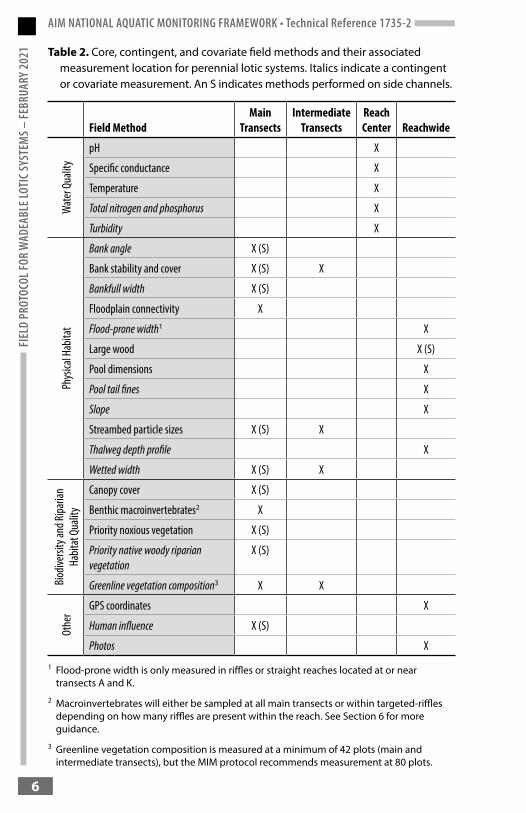
Table 2. Core, contingent, and covariate field methods and their associated measurement location for perennial lotic systems. Italics indicate a contingent or covariate measurement. An S indicates methods performed on side channels.
Field MethodMain
TransectsIntermediate
TransectsReach Center Reachwide
Wat
er Q
ualit
y
pH X
Specific conductance X
Temperature X
Total nitrogen and phosphorus X
Turbidity X
Phys
ical H
abita
t
Bank angle X (S)
Bank stability and cover X (S) X
Bankfull width X (S)
Floodplain connectivity X
Flood-prone width1 X
Large wood X (S)
Pool dimensions X
Pool tail fines X
Slope X
Streambed particle sizes X (S) X
Thalweg depth profile X
Wetted width X (S) X
Biod
iversi
ty an
d Ripa
rian
Habit
at Q
ualit
y
Canopy cover X (S)
Benthic macroinvertebrates2 X
Priority noxious vegetation X (S)
Priority native woody riparian vegetation
X (S)
Greenline vegetation composition3 X X
Othe
r
GPS coordinates X
Human influence X (S)
Photos X
1 Flood-prone width is only measured in riffles or straight reaches located at or near transects A and K.
2 Macroinvertebrates will either be sampled at all main transects or within targeted-riffles depending on how many riffles are present within the reach. See Section 6 for more guidance.
3 Greenline vegetation composition is measured at a minimum of 42 plots (main and intermediate transects), but the MIM protocol recommends measurement at 80 plots.

AIM NATIONAL AQUATIC MONITORING FRAMEWORK • Technical Reference 1735-2FIELD PROTOCOL FOR W
ADEABLE LOTIC SYSTEMS – FEBRUARY 2021
7
If monitoring objectives warrant higher levels of measurement accuracy for an individual sample reach, users should increase the number of measurements for the methods of interest by adding additional plots or taking additional samples within the reach. For example, data collectors might increase the number of bank stability and cover plots beyond 42 to be compatible with the multiple indicator monitoring protocol or increase the number of water quality samples taken through time to meet state water quality collection criteria (see MIM guidance in Appendix G). Such changes can be made while still maintaining method compatibility among sampled reaches.
1.2 Timing of Field Data Collection
This protocol seeks to maximize the precision of field measurements by specifying an index period within which data should be collected. With a few exceptions, all data collection should occur between June 1 and September 30. This time period generally corresponds to baseflow water levels (although exceptions exist), when streams can be safely waded, and when daily variability in chemical, physical, and biological conditions is minimized. Additional consideration should be made to collect data when plants can be accurately identified within the index period. Exceptions can be made where climatic conditions (e.g., monsoonal rains in the desert southwest) preclude sampling during this time period.
Some factors, such as rain or snow events, irrigation return flows, or dam release patterns, can cause discharge to be elevated for short durations during the index period. Field data collectors should consult local discharge gages, weather stations, and field offices to determine how recently such an event occurred and if evidence of dramatic flooding exists, for example. Following high flow events, consider whether data should be collected or whether the reach should be revisited at a later date. For example:
• Sampling should be delayed for approximately 1 month after bed mobilizing flows. Of concern are atypical physical habitat, macroinvertebrate, and water quality samples.
• Sampling should be delayed until discharge recedes to baseflow water levels and turbidity levels return to baseline conditions after significant rain events. Of concern are atypical water quality samples.
• If reaches are particularly difficult to access and field data collectors have made the effort to travel to a reach, it is suggested to collect all data as long as discharge is below bankfull. Field data collectors should record the observed hydrologic condition. Lastly, if anomalous field measurements are observed, efforts should be made to resample such methods at a later date.
AIM NATIONAL AQUATIC MONITORING FRAMEWORK • Technical Reference 1735-2FI
ELD
PROT
OCOL
FOR
WAD
EABL
E LOT
IC SY
STEM
S – FE
BRUA
RY 2
021
8
2. How to Use This Protocol
Individuals should not implement this protocol without first attending an AIM lotic training. BLM project leads overseeing AIM lotic protocol implementation are encouraged to attend training once every 3 years at a minimum, while field data collectors are required to attend training each year data is collected. It should not be assumed that expertise in ecology, hydrology, or geomorphology is a substitute for training. Training is required to ensure that the methods are followed correctly and consistently, thus maximizing data accuracy and precision. Method calibration is an important part of data quality assurance and quality control (QA/QC) and is incorporated into training to assess the accuracy and precision of field personnel implementing the protocol.
This protocol does not include technical explanations regarding method development or background information on the chemical, physical, and biological processes relevant to lotic systems. Rather, it is assumed that the requisite skills for protocol implementation will be obtained through training. To help facilitate the correct and consistent application of the protocol, Appendix B is a glossary that defines the technical terms used throughout the protocol. Glossary terms are distinguished throughout the protocol with bold and italics.
2.1 Protocol Overview
This protocol contains instructions on how to collect core, contingent, and covariate AIM data for wadeable streams and rivers (Table 1). The protocol is organized in a manner that allows each field method to be taken independently. For projects seeking to estimate the condition and/or trend of an individual or population of stream reaches in relation to the BLM’s land health standards, the intent is for data collection to include all the core methods and covariates. In contrast, a subset of core and contingent methods may be selected and measured for monitoring projects targeting individual reaches (e.g., restoration or reclamation effectiveness) or previously identified stressors (e.g., excessive thermal, sediment, or nutrient loading).
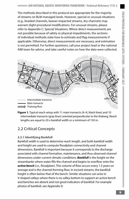
Data are collected along the length of a stream called a reach. Reach lengths are a minimum of 150 m or 20 x bankfull width. Eleven main transects (A-K) and 10 intermediate transects, oriented perpendicular to the thalweg, are established within each sample reach (Figure 1). Most measurements are taken at transects, but a few are taken between transects or at the reachwide scale (Table 2). Detailed descriptions of each method are provided in the respective sections of this protocol.
AIM NATIONAL AQUATIC MONITORING FRAMEWORK • Technical Reference 1735-2FIELD PROTOCOL FOR W
ADEABLE LOTIC SYSTEMS – FEBRUARY 2021
9
The methods described in this protocol are appropriate for the majority of streams on BLM-managed lands. However, special or unusual situations (e.g., braided channels, beaver-impacted streams, dry channels) may warrant slight procedural modifications. For unusual streams, please refer to Appendix C: Special Situations. Where direct measurements are not possible because of safety or physical impediments, the sections of individual methods state how to estimate and flag measurements if applicable. Otherwise, direct measurements are necessary, and estimation is not permitted. For further questions, call your project lead or the national AIM team for advice, and take careful notes on how the data were collected.
Figure 1. Typical reach setup with 11 main transects (A–K; black lines) and 10 intermediate transects (gray lines) oriented perpendicular to the thalweg. Reach lengths are equal to 20 x bankfull width or a minimum of 150 m.
2.2 Critical Concepts
2.2.1 Identifying BankfullBankfull width is used to determine reach length, and both bankfull width and height are used to compute floodplain connectivity and channel dimensions. Bankfull is important because it corresponds to the discharge associated with channel formation, maintenance, and thus observed channel dimensions under current climatic conditions. Bankfull is the height on the streambanks where water fills the channel and begins to overflow onto the active bench (i.e., floodplain). This volume of flow occurs every 1.5 years on average and is the channel-forming flow. In incised streams, the bankfull height is often below that of the bench. Similar situations can arise in V-shaped valleys where there is no valley bottom to support an active bench and benches are absent and not good indicators of bankfull. For example photos of bankfull, see Appendix D.
AIM NATIONAL AQUATIC MONITORING FRAMEWORK • Technical Reference 1735-2FI
ELD
PROT
OCOL
FOR
WAD
EABL
E LOT
IC SY
STEM
S – FE
BRUA
RY 2
021
10
The best location to identify bankfull is in narrow, straight sections of streams (e.g., riffles). Data collectors should exercise caution when identifying bankfull on the outside of meander bends or where large boulders, large wood, or unusual constrictions occur.
To identify bankfull, first look for and identify the following features. Note that not all bankfull features will be present in any one location, but two or more features should always be used to identify bankfull. It may be necessary to wade the entire reach to find consistent bankfull features at relatively similar elevations, especially where special situations occur.
• An active bench adjacent to the streambanks. The active bench will be a flat depositional area (i.e., floodplain) that is commonly vegetated with obligate, facultative wet, or facultative vegetation and above the baseflow water level. Note that some systems do not have the capacity to support active benches or, through channel incision, the bench is no longer actively flooded and has become an inactive bench or terrace.
• Changes in streambank slope. Bankfull will often correspond with the location on the streambank where a change in slope occurs (specifically, where the slope changes from the flat bench to relatively steep streambank sloping toward the stream). The bankfull elevation is the point where water would begin to spill out onto the active bench.
• Changes in streambed particle size distributions. Bankfull elevation is often found above the location where particle sizes change from coarser bed particles to finer particles deposited on the streambanks during high flow events.
• Depositional features such as point bars. Bankfull will typically be above all point bars. The highest elevation of a point bar usually indicates the lowest possible elevation for bankfull stage. Use caution when relying on point bar elevation, as unusually high or low flows can result in point bars above or below, respectively, the actual bankfull elevation.
• Changes in vegetation type. The bankfull elevation typically will be above the stream where woody riparian vegetation transitions from being shrubs to trees or where the vegetation transitions from being grassy and herbaceous to woody. The lowest elevation of cottonwood, birch, and alder can be a useful indication of the bankfull elevation, whereas dogwood and willows are often found both below and above the bankfull elevation.
In the absence of clear indications of bankfull, look for evidence of the previous season’s flooding or secondary indicators, including:• The ceilings of undercut banks in straight sections of the channel, which
are often just below the bankfull elevation. The ceiling of undercut banks is often the scour line, and bankfull is above this elevation.
AIM NATIONAL AQUATIC MONITORING FRAMEWORK • Technical Reference 1735-2FIELD PROTOCOL FOR W
ADEABLE LOTIC SYSTEMS – FEBRUARY 2021
11
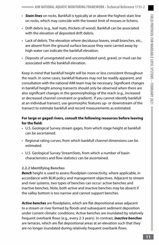
• Stain lines on rocks. Bankfull is typically at or above the highest stain line on rocks, which may coincide with the lowest limit of mosses or lichens.
• Drift debris (e.g., leaf mats, thickets of wood). Bankfull can be associated with the elevation of deposited drift debris.
• Lack of debris. The elevation where deciduous leaves, small branches, etc., are absent from the ground surface because they were carried away by high water can indicate the bankfull elevation.
• Deposits of unvegetated and unconsolidated sand, gravel, or mud can be associated with the bankfull elevation.
Keep in mind that bankfull height will be more or less consistent throughout the reach. In some cases, bankfull features may not be readily apparent, and consultation with the national AIM team may be necessary. Significant changes in bankfull height among transects should only be observed when there are also significant changes in the geomorphology of the reach (e.g., increased or decreased channel constraint or gradient). If you cannot identify bankfull at an individual transect, use geomorphic features up- or downstream of the transect to estimate bankfull and record measurements as estimated.
For large or gaged rivers, consult the following resources before leaving for the field:• U.S. Geological Survey stream gages, from which stage height at bankfull
can be ascertained.
• Regional rating curves, from which bankfull channel dimensions can be estimated.
• U.S. Geological Survey StreamStats, from which a number of basin characteristics and flow statistics can be ascertained.
2.2.2 Identifying BenchesBench height is used to assess floodplain connectivity, where applicable, in accordance with BLM policy and management objectives. Adjacent to stream and river systems, two types of benches can occur: active benches and inactive benches. Note, both active and inactive benches may be absent if the valley bottom is too narrow and cannot support benches.
Active benches are floodplains, which are flat depositional areas adjacent to a stream or river formed by floods and subsequent sediment deposition under current climatic conditions. Active benches are inundated by relatively frequent overbank flows (e.g., every 2-3 years). In contrast, inactive benches are terraces, which are flat depositional areas at an elevation such that they are no longer inundated during relatively frequent overbank flows.
AIM NATIONAL AQUATIC MONITORING FRAMEWORK • Technical Reference 1735-2FI
ELD
PROT
OCOL
FOR
WAD
EABL
E LOT
IC SY
STEM
S – FE
BRUA
RY 2
021
12
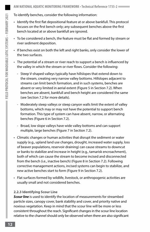
To identify benches, consider the following information:
• Identify the first flat depositional feature at or above bankfull. This protocol focuses on the first bench only; any subsequent benches above the first bench located at or above bankfull are ignored.
• To be considered a bench, the feature must be flat and formed by stream or river sediment deposition.
• If benches exist on both the left and right banks, only consider the lower of the two surfaces.
• The potential of a stream or river reach to support a bench is influenced by the valley in which the stream or river flows. Consider the following:
- Steep V-shaped valleys typically have hillslopes that extend down to the stream, creating very narrow valley bottoms. Hillslopes adjacent to streams can limit bench formation, and in such systems, benches are absent or very limited in aerial extent (Figure 5 in Section 7.2). When benches are absent, bankfull and bench height are considered the same (see Section 7.2 for more details).
- Moderately steep valleys or steep canyon walls limit the extent of valley bottoms, which may or may not have the potential to support bench formation. This type of system can have absent, narrow, or alternating benches (Figure 6 in Section 7.2).
- Broad, low slope valleys have wide valley bottoms and can support multiple, large benches (Figure 7 in Section 7.2).
• Climatic changes or human activities that disrupt the sediment or water supply (e.g., upland land use changes, drought, increased water supply, loss of beaver populations, reservoir draining) can cause streams to downcut or banks to stabilize and increase in height (e.g., tamarisk encroachment), both of which can cause the stream to become incised and disconnected from the bench (i.e., inactive bench) (Figure 8 in Section 7.2). Following corrective management actions, incised systems can begin to stabilize, and new active benches start to form (Figure 9 in Section 7.2).
• Flat surfaces formed by wildlife, livestock, or anthropogenic activities are usually small and not considered benches.
2.2.3 Identifying Scour LineScour line is used to identify the location of measurements for streambed particle sizes, canopy cover, bank stability and cover, and priority native and noxious vegetation. Keep in mind that the scour line will be more or less consistent throughout the reach. Significant changes in the scour line location relative to the channel should only be observed when there are also significant
AIM NATIONAL AQUATIC MONITORING FRAMEWORK • Technical Reference 1735-2FIELD PROTOCOL FOR W
ADEABLE LOTIC SYSTEMS – FEBRUARY 2021
13
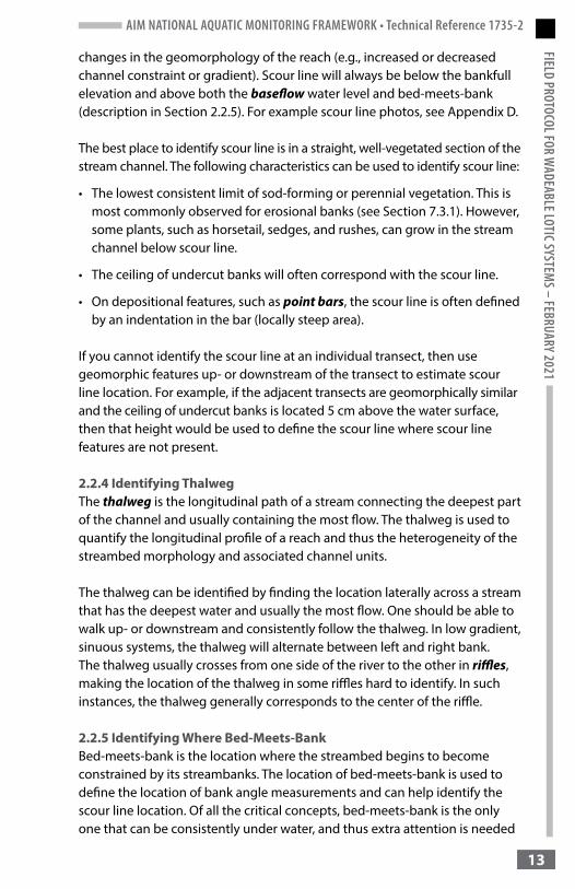
changes in the geomorphology of the reach (e.g., increased or decreased channel constraint or gradient). Scour line will always be below the bankfull elevation and above both the baseflow water level and bed-meets-bank (description in Section 2.2.5). For example scour line photos, see Appendix D.
The best place to identify scour line is in a straight, well-vegetated section of the stream channel. The following characteristics can be used to identify scour line:
• The lowest consistent limit of sod-forming or perennial vegetation. This is most commonly observed for erosional banks (see Section 7.3.1). However, some plants, such as horsetail, sedges, and rushes, can grow in the stream channel below scour line.
• The ceiling of undercut banks will often correspond with the scour line.
• On depositional features, such as point bars, the scour line is often defined by an indentation in the bar (locally steep area).
If you cannot identify the scour line at an individual transect, then use geomorphic features up- or downstream of the transect to estimate scour line location. For example, if the adjacent transects are geomorphically similar and the ceiling of undercut banks is located 5 cm above the water surface, then that height would be used to define the scour line where scour line features are not present.
2.2.4 Identifying ThalwegThe thalweg is the longitudinal path of a stream connecting the deepest part of the channel and usually containing the most flow. The thalweg is used to quantify the longitudinal profile of a reach and thus the heterogeneity of the streambed morphology and associated channel units.
The thalweg can be identified by finding the location laterally across a stream that has the deepest water and usually the most flow. One should be able to walk up- or downstream and consistently follow the thalweg. In low gradient, sinuous systems, the thalweg will alternate between left and right bank. The thalweg usually crosses from one side of the river to the other in riffles, making the location of the thalweg in some riffles hard to identify. In such instances, the thalweg generally corresponds to the center of the riffle.
2.2.5 Identifying Where Bed-Meets-BankBed-meets-bank is the location where the streambed begins to become constrained by its streambanks. The location of bed-meets-bank is used to define the location of bank angle measurements and can help identify the scour line location. Of all the critical concepts, bed-meets-bank is the only one that can be consistently under water, and thus extra attention is needed
AIM NATIONAL AQUATIC MONITORING FRAMEWORK • Technical Reference 1735-2FI
ELD
PROT
OCOL
FOR
WAD
EABL
E LOT
IC SY
STEM
S – FE
BRUA
RY 2
021
14
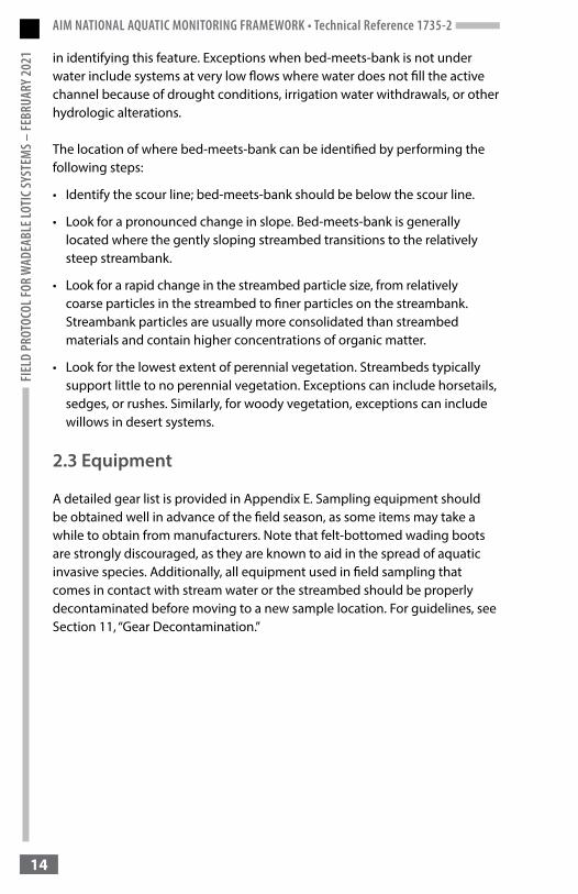
in identifying this feature. Exceptions when bed-meets-bank is not under water include systems at very low flows where water does not fill the active channel because of drought conditions, irrigation water withdrawals, or other hydrologic alterations.
The location of where bed-meets-bank can be identified by performing the following steps:
• Identify the scour line; bed-meets-bank should be below the scour line.
• Look for a pronounced change in slope. Bed-meets-bank is generally located where the gently sloping streambed transitions to the relatively steep streambank.
• Look for a rapid change in the streambed particle size, from relatively coarse particles in the streambed to finer particles on the streambank. Streambank particles are usually more consolidated than streambed materials and contain higher concentrations of organic matter.
• Look for the lowest extent of perennial vegetation. Streambeds typically support little to no perennial vegetation. Exceptions can include horsetails, sedges, or rushes. Similarly, for woody vegetation, exceptions can include willows in desert systems.
2.3 Equipment
A detailed gear list is provided in Appendix E. Sampling equipment should be obtained well in advance of the field season, as some items may take a while to obtain from manufacturers. Note that felt-bottomed wading boots are strongly discouraged, as they are known to aid in the spread of aquatic invasive species. Additionally, all equipment used in field sampling that comes in contact with stream water or the streambed should be properly decontaminated before moving to a new sample location. For guidelines, see Section 11, “Gear Decontamination.”
AIM NATIONAL AQUATIC MONITORING FRAMEWORK • Technical Reference 1735-2FIELD PROTOCOL FOR W
ADEABLE LOTIC SYSTEMS – FEBRUARY 2021
15
3. Office and Field Evaluation
Field data collector success in accessing point coordinates and sampling the stream reach will rely heavily upon predeparture investigation or “office evaluation,” especially for randomly chosen reaches. The value of this preparatory work cannot be overemphasized as it is critical to field data collector efficiency. This section provides an overview of the office and field evaluation processes, but users should reference the BLM’s Lotic Evaluation and Design Management Protocol (BLM 2020) for detailed instructions.
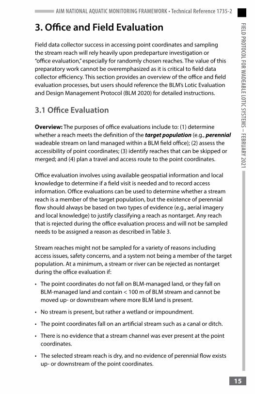
3.1 Office Evaluation
Overview: The purposes of office evaluations include to: (1) determine whether a reach meets the definition of the target population (e.g., perennial wadeable stream on land managed within a BLM field office); (2) assess the accessibility of point coordinates; (3) identify reaches that can be skipped or merged; and (4) plan a travel and access route to the point coordinates.
Office evaluation involves using available geospatial information and local knowledge to determine if a field visit is needed and to record access information. Office evaluations can be used to determine whether a stream reach is a member of the target population, but the existence of perennial flow should always be based on two types of evidence (e.g., aerial imagery and local knowledge) to justify classifying a reach as nontarget. Any reach that is rejected during the office evaluation process and will not be sampled needs to be assigned a reason as described in Table 3.
Stream reaches might not be sampled for a variety of reasons including access issues, safety concerns, and a system not being a member of the target population. At a minimum, a stream or river can be rejected as nontarget during the office evaluation if:
• The point coordinates do not fall on BLM-managed land, or they fall on BLM-managed land and contain < 100 m of BLM stream and cannot be moved up- or downstream where more BLM land is present.
• No stream is present, but rather a wetland or impoundment.
• The point coordinates fall on an artificial stream such as a canal or ditch.
• There is no evidence that a stream channel was ever present at the point coordinates.
• The selected stream reach is dry, and no evidence of perennial flow exists up- or downstream of the point coordinates.

AIM NATIONAL AQUATIC MONITORING FRAMEWORK • Technical Reference 1735-2FI
ELD
PROT
OCOL
FOR
WAD
EABL
E LOT
IC SY
STEM
S – FE
BRUA
RY 2
021
16
In addition, individual projects might make slight alterations to these rejection criteria or have additional criteria such as the point coordinates needing to fall on BLM land located within a specific administrative unit (e.g., allotment, field office, district). All utilized rejection criteria need to be documented for analysis purposes in monitoring design worksheets.
Office evaluations may be conducted by any team member that is closely involved with the field work and, whenever possible, should be completed before the field season starts to allow for adequate time to deal with access or other issues. Office evaluations can include, but are not limited to, reviewing previous evaluation information for each reach, visiting the sample reach in person, reviewing topographic maps and aerial imagery, consulting field office resource specialists, contacting private landowners to obtain access permissions and instructions, and checking water gaging stations for current flow conditions. Careful consideration should be given to identifying the best possible window of time for sampling, which can be influenced by snowpack, elevation and aspect, local precipitation regimes, flow variation associated with dams, and irrigation withdrawals and returns.
All office evaluation and access information should be given to the field data collectors prior to departure. If the person who performed the office evaluation is not going into the field, field data collectors should be given the opportunity to review the information prior to departing for the field in case they have questions.
3.2 Field Evaluation
Overview: Data collectors should navigate to the point coordinates and document how they accessed or attempted to access the point coordinates. If the point coordinates are accessible, determine if the reach can be sampled, and if so, set up the sample reach. If the point coordinates are inaccessible or the reach is unsampleable, classify why the reach was not sampled using one of the categories from Table 3. Use the flow diagram in Figure 2 to help with the decisionmaking process.
Point coordinates can be associated with “revisit” reaches, which are repeatedly sampled through time to detect changes in stream condition. Evaluate revisit reaches the same as all other reaches, except for moving point coordinates, which should only be done to increase the number of transects located on BLM land, or where the original reach spans two or more stream size categories. Revisit point coordinates should not be moved for any other reasons. If the sample reach has already been established, see Section 4.2, “Monumenting or Relocating Sample Reaches,” to locate established monuments.
AIM NATIONAL AQUATIC MONITORING FRAMEWORK • Technical Reference 1735-2FIELD PROTOCOL FOR W
ADEABLE LOTIC SYSTEMS – FEBRUARY 2021
17
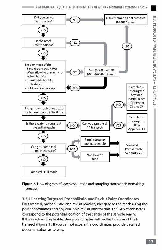
Figure 2. Flow diagram of reach evaluation and sampling status decisionmaking process.
3.2.1 Locating Targeted, Probabilistic, and Revisit Point CoordinatesFor targeted, probabilistic, and revisit reaches, navigate to the reach using the point coordinates and any available revisit information. The GPS coordinates correspond to the potential location of the center of the sample reach. If the reach is sampleable, these coordinates will be the location of the F transect (Figure 1). If you cannot access the coordinates, provide detailed documentation as to why.
AIM NATIONAL AQUATIC MONITORING FRAMEWORK • Technical Reference 1735-2FI
ELD
PROT
OCOL
FOR
WAD
EABL
E LOT
IC SY
STEM
S – FE
BRUA
RY 2
021
18
One of the main differences among targeted, probabilistic, and revisit reaches is that the location of targeted or revisit point coordinates should not be changed without first confirming this is allowable with the person who chose the sample reach location. When assessing potential stream reaches, there are three possible not sampled statuses:
• Reattempt: Access is possible via another route, at another time of year, with additional equipment or guidance, or with private landowner permission.
• Permanently inaccessible: Access to the reach is not possible now nor in the foreseeable future (e.g., 10 years) because of terrain barriers, landowner access, or wadeability issues. This designation should rarely occur for revisit reaches.
• Nontarget: The reach is not in the target population (e.g., point coordinates did not fall on a perennial wadeable stream or river located on lands managed by the BLM). This designation should rarely occur for revisit reaches.
Methods: 1. Navigate as close to the point coordinates as possible. If the provided
coordinates do not fall on a stream (sometimes they are adjacent to the stream because of National Hydrography Dataset mapping differences), navigate to the stream location that is closest to the coordinates (usually within approximately 50 m). Use maps or other resources to ensure that you are on the stream originally selected for sampling.
For revisit reaches, see Section 4.2 for guidance on relocating sample reach monuments.
2. Ensure that you do not cross onto posted private property without obtaining permission, while trying to access the point coordinates.
3. After all efforts have been made to navigate to the point coordinates, record whether you arrived at the point coordinates. Take a GPS coordinate of the location of the point coordinates or the closest location that you were able to access.
a. If you arrived at the point coordinates, continue to Section 3.2.2, “Field Evaluation Status.”
b. If you did not arrive at or within view of the point coordinates, classify the reach as “reattempt” or “permanently inaccessible,” and provide a specific description of the complication (Table 3 and Section 3.2.3). Record notes where applicable (e.g., need to come in from the top of the drainage rather than the bottom).
AIM NATIONAL AQUATIC MONITORING FRAMEWORK • Technical Reference 1735-2FIELD PROTOCOL FOR W
ADEABLE LOTIC SYSTEMS – FEBRUARY 2021
19
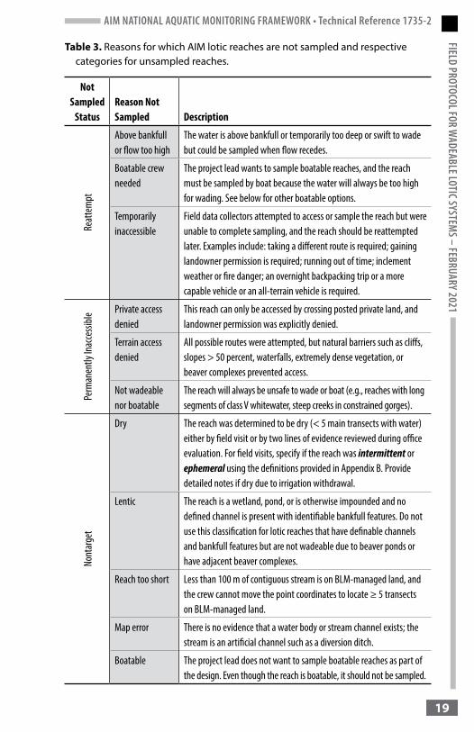
Table 3. Reasons for which AIM lotic reaches are not sampled and respective categories for unsampled reaches.
Not Sampled
StatusReason Not Sampled Description
Reat
tem
pt
Above bankfull or flow too high
The water is above bankfull or temporarily too deep or swift to wade but could be sampled when flow recedes.
Boatable crew needed
The project lead wants to sample boatable reaches, and the reach must be sampled by boat because the water will always be too high for wading. See below for other boatable options.
Temporarily inaccessible
Field data collectors attempted to access or sample the reach but were unable to complete sampling, and the reach should be reattempted later. Examples include: taking a different route is required; gaining landowner permission is required; running out of time; inclement weather or fire danger; an overnight backpacking trip or a more capable vehicle or an all-terrain vehicle is required.
Perm
anen
tly In
acce
ssible
Private access denied
This reach can only be accessed by crossing posted private land, and landowner permission was explicitly denied.
Terrain access denied
All possible routes were attempted, but natural barriers such as cliffs, slopes > 50 percent, waterfalls, extremely dense vegetation, or beaver complexes prevented access.
Not wadeable nor boatable
The reach will always be unsafe to wade or boat (e.g., reaches with long segments of class V whitewater, steep creeks in constrained gorges).
Nont
arge
t
Dry The reach was determined to be dry (< 5 main transects with water) either by field visit or by two lines of evidence reviewed during office evaluation. For field visits, specify if the reach was intermittent or ephemeral using the definitions provided in Appendix B. Provide detailed notes if dry due to irrigation withdrawal.
Lentic The reach is a wetland, pond, or is otherwise impounded and no defined channel is present with identifiable bankfull features. Do not use this classification for lotic reaches that have definable channels and bankfull features but are not wadeable due to beaver ponds or have adjacent beaver complexes.
Reach too short Less than 100 m of contiguous stream is on BLM-managed land, and the crew cannot move the point coordinates to locate ≥ 5 transects on BLM-managed land.
Map error There is no evidence that a water body or stream channel exists; the stream is an artificial channel such as a diversion ditch.
Boatable The project lead does not want to sample boatable reaches as part of the design. Even though the reach is boatable, it should not be sampled.

AIM NATIONAL AQUATIC MONITORING FRAMEWORK • Technical Reference 1735-2FI
ELD
PROT
OCOL
FOR
WAD
EABL
E LOT
IC SY
STEM
S – FE
BRUA
RY 2
021
20
3.2.2 Field Evaluation Status Overview: After locating the point coordinates, determine if the reach is sampleable or if the point coordinates can be moved to increase the number of sampleable transects. Revisit point coordinates can only be moved if the scenarios in steps 4a or 4b occur. See Appendix H for guidance on determining reach status in Alaska.
Methods:1. Measure the bankfull width of the stream to determine approximate
reach length.
a. If bankfull width is ≤ 7.5 m, reach length will be 150 m.
b. If bankfull width is > 7.5 m, reach length will be 20 x bankfull width. The maximum reach length is 4 km, but this will very rarely be encountered for wadeable systems.
2. Use the distance from point coordinates, as displayed on the GPS, to walk the approximate length of the reach. Take note of the approximate location of the 11 main transects, assuming transects are placed at one-tenth of the reach length (i.e., if the reach is 150 m long, transects will be set up every 15 m).
3. While walking the reach, determine if the reach meets the following criteria:
a. You can safely access and wade 5 or more main transects. All efforts should be made to sample transects located in dense vegetation, as long as personal safety is not in question.
b. Five or more main transects have water and are not impounded (i.e., contained in a lake, reservoir, pond, or beaver ponds).
c. A stream channel is present where bankfull can be identified at 5 or more main transects.
d. The current discharge level is below bankfull and is not at or approaching bankfull because of heavy rainfall, snowmelt, or dam releases.
If the reach does not meet each of these four criteria, continue to step 5, and determine if you can move the point coordinates to meet the minimum criteria.
If the reach meets these four criteria, it is sampleable; continue to step 4.
4. In addition to the previous criteria for determining if a reach is sampleable (step 3), assess whether the point coordinates need to be moved because:
a. All 11 main transects do not fall on BLM-managed land. Following the rules in step 5, move the point coordinates to maximize the number of transects sampled on BLM-managed land.
AIM NATIONAL AQUATIC MONITORING FRAMEWORK • Technical Reference 1735-2FIELD PROTOCOL FOR W
ADEABLE LOTIC SYSTEMS – FEBRUARY 2021
21
b. The stream spans two or more stream size categories because of a tributary junction located in the sample reach (e.g., the point coordinates were on a small stream, 7 main transects fell on the small stream, but 4 downstream transects fell on a large stream).
• Sample reaches should never span two stream size categories (e.g., small stream [SS] to a large stream [LS]). The stream size category can be determined from stream order in the National Hydrography Dataset (Strahler 1952). For the majority of AIM designs, first and second order streams are “small streams”; third and fourth order streams are “large streams”; and fifth and above order streams are considered “rivers.” Verify stream size categories with project leads.
• Following the rules in step 5, move the point coordinates to maximize the number of transects falling on a stream of the same size category to avoid sampling tributaries or receiving waters in a different stream size category.
If the reach contains any of these circumstances, continue to step 5, and determine if you can move the point coordinates to maximize the number of transects sampled on BLM-managed land and within the same stream size category.
If all transects fall on BLM-managed land and on the same stream size category, continue to step 6.
5. If the reach does not meet one or more of the criteria listed in steps 3 or 4, determine if you can move the point coordinates up- or downstream. “Moving the point coordinates” means that you will move your sample reach up- or downstream of the original location so that you can sample a stream that was otherwise unsampleable. Point coordinates should only be moved to meet the minimum criteria listed in step 3 and to avoid the situations in step 4; do not move the point coordinates farther than needed.
a. Follow these guidelines to determine how far the point coordinates can be moved:
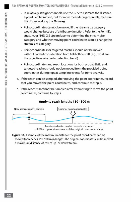
• For reaches 150-500 m in length, the point coordinates can be moved up- or downstream a maximum distance of 250 m from the original point coordinates, following the thalweg (Figure 3A).
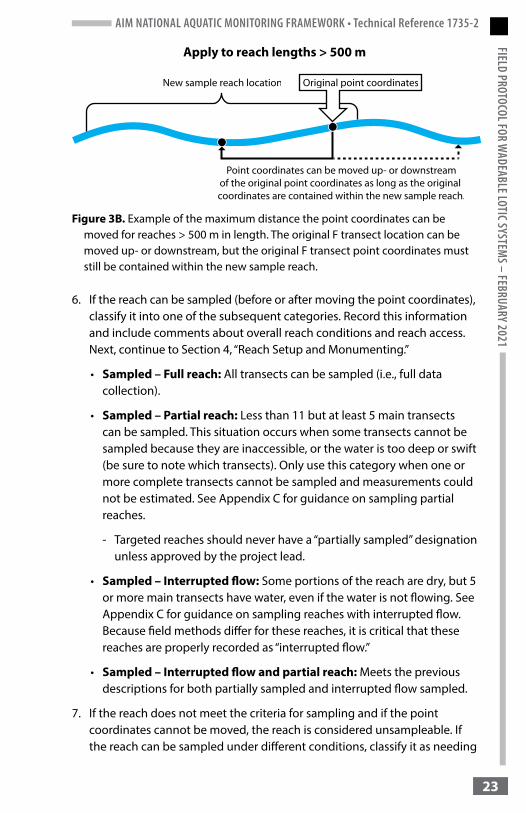
• For reaches > 500 m in length, the point coordinates can be moved up- or downstream, but the original point coordinates must be contained within the new sample reach (Figure 3B).
• When in doubt, contact the project lead to discuss your decision.
AIM NATIONAL AQUATIC MONITORING FRAMEWORK • Technical Reference 1735-2FI
ELD
PROT
OCOL
FOR
WAD
EABL
E LOT
IC SY
STEM
S – FE
BRUA
RY 2
021
22
• In relatively straight channels, use the GPS to estimate the distance a point can be moved, but for more meandering channels, measure the distance along the thalweg.
• Point coordinates cannot be moved if the stream size category would change because of a tributary junction. Refer to the PointID, stratum, or NHD GIS stream layer to determine the stream size category and whether moving point coordinates would change the stream size category.
• Point coordinates for targeted reaches should not be moved without careful consideration from field office staff (e.g., what are the objectives relative to detecting trend).
• Point coordinates and reach locations for both probabilistic and targeted reaches should not be moved from the provided point coordinates during repeat sampling events for trend analysis.
b. If the reach can be sampled after moving the point coordinates, record that you moved the point coordinates, and continue to step 6.
c. If the reach still cannot be sampled after attempting to move the point coordinates, continue to step 7.
Figure 3A. Example of the maximum distance the point coordinates can be moved for reaches 150-500 m in length. The original coordinates can be moved a maximum distance of 250 m up- or downstream.
AIM NATIONAL AQUATIC MONITORING FRAMEWORK • Technical Reference 1735-2FIELD PROTOCOL FOR W
ADEABLE LOTIC SYSTEMS – FEBRUARY 2021
23
Figure 3B. Example of the maximum distance the point coordinates can be moved for reaches > 500 m in length. The original F transect location can be moved up- or downstream, but the original F transect point coordinates must still be contained within the new sample reach.
6. If the reach can be sampled (before or after moving the point coordinates), classify it into one of the subsequent categories. Record this information and include comments about overall reach conditions and reach access. Next, continue to Section 4, “Reach Setup and Monumenting.”
• Sampled – Full reach: All transects can be sampled (i.e., full data collection).
• Sampled – Partial reach: Less than 11 but at least 5 main transects can be sampled. This situation occurs when some transects cannot be sampled because they are inaccessible, or the water is too deep or swift (be sure to note which transects). Only use this category when one or more complete transects cannot be sampled and measurements could not be estimated. See Appendix C for guidance on sampling partial reaches.
- Targeted reaches should never have a “partially sampled” designation unless approved by the project lead.
• Sampled – Interrupted flow: Some portions of the reach are dry, but 5 or more main transects have water, even if the water is not flowing. See Appendix C for guidance on sampling reaches with interrupted flow. Because field methods differ for these reaches, it is critical that these reaches are properly recorded as “interrupted flow.”
• Sampled – Interrupted flow and partial reach: Meets the previous descriptions for both partially sampled and interrupted flow sampled.
7. If the reach does not meet the criteria for sampling and if the point coordinates cannot be moved, the reach is considered unsampleable. If the reach can be sampled under different conditions, classify it as needing
AIM NATIONAL AQUATIC MONITORING FRAMEWORK • Technical Reference 1735-2FI
ELD
PROT
OCOL
FOR
WAD
EABL
E LOT
IC SY
STEM
S – FE
BRUA
RY 2
021
24
to be reattempted. If the reach cannot be sampled because it is nontarget or permanently inaccessible, classify it appropriately and provide a reason as to why you placed it in the chosen category (Table 3). Finally, provide detailed information on all attempts made to access and sample the reach, including directions, GPS coordinates, and photographs.
3.2.3 Documentation of Reaches that were Not Sampled Overview: If you were not able to access the point coordinates and associated reach, or if the reach is not sampled for any reason, provide detailed information on all attempts made to access and sample the reach, including directions, GPS coordinates, and photographs. If the reach could be accessed and sampled at a different time, be sure to note any stipulations that could help ensure the success of a reattempt to the reach.
Methods:1. If you have not already done so, record the GPS coordinates at the point
coordinates or the location closest to the point coordinates that you were able to access.
2. If you reached the point coordinates, take a photo of this location. Additionally, take notes, all other required photos (four possible as described in Section 10), and GPS coordinates of all barriers or complications that prevented sampling or accessing the point coordinates and associated reach (be specific).
3. Record the reason that the reach was not sampled using the categories in Table 3. Make sure to provide the details presented in the “Description” column in Table 3 and not just the category.
4. If you were unable to access the point coordinates, provide detailed route information about how you attempted to access the reach, and if applicable, provide possible alternate route suggestions for future field data collectors.

AIM NATIONAL AQUATIC MONITORING FRAMEWORK • Technical Reference 1735-2FIELD PROTOCOL FOR W
ADEABLE LOTIC SYSTEMS – FEBRUARY 2021
25
4. Reach Setup and Monumenting
4.1 Setting Up the Reach
Overview: After determining that the reach is sampleable and after collecting water quality data (Section 5), use the average of 5 bankfull widths to establish the reach length. Use the reach length to determine the distance between transects, and then set up all transects. This requires at least two people.
If the reach has been sampled in the past or is a new reach that will be revisited in the future for trend determinations, see Section 4.2 for additional guidance, and follow the subsequent steps.
Methods: 1. If you encounter any of the following, reference Appendix C, “Special
Situations,” and then continue to step 2:
a. Interrupted flow (Appendix C1)
b. Side channels (Appendix C2)
c. Beaver activity (Appendix C3)
d. Braided stream morphology (Appendix C4)
2. Work as a team to identify the following geomorphic features:
a. Scour line (Section 2.2.3)
b. Bankfull elevation (Section 2.2.1)
c. Benches (Section 2.2.2)
3. Measure (using a surveyor’s rod, tape measure, or laser range finder) the bankfull width at 5 locations of “typical” width up- or downstream of the F transect. Measurements should be spaced at intervals of one bankfull width or greater.
4. Record the 5 measurements, and compute reach length using the following rules:
• Reach length should be 20 times the average of the 5 bankfull width measurements (unless average bankfull width is ≤ 7.5 m or > 200 m).
• If the average bankfull width is ≤ 7.5 m, use 150 m for the reach length.
• If the average bankfull width is > 200 m, use 4 km for the maximum reach length.

AIM NATIONAL AQUATIC MONITORING FRAMEWORK • Technical Reference 1735-2FI
ELD
PROT
OCOL
FOR
WAD
EABL
E LOT
IC SY
STEM
S – FE
BRUA
RY 2
021
26
• For revisit reaches, see Section 4.2.2 for guidance comparing the computed reach length to the previous reach length(s).
5. Set up the F transect at the point coordinates or in the middle of the reach if the location of the original point coordinates was moved.
6. Identify and establish the location of all other transects.
Main transects will be labeled A–K; transect A = bottom or downstream end of the reach, and transect K = top or upstream end of the reach. Intermediate transects should be labeled as the combined transects (e.g., AB, BC, CD). Make sure you label all flags that will be used to mark both main and intermediate transect locations.
a. Start at the point coordinates (F transect), or if you moved the point coordinates, start at the new point coordinates (F transect).
b. With a tape measure, measure downstream along the thalweg one-twentieth of the reach length to the first intermediate transect (e.g., if the reach length is 150 m, measure 7.5 m to the first intermediate transect). It is important to capture the bends of the thalweg; do not pull the tape taught when following the thalweg.
c. Identify the transect location by placing a labeled pin flag (or hanging flagging if necessary) on each bank. Make sure the transect is set up perpendicular to the thalweg. If your transect falls on a meander bend, always flag the outside of the bend first. Then set up the inside flag perpendicular to the thalweg.
d. Repeat steps 6a.-6c. until you have established 6 main (transects A–F) and 5 intermediate transects downstream of the point coordinates. Label each main and intermediate transect with the corresponding letter(s), and alternate pin flag colors between main and intermediate transects.
e. While at the end of the reach, stand mid-channel and record the point coordinates.
f. Return to the F transect, and repeat steps 6a.-6e., this time moving upstream (transects F–K)
4.2. Monumenting or Relocating Sample Reaches
Overview: For managers seeking to detect changes in stream condition through time (i.e., trend), monumenting helps ensure the same stream reach is sampled during each visit. At a minimum, all sample reaches will be monumented using GPS coordinates, photos, and distinct geographic features. Individual BLM field offices can provide specific guidance as to whether reach markers should be installed as an additional reach monumenting tool.

AIM NATIONAL AQUATIC MONITORING FRAMEWORK • Technical Reference 1735-2FIELD PROTOCOL FOR W
ADEABLE LOTIC SYSTEMS – FEBRUARY 2021
27
4.2.1 Methods for Monumenting New ReachesThe minimum guidance for reach monumenting includes:
1. Take GPS coordinates of the A, F, and K transects. If the reach is only partially sampled, take GPS coordinates of the upper- and lowermost transects.
a. The use of high accuracy (e.g., < 2 m) Bluetooth GPS receivers can greatly improve the accuracy of GPS coordinates taken from an iPad or other device and is strongly recommended.
2. Identify a feature on the landscape that will be used to monument and identify the F transect location (i.e., F transect monument). Whenever possible, use an immovable permanent feature such as a large tree, boulder, fence line, road, etc. If the monumenting feature is located closer to the A or K transect, describe its location in relation to A or K and F (steps 3b and 4e). All systems will not have distinctive landscape features (e.g., sagebrush dominated, willow choked) to utilize as monuments. If this is the case, consider placing a permanent reach marker following BLM field office guidance.
3. Document the following information about the F transect monument:
a. GPS coordinates.
b. Descriptive narrative of the F transect monument, including what it is (e.g., boulder, large tree, fence post), its location in relation to the F transect (as well as the A or K transect, if relevant), and how to approach the F transect from the monument. All monument notes should be placed in the monument photos comment section.
c. Approximate distance from the F transect monument to where the thalweg intersects the F transect.
4. Take the following photos (see guidance in Section 10 for capturing high-quality photos):
a. Stand at the F transect, and photograph the F transect monument feature. If you cannot see the monument feature from the F transect, stand as close to the F transect as possible, while still seeing the feature.
b. Stand at the F transect monument, and photograph the location of the F transect. To help identify the F transect location in the photo, hang flagging at or near the F transect, and ensure the flagging is visible in the photo.
c. Stand so you can capture both the F transect monument feature and F transect in the same photo.
d. Annotate the photos in a., b., and c. to highlight the F transect and the monument feature.
AIM NATIONAL AQUATIC MONITORING FRAMEWORK • Technical Reference 1735-2FI
ELD
PROT
OCOL
FOR
WAD
EABL
E LOT
IC SY
STEM
S – FE
BRUA
RY 2
021
28
e. Annotate an aerial image (e.g., Google Earth image) with the locations of the F transect, F transect monument feature, and any other unique features to assist data collectors in relocating the F transect (see Figure 38 example in Section 10). Also, consider noting the locations of the A and K transects if they can be easily identified on the aerial image.
4.2.2 Methods for Relocating Established Monuments1. Use the previous data collector’s guidance to relocate the F transect
monument and sample reach. This guidance should include, but is not limited to:
a. GPS coordinates
b. Photos and photo descriptions
c. Annotated aerial image(s)
d. Descriptive narrative describing the F transect monument and transect location
2. Navigate to the F transect monument, and locate the F transect (if additional reach markers were installed for the A or K transects, also locate those).
a. If you are unable to locate the F transect after 20 minutes, remonument the reach following the methods for monumenting new reaches in Section 4.2.1.
3. Once an existing F transect is located, use reach photos, bankfull widths, reach length, and/or reach description to set up the reach (Section 4.1).
4. Compute reach length using the 5 bankfull width measurements taken in Section 4.1. Bankfull widths should be taken independently and compared to previous estimates as a check on data quality.
5. Compare the computed reach length to the previous reach length(s).
a. If the computed reach length differs from the previously established reach length by more than the main transect interval (e.g., 15 m for a 150 m reach), ensure you followed all procedures correctly. For example, were the 5 bankfull width measurements taken in a representative section of the reach? Are you confident in the bankfull determinations? Crews should independently make bankfull determinations and not rely on previous critical concept photos or measurements. The goal is to capture current geomorphic conditions. Only after measurements are taken should crews make comparisions to assess possible geomorphic changes or discrepancies with previous measurements.
AIM NATIONAL AQUATIC MONITORING FRAMEWORK • Technical Reference 1735-2FIELD PROTOCOL FOR W
ADEABLE LOTIC SYSTEMS – FEBRUARY 2021
29
• If you are confident the original reach length was computed incorrectly or geomorphic conditions changed significantly since the original sample event (e.g., beaver complex, new or abandoned meander bend), establish a new reach length; provide comments as to the rationale for this decision.
• If the original reach length was classified as “partially sampled” and more transects can now be sampled, the reach length can be extended or additional transects sampled. The goal is to sample as many transects as possible. If the reach length is extended, remonument the A and K reach markers if present.
• If the original reach was classified as “sampled” and now fewer than 11 and ≥ 5 main transects can be sampled, retain the original reach length. Classify the reach as “partially sampled,” and note which transects were sampled.
b. If the computed reach length does not differ by more than the main transect interval, use the newly established reach length, unless the A and K transects are monumented (see step 5c).
c. In locations where BLM field offices monumented the A and K transects in addition to the F transect:
• If the distances between the A and F transects and the F and K transects do not differ by more than two main transect intervals from the computed length, ensure that all transects from A to F and F to K are located within the original reach. Do not place transects outside of the A and K monuments, even if this means using a shorter transect interval.
• If the distances between the A monument and the F transect or the F transect and K monument differ by more than two main transect intervals from your computed length, assess whether the distance has changed because of new meander bends (i.e., longer reach distance) or the abandoning of channel meanders (i.e., shorter reach distance). If such conditions are observed, establish new A and/or K monuments.
6. Are the original GPS coordinates for the A, F, and K transects no longer located on the main channel? If this is observed, determine whether:
a. Differences in coordinate locations result from coordinate accuracy errors. If this is the case, move to the actual stream or river, and take new coordinates. Under such circumstances, no evidence of lateral channel migration would exist.

AIM NATIONAL AQUATIC MONITORING FRAMEWORK • Technical Reference 1735-2FI
ELD
PROT
OCOL
FOR
WAD
EABL
E LOT
IC SY
STEM
S – FE
BRUA
RY 2
021
30
b. Differences in coordinate locations appear to result from lateral river migration. For example, the river has migrated left or right within the valley bottom; the main channel migrated laterally to now be in a previous side channel; or a beaver dam was breached, forming a new channel. Under such circumstances, new A, F, or K coordinates and monuments need to be established following the guidance in Section 4.2.1.

AIM NATIONAL AQUATIC MONITORING FRAMEWORK • Technical Reference 1735-2FIELD PROTOCOL FOR W
ADEABLE LOTIC SYSTEMS – FEBRUARY 2021
31
5. Water Quality
Overview: The core measurements for water quality are pH, specific conductance, and temperature. The contingent measurements are total nitrogen, total phosphorus, continuous temperature, and turbidity (Table 1). Water quality measurements should be taken before any instream work is done and before the reach is set up to minimize disturbance of stream sediments and their influence on water quality measurements. All water quality measurements are taken at the F transect. See Appendix C for where to take water quality measurements in reaches with interrupted flow or beaver impacts. Water quality measurements are always taken, even at reaches with partial data collection.
5.1 pH, Specific Conductance, and Temperature (core)
Water quality sondes used to obtain in-situ water quality measurements must meet the following requirements:
• pH: accuracy of ± 0.2 SU and resolution of 0.1 SU
• Specific conductance: accuracy of ±2 μS/cm or ±10% of the measured value, whichever is greater, and resolution of 0.1 μS/cm
• Temperature: accuracy of ±0.2° C and resolution of 0.1° C
Methods:1. Data collectors should maintain a calibration log documenting when and
how water quality sondes were calibrated (e.g., 3 point pH calibration [4.0, 7.0, 10.0] completed on 8/22/2019).
2. Review the calibration log to ensure the sonde was calibrated for both pH and specific conductance following manufacturer recommendations or within the last 7 days, whichever is shorter.
3. Record the most current calibration date.
4. If the sonde has not been calibrated in the last 7 days or within the manufacturer’s recommended timeframe, the sonde will need to be calibrated following the manufacturer’s directions. Prior to calibration, ensure that calibration standards are not expired.
5. Standing in the thalweg at transect F and in flowing water, if present, lower the probe to a depth of 0.5 m below the water surface, taking care to avoid contacting the stream bottom. If water depth is < 1 m, take measurements at mid-depth.
6. Wait for the readings on the screen to stabilize (this could take up to a few minutes).

AIM NATIONAL AQUATIC MONITORING FRAMEWORK • Technical Reference 1735-2FI
ELD
PROT
OCOL
FOR
WAD
EABL
E LOT
IC SY
STEM
S – FE
BRUA
RY 2
021
32
7. Record the pH, temperature (°C), and specific conductance (μS, not mS). Ensure the sonde is set to take measurements in the appropriate units and that temperature-corrected conductivity (i.e., specific conductance) is being measured. Measurements of pH, temperature, and specific conductance must be taken at the stream reach. It is not acceptable to take these measurements later from a grab sample.
8. Record the model number and serial number of the instrument used so that any issues with the device can be tracked.
9. Note any odd water smells, surface films, or water discoloration observed during sampling.
5.2 Total Nitrogen and Phosphorus (contingent)
Overview: Take a single “grab sample” that will be analyzed for total nitrogen and phosphorus, and stabilize the sample with concentrated sulfuric acid. Freeze the sample once back at the office. Duplicate and blank samples should be collected for 10% of reaches where total nitrogen and phosphorus samples are collected.
Methods:1. Obtain a pair of new nitrile gloves, and place them on both hands, being
careful not to contaminate the outside of the gloves with substances such as sunscreen. Dispose of gloves after use.
2. If collecting a “blank” sample, process the blank first to avoid contaminating your gloves with stream water.
a. To collect a blank sample, rinse a 125 ml HDPE Nalgene bottle five times with deionized water (or distilled water if deionized water is not available), and then fill the bottle halfway with deionized water to allow head space for freezing.
b. Label the blank sample immediately in order to not confuse it with original and duplicate samples (see step 4).
3. Collect and process original and duplicate samples identically.
a. Obtain two new 125 ml HDPE Nalgene bottles.
b. Rinse both bottles five times with stream water. Be careful not to disturb the stream bottom.
c. Fill the bottles halfway with stream water directly from the stream; this will leave head space in the bottles for freezing.
4. Fill out a water quality label with the full PointID, stream name, date, your initials, and the type of sample (original, duplicate, or blank).
AIM NATIONAL AQUATIC MONITORING FRAMEWORK • Technical Reference 1735-2FIELD PROTOCOL FOR W
ADEABLE LOTIC SYSTEMS – FEBRUARY 2021
33
a. Record the day, month, and year, making sure to use letters rather than numerals for the month and to use four digits for the year (e.g., 27Aug2015).
b. Check the appropriate box as to whether the sample is the original, duplicate, or blank.
c. Water quality labels must be on Rite in the Rain paper and filled out with a pencil. Labels that are not Rite in the Rain paper will not withstand wet and frozen environments, while ink from pens will leach and become illegible.
5. Tape the label on the outside of the bottle with clear packing tape, making sure the tape is wrapped completely around the bottle.
6. Stabilize all samples, except for blank samples, with concentrated sulfuric acid.
a. Remove the dropper bottle from a Nalgene storage bottle containing baking soda.
b. Carefully remove the dropper bottle cap, while keeping clear of face. Invert and add 3 drops (0.15 ml) of sulfuric acid to the water quality sample, being careful not to touch the water sample with the dropper bottle tip.
c. Replace the dropper bottle cap and return the dropper to the Nalgene storage bottle.
d. Place the top on the water quality sample and shake vigorously for 5 seconds.
e. SAFETY NOTE: Exercise extreme caution and ensure nitrile gloves and sunglasses or safety goggles are worn at all times when working with acid. If acid comes in contact with the skin, rinse with a mild, soapy solution or rinse continuously with stream water if soapy water is not available. Do not apply baking soda to your skin. If acid comes in contact with the ground, apply generous amounts of baking soda to neutralize the spill and surrounding area. Continue adding baking soda until all acid is neutralized (i.e., cessation of bubbling and gas).
5.3 Turbidity (contingent)
Overview: Measure water clarity, which is directly affected by suspended solids. This protocol was written for use with a LaMotte turbidimeter, but other instruments meeting accuracy and resolution requirements can be used (see manufacturer instructions for other instruments).
AIM NATIONAL AQUATIC MONITORING FRAMEWORK • Technical Reference 1735-2FI
ELD
PROT
OCOL
FOR
WAD
EABL
E LOT
IC SY
STEM
S – FE
BRUA
RY 2
021
34
Turbidity meters must have an accuracy of ±2 NTU or ±10% of the measured value, whichever is greater, and a resolution of 0.1 NTU.
Methods:1. Calibrate the turbidimeter before each reading or following manufacturer
instructions, and record the calibration date in the calibration log.
2. Obtain a 50-ml container, and rinse it five times with stream water.
3. From the thalweg, collect a water sample using the rinsed 50-ml container. Be very careful not to disturb stream bottom sediments prior to or while collecting the water sample.
4. Rinse a glass vial from the LaMotte turbidimeter, specifically the one used in the calibration process, with stream water five times. Once rinsed, fill with stream water.
5. Pour off water from the glass vial such that the meniscus is level with the white line. The meniscus is the concave shape formed by the attraction of water molecules to the container. It is important that the bottom of the meniscus is level with the white line in order to have consistent and accurate turbidity readings.
6. While holding onto the cap only, thoroughly wipe the glass vial with Kimwipes to remove any fingerprints or debris.
7. Place the glass vial in the meter, aligning the vertical white line on the glass vial with the black arrow on the meter.
8. Close the meter, and obtain a measurement using the averaging feature provided in the meter instructions. Make sure you select an averaging option that has three or more readings. If your turbidimeter does not have an averaging option, take the following steps: Remove and invert the vial, while only handling the cap, and obtain a second reading. Repeat this for a third reading. Record all three readings. If any one of the three readings is 30% higher or lower than that of a single reading, it is recommended that you take additional readings of the same water sample until three homogenous readings are obtained.
9. Provide comments if unusual values or stream conditions are observed.
10. Do not store the meter in the sun. When the meter is exposed to heat, it can produce erratic readings.
11. If a glass vial becomes scratched, stop using as it can produce erratic results.

AIM NATIONAL AQUATIC MONITORING FRAMEWORK • Technical Reference 1735-2FIELD PROTOCOL FOR W
ADEABLE LOTIC SYSTEMS – FEBRUARY 2021
35
5.4 Continuous Temperature Monitoring (contingent)
Overview: Thermistors can be easily deployed to obtain a more temporally integrated picture of the thermal regime of a stream reach. A minimum deployment time of June 1 through September 15 is recommended to capture the annual thermal maxima. Many organisms can only survive within a narrow temperature range, and higher temperatures can limit the population viability of certain organisms.
Methods: More detailed protocols regarding thermistor setup and deployment are provided by Isaak et al. 2013 and Dunham et al. 2005.
1. Use the manufacturer’s software to program the thermistor to record at hourly intervals, and if the option exists, set the thermistor to not overwrite data when the memory is full.
2. Ensure the thermistor has been calibrated following manufacturer instructions.
3. Record the thermistor number and the date and time that the thermistor was deployed. Carefully check to ensure the number is correct. Then, check again.
4. Deploy the thermistor, and secure it with a metal cable or other attachment method, such as a piece of rebar and zip ties. When considering where to place the thermistor, think about high and low flows, and place it in a location that will not be affected by strong current or become dry at a later date. Adhere to the following guidance to select an appropriate location, and refer to Isaak et al. 2013 or Dunham et al. 2005 for details on securing thermistors.
• Attach the temperature logger cable to a tree trunk, a root wad, or the bank.
• Pick one of the deepest locations in the channel that you can access, focusing on the thalweg.
• If possible, do not attach the cable to rocks in the stream that are smaller than two times the size of a basketball, as higher flows can dislodge the rock and the probe could be lost. Use a longer cable to reach the bank.
• Use rocks to hold the thermistor in place by placing rocks on the cable and not the probe (if the flow drops, the rocks can absorb heat).
• If in a high traffic area, place the thermistor in a location that will be camouflaged from people. You can use grass, dirt, or moss to cover the wire.

AIM NATIONAL AQUATIC MONITORING FRAMEWORK • Technical Reference 1735-2FI
ELD
PROT
OCOL
FOR
WAD
EABL
E LOT
IC SY
STEM
S – FE
BRUA
RY 2
021
36
• Avoid areas just downstream of tributaries and obvious groundwater seeps, as water temperatures in these areas will not be representative of the stream reach. If there is a steep bank on one side of the stream, try to place the logger near the opposite side such that runoff from the hillside does not influence the temperature readings.
5. Draw a map, take photos, record GPS coordinates, and provide a written description of where you placed the thermistor.
• Note that the better you hide the temperature logger, the better your map and description need to be. When documenting the thermistor’s location, draw the map and write the description relative to the bottom of the reach.
• Record whether the thermistor is on the right or left bank, and use landmarks (e.g., wire attached to roots of enormous ponderosa pine, logger hidden underneath river left undercut bank).
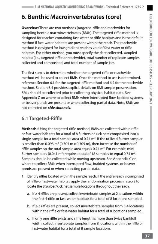
AIM NATIONAL AQUATIC MONITORING FRAMEWORK • Technical Reference 1735-2FIELD PROTOCOL FOR W
ADEABLE LOTIC SYSTEMS – FEBRUARY 2021
37
6. Benthic Macroinvertebrates (core)
Overview: There are two methods (targeted-riffle and reachwide) for sampling benthic macroinvertebrates (BMIs). The targeted-riffle method is designed for reaches containing fast-water or riffle habitats and is the default method if fast-water habitats are present within the reach. The reachwide method is designed for low gradient reaches void of fast-water or riffle habitats. For either method, you must specify the date collected, sampled habitat (i.e., targeted-riffle or reachwide), total number of replicate samples collected and composited, and total number of sample jars.
The first step is to determine whether the targeted-riffle or reachwide method will be used to collect BMIs. Once the method to use is determined, reference Section 6.1 for the targeted-riffle method and 6.2 for the reachwide method. Section 6.4 provides explicit details on BMI sample preservation. BMIs should be collected prior to collecting physical habitat data. See Appendix C on where to collect BMIs when interrupted flow, braided systems, or beaver ponds are present or when collecting partial data. Note, BMIs are not collected on side channels.
6.1 Targeted-Riffle
Methods: Using the targeted-riffle method, BMIs are collected within riffle or fast-water habitats for a total of 8 Surbers or kick nets composited into a single sample for a total sample area of 0.74 m2. If the utilized Surber sampler is smaller than 0.093 m2 (0.305 m x 0.305 m), then increase the number of riffle samples so the total sample area equals 0.74 m2. For example, mini Surber samplers (0.041 m2) require a total of 18 samples to equal 0.74 m2. Samples should be collected while moving upstream. See Appendix C on where to collect BMIs when interrupted flow, braided systems, or beaver ponds are present or when collecting partial data.
1. Identify riffles located within the sample reach. If the entire reach is comprised of riffle or fast-water habitat, apply the randomization process in step 2 to locate the 8 Surber/kick net sample locations throughout the reach.
a. If ≥ 4 riffles are present, collect invertebrate samples at 2 locations within the first 4 riffle or fast-water habitats for a total of 8 locations sampled.
b. If 2-3 riffles are present, collect invertebrate samples from 3-4 locations within the riffle or fast-water habitat for a total of 8 locations sampled.
c. If only one riffle exists and riffle length is more than twice bankfull width, collect invertebrate samples from 8 locations within the riffle or fast-water habitat for a total of 8 sample locations.
AIM NATIONAL AQUATIC MONITORING FRAMEWORK • Technical Reference 1735-2FI
ELD
PROT
OCOL
FOR
WAD
EABL
E LOT
IC SY
STEM
S – FE
BRUA
RY 2
021
38
d. If only one riffle exists and the length of the riffle is less than twice the bankfull width, use the reachwide method.
2. Determine the sample location(s) within each riffle or fast-water habitat by generating pairs of random numbers between 1 and 9, and multiply each number by 10. This can be done by using the last two numbers from the time displayed on a digital face watch.
a. The first number in each pair represents the percent upstream along the riffle’s length.
b. The second number in each pair represents the percent of the stream’s width from river left looking downstream.
c. Select all pairs of numbers for each riffle, and then sort them from smallest to largest based on riffle length to facilitate sampling from downstream to upstream.
d. Using the calculated percentages from steps a. and b., visually estimate where the two intersect for the sampling location.
e. Repeat this process to locate the other sampling locations.
f. Do not collect samples within 15% of the water’s edge, unless the stream is too narrow to accommodate this.
g. If it is not possible to collect BMIs at one of these locations (e.g., log in the way, too deep, cannot seal bottom of net), generate an additional set of random numbers, and sample the new location.
3. Begin at the riffle closest to the bottom of the reach, and collect a total of 8 Surber or kick net samples.
4. Follow the general collection and preservation methods in Sections 6.3 and 6.4.
6.2 Reachwide
Methods: Using the reachwide method, BMIs are collected just downstream from each of the 11 main transects, resulting in the collection of 11 Surbers or kick nets composited into a single sample for a total sample area of 1.023 m2. If the utilized Surber or kick net sampler has an area smaller than 0.093 m2 (0.305 m x 0.305 m), then increase the number of samples so the total sample area equals 1.023 m2. For example, mini Surber samples (0.041 m2) require a total of 25 samples to approximately equal 1.023 m2. Additional samples can be collected at intermediate transects. Samples should be collected while moving upstream. See Appendix C on where to collect BMIs when interrupted flow, braided systems, or beaver ponds are present or when collecting partial data.
AIM NATIONAL AQUATIC MONITORING FRAMEWORK • Technical Reference 1735-2FIELD PROTOCOL FOR W
ADEABLE LOTIC SYSTEMS – FEBRUARY 2021
39
1. Use the last number from the time displayed on a digital face watch to randomly select the starting location at transect A.
• 1 to 3 = Left (15% from the left wetted edge)
• 4 to 6 = Center (50% from the left wetted edge)
• 7 to 9 = Right (15% from the right wetted edge)
2. Sample at the randomly determined starting location.
3. Continue moving upstream, collecting just downstream from each transect. Alternate from left, to center, to right, depending on the randomly selected starting location (e.g., if the starting location was at the center for transect A, the next collection would be at the right for transect B).
a If it is not possible to collect BMIs at one of the transect locations (e.g., log in the way, too deep, cannot seal bottom of net), move up- or downstream approximately 1 m from the transect to a location that is sampleable.
4. Follow the general collection and preservation methods in Sections 6.3 and 6.4.
6.3 General Methods
Whenever possible, collect samples using a Surber sampler. Locations that are too deep to use a Surber sampler may be sampled with a kick net. The 8 or 11 replicate samples can be collected using both a Surber and kick net throughout the reach as needed. If at any point during the sampling or washing process the sample is compromised (e.g., dolphin bucket falls off, sample is spilled while cleaning), the sample will need to be discarded and retaken. If both a Surber sampler and kick net were used, combine the samples into one sample, and record the sampler that was used for > 50% of samples collected. For the targeted-riffle method, if both a Surber sampler and kick net were used equally, record either sampler, and make a note that each one was used four times. Do not collect samples from mussel beds.
Follow these steps when using a Surber sampler:1. Place the Surber sampler at the first randomly selected position so the
mouth of the net is facing upstream. Stand facing upstream with your feet on each side of the Surber but downstream of the sample frame.
a. If the stream is only one net wide at a transect, place the net across the entire stream width, and consider the sampling point to be “Center,” if using the reachwide method.
AIM NATIONAL AQUATIC MONITORING FRAMEWORK • Technical Reference 1735-2FI
ELD
PROT
OCOL
FOR
WAD
EABL
E LOT
IC SY
STEM
S – FE
BRUA
RY 2
021
40
b. If the stream lacks a sufficient amount of flow to move the water through the Surber sampler, the water may need to be manually scooped into the net, or the area downstream of the net opening may need to be excavated to make water flow into the net. If flows are too low and water is scooped into the net, note this in the comments.
c. If a sampling point is located in water that is too deep or unsafe to wade, randomly select an alternate sampling location.
2. Carefully scrub all stones contained within the frame of the Surber sampler with a scrub brush, focusing on cracks and crevices of large stones that are stuck to the bottom of the stream.
3. After removing all large stones, disturb small streambed particles (e.g., sand, gravel) to a depth of about 5 cm, if possible, by raking and stirring with hands or scrub brush.
4. After the area contained within the sample frame has been thoroughly cleaned, lift the net straight up off the streambed to ensure that all materials are retained within the net.
5. Repeat steps 1-4 for the remaining sample locations. If the dolphin bucket is full midway through the reach, empty contents into wash tub, bucket, or tray and continue.
6. Once sample collection is complete, rinse the net thoroughly in a wash tub, bucket, or tray with the squirt bottle, making sure to get all organic matter and any BMIs clinging to the net. Proceed to sample preservation steps in Section 6.4.
Use a kick net to sample transects that are too deep to sample with a Surber sampler. Follow these steps when using a kick net: 1. Hold the net firmly on the bottom of the stream so that the mouth of the
net is facing upstream.
2. Stand upstream of the net, and use your feet to disturb the sediment in an area roughly 31 x 31 cm (i.e., approximately the same area as the Surber net frame).
3. After the area has been thoroughly disturbed by foot, remove the net from the water, pulling it straight up so that any invertebrates and debris move downward in the net.
4. Repeat steps 1-3 at all transects requiring a kick net.
5. Empty the net contents into the wash tub, bucket, or tray as needed. If the water is fast and/or deep, the contents of the kick net will need to be
AIM NATIONAL AQUATIC MONITORING FRAMEWORK • Technical Reference 1735-2FIELD PROTOCOL FOR W
ADEABLE LOTIC SYSTEMS – FEBRUARY 2021
41
emptied into the dish tub/bin after every sample collected in order to prevent sample loss. Proceed to sample preservation steps in Section 6.4.
6.4 Sample Preservation
1. Move contents from the Surber sampler or kick net into the 500 μm sieve, and rinse thoroughly to remove fine sediment. During this process, all organic and inorganic materials should be retained and placed into sample jars unless thoroughly washed. Algae cannot be thoroughly washed, for example, and should be retained in the sample jar. This includes all collected organisms except fish.
2. Spoon or spatula the sample into sample jars, being careful to only fill jars halfway. Fill the remainder of the jar with 95% ethanol to preserve the sample.
3. Fill out a BMI label for the inside and outside of all the jars. Include the stream name, PointID, date, and number of jars (e.g., 1 of 5, 2 of 5).
a. Make sure to use the full PointID (e.g., XE-SS-4120).
b. Record the day, month, and year, making sure to use letters rather than numerals for the month and to use four digits for the year (e.g., 06Sep2014).
c. Place clear packing tape over the outside label, making sure the tape is wrapped completely around the jar.
d. BMI labels must be on Rite in the Rain paper and filled out with a pencil. Labels that are not Rite in the Rain paper will decompose from the ethanol, while ink from pens will leach and become illegible.
4. Tighten the lid of the sample jar, and secure it in place with electrical tape wrapped clockwise around the jar and lid. Do not use clear packing tape to secure the lid to the sample jar.
5. Record the number of jars, number of transects, area sampled, and type of sampler used.
6. Before leaving the reach, thoroughly rinse and clean the Surber net or kick net, dolphin bucket, and sieve in order to prevent contamination of future samples. Do not re-attach the dolphin bucket to the Surber net until all gravel and sand have been removed from the threads. In some low or no flow situations, you may need to clean the net with tap water after leaving the reach and before sampling the next reach.
7. Store jars upright. Check the jars throughout the season to ensure ethanol has not evaporated (top off if needed).
AIM NATIONAL AQUATIC MONITORING FRAMEWORK • Technical Reference 1735-2FI
ELD
PROT
OCOL
FOR
WAD
EABL
E LOT
IC SY
STEM
S – FE
BRUA
RY 2
021
42
7. Physical Habitat and Canopy Cover
Overview: The core physical habitat (PHAB) methods covered in this section include measurements of floodplain connectivity (bankfull and bench height), bank stability and cover, streambed particle sizes, large wood, and pool dimensions. The covariates include bankfull width, wetted width, flood-prone width, and slope, and the contingent methods include measurements of bank angle, thalweg depth profile, and pool tail fines. Measurements of canopy cover are also included in this section. The measurement locations are outlined in Table 2. See Appendix C on where to collect PHAB and canopy cover data when interrupted flow, side channels, braided systems, or beaver ponds are present or when collecting partial data. See Appendix F for a suggested workflow of all measurements.
7.1 Channel Widths
Overview: Measure the bankfull width along all main transects and the wetted width along all main and intermediate transects.
7.1.1 Wetted WidthOverview: Measure the width of the wetted channel at all main and intermediate transects. See Appendix C for guidance on measuring wetted width when interrupted flow, side channels, beaver activity, or braided systems are present.
Methods:1. Measure wetted width in meters rounded to the nearest 0.01 m using a
tape measure, depth rod, or laser range finder (for large rivers only). Wetted width measurements should be taken perpendicular to the thalweg. If the full wetted width cannot be measured because of dense vegetation or other obstacles, estimate width based on the extent of measurments that can be taken and flag accordingly.
2. Include the width of any mid-channel bars in the wetted width measurement (but not islands), and exclude disconnected backwaters where water is not contiguous with the main channel.
3. For channels with undercut banks, wetted width is measured as aerial width and does not include water under the banks that cannot be viewed when looking down on the stream. This refers to undercut banks only and not vegetation.
4. Measure and record the width of any mid-channel bars.

AIM NATIONAL AQUATIC MONITORING FRAMEWORK • Technical Reference 1735-2FIELD PROTOCOL FOR W
ADEABLE LOTIC SYSTEMS – FEBRUARY 2021
43
7.1.2 Bankfull WidthOverview: Measure the width between the bankfull elevation on one side of the channel to the bankfull elevation on the opposite side of the channel. Measurements should be taken perpendicular to the thalweg at all 11 main transects. See Appendix C for guidance on measuring bankfull when interrupted flow, side channels, or beaver activity are present and Appendix D for examples of bankfull locations.
Methods:1. Identify bankfull using the guidance in Section 2.2.1.
2. Using a tape measure, depth rod, or laser range finder, measure from bankfull on the left bank to bankfull on the right bank. The bankfull elevation is where the slope changes from the flat active bench to the relatively steep streambank, where water would begin to spill out onto the active bench, if present.
3. Record the measurement in meters rounded to the nearest 0.01 m. If the bankfull width cannot be measured because of dense vegetation or other obstacles, estimate width based on the extent of measurements that can be taken and flag accordingly.
4. If the bankfull elevation cannot be identified for an individual transect, then use geomorphic features up- or downstream of the transect to estimate bankfull elevation. The resulting measurement should be flagged as estimated.
7.2 Floodplain Connectivity
Overview: Floodplain connectivity is derived from measurements of bankfull height, bench height, and thalweg depth taken at each of the 11 main transects. Accurate measurements of floodplain connectivity depend on the proper identification of bankfull and bench heights.
7.2.1 Bankfull Height Overview: Identify the vertical distance (height) from the observed water surface up to the bankfull elevation on one side of the channel (Figure 4). See Appendix C for guidance on measuring bankfull height at dry transects and Appendix D for photos illustrating bankfull height.
Methods:1. Identify bankfull using guidance in Section 2.2.1.
2. Using two depth rods, place the metal end of depth rod A so that it is touching the bankfull elevation and directly in line with the transect flag.

AIM NATIONAL AQUATIC MONITORING FRAMEWORK • Technical Reference 1735-2FI
ELD
PROT
OCOL
FOR
WAD
EABL
E LOT
IC SY
STEM
S – FE
BRUA
RY 2
021
44
If an active bench is associated with the bankfull elevation, the rod should be placed on the streambank where the flat active bench begins to slope toward the water surface (Figure D9). Similarly, this is the location where water would begin to overflow onto and inundate the active bench.
3. Keeping the metal end in place, lower depth rod A so that it is parallel to the water surface and level (as indicated by the bubble level on the end of the depth rod).
4. Hold depth rod B so that it is touching, and perpendicular to, depth rod A with the metal end pointing down (Figure 4).
5. Lower the metal end of depth rod B vertically until it reaches the water’s surface at the transect.
6. Measure the height in cm where depth rod A (the horizontal rod) crosses depth rod B (the vertical rod) to the nearest 1 cm. The measurement is taken from the bottom of the horizontal depth rod.
7. If the bankfull elevation cannot be identified for an individual transect, then use geomorphic features up- or downstream of the transect to estimate bankfull elevation. Similarly, if dense vegetation or other
Figure 4. Example of how to use two depth rods to measure bankfull or bench height. For this transect, bankfull and bench height are at the same elevation. Note the position of the horizontal depth rod, which is at the same elevation of the flat, bench surface.

AIM NATIONAL AQUATIC MONITORING FRAMEWORK • Technical Reference 1735-2FIELD PROTOCOL FOR W
ADEABLE LOTIC SYSTEMS – FEBRUARY 2021
45
obstacles impede measurment, estimate bankfull elevation based on measurements that can be taken and flag accordingly.
8. After measuring the bankfull elevation to the water surface, use a depth rod to locate the deepest point within the thalweg along the transect, which may not always be found at mid-channel. Identify the thalweg using guidance in Section 2.2.4.
9. Measure water depth within the thalweg (from the streambed surface to the water surface) with the depth rod to the nearest cm. Read the depth on the side of the rod to avoid inaccuracies caused by holding the rod in moving water.
7.2.2 Bench HeightOverview: Measure the vertical distance (height) from the water surface to the elevation of the first flat depositional surface at or above bankfull. Two types of benches can occur adjacent to stream and river systems: active benches and inactive benches. Both active (i.e., floodplains) and inactive (i.e., terraces) benches may be absent if they cannot be supported by the valley bottom (Figures 5-9).
See Appendix C for guidance on measuring bench height at dry transects. Examples of active and inactive bench heights are demonstrated in Figures 5-9 and Appendix D.
Methods:1. Examine both left and right banks, and attempt to identify the bench
using guidance in Section 2.2.2.
a. If benches are present on both banks, measure the lower of the two surfaces. Bench height cannot be lower than bankfull height.
b. Do not measure bench height on a cut bank as this height is almost always higher than the bench height on the opposite bank.
c. Be careful not to mistake a flatter area of a hillside that did not form by alluvial processes as a bench (e.g., cattle or hiking trail).
d. Bench presence or height may not be consistent throughout the reach. For example, some systems may have a bench in certain areas, and in other areas there will be no bench present.
e. If sampling in a V-shaped valley or a canyon with steep walls that does not have the potential to support a bench, then bankfull and bench height should be recorded as the same value (Figure 5).

AIM NATIONAL AQUATIC MONITORING FRAMEWORK • Technical Reference 1735-2FI
ELD
PROT
OCOL
FOR
WAD
EABL
E LOT
IC SY
STEM
S – FE
BRUA
RY 2
021
46
f. If the transect falls on a section that has an adjacent side channel, do not measure bench height on the island. Instead, measure bench height on the outer bank of the main channel, even if this height is higher than that of the bench associated with the island and even if it is a cut bank.
2. Place the metal end of depth rod A so that it is touching the first or lowest bench surface (i.e., floodplain or terrace) and directly in line with the transect flag.
3. Keeping the metal end in place, lower depth rod A towards the water surface until the rod is level (as indicated by the bubble level on the end of the depth rod).
4. Place depth rod B vertical on the water’s surface at the transect flag.
5. Measure the height to the nearest 1 cm where the horizontal rod crosses the vertical rod, taking the measurement from the bottom of the horizontal depth rod (Figure 4).
a. Bench height should only be estimated if vegetation or other obstacles prevent direct measurement. Bench locations should not be estimated from up- or downstream features as can be done with bankfull height or width.
6. If the bench is too far from the water and requires multiple measurements:
a. “Leap frog” the rods by taking rod B and lowering it towards the ground until level (being careful not to move it from its previous position).
b. Take rod A and hold it horizontal next to the vertical rod, and measure the height.
c. Repeat this until the surface of the water is reached, and then add all the measurements to get bench height. Make sure to stay in line with the transect.
d. Alternatively, bench height can be measured with an auto level, hand level, or laser range finder, as long as measurement precision is within 0.1 m.
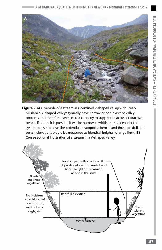
AIM NATIONAL AQUATIC MONITORING FRAMEWORK • Technical Reference 1735-2FIELD PROTOCOL FOR W
ADEABLE LOTIC SYSTEMS – FEBRUARY 2021
47
A
B
Figure 5. (A) Example of a stream in a confined V-shaped valley with steep hillslopes. V-shaped valleys typically have narrow or non-existent valley bottoms and therefore have limited capacity to support an active or inactive bench. If a bench is present, it will be narrow in width. In this scenario, the system does not have the potential to support a bench, and thus bankfull and bench elevations would be measured as identical heights (orange line). (B) Cross-sectional illustration of a stream in a V-shaped valley.

AIM NATIONAL AQUATIC MONITORING FRAMEWORK • Technical Reference 1735-2FI
ELD
PROT
OCOL
FOR
WAD
EABL
E LOT
IC SY
STEM
S – FE
BRUA
RY 2
021
48
Figure 6. (A) Example of a stream in a moderately confined valley with hillslopes that limit the extent of the valley bottom. This stream has a narrow, but well-established, active bench. In this scenario, bankfull and the active bench elevations are equal. (B) Cross-sectional illustration of a stream in a moderately confined valley with hillslopes that limit the extent of the valley bottom. These types of systems can be constrained by either the hillslope, inactive benches, or both. In this example, bankfull and bench heights are equal.
A
B
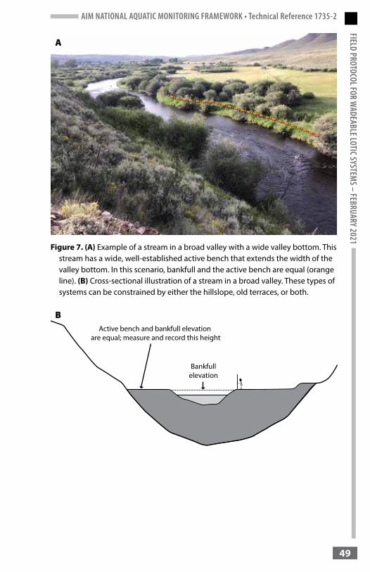
AIM NATIONAL AQUATIC MONITORING FRAMEWORK • Technical Reference 1735-2FIELD PROTOCOL FOR W
ADEABLE LOTIC SYSTEMS – FEBRUARY 2021
49
Figure 7. (A) Example of a stream in a broad valley with a wide valley bottom. This stream has a wide, well-established active bench that extends the width of the valley bottom. In this scenario, bankfull and the active bench are equal (orange line). (B) Cross-sectional illustration of a stream in a broad valley. These types of systems can be constrained by either the hillslope, old terraces, or both.
A
B
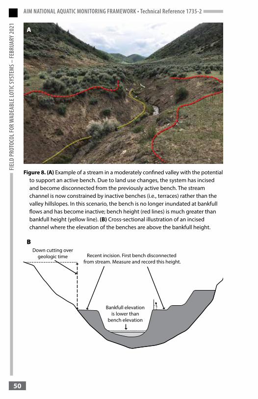
AIM NATIONAL AQUATIC MONITORING FRAMEWORK • Technical Reference 1735-2FI
ELD
PROT
OCOL
FOR
WAD
EABL
E LOT
IC SY
STEM
S – FE
BRUA
RY 2
021
50
Figure 8. (A) Example of a stream in a moderately confined valley with the potential to support an active bench. Due to land use changes, the system has incised and become disconnected from the previously active bench. The stream channel is now constrained by inactive benches (i.e., terraces) rather than the valley hillslopes. In this scenario, the bench is no longer inundated at bankfull flows and has become inactive; bench height (red lines) is much greater than bankfull height (yellow line). (B) Cross-sectional illustration of an incised channel where the elevation of the benches are above the bankfull height.
A
B
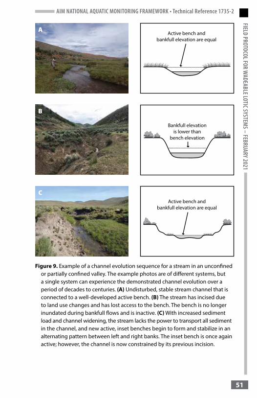
AIM NATIONAL AQUATIC MONITORING FRAMEWORK • Technical Reference 1735-2FIELD PROTOCOL FOR W
ADEABLE LOTIC SYSTEMS – FEBRUARY 2021
51
Figure 9. Example of a channel evolution sequence for a stream in an unconfined or partially confined valley. The example photos are of different systems, but a single system can experience the demonstrated channel evolution over a period of decades to centuries. (A) Undisturbed, stable stream channel that is connected to a well-developed active bench. (B) The stream has incised due to land use changes and has lost access to the bench. The bench is no longer inundated during bankfull flows and is inactive. (C) With increased sediment load and channel widening, the stream lacks the power to transport all sediment in the channel, and new active, inset benches begin to form and stabilize in an alternating pattern between left and right banks. The inset bench is once again active; however, the channel is now constrained by its previous incision.
A
B
C
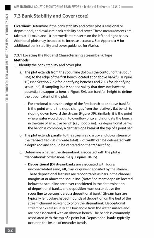
AIM NATIONAL AQUATIC MONITORING FRAMEWORK • Technical Reference 1735-2FI
ELD
PROT
OCOL
FOR
WAD
EABL
E LOT
IC SY
STEM
S – FE
BRUA
RY 2
021
52
7.3 Bank Stability and Cover (core)
Overview: Determine if the bank stability and cover plot is erosional or depositional, and evaluate bank stability and cover. These measurements are taken at 11 main and 10 intermediate transects on the left and right banks. Additional plots may be added to increase accuracy. See Appendix H for additional bank stability and cover guidance for Alaska.
7.3.1 Locating the Plot and Characterizing Streambank TypeMethods:1. Identify the bank stability and cover plot.
a. The plot extends from the scour line (follows the contour of the scour line) to the edge of the first bench located at or above bankfull (Figure 10) (see Section 2.2.2 for identifying benches and 2.2.3 for identifying scour line). If sampling in a V-shaped valley that does not have the potential to support a bench (Figure 5A), use bankfull height to define the upper extent of the plot.
• For erosional banks, the edge of the first bench at or above bankfull is the point where the slope changes from the relatively flat bench to sloping down toward the stream (Figure D9). Similarly, it is the point where water would begin to overflow onto and inundate the bench in the case of an active bench (i.e., floodplain). For depositional banks, the bench is commonly a gentler slope break at the top of a point bar.
b. The plot extends parallel to the stream 25 cm up- and downstream of the transect flag (50 cm wide total). Plot width can be delineated with a depth rod and should be centered on the transect flag.
c. Determine whether the streambank associated with the plot is “depositional” or “erosional” (e.g., Figures 10-15).
• Depositional (D) streambanks are associated with loose, unconsolidated sand, silt, clay, or gravel deposited by the stream. These depositional features are recognizable as bars in the channel margins at or above the scour line. (Note: Sediment deposits located below the scour line are never considered in the determination of depositional banks, and deposition must occur above the scour line to be considered a depositional bank.) Stream bars are typically lenticular-shaped mounds of deposition on the bed of the stream channel adjacent to or on the streambank. Depositional streambanks are usually at a low angle from the water surface and are not associated with an obvious bench. The bench is commonly associated with the top of a point bar. Depositional banks typically occur on the inside of meander bends.

AIM NATIONAL AQUATIC MONITORING FRAMEWORK • Technical Reference 1735-2FIELD PROTOCOL FOR W
ADEABLE LOTIC SYSTEMS – FEBRUARY 2021
53
Figure 10. Example of a bank stability and cover plot for an erosional streambank that is 100% covered. The dotted white line is the center of the plot location determined by the transect flag. The two solid white lines are the upstream and downstream extents of the plot, 25 cm on either side of the centerline. The lower extent of the plot is the contour of the scour line (blue line), and the upper extent of the plot is the first bench at or above bankfull (orange line). Note that the brown grass is senesced, firmly rooted in the ground, and connected to live vegetation; therefore, it is counted as foliar cover. The bank is covered, and erosional features are absent.
• Erosional (E) streambanks are all banks that are not depositional. Erosional streambanks are normally at a steeper angle to the water surface than depositional banks and are usually associated with a bench. Such banks typically occur on the outside of meander bends and on both sides of the stream in straight reaches. When there is sufficient stream energy, they may also occur on the inside bank of a meander.
AIM NATIONAL AQUATIC MONITORING FRAMEWORK • Technical Reference 1735-2FI
ELD
PROT
OCOL
FOR
WAD
EABL
E LOT
IC SY
STEM
S – FE
BRUA
RY 2
021
54
Figure 11. Example of an erosional and a depositional streambank. Depositional banks are composed of loose, unconsolidated materials deposited by the stream above scour line (blue line) and recognizable as bars in the channel; in this case, a point bar. The outside of the meander bend is an erosional bank. The erosional bank is at a steeper angle to the water surface than the depositional bank and associated with a bench.
7.3.2 Assessing Bank CoverOverview: View the bank stability and cover plot at 90 degrees from the ground surface and assess whether the streambank is “covered” or “uncovered.” Banks with 50% or more cover are classified as covered, and banks with less than 50% cover are classified as uncovered.
Methods:1. Determine whether the plot area is covered. To be covered, a bank must
contain 50% or more cover from one or more of the following within a height of 0.5 m from the soil surface.
• Absolute foliar cover of perennial vegetation (including visible live roots).
- Foliar cover is the percentage of ground surface covered by the aerial portion (leaves, stems, and visible roots) of plants when viewed from above.
- For vegetation, including tall grasses and shrub branches, to count as cover, it must be perennial and either rooted in the plot or overhanging the plot within a height of 0.5 m from the surface of the streambank.
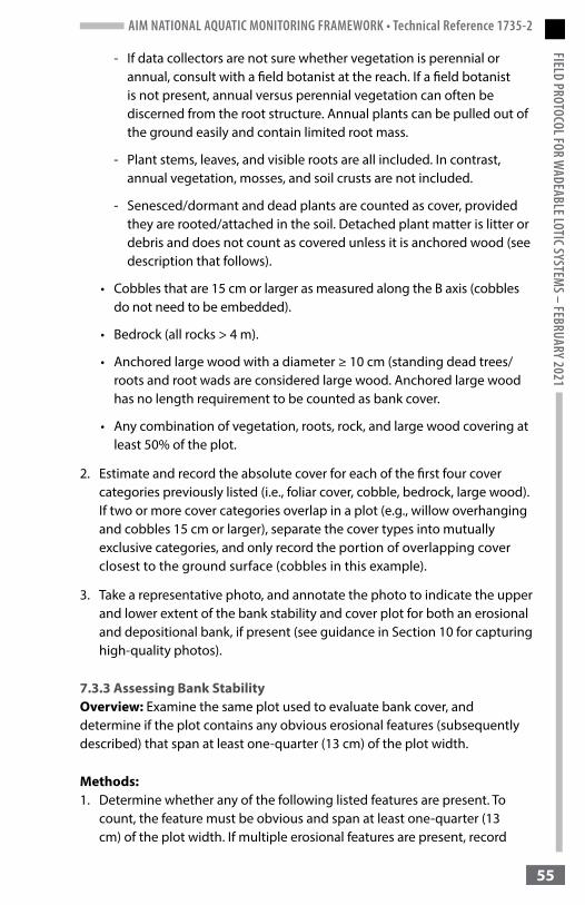
AIM NATIONAL AQUATIC MONITORING FRAMEWORK • Technical Reference 1735-2FIELD PROTOCOL FOR W
ADEABLE LOTIC SYSTEMS – FEBRUARY 2021
55
- If data collectors are not sure whether vegetation is perennial or annual, consult with a field botanist at the reach. If a field botanist is not present, annual versus perennial vegetation can often be discerned from the root structure. Annual plants can be pulled out of the ground easily and contain limited root mass.
- Plant stems, leaves, and visible roots are all included. In contrast, annual vegetation, mosses, and soil crusts are not included.
- Senesced/dormant and dead plants are counted as cover, provided they are rooted/attached in the soil. Detached plant matter is litter or debris and does not count as covered unless it is anchored wood (see description that follows).
• Cobbles that are 15 cm or larger as measured along the B axis (cobbles do not need to be embedded).
• Bedrock (all rocks > 4 m).
• Anchored large wood with a diameter ≥ 10 cm (standing dead trees/roots and root wads are considered large wood. Anchored large wood has no length requirement to be counted as bank cover.
• Any combination of vegetation, roots, rock, and large wood covering at least 50% of the plot.
2. Estimate and record the absolute cover for each of the first four cover categories previously listed (i.e., foliar cover, cobble, bedrock, large wood). If two or more cover categories overlap in a plot (e.g., willow overhanging and cobbles 15 cm or larger), separate the cover types into mutually exclusive categories, and only record the portion of overlapping cover closest to the ground surface (cobbles in this example).
3. Take a representative photo, and annotate the photo to indicate the upper and lower extent of the bank stability and cover plot for both an erosional and depositional bank, if present (see guidance in Section 10 for capturing high-quality photos).
7.3.3 Assessing Bank StabilityOverview: Examine the same plot used to evaluate bank cover, and determine if the plot contains any obvious erosional features (subsequently described) that span at least one-quarter (13 cm) of the plot width.
Methods:1. Determine whether any of the following listed features are present. To
count, the feature must be obvious and span at least one-quarter (13 cm) of the plot width. If multiple erosional features are present, record
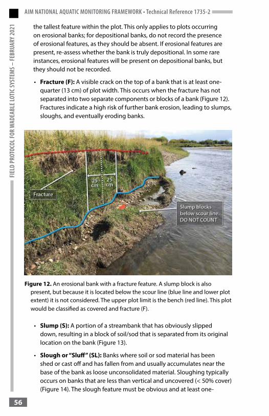
AIM NATIONAL AQUATIC MONITORING FRAMEWORK • Technical Reference 1735-2FI
ELD
PROT
OCOL
FOR
WAD
EABL
E LOT
IC SY
STEM
S – FE
BRUA
RY 2
021
56
the tallest feature within the plot. This only applies to plots occurring on erosional banks; for depositional banks, do not record the presence of erosional features, as they should be absent. If erosional features are present, re-assess whether the bank is truly depositional. In some rare instances, erosional features will be present on depositional banks, but they should not be recorded.
• Fracture (F): A visible crack on the top of a bank that is at least one-quarter (13 cm) of plot width. This occurs when the fracture has not separated into two separate components or blocks of a bank (Figure 12). Fractures indicate a high risk of further bank erosion, leading to slumps, sloughs, and eventually eroding banks.
Figure 12. An erosional bank with a fracture feature. A slump block is also present, but because it is located below the scour line (blue line and lower plot extent) it is not considered. The upper plot limit is the bench (red line). This plot would be classified as covered and fracture (F).
• Slump (S): A portion of a streambank that has obviously slipped down, resulting in a block of soil/sod that is separated from its original location on the bank (Figure 13).
• Slough or “Sluff” (SL): Banks where soil or sod material has been shed or cast off and has fallen from and usually accumulates near the base of the bank as loose unconsolidated material. Sloughing typically occurs on banks that are less than vertical and uncovered (< 50% cover) (Figure 14). The slough feature must be obvious and at least one-
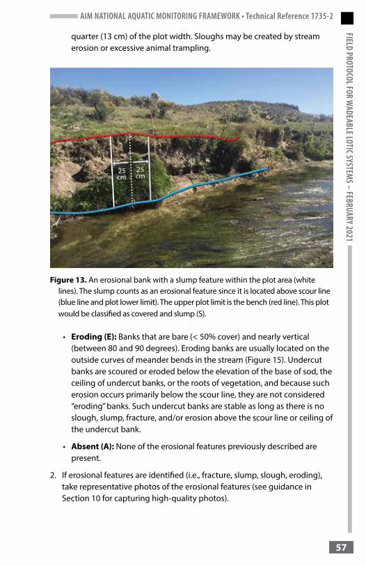
AIM NATIONAL AQUATIC MONITORING FRAMEWORK • Technical Reference 1735-2FIELD PROTOCOL FOR W
ADEABLE LOTIC SYSTEMS – FEBRUARY 2021
57
quarter (13 cm) of the plot width. Sloughs may be created by stream erosion or excessive animal trampling.
Figure 13. An erosional bank with a slump feature within the plot area (white lines). The slump counts as an erosional feature since it is located above scour line (blue line and plot lower limit). The upper plot limit is the bench (red line). This plot would be classified as covered and slump (S).
• Eroding (E): Banks that are bare (< 50% cover) and nearly vertical (between 80 and 90 degrees). Eroding banks are usually located on the outside curves of meander bends in the stream (Figure 15). Undercut banks are scoured or eroded below the elevation of the base of sod, the ceiling of undercut banks, or the roots of vegetation, and because such erosion occurs primarily below the scour line, they are not considered “eroding” banks. Such undercut banks are stable as long as there is no slough, slump, fracture, and/or erosion above the scour line or ceiling of the undercut bank.
• Absent (A): None of the erosional features previously described are present.
2. If erosional features are identified (i.e., fracture, slump, slough, eroding), take representative photos of the erosional features (see guidance in Section 10 for capturing high-quality photos).
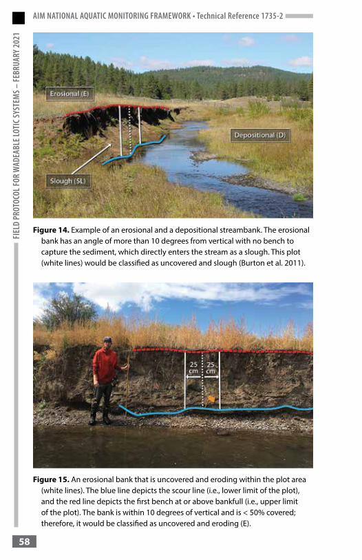
AIM NATIONAL AQUATIC MONITORING FRAMEWORK • Technical Reference 1735-2FI
ELD
PROT
OCOL
FOR
WAD
EABL
E LOT
IC SY
STEM
S – FE
BRUA
RY 2
021
58
Figure 14. Example of an erosional and a depositional streambank. The erosional bank has an angle of more than 10 degrees from vertical with no bench to capture the sediment, which directly enters the stream as a slough. This plot (white lines) would be classified as uncovered and slough (Burton et al. 2011).
Figure 15. An erosional bank that is uncovered and eroding within the plot area (white lines). The blue line depicts the scour line (i.e., lower limit of the plot), and the red line depicts the first bench at or above bankfull (i.e., upper limit of the plot). The bank is within 10 degrees of vertical and is < 50% covered; therefore, it would be classified as uncovered and eroding (E).
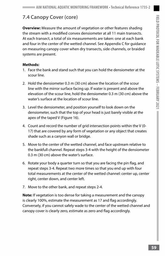
AIM NATIONAL AQUATIC MONITORING FRAMEWORK • Technical Reference 1735-2FIELD PROTOCOL FOR W
ADEABLE LOTIC SYSTEMS – FEBRUARY 2021
59
7.4 Canopy Cover (core)
Overview: Measure the amount of vegetation or other features shading the stream with a modified convex densiometer at all 11 main transects. At each transect, a total of six measurements are taken: one at each bank and four in the center of the wetted channel. See Appendix C for guidance on measuring canopy cover when dry transects, side channels, or braided systems are present.
Methods:1. Face the bank and stand such that you can hold the densiometer at the
scour line.
2. Hold the densiometer 0.3 m (30 cm) above the location of the scour line with the mirror surface facing up. If water is present and above the elevation of the scour line, hold the densiometer 0.3 m (30 cm) above the water’s surface at the location of scour line.
3. Level the densiometer, and position yourself to look down on the densiometer, such that the top of your head is just barely visible at the apex of the taped V (Figure 16).
4. Count and record the number of grid intersection points within the V (0-17) that are covered by any form of vegetation or any object that creates shade such as a canyon wall or bridge.
5. Move to the center of the wetted channel, and face upstream relative to the bankfull channel. Repeat steps 3-4 with the height of the densiometer 0.3 m (30 cm) above the water’s surface.
6. Rotate your body a quarter turn so that you are facing the pin flag, and repeat steps 3-4. Repeat two more times so that you end up with four total measurements at the center of the wetted channel: center up, center right, center down, and center left.
7. Move to the other bank, and repeat steps 2-4.
Note: If vegetation is too dense for taking a measurement and the canopy is clearly 100%, estimate the measurement as 17 and flag accordingly. Conversely, if you cannot safely wade to the center of the wetted channel and canopy cover is clearly zero, estimate as zero and flag accordingly.
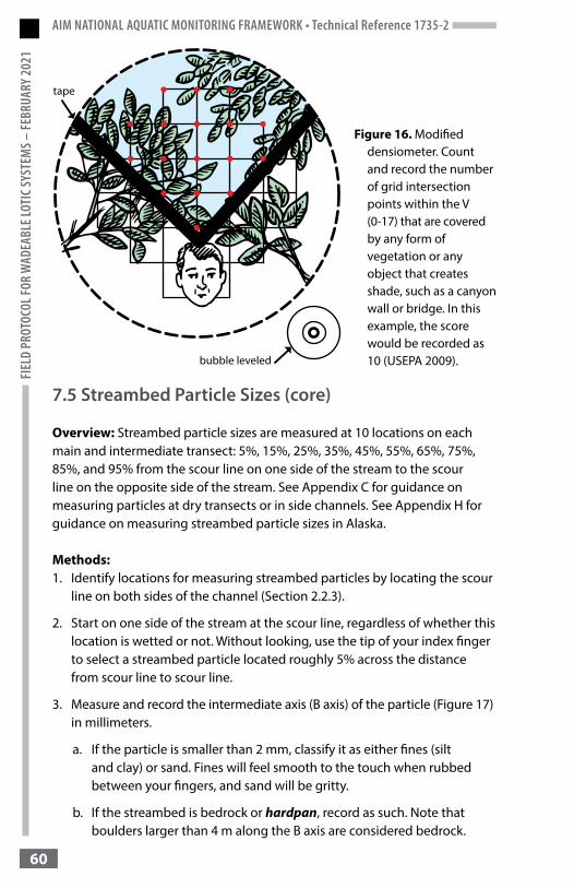
AIM NATIONAL AQUATIC MONITORING FRAMEWORK • Technical Reference 1735-2FI
ELD
PROT
OCOL
FOR
WAD
EABL
E LOT
IC SY
STEM
S – FE
BRUA
RY 2
021
60
Figure 16. Modified densiometer. Count and record the number of grid intersection points within the V (0-17) that are covered by any form of vegetation or any object that creates shade, such as a canyon wall or bridge. In this example, the score would be recorded as 10 (USEPA 2009).
7.5 Streambed Particle Sizes (core)
Overview: Streambed particle sizes are measured at 10 locations on each main and intermediate transect: 5%, 15%, 25%, 35%, 45%, 55%, 65%, 75%, 85%, and 95% from the scour line on one side of the stream to the scour line on the opposite side of the stream. See Appendix C for guidance on measuring particles at dry transects or in side channels. See Appendix H for guidance on measuring streambed particle sizes in Alaska.
Methods:1. Identify locations for measuring streambed particles by locating the scour
line on both sides of the channel (Section 2.2.3).
2. Start on one side of the stream at the scour line, regardless of whether this location is wetted or not. Without looking, use the tip of your index finger to select a streambed particle located roughly 5% across the distance from scour line to scour line.
3. Measure and record the intermediate axis (B axis) of the particle (Figure 17) in millimeters.
a. If the particle is smaller than 2 mm, classify it as either fines (silt and clay) or sand. Fines will feel smooth to the touch when rubbed between your fingers, and sand will be gritty.
b. If the streambed is bedrock or hardpan, record as such. Note that boulders larger than 4 m along the B axis are considered bedrock.
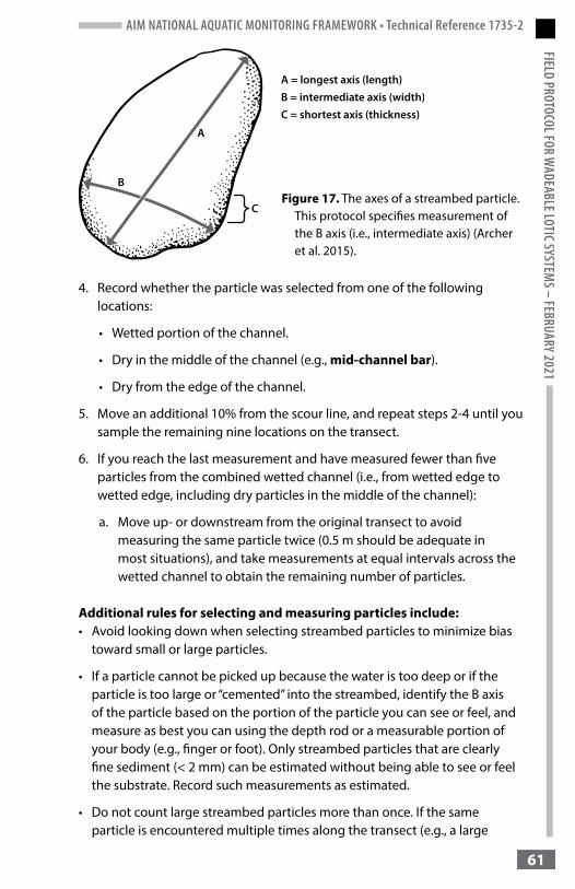
AIM NATIONAL AQUATIC MONITORING FRAMEWORK • Technical Reference 1735-2FIELD PROTOCOL FOR W
ADEABLE LOTIC SYSTEMS – FEBRUARY 2021
61
Figure 17. The axes of a streambed particle. This protocol specifies measurement of the B axis (i.e., intermediate axis) (Archer et al. 2015).
4. Record whether the particle was selected from one of the following locations:
• Wetted portion of the channel.
• Dry in the middle of the channel (e.g., mid-channel bar).
• Dry from the edge of the channel.
5. Move an additional 10% from the scour line, and repeat steps 2-4 until you sample the remaining nine locations on the transect.
6. If you reach the last measurement and have measured fewer than five particles from the combined wetted channel (i.e., from wetted edge to wetted edge, including dry particles in the middle of the channel):
a. Move up- or downstream from the original transect to avoid measuring the same particle twice (0.5 m should be adequate in most situations), and take measurements at equal intervals across the wetted channel to obtain the remaining number of particles.
Additional rules for selecting and measuring particles include: • Avoid looking down when selecting streambed particles to minimize bias
toward small or large particles.
• If a particle cannot be picked up because the water is too deep or if the particle is too large or “cemented” into the streambed, identify the B axis of the particle based on the portion of the particle you can see or feel, and measure as best you can using the depth rod or a measurable portion of your body (e.g., finger or foot). Only streambed particles that are clearly fine sediment (< 2 mm) can be estimated without being able to see or feel the substrate. Record such measurements as estimated.
• Do not count large streambed particles more than once. If the same particle is encountered multiple times along the transect (e.g., a large

AIM NATIONAL AQUATIC MONITORING FRAMEWORK • Technical Reference 1735-2FI
ELD
PROT
OCOL
FOR
WAD
EABL
E LOT
IC SY
STEM
S – FE
BRUA
RY 2
021
62
boulder), move up- or downstream 0.5 m or the distance required to avoid measuring the same particle twice, whichever is greater.
• If the streambed particle is covered by macrophytes, algae, wood, etc., measure the inorganic or mineral particle below the growth. Alternatively, if the substrate is organic matter and no mineral streambed particles exist below, select an alternative particle for measurement, or record such measurements as not collected. Make a comment if no alternative particles are present.
• If a streambed particle is covered with enough fine sediment or sand to “pinch” between your fingers, record the particle as either fines or sand. If a streambed particle is covered with fine sediment or sand but not enough to be “pinched,” measure the particle below the fines or sand.
• Depositional features (e.g., mid-channel bars) can be located above or below the scour line. Only measure particles located below the scour line.
• Partially wetted particles (i.e., those in the wetted section that extend above the water’s surface) should be considered as “wet.” This is especially common with larger particles including boulders.
7.6 Large Wood (core)
Overview: Count the number of large wood pieces contained throughout the main and side channels in the sample reach. See Appendix C for guidance on measuring large wood in side channels.
Large wood qualifications:To qualify, each piece of large wood:
• Must be ≥ 0.1 m (10 cm) in diameter for at least 1.5 m in length. If the diameter of the piece is < 10 cm at any point, visually cut the log, and do not use this portion for length estimates.
• Must be at least partially within or bridging the main bankfull channel for the qualifying section of wood, but record the entire length that qualifies. For assessing whether the piece of wood is within the bankfull channel, imagine the stream is flowing at bankfull, and count any piece whose qualifying stem would be wet.
• Must be dead vegetation or standing dead vegetation. Dead limbs spanning bankfull that are connected to live trees are counted as large wood if they meet the qualifying size criteria, but only the dead portion is measured, not the whole tree. Dead limbs should be clearly dead (e.g., limbs devoid of leaves or needles, shedding or devoid of bark, with small branches broken off).
AIM NATIONAL AQUATIC MONITORING FRAMEWORK • Technical Reference 1735-2FIELD PROTOCOL FOR W
ADEABLE LOTIC SYSTEMS – FEBRUARY 2021
63
• If a qualifying piece of large wood extends outside the reach, (i.e., downstream of transect A and/or upstream of transect K), only measure the portion within the reach.
Special situations: • If a forked piece of wood is encountered, measure only the qualifying stem
or branch with the largest diameter.
• If a root mass with many stems is encountered, measure only the qualifying stem or branch with the largest diameter. Roots should not be measured or included.
• Cracked or broken pieces. Include the entire length when two pieces are still connected at any point. Treat them separately if they are no longer touching or connected.
• Large wood embedded in streambanks must have an exposed portion that meets the length and diameter requirements to qualify.
Methods: 1. Starting at either the bottom or top of the reach, scan each stream
segment between two transects for large wood. Identify whether pieces are above or below the bankfull channel.
2. Place each qualifying piece of wood in the appropriate size category based on both the diameter at the large end and the length. If roots are involved, begin measurements where the roots attach to the base of the stem; do not include roots or branches in length measurements. Tally all pieces of qualifying wood for each size category and whether they were found: (1) entirely or partially below the bankfull elevation or (2) bridging above bankfull channel (Figure 18).
a. Large wood diameter size categories (large end):
• 0.1 m to 0.29 m
• 0.3 m to 0.59 m
• 0.6 m to 0.79 m
• ≥ 0.8 m
b. Length categories (consider sections of large wood with diameters of at least 0.1 m):
• 1.5 m to 2.9 m
• 3 m to 4.9 m
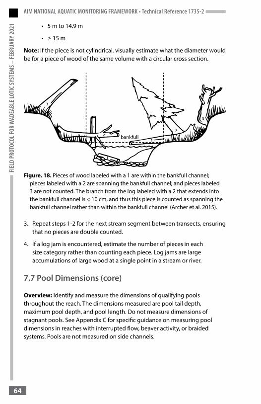
AIM NATIONAL AQUATIC MONITORING FRAMEWORK • Technical Reference 1735-2FI
ELD
PROT
OCOL
FOR
WAD
EABL
E LOT
IC SY
STEM
S – FE
BRUA
RY 2
021
64
• 5 m to 14.9 m
• ≥ 15 m
Note: If the piece is not cylindrical, visually estimate what the diameter would be for a piece of wood of the same volume with a circular cross section.
Figure. 18. Pieces of wood labeled with a 1 are within the bankfull channel; pieces labeled with a 2 are spanning the bankfull channel; and pieces labeled 3 are not counted. The branch from the log labeled with a 2 that extends into the bankfull channel is < 10 cm, and thus this piece is counted as spanning the bankfull channel rather than within the bankfull channel (Archer et al. 2015).
3. Repeat steps 1-2 for the next stream segment between transects, ensuring that no pieces are double counted.
4. If a log jam is encountered, estimate the number of pieces in each size category rather than counting each piece. Log jams are large accumulations of large wood at a single point in a stream or river.
7.7 Pool Dimensions (core)
Overview: Identify and measure the dimensions of qualifying pools throughout the reach. The dimensions measured are pool tail depth, maximum pool depth, and pool length. Do not measure dimensions of stagnant pools. See Appendix C for specific guidance on measuring pool dimensions in reaches with interrupted flow, beaver activity, or braided systems. Pools are not measured on side channels.
AIM NATIONAL AQUATIC MONITORING FRAMEWORK • Technical Reference 1735-2FIELD PROTOCOL FOR W
ADEABLE LOTIC SYSTEMS – FEBRUARY 2021
65
Pool qualifications: A pool is:
• A depression in the streambed that is laterally and longitudinally concave (i.e., bowl shaped).
• Characterized by water that is slower and flatter than up- or downstream waters at baseflow.
• Bound by a “tail” on the downstream end, which can be identified by a leveling of the streambed slope and reduction in depth (Figures 19 and 20). The pool tail is the shallowest downstream location in the pool from which water would spill if the flow were reduced to a trickle.
• Bound by a “head crest” on the upstream end, which can be identified by an increase in streambed slope and a coarsening of streambed particle sizes as one exits the pool from downstream to upstream (Figures 19 and 20).
This protocol distinguishes between qualifying and nonqualifying pools, and the dimensions of nonqualifying pools should not be measured. To qualify, the pool must meet all of the following six criteria:
1. The profile of the pool must be laterally and longitudinally concave.
2. The concave shape of the pool must span at least 50% of the wetted channel (measured perpendicular to the thalweg).
3. The pool must have a maximum water depth that is at least 1.5 times the pool tail depth.
4. The pool must be contained within the main channel.
5. The thalweg must run through the pool with flow going both in and out of the pool.
6. The pool must be longer than it is wide, unless the pool is a plunge pool (i.e., formed when the thalweg drops vertically off an obstruction such as a boulder or log). To qualify as a plunge pool, the max pool depth must be within 20% of the total length of the pool from the obstruction (e.g., if the plunge pool is 10 m long, then the max depth must be within 2 m of the obstruction). Plunge pools are the only pools that can be wider than they are long.
Note: Side channel or backwater pools should not be considered. Also, long sections of stream that are laterally but not longitudinally concave and/or that do not possess the requisite bowl-like shape should not be considered pools. These features are commonly referred to as “runs.”

AIM NATIONAL AQUATIC MONITORING FRAMEWORK • Technical Reference 1735-2FI
ELD
PROT
OCOL
FOR
WAD
EABL
E LOT
IC SY
STEM
S – FE
BRUA
RY 2
021
66
Figure 19. (A) Cross-sectional view and (B) bird’s eye view of a pool, showing pool features. Pools are identified by the concave shape bound by a head crest and tail and a max depth > 1.5 times the pool tail depth (modified from Dunne and Leopold 1978).
Figure 20. Example of a pool on the outside of a meander bend. Pools are bound by a head crest on the upstream end and a pool tail on the downstream end.

AIM NATIONAL AQUATIC MONITORING FRAMEWORK • Technical Reference 1735-2FIELD PROTOCOL FOR W
ADEABLE LOTIC SYSTEMS – FEBRUARY 2021
67
Methods:1. Starting at transect A, walk upstream looking for a change in slope on the
streambed that could indicate the presence of a pool; the water should increase in depth as you walk from the pool tail to the point of maximum pool depth.
2. When a potential pool is identified, determine if it has the required bowl-like shape and if it spans at least 50% of the wetted channel, not including bars, at any point in the concavity of the pool. For pools with undercut banks present, wetted width is measured as aerial width and does not include water under the banks that cannot be viewed when looking down on the stream. This refers to undercut banks only and not vegetation.
3. Find and measure the pool tail and maximum pool depths to the nearest 1 cm. To find the pool tail, imagine the downstream location of the pool that would be the last to have flowing water if the flow was slowly turned off to the stream. Measure the pool tail depth at this location. If the current water level through the pool tail is a trickle (i.e., < 1 cm), round up and record the pool tail depth as 1 cm.
a. If maximum pool depth is too deep to measure directly, follow this procedure.
• Use a stadia rod placed at an angle to reach the maximum pool depth.
• Determine the angle of the stadia rod by resting the compass/clinometer on the upper surface of the rod and reading the angle.
• Record the water depth on the rod and the rod angle.
b. If the current is too fast or other conditions preclude the angle method for measuring depth, estimate depth to the best of your ability based on measurements you are able to take and flag the measurement as estimated.
4. Determine if the pool qualifies by checking that the max pool depth is ≥ 1.5 times the pool tail depth. If the pool qualifies, record the pool tail and max pool depths, and determine if it is a full-channel or partial-channel pool.
• Full-channel pool: The concave shape of the pool (measured perpendicular to the thalweg) at any location is > 90% of the wetted channel width.
• Partial-channel pool: The concave shape of the pool (measured perpendicular to the thalweg) at any location is between 50% and 90% of the wetted channel width.
AIM NATIONAL AQUATIC MONITORING FRAMEWORK • Technical Reference 1735-2FI
ELD
PROT
OCOL
FOR
WAD
EABL
E LOT
IC SY
STEM
S – FE
BRUA
RY 2
021
68
5. Measure and record the length of the pool in meters, following the thalweg, from where the thalweg crosses the pool tail to where the thalweg crosses the pool head crest. Round the measurement to the nearest 0.01 m. The pool head crest is the upstream boundary of the pool and is where the water surface slope changes from being relatively flat to slightly steeper. This location also corresponds to an increase in the streambed slope and is often an abrupt transition.
a. If any portion of the pool is outside the sampling reach, only measure the length of the pool that is contained within the reach. Such pools must still meet all pool qualifications. However, the pool tail or max depth point can fall outside the reach.
b. If you cannot safely measure pool length along the thalweg, estimate length based on measurements you are able to take and flag accordingly.
6. Record the main transect letters contained within all qualifying pools. For a transect to be contained within a pool, it must occur between the pool tail and the head crest.
7. Record the length of the reach over which pools were delineated; exclude any length of stream that could not be assessed.
Methods for cases in which there appear to be two consecutive potential pools (Figure 21): Group adjacent or closely spaced potential pools into a single qualifying pool if their depth at a theoretical zero discharge stage is controlled by the height of a single downstream pool tail. This can be assessed quantitatively by measuring the depth of questionable pool tails. For example, if the downstream pool tail is deeper than the questionable upstream pool tail, then two qualifying pools are present (Figure 21B). Measure these two pools individually if all other pool qualifications are met for both pools. In contrast, if the downstream pool tail is shallower than all other questionable pool tails, only a single pool exists (Figure 21A).
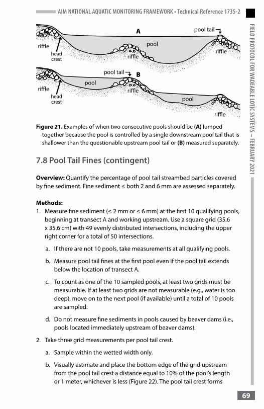
AIM NATIONAL AQUATIC MONITORING FRAMEWORK • Technical Reference 1735-2FIELD PROTOCOL FOR W
ADEABLE LOTIC SYSTEMS – FEBRUARY 2021
69
Figure 21. Examples of when two consecutive pools should be (A) lumped together because the pool is controlled by a single downstream pool tail that is shallower than the questionable upstream pool tail or (B) measured separately.
7.8 Pool Tail Fines (contingent)
Overview: Quantify the percentage of pool tail streambed particles covered by fine sediment. Fine sediment ≤ both 2 and 6 mm are assessed separately.
Methods:1. Measure fine sediment (≤ 2 mm or ≤ 6 mm) at the first 10 qualifying pools,
beginning at transect A and working upstream. Use a square grid (35.6 x 35.6 cm) with 49 evenly distributed intersections, including the upper right corner for a total of 50 intersections.
a. If there are not 10 pools, take measurements at all qualifying pools.
b. Measure pool tail fines at the first pool even if the pool tail extends below the location of transect A.
c. To count as one of the 10 sampled pools, at least two grids must be measurable. If at least two grids are not measurable (e.g., water is too deep), move on to the next pool (if available) until a total of 10 pools are sampled.
d. Do not measure fine sediments in pools caused by beaver dams (i.e., pools located immediately upstream of beaver dams).
2. Take three grid measurements per pool tail crest.
a. Sample within the wetted width only.
b. Visually estimate and place the bottom edge of the grid upstream from the pool tail crest a distance equal to 10% of the pool’s length or 1 meter, whichever is less (Figure 22). The pool tail crest forms
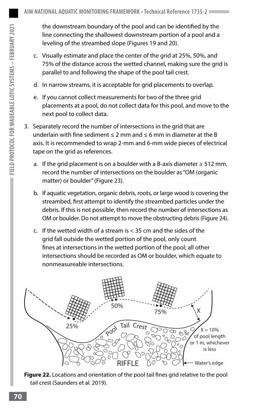
AIM NATIONAL AQUATIC MONITORING FRAMEWORK • Technical Reference 1735-2FI
ELD
PROT
OCOL
FOR
WAD
EABL
E LOT
IC SY
STEM
S – FE
BRUA
RY 2
021
70
the downstream boundary of the pool and can be identified by the line connecting the shallowest downstream portion of a pool and a leveling of the streambed slope (Figures 19 and 20).
c. Visually estimate and place the center of the grid at 25%, 50%, and 75% of the distance across the wetted channel, making sure the grid is parallel to and following the shape of the pool tail crest.
d. In narrow streams, it is acceptable for grid placements to overlap.
e. If you cannot collect measurements for two of the three grid placements at a pool, do not collect data for this pool, and move to the next pool to collect data.
3. Separately record the number of intersections in the grid that are underlain with fine sediment ≤ 2 mm and ≤ 6 mm in diameter at the B axis. It is recommended to wrap 2-mm and 6-mm wide pieces of electrical tape on the grid as references.
a. If the grid placement is on a boulder with a B-axis diameter ≥ 512 mm, record the number of intersections on the boulder as “OM (organic matter) or boulder” (Figure 23).
b. If aquatic vegetation, organic debris, roots, or large wood is covering the streambed, first attempt to identify the streambed particles under the debris. If this is not possible, then record the number of intersections as OM or boulder. Do not attempt to move the obstructing debris (Figure 24).
c. If the wetted width of a stream is < 35 cm and the sides of the grid fall outside the wetted portion of the pool, only count fines at intersections in the wetted portion of the pool; all other intersections should be recorded as OM or boulder, which equate to nonmeasureable intersections.
Figure 22. Locations and orientation of the pool tail fines grid relative to the pool tail crest (Saunders et al. 2019).
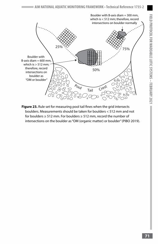
AIM NATIONAL AQUATIC MONITORING FRAMEWORK • Technical Reference 1735-2FIELD PROTOCOL FOR W
ADEABLE LOTIC SYSTEMS – FEBRUARY 2021
71
Figure 23. Rule set for measuring pool tail fines when the grid intersects boulders. Measurements should be taken for boulders < 512 mm and not for boulders ≥ 512 mm. For boulders ≥ 512 mm, record the number of intersections on the boulder as “OM (organic matter) or boulder” (PIBO 2019).
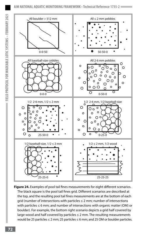
AIM NATIONAL AQUATIC MONITORING FRAMEWORK • Technical Reference 1735-2FI
ELD
PROT
OCOL
FOR
WAD
EABL
E LOT
IC SY
STEM
S – FE
BRUA
RY 2
021
72
Figure 24. Examples of pool tail fines measurements for eight different scenarios. The black square is the pool tail fines grid. Different scenarios are described at the top, and the resulting pool tail fines measurements are at the bottom of each grid (number of intersections with particles ≤ 2 mm; number of intersections with particles ≤ 6 mm; and number of intersections with organic matter (OM) or boulder). For example, the bottom right scenario depicts a grid half covered by large wood and half covered by particles ≤ 2 mm. The resulting measurements would be 25 particles ≤ 2 mm; 25 particles ≤ 6 mm; and 25 OM or boulder particles.
AIM NATIONAL AQUATIC MONITORING FRAMEWORK • Technical Reference 1735-2FIELD PROTOCOL FOR W
ADEABLE LOTIC SYSTEMS – FEBRUARY 2021
73
Reminders and tips:• Prior to sampling, briefly assess the condition of the streambed particles
in the pool tails. Fine sediment can accumulate in pool tails from sampling efforts throughout the reach. Avoid measuring recently deposited fine sediments in pool tails. If recently deposited sediment is in the pool tail and it is believed the crew contributed the fines by working in the stream, do not sample that pool tail.
• Only record particles that are ≤ 2 mm, ≤ 6 mm, or OM or boulder. All grid locations not marked as ≤ 2 mm, ≤ 6 mm, or OM or boulder are assumed to be mineral streambed particles between 7 mm and 511 mm, and the data collection application will record this value in the column labeled > 6 mm and < 512 mm.
• The number of intersections of fines ≤ 2 mm cannot exceed the number of intersections of fines ≤ 6 mm.
• The number of intersections of fines ≤ 6 mm plus the number of intersections marked as OM or boulder must be ≤ 50.
• If a streambed particle is covered with enough fine sediment to “pinch” between your fingers, record the particle as either ≤ 2 mm or ≤ 6 mm. If a streambed particle is covered with fine sediment but not enough to be “pinched,” measure the particle covered with the fines and record accordingly.
7.9 Flood-Prone Width (covariate)
Overview: Measure the width of the flood-prone area at riffles located nearest to transects A and K. In addition to flood-prone width, measurements of maximum water depth, bankfull height, and bankfull width are required. See Appendix C for guidance on measuring flood-prone width when interrupted flow is present.
Methods:1. Locate the closest representative riffles to transects A and K, while
staying within the sample reach. Representative riffles should be oriented parallel to the valley in which they flow, be of typical bankfull and bench elevations, and be accessible for taking all measurements without the need for estimation. If no riffles are present, take measurements within uniform, straight reaches closest to transects A and K.
a. Take at least one photo of each location where flood-prone width is measured: photos are taken looking upstream or downstream. Photos provide additional context to the landscape when reviewing data
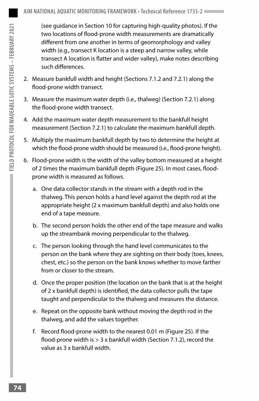
AIM NATIONAL AQUATIC MONITORING FRAMEWORK • Technical Reference 1735-2FI
ELD
PROT
OCOL
FOR
WAD
EABL
E LOT
IC SY
STEM
S – FE
BRUA
RY 2
021
74
(see guidance in Section 10 for capturing high-quality photos). If the two locations of flood-prone width measurements are dramatically different from one another in terms of geomorphology and valley width (e.g., transect K location is a steep and narrow valley, while transect A location is flatter and wider valley), make notes describing such differences.
2. Measure bankfull width and height (Sections 7.1.2 and 7.2.1) along the flood-prone width transect.
3. Measure the maximum water depth (i.e., thalweg) (Section 7.2.1) along the flood-prone width transect.
4. Add the maximum water depth measurement to the bankfull height measurement (Section 7.2.1) to calculate the maximum bankfull depth.
5. Multiply the maximum bankfull depth by two to determine the height at which the flood-prone width should be measured (i.e., flood-prone height).
6. Flood-prone width is the width of the valley bottom measured at a height of 2 times the maximum bankfull depth (Figure 25). In most cases, flood-prone width is measured as follows.
a. One data collector stands in the stream with a depth rod in the thalweg. This person holds a hand level against the depth rod at the appropriate height (2 x maximum bankfull depth) and also holds one end of a tape measure.
b. The second person holds the other end of the tape measure and walks up the streambank moving perpendicular to the thalweg.
c. The person looking through the hand level communicates to the person on the bank where they are sighting on their body (toes, knees, chest, etc.) so the person on the bank knows whether to move farther from or closer to the stream.
d. Once the proper position (the location on the bank that is at the height of 2 x bankfull depth) is identified, the data collector pulls the tape taught and perpendicular to the thalweg and measures the distance.
e. Repeat on the opposite bank without moving the depth rod in the thalweg, and add the values together.
f. Record flood-prone width to the nearest 0.01 m (Figure 25). If the flood-prone width is > 3 x bankfull width (Section 7.1.2), record the value as 3 x bankfull width.
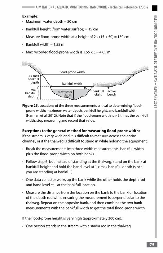
AIM NATIONAL AQUATIC MONITORING FRAMEWORK • Technical Reference 1735-2FIELD PROTOCOL FOR W
ADEABLE LOTIC SYSTEMS – FEBRUARY 2021
75
Example: • Maximum water depth = 50 cm
• Bankfull height (from water surface) = 15 cm
• Measure flood-prone width at a height of 2 x (15 + 50) = 130 cm
• Bankfull width = 1.55 m
• Max recorded flood-prone width is 1.55 x 3 = 4.65 m
Figure 25. Locations of the three measurements critical to determining flood-prone width: maximum water depth, bankfull height, and bankfull width (Harman et al. 2012). Note that if the flood-prone width is > 3 times the bankfull width, stop measuring and record that value.
Exceptions to the general method for measuring flood-prone width:If the stream is very wide and it is difficult to measure across the entire channel, or if the thalweg is difficult to stand in while holding the equipment:
• Break the measurements into three width measurements: bankfull width plus the flood-prone width on both banks.
• Follow step 6, but instead of standing at the thalweg, stand on the bank at bankfull height and hold the hand level at 1 x max bankfull depth (since you are standing at bankfull).
• One data collector walks up the bank while the other holds the depth rod and hand level still at the bankfull location.
• Measure the distance from the location on the bank to the bankfull location of the depth rod while ensuring the measurement is perpendicular to the thalweg. Repeat on the opposite bank, and then combine the two bank measurements with the bankfull width to get the total flood-prone width.
If the flood-prone height is very high (approximately 300 cm):
• One person stands in the stream with a stadia rod in the thalweg.
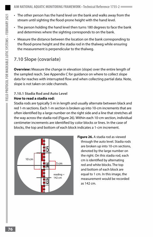
AIM NATIONAL AQUATIC MONITORING FRAMEWORK • Technical Reference 1735-2FI
ELD
PROT
OCOL
FOR
WAD
EABL
E LOT
IC SY
STEM
S – FE
BRUA
RY 2
021
76
• The other person has the hand level on the bank and walks away from the stream until sighting the flood-prone height with the hand level.
• The person holding the hand level then turns 180 degrees to face the bank and determines where the sighting corresponds to on the bank.
• Measure the distance between the location on the bank corresponding to the flood-prone height and the stadia rod in the thalweg while ensuring the measurement is perpendicular to the thalweg.
7.10 Slope (covariate)
Overview: Measure the change in elevation (slope) over the entire length of the sampled reach. See Appendix C for guidance on where to collect slope data for reaches with interrupted flow and when collecting partial data. Note, slope is not taken on side channels.
7.10.1 Stadia Rod and Auto LevelHow to read a stadia rod: Stadia rods are typically 5 m in length and usually alternate between black and red 1-m sections. Each 1-m section is broken up into 10-cm increments that are often identified by a large number on the right side and a line that stretches all the way across the stadia rod (Figure 26). Within each 10-cm section, individual centimeter increments are identified by color blocks or lines. In the case of blocks, the top and bottom of each block indicates a 1-cm increment.
Figure 26. A stadia rod as viewed through the auto level. Stadia rods are broken up into 10-cm sections, denoted by the large number on the right. On this stadia rod, each cm is identified by alternating red and white blocks. The top and bottom of each block are equal to 1 cm. In this image, the measurement would be recorded as 142 cm.
AIM NATIONAL AQUATIC MONITORING FRAMEWORK • Technical Reference 1735-2FIELD PROTOCOL FOR W
ADEABLE LOTIC SYSTEMS – FEBRUARY 2021
77
Methods:Slope requires two people to collect measurements. One person sets up the auto level and takes the measurements, and the other person holds the stadia rod. The procedure is repeated two or more times until there is less than a 10% difference between independent slope measurements.
Part A. Set up the tripod and auto level:The most challenging part of measuring slope is finding the best place to set up the tripod and auto level. Ideally, the tripod will only need to be set up and leveled once per pass, but this requires the entire reach to be visible from one location. In heavily vegetated reaches, the tripod may need to be moved multiple times.
1. Find a location that allows you to see the stadia rod when placed at both the bottom and top of the reach and when extended vertically.
2. Set up the tripod by extending the tripod legs, locking them, and firmly setting them into the ground. Adjust the legs so that the tripod does not wobble.
3. Place the auto level on the base plate, and tighten the center screw.
4. Adjust the tripod legs until the bubble is approximately in the center of the level.
5. Adjust the foot or fine screws until the bubble is exactly in the center of the circle.
6. Gently swivel the instrument to make sure the auto level is securely attached and level in all planes.
Part B. Take measurements:1. While the person holding the stadia rod stands at the bottom of the reach,
the recorder sights the stadia rod through the auto level and records the height reading to the nearest 1 cm (Figure 26). Hold the stadia rod as vertical as possible with the bottom end at the water’s surface and the numbers facing toward the auto level.
2. Move the stadia rod to the top of the reach (or the farthest location upstream that can still be seen through the level), and gently swivel the level to face the new stadia rod location. Make sure the bubble stays inside the center of the level. If the bubble is not level, it is an indication that the base screw was not tight or the tripod legs were not stable, and you must start over.
3. Hold the stadia rod vertically, with the bottom end at the water’s surface and the numbers facing toward the auto level.
AIM NATIONAL AQUATIC MONITORING FRAMEWORK • Technical Reference 1735-2FI
ELD
PROT
OCOL
FOR
WAD
EABL
E LOT
IC SY
STEM
S – FE
BRUA
RY 2
021
78
4. Sight the stadia rod through the auto level, and record the height to the nearest 1 cm, being careful to record the number that intersects the center of the cross hairs.
5. If the top of the reach is not visible from the auto level, do not move the stadia rod after the second reading has been taken. Instead, hold the stadia rod in the exact position (this serves as a reference point connecting the next line of readings [i.e., back sight]) while the recorder moves the auto level to a new location.
6. Move the auto level to a new location (and an unmeasured section) along the stream reach from which you can see the stadia rod and the remaining portion of the reach to be surveyed. Set up the auto level as before, making sure to readjust the level.
7. Backsight (BS) to the stadia rod, and record the measurement. The stadia rod can now be moved.
8. Move the stadia rod as far up the reach as possible, while remaining within sight of the auto level. Take a new foresight (FS) reading.
9. Continue repeating steps 4-8 until the stadia rod is sighted at the top of the reach.
10. Once at the top of the reach, repeat steps 1-9, working from the top of the reach to the bottom of the reach to complete a second pass (i.e., to get a second measurement of the total change in slope throughout the reach). Note that at the beginning of the second pass, the auto level can remain in the same general location, but it must be picked up, set down, and releveled.
11. Calculate the total change in elevation for each pass and the percent difference between the two measurements. If the percent difference is > 10%, conduct additional passes, until you have two passes that are within 10% of each other. For example:
a. The total change in elevation from the bottom of the reach to the top of the reach = (Transect A – FS1) + (BS1 - FS2) + (BS2 - FS3) + (BS3 - Transect K), accounting for all shots.
b. The total change in elevation from the top of the reach to the bottom of the reach = (FS1 - Transect K) + (FS2 - BS1) + (FS3 - BS2) + (Transect A - BS3), accounting for all shots.
c. Elevation of pass (cm) x 0.1 = 10% of elevation (cm)
d. Add and subtract the calculated 10% (in cm) from the original elevation to get the acceptable range of values that the elevation of your second pass must fall within. For example:
AIM NATIONAL AQUATIC MONITORING FRAMEWORK • Technical Reference 1735-2FIELD PROTOCOL FOR W
ADEABLE LOTIC SYSTEMS – FEBRUARY 2021
79
• Total elevation for pass 1 = 100 cm
• 100 cm x 0.1 = 10 cm (10% of pass one)
• 100 cm + 10 cm = 110 cm (upper limit)
• 100 cm - 10 cm = 90 cm (lower limit)
• Thus, the elevation of pass 2 must be between 90 and 110 cm to be within 10% of pass 1.
12. Record the length of the reach over which slope was measured.
Tips for measuring slope:• To avoid obstructions such as vegetation, set the tripod and auto level in as
high a position on the landscape as possible, while still being able to read the stadia rod.
• Gently waving the rod around through vegetation can help the recorder see the rod through the level.
• Sometimes modest vegetation trimming is required.
• Sighting across land can be easier than trying to move up the stream channel. Remember the stadia rod only needs to be at the water surface for the bottom and top of the reach, but it can be placed anywhere (e.g., bank, upland) between these two locations.
• It is reasonable to have a negative slope for a section of the reach, as long as the total reach slope is positive.
• When working in regions that are prone to afternoon thundershowers, it is wise to collect slope data early in the day.
• Using hand-held walkie talkie radios can assist with communication when measuring slope.
7.10.2 Alternative Slope MethodsOverview: In some locations, such as very remote streams that require overnight trips, it can be too cumbersome to collect slope using the preferred method of a stadia rod, tripod, and auto level. In these locations, data collectors should measure slope with a stadia rod and hand level. Additional time is needed to complete slope measurements with this method.
How to use the hand level:Look through the eyepiece of the hand level (with the clear window facing up). The field of view is split vertically; the left side has three horizontal black lines, and the right side contains a bubble used to level the device. To level
AIM NATIONAL AQUATIC MONITORING FRAMEWORK • Technical Reference 1735-2FI
ELD
PROT
OCOL
FOR
WAD
EABL
E LOT
IC SY
STEM
S – FE
BRUA
RY 2
021
80
the instrument, hold the hand level on top of a depth rod, and adjust the tilt until the bubble on the right side aligns with the center of the three black lines on the left side. Use both the eyepiece and the lens end telescope to focus while standing as close to the stadia rod as needed to accurately read the height on the stadia rod (this may be < 10 meters).
Methods:1. While the person holding the stadia rod stands at the bottom of the
reach, the recorder sights the stadia rod through the hand level and records the number (to the nearest 1 cm) that aligns with the middle line in the hand level’s field of view. Hold the stadia rod as vertical as possible with the bottom end at the water’s surface and the numbers facing toward the recorder.
2. Move the stadia rod 10-12 m upstream of the recorder. Hold the stadia rod as before, vertically with the numbers facing the recorder.
3. Pivot the hand level to face the stadia rod. Relevel the hand level without moving the depth rod.
4. Sight the stadia rod through the hand level, and record the reading (to the nearest 1 cm).
5. Do not move the stadia rod after the second reading has been taken. Instead, hold the stadia rod in the exact position (this serves as a reference point connecting the next line of readings) while the recorder moves the hand level to a new location.
6. Move the hand level to a new location (and an unmeasured section) of the stream reach from which you can see the stadia rod. Set up the level as before.
7. Backsight to the stadia rod, and record the measurement. The stadia rod can now be moved.
8. Move the stadia rod 10-12 m up the reach while remaining within sight of the hand level. Take a new reading.
9. Continue repeating steps 4-8 until the stadia rod is sighted at the top of the reach.
10. Once at the top of the reach, repeat steps 1-9 working from the top of the reach to the bottom of the reach to complete a second pass (i.e., to get a second measurement of the total change in slope throughout the reach). Note that at the beginning of the second pass, the hand level and depth rod can remain in the same general location, but the depth rod must be physically picked up and set down and the hand level must be releveled.

AIM NATIONAL AQUATIC MONITORING FRAMEWORK • Technical Reference 1735-2FIELD PROTOCOL FOR W
ADEABLE LOTIC SYSTEMS – FEBRUARY 2021
81
11. As with the auto level method, pass 1 and pass 2 elevations must be within 10%, or another pass will need to be completed until two passes are within 10%. See calculation details in Section 7.10.1, Part B, step 11.
12. Record the length of the reach over which slope was measured.
Tips for measuring slope with a hand level: • Avoid setting the depth rod on soft streambed particles where it may sink.
If this is unavoidable, push the rod down into the mud or sand until it meets resistance, or set it on a sizeable flat rock before taking measurements.
• If you are having trouble reading the stadia rod, try shorter distances and/or ask the person holding the rod to move their finger to the reading on the stadia rod.
7.11 Bank Angle (contingent)
Overview: Measure the angle of both left and right banks at all 11 main transects. At each transect, bank angle is measured from where the bed-meets-bank (lower limit) to the edge of the first bench located at or above bankfull (upper limit). Many rules apply to measuring bank angle; make sure to thoroughly read Sections 7.11.1 and 7.11.2 before attempting to apply the bank angle protocol. See Appendix C for guidance on measuring bank angle where side channels are present.
Methods:1. Make sure that the dial on the compass is set so that the north arrow is
in line with the 90° or 270° mark to ensure that the clinometer readings, measured using the compass, will be accurate.
2. Identify where to take the bank angle measurement by noting the locations of bed-meets-bank (Section 2.2.5), bankfull (Section 2.2.1), and scour line (Section 2.2.3).
3. Record whether the bank is obtuse or acute (Figure 27). Bank angle is measured in relationship to the water surface. A bank leaning away from the water is obtuse, and a bank leaning towards the water is acute.
4. Determine the location to measure bank angle(s) and which angle(s) will be measured based on Sections 7.11.1 and 7.11.2.
5. Lay or hold the depth rod on the bank, in line with the transect flag, and perpendicular to the channel.
6. Place the thin edge of the compass on the upward facing side of the depth rod, so that it is oriented parallel to the rod.
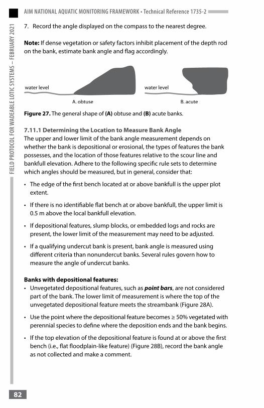
AIM NATIONAL AQUATIC MONITORING FRAMEWORK • Technical Reference 1735-2FI
ELD
PROT
OCOL
FOR
WAD
EABL
E LOT
IC SY
STEM
S – FE
BRUA
RY 2
021
82
7. Record the angle displayed on the compass to the nearest degree.
Note: If dense vegetation or safety factors inhibit placement of the depth rod on the bank, estimate bank angle and flag accordingly.
Figure 27. The general shape of (A) obtuse and (B) acute banks.
7.11.1 Determining the Location to Measure Bank AngleThe upper and lower limit of the bank angle measurement depends on whether the bank is depositional or erosional, the types of features the bank possesses, and the location of those features relative to the scour line and bankfull elevation. Adhere to the following specific rule sets to determine which angles should be measured, but in general, consider that:
• The edge of the first bench located at or above bankfull is the upper plot extent.
• If there is no identifiable flat bench at or above bankfull, the upper limit is 0.5 m above the local bankfull elevation.
• If depositional features, slump blocks, or embedded logs and rocks are present, the lower limit of the measurement may need to be adjusted.
• If a qualifying undercut bank is present, bank angle is measured using different criteria than nonundercut banks. Several rules govern how to measure the angle of undercut banks.
Banks with depositional features:• Unvegetated depositional features, such as point bars, are not considered
part of the bank. The lower limit of measurement is where the top of the unvegetated depositional feature meets the streambank (Figure 28A).
• Use the point where the depositional feature becomes ≥ 50% vegetated with perennial species to define where the deposition ends and the bank begins.
• If the top elevation of the depositional feature is found at or above the first bench (i.e., flat floodplain-like feature) (Figure 28B), record the bank angle as not collected and make a comment.

AIM NATIONAL AQUATIC MONITORING FRAMEWORK • Technical Reference 1735-2FIELD PROTOCOL FOR W
ADEABLE LOTIC SYSTEMS – FEBRUARY 2021
83
Figure 28A. Begin measuring the angle from the point where the deposition and bank meet (Archer et al. 2015).
Figure 28B. When the depositional feature covers the first flat bench (i.e., flat floodplain-like feature), do not measure an angle (Archer et al. 2015).
Erosional banks:1. If a fracture or slump is present (see Section 7.3.3 for definitions and
guidance), consider:
• If the connection point (i.e., where the fracture or slump meets the bank) is below the scour line, the lower limit of the measurement is the connection point (Figure 29B).
• If the connection point is above the scour line, the lower limit of the measurement is where bed-meets-bank (Figure 29A).
• Do not consider a slump that is not attached to the streambank.
Figure 29. Location of bank angle measurements with (A) a fracture still attached above the scour line and (B) a fracture still attached below the scour line (Archer et al. 2015).

AIM NATIONAL AQUATIC MONITORING FRAMEWORK • Technical Reference 1735-2FI
ELD
PROT
OCOL
FOR
WAD
EABL
E LOT
IC SY
STEM
S – FE
BRUA
RY 2
021
84
Figure 30. Measure undercut bank angle from the deepest point to the ceiling of the undercut; determine if the undercut has a qualifying depth (≥ 5 cm) by lowering the depth rod until it is horizontal (Archer et al. 2015).
Figure 31. Bank angle is typically measured at the deepest point of a qualifying undercut (angle A). However, if the depth of the back of the undercut is consistent, measure bank angle at the highest elevation of the undercut (angle B), not angle A (Archer et al. 2015).
2. Undercut banks:• Qualifying undercut banks are measured from the deepest point of the
undercut to the bottom edge of the overhang (Figure 30).
- A qualifying undercut must be ≥ 5 cm deep, ≥ 10 cm high, and > 10 cm wide, and the ceiling of the undercut must be below the bankfull height. The idea is that you could “hide” a box of this size in the undercut, without being able to see it from above.
- Occasionally, the depth at the back of the undercut is consistent, thereby lacking a deepest point. In this case, measure bank angle at the highest elevation of the undercut, resulting in the smallest angle (Figure 31).
- Enter the angle as 1° if the deepest part of the undercut is elevationally above the ceiling of the undercut (Figure 32).
• Nonqualifying undercut banks (< 5 cm deep, < 10 cm high, and ≤ 10 cm wide) are acute bank angles and should be considered in the context of all other angles. See guidance in Section 7.11.2 to determine which angle(s) to measure.
• Undercut banks with a ceiling above bankfull should be measured from where bed-meets-bank to the outside edge of the undercut; the angle of the undercut is not considered since the undercut is above bankfull (Figure 33).
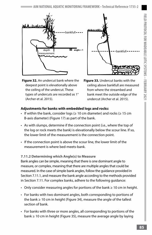
AIM NATIONAL AQUATIC MONITORING FRAMEWORK • Technical Reference 1735-2FIELD PROTOCOL FOR W
ADEABLE LOTIC SYSTEMS – FEBRUARY 2021
85
Adjustments for banks with embedded logs and rocks:• If within the bank, consider logs (≥ 10 cm diameter) and rocks (≥ 15 cm
B-axis diameter) (Figure 17) as part of the bank.
• As with slumps, determine if the connection point (i.e., where the top of the log or rock meets the bank) is elevationally below the scour line. If so, the lower limit of the measurement is the connection point.
• If the connection point is above the scour line, the lower limit of the measurement is where bed-meets-bank.
7.11.2 Determining which Angle(s) to MeasureBank angles can be simple, meaning that there is one dominant angle to measure, or complex, meaning that there are multiple angles that could be measured. In the case of simple bank angles, follow the guidance provided in Section 7.11.1, and measure the bank angle according to the methods provided in Section 7.11. For complex banks, adhere to the following guidance:
• Only consider measuring angles for portions of the bank ≥ 10 cm in height.
• For banks with two dominant angles, both corresponding to portions of the bank ≥ 10 cm in height (Figure 34), measure the angle of the tallest section of bank.
• For banks with three or more angles, all corresponding to portions of the bank ≥ 10 cm in height (Figure 35), measure the average angle by laying
Figure 32. An undercut bank where the deepest point is elevationally above the ceiling of the undercut. These types of undercuts are recorded as 1° (Archer et al. 2015).
Figure 33. Undercut banks with the ceiling above bankfull are measured from where the streambed and bank meet the outside edge of the undercut (Archer et al. 2015).

AIM NATIONAL AQUATIC MONITORING FRAMEWORK • Technical Reference 1735-2FI
ELD
PROT
OCOL
FOR
WAD
EABL
E LOT
IC SY
STEM
S – FE
BRUA
RY 2
021
86
the depth rod in a position where it is most representative of the overall bank angle.
Figure 34. Measure the bank angle corresponding to the highest portion of the bank when the bank has two dominant angles (Archer et al. 2015).
Figure 35. Measure the angle of banks with three or more angles by laying the rod along outer edges to best represent overall bank angle (Archer et al. 2015).
7.12 Thalweg Depth Profile (contingent)
Overview: Measure water depth along the thalweg for the entire sample reach. The spacing between thalweg depth measurements is a function of stream width. See Appendix C for guidance on how to take thalweg measurements in reaches with interrupted flow or in braided systems. Note, thalweg measurements should not be taken on side channels or in pools on the side of the main channel through which the thalweg does not flow. If continuous thalweg depth measurements are not taken along the entire reach, a thalweg depth measurement still needs to be taken at each transect in order to compute floodplain connectivity.

AIM NATIONAL AQUATIC MONITORING FRAMEWORK • Technical Reference 1735-2FIELD PROTOCOL FOR W
ADEABLE LOTIC SYSTEMS – FEBRUARY 2021
87
Guidance for determining where to measure thalweg depths: The location of the thalweg can be identified using the criteria in Section 2.2.4. Once the thalweg is identified, depth measurements are taken at one-sixteenth of transect spacing. For example, a reach of 150 m has transects every 15 m, and the thalweg will be measured every 94 cm.
Methods: 1. Starting at transect A, use a depth rod to locate the deepest point within
the thalweg, which may not always be found at mid-channel.
2. Measure water depth (from the streambed surface to the water surface) with the depth rod to the nearest cm. Read the depth on the side of the rod to avoid inaccuracies caused by holding the rod in moving water.
3. Use a depth rod, stadia rod, or tape measure to estimate or measure the distance to the next thalweg measurement location.
4. Record the presence/absence of flowing water at each thalweg measurement. If water is completely absent, record a thalweg depth of 0.
5. Repeat steps 1-4 until you reach the next main or intermediate transect.
6. Once thalweg measurements have been completed between all main and intermediate transects, measurements are complete.
7. Note that completing all thalweg measurements is critical for analysis. Make every attempt to estimate and record each measurement, rather than skipping a measurement and leaving it blank. Even an estimate to the nearest 0.5 m is better than no data, as long as it is appropriately recorded as an estimated measurement.
If the thalweg is too deep to measure directly, follow this procedure: 1. Stand in shallower water, and extend the stadia rod at an angle to reach
the maximum thalweg depth.
2. Determine the angle by resting the compass on the upper surface of the rod and reading the angle on the external scale of the clinometer on the compass.
3. Record the water depth on the rod and the rod angle.
Note: If the current is too fast or other conditions preclude the angle method for measuring depth, estimate depth based on measurements you are able to take and flag the measurements as estimated.

AIM NATIONAL AQUATIC MONITORING FRAMEWORK • Technical Reference 1735-2FI
ELD
PROT
OCOL
FOR
WAD
EABL
E LOT
IC SY
STEM
S – FE
BRUA
RY 2
021
88
8. Riparian Vegetation
Overview: The core method for riparian vegetation involves determining the presence/absence of priority noxious vegetation among 22 plots. The contingent methods involve determining the presence/absence of priority native woody riparian vegetation among 22 plots and assessing greenline vegetation composition across 80 plots. See Appendix C for guidance on measuring riparian vegetation when side channels are present. See Appendix H for riparian vegetation protocol differences for Alaska.
8.1 Priority Noxious (core) and Priority Native Woody Riparian (contingent) Vegetation
Plot size and location:The area of a vegetation plot is 10 m x 10 m, centered on each main transect (i.e., 5 m upstream and 5 m downstream). The plot starts at the scour line and extends 10 m away from the scour line, even if the extent of the plot is beyond that of riparian vegetation. All sides of the plot are straight lines, except the edge bordering the stream, which follows the contour of the scour line (Figure 36). Estimate the distance into the riparian zone from the scour line as if it were projected down from an aerial view. If side channels are present, see Appendix C for guidance on defining plots and recording measurements. If vegetation plots overlap in aerial extent (e.g., small sinuous streams), assess each plot independently.
Species lists:BLM state leads and field personnel developed standardized lists of both priority noxious species and priority native woody species. Priority native lists are restricted to woody species and sedges and rushes only, but priority noxious species lists encompass: noxious woody, noxious herbaceous, and noxious aquatic (i.e., obligate) species.
Prior to protocol implementation, data collectors should ensure proficiency in identification of the priority species for their respective state.
Methods:1. Stand at the scour line, and visually establish the 10 m x 10 m vegetation
plot (Figure 36). If you cannot see the full depth of the plot (e.g., distance of 10 m from the scour line), move from the scour line to obtain a better view. If you cannot safely view the plot, record as not collected.

AIM NATIONAL AQUATIC MONITORING FRAMEWORK • Technical Reference 1735-2FIELD PROTOCOL FOR W
ADEABLE LOTIC SYSTEMS – FEBRUARY 2021
89
2. Walk around the plot to assess the presence/absence (rooted in or overhanging the plot) of priority noxious species. Record each priority noxious species present.
a. For noxious aquatic species (riparian obligates), assess presence/absence in the 10 m x 10 m vegetation plot (rooted in or overhanging the plot), but also extend the plot to the center of the streambed (Figure 36).
b. For all identified noxious species, it is recommended to collect voucher specimens and/or photos for verification by local BLM field staff the first time a species is identified.
3. Walk around the vegetation plot to assess the presence/absence of priority native woody riparian species and sedges and rushes. Record each priority native woody riparian species and sedges and rushes present in the plot.
4. Repeat steps 1-3 for the opposite bank, and continue repeating steps 1-3 until all measurements are collected along all main transects.
5. Assessing plots for the presence/absence of priority vegetation should be rapid and take between 1 and 2 minutes per plot unless time is needed to research and verify vegetation identifications.
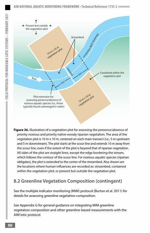
AIM NATIONAL AQUATIC MONITORING FRAMEWORK • Technical Reference 1735-2FI
ELD
PROT
OCOL
FOR
WAD
EABL
E LOT
IC SY
STEM
S – FE
BRUA
RY 2
021
90
Figure 36. Illustration of a vegetation plot for assessing the presence/absence of priority noxious and priority native woody riparian vegetation. The area of the vegetation plot is 10 m x 10 m, centered on each main transect (i.e., 5 m upstream and 5 m downstream). The plot starts at the scour line and extends 10 m away from the scour line, even if the extent of the plot is beyond that of riparian vegetation. All sides of the plot are straight lines, except the edge bordering the stream, which follows the contour of the scour line. For noxious aquatic species (riparian obligates), the plot is extended to the center of the streambed. Also shown are the locations where human influences are recorded as: streambed, contained within the vegetation plot, or present but outside the vegetation plot.
8.2 Greenline Vegetation Composition (contingent)
See the multiple indicator monitoring (MIM) protocol (Burton et al. 2011) for details for assessing greenline vegetation composition.
See Appendix G for general guidance on integrating MIM greenline vegetation composition and other greenline-based measurements with the AIM lotic protocol.

AIM NATIONAL AQUATIC MONITORING FRAMEWORK • Technical Reference 1735-2FIELD PROTOCOL FOR W
ADEABLE LOTIC SYSTEMS – FEBRUARY 2021
91
9. Human Influence (covariate)
Overview: Visually estimate the amount of human influence at all 11 main transects on both the left and right banks. Human influences are assessed both within and outside the defined vegetation plot area and are recorded by proximity to the stream (Figure 36). See Appendix C for guidance on assessing human influence when side channels are present.
Methods:Human influences are considered present if they can be seen while standing in the 10 m x 10 m vegetation plot. The same human influence may be marked present at more than one transect but should not be counted again if it must be sighted through another transect or vegetation plot.
1. Stand in the middle of the stream, and examine the streambed, bank, and 10 m x 10 m vegetation plot area adjacent to the stream for the following human influences. If you cannot see the full vegetation plot area from the middle of the stream, also walk in the plot.
• Wildfire (natural or human caused)• Row crops • Pastures, hay fields, fences • Presence of livestock or wild horses and burros, including feces,
cropped vegetation, or trails from grazing• Logging operations• Mining (e.g., gravel, open pit, placer mining) • Oil and gas wells and associated well pads• Walls, dikes, or bank stabilization structures such as riprap• Inlet or outlet pipes • Instream habitat restoration (e.g., gabion rock baskets, cabled large
wood, beaver dam analog structures)• Hydrologic alterations (irrigation diversions, impoundments, dams) • Utility/powerline/pipeline corridor• Buildings• Pavement/cleared lots (e.g., paved, graveled, dirt parking lot or
foundation) • Roads or railroads, including culverts • Landfills or trash (e.g., cans, bottles, trash heaps) • Parks or maintained lawns • Recreation (e.g., off-highway vehicle use, camping, trails, boating)
2. For each type of influence that is detected, determine its proximity to the stream and vegetation plot area (Figure 36). Proximity classes are:

AIM NATIONAL AQUATIC MONITORING FRAMEWORK • Technical Reference 1735-2FI
ELD
PROT
OCOL
FOR
WAD
EABL
E LOT
IC SY
STEM
S – FE
BRUA
RY 2
021
92
• Streambed: Present within the defined 10-m stream segment (5 m up- and downstream of the transect) and located in the streambed (i.e., within scour line on left bank to scour line on right bank). For the “streambed” class, all land and water from the centerline of the stream channel to the edge of the scour line is considered.
• Contained: Present within the 10 m x 10 m vegetation plot area but not located in the streambed (i.e., within scour line on left bank to scour line on right bank)
• Present: Present but outside the vegetation plot area.
• Absent: Not present within or adjacent to the 10-m stream segment or the vegetation plot area at the transect.
3. Repeat steps 1-2 for the opposite bank, and continue repeating steps 1-2 until human influence is evaluated along all main transects.
Note: If the vegetation plot extends over a meander bend and contains water from the main channel, mark the observed human influence as “contained” within the plot or “present” outside the plot.
AIM NATIONAL AQUATIC MONITORING FRAMEWORK • Technical Reference 1735-2FIELD PROTOCOL FOR W
ADEABLE LOTIC SYSTEMS – FEBRUARY 2021
93
10. Photos (covariate)
Overview: Photo documentation provides valuable insight regarding the overall character of the sample reach, changes through time, verification of critical concepts, and data interpretation. Therefore, it is important to accurately capture reach character at the time of sampling.
Take a minimum of 19 representative photos of each sample reach and a minimum of four photos of each failed reach. Failed reach photos should include the first four photos listed below, where possible. Photos should include:
• Bottom of the reach (transect A), facing upstream.• F transect.• Top of the reach (transect K), facing downstream.• Overview containing as much of the reach as possible. • Three monumenting photos and an aerial image that can be annotated
to assist subsequent data collectors with relocating the sample reach (see section 4.2, “Monumenting or Relocating Sample Reaches”).
• Two photos (plus annotated copies) identifying scour line, bankfull, and bench features: one closeup photo of the bank and one farther away with both banks visible.
• Two flood-prone width photos: one at each location where flood-prone width is measured (photos are taken looking upstream or downstream).
• Representative bank stability and cover plot indicating the lower and upper extent of the plot for both an erosional and depositional bank type. If no depositional banks are present, take two photos of erosional bank plot locations.
• Representative bank erosional features such as fractures, slumps, sloughs, or eroding banks.
• Two additional photos that do at least one of the following: - Represent the reach in ways that the previous photos do not portray. - Display special situations such as side channels, interrupted flow, or
beaver impacts (see Appendix C for more specific guidance). - Display impacts or signs of degradation to the stream or riparian area
(e.g., head cuts, excessive grazing, recreation). - Show features that created challenges for protocol implementation.
Adhere to the following guidelines to capture high-quality photos: • A 1.5-m depth rod should be present in all photos to provide scale. • Photos should be taken at the height of a depth rod unless environmental
conditions demand otherwise.• Do not use the zoom feature in any photos.

AIM NATIONAL AQUATIC MONITORING FRAMEWORK • Technical Reference 1735-2FI
ELD
PROT
OCOL
FOR
WAD
EABL
E LOT
IC SY
STEM
S – FE
BRUA
RY 2
021
94
• Avoid taking photos looking into the sun; try to take photos with the sun at your back.
• Try to avoid taking photos where part of the frame is in the shadows and part in the sun.
• Do not take photos of unprofessional behavior. • Sometimes photos must be taken with a device that does not use the data
collection application. For example, if an iPad battery is low, data collectors may use their phones to take photos, in which case photos are uploaded to the application later. Another example includes annotating critical concept photos before uploading them to the application. In circumstances such as these, it is important to upload the raw photos in their native resolution and quality. Do not upload reduced quality or resolution photos. If photos are taken on another device, do not delete the photos until you have confirmed with the national AIM team that all of the photos were uploaded at the maximum file size.
10.1 General Photo Methods
1. Considering stream size, vegetation, and sunlight, decide if it will be best to take the photograph looking upstream, downstream, or at a cross section.
2. Place or hold a depth rod within the frame of the photo for scale. Make note of the location of the depth rod (or other item for scale) in the photo (e.g., right bank at transect C).
3. Stand approximately 5 m from the depth rod and in a location where the photo will capture both banks. Do not zoom in for any photos.
4. Hold a depth rod vertically, set the camera on top of the depth rod, and take a photo.
5. Any photos pertinent to data collection should be taken within or uploaded to the data collection application. These photos will be automatically named and uploaded to the national AIM team with the rest of the field data.
a. If photos are taken outside the data collection application with the photos app, they should be uploaded to the app so that they are automatically named with the PointID and sent to the national AIM team.
b. It can also be helpful to take screenshots of the iPad screen and upload them into the app. This can be useful for navigation or recording app errors. Screenshots can be taken by holding down the power button and the home button at the same time and then releasing.

AIM NATIONAL AQUATIC MONITORING FRAMEWORK • Technical Reference 1735-2FIELD PROTOCOL FOR W
ADEABLE LOTIC SYSTEMS – FEBRUARY 2021
95
6. Preview the photo on the screen to ensure key elements are captured. If the photo did not turn out well, delete it and try again.
7. For all photos, record the following information.
a. Photo location or type (e.g., bottom of the reach, F transect, top of the reach, monument, overview, other).
b. Direction facing (upstream, cross section, downstream).
c. Letter of the closest transect.
8. Repeat steps 1-7 for all necessary photos.
10.2 Reach Overview Photo Methods
The purpose of taking reach overview photos is to capture the ecological and geomorphic context of the reach. Take reach overview photos from a location where as much of the reach is visible in the photo as possible. Ideally, reach overview photos should be taken from a hillside that overlooks the reach, but this will not always be practical.
10.3 Monument Photo Methods
The purpose of taking monument photos is to help data collectors relocate the F transect and F transect monument feature. See Section 4.2 for more information on monumenting or relocating sample reaches.
1. Take the following photos.
a. Stand at the F transect, and photograph the F transect monument feature. If you cannot see the monument feature from the F transect, stand as close to the F transect as possible while still seeing the feature.
b. Stand at the F transect monument, and photograph the location of the F transect. To help identify the F transect location in the photo, hang flagging at or near the F transect, and ensure the flagging is visible in the photo.
c. Stand so that you can capture both the F transect monument feature and F transect in the same photo. To help identify the F transect location in the photo, hang flagging at or near the F transect, and ensure the flagging is visible in the photo.
d. Annotate an aerial image taken from Google Earth or another source with the locations of the F transect, F transect monument feature, and any other unique features to assist data collectors in relocating the F transect (Figure 37).

AIM NATIONAL AQUATIC MONITORING FRAMEWORK • Technical Reference 1735-2FI
ELD
PROT
OCOL
FOR
WAD
EABL
E LOT
IC SY
STEM
S – FE
BRUA
RY 2
021
96
Figure 37. Annotated aerial image of a monumented reach. The corresponding monument narrative reads: “The F transect monument is approximately 67 meters northwest from the dirt parking area. Wrap around the base of the hill to the bottom of the first rock rib (i.e., F transect monument) coming down the hillside. Traverse approximately 76 meters upstream and northwest along the willows from the base of the rock rib to the F transect, which is located three-quarters of the way up the long riffle. The K transect is in a riffle just upstream of a big meander bend. The A transect is in the riffle adjacent to the big unvegetated point bar, slightly northeast from the parking area.”
10.4 Critical Concept Photo Methods
The purpose of critical concept photos is to ensure that geomorphic features are properly identified in the field and to assist with data quality control. New data collectors should review these photos with their project lead or crew supervisor after each trip.
1. Find a location within the reach with clear scour line, bankfull, and bench features. Note, multiple locations and photos may be needed if one location does not clearly represent all three features.
2. For scale, place a depth rod vertical next to the bank so that depth rod measurements can be read in the photo. It may be useful to have another depth rod pointing to features in photos.
3. Take at least two photos: one closeup photo focused on the bank and one in which both banks are visible so that geomorphic features can be traced up and down the reach. Take additional photos as needed so the diversity of the reach is adequately characterized.
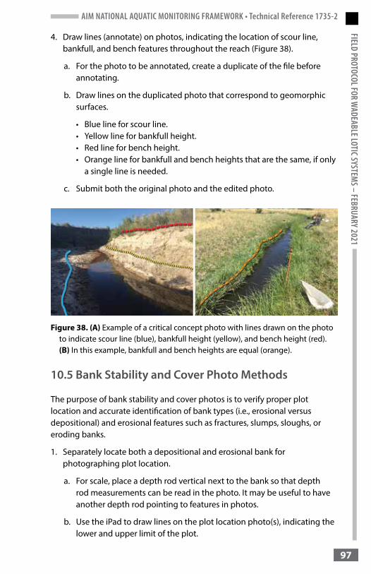
AIM NATIONAL AQUATIC MONITORING FRAMEWORK • Technical Reference 1735-2FIELD PROTOCOL FOR W
ADEABLE LOTIC SYSTEMS – FEBRUARY 2021
97
4. Draw lines (annotate) on photos, indicating the location of scour line, bankfull, and bench features throughout the reach (Figure 38).
a. For the photo to be annotated, create a duplicate of the file before annotating.
b. Draw lines on the duplicated photo that correspond to geomorphic surfaces.
• Blue line for scour line.• Yellow line for bankfull height.• Red line for bench height. • Orange line for bankfull and bench heights that are the same, if only
a single line is needed.
c. Submit both the original photo and the edited photo.
Figure 38. (A) Example of a critical concept photo with lines drawn on the photo to indicate scour line (blue), bankfull height (yellow), and bench height (red). (B) In this example, bankfull and bench heights are equal (orange).
10.5 Bank Stability and Cover Photo Methods
The purpose of bank stability and cover photos is to verify proper plot location and accurate identification of bank types (i.e., erosional versus depositional) and erosional features such as fractures, slumps, sloughs, or eroding banks.
1. Separately locate both a depositional and erosional bank for photographing plot location.
a. For scale, place a depth rod vertical next to the bank so that depth rod measurements can be read in the photo. It may be useful to have another depth rod pointing to features in photos.
b. Use the iPad to draw lines on the plot location photo(s), indicating the lower and upper limit of the plot.

AIM NATIONAL AQUATIC MONITORING FRAMEWORK • Technical Reference 1735-2FI
ELD
PROT
OCOL
FOR
WAD
EABL
E LOT
IC SY
STEM
S – FE
BRUA
RY 2
021
98
c. If only erosional banks are present, take two different photos of plot location for erosional banks.
2. Locate bank erosional features such as fractures, slumps, sloughs, or eroding banks throughout the reach, and photograph a minimum of one of each type of feature.
a. For scale, place a depth rod vertical next to the bank so that depth rod measurements can be read in the photo. It may be useful to have another depth rod pointing to features in photos.
10.6 Flood-Prone Width Photo Methods
The purpose of flood-prone width photos is to characterize the transect and valley bottom geometry where flood-prone width measurements are taken.
1. Take at least one photo of each location where flood-prone width is measured: photos are taken looking upstream or downstream. For the photo(s), try to capture the water surface, both left and right banks, and any benches present.

AIM NATIONAL AQUATIC MONITORING FRAMEWORK • Technical Reference 1735-2FIELD PROTOCOL FOR W
ADEABLE LOTIC SYSTEMS – FEBRUARY 2021
99
11. Gear Decontamination
Overview: To prevent the spread of aquatic invasive species, decontaminate waders and all equipment that came into contact with the water after every sample reach. Gear decontamination will be conducted in the field with a dilute solution prior to sampling a new reach. At the end of each trip, gear decontamination can occur in the field or upon returning to town. A default gear decontamination protocol is provided, but users should consult with BLM field offices for local recommendations.
Methods:1. The recommended disinfectant is Super HDQ Neutral. A concentration of
0.4% is required for effective decontamination with this chemical. This can be obtained with 3.1 ounces of Super HDQ Neutral per gallon of water (e.g., a 5-gallon jug of water requires 15.5 ounces of Super HDQ Neutral).
a. If an alternative disinfectant is used, follow manufacturer specifications for preventing the spread of invasive species, such as New Zealand mudsnails, Myxobolus cerebralis (which causes whirling disease), and rock snot.
2. Prior to leaving for the field, mix the solution in a well-sealed 5-gallon jug (labeled toxic). When it is time to disinfect equipment, pour the mixture contained in the 5-gallon jug into a much larger tote bin (at least 10 gallons) for gear decontamination.
3. Debris, mud, and vegetation must be cleaned off equipment and waders before placing in the decontamination solution.
4. Soak all gear items (e.g., waders, boots, bug nets) for at least 10 minutes in the solution or following manufacturer recommendations.
5. When decontamination is complete, allow gear to air dry. If possible, rinse gear with clean tap water to protect equipment from degradation caused by repeated exposure.
6. Pour the Super HDQ Neutral solution back into its designated container, using a funnel to minimize skin contact.
7. Muddy gear or repeated use of the solution can reduce its efficacy, and the mixture may need to be replaced. To check the effectiveness of the solution, make a 1:5 mixture of the solution and water (1 cup solution to 5 cups water). Then, use “Quat Check 1000” strips to ensure the solution is ≥ 600 ppm. If it is < 600 ppm, the solution must be replaced (step 1).
AIM NATIONAL AQUATIC MONITORING FRAMEWORK • Technical Reference 1735-2FI
ELD
PROT
OCOL
FOR
WAD
EABL
E LOT
IC SY
STEM
S – FE
BRUA
RY 2
021
100
8. Discard used Super HDQ Neutral solution down a drain that leads to a wastewater treatment facility. Run a faucet or hose while pouring down a drain. Do not pour into waterways or storm sewers.
11.1 Safety Precautions
Overview: Concentrated Super HDQ Neutral has toxic ingredients and:
1. Is harmful if swallowed.
2. Is harmful if inhaled.
3. Can cause severe skin burns and serious eye damage.
4. May cause an allergic reaction of the skin.
When handling concentrated or diluted Super HDQ Neutral solution, be sure to wear proper personal protective equipment. It is strongly advised that concentrated Super HDQ Neutral not be taken into the field and that diluted solutions are only mixed prior to leaving for the field where running water and emergency medical care is readily accessible. Do not repackage Super HDQ Neutral; if a hazardous level of exposure occurs, the label will be readily available to provide to an emergency responder or poison control center.
Follow these guidelines to avoid harmful exposure:1. Mix concentrate prior to leaving for the field.
2. Make sure to wear chemical-resistant gloves, eye protection, boots, and long sleeves when mixing concentrate and decontaminating equipment.
3. Wash hands and any exposed skin thoroughly after handling.
4. Do not eat, drink, or smoke when using this product.
5. Use only outdoors or in a well-ventilated area.
6. Do not breathe mist vapors or spray.
In case of exposure:• If in the eyes, rinse with water for several minutes.
• If swallowed, rinse mouth. Do not induce vomiting. Contact poison control if necessary.
• If inhaled, move to fresh air, and keep at rest in a position comfortable for breathing.
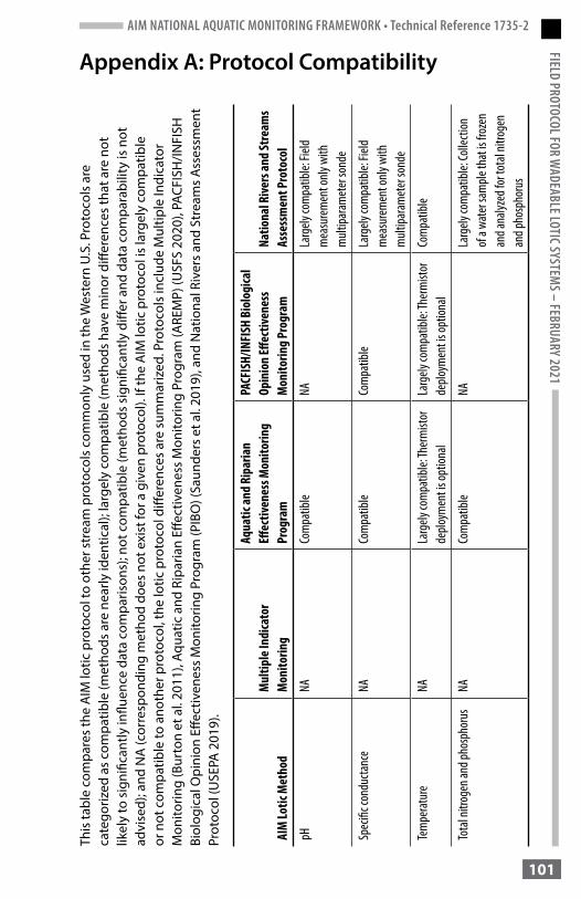
AIM NATIONAL AQUATIC MONITORING FRAMEWORK • Technical Reference 1735-2FIELD PROTOCOL FOR W
ADEABLE LOTIC SYSTEMS – FEBRUARY 2021
101
Appendix A: Protocol CompatibilityTh
is ta
ble
com
pare
s th
e A
IM lo
tic p
roto
col t
o ot
her s
trea
m p
roto
cols
com
mon
ly u
sed
in th
e W
este
rn U
.S. P
roto
cols
are
ca
tego
rized
as
com
patib
le (m
etho
ds a
re n
early
iden
tical
); la
rgel
y co
mpa
tible
(met
hods
hav
e m
inor
diff
eren
ces
that
are
not
lik
ely
to s
igni
fican
tly in
fluen
ce d
ata
com
paris
ons)
; not
com
patib
le (m
etho
ds s
igni
fican
tly d
iffer
and
dat
a co
mpa
rabi
lity
is n
ot
advi
sed)
; and
NA
(cor
resp
ondi
ng m
etho
d do
es n
ot e
xist
for a
giv
en p
roto
col).
If th
e A
IM lo
tic p
roto
col i
s la
rgel
y co
mpa
tible
or
not
com
patib
le to
ano
ther
pro
toco
l, th
e lo
tic p
roto
col d
iffer
ence
s ar
e su
mm
ariz
ed. P
roto
cols
incl
ude
Mul
tiple
Indi
cato
r M
onito
ring
(Bur
ton
et a
l. 20
11),
Aqua
tic a
nd R
ipar
ian
Effec
tiven
ess
Mon
itorin
g Pr
ogra
m (A
REM
P) (U
SFS
2020
), PA
CFIS
H/IN
FISH
Bi
olog
ical
Opi
nion
Effe
ctiv
enes
s M
onito
ring
Prog
ram
(PIB
O) (
Saun
ders
et a
l. 20
19),
and
Nat
iona
l Riv
ers
and
Stre
ams
Ass
essm
ent
Prot
ocol
(USE
PA 2
019)
.
AIM
Lotic
Met
hod
Mul
tiple
Indi
cato
r M
onito
ring
Aqua
tic an
d Ri
paria
n Eff
ectiv
enes
s Mon
itorin
g Pr
ogra
m
PACF
ISH/
INFI
SH B
iolo
gica
l Op
inio
n Eff
ectiv
enes
s M
onito
ring
Prog
ram
Natio
nal R
ivers
and
Stre
ams
Asse
ssm
ent P
roto
col
pHNA
Com
patib
leNA
Larg
ely co
mpa
tible:
Field
m
easu
rem
ent o
nly w
ith
mult
ipara
met
er so
nde
Spec
ific c
ondu
ctanc
eNA
Com
patib
leCo
mpa
tible
Larg
ely co
mpa
tible:
Field
m
easu
rem
ent o
nly w
ith
mult
ipara
met
er so
nde
Tem
pera
ture
NALa
rgely
com
patib
le: Th
erm
istor
de
ploym
ent i
s opt
ional
Larg
ely co
mpa
tible:
Ther
mist
or
deplo
ymen
t is o
ption
alCo
mpa
tible
Tota
l nitr
ogen
and p
hosp
horu
sNA
Com
patib
leNA
Larg
ely co
mpa
tible:
Colle
ction
of
a wa
ter s
ample
that
is fr
ozen
an
d ana
lyzed
for t
otal
nitro
gen
and p
hosp
horu
s
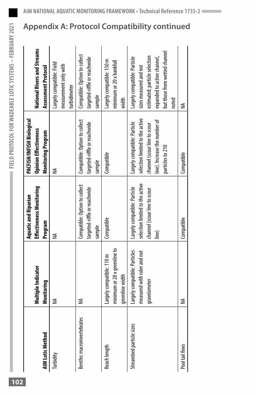
AIM NATIONAL AQUATIC MONITORING FRAMEWORK • Technical Reference 1735-2FI
ELD
PROT
OCOL
FOR
WAD
EABL
E LOT
IC SY
STEM
S – FE
BRUA
RY 2
021
102
AIM
Lotic
Met
hod
Mul
tiple
Indi
cato
r M
onito
ring
Aqua
tic an
d Ri
paria
n Eff
ectiv
enes
s Mon
itorin
g Pr
ogra
m
PACF
ISH/
INFI
SH B
iolo
gica
l Op
inio
n Eff
ectiv
enes
s M
onito
ring
Prog
ram
Natio
nal R
ivers
and
Stre
ams
Asse
ssm
ent P
roto
col
Turb
idity
NANA
NALa
rgely
com
patib
le: Fi
eld
mea
sure
men
t onl
y with
tu
rbidi
met
er
Bent
hic m
acro
inver
tebr
ates
NACo
mpa
tible:
Opt
ion to
colle
ct ta
rget
ed-ri
ffle o
r rea
chwi
de
sam
ple
Com
patib
le: O
ption
to co
llect
targ
eted
-riffl
e or r
each
wide
sa
mple
Com
patib
le: O
ption
to co
llect
targ
eted
-riffl
e or r
each
wide
sa
mple
Reac
h len
gth
Larg
ely co
mpa
tible:
110 m
m
inim
um or
20 x
gree
nline
to
gree
nline
widt
h
Com
patib
leCo
mpa
tible
Larg
ely co
mpa
tible:
150 m
m
inim
um or
20 x
bank
full
widt
h
Stre
ambe
d par
ticle
sizes
Larg
ely co
mpa
tible:
Parti
cles
mea
sure
d with
ruler
and n
ot
grav
elom
eter
Larg
ely co
mpa
tible:
Parti
cle
selec
tion l
imite
d to t
he ac
tive
chan
nel (
scour
line t
o sco
ur
line)
Larg
ely co
mpa
tible:
Parti
cle
selec
tion l
imite
d to t
he ac
tive
chan
nel (
scour
line t
o sco
ur
line)
. Incre
ase t
he nu
mbe
r of
parti
cles t
o 210
Larg
ely co
mpa
tible:
Parti
cle
sizes
mea
sure
d and
not
estim
ated
; par
ticle
selec
tion
expa
nded
to ac
tive c
hann
el,
but t
hose
from
wet
ted c
hann
el no
ted
Pool
tail fi
nes
NACo
mpa
tible
Com
patib
leNA
Appendix A: Protocol Compatibility continued
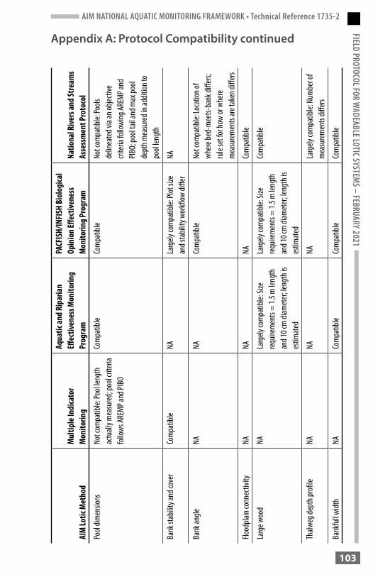
AIM NATIONAL AQUATIC MONITORING FRAMEWORK • Technical Reference 1735-2FIELD PROTOCOL FOR W
ADEABLE LOTIC SYSTEMS – FEBRUARY 2021
103
AIM
Lotic
Met
hod
Mul
tiple
Indi
cato
r M
onito
ring
Aqua
tic an
d Ri
paria
n Eff
ectiv
enes
s Mon
itorin
g Pr
ogra
m
PACF
ISH/
INFI
SH B
iolo
gica
l Op
inio
n Eff
ectiv
enes
s M
onito
ring
Prog
ram
Natio
nal R
ivers
and
Stre
ams
Asse
ssm
ent P
roto
col
Pool
dimen
sions
Not c
ompa
tible:
Pool
lengt
h ac
tuall
y mea
sure
d; po
ol cri
teria
fo
llows
AREM
P and
PIBO
Com
patib
leCo
mpa
tible
Not c
ompa
tible:
Pools
de
linea
ted v
ia an
objec
tive
crite
ria fo
llowi
ng AR
EMP a
nd
PIBO
; poo
l tail
and m
ax po
ol de
pth m
easu
red i
n add
ition
to
pool
lengt
h
Bank
stab
ility a
nd co
ver
Com
patib
leNA
Larg
ely co
mpa
tible:
Plot
size
an
d sta
bility
wor
kflow
diffe
r NA
Bank
angle
NANA
Com
patib
leNo
t com
patib
le: Lo
catio
n of
wher
e bed
-mee
ts-ba
nk di
ffers;
ru
le se
t for
how
or w
here
m
easu
rem
ents
are t
aken
diffe
rs
Flood
plain
conn
ectiv
ityNA
NANA
Com
patib
le
Larg
e woo
dNA
Larg
ely co
mpa
tible:
Size
re
quire
men
ts =
1.5 m
leng
th
and 1
0 cm
diam
eter
; leng
th is
es
timat
ed
Larg
ely co
mpa
tible:
Size
re
quire
men
ts =
1.5 m
leng
th
and 1
0 cm
diam
eter
; leng
th is
es
timat
ed
Com
patib
le
Thalw
eg de
pth p
rofil
eNA
NANA
Larg
ely co
mpa
tible:
Num
ber o
f m
easu
rem
ents
differ
s
Bank
full w
idth
NACo
mpa
tible
Com
patib
leCo
mpa
tible
Appendix A: Protocol Compatibility continued

AIM NATIONAL AQUATIC MONITORING FRAMEWORK • Technical Reference 1735-2FI
ELD
PROT
OCOL
FOR
WAD
EABL
E LOT
IC SY
STEM
S – FE
BRUA
RY 2
021
104
AIM
Lotic
Met
hod
Mul
tiple
Indi
cato
r M
onito
ring
Aqua
tic an
d Ri
paria
n Eff
ectiv
enes
s Mon
itorin
g Pr
ogra
m
PACF
ISH/
INFI
SH B
iolo
gica
l Op
inio
n Eff
ectiv
enes
s M
onito
ring
Prog
ram
Natio
nal R
ivers
and
Stre
ams
Asse
ssm
ent P
roto
col
Slope
NACo
mpa
tible
Com
patib
leLa
rgely
com
patib
le: Es
timat
ed
over
entir
e rea
ch an
d not
tra
nsec
t to t
rans
ect;
two r
each
-lon
g mea
sure
men
ts ta
ken t
o en
sure
estim
ate a
ccur
acy
Prior
ity no
xious
and p
riorit
y na
tive w
oody
ripar
ian
vege
tatio
n
NANA
NANA
Gree
nline
vege
tatio
n co
mpo
sition
Com
patib
leNA
Not c
ompa
tible
NA
Cano
py co
ver
NANo
t com
patib
le: D
ensio
met
er
used
as op
pose
d to s
olar
path
finde
r
NACo
mpa
tible
for c
ente
r rea
dings
; lar
gely
com
patib
le fo
r ban
k re
ading
s, wh
ich ar
e mea
sure
d wh
ere b
ed-m
eets-
bank
Flood
-pro
ne w
idth
NACo
mpa
tible
NANA
Appendix A: Protocol Compatibility continued
AIM NATIONAL AQUATIC MONITORING FRAMEWORK • Technical Reference 1735-2FIELD PROTOCOL FOR W
ADEABLE LOTIC SYSTEMS – FEBRUARY 2021
105
Appendix B: Glossary
active bench: flat depositional area adjacent to a stream or river formed by floods and subsequent sediment deposition under current climatic conditions. Active benches are inundated by overflow banks. This protocol uses the term active bench for a floodplain.
bankfull: the height on the streambanks where water fills the channel and begins to overflow onto the floodplain. This volume of flow occurs every 1.5 years on average and is the channel-forming flow.
baseflow: flow that is maintained in a stream or river channel from groundwater delivery to the channel. In many western rivers, baseflow is all water that is present during summer low flow conditions.
braided river or stream: river or stream that has multiple mid-channel bars below bankfull that form short and small subchannels, often with no obvious dominant channel.
contingent method: standardized procedure for collecting data with the same cross-program utility and definition as core methods but is measured only where applicable. Contingent methods are not expected to be informative or cost effective for every monitoring application and, thus, are only measured when there is reason to believe the resulting data will be important for management purposes.
core method: standardized procedure for collecting data that are applicable across many different ecosystems, management objectives, and agencies. Core lotic methods are recommended for application wherever the BLM implements monitoring and assessment of wadeable perennial streams.
covariate: measured or derived parameter used to account for natural spatial or temporal variation in a core, contingent, or supplemental method or indicator (e.g., gradient); covariates help determine the potential of a given stream or river reach to support a given condition or to assist in interpreting monitoring data.
cut bank: outside portion of a river bend or meander that is actively eroding and often near vertical in slope and/or has erosional features present (e.g., fracture, slump, eroding).

AIM NATIONAL AQUATIC MONITORING FRAMEWORK • Technical Reference 1735-2FI
ELD
PROT
OCOL
FOR
WAD
EABL
E LOT
IC SY
STEM
S – FE
BRUA
RY 2
021
106
ephemeral: a discharge pattern that is temporary, inconsistent, or infrequent through time. Ephemeral streams have less flow than intermittent streams and only flow in response to precipitation events. Definable scour line or bankfull features are not present, and there may be upland vegetation within the stream channel.
facultative vegetation: vegetation that has an equal likelihood of occurrence in wetlands or uplands.
facultative wet vegetation: vegetation usually occurring in wetlands or areas with high water tables.
hardpan: firm, consolidated fine sediment forming the stream bottom; fine sediment that has been compacted and/or wetted and dried to the point that it resembles bedrock.
inactive bench: a flat depositional area at an elevation such that it is no longer inundated during relatively frequent overbank flows. This protocol uses the term inactive bench for a terrace or an abandoned floodplain.
intermittent: a discharge pattern that is not continuous on an annual basis. Intermittent streams have flowing water during the wet season or following spring snowmelt. For intermittent streams, the channel may not be as well-defined as those observed for perennial systems, but evidence of erosion and deposition must be present, such as scour line, bankfull width, and point bars. Note that for field purposes, intermittent reaches in this protocol are reaches that have < 5 transects with water at the time of visit (constrained to the index period of June 1 through September 30, unless otherwise noted) but have definable erosional and deposition features, such as those previously listed.
islands: stream sediment deposits found in the active channel that have an elevation above bankfull; islands are almost always vegetated.
left and right bank: left and right bank are determined when facing downstream.
meander: a bend in a stream or river.
AIM NATIONAL AQUATIC MONITORING FRAMEWORK • Technical Reference 1735-2FIELD PROTOCOL FOR W
ADEABLE LOTIC SYSTEMS – FEBRUARY 2021
107
mid-channel bars: stream sediment deposits found in the active channel that have an elevation above the baseflow water level, but below the bankfull elevation. Mid-channel bars are almost always unvegetated. Individual boulders, regardless of size, do not qualify as mid-channel bars. Rather, an aggregation of deposited sediments is required.
obligate vegetation: vegetation that occurs almost exclusively in wetlands or areas with high water tables. Rarely found in uplands.
perennial: a discharge pattern that is continuous on an annual basis. Note, for the purposes of this field protocol, perennial streams are defined in a two-stage process. Potential perennial streams are identified using their flow classification in the National Hydrography Dataset, and then reaches must have ≥ 5 transects with water to be classified as perennial.
point bar: convex-shaped mounds of particles deposited by the stream and found on the inside bend of meanders at or below bankfull.
pool: streambed depression that is laterally and longitudinally concave (i.e., bowl shaped) and characterized by water that is slower and flatter than up- or downstream waters at baseflow. Pools are bound by a “head crest” (an upstream increase in streambed slope) and a “tail” (a downstream leveling of the streambed slope and reduction in depth). The pool tail is the shallowest downstream location in the pool from which water would spill if the flow were reduced to a trickle.
reach: the length of a stream over which data are collected. Reach lengths are a minimum of 150 m or 20 x bankfull width. Reach lengths are scaled to bankfull width to ensure adequate geomorphic diversity is sampled among streams of various sizes.
riffle: a length or portion of a stream or river that is locally steeper, shallower, and dominated by coarser streambed particles sizes than adjacent portions. The velocity is generally faster in riffles than adjacent portions and choppier on the surface.
scour line: the elevation of the ceiling of undercut banks at or slightly above the baseflow elevation and below the bankfull elevation. Scour line is often associated with the lower limit of sod-forming vegetation.
side channel: stream or river channel separated directly from the main channel by an island (not a mid-channel bar).

AIM NATIONAL AQUATIC MONITORING FRAMEWORK • Technical Reference 1735-2FI
ELD
PROT
OCOL
FOR
WAD
EABL
E LOT
IC SY
STEM
S – FE
BRUA
RY 2
021
108
sinuosity: ratio of channel length to valley length; curves departing from a linear course.
stain line: deposition of water precipitates, generally white, that forms over time on mineral streambed particles at a consistent elevation at or below bankfull.
supplemental method: standardized procedure for collecting data that are specific to a given ecosystem, land use, or management objective. No specific supplemental methods are recommended in this protocol, given the diversity of probable methods.
target population: in statistical surveys, the target population refers to the group of individuals or things that one seeks to make inference to (e.g., college freshman, wadeable streams in Utah, lakes less than 1 acre).
thalweg: the line along a stream channel (up- and downstream) connecting the lowest elevations or deepest water depths. The thalweg would be the last portion of the stream or river to contain water if it were to dry up, and it tends to move back and forth across the stream channel.

AIM NATIONAL AQUATIC MONITORING FRAMEWORK • Technical Reference 1735-2FIELD PROTOCOL FOR W
ADEABLE LOTIC SYSTEMS – FEBRUARY 2021
109
Appendix C: Special Situations
C1. Interrupted Flow
Overview: Reaches with interrupted flow have some portion of the reach that is dry, but 5 or more transects have at least standing water. Field methods at these reaches differ for transects without water and for reachwide measurements. Make sure to record which transects were dry and which had water. Point coordinates for revisit reaches should not be moved to obtain more wet transects, even if the result is a nontarget reach.
Follow the modified methods for:• Reach setup: For dry sections of the reach, use the average of 5 bankfull
widths to determine reach length. Measure reach length along the center of the dry channel to establish the distance between transects. In areas with water, follow the original methods (measure along the thalweg). All 21 transects are established if ≥ 5 main transects have water.
• Water quality: If the F transect is dry, collect water quality at the next closest location that has flowing water > 10 cm deep and > 1 m2 surface area. Note that if only stagnant water is present throughout the reach, samples should still be taken and a comment should be made indicating such. Similarly, if only stagnant water is present at the F transect, but flowing water is present elsewhere within the reach, take samples where flowing water is present.
• Benthic macroinvertebrates: Only collect macroinvertebrates where water is present; the water can be stagnant. If there is not enough flow (or no flow), you may need to scoop the sample into the net. For targeted-riffle methods, collect a total of 8 Surber or kick net samples from wetted riffles, even if only one riffle is present. For reachwide methods, collect a total of 11 Surber or kick net samples. Collect samples at main transects where water is present. Collect the remainder of needed samples at intermediate transects, or collect multiple Surber or kick net samples at different locations along a main transect, as water allows, to obtain a total of 11 Surber or kick net samples. Record comments if the quality of the samples was affected by lack of flow in any way. In some instances, this might require collecting samples where transects were not established (e.g., very narrow channels).
• Wetted width: Record 0 at dry transects; follow original methods for transects with water.
AIM NATIONAL AQUATIC MONITORING FRAMEWORK • Technical Reference 1735-2FI
ELD
PROT
OCOL
FOR
WAD
EABL
E LOT
IC SY
STEM
S – FE
BRUA
RY 2
021
110
• Bankfull and bench height: At dry transects, measure the height from the deepest point in the stream channel along the transect. Follow original methods for transects with water.
• Pool dimensions: Only measure pools that have inflow at the head crest and outflow from the pool tail (even a trickle) to the nearest cm, following the original methods. Do not measure stagnant pools. Measure and record the lengths of pools that have flow. If flow is separated by a dry section, be sure to add the length of all flowing sections together when determining pool reach length. For example, if 70 m of the reach has flowing water, the pool reach length is 70 m.
• Pool tail fines: Only measure pool tail fines for pools that have both inflow at the head crest and outflow from the pool tail (even a trickle).
• Canopy cover: At dry transects, take left and right bank densiometer readings by holding the densiometer 0.3 m (30 cm) above the dry scour line. For center densiometer readings, take measurements at the center of the dry channel by holding the densiometer 0.3 m (30 cm) above the dry channel bed.
• Streambed particle sizes: Follow original methods, but classify all particles as being collected from “dry middle.”
• Slope: If the A or K transect is dry or not flowing, place the stadia rod at bankfull (instead of the water’s surface), and take slope measurements at bankfull for both A and K transects. If both the A and K transects have flowing water, follow original methods using the water’s surface for stadia rod placement.
• Thalweg depth profile: Record depths as 0 when the bed is dry. Record the depth of water for stagnant pools, but record that the water was not flowing. Follow original methods for areas with flow. Make sure to record which thalweg locations were and were not flowing.
• Flood-prone width: Strive to take measurements from representative riffles close to transects A and K that are oriented parallel to the valley in which they flow and have representative bankfull and bench heights. Riffle representativeness should take precedence over the presence of flowing water. For flood-prone height measurements, measure bankfull height from the deepest point of the stream channel and multiply by two. Use the standard protocol for the remaining measurements of flood-prone width.
• Follow original methods for: bankfull width, bank stability and cover, large wood, bank angle (contingent), priority noxious vegetation, priority native woody riparian vegetation (contingent), greenline vegetation composition (contingent), and human influence.
AIM NATIONAL AQUATIC MONITORING FRAMEWORK • Technical Reference 1735-2FIELD PROTOCOL FOR W
ADEABLE LOTIC SYSTEMS – FEBRUARY 2021
111
Additional tips:In rare instances, the flow status of transects can change during the course of sampling a reach. If this occurs, keep the following in mind.
• If stage height increases or decreases gradually (e.g., evapotranspiration losses) while sampling the reach within a day, continue sampling and provide relevant comments.
• If stage height changes overnight or abruptly (e.g., rain storm, dam release), retake the following measurements for the entire reach: wetted width, bankfull and bench heights, and thalweg.
C2. Side Channels
Overview: Use the following guidance when sampling a reach with one or more side channels. Data should be collected on side channels regardless of size or presence of water. However, data should only be collected on a single side channel per transect. If multiple side channels are present, select and sample the one with the widest bankfull width. A side channel is defined as:
• A channel separated from the main channel by an island (not a mid-channel bar).
• A continuous channel that diverges from and reconnects to the main channel. Both the diverging and reconnecting of a side channel does not need to occur within the sample reach.
• A channel that has geomorphic features of a perennial or intermittent stream. For example, a clear definable channel, identifiable bankfull features, point bars, and other depositional/erosional features may exist. Perennial vegetation should not be growing within and dominate the bed of the channel.
• Types of side channels:
- Major side channel: Meets all side channel criteria and contains 16-49% of the total flow.
- Minor side channel: Meets all side channel criteria and contains ≤ 15% of the total flow.
- Dry side channel: Meets all side channel criteria and does not have any flowing water. It may be completely dry or contain isolated nonflowing pools.
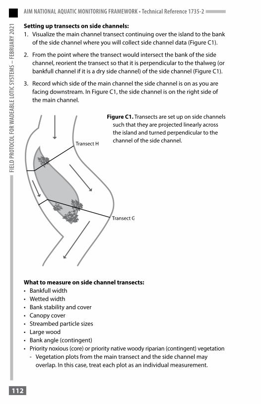
AIM NATIONAL AQUATIC MONITORING FRAMEWORK • Technical Reference 1735-2FI
ELD
PROT
OCOL
FOR
WAD
EABL
E LOT
IC SY
STEM
S – FE
BRUA
RY 2
021
112
Setting up transects on side channels: 1. Visualize the main channel transect continuing over the island to the bank
of the side channel where you will collect side channel data (Figure C1).
2. From the point where the transect would intersect the bank of the side channel, reorient the transect so that it is perpendicular to the thalweg (or bankfull channel if it is a dry side channel) of the side channel (Figure C1).
3. Record which side of the main channel the side channel is on as you are facing downstream. In Figure C1, the side channel is on the right side of the main channel.
Figure C1. Transects are set up on side channels such that they are projected linearly across the island and turned perpendicular to the channel of the side channel.
What to measure on side channel transects:• Bankfull width• Wetted width• Bank stability and cover • Canopy cover • Streambed particle sizes • Large wood• Bank angle (contingent) • Priority noxious (core) or priority native woody riparian (contingent) vegetation
- Vegetation plots from the main transect and the side channel may overlap. In this case, treat each plot as an individual measurement.

AIM NATIONAL AQUATIC MONITORING FRAMEWORK • Technical Reference 1735-2FIELD PROTOCOL FOR W
ADEABLE LOTIC SYSTEMS – FEBRUARY 2021
113
• Greenline vegetation (contingent)- The greenline follows the outside channel on each side of the island and
does not cross onto the island.• Human influence (covariate)
- If the vegetation plot extends beyond the island and contains water from the main channel, mark as “contained” or “present,” as appropriate.
Do not measure the following on side channels:• Benthic macroinvertebrates• Pool dimensions• Thalweg depth profile• Slope• Bankfull and bench heights• Pool tail fines
C3. Beaver-Impacted Reaches
Overview: If > 6 transects are impacted by beaver ponds, try to move the point coordinates so that 5 or more transects are not impacted. Impacted is defined as transects influenced by the presence of beaver dams, impounded water upstream of beaver dams, or altered geomorphology resulting from beaver pond formation and maintenance. If it is not possible to move the reach such that 5 or more transects are not inundated, the reach is not sampleable and should be classified as “reattempt” for status and “other” for reason not sampled (Section 3.2, Table 3).
Point coordinates for revisit reaches impacted by beaver dams should not be moved from the original location even if they were not previously impacted by beaver activity. Where relevant, seek to assess changes in chemical, physical, and biological conditions resulting from beaver activity.
Methods: 1. Reach setup
a. Orient transects that run across beaver ponds perpendicular to the thalweg of the beaver pond. If the thalweg cannot be identified, orient transects perpendicular to the pool’s center (Figure C2).
b. Note which transects are impacted by beavers using the comments field, and make sure to record the reach as influenced by beavers.
c. If multiple side channels exist, sample only the side channel with the widest bankfull width.
AIM NATIONAL AQUATIC MONITORING FRAMEWORK • Technical Reference 1735-2FI
ELD
PROT
OCOL
FOR
WAD
EABL
E LOT
IC SY
STEM
S – FE
BRUA
RY 2
021
114
d. If side channels exist and meet the requirements for sampling, follow the side channel protocol in Section C2 to determine if any additional channels should be sampled (but only if scour line and bankfull can be identified).
2. Photos: Take photos of the following features such that you can see as much of the feature as possible.
• The beaver dam, upstream and downstream.
• Overview of each beaver pool.
• Take all other photos as outlined in Section 10.
3. Water quality and temperature: Take measurements in a location with flowing water. Do not take water quality samples or measurements in or directly below a beaver pond.
4. Benthic macroinvertebrates
a. If riffles are present, distribute samples among riffles following standard procedures (Section 6), ensuring no riffles are impacted by beaver.
b. If riffles are not present and the reachwide protocol is being used, sample beaver ponds that are safe to wade and that do not have deep “bottomless” fine sediments.
c. Kick nets will frequently need to be used in beaver ponds as they can be very deep and have low flow. If kick nets are used, empty the net between each sample since the content can more easily fall out when sampling stagnant water.
d. If a transect cannot be sampled because it is not safe or too deep, move to sample an intermediate transect; all 11 samples need to be collected if the reachwide protocol is being used.
5. Pool dimensions: A beaver pond should be measured as a pool.
a. Use the top of the beaver dam on the downstream end of the pool as the pool tail. Record all pool tail measurements as 0 cm, unless there is flow over the top of the dam. In such instances, the water depth should be measured.
b. To define the head crest (upstream extent) of the beaver pool, look for:
• Flowing water of typical wetted width not impacted by beaver.
• A defined channel entering the pool of typical dimensions not impacted by beaver.
• Streambed particles typical of the reach not impacted by beaver.
• Standard head crest criteria identified in Section 7.7.
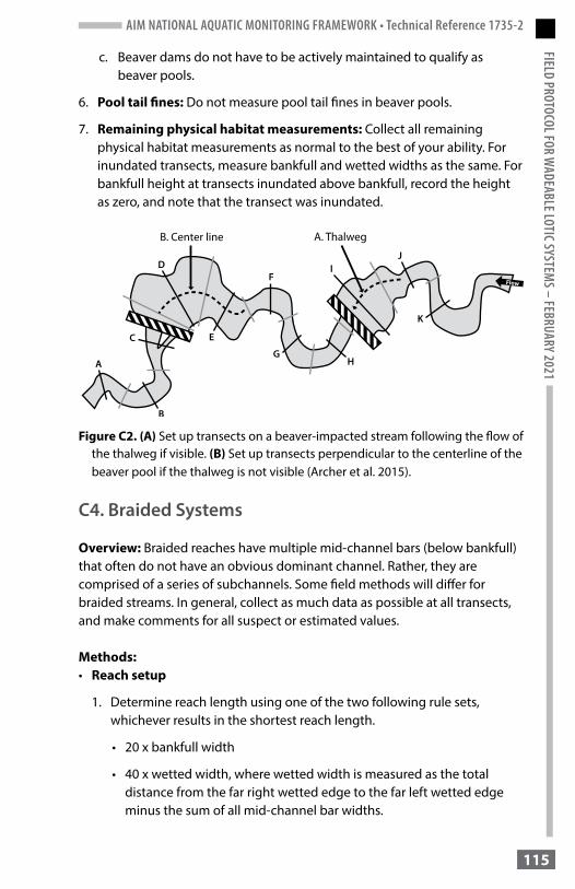
AIM NATIONAL AQUATIC MONITORING FRAMEWORK • Technical Reference 1735-2FIELD PROTOCOL FOR W
ADEABLE LOTIC SYSTEMS – FEBRUARY 2021
115
c. Beaver dams do not have to be actively maintained to qualify as beaver pools.
6. Pool tail fines: Do not measure pool tail fines in beaver pools.
7. Remaining physical habitat measurements: Collect all remaining physical habitat measurements as normal to the best of your ability. For inundated transects, measure bankfull and wetted widths as the same. For bankfull height at transects inundated above bankfull, record the height as zero, and note that the transect was inundated.
Figure C2. (A) Set up transects on a beaver-impacted stream following the flow of the thalweg if visible. (B) Set up transects perpendicular to the centerline of the beaver pool if the thalweg is not visible (Archer et al. 2015).
C4. Braided Systems
Overview: Braided reaches have multiple mid-channel bars (below bankfull) that often do not have an obvious dominant channel. Rather, they are comprised of a series of subchannels. Some field methods will differ for braided streams. In general, collect as much data as possible at all transects, and make comments for all suspect or estimated values.
Methods:• Reach setup
1. Determine reach length using one of the two following rule sets, whichever results in the shortest reach length.
• 20 x bankfull width
• 40 x wetted width, where wetted width is measured as the total distance from the far right wetted edge to the far left wetted edge minus the sum of all mid-channel bar widths.
AIM NATIONAL AQUATIC MONITORING FRAMEWORK • Technical Reference 1735-2FI
ELD
PROT
OCOL
FOR
WAD
EABL
E LOT
IC SY
STEM
S – FE
BRUA
RY 2
021
116
2. When establishing transects, follow the thalweg along the subchannel with the most flow. If all subchannels have similar flow, choose the most representative of the entire reach.
3. Flag each confluence and diffluence to ensure you sample the same subchannel for thalweg and pools throughout the reach.
• Benthic macroinvertebrates: Follow original methods, alternating among subchannels (separated by bars) for left, center, or right sampling locations. Do not alternate and sample in a side channel (separated by islands).
• Wetted width: Measure from the far right wetted edge to the far left wetted edge including all bars.
• Bar width: Add the widths of all mid-channel bars.
• Canopy cover: Measure center densiometer readings in the center of the wetted channel as defined by the far right wetted edge to the far left wetted edge, including bars. Follow original methods for all other densiometer measurements.
• Pool dimensions: Sample pools only in the channel used to set up the reach.
• Thalweg depth profile: Measure along the thalweg of the channel used to set up the reach.
• Scour line: Only identify scour line on the left and right banks.
Follow original methods for: water quality, bankfull width, bankfull and bench height, bank stability and cover, streambed particle sizes, large wood, slope, flood-prone width, bank angle (contingent), priority noxious vegetation, priority native woody riparian vegetation (contingent), greenline vegetation composition (contingent), pool tail fines (contingent), and human influence.
C5. Partial Data Collection
Overview: Field data collectors should always attempt to collect all data at any given reach. However, extenuating circumstances occasionally arise in which full data collection is not possible. There are usually two main situations in which field data collectors will collect partial data: (1) One or more of the 11 main and 10 intermediate transects are inaccessible (e.g., extremely dense vegetation impacting physical safety, dangerous rapids, limited portion of land managed by the BLM leading to shorter reach length than normal even after attempting to move the point coordinates); or (2) Insufficient time exists, and returning to the reach is not practical. Again, these situations should be rare and should not constitute more than 10–20% of your sample reaches per field season. Examples of circumstances that
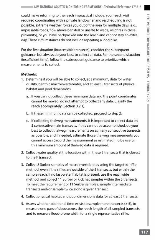
AIM NATIONAL AQUATIC MONITORING FRAMEWORK • Technical Reference 1735-2FIELD PROTOCOL FOR W
ADEABLE LOTIC SYSTEMS – FEBRUARY 2021
117
could make returning to the reach impractical include: your reach visit required coordinating with a private landowner and rescheduling is not possible, extreme weather forces you out of the area for multiple days (e.g., impassable roads, flow above bankfull or unsafe to wade, wildfires in close proximity), or you have backpacked into the reach and cannot stay an extra day. These circumstances do not include repeating a long hike.
For the first situation (inaccessible transects), consider the subsequent guidance, but always do your best to collect all data. For the second situation (insufficient time), follow the subsequent guidance to prioritize which measurements to collect.
Methods:1. Determine if you will be able to collect, at a minimum, data for water
quality, benthic macroinvertebrates, and at least 5 transects of physical habitat and pool dimensions.
a. If you cannot collect these minimum data and the point coordinates cannot be moved, do not attempt to collect any data. Classify the reach appropriately (Section 3.2.1).
b. If these minimum data can be collected, proceed to step 2.
c. If collecting thalweg measurements, it is important to collect data on 5 consecutive main transects. If this cannot be accomplished, do your best to collect thalweg measurements on as many consecutive transects as possible, and if needed, estimate those thalweg measurements you cannot access (record the measurement as estimated). To be useful, this minimum amount of thalweg data is required.
2. Collect water quality at the location within these 5 transects that is closest to the F transect.
3. Collect 8 Surber samples of macroinvertebrates using the targeted-riffle method, even if the riffles are outside of the 5 transects, but within the sample reach. If no fast-water habitat is present, use the reachwide method, and collect 11 Surber or kick net samples within the 5 transects. To meet the requirement of 11 Surber samples, sample intermediate transects and/or sample twice along a given transect.
4. Collect physical habitat and pool dimensions data for at least 5 transects.
5. Assess whether additional time exists to sample more transects (> 5), to measure one pass of slope across the reach length of all sampled transects, and to measure flood-prone width for a single representative riffle.

AIM NATIONAL AQUATIC MONITORING FRAMEWORK • Technical Reference 1735-2FI
ELD
PROT
OCOL
FOR
WAD
EABL
E LOT
IC SY
STEM
S – FE
BRUA
RY 2
021
118
a. If there is insufficient time to do all three, prioritize a slope measurement across the 5 sampled transects, then a measurement of flood-prone width, and do not sample additional transects. Record this information, and make a note about the reach length over which slope was measured.
b. If time exists to sample more transects and take at least a single slope and flood-prone width measurement, sample as many transects as possible including the collection of pool dimension data. Finish by measuring at least a single pass of slope of the total length of sampled reach and a flood-prone width measurement for a single representative riffle. Be sure to note the total reach length over which physical habitat and pool data were able to be collected.
6. When you have completed data collection, take GPS coordinates at the topmost (instead of at the top of the reach) and bottommost (instead of at the bottom of the reach) transects that were sampled.
7. Make notes about which data were and were not collected and why the data are incomplete.
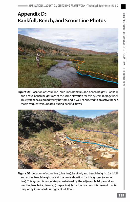
AIM NATIONAL AQUATIC MONITORING FRAMEWORK • Technical Reference 1735-2FIELD PROTOCOL FOR W
ADEABLE LOTIC SYSTEMS – FEBRUARY 2021
119
Appendix D: Bankfull, Bench, and Scour Line Photos
Figure D1. Location of scour line (blue line), bankfull, and bench heights. Bankfull and active bench heights are at the same elevation for this system (orange line). This system has a broad valley bottom and is well connected to an active bench that is frequently inundated during bankfull flows.
Figure D2. Location of scour line (blue line), bankfull, and bench heights. Bankfull and active bench heights are at the same elevation for this system (orange line). This system is moderately constrained by the adjacent hillslope and an inactive bench (i.e., terrace) (purple line), but an active bench is present that is frequently inundated during bankfull flows.
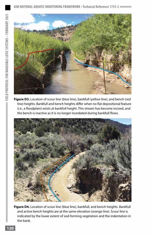
AIM NATIONAL AQUATIC MONITORING FRAMEWORK • Technical Reference 1735-2FI
ELD
PROT
OCOL
FOR
WAD
EABL
E LOT
IC SY
STEM
S – FE
BRUA
RY 2
021
120
Figure D3. Location of scour line (blue line), bankfull (yellow line), and bench (red line) heights. Bankfull and bench heights differ when no flat depositional feature (i.e., a floodplain) exists at bankfull height. This stream has become incised, and the bench is inactive as it is no longer inundated during bankfull flows.
Figure D4. Location of scour line (blue line), bankfull, and bench heights. Bankfull and active bench heights are at the same elevation (orange line). Scour line is indicated by the lower extent of sod-forming vegetation and the indentation in the bank.
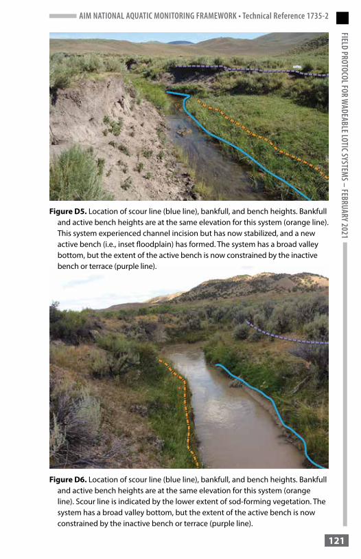
AIM NATIONAL AQUATIC MONITORING FRAMEWORK • Technical Reference 1735-2FIELD PROTOCOL FOR W
ADEABLE LOTIC SYSTEMS – FEBRUARY 2021
121
Figure D6. Location of scour line (blue line), bankfull, and bench heights. Bankfull and active bench heights are at the same elevation for this system (orange line). Scour line is indicated by the lower extent of sod-forming vegetation. The system has a broad valley bottom, but the extent of the active bench is now constrained by the inactive bench or terrace (purple line).
Figure D5. Location of scour line (blue line), bankfull, and bench heights. Bankfull and active bench heights are at the same elevation for this system (orange line). This system experienced channel incision but has now stabilized, and a new active bench (i.e., inset floodplain) has formed. The system has a broad valley bottom, but the extent of the active bench is now constrained by the inactive bench or terrace (purple line).

AIM NATIONAL AQUATIC MONITORING FRAMEWORK • Technical Reference 1735-2FI
ELD
PROT
OCOL
FOR
WAD
EABL
E LOT
IC SY
STEM
S – FE
BRUA
RY 2
021
122
Figure D7. Location of scour line (blue line), bankfull, and bench heights. Bankfull and active bench heights are at the same elevation for this system (orange line). This system is in a narrow canyon constrained by steep canyon walls. This system has narrow but well-established active benches that alternate between left and right banks.
Figure D8. Location of scour line (blue line), bankfull, and bench heights. Bankfull and active bench heights are at the same elevation for this system (orange line). Larger, low gradient systems generally have a higher sinuosity and form large point bars on the inside of meander bends. It is important to think “big” in these types of systems to ensure that the bankfull and scour line elevations are not underestimated. In this stream, the scour line is located at the top of the point bar and at the base of the bank (left side). This elevation corresponds to the lower extent of sod-forming vegetation on the right bank. The scour line in desert systems will commonly not be associated with sod-forming vegetation on both banks.
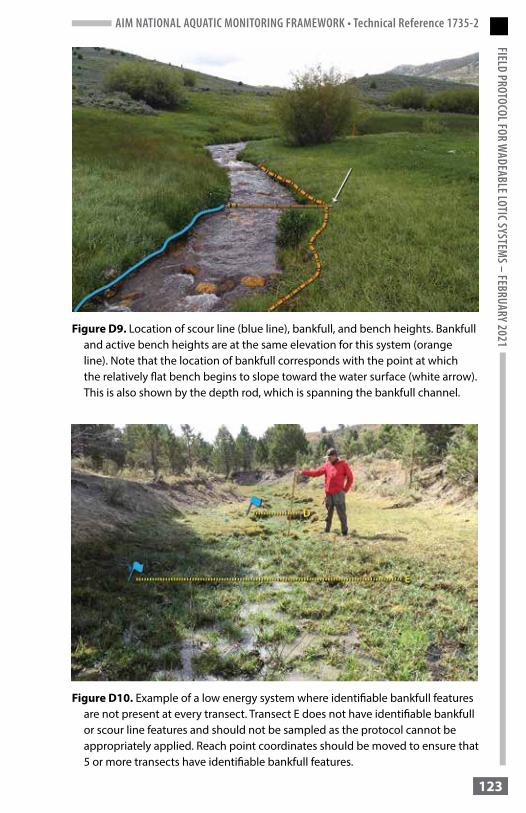
AIM NATIONAL AQUATIC MONITORING FRAMEWORK • Technical Reference 1735-2FIELD PROTOCOL FOR W
ADEABLE LOTIC SYSTEMS – FEBRUARY 2021
123
Figure D9. Location of scour line (blue line), bankfull, and bench heights. Bankfull and active bench heights are at the same elevation for this system (orange line). Note that the location of bankfull corresponds with the point at which the relatively flat bench begins to slope toward the water surface (white arrow). This is also shown by the depth rod, which is spanning the bankfull channel.
Figure D10. Example of a low energy system where identifiable bankfull features are not present at every transect. Transect E does not have identifiable bankfull or scour line features and should not be sampled as the protocol cannot be appropriately applied. Reach point coordinates should be moved to ensure that 5 or more transects have identifiable bankfull features.
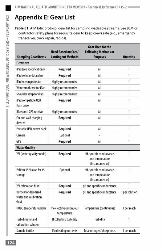
AIM NATIONAL AQUATIC MONITORING FRAMEWORK • Technical Reference 1735-2FI
ELD
PROT
OCOL
FOR
WAD
EABL
E LOT
IC SY
STEM
S – FE
BRUA
RY 2
021
124
Appendix E: Gear List
Table E1. AIM lotic protocol gear list for sampling wadeable streams. See BLM or contractor safety plans for requisite gear to keep crews safe (e.g., emergency transceiver, truck repair, radios).
Sampling Gear/ItemsNeed Based on Core/Contingent Methods
Gear Used for the Following Methods or
Purposes Quantity
Electronics
iPad (see specifications) Required All 1
iPad cellular data plan Required All 1
iPad screen protector Highly recommended All 1
Waterproof case for iPad Highly recommended All 1
Shoulder strap for iPad Highly recommended All 1
iPad compatible USB flash drive
Required All 1
Bluetooth GPS receiver Highly recommended All 1
Car and wall charging devices
Required All 1
Portable USB power bank Required All 1
Camera Optional - 1
GPS Required All 1
Water Quality
YSI (water quality sonde) Required pH, specific conductance, and temperature (instantaneous)
1
Pelican 1520 case for YSI storage
Optional pH, specific conductance, and temperature (instantaneous)
1
YSI calibration fluid Required pH and specific conductance 1
Bottles for deionized water and calibration fluid
Required pH and specific conductance 1 per solution
HOBO temperature probe If collecting continuous temperature
Temperature (continuous) 1 per reach
Turbidimeter and calibration solution
If collecting turbidity Turbidity 1
Sample bottles If collecting nutrients Total nitrogen/phosphorus 1 per reach
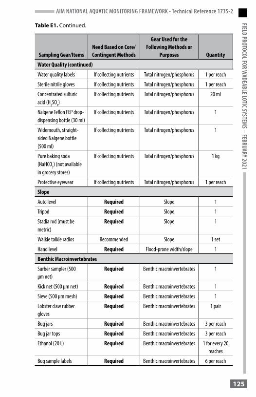
AIM NATIONAL AQUATIC MONITORING FRAMEWORK • Technical Reference 1735-2FIELD PROTOCOL FOR W
ADEABLE LOTIC SYSTEMS – FEBRUARY 2021
125
Sampling Gear/ItemsNeed Based on Core/Contingent Methods
Gear Used for the Following Methods or
Purposes Quantity
Water Quality (continued)
Water quality labels If collecting nutrients Total nitrogen/phosphorus 1 per reach
Sterile nitrile gloves If collecting nutrients Total nitrogen/phosphorus 1 per reach
Concentrated sulfuric acid (H2SO4)
If collecting nutrients Total nitrogen/phosphorus 20 ml
Nalgene Teflon FEP drop- dispensing bottle (30 ml)
If collecting nutrients Total nitrogen/phosphorus 1
Widemouth, straight-sided Nalgene bottle (500 ml)
If collecting nutrients Total nitrogen/phosphorus 1
Pure baking soda (NaHCO3) (not available in grocery stores)
If collecting nutrients Total nitrogen/phosphorus 1 kg
Protective eyewear If collecting nutrients Total nitrogen/phosphorus 1 per reach
Slope
Auto level Required Slope 1
Tripod Required Slope 1
Stadia rod (must be metric)
Required Slope 1
Walkie talkie radios Recommended Slope 1 set
Hand level Required Flood-prone width/slope 1
Benthic Macroinvertebrates
Surber sampler (500 µm net)
Required Benthic macroinvertebrates 1
Kick net (500 µm net) Required Benthic macroinvertebrates 1
Sieve (500 µm mesh) Required Benthic macroinvertebrates 1
Lobster claw rubber gloves
Required Benthic macroinvertebrates 1 pair
Bug jars Required Benthic macroinvertebrates 3 per reach
Bug jar tops Required Benthic macroinvertebrates 3 per reach
Ethanol (20 L) Required Benthic macroinvertebrates 1 for every 20 reaches
Bug sample labels Required Benthic macroinvertebrates 6 per reach
Table E1. Continued.
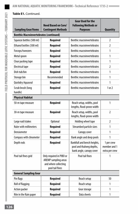
AIM NATIONAL AQUATIC MONITORING FRAMEWORK • Technical Reference 1735-2FI
ELD
PROT
OCOL
FOR
WAD
EABL
E LOT
IC SY
STEM
S – FE
BRUA
RY 2
021
126
Sampling Gear/ItemsNeed Based on Core/Contingent Methods
Gear Used for the Following Methods or
Purposes Quantity
Benthic Macroinvertebrates (continued)
Squeeze bottles (500 ml) Required Benthic macroinvertebrates 2
Ethanol bottles (500 ml) Required Benthic macroinvertebrates 2
Forceps/tweezers Required Benthic macroinvertebrates 1
Metal spoon Required Benthic macroinvertebrates 1
Clear packing tape Required Benthic macroinvertebrates 1
Electrical tape Required Benthic macroinvertebrates 2
Dish tub/bin Required Benthic macroinvertebrates 1
Storage bin Recommended Benthic macroinvertebrates 1
Quickdry Aquaseal Required Benthic macroinvertebrates 1
Scrub brush (long handle)
Required Benthic macroinvertebrates 1 or 2
Physical Habitat
50-m tape measure Required Reach setup, widths, pool lengths, flood-prone width
1
30-m tape measure Required Reach setup, widths, pool lengths, flood-prone width
2
Large nail/stakes Optional Holding wheel tape 2
Ruler with millimeters Required Streambed particle sizes 1
Densiometer Required Canopy cover 1
Compass with clinometer Required Bank angle and deep pools 1
Depth rods Required Bankfull and bench heights, pool and thalweg depths, bank angle, canopy cover
1 per crew member and 1 extra per crew
Pool tail fines grid Only required in PIBO or AREMP sampling areas and where collecting
pool tail fines
Pool tail fines 1
General Sampling Gear
Pin flags Required Reach setup 50
Roll of flagging Required Reach setup 1
Action packer Required Gear storage 1
Rite in the Rain paper Required Data sheets 1
Table E1. Continued.
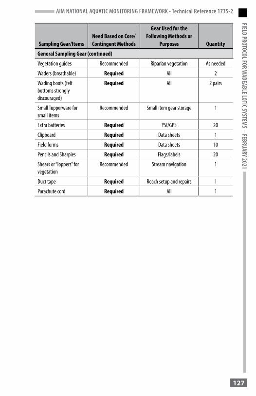
AIM NATIONAL AQUATIC MONITORING FRAMEWORK • Technical Reference 1735-2FIELD PROTOCOL FOR W
ADEABLE LOTIC SYSTEMS – FEBRUARY 2021
127
Sampling Gear/ItemsNeed Based on Core/Contingent Methods
Gear Used for the Following Methods or
Purposes Quantity
General Sampling Gear (continued)
Vegetation guides Recommended Riparian vegetation As needed
Waders (breathable) Required All 2
Wading boots (felt bottoms strongly discouraged)
Required All 2 pairs
Small Tupperware for small items
Recommended Small item gear storage 1
Extra batteries Required YSI/GPS 20
Clipboard Required Data sheets 1
Field forms Required Data sheets 10
Pencils and Sharpies Required Flags/labels 20
Shears or “loppers” for vegetation
Recommended Stream navigation 1
Duct tape Required Reach setup and repairs 1
Parachute cord Required All 1
AIM NATIONAL AQUATIC MONITORING FRAMEWORK • Technical Reference 1735-2FI
ELD
PROT
OCOL
FOR
WAD
EABL
E LOT
IC SY
STEM
S – FE
BRUA
RY 2
021
128
Appendix F: Suggested Workflow
This workflow is specific to two data collectors (and possibly a third data collector who is a field botanist) and is inclusive of all core and contingent methods and covariates. Sampling can be conducted in a series of “passes” up or down the reach, keeping in mind that more or less passes might be desirable depending on how difficult it is to walk up- or downstream. Upon completion of each pass and at the end of the reach, data should be reviewed for accuracy and completeness.
1. Reach establishment
a. Locate point coordinates.
b. Identify critical concepts as a team.
c. Collect water quality data, if the reach can be sampled.
d. Determine reach length and if the reach can be sampled. If the reach cannot be sampled, record the reason not sampled.
e. Set up the reach.
i. Both data collectors:
• Fill out reach status and 5 typical bankfull width measurements.• Take F transect coordinates and photos.• Measure and flag transects.• Take A and K transect photos and coordinates.
ii. If a field botanist is present, the botanist should develop and review a riparian plant list for the reach while reach setup occurs. All three data collectors should then review the plant list and ensure everyone can identify the priority noxious and priority native woody riparian plants.
2. Pass 1: Establish the reach monument, deploy temperature probe (contingent), collect benthic macroinvertebrates (core), and begin to assess the frequency of occurrence of priority noxious (core) and priority native woody riparian (contingent) vegetation and human influences (covariate). If a field botanist is present, begin assessing greenline vegetation composition (contingent).
a. One data collector samples and processes benthic macroinvertebrates.
b. The other data collector:
i. Establishes the monument at the F transect (and A and K, if applicable).
AIM NATIONAL AQUATIC MONITORING FRAMEWORK • Technical Reference 1735-2FIELD PROTOCOL FOR W
ADEABLE LOTIC SYSTEMS – FEBRUARY 2021
129
ii. Takes all photos and coordinates applicable to pass 1 data collection.
iii. Collects water quality data.
iv. Starts assessing frequency of occurrence of priority noxious and priority native woody riparian vegetation and human influences.
c. If a field botanist is present, start assessing greenline vegetation composition and/or assessing occurrence of priority noxious and priority native woody riparian vegetation and human influences. The field botanist is unlikely to participate in data collection during passes 2 through 5 given the time required to complete greenline vegetation composition measurements.
3. Pass 2: Implement physical habitat methods. Flood-prone width (covariate) can also be measured at the beginning and end of pass 2.
a. At each main transect, measure:
i. Bankfull and wetted width (covariate).
ii. Bankfull and bench height (lower of the two banks).
iii. Transect thalweg depth.
iv. Bank stability and cover (core).
v. Bank angle (contingent).
vi. Canopy cover (core).
vii. Streambed particle sizes (core).
b. Measure thalweg depth profile (contingent) between all transects.
c. At each intermediate transect, measure:
i. Wetted width (covariate).
ii. Bank stability and cover (core).
iii. Streambed particle sizes (core).
4. Pass 3: Measure pool dimensions (core), large wood (core), and pool tail fines (contingent) as a two-person team.
5. Pass 4: Measure slope (covariate). One data collector uses the auto level or hand level and records data, and the other data collector uses the stadia rod or tape measure.

AIM NATIONAL AQUATIC MONITORING FRAMEWORK • Technical Reference 1735-2FI
ELD
PROT
OCOL
FOR
WAD
EABL
E LOT
IC SY
STEM
S – FE
BRUA
RY 2
021
130
6. Pass 5: Measure flood-prone width (covariate). Alternatively, flood-prone width can also be measured at the beginning and end of pass 2. Complete measurements of human influences (covariate) and priority noxious and priority native woody riparian vegetation.
7. Reach completion
a. The lead data collector reviews data, performs quality control, and ensures all data have been collected. This step should occur upon completion of each pass and at the end of the reach.
b. The second data collector collects any missing data and cleans up the reach.
c. If a field botanist is present, ensure all voucher specimens are collected and review collected data.
8. Decontaminate gear (all data collectors).
AIM NATIONAL AQUATIC MONITORING FRAMEWORK • Technical Reference 1735-2FIELD PROTOCOL FOR W
ADEABLE LOTIC SYSTEMS – FEBRUARY 2021
131
Appendix G: Guidance for Integrating MIM Greenline Vegetation Composition and Other Greenline-Based Measurements with the AIM Lotic Protocol
Overview: Guidance is provided for critical concepts, reach setup, field measurements, plot layout, reach monumenting, and data collection and storage when measuring greenline vegetation composition (contingent) and other green-line based measurements using the multiple indicator monitoring (MIM) protocol (Burton et al. 2011) at AIM reaches.
Training and critical concepts:• Greenline: Locating the greenline is the main critical concept for
assessing greenline vegetation composition and other greenline-based measurements following the MIM protocol. It is the primary responsibility of the field botanist, with guidance from the BLM project lead, to be proficient in locating the greenline.
• MIM trainings: Contact the National Riparian Service Team (NRST) to identify MIM training opportunities for the upcoming field season. The NRST supports training for greenline vegetation composition and greenlined-based field measurements.
• It is recommended that only field staff conducting greenline-based procedures attend MIM training (e.g., field botanist who will perform plant identification). BLM project leads and contractor staff are also encouraged to attend. If individuals attend both MIM and AIM trainings, make sure those individuals do not confuse the two protocols. Data collectors should implement the MIM methods only for greenline-based measurements at AIM reaches.
• Prior to field data collection, riparian plant lists should be developed in cooperation with local BLM staff.
Reach setup and field measurements:• Reach length: If performing MIM greenline-based methods, follow AIM
lotic protocol guidance for reach length, which is equal to 20 x bankfull width or 150 m, whichever is greater. Under rare circumstances, factors such as land ownership or safety concerns preclude the sampling of a full reach length and thus partial reaches are sampled (minimum of 5 main transects).
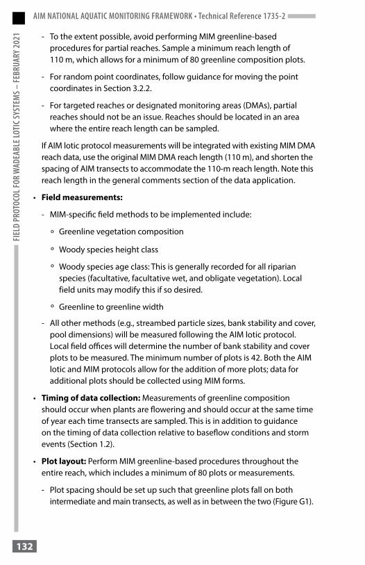
AIM NATIONAL AQUATIC MONITORING FRAMEWORK • Technical Reference 1735-2FI
ELD
PROT
OCOL
FOR
WAD
EABL
E LOT
IC SY
STEM
S – FE
BRUA
RY 2
021
132
- To the extent possible, avoid performing MIM greenline-based procedures for partial reaches. Sample a minimum reach length of 110 m, which allows for a minimum of 80 greenline composition plots.
- For random point coordinates, follow guidance for moving the point coordinates in Section 3.2.2.
- For targeted reaches or designated monitoring areas (DMAs), partial reaches should not be an issue. Reaches should be located in an area where the entire reach length can be sampled.
If AIM lotic protocol measurements will be integrated with existing MIM DMA reach data, use the original MIM DMA reach length (110 m), and shorten the spacing of AIM transects to accommodate the 110-m reach length. Note this reach length in the general comments section of the data application.
• Field measurements:
- MIM-specific field methods to be implemented include:
º Greenline vegetation composition
º Woody species height class
º Woody species age class: This is generally recorded for all riparian species (facultative, facultative wet, and obligate vegetation). Local field units may modify this if so desired.
º Greenline to greenline width
- All other methods (e.g., streambed particle sizes, bank stability and cover, pool dimensions) will be measured following the AIM lotic protocol. Local field offices will determine the number of bank stability and cover plots to be measured. The minimum number of plots is 42. Both the AIM lotic and MIM protocols allow for the addition of more plots; data for additional plots should be collected using MIM forms.
• Timing of data collection: Measurements of greenline composition should occur when plants are flowering and should occur at the same time of year each time transects are sampled. This is in addition to guidance on the timing of data collection relative to baseflow conditions and storm events (Section 1.2).
• Plot layout: Perform MIM greenline-based procedures throughout the entire reach, which includes a minimum of 80 plots or measurements.
- Plot spacing should be set up such that greenline plots fall on both intermediate and main transects, as well as in between the two (Figure G1).

AIM NATIONAL AQUATIC MONITORING FRAMEWORK • Technical Reference 1735-2FIELD PROTOCOL FOR W
ADEABLE LOTIC SYSTEMS – FEBRUARY 2021
133
º For 150-m reaches, plot spacing should be intervals of 3.75 m.
º For longer reaches, plot spacing is determined by dividing reach length by 40 (e.g., 200-m reach length = 5-m plot spacing).
- Note that AIM and MIM designate left and right bank differently. Data collectors should ensure bank designations are consistent with respective protocols and data applications.
- Since the point coordinates for AIM lotic reaches are randomly generated, it is not necessary to randomize the location of the first greenline plot. A systematic sampling interval is adequate.
• Reach monumenting: Where both AIM lotic and MIM greenline measurements are taken in tandem, field office-specific monumenting standards should be reviewed and coordinated with field data collectors.
• Data collection and storage: The AIM lotic data collection application for electronic data collection of AIM core and contingent methods does not currently support MIM greenline vegetation measurements. Record MIM greenline vegetation composition measurements in MIM Excel spreadsheets on separate devices. After each trip, MIM data should be backed up and checked by BLM staff.
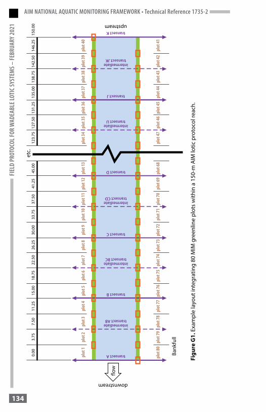
AIM NATIONAL AQUATIC MONITORING FRAMEWORK • Technical Reference 1735-2FI
ELD
PROT
OCOL
FOR
WAD
EABL
E LOT
IC SY
STEM
S – FE
BRUA
RY 2
021
134
Figu
re G
1. E
xam
ple
layo
ut in
tegr
atin
g 80
MIM
gre
enlin
e pl
ots
with
in a
150
-m A
IM lo
tic p
roto
col r
each
.

AIM NATIONAL AQUATIC MONITORING FRAMEWORK • Technical Reference 1735-2FIELD PROTOCOL FOR W
ADEABLE LOTIC SYSTEMS – FEBRUARY 2021
135
Appendix H: Implementation of the AIM Lotic Protocol in Alaska
Overview: The majority of reaches sampled in Alaska are extremely remote and often accessible only by helicopter. Due to the high cost of helicopters, there are some differences in the implementation of the AIM lotic protocol in Alaska to increase field sampling efficiency. In addition, there is a contingent method used only in Alaska. All methods not covered in this section are collected following standard procedures.
H1. Determining Reach Status
A helicopter landing zone is not always available at the original point coordinates due to tall and dense vegetation, steep and uneven terrain, or unstable marshy areas. Point coordinates can be moved upstream or downstream up to 1 kilometer from the original point coordinates. If a landing zone is present within a kilometer of original point coordinates, sample as close to original point coordinates as possible. If a minimum of 5 transects cannot be sampled or if a landing zone is not available within 1 kilometer of the original point coordinates, continue to the next reach. If a landing zone is not available for a reach that belongs to the target population, select “permanently inaccessible” for status and “terrain access denied” for reason not sampled.
Point coordinates should not be moved if the land status would change or if the stream size category (small stream – SS, large stream – LS, or river – RV) would change because of a tributary junction. Ensure data collectors consult with BLM project leads to understand how stream size categories were defined. The reach would be classified as “permanently inaccessible” for status and “terrain access denied” for reason not sampled.
H2. Streambed Particle Sizes
Streambed particle sizes are measured at 5 locations on each main and intermediate transect: at 10%, 30%, 50%, 70%, and 90% from the scour line on one side of the stream to the scour line on the opposite side of the stream for a total of 105 particles. See Appendix C for guidance on measuring particles at dry transects. Besides a reduction in number of measurements per transect and measurement location percentages, follow all other guidance in Section 7.5.
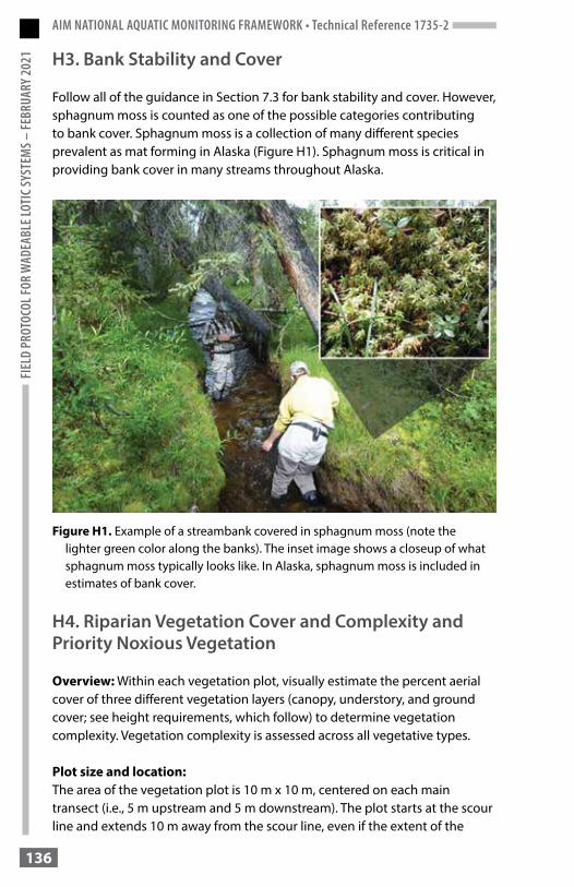
AIM NATIONAL AQUATIC MONITORING FRAMEWORK • Technical Reference 1735-2FI
ELD
PROT
OCOL
FOR
WAD
EABL
E LOT
IC SY
STEM
S – FE
BRUA
RY 2
021
136
H3. Bank Stability and Cover
Follow all of the guidance in Section 7.3 for bank stability and cover. However, sphagnum moss is counted as one of the possible categories contributing to bank cover. Sphagnum moss is a collection of many different species prevalent as mat forming in Alaska (Figure H1). Sphagnum moss is critical in providing bank cover in many streams throughout Alaska.
Figure H1. Example of a streambank covered in sphagnum moss (note the lighter green color along the banks). The inset image shows a closeup of what sphagnum moss typically looks like. In Alaska, sphagnum moss is included in estimates of bank cover.
H4. Riparian Vegetation Cover and Complexity and Priority Noxious Vegetation
Overview: Within each vegetation plot, visually estimate the percent aerial cover of three different vegetation layers (canopy, understory, and ground cover; see height requirements, which follow) to determine vegetation complexity. Vegetation complexity is assessed across all vegetative types.
Plot size and location:The area of the vegetation plot is 10 m x 10 m, centered on each main transect (i.e., 5 m upstream and 5 m downstream). The plot starts at the scour line and extends 10 m away from the scour line, even if the extent of the

AIM NATIONAL AQUATIC MONITORING FRAMEWORK • Technical Reference 1735-2FIELD PROTOCOL FOR W
ADEABLE LOTIC SYSTEMS – FEBRUARY 2021
137
plot is beyond that of riparian vegetation. All sides of the plot are straight lines, except the edge bordering the stream, which follows the contour of the scour line (Figure 36). Estimate the distance from the scour line as if it were projected down from an aerial view. If side channels are present, see Appendix C for guidance on defining plots and recording measurements. If vegetation plots overlap in aerial extent (e.g., small sinuous streams), derive estimates of aerial cover for each plot independently.
Estimating aerial cover:Vegetative complexity and cover are estimated for three vertical layers: canopy, understory, and ground cover within the 10 m x 10 m plot. Aerial cover is an estimate of the amount of shadow that would be cast by a particular vegetation type if the sun were directly over the plot area.
• Aerial cover estimates are based on five cover classes:
- 0 = absent: zero cover- 1 = sparse: < 10%- 2 = moderate: 10-40%- 3 = heavy: 41-75%- 4 = very heavy: > 75%
• Percent cover estimates within each layer (i.e., canopy, understory, ground) cannot be > 100%.
• Estimates among different layers (i.e., canopy, understory, ground) are independent of each other, so the sum of the aerial cover for the three layers combined could add up to 300%.
• Total percent cover for the canopy and understory layers can be < 100%, but percent cover for the ground cover layer must equal 100% because bare ground is included in the estimates.
Methods:1. Stand at the scour line, and visualize the 10 m x 10 m plot (Figure 36),
which starts at the scour line along each streambank. If you cannot see the full depth of the plot (e.g., 10 m into the riparian zone), move from the scour line to obtain a better view. If you cannot safely view the plot, record “not collected.”
2. Within the plot area, conceptually divide the riparian vegetation into three layers:
• Canopy (> 5 m high)• Understory (0.5 to 5 m high)• Ground cover (< 0.5 m high)
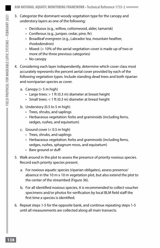
AIM NATIONAL AQUATIC MONITORING FRAMEWORK • Technical Reference 1735-2FI
ELD
PROT
OCOL
FOR
WAD
EABL
E LOT
IC SY
STEM
S – FE
BRUA
RY 2
021
138
3. Categorize the dominant woody vegetation type for the canopy and understory layers as one of the following:
• Deciduous (e.g., willow, cottonwood, alder, tamarisk)• Coniferous (e.g., juniper, cedar, pine, fir)• Broadleaf evergreen (e.g., Labrador tea, mountain heather,
rhododendron)• Mixed: (> 10% of the aerial vegetation cover is made up of two or
more of the three previous categories)• No canopy
4. Considering each layer independently, determine which cover class most accurately represents the percent aerial cover provided by each of the following vegetation types. Include standing dead trees and both riparian and nonriparian species as cover.
a. Canopy (> 5 m high)• Large trees: > 1 ft (0.3 m) diameter at breast height• Small trees: < 1 ft (0.3 m) diameter at breast height
b. Understory (0.5 to 5 m high)• Trees, shrubs, and saplings• Herbaceous vegetation: forbs and graminoids (including ferns,
sedges, rushes, and equisetum)
c. Ground cover (< 0.5 m high)• Trees, shrubs, and saplings• Herbaceous vegetation: forbs and graminoids (including ferns,
sedges, rushes, sphagnum moss, and equisetum)• Bare ground or duff
5. Walk around in the plot to assess the presence of priority noxious species. Record each priority species present.
a. For noxious aquatic species (riparian obligates), assess presence/absence in the 10 m x 10 m vegetation plot, but also extend the plot to the center of the streambed (Figure 36).
b. For all identified noxious species, it is recommended to collect voucher specimens and/or photos for verification by local BLM field staff the first time a species is identified.
6. Repeat steps 1-5 for the opposite bank, and continue repeating steps 1-5 until all measurements are collected along all main transects.
AIM NATIONAL AQUATIC MONITORING FRAMEWORK • Technical Reference 1735-2FIELD PROTOCOL FOR W
ADEABLE LOTIC SYSTEMS – FEBRUARY 2021
139
References
Archer, E.K., R.A. Scully, R. Henderson, B. Roper, B. Heitke, D. Jeremiah, and B. Boisjolie. 2015. PACFISH INFISH Biological Opinion Effectiveness Monitoring Program for Streams and Riparian Areas: 2015 Sampling Protocol for Stream Channel Attributes. U.S. Department of Agriculture, U.S. Forest Service.
Bauer, S.B., and T.A. Burton. 1993. Monitoring protocols to evaluate water quality effects of grazing management on western rangeland streams. EPA 910/R-93-017. Environmental Protection Agency, Seattle, WA.
BLM (Bureau of Land Management). 2020. BLM’s Lotic Assessment, Inventory, and Monitoring (AIM) 2020 Field Season: Evaluation and Design Management Protocol. Version 3.0. Bureau of Land Management, National Operations Center, Denver, CO. https://www.aim.landscapetoolbox.org/office-sample-point-evaluation/.
BLM (Bureau of Land Management). 2021. Assessment, Inventory, and Monitoring Support for BLM AIM Projects and Programs. Website. U.S. Department of the Interior, Bureau of Land Management, National Operations Center, Denver, CO. https://aim.landscapetoolbox.org.
Burton, T.A., S.J. Smith, and E.R. Cowley. 2011. Riparian Area Management: Multiple Indicator Monitoring (MIM) of Stream Channels and Streamside Vegetation. Tech Ref 1737-23. U.S. Department of the Interior, Bureau of Land Management, National Operations Center, Denver, CO.
Dunham, J., G. Chandler, B. Rieman, and D. Martin. 2005. Measuring Stream Temperature with Digital Data Loggers: A Users Guide. Gen Tech Rep RMRS-GTR-150www. U.S. Department of Agriculture, U.S. Forest Service, Rocky Mountain Research Station, Fort Collins, CO.
Dunne, T., and L.B. Leopold. 1978. Water in Environmental Planning. New York: W.H. Freeman and Company.
Gerth, W.J., and A.T. Herlihy. 2006. Effect of sampling different habitat types in regional macroinvertebrate bioassessment surveys. Journal of the North American Benthological Society 25: 501–512.
Hankin, D.G., and G.H. Reeves. 1988. Estimating total fish abundance and total habitat area in small streams based on visual estimation methods. Canadian Journal of Fisheries and Aquatic Sciences 45: 834–844.
Harman, W., R. Starr, M. Carter, K. Tweedy, M. Clemmons, K. Suggs, and C. Miller. 2012. A Function-Based Framework for Stream Assessment and Restoration Projects. EPA 843-K-12-006. U.S. Environmental Protection Agency, Office of Wetlands, Oceans, and Watersheds, Washington, DC.

AIM NATIONAL AQUATIC MONITORING FRAMEWORK • Technical Reference 1735-2FI
ELD
PROT
OCOL
FOR
WAD
EABL
E LOT
IC SY
STEM
S – FE
BRUA
RY 2
021
140
Harrelson, C.C., C.L. Rawlins, and J.P. Potyondy. 1994. Stream Channel Reference Sites: An Illustrated Guide to Field Technique. Gen Tech Rep RM-245. U.S. Department of Agriculture, U.S. Forest Service, Rocky Mountain Forest and Range Experiment Station, Fort Collins, CO.
Hawkins, C.P., J. Ostermiller, M. Vinson, R.J. Stevenson, and J. Olsen. 2003. Stream Algae, Invertebrate, and Environmental Sampling Associated with Biological Water Quality Assessments: Field Protocols. Utah State University, Department of Aquatic, Watershed, and Earth Resources, Logan, UT.
Hurlbert, S.H. 1984. Pseudoreplication and the Design of Ecological Field Experiments. Ecological Monographs 54: 187–211.
Isaak, D.J., D.L. Horan, and S.P. Wollrab. 2013. A Simple Protocol Using Underwater Epoxy to Install Annual Temperature Monitoring Sites in Rivers and Streams. Gen Tech Rep RMRS-GTR-314. U.S. Department of Agriculture, U.S. Forest Service, Rocky Mountain Research Station, Fort Collins, CO.
Lanigan, S.H. 2010. Field Protocol Manual: Aquatic and Riparian Effectiveness Monitoring Program; Regional Interagency Monitoring for the Northwest Forest Plan 2010 Field Season.
Lisle, T.E. 1987. Using “Residual Depths” to Monitor Pool Depths Independently of Discharge. Research Note PSW-394. U.S. Department of Agriculture, U.S. Forest Service, Pacific Southwest Forest and Range Experiment Station, Berkeley, CA.
Miller, S.W., B. Bohn, D. Dammann, M. Dickard, M. Gonzalez, J. Jimenez, E. Rumbold, S. Smith, and K. Stein. 2015. AIM National Aquatic Monitoring Framework: Introducing the Framework and Indicators for Lotic Systems. Tech Ref 1735-1. U.S. Department of the Interior, Bureau of Land Management, National Operations Center, Denver, CO.
Moore, K., K. Jones, and J. Dambacher. 2002. Methods for Stream Habitat Surveys. Oregon Department of Fish and Wildlife, Aquatic Inventories Project, Natural Production Program, Corvallis, OR.
Mulvey, M., L. Caton, and R. Hafele. 1992. Oregon Nonpoint Source Monitoring Protocols and Stream Bioassessment Field Manual for Macroinvertebrates and Habitat Assessment. Oregon Department of Environmental Quality Laboratory, Portland, OR.
Platts, W.S., C. Armour, G.D. Booth, M. Bryant, J.L. Bufford, P. Cuplin, S. Jensen, G.W. Lienkaemper, G.W. Minshall, S.P. Monsen, R.L. Nelson, J.R. Sedell, and J.S. Tuhy. 1987. Methods for Evaluating Riparian Habitats with Applications to Management. Gen Tech Rep INT-221. U.S. Department of Agriculture, U.S. Forest Service, Intermountain Research Station, Ogden, UT.

AIM NATIONAL AQUATIC MONITORING FRAMEWORK • Technical Reference 1735-2FIELD PROTOCOL FOR W
ADEABLE LOTIC SYSTEMS – FEBRUARY 2021
141
Rehn, A.C., P.R. Ode, and C.P. Hawkins. 2007. Comparisons of targeted-riffle and reach-wide benthic macroinvertebrate samples: Implications for data sharing in stream-condition assessments. Journal of the North American Benthological Society 26: 332–348.
Rosgen, D.L. 1996. Applied River Morphology. Pagosa Springs, CO: Wildland Hydrology.
Saunders, W.C., J.V. Ojala, A. Van Wagenen, D. Haynes, E.K. Archer, and R. Henderson. 2019. PacFish InFish Biological Opinion (PIBO) Monitoring Program: Effectiveness Monitoring Sampling Methods for Stream Channel Attributes. PIBO staff, Multi-federal Agency Monitoring Program, Logan, UT.
Strahler, A.N. 1952. Hypsometric (area-altitude) analysis of erosional topography. Geological Society of America Bulletin 63 (11): 1117–1142.
SWAMP (Surface Water Ambient Monitoring Program). 2007. Standard Operating Procedures for conducting field measurements and field collections of water and bed sediment samples in the Surface Water Ambient Monitoring Program. California Environmental Protection Agency, Department of Fish and Game, Marine Pollution Studies Laboratory, Moss Landing, CA.
Toevs, G.R., J.J. Taylor, C.S. Spurrier, W.C. MacKinnon, and M.R. Bobo. 2011. Bureau of Land Management Assessment, Inventory, and Monitoring Strategy: For Integrated Renewable Resources Management. U.S. Department of the Interior, Bureau of Land Management, National Operations Center, Denver, CO.
USEPA (U.S. Environmental Protection Agency). 2009. National Rivers and Streams Assessment: Field Operations Manual. EPA-841-B-07-009. U.S. Environmental Protection Agency, Office of Watershed and Office of Environmental Information, Washington, DC.
USEPA (U.S. Environmental Protection Agency. 2019. National Rivers and Streams Assessment 2018/19: Field Operations Manual – Wadeable. Version 1.2. EPA-841-B-17-003a. U.S. Environmental Protection Agency, Office of Water, Washington, DC.
USFS (U.S. Forest Service). 2005. Stream Condition Inventory (SCI) Technical Guide, Version 5.0. U.S. Department of Agriculture, U.S. Forest Service, Pacific Southwest Region, Vallejo, CA.

AIM NATIONAL AQUATIC MONITORING FRAMEWORK • Technical Reference 1735-2FI
ELD
PROT
OCOL
FOR
WAD
EABL
E LOT
IC SY
STEM
S – FE
BRUA
RY 2
021
142
USFS (U.S. Forest Service). 2020. Field Protocol Manual: Aquatic and Riparian Effectiveness Monitoring Program; Regional Interagency Monitoring for the Northwest Forest Plan 2020 Field Season. U.S. Department of Agriculture, U.S. Forest Service.
Wolman, M.G. 1954. A method of sampling coarse river-bed material. Transactions of the American Geophysical Union 35: 951-956.

AIM NATIONAL AQUATIC MONITORING FRAMEWORK • Technical Reference 1735-2FIELD PROTOCOL FOR W
ADEABLE LOTIC SYSTEMS – FEBRUARY 2021
143
Notes

AIM NATIONAL AQUATIC MONITORING FRAMEWORK • Technical Reference 1735-2FI
ELD
PROT
OCOL
FOR
WAD
EABL
E LOT
IC SY
STEM
S – FE
BRUA
RY 2
021
144
Notes

AIM NATIONAL AQUATIC MONITORING FRAMEWORK • Technical Reference 1735-2FIELD PROTOCOL FOR W
ADEABLE LOTIC SYSTEMS – FEBRUARY 2021
145
Notes

AIM NATIONAL AQUATIC MONITORING FRAMEWORK • Technical Reference 1735-2FI
ELD
PROT
OCOL
FOR
WAD
EABL
E LOT
IC SY
STEM
S – FE
BRUA
RY 2
021
146
Notes

AIM NATIONAL AQUATIC MONITORING FRAMEWORK • Technical Reference 1735-2FIELD PROTOCOL FOR W
ADEABLE LOTIC SYSTEMS – FEBRUARY 2021
147
Notes

AIM NATIONAL AQUATIC MONITORING FRAMEWORK • Technical Reference 1735-2FI
ELD
PROT
OCOL
FOR
WAD
EABL
E LOT
IC SY
STEM
S – FE
BRUA
RY 2
021
148
Notes

The mention of company names, trade names, or commercial products does not constitute endorsement or recommendation for use by the Federal Government.
