agrigrid - macaulay.ac.uk · fadn farm accountancy data network ... dimensional problems easy to be...
TRANSCRIPT

1
AGRIGRID
Methodological grids for payment calculations in
rural development measures in the EU (Project Reference: SSPE-CT-2006-044403)
Specific Targeted Research Project under priority 8.1 Sustainable
management of Europe’s natural resources:
8.1.B.1.1 Modernisation and sustainability of agriculture and forestry,
including their multifunctional role in order to ensure the
sustainable development and promotion of rural areas
Task 14 New methods for calculating premiums in the rural development
measures
Deliverable D11
Summary report on grid development
Task managers: Luca Cesaro, Filippo Chiozzotto, Lorenzo Tarasconi (INEA)
With contributions from: The Macaulay Institute (MLURI), Johann Heinrich von Thünen-Institute (vTI),
Agricultural University of Athens (AUA), Institute of Agricultural Economics and Information (ÚZEI),
MTT Agrifood Research Finland (MTT), Lithuanian Institute of Agrarian Economics (LAEI), Instituto
de Desarrollo Rural Sostenible (IDRiSi) and Agrotec Polska Sp. zoo.
Approved by Work Package Manager of WP8: Luca Cesaro, INEA
Date: November 2008
Approved by Project Coordinator: Gerald Schwarz, MLURI
Date: November 2008
This document was produced under the terms and conditions of Contract SSPE-CT-2006-044403 for the
European Commission.

2

3
This document presents results obtained within EU project SSPE-CT-2006-044403 on
Methodological grids for payment calculations in rural development measures in the EU
(http://www.macaulay.ac.uk/agrigrid/). It does not necessary reflect the view of the European
Union and in no way anticipates the commission’s future policy in this area.
List of project partners Project partner Short name EU Member States
The Macaulay Land Use Research Institute MLURI Scotland
Institute of Farm Economics Johann Heinrich von
Thuenen-Institute vTI Germany
Agricultural University of Athens AUA Greece
Institute of Agricultural Economics and
Information ÚZEI Czech Republic
Lithuanian Institute of Agrarian Economics LAEI Lithuania
MTT Agrifood Research Finland MTT Finland
National Institute of Agricultural Economics INEA Italy
Humboldt University Berlin HUB Germany
Subcontractor
Instituto de Desarrollo Rural Sostenible IDRiSi Spain
Agrotec Polska Sp. z o. o. - Poland

4

5
Table of contents
1. Introduction .............................................................................................................................. 9
1.1 Logic model diagrams and methodological grids: some preliminary information ............ 10
1.1.1 Complex problem solving: principles and mechanisms ............................................. 12
1.1.2 The concepts of Logic Model Diagrams ..................................................................... 13
1.1.3 Relations between Logic Models and Grids ............................................................... 15
2. Methodology ........................................................................................................................... 16
2.1 The phase of analysis and design of the preliminary grids ................................................ 16
2.2 The second phase: development of the methodological grids ........................................... 19
3. Logic framework for the application of methodological grids to RD payment
calculations ................................................................................................................................. 19
3.1 Assessment of baselines ..................................................................................................... 22
3.2 Identification of cost and revenue components ................................................................. 23
3.2.1 The Balance Sheet approach ....................................................................................... 26
3.2.2 The Practices approach............................................................................................... 26
3.3 Payment differentiation criteria ......................................................................................... 32
3.4 Final grids and step-by-step template ................................................................................ 33
5. Conclusions and recommendations ...................................................................................... 35
References ................................................................................................................................... 38
Annexes ....................................................................................................................................... 39

6
List of tables
Table 1. Examples of linkages between RD commitments and related baseline requirements ... 24 Table 2. General cost list for the statement of production processes........................................... 28 Table 3. Examples of implementation of the Practices approach ............................................... 29
Table 4. Implementation of the two calculation approaches in the methodological grids .......... 31
List of figures
Figure 1. Position of WP8 within the project phases ................................................................... 10 Figure 2. The art of complex problem solving (Clemens, 2008) ................................................. 13
Figure 3. Core components of the Program Logic Model (Gale, 2006) ...................................... 14 Figure 4. Example of linkare between baseline, RD commitments and respective costs/revenues
– Animal Welfare payments in ITER ............................................................................................ 17 Figure 5. Logic scheme of the analysis, as a result of the review of current RD payments ........ 18
Figure 6. General logic framework for the development of methodological grids ..................... 20 Figure 7. Logic frame work for the design of the Natura 2000 payments grid (from D6) .......... 21 Figure 8. Logic frame work of payment calcualtions in methodological grids for afforestation
measures (from D7) ..................................................................................................................... 21 Figure 9. Use of different data sources in the investigated countries and measures ................... 32 Figure 10. General design of the step-by-step template .............................................................. 35

7
List of abbreviations
AEM Agri-environmental measures
CZ Czech Republic
DE Germany
DEMWP Mecklenburg West-Pomerania (Germany)
DENRW North-Rhine Westphalia (Germany)
EC European Commission
EEC European Economic Community
ESBC Basque Country (Spain)
ESNAV Navarra (Spain)
EU European Union
FADN Farm Accountancy Data Network
FI Finland
GAEC Good Agricultural and Environmental Condition
GFI Gross Farm Income
GFM Gross Forestry Margin
GLM Gross Livestock Margin
GM Gross Margin
GR Greece
ha hectare
ITER Emilia-Romagna (Italy)
ITUMB Umbria (Italy)
ITVE Veneto (Italy)
LF Logic Framework
LM Logic Model
LMD Logic Model Diagram
LSU Livestock Units
LT Lithuania
MA Managing Authorities
MG Methodological grid
MS Member States
N Nitrate
NVZ Nitrate Vulnerable Zones
NWFP Non-wood forest products
PL Poland
RD Rural Development
RDP Rural Development Programme
RDR Rural Development Regulation
SCO Scotland
SGM Standard Gross Margin
SMR Statutory Management Requirement
UAA Utilised Agricultural Area
VAT Value Added Tax

8

9
1. Introduction All European Union member states implement Rural Development schemes. For the programming
period 2007-2013 these schemes are regulated by Reg. (EC) 1698/2005, which states that payments
granted for Rural Development must be based on verifiable estimates of farms’ costs and revenues.
In order to strengthen and, at the same time, make more clear this principle, the European Commission
circulated a Working Document1 named Agri-environment commitments and their verifiability. Despite
its title, the document addressed not only agri-environmental measures but also measures with similar
design and calculations, including “animal welfare payments, natural handicap and Natura 2000
payments, forest-environment payments or meeting standards”. The purpose was to highlight the general
principles of the measures’ design and the main standard assumptions for payment calculations.
Nevertheless, both the EC Regulation and the Working Document lack the definition of a standardised
and unequivocal process for the calculation of those payments, with the result that the methods for the
calculation of payments related to RD schemes vary considerably among member states and regions.
Hence, there is an obvious need for the development of a unifying approach which would set common
guidelines and methods for the calculations. In the AGRIGRID project, so-called methodological grids
have been developed for this purpose.
As shown in Figure 1, WP8 is a cross-cutting work package within phase 2 of the project. As mentioned
above, the objective of the WP was to provide the general design of the grids as well as contribute to the
software development, in particular for all the aspects related to its structure. All that activity mainly
took place in the middle of the project, after the definition of the necessary knowledge base, and can be
split into the reviews of payment calculation, and a literature review focusing on methodological issues
required by the grid development.
The starting point to develop a general framework for the design of the methodological grids is the idea
that every end-user must be able to obtain an input mask suitable for his valuation requirements. Even
though we are analysing the same measure or scheme, the needs of two evaluators may be very different
from each other. Hence, a grid must fulfil two main requirements: to provide an ever-effective general
structure for calculation; and to give the possibility, under specific conditions, of being adapted to every
single need.
1 Rural Development Committee, Working Document RD10/07/2006-final.

10
Figure 1. Position of WP8 within the project phases
1.1 Logic model diagrams and methodological grids: some preliminary
information
The concept and theory of logic models was introduced around the 1970s or earlier. It has then evolved
to meet new needs, and is a basic tool for problem analysis, management and evaluation.
Logic model diagrams and grids are essentially a schematic way of representing a complex problem.
Grids and logic models are used together in the representation of the problem in a way that makes multi-
dimensional problems easy to be considered and solved.
Grids are often used in complex problem analysis to represent the logic process to reach a solution.
Several applications of grid methodology are reported in the literature, encompassing various fields,
frequently computer science and biometric science. Moreover, logic models are often used in the theory
and practice of enterprise organization and business management.
As a schematic way to represent a decision-making process, a grid can be formulated as a simple
spreadsheet where different parameters influencing the decision are included. The increasing complexity
of the decision-making process often leads to a set of tables connected by links and logic connections.
The logic model should be sized in a way that allows readers to easily understand it without extensive
reference and cross-comparisons between pages. Ideally, the logic model is one or, at most, two pages
long. The level of detail should be sufficient for the reader to grasp the major items that go into an

11
organization or program, what occurs to those inputs, the various outputs that result and the overall
outcomes that occur.
In the case of payment calculation the logic framework is rather complex, as the different approaches
adopted (or adoptable) for each individual measure and country called for the implementation of a very
general framework for the standard grids which has then been modified and adapted at country level and
measure level.
A bibliographic research has been conducted during the first phase of the project. The analysis
of existing literature on logic models and methodological grids gave a first idea about how the
methodology has been applied in other fields of research and investigation.
Logic modeling is a thought process that program evaluators have found useful for at least forty years
and that has become increasingly popular among program managers during the last decade (Jordan
2003). However, in a more comprehensive definition, logic models are something more complex and
less clearly defined. In general terms, with reference to the issues of AGRIGRID project, a logic model
is a simple illustration of the logic behind a policy, program, or initiative. It represents and clearly
defines the links between the theoretical assumptions/principles of a program, the program activities (or,
better, the way they are implemented) and the outcomes.
The use of logic models to define the problem and find the solutions in AGRIGRID refers to the fact that
it has been necessary to consider a large number of diverse, dynamic and interdependent information and
elements belonging to different domains such as legislation, farm accountability, RD policies and socio-
economic and geographic differences among and within the member states and regions. All of them are
information, parameters or rules that an operator needs to draft correctly the calculation documents
required by the EC during the negotiation and in particular the measures’ approval phase.
At the beginning, the attention of the investigation was focused on some theoretical aspects related with
the resolution of complex problems: the key question was how a complex problem can be solved. The
issue of problem solving is studied in psychology and in the cognitive science from the point of view of
the mental processes involved. For the current purpose the interest was to outline some methodological
concepts, in order to better understand the width and complexity of the “project” problem. One of the
most feasible examples of a very general problem solving procedure is called “means-end analysis”
(Newell and Simon 1972). This method starts from the assessment of the differences between the current
problem state and the actual goal state, and it aims to find the systems as well as the tools that will
reduce that difference.
With respect to the context of the project, the current problem state, the goal state and the resolving
systems can be identified respectively as:
The current state: a number of different conditions and methods for payment calculation among
the EU member states, at both production and policy level, which must be harmonized and
managed by means of a structure and an ever-effective methodology;
The goal state: the creation of a unique method of calculating payments for different RD
measures and specific natural and agronomic assumptions, considering also socio-economic and
geographic differences at national, regional and farm level;
The resolving system: multidimensional grids containing all the information required for the
implementation of measure justification and, by means of a logic model, the possibility of
identifying the necessary relationship between policy, legislation and the accountable domains
the information belongs to.
The next paragraphs describe the main results of the literature review, which looks at both scientific
studies and practical/operative reports such as grey literature.

12
1.1.1 Complex problem solving: principles and mechanisms
The complex problem solving emerged as a field of psychology in its own right and it was usually
presented as a specific part of chapters on cognitive psychology, sometimes so technical that it is
difficult for non-experts to plough through (Sternenberg and Frensch 1991). In the last twenty years,
studying complex problem solving has became an important theme in several areas such as engineering,
mathematics, computer simulation or social sciences.
Independently from the field, researchers and philosophers have argued that the easier approach in
complex problem solving exists in the analysis of simple modular systems and their interaction, outlined
within the problem. (Simon 1969), (Fodor 1983). Although there are no guarantees that all complex
systems can be divided into simple subsystems, some can, so this behaviour seems to be the most
reasonable first step in the approach to a complex problem. The analysis of sub-components includes the
acquiring a detailed knowledge of each of them, always maintaining a wider look at their correlation. An
example of the theoretical procedures involved by complex problem solving can be visualised in Figure
2.
The model highlights the process of change from a given complex situation to a goal state, through a
series of mental efforts and operative passages, initially lead by the “visual modeller”, after involving
also the “actors”2. The important passages are represented by the three moments in the middle of the
figure (A, B, C). In A, the visual modeller’s efforts aim to explain his mental model in a visual model by
mapping out the components of the given problem. In B, the visual model has to be enriched by all
partners’ perspectives and knowledge. The C moment concerns the planning phase of the actions,
including a careful understanding of the problem and its potential solutions; such a phase culminates
with the production of an operative protocol.
The investigation has highlighted various methodological aspects concerning different methodological
approaches of complex problem solving; two of them have been reported here for their relevance. In the
first approach, the researcher focused on a sort of ever-effective methodology aiming at the
comprehension, exploration and control of complex and dynamic systems. Funke (1991) provides a list
of what are the principal tasks underlying the achievement of such purpose:
a. “Intransparency”: the complex system usually has variables that do not lend themselves to direct
observation. Their presence and knowledge is noticed in terms of “symptoms” from which one
has to infer the underlying state;
b. The presence of multiple possible goals, some of which can be contradictory;
c. The complexity of the situation is commonly measured proportionally to the abundance of the
processes or variables involved;
d. An high degree of connectivity among variables implies difficulty to anticipate all the possible
effects among them;
e. The attitude of complex situation to be affected by dynamic developments in time;
f. Time-delay effects of the actions performed.
2 The terms “visual modeller” and “actors” are taken from Clemens, 2008. In the context of the current project the
role of visual modeller is played by WP8 leading partner, while the actors are the other WP responsibles.

13
Figure 2. The art of complex problem solving (Clemens, 2008)
The second interesting study concerns the approach to complex mechanical problems.
Engineering problems are commonly characterized by semantically rich domains and their
development needs a domain-specific knowledge. As goals of the analysis’ phase, Hegarty
(1991) identifies the achievement of two different knowledges: (1) the conceptual knowledge as
knowledge of the principles of each domain and (2) the procedural knowledge, as knowledge of
the mechanisms of the problem solving and how to carry out the operations.
1.1.2 The concepts of Logic Model Diagrams
One of the methods proposed to represent and solve complex problems is the “logic model”. The
concepts and theory of logic models were introduced in the 1970s to improve programs evaluation and
planning for federal governments in the United States. Nazar (2006) gives a full detailed excursus of the
historic evolution of the Logic Model approach and its process of diffusion so far.
Logic models were born with the proliferation of social programs in the U.S., to answer the growing
demand for program evaluation. The prominent investigator of the theory is Joseph Wholey,
distinguishing himself in the field of program evaluation, developing an evaluation model based on the
detailed examination of: Resources, Activities, Outputs, and short-, intermediate- and long-term
Outcomes (Nazar 2006). Although the development in the recent decades of a great number of LM
applications, the fundamental structure still represents the core of the Logic Model approach.
A Logic Model is a diagram and a text that describe the key logical (causal) relationships among
program elements and the problem to be solved, thus defining measurements of success (Jordan, 2003).
The terminology may differ but the means of the main parts of the approach are always the same. In its
simplest form LM is characterised by:
INPUTS: they represent the resources (financial, human, organizational, etc.) a program has at its
disposal to direct towards its tasks;
A B C
14
OUTPUTS: they include activities done by the program with the resources (processes, tools, events,
technology, etc.) and the direct products;
OUTCOMES: they are the specific changes in program participants’ behaviour, knowledge, skills, status
and level of functioning. In other words, what can be measured as impact of the change, occurring in
organizations, communities and systems. Normally they are divided in short-term, medium-term and
long-term outcomes.
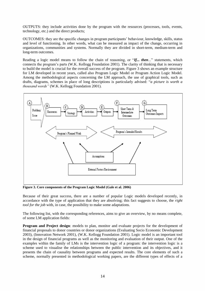
Reading a logic model means to follow the chain of reasoning, or “If... then...” statements, which
connects the program’s parts (W.K. Kellogg Foundation 2001). The clarity of thinking that is necessary
to build the model is crucial for the overall success of the program. Figure 3 shows an example structure
for LM developed in recent years, called also Program Logic Model or Program Action Logic Model.
Among the methodological aspects concerning the LM approach, the use of graphical tools, such as
drafts, diagrams, schemes in place of long descriptions is particularly advised: “a picture is worth a
thousand words” (W.K. Kellogg Foundation 2001).
Figure 3. Core components of the Program Logic Model (Gale et al. 2006)
Because of their great success, there are a number of popular Logic models developed recently, in
accordance with the type of application that they are absolving; this fact suggests to choose, the right
tool for the job with, in case, the possibility to make some adaptations.
The following list, with the corresponding references, aims to give an overview, by no means complete,
of some LM application fields:
Program and Project design: models to plan, monitor and evaluate projects for the development of
financial proposals to donor countries or donor organizations (Evaluating Socio Economic Development
2003), (Innovation Network 2001), (W.K. Kellogg Foundation 2001). Logic model is an important tool
in the design of financial programs as well as the monitoring and evaluation of their output. One of the
examples within the family of LMs is the intervention logic of a program: the intervention logic is a
scheme used to visualise the relationships between the public intervention and its objectives, and it
presents the chain of causality between programs and expected results. The core elements of such a
scheme, normally presented in methodological working papers, are the different types of effects of a

15
financial measure and the different types of objectives to which the measure can contribute (ECORYS
and IDEA 2005).
Research development: LM is a tool commonly used to plan and to strengthen the conduction of
relevant, strategic, basic and applied research, rather than the improvement of technology development
in close connection with the private sector. The flexibility of LM allows to consider in a unique logic
scheme the public or private inputs (funds, researchers, facilities, etc) the outputs of the research and the
technology development produced in collaboration with the private sector, conducting technical
demonstrations, tests and studies, including the building of a market infrastructure to support
technologies (Jordan 2003).
Strategic planning: to identify and prioritise major long-term desired results in an organisation, and
strategies to achieve those results (Gale 2006), (Information Society and Media DG 2005), (Evalsed
2008).
Organisational assessment and business management: comprehensive view of the current
situation in an organisation, but without prescribing how to change it in order to evaluate the actual
performance (National Institute of Standards and Technology 2008).
Resources and environmental management: as for the management of resources within a society
or organisation, LM is applied also for the evaluation of the efficiency in the use of natural
resources in a context of environmental management. (Turner et al. 2000; Rose 2002).
University and learning courses: LM theory and application are the core topics of university and
learning courses about programs’ evaluation (Harvard Family Research Project 2000; Cooperative
Extension 2008; Powell and Henert 2008; Frankel and Gage 2007).
1.1.3 Relations between Logic Models and grids
The representation and schematisation of a complex problem is often multidimensional. As already
briefly described, AGRIGRID is typically faced with this kind of problem. In fact, the analysis and
representation of how payments should be modulated in terms of MS, region, area, type of measure, etc.
is a typical multidimensional problem which cannot be represented by a simple LM. However, the
concept of grids includes two main aspects: the first one is mainly the representation of
multidimensional complex problems, while the second (and more represented in literature ) is the
interconnection, analysis and distribution of knowledge taken from different and un-homogeneous
sources.
On the last definition of grids, examples in literature are rather frequent, ranging from biomedical
sciences (Payne et al. 2007) to the prevention and management of natural disasters (Smirnov et al. 2007),
finally to Information Technology (Napier et al. 2009).
The design of grids involves, in that sense, both the multidimensional representation of the problem and
the systematisation and use of different sources of information. In the AGRIGRID framework, the
methodology applied has mainly considered the grids as a tool for representing the problem. However,
the way the problem of defining a methodology for payment analysis and calculation has been faced is
strictly related with the “grid” approach. In fact, sources of information are rather un-homogeneous,
knowledge is dispersed and a systematic approach is missing. In that way, the final product of the
AGRIGRID project can be considered as a first prototype of a knowledge grid, where a proper
methodology of analysis is codified and information/data originated from different sources are made
available.
16
2. Methodology During the project, and parallel to the bibliographic research, the comparative analysis of payment
calculations has outlined with more precision the whole methods with which the justification of the
investigated RD measures and countries/regions were implemented in the current programming period.
One of the first activities within WP8 was to study a way to link the different methodological aspects
found in literature and the experience and knowledge provided by specific analyses of the current
justification documents; this would grant a more reliable design of the desired structure of the grids.
The activities of analysis and design, described in more detail in the paragraph 2.1, had the main
objective of defining the logic model at the base of the methodological grids: the model links all the
information, criteria and domains involved in payment calculation and fixes the recommended
procedures to determine the final level of compensation for the acceptance of the RD commitments.
Beyond the drafting of the LMD, the design activity ended with the creation of a preliminary raw
structure for the grids.
Later on, the first grids were delivered to the WP2-WP6 leading partners and applied to the investigated
measures and MS, in order to test their performance and sensibleness. Thanks to such practical
experience, it was possible to bring the necessary modifications and improvements to the structure with
the synergic work of all partners; in this way, it has been possible to produce a user-friendly, flexible and
suitable tool applicable to the whole set of measures investigated, as well as to different countries or
regions. Paragraph 2.2 presents more specifically the single activities carried on to revise and adapt the
raw structure, in anticipation of the realisation of the final methodological grids.
2.1 The phase of analysis and design of the preliminary grids
One of the important results of the review of RD payment calculations across the EU was a more precise
knowledge of what has been done by the managing authorities to respect the new standards and rules for
the current programming period. The analysis of RDP documents, in particular of the payment
justifications, showed a high degree of variation in the extent of the implementation of a particular
measure in different countries. Among the justifications, there are various examples of exhaustive
accomplishment of the new EC dispositions (Figure 4): first the identification of the relevant baseline
practices, then their association with the RD commitments and finally the calculation of the payment
through the standard cost approach, based on the difference between the economic appraisal of the farm
performance in the baseline situation and that one participating to the measure.
These are not the most common situations observed across the set of member states and of investigated
measures. Several problems have been identified during the review of payment calculations: in some
cases the lack of methodological experience in payment administration implied that the baseline
practices were not always defined and their connection with the RD commitments were not transparent
and clear. In other cases, the standard cost approach did not take into account the wide range of different
circumstances. The lack of reliable technical and economical data negatively influenced the
representativeness of “standard” or average figures for costs and revenues.

17
Figure 4. Example of linkage between baseline, RD commitments and respective costs/revenues – Animal
Welfare payments in ITER
Grids and logic models are commonly used together to make multi-dimensional problems easy to
consider and solve. As a schematic way of representing a decision-making process, a grid can be
formulated as a simple spreadsheet where different parameters influencing the decision are included. The
increasing complexity of the decision-making process often leads to a set of tables connected by links
and logic connections. The standardisation of the procedures of selection of such parameters represents
also the recommended “guideline” for the correct implementation of the calculation process.
The last operation is rather complex and the different approaches adopted for each individual measure
and for each partner country impose the implementation of a very general framework as well as a set of
standard grids that can be modified and adapted at country level and measure level. Figure 5 shows the
logic scheme, the LMD of the methodological grids, as a theoretical process to determine the final level
of payment in every RD measure and MS. It includes an identification of Cross-Compliance for each
country and each measure, a consequent definition of the baseline, a clear identification of additional
commitments for each individual measure and, finally, a calculation of revenue losses and additional
costs for each measure and each of the “dimensions” considered in the calculation.
The main differences between existing grids and the proposed scheme are mainly due to the fact that:
for some measures it is rather difficult to define a proper baseline (e.g. natural handicap
payments, forestry measures);
cost lists and differentiation elements are rather diverse and standardisation seems to be very
difficult;
data sources are also very different and, again, a standardisation is almost impossible.
Baseline practiceRD
commitmentCosts and
revenues
in baseline
situation
Costs and
revenues
with
additional
commitmentsCost/revenue
componentsPayment
calculation

18
Figure 5. Logic scheme of the analysis, as a result of the review of current RD payments
In Figure 5 there are some specific aspects – like data sources and others – that, excluding the “level of
spatial detail” included in the domain of payment differentiation, apparently are not considered within
any of the above cited domains, but that definitely need to be taken into account to accomplish the EC
requirements for the implementation of payment calculation. In addition, the necessity to produce an
ever-effective tool over several measures, and all the EU member states/regions, inevitably implies a
series of complications in the grid development.
The following are the main factors that had to be considered before the design of the grids:
The necessity to consider some elements relevant within the calculation of payment, whose
effects are not very clear and observable:
Different countries and measures;
Sources of data;
Different methods of calculation of a single cost/revenue item;
Transaction costs;
Ceilings of the EC regulations;
Differentiation of payments according to the year of commitment;
The lack of information about baseline in some specific countries or within some
measures;
The extent of implementation of a particular measure in different countries implies the
involvement of information usually characterised by an high degree of variation among them
and within their domains; this fact means that their harmonisation and classification within the
domains is necessary;
The standardisation of the calculation methods contrasts with the necessity to have a flexible
structure always applicable among countries and measures.
These problems were very important for the correct definition of the structure of the grids themselves.
The identification of a resolution a priori is not unique. Hence the research for a solution was done
through the practical application of preliminary grids to the investigated measures. The following
paragraph reviews the main activities for producing the final methodological grids.

19
2.2 The second phase: development of the methodological grids
The second phase of the project was totally dedicated to the creation of a system applicable EU-wide as
well as differentiated by the nature of the measure. The following are the main operative procedures
carried out within this phase:
1. The creation of a preliminary model of methodological grids with a structure as similar as
possible to the draft outlined within the design phase.
2. The definition of guidelines for the application of preliminary grids to the set of measures the
project deals with. The work allowed the extraction of the different information, rules and
methods contained in each investigated measure and to obtain a reference data set to test the
applicability of every revision and adaptation of the raw structure.
3. Thanks to the practical experience of the partners in the use of the grids, it was possible to
identify the modifications, additions and lacks necessary to improve their applicability,
particularly in the integration of all the information and methods, and in the standardisation of
the implementation procedures for the calculations. An important role within this activity was
performed by the definition of specific classification systems to integrate the information among
the several measures and MS.
4. The definition of the general logic framework, representing the general functioning of the
methodological grids in a flux diagram; the general framework was then adapted to produce
measure-specific logic frameworks.
5. The definition of a proper layout for the methodological grids, both at general level and
measure-specific level.
The above activities constituted also the reference point for the implementation of the software tool.
3. Logic framework for the application of methodological grids to
RD payment calculations The logic framework provides the method to connect the different parts that make up the methodological
grids; it represents the logic sequence of actions that also a inexpert operator can follow to carry out the
recommended RD payment calculation process.
The framework derives from the LMD of the first phase of analysis. Indeed, the main objective of the
first part of the grid development was to represent, using a grid-based structure, the payment calculation
of each individual measure as it is, at present time, included in the Rural Development Programmes
2007-2013. While eligibility criteria and scheme commitments are often similar across countries, the
level of detail in the calculations varies between the different implementations. The standard cost
approach can be as simple as using an aggregate figure for both costs and revenues or can include
several cost and revenue components for a range of required activities. Similarly, approaches used to
quantify the different components vary from using expert studies or opinions to more detailed modelling
exercises. Therefore, developing such a structure required a detailed knowledge of present conditions
and methods at both production and policy level: existing payment calculations have been reviewed in
the nine partner countries to obtain a better understanding of how the calculations were carried out and
to collate a comprehensive database of calculation components.
The initial shape was that of a flux diagram because it gave the possibility to resume all the operations of
the calculation process in one page, highlighting the main passages. For the development of the
methodological grids, the logic framework developed in the first phases of the project has been useful to
know how the MS approached the problem in the definition of Rural Development programs. The
definitive formulation of the framework resulted from the synergic work among the project partners,
each contributing personal experience in the application of the preliminary grids to the specific

20
measures. After the logic framework was delivered to partners, it was adapted by the horizontal
packages to measure specific needs. The latter activity also helped the partners in the development of the
measure-specific grids.
Figure 6 is the general logic framework in its definitive layout: it has been designed as a sequence of
operations, according to the different phases of RD payment calculations:
The recognition of relevant baseline requirements and the comparison of these requirements
with the voluntary practices provided for by the RD measures;
The identification of cost and revenue components prompted by the RD commitments;
The definition of the most suitable criteria for the differentiation of payments.
Figure 6. General logic framework for the development of methodological grids
Nevertheless, payment calculations can still vary significantly between measures; this implied that
different logic frameworks needed to be developed and applied, which consequently resulted in different
designs of the measure-specific methodological grids.
Some of the measure-specific frameworks (e.g. in Animal Welfare or Natural Handicap Payments) are
quite similar to the general format, while others ended up in very altered structures, like the one designed
for Natura 2000 payments grid (Figure 7). But the most notable example can be probably found in the
afforestation measures (Figure 8), where special attention needed to be paid to design separate
calculations of establishment costs, maintenance costs and agricultural income foregone.
In the following paragraphs, the development of each of the above mentioned steps will be described.
Selection of costs and revenuesaroused by the application of
RD commitments
Selection of relevant Baseline
Comparison between Baseline and voluntary RD practices
Choice of relevant criteriato differentiate the payment
Creationof the
summary grid

21
Figure 7. Logic frame work for the design of the Natura 2000 payments grid (from D6)
Figure 8. Logic frame work of payment calculations in methodological grids for afforestation measures
(from D7)
Differentiation criteria
Specific practices
Administrative
land division
Type of crop
Additional costs
Income foregone
I. Payment calculated
RDR limits
III. Payment proposed
II: Payment adjusted
Additional limits
Woodland and
Trees
RDR payment rates
Overall amount of financial support
Type of woodland
/ tree Woodland
function Topography Type of land Type of
beneficiaries
Establishment cost Agricultural income foregone
RDR maximum payment per ha
Maintenance cost
Natura 2000,
LFA and WFD
areas
Other Areas Outermost
regions
Area designation
Area
designation
Type of
crop/animal
Technical
specification

22
3.1 Assessment of baselines
The baseline for the current programming period is clearly defined in the EU Commission working
document RD10/07/2006-final, which states that the baseline beyond which AEM commitments have to
go switches from good farming practices to a new set of obligation standards:
Based on EU legislation (relevant Cross-Compliance provisions according to Reg. (EC) No
1782/2003) which comprises:
a. Statutory Management Requirements – SMRs (as set out in Annex III of the Regulation)
b. minimum requirements to maintain land in good agricultural and environmental
conditions (GAECs as set out in Annex IV of the Regulation)
c. maintenance of land under permanent pasture [art. 5(2)]
National/regional legislation identified in the programme, which concerns:
a. minimum requirements for the use of fertilisers
b. minimum requirements for the use of plant protection products
c. other relevant mandatory requirements established by national/regional legislation.
An assessment of the European and national (or regional) baseline requirements regarding Rural
Development is necessary due to the Reg. (EC) 1968/2005 itself, which states that Rural Development
payments can compensate only commitments going beyond the minimum mandatory requirements.
Moreover, during the negotiations for the approval of the current RDPs, it has clearly emerged that the
difference between the baseline and the additional commitments must be properly described in the
programmes and must be coherent with the process of payment calculation. Therefore, the baseline must
be defined according to the description of RD measures in the considered RDPs, which in its turn must
be consistent with the definitions and commitments stated at European level.
This is why the logic framework for the calculation of RD payments takes into account the description of
the relevant baseline requirements and considers also the link between baseline, additional commitments
(specific obligations of the RD measures) and respective costs and revenues.
The starting point of the analysis was a review of how the assessment of the current baseline
requirements has been faced in the investigated RDPs. Using a set of standardised tables, each partner
collected information on SMRs, GAECs and additional requirements in their country (or region). The
additional baseline requirements are obviously neither SMRs or GAECs, but they refer to specific
national/regional legal acts set up by each Member State (or Region), which have no correspondence to
GAECs and/or SMRs as well as to common practices if they are used to define the baseline. Moreover, it
has to be recalled that if, for a particular RD measure or for some Cross-Compliance issue, there are no
relevant SMRs or GAECs, the common agricultural or forest management practices must be considered
as baseline. The reference to common agricultural or forest practices applies also in the case that these
practices (those adopted by the majority of farmers in the area) are more restrictive than SMRs and/or
GAECs. This occurrence seems to be rather uncommon in the RD measures investigated by our project,
nevertheless it had to be taken into consideration when assessing baseline requirements of those RD
measures (e.g. forestry measures) for which the baseline is not defined by a “legal act”.
This analysis provided a useful overview of which baseline requirements are more relevant for a
particular RD measure: for example, within Natura 2000 measures the baseline is represented mostly by
common practices and by the requirements stated in additional national legislation which applicants
have to meet in the Natura 2000 areas. A similar situation occurs with the forestry measures, for which
SMRs and GAECs are seldom applied in most of the investigated countries and regions. On the contrary,
baseline requirements under Reg. 1782/2003 are relevant for Animal Welfare measure across the EU.
Notwithstanding this, the review pointed out also the fact that the existing baseline requirements are
seldom considered directly in the calculation of RD payments.

23
According to EU legislation, it is the difference between a baseline practice and a RD requirement which
should determine the amounts of additional costs and revenue losses that settle on the amount of
payment. The lack of evidence of this relationship drove the European Commission to ask many
Member States for integrations in their current RDPs.
So, a general system of comparison between baseline and RD commitments, the so-called linkage table,
has been designed. Table 1 shows an example of how this table (in one of its provisional designs) has
been filled by partners, according to the commitments provided for by the RD measures investigated in
the project.
However, it has to be recalled that, although all regulative measures hold when implementing a RD
measure, not all of them influence payment calculations. More precisely, only baseline requirements
whose tightening up directly influence the balance of a firm in terms of additional costs and/or revenue
losses have to be considered in the payment calculation. For example, the baseline requirements for the
scheme of Protection of NVZs in Greece derive from the local Special Action Plan, issued in compliance
with the EEC Directive 91/979 which in its turn is part of the European SMRs. Yet, all provisions related
to manure handling, even though being part of the Special Action Plan, do not constitute an active
element in the specific calculation procedure since no manure is used in the production process under
examination.
A peculiar case is related to natural handicap payments (measures 211 and 212), since for these
measures the baseline requirement is basically the same as the RD commitment: i.e. to continue farming
and to comply with the minimum requirements. Therefore, what counts in the calculation of natural
handicap payments is the difference in the permanent natural handicap between the less favoured area
and the reference area. The reference areas are those where there are no permanent natural handicaps.
Examples of the final linkage tables implemented in the methodological grids are shown in the Annexes.
Most of the baseline requirements collected by partners have also been used to create a library that has
been implemented in the final software tool.
3.2 Identification of cost and revenue components
One of the key issues in the process of payment calculation is the recognition of how the implementation
of a RD commitment influences the balance of a farm in terms of additional costs and/or revenue losses.
The foremost step towards the creation of an organized cost/revenue structure has been trying to detect
relevant cost, revenue and income components used in the payment calculations of the current
programming period and to codify them in a standardized way. At an early stage FADN (European Farm
Accountancy Data Network) categories have been used as a basis to produce a first list of cost/revenue
items. The result was a roll of entries, which every partner had to adapt to the different measures and
countries, highlighting the most relevant elements and adding any missing one, on the basis of the
specificities come out from the investigated RDPs during the first phase of the project.

24
Table 1. Examples of linkages between RD commitments and related baseline requirements
RD commitment Baseline practice Type of baseline Additional cost element Additional revenue element
Sheep's meat
Ewe's milk
Grazing capacity Additional baseline
Goat 's meat
Goat's milk
RD commitment Baseline practice Type of baseline Additional cost element Additional revenue element
Release of 2 trees per hectare of
felled timber, chosen among the
larges t or oldest ones
Observance of the provis ions
concerning the realese of a single
tree for each cut hectare, chosen
among the largest or oldest ones
Additional baselineTopographic locat ion of trees
Forestry exploitation costsRevenue from forestry exploitation
RD commitment Baseline practice Type of baseline Additional cost element Additional revenue element
The applicant shall farm in
conformity with GAECAll GAEC GAEC
Commitment not inc luded in
calculationCommitment not included in calculation
The applicant shall ut ilize the
agricultural land for a set period of
t ime
Administrative condition – not
covered by payment
Administrative condition – not covered by
payment
The applicant shall assure that
grasslands are at least 1x grazed
or 2x mowed a year (with few
except ions) within fixed deadlines.
The mowed biomass shall be
removed from the parcel
Basic grasslands maintenance as
a common farming pract iceAdditional baseline
Commitment not inc luded in
calculationCommitment not included in calculation
Act No. 114/1992 Coll., on the
protection of nature and
landscape, as amended in
connection with the creation of the
Natura 2000 network
SMR SE295-Fertilisers Hay yield
The typical/general fert ilisation
level = 80 kg N/ha (mineral)Additional baseline SE281-Total specific cost Yield of meadows
After transit ion to the single
payment scheme, the applicant
shall comply within his entire
holding with the binding
requirements (SMR)
All SMR SMRCommitment not inc luded in
calculationCommitment not included in calculation
Measure 225 in Italy, Umbria Region
Measure 213 in Czech Republic
Application of fertilisers or farm
manure shall be avoided. In case
of pasture, grazing livestock may
produce at most 30 kg N per
hectare of grazed area
Measure 214 in Greece
214_5. Livestock farming extensification - 5.1. Rental of private pastures
Rental of private pastures
Maintain minimum livestock
densityGAEC SE375-Rent paid
Environmental management planActions for the avoidance of
degradation all of pasture areas
(old and new)
Avoid excessive stocking density GAEC

25
The selected balance sheet entries have been grouped in the following categories:
A) Production of crops / livestock activities (Yield * Price)
B) Subsidies
C) Variable Costs
D) Gross Income (A+B-C)
E) Transaction costs
F) Data sources (qualitative information)
As before mentioned, the proposed list was built starting from the FADN structure, adapted and
simplified to fit to the methodology of payment calculation in the RDPs. In particular the following
adaptations have been considered:
the list originally included only variable costs: this is clearly stated in the methodological
document RD/10/07/2006–final, which imposes that investments in machinery or installation
needed for the specific commitments fall under investments and cannot be considered in the
payment calculation. That is why only costs associated to the use of production means have been
considered;
opportunity costs are not included in the FADN cost/revenue structure, however the use of
opportunity costs is accepted in certain cases. One case is the opportunity cost of family labour,
which is one of the most frequent additional costs in the calculation of RD payments;
taxes, being a general cost calculated at farm level, were not considered in the first list; also
Value Added Tax (VAT) is normally internalised in the price of products and is generally not
explicit in the taxation system in agriculture;
items for transaction costs were left free as they do not fit into the FADN scheme;
the proposed list included also some categories of subsidies, as they can be relevant (in a few
cases, actually) for payment calculations; in fact, they can be relevant only if the possibility of
drawing an aid is somehow hampered by a particular RD measure (e.g. the RD commitments
modify the level of the subsidy).
The leading partners of Work Packages 2 to 6 adapted the proposed list to the RD measure they were
responsible of and afterwards every project partner verified and in case updated the proposed categories
using information drawn from their national/regional RDPs.
The outcome of this task was a long and diverse list of costs, revenues and other items, as well as a set of
reports delineating the importance that a particular entry has in the payment calculation of each
investigated RD measure. In the case of cost or revenue components not belonging to the FADN
database, the possible data sources for the component itself were also reported.
What emerged clearly is that many of the items reported in the final list could hardly be put in a FADN-
like balance sheet structure; nevertheless, most of them were relevant and have been also used in many
payment calculations of the current programming period. This happened because, in accordance also
with the EC document RD/10/07/2006–final, the proposed starting list was based on a profit-and-loss
account approach, while current payment calculations are often based on a so-called “production
process” approach. Hence, the listed entries can be divided in two general types:
cost/revenue items taken directly from the FADN database or, however, items that can be easily
related to an existing FADN variable. For example, entries with a higher detail with respect to
the European definitions but whose level of detail is available in the national FADN networks,
or balance-sheet items that cannot be included in a profit-and-loss account but are counted in
FADN as assets and are also relevant for some payment calculations;
other items (mainly costs) referring to a farming practice or to a production process, which is
affected by the implementation of a RD commitment and whose monetary value is directly
estimated in the calculation (e.g. the cost of mowing or for the drafting of a management plan);
In the definition of a new methodological path for the calculation of payments, we faced the difficulty of
combining the two types of cost/revenue items and, as a consequence, the two different calculation

26
methods that can be found in the Rural Development Programmes. Therefore, we took the decision of
splitting all entries in two separate lists and setting up two not combinable approaches to be followed
within the methodological grids: the Balance Sheet approach and the Practices approach.
3.2.1 The Balance Sheet approach
The Balance Sheet approach consists of a direct comparison, in a proper accounting exercise, of two
samples of farms: one undertaking a Rural Development scheme and one similar in terms of farming
system and local conditions, but not participating in the concerned scheme.
Once chosen the balance items that are influenced by the implementation of a RD commitment, the
difference existing between the two samples in all those revenue and cost components (i.e. the difference
in gross margin) determines the cost of participation in the scheme.
Evidently, the available data sources and the nature of the samples influence the level of detail that can
be reached in the selection of cost/revenue components for the calculation process. Hence, the grids give
the possibility to choose the appropriate level of detail, whether it is a simple comparison of total farm
output and costs or a very detailed calculation carried out considering yields and prices of products as
well as single components of production inputs.
A possible variation of the Balance Sheet approach is what in Deliverable 4 has been defined as partial
budgeting: this simplification of the main approach consists in the identification of an appropriate
sample of non-participants and the assessment of revenue and cost elements which are known to be
influenced by a RD commitment; then, variations due to the implementation of a measure are estimated
in the form of either a proportional or absolute value change.
This second calculation method has been largely used in the investigated Member States; nevertheless,
its application is not desirable because it often entails a wide resort to expert opinion instead of using
significantly representative figures.
What joins the two above mentioned methods is the obligation of using only a fixed balance-sheet
structure, with no chance of adding new items. This aspect, though giving the grids a certain
inflexibility, should allow easier comparison of different calculations, among Member States but also
among RD measures.
Furthermore, the original idea behind the creation of a calculation approach based exclusively on FADN
definitions was to give the possibility in the future to supplement the grids and the software with data
taken directly from the FADN datasets. Anyway, there is no constraint of using FADN data: figures for
calculations can be taken from every source.
The Balance Sheet approach suits the payment calculation of those RD measures whose commitments
involve the whole farming system; in fact, it has already been used in the payment calculation for the
introduction of organic farming in Germany and Czech Republic. Another example can be the
calculation of natural handicap payments (measures 211 and 212), as they consider the handicap of the
entire farm located in a less favoured area.
The full list of FADN items that has been implemented in the methodological grids is reported in the
Annexes.
3.2.2 The Practices approach
The implementation of most of the current RD measures (or sub-measures) usually involve just a few, if
not only one, production processes or farming practices. So, this approach consists in breaking down a

27
particular RD measure in commitments, according with the description of the measure itself in the
official documents.
Once identified which practices are influenced by the implementation of a RD measure3, the following
step consists in fixing how the “cost” of these practices varies when passing from the baseline situation
to the “committed” situation. This operation can be carried out in two ways:
directly assessing the cost of the practice, through available price lists or (less preferable)
through an expert opinion;
determining and quantifying the specific and implicit costs that can be attributed to the
implementation of the practice.
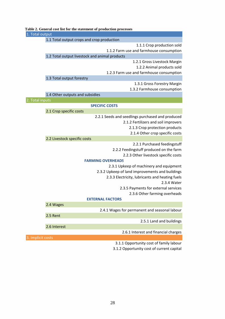
Evidently, the second option is the most effective; therefore, the working group drafted a short list of
cost components that could be used for the statement of every production process that have been
incorporated in the methodological grids. The statement is shown in Table 2 and the meaning of each of
the statement’s entries is explained in the Annexes. However, in the horizontal WPs a few adaptations
have been made, in order for the general statement to fit the measure-specific grids.
The main problem related to the adoption of this approach concerns the statement of the credit side of
the account. In fact, it is seldom possible to determine the revenue of a specific activity within a farming
system. For this reason, revenues can be assessed at farm level instead of the “practice” level.
Calculation approaches similar to this one were already used in the current programming period, for
example in many Natura 2000 schemes and in some very specific AEM measures. Table 3 reports a few
examples of how the Practices approach works within the investigated RD measures.
3 The working group has already supplied the methodological grids with a set of commitments and practices that
can be frequently noticed in the payment calculations of current RDPs.
28
Table 2. General cost list for the statement of production processes
1. Total output
1.1 Total output crops and crop production
1.1.1 Crop production sold
1.1.2 Farm use and farmhouse consumption
1.2 Total output livestock and animal products
1.2.1 Gross Livestock Margin
1.2.2 Animal products sold
1.2.3 Farm use and farmhouse consumption
1.3 Total output forestry
1.3.1 Gross Forestry Margin
1.3.2 Farmhouse consumption
1.4 Other outputs and subsidies
2. Total inputs
2.1 Crop specific costs
2.2.1 Seeds and seedlings purchased and produced
2.1.2 Fertilizers and soil improvers
2.1.3 Crop protection products
2.1.4 Other crop specific costs
2.2 Livestock specific costs
2.2.1 Purchased feedingstuff
2.2.2 Feedingstuff produced on the farm
2.2.3 Other livestock specific costs
2.3.1 Upkeep of machinery and equipment
2.3.2 Upkeep of land improvements and buildings
2.3.3 Electricity, lubricants and heating fuels
2.3.4 Water
2.3.5 Payments for external services
2.3.6 Other farming overheads
2.4 Wages
2.4.1 Wages for permanent and seasonal labour
2.5 Rent
2.5.1 Land and buildings
2.6 Interest
2.6.1 Interest and financial charges
3. Implicit costs
3.1.1 Opportunity cost of family labour
3.1.2 Opportunity cost of current capital
SPECIFIC COSTS
FARMING OVERHEADS
EXTERNAL FACTORS
29
Table 3. Examples of implementation of the Practices approach
Measure 214
RD Commitment Baseline Practice Revenue Costs
1 mowing/year mandatory 3 mowings/year mandatory if there's no
grazing Mowing
Fixed list of revenue
components
Fixed list of cost
components
Prohibition of use of any
pesticides, fertilisers and soil
improvers
Prohibition of use of some types of
pesticides
Fertilization Fixed list of cost
components
Crop protection Fixed list of cost
components
Establishment of catch-crops Cultivation of arable land
Ploughing
Fixed list of revenue
components
Fixed list of cost
components
Sowing Fixed list of cost
components
Removal Fixed list of cost
components
Production of organic cereals Production of conventional cereals Fixed list of revenue
components
Fixed list of cost
components
Measure 221 – Establishment costs
RD Commitment Baseline Practice Revenue Costs
Establishment of a new woodland
or forest No forest or woodland present
Site preparation
Fixed list of cost
components
Planting Fixed list of cost
components
Protection Fixed list of cost
components
Measure 221 – Agricultural income foregone
RD Commitment Baseline Practice Revenue Costs
Establishment of a new woodland
or forest on agricultural land
Active agricultural land management and
production
Fixed list of revenue
components
Fixed list of cost
components
Measure 213
RD Commitment Baseline Practice Revenue Costs
Grazing livestock may be at most
30 kg of N per ha of grazed area
The typical/general fertilisation level is
80 kg of N per ha (mineral) Fertilization
Fixed list of revenue
components
Fixed list of cost
components

30
Measure 215
RD Commitment Baseline Practice Revenue Costs
Conversion from stall-feeding to
mixed rearing (free range in
spring and summer pastures and
stall-feeding in the remaining
period)
Animals may be stall-fed
Feeding
Fixed list of revenue
components
Fixed list of cost
components
Grazing Fixed list of cost
components
Adoption of veterinary assistance
schedule
No mandatory plan or veterinary
schedule, except for calves
Veterinary
assistance
Fixed list of cost
components
Examples for agri-environmental measures:
The first example shows one commitment counting one practice, and one commitment counting two practices
The second example shows one commitment counting three practices
The third example shows one commitment without any practice
For each practice a fixed list (always the same, i.e. the one reported in Annex X) of cost components can be filled-in. Otherwise, a comprehensive cost value can be assigned
to the whole practice.
Revenue will be generally determined only once for the entire commitment (using a fixed list of revenue components or assigning a comprehensive value), as it is usually
difficult to assign a specific revenue to each practice.
Examples for forestry measures
Measure 221 – Establishment costs: one commitment and a number of practices with a list of cost components for each practice
Measure 221 – Agricultural income foregone: one commitment with no specific practices Gross margin calculation through a set of revenue and cost calculations
These examples reflect the possible splitting of forestry grid in sub-grids
Example for Natura 2000 on agricultural land
One commitment with one practice, whose “value” can be either directly stated or calculated through the fixed sets of revenue and cost components
Example for Animal Welfare
One commitment counting two practices, and one commitment counting one practice
For each practice the fixed list of cost components can be filled-in. Otherwise, a comprehensive cost value can be assigned to the whole practice.
Revenue may be determined only once for the whole farm (using a fixed list of revenue components or assigning a comprehensive value) as it is usually difficult to assign a
specific revenue to each practice.

31
Table 4 shows in which methodological grids the two calculation approaches have been implemented.
Table 4. Implementation of the two calculation approaches in the methodological grids
LFA Natura
2000 AEM
Animal
Welfare Forestry
Meeting
Standards
Balance
Sheet × × ×
Practices
= implemented; × = not implemented
Whatever is the approach chosen for the calculation of a certain payment, one must face the problem of
data availability. Considering the wide range of commitments and calculation approaches applied, it is
conceivable that each country uses a varied heap of data sources.
At the beginning of the grid development, based on the outcomes of the initial review of current payment
calculations (Figure 9), a list of possible data sources have been proposed; in this list, derived from an
Italian MoA’s document, the sources were catalogued in a theoretical order of representativeness:
ad hoc surveys
EUROSTAT data
national statistics
FADN database
monitoring and evaluation of previous RDPs
third party surveys
planning documents from Public Authority
periodic publications by Chambers of Commerce
data owned by producer associations
opinion of experts
other statistics and economic data
This preliminary list resulted insufficient to categorize all used data sources. Hence, the working group
decided to give each measure-specific grid’s developer the possibility to identify the most suitable data
sources for its grid. In fact, the methodological grids must be flexible enough to account for large
differences in available data. Hence, in the final grids the user is let free to use any data source, but
detailed information on the source and justification of inserted values needs to be provided.
Another crucial aspect of payment calculation is related to the fact that many cost and revenue
components can be broken down into simpler elements. This is why for each measure-specific grid a sort
of multi-layered calculation structure has been developed, which allows to calculate cost and revenue
components at different aggregation levels depending on the available information and data. The number
of calculation layers which can be added to the calculation process is flexible (depending also on the
concerned measure) and can be adjusted according to the calculation requirements and data availability.
Furthermore, each grid provides a basic set of formulas for the most common calculation elements.

32
Figure 9. Use of different data sources in the investigated countries and measures
3.3 Payment differentiation criteria
The third necessary step to design the final structure of the methodological grids was the definition and
description of the factors that must be taken into consideration during the calculation as “differentiation”
of payments. These are, of course, measure-specific elements as well as country-specific ones. As a
matter of fact, the differentiation of Rural Development payments can be considered as one of the main
systems to avoid under- and over-compensation.
Payment differentiations can be made according to various criteria. Using spatial criteria one can
identify at least three categories of differentiation, using either administrative, environmental or
agronomic data. A second broad classification approach is the use of structural characteristics of a farm.
A preliminary assessment of relevant differentiation criteria has been done by Partner 7 on the basis of
the Deliverable D2: taking as a starting point the categories identified on page 25 of the deliverable,
0 1 2 3 4 5 6 7 8 9
Norms and legislation
Scientific literature
Opinion of experts and stakeholders
Monitoring and evaluation of previous RDPs
FADN database
Surveys and statistics
0 1 2 3 4 5 6 7 8 9 10
CZ
DE
IT
LT
SCO
PL
ES
Norms and legislation
Scientific literature
Opinion of experts and stakeholders
Monitoring and evaluation of previous RDPs
FADN database
Surveys and statistics

33
some main types of payment differentiation that can be found in the various RDPs have been
highlighted. These were:
land use / animal species
crop / variety / breed
intensity of farming practices, production and conditions
farm size (ha, LSU, etc.)
administrative / regional / territorial differentiation
specific land or animal attributes
socio-economic indicators or indexes
For each of the above mentioned groups, a first brief inventory of differentiation elements coming out
from D2 have been listed. Task of each WP2-WP6 leading partner was to define a complete set of
relevant payment differentiation categories and to extend the list of differentiation elements under each
category, basing on the outcomes of the review carried out during the first phase of the project.
Subsequently, every partner country had to complete the above mentioned measure-specific lists adding
relevant country-specific elements used at present in the national/regional RDPs.
The reasons why each element have been included in the differentiation lists have been also reported in a
separate document.
Once again, the result was a very heterogeneous set of items, with partially overlapping categories, and
elements that could fit into more than one category. Moreover, there was also some mixing up of
differentiation elements with eligibility criteria and/or baseline situations. Besides, payment
differentiation varies significantly between different RD measures: in Agri-environmental measures a
great variety of differentiation approaches have been used, while Natura 2000 payments are less
differentiated, rather, most of the commitments show only one payment level per hectare. Quite complex
is the situation regarding Meeting Standards: in Greece this measure is not differentiated at all, while in
Veneto Region, Italy many variants were observed.
Task of Partner 7 has been to try and reorganize all the information in a structured but as simple as
possible configuration.
The final structure of the differentiation criteria is organized in three levels:
1. Categories 2. Sub-categories (groups of differentiation elements with the purpose of tidying up the lists)
3. Elements (they represent the basic way of differentiating a RD payment)
All the items reported in the final structure were mostly taken from the information provided by all
project partners, with the addition of a few more elements collected from already existing EUROSTAT
classifications like FADN, CORINE, etc. The structure of the differentiation criteria is presented in the
Annexes.
3.4 Final grids and step-by-step template
The final grids are just the end of the path followed through the logic framework: they can be considered
as a multi-layered set of tables, each of them containing all the information collected and worked out
during the various phases of the analysis.
In order to present in a simplified way the application of each developed grid, an easy-to-follow generic
template has been designed. This structure, presented in Figure 10, derives directly from the logic
framework and it basically consists in the various procedures that a user has to do when using the grids.
The seven main calculation steps that make up the general template are:
1. The choice of the approach for the calculation: in the first step, the user must to select one of
the two previously described approaches (Balance Sheet or Practices); once chosen, the
calculation approach cannot be changed.
34
2. Creation of the linkage relationship between relevant baseline and RD commitments, and
identification of cost, revenue and income components: at this stage, only the basic structure
of the calculation sheet is defined and no figures for selected calculation components have to be
specified.
3. Definition of payment differentiation criteria: depending on the characteristics of the
concerned measure, one or more differentiation levels can be specified; based on the chosen
differentiation criteria, separate calculation processes for each differentiation situation can be
prompted.
4. Calculation of monetary values for practices and cost, revenue and income components,
and/or identification of data sources for appropriate figures: at this step there are two data
entry options, i.e. to specify figures for both RD commitment and baseline situation to obtain a
calculated difference, or to put in the difference directly if specific data are missing.
5. Calculation of transaction costs: they include costs for information seeking, provision of
technical advices, bookkeeping, training courses and other opportunity costs and can be
calculated as a fixed amount or as percentage of the overall calculated payment (up to 20%).
6. Consideration of RDR payment limits and application to eligible payment elements: in the
RD Regulation maximum payment ceilings are specified for some measures, so the grids give
the user the chance to apply them to the calculation process.
7. Overview of final payment.
While the generic step-by-step structure is the same across all Rural Development measures, a few
special calculation issues need to be considered in the measure-specific grids. One clear example can be
found in the forestry grid, as the calculation process varies between different forestry measures.
Afforestation measures (including the agro-forestry measure) apply a similar logic framework to the
payment calculation. However, separate calculations of establishment costs, maintenance costs and
agricultural income foregone payments (where applicable) become necessary. These “sub-payments” of
afforestation measures have different practices and can have different payment differentiations within
the same forestry measure in the same country, thus requiring a separate calculation grid or matrix for
each of those “sub-payments”. This implies that, for example in afforestation measures of agricultural
land, the step-by-step approach and the calculation process has to be carried out for each of the three
“sub-payments”. The different grids are then brought together at the end of the overall calculation
process to represent the overall financial support provided through measure 221.
On the contrary, some of the developed grids do not include step 5 as transaction costs, according to
existing regulations, are applicable only for a few RD measures (e.g. agri-environmental measures and
animal welfare payments).

35
Figure 10. General design of the step-by-step template
5. Conclusions and recommendations The report provides a synthesis of activities and results of carried out within AGRIGRID project. WP8,
as clearly described in the introduction, has to be considered mainly as a coordination task: in fact, the
objective of the Work Package was to provide the general framework for the development of measure-
specific grids, as well as to contribute to the development of the software tool, in particular for all the
aspects related to its structure and organization. All the activities took place in the middle of the project,
after a preliminary phase of investigation on the existing methods for payment calculation.
The initial part of the report illustrates how the methodology has been investigated, and briefly describes
different methods and applications. The core part of the report focuses on the logic framework for the
process of payment calculation and on the general grids developed and proposed for the construction of
final measure-specific grids.
Then, in the final part of the report different approaches adopted for each individual measure have been
analysed, comparing the baseline definition, the cost/revenue structure adopted in the payment
calculation, the organization of the differentiation elements and the general grids adopted.
Methodological issues Concerning the adopted methodology and the assumptions, it should be recalled and underlined that the
logic scheme adopted by AGRIGRID is designed to be as coherent as possible with the main data
sources used and usable in the payment calculations, i.e. the Farm Accountancy Data Network. In fact,
the balance sheet scheme adopted in the logic framework and in the grids is strongly connected with the
structure of data collection and processing adopted by FADN. The two calculation approaches (Practices
and Balance Sheet) adopted are both directly derived from the FADN balance sheet scheme.
Step 1: Select approach for payment calculation
Step 2: Create and fill linkage table
Step 3: Definition of payment differentiation
Step 4: Calculation and/or source of practices and cost/revenue components
Step 5: Transaction costs
Step 6: RDR payment limits: Overview and calculation of eligible payment elements
Step 7: Overview of calculated payments

36
However, during the project it has been decided to create a standalone software, i.e. data derived from
FADN and other sources are used as inputs for the AGRIGRID software but no direct connections
between FADN or other datasets and AGRIGRID software have been created. This is motivated by the
fact that the format of FADN data and the processing work necessary to adapt them to AGRIGRID is too
complex and too diverse (between measures and MS/regions) to be standardised into an automatic
software procedure.
As often underlined in several reports and working documents during the project, payment
differentiation is one of the fundamental elements to avoid overcompensation. During the first part of the
project the comparison of payment calculations (D2) gave evidence of the fact that payment
differentiation is almost impossible to standardize. Hence, the standardization proposed in AGRIGRID
regarded only main categories of differentiation, living the differentiation elements free for each measure
and MS/Region.
From the point of view of the “economic theory” behind the AGRIGRID scheme, one problem emerged
during the project is related to the possibility of considering fixed costs in the payment calculation. It
must be recalled that the methodology proposed at EU level for payment calculation does not allow to
consider investment costs, even if formulated in depreciation form. There has been a strong discussion
during the negotiation of RDPs on this point and it is not our intent to take a position on it. However, we
suggest some reflections on one significant point: some of the measures (for example organic farming)
imply structural changes on the farm, and these changes are obviously connected with some investments
at farm level. There is, of course, a risk of double counting with Axis I measures but, when Managing
Authorities can certify that investments are not paid twice, a support of investments, either in Axis I
(which is probably better) or in Axis II in the form of depreciation, should be necessary to avoid under-
compensation.
Policy implications On the side of policy implications and suggestions, some important points are the following ones.
In general terms, it can be underlined how the proposed methodology is, for the Managing Authorities
(regions, state administration, agencies, etc.) easy to use and, if adopted, it could contribute to
homogenize the approach to payment calculations which is currently very diverse between regions/MS
and measures. In addition to that, the adoption of the AGRIGRID procedure and software gives the
Managing Authorities the possibility to follow a scheme that is coherent with what is required by EU
Commission, and to respect the economic “logic” behind the payment analysis.
From a practical point of view, the adoption of the AGRIGRID scheme could facilitate the MA in the
process of negotiation of RDPs with the European Commission, as it provides a common scheme of
analysis and respects the guidelines for payment analysis/justification.
Another important point is the possibility for MS and MA to carry on a sensitivity analysis, e.g. for price
variations or costs’ structure. This possibility is particularly important in a period, like the current one,
when price of products and cost of production factors are rather unsteady.
Other benefits of the LMD adoption are represented by the fact that it makes rather easy to verify the
type of data used by the MA in the payment calculation and the assumptions which are the basis for
payment differentiation. If adopted, the AGRIGRID scheme and software could give the possibility to
create a set of information which should allow to compare the situation in different Countries. Of course
a proper data network is still far to be created, however at the current state all data and information can
be stored locally and made available for all users. The creation of a proper data network, and also the
design of links between AGRIGRID and the various datasets used for the Payment Analysis should be
developed only in the framework of a joint project with FADN authorities.
37
With the ongoing process of revision and enhancement of the Rural Development policy within the
“Health Check”, some new strategic objectives have been introduced. This revision of the RD policy
will shortly cause the proposal and negotiation of new measures. This process of revision of RDPs could
be a good chance to test the methodology and the software.
Particularly during 2008 a discussion between MS and EC took place on the opportunity to modulate
payments (in particular agri-environmental ones) to price changes. Also in this case the adoption of the
AGRIGRID framework could facilitate the revision of payments’ scheme and the modulation of
payments.
The most important weak point of the methodology appears to be the availability of data. In the best
case, when using FADN data, the representativeness of the sample is often insufficient to represent very
detailed phenomena as those which are the basis for AGRIGRID calculations. In addition, the sample is
seldom representative for new measures and for measures with a very small uptake. For some measures
the use of FADN data is impossible, see for example forestry measures where no homogeneous data
collection exists at European level.
Another important limitation in the use of FADN data is represented by the fact the European standard
for FADN data collection does not include information on costs of production at the level of productive
process, which means that the only information available is referred to costs of production at farm level.
There are actually some research activity (FACEPA project within the 7th European Research Program
Research) facing this issue, but first results will not be available before the end of 2010.
Last but not least, in some of the measures investigated in the AGRIGRID project (e.g. natural handicap
payments) it has been difficult or impossible to define a proper baseline and to calculate costs/revenues
in the baseline situation. At EU level the measure is now under revision and it is probably convenient to
consider this problem in the process of re-design of the measure.
Remarks In a complex situation, as is the case of AEMs or Forestry measures, policy makers and administrators
tend to adopt measures easier to handle. Proposed innovative schemes that could be not easily monitored
due to complicated calculations for their design and assessment, should not be very popular. This is the
main argument for the usefulness of the calculation grids proposed through the specific project. The
proposed methodological grid for the calculation of AE payments as well as the software will enable
policy makers at all levels of administration to overcome the problem of complexity, increase their
flexibility and thus allow them to adopt innovative measures.
In this sense the adoption of the proposed methodology could be an incentive for decision makers to
adopt more effective measures, having at the same time a simpler approach to payment calculation.
38
References Clemens, M. (2008). The art of complex problem solving. In Idiagram: Visual modelling for complex
business problems. http://www.idiagram.com/CP/cpprocess.html.
Cooperative Extension (2008). Developing a logic model. University of Wisconsin - Extension.
ECORYS and IDEA (2005). Impact analysis: study on baseline and impact indicators for rural
development programming 2007-2013.
Evalsed (2008). The resources for the evaluating of socio-economic development. European
Commission.
Evaluating Socio Economic Development (2003). Sourcebook 2: techniques and tools logic models.
EVALSED.
Fodor, J.A. (1983). The modularity of the mind, Cambridge: MA: MIT press.
Frankel, N. and Gage, A. (2007). M&E fundamental. In A self-Guideed minicourse. U.S.A.I.D.
www.cpc.unc.edu/measure/publications/pdf/ms-07-20.pdf (checked 24.02.2009).
Gale, J., Loux S. and Coburn A. (2006). Creating Program Logic Models: A Toolkit for State Flex
Programs. Flex Monitoring Team
Harvard Family Research Project (2000). LEARNING FROM LOGIC MODELS IN OUT-OF-
SCHOOL TIME. Cambridge.
Information Society and Media DG (2005). GRID-Based Systems for Complex Problem-Solving.
European Commission.
Innovation Network (2001). Logic Model Workbook. p. 20.
Jordan, G.B. (2003). Using Logic Models for Research and Technology Development and Deployment
Programs. American Evaluation Association Annual Conference - November 6 , 2003.
Napier N. P., K.M., Tan F. B. (2009). IT project managers' construction of successful project
management practice: a repertory grid investigation. Information Systems Journal, Vol. 19.
National Institute of Standards and Technology (2008). Baldridge National Quality Program.
http://www.quality.nist.gov/index.html.
Nazar, B. (2006). The Logic Model: Past, Present and Future. Center for Applied Management Practices.
Newell, A., Simon H. (1972). Human problem solving: Englewood Cliffs, NJ: Presentice-Hall.
Payne P.R.O. et al (2007). Conceptual knowledge acquisition in biomedicine: A methodological review.
Journal of Biomedical informatics, 40.
Powell, E.T. and Henert E. (2008). Developing a logic model: Teaching and training guide. University
of Wisconsin - Extension.
Rose, M. (2002). Strengthening evaluation practice in environmental and non-governamental
organizations in the lower mainland. In School of resources and environmental management.
Simon Fraser University.
Simon H. A. (1969). The sciences of the artificial, (1° edn) Cambridge: MA: MIT Press.
Smirnov A., Shilov N. and Levashova T. (2007). Conceptual knowledge acquisition in biomedicine: A
methodological review. Proceedings ISCRAM2007 - B. Van de Walle, P. Burghardt and C.
Nieuwenhuis, eds.
Sternenberg, R.J. and Frensch P. A. (1991). Complex problem solving. Principles and mechanisms.
Turner, R.K., Brouwer R., Georgiou S. and Bateman I.J. (2000). Ecosystem functions and services: an
integrated framework and case study for environmental evaluation. Centre for Social and
Economic Research on the Global Environment.
W.K. Kellogg Foundation (2001). Logic Model Development Guide. p. 48.

39
Annexes
Annex 1
Examples of the final linkage tables implemented in the methodological grids
Annex 2
List of FADN entries implemented in the final grids (from AGRIGRID software)
Annex 3
Explanation of each of the statement’s entries for the Practices approach
Annex 4
Complete list of practices implemented in the methodological grids
Annex 5
Complete structure of payment differentiation criteria

40
Annex 1 Examples of the final linkage tables implemented in the methodological grids
Measure 211 and 212 – Natural handicap payments
Type of baseline Description Baseline practice RD commitment
SMR
Council Directive
91/676/EEC of 12
December 1991
concerning the
protection of waters
against pollution
caused by nitrates
from agricultural
sources.
SMR
Council Directive
91/676/EEC of 12
December 1991
concerning the
protection of waters
against pollution
caused by nitrates
from agricultural
sources.
GAEC Untilled headlands
Arable parcels
alongside
watercourses and
main ditches must
have an untilled
headland of at least
0.6 m, to which
fertilisers and plant
protection products
are not applied.
In the similar manner
in every less favoured
area in Finland, arable
parcels alongside
watercourses and
main ditches must
have an untilled
headland of at least
0.6 m, to which
fertilisers and plant
protection products
are not applied.
Measure 213 and 224 – Natura 2000 payments
Type of baseline Description Baseline practice RD commitment
Additional Baseline
National statistic
(consumption of
mineral fertilizers per
ha of agricultural
land)
The typical / general
fertilization level = 80
kg N/ha (mineral)
Application of
fertilisers or farm
manure should be
avoided. In the case
of pastures, at most
30 kg N/ha can be
supplied annually by
grazing livestock.
GAEC
Rules for the
maintenance of
grassland
On permanent
grasslands growing
vegetation has to be
cut and mulched
yearly, or mowed and
removed from the
land every second
year. These measures
may not be
undertaken between
1st April and 30th of
June
Obligation to keep
principles prohibiting
any deterioration of
the current state of
biotope qualities for
continuing
cultivation.

41
Additional Baseline
Law of the Forests
No. I-671 (approved
by the Seimas of the
Republic of
Lithuania,
22/11/1995).
Standard cultivation
requirements based on
the Forest Law
The final felling of
forests is forbidden,
or should be
postponed.
The final forest
cutting operations
have to be carried out
in non-clear cutting
manner.
An additional number
of living trees has to
be preserved and left
in clear cutting areas.
The cutting of drying
trees or dead wood is
forbidden or restricted
in forest stands 20
years old and more.
Measure 214 – Agri-environmental payments
Type of baseline Description Baseline practice RD commitment
SMR
Specific requirements
on storage, handling
and application
(period, method,
location) of manure
and fertilisers
(specific obligations
for nitrates).
An interval without
any growth during
annual crops
cultivation is required
to be limited because
of the elimination of
increased risk of
nutrient elutriation
according to Nitrate
Directive
Applicant shall sow
annually a specified
catch crop (defined
types of possible /
recommended seeds
in defined amount =
kg/ha) within the crop
rotation on a specified
area and a set
deadline
Additional Baseline
National statistics
(consumption of
mineral fertilizers per
1 ha of agricultural
land)
The typical/general
fertilisation level = 80
kg N/ha (mineral)
The average annual
application of
fertilizers may be at
most 80 kg N/ha (the
limit encompasses
application of
fertilizers, farm
manure and livestock
grazing). At least 5 -
55 kg N/ha of each
land block need to be
supplied annually by
grazing livestock,
which means
limitation of mineral
fertilizers application
and at the same time a
decrease of livestock
density.
Additional Baseline National statistics
Average intensity of
animal rearing on
permanent grassland
= 1.5 LU/ha

42
Annex 2 List of FADN entries implemented in the final grids (from AGRIGRID software)
AGRI01 - Net Income for justification
SE420 - Family farm income
SE415 - Farm net value added
SE410 - Gross farm income
SE131 - Total output
SE135 - Total output crops and crop production
SE140 - Cereals
SE145 - Protein crops
SE146 - Energy Crops
SE150 - Potatoes
SE155 - Sugar beet
SE160 - Oil seed crops
SE165 - Industrial crops
SE170 - Vegetables and flowers
SE175 - Fruit
SE180 - Citrus fruit
SE185 - Wine and grapes
SE190 - Olives and olive oil
SE195 - Forage crops
SE200 - Other crop outputs
SE206 - Total output livestock and livestock products
SE216 - Cows milk and milk products
SE220 - Beef and veal
SE225 - Pigmeat
SE230 - Sheep and goats
SE235 - Poultry meat
SE240 - Eggs
SE245 - Ewes and goats milk
SE251 - Other livestock and products
SE256 - Other output
SE605 - Total subsidies (excluding on investments)
SE610 - Total subsidies on crops
SE611 - Compensatory payments
SE612 - Set-aside premiums
SE613 - Other crop subsidies
SE615 - Total subsidies on livestock
SE616 - Dairying subsidies
SE617 - Other cattle subsidies
SE618 - Sheep and goat subsidies
SE619 - Other livestock subsidies
SE620 - Other subsidies
SE621 - Environmental subsidies
SE622 - LFA subsidies

43
SE623 - Other RD Payments
SE625 - Subsidies on intermediate consumption
SE626 - Subsidies on external factors
SE630 - Decoupled payment
SE631 - Single farm payment
SE632 - Single area payment
SE640 - Additional aid
SE270 - Total inputs
SE281 - Total specific costs
SE285 - Seeds and plants
SE290 - Seeds and plants (home grown)
SE295 - Fertilizers
SE300 - Crop protection
SE305 - Other crop specific costs
SE310 - Feed for grazing livestock
SE315 - Feed for grazing livestock (home grown)
SE320 - Feed for pigs and poultry
SE325 - Feed for pigs and poultry (home grown)
SE330 - Other livestock specific costs
SE331 - Forestry specific costs
SE336 - Total farming overheads
SE340 - Machinery and building current costs
SE345 - Energy
SE350 - Contract work
SE356 - Other direct costs
SE360 - Depreciation
AGRI02 - Investments (allowable by RD payments)
AGRI03 - Forest land including standing timber
SE365 - Total external factors
SE370 - Wages
SE375 - Rent
SE380 - Interest
AGRI04 - Opportunity cost of family labour

44
Annex 3 Explanation of each of the statement’s entries for the Practices approach
1. Total Output
In this section all farm revenues are taken into account. These revenues have different
characteristics/classifications, and many of them come from different sources (not necessarily FADN).
The main types of output are listed below:
- sales of crops and animal products, sales of livestock (animals)
- farm use and farmhouse consumption (crops and animal products)
- change in stock (positive or negative, relevant for crops and animal products)
- change in livestock evaluation
- farm subsidies
Four categories of activities are taken into account:
I. CROPS
II. LIVESTOCK AND ANIMAL PRODUCTS
III. FORESTRY
IV. OTHER PRODUCTS
1.1 Total output crops and crop production
1.1.1 Crop production sold includes all the returns received and due from product sale transactions
during the accounting year (quantity * price). Sales are entered without addition of any grants and/or
subsidies and without deduction of marketing costs, taxes or milk super levy.
In this account the change in stock is also included: this is the difference between the closing valuation
and the opening valuation (stocks of forage crops purchased as animal feed are excluded).
Sales Opening
evaluation
Closing
evaluation Production
sold
a b c a + (c-b)
1.1.2 Farmhouse consumption is the value of product consumed by the holder’s household, plus the
value of product used for payments in kind for labour and other goods and services. Farm use is the
value of the holding’s products used as inputs on the holding during the year. This includes feedingstuffs
as well as seeds and seedlings.
1.2 Total output livestock and animal products
1.2.1 To calculate the Gross Livestock Margin (GLM) it is necessary to take into account the difference
between the valuation of stock at the end and at the start of the accounting year together with purchases,
sales, births and deaths of animals. The following table sums up the calculation procedure:
Opening
valuation
Purchases and
birth
Closing
valuation
Sales and
death GLI
A B C D (C+D)-
(A+B)
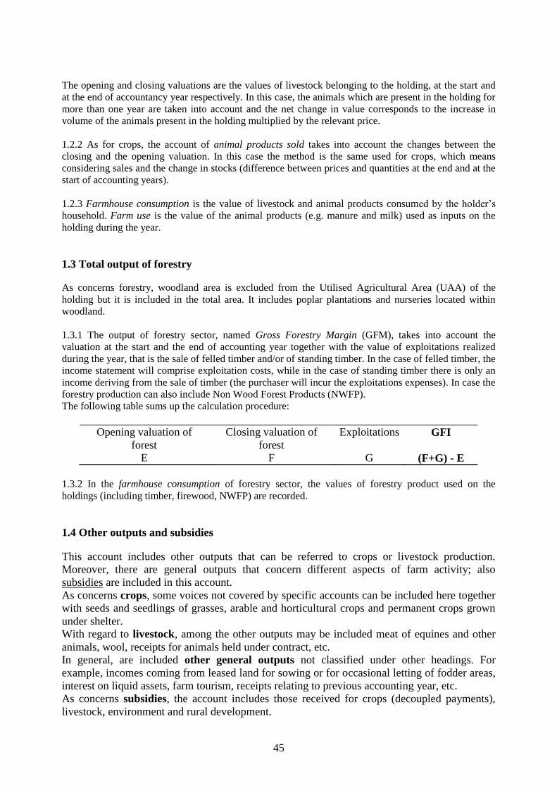
45
The opening and closing valuations are the values of livestock belonging to the holding, at the start and
at the end of accountancy year respectively. In this case, the animals which are present in the holding for
more than one year are taken into account and the net change in value corresponds to the increase in
volume of the animals present in the holding multiplied by the relevant price.
1.2.2 As for crops, the account of animal products sold takes into account the changes between the
closing and the opening valuation. In this case the method is the same used for crops, which means
considering sales and the change in stocks (difference between prices and quantities at the end and at the
start of accounting years).
1.2.3 Farmhouse consumption is the value of livestock and animal products consumed by the holder’s
household. Farm use is the value of the animal products (e.g. manure and milk) used as inputs on the
holding during the year.
1.3 Total output of forestry
As concerns forestry, woodland area is excluded from the Utilised Agricultural Area (UAA) of the
holding but it is included in the total area. It includes poplar plantations and nurseries located within
woodland.
1.3.1 The output of forestry sector, named Gross Forestry Margin (GFM), takes into account the
valuation at the start and the end of accounting year together with the value of exploitations realized
during the year, that is the sale of felled timber and/or of standing timber. In the case of felled timber, the
income statement will comprise exploitation costs, while in the case of standing timber there is only an
income deriving from the sale of timber (the purchaser will incur the exploitations expenses). In case the
forestry production can also include Non Wood Forest Products (NWFP).
The following table sums up the calculation procedure:
Opening valuation of
forest
Closing valuation of
forest
Exploitations GFI
E F G (F+G) - E
1.3.2 In the farmhouse consumption of forestry sector, the values of forestry product used on the
holdings (including timber, firewood, NWFP) are recorded.
1.4 Other outputs and subsidies
This account includes other outputs that can be referred to crops or livestock production.
Moreover, there are general outputs that concern different aspects of farm activity; also
subsidies are included in this account.
As concerns crops, some voices not covered by specific accounts can be included here together
with seeds and seedlings of grasses, arable and horticultural crops and permanent crops grown
under shelter.
With regard to livestock, among the other outputs may be included meat of equines and other
animals, wool, receipts for animals held under contract, etc.
In general, are included other general outputs not classified under other headings. For
example, incomes coming from leased land for sowing or for occasional letting of fodder areas,
interest on liquid assets, farm tourism, receipts relating to previous accounting year, etc.
As concerns subsidies, the account includes those received for crops (decoupled payments),
livestock, environment and rural development.

46
2. Total Input
The group of Total Input is composed by the value of all non-capital inputs used in the
production of non-capital products during the accounting year. Inputs received as payments in
kind are also included.
Costs exclude:
- inputs used to increase, repair or replace the holding’s fixed assets which are considered
as investments
- consumption of capital assets (depreciation and sales of capital)
- costs of production for private consumption
The inputs are the costs linked to agricultural activity/process and related to the output of
accounting year.
Three categories of costs have been considered:
SPECIFIC COSTS
FARMING OVERHEADS
EXTERNAL FACTORS
SPECIFIC COSTS
This account includes three headings:
2.1 Crop & forestry specific costs includes four kind of costs:
2.1.1 Seeds and seedlings purchased and produced by the farm: it includes costs of young
trees and bushes for new plantations (permanent crops and woodland).
2.1.2 Fertilizers and soil improvers: all purchased fertilizers and soil improvers including
lime, compost, peat and manure. It excludes manure produced in the holding.
2.1.3 Crop protection products: here are included all materials used for the protection of
crops and plants against diseases and bad weather (insecticides, fungicides, herbicides,
poisoned baits, etc.).
2.1.4 Other crop specific costs: all the general costs not recorded in the previous headings.
Labour costs, contract work and mechanisation are not included in this account.
2.2 Livestock specific costs includes feedingstuffs and other specific livestock cost.
2.2.1 Purchased feedingstuffs includes feedingstuffs purchased as standing crops (grass and
fodder plants), costs of use of pasture land not included in the UAA (short-term land
rental), purchased litter and straw for bedding, additives for storage and preservation
2.2.2 Feedingstuffs produced on the farm includes all the farm products used for animals
that is marketable feedingstuffs, forage crops (returned as farm use) and the value of litter
and straw produced on the holding but if marketable in the region and year in question
2.2.3 Other specific livestock costs comprises veterinary, medicines, artificial insemination,
castration, milk tests, handbook subscription and registration, products for cleaning
livestock equipment, packing and processing materials and all the other costs not covered in
the other specific livestock cost headings
FARMING OVERHEADS

47
Farming overheads are general costs not liked to specific production processes (costs to upkeep
the equipment, energy, motor fuels, contract work, insurance, etc.).
2.3.1 Upkeep of machinery and equipment: includes total cost of upkeep and minor repairs to
machinery, costs and purchase of small equipment, forcing frames, tyres, protective clothing,
detergents for general cleaning (not those used for livestock and crop production that entered
under other specific livestock costs or crop costs), and a proportion of the cost of private cars
corresponding to their use for farm purposes. These repairs do not change the value of
machinery or equipment: this kind of repairs or conversions are considered as investments and
not as costs.
2.3.2 Upkeep of land improvements and buildings: includes the maintenance of buildings and
land improvements financed by the holder. Includes also the purchase of necessary building
materials but not those for new investments.
2.3.3 Electricity, lubricants and heating fuels: considers the total consumption for farm business
use. Firewood is included.
2.3.4 Water: is the cost of connection and the consumption of water for all farm purposes. It
does not include the costs of using irrigation equipment that could be divided into upkeep of
machinery and equipment, electricity, etc.
2.3.5 Payments for external services: analysis, planning, technical assistance
2.3.6 Other farming overheads as insurance (all premium for farm risks, excluding employee
accident insurance that is entered under the social security costs), farm taxes arising from
current productive activity in the accounting year and other dues (secretarial services, office
expenses, telephone charges, etc.). As concern the taxes, they can be related to the farm
business (as environmental taxes or additional levy on milk) or be taxes on land and buildings,
paid in relation to the owner occupation or use of farmland, woodland and buildings by the
holder.
EXTERNAL FACTORS
This account is composed by three headings that concern the remuneration of inputs (work, land
and capital) which are not the property of the holder.
2.4 Wages: this heading includes the wages and social security charges (and insurance) of wage
earners, that is all payments to employees in return for work done.
In general, wage costs include:
- cash equivalent of payments in kind (e.g. rents, meals and lodging, etc)
- productivity bonuses and profit share-outs
- recruitment expenses
- employee social security contributions, taxes and insurance
It excludes the amounts received by workers considered as unpaid workers (wages lower than a
normal wage, persons who do not receive a salary) and all the holder’s and employer’s costs. It
excludes labour used on work under contract (contract work and machinery hire).
2.5 Rent: this heading includes the net value of cash and payments in kind for renting of land,
buildings, quotas and other rights for the farm business.
48
2.6 Interest: this heading includes interest and financial charges on loans for the farm business
(loans for purchase of land and buildings, purchase of land or working capital). The subsidies
on interest are not deducted and are entered under “grants and subsidies on costs”.
3. Implicit costs
While wages, rent and interest (recorded as external factors) have a monetary expression that
can be considered as explicit costs for the remuneration of inputs not in property of the holder,
the implicit costs deal with the holder’s labour and capital. To compute them, the opportunity
cost method is used, that is the value of input in its best alternative use.
For example: not paying rent on the self-owned property generate an implicit rent considered as
an implicit cost because while rent is a deductible expense, implicit rent is not. The same thing
happens with the implicit cost of liquid assets or shareholder’s capital that is the maximum
interest that would be earned on them as a fixed deposit or as an investment in alternative ways.
The most important implicit cost in the agricultural sector is that one related to the family work,
this is generally calculated multiplying the use of family work (hours, days, months or years) by
a reference income (usually equal to the earning of non-agricultural workers). However it has to
be recalled that the methodology to assess the opportunity cost of non monetary inputs is often
controversial and several different methods have been proposed and applied.
3.1.1 Opportunity cost of family labour: usually the units of family work (provided also by the
FADN) are multiplied by a reference income that could be, for example, the gross annual
earning of non-agricultural workers in the area (alternative jobs) or the wages in the agricultural
sector of the area, etc..
3.1.2 Opportunity cost of current capital: this opportunity cost is the expected return deriving
from other potential investment activities, that is the rate of return that investors could earn in
financial market. Usually, the rate of bonds is take into account.

49
Annex 4 Complete list of practices implemented in the methodological grids
Allow weeds to grow after harvest Maintenance of old- and dead-wood
Care of area between tree rows Mapping environmental aspects of farms
Care of under-tree area Nutrient management planning
Continue farming activities complying with Cross-
Compliance requirements Organize health care visits for livestock
Create beetle banks Permanent exclusion from felling
Create stone walls / fences Preservation of particular tree species composition
Create uncultivated/buffer strips Prohibition/limitation of using fertilizers
Develop an animal health and welfare plan Prohibition/restriction of final felling by clear cutting
Forest beating up Prohibition / temporal restriction of final felling
Forest brashing Prohibition of using particular share of grassland
Forest bush clearing Protection of forest plantations
Forest irrigation Protection of forest seedlings
Forest planning Protection of trees
Forest planting Purchase of additional material
Forest pruning Removal of tree stumps
Forest site preparation Removal of undesirable regenerations / tree species
Forest thinning Removing stock or other restrictions on grazing
Forest transportation Replacement of forest seedlings
Forest weeding Replacement of trees
Fulfill new obligations to farming practices Restriction of timing and frequency in mowing
meadows
Maintain beetle banks Retain stubble after harvest
Maintenance/development of specific biotopes Set-aside of land
Maintenance of forest protection Tree cutting to preserve forest structure

50
Annex 5 Complete structure of payment differentiation criteria
1 Administrative land division
1.1 NUTS II
Name of NUTS II
Name of NUTS II
Name of NUTS II
Other NUTS II
1.2 NUTS III
Name of NUTS III
Name of NUTS III
Name of NUTS III
Other NUTS III
1.3 EC Regulations / National laws / Regional laws
LFA Areas
Natura 2000 Areas
NVZ Areas
Protected Areas (National or Regional)
Other areas
1.4 Administrative land differentiation based on specific indicators
Municipality with average of >210 kg of N/ha of UAA
Municipality HA
Municipality HB
Area OA
Area OB
Area S
Area SX
Gemarkung 1 (LVZ)
Gemarkung X (LVZ)
Choerent Region 1
Choerent Region 2
Choerent Region 3
Area HUA
Area LUA
Standard regions (transport cost)
Fragile regions (transport cost)
Very fragile regions (transport cost)
More disadvantaged land (grazing categories)
Less disadvantaged land (grazing categories)
Ratio 1 (degree prot/usage restrictions)
Ratio 2 (degree prot/usage restrictions)
EMZ range 1
EMZ range 2
Other areas
2 Land characteristics
2.1 Slope
1° range of slope
2° range of slope
2.2 Soil fertility/quality
1° degree of fertility
2° degree of fertility

51
Improved soil
Unimproved soil
2.3 Altitude
Mountain
Hill
Plain
2.4 Exposure
---
2.5 Land use - Agricultural areas (CORINE)
Arable land
Permanent crops
Pastures
Heterogeneous agricultural areas
Other
2.6 Land Use - Forests and semi-natural areas (CORINE)
Forests
Shrubs and/or herbaceous vegetation associations
Sclerophyllous vegetation
Open spaces with little or no vegetation
Other
2.7 Land Use - Wetlands (CORINE)
Wetlands
Coastal wetlands
Other
2.8 Land Use - Water bodies (CORINE)
Inland waters
Marine waters
Other
2.9 Other geographic/social/economic features
3 Farm characteristics
3.1 Type of farming (TF8) (FADN)
Fieldcrops
Horticulture
Wine
Other permanent crops
Milk
Grazing livestock
Granivores
Mixed (crops and livestock)
3.2 Size classes (FADN classification)
< 2 ESU
2 - 4 ESU
4 - 6 ESU
6 - 8 ESU
8 - 12 ESU
12 - 16 ESU
16 - 40 ESU
40 - 100 ESU
100 - 250 ESU
≥ 250 ESU
3.3 Size classes (Other than FADN)
< 40 ha of UAA
> 40 ha of UAA

52
< 150 ha of UAA
151 - 250 ha of UAA
251 - 500 ha of UAA
> 500 ha of UAA
< 3000 kg of N produced
3000 - 6000 kg of N produced
> 6000 kg of N produced
LSU < n
LSU > n
3.4 Other charcterization of farm land
Inside UAA
Other
4 Type of animals
4.1 Horse
Horse for fattening (meat)
Breed Žemaitukai
Breed Lithuanian Weighted
Other
4.2 Cattle
Calves for fattening (meat)
Other cattle < 12 months
Male cattle 12 - 24 months
Female cattle 12 - 24 months
Male cattle > 24 months
Breeding heifers
Heifers for fattening (meat)
Dairy cows
Other cows
Breed Burlina
Dying breeds
4.3 Sheep
Ewe (female for breeding)
Other sheep (male for breeding)
Various breeds
Sheep for milk
Sheep for fattening (meat)
4.4 Goat
Goat for breeding (female)
Other goats (male for breeding)
Goat for fattening (meat)
4.5 Pig
Piglets
Breeding sow
Pigs for fattening (meat)
Other pigs (boars)
Various breeds
4.6 Poultry
Table chickens (meat)
Laying Hens
Other poultry
Breed gees
4.7 Other animals
5 Type of crops

53
5.1 Cereals
Durum Wheat
Soft Wheat
Maize
Rye
Barley
Oats
Ryce
Other cereals
5.2 Other fied crops
Dry pulses
Potatoes
Sugar beet
Sunflower
Soya
Hops
Cotton
Peas
Field beans
Beans
Groundnut
5.3 Vegetables and non-perennial fruit
Under shelter
Tomatoes
5.4 Flowers and ornamental plants
---
5.5 Seeds
---
5.6 Fodder crops and fallows
Fodder Maize
Other silage cereals
Other fodder plants (alfalfa)
Permanent pasture
Temporary grass
Fallows and set aside for previous regulation
Rough grazing
Peas
Field beans
Beans
Alfalfa
Meadows
Other
5.7 Permanent crops (excluding forestry)
Vines
Wine grapes
Table grapes
Raisins
Olives grooves
Table olives
Ollive oil
Fruit and berry orchards
Nuts
Citrus fruit orchards

54
Nursery (excludes tree nurseries)
6 Woodland and trees
6.1 Type of woodland
Conifers
Broadleaves
Mixed conifers & broadleaves
Afforestation
Arboricolture/Plantation
Riparian
Coppice
Native forest
6.2 Species
Oak
Populus sp.
Juglans regia
Castanea sativa
Platanus orientalis
Pistacia lentiscus var. chia
Celtis australis
Caretonia siliqua
Morus sp.
Aleppo pine
Turkish pine
Stone pine
Cypress
Down oak (quercus pubescens)
Horn-beam (Ostrya carpinifolia)
Other
6.3 Woodland function
Edges (Buffer zone)
Afforestation of set-aside land (Buffer zone)
Polyspecific
Protection
Productive (Fast growing)
Productive (traditional)
Productive (resin)
Naturalistic (conservation)
Naturalistic (regeneration)
Other
7 Planning and management
7.1 Type of husbandry
Summer pasture
Free stall barn with grazing
Free stall barn on straw
Free stall barn on straw with run-outs
Open cycle
Close cycle
7.2 Type of final product
Cheese Parmigiano
Cheese Grana Padano (or edible milk)
7.3 Specific technical choices (planning level)
1° type of material seeding
2° type of material seeding

55
Seeding frequency 1
Seeding frequency 2
Estabilshment density 1
Estabilshment density 1
Conifers with < 20% soft broadleaves
Conifers or soft broadleaves with < 20% hard braod leaves
Hard broadleaves and/or Tilia with mixed conifers and/or soft broadleves > 40%
Hard broadleaves + Tilia or Populus etc.
5 - 15 % (ARWS)
16 - 25 % (ARWS)
26 - 35 % (ARWS)
< 35 % (ARWS)
7.4 Specific practices (management level)
Animal Ration with low N and P
Fertirrigation
Solid fertilization
Normal/Typical
Respect of particular restrictions 1
Respect of particular restrictions 2
Respect of particular restrictions 3
8 Type of beneficiary
8.1 Legal status of beneficiaries
Farmer practising farming as his main occupation
Part-time farmer
Other than farmer farmer
Farmer associations
Private law bodies
Public authorities
8.2 Farmer qualification
Trained farmers
Successor of early retired
Young farmers
8.3 Other
Maintaining previous RDP commitments
Introduction RDP commitment
9 Year of commitment
9.1 Year
1°
2°
3°
4°
5°