agricultural finance review, department of agricultural
TRANSCRIPT


AGRICULTURAL FINANCE REVIEW, Department of Agricultural Economics, Cornell University Volume 51
Preface·
Agricultural Finance Review (AFR) provides a forum for research and discussion of issues in agricultural finance. This annual publication contains articles contributed by scholars in the field and refereed by peers.
Volume 43:wa.s the first to be published at Cornell University. The previous 42 volumes were published by the United States Deparbnent of Agriculture.AFR was begun in 1938 by Norman J. Wall and Fred L. Garlock, whose professional careers helped shape early agricultural finance research. Professional interest in agricultural finance has continued to grow over the years, involving more people and a greater diversity in research topics, methods of analysis, and degree of sophistication. We are pleased to be part of that continuing development. We invite your suggestions for improvement.
The effectiveness of this publication depends on its support by agricultural finance professionals. Your support has grown each year in terms of submissions and reviews of manuscripts. We especially express thanks to those reviewers listed below. Grateful appreciation is also expressed to the Economic Research Service, USDA, and to the W.I. Myers endowment for partial financial support.
Starting July 1, 1991, John Brake and Eddy LaDue will serve as coeditors of the Agricultural Finance Review.
VOLUME 51 REVIEWERS
Dale Adams Freddie Barnard Mike Boehlje George Casler Robert Chambers Raj Chhikara Craig Dobbins Mark Drabenstott Lynn Forster Paul Ellinger Allen Featherstone Cole Gustafson Thomas Frey Wayne Gineo Steve Hanson J. Arne Hallam Greg Hanson Peter Heffernan William Hardy Wayne Hayenga Danny Klinefelter William Herr Bruce Jones James Libbin Dave Leatham Warren Lee Charles Moss Dave Lins Mike Mazzocco James Richardson Glenn Pederson John Penson Bruce Sherrick Lindon Robison Bryan Schurle R. L. Tinnermeier Loren Tauer Bernard Tew Calum Turvey Myles Watts
Manuscripts will be accepted at any time, but the deadline for manuscripts for the 1992 issue is February 3, 1992.
Eddy L. LaDue, editor John R. Brake, associate editor

Agricultural Credit Mediation: Borrower and Creditor Perspectives in North Dakota ColeR. Gustafson, James F Baltezore, and F Larry Leistritz ALBERT R. MANI'
'IBRARY
Abstract This study presents an evaluation of the North Dakota Agricultural Mediation Service from borrower and creditor perspectives. Data were gathered by mail survey of borrower and creditor mediation participants. Farm borrowers in particular, and creditors in general, furnished favorable evaluations of the mediation process and the mediation service.
Key words: mediation, survey, farmers, creditors, borrowers, farm finance, costs, evaluation, motives, North Dakota.
ColeR. Gustafson is an assistant professor, James F. Baltezore is a research associate, and F. Larry Leistritz is a professor, Department of Agricultural Economics, North Dakota State University-Fargo. The authors benefited from the constructive comments provided by two anonymous reviewers. North Dakota Experiment Station paper no. 1915.
.JAN 0 ti 1~93
The 1980s were a time ·&4A(SrAI.ntNlfiai48 ~=:. stress for many farm borrowerJ and their creditors. Farm bankruptcies and foreclosures occurred at a rate seven times greater than the historic average (U.S. Department of Agriculture), a rate similar to farm financial conditions of the 1930s (Murdock and Leistritz). The United States Congress passed the Agricultural Credit Act of 1987 (P.L. 100-233, 1988) in an effort to relieve some of the financial problems facing farm borrowers and creditors.
The act restructured major financial institutions serving agriculture (Farmers Home Administration and Farm Credit Services), set forth conditions under which delinquent farm loans are either restructured or foreclosed upon, and provided delinquent borrowers with numerous borrower rights. Title V of the act established federal funding for development and operation of state-sponsored agricultural mediation programs to furnish a formal mechanism whereby agricultural borrowers and creditors could resolve their financial difficulties while minimizing legal expenses. As of 1 January 1991, 15 states had active mediation programs.
This article describes the North Dakota Agricultural Mediation Service and evaluates mediation as a means of resolving financial difficulties among farm borrowers and creditors. Results of a survey of farm borrowers and creditors who participated in mediation are also presented. The survey estimates expectations of borrowers and creditors prior to mediation, identifies motives of each party trying mediation, and evaluates mediation as a means of resolving farm borrower/creditor problems. Finally, suggestions for improvement in the mediation service, as indicated by survey respondents, are also provided.

2 Agricultural Credit Mediation
North Dakota Agricultural Mediation Service
North Dakota established a state mediation service in January I989, which held its first hearings in March I989. Over I ,385 requests for mediation were initiated during I989. Credit institutions initiated nearly all of the mediation requests. As of 3I December 1989, 212 cases (15%) were still unsettled. Of the I, I 7 4 mediation cases resolved during I989, 605 farm operators were offered or requested mediation and either declined mediation or did not respond to mediation requests and therefore lost the right to mediate. Some cases were settled by the borrower and lender reaching an agreement on their own, by voluntary borrower liquidation, or by foreclosure/bankruptcy proceedings. The remaining 569 cases went to or are in mediation.
Mediation is strictly voluntary for farm borrowers. However, certain creditors, namely the Farmers Home Administration (FmHA) and Farm Credit Services (FCS), must participate in mediation if a mediation hearing is requested by one of their delinquent farm borrowers. Either a farm borrower or a creditor of a delinquent farm borrower can ask for mediation. Mediation must be offered before foreclosure can be initiated, and only after mediation reaches an impasse can foreclosure proceedings begin.
The mediation service assigns farm borrowers a credit counselor/negotiator once mediation is requested. North Dakota credit counselors/negotiators prepare borrowers for mediation. They are unique in their mediation role compared to most other state programs because they are required by Jaw to represent the borrower's interests and negotiate on the borrower's behalf at the mediation table. Most credit counselors/negotiators employed by the mediation service are former or current farm operators. Other counselors are or were bankers, federal government employees, and agricultural-education instructors. As such, most credit counselors have an innate knowledge of agriculture which, when combined with intensive training sessions on financial statement
preparation, legal options available to delinquent farm borrowers, negotiation tactics, and personal counseling, prepares them for their role in the mediation process.
A mediator is also assigned to each case. The mediator acts as a facilitator responsible for contacting all parties involved, determining the participants' financial positions, organizing a time and place for mediation sessions, and bringing the borrower and lender together to reestablish communication needed to resolve their financial differences. North Dakota's mediation service is one of only three other state agricultural mediation programs in the U.S. requiring mediators to contact participants and organize meetings. The mediators employed by the mediation service are a former federal government employee, banker, small-business operator, and farmer. Mediators receive extensive training in agricultural finance and conflict resolution before they are permitted to mediate.
Other State Mediation Services
State mediation programs must comply with specific federal guidelines to receive certification and, in turn, matching federal grants. Legal processes and alternatives available to borrowers and creditors are similar across states, with the goal being to bring borrowers and creditors together for bargaining. However, each state is independent in developing its own administrative agencies, operational procedures, and personnel responsibilities as long as it adheres to federal guidelines. Thus, implementation of the program at the state level can affect the bargaining position of each party (i.e., assignment of a negotiator/credit counselor to borrowers in some states, but not all).
A telephone survey of state mediation programs was conducted to identify administrative, operational, and personnel-responsibility differences among them. State mediation services contacted were in Alabama, Indiana, Iowa, Kansas, Minnesota, Montana, Nebraska, New Mexico, North Dakota, Oklahoma, South Dakota,

Texas, Utah, and Wisconsin. Most mediation programs were similar in nature. Two interesting exceptions were noted in Minnesota and Texas.
Minnesota's Farm Credit Mediation Program was created in 1986 (Minnesota Extension Service). Besides New Mexico's program, Minnesota's program is the only other agricultural mediation program administered by the state's agricultural extension service. The Minnesota Extension Service had over 7,500 mediation requests by 30 June 1989. The extension service is the contact for farmers and creditors desiring mediation. Extension agents provide technical information to both creditors and farmers and help farmers complete financial documents necessary to participate in the mediation process. The service differs from North Dakota's in that extension agents (who perform a role similar to credit counselors/negotiators in North Dakota) do not negotiate on behalf of the farmer. Mediators act as a neutral third party to facilitate discussions between farmers and creditors. Minnesota mediators are typically community volunteers with educational backgrounds and experiences necessary to evaluate farm financial situations.
The Texas Agricultural Loan Mediation Program was initiated in the fall of 1988 (Condra 1989). Over 640 mediation requests have been made since its inception. The program is the only state agricultural mediation program administered by an agricultural economics department within a university system (Department of Agricultural Economics at Texas Tech University) (Condra 1990). The mediation process is similar to the process in North Dakota, with a credit counselor/negotiator and mediator being assigned to each case. In Texas, the negotiator assists the borrower in developing proposals and is required to negotiate on the borrower's behalf. Negotiators currently employed by the program are graduate students from the university majoring in agricultural finance. Mediators are responsible for facilitating communication and negotiations between borrowers and creditors. Mediators utilized by the program include both Texas Tech staff as well as contracted mediation professionals.
Gustafson, Baltezore, and Leistritz 3
Mediation Process and Potential Benefits
Mediation is a process whereby a neutral third party helps participants (farm borrowers and their creditors) reach a voluntary agreement to resolve financial disputes (Kochan eta!.). The effectiveness of mediation can be judged by the number of settlements reached. Alternatively, mediation can be described as a narrowing process. Participants start with a number of differences and resolve each, one by one, until an agreement that is satisfactory to each party can be reached. Therefore, mediation success can be evaluated by the number of individual issues resolved. Individual issues involved in agricultural mediation include estimating future cash flows, forgiving principle and interest payments, lowering interest rates, and extending loan duration.
Mediation has potential benefits for both farm borrowers and creditors. The major benefit of mediation is the opportunity to resolve borrower/creditor disputes before bankruptcy, thus avoiding associated monetary costs, time demands, and uncertainty (Gustafson, Saxowsky, and Braaten). Faiferlick and Harl estimated costs for borrowers involved in Chapter 12 bankruptcy to be $9,900 for attorney's fees and expenses, and $3,400 for trustee's fees. The time required to complete bankruptcy proceedings was nearly four times longer (and more expensive) than settlements negotiated outside of bankruptcy. Additional out-of-pocket bankruptcy expenses for borrowers and creditors were court costs, and bookkeeping and accounting costs. Other possible benefits of mediation include reduced legal costs, a quicker settlement, a more private settlement, and an overall more favorable settlement when compared to bankruptcy.
Farm borrowers could use mediation as a means of delaying foreclosure proceedings. Delays might allow borrowers more time to identify and evaluate legal, business, and personal alternatives. Delays might also allow more time for economic conditions in North Dakota to improve, especially after three consecutive years of drought. An additional step before foreclosure might

4 Agricultural Credit Mediation
extend the time involved in the overall settlement process, adding to creditor costs and potentially making creditors more willing to negotiate and make concessions.
Creditors face considerable economic costs as a result of delinquent or nonperforming loans (Gustafson et al.). Economic costs incurred include uncollected principle and interest, maintenance costs (insurance, property taxes, and repairs), and losses on the sale of collateral property. Creditors also face further financial uncertainty brought about by changes in collateral values from the time of default until the obligation becomes current or collateral is acquired. Mediation is a means creditors have of turning some delinquent loans into performing loans, thus reducing economic costs associated with delinquency.
Credit institutions may be willing to write down principle and interest payments in arrears, lower loan interest rates, and extend the loan duration in an attempt to establish a performing loan. The average loan write-down (debt forgiven to restructure loans) per FmHA borrower through November 1989 was $146,000 (Taylor). The average debt write-off (debt forgiven in loan buyouts and liquidations) during the same time period was $204,800 per FmHA borrower. This suggests that there may be a financial incentive for creditors to participate in mediation in an attempt to write down rather than write off delinquent loans. By shortening delinquency periods and using write-downs, overall losses to credit institutions may be less with mediated settlements when compared to bankruptcy.
Creditors may also want to avoid legal uncertainties associated with bankruptcy. Mediation provides creditors with an ample chance to participate in negotiations. The opportunity creditors have to influence and affect decisions may be lost in bankruptcy proceedings.
Survey Procedure Data used to evaluate North Dakota's Agricultural Mediation Service were collected from mail surveys of both farm borrowers and creditors. Although separate survey instruments were developed, major
sections of the creditor questionnaire were similar to the farm borrower questionnaire so that responses could be compared. Farm borrower and creditor responses were compared to identify differences in motives, expectations, and perceptions of the mediation process. Significant differences in opinions may indicate areas where the mediation process could be modified to improve program content and delivery.
The borrower sample consisted of nearly 480 farm operators who used the mediation service. Borrowers surveyed had mediated either with FmHA or FCS. Over 80% of the sample participated in mediation proceedings with FmHA.
The borrower survey instrument was designed to elicit attitudinal responses on the mediation process and mediation in general as a way of solving borrower/lender conflicts. The survey instrument was used to identify motives for trying mediation as well as borrower expectations prior to mediation. Several sets of statements were contained in the questionnaire for which respondents could select responses from a Likert-type scale (Likert).
Nearly 360 financial institutions in the state were also surveyed. This included 54 county and district FmHA offices, 32 branch and regional FCS associations, 115 credit unions, and 158 state or national banks operating in North Dakota.
A Kruskal-Wallis test (K-W) was used to identify differences in responses among surveys for questions with yes/no and Likert-type responses. K-W one-way analysis of variance by ranks is used to test whether independent samples are from different populations (Daniel). The K-W test determines if differences among samples represent merely chance variations or genuine population differences (Seigel). Scores are converted to ranks using more of the information in the observation than just a means test. The test is useful in situations where a normality assumption does not hold or is not critical (Mendenhall, Ott, and Larson).
Results After two mailings, 249 creditors and 183 farm borrowers returned questionnaires.

Response rates were 69% and 38% for the creditor and borrower surveys, respectively. The overall response rate was 52%.
Expectations
Most farm borrowers (50%) and creditors (65%) responding described their relationship as friendly or very friendly before entering into mediation. Twenty percent of the farm borrowers and 2% of the creditors responding described their relationship as hostile or very hostile. Over 30% of the farm borrowers expected creditors to be inflexible before mediation, while less than 20% of the creditors expected the majority of their borrowers to be inflexible. Nearly 30% of the borrowers responding felt fearful ( 19%) or extremely fearful (11%) about participating in mediation prior to attending their first mediation session. Less than 10% of the creditors responding were either fearful or extremely fearful. Borrowers were significantly more fearful of mediation than were creditors.
The majority of borrowers and creditors did not contact other borrowers/creditors who had participated in mediation to see what
Gustafson, Baltezore, and Leistritz 5
their experiences were before deciding on mediation. However, creditors contacted other credit institutions significantly more often (20%) than borrowers contacted other borrowers ( 10% ). Less than 35% of the borrowers and 30% of the creditors responding indicated they had little or no understanding of the mediation process before attending the first mediation session.
Motives Borrowers indicated their primary motive for mediation was an opportunity for a quicker settlement (Table I). Over 70% of the respondents either agreed or strongly agreed mediation would provide a quicker settlement. Sixty percent of the borrowers responding tried mediation because mediation was a more private means of settlement than bankruptcy. Nearly 30% of the borrowers strongly agreed that they tried mediation because it was a more private means of settlement. Borrowers to some extent used mediation as a stall tactic since over 45% of respondents agreed or strongly agreed that wanting to delay foreclosure was a motive for trying mediation. However, results suggest this was not one of the primary reasons for mediating.
Table I. Responses to Possible Motives for Trying Mediation, North Dakota Agricultural Mediation Survey, 1990
Motives/Survey Strongly Strongly Group Disagree Disagree Undecided Agree
Percent
Lower Legal Costsa Borrowers 15 18 18 35 Creditors 20 33 20 25
Quicker Settlementa Borrowers 4 7 18 46 Creditors 13 18 21 43
Other Party Suggested Media tiona
Borrowers 9 19 17 39 Creditors 3 10 12 52
Hoped to "Cut a Better Deal"a Borrowers 10 13 21 39 Creditors 27 29 28 16
More Private Means of Settlement than Bankruptcy"
Borrowers 10 13 15 33 Creditors 14 14 28 38
Wanted to Delay Foreclosure Borrower 14 20 20 21
"Indicates a significant difference in responses between the two survey groups based on a Kruskal-Wallis test and a 90% confidence level.
Agree
14 2
25 5
17 23
17 0
29 6
25

6 Agricultural Credit Mediation
Seventy-five percent of the creditors responding indicated that they participated in mediation because the farm operator wanted to. Nearly 50% of the creditors participated in mediation because it would provide a quicker settlement. However, more than 50% of the creditors responding disagreed that mediation would lower their legal costs and that they would get a better deal through mediation.
Mediation Settlements and Costs Over 50% of the borrowers responding indicated an agreement was reached through mediation. Over 70% of the creditors responding reached agreements through mediation. Based on the percentage of settlements reached, the mediation program offered by the North Dakota . Mediation Service appears to be an effective mechanism to resolve financial difficulties among farm borrowers and their creditors. Over 55% of borrowers and nearly 40% of creditors responding rated settlements reached through mediation as favorable when compared to bankruptcy.1
The average cost of participating in the mediation process for farm borrowers was $380 per borrower (includes lawyer and financial advisor fees, and travel expenses).2
Costs reported by borrowers ranged from a low of $0 to a high of $13,000. The average cost of participating in mediation for creditors responding was $103 per institution and ranged from $0 to $2,000. Mediation cost the average farm borrower significantly more than the average creditor. Lower mediation costs for creditors may be due to their ability to spread costs over more cases and internalize some of the costs of participating in mediation. Over 55% of borrowers and nearly 40% of
1This situation must be interpreted with care because the likelihood of farmers having direct experience with both mediation and bankruptcy is low.
2At the time of the survey, the North Dakota Agricultural Mediation Service provided mediators. and credit counselors/negotiators at no charge to cred1tors and delinquent farm clients. As of 1 January 1990, a nominal charge of $10 per hour for negotiators assisting borrowers (in cases requiring more than ten hours) and $25 per hour for mediators assessed to both creditors and borrowers will be charged. The charge is waived for borrowers unable to pay. These charges are similar to those of mediation services in other states.
creditors responding rated the cost of mediation as much less than the cost of bankruptcy.
Mediation Process
The majority of the borrowers surveyed were assisted/advised during the mediation process by the credit counselor/negotiator assigned to their case. Nearly 20% of the borrowers sought additional assistance from lawyers. Another 5% hired private consultants.
Sixty percent of borrowers and 70% of creditors rated the speed of the mediation process as faster when compared to bankruptcy proceedings. Over 60% of the borrowers responding rated mediation a good or very good way of solving borrower-creditor problems in general. Less than 30% of the creditors responding thought mediation was a good way to solve borrower-creditor problems. However, 50% of the creditors responding rated mediation as okay. When asked how they would rate mediation as a way of solving their financial problems, nearly 60% of the borrowers and less than 20% of the creditors responded good or very good. Over 45% of the creditors rated mediation as an okay way of solving their financial problems. Nearly 60% of the borrowers and 40% of the creditors thought the mediation procedure was fair. Similar findings were found in Texas, where over 50% of borrowers and over 35% of creditors surveyed rated mediation as fair (Condra 1989).
Mediators
Borrowers and creditors responding gave favorable evaluations of mediators assigned to their cases (Table 2). Borrower evaluations of mediators were significantly higher than creditor evaluations. Nearly 70% of the borrowers and 40% of the creditors responding rated the mediator as good or very good for each of the evaluation questions. However, around 10% of the creditors rated the mediator's competence, neutrality, understanding of the issues, and overall performance as poor.
The majority of borrowers and creditors had confidence in the mediator's ability to reach a settlement. Both sides felt the mediator assigned to their case(s) was

Gustafson, Baltezore, and Leistritz 7
Table 2. Mediator Evaluations, North Dakota Agricultural Mediation Survey, 1990 Very Very
Question/Survey Group Poor Poor Okay Good Good
Percent
Explanation of the Mediation Processa Borrower 0 3 24 41 32 Creditor 1 3 42 43 11
Understanding of the Issuesa Borrower 1 7 21 44 27 Creditor 3 10 47 31 9
Competence a
Borrower 2 4 26 34 34 Creditor 1 11 43 36 9
Neutrality" Borrower 1 5 26 37 31 Creditor 0 12 43 28 17
Trustworthinessa Borrower 1 4 25 31 39 Creditor 0 2 51 28 19
Patience Borrower 0 1 24 40 35 Creditor 0 2 46 32 20
Overall Performancea Borrower 1 5 20 36 38 Creditor 3 11 45 34 7
"Indicates a significant difference in responses between the two survey groups based on a Kruskai-Wallis test and a 90% confidence level.
sympathetic to their position. Nearly 95% of the borrowers and over 85% of the creditors responding indicated that their case( s) was presented fairly to all parties at the mediation session by the mediator. These findings were consistent with survey results from participants in the Texas Agricultural Mediation Program, where over 80% of borrowers and 70% of creditors responding indicated the mediator was impartial (Condra 1989).
Mediation Service Improvements
Borrowers and creditors responding offered similar suggestions to improve mediation service delivery. Specific recommendations regarding mediation sessions included requiring all creditors to be present, and documenting mediation sessions and agreements reached. In some instances, agreements could not be reached because the position of creditors not attending mediation sessions was unknown. Documenting sessions was important so both sides had written testimony of what was said and agreed upon. Recommendations to improve the overall mediation process included establishing
definite time intervals, requiring legally binding agreements, and developing a mechanism for follow-ups. Respondents wanted specific time periods established for each step in the mediation process so mediation would be completed in a timely manner. Many respondents also wanted agreements to be legally binding. Some creditors and borrowers responding indicated that one side or the other failed to uphold their end of the agreement. Devising a mechanism for following up on agreements would help resolve this situation.
Summary The purpose of this study was to evaluate the North Dakota Agricultural Mediation Service from both the farm borrower and creditor perspectives. An evaluation was based on a mail survey of both borrowers and creditors using the mediation service. Survey returns provided the basis for identifying participant expectations, motives, costs, and perceptions of the mediation service.
Generally, farm borrowers had a friendly relationship with the creditors involved in

8 Agricultural Credit Mediation
mediation. However, borrowers did not expect their creditor to be flexible in negotiations. Most borrowers had some understanding of the mediation process prior to the first mediation session, yet they were fearful about participating in mediation. Borrowers participated in mediation primarily with the hope of obtaining a quicker, more private settlement than through bankruptcy. Farm borrowers rated mediation as a good way of solving financial problems among farm borrowers and creditors, and believed the mediation procedure was fair.
Creditors perceived their relationship with borrowers as friendly but were undecided as to how flexible farm borrowers would be during the mediation process. Creditors understood the mediation process and felt relatively confident before attending the first session. The fundamental motive for creditors participating in mediation was that the farm borrower requested it. Furthermore, certain creditors (FmHA and FCS) participate primarily because it is mandated by the Agricultural Credit Act of 1987. Secondary motives were a quicker, more private settlement than bankruptcy. Creditors felt mediation was a satisfactory way of solving borrower-creditor problems in general. However, creditors rated mediation as a poor way of solving their problems with farm borrowers. Most creditors believed that the mediation procedure was neither fair nor unfair.
Mediation appears to be an effective mechanism for resolving borrower-creditor conflicts. It is supported by the majority of farm borrowers and, to a lesser extent, by creditors who have participated. Support for mediation from both sides of the issue implies that mediation is constructive in settling financial problems among farm borrowers and their creditors.
References
Condra, Gary D. Texas Agricultural Loan Mediation Program Annual Report. Texas Tech University, Department of Agricultural Economics, Lubbock, TX, 1989.
---- . "Agricultural Loan Mediation." In Handbook of Alternative Dispute Resolution, chapter 13, 1-8. 1990.
Daniel, Wayne W. Applied Nonparametric Statistics. Boston, MA: Houghton Mifflin Company, 1978.
Faiferlick, Chris, and Neil E. Harl. "The Chapter 12 Bankruptcy Experience in Iowa." J. Ag. Taxation and Law 9, no. 4( 1988):302-36.
Gustafson, ColeR., David M. Saxowsky, and Joan Braaten. "Economic Impact of Laws That Permit Delayed and Partial Repayment of Agricultural Debt." Agr. Fin. Rev. 47(1987):31-42.
Kochan, Thomas A., Mordehai Mirone, Ronald G. Ehrenberg, Jean Baderschneider, and Todd Jick. Dispute Resolution Under Fact-finding and Arbitration: An Empirical Analysis. New York: American Arbitration Association, 1979.
Likert, Rensis. "The Method of Constructing An Attitude Scale." In Readings in Attitude Theory and Measurement, 90-95. New York: John Wiley and Sons, Inc., 1967.
Mendenhall, William, Lyman Ott, and Richard F. Larson. Statistics: A Tool for the Social Sciences. North Scituate, MA: Duxbury Press, 1974.
Minnesota Extension Service. Farm Credit Mediation Program Studies: 1986-1990. AD-BU-3920. University of Minnesota, 1990.
Murdock, S.H., and F.L. Leistritz, eds. The Farm Financial Crisis: Socioeconomic Dimensions and Implications for Producers and Rural Areas. Boulder, CO: Westview Press, 1988.
Seigel, Sidney. Nonparametric Statistics for the Behavioral Sciences. York, PA: The Maple Press Company, 1956.
Taylor, Marci Zarley. "FmHA Pays Up." Farm Journal, May 1990.
U.S. Department of Agriculture. Economic Research Service. The Current Financial Condition of Farmers and Farm Lenders. Agricultural Information Bulletin no. 490. Washington, DC, 1985.

Financial Management Characteristics of Successful Farm Firms Garett 0. Plumley and Robert H. Hornbaker
Abstract Second degree stochastic dominance is used to identify three levels of financial success for 123 cash grain farms. Four annual observations of four performance measures are used in the analysis. Differences in financial ratio characteristics between the varying levels of success are examined. Overall, characteristics of successful farms, identified by net farm income per tillable acre, include higher liquidity, a fairly balanced composition of assets, lower debt, and higher profitability than the least successful farms. Successful farms ranked by management returns per tillable acre, net farm income per dollar of farm equity, and management returns per dollar of farm equity are inherently less liquid, have a lower level of farm real estate ownership, a range of debt levels, and are somewhat more profitable than least successful farms.
Key words: financial ratios, management characteristics, grain farms.
Garett 0. Plumley is a member of the Illinois Farm Business Farm Management Association field staff in Morrison, Illinois, and Robert H. Hornbaker is an associate professor in the Department of Agricultural Economics, University of Illinois at Urbana-Champaign. This study is derived from research sponsored by the Norris Institute and Doane Agricultural Services Company.
The recent economic environment encountered by the farm sector has placed increased emphasis on the role of finance in farm management. Specifically, a large body of research has been devoted to the causes of farm financial stress and failure. However, research has not adequately addressed the financial characteristics of successful farm firms. Ratio analysis shows the relationship between financial performance elements and various farm characteristics (Morehart, Nielson, and Johnson). For many years, nonagricultural industries have had access to numerous analytical ratios constructed from industry income and balance sheet statements. Robert Morris Associates has annually published a set of financial ratios for a wide range of businesses. However, this data is aggregate in nature and makes no attempt to stratify the businesses in terms of being more or less successful.
In the past, such stratified financial data have generally not been available for farm firms (Penson and Lins ). Because there are few readily available publications of financial ratios for farm firms, the use of ratio analysis is much more limited in agriculture. Farm operators can compare their own financial ratios over time, but without comparative standards for similar types of farms, such ratios are of limited value. A thorough examination of such ratios can direct attention to desirable and undesirable strategies. With standards identified, farmers can evaluate their relative position and possibly adopt the new strategies to improve their performance.
The objective of this study is to identify farm financial management characteristics of financially successful farm firms. To achieve this objective, groups of financially

10 Financial Management Characteristics
successful, less successful, and least successful farms are established. Standard financial ratio values and associated strategies for those farms exhibiting successful financial management are identified. It is then determined if financial ratio values differ significantly between the varying levels of success.
Previous Studies
The financial performance of several agribusiness industries within the U.S. agricultural sector has been evaluated using ratio analysis (Hudson, Hughes, and Lins; Gill, Hudson, and Lins). These studies examined relative performance in and across the specific industries using aggregate Robert Morris Associates Statement Studies. Similar studies have attempted to develop and use financial ratios for comparison of farms by type (Short) and size (Morehart et al.) using total farm sector government surveys and census data. Short noted that such aggregate statistics tend to mask changes in the financial structure and situation of specific farms. As a result, changes in aggregate indicators are often attributed to all types of farms and may provide misleading signals with regard to the financial well-being of the farm sector.
In 1987, Ellinger, Barry, Frey, and Scott conducted a study to describe the financial performance and characteristics of a sample of Illinois farms. The same study was repeated in 1988 and 1989. A shortcoming of their approach is that the sample is not comprised of the same farms from year to year. In addition, the number of farms in some categories is relatively small. Thus, one or two observations may significantly influence the mean of a ratio in a particular quartile. Moreover, no attempt is made to identify levels of financial ratios by either relative or absolute performance of the farms. However, the study does provide some general guidelines for individual farmers to compare their operations and financial performance measures to farms with similar characteristics and thus possibly diagnose strengths and weaknesses. In addition, the study demonstrates how ratio analysis can be applied to individual farm firms.
The Data A study of successful financial management characteristics necessitates a data set encompassing observations for a large number of farms over a number of years. A cross-sectional, time-series data set is required. Data used in this study are from the Illinois Farm Business Farm Management (FBFM) Association records. As of 1988, the FBFM Association consisted of 7,375 Illinois farms. About 1 out of every 5 Illinois commercial farms with over 500 acres is enrolled in the service. Participation in the program is voluntary, with cooperating farmers paying a fee for its services.
In compiling a suitable data set for this study, only farms with four years of certified income statements and balance sheets are selected. FBFM income statements are carefully screened and edited by professional field staff who certify about 4,000 statements per year as usable for comparative analysis. The income statements termed usable are on an accrual basis and free of any significant errors or omissions. The certification process for FBFM balance sheets began in 1985. For a balance sheet to be certified usable, the firm must be a sole proprietorship; current liabilities must be free of significant omissions due to oversight of accounts payable, accrual interest, accrual income taxes, and current portions of intermediate and long-term debt; accounts receivable and prepaid expenses must be specifically examined by the field staff for any errors or omissions; nonfarm assets and liability data must be complete; beginning balance plus money borrowed must equal ending balance plus principal paid for each loan; and the valuation of any equity on leased equipment must be added to the fair market value of equipment.
In recent years, cash grain operations provided the majority of the certified balance sheets. Therefore, to produce a consistent and accurate data set, several additional criteria are required. First, farmers must be classified as a fuli-time farmer. In this study, a farmer is classified as a full-time farmer if ten or more months of operator labor are used in the farm business. Farms must also be classified as

grain farms. These are farms where the value of feed fed is less than 40% of the crop returns and where the value of feed fed to dairy or poultry is not more than one-sixth of the crop returns. The farms used in this study met all of the previous requirements in each of the years 1985 to 1988.
Based on these criteria, the data set used in this study is comprised of 123 farms. This sample size is comparable to those used in other studies of this type (Thorpe; Kauffman and Tauer; Sonka, Hornbaker, and Hudson; Schurle and Williams).
The majority of the farms are located in the central regions of the state, which are generally considered the most productive. The farms are similar in their productivity potential. The average tillable acres per farm over the four years is 706 acres. Of the 123 farm operators, 80% are classified as part owners, 17% rent all of the land used in production, and 3% are full owners. Moreover, on average, operators owned 22% of the total land controlled by the operation. This suggests that a majority of the sample farms rent a substantial portion of their land base. Fifty-five percent of the farms have crop-share leases, 42% have a mixture of cash and crop-share leases, and 3% have strictly cash leases. All of these figures are consistent with recent trends in Illinois agriculture. The financial stress of the early 1980s caused a shift from buying to leasing land as farmers attempted to reduce their leverage. Overall, the farms in the sample are quite similar to the average Illinois cash grain farm. However, it is quite plausible that significant differences exist between farms within the sample with respect to their financial characteristics.
Methods In order to identify financial management strategies characteristic of successful farm firms, a method is needed to differentiate between financially successful, less successful, and least successful farms. Management, by nature, involves decision making. The decision maker must make those decisions in a risky environment. Therefore, decision analysis basically involves choosing among alternative probability distributions with the choice
Plumley and Hornbaker 11
based on how the characteristics of the distribution conform to the risk attitudes of the decision maker (Barry). In general, the risk-averse category is believed to dominate the attitudinal characteristics of farm decision makers, as indicated by most empirical studies of risk attitudes.
Stochastic dominance (SD) is a decision tool used to determine the efficient set of alternative courses of action in an uncertain environment. It divides the decision alternatives into mutually exclusive sets: an efficient set and an inefficient set, conforming to the restrictions on the utility function of a class of decision makers. Stochastic dominance has been applied to several decision situations in agriculture. These situations can be categorized as follows: (1) adoption of a new technology (Hardaker and Tanego; Klemme); (2) participation in government programs (King and Oamek; Kramer and Pope; Richardson and Nixon); (3) crop management decisions (Zacharias and Grube; McGuckin); and (4) selection of various farm management strategies (Pederson; Wilson and Eidman; Zering, McCorkle, and Moore; Schurle and Williams; Kauffman and Tauer).
The measurement and use of individual utility functions can be difficult. Stochastic dominance is designed to account for the estimation problems encountered in using single-valued utility functions and efficiency models, such as EV analysis, which require normal outcome distributions. The basic premise of first degree stochastic dominance (FSD) is that if x is the unsealed measure of outcome, such as profit, decision makers always prefer more to less of x (Anderson, Dillon, and Hardaker). Second degree stochastic dominance (SSD) requires the additional behavioral assumption that the decision maker is risk averse (Meyer). Second degree stochastic dominance with respect to a function (SDRF) is an alternative method. However, SDRF requires identification of the lower and upper bounds of each decision maker's absolute risk-aversion function (King and Robison).
For this study, second degree stochastic dominance is the method used to partition the sample farms as either successful, less successful, or least successful based on

12 Financial Management Characteristics
probability distributions of several performance measures. The goal of this study is not to identify a single farm that is dominant, but rather a group of farms to compare to those that are not dominant. The likelihood of excluding preferred prospects (Type 1 error) is less with SD analysis than with the use of single-valued utility functions or EV analysis.
The Stochastic Dominance Analysis Stochastic dominance analysis is performed for four different performance measures: Net Farm Income per Tillable Acre (NFI/AC), Management Returns per Tillable Acre (MR/AC), Net Farm Income per Dollar of Farm Equity (NFI/FEQ), and Management Returns per Dollar of Farm Equity (MR/FEQ). The four measures are chosen based on their ability to consistently distinguish between varying levels of overall farm financial performance (Thorpe). In addition, these measures are relative, therefore eliminating the possibility of domination due to farm size.
The four annual observations for the NFI/AC and MR/AC measures are deflated to 1985 dollars using the gross national product deflator (Economic Report of the President). Because the other two measures are relative, with both the numerator and denominator reflecting changes in the general price level, no deflation procedure is necessary. The determination of second degree stochastic dominance is accomplished through the use of a generalized stochastic dominance program (Cochran and Raskin). The quasi-second degree stochastic dominance (QSSD) option of the program does not perform a "true" second degree stochastic efficiency test since it is actually an approximate solution based on generalized stochastic dominance. In most cases, no significant differences are encountered between the true and the quasi-second degree stochastic dominance. An iterative procedure similar to that used by Kauffman and Tauer is followed in determining quasi-second degree stochastic efficiency for each of the four performance measures.
The iterative procedure is continued until all 123 farms are ordered by QSSD. Several
levels of success are desired for the analysis of financial management characteristics as opposed to arbitrarily setting a break point of 50% of the ordered farms as the division between two groups of farms. It was originally hypothesized that the data might present clear break points. Such a break would be indicated, for example, by a cumulative total of 20 farms identified as efficient after the fifth iteration, with the sixth iteration identifying an additional 30 farms in the single iteration. Such a margin would imply that the first 20 farms as well as the later 30 farms constitute distinct groups in terms of performance. However, such large margins between iterations do not occur in this study.
Stratification is achieved by dividing the farms into three levels of success: successful, less successful, and least successful. Cutoff points are approximately the first 25% and 75% of farms ordered by QSSD. This ordering process will often group two or more farms together in one iteration. For example, the first five farms ordered in the first iteration may be QSSD to the remainder of the sample. The second iteration may result in an additional three farms ordered after the first five farms. To maintain the integrity of the QSSD iteration groups, farms are identified in a particular level of success if the total number of farms ordered following an iteration is within 2% of the desired cutoff points of 25% or 75%. Therefore, the successful group may include between 23% and 27% of the farms. Likewise, the least successful category of success also may vary between 23% and 27%.
Mean Analysis
After establishing the three levels of success by each of the four performance measures, the next step is to examine the differences in financial ratio characteristics between the varying levels of success. The approach taken is to compare the successful level to the other two levels combined for each performance measure used in the stochastic dominance analysis. The least successful level is compared to the upper two categories in a similar fashion. For each performance measure, the performance measures themselves and the selected

Plumley and Hornbaker 13
financial ratios are evaluated. The performance measures and financial ratios are defined in Table 1. Each farm's four-year average value for the individual variable is used in the analysis. The successful category is referred to as "top" farms in the tables and the least successful farms are termed "bottom" farms.
farms and the remaining 92 farms. Six of the ratios differ between the bottom 33 farms and the other 90 farms. Table 2 suggests that all of the farms in the sample are fairly liquid as well as profitable. The successful farms' average ratio of earnings on assets is five times the effective interest rate of their operation. This ratio does not account for unpaid labor. In addition, such large
Net Farm Income per Tillable Acre average returns should be viewed with caution when considering the dispersion of earnings. Least successful farms also have a significantly higher ratio of cash operating expense to value of farm production (OPEXPNFP).
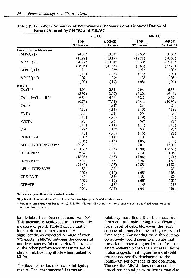
Table 2 presents the results of the mean analysis for farms ordered by NFI/AC and MRIAC. For farms ordered by NFI/AC, NFIIAC and MR/AC differ by more than $56 and $33, respectively, between the successful and least successful levels. Relatively large margins also exist for the other two performance measures. Table 2 continues with the financial ratios. Only 4 of the 13 ratios differ significantly between the top 31
Management Returns per Tillable Acre
Management returns are the residual remaining after imputed charges for interest on equity capital, and unpaid operator and
Table 1. Definitions and Abbreviations of Performance Measures, Financial Categories, and Ratiosa
Performance Measures NFIIAC MRIAC
NFIIFEQ MRIFEQ
liquidity CNCL CA + WCL + IL
Asset Management CAffA FAffA VFP!fA
Debt Management D/A INTEXP/VFP
NFI + INTEXP/INTEXP
Profitabili~ ROFAIINT
ROFE!INT
NFI + INTEXPNFP
Operating Efficiency OPEXPNFP DEPNFP
Net farm income per tillable acre Management returns per tillable acre (NFI less interest on
equity capital, and unpaid family and operator labor) Net farm income per dollar of farm equity Management returns per dollar of farm equity
Ratio of current assets to current liabilities Ratio of current and intermediate assets to current and
intermediate liabilities
Ratio of current assets to total asets Ratio of fixed assets to total assets Ratio of the value of farm production to total assets
Ratio of total debt to total assets Cash plus accrued interest expense divided by value of farm
production Times interest earned-net farm income plus accrual interest
expense divided by accrual interest expense
Rate of return on farm assets (net farm income plus accrual interest expense divided by farm assets) divided by the effective farm interest rate
Rate of return on farm equity (net farm income divided by farm equity) divided by the effective farm interest rate
Profit margin-net farm income plus accrual interest expense divided by the value of farm production
Ratio of cash operating expense to value of farm production Ratio of depreciation expense to value of farm production
"All balance sheet figures are on an end-of-year, fair-market-value basis.
b The effective farm interest rate is calculated as the cash plus accrued interest expense divided by total liabilities.
14 Financial Management Characteristics
Table 2. Four-Year Summary of Performance Measures and Financial Ratios of Farms Ordered by NFI/AC and MRIAC8
NFI/AC MRIAC
Top Bottom Top Bottom 31 Farms 33 Farms 32 Farms 32 Farms
Performance Measures NFI/AC ($) 74.31* 18.68* 62.35* 36.36*
(11.22) (13.15) (17.21) (26.86) MR/AC ($) 20.72* -13.00* 36.38* -39.10*
(28.08) ( 41.38) (9.53) (37.70) NFl!FEQ ($) .16 .08* .21* .06*
(.15) (.08) (.14) (.08) MR!FEQ ($) .07* .oo• .13* -.05*
(.09) (.10) (.08) (.06) Ratios
CA/CL** 4.09 2.56 2.94 5.55* (3.97) (3.90) (3.20) (6.46)
CA + WCL + IL** 6.64 4.47 5.32 8.57 (6.70) (7.55) (6.44) (10.95)
CAlf A .30 .24* .31 .24 (.10) (.13) (.10) (.13)
FAIT A .43 .45 .35 .48* (.16) (.21) (.18) (.22)
VFP!fA .25 .26 .32* .21* (.13) (.13) ( .11) (.13)
DIA .24* .47* .38 .23* (.18) (.20) (.16) (.21)
INTEXPNFP .06* .18* .10 .09 (.05) (.12) (.06) (.11)
NFI + INTEXP/INTEXP** 35.27 1.99 7.01 13.06 (124.65) (.92) (8.90) (23.66)
ROFAIINT** 5.62 1.05 2.10 1.08 (18.28) (.47) (1.06) (.76)
ROFEIINT** 7.21 1.37 3.26 1.43 (21.40) ( 1.28) (2.58) (1.50)
NFI + INTEXPNFP .39* .27* .41 .23 (.07) (.10) (.05) (.08)
OPEXPNFP .49* .58* .48 .60 (.07) (.10) (.06) (.07)
DEPNFP .14 .17* .14* .18* (.03) (.06) (.04) (.06)
•Numbers in parentheses are standard deviations.
'Significant difference at the 5% level between the subgroup farms and all other farms.
"Results of these ratios are based on 113, 113, 110, 108, and 108 observations, respectively, due to undefined ratios for some farms during the period.
family labor have been deducted from NFI. This measure is analogous to an economic measure of profit. Table 2 shows that all four performance measures differ significantly, as expected. A range of over $75 exists in MR/AC between the successful and least successful categories. The ranges of the other performance measures are of similar relative magnitude when ranked by MR/AC.
The financial ratios offer some intriguing results. The least successful farms are
relatively more liquid than the successful farms and are maintaining a significantly lower level of debt. Moreover, the least successful farms also have a higher level of fixed assets. Considering these three items collectively would seem to indicate that these farms have a higher level of farm real estate ownership than the successful farms. It also suggests that higher levels of debt are not necessarily detrimental to the longer-run performance of the operation. The fact that MR/ AC does not account for unrealized capital gains or losses may also
explain the results. The least successful farms ranked by MRIAC incur approximately 12% more of operating expenses as a percentage of value of farm production (OPEXPNFP), indicating that these farms may be less efficient in their use of crop inputs.
Net Farm Income per Dollar of Farm Equity
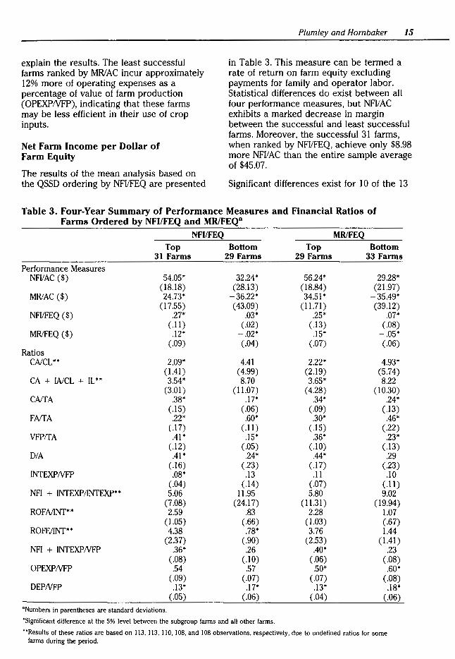
The results of the mean analysis based on the QSSD ordering by NFI/FEQ are presented
Plumley and Hornbaker 15
in Table 3. This measure can be termed a rate of return on farm equity excluding payments for family and operator labor. Statistical differences do exist between all four performance measures, but NFIIAC exhibits a marked decrease in margin between the successful and least successful farms. Moreover, the successful 31 farms, when ranked by NFIIFEQ, achieve only $8.98 more NFI/AC than the entire sample average of $45.07.
Significant differences exist for 10 of the 13
Table 3. Four-Year Summary of Performance Measures and Financial Ratios of Farms Ordered by NFI/FEQ and MRIFEQ8
NFI/FEQ MRIFEQ
Top Bottom Top Bottom 31 Farms 29 Farms 29 Farms 33 Farms
Performance Measures NFI/AC ($) 54.05* 32.24* 56.24* 29.28*
(18.18) (28.13) (18.84) (21.97) MR/AC ($) 24.73* -36.22* 34.51* -35.49*
(17.55) ( 43.09) (11.71) (39.12) NFI/FEQ ($) .27* .03* .25* .07*
( .11) (.02) (.13) (.08) MRIFEQ ($) .12* -.02* .15* -.05*
(.09) (.04) (.07) (.06) Ratios
CA/CL** 2.09* 4.41 2.22* 4.93* ( 1.41) (4.99) (2.19) (5.74)
CA + WCL + IL** 3.54* 8.70 3.65* 8.22 (3.01) (11.07) ( 4.28) (10.30)
CAliA .38* .17* .34* .24* (.15) (.06) (.09) (.13)
FAIT A .22* .60* .30* .46* (.17) ( .11) (.15) (.22)
VFP/TA .41* .15* .36* .23* (.12) (.05) (.10) (.13)
DIA .41* .24* .44* .29 (.16) (.23) (.17) (.23)
INTEXPNFP .08* .13 .11 .10 (.04) (.14) (.07) ( .11)
NFI + INTEXP/INTEXP** 5.06 11.95 5.80 9.02 (7.08) (24.17) (11.31) (19.94)
ROFA/INT** 2.59 .83 2.28 1.07 (1.05) (.66) ( 1.03) (.67)
ROFE/INT** 4.38 .78* 3.76 1.44 (2.37) (.90) (2.53) (1.41)
NFI + INTEXPNFP .36* .26 .40* .23 (.08) (.10) (.06) (.08)
OPEXP/VFP .54 .57 .so• .60* (.09) (.07) (.07) (.08)
DEPNFP .13* .17* .13* .18* (.05) (.06) (.04) (.06)
"Numbers in parentheses are standard deviations.
'Significant difference at the 5% level between the subgroup farms and all other farms.
"Results of these ratios are based on 113, 113, 110. 108, and 108 observations. respectively, due to undefined ratios for some farms during the period.

16 Financial Management Characteristics
financial ratios. The least successful farms exhibit even higher levels of liquidity and land ownership than those ordered by the MR/AC measure. The bottom 29 farms have over 60% fixed assets on average. Their debt levels are also significantly lower than the other 94 farms. The ROFE!INT ratio indicates the successful farms earned on their equity 4.38 times the effective farm interest rate.
Management Returns per Dollar of Farm Equity
Table 3 also presents the results of the mean analysis for farms ordered by MR!FEQ. The performance measures differ significantly in every case, as expected. However, NFIIAC for the successful farms exhibits a similar relative indifference to the entire sample average as it did when ranked by NFI!FEQ. Nine of the 13 financial ratios differ significantly across groups of success when ranked by MRIFEQ. The top farms are less liquid than the bottom farms but are still in a strong position by most standards. Balance sheet structure indicates a higher degree of current assets, as well as debt, for the successful farms. Cash plus accrued interest expense divided by the value of farm production (INTEXPNFP) did not, however, vary between levels of success. In terms of the profitability ratios, all farms were profitable; however, successful farms had a significantly higher profit margin.
Analysis Across Measures of Success
Having evaluated the variables of interest across levels of success, it is appropriate to discuss the trends and conclusions evidenced across the four success measures. Based on an examination of the two ratios representing liquidity, CA/CL and CA + WCL + IL (see Table 1 for definitions of these two ratios), the conclusion that the vast majority of farms in this data set are in a relatively liquid position is confirmed. Strictly higher levels of liquidity do not appear to necessarily indicate increased success. In fact, when ranking farms by MR/AC, NFI/FEQ, and MR!FEQ, liquidity ratios above 4:1 are associated with the least successful operations.
Successful farms identified by NFI/ AC do not have significant differences in asset
structure from the least successful farms. However, farms identified as successful by MR/AC, NFIIFEQ, and MR/FEQ appear to be structured differently than the least successful operations. Successful farms, by these measures, have a similar or higher percentage of current assets to fixed assets in addition to a higher ratio of the value of farm production to total assets (VFP/TA). The figures suggest that these farms are renting more land than owning land. The least successful operations exhibit a larger degree of fixed assets than current assets and lower VFP/TA, characteristic of more tenured operations. Farms ranked successful by NFI/AC have lower 0/A ratios, INTEXPNFP ratios, and higher NFI + INTEXP/INTEXP ratios. Conversely, successful farms ranked by MR/AC, NFI!FEQ, and MRIFEQ have higher 0/ A ratios and lower NFI + INTEXP/INTEXP ratios.
Analyzing those ratios representing asset management and debt management collectively, the NFIIAC ordering suggests that owning land and having a high equity position are the preferred strategies. The MR/AC, NFI/FEQ, and MR/FEQ rankings, however, suggest that renting land and a higher use of debt capital for non-real estate assets are the preferred management strategies. In addition, as earlier hypothesized, higher debt levels are not necessarily detrimental to firm performance. In fact, the data suggest the most successful farms have 0/A levels between .30 and .50.
The profitability ratios demonstrate consistent results across the four measures. There again exist similarities amongst certain performance measures, which are evidenced when examining the profitability ratios-ROFA/INT, ROFE!INT, and NFI + INTEXP/VFP (see Table 1 for definitions). Successful farms ordered by NFI/AC are nearly five and seven times as profitable with respect to the ROFA/INT and ROFE!INT ratios as the least successful farms. Top-ranked farms by MR/AC, NFI!FEQ, and MR!FEQ are more profitable than the least successful farms, but by a much narrower margin. In fact, when ranked by these three measures, profit levels of successful farms are nearly the same as the average of the entire sample.
The OPEXPNFP ratio indicates that successful farms ranked by any measure

have a lesser proportion of operating expenses to value of farm production. These farms are using crop inputs with greater efficiency than the least successful farms. The greater efficiency (lower OPEXPNFP) is achieved through lower input cost, higher yields, and/or higher market prices. Sonka, Hornbaker, and Hudson indicated that more successful managers often achieve greater efficiency from a combination of all three sources: lower per acre operating costs, higher yields, and higher output prices.
The DEPNFP ratio is also less for successful farms as compared to the least successful farms across all measures. Farms termed successful by MR/AC, NFIIFEQ, and MR!FEQ have higher levels of debt, but fewer fixed assets, which implies higher machinery debt. It would be expected that depreciation expense would be higher for these operations. However, this is not the case. Overall, these ratios present fewer significant results than the other ratios.
Conclusions on Mean Analysis
The four measures of success and the 13 financial ratios have been analyzed across levels of success and measures of success. From the analysis, several conclusions can be made. It appears that of the measures of success, NFI/AC presents different results than the other three measures. Characteristics of successful farms identified by NFI/AC include higher liquidity, a fairly balanced composition of assets, lower debt, and higher profitability than the least successful farms. Successful farms ranked by MR/AC, NFIIFEQ, and MRIFEQ are inherently less liquid, have a lower level of fixed assets, have a range of debt levels, and are somewhat more profitable than least successful farms. The characteristics of the successful group necessarily imply the preferred financial management characteristics.
A possible explanation for these two groups of measures is the inherent low accounting (current) rates of return to farmland. For nondepreciable assets such as farmland, the accounting rates of return are low and remain low as higher inflation causes the nominal economic rates of return for land and other assets to increase (Barry and Robison). When growth does not occur,
Plumley and Hornbaker 17
accounting rates equal real economic rates of return across assets. When growth does occur, current rates of return will be even lower. As growth occurs, current returns to assets will increase wealth, but the portion of real return will be dominated by capital gains relative to current income.
It is, therefore, understandable that when farms are ranked by MR/AC and MRIFEQ, those with higher tenure levels are ranked lower. This is because the higher-ownership firm's return is dominated by capital gain. The successful farms ranked by these measures have a return dominated not by capital gain, but rather by current income. However, an accurate measurement of unrealized capital gains or losses is not clear. In addition, farms with tenure have higher imputed equity charges, resulting in a lower current return than those operations that primarily rented land.
In order to identify to a greater degree more and less successful farms, subsets of farms that are consistently ranked either in the successful or least successful categories by MR/AC, NFIIFEQ, and MR/FEQ are obtained. This process results in 18 farms that are consistently successful and 19 farms that are consistently least successful. Mean analysis was conducted on these subsets, with the results reported in Table 4. The table substantiates the hypothesis that these measures are similar in their distinction of success. The mean analysis also suggests that those farms consistently ranked successful by MR/AC, NFI/FEQ, and MRIFEQ have a lower percentage of land owned to rented. Table 5 indicates that this is the case. The successful operations ranked consistently by the three measures own only 5% of the total land controlled, while the least successful operations own over 50%. The degree of tenure for each level of success is also presented for each individual measure of success.
Summary
The economic environment encountered by today's farmer requires a sound knowledge of financial management. A key component of financial management is the use of ratio analysis. Financial management strategies are often reflected in these individual ratios

18 Financial Management Characteristics
Table 4. Four-Year Summary of Performance Measures and Financial Ratios of Farms Ordered Consistently by MRIAC, NFI/FEQ, and MRIFEQa
All 123 Farms Top Bottom Variable in the Sample 18 Farms 19 Farms
Performance Measures NFI/AC ($) 45.07 61.75* 28.80*
(22.69) (17.91) (26.52) MR/AC ($) 4.52 35.70* -53.36*
(34.82) (11.42) (42.82) NFI/FEQ ($) .13 .29* .02*
(.11) (.14) (.02) MR/FEQ ($) .04 .17* -.04*
(.09) (.07) (.02) Ratios
CA/CL** 3.42 1.82* 5.26 (3.93) (.89) (5.75)
CA + WCL + IL** 5.89 2.88* 10.23 (6.89) (1.33) (12.84)
CArrA .28 .35* .17* (.13) (.10) (.05)
FArrA .43 .24* .59* (.20) (.15) (.11)
VFPffA .28 .40* .16* (.14) (.08) (.05)
DIA .33 .42 .21 * (.20) (.14) (.22)
INTEXPNFP .10 .08* .11 (.09) (.03) (.13)
NFI + INTEXP/INTEXP** 13.02 6.58 13.36 (64.03) (3.22) (26.23)
ROFAIINT** 2.45 2.68 .74 (9.05) (1.03) (.62)
ROFEIINT** 3.20 4.51 .77* (10.68) (2.75) (.94)
NFI + INTEXPNFP .32 .40* .22* (.09) (.05) (.09)
OPEXPNFP .58 .49* .59* (.09) (.07) (.06)
DEPNFP .15 .13 .19* (.05) (.05) (.06)
"Numbers in parentheses are standard deviations.
'Significant difference at the 5% level between the subgroup farms and all other farms .
.. Results of these ratios are based on 113, 113, 110, 108, and 108 observations, respectively, due to undefined ratios for some farms during the period.
that represent the various aspects of financial performance. Farm operators can compare their own financial ratios over time, but without comparative standards for like types of farms, the ratios are of limited value. In the past, comparative standards developed from continuous farm-level data of cash grain farms have not been readily available.
The analysis presented here compares the successful farms to the less and least successful farms combined for each of four performance measures. The least successful
farms are compared in a likewise manner to the upper two categories combined. Farms ordered by MRIAC, NFVFEQ, and MRIFEQ presented similar results. Overall, characteristics of successful farms identified by NFVAC include higher liquidity, a fairly balanced composition of assets, low debt, and much higher profitability than the least successful farms. Successful farms ranked by MR/AC, NFVFEQ, and MRIFEQ are inherently less liquid, have a lower level of fixed assets, have on average a higher ratio of debt to assets, and are somewhat more profitable than the least successful farms.
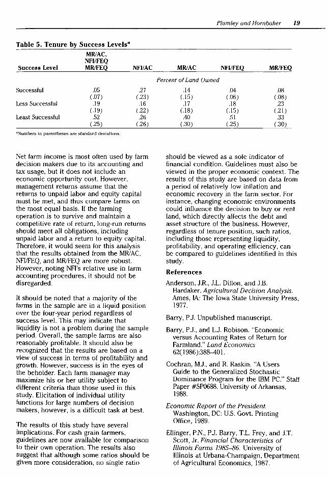
Table 5. Tenure by Success Levels8
MRIAC, NFI/FEQ
Success Level MRIFEQ NFI/AC
Successful .05 .27 (.07) (.23)
Less Successful .19 .16 ( .19) (.22)
Least Successful .52 .26 (.25) (.26)
"Numbers in parentheses are standard deviations.
Net farm income is most often used by farm decision makers due to its accounting and tax usage, but it does not include an economic opportunity cost. However, management returns assume that the returns to unpaid labor and equity capital must be met, and thus compare farms on the most equal basis. If the farming operation is to survive and maintain a competitive rate of return, long-run returns should meet all obligations, including unpaid labor and a return to equity capital. Therefore, it would seem for this analysis that the results obtained from the MRIAC, NFI/FEQ, and MRIFEQ are more robust. However, noting NFI's relative use in farm accounting procedures, it should not be disregarded.
It should be noted that a majority of the farms in the sample are in a liquid position over the four-year period regardless of success level. This may indicate that liquidity is not a problem during the sample period. Overall, the sample farms are also reasonably profitable. It should also be recognized that the results are based on a view of success in terms of profitability and growth. However, success is in the eyes of the beholder. Each farm manager may maximize his or her utility subject to different criteria than those used in this study. Elicitation of individual utility functions for large numbers of decision makers, however, is a difficult task at best.
The results of this study have several implications. For cash grain farmers, guidelines are now available for comparison to their own operation. The results also suggest that although some ratios should be given more consideration, no single ratio
Plumley and Hornbaker 19
MR/AC NFI/FEQ MR/FEQ
Percent of Land Owned
.14 .04 .08 (.15) (.06) (.08) .17 .18 .23
( .18) ( .15) ( .21) .40 .51 .33
(.30) (.25) (.30)
should be viewed as a sole indicator of financial condition. Guidelines must also be viewed in the proper economic context. The results of this study are based on data from a period of relatively low inflation and economic recovery in the farm sector. For instance, changing economic environments could influence the decision to buy or rent land, which directly affects the debt and asset structure of the business. However, regardless of tenure position, such ratios, including those representing liquidity, profitability, and operating efficiency, can be compared to guidelines identified in this study.
References
Anderson, J.R., J.L. Dillon, and J.B. Hardaker. Agricultural Decision Analysis. Ames, lA: The Iowa State University Press, 1977.
Barry, P.J. Unpublished manuscript.
Barry, P.J., and L.J. Robison. "Economic versus Accounting Rates of Return for Farmland." Land Economics 62( 1986 ):38~0 1.
Cochran, M.J., and R. Raskin. "A Users Guide to the Generalized Stochastic Dominance Program for the IBM PC." Staff Paper #SP0688. University of Arkansas, 1988.
Economic Report of the President. Washington, DC: U.S. Govt. Printing Office, 1989.
Ellinger, P.N., P.J. Barry, T.L. Frey, and J.T. Scott, Jr. Financial Characteristics of Illinois Farms 1985-86. University of Illinois at Urbana-Champaign, Department of Agricultural Economics, 1987.
20 Financial Management Characteristics
Gill, J.P., MA. Hudson, and DA. Lins. "Comparison of Financial Performance in Grain Related Industries." Unpublished manuscript.
Hardaker, J.B., and A.G. Tanego. "Assessment of the Output of a Stochastic Decision Model." The Australian J. of Agr. Econ. 17(1973):170-78.
Hudson, MA., M.N. Hughes, and DA. Lins. "Financial Performance in Meat and Poultry Manufacturing and Wholesaling: An Historical Perspective." J. Food Distrib. Res. Sept. 1988:63-74.
Kauffman, J.B., and L.W. Tauer. "Successful Dairy Farm Management Strategies Identified by Stochastic Dominance Analysis of Farm Records." Northeastern J. of Agr. and Resource Econ. 15(1986):168-77.
King, R.P., and G.E. Oamek. "Risk Management by Colorado Dryland Wheat Farmers and the Elimination of the Disaster Assistance Program." Amer. J. Agr. Econ. 65(1983):247-55.
King, R.P., and L.J. Robison. Implementation of the Interval Approach to the Measurement of Decision Maker Preferences. Michigan State University Agr. Exp. Sta. Bull. no. 418. Michigan State University, 1981.
Klemme, R.M. "A Stochastic Dominance Comparison of Reduced Tillage Systems in Corn and Soybean Production Under Risk." Amer. J. Agr. Econ. 67(1985):551-57.
Kramer, RA., and R.D. Pope. "Participation in Farm Commodity Programs: A Stochastic Dominance Analysis." Amer. J. Agr. Econ. 63(1981):119-28.
McGuckin, T. "Alfalfa Management Strategies for a Wisconsin Dairy Farm-An Application of Stochastic Dominance." N. Cent. J. Agr. Econ. 5(1983):43-49.
Meyer, J. "Choice Among Distributions." J. £con. Theory 14( 1977):326-36.
Morehart, MJ., E.G. Nielson, and J.D. Johnson. Development and Use of Financial Ratios for the Evaluation of Farm Businesses. Tech. Bull. no. 1753.
U.S. Dept. of Agriculture, Economic Research Service, Oct. 1988.
Pederson, G.D. "Selection of Risk-Preferred Rent Strategies: An Application of Simulation and Stochastic Dominance." N. Cent. J. Agr. Econ. 6(1984):17-27.
Penson, J.B., Jr., and DA. Lins. Agricultural Finance-An Introduction to Micro and Macro Concepts. Englewood Cliffs, NJ: Prentice-Hall, 1980.
Richardson, J.W., and C.J. Nixon. "Producer's Preferences for a Cotton Farmer Owned Reserve: An Application of Simulation and Stochastic Dominance." West. J. Agr. Econ. 7(1982):123-32.
Schurle, B.W., and J.R. Williams. Application of Stochastic Dominance Criteria to Farm Data. Kansas Agricultural Experiment Station Contribution no. 42-400-A. Kansas State University, Dept. of Agricultural Economics, 1982.
Short, S.D. Developing Financial Indicators for U.S. Farms by Type of Farm. Staff Report no. AGES850712. U.S. Dept. of Agriculture, Economic Research Service, Aug. 1985.
Sonka, S.T., R.H. Hornbaker, and MA. Hudson. "Managerial Performance and Income Variability For a Sample of Illinois Cash Grain Producers." N. Cent. J. Agr. Econ. 11(1989):39-47.
Thorpe, J.N. "Identifying Varying Levels of Long Term Managerial Performance and Their Causal Factors." Master's thesis, University of Illinois at Urbana-Champaign, 1987.
Wilson, P.N., and V.R. Eidman. "Dominant Enterprise Size in the Swine Production Industry." Amer. J. Agr. Econ. 67( 1985):279-88.
Zacharias, T.P., and A.H. Grube. "An Economic Evaluation of Weed Control Methods Used in Combination with Crop Rotation: A Stochastic Dominance Approach." N. Cent. J. Agr. Econ. 6(1984):113-20.
Zering, K.D., C.O. McCorkle, and C.V. Moore. "The Utility of Multiperil Crop Insurance for Irrigated, Multi-Crop Agriculture." West. J. Agr. Econ. 12(1987):50-59.

The Impact of Regulation on Shareholder Wealth in the Tobacco Industry: An Event-Study Approach MarkS. Johnson, Ron C. Mittelhammer, and Don P. Blayney
Abstract The event-study approach is offered as a tool that can be useful for measuring the impact of changes in government agricultural-commodity programs and other regulations on processors of those commodities. The event-study approach measures this impact through the use of financial data, namely, common stock prices. Product labeling requirements and advertising restrictions of the 1960s, and changes in agricultural policy of the 1980s were examined using two alternative models, the market-adjusted-return approach and the risk-adjusted CAPM approach. Support was found for the prior belief that events of the 1960s decreased firm value and that agricultural-policy changes of the 1980s had little impact on firm value.
Key words: regulation, tobacco processors, event study.
Mark S. Johnson is an assistant professor of finance at the University of Idaho. Ron C. Mittelhammer is a professor of agricultural economics at Washington State University. Don P. Blayney is an agricultural economist with the Economic Research Service, U.S. Department of Agriculture. The authors would like to thank Verner Grise for his help in gathering and interpreting tobacco event information. Additionally, the authors wish to thank two anonymous reviewers for helpful and constructive comments.
The problem of measuring the impact of changes in government policy and regulations on commodity processing firms has confronted many agribusiness policy researchers. Techniques used for measuring these effects have typically not utilized financial-market data explicitly. In this study, changes in common stock prices are used in the context of an event study to measure the effects of changes in agricultural-commodity programs on tobacco processing firms. The event-study approach is recognized by corporate-finance and financial-accounting researchers as a useful tool for measuring the impact of events on the value of publicly-held firms whose stocks are traded on efficient financial markets. Any changes in the structure of the firm, changes in its economic environment, or changes in investors' expectations regarding changes in firm structure or economic environment that may influence the firm's value can be identified as events.
Most published event studies have focused on measuring the impact of firm-specific events, such as dividend policy changes, capital-structure changes, and mergers and acquisitions, on the value of the firm. More recently, the event-study approach has been used to examine the impact of regulatory events on firm value. Examples of the regulatory changes examined in these studies are the effects of the Bank Holding Company Act of 1970 (Aharony and Swary), deposit ceilings (Dann and James), and merger regulations (Schipper, Thompson, and Weil). Schwert suggests that the event-study approach provides a new and more powerful test of regulatory impacts than previously available.

22 The Impact of Regulation on Shareholder Wealth in the Tobacco Industry
The measurement of regulatory impacts on the value of firm equity is important for several reasons. The most obvious reason is that it quantifies the effect of regulatory events on stockholder wealth and returns to investment. Perhaps a more important reason is that changes in firm value due to regulation will often cause resource reallocations that affect not only stockholders, but also industry workers and consumers of the industry's end products.
Resource reallocation occurs when capital budgeting is done on future investments due to events that cause the expected profitability of projects to be greatly reduced. If these effects are industry-wide, capital will be allocated out of the industry. In the long run, industry employment may decrease as the industry shrinks in size. The subsequent reduced output is likely to result in higher prices for consumers of the industry's end products.
During the last 30 years, many events occurred that could conceivably have had significant impacts on the value of tobacco processing firms. These events have included, but are not limited to, the following: product-liability lawsuits, state and federal tax changes, anti-smoking campaigns, elimination of smoking on certain commercial airline flights, elimination of smoking in public buildings and certain working situations, labeling requirements, advertising restrictions, and changes in federal agricultural policy (Grise and Griffen; Doron; U.S. Department of Health and Human Services).
Two sets of events are examined in this study-labeling and advertising restrictions of the 1960s, and agricultural program changes of the 1980s. The events of the 1960s are examined in part to document the sensitivity of the event-study methods in detecting value changes for the tobacco industry. There are self-evident, a priori reasons for believing that at least some of the labeling and advertising restrictions had impacts on demand and firm value, and it is expected that an effective event-study methodology would identify these events as being significant. Events of the
1980s-changes in agricultural programs affecting tobacco products-are probably of greater interest to most readers because similar policy changes have occurred for many other agricultural-commodity programs. However, whether these program changes had any significant impact on tobacco firm value is relatively less clear.
The remainder of the paper is organized as follows. First, the theoretical foundation of the event-study approach is discussed. Second, the potential methodologies and tests of significance are presented and the data are described. Third, an analysis of the major policy changes examined in this study is presented, along with the hypothesized impact on the value of the firms in the tobacco processing sector, the information arrival dates, and the results. A summary and conclusions are then provided, together with suggestions for further research opportunities.
The Theoretical Foundation of Event Studies
The theoretical foundation of the event-study approach is the efficient market hypothesis (EMH). The EMH indicates that stock prices should reflect all available information about future cash flows and risk of the firm at the time the stock prices are observed. The value of the firm, as perceived by investors and analysts, is the discounted value of expected future cash flows. The discount rate is determined by the riskiness associated with the firm, again as perceived by investors and analysts. Thus, changes in firm value occur in response to changes in investor expectations about future cash flows and risk. New information that is relevant to firm value is quickly incorporated into stock prices.
Most research on capital markets supports the conclusion that stock and bond markets are semi-strong form-efficient (Weston and Copeland). Semi-strong form-efficient markets are markets where prices quickly and fully reflect all publicly available information. Thus, if new information is

made available to the public regarding an event such as a regulatory change, and investors expect this event to affect the components of firm value, then stock prices will adjust quickly to the information. It is not surprising that capital markets are semi-strong form-efficient since investors and stock analysts have strong incentives to evaluate closely the firms they or their clients have invested in.
The event-study approach capitalizes on the EMH conclusion that when new information becomes publicly available, prices quickly reflect the changing expectations of the market participants. Thus, as Binder points out, two crucial aspects of any event study are (1) specifying the point in time when the new information reaches the market and (2) specifying the revision of investor expectations that occurred in response to the new information. For example, the introduction of legislation may provide more information to the market than the passage of legislation. This would be the situation if investors assigned a high subjective probability to the passage of the legislation at the time of the legislation's introduction. In fact, the signing of an agricultural-policy bill by the president may provide no information to the market since most topics of dispute have generally been resolved prior to sending the legislation to the president. Specifically, during the last ten years, presidents have not vetoed any agricultural-policy legislation that impacts tobacco.
To examine the impact of regulation on firm value, it is not appropriate simply to calculate the market value of the firm before and after the regulatory event and attribute the change in value to the regulatory event. Investors expect to earn a "normal" rate of return from holding stock. These normal returns, in the form of dividends or capital gains, are dependent upon the state of the macroeconomy and are correlated with the overall performance of the stock market. The impact of a regulatory event on firm value should thus be measured as the total change in firm value at the time of the event minus the change in firm value attributable to general market movement.
Johnson, Mitte/hammer, and Blayney 23
The Models
A difficulty associated with all event studies is the separation of the "natural" or "normal" rate of return for a stock during the event period from the "abnormal" return caused by the event. Three methodologies have been used in the literature to analyze abnormal returns: the mean-adjusted approach, the market-adjusted approach, and the risk-adjusted capital asset pricing model (CAPM) approach. Simulation results from Brown and Warner (1980, 1985) show that the power of test statistics associated with the mean-adjusted approach is low under conditions of clustering. Clustering is a condition where firms in the sample are from the same industry. Since our sample exhibits clustering, we concentrate on the market-adjusted and CAPM-adjusted approaches for statistical analysis.
Using the market-adjusted-return approach, the abnormal returns for firm i on day t are defined as the difference between the firm's actual rate of return and the rate of return on the market on day t. Equation ( 1) specifies this relationship.
(1)
where ARi1 is the abnormal return for firm i on day t, Rit is the actual return for firm i on day t, and R mt is the return on the market on day t. Therefore, an abnormal return should be interpreted as the return for holding stock in the firm that cannot be attributed to the movement of the entire market. Essentially, the abnormal return is the return for firm i that is attributable to new information made available to the market regarding firm value.
Following the convention of previous studies and the findings of Brown and Warner (1980), we use an equal-weighted index as a proxy for the return on the market. The market-return index is calculated using all firms on the New York Stock Exchange (NYSE), approximately 1,500 firms, and refers to a portfolio where one share of common stock is held for each firm

24 The Impact of Regulation on Shareholder Wealth in the Tobacco Industry
on the exchange. Even though there are many stocks traded on other exchanges, this equal-weighted index is likely to be a good proxy for the market because of its large size and the diversity of firms in the portfolio. The market-return index for all firms on the NYSE is calculated as
1500 1500 1500
L Pjt - L Pjt-I + L Djt j~I j~I j~I
Rmt=--------------------1500
L Pjt-I j~I
(2)
where Pjt equals firm j's price on day t, and D11 equals firm j's dividend payment on day t.
The actual return for firm i is calculated as the change in the firm's price from day t-1 to day t plus any dividends distributed on day t, all scaled by the price on day t- 1:
Pit-Pit-! +Dit Rit= ' pit-]
where Pit is the price of firm i's stock on day t, and Dil is the dividend for firm ion day t.
A three-day event window is used in this analysis. An event window is the time
(3)
period over which the impact of the informational event is examined. It is common to examine abnormal returns not only on the day of the event, but also for a time period before and after the event, to account for possible information leakage or late arrival of the information to the market. Information leakage to the market could occur if some participants in the market are privy to discussions amongst policy makers before public announcement of policy actions. Late arrival of information could also occur if, for example, public announcements are made near or at the end of the trading day for the stock exchange, in which case market reaction would occur on the next trading day.
To account for both the possible leakage of information and the late reporting of information, we examine the trading day before the event, the day of the event, and the trading day after the event. Since all of the events examined occurred on trading days, a three-day abnormal return can be computed as in equation (4)1:
I+ I
TARit = L ARij, j~t-1
where TAR;1 is the three-day abnormal return for firm i for event day t. TARit is then used to determine the impact of an event on firm i.
(4)
To determine the overall impact of the event on the industry, we calculate the three-day average abnormal return by summing across the firms in the industry as in equation (5):
N
TMR1 = L TARiN, (5) i~I
where TMR1 is the three-day average abnormal return for the industry for event day t, and N is the number of firms.
To examine whether the event has had a significant impact upon firm value, a test of the null hypothesis that the three-day average abnormal return equals zero is performed using the t-statistic, as suggested by Collins and Dent:
(6)
where a is the estimated standard deviation of the three-day abnormal returns across the firms. The standard deviation across firms is calculated as in equation (7):
10ther event windows were examined, including five, seven, and ten days. Under each of these conditions, significance of events was reduced.

a = J ± (TARit - TMR1i . N- I
i=1
(7)
Thus, the cross-sectional variation is being used in the test of the null hypothesis that the mean effect is zero.
Use of the CAPM-adjusted-return method is similar to the market-adjusted method in that abnormal returns are examined. The approach differs in the definition of normal return and the manner in which the significance of abnormal returns is determined. Normal returns for each firm are essentially determined from the co-movement of a firm's returns with the market rate of return, and abnormal returns are then determined by the component of the firm's risk that cannot be diversified away by holding a diversified portfolio of stocks in the marketplace.
Using the CAPM-adjusted approach requires the estimation of a return-generating equation for each firm from a pre-event period. Equation 8 specifies this relationship. The equation was estimated via least squares for each firm usin~ 60 days of observations prior to each event.
(8)
Rit and Rm1 are defined in precisely the same way as the mean-adjusted-returns approach described previously. Equation (8) is reestimated using a 60-day period prior to each event to allow for the possibility of changing structure in the returns-generating equation over time. The normal return for firm i in period t is specified as the return prediction that is obtained using the
20ther estimation periods were examined and produced a similar pattern of results. The choice of a 60-day estimation period was attractive in that estimates of the return-generating equations could be performed with no potential contamination from data involving previous events in almost all cases while still providing a relatively large number of degrees of freedom for estimating equation parameters. In two cases, the 60-day estimation period contained observations involving a previous event. However, both previous events were tested and found to be not statistically different from the non-event -period returns at the .05 level.
Johnson, Mittelhammer, and Blayney 25
estimated return-generating equation for firm i given the actual return on the market for period t. The abnormal return for firm i on day t is specified as ARit in equation (9):
(9)
Thus, the abnormal return is the actual return minus the return predicted from the return-generating equation.
As with the market-adjusted method, it is desirable to account for both leakage of information and possible late reporting of information. We examine a three-day abnormal-return event window, which leads to the definition of a three-day abnormal return as
1+1
TARil= L ARi/, (10) /=1-1
where TARit is the three-day abnormal return for firm ion day t. TARit is used to determine the impact of an event on firm i. 3
To determine the overall impact of the event on the industry, we calculate the three-day average abnormal return by summing across the firms as in equation (11):
N
TMRt = L TARill N, i=1
(II)
where TMR1 is the three-day average abnormal return for the industry for event day t, and N is the number of firms.
To examine whether the event has had a significant impact upon firm value, a test of the null hypothesis that the three-day average abnormal return equals zero is performed using the test statistic suggested by Brown and Warner ( 1980 ):
t = TMR1 !(v'3 a), (12)
30ther event windows were examined, including five, seven, and ten days. Under each of these conditions significance of events was reduced. '
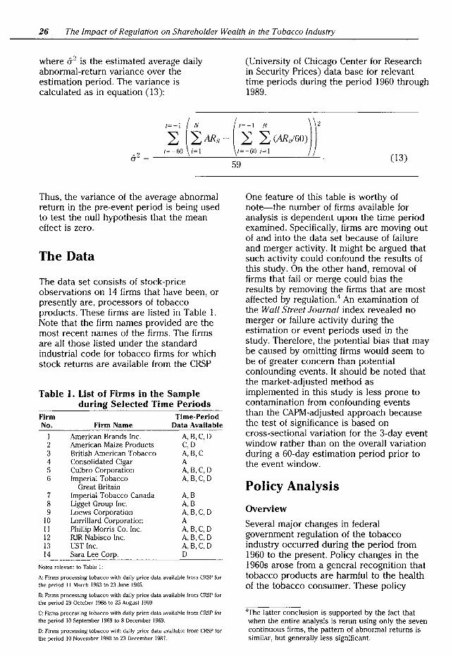
26 The Impact of Regulation on Shareholder Wealth in the Tobacco Industry
where &2 is the estimated average daily abnormal-return variance over the estimation period. The variance is calculated as in equation (13):
(University of Chicago Center for Research in Security Prices) data base for relevant time periods during the period 1960 through 1989.
I ( ~ AR, _ (I#. (AR;/60)) r (13)
Thus, the variance of the average abnormal return in the pre-event period is being used to test the null hypothesis that the mean effect is zero.
The Data
The data set consists of stock-price observations on 14 firms that have been, or presently are, processors of tobacco products. These firms are listed in Table 1. Note that the firm names provided are the most recent names of the firms. The firms are all those listed under the standard industrial code for tobacco firms for which stock returns are available from the CRSP
Table I. List of Firms in the Sample during Selected Time Periods
Firm No.
I 2 3 4 5 6
7 8 9
10 II 12 13 14
Firm Name
American Brands Inc. American Maize Products British American Tobacco Consolidated Cigar Culbro Corporation Imperial Tobacco
Great Britain Imperial Tobacco Canada Ligget Group Inc. Loews Corporation Lorrillard Corporation Phillip Morris Co. Inc. RJR Nabisco Inc. UST Inc. Sara Lee Corp.
Notes relevant to Table 1:
Time-Period Data Available
A,B,C,D C,D A,B,C A A,B,C,D A,B,C,D
A,B A,B A,B,C,D A A,B,C,D A,B,C,D A,B,C,D D
A: Firms processing tobacco with daily price data available from CRSP for the period 11 March 1963 to 23 June 1965.
B: Firms processing tobacco with daily price data available from CRSP for the period 29 October 1968 to 25 August 1969.
C: Firms processing tobacco with daily price data available from CRSP for the period 10 September 1969 to 8 December 1969.
D: Firms processing tobacco with daily price data available lrom CRSP for the period 10 November 1980 to 23 December 1987.
59
One feature of this table is worthy of note-the number of firms available for analysis is dependent upon the time period examined. Specifically, firms are moving out of and into the data set because of failure and merger activity. It might be argued that such activity could confound the results of this study. On the other hand, removal of firms that fail or merge could bias the results by removing the firms that are most affected by regulation.4 An examination of the Wall Street Journal index revealed no merger or failure activity during the estimation or event periods used in the study. Therefore, the potential bias that may be caused by omitting firms would seem to be of greater concern than potential confounding events. It should be noted that the market-adjusted method as implemented in this study is less prone to contamination from confounding events than the CAPM-adjusted approach because the test of significance is based on cross-sectional variation for the 3-day event window rather than on the overall variation during a 60-day estimation period prior to the event window.
Policy Analysis
Overview
Several major changes in federal government regulation of the tobacco industry occurred during the period from 1960 to the present. Policy changes in the 1960s arose from a general recognition that tobacco products are harmful to the health of the tobacco consumer. These policy
4The latter conclusion is supported by the fact that when the entire analysis is rerun using only the seven continuous firms, the pattern of abnormal returns is similar, but generally less significant.

changes attempted to decrease consumer demand by requiring that cigarettes be labeled with health warnings and that cigarette advertising be banned from radio and television. In fact, the events of the 1960s are used in this study in part to gauge the sensitivity of the alternate event-study methodologies in detecting changes in firm value because it is highly likely that some of the regulatory changes would have decreased product demand and firm value. Policy changes in the 1970s were minor at the federal government level, with most changes occurring at the state government level. Policy changes in the 1980s arose primarily from the need to reduce government expenditures on agricultural programs. Many of the provisions were included in the major farm bills of that era. It can be argued that results from the examination of events in the 1980s are more important to agricultural researchers, especially since similar program changes have occurred or will occur for other major commodities. In this study we limit ourselves to the examination of policy changes at the federal level.
Policy Analysis for the 1960s Several factors led the government to institute new tobacco industry policies in the 1960s. Some actions were rooted in reports that appeared during the 1950s linking cigarette smoking to lung cancer. A widely disseminated study-a 1950 publication by two English physicians, Dr. Richard Doll and Dr. A.B. Hill-showed higher cancer rates among smokers. These results may have signaled the beginning of public intervention that peaked in the 1960s (Doron, p. 12).
Government intervention in the marketplace for tobacco products occurred over a period of approximately ten years. The intervention involved several branches of the government: the Food and Drug Administration (FDA), the Federal Trade Commission (FTC), the Federal Communications Commission (FCC), the U.S. Senate, and the U.S. House of Representatives. With so many government bodies involved, it is not surprising that a large number of pronouncements and discussions occurred within and between agencies during this period. The major
Johnson, Mittelhammer, and Blayney 27
regulatory thrusts were the requirements on labeling of cigarettes (i.e., health warnings) and the banning of tobacco-product advertising on radio and television.
It is hypothesized that any information that leads investors to conclude that health warnings will be required or that tobacco-product advertising will be banned will reduce firm value. Conversely, information that leads investors to conclude that regulations will be delayed or weakened should increase firm value. Health warnings are likely to convince smokers to reduce their consumption or quit smoking altogether, and may convince some to never begin smoking. The likely subsequent decrease in current and future demand will induce a negative impact on stock prices. Similarly, advertising restrictions may decrease consumer demand, and thus firm value, because potential and current customers are not as frequently exposed to advertisements for tobacco products.
In contrast, Doron (pp. 86-105) suggests that the institution of these regulations may not negatively impact the processing firms due to the nature of the product and its market. He argues that demand for tobacco products is highly inelastic because of the addictive qualities of tobacco. Thus, he concludes health warnings and limitations on advertising may have no significant impact on current demand. Additionally, advertising restrictions may not only decrease future revenues, but may also decrease costs through a reduction in advertising expenditures. Therefore, he concludes that the net outcome of these actions may be interpreted as somewhat uncertain. On balance, we view the situation as less uncertain than Doron. The notion that the reduction in advertising expenditures will offset the reduction in revenues resulting from the lack of advertising belies the profit motive that has induced the industry to allocate resources to the advertising activity. Furthermore, the fact that tobacco-product demand is highly inelastic in no way prevents quantity demanded from being reduced by a backward shift in the demand schedule (as opposed to a price-induced change in quantity demanded). Finally, the vigorous opposition to the regulations by the tobacco

28 The Impact of Regulation on Shareholder Wealth in the Tobacco Industry
industry is de facto evidence of the detrimental nature of the regulations in the view of industry participants.
From the myriad of discussions, pronouncements, proposals, and legislative actions in the 1960s, it is difficult to determine which events were crucial in determining investors' expectations with respect to firm value. Table 2 provides the events we believe provided the greatest information to investors regarding likely government actions.
Table 3 presents the a priori hypothesized directions of event impacts and the results of the empirical analysis. As with any study of the impact of regulation on firm value, it is important to consider not only the sign and significance of individual events, but also the overall pattern of effects. This holistic approach to the examination of Table 3 is important for two reasons. First, the regulatory environment is such that investors' expectations may be formed cumulatively on the basis of more than one informational event. For example, there are at least five major informational events linked to the institution of labeling
requirements for cigarette packages. Precisely how and when expectations are formed is difficult to determine. We can, however, state with reasonable certainty that mean abnormal returns that are significantly different from zero reflect the arrival of new information.
Second, a single significant event may not "prove" that the regulation impacts firm value because of the possibility of a confounding event. A confounding event is an information event unrelated to the event that coincidentally occurs on the same date. Although we examined the Wall Street Journal index and found no confounding news stories around the time of our regulatory event dates, this possibility remains.
Examination of Table 3 leads to important observations regarding the consistency of results across event-study methodologies and the sensitivity of each method to firm-value changes. Out of the 25 events studied, only 5 events produced abnormal returns with different signs for the two methods, and of these latter 5 events, 4 events were attributed with statistically
Table 2. Regulatory Events Affecting the Tobacco Industry during the 1960s Event No.
2
3
4 5 6 7
8
9
10
11
Date
6 June 1963
18 January 1964
22 June 1964
19 August 1964 16 June 1965 22 June 1965 5 February 1969
I July 1969
7 July 1969
22 August 1969
5 December 1969
Event
Senate measure introduced to give FDA same power to police content, advertising, and labeling of cigarettes as it has over food, drugs, and cosmetics.
FTC issues its official notice of rule making pertaining to the labeling of cigarettes.
FTC promulgates its Trade Regulation Rule on Cigarette Labeling.
Implementation date of FTC rule is delayed. Cigarette labeling bill passes Senate. Cigarette labeling bill passes House. FCC proposes to ban all cigarette advertising from radio
and television. FTC holds hearings on a new health warning and
extension of the warning to advertising. Television Code Review Board of the National
Association of Broadcasters endorses phasing out of cigarette ads on radio and television by 1 September 1973.
The New York Times states in an editorial that all cigarette ads in its pages after January 1970 must carry the health warning currently required on all cigarette packages.
Senate Commerce Committee reports bill to ban cigarette advertising from the airwaves starting 1 January 1971. The bill prohibits FTC action on cigarette advertising until 1 July 1971.

Johnson, Mittelhammer, and Blayney 29
Table 3. Three-Day Mean Abnormal Returns Associated with Events Affecting the Tobacco Industry
Event Hypothesized Number of Number Direction Firms Affected
1 12 2 12 3 12 4 + 12 5 12 6 + 12 7 10 8 10 9 10
10 10 11 9 12 9 13 9 14 9 15 9 16 9 17 ? 9 18 + 9 19 9 20 9 21 + 9 22 9 23 + 9 24 + 9 25 + 9
'Significant at .05.
"Significant at .10.
insignificant abnormal returns by both methods. In the remaining case, statistical significance of the event is achieved for the market-adjusted method but not the CAPM method. Additionally, if a 95% confidence interval is formed around the CAPM-generated abnormal return, the market-adjusted abnormal return falls well within the confidence interval. Therefore, for the most part, the two methodologies are not inconsistent regarding directional impacts of events. The first II events listed in the table are events from the I960s. Earlier discussion of these events indicated that a number of these events were likely to have had significant impacts upon firm value. Given the strength of these prior beliefs, the CAPM method is disappointing, since only 2 events were judged to be significant at the .05 level. On the other hand, the market-adjusted method appears to be much more sensitive to firm-value changes related to these events.
From Table 3 it can be clearly seen that when the CAPM method is used to generate
Market-Adjusted CAPM Method(%) Method (%)
-1.7658* -2.2041 * -2.2376* -2.2780* -1.3384* -1.9163**
.7882 .5651 -1.6072* .2208
1.3209* .8789 -2.2235* -2.0938 -.4673 .4281
.4856 .1117
.6231 .8282 -.9921 -1.4127 -.5877 -1.2078 -.5049 -.2479
- 1.5847** -1.7030 1.5199* .8030
-1.0518* -1.0440 -1.4797 -.8888 -1.1961 .6299 -.7593 -1.1787
.2112 .0802
.1353 1.2846
.9424 -.8108 -.3771 -.8135
-1.5960 2.1176 .5513 .7081
abnormal returns, none of the events of the I980s (events I2-25) were found to have a significant impact on firm value. This result by itself is not deemed to be overly convincing, since the analysis of the I960s period (events I-II) suggested that the CAPM methodology was somewhat less sensitive to firm-value changes than the market-adjusted method. In the discussion that follows, we concentrate on the results generated by the market-adjusted approach. Given the results in Table 3, this can equivalently be viewed as judging an event to be significant if either of the event-study methodologies judged the event to be significant.
On 6 June I963, the first major event in the regulation of tobacco-product labeling and advertising occurred. A measure was introduced in the U.S. Senate that would give the FDA the power to police the content, advertising, and labeling of cigarettes. Although this measure never became law, market participants undoubtedly considered passage of the bill

30 The Impact of Regulation on Shareholder Wealth in the Tobacco Industry
a possibility and viewed it as predictive of the direction future labeling requirements and advertising restrictions were apt to take. The first event we found to be statistically significant and of the same sign as hypothesized. The mean abnormal return for this event was 1.8% of firm value.
Event 2 was a motion by the FTC indicating that it intended to make rules governing advertising and labeling. Event 3 was a report that the FTC would require cigarette manufacturers to label packages with the statement that "Cigarette smoking is dangerous to health and may cause death from cancer and other diseases." These actions represented a large step toward labeling requirements. Event 4, which occurred on 19 August 1964, indefinitely delayed the ruling of event 3 at the same time that Congress decided to discuss the issue. If investors viewed this delay as a reprieve from this type of legislation, then it might be anticipated that this event would have a positive impact on firm value.
Events 2 and 3 were found to be significant and negative, as hypothesized. In total, the two events represent approximately a 3.5% decrease in stockholder wealth. It is worthy of note that event 4, the official delay of the action, produced a positive mean abnormal return, as hypothesized, but its t-statistic was insignificant.
On first impression, events 5 and 6 would both appear to be detrimental to the tobacco processing firms. However, this may not be an appropriate interpretation of these eyents. The biJI passed by the Senate was clearly disappointing news for stockholders because it indicated that a final labeling rule was likely to be passed and signed into Jaw. The passage of the cigarette-labeling biJI by the House of Representatives may have been good news for the firms because the final biJI required a label that was noticeably Jess direct than the original FTC motion and required the FTC to wait five years before it could propose stiffer health warnings on cigarette packages. The labeling statement that passed the House was "Cigarette smoking may be hazardous to your health." The findings in Table 3 fit well with the second interpretation of the events. A large and statistically significant negative impact was
found for event 5, and a significant positive impact was found for event 6.
When the Federal Communications Commission (FCC) proposed a ban on all cigarette advertising on radio and television, event 7, it was the first indication that such a ban might be implemented. Event 7, in combination with event 11, the introduction of a biJI in the Senate to ban such advertising, is likely to reduce firm value if, as is expected, the detrimental impact on sales revenue is perceived by investors to be greater than the advertising cost savings to processors. It might be that the initial FCC proposal is the event that would have the largest impact upon the expectations of investors because it is the first mention of such an action and a similar chain of events occurred that eventually led to labeling requirements.
Results from Table 3 indicate that event 7 produced a mean abnormal return of - 2.2% and was significant at the .05 level. This supports our hypothesis that the net impact of an advertising ban on firm value is negative. Event 11 had a negative mean abnormal return, as predicted, but was insignificant.
Events 8, 9, and 10 are likely to be of less importance than the other events in this group because they are relatively minor actions and therefore may not provide much additional information to the marketplace. Event 8 is an extension of the package labeling requirements to all advertisements. Event 9 is the endorsement by the National Association of Broadcasters for the phasing out of cigarette ads on radio and television. Event 10 is an editorial in the New York Times that states that all cigarette ads published by the paper must carry health warnings after January 1970. The results indicate that events 8, 9, and 10 did not significantly impact investors' perceptions of firm value.
Policy Changes in the 1980s
Since the early 1930s, the federal government has operated programs to support and stabilize tobacco prices. During the 1933-38 period, cash payments were made to tobacco growers to restrict output. From 1938 to 1981, government policies

centered on two programs: the quota system, which provides a balanced and limited flow of products to the market; and the price-support program, which has attempted to maintain tobacco producer prices at levels specified by Congress. Under the price-support program, tobacco acquired by a cooperative association serves as collateral for a loan from the Commodity Credit Corporation (CCC). Under an agreement between the CCC and the association, the association arranges for receiving and storing tobacco under loan.
A desire on the part of the federal government to reduce its spending on agricultural programs has motivated many of the changes in agricultural legislation, including tobacco legislation, during the 1980s. Six of the seven legislative acts affecting the tobacco industry during the period 1981 to 1987 included provisions redefining the government's role in the tobacco price-support program. The seventh bill required importers of tobacco to test for pesticide and herbicide residues and to report the end use of these imported tobacco products.
It is possible, a priori, to make a general statement about the potential impact of policy changes on firm value. Any policy that increases (decreases) costs of production for the processing firms, ceteris paribus, may decrease (increase) profits and firm value. Specifically, these effects will occur if processors are unable to pass cost increases on to consumers or unable to conserve cost savings within the firm. Thus, the bill that requires importers to test and report the end use of their tobacco imports will increase costs and should reduce firm value. Additionally, a lowering of the price-support level should, ceteris paribus, decrease costs and increase firm value.
Casual intuition may suggest that a decrease in the level of financial support from the government for the price-support program is likely to cause wholesale tobacco prices to fall as the CCC reduces its price-support loan program that tends to keep product off the market. However, this would be a narrow view of the total impact of decreased government involvement. Legislation during the 1980s that decreased
Johnson, Mittelhammer, and Blayney 31
government involvement has not eliminated the price-support program, but rather has shifted the burden of financial support for and maintenance of the program to tobacco farmers. This implies that farmers must bear higher costs of production. Higher production costs and the prospect of some degree of resultant contraction in tobacco production capacity in the longer run could contribute to a perceived decrease in tobacco firm value by investors.
Choosing the events that provided the greatest possible information about tobacco policy changes in the 1980s was straightforward in comparison to the 1960s period. In contrast to the 1960s, when policy was set through legislation and regulatory-agency pronouncements, agricultural policy changes in the 1980s occurred through seven bills that were introduced and passed. With one exception, the first introduction of the bill into either the House of Representatives or the Senate and its passage by the originating body were the events examined. The exception to this rule is the 1981 farm bill, where the origination, revision, and passage of the bill by the Senate were examined (events 12, 13, and 14). We chose to examine the original introduction as an event because it provides the market with its first glimpse of changes likely to befall the industry. We chose to examine passage by the originating body because bills of this nature are rarely, if ever, vetoed by the president after passage by Congress. In fact, none of the bills relating to tobacco programs were vetoed during this period. Therefore, market participants would have been well justified in expecting that passage of the bill by Congress implied that it would be instituted.
Table 4 lists the informational events examined for the 1980s in chronological order. Note that numbering of the events begins where Table 2 ended.
Events 12, 13, and 14 identify information released to the public regarding the Agriculture and Food Act of 1981. The events coincide with the introduction of the act in the U.S. Senate, the revision of the bill, and final passage by the Senate. The intent of the tobacco-provisions bill was that the tobacco price-support and production-adjustment (quota) programs
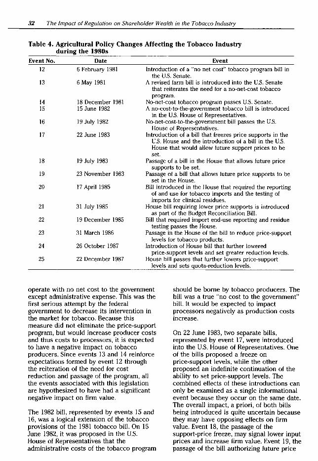
32 The Impact of Regulation on Shareholder Wealth in the Tobacco Industry
Table 4. Agricultural Policy Changes Affecting the Tobacco Industry during the 1980s
Event No. Date
12 6 February 1981
13 6 May 1981
14 18 December 1981 15 15 June 1982
16 19 July 1982
17 22 June 1983
18 19 July 1983
19 23 November 1983
20 17 April 1985
21 31 July 1985
22 19 December 1985
23 31 March 1986
24 26 October 1987
25 22 December 1987
Event
Introduction of a "no net cost" tobacco program bill in the U.S. Senate.
A revised farm bill is introduced into the U.S. Senate that reiterates the need for a no-net-cost tobacco program.
No-net-cost tobacco program passes U.S. Senate. A no-cost-to-the-government tobacco bill is introduced
in the U.S. House of Representatives. No-net-cost-to-the-government bill passes the U.S.
House of Representatives. Introduction of a bill that freezes price supports in the
U.S. House and the introduction of a bill in the U.S. House that would allow future support prices to be set.
Passage of a bill in the House that allows future price supports to be set.
Passage of a bill that allows future price supports to be set in the House.
Bill introduced in the House that required the reporting of and use for tobacco imports and the testing of imports for clinical residues.
House bill requiring lower price supports is introduced as part of the Budget Reconciliation Bill.
Bill that required import end-use reporting and residue testing passes the House.
Passage in the House of the bill to reduce price-support levels for tobacco products.
Introduction of House bill that further lowered price-support levels and set greater reduction levels.
House bill passes that further lowers price-support levels and sets quota-reduction levels.
operate with no net cost to the government except administrative expense. This was the first serious attempt by the federal government to decrease its intervention in the market for tobacco. Because this measure did not eliminate the price-support program, but would increase producer costs and thus costs to processors, it is expected to have a negative impact on tobacco producers. Since events 13 and 14 reinforce expectations formed by event 12 through the reiteration of the need for cost reduction and passage of the program, all the events associated with this legislation are hypothesized to have had a significant negative impact on firm value.
should be borne by tobacco producers. The bill was a true "no cost to the government" bill. It would be expected to impact processors negatively as production costs increase.
On 22 June 1983, two separate bills, represented by event 17, were introduced into the U.S. House of Representatives. One of the bills proposed a freeze on price-support levels, while the other proposed an indefinite continuation of the ability to set price-support levels. The combined effects of these introductions can only be examined as a single informational event because they occur on the same date. The overall impact, a priori, of both bills being introduced is quite uncertain because they may have opposing effects on firm value. Event 18, the passage of the support-price freeze, may signal lower input prices and increase firm value. Event 19, the passage of the bill authorizing future price
The 1982 bill, represented by events 15 and 16, was a logical extension of the tobacco provisions of the 1981 tobacco bill. On 15 June 1982, it was proposed in the U.S. House of Representatives that the administrative costs of the tobacco program

supports, may reduce firm value by reinforcing expectations that prices of inputs will not fall dramatically in the future.
Events 20 and 22 are the introduction and passage of a House bill that requires importers of tobacco products to test for herbicide and pesticide residues on imported tobacco and to report on the end use of these imports. Clearly these policy changes increase input costs and would be expected to decrease firm profits.
The last four events to be examined, events 21, 23, 24, and 25, involve the introduction and passage of two bills that reduced price-support levels. We hypothesize that these events should have a positive impact upon processor firm value because the two bills lead to reduced input costs for processors, at least in the short run.
After examining the results of Table 3 for events 12-25, we reach the startling conclusion that mean abnormal returns are significant for only three events-14, 15, and 16--, with event 14 significant at .10, and events 15 and 16 significant at .05. The lack of significance for most of the events might be explained by three factors. First, the cost of tobacco as an input into the production process is a small percentage of total production costs. Therefore, large changes in tobacco prices cause small changes in costs for tobacco processing firms. Second, the highly inelastic nature of the demand for tobacco products may allow processors to pass increased production costs on to consumers with little reduction in operating margins. Third, mergers within the industry may have reduced the importance of the tobacco component of these conglomerates. Specifically, these firms have generally grown in size through diversification, and the percentage of the firm associated with tobacco processing has declined. Therefore, any impacts on firm value will be lower with respect to the rate of return for the entire firm.
Events 14, 15, and 16 are associated with proposals that require the tobacco program to be of no net cost to the government. Regarding the significance and signs of these results, note that if any event should have impacted firms in a significant manner,
Johnson, Mittelhammer, and Blayney 33
it seems logical that it should have been the first bill, introduced on 6 February 1981. This bill represented a large change in government policy with respect to administration and funding of the price-support program. While introduction of this bill did not produce significant abnormal returns, its passage appears to have had a negative impact of approximately 1.6%, on average. This result can be explained if it is considered that market participants may have believed at the time of introduction that a bill such as this was unlikely to be passed because it was such a radical departure from previous policies. If this was the case, the passage of the bill would have provided the greatest amount of information regarding the perceived impact on firm value. Event 15, introduction of a similar no-net-cost bill to the House of Representatives, produced a positive average abnormal return of 1.5%. This event may have produced a positive abnormal return because the market participants clearly saw tobacco farmers and other industry participants lobbying for amendments that would weaken the bill, and it may have seemed likely that such efforts would be successful. Finally, event 16, the passage of the house bill, produced a negative average abnormal return of approximately 1.0%, and thus the ultimate passage of the no-net-cost bill was apparently perceived as bad news for processors. Perhaps the most important aspect of these three events is that, when viewed together, the net effect on processors is small, with the sum of average abnormal returns from the three events being a negative 1.12%. To place the magnitude of the effect in perspective, consider that the net effect of all the events in the 1960s was approximately a negative 5.7% of firm value. Thus, from a holistic perspective, the net impact of agriculturalpolicy changes was relatively small. Additionally, it should be noted that 11 of the 14 events were found to be insignificant. Therefore, a reasonable conclusion to make is that tobacco legislation in the 1980s had only a small impact on the value of tobacco processing firms.
Summary and Conclusions The event-study approach is well suited to the evaluation of government-policy

34 The Impact of Regulation on Shareholder Wealth in the Tobacco Industry
changes on the market value of firms impacted by the regulations. This approach can only be used for the examination of industries where firms are publicly held and stock is traded on organized exchanges. Most previous studies of agricultural-commodity firms have not explicitly utilized financial-market data. We suggest that this methodology may be useful for evaluating and measuring the impact of many other changes in government policies that have occurred in the 1980s and that will occur in the future.
The results of this study are quite revealing. For processors in the tobacco industry, we find that labeling requirements (i.e., health warnings) and advertising bans on radio and television have had a large negative impact on firm value. The legislation of the 1980s, which is primarily producer-oriented, had little or no impact on processors of tobacco products. This result provides insight into the factors that affect agricultural-commodity processors. Specifically, rules and regulations that affect the end product, rather than the underlying raw agricultural commodity, tended to have a greater impact on firm value.
References
Aharony, J., and I. Swary. "Effects of the 1970 Bank Holding Company Act: Evidence from Capital Markets." J. Fin. 36 (Sept. 1981):841-53.
Binder, J.J. "Measuring the Effects of Regulation with Stock Price Data." Rand J. of Econ. 16, no. 2(Summer 1985):167-83.
Brown, S.J., and J.B. Warner. "Measuring Security Price Performance." J. Financial Econ. 8( 1980 ):205-58.
----· "Using Daily Stock Returns: The Case of Event Studies." J. Financial Econ. 14(1985):3-31.
Collins, D.W., and W.T. Dent. "A Comparison of Alternative Testing Methodologies Used in Capital Market Research." J. Accounting Res. 22(1984):48-84.
Dann, L.Y., and C.M. James. "An Analysis of the Impact of Deposit Rate Ceilings on the
Market Values of the Thrift Institutions." J. Fin. 37(Dec. 1982):1259-75.
Doll, Richard, and A.B. Hill. "Smoking and Carcinoma of the Lung." British Medical Journal Iss. 4682( 1950):739-48.
Doron, G. The Smoking Paradox: Public Regulation in the Cigarette Industry. Abt Associates Inc., 1979.
Grise, V.N., and K.F. Griffin. "The U.S. Tobacco Industry." Report #589. U.S. Department of Agriculture, Economic Research Service, Sept. 1989.
Schipper, K., and R. Thompson. "The Impact of Merger-Related Regulations on the Shareholders of Acquiring Firms." J. Accounting Res. 21(Spring 1983):184-221.
Schipper, K., R. Thompson, and R.L. Wei!. "Disentangling Interrelated Effects of Regulatory Changes on Shareholder Wealth: The Case of Motor Carrier Deregulation." J. Law and Econ. 30(April 1987):67-100.
Schwert, G.W. "Stock Exchange Seats as Capital Assets." J. Financial Econ. 4( January 1987):51-78.
U. S. Department of Health and Human Services. "Reducing the Health Consequences of Smoking, 25 Years of Progress: A Report of the Surgeon General." 1989.
Weston, J.F., and T.E. Copeland. Managerial Finance. The Dryden Press, 1986.

An Empirical Investigation of Causal Relationships between the Money Supply, Prices, and Wages in the U.S. Agricultural Sector Peter J. Saunders
Abstract The effects of monetary changes on agricultural food prices, farm prices, and wages are investigated within the Granger causality testing framework. Causality testing relying upon the minimum final prediction error (FPE) method is carried out within the trivariate model specifications. While the tests indicate no empirical evidence of causal impact of monetary growth on farm-level prices and wages, monetary changes are found to have statistically significant effects on retail-level food prices and the overall agricultural sector's wages.
Key words: farm prices and wages, retail food prices, agricultural wages, money supply, Granger causality.
Peter J. Saunders is a professor, Department of Economics, Central Washington University.
There is a growing interest in examining linkages between the U.S. agricultural sector and the rest of the U.S. economy. Numerous studies have investigated the impact of macro changes, such as changes in the money supply, on the U.S. agricultural sector (Barnett, Bessler, and Thompson; Belongia and King; Bessler; Bordo; Chambers; Chambers and Just; Saunders). Empirical evidence presented within the causality testing framework indicates that monetary changes affect U.S. agricultural prices (Barnett et al.; Saunders). However, establishing a causal flow from the money supply to agricultural prices does not rule out the possibility that agricultural prices are also determined by other cost-push factors, such as wage increases. In other words, the cost-push theory of price determination is not ruled out in this case. On the whole, the theoretical issue of wage and price determination has important implications not only for the U.S. agricultural sector, but also for the macro policy conduct. From an economic-policy point of view, it is important to determine whether wages and prices in an economy are causally determined by an independent factor such as the money-supply growth (monetarists' position) or whether wages and prices causally affect one another. Essentially, the key theoretical issue is whether wages causally affect prices (cost-push theory of inflation) or whether the money-supply growth affects both wages and prices (monetarists' position).
An empirical examination of the linkages between the U.S. agricultural sector and the
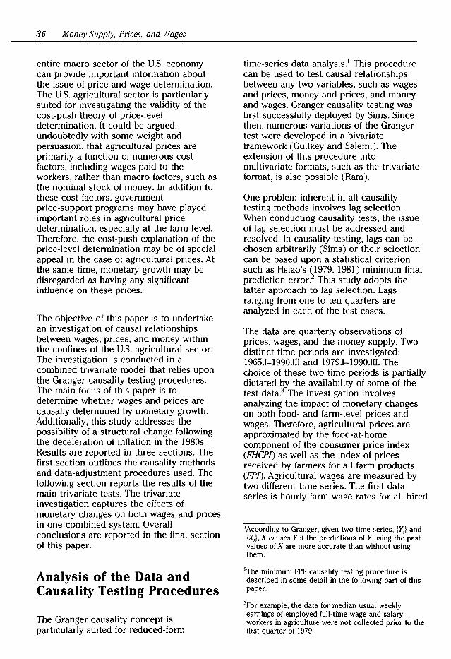
36 Money Supply, Prices, and Wages
entire macro sector of the U.S. economy can provide important information about the issue of price and wage determination. The U.S. agricultural sector is particularly suited for investigating the validity of the cost-push theory of price-level determination. It could be argued, undoubtedly with some weight and persuasion, that agricultural prices are primarily a function of numerous cost factors, including wages paid to the workers, rather than macro factors, such as the nominal stock of money. In addition to these cost factors, government price-support programs may have played important roles in agricultural price determination, especially at the farm level. Therefore, the cost-push explanation of the price-level determination may be of special appeal in the case of agricultural prices. At the same time, monetary growth may be disregarded as having any significant influence on these prices.
The objective of this paper is to undertake an investigation of causal relationships between wages, prices, and money within the confines of the U.S. agricultural sector. The investigation is conducted in a combined trivariate model that relies upon the Granger causality testing procedures. The main focus of this paper is to determine whether wages and prices are causally determined by monetary growth. Additionally, this study addresses the possibility of a structural change following the deceleration of inflation in the 1980s. Results are reported in three sections. The first section outlines the causality methods and data-adjustment procedures used. The following section reports the results of the main trivariate tests. The trivariate investigation captures the effects of monetary changes on both wages and prices in one combined system. Overall conclusions are reported in the final section of this paper.
Analysis of the Data and Causality Testing Procedures
The Granger causality concept is particularly suited for reduced-form
time-series data analysis.1 This procedure can be used to test causal relationships between any two variables, such as wages and prices, money and prices, and money and wages. Granger causality testing was first successfully deployed by Sims. Since then, numerous variations of the Granger test were developed in a bivariate framework (Guilkey and Salemi). The extension of this procedure into multivariate formats, such as the trivariate format, is also possible (Ram).
One problem inherent in all causality testing methods involves lag selection. When conducting causality tests, the issue of lag selection must be addressed and resolved. In causality testing, lags can be chosen arbitrarily (Sims) or their selection can be based upon a statistical criterion such as Hsiao's ~1979, 1981) minimum final prediction error. This study adopts the latter approach to lag selection. Lags ranging from one to ten quarters are analyzed in each of the test cases.
The data are quarterly observations of prices, wages, and the money supply. Two distinct time periods are investigated: 1965.1-1990.111 and 1979.1-1990.111. The choice of these two time periods is partially dictated by the availability of some of the test data? The investigation involves analyzing the impact of monetary changes on both food- and farm-level prices and wages. Therefore, agricultural prices are approximated by the food-at-home component of the consumer price index (FHCPI) as well as the index of prices received by farmers for all farm products (FPI). Agricultural wages are measured by two different time series. The first data series is hourly farm wage rates for all hired
1According to Granger, given two time series, {Y,} and {X,}, X causes Y if the predictions of Y using the past values of X are more accurate than without using them.
2The minimum FPE causality testing procedure is described in some detail in the following part of this paper.
3For example, the data for median usual weekly earnings of employed full-time wage and salary workers in agriculture were not collected prior to the first quarter of 1979.

Saunders 37
Table I. Dickey-Fuller Test Results for M2 , FHCPJ, FPI, W, and WFa,b
Variables t 1 f Implications
Mz 1.322c -13.7d The data have unit root. FHCPI 0.622 -13.7 The data have unit root. FPI -1.326 -13.7 The data have unit root. w -3.183 -13.3 The data have unit root. WF -0.9894 -13.7 The data have unit root.
"All tests are conducted at the 5% level of significance.
"The test period lor M2 , FHCPI, FPI, and WF is 1965.l-1990.1ll, whereas the test period for W is 1979.!-1990.111.
ell is the statistic generated by tests.
dfl is the critical statistic for H0.
farm workers (WF); the second measure is median usual weekly earnings of employed full-time wage and salary workers in agriculture (W).4 Using WF, W, FPI, and FHCPI allows for an empirical investigation of the relationship between wages and prices at both the farm and the food levels. The money measure is the M2 money supply.
Prior to invoking any econometric testing procedures, such as causality testing, the issue of the stationarity of the data must be addressed. Many time-series data are nonstationary in the sense that their mean and variance depend on time. Nonstationary time-series data must be detrended to induce stationarity. One way to resolve the issue of data stationarity and determine subsequent detrending procedures is to apply unit-root tests. Consequently, all the data were subjected to the Dickey-Fuller unit-root tests (Dickey and Fuller; Fuller).5
4Data on the median weekly earnings of employed full-time wage and salary workers in agriculture were obtained from unpublished tables of the Bureau of Labor Statistics. The farm wage rates series was obtained directly from a survey conducted by the U.S. Department of Agriculture. It is a quarterly survey conducted from the first quarter of 1959 to the third quarter of 1990. The major shortcoming of this survey of agricultural wages is the fact that methods of collecting the data have been changed over time. For example, in 1969 the definition changed from wage rate of all hired farm workers to per hour wage rate without board or room. However, this definitional change did not result in any substantial quantitative change.
5The main purpose of Dickey-Fuller tests is to indicate whether a variable is integrated or not (i.e., whether it is stationary or nonstationary). All integrated variables are nonstationary. The presence of a unit root indicates that a variable is integrated. For a further detailed discussion of this point, see Stock and Watson. Nonstationary time-series data contain stochastic trends. These stochastic trends can be removed by various data differencing procedures.
The test results are reported in Table 1. All of the test statistics are greater than the critical values for a one-tail 5% significance test of nonstationarity. This implies that all time-series data contained unit roots in their autoregressive specifications. Therefore, the data were found to be nonstationary, as they contained stochastic trends. These trends were removed by entering all variables into test equations in the first differences of their logarithms.
Trivariate Analysis Results
There have been numerous empirical investigations of bivariate causal flows between the money supply and other variables, such as nominal income and prices (Sims; Saunders; and many others). One shortcoming of the bivariate testing procedures is the fact that these methods allow only separate examinations of causal flows between two test variables. While examining causal flows between three different test variables, such as in the present case, it may be of interest to combine all variables into a trivariate framework. The main advantage of a trivariate analysis lies in its ability to examine causal flows between all three variables under consideration in one combined system. In the present case, this necessitates the examination of causal flows between the money supply, wages, and prices at both the farm level and the retail level. Therefore, two separate trivariate models are investigated, one utilizing M2 ,
FPI, and WF, while the other uses the data for M2 , FHCPI, and W. Additionally, the examination of the lag structure enables the researcher to make inferences about the relative length of time of the monetary impact on wages and prices. In this way,

38 Money Supply, Prices, and Wages
Table 2. Minimum FPE Causality Testing Method Results for M2 , WF, and FPI: 1965.1-1990.III
First Controlled Independent
Second Independent
Variable Equation Variable Variable FPE I 2 3 4 5 6
WF(6)a FPI (1) WF(6) FP/(1) WF(6) FP/(1)
FPI (1) WF(l) FPI (I) WF(I)
1.5797 2.1829 1.5971 2.1458 1.6169 2.1532
"Numbers in parentheses are lags for minimum FPE specifications. FPEs reported for all equations are the numerical values of each FPE multiplied by 103 • Format of report is modified from Ram.
one can determine whether wage changes precede price changes or vice versa.
As previously mentioned, the lag selection plays an important role in causality testing procedures. The arbitrary lag-selection method suffers from two major difficulties. The first involves the loss of degrees of freedom due to the lagging of test variables. In many cases, theory necessitates an examination of relatively long lags. However, extending the lag structure causes a diminishment of the degrees of freedom (Hsiao 1979). This problem is particularly troublesome in cases where relatively few observations are available. In such cases, the bias toward investigating primarily shorter lag specifications may well develop.
Second, causality test results may be influenced by the lag-selection method used. This point is noted by numerous authors. Hsiao (1979, 1981) claims that the distributions of test statistics are affected by the arbitrary choice of lag restrictions. When examining causal implications of monetary changes on agricultural prices, Saunders finds the test results sensitive to the lag selection. Similar conclusions are reached by Thornton and Batten in their recent study of the money-income causal relationships in the U.S. The authors examine three different lag-selection methods in causality testing: the Pagano and Hartley technique, the method outlined by Geweke and Meese, and Hsiao's (1979, 1981) minimum final prediction error (FPE) technique. The minimum FPE method performs well in the lag-structure identification.
Hsiao's minimum FPE technique is particularly suitable for the trivariate analysis of this study, as it alleviates
considerably both of the difficulties associated with an arbitrary lag-selection technique. The minimum FPE method permits an examination of all relevant lags. Additionally, test variables are allowed to be entered into regression equations with different lags. In this way, the problem associated with the loss of degrees of freedom and the subsequent bias towards investigating shorter lag specifications is avoided. This is of particular importance in the present case where relatively few observations of the data are available when the food sector is examined.6
Under the minimum FPE method, the lag selection and subsequent causality implications are based upon a statistical criterion. This criterion is the final prediction error. The final prediction error can be computed as (SEE) · (T + K)/T. SEE is the standard error of the regression, T is the number of observations, and K indicates the number of parameters. The minimum FPE method involves calculating FPEs of all lags in a predetermined lag range and selecting the lag specification that yields the minimum FPE. This method involves calculating minimum FPEs of several statistical steps.7
In the present study, lags ranging from one to ten quarters are examined. The specifications yielding minimum FPEs are selected and reported in Tables 2 and 3. In
6As mentioned previously, the W data were not collected prior to the first quarter of 1979. Therefore, the trivariate analysis of the food sector is limited to the investigation of the 1979.1-1990.III time period.
7 A detailed description of this method is beyond the scope of this paper. Interested readers are referred to Hsiao (1981, pp. 87-93) for a complete description of this procedure.

Saunders 39
Table 3. Minimum FPE Causality Testing Method Results for M2 , W, and FHCPJ: 1979.1-1990.111
First Second Independent
Variable Controlled Independent
Equation Variable Variable FPE 7 w C3Y 8 FHCP/(6) 9 w (3) FHCPJ (1)
1.5932 0.0972 1.6640 0.1022 1.5722 0.0772
10 FHCP/(6) w (1) 11 w (3) FHCPJ (1) 12 FHCPI (6) w (1)
"Numbers in parentheses are lags for minimum FPE specifications. FPEs reported for all equations are the numerical values of each FPE multiplied by 103 . Format of report is modified from Ram.
the case of the farm sector, equations (1) and (2) are univariate specifications, and equations (3) and ( 4) are bivariate specifications. The trivariate specifications are given by equations (5) and (6). A similar way of reporting is used for the food sector in Table 3. Consequently, the minimum FPE method yielded the following forms of equations (7) through (12) for the food sector:
3
Wt = ao + L boj W(t-j) + Uot j=l
6
(7)
FHCPft = a1 + L b1j FHCPI(t-j) + U!t (8) j= I
3
Wt = az + L bzj W(t-j) j=l
+ coj FHCPI(t-1) + Uzt 6
FHCPft = a3 + L b3j FHCPI(t-j) j=l
+ Cj W(t-1) + U3t 3
Wt = a4 + L b4j W(t-j) + Czj FHCPI(t-1) j=l
2
+ L doj Mz(t-j) + U4t j=l
6
(9)
(10)
(11)
FHCPit = as + L bsj FHCPI(t-jl + c3 W(l-ll
j=l
5
+ L dlj Mz(t-j) + Ust (12) j=l
In these specifications, j indicates the number of lags of test variables, while U01
through U51 are stochastic terms.
Ram outlines an interpretation of trivariate minimum FPE procedure results. The causality inferences are based upon the comparison of the minimum FPEs yielded by equations (3)-(6) for the farm sector and (9)-(12) for the food sector. The results for the farm sector are reported in Table 2. There is no indication that monetary growth has any statistically significant impact on farm prices or farm wages. This is clear by comparing the minimum FPEs of equations (3) and (5) (the wage equations) as well as equations ( 4) and (6) (the price equations). In each case, adding the lagged M2 variable increases the minimum FPE. In the case of the wage equations, this increase is from 1.5971 to 1.6169. The same result is apparent in the case of the price equations, where the increase in minimum FPE is from 2.1458 to 2.1532. This implies that money does not Granger-cause either farm wages or farm prices.
The results for the food sector are in contrast to those reported for the farm sector. They indicate that monetary growth plays an important role in both the price and the wage determination in this sector. The causality test results are summarized in detail in Table 3. There is clear evidence of causal flows from M2 to both food prices and wages. This evidence is obtained by comparing minimum FPEs of equations (9) and (11), and equations (10) and (12). An addition of the lagged M2 variable reduces the FPE from 1.6640 (minimum FPE of equation (9)) to 1.5722 (minimum FPE of equation (11)). A similar pattern emerges
40 Money Supply, Prices, and Wages
when the FPEs of equations (10) and (12) are compared. In this case, too, the inclusion of the monetary M2 variable reduces the FPE from 0.1022 to 0.0772. These results give strong support to the monetarists' position on price and wage determination. They indicate that monetary changes play an important causal role in wage and food-price determination.8
Additional important information about the impact of monetary changes on agricultural wages and food prices can be obtained by considering the lag structure of equations (11) and (12) as determined by the minimum FPE testing procedure. Examining this lag structure, one important observation can be made. The lagged response of equation (12) is distributed over five quarters, whereas a two-lag structure is appropriate for equation (11 ). Consequently, the effects of monetary changes on food prices are spread over a year and a quarter, while they affect wages only over two quarters. On the basis of this finding, it is fair to conclude that monetary changes affect food prices more in the long run, while wages appear to be impacted more in the short run. In this sense, wage changes precede price changes.
However, the fact that wage changes precede price changes does not mean that wages cause prices, since these two variables are statistically independent. This is evident by comparing minimum FPEs of bivariate causality test specifications of wages and prices as reported by equations (7)-(10). Equation (9) indicates that adding the FHCPI variable to the wage equation (equation (7)) increases the minimum FPE from 1.5932 to 1.6640. Similarly, the addition of the W variable (equation (10)) to the FHCPI equation (equation (8)) also increases the minimum FPE from 0.0972 to
8It should be noted that while the above-reported test results establish a causal flow from the money supply to both agricultural wages and prices, they do not rule out the possibility that other factors may influence wages and prices. Granger causality tests are not suitable for investigating structural relationships. Their primary contribution lies in examining bivariate relationships with an easy extension into a trivariate format. The purpose of this paper is to conduct reduced-form causality testing. Therefore, an investigation of structural relationships is beyond the scope of this paper.
0.1022. This result implies that wages and prices are statistically independent. Consequently, this result does not support the cost-push explanation. When analyzed within the trivariate structure, it merely indicates that monetary impact on wages is somewhat shorter than its impact on food prices.
Final statistical examination of the data must include analyzing possible effects of changes in an economy on the causal relationships under investigation. One way to accomplish this task is to submit the test equations to the Chow test. This test can indicate whether estimated parameters have remained stable over time. For example, the considerable deceleration of inflation in the mid-1980s could have caused structural changes. Consequently, the natural division of the test period was 1979.1-1984.1V and 1985.1-1990.111. This division of test periods captures accurately the changes in the rate of inflation computed on the quarterly basis.9 Equations (11) and (12) were subjected to the Chow test (Chow; Kmenta, pp. 420-22). In both cases, the null hypothesis of no structural changes was not rejected at the 5% significance level. This result is encouraging since, in spite of deceleration of inflation during the test period, the parameters of both the price equation and the wage equation have remained stable over the entire test period.10
Overall Conclusions This paper examines the linkages between the agricultural sector and the entire macro sector of the U.S. economy. In particular, relationships between agricultural food and farm prices, wages, and the money supply are investigated. This investigation is conducted within the causality testing framework at both the farm- and the overall
!?[here was an actual fall in prices (as measured by both quarterly FHCP! and FP/ data indexes) after the fourth quarter of 1984. This deceleration of inflation could lead to structural changes in an economy.
10The results imply that the coefficients in the model estimated by equations (II) and ( 12) have not changed across the two data periods investigated. Hence, the causal relationships under investigation have not been affected by the deceleration of inflation in the mid-1980s.
food-price level of the U.S. agricultural sector. Two separate time periods are examined: 1965.I-1990.III and 1979.1-1990.111. The first test period investigates the impact of monetary changes on farm prices and wages, whereas the second examines causality implications of monetary changes on food prices and overall agricultural wages. In both cases, the search for the evidence of causal factors in price and wage determination is conducted. The investigation is carried out within the trivariate causality testing framework.
During the 1965.1-1990.1II test period, there is no evidence of monetary changes having any statistically significant impact on farm prices and wages. However, when the second period is examined, a causal flow is established from M2 to both agricultural wages and food prices. These results imply that changes in M2 causally determine both agricultural wages and food prices. On the basis of these results, it is possible to conclude that although there is no evidence of monetary changes having a statistically significant impact on farm-level prices and wages, this evidence exists when the overall U.S. agricultural sector and the rest of the U.S. economy are examined. Therefore, an important linkage between the macro sector and the agricultural sector is established. It is also fair to conclude that monetary policy has an important impact on food prices and wages in the overall U.S. agricultural sector. In this sense, the results provide empirical evidence in support of the monetarist position with respect to the wage and food-price determination. At the same time, it is evident that factors other than monetary growth are instrumental in determining farm-level prices and wages.
When analyzing the lag structure resulting from the minimum FPE causality testing method, it appears that wage changes precede price changes. This result does not imply that wage changes cause price changes, as wages and prices are found to be statistically independent. However, it does indicate that monetary changes affect food prices more in the long run, while wages are impacted more in the short run.
Finally, tests of structural change indicate that the parameters of the estimated models remained stable during the period under
Saunders 41
investigation. This result is encouraging given the slowdown of inflation in the mid-1980s. Consequently, the causal relations investigated in this paper have not been affected by this considerable decrease in the rate of inflation.
References
Barnett, Richard C., David A. Bessler, and Robert L. Thompson. 'The Money Supply and Nominal Agricultural Prices." Amer. J. Agr. Econ. 65(1983):303-7.
Belongia, Mike, and Richard A. King. "A Monetary Analysis of Food Price Determination." Amer. J. Agr. Econ. 65(1983):131-35.
Bessler, David A. "Relative Prices and Money: A Vector Autoregression on Brazilian Data." Amer. J. Agr. Econ. 66(1984 ):25-30.
Bordo, Michael D. "The Effects of a Monetary Change on Relative Commodity Prices and the Role of Long-Term Contracts." J. Polit. Economy 88(1980):1088--1109.
Chambers, Robert G. "Agricultural and Financial Market Interdependence in the Short Run." Amer. J. Agr. Econ. 66(1984):12-24.
Chambers, Robert G., and Richard E. Just. "An Investigation of the Effect of Monetary Factors on Agriculture." Amer. J. Agr. Econ. 9(1982):235-47.
Chow, G.C. "Tests of Equality between Sets of Coefficients in Two Linear Regressions." Econometrica 28(1960):591-605.
Dickey, David A., and Wayne A. Fuller. "Distribution of the Estimators for Autoregressive Time Series with a Unit Root." J. Amer. Stat. Assoc. 74(1979):427-31.
Fuller, Wayne A. Introduction to Statistical Time Series. New York: John Wiley & Sons, 1976.
Geweke, John, and Richard Meese. "Estimating Regression Models of Finite

42 Money Supply, Prices, and Wages
but Unknown Order." Internal. Econ. Rev. 22(1981):55-70.
Granger, Clive W.J. "Investigating Causal Relations by Econometric Models and Cross-Spectral Methods." Econometrica 37( 1969):424-38.
Guilkey, David K., and Michael K. Salemi. "Small Properties of Three Tests for Granger-Causal Ordering in a Bivariate Stochastic System." Rev. Econ. and Stat. 64(1982):668-80.
Hsiao, Cheng. "Autoregressive Modeling of Canadian Money and Income Data." J. Amer. Stat. Assoc. 74(1979):553-60.
____ . "Autoregressive Modeling and Money-Income Causality Detection." J. Monetary Econ. 7(1981):85-106.
Kmenta, Jan. Elements of Econometrics. New York: Macmillan Co., 1986.
Pagano, Marcello, and Michael J. Hartley. "On Fitting Distributed Lag Models Subject to Polynomial Restrictions." J. Econometrics 16(1981):171-98.
Ram, Rati. "Causal Ordering Across Inflation and Productivity Growth in the Post-War United States." Rev. Econ. and Stat. 66(1984 ):4 72-77.
Saunders, Peter J. "Causality of U.S. Agricultural Prices and the Money Supply: Further Empirical Evidence." Amer. J. Agr. Econ. 70( 1988):588-96.
Sims, Christopher A. "Money, Income, and Causality." Amer. Econ. Rev. 62(1972):540-52.
Stock, James H., and Mark W. Watson. "Variable Trends in Economic Time Series." J. Econ. Perspectives 3(1988):147-74.
Thornton, Daniel L., and Dallas S. Batten. "Lag Length Selection and Tests of Granger Causality between Money and Income." J. Money, Credit and Banking 17(1985):164-78.
U.S. Department of Agriculture. Unpublished nationwide survey of farm wage rates.
U.S. Department of Labor. Unpublished survey of median usual weekly earnings of employed full-time wage and salary workers in agriculture.

Credit Scoring for Agricultural Loans: A Review with Applications Calum Greig Turvey
Abstract This paper reviews four alternative credit scoring models: the linear probability model, discriminant analysis, LOGIT, and PROBIT. The econometric models are based on 9,403 loan application observations from Canada's Farm Credit Corporation. Results indicate that there is not a great deal of difference in the predictive accuracies of the four model types, despite differences in underlying assumptions and statistical properties. The prediction accuracies of the four models are as follows: discriminant analysis, 71.5%; LOGIT, 69.7%; PROBIT, 69.4%; and linear probability model, 67.1 %. The paper stresses the point that both qualitative and quantitative considerations should be given to the choice of credit scoring model.
Key words: credit scoring, linear probability model, discriminant analysis, LOGIT, PROBIT, Farm Credit Corporation.
Calum Turvey is an assistant professor in the Department of Agricultural Economics and Business, University of Guelph. An earlier version of this paper was presented at the NC-161 annual meeting, 24-25 September 1990, Kansas City, MO. The author appreciates comments received from NC-161 participants, Gary Fisher, two anonymous reviewers, and the journal editor. All errors, omissions, etc. are the author's sole responsibility.
Statistical approaches to evaluating the credit-worthiness of agricultural loans have, in recent years, become an important topical issue. This is primarily due to the large number of farm failures and loan defaults among borrowers and, in the United States, bank failures. Models used by lenders to assess credit-worthiness are called credit scoring models. The models use statistical analyses of economic, financial, and qualitative variables to objectively screen loan applications in terms of their probability of default, to price loans in terms of default risk, and in some cases to establish loan loss provisions for regulatory accounting and tax purposes.
While a host of statistical approaches to credit scoring are available (see Chhikara for a nonparametric approach), the four most common are the linear probability model (LPM), discriminant analysis (DA), LOGIT regression, and PROBIT regression. The appropriateness of which method should be used is not clear from the current body of literature. For example, many academics would recommend one method over the other on the basis of statistical and econometric properties alone (e.g., Lo; McFadden; Madalla), while others are willing to weigh the statistical properties in light of more pragmatic issues such as ease of use (Fischer and Moore; Collins and Green) and overall accuracy of the model.
The purpose of this paper is to provide a review of the four alternative parametric approaches to credit scoring. The intent of this research is to provide academics and lenders with a base from which credit scoring models can be evaluated both in a qualitative sense and an empirical sense. Consequently, the paper does not conclude with a solid recommendation of practice because the results cannot, in light of other studies, be deemed conclusive. Rather, the

44 Credit Scoring for Agricultural Loans
conclusions are drawn from a framework of analysis that provides a comparative review of alternatives, which can be used as a first step in model selection and development.
The paper is outlined as follows. First, the LPM, DA, LOGIT, and PROBIT models are introduced, with special emphasis placed on their statistical properties and interrelationships, and applications. The empirical section follows using 9,403 loan applications from Canada's Farm Credit Corporation and their loan status as of 3I March I990. The paper concludes with a discussion of the empirical results.
Classification Techniques in Credit Scoring This section presents the econometric models for credit scoring: the linear probability model, discriminant analysis, LOGIT regression, and PROBIT regression.
Linear Probability Model
The linear probability model (LPM) uses ordinary least squares or weighted least squares to regress quantitative and qualitative independent variables against a dichotomous dependent variable that takes a value of I if the loan is in default and 0 otherwise. The model is specified as
n
Z; = _2:f1xij + e;, j~J
(I)
where Zb the credit score, is the (O,I) dependent variable; Bj is the estimated coefficient on the jth variable; Xij is the ith observation on variable j; and e; is the residual error term. The expected value of (I) (i.e., E[Z;iXd = L.J= 1 BjXij) is interpreted as a probability, Pb that a particular loan will go into default. The probability of the loan being current is I - P;·
Estimates of the LPM are not efficient using ordinary least squares (OLS) since the variance of e; is heteroscedastic. Correction for heteroscedasticity may be obtained using weighted least squares (WLS), with weights defined by the predicted OLS values for Z;. However, since there is no guarantee that Z; will lie in the unit interval (O,I ),
these weights may not be applicable to all observations. While it is possible to redefine the predicted probabilities outside of the unit interval to be near 0 or I, both Johnson, and Pyndick and Rubinfeld urge against it, with Pyndick and Rubinfeld recommending OLS and Johnson recommending neither.
Other problems related to the LPM are that the estimated standard errors are not consistent, thereby invalidating R2 and statistical tests on the coefficients, and the fitted relationships are sensitive to bunching in the explanatory variables. Also, even if the in-sample conditional probabilities fall within the unit interval, there is no guarantee that out-of-sample predictions would also do so (Judge et al.). Thus, the predictive ability of the LPM may be considered tenuous at best.
Linear Discriminant Analysis
An alternative linear approach to credit scoring is the widely used discriminant analysis. Discriminant analysis differs from the LPM in one important way. Whereas the LPM estimates are based on the distribution of Z; conditional on the X's, DA uses X conditional on Z. Thus, the objective of DA is not to provide the user with a probability of loan default per se, but rather a numerical range over which classes are defined.
The objective of DA is therefore to find a linear function,
n
Z; = _2:8jxij, j~J
(2)
that discriminates between the two loan classifications (0 or I). This requires analysis of variance that maximizes the between-group variance while minimizing the within-group variance. These dual objectives will maximize the discriminating power. Thus, the objective is to choose the vector, B, that maximizes the ratio of the between-group variance to the within-group variance (see Madalla, p. I7), that is
(3)
where Xo and X1 represent the vectors of expected values for the explanatory variables for each of the two subgroups, 8 is a vector of coefficients, and S is the covariance matrix assumed to be equal for each subgroup. Maximization of (3) gives
(4)
Each of the two classifications can thus be defined by
n n
j=l j=l
so that any observation can be discriminated if its value Z* is closer to one of the classification values (Z0 or Z1) than to the other.
The biggest problem with discriminant analysis is in the assumption that the explanatory variables in the two groups come from normal populations. 1 If they do not come from normal populations or the variance-covariance matrices are not equal, then the estimator is not consistent (Madalla; Lo ). Collins and Green state that for credit scoring models it is unlikely that the distribution of financial ratios is normal, and Press and Wilson indicate that the introduction of dummy variables as explanatory variables automatically violates the assumption of normality. Given these considerations, it would be difficult in most cases to successfully argue equal variances. However, the extent to which this may affect either tests of significance or classification performance has been shown to be small (Altman, Avery, Eysenbeis, and Sinkey).
Use of the linear discriminant model assumes that each of the classifications (current and noncurrent) has identical covariance matrices. (Unequal covariance matrices would require a quadratic, rather than a linear, discriminant model.) Even if the group covariances are not equal,
1The appropriate test of the linear discriminant function is against the null hypothesis that there are not significant differences in the means of the two groups. Altman et al. (1981, chapter 3) describe in detail these tests. In general, all of the tests described are reduced to the Mahalanobis generalized distance.
Turvey 45
significance tests appear to be robust if sample sizes are large and near equal proportions, but the tests may reject more frequently the null hypothesis of equal means if the class populations are substantially different. Furthermore, classification performance can be affected, especially if the class distances are small (Altman et al. 1981).
Altman et al. (1981) also point out the problem of statistical significance about the discriminant function coefficients. In practice, statistical hypotheses are obtained using the univariate F statistic. However, since discriminant function coefficients are not uniquely defined (unlike, for example, the LPM), it makes little sense to establish statistical hypotheses against a nonexistent null hypothesis (e.g., different than zero). Rather, statistical hypotheses in DA are expressed in terms of the relative importance of a variable in discrimination among classes.
The LOGIT Probability Model
The dichotomous logit model assumes a logistic cumulative distribution function of the form
(5)
where F(Z;) is the probability of being noncurrent, (1 - F(Z;)) is the probability of being current, and Z; = I.J= 1 BjXij + f.l;· In practice, the credit score, Z, itself is not Observable SO that the estimate, Ll= 1 n1.xij
+ f.l;, is an instrument of Z. Because o the inherent nonlinearity of the logistic distribution function, estimation of (5) uses maximum-likelihood techniques (Madalla).
The LOGIT model is appealing on many accounts. First, having solved for B, the probability estimate is easily obtained. However, the probability estimates of LPM and the credit score for DA also have this advantage. However, in addition to simplicity in form and implementation, LOGIT is asymptotically efficient and consistent. Moreover, probability estimates are guaranteed to fall within the unit interval. Hence, the LOGIT model does not have problems of efficiency, as indicated with the LPM, nor does it need the strict assumption of multivariate normality and

46 Credit Scoring for Agricultural Loans
~qual covariance matrices, as required by lmear DA. If the assumption of normality is satisfied, DA is asymptotically more efficient ~han LOGIT, but if the assumption fails, DA IS not consistent, whereas this property is retained for LOGIT (Madalla; Lo; McFadden).
The PROBIT Probability Model
An alternative to LOGIT is PROBIT, which assumes a cumulative normal distribution rather than a cumulative logistic distribution. Both logistic and normal cumulative probability distributions intersect at 50% probability, but they differ at the tails. For example, the logistic distribution is defined over a finite range of observations so that a closed-form solution can be obtained. However, the PROBIT model, in its assumption of normality, assumes a range from positive to negative infinite.
The solution procedure for solving the PROBIT likelihood function is similar to that of LOGIT, except in the definition of the density function, but is substantially more ~omp_Iex (see Madalla, p. 26). Having solved Iteratively for the PRO BIT coefficients B. h A ' J'
t e value for Z; = L:n 1 ox. is substituted . • j= J If mto the cumulative normal density function to obtain (usually from a polynomial approximation of the normal density function) an estimate of the probability of being noncurrent, P;· It is assumed that z. is distributed normally, with an expected ' value equal to 0 and variance equal to I.
Because the normal density resembles the logistic density, the parameter estimates are usually quite close such that the LOGIT estimates can be multiplied by (J5/1r) to obtain comparable PROBIT estimates (Madalla, p. 23). (Madalla also notes that Amemiya suggests using .625 rather than .551.2)
2Similar relationships can also be derived for comparison of LPM, DA, LOGIT, and PROBIT. These are (using Amemiya's approximation of .625) Bu,"" .2581. for coefficient; Bu, "" .2581. + .5 for intercept; BU' "" .4Bp for coefficient; BLP "" .481• + .5 for !ntercept; BoA = B~.p(N0 + N1 - 2)/RSS excluding mtercept , where N0 and N1 are proportions as O's and I, respectively, and RSS is the residual sum of squares. The subscripts LP, DA. L, and P are linear probability, discriminant analysis, LOGIT, and PROBIT, respectively.
Both PROBIT and LOGIT are asymptotically efficient and consistent so that standard log-likelihood test statistics can be used. Both models provide probability estimates that are between 0 and I.
Credit Scoring Applications The above discussion emphasized primarily the econometric estimation and statistical properties of the alternative models. In many cases, however, LPM and DA perform quite well in large samples, even when some properties are violated. For example, Press and Wilson show that when multivariate normality is violated, LOGIT performs only slightly better than DA. Similar findings are reported by Collins and Green, and Lo. In fact, Collins and Green find that the prediction accuracies of LOGIT, LPM, and DA are so close that they question whether or not the extra computational effort is worth it. One might extrapolate from this a similar query about PROBIT models.
In practice, criteria other than econometric considerations should be adopted when e~aluating alternative credit scoring models. Fischer and Moore provide the following reasonable criteria: the credit scoring model should be (I) able to contribute to the bank's loan classification system in screening loan applicants, diagnose credit weaknesses, and price loans based on credit quality; (2) accurate enough to contribute to sound lending decisions and valid Joan classification; (3) objective in its ability to price loans; (4) simple enough for Joan officers to compute and interpret credit scores for screening applicants; and (5) be statistically valid.
However, credit scoring models themselves will not be successful in assessing the success of a particular loan. Studies have shown that there is a great deal of subjectivity involved on the part of lenders that leads to variations in the amounts of loans awarded (Sonka, Dixon, and Jones; Stover, Teas, and Gardner). Nor can it be expected that credit scoring models be used in isolation of institutional restrictions, the bank loan portfolio, macroeconomic policy, and competition if differential pricing according to credit risk is to be practiced (Barry and Calvert; Gustafson). Moreover,

Turvey 47
Table I. Summary Statistics of Financial Variables for Current and Noncurrent Loans
Current Noncurrent Standard Standard
Variable Mean Deviation Mean Deviation
Estimating Sample
No. of Observations 4,735 2,785 DA .489 .196 .606 .282 ROA .098 .066 .103 .070 l.S .509 .212 .570 .209 CR 2.002 2.237 1.506 2.061 IC .759 .459 .843 .522 GR .881 1.251 .909 .203
Holdout Sample
No. of Observations l,l85 DA .480 ROA .099 l.S .506 CR 2.081 IC .753 GR .867
credit scoring models are not necessarily derived from probabilistic statistical models. Some lenders develop a credit scoring function using subjective, rather than objective, weights on key financial variables with the weights summing to I. We have proprietary information on one major Canadian chartered bank that provides branch lenders with such a model and guidelines for use on a voluntary basis. Barry and Ellinger illustrate the use of these models based upon scoring models used by the St. Louis and Louisville Farm Credit Banks in the U.S. There is no evidence that objectively based credit scoring models perform any better or worse than subjectively based models.
Credit Scoring for Agricultural Lending
A substantial literature applies credit scoring models to agricultural lending (Dunn and Frey; Lufburrow, Barry, and Dixon; Mortensen, Watt, and Leistritz; Fischer and Moore; Turvey and Brown; Miller and LaDue, and citations therein)? Most of these studies use measures of
3A great many studies have appeared in the nonagricultural literature. As well as those cited in the text, see Aziz and Lawson; Altman; Collins; Altman et al. (1977); Ohlson; and Scott. Altman et al. (1981) provide an extensive review of classification techniques in finance.
698 .194 .608 .180 .084 .101 .052 .209 .564 .211
2.245 1.313 1.975 .478 .872 .433 .202 .898 .190
liquidity, profitability, leverage, efficiency, and repayment ability as the explanatory variables (Lufburrow et al.; Barry and Ellinger; Miller and LaDue (see their Table I, p. 27); Turvey and Brown).
This research, too, uses the above measures to obtain estimates for the alternative credit scoring models for Canada's Farm Credit Corporation. The Farm Credit Corporation (FCC) is a crown corporation dedicated to providing term credit to Canadian farmers. Apart from administering some policies for the government of Canada, lending is its sole purpose. Traditionally the FCC has been viewed as a lender of last resort, so that its loan portfolio is very risky. The data were obtained from actual I98I, I982, and I983 FCC loan applications for which loans were made. The dichotomous dependent variable is I if the loan is noncurrent and 0 otherwise. These are based on the status of the loan as of 3I March I990. Using this data, the following variables were defined: liquidity was measured by the current or liquidity ratio (CR); profitability by the rate of return on assets (ROA); leverage was measured by three variables-the debt-to-asset ratio (DA), a dummy variable (DLOAN) that takes on a value of I if the loan is required for refinancing and 0 otherwise, and the loan-to-security ratio (LS); efficiency was measured by the gross

48 Credit Scoring for Agricultural Loans
ratio (GR), which is the ratio of expenses to gross revenue; and repayment ability was measured by the interest-coverage ratio (/C) and the ratio of off-farm income to cash income before interest payments (DOF). Binary dummy variables on province (major agricultural-producing provinces relative to the Maritime Provinces) and farm type (cash crop, dairy, hogs, poultry, and beef relative to other) are introduced to capture covariance relationships. This procedure is reported in Turvey and Brown (as are more formal definitions and explanations of the variables used) and is intended to capture regional and farm-type differences that may affect the probability of being noncurrent. The procedure recognizes that the FCC is a federal lending institution with a very heterogenous loan portfolio.
While in-sample statistical evidence is useful to compare the performance of the alternative models, performance should also be evaluated against a holdout sample. Thus, estimation was based on only 80% of the total sample (7,520 loans), with the remaining 20% (I ,883 loans) being used to evaluate prediction accuracy. The holdout sample was obtained using a simple random design that removed every fifth observation from the 9,403-observation data set.
Of the 9,403Ioans used (2,798 from 1981, 3,167 from 1982, and 3,438 from 1983), 5,920 were current (type = 0) and 3,483 were noncurrent (type = 1). Summary statistics for the financial variables are reported in Table 1. Both the estimating and holdout samples held the same proportions of current (.63) and noncurrent (.37) loans.
4Boyes, Hoffman, and Low point out that the population of borrowers is actually censored since only those that obtained loans are observed. This censoring may lead to biased estimates if lenders use other than objective measures to evaluate loans. This selectivity bias is troublesome since a purely objective measure of loan classification is virtually impossible. Moreover, it is not clear that credit scoring is intended to fully substitute for lenders' judgment. Another problem related to this study is that only those loans made in 1981, 1982, and 1983 (over 16,000 loans) that remained outstanding were used. Ideally, a third category could have been identified based on whether or not the loan was outstanding. However, reasons for a particular loan not being outstanding were not available; that is, whether a loan was paid out or lost could not be determined. This could also lead to biased estimates.
Model Results The results of the four credit scoring models are presented in Tables 2 through 5. Table 2 presents the estimated equations and coefficient values on the independent variables. General consistency was found for the signs on the parameters. A positive sign indicates that the probability of being noncurrent increases with the value of the variable, while a negative sign indicates a decrease. The variables DA, LS, and DLOAN were expected to have positive signs since they reflect financial risk. The coefficients on the remaining financial variables, ROA, CR, IC, and GR, all had negative signs, and these were consistent across the alternative models. GR was significantly different from zero in the LOGIT and PROBIT models only. Thus, profitability, liquidity, efficiency, and repayment capacity do interact to reduce the probability of default. Elasticities for the key financial variables (Table 3) indicate that financial leverage (DA) and liquidity (CR) have the greatest impact on the probability of default. For example, evaluated at the means, the LOGIT model indicates that a 1.00% increase in the leverage ratio increases the probability of default by 1.49%, and a 1.00% increase in the current ratio decreases the probability of default by 0.154%. The relative importance of these values are consistent with the studies by Lufburrow et al., Mortenson et al., and Miller and LaDue. The gross ratio, a measure of efficiency, has the lowest absolute elasticity value. All models consistently rank DA and lS as the most important determinants of credit risk, and GR is consistently the least important. The gross ratio measure appears to be a fragile variable. In their LOGIT estimates, Turvey and Brown (Table 5, p. 56) show that GR is highly significant in the hypothesized direction using the 1981 data alone, negative, but of moderate significance, using the 1982 data alone, and positive and significant using the 1983 data. Whether or not structural change or some other change might have caused such drastic swings in the significance of this variable cannot be determined. However, it is clear that even in large samples, care must be taken in delimiting and evaluating the relevant variables.
The interactions of farm type and province are presented in an analysis of covariance

Turvey 49
Table 2. Alternative Parameter Estimates of Credit Scoring Modelsa Unear
Probability Discriminant Variable Model Analysis LOG IT PRO BIT
Constant - .017* 2.165 -3.188* -1.922* DA .534* 2.765* 4.196* 2.444* ROA - .493* -2.551* - 2.770* -1.632* /..5 .215* 1.114* .990* .579* CR - .027* - .138* - .127* -.076* !C - .031* - .159* -.385* - .163* GR -.005 -.027 -.063* - .029** DLOAN .093* .484* .517* .307* OF/ - .006** -.032 - .132* - .056** Cash Crop .031 .159* .146 .092 Dairy - .181 * - .939* -1.211 * - .702* Beef - .128* - .661* -.815* - .467* Hogs .031 .161 * .203** .125* Poultry -.002 .009 .051 .036 British Columbia .198* 1.022* 1.065* .635* Alberta .213* 1.101 * 1.179* .697* Saskatchewan .144* .745* .896* .517* Manitoba .192* .995* 1.045* .612* Ontario - .039** -.202* - .232** - .146** Quebec -.007 - .037* -.015 -.015 Likelihood Ratio 1635.14 1636.97 F 81.58 81.58 Rzb .169 .20 .20
"A • indicates significance at the 5% level; " indicates significance at the 10% level. These use 1-tests, except for DA, which uses the F-test.
"These are approximate R2 values.
framework in Table 4.5 These are measured relative to "other" farm types and the four Maritime Provinces. The absolute values of the interactions differ across the models: LPM has sign consistency with DA for all enterprises except poultry, and LOGIT has sign consistency with PROBIT for all enterprises except dairy. In general, these covariance relationships can be used to adjust the probabilities. For example, all other things being equal, the LPM model indicates that a dairy farm in Ontario (- .221) is less likely to default on a loan than a dairy farm in Alberta (.032), and a cash-crop farm in British Columbia (.229) is more likely to default on a loan than a beef farmer in Ontario (- .167). In fact, since the LPM is linear, it can be stated that, ceteris paribus, the Alberta dairy farmer has a 25.2% greater probability of default than the
5While not reported here, Turvey and Brown show that both the crop and regional dummy variables contribute significantly to the LOGlT regression results. (Due to problems of efficiency and consistency with the LPM and DA models, testing the LOGIT model is appropriate. The LOGlT results can confidently be applied to the PROBIT results).
Ontario dairy farmer, and the British Columbia cash-crop farmer has a 36.4% greater probability of being noncurrent than the Ontario beef farmer.
Prediction-success tables for the four estimating models are presented in Table 5. These tables were compiled using the holdout sample and prior probabilities of 63% for current and 37% for noncurrent loans (see Hensher and Johnson). The results indicate that all models predict better than a pure naive model based on the same proportions (i.e., .63 and .37). The greatest prediction accuracy of 71.5% was found for DA, followed by LOGIT (69.7%), PROBIT (69.4%), and LPM (67.1%). These were only slightly higher than in-sample prediction accuracies of 70.3%, 68.6%, 68.4%, and 66.4% for DA, LOGIT, PROBIT, and LPM, respectively. The closeness of these prediction accuracies is consistent with other studies. In fact, the LOGIT-DA results are remarkably consistent with the findings of Collins and Green, and Press and Wilson, who found that DA performed only slightly worse than LOG IT, even when the

50 Credit Scoring for Agricultural Loans
Table 3. Estimated Elasticities on Key Financial Variables for Alternative Credit Scoring Models8
Linear Probability Discriminant
Variable Model Analysisb LOG IT DA .768 3.973 1.490 ROA -.133 -.688 -.184 LS .287 1.492 .329 CR -.131 -.678 -.154 IC -.066 -.341 -.203 GR -.013 -.067 -.037
"Elasticity at means.
"Since BnA = 5.1733 Bu'M> these elasticities are obtained by multiplying the LPM ela~ticities by 5.1733.
PRO BIT 1.405
-.176 .333
-.149 -.139 -.028
assumption of multivariate normality was borrowers as being acceptable, and Type II violated. errors arise from classifying acceptable
borrowers as a problem (Miller and LaDue). The main difference between the models is These errors are evaluated relative to the in the Type I and Type II errors. Type I percent predicted to actual in the errors arise from classifying problem prediction-success tables. For example, the
Table 4. Farm-Type and Province Covariance Matrix for Alternative Credit Scoring Models8
Cash Crop Dairy Beef Hogs Poult!I
Linear Probabili!Y Model
British Columbia .229 .017 .07 .229 .196 Alberta .244 .032 .085 .244 .211 Saskatchewan .175 -.037 .016 .175 .142 Manitoba .223 .011 .064 .223 .190 Ontario -.008 -.221 -.167 -.008 -.041 Quebec .024 -.188 -.135 .024 -.009
Discriminant Analysis
British Columbia 1.181 .083 .361 1.183 1.031 Alberta 1.260 .162 .44 1.262 1.11 Saskatchewan .904 -.194 .084 .906 .754 Manitoba 1.154 .056 .334 1.156 1.004 Ontario -.043 -1.141 -.863 -.041 -.193 Quebec .122 -.976 -.698 .124 -.028
LOGlT Regression
British Columbia 1.211 .146 .25 1.268 1.116 Alberta 1.325 -.032 .364 1.382 1.23 Saskatchewan 1.042 -.315 .081 1.099 .942 Manitoba 1.191 -.166 .23 1.248 1.096 Ontario -.086 1.443 -1.047 -.029 -.181 Quebec .131 -1.226 -.83 .188 -.196
PROBlT Regression
British Columbia .727 -.067 .168 .760 .671 Alberta .789 -.005 .230 .822 .733 Saskatchewan .609 -.185 .050 .642 .553 Manitoba .704 -.09 .145 .737 .648 Ontario -.054 -.848 -.613 -.021 -.11 Quebec .077 -.717 -.482 .110 .021
"Covariance measures are relative to "other" farm types and the Maritime Provinces of Prince Edward Island, Newfoundland, Nova Scotia, and New Brunswick.

Turvey 51
Table 5. Prediction-Success Tables for Holdout Sample Predicted Predicted Observed Observed
Current (O) Noncurrent (I) Count Share
Linear Probability Model
Actual Current (0) 1,160 25 1,185 .63 Actual Noncurrent (1) 594 104 698 .37 Percent Correctly Predicteda 66.1 80.6 67.1 Percent Predicted to Actual, 97.9 14.9 Predicted Share (% )" 93.1 6.9
Discriminant Analysis
Actual Current (0) 1,004 181 1,185 .63 Actual Noncurrent ( 1) 356 342 698 .37 Percent Correctly Predicted 73.8 65.4 71.5 Percent Predicted to Actual 84.7 49.0 Predicted Share (%) 72.2 27.8
LOGIT Regression
Actual Current (0) 1,114 71 1,185 .63 Actual Noncurrent ( 1) 500 198 698 .37 Percent Correctly Predicted 69.0 73.6 69.7 Percent Predicted to Actual 94.0 28.4 Predicted Share (%) 85.7 14.3
PROBIT Regression
Actual Current (0) 1,120 Actual Noncurrent ( 1) 512 Percent Correctly Predicted 68.6 Percent Predicted to Actual 94.5 Predicted Share (%) 86.7
arercent correctly predicted = actual/predicted.
bPercent predicted to actual = correctly predicted/actual.
"Predicted share = total predicted/total.
DA model predicts correctly 84.7% of current and 49.0% of noncurrent borrowers, whereas LOGIT predicts correctly 94.0% of current but only 28.4% of noncurrent borrowers.6 These results imply that LOGIT has lower Type II error (i.e., is better able to predict an acceptable loan) than DA but higher Type I error (i.e., is more likely to accept an unacceptable loan application). One might argue that the opportunity cost of a Type II error (in terms of revenue foregone) is less than the opportunity cost of Type I errors (in terms of loss of principle, interest income, and additional administrative, collection, and legal costs). Hence, a low Type I error is preferable to a
<>rhe percent correctly predicted refers to the proportion of total predicted to actual for each category. For example with the PROBIT model, of the I ,632 observations (I ,120 + 512) predicted as current, 68.6% (I ,120) were actually current. The predicted share is the posterior probability of a loan being current or noncurrent (see Hensher and Johnson).
65 1,185 .63 186 698 .37
74.1 69.4 26.6 13.3
low Type II error. This result may lead one to prefer DA over LOGIT, regardless of the obvious loss in some of the required statistical properties. However, whereas the relative overall prediction accuracies of the two models are similar to those of other studies, Collins and Green find lower Type I errors for LOGIT than for DA. Thus, nothing general can really be said on this aspect of model comparison.
Conclusions
The purpose of this paper was to review and empirically estimate four alternative credit scoring models: the linear probability model, discriminant analysis, LOGIT regression, and PROBIT regression. The DA and LOGIT models showed the highest prediction accuracy when a .37 prior probability of being noncurrent was used. The PROBIT and LPM models had slightly less predictive accuracy. In general, the

52 Credit Scoring for Agricultural Loans
Figure I. Cumulative Probability of Logistic Probability Distribution
1~----------------------------------~~~
0. VERY HIGH RISK
0.8
0.7
0.6 HIGH RISK
0.5-------------------------------------------------------------------------
0.4
0.3
0.2
MEDIUM RISK
LOW RISK 0.1
0~~~--~----+---~--~----~--~--~ -2 -1.5 -1 -0.5 0 0.5 1 1.5 2
Credit Score
models were more likely to accurately predict a current loan as being current than a noncurrent loan as being noncurrent. In fact, Type I error (of misclassifying noncurrent loans) is quite high. The lowest Type I error occurred with DA, which would imply (putting statistical issues aside) that DA is an appropriate estimator for classifying FCC loans. However, DA cannot, in general, be deemed superior since other research has shown higher Type I errors.
The high Type I error can be attributed to the fact that ten years of volatile commodity markets, drought, and low farm incomes have passed since the loans were actually made. Given this history and the fact that the FCC is considered a lender of last resort, an overall prediction accuracy of about 70% is quite good and is not out of line with other studies. Moreover, in personal conversations with FCC lenders, it was pointed out that between 10% and 20% of bad loans were due to personal misfortune such as health, injury, death, divorce, and in-family legal conflicts. Thus, substantial Type I error can arise from uncertainties that no probability-based model can predict.
Finally, statistical accuracy and predictive ability may not be sufficient measures of model selection. Ease of use and purpose should also be considered. PROBIT models, for example, are neither simple in form nor use. If the lender is appealing to a probability-based measure, then DA, which provides only a score, may not be appropriate. These considerations should be given to the appropriate selection of a credit scoring model.
In terms of our research on credit scoring for the Farm Credit Corporation, we presented our recommendations based on the LOGIT model? This recommendation was based on the LOGIT model's statistical properties, overall accuracy in prediction, as well as its ease of use (Turvey and Brown). The latter consideration is important. Many lenders do not have either an intuitive or academic understanding of probabilities. Yet the LOGIT model does not require an intuitive understanding of
7This in no way implicates the FCC with any responsibility related to this study, nor does it imply that any of the models will actually be adopted for credit scoring purposes.

probabilities. As can be seen in Figure 1, it is knowledge of the credit score that is important since it determines the probabilities. Thus, risk classes (an example is depicted in Figure 1) can be defined in terms of the credit score, with very high-risk loans having a score greater than 0.5, and low-risk loans having a score less than - 0.5. The probabilities of being noncurrent associated with these scores are greater than .75 and less than .25, respectively. Thus, lenders need only record the credit score from the linear LOGIT equation reported in Table 2, which is no more difficult to obtain than any of the other credit scoring functions reported.
References
Altman, E.I. "Financial Ratios, Discriminant Analysis, and the Prediction of Corporate Bankruptcy." J. of Fin. 23(1968):589-609.
Altman, E.I., R.B. Avery, RA. Eysenbeis, and J.F. Sinkey. Application of Classification Techniques in Business, Banking and Finance. Greenwich, CT: JAI Press, Inc., 1981.
Altman, E.I., R. Haldeman, and P. Narayanan. "Zeta Analysis: A New Model to Identify Bankruptcy Risk of Corporations." J. of Banking and Finance 1(1977):29-54.
Amemiya, T. "Qualitative Response Models: A Survey." J. of Econ. Lit. 19(1981 ):483-536.
Aziz, A., and G.H. Lawson. "Cash Flow Reporting and Financial Distress Models: Testing of Hypotheses." Financial Mgmt. 18(1989):55-63.
Barry, P J., and J.D. Calvert. "Loan Pricing and Customer Profitability Analysis by Agricultural Banks." Agr. Fin. Rev. 43(1983):21-29.
Barry, P.J., and P.N. Ellinger. "Credit Scoring, Loan Pricing, and Farm Business Performance." West. J. Agr. Econ. 14(1989):45-55.
Boyes, W.J., D.L. Hoffman, and SA Low. "An Econometric Analysis of the Bank
Credit Scoring Problem." J. of Econometrics 40(1989):3-14.
Turvey 53
Chhikara, R. "The State of the Art in Credit Evaluation." Amer. J. Agr. Econ. 71(1989):1138--44.
Collins, RA. "An Empirical Comparison of Bankruptcy Prediction Models." Financial Mgmt. 9(1980):52-57.
Collins, RA., and R.D. Green. "Statistical Methods for Bankruptcy Forecasting." J. Econ. and Business 34(1982):349-54.
Dunn, DJ., and T.L. Frey. "Discriminant Analysis of Loans for Cash-Grain Farms." Agr. Fin. Rev. 36(1976):60-66.
Fischer, M.L., and K. Moore. "An Improved Credit Scoring Function for the St. Paul Bank for Cooperatives." J. Agr. Cooperation 1(1986):11-21.
Gustafson, C.R. "Credit Evaluation: Monitoring the Financial Health of Agriculture." Amer. J. Agr. Econ. 71(1989):1145-51.
Hensher, DA., and L.W. Johnson. Applied Discrete Choice Modelling." New York: John Wiley and Sons, 1981.
Johnson, J. Econometric Methods. New York: McGraw-Hill Inc., 1984.
Judge, G.G., W.E. Griffiths, R.C. Hill, H. Lutkepohl, and T. Lee. The Theory and Practice of Econometrics. Toronto: John Wiley and Sons, Inc., 1980.
Lo, A.W. "LOGIT versus Discriminant Analysis: A Specification Test and Applications to Corporate Bankruptcy." J. of Econometrics 31(1986):151-78.
Lufburrow, J., P.J. Barry, and B.L. Dixon. "Credit Scoring for Farm Loan Pricing." Agr. Fin. Rev. 44(1984):S-14.
Madalla, G.S. Limited-Dependent and Qualitative Variables in Econometrics. Cambridge: Cambridge University Press, 1983.
Mcfadden, D. "A Comment on Discriminant Analysis versus LOGIT Analysis." Annals
54 Credit Scoring for Agricultural Loans
of Economics and Social Measurement 5(1976):511-23.
Miller, L.H., and E.L. LaDue. "Credit Assessment Models for Farm Borrowers: A LOGIT Analysis." Agr. Fin. Rev. 49( 1989):22-36.
Mortensen, T., D.L. Watt, and F.L. Leistritz. "Predicting Probability of Loan Default." Agr. Fin. Rev. 48(1988):60--67.
Ohlson, J. "Financial Ratios and the Probabilistic Prediction of Bankruptcy." J. of Account. Res. Spring 1980:109-31.
Press, S.J., and S. Wilson. "Choosing between Logistic Regression and Discriminant Analysis." J. of the Amer. Stat. Assoc. 73( 1978):699-705.
Pyndick, R.S., and D.L. Rubinfeld. Econometric Models and Economic Forecasts, 2nd ed. New York: McGraw Hill Book Co., 1981.
Scott, J. "The Probability of Bankruptcy: A Comparison of Empirical Predictions and Theoretical Models." J. of Bank. and Fin. Sept. 1981:317-44.
Sonka, S.T., B.L. Dixon, and B.L. Jones. "Impact of Farm Financial Structure on the Credit Reserve of the Farm Business." Amer. J. Agr. Econ. 62(1980):565-70.
Stover, R.D., R.K. Teas, and R.J. Gardner. "Agricultural Lending Decisions: A Multivariate Analysis." Amer. J. Agr. Econ. 67( 1985):513--20.
Turvey, C.G., and R. Brown. "Credit Scoring for a Federal Lending Institution: The Case of Canada's Farm Credit Corporation." Agr. Fin. Rev. 50(1990):47-57.

Credit Evaluation: Investigating the Decision Processes of Agricultural Loan Officers ColeR. Gustafson, Ronald J. Beyer, and David M. Saxowsky
Abstract A personal survey of ten Red River Valley agricultural lenders provides insight on credit evaluation procedures and lending heuristics used to analyze loan applications. Lenders utilize conservative credit evaluation procedures and base credit-granting decisions, including levels of credit and need for servicing action, on the borrower's collateral position, level of compensating balances, and character. These variables are assessed primarily through lender judgment of real estate and chattel asset values and credit history provided by the applicant's other creditors.
Key words: asset valuation, collateral, credit evaluation, decision models, financial statements.
Cole R. Gustafson is an assistant professor, Ronald J. Beyer is a former graduate student, and David M. Saxowsky is an associate professor, all of the Department of Agricultural Economics, North Dakota State University. The comments of colleagues and three anonymous reviewers are greatly appreciated. North Dakota State Experiment Station Paper no. 1933.
One outcome of the farm financial crisis of the 1980s appears to be lenders' heightened interest in modern loan analysis procedures. This is due, in part, to agricultural loan officers having been assigned partial responsibility for the recent crisis. Lenders have been faulted for administering liberal lending policies, inadequately analyzing borrowers' repayment capacities, failing to maintain current financial information on borrowers, and developing loan proposals with overly optimistic financial projections (General Accounting Office 1987, 1989). In general, commentators argue that lenders did not properly evaluate the credit-worthiness of borrowers at the time of loan origination nor at periodic intervals after loan requests were granted. As a consequence, lenders, like their farm borrower patrons, experienced significant personal and financial stress while resolving delinquent loans.
Several analytic advances in farm financial accounting, credit scoring, and comparative financial standards have been developed to assist lenders with their credit decisions. However, the extent of present lender use of these techniques is unknown. A related concern is the practicality of these analytical methods when credit information is limited. Farm borrowers do not routinely maintain the types of information required by agricultural lenders making a credit decision, causing loan officers to develop lending heuristics. 1
1Nilsson defines a heuristic as task-dependent information that reduces costs of searching for a solution. In lay terms, heuristics are referred to as "rules of thumb" or lending principles that are acquired through experience.

56 Credit Evaluation
The objectives of this study are to identify information sources that lenders now rely upon when evaluating agricultural loan proposals, to ascertain how Joan officers process the information collected, and to determine variables most relevant to their credit-granting decision. The following sections describe previous research on credit evaluation in agriculture, loan officer survey procedures, and results of the study.
Related Literature Agricultural lenders evaluate the credit-worthiness of farm borrowers to determine potential credit risks of lending. Such determinations allow lenders to distinguish between high and low credit risks, accept or reject loan applications, price loans to borrowers, identify credit situations requiring special supervision, and examine the quality of a Joan portfolio (Barry, Hopkin, and Baker). Costs of a Type II lending error (granting credit when the application should be rejected) are high as lenders Jose uncollected principle, associated acquisition costs, and administration costs (Lee and Baker).
Several analytical techniques have been advanced to assist agricultural lenders with credit evaluation. First, more rigorous and comprehensive financial statements supply lenders with more useful information for credit evaluation. Newport and Lins found that accrual-based financial statements measure firm profitability more accurately than farmers' traditional cash-based financial statements. Some lenders (such as Farm Credit Services of North Dakota) are beginning to prepare both historical cost valuation balance sheets and market-based balance sheets to determine sources of equity growth (Davidson, Stickney, and Weil). Equity increases due to inflation, gifts, or inheritance represent "unearned" growth and are now being discounted by these creditors because the increases do not necessarily reflect the business's financial performance.
A second innovation is the development of credit evaluation models. According to Miller and LaDue, credit screening models evaluate potential borrowers on the basis of loan application materials to discriminate between successful and unsuccessful loans,
whereas credit scoring models evaluate recent financial information of existing borrowers to determine the quality of unmatured loans. Chhikara, and Betubiza and Leatham each provide useful summaries of parametric and nonparametric evaluation methods that have evolved over the past two decades, while Gustafson outlines areas of research need.
Standardized farm financial statements will facilitate comparative financial analyses of peer farms (Forbes). Likewise, national benchmark management ratios enable analysts to compare the cost structure and profitability of individual farm operations with industry norms (Bertelsen). This information adds another dimension to farm financial analysis. In addition to historical trend analyses, lenders would seem to have greater capacity to make cross-sectional comparisons of farming operations.
Lender adoption of these formal credit evaluation methods remains modest, however. Lufburrow, Barry, and Dixon state, "In general, credit evaluations have mostly occurred through the personal observations and subjective judgments of Joan officers, using what data farmers have supplied." Although Pederson and Donovan report that 62% of Minnesota agricultural banks use either a credit-rating system or a farm financial analysis tool (as a substitute), what the former entails in not clear. Preliminary survey data suggest Jess that 25% of agricultural lenders in Illinois, Iowa, and North Dakota use a formal credit evaluation model (Ellinger).
Even when formal credit evaluation methods are used, considerable lender judgment is still required. A significant task involves verifying data provided by the borrower. Lenders granting credit on the basis of collateral values must ensure that accurate inventories of current, chattel, and real estate assets exist and are properly valued. Alternatively, lenders granting credit on the basis of repayment capacity must concur with the borrower's future farm plans and expectations of profitability and cash flow. Relatively little is known about the sources of information on which lenders rely to make these judgments and on which areas (assets) lenders place greatest emphasis. Irwin and Baker have found that
lender attitudes and judgments have a substantial influence on borrowers' choices of enterprises and business plans.
As agricultural loan officers review increasing numbers of loan applications, they gain experience and are able to develop lending heuristics (lending rules of thumb acquired through experience). Once developed, heuristics increase the accuracy and speed of credit evaluations possessing similar characteristics and aid decision processing when information is limited. Information on lending heuristics is important to knowledge engineers who design expert systems that attempt to replicate the decisions of loan officers. McGrann and Powell, and Phillips and Harsh have tested financial expert systems in agriculture. Increased knowledge of lending heuristics would also aid in the refinement of existing credit assessment models by identifying variables of practical importance to loan officers.
Survey Procedures Heuristic information is gathered by personally interviewing experts with knowledge or experience in the subject area (Nilsson). The advantage of a personal interview is that critical information can be elicited in a highly efficient manner. A major limitation of the personal-interview method is the possibility of interviewer bias, which results in selective questioning and/or judgment of respondents' answers (Collins).
The success of the personal-interview method is enhanced in this study by employing an interviewer with considerable expertise in agricultural lending. Although this expertise could bias respondents or lead to selective filtering of lenders' responses, the interviewer's experience proved critical to gaining respondent trust, assisting in the identification of rote responses provided by the respondent, and enabling further questioning when answers were perceived to be inconsistent. The interviewer took extreme care so as not to evaluate the responses or bias the lender being interviewed. All sessions were tape-recorded, transcribed, reviewed, and compared with lenders' survey responses in other studies to gauge the accuracy of the
Gustafson, Beyer, Saxowsky 57
personal-interview method as applied in this study.2
There are approximately 35 financial institutions (excluding Farm Credit Services and Farmers Home Administration) that extend agricultural credit to farmers in the Red River Valley of southeastern North Dakota and west-central Minnesota, which was defined as the area of interest for this study. From these, ten agricultural loan officers representing commercial banks, a credit union, and a life insurance company were surveyed? Each officer represented a unique financial institution. Individual lenders were selected on the basis of their perceived ability to articulate their credit evaluation process and their willingness to cooperate in the study, a nonrandom selection process. Trusting the interviewer and willingness to cooperate were critical because lenders were asked to describe how their institution actually conducts its affairs, as opposed to reporting stated policy.
Each surveyed loan officer had at least five years of farm-lending experience in the study area. This geographic area is relatively homogeneous in terms of farm sizes, enterprise mixes, weather, and competition from other agricultural lenders. Hence, loan officers in the area would be expected to have similar historical experiences and face comparable lending challenges.
Although lending environments are relatively homogenous and uniform, the small sample size and nonrandom selection process employed by this study do not
2Mail surveys conducted by Gustafson, Saxowsky, and Braaten; Gustafson and Solemsaas; and Gustafson, Baltezore, and Leistritz elicited information on financial-institution characteristics, loan officer lending authorities, and policies regarding administration of delinquent loans that were similar to questions asked in this survey. Although this comparison is not a sufficient test of accuracy, no evidence of bias was detected.
:lLoan officers from Farm Credit Services and Farmers Home Administration were not surveyed in this study because preliminary research found that credit analysis procedures lor these institutions were more objective relative to other lenders in the study area. Hence, the potential is greater lor eliciting information on subjective credit analysis procedures by surveying loan officers from other financial institutions.

58 Credit Evaluation
permit statistical inference. No attempt should be made to generalize the results of this study to a larger population of agricultural lenders or other geographic areas.
The survey instrument contained two types of questions.4 The first set of questions asked the respondents to describe their methods of credit evaluation, while the second section requested the Joan officers' response to a set of hypothetical lending situations. The purpose of the latter was to determine the consistency of earlier responses and to elicit information from lenders who may not have experienced a specific lending situation.
Initially, lenders were asked to describe the characteristics of their financial institution (total loan volume, agricultural Joan volume, historical loan losses, pricing policies, etc.) and their individual lending authority. Next, loan officers were questioned about which financial documents (balance sheet, income statement, cash flow statement, etc.) they used in various lending circumstances and the depth of financial analysis involved. An example of the type and format of questions asked during the interview follows.
12. Are projected income statements completed on a cash or accrual basis? In other words, are inventory adjustments considered when analyzing the profitability of a unit? If yes, which inventory items are considered? If no, why not? a. crop inventory b. livestock inventory c. breeding livestock d. prepaid expenses account e. accounts payable balance
The lenders were then asked to describe how their lending criteria changed for loans based on size, purpose, collateral, and financial position of the borrower.
For each financial document used, lenders were asked to describe their method of data
4A copy of the survey instrument is reproduced in the thesis of Beyer.
acquisition. For example, did the lenders rely solely on the borrowers' estimates, attempt to verify the values presented, or utilize secondary sources of data? Finally, lenders were asked to describe how they translate their findings into a decision on credit extension or necessary servicing actions.
The personal interviews facilitated follow-up questions, explanations, and discussion; this was especially important in understanding the officers' reasons for their lending practices. For example, was the infrequent use of cash flow statements due to the farmers' inability to provide the data, the lenders' uncertainty as to the use of the data, or that the information obtained from a cash flow statement did not justify the effort needed to prepare it? These responses provided insight into the loan officers' decision process and suggest which analytical procedures they may be willing to adopt in the future.
After responding to this first set of questions, lenders were asked to react to seven hypothetical credit situations. In each situation, loan officers had to make a credit decision, ranging from situations where a borrower possessed excellent credit factors but was reluctant to provide financial information to circumstances where a borrower converts crop collateral to meet obligations to another lender.
Results
The following sections summarize the results of the ten personal interviews.
Lender Characteristics and Authority
The largest financial institution had Jess than $85 million total loan volume. Agricultural Joan volume at these institutions were as follows: credit union, $0.4 million; commercial banks, $5.0 million to $15.0 million; and life insurance company, $30.0 million. Six lenders indicated their financial institution had no agricultural loan losses for two years. Three lenders reported that their institutions' annual agricultural loan losses (stated as a percentage of total agricultural loan volume) had declined since 1988.

The loan officers' individual lending authority ranged from $0 (no authority to write new loans) to $250,000. Eight of the loan officers had less than $100,000 of loan authority. In 1989, these lenders rejected an average of 5% to 25% of the applications received. In terms of loan pricing, only one lender used a specific formula to determine borrower interest rates. Remaining lenders (without specifying an order of importance) set interest rates according to the borrower's financial position, repayment capacity, collateral position, past repayment performance, earned equity change, size of loan, checking account balance, and investments in certificates of deposit (compensating balances).
Financial Documents
Financial information supplied by borrowers was an important input to the credit evaluation process for all lenders, although substantial variation occurred in the extent and type of documentation requested. The only uniform requirement among lenders was that the applicant must submit a balance sheet. This suggests that these lenders continue to place considerable reliance on the borrower's equity position; that is, they continue to practice collateral lending.
Eight of the lenders obtained income statements with each application for an operating loan, and the remaining two lenders solicited income statements only if the application was perceived to contain above-normal risk. Three lenders requested an income statement if the application was for a chattel loan, four lenders sought such information if the application involved a real estate loan. Again, all lenders required an income statement if they perceived the loan to be high-risk, regardless of the purpose of the loan.
Only one lender routinely requested a cash flow statement. In risky applications, two additional lenders relied on cash flow information. Although cash flow statements assisted lenders in determining necessary operating credit and helped borrowers monitor their financial position, lenders indicated cash flow statements were too subjective and unreliable for predicting a borrower's future financial status.
Gustafson, Beyer, Saxowsky 59
In cases where financial statements were required, the level and type of information requested varied by farm.5 Factors cited for the variation included the borrower's financial position, amount of credit requested, perceived riskiness of the loan, and previous credit record. Interestingly, loan officers did not require any financial information if levels of certificates of deposits held at the institution exceeded the amount of credit requested (compensating balances).
Verification of Balance Sheet Information
Given the apparent importance of the balance sheet to credit evaluation, it was informative to observe lenders' responses to situations where component items are incorrectly valued. If asset values (especially real estate) were perceived to be overstated, four of the lenders would prepare another statement. Another four officers indicated the inflated values would affect their credit decision, but they would not compile a revised statement. The remaining two officers would use the information "as is." Seven lenders would suggest their own estimates if farmers' valuations of chattel assets appeared incorrect, while only one lender would alter current asset information supplied by a farmer.
Lenders can assess borrowers' valuations through physical inspection of the collateral, independent appraisal, or judgment. None of the lenders used independent appraisers. Only one lender visually inspected assets and then only did so in cases of potential loan risk. Thus, most valuations were based on lender judgment. Lenders based real estate valuations on comparable-sales information and used machinery "blue books" and market values to determine chattel values. All lenders used livestock weights and quantities of crop inventory supplied by farmers.
5Methods of computing financial ratios and statistics varied slightly by loan officer. To facilitate comparisons but yet avoid bias, the interviewer ascertained each loan officer's calculation procedures but proceeded to use each lender's own terminology during the session.

60 Credit Evaluation
Current liabilities were verified by only one lender, primarily in cases of low equity.6
The other nine lenders felt it was too time-consuming to investigate outstanding liabilities at suppliers or unpaid real estate taxes. As for intermediate- and long-term liabilities, a search of the chattel abstract can reveal property encumbrances, and a title search of real estate can reveal real estate liens. None of the lenders utilized either of these sources of information to check the overall accuracy of the balance sheet. Instead, they only verified the existence of liens and encumbrances on specific collateral offered as security for the loan.
Verification of Income and Cash Flow Statement Information
Lenders appear to place minimal weight on income and cash flow statements and projections, even though these documents were routinely prepared. Determining borrowers' gross revenues was particularly difficult for lenders. The commodity prices used by loan officers have a significant impact on income statements, cash flow projections, and valuation of inventories. Seven loan officers used current market data to establish prices. The remainder used consensus prices established by a loan committee. Loan officers used numerous sources (including personal knowledge of the unit, farmer-supplied yields, multi-peril crop insurance forms, Agricultural Stabilization and Conservation Service (ASCS) county averages, and documented historical averages) to evaluate whether crop yields on the application seemed reasonable. Only one lender included inventory adjustments. Remaining lenders wanted to determine if the unit can project a profit without using inventories. Three lenders required ASCS participation worksheets to verify program crop acreages and allowable acreages for non-program crops.
Off-farm income can be a significant source of revenue for many farmers. All of the
"The portion of intermediate- and long-term debt due within one year is theoreticaJJy placed in the current-liability section of the balance sheet to obtain an accurate picture of the firm's working capital position and current ratio. However, only half of the lenders foJJowed this practice.
lenders considered off-farm sources of income, even though the loan may have been entirely for farm purposes. Six lenders estimated potential off-farm earnings based on historical levels reported on income tax returns. The remaining four elicited the information directly from the borrower.
Nine lenders estimated farm expenses based on information the farmer supplied; however, eight compared the farmer's estimates with at least three years of historical income tax records. One lender based per acre cropland expenses on ratios predetermined by the financial institution.
An interesting exception to these policies of expense estimation involves family living expenses, which all lenders felt was the most difficult expenditure to determine. They all used information supplied by the applicant but compared the estimate to what they judged to be appropriate for the area and family situation. Generally, lenders expected annual family living expenses (including self-employment and income taxes) to range from $15,000 to $25,000.
Only two of the lenders performed enterprise analysis. The remaining lenders focused instead on the performance of the entire unit. Only one lender conducted sensitivity analysis. Other lenders felt their income projections were conservative and further analysis was unnecessary.
Evaluation of Information
Solvency (positive net worth) was important to all ten lenders, whereas liquidity (current-asset ratio greater than 1.0) was important to eight lenders. Two of the lenders required at least 50% equity for new applicants; the others did not have a minimum requirement. All stated that they would make an exception for young farmers with limited equity. Beyond liquidity and solvency, use of other ratios was limited. Three lenders did not use ratio analysis to gauge production efficiency.
Six of the lenders analyzed previous financial statements (if they had them from their own past dealings with the borrower) to determine sources of equity growth (retained earnings, asset appreciation, or inheritance). Only one of the six lenders

prepared a historical-cost balance sheet. Reasons for not completing this analysis included time constraints and possibility of offending applicants by asking original purchase prices. For new applicants, these six lenders generally did not require previous statements because they questioned the accuracy of balance sheets compiled by another lender. The four lenders who focused entirely on the borrower's current situation felt that data was more important to the credit-granting decision.
Eight of the lenders based the maximum amount of credit they would grant on a fixed percentage of appraised collateral securing the loan. Rates varied from 50% to 80%, with lower rates applied to machinery. This variation, combined with diverse methods for determining appraised values, resulted in considerable diversity in lenders' judgments of a borrower's credit-worthiness.
After granting a chattel loan, eight of the lenders updated appraisals on an annual basis to determine credit limits of borrowers. One lender updated values every other year. Only one lender updated real estate values annually. Five lenders updated land values if servicing action was required, while the remaining four lenders did not change values once the loan was extended.
In addition to financial information, lenders placed significant weight on the borrower's personal characteristics (Table 1 ). Overall, honesty, integrity, and productionmanagement ability were most important, whereas community involvement, age, and marital status were of less importance.
Information on a borrower's credit history can be obtained from a credit bureau and verified from the applicant's other creditors. Eight of the lenders used both sources, while the remaining two lenders only sought documentation from other creditors.
Hypothetical Situations
The first question determined whether lenders based their evaluations on the whole farming unit or on the marginal investment supported by loan funds (the hypothetical situation involved the purchase
Gustafson, Beyer, Saxowsky 61
Table I. Ranking of Subjective Credit Factors
Credit Factor Honesty Integrity Production-Management
Ability Financial-Management
Ability Marketing Ability Goals Education Full-Time Farmer Marital Status Age Community Involvement
"I = high, II = low.
Ranka of II Credit Factors
Average Range 1.6 1-3 2.3 1-4
3.9 1-7
4.7 1-7 6.1 ~ 6.5 3-9 6.9 3-9 7.3 4-9 7.9 6-11 9.1 6-11 9.7 7-11
of an additional 160 acres). All of the loan officers considered both analyses but would grant credit if performance of the whole unit was satisfactory, regardless of whether the marginal investment showed profitable projections. Six of the officers indicated that they would discuss the risks of undertaking an unprofitable investment with the applicant in such a situation.
Next, lenders were asked if their credit decision was influenced by the purpose of the loan. Similar to the previous question, all of the lenders responded that if the borrower was credit-worthy, they did not care what the loan proceeds were used for. However, lenders had to have a general understanding of purpose (agricultural, commercial, consumer) so proper disclosures could be made to the applicant.
The third situation involved an application listing above-average living expenses. As previously indicated, loan officers had difficulty determining family living expenses, especially for a new applicant. In general, the lenders were not concerned with high living expenses unless financial viability of the firm was at issue.
The fourth situation involved a farmer in a solid financial position but who was reluctant to provide security. Lenders were divided on this issue. One group would still extend credit (even though unsecured and lacking quality financial information) primarily because they desired additional

62 Credit Evaluation
loan volume. A prerequisite, however, was that they have general knowledge of the applicant's financial position and past repayment performance. The other group of lenders would not extend the loan without securing the obligation.
The fifth scenario involved a present borrower who diverted proceeds securing the lender's crop loan to pay another creditor. All lenders surveyed had experienced such a situation. Their first response was to counsel the borrower and then give the borrower another chance, provided other credit factors remained positive.
Next, lenders were presented with a hypothetical borrower who intended to plant specialty crops. All lenders would more closely scrutinize the loan application but would not alter credit levels based solely on this factor. A major concern was the availability of markets for specialty crops. Interestingly, lenders would not grant credit to borrowers who must plant specialty crops and assume optimistic yields and prices for those crops in order to project a positive cash flow for the business.
Lenders were provided with an application of an inexperienced borrower to determine if evaluation procedures differed from those that are used to evaluate established borrowers. All lenders used the same method applied to experienced borrowers. However, their credit decisions varied as some required additional collateral, an FmHA guarantee, a personal guarantee, or a cosigned note.
The final situation involved an inexperienced borrower with financially strong parents. All lenders would require a personal guarantee and/or a cosigned note.
Conclusion This study surveyed ten agricultural lenders to determine information sources, credit evaluation procedures, and lending heuristics employed when analyzing borrower loan applications. Lenders surveyed in the study employed conservative credit evaluation procedures. In general, they based credit-granting
decisions, levels of credit, and need for servicing action on the borrower's collateral position, level of compensating balances, and character. These variables were assessed primarily through lender judgment of real estate and chattel asset values, and information provided by the applicant's other creditors. The surveyed lenders have not adopted evaluation procedures that emphasize cash flow or income projections.
There are two important limitations of this study. First, the study's results are based on the responses of only ten lenders. A need exists to (1) expand the sample size, (2) replicate this study in other geographic areas where competitive conditions vary among lenders, agricultural enterprises, and financial-institution characteristics, and (3) replicate this study among other types of agricultural lenders. In addition, other studies could ascertain lenders' knowledge of alternative evaluation techniques and their reasons for adoption or rejection. Second, alternative knowledge-acquisition techniques need to be tried to test the validity of the personal-interview method as applied in this study.
Results of this study have potentially significant implications for the refinement of credit assessment models, expert systems, and industry performance standards. If lenders in other geographic areas rely on similar types of information, credit decision models being developed must place more emphasis on variables and heuristics actually employed by lenders. At present, existing and proposed analytical methods do not appear to meet lender needs. Lender education may also stimulate understanding and adoption of these decision aids.
References
Barry, P.J., JA. Hopkin, and C.B. Baker. Financial Management in Agriculture. 4th ed. Danville, lL: The Interstate Printers and Publishers, Inc., 1988.
Bertelsen, D.R. Financial and Production Management Benchmarks From Farm Operator Survey Data. Tech. Bull. no. 1747. U.S. Dept. of Agriculture, Economic Research Service, Washington, DC, November 1988.

Betubiza, E., and DJ. Leatham. A Review of Agricultural Credit Assessment Research and an Annotated Bibliography. Texas Agricultural Experiment Station, B-1688. Texas A&M University, College Station, June 1990.
Beyer, RJ. "Credit Evaluation: Investigating the Decision Processes of Agricultural Loan Officers." Master's thesis, Dept. of Agricultural Economics, North Dakota State University, Fargo, July 1990.
Chhikara, R.K. "The State of the Art in Credit Evaluation." Amer. J. Agr. Econ. 71(1989):1138-44.
Collins, W. Andrew. "Interviewers' Verbal Idiosyncrasies as a Source of Bias." Public Opinion Quarterly 34( 1970):416-22.
Davidson, S., C.P. Stickney, and R.L. Wei!. Financial Accounting. 5th ed. The Dryden Press, 1988.
Ellinger, P. Personal conversation with the authors concerning unpublished NC-161 credit scoring survey results. Dept. of Agricultural Economics, University of Illinois, 21 January 1991.
Forbes, S.O. "Farm Financial Standards: The Focus is on the Future." J. Agr. Lending 3(1989):21-23.
General Accounting Office. Farm Credit: Actions Needed on Major Management Issues. GAO/GGD-87-51. Washington, DC: Government Printing Office, April 1987.
____ .Farmers Home Administration: Sounder Loans Would Require Revised Loan-making Criteria. GAO/RCED-89-9. Washington, DC: Government Printing Office, February 1989.
Gustafson, C.R. "Credit Evaluation: Monitoring the Financial Health of Agriculture." Amer. J. Agr. Econ. 71(1989):1145-51.
Gustafson, C.R., D.M. Saxowsky, and Joan Braaten. "Economic Impact of Laws that Permit Delayed and Partial Repayment of Agricultural Debt." Agr. Fin. Rev. 47(1987):31-42.
Gustafson, Beyer, Saxowsky 63
Gustafson, C.R., J.B. Baltezore, and F.L. Leistritz. "Agricultural Credit Mediation: Borrower and Creditor Perspectives in North Dakota." Agr. Fin. Rev. 51 ( 1991 ):forthcoming.
Gustafson, C.R., and P J. Solemsaas. "Lender Liability: Nature, Extent, and Economic Impact in North Dakota." Agr. Fin. Rev. 49(1989):74-81.
Irwin, G.D., and C.B. Baker. "Effects of Lender Decisions on Farm Financial Planning." Illinois Agricultural Experiment Station Bulletin no. 688. 1962.
Lee, W.F., and C.B. Baker. "Agricultural Risks and Lender Behavior." In Risk Management in Agriculture, edited by P J. Barry. Ames: Iowa State University Press, 1984.
Lufburrow, J., P J. Barry, and B.L. Dixon. "Credit Scoring for Farm Loan Pricing." Agr. Fin. Rev. 44(1984):8-14.
McGrann, J., and T. Powell. "The Texas Agricultural Financial Analysis Expert Systems: Their Development and Capabilities." Dept. of Agricultural Economics, Texas A&M University, College Station, February 1988.
Miller, L.H., and E.L. LaDue. "Credit Assessment Models for Farm Borrowers: A Logit Analysis." Working Paper 88-12. Department of Agricultural Economics, Cornell University, Ithaca, NY, 1988.
Newport, S.M., and DA. Lins. "An Evaluation of Differences Between Cash and Accrual Income For Illinois Farms." N. Cent. J. Agr. Econ. 12(1990):197-206.
Nilsson, N.J. Principles of Artificial Intelligence. Palo Alto, CA: Tioga Publishing Co., 1980.
Pederson, G., and C. Donovan. "Credit Rating at Agricultural Banks: Minnesota Survey Results." J. Agr. Lending 3(1990):32-40.
Phillips, J.J., and S.B. Harsh. "An Expert System Application to the Financial Analysis of Lender Case Records." Dept. of Agricultural Economics, Michigan State University, East Lansing, 1988.

Agricultural Credit Delivery Costs at Commercial Banks Paul N. Ellinger and Peter J. Barry
Abstract In light of the competitive forces in the agricultural financial-service industry, increasing attention has focused on the cost effectiveness in the management of lending programs and in the delivery of agricultural credit. This study measures the accounting cost relationships at agricultural banks using functional cost analysis, call report, and survey information. The results suggest bank size, bank holding company affiliation, agricultural dependence, and location in a metropolitan area may impact the cost structure of agricultural banks.
Key words: agricultural banks, accounting costs, bank holding company, cost structure, survey.
Paul N. Ellinger is a Ph.D. candidate in the Department of Finance and Peter J. Barry is a professor of agricultural finance in the Department of Agricultural Economics, both at the University of Illinois.
Profit margins of agricultural lenders have come under substantial pressures since the late 1970s due to the combined effects of greater competition in financial markets, higher and more volatile interest rates, new technologies in funds management, loan losses, costs of administering problem loans, escalating Federal Deposit Insurance Corporation (FDIC) insurance premiums, and the restructuring and consolidation of lending institutions. These factors have hampered institutional performance and strongly influenced the cost, availability, and other terms of credit for agricultural borrowers.
At the beginning of the 1990s, commercial banks and the Farm Credit System (FCS), along with numerous other entrants in the agricultural-lending market, are actively seeking profitable agricultural loans. The FCS has implemented new pricing procedures to help restore its lost market share and to distinguish among agricultural borrowers with significantly different lending costs. Agricultural banks, on average, have relatively high liquidity positions and are seeking to offer a competitively priced range of short-, intermediate-, and long-term credit services to farm borrowers. Merchants and dealers are more active in agricultural lending as well, as illustrated by the efforts of farm machinery companies to enhance machinery sales through leasing and credit programs.
In light of these competitive forces, increasing attention has focused on cost effectiveness in the management of lending programs and in the delivery of agricultural credit. Potential economies of size and scope in lending programs represent a major incentive for institutional restructuring, expanded size, and pricing tailored to the cost characteristics of
different types of agricultural borrowers. However, significant information gaps exist about cost relationships in agricultural lending and the implications for competition among financial institutions and for the availability and cost of credit to agricultural borrowers.
Many studies have analyzed the size and scope efficiencies of commercial banks (for reviews see Clark; Benston; Kolari and Zardkoohi), although the Kolari and Zardkoohi study is the only study to distinguish agricultural banks. A consistent finding of these studies is that economies of size only exist in small banks (i.e., below $IOO million in deposits), a size category that characterizes many agricultural banks. In addition, Claggett and Stansell consider economies of size in the lending associations of the Farm Credit System. However, research on lending costs by different loan categories (e.g., agriculture loans vs. commercial and consumer loans) is limited. LaDue, Moss, and Smith collected cost accounting data for agricultural loans from eight banks in New York State in I975, but the banks were relatively large in size and technological changes in banking since that time have likely yielded a significantly different cost structure for agricultural credit in the I990s.
A major reason for the lack of research on lending costs by type of loan is the limited availability of cost accounting data at financial institutions. Previous studies of commercial banks have used two principal sources of data: (I) the Board of Governors of the Federal Reserve System Call Report of Income and Condition (call reports) and (2) the Federal Reserve Functional Cost Analysis Program (FCAP).1 Only aggregated operating-cost data are available from the call reports. In addition, no information about the numbers of loans or deposits is available. The FCAP data contain detailed cost accounting information on a limited set of banks. However, the banks participating in the FCAP program may not be a
1Typically, the functional cost analysis program is abbreviated as FCA. In agricultural finance literature, FCA is traditionally used as an acronym for Farm Credit Administration; therefore, in this study the functional cost analysis program is abbreviated as FCAP.
Ellinger and Barry 65
representative sample of all commercial banks (Clark; Kolari and Zardkoohi). Furthermore, the FCAP program is voluntary, most of the participants are smaller banks (less than $200 million in deposits), and cost data on agricultural loans are included in the commercial, installment, and real estate loan categories.
Consequently, an up-to-date cost accounting data base for agricultural lending institutions is needed to evaluate the cost of delivering agricultural credit. One objective of this study is to measure the operating costs, funding costs, and risk-bearing costs of agricultural banks. In addition, survey data are used to relate the costs to the various loan-management and loan-review procedures of selected agricultural banks. Another objective is to compare and contrast the various agricultural loan review and monitoring procedures at commercial banks. Observing the procedures that bank managers use to evaluate and monitor agricultural loans in a competitive environment should provide insight on the manager's trade-offs between reducing operating costs and maintaining a profitable loan portfolio.
Commercial Bank Intermediation Costs The lending costs at financial intermediaries can be divided into three main accounting-cost components: (I) operating costs, (2) funding costs, and (3) risk-bearing costs. The availability of data and the expense items within each cost component are discussed in the following sections.
Operating Costs
The operating costs of credit delivery include expenses for officer and employee salaries, data services, occupancy, legal fees, and other miscellaneous items. The call reports include only three noninterest -expense categories: (I) salaries and employee benefits, (2) expenses of premises and fixed assets, and (3) other noninterest expenses. There are no allocations of operating-expense items to fund-acquisition or fund-using functions. In addition, the size of nonbanking functions of the bank cannot be defined with the call reports. For example, all expenses for the
66 Agricultural Credit Delivery Costs
farm management, trust, and safe-deposit departments are included in the above categories. Thus, obtaining operating-cost information that is directly associated with credit delivery is difficult with the call and income report data.
The operating costs are allocated across all fund-using and fund-acquiring functions with the FCAP data. Each participating bank allocates labor and other operating expenses among the various bank functions. Items not functionally distributed by the banks are allocated based on "experience factors" from previous FCAP data. The FCAP data have two major shortcomings for use in this study. First, only average aggregated cost data for three size categories of banks are published in the FCAP reports. Therefore, the variability of cost measures across banks and the characteristics of lower-cost banks cannot be determined with FCAP data. Second, agricultural loans are not a specifically allocated loan function; rather, they are included in the commercial-and-other-loan function, real-estate-mortgage function, and the installment-loan function.
Funding Costs
The major funding cost for commercial banks is the interest paid on deposits. Deposits include interest-bearing and non-interest-bearing transaction accounts (i.e., checking, NOW, ATS, etc.) and interest-bearing nontransaction accounts (i.e., COs, savings accounts, IRAs, etc.). Other sources of funds include borrowed funds, federal funds purchased, capital notes and debentures, and other market instruments and liabilities. Also included are operating costs associated with acquiring and administering deposits.
The interest costs are reported with the FCAP data. Furthermore, average interest costs for the various instruments can be estimated with the call and income report data. Since 1984, commercial banks are required to report interest paid and quarterly average balances for interest-bearing accounts. However, only average interest cost is available. To measure the cost of making new loans, the marginal interest rate paid on new funds would be more appropriate.
Noninterest funding costs include the allocated salaries of bank officers, tellers, and other personnel who collect and service deposits. In addition, FDIC insurance, data services, occupancy, and other fund-acquisition costs should be included. The data-services expense should include the opportunity cost for correspondent balances held at correspondent banks. Other funding costs include the o~portunity cost of holding required reserves. Concerns about using call report and FCAP data to estimate operating costs for fund acquisition are the same as those for the lending function (i.e., no allocated expenses with the call report data and only aggregate information with FCAP data).
Risk-Bearing Costs
The risk-bearing costs of commercial banks are generally based on probability of loan loss. The probability of loan loss is commonly measured by previous loss rates. Net losses on agricultural-production and other loans to farmers can be obtained directly from the call and income reports for all banks with assets greater than $300 million and for all other banks that have agricultural loans and other loans to farmers exceeding 5% of total loans. Loss rates specifically for agricultural loans are not reported with the FCAP data. Losses on agricultural loans are included in losses reported for commercial and other loans, real estate loans, and installment loans. The loss rates at agricultural banks are well documented and will not be considered (U.S. Department of Agriculture).
Data Representation This study uses three approaches to estimate the costs to deliver agricultural credit. The first approach is to report coefficients from the FCAP data. The second approach is to use a statistical cost
2ln July 1991, the Federal Reserve's reserve requirements were 3% for all net transaction accounts up to $41.1 million. The reserve requirement was 12% for all net transaction balances over $41.1 million. The Monetary Control Act of 1980 requires that the amount of transaction accounts against which the 3% reserve requirement applies be modified annually by 80% of the percentage change in transaction accounts held by all depository institutions as of June 30 each year.

Ellinger and Barry 67
Table 1. Costs and Returns for Commercial and Other Loans, Functional Cost Analysis Data, 1987-89
Banks with Less than Banks with $50M to $50M in Deposits $200M in Deposits
1989 Number of Banks 47
Income Loans 11.79 Service Charges and Fees 0.15
Total Income 11.94 Expenses
Officer Salaries 0.84 Employee Salaries 0.23 Fringe Benefits 0.24
Total Labor & Salary 1.31 Data Services 0.18 Occupancy 0.17 Fees: Legal and Other 0.13 Other Operating Expenses 0.61
Total Nonlabor & Salary 1.08 Total Operating Expenses 2.39
Net Earnings before Losses 9.55 Net Losses 0.57 Net Earnings 8.98 Total Cost of Money 6.86
Net Earnings after Cost of Moneyb 2.13 Memo: Agricultural Loans Income 10.78
Proportion Agr }Commercial & Other Loans 22.73
"Numbers may be different due to rounding.
bNet earnings are on a pre-income-tax basis.
accounting model with call report data to estimate the allocation of operating costs across various fund-using and fund-acquiring activities. The third approach is to survey individual banks.
FCAP Data
The FCAP cost and returns for "commercial and other loans" (including agricultural-production loans) from 1987 to 1989 are reported in Table I for two size categories: banks with less than $50 million in deposits (SMALL) and banks with $50 million to $200 million in deposits (MED).3 Items are reported as a percentage of functional volume of commercial and
3The dollar amount of deposits is used to measure size in this study to maintain consistency with previously reported results with FCAP data. Debt instruments and purchased funds are not predominant in smaller agricultural banks, and thus deposit size is only slightly less than asset size. On 31 December 1989 the average deposit-to-asset ratio at agricultural banks was 89%.
(SMALL) (MED)
1988 1987 1989 1988 1987 101 125 119 215 245
Percen~ 10.54 10.12 11.37 10.30 9.75 0.23 0.23 0.15 0.21 0.23
10.77 10.35 11.52 10.51 9.98
0.78 0.79 0.69 0.69 0.71 0.21 0.21 0.20 0.21 0.22 0.20 0.21 0.20 0.19 0.18 1.19 1.21 1.09 1.09 1.11 0.15 0.15 0.09 0.10 0.10 0.17 0.20 0.15 0.15 0.15 0.14 0.18 0.11 0.10 0.12 0.57 0.65 0.42 0.46 0.50 1.03 1.18 0.78 0.78 0.87 2.22 2.39 1.87 1.90 1.98 8.55 7.96 9.65 8.61 8.00 1.03 1.51 0.70 0.84 1.13 7.52 6.45 8.95 7.77 6.87 6.26 6.20 6.99 6.37 6.17 1.26 0.25 1.95 1.40 0.70
10.42 10.39 10.83 10.24 10.21 18.11 14.95 9.55 9.01 8.97
other loans. For example, in 1989 the average loan income for SMALL banks was 11.79%. Loan service charges and fees were 0.15%, resulting in total income for commercial and other loans of 11.94%. The average agricultural income from loans and service fees was 10.78%. The average proportion of agricultural-production loans to total commercial and other loans was 22.73%. After accounting for operating expenses, losses, and cost of money-2.39%, 0.57%, and 6.86%, respectively-the net earnings before income taxes for SMALL banks were 2.13%.
The loan and service charge and fee income on commercial and other loans by SMALL banks was 35 basis points higher than MED banks from 1987 to 1989. Labor expense allocated to loan delivery was 22 basis points higher for SMALL banks versus MED banks in 1989. Nonlabor expenses ranged between 25 and 31 points higher for SMALL banks versus MED banks from 1987 to 1989. Total operating expenses for SMALL banks

68 Agricultural Credit Delivery Costs
Table 2. Operating Costs for Selected Fund-Acquiring and Fund-Using Activities, 1989 FCAP Data
Labor Expense Nonlabor Expense Total Fund-Acquiring Activities
Demand Deposits Percentage of Functional Volume (%) SMALL a 2.06 2.11 4.17 MED 2.19 2.27 4.46
Time Deposits SMALL 0.35 0.49 0.84 MED 0.33 0.55 0.78
Fund-Using Activities Investments
SMALL 0.15 0.11 0.26 MED 0.11 0.09 0.20
Real Estate Loans SMALL 0.75 0.70 1.45 MED 0.66 0.49 1.15
Installment Loans SMALL 2.03 1.81 3.84 MED 1.72 1.44 3.16
Commercial and Other SMALL 1.31 1.08 2.39 MED 1.09 0.78 1.87
"SMALL banks are banks with deposits less than $50 million and MED banks are banks with deposits between $50M and $200M.
were 32 to 52 basis points higher than for MED banks.
Table 2 summarizes the FCAP operating costs for various fund-using and fund-acquiring activities for SMALL and MED banks. Operating costs for demand deposits exceeded 400 basis points, while operating costs for time deposits were under 100 basis points. The labor expense for small banks to acquire demand deposits was 206 basis points, while the average labor expense for MED banks was 219 basis points. Furthermore, the labor costs for time deposits for SMALL and MED banks were 35 and 33 basis points, respectively. Similar relationships existed for nonlabor expenses.
A wide variation of costs also exists among fund-using activities. Operating costs for installment loans were 384 and 316 basis points for SMALL and MED banks, respectively, while average operating costs for real estate loans were below 150 basis points, likely reflecting the larger sizes and lower monitoring costs of real estate loans. Operating costs for commercial and other loans at SMALL and MED banks were 239 and 187 basis points, respectively. Operating costs for investments at SMALL and MED banks were 26 and 20 basis points,
respectively. For fund-using activities, the proportion of operating costs allocated to labor expense ranged from 52% to 58% of total operating expense.
In general, the various FCAP cost measures for smaller banks are higher than those for larger banks; this relationship is consistent with the findings of other studies, although a greater degree of data disaggregation has occurred in this study.
Call and Income Report Data
Aggregate measures. Operating-cost measures for agricultural banks from the 1989 call and income reports are reported in Table 3. The banks are classified by size, bank holding company affiliation, and location. The cost differences by size were demonstrated with the FCAP data. Furthermore, banks affiliated with a multibank holding company may have a different cost structure and different operating objectives than nonaffiliated banks (Kolb; Ellinger and Barry). Banks in urban areas may have to compete more heavily for deposits and thus may have higher fund acquisition costs.
Average net overhead expense declines as bank size increases. In addition, net

Table 3. Operating-Cost Measures and Interest Cost of Money for Agricultural Banks by Bank Holding Company Mfiliation, Bank Size, and Location, 1989 Quarterly Call and Income Reportsa
Single-NOBHCb MBHCC
------------------ Total Deposits ------------------ ----------------- Total Deposits -----------------Less than Greater than Less than Greater than
$50M $50M $50M $50M RURALd URBAN RURAL URBAN RURAL URBAN RURAL URBAN
Number of Banks 2,549 305 427 51 499 79 170 25
Net Overhead Expense/ Average Earning Assets(%) 2.59 2.80 2.10 2.31 2.49 2.53 2.27 2.47
Salary Expense/Average Earning Assets (%) 1.73 1.88 1.40 1.58 1.55 1.61 1.42 1.58
Transaction Deposit Accounts/ Total Liabilities(%) 27.2 27.0 24.4 23.9 27.5 25.3 26.0 25.1
Large Certificates of Deposit (COs)/ Total Liabilities(%) 8.3 8.3 8.2 8.2 8.2 8.2 8.1 8.0
Non-Interest -Bearing Deposit Accounts/Total Liabilities (%) 12.2 13.7 11.1 12.2 11.5 10.9 11.8 13.1
Average Interest Cost of Money(%) 6.01 5.86 6.19 6.03 6.01 6.10 6.12 5.99 Selected Interest Costs (%)
Transaction Accounts (All) 2.80 2.56 2.76 2.38 2.88 2.81 2.65 2.49 Transaction Accounts
(Interest -Bearing) 5.03 5.02 5.07 4.89 4.98 5.03 4.87 4.85 MMD As 5.82 5.85 5.91 5.84 5.69 5.70 5.85 6.09 Large COs 7.82 7.81 7.75 7.81 7.90 8.10 8.10 7.91
Salary and Benefits per Employee ($000) 28.38 28.33 26.80 26.33 26.31 26.83 25.38 25.64
Earning Assets per Employee ($000) 1,767 1,673 2,057 1,800 1,799 1,781 1,892 1,764
"Agricultural banks are banks with an agricultural-loan ratio greater than the unweighted average for all commercial banks.
bSingle-NOBHC are commercial banks that are either aJfiliated with a single bank holding company or not alfiliated with a bank holding company.
'MBHC are commercial banks that are aJfiliated with a multi bank holding company.
dURBAN banks are commercial banks located in an MSA. RURAL banks are all commercial banks not located in an MSA.
~ ~-~ .... Q ~ Q..
tiJ Q
~
~

70 Agricultural Credit Delivery Costs
overhead expense is, on average, higher for banks located in a metropolitan statistical area (URBAN) than for banks in rural areas (RURAL). SMALL banks not affiliated with a multibank holding company (MBHC) tend to have larger net operating expense ratios than SMALL banks affiliated with a MBHC. The ratio of average salary expense as a proportion of earning assets declines as bank size increases. Salary expense as a proportion of earning assets is also, on average, higher for SMALL banks not affiliated with a multibank holding company.4
The ratios of transaction accounts, large COs, and non-interest-bearing deposit accounts to total liabilities are similar among all banks. URBAN banks not affiliated with a holding company have a statistically lower interest cost of money than their RURAL counterparts. In addition, with the exception of URBAN banks not affiliated with a multibank holding company, SMALL banks have a significantly lower interest cost than MED banks. The interest costs of selected accounts do not exhibit any specific trends by size, holding company affiliation, or location.
The average salary and benefits of bank employees are higher for SMALL banks and banks not affiliated with a multibank holding company.5 The size effect is likely due to the more diverse group of employees at larger banks (Federal Reserve Bank of Dallas). Large banks tend to have more middle-management salaried employees than small banks and thus lower average costs.
These aggregate cost-efficiency measures provide little information about the total cost efficiency and specific delivery costs of
4These mean differences are all significant at the 95% confidence level with the following exceptions: (I) the means between URBAN and RURAL banks are not significantly different for SMALUMBHC banks; (2) the means between SMALL and MED banks are not significantly different for URBAN/MBHC banks; and (3) the mean differences between Single-NOBHC and MBHC are not significantly different for MED banks.
5The size effect is significant at the 95% confidence level for all pairs of bank classifications except URBAN/MBHC banks. The holding company effect is significant for all pairs with the exception of LARGE/URBAN banks.
commercial banks. The higher net overhead expense to average earning asset ratio for small banks may reflect the predominant use of demand deposits at small banks. Results from the FCAP suggest a higher cost of administering demand deposits than time deposits. Similarly, banks that emphasize installment loans will have higher operating costs. Thus, higher bank operating expenses are not a direct indication of higher loan delivery costs. The portfolio mix of loans and deposits, along with interest costs, should also be considered to determine overall cost efficiency.
Cost accounting statistical model. One method to allocate operating costs across fund-acquisition and fund-using functions is the statistical cost accounting model (Kwast and Rose; Rose and Wolken). Revenue and costs are expressed as the weighted sum of a firm's assets and liabilities, where the weights are the average revenues or costs attributable to each item. Net income is represented as
M N
Y = 2: riAi + 2: dfi, (1) i=l j=l
where Ai is the ith asset, i = I, ... , M;~i is the jth liability (or equity), j = I, ... , N;Y is net income; and the coefficients ri and di are the net average rate of return attributed to each balance sheet item.6 For purposes of this study, the model is transformed into an operating cost accounting model. Net income (Y) is replaced with net operating costs.7 The coefficients (ri and d/ change to ai and 'A) are weights given to the average cost attributed to each balance sheet item.
In this study, three additional variables are added to the basic model. First, an intercept dummy variable for multibank holding company (MBHC) affiliation is included. Second, intercept and slope dummy variables indicating bank location in a metropolitan statistical area (MSA) are
6Negative coefficients are expected for d1.
7Net operating costs are the sum of salaries and employee benefits, expenses of premises and fixed assets, and other noninterest expenses, net of all noninterest and non-service-charge income.
added.8 Third, a variable indicating the degree of agricultural lending is also included. Banks that are more specialized in agricultural lending may experience operating efficiencies. The resulting cost accounting model is9•10
4
OC = ~~(1/TA) + L a;A; + L A.J-J i=l j=i
+ ~2MBHC + ~3URBAN + ~,y4GR + E, (2)
where
OC = bank net operating costs A; = ith asset, i = I, ... , 7 deflated
by total assets 11
Brhere is no a priori justification for assuming MBHC affiliation affects costs other than equi-proportionally across all balance sheets, and thus an intercept dummy for MBHC is included. Banks in urban areas may have to compete more heavily for deposits and thus spend more money on acquiring deposits (Aly et al.; Hannan and Rhoades; Mikesell). In addition, banks in urban areas may be located in separate labor and rental markets and have to pay different rates than rural banks. Thus, MSA intercept and slope dummies for loans and deposits were estimated in the original model. All dummy slope coefficients are insignificant at the 95% confidence level.
9A model separating agricultural loans was also estimated. The coefficient for agricultural loans was not significantly different than that of commercial loans. Thus, to maintain consistency with FCAP data, the model with agricultural loans included in commercial loans is reported.
10Due to the balance sheet identity, all assets and liabilities cannot be included as independent variables. Cash and equity are normally excluded from the model (Rose and Wolken; Kwast and Rose). The common arguments are that the expected return to cash is zero, while the cost of equity is not explicitly measured in costs and earnings. Rose and Wolken found a significant return to cash and suggested a transformed model that only excludes equity capital but is interpreted as the model outlined above. Thus, the Rose and Wolken model is used to estimate the regression coefficients for the statistical cost accounting model.
11To correct for heteroskedasticity, the balance sheet items are deflated by total assets. Loan-loss reserves and unearned income on loans are added to total assets, other assets, and equity capital. The individual loan categories do not include loan-loss reserves or unearned income, and thus to have all the asset proportions sum to unity, these adjustments need to be made.
Ellinger and Barry 71
A1 = cash and due from depository institutions
A2 = federal, state, and local securi-ties
A3 = federal funds sold A4 = real estate loans A5 = installment loans and loans to
individuals A6 = commercial and other loans A 7 = all other assets LJ = jth liability (or equity), j = I,
... , 4, deflated by total assets L1 = transaction accounts L2 = nontransaction deposit ac
counts L3 = federal funds purchased L4 = all other liabilities
1/TA = intercept term deflated by total assets
MBHC = multibank holding company affiliation (I if affiliated with a MBHC, 0 otherwise)
URBAN = MSA dummy variable (I if located in MSA, 0 otherwise)
AGR = agricultural loans divided by total loans
a; = estimated cost coefficient for asseti
A.J = estimated cost coefficient for liability j
~; = estimated coefficients, i = I, ... '4.
The sample includes all agricultural banks on 30 December I989. Univariate statistics of the balance sheet variables are reported in Table 4.
Results from the statistical model are shown in Table 5. Similar to the FCAP results reported with the FCAP data, installment loans exhibited the highest costs, followed by commercial and other loans, and real estate loans, respectively. The operating costs of acquiring transaction-accounts deposits were almost three times greater than those of nontransaction accounts. In addition, the MBHC, URBAN, and AGR variables are significant at the 99% confidence level. The negative sign on MBHC indicates that agricultural banks affiliated with a holding company have lower operating costs. The positive sign on the URBAN variable indicates banks in urban areas have higher costs than banks in rural areas. Furthermore, AGR is negative,

72 Agricultural Credit Delivery Costs
Table 4. Univariate Statistics of Variables in the Cost Accounting Model for Agricultural Banks, Call Reports, 1989
Average Std. Deviation Proportion of Proportion of
Variable Description Total Assets Total Assets Assets
AI Cash and Due from Depository Institutions 8.1 6.32 Az Federal, State and Local Securities 36.6 14.29 A3 Federal Funds Sold 5.8 4.88 A4 Real Estate Loans 17.7 9.96 As Installment Loans & Loans to Individuals 7.1 4.41 As Commercial and Other Loans A1 All Other Assets
Liabilities Ll Transaction Accounts Lz Nontransaction Deposit Accounts L3 Federal Funds Purchased L4 All Other Liabilities
indicating more specialized agricultural banks have lower operating costs.
The regression coefficients indicate costs that are directly associated with a specific asset or liability account. The coefficient values for liT A, A 1, A7, and L4 are not directly associated with the acquisition or use of funds and thus should be allocated. On average, this allocation would be approximately $175,000. If this entire amount was allocated as a proportion of loan volume to the three loan areas, the coefficients for a 4 , a 5, a 6 would increase by 1.0%, 1.0%, and 1.1 %, respectively.
The confidence limits allow a comparison between FCAP results and the cost accounting model. If at least 50% of the unallocated costs are allocated to the loan function, all of the confidence intervals encompass the FCAP values for SMALL and MED banks for real estate loans, installment loans, commercial and other loans, demand deposits, and time depositsP
The results from the statistical model are consistent with the FCAP reports. Transaction deposits and installment loans have higher average operating costs than other deposits and loans, respectively. The statistical cost model also suggests that banks located in rural communities have lower operating costs than banks located in
12For the purposes of this study, transaction deposit accounts are considered equivalent to demand deposits.
22.0 10.61 3.2 3.02
23.8 7.39 64.6 8.46
0.4 1.43 1.4 0.89
urban areas. Banks affiliated with multibank holding companies, on average, exhibited lower operating costs, and banks with a higher concentration in agricultural loans exhibited lower costs.
Survey Approach
The third approach in the estimation of agricultural delivery costs is to survey individual banks. The main objectives of the survey were to provide support for the measures obtained from the FCAP and call report data and to explore labor management costs more fully. A mail survey of agricultural banks in Illinois, Iowa, Indiana, Arkansas, and Missouri was conducted in July 1990. An agricultural bank was defined to have agricultural loans greater than $2.5 million or a ratio of agricultural loans to total loans that exceeded 0.25 at year end 1989. The dual criteria of a loan-concentration ratio and loan volume were used in order to include larger commercial banks with a large volume of agricultural loans, but not necessarily a high concentration in agricultural lending.
The survey elicited information from each person in the bank that was involved in lending or servicing agricultural loans. The respondents allocated their time between agricultural-production loans, agricultural real estate loans, other loans, deposit activities, investment activities, and nonbanking activities. In addition, each respondent gave his or her annual salary

Ellinger and Barry 73
Coefficient 95% Confidence Interval Coefficient Value P-Valuea LOW HIGH
aJ 0.662 0.8095 -0.472 0.605 <lz -0.409 0.0801 -0.867 0.049 a3 0.577 0.0478 0.006 1.150 a4 0.427 0.1070 -0.092 0.946 as 2.201 0.0001 1.560 2.843 as 1.585 0.0001 1.050 2.120 a7 4.269 0.0001 3.258 5.010 A. I 4.193 0.0001 3.629 4.757 Az 1.539 0.0001 1.032 2.047 A.3 2.188 0.0014 0.843 3.533 A.4 -0.511 0.6314 -1.578 2.600 13J 0.639 0.0001 0.598 0.678 13z -0.103 0.0001 -0.150 -0.056 133 0.158 0.0001 0.101 0.215 134 -0.683 0.0001 -0.824 -0.541 Adjusted R2 0.955
"One minus the p-value is the significance level of the regression coeUicient. For instance, a coefficient with a p-value of 0.050 or less is significant at the 95% confidence level.
range, an annual budget of specific expense items, and days spent for various agricultural-lending activities.
Information regarding the agricultural-loan completion process also was collected. This information includes the proportion of borrowers required to complete various financial statements, along with the average time spent with farm borrowers at various stages of the agricultural-lending process. Data on the number, size, and maturity of agricultural loans; numbers and average salaries of employees; and allocations of time between loan, deposit, investment, and other activities were requested. In addition, specific information regarding data services and correspondent fees and balances were also reported.
The overall response rate was 11%, with only 6% beinf. usable due to incomplete information.1 ·14 The low response rate was expected since the survey had to be completed by at least two people in each bank. Moreover, the low motivation for banks to complete this information is demonstrated by the relatively low
13The incomplete information occurred when only one of the two sections was returned by a bank.
14The low response rate may introduce the same selectivity bias as FCAP data; the wide cross-sectional results from the primary data provide information previously unavailable from other sources.
participation in the voluntary FCAP program. In 1989, fewer than 2% of commercial banks completed the FCAP survey information.
The results from the survey are reported in Table 6. The cost measures in the first section of the table indicate that small banks have fewer borrowers per loan officer than larger banks, while banks affiliated with a multibank holding company have larger loans than banks not affiliated with a bank holding company (Single-NOBHC). SMALUSingle-NOBHC banks have an average of 106 farm borrowers and $4.5 million of agricultural loans per full-time-equivalent loan officer, while SMALUMBHC banks have an average of 148 borrowers and $6.3 million of agricultural loans. Furthermore, MED/Single-NOBHC banks have an average of 129 farm borrowers and $8.8 million of agricultural loans and MED/MBHC banks have 146 farm borrowers and $10.0 million of agricultural loans per full-time-equivalent loan officer.
The second section reports allocated cost items as a percentage of agricultural loan volume. The average loan officer salary-and-benefits expense was significantly higher at the 90% confidence level for SMALL banks than for MED banks. In addition, banks affiliated with a multibank holding company tend to have lower labor costs than Single-NOBHC. Other

Table 6. Results on Labor and Data-Services Costs to Deliver Agricultural Credit, by Bank Size, University of Illinois Bank Survey
Single-NOBHC MBHC
--- Total Deposits --- ---Total Deposits ---
Less Greater Less Greater Significance
All than than than than Tests
Banks $50M $50M $50M $50M Size a BHCb
Number of Responses 79 39 18 10 12
Efficiency Measures as a Proportion of Full-Time-Equivalent Loan Officers (FTELO)
Loan-Officer Salruy!FTELO ($) 38,530 38,825 36,991 40,261 38,429 Farm Borrowers!FTELO 124 106 129 148 146 Agricultural Loans!FTELO ($000) 6,574 4,555 8,817 6,301 10,019
Specific Allocated Cost Items per $ of Agricultural Loan Volume
Loan-Officer Salruy and Benefits (%) 0.85 1.11 0.55 0.95 0.40 * Other Salaries & Wages(%) 020 021 022 020 021 Data Services Expense (%) 0.14 0.13 0.14 0.19 0.14
Estimated Loan-Officer Salruy Expense per $ of Agricultural Loan Volume for the Following Purposes
Problem Loans (%) 0.17 021 0.11 0.12 0.10
~
J:,.. CJQ ..., ;::;· t::
2 e. ;? ~ \::) ~ ;::::· <1l
~
g (;;

Agr. Public Relations (%) O.Q7 0.08 0.05 0.07 FmHA Compliance (%) 0.09 0.14 0.05 0.07
Average Loan Size Agricultural Production($) 71,513 54,824 78,508 81,980 Agricultural Real Estate ($) 102,205 80,171 121,485 102,160
Proportion of Loans Less than $50,000 Agricultural Production (%) 502 62.1 47.1 38.9 Agricultural Real Estate (%) 20.5 28.3 16.6 132
Proportion of Borrowers with both Real Estate and Production Loans (%) 25.0 22.0 25.0 31.0
Bank Personnel Time Spent Specifically with Each Borrower per Year
Average Bank Hours Allocated to Specific Agr. Loan Borrower (hrslborrowerlyr) 7.1 7.1 7.3 6.7
Proportion Time Farm Visits 17.6 15.6 21.6 14.6 Preparation Assistance 24.9 25.8 27.8 22.6 Analyzing, Verify, and Approving Loan 33.6 32.9 30.1 37.1 Monitoring Progress 23.9 25.6 20.4 25.7
100.0 100.0 100.0 100.0 Borrowers that Bank Makes at Least
1 Farm Visit per Year(%) 51.9 442 61.7 53.0
•• indicates that mean values are significantly different at the 90% confidence level by size in both holding company categories.
b• indicates that mean values are significantly different at the 90% confidence level by holding company in both size categories.
0.04 0.03
106,538 144,933
25.8 7.0
30.0
6.8
19.6 19.5 38.8 22.1
100.0
61.3
*
* * *
* * *
~ ~-.... § l:l.. l:x:l J::)
~
~

76 Agricultural Credit Delivery Costs
Table 7. Agricultural Delivery-Cost Comparisons of the Three Data Sources: Functional Cost Analysis, Call Reports, and University of Illinois Bank Survey
FCAPa Call Reportsb Ul Survey<
Less than $50M to Less than More than Less than More than $50M $200M $50M $50M $50M $50M
Deposits Deposits Assets Assets Assets Assets
Percentage of Functional Volume
Deposit Costs Interest Cost 5.61 5.67 6.00 6.15 6.23 6.16 Labor Cost 0.79 0.74 0.87 0.74 0.61 0.61 Data-Services Cost 0.15 0.17 NA NA 0.14 0.14 All Other Costsd 0.25e 0.35 0.701 0.72 0.861 0.91
Total Deposit Costs 6.80 6.93 7.57 7.61 7.84 7.82 Loan Delivery Costs
Labor Cost 1.31 1.09 1.41 1.03 1.32 0.68 Data Services Cost 0.18 0.09 NA NA 0.14 0.15 All Other Costs 0.90 0.69 0.93 0.63 0.67 0.71
Total Loan Delivery Costs 2.39 1.87 2.34 1.65 2.13 !.54
3Federal Reserve Bank functional cost analysis data for 1989. Loan delivery coefficients are from commercial and other loans.
~>call and income quarterly report information for 1989 and allocation of costs using FCAP components.
cuniversity of Illinois, Department of Agricultural Economics, bank survey, administered August 1990.
dlncludes deduction for service-charge income.
er>oes not include cost for reserve requirements.
1Includes cost for reserve requirements.
salaries and data services expenses exhibit little variation by bank size or holding company affiliation.
Section 3 indicates specific loan officer expenses as a proportion of agricultural loans. The cost of problem loans ranged from 21 basis points for SMALUSingle-NOBHC banks to 10 basis points for MED/MBHC banks.15 The average labor costs of agricultural public relations and FmHA compliance were 7 and 9 basis points, respectively.
The average loan size was lower for small banks and banks not affiliated with a multibank holding company. The average production-loan size for SMALUSingle-NOBHC banks was $54,824, while the average production-loan sizes for MED/Single-NOBHC, SMALUMBHC, and MED/MBHC banks were $78,508, $81 ,980, and $106,538, respectively. The proportion of production loans less than $50,000 ranged from 62.1% for SMALUSingle-NOBHC
15SMALUSingle-NOBHC banks have a significantly higher average cost of problem loan per loan officer and FmHA compliance per loan officer than each of the other size and holding company groups.
banks to only 25.8% for MED/MBHC banks. Results for agricultural real estate loans exhibited similar characteristics as production loans. Banks affiliated with multibank holding companies had a slightly higher proportion of borrowers with both real estate and production loans (30%) than banks not affiliated with a multibank holding company (23% ). This higher proportion of borrowers is one explanation for lower loan costs. The cost of obtaining borrower information should be reduced as subsequent loan requests are made.
The final section of Table 6 shows the amount and distribution of annual time spent with each borrower. On average, banks spend 7.1 hours per loan customer per year. Approximately one-fourth of that time is spent preparing financial statements and one-third is used for analyzing, verifying, and approving loans. The remaining time is used for farm visits and monitoring progress of the farm borrower. Larger banks tend to allocate more time for farm visits. MED banks visit over 60% of farm borrowers, while SMALL banks visit less than 50%. The lower incidence of visits for SMALL banks may reflect the larger predominance of small loans at these banks.

This study used various methods to measure the operating costs of agricultural banks. A summary of the results is shown in Table 7. The results are consistent across the three samples in terms of cost/size relationships. A common conclusion is total cost of money is relatively equal across banks of different size, location, and ownership structure. Another consistent result is the higher labor cost of delivering loans for smaller banks.
Conclusion and Implications In addition to the cost/size relationships discussed above, results also indicate that banks located in rural areas have lower operating costs than banks located in or near metropolitan areas. This result likely is attributed to lower competition for deposits and loans from other banks in rural regions and the differing labor and rental markets faced by metropolitan banks. Furthermore, banks with a higher concentration of agricultural loans exhibited lower operating costs. The trade-offs between operating cost efficiencies resulting from concentration and the increased susceptibility of loan loss due to lack of industry diversification are problems many agricultural bank managers must face.
The survey results indicate the higher labor cost per dollar of loan is largely due to a higher proportion of smaller loans at smaller banks than at larger institutions. Banks affiliated with a multibank holding company have concentrated more heavily on larger loans and borrowers that have information currently on file for other types of loans. The time spent per borrower is not significantly different between large and small banks or by affiliation with multibank holding companies. It appears the attention given the farm borrower does not differ by characteristic of bank, but does differ by size of the farm borrower.
The banking industry is currently undergoing a significant change in structure. Banks affiliated with holding companies currently control 93% of all bank assets. Bank-expansion regulations have been relaxed in most states, and it appears inevitable that nationwide branching will exist in the 1990s. These structural changes influence the future of agricultural lending
Ellinger and Barry 77
in two ways. The first is the effects of structural changes on the availability of credit for the small farmer. The second is the viability of small rural banks that compete directly with their larger counterparts. It is likely that loan rates to small farm borrowers will continue to increase to reflect the higher lending costs and that surviving small rural banks will be cost-effective high-performance institutions that specialize in the financing needs of rural areas.
Implications from this study indicate that larger banking organizations are concentrating more heavily on larger farm borrowers. Increases in technology and expanding information services have reduced the operating costs of obtaining and processing small-loan information for non-farm borrowers. Some districts of the Farm Credit System have implemented a more streamlined, lower-cost system to handle loans less than $50,000. The continued development of services to process borrower information for the farm sector is essential to the long-run availability of low-cost credit for smaller farms.
A more fundamental problem is the ability of the small agricultural bank to compete directly with larger, more diversified banks. Loan demand at agricultural banks currently is weak. The average loan-to-deposit ratio at agricultural banks on 31 December 1989 was 52.7%, with over 25% of banks with loan-to-deposit ratios less than 43.0%. Low loan demand, coupled with higher overhead costs at smaller banks, places these institutions in a vulnerable position when they have to compete with larger, regional banks. These smaller banks face the perplexing problem of stimulating loan demand while cutting operating costs.
More extensive marketing by commercial banks is essential as competitive forces increase. Many banks are now offering a full range of financing for farm borrowers. Banks offering real estate loan products may be able to lower monitoring and information-gathering costs per dollar loaned since they have information on a large proportion of their potential customers through non-real estate loan requests. Another approach for spreading

78 Agricultural Credit Delivery Costs
overhead costs is offering expanded services. The latest bank-reform proposal suggests that banks with sufficient capital will be allowed to perform some of the nontraditional lending functions. Small agricultural banks traditionally have an excess amount of capital.
Finally, banks must seriously evaluate their cost and profit structure. Traditionally, most agricultural banks have not evaluated their operations by profit center or banking function. Agricultural banks should take the same type of business-evaluation and cost-cutting approach as the farmers they financed in the 1980s. Some difficult cost-cutting decisions are needed, but the entire financial-services industry faces a similar problem. An extension of this study could more fully evaluate the options that small banks have to remain viable into the year 2000.
References
Aly, Hassan Y., Richard Grabowski, Carl Pasurka, and Nanda Rangan. "Technical, Scale, and Allocative Efficiencies in U.S. Banking: An Empirical lnvestigation."Rev. Econ. and Stat. 72(1990):211-18.
Benston, George J. "Economies of Scale in Financial Institutions." J. Money, Credit and Banking 4(May 1972):312-41.
Claggett, E. Tyler, and Stanley R. Stansell. "Economies of Scale in a Cooperative Financial System: A Study of Production Credit Associations." Quart. J. Bus. and Econ. 23(Spring 1987):20-45.
Clark, Jeffrey A. "The Economies of Scale and Scope at Depository Financial Institutions: A Review of the Literature." Econ. Rev. (Federal Reserve Bank of Kansas City) 73(1988):16-33.
Ellinger, Paul N., and Peter J. Barry. "Interest Rate Risk Exposure of Agricultural Banks: A Gap Analysis." Agr. Fin. Rev. 49(1989):9-21.
Federal Reserve Bank of Dallas. "Salary Survey 1990."
Hannan, T., and S. Rhoades. "Acquisition Targets and Motives: The Case of the
Banking Industry." Rev. Econ. and Stat. 69(1987):67-74.
Kolari, James W., and Asghar Zardkoohi. Bank Costs, Structure and Performance. Lexington, MA: Lexington Books, D.C. Heath and Company, 1987.
Kolb, Robert W. "Affiliated and Independent Banks: Two Behavioral Regimes." J. Banking and Fin. 5(1981):523-37.
Kwast, Myron L., and John T. Rose. "Pricing, Operating Efficiency, and Profitability Among Large Commercial Banks." J. Banking and Fin. 6( 1982):233-54.
LaDue, Eddy, Jerry L. Moss, and Robert Smith. "The Profitability of Agricultural Loans by Commercial Banks." J. Northeastern Agr. Econ. 7(April I 978):1-5.
Mikesell, James J. "Nonmetro, Metro and U.S. Bank Operating Statistics, 1986." Stat. Bulletin no. 787. U.S. Department of Agriculture, Economic Research Service, November 1989.
Rose, John T., and John D. Wolken. "Statistical Cost Accounting Models in Banking: A Reexamination and Application." Staff Paper. Board of Governors of the Federal Reserve System, May 1986.
U.S. Department of Agriculture. Economic Research Service. Agricultural Income and Finance Outlook and Situation Report. AF0-36. February 1990.
Impacts of Tax Law on Marketing Rangeland Calves and Yearlings James W Mjelde, Clair J. Nixon, and J. Richard Conner
Abstract A dynamic programming model of marketing calves and yearlings from a rangeland cow-calf operation is developed. Tax and equity considerations were incorporated into the marketing model. The results suggest that both considerations have an effect on the optimal marketing strategy. Given certain conditions, retaining weaned calves and selling them as yearlings is optimal. The optimal strategy indicates that in the fall, in general, enough yearlings should be sold to cover the current year's tax deductions. Furthermore, major differences are noted between marketing strategies that consider and that do not consider taxes.
Key words: dynamic programming, marketing, calves, yearlings, self-employment tax, income tax.
James W. Mjelde is an associate professor in the Department of Agricultural Economics, Clair J. Nixon is an associate professor in the Department of Accounting, and J. Richard Conner is a professor in the Department of Agricultural Economics, all at Texas A&M University. Texas Agricultural Experiment Station Technical Article number 27010.
Traditionally, spring-born calves are marketed in the fall at weaning (Gilliam). Yet, previous studies have indicated that retaining calves and selling them as yearlings may be more profitable than selling the calves at weaning (Lambert; Schroeder and Featherstone; Stokes, Farris, and Cartwright; Gebremeskel and Shumway). These studies have covered a wide breadth of methodological procedures, objective functions, and possible calf-retention decisions. The studies indicated that, in general, marketing strategies were highly dependent on economic and environmental conditions, and that retaining calves at weaning may increase profitability. The impact of taxes on the marketing strategies was ignored in all of the studies, despite the acknowledged high probability that taxes and the possibility of carrying over business losses or delaying income may have a profound effect on the marketing strategies.
Retaining calves from one year to the next allows the rancher to transfer income between years. This transfer effect, including the accompanying tax implications, may alter the optimal marketing strategies. The model developed here explicitly includes tax and equity considerations. Specific objectives are to determine if the inclusion of income and self-employment tax considerations and various equity positions has an effect on the "optimal" calf/yearling marketing strategy. To accomplish these objectives, a dynamic programming model representing a rangeland cow-calf producer on the Rolling Plains of Texas is developed.
Dynamic Programming Model The dynamic programming (DP) model presented here is a significant expansion of

80 Tax Law Impacts
the model presented in Garoian, Mjelde, and Conner. This expansion includes tax (income and self-employment) and equity considerations. To include taxes and an equity position, the model was expanded from a single-pasture to a whole-ranch model. Tax considerations required that items such as interest expense and marginal tax rates, along with two additional state variables, be added. Within the revised model, tax considerations are dynamic, but equity is static. Price equations for cull cows and utility bulls were added to the model and all other price equations were updated.
The model assumes the rancher derives all income from the ranch operations. One thousand one hundred cows are pastured on 12,000 acres, of which one-half of the acreage is leased and one-half is owned. Further, it is assumed that the rancher has leased an additional I ,000 acres for replacement heifers and bulls.
Specification of the decision model requires two stochastic and three deterministic state variables. Two decision points or stages are included in the model, May and October. Stochastic state variables are price (P) and forage availability (standing crop (SC)). Deterministic state variables are inventory (f), carryover business loss (L ), and May net returns (M). The price state variable represents calf price in October and short yearling price in May. Standing crop represents the amount of forage the rancher anticipates being available from the current stage to the next stage. The inventory state variable represents the number of short yearlings in May and the number of long yearlings in October. Carryover business loss allows the rancher to carry over an operating loss on the cow-calf operation from one year to the next for income tax purposes. The May net returns state variable is an accounting variable necessary to carry May income to October, when it is assumed the rancher pays estimated taxes. Control of the system is exerted by selecting the number of calves to sell in October and the number of yearlings to sell in May (D). These decisions influence the four state variables, /, SC, L, and M.
Quantification of the five state variables is achieved by approximating discrete
intervals for the continuous state variables. Standing crop is divided into six equally spaced intervals between zero and 2,856 lbs/a for each pasture. Calf prices in October range between $56 and $90 per hundredweight, whereas short yearling prices in May range between $51 and $85 per hundredweight. These ranges represent the highest and lowest prices for calves and yearlings used in estimating the transition equations. Both sets of prices are subdivided into five intervals of equal width. Both standing crop and cattle price state intervals are represented by interval midpoints. The decision variable and the inventory state variable are represented by six values starting at zero and increasing by increments of 20% of the weaned-calf crop. May net returns range from -$15,000 to $400,000 in eight equal intervals. Carryover business loss ranges from $0 to $150,000 in eight equal intervals. Both the May net returns and carryover business loss state variables are represented by the endpoints of the intervals. Linear interpolation is used in the recursive equation for both May net returns and carryover business loss.
The assumed objective is to maximize the expected present value of after-tax cash flows associated with the cow-calf-yearling operation over the planning horizon. This objective leads to the general recursive equation:
Vn(P,SC,I,L,M) = max Rn (P,SC,I,L,M,D) D
+ i3nErfiscVn-l (P,SC,I,L,M), (I)
where VnC•) is the expected present value of after-tax cash flows if an optimal policy is followed with n stages remaining in the planning horizon given states P, SC, I, L, and Mat stage n; Rk) is the immediate net returns associated with decision D given the current state; i3n is a one-period discount factor; EP and Esc are the expectation operators taken over the stochastic state variables price and standing crop; max represents the maximization operator; and P, SC, I, L, and M are as defined earlier. For simplicity, subscripts denoting the current stage are suppressed on the state variables. Equation (I) follows the usual convention of

numbering stages backward (i.e., according to the number of stages remaining in the planning horizon).
Various components comprise the immediate net return function, Rn( • ). Further, the components differ depending on the stage of the process, May or October. It is assumed that the rancher pays estimated taxes in October. Two forms of taxes are calculated within the model, self-employment tax and federal and state income taxes.
The largest returns associated with a cow-calf operation are generated by the sale of calves or yearlings. Per animal returns are calculated by multiplying the price state variable value times the animal's weight minus a commission and hauling charge. Assumed weights are 5.375 hundredweight for weaned calves in October and 7.05 hundredweight for short yearlings in May. The model forces all long yearlings to be sold in October. It is assumed long yearlings weigh 7.95 hundredweight. Because the price state variable represents weaned-calf prices in October, a relationship was estimated relating weaned-calf prices to long yearling prices. This relationship is
PLY= 5.4425 + 0.8707I PC> (2.11) (23.69) (2)
R2 = .98 a = 1.46 F = 561.0
where PLY represents long yearling prices, Pc represents calf price, and !-ratios are given in parentheses. Such a procedure reduces the dimensionality of the DP model, but allows prices for long yearlings to remain stochastic.
One other source of revenue is the sale of cull cows and bulls. It is assumed that cull animals are sold in October. The model further assumes that I 0% of the cow herd (110 cows) and one-sixth of the bulls (7 bulls) are culled each year at weights of 900 lbs and I ,600 lbs. As with long yearlings, the prices received for cull cows and bulls are based on an estimated price relationship with October calf prices.
Mjelde, Nixon, and Conner 81
These relationships are
Pee= 5.4234 + 0.47804Pc (2.01) (12.4I) (3)
R2 = .93 & = 1.53 F = I53.9
and
Pb = 21.899 + 0.44068Pc, (4.70) (6.63) (4)
R2 = .78 a =2.64 F =43.9
where P b represents the price of utility bulls, Pc is the price of calves, Pee is the price of cutter cows, and !-ratios are in parentheses. Equations (2}-( 4) show a strong relationship between calf prices and the price of long yearlings, utility bulls, and cull cows. The estimated price equations (2) and (3) are based on Amarillo auction data for the years I978-90 (Texas Department of Agriculture). Because Amarillo does not post prices for bulls, bull prices are from San Antonio auction data. All prices are monthly averages, with calves and long yearlings representing the average of heifer and steer prices. As with long yearlings, the use of these equations allows for reduced dimensionality in the model, while enabling the price of cull cows and bulls to remain stochastic.
The model assumes an 82% weaned-calf crop. Heifer calves equal to I2% of the total number of cows are retained for replacements (10% culled and 2% death loss to cows). Therefore, 770 calves (70% of I, I 00) are available each year for sale. The model does not distinguish between heifers and steers within the calf crop. This simplifying assumption allows the model to contain only one inventory state variable instead of one each for heifers and steers. Based on the assumption that the rancher is expensing all costs related to the herd, no depreciation is available on the replacement heifers.
Cost components included in the model include an operating expense of $99.32 per cow imposed on the returns function each October (Table I). A per head charge for retaining yearlings and retaining calves of $31.70 and $49.90, respectively, is imposed in May and October (Table I).
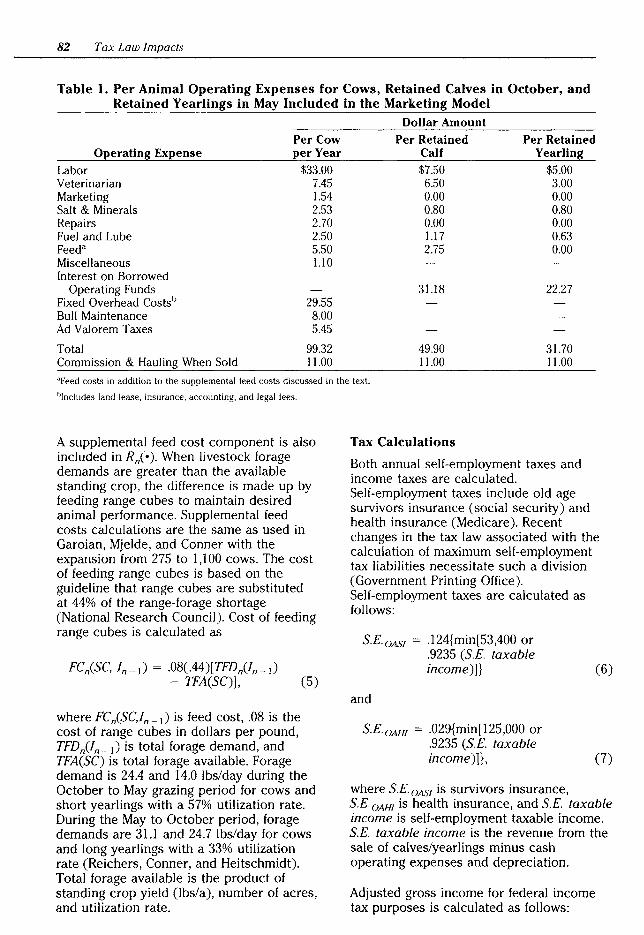
82 Tax Law Impacts
Table I. Per Animal Operating Expenses for Cows, Retained Calves in October, and Retained Yearlings in May Included in the Marketing Model
Operating Expense Labor Veterinarian Marketing Salt & Minerals Repairs Fuel and Lube Feed a
Miscellaneous Interest on Borrowed
Operating Funds Fixed Overhead Costs~> Bull Maintenance Ad Valorem Taxes
Total Commission & Hauling When Sold
Per Cow per Year
$33.00 7.45 1.54 2.53 2.70 2.50 5.50 1.10
29.55 8.00 5.45
99.32 11.00
Dollar Amount Per Retained
Calf $7.50 6.50 0.00 0.80 0.00 1.17 2.75
31.18
49.90 11.00
Per Retained Yearling
$5.00 3.00 0.00 0.80 0.00 0.63 0.00
22.27
31.70 11.00
"Feed costs in addition to the supplemental feed costs discussed in the text.
bJncludes land lease, insurance, accounting, and legal fees.
A supplemental feed cost component is also included in R,(•). When livestock forage demands are greater than the available standing crop, the difference is made up by feeding range cubes to maintain desired animal performance. Supplemental feed costs calculations are the same as used in Garoian, Mjelde, and Conner with the expansion from 275 to I ,100 cows. The cost of feeding range cubes is based on the guideline that range cubes are substituted at 44% of the range-forage shortage (National Research Council). Cost of feeding range cubes is calculated a<>
FCnCSC, /,_ 1) = .08(.44)[TFDnCI,_ 1)
- TFA(SC)], (5)
where FC,(SC,I, _1) is feed cost, .08 is the cost of range cubes in dollars per pound, TFDnCI, _ 1) is total forage demand, and TFA(SC) is total forage available. Forage demand is 24.4 and 14.0 lbs/day during the October to May grazing period for cows and short yearlings with a 57% utilization rate. During the May to October period, forage demands are 31.1 and 24.7 lbs/day for cows and long yearlings with a 33% utilization rate (Reichers, Conner, and Heitschmidt). Total forage available is the product of standing crop yield (lbs/a), number of acres, and utilization rate.
Tax Calculations
Both annual self-employment taxes and income taxes are calculated. Self-employment taxes include old age survivors insurance (social security) and health insurance (Medicare). Recent changes in the tax law associated with the calculation of maximum self-employment tax liabilities necessitate such a division (Government Printing Office). Self-employment taxes are calculated as follows:
S.E.oA'ii = .124{min[53,400 or .9235 (S.E. taxable income)]}
and
S.E.oAHI = .029{min[l25,000 or .9235 (S.E. taxable
(6)
income)]}, (7)
where S.E. OAS"I is survivors insurance, S.E.oAHI is health insurance, and S.E. taxable income is self-employment taxable income. S.E. taxable income is the revenue from the sale of calves/yearlings minus cash operating expenses and depreciation.
Adjusted gross income for federal income tax purposes is calculated as follows:
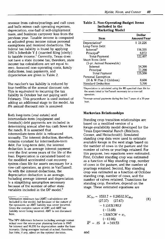
revenue from calves/yearlings and cull cows and bulls minus cash operating expenses, depreciation, one-half of self-employment taxes, and business carryover loss from the previous year. Taxable income is computed as adjusted gross income minus personal exemptions and itemized deductions. The federal tax liability is found by applying 1991's Schedule Y-1 (married filing jointly) to taxable income.1 Currently, Texas does not have a state income tax; therefore, state income tax calculations are set equal to zero. Assumed non-operating costs, family deductions, loan payments, and depreciation are given in Table 2.
The rancher's tax liability is reduced by four-twelfths of the annual discount rate. This is equivalent to incurring the tax liability in October but not paying until February. This procedure is used instead of adding an additional stage to the model. An 8% annual discount rate is assumed.
Both long-term (real estate) and intermediate-term (equipment and livestock) debt payments are included in determining annual after-tax cash flows for the ranch. It is assumed that intermediate-term debt is refinanced annually. The interest deduction, therefore, remains constant for intermediate-term debt. For long-term debt, the interest deduction is an average interest payment over the first seven years of the life of the loan. Depreciation is calculated based on the modified accelerated cost recovery system class life for assets necessary for a cow-calf operation, as given in VanTassell. As with the interest deductions, the depreciation deduction is an average. Including average interest and depreciation is a simplifying assumption necessary because of the number of other state variables included in the DP model.2
1Alternative minimum tax (AMT) calculations are included in the model, but because of the nature of the operation, an AMT liability was never incurred. Given the complex nature of AMT and AMT tax liability never being incurred, AMT is not discussed here.
2The NPV difference between including average versus actual over the seven-year planning horizon is $945 for interest and $1,030 for depreciation under the base scenario. Using averages instead of actual, therefore, has little, if any, effect on the optimal decision.
Mjelde, Nixon, and Conner 83
Table 2. Non-Operating-Budget Items Included in the Marketing Model
Item Depreciation a
Long-Term Debt Interestb Principalb
Total Payment Short-Term Debt
(5-yr. Annual Renewable) Interest Principal
Total Payment Personal Exemption
(H & W Plus 2 Children) Standard Deduction
Dollar Amount/Year
$ 21,226
116,335 6,072
122,407
54,300 71,200
125,500
8,600 5,700
"Depreciation is calculated using the IRS-specified class lile for the assets listed in VanTassell necessary for a cow-calf operation.
bAverage annual payments during the first 7 years of a 30-year loan.
Markovian Relationships
Standing crop transition relationships are based on a modified version of a forage-availability model developed for the Texas Experimental Ranch (Reichers, Conner, and Heitschmidt). Simulated standing crop data were used to estimate available forage in the next stage based on the number of cows in the pasture and the number of calves or yearlings retained. For this purpose, two equations were estimated. First, October standing crop was estimated as a function of May standing crop, number of cows in the pasture, and the number of yearlings retained. Second, May standing crop was estimated as a function of October standing crop, number of cows, and the number of calves retained. Transitions for standing crop, therefore, depend on the stage. These estimated equations are
SCoct = 1553.7 + 0.28532 SCMay (27.37) (27.67)
- l.l513LYRLS ( -13.68)
- l.9267CW + e1, ( -12.06)
R2 = .45 & = 349.53
and
(8)

84 Tax Law Impacts
SCMay = 845.65 + 0.68762 SCocr (49.30) (28.26) - 0.80I38SYRLS
(-6.04) - I.3718 CW + ez,
( -5.46) R2 = .39 & = 538.50
(9)
where LYRIS is the number of long yearlings, SYRLS is the number of short yearlings, CW is the cow-herd size, and t-ratios are in parentheses. Although t-ratios are meaningless when using simulated data, the estimated equations appear to show a strong Markovian relationship. Equations (8) and (9) were estimated for a 3,000-acre pasture and cow-herd sizes between 250 and 325. To use equations (8) and (9), it is assumed that the I2,000 acres standing crop transitions with I ,I 00 cows follow the same transitions as 3,000 acres with 275 cows. Stochastic transitions were developed by fitting separate cumulative distribution functions to the error terms for each estimated equation. This approach, which utilizes a hyperbolic tangent function, allows conditional probabilities to be generated (Taylor I984, I986).
Maximum-likelihood estimates for standardized errors associated with equations (8) and (9) are
F(e1) = .5 + .5 Tanh (0.040836 (2.27)
and
+ 0.80I909 eJ) (53.46)
F(e2) = .5 + .5 Tanh(0.096422 (5.36)
+ 0.864450 e2),
(54.03)
(10)
(II)
with t-ratios in parentheses. Inclusion of polynomial terms on the error terms was determined by maximizing the Schwarz criteria (Judge et al.). Equations (10) and (11) represent the stochastic nature of standing crop transitions within the model.
Price transitions were developed directly using hyperbolic tangent functions. Recall
that the price state variable represents calf prices in October and short yearling prices in May. Short yearling prices in May were used to predict October calf prices, and October calf prices were used to predict May short yearling prices. Two separate conditional cumulative distributions were estimated. Maximum-likelihood estimates of the cumulative price distributions using Amarillo auction data for the years I978-90 are
F(PsyiPc) = .5 + .5 Tanh ( -4.8866 ( -3.45)
+ 7.73I8Psy - 2.98II ~) (4.10) (-2.62)
and
F(PciPsy) = .5 + .5 Tanh ( -7.1520 (-4.03)
+ I3.5438Pc- 6.2749 P:y), (4.45) ( -3.87)
(12)
(13)
where F(•) is the cumulative distribution, Psy the price of short yearlings in May, Pc the price of calves in October, and t-ratios are in parentheses. The price-transition equations indicate that a strong Markovian relationship exists. Finally, the stochastic state variables are assumed to be independent.
The inventory relationship includes a reduced percentage of calves available for sale because of replacement assumptions. The inventory transition is given by
1,_ 1 = .70(l,IOO) -D if n - I represents May, and
= 1,- D if n - I represents October, (14)
where I,100 is the number of brood cows, .70 is the calving rate minus replacements, 1, is the inventory state variable, and Dis the decision, that is the number, to sell.
The May net returns state variable is used to carry any income or expenses incurred in May to October. This is necessary for tax calculations, as taxes are paid on total yearly income. For the transition from October to May, this state variable does not exist; therefore, its transition is degenerate

for this stage. In each October, yearly net returns, self-employment taxes, federal income taxes, and after-tax cash flows are determined. If the cow-calf operation experiences a loss, this loss is transferred to the next year by the business loss carryover state variable. Such losses are deductible on next year's taxes. The business loss carryover state variable is not affected by any actions in May. The result is this state variable, after being calculated in October, remains the same until next October. The two state variables, M and L, are necessary because of differences in calculation of income and self-employment taxes. May net returns are necessary to calculate both self-employment taxes and federal income taxes. Carryover business loss is only deductible for federal income tax purposes.
A multitude of values for May net returns and business losses are possible. As noted earlier, these values are discretized into eight intervals. The problem of a calculated value not matching up with the state space occurs whenever a continuous variable is discretized and is not limited to this model. Bias introduced by discretizing is reduced by using linear interpolation.
Results Concise reporting of results associated with large dynamic models is difficult. Reporting only convergent decision rules, however, reduces the difficulty of the presentation. For this model, optimal convergent decision rules have the property that the optimal decisions in May for year t are the same as the optimal decisions for May in year t + 1 , and similarly for October's decisions. Even with reporting only convergent decision rules, concise reporting of the calf-yearling marketing strategy is not possible. In October, for example, there are 11,520 possible states, with an optimal convergent decision associated with each state. Generalities associated with the optimal marketing strategy, therefore, are presented, along with a limited number of actual model decisions.
Base Scenario
Under the base scenario, the rancher is assumed to have recently refinanced the
Mjelde, Nixon, and Conner 85
rangeland. Interest and principal for this scenario are presented in Table 2. Assuming the rancher follows the optimal decision rules, cash flows associated with the cow-calf-yearling ranch operation range from -$355,426 to $514,602 over a seven-year time horizon, depending on initial conditions. The range of these figures illustrates the importance of initial conditions within the model.
The optimal marketing strategy in May is, generally, to sell all short yearlings the rancher has available. Retaining short yearlings to sell as long yearlings occurs only in the highest three standing crop states and prices of $68.00 and $74.80/cwt (approximately 1% of the state space). In all states in which short yearlings are retained, only 154 head are retained. Given the simplicity of the May decision rule, the discussion will concentrate on the October convergent decisions.
Each of the five state variables affects the optimal marketing decisions in October. The decision rules suggest that under a wide range of conditions, it may be profitable to retain calves in the fall and sell them as yearlings. Further, the results suggest it is not a matter of selling all calves or retaining all calves, rather it is a matter of degree of retained ownership. Finally, the decisions reflect that a high degree of interaction occurs between the state variables in determining the number of calves to retain.
For a given level of the remaining state variables, generalities associated with the October marketing strategies can be summarized as follows. As the four state variables-standing crop, long yearlings available for sale, fall calf price, and income carried over from May-increase, more calves are retained in October. Net operating loss carried over from the previous year has the opposite effect; that is, as losses increase, fewer calves are retained in October. The convergent decisions presented in Table 3 are representative of these generalities but also illustrate that if more than one state variable changes, an interactive effect is present in determining the optimal decision. The decisions represented in Table 3 are for both 0 and 154 long yearlings being present

86 Tax Law Impacts
Table 3. Number of Calves Sold in October for the No-Equity-in-Owned-Land Case
Calf Net Operating Loss (Dollars) Price
($/cwt) 0.00 2I,428 42,857 64,286 85,7I4 I07,I43 I28,57I I50,000
Number of Calves Sold Yearlings = 0.0 Standing Crop = I ,66I lbs/a Income= $I03,57I
59.40 616 616 770 770 770 770 770 770 66.20 616 616 616 770 770 770 770 770 73.00 462 616 616 616 770 770 770 770 79.80 462 462 616 616 616 770 770 770 86.60 462 462 462 616 616 616 770 770
Yearlings = 0.0 Standing Crop = I ,66I lbs/a Income = $I62,857
59.40 462 462 616 616 770 770 770 770 66.20 462 462 462 616 616 770 770 770 73.00 308 462 462 462 616 616 616 770 79.80 308 462 462 462 616 616 616 616 86.60 308 308 462 462 462 616 616 616
Yearlings = 154.0 Standing Crop = I ,66I 1bs/a Income = $103,571
59.40 462 462 616 66.20 308 462 462 73.00 308 308 462 79.80 308 308 308 86.60 308 308 308
in October, which reflects the May decision rule. Further, various income, calf price, operating loss, and standing crop levels are represented in Table 3. Even in the small state space represented in Table 3, the complexity of the October decision rule is demonstrated.
The generalities present in the decision rule are intuitively pleasing. As standing crop increases, the probability of having to feed decreases, thereby decreasing the costs associated with retained ownership. The effect of tax considerations is illustrated in the general strategies associated with the income, long yearlings, and operating loss state variables. Increasing income from May and the number of long yearlings (recall the model forces the sale of all long yearlings in October) increases the rancher's taxable income for the current year. Retaining ownership allows the rancher to transfer income to the following year, thereby potentially decreasing his or her current year's tax liability. Further, the potential for increased income occurs because short yearlings weigh more than weaned calves. This increase in weight may offset the lower prices usually received for the heavier animals.
616 616 462 462 308
616 770 770 770 616 616 770 770 462 616 616 616 462 462 616 616 462 462 462 616
The effect of calf prices appears to be caused by tax considerations and the estimated price probabilities. As calf prices increase, the rancher's taxable income increases. Again, retaining ownership allows the rancher to transfer income to the coming year and potentially increase his or her next year's income. Further, the estimated price probabilities reveal that if calf prices are high in October, then there is a high probability of high short yearling prices in May. This relationship occurs because in October, historically, the supply of calves is high and demand for cattle to place on rangeland is low (winter range is at its lowest supply during the year). In the spring, the supply of cattle to place on rangeland is usually low and the demand for such cattle is higher because of the increased availability of usable rangeland.
Another indication of the importance of tax considerations can be seen in the following decision rules. Reformulating the model such that no tax considerations are included gave an October marketing strategy that indicated it is not feasible to carry over calves if the calves must be fed. In the non-tax model, the October decision rule is to sell all calves in the lowest two

standing crop states, retain I 54 calves in the I ,I87 lbs/a standing crop state, and retain all calves in the highest-three standing crop states. This decision rule is not dependent on calf price or number of long yearlings present (May income and operating loss are not part of a non-tax model). The decision rule given by the tax model indicates in some cases it is profitable to retain calves in October even if they must be fed. Retained ownership occurs in low standing crop states when May income is high and/or a large number of long yearlings are present, at higher calf prices, and at low operating losses. Increased feed costs are balanced out by a decreased tax liability and the probability of potentially higher income the next year.
Equity Considerations
To examine the effect of equity positions on owned land, two different scenarios are contrasted to the base scenario. First, a full equity position on land is assumed; that is, the owner has no land mortgage payments. The second scenario assumes the landowner owns one-half of the land free and clear and the rancher has just refinanced the other half. Under this scenario, average annual land payments total $6I ,204, of which $58,259 is interest. Differences in the convergent decision rule for the various equity positions are discussed.
In May, increasing the equity position on owned land has the effect of increasing the number of states in which short yearlings are retained. With the one-half equity position, short yearlings are retained in less than 5% of the state space, whereas with full equity, short yearlings are retained in I9% of the state space. This contrasts to the base case when short yearlings are retained in approximately I% of the states. The number of short yearlings retained also depends on the state, but ranges from 0 to 462 for the one-half equity case to 0 to 616 in the full equity case. In determining the number of short yearlings to retain, operating losses appear to have little effect and there must be enough standing crop available to support the cattle herd without supplemental feeding. No other clear pattern is apparent.
Mjelde, Nixon, and Conner 87
As expected, the equity position has an effect on the cash flows from the cow-calf-yearling operations. Cash flows for the full equity case from following the optimal marketing strategies over the seven-year time horizon range from - $I75,265 to $662,792. For the one-half equity case, cash flows range from - $275,1I6 to $573,713. As with the base scenario, initial conditions have a major effect on the cash flows realized.
The generalities associated with the base scenario October decisions also apply to both the full and one-half equity scenarios with one major exception. In the full equity scenario, the effect of price is divided into two distinct effects. With low May income and low yearling numbers, the effect of price is the same as with the base case. As May income and/or number of long yearlings increases, the effect of price is reversed; that is, as price increases, more calves are sold in the fall. In the one-half equity case, the same reversal is seen but to a lesser extent. Here, the rancher's interest deduction is considerably smaller than under the base scenario. With fewer deductions, the rancher's taxable income rises and the rancher is likely to be in the top tax bracket for the current and next year. There is little incentive for the rancher to delay income recognition under these conditions. The rancher would likely choose to recognize the income from the sale of calves because he or she is already exceeding the maximum for self-employment taxes and is in the highest income tax bracket. Additional taxable income cannot push the rancher into a higher tax bracket.
In Table 4, the marketing strategies for some of the states that correspond to those in Table 3 are presented for the full and one-half equity scenarios. These results illustrate the second major difference associated with the October marketing strategies caused by different equity positions. In general, as the rancher's equity position on owned land increases, fewer calves are sold in October for a given state. This reflects the differences in taxable deductions associated with the various equity positions. As equity decreases, the rancher pays more interest. To fully take advantage of this deduction, the rancher

88 Tax Law Impacts
Table 4. Number of Calves Sold in October for the Full and One-Half Equity Scenarios
Calf Price ($/cwt)
Net Operating Loss (Dollars)
0.00 21,428 42,857 64,286 85,714 107,143 128,571 150,000
Yearlings = 0.0 Number of Calves Sold Standing Crop = 1,661 lbs/a Inco01e = $103,571
Full Equity 59.40 308 308 462 66.20 308 308 308 73.00 308 308 308 79.80 308 308 308 86.60 308 308 308
462 616 462 462 462 462 308 462 308 462
616 616 462 462 462
616 616 616 462 462
770 616 616 616 616
Yearlings = 0.0 Standing Crop = I ,661 lbs/a Inco01e = $103,571
One-Half Equity 59.40 462 462 616 66.20 462 462 462 73.00 462 462 462 79.80 308 462 462 86.60 308 308 462
must have enough income to equal the deductions. This is reflected in the decision rules for the various equity positions.
Adoption of Marketing Strategies
The current study and many previous studies have indicated that it may be profitable to retain ownership of weaned calves in the fall and sell them as yearlings. However, Gilliam indicates that the majority of calves are sold at weaning. The obvious question is, why haven't ranchers adopted such marketing strategies, or have they? One answer is that the results of the studies are not being disseminated to the ranchers. Additionally, some empirical evidence as to why the majority of calves are sold in the fall can be seen in the decision rules presented here.
Many cow-calf ranchers may be operating in the state space for which the optimal decision is to sell most or all of the current year's calf crop. Consider a rancher that wants to switch from selling all calves in the fall to the flexible marketing strategy developed in this study. Provided that the rancher derives most or all of the operation's income from the cow-calf operation, a rancher wanting to switch to the flexible strategy will, in the year of the switch, (I) have no long yearlings available for sale from the previous year and (2) be in one of the lower income states because no calves or yearlings will have been sold during the current tax year.
616 770 616 616 462 616 462 616 462 462
770 770 616 616 616
770 770 770 616 616
770 770 770 616 616
For the base scenario, examining the decision rules for the lowest-two income states and having no yearlings available for sale indicates that in 90% of the state space all of the calves are sold, whereas for the remaining I 0% of the states, 80% of the calf crop is sold. If the lowest-three income states are considered, between 60% and 100% of the calf crop should be sold. To take advantage of tax deductions, the rancher should sell the majority of the calf crop. This occurs even though business losses can be carried over to the next year. Further, personal exemptions and itemized deductions cannot be carried over, so they are either used or lost. An additional consideration is living expenses, which are not included in the current model. The inclusion of a minimum living expense would further bias the model towards selling calves in October.
For the one-half equity case, 60% to 100% of the weaned calves are sold in the lowesttwo income states if no yearlings are present (80% to 100% are sold in the lowest income state). In 72% of the state space all of the calves are sold, whereas in 23% of the states, 80% of the calves are sold, and in 5% of the states, 60% are sold. In the full equity case, between 40% to 100% of the calves are sold in the lowest-two income states. The percentage of states selling 40%, 60%, 80%, and 100% of the calves are 4%, 18%, 32%, and 46%, respectively. These results parallel the amount of tax deductions available. The results suggest

that a rancher wanting to switch to the flexible strategy or a rancher that has switched will still sell the majority of his or her calf crop in the fall.
Conclusions
A dynamic programming model of marketing calves and yearlings from a rangeland cow-calf-yearling operation was developed. Tax and equity considerations are included as a part of the decision environment. These factors have not been previously included in models examining marketing strategies associated with weaned calves. The results suggest the need to consider factors previously considered, such as price, standing crop, and number of yearlings available, as well as financial considerations such as net operating loss carryover and current-year taxable income, when considering retained ownership of weaned calves and short yearlings. A reformulation of the model without tax considerations showed a considerably different marketing strategy.
Results from the model may also help explain why the majority of spring-barn calves are sold in the fall. Depending on the state of the system, between 60% and I 00% of the weaned calves are sold in October if the rancher has no yearlings to sell and is in the lowest income state. This holds true for all three equity positions examined, even though minimum living expenses are excluded from the model. Taking advantage of tax deductions in the year they occur explains this finding.
As with all models, the results are limited to the situation analyzed, assumptions are made, and the results are subject to data limitations. Nonetheless, the generalizations are applicable to a wide range of situations in which winter range is available. Finally, price equations and transition probabilities, along with standing crop relationships for different areas, are required before specific results can be applied to alternative ranching operations.
References
Garoian, L., J.W. Mjelde, and J.R. Conner. "Optimal Strategies for Marketing Calves
Mjelde, Nixon, and Conner 89
and Yearlings from Rangeland." Amer. J. Agr. Econ. 72(1990 ):604-13.
Gebremeskel, T., and C.R. Shumway. "Farm Planning and Calf Marketing Strategies for Risk Management: An Application of Linear Programming and Statistical Decision Theory." Amer. J. Agr. Econ. 61(1979):363-70.
Gilliam, H.C. "The U.S. Beef Cow-Calf Industry." Agri. Econ. Rep. no. 51. U.S. Department of Agriculture, Economic Research Service, 1984.
Government Printing Office. "The Revenue Reconciliation Act of 1990." Washington, DC, 5 November 1990.
Judge, G.G., W.E. Griffiths, R.C. Hill, and T.C. Lee. The Theory and Practice of Econometrics. New York: John Wiley and Sons, 1980.
Lambert, D.K. "Calf Retention and Production Decisions over Time." West. J. Agr. Econ. 14(1989):9-19.
National Research Council. Nutrient Requirements for Beef Cattle. Washington, DC: National Academy of Sciences, 1984.
Reichers, R.K. "An Economic Analysis of Alternative Stocking Rate Adjustment for Short Duration Grazing Systems in the Texas Rolling Plains." Master's thesis, Texas A&M University, College Station, TX, 1986.
Reichers, R.K., J.R. Conner, and R.K. Heitschmidt. "Economic Consequences of Alternative Stocking Rate Adjustment Tactics: A Simulation Approach." J. Range Mgmt. 42(1989):165-71.
Schroeder, T.C., and A.M. Featherstone. "Dynamic Marketing and Retention Decisions for Cow-Calf Producers." Amer. J. Agr. Econ. 72(1990):1028-40.
Stokes, K.W., D.E. Farris, and T.C. Cartwright. "Economics of Alternative Beef Cattle Genotype and Management/Marketing Systems." Southern J. Agr. Econ. 13(1981):1-10.

90 Tax Law Impacts
Taylor, C.R. "A Flexible Method for Empirically Estimating Probability Density Functions." West. J. Agr. Econ. 9( 1984 ):66-76.
____ . "Risk Aversion versus Expected Profit Maximization with a Progressive Income Tax." Amer. J. Agr. Econ. 68(1986):137-43.
Texas Department of Agriculture. Texas Livestock Market News. Austin, TX, Selected weekly issues, 1978--90.
VanTassell, L.W. "Risk Management by Livestock Producers: A Ranch Simulation in Texas Rolling Plains." Ph.D. diss., Texas A&M University, May 1987.

A Note on Household Consumption Stress on New Zealand Sheep and Beef Farms Warren E. Johnston and Gerald A. G. Frengley
We previously, in this journal, examined financial performance of sheep and beef farms and the extenuated adjustment process following the 1984 deregulation of the New Zealand economy (Johnston and Frengley). Programs introduced during the 1970s and early 1980s promoted high levels of financial leverage in New Zealand's agricultural sector. Problems quickly befell the sector when government removed assistance to agriculture in the post-1984 period, leaving significant financial stress and debt burdens.
The analysis of financial stress used aggregate survey data for the New Zealand Meat and Wool Boards' Economic Service (NZMWBES) representative weighted-average "all-classes" sheep and beef farm over the two-decade period of the 1970s and 1980s (NZMWBES, various issues). The empirical evidence dealt primarily with declining net incomes and asset values, increased indebtedness, reduced equities, and negative cash surpluses for the NZMWBES all-classes farms. Financial ratios facilitated the analysis of those changes as they affected the financial performance of those firms over time.
At the time, we could not respond to reviewer inquiry about the degree of cross-sectional variability in the survey
Warren E. Johnston is a professor of agricultural economics, University of California, Davis, and a member of the Giannini Foundation of Agricultural Economics. Gerald A.G. Frengley is a reader in farm management, Lincoln University, New Zealand. The paper is based on joint research supported by the University of California's Pacific Rim Faculty Exchange Program, by the New Zealand Wool Board, and by cooperative agreement with the U.S. Department of Agriculture. Giannini Foundation Paper no. 1003.
statistics. Such variability, it was suggested, might reveal differential or distributional information about the impacts of deregulation among farm firms. Those aspects of adjustment outcomes were masked by the aggregate survey statistics then available for analysis of change for the all-classes representative sheep and beef farm.
This note responds more directly to reviewer concern about distributional aspects and provides additional insight into the incidence of stress on farm firms following the almost complete deregulation of the agricultural sector since 1984. We have since gained access to flow-of-funds information associated with equity groupings of all-classes farms for the 1988 production year (NZMWBES 1990 ). Specifically, we now have data on household drawings for consumption, and on savings and dissavings by equity classes. This information permits additional insight into the relative severity of financial stress among farms for the 1988 production year, with a particular emphasis on distributional consequences for farm households. Where previously we discussed financial stress in relation to the farm firm, we now wish to consider the additional concept of consumption stress as it may apply to the farm household.
1988 Production Year Outcomes, by Owner-Equity Classes
Table I contains information for the NZMWBES weighted-average all-classes sheep and beef farm, with distributional

92 Household Consumption Stress
Table I. Selected Farm and Household Financial Measures, New Zealand Sheep and Beef Farms, Production Year Ending June 1988
By Equity Ratio All Less Greater
Farms than 50% 50% to 65% 65% to 80% 80% to 95% than 95% Percent of Farms 100 20 19 21 27 13 Average Equity
Ratio(%) 71 25 58 73 88 98 Interest Expense($) 23,862 42,955 39,467 23,502 10,428 1,050 Interest/Gross Farm
Income(%) 19 38 27 18 8 1 Cash Surplus ($) -13,463 -35,121 -22,419 -18,585 3,904 4,490 Gross Drawings ($) 23,117 16,561 26,473 23,307 24,531 24,938 Savings($) -3,858 -11,980 -8,475 -6,427 4,158 2,654 Net Drawings($) 19,259 4,581 17,998 16,880 28,689 27,592
Source: New Zealand Meat and Wool Boards' Economic Service, 1990.
information for five equity classes. 1 In the 1988 production year, the average ratio of owner equities over all farms was 71% and interest expense amounted to $23,862 per farm (19% of gross farm income), on the average. In that year, the average gross farm income of all farms was $126,178, and the estimated net farm income was $28,487 per farm (Johnston and Frengley, Table 2).
There was wide variation in production-year outcomes among equity classes. While average owner equity was 71% in 1988, one-fifth (20%) of all farms had owner equities of less than 50% and about one-eighth (13%) were nearly debt-free, with equity ratios greater than 95%.
Financial Stress
Financial stress is related to the difficulty of the firm in servicing its debt. Interest payments are determined by debt levels, which are reflected in equity ratios, and prevailing interest rates, whether they be fixed or variable. Hence, one measure commonly used to reflect financial stress is the ratio of annual interest expense to gross farm income. That ratio (annual interest expense -:- gross farm income) ranged from 5.9% to 10.9% during the 1970s but rose significantly following deregulation to 20.2% for the 1986 production year (Johnston and Frengley, Table 3). The resultant high ratio
1The five equity classes are those with owner equities of less than 50%, 50% to 65%, 65% to 80%, 80% to 95%, and more than 95%. Equity ratios are the ratio of net worth to total farm assets, or equivalently [I -(debt/total farm assets)].
signified the heavily leveraged condition of many sheep and beef farms following deregulation and the continuing overburden of massive debts in the sector.
By 1988 the ratio had decreased only slightly to 19%. The amount of interest expense and its proportion of gross farm income appear to increase inversely to reported equities over all of the equity classes. For example, the lowest equity-ratio class (<50%) averaged only 25% equity across the class and interest expense amounted to an average of $42,955 per farm,2 or 38% of gross farm income. In contrast, the interest expense of the highest equity group (>95%) amounted to only $1,050 per farm, or 1% of gross farm income.
Household Consumption Stress
A concept similar to financial stress for the firm relates to the difficulty that the household faces in meeting its consumption needs. Household consumption stress occurs if current consumption opportunities are constrained below the household's previous consumption expectations. Just as there is a continuous need for funds to service the firm's debt, there is also the need for funds to support both the present and long-run desired levels of household consumption.
2This average is nearly twice the all-farms average.

A consequence of the heavily indebted farm firm is that the impact of changes in debt on household consumption expenditures and savings or investment is reciprocal, though the proportions may change as net farm income changes. Total interest payments, fixed by the level of debt and the interest rate, reduce household consumption opportunities. If the residual is less than consumption expectations and if capital-adjustment alternatives exist for the farm household, then the household will consider dissavings or disinvestments3 to augment expected shortfalls in consumption. Thus, the shortfall may be met by capital adjustments that, in turn, alleviate the level of consumption stress associated with reliance solely on residual . 4 f mcome or household expenditure demands in that time period. Consumption str~ss may be severe if there are no savings or mvestments from which the household may recall capital in times of net income shortfalls. The residual income, below household consumption expectations, may be insufficient to meet household needs.5
Household Incomes and Savings
While New Zealand sheep and beef farms have participated in the NZMWBES farm surv~.y for a long period, the survey has traditiOnally focused on annual production and income statistics, ignoring economic activity of the household not directly associated with production activities. The reporting of flow of funds has been a more recent addition to the statistical survey. Table I contains financial accounts that pertain to household consumption levels for I988.
The survey reports "cash surplus" in annual accounts, but it is not an accurate indicator of the firm's actual cash condition because the definition includes net income, plus depreciation, less drawings and tax and
31n farm or nonfarm assets.
4Residual income is that income after payment of all fixed and variable costs of the farm and including off-farm incomes, if any.
5The household may have as its only alternative the sale of its remaining equity, if any, in the farm, and the readjustment process may involve changes in employment and perhaps the exodus of the farm family from the farming community.
Johnston and Frengley 93
principal payments. The inclusion of non-cash depreciation clouds the severity of recent financial conditions, for even with the inclusion of non-cash depreciation, the cash surplus of the all-classes sheep and beef farm averaged a negative $I3,463 in I988.6
"Gross drawings" are more germane to the discussion of household consumption outcomes. As defined in the NZMWBES survey, gross drawings are funds used for ?ousehold expenses, including life msurance payments, school fees, and other personal expenditures. They reflect the level of household expenditure chosen to meet household needs, given the availability of savings and investments. The average of gross drawings over all farms was $23 II 7 in 1988. Gross drawings for farms with less than 50% equities were only $16,561 per farm, significantly below levels observed for all other owner-equity classes of farms. For farms with owner-equities of 50% or more gross drawings averaged within the rather' narrow range of $23,000 to $26,000 per farm. Farms in the very lowest equity-ratio class may have been severely constrained in their household consumption expenditures. All other farms had averages which at most varied by about $3,000 per farm.7
yve i~troduce the idea of net drawings to 1llummate the differential savings behavior of households among farm equity classes. Net drawings differ from gross drawings by acknowledging saving decisions of hous~holds. Net drawings equal either gross drawmgs plus positive savings or gross drawings less dissavings. The average of net drawings for all sheep and beef farms in 1988 was $19,259 per farm, ranging from a low of only $4,581 for farms with less than 50% equity and increasing upwards with equity-class increases to around $28 000 for farms with owner equities of 80% or'more. The differences between gross and net drawings among equity classes are
,;Cash-surplus estimates among owner-equity classes ranged from positive cash surpluses of about $4,000 per farm in the two highest equity classes downwards to a negative $35,121 cash surplus for the lowest (<50%) owner-equity class. Cash surpluses less ~on-cash-depreciation allowances would have resulted m even more negative cash positions for these farm firms.
7There are, of course, variations within equity classes.

94 Household Consumption Stress
"dissavings," ranging from $11 ,980 to $6,427 per farm for the three lowest equity classes (<50%, 50%-65%, and 65%--80%), and net positive savings for the two higher equity classes.
Concluding Comment On the basis of the distributional information presented in this note, it is clear that the most heavily indebted sheep and beef farms are, indeed, the most severely stressed financially because of the large share of gross farm incomes that must be allocated to payment of interest expense. One in five of all sheep and beef farms in New Zealand fall into this heavily indebted category. The severity of household consumption stress on those same farms is evidenced by significantly lower levels of household consumption expenditures (only $16,561), despite the highest level of dissavings among all farm owner-equity classes.
These farms, on which dissavings amounted to $11,980 per farm, on the average, also had gross drawings of $7,000 to $10,000 less than that of any other equity group. Dissavings of such a relatively large magnitude, amounting to 72% of gross drawings, were necessary because of the clear deficiency of available current income to meet household consumption expenditure demands. The relatively low gross drawings on those same farms reveal the likely paucity of capital-adjustment alternatives for these most severely stressed farm households.
While there is little alternative to stripping assets, the limited available assets constrain household consumption levels below those of farm households on higher owner-equity-class farms. And in the longer run, many will likely exit the sector unless households find improved gross-income prospects or are able to reduce the overwhelming cost of existing debt burdens.
In sharp contrast stand farm units characterized by owner equities of 80% or more with single-digit ratios of annual interest outlays to gross farm incomes. Household consumption expectations were fulfilled and positive savings made. About 40% of farms fell into this category under 1988 conditions.
The remaining 40% of farms constitute an intermediate group with respect to financial and household consumption stresses. These farms are those with 50% to 80% owner equities for which gross drawings for household consumption expenditures included dissavings in 1988. They are in an intermediate position. While dissavings may have permitted household consumption levels comparable to those for the higher equity group, capital-asset availabilities will ultimately limit dissavings over the long run unless there is an improved financial outlook for the agricultural sector.
Debt levels and interest costs both erode owner equities and constrain residual incomes available to support farm household consumption. In the longer run, they are unsustainable for a large share of New Zealand sheep and beef farms and for the households on those farm units.
References
Johnston, Warren E., and Gerald A.G. Frengley. "Financial Stress on New Zealand Sheep and Beef Farms: Analysis of Change in Financial Performance under Deregulation." Agr. Fin. Rev. 50(1990):100-11.
New Zealand Meat and Wool Boards' Economic Service (NZMWBES). The New Zealand Sheep and Beef Farm Survey: Production and Financial Analysis. Wellington, various annual issues, 1970--88.
____ . "Distribution of Sheep and Beef Farm Equity, June 1988." Paper no. Tl18. Wellington, 1990.

Measuring the Effect of Farm Financial Structure on Cost Efficiency Gerald W Whittaker and Mitchell J. Morehart
Abstract With the objective of measuring the relationship between farm financial structure and production organization, a sample of midwestern cash grain farms was analyzed using data envelopment analysis (DEA). DEA techniques were used to establish a cost-efficiency frontier. One out of five farms was constrained from achieving the best -practice cost -efficient frontier by debt and/or asset-value constraints. The results of this study confirm that farm financial structure must be taken into account in an analysis of efficiency in agricultural production. The data envelopment analysis employed is a promising alternative to econometric estimation.
Key words: financial structure, data envelopment analysis, cost efficiency, nonparametric.
Gerald W. Whittaker is an agricultural economist and Mitchell J. Morehart is leader of the Farm Costs and Return Section, both of the Economic Research Service, U.S. Department of Agriculture.
The volatile economic environment faced by farm businesses during the 1980s has focused more attention on finance decisions of farm operators. Farmers, faced with increasing capital requirements, must choose between internal equity capital, equity from nonfarm sources, or external debt capital. When debt capital is used to support investment in land, buildings, machinery, and other durable inputs, the production organization of the farm is affected over the course of the loan (Baker).
Farmers as business managers must function in three broad decision areas: production, marketing, and finance. Production decisions involve determining what commodities to produce and how to produce them. The marketing function involves the timing and source for purchases of inputs and sales of products. Decisions regarding the acquisition of funds and the use of those funds to acquire the services of various resources characterize the financial component of farm management decisions. 1
The objectives held for any of these areas may be different, yet each is interdependent and must be consistent with the overall objective(s) of the business. Gabriel and Baker demonstrated the link between production and investment decisions within the context of risk exposure. They argued that "the finance activity of the farm firm is a critical and pervasive one which should not be ignored in attempts to model the decision-making process at the farm level."
The purpose of this paper is to empirically
'Of course, decisions regarding the use of debt capital are not independent of lender preferences.

96 Measuring the Effect of Farm Financial Structure on Cost Efficiency
measure the relationship between a farm's financial structure and its production organization. Fare, Grosskopf, and Lee's variation of data envelopment analysis (DEA) introduced by Charnes, Cooper, and Rhodes is applied to establish a "best practice" frontier, and financial constraints are imposed to investigate the impact of financial structure on a farm's use of inputs, commodities produced, and, ultimately, overall profitability. Financial structure is represented by traditional measures such as assets or debt and is explicitly incorporated into the model specification.
Related Studies Lee and Chambers examined the impacts of incorporating expenditure constraints on farm production decisions. The constraints were related to the amount of preexisting wealth, retained earnings, and new borrowings contingent on the availability of funding for short-term operating loans. A profit maximization model was empirically measured to test the validity of an expenditure constraint. Observed expenditures on variable inputs were used to represent the expenditure constraint. Expenditure-constrained profit maximization was found to be an acceptable representation based on U.S. agriculture from 1947 to 1980.
In an extension of the work of Lee and Chambers, Fare, Grosskopf, and Lee used a nonparametric approach to examine the impact of expenditure constraints. Financial efficiency was defined as the profit or loss revealed through a comparison of the solutions obtained using the unconstrained and expenditure-constrained profit function. Financial efficiency represented one component of overall efficiency. The other component, termed actual efficiency, was measured as the ratio of actual profit to expenditure-constrained profit. Within their empirical application, the maximum allowable expenditure was calculated as observed expenditure on variable inputs. The results for a sample of California rice farms indicated that about 20% of the farms were financially inefficient. Yet on average, financially constrained farms performed better than financially unconstrained farms. The apparent inconsistency of these results may be related to the way in which a farm's
financial structure was represented in the model. Even though the model was specified to measure short-run profits, the amount of expenditures for variable inputs may not have provided a comprehensive picture of a farm's financial structure.
Medhian, Herr, Eberle, and Grabowski analyzed the overall efficiency of a sample of farms obtaining credit from the Farmers Home Administration (FmHA) compared to nonparticipants. A production frontier was constructed representing cash grain farms for two different time periods, 1981 and 1984. Statistical tests applied to the results from a pooled data series indicated that there were no significant differences in the level of efficiency between FmHA borrowers relative to nonborrowers. Correlation coefficients were constructed to examine the relationship between farm characteristics and the index of overall efficiency. No correlation was found between a farmer's debt/asset ratio and the efficiency index, as the average debt/asset ratio was higher for the lowest- and highest -efficiency groups.
Weersink, Turvey, and Godah calculated technical-efficiency measures for Ontario dairy farms using a nonparametric production function approach. Subsequent to fitting the production function, they regressed 23 variables on the technical-efficiency measure. The debt/asset ratio and building value per cow were found to be significant explanatory variables, but financial structure was not incorporated into the model.
White and Lyu provided a profit function specification where a capital constraint was imposed to recognize the need for capital in supporting the production function. This profit function was incorporated into a value maximization model to assess the sources of variation in the equity/debt ratio for U.S. agriculture. The suggestion of a capital constraint (White and Lyu) is the basis for the use of debt and asset constraints in this study. The model specified here is related to that of Fare, Grosskopf, and Lee, but employs a cost-efficiency concept.
Definition of Cost Efficiency The maximum amount of output that can be attained from a given set of resources with

fixed technology is theoretically represented by a production function. One approach used to empirically evaluate farmers' production decisions has been production-efficiency studies.
Farrell pioneered techniques for measuring efficiency based on the knowledge of the frontier unit isoquant. He described overall efficiency as consisting of two components, allocative and technical efficiency. The deviation of input allocation levels from the frontier unit isoquant was identified as technical inefficiency and deviations from cost-minimizing inputs were termed allocative inefficiency.
Since the contribution of Farrell, a variety of methods have been introduced to empirically measure efficiency (Aigner and Chu; Aigner, Lovell, and Schmidt; Greene; Meeusen and van den Broeck). Each method measures inefficiency relative to some best-practice frontier. The principal differences among methods used involve the determination of the frontier and the assessment of deviations from the frontier. These alternative approaches can be categorized based on the nature of the model specified: deterministic nonparametric, deterministic parametric, deterministic statistical, and stochastic.
While various definitions of cost efficiency have been applied, it is generally understood to refer to the cost of production, with a cost-efficient farm producing the most output for the lowest cost. Various interpretations of cost efficiency include cash cost per gross income (Miller, Rodewald, and McElroy), unit isoquant frontier (Grisley and Mascarenhas ), total costs divided by total revenue (Jensen), and costs per unit of output divided by an index of input prices (Cooke and Sundquist). In an analysis of banking efficiency, Ferrier and Lovell define cost efficiency as the provision of services at the lowest cost. A nonstochastic nonparametric measure of cost efficiency is applied in this study.
The measure of cost efficiency defined and applied here is explicitly based on expenditure data and does not require assumption of equal unit input prices or homogeneity of technology, as do many
Whittaker and Morehart 97
other microeconomic studies of efficiency (e.g., Byrnes, Fare, Grosskopf, and Kraft). Since the measure is nonparametric, there is no requirement for the specification of a functional form and its attendant disadvantages.
Finally, the nonparametric measures allow analysis that takes account of complex survey designs (also referred to as design-based surveys in the statistical literature). This is an important consideration because a key assumption for the application of most econometric methods used in the application of production function of dual approaches is that the data analyzed come from a simple random survey. A simple random survey requires that the sample be drawn randomly with replacement from a very large population with equal probabilities of selection. Design-based surveys commonly employ stratification, clustering of observations, and unequal probabilities of selection. If the survey sample design is not taken into account in the analysis of the survey data, all tests of significance of estimators will be biased (Cochran; Fuller; Kott). In the present state of statistical research, this requirement eliminates maximum-likelihood estimation, among other techniques.
In this study, cost efficiency is defined as the maximum profit achieved with minimum expenditure, by analogy to Farrell's definition of technical efficiency. A formal definition of cost efficiency follows.
Data Envelopment Measure of Cost Efficiency
Suppose there are k = 1, ... , K farms, each of which uses M inputs and produces N outputs. The prices r = (r1, ..• , rn) ERn+ and quantities u = (u 1, ••• , un) E Rn + of the outputs are observed. Total expenditure on each input x = (x1, ••. , xm) E Rm + is observed, but factor prices and quantities are unknown. M denotes a k x m matrix of observed input expenditures and N denotes a k x n matrix of observed outputs.
The objective is defined as profit maximization. The solution to the programming problem is the maximum
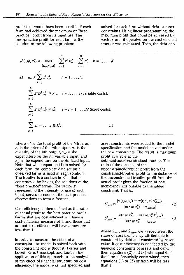
98 Measuring the Effect of Farm Financial Structure on Cost Efficiency
profit that would have been possible if each farm had achieved the maximum or "best practice" profit from its input use. The best-practice profit for each farm is the solution to the following problem:
1rk(r,w, /,) = max (Un,Xv,Z)
K
s.t. Un :s ,2: zku~, k=J
K
n=J m=J
n =I, ... ,N;
solved for each farm without debt or asset constraints. Using linear programming, the maximum profit that could be achieved by each farm if it operated on the cost-efficient frontier was calculated. Then, the debt and
k=I, ... ,K
,2: :z!w7 ~i :s Xu;, i = 1, ... , I (variable costs); k=l
K
,2: zkw~ x'fi :s x~, i =I+ I, ... ,M (fixed costs); k=J
K
,2: zk = 1, z E ~; k=l
where 1rk is the total profit of the kth farm, rn is the price of the nth output, un is the quantity of the nth output, Xu; is the expenditure on the ith variable input, and Xr; is the expenditure on the ith fixed input. Note that while equation ( 1) is solved for each farm, the complete data set on all observed farms is used in each solution. The frontier is a surface in ~ + that is constructed by linking the solutions of the "best practice" farms. The vector z, representing the intensity of use of each input, serves to connect the best-practice observations to form a frontier.
Cost efficiency is then defined as the ratio of actual profit to the best-practice profit. Farms that are cost-efficient will have a cost-efficiency measure of 1, and those that are not cost-efficient will have a measure less than 1.
In order to measure the effect of a constraint, the model is solved both with the constraint and without it (Ferrier and Lovell; Fare, Grosskopf, and Lee). In the application of this approach to the analysis of the effect of financial structure on cost efficiency, the model was first specified and
(1)
asset constraints were added to the model specification and the model solved under the new constraints. The result is maximum profit available at the debt-and-asset-constrained frontier. The ratio of the distance of the unconstrained-frontier profit from the constrained-frontier profit to the distance of the unconstrained-frontier profit from the actual profit gives the fraction of cost inefficiency attributable to the added constraint. That is,
k l1r(r,w,x~)- 7r(r,w,x~,~ebr)l sdebr = I k , C2)
7T(r, W, Xj) - 7T actuatl
k l1r(r,w,x~)- 7r(r,w,x~,_x!sser)l Sasset = I k) I ' (3)
'IT( r, W, Xr - 'IT actual
where Sdebr and Sasset are, respectively, the share of cost inefficiency attributable to constraint by debt and constraint by asset value. If cost efficiency is unaffected by the financial constraints of assets and debt, then equations (2) and (3) will equal 0. If the farm is financially constrained, then equations (1) or (2) or both will be less than 1.

The definition of inputs as expenditures is key to the interpretation of this measure. Fare, Grosskopf, and Lee assume that each farm faces identical input prices and uses identical technologies. On that basis, they show that the use of input expenditures is equivalent to using input quantities. These assumptions also allow the decomposition of the solution into overall technical and allocative efficiencies (Fare, Grosskopf, and Lovell). Since input quantities are unknown and input prices are not assumed equal in this study, a decomposition of cost efficiency in this manner is not possible.
Figure 1 is an illustration of the technique and its application in this paper. The observations A, B, C, D, and E are of a single-variable-input, single-output technology. Solution of equation (1) for this model would result in the frontier ABCD. The intensity parameter z serves to link the observations to form a convex hull. The price hyperplane L'L' is established by the objective function and finds the solution to the profit maximization problem at B, the highest intersection of the price hyperplane with the frontier. To achieve cost efficiency, A must increase input expenditure to
Figure I. Profit Maximization Constrained by Fixed Debt Level
Output
~-~~--~--- ~L-
Variable Input
Whittaker and Morehart 99
achieve the maximum profit, and C and D must reduce the input quantity.
Consider now the addition of a fixed land constraint to the single-input, single-output model. If A, B, C, and D all have the same amount of land (one acre, for example), all farms could move along the frontier to obtain the maximum profit. However, if B had more than one acre while the others still had only one acre, there would be two solutions to the maximization problem. The optimum solution would still be at B. Since land is fixed, A, C, and D could not adjust land use, and the optimum given their constraints would be at B'. The point B' represents the input-output combination used by B if restricted to one acre. The farms A, B, C, and D are said to be constrained by the fixed input, land.
In the application in this study, a multiple-input, multiple-output model is fitted without the fixed constraints of debt and asset value. A second model that includes debt and assets as fixed inputs is then fitted. A third version of the model that includes assets as a fixed input and debt as a variable input is used to establish whether a farm constrained by debt has too little or too much debt.
The stochastic-frontier production function first proposed by Aigner, Lovell, and Schmidt uses econometric techniques to fit a cost frontier below the cost-output data based on the assumption of a two-component distribution of residuals. The frontier established by this method is "average" in the sense that observations may lie above and below it. The DEA technique applied here fits a nonstochastic nonparametric frontier above the expenditure-output observations. The estimation methodology of both the stochastic frontier and the best-practice frontier (DEA) requires the optimal solution of some objective function. For the estimation of a stochastic frontier, the objective function is the minimization of squared errors. Varian has pointed out that this is merely a statistical measure of goodness-of-fit, and that it may differ greatly from the results obtained using an economic criterion. On the other hand, the nonparametric approach used here applies

100 Measuring the Effect of Farm Financial Structure on Cost Efficiency
the economic criteria of profit maximization as the objective function.
Description of Data
The data consisted of a subset of 216 farms from the 1 ,200 corn-producing farms enumerated in the 1987 Corn Version of the Farm Cost and Returns Survey (FCRS ). The FCRS is a multiframed, stratified survey, where the sample is drawn from stratified list and area frames. The Corn Version was designed to gather statistically representative data on the costs of producing corn as well as on other production and expenditure data.
The subset of FCRS data analyzed here represented 107,982 cash grain farms in the Lake States-Corn Belt production region (Illinois, Indiana, Iowa, Michigan, Minnesota, Missouri, Ohio, and Wisconsin) that had less than $100 in livestock sales and had no irrigation expenses. This sample selection changes only the analytic domain and has no effect on survey design. Therefore, observations in this subset reflect the subpopulation in the same manner that all observations in the survey represent the total population (Lee, Forthofer, and Lorimor, p. 40).
Three outputs--corn, soybeans, and wheat (measured in bushels)-were included in the model. Since different farms are sampled each year, it is not possible to equate value of production with sales since there is no way to track storage, inventories, or the timing of crop sales. Two different statistics provide a measure of the accuracy of limiting outputs to corn, soybeans, and wheat. First, these outputs accounted for an average of 96% of the value of production of each sample farm. Second, 11% of the sample farms had crop sales in 1987 that had more than 5% of their value from a crop other than the selected outputs. Even if storage or sale of inventories do not account for all discrepancies in outputs, the effect on the estimation will be negligible. There is at most a small fraction of the sample farms that is not very closely modeled using corn, soybeans, and wheat as the sole outputs. Even where this assumption is violated, the solution to equation (1) for such a farm would provide the optimal input-output mix
where the only output choices are corn, soybeans, and wheat. That is, the farm would be forced (in the model) to produce corn, soybeans, and wheat, and the expenditures actually made for some other crop would be allocated for profit maximization among these three crops. The comparison of unconstrained and constrained frontiers would be calculated on the optimal production of corn, soybeans, and wheat, even if these were not the sample farm's actual crops.
The measure of inputs by cash expenditures may be affected by lack of accrual data on inputs. An operator may have purchased inputs that are retained in inventory and do enter the production process. Operators who used inventory on hand would have lower expenses and appear to be more efficient than they really were, and the opposite would be true for those who accumulated inventories in 1987. Of course, several inputs cannot be stored, so the expenses for fertilizer and chemicals, fuels and oils, and seed would be the variables most affected by this problem. In the 1987 FCRS there was no information available on actual usage of inputs, which would allow calculation of accrual expenditures. No evaluation of the magnitude of error caused by this problem could be made.
Since the definition of cost efficiency used here is based on maximizing profits obtainable from a bundle of input expenditures, the variable and fixed inputs were chosen to represent all costs of farm production. The inputs must be viewed somewhat differently than in the usual production analysis. Each input is an expense required for production and does not necessarily represent a physical input to the production process. In this way, the model is able to represent both the production process and the financial structure required to support the production process.
Land is the only input measured by quantity (acres). Without a constraint on acres planted, production in the model expands until financial constraints are reached, resulting in some very small farms optimizing at physically impossible levels of production.

The variables used in the model are listed below. Outputs:
u1 =corn u2 = soybeans u3 =wheat
Output prices: r 1 = corn price r2 = soybean price r3 = wheat price
Variable-input expenses: x 1v =seed x2v = fertilizer and chemicals x3v = labor, calculated as the sum of (a)
a charge to management, (b) charge to operator labor, (c) charge to unpaid labor, (d) contract-labor expense, and (e) hired-labor expense (excluding family and operator). The charges are imputed from hours worked and state wage rates
X4v = fuels and oils x5v = repairs and maintenance, which
equals the sum of (a) repairs and replacement parts for all motor vehicle and farm machinery expenses, (b) miscellaneous equipment, hand tools, and supplies expense, (c) land, farm, irrigation, and building maintenance and repair expense
x6v = transportation and storage x7v = rent and lease payments, including
both cash and share rent payments
x8v = machine hire and custom work x9v = interest on operating loans
X10v = utilities x 11 v = other variable expenses
Fixed inputs: xu= land, acres planted xu = depreciation x:v = real estate and property taxes x 4r = interest on real estate debt x5r = insurance premiums
Financial fixed inputs: x6r = debt x7f = asset value
Profit (objective function): 3 II 5
'ITk = L ~u~ - L ~m - L x'fi n=l m=l /=1
k =I, ... ,K,
where n is outputs, m is variable inputs, f is fixed inputs, and K is the number of farms.
Whittaker and Morehart 101
Output prices are annual state averages. Note that debt and asset values do not directly enter the objective function. Such variables are termed "environmental" variables by Ferrier and Lovell. In this model, these variables represent the need for capital in supporting the agricultural production function. When these constraints are binding, the farm operator is not able to achieve cost efficiency as a direct result of a lack of the constraining variable. Therefore, it is inferred that the financial structure of the farm operation impacted upon cost efficiency.
Results
The maximum profit each farm could have generated was calculated in the solution of the series of linear programming problems in equation (1 ). The best-practice cost-efficiency frontier generated compares farms as if they all had the best management, soil, weather, etc. Separate solutions computed for the addition of each financial constraint, debt and asset, were used to calculate the share that financial constraints contributed to cost inefficiency of each farm operation.
Of the I 07,982 farms represented by the sample, 78.6% were not constrained by either debt or assets. From this observation it is inferred that financial structure (represented by asset and debt levels) imposed no limitation on achieving cost efficiency in this group. For the farms where financial structure limited cost efficiency, 12.0% were asset-constrained, I2.1% were debt-constrained, and 2.8% were both asset- and debt-constrained (Table I).
Distributions of financially constrained cash grain farms in the sample area were estimated using PCCARP, a computer package that calculates statistics based on sample design. The distributions by constraint are shown in Table 2. Of those operations that were debt-constrained, the 25% constrained the most had their cost efficiency reduced I1% or more. The asset-constrained operations had a similar distribution. The upper 25% were constrained more than I4% by a lack of assets. For the I% of farms most asset-constrained, 76% of cost inefficiency was due to the asset constraint. Only 30%

102 Measuring the Effect of Farm Financial Structure on Cost Efficiency
Table I. Financial Ratios by Constraint
Share of Farms (% )* Ratios
Debt/Asset Return on Assets Oper. ExpJGross Income Interest/Gross Income
'2.8% were constrained by debt and assets.
Financially Unconstrained
78.6
0.15 0.03 0.67 0.09
of the cost inefficiency for the most constrained by debt was due to the constraint. Financial structure had no effect on the cost efficiency of most farms, and the effect was small for many of the farms that were financially constrained.
The debt/asset ratio shown in Table 1 illuminates interpretation of the debt and asset constraints. The asset-constrained farms had relatively high debt/asset ratios. Where the asset constraint was binding, the operation generally had too much debt. Of the farm operations that were constrained by assets, 51% had debt higher than the optimum, 27% had the optimum level of debt, and 21% had less than the optimum debt. The asset-constrained farms needed more capital to support optimal production, but most had already borrowed to near capacity.
The case where the debt constraint is binding results from a farm operation underutilizing debt capital relative to the amount necessary to reach the cost-efficient frontier. All of these farm operations had very low debt relative to assets, suggesting that they have adequate credit capacity. There are several alternative explanations for this observation. For example, the farm operator may be risk-averse and choose a low level of debt, resulting in a lower cost efficiency. The addition of risk and price uncertainty into the model is an interesting topic for further research into this question.
It may be inferred from their high debt/asset ratio that the farm operations constrained by asset values also had relatively high debt. The fact that very few of these operations required higher debt to achieve cost efficiency supports this observation. Since the debt-constrained operations were mostly unfettered by asset value, this
Asset- Debt- All constrained constrained Farms
12.0 12.1 100.0
0.52 0.01 0.17 0.03 0.02 0.03 0.73 0.62 0.68 0.09 0.02 0.09
observation also indicates that the debt-constrained operators have, for reasons other than low asset value, chosen not to use large amounts of debt capital. The two constraint categories were almost mutually exclusive. Only 1.8% of the financially constrained farms were bound by both constraints, indicating very little interaction between the constraining effects of debt and asset limitations.
The sources of loans to farms in the sample are shown in Table 3. The federal government provides directly subsidized loans through the Farmers Home Administration (FmHA). Loans from the Farm Credit System (FCS) are indirectly subsidized through lower rates, due to the government-agency status of the FCS (Hughes and Osborn). FmHA and the FCS own 19.9% and 27.6%, respectively, of the total sample debt. Loans from commercial banks constitute another 27.7%. The remaining 24.8% of sample debt is owed to life insurance companies, implement dealers, co-ops and other merchants, individuals, CCC storage and drying loans, and taxes.
Table 2. Distribution of Asset- and Debt-constrained Farm Operations
Share of Inefficiency Percent Asset- Debt-
of Farms* constrained constrained 25 (less
constrained) .003 .001 50 .007 .01 75 .14 .11 90 .18 .23 95 .25 .27 99 (more
constrained) .76 .30
'The farms are ordered from the lowest values of S"·'·'"' and s""'" to the highest values.

Whittaker and Morehart 103
Table 3. Loan Sources by Amount of Debt, Financially Unconstrained Farms, and All Sample Farms
Greater Debt than
Item Optimum
Percent of Sample Farms 9.3 Percent of Total Debt 22.2 Loan Source
Farm Credit System 19.1 Farmers Home Administration 55.5 Banks 16.4 Other 9.0
As discussed above, farm operations that are constrained by the fixed debt constraint may have either too much or too little debt. It was ascertained whether a farm had too much or too little debt by making debt a choice variable in the model (equation 1 ). Although farm operations with greater-than-optimum debt made up only 9.3% of the expanded sample, they owed 22.2% of the total expanded sample debt. Farmers Home Administration held over half of the debt for this group, and federally subsidized loans made up three-fourths of the debt owed by this group. Since FmHA is considered the lender of last resort, the large proportion owed to FmHA by farm operations constrained by too much debt indicates that these farms are suffering grave financial difficulties. The debt they found necessary to incur prevents cost-efficient operation. This contrasts sharply with the group who owed less than the optimum debt, where only 5.9% of the debt was held by federally subsidized institutions and 89.9% of the debt was held by those in the "other" category.
Loan programs subsidized by the government make up a substantial proportion of the debt owed by farm operations that are not constrained by their debt level. Over three-quarters of the expanded sample were not constrained by debt (or asset value). This group owed 41.2% of its debt to government-subsidized loan programs. It is clear that government loan programs can play a substantial role in enabling farm operations to achieve cost efficiency.
This study does not address the issue of whether lenders (mostly the FmHA) should
Less Unconstrained All Debt than by Debt or Sample Optimum Asset Level Farms
Percent
12.0 78.6 100.0 3.1 74.6 100.0
5.9 31.1 27.6 0.0 10.1 19.9 4.4 32.0 27.7
89.9 26.8 24.8
not have extended credit to farms that have more than optimum debt. Further research into this topic would require inclusion of the term structure of debt and interest rates for each observation in the model. In addition, alternative goals, such as farm survival, might be included in the objective function. More elaborate models of farm behavior will not alone settle this issue. Studies of bank behavior must also be considered.
Conclusions
The financial structure of a sample of midwestern cash grain farms was analyzed using data envelopment techniques. DEA techniques were used to establish a best -practice cost -efficiency frontier. Additional constraints for debt and asset values were added to the model and the results used to calculate the contribution of financial structure to cost inefficiency.
One in five operations of a sample statistically representing 107,982 cash grain farms was constrained from achieving the best-practice cost-efficient frontier by debtand/or asset-value constraints. The DEA methodology provides a method of measuring the effect of financial structure on the production process by direct incorporation of variables traditionally used in financial analysis.
The results of this study confirm that farm financial structure must be taken into account in an analysis of efficiency in agricultural production. The data envelopment analysis employed here is a

104 Measuring the Effect of Farm Financial Structure on Cost Efficiency
promising alternative to econometric estimation. A more detailed specification of the composition of assets and debt may enhance the interpretation of binding constraints. Since the optimal financial structure derived through investment decisions may not be consistent with cost efficiency, further research incorporating risk and uncertainty into the model seems likely to shed more light on the production effects of financial structure.
Further research in this area directed toward evaluation of government credit policy is a promising application of this methodology. The financial constraints introduced into production in this study appear relatively unimportant in their effect on financial efficiency. However, an analysis of the sources of credit indicate that government credit programs play a significant part in the support of the production process. The Farm Credit System and Farmers Home Administration provide a level of credit that allows many operators to avoid financial constraints on the production process. It would also be interesting to research the determinants of overborrowing, mostly from the FmHA.
References
Aigner, D.G., and S.F. Chu. "On Estimating the Industry Production Function." Amer. Econ. Rev. 58(1968):826--39.
Aigner, D.G., K. Lovell, and P. Schmidt. "Formulation and Estimation of Stochastic Frontier Production Function Models." J. Econometrics 6(1977):21-37.
Baker, C.B. "Credit in the Production Organization of the Firm." Amer. J. Agr. Econ. 50(1968):507-20.
Byrnes, P., R. Fare, S. Grosskopf, and S. Kraft. "Technical Efficiency and Size: The Case of Illinois Grain Farms." European Rev. Agr. Econ. 14(1987):2-381.
Charnes, A., W.W. Cooper, and E. Rhodes. "Measuring the Efficiency of Decision Making Units." European J. Operations Research (1978):429-44.
Cochran, W.G. Sampling Techniques. 3rd ed. New York: John Wiley.
Cooke, S.C., and W.B. Sundquist. "Cost Efficiency in U.S. Corn Production." Amer. J. Agr. Econ. 71(1989):1003-10.
Hire, R., S. Grosskopf, and CA.K. Lovell. Measurement of Efficiency of Production. Boston: Kluwer Nijhoff, 1985.
Fare, R., S. Grosskopf, and H. Lee. "A Nonparametric Approach to Expenditure-Constraint Profit Maximization." Amer. J. Agr. Econ. 72(1990):574-81.
Farrell, MJ. "The Measurement of Production Efficiency." J. Royal Stat. Soc., Series A 120(1957):253-81.
Ferrier, G.D., and CA.K. Lovell. "Measuring Cost Efficiency in Banking." J. Econometrics 46(1990):229-45.
Fuller, W A. "Least Squares and Related Analyses for Complex Survey Designs." Survey Methodology 10(1984):97-118.
Gabriel, S.C., and C.B. Baker. "Concepts of Business and Financial Risk." Amer. J. Agr. Econ. 62(1980):560-64.
Greene, W.H. "On Estimation of a Flexible Frontier Production Model." J. Econometrics 13(1980):101-15.
Grisley, W., and J. Mascarenhas. "Operating Cost Efficiency on Pennsylvania Dairy Farms." Northeastern J. Agric. and Res. Econ. 14(1985):88-95.
Hughes, D.W., and N.K. Osborn. "Measuring Federal Farm Credit Subsidies." Agr. Fin. Rev. 47(1987):125-34.
Jensen, K. "An Economic View of the Debate of Farm Size in Saskatchewan." Can. J. Agr. Econ. 32(1984):187-200.
Kott, P.S. "The Effects of Food Stamps on Food Expenditures." Amer. J. Agr. Econ. 72(1990):731.
Lee, E.S., R.N. Forthofer, and R.J. Lorimor. Analyzing Complex Survey Data. Sage University Paper Series on Quantitative Applications in the Social Sciences, series no. 07-071. Beverly Hills: Sage Publications, 1990.

Lee, H., and R. Chambers. "Expenditure Constraints and Profit Maximization in U.S. Agriculture." Amer. J. Agr. Econ. 68(1986):857-65.
Medhian, S., W.M. Herr, P. Eberle, and R. Grabowski. "Toward An Appraisal of the FmHA Farm Credit Program: A Case Study of the Efficiency of Borrowers in Southern Illinois." S. J. Agr. Econ. 20(1988):93-99.
Meeusen, W., and J. van den Broeck. "Efficiency Estimation from Cobb-Douglas Production Functions with Composed Error." Int. Econ. Rev. 18(1977):435-44.
Miller, T A., G.E. Rodewald, and R.G. McElroy. Economies of Size in US. Field Crop Farming. Agricultural Economic Report no. 472. 1981.
Varian, H.R. "Goodness-of-Fit in Optimizing Models." J. Econometrics 46(1990):125-40.
Weersink, A., C.G. Turvey, and A. Godah. "Decomposition Measures of Technical Efficiency for Ontario Dairy Farms." Can. J. Agr. Econ. 38(1990):439-56.
White, F.C., and S.L. Lyu. "An Analysis of Debt Financing in U.S. Agriculture." Agr. Fin. Rev. 48(1988):68-74.
Whittaker and Morehart 105
Evaluating Annually Repriced Adjustable-Rate Mortgages Martin Fischer and Glenn Pederson
Abstract Analytical methods are increasingly used by real estate lenders to evaluate and price adjustable-rate mortgages (ARM). One such model is presented and used to illustrate the interplay between teased first-year rates, rate-adjustment caps, repricing margin, buy-down points, prepayment, and the uncertain behavior of future interest rates. Information is produced about the expected return and risk for annually repriced adjustable-rate mortgages using a rural residence lending situation faced by the St. Paul Farm Credit Bank.
Key words: adjustable-rate mortgage, loan pricing, stochastic simulation.
Martin Fischer is an economist with the St. Paul Farm Credit Bank, and Glenn Pederson is an associate professor at the University of Minnesota. Minnesota Agricultural Experiment Station Publication no. 18798.
Adjustable-rate mortgages (ARMs) were introduced in residential lending in the early 1980s and in farm real estate lending in the latter 1980s. ARMs have grown to 18% of the St. Paul Farm Credit District's real estate loan portfolio since 1989. Although one-, three-, and five-year ARMs are offered, the one-year (annually repriced) ARM presently accounts for most of the St. Paul district's ARM volume. Prior to offering ARM loans, variable- and fixed-rate farm real estate loans were offered in the St. Paul district.
ARM pricing characteristics differ from those of variable- or fixed-rate loans. The interest rate on an ARM loan is fixed for a period of time, and at the end of that period, a new rate is determined by adding a prespecified repricing margin to the value of an external index. Changes in the interest rate at ARM repricing dates are constrained by at-repricing and lifetime "adjustment caps."
The benefits of an ARM to a borrower include a lower initial interest rate and a potentially lower average life-of-loan interest rate than on a comparable fixed-rate mortgage. The borrower has the opportunity to "buy down" the initial interest rate (and, hence, the caps) by paying points. In contrast, variable-rate loans have administratively determined interest rates, with no guarantee that the rate will follow market rates, and no explicit interest-rate caps. 1 ARMs protect the lender from prepayment risk in a falling-interest-rate environment because lower rates are automatically passed on to
10ur usage of the terms "adjustable rate" and "variable rate" is consistent with that found among Farm Credit System institutions. Moreover, our definition of adjustable-rate mortgage is equivalent to that employed in the residential-lending industry.

customers at loan repricing dates and the incentive to prepay is reduced.2 Relative to fixed-rate loans, ARMs also protect the lender from interest-rate risk associated with certain asset/liability mismatches in a rising-rate environment. The U.S. Treasury recently cited the lack of indexing as a potential source of interest-rate risk on variable-rate loans at Farm Credit System (FCS) institutions. The Treasury recommended that all FCS institutions "tie the repricing of their variable-rate loan products to indices" (U.S. Dept. of Treasury, p. D-43). An identical recommendation was made by the Office of Management and Budget (OMB). Many FCS officials disagree with these recommendations, which would amount to transforming variable-rate loans into ARMs, perhaps without adjustment caps? The additional complexities involved in pricing ARMs and in evaluating their impact on farm real estate lender performance are strong justifications for exploring analytical methods that lenders can use.
The opportunity to "tease" the first-year interest rate on an ARM, by initially pricing the loan at less than the index plus a repricing margin, provides unique marketing opportunities for ARMs. However, the practice of teasing rates led to controversy in the residential-lending industry. First, competition resulted in teases as large as 3% on annually repriced ARMs and guaranteed losses to some lenders during the first year of the ARM. Attraction of customers by deeply teasing the first-year rate might have proven profitable if the loan remained in place for several years. However, some borrowers repaid heavily teased ARMs at the end of the period and refinanced with either new heavily teased ARMs or fixed-rate mortgages (Willoughby).
2Although the St. Paul Farm Credit Bank offers some fixed-rate loans with prepayment penalties, the majority of fixed-rate loans, and all variable- and adjustable-rate loans, have no prepayment penalty.
:~The arguments against indexation of variable-rate loans are the loss of lender discretion to adjust spreads in response to unexpected changes in debt costs or other expenses, and the potential for increased volatility of borrower rates. In addition, commercial banks may price off the prime rate (an administered rate) and FCS may also need an administered rate to compete effectively.
Fischer and Pederson 107
As a consequence, lenders did not recoup first-year losses on these deeply teased ARMs. In addition, there is concern that in combination with annual and lifetime adjustment caps, deeply teased ARMs could expose lenders to excessive "cap risk"-risk that the adjustment caps would prevent the interest rate on an ARM from fully adjusting in an upward-moving interest-rate environment. Buy-down points charged by lenders offset much of the first-year tease, but rate adjustment caps are imposed in relation to the initial teased rate, so a deep tease increases the probability that the annual adjustment cap will be effective in year two, and that the lifetime adjustment cap will be effective during later years of the mortgage. Finally, there was concern that borrowers did not fully understand the implications of teased ARMs. This led to extensive new truth-in-lending disclosure requirements for ARM loans originated after 1 October 1988. The St. Paul Farm Credit Bank (FCB) learned from the experience of residential lenders and elected not to tease farm real estate ARMs. In rural residence lending, however, market norms dictate some teasing in order to be competitive.
From the perspective of portfolio lenders and their regulators, ARM loans raise several important questions. For a given set of caps, buydown points, and first-year interest rates, what is the expected rate of return (ROA )? How does the expected ROA change when the initial rate is teased? How sensitive is the expected ROA to prepayment? What is the risk that the ROA will be negative? How do expected return and risk change when the level of interest rates changes or caps are altered?
One approach to pricing ARM loans is to evaluate expected returns and risk under several interest-rate scenarios (e.g., "expected," "optimistic," and "pessimistic"). Farm real estate lenders could than apply their subjective probabilities to these scenarios to assess risk. An advantage of this approach is its relative simplicity. The disadvantages include the limited information about risk obtained when only three interest-rate scenarios are used, lack of confidence in the ability to forecast beyond two or three years, and disbelief that three scenarios capture the true potential volatility of interest rates and ARM

108 Evaluating Annually Repriced Adjustable-Rate Mortgages
loan earnings over an extended number of years. Hendershott and Shilling used a variation of that approach. They simulated the behavior of an ARM during two historical periods: one period was characterized by relatively stable rates (1970-77); the other period was characterized by sharply rising rates (1977-84). They evaluated the size of the margin lenders needed to charge to generate a market return. They concluded that " ... margins lenders should be charging at any point in time depend on the relative likelihood of future interest rate paths, e.g., the 1970-77 pattern versus the 1977-84 pattern" (p. 331). Obviously, the probability distribution of future interest rates plays a critical role in ARM pricing decisions.
Simulation represents an alternative method for evaluating ARMs. Investment-banking firms, such as Goldman, Sachs & Co. (GS) and Salomon Brothers, Inc. (SB), developed stochastic simulation models that focus on determining the current market value for ARMs as well as the "options adjusted spread" (OAS).4 The market price and OAS are modeled as functions of ARM parameters (index, repricing margin, tease, caps) and the stochastic interest-rate environment.
This paper uses a stochastic simulation model to evaluate annually repriced ARM loans. In the first section we describe the random behavior of the underlying rate index, which is a key component of the model. Characterization of random Treasury index behavior must be understood and accepted for the model to be a credible tool for loan pricing. The simulation model is described in the second section. We discuss how the model captures the interaction between teased first-year rates, rate adjustment caps, buydown points, prepayment, and the uncertain behavior of future interest rates. Information is produced about the expected return and risk for an annually repriced ARM based on
"The OAS is defined by Kidder, Peabody & Co. as "the spread (in basis points) to the Treasury term structure that is expected to be earned across all future interest-rate scenarios, taking into account the uncertainty of future interest rates and prepayment rates" (Grupe, Tierney, and Willis, p. 31).
a rural residence lending situation faced by the St. Paul Farm Credit Bank in 1989. The model is used to explore relationships between model parameters and expected returns and risk in the next section. Subsequently, we examine the impacts of varying the size of the tease, buydown points, caps, and the initial value of the index, and their implications for loan pricing.
Modeling the One-Year Treasury Index Earnings on an ARM will depend on behavior of the underlying rate index. The One-Year Treasury Constant Maturity Series is shown in Figure 1 for 1970 through mid-1989 (Federal Reserve). This one-year Treasury index ranged from below 4% to over 17% and averaged 8.37%. The volatility of the index over this period was 26.9%, as measured by the standard deviation of the percent change in the index over 52-week intervals. The frequency distribution for the index (as shown in Figure 2) indicates that the distribution is positively skewed and that the majority of rate observations (60%) occurred in the 5% to 9% range during this period.
We assume that changes in the Treasury index between successive periods behave as a random variable (where each period is 52 weeks in length). Probability distributions for 52-week changes in the Treasury index were developed for each 1% interval of index values using the actual historical behavior of the index during 1970 through mid-1989. For illustration, we charted the frequency distributions for 52-week changes in the Treasury index when the index values are in the 6% to 7% interval (Figure 3) and in the 13% to 14% interval (Figure 4). When the index is "low" (e.g., in the 6% to 7% interval), there is a greater likelihood that the index will increase; that is, the conditional probability distribution for rate changes is skewed to the right of zero. This rightward skewness results in greater "cap risk." When the index is "high" (e.g., in the 13% to 14% range), there is relatively greater likelihood of a decrease in the index and the probability distribution of the index is skewed to the left of zero. This leftward skewness of the index distribution is indicative of less cap risk.

Fischer and Pederson 109
Figure 1. One-Year Treasury Bill Rate (Weekly Average)
18
17
16
15
14
13
~I I'~
12 +' c 11 <!! u '-<!! 10
0..
9
1~1 r~
h A.! ~ r v II ' \A .A
~ (VI ! 'l{il \ I J \ 8
7 1\~. ~I \ ~ ; ~·~ ~hI 6
5
4
' \ ~ r lN ~~f\ l Jl J' v
l 1\ rJ v \r '<(~'~'
\I \Jv ~
3
70 71 72 7 3 7 4 75 76 77 78 79 80 81 82 83 84 85 86 8 7 88 89
An example illustrates how the historical frequency distributions were used to generate random sequences of Treasury interest rates. First, let u be a uniformly distributed, random variable with interval (0, 100), R(t) be the initial value of the rate index, and Ll(t) be the change in the value of the rate index from period t to period t + 1. Our objective is to generate a distribution for Ll(t) that is identical to the historical distribution of rate changes. For example, when the initial value of R(t) is between 6% and 7%, we model the distribution of rate changes as follows.
Randomly select a value for u:
If 0 < u < 0.59, then Ll(t) = -3.50, If 0.59 < u < 1.76, then Ll(t) = - 3.00,
If 99.41 < u < 100.00, then Ll(t) = 3.50. (1)
The resulting frequency distribution for Ll(t) is reported in Figure 3. The values for Ll(t) represent the midpoints of the rate-change
Year
intervals, and the upper bounds on the intervals for u correspond with the cumulative frequency percentages. When the initial value of R(t) is between 13% and 14%, the same procedure is used, but the data is as reported in Figure 4. Based on this procedure, a new random number (u) is drawn in each time interval and a sequence of 30 random interest rates is generated as
R(t + 1) = R(t) + Ll(t). (2)
This specification of random Treasury-index behavior produces simulated volatility similar to the actual volatility experienced during 1970--89. Moreover, over a large number of iterations, the frequency distribution of simulated interest rates is similar to the historical distribution of Treasury rates over that period (as illustrated in Figure 2).
Other specifications of random Treasury behavior are of course possible. Buser, Hendershott, and Sanders modeled the pricing of life-of-loan rate caps by assuming that the spot rate of interest (r) follows a

110 Evaluating Annually Repriced Adjustable-Rate Mortgages
Figure 2. Historical Frequency Distribution for One-Year Treasury Bill Rates, 1970-Mid-1989
1 q -----···-~-~-~-
18
1 7
16
15
14
13 ;>, <) 12 Q)
11 :J (J Q) 10 \._
IL
Q) 9 -
.> ~ 8 0 Q)
[~ 7
fj
5
4
3
2
1 5 2.5 3.5 4.5 5.5 6.5 7.5 8.5 9.5 10.5 11.5 12 5 13.5 14.5 15.5 16.5 17.5 18.5
Midpoint of Rotc: lntervCJI
diffusion process with a mean-reverting drift:
dr = k(u - r)dt + sigma(r)dz, (3)
where u is the steady-state mean, k is the speed of adjustment, sigma(r) is the standard deviation of the spot rate, and dz is a Wiener process. They establish base parameters of k = 0.1 and sigma = 0.04, and examine sensitivity of simulation results to values of k ranging from 0.0 I (essentially no mean reversion) to a high of 0.20, and for values of sigma ranging from 0.02 to 0.06. Heuson assumed a zero-drift, constant-variance stochastic process in which" ... the natural logarithm of the ratio of the current value of the one-year Treasury yield to the previous week's observation follows a normal-density, zero-mean, independent increment process with variance t(sigma squared), where t measures time" (p. 163). Based on Kolmogorov-Smirnov tests, Heuson demonstrated that the assumption of a Jog-normal ratio distribution is reasonable during some subperiods, but not over other
extended subperiods. Waldman and Modzelewski describe a procedure for simulating the future one-year Treasury rate as a Jog-normal random walk. Their specification is:
(4)
where "the U; are independent normal shocks, the M; are chosen in advance in such a way that all Treasuries have zero effective margin, and the standard deviation of each U; is constant and equal to the volatility of yields" (p. 13). The "effective margin" is the option adjusted spread (OAS), and M; are chosen to center the distribution of future one-year rates so that various Treasury maturities have zero OAS's. As a result, the present values computed by the model for the current-coupon Treasury issues match their market prices.5
5According to Waldman and Modzelewski, "This is analogous to centering the distribution around the implied forward rates, but is not quite the same" (p. 3).

Fischer and Pederson 111
Figure 3. Historical Frequency Distribution of 52-Week Changes in One-Year Treasury Bill Rates when the Initial Rate Interval is 6% to 7%, 1970-Mid-1989
1/ -,----------------------------------------------------------------
11 -----------------------
1 0 -f------------------------- ---------- "-----------------------------
9 ----------------------------------- t---- --- -------- -------------------
.,.....-., 8 --1--------------------------- r---- -- ,-------------------------+' c QJ OJ 'QJ
[l_
7 ---------------------- ~-------
,___.
A I)
c QJ :J ry QJ 'lL
6 ~------------------==----
5 4-------------------
4 4-------------------
3 ~-----------------
2 1---------------
1 ---
0-l-JJD l -4.00 -3.00 -2.00 -1.00
-----------------------
--
---- --
0.00 1.00 2.00 3.00 4.00
Midpoint of C::honge Interval
Midpoint of Change
Interval Frequency Percentage
Cumulative Frequency Percentage
-3.50 -3.00 -2.75 -2.50
3.25 3.50
Our specification of the stochastic interest-rate environment offers several advantages over these alternative specifications. First, our specification does not generate any interest rates below 3% or above 18%, while other specifications may produce extreme rates. Second, the frequency distribution of rates generated by our model is essentially identical to the actual distribution of rates observed during the last 20 years. None of the alternative specifications have this characteristic. Third, the change in interest rates (from t to t + 1) in our specification has a distribution that is contingent on the level
0.59 1.18 0.59 0.59
2.35 0.59
0.59 1.76 2.35 2.94
99.41 100.00
of rates, is consistent with historical data, and exhibits reasonable skewness. Fourth, our specification makes no presumption that expected future rates equal the forward rates implied by the term structure. Such a presumption ignores liquidity premiums and is empirically indefensible during the last decade.6 The chief advantage of the
&rhe notion that expected future rates are equal to implied forward rates may be called the "naive expectations hypothesis" (Meiselman). The chief problem with this hypothesis is that it ignores liquidity premiums and risk premiums associated with futurity. Furthermore, during the last decade, the

112 Evaluating Annually Repriced Adjustable-Rate Mortgages
Figure 4. Historical Frequency Distribution of 52-Week Changes in One-Year Treasury Bill Rates when the Initial Rate Interval is 13% to 14%, 1970-Mid-1989
17 ,---------------------------------------------------------------, 16 ,_ ______ .. ____________________________________________________ ~
15 ,_ ______ .. ____________________________________________________ ~
14 ,_ ______ .. ____________________________________________________ ~
13 ,_ ______ .. ~--------------------------------~·----------------~
~' +' c Q)
v 'Q)
CL
>, \}
c Q)
:J CT
~ LL
12
11
1 0 -1-------
9 -+------
8
7 ,_ ____ _
6 -+------
5 -+------
4 ,_--~--.. ~--~~--------------------------~--~~ .. --------~ 3 -
2 -+-----~ .. ~~~~----~------------~~----~~~L_ .. ~~~--~ 0 ~----~~~~~~~~L,-,-,-1,-,-,-,~~,1~~~~-,~~~~,-,-r
-6.00 -5.00 -4.00 -3.00 -2.00 -1.00 0.00 1.00 2.00
Midpoint of Change Interval
Midpoint of Change
Interval Frequency Percentage
Cumulative Frequency Percentage
-5.25 -5.00 -4.75 -4.50
1.50 1.75
alternative specifications is that they treat certain characteristics of the distribution of interest rates as parameters. This allows new estimates of an ARM's value to be derived when evidence of a change in the distribution of future rates becomes available. It is clear that the specification one selects for modeling the stochastic
Treasury yield curve generally sloped upward, so the implied forward rate for one-year treasuries (one-year hence) generally exceeded the one-year spot rate. Anyone who made decisions based on expected rates equal to implied forward rates was consistently wrong because rates generally decreased.
3.33 16.67 13.33 0.00
3.33 3.33
3.33 20.00 33.33 33.33
96.67 100.00
behavior of the interest-rate index has important implications for the evaluation of ARM loans.
Model Description
We take the approach that lenders evaluate adjustable-rate instruments in terms of the rate of return generated. A model of the rate of return (ROA) needs to account for several parameters of the ARM. Those parameters include the annual and lifetime adjustment caps; the spread between the lender's debt cost and the Treasury index;

Table 1. Simulation-Model Parameters for Rural-Residence Application at the St. Paul Farm Credit Bank, 1989
Determined by Competitive Market Conditions Beginning Index Value 8.15% + Repricing Margin 2.75% = Fully Indexed Rate 10.90%
- First-Year Tease 2.50% = First-Year Stated Rate 8.40%
Lifetime Cap 6% Annual Adjustment Cap 2% Buydown Points Charged 2%
Specific to the St. Paul Farm Credit Bank Debt-Cost Spread 0.40% Annual Expenses 1.25%
expenses (operating, credit risk, insurance, etc.); the repricing margin; the initial index value; the buydown points charged; and the tease. Accordingly, the rate of return on the ARM is defined as
ROA = Stated Interest Rate Index Value
- Debt-Cost Spread
Fischer and Pederson 113
- Annual Expenses + Spread Equivalent
of Points. (5)
For the first year of the mortgage, the stated interest rate is equal to the beginning index value plus a repricing margin minus the first-year tease. Using model parameters reported in Table I, the stated first-year rate is 8.40% (8.15 + 2.75 - 2.50). These parameters are determined by competitive market conditions and are based on a rural residence lending analysis done by the St. Paul Farm Credit Bank in 1989. In the second and subsequent years, the stated interest rate is determined by the index value plus the repricing margin, subject to annual and lifetime adjustment caps. With the first-year rate at 8.40%, a 2% annual adjustment cap implies that the second-year rate cannot exceed 10.40%. The lifetime cap of 6% implies that the rate cannot rise above 14.40% during the life of the mortgage. The spread equivalent of buydown points is the amortized value of the buydown points over the life of the mortgage, calculated using a discount rate
Figure 5. Treasury Index Values and One-Year ARM Interest Rates for One Random Iteration
17
16
15
14
13
12
11 .... c: Cl) 10 u ... Cl)
0... 9
8
7
6
5
4
6 11 16 21 26
0 Index + Rote on Mortgage

114 Evaluating Annually Repriced Adjustable-Rate Mortgages
equal to the marginal debt cost (index value + debt-cost spread). For example, when the discount rate is 8.55, the spread equivalent of 2.00 buydown points is 0.3914% per year over a seven-year mortgage. Based on equation (5) and parameters in Table 1, the resulting first-year ROA is - 1.01 (8.40 -8.15 - 0.40 - 1.25 + 0.3914).
The simulation model is used to generate expected returns to the St. Paul FCB for three prepayment scenarios: prepayment at the end of year 2; prepayment at the end of year 7; and no prepayment (i.e., the mortgage remains on the books for the full 30 years). These results are indicators of the sensitivity of expected ROA to prepayment behavior. Different financial institutions may find that alternative prepayment intervals are more consistent with their experiences. The St. Paul FCB used a 7-year life-of-loan assumption for pricing and evaluating I-year residential ARMs. The assumption of a 7 -year life is a conservative approach to capturing the impact of prepayment risk on residential mortgages. Fannie Mae assumes prepayment after 8 years when pricing residential mortgages with 30-year amortizations. For farm real estate mortgages, however, a loan life expectancy longer than 7 years may be more appropriate because farm real estate mortgages are less susceptible to prepayment caused by borrower relocation.
Each iteration of the model consists of one random 30-year scenario for the Treasury index. The corresponding values for the stated interest rate on the ARM (which is subject to annual and lifetime adjustment caps) and the rate of return on the mortgage are calculated and stored. The average ROA over the first 2 years, 7 years, and 30 years is calculated for each iteration and stored. This process is repeated I ,000 times. The average 2-year ROA, 7 -year ROA, and 30-year ROA are calculated across 1 ,000 iterations of the model and reported. We report the frequency distribution of the 7 -year ROA to provide information about risk.
Figure 5 shows the random Treasury index and stated interest rate on an ARM for one iteration of the model. The lifetime cap is effective in years 8--10, I7, I9, 2I, and 23--25, or in nine years out of thirty. This is
an indicator of the implied cap risk. The annual adjustment cap restricts upward movement of the stated rate in years 2, 6, I4, and I6, and restricts downward movement in the stated rate in years II, 20, 22, and 28.
For the first year of the random iteration (shown in Figure 5), with points amortized over 7 years, the ROA is - 1.0086% (8.40 -8.15 - 0.40 - 1.25 + 0.3914) based on equation (5). The average ROAs over 2, 7, and 30 years are 0.23%, 0.85%, and 0.47%, respectively, for this iteration. This illustrates only one random iteration, corresponding to just one possible interest-rate scenario. Obviously, looking at just one scenario does not answer two fundamental questions: What is the expected ROA? and How much risk is associated with that expected ROA?
Expected ROA is derived by replicating the above process I ,000 times and computing the average ROA across all 1 ,000 iterations. For the parameters of our analysis, the expected ROAs for the following mortgage lives are: 2 years, 0.2927%; 7 years, 0.6261 %; and 30 years, 0.8391%. Thus, the expected ROA increases with mortgage life. The level of risk may be assessed by examining the frequency distribution of the 7 -year average ROA (Table 2). The frequency distribution suggests that the 7 -year average ROA has about a I7% chance of being negative, nearly a I6% chance of being between 0 and 0.5%, just under a 33% chance of being between 0.5% and 1.0%, and about a 37% chance of being above 1.0%. While this frequency distribution pertains only to a particular mortgage (or pool of mortgages), the "law
Table 2. Frequency Distribution of 7-Year Average ROA8
Average ROA Over First 7 Years
BelowO.O 0.00 to 0.50 0.50 to 1.00 1.00 to 1.50 Above 1.50
Total
Percent
Frequency
17.1 15.5 32.8 36.3
0.3 100.0
•Results were generated using parameters reported in Table I.

Fischer and Pederson 115
Table 3. Expected 7-Year ROAs and Buydown Points Required at Selected First-Year Rate Teasesa
Expected 7-Year ROA (with Zero
Rate Tease Buydown Points)
Percent Percent
0.0 0.9755 0.5 0.8553 1.0 0.7245 1.5 0.5690 2.0 0.3910 2.5 0.2347 3.0 0.0002
•Results were generated using parameters reported in Table I.
of large numbers" suggests that if a continuous stream of mortgages is originated by the St. Paul FCB, the actual ROA should approach the expected ROA.
Applications of the Model Initially, the model is used to evaluate the cost of teased first-year rates. We determine how these costs differ in different interest-rate environments and evaluate the cost of annual and lifetime adjustment caps.
Cost of Tease
Expected 7 -year ROAs for various levels of tease on the first-year rate (assuming zero buydown points) are reported in Table 3. We also report the buydown points that would need to be charged to bring the expected ROA up to various target-return levels. For example, a 2.50% tease results in an expected 7-year ROA of only 0.2347% if zero points are charged. To bring the expected 7-year ROA up to 0.50%, 1.36 points must be charged. To achieve a 1.00% expected ROA, 3.91 points must be charged. The negative buydown points reflect the amount the lender could afford to pay the borrower at time of origination and still generate the target expected ROA.
One can also use the information in Table 3 to find the expected return for combinations of tease and buydown points. For example, if 2.00 points are charged for a 2.5% tease, the expected return is between 0.5% and 0.75%. The "cost" of any particular tease, relative to any other tease, can also be determined from Table 3 by comparing expected returns. Starting with a 2.5% tease,
Target 7-Year Expected ROA
0.50% 0.75% 1.00%
-------------------- B uydown Points --------------------
-2.43 -1.15 0.12 -1.82 -0.54 0.74 -1.15 0.13 1.40 -0.35 0.93 2.20
0.56 1.83 3.11 1.36 2.63 3.91 2.55 3.83 5.11
the "cost" of increasing the tease to 3.0% is the reduction in expected ROA, or 0.2345% (0.2347 - 0.0002).
Impact of Interest-Rate Level
A characteristic of the model is that when interest rates are "low," there is greater probability that rates will increase, and cap risk is high. Conversely, when rates are "high," there is greater probability that rates will decrease, and cap risk is low. Consequently, expected ROA before buydown points with any given level of tease is lower when interest rates are low. This is illustrated in Table 4. When the initial Treasury index rate is at 6.15%, the expected ROA is 0.9541%, compared with a 1.4945% expected ROA when the index is initially at 12.15%. Similar comparisons apply when the rate tease is increased. An implication is that lenders would be expected to increase their buydown points for any given tease when rates are low. In fact, when the Treasury index fell to the 6.0% to 6.5% range in 1991, the St. Paul FCB increased the buydown points for rural residence loans. Alternatively, a lender may want to consider varying its buydown pricing schedule as the level of interest rates changes to approximate the desired ROA level. Thus, Table 4 illustrates our earlier comment that a deep tease (say 3.0%), given a low Treasury index (6.15%) and zero points, results in an expected loss for the lender.7
7Negative returns can also be generated when rates are initially high as a result of prepayment of deeply teased ARMs when rates subsequently drop.
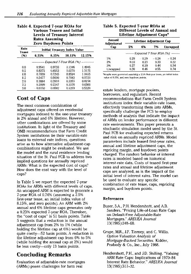
116 Evaluating Annually Repriced Adjustable-Rate Mortgages
Table 4. Expected 7-year ROAs for Various Teases and Initial Levels of Treasury Interest Rates Assuming Zero Buydown Points
Rate Initial Treasury Index Value Tease
(%) 6.15% 8.15% 10.15% 12.15%
------------Expected 7-Year ROA (%) ------------
0.0 0.9541 0.9755 1.1346 1.4945 0.5 0.8275 0.8553 1.0270 1.3175 1.0 0.7039 0.7245 0.8594 1.1655 1.5 0.5477 0.5690 0.7183 0.9723 2.0 0.3884 0.3910 0.5355 0.8258 2.5 0.2099 0.2347 0.3370 0.6560 3.0 -0.0150 0.0002 0.1259 0.5320
Cost of Caps The most common combination of adjustment caps offered on residential mortgages indexed to the one-year treasury is 2% annual and 6% lifetime. However, other combinations are offered by some institutions. In light of the Treasury and OMB recommendations that Farm Credit System institutions tie their variable-rate loans to external rate indices, questions arise as to how alternative adjustment-cap combinations might be evaluated. We use the model and the rural residence lending situation of the St. Paul FCB to address two implied questions for annually repriced ARMs: What is the expected cost of caps? How does the cost vary with the level of caps?
In Table 5 we report the expected 7-year ROAs for ARMs with different levels of caps. An uncapped ARM is expected to generate a 7-year ROA of 0.74% (assuming a 2.5% first-year tease, an initial index value of 8.15%, and zero points). An ARM with 2% annual and 6% lifetime caps generates only a 0.23% expected 7 -year ROA. Therefore, the "cost of caps" is 51 basis points. Table 5 suggests that a reduction in the a?nual adjustment cap from 2% to 1% (while holding the lifetime cap at 6%) would be quite costly-52 basis points. A reduction in the lifetime adjustment cap from 6% to 5% (while holding the annual cap at 2%) would be less costly--only 13 basis points.
Concluding Remarks Evaluation of adjustable-rate mortgages (ARMs) poses challenges for farm real
Table 5. Expected 7-year ROAs at Different Levels of Annual and Lifetime Adjustment Caps8
Annual Adjustment
Cap
1% 2% 3% Uncapped
Lifetime Adjustment Cap
5% 6% 7% Uncapped
--------Expected 7-Year ROA (%} --------
-0.29 - 0.29 - 0.28 -0.24 0.10 0.23 0.30 0.32 0.27 0.39 0.44 0.54 0.30 0.46 0.55 0.74
ilResults were generated assuming a 2.5%, first-year tease, an Initial index
value of 8.151t•6, and zero buydown points.
estate lenders, mortgage poolers, borrowers, and regulators. Recent recommendations that Farm Credit System institutions index their variable-rate loans, effectively transforming them into ARMs, specifically challenge the FCS to employ methods of analysis that indicate the impact of ARMs on lender performance in different rate environments. This paper presents a stochastic simulation model used by the St. Paul FCB for evaluating expected returns and risk on annually repriced ARMs. Model parameters include teased first-year rates, annual and lifetime adjustment caps, the repricing margin, and buydown points charged. The random behavior of interest rates is modeled based on historical interest-rate data. Costs of teased first-year rates and annual and lifetime adjustment caps are analyzed, as is the impact of the initial level of interest rates. The model can be used to evaluate any specific combination of rate tease, caps, repricing margin, and buydown points.
References
Buser, SA., P.H. Hendershott, and A.B. Sanders. "Pricing Life-of-Loan Rate Caps on Default-Free Adjustable-Rate Mortgages." AREUEA Journal 13( 1985):248--60.
Grupe, M.R., J.F. Tierney, and C. Willis. Option Valuation Analysis of Mortgage-Backed Securities. Kidder, Peabody & Co., Inc., July 1988.
Hendershott, P.H., and J.D. Shilling. "Valuing ARM Rate Caps: Implications of 1970-84 Interest Rate Behavior." AREUEA Journal 13(1985):317-32.

Heuson, AJ. "Managing the Short-Term Interest Rate Exposure Inherent in Adjustable Rate Mortgage Loans." AREUEA Journal16(1988):160-71.
Roll, R., and J. Berk. "Adjustable Rate Mortgages: Valuation." In Adjustable Rate Mortgages. Goldman, Sachs & Co., Oct. 1987.
U.S. Dept. of Treasury. Report to the Secretary of the Treasury on Government Sponsored Enterprises. Washington, DC, May 1990.
U.S. Office of Management and Budget. Budget of the United States Government-Fiscal Year 1992. Washington, DC, Jan. 1991.
Waldman, M., and S. Modzelewski. "Part 2: The Salomon Brothers ARM Pricing Model: A Framework for Evaluating ARMs." Salomon Brothers, n.d.
Willoughby, J. "Teasing the Teasers." Forbes, 3 April 1989.
Fischer and Pederson 117


Guidelines for Submitting Manuscripts
We invite submission of manuscripts in agricultural finance, including methodological, empirical, historical, policy, or review-oriented works. Papers must be original in content. Submissions will be reviewed by agricultural finance professionals. The final decision of publication will be made by the editors.
State in a cover letter why the manuscript would interest readers of the Review and indicate whether the material has been published elsewhere. Please prepare manuscripts to conform to the following outline.
Title. Short and to the point, preferably not more than seven or eight words.
Abstract. No more than I 00 words.
Key Words. Indicate main topics of the article.
Author's Affiliation. Institutional affiliation appears as a footnote at the bottom of the first page of the article.
Specifications. Manuscripts should not exceed 25 pages of typewritten, double-spaced material including tables, footnotes, and references. Put tables and figures on separate pages. Provide cameraready art for figures. Number footnotes consecutively throughout the manuscript and type them on a separate sheet. Margins should be a minimum of one inch on all sides. Please number pages.
References. List alphabetically by the author's last name. Include only sources that are referred to in the article. Within the body of the article, references to these sources should state the author's last name (year of publication only if two or more publications are cited by the same author) and placed in parentheses.
Procedure. Submit three typewritten copies to the editor. After the manuscript has been reviewed, the editor will return review copies to the author with a letter stating whether the article is accepted, rejected, or needs additional revision.
Published articles will be subject to a page charge of $40 per printed page. If an author has no financial support from an employer or agency, an exemption from the page charge may be petitioned.
Submit manuscripts to John R. Brake or Eddy L. LaDue, coeditors, Agricultural Finance Review; 155 Warren Hall; Cornell University; Ithaca, New York 14853-7801.
