agreps – access global and regional ensemble prediction
TRANSCRIPT

The Centre for Australian Weather and Climate ResearchA partnership between CSIRO and the Bureau of Meteorology
AGREPS – ACCESS Global and Regional Ensemble Prediction System: Introduction and Experiments
Gregory Roff, David Smith, Michael Naughton, and Asri Sulaiman + Earth System Modelling teamBureau of MeteorologyCAWCR Earth System Modelling Program
SNAP 2013 Workshop, Reading, April 2013

Introduction
•AGREPS • AGREPS Introduction• Verification AGREPS1 v AGREPS0 [N216L70 v
N144L50]• Why do we want AGREPS? Case studies: Queensland
Flooding; Tropical cyclones• Deconstructing AGREPS errors
•Seasonal prediction – another ensemble method•SNAP
• Model development• Why should we include a well resolved stratosphere?• Where is this extra skill?• Potential SNAP tasks

AGREPS – ACCESS ensemble prediction system
24-member ensemble designed for medium-range and short-range forecasting
• Based on UKMO MOGREPS• Global ensemble to 10 days• Regional ensemble over Australian Region to
3 days• Global ETKF for initial condition perturbations • Stochastic model perturbations
Global N320L50 (40km) -> N612L70 (26km)
AGREPS-Global N144L50 (80km) -> N216L70 (60km)
ACCESS-G 40km (N320) – 25km (N512) AGREPS-G 80km (N144) – 60km (N216)
ACCESS-R 12 km AGREPS-R 24 km
HI-RES 5km
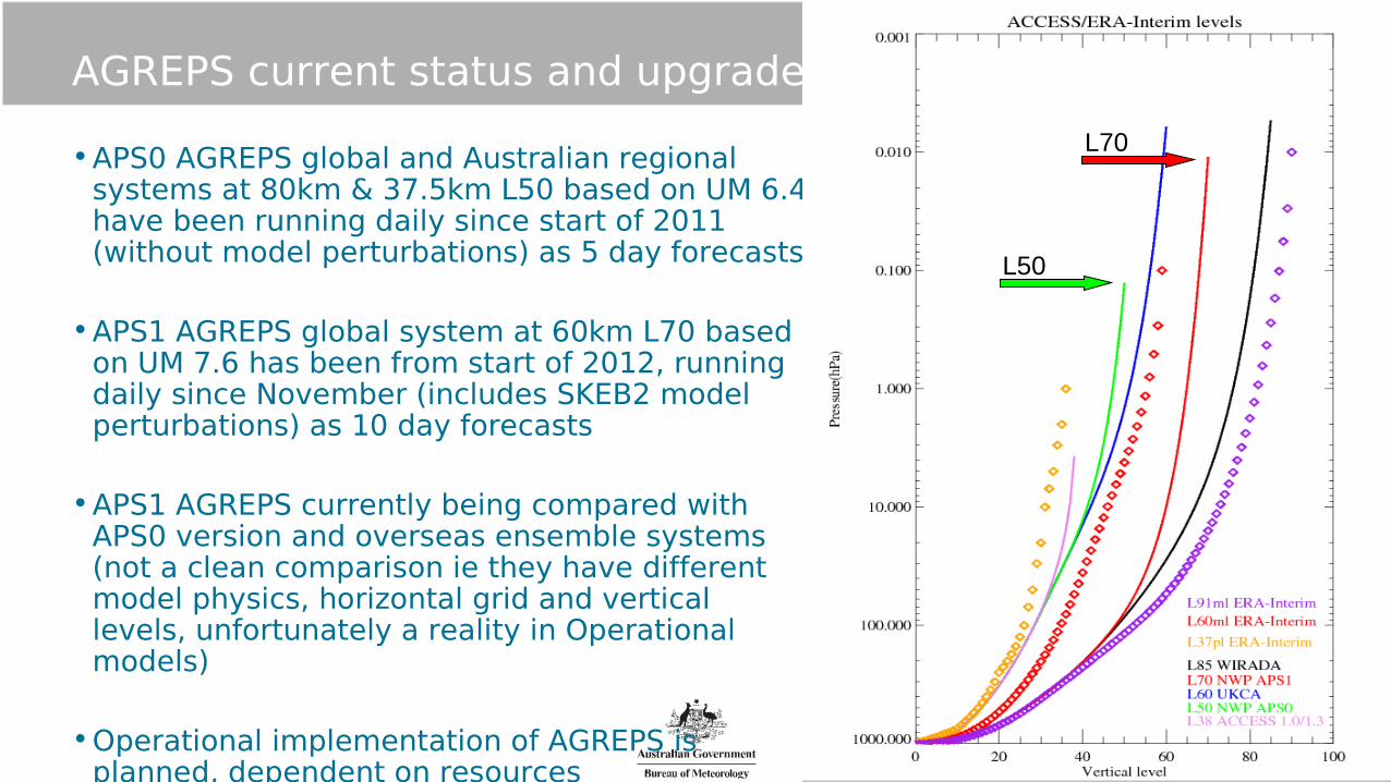
AGREPS current status and upgrade
•APS0 AGREPS global and Australian regional systems at 80km & 37.5km L50 based on UM 6.4 have been running daily since start of 2011 (without model perturbations) as 5 day forecasts
•APS1 AGREPS global system at 60km L70 based on UM 7.6 has been from start of 2012, running daily since November (includes SKEB2 model perturbations) as 10 day forecasts
•APS1 AGREPS currently being compared with APS0 version and overseas ensemble systems (not a clean comparison ie they have different model physics, horizontal grid and vertical levels, unfortunately a reality in Operational models)
•Operational implementation of AGREPS is planned, dependent on resources
L50
L70
AGREPS science
•Ensembles will be key element of data assimilation through provision of capability for flow-dependent error covariances; we plan to incorporate Met Office hybrid DA approach into upcoming ACCESS NWP suites
•Ensembles for high resolution ACCESS systems are also planned

Verification – Spread-skill MSLP
AGREPS N216 (60km) v N144 (80km)MSLP December 2012
austnz: •N216 rmse ~ spread <5days underspread for >5days•N144 underspread >1day
tropics•Both underspread, N216 better
n.hemi•Both underspread ~ same amount
s.Hemi•Similar to austnz, but N216 underspread >3days

Verification – Spread-skill T850
AGREPS N216 (60km) v N144 (80km)T850 December 2012
austnz: •N216 underspread for >1days•N144 underspread much worse
tropics•Both underspread, N216 better
n.hemi•Both underspread ~ same amount
s.Hemi•Similar to austnz, but N216 underspread much worse
NOTE: both this and previous slide showN216 better except in n.Hemi !
Similar improvement seen with Brier score/ROCA

Verification – Spread-skill c.f. other centres
AGREPS N216ECMWFNCEPJMA
MSLP August 2012Southern Hemisphere
Error (solid) spread (dashed) showECMWF best, all start with underspreadingJMA remains underspreadNCEP flips by day 5AGREPS flips by day 4 and again day 8ECMWF flips by day 9

Case study: Queensland & NSW flooding – 22-29 Jan 2013
Ensemble forecasts of high rainfall period of the event
•Ensemble forecasts predicted rainfall event to travel down the Queensland coast•4-day forecasts from AGREPS and EC-EPS identified probability of high rainfall for
27 January•2-day forecasts strengthened the forecast probability

Queensland & NSW flooding – 22-29 Jan 2013
This event followed the monsoon onset in mid-January. TC Oswald formed in the western part of Gulf of Carpentaria around 20 January. It existed briefly as TC until it made landfall and moved across the Cape York peninsula as a tropical low, then progressed over following week down the Queensland coast and through to the northern NSW as far as Sydney region, before moving off to the east on 29 January.

Queensland & NSW flooding – 22-29 Jan 2013
Floodwaters cover the central Queensland city of Bundaberg in the wake of ex-tropical cyclone Oswald,
January 29, 2013.
ABC: Audience submitted: John McDermottabc.net.au/news/2013-01-27/queensland-floods-as-
oswald-moves-south/4486174

Queensland & NSW flooding – 22-29 Jan 2013
The Fitzroy River floods and fills the surrounding landscape,
January 29, 2013.
ABC Capricorniaabc.net.au/news/2013-01-27/queensland-floods-as-oswald-moves-south/4486174

Queensland & NSW flooding – 22-29 Jan 2013
Canadian astronaut Chris Hadfield takes a picture of floodwater on the Burnett River
running out to sea at Bundaberg on January 29, 2013.
Twitter: @Cmdr_Hadfield
abc.net.au/news/2013-01-27/queensland-floods-as-oswald-moves-south/4486174

Queensland & NSW flooding – 22-29 Jan 2013
This event followed the monsoon onset in mid-January. TC Oswald formed in the western part of Gulf of Carpentaria around 20 January. It existed briefly as TC until it made landfall and moved across the Cape York peninsula as a tropical low, then progressed over following week down the Queensland coast and through to the northern NSW as far as Sydney region, before moving off to the east on 29 January.

Queensland & NSW flooding – 22-29 Jan 2013
Initial period – NWP forecasts of initial period of transit of tropical low to east coast
•Deterministic 5-day forecasts from 20 January showed large variation in location of low centre
• UK & ACCESS forecasts favoured movement to east• ECMWF and US had low staying further west
•AGREPS and EC-EPS captured different possibilities amongst ensemble members, with EC_EPS ensemble mean still further west than AGREPS
•Actual movement was east then south-east
•Forecasts for 25 January converged at 3-day period

Queensland flooding – 27 Jan 2013
Ensemble forecasts of Central Queensland coast heavy rainfall period.
AGREPS and EC-EPS ensemble means and precip-probabilities both picked up likelihood of heavy rain event 4 days ahead

Queensland flooding – 27 Jan 2013
AGREPS ECMWF-EPS

Queensland flooding – 27 Jan 2013
AGREPS and ECMWF-EPS 4-day forecasts
Probability of 24 hr precip exceeding 25 mm
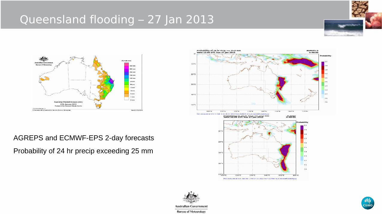
Queensland flooding – 27 Jan 2013
AGREPS and ECMWF-EPS 2-day forecasts
Probability of 24 hr precip exceeding 25 mm

Case studies: TC strike probabilities – Combined ACCESS-TC & AGREPS-R
TC Iggy
TC Freda
TC Yasi
72 hr forecast
ACCESS-TC 12Z & 00Z tracks
AGREPS-R 18Z strike probability, control and ensemble mean tracks

Spread and multiscale verification – zonal waves
Can we try to understand where the ensemble is failing?
One method is to split the data into planetary/synoptic and sub-synoptic bands and see how these bands contribute to the spread and error.
An example of this can be seen in the Z250 30 day forecast spread/error (solid/dashed) curves averaged over 20S:90S. Here: black shows unfiltered values; while zonal wavenumbers 0-3/4-14/>=15, representing planetary/synoptic and sub-synoptic waves are coloured blue/red/pink. The N144 and N216 runs are thick/thin, respectively.
The unfiltered N216 (thin black) curves show initial good spread followed by overspreading from day 12, a not uncommon feature in many ensemble models; N144 is underspreading at all times, and by a much larger amount.

Spread and multiscale verification – zonal waves
The planetary and synoptic scale spread/error curves are better for N216 than N144 except for the planetary scale after day 24.
One can also see where unfiltered excursions in the error are due mainly to (1) planetary, (2) synoptic or (3) bothand use this to examine these situations in more detail.
3
1 2
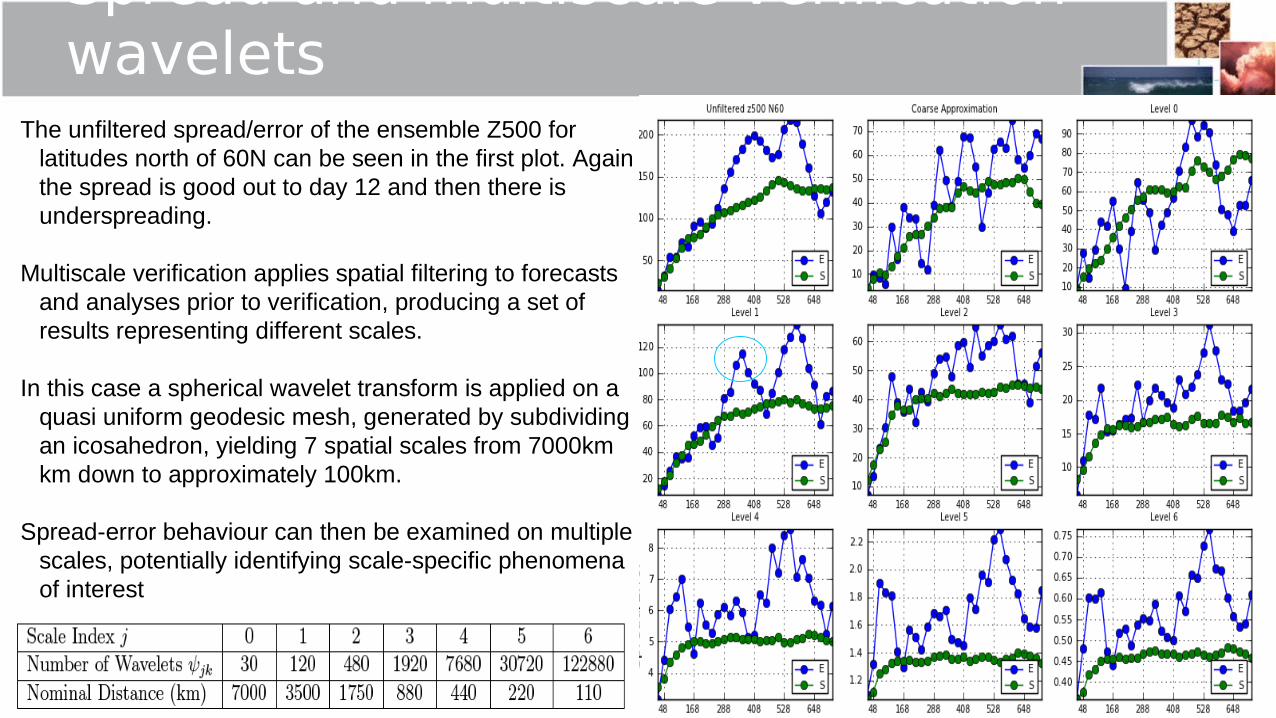
Spread and multiscale verification - wavelets
The unfiltered spread/error of the ensemble Z500 for latitudes north of 60N can be seen in the first plot. Again the spread is good out to day 12 and then there is underspreading.
Multiscale verification applies spatial filtering to forecasts and analyses prior to verification, producing a set of results representing different scales.
In this case a spherical wavelet transform is applied on a quasi uniform geodesic mesh, generated by subdividing an icosahedron, yielding 7 spatial scales from 7000km km down to approximately 100km.
Spread-error behaviour can then be examined on multiple scales, potentially identifying scale-specific phenomena of interest

AGREPS Summary
•AGREPS global and Australian regional ensemble system has been upgraded in line with upgrade to APS operational NWP systems and UKMO MOGREPS Operational ensemble system
•Improvement has been demonstrated in upgraded system compared with original APS0 version
•AGREPS system delivers comparable performance to overseas operational EPS systems
•AGREPS system is ready for operational implementation
•Zonal wave band analysis and wavelet analysis is being used to study where AGREPS can be improved
Seasonal ensemble prediction: Not using AGREPS
WIRADA; Water Information Research and Development Alliance•ACCESS 1.3 N96L38/L85 comparison•Ensemble of 30day hindcasts run 1,11,21 every month for 1982:2010•10 ensembles created by initializing i*6hr before start date using ERA-Interim data, running to start date, then relabelling dump file as start date and then running the hindcast
•Note: ACCESS 1.3 was tuned for L38, not for L85

spatial COR for Sept-Nov (zonal mean T, 25-
75S)
L85 L38
skill score using spatial correlation: (L85-L38)/(1-L38)
Seasonal ensemble prediction

SNAP: Where does stratosphere fit in model development in CAWCR?
Model improvements include:1. newer physics/dynamical core - steady improvement, these are major changes2. increased vertical resolution in the boundary layer/lower troposphere - often goes with the above,
can be dangerous3. increased horizontal resolution - easy to implement, depend on computer power, most centres are
running at the maximum they can at any time4. coupling the model to an ocean - expensive, but increasing demand as forecasts expand from 5-10
-> monthly 5. extending the model top - most centres are up as high as they will go (~80km)?6. increasing resolution in the stratosphere - present NWP response: no real need seen for this once we
have data assimilation ok; seasonal response is – do we do better with this?
Actions 1- 4 will continue to evolve, because that’s what we do!Action 5 is done as most centres are up as high as they need to be Action 6 we need to justify getting more vertical levels here, rather than lower down where NWP
“knows” improvements can be made with increased vertical resolutionGlobal NWP models now have high tops (the main NWP driver for this was to get better initial
conditions via satellite data assimilation), but Seasonal prediction and ensemble models want to know is it worth them raising their lids?

Model developmentThings to consider:• Tropospheric model vertical levels will change as
computer power increases, but NWP does not like to change them as many paramerizations are tuned to vertical level placements
• =>adding deep/shallow high/low res strat can be done ok, but remember eg EI runs to 0.01hPa but outputs only to 1hPa
• NWP wants a well resolved stratosphere – to enable better assimilation of satellite data as ic and data assimilation have a huge impact on nwp 5-10 day forecasts, not to necessarily model the stratosphere better
• LAMs are increasing in resolution and are used for short period forecasting and do not need the well resolved stratosphere
• Cost in vertical resolution increase is much less than horizontal, so why not do it? Because most operations centres have strong time demands (we needed to find 10minutes to get our model into the allotted operational compute time-slot). So we need to justify the extra stratospheric levels.

Why should we include the stratosphere in ensembles?
•From operational point of view – do we get much gain by including the stratosphere?
•Yes, there have been cases where this is shown, but is it mainly when the Stratosphere is active (during vortex breakdown periods)
•Ensembles are expensive and (we are waiting for a larger computer before ensembles go operational) so we need a convincing argument for them to be extended vertically
•NWP is out to 10day forecasts, so is there any real impact there?; seasonal would be better placed to want a well resolved stratosphere
•What is a well resolved stratosphere?

SNAP question: Where do we get improved skill from incorporating a “well” resolved stratosphere?
• 0-15 days, some suggestions of improvement near 5 days => need for SNAP to show this is so. But is this improvement really just due to the assimilation of the SSW anomaly into the ic, as suggested below?
• 15-30 days: pretty confident in NHwinter/SHspring high latitudes out near day 20 – related to starting the run within the “Goldilocks” region of the SSW+final warming ie too far before the SSW, your ic has no anomaly to propagate down; too long after the SSW and there is no anomaly to propagate; so you have to initialize within the SSW where the anomaly is large enough to be just right
• 30+ days: none, until yesterday and Adam/Alberto with NAO BUT need high resolution ocean+atm – which we (many?) do not have
So where do we get improved forecast skill from including a well resolved stratosphere?
NWP Extended range Seasonal
Goldilocks

SNAP question: Where do we get improved skill from incorporating a “well” resolved stratosphere?
• 0-15 days, some suggestions of improvement near 5 days => need for SNAP to show this is so. But is this improvement really just due to the assimilation of the SSW anomaly into the ic, as suggested below?
• 15-30 days: pretty confident in NHwinter/SHspring high latitudes out near day 20 – related to starting the run within the “Goldilocks” region of the SSW+final warming ie too far before the SSW, your ic has no anomaly to propagate down; too long after the SSW and there is no anomaly to propagate; so you have to initialize within the SSW to be just right
• 30+ days: none, until yesterday and Adam/Alberto with NAO BUT need high resolution ocean+atm – which we (many?) do not haveForecasting 1- 10 days
Stratospheric anomaly resolved in the ic?
Lat\Sea Summer Autumn Winter Spring
N90-45 ?
N45-EQ
EQ-S45
S45-90 ?
Forecasting 10- 30 daysStratospheric anomaly descending?
Lat\Sea Summer Autumn Winter Spring
N90-45
N45-EQ
EQ-S45
S45-90
Forecasting 1-9 monthsCapture NAO – need N216L85 + Ocean 0.25deg?
Lat\Sea Summer Autumn Winter Spring
N90-45
N45-EQ
EQ-S45
S45-90NWP Extended range Seasonal
Goldilocks

SNAP tasks?
Forecasting days 1- 15Stratospheric anomaly resolved in the ic?
Lat\Sea Summer Autumn Winter Spring
N90-45 ?
N45-EQ
EQ-S45
S45-90 ?
Forecasting days 15- 30Stratospheric anomaly descending?
Lat\Sea Summer Autumn Winter Spring
N90-45
N45-EQ
EQ-S45
S45-90
Forecasting days 30+Capture NAO – need N216L85 + Ocean 0.25deg?
Lat\Sea Summer Autumn Winter Spring
N90-45
N45-EQ
EQ-S45
S45-90NWP Extended range Seasonal
Can we fill in some more regions in the tables via:• Do some targeted experiments in both stratospheric active and
inactive periods to see if we can demonstrate improved skill in the 0-15day forecast period?
• Use the present operational hindcasts routinely generated to determine if there is any skill in the troposphere out at days 15-30 and beyond in any season?
• Suggest better diagnostics that we could request from present operational centres to output with their hindcast data eg w* 70hPa; fields at selected vertical levels
• Suggest: better placement of vertical levels? Is there a minimum for a “good” stratosphere? Run hi-top only in seasons which show promise to save cost?

The Centre for Australian Weather and Climate Research A partnership between CSIRO and the Bureau of Meteorology
The Centre for Australian Weather and Climate ResearchA partnership between CSIRO and the Bureau of Meteorology
Greg Roff
Phone: +61-3-9669-4822Email: [email protected]: www.cawcr.gov.au
www.cawcr.gov.au