AgilentFundamentals of RF and Microwave Power Measurements (Part 3)

Application Note 1449-3

Power Measurement Uncertainty per International Guides

Fundamentals of RF and Microwave Power Measurements (Part 1)Introduction to Power, History, Definitions, InternationalStandards, and TraceabilityAN 1449-1, literature number 5988-9213EN

Part 1 introduces the historical basis for power measurements, and provides definitions for average, peak, and complex modulations. This application note overviews various sensor technologies needed for the diversity of test signals. It describes the hierarchy of international power traceability, yielding comparison to national standards at worldwide National Measurement Institutes (NMIs) like the U.S. National Institute of Standards and Technology. Finally, the theory and practice of power sensor comparison procedures are examined with regard to transferring calibration factors and uncertainties. A glossary is included which serves all four parts.

Fundamentals of RF and Microwave Power Measurements (Part 2)Power Sensors and InstrumentationAN 1449-2, literature number 5988-9214EN

Part 2 presents all the viable sensor technologies required to exploit the users’ wide range of unknown modulations and signals under test. It explains the sensor technologies, and how they came to be to meet certain measurement needs. Sensor choices range from the venerable thermistor to the innovative thermocouple to more recent improvements in diode sensors. In particular, clever variations of diode combinations are presented, which achieve ultra-wide dynamic range and square-law detection for complex modulations. New instrumentation technologies, which are underpinned with powerful

computational processors, achieve new data performance.

Fundamentals of RF and Microwave Power Measurements (Part 3)Power Measurement Uncertainty per International GuidesAN 1449-3, literature number 5988-9215EN

Part 3 discusses the all-important theory and practice of expressing measurement uncertainty, mismatch considerations, signal flowgraphs, ISO 17025, and examples of typical calculations. Considerable detail is shown on the ISO 17025, Guide for the Expression of Measurement Uncertainties, has become the international standard for determining operating specifications. Agilent has transitioned from ANSI/NCSL Z540-1-1994 to ISO 17025.

Fundamentals of RF and Microwave Power Measurements (Part 4) An Overview of Agilent Instrumentation for RF/Microwave Power MeasurementsAN 1449-4, literature number 5988-9216EN

Part 4 overviews various instrumentation for measuring RF and microwave power, including spectrum analyzers, microwave receivers, network analyzers, and the most accurate method, power sensors/meters. It begins with the unknown signal, of arbitrary modulation format, and draws application-oriented comparisons for selection of the best instrumentation technology and products.

Most of the note is devoted to the most accurate method, power meters and sensors. It includes comprehensive selection guides, frequency coverages, contrasting accuracy and dynamic performance to pulsed and complex digital modulations. These are especially crucial now with the advances in wireless communications formats and their statistical measurement needs.

2

For user convenience, Agilent’s Fundamentals of RF and Microwave Power Measurements, application note 64-1, literature number 5965-6330E, has been updated and segmented into four technical subject groupings. The following abstracts explain how the total field of power measurement fundamentals is now presented.

3

I. Introduction ........................................................................................................ 4

II. Power Transfer, Signal Flowgraphs ...................................... 5

Power transfer, generators and loads .......................................................... 5 RF circuit descriptions ..................................................................................... 5 Reflection coefficient ....................................................................................... 7 Signal flowgraph visualization ....................................................................... 8

III. Measurement Uncertainties .......................................................... 12

Mismatch loss uncertainty ............................................................................. 12

Mismatch loss and mismatch gain ............................................................... 13

Simple techniques to reduce mismatch loss uncertainty ........................ 13

Advanced techniques to improve mismatch uncertainty ......................... 17

Eliminating mismatch uncertainty by measuring source and load complex reflection coefficients and computer correcting ........... 18

Other sensor uncertainties ............................................................................. 18

Calibration factor .............................................................................................. 19

Power meter instrumentation uncertainties ............................................... 20

IV. Alternative Methods of Combining Power Measurement Uncertainties .......................................................... 23

Calculating total uncertainty .......................................................................... 23

Power measurement equation ....................................................................... 23

Worst-case uncertainty method .................................................................... 25

RSS uncertainty method ................................................................................. 26

A new international guide to the expression of uncertainty in

measurement (ISO GUM) ............................................................................ 27

Power measurement model for ISO process .............................................. 29

Standard uncertainty of mismatch model ................................................... 31

Example of calculation of uncertainty using ISO model ........................... 32

Example of calculation of uncertainty of USB sensor using

ISO model ....................................................................................................... 35

Table of Contents

The purpose of the new series of Fundamentals of RF and Microwave Power Measurements application notes, which were leveraged from former note 64-1, is to

1) Retain tutorial information about historical and fundamental considerations of RF/microwave power measurements and technology which tend to remain timeless.

2) Provide current information on new meter and sensor technology.

3) Present the latest modern power measurement techniques and test equipment that represents the current state-of-the-art.

Part 3 of this series, Power Measurement Uncertainty per International Guides, is a comprehensive overview of all the contributing factors (there are 12 described in the International Standards Organization (ISO) example) to power measurement uncertainty of sensors and instruments. It presents signal flowgraph principles and a characterization of the many contributors to the total measurement uncertainty.

Chapter 2 examines the concept of signal flow, the power transfer between generators and loads. It defines the complex impedance, its effect on signal reflection and standing waves, and in turn its effect on uncertainty of the power in the sensor. It introduces signal flowgraphs for better visualizations of signal flow and reflection.

Chapter 3 breaks down all the various factors that influence measurement uncertainty. It examines the importance of each and how to minimize each of the various factors. Most importantly, considerable space is devoted to the largest component of uncertainty, mismatch uncertainty. It presents many practical tips for minimizing mismatch effects in typical instrumentation setups.

Chapter 4 begins by presenting two traditional methods of combining the effect of the multiple uncertainties. These are the "worst-case" method and the "RSS" method. It then examines in detail the increasingly popular method of combining uncertainties, based on the ISO Guide to the Expression of Uncertainty in Measurement, often referred to as the GUM.[1] ISO is the International Standards Organization, an operating unit of the International Electrotechnical Commission (IEC). The reason the GUM is becoming more crucial is that the international standardizing bodies have worked to develop a global consensus among National Measurement Institutes (such as NIST) and major instrumentation suppliers as well as the user community to use the same uncertainty standards worldwide.

Note: In this application note, numerous technical references will be made to the other published parts of the series. For brevity, we will use the format Fundamentals Part X. This should insure that you can quickly locate the concept in the other publication. Brief abstracts for the four-part series are provided on the inside front cover.

[1] “ISO Guide to the Expression of Uncertainty in Measurement," International Organization for Standardization,

Geneva, Switzerland, ISBN 92-67-10188-9, 1995.

4

I. Introduction

Power transfer, generators and loadsThe goal of an absolute power measurement is to characterize the unknown power output from some source (for example a generator, transmitter, or oscillator). Sometimes the generator is an actual signal generator or oscillator where the power sensor can be attached directly to that generator. On other occasions, however, the generator is actually an equivalent generator. For example, if the power source is separated from the measurement point by such components as transmission lines, directional couplers, amplifiers, mixers, etc., then all those components may be considered as parts of the generator. The port that the power sensor connects to, would be considered the output port of the equivalent generator.

To analyze the effects of impedance mismatch, this chapter explains mathematical models that describe loads, including power sensors and generators, which apply to the RF and microwave frequency ranges. The microwave descriptions begin by relating back to the equivalent low-frequency concepts for those familiar with those frequencies. Signal flowgraph concepts aid in analyzing power flow between an arbitrary generator and load. From that analysis, the terms mismatch loss and mismatch loss uncertainty are defined.

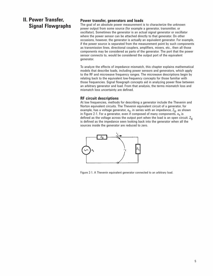
RF circuit descriptionsAt low frequencies, methods for describing a generator include the Thevenin and Norton equivalent circuits. The Thevenin equivalent circuit of a generator, for example, has a voltage generator, es, in series with an impedance, Zg, as shown in Figure 2-1. For a generator, even if composed of many components, es is defined as the voltage across the output port when the load is an open circuit. Zg is defined as the impedance seen looking back into the generator when all the sources inside the generator are reduced to zero.

Figure 2-1. A Thevenin equivalent generator connected to an arbitrary load.

5

II. Power Transfer, Signal Flowgraphs

The power delivered by a generator to a load is a function of the load impedance. If the load is a perfect open or short circuit, the power delivered is zero. Analysis of Figure 2-1 would show that the power delivered to the load is a maximum when load impedance, Zl, is the complex conjugate of the generator impedance, Zg. This power level is called the "power available from a generator," or "maximum available power," or "available power." When Zl= (Rl + jXl) and Zg = (Rg + jXg) are complex conjugates of each other, their resistive parts are equal and their imaginary parts are identical in magnitude but of opposite sign; thus Rl = Rg and Xl = –Xg. Complex conjugate is written with an * so that Zl = Zg* is the required

relationship for maximum power transfer.

The Thevenin equivalent circuit is not very useful at microwave frequencies for a number of reasons. First, the open circuit voltage is difficult to measure because of fringing capacitance and the loading effect of a voltmeter probe. Further, the concept of voltage loses usefulness at microwave frequencies where it is desired to define the voltage between two points along a transmission path, separated by a significant fraction of a wavelength. If there is a "standing wave" along a transmission line, the voltage varies along the line. Also, there are problems with discussing voltage in rectangular waveguide. As a result, the concept of power is much more frequently used than voltage for characterizing generators at RF and microwave frequencies.

The open circuit that defines the Thevenin equivalent voltage generator is useless for measuring power because the power dissipated in an open termination is always zero. The reference impedance used for characterizing RF generators is almost always 50 Ω. The reason for this is that 50 Ω is easy to realize over the entire frequency range of interest with a transmission line of 50 Ω characteristic impedance and with a reflection-less termination.

The standard symbol for characteristic impedance, Zo, is also the standard symbol for reference impedance. In some cases, for example, where 75 Ω transmission lines are used in systems with a 50 Ω reference impedance, another symbol, such as Zr, should be used for reference impedance. Zo will be used in this application note to mean reference impedance. A generator is characterized, therefore, by the power it delivers to a reference load Zo = 50 Ω. In general, that power is not equal to the maximum available power from the generator; they are equal only if Zg = Zo.

As frequencies exceed 300 MHz, the concept of impedance loses usefulness and is replaced by the concept of reflection coefficient. The impedance seen looking down a transmission line toward a mismatched load, varies continuously with the position along the line. The magnitude and the phase of impedance are functions of line position. Reflection coefficient is well-behaved; it has a magnitude that is constant and a phase angle that varies linearly with distance from the load.

6

7

Reflection coefficientAt microwave frequencies where power typically is delivered to a load by atransmission line that is many wavelengths long, it is very convenient to replace the impedance description of the load, involving voltage and current and their ratio (Ohm’s law), with a reflection coefficient description involving incident and reflected traveling waves, and their ratio. To characterize a passive load, Ohm’s law is replaced by:

where al is proportional to the voltage of the incident wave, bl is proportional to the voltage of the reflected wave, and Γl is defined to be the reflection coefficient of the load. All three quantities are, in general, complex numbers and change with frequency. The quantities al and bl are normalized1 in such a way that the following equations hold:

where Pi is power incident on the load and Pr is power reflected by it. The netpower dissipated by the load, Pd , is given by:

This power is the total power obtained from the source; it includes not only power converted to heat, but also power radiated to space and power that leaks through accessory cables to other pieces of equipment.

Transmission line theory relates the reflection coefficient, Γl of a load to itsimpedance, Zl, as follows:

where Zo is the characteristic impedance of the system. Further, the load voltage, vl, and load current, il, are given by:

since current in a traveling wave is obtained from the voltage by dividing by Zo. Solving for al and bl results in:

1. If the transmission line characteristic impedance is Zo the normalization factor is √Zo; that is, al is obtained from

the voltage of the incident wave by dividing by √Zo. Similarly, bl is obtained from the voltage of the reflected wave

by dividing by √Zo.

= Γlblal

(Equation 2-1)

|al|2 = Pi (Equation 2-2)

(Equation 2-3)|bl|2 = Pr

Pd = Pi – Pr = |al|2 – |bl|2 (Equation 2-4)

Γl =Zl – Zo

Zl + Zo (Equation 2-5)

il = Incident current – reflected current

= (al – bl)

Vl = Incident voltage + reflected voltage

= √ Zo (al + bl) (Equation 2-6)

1

√Zo

(Equation 2-7)

1

2√Zo

al = (vl + Zoil)1

2√Zo(Equation 2-8)

bl = (vl − Zoil) (Equation 2-9)

These equations are used in much of the literature to define al and bl (see thereference by Kurakawa.)[1] The aim here, however, is to introduce al and bl more intuitively. Although equations 2-8 and 2-9 appear complicated, the relationships to power (equations 2-2, 2-3, and 2-4) are very simple. The Superposition Theorem, used extensively for network analysis, applies to al and bl; the Superposition Theorem does not apply to power.

Reflection coefficient, Γl, is frequently expressed in terms of its magnitude, ρl, and phase, φl. Thus ρl gives the magnitude of bl with respect to al and φl gives the phase of bl with respect to al.

The most common methods of measuring reflection coefficient involve observing al and bl separately and then taking the ratio. Sometimes it is difficult to observe al and bl separately, but it is possible to observe the interference pattern of the counter-travelling waves formed by a and b on a transmission line. This pattern is called the standing wave pattern. The interference pattern has regions of maximum and of minimum signal strength. The maximums are formed by constructive interference between al and bl and have amplitude |al| + |bl|. The minimums are formed by destructive interference and have amplitude |al| – |bl|. The ratio of the maximum to the minimum is called the standing-wave ratio (SWR, sometimes referred to as voltage-standing-wave-ratio, VSWR).1 It can be measured with a slotted line and moveable probe, or more commonly with network analyzers. SWR is related to the magnitude of reflection coefficient ρl by:

Signal flowgraph visualizationA popular method of visualizing the flow of power through a component or among various components is by means of a flow diagram called a signal flowgraph.[1,2] This method of signal flow analysis was popularized in the mid-1960’s, at the time that network analyzers were introduced, as a means of describing wave travel in networks.

The signal flowgraph for a load (Figure 2-2) has two nodes, one to represent the incident wave, al, and the other to represent the reflected wave, bl. They are connected by branch Γl, which shows how al gets changed to become bl.

Just as the Thevenin equivalent had two quantities for characterizing a generator, generator impedance, and open circuit voltage, the microwave equivalent has two quantities for characterizing a microwave or RF generator, Γg and bs.

8

Figure 2-2. Signal flowgraph for a load.

SWR = |al| + |bl|

|al| – |bl| (Equation 2-10)=

1 + |bl/al|

1 – |bl/al| =

1 + ρl

1 – ρl

1. Traditionally VSWR and PSWR referred to voltage and power standing wave ratio. Since PSWR has fallen

to dis-use, VSWR is shortened to SWR.

9

The equation for a generator is (see Figure 2-3):

where:

bg is the wave emerging from the generatorag is the wave incident upon the generator from other componentsΓg is the reflection coefficient looking back into the generatorbs is the internally generated wave

Γg is related to Zg by:

which is very similar to Equation 2-5. The bs is related to the power to a reference load from the generator, Pgzo, by:

bs is related to the Thevenin voltage, es, by:

The signal flowgraph of a generator has two nodes representing the in cident, wave ag and reflected wave bg. The generator also has an internal node, bs, that represents the ability of the generator to produce power. It contributes to output wave, bg, by means of a branch of value one. The other component of bg is that portion of the incident wave, ag, that is reflected off the generator.

Now that equivalent circuits for a load and generator have been covered, the flow of power from the generator to the load may be analyzed. When the load is connected to the generator, the emerging wave from the generator becomes the incident wave to the load and the reflected wave from the load becomes the incident wave to the generator. The complete signal flowgraph (Figure 2-4) shows the identity of those waves by connecting node bg to al and node bl to ag with branches of value one.

Figure 2-4 shows the effect of mismatch or reflection. First, power from the generator is reflected by the load. That reflected power is re-reflected from the generator and combines with the power then being created by the generator, generating a new incident wave. The new incident wave reflects and the process continues on and on. It does converge, however, to the same result that will now be found by algebra.

The equation of the load (2-1) is rewritten with the identity of ag to bl added as:

The equation of the generator (2-11) is also rewritten with the identity of al to bg added as:

bg = bs + Γgag (Equation 2-11)

Γg = Zg – Zo

Zg + Zo (Equation 2-12)

Pgzo = |bs|2(Equation 2-13)

bs = es √Zo

Zo + Zg (Equation 2-14)

bl = Γl al = ag (Equation 2-15)

Figure 2-3. Signal flowgraph of a microwave generator.

Figure 2-4. The complete signal flowgraph of a generator connected to a load.

bg = bg + Γgag = al (Equation 2-16)

10

Equations 2-15 and 2-16 may be solved for al and bl in terms of bs , Γl and Γg:

From these solutions the load’s incident and reflected power can be calculated:

Equation 2-19 yields the somewhat surprising fact that power flowing toward the load depends on the load characteristics.

The power dissipated, Pd, is equal to the net power delivered by the generator to the load, Pgl:

Two particular cases of Equation 2-21 are of interest. First, if Γl were zero, that is if the load impedance were Zo, Equation 2-21 would give the power delivered by the generator to a Zo load:

This case is used to define bs as the generated wave of the source.

The second case of interest occurs when:

where * indicates the complex conjugate. Interpreting Equation 2-23 means that the reflection coefficient looking toward the load from the generator is the complex conjugate of the reflection coefficient looking back toward the generator. It is also true that the impedances looking in the two directions are complex conjugates of each other. The generator is said to be "conjugately matched." If Γl is somehow adjusted so that Equation 2-23 holds, the generator puts out its "maximum available power," Pav, which can be expressed as:

Comparing Equations 2-22 and 2-24 shows that Pav ≥ PgZo. Unfortunately, the term "match" is popularly used to describe both con ditions, Zl = Zo and Zl = Zg*. The use of the single word "match" should be dropped in favor of "Zo match" to describe a load of zero reflection coefficient, and in favor of "conjugate match" to describe the load that provides maximum power transfer.

al = bs

1 – ΓgΓl(Equation 2-17)

bl = bsΓl1 – ΓgΓl

(Equation 2-18)

Pi = |al|2 = |bs|2(Equation 2-19)

1

|1 – ΓgΓl|2

Pr = |bl|2 = |bs|2 (Equation 2-20) Γl

2

|1 – ΓgΓl|2

Pd = Pgl = Pi – Pr = |bs|2 (Equation 2-21)1 – |Γl|2

|1 – ΓgΓl|2

Pgl|Zl = Zo

= PgZo = |bs|2

(Equation 2-22)

Γg = Γl* (Equation 2-23)

Pav = (Equation 2-24)|bs|2

1 – |Γg|2

Now the differences can be plainly seen. When a power sensor is attached to agenerator, the measured power that results is Pgzo of Equation 2-21, but the proper power for characterizing the generator is Pgzo of Equation 2-22. Theratio of equations 2-22 to 2-21 is:

or, in dB:

This ratio (in dB) is called the "Zo mismatch loss." It is quite possible that Equation 2-25 could yield a number less than one. Then Equation 2-26 would yield a negative number of dB.

In that case more power would be transferred to the particular load being used than to a Zo load, where the Zo mismatch loss is actually a gain. An example of such a case occurs when the load and generator are conjugately matched.

A similar difference exists for the case of conjugate match; the measurement of Pgl from Equation 2-21 differs from Pav of Equation 2-24. The ratio of those equations is:

or, in dB:

This ratio in dB is called the "conjugate mismatch loss."

If Γl and Γg were completely known, or easily measured versus frequency, the power corrections would be simplified. The power meter reading of Pgl would be

combined with the proper values of Γl and Γg in Equations 2-25 or 2-27 to calculate Pgzo or Pav. The mismatch would be corrected and there would be no uncertainty. Yet in the real world, most power measurements are made without

the Γl and Γg corrections in the interest of time. For certain special procedures, such as power sensor calibrations, where utmost accuracy is required, the time is taken to characterize the generator and load (sensor) complex reflection coefficients versus frequency, and corrections made for those effects.

11

(Equation 2-25) |1 – ΓgΓl|2

1 – |Γl|2

Pgzo Pgl

=

dB = 10 log (Equation 2-26)Pgzo

Pgl

dB = 10 log |1 – ΓgΓl|2 – 10 log (1 – |Γl|2)

(Equation 2-27)

|1 – ΓgΓl|2

(1 – |Γg|2)(1 – |Γl|2)

Pav

Pgl=

dB = 10 log

(Equation 2-28)

PavPgl

dB = 10 log |1 – ΓlΓg|2 – 10 log (1 – |Γg|2) – 10 log (1 – |Γl|2)

[1] K. Kurakawa, “Power Waves and the Scattering Matrix,” IEEE Trans. on Microwave Theory and Techniques,

Vol. 13, No. 2, Mar 1965.

[2] N.J. Kuhn, “Simplified Signal Flow Graph Analysis,” Microwave Journal, Vol 6, No 10, Nov. 1963.

12

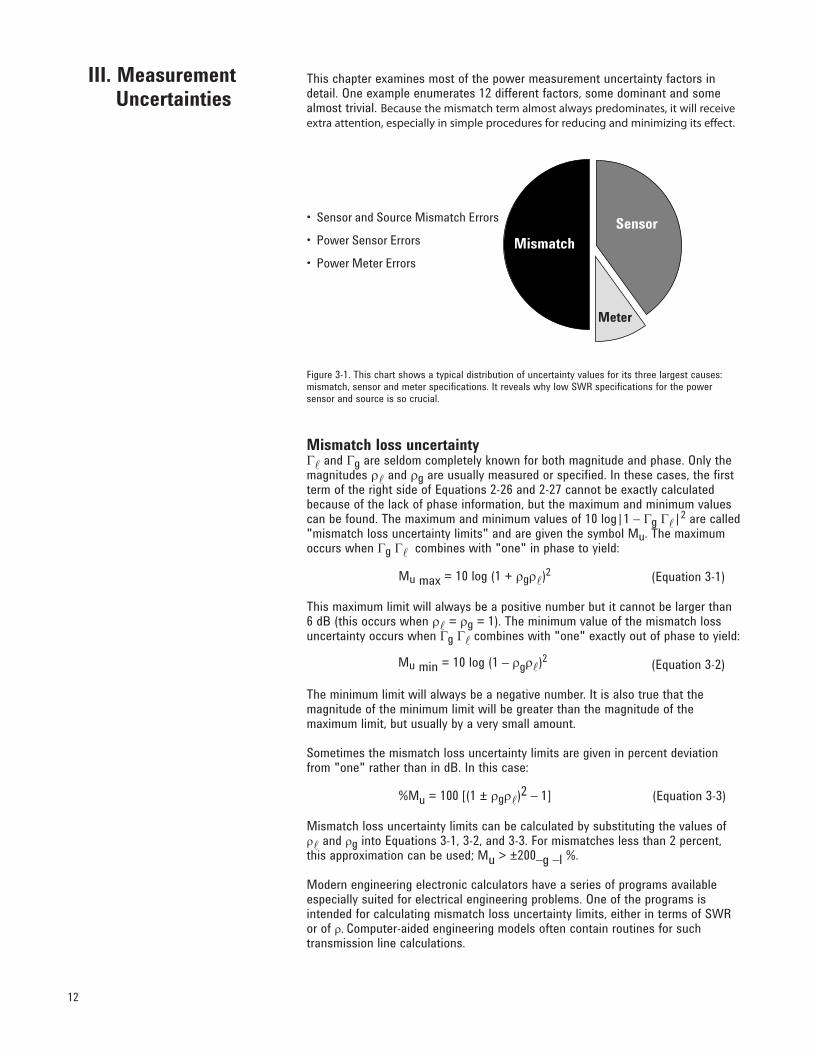
This chapter examines most of the power measurement uncertainty factors in detail. One example enumerates 12 different factors, some dominant and some almost trivial. Because the mismatch term almost always predominates, it will receive

extra attention, especially in simple procedures for reducing and minimizing its effect.

Figure 3-1. This chart shows a typical distribution of uncertainty values for its three largest causes: mismatch, sensor and meter specifications. It reveals why low SWR specifications for the power sensor and source is so crucial.

Mismatch loss uncertaintyΓl and Γg are seldom completely known for both magnitude and phase. Only the magnitudes ρl and ρg are usually measured or specified. In these cases, the first term of the right side of Equations 2-26 and 2-27 cannot be exactly calculated because of the lack of phase information, but the maximum and minimum values can be found. The maximum and minimum values of 10 log|1 – Γg Γl|2 are called "mismatch loss uncertainty limits" and are given the symbol Mu. The maximum occurs when Γg Γl combines with "one" in phase to yield:

This maximum limit will always be a positive number but it cannot be larger than 6 dB (this occurs when ρl = ρg = 1). The minimum value of the mismatch loss uncertainty occurs when Γg Γl combines with "one" exactly out of phase to yield:

The minimum limit will always be a negative number. It is also true that the magnitude of the minimum limit will be greater than the magnitude of the maximum limit, but usually by a very small amount.

Sometimes the mismatch loss uncertainty limits are given in percent deviation from "one" rather than in dB. In this case:

Mismatch loss uncertainty limits can be calculated by substituting the values of ρl and ρg into Equations 3-1, 3-2, and 3-3. For mismatches less than 2 percent, this approximation can be used; Mu > ±200–g –l %.

Modern engineering electronic calculators have a series of programs availableespecially suited for electrical engineering problems. One of the programs isintended for calculating mismatch loss uncertainty limits, either in terms of SWR or of ρ. Computer-aided engineering models often contain routines for such transmission line calculations.

III. Measurement Uncertainties

• Sensor and Source Mismatch Errors

• Power Sensor Errors

• Power Meter Errors

MismatchSensor

Meter

Mu max = 10 log (1 + ρgρl)2 (Equation 3-1)

Mu min = 10 log (1 – ρgρl)2 (Equation 3-2)

%Mu = 100 [(1 ± ρgρl)2 – 1] (Equation 3-3)

13

Mismatch loss and mismatch gainTraditionally, the transmission power loss due to signal reflection was termedmismatch loss. This was done in spite of the fact that occasionally the two reflection coefficient terms would align in a phase that produced a small "gain." More recent usage finds the term mismatch gain more popular because it is a more inclusive term and can mean either gain (positive number) or loss (negative number). Similarly, it is more difficult to think of a negative mismatch loss as a gain. In this note, we use the terms interchangeably, with due consideration to the algebraic sign.

The second term on the right side of Equation 2-26, –10 log (1 – |Γl|2), is called mismatch loss. It accounts for the power reflected from the load. In power measurements, mismatch loss is usually taken into account when correcting for the calibration factor of the sensor, to be covered below.

The conjugate mismatch loss of Equation 2-28 can be calculated, if needed. The uncertainty term is the same as the Zo mismatch loss uncertainty term and the remaining terms are mismatch loss terms, one at the generator and one at the load. The term conjugate mismatch loss is not used much anymore. It was used when reflections were tuned out by adjusting for maximum power (corresponding to conjugate match). Now the various mismatch errors have been reduced to the point where the tedious tuning at each frequency is not worth the effort. In fact, modern techniques without tuning might possibly be more accurate because the tuners used to introduce their own errors that could not always be accounted for accurately.

Mismatch in power measurements generally causes the indicated power to bedifferent from that absorbed by a reflection-less power sensor. The reflection from the power sensor is partially accounted for by the calibration factor of the sensor which is considered in the next chapter. The interaction of the sensor with the generator (the re-reflected waves) could be corrected only by knowledge of phase and amplitude of both reflection coefficients, Γl and Γg. If only the standing wave ratios or reflection coefficient magnitudes ρl and ρg are known, then only the mismatch uncertainty limits can be calculated. The mismatch uncertainty is combined with all the other uncertainty terms later where an example for a typical measurement system is analyzed.

Simple techniques to reduce mismatch loss uncertainty [1]Before embarking on some practical tips for controlling mismatch uncertainties, Figure 3-2 shows a graphical perspective for the mismatch uncertainty that occurs when a signal passes between two different reflection coefficients. The power equations can easily compute the exact uncertainties based on the magnitude of Γ (ρ). One of the unknown reflection coefficients is plotted on the horizontal and the other on the vertical axis. For example, if the source and load both had a ρ of 0.1, the approximate mismatch uncertainty would be approximately 0.09 dB.

Figure 3-2. A profile of mismatch uncertainty (dB) values resulting from two reflection coefficients.

One important conclusion to draw from this chart is that if one of the reflection coefficients (ρ1) is less than, for example 0.05 (SWR is about 1.1), you can look along the horizontal line and see that even if the ρ2 reflection coefficient goes up to 0.5 (SWR = 3.0), the mismatch uncertainty only increases to about 0.2 dB. This gives us a strong hint that choosing a power sensor with the lowest SWR specification is recommended.

Controlling mismatch uncertainty is as simple as reducing the reflection coefficient on any transmission lines or components that are part of the test arrangement. Assuming that equipment with the lowest practical SWR has been selected, many other simple measures can be taken to ensure that the performance of the test system does not become degraded.

At lower frequencies, for example less than 300 MHz, minimize the length of the transmission lines to reduce the changes of phase with frequency. This is not a viable method for higher frequencies, because even short lengths of cable form significant fractions of a wavelength, as shown in Example 1 below.

The use of good quality cables intended for many instrumentation and measurement applications is highly recommended. This means that connectors should be designed for hundreds of connection/disconnection cycles. The popular and inexpensive SMA coaxial connector would not be used because it is not designed to endure dozens or hundreds of connections.

This is particularly important for the connection to the unit-under-test (UUT), as this connection may be repeatedly made and broken. Some manufacturers produce cables with specified SWR and loss values at frequencies up to 18 GHz. This is a good indication of the intended purpose of these cables. They should be far more reliable than general-purpose test cables intended for use at lower frequencies.

Semi-rigid cables are preferred if the equipment is fixed in place. However, it is important not to use semi-rigid cables for connections to the UUT where it may often be flexed and will soon become damaged. In this regard, do not go below the minimum bend radius, specified by the cable manufacturer, or it may be permanently damaged.

14

15

Example 1.

A 75-Ω cable used between a 50-Ω impedance signal generator and 50-Ω

power meter

You pull out an unmarked cable with BNC connectors from a drawer, or borrow one from a colleague. Unknowingly, you connect a 75-Ω cable into your 50-Ω test-system. In that system, Figure 3-3, four components that do not individually vary with frequency, can cause the power dissipated in the load to vary with frequency. Figure 3-4 shows the simulated power dissipated in the load resistor for a 75-Ω transmission line with a 1 ns delay. In practice, this cable would be only 200 mm (8-in) long.

Figure 3-3. 50-Ω signal generator and 50-Ω power sensor connected by a 75-Ω cable.

At low frequencies, for example below 10 MHz, the system behaves as if the source and load were connected directly together. The load sees half the source voltage. However, as the frequency increases, the power dissipated in the load reduces at first and then increases again in cyclic fashion. When the two-way transit time of the cable is equal to one cycle of the generator frequency, the power cycle begins again. This is at 500 MHz with a 1-ns cable delay. The peak-to-peak variation is about 0.7 dB, and can be calculated from the mismatch uncertainty limits.

Figure 3-4. Even a short (8-in) length of 75-Ω transmission line connecting two 50-Ω systems causes regular variations of power with frequency, with a peak excursion of 0.7 dB. All this is below 1000 MHz.

R1

T150

2Vac0Vdc

O O

V150

Example 2.

A power meter connected to a signal generator

Consider measuring the output power of a signal generator, using a power meter at 2.4 GHz. This is the RF frequency for Bluetooth™ and IEEE 802.11b wireless LAN radio systems. Consider further that the Agilent E4433A signal generator, E4418B power meter and 8481A power sensor are chosen for the measurements. The output SWR of the E4433B at 2.4 GHz is 1.9, with an electronically switched attenuator, or 1.35, with a mechanically switched attenuator.

The specified SWR of an 8481A sensor at 2.4 GHz is 1.18, with a reflection coefficient of 0.0826. The 1.9 SWR of the signal generator is equivalent to ρg = 0.310, so the mismatch uncertainty is +0.219, –0.225 dB.

If the mechanical attenuator version of the signal generator is acceptable as a replacement for the electronically switched standard attenuator, the SWR comes down to 1.35, and the reflection coefficient equals 0.149. The mismatch uncertainty now is reduced by half, to +0.106 dB, –0.107 dB. Note that the manufacturer's accuracy specification cannot include mismatch uncertainty because the load SWR is unknown and variable. The electronically switched attenuator is likely to be more reliable in an automatic test system; however, the mechanically switched version shows less mismatch uncertainty and allows a higher maximum output-power level. The measurement application indicates the best choice, but knowledge of the effects of mismatch helps with the analysis.

Connector choice is also important. The connection on the UUT will probably not be under your control, but for the other cables, choose precision threaded connector types like type-N or APC-3.5 in preference to bayonet type, such as BNC, as they provide more repeatable results. When tightening the screw-type connectors, use a torque wrench to avoid over- or under-tightening the connector; then there will be little variation in tightness when another operator takes over.

Using adapters to convert between different families of connectors may be unavoidable, but should be minimized. Adapters should convert directly and should not be stacked. For example, do not convert from type-N to BNC, and then BNC to SMA. Use the proper type-N to SMA adapter. Also, be wary of mating between dissimilar connectors. For example, APC-3.5 and SMA look very similar but have different mechanical interfaces. The use of a precision adapter or "connection saver" is recommended between APC3.5 and SMA connectors.

There are several kinds of type-N connectors, two of which are the 50-Ω and the rarer 75-Ω type (which uses a smaller diameter center conductor). A male, 75-Ω type-N connector connected to a 50-Ω, female type-N connector will often result in an open circuit because the center-mating pin of a 75-Ω connector is smaller in diameter than the 50-Ω version. If a 50-Ω, male type-N connector is inserted into a 75-Ω, type-N female connector then the male connector will cause irreparable damage to the female connector. This is one reason why 75-Ω type-N connectors are rare! BNC connectors also come in 50-Ω and 75-Ω varieties, but usually mixing the two kinds does not cause damage, although premature wear is possible and the SWR will not be as good as it could be.

The best way to check the performance of cables and adapters is to use a vector network analyzer and record the results for comparison at the next regular audit of the test station. The ultimate connectors are sexless, meaning there is only one sex of connector. This means that male-male and female-female adapters are never required. Examples of this kind of connector are APC-7 and the older General Radio 874 connector.

16

Finally, precision connectors should be regularly cleaned and gauged—measured with a special dial gauge to ensure that they have not been mechanically damaged. A damaged connector can instantly ruin the mated part.

In summary,

• Select test equipment for lowest SWR.• Keep cable length as short as possible.• Use good quality cables.• Select appropriate connectors.• Keep the connectors clean.• Measure (gauge) the connectors regularly. • Replace faulty, worn, or damaged cables and connectors promptly.• Do not make your own cables for use at high frequencies unless you test them first.• Minimize the number of adapters.• If possible, use semi-rigid cables for permanently connected cables. • Follow the cable manufacturer's recommendation for minimum bend-radius. • Fix the measurement equipment to the bench if possible (or rack it up).• Do not over-tighten connectors and do not allow them to become loose—use a torque wrench.• Do not mate dissimilar families, for example APC-3.5 and SMA.• Avoid temperature extremes.

Advanced techniques to improve mismatch uncertaintyWhen the performance of a test arrangement is simply not good enough for the job, there are a number of techniques that allow an improvement in accuracy. These include adding an attenuator to one end of the transmission line to improve the test SWR. An isolator component can also reduce reflections from a load. Or, as in the case of the power-splitter method of sensor calibration described in Fundamentals Part 1, the use of a leveling loop, effectively creates a Zo impedance at the centerpoint of the splitter, with the resulting "generator output impedance" being equivalent to the highly-matched microwave resistor in the second arm of the splitter. [2]

The use of an attenuator (pad) to improve the flatness of a transmission line depends on the fact that the return loss of the attenuator is better than the original source or load. The attenuator is usually placed at the end of the line with the worst return loss. Clearly, the generator level will need to be increased to keep the signal-level constant at the load, which may limit the applicability of this method to the mid-range of power levels.

Attenuators are usually broadband devices. In a similar fashion, you can use an isolator to reduce the reflected energy on the line. Isolators are applied at high power levels, where the economic cost of the power lost in an attenuator would be high, and at very low power levels, where the signal would be masked by thermal noise. They are narrow-band devices and are likely to be more expensive than attenuators.

A leveling loop uses low-frequency feedback to improve the effective source match to the line. This requires a two-resistor power splitter or a directional coupler. The output of the generator is measured on a power meter and the generator is adjusted so that the indicated power is at the level you need. This technique depends on having a power meter that is better matched than the signal generator, and an accurately matched two-resistor power-splitter or directional coupler.

As the measurement frequency increases, so does the importance of maintaining a low SWR on the transmission line. You can never completely eliminate mismatch uncertainty, but simple practical measures allow you to keep SWRs to a minimum.

17

Eliminating mismatch uncertainty by measuring source and load complex reflection coefficients and computer correctingAs described in Fundamentals Part 1, Chapter 3, most modern sensor calibration systems utilize a method that all but eliminates the mismatch uncertainties between the signal source and the standard sensor or the sensor under test. By characterizing the complex reflection coefficient of both the source and sensor across the frequency range of interest, a software program can then provide signal transfer corrections using the individual phase/amplitude of each reflection coefficient at each frequency of calibration.

In critical power measurement applications, the user could resort to this technique, even though it requires extra test runs to characterize the reflection coefficient of each source and each load. However, it must be recognized that the ordinary power measurements made in production test or R&D labs rely on non-correction procedures. By simply using power sensors with very low SWR, excellent and usually adequate uncertainties can be realized.

Other sensor uncertaintiesAfter mismatch uncertainty, the second source of error is the imperfect efficiency of the power sensor. There are two parameters that define the design efficiency of a sensor, effective efficiency and calibration factor. Although Agilent now furnishes only calibration factor data with its sensors, since both parameters are still available as measurement services for thermistor sensors from the NIST, they will be reviewed here.

For a power sensor, the power input is the net power delivered to the sensor; it is the incident power minus the reflected power (Pi – Pr). However, not all that net input power is dissipated in the sensing element. Some might be radiated outside the transmission system or leaked into the instrumentation, some dissipated in the conducting walls of the structure, or in a capacitor component of the sensor, or a number of other places that are not metered by the instrumentation. The metered power indicates only the power that is dissipated into the power sensing element itself.

For metering, the dissipated high frequency power must go through a conversion process to an equivalent DC or low frequency level. The DC or low frequency equivalent is called Psub, for substituted power. There are errors associated with the substitution process. In thermistor sensors, for example, errors result from the fact that the spatial distributions of current, power, and resistance within the thermistor element are different for DC and RF power.

18

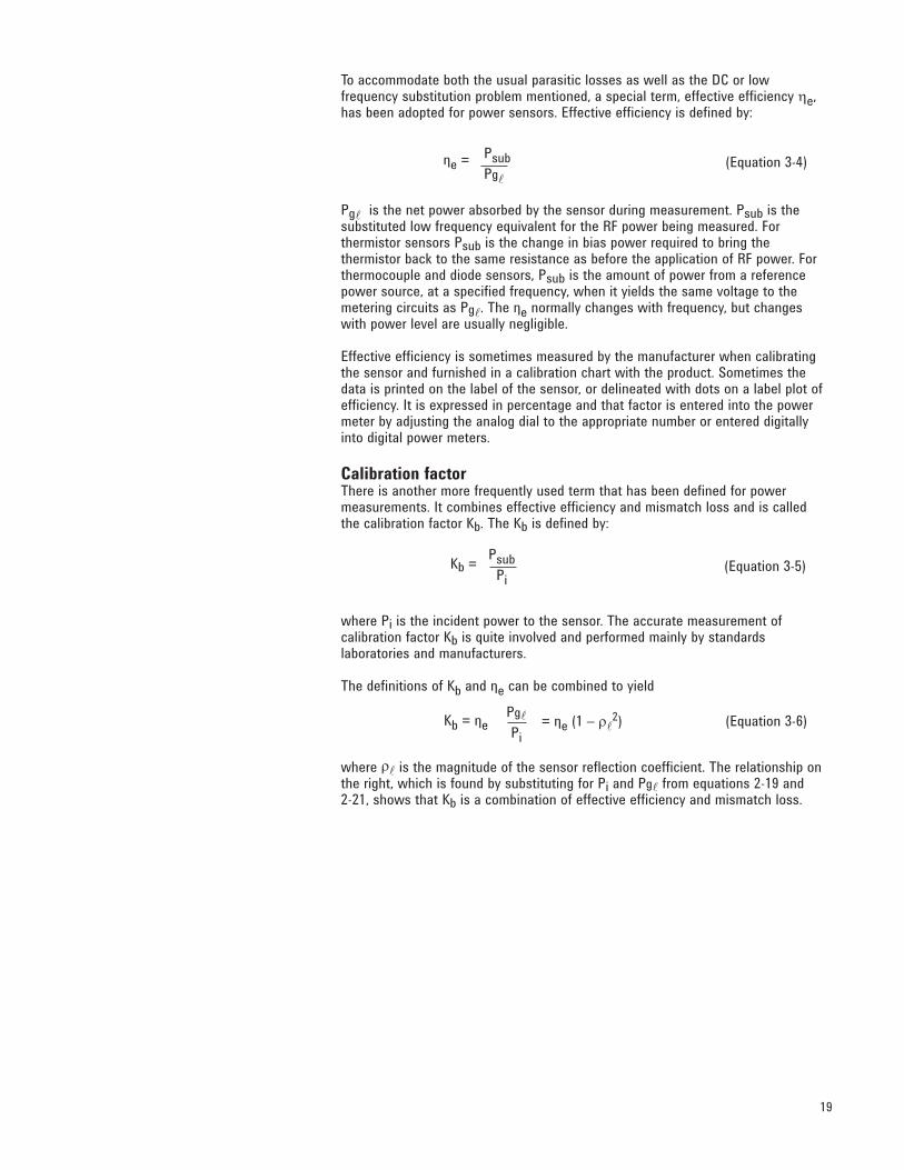
To accommodate both the usual parasitic losses as well as the DC or low frequency substitution problem mentioned, a special term, effective efficiency ηe, has been adopted for power sensors. Effective efficiency is defined by:

Pgl is the net power absorbed by the sensor during measurement. Psub is the substituted low frequency equivalent for the RF power being measured. For thermistor sensors Psub is the change in bias power required to bring the thermistor back to the same resistance as before the application of RF power. For thermocouple and diode sensors, Psub is the amount of power from a reference power source, at a specified frequency, when it yields the same voltage to the metering circuits as Pgl. The ηe normally changes with frequency, but changes with power level are usually negligible.

Effective efficiency is sometimes measured by the manufacturer when calibrating the sensor and furnished in a calibration chart with the product. Sometimes the data is printed on the label of the sensor, or delineated with dots on a label plot of efficiency. It is expressed in percentage and that factor is entered into the power meter by adjusting the analog dial to the appropriate number or entered digitally into digital power meters.

Calibration factorThere is another more frequently used term that has been defined for powermeasurements. It combines effective efficiency and mismatch loss and is calledthe calibration factor Kb. The Kb is defined by:

where Pi is the incident power to the sensor. The accurate measurement ofcalibration factor Kb is quite involved and performed mainly by standards laboratories and manufacturers.

The definitions of Kb and ηe can be combined to yield

where ρl is the magnitude of the sensor reflection coefficient. The relationship on the right, which is found by substituting for Pi and Pgl from equations 2-19 and 2-21, shows that Kb is a combination of effective efficiency and mismatch loss.

19

ηe = Psub

Pgl(Equation 3-4)

Kb = Psub

Pi(Equation 3-5)

Kb = ηePgl

Pi

(Equation 3-6)= ηe (1 – ρl2)

20

Most modern power meters have the ability to correct their meter reading by setting a dial or keying in a digital number to the proper value of Kb. Then Pi is actually read off the meter. Values of Kb for various frequencies are indicated on each Agilent power sensor (except for the E series sensors, which have the data stored on EEPROM). When this feature is used, the indicated or metered power Pm is (using Equation 2-19):

But the desired quantity is usually not Pi to the sensor but Pgzo, the power that would be dissipated in a Zo load. Since Pgzo is by definition |bs|2, the ratio of Pgzo to the meter indication is:

The right side of Equation 3-8 is the mismatch uncertainty. Since the use of Kb corrects for efficiency and mismatch loss, only the mismatch uncertainty remains. It should be pointed out that there is an additional, unavoidable uncertainty associated with Kb. That uncertainty is due to inaccuracies in the measurement of Kb by the manufacturer, NIST or standards laboratories and thus the uncertainty of Kb is specified by the calibration supplier.

Power meter instrumentation uncertainties (including sensor)There are a number of uncertainties associated within the electronics of the power meter. The effect of these errors is to create a difference between Pm and Psub/Kb.

Reference oscillator uncertaintyOpen-loop power measurements, such as those that use thermocouples or semiconductor diode sensors, require a known source of power to verify and adjust for the sensitivity of the sensor. Many power meters, such as the Agilent EPM and EPM-P, have a stable power reference built in. No matter what power reference is used, if it deviates from the expected power output, the calibration adjustment is in error. The uncertainty in the power output from the reference oscillator is specified by the manufacturer. Thermistor power measurements, being closed-loop and having no need for a reference oscillator, are free of this error.

Agilent has recently made improvements in the uncertainty specifications of the 50 MHz reference oscillator in all its power meters. It is now factory set to ±0.4 percent and traceable to the National Physical Laboratory of the UK. Expansion of the operating specification includes the following aging characteristics, which are now valid for 2 years:

Accuracy: (for 2 years)±0.5% (23 ±3 °C)±0.6% (25 ±10 °C) ±0.9% (0 to 55 °C)

Since the reference oscillator represents a reasonably large portion of the ultimate power measurement uncertainty budget, these smaller accuracy numbers in the specification lead to a lower overall measurement uncertainty. Another positive note is that the meters require less downtime in the calibration lab, now having a 2-year calibration cycle.

Pm =Pgzo

Kb

(Equation 3-7)= Pi =|bs|2

|1 – ΓgΓl|2

Pgzo

Pm(Equation 3-8) = |1 – ΓlΓg|2

Reference oscillator mismatch uncertaintyThe reference oscillator has its own reflection coefficient at the operating frequency. This source reflection coefficient, together with that from the power sensor, creates its own mismatch uncertainty. Because the reference oscillator frequency is low, where the reflection coefficients are small, this uncertainty is small (approximately ±0.01 dB or ±0.2 percent).

Instrumentation uncertaintyInstrumentation uncertainty is the combination of such factors as meter tracking errors, circuit nonlinearities, range-changing attenuator inaccuracy, and amplifier gain errors. The accumulated uncertainty is guaranteed by the instrument manufacturer to be within a certain limit.

There are other possible sources of uncertainty that are, by nature or design, so small as to be included within the instrumentation uncertainty.

An example of one such error is the thermoelectric voltage that may be introduced by temperature gradients within the electronic circuits and interconnecting cables. Proper design can minimize such effects by avoiding junctions of dissimilar metals at the most sensitive levels. Another example is the small uncertainty which might result from the operator’s interpolation of the meter indication.

Zero setIn any power measurement, the meter must initially be set to zero with no RF power applied to the sensor. Zero setting is usually accomplished within the power meter by introducing an offset voltage that forces the meter to read zero, by either analog or digital means. The offset voltage is contaminated by several sources including sensor and circuit noise. The zero set error is specified by the manufacturer, especially for the most sensitive range. On higher power ranges, error in zero setting is small in comparison to the signal being measured.

NoiseNoise is also known as short-term stability and it arises from sources within both the power sensor and circuitry. One cause of noise is the random motion of free electrons due to the finite temperature of the components. The power observation might be made at a time when this random fluctuation produces a maximum indication, or perhaps a minimum. Noise is specified as the change in meter indication over a short time interval (usually one minute) for a constant input power, constant temperature, and constant line voltage.

21

DriftThis is also called long-term stability and is mostly sensor induced. It is the change in meter indication over a long time (usually one hour) for a constant input power, constant temperature, and constant line voltage. The manufacturer may state a required warm-up interval. In most cases the drift is actually a drift in the zero setting. This means that for measurements on the upper ranges, drift contributes a very small amount to the total uncertainty. On the more sensitive ranges, drift can be reduced to a negligible level by zero setting immediately prior to making a reading.

Power linearityPower measurement linearity is mostly a characteristic of the sensor. Deviation from perfect linearity usually occurs in the higher power range of the sensor. For thermocouple sensors, linearity is negligible except for the top power range of +10 to +20 dBm, where the deviation is specified at ±3 percent.

For a typical Agilent 8481D Series diode sensor, the upper power range of –30 to –20 dBm exhibits a specified linearity deviation of ±1 percent.

With their much wider dynamic power range, the Agilent E Series sensors exhibit somewhat higher deviations from perfect linearity. It is mostly temperature-driven effect and specifications are given for several ranges of temperature. For example, in the 25 ±5 °C temperature range and the –70 to –10 dBm power range, the typical deviation from linearity is ±2 percent RSS.

[1] Lymer, Anthony, “Improving Measurement Accuracy by Controlling Mismatch Uncertainty.” TechOnLine, September 2002. website: www.techonline.com.

[2] Johnson, Russell A., “Understanding Microwave Power Splitters,” Microwave Journal, December 1975.

22

Calculating total uncertaintyIn Chapter 3, only the individual uncertainties were discussed; now a total uncertainty must be found. The first descriptions will use the traditional analysis for combining the individual uncertainty factors. These are usually termed the "worst case" and the "RSS (root sum of squares) methods."

Most attention will be devoted to the new international process based on the ISO process, to be described below, since the world’s test and measurement communities are converting over to a commonly agreed standard method.

Power measurement equationThe purpose of this section is to develop an equation that shows how a powermeter reading, Pm, is related to the power a generator would deliver to a Zo load, Pgzo (Figure 4-1). The equation will show how the individual uncertainties contribute to the difference between Pm and Pgzo.

Figure 4-1. Desired power output to be measured is Pgzo , but measurement results in the reading Pm.

Starting from the generator in the lower part of Figure 4-1, the first distinction is that the generator dissipates power Pgl in the power sensor instead of Pgzo because of mismatch effects. That relationship, from Equation 2-25 is:

The next distinction in Figure 4-1 is that the power sensor converts Pgl to the DC or low frequency equivalent, P sub, for eventual metering. However, this conversion is not perfect due to the fact that effective efficiency, ηe, is less than 100 percent. If Pgl is replaced by Psub/ηe from Equation 3-4, then Equation 4-1 becomes:

The first factor on the right is the mismatch uncertainty term, Mu, discussedpreviously. Mu is also referred to as "gain due to mismatch." The denominator of the second factor is the calibration factor Kb from Equation 3-6. Now Equation 4-2 can be written:

The last distinguishing feature of Figure 4-1 is that the meter indication Pm, differs from Psub. There are many possible sources of error in the power meter electronics that act like improper amplifier gain to the input signal Psub. These include uncertainty in range changing attenuators and calibration-factor amplifiers, imperfections in the metering circuit and other sources totaled as instrumentation uncertainty. For open-loop power measurements this also includes those uncertainties associated with the calibration of amplifier gain with a power-reference oscillator. These errors are included in the symbol m for magnification.

IV. Alternative Methods of Combining Power Measurement Uncertainties

(Equation 4-1)|1 – ΓlΓg|2

1 – |Γl|2Pgzo = Pgl

(Equation 4-2)1

ηe (1 – ρl2 )Pgzo = |1 – ΓlΓg|2 Psub

(Equation 4-3)1

KbPgzo = Mu Psub

23

24

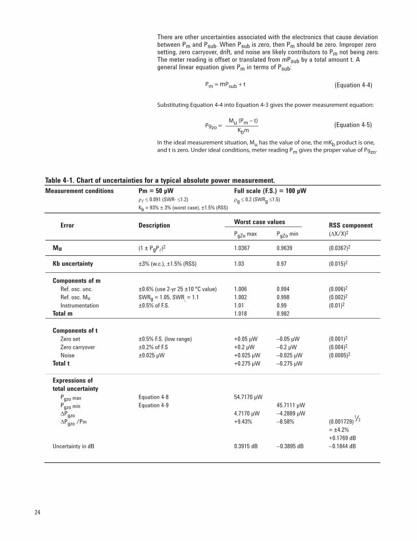
There are other uncertainties associated with the electronics that cause deviation between Pm and Psub. When Psub is zero, then Pm should be zero. Improper zero setting, zero carryover, drift, and noise are likely contributors to Pm not being zero. The meter reading is offset or translated from mPsub by a total amount t. A general linear equation gives Pm in terms of Psub:

Substituting Equation 4-4 into Equation 4-3 gives the power measurement equation:

In the ideal measurement situation, Mu has the value of one, the mKb product is one,

and t is zero. Under ideal conditions, meter reading Pm gives the proper value of Pgzo.

Table 4-1. Chart of uncertainties for a typical absolute power measurement.

Measurement conditions Pm = 50 µW Full scale (F.S.) = 100 µW

ρl ≤ 0.091 (SWR¯ ≤1.2) ρg ≤ 0.2 (SWRg ≤1.5)

Kb = 93% ± 3% (worst case), ±1.5% (RSS)

Error Description Worst case values

RSS component

PgZo max PgZo min (ΔX/X)2 Mu (1 ± PgPl)2 1.0367 0.9639 (0.0367)2

Kb uncertainty ±3% (w.c.), ±1.5% (RSS) 1.03 0.97 (0.015)2

Components of m Ref. osc. unc. ±0.6% (use 2-yr 25 ±10 °C value) 1.006 0.994 (0.006)2

Ref. osc. Mu SWRg = 1.05, SWR, = 1.1 1.002 0.998 (0.002)2

Instrumentation ±0.5% of F.S. 1.01 0.99 (0.01)2

Total m 1.018 0.982

Components of t

Zero set ±0.5% F.S. (low range) +0.05 µW –0.05 µW (0.001)2

Zero carryover ±0.2% of F.S +0.2 µW –0.2 µW (0.004)2

Noise ±0.025 µW +0.025 µW –0.025 µW (0.0005)2

Total t +0.275 µW –0.275 µW

Expressions of

total uncertainty

Pgzo max Equation 4-8 54.7170 µW Pgzo min Equation 4-9 45.7111 µW ΔPgzo 4.7170 µW –4.2889 µW ΔPgzo /Pm +9.43% –8.58% (0.001729) = ±4.2% +0.1769 dB Uncertainty in dB 0.3915 dB –0.3895 dB –0.1844 dB

(Equation 4-5)Mu (Pm – t)

KbmPgzo =

(Equation 4-4)Pm = mPsub + t

1/2

Worst-case uncertaintyOne method of combining uncertainties for power measurements in a worst-case manner is to add them linearly. This situation occurs if all the possible sources of error were at their extreme values and in such a direction as to add together constructively, and therefore achieve the maximum possible deviation between Pm and Pgzo. Table 4-1 is a chart of the various error terms for the power measurement of Figure 4-1. The measurement conditions listed at the top of Table 4-1 are taken as an example. The conditions and uncertainties listed are typical and the calculations are for illustration only. The calculations do not indicate what is possible using the most accurate technique. The description of most of the errors is from a manufacturer’s data sheet. Calculations are carried out to four decimal places because of calculation difficulties with several numbers of almost the same size.

Instrumentation uncertainty, i, is frequently specified in percent of full scale (full scale = Pfs). The contribution to magnification uncertainty is:

The several uncertainties that contribute to the total magnification uncertainty, m, combine like the gain of amplifiers in cascade. The minimum possible value of m occurs when each of the contributions to m is a minimum. The minimum value of m (0.9762) is the product of the individual factors (0.988 * 0.998 * 0.99). The factors that contribute to the total offset uncertainty, t, combine like voltage generators in series; that is, they add. Once t is found, the contribution in dB is calculated from:

The maximum possible value Pgzo using Equation 4-5 and substituting the values of Table 4-1, is:

In Equation 4-8, the deviation of Kbm from the ideal value of one is used to calculate Pgzo max. In the same way, the minimum value of Pgzo is:

25

(Equation 4-6)(1 + i) Pfs

Pmmi =

(Equation 4-7)t

PmtdB = 10 log (1 ± )

(Equation 4-8)Mu max (Pm – tmin)

Kb min mminPgzo max =

=1.0367 (50 µW + 0.275 µW)

(0.97) (0.982)

= 54.7170 µW = 1.0943 Pm

(Equation 4-9)Mu min (Pm – tmax)

Kb max mmaxPgzo min =

=0.9639 (50 µW – 0.275 µW)

(1.03) (1.018)

= 45.7111 µW = 0.9142 Pm

26

The uncertainty in Pgzo may be stated in several other ways:

(1) As an absolute differential in power:

(2) As a fractional deviation:

Figure 4-2. Graph of individual contributions to the total worst-case uncertainty.

(3) As a percent of the meter reading:

(4) As dB deviation from the meter reading:

An advantage to this last method of expressing uncertainty is that this number can also be found by summing the individual error factors expressed in dB.

Figure 4-2 is a graph of contributions to worst-case uncertainty shows that mismatch uncertainty is the largest single component of total uncertainty. This is typical of most power measurements. Magnification and offset uncertainties, the easiest to evaluate from specifications and often the only uncertainties evaluated, contribute less than one-third of the total uncertainty.

RSS uncertainty methodThe worst-case uncertainty is a very conservative approach. A more realistic method of combining uncertainties is the root-sum-of-the-squares (RSS) method. The RSS uncertainty is based on the fact that most of the errors of power measurement, although systematic and not random, are independent of each other. Since they are independent, it is reasonable to combine the individual uncertainties in an RSS manner.

(Equation 4-10)∆Pgzo = Pgzo –Pm = µWmaxmin

+4.7170

–4.2889

∆Pgzo

Pm=

+4.7170–4.2889

50

+0.0943

–0.0858= (Equation 4-11)

+0.5

+0.4

+0.3

+0.2

+0.1

0

Magnification

Calibration factor

Mismatch

Instrument

Ref OscOffset

ΔPgZo

Pm

∆Pgzo

Pm

+9.43

–8.58=

(Equation 4-12)%100 ×

+0.3915

–0.3895= (Equation 4-13)dB ( )1.0943

0.9142dB = 10 log

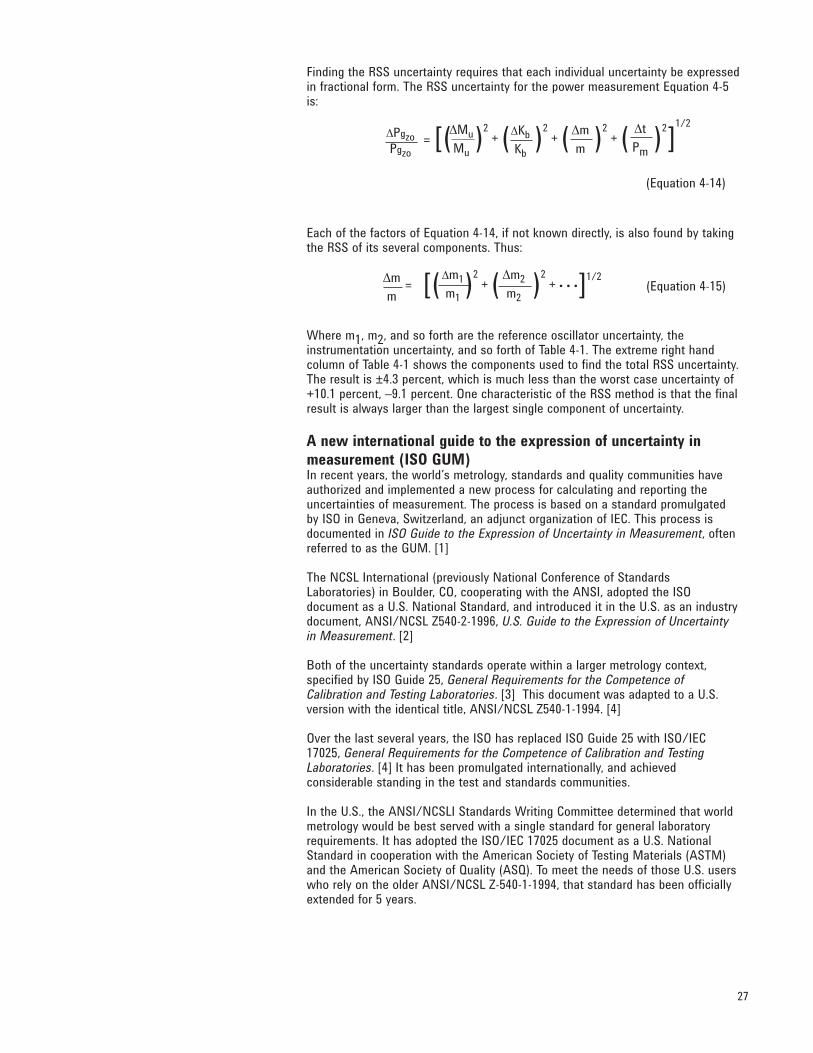
Finding the RSS uncertainty requires that each individual uncertainty be expressed in fractional form. The RSS uncertainty for the power measurement Equation 4-5 is:

Each of the factors of Equation 4-14, if not known directly, is also found by taking the RSS of its several components. Thus:

Where m1, m2, and so forth are the reference oscillator uncertainty, the instrumentation uncertainty, and so forth of Table 4-1. The extreme right hand column of Table 4-1 shows the components used to find the total RSS uncertainty. The result is ±4.3 percent, which is much less than the worst case uncertainty of +10.1 percent, –9.1 percent. One characteristic of the RSS method is that the final result is always larger than the largest single component of uncertainty.

A new international guide to the expression of uncertainty in measurement (ISO GUM)In recent years, the world’s metrology, standards and quality communities have authorized and implemented a new process for calculating and reporting the uncertainties of measurement. The process is based on a standard promulgated by ISO in Geneva, Switzerland, an adjunct organization of IEC. This process is documented in ISO Guide to the Expression of Uncertainty in Measurement, often referred to as the GUM. [1]

The NCSL International (previously National Conference of Standards Laboratories) in Boulder, CO, cooperating with the ANSI, adopted the ISO document as a U.S. National Standard, and introduced it in the U.S. as an industry document, ANSI/NCSL Z540-2-1996, U.S. Guide to the Expression of Uncertainty in Measurement. [2]

Both of the uncertainty standards operate within a larger metrology context, specified by ISO Guide 25, General Requirements for the Competence of Calibration and Testing Laboratories. [3] This document was adapted to a U.S. version with the identical title, ANSI/NCSL Z540-1-1994. [4]

Over the last several years, the ISO has replaced ISO Guide 25 with ISO/IEC 17025, General Requirements for the Competence of Calibration and Testing Laboratories. [4] It has been promulgated internationally, and achieved considerable standing in the test and standards communities.

In the U.S., the ANSI/NCSLI Standards Writing Committee determined that world metrology would be best served with a single standard for general laboratory requirements. It has adopted the ISO/IEC 17025 document as a U.S. National Standard in cooperation with the American Society of Testing Materials (ASTM) and the American Society of Quality (ASQ). To meet the needs of those U.S. users who rely on the older ANSI/NCSL Z-540-1-1994, that standard has been officially extended for 5 years.

∆PgzoPgzo

= [( )2 + ( )

2 + ( )

2 + ( )

2

]1/2

∆Mu

Mu

∆Kb

Kb

∆m

m

∆t

Pm

(Equation 4-14)

∆m

m= [( )

2 + ( )

2 + • • •]1/2∆m1

m1

∆m2

m2(Equation 4-15)

27

Because of its international scope of operations, Agilent has moved quickly to adopt ISO/IEC 17025 in lieu of its previous commitment to ANSI/NCSL Z-540-1. As a result, most of Agilent’s production and support operations are moving to offer optional product-specific test data reports compliant to 17025. Agilent has assigned Option 1A7 to all of its products which meet the ISO 17025-compliant processes. Option 1A7 will assure compliance with 17025 for new products shipped from the factory and Agilent will provide for support re-calibrations to the same 17025-compliant processes, data and testing.

Generally, the impact of the ISO GUM is to inject a little more rigor and standardization into the metrology analysis. Traditionally, an uncertainty was viewed as having two components, namely, a random component and a systematic component. Random uncertainty presumably arises from unpredictable or stochastic temporal and spatial variations of influence quantities. Systematic uncertainty arises from a recognized effect or an influence that can be quantified.

The ISO GUM groups uncertainty components into two categories based ontheir method of evaluation, Type A and Type B. These categories apply touncertainty, and are not substitutes for the words "random" and "systematic."Some systematic effects may be obtained by a Type A evaluation while in othercases by a Type B evaluation. Both types of evaluation are based on probabilitydistributions. The uncertainty components resulting from either type are quantified by variances or standard deviations.

Briefly, the estimated variance characterizing an uncertainty component obtained from a Type A evaluation is calculated from a series of repeated measurements and is the familiar statistically estimated variance. Since standards laboratories regularly maintain histories of measured variables data on their standards, such data would usually conform to the Type A definition.

For an uncertainty component obtained from a Type B evaluation, the estimated variance, u2, is evaluated using available knowledge. Type B evaluation is obtained from an assumed probability density function based on the belief that an event will occur, often called subjective probability, and is usually based on a pool of comparatively reliable information. Others might call it "measurement experience." Published data sheet specifications from a manufacturer would commonly fit the Type B definition.

Readers who are embarking on computing measurement uncertainties according to the ISO GUM should recognize that the above-mentioned documents may seem relatively simple enough in concept, and they are. But for more complex instrumentation the written specification uncertainties can often depend on multiple control settings and interacting signal conditions.

Impedance bridges, for example, measure parameters in complex number format. Network and spectrum analyzers have multi-layered specifications. Considerable attention is being expended by test and measurement organizations to define and characterize these important extensions of the basic GUM. [5, 6, 7]

28

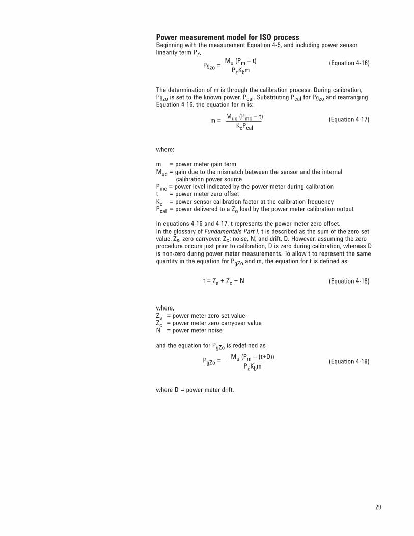
Power measurement model for ISO processBeginning with the measurement Equation 4-5, and including power sensor linearity term Pl,

The determination of m is through the calibration process. During calibration,Pgzo is set to the known power, Pcal. Substituting Pcal for Pgzo and rearranging Equation 4-16, the equation for m is:

where:

m = power meter gain termMuc = gain due to the mismatch between the sensor and the internal calibration power sourcePmc = power level indicated by the power meter during calibrationt = power meter zero offsetKc = power sensor calibration factor at the calibration frequencyPcal = power delivered to a Zo load by the power meter calibration output

In equations 4-16 and 4-17, t represents the power meter zero offset.In the glossary of Fundamentals Part I, t is described as the sum of the zero set value, Zs; zero carryover, Zc; noise, N; and drift, D. However, assuming the zero procedure occurs just prior to calibration, D is zero during calibration, whereas D is non-zero during power meter measurements. To allow t to represent the same quantity in the equation for PgZo and m, the equation for t is defined as:

where,Zs = power meter zero set valueZc = power meter zero carryover valueN = power meter noise

and the equation for PgZo is redefined as

where D = power meter drift.

29

(Equation 4-16)Mu (Pm – t)

PlKbmPgzo =

(Equation 4-17)Muc (Pmc – t)

KcPcalm =

(Equation 4-18)t = Zs + Zc + N

(Equation 4-19)Mu (Pm – (t+D))

PlKbmPgZo =

Equation 4-19 is the measurement equation for a power meter measurement. There are eleven input quantities that ultimately determine the estimated value of Pgzo. These are Mu, Pm, D, Kb from Equation 4-19; Zs, Zc, N from Equation 4-18; and Muc, Pmc, Kc, and P cal from Equation 4-17. It is possible to combine equations in order to represent Pgzo in terms of the 11 defined input quantities. This is a relatively complicated derivation, but the result is the uncertainty in terms of the 11 quantities:

Solving with some nominal values of several input quantities simplifies Equation 4-20,

Mu = 1Muc = 1Pmc = PcalZs = 0Zc = 0N = 0D = 0t = 0m = 1/Kc

The following Table 4-2 summarizes the various uncertainties shown in Equation 4-21.

30

(Equation 4-20)

u2 (Mu)

Mu2

u2(Pgzo) = Pgzo2 [ +

u2 (Pm)

(Pm– (t + D))2+

u2 (D)

(Pm– (t + D))2+

u2 (Kb)

Kb2

+u2

(Muc)

Muc2

+u2

(Pmc)

(Pmc– t)2+

u2 (Kc)

Kc2

+u2

(Pcal)

Pcal2

+ ( ( )1

(Pm– (t+D))2+

1

(Pmc– t)2–

2

KcPcalm(Pm– (t+D))) u2 (Zs) + u2 (Zc) + u2(N)

(Equation 4-21)

u2 (Mu)u2(Pgzo)

Pgzo2

+ u2 (Pm)

Pm2

+ + u2 (Kb)

Kb2

+ u2 (Pmc)

Pmc2

+u2

(Kc)

Kc2 +

u2 (Pcal)

Pcal2

( 1

Pm–

1

Pcal)

2(u2(Zs) + u2(Zc) + u2(N))

u2 (D)

Pm2

u2 (Muc)

+

+

u2 (Pl)

Pl2

=

+

]

31

Standard uncertainty of the mismatch modelThe standard uncertainty of the mismatch expression, u(Mu), assuming noknowledge of the phase, depends upon the statistical distribution that bestrepresents the moduli of Γg and Γl.

Combining equations 2-21 and 2-22, the power dissipated in a load whenΓl is not 0 is:

The numerator in Equation 4-22 is known as mismatch loss, and the denominator represents the mismatch uncertainty:

Mu is the gain or loss due to multiple reflections between the generator andthe load. If both the moduli and phase angles of Γg and Γl are known, Mu can be precisely determined from Equation 4-23. Generally, an estimate of the moduli exists, but the phase angles of Γg and Γl are not known.

Table 4-2. Standard uncertainties for the Z540-2 process.

Standard uncertainty Source u(Mu) Mismatch gain uncertainty between the sensor and the generator. The standard uncertainty is dependent upon the reflection coefficients of the sensor and the generator. Refer to the mismatch model. Reflection coefficients may have different distributions as shown in Figure 4-3.

u(Muc) Mismatch gain uncertainty between the sensor and the calibrator output of the power meter. The standard uncertainty is dependent upon the reflection coefficients of the sensor and the calibrator output. Refer to the mismatch model. Note: the calibrator output reflection coefficient is not a specified parameter of the E4418A power meter. AN64-1 suggests ρg = 0.024.

u(Pm) Power meter instrumentation uncertainty.

u(Pmc) Power meter instrumentation uncertainty (during calibration)

u(D) Power meter drift uncertainty.

u(Kb) Sensor calibration factor uncertainty. Typically, the value of the uncertainty is reported along with the calibration factor by the calibration laboratory or the manufacturer.

u(Kc) Sensor calibration factor uncertainty at the frequency of the power meter calibrator output. If the sensor is calibrated relative to the associated calibrator output frequency, Kc = 1 and u(Kc) = 0.

u(Pl) Power sensor linearity, which is related to power range. Generally negligible on lower ranges but has higher uncertainty at high power levels.

u(Pcal) Calibrator output power level uncertainty.

u(Zs) Power meter zero set uncertainty.

u(Zc) Power meter zero carryover uncertainty. u(N) Power meter and sensor noise uncertainty.

Pd = Pgzo (Equation 4-22)1 – |Γl|2

|1 – Γg Γl|2

(Equation 4-23)|1 – Γg Γl|2Mu =

32

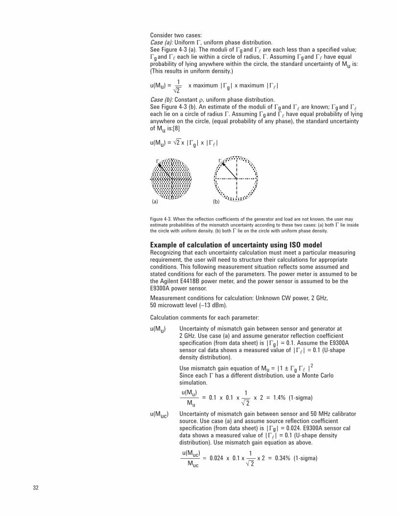
Consider two cases:Case (a): Uniform Γ, uniform phase distribution.See Figure 4-3 (a). The moduli of Γg and Γl are each less than a specified value;Γg and Γl each lie within a circle of radius, Γ. Assuming Γg and Γl have equalprobability of lying anywhere within the circle, the standard uncertainty of Mu is: (This results in uniform density.)

1u(Mu) =

√2 x maximum |Γg| x maximum |Γl|

Case (b): Constant ρ, uniform phase distribution.See Figure 4-3 (b). An estimate of the moduli of Γg and Γl are known; Γg and Γleach lie on a circle of radius Γ. Assuming Γg and Γl have equal probability of lying anywhere on the circle, (equal probability of any phase), the standard uncertainty of Mu is:[8]

u(Mu) = √2 x |Γg| x |Γl|

Figure 4-3. When the reflection coefficients of the generator and load are not known, the user may estimate probabilities of the mismatch uncertainty according to these two cases: (a) both Γ lie inside the circle with uniform density. (b) both Γ lie on the circle with uniform phase density.

Example of calculation of uncertainty using ISO modelRecognizing that each uncertainty calculation must meet a particular measuring requirement, the user will need to structure their calculations for appropriate conditions. This following measurement situation reflects some assumed and stated conditions for each of the parameters. The power meter is assumed to be the Agilent E4418B power meter, and the power sensor is assumed to be the E9300A power sensor.

Measurement conditions for calculation: Unknown CW power, 2 GHz, 50 microwatt level (–13 dBm).

Calculation comments for each parameter:

u(Mu) Uncertainty of mismatch gain between sensor and generator at 2 GHz. Use case (a) and assume generator reflection coefficient specification (from data sheet) is |Γg| = 0.1. Assume the E9300A sensor cal data shows a measured value of |Γl| = 0.1 (U-shape density distribution).

Use mismatch gain equation of Mu = |1 ± Γg Γl |2

Since each Γ has a different distribution, use a Monte Carlo simulation.

u(Muc) Uncertainty of mismatch gain between sensor and 50 MHz calibrator source. Use case (a) and assume source reflection coefficient specification (from data sheet) is |Γg| = 0.024. E9300A sensor cal data shows a measured value of |Γl| = 0.1 (U-shape density distribution). Use mismatch gain equation as above.

Γ Γ

(a) (b)

= 0.1 x 0.1 x x 2 = 1.4% (1-sigma) 1

√ 2

u(Mu)

Mu

= 0.024 x 0.1 x x 2 = 0.34% (1-sigma) 1

√ 2

u(Muc)

Muc

33

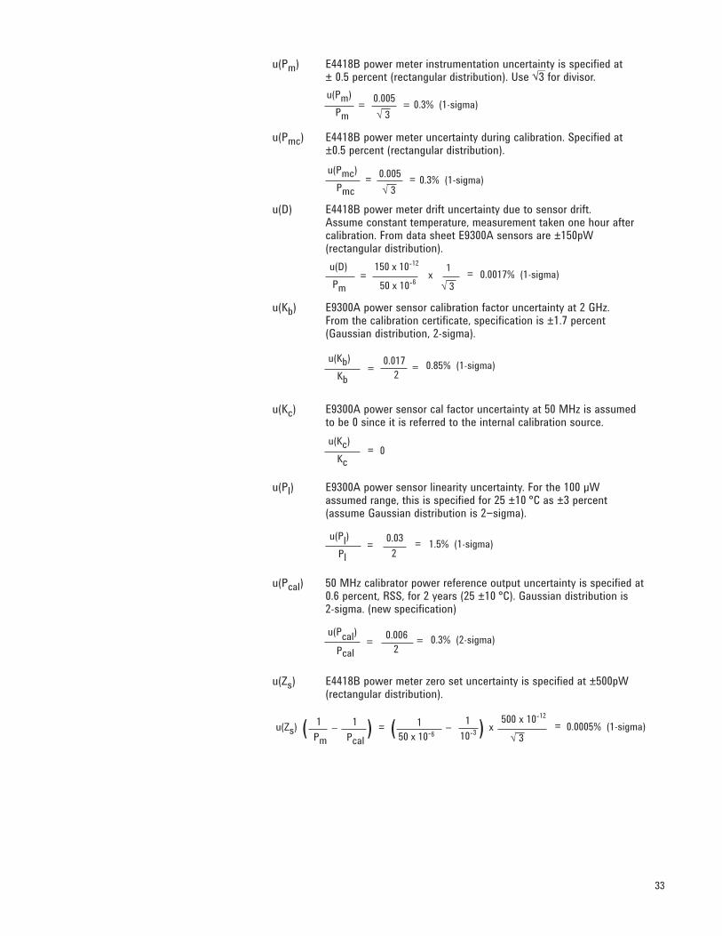
u(Pm) E4418B power meter instrumentation uncertainty is specified at ± 0.5 percent (rectangular distribution). Use 3 for divisor.

u(Pmc) E4418B power meter uncertainty during calibration. Specified at ±0.5 percent (rectangular distribution).

u(D) E4418B power meter drift uncertainty due to sensor drift. Assume constant temperature, measurement taken one hour after calibration. From data sheet E9300A sensors are ±150pW (rectangular distribution).

u(Kb) E9300A power sensor calibration factor uncertainty at 2 GHz. From the calibration certificate, specification is ±1.7 percent (Gaussian distribution, 2-sigma).

u(Kc) E9300A power sensor cal factor uncertainty at 50 MHz is assumed to be 0 since it is referred to the internal calibration source.

u(Pl) E9300A power sensor linearity uncertainty. For the 100 µW assumed range, this is specified for 25 ±10 °C as ±3 percent (assume Gaussian distribution is 2−sigma).

u(Pcal) 50 MHz calibrator power reference output uncertainty is specified at 0.6 percent, RSS, for 2 years (25 ±10 °C). Gaussian distribution is 2-sigma. (new specification)

u(Zs) E4418B power meter zero set uncertainty is specified at ±500pW (rectangular distribution).

u(Pl)

Pl

0.03

2= = 1.5% (1-sigma)

u(Pcal)

Pcal

0.006

2= = 0.3% (2-sigma)

u(Kc)

Kc= 0

u(Kb)

Kb=

0.017

2= 0.85% (1-sigma)

=150 x 10-12

50 x 10-6

1

√ 3x = 0.0017% (1-sigma)

u(D)

Pm

u(Pm)

Pm

0.005

√ 3 = 0.3% (1-sigma) =

u(Pmc)

Pmc

0.005

√ 3 = 0.3% (1-sigma) =

1

Pm

=( ) ( ) u(Zs) 1

50 x 10-6x

500 x 10-12

√ 3= 0.0005% (1-sigma)

1

Pcal

– 1

10-3–

u(Zc) E4418B power meter zero carryover is included in the overall instrument uncertainty specification, since there are no ranges as such in this meter. For other power meters this would need to be considered.

u(N) E4418B power meter noise uncertainty is ±700 pW and negligible at the 50 mW power level.

Using the above comments, Table 4-3 summarizes the various uncertainty factors. Each factor is normalized to a one sigma value. In the case of a data sheet specification, the divisor factor used to convert to one sigma is square root of three. These sigma values are added in RSS fashion and then multiplied with the coverage factor. The coverage factor is a guard band number, typically two is used, but experience and knowledge of the measurement process allows for the user to establish any other value.

34

Symbol Source of uncertainty Value ±% Probability distribution Divisor D(Kx)

Mu Mismatch gain between |Γg| = 0.1 U-shape density √ 2 1.4% generator and sensor |Γs| = 0.1 Muc Mismatch gain between |Γg| = 0.024 √ 2 0.34% calibration source and sensor |Γs| = 0.1 U-shape density Pm Power meter instrumentation 0.5% rectangular √ 3 0.29% Pmc Power meter instrumentation 0.5% rectangular √ 3 0.29% during calibration D Power meter drift ±150 pW rectangular √ 3 0.017% Kb Sensor calibration factor 1.7% Gaussian 2 0.85% Kc Sensor calibration factor at 50 MHz 0 rectangular — 0

Pl Power sensor linearity 3.0% Gaussian 2 1.5%

Pcal Calibrator output power 0.6% Gaussian 2 0.3%

Zs Power meter zero set ±500 pW rectangular √ 3 0.0005%

Zc Power meter zero carryover 0 rectangular √ 3 0

N Power meter and sensor noise ±700 pW rectangular √ 3 0.0007%

Combined uncertainty—RSSed 2.30%

Expanded uncertainty Coverage factor K = 2 4.61%

Table 4-3. Worksheet for uncertainties calculation using ISO process.

(1) Monte Carlo simulation

1

Pm

=( ) ( ) u(N) 1

50 x 10-6x

700 x 10-12

√ 3= 0.0007% (1-sigma)

1

Pcal

– 1

10-3–

1

Pm

1

Pcal

= 0( ) u(Zc) –

35

Example of calculation of uncertainty of USB sensor using ISO modelThere will be some differences in measurement uncertainty calculations when using the U2000A series USB power sensors instead of the usual power meter and power sensor combination as shown in the following example.

Let us assume the power sensor to be a U2000A power sensor, taking the same measurement conditions for the following calculations: Unknown CW power, 2 GHz, 50 microwatt level (–13 dBm).

Calculation comments for each parameter:

u(Mu) Uncertainty of mismatch gain between sensor and generator at 2 GHz. Assume generator reflection coefficient specification (from data sheet) is|Γg| = 0.111 (U-shape density distribution). The U2000A sensor cal data shows a measured value of |Γl| = 0.087 (U-shape density distribution).

u(Mu)

Mu

u(Muc) Uncertainty of mismatch gain between sensor and 50 MHz calibrator source is not applicable in this case because of the absence of the 50 MHz calibrator.

u(Pm) U2000A power sensor will measure power without involving power meter. Therefore, power meter instrumentation uncertainty is irrelevant and not applicable.

u(Pmc) U2000A power meter uncertainty calibration does not apply for similar reason.

u(D) U2000A power sensor drift uncertainty. Let us assume constant temperature, measurement taken within one hour after zero set and after 24-hour warm-up of the power sensor. Then from the datasheet, U2000A sensor zero drift is ±1.5 nW (rectangular distribution).

u(D)

Pm

u(Kb) U2000A power sensor calibration factor uncertainty at 2 GHz. From the datasheet, the specification is ±2.0 percent (Gaussian distribution, 2-sigma).

u(Kc) No calibration is required for the U2000A as there will not be any sensor-meter path loss calibration.

u(Pa) U2000A power sensor absolute power uncertainty. This uncertainty includes calibration uncertainties of reference power and linearity. The specification at –13 dBm is ±3 percent when operated within 25 ±10 °C (assume Gaussian distribution is 2−sigma).

= 0.111 x 0.087 x x 2 = 1.3633% 1

√ 2

=1.5 x 10-9

50 x 10-6

1

√ 3x = 0.0017%

u(Kb)

Kb=

0.02

2= 1.0000%

u(Pa)

Pa

0.03

2= = 1.5000%

36

u(Pcal) There is no 50 MHz calibration for the U2000A. Therefore, there is no uncertainty contributed.

u(Zs) U2000A power sensor internal zero set uncertainty is specified at ±12nW (rectangular distribution).

u(Zc) Usage of U2000A does not require a power meter. Therefore, there is no power meter zero carry over.

u(N) U2000A power sensor noise uncertainty is ±15 nW (rectangular distribution). Assume number of averages is set to 16 and hence, the noise multiplier is one.

Using the above comments, Table 4-4 summarizes the various uncertainty factors.

Symbol Source of uncertainty Value ±% Probability distribution Divisor D(Kx)

Mu Mismatch gain between |Γg| = 0.111 U-shape density √ 2 1.3633% generator and sensor |Γs| = 0.087 D Power meter drift ±1.5 nW rectangular √ 3 0.0017%

Kb Sensor calibration factor 1.7% Gaussian 2 1.0000% Pa Power sensor absolute power 3.0% Gaussian 2 1.5%

Zs Power meter zero set ±12 nW rectangular √ 3 0.0138%

N Power meter and sensor noise ±15 nW rectangular √ 3 0.0173%

Combined uncertainty—RSSed 2.26%

Expanded uncertainty Coverage factor K = 2 4.52%

Table 4-4. Worksheet for uncertainties calculation of USB sensor using ISO process.

1

50 x 10-6

12 x 10-9

√ 3x = 0.0138%

1

Pm

u(Zs) ( ) =

1

50 x 10-6

15 x 10-9

√ 3x = 0.0173%

1

Pm

u(N) ( )=

37

[1] "ISO Guide to the Expression of Uncertainty in Measurement," International Organization for Standardization, Geneva, Switzerland, ISBN 92-67-10188-9, 1995.

[2] "U.S. Guide to the Expression of Uncertainty in Measurement," ANSI/NCSL Z540-2-1996, NCSL International, Boulder, CO.

[3] ISO Guide 2, "General Requirements for the Competence of Calibration and Testing Laboratories," ISO Guide 25, International Organization for Standardization, Geneva, Switzerland. This same title now applies to ISO/IEC EN 17025.

[4] "General Requirements for the Competence of Calibration and Testing Laboratories," ANSI/NCSL Z540-1-1994, NCSL International, Boulder, CO.

[5] Moens, Jon C. "Software Technology to Support Measurement Uncertainty for Complex Electronic Test Equipment," NCSLI 2002 San Diego Conference, NCSL International, Boulder, CO.

[6] Kasuga, Makoto, "Adapting The ISO GUM For A Practical Approach To Uncertainty Calculation Of Complex Numbers," NCSLI 2002 San Diego Conference, NCSL International, Boulder, CO.

[7] Abell, David and Moens, Jon C., "Meeting ISO 17025 Requirements for Complex Electronic Test Equipment," Cal Lab Magazine, Oct/Dec, 2002.

[8] Harris, I.A., and Warner, F.L., "Re-examination of Mismatch Uncertainty when Measuring Microwave Power and Attenuation," Proceedings of the British IEE, Vol. 128, pp 35-41, Feb 1981.

General References

NAMAS NIS 3003, "The Expression of Uncertainty and confidence in Measurement for Calibrations," Edition 8, NAMAS Executive, National Physical Laboratory, Teddington, TW11 0LW, England, 1995.

B. N. Taylor and C. E. Kuyatt, "Guidelines for Evaluating and Expressing the Uncertainty of NIST Measurement Results," NIST Technical Note 1297, National Institute of Standards and Technology.

NCSL Recommended Practice RP-12, "Determining and Reporting Measurement Uncertainties," National Conference of Standards Laboratories.

Agilent Technologies’ Test and Measurement Support, Services, and Assistance

Agilent Technologies aims to maximize the value you receive, while minimizing your risk and problems. We strive to ensure that you get the test and measurement capabilities you paid for and obtain the support you need. Our extensive support resources and services can help you choose the right Agilent products for your applications and apply them successfully. Every instrument and system we sell has a global warranty. Support is available for at least five years beyond the production life of the product. Two concepts underlie Agilent’s overall support policy: "Our Promise" and "Your Advantage."

Our Promise

Our Promise means your Agilent test and measurement equipment will meet its advertised performance and functionality. When you are choosing new equipment, we will help you with product information, including realistic performance specifications and practical recommendations from experienced test engineers. When you use Agilent equipment, we can verify that it works properly, help with product operation, and provide bas ic measurement assistance for the use of specified capabilities, at no extra cost upon request. Many self-help tools are available.

Your Advantage

Your Advantage means that Agilent offers a wide range of additional expert test and measurement services, which you can purchase according to your unique technical and business needs. Solve problems efficiently and gain a competitive edge by contracting with us for calibration, extra-cost upgrades, out-of-warranty repairs, and onsite education and training, as well as design, system integration, project management, and other professional engineering services. Experienced Agilent engineers and technicians worldwide can help you maximize your productivity, optimize the return on investment of your Agilent instruments and systems, and obtain dependable measurement accuracy for the life of those products.

www.agilent.com/find/emailupdatesGet the latest information on the products and applications you select.

Agilent T&M Software and Connectivity

Agilent’s Test and Measurement software and connectivity products, solutions and developer network allows you to take time out of connecting your instruments to your computer with tools based on PC standards, so you can focus on your tasks, not on your connections. Visit www.agilent.com/find/connectivity for more information.

By internet, phone, or fax, get assistance with all your test & measurement needs

Online Assistance:

www.agilent.com/find/assist

Product specifications and descriptions in this document subject to change without notice.

© Agilent Technologies, Inc. 2009Printed in USA June 5, 2009

5988-9215EN

Phone or Fax

United States:

(tel) 800 452 4844Canada:

(tel) 877 894 4414(fax) 905 282 6495China:

(tel) 800 810 0189(fax) 800 820 2816Europe:

(tel) (31 20) 547 2323(fax) (31 20) 547 2390Japan:

(tel) (81) 426 56 7832(fax) (81) 426 56 7840

Korea:

(tel) (82 2) 2004 5004 (fax) (82 2) 2004 5115Latin America:

(tel) (305) 269 7500(fax) (305) 269 7599Taiwan:(tel) 0800 047 866 (fax) 0800 286 331Other Asia Pacific Countries:

(tel) (65) 6375 8100 (fax) (65) 6836 0252Email: tm_asia@agilent.com

Agilent Email Updates

Bluetooth is a trademark owned by Bluetooth SIG, Inc., U.S.A. and licensed to Agilent Technologies, Inc.