aggregation operator for assignment of resources...

(IJACSA) International Journal of Advanced Computer Science and Applications,

Vol. 8, No. 10, 2017

406 | P a g e

www.ijacsa.thesai.org

Aggregation Operator for Assignment of Resources in

Distributed Systems

David L. la Red Martínez

Northeastern National University,

Corrientes, Argentine

Abstract—In distributed processing systems it is often

necessary to coordinate the allocation of shared resources that

should be assigned to processes in the modality of mutual

exclusion; in such cases, the order in which the shared resources

will be assigned to processes that require them must be decided;

in this paper we propose an aggregation operator (which could

be used by a shared resources manager module) that will decide

the order of allocation of the resources to the processes

considering the requirements of the processes (shared resources)

and the state of the distributed nodes where the processes operate

(their computational load).

Keywords—Aggregation operators; concurrency control;

communication between groups of processes; mutual exclusion;

operating systems; processor scheduling

I. INTRODUCTION

The proliferation of computer systems, many of them distributed in different nodes with multiple processes that cooperate for the achievement of a particular function, require decision models that allow groups of processes to use shared resources that can only be accessed in the modality of mutual exclusion.

The traditional solutions for this problem are found in [1] and [2], which describe the main synchronization algorithms in distributed systems; in [3], it presents an efficient and fault tolerant solution for the problem of distributed mutual exclusion; in [4]-[6], which present algorithms to manage the mutual exclusion in computer networks; in [7], which details the main algorithms for distributed process management, distributed global states and distributed mutual exclusion.

In addition, a reliable communication protocol in the presence of faults is presented in [8]. In [9] a multicast communication protocol is presented for groups of processes in the atomic mode, [10] study technologies, web services and applications of reliable distributed systems; in [11] reliable communication protocols are presented in broadcast mode; in [12] the main communication algorithms in distributed systems are described, [13] describes a network architecture for large-scale virtual environments to support communication between groups of distributed processes, and in [14] the main algorithms of distributed coordination and management of the mutual exclusion.

Similarly, in [15] the communication between groups of processes is analyzed in depth, analyzing protocols such as FLIP: Fast Local Internet Protocol and BP: Broadcast Protocol, analyzing reliable and efficient group

communication, parallel programming, the fault-tolerant programming using broadcasting and proposing a three-level architecture, the lower one for FLIP protocol, the medium for communication in groups of processes and the upper one for the applications. Additional information can be found in [16].

Also, solutions (which may be considered classic or traditional) have been proposed for very different types of systems distributed in [17]-[21]. Other works focused on ensuring mutual exclusion have been presented in [22] and [23]. An interesting distributed solution based on permissions is presented in [24] and a solution based on process priorities in [25].

The traditional solutions for the allocation of shared resources distributed in the modality of mutual exclusion are concentrated on guaranteeing mutual exclusion, without considering the computational load on the nodes where the processes operate and the impact that will create on the access to the shared resources requested by the processes in the context of such load.

However, this allocation of resources in processes should be performed taking into account the priorities of the processes and also the current workload of the computational nodes on which the processes are executed.

The new decision models for allocating shared resources could be executed in the context of a shared resource manager for the distributed system, which would receive the shared resource requirements of the processes running on the different distributed nodes, as well as the computational load state of the nodes and, considering that information, the order (priority) of allocation of the requested resources for the requesting processes should be decided on. Consequently, there is a need for specially designed aggregation operators.

In this paper, a new aggregation operator will be presented specifically for the aforementioned problem. This falls under the category of OWA (Ordered Weighted Averaging) operators, and more specifically Neat OWA.

The use of aggregation operators in group decision models has been extensively studied, for example, in [26] a group decision model is presented with the use of aggregation operators of the OWA family; in [27] the use of OWA aggregation operators (Ordered Weighted Averaging) for decision making is presented; in [28] methodologies are introduced to solve problems in the presence of multiple attributes and criteria and in [29] the way of obtaining a collective priority vector is studied, which is created from


Vol. 8, No. 10, 2017

407 | P a g e


different formats of expression of the preferences of the decision makers. The model can reduce the complexity of decision making and avoid the loss of information when the different formats are transformed into a unique format of expression of the preferences.

Also, in [30]-[32] several aggregation operators that can be used to make decisions in groups are presented; in [33] the operator WKC-OWA is presented to add information on problems of democratic decision; in [34] a group decision model is presented with the use of linguistic tags and a new form for expression of the preferences of the decision makers; in [35] the main mathematical properties and behavioral measures related to aggregation operators are presented; in [36] a review about aggregation operators, especially those of the OWA family is presented; in [37]-[39] majority aggregation operators and their possible applications to group decision making are analyzed; in [40] and [41] the OWA (Ordered Weighted Averaging) operators applied to multicriteria decision making are presented and analyzed, and in [42] and [43] the OWA operators and their applications in the Multi-agent decision making are discussed.

In turn, in [44] the connection of the linguistic hierarchy and the numerical scale for the 2-tuple linguistic model and its use to treat unbalanced linguistic information is studied; in [45] a complex and dynamic problem of group decision making with multiple attributes is defined and a resolution method that uses a consensus process for groups of attributes, alternatives and preferences, resulting in a decision model for real-world problems is proposed.

This article, which will present an innovative method for shared resource management in distributed systems, has been structured as follows: Section 2 will explain the data structures to be used by the proposed operator, in Section 3 the aggregation operator is described, Section 4 will show a detailed example of this, then the Conclusions and Future Work Lines will be presented, ending with the Acknowledgments and References.

II. DATA STRUCTURES TO BE USED

The following premises and data structures will be used.

You have groups of processes distributed in process nodes that access critical resources. These resources are shared in the form of distributed mutual exclusion and it must be decided, according to the demand for resources by the processes, what the priorities to allocate the resources to the processes that require them will be (only the available resources that have not yet been allocated to processes will need to be considered):

The access permission to the shared resources of a node will not only depend on whether the nodes are using them or not, but on the aggregation value of the preferences (priorities) of the different nodes regarding granting access to shared resources (alternatives) as well.

The opinions (priorities) of the different nodes regarding granting access to shared resources (alternatives) will depend on the consideration of the

value of variables that represent the state of each of the different nodes. Each node must express its priorities for assigning the different shared resources according to the resource requirements of each process (which may be part of a group of processes).

Nodes hosting processes: 1, …. , n. The set of nodes is represented as follows:

Nodes = {n1, …. , nn}

Processes housed in each of the n nodes: 1, …. , p. The set of processes is represented as follows:

Processes = {pij} with i = 1, …, n (number of nodes in the distributed system) and j = 1, …, p (maximum number of processes in each node), which can be expressed by the Table 1.

TABLE I. PROCESSES AT EACH NODE

Nodes Processes 1 p11 p12 …. p1p

…. …. …. … ….

i pi1 pi2 …. pip

…. …. …. … ….

n pn1 pn2 …. pnp

Distributed process Groups: 1, …. , g. The set of distributed process groups is represented as follows:

Groups = {pij} with i indicating the node and j the process in this node.

Size of each of the g process groups. The number of processes in each group indicates the group's cardinality and is represented as follows:

Card = {card(gi)} with i = 1, …, g indicating the group.

Group priority of each of the g processes groups. These priorities can be set according to different criteria; in this proposal, it will be considered to be a function of the cardinality of each group and is represented as follows:

prg = {prgi = card(gi)} with i = 1, …, g indicating the group.

Shared resources in distributed mutual exclusion mode available on n nodes: 1, …., r. The set of resources is represented as follows:

Resources = {rij} with i = 1, …, n (number of nodes in the distributed system) and j = 1, …, r (maximum number of resources at each node), which can be expressed by Table 2.

TABLE II. SHARED RESOURCES AVAILABLE AT EACH NODE

Nodes Resources 1 r11 r12 …. r1r

…. …. …. … ….

i ri1 ri2 …. rir

…. …. …. … ….

n rn1 rn2 …. rnr

These available shared resources hosted on different nodes of the distributed system may be required by the processes (clustered or independent) running on the nodes; these requests for resources by the processes are shown in Table 3.


Vol. 8, No. 10, 2017

408 | P a g e


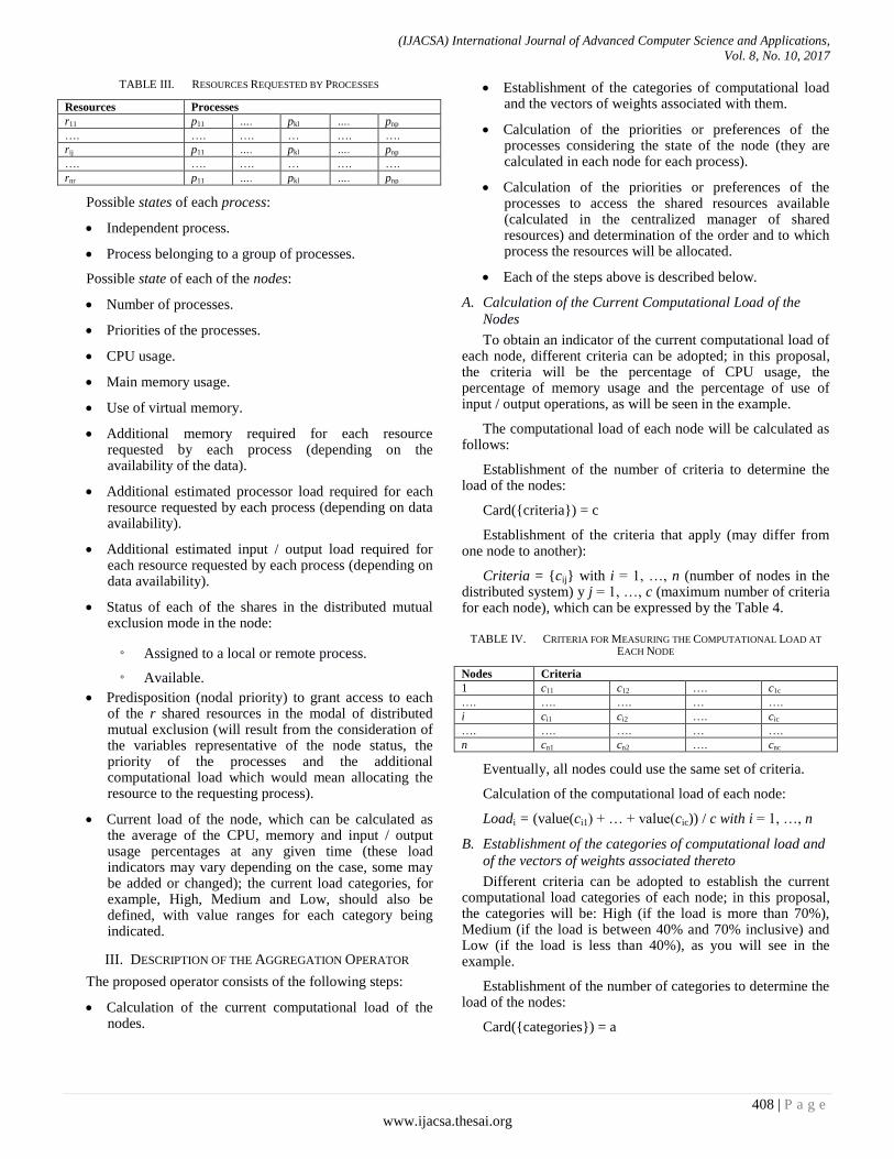
TABLE III. RESOURCES REQUESTED BY PROCESSES

Resources Processes r11 p11 …. pkl …. pnp

…. …. …. … …. ….

rij p11 …. pkl …. pnp

…. …. …. … …. ….

rnr p11 …. pkl …. pnp

Possible states of each process:

Independent process.

Process belonging to a group of processes.

Possible state of each of the nodes:

Number of processes.

Priorities of the processes.

CPU usage.

Main memory usage.

Use of virtual memory.

Additional memory required for each resource requested by each process (depending on the availability of the data).

Additional estimated processor load required for each resource requested by each process (depending on data availability).

Additional estimated input / output load required for each resource requested by each process (depending on data availability).

Status of each of the shares in the distributed mutual exclusion mode in the node:

◦ Assigned to a local or remote process.

◦ Available.

Predisposition (nodal priority) to grant access to each of the r shared resources in the modal of distributed mutual exclusion (will result from the consideration of the variables representative of the node status, the priority of the processes and the additional computational load which would mean allocating the resource to the requesting process).

Current load of the node, which can be calculated as the average of the CPU, memory and input / output usage percentages at any given time (these load indicators may vary depending on the case, some may be added or changed); the current load categories, for example, High, Medium and Low, should also be defined, with value ranges for each category being indicated.

III. DESCRIPTION OF THE AGGREGATION OPERATOR

The proposed operator consists of the following steps:

Calculation of the current computational load of the nodes.

Establishment of the categories of computational load and the vectors of weights associated with them.

Calculation of the priorities or preferences of the processes considering the state of the node (they are calculated in each node for each process).

Calculation of the priorities or preferences of the processes to access the shared resources available (calculated in the centralized manager of shared resources) and determination of the order and to which process the resources will be allocated.

Each of the steps above is described below.

A. Calculation of the Current Computational Load of the

Nodes

To obtain an indicator of the current computational load of each node, different criteria can be adopted; in this proposal, the criteria will be the percentage of CPU usage, the percentage of memory usage and the percentage of use of input / output operations, as will be seen in the example.

The computational load of each node will be calculated as follows:

Establishment of the number of criteria to determine the load of the nodes:

Card({criteria}) = c

Establishment of the criteria that apply (may differ from one node to another):

Criteria = {cij} with i = 1, …, n (number of nodes in the distributed system) y j = 1, …, c (maximum number of criteria for each node), which can be expressed by the Table 4.

TABLE IV. CRITERIA FOR MEASURING THE COMPUTATIONAL LOAD AT

EACH NODE

Nodes Criteria

1 c11 c12 …. c1c

…. …. …. … ….

i ci1 ci2 …. cic

…. …. …. … ….

n cn1 cn2 …. cnc

Eventually, all nodes could use the same set of criteria.

Calculation of the computational load of each node:

Loadi = (value(ci1) + … + value(cic)) / c with i = 1, …, n

B. Establishment of the categories of computational load and

of the vectors of weights associated thereto

Different criteria can be adopted to establish the current computational load categories of each node; in this proposal, the categories will be: High (if the load is more than 70%), Medium (if the load is between 40% and 70% inclusive) and Low (if the load is less than 40%), as you will see in the example.

Establishment of the number of categories to determine the load of the nodes:

Card({categories}) = a


Vol. 8, No. 10, 2017

409 | P a g e


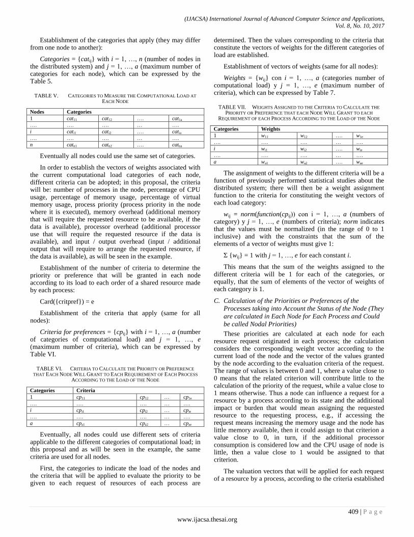
Establishment of the categories that apply (they may differ from one node to another):

Categories = {catij} with i = 1, …, n (number of nodes in the distributed system) and j = 1, …, a (maximum number of categories for each node), which can be expressed by the Table 5.

TABLE V. CATEGORIES TO MEASURE THE COMPUTATIONAL LOAD AT

EACH NODE

Nodes Categories

1 cat11 cat12 …. cat1a

…. …. …. … ….

i cati1 cati2 …. catia

…. …. …. … ….

n catn1 catn2 …. catna

Eventually all nodes could use the same set of categories.

In order to establish the vectors of weights associated with the current computational load categories of each node, different criteria can be adopted; in this proposal, the criteria will be: number of processes in the node, percentage of CPU usage, percentage of memory usage, percentage of virtual memory usage, process priority (process priority in the node where it is executed), memory overhead (additional memory that will require the requested resource to be available, if the data is available), processor overhead (additional processor use that will require the requested resource if the data is available), and input / output overhead (input / additional output that will require to arrange the requested resource, if the data is available), as will be seen in the example.

Establishment of the number of criteria to determine the priority or preference that will be granted in each node according to its load to each order of a shared resource made by each process:

Card({critpref}) = e

Establishment of the criteria that apply (same for all nodes):

Criteria for preferences = {cpij} with i = 1, …, a (number of categories of computational load) and j = 1, …, e (maximum number of criteria), which can be expressed by Table VI.

TABLE VI. CRITERIA TO CALCULATE THE PRIORITY OR PREFERENCE

THAT EACH NODE WILL GRANT TO EACH REQUIREMENT OF EACH PROCESS

ACCORDING TO THE LOAD OF THE NODE

Categories Criteria

1 cp11 cp12 … cp1e

…. …. …. … ….

i cpi1 cpi2 … cpie

…. …. …. … ….

a cpa1 cpa2 … cpae

Eventually, all nodes could use different sets of criteria applicable to the different categories of computational load; in this proposal and as will be seen in the example, the same criteria are used for all nodes.

First, the categories to indicate the load of the nodes and the criteria that will be applied to evaluate the priority to be given to each request of resources of each process are

determined. Then the values corresponding to the criteria that constitute the vectors of weights for the different categories of load are established.

Establishment of vectors of weights (same for all nodes):

Weights = {wij} con i = 1, …, a (categories number of computational load) y j = 1, …, e (maximum number of criteria), which can be expressed by Table 7.

TABLE VII. WEIGHTS ASSIGNED TO THE CRITERIA TO CALCULATE THE

PRIORITY OR PREFERENCE THAT EACH NODE WILL GRANT TO EACH

REQUIREMENT OF EACH PROCESS ACCORDING TO THE LOAD OF THE NODE

Categories Weights

1 w11 w12 …. w1e

…. …. …. … ….

i wi1 wi2 …. wie

…. …. …. … ….

a wa1 wa2 …. wae

The assignment of weights to the different criteria will be a function of previously performed statistical studies about the distributed system; there will then be a weight assignment function to the criteria for constituting the weight vectors of each load category:

wij = norm(function(cpij)) con i = 1, …, a (numbers of category) y j = 1, …, e (numbers of criteria); norm indicates that the values must be normalized (in the range of 0 to 1 inclusive) and with the constraints that the sum of the elements of a vector of weights must give 1:

Σ {wij} = 1 with j = 1, …, e for each constant i.

This means that the sum of the weights assigned to the different criteria will be 1 for each of the categories, or equally, that the sum of elements of the vector of weights of each category is 1.

C. Calculation of the Priorities or Preferences of the

Processes taking into Account the Status of the Node (They

are calculated in Each Node for Each Process and Could

be called Nodal Priorities)

These priorities are calculated at each node for each resource request originated in each process; the calculation considers the corresponding weight vector according to the current load of the node and the vector of the values granted by the node according to the evaluation criteria of the request. The range of values is between 0 and 1, where a value close to 0 means that the related criterion will contribute little to the calculation of the priority of the request, while a value close to 1 means otherwise. Thus a node can influence a request for a resource by a process according to its state and the additional impact or burden that would mean assigning the requested resource to the requesting process, e.g., if accessing the request means increasing the memory usage and the node has little memory available, then it could assign to that criterion a value close to 0, in turn, if the additional processor consumption is considered low and the CPU usage of node is little, then a value close to 1 would be assigned to that criterion.

The valuation vectors that will be applied for each request of a resource by a process, according to the criteria established


Vol. 8, No. 10, 2017

410 | P a g e


for the determination of the priority that in each case and moment will fix the node in which the request occurs, are the following:

Valuations (rij pkl) = {cpm} con i = 1, …, n (node where the resource resides), j = 1, …, r (resource on node i), k = 1, …, n (node where the process resides), l = 1, …, p (process at node k) and m = 1, …, e (valuation criteria of the requirement priority), which can be expressed by Table 8.

TABLE VIII. EVALUATIONS ASSIGNED TO THE CRITERIA TO CALCULATE

THE PRIORITY OR PREFERENCE THAT EACH NODE WILL GRANT EACH

REQUIREMENT OF EACH PROCESS ACCORDING TO THE NODE LOAD

Resources -

Processes Criteria

r11 p11 cp1 …. cpm …. cpe

…. …. …. … …. ….

rij pkl cp1 …. cpm …. cpe

…. …. …. … …. ….

rnr pnp cp1 …. cpm …. cpe

To sum up, the nodal priority (to be calculated at the node where the request occurs) of a process to access a given resource (which can be at any node) is calculated by the scalar product of the mentioned vectors:

Nodal priority (rij pkl) = Σ wom * cpm indicating o the weights vector according to the load of the node, keeping the other subscripts, the meanings explained above.

D. Calculation of Process Priorities or Preferences to Access

Available Shares (it is calculated in the Centralized

Manager of the Shared Resources). In Addition,

Determining the Order in Which the Resources will be

allocated and to Which Process Each Resource will be

allocated

At this stage, the nodal priorities calculated in the previous stage are considered for each requirement of access to resources by the processes. The global or final priorities must be calculated from these nodal priorities, that is, with what priority, or in what order, the requested resources will be provided and to which processes the allocation will be made. The requirements that cannot be attended because they result in low priorities will be considered again in the next iteration of the method.

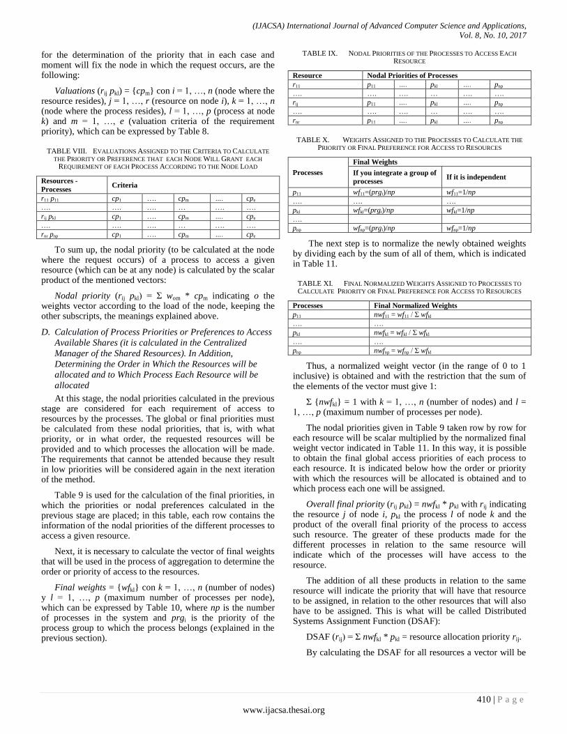
Table 9 is used for the calculation of the final priorities, in which the priorities or nodal preferences calculated in the previous stage are placed; in this table, each row contains the information of the nodal priorities of the different processes to access a given resource.

Next, it is necessary to calculate the vector of final weights that will be used in the process of aggregation to determine the order or priority of access to the resources.

Final weights = {wfkl} con k = 1, …, n (number of nodes) y l = 1, …, p (maximum number of processes per node), which can be expressed by Table 10, where np is the number of processes in the system and prgi is the priority of the process group to which the process belongs (explained in the previous section).

TABLE IX. NODAL PRIORITIES OF THE PROCESSES TO ACCESS EACH

RESOURCE

Resource Nodal Priorities of Processes

r11 p11 …. pkl …. pnp

…. …. …. … …. ….

rij p11 …. pkl …. pnp

…. …. …. … …. ….

rnr p11 …. pkl …. pnp

TABLE X. WEIGHTS ASSIGNED TO THE PROCESSES TO CALCULATE THE

PRIORITY OR FINAL PREFERENCE FOR ACCESS TO RESOURCES

Processes

Final Weights

If you integrate a group of

processes If it is independent

p11 wf11=(prgi)/np wf11=1/np

…. …. ….

pkl wfkl=(prgi)/np wfkl=1/np

….

pnp wfnp=(prgi)/np wfnp=1/np

The next step is to normalize the newly obtained weights by dividing each by the sum of all of them, which is indicated in Table 11.

TABLE XI. FINAL NORMALIZED WEIGHTS ASSIGNED TO PROCESSES TO

CALCULATE PRIORITY OR FINAL PREFERENCE FOR ACCESS TO RESOURCES

Processes Final Normalized Weights

p11 nwf11 = wf11 / Σ wfkl

…. ….

pkl nwfkl = wfkl / Σ wfkl

…. ….

pnp nwfnp = wfnp / Σ wfkl

Thus, a normalized weight vector (in the range of 0 to 1 inclusive) is obtained and with the restriction that the sum of the elements of the vector must give 1:

Σ {nwfkl} = 1 with k = 1, …, n (number of nodes) and l = 1, …, p (maximum number of processes per node).

The nodal priorities given in Table 9 taken row by row for each resource will be scalar multiplied by the normalized final weight vector indicated in Table 11. In this way, it is possible to obtain the final global access priorities of each process to each resource. It is indicated below how the order or priority with which the resources will be allocated is obtained and to which process each one will be assigned.

Overall final priority (rij pkl) = nwfkl * pkl with rij indicating the resource j of node i, pkl the process l of node k and the product of the overall final priority of the process to access such resource. The greater of these products made for the different processes in relation to the same resource will indicate which of the processes will have access to the resource.

The addition of all these products in relation to the same resource will indicate the priority that will have that resource to be assigned, in relation to the other resources that will also have to be assigned. This is what will be called Distributed Systems Assignment Function (DSAF):

DSAF (rij) = Σ nwfkl * pkl = resource allocation priority rij.

By calculating the DSAF for all resources a vector will be


Vol. 8, No. 10, 2017

411 | P a g e


obtained, and by ordering its elements from highest to lowest, the priority order of allocation of resources will be obtained. In addition, as already indicated, the largest of the products nwfkl * pkl for each resource will indicate the process to which the resource will be assigned. This is shown in Table 12.

TABLE XII. ORDER OR FINAL PRIORITY OF ALLOCATION OF THE

RESOURCES AND PROCESS TO WHICH EACH RESOURCE IS ASSIGNED

Order of allocation of resources Process to which the resource

will be assigned

1°: rij of the Maximum(DSAF(rij))

pkl of the

Maximum (nwfkl * pkl) for rij

assigned

2°: rij of the Maximum(DSAF(rij)) for

unassigned rij

pkl of the Maximum (nwfkl * pkl)

for rij assigned

…. ….

Last: unassigned rij pkl of the Maximum (nwfkl * pkl)

for rij assigned

Considerations for Aggregation Operations

The characteristics of the aggregation operations described allow considering that the proposed method belongs to the family of aggregation operators Neat-OWA, which are characterized by the following:

The definition of OWA operators indicates that

1 2

1

, , ,n

n j j

j

f a a a w b

, where bj is the jth highest

value of the an, with the restriction for weights to satisfy (1) [ ] and (2) ∑

.

For the Neat OWA operator family the weights will be calculated according to the elements that are added, or more exactly of the values to be added orderly, the bj, maintaining conditions (1) and (2). In this case the weights are:

1( ,..., )i i nw f b b , defining the operator

1 1( ,... ) ( ,..., )·n i n i

i

F a a f b b b

For this family, where the weights depend on the aggregation, the satisfaction of all properties of OWA operators is not required.

In addition, in order to be able to assert that an aggregation operator is neat, the final aggregation value needs to be

independent of the order of the values. 1( ,..., )nA a a being

the entries to add, 1( ,..., )nB b b being the ordered entries

and 1 1( ,..., ) ( ,..., )n nC c c Perm a a a permutation of the

entries. An OWA operator is defined as neat if

1 2

1

, , ,n

n i i

i

F a a a w b

It produces the same result for any assignment C = B.

One of the characteristics to be pointed out by Neat OWA operators is that the values to be added need not be sorted out

for their process. This implies that the formulation of a neat operator can be defined by directly using the arguments instead of the orderly elements.

In the proposed aggregation operator, the weights are calculated according to context values. From this context arise the values to be aggregated.

IV. EXAMPLE AND DISCUSSION OF RESULTS

This section will explain in detail an example application of the proposed aggregation operator. The distributed processing system has three nodes:

Nodes = {1, 2, 3}

The processes running on the nodes are as follows: three processes on node 1, five processes on node 2 and seven processes on node 3.

Processes = {pij} with i indicating the node and j

indicating the process, which can be expressed by Table 13.

TABLE XIII. PROCESSES IN EACH NODE

Nodes Processes

1 p11 p12 p13

2 P21 P22 P23 P24 P25

3 P31 P32 P33 P34 P35 P36 P37

Several processes are independent and others constitute groups of cooperative processes. In this example four groups will be considered, as shown in Table 14.

TABLE XIV. PROCESSES IN EACH GROUP

Groups Processes

1 p11 p25 p37

2 p12 p21

3 p22 p31

4 p13 p23 p34

The number of processes in each group indicates the cardinality of the group and is represented as follows:

Card = {card (gi)} = {3, 2, 2, 3} with i indicating the group.

The priority of the groups of processes will be considered the cardinality of each group and is represented as follows:

prg = {prgi = card(gi)} = {3, 2, 2, 3} with i indicating the group.

The shared resources available in the nodes are as follows: three resources in node 1, four resources in node 2 and three resources in node 3.

Resources = {pij} with i indicating the node and j indicating the process, as expressed in Table 15.

TABLE XV. SHARED RESOURCES AVAILABLE AT EACH NODE

Nodes Resources

1 r11 r12 r13

2 r21 r22 r23 r24

3 r31 r32 r33

The requests for resources by the processes are shown in Table 16.


Vol. 8, No. 10, 2017

412 | P a g e


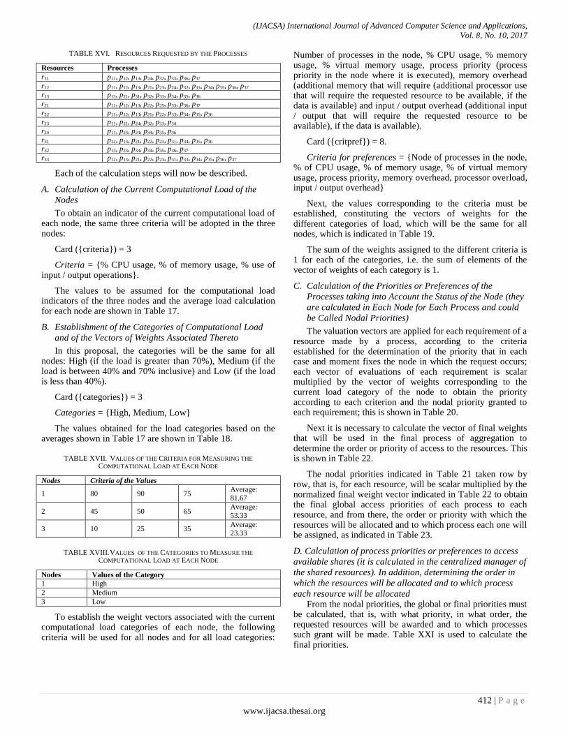
TABLE XVI. RESOURCES REQUESTED BY THE PROCESSES

Resources Processes

r11 p11, p12, p13, p24, p32, p33, p36, p37

r12 p11, p12, p13, p21, p23, p24, p32, p33, p34, p35, p36, p37

r13 p13, p21, p31, p32, p33, p34, p35, p36

r21 p11, p12, p13, p22, p25, p33, p36, p37

r22 p11, p12, p13, p21, p22, p33, p34, p35, p36

r23 p11, p21, p24, p32, p33, p34

r24 p11, p23, p24, p34, p35, p36

r31 p12, p13, p21, p22, p23, p31, p34, p35, p36

r32 p13, p23, p33, p34, p35, p36, p37

r33 p12, p13, p21, p22, p23, p31, p33, p34, p35, p36, p37

Each of the calculation steps will now be described.

A. Calculation of the Current Computational Load of the

Nodes

To obtain an indicator of the current computational load of each node, the same three criteria will be adopted in the three nodes:

Card ({criteria}) = 3

Criteria = {% CPU usage, % of memory usage, % use of input / output operations}.

The values to be assumed for the computational load indicators of the three nodes and the average load calculation for each node are shown in Table 17.

B. Establishment of the Categories of Computational Load

and of the Vectors of Weights Associated Thereto

In this proposal, the categories will be the same for all nodes: High (if the load is greater than 70%), Medium (if the load is between 40% and 70% inclusive) and Low (if the load is less than 40%).

Card ({categories}) = 3

Categories = {High, Medium, Low}

The values obtained for the load categories based on the averages shown in Table 17 are shown in Table 18.

TABLE XVII. VALUES OF THE CRITERIA FOR MEASURING THE

COMPUTATIONAL LOAD AT EACH NODE

Nodes Criteria of the Values

1 80 90 75 Average:

81.67

2 45 50 65 Average:

53.33

3 10 25 35 Average:

23.33

TABLE XVIII. VALUES OF THE CATEGORIES TO MEASURE THE

COMPUTATIONAL LOAD AT EACH NODE

Nodes Values of the Category

1 High

2 Medium

3 Low

To establish the weight vectors associated with the current computational load categories of each node, the following criteria will be used for all nodes and for all load categories:

Number of processes in the node, % CPU usage, % memory usage, % virtual memory usage, process priority (process priority in the node where it is executed), memory overhead (additional memory that will require (additional processor use that will require the requested resource to be available, if the data is available) and input / output overhead (additional input / output that will require the requested resource to be available), if the data is available).

Card ({critpref}) = 8.

Criteria for preferences = {Node of processes in the node, % of CPU usage, % of memory usage, % of virtual memory usage, process priority, memory overhead, processor overload, input / output overhead}

Next, the values corresponding to the criteria must be established, constituting the vectors of weights for the different categories of load, which will be the same for all nodes, which is indicated in Table 19.

The sum of the weights assigned to the different criteria is 1 for each of the categories, i.e. the sum of elements of the vector of weights of each category is 1.

C. Calculation of the Priorities or Preferences of the

Processes taking into Account the Status of the Node (they

are calculated in Each Node for Each Process and could

be Called Nodal Priorities)

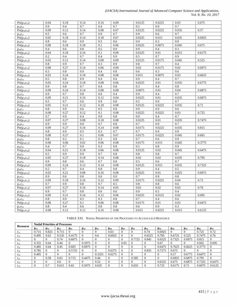
The valuation vectors are applied for each requirement of a resource made by a process, according to the criteria established for the determination of the priority that in each case and moment fixes the node in which the request occurs; each vector of evaluations of each requirement is scalar multiplied by the vector of weights corresponding to the current load category of the node to obtain the priority according to each criterion and the nodal priority granted to each requirement; this is shown in Table 20.

Next it is necessary to calculate the vector of final weights that will be used in the final process of aggregation to determine the order or priority of access to the resources. This is shown in Table 22.

The nodal priorities indicated in Table 21 taken row by row, that is, for each resource, will be scalar multiplied by the normalized final weight vector indicated in Table 22 to obtain the final global access priorities of each process to each resource, and from there, the order or priority with which the resources will be allocated and to which process each one will be assigned, as indicated in Table 23.

D. Calculation of process priorities or preferences to access

available shares (it is calculated in the centralized manager of

the shared resources). In addition, determining the order in

which the resources will be allocated and to which process

each resource will be allocated From the nodal priorities, the global or final priorities must

be calculated, that is, with what priority, in what order, the requested resources will be awarded and to which processes such grant will be made. Table XXI is used to calculate the final priorities.


Vol. 8, No. 10, 2017

413 | P a g e


TABLE XIX. WEIGHTS ASSIGNED TO THE CRITERIA TO CALCULATE THE PRIORITY OR PREFERENCE THAT EACH NODE WILL GRANT TO EACH REQUIREMENT OF

EACH PROCESS ACCORDING TO THE LOAD OF THE NODE

Categories

Weights

N°

Proc. % CPU

%

Mem. % VM Priority Proc.

Load

Mem. Load Proc.

Load

I/O

High 0.05 0.05 0.1 0.5 0.1 0.1 0.05 0.05

Medium 0.1 0.2 0.3 0.1 0.2 0.05 0.025 0.025

Low 0.1 0.3 0.2 0.2 0.1 0.025 0.025 0.05

TABLE XX. THE VALUATIONS ASSIGNED TO THE CRITERIA TO CALCULATE THE PRIORITY OR NODAL PREFERENCE THAT EACH NODE WILL GRANT EACH

REQUIREMENT OF EACH PROCESS ACCORDING TO THE NODE LOAD

Processes–

Resources

Criteria Nodal

Priorities #

Proc. % CPU

%

Mem. % VM Priority Proc. Load Mem. Load Proc. Priority I/O

p11r11 0.7 0.5 0.7 0.9 0.8 0.2 0.3 0.4

Pri(p11r11) 0.035 0.025 0.07 0.45 0.08 0.02 0.015 0.02 0.715

p11r12 0.8 0.7 0.4 0.5 0.3 0.7 0.2 0.4

Pri(p11r12) 0.04 0.035 0.04 0.25 0.03 0.07 0.01 0.02 0.495

p11r21 0.3 0.4 0.5 0.2 0.9 0.2 0.5 0.7

Pri(p11r21) 0.015 0.02 0.05 0.1 0.09 0.02 0.025 0.035 0.355

p11r22 0.5 0.5 0.7 0.4 0.8 0.3 0.5 0.6

Pri(p11r22) 0.025 0.025 0.07 0.2 0.08 0.03 0.025 0.03 0.485

p11r23 0.5 0.6 0.8 0.8 0.95 0.9 0.7 0.6

Pri(p11r23) 0.025 0.03 0.08 0.4 0.095 0.09 0.035 0.03 0.785

p11r24 0.3 0.5 0.9 0.2 0.6 0.6 0.7 0.4

Pri(p11r24) 0.015 0.025 0.09 0.1 0.06 0.06 0.035 0.02 0.405

p12r11 0.4 0.7 0.5 0.9 1 0.9 0.8 0.8

Pri(p12r11) 0.02 0.035 0.05 0.45 0.1 0.09 0.04 0.04 0.825

p12r12 0.2 0.7 0.3 0.7 0.8 0.3 0.8 0.9

Pri(p12r12) 0.01 0.035 0.03 0.35 0.08 0.03 0.04 0.045 0.62

p12r21 0.7 0.4 0.3 0.7 0.8 0.9 0.5 0.2

Pri(p12r21) 0.035 0.02 0.03 0.35 0.08 0.09 0.025 0.01 0.64

p12r22 0.9 0.6 0.7 0.7 0.8 0.2 0.5 0.4

Pri(p12r22) 0.045 0.03 0.07 0.35 0.08 0.02 0.025 0.02 0.64

p12r31 0.2 0.5 0.7 0.7 0.3 0.2 0.7 0.8

Pri(p12r31) 0.01 0.025 0.07 0.35 0.03 0.02 0.035 0.04 0.58

p12r33 0.4 0.5 0.7 0.9 0.3 0.4 0.5 0.8

Pri(p12r33) 0.02 0.025 0.07 0.45 0.03 0.04 0.025 0.04 0.7

p13r11 0.5 0.7 0.7 0.8 0.6 0.5 0.7 0.8

Pri(p13r11) 0.025 0.035 0.07 0.4 0.06 0.05 0.035 0.04 0.715

p13r12 0.7 0.8 0.7 0.4 0.9 0.2 0.9 0.7

Pri(p13r12) 0.035 0.04 0.07 0.2 0.09 0.02 0.045 0.035 0.535

p13r13 0.7 0.6 0.7 0.8 0.9 0.4 0.8 0.7

Pri(p13r13) 0.035 0.03 0.07 0.4 0.09 0.04 0.04 0.035 0.74

p13r21 0.7 0.4 0.9 0.3 0.5 0.7 0.2 0.3

Pri(p13r21) 0.035 0.02 0.09 0.15 0.05 0.07 0.01 0.015 0.44

p13r22 0.5 0.9 0.8 0.3 0.5 0.4 0.9 0.3

Pri(p13r22) 0.025 0.045 0.08 0.15 0.05 0.04 0.045 0.015 0.45

p13r31 0.5 0.7 0.3 0.6 0.8 0.9 0.9 0.5

Pri(p13r31) 0.025 0.035 0.03 0.3 0.08 0.09 0.045 0.025 0.63

p13r32 0.6 0.9 0.3 0.6 0.4 0.8 0.7 0.8

Pri(p13r32) 0.03 0.045 0.03 0.3 0.04 0.08 0.035 0.04 0.6

p13r33 0.6 0.2 0.4 0.6 0.9 0.8 0.5 0.8

Pri(p13r33) 0.03 0.01 0.04 0.3 0.09 0.08 0.025 0.04 0.615

p21r12 0.2 0.1 0.3 0.8 0.7 0.7 0.5 0.8

Pri(p21r12) 0.02 0.02 0.09 0.08 0.14 0.035 0.0125 0.02 0.4175

p21r13 0.2 0.4 0.8 0.9 0.7 0.4 0.5 0.2

Pri(p21r13) 0.02 0.08 0.24 0.09 0.14 0.02 0.0125 0.005 0.6075

p21r22 0.3 0.5 0.8 0.9 0.5 0.6 0.2 0.4

Pri(p21r22) 0.03 0.1 0.24 0.09 0.1 0.03 0.005 0.01 0.605

p21r23 0.7 0.5 0.6 0.8 0.5 0.2 0.9 0.4

Pri(p21r23) 0.07 0.1 0.18 0.08 0.1 0.01 0.0225 0.01 0.5725

p21r31 0.7 0.5 0.8 0.6 0.9 0.4 0.9 0.9


Vol. 8, No. 10, 2017

414 | P a g e


Pri(p21r31) 0.07 0.1 0.24 0.06 0.18 0.02 0.0225 0.0225 0.715

p21r33 0.7 0.4 0.9 0.8 0.4 0.8 0.6 0.6

Pri(p21r33) 0.07 0.08 0.27 0.08 0.08 0.04 0.015 0.015 0.65

p22r21 0.5 0.4 0.7 0.8 0.6 0.4 0.6 0.9

Pri(p22r21) 0.05 0.08 0.21 0.08 0.12 0.02 0.015 0.0225 0.5975

p22r22 0.5 0.9 0.6 0.8 0.9 0.4 0.2 0.1

Pri(p22r22) 0.05 0.18 0.18 0.08 0.18 0.02 0.005 0.0025 0.6975

p22r31 0.5 0.4 0.5 0.2 0.4 0.8 0.2 0.9

Pri(p22r31) 0.05 0.08 0.15 0.02 0.08 0.04 0.005 0.0225 0.4475

p22r33 0.8 0.4 0.3 0.2 0.8 0.9 0.5 0.8

Pri(p22r33) 0.08 0.08 0.09 0.02 0.16 0.045 0.0125 0.02 0.5075

p23r12 0.5 0.6 0.8 0.3 0.5 0.7 0.5 0.5

Pri(p23r12) 0.05 0.12 0.24 0.03 0.1 0.035 0.0125 0.0125 0.6

p23r24 0.6 0.2 0.1 0.7 0.3 0.8 0.9 0.4

Pri(p23r24) 0.06 0.04 0.03 0.07 0.06 0.04 0.0225 0.01 0.3325

p23r31 0.3 0.1 0.4 0.8 0.7 0.9 0.4 0.6

Pri(p23r31) 0.03 0.02 0.12 0.08 0.14 0.045 0.01 0.015 0.46

p23r32 0.4 0.4 0.8 0.2 0.4 0.6 0.6 0.6

Pri(p23r32) 0.04 0.08 0.24 0.02 0.08 0.03 0.015 0.015 0.52

p23r33 0.3 0.6 0.8 0.2 0.9 0.6 0.4 0.2

Pri(p23r33) 0.03 0.12 0.24 0.02 0.18 0.03 0.01 0.005 0.635

p24r11 0.4 0.6 0.7 0.9 0.5 0.7 0.9 0.5

Pri(p24r11) 0.04 0.12 0.21 0.09 0.1 0.035 0.0225 0.0125 0.63

p24r12 0.3 0.6 0.7 0.8 0.9 0.7 0.6 0.9

Pri(p24r12) 0.03 0.12 0.21 0.08 0.18 0.035 0.015 0.0225 0.6925

p24r23 0.4 0.9 0.4 0.8 0.8 0.7 0.6 0.3

Pri(p24r23) 0.04 0.18 0.12 0.08 0.16 0.035 0.015 0.0075 0.6375

p24r24 0.5 0.8 0.7 0.9 0.3 0.4 0.8 0.7

Pri(p24r24) 0.05 0.16 0.21 0.09 0.06 0.02 0.02 0.0175 0.6275

p25r21 0.2 0.8 0.8 0.9 0.4 0.5 0.6 0.8

Pri(p25r21) 0.02 0.16 0.24 0.09 0.08 0.025 0.015 0.02 0.65

p31r13 0.6 0.9 0.6 0.9 0.7 0.4 0.9 0.8

Pri(p31r13) 0.06 0.27 0.12 0.18 0.07 0.01 0.0225 0.04 0.7725

p31r31 0.8 0.3 0.9 0.5 0.7 0.3 0.9 0.7

Pri(p31r31) 0.08 0.09 0.18 0.1 0.07 0.0075 0.0225 0.035 0.585

p31r33 0.4 0.7 0.7 0.5 0.9 0.9 0.7 0.7

Pri(p31r33) 0.04 0.21 0.14 0.1 0.09 0.0225 0.0175 0.035 0.655

p32r11 0.6 0.9 0.8 0.5 0.9 0.7 0.3 0.7

Pri(p32r11) 0.06 0.27 0.16 0.1 0.09 0.0175 0.0075 0.035 0.74

p32r12 0.7 0.4 0.6 0.9 0.8 1 0.9 0.7

Pri(p32r12) 0.07 0.12 0.12 0.18 0.08 0.025 0.0225 0.035 0.6525

p32r13 0.8 0.9 1 0.7 0.9 0.3 0.5 0.9

Pri(p32r13) 0.08 0.27 0.2 0.14 0.09 0.0075 0.0125 0.045 0.845

p32r23 0.8 0.8 1 0.9 0.6 0.8 0.4 0.9

Pri(p32r23) 0.08 0.24 0.2 0.18 0.06 0.02 0.01 0.045 0.835

p33r11 0.2 0.7 0.9 0.8 0.6 0.9 1 0.3

Pri(p33r11) 0.02 0.21 0.18 0.16 0.06 0.0225 0.025 0.015 0.6925

p33r12 0.9 1 0.9 0.7 0.3 0.5 0.7 0.3

Pri(p33r12) 0.09 0.3 0.18 0.14 0.03 0.0125 0.0175 0.015 0.785

p33r13 0.9 0.5 0.7 0.9 0.3 0.4 0.5 0.8

Pri(p33r13) 0.09 0.15 0.14 0.18 0.03 0.01 0.0125 0.04 0.6525

p33r21 0.4 0.6 0.7 0.8 0.8 0.4 0.8 0.8

Pri(p33r21) 0.04 0.18 0.14 0.16 0.08 0.01 0.02 0.04 0.67

p33r22 0.9 0.4 0.7 0.8 0.7 0.4 0.9 0.7

Pri(p33r22) 0.09 0.12 0.14 0.16 0.07 0.01 0.0225 0.035 0.6475

p33r23 0.4 0.6 0.9 1 0.6 0.4 0.7 0.8

Pri(p33r23) 0.04 0.18 0.18 0.2 0.06 0.01 0.0175 0.04 0.7275

p33r32 0.6 0.6 0.7 0.8 0.4 0.5 0.8 0.8

Pri(p33r32) 0.06 0.18 0.14 0.16 0.04 0.0125 0.02 0.04 0.6525

p33r33 0.6 1 0.7 0.4 0.6 0.8 0.8 0.9

Pri(p33r33) 0.06 0.3 0.14 0.08 0.06 0.02 0.02 0.045 0.725

p34r12 0.8 1 0.3 0.5 0.7 0.3 0.8 0.7

Pri(p34r12) 0.08 0.3 0.06 0.1 0.07 0.0075 0.02 0.035 0.6725

p34r13 0.2 1 0.8 0.5 0.8 0.6 0.9 0.7

Pri(p34r13) 0.02 0.3 0.16 0.1 0.08 0.015 0.0225 0.035 0.7325

p34r22 0.9 0.8 0.6 0.8 0.9 0.8 0.5 0.6

Pri(p34r22) 0.09 0.24 0.12 0.16 0.09 0.02 0.0125 0.03 0.7625

p34r23 0.4 0.6 0.7 0.8 0.9 0.5 0.9 0.6


Vol. 8, No. 10, 2017

415 | P a g e


Pri(p34r23) 0.04 0.18 0.14 0.16 0.09 0.0125 0.0225 0.03 0.675

p34r24 0.9 0.4 0.7 0.4 0.7 0.5 0.9 0.7

Pri(p34r24) 0.09 0.12 0.14 0.08 0.07 0.0125 0.0225 0.035 0.57

p34r31 0.5 0.6 0.7 0.9 0.7 0.9 0.6 0.7

Pri(p34r31) 0.05 0.18 0.14 0.18 0.07 0.0225 0.015 0.035 0.6925

p34r32 0.8 0.6 0.9 0.5 0.6 0.9 0.3 0.9

Pri(p34r32) 0.08 0.18 0.18 0.1 0.06 0.0225 0.0075 0.045 0.675

p34r33 0.4 0.6 0.8 0.5 0.9 0.9 0.4 0.3

Pri(p34r33) 0.04 0.18 0.16 0.1 0.09 0.0225 0.01 0.015 0.6175

p35r12 0.2 0.4 0.7 0.4 0.9 0.5 0.7 0.9

Pri(p35r12) 0.02 0.12 0.14 0.08 0.09 0.0125 0.0175 0.045 0.525

p35r13 0.8 0.9 0.7 0.3 0.9 0.8 0.7 0.4

Pri(p35r13) 0.08 0.27 0.14 0.06 0.09 0.02 0.0175 0.02 0.6975

p35r22 0.3 0.8 0.9 0.4 0.8 0.6 0.3 0.6

Pri(p35r22) 0.03 0.24 0.18 0.08 0.08 0.015 0.0075 0.03 0.6625

p35r24 0.5 0.8 0.9 0.4 0.6 0.9 0.4 0.7

Pri(p35r24) 0.05 0.24 0.18 0.08 0.06 0.0225 0.01 0.035 0.6775

p35r31 0.9 0.8 0.7 0.4 0.8 0.3 0.4 0.8

Pri(p35r31) 0.09 0.24 0.14 0.08 0.08 0.0075 0.01 0.04 0.6875

p35r32 0.9 0.7 0.8 0.6 0.4 0.9 0.4 0.7

Pri(p35r32) 0.09 0.21 0.16 0.12 0.04 0.0225 0.01 0.035 0.6875

p35r33 0.5 0.7 0.6 0.9 0.8 0.5 0.9 0.7

Pri(p35r33) 0.05 0.21 0.12 0.18 0.08 0.0125 0.0225 0.035 0.71

p36r11 0.8 0.9 0.6 0.5 0.8 0.9 0.9 0.6

Pri(p36r11) 0.08 0.27 0.12 0.1 0.08 0.0225 0.0225 0.03 0.725

p36r12 0.7 0.9 0.4 0.9 0.8 0.9 0.4 0.7

Pri(p36r12) 0.07 0.27 0.08 0.18 0.08 0.0225 0.01 0.035 0.7475

p36r13 0.9 0.9 0.8 0.7 0.8 0.7 0.9 0.7

Pri(p36r13) 0.09 0.27 0.16 0.14 0.08 0.0175 0.0225 0.035 0.815

p36r21 0.8 0.9 0.5 0.3 0.7 0.7 0.9 0.9

Pri(p36r21) 0.08 0.27 0.1 0.06 0.07 0.0175 0.0225 0.045 0.665

p36r22 0.8 0.2 0.1 0.3 0.8 0.7 0.6 0.9

Pri(p36r22) 0.08 0.06 0.02 0.06 0.08 0.0175 0.015 0.045 0.3775

p36r24 0.4 0.7 0.9 0.3 0.8 0.5 0.8 0.9

Pri(p36r24) 0.04 0.21 0.18 0.06 0.08 0.0125 0.02 0.045 0.6475

p36r31 0.5 0.9 0.9 0.7 0.8 0.8 0.8 0.7

Pri(p36r31) 0.05 0.27 0.18 0.14 0.08 0.02 0.02 0.035 0.795

p36r32 0.9 0.8 0.6 0.7 0.8 0.5 0.6 0.7

Pri(p36r32) 0.09 0.24 0.12 0.14 0.08 0.0125 0.015 0.035 0.7325

p36r33 0.2 0.7 0.4 0.8 0.8 0.9 0.4 0.5

Pri(p36r33) 0.02 0.21 0.08 0.16 0.08 0.0225 0.01 0.025 0.6075

p37r11 0.9 0.6 0.8 0.6 0.9 0.7 0.9 0.8

Pri(p37r11) 0.09 0.18 0.16 0.12 0.09 0.0175 0.0225 0.04 0.72

p37r12 0.7 0.9 0.8 0.7 0.5 0.8 0.8 0.6

Pri(p37r12) 0.07 0.27 0.16 0.14 0.05 0.02 0.02 0.03 0.76

p37r21 0.9 0.7 0.8 0.6 0.6 0.9 0.5 0.4

Pri(p37r21) 0.09 0.21 0.16 0.12 0.06 0.0225 0.0125 0.02 0.695

p37r32 0.8 0.9 0.5 0.3 0.8 0.7 0.4 0.6

Pri(p37r32) 0.08 0.27 0.1 0.06 0.08 0.0175 0.01 0.03 0.6475

p37r33 0.8 0.4 0.6 0.8 0.8 0.6 0.9 0.3

Pri(p37r33) 0.08 0.12 0.12 0.16 0.08 0.015 0.0225 0.015 0.6125

TABLE XXI. NODAL PRIORITIES OF THE PROCESSES TO ACCESS EACH RESOURCE

Resourse Nodal Priorities of Processes

p11 p12 p13 p21 p22 p23 p24 p25 p31 p32 p33 p34 p35 p36 p37

r11 0.715 0.825 0.715 0 0 0 0.63 0 0 0.74 0.6925 0 0 0.725 0.72

r12 0.495 0.62 0.535 0.4175 0 0.6 0.6925 0 0 0.6525 0.785 0.6725 0.525 0.7475 0.76

r13 0 0 0.74 0.6075 0 0 0 0 0.7725 0.845 0.6525 0.7325 0.6975 0.815 0

r21 0.355 0.64 0.44 0 0.5975 0 0 0.65 0 0 0.67 0 0 0.665 0.695

r22 0.485 0.64 0.45 0.605 0.6975 0 0 0 0 0 0.6475 0.7625 0.6625 0.3775 0

r23 0.785 0 0 0.5725 0 0 0.6375 0 0 0.835 0.7275 0.675 0 0 0

r24 0.405 0 0 0 0 0.3325 0.6275 0 0 0 0 0.57 0.6775 0.6475 0

r31 0 0.58 0.63 0.715 0.4475 0.46 0 0 0.585 0 0 0.6925 0.6875 0.795 0

r32 0 0 0.6 0 0 0.52 0 0 0 0 0.6525 0.675 0.6875 0.7325 0.6475

r33 0 0.7 0.615 0.65 0.5075 0.635 0 0 0.655 0 0.725 0.6175 0.71 0.6075 0.6125


Vol. 8, No. 10, 2017

416 | P a g e


TABLE XXII. FINAL WEIGHTS AND NORMALIZED FINAL WEIGHTS ASSIGNED TO PROCESSES TO CALCULATE THE PRIORITY OR FINAL PREFERENCE FOR ACCESS

TO RESOURCES

Processes


Final

Weights 0.2 0.133 0.2 0.133 0.133 0.2 0.067 0.2 0.133 0.067 0.067 0.2 0.067 0.067 0.2

Normalized

Final

Weights

0.097 0.065 0.097 0.065 0.065 0.097 0.032 0.097 0.065 0.032 0.032 0.097 0.032 0.032 0.097

TABLE XXIII. FINAL GLOBAL PRIORITIES OF THE PROCESSES TO ACCESS EACH RESOURCE

Resourse Final Global Priorities of the Processes


r11 0.069 0.053 0.069 0 0 0 0.020 0 0 0.024 0.022 0 0 0.023 0.070

r12 0.048 0.04 0.052 0.027 0 0.058 0.022 0 0 0.021 0.025 0.065 0.017 0.024 0.074

r13 0 0 0.072 0.039 0 0 0 0 0.050 0.027 0.021 0.071 0.023 0.026 0

r21 0.034 0.041 0.043 0 0.039 0 0 0.063 0 0 0.022 0 0 0.021 0.067

r22 0.047 0.041 0.044 0.039 0.045 0 0 0 0 0 0.021 0.074 0.021 0.012 0

r23 0.076 0 0 0.037 0 0 0.021 0 0 0.027 0.023 0.065 0 0 0

r24 0.039 0 0 0 0 0.032 0.020 0 0 0 0 0.055 0.022 0.021 0

r31 0 0.037 0.061 0.046 0.029 0.045 0 0 0.038 0 0 0.067 0.022 0.026 0

r32 0 0 0.058 0 0 0.050 0 0 0 0 0.021 0.065 0.022 0.024 0.063

r33 0 0.045 0.060 0.042 0.033 0.061 0 0 0.042 0 0.023 0.060 0.023 0.020 0.060

The greatest of these products made for the different processes in relation to the same resource will indicate which of the processes will have access to the resource (in the case of ties the process identified with the smallest number could be chosen); this is shown in bold in Table 23.

The addition of all these products in relation to the same resource will indicate the priority of such resource to be assigned. This is the Distributed Systems Assignment Function (DSAF), which is shown in Table 24.

The final allocation order of the resources and the target processes are obtained by ordering Table 24, which is shown in Table 25.

The next step is to reiterate the procedure, but removing from the requests for resources the assignments already made; it should also be taken into account that the allocated resources will be available when the processes have released them and can therefore be assigned to other processes. The results of successive iterations are shown in Tables 26 to 36.

TABLE XXIV. FINAL GLOBAL PRIORITIES FOR ALLOCATING RESOURCES

DSAF Final Global Priority to Assign Resource Processes

r11 0.35120968 r11 al p37

r12 0.47306452 r12 al p37

r13 0.32862903 r13 al p13

r21 0.33 r21 al p37

r22 0.34403226 r22 al p34

r23 0.24919355 r23 al p11

r24 0.18951613 r24 al p34

r31 0.37048387 r31 al p34

r32 0.30322581 r32 al p34

r33 0.46798387 r33 al p23

TABLE XXV. ORDER OR FINAL PRIORITY OF ALLOCATION OF RESOURCES

AND PROCESS TO WHICH EACH RESOURCE IS ASSIGNED

Final Global Priority Order Assignment

0.47306452 r12 al p37

0.46798387 r33 al p23

0.37048387 r31 al p34

0.35120968 r11 al p37

0.34403226 r22 al p34

0.33 r21 al p37

0.32862903 r13 al p13

0.30322581 r32 al p34

0.24919355 r23 al p11

0.18951613 r24 al p34

TABLE XXVI. ORDER OR FINAL PRIORITY OF ALLOCATION OF RESOURCES

AND PROCESS TO WHICH EACH RESOURCE IS ASSIGNED (SECOND ITERATION)


0.40653226 r33 al p34

0.39951613 r12 al p34

0.30346774 r31 al p13

0.28153226 r11 al p11

0.27024194 r22 al p11

0.26274194 r21 al p25

0.25701613 r13 al p34

0.23790323 r32 al p37

0.17322581 r23 al p34

0.13435484 r24 al p11


Vol. 8, No. 10, 2017

417 | P a g e


TABLE XXVII. ORDER OR FINAL PRIORITY OF ALLOCATION OF

RESOURCES AND PROCESS TO WHICH EACH RESOURCE IS ASSIGNED (THIRD

ITERATION)


0.34677419 r33 al p13

0.33443548 r12 al p23

0.2425 r31 al p21

0.22330645 r22 al p13

0.21233871 r11 al p13

0.19983871 r21 al p13

0.18612903 r13 al p31

0.17524194 r32 al p13

0.10790323 r23 al p21

0.09516129 r24 al p23

TABLE XXVIII. ORDER OR FINAL PRIORITY OF ALLOCATION OF

RESOURCES AND PROCESS TO WHICH EACH RESOURCE IS ASSIGNED (FOURTH

ITERATION)


0.28725806 r33 al p37

0.27637097 r12 al p13

0.19637097 r31 al p23

0.17975806 r22 al p12

0.15725806 r21 al p12

0.14314516 r11 al p12

0.13629032 r13 al p21

0.11717742 r32 al p23

0.07096774 r23 al p32

0.06298387 r24 al p35

TABLE XXIX. ORDER OR FINAL PRIORITY OF ALLOCATION OF RESOURCES

AND PROCESS TO WHICH EACH RESOURCE IS ASSIGNED (FIFTH ITERATION)


0.22798387 r33 al p12

0.22459677 r12 al p11

0.15185484 r31 al p31

0.13846774 r22 al p21

0.11596774 r21 al p22

0.09709677 r13 al p32

0.08991935 r11 al p32

0.06685484 r32 al p36

0.04403226 r23 al p33

0.04112903 r24 al p36

TABLE XXX. ORDER OR FINAL PRIORITY OF ALLOCATION OF RESOURCES

AND PROCESS TO WHICH EACH RESOURCE IS ASSIGNED (SIXTH ITERATION)


0.18282258 r33 al p31

0.17669355 r12 al p12

0.1141129 r31 al p12

0.09943548 r22 al p22

0.07741935 r21 al p11

0.06983871 r13 al p36

0.06604839 r11 al p36

0.04322581 r32 al p35

0.02056452 r23 al p24

0.02024194 r24 al p24

TABLE XXXI. ORDER OR FINAL PRIORITY OF ALLOCATION OF RESOURCES

AND PROCESS TO WHICH EACH RESOURCE IS ASSIGNED (SEVENTH ITERATION)


0.14056452 r33 al p21

0.13669355 r12 al p21

0.07669355 r31 al p22

0.05443548 r22 al p35

0.04354839 r13 al p35

0.04306452 r21 al p33

0.04266129 r11 al p33

0.02104839 r32 al p33

TABLE XXXII. ORDER OR FINAL PRIORITY OF ALLOCATION OF

RESOURCES AND PROCESS TO WHICH EACH RESOURCE IS ASSIGNED (EIGHTH

ITERATION)


0.10975806 r12 al p33

0.09862903 r33 al p22

0.04782258 r31 al p36

0.03306452 r22 al p33

0.02145161 r21 al p36

0.02104839 r13 al p33

0.02032258 r11 al p24

TABLE XXXIII. ORDER OR FINAL PRIORITY OF ALLOCATION OF

RESOURCES AND PROCESS TO WHICH EACH RESOURCE IS ASSIGNED (NINTH

ITERATION)


0.08443548 r12 al p36

0.0658871 r33 al p33

0.02217742 r31 al p35

0.01217742 r22 al p36

TABLE XXXIV. ORDER OR FINAL PRIORITY OF ALLOCATION OF

RESOURCES AND PROCESS TO WHICH EACH RESOURCE IS ASSIGNED (TENTH

ITERATION)


0.06032258 r12 al p24

0.0425 r33 al p35

TABLE XXXV. ORDER OR FINAL PRIORITY OF ALLOCATION OF


(ELEVENTH ITERATION)


0.03798387 r12 al p32

0.01959677 r33 al p36

TABLE XXXVI. ORDER OR FINAL PRIORITY OF ALLOCATION OF


(TWELFTH ITERATION)


0.01693548 r12 al p35

In this way, all the requests for resources of all the processes have been taken care of, respecting the mutual exclusion and the priorities of the processes, the nodal priorities and the final priorities.


Vol. 8, No. 10, 2017

418 | P a g e


V. FINAL CONSIDERATIONS

A. Conclusions

The proposed model makes it possible for the distributed system to self-regulate repeatedly according to the local state of the n nodes, resulting in an update of their local states, as a consequence of the evolution of their respective processes and the decisions of access to resources: the distributed system in which groups of processes requiring access to critical resources are executed, produces access decisions to resources that modify the state of the system and readjusts it repetitively, also guaranteeing the mutual exclusion in access to the shared resources, indicating the priority of granting access to each resource and the process to which it is assigned. This process is repeated as long as there are processes that request access to shared resources.

The proposed model includes as a particular case one of the most used methods, consisting in considering only the priority of the processes, instead of a group of state variables of each node. Another notable feature of the proposal is its ease of deployment in a centralized shared resource manager environment of a distributed system.

B. Future Work

It is planned to develop variants of the proposed method considering other aggregation operators (especially the OWA family) and the possibility of being used by a resource manager shared (instead of centralized as in the proposed method).

ACKNOWLEDGMENT

This work was carried out in the context of the research projects code 12F003 and 16F001 of the Northeastern National University, Argentine (Resolution No. 960/12 C.S. and No. 241/17 C.S.).

REFERENCES

[1] A. S. Tanenbaum. Sistemas Operativos Distribuidos. Prentice - Hall Hispanoamericana S.A. México, 1996.

[2] A. S. Tanenbaum. Sistemas Operativos Modernos. 3ra. Edición. Pearson Educación S. A. México, 2009.

[3] D. Agrawal and A. El Abbadi. An Efficient and Fault-Tolerant Solution of Distributed Mutual Exclusion. ACM Trans. on Computer Systems. Vol. 9. Pp. 1-20. USA, 1991.

[4] G. Ricart, and A. K. Agrawala. An Optimal Algorithm for Mutual Exclusion in Computer Networks. Commun. of the ACM. Vol. 24. Pp. 9-17, 1981.

[5] G. Cao and M. Singhal. A Delay-Optimal Quorum-Based Mutual Exclusion Algorithm for Distributed Systems. IEEE Transactions on Parallel and Distributed Systems. Vol. 12, no. 12. Pp. 1256-1268. USA, 2001.

[6] S. Lodha and A. Kshemkalyani. A Fair Distributed Mutual Exclusion Algorithm. IEEE Trans. Parallel and Distributed Systems. Vol. 11. N° 6. Pp. 537-549. USA, 2000.

[7] W. Stallings. Sistemas Operativos. 5ta. Edición. Pearson Educación S.A. España, 2005.

[8] K. P. Birman and T. Joseph. Reliable Communication in the Presence of Failures. ACM Trans. on Computer Systems. Vol. 5. Pp. 47-76. USA, 1987.

[9] K. P. Birman, A. Schiper and P. Stephenson. Lightweight Causal and Atomic Group Multicast. ACM Trans. on Computer Systems. Vol. 9. Pp. 272-314. USA, 1991.

[10] K. Birman. Reliable Distributed Systems: Technologies, Web Services and Applications. New York: Springer-Verlag, 2005.

[11] T. A. Joseph and K. P. Birman. Reliable Broadcast Protocols, en Distributed Systems. Mullender, S. (Ed). ACM Press. USA, 1989.

[12] A. S. Tanenbaum and M. van Steen. Sistemas Distribuidos – Principios y Paradigmas. 2da. Edición. Pearson Educación S. A. México, 2008.

[13] M. R. Macedonia, M. J. Zyda, D. R. Pratt, D. P. Brutzman and P. T. Barham. Exploiting Reality with Multicast Groups: A Network Architecture for Large-scale Virtual Environments. Proc. of IEEE VRAIS (RTP, NC, Mar., 1995), pp. 2-10, 1995.

[14] A. Silberschatz, P. B. Galvin and G. Gagne. Fundamentos de Sistemas Operativos. 7ma. Edición. McGraw-Hill / Interamericana de España. S.A.U. España, 2006.

[15] M. K. Kaashoek. Group Communication In Distributed Computer Systems, Centrale Huisdrukkerij Vrije Universiteit, Amsterdam, 1992.

[16] R. Renesse, K. Birman, W. Vogels. Astrolabe: A robust and scalable technology for distributed systems monitoring, management, and data mining. ACM Transactions on Computer Systems, 21(3), 2003.

[17] G. Andrews. Foundation of Multithreaded, Parallel, and Distributed Programming. Reading, MA: Addison-Wesley, 2000.

[18] R. Guerraoui and L. Rodrigues. Introduction to Reliable Distributed Programming. Berlin: Springer-Verlag. 2006.

[19] N. Lynch. Distributed Algorithms. San Mateo, CA: Morgan Kauffman, 1996.

[20] G. Tel. Introduction to Distributed Algorithms. Cambridge, UK: Cambridge University Press, 2nd ed., 2000.

[21] H. Attiya and J. Welch. Distributed Computing Fundamentals, Simulations, and Advanced Topics. New York: John Wiley, 2nd ed., 2004.

[22] P. Saxena and J. Rai. A Survey of Permission-based Distributed Mutual Exclusion Algorithms. Computer Standards and Interfaces, (25)2: 159-181, 2003.

[23] M. Velazquez. A Survey of Distributed Mutual Exclusion Algorithms. Technical Report CS-93-116, University of Colorado at Boulder, 1993.

[24] S.-D. Lin, Q. Lian, M. Chen and Z. Zhang. A Practical Distributed Mutual Exclusion Protocol in Dynamic Peer-to-Peer Systems. Proc. Third International Workshop on Peer-to-Peer Systems, vol. 3279 of Lect. Notes Compo Sc., (La Jolla, CA). Berlin: Springer-Verlag, 2004.

[25] L. Sha, R. Rajkumar, and J. P. Lehoczky. Priority inheritance protocols: An approach to real-time synchronization. Computers, IEEE Transactions on, 39(9):1175–1185, 1990.

[26] J. M. Doña, A. M. Gil, J. I. Peláez and D. L. La Red Martínez. A System Based on the Concept of Linguistic Majority for the Companies Valuation. Revista EconoQuantum. V. 8 N° 2. Pp. 121-142. México, 2011.

[27] R. Fullér. OWA Operators in Decision Making. En Carlsson, C. ed. Exploring the Limits of Support Systems, TUCS General Publications, No. 3, Turku Centre for Computer Science. 85-104, 1996.

[28] S. Greco, B. Matarazzo and R. Slowinski. Rough sets methodology for sorting problems in presence of multiple attributes and criteria. European Journal of Operational Research. V.138. Pp. 247-259, 2002.

[29] X. Chao, G. Kou and Y. Peng. An optimization model integrating different preference formats, 6th International Conference on Computers Communications and Control (ICCCC), pp. 228 – 231, 2016.

[30] F. Chiclana, F. Herrera and E. Herrera-Viedma. The Ordered Weighted Geometric Operator: Properties and Application. In: Proc. Of 8th International Conference on Information Processing and Management of Uncertainty in Knowledge-based Systems. Pp. 985–991. España, 2000.

[31] F. Chiclana, F. Herrera and E. Herrera-Viedma. Integrating Multiplicative Preference Relations In A Multipurpose Decision Making Model Based On Fuzzy Preference Relations. Fuzzy Sets and Systems. 112: 277–291, 2001.

[32] F. Chiclana, E. Herrera-Viedma, F. Herrera and S. Alonso. Induced Ordered Weighted Geometric Operators and Their Use in the Aggregation of Multiplicative Preferences Relations. International Journal of Intelligent Systems. 19: 233-255, 2004.


Vol. 8, No. 10, 2017

419 | P a g e


[33] D. L. La Red, J. M. Doña, J. I. Peláez and E. B. Fernández. WKC-OWA, a New Neat-OWA Operator to Aggregate Information in Democratic Decision Problems. International Journal of Uncertainty, Fuzziness and Knowledge-Based Systems, World Scientific Publishing Company, pp. 759-779. Francia, 2011.

[34] D. L. La Red, J. I. Peláez and J. M. Doña. A Decision Model to the Representative Democracy With Expanded Vote. V. 1 N° 1. Revista Pioneer Journal of Computer Science and Engineering Technology. Pp. 35-45. India, 2011.

[35] D. L. La Red Martínez, J. C. Acosta. Aggregation Operators Review - Mathematical Properties and Behavioral Measures; Volume 7 – N° 10; International Journal of Intelligent Systems and Applications (IJISA); pp. 63-76; Hong Kong, 2015.

[36] D. L. La Red Martínez, N. Pinto. Brief Review of Aggregation Operators; Volume 22 – N° 4; Wulfenia Journal; pp. 114-137; Austria, 2015.

[37] J. I. Peláez and J. M. Doña. Majority Additive-Ordered Weighting Averaging: A New Neat Ordered Weighting Averaging Operators Based on the Majority Process. International Journal of Intelligent Systems. 18, 4: 469-481, 2003.

[38] J. I. Peláez, J. M. Doña, D. L. La Red Martínez and A. Mesas. Majority Opinion in Group Decision Making Using the QMA-OWA Operator. Proceeding of ESTYLF. 449-454, 2004.

[39] J. I. Peláez, J. M. Doña and J. A. Gómez-Ruiz. Analysis of OWA Operators in Decision Making for Modelling the Majority Concept. Applied Mathematics and Computation. Vol. 186. Pp. 1263-1275, 2007.

[40] R. Yager. On Ordered Weighted Averaging Aggregation Operators In Multi-Criteria Decision Making. IEEE Trans. On Systems, Man and Cybernetics 18: 183-190, 1988.

[41] R. Yager. Families Of OWA Operators. Fuzzy Sets and Systems. 59: 125-148, 1993.

[42] R. Yager and J. Kacprzyk. The Ordered Weighted Averaging Operators. Theory And Applications. Kluwer Academic Publishers. USA, 1997.

[43] R. Yager and G. Pasi. Modelling Majority Opinion in Multi-Agent Decision Making. International Conference on Information Processing and Management of Uncertainty in Knowledge-Based Systems, 2002.

[44] Y. Dong, C-C Li, and F. Herrera. Connecting the linguistic hierarchy and the numerical scale for the 2-tuple linguistic model and its use to deal with hesitant unbalanced linguistic information, Information Sciences, Volumes 367–368, Pages 259–278, Elsevier, 2016.

[45] Y. Dong, H. Zhang, and E. Herrera-Viedma, E. Consensus reaching model in the complex and dynamic MAGDM problem, Knowledge-Based Systems, Volume 106, Pages 206–219, Elsevier, 2016.

aggregation operator for assignment of resources...

Documents