1

AGGREGATE SUPPLY AND AGGREGATE DEMAND

MD Siyam HossainBangladesh Institute of Business & TechnologyNarayangonj,DhakaDhaka,Bangladeshwww.facebook.com/mdsiyamhossain

2

1. AGGREGATE SUPPLY AND DEMAND MODEL

Aggregate Supply-Demand ScheduleAggregate supply-demand curves are tool for studying: Fluctuations in output Price level and Inflation rate

Aggregate supply-demand curves helps to understand: Why the economy deviates from growth path over

time Aggregate supply-demand curves helps to investigate

the impact of policies on: Employment Output, and Inflation

3

Aggregate Supply Schedule

Aggregate supply curve (AS) represent: Quantity of output firms willing to supply for a given

price levels Aggregate Supply curve is upward sloping

Aggregate Supply Says: At higher price firms are willing to supply more

output and At lower price firms supply les output (Figure-1)

4

Aggregate Demand Schedule

Aggregate demand (AD) Schedule shows that goods and money markets are in equilibrium at certain (Figure-1):Price level and Level of output Aggregate demand (AD) Schedule is downward sloping

Aggregate demand (AD) Schedule shows that higher prices:

Reduce the value of the money and Demand for output sinks Intersection of the AD and AS Schedule

5

Intersection of the AD and AS determines:

Equilibrium level of output and Equilibrium level of output priceIntersection of AD and AS at E determines the equilibrium level of output Yo, and the equilibrium price

level, Po (Figure-1)

Shift either of demand and supply schedule causes:

Change in price level and Change in output level (Figure-1)

6

P Price Level AS

Po E

AD

0 Yo Y (Aggregate supply/demand)

Figure-1: Aggregate supply and demand

7

Causes for Shifting of Aggregate Demand Schedule

On following grounds the aggregate demand curve shifts: Increases in government spending, Cuts in taxes Increases in the money supply and Consumer and investor confidence also (i) Increases in government spending

Increase in government spending increases: Could increase money supply

As a result: Demand of output increases And price increases and AD curve moves to the right

8

(i) Cuts in taxes

Tax Cuts: Increases ultimate income and demand This shifts the demand schedule rightward

As a result: Demand of output increases Output increases And price increases

9

(ii) Increase in confidence of the consumer and investor

Increase in the confidence of the consumer: Increase in the confidence of the consumer increases

demand The AD curve moves to the right

As a result: Demand of output increases Output increases And price increases Increase in the confidence of the investor increases: Increase in the confidence of the investor increases

investment

10

As a result:

Output increases,

Demand increases

And price increases

The AD curve moves to the right

When confidence of consumer and investor drops demand

Demand decreases

Output decreases

Price decreases

The AD curve moves to the left

11

(iii) Increases in the money supply

Increase in money supply is only then real money supply, when:

Money supply increases the value of the money That is, when money supply increases real income When money supply increases income then it is

called real money supply

Increases in the real money supply: Increases income Increases demand Increases output Increases price

12

Condition of real money supply

Real money supply depends on the value of M/P

Where M is money supply and P is price level

So, when M/P increases, real money supply increases

That is, when increase in money supply (M) more than price (P) increases

When M/P decreases, real money supply decreases

That is, when price (P) increase is more than money supply (M)

13

When money supply causes real money supply, then: Interest rate falls Investment rises Output also increases Real income increases Aggregate demand increase

On the contrary, when money supply decreases value of money:

Interest rate increases Investment decreases Output also decreases Real income decreases Aggregate demand decreases

14

ANALYSING BEHAVIOUR OF THE SUPPLY AND DEMAND CURVE

Let us suppose that the government increases the money supply

What impact will have this on the price level?

Will have the increase in the money supply cause inflation?

Will the output increase?

Or do both output and the price level rise?

15

An increase in the money supply:

Shifts the aggregate demand curve AD to the right to AD1 (Figure-2)

Shifting of aggregate demand curve moves equilibrium of economy from E to E1

The price level rises from Po to P1

This shifting moves also the level of output from Yo

to Y1

Increase in money supply increases level of output and price (Figure-2)

16

Figure-2: Impact of an increase in money supply on output and price level

P Price Level AS P1

Po E1

E

0 Yo Y1 Demanded Output

17

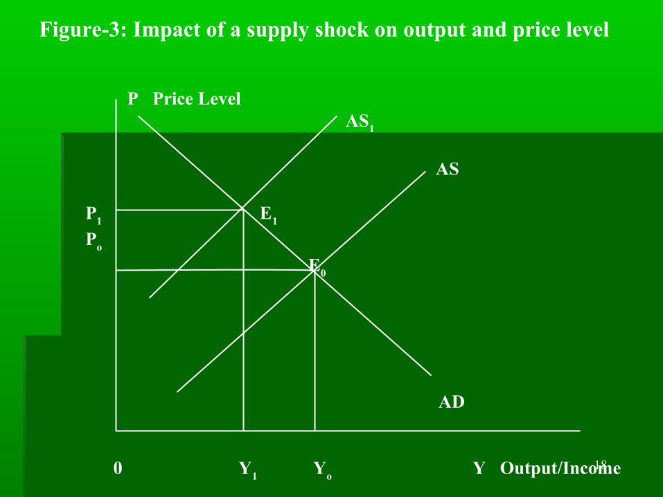
Impact of supply shock on output and price:

Supply shocks means abrupt sinking of the supply

In supply shocks supply decreases suddenly creating shock

OPEC oil embargo from 1973 created a supply shock

As by supply shock supply sinks, supply curve shifts leftward (Figure-3)

So, output is cut

Price increases (Figure-3)

18

Figure-3: Impact of a supply shock on output and price level

P Price Level AS1

AS P1 E1

Po

E0

AD

0 Y1 Yo Y Output/Income

19

2. THE AGGREGATE SUPPLY CURVE

Short-run aggregate supply curve

Aggregate supply curve presents: Quantity of output that firms are willing to supply at

a given price level

If in short-run demand increases: Firms increase supply Firms use this opportunity to achieve extra gain They keep price unchanged and increase supply So, in short-run aggregate supply curve remains

horizontal (Figure-4a) Long-run aggregate supply curve

20

In the long-run: Per capital GDP is constant Per capita capital in constant, and Full employment is achieved

So, if the long-run demand increases: Firms have no possibility to increase supply

(because of full employment)

Hence, if in the long run demand increases: It increases only price level However, output remains unchanged Hence, in the long run aggregate supply curve is

Vertical (Figure-4b)

21

Figure-4a: Short run aggregate supply curve P Price Level

P1 AS

0 Y Output, Income

22

Figure-4b: Long run aggregate supply curve P Price Level AS0

P1

P0

AS1

0 Yo Y Output/Income

23

2.1 CHANG OF AGGREGATE SUPPLY CURVE OVER TIME

Over time the economy accumulates resources, technology improves and GDP grows

So, over time aggregate supply curve moves to the right (Figure-5a Figure-5b)

The Changes of GDP over a short period is usually small (Bangladesh 5%)

So, a single vertical line can be drawn to represent short-run supply of GDP

Annual changes of GDP do not depend on the price level

Annual supply of GDP is ‘exogenous to the price level’ (Figure-5b)

24

Figure-5a: Output Change Over Time

Y Output

Y2

Y1

Y0

0 to t1 t2 Time

25

Figure-5b: Supply Independent of Price

P Price Level

ASo AS1 AS2

0 Y0 Y1 Y2 Y Output

26

2.2 SHORT RUN (KEYNESIAN) AGGREGATE SUPPLY CURVE

The idea of short run supply curve implies that there is unemployment

The firms can obtain as much labour as they want at present wage

So, the costs of production do not to change as output levels change

Firms are willing to supply as much as demanded at existing price

So, short run (Keynesian) aggregate supply is horizontal

This indicates that firms supply whatever demanded at the existing price

27

2.3 FRIC11ONAL OR NATURAL UNEMPLOYMENT

Classical model implies that there is no unemployment

Everyone who wants to work get work But practically there is always some

unemployment This unemployment is associated with

market friction Labour market is in continuous change Some people are moving and changing jobs Other looking for jobs

28

Some firms are expanding and hiring new workers Others firms reduce employment by firing workers Under such condition to find the right job toilsome So, there is always some frictional unemployment Frictional unemployment exists because of shifting

one job and for new Such unemployment is also called the natural

unemployment It exists when the labour market is in equilibrium Currently natural rate in United States is about

5.5%

In spite of some frictional unemployment, we can say there is full employment: If those who wish to work are able to get work

29

2.4 STRUCTURAL UNEMPLOYMENT In modem economy, man by himself hardly produces

anything Even primitive man needed some tools like bow and

arrow for his livelihood With growth of technology, much more capital

needed for productive activity All instruments of production constitute stock of

capital Now, if working force grows faster than capital stock

of a country, entire labour force cannot be absorbed in productive employment

So, some will remain unemployed Such unemployment is known as structural

(Marxian) unemployment

30

2.5 SEASONAL UNEMPLOYMENT

Some productive activity has seasonal character In these sectors (activities), during the slack season

people become unemployed Such unemployment is known as seasonal

unemployment Agriculture work is normally a seasonal occupation So, farmers have not sufficient work to do during

the slack season Other examples of seasonal industry are: Ice factories Rice mills Sugar factories, etc

31

2.6. KEYNESIAN UNEMPLOYMENT OR CYCLICAL UNEMPLOY-MENT

Equilibrium level of income and employment may be established at less than full employment level

That means, there is some unemployment It is known as Keynesian unemployment It is due to deficiency of aggregate effective demand It is also called cyclical unemployment It is called cyclical, because business depression

occurs at cyclical intervals During depression, business activity is at low ebb and

unemployment increases Some people are thrown out of employment

altogether Some are partially employed

32

This type of unemployment arises not because of too little capital as for structural unemployment

It occurs because of too much capital

This type of unemployment occurs because total effective demand is not sufficient to absorb the entire production of goods that can be produced with the available stock of capital

Business cannot sell their entire output

So, output is reduced that occurs creates unemployment

33

Measures Removing Cyclical or Keynesian Unemployment

This unemployment is due to the deficiency of effective demand

It could be removed by boosting effective demand

Boosting effective demand following should be done:

Government boost consumption by reducing tax rates on incomes and consumption

Government subsidies private consumption

Government increases its own consumption

34

4. FISCAL AND MONETARY POLICY UNDER ALTERNATIVE SUPPLY ASSUMPTIONS

4.1 SHORT RUN (KEYNESIAN) FISCAL POLICY

Fiscal policy includes govt income (tax) and expenditure policy

The fiscal policy could be expansionary or contractiveExpansionary fiscal policy includes tax cut and

expansion of the marketContractive fiscal policy includes increasing tax and

cutting marketLet the market is equilibrium in at point E (Figure-6)At point E the aggregate demand and supply

schedules intersectLet us now consider a short run change

35

Let us consider a fiscal expansion Let government expands spending (or cut tax) Demand increases and shifts rightward from AD to

AD1 (Figure-6)

As it is a short run change, supply schedule is a horizontal line AS passing through E

The Supply schedule intersects the new demand schedule at equilibrium point E1

Output increases, but no prices increase (Figure-6) Impact of higher government spending (or tax cut) is:

Increase in output (Y1)

No prices increase (P0)

Generate employment

36

Figure-6: Impact of short run fiscal expansion P Price Level

E E1

Po AS

AD1

0 Yo Y1 Output/Spending

37

4.2 IMPACT OF LONG RUN FISCAL POLICY

Let us analyse the impact of fiscal policy in the long run

Fiscal policy includes govt income (tax) and expenditure policy

Fiscal policy could be expansionary or contractive Expansionary fiscal policy means tax cut and

expansion of the market Contractive fiscal policy means increasing tax and

cutting market Let us consider that government follows an

expansionary fiscal policy Let government expands spending

38

In long run the aggregate supply curve is vertical Supply cannot be increased because there is full-

employment Level of output (Y*) remains constant (Figure-7) Impact of Expansionary fiscal policy in the long run

is: No increase in output Per capital GDP remains constant Price increase Let us consider that government follows an

expansionary fiscal policy

It cuts tax, so: Demand increases and demand schedule shifts

rightward from AD to AD1

39

If there is unemployment economy move to E1 in short

run Supply increase by unchanged price P0 to E1

Firms cannot obtain labour to produce more output New demand schedule intersects the vertical aggregate supply schedule at point E2

This is new equilibrium and at point E2 there is full

employment Supply of output cannot be increased to meet

increased demand Firms charge higher prices for their output and price

increases Impact of tax cut in the long run is:

No increase in outputPrice increase

40

Figure-7: Impact of expansive fiscal policy in the long run P Price Level AS

E1

P1

Po E E1

AD1

AD

0 Yo Y1 Output/Spending

41

The process of price increase: Let before the tax cut the real money stock was M/P M was money supple, P was the price level and there

was equilibrium Let because of tax cut money supply increases to M1

Demand increases Output can’t be increased So, price level increases

Price level increases to P1 so that: M/P = M1/P1

There is new equilibrium at higher price (P1) That means, same output is supplied at higher price

42

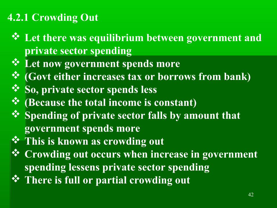
4.2.1 Crowding Out

Let there was equilibrium between government and private sector spending

Let now government spends more (Govt either increases tax or borrows from bank) So, private sector spends less (Because the total income is constant) Spending of private sector falls by amount that

government spends more This is known as crowding out Crowding out occurs when increase in government

spending lessens private sector spending There is full or partial crowding out

43

5. ONGOING MONEY GROWTH AND INFLATION IN LONG RUN

In long run money supply leads to increase price level

If money supply grows 10% a year Demand schedule would move up 10% annually Point of equilibrium of demand and supply would

move up 10% It means, in the long run prices would rise 10%

annually So we see ongoing money growth leads to inflation In the long run fiscal policy cannot affect output So, neutrality of money has strong policy

implications

44

If money were neutral, inflation could be reduced

For this, growing of the money stock would have to be stopped

In practice, it is difficult to reduce inflation without recession

Lower growth rate of money leads to demand sinks

Consequently, output sinks and unemployment increases

So, money is not neutral

Changes in quantity of money have real effects

Monetary policy affects the level of output

45

6. SUPPLY-SIDE ECONOMICS

Some economists favour policies: Those shift supply curve right ward

And increases GDP

Arguments are: Increased supply creates job

And increases per capita income

46

So, following policies suggested for increasing supply:

Removing unnecessary regulation of the economy Cutting tax rates Encouraging technological progress Some economists refer ‘supply-side economics’ as

‘voodoo (curse) economics’

Let us analyse what happens if tax rates are cut Tax cut has effects both on aggregate supply and

aggregate demand Aggregate demand increases (Demand schedule shifts right from AD to

AD1/Figure-7)

47

This shift is relatively large

Aggregate supply also increases

(Supply curve shifts to the right from AS to AS1/Figure -7)

Lower tax rates increase the incentive to work

The effect of such an incentive is quite small

So, rightward shift of GDP is small

So, in short run GDP is higher but very small amount

However, total tax collections fall and the deficit rises

In addition, prices are permanently higher

48

Supply Side Economics: Experiences in the USA

Tax was cut in USA in 1981-1983 Output increased very small Price increased Budget deficit increased

Many economists don't believe in magic of tax cut Conservative economists argue that tax cut has a

small but real effective incentive They suggest that cutting of tax & govt spending

should fall at same time: Tax collections fall, so fall also government

spending So, effect on budget is nearly neutralised