aggregate lte: characterizing user equipment emissions
TRANSCRIPT

11/28/2017
1
Aggregate LTE:
Characterizing User Equipment Emissions
Metrology Plan
Prepared by: Technical Lead
Paul Hale, Ph. D.
Program Manager
Sheryl Genco, Ph. D.
Contributors:
Jason Coder
Mark Lofquist
Adam Wunderlich, Ph. D.
John Ladbury
Azizollah Kord
Jonathan Cook
Timothy Hall, Ph. D.
Keith Hartley, D. C. Sc.
Reviewed and approved by: xxxx, xxxx
11/28/2017
2
National Advanced Spectrum and Communications Test Network (NASCTN)
The mission of the National Advanced Spectrum and Communications Test Network (NASCTN) is to
provide, through its members, robust test processes and validated measurement data necessary to develop,
evaluate and deploy spectrum sharing technologies that can increase access to the spectrum by both
federal agencies and non-federal spectrum users.
NASCTN was formed to provide a single focal point for engaging industry, academia, and other
government agencies on advanced spectrum technologies, including testing, measurement, validation, and
conformity assessment. The National Institute of Standards and Technology (NIST) hosts the NASCTN
capability at the Department of Commerce Boulder Laboratories in Boulder, Colorado.
NASCTN is a membership organization under a charter agreement. Members
• Make available, in accordance with their organization’s rules policies and regulations,
engineering capabilities and test facilities, with typical consideration for cost.
• Coordinate their efforts to identify, develop and test spectrum sharing ideas, concepts and
technology to support the goal of advancing more efficient and effective spectrum sharing.
• Make available information related to spectrum sharing, considering requirements for the
protection of intellectual property, national security, and other organizational controls, and, to the
maximum extent possible, allow the publication of NASCTN test results.
• Ensure all spectrum sharing efforts are identified to other interested members.
Current charter members are:
• National Telecommunications and Information Administration (NTIA)
• National Institute of Standards and Technology (NIST)
• Department of Defense Chief Information Officer (DoD CIO)

11/28/2017
3
Table of Contents
0 Acronyms .............................................................................................................................................. 5
1 Introduction ........................................................................................................................................... 7
2 Background ........................................................................................................................................... 7
3 Objective ............................................................................................................................................. 11
4 Scope ................................................................................................................................................... 11
5 Deliverables ........................................................................................................................................ 11
6 Measurements ..................................................................................................................................... 12
6.1 Test Description .......................................................................................................................... 15
6.1.1 Channel Emulation .............................................................................................................. 16
6.2 Summary of Test Equipment ...................................................................................................... 17
6.3 UE Traffic Generator Configuration ........................................................................................... 18
6.4 Macro-cell eNodeB Configuration .............................................................................................. 19
6.5 DUT UE Configuration ............................................................................................................... 21
6.6 Channel Emulator Configuration ................................................................................................ 21
6.7 Use of LTE Protocol Analyzer .................................................................................................... 22
6.8 Data Measured and Collected ..................................................................................................... 22
6.9 Measurements of specific events ................................................................................................ 23
6.10 Determination of EIRP................................................................................................................ 24
6.10.1 Conducted Tests .................................................................................................................. 25
6.10.2 Radiated Tests ..................................................................................................................... 25
6.10.3 UE Directivity ..................................................................................................................... 25
6.11 Frequency Band .......................................................................................................................... 26
6.12 Measurement Protocol ................................................................................................................ 26
6.13 Calibration/Reference Measurement Procedure ......................................................................... 27
7 Statistical Considerations .................................................................................................................... 27
7.1 Relevant Experimental Variables ................................................................................................ 27
7.1.1 Response Variables ............................................................................................................. 27
7.1.2 Controlled Variables (Factors) ............................................................................................ 27
7.1.3 Uncontrolled Variables ....................................................................................................... 28
7.1.4 Sources of Uncertainty ........................................................................................................ 28
7.2 Data Analysis Plan ...................................................................................................................... 28
7.3 Experimental Design ................................................................................................................... 29
7.3.1 Determination of Sample-Size Parameters ......................................................................... 29
7.3.2 Test Matrix Design.............................................................................................................. 29
7.4 Potential Biases and Their Mitigation ......................................................................................... 30
11/28/2017
4
8 Data Management ............................................................................................................................... 30
9 Coordination and outreach .................................................................................................................. 31
10 Schedule .......................................................................................................................................... 32
11 Safety .............................................................................................................................................. 32
References ................................................................................................................................................... 32
Appendix A. Baseline LTE Uplink Characteristics from [A.1] ........................................................... 34
A.1. UE Transmit Characteristics ........................................................................................................... 34
A.2. References ....................................................................................................................................... 36
Appendix B. Example Factor Prioritization ......................................................................................... 37

11/28/2017
5
0 Acronyms
3GPP 3rd Generation Partnership Project
AWS-3 3rd group of Advanced Wireless Services bands
CDF Cumulative Distribution Function
CR Coordination Request
CRADA Cooperative Research and Development Agreement
CRE Coordination Request Evaluation
C-RNTI Cell Radio Network Temporary Identifier
CSMAC Commerce Spectrum Management Advisory Committee
CW Continuous Wave
DCI Downlink Control Information
DISA Defense Information Systems Agency
DL Down Link
DoD Department of Defense
DSO Defense Spectrum Organization
DUT Device Under Test
EEPAC Early Entry Portal Analysis Capability
e-ICIC enhanced Intercell Interference Coordination
EIRP Equivalent Isotropic Radiated Power
eNB evolved UTRAN Node B or Evolved Node B
EPC Evolved Packet Core
e-UTRA Evolved Universal Terrestrial Radio Access
e-UTRAN Evolved UMTS Terrestrial Radio Access Network
FCC Federal Communications Commission
FD Frequency Domain
FDD Frequency Division Duplex
FPGA Field Programmable Gate Array
ICIC Intercell Interference Coordination
IMS Internet Protocol Multimedia Subsystem
IP Internet Protocol
ISD Inter-Site Distance
ITS Institute for Telecommunication Science
ITU International Telecommunications Union
LTE Long Term Evolution
MCS Modulation and Coding Scheme
NAS Non-Access Stratum
NASCTN National Advanced Spectrum and Communications Test Network
NIST National Institute of Standards and Technology
NTIA National Telecommunications and Information Administration
PDCCH Physical Downlink Control Channel
PRB Physical Resource Block
QCI QoS Class Identifier
QoS Quality of Service
RAID Redundant Array of Independent Disks
RAN Radio Access Network
RF Radio Frequency
RLC Radio Link Control
RMS Root-Mean Square
RRC Radio Resource Control
RSRP Reference Signal Received Power

11/28/2017
6
SIMO Single Input Multiple Output
SNR Signal to Noise Ratio
SRF Spectrum Relocation Fund
SSTD Spectrum Sharing Test and Demonstration (also SST&D)
TRP Total Radiated Power
TTI Transmission Time Interval
UDP User Datagram Protocol
UE LTE User Equipment
UL Up Link
UTG UE Traffic Generator
UTMS Universal Mobile Telecommunications System
VOLTE Voice Over LTE
VSA Vector Signal Analyzer
VT-ARC Virginia Tech Advanced Research Center
WNO Wireless Network Operator

11/28/2017
7
1 Introduction
The Defense Information Systems Agency (DISA) Defense Spectrum Organization (DSO) through the
Spectrum Sharing Test & Development (SST&D) program proposed to NASCTN a measurement
campaign to quantitatively characterize Long Term Evolution (LTE) Up Link (UL) waveforms generated
by User Equipment (UE) in the 1755 MHz to1780 MHz band, with the intent to develop realistic models
of UE emissions. These models will be used for assessing interference to Department of Defense (DoD)
systems that, for a time, will remain in the 1755 MHz to1780 MHz band.
The test plan, developed by NASCTN and described in this document, is one of a series of potential
measurements designed to better understand the emission of commercial UEs, both individually and in
aggregate. This plan will perform a series of controlled laboratory measurements over a variety of LTE
network settings and are designed to better understand UE emissions behavior, over both frequency and
time, and their sensitivity to various network configurations. In contrast to field-based measurements with
limited knowledge of network settings, laboratory measurements will allow control and manipulation of
all aspects of the network, giving the ability to generate a quantitative predictive model of the UE
emission and its dependence on specific network parameters. The work will include an analysis of the
assumptions and measurement uncertainties, and their effects on the uncertainty of the estimated
parameters.
2 Background
In the 2010 Presidential Memorandum on Unleashing the Wireless Broadband Revolution [1], the
National Telecommunications and Information Administration (NTIA) was tasked to identify
underutilized spectrum suitable for wireless broadband use. In the subsequent NTIA Fast Track Report
[2], many federal bands were identified as commercially viable. From this report, the Federal
Communication Commission (FCC) identified 1695 MHz to 1710 MHz, 1755 MHz to 1780 MHz, and
2155 MHz to 2180 MHz together as the 3rd advanced wireless services group of bands (called together
Advanced Wireless Service – 3 (AWS-3)) in July 2013, shown in Figure 1. The FCC adopted a Report
and Order in March 2014 with allocation, technical, and licensing rules for commercial use of the AWS-3
bands [3]. The uplink blocks of interest here are the 5 MHz blocks labeled G, H, and I and the 10 MHz J
block.
Through Auction 97 [4], the AWS-3 band was auctioned for commercial mobile broadband usage in the
United States. The auction raised $41B in revenue for the United States Treasury and required federal
agencies in the AWS-3 band to look for other ways to accomplish their missions. In the 1755 MHz to 1780
MHz portion of the AWS-3 band, the DoD is using a combination of sharing, compression, and relocation
to other bands (including the 2025 MHz to 2110 MHz band).

11/28/2017
8
Figure 1. Description of the AWS-3 band.
In 2012, the Commerce Spectrum Management Advisory Committee (CSMAC) was tasked with
exploring ways to lower the repurposing costs and/or improve or facilitate industry access to spectrum
while protecting specific federal operations from adverse impact, particularly in the AWS-3 band. In
carrying out their work, the CSMAC made several assumptions on the LTE UE and base station
configurations, listed in Appendix A [5]. These assumptions were used to estimate Equivalent Isotropic
Radiated Power (EIRP) distribution functions (shown in the appendix) for a UE in rural and suburban
network laydowns.
From the AWS-3 auction proceeds, DoD is receiving a spectrum relocation fund (SRF) to implement its
approved transition plans. The SRF is also funding evaluation of early entry coordination requests from
the auction winners in the AWS-3 band through the DoD early entry portal analysis capability (EEPAC),
which is managed by DISA DSO. The portal receives requests from auction winners to enter band(s)
before the DoD has transitioned out of the bands. These requests must be considered carefully and
impartially to deliver a fair answer. If early entry is granted and there is interference to DoD systems, it
would be very costly to the DoD in terms of both financial and mission completeness. If early entry is
denied to a commercial carrier for overly conservative reasons, it could be very costly to their business
model. To avoid these costs, it is crucial that the findings of the EEPAC are fair and based on a well
understood and openly documented methodology.
Towards this end, the DSO is evaluating entry requests by use of the updated interference equation
(below) and the EIRP distributions assumed by the CSMAC. To gain further confidence in their
calculations, the DSO has asked NASCTN to develop a measurement-based plan for gaining an improved
quantitative understanding of LTE uplink emissions. More specifically, NASCTN will investigate how
the LTE user equipment behaves in frequency and power under realistic operating conditions, and how
this behavior depends on the network configuration, going beyond the CSMAC analysis with its fixed
(and possibly unrealistic) network configurations.
The interference equation used by the EEPAC1 [6] is
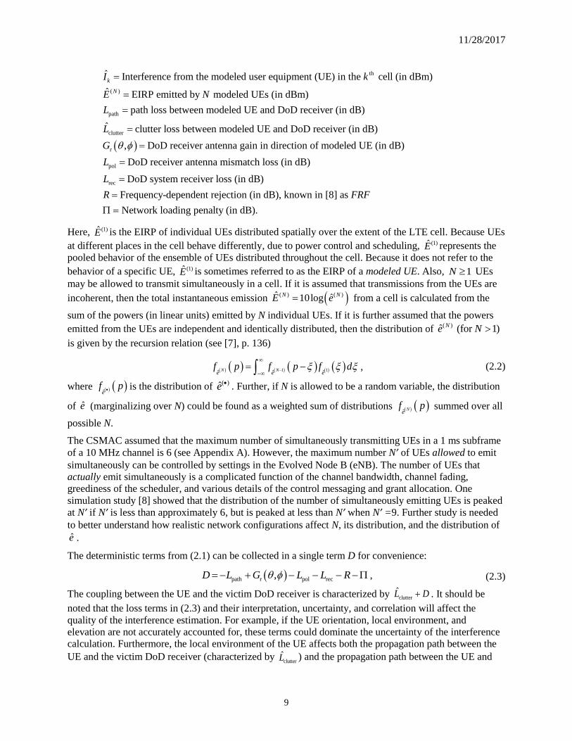
𝐼k = ��(𝑁) − 𝐿path − ��clutter + 𝐺𝑟(𝜃, 𝜙) − 𝐿pol − 𝐿rec − 𝑅 − Π, (2.1)
where
1 We follow the notation of [6]; lower case variables denote numbers in linear units (e.g., mW) while upper case
variables use a logarithmic scale (e.g., dBm). Random variables are denoted by a caret. The symbols for the last two
terms have been changed from [6] to a single letter for readability.
11/28/2017
9
th
( )
path
clutter
ˆ Interference from the modeled user equipment (UE) in the cell (in dBm)
ˆ EIRP emitted by modeled UEs (in dBm)
path loss between modeled UE and DoD receiver (in dB)
ˆ clutter
k
N
I k
E N
L
L
r
pol
rec
loss between modeled UE and DoD receiver (in dB)
, DoD receiver antenna gain in direction of modeled UE (in dB)
DoD receiver antenna mismatch loss (in dB)
DoD system receiver loss (in dB)
G
L
L
R
Frequency-dependent rejection (in dB), known in [8] as
Network loading penalty (in dB).
FRF
Here, (1)E is the EIRP of individual UEs distributed spatially over the extent of the LTE cell. Because UEs
at different places in the cell behave differently, due to power control and scheduling, (1)E represents the
pooled behavior of the ensemble of UEs distributed throughout the cell. Because it does not refer to the
behavior of a specific UE, (1)E is sometimes referred to as the EIRP of a modeled UE. Also, 1N UEs
may be allowed to transmit simultaneously in a cell. If it is assumed that transmissions from the UEs are
incoherent, then the total instantaneous emission ( ) ( )ˆ ˆ10logN NE e from a cell is calculated from the
sum of the powers (in linear units) emitted by N individual UEs. If it is further assumed that the powers
emitted from the UEs are independent and identically distributed, then the distribution of ( )ˆ (for 1)Ne N
is given by the recursion relation (see [7], p. 136)
1 1ˆ ˆ ˆ
N Ne e e
f p f p f d
, (2.2)
where e
f p• is the distribution of ( )e •
. Further, if N is allowed to be a random variable, the distribution
of e (marginalizing over N) could be found as a weighted sum of distributions ˆ
Ne
f p summed over all
possible N.
The CSMAC assumed that the maximum number of simultaneously transmitting UEs in a 1 ms subframe
of a 10 MHz channel is 6 (see Appendix A). However, the maximum number N’ of UEs allowed to emit
simultaneously can be controlled by settings in the Evolved Node B (eNB). The number of UEs that
actually emit simultaneously is a complicated function of the channel bandwidth, channel fading,
greediness of the scheduler, and various details of the control messaging and grant allocation. One
simulation study [8] showed that the distribution of the number of simultaneously emitting UEs is peaked
at N’ if N’ is less than approximately 6, but is peaked at less than N’ when N’ =9. Further study is needed
to better understand how realistic network configurations affect N, its distribution, and the distribution of
e .
The deterministic terms from (2.1) can be collected in a single term D for convenience:
path r pol rec,D L G L L R , (2.3)
The coupling between the UE and the victim DoD receiver is characterized by clutterL D . It should be
noted that the loss terms in (2.3) and their interpretation, uncertainty, and correlation will affect the
quality of the interference estimation. For example, if the UE orientation, local environment, and
elevation are not accurately accounted for, these terms could dominate the uncertainty of the interference
calculation. Furthermore, the local environment of the UE affects both the propagation path between the
UE and the victim DoD receiver (characterized by clutterL ) and the propagation path between the UE and

11/28/2017
10
eNB, with the latter affecting the power generated by the UE and its probability distribution. While the
clutter loss term, in principle, handles the shadowing and fading losses between the UE and victim
receiver, it does not account for similar effects in the path between the UE and eNB. This latter effect of
local environment is implicit in the UE EIRP and its distribution.
The frequency-dependent rejection term R is a function of the government receiver selectivity and the UE
emission spectra. The emission spectra are a complicated function of the UE mode of operation, resource
block allocation, various details of the control channel allocation and power control, and the guard band
between blocks. Furthermore, licensees with adjacent frequency blocks in the same geographic area can
combine uplink bands to form 10, 15, or 20 MHz blocks. Use of realistic spectrum information that
includes guard bands and control channel allocations could provide significant portions of the AWS-3
band, at the block edges, with much less interference levels than are currently calculated, based on the
CSMAC assumed flat spectrum. Further study is needed to understand realistic UE spectra and realize
these benefits.
The DSO has also recruited other organizations to better inform their calculation of aggregate interference
with DOD assets, including the NTIA Institute for Telecommunication Science (ITS), Virginia Tech
Advanced Research Center (VT-ARC), Georgia Tech Applied Research Corp., Excelis, Harris
Corporation, MITRE Corporation, and others for LTE modeling, simulation, and drive testing. An
extensive summary of this work is given in [9]. We do not attempt a review of the above work here, but
note as an example, that the MITRE team used the Riverbed Modeler (OPNET) to model an LTE
network, design simulations, and collect statistics on the LTE uplink emissions. These simulations helped
to create a cumulative distribution function (CDF) of LTE uplink transmit power values from UEs
throughout various locations in a cell. The CDFs were used to perform a sensitivity analysis of uplink
power CDF based on inter-site distance (ISD), UL demand, and network congestion and laydown [10].
The resulting simulations deviated from the original CSMAC findings, but the cause was unknown. In
addition, ISD, UL demand, and network congestion and layout were confirmed to significantly change the
transmit power CDF.
The MITRE team extended their LTE emission work into drive testing to better understand the effects
those added environments on the transmit power CDF curves. The drive tests considered the following
factors that could affect UE transmit power statistics:
• Inter-site distance
• Cell site antenna height
• Propagation loss environment
• Neighboring cell interference
• UE traffic demand
However, multiple factors were varied simultaneously, but not systematically, making it difficult to
determine the effect of any individual factor. General findings and trends included;
• The urban, suburban, and rural morphologies all have distinct CDF curves, showing how UE transmit
power increases/decreases with the varying morphologies.
• Using only two morphologies, based on CSMAC, may cause the UE power to be significantly under-
or over-estimated in some areas. There is greater than 10 dB difference in power between the
suburban drive tests by two different wireless network operators (WNOs) and the CSMAC
suburban/rural CDF curve.
• The rural drive tests by two different WNOs both show power levels much higher (≈6 dB) than
CSMAC suggests.

11/28/2017
11
3 Objective
The objective of this NASCTN test plan is to describe how to empirically estimate parameters, pertaining
to the UE emissions and physical resource block (PRB) usage, that contribute to the interference equation
(2.1) while controlling or mitigating some of the uncontrolled variables of previous measurement efforts.
These estimates will attempt to capture behaviors of actual deployed UEs and will include an uncertainty
analysis based on an evaluation of the assumptions and sources of uncertainty in the measurements. In
particular, the parameters of interest in this study are:
1. (1)E : The distribution of EIRP emitted by a UE in a 1 ms subframe, marginalized (averaged) over the
cell spatial distribution.
2. The emitted spectrum of an actively transmitting UE.
3. N: The number of UEs emitting into a 5 MHz or 10 MHz band per 1 ms subframe per cell
(#UEs/MHz/ms/cell).
Also of interest for a potential Phase 2, and of secondary importance is
4. Characterization of the accuracy of UE self-reported power and its correspondence to the EIRP.
5. Development, validation, and documentation that could inform potential field measurement
procedures.
NASCTN plans to achieve the objectives will focus on estimates based on laboratory measurements of
the above parameters, facilitating more control of critical variables than will be achievable in field tests.
Specifically, laboratory experiments will allow us to control and manipulate the key variables that can
affect the UE behavior, including (but not limited to): eNB power control variables and scheduling
algorithms, propagation channel, traffic type, and in-cell and adjacent-cell loading. Such control will be
critical for the sensitivity analysis required for analysis of uncertainty in laboratory measurements.
Furthermore, controlled experiments, combined with systematic design of experiment procedures, will
allow NASCTN to assemble a predictive model for the above parameters that depends on all factors
tested. These models could be used by the DSO to tailor the CDF input into the EEPAC to the specific
network laydown of a coordination request (CR).
4 Scope
The study will specifically address the characterization of LTE Frequency Division Duplex (FDD) signals
and groups of signals (i.e., emissions from multiple UEs transmitting simultaneously) in the UL
frequencies of 1755 MHz to 1780 MHz. As described in Section 3, the signal statistics obtained from
these measurements can feed into the interference calculation of (2.1) as implemented in the EEPAC. The
goal of this characterization, with a documented methodology and uncertainty, is to give AWS-3
stakeholders more confidence in the Coordination Request Evaluation (CRE) process.
The study will be limited to estimates of the variables listed in Section 3 above, based on laboratory
measurements, with analysis of the effects of key variables that can affect the UE behavior: eNB power
control variables and scheduling algorithms, propagation channel, traffic type, and in-cell and adjacent-
cell loading.
Future studies could extend this plan to include field tests.
5 Deliverables
The deliverables of this study are predictive models of the following parameters based on laboratory
measurements:

11/28/2017
12
1. The distribution of (1)E ; the EIRP emitted by a UE in a 1 ms subframe, marginalized (averaged) over
the cell spatial distribution. Distributions of both peak and root-mean-square (RMS) EIRP in a 1 ms
subframe will be reported.
2. The emitted in-band spectrum of an actively transmitting UE. This will be delivered as a series of
spectra, showing the relative power level in each part of the LTE channel when the Device Under
Test (DUT) UE is actively transmitting, and metadata regarding which PRBs are in use by the DUT
UE.
3. N: The number of UEs emitting into a 5 MHz or 10 MHz band per 1 ms LTE subframe per cell. This
will be presented as a series of distributions depicting the probability of N=1, 2, … UEs being active.
The estimates will include an analysis of the assumptions and measurement uncertainties and their effect
on the uncertainty of the estimated parameters.
Secondary deliverables are:
1. Characterization of the accuracy of generated power as reported by the UEs available for testing and
its correspondence to the measured EIRP.
2. Ideas for a potential future field measurement of the above variables.
6 Measurements
Conceptually, the first deliverable – distribution of EIRP emitted by a UE – can be empirically measured
by measuring the output of a UE as it traverses through a cell and then pooling the data over the cell2. In
the real world, this can be accomplished by monitoring a UE via diagnostic monitoring software as it
completes a drive test. This real-world approach can be problematic because there are many uncontrolled
variables and sources of error: the accuracy of the self-reported power, the repeatability of the drive test,
the unknown eNB configuration, etc.
The goal of the measurements is to develop a realistic, laboratory based scenario that will enable
empirical measurement of parametric deliverables while controlling the measurement configuration. This
will not only allow measurement of the parameters of interest, but also enable the determination of the
sensitivity of those parameters to the system settings and configuration. In turn, this will give an
understanding of which system laydown and configuration variables are most significant in the
interference aggregation calculation.
The above scheme can be replicated in a laboratory setting by use of an eNB, UE, vector signal analyzer
(VSA), and channel emulator. The channel emulator can simulate changes in the propagation
environment between the UE and eNB as the UE virtually changes position relative to the eNB. During
these changes in propagation, the VSA can measure the power emitted from the UE in different channel
conditions.
This measurement setup can also yield information on the second deliverable – the emitted in-band
spectrum of a UE. Though it can easily be measured, for these data to be of value, the PRBs assigned to
the UE must be known. With this information, the measured spectrum can be correlated with a given
number of PRBs and plots of the emitted spectrum can be produced for each PRB configuration that was
observed. Knowledge of the assigned PRBs can come from a wireless protocol analyzer in real-world
measurements, or it can come from having control of all the UEs in a cell in a laboratory setting. If the
fidelity of the spectrum measurement is sufficient, it is possible to infer the PRBs in use directly from the
spectrum measurement. To do this, each sub-carrier in the subframe needs to be resolved and analyzed.
2 Here we assume ergodicity, i.e., we assume that the power emitted by a single UE, pooled over different positions
in the cell is distributed identically to the distribution of power emitted by an ensemble of many UEs placed
throughout the cell and emitting individually at any given instant.

11/28/2017
13
The third deliverable – the number of UEs emitting into a channel in each subframe – requires knowledge
like that required to produce the second deliverable. One needs to have some knowledge of the other UEs
in the cell, which ones are active, and what resources they are assigned. In the real-world, this can be
obtained by use of the wireless protocol analyzer mentioned above. But in a controlled, laboratory setting,
a UE traffic generator (UTG) can be used to generate traffic and load the eNB. When the demand for eNB
resources is large, there will be more UEs requesting resources than can be accommodated in a single
subframe. The eNB will then schedule – based on demand – some number of UEs to transmit in each
subframe. The scheduling/resource allocation information can be obtained from the logs on the UTG or
from the use of the protocol analyzer in the laboratory setting.
Figure 2 graphically depicts the laboratory setup discussed above. In this setup, there are two adjacent
cells, each populated with enough UEs to sufficiently load the scheduling algorithm in the eNB. These
“loading UEs” will be distributed throughout the cells in static positions. A DUT UE will then be
virtually placed, at different locations in Cell , and its emissions measured, along with its PRB
allocations and the PRB allocations of the loading UEs. The detailed use of the loading UEs will be
discussed in Section 6.3.
A detail of Cell from Figure 2 is shown in Figure 3. Here, we see that at each DUT UE location, a
propagation channel between the UE and eNB will be accounted for as part of the UE emissions
measurement. Also, the emissions from the loading UEs in the adjacent cell will be present (at an
appropriate amplitude) within Cell and at the radio frequency (RF) ports of the eNB.
Replicating this scenario in a laboratory setting will enable the control of the cell size, distribution of
loading UEs, placement of the DUT UE, influence of adjacent cell emissions, eNB power control
parameters and scheduling algorithms, and the propagation channel. Each of these variables can be
adjusted individually, allowing for a characterization of UE emissions and resource block allocations
across a variety of scenarios.
The setup depicted in Figure 2 and 3 is realized in terms of laboratory equipment in Section 6.1 and
discussed in detail in Sections 6.3-6.12. These sections outline the detailed configuration of each key
piece of laboratory instrumentation required to replicate the setup described above. Section 6.2 provides a
high-level overview of the instrumentation required.

11/28/2017
14
Figure 2. The hypothetical scenario being replicated by the laboratory testing.3
Figure 3. A more detailed schematic of the hypothetical cell shown in Figure 2.
3 Note: These figures are shown for illustrative purposes only. Technical details of the cell configurations are
discussed throughout Section 6.

11/28/2017
15
6.1 Test Description
The test setup shown in Figure 4 seeks to realize the hypothetical scenario shown in Figure 2 and 3. This
realization involves two commercial macro-cell-loaded eNBs and a UTG, sometimes referred to as an
“LTE radio access network (RAN) load tester”, to simulate the loading UEs. The cells can be serviced
with two separate commercial eNBs, or with a single eNB capable of supporting two cells. A controlled
DUT UE will be inserted into Cell . This DUT UE will be a real, commercially available UE that
attaches to the same cell as the loading UEs and is assigned resources from the eNB’s scheduling
algorithm. Both the loading UEs and the DUT UE will transact a specified data type (e.g., User Datagram
Protocol (UDP)) at a specified data rate.
Figure 4. Measurement system schematics. The top diagram (a) shows the configuration for conducted
testing, while the bottom figure (b) shows the configuration for UEs that must be tested using a radiated
method.

11/28/2017
16
Previous work [10] posited that the emissions of UEs located in an adjacent cell can influence the radiated
power level of a UE (or a group of UEs) in another sector. In essence, the adjacent cell UEs increase the
noise floor in the cell-of-interest and cause the UEs to transmit more power to overcome the increased
noise. This effect is accounted for in the laboratory testing proposed in Figure 4. The amount of adjacent
cell influence can be controlled via the combination of two variable attenuators and three directional
couplers. The amount of influence from Cell should be appropriate given the selected propagation
conditions and cell size.
The DUT UE is drawn as being connected to a directional coupler with the output port connected to a
diplexer (splitting/combining the uplink/downlink), and the side-arm connected to the input of a VSA.
The VSA is used to collect the emission spectra of the DUT UE during the test.
The output of the coupler is passed through the diplexer, and connected to a channel emulator. This
channel emulator simulates the desired propagation channel between the DUT UE and the eNB. Both the
uplink and downlink channels are passed through the emulator, but because they are at different
frequencies, the channels are slightly different. The signal generator shown supplies the uplink and
downlink carrier frequencies; a requirement for some channel emulators. The output of the channel
emulator passes through another diplexer and is combined with the loading UEs. The combined signal is
fed into the eNB. Note that if the channel emulator is capable of full duplex operation, the diplexer may
not be required.
During the measurement process, the DUT UE will run diagnostic monitoring software capable of
capturing the self-reported transmit power. These data will be transferred to a computer and recorded.
Data will be timestamped, such that they can be lined up with captures from the VSA for further analysis.
For the purposes of investigating potential Phase 2 measurements of live networks, an LTE protocol
analyzer is inserted into the system adjacent to the eNB. This analyzer will capture, decode, and record
the LTE traffic. These data can then be used to help understand how many UEs are transmitting in any
given LTE subframe. While these data can also be gathered from a combination of the VSA and the UTG,
the use of this protocol analyzer will help facilitate its use for potential future in-field data collection
where the loading UEs are replaced with live UEs.
Note that both the uplink and downlink signals are passed through the physical layer in this measurement
setup. In the case of the loading UEs, the downlink signals are passed back through the same combination
of splitters and couplers as the uplink signal. The uplink/downlink signal for the DUT UE is split via a
diplexer and handled separately in the channel emulator.
Below, the detailed description and configuration of each element are given, along with a sample
measurement sequence. Specific configuration parameters will be varied with a design of experiment
strategy (described in Section 7.3) to determine the sensitivity and cross-dependence of the measurands
on each parameter.
6.1.1 Channel Emulation
One of the key aspects of this test is how the propagation channel will be emulated. The propagation
channel, and its emulation, can impact the emissions of the DUT UE, allocation of PRBs, and the signals
from the adjacent cell (Cell ).
In this test, there are three different propagation channels that must be accounted for: the channel between
the DUT UE and the Cell eNB, the channel between the loading UEs in Cell and the Cell eNB,
and the channel between the loading UEs in Cell and the Cell eNB.
In the above test description and diagram, each of these three channels are accounted for in a different
manner. The channel between the DUT UE and the Cell eNB is handled by a dedicated channel

11/28/2017
17
emulator. As described below, this channel emulator will have enough fidelity to implement custom
channel models that account for path loss, fading, and clutter parameters. This fidelity is necessary as the
ability to emulate this propagation channel has a direct impact on the accuracy of the final results.
The channel between the Cell loading UEs and the Cell eNB is implemented by use of the UTG.
Most UTGs implement some form of propagation loss and channel characteristics (generally defined in
3rd Generation Partnership Project (3GPP) specifications). These implementations are generally done in
the signaling layers, not in the physical layer. These channels will be of lower fidelity than the DUT
UE/eNB channel, but in this case, the primary goal of this propagation channel is to ensure that the
loading UEs are assigned PRBs in ways that are consistent with the environment they’re in.
The fact that the channels are implementing in the signaling layer is not necessarily a disadvantage. The
primary goal of the Cell loading UEs is to load the Cell eNB scheduler. Thus, as long as the Cell
eNB thinks the loading UEs are in a given RF condition, the scheduler will allocate resources
accordingly. The RF waveform associated with the loading UEs is not of interest to the DUT UE as it
won’t receive or sense the UL signal of the loading UEs.
The third channel – between the Cell loading UEs and the Cell eNB – is accounted for via RF
attenuators. In this case, there is no signaling between these UEs and the Cell eNB. The Cell
loading UEs serve only to raise the noise floor in Cell . Thus, we only need to ensure that the
amplitude of the RF signal impinging on the Cell eNB port is appropriate given the desired
propagation channel4. This amplitude will be verified (e.g., by use of a spectrum analyzer) prior to the
start of each test. Because the locations of Cell and eNBs is fixed, the amplitude is not expected to
change during the testing of a given morphology/scenario.
When selecting a channel to be emulated, it is imperative to ensure that a similar channel is modeled in
each of the three implementations. Discrepancies in the channels being modeled may result in biasing the
results. For example, giving the loading UEs a more favorable propagation channel than the DUT UE
(when it isn’t warranted) may result in the eNB scheduler allocating resources in an unrealistic manner,
potentially impacting the DUT UE’s distribution of radiated power.
6.2 Summary of Test Equipment
The equipment needed to conduct these measurements are as follows:
1. Macro-cell eNB hardware capable of serving two cells and supporting backend network hardware
(e.g., Evolved Packet Core (EPC)), with the ability to handover from one cell to the other. If possible,
testing should be performed with hardware from multiple vendors (e.g., one test with two Nokia cells,
one test with two Ericsson cells)5.
2. An LTE UE Emulator/Traffic Generator capable of generating LTE traffic in two cells and capable of
loading both cells such that UEs are requesting more resources than are available in a single frame.
The number of UEs in a cell during a test is discussed in Section 6.3 and is analyzed in the factor
selection tests discussed in Section 7.3.
3. Channel emulator capable of emulating both uplink and downlink channels for mobile scenarios. The
signal generator shown in Figure 4 is included as some channel emulators require that a continuous
4 Though this ensures the general amplitude of the signal is correct, the shape of the signal may not be. This is a
result of the fact that the individual channels between each Cell loading UE and the Cell eNB are not accounted
for. If this amplitude proves to be of significant influence on the DUT UE behavior, additional study – including
accounting for the individual channels – may be warranted. 5 Trade names are used here to describe possible measurement configurations and do not imply an endorsement by
NIST or NASCTN. Other equipment may work as well or better for the work described here.

11/28/2017
18
wave (CW) carrier be provided as an external input; one at the uplink frequency, and one at the
downlink frequency. The emulator should support the input of user-defined channel models for rural,
suburban and urban canyon environments and for terrain (flat and hilly) features.
4. Wireless LTE Protocol Analyzer capable of capturing the LTE traffic. This traffic may be decoded in
real-time, or stored and decoded after the measurement. The analyzer must be capable of capturing
the downlink control information (DCI) messages, as well as the cell radio network temporary
identifier (C-RNTI) information.
5. UE Diagnostic Software capable of recording the UE transmit power. Note that not all diagnostic
software applications are compatible with all UE chipsets. The output of this software should be
timestamped so it can be correlated with data from other instruments (e.g., VSA and UTG).
6. VSA or real-time spectrum analyzer, capable of continuous data streaming over greater than the
channel bandwidth without loss of data. If possible field programmable gate array (FPGA)-based
trigger on events with a defined frequency-domain threshold.
7. Several DUT UEs that are representative of the UEs deployed in the band of interest:
a. If the DUT UE output signal is conducted, then appropriate cabling will be required to
connect the UE to the rest of the measurement system.
b. If the DUT UE output signal is radiated, then a shielded enclosure (preferably anechoic) will
be necessary to isolate the emissions from the ambient signals. An antenna will be placed
inside the shielded enclosure and connected to the measurement system.
8. Directional couplers that have a flat response across UL and DL bands.
9. 3 dB splitters that have flat response across UL and DL bands (6 dB resistive splitters can also be
used).
10. Variable attenuators. The range and step size of these attenuators will be determined during the factor
selection phase. Step sizes more granular than 1 dB are not expected.
11. Delay lines that can delay the transmitted signal arriving at the eNB, or the downlink signal arriving
at the UTG. These delay lines enable the UTG and eNB to utilize receive diversity.
12. Diplexers for the selected UL and DL bands.
6.3 UE Traffic Generator Configuration
The UTG should emulate enough UEs to load the scheduler in the eNB. A loaded cell is crucial to
demonstrating uplink scheduling behavior.
UEs will be simulated in locations spread throughout the cell coverage area to determine the effect of UE
placement on eNB scheduling behavior. Three UE distributions will be used: 1) UEs placed in a tight
cluster immediately adjacent to the eNB, 2) UEs distributed around the edge of the cell, but configured
such that they do not get handed off to the adjacent cell, and 3) with a random distribution throughout the
cell. In addition to these UE distributions, the number of UEs present can also be varied based on the
morphology of interest (e.g., many UEs for urban scenarios and few UEs for rural scenarios).
The geographic size of the cell is also defined in the UTG.6 The cell size used should correspond to the
different morphologies of interest. Information on the statistics of cell sizes could come from WNOs, or
approximations of cell sizes for different morphologies can be found in [5] and [11]-[13]. The size of the
cell is one of the variables considered in testing, and is discussed in Section 7. Channel models for the
emulated UEs will be determined later, based on the final morphologies selected for testing. However, it
is important to note that different traffic generators model channels differently. Some UTGs model
channels in the signaling layer, some in the physical layer, and some use a combination of both. Any of
the three can be adapted for the testing described here.
6 Because the testing is conducted, UTGs generally ignore the pattern and tilt of the base station antenna.

11/28/2017
19
In a similar vein, UTGs do not account for the antenna pattern of the base station, it’s height, or it’s down
tilt. The height and down-tilt of the base station antennas is roughly accounted for when a sector is
defined to have a given radius in the UTG software. Base station antenna patterns are generally assumed
to be uniform and not specifically accounted for in the UTG.
The uplink traffic will be of UDP type, which requires no handshaking from the receiving end. Since
minimal downlink traffic is required, the uplink traffic flow will not be interrupted if the downlink traffic
is restricted. Voice or voice over LTE (VOLTE) traffic7 can be generated if the UTG can do so, but the
network infrastructure (e.g., internet protocol multimedia subsystem (IMS)) behind the eNB must also be
able to support such traffic.
The exclusive use of UDP traffic is not without drawbacks. There is some indication [13] that the amount
of power a UE will transmit varies based on whether the UE is in “voice mode” or “data mode.” Though
calls (voice or VOLTE) are still made, in terms of PRBs, they represent a small fraction of the total
allocated PRBs. That is, the use of other data functions on UEs (e.g., video, web browsing, etc.) are so
prolific that the clear majority of allocated LTE PRBs in the United States are allocated for the use of
data, rather than voice traffic [14].
As an alternative to measurements with voice/VOLTE, measurements can be done where a certain
percentage of loading UEs are forced to have a different QCI (Quality of Service (QoS) Class Identifier)
value [15]. Adjusting the QCI for loading UE traffic in the cell would simulate certain UEs having higher
priority traffic than others. This difference in traffic priority could have an impact on the distribution of
PRB grants and the number of PRBs the DUT UE is granted. An example of exercising QCI would be to
run a measurement where all of the loading UEs have the same QCI value (e.g., 9), then run another
measurement where some portion of the loading UEs have a different QCI value (e.g., 7). These two tests
may help simulate scenarios where the traffic types are varied.
The UE’s data rate can be one of the variables investigated. To load the eNB scheduler, it can be set to the
maximum (and the transmit buffer kept full with data). Data rates (also referred to as “data demand” or
“offered load”) can be made variable if further information on the number of active UEs or their data rates
in a given scenario is available (from a WNO). Scenarios involving UEs that are periodically idle, or UEs
that have less than full transmit buffers can be tested by use of this method. Tests under these conditions
may result in different outcomes for the number of UEs transmitting/frame (deliverable #3).
In addition to the UTG, some supporting hardware that isn’t shown in Figure 4 may be necessary. This
hardware includes server(s) for generating the loading UE traffic and server(s) that act as a destination for
the DUT UE and loading UE traffic. Servers used will need to be configured in such a way as to not
interfere with the physical layer testing being performed. That is, these servers should be capable of
supporting a sufficient amount of throughput.
6.4 Macro-cell eNodeB Configuration
The eNB will be configured as closely as possible to the configuration that is used by WNOs8. However,
some variations should be explored to determine if there are significant effects on the UE output power
and the number of UEs using any given subframe.
It is crucial that the eNB(s) used in these measurements can support enough active connections to
sufficiently load the scheduling algorithm. Certain software defined implementations may not be able to
support enough simultaneous active connections to create the desired loading effect. Most eNBs have a
configurable parameter that determines the maximum number of connections. For the tests described
7 A UE with VOLTE traffic will appear in more subframes than when loaded with UDP traffic. The use of VOLTE
traffic is not likely to affect the measurement results. Traffic type will change the frequency at which any given UE
appears in multiple subframes. 8 WNO feedback is critical for this aspect of the measurements.
11/28/2017
20
here, that parameter should be set high enough that it does not impinge on the number of UEs transmitting
in each subframe and allows for the scheduling algorithm to be loaded.
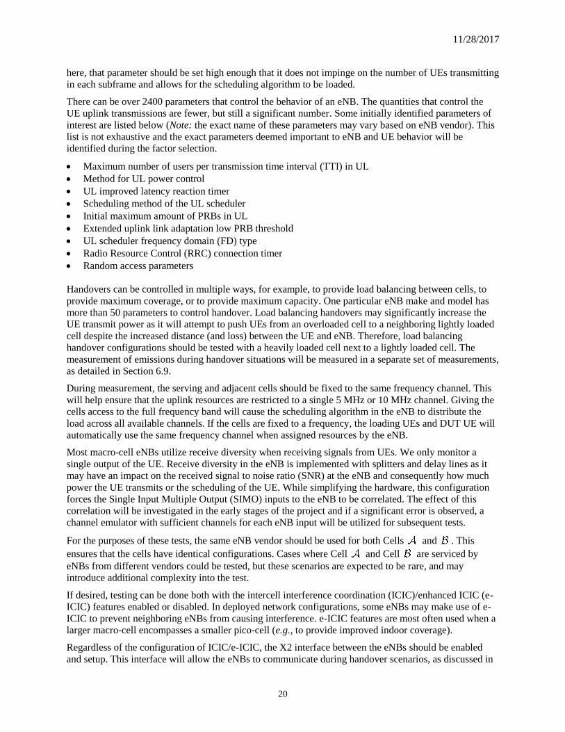
There can be over 2400 parameters that control the behavior of an eNB. The quantities that control the
UE uplink transmissions are fewer, but still a significant number. Some initially identified parameters of
interest are listed below (Note: the exact name of these parameters may vary based on eNB vendor). This
list is not exhaustive and the exact parameters deemed important to eNB and UE behavior will be
identified during the factor selection.
• Maximum number of users per transmission time interval (TTI) in UL
• Method for UL power control
• UL improved latency reaction timer
• Scheduling method of the UL scheduler
• Initial maximum amount of PRBs in UL
• Extended uplink link adaptation low PRB threshold
• UL scheduler frequency domain (FD) type
• Radio Resource Control (RRC) connection timer
• Random access parameters
Handovers can be controlled in multiple ways, for example, to provide load balancing between cells, to
provide maximum coverage, or to provide maximum capacity. One particular eNB make and model has
more than 50 parameters to control handover. Load balancing handovers may significantly increase the
UE transmit power as it will attempt to push UEs from an overloaded cell to a neighboring lightly loaded
cell despite the increased distance (and loss) between the UE and eNB. Therefore, load balancing
handover configurations should be tested with a heavily loaded cell next to a lightly loaded cell. The
measurement of emissions during handover situations will be measured in a separate set of measurements,
as detailed in Section 6.9.
During measurement, the serving and adjacent cells should be fixed to the same frequency channel. This
will help ensure that the uplink resources are restricted to a single 5 MHz or 10 MHz channel. Giving the
cells access to the full frequency band will cause the scheduling algorithm in the eNB to distribute the
load across all available channels. If the cells are fixed to a frequency, the loading UEs and DUT UE will
automatically use the same frequency channel when assigned resources by the eNB.
Most macro-cell eNBs utilize receive diversity when receiving signals from UEs. We only monitor a
single output of the UE. Receive diversity in the eNB is implemented with splitters and delay lines as it
may have an impact on the received signal to noise ratio (SNR) at the eNB and consequently how much
power the UE transmits or the scheduling of the UE. While simplifying the hardware, this configuration
forces the Single Input Multiple Output (SIMO) inputs to the eNB to be correlated. The effect of this
correlation will be investigated in the early stages of the project and if a significant error is observed, a
channel emulator with sufficient channels for each eNB input will be utilized for subsequent tests.
For the purposes of these tests, the same eNB vendor should be used for both Cells and . This
ensures that the cells have identical configurations. Cases where Cell and Cell are serviced by
eNBs from different vendors could be tested, but these scenarios are expected to be rare, and may
introduce additional complexity into the test.
If desired, testing can be done both with the intercell interference coordination (ICIC)/enhanced ICIC (e-
ICIC) features enabled or disabled. In deployed network configurations, some eNBs may make use of e-
ICIC to prevent neighboring eNBs from causing interference. e-ICIC features are most often used when a
larger macro-cell encompasses a smaller pico-cell (e.g., to provide improved indoor coverage).
Regardless of the configuration of ICIC/e-ICIC, the X2 interface between the eNBs should be enabled
and setup. This interface will allow the eNBs to communicate during handover scenarios, as discussed in

11/28/2017
21
Section 6.9. If the X2 interface is not enabled or available, it will result in the DUT UE being detached
and reattached (also known as a handoff) rather than handed over.
6.5 DUT UE Configuration
The default UE configuration should be sufficient for these measurements (i.e., the standard commercial
configuration) because the UE’s relevant behavior will be dictated by the eNB during the measurements.
Diagnostic monitoring software will be used to collect self-reported information from the UE. Such
information includes: UE transmit power, number of PRBs used, modulation and coding scheme (MCS),
and handover events. Depending on the software used, additional parameters of interest may be collected
from the monitoring software for future use, including but not limited to power headroom and evolved
Universal Mobile Telecommunications System (UMTS) Terrestrial Radio Access Network (e-UTRAN)
messages.
The diagnostic monitoring software used should be capable of capturing the above information from the
UE’s chipset. It is important to use diagnostic monitor software that does not interfere with or influence
the operation of the UE. Most diagnostic monitoring software available from chipset vendors does not
influence the operation of the UE. However, the use of monitoring “apps” installed on the DUT UE may
unduly influence the operation of the UE and thus the measurement results.
Data sent from the UE to the eNB (and onward to the internet protocol (IP) side of the network) will be
generated by use of commonly available tools for generating network data streams. This data stream will
originate from the UE and go to an application server accessible from the LTE network.
The number and type of UEs tested in these experiments is an aspect of the test that is left up to the end
user/sponsor. Multiple UEs may be tested to understand variations that exist from UE to UE and are
another factor to consider in experimental design (see Section 7.1 and 7.3). Variations from UE to UE
may be seen in the self-reported terminal power/EIRP. Variations in PRB usage are not expected as this
behavior is controlled by the eNB.
6.6 Channel Emulator Configuration
The channel between the DUT UE and the eNB will be simulated via the channel emulator shown in
Figure 4. This emulator will simulate a slightly different propagation scenario as the DUT UE moves
virtually around the cell to different positions. Each propagation scenario will be calculated from the ITU-
R P.1546-5 [16] point-to-area propagation models or other models. These models use interpolation and
extrapolation from empirically-defined field-strength curves based on distance, base antenna height,
frequency and percentage of time above the median value in the area. They also add corrections to
account for clutter near the base station and the terrain clearance angle of the UE antenna. The
propagation loss for each scenario (i.e., UE location in the cell) will be calculated and the result input into
the channel emulator. Regardless of the channel emulated, the uplink and downlink channel fading should
be uncorrelated. We expect that the UE EIRP will be directly related to the channel loss, so the channel
model and its uncertainty will be of critical importance in this study.
In the measurements discussed here, only static loading UE and static DUT UE positions are considered.
The use of dynamic UEs (i.e., UE following a virtual drive test path) is possible, but careful
synchronization between the acquisition instruments would be required (UTG, VSA, channel emulator,
and UE diagnostic monitoring software). From a statistical perspective, the meaning of the output of
dynamic measurements may be less clear as the UE EIRP is then calculated over a 3D path instead of at
fixed locations.
The use of static UE locations also enables better control over handover and attach/detach scenarios.
These scenarios are discussed in more detail in Section 6.9.
As discussed in Section 6.3, three loading UE configurations will be used. For each of these
configurations, the DUT UE will be moved virtually (via the channel emulator) to various points

11/28/2017
22
throughout the sector. The DUT UE locations will be determined at random for each test case. Other
details related to this sampling are discussed in Section 7.
In addition to the channel emulator shown in Figure 4, some UTGs are also capable of emulating a
channel for the loading UEs. Caution must be exercised here because not all aspects of the channel model
are implemented in the physical layer, and thus may not have an impact on the measured UE emissions.
However, channel models not implemented in the physical layer may still have a measurable impact on
the usage and allocation of resource blocks; simulated poor channels will cause a drop in MCS and the
number of available resource blocks. If a channel model is implemented between the loading UEs and the
eNB, the same model should be used between the adjacent cell loading UEs and the eNB. The channel
model implemented for the loading UEs should be similar to the channel model used on the DUT UE.
Regardless of the DUT UE used, a correction needs to be applied to the channel loaded into the emulator
to account for the effects of the path between the DUT UE and the channel emulator. For conducted DUT
UEs, this correction accounts for the conducted path between the UEs and the channel emulator. When a
radiated DUT UE is used, the correction will include the effects of the radiated channel between the DUT
UE antenna and the receiving antenna in the shielded enclosure as well as the conducted path between the
receiving antenna and the channel emulator. Any aspects of this path that can’t be corrected for should be
accounted for in the uncertainty of the measurement, as discussed in Section 7.4.
6.7 Use of LTE Protocol Analyzer
This device monitors both uplink and downlink transmissions in the cell. It can decode all messages
between the eNB and the UEs in the cell (excluding payload), although encryption can influence the
amount of information that can be read on a live network. The number of UEs and number of resource
blocks per TTI can be determined from the captured messages. Individual UEs can be distinguished (but
not identified) as their C-RNTI is also captured.
6.8 Data Measured and Collected
Data will be collected from four of the instruments shown in Figure 4: the UTG, VSA, wireless protocol
analyzer, and UE diagnostic monitor. No information will be collected from the eNB. This is because
most eNBs only collect data in 15 minute increments; a resolution that is too coarse for use in these
measurements. Alternatively, IP packet captures from the network connection between the eNB and the
LTE network core may yield some information on UE attaches and data rates, but in these measurements,
these data are more easily collected from the other instrumentation.
From the VSA, in-phase (I) and quadrature(Q) samples9 leading to direct measurement of the UE radiated
power will be collected. The waveform will be sampled at a rate high enough such that effects of the VSA
anti-aliasing filter response, Nyquist sample rate effects, and local oscillator leakage effects can be
minimized. The data will be streamed to a fast RAID (redundant array of independent disks) without
dropping samples over a pre-determined time interval (the specific time interval will be discussed in
Section 7.3). Exact data streaming rate and data storage requirements are dependent on the specific
hardware used for implementation.
From the UTG, the entire DCI for each subframe, the C-RNTI, reference signal received power (RSRP),
radio resource control (RRC) messages, and non-access stratum (NAS) messages will be collected. These
data are not accessible in real-time, so they will be examined during post-processing.
9 Capturing power as a function of time and frequency from sampled time-domain data would be sufficient,
potentially reducing requirements on data streaming rate and data storage. Particular note should be made of the
windowing and record length used with the Fourier transform, as they can affect the estimated power of waveforms
that differ from white Gaussian noise.

11/28/2017
23
The UE diagnostic software will provide the self-reported UE transmit power, number of PRBs used by
the DUT UE, MCS, and information on handover events. Like the UTG, these data are not accessible in
real-time, so they will be examined during post-processing. Additional parameters of interest may be
available including, but not limited to, power headroom and e-UTRAN messages.
The VSA will measure the actual UE transmit power. This supports the secondary deliverable to
compared the self-reported power to the measured EIRP.
The wireless protocol analyzer will collect the DCI messages and C-RNTI information from all the
loading UEs and the DUT UE.
During acquisition, data will be collected by each piece of instrumentation independently. This is a result
of the fact that most UTGs and UE diagnostic monitors do not provide real-time data for on-the-fly
processing. These instruments can be triggered to perform a task, but the output of the task is generally
not available until the end of the measurement. Therefore, the data from each piece of instrumentation
will be timestamped during acquisition and correlated in post processing. Through post processing, we
can see what each piece of instrumentation recorded for a given LTE subframe. Pre-measurement checks
of the measurement system will include a test to verify that the time synchronization is accurate enough to
consistently align data at the subframe level.
This correlation will be essential for the use of the wireless protocol analyzer as events recorded from it
will be compared to events from the UTG. Differences between the two will be noted and considered for
potential follow-on measurements.
Data recorded from the diagnostic monitor and the VSA will be time correlated to investigate how close
the UE self-reported transmit power is to the measured transmit power. This fulfills one of the secondary
deliverables from Section 5 and may also be useful for potential future measurements.
Once the data have been time correlated in post processing, the data can be separated into sets that can be
used to compute the distribution of peak and RMS EIRP emitted by a UE. These data sets will then be
calibrated to account for the measurement method. That is, if the DUT UE was radiated, corrections will
be applied to account for the sensing antenna, loss through the shielded enclosure, and other factors
discussed in 6.10 related to the measurement of TRP. If the DUT UE is conducted, the captured data sets
will be corrected to account for the effects of the antenna and RF chain that were bypassed during the
measurement of RF power at the conducted terminal. The VSA data can also be processed to show the in-
band spectrum (power vs. frequency) of the DUT UE in various scenarios.
Identifying the number of UEs emitting into a given subframe and their resource block allocations can be
done directly from the wireless protocol analyzer, or a combination of the UTG data (proving information
on the loading UEs) and the data from the UE diagnostic software (providing information on the DUT
UE). Here, the C-RNTI for each UE will be captured and an analysis of each unique C-RNTI number will
be done to examine the individual resource blocks it was allocated and at what times the allocation
occurred.
6.9 Measurements of specific events
The measurement setups shown in Figure 4 can be used to measure three distinctly different scenarios of
interest: 1) “normal” UE operation, 2) DUT UE emissions while the UE is attaching to the eNB, and 3)
DUT UE emissions while the UE is being handed over from one cell to another. In scenario #1, all test
variables should be swept through and the most thorough analysis done, as this is the most common UE
mode of operation. Scenarios #2 and #3 can be examined for a limited number of cases (e.g., with only
two propagation channels, a reduced number of eNB configurations, etc.) with the intent that these
scenarios will provide information relative to Scenario #1. In other words, scenarios #2 and #3 will enable
one to conclude that the emissions during these types of events are relatively similar to, or relatively

11/28/2017
24
different than normal UE emissions (scenario #1). If indicated by these results, a more in-depth analysis
could be conducted for the latter two scenarios.
When measuring scenario #2, the configuration of the UTG (excluding loading UE distribution, as
discussed earlier), VSA, and wireless protocol analyzer remain unchanged from scenario #1. That is, the
loading UEs should not be attaching/detaching10. What does change is that the DUT UE will be forced to
detach from the eNB and reattach. During this time, its spectrum will be recorded on the VSA.
The crucial part of scenario #2 is the attach process. To capture a useful spectrum of the phone during an
attach, the phone must be completely detached from the eNB, not simply idle or inactive. To ensure the
DUT UE is detached, it can be temporarily put into “airplane mode”, which turns off the LTE radio in the
phone. This can be done by hand or script, but can take time, and increase the overall amount of time
required for testing. A more efficient method is to force the UE to detach by use of the UE diagnostic
software, or via UE debugging software (e.g., the Android Debug Bridge software). The last two options
enable the phone to be detached or put into airplane mode via a remote script, thus eliminating the human
interaction. The use of these methods should not influence the measurement results.
The configurations in scenario #1 can be modified to measure cell-to-cell handovers (scenario #3) by
adjusting the parameters in the eNB that control cell-to-cell handovers. Examples of parameters that
influence when a eNB decides to hand a UE over to an adjacent cell include:
• A3 timing and offset (a neighbor cell RSRP is better than serving cell)
• A5 timing and thresholds (a neighbor cell RSRP is above a threshold and serving cell RSRP is below
a different threshold)
• Enable better cell handover (Boolean value)
• Enable coverage handover (Boolean value)
• Load balancing profile
• Handover margin
UE handovers can occur for a variety of reasons (e.g., UE movement, load balancing, etc.). When load
balancing handovers are the subject of testing, the UTG will need to be configured to have a significantly
larger number of loading UEs in the serving cell and a significantly lower number of UEs in the handover
cell.
When conducting measurements of the hand over process, it is still suggested that the DUT UE not be
dynamically moved via the channel emulator. The DUT UE should be stepped up to and over the serving
cell boundary. At discrete locations on either side of the cell boundary, the VSA may be triggered to
acquire data as in scenario #1. However, during the actual handover, data may need to be streamed from
the VSA for the duration of the handover event.
The measurements associated with scenarios #2 and #3 are best done during the factor selection phase of
the testing. Doing this will give an indication of how different the UE emissions are during these
conditions and if a deeper analysis is warranted. This aspect of the experiment design is discussed in
Section 7.
6.10 Determination of EIRP
Here, we adopt the IEEE definition [17] of equivalent isotropic radiated power (EIRP):
In a given direction, the gain of a transmitting antenna multiplied by the net power accepted by the
antenna from the connected transmitter. Syn: effective isotropically radiated power.
10 Loading UEs attaching/detaching could raise the noise floor affecting the DUT UE power. We expect/assume this
is a high-order effect that will not significantly change the EIRP distribution.
11/28/2017
25
However, for a system with an integrated antenna such as a typical UE, both terms in the definition are
difficult, if not impossible, to determine. Even if the DUT UE provides a conducted test port that allows
direct connection between the DUT UE and test equipment, the problem is just as difficult, since we do
not know the RF properties of the test port, the internal transmission line, or the antenna, and do not know
if connecting to the test port disconnects the antenna or leaves it connected. As an alternative, we can
obtain the same result by determining the TRP (Total Radiated Power) and directivity of the DUT UE.
Here, we adopt a modified the definition of EIRP:
In a given direction, the directivity of a transmitting antenna multiplied by the total power radiated by the
antenna (TRP) from the connected transmitter over the frequency channel of interest.
There are two standard procedures for determining the TRP of a UE, one in an anechoic chamber [18]
(which gives information on both the TRP and the directivity), and another in a reverberation chamber
[19] (this procedure as written is geared towards physically larger UEs, but can be used with the UEs
anticipated for these tests with no modification), and either is suitable for our purposes. Other methods
may be more accurate or reliable, and any method used should be fully documented and/or referenced.
Note that, EIRP is always considered across the entire band of interest. This should limit the EIRP
variations from subframe to subframe.
In general, conducted DUT UE measurements will be more robust and repeatable than radiated
measurements. This motivates performing conducted tests for measurements. Unfortunately, few UEs
manufactured after around 2015 have conducted ports, so we provide procedures for tests in both
conducted and radiated modes.
6.10.1 Conducted Tests
For conducted tests, a measurement setup diagram is provided in Figure 4a. Here, the UE is connected to
the channel emulator through a directional coupler. The UE power is measured through the directional
coupler using a VSA, and the self-reported UE power is captured by the diagnostic monitoring software.
A conservative approach is to assume that TRP is equal to measured power (resulting in the highest
radiated fields), but more realistic values may be more appropriate. We will assume that TRP is simply a
scaled version of measured power, with some nominal scale factor and distribution. This scale factor can
then be adjusted or corrected later based on additional information or actual measurements of TRP.
6.10.2 Radiated Tests
For radiated tests, a measurement setup diagram is provided in Figure 4b. Here, the UE is mounted to a
fixture and placed a fixed distance from a sampling antenna connected to the channel emulator through a
directional coupler. The power received from the sampling antenna is measured using a VSA, and the
self-reported UE power is captured by the diagnostic monitoring software.
The measured received power should be proportional to the TRP, assuming a flat frequency response for
efficiency and mismatch of both the UE antenna and the sampling antenna.
We will assume that TRP is simply a scaled version of measured power, with scale factor determined by
actual measurements of TRP.
6.10.3 UE Directivity
Once TRP is estimated, this can be converted to EIRP based on estimates or measurements of the
directivity D of the UE. Based on the definition for EIRP given above, which is a function of the direction
away from the UE. The process can be simplified by determining the maximum directivity DMax of the UE
and scaling the TRP by DMax. This is a very conservative approach which assumes that the UE antenna
amplifies the input signal (by the antenna gain) and then radiates this amplified signal equally in all
directions. The result is accurate only in the direction of maximum directivity; in all other directions, this

11/28/2017
26
results in an overestimate of EIRP. DMax can be determined by evaluating the pattern characteristics of the
DUT UE, or can be estimated based on typical size of DUT UE, operating frequency, and a general desire
to keep the DUT UE directivity low so that there are limited variations in signal strength as a function of
DUT UE orientation. Directivity is unlikely to be less than that of a half-wave dipole (2.2 dB), so we will
initially assume a directivity of 3 dB, which can be refined based on evaluations of several DUT UEs.
Once directivity has been determined, this can be used to convert TRP to EIRP. For example, if a DUT
UE radiates a TRP of 20 dBm and has a directivity of 3 dBi, then the EIRP is 20 dBm + 3 dB = 23 dBm.
As in the CSMAC analysis of [5] we will assume the DUT UE is a handset located outdoors and that the
antenna pattern is not loaded by its surroundings, e.g., a human body or table. We will account for the
expected variability due to UE orientation by a statistical model based on the above half-wave dipole (or
similar) assumption. If larger DUT UEs are of interest (e.g., tablets, devices mounted on vehicles, fixed
machines, etc.) then there may be a need to measure the antenna pattern. If the pattern is somewhat
focused, that will also need to be accounted for. Additionally, if the DUT UE is placed inside a building
or vehicle further measurements and analysis would be required. These problems are outside the scope of
the present test.
6.11 Frequency Band
The above proposed test plan and discussion of measurement configurations is generally frequency
agnostic. However, given the band of interest is AWS-3 and deployments are still in the early stages, a
similar or surrogate frequency band may be of interest. There are two evolved universal terrestrial radio
access (E-UTRA) frequency bands [20] that are close to the recently allocated AWS-3: Band 3 (uplink:
1710 MHz to 1785 MHz) and Band 4/AWS-1 (uplink: 1710 MHz to 1755 MHz). UEs and eNBs from
these frequency bands may be used in place of AWS-3 hardware. If Band 3 or 4 hardware is used in place
of AWS-3 hardware, the above measurement setup will likely produce results for the primary and
secondary deliverables that are similar to what would be obtained if the measurements were done with
AWS-3 hardware.
However, caution should be used when conducting these measurements with something other than an
AWS-3 eNB. Band 3 or 4 eNBs may utilize software/firmware and a scheduling algorithm that is now
out-of-date. If alternate band hardware is used, it should be running the latest firmware to ensure that it’s
scheduling algorithm is the same as would be found on an AWS-3 eNB.
6.12 Measurement Protocol
A sample measurement sequence is listed below. This is shown primarily for illustrative purposes and to
convey the general flow of the measurement process for each of the three scenarios. A more detailed
measurement sequence will be established and documented once the hardware used in the testing
becomes known.
1. Initialize relevant parameters (e.g., eNB configuration, loading UE distribution, initial DUT UE
position, VSA, wireless protocol analyzer, etc.).
2. Initialize DUT UE and loading UE’s traffic streams.
3. Start data collection on UTG and DUT UE diagnostic software.
4. Move DUT UE to first of some number S of spatial locations in the cell.
5. Dwell for enough time for emulator and eNB scheduling to stabilize at position.
6. Acquire VSA data for predetermined time.
7. Move to next spatial positon in the set S.
8. Repeat steps 4 through 7 until all positions have been measured.

11/28/2017
27
9. Download diagnostic recordings, UTG logs, and data from wireless protocol analyzer.11
10. Change relevant parameters and go to step 2.
6.13 Calibration/Reference Measurement Procedure
In general, hardware used in these measurements should have a valid calibration, per the original
equipment manufacturer’s specifications.
If required, the VSA scaling can be calibrated by use of a direct comparison method or wave parameter-
based method, such as described in the Appendix A of [21]. Frequency-dependent losses in the
interconnecting cables and other passive components will be measured with a vector network analyzer
and accounted for in the channel loss models.
7 Statistical Considerations
This section summarizes experimental variables, experimental design, and analysis methods. In addition,
potential biases and their mitigation are discussed. The discussion is focused on the laboratory
measurements.
7.1 Relevant Experimental Variables
7.1.1 Response Variables
Samples of the waveform transmitted by the DUT UE will be collected over a specified measurement
interval for each combination of factors specified by the experimental design. In addition, traffic logs will
be collected from the UTG, UE diagnostic software, and LTE protocol analyzer for the duration of the
measurement.
7.1.2 Controlled Variables (Factors)
A list of controlled variables (factors) to be considered in this study is given in Table 1. We welcome
feedback from the wireless network operators regarding the typical values and distribution of these
variables in real network deployments.
Table 1. List of factors to be considered in the proposed test.
eNodeB
Make and model Initial maximum amount of PRBs in UL
DL scheduling algorithm, e.g., proportionally
fair low, proportionally fair high, round-robin
UL power control algorithm
Maximum number of UEs allowed to transmit
in a given 5 MHz channel in each 1 millisecond
TTI
Power control parameters:
P0 = desired power from UE
α = scale parameters for path loss
UL scheduling algorithm Extended uplink link adaptation low PRB
threshold
UL scheduler FD type UL improved latency reaction timer
Receive diversity
UE Traffic Generator
Number of UEs in Cells and Channel model for simulated UEs
11 Depending on the hardware used in the testing, this may not be necessary. It is suggested as a good practice to
move these data sets off the acquisition PC and to data storage between configurations. This will prevent a situation
where there is no remaining space on the acquisition PC. Should this occur during a measurement, it would halt the
measurement and delay progress.

11/28/2017
28
Spatial size of cells Spatial distribution of UEs
QCI value of loading UEs
DUT UE
Make and model Type, e.g., cell phone, dongle, internet of things
(IoT)
Channel Emulator
Location of UE under test relative to eNB Channel type, e.g., urban, rural, inside building
Special Conditions
Handover between cells Detach/reattach
7.1.3 Uncontrolled Variables
• spurious emissions from external sources
• environmental temperature and humidity
• changes in equipment performance due to heating from power dissipation
7.1.4 Sources of Uncertainty
• eNB scheduling implementation
• eNB’s power control of UEs
• UE traffic emulation
• Emulated uplink channel from UE to eNB
• Laboratory environmental conditions
• Antenna characteristics and positioning
• Measurement equipment (e.g., the VSA’s ability to acquire and digitize an RF signal)
7.2 Data Analysis Plan
When computing the distribution12 of EIRP, active LTE transmissions from the DUT UE can potentially
be extracted from the VSA recordings by retroactively synchronizing them with the UE diagnostic
software output. If that option is determined to not be feasible, then active transmissions will be extracted
from the recorded waveform by using amplitude threshold detection. The LTE transmission will be
divided into one millisecond TTIs. For each set of measurement conditions, the resulting set of LTE
waveforms (each of duration 1 ms) will be used to estimate the
1) CDF of the peak and RMS EIRP for a 5 MHz block over a one millisecond TTI, marginalized
(averaged) over the cell spatial distribution, given that the DUT UE is actively transmitting, and
the
2) peak and RMS power spectrum of the DUT UE waveform over a one millisecond TTI,
marginalized (averaged) over the cell spatial distribution, given that the DUT UE is actively
transmitting.
Furthermore, the traffic generator logs, in conjunction with the UE diagnostic monitoring software, and
protocol analyzer will be used to determine the number of actively transmitting UEs in a cell for a given 1
ms TTI; these data will be used to estimate a distribution function.
Because the data described above are derived from correlated time-series, conventional estimates of
uncertainty in the empirical CDF estimate may break down, since they are designed for independent
samples. Therefore, it may be necessary to down-sample the data in time to reduce correlations and obtain
valid uncertainty estimates for estimated CDFs.
12 Assuming that the EIRP is a strictly stationary random process with a well-defined distribution.

11/28/2017
29
Note that the factor-space for the experiment is multi-dimensional, and consequently, the distributions
and power spectra specified above are multivariate. The analysis will aim to determine how changing
each factor impacts these multivariate functions. Therefore, it will provide guidance on how a given set of
parameters may be used to estimate, e.g., the RMS EIRP distribution.
7.3 Experimental Design
7.3.1 Determination of Sample-Size Parameters
For any given set of experimental settings, two sample-size parameters must be specified: (1) the duration
of data collection for each DUT UE location, and (2) the number of spatial locations in a cell for the DUT
UE. To determine these parameters, we propose a limited set of experiments where all other experimental
factors are set to nominal settings.
First, for a nominal test configuration, measurements will be collected for several durations, e.g., 1, 1.5, 2,
2.5, 3, 3.5, and 4 minutes at a few representative DUT UE locations within a cell, e.g., near eNB,
intermediate distance from eNB, and near cell edge. For each measurement duration, EIRP CDFs and
power spectra for active UE emissions over a 1ms TTI will be estimated, along with associated
uncertainties. Note that different measurement durations will correspond to different numbers of active
DUT UE emissions over a TTI. The results will then be used to deduce a minimum measurement duration
that is sufficient to ensure stable estimates with uncertainties at or below acceptable levels for a fixed
DUT UE location. Here, a “stable” estimate means that increasing the measurement duration yields small
changes in the estimated CDFs or power spectra.
Second, measurements of the decided duration will be collected for various numbers of randomized DUT
UE locations, e.g., 3, 5, 10, 20, 50, 100. Then, for each number of spatial locations, EIRP CDFs and,
power spectra, marginalized over the UE cell location and their associated uncertainties will be estimated
from the spatially-aggregated measurements, under the assumption that the UE measurements from
different spatial locations are statistically independent. Finally, a minimum number of DUT UE locations
will be established that is sufficient to ensure stable estimates (as the number of locations is increased)
with acceptable uncertainty levels.
The sample-size parameters discussed above determine the extent of time and spatial sampling, and
consequently, the degree to which the results will be averaged over time and space. In addition, for a
given set of experimental conditions, these sample-size parameters control the total measurement time
and the amount of data that will be produced and stored.
7.3.2 Test Matrix Design
Due to the large number of experimental factors (≈20) outlined above in Section 7.1, a full-factorial
experimental design is impractical. For example, a full-factorial design with two levels (settings) for 20
factors would require 220 measurements. Commonly, a small proportion of the factors (e.g., 20 %) drive
most of the effects (e.g., 80 %); this rule of thumb is known as the Pareto principle [22]. Thus,
identification of a reduced number of dominant factors is both necessary and plausible. Moreover,
because higher-order effects that depend on 3 or more factors are typically weak or non-existent, the
experimental design appropriately should not commit large resources to their estimation.
We propose a two-pronged factor selection process to reduce the number of factors in the final
experimental design. First, engineering expertise and input from stakeholders will be used to prioritize
experimental factors; an example factor prioritization is given in Appendix B. Second, given a set of
prioritized factors, a factor screening experiment will be performed.
For the factor screening experiment, we propose a two-level (two-settings for each factor) fractional
factorial design of resolution V. A resolution V design is a design in which no main (single factor) effect
or two-factor interaction is confounded (a.k.a. aliased) by any other main effect or two-factor interaction,
but two-factor interactions are confounded by three-factor interactions. Further details on fractional

11/28/2017
30
factorial designs can be found in [23] and [24]. The ‘FrF2’ package in R [25] can be used to create 2-level
fractional factorial designs of a given resolution. For example, this program shows that 2-level designs of
resolution V with 10, 15, and 20 factors can be conducted with 128, 256, and 512 runs, respectively.
To infer the sensitivity of the EIRP CDF to each factor, response differences will be assessed by
measuring the distance between empirical CDFs with the Kolmogorov-Smirnov statistic [26]. The
Kolmogorov-Smirnov statistic is a robust, real-valued measure of the distance between two
experimentally-observed CDFs. To validate the suitability of the Kolmogorov-Smirnov measure for the
proposed purpose, alternative response-difference measures based on order statistics will also be
investigated. Principal component analysis of the reduced factor space may allow still further
dimensionality reduction.
After the dominant main effects and associated 2nd order interactions are identified by the factor
screening, a final experimental design with fewer factors will be constructed. The final design will
accommodate a nonuniform number of levels per factor, and avoid confounding interactions between
factors.
The proposed two-stage design plan is adaptive, allowing the data collection process to proceed
efficiently and efficaciously by exploiting structure (and lack thereof) among the experimental factors.
The purpose of the factor-screening stage is to reduce the dimensionality of the factor space. The
fractional factorial design used in this stage has the property that in the subspace of the significant factors,
the data will automatically have the resolution of a stronger design. This process allows unexpected
structure to be captured as it reveals itself in the data.
7.4 Potential Biases and Their Mitigation
• Emulated system parameters may not cover the full range of real-world systems and environments.
This issue will be mitigated by requesting real-world information and support from WNOs.
• The final experimental design may not include all relevant factors or may confound some important
factor interactions. Some configuration parameters will be left fixed for all experiments and will not
be explored through design of experiment. This bias will be minimized by soliciting feedback from
WNOs and other stakeholders, prior to measurement, on the most relevant parameters and their
typical settings.
• It may not be possible to correct for all the frequency dependent of losses in the RF paths shown in
Figure 4. High-quality cables, attenuators, and other passive components will be used to minimize
these effects. Additional uncertainties may need to be added to account for uncorrected RF transfer
functions.
• If it is necessary to apply amplitude thresholding to the recorded UE waveforms to extract active UE
transmissions, the resulting distribution of power levels would be truncated, resulting in a selection
bias. This selection bias can be mitigated by investigating different thresholds in post-processing.
• Time-correlations in the measurements could bias uncertainty estimates for the empirical CDFs. This
issue will be mitigated by estimating empirical CDFs with varying amounts of down-sampling.
8 Data Management
Data will be collected from the UTG, UE monitoring software, VSA, and LTE protocol analyzer. The
data format and size will depend on the make of the adopted instrument, bandwidth, time over which data
is collected, the number of measurements, and storage format. The experimental test factors will be
determined within the proposed test (see Sections 8.1 and 8.3 above). Once these parameters are known
and specific instruments are targeted for use, the approximate size of the data can be found if the data
generation rate is known, e.g., as in Table 2. For example, if 1024 measurement scenarios are
implemented with 100 measurement locations, each with acquisition over 90 seconds, the data storage
requirement would be approximately 450 TB, requiring over 100 days of non-stop measurements.

11/28/2017
31
Clearly, the data storage requirements are determined by the VSA, which generates the most data per unit
time. A real-time spectrum analyzer with data of 15 kHz subcarrier and 66.7 s resolution could reduce
these requirements by roughly a factor of 2 to 3.
Table 2 Examples of data generation in one minute for some possible instruments to be used in this test.
Instrument Approximate Acquisition Rate, 5 MHz Band
UE monitoring software 27 MB
UTG 35 kB
VSA 2.9 GB
LTE protocol analyzer 240 MB
The data will be stored and backed up for the duration of the subsequent phase(s) of the project and for
three years later for possible follow-on NIST research. The data will only be accessible to the NASCTN
test team and authorized NIST personnel.
Various instruments, software, manuals, etc. used in the test may be proprietary in nature. NASCTN is
prepared to protect such proprietary information by drafting contracts such as non-disclosure agreements
(NDAs) or cooperative research and development agreements (CRADA).
9 Coordination and outreach
A NASCTN test brings science, outreach and information handling components to its tests. The
coordination and outreach plan for this test began during the test plan drafting stages. This plan was
reviewed by peers at NIST and the larger spectrum stakeholder community including the sponsor. To
expand the reach for community comment solicitation, this test plan will be posted on the NASCTN
website (https://www.nist.gov/communications-technology-laboratory-ctl/nasctn/projects/) and emailed to
known stakeholders and interested organizations. We encourage further distribution to their membership.
Comments will be requested via a form and subsequently adjudicated. The comment period will be one
month with a briefing for a face-to-face opportunity to learn about the test’s objectives and plans. After
the comment period ends, the draft will be updated if needed. Test execution will then begin.
The NASCTN test team is interested in cell site specific parameters the WNOs can specifically help to
answer. These parameters may be controlled information that a WNO may not wish to share outside of
NASCTN. In the case of working with controlled information, NASCTN is prepared to protect
information by drafting contracts such as NDAs or CRADAs. Contact the NASCTN Program Manager,
Dr. Sheryl Genco ([email protected], 303.497-3591) to discuss implementing agreements.
Controlled experimental parameters that the test team would like assistance in choosing to better mimic
reality are given in Table 3 [13].
Table 3. Desired Feedback from Wireless Network Operators.
Settings Suggested settings (from Wireless Network Operators)
Range of eNB power control
parameters (such as 𝑃0 𝑎𝑛𝑑 𝛼)
Other eNB settings that might
impact UL traffic (such as scheduler
and number of simultaneous UEs)
Range of geographic cell sizes (rural,
suburban, urban) and corresponding
user density

11/28/2017
32
Cell morphologies (user density, site
topography, man-made structure,
etc.)
To maintain impartiality, NASCTN will manage the test execution and data analysis to obtain the highest
degree of trust amongst all stakeholders. The final test report will be peer reviewed and published as a
NIST Technical Note. The report will be provided to the sponsor of the test upon completion of the
Editorial Review Board process. NASCTN will also provide an out-brief, describing test execution and
results made at a time agreeable to the sponsor and key stakeholders.
10 Schedule
The following are the major tasks of the project.
• Brief plan to DSO & NASCTN Steering Committee for execution decision
• Project resource identification, negotiation, procurement and scheduling.
• Conduct laboratory measurements
• Report preparation
• Editorial review
• Issue report and links to downloadable files
11 Safety
Electrical safety training, fall training, reverberation chamber training, and/or anechoic chamber training
may be applicable.
References
[1] “Presidential Memorandum: Unleashing the wireless broadband revolution”, June 18, 2010,
accessible at https://www.gpo.gov/fdsys/pkg/CFR-2011-title3-vol1/pdf/CFR-2011-title3-vol1-
other-id236.pdf.
[2] “An assessment of the near-term viability of accommodating wireless broadband systems in the
1675-1710 MHz, 1755-1780 MHz, 3500-3650 MHz, and 4200-4220 MHz, 4380-4400 MHz
bands”, (NTIA, October, 2010), accessible at
https://www.ntia.doc.gov/files/ntia/publications/fasttrackevaluation_11152010.pdf.
[3] “Amendment of the commission’s rules with regard to commercial operations in the 1695-1710
MHz, 1755-1780 MHz, and 2155-2180 MHz Bands” FCC Report and Order, FCC 14-31, March
31, 2014, accessible at
https://transition.fcc.gov/Daily_Releases/Daily_Business/2014/db0401/FCC-14-31A1.pdf.
[4] FCC Auction 97, “Advanced wireless services (AWS-3)”, accessible at
http://wireless.fcc.gov/auctions/default.htm?job=auction_summary&id=97
[5] “Commerce spectrum management advisory committee Final report: Working group 1 – 1695-
1710 MHz meteorological-satellite”, Jan. 22, 2013, accessible at
https://www.ntia.doc.gov/files/ntia/publications/wg_1_report.pdf.
[6] “Advanced wireless services-3 early entry portal analysis capability algorithm definition
document,” DSO-HDBK-16-097, DISA, DSO, Strategic Planning Office, Mar. 7, 2016.
[7] A. Papoulis, Probability, random variables, and stochastic processes, 3rd ed., McGraw-Hill, 1991.
[8] A. Ghosh, “LTE uplink analysis”, presented to CSMAC, Aug. 2012.
[9] “Spectrum sharing test and demonstration (SST&D) LTE performance and emissions
characteristics”, DSO-TN-17-003, DISA, DSO, Joint Spectrum Center, Mar. 15, 2017.

11/28/2017
33
[10] “MITRE spectrum sharing test and demonstration (SSTD) program LTE interim report” D. Swain-
Walsh, et al., Jan. 29, 2016.
[11] 3GPP 36.942, “Evolved universal terrestrial radio access; radio frequency system scenarios,”
2017.
[12] ITU-R M.2315-1, “Guidelines for evaluation of radio interference technologies for IMT-
advanced”, Dec. 2009
[13] “Factors to consider for undertaking realistic mobile broadband sharing studies: Industry views
post ISART-15 workshop”, ISART 2015, Boulder, Colorado, May 15, 2015.
[14] “The zettabyte era: Trends and analysis, June 2017”, Cisco public white paper, accessible at
http://www.cisco.com/c/en/us/solutions/collateral/service-provider/visual-networking-index-
vni/vni-hyperconnectivity-wp.html.
[15] 3GPP 23.203, “Policy and charging control architecture,” 2017.
[16] “Method for point-to-area predictions for terrestrial services in the frequency range 30 MHz to 3
000 MHz”, ITU-R P.1546-5, Aug., 2013.
[17] “IEEE standard for definitions of terms for antennas,” IEEE Std. 145-2013, 2013.
[18] “CTIA test plan for wireless device over-the-air performance: Method of measurement for radiated
RF power and receiver performance”, Version 3.6, June, 2016.
[19] “CTIA test plan for wireless large-form-factor device over-the-air performance”, Version 1.0.1,
Oct. 2016.
[20] “LTE; Evolved universal terrestrial radio access (E-UTRA); user equipment(UE) radio
transmission and reception”, 3GPP TS 36.101, Version 14.3.0, Release 14, Apr. 2017.
[21] A. Dienstfrey, P. D. Hale, D. A. Keenan, T. S. Clement, and D. F. Williams, “Minimum-phase
calibration of sampling oscilloscopes,” IEEE Trans. Microwave Theory Tech., Vol. 54, pp. 3197-
3208, Aug. 2006.
[22] D. Coleman and B. Gunter, A DOE handbook: A Simple Approach to Basic Statistical Design of
Experiments, CreateSpace Publishing, 2014.
[23] NIST/SEMATECH e-Handbook of Statistical Methods, May 2017, accessible at
http://www.itl.nist.gov/div898/handbook.
[24] G. E. P. Box, J.S. Hunter, W. G. Hunter, Statistics for Experimenters, 2nd Ed., John Wiley & Sons,
2005.
[25] U. Groemping, Fractional Factorial Designs with 2-Level Factors, `FrF2’ R Package, Version
1.7-2, 2016, accessible at https://cran.r-project.org/web/packages/FrF2/
[26] R. Bhattacharya, L. Lin, and V. Patrangenaru, A Course in Mathematical Statistics and Large
Sample Theory. Springer, 2016.

11/28/2017
34
Appendix A. Baseline LTE Uplink Characteristics from [A.1]13
A.1. UE Transmit Characteristics
Assumptions for generation of CDF data (shown in Figure A.1)
• LTE Frequency Division Duplex (FDD) system
• 10 MHz LTE Bandwidth
• 100% system loading at LTE Base Station (eNB)
o All Physical Resource Blocks (PRB) are occupied at all times
• 100% outdoor UE distribution
• P0 = -90 dBm and = 0.8 for UL Power Control (urban/suburban/rural)
• Proportional fair algorithm for LTE Scheduler
• Full-buffer traffic model (i.e. All UEs have data in their Radio Link Control (RLC) layer buffer at
Figure A.1. Cumulative distribution function (CDF) of total EIRP per scheduled UE.
13 We note that listing these assumptions here does not endorse or question the CSMAC model. Other assumptions
and/or models may work as well or better.
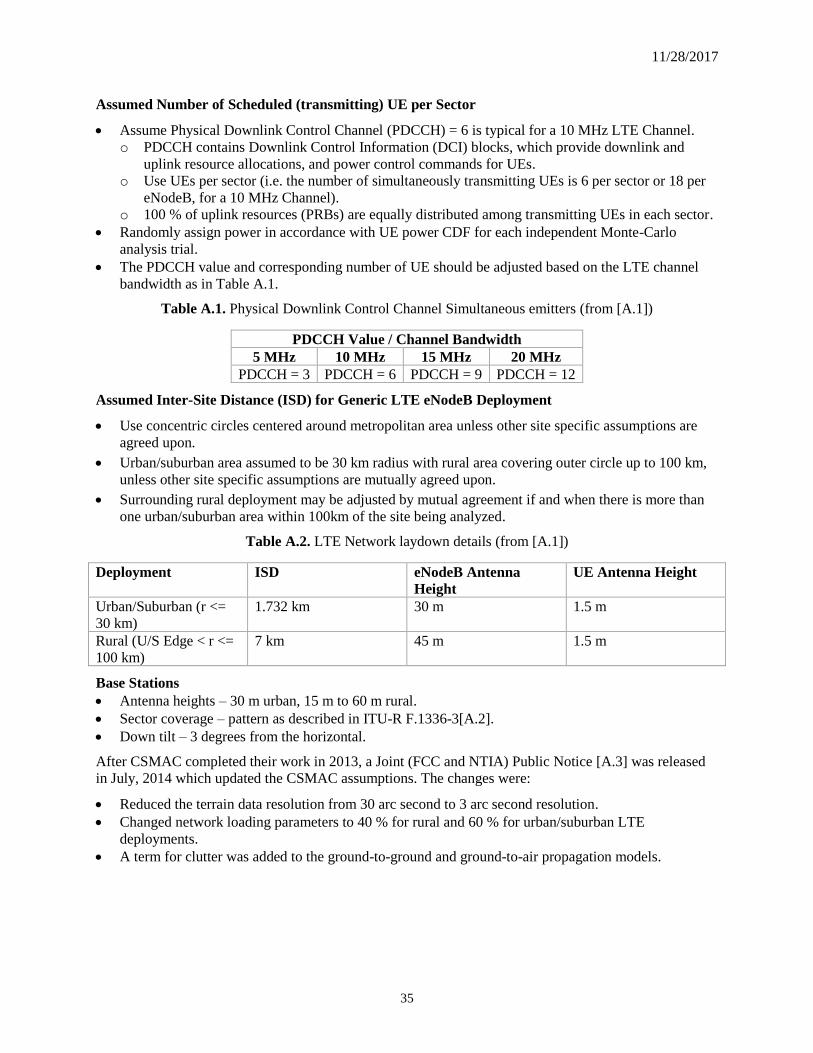
11/28/2017
35
Assumed Number of Scheduled (transmitting) UE per Sector
• Assume Physical Downlink Control Channel (PDCCH) = 6 is typical for a 10 MHz LTE Channel.
o PDCCH contains Downlink Control Information (DCI) blocks, which provide downlink and
uplink resource allocations, and power control commands for UEs.
o Use UEs per sector (i.e. the number of simultaneously transmitting UEs is 6 per sector or 18 per
eNodeB, for a 10 MHz Channel).
o 100 % of uplink resources (PRBs) are equally distributed among transmitting UEs in each sector.
• Randomly assign power in accordance with UE power CDF for each independent Monte-Carlo
analysis trial.
• The PDCCH value and corresponding number of UE should be adjusted based on the LTE channel
bandwidth as in Table A.1.
Table A.1. Physical Downlink Control Channel Simultaneous emitters (from [A.1])
PDCCH Value / Channel Bandwidth
5 MHz 10 MHz 15 MHz 20 MHz
PDCCH = 3 PDCCH = 6 PDCCH = 9 PDCCH = 12
Assumed Inter-Site Distance (ISD) for Generic LTE eNodeB Deployment
• Use concentric circles centered around metropolitan area unless other site specific assumptions are
agreed upon.
• Urban/suburban area assumed to be 30 km radius with rural area covering outer circle up to 100 km,
unless other site specific assumptions are mutually agreed upon.
• Surrounding rural deployment may be adjusted by mutual agreement if and when there is more than
one urban/suburban area within 100km of the site being analyzed.
Table A.2. LTE Network laydown details (from [A.1])
Deployment ISD eNodeB Antenna
Height
UE Antenna Height
Urban/Suburban (r <=
30 km)
1.732 km 30 m 1.5 m
Rural (U/S Edge < r <=
100 km)
7 km 45 m 1.5 m
Base Stations
• Antenna heights – 30 m urban, 15 m to 60 m rural.
• Sector coverage – pattern as described in ITU-R F.1336-3[A.2].
• Down tilt – 3 degrees from the horizontal.
After CSMAC completed their work in 2013, a Joint (FCC and NTIA) Public Notice [A.3] was released
in July, 2014 which updated the CSMAC assumptions. The changes were:
• Reduced the terrain data resolution from 30 arc second to 3 arc second resolution.
• Changed network loading parameters to 40 % for rural and 60 % for urban/suburban LTE
deployments.
• A term for clutter was added to the ground-to-ground and ground-to-air propagation models.

11/28/2017
36
A.2. References
[A.1] Commerce Spectrum Management Advisory Committee Final report: Working Group 1 – 1695-
1710 mhz Meteorological-Satellite,” Jan. 22, 2013, accessible at
https://www.ntia.doc.gov/files/ntia/publications/wg_1_report.pdf.
[A.2] “Reference radiation patterns of omnidirectional, sectoral and other antennas for the fixed and
mobile service for use in sharing studies in the frequency range from 400 MHz to about 70 GHz”,
ITU-R F.1336-4, Feb., 2014.
[A.3] The Federal Communications Commission and the National Telecommunications and Information
Administration: Coordination Procedures in the 1695-1710 MHz and 1755-1780 MHz bands GN
Docket No. 13-185.

11/28/2017
37
Appendix B. Example Factor Prioritization
An example factor prioritization for the experimental design is given below. Further details on the proposed experimental design plan are given in Section 7.3. Note that this prioritization is done assuming the parameters are independent. That is, only the impact of the listed parameter is categorized into a tier. Combinations of factors may yield scenarios which are not part of this categorization.
Tier 1 Changes in the value of these parameters are likely to have a meaningful impact on the measurement results. Factors in Tier 1 should be extensively investigated in the factor selection process, and are likely to be the subject of many measurements.
Parameter Hardware Deliverables Impacted
Simulated DUT UE position, relative to serving eNB Channel emulator 1,2 Channel type (urban, rural, etc.) Channel emulator 1,2
Spatial size of cell UTG 1,2,3 Number of loading UEs in serving cell UTG 1,3 Closed-loop power control parameters (P0, alpha) eNB 1,2 eNB scheduling algorithm type eNB 3
Tier 2 Changes in the value of these parameters are likely to have a measurable, but not necessarily meaningful impact on the measurement results. Factors in this tier should be investigated during the factor selection process and be included during the measurement campaign.
Parameter Hardware Deliverables Impacted
UE cell-cell handover DUT UE 1,2 UE Attaching to eNB DUT UE 1,2 Channel model of loading UEs UTG 1,2,3
Number of loading UEs in adjacent cell UTG 1 Spatial distribution of UEs UTG 1,2,3 Method for UL power control14 eNB 1,2
QCI value of loading UEs UTG 2,3
Tier 3 Changes in the value of these parameters are likely to cause changes in the measurements that could be considered insignificant. Factors in this tier may be considered “optional”. Individual experiments may be done to confirm their placement in Tier 3.
Parameter Hardware Deliverables Impacted
UE Make/Model DUT UE 1,2 UE Type (handset, dongle, etc.) DUT UE 1,2 eNB Make/Model eNB 3
Max. number of UEs allowed to transmit in single frame
eNB 3
UL improved latency timer reaction eNB 3 Method for UL power control11 eNB 1,2
Initial maximum amount of RBs eNB 3 Extended UL link adaptation low PRB threshold eNB 1,3
14 For measurement scenario #1 and #3, tier 3; for scenarios #2, tier 2.