Aggregate Estimations over Location Based Services

Weimo Liu†, Md Farhadur Rahman‡, Saravanan Thirumuruganathan‡, Nan Zhang†, Gautam Das‡The George Washington University†, University of Texas at Arlington‡

ABSTRACTLocation based services (LBS) have become very popular in re-cent years. They range from map services (e.g., Google Maps)that store geographic locations of points of interests, to online so-cial networks (e.g., WeChat, Sina Weibo, FourSquare) that lever-age user geographic locations to enable various recommendationfunctions. The public query interfaces of these services may beabstractly modeled as a kNN interface over a database of two di-mensional points on a plane: given an arbitrary query point, thesystem returns the k points in the database that are nearest to thequery point. In this paper we consider the problem of obtainingapproximate estimates of SUM and COUNT aggregates by onlyquerying such databases via their restrictive public interfaces. Wedistinguish between interfaces that return location information ofthe returned tuples (e.g., Google Maps), and interfaces that do notreturn location information (e.g., Sina Weibo). For both types of in-terfaces, we develop aggregate estimation algorithms that are basedon novel techniques for precisely computing or approximately es-timating the Voronoi cell of tuples. We discuss a comprehensiveset of real-world experiments for testing our algorithms, includingexperiments on Google Maps, WeChat, and Sina Weibo.

1. INTRODUCTION

1.1 LBS with a kNN InterfaceLocation based services (LBS) have become very popular in re-

cent years. They range from map services (e.g., Google Maps)that store geographic locations of points of interests (POIs), to on-line social networks (e.g., WeChat, Sina Weibo, FourSquare) thatleverage user geographic locations to enable various recommenda-tion functions. The underlying data model of these services maybe viewed as a database of tuples that are either POIs (in case ofmap services) or users (in case of social networks), along with theirgeographical coordinates (e.g., latitude and longitude) on a plane.

However, third-party applications and/or end users do not havecomplete and direct access to this entire database. The database isessentially “hidden”, and access is typically limited to a restrictedpublic web query interface or API by which one can specify an

This work is licensed under the Creative Commons Attribution-NonCommercial-NoDerivs 3.0 Unported License. To view a copy of this li-cense, visit http://creativecommons.org/licenses/by-nc-nd/3.0/. Obtain per-mission prior to any use beyond those covered by the license. Contactcopyright holder by emailing info@vldb.org. Articles from this volumewere invited to present their results at the 41st International Conference onVery Large Data Bases, August 31st - September 4th 2015, Kohala Coast,Hawaii.Proceedings of the VLDB Endowment, Vol. 8, No. 12Copyright 2015 VLDB Endowment 2150-8097/15/08.

arbitrary location as a query, which returns at most k nearest tuplesto the query point (where k is typically a small number such as10 or 50). For example, in Google maps it is possible to specify anarbitrary location and get the ten nearest Starbucks. Thus, the queryinterfaces of these services may be abstractly modeled as a “nearestneighbor” kNN interface over a database of two dimensional pointson a plane: given an arbitrary query point, the system returns the kpoints in the database that are nearest to the query point.

In addition, there are important differences among the servicesbased on the type of information that is returned along with thek tuples. Some services (e.g., Google maps) return the locations(i.e., the x and y coordinates) of the k returned tuples. We refer tosuch services as Location-Returned LBS (LR-LBS). Other services(e.g., WeChat, Sina Weibo) return a ranked list of k nearest tuples,but suppress the location of each tuple, returning only the tuple IDand perhaps some other attributes (such as tuple name). We referto such services as Location-Not-Returned LBS (LNR-LBS).

Both types of services impose additional querying limitations,the most important being a per user/IP limit on the number of queriesone can issue over a given time frame (e.g., by default, Google mapAPI imposes a query rate limit of 10,000 per user per day).

1.2 Aggregate EstimationsFor many interesting third-party applications, it is important to

collect aggregate statistics over the tuples contained in such hid-den databases − such as sum, count, or distributions of the tuplessatisfying certain selection conditions. For example, a hotel rec-ommendation application would like to know the average reviewscores for Marriott vs Hilton hotels in Google Maps; a cafe chainstartup would like to know the number of Starbucks restaurants in acertain geographical region; a demographics researcher may wishto know the gender ratio of users of social networks in China etc.

Of course, such aggregate information can be obtained by en-tering into data sharing agreements with the location-based serviceproviders, but this approach can often be extremely expensive, andsometimes impossible if the data owners are unwilling to share theirdata. Therefore, in this paper we consider the problem of obtain-ing approximate estimates of such aggregates by only querying thedatabase via its restrictive public interface. Our goal is to minimizequery cost (i.e., ask as few queries as possible) in an effort to adhereto the rate limits or budgetary constraints imposed by the interface,and yet make the aggregate estimations as accurate as possible.

1.3 Outline of Technical ResultsResults over LR-LBS Interfaces: We first describe our resultsover LR-LBS interfaces. Like [10], our approach is also based ongenerating random point queries and computing the area of Voronoi

1334

cells of the returned tuples, but a key differentiator is that our ap-proach provides an efficient yet precise computation of the areaof Voronoi cells. This procedure is fundamentally different fromthe approximate procedure used in [10] for estimating the area ofVoronoi cells, and is one of the significant contributions of ourpaper. This leads to unbiased estimations of SUM and COUNTaggregates over LR-LBS interfaces; in contrast, the estimationsin [10] have inherent (and unknown) sampling bias.

Moreover, we also leverage the top-k returned tuples of a query(and not just the top-1) by generalizing to the concept of a top-kVoronoi cell, leading to significantly more efficient aggregate esti-mation algorithms. We also developed four different techniques forreducing the estimation error (and thereby estimation error) overLR-LBS interfaces: faster initialization, leveraging history, vari-ance reduction through dynamic selection of query results, and aMonte Carlo method which leverages current knowledge of up-per/lower bounds on the Voronoi cell without sacrificing the un-biasedness of estimations. We combine the above ideas to pro-duce Algorithm LR-LBS-AGG, a completely unbiased estimatorfor COUNT and SUM queries with or without selection conditions.We note that AVG queries can be computed as SUM/COUNT.Results over LNR-LBS Interfaces: We also consider the problemof aggregate estimations over LNR-LBS interfaces. To the best ofour knowledge, this is a novel problem with no prior work. Recallthat such type of kNN interfaces only return a ranked list of thetop-k tuples in response to a point query, and location informationfor these tuples is suppressed. None of the prior work for LR-LBSinterfaces can be extended to LNR-LBS interfaces. For such in-terfaces, we develop aggregate estimation algorithms that are notcompletely bias-free, but can guarantee an arbitrarily small sam-pling bias. The key idea here is the inference of a tuple’s Voronoicell to an arbitrary precision level with a small number of queriesfrom merely the ranks of the returned tuples. We also study a sub-tle extension to cases where k > 1; in particular we study thechallenge brought by this case by the (possibly) concave nature oftop-k Voronoi cells, and develop an efficient algorithm to detectpotential concaveness and guarantee the accuracy of the inferredVoronoi cell. We combine the above ideas to produce AlgorithmLNR-LBS-AGG, an estimator for COUNT and SUM queries withor without selection conditions. Unlike Algorithm LR-LBS-AGG,this estimator may be biased, but the bias can be controlled to anyarbitrary desired precision.

1.4 Summary of Contributions• We consider the problem of aggregate estimation over loca-

tion based services. We consider both LR-LBS (locationsreturned) as well as the more novel LNR-LBS (locations notreturned) interfaces.• For LR-LBS interfaces, we develop Algorithm LR-LBS-AGG

for estimating COUNT and SUM aggregates with or withoutselection conditions. It represents a significant improvementover prior work along multiple dimensions: a novel way ofprecisely calculating Voronoi cells leads to completely unbi-ased estimations; top-k returned tuples are leveraged ratherthan only top-1; several innovative techniques developed forreducing error and increasing efficiency.• For LNR-LBS interfaces, we develop Algorithm LNR-LBS-

AGG for aggregate estimation. This is a novel problem withno prior work. The estimated aggregates are not bias-free,but the bias can be controlled to any desired precision.• We conduct a comprehensive set of real-world experiments.

Specifically, we conducted online tests over a number of real-world LBS, such as Google Maps, WeChat and Sina Weibo.

2. BACKGROUND

2.1 Model of LBSA location based service (LBS) supports kNN queries over a

database D of tuples with location information. These tuples canbe points of interest (e.g. Google Maps) or users (e.g. WeChat,Sina Weibo). A kNN query q takes as input a location (e.g., longi-tude/latitude combination), and returns the top-k nearest tuples se-lected and ranked according to a pre-determined ranking function.Since the only input to a query is a location, we use q to also denotethe query’s location without introducing ambiguity. Almost all ofthe popular LBS follow kNN query model. For most parts of thepaper, we consider the ranking function to be Euclidean distancebetween the query location and each tuple’s location. Extensionsto other ranking functions are discussed in [20].

Note that tuples in an LBS system contain not only location in-formation but other many other attributes - e.g., a POI in GoogleMaps includes attributes such as POI name, average review ratingsetc. Depending on which attributes of a tuple are returned by thekNN interface - more specifically, whether the location of a tupleis returned - we can classify LBS into two main categories:LR-LBS: A Location-Returned-LBS (LR-LBS) returns the preciselocation for each of the top-k returned tuples, along with possiblyother attributes. Google Maps, Bing Maps, Yahoo! Maps, etc., areprominent examples of LR-LBS, as all of them display the preciselocation of each returned POI. Note that some LBS may return avariant of the precise locations - e.g., Skout and Momo returns notthe precise location of a tuple, but the precise distance betweenthe query location and the tuple location. We consider such LBSto be in the LR-LBS category because, through previously studiedtechniques such as trilateration (e.g., [17]), one can infer the preciselocation of a tuple with just 3 queries.LNR-LBS: A Location-Not-Returned-LBS (LNR-LBS), on the otherhand, does not return tuple locations - i.e., only other attributessuch as name, review rating, etc., are returned. This category ismore prevalent among location based social networks (presumablybecause of potential privacy concerns on precise user locations).Examples here include WeChat, which returns attributes such asname, gender, etc., for each of the top-k users, but not the preciselocation/distance. Other examples include Sina Weibo, WeChat,etc., which feature a similar query return semantics.Common Interface Features and Limitations: Generally speak-ing, there are two ways through which an LBS (either LR- or LNR-LBS) supports a kNN query. One is an interactive web or APIinterface which allows a location to be explicitly specified as a lat-itude/longitude pair. Google Maps is an example to this end. An-other common way is for the LBS (e.g., as a mobile app) to directlyretrieve the query location from a positioning service (such as GPS,WiFi or Cell towers) and automatically issue a kNN query accord-ingly. In the second case, there is no explicit mechanism to enterthe location information. Nonetheless, it is important to note that,even in this case, we have the ability to issue a query from any ar-bitrary location without having to physically travel to that location.All mobile OS have debugging features that allow arbitrary locationto be used as the output of the positioning (e.g., GPS) service.

Many LBS also impose certain interface restrictions: One is theaforementioned top-k restriction (i.e., only the k nearest tuples arereturned). Another common one is a query rate limit - i.e., manyLBS limit the maximum number of kNN queries one can issue perunit of time. For example, by default Google Maps allows 10,000location queries per day while Sina Weibo allows only 150 queriesper hour. This is an important constraint for our purpose because it

1335

makes the query-issuing process the bottleneck for aggregate esti-mation. To understand why, note that even with the generous limitprovided by Google Maps, one can issue only 7 queries per minute- this 8.6 second per query overhead1 is orders of magnitude higherthan any offline processing overhead that may be required by theaggregate estimation algorithm. Thus, this interface limitation es-sentially makes query cost the No. 1 performance metric to opti-mize for aggregate estimation. An LBS might impose other, moresubtle constraints - e.g., a maximum coverage limit which forbidstuples far away (say more than 5 miles away) from a query locationto be returned. Extensions to address these constraints are in [20].

2.2 Voronoi CellsVoronoi cell [15] is a key geometric concept used extensively by

our algorithms developed in the paper. Consider each tuple t ∈ Das a point on a Euclidean plane bounded by a box B (which coversall tuples in D). We have the following definition.

DEFINITION 1 (VORONOI CELL). Given a tuple t ∈ D, theVoronoi cell of t, denoted by V (t), is the set of points on the B-bounded plane that are closer to t than any other tuple in D.

Note that the B-bound ensures that each Voronoi cell is a finiteregion. The Voronoi cells of different tuples are mutually exclusive- i.e., the Voronoi diagram is the subdivision of the plane into re-gions, each corresponding to all query locations that would returna certain tuple as the nearest neighbor2.

For the purposes of our paper, we define an extension of theVoronoi cell concept to accommodate the top-k (when k > 1)query return semantics. Specifically, given a tuple t ∈ D, we definethe top-k Voronoi cell of t, denoted by Vk(t), as the set of query lo-cations on the plane that return t as one of the top-k results. Thereare four important observations about this concept:

First, the top-k Voronoi cells for different tuples are no longermutually exclusive. Each location l belongs to exactly k top-kVoronoi cells corresponding to the top-k tuples returned by queryover l. For example, if query over l returns ti, tj, then l ∈ Vk(ti)and l ∈ Vk(tj). Second, our concept of top-k Voronoi cells is fun-damentally different from the k-th ordered Voronoi cells in geom-etry [15] - each of which is formed by points with the exact samek closest tuples. The difference is illustrated in Figure 1 - whileeach colored region is a k-th ordered Voronoi cell, a top-k Voronoicell may cover multiple regions with different colors. For example,the top-2 Voronoi cell for tuple A is marked by a red border andconsists of two different k-th ordered Voronoi cells (AB and AE).

A

E

D

CB

AB BC

CD

DE

AEBE

DB

Figure 1: Concavity of top-k Voronoi Diagrams

Third, while both top-1 Voronoi cells and k-th order Voronoicells are guaranteed to be convex [15], the same does not hold fortop-k Voronoi cells when k > 1. For example, from Figure 1 wecan see that the aforementioned top-2 Voronoi cell for tuple A isconcave. Fourth, a top-k Voronoi cell tend to contain many more1Of course, one can shorten it with multiple IP addresses and API accounts - butsimilarly, one can use parallel processing to speed up offline processing as well.2We assume general positioning [15] - i.e., no two tuples have the exact same locationand no four points on the same circle.

edges than a top-1 Voronoi cell. As we shall discuss later in thepaper, the larger number of edges and the potential concavenessmakes computing the top-k Voronoi cell of a tuple t more difficult.

2.3 Problem DefinitionIn this paper, we address the problem of aggregate estimations

over LBS. Specifically, we consider aggregate queries of the formSELECT AGGR(t) FROM D WHERE Cond where AGGR is an ag-gregate function such as SUM, COUNT and AVG that can be eval-uated over one or more attributes of t, and Cond is the selectioncondition. Examples include the COUNT of users in WeChat orAVG rating of restaurants in Texas at Google Maps.

There are two important notes regarding the selection conditionCond. First, we support any selection condition that can be inde-pendently evaluated over a single tuple - i.e., it is possible to de-termine whether a tuple t satisfies Cond based on nothing but t.Second, for both LR- and LNR-LBS, we support the specificationof a tuple’s location as part of Cond - even when such a location isnot returned, like in LNR-LBS. The technical report [20] describesa technique that allows one to derive the location of a tuple (evenwith LNR-LBS) to arbitrary precision after issuing a small numberof queries. As such, we support aggregates such as the percentageof female WeChat users in Washington, DC. In most part of thetechnical sections, we focus on aggregates without selection condi-tions - the straightforward extensions to various types of selectionconditions will be discussed in §5.Performance Measures: The performance of an aggregate esti-mation algorithm is measured in terms of efficiency and accuracy.Given the query-rate limit enforced by all LBS, the efficiency ismeasured by query cost - i.e. the number of queries and/or APIcalls that the algorithm issues to LBS. Often, we are given a fixedbudget (based on the rate limits) and hence designing an efficientalgorithm that generates accurate estimates within the budgetaryconstraints is crucial. The accuracy of an estimation θ of an ag-gregate θ could be measured by the standard measure of relativeerror |θ − θ|/θ. For any sampling-based approach (like ours), therelative error is determined by two factors: bias, i.e. |E(θ − θ)| ,and variance of θ. The mean squared error, MSE of the estimationis computed as MSE = bias2 + variance.

An interesting question often arises in practice is how we candetermine the relative error achieved by our estimation. If the pop-ulation variance is known, then one can apply standard statisticstechniques to compute the confidence interval of aggregate estima-tions [16]. Absence of such knowledge, a common practice is toapproximate the population variance with sample variance, whichcan be computed from the samples we use to generate the final es-timation and use Bessel’s correction [16] to correct the result.

3. LR-LBS-AGGWe start this section with our key idea of precisely computing the

(top-k) Voronoi cell of a given tuple, which enables the unbiasedaggregate estimations over LR-LBS query interfaces. However, itmay require a large number of queries leading to a large error whenthe query budget is limited. Hence we develop four techniques forreducing the estimation error while maintaining the complete unbi-asedness of aggregate estimations. Finally, we combine all ideas toproduce Algorithm LR-LBS-AGG at the end of this section.

3.1 Key Idea: Precisely Compute Voronoi CellsReduction to Computing Voronoi Cells: We start by describinga baseline design which illustrates why the problem of aggregateestimations over an LBS’s kNN interface ultimately boils down to

1336

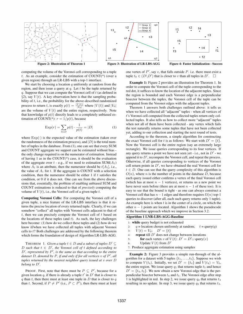
Figure 2: Illustration of Theorem 1

t1

t5 t4

t3

t2Step 1Step 3Step 4

q3

q1 q2

q4

Figure 3: Illustration of LR-LBS-AGG

t1 t2

t3

t4

t5

f4

f3

f2

f1

Figure 4: Faster Initialization - Success

computing the volume of the Voronoi cell corresponding to a tuplet. As an example, consider the estimation of COUNT(*) (over agiven region) through an LR-LBS with a top-1 interface.

We start by choosing a location q uniformly at random from theregion, and then issue a query at q. Let t be the tuple returned byq. Suppose that we can compute the Voronoi cell of t (as defined in§2), say V (t). A key observation here is that the sampling proba-bility of t, i.e., the probability for the above-described randomizedprocess to return t, is exactly p(t) = |V (t)|

|V0|where |V (t)| and |V0|

are the volume of V (t) and the entire region, respectively. Notethat knowledge of p(t) directly leads to a completely unbiased es-timation of COUNT(*): r = 1/p(t), because

Exp(r) =∑t∈D

p(t) · 1

p(t)= |D| (1)

where Exp(·) is the expected value of the estimation (taken overthe randomness of the estimation process), and |D| is the total num-ber of tuples in the database. From (1), one can see that every SUMand COUNT aggregate we support can be estimated without bias -the only change required is on the numerator of estimation. Insteadof having 1 as in the COUNT(*) case, it should be the evaluationof the aggregate over t - e.g., if we need to estimation SUM(A1)where A1 is an attribute, then the numerator should be t[A1], i.e.,the value of A1 for t. If the aggregate is COUNT with a selectioncondition, then the numerator should be either 1 if t satisfies thecondition, or 0 if it does not. One can see from the above discus-sions that, essentially, the problem of enabling unbiased SUM andCOUNT estimations is reduced to that of precisely computing thevolume of V (t), i.e., the Voronoi cell of a given tuple t.

Computing Voronoi Cells: For computing the Voronoi cell of agiven tuple, a nice feature of the LR-LBS interface is that it re-turns the precise location of every returned tuple. Clearly, if we cansomehow “collect” all tuples with Voronoi cells adjacent to that oft, then we can precisely compute the Voronoi cell of t based onthe locations of these tuples (and t). As such, the key challengeshere become: (1) how do we collect these tuples and (2) how do weknow if/when we have collected all tuples with adjacent Voronoicells to t? Both challenges are addressed by the following theoremwhich forms the foundation of design of Algorithm LR-LBS-AGG.

THEOREM 1. Given a tuple t ∈ D and a subset of tuples D′ ⊆D such that t ∈ D′, the Voronoi cell of t defined according toD′, represented by P ′, is the same as that according to the entiredataset D, denoted by P , if and only if for all vertices v of P ′, alltuples returned by the nearest neighbor query issued at v over Dbelong to D′.

PROOF. First, note that there must be P ⊆ P ′, because for agiven location q, if there is already a tuple t′ in D′ that is closer toq than t, then there must at least one tuple in D that is closer to qthan t. Second, if P 6= P ′ (i.e., P ⊂ P ′), then there must at least

one vertex of P ′, say v, that falls outside P . i.e. there must exist atuple t0 ∈ (D\D′) that is closer to v than all tuples in D′.

Example 1: Figure 2 provides an illustration for Theorem 1. Inorder to compute the Voronoi cell of the tuple corresponding to thered dot, it suffices to know the location of the adjacent tuples. Sincethe region is bounded and each Voronoi edge is a perpendicularbisector between the tuples, the Voronoi cell of the tuple can becomputed from the Voronoi edges with the adjacent tuples.

Theorem 1 answers both challenges outlined above: it tells uswhen we have collected all “adjacent” tuples - when all vertices oft’s Voronoi cell computed from the collected tuples return only col-lected tuples. It also tells us how to collect more “adjacent” tupleswhen not all of them have been collected - any vertex which failsthe test naturally returns some tuples that have not been collectedyet, adding to our collection and starting the next round of tests.

According to the theorem, a simple algorithm for constructingthe exact Voronoi cell for t is as follows: We start with D′ = t.Now the Voronoi cell is the entire region (say an extremely largerectangle). We issue queries corresponding to its four vertices. Ifany query returns a point we have not seen yet - i.e., not in D′ - weappend it toD′, recompute the Voronoi cell, and repeat the process.Otherwise, if all queries corresponding to vertices of the Voronoicell return points in D′, we have obtained the real Voronoi cell fort ∈ D. One can see that the query complexity of this algorithm isO(n), where n is the number of points in the database D, becauseeach query issued either confirms a vertex of the final Voronoi cell(which has at most n − 1 vertices), or returns us a new point wehave never seen before (there are at most n − 1 of these too). It iseasy to see that the bound is tight - as one can always construct aVoronoi cell that has n−1 edges and therefore requires Ω(n) top-1queries to discover (after all, each such query returns only 1 tuple).An example here is when t is in the center of a circle, on which theother n− 1 points are located. Algorithm 1 shows the pseudocodeof the baseline approach which we improve in Section 3.2.

Algorithm 1 LNR-LBS-AGG-Baseline1: while query budget is not exhausted2: q = location chosen uniformly at random; t = query(q)3: V (t) = V0; D′ = t4: repeat till D′ does not change between iterations5: for each vertex v of V (t): D′ = D′∪ query(v)6: Update V (t) from D′

7: Produce aggregate estimation using samples

Example 2: Figure 3 provides a simple run-through of the al-gorithm for a dataset with 5 tuples t1, . . . , t5. Suppose we wishto compute V (t4). Initially, we set D′ = t4 and V (t4) = V0,the entire region. We issue query q1 that returns tuple t5 and henceD′ = t4, t5. We now obtain a new Voronoi edge that is the per-pendicular bisector between t4 and t5. The Voronoi edge after step1 is highlighted in red. In step 2, we issue query q2 that returns t4resulting in no update. In step 3, we issue query q3 that returns t3.

1337

D′ = t3, t4, t5 and we obtain a new Voronoi edge as the per-pendicular bisector between t3 and t4 depicted in green. In step 4,we issue query q4 that returns t2 resulting in the final Voronoi edgedepicted in blue. Further queries over the vertices for V (t4) doesnot result in new tuples concluding the invocation of the algorithm.Extension to k > 1: Interestingly, no change is required to theabove algorithm when we consider the top-k Voronoi cell ratherthan the traditional, i.e., top-1 Voronoi cell. To understand why,note that Theorem 1 directly extends to top-k Voronoi cells - as atop-k Voronoi computed from D′ still must completely cover thatfor D; and any vertex of the top-k Voronoi from D′ which is out-side that from D must return at least one tuple outside D′. Wefurther describe how to leverage k > 1 in Sections 3.2.3 and 4.2.

3.2 Error ReductionBefore describing the various error reduction techniques we de-

velop for aggregate estimations over LR-LBS, we would like tofirst note that, while we use the term “error reduction” as the titleof this subsection, some of the techniques described below indeedfocus on making the computation of a Voronoi cell more efficient.The reason why we call all of them “error reduction” is becauseof the inherent relationship between efficiency and estimation error- if the Voronoi-cell computation becomes more efficient, then wecan do so for more samples, leading to a larger sample size and ul-timately, a lower estimation error (which is inversely proportionalto the square root of sample size [16]).

3.2.1 Faster InitializationA key observation from the design in §3.1 is its bottleneck: the

initialization process. At the beginning, we know nothing aboutthe database other than (1) the location of tuple t, and (2) a largebounding box corresponding to the area of interest for the aggregatequery. Naturally,D′ = t, leading to the initial Voronoi cell beingthe bounding box, and our first four queries being the corners ofthese bounding boxes. Of course, the tentative Voronoi cell willquickly close in to the real one with speed close to a binary search -i.e., the average-case query cost is at log scale of the bounding boxsize. Nonetheless, the initialization process can still be very costly,especially when the bounding box is large.

To address this problem, we develop a faster initialization tech-nique which features a simple idea: Instead of starting with D′ =t, we insert four fake tuples into D′, say D′ = t, tF1 , . . . , tF4 ,where tF1 , . . ., tF4 that form a bounding box around t. The size ofthe bounding box should be conservatively large - even though awrong size will not jeopardize the accuracy of our computation.

By computing the initial Voronoi cell from D′ and then issuequeries corresponding to its vertices, there are two possible out-comes: One is that these queries return enough real tuples (besidest, of course) that, after excluding the fake ones fromD′, we still geta bounded Voronoi cell for t. One can see that, in this case, we cansimply continue the computation while having saved a significantnumber of initialization queries. The other possible outcome, how-ever, is when the bounding box is set too small, and we do not haveenough real tuples to “bound” t with a real Voronoi cell. Specif-ically, in the extreme-case scenario, all four vertices of the initialVoronoi cell could return t itself. In this case, we simply revertback to the original design, wasting nothing but four queries.

One can see that the faster initialization process still guaranteesthe exact computation of a tuple’s Voronoi cell. It has the potentialto save a large amount of initialization queries in the average-casescenario, while in the worst case, it wastes at most four queries. Al-gorithm 2 provides the pseudocode for faster initialization strategy.

Algorithm 2 Fast-Init

1: Input: t; Output: V (t)2: D′ = t, tF1 , tF2 , tF3 , tF4 ; Compute V (t) from D′

3: If all queries over vertices of V (t) return t, then Vt = V0

4: repeat till D′ does not change between iterations5: for each vertex v of V (t): D′ = D′∪ query(v)6: Update V (t) from D′

7: return V (t)

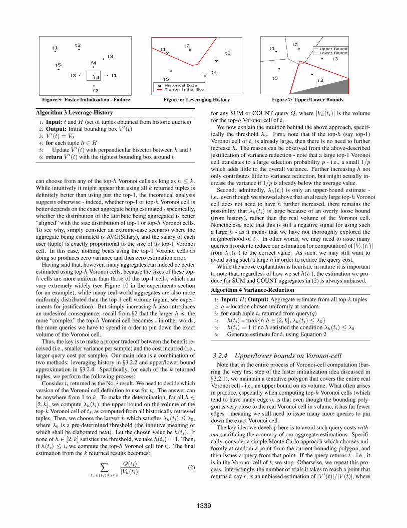
Example 3: Figures 4 and 5 show two different scenarios wherethe strategy is successful and not successful respectively based onwhether the bounding box due to fake tuples is conservatively large.Given a small dataset with tuples t1, . . . , t5, we initialize themwith a bounding box induced by fake tuples f1, . . . , f4. In Fig-ure 4, the initial bounding box is tight enough and results in thecomputation of the precise V (t4) with much lower query cost (i.e.only tuples t3, t5 are visited as against tuples t2, t3, t5 fromExample 2. If the bounding box is not tight (as in Figure 5), thenqueries over all the vertices of the bounding box return t4 and werevert to original bounding box V0.

In practice, external knowledge such as US Census data [1] canbe used to compute the bounding box. Since the distribution ofPOIs are often correlated with population density, one can utilizea smaller bounding box (say, 1 square mile) for urban areas and alarger bounding box (say, 50 square miles) for rural areas.

3.2.2 Leverage history on Voronoi-cell computationAnother natural optimization is to leverage the information that

is gleaned from computing the Voronoi cells of past tuples to com-pute a tighter initial Voronoi cell. Recall that our algorithm to com-pute Voronoi cell of a tuple t (i.e V (t)), using Theorem 1 starts withan initial Voronoi cell that is an extremely large bounding box thatcovers the entire plane that then converges to V (t). In the processof computing this Voronoi cell, our algorithm retrieved additionalnew tuples (by issuing queries for each vertex of the bounding box).Notice that for a LBS with static tuples (such as POIs in GoogleMaps), the results of location query ordered by distance remainsstatic. Hence it is not necessary to restart every iteration of thealgorithm with the same large bounding box. Specifically, whencomputing the Voronoi cell for the next tuple, we could leveragehistory by starting with a “tighter” initial bounding box whose ver-tices are the set of tuples that we have seen so far. In other words,we reuse the tuples that we have seen so far and make them as in-put to further rounds. Notice that this approach remains the samefor both k = 1 and k > 1. Since the location of each tuple intop-k are returned in LR-LBS, each of these tuples could be lever-aged. As we see more tuples, the initial Voronoi cell becomes moregranular resulting in substantial savings in query cost. Algorithm 3provides the pseudocode for the strategy. While the pseudocodeuses the simple perpendicular bisector half plane approach [15], itcould also use more sophisticated approaches such as Fortune’s al-gorithm [15] to compute the bounding box around tuple t using thetuples from historic queries.

Example 4: As part of computing V (t4) (see Example 1), weobtained the locations of t2, . . . , t5. When computing V (t2), in-stead of starting with V0 (entire region), we could start with atighter bounding box (shown in red in Figure 6) that can be com-puted offline - i.e. without issuing any queries from previous tuples.

3.2.3 Variance reduction with larger kWhen the system has k > 1, we can of course still choose to use

the top-1 Voronoi cell as if only the top result is returned. Or we

1338

t1 t2

t3

t4

t5 f4

f3

f2

f1

Figure 5: Faster Initialization - Failure

t1

t5t4

t3

Historical DataTighter Initial Box

t2

Figure 6: Leveraging History

t1

t5 t4

t3

Upper BoundLower Bound

t2

Figure 7: Upper/Lower Bounds

Algorithm 3 Leverage-History1: Input: t and H (set of tuples obtained from historic queries)2: Output: Initial bounding box V ′(t)3: V ′(t) = V0

4: for each tuple h ∈ H5: Update V ′(t) with perpendicular bisector between h and t6: return V ′(t) with the tightest bounding box around t

can choose from any of the top-h Voronoi cells as long as h ≤ k.While intuitively it might appear that using all k returned tuples isdefinitely better than using just the top-1, the theoretical analysissuggests otherwise - indeed, whether top-1 or top-h Voronoi cell isbetter depends on the exact aggregate being estimated - specifically,whether the distribution of the attribute being aggregated is better“aligned” with the size distribution of top-1 or top-h Voronoi cells.To see why, simply consider an extreme-case scenario where theaggregate being estimated is AVG(Salary), and the salary of eachuser (tuple) is exactly proportional to the size of its top-1 Voronoicell. In this case, nothing beats using the top-1 Voronoi cells asdoing so produces zero variance and thus zero estimation error.

Having said that, however, many aggregates can indeed be betterestimated using top-h Voronoi cells, because the sizes of these top-h cells are more uniform than those of the top-1 cells, which canvary extremely widely (see Figure 10 in the experiments sectionfor an example), while many real-world aggregates are also moreuniformly distributed than the top-1 cell volume (again, see exper-iments for justification). But simply increasing h also introducesan undesired consequence: recall from §2 that the larger h is, themore “complex” the top-h Voronoi cell becomes - in other words,the more queries we have to spend in order to pin down the exactvolume of the Voronoi cell.

Thus, the key is to make a proper tradeoff between the benefit re-ceived (i.e., smaller variance per sample) and the cost incurred (i.e.,larger query cost per sample). Our main idea is a combination oftwo methods: leveraging history in §3.2.2 and upper/lower boundapproximation in §3.2.4. Specifically, for each of the k returnedtuples, we perform the following process:

Consider ti returned as the No. i result. We need to decide whichversion of the Voronoi cell definition to use for ti. The answer canbe anywhere from 1 to k. To make the determination, for all h ∈[2, k], we compute λh(ti), the upper bound on the volume of thetop-k Voronoi cell of ti, as computed from all historically retrievedtuples. Then, we choose the largest h which satisfies λh(ti) ≤ λ0,where λ0 is a pre-determined threshold (the intuitive meaning ofwhich shall be elaborated next). Let the chosen value be h(ti). Ifnone of h ∈ [2, k] satisfies the threshold, we take h(ti) = 1. Then,if h(ti) ≤ i, we compute the top-h Voronoi cell for ti. The finalestimation from the k returned results becomes:∑

ti:h(ti)≤i≤k

Q(ti)

|Vh(ti)|(2)

for any SUM or COUNT query Q, where |Vh(ti)| is the volumefor the top-h Voronoi cell of ti.

We now explain the intuition behind the above approach, specif-ically the threshold λ0. First, note that if the top-h (say top-1)Voronoi cell of ti is already large, then there is no need to furtherincrease h. The reason can be observed from the above-describedjustification of variance reduction - note that a large top-1 Voronoicell translates to a large selection probability p - i.e., a small 1/pwhich adds little to the overall variance. Further increasing h notonly contributes little to variance reduction, but might actually in-crease the variance if 1/p is already below the average value.

Second, admittedly, λh(ti) is only an upper-bound estimate -i.e., even though we showed above that an already large top-hVoronoicell does not need to have h further increased, there remains thepossibility that λh(ti) is large because of an overly loose bound(from history), rather than the real volume of the Voronoi cell.Nonetheless, note that this is still a negative signal for using sucha large h - as it means that we have not thoroughly explored theneighborhood of ti. In other words, we may need to issue manyqueries in order to reduce our estimation (or computation) of |Vh(ti)|from λh(ti) to the correct value. As such, we may still want toavoid using such a large h in order to reduce the query cost.

While the above explanation is heuristic in nature it is importantto note that, regardless of how we set h(ti), the estimation we pro-duce for SUM and COUNT aggregates in (2) is always unbiased.

Algorithm 4 Variance-Reduction1: Input: H; Output: Aggregate estimate from all top-k tuples2: q = location chosen uniformly at random3: for each tuple ti returned from query(q)4: h(ti) = maxh|h ∈ [2, k], λh(ti) ≤ λ05: h(ti) = 1 if no h satisfied the condition λh(ti) ≤ λ0

6: Generate estimate for ti using Equation 2

3.2.4 Upper/lower bounds on Voronoi-cellNote that in the entire process of Voronoi-cell computation (bar-

ring the very first step of the faster initialization idea discussed in§3.2.1), we maintain a tentative polygon that covers the entire realVoronoi cell - i.e., an upper bound on its volume. What often arisesin practice, especially when computing top-k Voronoi cells (whichtend to have many edges), is that even though the bounding poly-gon is very close to the real Voronoi cell in volume, it has far feweredges - meaning we still need to issue many more queries to pindown the exact Voronoi cell.

The key idea we develop here is to avoid such query costs with-out sacrificing the accuracy of our aggregate estimations. Specifi-cally, consider a simple Monte Carlo approach which chooses uni-formly at random a point from the current bounding polygon, andthen issues a query from that point. If the query returns t - i.e., itis in the Voronoi cell of t, we stop. Otherwise, we repeat this pro-cess. Interestingly, the number of trials it takes to reach a point thatreturns t, say r, is an unbiased estimation of |V ′(t)|/|V (t)|, where

1339

|V ′(t)| and |V (t)| are the volumes of the bounding polygon andthe real Voronoi cell of t, respectively.

Exp(r) =

∞∑i=1

[i ·(

1− |V (t)||V ′(t)|

)i−1

· |V (t)||V ′(t)|

]=|V ′(t)||V (t)| .

In other words, we can maintain the unbiasedness of our estima-tion without issuing the many more queries required to pin downthe exact Voronoi cell. Instead, when V ′(t) is close enough toV (t), we can simply use call upon above-described method which,in most likelihood, requires just one more query to produce an un-biased SUM or COUNT estimation. For example, we can simplymultiply the number of trials r by |V0|/|V ′(t)|, where |V0| is thevolume of the entire region under consideration, to produce an un-biased estimation for COUNT(*). Other SUM and COUNT aggre-gates can be estimated without bias in analogy.

Before concluding this idea, there is one more optimization wecan use here: a lower bound on the top-k Voronoi cell of t. In thefollowing, we first discuss how to use such a lower bound to furtherreduce query cost, and then describe the idea for computing sucha lower bound. Note that once we have knowledge of a region Rthat is covered entirely by the real (top-k) Voronoi cell, if in theabove process, we randomly choose a point q (from V ′(t)) whichhappens to belong in R, then we no longer need to actually queryq - instead, we immediately know that q must belong to V (t) andcan produce an unbiased estimation accordingly. This is the costsaving produced by knowledge of a lower bound R.

To understand how we construct this lower bound region, a keyunderstanding is that, at anytime during the execution of our algo-rithm, we have tested certain vertices of V ′(t) which are alreadyconfirmed to be part of V (t). Consider such a vertex v. Let C(v, t)be a circle with v being the center and the distance between t andv being the radius. Note that we are guaranteed to have observedall tuples within C(v, t). This essentially leads to a lower-boundestimation of V (t). Specifically, a point q is in this lower-boundregion if and only if C(q, t), i.e., a circle centered on q with radiusbeing the distance between q and t, is entirely covered by the unionof C(v, t) for all vertices v of V ′(t) that have been confirmed tobe within V (t). As such, for any q in this region, we can save thequery on it in the above process.

Example 5: The upper bound V ′(t4) of V (t4) after Step 3 in theExample 2 (i.e. run-through of Algorithm LR-LBS-AGG-Baseline)is shown in Figure 7 as a quadrilateral with red edges. The threelower vertices of V ′(t4) are guaranteed to be in V (t4) using thecriteria described above and hence the polygon induced by themprovides a lower bound estimate for V (t4).

3.3 Algorithm LR-LBS-AGGBy combining the baseline idea for precisely computing the Voronoi

cells with the 4 techniques for error reduction, we can design an ef-ficient algorithm LR-LBS-AGG for aggregate estimation over LR-LBS. Algorithm 5 shows the pseudocode for LR-LBS-AGG.

4. LNR-LBS-AGG

4.1 Voronoi Cell Computation: Key IdeaWe now consider the case where only a ranked order of points

are returned - but not their locations. We shall start with the case ofk = 1, and then extend to the general case of k > 1.

We start by defining a primitive operation of “binary search” asfollows. Consider the objective of finding the Voronoi cell of a tu-ple t in the database. Given any location c1 and c2 (not necessarilyoccupied by any tuple), where c1 returns t, consider the half-line

Algorithm 5 LR-LBS-AGG1: while query budget is not exhausted2: q = location chosen uniformly at random3: for each tuple ti in query(q)4: Compute optimal h for ti5: Construct initial Vh(ti) using Algorithms 2 and 36: D′= vertices of Vh(ti)7: repeat till D′ is not updated or Voronoi bound is tight8: for each vertex v of Vh(ti): D′ = D′∪ query(v)9: Update Vh(ti) and V ′h(ti) from D′

10: Produce aggregate estimation using samples

from c1 passing through c2. Since a Voronoi cell is convex and c1resides within the Voronoi cell, this half-line has one and only oneintersection with the Voronoi cell - which is associated with one ortwo edges of the Voronoi cell. We define the primitive operationof binary search for given c1, c2 to be the binary search process offinding one Voronoi edge associated with the intersection. Pleaserefer to Appendix A for the detailed design of this process.

Naturally, such a binary search process is associated with an er-ror bound on the precision of the derived edge. For example, wecan set an upper bound ε on the maximum distance between anypoint on the real Voronoi edge (i.e., a line segment) and its closestpoint on the derived edge, which we refer to as the maximum edgeerror, and use ε as the objective of the binary search operation. Onecan see that the number of queries required for this binary search isproportional to log(1/ε). Due to space limitations, detailed analy-sis of the query complexity can be found in [20].

Given this definition, we now show that one can discover theVoronoi cell of t (up to whatever precision level afforded to us bythe binary search operation) with a query complexity ofO(m log(1/ε)),where m is the number of edges for the Voronoi cell. Here is thecorresponding process:

We start with one query at point q which returns t. Then, weconstruct 4 points that bound q (say q1 : 〈x(q) − 1, y(q)〉, q2 :〈x(q) + 1, y(q)〉, q3 : 〈x(q), y(q) − 1〉, q4 : 〈x(q), y(q) + 1〉,where x(·) and y(·) are the two dimensions, e.g., longitude and lat-itude, of a location, respectively) and call upon the binary searchoperation to find the corresponding Voronoi edges intercepting thehalf lines from q to q1, . . . , q4, respectively. One can see that, nomatter what the discovered edges might be, they must form a closedpolygon3 which we can use to initiate the testing process describedin §3.1. If all vertices pass the test, then we have already obtainedthe Voronoi cell of t. Otherwise, for each vertex (say v) that failsthe test, we perform the binary search operation on the locationof v to discover another Voronoi edge. We repeatedly do so un-til all vertices pass the test - at which time we have obtained thereal Voronoi cell - subject to whatever error bound specified for thebinary search process (as described above).

To compute the query cost of this process, a key observation isthat each call of the binary search process after the initial step (i.e.,a call caused by a vertex failing the test) increases the number ofdiscovered (real) edges for the Voronoi cell by 1. Thus, the numberof times we have to call the binary search process isO(m), leadingto the overall query-cost complexity of O(m log(1/ε)). For theestimation error, we have the following theorem.

THEOREM 2. The estimation bias for COUNT(*) is at most

|E(θ − θ)| ≤∑t∈D

ε2 − 2 · d(t) · ε(d(t)− ε)2 , (3)

3In the extreme-case, some edges of this polygon might be part of the bounding box.

1340

t1

t5 t4

t3

t2Step 1Step 2

q1

p2

p1

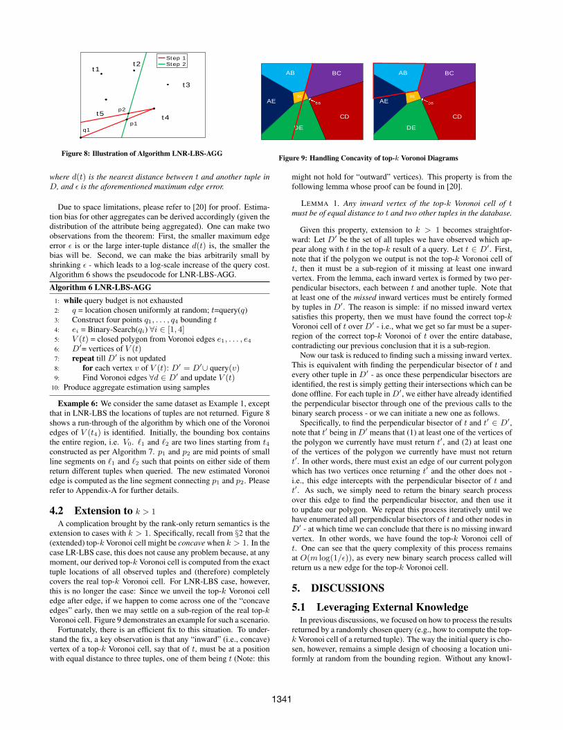
Figure 8: Illustration of Algorithm LNR-LBS-AGG

AB BC

CD

DE

AEBE

DB

AB BC

CD

DE

AEBE

DB

Figure 9: Handling Concavity of top-k Voronoi Diagrams

where d(t) is the nearest distance between t and another tuple inD, and ε is the aforementioned maximum edge error.

Due to space limitations, please refer to [20] for proof. Estima-tion bias for other aggregates can be derived accordingly (given thedistribution of the attribute being aggregated). One can make twoobservations from the theorem: First, the smaller maximum edgeerror ε is or the large inter-tuple distance d(t) is, the smaller thebias will be. Second, we can make the bias arbitrarily small byshrinking ε - which leads to a log-scale increase of the query cost.Algorithm 6 shows the pseudocode for LNR-LBS-AGG.

Algorithm 6 LNR-LBS-AGG1: while query budget is not exhausted2: q = location chosen uniformly at random; t=query(q)3: Construct four points q1, . . . , q4 bounding t4: ei = Binary-Search(qi) ∀i ∈ [1, 4]5: V (t) = closed polygon from Voronoi edges e1, . . . , e46: D′= vertices of V (t)7: repeat till D′ is not updated8: for each vertex v of V (t): D′ = D′∪ query(v)9: Find Voronoi edges ∀d ∈ D′ and update V (t)

10: Produce aggregate estimation using samples

Example 6: We consider the same dataset as Example 1, exceptthat in LNR-LBS the locations of tuples are not returned. Figure 8shows a run-through of the algorithm by which one of the Voronoiedges of V (t4) is identified. Initially, the bounding box containsthe entire region, i.e. V0. `1 and `2 are two lines starting from t4constructed as per Algorithm 7. p1 and p2 are mid points of smallline segments on `1 and `2 such that points on either side of themreturn different tuples when queried. The new estimated Voronoiedge is computed as the line segment connecting p1 and p2. Pleaserefer to Appendix-A for further details.

4.2 Extension to k > 1

A complication brought by the rank-only return semantics is theextension to cases with k > 1. Specifically, recall from §2 that the(extended) top-k Voronoi cell might be concave when k > 1. In thecase LR-LBS case, this does not cause any problem because, at anymoment, our derived top-k Voronoi cell is computed from the exacttuple locations of all observed tuples and (therefore) completelycovers the real top-k Voronoi cell. For LNR-LBS case, however,this is no longer the case: Since we unveil the top-k Voronoi celledge after edge, if we happen to come across one of the “concaveedges” early, then we may settle on a sub-region of the real top-kVoronoi cell. Figure 9 demonstrates an example for such a scenario.

Fortunately, there is an efficient fix to this situation. To under-stand the fix, a key observation is that any “inward” (i.e., concave)vertex of a top-k Voronoi cell, say that of t, must be at a positionwith equal distance to three tuples, one of them being t (Note: this

might not hold for “outward” vertices). This property is from thefollowing lemma whose proof can be found in [20].

LEMMA 1. Any inward vertex of the top-k Voronoi cell of tmust be of equal distance to t and two other tuples in the database.

Given this property, extension to k > 1 becomes straightfor-ward: Let D′ be the set of all tuples we have observed which ap-pear along with t in the top-k result of a query. Let t ∈ D′. First,note that if the polygon we output is not the top-k Voronoi cell oft, then it must be a sub-region of it missing at least one inwardvertex. From the lemma, each inward vertex is formed by two per-pendicular bisectors, each between t and another tuple. Note thatat least one of the missed inward vertices must be entirely formedby tuples in D′. The reason is simple: if no missed inward vertexsatisfies this property, then we must have found the correct top-kVoronoi cell of t over D′ - i.e., what we get so far must be a super-region of the correct top-k Voronoi of t over the entire database,contradicting our previous conclusion that it is a sub-region.

Now our task is reduced to finding such a missing inward vertex.This is equivalent with finding the perpendicular bisector of t andevery other tuple in D′ - as once these perpendicular bisectors areidentified, the rest is simply getting their intersections which can bedone offline. For each tuple inD′, we either have already identifiedthe perpendicular bisector through one of the previous calls to thebinary search process - or we can initiate a new one as follows.

Specifically, to find the perpendicular bisector of t and t′ ∈ D′,note that t′ being inD′ means that (1) at least one of the vertices ofthe polygon we currently have must return t′, and (2) at least oneof the vertices of the polygon we currently have must not returnt′. In other words, there must exist an edge of our current polygonwhich has two vertices once returning t′ and the other does not -i.e., this edge intercepts with the perpendicular bisector of t andt′. As such, we simply need to return the binary search processover this edge to find the perpendicular bisector, and then use itto update our polygon. We repeat this process iteratively until wehave enumerated all perpendicular bisectors of t and other nodes inD′ - at which time we can conclude that there is no missing inwardvertex. In other words, we have found the top-k Voronoi cell oft. One can see that the query complexity of this process remainsat O(m log(1/ε)), as every new binary search process called willreturn us a new edge for the top-k Voronoi cell.

5. DISCUSSIONS

5.1 Leveraging External KnowledgeIn previous discussions, we focused on how to process the results

returned by a randomly chosen query (e.g., how to compute the top-k Voronoi cell of a returned tuple). The way the initial query is cho-sen, however, remains a simple design of choosing a location uni-formly at random from the bounding region. Without any knowl-

1341

edge of the distribution of tuple locations, uniform distribution isthe natural choice. However, in real-world applications, we oftenhave certain a priori knowledge of the tuple distributions, whichwe can leverage to optimize the sampling distribution of queries.

For example, if our goal is to estimate an aggregate, say COUNT,of Point-Of-Interests (POIs, e.g., restaurants) in the US, a reason-able assumption is that the density of POIs in a region tends to bepositively correlated with the region’s population density. Thus,we have two choices: either to sample a location uniformly at ran-dom - which leads to POIs in rural areas to be returned with a muchhigher probability (because their Voronoi cells tend to be larger); orto sample a location with probability proportional to its populationdensity - which hopefully leads to a more-or-less uniform selectionprobabilities over all POIs. Clearly, the second strategy is likelybetter for COUNT estimation, as a more uniform selection prob-ability distribution directly leads to a smaller estimation variance(and therefore error). For example, in the extreme-case scenariowhere all POIs are selected with equal probability, our COUNTestimation will be precise with zero error. Thus, an optimizationtechnique we adopt in this case is to design the initial sampling dis-tribution of queries according to the population density informationretrieved from external sources, e.g., US Census data [1].

There are two important notes regarding this optimization: First,regardless of the accuracy of external knowledge, the COUNT andSUM estimations remain unbiased as Equation 1 in §3.1 guaran-tees unbiasedness no matter what the sampling distribution p(t) is.Second, the optimal sampling distribution depends on both the tu-ple distribution and the aggregate query itself. For example, if wewant to estimate the SUM of review counts for all POIs, then theoptimal sampling distribution is to sample each tuple with proba-bility proportional to its review count (as this design produces zeroestimation variance and error). Given the difficulty of predictingthe aggregate (e.g., review COUNT in this case) ahead of time,leveraging external knowledge is better considered as a heuristic (avery effective one, as we shall demonstrate in experimental results).

Other Extensions: Detailed discussion about the following ex-tensions can be found in [20].• Tuple Position Computation: We show how one can infer

the position of a tuple in LNR-LBS at a level of arbitrary pre-cision. This problem, while of independent interest, is alsocritical for enabling the estimations of aggregates that featureselection conditions on tuples’ locations (e.g., the COUNT ofsocial network users within 10 meters of major highways).• Aggregates with Selection Conditions: In our paper, we

considered aggregates without selection condition. Exten-sion to selection conditions is relatively straightforward. Wediscuss both selection conditions that can be “passed through”to LBS and those that are not supported by the LBS.• Special LBS Constraints: Often, real-world LBS enforce a

number of constraints such as maximum radius (that trun-cates tuples beyond a fixed threshold) and more complexranking functions that take additional factors into account.• Extension to Higher Dimensions: All popular LBS are lim-

ited to 2D. However, extending our algorithms to higher di-mensions (if only for theoretical interests) is straightforward.

6. EXPERIMENTAL RESULTS

6.1 Experimental SetupHardware and Platform: All our experiments were performed ona quad-core 2.5 GHz Intel i7 machine running Ubuntu 14.10 with16 GB of RAM. The algorithms were implemented in Python.

Offline Real-World Dataset: To verify the correctness of our re-sults, we started by testing our algorithms locally over OpenStreetMap[4], a real-world spatial database consisting of POIs (including restau-rants, schools, colleges, banks, etc.) from public-domain data sourcesand user-created data.

We focused on the USA portion of OpenStreetMap. To enrichthe SUM/COUNT/AVG aggregates for testing, we grew the at-tributes of POIs (specifically, restaurants and schools) by “JOIN-ing” OpenStreetMap with two external data sources, Google Maps[3] and US Census [1]. Specifically, we added for each (applica-ble) restaurant POI its review ratings from Google Maps; and eachschool POI its enrollment number from US Census. The US Cen-sus data is also used as the (optional) external knowledge source- i.e., to provide the population density data for the optimizationtechnique discussed in §5.

Note that we have complete access to the enriched dataset andfull control over its query interface. Thus, we implemented a kNNinterface with ranking function being the Euclidean distance; re-turned attributes either containing all attributes including location(for testing LR-LBS) or without location (for LNR-LBS); and vary-ing k to observe the change of performance for our algorithms.Online LBS Demonstrations: In order to showcase the efficacyof our algorithms in real-world applications, we also conductedexperiments online over 3 very popular real-world LBS: GoogleMaps [3], WeChat [6], and Sina Weibo [5]. Each of these serviceshas at least hundreds of millions of users. Unlike the offline exper-iments, we do not have direct access to the ground-truth aggregatesdue to the lack of partnership with these LBS. Nonetheless, we didattempt to verify the accuracy of our aggregate estimations with in-formation provided by external sources (e.g., news reports) - moredetails later in the section.

In online experiments for LR-LBS, we used Google Maps, specif-ically its Google Places API [3], which takes as input a query lo-cation (latitude/longitude pair) and (optionally) filtering conditionssuch as keywords (e.g., “Starbucks”) or POI type (e.g., “restau-rant”), and returns at most k = 60 POIs nearby, ordered by distancefrom low to high, with location and other relevant information (e.g.,review ratings) returned for each POI.

For LNR-LBS, we tested WeChat and Sina Weibo using their re-spective Android apps. Both directly fetch locations from the OSpositioning service and search for nearby users, with WeChat re-turning at most k = 50 and Sina Weibo returning k = 100 nearestusers. Unlike Google Maps, these two services do not return theexact locations of these nearby users - but only provide attributessuch as name, gender, etc.

An implementation-related issue regarding WeChat is that, un-like its mobile apps, its API does not support nearest-neighborsearch. Thus, we conducted our experiments by running its An-droid app (with support for nearest-neighbor search) on the offi-cial Android emulator, and used the debugging feature of locationspoofing to issue queries from different locations. We then usedthe MonkeyRunner tool4 for Android emulator to interact with theapp - i.e., sending queries and receiving results. Specifically, toextract query answers from the Android emulator, we first took ascreenshot of the query-answer screen, and then parsed the resultsthrough an OCR engine, tesseract-ocr5.Algorithms Evaluated: We mainly evaluated three algorithms inour experiments: LR-LBS-AGG and LNR-LBS-AGG from §3 and§4, respectively, along with the only existing solution for LR-LBS

4http://developer.android.com/tools/help/monkeyrunner_concepts.html5https://code.google.com/p/tesseract-ocr/

1342

Figure 10: Voronoi Decomposition of Starbucks in US

(note there is no existing solution for LNR-LBS), which we referto as LR-LBS-NNO [10]. LR-LBS-NNO has a number of tuneableparameters - we picked the parameter settings and optimizationsfrom [10] that provided the best performance.Performance Measures: As discussed in §2, we measure effi-ciency through query cost, i.e., the number of queries issued tothe LBS. Our estimation accuracy is measured experimentally byrelative error. Each data point is obtained as the average of 25 runs.

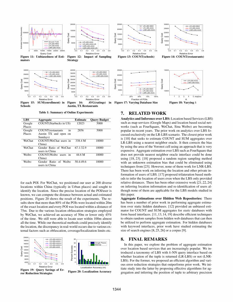
6.2 Experiments over Real-World DatasetsUnbiasedness of Estimators: Our first experiment seeks to showthe unbiasedness of our estimators for LR-LBS-AGG and LNR-LBS-AGG even after incorporating the various error reduction strate-gies. LR-LBS-NNO is known to be unbiased from [10] after an ex-pensive bias correction step. Figure 11 shows a trace of the three al-gorithms when estimating COUNT of all restaurants in US by plot-ting the current estimate periodically after fixed number of querieshave been issued to LBS. We can see that LR-LBS-NNO has ahigh variance and takes significantly longer to converge while ourestimators quickly converge to the ground truth much before LR-LBS-NNO. This indicates that the error reduction techniques suc-cessfully reduce the variance of our estimators.Query Cost versus Relative Error: We start by testing the keytradeoff - i.e., query cost vs. relative error - for all three algo-rithm over various aggregates. Specifically, Figures 13, 14, 15 and16 show the results for four queries, COUNT of schools in US,COUNT of restaurants in US, SUM of school enrollments in US,and AVG of restaurant ratings in Austin, Texas, respectively. Onecan see that not only our LR-LBS-AGG algorithm significantly out-perform the previous LR-LBS-NNO [10] in all cases, even our al-gorithm for the LNR-LBS case achieves much better performancethan the previous algorithm (despite the lack of tuple locations inquery results).Query Cost versus LBS Size: Figure 17 shows the impact of LBSdatabase size (in terms of number of POIs or users) on query cost toestimate the COUNT of schools in US for a fixed relative error of0.1 . We varied the database size by picking a subset of the database(such as 25%, 50%, etc) uniformly at random and estimating theaggregate over it. As expected for a sampling-based approach, theincrease in database size do not have any major impact and onlyresults in a slight increase in overall query cost (due to the morecomplex topology of Voronoi cells).Query Cost versus k: Figure 18 shows how the value of k (thenumber of tuples returned by k-NN interface) affects the querycost. Again, we measure the query cost required to achieve a rel-ative error of 0.1 on the aggregate COUNT of schools in US. We

compared an variant that leverages our variance reduction strategythat adaptively decides which subset of tuples (i.e. h of top-k)to use with fixed variants that uses all the top-k tuples. As ex-pected, our adaptive strategy has a lower query cost and consis-tently achieves a saving of 10% of query cost.Efficacy of Error Reduction Strategies: We started by verifyingthe effectiveness of weighted sampling using external knowledge -Figure 12 compares the performance of the two sampling strategies- uniform and weighted - while estimating the COUNT of schoolsin US. One can see that the weighted sampling variants result insignificant savings in query cost.

In our final set of experiments, we evaluated the efficacy of thevarious error reduction strategies we described in the paper. Wecompared 5 different variants of our algorithm for LR-LBS rang-ing from no error reduction strategies (LR-LBS-AGG-0) to sequen-tially adding them one by one in the order discussed in the paperculminating in LR-LBS-AGG that incorporates all of them. Fig-ure 19 shows the results of this experiment. As expected the firsttwo strategies of faster initialization and leveraging history causeda significant reduction in query cost. We observed that the resultsfor LNR-LBS were very similar.

6.3 Online DemonstrationsGoogle Places: Our first online demonstration of LR-LBS-AGGwas on Google Places API and estimating two aggregates with dif-ferent selection conditions. The first involves selection conditionsthat can be passed over to LBS (COUNT of Starbucks in US) whilethe second involves aggregates with selection condition that cannotbe passed over (see §5 for discussion) such as COUNT of restau-rants in Austin, Texas that are open on Sundays.

Table 1 shows the results of the experiments. We also verified theaccuracy of our estimates for first aggregate (COUNT of Starbucks)through the public release of Starbucks Corp [2]. One can see fromthe table that, with just 5000 queries, LR-LBS-AGG achieves veryaccurate estimations (< 5% relative error) for the count.

To provide an intuitive illustration of the execution of our algo-rithm, we also continued the estimation of COUNT(“Starbucks”)until enumerating all Starbucks in the US. Figure 10 demonstratesthe Voronoi diagram constructed by our algorithm at the end. Onecan see the vastly different sizes of Voronoi cells - spanning hun-dreds of thousands km2 in rural areas and smaller than 1km2 inurban cities, justifying the effectiveness of weighted sampling.WeChat and Sina Weibo: We estimated two aggregates, (1) totalnumber of users and (2) gender ratio, over two LNR-LBS, WeChatand Sina Weibo, respectively. Table 1 shows the results of the ex-periments. One can observe from the table that our estimationsquickly converge to a narrow range (+/- 5%) after issuing a smallnumber of queries (10000). While we do not have access to theground truth this time, we do note an interesting observation fromour results: the percentage of male users is much higher on WeChatthan on Sina Weibo - an observation verified by various surveys inChina [7]. We would like to note that the COUNT aggregate mea-sures the number of users who have enabled the location feature ofWeChat and Weibo respectively and is different from the numberof registered or active accounts.Localization Accuracy: As a final set of experiments, we alsoevaluated the effectiveness of our Tuple position computation ap-proaches in tracking real world users. Specifically, we sought toidentify the precise location of static objects located across the re-gion. We conducted this experiment over Google Places in US andWeChat in China. We treated Google Places as LNR-LBS by ignor-ing the location provided its API. We sought to identify the loca-tion of 200 randomly chosen POIs after issuing at most 100 queries

1343

0 5000 10000 15000 20000 25000

100000

150000

Estim

ated

Cou

nt (R

esta

uran

ts)

Query Cost

Ground Truth LR-LBS-NNO LR-LBS-AGG LNR-LBS-AGG

Figure 11: Unbiasedness of Esti-mators

0.0 0.1 0.2 0.3 0.4 0.5 0.60

5000

10000

15000

20000

Que

ry C

ost

Relative Error

LR-LBS-AGG LR-LBS-AGG-US LNR-LBS-AGG LNR-LBS-AGG-US

Figure 12: Impact of SamplingStrategy

0.0 0.1 0.2 0.3 0.4 0.5 0.60

5000

10000

15000

20000

25000

Que

ry C

ost

Relative Error

LR-LBS-NNO LR-LBS-AGG LNR-LBS-AGG

Figure 13: COUNT(schools)

0.0 0.1 0.2 0.3 0.4 0.5 0.60

5000

10000

15000

20000

25000

30000

Que

ry C

ost

Relative Error

LR-LBS-NNO LR-LBS-AGG LNR-LBS-AGG

Figure 14: COUNT(restaurants)

0.0 0.1 0.2 0.3 0.4 0.5 0.60

5000

10000

15000

20000

25000

30000

Que

ry C

ost

Relative Error

LR-LBS-NNO LR-LBS-AGG LNR-LBS-AGG

Figure 15: SUM(enrollment) inSchools

0.0 0.1 0.2 0.3 0.4 0.5 0.60

5000

10000

15000

20000

25000

30000

35000

40000Q

uery

Cos

t

Relative Error

LR-LBS-NNO LR-LBS-AGG LNR-LBS-AGG

Figure 16: AVG(ratings) inAustin, TX Restaurants

25% 50% 75% 100%0

5000

10000

15000

20000

25000

Que

ry C

ost

Fraction of POIs

LR-LBS-NNO LR-LBS-AGG LNR-LBS-AGG

Figure 17: Varying Database Size

1 2 3 4 5 Adaptive

10000

15000

Que

ry C

ost

K

LR-LBS-AGG LNR-LBS-AGG

Figure 18: Varying k

Table 1: Summary of Online Experiments

LBS Aggregate Estimate Query BudgetGooglePlaces

COUNT(Starbucks in US) 12023 5000

GooglePlaces

COUNT(restaurants inAustin TX and open onSundays)

2856 5000

WeChat COUNT(WeChat users inChina)

338.4 M 10000

WeChat Gender Ratio of WeChatusers in China

67.1:32.9 10000

Weibo COUNT(Weibo users inChina)

44.6 M 10000

Weibo Gender Ratio of Weibousers in China

50.4:49.6 10000

for each POI. For WeChat, we positioned our user at 200 diverselocations within China (typically in Urban places) and sought toidentify the location. Since the precise location of the POI/user isknown, we can compute the distance between actual and estimatedpositions. Figure 20 shows the result of the experiments. The re-sults show that more than 80% of the POIs were located within 20mof the exact location and every POI was located within a distance of75m. Due to the various location obfuscation strategies employedby WeChat, we achieved an accuracy of 50m or lower only 45%of the time. We still were able to locate user within 100m almostall the time. While our theoretical methods could precisely identifythe location, the discrepancy in real-world occurs due to various ex-ternal factors such as obfuscation, coverage/localization limits etc.

0.0 0.1 0.2 0.3 0.4 0.5 0.64000

6000

8000

10000

12000

14000

16000

18000

20000

Que

ry C

ost

Relative Error

LR-LBS-AGG-0 LR-LBS-AGG-1 LR-LBS-AGG-2 LR-LBS-AGG-3 LR-LBS-AGG

Figure 19: Query Savings of Er-ror Reduction Strategies

0-10 10-20 20-30 30-40 40-50 50-60 60-70 70-80 80-9090-100100-150

0

10

20

30

40

50

60

Perc

ent S

ucce

ss

Localization Accuracy (m)

Google Places WeChat

Figure 20: Localization Accuracy

7. RELATED WORKAnalytics and Inference over LBS: Location based Services (LBS)such as map services (Google Maps) and location based social net-works (such as FourSquare, WeChat, Sina Weibo) are becomingpopular in recent years. The prior work on analytics over LBS fo-cussed exclusively on the LR-LBS scenario. The closest prior workis [10] that seeks to estimate COUNT and SUM aggregates overLR-LBS using a nearest neighbor oracle. It then corrects the biasby using the area of the Voronoi cell using an approach that is veryexpensive. Aggregate estimation over LBS such as FourSquare thatdoes not provide nearest neighbor oracle interface could be doneusing [18, 23]. [18] proposed a random region sampling methodwith an unknown estimation bias that could be eliminated usingtechniques from [23]. However, none of them work for LNR-LBS.There has been work on inferring the location and other private in-formation of users of LBS. [17] proposed trilateration based meth-ods to infer the location of users even when the LBS only providedrelative distances. There has been other extensive work [21,22,24]on inferring location information and re-identification of users al-though none of them are applicable for the LBS models studied inthis paper.Aggregate Estimations over Hidden Web Repositories: Therehas been a number of prior work in performing aggregate estima-tion over static hidden databases. [12] provided an unbiased esti-mator for COUNT and SUM aggregates for static databases withform based interfaces. [11, 13, 14, 19] describe efficient techniquesto obtain random samples from hidden web databases that can thenbe utilized to perform aggregate estimation. For hidden databaseswith keyword interfaces, prior work have studied estimating thesize of search engines [8, 25, 26] or a corpus [9].

8. FINAL REMARKSIn this paper, we explore the problem of aggregate estimation

over location based services that are increasingly popular. We in-troduced a taxonomy of LBS with k-NN query interface based onwhether location of the tuple is returned (LR-LBS) or not (LNR-LBS). For the former, we proposed an efficient algorithm and vari-ous error reduction strategies that outperforms prior work. We ini-tiate study into the latter by proposing effective algorithms for ag-gregation and inferring the position of tuple to arbitrary precision

1344

which might be of independent interest. We verified the effective-ness of our algorithms by using a comprehensive set of experimentson a large real-world geographic dataset and online demonstrationson high-profile real-world websites.

9. ACKNOWLEDGEMENTSThe authors were partially supported by National Science Foun-

dation under grants 0915834, 1018865, 0852674, 1117297, 1343976,Army Research Office under grant W911NF-15-1-0020 and a grantfrom Microsoft Research.

10. REFERENCES[1] http://www.census.gov/2010census/data/.[2] . http://investor.starbucks.com/phoenix.

zhtml?c=99518&p=irol-financialhighlights.[3] Google Places API. https://developers.google.

com/places/documentation/.[4] OpenStreetMap. http://www.openstreetmap.org/.[5] Sina Weibo. http://weibo.com/.[6] WeChat. http://www.wechat.com/en/.[7] WeChat/Weibo Statistics. http://www.guancha.cn/

Media/2015_01_29_307911.shtml.[8] Z. Bar-Yossef and M. Gurevich. Random sampling from a

search engine’s corpus. Journal of the ACM, 55(5), 2008.[9] A. Broder and et.al. Estimating corpus size via queries. In

CIKM, 2006.[10] N. Dalvi, R. Kumar, A. Machanavajjhala, and V. Rastogi.

Sampling hidden objects using nearest-neighbor oracles. InSIGKDD, 2011.

[11] A. Dasgupta, G. Das, and H. Mannila. A random walkapproach to sampling hidden databases. In SIGMOD, 2007.

[12] A. Dasgupta and et.al. Unbiased estimation of size and otheraggregates over hidden web databases. In SIGMOD, 2010.

[13] A. Dasgupta, N. Zhang, and G. Das. Leveraging countinformation in sampling hidden databases. In ICDE, 2009.

[14] A. Dasgupta, N. Zhang, and G. Das. Turbo-charging hiddendatabase samplers with overflowing queries and skewreduction. In EDBT, 2010.

[15] M. De Berg, M. Van Kreveld, M. Overmars, and O. C.Schwarzkopf. Computational geometry. Springer, 2000.

[16] D. A. Freedman. Statistical models: theory and practice.cambridge university press, 2009.

[17] M. Li and et.al. All your location are belong to us: Breakingmobile social networks for automated user location tracking.In MobiHoc, 2014.

[18] Y. Li, M. Steiner, L. Wang, Z.-L. Zhang, and J. Bao.Dissecting foursquare venue popularity via random regionsampling. In CoNEXT workshop, 2012.

[19] W. Liu and et.al. Aggregate estimation over dynamic hiddenweb databases. In VLDB, 2014.

[20] W. Liu, M. F. Rahman, S. Thirumuruganathan, N. Zhang,and G. Das. Aggregate estimations over location basedservices. arXiv preprint arXiv:1505.02441, 2015.

[21] C. Y. Ma, D. K. Yau, and N. S. Rao. Privacy vulnerability ofpublished anonymous mobility traces. ToN, 2013.

[22] M. Srivatsa and M. Hicks. Deanonymizing mobility traces:Using social network as a side-channel. In CCS, 2012.

[23] P. Wang and et.al. An efficient sampling method forcharacterizing points of interests on maps. In ICDE, 2014.

[24] H. Zang and et.al. Anonymization of location data does notwork: A large-scale measurement study. In MobiCom, 2011.

[25] M. Zhang, N. Zhang, and G. Das. Mining a search engine’scorpus: efficient yet unbiased sampling and aggregateestimation. In SIGMOD, 2011.

[26] M. Zhang, N. Zhang, and G. Das. Mining a search engine’scorpus without a query pool. In CIKM, 2013.

APPENDIXA. BINARY SEARCH PROCESSDesign of Binary Search: Given the half-line ` from c1 passingthrough c2, we conduct the binary search as follows. First, we findcb, the intersection of this half-line with the bounding box. Then,we perform a binary search between c1 and cb to find a segment ofthe half-line with length at most δ, say with two ends being c3, c4(with the distance between c3 and c4 at most δ), such that while c3returns t, c4 returns another tuple, say t′. This step takes at mostlog(b/δ) queries, where b is the perimeter of the bounding box.

Then, we consider two half-lines `1 and `2, both of which startfrom c1 and form an angle of − arcsin(δ′/r) and + arcsin(δ′/r)with `, respectively, where δ′ is a pre-determined (small) thresholdand r is the distance between c1 and c4. For each `i, we perform theabove binary search process to find a (at most) δ-long segment thatreturns t on one end and t′ on the other. Note that such a processmight fail - e.g., there might no point on `i which returns t′. We settwo rules to address this situation: First, we terminate the searchfor `i if we have reached a segment shorter than δ, with one endreturning t and the other returning a tuple other than t′. Second,we move on to the next step as long as (at least) one of `1 and `2gives us a satisfactory δ-long segment. If neither can produce thesegment, we terminate the entire process and output the following(estimated) Voronoi edge: the perpendicular bisector of (c3, c4).

Now suppose that `1 produces a satisfactory segment of at mostδ long. Let this segment be (c5, c6). We simply return our (esti-mated) Voronoi edge as the line that passes through: (1) the mid-point of (c3, c4), and (2) the midpoint of (c5, c6). One can seethat the overall query cost of the binary search process is at most3 log(b/δ). Analysis for the error bound can be found in [20]. Al-gorithm 7 provides the pseudocode for Binary Search process.

Algorithm 7 Binary-Search1: Input: Tuple t, Locations c1, c2 where query(c1) returns t2: Output: An edge of V (t)3: cb = Intersection of half-line c1, c2 with bounding box4: Find c3, c4 s.t. dist(c3, c4) < δ and query(c3) 6= query(c4)5: r = dist(c1, c4)6: Construct lines `1, `2 from c1 with angles ± arcsin(δ′/r)7: (c5, c6) = line segment on `1 or `2 with dist(c5, c6) < δ and

query(c5) 6= query(c6)8: if none exists, return perpendicular bisector of (c3, c4)9: else return line segment passing through midpoints of (c3, c4)

and (c5, c6)

1345