arX

iv:n

lin/0

5060

32v2

[nl

in.C

D]

15

Mar

200

6

A generalized model of active media with a set of

interacting pacemakers: Application to the heart beat

analysis

SERGEI RYBALKO† and EKATERINA ZHUCHKOVA‡

† Department of Physics, Kyoto University, Kyoto 606-8502, Japan

‡ Physics Faculty, Moscow State University, Leninskie gory, Moscow 119992, Russia

E-mail: rybalko@polly.phys.msu.ru

Abstract

We propose a quite general model of active media by consideration of the inter-

action between pacemakers via their phase response curves. This model describes a

network of pulse oscillators coupled by their response to the internal depolarization

of mutual stimulations.

First, a macroscopic level corresponding to an arbitrary large number of oscilla-

tory elements coupled globally is considered. As a specific and important case of the

proposed model, the bidirectional interaction of two cardiac nodes is described. This

case is generalized by means of an additional pacemaker, which can be expounded

as an external stimulater. The behavior of such a system is analyzed. Second, the

microscopic level corresponding to the representation of cardiac nodes by one– and

two–dimensional lattices of pulse oscillators coupled via the nearest neighbors is de-

scribed. The model is a universal one in the sense that on its basis one can easily

construct discrete distributed media of active elements, which interact via phase

response curves.

PACS 05.45.Ac, 82.40.Bj, 95.10.Fh, 87.19.Hh

Keywords: Active media; entrainment; cardiac dynamics; phase response curve.

Short title: A generalized model of active media

1

1 Introduction

Representation of an active distributed system by ensembles of coupled excitable or oscil-

latory elements is very useful method of the analysis because it allows to understand main

dynamical processes inherent in the considered medium. As is known, this approach goes

back to the model of Wiener and Rosenblueth [Wiener & Rosenblueth, 1946], according to

which a medium consists of single elements being in one of three possible states: excited,

refractory or rest. Later such models as coupled limit cycle oscillators and chaotic maps

[Kaneko, 1990; Shibata & Kaneko, 1998] have played an important role not only in a quite

realistic description of active media but also in the understanding of a possible behavior of

systems far from equilibrium. Many useful concepts like phase–locked patterns, synchro-

nization and spatio–temporal chaos have become popular due to detailed studies of similar

nonlinear models [Kuramoto, 1984; Kuramoto, 1995; Winfree, 2000].

Investigations of such an example of an active medium as cardiac tissue are of signif-

icant scientific interest owing to vital importance of its rhythm stability. Real heart cells

exhibit oscillatory properties (can be reset and entrained), they are excitable and have

a refractory time, during which they do not respond to external stimulation. Hence, the

heart can be considered as consisting of oscillatory (conductive cardiomyocytes, which have

automaticity) and excitable (contractile heart cells, which do not initiate electrical activity

under normal conditions) elements.

Due to extraordinary complexity of the heart, many qualitative discrete and continuous

models have been tested. Majority of computational models of cardiac tissue of last gener-

ation takes into consideration the kinetics of excitable cells, how the excitation propagates

from cell to cell and how contractile cardiomyocytes are arranged and connected in space

[Clayton, 2001]. Such models mainly serve for studying sustained by re-entrant activity

lethal arrhythmia – ventricular fibrillation, during which the spatio–temporal behavior is

very complex [Clayton et al., 2006].

Other models treat the cardiac tissue as an active conductive system, taking into ac-

count oscillatory properties of heart cells. In this case the cardiac rhythms can be described

on the basis of the dynamical system theory (see e.g. [Courtemanche et al., 1989; Gold-

berger, 1990; Bub & Glass, 1994; Glass et al., 2002; Loskutov et al., 2004] and refs. therein).

2

Hereinafter we hold this approach.

Under normal conditions the electrical activity of the heart (action potentials) is spon-

taneously initiated in a region of the right atrium, sino–atrial (SA) node, so–called lead-

ing pacemaker. Automatic excitation is a distinctive feature not only of the cells of the

SA node, but also of other conductive heart cells, so-called latent pacemakers. In addi-

tion, contractile cardiomyocytes can initiate a spontaneous action potential in pathology.

Electrophysiological studies have suggested that the activity of cardiomyocytes with auto-

maticity (e.g. P-cells of the SA node, of the atrioventricular (AV) junction, Purkinje cells)

can be modulated by current pulses stimulating (super-threshold depolarizing) applied ex-

tracellularly [Jalife & Moe, 1976; Sano et al., 1978; Jalife et al., 1980; Antzelevitch et al.,

1982].

Effects of external stimuli on biological oscillators are observed in a wide range of

species. Experimentally obtained characteristics can be represented by a phase response

curve (PRC) [Jalife & Moe, 1976; Antzelevitch et al., 1982; Reiner & Antzelevitch, 1985].

To establish the shape of the PRC experimentally, stimulation of an oscillator at various

phases of its intrinsic cycle is applied [Jalife et al., 1980; Guevara & Shrier, 1987]. It

has been found that in different pacemaker cells early stimuli delay the next pacemaker

discharge and late pulses advance it. Therefore, the typical PRC shape is biphasic [Jalife

et al., 1980; Reiner & Antzelevitch, 1985].

The rhythm of autonomous biological oscillators can also undergo an external periodic

perturbation (e.g. activity of cells of the AV junction is subjected to sinus rhythm),

depending on both the stimulus magnitude and its phase within the cycle. It is known that

when the frequency and the amplitude of the external periodic stimulation are varied, a

diversity of phase diagrams can be established between the stimulus and the self-sustained

oscillator (see e.g. [Loskutov et al., 2004]). In some situations the rhythm of the biological

oscillator is entrained (or phase-locked) to the external stimulation so that for each M

cycles of the stimulation there are N cycles of the autonomous oscillator rhythm. This

occurs at a fixed phase (or phases) of the stimulus and is called M : N phase-locking or

entrainment, which appears as a time–periodic sequence. In particular, entrainment of

1 : 1, during which the rhythms of the oscillator and external stimulus are matched, is

defined as synchronization phenomenon.

3

In the present paper we develop a general simplified model describing a network of pulse

oscillators coupled by their response to the internal depolarization of mutual stimulations.

Our primary aim is to keep the model as simple as possible and to introduce a minimal

number of parameters. Therefore, in our model the pacemakers are fully characterized by

their intrinsic cycle length and are represented as pulse oscillators. Their interaction is

described by PRCs. At first, we will consider two bidirectionally interacting pacemakers to

demonstrate the basic concepts of the model. Then we will apply this approach to construct

a pacemaker network model with global coupling. As the following step, we will analyze

two specific cases of this PRC based model of coupled pulse oscillators: two and then three

interacting cardiac nodes. An additional pacemaker can also be expounded as an external

stimulater. Our further intention is to go on to the next (microscopic) level and represent

each pacemaker as an ensemble of interacting oscillatory elements. Extrapolation of our

approach to one– and two–dimensional matrixes (or lattices) of pacemaker cells interacting

via nearest neighbors concludes the present study.

2 Development of the General Model

In this part we construct a system with two pacemakers and then consider a quite general

model of a set of interacting pacemakers coupled by their PRCs.

2.1 Two interacting pacemakers: outline of the approach

Consider two interacting pulse oscillators (or pacemakers) A and B with intrinsic periods

of their autonomous beating Ta and Tb respectively. An interaction between oscillators is

governed by so-called phase response curve (PRC). This means that a phase shift of one

of the oscillators happens as a result of an impact of the another one. To construct an

adequate mathematical model, it is necessary to accept some restrictions concerning the

character of the interaction. We describe them briefly [Ikeda, 1982; Glass et al., 1986;

Glass & Zeng, 1990].

1. The phase of the disturbed oscillator is shifted to a new value instantly after an

impact.

2. The phase shift depends only on two main parameters: a) on the phase difference

4

of oscillators and b) on the influence strength. In turn, this influence strength depends on

its amplitude and the coupling coefficient of the oscillators. In a real system the coupling

coefficient is the average factor that shows how the strength of the pulse decreases during

its passing from one oscillator to another. Thus, the phase shift Φ determining a new phase

of the disturbed oscillator with period T can be represented as follows:

Φ = ∆/T ≡ Φ(ϕ, ε), (1)

where ∆ is the time shift of the disturbed oscillator, ϕ is the phase difference of the

oscillators and ε is the influence strength.

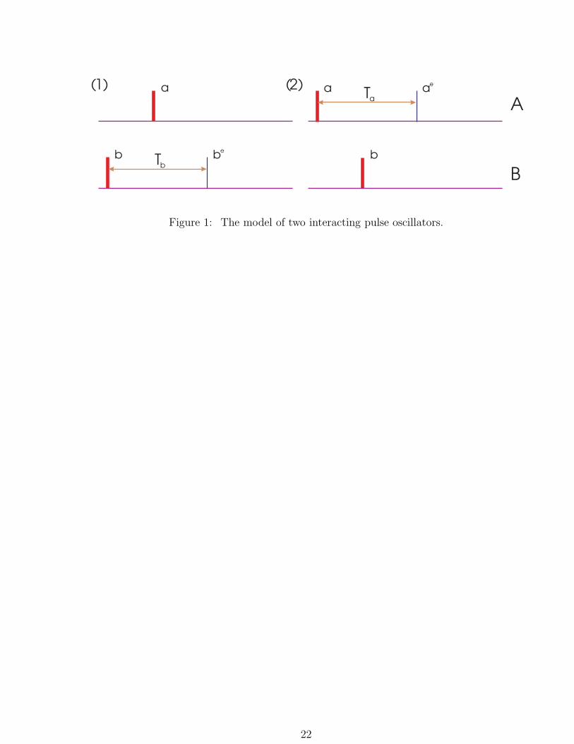
Pacemakers can be represented as a set of separated firing peaks on a time scale. Assume

that the instants of the last firings of the oscillators A and B are a and b respectively

(Fig. 1). Note that a and b are the moments of the impacts after all previous phase shifts

of the oscillators. In other words, one can observe the oscillators’ firings at these particular

instants. Then it is necessary to analyze two cases:

1. b < a. This is the case 1 in Fig. 1, i.e. when the oscillator B has fired before the

oscillator A. Let us follow the dynamics of the system in real time. The nearest

event, that affects on the further behavior of the entire system, is an appearance of

the pulse A at time a. Let us stop on at this moment and make the forecast. To this

end we define a concept of the moments of expected firings of the oscillators, i.e. ae

and be. Let us imagine that we have shifted back in time with respect to the moment

a. Since the oscillator A has not fired yet, one should expect the appearance of the

next A and B pulses at the moments ae = a and be = b + Tb respectively, where Tb

is the period of B. We call this situation as “A fires and B is at an expected state”

and denote symbolically as (a, be). Now we consider the instant a. Since A fires, the

next expected values can be transformed to

aenext = a + Ta = ae + Ta,benext = b+ Tb +∆b(ϕb, εb) = be +∆b(ϕb, εb),

where ∆b(ϕb, εb) is the time shift of the oscillator B due to the impact of A. It

depends on the phase ϕb of the pacemaker A with respect to B and the influence

strength εb. The phase ϕb can be calculated as follows

ϕb =a− b

Tb

(mod 1)

5

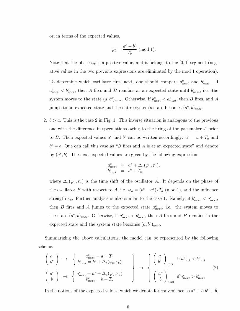
or, in terms of the expected values,

ϕb =ae − be

Tb

(mod 1).

Note that the phase ϕb is a positive value, and it belongs to the [0, 1] segment (neg-

ative values in the two previous expressions are eliminated by the mod 1 operation).

To determine which oscillator fires next, one should compare aenext and benext. If

aenext < benext, then A fires and B remains at an expected state until benext, i.e. the

system moves to the state (a, be)next. Otherwise, if benext < aenext, then B fires, and A

jumps to an expected state and the entire system’s state becomes (ae, b)next.

2. b > a. This is the case 2 in Fig. 1. This inverse situation is analogous to the previous

one with the difference in speculations owing to the firing of the pacemaker A prior

to B. Then expected values ae and be can be written accordingly: ae = a + Ta and

be = b. One can call this case as “B fires and A is at an expected state” and denote

by (ae, b). The next expected values are given by the following expression:

aenext = ae +∆a(ϕa, εa),benext = be + Tb,

where ∆a(ϕa, εa) is the time shift of the oscillator A. It depends on the phase of

the oscillator B with respect to A, i.e. ϕa = (be − ae)/Ta (mod 1), and the influence

strength εa. Further analysis is also similar to the case 1. Namely, if benext < aenext,

then B fires and A jumps to the expected state aenext, i.e. the system moves to

the state (ae, b)next. Otherwise, if aenext < benext, then A fires and B remains in the

expected state and the system state becomes (a, be)next.

Summarizing the above calculations, the model can be represented by the following

scheme:(

abe

)→

{aenext = a + Ta

benext = be +∆b(ϕb, εb)

(ae

b

)→

{aenext = ae +∆a(ϕa, εa)

benext = b+ Tb

→

(abe

)

next

if aenext < benext

(ae

b

)

next

if aenext > benext

(2)

In the notions of the expected values, which we denote for convenience as ae ≡ a be ≡ b,

6

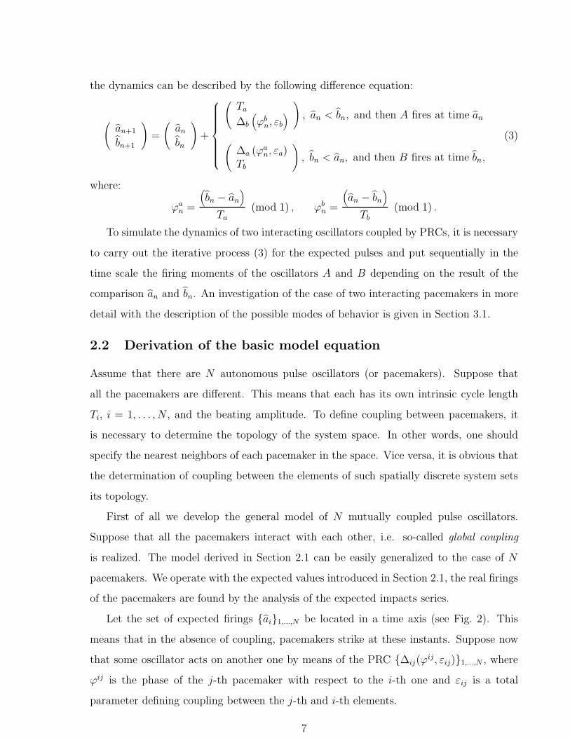
the dynamics can be described by the following difference equation:

(an+1

bn+1

)=

(anbn

)+

(Ta

∆b

(ϕbn, εb

)), an < bn, and then A fires at time an

(∆a (ϕ

an, εa)

Tb

), bn < an, and then B fires at time bn,

(3)

where:

ϕan =

(bn − an

)

Ta

(mod 1) , ϕbn =

(an − bn

)

Tb

(mod 1) .

To simulate the dynamics of two interacting oscillators coupled by PRCs, it is necessary

to carry out the iterative process (3) for the expected pulses and put sequentially in the

time scale the firing moments of the oscillators A and B depending on the result of the

comparison an and bn. An investigation of the case of two interacting pacemakers in more

detail with the description of the possible modes of behavior is given in Section 3.1.

2.2 Derivation of the basic model equation

Assume that there are N autonomous pulse oscillators (or pacemakers). Suppose that

all the pacemakers are different. This means that each has its own intrinsic cycle length

Ti, i = 1, . . . , N , and the beating amplitude. To define coupling between pacemakers, it

is necessary to determine the topology of the system space. In other words, one should

specify the nearest neighbors of each pacemaker in the space. Vice versa, it is obvious that

the determination of coupling between the elements of such spatially discrete system sets

its topology.

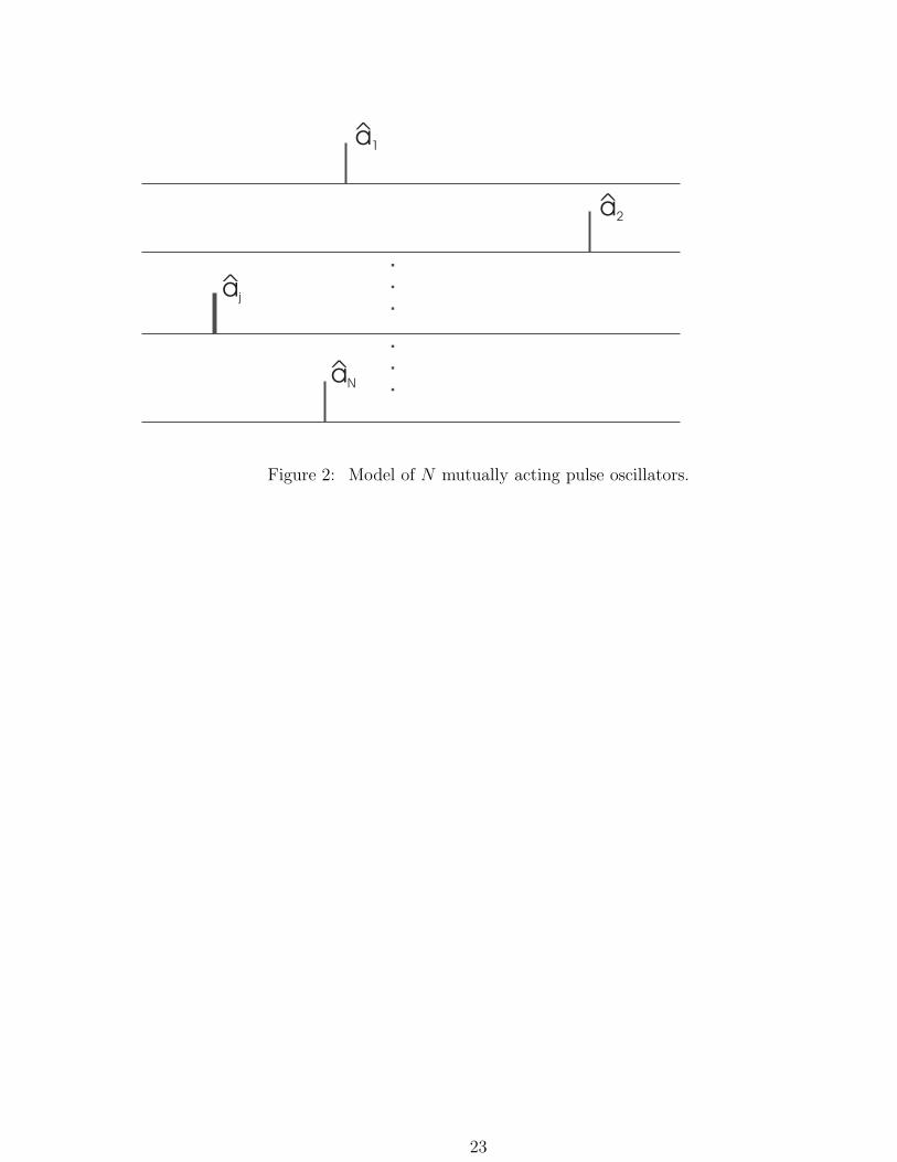
First of all we develop the general model of N mutually coupled pulse oscillators.

Suppose that all the pacemakers interact with each other, i.e. so-called global coupling

is realized. The model derived in Section 2.1 can be easily generalized to the case of N

pacemakers. We operate with the expected values introduced in Section 2.1, the real firings

of the pacemakers are found by the analysis of the expected impacts series.

Let the set of expected firings {ai}1,...,N be located in a time axis (see Fig. 2). This

means that in the absence of coupling, pacemakers strike at these instants. Suppose now

that some oscillator acts on another one by means of the PRC {∆ij(ϕij, εij)}1,...,N , where

ϕij is the phase of the j-th pacemaker with respect to the i-th one and εij is a total

parameter defining coupling between the j-th and i-th elements.

7

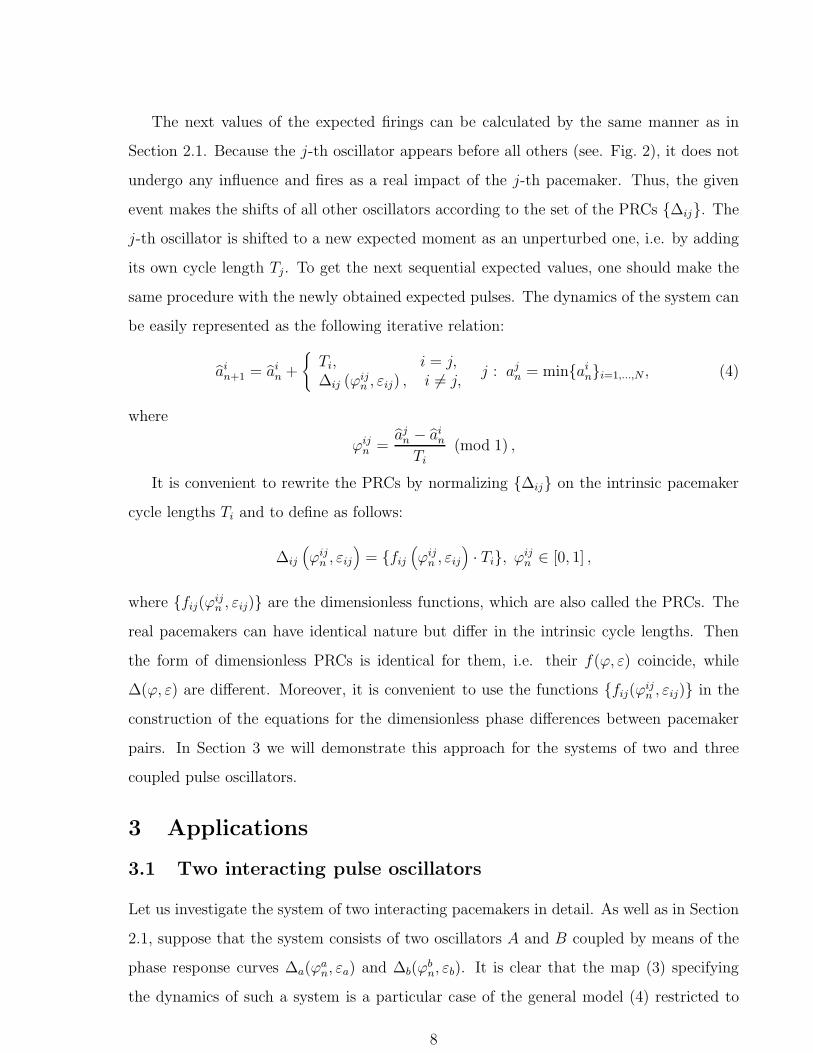
The next values of the expected firings can be calculated by the same manner as in

Section 2.1. Because the j-th oscillator appears before all others (see. Fig. 2), it does not

undergo any influence and fires as a real impact of the j-th pacemaker. Thus, the given

event makes the shifts of all other oscillators according to the set of the PRCs {∆ij}. The

j-th oscillator is shifted to a new expected moment as an unperturbed one, i.e. by adding

its own cycle length Tj. To get the next sequential expected values, one should make the

same procedure with the newly obtained expected pulses. The dynamics of the system can

be easily represented as the following iterative relation:

ain+1 = ain +

{Ti, i = j,∆ij (ϕ

ijn , εij) , i 6= j,

j : ajn = min{ain}i=1,...,N , (4)

where

ϕijn =

ajn − ainTi

(mod 1) ,

It is convenient to rewrite the PRCs by normalizing {∆ij} on the intrinsic pacemaker

cycle lengths Ti and to define as follows:

∆ij

(ϕijn , εij

)= {fij

(ϕijn , εij

)· Ti}, ϕ

ijn ∈ [0, 1] ,

where {fij(ϕijn , εij)} are the dimensionless functions, which are also called the PRCs. The

real pacemakers can have identical nature but differ in the intrinsic cycle lengths. Then

the form of dimensionless PRCs is identical for them, i.e. their f(ϕ, ε) coincide, while

∆(ϕ, ε) are different. Moreover, it is convenient to use the functions {fij(ϕijn , εij)} in the

construction of the equations for the dimensionless phase differences between pacemaker

pairs. In Section 3 we will demonstrate this approach for the systems of two and three

coupled pulse oscillators.

3 Applications

3.1 Two interacting pulse oscillators

Let us investigate the system of two interacting pacemakers in detail. As well as in Section

2.1, suppose that the system consists of two oscillators A and B coupled by means of the

phase response curves ∆a(ϕan, εa) and ∆b(ϕ

bn, εb). It is clear that the map (3) specifying

the dynamics of such a system is a particular case of the general model (4) restricted to

8

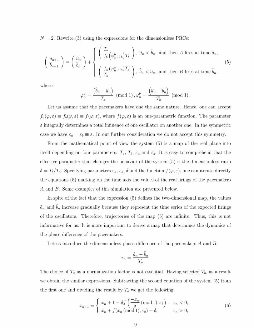
N = 2. Rewrite (3) using the expressions for the dimensionless PRCs:

(an+1

bn+1

)=

(anbn

)+

(Ta

fb(ϕbn, εb

)Tb

), an < bn, and then A fires at time an,

(fa (ϕ

an, εa)Ta

Tb

), bn < an, and then B fires at time bn,

(5)

where:

ϕan =

(bn − an

)

Ta

(mod 1) , ϕbn =

(an − bn

)

Tb

(mod 1) .

Let us assume that the pacemakers have one the same nature. Hence, one can accept

fa(ϕ, ε) ≡ fb(ϕ, ε) ≡ f(ϕ, ε), where f(ϕ, ε) is an one-parametric function. The parameter

ε integrally determines a total influence of one oscillator on another one. In the symmetric

case we have εa = εb ≡ ε. In our further consideration we do not accept this symmetry.

From the mathematical point of view the system (5) is a map of the real plane into

itself depending on four parameters: Ta, Tb, εa and εb. It is easy to comprehend that the

effective parameter that changes the behavior of the system (5) is the dimensionless ratio

δ = Tb/Ta. Specifying parameters εa, εb, δ and the function f(ϕ, ε), one can iterate directly

the equations (5) marking on the time axis the values of the real firings of the pacemakers

A and B. Some examples of this simulation are presented below.

In spite of the fact that the expression (5) defines the two-dimensional map, the values

an and bn increase gradually because they represent the time series of the expected firings

of the oscillators. Therefore, trajectories of the map (5) are infinite. Thus, this is not

informative for us. It is more important to derive a map that determines the dynamics of

the phase difference of the pacemakers.

Let us introduce the dimensionless phase difference of the pacemakers A and B:

xn =an − bn

Ta

.

The choice of Ta as a normalization factor is not essential. Having selected Tb, as a result

we obtain the similar expressions. Subtracting the second equation of the system (5) from

the first one and dividing the result by Ta we get the following:

xn+1 =

xn + 1− δf(−xn

δ(mod 1), εb

), xn < 0,

xn + f(xn (mod 1), εa)− δ, xn > 0,(6)

9

where δ = Tb/Ta. Here we take into account that xn < 0 if an < bn and xn > 0 if an > bn.

Let us make a brief analysis of the developed map. Because in general x ∈ (−∞;∞), the

equation (6) represents a one-dimensional nonlinear map of the real axis into itself. Note

that the map can not be reduced to a circle map by the restriction of x to the range [0; 1]

as it is usually done for two pacemakers interacting by PRCs. It is essentially asymmetric

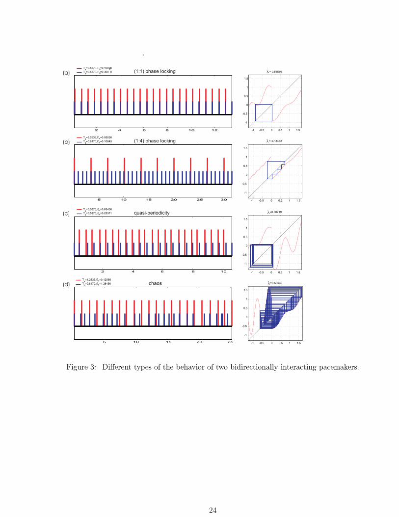
with respect to changing x to −x (see Fig. 3). If f(x, ε) is a nonmonotonic function, then

the map (6) is nonlinear, and it can exhibit a big variety of the behavior: from complex

periodic motion to chaotic dynamics. Owing to x ∈ (−∞;∞), in a rigorous sense it is not

a difference of phases of the pacemakers. In this context one can call x as the generalized

phase difference. Analyzing Eq. (6) one can find out which oscillator, A or B, fires at the

given discrete time n. This depends on the sign of x: A fires if xn < 0 and B fires when

xn > 0. Thus, it makes possible to determine the phase-locking degree of the pacemakers.

However, taking into consideration only the values xn, we may not reconstruct the initial

time series of firing events of the pacemakers A and B. Using xn, one can say only about

their phase difference.

Let us show how the model equations (5), (6) can be applied to the investigation of the

behavior of two interacting pacemakers.

Analysis of real systems [Glass et al., 1987] shows that the function f(x, ε) can take

different forms. But, as a rule, it obeys a number of general properties. For example,

f(0, ε) = f(1, ε) = 0. Usually it has a maximum and a minimum. Sometimes instead of

extrema it has breaks. Let the function f(x, ε) be in an elementary form that is often used

(see, e.g. [Glass & Zeng, 1990]). Namely, let f(x, ε) = ε sin 2πx. This leads to an array of

dynamical equations:

(an+1

bn+1

)=

(anbn

)+

(Ta

εb sin(2πϕb

n

)Tb

), an < bn,

(εa sin (2πϕ

an)Ta

Tb

), bn < an.

(7)

xn+1 =

xn + 1− δεb sin(−xn

δ(mod 1) · 2π), xn < 0,

xn + εa sin(xn (mod 1) · 2π)− δ, xn > 0.(8)

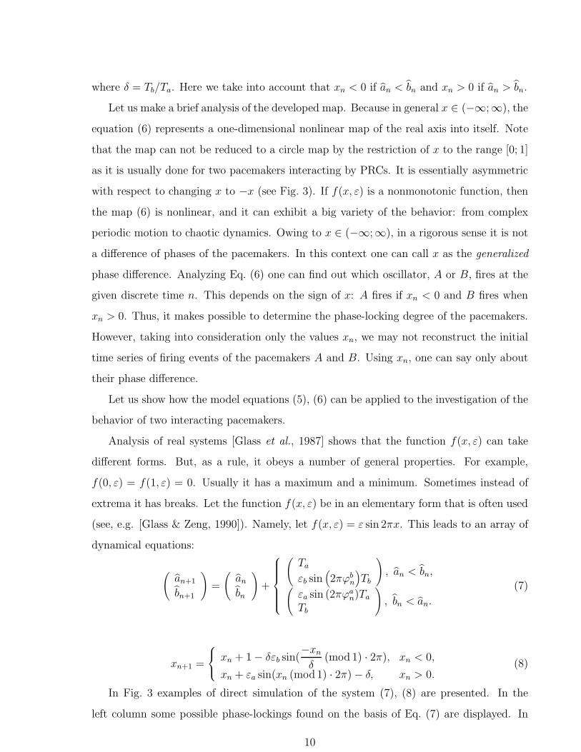
In Fig. 3 examples of direct simulation of the system (7), (8) are presented. In the

left column some possible phase-lockings found on the basis of Eq. (7) are displayed. In

10

the right column the corresponding map (8), its periodic orbit and values of Lyapunov

exponents are shown. Fig. 3d represents the existence of the chaotic behavior for the

system at εa = 0.1205, εb = 1.2845 and δ = 0.6465.

As a conclusion of this section it should be noted that the system of two bidirectionally

acting pacemakers has been already intensively investigated (see, e.g., [Ikeda et al., 2004]

and references herein) as a qualitative model of cardiac arrhythmia known as modulated

parasystole. The interacting oscillators represented the pairs of cardiac pacemakers such

as: the sinoatrial (SA) node and the ventricle contracting by different factors, e.g. ectopic

pacemaker, etc. Hereby the authors used various kinds of PRCs f(x, ε) approximating

the experimental data on stimulating the cardiac cells of animals by single electric current

pulses. Recently in the paper [Loskutov et al., 2004] the system of two interacting pacemak-

ers similar to (7), (8) has been analyzed. In this paper taking into account the refractory

time the various types of the smooth PRCs were examined and the bifurcation diagrams

of possible phase-lockings were constructed. However, in [Loskutov et al., 2004] the be-

havior regimes when the firings of the pacemakers are not alternated, i.e. cases of strong

discrepancies in the intrinsic cycle length (Ta ≫ Tb and vice versa), were not investigated.

The system (7), (8) is more general and takes into account all possible variants.

3.2 Three pacemakers

Below we explain why the special case of three interacting oscillators is worth individual

attention. First, as is known there are three drivers of the rhythm in the cardiac conductive

system: the SA node is a leading pacemaker, the AV junction and Purkinje fibers are

latent pacemakers, which under normal conditions are suppressed by the sinus rhythm.

However, at violations of conductivity and pulse initiation, the cardiac pacemakers can

influence on each other, i.e. so-called bidirectional coupling may be realized. Second, in

pathology a group of contractile cardiomyocytes can also initiate action potentials: an

ectopic (abnormal) cardiac pacemaker may emerge and start to compete with the SA node

for leading the heart rhythm. Third, at stimulating the cardiac tissue by external current

impulses (cardio-stimulation), the cardiac rate is changed. The external stimulaters can

be naturally included in our general model of interacting pacemakers as additional leading

pulse oscillators.

11

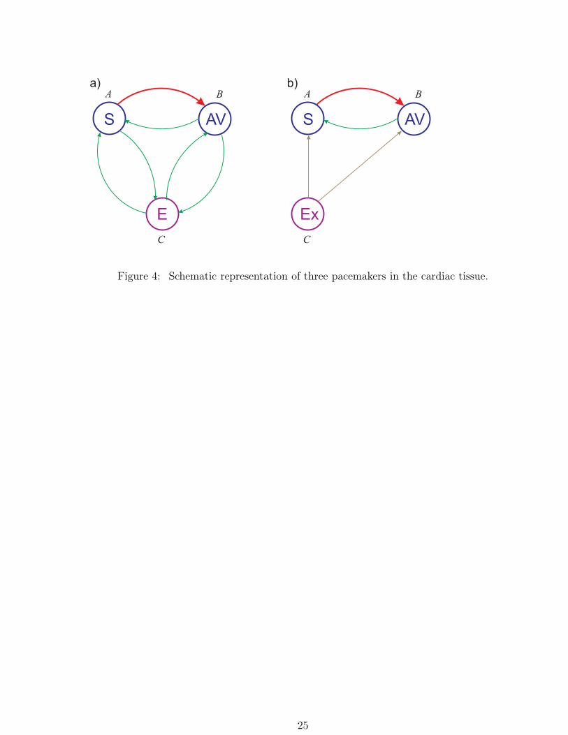
Thus, representation of the heart conductive system as at least three coupled au-

tonomous oscillators (Fig. 4) is very useful for understanding which influence of an ad-

ditional pacemaker exerts on a system of two bidirectionally interacting drivers of the

rhythm (i.e. the SA and AV nodes) considered above. Investigation of the possible behav-

ior modes of a larger amount of interacting pacemakers turns out to be a very complicated

both analytical (mathematical) and numerical problem. For example for a system of five

coupled pulse oscillators we have 25 various functions and 29 different parameters (25 val-

ues of εij and 4 independent ratios Ti/Tj). This is due to the fact that, in general, the

cardiac pacemakers have various frequencies (or intrinsic cycle lengths Ti ) and the different

nature. This means that the PRCs {fij(x, εij)} determining coupling between a pair of

pacemakers have different forms. For some heart pacemakers PRCs have been measured

by the direct experiments on cardiomyocytes of animals (see [Glass et al., 1986]). Other

PRCs can be chosen using general principles based on the nature of nodes or on the basis

of the collateral measurements [Ikeda et al., 1988].

Applying the general model equations (4) for three interacting pacemakers, one can get

the following system:

an+1

bn+1

cn+1

=

anbncn

+

Ta

∆ba

(ϕban , εba

)

∆ca (ϕcan , εca)

, if an < bn, cn; A fires at time an

∆ab

(ϕabn , εab

)

Tb

∆cb

(ϕcbn , εcb

)

, if bn < an, cn; B fires at time bn

∆ac (ϕacn , εac)

∆bc

(ϕbcn , εbc

)

Tc

, if cn < an, bn; C fires at time cn

(9)

where

ϕban =

an − bnTb

(mod 1) , ϕcan =

an − cnTc

(mod 1)

ϕabn =

bn − anTa

(mod 1) , ϕcbn =

bn − cnTc

(mod 1)

ϕacn =

cn − anTa

(mod 1) , ϕbcn =

cn − bnTb

(mod 1)

The response functions ∆ij are supposed to have a form ∆ij(ϕijn , εij) = fij(ϕ

ijn , εij)Ti, ϕ

ijn ∈

[0; 1], i, j = a, b, c. The example of a system of three bidirectionally interacting cardiac

12

pacemakers: the SA node, the AV junction and ectopic pacemaker, is shown in Fig. 4a.

It is convenient to study Eqs. (9) introducing phase differences of the pacemakers. Let

us define,

xn =an − bn

Tb

, yn =cn − bn

Tb

, α =Ta

Tb

, β =Tc

Tb

.

Then for the phase differences we obtain the map of the real plane into itself:

(xn+1

yn+1

)=

(xn

yn

)+

+

α− fba ({xn} , εba)

βfca

({xn − yn

β

}, εca

)− fba ({xn} , εba)

, xn < 0, xn < yn

αfab

({−xn

α

}, εab

)− 1

βfcb

({−ynβ

}, εcb

)− 1

, xn > 0, yn > 0

αfac

({yn − xn

α

}, εac

)− fbc ({yn} , εbc)

β − fbc ({yn} , εbc)

, yn < xn, yn < 0

(10)

Here we denote {x} as the fractional part of x. The conditions in the right hand side

of (10) divide the plane into three areas corresponding to the firing pacemaker (see Fig. 5).

The map (10) has breaks on the boundaries of these areas.

Suppose that the pacemaker B is an external stimulus (see Fig. 4b). Then the ex-

pressions (9), (10) become simpler. The stimulus B acts on the pacemakers A and C but

does not experience any influence. In this situation fba(x, εba) ≡ fbc(x, εbc) ≡ 0 and the

model (9), (10) can be rewritten as follows:

an+1

bn+1

cn+1

=

anbncn

+

Ta

0∆ca (ϕ

can , εca)

, if an < bn, cn; A fires at time an

∆ab

(ϕabn , εab

)

Tb

∆cb

(ϕcbn , εcb

)

, if bn < an, cn; B fires at time bn

∆ac (ϕacn , εac)

0Tc

, if cn < an, bn; C fires at time cn

(11)

13

The corresponding expression for the phase differences takes the form:

(xn+1

yn+1

)=

(xn

yn

)+

+

α

βfca

({xn − yn

β

}, εca

) , xn < 0, xn < yn

αfab

({−xn

α

}, εab

)− 1

βfcb

({−ynβ

}, εcb

)− 1

, xn > 0, yn > 0

αfac

({yn − xn

α

}, εac

)

β

, yn < xn, yn < 0.

(12)

In Fig. 5 some examples of phase-lockings and complex dynamics for the system (9), (10)

are shown. The PRCs are chosen in the sinus form, i.e. fij(x, εij) = εij sin(2πx). Ti and εij

are indicated in the legends. It is obvious that the model of three interacting pacemakers

requires further investigation in detail. In particular, we believe that appropriate choice

of influence strength and period of external stimulation in the equations (12) will remove

the system from undesirable complex behavior to the normal heart rhythm. It will be

represented within forthcoming works.

4 Lattices of Coupled Pulse Oscillators

Let us demonstrate briefly the way how one can approximate discrete distributed media on

the basis of the general model of coupled oscillators (4). Considering a cardiac pacemaker

on the microscopic level, one can represent it as a large group of cells, which generate the

heart rhythm and synchronize their action potentials to initiate the cardiac contraction.

Thus, instead of examining a single pacemaker we should construct a lattice of coupled

pulse oscillators. In this paper we restrict ourselves to the one- (chain) and two-dimensional

(lattice) cases.

Let us suppose that the autonomous pacemakers are located in sites of the two-dimensional

square lattice of the size N ×M . An element of the lattice with coordinates (i, j) is des-

ignated as Ai,j, where i = 1, . . . , N and j = 1, . . . ,M . We restrict consideration to the

14

homogeneous medium and accept a number of limitations on anisotropy. This means that

the pacemakers of the lattice are identical, i.e. they have the same cycle length Ti,j ≡ T ,

i = 1, . . . , N, j = 1, . . . ,M (however, in fact, cells from the periphery of the sinus pace-

maker show the shortest cycle length, although the centre acts as the leading pacemaker

site). This limitation decreases a quantity of parameters of the system and hence simplifies

the study of the model. Now we should define coupling between elements. In works devoted

to the coupled map lattices (CML) two main types of coupling are usually assumed: the

nearest neighbors and global couplings (see, e.g., [Kaneko, 1989]). Since in the previous

sections we supposed that pacemakers interact with each other, this time as an example we

consider lattices with the coupling to nearest neighbors: first, a two-dimensional lattice,

and then a chain of coupled pulse oscillators.

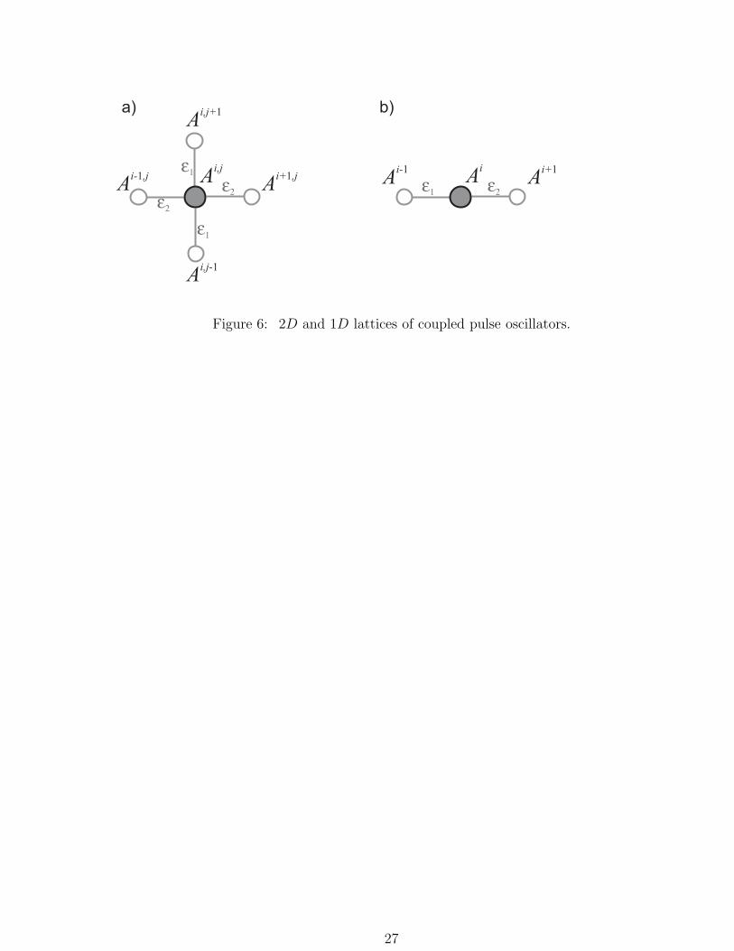
Within the square lattice each pacemaker Ai,j interacts with four of the neighbors

according to the schematic picture in Fig. 6a. Taking into account the limitation of homo-

geneous medium, one can assert that all couplings of the lattice are identical, i.e. each two

adjacent elements interact with each other by a general law defined by the identical PRCs

f(x, ε). Moreover, suppose that the coupling between a pair of elements is isotropic in such

a sense that ε(i,j)(i′,j′) = ε(i′,j′)(i,j), and is equal to one of the values ε1 or ε2 depending on

the relative position of elements. This means that there is an anisotropy of the influence

strength in vertical and horizontal directions. In other words, if two pacemakers are the

neighbors in the vertical direction, they interact by f(x, ε1), and if they are horizontal

neighbors, then they are coupled by f(x, ε2).

Note that all these restrictions are made for the simplification of the analytical form of

the resulting model. In general, it is possible to write the expressions for a two-dimensional

lattice of coupled pulse oscillators without any limitations. It is a subject of a standalone

investigation and lies beyond the framework of the given study.

Let us write equations that determine the iterative dynamics of the expected firings of

the pacemakers {ai,j}i=1,...,N

j=1,...,M

on the basis of the approach represented in Sec.2.2. To obtain

the (n+1)-th value of the individual element ai,j , it is necessary to analyze all elements of

the lattice since they are coupled with each other by means of a local coupling. In other

words, the considered element cannot be affected by others at the n-th time step because

the latter is suppressed by the influence of other elements and remains at the expected state

15

until the (n + 1)-th step. Then dynamics of the model can be described by the following

expression:

ai,jn+1 = ai,jn +

T, if ai,jn = amin,f(ϕ(i,j)(0,+1)

n , ε1) · T, if ai,j+1n = amin,

f(ϕ(i,j)(0,−1)n , ε1) · T, if ai,j−1

n = amin,f(ϕ(i,j)(+1,0)

n , ε2) · T, if ai+1,jn = amin,

f(ϕ(i,j)(−1,0)n , ε2) · T, if ai−1,j

n = amin,0, otherwise

amin = min{ai,jn } i=1...Nj=1...M

(13)

where the phases are

ϕ(i,j)(0,+1)n =

{ai,j+1n − ai,jn

T

}

ϕ(i,j)(0,−1)n =

{ai,j−1n − ai,jn

T

}

ϕ(i,j)(+1,0)n =

{ai+1,jn − ai,jn

T

}

ϕ(i,j)(−1,0)n =

{ai−1,jn − ai,jn

T

}

The constructed model demands detailed investigation on the basis of the approach

developed for the CML (see, e.g., [Kaneko, 1989]). It will be represented in the succeeding

works.

As the second example let us consider a chain of the identical pulse oscillators coupled by

the nearest neighbor principle. We restrict ourselves to a homogeneous case with anisotropy

of the right and left direction in the influence strength between the nearest neighbors. The

schematic picture of the chain is shown in Fig. 6b. Similarly to the above consideration

one can get:

ain+1 = ain+

T, if ain = amin,f(ϕi,+1

n , ε2) · T, if ai+1n = amin,

f(ϕi,−1n , ε1) · T, if ai−1

n = amin,0, otherwise

amin = min{ain}i=1...N (14)

where the phases are the following

ϕi,+1n =

{ai+1n − ain

T

}ϕi,−1n =

{ai−1n − ain

T

}.

If ε1 = 0 (or ε2 = 0), then Eqs (14) define the so-called open-flow model [Willeboordse &

Kaneko, 1994].

16

Because in this work we present a general approach of developing models without the

detailed analysis of their behavior, the type of boundary conditions for both lattices has

not been indicated. Hence, to investigate such systems analytically or numerically, one

should set the boundary conditions along with the PRCs f(x, ε). Usually the boundary

conditions are chosen as periodic, i.e. ai,j+M ≡ ai,j; ai+N,j ≡ ai,j for the two-dimensional

lattice and ai+N ≡ ai for the one-dimensional one. For the open-flow model a condition of

the fixed left boundary, a1n ≡ const, is frequently accepted.

The described models (4), (13) and (14) admit generalization to a natural inhomoge-

neous case by placing different intrinsic cycle lengths of the pacemakers, PRCs and influ-

ence strengths for various groups of elements. However, consideration of inhomogeneous

anisotropic lattices is extremely difficult problem even for numerical analysis. The first

attempts of investigating inhomogeneous lattices of coupled maps (ICML) were described

in [Vasil’ev et al., 2000; Loskutov et al., 2002; Rybalko & Loskutov, 2004].

5 Summary and Limitations

In the present study we propose a quite general discrete model of active media by in-

troducing a simple phase response curve interaction between leading centers. We have

shown that the PRC can be a useful “tool” for representation of the interaction between

pacemakers in cardiac tissue both on a large and small scales. This PRC based model to-

gether with demonstrating complex (chaotic) behavior, can describe the entrainment and

synchronization phenomena of interacting pulse oscillators. It can also aid to understand

their response to an external stimulus with variable intensity and duration (see Fig. 4b),

as previously observed in experimental studies [Jalife et al., 1976; Jalife et al., 1980].

Starting with consideration of two interacting pulse oscillators and introducing new

concepts of expected values, we have extrapolated our PRC based approach to investigate

the mutual influence among an arbitrary large ensemble of pacemakers. The specific cases

of the proposed model show that it can be very useful for investigating the dynamical

interaction of cardiac nodes.

The last part of our study suggests that the derived general model can be easily applied

to construct one– and two–dimensional lattices of active elements interacting by the nearest

17

neighbors type. Extension of the model to a three–dimensional case is straightforward.

Finally, some limitations of our approach should be mentioned. First, the proposed

model is not complete, there is no a time delay in pulse propagation among pacemakers,

which can be very important for describing cardiac arrhythmias. Second, we represented

cardiac tissue as a discrete one and used iterative approach to investigate its behavior.

However, a large amount of realistic examples of active media is treated as continuous.

Nevertheless, cardiac tissue is not a continuum, but is built up by discrete cardiomyocytes

(or nodes with approximate dimensions 0.15 mm × 0.02 mm × 0.01 mm) [Kuramoto,

1984].

Third and most important, to analyze the essential features governing dynamics of

network of active elements, we have not included many important properties of the real

conductive cells. These include the relaxation after stimulating, the prolonged (non-peak)

form of pulses profiles, realistic topological structure, etc. Further investigations are re-

quired to incorporate these features to the general combined model.

6 Acknowledgements

This paper was partially supported by INTAS fellowship No 03-55-1920, granted to Ekate-

rina Zhuchkova. Also, we would like to thank Prof.Alexander Loskutov for critical reading

of the manuscript.

18

References

Antzelevitch, C., Jalife, J. & Moe, G. K. [1982] “Electrotonic modulation of pacemaker ac-

tivity - further biological and mathematical observations on the behavior of modulated

parasystole,” Circulation 66(6), 1225–1232.

Bub, G. & Glass, L. [1994] “Bifurcations in a continuous circle map: A theory for chaotic

cardiac arrhythmia,” Int. J. Bifurcation and Chaos 5(2), 359–371.

Clayton, R. H. [2001] “Computational models of normal and abnormal action potential prop-

agation in cardiac tissue: linking experimental and clinical cardiology,” Physiol. Meas. 22,

R15–R34.

Clayton, R. H., Zhuchkova, E. A. & Panfilov, A. V. [2006] “Phase singularities and filaments:

Simplifying complexity in computational models of ventricular fibrillation,” Prog. Biophys.

Mol. Biol. 90, 378–398.

Courtemanche, M., Glass, L., Belair, J., Scagliotti, D. & Gordon, D. [1989] “A circle map in

a human heart,” Physica D 49, 299–310.

Glass, L., Goldberger, A. L. & Belair, J. [1986] “Dynamics of pure parasystole,” Am. J.

Physiol. 251(4), H841–H847.

Glass, L., Goldberger, A. L., Courtemanche, M. & Shrier, A. [1987] “Nonlinear dynamics,

chaos and complex cardiac arrhythmias,” Proc. R. Soc. London Ser. A-Math. Phys. Eng.

Sci. 413(1844), 9–26.

Glass, L. & Zeng, W. Z. [1990] “Complex bifurcations and chaos in simple theoretical models

of cardiac oscillations,” Ann. N.Y. Acad. Sci. 591, 316–327.

Glass, L., Nagai, Yo., Hall, K., Talajie, M. & Nattel, S. [2002] “Predicting the entrainment of

reentrant cardiac waves using phase resetting curves,” Phys. Rev. E 65, 021908-1–021908-

10.

Goldberger, A. L. [1990] “Nonlinear dynamics, fractals and chaos: Applications to cardiac

electrophysiology,” Ann. Biomed. Eng. 18(2), 195–198.

Guevara, M. R. & Shrier, A. [1987] “Phase resetting in a model of cardiac Purkinje fiber,”

Biophys. J. 52(2), 165–175.

Ikeda, N. [1982] “Model of bidirectional interaction between myocardial pacemakers based on

the phase response curve,” Biol. Cybern. 43(3), 157–167.

19

Ikeda, N., DeLand, E., Miyahara, H., Takeuchi, A., Yamamoto, H. & and Sato, T. [1988] “A

personal computer-based arrhythmia generator based on mathematical models of cardiac

arrhythmia,” J. Electrocardiol. 21(Suppl).

Ikeda, N., Takeuchi, A., Hamada, A., Goto, H., Mamorita, N. & Takayanagi, K. [2004] “Model

of bidirectional modulated parasystole as a mechanism for cyclic bursts of ventricular

premature contractions,” Biol. Cybern. 91(1), 37–47.

Jalife, J. & Moe, G. K. [1976] “Effects of electronic potentials on pacemaker activity of canine

Purkinje fibers in relation to parasystole,” Circ. Res. 39(6), 801–808.

Jalife, J., Hamilton, A. J., Lamanna, V. R. & and Moe, G. K. [1980] “Effects of current flow

on pacemaker activity of the isolated kitten sinoatrial node,” Am. J. Physiol. 238(3),

H307–H316.

Kaneko, K. [1989] “Spatiotemporal chaos in one-dimensional and two-dimensional coupled

map lattices,” Physica D 37(1-3), 60–82.

Kaneko, K. [1990] “Clustering, coding, switching, hierarchical ordering, and control in a

network of chaotic element,” Physica D 41(2), 137–172.

Kuramoto, Y. [1984] Chemical Oscillations, Waves, and Turbulence (Springer-Verlag, Berlin).

Kuramoto, Y. [1995] “Scaling behavior of turbulent oscillators with nonlocal interaction,”

Prog. Theor. Phys. 94(3), 321–330.

Loskutov, A., Prokhorov, A. K. & Rybalko, S. D. [2002] “Dynamics of inhomogeneous chains

of coupled quadratic maps,” Theor. Math. Phys. 132(1), 983–999.

Loskutov, A., Rybalko, S. & Zhuchkova, E. [2004] “Model of cardiac tissue as a conductive

system with interacting pacemakers and refractory time,” Int. J. Bifurcation and Chaos

14(7), 2457–2466.

Reiner, V. S. & Antzelevich, C. [1985] “Phase resetting and annihilation in a mathematical

model of sinus node,” Am. J. Physiol. 249, H1143–H1153.

Rybalko, S. & Loskutov, A. [2004] “Dynamics of inhomogeneous one-dimensional coupled

map lattices,” http://arxiv.org/abs/nlin.CD/0409014.

Sano, T., Sawanobori, T. & Adaniya, H. [1978] “Mechanism of rhythm determination among

pacemaker cells of the mammalian sinus node,” Am. J. Physiol. 235, H379–H384.

Shibata, T. & Kaneko, K. [1998] “Collective chaos,” Phys. Rev. Lett. 81(19), 4116–4119.

Vasil’ev, K. A., Loskutov, A., Rybalko, S. D. & Udin, D. N. [2000] “Model of a spatially

20

inhomogeneous one-dimensional active medium,” Theor. Math. Phys. 124(3), 1286–1297.

Wiener, N. & Rosenblueth, A. [1946] “Conduction of impulses in cardiac muscle,” Arch. Inst.

Cardiol. Mex. 16, 205–265.

Willeboordse, F. H. & Kaneko, K. [1994] “Bifurcations and spatial chaos in an open flow

model,” Phys. Rev. Lett. 73(4), 533–536.

Winfree, A. T. [2000] The Geometry of Biological Time (Springer-Verlag, New York), 2nd ed.

21

A

B

b

a ae

Ta

a

b be

Tb

(1) (2)

Figure 1: The model of two interacting pulse oscillators.

22

a1

.

.

.

.

.

.

a2

aj

aN

Figure 2: Model of N mutually acting pulse oscillators.

23

λ

λ

λ

λ

εa

εb (1:1) phase locking

εa

εb (1:4) phase locking

εa

εb quasi-periodicity

εa

εb chaos

(a)

(b)

(c)

(d)

Figure 3: Different types of the behavior of two bidirectionally interacting pacemakers.

24

S AV

E

A B

C

S AV

Ex

A B

C

a) b)

Figure 4: Schematic representation of three pacemakers in the cardiac tissue.

25

(1:1:1) phase locking

(2:6:1) phase locking

complex behavior

(a)

(b)

(c)

A B

C

A B

C

A B

C

εε

εεε ε

εεε

εεε

ε εεε

εε

Figure 5: Different types of the behavior of three pulse oscillators.

26

Ai,j+1

Ai+ ,j1

Ai- ,j1

Ai,j-1

Ai,jε1

ε1

ε2

ε2

Ai+1

Ai-1 A

i

ε1 ε2

a) b)

Figure 6: 2D and 1D lattices of coupled pulse oscillators.

27