agency washington, d.c. 20460 environmental … m. hightower environmental characterization and...

Environmental TechnologyVerification Program

United States Office of Research and EPA/600/R-97/149Environmental Protection Development December 1997Agency Washington, D.C. 20460

Environmental Technolo gyVerification Report

Field Portable GasChromatograph/MassSpectrometer

Bruker-Franzen Analytical Systems,Inc. EM640™

Environmental Technolo gyVerification Report

Field Portable Gas Chromatograph/ MassSpectrometer

Bruker-Franzen Analytical Systems, Inc.EM640™

Prepared By

Wayne EinfeldSusan F. Bender

Michael R. KeenanSteven M. ThornbergMichael M. Hightower

Environmental Characterizationand Monitoring Department

Sandia National LaboratoriesAlbuquerque, New Mexico

Sponsored by

U.S. ENVIRONMENTAL PROTECTION AGENCYOFFICE OF RESEARCH AND DEVELOPMENT

NATIONAL EXPOSURE RESEARCH LABORATORYENVIRONMENTAL SCIENCES DIVISION

LAS VEGAS, NEVADA

ii

Notice

The information in this document has been funded wholly or in part by the U.S. Environmental ProtectionAgency (EPA) under an Interagency Agreement number DW89936700-01-0 with the U.S. Department ofEnergy’s Sandia National Laboratories. This verification effort was supported by the Consortium for SiteCharacterization Technology, a pilot operating under the EPA’s Environmental Technology Verification(ETV) Program. It has been subjected to the Agency’s peer and administrative review, and it has beenapproved for publication as an EPA document. Mention of corporation names, trade names, or commercialproducts does not constitute endorsement or recommendation for use of specific products.

In 1995, the U. S. Environmental Protection Agency established the Environmental TechnologyVerification Program. The purpose of the Program is to promote the acceptance and use of innovativeenvironmental technologies. The verification of the performance of the Bruker-Franzen AnalyticalSystems, Inc. EM640™ field transportable gas chromatograph/mass spectrometer (GC/MS) systemrepresents one of the first attempts at employing a testing process for the purpose of performanceverification. One goal of this process is to generate accurate and credible data that can be used to verify thecharacteristics of the technologies participating in the program. This report presents the results of our firstapplication of the testing process. We learned a great deal about the testing process and have applied whatwe learned to improve upon it. We expect that each demonstration will serve to improve the next and thatthis project merely represents the first step in a complex process to make future demonstrations moreefficient, less costly, and more useful.

vi

Foreword

��

�� !�� "� � ��#��$�� !�#$��% ��

�� %�� % ��%��& ��%��'��

�� !�#$�� (�� % ��

��)�� %��*�� *��+��,�� +��

�-�� %%�� %��

��

�� .��%�� .�� %�� %

� �� % ��%�� % �� %��

��.�� % ��

%�� /�%%�� .�� % ��

� ��*�� *��*�� %��

�� % ��0 �� 0�� % ��

��)�� %�� % ��#�� #��

�� 0�� % ��

�� %�� *��)�� *�� 1�� %

�0��*��2 �� 2�� *��

�� %%��

�� (�� %�� *��,�� '��

�� *��-�� %%��*��3�� %�� %��

�� !�#$�� 4�� $��.��*

!��

�� % �� %� �� '��

�� .��0�� *��

�� %�� %�� 5��

�� *��% �� %��

6��7��8 ��*��4�

4��

!�� "� � ��#��$��

1%%�� %�#��4��

vii

Acknowledgment

The authors wish to acknowledge the support of all those who helped plan and conduct the demonstrations,analyze the data, and prepare this report. In particular we recognize the technical expertise of SusanBender, Jeanne Barrera, Dr. Steve Thornberg, Dr. Mike Keenan, Grace Bujewski, Gary Brown, BobHelgesen, Dr. Curt Mowry, and Dr. Brian Rutherford of Sandia National Laboratories. The contributionsof Gary Robertson, Dr. Stephen Billets, and Eric Koglin of the EPA’s National Exposure ResearchLaboratory, Environmental Sciences Division in Las Vegas, Nevada, are also recognized in the variousaspects of this project.

Demonstration preparation and performance also required the assistance of numerous personnel from theSavannah River Technology Center and University of Michigan/Wurtsmith Air Force Base. Thecontributions of Joe Rossabi and co-workers at the Savannah River Technology Center and MikeBarcelona and co-workers at the University of Michigan are gratefully acknowledged. The Wurtsmith siteis a national test site funded by the Strategic Environmental Research and Development Program.Cooperation and assistance from this agency is also acknowledged.

Performance evaluation (PE) samples provided a common reference for the field technologies. Individualsand reference laboratories who analyzed water and soil samples included Alan Hewitt, of the U.S. ArmyCold Regions Research and Engineering Laboratory, for soil PE samples; and Michael Wilson, of the U.S.EPA Office of Emergency and Remedial Response, Analytical Operations and Data Quality Center, for thewater PE samples.

We also acknowledge the participation of Bruker-Franzen Analytic GMBH, in particular, Ms. Nölke andMr. Zey who operated the Bruker instrument during the demonstrations.

For more information on the Bruker GC/MS demonstrations, contact:

Gary Robertson, Project Technical LeaderEnvironmental Protection AgencyNational Exposure Research LaboratoryHuman Exposure and Atmospheric Sciences DivisionP.O. Box 93478Las Vegas, Nevada 89193-3478(702) 798-2215

For more information on the Bruker GC/MS technology, contact:

Paul Kowalski or Mark Emmons Bruker Instruments, Inc.19 Fortune Drive, Manning ParkBillerica, MA 01821(508) 667-9580fax (508) 667-5993

viii

Contents

Notice . . . . . . . . . . . . . . . . . . . . . . . . . . . . . . . . . . . . . . . . . . . . . . . . . . . . . . . . . . . . . . . . . . . . . . . . . . . . iiVerification Statement. . . . . . . . . . . . . . . . . . . . . . . . . . . . . . . . . . . . . . . . . . . . . . . . . . . . . . . . . . . . . . iiiForeword . . . . . . . . . . . . . . . . . . . . . . . . . . . . . . . . . . . . . . . . . . . . . . . . . . . . . . . . . . . . . . . . . . . . . . . . viAcknowledgment. . . . . . . . . . . . . . . . . . . . . . . . . . . . . . . . . . . . . . . . . . . . . . . . . . . . . . . . . . . . . . . . . . viiFigures . . . . . . . . . . . . . . . . . . . . . . . . . . . . . . . . . . . . . . . . . . . . . . . . . . . . . . . . . . . . . . . . . . . . . . . . . . xiiTables. . . . . . . . . . . . . . . . . . . . . . . . . . . . . . . . . . . . . . . . . . . . . . . . . . . . . . . . . . . . . . . . . . . . . . . . . .xiiiAbbreviations and Acronyms. . . . . . . . . . . . . . . . . . . . . . . . . . . . . . . . . . . . . . . . . . . . . . . . . . . . . . . . xiv

Sections

1. Executive Summary . . . . . . . . . . . . . . . . . . . . . . . . . . . . . . . . . . . . . . . . . . . . . . . . . . . . . . . . . . . . . . 1

Technology Description . . . . . . . . . . . . . . . . . . . . . . . . . . . . . . . . . . . . . . . . . . . . . . . . . . . . . . . 2

Demonstration Objectives and Approach . . . . . . . . . . . . . . . . . . . . . . . . . . . . . . . . . . . . . . . . . . 2

Demonstration Results. . . . . . . . . . . . . . . . . . . . . . . . . . . . . . . . . . . . . . . . . . . . . . . . . . . . . . . . 2

Performance Evaluation . . . . . . . . . . . . . . . . . . . . . . . . . . . . . . . . . . . . . . . . . . . . . . . . . . . . . . . 3

2. Introduction. . . . . . . . . . . . . . . . . . . . . . . . . . . . . . . . . . . . . . . . . . . . . . . . . . . . . . . . . . . . . . . . . . . . . 4

Site Characterization Technology Challenge . . . . . . . . . . . . . . . . . . . . . . . . . . . . . . . . . . . . . . . 4

Technology Verification Process. . . . . . . . . . . . . . . . . . . . . . . . . . . . . . . . . . . . . . . . . . . . . . . . 4Needs Identification and Technology Selection . . . . . . . . . . . . . . . . . . . . . . . . . . . . . . . . 5Demonstration Planning and Implementation . . . . . . . . . . . . . . . . . . . . . . . . . . . . . . . . . . 5Report Preparation . . . . . . . . . . . . . . . . . . . . . . . . . . . . . . . . . . . . . . . . . . . . . . . . . . . . . . . 5Information Distribution . . . . . . . . . . . . . . . . . . . . . . . . . . . . . . . . . . . . . . . . . . . . . . . . . . 6

The GC/MS Demonstration . . . . . . . . . . . . . . . . . . . . . . . . . . . . . . . . . . . . . . . . . . . . . . . . . . . . 6

3. Technology Description . . . . . . . . . . . . . . . . . . . . . . . . . . . . . . . . . . . . . . . . . . . . . . . . . . . . . . . . . . . 9

Theory of Operation and Background Information. . . . . . . . . . . . . . . . . . . . . . . . . . . . . . . . . . . 9

Operational Characteristics . . . . . . . . . . . . . . . . . . . . . . . . . . . . . . . . . . . . . . . . . . . . . . . . . . . . . 9

Performance Factors . . . . . . . . . . . . . . . . . . . . . . . . . . . . . . . . . . . . . . . . . . . . . . . . . . . . . . . . . 10Detection Limits . . . . . . . . . . . . . . . . . . . . . . . . . . . . . . . . . . . . . . . . . . . . . . . . . . . . . . . 11Dynamic Range . . . . . . . . . . . . . . . . . . . . . . . . . . . . . . . . . . . . . . . . . . . . . . . . . . . . . . . . 11Sample Throughput . . . . . . . . . . . . . . . . . . . . . . . . . . . . . . . . . . . . . . . . . . . . . . . . . . . . . 11

Advantages of the Technology . . . . . . . . . . . . . . . . . . . . . . . . . . . . . . . . . . . . . . . . . . . . . . . . . 11

Limits of the Technology . . . . . . . . . . . . . . . . . . . . . . . . . . . . . . . . . . . . . . . . . . . . . . . . . . . . . 12

ix

4. Site Descriptions and Demonstration Design . . . . . . . . . . . . . . . . . . . . . . . . . . . . . . . . . . . . . . . . . . 14

Technology Demonstration Objectives . . . . . . . . . . . . . . . . . . . . . . . . . . . . . . . . . . . . . . . . . . . 14Qualitative Assessments. . . . . . . . . . . . . . . . . . . . . . . . . . . . . . . . . . . . . . . . . . . . . . . . . 14Quantitative Assessments. . . . . . . . . . . . . . . . . . . . . . . . . . . . . . . . . . . . . . . . . . . . . . . . 14

Site Selection and Description . . . . . . . . . . . . . . . . . . . . . . . . . . . . . . . . . . . . . . . . . . . . . . . . . 15Savannah River Site Description . . . . . . . . . . . . . . . . . . . . . . . . . . . . . . . . . . . . . . . . . . . 15Wurtsmith Air Force Base Description . . . . . . . . . . . . . . . . . . . . . . . . . . . . . . . . . . . . . . 17

Overview of the Field Demonstrations . . . . . . . . . . . . . . . . . . . . . . . . . . . . . . . . . . . . . . . . . . . 21

Overview of Sample Collection, Handling, and Distribution . . . . . . . . . . . . . . . . . . . . . . . . . . 21SRS Sample Collection . . . . . . . . . . . . . . . . . . . . . . . . . . . . . . . . . . . . . . . . . . . . . . . . . . 21WAFB Sample Collection . . . . . . . . . . . . . . . . . . . . . . . . . . . . . . . . . . . . . . . . . . . . . . . . 24

Reference Laboratory Selection and Analysis Methodology . . . . . . . . . . . . . . . . . . . . . . . . . . 25 General Engineering Laboratory . . . . . . . . . . . . . . . . . . . . . . . . . . . . . . . . . . . . . . . . . . . 26 Traverse Analytical and Pace Environmental Laboratories. . . . . . . . . . . . . . . . . . . . . . 26

SRS and WAFB On-Site Laboratories. . . . . . . . . . . . . . . . . . . . . . . . . . . . . . . . . . . . . . 26

Pre-demonstration Sampling and Analysis . . . . . . . . . . . . . . . . . . . . . . . . . . . . . . . . . . . . . . . . 26

Deviations from the Demonstration Plan . . . . . . . . . . . . . . . . . . . . . . . . . . . . . . . . . . . . . . . . . 27Pre-demonstration Activities. . . . . . . . . . . . . . . . . . . . . . . . . . . . . . . . . . . . . . . . . . . . . . 27SRS Soil Spike Samples . . . . . . . . . . . . . . . . . . . . . . . . . . . . . . . . . . . . . . . . . . . . . . . . . 27SRS Soil Gas Survey Evaluation . . . . . . . . . . . . . . . . . . . . . . . . . . . . . . . . . . . . . . . . . . . 27Soil Gas Samples at WAFB . . . . . . . . . . . . . . . . . . . . . . . . . . . . . . . . . . . . . . . . . . . . . . 27Water Samples at WAFB . . . . . . . . . . . . . . . . . . . . . . . . . . . . . . . . . . . . . . . . . . . . . . . . 28Calibration Check Sample Analysis . . . . . . . . . . . . . . . . . . . . . . . . . . . . . . . . . . . . . . . . 28

5. Reference Laboratory Analysis Results and Evaluation. . . . . . . . . . . . . . . . . . . . . . . . . . . . . . . . . . 29Laboratory Operations . . . . . . . . . . . . . . . . . . . . . . . . . . . . . . . . . . . . . . . . . . . . . . . . . . . . . . . 29

General Engineering Laboratories . . . . . . . . . . . . . . . . . . . . . . . . . . . . . . . . . . . . . . . . . . 29SRS On-Site Laboratory . . . . . . . . . . . . . . . . . . . . . . . . . . . . . . . . . . . . . . . . . . . . . . . . . 29Traverse Analytical Laboratory . . . . . . . . . . . . . . . . . . . . . . . . . . . . . . . . . . . . . . . . . . . . 29Pace Inc. Environmental Laboratories. . . . . . . . . . . . . . . . . . . . . . . . . . . . . . . . . . . . . . . 30WAFB On-Site Laboratory . . . . . . . . . . . . . . . . . . . . . . . . . . . . . . . . . . . . . . . . . . . . . . . 30

Laboratory Compound Detection Limits . . . . . . . . . . . . . . . . . . . . . . . . . . . . . . . . . . . . . . . . . 30

Laboratory Data Quality Assessment Methods. . . . . . . . . . . . . . . . . . . . . . . . . . . . . . . . . . . . . 31Precision Analysis . . . . . . . . . . . . . . . . . . . . . . . . . . . . . . . . . . . . . . . . . . . . . . . . . . . . . . 31Accuracy Analysis . . . . . . . . . . . . . . . . . . . . . . . . . . . . . . . . . . . . . . . . . . . . . . . . . . . . . . 31Laboratory Internal Quality Control Metrics. . . . . . . . . . . . . . . . . . . . . . . . . . . . . . . . . . 32

Laboratory Data Quality Levels . . . . . . . . . . . . . . . . . . . . . . . . . . . . . . . . . . . . . . . . . . . . . . . . 33

x

Laboratory Data Validation for the SRS Demonstration . . . . . . . . . . . . . . . . . . . . . . . . . . . . . 33GEL Data Quality Evaluation . . . . . . . . . . . . . . . . . . . . . . . . . . . . . . . . . . . . . . . . . . . . . 33GEL Data Quality Summary . . . . . . . . . . . . . . . . . . . . . . . . . . . . . . . . . . . . . . . . . . . . . . 35SRS On-Site Laboratory Data Quality Evaluation . . . . . . . . . . . . . . . . . . . . . . . . . . . . . 35SRS Laboratory Data Quality Summary . . . . . . . . . . . . . . . . . . . . . . . . . . . . . . . . . . . . . 36

Laboratory Data Validation for the WAFB Demonstration . . . . . . . . . . . . . . . . . . . . . . . . . . . 36Traverse Data Quality Evaluation . . . . . . . . . . . . . . . . . . . . . . . . . . . . . . . . . . . . . . . . . . 37Traverse Laboratory Data Quality Summary . . . . . . . . . . . . . . . . . . . . . . . . . . . . . . . . . 39Pace Data Quality Evaluation . . . . . . . . . . . . . . . . . . . . . . . . . . . . . . . . . . . . . . . . . . . . . 39Pace Data Quality Summary . . . . . . . . . . . . . . . . . . . . . . . . . . . . . . . . . . . . . . . . . . . . . . 41

Summary Description of Laboratory Data Quality . . . . . . . . . . . . . . . . . . . . . . . . . . . . . . . . . . 41

6. Technology Demonstration Results and Evaluation. . . . . . . . . . . . . . . . . . . . . . . . . . . . . . . . . . . . . 43

Introduction. . . . . . . . . . . . . . . . . . . . . . . . . . . . . . . . . . . . . . . . . . . . . . . . . . . . . . . . . . . . . . . . 43

Pre-Demonstration Developer Claims . . . . . . . . . . . . . . . . . . . . . . . . . . . . . . . . . . . . . . . . . . . 43

Field Demonstration Data Evaluation Approach . . . . . . . . . . . . . . . . . . . . . . . . . . . . . . . . . . . 44 Instrument Precision Evaluation . . . . . . . . . . . . . . . . . . . . . . . . . . . . . . . . . . . . . . . . . . . 44

Instrument Accuracy Evaluation . . . . . . . . . . . . . . . . . . . . . . . . . . . . . . . . . . . . . . . . . . . 45Instrument Comparison with Reference Laboratory Data . . . . . . . . . . . . . . . . . . . . . . . . 46

Summary of Instrument Performance Goals . . . . . . . . . . . . . . . . . . . . . . . . . . . . . . . . . . . . . . . 49 Accuracy . . . . . . . . . . . . . . . . . . . . . . . . . . . . . . . . . . . . . . . . . . . . . . . . . . . . . . . . . . . . . 49

Precision . . . . . . . . . . . . . . . . . . . . . . . . . . . . . . . . . . . . . . . . . . . . . . . . . . . . . . . . . . . . . 50Bruker to Reference Laboratory Comparison . . . . . . . . . . . . . . . . . . . . . . . . . . . . . . . . . 51

Field Operation Observations . . . . . . . . . . . . . . . . . . . . . . . . . . . . . . . . . . . . . . . . . . . . . . . . . . 52 SRS Demonstration . . . . . . . . . . . . . . . . . . . . . . . . . . . . . . . . . . . . . . . . . . . . . . . . . . . . . 52

WAFB Demonstration . . . . . . . . . . . . . . . . . . . . . . . . . . . . . . . . . . . . . . . . . . . . . . . . . . . 52

Bruker Accuracy and Precision Results. . . . . . . . . . . . . . . . . . . . . . . . . . . . . . . . . . . . . . . . . . 54 Bruker Accuracy -- SRS Demonstration . . . . . . . . . . . . . . . . . . . . . . . . . . . . . . . . . . . . . 54

Bruker Accuracy -- WAFB Demonstration . . . . . . . . . . . . . . . . . . . . . . . . . . . . . . . . . . . 54Overall Bruker Accuracy Performance . . . . . . . . . . . . . . . . . . . . . . . . . . . . . . . . . . . . . . 55Bruker Precision -- SRS Demonstration . . . . . . . . . . . . . . . . . . . . . . . . . . . . . . . . . . . . . 57Bruker Precision -- WAFB Demonstration . . . . . . . . . . . . . . . . . . . . . . . . . . . . . . . . . . . 58Overall Bruker Precision Performance . . . . . . . . . . . . . . . . . . . . . . . . . . . . . . . . . . . . . . 59

Bruker to Reference Laboratory Data Comparison . . . . . . . . . . . . . . . . . . . . . . . . . . . . . . . . . . 59Scatter Plots/Histograms -- SRS Demonstration . . . . . . . . . . . . . . . . . . . . . . . . . . . . . . . 61Scatter Plots/Histograms -- WAFB Demonstration . . . . . . . . . . . . . . . . . . . . . . . . . . . . . 61Overall Bruker to Laboratory Comparison Results. . . . . . . . . . . . . . . . . . . . . . . . . . . . . 67

Summary of Bruker Accuracy, Precision, and Laboratory Comparison Performance . . . . . . . 68

xi

Other Bruker GC/MS Performance Indicators . . . . . . . . . . . . . . . . . . . . . . . . . . . . . . . . . . . . . 69Target Compound Identification in Complex Mixtures . . . . . . . . . . . . . . . . . . . . . . . . . 69Field Handling and Operation . . . . . . . . . . . . . . . . . . . . . . . . . . . . . . . . . . . . . . . . . . . . . 69

Overall Bruker GC/MS Performance Conclusions . . . . . . . . . . . . . . . . . . . . . . . . . . . . . . . . . . 70

7. Applications Assessment. . . . . . . . . . . . . . . . . . . . . . . . . . . . . . . . . . . . . . . . . . . . . . . . . . . . . . . . . . 72

Applicability to Field Operations . . . . . . . . . . . . . . . . . . . . . . . . . . . . . . . . . . . . . . . . . . . . . . . 72

Capital and Field Operation Costs . . . . . . . . . . . . . . . . . . . . . . . . . . . . . . . . . . . . . . . . . . . . . . 72

Advantages of the Technology . . . . . . . . . . . . . . . . . . . . . . . . . . . . . . . . . . . . . . . . . . . . . . . . . 72Rapid Analysis . . . . . . . . . . . . . . . . . . . . . . . . . . . . . . . . . . . . . . . . . . . . . . . . . . . . . . . . 72Sampling and Sample Cost Advantages . . . . . . . . . . . . . . . . . . . . . . . . . . . . . . . . . . . . . 73Transportability . . . . . . . . . . . . . . . . . . . . . . . . . . . . . . . . . . . . . . . . . . . . . . . . . . . . . . . . 74Field Screening of Samples . . . . . . . . . . . . . . . . . . . . . . . . . . . . . . . . . . . . . . . . . . . . . . . 74Sample Size . . . . . . . . . . . . . . . . . . . . . . . . . . . . . . . . . . . . . . . . . . . . . . . . . . . . . . . . . . . 74Interferences . . . . . . . . . . . . . . . . . . . . . . . . . . . . . . . . . . . . . . . . . . . . . . . . . . . . . . . . . . 74

Conclusions . . . . . . . . . . . . . . . . . . . . . . . . . . . . . . . . . . . . . . . . . . . . . . . . . . . . . . . . . . . . . . . . 74

8. Developer’s Forum . . . . . . . . . . . . . . . . . . . . . . . . . . . . . . . . . . . . . . . . . . . . . . . . . . . . . . . . . . . . . 75

9. Previous Deployments . . . . . . . . . . . . . . . . . . . . . . . . . . . . . . . . . . . . . . . . . . . . . . . . . . . . . . . . . . . 77

10. References . . . . . . . . . . . . . . . . . . . . . . . . . . . . . . . . . . . . . . . . . . . . . . . . . . . . . . . . . . . . . . . . . . . . 78

Appendix

A: Environmental Monitoring Management Council (EMMC) Method. . . . . . . . . . . . . . . . . . . . . A-1

xii

Figures

2-1 Example total ion chromatogram of a complex mixture . . . . . . . . . . . . . . . . . . . . . . . . . . . . . . . . 73-1 Block Diagram of Bruker-Franzen EM640 GC/MS. . . . . . . . . . . . . . . . . . . . . . . . . . . . . . . . 10TM

4-1 Location of the Savannah River Site. . . . . . . . . . . . . . . . . . . . . . . . . . . . . . . . . . . . . . . . . . . . . 164-2 SRS M-Area Well Locations . . . . . . . . . . . . . . . . . . . . . . . . . . . . . . . . . . . . . . . . . . . . . . . . . . . 184-3 Location of Wurtsmith Air Force Base. . . . . . . . . . . . . . . . . . . . . . . . . . . . . . . . . . . . . . . . . . . . 194-4 WAFB Fire Training Area 2 Sampling Locations . . . . . . . . . . . . . . . . . . . . . . . . . . . . . . . . . . . 206-1 Example scatter plots with simulated data . . . . . . . . . . . . . . . . . . . . . . . . . . . . . . . . . . . . . . . . . 486-2 Example histograms with simulated data . . . . . . . . . . . . . . . . . . . . . . . . . . . . . . . . . . . . . . . . . . 506-3 Plot of daily temperatures during the SRS demonstration . . . . . . . . . . . . . . . . . . . . . . . . . . . . . 536-4 Plot of daily temperatures during the WAFB demonstration . . . . . . . . . . . . . . . . . . . . . . . . . . . 536-5 Absolute percent accuracy histogram for Bruker soil samples . . . . . . . . . . . . . . . . . . . . . . . . . . 566-6 Absolute percent accuracy histogram for Bruker water samples . . . . . . . . . . . . . . . . . . . . . . . . 566-7 Absolute percent accuracy histogram for Bruker soil gas samples . . . . . . . . . . . . . . . . . . . . . . . 566-8 Relative percent difference histogram for Bruker soil samples . . . . . . . . . . . . . . . . . . . . . . . . . 606-9 Relative percent difference histogram for Bruker water samples . . . . . . . . . . . . . . . . . . . . . . . . 606-10 Relative percent difference histogram for Bruker soil gas samples . . . . . . . . . . . . . . . . . . . . . . 606-11 Bruker vs. Laboratory data for SRS low concentration water samples . . . . . . . . . . . . . . . . . . . . 626-12 Bruker vs. Laboratory data for SRS high concentration water samples . . . . . . . . . . . . . . . . . . . 626-13 Percent difference histogram for SRS water samples . . . . . . . . . . . . . . . . . . . . . . . . . . . . . . . . . 636-14 Bruker vs. Laboratory data for SRS soil gas samples . . . . . . . . . . . . . . . . . . . . . . . . . . . . . . . . . 636-15 Percent difference histogram for SRS soil gas samples . . . . . . . . . . . . . . . . . . . . . . . . . . . . . . . 636-16 Bruker vs. Laboratory data for WAFB soil samples . . . . . . . . . . . . . . . . . . . . . . . . . . . . . . . . . . 646-17 Relative percent difference histogram for WAFB soil samples . . . . . . . . . . . . . . . . . . . . . . . . . 646-18 Bruker vs. Laboratory data for WAFB low concentration water samples . . . . . . . . . . . . . . . . . 656-19 Bruker vs. Laboratory data for WAFB high concentration water samples . . . . . . . . . . . . . . . . . 656-20 Relative percent difference histogram for WAFB water samples . . . . . . . . . . . . . . . . . . . . . . . . 666-21 Bruker vs. Laboratory data for WAFB soil gas samples . . . . . . . . . . . . . . . . . . . . . . . . . . . . . . 666-22 Relative percent difference histogram for WAFB soil gas samples . . . . . . . . . . . . . . . . . . . . . . 666-23 Absolute percent difference histogram for soil samples . . . . . . . . . . . . . . . . . . . . . . . . . . . . . . . 676-24 Absolute percent difference histogram for water samples . . . . . . . . . . . . . . . . . . . . . . . . . . . . . 686-25 Absolute percent difference histogram for gas samples . . . . . . . . . . . . . . . . . . . . . . . . . . . . . . . 686-26 Bruker GC/MS reconstructed chromatogram of target analytes in a WAFB water sample.. . . . 69

xiii

Tables

3-1 Bruker-Franzen EM640™ GC/MS Instrument Specifications. . . . . . . . . . . . . . . . . . . . . . . . . 114-1 PCE and TCE Concentrations in SRS M-Area Wells. . . . . . . . . . . . . . . . . . . . . . . . . . . . . . . . 174-2 Historical Ground Water Contamination Levels at WAFB. . . . . . . . . . . . . . . . . . . . . . . . . . . . 184-3 VOC Concentrations in WAFB Fire Training Area 2 Wells. . . . . . . . . . . . . . . . . . . . . . . . . . . 204-4 Sample Terminology and Description. . . . . . . . . . . . . . . . . . . . . . . . . . . . . . . . . . . . . . . . . . . . 224-5 SRS Demonstration Sample Type and Count. . . . . . . . . . . . . . . . . . . . . . . . . . . . . . . . . . . . . . 234-6 WAFB Demonstration Sample Type and Count. . . . . . . . . . . . . . . . . . . . . . . . . . . . . . . . . . . . 245-1 Reference Laboratory Practical Quantitation Limits. . . . . . . . . . . . . . . . . . . . . . . . . . . . . . . . . 305-2 GEL Laboratory Accuracy Data. . . . . . . . . . . . . . . . . . . . . . . . . . . . . . . . . . . . . . . . . . . . . . . . 345-3 GEL Laboratory Precision Data. . . . . . . . . . . . . . . . . . . . . . . . . . . . . . . . . . . . . . . . . . . . . . . . 355-4 SRS Laboratory Accuracy Data. . . . . . . . . . . . . . . . . . . . . . . . . . . . . . . . . . . . . . . . . . . . . . . . 365-5 SRS Laboratory Precision Data. . . . . . . . . . . . . . . . . . . . . . . . . . . . . . . . . . . . . . . . . . . . . . . . . 365-6 Traverse Laboratory Accuracy Data. . . . . . . . . . . . . . . . . . . . . . . . . . . . . . . . . . . . . . . . . . . . . 375-7 WAFB Water and Soil PE/Spike Sample Reference Concentrations. . . . . . . . . . . . . . . . . . . . 385-8 Traverse Laboratory Precision Data. . . . . . . . . . . . . . . . . . . . . . . . . . . . . . . . . . . . . . . . . . . . . 385-9 WAFB Water and Soil Duplicate Sample Concentrations . . . . . . . . . . . . . . . . . . . . . . . . . . . . 385-10 Pace Laboratory Accuracy Data . . . . . . . . . . . . . . . . . . . . . . . . . . . . . . . . . . . . . . . . . . . . . . . . 405-11 WAFB Soil Gas PE/Spike Sample Reference Concentrations . . . . . . . . . . . . . . . . . . . . . . . . . 405-12 Pace Laboratory Precision Data . . . . . . . . . . . . . . . . . . . . . . . . . . . . . . . . . . . . . . . . . . . . . . . . 415-13 WAFB Soil Gas Duplicate Sample Concentrations. . . . . . . . . . . . . . . . . . . . . . . . . . . . . . . . . 415-14 SRS Demonstration Laboratory Data Quality Ranking. . . . . . . . . . . . . . . . . . . . . . . . . . . . . . 415-15 WAFB Demonstration Laboratory Data Quality Ranking. . . . . . . . . . . . . . . . . . . . . . . . . . . . 426-1 Bruker Recoveries at SRS. . . . . . . . . . . . . . . . . . . . . . . . . . . . . . . . . . . . . . . . . . . . . . . . . . . . 546-2 Bruker Recoveries at Wurtsmith. . . . . . . . . . . . . . . . . . . . . . . . . . . . . . . . . . . . . . . . . . . . . . . . 556-3 Bruker and Reference Laboratory Accuracy Summary. . . . . . . . . . . . . . . . . . . . . . . . . . . . . . 576-4 Bruker Precision for SRS Demonstration. . . . . . . . . . . . . . . . . . . . . . . . . . . . . . . . . . . . . . . . . 586-5 Bruker Precision for Wurtsmith Demonstration. . . . . . . . . . . . . . . . . . . . . . . . . . . . . . . . . . . . 586-6 Bruker and Reference Laboratory Precision Summary. . . . . . . . . . . . . . . . . . . . . . . . . . . . . . . 616-7 Bruker-Laboratory Comparison Summary. . . . . . . . . . . . . . . . . . . . . . . . . . . . . . . . . . . . . . . . 676-8 Summary Performance of the Bruker GC/MS. . . . . . . . . . . . . . . . . . . . . . . . . . . . . . . . . . . . . 696-9 Identified Target Compounds from a Wurtsmith Water Sample Analysis. . . . . . . . . . . . . . . . 706-10 Summary of Bruker Performance Goals and Actual Performance. . . . . . . . . . . . . . . . . . . . . . 717-1 Bruker EM640™ GC/MS Capital and Field Operation Costs. . . . . . . . . . . . . . . . . . . . . . . . . 73

xiv

Abbreviations and Acronyms

AC Alternating currentamu Atomic mass unitamp AmpereAPA Absolute percent accuracyAPD Absolute percent differenceBTEX Benzene, toluene, ethylbenzene, xylenesCSCT Consortium for Site Characterization TechnologyDNAPL Dense nonaqueous phase liquidDCE DichloroethyleneDIF Percent differenceDoD Department of DefenseDOE Department of EnergyDOT Department of TransportationEPA Environmental Protection AgencyESD-LV Environmental Sciences Division of the National Exposure Research LaboratoryETV Environmental Technology Verification ProgramETVR Environmental Technology Verification Reportg GramGC/MS Gas chromatograph/mass spectrometerGEL General Engineering LaboratoriesHz Hertzkg KilogramkW KilowattL Liter�g Microgrammg Milli grammL MilliliterMS Mass spectrometerNCIBRD National Center for Integrated Bioremediation Research and DevelopmentNA Not analyzedND Not detected or no determinationNERL National Exposure Research LaboratoryNETTS National Environmental Technology Test Sites Programng nanogramNP Not presentPAH Polycyclic aromatic hydrocarbonsPCE TetrachloroethenePE Performance evaluationppb Parts per billionppm Parts per millionppt Parts per trillionPQL Practical quantitation limitQA Quality assuranceQC Quality controlREC Percent recoveryRPD Relative percent differenceRSD Relative standard deviation

xv

SERDP Strategic Environmental Research and Development ProgramSIM Single ion monitoringSNL Sandia National LaboratoriesSRS Savannah River SiteSUMMA® (Registered trademark for Passivated Canister Sampling Apparatus)TCA TrichloroethaneTCE Trichloroethenev VoltsVOA Volatile organic analysisVOC Volatile organic compoundWAFB Wurtsmith Air Force BaseW Watt

The company is now known as Bruker Instruments, Inc.1

1

Section 1Executive Summary

The performance evaluation of innovative and alternative environmental technologies is an integral part ofthe U.S. Environmental Protection Agency’s (EPA) mission. Early efforts focused on evaluatingtechnologies that supported the implementation of the Clean Air and Clean Water Acts. In 1987 theAgency began to demonstrate and evaluate the cost and performance of remediation and monitoringtechnologies under the Superfund Innovative Technology Evaluation (SITE) program (in response to themandate in the Superfund Amendments and Reauthorization Act of 1987). In 1990, the U.S. TechnologyPolicy was announced. This policy placed a renewed emphasis on “…making the best use of technology inachieving the national goals of improved quality of life for all Americans, continued economic growth, andnational security.” In the spirit of the technology policy, the Agency began to direct a portion of itsresources toward the promotion, recognition, acceptance, and use of U.S.-developed innovativeenvironmental technologies both domestically and abroad.

The Environmental Technology Verification (ETV) Program was created by the Agency to facilitate thedeployment of innovative technologies through performance verification and information dissemination.The goal of the ETV Program is to further environmental protection by substantially accelerating theacceptance and use of improved and cost-effective technologies. The ETV Program is intended to assistand inform those involved in the design, distribution, permitting, purchase, and use of environmentaltechnologies. The ETV Program capitalizes upon and applies the lessons that were learned in theimplementation of the SITE Program to the verification of twelve categories of environmental technology:Drinking Water Systems, Pollution Prevention/Waste Treatment, Pollution Prevention/ InnovativeCoatings and Coatings Equipment, Indoor Air Products, Advanced Monitoring Systems, EvTEC (anindependent, private-sector approach), Wet Weather Flows Technologies, Pollution Prevention/MetalFinishing, Source Water Protection Technologies, Site Characterization and Monitoring Technology (a.k.a.Consortium for Site Characterization Technology (CSCT)), and Climate Change Technologies. Theperformance verification contained in this report is based on the data collected during a demonstration of afield portable gas chromatograph/mass spectrometer (GC/MS) system. The demonstration wasadministered by the Consortium for Site Characterization Technology.

For each pilot, EPA utilizes the expertise of partner "verification organizations" to design efficientprocedures for conducting performance tests of environmental technologies. EPA selects its partners fromboth the public and private sectors including Federal laboratories, states, and private sector entities.Verification organizations oversee and report verification activities based on testing and quality assuranceprotocols developed with input from all major stakeholder/customer groups associated with the technologyarea. The U.S. Department of Energy’s Sandia National Laboratories, Albuquerque, New Mexico, servedas the verification organization for this demonstration.

In 1995, the Consortium conducted a demonstration of two field portable gas chromatograph/massspectrometer systems. These technologies can be used for rapid field analysis of organic-contaminated soil,ground water, and soil gas. They are designed to speed and simplify the process of site characterization andto provide timely, on-site information that contributes to better decision making by site managers. The twosystem developers participating in this demonstration were Bruker-Franzen Analytical Systems, Inc. and1

Viking Instruments Corporation. The purpose of this Environmental Technology Verification Report(ETVR) is to document demonstration activities, present demonstration data, and verify the performance of

2

the Bruker-Franzen EM640™ field transportable GC/MS. Demonstration results from the other system arepresented in a separate report.

Technology Description

The Bruker-Franzen EM640™ GC/MS consists of a temperature-programmable gas chromatographcoupled to a mass spectrometer. This field transportable system uses a small gas chromatographic columnand accompanying mass spectrometer to provide separation, identification, and quantification of volatileand semi-volatile organic compounds in soils, liquids, and gases. In the demonstration, the system used aspray-and-trap technique for water analysis, as well as direct injection and head space analysis for soil gasand soil analyses, respectively. The column enables separation of individual analytes in complex mixtures.As these individual analytes exit the column, the mass spectrometer detects the analytes, providing acharacteristic mass spectrum that identifies each compound. An external computer system providesquantitation by comparison of detector response with a calibration table constructed from standards ofknown concentration. The system provides very low detection limits for a wide range of volatile and semi-volatile organic contaminants.

Demonstration Objectives and Approach

The GC/MS systems were taken to two geologically and climatologically different sites: the U. S.Department of Energy’s Savannah River Site (SRS), near Aiken, South Carolina, and Wurtsmith Air ForceBase (WAFB), in Oscoda, Michigan. The demonstration at the Savannah River Site was conducted in July1995 and the Wurtsmith AFB demonstration in September 1995. Both sites contained soil, ground water,and soil gas that were contaminated with a variety of volatile organic compounds. The demonstrationswere designed to evaluate the capabilities of each field transportable system.

The primary objectives of this demonstration were: (1) to evaluate instrument performance; (2) todetermine how well each field instrument performed compared to reference laboratory data; (3) to evaluateinstrument performance on different sample media; (4) to evaluate adverse environmental effects oninstrument performance; and, (5) to determine logistical needs and field analysis costs.

Demonstration Results

The demonstration provided adequate analytical and operational data with which to evaluate theperformance of the Bruker-Franzen EM640™ GC/MS system. Accuracy was determined by comparing theBruker GC/MS analysis results with performance evaluation and spiked samples of known contaminantconcentrations. Absolute percent accuracy values from both sites were calculated for five target analytes.For soil, most of the values are scattered in the 0-90% range with a median of 39%. For water, most of thevalues fall in the 0-70% range with a median of 36%. The soil gas accuracy data generally fall in the 0-70% range with a median of 22%. Precision was calculated from the analysis of a series of duplicatesamples from each media. The results are reported in terms of relative percent difference (RPD). Thevalues compiled from both sites generally fell within the range of 0 to 25% RPD for soil and 0 to 50% forthe water and soil gas samples. The EM640™ produced water and soil gas data that were comparable tothe reference laboratory data. However, the soil data were not comparable. This was due in part todifficulties experienced by the reference laboratory in analyzing soil samples and other problemsassociated with sample handling and transport.

Considerable variability was encountered in the results from reference laboratories, illustrating the degreeof difficulty associated with collection, handling, shipment, storage, and analysis of soil gas, water, andsoil samples using off-site laboratories. This demonstration revealed that use of field analytical methods,with instruments such as the Bruker GC/MS, can eliminate some of these sample handling problems.

3

Performance Evaluation

Overall, the results of the demonstration indicated that most of the performance goals were met by theBruker GC/MS system under field conditions, and that the system can provide good quality, near-real-timefield analysis of soil, water, and soil gas samples contaminated by organic compounds. The system waseasily transportable in a van and required only two technicians for operation. A limited analysis of capitaland field operational costs for the Bruker system shows that field use of the system may provide some costsavings when compared to conventional laboratory analyses. Based on the results of this demonstration, theBruker EM640™ GC/MS system was determined to be a mature field instrument capable of providing on-site analyses of water and soil gas samples comparable to those from a conventional fixed laboratory.

4

Section 2Introduction

Site Characterization Technology Challenge

Rapid, reliable, and cost-effective field screening and analysis technologies are needed to assist in thecomplex task of characterizing and monitoring hazardous and chemical waste sites. Environmentalregulators and site managers are often reluctant to use new technologies which have not been validated inan objective EPA-sanctioned testing program or similar process which facilitates acceptance. Until fieldcharacterization technology performance can be verified through objective evaluations, users will remainskeptical of innovative technologies, despite their promise of better, less expensive, and fasterenvironmental analyses.

The Environmental Technology Verification (ETV) Program was created by the U. S. EnvironmentalProtection Agency (EPA) to facilitate the deployment of innovative technologies through performanceverification and information dissemination. The goal of the ETV Program is to further environmentalprotection by substantially accelerating the acceptance and use of improved and cost-effectivetechnologies. The ETV Program is intended to assist and inform those involved in the design, distribution,permitting, purchase, and use of environmental technologies. The ETV Program capitalizes upon andapplies the lessons that were learned in the implementation of the SITE Program to the verification oftwelve categories of environmental technology: Drinking Water Systems, Pollution Prevention/WasteTreatment, Pollution Prevention/Innovative Coatings and Coatings Equipment, Indoor Air Products,Advanced Monitoring Systems, EvTEC (an independent, private-sector approach), Wet Weather FlowsTechnologies, Pollution Prevention/Metal Finishing, Source Water Protection Technologies, SiteCharacterization and Monitoring Technology (a.k.a. Consortium for Site Characterization Technology(CSCT)), and Climate Change Technologies. The performance verification contained in this report wasbased on the data collected during a demonstration of field transportable gas chromatograph/massspectrometer (GC/MS) systems. The demonstration was administered by the Consortium for SiteCharacterization Technology. The mission of the Consortium is to identify, demonstrate, and verify theperformance of innovative site characterization and monitoring technologies. The Consortium alsodisseminates information about technology performance to developers, environmental remediation sitemanagers, consulting engineers, and regulators.

For each pilot, EPA utilizes the expertise of partner "verification organizations" to design efficientprocedures for conducting performance tests of environmental technologies. EPA selects its partners fromboth the public and private sectors including Federal laboratories, states, and private sector entities.Verification organizations oversee and report verification activities based on testing and quality assuranceprotocols developed with input from all major stakeholder/customer groups associated with the technologyarea. The U.S. Department of Energy’s Sandia National Laboratories, Albuquerque, New Mexico, servedas the verification organization for this demonstration.

Technology Verification Process

The technology verification process is intended to serve as a template for conducting technologydemonstrations that will generate high-quality data which EPA can use to verify technology performance.Four key steps are inherent in the process:

� Needs Identification and Technology Selection;� Demonstration Planning and Implementation;� Report Preparation; and,� Information Distribution.

5

Each component is discussed in detail in the following paragraphs.

Needs Identification and Technology Selection

The first aspect of the technology verification process is to determine technology needs of the EPA and theregulated community. EPA, the U.S. Department of Energy, the U.S. Department of Defense, industry, andstate agencies are asked to identify technology needs and interest in a technology. Once a technology needis established, a search is conducted to identify suitable technologies that will address the need. Thetechnology search and identification process consists of reviewing responses to Commerce Business Dailyannouncements, searches of industry and trade publications, attendance at related conferences, and leadsfrom technology developers. Characterization and monitoring technologies are evaluated against thefollowing criteria:

� Meets user needs.� May be used in the field or in a mobile laboratory.� Applicable to a variety of environmentally impacted sites.� High potential for resolving problems for which current methods are unsatisfactory.� Costs are competitive with current methods.� Performance is better than current methods in areas such as data quality, sample.

preparation, or analytical turnaround time.� Uses techniques that are easier and safer than current methods.� Is a commercially available, field-ready technology.

Demonstration Planning and Implementation

After a technology has been selected, EPA, the verification organization, and the developer agree toresponsibilities for conducting the demonstration and evaluating the technology. The following issues areaddressed at this time:

� Identifying demonstration sites that will provide the appropriate physical or chemicalattributes, in the desired environmental media;

� Identifying and defining the roles of demonstration participants, observers, and reviewers;

� Determining logistical and support requirements (for example, field equipment, power andwater sources, mobile laboratory, communications network);

� Arranging analytical and sampling support; and,

� Preparing and implementing a demonstration plan that addresses the experimental design,sampling design, quality assurance/quality control (QA/QC), health and safetyconsiderations, scheduling of field and laboratory operations, data analysis procedures,and reporting requirements.

Report Preparation

Innovative technologies are evaluated independently and, when possible, against conventionaltechnologies. The field technologies are operated by the developers in the presence of independenttechnology observers. The technology observers are provided by EPA or a third party group.Demonstration data are used to evaluate the capabilities, limitations, and field applications of eachtechnology. Following the demonstration, all raw and reduced data used to evaluate each technology are

6

compiled into a technology evaluation report, which is mandated by EPA as a record of the demonstration.A data summary and detailed evaluation of each technology are published in an ETVR.

Information Distribution

The goal of the information distribution strategy is to ensure that ETVRs are readily available to interestedparties through traditional data distribution pathways, such as printed documents. Documents are alsoavailable on the World Wide Web through the ETV Web site (http://www.epa.gov/etv) and through a Website supported by the EPA Office of Solid Waste and Emergency Response’s Technology InnovationOffice (http://clu-in.com).

The GC/MS Demonstration

In late 1994, the process of technology selection for the GC/MS systems was initiated by publishing anotice to conduct a technology demonstration in the Commerce Business Daily. In addition, activesolicitation of potential participants was conducted using manufacturer and technical literature references.Final technology selection was made by the Consortium based on the readiness of technologies for fielddemonstration and their applicability to the measurement of volatile organic contaminants atenvironmentally impacted sites.

GC/MS is a proven laboratory analytical technology that has been in use in environmental laboratories formany years. The instruments are highly versatile with many different types of analyses easily performed onthe same system. Because of issues such as cost and complexity, the technology has not been fully adoptedfor use by the field analytical community. The purpose of this demonstration was to provide not only anevaluation of field portable GC/MS technology results compared to fixed laboratory analyses, but also toevaluate the transportability, ruggedness, ease of operation, and versatility of the field instruments.

For this demonstration, three instrument systems were initially selected for verification. Two of the systemsselected were field portable GC/MS systems, one from Viking Instruments Corporation and the other fromBruker-Franzen Analytical Systems, Inc. The other technology identified was a portable direct samplingdevice for an ion trap mass spectrometer system manufactured by Teledyne Electronic Technologies.However, since the direct sampling inlet for this MS system was not commercially available, itsperformance has not been verified. In the summer of 1995, the Consortium conducted the demonstrationwhich was coordinated by Sandia National Laboratories.

The versatility of field GC/MS instruments is one of their primary features. For example, an instrumentmay be used in a rapid screening mode to analyze a large number of samples to estimate analyteconcentrations. This same instrument may be used the next day to provide fixed-laboratory-quality data onselected samples with accompanying quality control data. The GC/MS can also identify other contaminantsthat may be present that may have been missed in previous surveys. Conventional screening instruments,such as portable gas chromatographs, would only indicate that an unknown substance is present.

An example of compound selectivity for a GC/MS is shown in Figure 2-1. The upper portion of the figureis a GC/MS total ion chromatogram from a water sample containing numerous volatile organiccompounds. The total ion chromatogram is a plot of total mass detector response as a function of time fromsample injection into the instrument. Many peaks can be noted in the retention time window between 7 and11 minutes. In many cases the peaks are not completely resolved as evidenced by the absence of a clearbaseline. The inset figure shows a reconstructed ion chromatogram for ion mass 146. This corresponds tothe molecular ion peak of the three isomers of dichlorobenzene. The relative intensities of these peaks areat a level of about 60,000 with the background considerably higher at an intensity level between 500,000and 1,000,000. This is an example of the ability of the GC/MS to detect and quantitate compounds in themidst of high background levels of other volatile organic compounds.

7

Figure 2-1. Example total ion chromatogram of a complex mixture. The inset shows the ability of the GC/MSsystem to detect the presence of dichlorobenzenes in a high organic background.

The objectives of this technology demonstration were essentially five-fold:

� To evaluate instrument performance;� To determine how well each field instrument performed compared to reference laboratory data;� To evaluate developer goals regarding instrument performance on different sample media;� To evaluate adverse environmental effects on instrument performance; and,� To determine the logistical and economic resources needed to operate each instrument.

The information presented in the remainder of Section 3 was provided by Bruker. It has been minimally edited. This information is solely that of1

Bruker and should not be construed to reflect the views or opinions of EPA.

9

Section 3Technology Description

Theory of Operation and Background Information

Gas chromatography/mass spectrometry (GC/MS) is a proven laboratory technology that has been in use infixed analytical laboratories for many years. The instruments are highly versatile, with many different typesof analyses easily performed on the same instrument. The combination of gas chromatography and massspectrometry enables rapid separation and identification of individual compounds in complex mixtures.One of the features of the GC/MS is its ability to detect and quantitate the compounds of interest in thepresence of large backgrounds of interfering substances. Using GC/MS, an experienced analyst can oftenidentify every compound in a complex mixture.

The varying degrees of affinity of compounds in a mixture to the GC column coating makes theirseparation possible. The greater the molecular affinity, the slower the molecule moves through the column.Less affinity on the other hand causes the molecule to elute from the column more rapidly. A portion of theGC column effluent is directed to the MS ion source where the molecules are fragmented into chargedspecies. These charged species are in turn passed through a quadrupole filter which separates them on thebasis of their charge-to-mass ratio. The charged fragments are finally sensed at an electron multiplier at theopposite end of the quadrupole filter. The array of fragments detected for each eluting compound is knownas a mass spectrum and provides the basis for compound identification and quantitation. The GC/MS massspectrum can be used to determine the molecular weight and molecular formula of an unknown compound.In addition, characteristic fragmentation patterns produced by sample ionization can be used to deducemolecular structure. Typical detection limits of about 10 g can be realized with MS.-12

Operational Characteristics 1

The Bruker-Franzen EM640™ shown in Figure 3-1 is a complete GC/MS system that provides laboratory-grade performance in a field transportable package. The system is based on transferring VOCs in liquid orsolid samples to the gas phase. General instrument specifications are presented in Table 3-1. VOCsextracted from air, liquid, or solid samples are introduced in the gas phase into a gas chromatograph (GC)for separation. Compounds eluting from the GC column permeate through an inlet membrane into thevacuum chamber of the MS. The molecules are ionized by electron impact and subsequently pass througha mass selective filter. The ions are detected in an electron multiplier that generates an electrical signalproportional to the number of ions. The data system records these electrical signals and converts them intoa mass spectrum. The sum of all ions in a mass spectrum at any given instant corresponds to one point inthe total detector response (total ion chromatogram) that is recorded as a function of time. A mass spectrumis like a fingerprint of a compound. These fingerprints are compared with stored library spectra and usedtogether with the GC retention times for the identification of the compounds. The signal intensity ofselected mass peaks is used for quantitation of pre-selected target compounds.

Recommended ancillary analysis equipment is the Spray-and-Trap Water Sampler (Bruker AnalyticalSystems Inc., Billerica, MA). The Spray-and-Trap Water Sampler device consists of a mechanical pump toinject a continuous flow of an aqueous sample into a sealed extraction chamber through a spray nebulizer.The droplet formation enormously increases the total interfacial area between the sprayed water and thecarrier gas, which supports the transfer of the VOCs into the gas phase. The steadily flowing carrier gas istransferred to a suitable sorbent tube which collects the extracted VOCs. In contrast to the purge-and-trap

10

Figure 3-1. Block Dia gram of Bruker-Franzen EM640 GC/MS .TM

method, spray-and-trap utilizes a dynamic equilibrium. During water spray, an equilibrium VOC transfer ratebetween the droplet surfaces and flowing carrier gas is established.

Performance Factors

The following sections describe the Bruker-Franzen EM640™ GC/MS performance factors. These factorsinclude detection limits, sensitivities, and sample throughput.

11

Table 3-1. Bruker-Franzen EM640™ GC/MS Instrument Specifications.

Parameter Developer’s Specification

Practical Quantitation Limits (scanmode)

20 ppb air (soil gas), 0.1 �g/L water, and 50 mg/kg soil

Mass range 1 - 650 amu

Dynamic Range 4 - 5 orders of magnitude

Sample throughput 10 minutes per sample including analysis time

Maximum scan speed 2000 amu/sec

Temperature range -10 to 45�C

Power requirements 500 W

Weight ca. 65 kg

Size 750 x 450 x 350 mm

Operator and training required Full chemist (1 week operation, method development, evaluation), laboperator (3 weeks execution of methods, protocol)

Support equipment Spray-and-trap extractor, batteries, power generator (as an alternative tobatteries)

Computer requirements PC with OS/2 multitask software

Cost Baseline $170K + cost of inlet system

Practical Quantitation Limits

Detection limits vary depending on compound, media, operation mode of the MS (“scan” or “single ionmonitoring”), and sample volume. Generally, for thirty-six of the most common VOCs, the practicalquantitation limits (PQL) in the “scan mode” are: 20 ppb for soil gas (100 mL sample volume); 0.1 �g/L forwater samples (250 mL sample volume); and, 50 mg/kg for soil samples (6 g sample weight). The “single ionmonitoring” (SIM) mode of operation increases the sensitivity by a factor of 10. To express this in absolutevalues, the mass spectrometer needs 1 ng of a compound to produce a signal-to-noise ratio of 10 in the scanmode.

Dynamic Range

Approximately 4 - 5 orders of magnitude linear dynamic range are possible with the Bruker-Franzen EM640™depending upon the analyte and the analysis conditions.

Sample Throughput

Sample throughput measures the amount of time required to prepare and analyze one field sample. Bruker-Franzen claims that the complete analysis time is as follows: air and water samples, 8-10 minutes per sample or6 samples per hour, soil samples, 7 - 10 minutes or 7 - 8 samples per hour. This does not include samplehandling, data documentation, or difficult dilutions and concentrations.

Advantages of the Technology

The EM640™ offers the following advantages:

12

� It is a ruggedized instrument, built for reliability and ease of operation. It is shock and vibration proofand can be successfully transported in a four wheel drive vehicle in rough terrain (a special dampingbed with quick release connector is used to mount the instrument).

� The instrument can be calibrated during transport to the site, therefore increasing overall analysis timeon site.

� The application of fast analysis runs results in 6 to 8 sample analyses per hour, as a result of the short-column GC analysis technique applied. Incomplete GC separation is compensated for by mathematicalseparation routines.

� The analysis report for a sample is available within a few minutes after start of the analysis, making itpossible to evaluate and direct the sampling strategy in the field. With one or two EM640™instruments in a small van, the analysis speed can be adapted to the sampling speed of a sampling team.Sampling and analysis can easily progress simultaneously.

� The EM640™ analytical procedures can be optimized with respect to a variety of parameters, e.g.highest analysis speed, safest substance identification, maximum precision, or lowest detection limits.

� The EM640™ GC/MS technology offers low cost sample analysis. Costs should be considerably lowerthan 25% of those incurred using conventional laboratory analysis.

� The high sample throughput rate allows for the analysis of many QA/QC samples during the day,providing better quality control for the analyses.

� A calibration gas stored inside a small container inside the instrument is the only consumable of theEM640™. The GC column is operated using an ambient air as the carrier gas. There are no pump oils,lubricants, or other maintenance materials. Little maintenance is necessary. No ion source cleaning isrequired. The high vacuum pump inside the EM640™ does not contain any moving parts, andthere is no roughing pump at all. To aid in trouble-shooting, the EM640™ features internalmonitoring of all electric functions.

� The preparation of samples is simplified by the use of a large dynamic measuring range, featuringa linear calibration curve over four to five orders of magnitude.

� For soil extraction, a special battery-operated ultra sound extraction method with acetone has beendeveloped, minimizing the use of chlorinated solvents that must be treated as hazardous waste.

Limits of the Technology

Some limitations associated with the EM640™ are listed below:

� Detection limits in air: By sampling 500 mL of air on a sorption tube, the limit of detection fortoluene is approximately 10 ppb, using the instrument in full-scan mode. The limit of detection fortoluene in air is 1 ppm, if measured with the instrument’s flexible probe in full-scan mode withoutany enrichment.

� Detection limits in water: Spraying 300 mL of water by the Spray and Trap Water Sampler, whichtakes about two minutes, a detection limit of 0.1 �g/L is measured for most volatile substances liketrichloroethene and perchloroethene. Less polar substances have lower detection limits; more polarcompounds have higher detection limits.

� GC limitations: The GC usually operates with air as the carrier gas, therefore the maximumtemperature of the column is restricted to 240°C. Most analytical separations can be achievedwithin this temperature limitation by selection of the right type of GC column. Nitrogen can beused to extend the useful temperature range to 300° C if high boiling point semi-volatiles are to beanalyzed.

13

� Analyte limitations: The membrane inlet system limits the analytes that can be analyzed. Extremelypolar compounds cannot be analyzed with the same sensitivity as non-polar compounds. Someclasses of compounds are not easily analyzed.

� Sample Media Effects: In general, air and water samples are more easily analyzed than soil byGC/MS instruments. Therefore, accuracy and precision for soil is expected to be lower.Additionally, soil is often more difficult to homogenize, giving rise to additional analyticalvariation.

� Spectral Interference: With GC/MS technology in general, interference can occur with excessivewater vapor and with contamination. Water vapor may increase some detection levels;contamination may reside in sampling equipment which must be periodically checked; crosscontamination may occur with sequential high and low concentration samples. This can bechecked and eliminated by periodically analyzing reagent blanks.

14

Section 4Site Descriptions and Demonstration Design

This section provides a brief description of the sites used in the demonstration and an overview of thedemonstration design. Sampling operations, reference laboratory selection, and analysis methods are alsodiscussed. A comprehensive demonstration plan entitled "Demonstration Plan for the Evaluation of FieldTransportable Gas Chromatograph/Mass Spectrometer" [SNL, 1995] was prepared to help guide thedemonstration. The demonstration plan was designed to ensure that the demonstration would berepresentative of field operating conditions and that the sample analytical results from the field GC/MStechnologies under evaluation could be objectively compared to results obtained using conventionallaboratory techniques.

Technology Demonstration Objectives

The purpose of this demonstration was to thoroughly and objectively evaluate field transportable GC/MStechnologies during typical field activities. The primary objectives of the demonstration were to:

� To evaluate instrument performance;� To determine how well each field instrument performed compared to reference laboratory data;� To evaluate developer goals regarding instrument performance on different sample media;� To evaluate adverse environmental effects on instrument performance; and,� To determine the logistical and economic resources needed to operate each instrument.

In order to accomplish these objectives, both qualitative and quantitative assessments of each system wererequired and are discussed in detail in the following paragraphs.

Qualitative Assessments

Qualitative assessments of field GC/MS system capabilities included the portability and ruggedness of thesystem and its logistical and support requirements. Specific instrument features that were evaluated in thedemonstration included: system transportability, utility requirements, ancillary equipment needed, therequired level of operator training or experience, health and safety issues, reliability, and routinemaintenance requirements.

Quantitative Assessments

Several quantitative assessments of field GC/MS system capabilities related to the analytical data producedby the instrument were conducted. Quantitative assessments included the evaluation of instrumentaccuracy, precision, and data completeness. Accuracy is the agreement between the measuredconcentration of an analyte in a sample and the accepted or “true” value. The accuracy of the GC/MStechnologies was assessed by evaluating performance evaluation (PE) and media spike samples. Precisionis determined by evaluating the agreement between results from the analysis of duplicate samples.Completeness, in the context of this demonstration, is defined as the ability to identify all of thecontaminants of concern in the samples analyzed. Sites were selected for this demonstration with as manyas fifteen contaminants to identify and analyze and with high background hydrocarbon concentrations.Additional quantitative capabilities assessed included field analysis costs per sample, sample throughputrates, and the overall cost effectiveness of the field systems.

Site Selection and Description

Sandia National Laboratories and the EPA’s National Exposure Research Laboratory/EnvironmentalSciences Division-Las Vegas (NERL/ESD-LV) conducted a search for suitable demonstration sitesbetween January and May 1995. The site selection criteria were guided by logistical demands and the need

Much of this site descriptive material is adapted from information available at the Savannah River Site web page (http://www.srs.gov/general/srs-1

home.html)

15

to demonstrate the suitability of field transportable GC/MS technologies under diverse conditionsrepresentative of anticipated field applications. The site selection criteria were:

� Accessible to two-wheel drive vehicles;

� Contain one or more contaminated media (water, soil, and soil gas);

� Provide a wide range of contaminant types and concentration levels to truly evaluate thecapabilities and advantages of the GC/MS systems;

� Access to historical data on types and levels of contamination to assist in sampling activities;

� Variation in climatological and geological environments to assess the effects of environmentalconditions and media variations on performance; and,

� Appropriate demonstration support facilities and personnel.

Several demonstration sites were reviewed and, based on these selection criteria, the U. S. Department ofEnergy’s Savannah River Site (SRS) near Aiken, South Carolina, and Wurtsmith Air Force Base (WAFB)in Oscoda, Michigan, were selected as sites for this demonstration.

The Savannah River Site is a DOE facility, focusing on national security work; economic development andtechnology transfer initiatives; and, environmental and waste management activities . The SRS staff have1

extensive experience in supporting field demonstration activities. The SRS demonstration provided thetechnologies an opportunity to analyze relatively simple contaminated soil, water, and soil gas samplesunder harsh operating conditions. The samples contained only a few chlorinated compounds (solvents)with little background contamination, but high temperatures and humidity offered a challenging operatingenvironment.

WAFB is one of the Department of Defense’s (DoD) National Environmental Technology Test Site(NETTS) test sites. The facility is currently used as a national test bed for bioremediation field research,development, and demonstration activities. The WAFB demonstration provided less challengingenvironmental conditions for the technologies but much more difficult samples to analyze. The soil, water,and soil gas samples contained a complex matrix of fifteen target VOC analytes along with relatively highconcentration levels of jet fuel, often about 100 times the concentration levels of the target analytes beingmeasured.

Savannah River Site Description

Owned by DOE and operated under contract by the Westinghouse Savannah River Company, theSavannah River Site complex covers 310 square miles, bordering the Savannah River between westernSouth Carolina and Georgia as shown in Figure 4-1.

The Savannah River Site was constructed during the early 1950's to produce the basic materials used in thefabrication of nuclear weapons, primarily tritium and plutonium-239. Weapons material production at SRShas produced unusable byproducts such as intensely radioactive waste. In addition to these high-levelwastes, other wastes at the site include low-level solid and liquid radioactive wastes; transuranic waste;

16

Figure 4-1. Location of the Savannah River Site.

hazardous waste; mixed waste, which contains both hazardous and radioactive components; and sanitarywaste, which is neither radioactive nor hazardous. Like many other large production facilities, chemicalshave been released into the environment during production activities at SRS. These releases and thecommon disposal practices of the past have resulted in subsurface contamination by a variety ofcompounds used in or resulting from production processes.

SRS Geologic and Hydrologic Characteristics

The facility is located on the upper Atlantic coastal plain on the Savannah River, approximately 30 milessoutheast of Augusta, Georgia and about 90 miles north of the Atlantic coast. The site is underlain by athick wedge (approximately 1,000 feet) of unconsolidated Tertiary and Cretaceous sediments that overlaythe basement which consists of Precambrian and Paleozoic metamorphic rocks and consolidated Triassicsediments (siltstone and sandstone). The younger sedimentary section consists predominantly of sand,clayey sand, and sandy clay.

Ground water flow at the site is controlled by hydrologic boundaries. Flow at or immediately below thewater table is predominately downward and toward the Savannah River. Ground water flow in the shallowaquifers in the immediate vicinity of the demonstration site is highly influenced by eleven pump-and-treatrecovery network wells.

SRS Demonstration Site Characteristics

Past industrial waste disposal practices at the Savannah River Site, like those encountered at other DOEweapons production sites, often included the release of many chemicals into the local environment. Thesereleases and early disposal practices have resulted in the contamination of the subsurface of many site areasby a number of industrial solvents used in, or resulting from the various weapons material productionprocesses. The largest volume of contamination has been from chlorinated volatile organic compounds.

17

Table 4-1. PCE and TCE Concentrations in SRS M Area Wells.

Conc. LevelWater Soil Gas

Well PCE (�g/L) TCE (�g/L) Well PCE (ppm) TCE (ppm)

Low MHT-11C 12 37 MHV-2C 10 5

Medium MHT-12C 110 100 CPT-RAM 15 80 50

High MHT-17C 3700 2700 CPT-RAM 4 800 350

The primary VOCs encountered at SRS include: tetrachloroethene (PCE), trichloroethene (TCE),trichloroethane (TCA), Freon 11, and Freon 113.

The area selected for the demonstration is designated the M-Area. The M-Area is located in the northwestsection of SRS and consists of facilities that fabricated reactor fuel and target assemblies for the SRSreactors, laboratory facilities, and administrative support facilities. Operations at these and other facilitiesresulted in the release of the chlorinated solvents previously mentioned. The releases have resulted in thecontamination of soil and ground water within the area. The technology staging site was located near anabandoned process sewer line which carried waste water from M-Area processing facilities to a settlingbasin for 27 years, beginning in 1958. Site characterization data indicate that several leaks existed in thesewer line, located about 20 feet below the surface, producing localized sources of contamination.Although the use of the sewer line was discontinued in 1985, estimates are that over 2 million pounds ofthese solvents were released into the subsurface during its use.

Typical PCE and TCE concentrations are listed in Table 4-1 for the demonstration wells identified inFigure 4-2. The soil and underlying sediments at the demonstration site are highly contaminated withchlorinated solvents at depths in excess of 50 feet. Identification of the contaminant concentration levels inthe soil and sediments has been complicated by the nature of these media at SRS. They have very loworganic content, resulting in significant contaminant loss during typical sampling operations. Thesesampling concerns and limitations, and their influence on the demonstration, are discussed in detail later inthis section.

Wurtsmith Air Force Base Description

Wurtsmith Air Force Base covers approximately 7.5 square miles and is located on the eastern side ofMichigan’s lower peninsula on Lake Huron, about 75 miles northeast of Midland, Michigan, near the townof Oscoda (Figure 4-3). It is bordered by three connected open water systems; Lake Huron to the east,shallow wetlands and the Au Sable River to the south, and Van Etten Lake to the north. State and NationalForest lands surround much of the base. WAFB began operations as an Army Air Corps facility, known asCamp Skeel, in 1923. It was originally used as a bombing and artillery range and as a winter trainingfacility. The WAFB was decommissioned in 1993 and is currently being used as a national test bed forbioremediation field research, development, and demonstration. The National Center for IntegratedBioremediation Research and Development (NCIBRD) of the University of Michigan coordinates thesebioremediation activities. Several contaminant features consistent with its history as an Air Force base have

M-AREA SAVANNAH RIVER SITE

18

Figure 4-2. SRS M-Area Well Locations.

Table 4-2. Historical Ground Water Contamination Levels at WAFB.

Conc. Level DCE TCE PCE Benz. Ethyl Benz. Tol. Xyl. Chlorobenzene DCB

Low <1 <1 <1 <1 <1 <1 <1 <1 <1

Med 200 <1 <1 20 300 10 200 5 5

High 700 2 <1 250 1200 400 600 30 20Note: Concentration levels in units of �g/L.

been identified at WAFB. These include landfills with mixed leachate, gasoline and jet fuel spills, a firefighting training area, leaking underground storage tanks, an airplane crash site, and pesticidecontamination.

Contamination has spread to soil and ground water under approximately 20 percent of the base. A numberof VOC contaminants, some of which are identified in Table 4-2, are commingled at the site. The groundwater contaminants include: chlorinated solvents such as DCE, TCE, PCE and chlorobenzenes; polycyclicaromatic hydrocarbons (PAHs); aromatic hydrocarbons such as benzene, toluene, ethylbenzene, andxylenes (BTEX); and, other hydrocarbons such as aldehydes, ketones, gasoline, and jet fuel. Many of theVOC contaminants are found in the capillary fringe at the water table as part of a non-aqueous or freephase hydrocarbon medium. Contaminant concentration levels in this medium can be several orders ofmagnitude higher than in the ground water. Current remediation efforts at WAFB include three pump-and-treat systems using air strippers.

WAFB Geologic and Hydrologic Characteristics

The WAFB site rests on a 30-80 foot thick layer of clean, medium-grained sand and gravel sedimentsformed by glacial meltwater, channel, deltaic and upper shore face-beach depositional processes. Thissurface layer is underlain by a 100-250 foot thick layer of silty-clay deposited through settlement of the silt

19

Figure 4-3. Location of Wurtsmith Air Force Base.

and clay-sized particles from glacial meltwater following glacier retreat after the glacial episodes of thePleistocene Epoch. This layer lies on top of bedrock that consists of Mississippian sandstone and shaleformations that have a structural dip to the southwest into the Michigan Basin. The water table ranges fromabout 5 feet below land surface in the northern regions to 20 feet below land surface in the southernregions. A ground water divide runs diagonally across the base from northwest to southeast. South of thedivide, ground water flows toward the Au Sable River, and north of the divide, toward Van Etten Creekand Van Etten Lake. Eventually, all water from WAFB reaches Lake Huron.

WAFB Demonstration Site Characteristics

The demonstration area selected is located at the former Fire Training Area 2, near the southern boundaryof the base (Figure 4-4). A wide range of organic contaminants from former fire training and other

20

Figure 4-4. WAFB Fire Training Area 2 Sampling Locations. The cross-hatched region shows the approximate locationof the below-ground contaminant plume. A number of deep (D), medium (M), and shallow (S) well locationsare also shown.

Table 4-3. VOC Concentrations in WAFB Fire Training Area 2 Wells.

Conc. Level Water Soil Gas

Well Benzene(�g/L)

Toluene(�g/L)

Xylenes(�g/L)

Well Total VOCs(ppm)

Low FT5S 0.24 0.20 20 SB3 at 4� 30

Medium FT3 20 15 400 SB3 at 7� 55

High FT8S 225 2 1800 SB3 at 10� 62

activities exist in the soil and ground water at the site. Based on historic data, over fifteen organiccontaminants exist at the site. Additionally, high background levels of petroleum hydrocarbons such as jetand diesel fuel exist at the site. Historic contaminant concentration levels are listed in Table 4-3 for themonitoring wells at the Fire Training Area. The monitoring wells at this site are often clustered togetherwith one well screened at a shallow depth, denoted by an (S), and one screened at a deeper depth denotedby a (D). No historical data regarding the expected soil contamination levels were available for the site.

21

Overview of the Field Demonstrations

The demonstrations were designed to evaluate both the analytical and operational capabilities of the fieldGC/MS technologies under representative field conditions. The analytical method for the operation of theBruker GC/MS is provided in Appendix A. The SRS field demonstration was conducted in July 1995 andlasted three days. The technologies arrived at the demonstration site on Monday, July 17. As is typicallythe case for this part of the country in mid-summer, the weather was hot (up to 95°F) and humid but withno rain. Each day the technologies arrived at the site about 6:30 a.m. They were set-up, calibrated, andready for sample analysis by about 7:30 a.m. Sample analysis typically lasted through mid-afternoon. Soilvapor samples were prepared and analyzed on-site by the participants on Tuesday, July 18. The water andsoil samples were collected and analyzed by the participants on Wednesday and Thursday, respectively.Each developer provided their own transportation, personnel, and equipment needed to conduct theiranalyses. At SRS, the developers were required to provide their own electrical power as part of their fieldoperations. The field demonstration was completed by Friday, July 21.

The WAFB field demonstration was conducted in September 1995. The participants arrived at thedemonstration site on Sunday, September 10. The weather was generally cool, typically 40°F in themornings, warming to about 70°F during the afternoons. No appreciable precipitation was encounteredduring the demonstration. Each participant arrived with their respective instrument early in the morning.Following set up and calibration, instruments were ready for sample analysis by 7:30 a.m. Samplecollection and on-site analysis took three days, one day for each media. A fourth day was used as a “mediaday” to showcase the participating technologies. As at SRS, each developer provided their owntransportation, personnel, equipment, etc., to conduct the sample analyses.

Overview of Sample Collection, Handling, and Distribution

Soil gas, water, and soil samples were collected during the demonstrations at both sites. Sample splits wereprovided to the technology developers for on-site analysis the day of the sampling and shipped to referenceanalytical laboratories for analysis using conventional methods. Formal chain-of-custody forms were usedfor distribution of the samples to each of the reference laboratories. The samples were collected, numbered,stored, and shipped to the laboratories in accordance with laboratory procedures that incorporate EPAsampling guidelines. Somewhat less formal chain-of-custody records were maintained for distribution ofthe samples analyzed on site. An overview of the site-specific sampling plans and the procedures forcollecting, handling, and distributing the samples is presented below. Additional sampling details can befound in the demonstration plan referenced earlier. A description of the sampling terminology used in thecontext of this demonstration is presented in Table 4-4.

SRS Sample Collection

A total of 33 samples were collected and analyzed in the SRS demonstration. The samples were distributedamong the three sample media, soil gas, water, and soil, as identified in Table 4-5. Sample collection andon-site analysis took place over a three day period in July 1995. Water and soil gas samples were obtainedfrom the six M-Area wells identified in Table 4-1. The principal analytes were TCE and PCE atconcentration ranges noted in the table, but other contaminants such as TCA, Freon 11, Freon 113, andtheir degradation products were sometimes present at lower concentrations in the wells.

SRS Soil Gas Survey

Wells MHV-2C, CPT-RAM 15, and CPT-RAM 4, shown in Figure 4-2, were sampled using TedlarTM

bags and SUMMA canisters. The Tedlar bags were used for on-site analyses and the SUMMATM TM TM

A soil gas survey is conducted to measure the vapor phase concentration of VOC contaminants in a soil sample.2

This vapor phase contaminant concentration is commonly referred to as the soil gas concentration. The terms soilvapor and soil gas are used interchangeably in this report.

22

Table 4-4. Sample Terminology and Description.

Term Description

Method Blanks Method blanks are samples which do not contain the target analytes. Water blanksconsisted of deionized water; Soil blanks consisted of uncontaminated soil representativeof the site being sampled; Soil gas blanks consisted of dry nitrogen gas.

Spike Samples Spike samples are generated by adding a known amount of analyte to a sample matrix.Spike samples are used to evaluate the accuracy of an instrument by comparing theconcentration measured to the prepared reference concentration (spike recovery).

PerformanceEvaluationSamples

Performance evaluation (PE) samples are samples having a certified concentration forspecific analytes of interest. PE samples may include dilutions of a certified sample whereso noted. PE samples are also used to evaluate the accuracy of a technology or laboratoryduring sample analysis by comparing the measured concentration to the defined referenceconcentration.

At both SRS and WAFB, water PE samples were obtained, diluted to appropriateconcentrations, and submitted for analysis to the developers and the reference laboratories.At SRS, a soil vapor PE sample was generated using a VOC vapor standard from SRS. AtWAFB, the soil PE samples were acquired in sealed vials and were submitted to thedevelopers and laboratories. Each laboratory did their own dilutions as appropriate.

Duplicate or SplitSamples

A duplicate sample is a split of an initial sample. Duplicate samples are used to evaluatethe precision of an instrument by comparing the relative difference between the duplicatemeasurements. For water and soil gas samples, a duplicate sample is often considered asecond sample taken sequentially from the same well.

Table 4-5. SRS Demonstration Sample Type and Count.

Media ConcentrationLevel

Samples Duplicates Spikes PE Samples Total

Soil gas BlankLow

MediumHigh

2111

111

111

1

113

Water BlankLow

MediumHigh

2111

111

111

2

13

Soil BlankLow

MediumHigh

13

37

canisters were sent to the reference laboratory for analysis. For the soil gas survey, soil vapor from each2

23

well was pumped sequentially into three Tedlar bags. The first bag was used to fill a SUMMA canisterTM TM

while the other two bags were used for analysis by the developers. A sample aliquot was taken directlyfrom the Tedlar bags by each developer for analysis on a round-robin basis.TM

Additional aliquots were taken by the SRS on-site laboratory prior to and following drawing developersamples from each bag in order to monitor the stability of both TCE and PCE in the bags during theanalysis. A blank sample, a Tedlar bag filled with nitrogen, was provided to participants at the beginningTM

and another blank provided at the end of the analyses. Spike samples were prepared by the SRS on-sitelaboratory by injecting a known volume of TCE and PCE into a Tedlar bag filled with a known volumeTM

of nitrogen. Two gas PE samples from certified cylinders were metered into Tedlar bags for analysis byTM

the participants. Sample aliquots were also taken by the developers from each of the PE and blank samplebags on a round-robin basis.

SRS Water Sampling

Water samples were collected from wells MHT-11C, MHT-12C, and MHT-17C (Figure 4-2). Each wellwas initially purged and a 2 liter sample collected. Immediately after collection, the sample was sealed andstirred for 10 minutes. The homogenized sample was then split into individual sample vials for distributionand analysis. Two blank samples consisting of deionized water were provided to the participants foranalysis. Two water PE samples, prepared for the EPA’s Hazardous Substances Evaluation Division inWashington, DC for use in the Contract Laboratory Program, were also provided to the participants foranalysis. For on-site analysis, the PE sample ampules were mixed with the appropriate volume of water toobtain the defined reference concentration. For the reference laboratory analysis, the ampules wereprovided directly to the laboratories without prior dilution.

SRS Soil Spike Samples

Soils and sediments at the demonstration site are highly contaminated with PCE and TCE. Accurateanalyses of the sediments at depths greater than 50 feet, where contaminant levels appropriate to therequirements of this demonstration exist, have been difficult because the SRS soils have low organiccontent and the VOCs do not bind well to the soil matrix. The expense of drilling and sampling at thesedepths and the composition of the soil at the site indicated that collecting standard soil core samples foranalysis was inappropriate for this demonstration. In order to maximize the amount of data that could bederived from the demonstration under these circumstances, the demonstration plan contained a procedurefor using spiked soil samples in the place of soil core samples. This procedure called for soil to be collectedfrom an erosion pit at SRS, homogenized, spiked with solutions of TCE and PCE, separated into 5-gramportions, and placed in 40 mL VOA vials equipped with screw-top lids and septa. This vial configurationallowed participants the option of either purge and trap or head space sample introduction and analysis. Actualsample preparation was done differently from that presented in the demonstration plan. These deviations arediscussed later in this section.

SRS Sample Handling, Storage, and Shipping

Developers analyzed the samples as soon as practical following collection or preparation, but generally within anhour of sampling. Formal chain of custody protocol was maintained for the reference laboratory samples. Thefield-analyzed samples had less formal custody procedures, but all transfers were recorded in log books.Samples collected for laboratory analysis were transported to the reference laboratory at the end of each day.Possible loss of VOCs in the samples was a major concern; therefore, all water, soil vapor, and soil sampleswere stored and shipped in coolers maintained at approximately 40�F.

24

Table 4-6. WAFB Demonstration Sample Type and Count.

Media Concentration Level Samples Duplicates Spikes PE Samples Total

Soil gas BlankLow

MediumHigh

2111

111

111

11

Water BlankLow

MediumHigh

2111

111

111

2

13

Soil BlankLow

MediumHigh

2111

222 2

13

WAFB Sample Collection

A total of 37 samples were collected and analyzed in the WAFB demonstration. The distribution of the samplesfrom each media, soil, water, and soil gas are presented in Table 4-6. Sample collection and on-site analysis tookplace over a three day period in September 1995. Water and soil gas samples were obtained from the wellsidentified in Table 4-3. Historical sampling and analysis data show VOC concentrations ranging from 0.2 to1800 �g/L in water and total VOC concentrations in soil gas ranging from 30 to 62 ppm.

WAFB Soil Gas Survey

Well SB3, shown in Figure 4-4, was sampled at three depths using Tedlar bags. At each depth, two bags wereTM

sequentially filled. The bags were used for on-site developer analyses and the residual gas in each bag was usedto fill SUMMA canisters for analysis by the reference laboratory. For on-site analysis, sample aliquots wereTM

drawn from the bags by each developer in a round-robin format like that used at SRS. A blank sample, aTedlar bag filled with nitrogen, was used at the beginning and at the end of the soil gas analytical sequence. ATM

spiked sample for each concentration level was made by injecting a known volume of liquid into a Tedlar bagTM

filled with a known volume of nitrogen.

WAFB Water Sampling

Water samples were collected from wells FT5S, FT3, and FT8S (Figure 4-4). Each well was purged for tenminutes. Water samples were then drawn to sequentially fill standard 40 mL VOA vials. A blank sampleconsisting of deionized water was provided to each developer at the beginning and at the end of the analysis run.Two water PE samples were provided to each developer for analysis. Two samples were provided to eachparticipant from each well for duplicate analysis.

WAFB Soil Sampling

Three soil samples were obtained as sub-cores from a sediment boring taken with a two-inch diameter Geoprobeat a location 100 feet south of well FT6, identified as SS-1 in Figure 4-4. On-site photoionization detectorreadings taken while drilling allowed the core sample to be subdivided into segments having varying levels ofVOC contamination. The three segments, 8 to 9, 9 to 10, and 10 to 11 feet below the surface, were eachhomogenized, split, and placed in vials. All soil samples were weighed using a calibrated balance. The referencelaboratory and each developer received splits from the homogenized samples for analysis. Two soil PE samples,

25

prepared by the Army’s Cold Regions Research and Engineering Laboratory in Hanover, New Hampshire werealso provided to the participants for analysis.

WAFB Sample Handling, Storage, and Shipping

After the water and soil samples were collected, they were placed in a cooler containing double-bagged ice tomaintain an approximate 40�F temperature. The water samples sent to the reference laboratory were preservedwith 1 percent sodium bisulfate (NaHSO ), and placed in an ice-filled cooler for storage and shipment. The soil4

gas samples for reference laboratory use were transferred to SUMMA canisters for shipment to the laboratory.TM

All reference laboratory samples were picked up by the laboratories at the end of each day. All samples collectedfor on-site analysis during the demonstration were presented to the developers for analysis as soon as practical.Analysis always occurred on the day of sample collection and often within an hour of collection.

Reference Laboratory Selection and Analysis Methodology

One objective of this demonstration was to determine how well each developer’s field instrument performed incomparison to conventional laboratory methods and protocols. Standard analytical methods applicable to thesample media and analytes of interest in these demonstrations were selected as the standard of comparison.These include EPA SW-846 Method 8260 Gas Chromatography/Mass Spectroscopy for Volatile Organics:Capillary Column Technique for water and soil analyses, and EPA Compendium Method TO-14 TheDetermination of Volatile Organic Compounds in Ambient Air Using Summa Passivated Canister Samplingand GC/MS Analysis for soil gas analyses.

The selection of reference analytical laboratories for this demonstration was based on consideration of severalcriteria including:

� Certification in one or more states;

� Recommendation from the site manager of prior use;

� Proximity to the site (generally within 3 hours driving time) to minimize sample transport andhandling;

� Proven capability to measure VOCs at the required concentration ranges in the appropriate mediaand in accordance with the selected analytical methodologies as determined from a review ofquality assurance (QA)/quality control (QC) data results;

� Proven capability to provide an analytical data package consistent with the requirements of Method8260 and TO-14 as determined by a review of QA/QC data results; and,

� Passing a pre-demonstration audit by Sandia that included a review of facilities, personnel, QA/QCprocedures, protocols, and overall operations.

Based on recommendations from each of the sites, several analytical laboratories were identified for possible useas reference laboratories for the demonstration. Each laboratory identified was asked to provide information onits QA/QC procedures and sample analysis data, using the same methods, for review. Based on a review of thisinformation, discussions with the site managers, and discussions with other users, three laboratories wereidentified for further evaluation. These were the General Engineering Laboratory, Inc. for the SRSdemonstration, and Traverse Analytical Laboratory and Pace Incorporated Environmental Laboratories for theWAFB demonstration.

Further evaluation included a pre-demonstration audit of each of the laboratories. Each pre-demonstration auditincluded meeting with laboratory personnel; touring the facility; and reviewing laboratory operations, personnelqualifications, and laboratory QC procedures. Chain of custody procedures, sample holding areas andprocedures, and analytical equipment operation were also reviewed. During the Traverse pre-demonstrationaudit, it was determined that soil gas analysis was not routinely conducted at their laboratory and that Traverse

26

commonly subcontracted soil gas analyses to Pace. Therefore, Pace was considered for soil gas analysis for theWAFB demonstration and was audited in the same manner as GEL and Traverse.

General Engineering Laboratory

General Engineering Laboratory (GEL) is located in Charleston, South Carolina, and is certified in SouthCarolina, Georgia, Alabama, and Florida. This laboratory is close to the SRS facility and has been usedextensively by SRS to analyze environmental site characterization and monitoring samples. GEL providedQA/QC documentation of their operations for review. Based on the results of the pre-demonstration audit, GELwas found to conduct their analyses in accordance with the analytical methods identified for this demonstrationand was selected as the reference laboratory for the SRS demonstration. GEL personnel picked up andtransported samples daily to their laboratory in Charleston and performed the analyses for all three media. Thefinal data packages provided also included the corresponding QC results.

Traverse Analytical and Pace Environmental Laboratories

Traverse Analytical Laboratory is located in Traverse City, Michigan, and is certified by the state of Wisconsin.Michigan has no laboratory certification program. This laboratory is close to WAFB and had been previouslyused by WAFB for environmental sample analysis. Traverse provided QA/QC documentation of their operationsfor review. The pre-demonstration audit by Sandia determined that their analyses were conducted in accordancewith the analytical methods identified for this demonstration. Based on these audit results, Traverse was selectedas the reference laboratory for soil and water analyses for the WAFB demonstration.

Traverse suggested that Pace in Camarillo, California, conduct the soil gas analyses for the WAFBdemonstration. Pace provided QA/QC documentation on their analytical procedures for review. Based on thepre-demonstration audit of the laboratory by Sandia, they were found to conduct their analyses in accordancewith the analytical methods identified and were selected as the reference laboratory for soil gas analysis for theWAFB demonstration. Traverse personnel picked up and transported samples daily to their laboratory andconducted the analyses on the water and soil samples. The soil gas samples were shipped from Traverse to Pacefor analysis. Both laboratories provided data packages with accompanying QC results.

SRS and WAFB On-Site Laboratories

In addition to the selected reference analytical laboratories, the on-site laboratories at both SRS and WAFBprovided rapid analyses to confirm general sample integrity and to ensure that the samples collected containedthe expected levels of contamination. Both on-site laboratories use gas chromatograph systems for routinesample analysis. The laboratory analytical methods and corresponding QC protocol were reviewed by Sandia toconfirm their use of acceptable laboratory procedures.

Pre-demonstration Sampling and Analysis

Pre-demonstration sampling and analysis were conducted at both demonstration sites to establish that samplesfrom the sites were appropriate for analysis by the GC/MS technologies and that the technology results could beobjectively compared to reference laboratory data. The pre-demonstration activities allowed the technologydevelopers an opportunity to refine their systems, revise operating procedures as necessary, and evaluate mediaeffects or interferences that could influence their analytical results. The pre-demonstration sampling eventsrequired one field day at each site and took place on June 5, 1995 at SRS and on July 30, 1995 at WAFB.The pre-demonstration samples consisted of one SUMMA canister of soil gas from a medium-concentration®

soil gas well at each site (CPT-RAM 15 at SRS and SB3 at WAFB), and three water samples from a medium-concentration well (MHT-12C at SRS and FT4S at WAFB). No pre-demonstration soil samples were providedfor developer analysis from either site. The soil gas and water samples were split and sent to the developers andthe respective reference laboratories for analysis. The reference laboratories used EPA Compendium MethodTO-14 for soil gas analysis and EPA SW-846, Method 8260 for water analysis. Unfortunately, the results fromthese laboratory analyses were not available prior to the SRS demonstration to help guide the technology

27

developers. The SRS and WAFB pre-demonstration sample analytical results were available to assist thedevelopers prior to the WAFB demonstration. No interpretation or analysis of the analytical results wasconducted since these data were intended primarily to assist the developers in refining their operations andprocedures for this demonstration.

Deviations from the Demonstration Plan

Several deviations from the demonstration plan occurred as the demonstrations progressed and are discussedbelow.

Pre-demonstration Activities

The pre-demonstration activities identified in the demonstration plan called for analysis of pre-demonstrationsamples to allow the technology developers to refine their methodologies, revise operating parameters, and identifymatrix effects or interferences. Predemonstration sample analytical results from the reference laboratory were notavailable prior to the SRS demonstration. Also, no soil samples from either site were provided for evaluation ofmedia effects. The omission of pre-demonstration soil sampling at SRS led to soil sampling problems at SRSduring the demonstration.

SRS Soil Spike Samples

A number of deviations occurred in the soil sample preparation procedures used during the SRS demonstration.The demonstration plan deviations were not discovered until the day of the sample analysis. Consequently, newsoil spike samples could not be prepared in the allotted time. These deviations in sample preparation werejudged to be significant. Consequently, no assessment or comparison can be made between the Bruker GC/MSand the reference laboratory on the results of soil sample analyses.

SRS Soil Gas Survey Evaluation

Of the thirteen soil vapor samples analyzed by GEL, ten were reported as estimated values. In particular, thesedata were obtained by extrapolation of the calibration curve beyond the normal calibration range of thelaboratory instrument used for analysis. This deviation is significant in that no quantitative information onlaboratory precision or accuracy can be derived from such data. Consequently, the GEL soil gas data were notused as a reference data set for comparison with the Bruker GC/MS data.

Soil Gas Samples at WAFB

No initial or final analysis of each Tedlar bag gas sample was conducted by the field laboratory as called for inTM

the demonstration plan. Therefore, no data are available on the stability of the vapor sample in these bags duringthe round-robin sampling and analysis by the developers. Based on the results from a similar analysis at SRSwhere the vapor sample was determined to be very stable, this is not considered a significant deviation.

Condensation was noted by the participants in the Tedlar bags from the well samples. It was not possible toTM

determine if this was liquid contaminant or simply water condensation from the samples given that the ambientair temperatures during the morning of the sampling was below the soil temperatures in the sampling well. Ineither case, the analytical results from these samples could differ as a result of variation in the vapor phasesample constituent concentrations over the sample handling and transfer interval. No determination could bemade of the significance of the condensation and its effect on the analytical results.

Appropriate soil gas PE samples could not be obtained from suppliers in time for the WAFB demonstration.Consequently, the number of samples to evaluate laboratory and developer accuracy was limited. To minimizethe significance of this deviation, the number of spike samples prepared on-site was increased.

Water Samples at WAFB

28

The compound 1,4-difluorobenzene was included in the spike mixture used for water samples at WAFB. Thiscompound is normally used as a Method 8260 internal standard by the Traverse reference laboratory. Inclusionof this compound in the spike mixture required the reference laboratory analyst to revert to an external standardmethod for quantitative measurements of 1,4-difluorobenzene in the spike samples. Reference laboratory dataquality was not adversely impacted by use of the external standard method.

Calibration Check Sample Analysis

The demonstration plan called for the participants to run calibration check samples throughout the day in orderto facilitate the assessment of instrument stability. Given the intensity of the schedule for analyzing the samplesas quickly as they were distributed, periodic analysis of calibration check samples was not completed. Thecalibration data were not used in evaluating instrument performance, but were only for use by the instrumentoperator. This deviation was not considered significant.

29

Section 5Reference Laboratory Analysis Results and Evaluation

An important objective of this demonstration was to provide the technology developers with a validateddata set from conventional laboratory analyses of water, soil, and soil gas samples. Validated laboratoryresults are essential for direct comparison with the analytical results from the field methods underevaluation. This section describes a number of qualitative and quantitative data quality indicators that wereused to evaluate and validate the analytical results from the reference laboratories. Qualitative factorsreviewed included adequacy of laboratory QA/QC procedures and deviations from standard procedures.Quantitative factors reviewed included accuracy and precision of the reference laboratories’ analyses ofreference samples. The laboratories evaluated were the General Engineering Laboratories for the SavannahRiver Site demonstration, and the Traverse Analytical Laboratory and Pace Inc. EnvironmentalLaboratories for the Wurtsmith demonstration. The on-site SRS laboratory was evaluated to a limitedextent as a result of some data limitations encountered with GEL. The National Center for IntegratedBioremediation Research and Development laboratory was used as an on-site screening laboratory and notin a reference capacity at the Wurtsmith demonstration. Consequently, no formal data quality evaluationwas done for this laboratory.

Laboratory Operations

General Engineering Laboratories

Prior to the demonstration, GEL provided a quality assurance plan that described laboratory and personnelcapabilities, analytical methods, and internal quality control procedures. A complete description of theanalytical methods used in the soil, water, and soil gas sample analysis was also included in their plan. Thelaboratory quality assurance plan was prepared using EPA guidance [U.S. EPA, 1991]. Water and soilanalyses were done using EPA SW-846, Method 8260 for purge and trap GC/MS. Soil gas analysisfollowed EPA Compendium Method TO-14. A number of laboratory performance quality controlindicators were provided in the data package including: daily mass spectrometer tuning results, dailycalibration check results, daily blank check results, continuing calibration check results, and surrogatecompound recovery results.

SRS On-Site Laboratory

The SRS on-site laboratory was intended to provide rapid on-site analysis to assist in determining sampleintegrity during the demonstration, and was not identified as a reference laboratory in the demonstrationplan. Analyses were conducted using a Hewlett Packard 5890 GC with flame ionization and electroncapture detectors. Water samples were analyzed using headspace methods, while the soil gas analysisfollowed EPA Method TO-14. All samples were analyzed on-site the day of the sampling. No formalQA/QC plan was obtained from the SRS laboratory prior to the demonstration. When SRS data wererecognized as a possible replacement for GEL data, an informal quality control package was obtained fromlaboratory personnel that documented the calibration performance of the GC system for several monthsprior to the demonstration.

Traverse Analytical Laboratory

Prior to the demonstration, Traverse provided a complete quality assurance plan much like that submittedby GEL. Water and soil analyses were conducted using EPA SW-846, Method 8260 for purge and trapGC/MS and samples were analyzed within 14 days of receipt. As a result of equipment limitations,Traverse did not conduct any soil gas analyses. Instead, this activity was subcontracted to Pace Inc.Environmental Laboratories. A number of laboratory performance quality control indicators were providedin the Traverse data package including: mass spectrometer tuning results, daily calibration check results,

30

blank check results, continuing calibration check results, internal duplicate analysis data, and surrogaterecovery analysis data on selected compounds.

Pace Inc. Environmental Laboratories

Pace conducted soil gas analysis for the Wurtsmith demonstration under contract to Traverse. Prior to thedemonstration, Pace provided a complete QA package similar to those provided by the other referencelaboratories. Complete method descriptions were also given in the QA/QC plan. The analyses were carriedout in accordance with EPA Method TO-14. A number of internal laboratory quality control indicators,including blank and internal laboratory gas spike analytical results, were provided in the data package.

WAFB On-Site Laboratory

The on-site laboratory at WAFB is the NCIBRD Field Laboratory. The function of this laboratory wasmuch like that of the on-site SRS laboratory during the SRS demonstration. The laboratory was usedprimarily for on-site, quick-turnaround analyses to help in the assessment of field sample integrity prior todistribution to the participants. Water analyses were conducted using a Perkin-Elmer gas chromatographwith a Tekmar 2016 purge and trap system following EPA Method 502. Samples were analyzed on-site theday of sample collection. A photoionization detector was used for on-site soil gas screening prior to sampledistribution to the participants. Soil sample analysis was not conducted by this laboratory.

Laboratory Compound Detection Limits

Detection limits for various compounds are identified for each EPA method. These limits vary both bycompound and sample media type. Each of the data packages provided by the reference laboratoriesdefined practical quantitation limits (PQL) for each media and analyte. The PQL is defined as the level atwhich instrument noise and method inaccuracies have negligible effects on the accuracy and precision ofthe analytical results. This value is commonly considered to be about three times higher than the methoddetection limit. The PQLs for each of the laboratories are presented in Table 5-1. Although the PQLs areanalyte and method specific, this table is provided to illustrate the range of PQLs for all target analytes inthe three media for each of the four laboratories generating reference data used in this demonstration.

Table 5-1. Reference Laboratory Practical Quantitation Limits.

Laboratory Media PQL

GEL Soil Gas 10 ppbWater 2 � g/L

Soil 100 � g/kg

SRS Soil Gas 10 ppbWater 2 � g/L

Soil 100 � g/kg

Traverse Water 1 � g/LSoil 100 � g/kg

Pace Soil Gas 10 ppb

Laboratory Data Quality Assessment Methods

All analytical data are subject to some level of inaccuracy and imprecision. This section discusses themethods used in determining the level of confidence placed in the analytical results from the referencelaboratories participating in these demonstrations.

RPD �

�x1

�x2

�

x� 100

REC �

xinstrument

xreference

� 100

31

Precision Analysis

Precision is a measure of the degree to which repeated analytical measurements of the same sample agreewith one another. In the context of this study, precision is indicative of the random errors associated withthe measurement process and is intended to yield a measure of the variability encountered in the normaloperation of a laboratory or field instrument. In the absence of any inaccuracy or bias in a measurement,repeated determinations of a given analyte in a single sample will be evenly distributed above and belowthe analyte’s true concentration, and the average of several measurements will be a better estimation of thetrue value than is any individual measurement. A simple way to express precision for duplicatemeasurements is relative percent difference (RPD), which is defined as follows:

where x and x are the duplicate measurements and � is the average of x and x . The precision of1 2 1 2

reference laboratory measurements is assessed by using analytical results from duplicate field, PE, or spikesamples. However, caution is warranted where sequential samples, often called duplicates, are drawn froma well. These sequential samples may not be equivalent and care must be taken in their evaluation asduplicates.

The standard methods employed in this demonstration generally call for RPD values of 20% or less as anindicator of acceptable analytical precision. In some sampling media these criteria are relaxed to values ashigh as 50% for selected compounds. The specific acceptance criteria are discussed in more detail in thesections dealing with the laboratory data evaluation.

Accuracy Analysis

In the context of this demonstration, accuracy is defined as the agreement between the measuredconcentration of a reference sample and the accepted or “true” concentration of the sample. Bias is a termthat is related to accuracy. Bias can be either positive or negative depending on whether the measuredvalues are consistently higher or lower, respectively, than the true value, whereas accuracy is normallygiven in terms of absolute variation with no reference to positive or negative direction. An observed biasindicates the presence of systematic errors in the measurement process. For example, a calibration error inthe setup of an instrument may produce a consistent negative or positive bias in the measurement results.Consistently lower values from a particular method may be indicative of evaporation losses, chemicalreactions, biological degradation or other analyte loss mechanisms.

Accuracy is often reported in terms of percent recovery. The analysis result from a sample run on aninstrument can be compared with the “true” or “reference” value of the sample and expressed in terms ofpercent recovery (REC). The percent recovery is computed as follows:

where x is the measured concentration by a field instrument and x is the true concentration.instrument reference

The evaluation of accuracy is considerably more difficult than the evaluation of precision since therealways exists some uncertainty in the “true” value of the reference material’s concentration. Whileprecision can be measured in the absence of information about the true concentrations, accuracy cannot beassessed without some level of confidence in the reference value used in the determination.

The accuracy of reference laboratory measurements is assessed by analyzing two types of referencematerials, namely, performance evaluation (PE) samples and media spike samples. PE samples aretypically purchased chemical standards with an accompanying certification of the chemical composition of

32

the sample. In some cases, the PE samples require additional preparation in the field, for example, sampledilution prior to distribution. Media spike samples are prepared by adding known quantities of the purechemicals of interest to uncontaminated samples of the various media. For these demonstrations, the spikesamples were prepared by the on-site laboratories and provided to all participants, including the referencelaboratories, for analysis. The quality of the prepared media spikes must always be reviewed carefullybecause of the potential errors that can occur during their preparation. Since they are prepared in the field,a certificate of analysis is not available to confirm the composition of the sample.

Standard EPA methods such as TO-14 and 8260 indicate that appropriate recovery levels for thecompounds of interest in this demonstration should generally be in the range of 80-120%. In some cases,the acceptable recovery level range is extended to 50-150% or greater depending on the nature of themedia and the analyte. In most cases, these recovery levels are empirically derived by the laboratory duringroutine method use and are incorporated into the laboratory’s QA plan. The specific acceptance criteria foreach laboratory are discussed in more detail in the sections dealing with laboratory data evaluation.

Laboratory Internal Quality Control Metrics

Each of the reference laboratories provided internal quality control data along with their analytical results.These data were used as one of several indicators of laboratory data quality. Specific laboratory internalquality control indicators that were evaluated are discussed below.

Blank Analysis

The results from the analysis of blank samples are used primarily as a measure of instrument contaminationand as a secondary check on compound detection limits for the laboratory instruments.

Continuing Calibration Check

A continuing calibration verification procedure uses a calibration solution containing target analytes that isperiodically analyzed during a sample batch analysis. The analysis results are recorded as a series ofpercent recoveries relative to the starting calibration value. The procedure gives an indication of thecalibration or accuracy drift of the instrument over time. Control limits of ±25% are normally applied forMethod 8260 for water and soil and Method TO-14 for soil gas. Values falling outside these limits aresuggestive of inadequate analytical process control and questionable data quality.

Internal Duplicate Analysis

The standard methods for water, soil, and soil gas analysis require periodic duplicate analysis of bothstandards and field samples. These data provide a measure of laboratory precision, often expressed in termsof RPD, as described earlier. The methods used in this demonstration generally call for RPD values of lessthan 20% in a specified concentration range. For example, Method TO-14 indicates that the RPD forduplicate measurements must be within 20% only for those compounds detected at a level of 5 timesgreater that the instrument detection level for the compound of interest. Significant variations in duplicatesample measurements are indicative of inadequate analytical process control and questionable data quality.

Laboratory Data Quality Levels

Each of the reference laboratories data were evaluated and assigned one of three levels of data qualitybased on laboratory internal quality control, accuracy, and precision results. This ranking method identifiesthose laboratory data that do not meet commonly accepted data quality criteria and therefore are unsuitableor inappropriate for comparison with field technology data. The data quality levels are further describedbelow:

Good internal lab quality control indicates that a complete QC package was received with the sample analysis data5

and that the QC data were within method or laboratory guidelines.

Satisfactory internal lab quality control indicates that an incomplete QC package was received with the sample6

analysis data but that the available QC data were within method or laboratory guidelines.

33

Good Data Quality

� Good laboratory internal quality control results (e.g., internal blanks, duplicates, continuous5

calibration, and control samples);

� Analytical accuracy results, based on external (supplied by the project) PE and spike samples,consistently within +30% of the reference concentrations; and,

� Analytical precision results, as determined by RPD on duplicate samples, consistently lessthan 30%.

Satisfactory Data Quality

� Satisfactory laboratory internal quality control results;6

� Analytical accuracy results, based on PE and spike samples, consistently within +50% of thereferences concentrations; and,

� Analytical precision results, as determined by RPD on duplicate samples, consistently lessthan 50%.

Unacceptable Data Quality

� Poor or missing internal quality control results; or

� Analytical accuracy results, based on PE and spike samples, consistently exceeding +50% ofthe reference concentrations; or,

� Analytical precision results, as determined by RPD on duplicate samples, consistentlyexceeding 50%.

Laboratory Data Validation for the SRS Demonstration

GEL Data Quality Evaluation

GEL QA/QC procedures were audited by Sandia personnel prior to the demonstration and were found tobe operating in accordance with accepted good laboratory practice and the requirements outlined in thestandard methods used in analysis of these demonstration samples. GEL analyzed all three sample mediatypes from the SRS demonstration and provided a quality control data package with their analysis results.These results and a discussion of the analytical data are presented below.

Two out-of-limit conditions were identified in the quality control data package sent along with the analysisresults. Eight water samples were flagged as missing the maximum holding time by one day. Thisoccurrence was judged not to have significant impact on data quality. Also, ten of thirteen soil gas sampleanalyses were reported as estimated values since they were outside the calibration range for the species ofinterest. These reported values were judged to be of unacceptable data quality as further discussed below.

34

Table 5-3. GEL Laboratory Precision Data.

Sample Media/Description Reference Concentration in � g/L Relative Percent DifferencePCE TCE PCE TCE

Water Low 10 60 3 22

Water Medium 150 160 2 5

Water High 12,200 6,000 5 2

GEL Internal Quality Control Data

The quality control data package revealed that the GEL GC/MS passed daily calibration and internal blankchecks during analysis of SRS samples. Surrogate chemical spikes were used for all seven soil samplesanalyzed and recoveries were within the 80-120% range prescribed by Method 8260. Internal laboratoryduplicates of soil and water spikes gave RPD values that were less than 20%. Overall, the internal qualitycontrol data reveal good laboratory procedures and results.

GEL Accuracy Data

The accuracy results for GEL are presented in Table 5-2 and derived from the analysis of spike and PEsamples containing TCE and PCE. EPA Method 8260 calls for empirical derivation of acceptablecompound recovery ranges by each lab as they routinely conduct analyses.

Table 5-2. GEL Laboratory Accuracy Data.

Sample Media/Description Reference Concentration in � g/L Percent Recovery

PCE TCE PCE TCE

Water Low Spike 2.7 2.6 116 220

Water Medium Spike 40.4 38.3 106 210

Water High Spike 270 256 130 276

Water PE Sample 1 NP NP - -

Water PE Sample 2 19.8 46 127 128Notes: NP = Not Present, TCE or PCE not present in sample

The GEL water analyses results reveal percent recoveries for PCE for all samples within the acceptablerange of 64-148% as provided in GEL’s implementation of Method 8260 in their QA plan. However, thespike recoveries for TCE in water are in excess of 200%. Recovery limits for TCE, stated in GEL’simplementation of Method 8260, are 71-157%. On the other hand, the TCE recovery values for PE SampleNo. 2 is within prescribed limits. The result for the PE sample is given precedence over the results from thespike samples since the water spikes were prepared in the field by SRS laboratory personnel and theirreference values were not independently certified.

As noted previously in Section 4, problems were encountered in soil spike preparation at the SRSdemonstration and the overall quality of the spikes was judged to be unacceptable as reference material.

No accuracy determinations were made for the soil gas samples because all the analytical values reportedby GEL were estimates.

GEL Precision Data

The precision analysis results for GEL are presented in Table 5-3 and are based on the results of duplicatesample analyses.

35

Table 5-4. SRS Laboratory Accuracy Data.

Sample Media/Description Reference Concentration in ppm Percent RecoveryPCE TCE PCE TCE

Soil Gas Low Spike 1.18 1.34 56 78

Soil Gas Medium Spike 118 134 76 77

Soil Gas High Spike 1,182 1,340 99 91

Soil Gas PE Sample 1 1 1.1 61 91

Soil Gas PE Sample 2 93 98 94 95

Precision results for the water duplicate samples show good precision for both PCE and TCE for all threesamples. Precision results for the soil gas duplicate samples could not be evaluated since all the reportedvalues were estimated.

GEL Data Quality Summary

The soil gas analysis results from GEL indicate that this data set is unsuitable for comparison with the fieldtechnology results. The soil gas analyses are unacceptable because the sample analysis values wereestimated values only and cannot be used for comparisons with the field technologies. The precision datafor the water analyses were judged to be good. The accuracy data for the water analyses were also good ifthe recovery data for the TCE spike samples are discounted. The general data quality for the GEL wateranalyses was considered good and suitable for comparison with the different technologies.

SRS On-Site Laboratory Data Quality Evaluation

As noted previously, the SRS Laboratory analyzed soil, water, and soil gas samples during the SRSdemonstration; however, their data were not originally intended for reference use. Because of the semi-quantitative nature of the GEL soil gas data, the SRS on-site soil gas data were evaluated as a possiblereplacement. A post-demonstration evaluation of their soil gas data and accompanying quality control datawas carried out in the hope that the SRS laboratory data were of sufficient quality for comparison withfield technology results.

SRS Internal Quality Control Data

The SRS Laboratory Hewlett-Packard Model 5890 gas chromatograph, equipped with dual flameionization and electron capture detectors, was calibrated daily and internal blank checks showed acceptableperformance in terms of detection levels and instrument contamination. The SRS Laboratory also provideda record of calibrations performed on their system for seven chlorinated compounds. These data give anindication of the day-to-day variability of the GC system. Multiple analyses of standard solutions gaverelative standard deviations in the range of 2 to 11% for high (1,000 ppm) vapor concentrations; in therange of 5 to 9% for medium (100 ppm) concentrations, and in the range of 6 to 11% for low (10 ppm)concentrations. These data indicate that the SRS GC system meets the 30% precision criteria, indicatinggood overall quality control procedures and instrument performance.

SRS Accuracy Data

The accuracy data for the SRS Laboratory soil gas analyses are summarized in Table 5-4. The results arebased on the laboratory analyses of TCE and PCE spike and PE samples.

Accuracy results for the SRS Laboratory soil gas sample analyses show that of the ten analyses conducted,all but two fall within the accepted limits of 75-125% specified in method TO-14, while all of the resultsare within +50%. Low recovery results are observed for the spike samples nearer the 10 ppm instrumentPQL. The SRS Laboratory GC-flame ionization detector data were used for this evaluation since this

36

system was best suited for analysis of the medium and high level spike and PE sample concentrations.Although the recoveries for these samples are consistently low, they generally indicate satisfactoryperformance for both PCE and TCE over this wide concentration range.

SRS Precision Data

The soil gas precision data for the SRS Laboratory are presented in Table 5-5. The precision analysis of thesoil gas data shows RPD values less than 30% for PCE and TCE at all three concentration levels. Thisindicates that the performance of the laboratory was good and these data can be used in the verification.

Table 5-5. SRS Laboratory Precision Data.

Sample Media/Description Reference Concentration in ppm Relative Percent Difference

PCE TCE PCE TCE

Soil Gas Low 1 0.1 8 <1

Soil Gas Medium 80 100 3 3

Soil Gas High 250 500 1 3

SRS Laboratory Data Quality Summary

The accuracy and precision results for the soil gas samples consistently fall within 30% of the referencevalues. Overall, the soil gas analyses results reveal satisfactory data quality, and are a suitable replacementfor the GEL soil gas data.

Laboratory Data Validation for the WAFB Demonstration

At least 15 VOC contaminants are known to exist at the WAFB demonstration site. Typical concentrationlevels of these major contaminants in soil, water, and gas media were provided to the developers in thedemonstration plan [SNL, 1995]. As stated in Section 4, the contaminants at the WAFB Site includeBTEX, chlorinated hydrocarbons, and other organics. High background levels of petroleum hydrocarbons(jet fuel) are encountered as well. Based on the information in the demonstration plan and the pre-demonstration activities, each developer chose at least ten of the identified contaminants for analysis. Notall the target contaminants were detected in all of the samples collected and not all of the developers choseto analyze the same contaminants. Therefore, the data quality evaluation of the analytical laboratoriesparticipating in the WAFB demonstration were based on the analytical results from five compounds thatwere analyzed by each of the laboratories and the field technologies. The compounds used for evaluationwere benzene, toluene, total xylenes, PCE, and TCE. In a few cases, dichloroethene (DCE) was alsoincluded where TCE or PCE was not detected.

Traverse Data Quality Evaluation

The laboratory QA/QC plan had been audited by Sandia prior to the demonstration. Laboratory operationswere found to be in accordance with good laboratory practice guidelines and the requirements stated in thevarious standard methods used in the analysis of samples.

Traverse Analytical Laboratory analyzed soil and water samples from the WAFB demonstration andprovided Sandia with complete analysis results and accompanying quality control data package. Acomplete description of the analytical methods used in the analysis was also included in the quality controlpackage. No out-of-limit quality control conditions were reported in the data package. The internal qualitycontrol results and a discussion of the analytical data with respect to accuracy and precision are presentedbelow.

Traverse Internal Quality Control Data

37

Table 5-7. WAFB Water and Soil PE/Spike Sample Reference Concentrations.

Sample Media/ Description

Reference Concentrations

Benzene Toluene Xylenes PCE TCE

Soil PE No. 1 (� g/kg) 61,000 55,000 76,000 91,000 7,900Soil PE No. 2 (� g/kg) 64,000 59,000 81,000 98,000 8,600Water Low Spike (� g/L) 59 45 190 63 27Water Medium Spike (� g/L) 1,180 904 3,790 1,256 715Water High Spike (� g/L) 66,140 50,620 212,300 70,340 40,040Water PE Sample 1 (� g/L) 66 NP 158 NP NPWater PE Sample 2 (� g/L) 20 20 50 20 46

Note: NP = not present in sample

Daily quality control results for the GC/MS instrument used for the sample analyses included massspectrometer tuning, blank checks, and initial and continuing calibration checks. The quality control resultsreveal good instrument performance throughout the course of the WAFB demonstration sample analyses.Surrogate chemical spikes were also used for all seven soil samples analyzed and surrogate chemicalrecoveries were within the 80-120% that is considered acceptable according to Method 8260. Internallaboratory duplicates of selected soil and water spike samples also met the RPD criteria of less than 20%.Overall, the internal quality control results indicate good quality control and instrument performanceduring the analyses.

Traverse Accuracy Data

The accuracy data for Traverse is presented in Table 5-6 and is based on the results of spike recoveries andPE sample recoveries of the five target analytes for the soil and water media analyzed. Table 5-7 providesthe reference concentration levels for each of these analytes.

Table 5-6. Traverse Laboratory Accuracy Data.

Sample Media/ Percent RecoveryDescription Benzene Toluene Xylenes PCE TCE

Soil PE No. 1 89 98 87 154 85

Soil PE No. 2 66 71 65 102 62

Water Low Spike 97 95 112 105 120

Water Medium Spike 119 93 106 96 84

Water High Spike 76 79 81 75 70

Water PE Sample 1 78 NA 101 NA NA

Water PE Sample 2 81 89 101 76 85Note: NA = not analyzed; analyte not present in sample

The percent recoveries for eight out of ten soil analyses fall within accepted recovery levels of 65-135%, asgiven in the Traverse QA documentation. On the basis of these results, overall laboratory accuracyperformance is judged to be good. Likewise, the percent recoveries for the water analyses reveal recoveriesfor the five target analytes, over a wide range of concentrations, well within the laboratory’s acceptancelimits for all 22 analyses.

Traverse Precision Data

The precision data for Traverse is presented in Table 5-8 and is based on the results of duplicate and insome cases triplicate analysis of the analytes in the two media. Table 5-9 shows the reference concentrationlevels for each of the target analytes evaluated.

38

Table 5-8. Traverse Laboratory Precision Data.

Sample Media/ Relative Percent DifferenceDescription Benzene Toluene Xylenes PCE TCE

Soil PE No. 1 16 8 6 7 6Soil PE No. 2 <1 9 8 9 8Soil Low * * * * *Soil Medium * * 122 * *Soil High * 13 14 * *Water Low <1 * <1 <1 *Water Medium 7 11 8 * *Water High 9 * 22 * *

Note: * = No evaluation as a result of non-detectable levels in one or more samples

Table 5-9. WAFB Water and Soil Duplicate Sample Concentrations.

Sample Media/ Reference ConcentrationsDescription Benzene Toluene Xylenes PCE TCE

Soil PE Sample No. 1 (� g/kg) 61,000 55,000 76,000 91,000 7,900

Soil PE Sample No. 2 (� g/kg) 64,000 59,000 81,000 98,000 8,600

Soil Low (� g/kg) ND ND ND ND ND

Soil Medium (� g/kg) ND ND 5,000 ND ND

Soil High (� g/kg) ND 600 55,000 ND ND

Water Low (� g/L) 2 ND 20 2 ND

Water Medium (� g/L) 40 35 385 ND ND

Water High (� g/L) 20 2 50 ND NDNote: ND = not detected

A number of non-detects were reported for the five target analytes in the soil duplicate samples. Since thesoil samples were prepared in triplicate, the RPD values shown are an average of the two or three RPDvalues. For the available data, except for one high xylene RPD value, the RPD results for the soil analysesare less than 30%.

Low RPD values were observed for the eight water samples that could be evaluated. Unfortunately, mostof the samples had non-detectable levels of TCE and PCE and could not be evaluated in terms of precision.Overall, the observed precision for the water samples, where precision determinations were possible, wasless than 30% and judged to be good.

Traverse Laboratory Data Quality Summary

The Traverse internal quality control results revealed good laboratory procedures and instrumentperformance. Accuracy and precision data for the water samples are consistently at values of 30% or less.On the basis of these considerations, the Traverse water data set was judged to be of good quality andsuitable for use as reference data. Likewise, the soil accuracy and precision analysis data also areconsistently (with one exception concerning the precision of a xylene analysis) within 30% of the referencevalues; however, evaluations were carried out only at relatively high (>1 mg/kg) compound concentrationlevels. These data are judged to be of good quality and suitable for reference use, with the caution that soilmatrix precision and accuracy are not determined at lower concentrations ranges.

Pace Data Quality Evaluation

39

Table 5-10. Pace Laboratory Accuracy Data.

Sample Media/Description

Percent Recovery

Benzene Toluene Xylenes PCE TCE DCE

Soil Gas Low Spike1 112 96 88 107 61 95

Soil Gas Medium Spike 93 NA 82 NA 48 65

Soil Gas High Spike 44 NA 43 NA 20 32Note: - recovery values shown corrected by a factor of ten, see text for discussion.1

NA = not analyzed, contaminants not present in spike mixture

Table 5-11. WAFB Soil Gas PE/Spike Sample Reference Concentrations.

Sample Media/Description

Reference Concentrations in ppm

Benzene Toluene Xylene PCE TCE DCE

Soil Gas Low Spike1 3 2 8 1 1 2

Soil Gas Medium Spike 50 NA 73 NA 50 58

Soil Gas High Spike 250 NA 364 NA 250 291Note: - reference values shown corrected by factor of 10, see text for further discussion1

NA = Not applicable; analyte not present in spike mixture

The Pace QA plan was audited by Sandia personnel prior to the demonstration. Laboratory operations werefound to be in accordance with good laboratory practice guidelines and the requirements stated in EPAMethod TO-14.

As noted earlier, Pace analyzed soil gas samples from the WAFB demonstration and provided analysisresults and a quality control data package. The results and a discussion of the analytical data are providedbelow. No out-of-limit quality control conditions were reported in the analysis results data package. Aswith Traverse, the assessment of precision and accuracy of the analytical laboratory are considered usingthe data from the five target compounds. Because the results for the soil gas analyses for both PCE andTCE generally showed non-detects, another chlorinated solvent that was detected in the analysis, DCE,was included in the soil gas accuracy and precision analyses.

Pace Internal Quality Control Data

Blank soil gas samples were analyzed in the laboratory and the results were in accordance withperformance specified in the TO-14 method. Spiked vapor samples were also run on two different days.Calibration check recoveries for the five target compounds ranged from a low of 94% to a high of 110%,all within the 75-125% acceptance criteria called for in Method TO-14. The quality control data providedin the analysis report indicated good instrument performance.

Pace Accuracy Data

The accuracy data for Pace analysis of Summa™ canisters are presented in Table 5-10 and is based on theresults of spike recoveries of the target analytes. Table 5-11 provides the associated reference concentrationvalues for the compounds evaluated. Data from Tedlar bag samples are not included in the analyses sincethe TO-14 method requires the use of passivated steel canisters for better sample stability and recovery.

Initial evaluation of the low spike sample recoveries yielded values in the range of 1,000% and weresuggestive of a factor of ten error. A calculation error in computation of the reference values wassuspected; however, a definite error was not found. Some uncertainty exists, as recorded in laboratorynotebooks, as to whether the air volume into which the spike was injected was 1 or 10 liters. A review ofthe data from each of the field participants showed a similar very high recovery trend, giving furthersupport for the factor of ten error. In view of these combined results, the low spike reference value wasincreased by a factor of ten as shown in Table 5-11 with resultant changes in Table 5-10. Compound

40

Table 5-12. Pace Laboratory Precision Data.

Sample Media/Description Relative Percent Difference


Soil Gas Low 76 NA 66 NA NA 47

Soil Gas Medium 9 22 5 NA NA 9

Soil Gas High 3 12 7 NA NA 7Note: NA = Not analyzed, contaminant not detected in one or both samples

Table 5-13. WAFB Soil Gas Duplicate Sample Concentrations.

Sample Media/Description Reference Concentrations in ppm


Soil Gas Low 2 0.1 20 ND ND 8

Soil Gas Medium 7 0.5 30 ND ND 10

Soil Gas High 9 1 50 ND ND 13Note: ND = not detected

recovery for Pace is marginal with satisfactory recovery at the low and medium ranges and poor recovery athigher concentration ranges. Recovery is also generally better for non-chlorinated compounds than forchlorinated compounds.

The soil gas spikes were transferred from bags to canisters prior to shipment to the Pace. These transfers,as well as dilution required for the high spike sample analysis, may have caused significant changes in thesample composition. Previous WAFB soil gas survey results presented in Table 4-3 show that theconcentration ranges of interest at this demonstration site are generally less than 100 ppm for most VOCcompounds. As noted in Table 5-10, recovery data for Pace at contaminant concentration levels less than100 ppm are generally good. Since the field sample concentration levels are reasonably well matched to theconcentration levels at which Pace performance is satisfactory, the laboratory results are consideredsuitable as reference data for soil gas contaminant concentrations less than 100 ppm.

Pace Precision Data

The soil gas samples used for this analysis were taken sequentially over approximately a two minute periodfrom the monitoring well at each of the three levels selected for sampling. As stated previously, thesesequential samples may not be true duplicate samples. As with the other field duplicates taken sequentiallyfrom monitoring wells during this demonstration, an assumption is made for the purposes of the precisionevaluation that the sequential samples are equivalent. Calculation of RPD values based on these samplesthen gives an upper limit of the laboratory instrument RPD since some portion of the RPD could beattributable to sample differences. Precision determinations, based on these assumptions for the Pace soilgas analyses, are given in Table 5-12, while Table 5-13 provides the reference concentration levels for thesoil gas samples.

The precision data in Table 5-12 show that eight of 11 values fall within 30% margin. Nine of the 11 RPDvalues fall within the 0-50% range. On the basis of these data, Pace precision performance is judged to besatisfactory.

Pace Data Quality Summary

Based on the accuracy and precision results and the concentration ranges shown in Tables 5-11 and 5-13,the Pace soil gas analysis data quality can be regarded as satisfactory for soil gas contaminantconcentration ranges between 1 and 100 ppm and are suitable for comparison with the various technologiesonly within this range.

41

Summary Description of Laboratory Data Quality

The data quality from each of the laboratory analyses was systematically evaluated for each of the threesampling media selected for study in this demonstration. The results of these evaluations have beenpreviously discussed in detail and are summarized in Table 5-14 for the SRS demonstration and Table 5-15for the WAFB demonstration. Because of the number of laboratories, evaluation criteria, and media, aspreviously discussed, an overall data quality grade of good, satisfactory, or unacceptable has beenassigned to each of the reference laboratory data sets. Data sets falling into the good or satisfactorycategories are considered suitable for comparison with field technologies. An unacceptable data qualityranking indicates that these data are unsuitable for use as reference data.

For SRS each sample media type except soil was determined to have a satisfactory or better reference dataset. The data quality for the WAFB demonstration was determined to have a satisfactory or better referencedata set for comparison to field analytical results.

42

Table 5-14. SRS Demonstration Laboratory Data Quality Ranking.

Sample Media Laboratory

GEL SRS

Soil No Determination No Determination

Water Good No Determination

Soil Gas Unacceptable Satisfactory

Table 5-15. WAFB Demonstration Laboratory Data Quality Ranking.

Sample Media Laboratory

Traverse Pace

Soil Good No Determination

Water Good No Determination

Soil Gas No Determination Satisfactory

43

Section 6Technology Demonstration Results and Evaluation

Introduction

Analytical results and an evaluation of the Bruker GC/MS data collected during the SRS and WAFBdemonstrations are presented in this section. Both demonstrations provided an opportunity for analysis ofsoil, water, and soil gas media by the Bruker GC/MS system. Data from the Bruker GC/MS system arecompared to the previously discussed reference laboratory data. Following presentation of the Brukersample analysis data, instrument performance is assessed using a number of performance goals alsodescribed in this section.

Pre-Demonstration Developer Claims

Before the actual field demonstration, the Consortium requested GC/MS instrument performance claimsfrom Bruker. The performance claims provided by Bruker were, to a limited extent, discussed with theConsortium; however, they were not significantly altered prior to their inclusion in the demonstration plan.Since this was a pilot demonstration, the various proposed methodologies for field instrument comparisonwith reference laboratories were largely unproved. Consequently, the claims made by the developer,although loosely defined at the outset, were accepted with the expectation that specific performanceevaluation goals would be developed as experience was gained carrying out the demonstration and thesubsequent data analysis. The initial claims made by Bruker for the GC/MS system taken from thedemonstration plan prepared prior to the field demonstrations [SNL, 1995] are as follows:

� Accuracy: GC/MS data within ±35% of reference laboratory values for soil, water, and soil gasanalyses.

� Precision: GC/MS relative percent differences less than 30% for water and soil gas analyses; lessthan 35% for soil analyses.

� Completeness: For all samples analyzed, 95% of target VOC compounds detected by referencelaboratory also detected by GC/MS system.

� Sample throughput: Water and Soil Gas: 8-10 min/sample, 6 sample/hour; Soil: 7-9 min/sample,7-8 sample/hour.

� Methodology: Soil via headspace analysis; Water via spray and trap accessory; Soil gas viasorbent trapping/thermal desorption.

� Reported Data: Quantitative results submitted at the end of each run.

� Deployment: The GC/MS system can be set up and ready for sample runs within 60 minutes.

The performance claims stated above address the critical areas of instrument performance and provide aframework to evaluate the capabilities and utility of the technology. However, the claims as stated do nottake such issues as statistical variation in the reference laboratory and the field technology data intoconsideration. An evaluation based solely on these claims may not fairly evaluate technology performance.For example, the following questions illustrate problems that can arise when considering the above claims:

� Is the instrument accuracy or precision claim considered met if one or two outliers or extremevalues do not meet the claim?

� Should reference laboratory data be used for comparison with technology data if significantinaccuracies are encountered in the reference laboratory data?

RPD �

�x1

�x2

�

x� 100

44

As a result of these considerations, the original developer claims were used as a basis in formulating morespecific performance goals such that instrument performance could be more fairly evaluated. Theperformance goals incorporated a consideration of the statistical characteristics of the reference laboratoryand technology measurements, rather than simply evaluating individual measurements. This approachserves to decrease the effect of an occasional outlier data point on the overall evaluation of the technologyor the reference laboratory. The rationale and approach used in setting the performance goals for each ofthe identified criteria, such as accuracy and precision, generally follows that stated in EPA Method 8260for water and soil analyses. The development of these performance goals and evaluation criteria arediscussed in further detail in the following sections.

Field Demonstration Data Evaluation Approach

A discussion of the methodology and its underlying rationale used for Bruker instrument performanceassessment is given in the following paragraphs. The methodology is based on instrument performance inthree specific areas: precision, accuracy, and comparability of Bruker data to reference laboratory data. Theevaluation methodology uses instrument performance claims made by Bruker as a starting point in theformulation of specific instrument performance goals.One of the limitations encountered in this particular study is the existence of a limited number of datapoints for each target analyte in the sample media. For example, analysis of water samples fordichlorobenzene at the Wurtsmith demonstration by Bruker and the reference laboratory produced onlyfive sample pairs that could be compared. A small sample size of five pairs significantly limits the abilityto draw conclusions about the performance of the Bruker instrument for this particular compound. Onemethod of dealing with small sample sizes and their associated uncertainties is to pool the data for allanalytes in a particular sampling medium and apply statistical techniques to the pooled data set in order togain an understanding of the overall performance of a field instrument relative to reference data. Many ofthe factors contributing to measurement uncertainty are random and thus tend to average out when manyanalysis results are considered together. However, in pooling these data, the assumption must be made thatthe GC/MS responds to the various target compounds in a similar fashion. As an example, the instrumentaccuracy and precision for benzene is not assumed to be significantly different than its accuracy andprecision for trichloroethene. This is a reasonable assumption for the compounds under investigation inthis study. All of the target compounds were either aliphatic or aromatic compounds with a subset of thesebeing chlorinated species with similar chromatographic and detection properties. Compounds withsignificantly different chromatographic properties, such as alcohols, ethers, ketones, etc., which havedifferent GC/MS response characteristics, were not included in the target analyte list.

Instrument Precision Evaluation

The precision of the field instrument is obtained by the analysis of duplicate samples and is based on thepercent difference between the two analytical results. The definition for relative percent difference (RPD)is as follows:

where x and x are duplicate measurements and � is the average of the two measurements. Precision1 2

provides a measure of the stability of the instrument under actual field operations and is one of the keyindicators of instrument performance. The overall precision claim made by Bruker was that RPD values of30% or less would be achieved for water and soil gas and less than 35% for soil. Refinement of theseclaims into more specific performance goals was done following the demonstration in order to incorporatestatistical considerations of the data. For a first test, the Bruker RPD data are pooled by sampling mediaand a determination is made as to whether the median value of the distribution falls in the respective range.

REC �

xinstrument

xreference

� 100

APA REC= − 100

Paragraph 8.5.5 of Method 8260 states in part: “Results are comparable if the calculated percent relative standard7

deviation (RSD) does not exceed 2.6 times the single laboratory RSD or 20% whichever is greater and the meanrecovery lies within the interval R ± 3S or R ± 30%, whichever is greater.”

45

This first precision performance criterion is consistent with that specified in Methods 8260 and TO-14. If7

this first test criteria is not met, a second evaluation is done. In the second test, the determination is madeas to whether the median Bruker RPD value is less than or equal to the 95th percentile of RPD valuessimilarly pooled from the reference laboratory data. The underlying rationale is that Bruker precision isadequate if it is comparable to that observed in the reference laboratory data in this demonstration. Thus, ifeither precision criteria are met, Bruker precision performance is judged acceptable.

Instrument Accuracy Evaluation

Instrument data accuracy is evaluated by comparing the Bruker GC/MS analysis results from PE and spikesamples with known VOC contaminant levels. The spike samples were prepared in the field in soil, water,and gas media from pure compounds or known mixtures. Performance evaluation samples, on the otherhand, were purchased or obtained from independent vendors and had undergone extensive analysis bymultiple laboratories. They were accompanied by a certificate of analysis in which the concentration levelsof the sample components were specified. Often an uncertainty or confidence interval, based upon the mul-tiple laboratory results, was also provided. One way of expressing instrument accuracy, relative to thereference concentration of the PE or spike sample, is by the use of the term percent recovery (REC), asdescribed below:

where x is the measured concentration by a field instrument and x is the true concentration. Forinstrument reference

example, if the benzene content in a PE sample was 100 ppm and the field instrument analytical result was110 ppm, the percent recovery would be 110%. The absolute percent accuracy (APA), also used in theseevaluations, is defined as follows:

Acceptable limits of recovery are empirically derived by a particular laboratory during routine use ofMethods 8260 and TO-14. Consequently, they vary somewhat among laboratories and compounds.However, recovery values falling within the range of 70 - 130% are considered acceptable in terms ofinstrument and method quality control [EPA, 1987]. Recoveries that fall outside this range may still beacceptable for some compounds and must be evaluated on an individual compound and laboratory basis.

Initial Bruker claims regarding accuracy were made only in the context of reference laboratory data.Strictly speaking, accuracy assessments should only be made against samples for which a true or certifiedvalue is available. Reference laboratory results do not necessarily represent the true VOC contaminantcontent of the samples. Bruker accuracy performance goals are stated in the context of Bruker andreference laboratory analytical results on PE and spike samples for which reference values were available.They are much like those developed for precision assessment, in the sense that they also include statisticalconsiderations. As with RPD, the absolute percent accuracy values for Bruker are pooled by samplingmedium. An initial determination is then made as to whether the median APA value is less than 35%. Thisinitial test criteria closely follows that specified in Methods 8260 and TO-14 for the precision evaluation.For example, Method 8260 specifies that the APA should be less than 30% for most compounds coveredby the method. A second evaluation is done if the first criterion is not met. In this test, a determination is

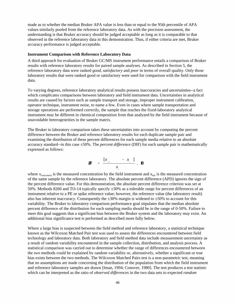
DIF �

[xinstrument

� xlab

]

xlab

� 100

46

made as to whether the median Bruker APA value is less than or equal to the 95th percentile of APAvalues similarly pooled from the reference laboratory data. As with the precision assessment, theunderstanding is that Bruker accuracy should be judged acceptable as long as it is comparable to thatobserved in the reference laboratory data in this demonstration. Thus, if either criteria are met, Brukeraccuracy performance is judged acceptable.

Instrument Comparison with Reference Laboratory Data

A third approach for evaluation of Bruker GC/MS instrument performance entails a comparison of Brukerresults with reference laboratory results for paired sample analyses. As described in Section 5, thereference laboratory data were ranked good, satisfactory and poor in terms of overall quality. Only thoselaboratory results that were ranked good or satisfactory were used for comparison with the field instrumentdata.

To varying degrees, reference laboratory analytical results possess inaccuracies and uncertainties--a factwhich complicates comparisons between laboratory and field instrument data. Uncertainties in analyticalresults are caused by factors such as sample transport and storage, improper instrument calibration,operator technique, instrument noise, to name a few. Even in cases where sample transportation andstorage operations are performed correctly, the sample that reaches the fixed-laboratory analyticalinstrument may be different in chemical composition from that analyzed by the field instrument because ofunavoidable heterogeneities in the sample matrix.

The Bruker to laboratory comparison takes these uncertainties into account by computing the percentdifference between the Bruker and reference laboratory results for each duplicate sample pair andexamining the distribution of these percent differences for each sample media relative to an absoluteaccuracy standard--in this case ±50%. The percent difference (DIF) for each sample pair is mathematicallyexpressed as follows:

where x is the measured concentration by the field instrument and x is the measured concentrationinstrument lab

of the same sample by the reference laboratory. The absolute percent difference (APD) ignores the sign ofthe percent difference value. For this demonstration, the absolute percent difference criterion was set at50%. Methods 8260 and TO-14 typically specify ±30% as a tolerable range for percent differences of aninstrument relative to a PE or spike reference value; however, the reference value (the laboratory result)also has inherent inaccuracy. Consequently the ±30% margin is widened to ±50% to account for thisvariability. The Bruker to laboratory comparison performance goal stipulates that the median absolutepercent difference of the distribution for each sampling media should be in the range of 0-50%. Failure tomeet this goal suggests that a significant bias between the Bruker system and the laboratory may exist. Anadditional bias significance test is performed as described more fully below.

Where a large bias is suspected between the field method and reference laboratory, a statistical techniqueknown as the Wilcoxon Matched Pair test was used to assess the differences encountered between fieldtechnology and laboratory data. Both laboratory and field method data include measurement uncertainty asa result of random variability encountered in the sample collection, distribution, and analysis process. Astatistical comparison was carried out to determine whether the range of differences encountered betweenthe two methods could be explained by random variability or, alternatively, whether a significant or truebias exists between the two methods. The Wilcoxon Matched Pairs test is a non-parametric test, meaningthat no assumptions are made concerning the distribution of the population from which the field instrumentand reference laboratory samples are drawn [Iman, 1994; Conover, 1980]. The test produces a test statisticwhich can be interpreted as the ratio of observed differences in the two data sets to expected random

47

differences in the same two data sets. Thus, in very general terms, a large test statistic indicates asignificant difference between two instruments or methods. The Wilcoxon test statistic is influenced to agreater extent by the larger values in the data sets being compared, particularly when the data span manyorders of magnitude such as encountered in this study. In order to eliminate this undesired effect, the datapairs were normalized by using the percent difference determination for each sample pair, as describedearlier. The percent difference computed for each Bruker measurement relative to the paired samplelaboratory value is compared against a reference percent difference value of zero in the statistical test.

The quantitative aspect of the Wilcoxon test is given by the p-value, or probability, associated with acomputed test statistic. For example, a test result with a p-value of 0.05 indicates that the probability of twoequivalent techniques producing the observed differences as a result of random variability alone would be0.05. By convention, a p-value of 0.05 is often used as the decision point as to whether a statisticallysignificant bias exists between the two sets of measurements. A p-value less than 0.05 is generallyunderstood to indicate differences between two methods that cannot be explained by random variationalone. On the other hand, p-values greater than 0.05, indicate that observed differences between twomethods can be explained by random variation alone and that the methods can be considered comparable.

The outcome of the Wilcoxon test is used to make a final decision as to whether one is justified in callingthe Bruker field measurements comparable or not comparable to reference laboratory measurement. AWilcoxon test result with a p-value less than 0.05 indicates that Bruker data are not comparable toreference laboratory data for a particular sampling medium.

In summary then, two criteria are used for assessing Bruker to laboratory accuracy. First a determination ismade as to whether the median absolute percent difference is in the range of 0-50%. If this criteria is notmet, the Wilcoxon test is performed on the data set to test the significance of the observed bias. If the testresult indicates significance, the overall Bruker to laboratory comparison goal is judged not met.Alternatively, if the test indicates no significance, the goal is judged to have been met.

Scatter Plots

Another way to evaluate the performance of the of the Bruker GC/MS with respect to the referencelaboratory is through the use of scatter plots. The plots are prepared in log-log format since the dataconcentrations generally spanned many orders of magnitude. Two solid lines are positioned on each graphwhich mark the ±50% difference about the zero bias line. As noted in earlier discussion, the ±50% marginsare chosen as an indicator of acceptable instrument performance relative to reference laboratory data. Thevalue is derived as follows: If the assumption is made that the uncertainty on field technology andlaboratory measurements is ±20%, then a worst case percent difference between two measurements ateither extremes of the ±20% range would be ±50%. As an example, consider a sample with a trueconcentration of a target analyte of 100 mg/L. The field method reports a value 20% high at 120 mg/L andthe laboratory reports the value 20% low at 80 mg/L. The percent difference between these two values is50%. Thus, the ±50% bias lines denote acceptable tolerances on field instrument comparisons to referencelaboratory data.

1

10

100

1000

1 10 100 1000

Lab Value

Fie

ld M

etho

d V

alue

1

10

100

1000

1 10 100 1000

Lab Value

Fie

ld M

etho

d V

alue

1

10

100

1000

1 10 100 1000

Lab Value

Fie

ld M

etho

d V

alue

1

10

100

1000

1 10 100 1000

Lab Value

Fie

ld M

etho

d V

alue

Correlation is a measure of the degree of linear relationship between two variables.8

48

(b) High correlation; positive bias

(d) Low correlation; positive bias

(a) High correlation; low bias

(c) Low correlation; low bias

Figure 6-1. Example scatter plots with simulated data. The four plots illustrate various degrees ofmeasurement correlation and method bias or accuracy. The reference laboratory value isplotted on the x-axis and the paired field technology value on the y-axis. The solid linesmark the ±50% interval about the zero bias line.

In some cases where the data span five or more orders of magnitude, two plots are used. The plots give thereader an indication of instrument bias and correlation relative to reference laboratory data. Here, bias is8

defined as a systematic difference of one method relative to another across a portion of or the entiremeasurement range of the instrument. Bias is directly related to accuracy. A method with low bias is onewith high accuracy. A method with a -10% bias is accurate to within 10%. As an example, Figure 6-1shows four sets of simulated data with various amounts of bias and random “noise” added. The zero biasline, not shown in the plots, extends from the lower left to the upper right corners of each plot. Thesefindings are based on the assumption that any bias is a constant fraction of the actual value of the result,and that instrument performance is linear over several orders of magnitude.

Data with low bias and high correlation are shown in Figure 6-1a. The data are closely clustered betweenthe ±50% lines near the zero bias line. A low bias and low correlation example is shown in Figure 6-1c.Most of the data fall within the ±50% lines; however, the scatter is larger than that observed in Figure 6-1a.

The specific accuracy evaluation procedure is as follows:9

� Pool all the Bruker PE and spike sample analytical results, in terms of absolute percent accuracy, for eachsample medium for which a reference value is known. Data from SRS and WAFB are combined in thisanalysis. All sample data are excluded whose reference values are less than 2�PQL .Bruker

� Compile these data into a frequency histogram and compute the median (APA ) , 80th percentile.5 Bruker

(APA ) , and 95th percentile (APA ) values. .8 Bruker .95 Bruker

� Do the same compilations for the reference laboratory data combined from both demonstration sites bysampling media.

� Apply the following assessment criteria to the absolute percent accuracy distributions:

49

Positive bias is illustrated in Figures 6-1b and 6-1d for high and low correlation data, respectively. In eachcase, the data are grouped about a line that is shifted well above the zero bias line. As in the otherexamples, the degree of data scatter is greater for the low correlation case.

Histograms

A final means to evaluate performance is accomplished by computing the percent difference between thefield and laboratory value for each paired sample analysis and pooling these data across all compounds bysample medium. These percent difference computations were then tabulated into frequency histograms,examples of which are shown in Figure 6-2. The histogram gives the frequency of occurrence as a functionof the percent difference interval and enables a visual evaluation of the field technology data whencompared with reference laboratory data. As an example, in Figure 6-2a, nearly all the percent differencecomputations fall within the ±30% interval, indicating relatively good data correlation. The center of massof the histogram falls near zero, indicating an average bias near zero. A low correlation, low bias exampleis shown in Figure 6-2c. In this example, 12 of the 42 total observations fall outside the ±30% range.Although the overall average percent difference falls near zero, the width of the distribution revealsdiminished instrument correlation. Figures 6-2a and 6-2c illustrate the same type of data shown in scatterplot format in Figures 6-1a and 6-1c, respectively. Positive bias examples with high and low correlation areillustrated in Figure 6-2b and 6-2d, respectively. In these examples, the center of mass of the histogramfalls at a point other than zero, thereby revealing an overall measurement bias. Figures 6-2b and 6-2dillustrate the same type of data shown in the scatter plots in Figures 6-1b and 6-1d, respectively.

Summary of Instrument Performance Goals

The original instrument performance claims, although relevant to the objectives of the demonstration, weredetermined to be somewhat vague following compilation and evaluation of all demonstration data. Forexample, should all measurements fall within ±35% of reference laboratory results or should the averageresults for a particular sample medium meet the 35% criterion? To maintain objectivity in the process ofinstrument evaluation, instrument performance goals were modified and restated in such a manner that asimple yes are no answer describes whether the goals were met. A summary description of the performancegoals, developed in the preceding paragraphs, and how data are evaluated in the context of those goals ispresented below.

Accuracy

Two goals are stated. If the first goal is met, no evaluation is done relative to the second.

Accuracy Goal 1: Median Bruker absolute percent accuracy for each sampling medium is in therange of 0-35%.

Accuracy Goal 2: Median Bruker absolute percent accuracy for each sampling medium is lessthan or equal to the 95th percentile of the pooled reference laboratory absolute percent accuracyfor each sampling medium .9

Percent Dif ference Interval

No

of o

bs0

1

2

3

4

5

6

7

8

-30 -20 -10 0 10 20 30 40 50 60 70 80 90 100


No

of o

bs

0

1

2

3

4

5

6

7

8

9

10

11

12

13

-70 -60 -50 -40 -30 -20 -10 0 10 20 30 40 50Percent Dif ference Interval

No

of o

bs

0

1

2

3

4

5

6

7

8

9

10

11

12

13

-30 -20 -10 0 10 20 30 40 50 60 70 80 90


No

of o

bs

0

1

2

3

4

5

6

7

8

-70 -60 -50 -40 -30 -20 -10 0 10 20 30 40 50 60

(1) If (APA ) �35%: Accuracy Goal 1 Met -- Bruker accuracy performance is better than or.5 Bruker

equal to that specified in Methods 8260 and TO-14.(2) If Bruker (APA ) � (APA ) : Accuracy Goal 2 Met -- Bruker performs comparably to.5 Bruker .95 Lab

conventional laboratory using accepted analytical methodologies.(3) If (APA ) > (APA ) Accuracy Goal 2 Not Met -- Bruker data does not compare with the.5 Bruker .95 Lab:

reference laboratory data.

50

(d) Low correlation; positive bias

(a) High correlation; low bias (b) High correlation; positive bias

(c) Low correlation; low bias

Figure 6-2. Example histograms with simulated data. Various combinations of measurement correlation andbias are shown.

Precision

In a similar manner as described for accuracy evaluation, two precision goals are stated. If the first goal ismet, no evaluation is done relative to the second.

Precision Goal 1: Median Bruker relative percent difference for each sampling medium is in therange of 0-30% for water and soil gas samples and 0-35% range for soil samples.

The specific precision evaluation procedure is as follows:10

� Pool all the Bruker duplicate sample results, in terms of relative percent difference (RPD) for each samplemedium (soil, water, and gas) for which a reference value is known. Data from SRS and WAFB arecombined in this analysis. All sample data are excluded whose reference values are less than 2�PQL .Bruker

� Compile these data into a frequency histogram and compute the median (RPD ) , 80th percentile.5 Bruker

(RPD ) , and 95th percentile (RPD ) values. .8 Bruker .95 Bruker

� Do the same compilations for the reference laboratory data combined from both demonstration sites bysampling media.

� Apply the following assessment criteria to the absolute percent accuracy distributions:(1) If (RPD ) � 30% (water and soil gas), 35% (soil): Precision Goal 1 Met -- Bruker precision.5 Bruker

performance within the range identified in original developer claims and is very near that specified inMethods 8260 and TO-14.

(2) If Bruker (RPD ) � (RPD ) : Precision Goal 2 Met -- Bruker performs comparably to.5 Bruker .95 Lab

conventional laboratory using accepted analytical methodologies.(3) If (RPD ) > (RPD ) :Precision Goal 2 Not Met -- Bruker precision performance is worse.5 Bruker .95 Lab

than that reported by reference laboratories despite considerable allowance given for field variability.

The specific Bruker to laboratory evaluation procedure is as follows:11

� Compute the percent difference and the absolute percent difference for each set of Bruker-laboratory pairedsample results.

� Compile the percent difference and absolute percent difference data into frequency histograms and computethe median (APD ) , 80th percentile (APD ) , and 95th percentile (APD ) values for.5 Bruker-Lab .8 Bruker-Lab .95 Bruker-Lab

each distribution.� Apply the following assessment criteria to the compiled absolute percent differences:

(1) If (APD ) � 50%: Comparison Goal 1 Met -- Bruker results are consistently within ±50%.5 Bruker-Lab

of reference laboratory results.(2) If (APD ) > 50%: Proceed to Step (3) for further evaluation..5 Bruker-Lab

(3) Perform Wilcoxon test to determine if the observed bias is statistically significant. The percentdifference values (not absolute percent difference values since the sign of the difference is necessaryinformation in the Wilcoxon Test) are compared to a value of zero percent difference.

(a) If p-value for the test > 0.05: Comparison Goal 2 Met(b) If p-value for the test < 0.05: Comparison Goal 2 Not Met

51

Precision Goal 2: Median Bruker relative percent difference for each sampling medium is lessthan or equal to the 95th percentile of the pooled reference laboratory relative percent differencesfor each sampling medium .10

Bruker to Reference Laboratory Comparison

Two goals are stated. If the first goal is met, no evaluation is done relative to the second.

Comparison Goal 1: Median absolute percent difference is in the range of 0-50%.

Comparison Goal 2: If Goal 1 not met, the Wilcoxon test result between Bruker and referencelaboratory data should indicate no significant bias (p > 0.05) .11

Field Operation Observations

SRS Demonstration

The SRS demonstration consisted of three days of sample analysis by the Bruker analytical team.Following pre-demonstration calibration, the instrument was shipped to the USA from Germany by airfreight with no degradation of instrument performance noted following its transport. The instrument was

52

installed in a small air conditioned van and driven to the demonstration site. The instrument was operatedfrom batteries and was also set up for operation during transit from the hotel to the measurement site, atime-saving feature of interest in these field investigations. The Bruker GC/MS was also operated for someportion of the time under ambient air temperatures during the hot afternoons to demonstrate its fieldversatility. Typical temperatures during the SRS demonstration are shown in Figure 6-3.

On the first day of the demonstration, each developer was provided soil gas samples for analysis. EighteenGC/MS runs, that included blanks, calibration checks and field samples were completed and data reportswere submitted for 16 of these. Two runs were not submitted because power supply problems affected theinstruments’ performance.

The second day at SRS was dedicated to water analysis. Fifteen blank, calibration and sample runs werecompleted and data reports were submitted for all runs.

The third day was devoted to soil analysis. Eight runs were completed and data reports were submitted forall runs completed. The Bruker analytical team did their soil analysis using headspace vapor measurementsand had calibrated the system using 10 mL vials.

The Bruker team included internal standards in most of their analyses. In nearly all cases, recovery of thesecompounds was good. However, in some cases, significant changes were noted in the surrogatecompounds in water samples. Since much of the sample preparation was done under the changing ambientconditions, the Bruker analysts suspected that the high ambient temperature influenced sample preparationor storage stability. Sample run times were on the order of 12 minutes for all media.

WAFB Demonstration

Analysis at WAFB proceeded much like that at SRS, with soil gas analysis done on the first day, wateranalysis on the second, and soil analysis on the third. Typical temperatures encountered during the WAFBdemonstration are shown in Figure 6-4. Fifteen soil gas runs, including calibration checks, blank analyses,and field sample analyses, were completed on the first day of the demonstration. An instrument breakdownwas noted during one run. The problem was resolved and the instrument was brought back on-line in about60 minutes. Blank soil gas sample analyses results for target analytes were less than 10 ppb.

A total of 17 water sample analysis runs were completed on the second day of the WAFB demonstration.Power problems were encountered during one run which were related to the fact that input voltage to theinstrument exceeded the 28 volt maximum for which the instrument was configured. This caused someshifts in calibration data; however, the data were still usable from the run. Blank water sample analysesproduced results for the target analytes in the range of 0.1 to 8 �g/L.

Eighteen runs were completed on the third day of the demonstration which was devoted to soil sampleanalysis. Blank soil sample analyses produced results of about 50 �g/kg for the target analytes. The Brukeranalysts noted more scatter in the soil analysis results for their internal standards and suspected that to betrue for the target analytes as well.

40

45

50

55

60

65

70

75

80

06:00 AM 08:00 AM 10:00 AM 12:00 PM 02:00 PM 04:00 PM 06:00 PM

Time of Day

09/11/95

09/13/95

53

Figure 6-3. Plot of dail y temperatures durin g the SRS demonstration. Note that two data pointsare missin g from Jul y 20, 1995.

Figure 6-4. Plot of daily temperatures during the WAFB demonstration.

54

Bruker Accuracy and Precision Results

Bruker Accuracy -- SRS Demonstration

As discussed in Sections 4 and 5, SRS is predominately contaminated with the chlorinated solvents TCEand PCE. Consequently, all of the Bruker GC/MS data and corresponding laboratory data are limited tothese two contaminants. Recovery data for the Bruker GC/MS system for SRS spike and PE samples forwater and soil gas are presented in Table 6-1. Data from reference values lower than the Bruker PQL arenot shown in the table.

Table 6-1. Bruker Recoveries at SRS.

Sampling Medium / Description Percent Recovery

TCE PCE

Water Medium Spike 102 64

Water High Spike 145 71

Water PE No. 2 78 152

Soil Gas Low Spike 134 195

Soil Gas Medium Spike 52 80

Soil Gas High Spike 36 44

Soil Gas PE No. 1 127 265

Soil Gas PE No. 2 78 51

Because of significant deviations from the demonstration plan, discussed earlier in Section 4, no data areavailable for assessment of Bruker instrument accuracy on soil samples at SRS.

Percent recoveries for the water spike and PE samples are provided in Table 6-1. Five of the six data pointsare in the 50-150% range. A recovery value of 145% was obtained for the high TCE spike. The percentrecoveries from the reference laboratories for this sample showed similar high recovery results leading toquestions about the validity of the reported reference value for this particular sample. The other high valueof 152% was for PCE in a PE sample at a relatively low level of 30 �g/L.

Recoveries for soil gas measurements are also shown in Table 6-1. The level of confidence in the referencevalues for the soil gas spike samples is high since they were drawn from gas cylinders with accompanyingcertificates of analysis. The low spike recoveries are shown since the TCE and PCE content of this samplewas above the reported PQL of the Bruker instrument. Recoveries generally fall into two categories: theyare high (>100%) for low level spikes and low (<100%) for high level spikes and nearly all the reportedvalues fall outside the 70-130% recovery range. These data suggest questionable accuracy performance forthe Bruker system during the SRS demonstration.

Bruker Accuracy -- WAFB Demonstration

The sampling media at the WAFB demonstration site are contaminated with a wide range of VOCsincluding petroleum hydrocarbons and chlorinated solvents. Approximately fifteen different VOCs wereanalyzed by both the reference laboratories and the field technologies, though several of these compoundswere found in only trace amounts in the different media. To most efficiently evaluate the Bruker GC/MS, asubset of analytes was chosen for accuracy and precision evaluation using the spike and PE samples. Thesubset included benzene, toluene, ethylbenzene, and xylenes, as well as TCE and PCE. Unless otherwisenoted, ethylbenzene is grouped with xylenes in the total xylenes category. Recovery data for the WAFB

The Bruker recovery for the lowest soil gas spike sample is shown in Table 6-2 since it is above the reported12

Bruker PQL. Initially, the computed Bruker recoveries for this particular sample were consistently high by afactor of ten for all target analytes. Results similar to those from Bruker were obtained by other participants,suggesting an error in the reference sample preparation. A review of the laboratory and field data and log booksstrongly suggest that a factor of ten error occurred in the reference sample concentration computation. Thereference values were changed accordingly and the reported Bruker recovery data are based on the correctedvalues.

55

demonstration from Bruker GC/MS analysis of PE and spike samples is presented for soil, water, and soilgas samples in Table 6-2.

Two soil PE samples were available for accuracy determinations. These samples were laboratory-preparedin sealed ampules and were judged to be reliable standards. Bruker GC/MS recoveries for the five targetcompounds fall in the range of 90 to 190%. Computed recoveries from spike and PE water samples, alsoshown in Table 6-2, are consistently above 100%, and fall in the range of 112 to 177%. The recoveryresults are similar for all target analytes and indicate no obvious instrument response changes across therange of target compounds.

Soil gas sample recoveries shown in Table 6-2 are all in the range of 60-108% and, in contrast to the SRSrecovery data, reveal good accuracy performance during the WAFB demonstration .12

Table 6-2. Bruker Recoveries at Wurtsmith.

Sampling Medium/DescriptionPercent Recovery

TCE PCE Benzene Toluene TotalXylenes

Soil PE No. 1 190 143 153 93 101

Soil PE No. 2 174 133 152 134 94

Water Low Spike 153 123 119 142 160

Water Medium Spike 140 112 152 177 145

Water High Spike 132 132 130 156 161

Water PE No. 1 ND ND ND ND ND

Water PE No. 2 128 136 131 134 144

Soil Gas Low Spike 72 91 79 89 83

Soil Gas Medium Spike 108 ND 87 ND 104

Soil Gas High Spike 82 ND 62 ND 99

Notes: ND = Not detected, compound not present in spike; no recovery data available.See Tables 5-7 and 5-11 for approximate target analyte concentrations in the various PE/Spike samples.

Overall Bruker Accuracy Performance

The absolute percent accuracy values from both sites were compiled for the target analytes by samplingmedia and are shown as histograms in Figures 6-5, 6-6 and 6-7 for soil, water, and soil gas, respectively.For soil, most of the values are scattered in the 0-90% range with no clear clustering of results. For water,most of the values fall in the 0-70% range. The soil gas accuracy data generally fall in the 0-70% range.

Bruker Soil Accurac y

Absolute Percent Accurac y Interval

No

of o

bs

0

1

2

3

0 10 20 30 40 50 60 70 80 90 100

Bruker Water Accurac y


No

of o

bs

0

1

2

3

4

0 10 20 30 40 50 60 70 80 90 100

Bruker Soil Gas Accurac y


No

of o

bs

0

1

2

3

4

5

0 20 40 60 80 100 120 140 160 180 200

56

Figure 6-5. Absolute percent accuracy histogram for Brukersoil samples. The number of observations areshown on the y-axis.

Figure 6-6. Absolute percent accuracy histogram for Brukerwater samples.

Figure 6-7. Absolute percent accuracy histogram for Brukersoil gas samples.

57

Summary data from the absolute percent accuracy distributions are shown in Table 6-3 for all media. Ingeneral, the lower the number the better the performance. For example, the median absolute percentaccuracy was 22% for the pooled reference laboratory soil data. The laboratory’s 95th percentile value is47%. In comparison, the Bruker median absolute percent accuracy for soil samples was 39% and less thanthe 95th percentile value for the reference laboratories.

Table 6-3. Bruker and Reference Laboratory Accuracy Summary.

Data Set/Media Type n Absolute Percent Accuracyx x x.5 .8 .95

Ref. Lab - Soil 10 22 36 47

Bruker - Soil 10 39 57 83

Ref. Lab - Water 30 19 27 116

Bruker - Water 26 36 52 61

Ref. Lab - Soil Gas 24 20 47 66

Bruker - Soil Gas 21 22 49 95

Note: x = 50th percentile (median); x = 80th percentile; x = 95th percentile.5 .8 .95

Assessment of Bruker performance in terms of the accuracy goals stated previously results in the followingdeterminations:

Soil: (APA ) > 35%: Accuracy Goal 1 Not Met.5 Bruker-Soil

(APA ) � (APA ) : Accuracy Goal 2 Met.5 Bruker-Soil .95 Lab-Soil

Water: (APA ) > 35%: Accuracy Goal 1 Not Met.5 Bruker-Water

(APA ) � (APA ) : Accuracy Goal 2 Met.5 Bruker-Water .95 Lab-Water

Soil Gas: (APA ) < 35%: Accuracy Goal 1 Met .5 Bruker-Gas

Bruker accuracy performance is acceptable in terms of established performance goals for all media. Themost stringent performance goals for accuracy were not met for soil and water; however, median Brukerperformance was as good as or better than reference laboratory results from similar analyses. Soil gasaccuracy performance was better than the most restrictive goal of 35% absolute percent accuracy.

Bruker Precision -- SRS Demonstration

Bruker GC/MS RPD values from the SRS demonstration are presented in Table 6-4 and are based on theresults of duplicate field sample analysis. No precision determination was done on SRS soil sample data asdiscussed previously.

Relative percent differences for water samples, shown in Table 6-4, are from split water samples. Thecalculated RPD values range from 5-38%. Low concentration samples near the Bruker PQL exhibit thesame level of precision as higher concentration samples.

Soil gas duplicate samples were actually gas samples drawn sequentially from each well within a timeinterval of about 2 minutes. The degree of chemical equivalence of these sequential samples could not bedetermined since a real-time measure of soil gas species was not made at the wellhead when the

58

Table 6-4. Bruker Precision for SRS Demonstration.

Sampling Media / Description Relative Percent Difference

TCE PCE

Water Low Sample 34 38

Water Medium Sample 37 29

Water High Sample 24 24

Soil Gas Low Sample 22 25

Soil Gas Medium Sample 5 10

Soil Gas High Sample 10 14

Table 6-5. Bruker Precision for Wurtsmith Demonstration.

Sampling Medium / Description Relative Percent Difference

TCE PCE Benzene Toluene TotalXylenes

Soil Low Sample ND ND ND ND ND

Soil Medium Sample ND ND ND ND 12

Soil High Sample 14 ND 21 12 8

Water Low Sample 5 5 10 27 8

Water Medium Sample 47 21 12 9 8

Water High Sample 120 99 15 119 21

Soil Gas Low Sample 29 ND 26 43 52

Soil Gas Medium Sample 6 ND 7 <1 10

Soil Gas High Sample 108 ND 17 46 11Notes: ND = not detected; Analyte was either below detection or not present in the sample.

sequential samples were collected. In this analysis, a worst case precision determination was carried out byassuming that the sequential samples were chemically equivalent. The RPD values for the low, medium,and high vapor samples, provided in Table 6-4, are less than 25%. These data are indicative of goodBruker precision performance.

Bruker Precision -- WAFB Demonstration

The Bruker precision data for the WAFB demonstration are presented in Table 6-5. The tabulated RPDvalues are based on the analysis of a number of duplicate samples for each media.

For soil sample analyses, Bruker reported a number of results that were below its PQL of 50 mg/kg.Precision analysis was performed using only those concentrations that were greater than the PQL. Theresults are shown in Table 6-5.

The low, medium, and high concentration water samples collected at WAFB generally contained only lowconcentrations of the target analytes (Table 5-9). The RPDs in Table 6-5 are attributed to the fact that theBruker GC/MS was operating at or very near its PQL. The Bruker operator was told to expect samples thatwould have analyte concentrations in predetermined ranges, therefore, he performed dilutions based on theexpectations. This caused the operator to perform dilutions on low concentration samples, which may haveimpacted the precision of the measurement.

As noted earlier in the discussion of SRS demonstration results, the duplicate soil gas samples wereactually samples drawn sequentially from different levels of the well. The assumption is made that thesequential samples are chemically equivalent. Thus, the RPD value represents a worst-case estimate of

59

Bruker GC/MS precision since some of the variability encountered in the analysis result may in fact beattributable to variation between two sequential samples. The data in Table 6-5 must be interpreted in lightof the target analyte concentrations provided previously in Table 5-13. For example, the referencelaboratory reported non-detectable levels of TCE and PCE in all the soil gas samples (low, medium, andhigh). The Bruker system was able to detect TCE in the samples; however, the levels are near the PQL ofthe system where precision is not expected to be as good. Taking these considerations into account, theoverall Bruker precision for soil gas analyses is satisfactory.

Overall Bruker Precision Performance

The relative percent differences for both sites were compiled by sample media and are shown ashistograms in Figures 6-8, 6-9 and 6-10 for soil, water, and soil gas, respectively. For soil, most of theRPD values fall in the 0-25% range. For water and soil gas, nearly all reported values fall in the 0-50%range.

Summary data from the relative percent difference distributions are shown in Table 6-6 for the threesampling media.

Bruker performance with respect to precision goals are as follows:

Soil: (RPD ) < 35%: Precision Goal 1 Met.5 Bruker-Soil

Water: (RPD ) < 30%: Precision Goal 1 Met.5 Bruker-Water

Soil Gas: (RPD ) < 30%: Precision Goal 1 Met.5 Bruker-Gas

Bruker precision performance, relative to these performance goals, is judged acceptable for soil, water, andsoil gas analyses.

Bruker to Reference Laboratory Data Comparison

As discussed earlier in this section, comparisons of the Bruker GC/MS analytical data with the referencelaboratory analytical data for water, soil, and soil gas samples are presented in a number of formats thatinclude log-log scatter plots, percent difference histograms, and formal performance assessment in light ofestablished goals. All reported values that were less than two times the Bruker GC/MS PQL, althoughplotted, are not included in any of the statistical analyses. Analytical results from only one of the duplicateor triplicate sample set is included in the statistical analyses since their inclusion would violaterequirements for a random sample.

Bruker Soil Precision

Relative Percent Difference Interval

0

1

2

3

4

0 5 10 15 20 25 30

Bruker Water Precision


0

1

2

3

4

5

6

7

0 20 40 60 80 100 120 140

Bruker Soil Gas Precision


0

1

2

3

4

5

6

7

8

0 10 20 30 40 50 60 70 80 90 100 110 120

60

Figure 6-8. Relative percent difference histogram for Brukersoil samples.

Figure 6-9. Relative percent difference histogram for Brukerwater samples.

Figure 6-10. Relative percent difference histogram for Brukersoil gas samples.

61

Table 6-6. Bruker and Reference Laborator y Precision Summar y.Data Set/Media Type n Relative percent difference

x.5 x.8 x.95

Ref. Lab Soil 13 8 13 58

Bruker Soil 5 12 15 20

Ref. Lab Water 14 5 10 22

Bruker Water 21 24 38 119

Ref. Lab Soil Gas 17 7 20 68

Bruker Soil Gas 18 16 37 60

Note: x = 50th percentile (median); x = 80th percentile; x = 95th percentile.5 .8 .95

Scatter Plots/Histograms -- SRS Demonstration

Target analytes at this site were limited to TCE and PCE. The GEL water data are used as the referencedata set. The on-site SRS laboratory soil gas data were judged to be an acceptable reference data set.

Plots of Bruker GC/MS water analysis results for TCE and PCE are given versus the laboratory referencedata in Figure 6-11 and Figure 6-12 for low (1-100 �g/L) and high (0.1-100 mg/L) concentration ranges,respectively. All but six of the 21 points fall within the ±50% interval about the zero bias line on both thelow and high concentration plots.

The distribution of percent difference values is shown as a histogram in Figure 6-13. Differences rangefrom a low of -60 % to a high of 80%.

A plot of the Bruker soil gas data for TCE and PCE relative to the SRS reference laboratory data areshown in Figure 6-14. Half of the data points fall either above or below the 50% bias lines. Theaccompanying histogram, shown in Figure 6-15, reveals no obvious positive or negative data bias.

Scatter Plots/Histograms -- WAFB Demonstration

As discussed in Section 5, the Traverse laboratory data were given a good ranking for soil sample analysesand a good ranking for water sample analyses. These data are used as reference data for comparison withBruker GC/MS results. The Pace laboratory data were given a satisfactory ranking for soil gas sampleanalyses and are used as the reference data set for the soil gas measurements.

Considerably more compounds were detected in the various samples at Wurtsmith AFB than at theSavannah River Site. For the Wurtsmith demonstration, all target analytes have been combined in the plotsand statistical analysis. However, duplicate samples are not included in the statistical analysis.

A plot of Bruker data versus Traverse data for all soil analyses is presented in Figure 6-16. Elevenobservations fall outside the ±50% margins and 8 fall inside. In general, the Bruker measurements are highwith respect to the laboratory data. The percent difference histogram, shown in Figure 6-17, shows nearlyall observations on the positive bias side with a significant number in the 120-200% range.

Bruker vs. Laboratory - SRS Water (Low)

1

10

100

1 10 100

Laboratory Value, µg/L

Bruker vs. Laboratory - SRS Water (High)

1

0.1

10

100

0.1 1 10 100

Laboratory Value, mg/L

62

Figure 6-11. Bruker vs. Laboratory data for SRS low concentration watersamples. The solid lines show the ±50% range about a zero-bias(dashed) line.

Figure 6-12. Bruker vs. Laboratory data for SRS high concentration watersamples. The solid lines show the ±50% range about a zero-bias(dashed) line.

Bruker vs. Laborator y - SRS Water

Percent Difference Interval

No

of o

bs

0

1

2

3

-80 -70 -60 -50 -40 -30 -20 -10 0 10 20 30 40 50 60 70 80 90 100

Bruker vs. Laboratory - SRS Soil Gas

0.01

0.1

1

10

100

1000

10000

0.01 0.1 1 10 100 1000 10000

Laboratory Value, ppm

Bruker vs. Laborator y - SRS Soil Gas


No

of o

bs

0

1

2

3

4

5

-150 -100 -50 0 50 100 150 200 250 300 350 400 450

63

Figure 6-13. Percent difference histo gram for SRS watersamples.

Figure 6-14. Bruker vs. Laborator y data for SRS soil gas sam ples

Figure 6-15. Percent difference histogram for SRS soil gassamples.

Bruker vs. Laboratory - WAFB Soil

10

100

1000

1 10 100 1000

Laboratory Value, mg/kg

Bruker vs. Laborator y - WAFB Soil


No

of o

bs

0

1

2

-80 -60 -40 -20 0 20 40 60 80 100 120 140 160 180 200 220 240 260

64

Figure 6-16. Bruker vs. Laboratory data for WAFB soil samples.

Figure 6-17. Relative percent difference histogram for WAFBsoil samples.

Plots of Bruker data versus Traverse data for all water analyses are presented in Figures 6-18 and 6-19 forthe low (�g/L) and high (mg/L) ranges, respectively. Most Bruker values fall within the ±50% margins onthe low concentration plot. In the high concentration plot, 6 observations fall on the high side of the 50%margin and 11 fall inside the margins. The percent difference histogram for the combined data, shown inFigure 6-20, reveals most values in the -20 to 100% range.

A plot of Bruker GC/MS data versus Traverse data for all WAFB soil gas analyses is presented in Figure6-21. Most of the observations fall inside the ±50% margin lines on the plot, revealing relatively goodagreement with the reference laboratory. The histogram, shown in Figure 6-22, shows most observationsfalling in the 0 to -50% range.

Bruker vs. Laboratory - WAFB Water (Low)

1

10

100

1000

1 10 100 1000

Laboratory Value, µg/L

Bruker vs. Laboratory - WAFB Water (High)

1

10

100

1000

1 10 100 1000

Laboratory Value, mg/L

65

Figure 6-18. Bruker vs. Laborator y data for WAFB low concentration watersamples.

Figure 6-19. Bruker vs. Laboratory data for WAFB high concentration watersamples.

Bruker vs. Laborator y - WAFB Water


No

of o

bs0

2

4

6

8

10

12

14

16

-100 -80 -60 -40 -20 0 20 40 60 80 100 120 140 160 180 200

Bruker vs. Laboratory - WAFB Soil Gas


No

of o

bs

0

2

4

6

8

10

12

14

16

18

20

22

-100 0 100 200 300 400 500 600 700

66

Figure 6-20. Relative percent difference histogram for WAFBwater samples.

Figure 6-21. Bruker vs. Laboratory data for WAFB soil gassamples.

Figure 6-22. Relative percent difference histogram for WAFBsoil gas samples.

Bruker vs. Laboratory - Soil

Absolute Percent Difference Interval

0

1

2

3

4

-20 0 20 40 60 80 100 120 140 160 180 200 220 240

67

Figure 6-23. Absolute percent difference histogram for soilsamples. Data are from WAFB demonstrationonly.

Overall Bruker to Laboratory Comparison Results

Absolute percent differences from both sites were compiled by sampling media and are shown ashistograms in Figures 6-23, 6-24 and 6-25 for soil, water, and soil gas, respectively. For soil, absolutepercent differences occur with equal frequency across the 0 to 200% range. Water results are similar withapproximately equal distribution across the 0 to 100% range. As noted earlier, soil gas differencesgenerally fall in the 0-50% range.

Summary data from the three absolute percent difference distributions for the three sampled media areshown in Table 6-7.

Table 6-7. Bruker-Laboratory Comparison Summary.

Media Type n Absolute Percent Difference

x x x.5 .8 .95

Soil 17 72 159 186

Water 71 39 72 95

Soil Gas 49 40 73 275Note: x = 50th percentile (median); x = 80th percentile; x = 95th percentile.5 .8 .95

Bruker performance assessment in terms of the comparison goals result in the following determinations:

Soil: (APD ) > 50%: Comparison Goal 1 Not Met.5 Bruker-Lab

Wilcoxon test result: p < 0.05: Comparison Goal 2 Not Met

Water: (APD ) < 50%: Comparison Goal 1 Met.5 Bruker-Lab

Soil Gas: (APD ) < 50%: Comparison Goal 1 Met .5 Bruker-Lab

Overall comparison results, in light of established performance goals, indicate that the first goal was metfor water and soil gas media. However, the Bruker to laboratory comparison did not meet either the first orsecond comparison goal for soil. The Wilcoxon test results point to the presence of a significant positivebias of the Bruker data relative to that of the laboratory.

Bruker vs. Laborator y - Water, All Sites


No

of o

bs

0

1

2

3

4

5

6

7

8

9

10

11

12

13

-10 0 10 20 30 40 50 60 70 80 90 100 110 120 130 140

Bruker vs. Laborator y - Soil Gas, All Sites


No

of o

bs

0

5

10

15

20

25

30

35

0 50 100 150 200 250 300 350 400 450 500 550 600 650

68

Figure 6-24. Absolute percent difference histogram for watersamples.

Figure 6-25. Absolute percent difference histogram for gassamples.

Summary of Bruker Accuracy, Precision, and Laboratory Comparison Performance

A summary of Bruker GC/MS performance for both demonstration sites is given in Table 6-8. The resultsof the foregoing evaluation are summarized with respect to accuracy, precision, and comparison of Brukerand reference laboratory data. The summary information in the table shows that the Bruker GC/MS metperformance goals in eight of the nine evaluation categories. Precision was judged acceptable for soilanalyses; however, only a very limited sample size (n=5) was available for evaluation. Accuracy of soilanalyses also met established goals. Accuracy, precision, and the Bruker to reference laboratorycomparison goals were also met for water analyses. For additional insight and evaluation, the data qualityrankings of the reference laboratories are given in the table as well. Traverse received a good data qualityranking for soil analyses. The Wilcoxon test result for the soil media indicates that the observed differencebetween Bruker and reference laboratory data cannot be explained by random variation alone and it islikely that some other factor was causing the Bruker data to be high relative to the laboratory data. PossibleBruker or laboratory factors could be a calibration, sample handling, or injection error by either Bruker orthe reference laboratory. For example, the Traverse results on the soil PE samples were consistently low,whereas the Bruker results were much closer to the reference values.

69

Figure 6-26. Bruker GC/MS reconstructed chromatogram of target analytes ina WAFB water sample.

Table 6-8. Summary Performance of the Bruker GC/MS.

Sample Accuracy via Precision via Bruker-Lab Data Reference LabMedium PE/Spike Samples Duplicate Analyses Comparison Data Quality

1 2

3

Soil Goal Met Goal Met Goal Not Met SRS: UndeterminedWAFB: Good

Water Goal Met Goal Met Goal Met SRS: GoodWAFB: Good

Soil Gas Goal Met Goal Met Goal Met SRS: SatisfactoryWAFB: Satisfactory

Other Bruker GC/MS Performance Indicators

Target Compound Identification in Complex Mixtures

The ability of the instrument to identify a broad range of compounds in complex mixtures was also amplydemonstrated with many of the WAFB samples. An example of a Bruker reconstructed ion chromatogramfor a selection of target compounds in a water sample containing numerous volatile organic compounds isshown in Figure 6-26. A listing of the identified target compounds, corresponding to the peak numbersshown in Figure 6-26, is presented in Table 6-9. An on-site computerized library search of Bruker GC/MSanalysis results from a similar WAFB water sample produced over 100 tentatively identified compoundsrevealing the complex nature of this particular water matrix.

Field Handling and Operation

The Bruker GC/MS is designed to be shipped to the field and is shock mounted for durability in handlingand field use. Prior to the WAFB demonstration, the system was transported by air freight from Germanyto the USA. The ruggedized design contributed to stable instrument calibrations over the duration of eachdemonstration, despite several days of travel on dirt roads during the course of the demonstration. At eachsite, the system was operated for several days in a row, typically 8-10 hours per day. The instrument was

70

Table 6-9. Identified Target Compounds from a Wurtsmith Water Sample Analysis.

Peak No. Compound

1 Ethene, 1,1-dichloro-2 Methylene chloride3 Ethene, 1,2-dichloro-, trans4 Ethene, 1,2-dichloro-, cis5 Chloroform6 Methane, dibromofluoro-7 Benzene, pentafluoro-8 Ethane, 1,2-dichloro-9 Ethane, 1,1,1-trichloro-10 Benzene11 Benzene,1,4-difluoro-12 Trichloroethene13 Methyl isobutyl ketone14 Toluene-d815 Toluene16 Tetrachloroethene17 Benzene-d5-,chloro-18 Benzene, chloro-19 Ethylbenzene / m-Xylene20 p-Xylene21 Styrene22 o-Xylene23 p-Bromofluorobenzene24 Benzene-d4, 1,4-dichloro25 Benzene,1,2(1,3)-dichloro26 Benzene,1,4-dichloro27 Naphthalene

Note: The peak numbers refer to those given in Figure 6-26.

exposed to ambient temperatures ranging from 40� to 95�F. During both demonstrations, the instrumentoperated properly and without significant breakdowns or mechanical problems.

System set-up was simple and uncomplicated. Set-up procedures involved connecting the ancillaryequipment and checking the instrument calibration. Sample analysis time varied according to the samplemedia and the mode of injection; however, a typical time interval was on the order of 12 minutes persample. Hard copy data were available at the end of each run.

Overall Bruker GC/MS Performance Conclusions

The Bruker GC/MS system was tested at two locations during this technology demonstration in order toevaluate its capabilities and performance during on-site analysis of VOC contaminated soil, water and soilgas samples. The objectives of the demonstration were: (1) to evaluate instrument performance; (2) todetermine how well each field instrument performed compared to reference laboratory data; (3) to evaluateinstrument performance on different sample media; (4) to evaluate adverse environmental effects oninstrument performance; and, (5) to determine logistical needs and field analysis costs. The systemperformance goals are summarized in Table 6-10 along with an assessment, based on the data produced inthis demonstration, as to whether these goals were met.

As shown in Table 6-10, Bruker GC/MS performance goals were met with two exceptions. Instrumentperformance in terms of accuracy, precision, and comparison with reference laboratory data met

71

established performance goals for water and soil gas analyses. The comparison of the Bruker data to thelaboratory data was below established goals for soil analyses. Performance goals related to datacompleteness and data availability were met. The initial Bruker claims of sample throughput rates of 8samples per hour for soil samples and 6 samples per hour for water and soil gas samples were met duringthe SRS demonstration. Throughput rates at the WAFB demonstration were about 5 per hour and were notsignificantly less than the original claims. The sample matrix at WAFB was considerably more complexthan that encountered at SRS. This resulted in longer analysis times and reduced sample throughput atWAFB.

Table 6-10. Summary of Bruker Performance Goals and Actual Performance.

Performance Goal Performance Goal Met?

ACCURACY :Median absolute percent accuracy within 35% of reference value; or, Median accuracy comparable to reference laboratory accuracy.

Soil gas less than 35% accuracy; Water: YesWater and soil comparable to Soil Gas: Yesreference laboratories. Soil: Yes

PRECISION:Median relative percent difference within 30% (water, soil), 35% (soil) or,Median relative percent difference comparable to laboratory precision.

Water, soil, and soil gas RPD Water: Yesless than 30% Soil Gas: Yes

Soil: Yes

REFERENCE LABORATORY DATA COMPARISON :Median absolute percent difference less than 50%; or,if greater than 50% , no significant bias via statistical test.

Water and soil gas differences Water: Yesless than 50%; soil data not Soil Gas: Yescomparable Soil: No

COMPLETENESS: At least 95% of target compounds detected by reference laboratory alsodetected by Bruker.

Soil > 99% YesWater > 99%Soil Gas > 99%

SAMPLE THROUGHPUT : Method dependent: Soil - 8 samples/hr;Water and soil gas - 6 samples per hour.

Sample throughput met claim at Yes (SRS)SRS; slightly less than claim No (WAFB)(5/hr) at WAFB.

DATA : Quantitative results submitted at the end of sample analyses. Data were submitted at the end Yesof each run

DEPLOYMENT : The Bruker EM640 can be set up and ready to runwithin 60 minutes.

The system was ready to run Yessamples in 60 min.

72

Section 7Applications Assessment

The Bruker-Franzen EM640™ field portable GC/MS instrument was demonstrated during this verificationeffort at two geologically and climatologically different sites with a wide range of volatile contaminants.The instrument was used to analyze soil gas, water, and soil samples on-site and in near-real-time. Asdemonstrated, the Bruker field portable GC/MS system has an application in several field screening andanalysis scenarios.

Applicability to Field Operations

From a logistical viewpoint the Bruker-Franzen EM640™ GC/MS has been ruggedized for installation in avan or truck for use in field operations. Since the instrument is not totally self-contained, the van isrequired to carry the additional equipment needed to support the GC/MS instrument. Required ancillaryequipment includes a separate computer system, batteries, or alternatively, a power generator, and a largecylinder of compressed carrier gas. In this configuration, the system can be reliably operated in the fieldover a wide range of temperatures and relative humidity. Additionally, the system can be operated in amoving vehicle thus increasing the amount of time for on-site sample analysis. System set-up andoperation may require a two-person operation for maximum sample throughput. The system uses uniquedata handling and analysis software.

Capital and Field Operation Costs

On-site field analysis of samples has the potential to reduce overall site characterization and cleanup costs.Real-time and on-site analysis of samples can provide immediate direction to a sampling team during sitecharacterization, thus reducing both the number of sampling trips to the site and the number of samples tobe analyzed. Additionally, real-time analysis of samples during site remediation can often minimize theamount of material treated, thus reducing both remediation costs and the time required for site cleanup.The actual cost savings that can be realized from the field analysis of samples depends on many factors.These include: the capital costs of the field analysis system; field operation costs for equipment, supplies,travel, and per diem; labor and overhead costs; sample analysis requirements; and the overall utilizationrate of the field instrument.

Capital and field operation costs for the Bruker EM640™ were determined during the demonstration andare presented in Table 7-1. Estimates of sample throughput rates for the single ion monitoring andscanning analysis modes for the Bruker instrument are also provided. Actual sample analysis rates willvary as a function of the media and the contaminants being analyzed. The values provided in Table 7-1 canbe used as a guide in assessing the utility and cost effectiveness of using this system for variousapplications.

Discussion of the Technology

Rapid Analysis

The use of the Bruker field transportable GC/MS system provides near-real-time analysis of samples on-site. This approach is significantly faster than laboratory methods and expedites real-time decision makingin the field. This is especially important in guiding sampling activities. Near-real-time analysis of sampleson-site may eliminate the need and cost of return trips to the field to collect additional samples. Calibrationchecks can be done quickly in the field using 24 internal compound standards. As many as five to sixlaboratory quality sample analyses can be conducted in an hour with this system.

73

Table 7-1. Bruker EM640™ GC/MS Capital and Field Operation Costs.

Capital CostsBruker-Franzen EM640™ GC/MS (data system and 1 yr. warranty) $185K

Ancillary Equipment - Pumps, water sampler, generator $25K

Four-year service contract $84K

Vehicle $35K

Equipment installation $15K

Training (2 people for two weeks) $6K

Total $350K

Annualized system costs for five years ($350K ÷ 5 years) $70K/yearMaintenance (annually 10% of capital equipment costs)

Includes new columns, preventive maintenance, software and hardware $2.5K/yearupgrades, etc:

Five-year annual system and maintenance costs $72.5K/year

Field Operation CostsField chemist ($60K/year including overhead) $230/day

Chemical technician ($50K/year including overhead) $190/day

Per diem (lodging and meals - 2 people) $200/day

Supplies and consumables (standards, syringes, vials, gas, etc.) $ 80/day

Total $700/day

Sample Analysis RatesSingle ion monitoring analysis 60 samples/dayScanning monitoring analysis 100 samples/day

Sampling and Sample Cost

A major cost savings obtained by the use of field analyses arises from the reduction in time required toobtain the analytical results needed for decision making. In its configuration during this demonstration, theBruker GC/MS, in most cases, produced good quality data in the field. The ability to generate good qualitydata in near-real-time allows decisions to be made concerning the extent and completeness of cleanupoperations while field equipment is still mobilized. This can result in significant cost reductions byeliminating re-mobilizations or the removal of extra materials to be assured that the cleanup is complete.Similar savings can be achieved during site characterization by eliminating the need for multiple samplingmobilizations as additional sampling efforts can be directed based on real-time data.

74

Transportability

The ruggedness of the Bruker GC/MS was illustrated by its daily transportation in a vehicle to and fromthe demonstration sites. Mounted in a small van or truck for field operations, the system is self containedand does not need additional support equipment. This ruggedness and portability provides the system withthe ability to perform good quality sample analysis.

Field Screening of Samples

The system’s capabilities for transportability and real-time analysis make the instrument useful as a tool forsite characterization and monitoring activities. The instrument may be used as a high volume screening tool(scan mode) to guide sampling and remediation efforts or to provide higher quality analyses on selectedsamples (single ion monitoring mode). The capability to identify unknown compounds with the portableGC/MS enables a site manager to investigate a site for a wide range of contaminants at a single time. Theuse of the system as a screening tool to guide sampling efforts in the field can provide significant costsavings in terms of the number of samples needed and need for return trips to the field.

Sample Size

The preferred method for water analysis using this system is spray and trap. This process requires a largerthan normal sample, at least 250 mL, for water analysis. Since this is significantly larger than normalsample needs, standard sample collection procedures may have to be modified for this system.

Interferences

The presence of contamination can be periodically checked through the analysis of reagent blanks--aprocedure normally followed with most laboratory and field GC/MS systems. Since calibration of thesystem takes only 30 minutes, the sample throughput is not significantly affected by the need to re-calibrate.

Conclusions

The Bruker-Franzen EM 640™ GC/MS can provide good quality sample analysis on-site and in near-real-time. The technology may offer time and cost saving advantages over conventional sampling andlaboratory analysis strategies. The system or others like it may never entirely replace conventionallaboratory analysis, but the technology can add significant benefits in terms of defining the nature andextent of contamination at a site. The limitations of the system are generally related to the underlyingoperational considerations associated with the basic use of GC/MS systems.

75

Section 8Developer’s Forum

These comments were provided by Bruker. Their purpose is to provide the technology developer with theopportunity to share their comments about the verification program. The comments have been minimallyedited. The views are solely those of Bruker Instruments Inc. and should not be construed to reflect theviews of EPA.

1. Lessons learned:

� It can easily happen in the field, that samples are mistakenly switched, even by official samplingpersonnel. Therefore: Do not trust the labels on sample tubes, and if you run into saturation with asample marked “low concentration”, do not immediately start to dilute the samples marked“medium concentration” and “high concentration”, you may have to multiply measuredconcentrations near the detection limit by extremely high numbers! (It’s a wonder that we cameout sufficiently well for these samples).

� Don’t be proud to deliver results much below the practical detection limit defined by yourself foryour method. You may not fulfill the accuracy you claimed with these numbers because these arepitilessly included into the evaluation, even if the reference laboratory claimed these samples asnot applicable (non-detectable levels).

� We should not be shy to apply not established but field practical evaluation methods. Example:The calibration check samples for water analysis at WAFB shows average recoveries over 135%.If we had used these recovery rates for continuous corrections of field analytical results, all ourresults had fulfilled our own accuracy and precision claims (±35%). We are considering to applythis method in the future.

2. How to do better:

� The analytical task should be more specifically and more uniformly defined for all participants inthe test. The substances for quantitative measurements should be precisely listed, not given asvague recommendations in order to let the participants select.

� At least two independent reference laboratories should be used. (We simply don’t believe inresults from reference laboratories, field analytics is better).

� More samples and more duplicates should have been analyzed, especially for Spike and PEsamples, which were used to determine the accuracy of each instrument. For example: If 2 of the 5samples used for accuracy determination are mistakenly switched, this has a tremendous impact onthe overall test results.

3. And some criticisms:

� We did not take part in the sampling process, neither in the definition, nor in the real sampling orin the documentation. For example: There were droplets in some of the Tedlar bags used to bringsoil air. We doubt that anyone has documented this fact.

� The high cost of the laboratory analyses was defined in the kickoff meeting as the primary reasonsfor this test of field transportable GC/MS systems. However, later in the evaluation and assess-ments, costs (and therefore short analysis cycle times) were listed under “secondary objectives”.

76

� Continuously performed quality assurance measures were not merited in the assessment:

Several internal standards and surrogates in all samplesMonitoring of mass 40 amu (Argon) throughout all measurements for monitoring theinstrument performance.

� PE samples, used to measure the accuracy, should generally be delivered in duplicates.

77

Section 9

Previous Deployments

Fenstheen, Germany (October 1994). Evaluation of the ability of field GC/MS, in conjunction with othersensor techniques, to detect trace amounts of hazardous contaminants. Bruker contacts John Wronka,USA, Phone: (508) 667-9580, Birgit Nolke, Germany, Phone: 001-49-421-2205-0.

78

Section 10

References

Bury, K. V. 1975. Statistical Models in Applied Science, John Wiley & Sons, New York.

Conover, W.J. 1980. Practical Nonparametric Statistics, 2nd Ed., John Wiley & Sons, New York, pp 281-288.

Iman, R.L. 1994. A Data-Based Approach to Statistics, Duxbury Press, Belmont, California, pp 349-382.

National Center for Integrated Bioremediation Research and Development. 1995. “Draft Field SamplingPlan,” University of Michigan, Ann Arbor, Michigan.

Rossabi, J. 1996. Personal Communication, April 1996.

Sandia National Laboratories. 1995. “Demonstration Plan for the Evaluation of Field Transportable GasChromatography/Mass Spectrometers,” Albuquerque, New Mexico.

SAS Institute Inc. 1985. "SAS Users Guide: Statistics, Version 5 Edition," Cary, North Carolina.

U.S. Environmental Protection Agency. 1987. “Method 8260: Gas Chromatography/Mass Spectrometryfor Volatile Organics: Capillary Column Technique, as contained in Test Methods for Evaluating SolidWaste, Physical/Chemical Methods, SW-846, 3rd Edition.” Research Triangle Park, North Carolina. EPASW-846.3.1.

U.S. Environmental Protection Agency. 1988. “Method TO-14: The Determination of Volatile OrganicCompounds in Ambient Air Using SUMMA® Passivated Canister Sampling and Gas Chromatograph(GC) Analysis, as contained in Compendium of Methods for the Determination of Toxic OrganicCompounds in Ambient Air, 2nd Supplement.” Research Triangle Park, North Carolina. EPA/600-489018.

U.S. Environmental Protection Agency. 1991. “Preparation Aids for the Development of Category IIQuality Assurance Project Plans. Washington, D.C. EPA/600/8-91/004.

U.S. Environmental Protection Agency. 1994. “Guidance Manual for the Preparation of SiteCharacterization Technology Demonstration Plans,” Las Vegas, Nevada.

Westinghouse Savannah River Company. 1992. “Assessing DNAPL Contamination, A/M-Area, SavannahRiver Site: Phase I Results (U),” Aiken, SC.

A-1

Appendix A

Analytical Method for the Operation of the Bruker EM640™ GasChromatograph/Mass Spectrometer System

Prepared by

Bruker Instruments, Inc.(Formerly Bruker-Franzen Analytical Systems, Inc.)

1.0 Scope and Application

Using the EM640™ GC/MS system, organic compounds in air (soil gas), water, and soil are qualitativelyand quantitatively analyzed. This method applies to the use of the EM640™ for the analysis of volatilecompounds in all these three environmental matrices. The compounds in Table A can be determined byapplying this method.

Table A. Volatile Organic Compounds Detected with the EM640™

Analyte CAS No. (a)

Chloromethane 74-87-3

Bromomethane 74-83-9

Vinyl Chloride 75-01-4

Chloroethane 75-00-3

Methylene Chloride 75-09-2

Acetone 67-64-1

Carbon Disulfide 75-15-0

1,1-Dichloroethene 75-35-4

1,1-Dichloroethane 75-34-3

1,2-Dichloroethene (cis) 156-69-4

1,2-Dichloroethene (trans) 156-60-5

Chloroform 67-66-3

1,2-Dichloroethane 107-06-2

2-Butanone 78-93-3

1,1,1-Trichloroethane 71-55-6

Carbon Tetrachloride 56-23-5

Vinyl Acetate 108-05-4

Bromodichloromethane 75-27-4

1,2-Dichloropropane 78-87-5

cis-1,3-Dichloropropene 10061-01-5

Trichloroethene 79-01-6

Dibromochloromethane 124-83-1

1,1,2-Trichloroethane 79-00-5

Benzene 71-43-2

A-2

TABLE A Continued

trans-1,3-Dichloropropene 10061-02-6

Bromoform 75-25-2

4-Methyl-2-Pentanone 108-10-1

2-Hexanone 591-78-6

Tetrachloroethene 127-18-4

1,1,2,2-Tetrachloroethane 79-34-5

Toluene 108-88-3

Chlorobenzene 108-90-7

Ethyl Benzene 100-41-1

Styrene 100-42-5

p-& m- Xylene 106-42-3,108-38-3

o-Xylene 95-47-6

(a) Chemical Abstract Services Registry Number.

1.1 Principle of Operation

Volatile organic compounds (VOCs) in liquid or solid samples have to be transferred to the gas phase. Thegas phase carrying the VOCs extracted from liquid or solid samples, as well as gaseous samples, areintroduced into a gas chromatograph (GC) for separation. Compounds eluting out of the GC columnpermeate through an inlet membrane into the vacuum chamber of the mass spectrometer (MS). In the ionsource, the molecules are ionized by electron impact. All ions pass through the quadrupole which filtersthem depending on their mass-to-charge ratios (m/z). Finally, the ions are detected in an electron multiplierand an electrical signal is generated proportional to the number of ions. The data system records theseelectrical signals and converts them into a mass spectrum. The sum of all ions in a mass spectrumcorresponds to one point in the gas chromatogram (total ion chromatogram). A mass spectrum is like afingerprint of a compound. These fingerprints are compared with stored library spectra and used togetherwith the GC retention times for the identification of the compounds. The integrated area under a GC peakis used for quantitation.

1.2 Detection Limits

Detection limits vary depending on compound, media, operation mode of the MS (“scan” or “single ionmonitoring”) and sample volume. Generally, for most of the compounds in Table A the practicalquantitation limits (PQL) in the “scan mode” are 100 ng/L for air (100 mL sample volume) and watersamples (250 mL sample volume). For soil samples (6 g) the PQL is approximately 50 mg/kg. Theoperation mode “single ion monitoring” (SIM) of the MS gives a factor of 10 in sensitivity. To express thisin absolute values, the mass spectrometer needs 1 ng of a compound to produce a signal-to-noise ratio of10 in the scan mode.

2.0 Summary of Method

2.1 Water Samples

Water samples of 250 ML volume are sprayed in a spray chamber. During the spray process volatilecompounds are extracted into the gas phase (purified air), transferred to a Tenax tube, and trapped. In thedesorption port of the EM640™ the sorbent tube is heated and backflushed with air to desorb trapped

A-3

sample components. The analytes are desorbed directly to a capillary for GC/MS analysis (8 m DB5column; phase: 5 µm; I.D.: 0.32 µm). The GC-capillary is temperature-programmed. Analytes separated inthe capillary are then detected with the quadrupole mass spectrometer interfaced to the gas chromatograph.The mass spectrometer (EM640™) is equipped with a membrane separator, which can be used with shortcapillary columns with high carrier gas flows and protects the ion source from contamination. Finally, thedetected compounds are automatically identified (library comparison), quantified (internal standardmethod), and reported.

2.2 Air Samples

100 mL air is drawn through a Tenax tube, where the organic compounds are collected. Desorption and theanalysis processes are analogous to those for the water samples.

2.3 Soil Samples

Soil samples are analyzed by a headspace technique. Six grams of soil are weighed in a scrubbed vial. Thevial is heated up in a water bath after sealing. Volatile compounds establish an equilibrium between solidand gas phase. The headspace gas is then drawn into the GC/MS. The procedures for separation anddetection of the compounds are similar to those for the air and water samples.

Sample sizes are flexible and depend primarily on the contaminant concentration. However, the calibrationshould be done with the same sample size as in the analysis.

3.0 Interferences

If isomers elute from the GC capillary at the same time and have an equal mass spectrum, they cannot beidentified as different compounds. In such cases it is only possible to give the sum of the isomers forquantitation. Another quantitation problem can appear if the target mass of a compound is also found in themedia compound that elutes at the same time (for example Benzene-d with the target ion m/z 84 and at the6

same position in the gas chromatogram is a hydrocarbon that has also an ion with the m/z 84).

Major contaminant sources are volatile substances present on site as well as organic solvents that may beused for sample extraction. The use and frequent replacement of carbon filters on the GC reduces thelevels of the on-site contamination during sample analyses.

Interfering contamination may occur when a sample containing low concentrations of volatile organiccompounds is analyzed immediately after a sample containing high concentrations of volatile organiccompounds. The preventive technique is rinsing of the purging apparatus (for water samples) one timebetween samples. After analysis of a sample containing high concentrations of volatile organic compounds,one or more calibration blanks should be analyzed to check for cross contamination.

4.0 Equipment and Supplies

4.1 The Spray Extractor

The recommended spray equipment is the Spray-and-Trap Water Sampler (Bruker Analytical Systems Inc.,Billerica, MA) or for very sludgy samples the Spray-and-Trap suitcase (ecb ONLINE; Schwerin,Germany). The Bruker Spray-and-Trap Water Sampler device consists of a mechanical pump to inject a

A-4

continuous flow of an aqueous sample into a sealed extraction chamber through a spray nebulizer. Thedroplet formation enormously increases the total interfacial area between the sprayed water and the carriergas, which supports the transfer of the VOCs into the gas phase. The steadily flowing carrier gas istransferred to a suitable sorbent tube, which collects the extracted VOCs. In contrast to the purge-and-trapmethod, spray-and-trap utilizes a dynamic equilibrium.

4.1.1 Purge and Trap

Alternative to the spray-and-trap, a standard purge-and-trap system can be used to load a sorbent tube.

4.2 The Sorbent Tube

The trap recommended must be a glass tube 110 mm long with an 0.8 mm OD and 0.6 mm ID. The glassshould be sealed prior to use to avoid contamination. The trap must contain the following amounts ofadsorbents: 1/3 of the trap 2,6-Diphenyl phenylene oxide polymer (Tenax), another 1/3 silica gel, and thelast 1/3 Carbopack B. Silanized glass wool is used to separate each adsorbent and also to plug each end toretain the packing material. If it is not necessary to analyze for dichlorodifluoromethane or otherfluorocarbons of similar volatility, the charcoal can be eliminated and the polymer increased to fill the 2/3of the trap. If only compounds boiling above 35°C are to be analyzed, both the silica gel and Carbopackcan be eliminated and the polymer Tenax increased to fill the entire trap.

The polymer alone also can be used if the concentrations are large enough. In this case the breakthroughvolumes of the above compounds can easily be reached. A dynamic equilibrium will be formed, where thesame amount of a compound that enters the sorbent tube leaves it at the other end. Thus, the sampledamount of the compound does not change with increased sampling time. The only way to use this specialmethod is to always analyze an equal volume and to have a constant flow rate.

4.3 The Injector Systems

4.3.1 The Desorber Module

The desorber module is used for air and water analysis. A loaded sorbent tube is inserted into this moduleand heated up rapidly (400°C/min) to 250°C. After the split injection the tube is backflushed with purifiedair. Desorption and injection time, desorption temperature, backflush time and temperature and the carriergas pressure are programmable and controlled by the software .

4.3.2 The Headspace Module

At one side of this module is an injection needle. This needle sticks through the septum of a headspacevial. The needle is coupled to an “Ultimetal” capillary, which is at its other end directly connected to theGC column. At the downstream side from the inlet membrane of the MS is a pump which regulates thepressure inside this hollow fiber membrane. This pump is used to draw vapor out of the headspace vial(time and flow are programmable) into the GC column in the MS. The Ultimetal capillary is heated andbackflushed after injection.

4.4 Gas Chromatograph

The GC is temperature programmable and equipped with a flow controller to maintain a constant flow ofthe carrier gas through the column during operation. Filtered ambient air or nitrogen is used as the carriergas. The GC is interfaced to the MS with a polysiloxane membrane.

A-5

4.4.1 The GC column

A 8 m long DB-5 (J&W Scientific) narrow bore capillary GC column with 0.32 mm i.d. and 5 µm filmthickness is normally used. The temperature of the column is held at 50�C as starting temperature, thenincreased to 240�C at 20�C per minute, and held until all expected compounds have eluted. If it isacceptable to have a lesser degree of chromatographic separation (or only a few compounds to beanalyzed), the analysis time can be shortened by increasing the slope of the temperature ramp or vice versa.As carrier gas, charcoal filtered air or nitrogen is used.

4.5 The Mass Spectrometer

Mass spectral data are obtained with electron impact ionization at a nominal electron energy of 70eV. Themass spectrometer is capable of scanning from 2 to 640 u in less than half a second (max speed 2000 u/s).To ensure sufficient precision of mass spectral data, the desirable MS scan rate allows acquisition of atleast five spectra while a sample component elutes from the GC.

4.6 The Data System

The core of the data system is a ruggedized computer, that allows measurements during moving and has anOS/2 multi-tasking software. Thus, data storage and data analysis can take place simultaneously. Thesoftware is capable of automated peak picking, comparison with stored library spectra, quantitation, andprinting a final report. In addition, all analysis parameters are stored for quality control purposes.

4.7 Microsyringes - 10, 25, 100, 500, and 1,000 µL.

4.8 Balance - Top loading, capable of accurately weighing 0.001 g.

4.9 Disposable pipets

4.10 Vials - 2.0 mL, 5.0 mL, and 22 mL with cap and septum.

4.11 A flow-controlled pump for air sampling.

5.0 Reagents and Standards

5.1 Methanol

Methanol should be of a purge-and-trap grade, demonstrated to be free of analytes. It should be storedapart from other solvents.

5.2 Distilled Water

Distilled water must be free of interferents at the method detection limit (MDL) of the analytes of interest.

5.3 Stock Solutions

A-6

Stock solutions may be prepared from pure standard materials or purchased as certified solutions. Preparestock standard solutions in methanol for water and air (injection in a Tedlar bag) analysis and in ethyleneglycol for soil analysis.

5.4 Secondary dilution standards

Using stock standard solutions, use methanol (ethylene glycol for soil) to prepare secondary dilutionstandards containing the compounds of interest mixed together. Secondary dilution standards must bestored with minimal headspace and should be checked frequently for signs of degradation or evaporation,especially just prior to preparing calibration standards from them. Store in a vial with no headspace for amaximum of one to two weeks.

5.5 Surrogate standard

A surrogate standard for all described methods is a mixture of three compounds (Dibromofluoromethane,Toluene-d and 4-Bromofluorobenzene) in methanol. This mixture is suggested for EPA method 8260A,8

and used for the EM640™ methods.

5.6 Internal standard

The internal standard recommended is a mixture of Benzene-d and Xylene-d in methanol or, if many6 10

hydrocarbons are in the samples, the suggested mixture for EPA method 8260A (Chlorobenzene-d , 1,4-5

Dichlorobenzene-d , 1,4-Difluorobenzene and Pentafluorobenzene in methanol). An internal standard4

spiking solution should be prepared from a stock at a needed concentration. The surrogate spiking solutionand the internal standard spiking solution may be combined into one vial.

5.7 Calibration standards

Calibration standards at a minimum of three, preferredly 5-10, concentration levels should be preparedfrom a secondary dilution of stock standards. One of the concentration levels should be at a concentrationnear, but above, the method detection limit. The remaining concentration levels should correspond to theexpected range of concentrations found in real samples but should not exceed the working range of theGC/MS system. Each standard should contain each analyte for detection by this method. Calibrationstandards must be prepared daily.

5.8 Media spike standards

Media spike standards can be purchased as certified solutions.

6.0 Procedure

6.1 Initial Calibration

6.1.1 Tune and Calibration of the MS

Before the initial calibration the automated mass scale calibration of EM640™ should be started. Afterfinishing this calibration, the automated tune program (tuning of ion source and detectors) can run. Ingeneral, a mass scale calibration is only necessary once a month.

6.1.2 Analyte Calibration

A-7

A set of minimum of three, preferredly 5-10, calibration standards containing the method analytes,surrogates, and internal standard are needed. For a calibration over a high dynamic range it is necessary tohave two calibration points for each decade. The analytes should be spiked at concentrations above thedetection limit through the upper concentration range expected during sample analysis. The surrogatestandard should be added in the same amount as the analytes, but the internal standard should remain at afixed concentration level (6 µg/l for air, 8 µg/l for water and 1 mg/kg for soil samples). Analyze thesamples as described in Section 6.3.

6.1.3 Calibration Curves

Tabulate the area response of the characteristic ions against concentration for each compound and eachinternal standard. Calculate response factors (RF) for each compound relative to the internal standard ormake a linear regression curve for all compounds also relative to the internal standard.

6.2 Daily calibration

Prior to sample analysis a standard (calibration check) should be run that contains all analytes of interestnear the midpoint concentration for the working range of the initial calibration. Then calculate theconcentrations from all analytes. The software generates a report which contains the percent recovery forall detected and calibrated compounds. If the percent recovery for all analytes is between 65% and 135%,the initial calibration curve are used to calculate sample analyte concentration. If the criterion is not met forany one of the analytes corrective action must be taken. This involves the re-analysis of the continuingcalibration standard, using new stock standard solutions, or the generation of a new initial calibrationcurve. The calibration check standard should be run at least after every 10th analysis. Thus, in the field,where a system recalibration is sometimes not possible, with these standard measurements during thewhole day, corrective action to the initial calibration curve have to be made.

6.2.1 Internal Standard Control

The internal standard responses in the samples must be evaluated after or during data acquisition. If theExtracted Ion Current Profile (EICP) area for the internal standard from the samples changes by a factor oftwo (-50% to +100%) from the last daily calibration standard check, the sample must be reanalyzed and themass spectrometer must be inspected for malfunctions and corrections must be made, as appropriate.Sometimes sample media interferences can adversely affect the internal standard area. If the re-analysisconfirms the deviation of a factor of two or more of the internal standard, the sample results should beflagged as questionable due to media interferences. If the EICP is different only for one of the 2 or 4 addedinternal standard compounds, then use for quantitation only the correct ones. The software allows it easilyto change the calculation in a way, that all relations from the incorrect internal standard are changed to oneof the correct ones. This is the case for the calculation of the calibration curve (or response factor), as wellas for the quantitation of the samples.

6.3 GC/MS Analysis

Prior to sample analysis, the mass scale calibration of the MS and the tune parameters of the ion sourceshould be checked. This is performed by a special program in the software.

A-8

6.3.1 Surrogate Control

For each sample analyzed, the percent recovery of each surrogate in the sample is calculated. If the percentrecovery is greater than 65% but less than 135%, the sample analysis is assumed to be valid. If the criterionis not met, the sample must be reanalyzed. Sometimes sample media interferences can adversely affect thesurrogate recovery. If the re-analysis confirms the percent recovery being outside the criterion range, thesample results should be flagged as questionable due to media interferences.

6.3.2 Sample Storage

The advantage of field instruments is to analyze the samples directly after their collection, which makessample preservation and storage unnecessary.

6.3.3 Air Analysis

If the air samples are in a Tedlar-bag or a similar gas container, add the internal standard and the surrogatemixtures to the gaseous samples. If the samples are collected directly, without any container, inject thesemixtures in the sorbent tube (direct on Tenax). Connect a flow-controlled pump to the sorbent tube andsample at least 200 mL purified air (outside air filtered through charcoal) through the tube to get rid of themethanol. Then suck the sample through the tube with a flow of 100 mL/min. The sample volume dependson the expected concentration. A useable range is between 100 and 1000 mL. It is absolutely necessary touse exactly the same sample volume for calibration and for samples, if the internal standard is injected inthe tube, if only Tenax is used as sorbent and the sample contains compounds with boiling points under35�C (Section 4.2). After sampling, insert the sorption tube in the desorption oven and press the startbutton.

Now, the programmed analysis is running. The sorption tube is heated with a temperature gradient of400°C/min up to 250°C for 90 s. The desorbed compounds were injected for 20 s. After injection, the tubeis backflushed and the GC program starts. The column used and the temperature program depends on theanalytical task. For normal fast field analyses use a short 8 m thick film (5 µm) DB 5 capillary with an i.d.of 0.32 µm. Start at a temperature of 50 °C and heat with a gradient of 20 °C/min up to 240 °C. It isrecommended to optimize between necessary separation and shortest time, if many samples of the samekind should be analyzed.

Such a temperature program can for example look like this: Start at 50�C and heat with a gradient of15�C/min up to 80�C. Then continue heating slower with a gradient of 10�C/min up to 100�C, becausenow, in these special samples, many compounds elute from the GC. After reaching 100°C heat the columnwith a steep gradient of 45�C/min up to the final temperature of 220�C (This temperature program wasused for the GC/MS demonstration at Wurtsmith Air Force Base). The carrier gas (charcoal-filtered air)pressure was 450 mbar and the split is set on 20 mL/min. For screening analysis use a 3 m thinfilm (1 µm)DB 5 capillary and start at 100�C and heat with a gradient of 30�C/min the column up to 240�C (thecarrier gas pressure should be not more than 300 mbar). For most separations a 20 m RTX 624 columnwith a film thickness of 1.8 µm and an i.d. of 0.32 µm can be used. Start at 30�C, hold for 2 min and thenheat with a gradient of 10 °C/min or less up to a temperature of 240�C. Analytes separated in the capillaryare then detected with the quadrupole mass spectrometer interfaced to the gas chromatograph.

6.3.4 Water Analysis

Fill a normal 250 mL laboratory bottle with the water sample. Add the internal standard and surrogatesolution and connect the bottle to the water sampler. The cap of this bottle has a hole in the middle,

A-9

through which a tubing is fitted. This tubing is connected to the water inlet of the water sampler with aSwagelok ferrule. The sampler has to be driven with an equal carrier gas and water (sample) flow rate asduring the calibration. Recommended values are 250 mL/min for the carrier gas flow and 80 mL/min forthe water flow rate. An automated program pumps the water sample at the beginning for 15 s over a bypassto fill all sampler tubes with the new sample. Then, the aqueous sample is sprayed for 2 min into thesteadily flowing carrier gas in the extraction chamber. The extracted VOCs are trapped in a sorption tubewhich is placed in the gas outlet stream of the sampler. After finishing the sampling, the tube is inserted inthe desorber module of the EM640™. The GC/MS analysis is the same as procedure described in Section6.3.1.

6.3.5 Soil Analysis

Weigh 6 g soil sample in a 22 mL headspace vial and seal it. Inject the internal standard and the surrogatesolution through the septum of the vial directly into the soil sample. Do not inject the solutions at the wallsof the vial. Put the vial for exactly 10 min into a waterbath heated on 80°C. Stick a needle through theseptum, to have atmospheric pressure inside the vial, immediately press the start button of the headspaceinjector module from the EM640™ and with the other hand (at the same time) place the vial under theinjection needle of the injector. After 15 s injection time, the vial can be removed from the injectormodule. The GC/MS analysis is the same as procedure described in Section 6.3.1.

6.3.6 Qualitative Analysis

For the evaluation of the data different methods can be selected. An evaluation file is generated with themeasurement of the standard. This file contains for every compound a time window for the retention time,the compound´s name, and the method for quantitation (for example the target mass of each compound).The GC peak in this time window is detected and an average spectrum of 5 mass spectra is calculated.With this spectrum a library search is activated. Only if the correct compound (the compound out of theevaluation file) is found, the area under the target mass trace is integrated for quantitation. If theidentification is not positive, because it is another compound or because the compound is overlapped witha media compound, the data postprocessing switches to a manual mode and the user can take a look at themass spectrum of this compound by himself. It is the analysts decision to determine if the target ion shouldbe integrated or not (if the compound is the right one or not). In the worst case, the overlapped mediacompound contains the target ion another target ion has to be selected for this special compound. But, ifparameters are changed, a new generation of the calibration curve is needed with the original stored data.

The second mode is completely automated. The dissect algorithm calculates the mass spectra of each GCpeak in a defined time window. This special algorithm is capable of separating compounds, even if theirGC peaks are almost completely overlapped, as long as the compounds have different mass spectra (at leastone significant mass must be different), and as long as their retention time difference is larger than theacquisition time of half a mass spectrum. The calculated mass spectrum of the pure compound is used forthe library search. If the identification is positive, then the area under the calculated trace is integrated andused for quantitation of this compound. Negative identification is interpreted in such a way that thecompound found, is not the compound out of the evaluation list and therefore, a calibration curve does notexist. Calculated quantitative results are printed out in a report.

All compounds that are not in the evaluation file (not quantified) are detected and identified by the dissectalgorithm. In addition, an automatic library search can be done. The result of the evaluation file is to have acomplete identification of all compounds in an analysis and a specific one for all compounds (target ion or“dissect” area depends on specification).

A-10

6.3.7 Quantitative analysis

The concentrations of the compounds are calculated using the determined peak areas. The quantificationwill take place using the internal standard technique. In the quantitation file (stored calibration curves) it isdefined which compound is related to which internal standard.

All compounds that are found by the dissect algorithm but are not in the quantitation file are identified by alibrary search. These compounds are listed including their “dissected” areas in the report as tentativelyidentified. The internal standards are also listed with their “dissected” areas. Since the concentration of theinternal standards are known, rough concentrations of the compounds can be calculated.

7.0 Quality Control

7.1 Blank Analysis

Before processing any samples the analyst should demonstrate, through the analysis of a calibration blank,that interferences from the analytical system, glassware, and reagents are under control. Each time a set ofsample is extracted or there is a change in reagents, a reagent blank should be processed as a safeguardagainst contamination. The blanks should be carried through all stages of sample preparation andmeasurement.

It is necessary to analyze a reagent blank following a heavily contaminated sample where saturated peakshave occurred. This will eliminate problems of carry over from one sample to the next.

7.2 Calibration Check Standards

Calibration check standards should be run at least after every 10th analysis to determine if the GC/MSsystem is operating properly.

7.3 System set up

Prior to sample analysis the mass scale calibration of the MS and the tune parameters of the ion sourceshould be checked. This is done by a special software program.

7.4 Initial Calibration

For quantitative analysis, an initial calibration of the GC/MS system must exist as specified in Section 6.1.

7.5 Surrogates

For each sample analyzed, the percent recovery of each surrogate in the sample is calculated. For allsamples of the same media (of one batch), the average percent recovery (p), and the standard deviation ofthe percent recovery (sp) for each of the surrogates are calculated.

7.6 MS Control

In each analysis run the ion mass 40 (argon, if air is used as carrier gas), or the ion mass 28 (N , if nitrogen2

is used as carrier gas) is measured. These ions are produced by the carrier gas and can be used as internalstandard for MS sensitivity. Thus a permanent control of the MS system is achieved.

A-11

8.0 Method Performance

8.1 Accuracy

The method accuracy for all three matrices (air, water and soil) is 35%. That means 99% of all measuredresults are between 65% and 135 % of the true values.

8.2 Precision

The method precision for air and water analysis is 30% RPD (relative percent difference). For soil analysisthe RPD is 35%.

Method precision and accuracy are determined in a field application for 3 surrogate compounds. Thesurrogate concentrations added to the samples, were always the same independent of the concentration ofthe analytes (see table B).

Table B:

Surrogates RPD1 A.A.1 RPD2 A.A.2 RPD3 A.A.3

% % %

p-Bromofluorobenzene 18.2 91 12.5 105 19.1 104

Dibromofluoromethane 12.5 106 10.2 101 46.5* 135

Toluene-d 07.6 90 09.0 110 20.7 1088

RPD: Relative Percent Difference

A.A.: Average Accuracy

1: 10 Air Samples

2: 11 Water Samples

3: 13 Soil Samples

*: This value is out of range. A reason could be the media influence on this compound.

9.0 References

1. Method 8260 - GC/MS for Volatile Organics: Capillary Column Technique. Test Methods forEvaluating Solid Waste Physical/Chemical Methods - Third Edition Proposed Update Package., USEPA, Washington, DC, 1989.

2. Bruker Method B24 (VOA): Gas Chromatography/mass Spectrometry for Volatile Organics:Capillary Column Technique for On Site Analysis.

3. B. Nölke, G. Baykut, “Enhanced efficiency spray extractor for sampling volatile organic compoundsin aqueous systems” Rev. Sci. Instrum. 65 (1994) 363.