University of PennsylvaniaScholarlyCommons

Publicly Accessible Penn Dissertations

Fall 12-22-2010

AGENCY PROBLEMS IN CORPORATEFINANCEIndraneel ChakrabortyUniversity of Pennsylvania, ichakrab@wharton.upenn.edu

Follow this and additional works at: http://repository.upenn.edu/edissertations

Part of the Finance and Financial Management Commons

This paper is posted at ScholarlyCommons. http://repository.upenn.edu/edissertations/256For more information, please contact libraryrepository@pobox.upenn.edu.

Recommended CitationChakraborty, Indraneel, "AGENCY PROBLEMS IN CORPORATE FINANCE" (2010). Publicly Accessible Penn Dissertations. 256.http://repository.upenn.edu/edissertations/256

AGENCY PROBLEMS IN CORPORATE FINANCE

AbstractI investigate: (i) Agency problems between debt and equity holders, and their impact on capital structure andinvestment policy; (ii) Agency problems between firm managers and capital providers.

The first chapter, "Investment and Financing under Reverse Asset Substitution", shows that banks placeinvestment and borrowing restrictions on firms that are in lending relationships even when firms face no riskof bankruptcy, in order to continue extracting surplus from the firms over multiple periods. This agencyproblem is especially severe for firms that suffer from larger information asymmetries with the credit market. Iuse the term Reverse Asset Substitution (RAS) to express this partial transfer of control that benefits banks atthe expense of equity holders of the firm. Using six different approaches, including triple difference indifference, Instrumental Variables, Propensity Score Matching and Endogenous Self-Selection, I provideempirical evidence consistent with the existence of RAS. I find that firms enjoying perfect competition incredit supply invest 2% more in PP&E than firms facing a monopoly in credit supply by banks. RAS reducesfirmgrowth (11% lower PP&E) and leverage (24% lower).

In the chapter titled "Heterogeneity in Corporate Governance: Theory and Evidence", I propose that theamount of management autonomy in a firm is chosen as a best response to exogenous firmcharacteristics, suchas output variance. Shareholders in firms with higher exogenous variance attempt to reduce the informationdisadvantage they face by reducing autonomy of management. In addition, I find that over time, thisinformation gap has decreased in US capital markets, and since Sarbanes-Oxley the information asymmetrydoes not play a role in the choice of corporate governance mechanisms.

In the last chapter, "Effort, Risk and Walkaway under High Water Mark Style Contracts", Sugata Raybegin_of_the_skype_highlighting end_of_the_skype_highlighting and I model a hedge fund stylecompensation contract in which management fees, incentive fees and a high water mark (HWM) provisiondrive a fund manager’s effort and risk choices aswell as walkaway decisions by both the fund manager and theinvestor.Welfare results for the calibrated model show that a higher management fee and lower incentive fee(e.g. a 2.5/10 contract) lead to Pareto improvement.

Degree TypeDissertation

Degree NameDoctor of Philosophy (PhD)

Graduate GroupFinance

First AdvisorDavid K. Musto, Ronald O. Perelman Professor in Finance

Second AdvisorFranklin Allen, Nippon Life Professor of Finance and Economics

This dissertation is available at ScholarlyCommons: http://repository.upenn.edu/edissertations/256

Third AdvisorDavid S. Scharfstein, Edmund Cogswell Converse Professor of Finance and Banking

KeywordsReverse Asset Substitution, Agency Problems, Financial Intermediation, Banking, Lending Relationship,Covenants

Subject CategoriesFinance and Financial Management

This dissertation is available at ScholarlyCommons: http://repository.upenn.edu/edissertations/256

AGENCY PROBLEMS IN CORPORATE FINANCE

Indraneel Chakraborty

A DISSERTATION

in

Finance

For the Graduate Group in Managerial Science and Applied Economics

Presented to the Faculties of the University of Pennsylvania

in

Partial Fulfillment of the Requirements for the Degree of Doctor of Philosophy

2010

Supervisor of Dissertation

David K. Musto, Ronald O. Perelman Professor in Finance

Graduate Group Chairperson

Eric T. Bradlow, Professor of Marketing, Statistics and Education

Dissertation Committee

David K. Musto (Chair), Ronald O. Perelman Professor in Finance

Franklin Allen (Co-Chair), Nippon Life Professor of Finance and Economics

João F. Gomes, Howard Butcher III Professor of Finance

A. Craig MacKinlay, Joseph P. Wargrove Professor of Finance

David S. Scharfstein, Edmund Cogswell Converse Professor of Finance and

Banking

To my parents.

ii

Acknowledgements

I am extremely grateful to my dissertation advisors: Franklin Allen, João Gomes, Craig MacKin-

lay, David Musto and David Scharfstein for their ideas, guidance and continued support. I

would like to thank Andew Abel, Viral Acharya, Philip Bond, Mark Carey, Sudheer Chava, Thomas

Chemmanur, Jeffrey Coles, Domenico Cuoco, Alex Edmans, Paolo Fulghieri, Itay Goldstein,

Todd Gormley, Gustavo Grullon, Philipp Illeditsch, Richard Kihlstrom, Andrew Metrick, Gregory

Nini, Mitchell Petersen, Sugata Ray, Krishna Ramaswamy, Michael Roberts, Nicholas Souleles,

Lucian Taylor and seminar participants at AFA 2010 Atlanta Meetings, Darden, Emory, Fed NY,

Fed SFO, Penn State, SMU, UNC Chapel Hill and Wharton for helpful comments and sugges-

tions. I gratefully acknowledge financial support from the Rodney L. White Center (Morgan

Stanley Research Fellowship) and the Weiss Center. All remaining errors are my own. Phone:

312-208-1283 E-mail: ichakrab@wharton.upenn.edu Address: 2419 Steinberg Hall-Dietrich Hall,

3620 Locust Walk, Philadelphia, PA.

iii

ABSTRACT

AGENCY PROBLEMS IN CORPORATE FINANCE

Indraneel Chakraborty

David K. Musto

I investigate: (i) Agency problems between debt and equity holders, and their impact on cap-

ital structure and investment policy; (ii) Agency problems between firm managers and capital

providers.

The first chapter, "Investment and Financing under Reverse Asset Substitution", shows that

banks place investment and borrowing restrictions on firms that are in lending relationships

even when firms face no risk of bankruptcy, in order to continue extracting surplus from the

firms over multiple periods. This agency problem is especially severe for firms that suffer from

larger information asymmetries with the credit market. I use the term Reverse Asset Substitu-

tion (RAS) to express this partial transfer of control that benefits banks at the expense of equity

holders of the firm. Using six different approaches, including triple difference in difference,

Instrumental Variables, Propensity Score Matching and Endogenous Self-Selection, I provide

empirical evidence consistent with the existence of RAS. I find that firms enjoying perfect com-

petition in credit supply invest 2% more in PP&E than firms facing a monopoly in credit supply

by banks. RAS reduces firm growth (11% lower PP&E) and leverage (24% lower).

In the chapter titled "Heterogeneity in Corporate Governance: Theory and Evidence", I pro-

pose that the amount of management autonomy in a firm is chosen as a best response to ex-

iv

ogenous firm characteristics, such as output variance. Shareholders in firms with higher exoge-

nous variance attempt to reduce the information disadvantage they face by reducing autonomy

of management. In addition, I find that over time, this information gap has decreased in US

capital markets, and since Sarbanes-Oxley the information asymmetry does not play a role in

the choice of corporate governance mechanisms.

In the last chapter, "Effort, Risk and Walkaway under High Water Mark Style Contracts",

Sugata Ray and I model a hedge fund style compensation contract in which management fees,

incentive fees and a high water mark (HWM) provision drive a fund manager’s effort and risk

choices as well as walkaway decisions by both the fund manager and the investor.Welfare results

for the calibrated model show that a higher management fee and lower incentive fee (e.g. a

2.5/10 contract) lead to Pareto improvement.

v

Table of Contents

Acknowledgements iii

Abstract iv

Table of Contents vi

List of Tables ix

List of Figures xi

1 Investment and Financing under Reverse Asset Substitution 1

1.1 Introduction . . . . . . . . . . . . . . . . . . . . . . . . . . . . . . . . . . . . . . . . . . . . . . . . . . . . 1

1.2 Reverse Asset Substitution . . . . . . . . . . . . . . . . . . . . . . . . . . . . . . . . . . . . . . . . . . 8

1.2.1 The Concept of Reverse Asset Substitution (RAS) . . . . . . . . . . . . . . . . . . . . 8

1.2.2 Testable Implications . . . . . . . . . . . . . . . . . . . . . . . . . . . . . . . . . . . . . . . . 10

1.3 Data . . . . . . . . . . . . . . . . . . . . . . . . . . . . . . . . . . . . . . . . . . . . . . . . . . . . . . . . . . 12

1.3.1 Dealscan . . . . . . . . . . . . . . . . . . . . . . . . . . . . . . . . . . . . . . . . . . . . . . . . . 12

1.3.2 Call Report . . . . . . . . . . . . . . . . . . . . . . . . . . . . . . . . . . . . . . . . . . . . . . . . 14

1.3.3 Summary of Deposits . . . . . . . . . . . . . . . . . . . . . . . . . . . . . . . . . . . . . . . . 14

1.3.4 Sample Selection . . . . . . . . . . . . . . . . . . . . . . . . . . . . . . . . . . . . . . . . . . . 15

vi

1.4 Empirical Results . . . . . . . . . . . . . . . . . . . . . . . . . . . . . . . . . . . . . . . . . . . . . . . . 16

1.4.1 An Interval Study of Firms taking Loans . . . . . . . . . . . . . . . . . . . . . . . . . . . 16

1.4.2 A Natural Experiment . . . . . . . . . . . . . . . . . . . . . . . . . . . . . . . . . . . . . . . . 17

1.4.3 RAS Depending on Access to Public Debt Markets . . . . . . . . . . . . . . . . . . . 18

1.4.4 Estimating Average Treatment Effect using Propensity Score . . . . . . . . . . . 20

1.4.5 Estimating RAS using Banks’ Market Power . . . . . . . . . . . . . . . . . . . . . . . . 23

1.4.6 Estimation of RAS using a Self-Selection Model . . . . . . . . . . . . . . . . . . . . . 25

1.4.7 Evidence Against Other Hypotheses . . . . . . . . . . . . . . . . . . . . . . . . . . . . . 28

1.5 Conclusion . . . . . . . . . . . . . . . . . . . . . . . . . . . . . . . . . . . . . . . . . . . . . . . . . . . . . 30

2 Heterogeneity in Corporate Governance: Theory and Evidence 49

2.1 Introduction . . . . . . . . . . . . . . . . . . . . . . . . . . . . . . . . . . . . . . . . . . . . . . . . . . . . 49

2.2 Model . . . . . . . . . . . . . . . . . . . . . . . . . . . . . . . . . . . . . . . . . . . . . . . . . . . . . . . . 52

2.2.1 Framework . . . . . . . . . . . . . . . . . . . . . . . . . . . . . . . . . . . . . . . . . . . . . . . 53

2.2.2 The Problem . . . . . . . . . . . . . . . . . . . . . . . . . . . . . . . . . . . . . . . . . . . . . . 56

2.2.3 Optimal Policy under Adjustment Cost . . . . . . . . . . . . . . . . . . . . . . . . . . . 60

2.2.4 Optimal Leverage given Optimal Control by shareholders . . . . . . . . . . . . . 68

2.3 Evidence . . . . . . . . . . . . . . . . . . . . . . . . . . . . . . . . . . . . . . . . . . . . . . . . . . . . . . 69

2.3.1 Data . . . . . . . . . . . . . . . . . . . . . . . . . . . . . . . . . . . . . . . . . . . . . . . . . . . . 70

2.3.2 Testing the Model . . . . . . . . . . . . . . . . . . . . . . . . . . . . . . . . . . . . . . . . . . . 70

2.3.3 Relation between Blockholders and Autonomy . . . . . . . . . . . . . . . . . . . . . 72

2.3.4 Further Robustness Checks . . . . . . . . . . . . . . . . . . . . . . . . . . . . . . . . . . . 73

2.3.5 Relation between Leverage and Autonomy . . . . . . . . . . . . . . . . . . . . . . . . 73

2.3.6 Does autonomy change with firm characteristics? : A Causality Test . . . . . . 74

2.3.7 Dividend Smoothing . . . . . . . . . . . . . . . . . . . . . . . . . . . . . . . . . . . . . . . . 74

2.4 Conclusion . . . . . . . . . . . . . . . . . . . . . . . . . . . . . . . . . . . . . . . . . . . . . . . . . . . . . 76

vii

3 Effort, Risk and Walkaway Under High Water Mark Contracts 89

3.1 Introduction . . . . . . . . . . . . . . . . . . . . . . . . . . . . . . . . . . . . . . . . . . . . . . . . . . . . 89

3.2 Model . . . . . . . . . . . . . . . . . . . . . . . . . . . . . . . . . . . . . . . . . . . . . . . . . . . . . . . . 94

3.2.1 One period model without continuation value . . . . . . . . . . . . . . . . . . . . . . 94

3.2.2 One period model with continuation value and investor walkaway . . . . . . . 95

3.2.3 Infinite Period Model and Solution . . . . . . . . . . . . . . . . . . . . . . . . . . . . . . 101

3.3 Model Calibration . . . . . . . . . . . . . . . . . . . . . . . . . . . . . . . . . . . . . . . . . . . . . . . . 108

3.4 Welfare Analysis . . . . . . . . . . . . . . . . . . . . . . . . . . . . . . . . . . . . . . . . . . . . . . . . . 111

3.4.1 Renegotiation . . . . . . . . . . . . . . . . . . . . . . . . . . . . . . . . . . . . . . . . . . . . . 114

3.5 Conclusion . . . . . . . . . . . . . . . . . . . . . . . . . . . . . . . . . . . . . . . . . . . . . . . . . . . . . 115

A Supplement to Investment and Financing under Reverse Asset Substitution 129

A.1 Identification of Selection (Roy) Model . . . . . . . . . . . . . . . . . . . . . . . . . . . . . . . . 129

A.2 Likelihood Estimation for Selection Model . . . . . . . . . . . . . . . . . . . . . . . . . . . . . . 132

A.3 Data Description . . . . . . . . . . . . . . . . . . . . . . . . . . . . . . . . . . . . . . . . . . . . . . . . 133

A.3.1 Bank Variables . . . . . . . . . . . . . . . . . . . . . . . . . . . . . . . . . . . . . . . . . . . . . 133

A.3.2 Firm Variables (Annual) . . . . . . . . . . . . . . . . . . . . . . . . . . . . . . . . . . . . . . 133

B Supplement to Heterogeneity in Corporate Governance: Theory and Evidence 135

B.1 A Simple Static Model . . . . . . . . . . . . . . . . . . . . . . . . . . . . . . . . . . . . . . . . . . . . . 135

B.2 Proof of Lemma 2.2.2 . . . . . . . . . . . . . . . . . . . . . . . . . . . . . . . . . . . . . . . . . . . . . 139

B.3 Proof of Theorem 2.2.3 . . . . . . . . . . . . . . . . . . . . . . . . . . . . . . . . . . . . . . . . . . . . 140

B.4 Proof of Theorem 2.2.4 . . . . . . . . . . . . . . . . . . . . . . . . . . . . . . . . . . . . . . . . . . . . 142

B.5 Proof of Theorem 2.2.8 . . . . . . . . . . . . . . . . . . . . . . . . . . . . . . . . . . . . . . . . . . . . 143

Bibliography 145

viii

List of Tables

1.1 Incidence of Covenants by Frequency . . . . . . . . . . . . . . . . . . . . . . . . . . . . . . . . . 32

1.2 Summary Statistics of Banks in the sample . . . . . . . . . . . . . . . . . . . . . . . . . . . . . . 33

1.3 Firm, Loan and Bank Sample Collection Comparison . . . . . . . . . . . . . . . . . . . . . . 34

1.4 An event study approach to investments and returns . . . . . . . . . . . . . . . . . . . . . . 35

1.5 Does the influence of banks depend on firm access to debt markets? . . . . . . . . . . . 36

1.6 Probit Estimation of Access to Public Debt Markets . . . . . . . . . . . . . . . . . . . . . . . 37

1.7 Effect on Investment of Access to Public Debt Markets as Treatment . . . . . . . . . . . 38

1.8 Effect on Leverage of Access to Public Debt Markets as Treatment . . . . . . . . . . . . . 39

1.9 Effect on Investment of Banks’ Market Power . . . . . . . . . . . . . . . . . . . . . . . . . . . . 40

1.10 Log Likelihood Estimation Results for Roy Model . . . . . . . . . . . . . . . . . . . . . . . . . 41

1.11 Evidence Against Competing Explanations of Reduction in Investment . . . . . . . . . 42

2.1 Regression of Management Autonomy on Firm Characteristics . . . . . . . . . . . . . . . 82

2.2 Regression of Firm Variance on Governance Index, Leverage and Other Firm Char-

acteristics . . . . . . . . . . . . . . . . . . . . . . . . . . . . . . . . . . . . . . . . . . . . . . . . . . . . . 83

2.3 Relation between Firm Assets Variance, Growth and Median and Governance In-

dex (Pre 2000) . . . . . . . . . . . . . . . . . . . . . . . . . . . . . . . . . . . . . . . . . . . . . . . . . . . 84

2.4 Relation between Firm Assets Variance, Growth and Median and Governance In-

dex (Post 2000) . . . . . . . . . . . . . . . . . . . . . . . . . . . . . . . . . . . . . . . . . . . . . . . . . . 85

ix

2.5 Relation between Firm Characteristics, Outside Block holders and Corporate Gov-

ernance . . . . . . . . . . . . . . . . . . . . . . . . . . . . . . . . . . . . . . . . . . . . . . . . . . . . . . . 86

2.6 Relation between Leverage and Corporate Governance . . . . . . . . . . . . . . . . . . . . . 87

2.7 Granger Test: Does change in Firm characteristics cause change in Autonomy? . . . 88

3.1 Summary Statistics . . . . . . . . . . . . . . . . . . . . . . . . . . . . . . . . . . . . . . . . . . . . . . . 126

3.2 Model Calibration . . . . . . . . . . . . . . . . . . . . . . . . . . . . . . . . . . . . . . . . . . . . . . . . 127

3.3 Welfare Analysis . . . . . . . . . . . . . . . . . . . . . . . . . . . . . . . . . . . . . . . . . . . . . . . . . 128

x

List of Figures

1.1 Application of Covenants on Firms . . . . . . . . . . . . . . . . . . . . . . . . . . . . . . . . . . . 43

1.2 Timeline of Capital Expenditure Covenants on Firms relative to Public Debt Mar-

ket Access . . . . . . . . . . . . . . . . . . . . . . . . . . . . . . . . . . . . . . . . . . . . . . . . . . . . . . 44

1.3 Event Tree . . . . . . . . . . . . . . . . . . . . . . . . . . . . . . . . . . . . . . . . . . . . . . . . . . . . . 45

1.4 Deposits in Banks by Geography & Metropolitan Areas in United States . . . . . . . . . 46

1.5 Issuance Volume of Collateralized Debt Obligations . . . . . . . . . . . . . . . . . . . . . . . 47

1.6 Growth in Corporate Debt Market in the Euro Zone & Relative Growth Rates of

Firms in the Euro Zone in 1999 . . . . . . . . . . . . . . . . . . . . . . . . . . . . . . . . . . . . . . 48

2.1 Distribution of Governance Index among 1500 Large Firms . . . . . . . . . . . . . . . . . 77

2.2 Relative Performance of Growth/Value Firms and Democracy/Dictatorship Firms . 78

2.3 Tradeoff between higher autonomy and higher effort . . . . . . . . . . . . . . . . . . . . . . 79

2.4 Optimal Control Policy and Region of Inaction . . . . . . . . . . . . . . . . . . . . . . . . . . . 80

2.5 Size, Growth and Variance of the Median Firm sorted by Governance Index : The

top figure is pre 2000 and the Bottom is post 2000 . . . . . . . . . . . . . . . . . . . . . . . . . 81

3.1 One period model timeline . . . . . . . . . . . . . . . . . . . . . . . . . . . . . . . . . . . . . . . . . 117

3.2 Optimal effort and risk under a one period model with continuation value . . . . . . 118

xi

3.3 Manager’s value function and components under a one period model with con-

tinuation value . . . . . . . . . . . . . . . . . . . . . . . . . . . . . . . . . . . . . . . . . . . . . . . . . . 119

3.4 Expected value of fund after management fees at time t1 . . . . . . . . . . . . . . . . . . . 120

3.5 Optimal Effort and Risk Choices for Manager . . . . . . . . . . . . . . . . . . . . . . . . . . . . 121

3.6 Walkaway decision and return moments as observed by Investor . . . . . . . . . . . . . 122

3.7 Value function for manager . . . . . . . . . . . . . . . . . . . . . . . . . . . . . . . . . . . . . . . . . 123

3.8 Effort and Risk Choices of Fund Manager under 2.5/10 vs. 2/20 . . . . . . . . . . . . . . 124

3.9 Manager’s value function and investor’s expected return after fees under 2.5/10

vs. 2/20 . . . . . . . . . . . . . . . . . . . . . . . . . . . . . . . . . . . . . . . . . . . . . . . . . . . . . . . 125

xii

Chapter 1

Investment and Financing under

Reverse Asset Substitution

1.1 Introduction

Bank financing is the most important source of external financing for firms. Using US data

on borrowing firms, lending banks and credit agreements, I show that banks place investment

and borrowing restrictions on firms that are in lending relationships even when firms face no

risk of bankruptcy. Banks restrict growth of the borrowing firms to continue extracting surplus

over multiple periods. If banks do not share the upside of firms’ growth beyond avoidance of

bankruptcy, they may restrict firm growth to benefit from a longer lending relationship. This

phenomenon is more pronounced for firms that suffer from larger information asymmetries

with the credit market and hence have limited alternatives to bank financing. When the firms

grow, and cost of collection of information in proportion to loan size decreases, other lenders

compete and lending relationships become transactional and relatively less profitable for all

lenders.

1

I start by showing two prominent features of bank covenants that are undocumented and

unexplained by previous literature. These features are illustrated in Figures 1.1 and 1.2. Fig-

ure 1.1 shows the distribution of various covenants imposed by banks on borrowing firms. The

panel on the right shows that more covenants of certain types (Minimum Debt to Tangible Net-

worth, Minimum Current Ratio, Minimum Quick Ratio) are placed on firms that are smaller,

which is consistent with theory that smaller firms face higher chances of asset substitution and

other agency conflicts. However, the figure to the left, shows that a different set of covenants

(Maximum Capex, Max Debt to EBITDA, Min. Interest Coverage and Min. Fixed Charge Cover-

age) are imposed in firms that are in the middle range. Most of these firms are in no immediate

danger of bankruptcy. This relatively higher weight of covenants on the firms in the middle

range is at odds with the notion that banks are imposing covenants to reduce the possibility of

asset substitution. Secondly, Figure 1.2 provides the incidence of Capital Expenditure covenants

among firms based on their access to debt markets and shows Capital Expenditures are popu-

lar over and beyond other covenants in firms that are closer to public debt market access. This

feature suggests that banks are restricting firms that are about to access external financing, not

just the firms that are close to bankruptcy.

These two features, (i) higher incidence of covenant restricting investment on mid-size firms

and (ii) higher incidence of Capital Expenditures on firms closer to public debt market ac-

cess, cannot be explained by existing literature. Covenants dealing with possibility of repay-

ment of loan in case of bankruptcy (where the limiting term is either current assets or tangible

networth) are consistent with the view that banks impose covenants to protect themselves in

case of bankruptcy, i.e. to mitigate asset substitution. However, Capital Expenditure covenants

that restrict the dollar amount of capital expenditures by a firm, even if the firm is not close

to bankruptcy, cannot be explained unless we accept that different covenants are imposed with

different motives. All covenants are not imposed for the sole purpose of mitigating conventional

2

asset substitution. This paper provides this other motive of lenders when entering financing

contracts with firms, as discussed below.

Firms have “soft” information (such as the ability of the entrepreneur, quality of the product,

etc.) that cannot be credibly communicated to outsiders. Thus, lending banks have informa-

tion about their borrowers that other prospective lenders do not have. Lending banks capitalize

on the private information about borrowing firms and attempt to lock-in borrowing firms in

profitable long-standing relationships. To do so, lending banks restrict investment decisions of

firms so that the firms grow slowly. I refer to this transfer of wealth from a firm’s equity holders

to debt holders (i.e. banks) as Reverse Asset Substitution (RAS). This is in contrast to conven-

tional asset substitution where in expectation, there is a transfer of wealth from debt holders

to equity holders. Asset substitution is the agency problem when equity holders find it attrac-

tive to undertake risky projects. This is because if the project is successful, equity holders get

all the upside, whereas if it is unsuccessful, debt holders get all the downside. Debt holders

impose investment and borrowing restrictions on the borrowing firm to mitigate the possibil-

ity of conventional asset substitution. In this paper, I show that the investment and borrowing

restrictions on firms are imposed even when the borrowing firm is not prone to conventional

asset substitution, thus allowing the lending bank to extract benefits of a lending relationship

from the borrowing firm for a longer period. I argue that RAS has important quantitative impli-

cations, and leads to significant under-leverage in equilibrium, as borrowers trade-off financial

flexibility against investment flexibility.

The questions answered in this work are the following: (i) When a firm uses bank financ-

ing, how are the firm’s investment decisions impacted by the bank’s objective to maximize its

own profits? (ii) Is bankruptcy cost the only cost of bank debt or are there any agency costs as

well? (iii) What are the quantitative effects of bank’s policies on a firm’s investment, leverage

and equity value? To answer the research questions (i) I discuss implications of the hypotheses

3

proposed in this paper; (ii) using firm, bank and bank-loan data, I test the implications; and (iii)

I estimate the impact of Reverse Asset Substitution on firm investment and leverage decisions.

The testable implications of the contract between the lender and the borrower when the

lender enjoys an exclusive relationship with the borrower are as follows: (P1): Firms that have

limited outside options for borrowing, find that incumbent creditors impose investment con-

straints even when the firm is not prone to conventional asset substitution. (P2): Firms have

lower leverage ex-ante as they are apprehensive of their growth being stymied by Reverse Asset

Substitution. As soon as the relationship between the bank and the firm ends, a firm increases

its leverage. (P3): The investment constraints are imposed using covenants on firm charac-

teristics. Thus certain firm characteristics (such as leverage, networth, current ratio) that are

used by lenders to write debt covenants have significance in investment decisions. (P4): The

investment of a firm that has limited access to external financing is more sensitive to cash flow

innovations and less sensitive to innovations in Tobin’s Q than the investment of a firm that has

access to public debt markets.

I employ six different approaches to provide evidence for propositions (P1)-(P4) and also

estimate the impact of RAS on investment and leverage of firms: (i) An interval study of firms

taking loans, (ii) a natural experiment with a triple difference in difference approach, (iii) An IV

approach to measure the influence of banks on firm investment decision, (iv) Propensity Score

Method to estimate Average Treatment Effect, (v) a bank credit supply model to measure the

impact of bank market power on investment using a difference in difference approach, (vi) a

self-selection model based approach. All these methods independently corroborate proposi-

tions (P1)-(P4).

Using Method (i), I find that within a year after ending the credit relationship with a bank,

a firm increases investment and increases leverage, supporting proposition (P2). Firms also

respond differently to innovations in cash flow and Tobin’s Q after they gain access to debt mar-

4

kets, supporting proposition (P4). Using Method (ii), I find evidence that firms that achieve a

large increase in bargaining power against banks due to an improved ability to tap public debt

markets, are the ones that invest the fastest, supporting proposition (P1) that banks limit growth

of certain firms. Using Method (iii), I show that investment decisions of firms that cannot issue

investment grade bonds are influenced by firm characteristics on which bank loan covenants

are written. However, once the firm has credible outside options of financing, banks appear to

have no additional influence on firm investment decisions. This supports propositions (P1) and

(P3). I also differentiate firms based upon their financial health characteristics and empirically

find that banks influence firm investment decisions in all groups, providing further evidence in

support of proposition (P1). Thus, it is not the case that firms closer to bankruptcy are the only

ones affected by creditors’ interests - a conventional asset substitution story. I find that firms far

away from bankruptcy are also restricted in their investment opportunities by banks.

In Method (iv), I show that firms in perfect competition can invest 2% more in their PP&E

annually than firms facing a monopoly in credit supply. This supports proposition (P1). By

noting the coefficient of the interaction term (Cash Flow × Market Power of Local Banks), I

infer that a firm borrowing from a bank that enjoys a lending monopoly invests 3% of PP&E

more for the same unit increase in cash flow than a firm facing perfect competition among

banks. Thus, internal cash flow becomes more important as lenders become more restrictive.

Using Methods (v) & (vi), I find further empirical evidence in support of the implications of the

model by using a Propensity Score Method and a generalized self-selection (Roy model) setup.

I find that firms with no or limited access to the public debt markets, are negatively impacted

by the RAS channel. Ceteris paribus, such firms lag in annual investment by 11% of their PP&E

compared to firms that have access to public debt markets. Firms that have access to public

debt markets show no influence by the RAS channel. This further supports proposition (P1).

This paper contributes to the literature on Relationship Banking. Mayer (1988) discusses

5

the general inability of firms and creditors to commit to a mutually beneficial course of action

since firms cannot commit to sharing future rents with their creditors. Fischer (1990) models the

problem posed by competitive credit markets and suggests that a firm can commit to sharing

future profits if the lending bank has information monopoly. Rajan (1992) shows that even the

bank’s information monopoly may be insufficient to bind the firm when competition comes

from arm’s-length markets. I argue that banks may restrict growth of the firm by limiting lending

or investment to extend the duration of information monopoly. The firm may commit to this

arrangement explicitly by accepting investment or debt covenants, or implicitly by accepting

lower amounts of financing from the bank in each period. The arrangement thus allows the firm

to commit to sharing future rents with the bank, which is mutually beneficial and circumvents

the problem pointed out in Mayer (1988).

Literature on Financial Intermediation has shown under various scenarios that relationship

banking has its benefits and costs. Regarding benefits, Hoshi, Kashyap, and Scharfstein (1991),

Petersen and Rajan (1994) and recently Bharath, Dahiya, Saunders, and Srinivasan (2009) show

that availability of bank financing increases if banks have closer ties with the firms. Petersen

and Rajan (1995) show that banks are more likely to finance credit constrained firms if credit

markets are concentrated. On the other hand, Sharpe (1990) and Rajan (1992) show that banks

that enjoy information monopoly may extract surplus from the borrowing firms. Hale and San-

tos (2009) show that firms are able to borrow at lower interest rates following their bond IPO,

providing evidence that banks price their information monopoly. Rice and Strahan (2010) show

that small firms borrow at interest rates 80 to 100 basis points lower if states are more open

to branch expansion by banks. In this paper, I follow the aforementioned literature regarding

costs. I study the investment and financing restrictions (that may be explicit as covenants) that

a borrowing firm faces when it is in such a relationship. The bank does not want to lose this

profitable exclusive relationship - an eventuality as the firm grows. Hence, the lending bank re-

6

stricts the growth of the borrowing firm to reduce the possibility of losing the relationship with

the firm. The result is that a firm invests less and takes lower leverage even in the absence of the

possibility of bankruptcy.

This paper contributes to the literature on Capital Structure, specifically the “Under-Leverage”

puzzle. Graham (2000) and subsequently Graham (2003) find that if a typical firm levers up to

the point at which the marginal tax benefits begin to decline, it could add 7.5% to firm value,

after netting out the personal tax penalty. Given that firms can borrow cheaply and also get tax

advantage on interest payments, why do firms not take more debt? What are the counterbal-

ancing costs of debt - is it only the bankruptcy cost? The findings of Dichev and Skinner (2002) -

that covenant restrictions are placed relatively tightly and lenders do not impose serious conse-

quences on borrowing firms in case of violations - would further exacerbate the under-leverage

puzzle. I argue that the agency problem between equity holders and debt-holders is a two-way

street, and while conventional asset substitution is a possibility, over-restriction is also observed

in practice and is having an impact on firms’ willingness to take bank loans. This leads to a sig-

nificant reduction in firm leverage due to the cost of explicit or implicit restrictions on firm

investment policy.

Recent literature has investigated the impact of specific features of financing contracts on

firm investment. Nini, Smith, and Sufi (2009) find that 32% of the agreements between banks

and public firms in their dataset contain an explicit restriction on the capital expenditures of the

firms. Acharya and Subramanian (2009) show that when bankruptcy code is creditor friendly,

excessive liquidations cause levered firms to shun innovation. Acharya, Amihud, and Litov

(2010) show that stronger creditor rights in bankruptcy reduce corporate risk-taking by inducing

firms to make diversifying acquisitions. Thus, creditor rights in bankruptcy changes the invest-

ment behavior of firms. Rauh and Sufi (2008) find that while high credit quality firms enjoy

access to a variety of sources of discretionary flexible sources of finance, low credit quality firms

7

rely on tightly monitored secured bank debt for liquidity. In this paper, I find that firms with

lower credit quality or with no access to public debt markets are more susceptible to Reverse

Asset Substitution. Thus, in addition to the ex post bankruptcy costs, the ex ante restrictions

that come with the loan increase the cost of bank loans for firms.

Section 1.2 discusses the concept of Reverse Asset Substitution and testable implications

(P1)-(P4). Section 1.3 describes the data used for analysis. Section 1.4 provides empirical sup-

port for the implications discussed in Section 1.2 and also estimates the impact of RAS on firms’

investment and financing policy. Section ?? concludes.

1.2 Reverse Asset Substitution

This section illustrates RAS in practice as it may play out between firms and lending banks. It

then discusses implications that can be empirically tested.

1.2.1 The Concept of Reverse Asset Substitution (RAS)

The concept of RAS can be illustrated by a two period example. At date 0, an entrepreneur finds

an investment opportunity, that has no possibility of capital loss. The project pays a certain

return r > 0 when it is successful, and returns the whole investment in case of failure. This

assumption is for exposition purposes - it helps remove the motivation of the bank of mitigating

Asset Substitution completely, since even in case of failure of the project, the bank gets back

the whole investment. Hence the bank should not limit firm investment de to fear of Asset

Substitution. We next show that yet, the bank will choose to restrict firm growth: due to RAS.

The entrepreneur would like to borrow L. There are two types of lenders, a bank (represent-

ing a syndicate of banks or the whole bank sector) and a public debt market. Public debt market

lenders are arm’s length lenders as they cannot monitor a small firm day to day due to relatively

large costs of monitoring compared to the size of loan. One the other hand, if a bank has private

8

information about the lender then this allows the bank to give the entrepreneur a better rate

in the first period. The entrepreneur in such a case goes to the bank to get the loan in the first

period. The private information about the entrepreneur becomes public in the second period

if the firm grows sufficiently. This will allow the public debt markets to compete in the second

period with the bank to lend to the firm.

If the bank does not consider its own profits in future periods, then the bank should lend the

maximum amount L to the entrepreneur in the first period, and charge an interest rate that ex-

tracts all the surplus so that the entrepreneur is indifferent between borrowing or not. This how-

ever, means that in the next period, the entrepreneur can go to the public debt markets, where

she can borrow at the competitive rate. The bank anticipates this possibility, and only lends

LRAS to the entrepreneur, where LRAS < L. By limiting lending and thus investment, the bank

ensures that the entrepreneur will return to the bank in the next period, allowing the bank to

maximize profits over multiple periods. The bank can now extract rents from the entrepreneur

for two periods in place of one - a dominating strategy if discount rate for the bank is sufficiently

low. The firm’s equity holders do not realize full growth potential in the first period, and suffer

continued transfer of wealth in the second period. Thus debt holders have higher profits at the

expense of equity holders. This transfer of assets from equity holders to debt holders is referred

to as Reverse Asset Substitution (RAS) in this work.

Figure 1.3 serves as an illustration of RAS. E represents equity of the entrepreneur in the firm

at each stage. Superscript s , f represent success or failure in each period. q is the probability

of success or failure of the project in each stage. The minimum amount of equity above which

the entrepreneur switches to arm’s length debt financing is shown by the horizontal line. E RAS1

is the amount of equity the owner will have at the end of the first period if the project succeeds

in the presence of RAS. The bank realizes that if the entrepreneur has equity E S1 , then she will

switch to public debt financing, and hence the bank limits the growth of the firm to E RAS1 even

9

in case that the bank faces no possibility of loss of capital.

1.2.2 Testable Implications

I discuss the testable implication that are consistent with Reverse Asset Substitution below.

Expensive Financing

We know that banks can monitor firms better than arm’s length lenders, specially those firms

that have more “soft information”. Hence banks should be able to provide cheapest financing

to such firms.

Even then, many firms diversify away from banks to other sources of financing. If a firm

wants to diversify away from the bank so that it can escape monitoring, then the arm’s length

investors of the public debt market should anticipate this motive of the firm, and charge a higher

rate since they have lower ability to monitor. This will mean that the cost of financing will in-

crease when a firm goes to public debt markets.

However if RAS is present, and a bank charges information monopoly rents and tries to keep

the firm in an exclusive relationship with itself, then when the firm diversifies away, it should

pay a lower cost of financing than before. This would mean that the firm’s investment rate and

leverage will go up after it accesses external financing.

Borrowing or Investment Restrictions

An important feature of RAS is that banks place explicit or implicit borrowing and investment

restrictions on firms. In this way, banks prevent firms from growing so that banks can extract

rents in future periods as well. Thus, one testable implication of RAS is that firms that are closer

to the point of getting a bond rating should find themselves facing more restrictions on invest-

ment and financing. Firms that have limited sources of external financing, should see stronger

10

restrictions when they are close to accessing new financing, than large firms that already have

outside financing options.

Sensitivity of Investment to Innovations

Another testable prediction of investment restrictions is the sensitivity of investment to inno-

vations in firm’s improved prospects. If the firm finds that it has more cash flow than expected,

existing literature suggests that a fraction of it will be reinvested. However, if there are restric-

tions on the firm that the firm is trying to escape, then its investment will be even more sensitive

to innovations in cash flow.

A separate effect may take place when growth options of a firm improve. Such a firm should

respond by increasing investment. However, if the firm is restricted from growing due to RAS,

then the firm will show lower sensitivity to improvement in Tobin’s Q than an otherwise similar

firm that has no or fewer restrictions to start with.

I summarize the testable implications below: (P1): Firms that have limited outside options

for borrowing, find that incumbent creditors impose investment constraints even when the firm

is not prone to conventional asset substitution. (P2): Firms have lower leverage ex-ante as they

are apprehensive of their growth being stymied by Reverse Asset Substitution. As soon as the

relationship between the bank and the firm ends, a firm increases its leverage. (P3): The in-

vestment constraints are imposed using covenants on firm characteristics. Thus certain firm

characteristics (such as leverage, networth, current ratio) that are used by lenders to write debt

covenants have significance in investment decisions. (P4): The investment of a firm that has

limited access to external financing is more sensitive to cash flow innovations and less sensitive

to innovations in Tobin’s Q than the investment of a firm that has access to public debt markets.

Section 1.3 will introduce the data that I will use to provide empirical support for the impli-

cations of propositions (P1)-(P4).

11

1.3 Data

In this section, I provide a summary of the four main data sources used in this paper. Standard

and Poor’s Compustat database merged with CRSP tapes is used to obtain firm specific vari-

ables. I use the Compustat sample of firms due to availability of firm characteristics needed for

analysis. Reports of Condition and Income data (Call reports) for all banks regulated by the Fed-

eral Reserve System, Federal Deposit Insurance Corporation (FDIC), and the Comptroller of the

Currency are collected from the website of Federal Reserve Bank of Chicago. The relationship

between firms and banks is established using Loan Pricing Corporation’s Dealscan database.

The Summary of Deposits (SOD) obtained from FDIC contains deposit data for branches and

offices of all FDIC-insured institutions.

All financial and utilities firms (i.e. firms with SIC code 6000 - 6999 and 4900 - 4999 respec-

tively) are excluded from the database. The database is then merged with CRSP database with

the help of historical links.

1.3.1 Dealscan

Loan information is obtained from Loan Pricing Corporation’s (LPC) Dealscan database. The

data consists of private loans made by bank (e.g., commercial and investment) and non-bank

(e.g., insurance companies and pension funds) lenders to U.S. corporations during the period

1987-2006. Dealscan records loans that firms have taken and also lists the corresponding banks

involved in the deal. The basic unit of observation in Dealscan is a loan, also referred to as a

facility or a tranche. Loans are often grouped together into deals or packages. Most of the loans

used in this study are senior secured claims, which have features common to commercial loans,

as noted in Bradley and Roberts (2004). The data contain information on many aspects of the

loan such as amount, promised yield, maturity, and information on restrictive covenants.

Compustat data is merged with Dealscan data by matching company names. Financing of

12

continuing operations sums up to more than 75.56% of the reasons given for taking a loan. Cor-

porate events (such as mergers and acquisitions including leveraged buyouts) are only 4th, 5th

and 6th in the sorted list summing up to 16.67%. Table 1.1 reports the incidence of covenants in

the database in decreasing order of popularity. 7.5% covenants of all covenants are on the dol-

lar amount of capital expenditures by a firm, irrespective of the health of the firm, supporting

proposition (P1) that creditors do not impose investment constraints for mitigating Asset Sub-

stitution only but also due to RAS. Interest Coverage1 and Fixed Charge Coverage2 covenants are

26.84% of all covenants. (Tangible) Networth covenants are 18.32% of all covenants. Covenants

on the amount of debt over earnings (Maximum Debt to EBITDA and Max. Senior Debt to

EBITDA) form another 18.95% of the covenants. Current Ratio3 and Quick Ratio4 covenants

combine to form 6.17% of all covenants.

Dealscan data is also used to match lenders with Callreport data. Dealscan has 3335 unique

banks which are sorted by frequency of their appearance in loans. One loan may have more than

one bank due to syndication. The first 117 US banks are chosen that represent 30.52% (79238

out of 259600) unique appearances of banks in Dealscan loans. When manually matched with

Callreport, this leads to 32 matches that in turn provide 23 unique bank holding companies.

1Interest Coverage Ratio is defined as EBIT divided by Interest payments. Interest Coverage is a measure of acompany’s ability to meet its interest payments.

2Indicates the number of times the interest (on bonds and long-term debt) and lease expenses can be coveredby the indebted firm’s earnings (revenue). Since a failure to meet interest payments would mean a default underthe terms of a bond indenture, this ratio indicates the available margin of safety. Formula: (EBIT + lease expense) /(Interest + lease expense).

3An indicator of a company’s ability to meet short-term debt obligations; the higher the ratio, the more liquidthe company is. Current ratio is equal to current assets divided by current liabilities. If the current assets of a com-pany are more than twice the current liabilities, then that company is generally considered to have good short-termfinancial strength.

4A measure of a company’s liquidity and ability to meet its obligations. Quick ratio, often referred to as acid-testratio, is obtained by subtracting inventories from current assets and then dividing by current liabilities. In general, aquick ratio of 1 or more is accepted by most creditors; however, quick ratios vary greatly from industry to industry.

13

1.3.2 Call Report

Call report data has been obtained from Chicago Federal Reserve Website. Data are available

from 1976 to present in SAS XPORT format. The data used in this paper is from 1989 to 2006. I

follow Kashyap and Stein (2000) to interpret the downloaded data and extract total assets, total

loans extended and total Tier One capital as reported by the bank on the Report of Condition

and Income Report. Variable descriptions are provided in Appendix A.3.

Table 1.2 presents summary statistics of bank characteristics for the sample of banks used in

this paper. The individual bank level data as reported have been aggregated using bank holding

level information to form total assets, securities market value, total loans, commercial loans,

total capital, tier 1 capital, excess allowance and net risk weighted assets respectively. Details

on the variables is in appendix A.3. All reported numbers in Table 1.2 are in percentage of total

assets, except excess allowance which is in basis points. All loans form 62.57% of the total assets

of a median bank’s portfolio. Commercial loans are 15.94% of the median bank’s portfolio in the

sample. Securities held are 20.71% of the median bank’s assets. Tier I (core) Capital5 is 7.29% of

total assets of the median bank. Net Risk Weighted Assets6 are 73.28% of the total assets. Excess

Allowance is the extra capital the bank has posted above regulatory requirements, which in this

case is 5.11 basis points of total assets.

1.3.3 Summary of Deposits

I obtain Summary of Deposits data from FDIC. The Summary of Deposits (SOD) contains de-

posit data for branches and offices of all FDIC-insured institutions. The Federal Deposit Insur-

5Tier 1 Capital is composed of core capital, which consists primarily of common stock and disclosed reserves (orretained earnings), but may also include irredeemable non-cumulative preferred stock. Tier 1 and Tier 2 capital aredefined in the Basel II capital accord. The Tier 1 capital ratio is the ratio of a bank’s core equity capital to its totalrisk-weighted assets.

6Risk-weighted assets are the total of all assets held by the bank which are weighted for credit risk according toa formula determined by regulators who generally follow the Bank of International Settlements (BIS) guidelines.Assets like cash and coins usually have zero risk weight, while debentures might have a risk weight of 100%.

14

ance Corporation (FDIC) collects deposit balances for commercial and savings banks as of June

30 of each year. Figure 1.4 shows the deposits in banks by geography and metropolitan areas in

United States.

I calculate the relative competition between banks using deposits in each geographical unit.

The geographical unit is either the city or the Metropolitan Statistical Area (MSA) of the city

when available. The MSAs are based on the 2000 Census. These areas correspond to the state

/ county / CBSA relationships as defined by the Census Bureau. The Herfindahl Index7 from

Hirschman (1964) proxies the market power of banks in that geographical location.

1.3.4 Sample Selection

Unless otherwise stated, the results use the sample set that consists of all firm-years in Compustat-

CRSP merged database merged with Dealscan and banks in Callreport as described above. Each

record in the dataset has both firm and bank characteristics. The time period of the sample

dataset is 1989 - 2006. In total, there are 19,156 firm-year observations.

Summary statistics of the firms are shown in Table 1.3. Firms in an active relationship can

borrow more and invest more than when they are not in an active relationship. This is because

firms are better off in a lending relationship with a bank than just using their internal cash flow

for investment. This, however, is different from Reverse Asset Substitution. RAS happens when

banks limit firm’s growth to continue extracting benefits of private information for a longer pe-

riod. RAS implies that firms with bank relationship are borrowing and investing less than other-

wise comparable firms with access to public debt markets. I provide evidence that this is indeed

the case in Section 1.4.

7The Herfindahl index, also known as Herfindahl-Hirschman Index or HHI, is a measure of the size of firms inrelation to the industry and an indicator of the amount of competition among them. It is defined as the sum of thesquares of the market shares of all the firms. It can range from 0 to 1, moving from a huge number of very small firmsto a single monopolistic producer. Increases in the Herfindahl index generally indicate a decrease in competitionand an increase of market power and vice-versa.

15

1.4 Empirical Results

In this section, I test implications (P1)-(P4). I employ six different approaches in this section to

provide evidence for the propositions (P1)-(P4) and also estimate the impact of RAS on invest-

ment and leverage: (i) An interval study of firms taking loans, (ii) A natural experiment with a

triple difference in difference approach, (iii) An IV approach to measure the influence of banks

on firm investment decision, (iv) Propensity Score Method to estimate Average Treatment Ef-

fect, (v) A bank credit supply model to measure the impact of bank market power on investment

using a difference in difference approach, (vi) A self-selection model based approach. All these

methods independently corroborate propositions (P1)-(P4).

1.4.1 An Interval Study of Firms taking Loans

In this section, I show that firms increase investment at a much faster rate after their bank lend-

ing relationships end. To do this, I follow an event study approach. I follow each firm individu-

ally, and predict the level of investment in each period using Tobin’s Q and cash flow.

Table 1.4 reports the abnormal change in investment and leverage in the following four pe-

riods relative to the time when a loan relationship is active between a firm and a bank: (a) the

year before the relationship, (b) in the first year of the loan relationship, (c) in the last year of

the loan and (d) the year after the end of the loan contract. In the first row, the numbers quoted

provide abnormal return compared to long term investment over capital rates. As can be seen,

as soon as the facility ends, the firm increases investment by 5.99% of capital. As investment is

on an average 20% of capital annually, as shown in Table 1.3, this represents approximately 30%

increase in investments just after a lending relationship ends.

This is strong evidence in favor of the proposition (P1) that states that investment is cur-

tailed in presence of creditors. However, once the creditors leave, the firm increases invest-

ment. This cannot be considered conventional asset substitution since creditors have already

16

left. This can only be considered that Reverse Asset Substitution - i.e. restriction of firm in-

vestment policy so as to curtail some legitimate capital expenditure - ends when an exclusive

lending relationship ends.

1.4.2 A Natural Experiment

In this section, I show that firms that exhibit a large increase in bargaining power against banks

due to an improved ability to tap public debt markets, are the ones that invest the fastest, sup-

porting the proposition that banks limit growth of certain firms. The natural experiment an-

alyzes the European Corporate Bond market which got a big positive liquidity shock after the

introduction of Euro in 1999. This is the natural experiment: due to this exogenous change in

public debt markets’ liquidity, firms that previously had access only to bank loans now have the

ability to go to public debt markets, improving their bargaining power against their banks.

I follow a triple difference in difference approach to see the impact of the exogenous change

in credit supply on firms in Europe. The triple differences are: Investment in (i) year 1999 against

year 1998, (ii) in France and Germany which adopted the Euro, compared to UK which did not

adopt the Euro, (iii) between larger and smaller firms. Figure 1.6 (left panel) reports the volume

of bond issuances by credit quality in the countries that adopted Euro as the common currency

in 1999. Figure 1.6 (right panel) compares the growth in investment of firms by decile in Conti-

nental Europe to those in United Kingdom after introduction of Euro as the common currency

in Continental Europe on Jan 1st, 1999. The firms are divided into deciles by sales, and the

investment grows fastest in the smaller firms.

Figure 1.6 shows that when compared to their counterparts in United Kingdom, small firms

in Continental Europe invest at an average 6% more of their PP&E in 1999 compared to 1998.

This result is consistent with proposition (P1), because the firms that were previously restricted

are growing the fastest, and those are the mid-size firms that were closer to accessing public

17

debt markets through growth. The smallest firms, that have no possibility to go to debt markets,

do not grow faster as they do not gain as much bargaining power from the introduction of Euro

in the first place.

1.4.3 RAS Depending on Access to Public Debt Markets

In this section, I establish that firms that have fewer outside financing options find that their

investment decisions are influenced by banks more than firms that have better outside financ-

ing options. Evidence in support of the aforementioned claim is consistent with propositions

(P1) and (P3). Faulkender and Petersen (2006) show that firms with access to public markets

take more debt. In that case, there is more competition among creditors for providing capital

to such firms that have a larger choice set of creditors, and the influence of competing creditors

on firm investment policy should be lower.

The IV regression model for investment is as follows (suppressing time subscripts) :

Y = γ0+γ1Q+γ2CF+γ′3Z+η (1.1)

I/K = β0+β1Q +β2CF+β3Y+ε, (1.2)

where I /K represents investment in period t , scaled by net Property, Plant and Equipment

(PP&E) K at the end of the previous period , Q represents Tobin’s Q, and C F represents cash flow

also scaled by previous period’s PP&E. Y, Z represent a relevant set of firm and bank characteris-

tics respectively in time period t , and ε and η are error terms. I assume that bank’s characteris-

tics have no direct impact on the borrowing firm’s investment decisions other than through the

covenant channel. Two-step efficient generalized method of moments (GMM) is used for esti-

mation. The standard errors are robust under heteroscedasticity. The variables I ,Q ,C F among

others are described in appendix A.3. Firm quarterly data and bank data are relevant for the

18

discussion in this section.

In equation 1.1, firm characteristics are instrumented using bank characteristics to address

possible endogeneity of characteristics relevant for covenants with the firm borrowing from the

bank in the first place. The bank’s characteristics used to instrument firm characteristics are

of the lending bank only. I take three different firm characteristics Y to be instrumented: (a)

Tangible Net Worth (scaled by Total Assets of the firm) (b) Current Ratio (Current Assets / Cur-

rent Liabilities) (c) (Book) Leverage. The choice of these three characteristics is based on their

wide use in practice. (See Chava and Roberts (2007) for details on various types of covenants in

DealScan). Also, these three firm characteristics are relatively easier to quantify accurately using

Compustat data. Tangible Net Worth scaled by Total Assets gives an indication of the recovery

rate of debt in case of default. Existing literature has established tangibility as an important

characteristic in the determination of leverage of firms (See Rajan and Zingales (1995) ). The

ratio of Current Assets to Current Liabilities is an important measure of the short term solvency

of a firm. A related measure is Quick Ratio, that excludes inventories from current assets. The

intuition in both cases is to measure the ability of a firm to pay its short term liabilities out of its

short term assets so that it can continue operations. The third characteristic used in the analysis

is (Book) Leverage. Bank characteristics Z that are used to instrument the firm characteristics

are (a) Tier 1 Capital and (b) Total loans extended, both scaled by the total assets of the bank.

Appendix A.3 provides details about the exact fields used from the databases.

I divide firms that have active relationships with banks on the basis of the credit rating of the

firm. Following Faulkender and Petersen (2006), I use the presence of credit rating to establish

whether a firm has access to public debt markets or not. If propositions (P1) and (P3) hold, then

we should see that firms that have better access to external debt are less influenced by banks,

and therefore investment is less sensitive to firm characteristics denoted by Y, for such firms.

The results are reported in Table 1.5. Panel A shows all unrated firms and panel B shows all

19

investment grade firms. In both cases, as expected, Tangible Networth and Current Ratio have a

positive impact on investment, and leverage has a negative impact. This is because debtors can

allow a firm with more tangible assets and more current assets more autonomy, all else being

equal. Similarly, debtors allow firms with higher leverage lower autonomy. The three instru-

mented variables, Tangible Networth, Current Ratio and Leverage are statistically significant in

Panel A. In Panel B, the same characteristics for a similar order of magnitude of observation set

have no statistical significance. This implies that the instrumented characteristics do not influ-

ence the investment of firms in Panel B, i.e. the investment grade firms, implying that access to

public debt markets reduces the ability of banks to influence firms’ investment decisions. Thus,

Table 1.5 shows that firms with limited access to public markets are more influenced by lenders

(in this case banks) in their investment policy decision than their counterparts that have access

to public debt markets.

1.4.4 Estimating Average Treatment Effect using Propensity Score

In this section, I estimate the average partial effects of access to debt markets on investment

and leverage under conditional moment independence assumptions. I estimate the following

model:

I/K=β0+β1Q+β2CF+β31(Access)+β41(Access)Q +β51(Access)CF+ε (1.3)

Here, I regress investment on an indicator variable 1(Access) that marks the time when a firm

gets access to credit markets, after controlling for Tobin’sQ and cash flow C F (scaled by previous

period’s PP&E). I also include interaction terms between firm characteristics (Tobin’sQ and cash

flow C F ) and access to public debt markets: 1(Access)Q and 1(Access)CF respectively.

Tables 1.6 and 1.7 report the results of the analysis. Table 1.7 reports results for investment

regression (I /K ) using annual observations. All numbers are in %. The standard errors are

20

robust under heteroscedasticity. Column (2) shows that firms that gain access to public debt

markets invest more in net Property, Plant and Equipment each year. However this estimate has

a selection bias, that I will correct for next. Columns (3) and (4) estimate the average treatment

effect of getting access to public debt market financing on investment for firms that previously

only had access to bank financing for credit. The endogeneity problem in column (2) is that

firms that use public debt differ from firms that use bank financing over many firm characteris-

tics, and hence any treatment effect measurement needs to control for this difference. To solve

this problem, I follow the propensity score method suggested for non-random sampling (See

Horvitz and Thompson (1952), Rosenbaum and Rubin (1983) and Wooldridge (2004)). To do

this, I estimate probability of treatment p (x ) given the covariates x , which are the firm charac-

teristics in this case:

p (x ) = P(w = 1|x ),

where w is an indicator for treatment and p (x ) is the propensity score of accessing the public

debt markets. Denis and Mihov (2003), examine the determinants of the source of new debt.

Using their work, I use firm size (measured by log(assets)), Tobin’s Q and cash flow scaled by

PP&E (to measure growth options), fixed asset ratio (Property, Plant and Equipment over To-

tal Assets), Book Leverage (Debt/ Total Assets), Profitability (Operating Income / Total Assets)

to predict the source of debt financing using a probit model. Table 1.6 reports the estimation

results of the probit regression. Column (4), that includes fixed asset ratio, profitability, book

leverage, firm age, firm size, Tobin’s Q and cash flow as right hand side firm characteristics, is

used for the estimation of the propensity score (propensity of having access to public debt mar-

ket access). The predicted value p (x ) is then used as a control in the regression:

I/K=β0+β1Q+β2CF+β3p (x )+β41(Access)+∑

i

βi Iteraction Termsi +ε. (1.4)

21

Rosenbaum and Rubin (1983) and Wooldridge (2004) show that the coefficient on the access

indicator variable and interaction variables are consistent for the average treatment effect, ATE.

Table 1.7 reports the results of the estimation of the average partial effects of access to debt

markets on investment under conditional moment independence assumptions. I use annual

observations for firms in DealScan Database that could be matched to Compustat. All numbers

are in %. The standard errors are robust under heteroscedasticity. I obtain the historical ratings

from S&P Credit Ratings database. In column (3), I find that after controlling for propensity

score, Tobin’s Q and C F , and other interaction terms, firms with access to public debt markets

invest 11% more PP&E per annum. This supports proposition (P1). Column (5) excludes the

firms that have propensity scores above 90% or below 10%. This excludes firms that have no

possibility of being in the other category (access or no access). The sample now contains firms

that are closer in characteristics. This is confirmed by noting that the propensity score is not

significant anymore in the estimation consistent with the premise that the selection bias has

been controlled for. When looking at this set of firms that have a larger common support in

the sample, I find that firms with access to debt markets grow faster by 11% of their PP&E per

annum. Time and firm fixed effects are included for all columns. The reported standard errors

are robust to heteroscedasticity and allow for firm level intra-cluster correlation of errors.

Table 1.7 also provides evidence in support of proposition (P4). As expected, investment

is not as sensitive to innovations in cash flow when the firm has access to only bank debt,

which comes with investment restrictions. I infer this by noting the coefficient of the inter-

action term (Cash Flow)×Access. In column (6), one percentage increase in cash flow leads to

7% excess increase in investment for firms with limited access to public debt markets in column

(4). Proposition (P4) also suggests that when the outside financing options of an unconstrained

firm improve, its investment shows a higher sensitivity to Tobin’s Q than a firm that has more

restrictions. This inference is corroborated by noting the coefficient of 0.6% for the interaction

22

term Q ×Access, giving support to proposition (P4).

Table 1.8 estimates the average partial effects of access to debt markets on leverage under

conditional moment independence assumptions. The model estimated is as follows:

Leverage = β0+β1Profitability+β2Fixed Asset Ratio+β3Market to Book

+β4Sales+β5p (x )+β61(Access)+ε. (1.5)

In column (2), after controlling for propensity score, profitability, tangibility, size and growth

options (which are commonly used explanatory variables for leverage) and interaction terms, I

estimate that firms, when they get access to public debt markets, have an average of 35% more

leverage. This supports proposition (P2). Faulkender and Petersen (2006) have also shown that

firms with access to debt market take similar amount of additional leverage. Column (3) ex-

cludes the firms that have propensity scores above 90% or below 10%. This excludes firms that

have no possibility of being in the other category (access or no access). Even then, access to

public debt markets has an average treatment effect of 24% Time and firm fixed effects are in-

cluded. The reported standard errors are robust to heteroscedasticity and allow for firm level

intra-cluster correlation of errors.

1.4.5 Estimating RAS using Banks’ Market Power

In this section, I estimate the differential impact of banks’ market power on firm investment. I

estimate the following model:

I/K = β0+β1Q+β2CF+β3Market Power of Local Banks

+β4Mkt. Power of Local Banks×Q +β5Mkt. Power of Local Banks×CF+ε (1.6)

23

Here, I regress investment on a variable Market Power of Local Banks that proxies the outside

options of the borrowing firms, and the market power of each bank, after controlling for Tobin’s

Q and cash flow C F (scaled by previous period’s PP&E). I also include interaction terms between

firm characteristics (Tobin’sQ and cash flow C F ) and market power of banks: Market Power of Local Banks×

Q and Market Power of Local Banks×CF respectively. The market power used in the above esti-

mation is computed using the banks that are in the same Metropolitan Statistical Area (MSA) as

the firm.

Table 1.9 reports results for investment regression (I /K ) using annual observations. All

numbers are in %. The standard errors are robust under heteroscedasticity. Column (1) shows

that as competition between banks decreases, firms grow their PP&E at a lower rate. Firms in

perfect competition can invest 2% more in their PP&E annually, than firms facing a monopoly

in credit supply. This is relatively 10% more investment since mean sample investment in PP&E

is 20%. This supports proposition (P1). Column(2) shows that for only investment grade firms,

competition between banks has no effect on investment. Thus, the effect is concentrated in

firms that depend on bank financing since such firms have limited or no access to public debt

markets.

Banks limit borrowing firms’ growth if they are apprehensive that the competing banks will

steal their business once the firms grow. This means that a firm that faces a lending bank that

has higher market power, is less constrained by its bank as the bank is less apprehensive of

losing the firm’s business. On the other hand, growth in this case means larger loan sizes in

the future and more profits for the bank. This is supported in data. By noting the coefficient

of the interaction term (Cash Flow)×Market Power of Local Banks in columns (3)− (5), I infer

that a firm in a bank monopoly invests 3% of PP&E more for the same unit increase in cash

flow than a firm in perfect competition. Proposition (P4) also suggests that when a bank is less

restrictive of a firm, which the bank can afford to be when competition among banks decreases

24

(Herfindahl Index increases), then the borrowing firm’s investment shows a lower sensitivity

to improvement in Tobin’s Q than a firm that has more restrictions to start with, and benefits

more from outside options. This inference is corroborated by noting the negative coefficient

0.20% for the interaction term Q×Market Power of Local Banks in column (5), giving support to

proposition (P4).

1.4.6 Estimation of RAS using a Self-Selection Model

So far, I have provided evidence in support of the implications of the propositions presented

in section 1.2. Firms realize that if they go to the banks the information asymmetry with the

bank will be less, but the bank will impose investment restrictions on the firm over and beyond

bankruptcy costs due to RAS. The firm owners also know that this will not happen with public

debt market, but entering that market is costly. I will now show that even though RAS cannot be

directly observed, it can be identified off of firms’ choice of debt source.

Using a generalized Roy (1951) framework, I am able to estimate the sensitivity of invest-

ment to RAS controlling for Tobin’s Q and cash flow. I will show that RAS does not have an

influence in the group of firms that have outside financing options (access to public debt mar-

kets), while it has a strong negative influence on investment for firms that do not have outside

financing options. This evidence supports propositions (P1) and (P4) and also estimates the im-

portance of the Reverse Asset Substitution channel for investment. The selection model allows

for endogeneity in the choice of financing (public debt or bank loan) exercised by a firm. The

firm can graduate to a group with access to public debt markets by paying a cost based on its

characteristics, similar to the education choice decisions in labor economics literature where

the approach used in this section is usually applied, such as in Heckman and Navarro-Lozano

(2003), Carneiro, Hansen, and Heckman (2003) and Cunha, Heckman, and Navarro (2005).

In my framework, a firm can choose to go to the public debt markets at a cost. If it does

25

not pay the cost, it stays in the group where firms have access only to banks, and faces stronger

RAS. Let s = 0, 1 represent the two choices available to firms. In this case, firms are divided

into those that have investment grade ratings and thus have good access to public debt markets

(s = 1) and firms that do not have any credit rating (s = 0). Small firms often belong to the

second group. Following Denis and Mihov (2003), I estimate the cost of getting access to the

public debt markets using Q, Leverage, Firm Size, Firm Age, Fixed Asset Ratio, Profitability. The

investment decision depends on Tobin’s Q and cash flow. Variable θ is used to denote RAS: the

unobservable channel of influence on firm investment when the firm has access to only bank

debt. In the estimation of the cost function, RAS also plays a role because if the lending bank

exerts strong influence on the firm’s investment decision, then the firm finds it harder to switch

to public debt markets. This is because due to RAS, the firm’s growth is impeded, and therefore

the firm remains smaller, thus increasing costs of access to public debt markets. Therefore,

RAS plays a role in the investment equation, as shown by implications (P1)-(P4) discussed in

section 1.2.

For notational convenience, in this section, let I represent investment and C represent the

cost of accessing public debt markets. C F, Q continue to represent cash flow and Tobin’s Q. I

assume that the error terms ε0,ε1 and εc are mutually independent of each other and that factor

θ is independent of the error terms, εc . I denote the firm characteristics that affect investment

I by X) and that affect cost C of accessing public debt markets by Z:

X = [1, Q, CF]

Z = [Q, Leverage, Firm Size, Firm Age, Fixed Asset Ratio, Profitability]. (1.7)

The system of equations to be estimated is as follows (suppressing time subscripts t , but keep-

26

ing individual firm subscripts i for clarity):

Iis = β0,s +β1,sQ i +β2,s C F i +αsθ

i +εis s ∈ {0, 1} (1.8)

Ci = γ′Z+αcθi +εi

c , (1.9)

where s = 0, 1 represents the two groups - group (0) has no access to public debt markets, and

group (1) has access to public debt markets. βj , s for j = 0, 1, 2 represent constant, and the coef-

ficients of Tobin’s Q and cash flow respectively for each group s = 0, 1. αs represents coefficient

for unobservable characteristic θ that represents RAS for each group s . γ represents a vector

of coefficients for firm characteristics that affect the ability of the firm to access public debt

markets. The errors are assumed to follow normal distribution:

εi0

εi1

εc

∼N

0

0

0

,

σ2ε 0 0

0 σ2ε 0

0 0 σ2c

The unobservable term θ that represents RAS is also assumed to be drawn from a normal dis-

tribution θ ∼N (0,σ2θ ).

More details of the identification and estimation strategy are in Appendix A.2. The results

of maximizing the log likelihood function (Equation A.19 in Appendix A.2) are reported in Ta-

ble 1.10. The dataset is at annual frequency and the same as described in section 1.3. Panel

A and B tabulate the estimation results of equations 1.8 and 1.9. In total, 17 parameters are

estimated using MLE. The reported values are mean and standard error. All values are in %.

Table 1.10 shows strong evidence directly in favor of RAS. α0 is the coefficient of RAS for

firms that do not have access to public debt markets and α1 is the coefficient of RAS for firms

that have access to public debt markets. I find that RAS has no impact on firms with access to

27

public debt markets, i.e. α1 is statistically indistinguishable from 0. The coefficient of θ that

represents RAS in Panel A first column is α0 = −17.4% compared to α1 = 0 in second column,

implying that the difference between the mean rates of growth of PP&E between firms that face

RAS and those that do not is 17.4% of PP&E annually. This is in comparison to a lower 11%

impact of RAS estimated by the propensity score method in Section 1.4.4 that does not allow

for endogenous selection. The loading on RAS is thus quite large for firms that have difficulty

switching from their bank with which they have lending relationship to public debt markets.

This is strong evidence in support of proposition (P1). Table 1.10 also shows that firms that

suffer more from RAS. By comparing coefficients of cash flow in Panel A, I infer that the firms

with no access to public debt markets - show economically significant higher sensitivity to cash

flow. When such firms get an innovation in internal cash flow, they are willing to invest a larger

fraction of it so that they can escape their bank lending relationships. This is consistent with

proposition (P4).

1.4.7 Evidence Against Other Hypotheses

In this section, I will provide evidence against competing hypotheses that could appear to pro-

vide partial explanations for the empirical evidence.

The first alternative hypothesis that I consider is that banks are not trying to maximize prof-

its as stated by RAS, instead, they only restrict firms that make risky investment decisions. I

use Altman Z-Score to proxy for the probability of bankruptcy of a firm8. Table 1.11 report the

results of the regression. As noted in the third row column (1) and (2), the impact of bank’s mar-

ket power remains negative and similar in magnitude (1.7%) even after this control, providing

evidence against this alternate hypothesis. Thus, banks restrict firm growth even when the firm

8Altman Z-Score is used to predict the probability that a firm will go into bankruptcy within two years. The Z-score is a linear combination of four or five common business ratios, weighted by coefficients. The coefficients wereestimated by identifying a set of firms which had declared bankruptcy and then collecting a matched sample of firmswhich had survived, with matching by industry and approximate size (assets).

28

is not prone to asset substitution. Furthermore the coefficient on the interaction term between

bank’s market power and the proxy for riskiness of firm (Altman Z-Score×Banks’ Market Power)

is not significant in the 5th row of column (2) suggesting that banks restrict growth of all bor-

rowing firms irrespective of how risky the firms are. Therefore, this alternative hypothesis does

not hold.

Another competing hypothesis is that banks are still lending at zero profits, but since they

do not have the ability to get the loans off their books, they have to limit the risk they take and

hence, they limit firm investments. Figure 1.5 shows the development of the Collateralized Debt

Obligations (CDO) markets in United States. I include year 1998 and year 2003 as time dummies

when the CDO market made significant strides. Columns (3)-(6) of Table 1.11 report the results.

The impact of bank’s market power (coefficients reported in the third row of respective columns)

remains negative and similar in magnitude even after this control, providing evidence against

this hypothesis.

A third argument against some implications of RAS could be made using the omitted vari-

able bias argument: firms that go to the banks and the firms that go to the debt markets are

inherently different based on characteristics that I have not controlled for in section 1.4.4. To

address this concern, I use bank’s concentration power in the geography of the firm to instru-

ment firm’s access to public debt markets. The intuition for the instrument is that higher bar-

gaining power of banks makes public debt market access more attractive, and that this variation

in banks’ market power by geography is as good as randomly assigned. The results of the first

stage are reported in column (7) of Table 1.11. The second stage regression results reported in

column (8) estimate the impact of public debt market access on firms’ ability to investment.

The results are free of omitted variable bias as long as the omitted firm characteristics are or-

thogonal to local banks’ market power. The result is a large positive impact (18.1% of PP&E as

reported in the last row of column (8)) of access to public debt markets on firms’ investment,

29

consistent with earlier results in section 1.4.6 obtained using a completely different methodol-

ogy. This corroboration of estimated impact of access to public debt markets provides robust

evidence against any omitted variable bias argument.Therefore this alternative hypothesis also

does not hold.

Section 1.4 tested the propositions presented in Section 1.2 that are consistent with the

existence of RAS. It also estimated the impact of RAS on firm investment (reduction of PP&E

growth by 11%) and leverage (reduction of 24%). It showed that firms with limited outside op-

tions in terms of financing, face restrictions on investment, even if bankruptcy is not probable.

This supports the hypothesis that banks limit firm growth to extract benefits of information

monopoly from lending relationships for a longer duration.

1.5 Conclusion

If a lender has private information about the borrower, then the lender can extract benefits from

the borrower for a longer period if the borrower grows slowly. I use the term Reverse Asset Sub-

stitution (RAS) to express the agency problem where creditors benefit from slower growth of

borrowing firms. This agency problem is more pronounced for firms that have larger informa-

tion asymmetries with the credit market and the firms that do not have access to public debt

markets. Equity holders take this agency problem along with potential bankruptcy costs of debt

into account when choosing firm leverage. RAS can explain low leverage levels observed in

practice.

In this paper, I present four testable propositions (P1)-(P4) that are consistent with Reverse

Asset Substitution. I find empirical evidence in support of the propositions by following six

different approaches including an IV approach using GMM, and a Roy Model based approach

using MLE. Confirming the propositions, I find that firms with no or limited access to the public

debt markets are negatively impacted by the RAS channel. Firms that have access to public debt

30

markets show no influence by the RAS channel. Using a completely different method (Average

Treatment Effect with matching using Propensity Score Method) I find robust confirmation that

RAS has a strong negative influence on investment (a reduction of 11% PP&E per year) and

leverage (24% lower) for affected firms. I also find that firms in perfect credit supply competition

can invest 2% more in their PP&E annually than firms facing a monopoly in credit supply by

banks.

Agency problems between equity holders and debt-holders are a two way street, and while

conventional asset substitution is a possibility, over restriction of investment by debt holders is

also observed in practice and is having an impact on firms’ willingness to take bank loans.

If banks can also share the upside with firms, then the bank will not restrict the growth of the

firm. Thus, if a bank holding company has a commercial bank arm that lends to firms when they

are less successful, and also has an investment bank arm that will benefit from the firm growing

and issuing public debt, then the agency problem discussed in this work will be less severe.

Recent market developments of major investment banks changing to bank holding companies,

may have this unexpected and welcome effect of improving credit supply to firms.

31

Table 1.1: Incidence of Covenants by Frequency

This table reports the incidence of covenants for firms in DealScan. The sample pe-riod is 1987-2006. Number of Deals counts each package where a certain covenanthas been imposed. The frequency column gives the relative frequency of eachcovenant type in the whole sample.

Covenant Number of Deals FrequencyMax. Debt to EBITDA 6,817 15.81Min. Interest Coverage 6,023 13.97Min. Fixed Charge Coverage 5,590 12.97Min. Tangible Net Worth 4,248 9.85Min. Net Worth 3,650 8.47Max. Capex 3,081 7.15Max. Leverage ratio 2,801 6.5Max. Debt to Tangible Net Worth 2,628 6.1Min. Debt Service Coverage 2,303 5.34Min. Current Ratio 2,004 4.65Min. EBITDA 1,374 3.19Max. Senior Debt to EBITDA 1,353 3.14Min. Quick Ratio 656 1.52Min. Cash Interest Coverage 281 0.65Max. Debt to Equity 239 0.55Max. Loan to Value 40 0.09Max. Senior Leverage 21 0.05

43,109 100

32

Table 1.2: Summary Statistics of Banks in the sample

This table presents summary statistics for bank holding level data. The source ofbank characteristics is Call Report data from Chicago Federal Reserve Website forthe period 1989-2006. All reported numbers are in percentage of total assets, exceptexcess allowance which is in basis points. The individual bank level data as reportedhave been aggregated using bank holding level information. Details on the variablesis in appendix A.3.

Mean Median Std. Dev.Total Loans 55.61 62.57 19.82Commercial Loans 15.75 15.94 8.35Securities Market Value 24.55 20.71 16.04Tier 1 Capital 7.22 7.29 3.78Excess Allowance 17.52 5.11 3.62Net Risk Weighted Assets 69.11 73.28 21.23Num of Observations 2,219

33

Table 1.3: Firm, Loan and Bank Sample Collection Comparison

This table presents summary statistics - means, [medians], and standard deviation - forfour samples of firm-bank-year observations. The CRSP-Compustat sample consistsof all firm-year observations from nonfinancial firms in the merged CRSP-Compustatdatabase. The Dealscan sample consists of all firm-bank-year observations from non-financial firms in the merged CRSP-Compustat database for which a private loan wasfound in Dealscan. The time period of the sample dataset is 1989 - 2006. The duringand before/after samples consist respectively of firm-bank-year observations whena lending relationship is active or inactive. Tangible Networth/Assets, ROA, Capi-tal/Assets, Investment/Capital, Cash Flow, Leverage are quoted in percentage. All val-ues are winsorized at 1%.

CRSP-Compustat DealScan Relation Inactive Relation ActiveVariable Mean SD Mean SD Mean SD Mean SDCurrent Ratio 2.25 1.63 2.05 1.37 2.13 1.44 1.78 1.08

[1.80] [1.71] [1.77] [1.55]Net Worth 1224.49 4921.61 1247.03 5444.97 1096.72 5031.04 1708.00 6532.47

[168.08] [201.61] [170.93] [351.20]Tangible NW/Assets 31.22 29.54 27.99 28.47 30.61 28.30 19.93 27.45

[32.10] [29.56] [31.88] [21.40]log(Assets) 5.98 2.16 6.26 1.99 6.07 1.97 6.85 1.94

[5.92] [6.20] [5.98] [6.87]Market/Book 1.43 1.06 1.39 0.98 1.41 0.99 1.36 0.92

[1.10] [1.09] [1.09] [1.07]Tobin’s Q 3.93 7.68 3.47 6.96 3.54 7.14 3.27 6.36

[1.59] [1.47] [1.47] [1.52]Capital/Assets 37.74 22.73 40.07 23.00 39.86 23.24 40.71 22.25

[34.00] [36.32] [36.02] [37.20]Investment/Capital 18.60 17.17 19.87 19.03 19.36 18.44 21.44 20.69

[13.94] [14.96] [14.59] [15.95]Book Leverage 19.89 16.92 22.60 17.97 21.31 17.95 26.58 17.40

[18.11] [21.28] [19.51] [25.47]Num of Obs. 269,844 19,156 14,445 4,711

34

Table 1.4: An event study approach to investments and returns

This table reports the change in investment and leverage in the following four periodrelative to the time when a loan relationship is active between a firm and a bank: (a)the year before the relationship ends, (b) in the first year of the loan relationship, (c) inthe last year of the loan and (d) the year after the end of the loan contract. The CRSP-Compustat sample consists of all firm-year observations from nonfinancial firms in themerged CRSP-Compustat database. The Dealscan sample consists of all firm-year ob-servations from nonfinancial firms in the merged CRSP-Compustat database for whicha private loan was found in Dealscan. The time period of the sample dataset is 1989-2006. The reported values are mean and (standard error).

(1) (2) (3) (4)Investment/Capital 0.60 −6.65∗∗ 2.33 5.99∗∗

(4.72) (2.63) (2.05) (2.66)Leverage 1.32∗∗∗ 1.37 −0.78 3.19∗∗

(0.44) (1.67) (3.85) (1.32)Standard errors in parentheses∗ p < 0.10, ∗∗ p < 0.05, ∗∗∗ p < 0.01

35

Table 1.5: Does the influence of banks depend on firm access to debt markets?

Panel A reports results for investment regression (I/K using equations 1.1 and 1.2) dur-ing the facility for the unrated and below investment grade firms. Panel B reports invest-ment regression results using data during the time when the bank has an active loan facilitywith the firm for the investment grade firms. Reported coefficients are for quarterly invest-ments scaled up by 1000 over net PP&E. Two-step efficient generalized method of moments(GMM) is used for estimation. The standard errors are robust under heteroscedasticity. Thereported values are mean and (standard error).

Panel A(1) (2) (3) (4)

Tobin’s Q 3.33∗∗∗ 1.02∗∗∗ 1.76 2.34(1.04) (0.27) (6.72) (3.31)

Cash Flow 3.48 1.87 2.29 3.40(2.14) (1.88) (5.32) (2.31)

Tangible NW/Assets 76.89∗∗∗

(26.69)Current Ratio 89.28

(55.73)Leverage −150.32∗∗∗

(37.44)Constant 77.79∗∗∗ 28.35∗∗∗ 121.05 106.70∗∗∗

(10.88) (9.84) (110.72) (11.56)Number of obs. 13, 362 11, 964 11, 968 12, 124Number of groups 2, 799Time Dummy? Yes Yes Yes Yes

Panel B(1) (2) (3) (4)

Tobin’s Q 9.17∗∗∗ 6.78∗∗∗ 8.07∗∗∗ 8.57(0.91) (2.23) (1.92) (7.53)

Cash Flow 32.23∗∗∗ 59.84∗∗∗ 59.55∗∗∗ 47.24∗∗∗

(5.40) (18.68) (18.92) (12.41)Tangible NW/Assets 81.98

(82.06)Current Ratio 2.39

(8.52)Leverage −3.32

(346.69)Constant 52.30∗∗∗ 13.44 37.54∗∗∗ 42.36

(4.06) (27.31) (11.33) (88.40)Number of obs. 5, 610 4, 783 4, 790 4, 903Number of groups 1, 155Time Dummy? Yes Yes Yes YesStandard errors in parentheses∗ p < 0.10, ∗∗ p < 0.05, ∗∗∗ p < 0.01

36

Table 1.6: Probit Estimation of Access to Public Debt Markets

This table reports the loadings on various firm characteristics x to estimate the probabilityP(w = 1|x ) of a firm having access to public debt markets. The sample set is annual ob-servations for firms in DealScan Database that could be matched to Compustat. The timeperiod of the sample dataset is 1989-2006. The reported values are mean and (standarderror).

(1) (2) (3) (4)Fixed Asset Ratio 0.924∗∗∗ 0.515∗∗∗ 0.290∗∗∗ 0.206∗∗∗

(0.0324) (0.0346) (0.0422) (0.0473)Profitability 0.246∗∗ 0.866∗∗∗ 0.856∗∗∗ 0.951∗∗∗

(0.0976) (0.102) (0.135) (0.139)Book Leverage 1.678∗∗∗ 1.416∗∗∗ 1.400∗∗∗

(0.0447) (0.0533) (0.0536)Firm Age 0.129∗∗∗ 0.115∗∗∗

(0.0168) (0.0170)Firm Size 0.616∗∗∗ 0.618∗∗∗

(0.00694) (0.00695)Q -0.00554∗∗∗

(0.00177)Cash Flow/K -0.0292

(0.0396)Constant -0.635∗∗∗ -0.952∗∗∗ -5.145∗∗∗ -5.061∗∗∗

(0.0195) (0.0219) (0.0667) (0.0696)Observations 29,092 29,092 29,092 29,092Standard errors in parentheses∗ p < 0.10, ∗∗ p < 0.05, ∗∗∗ p < 0.01

37

Table 1.7: Effect on Investment of Access to Public Debt Markets as Treatment

This table reports results of the estimation of the average treatment effect of access to debtmarkets on investment (I /K ) using annual observations for firms in DealScan Databasethat could be matched to Compustat. I follow the propensity score method suggested fornon-random sampling. To do this, I need to estimate probability of treatment p (x ) giventhe covariates x , which are the firm characteristics in this case p (x ) = P(w = 1|x ), wherew is an indicator for treatment and p (x ) is the propensity score of accessing the publicdebt markets. I use firm size (measured by log(assets)), Tobin’s Q and cash flow scaledby PP&E (to measure growth options), fixed asset ratio (Property, Plant and Equipmentover Total Assets), Book Leverage (Debt/ Total Assets), Profitability (Operating Income /Total Assets) to predict the source of debt financing using a probit model. Table 1.6 reportsthe estimation results of the probit regression. Column (4), that includes fixed asset ratio,profitability, book leverage, firm age, firm size, Tobin’s Q and cash flow as right hand sidefirm characteristics, is used for the estimation of the propensity score (propensity of havingaccess to public debt market access). The predicted value p (x ) is then used as a control inthe regression:

I/K=β0+β1Q+β2CF+β3p (x )+∑

i

βi Iteraction Termsi +ε

All numbers are in %. The CRSP-Compustat sample consists of all firm-year observationsfrom nonfinancial firms in the merged CRSP-Compustat database. The time period of the

sample dataset is 1989 - 2006. Time and firm fixed effects are included. The standarderrors are robust under heteroscedasticity and adjusted for clustering at firm level. The

reported values are mean and (standard error).

(1) (2) (3) (4) (5) (6)Cash Flow/K 5.575∗∗∗ 5.572∗∗∗ 4.490∗∗∗ 4.387∗∗∗ 4.482∗∗∗ 6.080∗∗∗

(0.961) (0.961) (1.309) (1.194) (1.549) (1.696)Q 0.654∗∗∗ 0.653∗∗∗ 0.715∗∗∗ 0.661∗∗∗ 0.724∗∗∗ 0.636∗∗∗

(0.0585) (0.0584) (0.0892) (0.0842) (0.106) (0.0895)Access to Debt Mkt 50.56∗ 10.70∗∗∗ 8.675∗∗∗ 10.80∗∗∗ 9.203∗∗∗

(26.10) (1.140) (1.713) (1.279) (1.953)Propensity Score 23.35∗∗∗ 22.47∗∗∗ 21.70∗∗∗ 21.87∗∗∗

(4.296) (4.410) (4.875) (4.816)Q ×Access to Debt Mkt 0.472 0.589∗

(0.289) (0.324)Cash Flow/K ×Access to Debt Mkt -0.867 -6.982∗∗

(3.823) (3.444)Constant 16.34∗∗∗ 6.134 9.177∗∗∗ 9.709∗∗∗ 7.888∗∗∗ 8.152∗∗∗

(0.663) (5.304) (1.039) (1.086) (1.408) (1.503)Observations 15450 15450 9989 9989 6272 6272Adjusted R2 0.130 0.131 0.135 0.138 0.136 0.140∗ p < 0.10, ∗∗ p < 0.05, ∗∗∗ p < 0.01

38

Table 1.8: Effect on Leverage of Access to Public Debt Markets as Treatment

This table reports results for fixed effects book leverage regression using annual observa-tions for firms in DealScan Database that could be matched to Compustat. I follow thepropensity score method suggested for non-random sampling. Propensity score estimate(propensity of having access to public debt market access) from Table 1.6 Column (4), thatincludes fixed asset ratio, profitability, book leverage, firm age, firm size, Tobin’s Q and cashflow as right hand side firm characteristics, is used for the second stage reported in this ta-ble. The model estimated is as follows:

Leverage = β0+β1Profitability+β2Fixed Asset Ratio+β3Q

+β4Sales+β5p (x )+β61(Access)+ε.

All numbers are in %. The CRSP-Compustat sample consists of all firm-year observationsfrom non-financial and non-utilities firms in the merged CRSP-Compustat database. Thetime period of the sample dataset is 1989 - 2006. Time and firm fixed effects are included.

The standard errors are robust under heteroscedasticity and adjusted for clustering atfirm level. The reported values are mean and (standard error). In column (4) observationswith extreme propensity scores (higher than 90% and less than 10%) have been dropped

for comparing observations closer to common support.

(1) (2) (3)Profitability -31.78∗∗∗ -29.53∗∗∗ -41.16∗∗∗

(2.733) (3.441) (4.763)Fixed Asset Ratio 18.48∗∗∗ 8.778∗∗∗ -2.649

(2.515) (2.871) (3.315)Q 0.00303 -0.0384 -0.152∗∗

(0.0246) (0.0284) (0.0627)Log Sales 3.167∗∗∗ -8.114∗∗∗ -22.78∗∗∗

(0.539) (1.006) (1.443)Propensity Score 97.21∗∗∗ 138.4∗∗∗

(5.210) (6.190)Access to Debt Mkt 34.73∗∗∗ 24.06∗∗∗

(1.266) (1.407)Constant 3.823 40.06∗∗∗ 126.9∗∗∗

(2.923) (5.200) (7.839)Observations 15432 9989 6272Adjusted R2 0.077 0.294 0.502Standard errors in parentheses, ∗ p < 0.10, ∗∗ p < 0.05, ∗∗∗ p < 0.01

Table 1.9: Effect on Investment of Banks’ Market Power

This table estimates the impact of banks’ market power on firm investment. I estimate thefollowing model:

I/K = β0+β1Q+β2CF+β3Market Power of Local Banks

+β4Market Power of Local Banks×Q +β5Market Power of Local Banks×CF+ε

The table reports results of regression of investment on Market Power of Local Banks thatproxies the outside options of the borrowing firms, and the market power of each bank,

after controlling for Tobin’s Q and cash flow C F (scaled by previous period’s PP&E).Column(2) reports results for only firms that have investment grade access. I also includeinteraction terms between firm characteristics (Tobin’s Q and cash flow C F ) and marketpower of banks: Market Power of Local Banks×Q and Market Power of Local Banks×CF

respectively. The market power used in the above estimation is computed using the banksthat are in the same MSA as the firm. The data set annual observations for nonfinancialfirms in DealScan Database that could be matched to Compustat. All numbers are in %.The time period of the sample dataset is 1989 - 2006. The Herfindahl Index proxies the

market power of banks in the geographical location of the respective firm. The standarderrors are robust under heteroscedasticity and adjusted for clustering at firm level. The

reported values are mean and (standard error).

(1) (2) (3) (4) (5)Cash Flow/K 6.848∗∗∗ 8.932∗∗∗ 5.540∗∗∗ 5.559∗∗∗ 5.595∗∗∗

(0.472) (1.912) (0.677) (0.671) (0.671)Q 0.694∗∗∗ 0.351∗∗∗ 0.775∗∗∗ 0.701∗∗∗ 0.694∗∗∗

(0.0334) (0.085) (0.0479) (0.0478) (0.0481)Banks’ Market Power -1.776∗∗∗ -0.664 -2.371∗∗∗ -1.891∗∗∗ -7.106∗∗

(0.555) (0.654) (0.702) (0.697) (3.490)Q ×Banks’ Market Power -0.229∗∗ -0.224∗∗ -0.203∗∗

(0.0978) (0.0970) (0.0979)Cash Flow/K ×Banks’ Market Power 3.691∗∗∗ 3.467∗∗ 3.390∗∗

(1.372) (1.361) (1.362)Firm’s Age -4.870∗∗∗ -5.423∗∗∗

(0.371) (0.519)Firm’s Age × Banks’ Market Power 1.660

(1.089)Constant 15.87∗∗∗ 8.906∗∗∗ 16.07∗∗∗ 29.99∗∗∗ 31.71∗∗∗

(0.786) (1.199) (0.800) (1.324) (1.741)Observations 9,787 2,592 9,787 9,787 9,787Adjusted R2 14.71 30.76 14.76 16.23 16.24Time Dummy? Yes Yes Yes Yes YesStandard errors in parentheses∗ p < 0.10, ∗∗ p < 0.05, ∗∗∗ p < 0.01

40

Table 1.10: Log Likelihood Estimation Results for Roy Model

This table reports results for Roy (Self-Selection with unobserved heterogeneity) modelwhere firms are divided into two groups: (i) Firms with no access to public debt markets,and (ii) Firms that have access to public debt markets. A firm can choose to go to the publicdebt markets at a cost. If the firm does not pay the cost, it stays in the group where firmshave access only to banks, and faces stronger RAS. The investment decision depends onTobin’s Q, Cash flow and an unobservable RAS. The results are reported in Panel A. PanelB estimates the cost of getting access to the public debt markets using Tobin’s Q, Leverage,Firm Size, Firm Age, Fixed Asset Ratio, Profitability. I /K represents investment and C rep-resents the cost of accessing public debt markets. C F,Q continue to represent cash flowand Tobin’s Q. Assume that the error terms ε0,ε1 and εc are distributed normally and mu-tually independent of each other. RAS represented by θ is also assumed to be independentof the error terms. The system of equations to be estimated is as follows (suppressing timesubscripts t , but keeping individual firm subscripts i for clarity):

I/Kis = β0,s +β1,sQ i +β2,s C F i +αsθ

i +εis s ∈ {0, 1}

Ci = γ′Z+αcθi +εi

c ,

where Z= [Q, Leverage, Firm Size, Firm Age, Fixed Asset Ratio, Profitability], and theunobservable term is drawn from a standard normal distribution. The reported values are

mean and (standard error). All values in Panel A are in percentage.Panel A: Estimated Parameters

Firm with no access Firms with accessTobin’s Q 0.60∗∗∗ 0.68∗∗∗

(0.004) (0.25)Cash Flow 5.21∗∗∗ 2.29∗∗∗

(0.08) (8.29)RAS -17.41∗∗∗ 0.0002

(0.03) (0.14)Constant 12.52∗∗∗ 8.58∗∗

(0.02) (4.04)

Panel B: Estimation of Cost FunctionMean Standard Error

σε 0.097∗∗∗ 0.000964Tobin’s Q -0.39 2.46Leverage -1.03∗∗∗ 0.06Firm Size -3.39∗∗∗ 1.23Firm Age -2.46∗∗∗ 0.56Fixed Asset Ratio -2.15∗∗∗ 0.09Profitability 1.17∗∗∗ 0.03RAS -0.17 0.24Constant 0.96 1.29Standard errors in parentheses, ∗ p < 0.10, ∗∗ p < 0.05, ∗∗∗ p < 0.01

Tab

le1.

11:E

vid

ence

Aga

inst

Co

mp

etin

gE

xpla

nat

ion

so

fRed

uct

ion

inIn

vest

men

t

Th

ista

ble

pro

vid

esev

iden

ceag

ain

stex

pla

nat

ion

sth

atco

mp

ete

wit

hR

AS.

Th

eta

ble

rep

ort

sre

sult

sfo

rin

vest

men

treg

ress

ion

I/K

usi

ng

ann

ual

ob

serv

atio

ns

for

no

nfi

nan

cial

firm

sin

Dea

lSca

nD

atab

ase

that

cou

ldb

em

atch

edto

Co

mp

ust

at.A

lln

um

ber

sar

ein

%.T

he

Her

fin

dah

lIn

dex

pro

xies

the

mar

ket

pow

ero

fban

ksin

the

geo

grap

hic

allo

cati

on

oft

he

resp

ecti

vefi

rm.T

he

colu

mn

mar

ked

"Acc

ess?

"re

po

rts

the

resu

lts

oft

he

firs

tst

age

regr

essi

on

wh

ere

acce

ssto

pu

blic

deb

tmar

kets

ises

tim

ated

usi

ng

firm

char

acte

rist

ics

and

ban

ks’m

arke

tp

ower

.Th

ere

po

rted

valu

esar

em

ean

and

(Std

.Err

or)

.Co

nst

anti

sn

otr

epo

rted

.(1

)(2

)(3

)(4

)(5

)(6

)(7

)(8

)I/

KI/

KI/

KI/

KI/

KI/

KA

cces

s?I/

KC

ash

Flow/K

4.96

0∗∗∗

4.95

9∗∗∗

5.04

8∗∗∗

5.04

7∗∗∗

4.83

3∗∗∗

4.83

4∗∗∗

0.04

46∗∗∗

5.53

7∗∗∗

(0.9

69)

(0.9

70)

(0.9

82)

(0.9

83)

(0.9

71)

(0.9

71)

(0.0

109)

(1.0

90)

Q0.

522∗∗∗

0.52

2∗∗∗

0.53

9∗∗∗

0.53

9∗∗∗

0.54

0∗∗∗

0.54

0∗∗∗

0.00

0510

0.60

5∗∗∗

(0.0

502)

(0.0

503)

(0.0

515)

(0.0

515)

(0.0

514)

(0.0

514)

(0.0

0051

9)(0

.054

0)B

anks

’Mar

ketP

ower

-1.7

16∗∗∗

-1.9

53∗∗

-1.7

79∗∗∗

-1.9

76∗∗∗

-1.7

76∗∗∗

-1.8

35∗∗∗

-0.0

805∗∗∗

(0.4

27)

(0.8

56)

(0.4

31)

(0.5

97)

(0.4

31)

(0.4

69)

(0.0

116)

Alt

man

Z-S

core

0.25

3∗∗∗

0.23

3∗∗∗

0.23

8∗∗∗

0.23

8∗∗∗

0.25

2∗∗∗

0.25

2∗∗∗

(0.0

646)

(0.0

902)

(0.0

658)

(0.0

658)

(0.0

654)

(0.0

654)

Alt

man

Z-S

core×

Ban

ks’M

arke

tPow

er0.

0563

(0.1

84)

Year>

1998

-1.3

95∗∗∗

-1.5

49∗∗∗

(0.3

31)

(0.4

70)

Year>

1998×

Ban

ks’M

arke

tPow

er0.

443

(0.8

50)

Year>

2003

-1.5

15∗∗∗

-1.6

41∗∗∗

(0.4

01)

(0.5

72)

Year>

2003×

Ban

ks’M

arke

tPow

er0.

364

(1.1

38)

Firm

’sA

ge0.

0783∗∗∗

-6.2

85∗∗∗

(0.0

0768

)(0

.666

)Fi

xed

Ass

etR

atio

0.04

47∗∗

13.8

2∗∗∗

(0.0

210)

(1.2

69)

Bo

ok

Leve

rage

0.51

5∗∗∗

-11.

38∗∗∗

(0.0

235)

(3.3

65)

Pro

fita

bili

ty0.

0972∗∗

7.30

2∗∗

(0.0

428)

(3.0

58)

Acc

ess

toP

ub

licD

ebtM

arke

t18

.12∗∗∗

(6.1

19)

Ob

serv

atio

ns

1231

812

318

1231

812

318

1231

812

318

9992

9972

Ad

just

edR

20.

161

0.16

10.

143

0.14

30.

143

0.14

30.

071

0.06

2St

and

ard

erro

rsin

par

enth

eses∗

p<

0.10

,∗∗

p<

0.05

,∗∗∗

p<

0.01

42

Figu

re1.

1:A

pp

licat

ion

ofC

oven

ants

on

Firm

s

Th

isfi

gure

pro

vid

esth

ed

istr

ibu

tio

no

fcov

enan

tsam

on

gfi

rms

div

ided

into

dec

iles

bas

edo

nth

eir

sale

s.T

he

dat

aset

isal

lfirm

sin

Dea

lSca

nd

atab

ase.

Th

efi

gure

toth

eri

ghts

how

sth

atm

ore

cove

nan

tso

fcer

tain

typ

es(M

inim

um

Deb

tto

Tan

gib

leN

etw

ort

h,M

inim

um

Cu

rren

tRat

io,M

inim

um

Qu

ick

Rat

io)

are

pla

ced

on

firm

sth

atar

esm

alle

r.H

owev

er,t

he

figu

reto

the

left

,sh

ows

that

mo

reco

ven

ants

ofc

erta

inty

pes

(Max

imu

mC

apex

,M

axD

ebtt

oE

BIT

DA

,Min

.In

tere

stC

over

age

and

Min

.Fix

edC

har

geC

over

age)

are

imp

ose

din

firm

sth

atar

ein

the

mid

dle

ran

ge.T

he

rela

tive

dis

trib

uti

on

ofc

oven

ants

oft

wo

dif

fere

nt

typ

esca

nn

ot

be

exp

lain

edif

all

cove

nan

tsp

lay

the

sam

ero

leo

fju

stre

du

cin

gas

sets

ub

stit

uti

on

.

12

34

56

78

910

4567891011121314

Firm

s di

vide

d in

to D

ecile

s by

Sal

es

Relative Frequency of Covenants in %

M

ax. C

apex

Max

. Deb

t to

EB

ITD

AM

in. I

nter

est C

over

age

Min

. Fix

ed C

harg

e C

over

age

12

34

56

78

910

051015202530

Firm

s di

vide

d in

to D

ecile

s by

Sal

es

Relative Frequency of Covenants in %

M

ax. D

ebt t

o T

angi

ble

Net

wor

thM

in. C

urre

nt R

atio

Min

. Qui

ck R

atio

43

Figure 1.2: Timeline of Capital Expenditure Covenants on Firms relative to Public Debt MarketAccess

The figure provides the incidence of Maximum Capital Expenditure covenants amongfirms based on their access to debt markets. The dataset is all firms in DealScan database

that eventually received a credit rating. The vertical axis shows the number of capitalexpenditure covenants scaled by the number of total covenants. The horizontal axis is

time in years. Time 0 is when a firm gets access to public debt markets. The relativefrequency of capital expenditure covenants are adjusted by total number of covenants in

each bin, to see differential importance of Capital Expenditure covenants over othercovenants.

−10 −8 −6 −4 −2 0 2 4 6 8 100

0.02

0.04

0.06

0.08

0.1

0.12

0.14

0.16

0.18

Time in Years Relative to the First Access to Debt Markets

Inci

denc

e of

Cov

enan

ts

44

Figu

re1.

3:E

ven

tTre

e

Th

isfi

gure

show

sth

ep

oss

ible

even

tsin

the

two

-per

iod

setu

pp

rese

nte

din

sect

ion

1.2.

Ere

pre

sen

tseq

uit

yo

fth

een

trep

ren

eur

inth

efi

rmat

each

stag

e.Su

per

scri

pts

,fre

pre

sen

tsu

cces

so

rfa

ilu

rein

each

per

iod

.qis

the

pro

bab

ility

ofs

ucc

ess

or

failu

reo

fth

ep

roje

ctin

each

stag

e.T

he

min

imu

mam

ou

nt

ofe

qu

ity

abov

ew

hic

hth

een

trep

ren

eur

swit

ches

toar

m’s

len

gth

deb

tfin

anci

ng

issh

own

by

the

ho

rizo

nta

llin

e.E

RA

S1

isth

eam

ou

nt

of

equ

ity

the

own

erw

illh

ave

atth

een

do

fth

efi

rstp

erio

dif

the

pro

ject

succ

eed

sin

the

pre

sen

ceo

fRA

S.T

he

ban

kre

aliz

esth

atif

the

entr

epre

neu

rh

aseq

uit

yE

S 1,t

hen

she

will

swit

chto

pu

bli

cd

ebt

fin

anci

ng,

and

hen

ceth

eb

ank

limit

sth

egr

owth

oft

he

firm

toE

RA

S1

even

inca

seo

fsu

cces

so

fth

ep

roje

ctin

the

firs

tp

erio

d.

q

1-qq

1-q

q 1-q

E 0

Es 1

Ef 1

Ess2

Esf2

Efs2

Eff2

EER

AS 1

45

Figure 1.4: Deposits in Banks by Geography & Metropolitan Areas in United States

This first figure provides the deposits in US Banks by state. The second figure shows theMetropolitan Statistical Areas in United States. The information is used to compute bankdeposit concentration (Herfindahl Index) by geography, that proxies the market power of

banks in the geographical location of the respective firm.

Federal Deposit Insurance CorporationSummary of Deposits

Branch Office Deposits of FDIC-Insured Institutions, by StateAs of June 30, 2008

$ Billions

Excludes OTS trust institutions that are not required to file the Branch Office Survey.

Chart - 5 June 30, 2008

Greater than $500 Billion

$150 to $499 Billion

$50 to $149 Billion

Less than $50 Billion

Alabama 76.6

Alaska 13.7

Arizona 78.7 Arkansas

47.1

California762.8

Colorado 83.1

CT : 83.2

DE : 176.9

DC : 23.4

FL380.3

Georgia184.3

Hawaii 26.2

Idaho 17.2

Illinois344.6

IN 90.6

Iowa 60.1

Kansas 57.9

Kentucky 64.4

LA 74.7

Maine 19.5

MD : 96.6

MA : 185.3

Michigan157.2

Minnesota101.1

MS 45.5

Missouri110.7

Montana 15.5

Nebraska 38.8

Nevada199.8

NH : 23.0

NJ : 227.2

New Mexico 22.3

New York763.3

North Carolina219.5

North Dakota 15.3

Ohio227.8

Oklahoma 63.0

Oregon 49.2

Pennsylvania271.7

RI : 29.6

South Carolina 66.5

South Dakota 74.9

Tennessee104.8

Texas484.2

Utah229.3

VT : 9.9

Virginia193.9

Washington112.3

WV 26.9

Wisconsin114.8

Wyoming 11.1

Puerto Rico 64.5

WACO TYLER

SAN ANTONIO

AUSTIN-SAN MARCOS

KILLEEN-TEMPLE

McALLEN-EDINBURG-MISSION

SANTA FE

ALBUQUERQUE

LAS CRUCES

EL PASO

AMARILLO

LUBBOCK WICHITA FALLS

ABILENE

SAN ANGELO

ENID TULSA

WICHITA

TOPEKA

SIOUX FALLS RAPID CITY

LINCOLN

GREAT FALLS

BILLINGS

CASPER

CHEYENNE

FORT COLLINS-LOVELAND PROVO-OREM

COLORADOSPRINGS

PUEBLO

GRAND JUNCTION

FLAGSTAFF

SALT LAKE CITY-OGDEN

SPOKANE

BELLINGHAM

YAKIMA

EUGENE-SPRINGFIELD

BOISE CITY MEDFORD-ASHLAND

RENO REDDING

STOCKTON-LODI MODESTO MERCED FRESNO

SALINAS

SANTA BARBARA-SANTA MARIA-LOMPOC

SAN LUIS OBISPO-ATASCADERO-PASO ROBLES

LAS VEGAS

PHOENIX-MESA

TUCSON

GRAND FORKS

FARGO-MOORHEAD

SIOUX CITY

OMAHA

BRYAN-COLLEGE STATION

LONGVIEW-MARSHALL

LAWTON

CORPUS CHRISTILAREDO

ODESSA-MIDLAND

BISMARCK

POCATELLO

RICHLAND-KENNEWICK-PASCO

CHICO-PARADISE

VISALIA-TULARE-

BAKERSFIELD

PORTERVILLE

YUMA

VICTORIA

SHERMAN-DENISON

OKLAHOMACITY FORT

SMITH

LAWRENCE

SAN DIEGO

YUBACITY

MISSOULA

PORT ARTHURBEAUMONT-

HARLINGEN-SAN BENITOBROWNSVILLE-

CORVALLIS

HOUMA

JAMESTOWN

JACKSONVILLE

WILMINGTON FAYETTEVILLE

CHARLOTTE-

GASTONIA-

ROCK HILL

ROANOKE

LEXINGTON LOUISVILLE

OWENSBORO

LANSING-

EAST LANSING

MADISON

ROCKFORD

IOWA CITY FORT WAYNE

KNOXVILLE

ATLANTA

SAVANNAH

JACKSONVILLE

ALBANY

SUMTER

COLUMBIA

ANNISTON

DAYTONA BEACH

MELBOURNE-TITUSVILLE-PALM BAY

FORT PIERCE-PORT ST. LUCIE

NAPLES FORT MYERS-CAPE CORAL

SARASOTA-BRADENTON

TAMPA-ST. PETERSBURG-CLEARWATER ORLANDO

TALLAHASSEE

PANAMA CITY

BILOXI-GULFPORT-PASCAGOULA

TUSCALOOSA

JACKSON

PINE BLUFF

NEW ORLEANS

DECATUR

MEMPHIS

JACKSON

CLARKSVILLE-HOPKINSVILLE

ST. JOSEPH

ST. LOUIS

SPRINGFIELD

MINNEAPOLIS-ST. PAUL

ST. CLOUD

DULUTH-SUPERIOR

MUNCIE DECATUR

CHAMPAIGN-URBANA

NORMALBLOOMINGTON-

ELKHART-GOSHEN

BENTONHARBOR

MANSFIELD

WHEELING

STEUBENVILLE-

WEIRTON

EAU CLAIRE WAUSAU

STATECOLLEGE

SOUTHBEND

SAGINAW-BAY CITY-MIDLAND

GRAND RAPIDS-

MUSKEGON-HOLLAND

PARKERSBURG-

MARIETTA CUMBERLAND

YOUNGSTOWN- WARREN

LAKELAND-

WINTER HAVEN

PUNTA GORDA

OCALA

BEACHFORT WALTON

HATTIESBURG PENSACOLA MOBILE

MONTGOMERY MONROE

BATON ROUGE

BIRMINGHAM

GADSDEN

FLORENCE HUNTSVILLE

COLUMBUS

JOPLIN SPRINGFIELD

COLUMBIA KANSAS CITY

CEDAR RAPIDS

LAFAYETTE

JACKSON

KALAMAZOO-BATTLECREEK

KOKOMO

TERREHAUTE

EVANSVILLE-HENDERSON

BLOOMINGTON

HICKORY

LENOIRMORGANTON- GREENVILLEMOUNTROCKY

JOHNSTOWN PITTSBURGH

ALTOONA

CHATTANOOGA

JOHNSON CITY-

KINGSPORT-BRISTOL

JONESBORO

LITTLE ROCK-NORTH LITTLE ROCK

INDIANAPOLIS

SHARON ERIE

APPLETON-OSHKOSH-NEENAH

DUBUQUEWATERLOO-CEDAR FALLS

LAFAYETTE

DOTHAN

GAINESVILLE

AUGUSTA-AIKEN

MACON

ASHEVILLE

GREENVILLE-

ANDERSON

FLORENCE

SPARTANBURG-

NASHVILLE

LIMA TOLEDO

SPRINGFIELD

CHARLESTON CHARLOTTESVILLE

WINSTON-SALEM--GREENSBORO--

HIGH POINT

MYRTLEBEACH

GOLDSBORO

LYNCHBURG

DANVILLE

ATHENS

DAYTON-

ASHLANDHUNTINGTON-

COLUMBUS

CANTON-MASSILLON

ROCHESTER

LA CROSSE SHEBOYGAN

DESMOINES

PEORIA-PEKIN

SPRINGDALE-FAYETTEVILLE-

ROGERS

BUFFALO-

NIAGARA FALLS

GREENBAY

TEXARKANA-TEXARKANA

SHREVEPORT-BOSSIER CITY

ALEXANDRIA

RALEIGH-DURHAM- CHAPEL HILL

JANESVILLE-BELOIT

DAVENPORT-MOLINE-

ROCK ISLAND

LAKECHARLES

CHARLESTON-

NORTH CHARLESTON

WEST PALM BEACH-

BOCA RATON

BANGOR

ROCHESTER

NORFOLK-VIRGINIA BEACH-NEWPORT NEWS

RICHMOND-PETERSBURG

AUBURN-OPELIKA

SAN FRANCISCO-OAKLAND-SAN JOSE

SEATTLE-TACOMA-BREMERTON

PORTLAND-SALEM

LOS ANGELES-RIVERSIDE-ORANGE COUNTY

DENVER-BOULDER-GREELEY

DALLAS-FORT WORTH

SACRAMENTO-YOLO

HOUSTON-GALVESTON-BRAZORIA

CLEVELAND- AKRON

CHICAGO-GARY-KENOSHA

DETROIT-ANN ARBOR-FLINT

CINCINNATI-HAMILTON

MILWAUKEE-RACINE

MIAMI-FORT LAUDERDALE

WASHINGTON-

BALTIMORE

BOSTON-

WORCESTER-

LAWRENCE

NEW YORK-

NORTHERN NEW JERSEY-

LONG ISLAND

PHILADELPHIA-

WILMINGTON-

ATLANTIC CITY

Brazoria

Houston

Bremerton

Portland-Vancouver

Santa Rosa San Francisco

Ventura

Oakland San JoseSanta Cruz-Watsonville

Galveston-Texas City

Dallas

Greeley

Boulder-Longmont

Olympia

Salem

Vallejo-Fairfield-Napa Yolo

Riverside-San Bernardino

Denver

Sacramento

Seattle-Bellevue-Everett

Tacoma

Fort Worth-Arlington

CountyOrange

Los Angeles-Long Beach

Kankakee

Akron

Milwaukee-Waukesha

Detroit

Middletown

Racine Kenosha

Chicago

Gary

Flint

Cleveland-

Lorain-Elyria

Cincinnati

Ann Arbor

Hamilton-

Miami

Fort Lauderdale

0 100 200 300 Miles1:13,500,000

0 100 200 300 400 Kilometers

ANCHORAGE

0 300 600 Miles1:45,000,000

0 300 600 900 Kilometers

HONOLULU

0 100 200 Miles1:15,000,000

0 100 200 300 Kilometers

MAYAGÜEZ

AGUADILLA

PONCE

SAN JUAN-CAGUAS-ARECIBO

Caguas

San Juan-Bayamón Arecibo

0 20 40 Miles1:5,000,000

0 20 40 Kilometers

LEGENDAMARILLO Metropolitan Statistical Area (MSA)

PORTLAND-SALEM Consolidated Metropolitan Statistical Area (CMSA)Yolo Primary Metropolitan Statistical Area (PMSA)

StateMetropolitan county or county equivalent

U.S. DEPARTMENT OF COMMERCE, Economics and Statistics Administration, Bureau of the Census

Metropolitan Areas of the United States and Puerto Rico: 1999

INSET

PUERTO RICO

ALASKA

HAWAII

METROPOLITAN AREASMETROPOLITAN AREAS OF THE UNITED STATES AND PUERTO RICO

(MSAs, CMSAs, and PMSAs)June 30, 1999

Metropolitan Area boundaries and names are those defined by theFederal Office of Management and Budget on June 30, 1999. Allother boundaries and names are as of June 30, 1999.

46

Figu

re1.

5:Is

suan

ceVo

lum

eo

fCo

llate

raliz

edD

ebtO

blig

atio

ns

Th

efi

gure

show

sth

etr

end

san

dju

mp

sin

secu

riti

zati

on

inU

nit

edSt

ates

.Sp

ecifi

cally

,it

rep

ort

sth

evo

lum

eo

fC

olla

tera

lized

Deb

tOb

ligat

ion

s(C

DO

s)is

sued

inU

nit

edSt

ates

each

year

.Var

iou

ssh

ades

are

use

dto

mar

kin

div

idu

alty

pes

ofC

DO

s.

Figu

re1.

6:G

row

thin

Co

rpo

rate

Deb

tMar

keti

nth

eE

uro

Zo

ne

&R

elat

ive

Gro

wth

Rat

eso

fFir

ms

inth

eE

uro

Zo

ne

in19

99

Th

efi

rstfi

gure

rep

ort

sth

evo

lum

eo

fiss

uan

ceb

ycr

edit

qu

alit

yin

the

cou

ntr

ies

that

ado

pte

dE

uro

asth

eco

mm

on

curr

ency

in19

99.T

he

seco

nd

figu

reco

mp

ares

the

grow

thin

inve

stm

ent

offi

rms

inC

on

tin

enta

lE

uro

pe

toth

ose

inU

nit

edK

ingd

om

afte

rin

tro

du

ctio

no

fEu

roas

the

com

mo

ncu

rren

cyo

nJa

n1s

t,19

99.T

he

Eu

rop

ean

Co

rpo

rate

Bo

nd

mar

ketg

ota

big

po

siti

veliq

uid

ity

sho

ckaf

ter

the

intr

od

uct

ion

ofE

uro

.It

isa

visu

alre

pre

sen

tati

on

ofa

trip

led

iffe

ren

cem

eth

od

olo

gy,w

ith

nat

ion

s(F

ran

ce,G

erm

any)

agai

nst

nat

ion

(UK

),ye

ar(1

999)

over

year

(199

8)an

dla

rge

firm

s(r

igh

tdec

iles)

agai

nst

smal

lfirm

s(l

eft

dec

iles

).

From

a d

eman

d or

inve

stor

per

spec

tive,

inve

stor

s no

long

er

need

ed t

o di

vers

ify e

xcha

nge

rate

ris

k ac

ross

Eur

o A

rea

coun

trie

s. I

nves

tmen

t st

rate

gies

bas

ed o

n cr

oss-

curr

ency

yiel

d ar

bitr

age

and

dire

ctio

nal b

ets

on n

atio

nal i

nter

est r

ates

beca

me

obso

lete

in

Janu

ary

1999

. Th

e si

ngle

cur

renc

y

enco

urag

ed b

ond

inve

stor

s to

foc

us m

ore

clos

ely

on t

he

asse

ssm

ent

and

pric

ing

of c

redi

t ri

sk. I

nves

tors

in E

uro

Are

a

corp

orat

e bo

nds

star

ted

to e

duca

te t

hem

selv

es in

the

eva

lu-

atio

n an

d m

anag

emen

t of

cre

dit

risk

and

dev

elop

ed a

n

incr

ease

d ap

petit

e fo

r it.

The

pro

gres

sive

exp

ansi

on o

f th

e

corp

orat

e bo

nd m

arke

t to

war

ds l

ower

cre

dit

ratin

gs,

as

show

n in

Fig

ure

2, b

ears

witn

ess

to th

is p

roce

ss. I

nstit

utio

nal

and

othe

r in

vest

ors

star

ted

to i

nves

t m

ore

in c

orpo

rate

bond

s, d

rive

n by

the

ir h

ighe

r yi

elds

as

com

pare

d to

con

ven-

tiona

l go

vern

men

t bo

nds.

The

se y

ield

diff

eren

tials

can

be

subs

tant

ial.

In t

he f

irst

eigh

t ye

ars

of t

he e

uro

the

aver

age

spre

ad b

etw

een

the

yiel

ds o

n lo

ng-t

erm

inv

estm

ent-

grad

e

corp

orat

e bo

nds

and

gove

rnm

ent

bond

s va

ried

bet

wee

n 25

basi

s po

ints

for

AA

A-ra

ted

corp

orat

e bo

nds

and

140

basi

s

poin

ts fo

r BB

B-ra

ted

bond

s.

From

a s

uppl

y or

issu

er p

ersp

ectiv

e, c

orpo

rate

bon

d is

suer

s

star

ted

to h

ave

a Eu

ro A

rea-

wid

e pe

rspe

ctiv

e an

d be

nefit

ed

from

eas

ier

acce

ss t

o th

e la

rger

hom

e-cu

rren

cy (

inst

itutio

n-

al)

inve

stor

bas

e, in

par

ticul

ar t

he a

bilit

y to

issu

e in

siz

e. In

the

earl

y ye

ars

of th

e eu

ro, t

he o

ngoi

ng p

roce

ss o

f cor

pora

te

rest

ruct

urin

gs, p

riva

tizat

ions

of s

tate

com

pani

es, a

nd li

bera

l-

izat

ions

in

man

y pr

oduc

t m

arke

ts r

esul

ted

in a

str

ong

dem

and

for

M&A

-rel

ated

fun

ds. T

hese

fun

ds, i

n tu

rn, w

ere

in

part

fund

ed b

y bo

nds.

Mos

t not

able

was

a s

tron

g de

man

d fo

r

fund

s by

tel

ecom

mun

icat

ion

com

pani

es t

o fin

ance

the

grow

th o

f m

obile

tel

epho

ny a

nd t

he c

osts

of

wire

less

ser

vic-

es. I

n 20

00 a

nd 2

001,

tele

com

bon

ds a

ccou

nted

for

alm

ost

40%

of a

ll no

n-fin

anci

al c

orpo

rate

bon

d is

suan

ce. N

o pe

rma-

nent

shi

ft i

n th

e se

ctor

dis

trib

utio

n of

non

-fin

anci

al b

ond

issu

ance

has

, ho

wev

er,

take

n pl

ace

sinc

e 19

99.

Indu

stri

al,

ener

gy,

and

pow

er c

ompa

nies

wer

e, b

efor

e an

d af

ter

1999

,

gene

rally

am

ong

the

mos

t im

port

ant

non-

finan

cial

cor

pora

te

issu

ers.

Wha

t do

empi

rica

l est

imat

es o

f the

impa

ct o

f the

eur

o on

the

corp

orat

e bo

nd m

arke

t gr

owth

tel

l us

? Te

ntat

ive

empi

rica

l

evid

ence

for

the

first

five

yea

rs o

f the

eur

o su

gges

ts th

at th

e

sing

le c

urre

ncy

had

inde

ed a

sta

tistic

ally

siz

eabl

e di

rect

impa

ct o

n bo

nds

issu

ed b

y no

n-ba

nk fi

nanc

ials

[de

Bond

t and

Lich

tenb

erge

r (2

004)

]. Th

is p

erm

anen

t ef

fect

has

bee

n es

ti-

16–

The

jour

nal o

f fin

anci

al t

rans

form

atio

n

Figu

re 2

– F

our-

quar

ter

cum

ulat

ed g

ross

bon

d is

suan

ce b

y Eu

ro A

rea

non-

finan

cial

cor

pora

tions

bro

ken

dow

n by

S&P

ratin

g cl

asse

s: in

€bi

llion

(lef

t pan

el) a

nd in

per

cent

age

shar

es

of to

tal i

ssua

nce

(rig

ht p

anel

)

Sour

ce: T

hom

son

Dea

ls

200

180

160

140

120

100 80 60 40 20 0

1994

1998

2002

1996

2000

2004

2006

1994

1998

2002

1996

2000

2004

2006

AA

AA

AA

B –

BBB

high

yie

ld

100 90 80 70 60 50 40 30 20 10 0

AA

A –

AA

A –

hig

h yi

eld

12

34

56

78

9−0

.020

0.02

0.04

0.06

0.080.

1

0.12

0.14

Firm

s di

vide

d in

to D

ecile

s by

Sal

es

Investment scaled by Net PP&E

Fr

ance

& G

erm

any

UK

48

Chapter 2

Heterogeneity in Corporate

Governance: Theory and Evidence

2.1 Introduction

I argue that firm specific exogenous performance uncertainty plays an important role in the

choice of managerial discretion allowed by investors. Ideally, insider management and outside

investors can write an optimal contract so that the manager’s actions are incentive compatible.

In such a case, no intermediate interference by outside investors is necessary. However, the

amount of ownership that management needs to have for incentive compatibility, is often not

practical for large firms. I argue that corporate governance mechanisms help achieve second

best control for the investor under such conditions.

Figure 2.1 suggests a heterogeneity in corporate governance levels adopted by equity-holders

in 1500 largest US firms. This distribution is among the largest firms, where highly concentrated

ownership is less frequent, hence blockholder heterogeneity (as in Burkart, Gromb, and Panunzi

(1997)) cannot explain this heterogeneity. Since, these are all US firms as well, that are mostly

49

incorporated in Delaware, laws (as in La Porta, Lopez-de Silanes, Shleifer, and Vishny (2000)) do

not have a large effect as well. Hence, the heterogeneity in corporate governance among 1500

largest US firms is puzzling. Figure 2.2 presents another puzzling fact. It shows how the relative

performance of firms deemed democratic and dictatorial in Gompers, Ishii, and Metrick (2003)

varies over time. Gompers, Ishii, and Metrick (2003) show that in the 1990s, an abnormal re-

turn of 8.5% could have been earned by buying more democratic firms and selling firms that

practice near dictatorship. This is referred to as the governance portfolio. Core, Guay, and Rus-

ticus (2006) and Yang (2005) find that the abnormal returns of the governance portfolio become

negative between 2000 and 2003. In any case, it can be concluded from above literature, that

corporate governance has an important effect on firm output. The figure also shows the puz-

zling correlation that relative performance of growth and value firms have with the democracy

- dictatorship portfolio.

This paper answers the following questions: (i) Why do we need corporate governance mea-

sures if optimal contracts are possible? (ii) What features of optimal contracts between outside

investors and insiders are hard to implement? (iii) Can laws, blockholder heterogeneity, or man-

agerial talent heterogeneity explain the heterogeneity in corporate governance? If not, what de-

termines the level of control that firm investors choose to give to the firm management? (iv)

Did the Sarbanes-Oxley Act of 2002, also known as the Public Company Accounting Reform and

Investor Protection Act have an impact on investors’ choice of managerial discretion?

To answer these questions, I first introduce the optimal contract in a principal agent frame-

work, where the insider agent has more information about firm performance than the outsider

principal. There is heterogeneity among firms as firms face shocks that are not equal in vari-

ance - i.e. shocks are heteroscedastic over the distribution of firms. The agent also has a private

diversion technology. The shareholders own the company and have incomplete information

about the day to day workings, and the management get a certain wage to manage the assets

50

of the firm. There are no creditors. Shareholders can affect management quality by voting on

governance guidelines. On the other hand, management affects productivity through day to

day operating decisions. A higher autonomy vested in the management allows it to contribute

more to the firm, but also allows the management to divert more funds for private benefits.

Tighter governance control has the opposite effect. I show that for large enough firms, opti-

mal contracts become impractical, and corporate governance is the only answer. Investors use

corporate governance mechanisms to enforce second best control over insider management.

Corporate governance controls implemented by investors depend upon the firm specific un-

certainty, and hence we observe heterogeneity in managerial discretion. I find that autonomy

of management is positively correlated with size of the firm, but controlling for autonomy, there

is a negative correlation between variance and autonomy. I also find evidence indicating that

over time, the information asymmetry between shareholders and management has decreased.

Furthermore, since the implementation of Sarbanes-Oxley Act, the choice of corporate gover-

nance mechanisms are statistically independent of this information asymmetry.

This work contributes to the literature on corporate governance by making governance qual-

ity endogenous to the contract between equity-holders and management. I show that under

small enough adjustment cost, management decisions to take or reject risky projects depends

on the contract it faces, and shareholders respond to management behavior by choosing the

level of governance to maximize the value of their interests. When management chooses to take

new projects with higher asset variance, it is optimal for the shareholders to rein in such a man-

agement with higher shareholder rights and less autonomy - if allowed by adjustment costs. On

the other hand, if volatility of capital growth of the firm is low, it is optimal for the shareholders

to allow such a management more freedom, so as to encourage the latter to take projects with

higher asset variance. Thus, I argue that the governance policy and management investment

policy are jointly determined, compared to the common consensus in the literature that man-

51

agement responds to corporate governance chosen by shareholders but not vice-versa. Having

an equilibrium of our form allows us to explain the corporate governance heterogeneity that

exists in practice.

This work contributes to the contracting literature, by suggesting that even if optimal con-

tracts may be possible, it may not always be practical. Under perfect information, Holmstrom

and Milgrom (1987) and more recently Ou-Yang (2005) have shown that the optimal contract

is composed of the reservation wage of the management, its effort cost and a share of the risk

in the price movements of the stock. Principal agent problems with incomplete information

are generally posed between an entrepreneur (who also owns the firm) and creditors. Hart and

Moore (1998) have shown that debt contract is optimal in such a setup. Dewatripont, Legros,

and Matthews (2003) show that under limited liability and investor’s earnings having a mono-

tonic relation with firm profits, debt and convertible debt maximize the entrepreneur’s incen-

tives to exert effort. DeMarzo and Sannikov (2006) also have a principal that suffers from an

information disadvantage compared to the agent. In their solution they provide management

with enough equity stake to dissuade the agent from private diversion of firm funds. This pa-

per addresses the case when the agent cannot be given such an equity stake, due to practical

reasons - such as when the firm is large.

Section 2.2 presents the principal agent model, and solves for the optimal autonomy and

optimal corporate governance policy. Section 2.3 presents data to support the model and dis-

cusses the results. Section 2.4 concludes.

2.2 Model

I start by showing the main tradeoff in section 2.2.1. Section 2.2.2 presents the dynamic optimal

contract.

52

2.2.1 Framework

This is a principal (P) agent (A) model with incomplete information. The next three paragraphs

describe the actors in the play:

The Agent

The agent chooses the amount of effort η(t ) she puts in the firm and the amount of output

d (K , M , t ) she diverts for private consumption. M is a measure of the autonomy given to the

agent by the principal, i.e. as the value of M increases, the oversight faced by the agent de-

creases. I use the governance index of Gompers, Ishii, and Metrick (2003), as an instrument for

M .

Assumption 2.2.1 The agent incurs a cumulative cost of∫ T

0c (η, t )d t associated with managing

the firm from time 0 to T . The cost rate is given by a convex function:

c (η, t ) =1

2κ(t )η2(t ) (2.1)

where κ(t ) is a deterministic function of time t and where the marginal cost rate increases with

the level of effort, thus guaranteeing a solution to the manager’s maximization problem. κ(t )may

serve as a proxy for a manager’s skill, that is, the higher a manager’s skill, the lower the value of

k (t ).

Furthermore, I make an assumption about the diversion function of the agent:

Assumption 2.2.2 The amount of output the agent can divert for personal consumption non-

verifiably is also a convex function of the form:

d (M , K , t ) =1

2ζK (t )M (t )2, (2.2)

53

where ζ is a proxy for the propensity of the agent to divert capital.1

The agent has a negative exponential utility, and has a risk aversion of RA . W A represents the

certainty equivalent wealth of the agent required for him to run the firm. At time T , the agent

receives a salary S(T ) from the principal as compensation for their expended effort η in running

the firm. The salary and the diversion d (K , M , t ) of output for private consumption are the only

two sources of income for the agent. The salary is, of course, observable by the principal, but

the diversion is not.

Given the principal’s contract S(T ), the agent expends effort to maximize her own expected

utility:

supη(t ),d (M ,K ,t )

E0

�

−1

RAexp

�

−RA

�

S(T )+

∫ T

0

d (K , M , t )− c (η, t )d t

���

, (2.3)

where {η(t ), d (M , K , t )} ≡ {η(t ), d (M , K , t ) : 0 ≤ t ≤ T } ∈ Ξ0,T , with Ξ0,T ∈H 2 representing the

set of measurable processes on [0, T ] adapted to the agent’s information. Since κ(t ) in equa-

tion 2.1 is deterministic function of time, κ(t ) ≡ e−r t κ(t ) and hence I omit the discount factor

for agent’s cost function in equation 2.3, as in Ou-Yang (2005).

The Firm

The firm has a stochastic Cobb Douglas production function of the form:

d Y (t ) = K (t )αM (t )η(t )d t +σ(Y )d w , (2.4)

the production Y (t ) of the firm depends on the capital K with an exponent of firm capital share

α, and also on M with an agent share of production η. The agent’s share of production and

the effort agent chooses to exert are equivalent in this model. M represents a measure of au-

1As we shall see later, the agent may not divert the maximum amount allowed, since in an incomplete informationsetting, she might want to smooth output. Smoothing output reduces the information the principal can infer fromobserving the output of the firm regarding the characteristics of the agent. But, more on that will follow later!

54

tonomy granted to the agent by the principal. Higher autonomy allows the agent to work more

effectively, thus increasing output. Labor is conspicuous by its absence, which I assume to be

completely inelastic in our setting.

The Principal

The principal pays the agent S(t ). I treat the shareholders or the principal as a homogeneous

group as this paper addresses the dynamics between the principal i.e. shareholders and the

agent i.e. the management.

The principal does not observe: (i) shocks to productivity d w (even though I assume σ(Y )

is known by the principal, this assumption can be relaxed, but does not help gain any intuition

in our work), and (ii) diversion d by the agent. The principal observes (i) Cost of effort κ(t ) for

agent, (ii) Risk aversion RA of the agent, and (iii) Required reservation wage W A of the agent.

The principal, much as the agent, has a negative exponential utility function with a constant

risk-aversion coefficient RP . The principal owns the capital of the firm.The principal decides on

the level of autonomy M she would give to the agent. She increases or decreases M using control

up U or down D respectively. Thus, by choosing controls U , D and the wage contract with the

agent S(t ), the principal attempts to maximize expected utility over her terminal wealth:

maxU ,D,S(t )

E0

�

−1

RPexp

�

−RP

�

K (T )−S(T )−D(T )���

, (2.5)

subject to agent’s participation and incentive compatibility constraints as well as the investor’s

budget constraints that will be stated shortly.

I assume the principal cannot solve her problems and attain risk neutrality by trading away

shares or diversifying the portfolio. This is a reasonable assumption for large blockholders.

55

2.2.2 The Problem

Armed with the knowledge of the economy, I pose the complete problem. The problem of the

principal is to maximize her expected terminal wealth by choosing optimal wage contract for

the agent S and optimal management control M while she suffers from incomplete information

on agent’s behavior and firm output. Formally:

maxM ,S

E0

�

−1

RPexp

�

−Rp

�

K (T )−S(T )−D(T )���

s.t. d K (t ) = d Y (t )− ((r +δ)K (t )− d (M , K , t ))d t

subject to the incentive compatibility (IC) and participation constraint (PC) of the agent. The

principal above has a negative exponential utility with risk aversion RP . She only cares about her

capital K at time T net of agent’s wage S(T ) and cumulative (and properly discounted) diversion

D(T ) i.e. K (T )−S(T )−D(T ).

The capital of the firm incurs a cost of capital r and depreciates at rate δ. The agent’s di-

version of capital for private consumption d (M , K , t ) is also funded from the capital of the firm.

Along with the drift term, the control exercised by principal U , D also changes management

autonomy.

Since the certainty equivalent wealth required by the agent is W A and the wage contract is

S(t ), the participation constraint (PC) for the agent, at equilibrium effort η∗(t ) and equilibrium

management oversight M ∗(t ) is:

maxη,dE0

�

−1

RAexp

�

−RA

�

S(T )+

∫ T

0

d (M , K , t )− c (η∗, t )d t

���

≥−1

RAexp(−RA W A ). (2.6)

This constraint allows the agent to get a minimum level of expected utility that is equal to her

outside option of working elsewhere. c (η, t ) includes the cost of effort and the private diversion

of capital by the agent.

56

The incentive compatibility (IC) constraint of the agent is that given S(t ), the agent’s equi-

librium effort η∗(t ) satisfies the agent’s dynamic maximization problem:

η(t )∗ = arg maxη(t )E0

�

−1

RAexp

�

−RA

�

S(T )+

∫ T

0

d (M , K , t )− c (η∗, t )d t

���

(2.7)

To solve the problem I take the following approach: I solve for the optimal contract under

no adjustment cost of changing agent’s autonomy M . I then introduce adjustment costs and

solve for optimal control where agent tries to maximize private benefits of diversion from d and

principal tries to minimize it.2

Optimal Contract

As the principal’s maximization problem is subject to agent’s PC and IC constraint, I will first

impose these constraints on the contract form 2.8 and then I can solve the unconstrained prob-

lem.

I start by making an assumption about the space of the compensation contract of the agent

in the tradition of Holmstrom and Milgrom (1987), Schattler and Sung (1993) and Ou-Yang

(2005).

Assumption 2.2.3 The compensation to the agent is given by:

S(T ) =q (T, K (T ))+

∫ T

0

g (t , K (t ))d t +

∫ T

0

h(t , K (t ))d K (t ), (2.8)

where functions q (T, K (T )) ∈ R and g (t , K (t )), h(t , K (t )) are continuous on [0, T ]×R . Thus

q (T, K (T )), g (.) and h(.) are measurable and adapted to principal’s information setFt = {Ks : s =

t }.2I am working on solving for the evolution of the wage contract as the principal updates the beliefs about the

characteristics of the agent from her behavior as follow up research.

57

Before getting an expression for the agent’s equilibrium compensation, I also need the fol-

lowing definition.3

Definition 2.2.1 Given the agent’s compensation S(t ) in equation 2.8, the value function process

VA (t , K (t )) for the agent’s maximization problem is given by:

supη,d

Et

�

−1

RAexp

�

−RA

�

q (T, K )+

∫ T

t

[g (u , K )+ d (M , K , u )− c (η, u )]d u +

∫ T

t

h(u , K )d K

���

,

(2.9)

where the agent’s information set is given by F (t ) = {K (s ), s ≤ t }. V(t,K(t)) is assumed to be

continuously differentiable in t and twice continuously differentiable in K ∈R .

The Bellman equation for the agent’s maximization problem is given by:

0 = supη,d

−RA V (t , K )�

g (t , K )+h(t , K )µ(K )+ d (M , K , t )− c (η, t )−1

2RAσ(K )2h2(t , K )

�

+Vt +VK

�

µ(K )−RAσ2(K )h(t , K )

�

+1

2VK Kσ(K )2, (2.10)

where µ(K ),σ(K ) are defined as below from the law of motion of capital in equation 2.6.

µ(K ) ≡ K (t )αM (t )η(t )− (r +δ)K (t )− d

σ(K ) ≡ σ(Y ) (2.11)

The derivation of agent’s equilibrium contract is given in appendix B.2. I state the equilib-

rium contract here as a lemma.

Lemma 2.2.2 The agent’s equilibrium compensation is given by:

S(T ) =W A +

∫ T

0

[c (η, t )− d (M , K , t )+RA

2σ(K )2h

2]d t +

∫ T

0

σ(K )hd w (t ), (2.12)

3The time argument has been removed to reduce clutter.

58

where h ≡ h(t , K (t ))− V (T )KRA V . Agent’s certainty equivalent wealth W A and cost of effort c (η, t ) have

already been introduced in section 2.2.1.

Thus, the principal pays the agent a reservation wage, reimburse the agent’s effort costs and

compensates the agent with the third term for the risk borne by the agent in the fourth term

that is stochastic.

Now, I will incorporate the agent’s IC constraint, into the principal’s maximization problem.

To do so, I need to impose the first-order condition (FOC) of the agent’s Bellman equation 2.10

on the principal’s problem.

From the FOC by differentiating on η, I get:

0 =∂

∂ η

�

g (t , K )+ hµ(K )− c (η, t )−1

2RAσ

2(K )h2(t , K )�

h =κ(t )η(t )

K (t )αM (t )η(t ) log M (t ), (2.13)

where η(t ) and h shall be determined from the principal’s maximization problem. The agent’s

PC and IC will now be satisfied if we substitute h derived above into the expression for agent’s

compensation 2.2.2.

Now, I can solve the principal’s maximization problem for optimal ηwithout any additional

constraints. We can then construct the optimal contract in terms of variables such as capital

which are observed by both the principal and the agent. The proof of the next theorem which

solves for the optimal contract and the optimal effort is in appendix.

Theorem 2.2.3 The optimal effort levelη∗, the optimal management M and the optimal contract

59

S(t ), respectively, are given by the system of equations:

(RA +RP )log M

σ2K hκ

1

K αMη∗[1−η log M ]+K αMη log M e−

∫ T

0µ(K )d t

�

K αMη+RPκη

K αMη log Mσ2(K )

�

−e−∫ T

0µ(K )d t

�

K αMη∗ log M +RPκ

K αMη∗ log M[1−η log M ]σ2(K )

�

=−κη∗

−(RA +RP )σ(K )2hκη(1+η log M )

(log M )2K αMη+1+ηK αMη−1e−

∫ T

0µ(K )d t

�

K αMη+RPκη

K αMη log Mσ2

K

�

−e−∫ T

0µ(K )d t

�

ηK αMη−1−RPκη(1+η log M )σ2

K

(log M )2K αMη+1

�

= ζM

and:

S(t ) =W A +1

2

∫ T

0

�

c (η∗, M (t ), d )+RA

2h2σ2(K )d t − hµ(K )

�

d t +

∫ T

0

hd K (t ), (2.14)

where, µ(K ),σ(K ) are defined in equation 2.11, and h is shown in equation 2.13.

The above relations might not be so enlightening, and in fact, a bit disheartening, as I do not

get closed form solutions.

However, consider this simplification obtained from the system of equations 2.14:

�

1−η log M

1+η log M

��

M log M

η

�

=

∂∂ η

�

µ(K )− c (η, M , d )e−∫ T

0µ(K )d t

�

∂∂M

�

µ(K )− c (η, M , d )e−∫ T

0µ(K )d t

� (2.15)

that shows the relative tradeoff between η and M . At the margin, the net increase in capital

growth obtained by increasing η after paying the agent’s effort cost, and the relative increase in

capital growth by increasing the management capital M after paying the increased amount the

agent can divert have a ratio given by the left hand side of equation 2.15.

2.2.3 Optimal Policy under Adjustment Cost

I now introduce adjustment costs and solve for optimal control where agent tries to maximize

private benefits of diversion from d and principal tries to minimize it. I rewrite the maximiza-

60

tion problem of the principal in continuous time, adding a proportional cost λM for changing

management:

maxU ,D

E0

�

−1

RPexp

�

−RP

�

K (T )−D(T )−S(T )���

s.t. d K (t ) = d Y (t )− ((r +δ)K (t )− d )d t − (1+λ+)M dUt − (1−λ−)M d Dt

d M t = dUt −d Dt , (2.16)

where K (T ) represents the firm capital at the terminal time T , D(T ) represents the cumulative

diversion done till time T and S(T ) is the contracted wage given to agent A. The principal has

constant absolute risk averse risk preferences with RP > 0 as the coefficient of absolute risk

aversion. The principal uses controls U , D (up/down) to change autonomy M and maximize

terminal capital K (T ) of the firm which she consumes at time T after suffering diversion and

paying the contracted wage to the agent. The charges for a change in management autonomy

are λ−M if the management autonomy is reduced and λ+M if the autonomy is increased.

The principal’s position in firm capital K (t ) and management autonomy M (t ) are con-

strained to lie in the closed region:

S = {(x , y )∈R2 : x − (1+λ+)M dUt − (1−λ−)M d Dt ≥ 0 and y ∈R} (2.17)

The solution for optimal policy is in the tradition of Davis and Norman (1990). A pol i c y for

governance is a couplet (D(t ),U (t )) of adapted processes that represent the cumulative de-

crease and increase of management autonomy. {D(t )} and {U (t )} are right-continuous and

non-decreasing with D(0) =U (0) = 0. As shown in problem 2.16, the principal’s holdings (K (t ), M (t ))

starting with a position (x , y ) ∈ S evolve in the following way in response to a given policy

61

(U , D):

d K t = d Yt − (r +δ)K t d t −d (M , t )d t − (1+λ+)M dUt − (1−λ−)M d Dt , K0 = x

An admissible policy is a policy (D,U ) for which τ = ∞ a.s. or equivalently, P[(K t , M t ) ∈

S ∀t ≥ 0] = 1. I denote byU the set of admissible policies.

The principal’s objective is to maximize overU the utility:

Jx ,y (U , D) =Ex ,y

�

−1

RPexp

�

−RP

�

K (T )−D(T )−W A

���

,

where x , y represent the initial positions in K , M .

Theorem 2.2.4 The optimal growth of capital d K (t ), the optimal policy to change management

U , D is given by:

d K ∗ =−1

RPlog

�

JK

RP

�

(2.18)

l =

θ φM ≥ (1+λ−)e−∫ T

0µK d t

0 φA < (1+λ−)e−∫ T

0µK d t

u =

θ φA ≥ (1−λ+)e−∫ T

0µK d t

0 φA < (1−λ+)e−∫ T

0µK d t

where the principal’s value function is given by:

J (t , K t , M t ) = −1

RPexp[−RP ( f 1(t )K t + f 2(t )+φ(M ))]

f 1 = e−∫ T

0µK d t

When the marginal of φ, which is part of the value function, with respect to M crosses a

62

threshold that depends on rate of growth of capital and transaction cost λ, the principal needs

to increase or decrease management autonomy to keep it inside the threshold. In other words,

we have a bang-bang equilibrium.

Optimal Bounds for Optimal Policy

So far, I have not talked about the nature of the transaction cost. This is where the incomplete

monitoring nature of the game plays a role. Kalai and Lehrer (1993) show that when playing

a Harsanyi-Nash equilibrium of an infinitely repeated game of incomplete information about

opponents’ payoff matrices, players will eventually play a Nash equilibrium of the real game, as

if they had complete information. However, this takes time. Agents hired by the principal do

not run the firm for an infinite time.

The result is the following sub-optimal choices which will happen on the equilibrium path

until principal has learnt enough of the agent:

• Type I error or False Positive: In this case, the growth of capital of the firm is low due to

unfavorable shock. However, the principal decides to reduce autonomy as she blames the

agent for it. This results in lower ability of the agent to perform and is thus a cost which I

represent by λ−.

• Type II error or False Negative: In this case, the growth of capital of the firm is high due to

favorable shock. However, the principal decides to increase autonomy as she credits the agent

for it. This results in higher ability of the agent to steal and is thus a cost which I represent by

λ+.

As everything else is observable, the probability of making the errors mentioned above depends

on the unobservable diversion principal thinks the agent is making and the unobservable pro-

63

ductivity shocks:

λ− ≡ P(F P) = P(−∫ T

0

σd W >

∫ T

0

µK −d K d t |d K < d K )

λ+ ≡ P(F N ) = P(

∫ T

0

σd W >

∫ 0

T

d K − µK d t |d K > d K ), (2.19)

where τ represents the time when principal chooses to exercise control M . The next lemma

shows the probability of the errors dependent upon the time T the agent has been at the helm

of the firm.

Lemma 2.2.5 The probabilities of type I and type II errors are:

P(F P) = Φ�

log(K /K )+ 12σ

2(T − t )

σp

T − t

�

P(F N ) = Φ�

log(K /K )+ 12σ

2(T − t )

σp

T − t

�

(2.20)

This is an intuitive result. The probability of making wrong control decisions depends on the

variance σ2 of the output and also on the acceptable rates of growth of capital K /K . Further-

more, the longer the principal takes to decide i.e. T , the lower the probability of an error.4 Let us

assume for now that the principal observes the capital growth at constant intervals, such as in

annual shareholder meetings. In such a case, as σ2 increases, to hold the rate of making errors

constant, the bounds K /K of the bang-bang equilibrium need to widen.

4However, waiting infinitely is not optimal, since then the agent will have deviated an enormous amount of capitalbefore getting reigned in. Abel, Eberly and Panageas (2007) address the question of optimal inattention with costlyinformation access for an investor. A similar question arises here, due to incomplete information. Two paths existfor us: Choosing optimal bounds on capital growth K /K or choosing optimal T . I presently hold T constant andfocus on capital growth.

64

Filtering Problem

In this problem I have (d , K ) as a two-dimensional partially observable random process where

true diversion by management d = (d t ,Ft ), 0 ≤ t ≤ T , is the unobservable component, and

K = (K t ,Ft ) is the observable component. Shareholders in our problem will face the optimal

filtering problem for a partial observable process (d , K ) which will require the construction of

an optimal mean square estimate of someFt measurable function d t of (d , K ) on the basis of

observation results Ks , s < t .

Assumption 2.2.4 I need a few assumptions to characterize πt (d ):

• M d 2t <∞. In such a case, the optimal estimate is the a posteriori mean πt (d ) =M (d t |F K

t ).

• The process d , K ), t ≤ T , can be represented as follows:

d t = d 0+

∫ t

0

Ds Ks d s +x t , (2.21)

where X = (x t ,Ft , t ≤ T is a martingale, and D = (Dt ,Ft ), t ≤ T, is a random process with∫ T

0|Ds |d s <∞ almost surely.

• The observable process K = (K t ,Ft ) is an Itô process:

K t = K0+

∫ t

0

Γs (ω)d s +

∫ t

0

Bs (K )d ws , (2.22)

with Γ≡ A t K αt M

ηt − (r +δ)K t −Dt K t and Bs (K )d ws ≡σY (K )d ws −x t .

Now, I am ready to use Theorem 8.1 from Lipster and Shiryaev (2001) to write the optimal

nonlinear filtering equation for our problem:

65

Lemma 2.2.6 Under correct assumptions, I have for each t , 0≤ t ≤ T,:

πt (d t ) =π0(d )+

∫ t

0

πs (D)d s +

∫ t

0

�

πs

�

d < x , w >t

d t

�

+�

πs (dΓ)−πs (d )πs (Γ)�

B−1s (K )

�

d ws ,

(2.23)

where

ws =

∫ t

0

d K t −πs (Γ)d s

Bs (K )

Shareholders update their optimal estimate πt (d t ) of diversion using the equation above.

But management knows that too. Hence, the problem faced by management is:

max{x },{D}

d −π(d ), (2.24)

i.e. management tries to maximize diversion while minimizing estimate of diversion at each

instant.

To see the importance of optimal governance, let us first discuss the solution to the uncon-

strained problem posed above. I obtain a corner solution in such a case as the third and fourth

term which are essentially covariance terms can be minimized by taking maximum feasible and

opposing value of x for every value of w .

The management will thus attempt to create a pessimistic picture of the firm - whenever

there are profits, management will divert it to show minimum growth required for maintaining

employment at the firm. Naturally, the question arises, what is the lower bound of performance

the management can get away with? This is where corporate governance control are needed.

The bounds provided in section 2.2.3 provide the minimum performance required by share-

holders under the optimal policy outlined in section 2.2.3.

66

Optimal diversion by agent in equilibrium

Let us assume that the production shocks in equation 2.4 are i.i.d. with mean 0. Furthermore,

if the agent has no advantage of information on the principal, the agent’s diversion policy will

be independent of the shocks. However, let us now assume that the shock is composed of two

factors:

w = v + u , (2.25)

where v is observed by the agent before the shock is realized, giving her private information

about production. This is a reasonable assumption as insiders have more information about a

firm’s fortunes than the market. Kyle (1985) now provides inspiration as I am looking at a setting

where an insider, who knows v beforehand, is trying to maximize payoff in presence of noise

created by u .

So far, in the game, the principal has chosen the contract and optimal policy. Now, the

agent chooses the quantity of capital d she diverts, after observing v , i.e. d = V (v ), where V (.)

is a measurable function of v . In the next step, the principal observes v + u jointly, and tries to

make the best estimate d of d , i.e. d =D(v + u ), where D(.) is a measurable function of v + u .

The profits of the agent, denoted π are given by π(V, D) = d (V, D)− d (V, D).

Definition 2.2.7 An equilibrium is defined as a pair defined by V, D such that the agent max-

imizes cumulative diversion while minimizing the knowledge of the diversion process that the

principal infers by observing net capital growth.

supV :D

∫ T

0

(d − d )d t (2.26)

Theorem 2.2.8 There exists a unique equilibrium in which actual diversion by the agent d and

67

diversion expected by the principal d are linear functions. The equilibrium d and d are given by:

d =β v , d (d + u ) =λ(d + u ) (2.27)

The above lemma postulates that a fraction of output proportional to the variance of the

firm will be diverted by the management.

2.2.4 Optimal Leverage given Optimal Control by shareholders

As diversion by management can increase in case of positive shocks, management has an in-

centive in choosing higher leverage. The downside is that higher leverage may mean that in

case of bad shocks, the firm might go bankrupt if the firm capital deteriorates.

In other words, a firm with capital K and choice of leverage L, can see its capital deteriorate

to K(L) with a probability p (L) and increase to K (L)with probability 1−p (L), such that:

K (L)≤ K ≤ K (L)

However, if firm capital falls below K (L), then the shareholders of the firm will remove the man-

agement. Thus, management will always take on leverage, such that if a bad shock hits, and it is

going to be removed, then the firm might as well go bankrupt. Debtholders, know that, and in

equilibrium will not provide any leverage that in any state with measure allows firm capital to

be lower than the performance bound allowed by the shareholders:

K (L) = K (2.28)

The lower performance bound chosen by shareholders is a function of autonomy granted, thus

giving us a relation between autonomy and leverage. Firms with higher autonomy, should show

68

higher leverage, and that is what we observe in practice.

In this section, I first introduce the optimal contract in a principal agent framework, where

the insider agent has more information about firm performance than the outsider principal.

There is heterogeneity among firms as firms face shocks that are not equal in variance - i.e.

shocks are heteroscedastic over the distribution of firms. The agent also has a private diversion

technology. The shareholders own the company and have incomplete information about the

day to day workings, and the management get a certain wage to manage the assets of the firm.

There are no creditors. Shareholders can affect management quality by voting on governance

guidelines. On the other hand, management affects productivity through day to day operating

decisions. A higher autonomy vested in the management allows it to contribute more to the

firm, but also allows the management to divert more funds for private benefits. Tighter gover-

nance control has the opposite effect. I show that investors use corporate governance mecha-

nisms to enforce second best control over insider management. Corporate governance controls

implemented by investors depend upon the firm specific uncertainty, and hence we observe

heterogeneity in managerial discretion.

2.3 Evidence

In this section we test the implications of the theory presented in section 3.2. Section 2.3.1 de-

scribes the main data used. Section 2.3.2 describes the reduced form that is used for estimation

of the importance of various determinants of corporate governance. As a robustness check,

section 2.3.3 includes block holders as suggested in Burkart, Gromb, and Panunzi (1997) as a

determinant of corporate governance. The importance of firm characteristics remains robust

to this treatment.

69

2.3.1 Data

The data for corporate governance is obtained from Investor Responsibility Research Center

(IRRC) corporate governance data from Wharton Research Data Services (WRDS) . The IRRC

Governance database (also known as IRRC Takeover Defense database) provides information on

takeover defense and other corporate governance provisions for major US firms. It also includes

state takeover laws. IRRC indicates that they collect the data from 10-K, 10-Q, annual reports,

and other documents filed with the SEC. This is supplemented with data obtained from other

public sources. The IRRC Governance database in WRDS also includes the Gompers, Ishii and

Metrick Governance Index (Gindex). I use this index as an instrument for corporate governance.

Explanations and definitions of the variables in the dataset and details on the construction of

Gindex are provided in Gompers, Ishii, and Metrick (2003). I match the Investor Responsibility

Research Center (IRRC) corporate governance data to the Center for Research in Security Prices

(CRSP) and Standard and Poors Compustat database. Our sample includes an average of 1,700

firms per year from September 1990 to December 2006.

2.3.2 Testing the Model

The model described above posits that a fraction of the variance of the output will be diverted

by the management. This will still leave the remaining fraction of the volatility drag as part of

the growth rate of the firm.

I regress Governance Index which instruments management autonomy on assets growth,

and variance in assets. The equation used is as follows:

log M t = log

�

constant+ν�

K t+1

K t

�

+θσ2K

�

− (α−1) log K t , (2.29)

which is rewritten from the law of motion of capital.

70

Equation 2.27 shows that in equilibrium when shareholders suffer from incomplete infor-

mation about the output of the firm, management diverts capital in proportion to variance of

assets. A higher variance, in our model, implies higher diversion, when the shareholders have

incomplete information about the firm. To reign in the management, the shareholders reduce

the autonomy so that despite of higher variation, less diversion happens. Hence, to support our

hypothesis that shareholders choose management depending on the process of capital growth,

I expect to find a negative coefficient to variance in the above regression.

θ represents the coefficient of variance in the regressions below. I find θ is negative and

significant before and inclusive of 2000 (1980-2000). I see a progressive increase in the value of

θ over the years (1980-1990 and 1990-2000). In fact, in recent times, θ is not differentiable from

0 at 95% level and the point estimate is positive (2000-2004). One possible explanation for this

is the information disadvantage of shareholders has decreased, and hence they do not feel the

need to control the autonomy of the firm to avoid diversion. This can be an evidence in favor of

Sarbanes-Oxley (2002), or parts of it. Laws that encourage disclosure to increase transparency

can help shareholders feel more confident to provide the firm larger autonomy, which, in our

model, leads to higher returns through equation 2.4. However, even before the law was enacted,

as per our model, US Capital Markets were becoming more transparent progressively5.

The coefficient of growth ν is consistently negative - showing that firms with higher growth

are more democratic. As firms grow faster, shareholders are less pressed to give the manage-

ment autonomy to increase growth rate - since that would mean larger bounds on diversion on

the flip side. α, the exponent of capital in our model, is consistently less than 1 - which shows

that as firm size K t increases, firms become more autocratic. This is consistent with the litera-

ture on management entrenchment and empire building6.

5under the assumption that the composition of firms in the cross section has remained the same6Representative literature includes seminal work by Shleifer and Vishny (1989) and Scharfstein and Stein(2000)

71

2.3.3 Relation between Blockholders and Autonomy

As an alternate specification, let production function of the firm be:

d Yt = K αt MηBβd t +σY d w , (2.30)

where B represents the percentage of shares held by outside blockholders - another determi-

nant of control shareholders have on management. I regress Governance Index now on assets

growth, and variance in assets and percentage shares held by outside blockholders. The equa-

tion used is as follows:

log M t = log

�

constant+ν�

K t+1

K t

�

+θσ2K

�

− (α−1) log K t +β log Bt . (2.31)

Table 2.5 shows the results of the regression for various time periods. As in Table 2.1, θ repre-

sents the coefficient of variance in the regressions below. I again find θ is negative and signifi-

cant before and inclusive of 2000 (1980-2000) - as our model predicts. The progressive increase

in the point estimate of θ over the years (1980-1990 and 1990-2000) is seen here as well. In the

period since 2000, θ is not differentiable from 0 at 95% level in this alternative model specifi-

cation as well. This evidence gives further credence to our hypothesis that information disad-

vantage of shareholders has decreased, and they feel less pressed to control the autonomy of

the firm to avoid diversion. Introduction of shares held by blockholders does not change the

coefficient of growth ν . It is consistently negative in this model as well - showing that firms with

higher growth are more democratic. Similar to table 2.1, α, the exponent of capital, is consis-

tently less than 1 - which shows that as firm size K t increases, firms become more autocratic.

72

2.3.4 Further Robustness Checks

I sort of 1500 largest firms for which I have governance data into 4 bins according to governance

index and sort each bin further into 5 quintiles according to size. Then I tabulate the mean

assets, mean growth rate and variance of the median firm for each of the 20 bins thus created.

Table 2.3 and 2.4 shows the results for periods of 1980-2000 and 2000-2004 respectively.

Figure 2.5 shows the same results visually. It is clear on inspection that as management

autonomy increases, variance decreases in both periods. However, it the gradient of descent

is much steeper in the earlier period of 1980-2000 : this endorses the results of the regressions

about the significant negative θ values before 2000 and the almost 0 value of θ after 2000. The

trends in growth are descending but much less so, as was predicted by the small values of ν in

the regression. Finally, the positive correlation between management autonomy and firm size

is shown in the rightmost subplot.

2.3.5 Relation between Leverage and Autonomy

Firms with higher autonomy, should show higher leverage. This is because management will

always take on leverage, such that if a bad shock hits, and it is going to be removed, then as far

as the manager is concerned, the firm might as well go bankrupt. Debt holders, know that, and

in equilibrium will not provide any leverage that in any state with measure allows firm capital

to be lower than the performance bound allowed by the shareholders: Lower bound on capital

by debt holders= Lower bound on firm capital by shareholders. The lower performance bound

chosen by shareholders is a function of autonomy granted, thus giving us a relation between

autonomy and leverage. Firms with higher autonomy, should show higher leverage, and that is

what is observed in the table below. I regress firm leverage (Long term Debt/Assets) on G Index

73

and moments of TobinŠs Q:

Leverage=α1G Index+α2Variance in Firm Q+α3Q+α4Mean growth in Q+α5Time Dummy

(2.32)

Table 2.6 reports the results.

I find that as autonomy increases, debt holders also let the firm take on large debt. I also

observe the known fact that growth firms that have larger TobinŠs Q, take on less debt - this is

because such firms have less collateralizable assets. In other words, it is due to equity being

cheaper in comparison to debt.

2.3.6 Does autonomy change with firm characteristics? : A Causality Test

I have proposed in this paper that shareholders choose autonomy as a response to firm charac-

teristics. Thus, when TobinŠs Q changes enough, if shareholders are really responding to firm

characteristics, then management autonomy should change as well.

In table 2.7, The unrestricted model tests whether the G-Index values of last two years and

TobinŠs Q of last two years Granger causes present G-Index. The restricted model tests causality

against only G-Index values of last two years. The results test compare the errors from the two

models and show that changes in Q causes changes in autonomy. The null is not rejected. This

supports our theory that investors choose autonomy as a response to change in firm character-

istics.

2.3.7 Dividend Smoothing

The accounting literature has built up a strong case that managers engage in income smoothing.

This work has contributes to that literature. In Fudenberg, Drew and Tirole, Jean (1995), income

smoothing arises due to the following features. First, the manager enjoys a private benefit from

74

running the firm - which they call incumbency rent. Second, the firm cannot commit itself to

a long-term incentive contract. The third key feature is that recent income observations are

more informative than older ones about the future prospects. In Trueman and Titman (1988)

the managers act to defend the shareholders’ interests rather than their own. These papers

also specify a preference for smoother income on the part of the external capital market. In

Lambert (1984), risk-averse managers without access to capital markets want to smooth the

firm’s reported income in order to provide themselves with insurance. Except Fudenberg, Drew

and Tirole, Jean (1995), the other papers do not consider optimal contracts, and it is not clear

whether income smoothing could be eliminated by a change in the managerial compensation

scheme.

Our model also generates income smoothing. I have shown that with higher variance, man-

agement autonomy is reduced in our model. Higher management autonomy allows higher pri-

vate diversion. Now, if shareholders do not know variance σ2Y of the firm, it is in the interest of

the manager to have a lower observable variance σ2Y , so that shareholders respond with higher

autonomy to the management. Of course, in equilibrium, shareholders will converge to the

right value. However, firm characteristics are ever changing and management tenures are short,

hence the updating of beliefs regarding variance may not be fast enough - thus yielding more

than nominal transitory gains for management while shareholders learn.

In this section, I have shown that firm specific exogenous performance uncertainty plays

an important role in the choice of managerial discretion allowed by investors. Equityholders in

firms with higher exogenous variance attempt to reduce the information disadvantage they face

by reducing autonomy of management. Thus, in practice, we observe a range of governance

control that is negatively correlated to the variance of firm output.

75

2.4 Conclusion

I show that for large enough firms, optimal contracts become impractical, and corporate gov-

ernance is the only answer. Investors use corporate governance mechanisms to enforce sec-

ond best control over insider management. Corporate governance controls implemented by

investors depend upon the firm specific uncertainty, and hence we observe heterogeneity in

managerial discretion. I find that autonomy of management is positively correlated with size

of the firm, but controlling for autonomy, we see a negative correlation between variance and

autonomy. I find evidence indicating that over time, the information asymmetry between share-

holders and management has decreased. Furthermore, since the implementation of Sarbanes-

Oxley Act, the choice of corporate governance mechanisms are statistically independent of this

information asymmetry.

Management decisions to take or reject risky projects depends on the contract it faces, and

shareholders respond to management behavior by choosing the level of governance to maxi-

mize the value of their interests. When management chooses to take new projects with higher

asset variance, it is optimal for the shareholders to rein in such a management with higher

shareholder rights and less autonomy - if allowed by adjustment costs. On the other hand, if

volatility of capital growth of the firm is low, it is optimal for the shareholders to allow such a

management more freedom, so as to encourage the latter to take projects with higher asset vari-

ance. This work argues that governance policy and management investment policy are jointly

determined, compared to the common consensus in the literature that management responds

to corporate governance chosen by shareholders but not vice-versa. Having an equilibrium as

described here provides an explanation of the corporate governance heterogeneity that exists

in practice.

76

Figure 2.1: Distribution of Governance Index among 1500 Large Firms

2 4 6 8 10 12 14 16 180

50

100

150

200

250

300

350

G Index Values

Num

ber

of F

irms

in e

ach

bin

The figure shows us the heterogeneity in corporate governance as measured by G-Indexthat exists in practice. We argue that the governance policy and management investmentpolicy are jointly determined, after taking exogenous firm variance into account. This is incontrast to the common consensus in the literature that management responds to corpo-rate governance chosen by shareholders but not vice-versa. Having an equilibrium of ourform allows us to explain the corporate governance heterogeneity observed above.

77

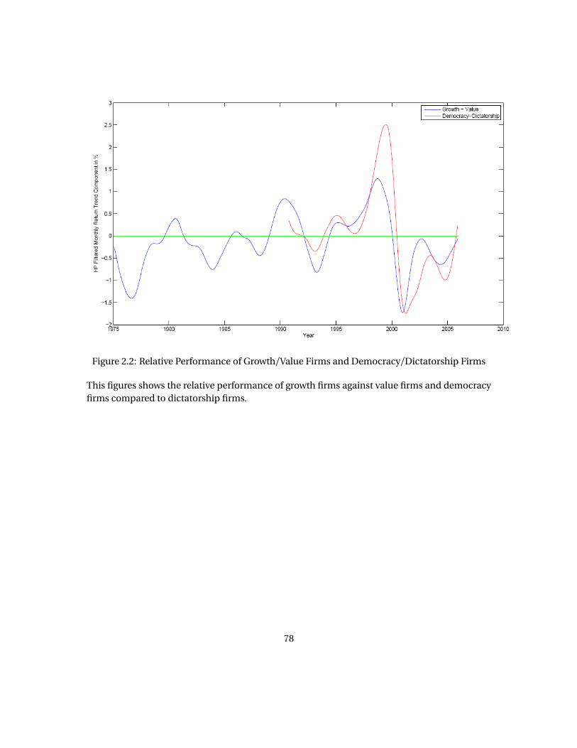
Figure 2.2: Relative Performance of Growth/Value Firms and Democracy/Dictatorship Firms

This figures shows the relative performance of growth firms against value firms and democracyfirms compared to dictatorship firms.

78

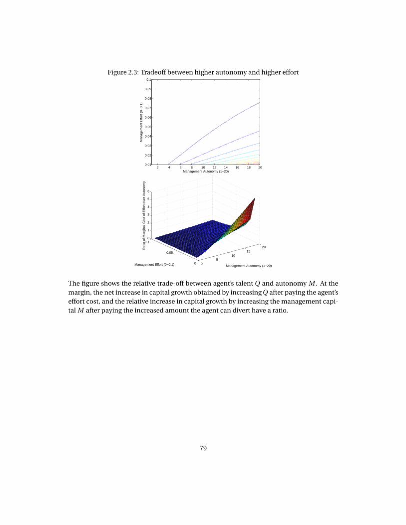
Figure 2.3: Tradeoff between higher autonomy and higher effort

Management Autonomy (1−20)

Man

agem

ent E

ffort

(0−

0.1)

2 4 6 8 10 12 14 16 18 200.01

0.02

0.03

0.04

0.05

0.06

0.07

0.08

0.09

0.1

05

1015

20

0

0.05

0.10

1

2

3

4

5

6

Management Autonomy (1−20)Management Effort (0−0.1)

Rat

io o

f Mar

gina

l Cos

t of E

ffort

ove

r A

uton

omy

The figure shows the relative trade-off between agent’s talent Q and autonomy M . At themargin, the net increase in capital growth obtained by increasing Q after paying the agent’seffort cost, and the relative increase in capital growth by increasing the management capi-tal M after paying the increased amount the agent can divert have a ratio.

79

Figure 2.4: Optimal Control Policy and Region of Inaction

Mar

gina

l Firm

Val

ue w

.r.t.

Aut

onom

y

Marginal Firm Value w.r.t. outside option for principal

No Change in Autonomy Region

Agent’s autonomy is increased

Agent’s autonomy is decreased

Optimal Agent Wage Contractunder Perfect Information (with no moral hazard or diversion)

This figure shows that when the marginal of φ, which is part of the value function of theprincipal, with respect to autonomy M crosses a threshold that depends on rate of growthof capital and transaction cost λ, the principal needs to increase or decrease autonomyof the management to stay inside the threshold. In other words, we have a bang-bangequilibrium.

80

Figure 2.5: Size, Growth and Variance of the Median Firm sorted by Governance Index : The topfigure is pre 2000 and the Bottom is post 2000

1 2 3 4−3.4

−3.2

−3

−2.8

−2.6

−2.4

−2.2

−2

−1.8

−1.6

−1.4

Firm

Ass

et V

aria

nce

G Index

Asset Variance on G Index

1 2 3 4−0.1

0

0.1

0.2

0.3

0.4

0.5

0.6

Ass

et G

row

th

G Index

Asset Growth on G Index

1 2 3 44

4.5

5

5.5

6

6.5

7

7.5

8

8.5

9

Firm

Ass

ets

G Index

Firm Assets on G Index

1 2 3 4−5

−4.5

−4

−3.5

−3

−2.5

Firm

Ass

et V

aria

nce

G Index

Asset Variance on G Index

1 2 3 4−0.2

0

0.2

0.4

0.6

0.8

1

1.2

1.4

1.6

1.8

Ass

et G

row

th

G Index

Asset Growth on G Index

1 2 3 45.5

6

6.5

7

7.5

8

8.5

9

9.5

10

Firm

Ass

ets

G Index

Firm Assets on G Index

e sort 1500 largest firms for which we have governance data into 4 bins according to gover-nance index and sort each bin further into 5 quintiles according to size. Then we tabulatethe mean assets, mean growth rate and variance of the median firm for each of the 20bins thus created. The top figure is pre 2000 and the Bottom is post 2000. It is clear oninspection that as management autonomy increases, variance decreases in both periods.However, the gradient of descent is much steeper in the earlier period of 1990-2000 : thisendorses the results of the regressions about the significant negative θ (coefficient of vari-ance) values before 2000 and the almost 0 value after 2000. Notice, the largest firms do notobey this negative relationship between variance and autonomy. Our story is based uponincomplete information about the firm - and we know that the largest firms face the mostscrutiny by media and analysts. Hence, the fact that they do not obey the relationship, infact, supports our theory even more. The trends in growth are descending but much lessso, as was predicted by the small values of ν in the regression (coefficient of asset growth).Finally, the positive correlation between management autonomy and firm size is shown inthe rightmost subplot.

81

Table 2.1: Regression of Management Autonomy on Firm Characteristics

I use Non Linear Least Squares using Maximum Likelihood as the estimation procedure.Governance Index instruments management autonomy on the left hand and assets growth,and variance in assets on the right. The equation used is as follows:

log M (t ) = log

�

constant+ν�

K (t +1)K (t )

�

+θσ(K )2�

− (α−1) log K (t ),

which is rewritten from the law of motion of capital. In equilibrium when shareholders suf-fer from incomplete information about the output of the firm, management diverts capitalin proportion to variance of assets. A higher variance, in our model, implies higher diver-sion, when the shareholders have incomplete information about the firm. To reign in themanagement, the shareholders reduce the autonomy so that inspite of higher variation,less diversion happens. In panel A, we show supporting evidence for the hypothesis thatshareholders choose management depending on the process of capital growth. we expectto find a negative coefficient to variance in the above regression. θ represents the coeffi-cient of variance in the table I. We find θ is negative and significant before and inclusive of2000 (1990-2000). We see a progressive increase in the value of θ over the years. In fact, inrecent times, θ is not differentiable from 0 at 95% level and the point estimate is positive(2000-2006). One possible explanation for this is the information disadvantage of share-holders has decreased, and hence they do not feel the need to control the autonomy of thefirm to avoid diversion. This can be an evidence in favor of Sarbanes-Oxley (2002), or partsof it. Laws that encourage disclosure to increase transparency can help shareholders feelmore confident to provide the firm larger autonomy, which, in our model, leads to higherreturns. However, even before the law was enacted, as per our model, US Capital Marketswere becoming more transparent progressively. The coefficient of growth ν is consistentlynegative - showing that firms with higher growth are more democratic. As firms grow faster,shareholders are less pressed to give the management autonomy to increase growth rate -since that would mean larger bounds on diversion on the flip side. α, the exponent of cap-ital in our model, is consistently less than 1 - which shows that as firm size K (t ) increases,firms become more autocratic. This is consistent with the literature on management en-trenchment and empire building.

Time periods α ν θ Pr > F Value1990−2006 0.9686 −0.0005 −0.2816 < 0.0001

(0.00123) (0.000258) (0.0387)1990−2000 0.9638 −0.0005 −0.6886 < 0.0001

(0.00171) (0.000216) (0.0530)2000−2006 0.9737 −0.0011 0.1636 < 0.0001

(0.00209) (0.000471) (0.1124)

82

Tab

le2.

2:R

egre

ssio

no

fFir

mV

aria

nce

on

Gov

ern

ance

Ind

ex,L

ever

age

and

Oth

erF

irm

Ch

arac

teri

stic

s

Ireg

ress

vari

ance

infi

rm’s

Tob

in’s

Qsc

aled

by

bo

ok

valu

eo

fth

efi

rmo

ngo

vern

ance

ind

ex,l

ever

age

and

firs

ttw

om

om

ents

ofT

ob

in’s

Q(s

cale

dag

ain

by

bo

ok

valu

eo

fth

efi

rm)

on

the

righ

t.T

he

equ

atio

nu

sed

isas

follo

ws:

Var

ian

cein

Firm

’sQ=

α1G

Ind

ex+α

2Le

vera

ge+α

3M

ean

Q×

Bo

ok

Val

ue

+α

4M

ean

Gro

wth

inQ×

Bo

ok

Val

ue+α

5T

ime

Du

mm

y,

Th

ere

sult

sag

ain

show

an

egat

ive

rela

tio

nb

etw

een

ob

serv

edva

rian

cein

Tob

in’s

Qan

dgo

vern

ance

inth

eea

rlie

rp

erio

d,a

nd

asi

mila

rre

vers

alin

tren

din

last

few

year

sas

ob

serv

edin

Pan

elA

.As

exp

lain

edb

efo

re,I

con

sid

erit

evid

ence

infa

vor

ofm

yh

ypo

thes

isth

atin

form

atio

nd

isad

van

tage

ofs

har

eho

lder

sh

asd

ecre

ased

,an

dh

ence

they

do

no

tfe

elth

en

eed

toco

ntr

olt

he

auto

no

my

of

the

firm

toav

oid

div

ersi

on

.In

fact

,th

eyal

low

mo

reau

-to

no

my

toen

joy

hig

her

pro

du

ctiv

ity

of

man

agem

ent

wh

ich

com

esw

ith

mo

reau

ton

om

y.T

hu

s,th

ere

sult

sar

ero

bu

stto

the

cho

ice

ofp

erfo

rman

cem

easu

re-

Tob

in’s

Q,F

irm

Ass

ets

or

oth

erm

easu

res.

Tim

ep

erio

ds

GIn

dex

Leve

rage

Mea

nQ×

Bo

ok

Val

ue

Mea

nG

row

tho

fQ×

Bo

ok

Val

ue

Tim

eD

um

my

R-S

qu

are

1980−

2006

−69

.51

−75

5.83

0.74

11−

128.

38−

3.93

0.90

(18.

80)

(260

.09)

(0.0

014)

(7.1

7)(9

.31)

2000−

2006

81.9

6−

737.

460.

2018

0.46

578.

790.

86(1

8.78)

(231

.03)

(0.0

008)

(2.3

9)(2

5.17)

1990−

2000

−11

2.71

−10

56.9

10.

6192

−60

.10

33.5

30.

83(2

0.44)

(299

.13)

(0.0

022)

(4.2

1)(1

8.55)

83

Table 2.3: Relation between Firm Assets Variance, Growth and Median and Governance Index(Pre 2000)

We sort 1500 largest firms for which we have governance data into 4 bins according to gov-ernance index and sort each bin further into 5 quintiles according to size. Then we tabulatethe mean assets, mean growth rate and variance of the median firm for each of the 20 binsthus created. The top row in each cell is asset variance, middle row is asset growth andbottom row is mean assets of the median firm. This table shows the results for periods of1990-2000 and 2000-2006. It is clear that as management autonomy increases, variancedecreases in both periods. However, the gradient of descent is much steeper in the earlierperiod of 1990-2000 : this endorses the results of the regressions about the significant neg-ative θ (coefficient of variance) values before 2000 and the almost 0 value after 2000. Thetrends in growth are descending but much less so, as was predicted by the small values ofν in the regression (coefficient of asset growth). Finally, the positive correlation betweenmanagement autonomy and firm size is shown in the third number in each cell - suggestingmanagement entrenchment.

Governance Index

Asset Percentile 0−5 5−9 10−13 14−Bottom 20% −2.4362 −2.4267 −2.6206 −3.2948

0.0109 −0.0031 0.0054 0.01644.4503 4.8173 5.1151 5.3384

20−40% −1.6411 −2.1619 −2.2013 −1.56400.1450 0.0676 0.0877 0.09795.1048 5.4919 5.9425 6.1026

40−60% −1.6686 −1.7908 −2.0913 −2.23750.1469 0.1160 0.1183 0.08165.6585 6.0488 6.8170 7.3223

60−80% −2.2948 −1.9256 −2.3765 −2.23860.1261 0.1536 0.1308 0.19286.7898 6.9606 7.8828 7.7408

Top 20% −1.7973 −2.0913 −2.0444 −1.83210.3425 0.2080 0.1651 0.52258.2637 8.6567 8.8859 8.9969

84

Table 2.4: Relation between Firm Assets Variance, Growth and Median and Governance Index(Post 2000)Top row in each cell is Asset Variance, Middle row is Asset Growth and Bottom row is Meanassets of the Median firm

Governance Index

Asset Percentile 0−5 5−9 10−13 14−Bottom 20% −2.9104 −2.9744 −3.2059 −4.6560

−0.0974 −0.1323 −0.0645 −0.06625.5031 5.5481 5.8804 6.1493

20−40% −3.4290 −3.0446 −3.5671 −2.8385−0.0107 −0.0246 0.0211 0.1029

6.4551 6.4127 7.0422 7.356040−60% −3.1279 −3.1946 −3.6780 −3.2500

0.0241 0.0745 0.0900 0.20317.0482 7.1293 7.8822 8.1964

60−80% −3.4258 −3.2808 −3.8440 −3.39990.1617 0.1533 0.1753 0.37537.8166 8.0121 8.8251 8.7676

Top 20% −3.2819 −3.3592 −3.8812 −3.04841.6314 0.4047 0.4604 0.90359.8168 9.7582 9.9704 9.8024

85

Table 2.5: Relation between Firm Characteristics, Outside Block holders and Corporate Gover-nanceAs an alternate specification, we let production function of the firm be:

d Y (t ) = K (t )αMηBβd t +σ(Y )d w ,

where B represents the percentage of shares held by outside block holders - another determi-nant of control shareholders have on management, raised to a constant β . We regress Gover-nance Index now on assets growth, and variance in assets and percentage shares held by outsideblock holders. The equation used is as follows:

log M (t ) = log

�

constant+ν�

K (t +1)K (t )

+θσ(K )2�

− (α−1) log K (t )+β log Bt .

This table shows the results of the regression for various time periods. As in panel A of TableI, θ represents the coefficient of variance in the regressions below. We again find θ is negativeand significant before and inclusive of 2000 (1990-2000) - as our model predicts. The increasein the point estimate of θ over the years is seen here as well. In the period since 2000, θ isnot differentiable from 0 at 95% level in this alternative model specification as well. This evi-dence gives further credence to our hypothesis that information disadvantage of shareholdershas decreased, and they feel less pressed to control the autonomy of the firm to avoid diversion.Introduction of shares held by blockholders does not change the coefficient of growth ν . It isconsistently negative in this model as well - showing that firms with higher growth are moredemocratic. α, the exponent of capital, is consistently less than 1 - which shows that as firm sizeK(t) increases, firms become more autocratic.

Time periods α ν θ β Pr > F Value1990−2006 0.9726 −0.0005 −0.4466 0.00200 < 0.0001

(0.00145) (0.000281) (0.0461) 0.0001811990−2000 0.9672 −0.0005 −0.8736 0.00186 < 0.0001

(0.00190) (0.000233) (0.0587) (0.000231)2000−2004 0.9795 −0.0010 −0.3056 0.00291 < 0.0001

(0.00275) (0.000659) (0.1886) (0.000351)

86

Table 2.6: Relation between Leverage and Corporate GovernanceManagement will always take on leverage, such that if a bad shock hits, and it is going to beremoved, then as far as the manager is concerned, the firm might as well go bankrupt. Debtholders, know that, and in equilibrium will not provide any leverage that in any state with mea-sure allows firm capital to be lower than the performance bound allowed by the shareholders:Lower bound on capital by debt holders = Lower bound on firm capital by shareholders. Thelower performance bound chosen by shareholders is a function of autonomy granted, thus giv-ing us a relation between autonomy and leverage. Firms with higher autonomy, should showhigher leverage, and that is what we observe in the table below. We regress firm leverage (Longterm Debt/Assets) on G Index and moments of Tobin’s Q.

Leverage=α1G Index+α2Variance in Firm Q+α3Q+α4Mean growth in Q+α5Time Dummy

we find that as autonomy increases, debt holders also let the firm take on large debt. We alsoobserve the known fact that growth firms that have larger TobinŠs Q, take on less debt - this isbecause such firms have less collateralizable assets. In other words, it is due to equity beingcheaper in comparison to debt.

Time periods G Index Variance in Q Q Mean Growth of Q Time Dummy1990 - 2006 0.0031 -0.0074 -0.0056 -0.0084 -0.00003

(0.00041) (0.00061) (0.00049) (0.0053) (0.0002)2000 - 2006 0.0046 -0.0040 -0.0082 -0.0068 -0.0019

(0.00076) (0.0027) (0.0015) (0.0098) (0.0010)1990 - 2000 0.0034 -0.0031 -0.0060 -0.0062 0.0019

(0.00054) (0.00076) (0.00066) (0.0021) (0.00049)

87

Table 2.7: Granger Test: Does change in Firm characteristics cause change in Autonomy?We have proposed in this paper that shareholders choose autonomy as a response to firmcharacteristics. Thus, when Tobin’s Q changes enough, if shareholders are really respondingto firm characteristics, then management autonomy should change as well. The unrestrictedmodel tests whether the G-Index values of last two years and Tobin’s Q of last two years Grangercauses present G-Index. The restricted model tests causality against only G-Index values of lasttwo years. The results test compare the errors from the two models and show that changesin Q causes changes in autonomy. The Granger test shows that the null hypothesis that statesthat changes in Q cause changes in Autonomy is not rejected. This supports our theory thatinvestors choose autonomy as a response to change in firm characteristics.

Time periods F-Test Chi Test p-Value1990−2006 18682.20 37369.47 01990−2000 5934.39 11871.66 02000−2006 450.21 901.25 0

88

Chapter 3

Effort, Risk and Walkaway Under HighWater Mark Contracts

With Sugata Ray

3.1 Introduction

As more and more funds found themselves under their high water marks (HWMs) though the

course of the recent economic crisis, investors and the financial press increased their scrutiny

of the impact of a distant high water mark (HWM) on fund manager incentives. Most hedge

funds have a management fee (generally 2%) and a performance fee (generally 20%) with a high

water mark that stipulates the performance fee is paid only on “new” profits. In other words, if

a fund with a HWM stipulation has made a loss, it must recoup the loss before earning the 20%

performance fee. This leads to a distortion of incentives when funds are below their HWMs. In

particular, fund managers far below their HWMs may increase portfolio risk and lose focus on

alpha generation, which in turn may lead to investors pulling out of such funds. With over two

trillion dollars under management in hedge funds and much of it still under their respective

HWMs, both fund managers and investors are currently grappling with this very problem.

The central role of the high water mark feature in driving fund managers’ and investors’

89

behavior is readily apparent in the following anecdote. Following the beginnings of the credit-

related market correction in August 2007, a well known hedge fund at a bulge bracket bank,

which had lost a lot of money and was reportedly more than 30% below its high water mark,

offered a ‘sale’ on new fund inflows. Fees charged on new money would consist solely of a

10% incentive on any profits generated, and the management fee would be waived. That is,

the fund adopted a “0/10” structure rather than the standard “2/20.” The implications of such

a move were manifold. Original monies in the fund were sufficiently far away from their high

water mark that fund employees, discouraged about prospects of ever hitting the high water

mark (and earning substantial bonuses), considered leaving and joining other funds. As a re-

sult, original investors in the fund questioned whether the fund would be able to maintain its

team through the crisis and considered withdrawing funds. Investors might also have been con-

cerned that managers would take inordinate risks in a desperate attempt to generate returns

above the high water mark. The infusion of new capital, fresh and untethered to the old high

water mark, alleviated these concerns. Employees would stand to earn incentive fees (and thus

bonuses) on this new money immediately, although the fees would accrue at the rate of 10%

rather than the full 20%. The original investors were reassured that the fund would be able to

maintain its team and did not withdraw their funds.1

We focus this study on this intricate set of risk, effort and walkaway decisions driven by

the high water mark (HWM) feature of the hedge fund contract. Modeling a simple one period

principal-agent relationship governed by such a contract, we derive the empirical predictions in

terms of risk choices, effort choices and walkaway behavior of the parties. Extending the model

to infinite periods, we highlight the disciplining role of investor walkaway on manager behavior.

We calibrate parameters in the infinite period model using observed hedge fund return data and

1Although the fund staved off immediate closure and the cash inflows from the sale led to a positive bounce, thehedge fund eventually lost money over the rest of the year as the credit crisis worsened, ending the year with a 38%loss.

90

use the calibrated model to posit welfare enhancing modifications to the current ‘2/20’ contract.

Although the model itself is fairly complex due to the optionality embedded in the hedge

fund contract, the empirical implications of the model resonate with the intuition that the con-

tract functions as if the fund manager simply has a call option on the returns of the fund. The

strike price of this option is the HWM and the return required to hit the HWM (RR) is a measure

of the moneyness of this option (the higher RR, the further the option is out of the money). In

particular, we predict differences in both fund manger and investor behavior depending on how

close the manager’s option is to being in the money. We expect the following: (i) The lower the

return required to hit the HWM (RR), the more likely the fund manager is to expend costly ef-

fort, and the higher the subsequent period returns will be. (ii) The manager of a fund far below

from the HWM is likely to increase the risk of his portfolio in the hopes of breaking the HWM

barrier again and earning performance fee based bonuses. (iii) Once a fund falls to a certain

point below the HWM, the danger of walkaway increases, as the principal may worry that the

agent is no longer expending an appropriate level of effort and is taking too much risk. These

empirical predictions are supported by empirical findings from Ray (2009).

We calibrate the free parameters of the model to observed hedge fund return data. Once

calibrated, moments generated from simulating an economy of model hedge funds an investors

closely match actual observed moments. Using the calibrated model, we examine various other

permutations of a “x/y%” management/incentive fee contract in search of a contract that pro-

vides better incentives for the fund manager without raising the expected fees paid by the in-

vestor. We find that substituting an increased management fee in lieu of incentive fees (e.g.,

a “2.5/10” contract rather than the standard “2/20” contract) leads to improved outcomes for

both the investor and the fund manager.

For funds near the HWM, this is achieved through improved risk sharing. In addition to im-

proved risk sharing, for funds further away from the HWM, the increased continuation value of

91

such a contract, combined with the enhanced ability to maintain a costly alpha-generating team

through periods of poor returns, leads to more investor-friendly behavior by the fund manager

and a correspondingly lower incidence of walkaway by the investor.

We also find that a constantly renegotiated HWM improves manager welfare at the expense

of investor welfare. Such a renegotiation is akin to the manager always having an at the money

option and although it mitigates some of the incentive problems in the original contract, it gen-

erates a fresh set of perverse incentives for fund managers.

While we admit that the welfare analysis is largely a thought experiment, as changing the

contract form will likely change other calibrated parameters that were held constant in the wel-

fare analysis, the results do highlight potential implications of changing the contract terms as

well as the effects of renegotiation. These implications suggest numerous practical applications:

(1) Portfolio allocation decisions by investors and fund-of-funds would find direct use for these

findings in optimizing their portfolios. In particular, investors should carefully consider how far

they should let their funds drop below the HWM before renegotiating or walking away entirely.

(2) Additionally, the welfare analysis suggests higher management fees and lower incentive fees

(e.g., the “2.5/10” contract above) may lead to improved outcomes for both investor and man-

ager. (3) These findings also have implications for hedge fund marketing strategies. The anec-

dote above, where the fund had the ‘0/10’ sale to mitigate many of these concerns, exemplifies

this. (4) A clearer level of disclosure about a fund’s high water mark(s), might also generate value

for current and potential investors alike.

Extant literature related to this study includes Goetzmann, Ingersoll, and Ross (2003), a sem-

inal paper in this field which examines the unique, high watermark (HWM) structure of the

hedge fund compensation contract and computes the alpha-generation potential necessary to

justify paying a fund manager according to such a contract. Hodder and Jackwerth (2007) con-

ducts a theoretical study of the impact of the HMW in a finite time horizon setting. Panageas

92

and Westerfield (2008) presents and solves a theoretical model where an exogenously set fund

closure point (bankruptcy) leads to fund managers moderating risk taking behavior despite the

optionality in the contract. Kerr Christoffersen and Musto (2008) considers the impact of the

HWM in a two period model with Bayesian learning and show how varying levels of perfor-

mance, in conjunction with the HWM, affect fund flows, fund closure and alpha generation

by the hedge fund. Metrick and Yasuda (2007) looks at the empirical differences between the

“2/20” fee structures of hedge funds, venture capital firms and private equity shops.

Our paper contributes to this body of research through two extensions. The first contri-

bution is to theory; our model is the first to formalize endogenous investor walkaway in the

context of a hedge fund HWM contract. This feature has been explicitly suggested in Panageas

and Westerfield (2008). Using this extension, we are able to posit clear empirical predictions of

the impact of the HWM on walkaway. We are also able to calibrate our model to match hedge

fund walkaway rates, among other moments, and obtain economically meaningful model pa-

rameters, such as the manager’s risk aversion and the fraction of investors who monitor their

investments. The second contribution is to the quantification of welfare implications of chang-

ing the contract. Using the calibrated model, we calculate investor expected returns and fund

manager expected utility under different contract forms. This also allows us to search for Pareto

improving contracts in our calibrated model and examine policy functions under such contracts

to gain intuition on what, specifically, drives the Pareto improvement.

The rest of this paper is divided into four sections. Section 3.2 describes the model and

presents the solutions to the model (the solutions to the model include optimal effort and risk

choices by the manager and optimal walkaway decisions for the investor). Section 3.3 calibrates

the model to observed empirical data. Section 3.4 uses the calibrated model to examine the

welfare implications of changing the hedge fund manager compensation contract and section

3.5 concludes.

93

3.2 Model

We model a risk averse hedge fund manager (the agent) and a risk neutral principal in a hedge

fund contract, with management fees, incentive fees, and a high water mark driving manager

actions and investment decisions. We begin by examining a one period model under such a

setup and use this to gain insight into the manager’s decision making. We then extend the model

to infinite periods and incorporate the investor’s walkaway decision (Section 3.2.3).

3.2.1 One period model without continuation value

In this single period model, we have a hedge fund manager who has been given a sum of money,

v0, by the principal at time t0. The manager will be compensated at t1 according to the returns

to the fund. The fund starts at the high water mark and all returns will be subject to the incentive

fee over the t0→ t1 period.

w1 = k v0+ s v0m a x (r , 0), (3.1)

where

r = a +σε

ε ∼ U (−1, 1)

w1 denotes the compensation of the hedge fund manager at t1. Thus, in a standard 2/20

contract, k = 2% and s = 20%. The r is the return before fees in the next period, a andσ are ef-

fort and risk choices made by the manager. Effort is costly to produce, and risk can be increased

costlessly. The manager has CRRA utility and strives to maximize his utility from t1 wealth. The

shock is uniform over the [−1, 1] interval. The manager’s problem can be represented as follows:

Vm =maxa ,σEβ�

u (k v0+ s v0 max(0, r )−v0

2ca a 2)

�

(3.2)

94

where

u (x ) =x 1−γ

1−γ

(3.3)

Vm is the value of the contract to the agent, which he seeks to maximize. u (x ) represents the

agent’s utility function and β and γ are the agent’s discount rate and coefficient of risk aver-

sion, respectively. v02 ca a 2 is the term that represents the cost of effort that is paid at t1. We

assume a quadratic cost of effort, scaled by v0. This is similar to the form used in Hodder and

Jackwerth (2007) and is consistent with decreasing returns to scale with respect to increased

effort expenditure. Although effort can be interpreted traditionally as how hard the manager

works, a more apt interpretation views it as hiring costly alpha-generating talent from a com-

mon portfolio manager pool. ca is a parameter representing the cost of effort in this market for

alpha-generating talent.

We solve this simple model and show that effort, a , has an interior solution (given a finite

and fixed σ). σ will not have an interior solution - it is either 0% or infinity, depending on the

choice of a , the distribution of shocks, ε, γ and other contract parameters.

3.2.2 One period model with continuation value and investor walkaway

We can extend this one period model to capture investor walkaway and some of the effects of the

HWM by treating this as a hedge fund that has been in existence for some time. Thus, the fund

may potentially be below the HWM. The distance of the fund from the HWM is characterized by

the return required to hit the HWM (RR), denoted by r r0.

1+ r r0 =max(h0/v0, 1), (3.4)

r r0 is the return required to hit the HWM at t0. v0 is the value of the fund at t0 and h0 is the

95

HWM at t0. If the fund is at the HWM, h0 = v0 and the return required to hit the HWM is zero

(r r0 = 0). Additionally, the model allows the investor to withdraw the investment, v0, at time

t0, before the manager can make his effort and risk choices. The investor is risk neutral and

will withdraw the investment if the expected value of the fund after fees in the second period is

lower than the value of the fund currently. If the investor decides to continue, then the manager

will make effort and risk choices, the return will be realized, and the contract will terminate at

t1. To capture the continuation value of the contract to the manager, the investor will also have

the opportunity to withdraw funds in t1. If the investor withdraws the funds, the manager will

receive his outside option, vy . If the investor remains invested, the manager will receive a lump

sum value, vc , representing the continuation value of the contract. We will assume that the

continuation value of the contract is higher than the manager’s outside option (vc > vy ).

A timeline for this extension is as follows, and a graphical representation of the timeline can

be found in figure 3.1:

• At time t0:

– Assets under management (AUM) are v0 and the fund high watermark is at h0.

– r r0 represents the return required to reach the last watermark (RR). (as calculated in equa-

tion 3.4

– The investor remains invested in the firm if she anticipates that the effort and variance

chosen by the manager will lead to positive expected returns after fees are deducted.

– However, if she chooses to walk away from the fund, the contract is terminated, the investor

receives the fund value v0, and the agent receives his outside option.

– If the investor chooses to continue with the portfolio manager at t0, then the manager

chooses effort, a , and variance,σ. (See section 3.2.2).

96

• At time t1:

– The management fee is paid to the fund manager based on the previous period’s AUM (k v0)

– The rate of return, r01 is realized. If the old HWM is exceeded, or r01 > r r0, then an incentive

fee of s ×v0(r01− r r0) is paid to the fund manager.

– The return required to hit the HWM (RR) at t1, r r1, is computed, and the investor makes

a decision based on r r1 whether to continue investing in the fund going forward. There

is a walkaway threshold, r r ∗1 , above which the investor will walk away at time t1. r r ∗1 is set

exogenously in the one period model, although this will become endogenous in the infinite

period model.

– If the investor does not walk away, then the manager receives a lump sum vc , which repre-

sents the continuation value of the contract - a stylized way to capture future incentive and

management fees. If walkaway occurs, the manager will receive his outside option, vy . We

will assume that vc > vy . In the infinite period model, vc will be replaced by a function of

RR, allowing us to construct a Bellman equation for the manager’s problem.

– The contract then terminates at time t1.

We solve for the manager’s effort and risk decisions at time t0, depending on what r r0 is,

such that the manager maximizes expected utility from incentive fees, management fees, and

potential contract continuation. Given the manager’s actions, we can determine the investor’s

expected returns after fees as a function of r r0 and the region of r r0 for which this expected

return is negative. In this region, the investor will walk away in time t0, before the manager

makes the decision.

97

Portfolio Manager’s Problem

The portfolio manager will act at t0 to maximize his expected utility at t1. Vm is the fund man-

ager’s expected utility at t0:

Vm =maxa ,σ

βE�

u (k v0+ s v0 max(0, r01− r r0)−v0

2ca a 2)+p (r01 > r ∗01)×π

�

, (3.5)

where

u (x ) =x 1−γ

1−γ

1+ r ∗01 =1+ r r0

1+ r r ∗1

r01 = 1+a +σε

π = u (vc )−u (vy )

ε ∼ U (−1, 1)

where r01 represents the rate of return from time t0 to t1. The utility function remains the same

as before, with γ representing the coefficient of risk aversion for the CRRA manager and β rep-

resenting his discount rate. The cost of effort also remains the same as before, v02 ca a 2. The

difference now is that the fund may not be at the HWM, and thus, the incentive fee is paid only

on returns above the HWM (s v0 max(0, r01 − r r0)). The shock retains the uniform distribution,

ε ∼U (−1, 1). p (r01 > r ∗01) is the probability that the return over the period leads to a RR in the

second period that is low enough to ensure the continuation of the fund, and π is the increased

utility to the manager from receiving this continuation value instead of the outside option. The

manager will choose effort a and riskσ for the next period to maximize his expected utility:

{a ∗,σ∗}= arg maxa ,σ

βE�

u (k v0+ s v0 max(0, r01− r r0)−v0

2ca a 2)+p (r01 > r ∗01)×π

�

(3.6)

98

Investor’s problem

The investor’s walkaway decision at t0 depends on the returns after fees that she can expect

given r r0, the RR at time t0, and the manager’s optimal effort and risk choices for this r r0. The

value of the fund after fees at t1 can be represented as follows:

E[v1] =E[v0r01−k v0− s v0 max(0, r01− r r0)|r01 = 1+a ∗+σ∗ε], (3.7)

where v0, v1 are fund values at time t0, t1, respectively, and r01 is the return given the manager’s

anticipated choice of effort, a ∗, and variance, σ∗2, as given in equation 3.6. Fees paid to the

manager in the above equation are simply the management and incentive fees from the contract

(k v0+s v0 max(0, r01−r r0)). As the investor is risk neutral, ifE[v1|r r0]≤ v0, the investor will walk

away at time t0. E [v1] is decreasing in r r0 and the minimum RR at which the investor walks

away is denoted by r r ∗0 .

At time t1, the investor walks away if return required, r r1, is greater than an assumed and

fixed r r ∗1 (akin to r r ∗0 walkway point discussed above, but fixed by assumption in the one period

model). This leads to a t1 walkaway point in terms of the realized return for the period:

1+ r ∗01 =1+ r r0

1+ r r ∗1(3.8)

If r01 < r ∗01, the investor will walk away at t1. In the infinite period model, this walkaway point

will be determined endogenously using the Bellman equation.

Optimal Effort, Risk and Walkaway in the one period case

Although closed form solutions to the manager’s optimal effort and risk choices, a ∗ and σ∗,

exist, it is easier to glean intuition from graphical representations of these solutions which are

presented in Figure 3.2. We can see that optimal effort generally decreases with RR: optimal

effort remains at its maximum, 5%, until RR = 1.8%, then falls to about 2% and then slowly

99

decreases to near-zero levels at RR = 10%. Optimal risk is at the minimum when RR < 1.8%.

Above this, risk spikes to its maximum value, 10%, and remains there for RR ≥ 1.8%.

Given this set of optimal effort and risk choices, we solve for the fund manager’s value from

the contract (given no investor walkaway at t0) as a function of RR. This is shown in figure 3.3.

This graph has three lines. The “Payoff from Present Period” is the utility derived from the net

of the management fees, incentive fees and cost of effort (u (k v0+s v0 max(0, r01−r r0)− v02 ca a 2)

from equation 3.5. The “Payoff from Continuation” is the expected utility from receiving the

continuation value over the outside option (p (r01 > r ∗01)×π from equation 3.5. Finally, the “To-

tal Payoff” is the sum of these and reflects the total expected utility to the manager from this

contract, given the RR. Note that given the power utility function, the sum of the utility from

the total payoff is not the sum of the utilities from the individual components. We see that the

manager’s utility decreases monotonically with RR, and the contract continues with certainty

until RR = 1.8%. Beyond that, the probability of continuation in the second period decreases

linearly with RR.

Finally, using the optimal effort and risk policies above, we can determine the expected re-

turn after fees, given fund continuation. This is shown as a function of RR in figure 3.4. We see

that this increases from 1% to its peak at 2.25% as the fund goes from 5% above the HWM to

1.8% below it. Then it precipitously falls to -0.6% and slowly decreases with RR, finally settling

at about -2% for RR > 10%. The precipitous fall coincides with the switch in optimal risk policy

from minimum risk to maximum risk. A rational investor would thus withdraw the funds at t0

if RR > 1.8%. We also note the initial increasing expected return after fees (over the domain

−5% ≤ RR ≤ 1.8%) is due to the reduced incidence of fees. The further the fund is below the

HWM, the less it will have to pay in terms of incentive fees, as these fees are only charged on

returns over the HWM.

100

3.2.3 Infinite Period Model and Solution

To extend this model to a more realistic infinite period contract, we convert equation 3.5 into a

Bellman equation. We retain the timing of the decisions made by the players from section 3.2.2.

Specifically, during each period, the decisions are made as follows:

1. The investor, who has funds with the manager indexed to a HWM, decides whether to remain

invested with the manager or whether to withdraw funds

2. If the investor remains invested, the manager chooses how much effort to expend and how

much risk to take

3. The return is realized as per the shock and the effort and risk choices

4. Management and incentive fees, if any, are paid to the manager

5. Any returns to the fund are disbursed, and if the fund loses money, the investor replenishes

the fund to v0 with new money entering indexed to the old HWM

6. A new HWM is established if the old one is exceeded and the investor contemplates the walk-

away decision all over again

Once we replace the lump sum continuation value in the second period in equation 3.5

with a function of the RR to represent the continuation value of the contract, the agent’s value

function becomes the Bellman equation shown in section 3.2.3 below. We assume (in step 5

above) that the investor will maintain assets of the fund at v0. That is, she will withdraw funds

above v0 if the fund made a profit and will replenish the fund to v0 if it made a loss. We will

further assume that the contract allows her to replenish the fund with monies indexed to her old

watermark, although this is not a central assumption.2 We can appeal to an optimal fund size for

2Allowing the investor to replenish funds such that the funds invested have a blended HWM also produces quali-tatively similar results.

101

alpha-generation to justify this assumption. An S-shape alpha-generation function (with initial

economies of scale followed by decreasing returns to scale) will provide some justification for

this optimal v0 fund size. Additionally, a number of hedge fund investors, such as pension funds,

fund of funds, and high net worth individuals, often have portfolio allocation targets, which

comport with maintaining the investment in the fund at a given size. These assumptions greatly

increase tractability and allow us to isolate the impact of the watermark on the incentives of the

fund manager, rather than reflecting the manager’s incentive to grow the fund to increase fee

revenue. While flow of funds constitutes an important part of the asset management literature

(see Kerr Christoffersen and Musto (2008) and Berk and Green (2004)), the natural convexity of

the ‘2/20’ contract allows us to discern the impact of incentives on the control variables without

considering fund flows.

Portfolio Manager’s Problem

The portfolio manager’s value function can be represented as the Bellman equation below:

Vm (r r ) =maxa ,σ

β E�

u (k v0+ s v0 max(0, r − r r )−v0

2ca a 2)+Vn (r r ′)

�

(3.9)

where

u (x ) =x 1−γ

1−γ

r r ′ = max(0,r r − ˜rp f

1+ ˜rp f)

r = a +σε

˜rp f = r −k − s max(0, r − r r )

ε ∼ N (0, 1)

and

102

Vn (r r ′) =

Vm (r r ′) for W (r r ′) = 0

αVy +(1−α)Vnw a (r r ′) for W (r r ′) = 1(3.10)

The payoff in the next period from incentive fees, management fees and cost of effort re-

mains the same as in the one period model. Note that all payouts (including the cost of effort

paid by the manager) occur at the end of the current period. This allows us to avoid a savings

decision for the manager. There is an active literature on other specifications for agent con-

sumption and savings (see Brown, Goetzmann, and Ibbotson (1999) and Brown, Goetzmann,

and Park (2001) among others), however, in our paper, the manager will consume all income

from a given period. He will not have a savings decision, nor is he able to invest in his own fund.

W (r r ′) = 1 and W (r r ′) = 0 represent the walkaway point, in terms the RR, being breached or not

being breached in the second period, respectively. This function is described further in section

3.2.3 below. Vy and Vnw a are the value functions for a manager receiving his outside option, and

a manager with an investor who does not monitor, respectively. Given the specification of the

cost of effort and the utility function, together with the replenishing of the fund (step 5 in the

timing above), the fund size, v0 is not a state variable and is normalized to 1 in the solution and

calibration sections. α is the fraction of investors who monitor their investments. We discuss

this fraction in further detail in section 3.2.3 below. Setting α = 1 would represent a world in

which all investors monitored, and the manager would always receive the outside option if the

walkaway threshold were to be breached. Vy and Vnw a (r r ) can be represented as follows:

Vy =∞∑

i=0

β i u (y v0) (3.11)

and

Vnw a (r r ) =maxa ,σ

β E�

u (k v0+ s v0 max(0, r − r r )−v0

2ca a 2)+Vnw a (r r ′)

�

(3.12)

103

If the manager learns that the investor monitors (this happens once the walkaway threshold

is breached, with probability α), his choices are no longer relevant, as the fund would have been

liquidated; the manager will take up his outside option and earn y v0 into perpetuity. This can be

interpreted as taking up a position at an actively managed mutual fund with the same AUM as

the hedge fund at the time of closure and making a fixed expense ratio, y , on these investments

forever. However, if the manager learns that the investor does not monitor (this happens once

the walkaway threshold is breached, with probability 1−α), he will correctly determine that the

investor will never walk away and will act as if this contract will never be terminated. Note that

the continuation value (Vnw a (r r ′)) in the no walkaway Bellman equation remains of the same

form, regardless of how far the fund falls from the HWM. This is in contrast to the case for the

manager who does not yet know if the investor monitors, and the continuation value is of a

different form (Vn (r r ′) rather than Vm (r r ) in equation 3.9).

Before solving the manager’s problem, we consider the investor’s walkaway decision in order

to obtain W (r r ′) above.

Monitoring Investor’s Problem

We modify the investor’s walkaway decision from equation 3.7 in the one period model. We

assume that only a fraction of investors, α, monitor their investments.3 The investors who do

not monitor will never walk away. This section discusses the monitoring investor’s walkaway

decision.

The “monitoring” parameter, α, represents the fraction of investors who constantly monitor

their investments. Each fund either has an investor who constantly monitors the fund at zero

cost, or has an investor who has a prohibitively high cost of monitoring the fund and does not

monitor. α is the fraction of total investors who costlessly monitor the fund. If the investor does

3The purpose of α becomes clear in the calibration section as we try to match the dispersion of fund observationsby distance from the HWM. For now, setting α = 1 would represent a world where all investors monitor and theremaining analysis would go through.

104

not monitor, she will never walk away. Initially, the manager does not know what type of investor

he works for; the manager will act such that there is α probability that the investor monitors

and 1−α probability that the investor will not monitor and will never walkaway. This concept

of the attentive/inattentive actor is not new in the literature. Both the mutual fund literature

and mortgage literature have extensively studied this phenomenon (see Berk and Tonks (2007),

Christoffersen and Musto (2002), Carhart, Carpenter, Lynch, and Musto (2002) and Schwartz

and Torous (1989)). While it might be argued that investors in hedge funds are different and are

much less likely to leave their funds unattended, we note that there is a large variation in the

type of hedge fund investors. A large fund of hedge funds would be unlikely to leave its funds

unmonitored indefinitely, but retired high net worth individuals and pension funds might well

adopt this “set it and forget it” stance seen among non-monitoring investors.

The monitoring investor is risk neutral and seeks to maximize expected funds by deciding

when/if to withdraw funds from this alternative investment and to deposit them into an account

bearing no interest.4 In order to posit an equilibrium, we assume the investor believes that if

she does not walk away when she should, the manager will behave as if the investor is of the

unmonitoring type and will never walk away (i.e. the manager will determine a ∗ and σ∗ by

solving Vnw a (r r ) from equation 3.12). This is an off the equilibrium path belief. In equilibrium,

the monitoring investor will always walk away when the walkaway condition is met.

Even with these beliefs, there may still be multiple equilibria for the investor’s walkaway

threshold. We take a number of steps to identify one such equilibrium. We posit a walkaway

rule consistent with the off the equilibrium path beliefs discussed above, and we verify that

this rule, combined with the manager’s actions under that walkaway policy, constitutes a stable

equilibrium. We propose the following walkaway policy: The investor will walk away based on

4Although we do not consider reinvestment into another fund as an admissible strategy in our model, if such areinvestment were to be accompanied by an upfront sales fee that expropriated all investor surplus from entering acontract at the HWM, this would be equivalent to having a zero-interest bearing deposit account as an alternative.

105

the outcome of returns and fees over the next N periods. More specifically, the investor will walk

away if expected returns from the next N periods are negative, regardless of interim walkaway,

given the RR and that the manager’s investment decisions are as in the no walkaway case (i.e.

given a ∗ and σ∗ from the solution to Vnw a (r r ) for each given r r from equation 3.12). Thus, the

walkaway rule can be expressed as:

W (r r ) =

1 for Enw a [rp f ,t0→tn |r r ]< 0

0 for otherwise

∀ n ∈ [1, 2, 3...N ]

(3.13)

Where Enw a [rp f ,t0→tn |r r ] represents the expected return after fees under the belief that the

manager will behave as if the investor never monitors over the next n periods. Such a rule can be

interpreted as assuming a bounded rational investor who is willing to analyze the next N periods

to make the right decision. We now have to verify that this rule is consistent with the behavior

of a value maximizing investor. It is easy to show that the investor should never walk away when

W (r r ) = 0 because (1) expected returns will always be higher when the manager is uncertain if

the investor is monitoring than when the manager knows for sure the investor is not monitoring

(this is shown for the calibrated model in section 3.2.3 below) and (2) expected returns for the

investor will be positive (over some period from t1 to tN ) under the belief that the manager acts

as if the investor is not monitoring. (1) and (2) together imply that walking away when W (r r ) = 0

would mean walking away from positive expected returns and depositing the funds in a zero

interest bearing account, which is suboptimal. We also to verify that continuing the contract

when W (r r ) = 1 is suboptimal in terms of returns over the next N periods. This is trivially true

given the walkaway condition in equation 3.13. Note that while this is a walkaway threshold

consistent with the investor’s beliefs, we do not identify it as a unique walkaway threshold. It

is possible that a different walkaway threshold may be a feasible policy function in equilibrium

as well. This walkaway policy does, however, provide us a clear path to solving the problem:

106

(1) We solve for the manager’s optimal policy in a world where he believes the investor does

not monitor. (2) Using these policies, we determine the walkaway policy for the investor from

equation 3.13. (3) Using the walkaway policy, we solve for the manager’s policy functions using

the Bellman equation, equation 3.9.

Optimal effort, risk and walkaway in the infinite period case

We solve for the optimal effort and risk policy functions for the manager in the no walkaway

case using value function iteration. The functions are shown in figure 3.5. These simply rep-

resent how a manager would behave if he knew the investor would never walk away, and they

are the solutions to the maximization problem in equation 3.12. Using these functions, we can

determine the regions of walkaway as per the walkaway condition above (equation 3.13). The

walkaway decision is shown in figure 3.6 and is the function presented in equation 3.13. Under

the model, only α fraction of the investors monitor their funds. The only way for the manager to

find out if the investor is of the monitoring type is if the fund ever reaches a point where the re-

turn required is higher than the walkaway threshold shown in figure 3.6. At that point, the value

function is resolved into either Vy or Vnw a (r r ). Once we add in the walkaway policy for the mon-

itoring investor, we can model the manager as choosing a and σ as per the Bellman equation

above (equation 3.9) with investor walkaway policy in figure 3.6, conditional on the monitoring

investor not walking away. Using value function iteration, we solve for the manager’s optimal

policy and value function. The policy functions are shown in figure 3.5. Combining the opti-

mal policy functions for the manager and the investor, we determine the value function for the

manager, which is shown in figure 3.7. Note the steep dropoff to the right of the walkaway point

indicating the potential loss of the contract. The expected moments for investors’ returns under

the solved model are shown in figure 3.6. We can see that expected return next period decreases

and expected return variance increases with RR.

Finally, we confirm that both the attentive investor’s behavior and the manager’s actions

107

constitute a Nash equilibrium. The investor will never walk away in regions to the left of the

walkaway boundary in figure 3.6, as it is unprofitable to do so. To right of the boundary, she

will always walk away as she believes that the manager will revert to a no-walkaway effort and

risk policy if she does not. She will end up paying more in fees than she can hope to recoup in

expected returns according to her off the equilibrium path beliefs, and thus, she will walk away.

The manager will also not deviate, as every control decision taken by the manager optimizes the

Bellman equation shown in equation 3.9, and deviation can only lower the manager’s expected

utility. Given that no unilateral deviation on the part of either party can improve their outcomes,

these policy functions constitute a Bayesian Nash equilibrium.

3.3 Model Calibration

Using the empirically observed moments from Ray (2009), we calibrate a number of free pa-

rameters in our model. In particular, we are interested in the agent’s risk aversion (γ), the cost

of effort (ca ), the fraction of investors that monitor their funds (α), and the time horizon of the

monitoring investor, N . Additionally, we also determine the impact of the outside option, y , and

the discount factor for the agent, β . We also calibrate the domain of choice variables considered

(the range of potential effort choices, a , and potential risk choices,σ). Using these parameters,

we attempt to match observed data moments, including the population average after fee re-

turns, the variance of the average after fee returns, walkaway rates, the relationship between

investor returns and return required to hit the HWM, and the dispersion of fund-period obser-

vations in terms of how far funds are from the HWM. The summary statistics we try to match

are reproduced from Ray (2009) and presented in Table 3.1.

Table 3.2 shows the moments generated by simulating the model under various sets of pa-

rameters alongside the actual empirical moments. We simulate 20,000 funds running for be-

tween 1 and 200 periods, each starting at the HWM. The fund starting points are distributed uni-

108

formly over the interval to simulate the staggered starting points of hedge funds in the CISDM

dataset. The funds all have a 1.5/17.5 fee structure, mirroring the average management and

incentive fees seen in the CISDM dataset.

The first column in the table shows moments obtained from Ray (2009), and the second

column shows our base parameters. The observed sample moments can be matched quite

closely by the simulation. In particular, the average returns and return standard deviation are

slightly lower (0.86% vs. 0.95% and 5.78% vs. 5.99%)). The walkaway rate predicted by the model

(0.74%) is also slightly lower than that observed in the data (0.87%). The coefficients describing

the relationship between expected returns, return variance and distance from the HWM also

match directionally and in magnitude. δ1 suggests the model predicts that a fund 10% below

the HWM will underperform a fund at the HWM by 1.9% in the next period. Multivariate regres-

sion analysis in Ray (2009) shows that in observed actual data, a fund 10% below the HWM will

underperform a fund at the HWM by 2.8% over the following six months. Similarly, the model

predicts that the standard deviation of monthly returns for a fund 10% below the HWM will be

9.4% higher than the standard deviation of a fund at the HWM. Multivariate regressions in Ray

(2009) suggest that the standard deviation of monthly returns using 6 months of data are 1.6%

higher for funds requiring a 10% return to hit the HWM compared to funds at the HWM. We

face a tradeoff between using more periods to obtain a more accurate standard deviation of re-

turns and diluting the impact of the HWM on risk in the next period, or using fewer periods and

introducing noise into the measure of standard deviation. We use six months of returns to esti-

mate the standard deviation of returns. We are not concerned that the sensitivity of risk to RR

predicted by the model is higher than the observed sensitivity because risk calculation for the

observed sensitivity relies on returns further into the future, which are less likely to be affected

by the RR in the current period. We analytically compute investor-observed moments (average

returns and return standard deviation), and how they vary depending on the return required to

109

hit the HWM. These moments are displayed in figure 3.6 and are used to determine the regres-

sion coefficients above. Finally, we note that the dispersion of the simulated observations by the

distance required to hit the HWM also comports with observed data, except for a higher concen-

tration in the RR > 100% category at the expense of lower concentration in 10% < RR ≤ 100%

category.

The third column shows an increase in the cost of effort ca to 0.85. It principally shows

that due to the endogeneity of the walkaway, ca (and many other parameters) affects almost all

the moments. As the cost of effort increases, expected returns decrease, and the contract has

less value to the manager. Thus, the manager is more willing to gamble because losing the less

valuable contract and receiving the outside option are less distressing now than when the cost of

effort was lower. This naturally leads to increased risk and walkaway incidence. In general, the

Jacobian of the parameter-moment relationship has very few zero elements, reflecting generally

that parameters affect all moments due to the endogeneity of walkaway and choice variables.

Additionally, to confirm that the parameters in the model can be uniquely identified, we note

that this Jacobian matrix, evaluated at the base parameter set, has full rank.

The fourth column shows the impact of settingα= 1. In a world where all investors monitor,

we note that the dispersion of observations will never have any fund periods with RR > 10%.

The manager’s discount rate (β ) and outside option (y ) are left unchanged through the results

presented in the table. The outside option can be thought of as the manager leaving the hedge

funds to go manage an actively managed mutual fund with similar assets under management.

We set the expense ratio of the fund at 1.5%, although reducing this has little effect on the results,

save to reduce the variance of the simulated returns. β also has a limited impact, and the higher

β is, the less risk the manager takes. Additionally, at very high levels of β (β > 0.99), the value

function convergence slows, and obtaining meaningful solutions numerically becomes a time-

intensive process. The parameters restricting policy function choice variables (a ∈ [0%, 2%] and

110

σ ∈ [3%, 11%]) primarily allow us to control the overall level of risk and excess return. While

it is possible to introduce additional parameters in the cost of effort function or a Sharpe ratio

to achieve similar results, we opt for a more transparent approach of simply limiting the range

of a and σ. We note that Hodder and Jackwerth (2007) similarly restrict their alpha-generation

choices. We also note that in addition to risk aversion and the threat of walkaway, hedge funds

typically have risk management divisions that often prohibit egregious risk taking.

Despite our ability to match a number of the moments quite closely with the model, we note

that our model, like all models, does not capture the reality of these contracts in its entirety. For

example, we do not capture Bayesian learning, by which the investor learns more about the

skill of a manager through the return process (see Kerr Christoffersen and Musto (2008) for a

model of this feature and its interaction with the HWM). We also do not capture renegotiation

or new fund flows. The anecdote cited in the introduction, in which a fund below its HWM had

a sale, shows both of these at work. In particular, fees can be renegotiated downwards to stave

off fund closure, and new money introduced into a fund below the HWM will also prevent fund

closure. Finally, we also note that reporting and survival biases will likely affect a number of

the moments we seek to match. In particular, given the general positive bias of fund reporting,

average investor returns are likely to be lower than observed, and walkaway rates are likely to

be higher. These, together with the continued evolution of the hedge fund space, suggest that

the calibration exercise does the best with the data we have and bears revisiting as new data

become available and regulations surrounding the reporting of returns are codified.

3.4 Welfare Analysis

Using the calibrated model, we can analyze welfare considerations from modifying the specifi-

cations of the contract. Rather than adopting a completely free contract form, we maintain the

basic HWM structure, where there is a fixed management fee and an incentive fee based on per-

111

formance relative to a historical HWM. Thus the return required to hit the HWM, r r ′, follows the

same laws of motion from equation 3.9. We vary the management fee (the 2% in 2/20 contracts)

and the linear incentive fee (the 20% in 2/20 contracts). The initial metrics for measurement of

welfare are the expected return for the investor after fees at the inception of the contract (E [ ˜rp f ]

evaluated at r r = 0) and the value function for the agent evaluated at r r = 0. Since these two

metrics cannot be added together, we look for Pareto improvements on the existing 2/20 con-

tract, rather than finding a contract that maximizes “societal” welfare.

Optimal contract literature has benefitted from strong theoretical research - some of the

representative papers include, but are not limited to, Holmstrom and Milgrom (1987), Jewitt

(1988), Laffont and Tirole (1988), Kuhn (1994), Ou-Yang (2003), Demarzo and Sannikov (2004),

Cadenillas, Cvitanic, and Zapatero (2005) and Sannikov (2006) among others. These papers

provide optimal contracts for agents, such as portfolio managers, often focusing on proving

that a linear (or other) contract form is optimal. This paper does not consider the optimality

of a “x/y”, HWM contract, but focuses instead on identifying exact specifications that lead to

Pareto improvement over the standard 2/20 contract under the calibrated model.

The methodology used for this analysis is as follows:

• We assume different contract forms, as given by different management and incentive fee

specifications, while retaining the HWM structure of the contract

• Using the calibrated model from section 3.2.3 and section 3.3, we solve for the optimal effort

and risk policy for the manager and the corresponding walkaway threshold for the investor

for each contract specification

• This obtains the value function for the hedge fund manager and the expected return after fees

for the investor in the next period across the domain of RR

• We compare the proposed welfare metrics across the different contract specifications. In par-

112

ticular, we compare the expected return for the investor after fees at the inception of the

contract (E [ ˜rp f ] evaluated at r r = 0 from equation 3.9) and the value function for the agent

evaluated at r r = 0 and search for Pareto improvements over the base (2/20) case

The results are shown in table 3.3. The columns show varying management fee levels from

1.5% to 3%, and the rows show varying incentive fee levels from 2.5% to 40%. We see that, in

general, lowering the incentive fee and increasing the management fee leads to Pareto improve-

ment for both the fund manager and the investor. In particular, we focus on a 2.5/10 contract

and see that the investor expects to make a 1.33% return from a fund at the HWM compared to

a 1.15% return from a 2/20 contract fund at the HWM. The manager, too, is better off by 75%

(this simply means −(vm (0|2.5/10)−vm (0|2/20))vm (0|2/20) = 75%), where vn is the manager’s value function from

equation 3.9, the Bellman equation.

The policy functions for the manager under these 2 contracts sheds light on this interesting

finding. Figure 3.8 illustrates the policy functions under these two cases. Although there is no

difference in manager policy at the HWM, as the manager is on his “best” behavior in both

cases, the Pareto improvement comes from improved risk sharing. However, in the regions with

RR > 0, we see that the manager exerts in more effort and takes lower risk for the 2.5/10 contract

compared to the 2/20 contract. These management policy functions also serve to increase the

walkaway threshold for the investor. These differences in the policy functions suggest that the

higher continuation value of contracts and the enhanced ability of high-management-fee funds

to retain costly alpha generating talent through periods of poor returns also improve manager

and investor outcomes across the entire spectrum of RR. In figure 3.9, we graph the expected

return after fees for the investor and the value function for the manager over RR for these two

cases and find that for both investor and the manager, the 2.5/10 contract outcomes dominate

the 2/20 contract outcomes across the RR spectrum.

This also comports with analysis from Ray (2009) comparing funds across the AUM and fee

113

structure spectrum, which finds that large funds and funds with higher fee structures have a

positive relationship between RR and expected returns after fees, further supporting the hy-

pothesis that these funds are able to retain their costly alpha generating teams through periods

of poor returns.

3.4.1 Renegotiation

Recently, a number of funds have been renegotiating their HWMs. This can be done explicitly

through simply lowering the old HWM, or implicitly through increased new fund inflows from

discounting (such as the case mentioned in the introduction). Using the calibrated model, we

examine the effect of such renegotiation on the manager choices and investor welfare.

There are a number of ways to implement renegotiation. We choose a simple, transparent

renegotiation where the HWM is simply rest each time the fund falls below it through constant

renegotiation. Under such a set up, the investor never walks away and the r r state variable is

always reset to 0. We implement such a set up using a 2/20 contract.

While such a contract does not suffer from the adverse effects when r r is high, the investor’s

expected return after fees when r r = 0 (which is all the time, due to the constant renegotiation),

is 0.56% per month, compared to 1.15% when r r = 0 in the 2/20 contract that is not renegotiated

(this is obtained from table 3.3, 2% management fee, 20% incentive fee cell). The manager is

also 19.4% better off with renegotiation compared to a manager at the HWM holding a similar

2/20 contract without the prospect of renegotiation. Renegotiation removes the threat of falling

below the HWM along with potential loss of incentive fees and investors funds and leads to

reduced effort and higher risk choices by the manager.

Comparing the 2/20 contract that is never renegotiated (see Figure 3.9) with one that is con-

stantly renegotiated, as long as r r ≤ 16.5% (which is also the walkaway point for the monitoring

investor), the contract without renegotiation outperforms for the investor.

In reality, renegotiation often occurs only when a fund has fallen significantly below the

114

HWM. Additionally, renegotiation is often accompanied with fee reductions and other conces-

sions by the fund manager. These can certainly be instituted in the calibrated model, but the

negative effects of the renegotiation for the investor will be based on the same intuition de-

scribed above, although they may be mitigated by savings in fees.

3.5 Conclusion

While some funds have largely recovered from the recent economic crisis, many others still find

themselves far below their HWMs. The funds’ losses have irked investors and many funds have

offered lowered fees as a concession to retain assets under management. A number of funds

have also attempted renegotiating the HWM with their investors to better align fund manage-

ment and investor incentives: some have succeeded and are back on track to earning incentive

fees; some others have failed and are slowly chipping away at their old losses in the hope of once

again making their 20% incentive fees.

All of these contracting decisions have direct impacts on fund manager incentives and affect

management risk decisions, as well as the ability of management to retain costly investment

talent. These decisions also affect investor portfolio allocation decisions: many disillusioned

investors on the verge of withdrawing their funds have been persuaded to stay invested through

a combination of fee reductions, HWM renegotiations and increased investment transparency.

We model the effects of the HWM fee structure on manager and investor behavior and cal-

ibrate the model to empirical data. We use the calibrated model to examine the impact of

renegotiation and fee changes on investor and manager incentives, decisions and welfare. In

addition to re-iterating the known incentive hazards associated with being below the HWM,

the study suggests that increasing the management fee and decreasing the incentive fee (e.g.,

a 2.5/10 contract) may lead to Pareto improvement through improved risk sharing, moderated

risk-taking by fund management and fund talent retention through periods of poor returns. The

115

study also highlights the theoretical time inconsistency problem of renegotiation, which, while

optimal ex post, once a fund is below the HWM, leads to a poorer management behavior ex

ante.

Overarching all the issues related to HWMs highlighted in this study, questions about the op-

timality of the prevailing management/incentive fee with a HWM contract remain. Even as the

worst of the recent crisis recedes, we see changes to the standard hedge fund contract emerging

(e.g. lower fees, increased transparency, implementation of clawbacks). While our calibrated

model provides a starting point with which we can examine the welfare implications of these

and other contract forms in a partial equilibrium setting, the elusive search for the optimal con-

tract remains just that, elusive.

116

Figure 3.1: One period model timeline

The figure illustrates the timing of the decisions and the realization of shocks.

T0

Contract begins

Yes: back v1

No: principal remains invested

agent gets V

T1

Contract ends

walkaway?

Yes: principal gets back v0

No: principal remains invested

c

State : v,h

walkaway?

principal gets

Control: a, sigma

r

117

Figure 3.2: Optimal effort and risk under a one period model with continuation value

The graphs present the joint solution for optimal effort and optimal variance as a functionof RR. These policy functions are under the one period setup with continuation value de-scribed in section 3.2.2. The parameters used for these solutions are k = 0.02, s = 0.2, r r1

∗ =5%, ca = 3,π= u (0.2)−u (0.05),γ= 3.5,ε∼U [−1, 1].

−0.05 0 0.05 0.1 0.150

0.005

0.01

0.015

0.02

0.025

0.03

0.035

0.04

0.045

0.05

Required Return

Opt

imal

Effo

rt

−0.05 0 0.05 0.1 0.150.03

0.04

0.05

0.06

0.07

0.08

0.09

0.1

Required Return

Opt

imal

Std

. Dev

iatio

n

118

Figure 3.3: Manager’s value function and components under a one period model with continu-ation value

Manager’s value from the hedge fund contract as a function of RR under the one periodsetup with continuation value described in section 3.2.2. The parameters used for thesesolutions are k = 0.02, s = 0.2, r r1

∗ = 5%, ca = 3,π = u (0.2)−u (0.05),γ = 3.5,ε ∼U [−1, 1].These values assume no investor walkaway in period t0.

−0.05 0 0.05 0.1 0.15−8000

−7000

−6000

−5000

−4000

−3000

−2000

−1000

0

1000

Required Return

Exp

ecte

d U

tility

of A

gent

Total PayoffPayoff from ContinuationPayoff from Present Period

119

Figure 3.4: Expected value of fund after management fees at time t1

Investor’s expected return after fees as a function of RR under the one period setup withcontinuation value described in section 3.2.2. The parameters used for these solutions arek = 0.02, s = 0.2, r r1

∗ = 5%, ca = 3,π = u (0.2)−u (0.05),γ = 3.5,ε ∼U [−1, 1]. These valuesassume no investor walkaway in period t0. A horizontal reference line of v1 = 1 representsthe investor’s outside option if she chooses to walk away at t0.

−0.05 0 0.05 0.1 0.150.98

0.985

0.99

0.995

1

1.005

1.01

1.015

1.02

1.025

Required Return

Exp

ecte

d V

alue

of f

und

at ti

me

1 af

ter

fees

120

Figure 3.5: Optimal Effort and Risk Choices for Manager

This figure presents the joint solutions for optimal effort and optimal variance in the infi-nite period model described in section 3.2.3. The parameters used are the base parameterset presented in table 3.2 and discussed in section 3.3.

−0.2 −0.1 0 0.1 0.2 0.3 0.4 0.50

0.002

0.004

0.006

0.008

0.01

0.012

0.014

0.016

0.018

0.02

Required Return

Effo

rt

Optimal Effort Policy

Investor may monitorInvestor does not monitor

−0.2 −0.1 0 0.1 0.2 0.3 0.4 0.50.03

0.04

0.05

0.06

0.07

0.08

0.09

0.1

0.11

Required Return

Ris

k

Optimal Risk Policy

Investor may monitorInvestor does not monitor

121

Figu

re3.

6:W

alka

way

dec

isio

nan

dre

turn

mo

men

tsas

ob

serv

edb

yIn

vest

or

Th

isfi

gure

pre

sen

tsth

ew

alka

way

dec

isio

nta

ken

by

the

inve

sto

ran

din

vest

or

ob

serv

edm

om

ents

inth

ein

fin

ite

per

iod

mo

del

des

crib

edin

sect

ion

3.2.

3.T

he

par

amet

ers

use

dar

eth

eb

ase

par

amet

erse

tp

rese

nte

din

tab

le3.

2an

dd

iscu

ssed

inse

ctio

n3.

3.

−0.

2−

0.1

00.

10.

20.

30.

40.

50

0.1

0.2

0.3

0.4

0.5

0.6

0.7

0.8

0.91

Opt

imal

Wal

kaw

ay P

oint

Req

uire

d R

etur

n

Walkaway?

−0.

2−

0.1

00.

10.

20.

30.

40.

5−

0.04

−0.

020

0.02

0.04

0.06

0.080.

1

0.12

Inve

stor

Obs

erve

d M

omen

ts

Req

uire

d R

etur

n

Percentage

Exp

ecte

d R

etur

nR

etur

n S

td. D

evia

tion

122

Figure 3.7: Value function for manager

The figure presents the value function for the manager in the infinite period model de-scribed in section 3.2.3. The parameters used are the base parameter set presented in table3.2 and discussed in section 3.3.

−0.2 −0.1 0 0.1 0.2 0.3 0.4 0.5−2

−1.9

−1.8

−1.7

−1.6

−1.5

−1.4x 1018

Required Return

Val

ue fu

nctio

n

Investor may monitorInvestor does not monitor

123

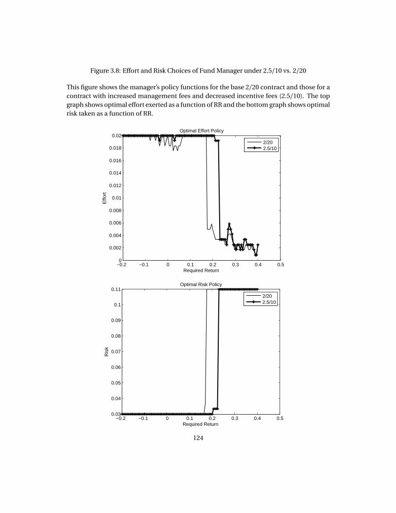
Figure 3.8: Effort and Risk Choices of Fund Manager under 2.5/10 vs. 2/20

This figure shows the manager’s policy functions for the base 2/20 contract and those for acontract with increased management fees and decreased incentive fees (2.5/10). The topgraph shows optimal effort exerted as a function of RR and the bottom graph shows optimalrisk taken as a function of RR.

−0.2 −0.1 0 0.1 0.2 0.3 0.4 0.50

0.002

0.004

0.006

0.008

0.01

0.012

0.014

0.016

0.018

0.02

Required Return

Effo

rt

Optimal Effort Policy

2/202.5/10

−0.2 −0.1 0 0.1 0.2 0.3 0.4 0.50.03

0.04

0.05

0.06

0.07

0.08

0.09

0.1

0.11

Required Return

Ris

k

Optimal Risk Policy

2/202.5/10

124

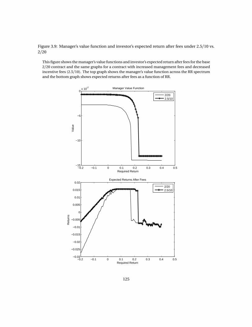
Figure 3.9: Manager’s value function and investor’s expected return after fees under 2.5/10 vs.2/20

This figure shows the manager’s value functions and investor’s expected return after fees for the base2/20 contract and the same graphs for a contract with increased management fees and decreasedincentive fees (2.5/10). The top graph shows the manager’s value function across the RR spectrumand the bottom graph shows expected returns after fees as a function of RR.

−0.2 −0.1 0 0.1 0.2 0.3 0.4 0.5−15

−10

−5

0x 1017

Required Return

Val

ue

Manager Value Function

2/202.5/10

−0.2 −0.1 0 0.1 0.2 0.3 0.4 0.5−0.03

−0.025

−0.02

−0.015

−0.01

−0.005

0

0.005

0.01

0.015

0.02

Required Return

Ret

urns

Expected Returns After Fees

2/202.5/10

125

Table 3.1: Summary Statistics

The table reports the summary statistics of the database of hedge fund returns used and isreproduced from Ray (2009). Panel A reports the characteristics of the funds and Panel Breports the return and walkaway characteristics of the funds.

Panel A: Fund Types and Fee Structures

Variable Mean Std. Dev NIncentive Fee (%) 17.23 6.45 8143Management Fee (%) 1.51 0.91 8304Sales Fee (%) 0.56 2.11 6326Active 0.51 0.5 8752Gate Percent (%) 12.7 15.92 175HWM Used? 0.96 0.19 872CPO Flag 0.13 0.33 8752CTA Flag 0.13 0.33 8752Hedge Fund Flag 0.5 0.5 8752Fund of Fund Flag 0.24 0.43 8752Index Flag 0.01 0.08 8752

Panel B: Return and Walkaway Characteristics

Variable Mean Std. Dev NExcess Returns (%) 0 5.786 493719Monthly Returns (%) 0.947 5.997 493719Return Process 1.991 2.397 493719Return to HWM 0.324 40.443 493719Walkaway 0.007 0.083 493719

126

Table 3.2: Model Calibration

The table shows model generated simulated moments alongside moments observed inempirical data as described in Ray (2009). The rows display the parameters used, popu-lation moments, regression results and observation dispersion across return required. Thefirst column shows actual moments observed in the data, the second column shows re-sults for base parameters, the third column shows results for a higher cost of effort and thefourth column shows results where all principals constantly monitor their investments.The regression coefficients are those obtained from the following two regressions.

r =α+δ1RR +δ′cont rol s +ε

and

σ=α+δ2RR +δ′cont rol s +ε

Observed Base γ= 0 α= 1

Parametersca 2 2 2γ 6 0 6α 0.85 0.85 1y 0.02 0.02 0.02β 0.95 0.95 0.95Sa 0.064 0.064 0.064 0.064Sb 0.65 0.65 0.65 0.65

Population MomentsAvg. Investor Returns (%) 0.95 1.53 3.63 1.44Return Std. Dev (%) 6.00 6.00 8.41 2.92Walkaway Rate (%) 0.70 1.33 0.00 2.07

Coefficientsβ1(0% ≤ RR < 10%) -5.8 -25.7 +7.5 -11.4β2(0% ≤ RR < 10%) +16.3 +192.6 +30.1 83.5β1(RR ≥ 10%) -0.0 +0.3 +7.5 -11.4β2(RR ≥ 10%) +0.0 +16.5 +30.1 83.5

Observation Dispersion(%)RR = 0% 40.5 62.5 66.5 66.20% < RR ≤ 10% 26.7 33.5 24.7 33.810%<RR≤100% 30.1 1.1 5.2 0.0100% < RR 2.7 2.9 3.6 0.0

127

Table 3.3: Welfare Analysis

This table shows model expected returns for the investor and for the hedge fund managerfor different contracts. The columns vary management fee from 1.5% to 3.0%. The rowsvary the incentive fees from 2.5% to 40.0%. The body of the table presents the expectedreturn after fees (ERAF) for the investor in the next period for a fund at the HWM and thechange in utility vis-a-vis the standard 2/20 contract for the fund manager managing afund at the HWM (∆ vm (.) is computed as −(vm (0|x/y )−vm (0|2/20))

vm (0|2/20) ). For example, for a 2.5/10contract, the investor expects a 1.33% return in the following period and the manager ishappier by 74.94% compared to the 2/20 contract.

Management FeeIncentive Fee Data 1.50% 2.00% 2.50% 3.00%2.50% rp f 0.76% 1.54% 1.50% 1.46%

∆ vm (.) -563.02% -115.96% 17.88% 57.69%5.00% rp f 0.88% 1.48% 1.44% 1.40%

∆ vm (.) -524.75% -27.78% 71.10% 88.61%7.50% rp f 1.08% 1.43% 1.39% 1.34%

∆ vm (.) -512.99% -11.58% 73.13% 91.51%10.00% rp f 1.03% 1.37% 1.33% 1.29%

∆ vm (.) -505.96% -12.85% 74.94% 91.16%12.50% rp f 0.98% 1.32% 1.27% 1.23%

∆ vm (.) -501.18% -1.31% 75.47% 92.01%15.00% rp f 0.93% 1.26% 1.22% 1.18%

∆ vm (.) -497.80% -0.06% 74.86% 92.14%17.50% rp f 0.88% 1.20% 1.16% 1.12%

∆ vm (.) -489.12% 0.11% 75.13% 92.24%20.00% rp f 0.83% 1.15% 1.10% 1.06%

∆ vm (.) -493.28% 0.00% 75.33% 92.31%22.50% rp f 0.78% 1.09% 1.05% 1.01%

∆ vm (.) -491.64% 0.60% 75.50% 91.71%25.00% rp f 0.73% 1.03% 0.99% 0.95%

∆ vm (.) -490.24% 1.12% 74.08% 92.42%27.50% rp f 0.68% 0.98% 0.93% 0.89%

∆ vm (.) -489.06% 0.48% 74.82% 91.80%30.00% rp f 0.63% 0.92% 0.88% 0.84%

∆ vm (.) -487.98% -1.95% 72.56% 90.63%32.50% rp f 0.58% 0.86% 0.82% 0.78%

∆ vm (.) -487.08% -1.61% 72.65% 90.19%35.00% rp f 0.53% 0.81% 0.76% 0.72%

∆ vm (.) -486.24% -3.25% 72.72% 88.84%37.50% rp f 0.48% 0.75% 0.71% 0.67%

∆ vm (.) -485.54% -8.26% 71.69% 88.87%40.00% rp f 0.43% 0.69% 0.65% 0.61%

∆ vm (.) -508.08% -8.04% 68.43% 86.88%

128

Appendix A

Supplement to Investment and

Financing under Reverse Asset

Substitution

A.1 Identification of Selection (Roy) Model

I want to identify the relative loadings of αs for s = {0, 1} on the term that represents RAS in

equation 1.8. If I find that firms with no access to the public debt markets have negative loading

on RAS variable, and if I find that firms with access to public debt markets do not load signifi-

cantly on RAS term, then that will be strong evidence in support of implications (P1) and (P2).

I need two normalizations on factor loadings to identify the model, hence normalizingσ2θ =

1, andσ2c = 1 suffices. These normalizations do not change the relative weights of α0,α1, which

is what is the goal of the exercise.

For shorthand, let us define:

U0 = α0θ +ε0

U1 = α1θ +ε1

Uc = αcθ +εc (A.1)

The additional investment D that the borrowing firm can make if the firm has access to public

129

debt markets is:

D = E[(I1− I0)−C |I ]

= X (β1−β0)−Zγ+E((U1−U0)−Uc |I ), (A.2)

where I represents the information set available to the borrowing firm making the choice be-

tween public debt markets and continued relationship with the lending bank. Using the defini-

tions from equation A.1, I get:

D =X (β1−β0)−Zγ− [(α0−α1)+αc ]θ −εc , (A.3)

please note that the above decomposition assumes that agents know the β , γ, and α. For the

sake of clarity in derivation, I now define two terms that represent the costs and benefits in

equation A.3.

µI (X ,Z ) ≡ X (β1−β0)−Zγ (A.4)

ϕ ≡ [(α0−α1)+αc ]θ +εc (A.5)

The above definition implies that ϕ ∼N (0,σ2φ)where

σ2ϕ = [(α0−α1)+αc ]2+1 (A.6)

Furthermore, we know that Cov(εs ,ϕ) = 0 for s = 0, 1 and

Cov(θ1,ϕ) = [(α0−α1)+αc ] (A.7)

The decision rule of whether to pay the cost and access the public debt markets or to con-

tinue in a relationship with the bank and suffer RAS, depends on whether µI (X ,Z ) is less than

or more than can now be rewritten as:

S = 1 ⇔ ϕ ≤ µI (X ,Z ), S = 0 ⇔ ϕ > µI (X ,Z ), (A.8)

130

Thus I can calculate the expectation of firms accessing public debt markets:

E(S|X ,Z ) = P(S = 1|X ,Z ) =P(ϕ ≤ µI (X ,Z ))

= Φ(X(β1−β0)σϕ

−Zγ

σϕ) (A.9)

We can show that mean observed investment satisfies:

E(I0|X ,Z ,ϕ > µI (X ,Z )) = Xβ0+α0[(α0−α1)+αc ]

σϕ

φ( µI (X ,Z )σϕ)

1−Φ(( µI (X ,Z )σϕ))

(A.10)

E(I1|X ,Z ,ϕ ≤ µI (X ,Z )) = Xβ1+α1[(α0−α1)+αc ]

σϕ

φ( µI (X ,Z )σϕ)

Φ(( µI (X ,Z )σϕ))

(A.11)

I now apply Heckman (1976) two-step procedure. From equation (A.9), I obtain consistent esti-

mator of γσϕ

and (β1−β0)σϕ

. From equation (A.10) and (A.11), I obtain consistent estimator of βs for

s = 0, 1. Now, to identify α0,α1, I use the variance and covariance relationships:

Cov(I0, D |X ,Z ) =α0[(α0−α1)+αc ]

Cov(I1, D |X ,Z ) =α1[(α0−α1)+αc ] (A.12)

The scaled covariance gives us a relation between the loadings on RAS in the two groups:

Cov(I1, D |X ,Z )Cov(I0, D |X ,Z )

=α1

α0(A.13)

The other moment condition can be obtained from the variance equations:

Var(I0, D |X ,Z ) =α20+σ

2ε

Var(I1, D |X ,Z ) =α21+σ

2ε. (A.14)

The above equations provide the following moment condition:

Var(I1, D |X ,Z )−Var(I0, D |X ,Z ) =α21−α

20 (A.15)

Using moment conditions A.13 and A.15, I identify α0,α1. Furthermore, once I have α0,α1, I

131

also identifyσε using the set of variance equations A.14.

A.2 Likelihood Estimation for Selection Model

I calculate likelihood by constructing the likelihood conditional on the unobservable θ and then

integrating θ out. First, I assume that the factor θ is observable. In this case, the data would be

(I ,S, X ,θ )where

Y = (1−S)I0+SI1, (A.16)

and let (I i , s i , X i ,θ i ) denote the data from firm i . The likelihood is:

L =ΠIi=1[ f (I

i0 |s

i = 0,θ i )P(s i = 0|θ i ) f (θ i )]1−s i[ f (I i

1 |si = 1,θ i )P(s i = 1|θ i ) f (θ i )]s

i

where

f (θ i ) = (2π)−1(σ21σ

22)− 1

2 exp (−1

2σ21

(θ i )2)

f (y i0 |s

i = 0,θ i ) = (2π)−12 (σ2

ε)− 1

2 exp{−1

2σ2ε

(I i0 −X iβ0−α0θ

i )2}

f (y i1 |s

i = 1,θ i ) = (2π)−12 (σ2

ε)− 1

2 exp{−1

2σ2ε

(I i1 −X iβ1−α1θ

i )2}

P(s i = 1|θ i ) = Φ(µI (X i ,Z i )− [(α0−α1)+αc ]θ i ) (A.17)

Now I recognize the fact that we do not observe θ , hence we can not write the likelihood condi-

tional on θ . I integrate it out:

L =ΠIi=1

∫

[ f (y i0 |s

i = 0,θ i )P(s i = 0|θ i ) f (θ i )]1−s i[ f (y i

1 |si = 1,θ i )P(s i = 1|θ i ) f (θ i )]s

idθ i (A.18)

The log-likelihood can thus be written as:

l =I∑

i=1

ln

∫

[ f (y i0 |s

i = 0,θ i )P(s i = 0|θ i ) f (θ i )]1−s i[ f (y i

1 |si = 1,θ i )P(s i = 1|θ i ) f (θ i )]s

idθ i (A.19)

132

A.3 Data Description

A.3.1 Bank Variables

• Total Assets of the Bank: RCFD2170 from Commercial Bank Data.

• Total Loans extended: RCFD2122 from Commercial Bank Data.

• Loan Ratio: Total loans as a fraction of total assets of the bank.

• Tier 1 Capital of the Bank: RCFD8274 from Commercial Bank Data.

• Capital Ratio: Total tier 1 capital as a fraction of total assets of the bank.

• Bank Holding Company ID: RSSD9348 (See Structure and Geographical Variables).

A.3.2 Firm Variables (Annual)

Annual data items from the CRSP/Compustat Merged database, are first listed, followed by the

calculations underlying the constructed variables. The construction of the variables follows

Eberly, Rebelo, and Vincent (2008), and hence this part of the appendix also follows the same.

• I, Investment : expenditures on property, plant, and equipment, data 30

• CF, CashFlow : Income before extraordinary items+ depreciation and amortization+minor

adjustments, calculated as follows (from the Compustat manual): Income Before Extraordi-

nary Items, 123 +Depreciation and Amortization, 125

+ Extraordinary Items and Discontinued Operations, 124

+Deferred Taxes, 126

+ Equity in Net Loss (Earnings), 106

+ Sale of Property, Plant, and Equipment and Sale of Investments .Loss(Gain), 213

+ Funds from Operations - Other, 217

+ Accounts Receivable - Decrease (Increase), 302

+ Inventory - Decrease (Increase), 303

+ Accounts Payable and Accrued Liabilities - Increase (Decrease), 304

+ Income Taxes - Accrued - Increase (Decrease), 305

+ Assets and Liabilities - Other (Net Change), 307

133

=Operating Activities - Net Cash Flow, 308

• Inventories : total inventories (end of period), data 3 30

• Debt: Long-term debt (end of period), data 9

• PPE: Book value of capital: property, plant, and equipment, - data 182: PPE - Beginning Bal-

ance - check if it is still reported after

1997; - data 187: PPE - Ending Balance (Schedule V);

- data 184: PPE - Retirements (Schedule V) - not reported after 1997;

- data 185: PPE - Other Changes (Schedule V) - not reported after 1997.

• Price of capital: implicit price deflator for nonresidential investment, Economic Report of

the President, Table B-3, various years.

• Market Value of Equity: Closing stock price times number of common shares outstanding

(end of period) plus redemption value of preferred stock (end of period) = prc * shrout/1000

+ data56, where,

- prc: closing stock price ;

- shrout: Common shares outstanding ;

- data 56: Preferred Stock - Redemption Value.

• L: Useful life of capital goods: by two-digit industry, the useful life of cap- ital goods is calcu-

lated as L j ≡ 1N j

∑

i∈jPPE i ,t−1+DE PRi ,t−1+I i ,t

DE PRi ,t, where N j is the number of firms, i, in industry j.

Using the double-declining balance method, the implied depreciation rate for industry j, δj ,

is 2/L j .

• K, replacement value of capital stock: Using the method of Salinger and Summers (1983) the

replacement value of the capital stock is constructed by firm from its book value using the

recursion: K i ,t =�

K i ,t−1PK ,t

PK ,t−1+ I i ,t

�

(1−δj ), where the recursion is initialized using the book

value of capital.

• Q, Tobin’s Q: [(market value of equity)t−1+(debt)t−1− (inventories)t−1]/K t .

134

Appendix B

Supplement to Heterogeneity inCorporate Governance: Theory andEvidence

B.1 A Simple Static Model

The firm with capital K pays an adjustment cost φ(I /K ) on its investments I . Thus, the totalcost per unit capital of investment is:

c (i )≡I

K+φ(I /K )

The firm faces a depreciation rate of δ > 0 on its capital. Therefore, the law of motion of capitalis:

d K t = (I t −δK t )d t , t ≥ 0

The cash flow process for the firm is as follows:

d Yt = K t (d A t − c (i t )d t )

where A t is the production technology of the firm.The agent’s efforts a t and the autonomy M t given to the agent affects the firm’s production

technology as below:d A t = a t M tµd t +σdZt , t ≥ 0

The agent enjoys private benefits at the rate λ(M t −a t )µd tSuppose that the performance q of a firm is equal to effort a times management autonomy

m with return to scale γminus money d that the agent can divert without possible verification

135

by the principal plus noise ε:q = a m γ−d +ε, (B.1)

where ε is normally distributed with zero mean and varianceσ2ε. The principal is assumed to be

risk neutral. The agent has constant absolute risk averse (CARA) risk preferences representedby the following negative exponential utility function:

u (w , a ) =−e−η[w+d−ψ(a )], (B.2)

where w is the monetary compensation and η> 0 is the agent’s coefficient of absolute risk aver-sion. Cost of effort ψ(a ) is assumed to be quadratic: ψ(a ) = 1

2 c a 2. Suppose that the principaland agent can write only linear contracts of form1:

w = t + sq , (B.3)

where t is the fixed compensation level and s is the variable performance related compensationof compensation and w is the contracted wage. The amount d that the agent can divert isproportional to autonomy m and private information u that the agent has about the output ofthe firm in the next period. The shock ε (say at time t ) experienced by the firm is composed oftwo parts: u that is observed by the agent before the period starts (at time t − 1), and a part vwhich is unknown to both the principal and an agent.

ε= u +v, (B.4)

The agent chooses to divert a constant fraction θ of observed shock. But she does so only whenthe shock observed is positive, i.e. u > 02. This means the real wage the agent is getting is:

w = w +d = t + sq +θ1(u > 0) (B.5)

The principal maximizes the output of the firm after paying the wage of the agent, subjectto the agent’s IC and IR constraints. The principal’s problem is then to solve:

maxa ,m ,s ,t E(q −w )

s.t. a ∈ arg maxaE�

− e−η(w−12 c a 2)

�

e−ηw mµ ≤E�

− e−η[w−ψ(a )]�

(B.6)

The first constraint above is the IC constraint of the agent - agent chooses her effort to optimize

1This constraint is not required in the general case, but helps convey our point. In later sections, we will considera larger contract space.

2This assumption can also be generalized. However, we will not do so in this section. The full model presentedlater does not make this assumption

136

her total wage. The IR constraint, follows, where w mµ gives the reservation wage of the agent.As in Gabaix and Landier (2007) and Edmans, Gabaix and Landier (2007), we make the assump-tion that talent of CEOs vary. The principal first solves the optimal autonomy problem and thenpicks an agent from a pool with the correct talent level to handle optimal autonomy. Thus,autonomy and talent, have one to one correspondence to each other and as talent increases,autonomy increases as well and vice-versa. The reservation wage of such an agent, hence, alsois proportional to autonomy m raised to a factor µ that represents talent.

The utility function of the agent can be rewritten as:

u (a , d ) = −e−η(t+s (a mγ−d+ε)+d− 12 c a 2)

= −e−η(t+s a mγ+d (1−s )− 12 c a 2+sε)

= −e−η(t+s a mγ− 12 c a 2+ f (η,m 2,σ2

u )(1−s )− η2 s 2σ2ε)

≡ −e−ηw (a ,m ), (B.7)

where c e w (a , m ) is the certainty equivalent compensation of the agent. The certainty equiv-alent wage consists of her expected compensation and option value of private diversion net ofcost of effort and risk premium. f (η, m 2,σ2

u ) represents the option value of private diversion.Risk premium η

2 s 2σ2ε is increasing in coefficient of risk aversion η, share of firm output s and

variance of firm output σ2ε. The option value increases in agent autonomy m , risk aversion η

and variance of private information about firm output σ2u . However, the option value is multi-

plied by 1−s as the agent denies herself a fraction s of the output of the firm if she diverts beforereporting firm performance.

The optimization problem of the agent is to get the most certainty equivalent wage by choos-ing effort a :

a ∈ arg maxa

c e w (a , m )

= t + s a m γ−1

2c a 2+ f (η, m 2,σ2

u )(1− s )−η

2s 2σ2

ε

s m γ− c a = 0

a ∗ =s m γ

c, (B.8)

i.e. the optimal effort by the agent increases in fraction of output she receives, the autonomyshe enjoys and decreases in the cost of effort she has to exert. We can now obtain the maximumcertainty equivalent payoff for the agent in terms of her effort a ∗:

w (a ∗, m ) = t +1

2

s 2m 2γ

c+ f (η, m 2,σ2

u )(1− s )(1− s )−η

2s 2σ2 (B.9)

137

Given the optimal level of effort a ∗ by the agent, principal solves the following problem:

maxm ,t ,sE[q −w ] = E[q − t − sq ]

= E[−t +(1− s )q ]

= E[−t +(1− s )(a m −d +ε)]

= −t +(1− s )�

s m 2γ

c− g (η, m 2,σ2

u )�

(B.10)

where the agent’s optimal effort enters as a constraint:

t +1

2

s 2m 2γ

c+ f (η, m 2,σ2

u )(1− s )−η

2s 2σ2 = w mµ (B.11)

E[d ] = g (η, m 2,σ2u ) represents private diversion that the principal expects the agent to make.

This may not be the real amount diverted. The dynamic game of interest is to figure out theoptimal policy of diversion of the agent, given that she knows that the principal is updating hisexpectation about agent’s diversion from output reported. The difference between f (.) and g (.)will decide the autonomy chosen by the principal, as we shall see later in equation B.14.

The Lagrangian in this case is:

L =−t +(1− s )�

s m 2γ

c− g (η, m 2,σ2

u )�

+λ(t +1

2

s 2m 2γ

c+ f (η, m 2,σ2

u )(1− s )−η

2s 2σ2− w mµ)

(B.12)on differentiating w.r.t. t we get:

λ= 1

Differentiating w.r.t. s , we get:

∂L∂ s

=∂

∂ s[−

1

2

s 2m 2γ

c+

s m 2γ

c−η

2s 2σ2

ε]

= −s m 2γ

c+

m 2γ

c−ηsσ2

ε

This yields optimal fraction s ∗ in terms of variance and autonomy:

s ∗ =m 2γ

m 2γ+ηcσ2 , (B.13)

i.e. the fraction of the performance to be given to the agent increases with the autonomy en-joyed by the agent, and decreases with variance of output, risk aversion of agent and cost ofexerting effort by the agent. As agent autonomy increases, is fraction of firm performance doesnot increase, then agent’s incentive to divert will increase, and hence the result is intuitive.

138

Differentiating the lagrangian w.r.t. autonomy m , we get:

∂L∂m

=∂

∂m

�

(1− s )�

s m 2γ

c− g (η, m 2,σ2

u )�

+1

2

s 2m 2γ

c+ f (η, m 2,σ2

u )(1− s )− w mµ

�

=∂

∂m

�

(1− s )�

s m 2γ

c− g (η, m 2,σ2

u )+ f (η, m 2,σ2u ))�

+1

2

s 2m 2γ

c− w mµ

�

= (1− s )�

2γs m 2γ−1

c− g ′(η, m 2,σ2

u )+ f ′(η, m 2,σ2u )�

+γs m 2γ−1

c−µw mµ−1

Equating the right hand side to zero, we get:

[(1− s )c ( f m (η, m 2,σ2u )− g m (η, m 2,σ2

u ))]+ [(2− s )γs m 2γ−1−µw mµ−1] = 0 (B.14)

Taking the constant return to scale case on autonomy i.e. γ= 1,µ= 1 and assuming princi-pal expects no diversion i.e. g (η, m 2,σ2

u ) = 0 we have:

(1− s )c f m (η, m 2,σ2u ) =µw − (2− s )γs m (B.15)

Option value increases in σ2u . Assuming that private information u is a (stationery) fraction of

total information ε, we have shown that there is a negative relation between observed outputvariance and autonomy.

Section 2.2.1 provides a dynamic model and shows that the negative relation exists there aswell.

B.2 Proof of Lemma 2.2.2

This lemma derives from Theorem 6 of Hölmstrom and Milgrom (1987), Corollary 4.1 of Schät-tler and Sung (1993), corollary B of Ou-Yang (2003) and Lemma 2 of Ou-Yang (2005).

By Ito’s Lemma, d V (t , K (t ), Y (t ), M (t ))≡ d V (t , X (t )) is given by:

d V (t , X (t )) =�

Vt (X (t ), t )+VX (X (t ), t )Tµ(X (t ))+1

2tr[VX X (X (t ), t )σ(K )σ(K )T ]

�

d t

+VX (X (t ), t )Tσ(K )d w (t ) (B.16)

Rewriting agent’s bellman condition 2.10, we have:

Vt +VK µ(X (t ))+1

2tr[VX X (X (t ), t )σ(K )σ(K )T ] =RA V (t , K )[g (t , X )+h(t , X )µ(X )− c (t ,η, M , d )

−1

2RAσ(X )h(t , X )hT (t , X )σT (X )]+VK RAσ(Y )h(t , X )σT (Y ) (B.17)

139

Substitute for the drift term in equation B.16 with the above equation, we get:

d V (t , X (t )) =�

RA V (t , K )[g (t , K )+h(t , K )µ(X )− c (t ,η(t ), M (t ), d )

−1

2RAσ(X )h(t , X )hT (t , X )σ(X )]+VX RAσ(Y )h(t , X )σT (Y )

�

d t +VXσ(Y )d w (B.18)

We now define W (t ) such that RA W (t ) =− log[−RA V (T, X (t ))], where WT = q (T, KT ) as definedin equation 2.8.

Differentiating W (t ), and using the expression of d V (t , X (t )), we get:

RA d W (t ) = −d V

V+

1

2

�

d V

V

�2

= −RA

�

g +hµ(X )− c −1

2RA hσ(X )σT (X )h

T�

d t +RA (h −h)σ(Y )d w , (B.19)

where h ≡ h − VKRA V .

The last expression can be rearranged as:

d W (t )+ g (.)d t +h(µ(X )d t +σ(Y )d w ) = c d t +RA

2hσ(Y )σT (Y )hd t +hσ(Y )d w (B.20)

which is the same as:

S(t ) =W M +

∫ T

0

c (t ,η(t ), M (t ), d )d t +RA

2

∫ T

0

hσ(Y )σT (Y )hd t +

∫ T

0

hσ(X )d w (t ) (B.21)

B.3 Proof of Theorem 2.2.3

The investor’s value function is given by:

J (t , K , M ) = supηE0

�

−1

RPe−RP (d Wt−dSt )

�

,

where K and M are the initial capital and autonomy values. Thus, we get the principal’s Bellmanequation:

supη

J

�

RP c +RA RP

2h2σ2

K

�

+R2

P

2h2σ2

K + Jt + JW

�

r W +µQ +RP hσ2K

�

+1

2JW Wσ

2K + JK

�

µK +RPσ2K h

�

+1

2JK Kσ

2K + JW Kσ

2K = 0. (B.22)

140

Conjecture that the principal’s value function is given by:

J (t , K t , M t ) =−1

RPexp[−RP ( f 1(t )K t + f 2(t ))],

where f 1(t ), f 2(t ) are continuous deterministic functions of time with boundary conditions f 1(∞) =1, f 2(∞) = 0.

The Bellman equation then becomes:

supη

�

c +RA +RP

2σ2

K h2− f 1(t )K − f 2(t )− f 1(t )�

µK +RP hσ2K

�

+RP

2f 2

1 (t )σ2K

�

= 0

To satisfy the above Bellman equation, we must have the following condition (by taking thecoefficient of W from above):

f 1(t )+µK f 1(t ) = 0 or f 1 = e−∫ t+d t

tµK d t

The FOC with respect to η now reduces to:

κη+(RA +RP )

log mσ2

K hκ(t )∂

∂ η

η

K αMη−∂

∂ ηf 1(t )

�

K αMη+RPκ(t )η

K αMη log Mσ2

K

�

= 0

which yields an implicit solution for η∗:

κη∗+(RA +RP )

log Mσ2

K hκ(t )1

K αMη∗[1−η log M ]

−e−∫ t+d t

tµK d t

�

K αMη∗ log M +RPκ(t )

K αMη∗ log M[1−η log M ]σ2

K

�

+K αMη log M e−∫ t+d t

tµK d t

�

K αMη+RPκ(t )η

K αMη log Mσ2

K

�

= 0

The FOC with respect to M reduces to:

− d (t )+ (RA +RP )σ2K hκ(t )η

∂

∂M

1

K αMη log M−∂

∂Me−

∫ t+d tt

µK d t�

K αMη+RPκ(t )η

K αMη log Mσ2

K

�

= 0

which yields:

−ζ(t )M −(RA +RP )σ2

K hκ(t )η(1+η log M )(log M )2K αMη+1

−e−∫ t+d t

tµK d t

�

ηK αMη−1−RPκ(t )η(1+η log M )σ2

K

(log M )2K αMη+1

�

+ηK αMη−1e−∫ t+d t

tµK d t

�

K αMη+RPκ(t )η

K αMη log Mσ2

K

�

= 0

141

B.4 Proof of Theorem 2.2.4

The principal’s value function is given by:

J (t , K , M ) = supd ,uE0

�

−1

RPe−RP (d Wt−dSt )

�

,

where K and M are the initial capital and autonomy values. As in Davis and Norman (1990), toeasily characterize optimal policies, let us consider a restricted class of policies in which D andU are constrained to be absolutely continuous with bounded derivatives, i.e.

Dt =

∫ t

0

d s d s , Ut =

∫ t

0

u s d s , 0≤ l s , u s ≤ θ , (B.23)

Thus, we get the principal’s Bellman equation:

supη

J

�

RP c +RA RP

2h2σ2

K

�

+R2

P

2h2σ2

K + Jt

+JK

�

µK +RP hσ2K

�

+1

2JK Kσ

2K + JM

�

r M +RP hσ2K

�

+1

2JM Mσ

2K + JK Mσ

2K

+[JM − (1+λ−)JK ]l +[JK (1−λ+)− JM ]u = 0. (B.24)

Conjecture that the principal’s value function is given by:

J (t , K t , M t ) =−1

RPexp[−RP ( f 1(t )K t + f 2(t )+φ(M ))],

where f 1(t ), f 2(t ) are continuous deterministic functions of time with boundary conditions f 1(∞) =1, f 2(∞) = 0.

The Bellman equation then becomes:

supη

�

c +RA +RP

2σ2

K h2− f 1(t )K − f 2(t )− f 1(t )�

µK +RP hσ2K

�

+RP

2f 2

1 (t )σ2K

−φM

�

r M +RP hσ2K

�

+RP

2φM Mσ

2K +

RP

2f 2

3 (t )φ2Mσ

2K +

RP

2f 1(t )φMσ

2K

+[φM − (1+λ−) f 1(t )]l +[ f 1(t )(1−λ+)−φM ]u = 0.

�

= 0

To satisfy the above Bellman equation, we must have the following condition (by taking thecoefficient of K from above):

f 1(t )+µK f 1(t ) = 0 or f 1 = e−∫ t+d t

tµK d t

142

Taking the coefficients of controls l , u :

e−∫ t+d t

tµK d t (1−λ+)≤φM ≤ (1+λ−)e−

∫ t+d t

tµK d t

B.5 Proof of Theorem 2.2.8

We give a quick intuition first:d =µ+λy , d =α+βv

Given the rules above, diversion can be written as:

(d − d (d + u ))(σ2) = (v −µ−λσ2)σ2

We thus have from FOC:1/β = 2λ, α=−µβ

In equilibrium,d =E(v |α+β v + u = y ),

which yields:

λ=βvar(v)

β2var(v)+var(u), µ= 0

Thus optimal diversion in equilibrium is proportional to the variance of output of the firm.Now for the full proof. Substituting the laws of motion of capital and optimal contract, the

agent’s objective function becomes:

supV :DE0−

1

RAexp

�

−RA

�

W M−d+d+RA

2h2σ2

K d t−hµK

�

d t+h

�

(K αt Mη+(r+δ)K t−d )d t+σY d w

��

which can be written as:

supV :DE0−

1

RAexp

�

−RA

�

(g (K , M ,η)+ d (1− h)− d )d t +σY d w

��

,

where g (.) collects all the terms which do not depend on the choice of d in the present period.Taking out g (K , M ,η) from the exponential so that exp g (.)≡G (.), we have:

supV :D−

G (K , M ,η)RA

exp

�

−RA

�

(d (1− h)− d −1

2h2σ2

U )d t

��

,

As this is a negative exponential utility function, the optimal policy V for the principal givenagent’s policy D is to have policy:

d (1− h)− d −1

2h2σ2

U = 0,

143

i.e.:

d =1

1− h[d +

h2

2σ2

U ]

In equilibrium, if d = v , then:

d =1

1− h[v +

h2

2σ2

U ] (B.25)

144

Bibliography

Acharya, Viral V, Yakov Amihud, and Lubomir P. Litov, 2010, Creditor Rights and Corporate Risk-

taking, Journal of Financial Economics Forthcoming.

Acharya, Viral V., and Krishnamurthy V. Subramanian, 2009, Bankruptcy Codes and Innovation,

Review of Financial Studies 22, 4949–4988.

Berk, Jonathan B., and Richard C. Green, 2004, Mutual Fund Flows and Performance in Rational

Markets, Journal of Political Economy 112, 1269–1295.

Berk, Jonathan B., and Ian Tonks, 2007, Return persistence and fund flows in the worst perform-

ing mutual funds, Working Paper.

Bharath, Sreedhar T., Sandeep Dahiya, Anthony Saunders, and Anand Srinivasan, 2009, Lending

Relationships and Loan Contract Terms, The Review of Financial Studies p. Forthcoming.

Bradley, Michael, and Michael R. Roberts, 2004, The Structure and Pricing of Corporate Debt

Covenants, SSRN eLibrary.

Brown, Stephen J, William N Goetzmann, and Roger G Ibbotson, 1999, Offshore Hedge Funds:

Survival and Performance, 1989-95, Journal of Business 72, 91–117.

Brown, Stephen J., William N. Goetzmann, and James Park, 2001, Careers and Survival: Compe-

tition and Risk in the Hedge Fund and CTA Industry, Journal of Finance 56, 1869–1886.

145

Burkart, Mike, Denis Gromb, and Fausto Panunzi, 1997, Large Shareholders, Monitoring, and

the Value of the Firm, The Quarterly Journal of Economics 112, 693–728.

Cadenillas, Abel, Jaksa Cvitanic, and Fernando Zapatero, 2005, Dynamic Principal-Agent Prob-

lems with Perfect Information, Working Paper.

Carhart, Mark M., Jennifer N. Carpenter, Anthony W. Lynch, and David K. Musto, 2002, Mutual

Fund Survivorship, Rev. Financ. Stud. 15, 1439–1463.

Carneiro, Pedro, Karsten T. Hansen, and James J. Heckman, 2003, Estimating Distributions of

Treatment Effects with an Application to the Returns to Schooling and Measurement of the

Effects of Uncertainty on College Choice, IZA Discussion Papers 767 Institute for the Study of

Labor (IZA).

Chava, Sudheer, and Michael R. Roberts, 2007, How Does Financing Impact Investment? The

Role of Debt Covenants, Journal of Finance.

Christoffersen, Susan E. K., and David K. Musto, 2002, Demand Curves and the Pricing of Money

Management, Rev. Financ. Stud. 15, 1499–1524.

Cunha, Flavio, James Heckman, and Salvador Navarro, 2005, Separating uncertainty from het-

erogeneity in life cycle earnings, Oxford Economic Papers 57, 191–261.

Demarzo, Peter M., and Yuliy Sannikov, 2004, A Continuous-Time Agency Model of Optimal

Contracting and Capital Structure, Working Paper.

DeMarzo, Peter M., and Yuliy Sannikov, 2006, Optimal Security Design and Dynamic Capital

Structure in a Continuous-Time Agency Model, Journal of Finance 61.

146

Denis, David J., and Vassil T. Mihov, 2003, The choice among bank debt, non-bank private debt,

and public debt: evidence from new corporate borrowings, Journal of Financial Economics

70, 3 – 28.

Dewatripont, Mathias, Patrick Legros, and Steven A. Matthews, 2003, Moral Hazard and Capital

Structure Dynamics, Journal of the European Economic Association 1, 890–930.

Dichev, Ilia D., and Douglas J. Skinner, 2002, Large-Sample Evidence on the Debt Covenant

Hypothesis, Journal of Accounting Research 40, 1091–1123.

Eberly, Janice, Sergio Rebelo, and Nicolas Vincent, 2008, Investment and Value: A Neoclassical

Benchmark, Working Paper 13866 National Bureau of Economic Research.

Faulkender, Michael, and Mitchell A. Petersen, 2006, Does the Source of Capital Affect Capital

Structure?, Rev. Financ. Stud. 19, 45–79.

Fischer, Klaus, 1990, Hausbankbeziehungen als Instrument der Bindung zwischen Banken und

Unternehmen, Ph.D. Thesis, Universität Bonn.

Fudenberg, Drew, and Tirole, Jean, 1995, A Theory of Income and Dividend Smoothing Based

on Incumbency Rents, The Journal of Political Economy 103, 75–93.

Goetzmann, William N., Jonathan E. Ingersoll, and Stephen A. Ross, 2003, High-Water Marks

and Hedge Fund Management Contracts, Journal of Finance 58, 1685–1718.

Gompers, Paul A., Joy L. Ishii, and Andrew Metrick, 2003, Corporate Governance and Equity

Prices, Quarterly Journal of Economics 118, 107–155.

Graham, John R., 2000, How Big Are the Tax Benefits of Debt?, The Journal of Finance 55, 1901–

1941.

147

Graham, John R., 2003, Taxes and Corporate Finance: A Review, Review of Financial Studies 16,

1075–1129.

Hale, Galina, and João A.C. Santos, 2009, Do banks price their informational monopoly?, Journal

of Financial Economics 93, 185–206.

Hart, Oliver, and John Moore, 1998, Default And Renegotiation: A Dynamic Model Of Debt, The

Quarterly Journal of Economics 113, 1–41.

Heckman, James J., 1976, A Life-Cycle Model of Earnings, Learning, and Consumption, The Jour-

nal of Political Economy 84, S9–S44.

Heckman, James J., and Salvador Navarro-Lozano, 2003, Using Matching, Instrumental Vari-

ables and Control Functions to Estimate Economic Choice Models, IZA Discussion Papers

768 Institute for the Study of Labor (IZA).

Hirschman, Albert O., 1964, The Paternity of an Index, The American Economic Review 54, 761–

762.

Hodder, James E., and Jens C. Jackwerth, 2007, Incentive Contracts and Hedge Fund Manage-

ment, Journal of Financial and Quantitative Analysis 42.

Holmstrom, Bengt, and Paul Milgrom, 1987, Aggregation and Linearity in the Provision of In-

tertemporal Incentives, Econometrica 55, 303–328.

Horvitz, D. G., and D. J. Thompson, 1952, A Generalization of Sampling Without Replacement

From a Finite Universe, Journal of the American Statistical Association 47, 663–685.

Hoshi, Takeo, Anil Kashyap, and David Scharfstein, 1991, Corporate Structure, Liquidity, and

Investment: Evidence from Japanese Industrial Groups, The Quarterly Journal of Economics

106, 33–60.

148

Jewitt, Ian, 1988, Justifying the First-Order Approach to Principal-Agent Problems, Econometrica

56, 1177–1190.

Kalai, Ehud, and Ehud Lehrer, 1993, Rational Learning Leads to Nash Equilibrium, Economet-

rica 61, 1019–1045.

Kashyap, Anil K, and Jeremy C. Stein, 2000, What Do a Million Observations on Banks Say about

the Transmission of Monetary Policy?, The American Economic Review 90, 407–428.

Kerr Christoffersen, Susan E., and David K. Musto, 2008, High Water Marks in Competitive Cap-

ital Markets, SSRN eLibrary.

Kuhn, Peter, 1994, Nonrevelation in Employment Contracts, International Economic Review 35,

261–282.

Kyle, Albert S., 1985, Continuous Auctions and Insider Trading, Econometrica 53, 1315–1335.

La Porta, Rafael, Florencio Lopez-de Silanes, Andrei Shleifer, and Robert Vishny, 2000, Investor

Protection and Corporate Governance, The Journal Of Financial Economics, 2000 58, 3–27.

Laffont, Jean-Jacques, and Jean Tirole, 1988, The Dynamics of Incentive Contracts, Economet-

rica 56, 1153–1175.

Lambert, Richard A., 1984, Income Smoothing as Rational Equilibrium Behavior, The Account-

ing Review 59, 604–618.

Mayer, Colin, 1988, New issues in corporate finance, European Economic Review 32, 1167 – 1183.

Metrick, Andrew, and Ayako Yasuda, 2007, The Economics of Private Equity Funds, Working

Paper.

Nini, Gregory, David C. Smith, and Amir Sufi, 2009, Creditor Control Rights and Firm Investment

Policy, Journal of Financial Economics.

149

Ou-Yang, Hui, 2003, Optimal Contracts in a Continuous-Time Delegated Portfolio Management

Problem, Review of Financial Studies 16, 173–208.

Ou-Yang, Hui, 2005, An Equilibrium Model of Asset Pricing and Moral Hazard, Rev. Financ. Stud.

18, 1253–1303.

Panageas, Stavros, and Mark M. Westerfield, 2008, High-Water Marks: High Risk Appetites? Con-

vex Compensation, Long Horizons, and Portfolio Choice, forthcoming, Journal of Finance.

Petersen, Mitchell A, and Raghuram G Rajan, 1994, The Benefits of Lending Relationships: Evi-

dence from Small Business Data, Journal of Finance 49, 3–37.

Petersen, Mitchell A., and Raghuram G. Rajan, 1995, The Effect of Credit Market Competition

on Lending Relationships, The Quarterly Journal of Economics 110, 407–443.

Rajan, Raghuram G, 1992, Insiders and Outsiders: The Choice between Informed and Arm’s-

Length Debt, Journal of Finance 47, 1367–400.

Rajan, Raghuram G., and Luigi Zingales, 1995, What Do We Know about Capital Structure? Some

Evidence from International Data, The Journal of Finance 50, 1421–1460.

Rauh, Joshua D., and Amir Sufi, 2008, Capital Structure and Debt Structure, NBER Working Pa-

pers 14488 National Bureau of Economic Research, Inc.

Ray, Sugata, 2009, The Downside of High Water Marks, Working Paper.

Rice, Tara, and Philip E. Strahan, 2010, Does Credit Competition Affect Small-Firm Finance?,

Journal of Finance 65, 861–889.

Rosenbaum, Paul R., and Donald B. Rubin, 1983, The central role of the propensity score in

observational studies for causal effects, Biometrika 70, 41–55.

150

Roy, A. D., 1951, Some Thoughts on the Distribution of Earnings, Oxford Economic Papers 3,

135–146.

Sannikov, Yuliy, 2006, A Continuous-Time Version of the Principal-Agent Problem, Working Pa-

per.

Schattler, Heinz, and Jaeyoung Sung, 1993, The First-Order Approach to the Continuous-Time

PrincipalUAgent Problem with Exponential Utility, Journal of Economic Theory, 61, 331–371.

Schwartz, Eduardo S., and Walter N. Torous, 1989, Prepayment and the Valuation of Mortgage-

Backed Securities, The Journal of Finance 44, 375–392.

Sharpe, Steven A., 1990, Asymmetric Information, Bank Lending and Implicit Contracts: A Styl-

ized Model of Customer Relationships, The Journal of Finance 45, 1069–1087.

Trueman, Brett, and Sheridan Titman, 1988, An Explanation for Accounting Income Smoothing,

Journal of Accounting Research 26, 127–139.

Wooldridge, Jeffrey M., 2004, Estimating average partial effects under conditional moment inde-

pendence assumptions, CeMMAP working papers CWP03/04 Centre for Microdata Methods

and Practice, Institute for Fiscal Studies.

151