Age-Structured Modeling of

Hematopoiesis

Joseph M. Mahaffy∗

CRM-2609

May 1999

∗Department of Mathematical Sciences, San Diego State University, San Diego, CA 92182. This work was sup-ported in part by NSF grant DMS-9608290.

Abstract

Age-structured models for hematopoiesis allow the study of several dynamic hematolog-ical diseases and the effects of a phlebotomy in normal human subjects. The methodof characteristics with several simplifying assumptions reduces the age-structured modelto a system of delay differential equations, which is analyzed for Hopf bifurcations andis more easily simulated. The model can explain the appearance of oscillations in ery-throcyte counts in rabbits with an induced auto-immune hemolytic anemia. The modelcan match cumulative data following a blood donation, but falls short of predicting anormal individual due to other feedback controls.

Some Key Words and Phrases:Age-structured models ; hematopoiesis, periodicdiseases ; erythropoiesis ; delay differential equations ; method of characteristics ; Hopfbifurcation.

Resume

Les modeles d’hematopoıese avec structure d’age permettent d’etudier de nombreusesmaladies dynamiques hematologiques, de meme que l’effet d’une phlebotomie chez unsujet normal. La methode des caracteristiques permet, sous des hypotheses simplifica-trices, la reduction de ces modeles structures a un systeme d’equations differentielles aretards, qu’il est plus aise d’analyser, pour detecter des bifurcations de Hopf, et de simu-ler numeriquement. Ce modele peut expliquer la presence d’oscillations dans le niveaudes erythrocytes chez le lapin atteint d’une anemie hemolytique auto-immune induite.Le modele peut reproduire la moyenne des niveaux de cellules chez les donneurs, maisn’est pas suffisamment sensible aux nombreux autres mecanismes de retroaction pourbien representer les fluctuations chez un individu.

Introduction

Age-structured mathematical models provide an effective means of understanding various biologicalphenomena for large populations. Hematopoiesis is the process by which stem cells residing primarilyin the bone marrow, spleen, and liver proliferate and differentiate into the major types of blood cells.Thus, hematopoiesis with its many stages of development lends itself naturally to age-structuredmodeling and has been studied by numerous researchers in this manner [3, 16, 29, 30, 44, 48, 49, 52].

Various other modeling techniques have been applied to hematopoietic systems, including com-partmental models [61, 62, 63, 64, 77], stochastic models [37, 41, 54, 71, 72], and delay differentialequations [2, 32, 33, 42, 43, 44, 46, 75]. This survey shows a connection between the age-structuredmodels and delay differential equation models [3, 44, 48, 49]. The age-structured models relatemore easily to the biological system, while the delay differential equations are easier to analyzemathematically.

Our interest in studying mathematical models for hematopoiesis centers on two areas. Thefirst area of study examines dynamic hematological diseases [17, 26, 32, 44, 45, 59], where one ormore of the circulating hematopoietic cell lines oscillate. Examples of these periodic hematologicaldisorders include cyclical neutropenia [12, 13, 32, 35, 39, 62, 64, 79, 80], chronic myelogenousleukemia [9, 14, 22, 25, 36, 50, 51, 60, 65, 76], periodic auto-immune hemolytic anemia [28, 56, 58],polycythemia vera [53], and cyclical thrombocytopenia [5, 6, 8, 10, 15, 18, 27, 40, 66, 70, 74, 78].It is likely that abnormalities in the regulatory control processes result in the observed oscillatoryphenomena, but often the defective mechanisms are not known.

A second area of study looks at the normal production of red blood cells, erythropoiesis, todetermine if a mathematical model might be used to optimize the collection of blood. The diseaseAIDS has caused great public alarm in the blood supplies. Though tremendous gains have beenmade in protecting the safety of the blood supplies, there are many times when the national bloodsupply is low. A mathematical model might suggest ways to improve the rate of collection from thecurrent eight week time table between blood donations or increase the amount of blood collectedfrom autologous donors, who donate for their own elective surgery.

This review article provides a brief summary of the physiological processes for erythropoiesis,then transforms this descriptive biological model into an age-structured model. Next several simpli-fying assumptions allow the reduction of the age-structured model to a system of delay differentialequations, using the method of characteristics. A Hopf bifurcation analysis shows how this modelcan produce oscillatory behaviors. In Section 4, the system of delay differential equations has itsparameters identified by comparison to experimental data in the literature for both a rabbit with aninduced auto-immune hemolytic anemia and normal human males following a phlebotomy. Finally,a discussion follows to summarize the results of our modeling efforts to date.

1 The Physiology and an Age-Structured Model

Hematopoiesis begins from a population of undifferentiated stem cells, primarily in the bone marrow,spleen, and liver. Under the influence of many growth factors and hormones, some stem cells divideand become committed to a specific cell type, such as erythrocytes, granulocytes, lymphocytes,monocytes, or platelets. Once a stem cell differentiates into a particular cell type, then severallineage-specific hormones promote rapid cellular proliferation or decrease preprogrammed cell death(apoptosis) to control these cell quantities. The granulocytic pathway leads to different cell typesin the immune system. If the stem cell becomes a megakaryocyte, then the cell increases in sizeundergoing only nuclear division until the cell reaches maturity and separates into thousands of

1

Myeloblast

Neutrophils

Monocytes

Immune CellsBFU-E

Megakaryoblast

Platelets CFU-E Loss by Apoptosis

Proerythroblast

Bone Marrow Reticulocytes

Proliferative Stage

Peripheral Blood Reticulocytes

Mature Erythrocytes

Renal OxygenSensors

Erythropoietin

Synthesizing Cells

Erythropoietin

NegativeFeedback

Pluripotential Stem Cell

Active Degradation by Macrophages (~120 da)

Figure 1.1: An overview of erythropoiesis.

platelets, which are used for the clotting of blood. By volume the largest hematopoietic systemproduces the erythrocytes, whose primary function is the transport of O2 to the tissues. The growthand differentiation of these cell lines use complicated hormonal controls, which under abnormalcircumstances may result in one of the diseased states listed in the introduction.

For development of the mathematical model, the physiology for erythropoiesis is described insome detail. (See William’s Hematology [20] for more details.) Oxygen is vital for generating energyin the tissues of all mammals, and erythrocytes supply most tissues with this O2, using the proteinhemoglobin. There are 3.5 × 1011 erythrocytes for each kilogram of body weight, so almost 7% ofthe body mass is red blood cells. The turnover rate is about 3×109 erythrocytes/kg of body weighteach day, which must be carefully regulated by several O2 sensitive receptors and a collection ofgrowth factors and hormones.

Erythrocytes are not a self-sustaining group of cells, and in fact, they do not even possess anucleus for DNA replication or transcription. Fig. 1.1 provides an overview of erythropoiesis. Thisprocess begins with the pluripotential stem cells, which can produce a variety of cell types. Underthe influence of certain hormones, some of the stem cells differentiate into burst forming units, BFU-E, which may form a temporary self-sustaining pool or may proliferate and further differentiate into

2

colony forming units, CFU-E. The CFU-E are a critical stage in the erythroid line that requiresadequate supplies of the hormone erythropoietin or EPO. Many BFU-E enter the CFU-E stage ofdevelopment, but only a fraction receive sufficient EPO to continue their rapid proliferation. Theremaining CFU-E apparently self-destruct in the process known as apoptosis. For the next fewgenerations the erythroblasts continue cellular division at approximately 8 hr intervals under theinfluence of EPO and other hormones, completing 11 or 12 cell cycles. During these divisions, thecell decreases in size and becomes more specialized by increasing hemoglobin concentrations andlosing general cellular organelles.

After about 4 days the erythroblast has matured into a reticulocyte. For the next coupleof days, the cell ceases mitotic divisions and concentrates on producing hemoglobin, while othercellular components degenerate. This phase of development appears to be largely independent ofEPO concentrations. The reticulocytes continue to shrink in size and eventually squeeze out of thebone marrow into the blood stream and circulate throughout the body. Within the first coupleof days, the circulating reticulocytes eject their nuclei and form mature erythrocytes, which arefunctionally a collection of hemoglobin molecules surrounded by a cellular membrane.

Mature erythrocytes are larger in diameter than the capillaries that feed the tissues of the body,so these cells must squeeze through to deliver their O2 from the lungs. The process of deforming themembrane results in some damage, which cannot be repaired without the nuclear machinery in place.After about 120 days, most of the red blood cells have sufficient damage to their cell membranesthat they lose pliability, so are marked by antibodies for destruction by the macrophages (a celltype produced by granulopoiesis). This active degradation results in about 90% of the erythrocytesbeing destroyed within 15 days either side of 120 days from when they entered the blood stream.Most of the other cells are destroyed earlier by physical movement, which breaks capillaries, impact,such as the crushing force on feet caused by running, or high velocity impact with the walls in majorarteries like the aorta.

The circulating erythrocytes carrying O2 are monitored by special sensory cells located primarilyin the peritubular interstitial cells of the outer cortex of the kidneys. Based on the availability of O2,these specialized renal cells release EPO in the blood via a negative feedback mechanism. Thus, O2

inhibits the release of EPO, while EPO in the blood bathing the progenitors of the red blood cells inthe bone marrow stimulates differentiation and proliferation. Clearly, this is an over-simplificationof the process of erythropoiesis as significant factors such as dietary iron and other hormones havenot been discussed, yet are known to play crucial roles.

Our mathematical model is developed from the ideas described above and follows the techniquesof Belair et al. [3] and Mahaffy et al. [48]. Additional material on the development and analysisof age-structured models can be found in Cushing [11], Gurney and Nisbet [31, 55], and Metz andDiekmann [52].

Mahaffy et al. [48] develop an age-structured model for erythropoiesis based on precursor cells,p(t, µ), with time t and age µ and mature cells, m(t, ν), with time t and age ν, controlled by thehormone EPO, E(t). If a variable velocity of aging dependent on E, V (E), affects the precursorcell with mature cells simply aging with time t, then the partial differential equations describing pand m are given by:

∂p

∂t+ V (E)

∂p

∂µ= V (E)[β(µ, E)− α(µ, E)−H(µ)]p, (1.1)

t > 0, 0 < µ < µF ,∂m

∂t+

∂m

∂ν= −γ(ν)m, (1.2)

t > 0, 0 < ν < νF (t),

3

where β(µ, E) is the birth rate for proliferating precursor cells, α(µ, E) represents the death ratefrom apoptosis, and H(µ) is the disappearance rate function for precursor cells that mature with

H(µ) =h(µ− µ)∫ µF

µ h(s− µ)ds

and ∫ µF

0h(µ− µ)dµ = 1.

The function γ(ν) represents the death rate of mature cells.The boundary conditions for the model are given by:

V (E)p(t, 0) = S0(E), (1.3)

m(t, 0) = V (E)∫ µF

0h(µ− µ)p(t, µ)dµ, (1.4)

(1− νF (t))m(t, νF (t)) = Q, (1.5)

where S0(E) represents the recruitment of stem cells into the precursor population, µF representsthe maximum age for a precursor cell to reach maturity, and Q is a fixed erythrocyte removal rate.This last boundary condition assumes preferrential removal of the oldest cells at a constant rate bythe macrophages and was derived in Mahaffy et al. [48].

The renal sensors detect the partial pressure of O2 in the blood, which we assume is directlyproportional to the total population of erythrocytes, provided the blood volume remains relativelyconstant. The O2 carrying ability of the blood is found by integrating over all the age classes ofm(t, ν), giving the total population of erythrocytes:

M(t) =∫ νF (t)

0m(t, ν)dν. (1.6)

The concentration of EPO, E(t), is governed by the differential equation:

dE

dt= f(M)− kE, (1.7)

where f(M) represents the rate of production of EPO and the last term in (1.7) represents degra-dation of EPO. The negative feedback function f(M) is a monotone decreasing function of M andis assumed to have the form

f(M) =a

1 + KM r, (1.8)

which is a Hill function that often occurs in enzyme kinetic problems.

2 Mathematical Analysis of the Model

Mahaffy et al. [48] reduce the age-structured model given by Eqns. (1.1)–(1.7) to a system of thresh-old delay equations following the techniques of several authors [3, 23, 24, 52, 67]. The techniqueassumes that E(t) is known, then the method of characteristics is used to find p(t, µ) and m(t, ν).Several simplifying assumptions are necessary to reduce the model to a system of delay differen-tial equations. In this review paper we introduce the simplifying assumptions first, then by usingthe method of characteristics, a system of delay differential equations with a fixed delay in oneequation and a state-dependent delay in another is derived. Below we demonstrate the method ofcharacteristics and show how the age-structured model and delay differential equations are related.

4

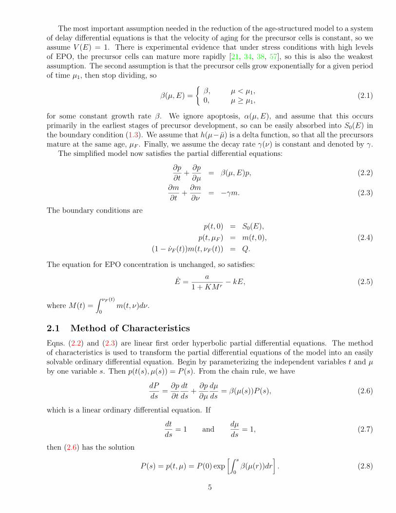
The most important assumption needed in the reduction of the age-structured model to a systemof delay differential equations is that the velocity of aging for the precursor cells is constant, so weassume V (E) = 1. There is experimental evidence that under stress conditions with high levelsof EPO, the precursor cells can mature more rapidly [21, 34, 38, 57], so this is also the weakestassumption. The second assumption is that the precursor cells grow exponentially for a given periodof time µ1, then stop dividing, so

β(µ, E) =

{β, µ < µ1,0, µ ≥ µ1,

(2.1)

for some constant growth rate β. We ignore apoptosis, α(µ, E), and assume that this occursprimarily in the earliest stages of precursor development, so can be easily absorbed into S0(E) inthe boundary condition (1.3). We assume that h(µ− µ) is a delta function, so that all the precursorsmature at the same age, µF . Finally, we assume the decay rate γ(ν) is constant and denoted by γ.

The simplified model now satisfies the partial differential equations:

∂p

∂t+

∂p

∂µ= β(µ, E)p, (2.2)

∂m

∂t+

∂m

∂ν= −γm. (2.3)

The boundary conditions are

p(t, 0) = S0(E),

p(t, µF ) = m(t, 0), (2.4)

(1− νF (t))m(t, νF (t)) = Q.

The equation for EPO concentration is unchanged, so satisfies:

E =a

1 + KM r− kE, (2.5)

where M(t) =∫ νF (t)

0m(t, ν)dν.

2.1 Method of Characteristics

Eqns. (2.2) and (2.3) are linear first order hyperbolic partial differential equations. The methodof characteristics is used to transform the partial differential equations of the model into an easilysolvable ordinary differential equation. Begin by parameterizing the independent variables t and µby one variable s. Then p(t(s), µ(s)) = P (s). From the chain rule, we have

dP

ds=

∂p

∂t

dt

ds+

∂p

∂µ

dµ

ds= β(µ(s))P (s), (2.6)

which is a linear ordinary differential equation. If

dt

ds= 1 and

dµ

ds= 1, (2.7)

then (2.6) has the solution

P (s) = p(t, µ) = P (0) exp[∫ s

0β(µ(r))dr

]. (2.8)

5

t s µ s( ( ), ( ))( ( ), ( ))

t s µ s( ( ), ( ))( ( ), ( ))

t

0 µ µ

t

µ

C

F

00( , 0)

0(0, )

µ

µ>t

<t

Figure 2.1: Diagram showing the characteristics for the simplified age-structured model.

The solution of (2.7) creates the characteristic lines along which (2.8) is valid. Fig. 3.1 illustratesthese simple characteristics. For t < µ, t(s) = s and µ(s) = µ0 + s. For t > µ, t(s) = t0 + s andµ(s) = s. The general solution, (2.8), becomes

p(t, µ) =

{p(0, µ− t)exp

[∫ t0 β(s)ds

], t < µ,

p(t− µ, 0)exp [∫ µ0 β(s)ds] , t > µ.

By examining only long time behavior with t > µ and evaluating µ at µF , our assumption onβ(µ, E) gives

p(t, µF ) = p(t− µF , 0)eβµ1 = eβµ1S0(E(t− µF )).

From the form of (2.3), it is easy to see that a very similar set of solutions for m(t, ν) are obtainedusing the method of characteristics. Thus,

m(t, ν) = m(t− ν, 0)e−γν , for t > ν.

From the expression for M(t) and the second boundary condition in (2.4), we obtain

M(t) =∫ νF (t)

0m(t− ν, 0)e−γνdν,

=∫ νF (t)

0p(t− µF − ν, 0)e−γνdν,

=∫ νF (t)

0eβµ1S0(E(t− µF − ν))e−γνdν,

= e−γ(t−µF )eβµ1

∫ t−µF

t−µF−νF (t)S0(E(w))eγwdw,

6

where the last integral is obtained by letting w = t− µF − ν in the previous expression. To obtaina differential equation for M(t), Leibnitz’s rule for differentiating an integral gives:

M(t) = −γe−γ(t−µF )eβµ1

∫ t−µF

t−µF−νF (t)S0(E(w))eγwdw

+e−γ(t−µF )eβµ1

[S0(E(t− µF ))eγ(t−µF )

− S0(E(t− µF − νF (t)))eγ(t−µF−νF (t))(1− νF (t))]

= −γM(t) + eβµ1S0(E(t− µF ))−Q,

from m(t, νF (t)) = eβµ1S0(E(t−µF−νF (t)))e−γνF (t) and the constant flux boundary condition (2.4).It is easy to interpret this last expression for M(t) from a conservation of mass idea. The secondterm is the production of new mature cells, which result from the exponential growth of the stemcells that were recruited µF units of time earlier. The loss of mature cells come from two sources.The first term represents the random destruction of mature cells throughout their lifetime, whilethe last term represents the constant flux due to active degradation of the oldest mature cells.

2.2 Delay Differential Equations and Linear Analysis

With the simplifying assumptions above, the method of characteristics eliminates the need of theage-structured populations, p and m, and replaces them with a differential delay equation for thetotal mature population, M(t). Thus, the system of partial differential equations are replaced withan equivalent system of delay differential equations with the state variables, M(t), E(t), and νF (t).The last variable results from the need to keep track of the length of time that mature cells may live.The differential equation describing its behavior is easily derived from the expression for m(t, νF (t))and the constant flux boundary condition in (2.4). Let T = µF , then the following system of delaydifferential equations with a fixed delay T and a state dependent delay occurring in the equationfor νF is obtained:

dM(t)

dt= eβµ1S0(E(t− T ))− γM(t)−Q,

dE(t)

dt= f(M(t))− kE(t), (2.9)

dνF (t)

dt= 1− QeγνF (t)

eβµ1S0(E(t− T − νF (t)).

Though initially it appears as if we have replaced a complicated system of partial differential equa-tions with a difficult state-dependent delay differential equation, it is easily seen that the νF (t)equation is uncoupled from the other two equations and that the equation for M(t) has only thesingle time delay T . This makes the stability analysis of this system relatively easy.

The stability analysis of (2.9) uses standard techniques. A unique equilibrium, (M,E, νF ), existssince S0(E) is monotonically increasing and f(M) is a negative feedback function. The simplifiedmodel given by (2.9) is linearized about its equilibrium, and the resulting linear system is given by:

ML(t) = eβµ1S ′0(E)EL(t− T )− γML(t),

EL(t) = f ′(M)ML(t)− kEL(t), (2.10)

νLF (t) =1

EEL(t− T − νF )− γνLF (t),

7

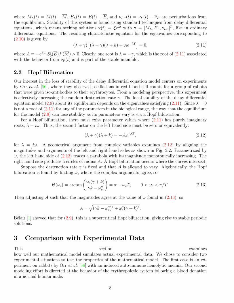
where ML(t) = M(t) − M , EL(t) = E(t) − E, and νLF (t) = νF (t) − νF are perturbations fromthe equilibrium. Stability of this system is found using standard techniques from delay differentialequations, which means seeking solutions x(t) = ξeλt with x = [ML, EL, νLF ]T , like in ordinarydifferential equations. The resulting characteristic equation for the eigenvalues corresponding to(2.10) is given by

(λ + γ)[(λ + γ)(λ + k) + Ae−λT

]= 0, (2.11)

where A ≡ −eβµ1S ′0(E)f ′(M) > 0. Clearly, one root is λ = −γ, which is the root of (2.11) associated

with the behavior from νF (t) and is part of the stable manifold.

2.3 Hopf Bifurcation

Our interest in the loss of stability of the delay differential equation model centers on experimentsby Orr et al. [56], where they observed oscillations in red blood cell counts for a group of rabbitsthat were given iso-antibodies to their erythrocytes. From a modeling perspective, this experimentis effectively increasing the random destruction rate γ. The local stability of the delay differentialequation model (2.9) about its equilibrium depends on the eigenvalues satisfying (2.11). Since λ = 0is not a root of (2.11) for any of the parameters in the biological range, the way that the equilibriumfor the model (2.9) can lose stability as its parameters vary is via a Hopf bifurcation.

For a Hopf bifurcation, there must exist parameter values where (2.11) has purely imaginaryroots, λ = iω. Thus, the second factor on the left hand side must be zero or equivalently:

(λ + γ)(λ + k) = −Ae−λT , (2.12)

for λ = iω. A geometrical argument from complex variables examines (2.12) by aligning themagnitudes and arguments of the left and right hand sides as shown in Fig. 3.2. Parametrized byω, the left hand side of (2.12) traces a parabola with its magnitude monotonically increasing. Theright hand side produces a circles of radius A. A Hopf bifurcation occurs where the curves intersect.

Suppose the destruction rate γ is fixed and that A is allowed to vary. Algebraically, the Hopfbifurcation is found by finding ωc where the complex arguments agree, so

Θ(ωc) = arctan

(ωc(γ + k)

γk − ω2c

)= π − ωcT, 0 < ωc < π/T. (2.13)

Then adjusting A such that the magnitudes agree at the value of ω found in (2.13), so

A =√

(γk − ω2c )

2 + ω2c (γ + k)2.

Belair [1] showed that for (2.9), this is a supercritical Hopf bifurcation, giving rise to stable periodicsolutions.

3 Comparison with Experimental Data

This section examineshow well our mathematical model simulates actual experimental data. We chose to consider twoexperimental situations to test the properties of the mathematical model. The first case is an ex-periment on rabbits by Orr et al. [56] with an induced auto-immune hemolytic anemia. Our secondmodeling effort is directed at the behavior of the erythropoietic system following a blood donationin a normal human male.

8

A

A

ω

Θ

c T

Figure 2.2: Geometrical argument for finding a Hopf bifurcation.

3.1 Auto-Immune Hemolytic Anemia

Orr et al. [56] injected a collection of rabbits with an iso-antibody for their erythrocytes every 2–3days, which produced an induced auto-immune hemolytic anemia. The populations of erythrocytesin these anemic rabbits oscillated about a subnormal mean population of erythrocytes. Their article([56], Fig. 3) showed one rabbit with regular oscillations of its erythrocytes around 75% of normalwith an amplitude of about 10–15% and a period around 17 days. From a modeling perspective,these experiments are equivalent to increasing the random destruction rate γ in the mathematicalmodel given by (2.9).

In order to simulate the mathematical model and determine where the system undergoes aHopf bifurcation and loses stability, several of the parameters must be determined. From theobservations of Orr et al. [56], we chose M = 2.63(×1011 erythrocytes/kg of body weight), which is75% of normal. Belair et al. [3] used a least squares fit to the data of Erslev [19] to obtain E = 71.1(mU/ml). Burwell et al. [7] give the lifespan of erythrocytes of rabbits to be 45–50 days, so we tookνF = 50 days. Orr et al. [56] estimated the half-life of circulating EPO to be 2.5 hr, based on rats,so we took k = 6.65 day−1 for rabbits. The nonlinear fit of Belair et al. [3] found the parametersin (2.5) to be a = 15, 600 (mU/ml/day), K = 0.0382, and r = 6.96. We assumed β = 2.773 day−1

(cell doubling every 6 hr) and µ1 = 3 days.

Mahaffy et al. [48] used these parameters in (2.9) and adjusted T and γ to yield simulatedM(t) close to the one of the experimental rabbits of Orr et al. [56]. A reasonable fit was foundwith T = 4.1 days and γ = 0.065 days−1. These parameters and an equilibrium analysis yieldS ′

0(E) = 0.0025 and Q = 0.0069. The simulation of (2.9) has a period of 15.9 days with erythrocyteoscillations between 0.67 and 0.91 (fraction of normal) and EPO concentration fluxuating between20.2 and 154.5 mU/ml. Fig. 4.1 graphically shows our simulation (solid line) with the data (dash-dot line), which is comparable if one ignores the first 40–50 days in what might be transient effects.

9

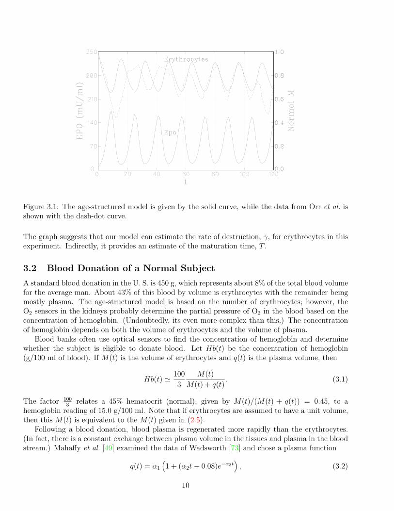
Figure 3.1: The age-structured model is given by the solid curve, while the data from Orr et al. isshown with the dash-dot curve.

The graph suggests that our model can estimate the rate of destruction, γ, for erythrocytes in thisexperiment. Indirectly, it provides an estimate of the maturation time, T .

3.2 Blood Donation of a Normal Subject

A standard blood donation in the U. S. is 450 g, which represents about 8% of the total blood volumefor the average man. About 43% of this blood by volume is erythrocytes with the remainder beingmostly plasma. The age-structured model is based on the number of erythrocytes; however, theO2 sensors in the kidneys probably determine the partial pressure of O2 in the blood based on theconcentration of hemoglobin. (Undoubtedly, its even more complex than this.) The concentrationof hemoglobin depends on both the volume of erythrocytes and the volume of plasma.

Blood banks often use optical sensors to find the concentration of hemoglobin and determinewhether the subject is eligible to donate blood. Let Hb(t) be the concentration of hemoglobin(g/100 ml of blood). If M(t) is the volume of erythrocytes and q(t) is the plasma volume, then

Hb(t) ' 100

3

M(t)

M(t) + q(t). (3.1)

The factor 1003

relates a 45% hematocrit (normal), given by M(t)/(M(t) + q(t)) = 0.45, to ahemoglobin reading of 15.0 g/100 ml. Note that if erythrocytes are assumed to have a unit volume,then this M(t) is equivalent to the M(t) given in (2.5).

Following a blood donation, blood plasma is regenerated more rapidly than the erythrocytes.(In fact, there is a constant exchange between plasma volume in the tissues and plasma in the bloodstream.) Mahaffy et al. [49] examined the data of Wadsworth [73] and chose a plasma function

q(t) = α1

(1 + (α2t− 0.08)e−α3t

), (3.2)

10

where 0.08 reflects the plasma lost at t = 0 (time of the phlebotomy). The parameter α1 is calculatedfrom the equilibrium values M and Hb in (3.1). The parameters α2 and α3 are found using a leastsquares best fit to the data of Maeda et al. [47] and Wadsworth [73].

To study the effects of a phlebotomy, including the loss of blood plasma, Mahaffy et al. [49]modified the erythropoietic model given by (2.9). The new system of delay differential equationsbecomes:

dM(t)

dt= eβµ1S0(E(t− T ))− γM(t)−Q,

dE(t)

dt= f(Hb(t))− kE(t), (3.3)

dνF (t)

dt= 1− Qe−βµReγνF (t)

S0(E(t− T − νF (t)),

where f has the same form as (1.8) and Hb(t) is found from Eqns. (3.1) and (3.2). This systemof delay differential equations is readily simulated using an adaptation of the fourth order Runge-Kutta for ordinary differential equations, which simplifies our problem of fitting parameters in themodel to the experimental data.

Wadsworth [73] and Maeda et al. [47] collected data on hemoglobin concentrations for normalhuman males following a phlebotomy for an extended period of time. Maeda et al. [47] also collecteddata on the EPO concentrations of their subjects. Many of the parameters are determined from theliterature, and the remainder were found by using a least squares best fit to the data of Wadsworth[73] and Maeda et al. [47]. Details on finding the parameters can be found in Mahaffy et al. [49]. Forour simulation, we assumed that Hb = 15.29 (g/100 ml), E = 16.95 (mU/ml), and νF = 120 (days).Since M = 3.5, α1 = 4.13. From the information in the literature, we chose β = 2.079 (days−1),µ1 = 4.0 (days), T = 6 (days) and γ = 0.001 (days−1). With the assumption that S0(E) is linear, asteady-state analysis of (3.3) yields S0(E) = 4.45 × 10−7E and Q = 0.0275. With r = 7, the leastsquares best fit yields α2 = 0.05421, α3 = 0.1214, a = 198.1, and K = 9.262×10−9. We constrainedthe half-life of EPO to be between 4 and 24 hr, and the least squares functional was minimized atk = 4.16 (days−1), corresponding to the shortest EPO half-life allowed.

With the parameters given above, the mathematical model (3.3) is simulated for 60 days. Theresults are shown in Fig. 4.2 with the experimental data. The simulation fits the experimental datareasonably well with a minimum occurring in a little over a week and 90% recovery in about 30 days.Wadsworth [73] (often quoted by blood banks) states “that recovery of haemoglobin concentrationwas completed within 3–4 weeks of the haemorrhage,” which the model supports.

Since the mathematical model for a phlebotomy simulates the data of Wadsworth [73] and Maedaet al. [47] fairly well, we might expect that the model could test alternative blood collection schemesand help enhance blood supplies of autologous donors. However, the data shown was a compositeof only 15 individuals. In Mahaffy et al. [49], two of the authors enlisted the help of the San DiegoBlood Bank to study their own response to a blood donation with data collected very often for 8weeks. These data are shown in Fig. 4.3 overlaying the simulation of the mathematical model. Thesedata clearly do not have the same behavior as the averaged data of Fig. 4.2 or the mathematicalmodel. Only the initial trend of an immediate drop in the concentration of hemoglobin is consistentwith the model, and this is very short-lived with normal concentrations being observed 4–5 daysafter the phlebotomy. Soon the data follows an almost random pattern with a mean of 14.66 and15.10 (g/100 ml) for Mahaffy and Polk, respectively. (The standard deviation was 0.86 and 0.91 forMahaffy and Polk, respectively.) The subjects of this study were not in a controlled experiment, sotheir diet and exercise regimes varied significantly (though measurements were taken at the sametime each day). Careful analysis of the data indicated that following heavy exercise (or SCUBA

11

Figure 3.2: The graph shows the behavior of the mathematical model for a normal male subjectfollowing a phlebotomy, while the data are shown for comparison.

diving in one case), the body adapts by lowering the concentration of hemoglobin. This suggests asignificant rapid response mechanism available to the body for increasing O2 availability by dilutingthe blood, thus lowering its viscosity.

3.3 Variable Velocity of Aging

The weakest assumption is where the precursor cells age at a constant rate, which was used toreduce the age-structured model to a system of delay differential equations. Williams ([20], p. 436)claims that under extreme stress, the maturing stage of erythropoiesis is shortened. Studies usingradioiron [21, 34, 38, 57] show that anemic conditions can decrease transit time (time of maturation)in the bone marrow for precursor cells by over a day and, furthermore, the stress of blood lossresults in early release of “shift reticulocytes.” Mahaffy et al. [49] use numerical methods basedon the method of characteristics from Sulsky [68, 69] to simulate the age-structured model. Thenumerical simulations indicated that a variable velocity of aging could have profound stabilizingeffect, especially in a diseased state. Belair and Mahaffy [4] have proved this analytically by a linearanalysis of reduced threshold-type delay equations, resulting from the application of the method ofcharacteristics to the age-structured model that includes V (E). Biologically, this result implies thatplasticity in the aging of hematopoietic precursor cells aids in stabilizing the populations of matureerythrocytes, which should help maintain constant supplies of O2 to the tissues.

4 Discussion

This review article demonstrates how age-structured models can be applied to a variety of problemsin hematopoiesis. The mathematical models provide a valuable tool for examining hematopoieticdiseases. Our study of the experiment by Orr et al. [56] for an induced auto-immune hemolytic

12

Figure 3.3: The solid curve shows the level of hemoglobin following a blood donation predictedby the model. The data with ◦ are from the author Mahaffy, while the data with + are from hiscollaborator Polk after a blood donation at t = 0.

anemia in rabbits demonstrated that the qualitative behavior can be simulated reasonably wellby adjusting a parameter in the model corresponding to the increased random destruction of ery-throcytes by the injected iso-antibody. Additional studies of the physiological parameters in themathematical model could provide insight into the causes of other hematopoietic diseases or couldsuggest appropriate therapies for improving the condition of the animal.

Our study of the age-structured model for erythropoiesis following a phlebotomy in normalmales gave mixed results. We were able to match averaged data for a collection of subjects, butthe model was not a good means of predicting the hemoglobin concentrations in an individual.The study of Mahaffy et al. [49] indicates a need to better understand the exchange of plasmaand the role of viscosity in blood to the varying needs of O2 in the tissues. This modeling effortshows the complexity of the physiological controls that have evolved for this crucial O2 deliverysystem. Our simplified mathematical model fails to adequately explain the adaptations required bythe circulatory system to the external environment.

The studies of Mahaffy et al. [49] and Belair and Mahaffy [4] on the variable velocity of aging forthe precursor cells showed an increase in stability of the mathematical model. This suggests thatanimals have developed a plasticity in their hematopoietic systems in the early stages of developmentin order to maintain a homeostasis. The analysis of the complete age-structured model demonstratesthe importance of certain evolutionary adaptations that the simpler delay differential equationsmodels cannot detect.

Mathematically, Belair et al. [3] and Mahaffy et al. [48] determined the assumptions necessaryto connect the more complicated age-structured models, e.g., Grabosch and Heijmans [29] and Metzand Diekmann [52], to the simpler delay differential equation models, e.g., Belair and Mackey [2].The simpler delay differential equations allow a more complete analysis and are computationallyeasier for testing parameters. Yet they are adequate for understanding many aspects of the biologicalcontrols, especially in certain diseased states.

13

ACKNOWLEDGEMENT: Part of the work was done when the author was visiting the Centre de Recherches Mathematiques at theUniversite) de Montreal and the IMA at the University of Minnesota.

References[1] J. Belair. Stability analysis of an age-structured model with a state-dependent delay. Can. Appl. Math. Quart., 6:305–319, 1998.

[2] J. Belair and M. C. Mackey. A model for the regulation of mammalian platelet production. Ann. N. Y. Acad. Sci., 504:280–282,1987.

[3] J. Belair, M. Mackey, and J. M. Mahaffy. Age-structured and two-delay models for erythropoiesis. Math. Biosci., 128:317–346, 1995.

[4] J. Belair and J. M. Mahaffy. Parameter sensitivity in hematopoietic models. Preprint 1999.

[5] J. Bernard and J. Caen. Purpura thrombopenique et megacaryocytopenie cycliques mensuels. Nouv. Rev. franc. Hemat., 2:378–386,1962.

[6] O. Brey, E. P. R. Garner, and D. Wells. Cyclic thrombocytopenia associated with multiple antibodies. Brit. Med. J., 3:397–398,1969.

[7] E. L. Burwell, B. A. Brickley, and C. A. Finch. Erythrocyte life span in small mammals. Amer. J. Physiol., 172:718, 1953.

[8] J. Caen, G. Meshaka, M. J. Larrieu, and J. Bernard. Les purpuras thrombopeniques intermittents idiopathiques. Sem. Hop. Paris,40:276–282, 1964.

[9] G. Chikkappa, G. Borner, H. Burlington, A. D. Chanana, E. P. Cronkite, S. Ohl, M. Pavelec, and J. S. Robertson. Periodic oscillationof blood leukocytes, platelets, and reticulocytes in a patient with chronic myelocytic leukemia. Blood, 47:1023 –1030, 1976.

[10] T. Cohen and D. P. Cooney. Cyclical thrombocytopenia: Case report and review of literature. Scand. J. Haemat., 12:9–17, 1974.

[11] J. M. Cushing. Structural population dynamics. In S.A. Levin, editor, Frontiers in Theoretical Biology. Volume 100, Lecture Notesin Biomathematics, pages 280–295. Springer-Verlag, Berlin and New York, 1994.

[12] D. C. Dale, D. W. Alling, and S. M. Wolff. Cyclic hematopoiesis: The mechanism of cyclic neutropenia in grey collie dogs. Journalof Clinical Investigation, 51:2197–2204, 1972.

[13] D. C. Dale and W. P. Hammond. Cyclic neutropenia: A clinical review. Blood Reviews, 2:178–185, 1988.

[14] J. Delobel, P. Charbord, P. Passa, and J. Bernard. Evolution cyclique spontanee de la leucocytose dans un cas de leucemie myeloidechronique. Nouv. Rev. Fr. Hematol., 13:221–228, 1973.

[15] T. Demmer. Morbus maculosus werlhofii in regelmassigen vierwochentlichen schuben bei einem 60 jahrigen mann, nebst unter-suchungen uber die blutplattchen. Folia Haemat., 26:74–86, 1920.

[16] O. Diekmann and J. A. J. Metz. On the reciprocal relationship between life histories and population dynamics. In S.A. Levin,editor, Frontiers in Theoretical Biology. Volume 100, Lecture Notes in Biomathematics, pages 19–22. Springer-Verlag, Berlin andNew York, 1994.

[17] C. D. R. Dunn. Cyclic hematopoiesis: The biomathematics. Experimental Hematology, 11:779–791, 1983.

[18] K. Engstrom, A. Lundquist, and N. Soderstrom. Periodic thrombocytopenia or tidal platelet dysgenesis in a man. Scand. J.Haemat., 3:290–292, 1966.

[19] A. J. Erslev. Erythropoietin titers in health and disease. Seminars in Hematology, 28 Sup.3:2–8, 1991.

[20] A. J. Erslev and E. Beutler. Production and destruction of erythrocytes. In E. Beutler, M. A. Lichtman, B. S. Coller, and T. J.Kipps, editors, William’s Hematology, chapter 39. McGraw-Hill Inc., New York, 5th edition, 1995.

[21] C. A. Finch, L. A. Harker, and J. D. Cook. Kinetics of the formed elements of human blood. Blood, 50:699–707, 1977.

[22] P. Fortin and M. C. Mackey. Periodic chronic myelogenous leukaemia: Spectral analysis of blood cell counts and aetiologicalimplications. Br. J. Haemato., 104:336–345, 1999.

[23] J. A. Gatica and P. Waltman. A threshold model of antigen antibody dynamics with fading memory. In V. Lakshmikantham, editor,Nonlinear Phenomena in Mathematical Sciences. Academic Press, New York, 1982.

[24] J. A. Gatica and P. Waltman. A system of functional differential equations modeling threshold phenomena. Appl. Anal., 28:39–50,1988.

14

[25] R. A. Gatti, W. A. Robinson, A. S. Deinare, M. Nesbit, J. J. McCullough, M. Ballow, and R. A. Good. Cyclic leukocytosis inchronic myelogenous leukemia. Blood, 41:771–782, 1973.

[26] L. Glass and M. C. Mackey. Pathological conditions resulting from instabilities in physiological control systems. Ann. N. Y. Acad.Sci., 316:214–235, 1979.

[27] B. Goldschmidt and R. Fono. Cyclic fluctuations in platelet count, megakaryocyte maturation and thrombopoietin activity incyanotic congenital heart disease. Acta. Paediat. Scand., 61:310–314, 1972.

[28] R. R. Gordon and S. Varadi. Congenital hypoplastic anemia (pure red cell anemia) with periodic erythroblastopenia. Lancet,i:296–299, 1962.

[29] A. Grabosch and H. J. A. M. Heijmans. Cauchy problems with state-dependent time evolution. Japan J. Appl. Math., 7:433–457,1990.

[30] A. Grabosch and H. J. A. M. Heijmans. Production, development and maturation of red blood cells. A mathematical model. InD.E. Axelrod O. Arino and M. Kimmel, editors, Mathematical Population Dynamics, pages 189–210. Marcel Dekker, New York,1991.

[31] W. S. C. Gurney and R. M. Nisbet. The systematic formulation of delay-differential models of age or size structured populations. InH. I. Friedman and C. Strobeck, editors, Population Biology, Volume 52, Lecture Notes in Biomathematics. Springer-Verlag, Berlin,1983.

[32] C. Haurie, D. C. Dale, and M. C. Mackey. Cyclical neutropenia and other periodic hematological disorders: A review of mechanismsand mathematical models. Blood, 92:2629–2640, 1998.

[33] T. Hearn, C. Haurie, and M. C. Mackey. Cyclical neutropenia and the peripheral control of white blood cell production. J. theor.Biol., 192:167–181, 1998.

[34] R. S. Hill. Characteristics of marrow production and reticulocyte maturation in normal man in response to anemia. J. Clin. Invest.,48:443–453, 1969.

[35] J. B. Jones and R. D. Lange. Cyclic hematopoiesis: Animal models. Immunology and Hematology Research Monographs, 1:33–42,1983.

[36] B. J. Kennedy. Cyclic leukocyte oscillations in chronic myelogenous leukemia. Blood, 35:751–760, 1970.

[37] A. P. Korn, R. M. Henkelman, F. P. Ottensmeyer, and J. E. Till. Investigations of a stochastic model of haemopoiesis. Exp. Hemat.,1:362–375, 1973.

[38] S. Labardini, Th Papayannopoulou, J. D. Cook, J. W. Adamson, R. D. Woodson, J. W. Eschbach, and R. S. Hill. Marrow radioironkinetics. Haematologia, 7:301–312, 1973.

[39] R. D. Lange. Cyclic hematopoiesis: Human cyclic neutropenia. Experimental Hematology, 11:435–451, 1983.

[40] M. L. Lewis. Cyclic thrombocytopenia: A thrombopoietin deficiency? J. Clin. Path., 27:242–246, 1974.

[41] C. A. Macken and A. S. Perelson. Stem cell proliferation and differentiation, Volume 76, Lecture Notes in Biomathematics. Springer-Verlag, Berlin, 1980.

[42] M. C. Mackey. Periodic auto-immune hemolytic anemia: An induced dynamical disease. Bull. Math. Biol., 41:829–834, 1979.

[43] M. C. Mackey. Some models in hemopoiesis: Predictions and problems. In M. Rotenberg, editor, Biomathematics and Cell Kinetics,pages 23–38. Elsvier/North Holland, 1981.

[44] M. C. Mackey. Mathematical models of hematopoietic cell replication and control. In M. A. Lewis & J. C. Dalton H. G. Othmer,F. R. Adler, editor, The Art of Mathematical Modeling: Case Studies in Ecology, Physiology & Biofluids, pages 149–178. PrenticeHall, 1997.

[45] M. C. Mackey and L. Glass. Oscillation and chaos in physiological control systems. Science, 197:287–289, 1977.

[46] M. C. Mackey and J. G. Milton. Feedback, delays and the origin of blood cell dynamics. Comments Theor. Biol., 1:299–327, 1990.

[47] H. Maeda, Y. Hitomi, R. Hirata, H. Tohyama, J. Suwata, S. Kamata, Y. Fujino, and N. Murata. The effect of phlebotomy on serumerythropoietin levels in normal healthy subjects. Int. J. Hemat., 55:111–115, 1992.

[48] J. M. Mahaffy, J. Belair, and M. Mackey. Hematopoietic model with moving boundary condition and state dependent delay:Applications in erythropoiesis. J. theor. Biol., 190:135–146, 1998.

[49] J. M. Mahaffy, S. W. Polk, and R. K. W. Roeder. An age-structured model for erythropoiesis following a phlebotomy. submittedto Bul. Math. Biol., 1999.

15

[50] R. Mastrangelo, A. Stabile, D. Parenti, and G. Cimatti. A specific spontaneous leukocyte cycle in chronic myelogenous leukemia.Tumori, 62:197–204, 1976.

[51] R. Mastrangelo, A. Stabile, D. Parenti, and G. Segni. Spontaneous leukocyte oscillation during blastic crisis of chronic myeloidleukemia. Cancer, 33:1610–1614, 1974.

[52] J. A. J. Metz and O. Diekmann. The Dynamics of Physiologically Structured Populations, Volume 68, Lecture Notes in Biomathe-matics. Springer-Verlag, Berlin, 1986.

[53] A. Morley. Blood-cell cycles in polycythaemia. Aust. Ann. Med., 18:124–126, 1969.

[54] T. Nakahata, A. J. Gross, and M. Ogawa. A stochastic model of self-renewal and commitment to differentiation of the primitivehemopoietic stem cells in culture. J. Cell. Physiol., 113:455–458, 1982.

[55] R. M. Nisbet and W. S. C. Gurney. The formulation of age-structured models. In T. G. Hallam and S. A. Levin, editors, MathematicalEcology, Volume 17, Lecture Notes in Biomathematics. Springer-Verlag, Berlin, 1986.

[56] J. S. Orr, J. Kirk, K. G. Gray, and J. R. Anderson. A study of the interdependence of red cell and bone marrow stem cell populations.Brit. J. Haemat., 15:23–34, 1968.

[57] Th Papayannopoulou and C. A. Finch. Radio-iron measurements of red cell maturation. Blood Cells, 1:535–546, 1975.

[58] P. Ranlov and A. Videbaek. Cyclic haemolytic anaemia synchronous with Pel-Ebstein fever in a case of Hodgkin’s disease. ActaMedica Scandinavica, 174:583–588, 1963.

[59] H. A. Reimann. Periodic Diseases. F.A. Davis Company, Philadelphia, 1963.

[60] A. R. Rodriguez and C. L. Lutcher. Marked cyclic leukocytosis leukopenia in chronic myelogenous leukemia. American Journal ofMedicine, 60:1041–1047, 1976.

[61] S. Schmitz, H. Franke, J. Brusis, and H. E. Wichmann. Quantification of the cell kinetic effects of G-CSF using a model of humangranulopoiesis. Exp. Hematol., 21:755–760, 1993.

[62] S. Schmitz, H. Franke, H. E. Wichmann, and V. Diehl. The effect of continuous G-CSF application in human cyclic neutropenia: Amodel analysis. Br. J. Haematol., 90:41–47, 1995.

[63] S. Schmitz, M. Loeffler, J. B. Jones, R. D. Lange, and H. E. Wichmann. Synchrony of bone marrow proliferation and maturationas the origin of cyclic haemopoiesis. Cell Tissue Kinet., 23:425–442, 1990.

[64] G. K. von Schulthess and N. A. Mazer. Cyclic neutropenia (CN): A clue to the control of granulopoiesis. Blood, 59:27–37, 1982.

[65] R. K. Shadduck, A. Winkelstein, and N. G. Nunna. Cyclic leukemia cell production in CML. Cancer, 29:399–401, 1972.

[66] W. A. Skoog, J. S. Lawrence, and W. S. Adams. A metabolic study of a patient with idiopathic cyclical thrombocytopenic purpura.Blood, 12:844–856, 1957.

[67] H. L. Smith. Reduction of structured population models to threshold-type delay equations and functional differential equations: Acase study. Math. Biosci., 113:1–23, 1993.

[68] D. Sulsky. Numerical solution of structured population models: I Age structure. J. Math. Biol., 31:817–839, 1993.

[69] D. Sulsky. Numerical solution of structured population models: II Mass structure. J. Math. Biol., 32:491–514, 1994.

[70] J. L. Swinburne and M. C. Mackey. Cyclical thrombocytopenia: Characterization by spectral analysis. Submitted to J. Theor.Med., 1998.

[71] J. E. Till, E. A. McCulloch, and L. Siminovitch. A stochastic model of stem cell proliferation, based on the growth of spleencolony-forming cells. Proc. Natl. Acad. Sci. USA, 51:29–34, 1964.

[72] H. Vogel, H. Niewisch, and G. Matioli. Stochastic development of stem cells. J. theor. Biol., 22:249–270, 1969.

[73] G. R. Wadsworth. Recovery from acute haemorrhage in normal men and women. J. Physiol., 129:583–593, 1955.

[74] C. Wasastjerna. Cyclic thrombocytopenia of acute type. Scand. J. Haemat., 4:380–384, 1967.

[75] T. E. Wheldon. Mathematical models of oscillatory blood cell production. Math. Biosci, 24:289–305, 1975.

[76] T. E. Wheldon, J. Kirk, and H. M. Finlay. Cyclical granulopoiesis in chronic granulocytic leukemia: A simulation study. Blood,43:379–387, 1974.

[77] H. E. Wichmann and M. Loeffler. Mathematical Modeling of Cell Proliferation: Stem Cell Regulation in Hemopoiesis. CRC Press,Boca Raton, 1988.

16

[78] T. Wilkinson and B. Firkin. Idiopathic cyclical acute thrombocytopenic purpura. Med. J. Aust., 1:217–219, 1966.

[79] D. G. Wright, D. C. Dale, A. S. Fauci, and S.M. Wolff. Human cyclic neutropenia: clinical review and long term follow up ofpatients. Medicine, 60:1 –13, 1981.

[80] D. G. Wright, R. F. Kenney, D. H. Oette, V. F. LaRussa, L. A. Boxer, and H. L. Malech. Contrasting effects of recombinanthuman grnulocyte-macrophage colony-stimulating factor (CSF) and granulocyte CSF treatment on the cycling of blood elements inchildhood-onset cyclic neutropenia. Blood, 84:1257–1267, 1994.

17