AGA Report No. 11 API MPMS Chapter 14.9

Measurement of Natural Gas by

Coriolis Meter

Prepared by

Transmission Measurement Committee

Second Edition, February 2013

AGA Report No. 11 □ API MPMS Chapter 14.9

Measurement of Natural Gas by Coriolis Meter

Prepared by

Transmission Measurement Committee

Second Edition, February 2013

Copyright 2013 © American Gas Association All Rights Reserved

Catalog # XQ1301

ii

 

iii

DISCLAIMER AND COPYRIGHT  The American Gas Association’s (AGA) Operations and Engineering Section provides a forum for industry experts to bring their collective knowledge together to improve the state of the art in the areas of operating, engineering and technological aspects of producing, gathering, transporting, storing, distributing, measuring and utilizing natural gas.

Through its publications, of which this is one, AGA provides for the exchange of information within the natural gas industry and scientific, trade and governmental organizations. Many AGA publications are prepared or sponsored by an AGA Operations and Engineering Section technical committee. While AGA may administer the process, neither AGA nor the technical committee independently tests, evaluates or verifies the accuracy of any information or the soundness of any judgments contained therein.

AGA disclaims liability for any personal injury, property or other damages of any nature whatsoever, whether special, indirect, consequential or compensatory, directly or indirectly resulting from the publication, use of or reliance on AGA publications. AGA makes no guaranty or warranty as to the accuracy and completeness of any information published therein. The information contained therein is provided on an “as is” basis and AGA makes no representations or warranties including any expressed or implied warranty of merchantability or fitness for a particular purpose.

In issuing and making this document available, AGA is not undertaking to render professional or other services for or on behalf of any person or entity. Nor is AGA undertaking to perform any duty owed by any person or entity to someone else. Anyone using this document should rely on his or her own independent judgment or, as appropriate, seek the advice of a competent professional in determining the exercise of reasonable care in any given circumstances.

AGA has no power, nor does it undertake, to police or enforce compliance with the contents of this document. Nor does AGA list, certify, test or inspect products, designs or installations for compliance with this document. Any certification or other statement of compliance is solely the responsibility of the certifier or maker of the statement.

AGA does not take any position with respect to the validity of any patent rights asserted in connection with any items that are mentioned in or are the subject of AGA publications, and AGA disclaims liability for the infringement of any patent resulting from the use of or reliance on its publications. Users of these publications are expressly advised that determination of the validity of any such patent rights, and the risk of infringement of such rights, is entirely their own responsibility.

Users of this publication should consult applicable federal, state and local laws and regulations. AGA does not, through its publications intend to urge action that is not in compliance with applicable laws, and its publications may not be construed as doing so.

Changes to this document may become necessary from time to time. If changes are believed appropriate by any person or entity, such suggested changes should be communicated to AGA in writing and sent to: Operations & Engineering Section, American Gas Association, 400 North Capitol Street, NW, 4th Floor, Washington, DC 20001, U.S.A. Suggested changes must include: contact information, including name, address and any corporate affiliation; full name of the document; suggested revisions to the text of the document; the rationale for the suggested revisions; and permission to use the suggested revisions in an amended publication of the document. Copyright © 2013, American Gas Association, All Rights Reserved.

  

iv

FOREWORD  This report has been written in the form of a performance-based specification. If this performance-based specification is used, Coriolis meters shall meet or exceed the function, accuracy, and testing requirements specified in this report and designers shall follow the applicable installation recommendations. This report is split into two distinct sections – the main body of the report and a series of appendices. The main body should be considered normative as it describes working practice when applying and using Coriolis meters to measure natural gas flow. The appendices are informative and contain additional material, background and examples of how Coriolis meters are installed and operated. Methods for verifying a meter’s accuracy and/or applying a Flow Weighted Mean Error (FWME) correction factor to minimize the measurement uncertainty are contained in Appendix A, “Coriolis Gas Flow Meter Calibration Issues.” Depending on the design, it may be necessary to flow-calibrate each meter on a gas similar to that expected in service. In order to guide the designer in the specification of a Coriolis meter, Appendix B, “Coriolis Meter Data Sheet,” has been provided. As a reference for background information on Coriolis natural gas metering, Appendix C, “AGA Engineering Technical Note, XQ0112, Coriolis Flow Measurement for Natural Gas Applications,” is provided. Due to the unique principle of operation and atypical performance characteristics of Coriolis mass flow meters, in comparison to volumetric flow meters, readers who are not familiar with the technology are encouraged to read the Appendix C prior to applying the general concepts and guidelines of this report. This report offers general criteria for the measurement of natural gas by Coriolis meters. It is the cumulative result of years of experience of many individuals and organizations acquainted with measuring gas flow rate and/or the practical use of Coriolis meters for gas measurement. Changes to this report may become necessary from time to time.

v

ACKNOWLEDGEMENTS 

The revision work of this report was undertaken by a task group the Transmission Measurement Committee (TMC). The task group was chaired by Angela Floyd who was with ConocoPhillips during the development and finalization of this report. Angela was supported by the vice chair, Karl Stappert with Micro Motion. A special subcommittee of the task group was formed later to assemble additional technical information, compose the drafts of the revised report for balloting and finally resolve the ballot comments and prepare the final report. The members of the special subcommittee who devoted an extensive amount of their time and deserve special thanks are –

Kerry Checkwitch, Spectra Energy Transmission Craig Chester, Williams Gas P/L

John Daly, GE Sensing Robert DeBoom, Consultant

Robert Fallwell, TransCanada P/L Ron Gibson, ONEOK, Inc.

Terry Grimley, Southwest Research Institute (SwRI) John Hand, Spectra Energy Transmission

Michael Keilty, Endress + Hauser Flowtec AG Allen Knack, Consumers Energy

Brad Massey, Southern Star Central Gas P/L Paul LaNasa, CPL and Associates Stephanie Lane, Micro Motion, Inc.

Dannie Mercer, Atmos Energy Corporation Gary McCargar, ONEOK, Inc.

Bill Morrow, Telvent Mark Pelkey, National Fuel Gas Supply Corporation

Dan Rebman, Universal Ensco Don Sextro, Targa Resources, Inc.

Martin Schlebach, Daniel Measurement and Control, Inc. Tushar Shah, Eagle Research Corp.

James N. Witte, El Paso Pipeline Group AGA acknowledges the contributions of the above individuals and thanks them for their time and effort in getting this document revised. Christina Sames Ali Quraishi Vice President Director Operations and Engineering Operations and Engineering

 

 

vi

TABLE OF CONTENTS 

DISCLAIMER AND COPYRIGHT .................................................................................................................................. III FOREWORD .............................................................................................................................................................. IV ACKNOWLEDGEMENTS ............................................................................................................................................. V 

1   INTRODUCTION ........................................................................................................................................ 1 

1.1  SCOPE ................................................................................................................................................................ 1 1.2  PRINCIPLE OF MEASUREMENT ................................................................................................................................. 1 

2   TERMINOLOGY, UNITS, DEFINITIONS & SYMBOLS ..................................................................................... 1 

2.1  TERMINOLOGY ..................................................................................................................................................... 1 2.2  ENGINEERING UNITS ............................................................................................................................................. 2 2.3  TERMS AND DEFINITIONS ....................................................................................................................................... 2 2.4  SYMBOLS ............................................................................................................................................................ 6 

3   OPERATING CONDITIONS ......................................................................................................................... 8 

3.1  GAS QUALITY ...................................................................................................................................................... 8 3.2  OPERATING PRESSURES ......................................................................................................................................... 8 3.3  TEMPERATURE: GAS AND AMBIENT ......................................................................................................................... 8 3.4  GAS FLOW CONSIDERATIONS .................................................................................................................................. 8 3.5  UPSTREAM PIPING AND FLOW PROFILES ................................................................................................................... 9 

4   METER REQUIREMENTS ............................................................................................................................ 9 

4.1  CODES AND REGULATIONS ..................................................................................................................................... 9 4.2  QUALITY ASSURANCE ............................................................................................................................................ 9 4.3  METER SENSOR ................................................................................................................................................... 9 

4.3.1  Pressure Rating ...................................................................................................................................... 9 4.3.2  Corrosion Resistance .............................................................................................................................. 9 4.3.3  Meter Lengths and Diameters ............................................................................................................. 10 4.3.4  Pressure Measurement ........................................................................................................................ 10 4.3.5  Miscellaneous ...................................................................................................................................... 10 4.3.6  Meter Body Markings .......................................................................................................................... 10 

4.4  ELECTRONICS ..................................................................................................................................................... 10 4.4.1  General Requirements ......................................................................................................................... 10 4.4.2  Output Signal Specifications ................................................................................................................ 11 4.4.3  Electrical Safety Design Requirements ................................................................................................. 11 4.4.4  Cable Jackets and Insulation ................................................................................................................ 11 

4.5  COMPUTER PROGRAMS ....................................................................................................................................... 11 4.5.1  Firmware .............................................................................................................................................. 11 4.5.2  Configuration and Maintenance Software .......................................................................................... 11 4.5.3  Inspection and Auditing Functions ....................................................................................................... 12 4.5.4  Alarms .................................................................................................................................................. 12 4.5.5  Diagnostic Measurements ................................................................................................................... 12 

4.6  DOCUMENTATION .............................................................................................................................................. 13 4.7  MANUFACTURER TESTING REQUIREMENTS .............................................................................................................. 13 

4.7.1  Static Pressure Testing ......................................................................................................................... 13 4.7.2  Alternative Calibration Fluids ............................................................................................................... 13 4.7.3  Calibration Requirements .................................................................................................................... 14 4.7.4  Calibration Test Reports ....................................................................................................................... 14 4.7.5  Quality Assurance ................................................................................................................................ 14 

vii

5   METER SIZING SELECTION CRITERIA ......................................................................................................... 15 

5.1  MINIMUM FLOW RATE ........................................................................................................................................ 15 5.2  TRANSITIONAL FLOW RATE ................................................................................................................................... 15 5.3  MAXIMUM FLOW RATE ....................................................................................................................................... 15 

5.3.1  Meter Pressure Loss ( P ) .................................................................................................................. 15 5.4  METER SIZING METHODOLOGY ............................................................................................................................. 17 

6   PERFORMANCE REQUIREMENTS .............................................................................................................. 19 

6.1  MINIMUM PERFORMANCE REQUIREMENTS ............................................................................................................. 19 6.2  PERFORMANCE ENHANCEMENTS ........................................................................................................................... 20 

7   GAS FLOW CALIBRATION REQUIREMENTS ............................................................................................... 20 

7.1  FLOW CALIBRATION TEST ..................................................................................................................................... 21 7.1.1  Preparation for Flow Calibration ......................................................................................................... 21 7.1.2  Calibration of Metering Module .......................................................................................................... 21 

7.2  CALIBRATION ADJUSTMENT FACTORS ..................................................................................................................... 22 7.3  CALIBRATION REPORTS ........................................................................................................................................ 22 7.4  ADDITIONAL CONSIDERATIONS .............................................................................................................................. 23 

7.4.1  Pressure Effect Compensation ............................................................................................................. 23 7.4.2  Coriolis Flowmeter Diagnostics ............................................................................................................ 24 

7.5   FINAL CONSIDERATIONS ......................................................................................................................................... 24 

8    INSTALLATION REQUIREMENTS ................................................................................................................ 24 

8.1  GENERAL REQUIREMENTS .................................................................................................................................... 24 8.1.1  Temperature ........................................................................................................................................ 24 

8.1.1.1   Ambient .................................................................................................................................................... 24 8.1.1.2   Process ...................................................................................................................................................... 24 

8.1.2  Pressure ............................................................................................................................................... 25 8.1.3  Vibration .............................................................................................................................................. 25 8.1.4  Electrical Noise ..................................................................................................................................... 25 

8.2  METER MODULE DESIGN ..................................................................................................................................... 25 8.2.1  Piping Configuration ............................................................................................................................ 25 8.2.2  Flow Direction ...................................................................................................................................... 27 8.2.3  Protrusions ........................................................................................................................................... 27 8.2.4  Meter Mounting ................................................................................................................................... 27 8.2.5  Orientation ........................................................................................................................................... 28 8.2.6  Filtration .............................................................................................................................................. 28 8.2.7  Provision for Sample Probe(s) .............................................................................................................. 28 8.2.8  Gas Velocity ......................................................................................................................................... 28 8.2.9  Multiple Meters in Close Proximity ...................................................................................................... 28 8.2.10 Performance Baseline ............................................................................................................................. 28 

8.3  ASSOCIATED FLOW COMPUTER ............................................................................................................................. 29 8.3.1  Flow Computer Calculations ................................................................................................................ 29 

8.4  MAINTENANCE .................................................................................................................................................. 30 

9    METER VERIFICATION AND FLOW PERFORMANCE TESTING ..................................................................... 31 

9.1  FIELD METER VERIFICATION ................................................................................................................................. 31 9.2  FLOW PERFORMANCE TESTING ............................................................................................................................. 32 

9.2.1  Verification of Gas Calibration Performance through Alternative Fluids Flow Test ............................. 33 9.2.2  Field/In‐situ Flow Performance Test .................................................................................................... 33 

9.3  RECALIBRATION.................................................................................................................................................. 34 

viii

10    CORIOLIS METER MEASUREMENT UNCERTAINTY DETERMINATION ......................................................... 34 

10.1    TYPES OF UNCERTAINTIES .................................................................................................................................... 34 10.1.1    Meter Calibration Uncertainty.............................................................................................................. 34 10.1.2    Uncertainties Arising from Differences between the Field Installation and the Calibration Lab .......... 34 

10.1.2.1  Parallel Meter Runs .................................................................................................................................... 35 10.1.2.2  Installation Effects ..................................................................................................................................... 35 10.1.2.3  Pressure and Temperature Effects ............................................................................................................. 35 10.1.2.4    Gas Quality Effects ................................................................................................................................... 35 

10.1.3     Uncertainties Due to Secondary Instrumentation ........................................................................ 35 10.2  UNCERTAINTY ANALYSIS PROCEDURE ................................................................................................................ 36 

11    REFERENCE LIST ...................................................................................................................................... 37 

APPENDIX A  CORIOLIS GAS FLOW METER CALIBRATION ISSUES ...................................................................... A‐1 

A.1   GENERAL .......................................................................................................................................................... A‐1 A.2   FLOW CALIBRATION DATA EXAMPLE ...................................................................................................................... A‐1 A.3   METHODS FOR CORRECTING CORIOLIS FLOW MEASUREMENT ERRORS ......................................................................... A‐3 A.4   FLOW‐WEIGHTED MEAN ERROR (FWME) CALCULATIONS ........................................................................................ A‐4 A.5   FLOW‐WEIGHTED MEAN ERROR (FWME) – EXAMPLE CALCULATION. ......................................................................... A‐5 

APPENDIX B  EXAMPLE CORIOLIS METER DATA SHEET ..................................................................................... B‐1 

APPENDIX C  AGA ENGINEERING TECHNICAL NOTE ON CORIOLIS FLOW MEASUREMENT .................................. C‐1 

APPENDIX D  EXAMPLES OF OVERALL MEASUREMENT UNCERTAINTY CALCULATIONS – CORIOLIS METER ........ D‐1 

D.1   GENERAL .......................................................................................................................................................... D‐1 D.2   MATHEMATICAL MODEL ..................................................................................................................................... D‐1 D.3   CONTRIBUTORY VARIANCES .................................................................................................................................. D‐1 

D.3.1  Uncertainty in the Mass Flow Rate .................................................................................................... D‐1 

D.3.2  Uncertainty in Flow Pressure Effect Compensation Factor ( pF) ...................................................... D‐2

D.3.3  Uncertainty in the Determination of Base Density ( b ) ................................................................... D‐3D.4   COMBINED UNCERTAINTY .................................................................................................................................... D‐3 D.5   EXPANDED UNCERTAINTY .................................................................................................................................... D‐3 

APPENDIX E  CORIOLIS GAS FLOW MEASUREMENT SYSTEM ..............................................................................E‐1 

E.1   CORIOLIS MEASUREMENT SYSTEM ARCHITECTURE .................................................................................................... E‐1 E.2   TRANSMITTER TO FLOW COMPUTER INTERFACE ........................................................................................................ E‐2 

E.2.1  Unidirectional Discrete I/0 Interface .................................................................................................. E‐2 E.2.2  Bidirectional Communications Interface ............................................................................................ E‐3 

E.3   TRANSMITTER .................................................................................................................................................... E‐3 E.3.1  Transmitter Flow Calculations ........................................................................................................... E‐3 E.3.2  Transmitter Algorithms and Variables of Metrological Interest ........................................................ E‐3 

E.4   FLOW COMPUTER MEASUREMENT METHODS .......................................................................................................... E‐4 E.4.1  Flow Computer Calculations .............................................................................................................. E‐4 E.4.2  Sampling Rate .................................................................................................................................. E‐10 E.4.3  No Flow Cut Off ................................................................................................................................ E‐10 E.4.4  Quantity Calculation Period (QCP) ................................................................................................... E‐11 E.4.5  Average Value Determination for Live Inputs .................................................................................. E‐11 E.4.6  Relative Density, Density, Heating Value and Composition ............................................................. E‐11 

ix

E.4.7  Transmitter and Flow Computer Measurement Record .................................................................. E‐11 E.4.7.1   Coriolis Measurement System Configuration Record/Log .......................................................................... E‐11 E.4.7.2   Event Record / Log ...................................................................................................................................... E‐13 E.4.7.3   Data Record ................................................................................................................................................. E‐13 

E.5   ALTERNATIVE METHOD ...................................................................................................................................... E‐14 E.5.1   Alternative method for Computing Flow and the Recording of Measurement Data  ...................... E‐14 

using a Constant Gravity or Base Density E.5.2   Data Record ..................................................................................................................................... E‐15 

E.6   RECALCULATION METHODS .................................................................................................................................... 15 

APPENDIX F   CORIOLIS METER SIZING EQUATIONS ........................................................................................... F‐1 

F.1   GENERAL ............................................................................................................................................................ F‐1 F.2   SIZING EXAMPLE .................................................................................................................................................. F‐1 F.3   CALCULATION OF FLOW RATE BASED ON PRESSURE DROP ........................................................................................... F‐3 F.4   CALCULATION OF PRESSURE DROP BASED ON FLOW RATE ........................................................................................... F‐5 F.5   CALCULATION OF ACCURACY AT FLOW RATE ............................................................................................................. F‐5 F.6   CALCULATION OF VELOCITY AT FLOW RATE ............................................................................................................... F‐6 

APPENDIX G   NOTES OF INTEREST ................................................................................................................... G‐1 

FORM TO PROPOSE CHANGES ......................................................................................................................... H‐1 

x

1

1   INTRODUCTION 

  1.1  SCOPE 

This report was developed for the specification, calibration, installation, operation, maintenance and verification of Coriolis flow meters and is limited to the measurement of single phase natural gas, consisting primarily of hydrocarbon gases mixed with other associated gases usually known as “diluents.” Although Coriolis meters are used to measure a broad range of compressible fluids, non-natural gas applications are beyond the scope of this document.

  1.2  PRINCIPLE OF MEASUREMENT 

Coriolis meters measure mass flow rate by measuring tube displacement resulting from the Coriolis effect. Coriolis meters operate on the principle of the bending force known as the “Coriolis force” (named after the French mathematician Gustave-Gaspard de Coriolis). When a fluid particle inside a rotating body moves in a direction toward or away from a center of rotation, that particle generates an inertial force (known as the “Coriolis force”) that acts on the body. In case of a Coriolis flow meter, the body is a tube through which fluid flows. Coriolis meters create a rotating motion by vibrating the tube or tubes through which the fluid flows. Coriolis meters have the inherent ability to measure flow in either direction with equal accuracy; i.e., they are bidirectional. The inertial force that results is proportional to the mass flow rate. The mass flow rate, thus determined, is divided by the gas base density to obtain the base volume flow rate. The flowing density of a gas as indicated by a Coriolis meter is not of sufficient accuracy to be used for the purpose of calculating flowing volume from flowing mass of the gas and shall not be used for this purpose.

2   TERMINOLOGY, UNITS, DEFINITIONS & SYMBOLS 

For the purposes of this report, the following terminology, definitions and units apply.

  2.1  TERMINOLOGY 

Auditor Representative of the operator or other interested party who audits the measuring system. Also referred to as the “inspector.”

Designer Representative of the operator that designs and/or constructs metering

facilities and specifies Coriolis meters.

Manufacturer Company that designs and manufactures Coriolis meters. Operator Representative of the operator, that operates Coriolis meters and

performs normal maintenance, also known as the “user.” Sensor An element of a measuring instrument (meter) or measuring chain that is

directly affected by the measured quantity. Transmitter Part of the measuring system that receives and processes measurement

signals from the Coriolis sensor and possibly other associated measuring instruments, such as from a pressure or a temperature device. It includes circuitry that receives and transmits data to the peripheral equipment. It may also be referred to as a signal processing unit (SPU).

   

2

  2.2  ENGINEERING UNITS 

The following units should be used for the various values associated with the Coriolis meter.

Parameter U.S. Units SI Units

Volume ft3 m3

Density lb/cf kg/m3

Energy Btu J

Mass lb kg

Pipe Diameter in mm

Pressure psi or lbf/in2 bar or kPa

Temperature F or R C or K

Time (sec, min, hr, day) s, m, h, d s, m, h, d

Velocity ft/s m/s

Viscosity, Absolute Dynamic lb/(fts) cP or Pas

 

  2.3  TERMS AND DEFINITIONS 

For the purposes of this report, the following definitions apply:

Accuracy A qualitative concept of the closeness in agreement of a measured value and an accepted reference value. Accuracy is not expressed in any quantitative numerical value; rather it is an indication that a measurement is more accurate when it offers less error or uncertainty.

Allowable Pressure The differential pressure available for consumption by the metering

Drop module, as specified by the designer. Ancillary Device A device intended to perform a particular function, directly involved in

elaborating, transmitting or displaying measurement results. Application Gas A gas of known physical properties which will be measured. Base Conditions Defined pressure and temperature conditions used in the custody

transfer measurement of fluid volume and other calculations. Base conditions may be defined by regulation, contract, local conditions or organizational needs. In the United States for inter-state custody transfer of natural gas, it is considered to be 60 F and 14.73 psia.

Baseline Point Clearly defined starting point (point of departure) from where

implementation begins Calibration The process of determining, under specified conditions, the relationship

between the output (or response) of a device to the value of a traceable reference standard with documented uncertainties. The relationship may be expressed by a statement, calibration function, calibration diagram, calibration curve, or calibration table. In some cases, it may consist of an additive or multiplicative correction of the indication with associated measurement uncertainty. Any adjustment to the device, if performed,

3

following a calibration, requires a verification against the reference standard.

Any adjustment to the device, if performed, following a calibration requires a verification against the reference standard.

Calibration Factor Manufacturer flow calibration scalars that are applied to the meter’s

output(s) value to adjust the output(s) value(s) to the as-built performance (i.e. zero, span, linearity, etc.) of the sensor.

Confidence Level The degree of confidence, expressed as a percentage, that the true

value lies within the stated uncertainty. For example: A proper

uncertainty statement would read: " mQ=500 lb/h ±1.0% at a 95% level of

confidence." This means that 95 out of every 100 observations are between 495 and 505 lb/h.

Compressibility factor A factor calculated by taking the ratio of the actual volume of a given

mass of gas at a specified temperature and pressure to its volume calculated from the ideal gas law at the same conditions.

Cross Talk Vibration interaction of two Coriolis sensors that are mechanically

connected and whose resonant frequencies are identical. Discrete Error Value An estimate of error for an individual measurement, expressed in

“percent of reading” or in engineering units. Drift A slow change of a metrological characteristic of a measuring

instrument. Drive Signal An electrical signal produced by the transmitter to initiate and maintain

cyclic vibration of the sensor (measuring transducer) flow tube(s). Error The difference between a measured value and the true value of the

measured quantity. (Note: Since the true value cannot be determined, in practice a conventional true or reference value is used, as determined by means of a suitable standard device.)

Flow Pressure Effect The effect on accuracy when measuring mass flow at an operating

pressure that differs from the calibration pressure Flow Pressure Effect A factor that adjusts mass flow for operating line pressure. Compensation Factor Flow Weighted Mean The calculation of the FWME of a meter from actual flow test data is a Error ( FWME) method of calibrating a meter when only a single correction factor is

applied to the meter output. FWME is only one of many techniques for adjustment of a Coriolis meter calibration to minimize the flow measurement uncertainty of the meter. Note: FWME is calculated per Equation A.1 in Appendix A.

Influence Quantity A quantity that is not the measured quantity but that affects the result of

the measurement. Installation Effect Any difference in performance of a component or the measuring system

arising between the calibration under ideal conditions and actual conditions of use. This difference may be caused by different flow

4

conditions due to velocity profile and perturbations, or by different working regimes (pulsation, intermittent flow, alternating flow, vibrations, etc.).

Maximum The largest allowable difference between the upper-most error point and Peak-to-Peak Error the lower-most error point as shown in Figure 6.1 and Section 6.1. This

applies to all error values in the flow rate range between tQ and maxQ

. Maximum permissible The extreme error of a meter’s indicated value in percentage of the Error (MPE) reference value with which it is compared. (see Section 6.1). Mean Error The arithmetic mean of all the observed errors or data points for a given

flow rate. Measuring System A system that includes the metering module and all the ancillary devices. Measuring Transducer A device that provides an output quantity having a determined

relationship to the input quantity. Measurement Parameter associated with the result of a measurement that Uncertainty characterizes the dispersion of the values that could reasonably be

attributed to the measured quantity. The dispersion could include all components of uncertainty including those arising from systematic effect. The parameter is typically expressed as a standard deviation (or a given multiple of it), defining the limits within which the measured value is expected to lie with a stated level of confidence.

Meter A measurement instrument comprised of the sensor, which includes the

flow tube(s) and measuring transducers, and the transmitter intended to measure continuously, memorize and display the volume or mass of gas passing through the sensor at metering conditions.

Meter Sensor Mechanical assembly consisting of vibrating flow tube(s), drive system,

flow tube position sensors, process connections/flanges, flow manifolds, supporting structure, and housing

Metering Conditions The conditions of the gas, at the point of measurement, where the flow

rate is measured, (temperature, pressure, composition, and flow rate of the measured gas).

Metering Module The subassembly of a measuring system, which includes the sensor and

all other devices (i.e., flow conditioners, straight pipe and/or metering tubes) required to ensure correct measurement of the measuring system’s gas circuit.

MUT Acronym for “Meter Under Test.” No Flow Cut-Off A flow rate below which any indicated flow by the meter is considered to

be invalid and indicated flow output is set to zero. (Historically referred to as “low flow cut-off.”)

Operating Range The range of ambient conditions, gas temperature, gas pressure, and

gas flow rate over which a meter is designed to operate accurately.

5

Performance Test A test intended to verify whether the measuring equipment under test is capable of accomplishing its intended functions.

Pickoff Electrical devices mounted at the inlet and outlet of the flow tube(s) that

create signals due to the cyclic vibration of the sensor (measuring transducer). The signals are used by the transmitter to determine the magnitude of the Coriolis force.

Pressure Loss Permanent pressure reduction across or through any device, vessel, or

length of pipe within a flowing stream. Reference A meter or test facility that is traceable to a recognized national or

international measurement standard. Reference Gas A gas of known physical properties used as a reference; e.g. air. Rangeability Rangeability or Turndown Ratio of a flow meter is the ratio of the

maximum to minimum flow rates in the range over which the meter meets a specified error limits.

Repeatability Closeness of the agreement between the results of successive

measurements of the same measurand carried out under the same conditions of measurement. These conditions include: the same measurement procedure, the same observer, the same measuring instrument used under the same conditions, the same location and repetition over a short period of time. Repeatability may be expressed quantitatively in terms of the dispersion characteristics of the results (flow data). A valid statement of repeatability requires specifications of the conditions of measurement, such as pressure, temperature, and gas composition.

Standard Conditions The definition may vary from region to region, country to country and

even organization to organization within the same country. Typically, in the oil and gas industry in the USA, it is often interchangeably used with the base conditions (see definition of “base conditions”).

Turndown Ratio See the definition of “Rangeability.”Sensor Flow Tubes Flow conduit(s)

located between the inlet and outlet manifolds that are forced to vibrate at resonant frequency and couple with the flowing gas due to the Coriolis force.

Uncompensated Mass The mass flow from a Coriolis meter that has not been compensated for

flow pressure effect. Verification The process of confirming or substantiating that the output of a device is

within the specified requirements Wetted The surface area of the meter that is exposed to the flowing fluid; e.g.

flanges, flow manifold, flow tubes Zero Stability (ZS) The mass flow limits within which the meter zero-flow reading may drift

with no flow through the meter. This value should be constant over the operating range of the meter. (See Appendix C, Section 3.1.2.4 for more information)

6

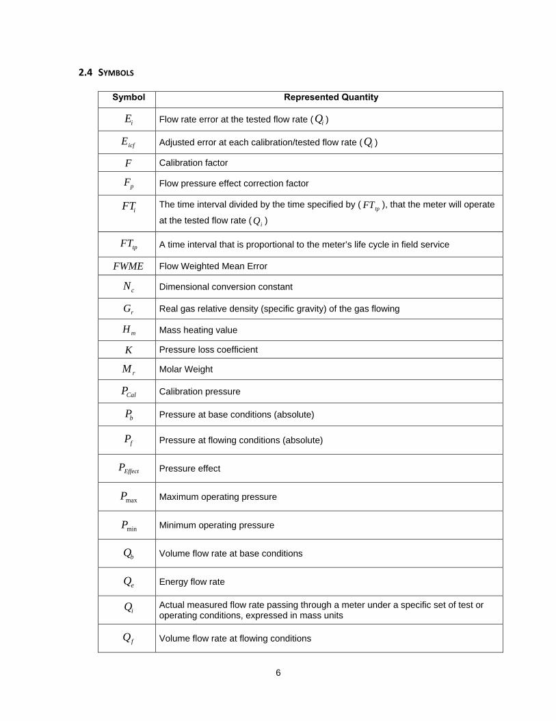
  2.4  SYMBOLS 

Symbol Represented Quantity

iE Flow rate error at the tested flow rate ( iQ )

icfE Adjusted error at each calibration/tested flow rate ( iQ )

F Calibration factor

pF Flow pressure effect correction factor

iFT The time interval divided by the time specified by ( tpFT ), that the meter will operate

at the tested flow rate ( iQ )

tpFT A time interval that is proportional to the meter’s life cycle in field service

FWME Flow Weighted Mean Error

cN Dimensional conversion constant

rG Real gas relative density (specific gravity) of the gas flowing

mH Mass heating value

K Pressure loss coefficient

rM

Molar Weight

CalP

Calibration pressure

bP Pressure at base conditions (absolute)

fP

Pressure at flowing conditions (absolute)

EffectP Pressure effect

maxP Maximum operating pressure

minP Minimum operating pressure

bQ

Volume flow rate at base conditions

eQ

Energy flow rate

iQ Actual measured flow rate passing through a meter under a specific set of test or operating conditions, expressed in mass units

fQ Volume flow rate at flowing conditions

7

mQ

Mass flow rate

dCompensatemQ Mass flow rate compensated for flow pressure effect

tedUncompensamQ Mass flow rate uncompensated for flow pressure effect

maxQ Maximum allowable flow rate through the meter, as specified by the meter manufacturer, expressed in mass units

minQ Minimum allowable flow rate through the meter, as specified by the meter manufacturer, expressed in mass units

tQ Transitional flow rate at which the maximum permissible measurement error and peak-to-peak error limit change, expressed in mass units

R Gas constant (8.314472 J mol-1 K-1, 10.7316 psia ft3 (lbmol ˚R) -1)

bT Temperature at base conditions (absolute)

fT Temperature at flowing conditions (absolute)

v Velocity of flowing gas

iWF Weighting factor for a tested flow rate ( iQ )

bZ Compressibility factor at base conditions

fZ Compressibility factor at flowing conditions

ZS Zero Stability

b Density at base conditions

f Density at flowing conditions

P Pressure drop or pressure loss across meter

 

8

3   OPERATING CONDITIONS 

  3.1  GAS QUALITY 

At a minimum, the meter shall operate accurately with any of the “normal range” natural gas composition mixtures specified in AGA Report No. 8 - Compressibility Factors of Natural Gas and Other Related Hydrocarbon Gases. This includes relative gas densities between 0.554 (pure methane) and 0.87. This document is limited to application of meters in the single phase gas flow.

The manufacturer should be consulted for wetted material recommendations,, if any of the following are possible:

Operation near the hydrocarbon dew point temperature of the natural gas mixture Total sulfur levels or other elements exceeding those specified in the National

Association of Corrosion Engineers (NACE) guidelines Presence of halogen elements in the gas mixture; i.e., chlorine, bromine, etc.

  3.2  OPERATING PRESSURES 

The manufacturer shall specify the maximum operating pressure. The flowing density, maximum acceptable pressure drop relative to gas flowing density (see Section 5.3.1, Equation 5.2), and desired meter performance will determine the minimum operating pressure. Therefore, the minimum operating pressure of a Coriolis sensor is application dependent. (See Section 4, “Meter Requirements,” for additional information.)

Some Coriolis meters exhibit sensitivity to changes in operating pressure, called “flow pressure effect”, which may create a negative bias in flow rate indication at operating pressures above calibration pressure and a positive bias at operating pressures below calibration pressure. This effect can be compensated for by use of an average flowing pressure correction (fixed value) or variable pressure correction using an external pressure measurement device. Since this effect is design and size specific, the designer shall consult with the manufacturer to identify the magnitude of the pressure effect at operating conditions. (See Section 4.3.4 “Pressure Measurement,” for further discussion)

  3.3  TEMPERATURE: GAS AND AMBIENT 

Coriolis sensors should operate over a flowing gas temperature range of -40 to 200F (-40 to 93C). It is recommended that the flowing gas temperature remain above the hydrocarbon dew point temperature of the gas.

  3.4  GAS FLOW CONSIDERATIONS 

The manufacturer’s flow range of a specific size flow sensor is determined by the acceptable accuracy at minimum flow rate and design limitations at maximum flow rate. The maximum allowable mass flow rate specified by the manufacturer may create fluid velocities and/or pressure drops beyond acceptable levels for a particular applications. Therefore, the designer’s application of a specific size flow sensor is determined by ensuring the expected flow rate range is within the manufacturer’s meter design limitations, application requirements, and the accuracy

requirements for minQ , tQ, and maxQ

as stated in Section 6.1 of this report.

The designer is to examine the maximum upstream and downstream piping velocities for noise and piping safety (thermowell vibrations, etc.) considerations. (For further information on probe vibration see American Petroleum Institute’s Manual of Petroleum Measurement Standards, Chapter 14, Part 1).

. Coriolis meters have the inherent ability to measure flow in either direction with equal accuracy; i.e. they operate bi-directionally. Coriolis flow sensors should not be installed where flow pulsation frequencies might coincide with the natural resonant frequency of the flow tube(s). Flow

9

pulsations at the meter’s resonant frequency may produce an error quantity. The magnitude and sign of the error is meter design specific. Flow pulsations may be caused by vortices created by piping design, flow obstructions (e.g. valves, thermowells, probes, etc.), regulator valve oscillation at low flows, and reciprocating engines/compressors. The meter manufacturer shall be consulted before installing a Coriolis flow sensor where pulsations are present.

  3.5  UPSTREAM PIPING AND FLOW PROFILES 

Upstream piping configurations (i.e., various combinations of upstream fittings, valves, regulators, and lengths of straight pipe) may affect the gas velocity profile entering a Coriolis sensor to such an extent that significant flow rate measurement error results. The magnitude and sign of the measurement error, if any, will be, in part, a function of the meter’s ability to correctly compensate for such conditions. In general, research has shown that this effect is dependent on meter design, as well as the type and severity of the flow field distortion produced at the meter. Nevertheless, Coriolis meters have shown to be somewhat immune to these effects

Meter station designers are encouraged to gain insight into expected meter performance for given upstream piping configuration by soliciting available test results for a particular meter design from the meter manufacturer or by reviewing test data found in open literature. When installation effects test data for a particular meter design do not exist, to truly confirm meter performance, flow testing of the metering module is usually required. The designer should consult the meter manufacturer and review the latest meter test results or verify installation effects through other means (e.g., experimental evaluation, see reference GRI-01/0222).

4   Meter Requirements 

  4.1  CODES AND REGULATIONS 

The meter sensor and all other parts of the pressure-containing structures and external electronic component enclosures, shall be designed and constructed of materials suitable for the service conditions for which the meter is rated and in accordance with applicable codes specific to the installation, as specified by the designer.

  4.2  QUALITY ASSURANCE 

The manufacturer shall establish and follow a written comprehensive quality assurance program for the production, assembly and testing of the meter and its electronic system (ISO 9000, API Specification Q1, etc.) This quality assurance program should be available for inspection.

  4.3  METER SENSOR 

4.3.1  Pressure Rating 

The meter sensor shall meet all applicable industry codes for the installation site and other requirements specific to the application, including the maximum allowable operating pressure over the temperature range. Meters should be manufactured to meet one of the common pipeline flange classes; e.g., ANSI (American National Standards Institute) Class 300, 600, 900. The maximum operating pressure of the meter shall be the lowest maximum design pressure of the wetted components of the meter including manifolds, sensor tube(s) and flanges. The pressure rating of the meter case, a non-wetted component, shall be specified as appropriate for the installation and application.

4.3.2  Corrosion Resistance 

Wetted parts of the sensor shall be manufactured of materials compatible with natural gas and related flow stream constituents described in Section 3.1 of this report.

10

All external parts of the meter should be made of a corrosion-resistant material or sealed with a corrosion-resistant coating suitable for use in environmental conditions typically found at the applicable meter installation site.

4.3.3  Meter Lengths and Diameters 

Manufacturers shall publish overall face-to-face length of the meter body with connections/flanges, piping diameter and the internal diameter of Coriolis flow sensor. The diameters of sensor and the process connections may differ.

4.3.4  Pressure Measurement 

The location of the pressure measurement can typically be made in close proximity, either upstream or downstream, of the sensor. In an application where high turndowns are required and a high-pressure drop across the meter may exist, the designer should locate the pressure tap upstream of the sensor where line pressure will vary less. For further information, see Section 8.1.2

4.3.5  Miscellaneous 

The meter should be designed in such a way that permits easy and safe handling of the meter during transportation and installation. Hoisting eyelets or clearance for lifting straps should be provided. Most Coriolis meters incorporate a housing or enclosure to protect the flow tubes and instrumentation. These housings are normally not designed for pressure containment. The designer should consult the manufacturer for possible secondary pressure containment.

4.3.6  Meter Body Markings 

Information indicating the following should be affixed to the meter body. Manufacturer, model number, and serial number Purchase Order Number or Shop Order Number (optional) Wetted material within the sensor Meter sensor size and flange class ANSI or equivalent rating system Operating temperature range Operating (gas) temperature range Tag number Applicable hazardous area approvals Direction of positive or forward flow

  4.4  ELECTRONICS 

4.4.1  General Requirements 

The Coriolis transmitter is an electronic system that includes a power supply, micro computer, processing circuits for the flow sensor drive signals, signal barriers for safe installation and output circuits. The transmitter may be integrally mounted on the flow sensor or remote from the flow sensor and connected by cabling.

The electronic system shall operate correctly over the entire range of environmental conditions specified by the meter manufacturer. It shall also be possible to replace the transmitter without a change in the meter performance, more than the “repeatability” specified in Section 6.1, “Minimum Performance Requirements.” The system shall include an automatic restart function, in the event of a computer program fault or lock-up.

11

The meter should operate at a nominal power supply voltage of 240V AC or 120V AC at 50 or 60 Hz, or from 12V DC or 24V DC power supply/battery systems, as specified by the designer.

4.4.2  Output Signal Specifications 

The meter should be equipped with at least one of the following outputs: Serial data interface; RS-232, RS-485, or equivalent Frequency, representing flow rate The meter may also be equipped with an analog (4-20mA) output for flow rate. A no-flow cut-off function should be provided that sets the flow rate output to zero when the indicated flow rate is below a set value. Meters used bi-directionally shall provide a method for differentiating forward from reverse flow to facilitate the separate accumulation of totals by the associated flow computer(s). All outputs should be isolated from ground and have the necessary voltage protection.

4.4.3  Electrical Safety Design Requirements  

The design of the meter, including the transmitter, as a minimum, should be analyzed, tested, and certified by an applicable laboratory, and then each meter should be labeled as approved for operation in a National Electric Code Class I, Division 2, Group D Hazardous Area.

4.4.4  Cable Jackets and Insulation  

Cable jackets, rubber, plastic and other exposed parts should be resistant to the environment to which the meter is exposed.

  4.5  COMPUTER PROGRAMS 

4.5.1  Firmware 

Processing software or firmware in the transmitter responsible for the control and operation of the meter shall be stored in a non-volatile memory. All configurable parameters shall be stored in non-volatile memory. For auditing purposes, it shall be possible to verify all flow calculation constants and parameters while the meter is in operation. The manufacturer shall maintain a record of all firmware revisions including revision serial number, date of revision, applicable meter models, circuit board revisions, and description of changes to firmware.

The firmware revision number, revision date, serial number, and/or checksum should be either available to an auditor by visual inspection of the marking on the firmware chip or capable of being displayed by the meter or ancillary device. The manufacturer may offer software upgrades from time to time to improve the performance of the meter or to add features. The manufacturer shall inform the meter operator if the firmware revision will affect the accuracy of a flow-calibrated meter.

4.5.2  Configuration and Maintenance Software 

The manufacturer shall supply a capability to configure and monitor the operation of the meter, either locally through embedded software or remotely through PC based software.

12

As a minimum the following parameters shall be available: flow rate, temperature, flowing density, and performance indicating parameter(s); e.g., drive power, signal quality etc.

4.5.3  Inspection and Auditing Functions 

It should be possible for an auditor to view and print the flow measurement configuration parameters used by the transmitter while the meter is in operation, either locally or remotely, with an appropriate data acquisition device using the configuration and maintenance software. In general, the measuring system should conform to the requirements provided in API’s MPMS, Chapter 21, Part 1 for electronic gas measurement. Provisions shall be made available to the operator/user to prevent an accidental or undetectable alteration of those parameters that affect the performance of the meter from that established by the manufacturer. For example, suitable provisions may include a sealable switch or jumper, single or multiple password levels in the transmitter, or a permanent programmable read-only memory chip.

4.5.4  Alarms 

When specified by the designer, the Coriolis meter may be available with alarm status outputs. The alarm-status outputs should be provided in the form of fail-safe, dry, relay contacts or voltage free solid-state switches isolated from ground. The alarm status may be set for the following.

Hard Failure: When any of several internal measurements (e.g., drive signal, pickoff signal, RTD, algorithms, etc.) fail for a specified length of time

Soft Failure: When the meter does not produce a useable output (see Section 8.2.5 for descriptions of example operating conditions that may cause a soft failure to occur)

4.5.5  Diagnostic Measurements 

Coriolis meter designs may offer diagnostics that automatically or through a manual process identify conditions that may affect meter performance. Diagnostic methods may require the use of an external tool or may be integrated into a meters design. The following lists examples of parameters or analysis measures that a manufacturer may provide for diagnostic measurement via a local display or a digital interface (e.g., RS-232, RS-485):

EPROM checksum Configuration change flag Drive gain or power indication Pickoff or signal amplitude Temperature output(s) Live zero flow indication Status and measurement quality indicators Alarm and failure indicators Flowing density or flow tube resonant frequency Flow tube health indication Flow tube balance or symmetry Frequency output test Digital status output test Analog output test

Note: Please consult manufacturer for the diagnostic parameters that are available.

To further optimize the use of diagnostics, the operator should baseline a meter’s diagnostic indicators either manually and/or through an automated process inherent to the

13

meter’s design during either meter calibration or initial installation, or both. Deviations from baseline diagnostics are useful in establishing acceptance criteria.

  4.6  DOCUMENTATION 

The manufacturer should provide or make available the following set of documents, as a minimum, when requested for quotation.. All documentation shall be dated.

Description of the meter giving the technical characteristics and the principle of its

operation Dimensioned drawing and/or photograph of the meter Nomenclature of parts with a description of constituent materials of such parts General description of operation Description of the available output signals and any adjustment mechanisms A list of the documents submitted Recommended spare parts

The manufacturer shall provide all necessary data, certificates and documentation for correct configuration, set-up and use of the particular meter upon delivery of the meter. The manufacturer should provide the following set of documents upon request. All documentation shall be dated

Meter-specific outline drawings, including overall process connection dimensions, ratings, maintenance space clearances, conduit connection points, and estimated weight.

Meter-specific electrical drawings showing customer the wiring termination points and associated electrical schematics for all circuit components back to the first isolating component; e.g., optical isolator, relay, etc.

Instructions for installation, operation, periodic maintenance and troubleshooting. Description of software functions, configuration parameters (including default value) and

operating instructions. Documentation that the design and construction comply with applicable safety codes and

regulations. A field verification test procedure as described in Section 9.1. “Field Meter Verification.” Drawing showing the location of verification marks and seals. Drawing of the data plate or face-plate and of the arrangements for inscriptions. Drawing of any auxiliary devices. A list of electronic interfaces and operator wiring termination points with their essential

characteristics.

The operator or designer may also request that copies of hydrostatic-test certificates, material certificates, and weld radiographs be supplied with delivery of the meter.

  4.7  MANUFACTURER TESTING REQUIREMENTS  

4.7.1  Static Pressure Testing 

The manufacturer shall test the integrity of all pressure-containing components for every Coriolis meter. The test shall be conducted in compliance with the appropriate industry standard, (ANSI/ASME B16.1, B16.5, B16.34, B31.8 or other, as applicable).

4.7.2  Alternative Calibration Fluids 

A representative number of samples of a given meter type and size should be calibrated using an alternative calibration fluid (e.g., water, air, etc.) and natural gas to adequately characterize any differences in meter performance (e.g., meter accuracy) produced by the different test media. Based on the results of this characterization process, an adjustment to the meter calibration factor may be made to ensure acceptable meter performance in gas service. The uncertainty of measurement for the meter shall be stated as applicable to the

14

intended gas service. Any limitations or restrictions to the operational range of the meter in gas service must also be stated.

4.7.3  Calibration Requirements 

Each meter should be calibrated against a recognized national or international measurement standard over a flow range that is representative of the application rate(s) and sufficient to establish meter accuracy and linearity, i.e. within maximum peak-to-peak error limit.

4.7.4  Calibration Test Reports  

All meter test results will be documented in a written report that shall be archived by the meter manufacturer at the time of meter shipment to the owner/operator. At least one copy of the complete report shall be provided to the meter owner/operator. The meter manufacturer should keep a copy of the test report on file for at least 10 years and make the complete report available to the owner/operator upon request, at any time during that period. The report shall include the following, as a minimum:

Name and address of the meter manufacturer. Name and address of the test facility. Test meter model and serial number. Test meter line size or capacity rating. Test meter software revision number. Date(s) of the test. Name and title of those who conducted the tests. Flow testing calibration value(s) vs. flow rate. Meter software configuration parameters. All measured test data, including flow rates, pressures, temperatures, gas

composition (if so calibrated), and estimates of the measurement uncertainty of the test facility and the test meter.

An uncertainty statement of the flow facility reference at each flow rate the meter is calibrated.

The following shall be available upon request

A written description of all test procedures and pertinent test conditions. Meter mounting arrangement, including upstream/downstream piping

configurations (If applicable). Report of diagnostic information.

4.7.5  Quality Assurance  

The manufacturer should establish and follow a comprehensive quality-assurance program for the assembly and testing of the meter and its electronic system (e.g., ISO 9000, API Specification Q1, etc.). The user shall have access to the quality assurance documents and records. Test facilities used for meter calibration shall be able to demonstrate traceability to relevant national primary standards and to provide test results that are comparable to those from other such facilities.

 

 

 

15

5   Meter Sizing Selection Criteria 

The major consideration when sizing a Coriolis meter is the tradeoff between pressure loss and usable meter range for a given accuracy. In order to properly size a Coriolis meter, the designer/user should provide the manufacturer the following information.

a. Flow rate range. b. Pressure range. c. Temperature range. d. Allowable pressure drop. e. Gas composition or flow density at minimum operating pressure and maximum operating

temperature. f. Required meter accuracy.

Properly sizing a Coriolis meter consists of choosing a meter size that optimizes the tradeoff between measurement error at minimum flow rate and pressure loss and/or gas velocity at maximum flow rate. At a given flow rate, pressure drop and gas velocity are higher through a smaller diameter meter, but potential measurement error at the lowest flow rates is generally reduced and useable turndown ratio is typically increased. Likewise, pressure drop and gas velocity are lower when a larger diameter meter is chosen, but potential measurement error at a similar low flow rate may increase and turndown ratio decrease.

  5.1  MINIMUM FLOW RATE  

The minimum flow rate ( minQ ) of a Coriolis meter is specified by the manufacturer and determined by defining the lowest flow rate at which the meter error will not exceed the limit specified in Figure 6.1. While at high flow rates, the meter error is dominated by flow noise and other influences; at low flow rates the meter error is dominated by the meter’s zero stability. Thus,

the measurement error of a Coriolis meter below Q t is primarily determined from the meter’s

zero stability ( ZS ) and the manufacturer’s published accuracy equation. Since the minimum flow

rate of a Coriolis meter is relative to mass flow, once minQ is determined in base volume units for a particular gas mixture, it will remain a constant over the range of temperature, pressure and flow velocity. Only a change in gas composition or base volume conditions will cause the value of

minQ to change.

  5.2  TRANSITIONAL FLOW RATE  

This is the flow rate at which the allowable error changes. (See Section 6.1 for performance limit definition).

  5.3  MAXIMUM FLOW RATE  

The maximum flow rate ( maxQ) of a Coriolis meter is specified by the manufacturer. The designer

may choose a lower maximum flow rate based on the acceptable pressure drop across the meter and/or flow velocity.

5.3.1  Meter Pressure Loss ( P ) 

The designer will size the Coriolis flow meter to optimize the meter performance over the flow rate range with a pressure drop that is acceptable for the application. If pressure drop is a priority, meter selection will be made to provide the lowest possible pressure drop at maximum flow while maintaining an acceptable measurement error at minimum flow rates. As examples, figures 5.1 and 5.2 show the relationship between pressure drop and measurement error at line pressures of 1,000 and 500 psia, respectively, with 0.6 gravity natural gas at flow rates up to 50 Mcf per hour for several typical line sizes for one particular meter design.

16

Figure 5.1

Example Flow Rate vs. Meter Error on 2-inch and 3-inch Coriolis meters with 0.6 gravity natural gas at 1000 psia and 60 F

Figure 5.2

Example Flow Rate vs. Meter Error on 2-inch and 3-inch Coriolis meters with 0.6 gravity natural gas at 500 psia and 60 F

17

Pressure drop is determined by a constant called the pressure loss coefficient ( K ) defined as

2

2

v

PNGK

f

cc

Re-writing the equation to solve for pressure drop ( P ), the equation becomes:

cc

f

NG

vKP

2

2

Parameter U.S. Units SI Units

Pressure drop ( P ) psi kpa

Pressure loss coefficient ( K ) non-dimensional non-dimensional

Density flowing ( f ) lb/cf kg/m3

Velocity ( v ) ft/s m/s

Dimensional constant ( cN ) 4633.06 32174

Acceleration of gravity ( cg ) 32.174 ft/s2 1

The equation shows that with flowing density ( f) constant, the pressure loss ( P ) is

directly proportional to the square of the flowing gas velocity ( v ). Because the pressure drop increases with the square of the velocity, choosing a larger line size meter will significantly lower the pressure drop. However, the measurement error over the operating flow rate range below the transitional flow rate for the larger size meter will typically be greater. Every manufactured type and size of Coriolis meter will have a different pressure drop for a given flow rate. The designer should consult the meter manufacturer for specific pressure drop information for a given meter type and size.

  5.4  METER SIZING METHODOLOGY 

Meter size is selected based on such designer criteria as pressure drop at maximum flow, flow rate requirements, accuracy at minimum flow, etc. The flow chart in Figure 5.3 describes methodology using pressure drop and details that a designer may use for selecting the appropriate meter size for a given application. If a specific measurement error limit at maximum and minimum flow rates is desired, the required performance can be determined and a suitable meter selected. Once the meter type and size are selected, the meter manufacturer shall provide the estimated measurement error at the maximum and minimum flow rates. The following flow chart depicts this process.

Eq. (5.1)

Eq. (5.2)

18

Figure 5.3

Sizing Methodology Flow Chart Notes:

1) Meter sizing may be optimized by relocating the meter to a point in the piping where the gas is at

a higher pressure, i.e., upstream of a pressure regulator. Higher process pressures improve meter turndown ratio by increasing gas density and reducing the pressure drop across the mass flow rate range. Utilizing higher process pressures can also reduce meter size requirements.

2) Choosing a meter with better performance at minimum flow rate may result in a higher pressure drop at maximum flow rate. If a suitable meter is not available, the designer or operator should review the application requirements. Performance requirements at minimum flow may need to be relaxed, and/or allowable pressure drop at maximum flow may need to be increased.

Appendix F details sizing examples and equations to aid designers in the sizing of Coriolis meters.

Error @ Max flow < 0.7%?

Select smaller meter, or one with

smaller ZS

Review Application (Notes 1, 2)

Pressure drop and velocity

OK?

Yes No

Error @ Min flow <

1.4%?

Calc flow rate @ 1.4%

No (Note 2)

Meter choice is

acceptable

Yes

No

Meter choice is

acceptable

Yes

No

Meter selected by pressure drop and

velocity at maximum flow rate

Meter error at minimum flow rate

calculated using ZS

OK?

Meter selected by pressure drop and

velocity at maximum flow rate

19

6   Performance Requirements 

The meter manufacturer shall state the meter performance specifications for each meter type and line size. The pressure drop through the meter will be charted, graphed or made available through a sizing process utilizing the pressure loss coefficient ( K ) or correlative equations and reference data to allow the determination of the pressure drop at the gas flow application conditions.

Each meter shall be individually calibrated and traceable documentation provided as evidence that the individual meter meets the stated performance (see Section 6.1). The Coriolis meter will be calibrated over the mass flow rate range for the intended application, if known. The specific performance of the meter over the given flow range is dependent on the meter size and design/type. Once the meter size is chosen (see Section 5), the meter performance at the application conditions shall meet or exceed the performance requirements stated here. For Coriolis flow meters that are calibrated using a liquid medium, or other gas medium, data will be provided showing results for calibrations done on the same liquid or gas medium, and natural gas for meters of the same design/type and size. Additional or other information and/or calibration data (see Sections 4.7.3 and 4.6) may be provided, as agreed upon between the designer/operator and the meter manufacturer.

  6.1  MINIMUM PERFORMANCE REQUIREMENTS 

In the sizing and selection of Coriolis meters for natural gas applications, the following minimum performance requirements shall be met by the meter, as supplied directly from the manufacturer, prior to making any calibration factor adjustments based on an independent third party flow calibration of the meter.

Repeatability: + 0.35% of reading for tQ < iQ < maxQ

+ 1.0% of reading for minQ < iQ < tQ

Maximum Mean Error: + 0.7% of reading for tQ < iQ < maxQ

+ 1.4% of reading for minQ < iQ < tQ

Maximum Peak-to-Peak Error: + 0.7% of reading for tQ < iQ < maxQ

+ 1.4% of reading for minQ < iQ < tQ

20

Figure 6.1

Performance Specification Graphical Representation

  6.2  PERFORMANCE ENHANCEMENTS  

At the request of the designer/operator, the manufacturer shall state the sensitivity of meter accuracy to changes in gas pressure, temperature, fluid composition, and fluid flowing density over the operating range. This information may be used by the designer/operator to further enhance meter performance.

The designer/operator shall evaluate the meter operating conditions and determine the need to apply a fixed calibration factor adjustment or an active calibration factor adjustment, based on the expected variation in operating conditions.

7   Gas Flow Calibration Requirements 

Manufacturers are responsible for initial flow calibration of Coriolis meters prior to delivery (see Section 4.7.3). Calibration with an alternative calibration fluid (e.g., water) is valid with Coriolis sensor designs where the transferability of the alternative calibration fluid, with an added uncertainty relative to gas measurement, has been demonstrated by the meter manufacturer through tests conducted by an independent flow calibration laboratory. When the transferability of the manufacturer’s calibration fluid to gas cannot be verified, the meter shall be flow calibrated on gas as per the requirements in Section 7.1 If the Coriolis sensor design is sensitive to installation effects, the metering module shall be calibrated on gas. In this instance, the metering module includes adequate upstream piping, flow conditioning, downstream piping and, if applicable, thermowells and sample probes to insure that there is no

21

significant difference between the velocity profile experienced by the meter in the laboratory and the velocity profile experienced in the final installation.

  7.1  FLOW CALIBRATION TEST 

It is a requirement that all flow calibration be completed in a certified flow calibration facility or by a calibration system that is traceable to a recognized national/international standard.

The designer, operator and/or manufacturer shall provide the calibration facility with the following information:

Meter size.

Piping data (i.e., dimensional, process connection, and ANSI rating).

Flow calibration test points (i.e., flow rate, pressure, temperature).

Output signal to be used for calibration (digital data, frequency, or analog).

Any special calibration instructions (e.g., for bi-directional calibrations duplicate flow calibration test points in both directions).

A drawing showing the metering module assembly.

Any thermodynamic or physical properties (e.g., density, compressibility, speed of sound, critical flow factor, etc.) used during flow calibration shall be computed using latest revision of the GERG equation of state or Detailed Characterization Method from AGA Report No. 8, Compressibility Factors of Natural Gas and Other Related Hydrocarbon Gasses, and AGA Report No. 10, Speed of Sound in Natural Gas and Other Related Hydrocarbon Gasses.

7.1.1  Preparation for Flow Calibration 

The calibration provider shall perform the following as regular procedure.

Inspect the meter module for any obvious physical damage and verify that its physical configuration matches the configuration specified by the user.

Verify that the electronic configuration in the meter, related to flow measurement, matches the configuration provided by the manufacturer. If the manufacturer recommends any changes to the meter configuration prior to calibration, the calibration provider is responsible for following the manufacturer’s recommendations.

Calibrate using the meter output signal requested by the user.

Perform a zero flow verification test and re-zeroing (if applicable) of the Coriolis meter prior to calibration. This shall be performed in accordance with the manufacturer’s specification and at the intended flow calibration average pressure and temperature.

Provide a record of the “As Found” meter configuration and performance (when requested) along with a record of all subsequent changes or the “As Left” meter configuration and performance to the user.

7.1.2  Calibration of Metering Module 

The calibration will involve flowing gas, one or more reference meters in series with the meter module under test and at the flow rates recommended in Section 7.1 above. Flow, temperature, pressure and fluid property data will be acquired or calculated and an error for the meter will be calculated at each flow rate.

22

All calibrations will be designed using sound statistical techniques to determine the number of calibration points, the number of samples at each point and the size of each sample. A calibration point will be derived from a statistically significant measurement. At least 5 flow rate test points should be selected throughout the range of flow rates over which the meter is to be applied. The designer may specify additional flow calibration tests or a modified set that more closely represents field operating conditions. If a calibration factor(s) is applied to the meter, then at least one verification point(s) shall be run.

  7.2  CALIBRATION ADJUSTMENT FACTORS 

Calibration adjustment factors shall be applied, if necessary, only over the range of tQ to maxQ to minimize or eliminate any indicated meter bias error. Adjustment of a calibrated meter’s performance, shown to be within the uncertainty of the flow calibration reference is not recommended, but is left to the discretion of the user. The accepted methods of applying adjustment factors are:

Using the flow-weighted mean error (FWME) over the meter’s expected flow range (Calculation of FWME is shown in Appendix A).

Using a polynomial algorithm.

Multipoint linear interpolation.

Piecewise linearization method.

For bi-directional flow calibrations, in the absence of the manufacturer demonstrating identical forward and reverse performance for a particular design, a reverse flow calibration test shall be conducted and a second set of calibration adjustment factors shall be applied, if necessary, for reverse flow.

  7.3  CALIBRATION REPORTS  

The results of each calibration performed shall be documented in a written report supplied to the designer or the operator. For each meter, the report should include the following, at a minimum:

1. The name of the manufacturer.

2. The name and address of the facility.

3. The model and serial number of the meter.

4. The transmitter firmware revision number.

5. The date(s) of the test.

6. The name and title of the person(s) who conducted the tests.

7. Basic description of the test method.

8. The upstream and downstream piping configuration, including flow conditioner (If applicable).

9. The serial numbers of all piping and flow conditioners (If applicable) forming the meter module as supplied by the user.

10. A statement of uncertainty for the facility with reference to the method used and date of last verification of traceability to a recognized national/international standard.

11. All test data, including flow rates, errors, pressure, temperature and gas density/composition.

12. Graph of “as found” performance.

13. Identification of adjustment method and any adjustment factors applied.

14. Verification test data, including flow rates, errors, pressure, temperature, and gas density/composition.

23

15. “As left” performance; i.e., graph of theoretical performance after adjustment including any performance verification points taken

16. A report of the software configuration parameters

17. A report of diagnostic information

18. Page and page number of the calibration document, e.g., (1 of 12)

19. Typed names below signatures of all persons who sign calibration document.

At least one copy of the complete report shall be sent to the designer or the operator. For the initial gas calibration of new meters conducted by the manufacturer, one copy will be retained in the manufacturer’s files. The manufacturer shall ensure that the complete report is available to the operator upon request for a period of 10 years after shipment of any meter. Flow calibration facilities shall ensure that the complete report is available, for a period of 10 years after shipment of any meter.

  7.4  ADDITIONAL CONSIDERATIONS                 

7.4.1  Pressure Effect Compensation 

Flow pressure effect compensation should be addressed during gas flow calibration. Coriolis meters are typically calibrated on water at pressures below 50 psig by the manufacturer. Gas flow testing of a Coriolis meter above the manufacturer’s water calibration pressure will induce a negative flow bias relative to the flow pressure effect specification for the particular meter design.

Example: A specific Coriolis meter sensor design has a flow pressure effect of -0.001%

per psig. The meter was initially water-calibrated at 50 psig. The meter was subsequently gas-flow-tested at 550 psig. If the flow pressure effect compensation is disabled and a flow pressure calibration factor is not applied, the use of the meter would result in an under registration of 0.5%, due to the pressure difference between the initial water calibration and subsequent gas test.

Pressure effect compensation may be applied in several ways depending upon the Coriolis flowmeter design.

Where the pressure will vary significantly, an input may be provided to the transmitter that represents the active line pressure. The transmitter or flow computer is programmed with the calibration pressure value and the pressure correction factor supplied by the manufacturer.

Where the pressure will not vary significantly, a fixed correction value is applied representing the average operating pressure. The correction value may be applied as a fixed value in the transmitter or as a correction value applied to the calibration factor.

If flow pressure effect compensation is applied during flow calibration, it should be noted that the compensation applied by the meter is referenced to the water calibration pressure. If a calibration factor is applied to the meter based on data collected while pressure compensation is being applied by the meter, the meter’s reference calibration pressure

( CalP) will remain at the pressure at which the original water calibration was performed.

The user may choose to establish a new calibration pressure (Cal P) for the meter relative to the gas calibration pressure during flow calibration. The user must direct the gas flow calibration facility to disable the flow pressure effect compensation. By doing this the data collected during gas flow test will include that of flow pressure effect from the water calibration pressure to the gas flow test pressure. Thus, when a flow calibration correction

24

factor is applied, it will correct the meters performance from the water calibration pressure to the gas flow test pressure. This method may be preferred by the user as it retains the traceability of the gas flow calibration pressure to that at which the flow calibration factor

was established at; i.e., the calibration pressure ( CalP) and the flow calibration factor will

be contained on the same calibration certificate. Assuming the meter was gas flow calibrated at average operating pressure, this method also minimizes the magnitude of flow pressure effect compensation required during field operation to only pressure deviations away from average operating pressure.

7.4.2  Coriolis Flowmeter Diagnostics 

During the calibration, meter diagnostics should be monitored for alarm or an out-of-tolerance condition. If an advanced diagnostic for flow tube health exists, this diagnostic test should be performed after calibration is completed and results reported. Actual diagnostic capabilities vary by design; the flow calibration facility should consult with the manufacturer to determine an appropriate set of diagnostics for the particular design. Refer to Section 4.5.5 A meter log file generated at calibration can establish the meter baseline data. Meter log data and/or the results of an automated flow tube health diagnostic should be included to provide a baseline of the metering module performance at calibration. This baseline data can be used to verify the meter’s performance upon startup, during operation, and after component changes. The baseline data can also be useful in conducting health checks of the metering module. It is recommended that manufacturers identify the parameters that define the baseline performance for their products.

  7.5   FINAL CONSIDERATIONS 

Upon completion write protect jumpers/switches should be installed and software security relative to metrology enabled or access to transmitter communications sealed to prevent metrology affecting parameter changes.

8   Installation Requirements 

This section is directed to the designer to ensure that Coriolis flow meters will be installed in a suitable environment and in a piping configuration in which Coriolis meters can meet the expected performance requirements described in Section 6 of this report. This section also addresses the commissioning and maintenance processes inherent to achieving and maintaining performance.

  8.1  GENERAL REQUIREMENTS

8.1.1  Temperature 

8.1.1.1    Ambient Coriolis flow meters should operate properly over a minimum ambient temperature range of –13 to 131F (-25 to 55C). Special consideration should be given to extreme ambient environments; e.g., painting the meter white, providing shade to reduce solar radiation in direct sunlight, a suitable enclosure in colder climates, or insulating the meter.

8.1.1.2    Process

Due to mass, base volume, and energy relationships, a temperature measurement is not required to calculate base volume and energy. The Coriolis sensor measures temperature to correct for the effect of temperature change according to Young’s modulus on the flow tube(s). Routine meter verification procedures include the verification of the Coriolis sensor’s temperature indication

25

to be within the manufacturer’s specified tolerance. Designers are encouraged to install a thermowell upstream of the Coriolis sensor for temperature verification purposes and issues related to Joule-Thomson effects at high pressure drops.

   8.1.2  Pressure 

If pressure compensation is used, the location of the pressure measurement should be made in close proximity to the sensor. The pressure tap can be located either upstream or downstream of the sensor, though upstream is preferred.

 

8.1.3  Vibration 

Coriolis meters are mostly immune to vibrations away from the natural resonant frequency of its flow tube(s). Coriolis flow sensors should not be installed where mechanical/structural vibration levels might excite the natural resonant frequency of the flow tube(s). Vibrations at the natural resonant frequency of the flow tube(s) will induce an influence quantity. The magnitude and sign of the error is meter design specific. The natural resonant frequency of a Coriolis meter is dependent upon design and operating conditions.

8.1.4  Electrical Noise 

Although a Coriolis flow meter is designed to withstand electrical noise influences, the designer should not expose the Coriolis flow meter or the connected wiring to any unnecessary electrical noise; i.e., electromagnetic interference (EMI), radio frequency interference (RFI), solenoid transients, etc. Refer to the manufacturer’s recommended installation instructions for further guidance.

  8.2  METER MODULE DESIGN 

Testing to date has shown that some bending-mode Coriolis flow sensors are generally immune to velocity profile distortion, pulsations and swirl effects, thus allowing the designer flexibility restricted only by good piping support practices to minimize structural stresses on the sensor body.

It is recommended that the meter manufacturer be consulted regarding upstream and downstream piping configuration requirements, as well as any requirements pertaining to the use of a flow conditioner upstream of the sensor. When velocity profile is of concern, the designer may also choose to do one or more of the following:

Install a flow conditioner upstream of the sensor that will produce a fully-developed

turbulent velocity flow profile, regardless of the upstream piping configuration.

Flow-calibrate the Coriolis meter in-situ or in a flow calibration facility using a piping configuration identical to the planned installation.

Provide a sufficient straight length of upstream pipe to achieve a fully developed turbulent

velocity flow profile, determined by analysis and/or field-testing.

A fully developed, swirl-free, turbulent velocity flow profile is generally the most desirable condition entering any flow meter. Further information may be found in GTI Topical Report GRI-01/0222 Coriolis Mass Flow Meter Performance with Natural Gas.

8.2.1  Piping Configuration 

For Coriolis meters not susceptible to profile distortions, examples of Coriolis piping configurations are shown in Figures 8.1 and 8.2 The Coriolis sensor is typically one or

26

more sizes in flow diameter smaller than the system piping. It is good practice to provide the following components in the piping design.

Bypass Provides an alternate path for process supply during meter

maintenance and inspection procedures. Consideration should be given to prevent inadvertent bypassing of the meter. Note: Use of valves incorporating double block and bleed mechanisms can facilitate the identification of bypass leaks caused by a leaking block valve seat.

Isolation Block Valves Allows isolation of the Coriolis sensor from process conditions

and thermally driven flows during maintenance and inspection. Isolation block valves should be located in close proximity to the meter to facilitate accurate zeroing. Note: Use of valves incorporating double block and bleed mechanisms can improve maintenance efficiency and the certainty of isolation.

Pressure and Provides for the monitoring of process pressure when required. Blow-down Port When used for the correction of flow pressure effect, the process

connection should be located directly upstream of the sensor. A blow-down valve incorporated into the design facilitates leak checking of Coriolis upstream and downstream isolation block valves (if not double block and bleed type) prior to the sensor zeroing process, relief of process pressure prior to maintenance and the installation of a re-calibrated Coriolis meter/meter module, if required.

Thermowell Port Provides for use of a flow temperature reference in the

verification of the Coriolis sensor’s temperature measurement. This process connection should be located upstream of the Coriolis sensor.

Figure 8.1

Installation Example

27

In gas measurement applications, a Coriolis sensor’s flow diameter will typically be one or more pipe sizes smaller than the upstream and downstream piping to which -it is connected, requiring the use of reducers and expanders in the design. Excessive lengths of small diameter pipe, rapid flow diameter reductions, rapid changes in flow direction (tees, short radius elbows, etc.) can adversely affect piping pressure drop. The designer should employ conservative piping design techniques when the magnitude of pressure drop is of concern in a particular application. Figure 8.2 shows an example of a Coriolis meter installation where conservative piping design is employed to reduce operating pressure drop.

Figure 8.2

Installation Example Minimizing Operating Pressure Drop

8.2.2  Flow Direction 

For bi-directional flow applications, both ends of the sensor shall be considered "upstream,” particularly if the sensor is sensitive to velocity profile distortion effects.

8.2.3  Protrusions 

Changes in internal diameter, protrusions and misaligned flanges shall be avoided on meter modules when the sensor is sensitive to velocity profile distortion effects.

8.2.4  Meter Mounting 

The manufacturer shall be consulted for specific mounting requirements. Proper mounting of the sensor is required to achieve the desired meter performance. Consideration shall be given to the support of the sensor and the alignment of the inlet and outlet flanges with the sensor. A pipe spool piece should be used in place of the meter to align the upstream and downstream piping during the construction phase.

Piping should meet the requirements of typical industry piping codes. Meter performance, specifically zero stability, can be adversely affected by axial, bending and torsion stresses from pressure, weight, and thermal effects. Utilizing properly aligned pipe-work and properly designed supports can minimize these stresses and associated loads.

28

The Coriolis transmitter should be mounted so that it can be easily accessed to attach communications equipment for operation and maintenance needs. Most Coriolis flow meters are configured in two basic ways, with either the transmitter mounted to the sensor or the transmitter mounted remotely.

8.2.5  Orientation 

The designer shall consult the manufacturer installation guidelines for proper orientation of the meter. In general, sensor orientation does not affect performance, but orientation range is limited by flow tube geometry and the potential for settling or the loading of condensates. As a rule, orient the sensor flow tubes in such a way as to minimize the possibility of loading condensate in the vibrating portion of the sensor; i.e., flow tubes oriented in a upward direction in gas service. Solids, sediment, coatings, trapped liquids or plugging of the flow path(s) can affect the meter performance, especially when present during zeroing of the meter. In applications where condensates regularly exist (e.g., production), the sensor should be mounted in a self-draining position.

8.2.6  Filtration 

Filtration of the flowing gas is not necessary for most applications of a Coriolis flow meter. However, if there are abrasive contaminants or other debris in the gas flow stream, erosion or damage of the wetted meter components may be a concern, the designer should consider the use of upstream filtration. Susceptibility to this effect is specific to sensor design, size, and velocity.

8.2.7  Provision for Sample Probe(s) 

Provision for sample probe(s) utilized in the monitoring of gas composition, density or gravity can be located either upstream or downstream, when required. Downstream is preferred when concern for flow bypass exists.

8.2.8  Gas Velocity 

Coriolis sensors are typically designed with nickel alloy wetted components and are highly immune to the high velocity gas flow erosion associated with carbon steel pipe, which is induced by corrosive contaminants (e.g. H2O, H2S, etc.) in the gas stream. The gas contaminant levels that raise these concerns are mainly associated with the operating conditions in gas production. Designers regularly design carbon steel piping with these concerns in mind, but the use of reducers and expanders upstream and downstream of the Coriolis sensor is common. When high levels of corrosive contaminants exist, the designer should consider the use of reducers and expanders constructed of a nickel alloy or the user should employ inspection procedures to identify if, in a particular application, a problem exists.

8.2.9  Multiple Meters in Close Proximity 

In some applications, it may be necessary to install multiple flow sensors in close proximity, either in parallel or series. In this case, the vibrations generated by each sensor could interfere with each other, affecting the measurement output of each — this effect is called “cross talk.” Vibration isolation or dampening can be achieved by altering piping, isolation valves and/or supports. Some manufacturers may also be able to alter the drive frequency of their sensors, thereby reducing the possibility of mechanical cross talk between adjacent meters.

8.2.10 Performance Baseline 

The operator should baseline the meter, either manually or through an automated process inherent to the meter’s design, during the meter’s calibration and/or initial installation. Some parameters that can be used to baseline a Coriolis meter’s

29

performance are drive gain, pickoff coil amplitude and zero value. Some manufacturers offer diagnostics that directly infer change in a meter’s flow performance or flow factor. These baseline relationships are useful in establishing acceptance criteria for the various relationships and the need for a flow performance test and adjustment (if necessary).

  8.3  ASSOCIATED FLOW COMPUTER 

In applications where a flow computer is utilized, the Coriolis transmitter output to the flow computer is typically uncompensated mass, either per a unit of time or accumulated. Therefore, if capable, the associated flow computer may apply any flow pressure effect compensation necessary. Optionally, the flow pressure effect compensation can be performed within the Coriolis transmitter.

For bidirectional applications, the Coriolis meter should be treated as two separate meters or associated to two “separate meter runs” in a single flow computer.

For detailed requirements, refer to Appendix E, “Coriolis Gas Flow Measurement System” and API MPMS Chapter 21.1, Flow Measurement Using Electronic Metering Systems, in which, a Coriolis meter is classified as a “Linear Meter”.

8.3.1  Flow Computer Calculations 

The equations for measuring a gas with a Coriolis meter are summarized with the following expressions. When measuring mass flow away from calibration pressure, there is a secondary effect on a Coriolis meter’s indicated flow rate called the “flow pressure effect.” To correct for

this effect, a flow pressure effect compensation factor ( pF ) must be applied by the flow

computer to the uncompensated mass flow indication from the transmitter. This relationship is such that,

)( pmm FQQtedUncompensadCompensate

Eq. (8.1)

Where: dCompensatemQ = Mass flow rate of gas compensated for flow pressure effect

tedUncompensamQ

= Mass flow rate of gas uncompensated for flow pressure effect

pF = Flow pressure effect compensation factor

The flow pressure effect compensation factor ( pF) is calculated in accordance with the

following equation.

))(*)100/((11

CalfEffectp PPP

F

Eq. (8.2)

Where: pF = Flow pressure effect compensation factor

EffectP = Flow pressure effect in percent of rate per psig

fP = Measurement fluid static pressure in psig

CalP = Calibration static pressure in psig

30

The flow rate from a Coriolis measurement system can take several forms, depending on whether the ultimate quantity being measured is mass, volume at base conditions, energy or volume at flowing conditions. Appropriate conversions, relative to the gas physical properties and process conditions, must be applied to accurately obtain the desired quantity. The equation for flow rate at base conditions, including flow pressure

effect compensation factor ( pF), is such that,

)( Airbr

pm

b

pmb G

FQ

FQQ

edUncmpensattedUncompensa Eq. (8.3)

Where: bQ = Volume flow of gas at base conditions

tedUncompensamQ = Mass flow of gas uncompensated for flow pressure

effect

pF = Flow pressure effect compensation factor

b = Density of gas at base conditions

rG = Relative density of gas at base conditions

)( Airb = Density of air at base conditions

The relationship for the calculation of energy, including flow pressure effect

compensation factor ( pF), is such that,

)( mpme HFQQtedUncompensa

Eq. (8.4)

Where: eQ = Energy rate of gas

tedUncompensamQ = Mass flow of gas uncompensated for flow pressure

effect

pF = Flow pressure effect compensation factor

mH = Mass heating value

   8.4  MAINTENANCE 

Users should follow the manufacturer’s recommendations for maintenance. Monitoring diagnostics, performing the periodic meter verification procedures discussed in Section 9.1 and possibly the trending/long-term monitoring of performance indicators, can identify if abnormal conditions develop.

Maintenance procedures, such as cleaning, should be condition-based (based upon meter diagnostics, process conditions, and/or meter usage). The monitoring of performance indicators can identify the need for cleaning. For example, by monitoring the measured flowing density and comparing it with the calculated/real density, it is possible to infer coating on the flow tubes. Performance indicators available to the user are design specific and the meter manufacturer should be consulted on performance indicators available and their interpretation.

The decision to perform periodic flow test is left to the user or defined by contract. Periodic flow test can be calendar-based or, as a minimum, condition-based. A number of companies have

31

flow-tested Coriolis meters that have been in service for significant (in excess of 15 years) periods of time. These test results have shown that meters, free from flow tube corrosion, erosion or mechanical damage, perform as originally flow-calibrated, within the uncertainty of the flow lab. This testing has also shown that coating of the flow tubes by debris or product residue may change flow tube balance and cause a subsequent zero shift, but if the coating is stable, left as-is and the meter is re-zeroed, the meter performs as originally calibrated. See Section 9.2, “Flow Performance Testing” for further discussion.

  

9   Meter Verification and Flow Performance Testing 

The meter manufacturer should provide the meter operator with written field meter verification test procedures that will allow the Coriolis meter, as a component of the measuring system, to be verified as operating properly and performing within the measurement uncertainty limits required by the designer/operator. Further discussion of these checks can also be found in Appendix C, Section 3.4.1.

  9.1  FIELD METER VERIFICATION 

The field verification of a Coriolis metering system consists of monitoring and evaluating metering conditions, diagnostic indicators output by the transmitter and/or ancillary devices of the metering system designed to identify possible change in the system’s performance and the cause. The evaluation of these indicators will guide the operator in determining the need to re-zero the Coriolis meter, execute a flow performance test (in-situ or laboratory), adjust maintenance intervals and implement design improvements, if necessary, to the metering system.

The operator should follow design-specific meter verification procedures recommended by the manufacturer and as a minimum the following general meter verification procedures should be performed.

Meter Transmitter Verification – The meter transmitter verification should coincide with

the meter zero check. It should include the following procedures:

o Verify the sensor calibration and correction factors in the configuration of the transmitter to be unchanged from most recent calibration.

o Verify all transmitter diagnostic indicators to be in the normal state.

Coriolis Sensor Verification – Sensor diagnostics may be available that continuously,

on-command or procedurally verify the performance of the sensor and/or infer change in measurement performance. Users should consult the meter manufacturer for the availability of these types of diagnostics.

Temperature Verification – The Coriolis transmitter monitors a temperature element

bonded to the flow tubes of the Coriolis sensor to correct for Young’s modulus of the flow tubes. Although transmitter diagnostics on this element exist, they typically identify only catastrophic failures; e.g., element open, element short, and an opening in the compensation loop.

Use a temperature reference placed in an upstream thermowell or temporarily placed tightly against the upstream flow splitter/inlet and insulated, to verify the temperature indicated by the Coriolis meter to be within the published uncertainty of the Coriolis meter’s temperature measurement plus the accuracy of the temperature reference.

Meter Zero Verification – A change in the meter zero value can be used as an indicator of change in the metering conditions. This can be caused by contamination and coating of

32

the flow tubes (e.g., condensates, glycol, amines, water, oil, dirt, etc.), erosion, corrosion, inadequate structural support, and/or out-of-square components constructed into the meter module. These influences may cause a bias in the meter zero through change in the dynamic balance of the meter’s flow tubes.

It is recommended, as a minimum, that the meter zero be checked at flowing pressure and temperature within 1 to 4 weeks of installation and quarterly during the first year of its field service. The frequency of subsequent zero verifications should be guided by the record of meter zero data and operating conditions, and by operator policy. The meter zero verification should include the following procedures:

o Thermal stability is critical for obtaining a proper meter zero. For flowing stations, it is

recommended to flow above the station’s transitional flow rate ( tQ) until temperature

has stabilized. For non-flowing stations the sensor temperature must be uniform and stable. Zero verification cannot be performed correctly without thermal stability. Close upstream and downstream block valves to ensure a zero flow condition exists under line pressure conditions.

o Record the as-found zero

o Verify the indicated meter zero value to be within manufacturer specification limits

If meter zero is within specification,

record the as-left meter zero value, and

return the meter to service.

If meter zero is out of specification,

- verify isolation valves are not leaking and check for other potential leak sources. If leaks are present, zero verification cannot be performed correctly,

- record current zero value,

- re-zero the meter and record the new zero value,

- open upstream and downstream block valves placing meter back into service and

- evaluate indicated meter zero value against its history to identify the long-term performance of the meter zero and potential influences (consult manufacturer).

The manufacturer should provide an uncertainty analysis to demonstrate that its recommended meter verification tests are sufficient to validate the meter’s specified physical and electrical performance characteristics. The manufacturer should make reference to the uncertainty method used in this analysis.

  9.2  FLOW PERFORMANCE TESTING  

The decision to perform a periodic field (in-situ) flow performance test or laboratory flow test and the frequency of these tests, should be guided by the results of the Section 9.1, “Field Meter Verification” procedures and is at the discretion of the operator. Some regulatory agencies and/or contractual agreements specify a flow test interval.

Should the flow performance testing of a Coriolis meter be required, one of several methods can be employed using certified traceable reference standards.

Remove from service and send to the manufacturer or third party lab. In-situ flow test as outlined in this section or in accordance with AGA Report No. 6, Field

Proving of Gas Meters Using Transfer Methods. Remove from service for flow test with a portable weigh scale system or certified meter

using an alternative fluid.

33

When a Meter Under Test (MUT) is tested against a field reference, the MUT should not be

adjusted if the performance is found to be within the uncertainty of the field reference (see Section 9.3).

9.2.1  Verification of Gas Calibration Performance through Alternative Fluids Flow Test 

Some regulatory agencies and/or contractual agreements require that the initial performance of a Coriolis meter to be used in a gas application is documented by a gas calibration or flow test. Calibration with an alternative fluid is acceptable where transferability to natural gas has been demonstrated by the manufacturer and accepted by the involved parties.

9.2.2  Field/In‐situ Flow Performance Test 

A field flow performance test verifies a meter’s performance at field operating conditions. Operating conditions can affect the accuracy and repeatability of a meter. A field performance test should generally compensate for those influences. Susceptibility of a meter to operating condition influences is design specific. Common influences that might affect the field performance of a meter are:

a. Mechanical stress on the meter. b. Flow variations. c. Piping configurations. d. Extreme variations in fluid pressure and temperature. e. Ambient temperature changes. f. Fluid phase and composition.

It is important for the designer/operator to establish procedures for flow performance testing of meters prior to design and installation of the metering system in the field. If field flow performance testing is desired by the operator, the metering system piping should be designed to incorporate or facilitate the attachment of a reference meter/meter module. Figure 9.1 is an example design diagram that could allow for field performance testing with a reference meter/meter module.

PIT

CORIOLISMETER

REFERENCEMETER

TIT PIT TIT

Figure 9.1

Example Configuration for Field Performance Testing

When utilizing a reference meter/meter-module for field performance testing, a reference meter/meter module (master meter) calibrated in a laboratory traceable to a recognized national or international measurement standard shall be used. The flow calibration of the reference meter/meter module should be performed at similar metering conditions and with a calibration fluid having similar physical properties to the process fluid that is to be metered during field performance testing. Depending on the type and design of reference

34

meter/meter module used, the calibration fluid and metering conditions at which the reference meter is calibrated may differ from the field process. In any case, the reference meter should have a measurement uncertainty less than the field meter that is being tested.

  9.3  RECALIBRATION 

Some regulatory agencies and/or contracts specify a recalibration interval or m eter diagnostics may be used to assess the condition of the meter and determine if recalibration is necessary. A flow performance test does not mandate adjustment. Performance adjustment or recalibration of the MUT should not be performed if the MUT’s performance is within the uncertainty of the reference and meter specifications

Recalibration should be in accordance with AGA Report No. 6, Field Proving of Gas Meters Using Transfer Methods, or at certified flow calibration facility.

Calibration reports generated for all meters should include “before” and “after” adjustment accuracy data to allow assessment of any error encountered.

10   Coriolis Meter Measurement Uncertainty Determination  

Procedures for expressing the uncertainty of measurement using Coriolis flow meters shall conform to the following guides. Additional guidance can be found in ISO 5168, Measurement of fluid flow – Procedures for the evaluation of uncertainties and ISO GUM, Guide to the Expression of Uncertainty in Measurement.

    10.1    TYPES OF UNCERTAINTIES   

The in-situ measurement uncertainty of systems based on Coriolis flow meters is comprised of:

a) Calibration uncertainties associated with the meter calibration. b) Uncertainties arising from differences between the field installation and the calibration

lab, including those that are a function of age, flow conditions or contamination. c) Uncertainties associated with secondary instrumentation, such as pressure and

temperature sensors, gas composition measurement and flow computers.

    10.1.1    Meter Calibration Uncertainty 

Commercial flow calibration facilities maintain formal estimates of uncertainty. These estimates recognize the contributing influence of all measurement parameters involved in the calibration at the flow facility. A stated estimate of calibration uncertainty must accompany the documentation of each meter calibration. The uncertainty of meter calibration remains with the meter assembly for as long as the calibration parameters are applied to meter’s operation.

   10.1.2    Uncertainties Arising from Differences between the Field Installation and the Calibration Lab 

Measurement uncertainty increases when:

the in-situ condition of the meter differs materially from its condition during calibration

the in-situ characteristics of the fluid flow differ materially from those present during calibration

35

10.1.2.1  Parallel Meter Runs  As described in Annex J of ISO 5168, a special situation exists for meters used in parallel. The combined uncertainty of parallel meter runs may be less than that of individual meter runs. The process for estimating uncertainty identifies sources that produce different effects in each meter run and, therefore are uncorrelated, versus those that produce the same effect in each meter assembly (correlated).

10.1.2.2  Installation Effects Although bending mode Coriolis sensors have been shown to be mostly immune to flow distortions, some Coriolis designs may be susceptible to flow distortions from upstream piping elements (valves, headers, flow conditioners, etc.) changing the registration of a meter. The manufacturer of the meter should be consulted for estimation of the associated uncertainty. Meter performance, specifically zero stability, can be adversely

affected by changes in axial, bending, and torsion stresses caused by misaligned piping and poor piping weight support, that change with temperature.

Improper installation as referenced in Section 8.2.5 of the meter module can lead to increased uncertainty

10.1.2.3  Pressure and Temperature Effects 

a) At low flow rates (below tQ ), due to differences in ambient and gas

flowing temperature conditions, thermal gradients can develop in the sensor affecting zero stability. Although the symptoms of this effect may be masked with automated “no-flow cut-offs,” uncertainty may be increased if the cut-off points are too high, resulting in un-measured gas.

b) Meter performance, specifically zero stability, can be adversely affected by changes in axial, bending and torsion stresses caused by misaligned piping and poor piping weight support that change with temperature.

c) Some Coriolis sensors exhibit a sensitivity to changes in operating pressure, called “flow pressure effect.” However, this effect can be compensated for through use of external pressure measurement. The manufacturer should be consulted to identify the magnitude of flow pressure effect at operating conditions and the uncertainty associated with same if uncompensated for.

10.1.2.4   Gas Quality Effects  Coriolis sensor flow tube surface contamination or coating may produce

changes to the dynamic balance of the sensor’s flow tube(s) affecting zero stability. However, if the coating is stable, the meter can be re-zeroed and low-end flow performance re-established.

      10.1.3    Uncertainties Due to Secondary Instrumentation 

The uncertainties of field equipment include the permanent, in-situ equipment as well as calibration devices used to maintain the equipment. Local operating conditions, such as ambient temperature and current gas temperature and pressure may influence the performance of in-situ equipment as well as calibration equipment.

36

The performance of pressure and temperature sensors does not have the same importance to mass measurement with a mass flow meter as it does for volume flow. The advantage of mass is the elimination of uncertainty related to flowing temperature and pressure measurement, and the equation of state used to determine flowing compressibility. Secondary equipment includes devices, such as flow computers that are responsible for converting real-time, uncompensated measurement data to fully compensated mass, volume, and energy data. Applicable standards, such as API MPMS Chapter 21.1, prescribe the industry-recommended practices with respect to:

sampling and Integration Frequencies, linear meter K factors, variable averaging and integration, no flow cut-off, and equations of state

      10.2  UNCERTAINTY ANALYSIS PROCEDURE 

The simplified analysis procedure consists of the five basic steps listed below.

1. Write an equation, called the data reduction equation, which gives the desired output as a function of one or more error components.

2. Identify those components of the data reduction equation that potentially contribute uncertainty.

3. Determine the sensitivity coefficients for each component in Item 2. 4. Obtain numerical values for the uncertainty of each component in Item 2. 5. Combine the numerical values obtained in Item 4 to give a numerical value for the

uncertainty.

Refer to Appendix D: “Examples of Overall Measurement Uncertainty Calculations –Coriolis Meter.”

37

11   Reference List 

AGA Engineering Technical Note XQ0112, Coriolis Flow Measurement for Natural Gas Applications, American Gas Association, 400 N. Capitol Street, N.W., 4th Floor, Washington, DC 20001

AGA Engineering Technical Note M-96-2-3, Ultrasonic Flow Measurement for Natural Gas Applications, American Gas Association, 1515 Wilson Boulevard, Arlington, VA 22209

AGA Report No. 3, Orifice Metering of Natural Gas and Other Related Hydrocarbon Fluids, American Gas Association, 1515 Wilson Boulevard, Arlington, VA 22209

AGA Report No. 7, Measurement of Gas by Turbine Meters, American Gas Association, 1515 Wilson Boulevard, Arlington, VA 22209

AGA Report No. 8, Compressibility Factors of Natural Gas and Other Related Hydrocarbon Gases, American Gas Association, 1515 Wilson Boulevard, Arlington, VA 22209

AGA Report No. 9, Measurement of Gas by Multipath Ultrasonic Meters, American Gas Association, 1515 Wilson Boulevard, Arlington, VA 22209

ANSI B16.5, Pipe Flanges and Flanged Fittings, American National Standards Institute, 25 West 42nd Street, New York, NY 10036

ANSI/NFPA 70, National Electrical Code, 2008, American National Standards Institute (ANSI), 11 West 42nd Street, New York, NY 10036

API Manual of Petroleum Measurement Standards, Chapter 21, Part 1, September 1993, Flow Measurement Using Electronic Metering Systems, American Petroleum Institute, 1220 L Street NW, Washington, DC 20005

ASME B31.3, Pipe, American Society of Mechanical Engineers, Three Park Avenue, 23S2, New York, NY 10016-5990

ASME MFC-11M, 2006, Measurement of Fluid Flow by Means of Coriolis Mass Flowmeters, American Society of Mechanical Engineers, Three Park Avenue, 23S2, New York, NY 10016-5990

DOT, Code of Federal Regulations, Title 49, Subchapter D, Pipeline Safety (49CFR), Part 192, Pipeline Safety Regulations, Transportation of Natural Gas and Other Gas by Pipeline: Minimum Federal Safety Standards

ISO 5168, 2005, Measurement of fluid flow - Procedures for the evaluation of uncertainties, International Organization for Standardization, Case Postale 56, CH-1211 Geneve 20, Switzerland

ISO 9951, 1993, Measurement of gas flow in closed conduits - Turbine meters, International Organization for Standardization, Case Postale 56, CH-1211 Geneve 20, Switzerland

ISO 10790, 1999, Measurement of fluid flow in closed conduits – Coriolis meters, International Organization for Standardization, Case Postale 56, CH-1211 Geneve 20, Switzerland

38

GUM:1995, ISO Guide to the Expression of Uncertainty in Measurement (GUM), International Organization for Standardization, Case Postale 56, CH-1211 Geneve 20, Switzerland

ISO/IEC Guide 99:2007, International Vocabulary of Metrology - Basic and General Concepts and Associated Terms (VIM), International Organization for Standardization, Case Postale 56, CH-1211 Geneve 20, Switzerland

ISO 17025, 2005, General requirements for the competence of testing and calibration laboratories, International Organization for Standardization, Case Postale 56, CH-1211 Geneve 20, Switzerland

GTI Topical Report, GRI-01/0222, Coriolis mass flow meter performance with natural gas, Gas Technology Institute, 1700 South Mount Prospect Road, Des Plaines, IL 60018

GRI Topical Report, GRI-04/0172, Coriolis mass flow meter performance with water, air, dry gas & wet gas, Gas Research Institute, 1700 South Mount Prospect Road, Des Plaines, Illinois 60018

OIML D 11 Edition 1994 (E), International Document, General requirements for electronic measuring instruments, Organisation Internationale de Métrologie Légale, Bureau International de Métrologie Légale, 11, rue Turgot - 75009 Paris - France

OIML R 6 Edition 1989 (E), International Recommendation, General provisions for gas volume meters, Organisation Internationale de Métrologie Légale, Bureau International de Métrologie Légale, 11, rue Turgot - 75009 Paris – France

  

A - 1

APPENDIX A 

Coriolis Gas Flow Meter Calibration Issues 

(Informative) 

A.1   GENERAL 

The improvement of Coriolis flow meter technology in recent years has enabled several manufacturers to offer Coriolis meter designs that can be calibrated using a liquid flowing medium and applied to the measurement of gas mediums with some variations in the performance specifications, in comparison with their liquid performance. The performance requirements in Section 6 permit a maximum measurement error of up to 0.7% of reading and a maximum peak-

to-peak error of 0.7% of reading for gas flow rates between tQ and maxQ for Coriolis meters used

in natural gas service.

Although some Coriolis meter designs easily operate within these performance limits after being calibrated using a liquid test medium, other Coriolis meter designs may not. For some Coriolis flow meter designs, a gas flow calibration may minimize the measurement uncertainty of the water calibration transference to gas.

The following sections provide an example of a flow meter gas calibration, address flow pressure effect compensation, and utilize flow-weighted mean error correction techniques.

A.2   FLOW CALIBRATION DATA EXAMPLE 

A designer of Coriolis metering systems purchased a 3-inch diameter Coriolis meter for the measurement of 0.600 specific gravity natural gas at a pressure-reducing location. The meter was sized to supply a flow rate range of 30 Mscf/h to 1,400 Mscf/h, with a maximum allowable pressure drop of 25 psi at an operating pressure range of 500 to 700 psig at 60 oF.

Sizing of the 3-inch meter in accordance with the manufacturers specifications yielded following results:

Flow

Specification Flow Rate (Mscf/h)

Flow Rate (lbm/h)

Pressure Drop (psi)

Velocity (ft/sec)

Accuracy (%)

maxQ 1700.0 78,047 25.249 400 0.35

Application Maximum Flow

1400.0 64274 17.414 335 0.35

tQ 46.5 2135 0.019 11 0.70

Application Minimum Flow

30.0 1377 0.008 7 1.09

minQ 23.5 1079 0.004 5 1.40

Table A.1 Sizing Results

Note: The maximum flow rate ( maxQ ) as specified by the manufacturer is a velocity of 400

ft/sec at operating conditions.

The designer chose to gas calibrate the meter at an average operating pressure of 600 psig to reduce the uncertainty of the calibration. The designer also chose not to apply active pressure effect compensation with a separate pressure transmitter input to the Coriolis flowmeter

A - 2

transmitter. In specifying a calibration pressure away from the water calibration pressure, the designer then calculated flow pressure effect at a pressure of 600 psig based upon the manufacturer’s published data. It was identified that the published value for flow pressure effect is –0.0006% of rate per psi and calibrating the meter at a pressure 600 psig higher than water calibration would induce a bias of approximately -0.36%.

In order to preserve traceability of the gas calibration pressure with that of the gas flow calibration factor, the designer chose to calibrate the meter without flow pressure effect compensation. The calibration factor resulting from the 600 psi gas calibration now includes the pressure effect correction and any other systematic bias on the Coriolis flow meter’s performance at the gas

calibration facility and establishes a new reference for calibration pressure ( CalP ) of 600 psig.

Now the pressure effect bias for the application pressure range of +/- 100 psi can be calculated as a bias of +/- 0.06%.

Flow calibration of the meter at a test laboratory yielded the results in Table A.1, at 0%, 25%, 50%, 75%, and 100% of the user specified flow range.

Nominal

Test Rate(lbm/h)

Actual Test Rate Reference*

(lbm/h)

Meter Reported Rate*

( lbm/h)

Measurement error (%)

Max Flow Reference

(%)

0% user range 1,377 1370 1353 -1.2069 2.1

25% user range 17,101 17,100 17008 -0.5378 26.6

50% user range 32,836 32,800 32633 -0.5099 51.1

75% user range 48,550 48,500 48257 -0.5001 75.5

100% user range 64,274 64,200 63882 -0.4951 100.0

Table A.2 Flow Calibration Data for 3-inch Diameter Coriolis Flow Meter

* Data values have been rounded to the nearest whole number.

The flow-calibration data from Table A.2 are plotted in Figure A.1.

Note that the data points in Figure A.1 represent averaged values for multiple test runs near each of the recommended nominal test rates.

Figure A.1 Flow Calibration Data for 3-inch Diameter Coriolis Flow Meter

Uncompensated for Pressure

A - 3

The flow calibration data example in Figure A.1 illustrates the magnitude and direction (i.e., overestimation or underestimation) of the measurement error relative to flow rate through the 3-inch diameter Coriolis flow meter operating at 600 psig without applied pressure compensation.

An evaluation of the meter’s performance was performed by calculating the pressure effect as it applies to the results at each flow rate test point. Figure A.2 shows the As Found data from the gas calibration test and the calculated pressure effect. Note the -0.36% bias impact on the flow meter performance at 600 psig without active pressure compensation applied with a pressure input to the transmitter. Section A.5 describes a methodology to derive a calibration factor(s) from the results listed in Table A.1

Figure A.2

Flow Calibration Data for 3-inch Diameter Coriolis Flow Meter Uncompensated and Compensated for Pressure at 600 psig

. A.3   METHODS FOR CORRECTING CORIOLIS FLOW MEASUREMENT ERRORS 

The total flow measurement error of a Coriolis meter consists of two parts: (1) random (or precision) errors and (2) systematic (or bias) errors. Random errors can be caused by numerous influences on meter operation. Random errors typically follow a normal or Gaussian statistical distribution The magnitude of the random error can usually be reduced by acquiring multiple measurement samples and then applying accepted statistical principles. Systematic errors are repeatable measurement biases of known magnitude and sign. The cause of a systematic error may or may not be known. Usually, most systematic errors can be identified and eliminated by flow calibration of the meter.

Due to meter design, component tolerances, the variation of manufacturing processes and other factors, each Coriolis meter has its own unique operating characteristics. In order to minimize the measurement uncertainty of a particular Coriolis flow meter, a meter manufacturer may calibrate the meter and then apply the calibration data to compensate for the “as built” measurement error associated with the meter. Depending on the meter application and the needs of the meter owner/operator, there are a number of error correction techniques that the meter manufacturer can use.

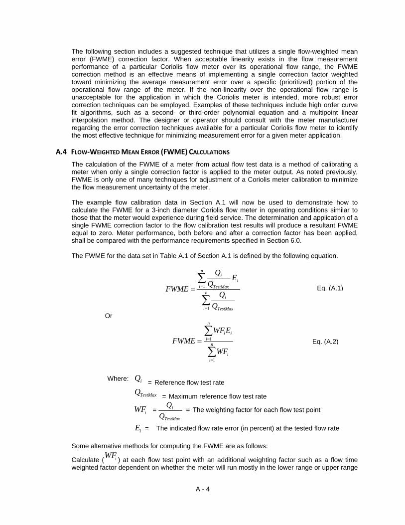
A - 4

The following section includes a suggested technique that utilizes a single flow-weighted mean error (FWME) correction factor. When acceptable linearity exists in the flow measurement performance of a particular Coriolis flow meter over its operational flow range, the FWME correction method is an effective means of implementing a single correction factor weighted toward minimizing the average measurement error over a specific (prioritized) portion of the operational flow range of the meter. If the non-linearity over the operational flow range is unacceptable for the application in which the Coriolis meter is intended, more robust error correction techniques can be employed. Examples of these techniques include high order curve fit algorithms, such as a second- or third-order polynomial equation and a multipoint linear interpolation method. The designer or operator should consult with the meter manufacturer regarding the error correction techniques available for a particular Coriolis flow meter to identify the most effective technique for minimizing measurement error for a given meter application.

A.4   FLOW‐WEIGHTED MEAN ERROR (FWME) CALCULATIONS 

The calculation of the FWME of a meter from actual flow test data is a method of calibrating a meter when only a single correction factor is applied to the meter output. As noted previously, FWME is only one of many techniques for adjustment of a Coriolis meter calibration to minimize the flow measurement uncertainty of the meter.

The example flow calibration data in Section A.1 will now be used to demonstrate how to calculate the FWME for a 3-inch diameter Coriolis flow meter in operating conditions similar to those that the meter would experience during field service. The determination and application of a single FWME correction factor to the flow calibration test results will produce a resultant FWME equal to zero. Meter performance, both before and after a correction factor has been applied, shall be compared with the performance requirements specified in Section 6.0.

The FWME for the data set in Table A.1 of Section A.1 is defined by the following equation.

n

i TestMax

i

n

ii

TestMax

i

Q

Q

EQ

Q

FWME

1

1

Or

n

ii

n

iii

WF

EWFFWME

1

1

Where: iQ

= Reference flow test rate

TestMaxQ = Maximum reference flow test rate

iWF =

TestMax

i

Q

Q = The weighting factor for each flow test point

iE = The indicated flow rate error (in percent) at the tested flow rate

Some alternative methods for computing the FWME are as follows:

Calculate ( iWF) at each flow test point with an additional weighting factor such as a flow time

weighted factor dependent on whether the meter will run mostly in the lower range or upper range

Eq. (A.1)

Eq. (A.2)

A - 5

of the meter during field service. To apply this method, the weighting factor ( iWF) in Equation

(A.2) would be defined as.

TestMax

i

tp

ii Q

Qx

FT

FTWF

Where: tpFT = A time that is proportional and represents the meters life

cycle in field service.

iFT = The flow time over the time period specified by ( tpFT )

that the meter will operate at the test flow rate ( iQ ).

For example, if the meter spent 18 hours of a day operating in the range of the two lowest test flow rates and the remainder of the day in the range of the upper test flow

rates. The two lowest test flow rates would be given an ( iFT ) of 18 and the upper test

flow rates would be given an ( iFT ) of 6. Furthermore, the value of ( tpFT ) would be 24.

If the specified measuring range of a meter or metering module is known beforehand and when

this range is smaller than the maximum specified measuring range of the meter, it is recommended to determine the FWME and adjust the meter over the actual operating range only.

A.5   FLOW‐WEIGHTED MEAN ERROR (FWME) – EXAMPLE CALCULATION. 

Applying Equation A.2 to calculate the FWME for the test data in Table A.1 excluding test data collected below the transitional flow rate (i.e. below 2135 lbm/hr), as specified in Section 7.2,

produces the result shown in Table A.2. The weighting factor ( iWF) is included in Table A.2 to

show the value of the factor before it is applied to each flow rate error ( iE ).

Actual

Test Rate Reference

Meter (lbm/h)

iWF

iE

(%) iWF x iE

(%)

17,101 0.2664 -0.5378 -0.1433 32,836 0.5109 -0.5099 -0.2605 48,550 0.7555 -0.5001 -0.3778 64,274 1.0000 -0.4951 -0.4951

Sum = 2.5327 Sum = -1.2767

Table A.3

FWME Calculation Summary for 3-inch Diameter Coriolis Flow Meter

EQ. (A.3)

A - 6

The FWME value for the test data in Table A.2 is calculated using Equation A.2 as follows:

%5041.05327.2

2767.1

1

1

n

ii

n

iii

WF

EWFFWME

A single FWME calibration factor (F) can now be applied to the meter output to reduce the magnitude of the measurement error. The calibration factor (F ) is calculated as follows:

)100/(100 FWMEF 0051.1)5041.0100/(100 F

This calibration factor may be applied in the flow computer of the Coriolis flow metering system.

As a final step, the designer may want to validate the application of the calibration factor using the same FWME calculations. By multiplying the Coriolis meter error results by the calibration factor

(F), the adjusted error can be determined. The adjusted error ( icfE ) at each calibration flow rate

( iQ ) can be calculated by the following equation:

100))100(( xFEE iicf

Applying -Eequations A.4 and A.5, the adjusted error for each calibration flow is calculated as shown in Table A.3.

iE

(%) iWF icfE

(%) iWF x icfE

(%) -0.5378 0.2664 -0.0339 -0.0090 -0.5099 0.5109 -0.0059 -0.0030 -0.5001 0.7555 0.0040 0.0030 -0.4951 1.0000 0.0090 0.0090

Sum = 2.5327 Sum = 0.0000

Table A.4

Correction Factor Adjusted FWME Calculation Summary for 3–inch Diameter Coriolis Flow Meter

Using the adjusted data from Table A.3 and applying Equation A.2, the “Correction Factor Adjusted FWME” can be calculated as follows:

%0000.05327.2

0000.0

1

1

n

ii

n

iicfi

WF

EWFFWME

Note that the slight errors indicated by the “Correction Factor Adjusted FWME” are caused by rounding errors.

Eq. (A.4)

Eq. (A.5)

A - 7

By applying the FWME calibration factor (F) to the flow calibration data in Figure A.1, the corrected flow rate error data are as presented in Figure A.3.

Figure A.3

FWME-Corrected Flow Calibration Data for 3-inch Diameter Coriolis Flow Meter

This method of calculating a FWME calibration factor accomplishes the following:

Incorporates the correction for flow pressure effect compensation from the watercalibration pressure to gas test pressure into the FWME correction factor.

Re-establishes the calibration pressure ( CalP) of the meter to the gas calibration test

pressure. Weight the measurement error at the test flow rates according to the rate at which the

gas is flowing. Maintains the original manufacturer’s calibration traceability.

Using this method always weights the correction factor for the best correction at the upper-most test flow rates. This correction method may result in somewhat less precise measurement performance for the lower-most test flow rates because only a single calibration factor is applied. Another method could be employed wherein data is linearized in the flow computer using curve fitting techniques to improve the meter correction over the entire flow rate range. The uncertainty of the flow reference to which a meter is compared, should be the primary influence on the decision to linearize. Due to the inherent linearity of a Coriolis meter, non-linearity outside the reference uncertainty is typically not found.

A - 8

 

B - 1

APPENDIX B 

Example Coriolis Meter Data Sheet 

(Informative) 

(Company Logo)

SPECIFICATION FORMS FOR PROCESS MEASUREMENT AND CONTROL

INSTRUMENTS, PRIMARY ELEMENTS AND CONTROL VALVES

PAGE

1 OF

1

DATA SHEET - CORIOLIS FLOW METER

SPEC:

REV.:

PROJECT NAME

Project description

REV.

BY

DAT

E ISSUE

DATE:

REQ.#:

P.O.:

BY:

CHK.:

APPR.:

G 1 CORIOLIS OPERATING MODE:

E 2 POWER:

N 3 COMMUNICATION:

E 4 PROCESS CONNECTION:

R 5 AGA-11 REQUIREMENTS:

A 6 OUTPUT:

L 7 OUTPUT SCALING (UNITS):

8 HAZARDOUS AREA CLASSIFICATION:

9 TAG NUMBER:

F 10 CUSTOMER:

L 11 SERVICE:

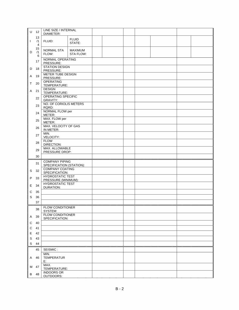
B - 2

U 12 LINE SIZE / INTERNAL DIAMETER:

I 13/14

FLUID: FLUID STATE:

D 15/16

NORMAL STA FLOW:

MAXIMUM STA FLOW:

17 NORMAL OPERATING PRESSURE:

D 18 STATION DESIGN PRESSURE:

A 19 METER TUBE DESIGN PRESSURE:

T 20 OPERATING TEMPERATURE:

A 21 DESIGN TEMPERATURE:

22 OPERATING SPECIFIC GRAVITY:

23 NO. OF CORIOLIS METERS RQRD:

24 NORMAL FLOW per METER:

25 MAX. FLOW per METER:

26 MAX. VELOCITY OF GAS IN METER:

27 MIN. VELOCITY:

28 FLOW DIRECTION:

29 MAX. ALLOWABLE PRESSURE DROP:

30

31 COMPANY PIPING SPECIFICATION (STATION):

S 32 COMPANY COATING SPECIFICATION:

P 33 HYDROSTATIC TEST PRESSURE (MINIMUM):

E 34 HYDROSTATIC TEST DURATION:

C 35

S 36

37

38 FLOW CONDITIONER SYSTEM:

A 39 FLOW CONDITIONER SPECIFICATION:

C 40

C 41

E 42

S 43

S 44

45 SEISMIC :

A 46 MIN. TEMPERATURE:

M 47 MAX. TEMPERATURE:

B 48 INDOORS OR OUTDOORS:

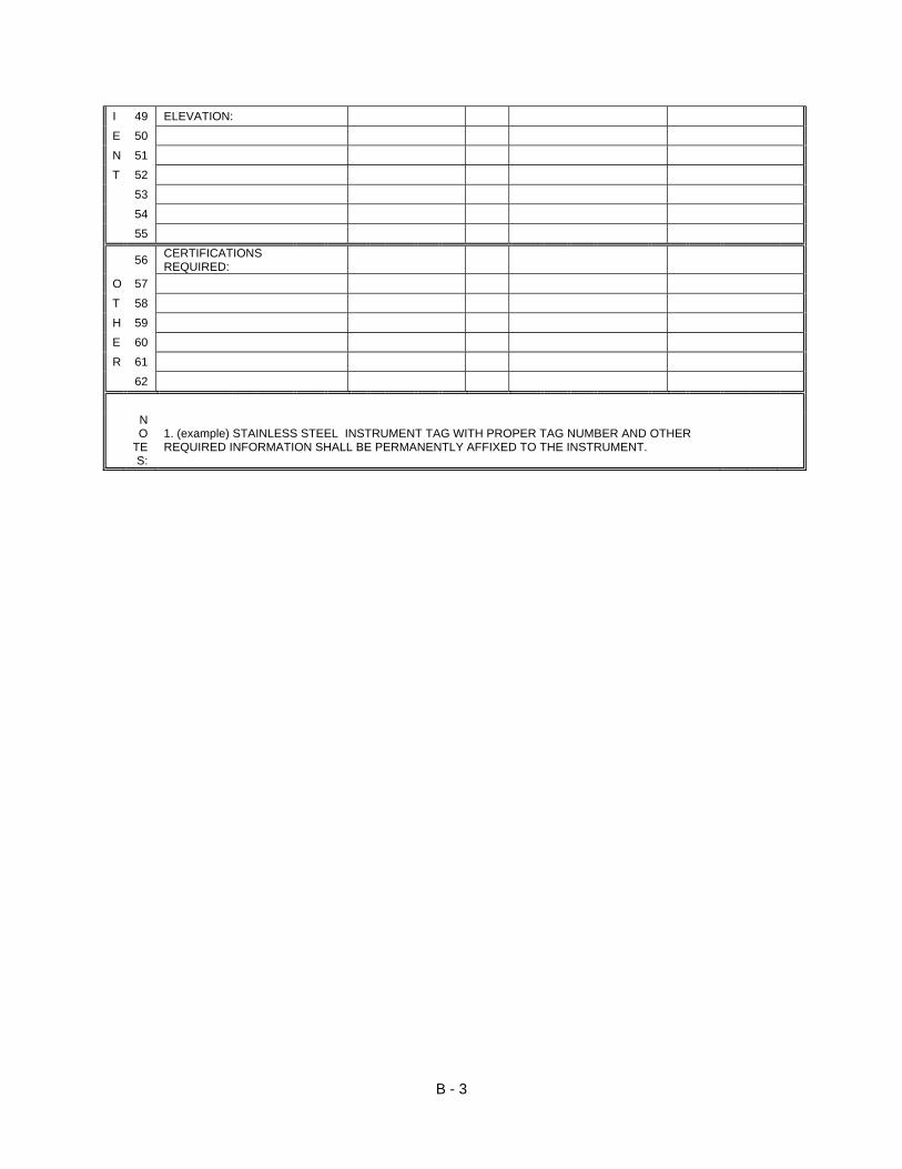
B - 3

I 49 ELEVATION:

E 50

N 51

T 52

53

54

55

56 CERTIFICATIONS REQUIRED:

O 57

T 58

H 59

E 60

R 61

62

NO

TES:

1. (example) STAINLESS STEEL INSTRUMENT TAG WITH PROPER TAG NUMBER AND OTHER REQUIRED INFORMATION SHALL BE PERMANENTLY AFFIXED TO THE INSTRUMENT.

   

B - 4

C - 1

APPENDIX C 

AGA Engineering Technical Note on Coriolis Flow Measurement 

(December 2001)

(Informative)  

AGA Report No. 11, Second Edition, February 2013 APPENDIX C

Engineering Technical Note

Coriolis Flow Measurement for Natural Gas Applications

This technical note contains reference information for measuring natural gas using Coriolis flow meters, including principle of operation, technical issues, evaluation of measurement performance, error analysis, calibration and reference literature. Note that this document is not intended to be used as the basis for contracts or agreements.

Copyright © 2001 American Gas Association All Rights Reserved

Catalog No. XQ0112 December, 2001

PREPARED BY OPERATING SECTION The Coriolis Meter Task Group Transmission Measurement Committee 400 N. Capitol St., N.W., 4th Floor Washington, DC 20001 U.S.A. Phone: 202-824-7000 Fax: 202-824-7082 Web site: www.aga.org

AGA Report No. 11, Second Edition, February 2013 APPENDIX C

ii

AGA Report No. 11, Second Edition, February 2013 APPENDIX C

Disclaimers and Copyright

Nothing contained in this publication is to be construed as granting any right, by implication or otherwise, for the manufacture, sale, or use in connection with any method, apparatus, or product covered by letters patent, or as insuring anyone against liability for infringement of letters patent.

Efforts have been made to ensure the accuracy and reliability of the data contained in this publication; however, AGA makes no representation, warranty, or guarantee in connection with this publication and hereby expressly disclaims any liability or responsibility for loss or damage resulting from its use or from the use of any product or methodology described herein; for any violation of any federal, state, or municipal regulation with which this publication may conflict; or for the infringement of any patent from the use of this publication. Nothing contained in this publication should be viewed as an endorsement by AGA of any particular manufacturer’s products. Permission is granted to republish material herein in laws or ordinances, and in regulations, administrative orders, or similar documents issued by public authorities. Those desiring permission for other publications should consult the Operating and Engineering Section, American Gas Association, 400 North Capitol Street, NW, 4th Floor, Washington, DC 20001, U.S.A. Copyright 2001 American Gas Association, All Rights Reserved

iii

AGA Report No. 11, Second Edition, February 2013 APPENDIX C

TABLE OF CONTENTS

DISCLAIMERS AND COPYRIGHT ....................................................................................................... III

ACKNOWLEDGMENTS .........................................................................................................................VII

1. INTRODUCTION ................................................................................................................................ 1 1.1. TASK GROUP SCOPE ........................................................................................................................ 1 1.2. ENGINEERING TECHNICAL NOTE SCOPE .......................................................................................... 2

2. PRINCIPLE OF OPERATION .......................................................................................................... 3 2.1. INTRODUCTION ................................................................................................................................ 3 2.2. THEORY OF CORIOLIS FLOW MEASUREMENT .................................................................................. 5 2.3. METER CONSTRUCTION ................................................................................................................... 7

2.3.1. General ................................................................................................................................... 7 2.3.2. Sensor ..................................................................................................................................... 7 2.3.3. Secondary Containment .......................................................................................................... 7 2.3.4. Transmitter ............................................................................................................................. 7

FIGURE 5: SYSTEM BLOCK DIAGRAM TECHNICAL CONSIDERATIONS ................................... 7

POWER ......................................................................................................................................................... 7

SIGNALS ...................................................................................................................................................... 7

TECHNICAL CONSIDERATIONS ........................................................................................................... 8 2.4. CORIOLIS METER SELECTION CRITERIA .......................................................................................... 8

2.4.1. Applications ............................................................................................................................ 9 2.4.2. Sizing Considerations ............................................................................................................. 9

2.4.2.1. Pressure Loss ................................................................................................................................... 10 2.4.2.2. Velocity ............................................................................................................................................ 11 2.4.2.3. Meter Error vs. Flow Rate ............................................................................................................... 11 2.4.2.4. Zero Stability .................................................................................................................................... 12 2.4.2.5. Temperature and Pressure Compensation ....................................................................................... 13 2.4.2.6. Turndown Ratio ................................................................................................................................ 13 2.4.2.7. Vibration Effects............................................................................................................................... 14

2.5. CONVERSION OF MASS FLOW RATE TO VOLUMETRIC FLOW RATE AT BASE (REFERENCE OR

STANDARD) CONDITIONS ...........................................................................................................................14 2.6. INSTALLATION REQUIREMENTS ......................................................................................................15

2.6.1. Mounting ................................................................................................................................15 2.6.2. Orientation ............................................................................................................................16 2.6.3. Fluid swirl and flow profile effects ........................................................................................16 2.6.4. Effects of contaminants, such as compressor oil, liquids and free mists ...............................16 2.6.5. Vibration and fluid pulsation .................................................................................................16

2.7. OPERATION AND MAINTENANCE CONSIDERATIONS .......................................................................16 2.7.1. Common Field Checks ...........................................................................................................16

2.7.1.1. Meter zero ........................................................................................................................................ 17 2.7.1.2. Sensor checks ................................................................................................................................... 17 2.7.1.3. Secondary element (transmitter) ...................................................................................................... 17 2.7.1.4. Density checks .................................................................................................................................. 18

3. UNCERTAINTY ANALYSIS AND METER ERROR ....................................................................19 3.1. UNCERTAINTY ANALYSIS ...............................................................................................................19 3.2. FLOW METER BASE ERROR ............................................................................................................19 3.3. ZERO STABILITY VALUE ................................................................................................................20

iv

AGA Report No. 11, Second Edition, February 2013 APPENDIX C

4. CALIBRATION ..................................................................................................................................21

4.1. FACTORY CALIBRATION .................................................................................................................21 4.2. LIQUID CALIBRATIONS FOR NATURAL GAS APPLICATIONS ............................................................21 4.3. BIDIRECTIONAL CALIBRATION ......................................................................................................21

5. RECOMMENDATIONS ....................................................................................................................22 5.1. INDUSTRY .......................................................................................................................................22 5.2. USERS ............................................................................................................................................22

5.2.1. FIELD PERFORMANCE TEST DATA SHEET .....................................................................24 TEST DATA ................................................................................................................................................. 24

5.3. MANUFACTURERS ..........................................................................................................................25 5.4. RESEARCHERS ................................................................................................................................25

APPENDIX A ..............................................................................................................................................26 FUTURE TEST PLANS ..................................................................................................................................26 A.1. PHASE I BASELINE TESTING ...............................................................................................................26

A.1.1. Conditions: ..................................................................................................................................26 A.1.2. Flow rates: ..................................................................................................................................26 A.1.3. Test Parameters: .........................................................................................................................26

A.2. PHASE II .............................................................................................................................................26 A.3. PHASE III ............................................................................................................................................27

APPENDIX B ...............................................................................................................................................28 REFERENCE LITERATURE ...........................................................................................................................28

APPENDIX C ..............................................................................................................................................31 DEFINITIONS...............................................................................................................................................31

APPENDIX D ..............................................................................................................................................33 FLOW AT STANDARD CONDITIONS .............................................................................................................33 NON-IDEAL GAS LAW (EQUATION OF STATE) ............................................................................................34 RELATIONSHIP OF ACTUAL VOLUMETRIC FLOW RATE AND BASE (REFERENCE OR STANDARD)

VOLUMETRIC FLOW RATE ..........................................................................................................................35 SUMMARY ..................................................................................................................................................36

APPENDIX E ...............................................................................................................................................37 GEOMETRIC CONFIGURATIONS ...................................................................................................................37

APPENDIX F ...............................................................................................................................................38 INFORMATION OF INTEREST TO USERS .......................................................................................................38

FLOWMETER .......................................................................................................................................38 TRANSMITTER .....................................................................................................................................39 OPTIONS...............................................................................................................................................39

APPENDIX G ..............................................................................................................................................40 FLUID PULSATION AND VIBRATION ............................................................................................................40

APPENDIX H ..............................................................................................................................................42 UNCERTAINTY ANALYSIS FOR STRAIGHT TUBE–RADIAL–MODE CORIOLIS METERS ON NATURAL GAS ...42 H1. INTRODUCTION ....................................................................................................................................42 H2. FLOW TEST SYSTEM ............................................................................................................................42 H3. RADIAL MODE SENSOR OPERATING THEORY ......................................................................................42

H3.1. Radial-Mode Signals ...................................................................................................................43

RADIAL MODE SENSOR OPERATION ................................................................................................43

v

AGA Report No. 11, Second Edition, February 2013 APPENDIX C

H3.2. Meter Sensitivity Compensation ..................................................................................................44

H4. METER BASE ERROR UNCERTAINTY....................................................................................................44 H4.1. The Standard Uncertainty ............................................................................................................45 H4.2. Covariance...................................................................................................................................45 H4.3. Sensitivity Coefficients .................................................................................................................45

H5. STRAIGHT TUBE CORIOLIS METER OPERATING EQUATION .................................................................46 H5.1. Data Acquisition of Signals .........................................................................................................46 H5.2. Reference Force System ...............................................................................................................47 H5.3. Sources of Error ..........................................................................................................................47

H5.3.1. Vc ...................................................................................................................................................... 47 H5.3.2. Vzo ..................................................................................................................................................... 47 H5.3.3. Vref .................................................................................................................................................... 47 H5.3.4. ............................................................................................................................................................... 47 H5.3.5. Ttf........................................................................................................................................................... 47 H5.3.6. Tst .......................................................................................................................................................... 48 H5.3.7. Fm .......................................................................................................................................................... 48 H5.3.8. Fc ........................................................................................................................................................... 48 H5.3.9. Fgc ......................................................................................................................................................... 48 H5.3.10. βm ........................................................................................................................................................ 48 H5.3.11. βc ......................................................................................................................................................... 48

H6. METER CALIBRATION ..........................................................................................................................49 H6.1. Calibration Facility and Flowing Conditions ..............................................................................49 H6.2. Meters and Data Points ...............................................................................................................49 H6.3. Calculated Standard Uncertainty, uc ...........................................................................................50

H7. EXPANDED BASE ERROR UNCERTAINTY, U .........................................................................................50 H8. METER ZERO STABILITY ......................................................................................................................51 H9. TOTAL METER ERROR .........................................................................................................................51

APPENDIX I ................................................................................................................................................52 UNCERTAINTY ANALYSIS FOR CURVED TUBE METERS ..............................................................................52 I1. INTRODUCTION......................................................................................................................................52

I1.1. Curved Tube Coriolis Operating Equation ...................................................................................53 I1.2. Flow Calibration Factor ...............................................................................................................53 I1.3. Phase-Shift ....................................................................................................................................54 I1.4. Temperature Effect ........................................................................................................................54 I1.5. Pressure Effect ..............................................................................................................................55 I1.6. Sensitivity Coefficients ..................................................................................................................55 I1.7. Total Uncertainty ..........................................................................................................................56 I1.8. Zero Effects ...................................................................................................................................56 I1.9. Zero Effects – Temperature ...........................................................................................................58

APPENDIX J ...............................................................................................................................................59 CALIBRATION DATA — LIQUID CALIBRATIONS FOR NATURAL GAS APPLICATIONS ..................................59

FORM FOR PROPOSALS ON ENGINEERING TECHNICAL NOTE ..................................................... I

vi

AGA Report No. 11, Second Edition, February 2013 APPENDIX C

ACKNOWLEDGMENTS

This technical note represents a great deal of work by the members of the AGA Transmission Measurement Committee ─ Coriolis Meter Task Group, chaired by Steve Baldwin, Unocal Corp. The collaboration of the American Petroleum Institute (API) ─ COGFM Alternative Meter Task Group under the chairmanship of Steve Caldwell, Colorado Engineering Experimental Station Inc. (CEESI), is appreciated. Support from PRCI/GTI ─ MTC under the co-chairmanship of Chuck French and Jim Witte for Coriolis meter research work and services of Ed Bowles of Southwest Research Institute are recognized. In addition, the following list includes those who provided information for the technical note, reviewed the drafts, offered comments and helped in the writing of this document. Their contributions are acknowledged with thanks. Though every attempt was made to include in the list everyone who contributed, we sincerely regret if any omissions have occurred.

Last Name First Name Organization Baldwin Steve Unocal Bowles Ed Southwest Research Institute Caldwell Steve CEESI DeBoom Bob Micro Motion Inc. Decker Herb Krohne Dutton Robin Micro Motion Inc. Fraser Larry Measurement Canada George Darin Southwest Research Institute Grimley Terry Southwest Research Institute Harris Danny Columbia Husain Zaki Texaco, Inc. Karnik Umesh Nova Chemicals Lansing John Daniel Industries Mattar Wade Foxboro Mesnard Dave FMC Measurement Solutions O'Banion Tom Micro Motion Inc. O'Connell John Krohne Otto Ed FMC Measurement Solutions Patten Tim Micro Motion Inc. Pelke Mark N l Fuel Rans Rick Trans-Canada Rebman Dan Williams Sawchuk Blaine Canada Pipeline Accessories Schidlowsky Lloyd NovaTrans Canada Pipeline Seaman Lee Xcel Energy Stark Steve Stark & Assoc. Stephens William Kinder Morgan Stuart John Pacific Gas & Electric Thirumalai Mukundh Schlumberger VanOrsdol Fred Williams Walker James E&H Witte James El Paso Energy Lori Traweek, Sr. Vice President Ali M. Quraishi, Staff Executive Operations and Engineering Transmission Measurement Committee American Gas Association

vii

AGA Report No. 11, Second Edition, February 2013 APPENDIX C

viii

AGA Report No. 11, Second Edition, February 2013 APPENDIX C

1. Introduction

The Transmission Measurement Committee of the American Gas Association submits the following reference information for measuring natural gas with Coriolis flow meters. Coriolis meters are of interest for use in the measurement of natural gas because it is considered to have several desirable characteristics, some of which are: • Low maintenance, no wearing parts • High turndown • Linear response • Stable calibration

Coriolis meters infer mass flow rate of the gas stream by sensing the Coriolis force. This mass rate, however, requires conversion to standard volume units if it is to be of practical use in the custody transfer of natural gas. It should be noted that Coriolis meters can be used for bidirectional flow applications. To convert to standard volumetric units from mass flow, knowledge of the gas composition is required to calculate base or relative density of the flowing gas. Temperature and pressure measurements are not needed to convert to standard volumetric units. Some manufacturers use the process pressure to compensate for a sensor-pressure effect. This process typically is pressure measured near the inlet of the Coriolis sensor. Coriolis sensors include a temperature sensor that is mounted on the outside of the sensor tube(s). The temperature measurement of the sensor tube(s) is used to compensate for the elasticity of the sensor tube(s) material (Young’s modulus). The use of this temperature measurement as the actual flowing gas temperature may be in error because this temperature measurement can be affected by the gas temperature, ambient temperature, flow rate and sensor insulation. Some Coriolis meter performance data for gas flow measurement exist, but additional data are needed to better define precision and bias error limits and to substantiate the existing measurement uncertainty claims. The existing data suggest that the measurement uncertainty of Coriolis meters is comparable to the uncertainty of other meter types, such as orifice, turbine and ultrasonic. Additional lab performance testing is needed to substantiate Coriolis baseline uncertainty claims as well as contributing sources of error and bias. As with any fluid measurement technology, care must be taken by the user in order to ensure a proper understanding of the characteristics and limitations of Coriolis meters, so that total measurement uncertainty will be within acceptable limits. The scope of this document is limited to natural gas, but Coriolis meter technology may be used to measure a broad range of compressible fluids (gases).

1.1. Task Group Scope

Develop an AGA Engineering Technical Note that includes the following:

• A review of the current state of Coriolis metering technology.

1

AGA Report No. 11, Second Edition, February 2013 APPENDIX C

• Identification of technical issues or limitations of Coriolis meters and related research

needs. • A review of current industry standards with a view to developing an AGA report for

the installation and operation of Coriolis meters for natural gas applications.

1.2. Engineering Technical Note Scope

This technical note is limited to Coriolis meters used for relatively low volumetric flow rate and medium to high-pressure natural gas applications (Reference Table 1). Although some references are made to Coriolis meters for liquid flow applications, the general theme and the discussions relate specifically to natural gas applications.

Coriolis Meter Flow Rate vs. Maximum Pressure Loss / Pipe Velocity

Conditions: Natural Gas, Gr=0.60, T=60° F, Pb = 14.73 psia, Tb= 60° F

Meter Type and Size

Nom Pipe Size

Pressure, psig

Flow Rate, scfh

Pressure Loss,

In. WC

Gas velocity (Pipe), ft/sec

Gas Velocity (Meter), ft/sec

2" Bent tube, Bending mode

2", Sch40

100 100,000 28 151 287

500 440,000 493 139 265

1480 830,000 509 78 149

3" Bent tube, Bending mode

3", Sch40

100 220,000 57 150 228

500 1,050,000 272 150 228

1480 2,600,000 492 111 169

4" Straight tube, Bending mode

4", Sch40

100 375,000 101 149 296

500 1,800,000 487 150 297

1480 3,400,000 500 85 168

2" Straight tube, Radial mode

3", Sch40 100 220,000 172 150 427

500 830,000 507 119 337

2", Sch40 1480 1,580,000 464 149 192

4" Straight tube, Radial mode

6", Sch40 100 855,000 130 150 412

500 3,700,000 505 135 373

4", Sch40 1480 6,000,000 310 149 181

Table 1: Coriolis Meter Flow Rate vs. Maximum Pressure Loss/Pipe Velocity

Notes: • These values were calculated using manufacturer provided data. • Flow rates are based on a maximum pipe velocity of 150 ft/sec, or a maximum pressure

loss of 500 inches WC, whichever is exceeded first. • Pressure loss includes reducers and straight piping requirements, when the nominal pipe

size is larger than the meter size.

2

AGA Report No. 11, Second Edition, February 2013 APPENDIX C

2. Principle of Operation

2.1. Introduction

Coriolis meters infer the gas mass flow rate by sensing the Coriolis force on a vibrating tube or tubes. The conduit consists of one or more tubes and is forced to vibrate at a resonant frequency. Sensing coils located on the inlet and outlet sections of the tube(s) oscillate in proportion to the sinusoidal vibration. During flow, the vibrating tube(s) and gas mass flow couple together due to the Coriolis force, causing a phase shift between the vibrating sensing coils. The phase shift, which is measured by the Coriolis meter transmitter, is directly proportional to the mass flow rate. There are secondary influences that can affect the phase shift. These topics are discussed in the Appendices. Note that the vibration frequency is proportional to the flowing gas density, but the use of this feature is not included in the scope of this document. At the date of publication of this document, the density measurement from the Coriolis meter is not of sufficient accuracy to assist with the computation of the volumetric flow rate at flowing (actual) conditions for natural gas applications. (See discussion in Section 3.2.) There are three common implementations of Coriolis technology. These are: ♦ Bent tube – bending mode ♦ Straight tube – bending mode ♦ Straight tube – radial mode

Below are cut-away views. See Appendix E for additional configurations of flow tube(s).

Figure 1: Key Components of a Bent tube – Bending Mode Configuration

RTD

Sensor CoilSensor Coil

Drive CoilFlow Tubes

Case

3

AGA Report No. 11, Second Edition, February 2013 APPENDIX C

Figure 2: Key Components of a Straight Tube – Bending Mode Configuration

Figure 3: Key Components of a Straight Tube – Radial Mode Configuration

Secondary Containment

Electrodynamic Sensors

Exciter (Drive Coil) Measuring Tube

Temperature sensors (RTD)

Process Fitting

Straight Tube - Bending Mode Coriolis Flow

4

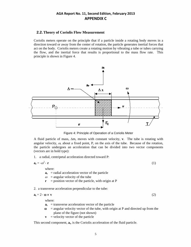
AGA Report No. 11, Second Edition, February 2013 APPENDIX C

2.2. Theory of Coriolis Flow Measurement

Coriolis meters operate on the principle that if a particle inside a rotating body moves in a direction toward or away from the center of rotation, the particle generates inertial forces that act on the body. Coriolis meters create a rotating motion by vibrating a tube or tubes carrying the flow, and the inertial force that results is proportional to the mass flow rate. This principle is shown in Figure 4.

Figure 4: Principle of Operation of a Coriolis Meter

A fluid particle of mass, ∆m, moves with constant velocity, v. The tube is rotating with angular velocity, ω, about a fixed point, P, on the axis of the tube. Because of the rotation, the particle undergoes an acceleration that can be divided into two vector components (vectors are in bold type):

1. a radial, centripetal acceleration directed toward P:

ar = -ω2 ⋅ r (1)

where: ar = radial acceleration vector of the particle ω = angular velocity of the tube r = position vector of the particle, with origin at P

2. a transverse acceleration perpendicular to the tube:

at = 2 ⋅ ω × v (2)

where: at = transverse acceleration vector of the particle ω = angular velocity vector of the tube, with origin at P and directed up from the plane of the figure (not shown) v = velocity vector of the particle

This second component, at, is the Coriolis acceleration of the fluid particle.

5

AGA Report No. 11, Second Edition, February 2013 APPENDIX C

As the particle is accelerated, it imparts an inertial force on the tube wall known as the Coriolis force. This inertial force equals the product of the particle mass and its Coriolis acceleration, but it is in the opposite direction from at, as shown by the vector ∆Fc in Figure 4. Since the vectors involved are at right angles, the cross product in equation 2 can be rewritten using scalars, and the magnitude of the Coriolis force, ∆Fc, can be expressed by equation 3.

∆Fc = ∆m ⋅ at = 2 ω ⋅ v ⋅ ∆m (3)

The mass of the fluid particle can be expressed as:

∆m = ρ ⋅ A ⋅ ∆x (4)

Where:

ρ = density of the fluid particle A = internal area of the tube ∆x = length of the particle

The mass flow rate, qm, of fluid in the tube is given by:

qm = ρ ⋅ v ⋅ A (5)

By combining equations 3, 4 and 5, the Coriolis force of the fluid particle is found to be proportional to its “mass flow rate” in the tube.

∆Fc = 2 ω ⋅ qm ⋅ ∆x (6)

Because flow tubes often are bent into a convenient shape, equation 6 cannot be directly integrated along the tube axis to find the total Coriolis force on the tube. When a simple integration of equation 6 is used, a proportionality constant, c, is included to correct for the effects of bending and other assumptions made in integration:

Fc = 2 c ⋅ ω ⋅ qm ⋅ d (7)

Where:

d = length of the tube.

Finally, the mass flow rate can be expressed as a function of the Coriolis force on the entire tube.

qm = Fc / (2 c ⋅ ω ⋅ d) (8)

For practical Coriolis meters, the rotation ω is produced by cyclically vibrating the tube. The flow tube often is bent (see Figure 1) so that the inlet and outlet sides vibrate in the same direction, but the fluid flows in opposite directions. As a result, the Coriolis forces act in opposite directions on the two sides and produce a secondary twisting vibration in the tube. The amount of twist is proportional to the Coriolis force, so position detectors can be used to determine the mass flow rate from this motion.

6

AGA Report No. 11, Second Edition, February 2013 APPENDIX C

2.3. Meter Construction

2.3.1. General

The Coriolis flow meter measuring system consists of two basic components. The flow sensor may be referred to as the “primary” or “primary device.” The transmitter may be referred to as the “secondary” or “secondary device.”

2.3.2. Sensor

The flow sensor is a mechanical assembly consisting of a vibrating tube(s), drive system, sensing coils, supportive structure and housing. Cyclic mechanical stresses in the sensor are a common concern. Material selection must ensure adequate fatigue life and corrosion/erosion protection from, for example, sour gas or corrosive fluids.

2.3.3. Secondary Containment

Secondary containment refers to the enclosure around the vibrating tube(s). The secondary containment may have its own pressure rating. Although also used to protect the sensor tubes, secondary containment is not a requirement for meter operation.

2.3.4. Transmitter

The transmitter is the electronic control system that provides the drive power, processes the signals and generates output(s) of measured and inferred parameters; it also may provide corrections derived from parameters such as temperature and pressure. The transmitter can be remotely or integrally mounted to the sensor.

Figure 5 represents the Coriolis flow meter measuring system block diagram (remote transmitter configuration). Note: Actual physical configuration will vary by manufacturer.

Figure 5: System Block Diagram

SSeennssoorr

TTrraannssmmiitttteerr

Pow

Signa

P T (optional)

7

AGA Report No. 11, Second Edition, February 2013 APPENDIX C

Technical Considerations

This section discusses technical considerations related to the operation and installation of Coriolis meters. Because the meter configuration varies among manufacturers, the sensitivities of Coriolis meters to various influences also vary. Therefore, it is important to consult the manufacturer for recommendations regarding specific meter applications.

2.4. Coriolis Meter Selection Criteria

Coriolis flow meter selection is based on a variety of factors; the most important of which are safe, accurate, and repeatable performance over the required measuring range.

General considerations are:

• Mass flow measurement uncertainty

• Minimum, maximum and normal flow rate

• Minimum, maximum and normal operating fluid temperature

• Minimum, maximum and normal fluid pressures

• Fluid specific gravity

• Fluid viscosity

• Allowable pressure loss

• Unidirectional or bidirectional flow

• Flow meter wetted materials

• Process connection size and pressure rating

• Secondary containment rating

• Measured variable outputs and required format (e.g., 4-20 ma, pulse, digital, etc.)

• Remote or local diagnostic capabilities

• Environmental requirements

• Area safety classification

• Gas quality (e.g., liquid condensate, particulate, etc.)

• Other operating considerations (e.g., pulsation, swirl, mechanical stresses, vibration, etc.)

• Requirements of contracts, agreements and laws

• Performance, auditing, and accounting considerations as outlined in API Manual of Petroleum Measurement Standards (MPMS), Chapter 21.1, “Electronic Gas Measurement.”

• Power source availability and quality

• Installation piping configuration

8

AGA Report No. 11, Second Edition, February 2013 APPENDIX C

2.4.1. Applications

Typical applications include measuring single-phase gas flow typically found in production facilities, transmission pipelines, distribution systems and end-use fuel measurement.

Most Coriolis meters offer bi-directional flow measurement, so applications requiring bi-directional flow can be accommodated.

2.4.2. Sizing Considerations

At the date of publication of this document, Coriolis flow meters for gas measurement were available in line diameters from ¼ to 4 inches. There are three major considerations when sizing a Coriolis meter:

• Pressure loss

• Velocity of the gas inside the sensor

• Total meter error

These considerations or criteria interact; properly sizing a Coriolis meter consists of choosing the sensor size that best optimizes the tradeoff between pressure loss and accuracy, at acceptable gas velocity through the sensor tube(s). Pressure loss and gas velocities are higher through a smaller sensor, but meter error is generally smaller as well. Likewise, pressure loss and gas velocities are lower when a larger sensor is chosen, but meter error increases.

The following example illustrates the interaction between accuracy and pressure loss, at two different operating pressures.

Natural gas, Gr = 0.59

Q = 1 MMscfh maximum

P = 500 psig (case 1); 1,000 psig (case 2)

T = 60° F

Desired pressure loss @ maximum flow = 500 inches water column (WC)

A 3-inch bent tube, bending mode Coriolis meter is chosen. As shown in Figure 6, pressure loss meets the 500-inch WC constraint at 500 psig (case 1). Meter error is better than +/-1% down to 100,000 scfh, and better than +/-2% down to 50,000 scfh.

At 1,000 psig operating pressure (case 2), pressure loss decreases to 250 inches WC at maximum flow. Meter error is unchanged, since it is based on mass (standard volume) flow. A more detailed explanation of pressure loss, gas velocity inside the sensor tube(s) and meter error is presented in subsequent sections.

9

AGA Report No. 11, Second Edition, February 2013 APPENDIX C

Flow Error and Pressure Loss vs. Flow Rate, 3" Bending Mode Coriolis MeterGas Conditions: Gr = 0.59, Tf = 60 F

-3.00

-2.00

-1.00

0.00

1.00

2.00

3.00

0 200000 400000 600000 800000 1000000

Flow Rate, SCFH

Flo

w R

ate

Err

or, %

0

100

200

300

400

500

600

Pre

ssur

e Lo

ss, i

nche

s H

2O

Error limit

Pressure loss-1000 psig

Pressure loss-500 psig

Figure 6: Flow Error and Pressure Loss vs. Flow Rate

Meter designs of the three major types (bent tube – bending mode, straight tube – bending mode and straight tube – radial mode) vary somewhat in their specific accuracy, pressure loss and velocity characteristics. Table 1 provides sample flow rate, velocity and pressure loss limits for bent tube – bending mode and straight tube – radial mode meter designs and sizes.

2.4.2.1. Pressure Loss

Sensor geometry, gas density and velocity determine the permanent pressure loss through the meter. Coriolis meters for natural gas service are usually sized to produce a pressure loss up to 500 inches WC. As described in the next section, the maximum gas velocity allowed through the sensor tube(s) may be reached before a 500-inch WC pressure drop is reached. In these cases, velocity becomes the practical sizing criterion. The pressure loss through a Coriolis meter is usually expressed in inches of WC or psia, but may be expressed as a pressure loss coefficient. The pressure loss coefficient is considered a constant for Reynolds numbers in the turbulent range. Note that the laminar flow regime is below the normal flow rate range of Coriolis meters. The pressure loss coefficient K is defined as ∆P/(½ρV2gc) and is based on pipeline gas velocity. It also is useful to express pressure loss through a Coriolis meter via the equivalent length method (i.e., the meter pressure loss is equivalent to the pressure loss in a length of straight-run pipe).

10

AGA Report No. 11, Second Edition, February 2013 APPENDIX C

Pressure loss also is affected by any pipefitting required for meter installation. Pipe reducers, valves and straight pipe requirements (required for some Coriolis meter designs) should be considered when calculating the loss in pressure for the selected meter. Consult with the manufacturer to determine if reported pressure loss includes additional pressure loss from these additional piping components.

2.4.2.2. Velocity

Coriolis meters may have performance limitations at higher gas velocities due to noise imposed on the meter signal. Such signal noise can affect meter accuracy and repeatability. The gas velocity at which signal noise becomes a problem is design-specific. Signal noise is seldom a concern when the gas velocity in the meter sensor is below 200 ft/s. Note that gas velocity may be the limiting factor in sizing, before a pressure loss of 500 inches WC is reached. A Mach number limit is usually provided by the meter manufacturer to define the maximum recommended velocity.

If there are abrasive contaminants in the gas flow stream, erosion of the wetted meter components may be a concern when the meter is exposed to high gas velocities. This effect is design specific.

2.4.2.3. Meter Error vs. Flow Rate

Meter error versus flow rate is determined from a performance curve. Figure 7 is an example based on a 3-inch bent tube – bending mode meter. Pressure loss is measured across the meter inlet and outlet flanges. The error versus flow rate curve is based on the results of gas laboratory calibrations. Most manufacturers state the probable meter error as a percentage of flow rates, plus the zero stability value. Third-party meter error data are referenced in Appendix B. The error is typically expressed as:

% Error = ± [base error, % ± (zero stability/flow rate) x 100] (9)

The actual meter base-error value is determined from laboratory calibration. The error typically includes the effects of laboratory uncertainty, linearity, hysteresis and repeatability.

11

AGA Report No. 11, Second Edition, February 2013 APPENDIX C

Flow Error and Pressure Loss vs. Flow Rate, 3" Bending Mode Coriolis MeterGas Conditions: Gr = 0.59, Tf = 60 F

-3.00

-2.00

-1.00

0.00

1.00

2.00

3.00

0 200000 400000 600000 800000 1000000

Flow Rate, SCFH

Flo

w R

ate

Err

or,

%

0

100

200

300

400

500

600

Pre

ssur

e L

oss

, inc

hes

H2

O

Error limit

Pressure loss-1000 psig

Pressure loss-500 psig

Figure 7: Flow Error and Pressure Loss vs. Flow Rate

2.4.2.4. Zero Stability

The zero-stability value defines the limits within which the meter zero may drift during operation and is constant over the operating range (all other affecting parameters fixed). It may be given as a value in flow rate units or as a percentage of a stated nominal mass flow rate. The zero stability value is the limiting factor when establishing meter turndown ratio. The stated zero stability is achievable when the Coriolis flow meter is installed and when re-zeroed at operating conditions. Drift of the zero value outside of the given zero stability will typically not occur for Coriolis meters at stable operating conditions. Resetting the meter zero will bring the drift back to an insignificant value. See Section 3.1.2.5 for information on the effects of pressure and temperature on the meter zero.

Because process temperature or pressure changes, and/or environmental temperature changes, will affect the meter zero stability, the estimated value of the zero stability is usually limited to meters at thermal and pressure equilibrium. Limits for changes in these parameters may be given which, when exceeded, will require a re-zeroing of the meter to reestablish the specified zero stability.

Since the zero stability is a constant error over the operating range for a given meter, it has the greatest effect at the lowest flow rate. This is shown graphically in Figures 6 and 7.

12

AGA Report No. 11, Second Edition, February 2013 APPENDIX C

2.4.2.5. Temperature and Pressure Compensation

Changes in operating temperature and pressure can affect the meter performance. The magnitude of these effects is small in comparison with base error, but should be compensated to achieve optimum meter performance.

Temperature compensation:

• Sensor tube temperature. The meter response to flow, which determines the calibration factor, is called the sensitivity. Changes in the sensor tube temperature (e.g., caused by a change in the gas temperature or the ambient temperature) produce a bias that can be compensated for. Most meter designs automatically compensate for these changes (i.e., the effect of Young’s modulus) by measuring the temperature of the sensor tube(s).

• Sensor structure temperature. Changes in the temperature of the meter structure also result in errors affecting the meter zero. This effect is dependent on the meter but can be eliminated when the meter zero is set. The zero should only need to be reset when the conditions change sufficiently to cause the performance to fall outside of acceptable limits.

• Pressure compensation: Changes due to pressure are compensated for using an external pressure transmitter or by entering a fixed adjustment for the known pressure.

Other meter designs periodically check meter sensitivity by applying a waveform reference force to the tube(s) during field operation and comparing the system response with that achieved under reference flowing conditions. This system can compensate for both pressure and temperature effects.

2.4.2.6. Turndown Ratio

Flow meter turndown ratio is the ratio of the acceptable maximum mass flow rate to the acceptable minimum mass flow rate. The turndown ratio is application-specific and dependent on gas conditions, allowable pressure loss across the meter and allowable meter error. The maximum pressure loss (at maximum flow rate) across the meter can be determined once the meter diameter, piping installation configuration and maximum allowable gas velocity are specified. Typically, the meter selected is one line diameter smaller than the size of the pipe in which the meter is installed. This usually provides more accurate measurement at lower flow rates. However, the resulting permanent pressure loss for a given flow rate is higher than what it would be if the meter diameter was the same as the pipe diameter. Because higher-pressure gas has a higher mass flow rate for the same velocity, higher pressures will produce higher flow turndowns for the same meter arrangement. A family of curves can be generated showing flow turndown for different gas pressures. Figure 8 presents typical values of this relationship for a pressure loss of 500 inches WC.

13

AGA Report No. 11, Second Edition, February 2013 APPENDIX C

Error at Minimum Flow vs Turndown

3" Bending Mode Coriolis Meter, Natural Gas, G r = 0.59, T f = 60° F

Pressure Loss at Max Flow = 1% of Line Pressure

0

20

40

60

80

100

0.5 1.0 1.5 2.0 2.5 3.0

Error at Minimum Flow, Percent

Flo

w T

urn

do

wn

1,480 psig

1,000 psig

500 psig

100 psig

Figure 8: Error at Minimum Flow vs. Flow Turndown Ratio

2.4.2.7. Vibration Effects

Coriolis sensors are dynamic systems that vibrate at a natural resonant frequency. External vibration sources can influence flow meter performance. Consult the manufacturer and available research for specific precautions and recommendations. See Section 3.3.5 for installation requirements and see Appendix G.

2.5. Conversion of Mass Flow Rate to Volumetric Flow Rate at Base (Reference or Standard) Conditions

The mass flow rate is related to volumetric flow rate at standard (or reference) conditions by the density at standard conditions. In the following equations, the subscript “b” refers to standard conditions, commonly 60°F and 14.73 psia.

14

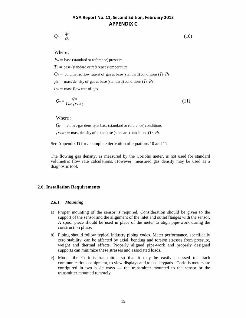
AGA Report No. 11, Second Edition, February 2013 APPENDIX C

gas of rate flow mass

( conditions (standard) baseat gas ofdensity mass

( conditions (standard) baseat gas ofat rate flow volumetric

re temperatureference)or (standard base

pressure reference)or (standard base

,

,

:Where

(10)

=====

=

m

bbb

bbv

b

b

b

mv

qPT

PTQTP

qQ

ρ

ρ

bbairb

r

airbr

mv

PTG

GqQ

,)(

)(

( conditions (standard) baseat air ofdensity mass

conditions reference)or (standard baseat density gas relative

:Where

(11)

==

×=

ρ

ρ

See Appendix D for a complete derivation of equations 10 and 11.

The flowing gas density, as measured by the Coriolis meter, is not used for standard volumetric flow rate calculations. However, measured gas density may be used as a diagnostic tool.

2.6. Installation Requirements

2.6.1. Mounting

a) Proper mounting of the sensor is required. Consideration should be given to the support of the sensor and the alignment of the inlet and outlet flanges with the sensor. A spool piece should be used in place of the meter to align pipe-work during the construction phase.

b) Piping should follow typical industry piping codes. Meter performance, specifically zero stability, can be affected by axial, bending and torsion stresses from pressure, weight and thermal effects. Properly aligned pipe-work and properly designed supports can minimize these stresses and associated loads.

c) Mount the Coriolis transmitter so that it may be easily accessed to attach communications equipment, to view displays and to use keypads. Coriolis meters are configured in two basic ways — the transmitter mounted to the sensor or the transmitter mounted remotely.

15

AGA Report No. 11, Second Edition, February 2013 APPENDIX C

2.6.2. Orientation

As a general rule, orient the sensor tubes in such a way as to minimize the possibility of heavier components, such as condensate, settling in the vibrating portion of the sensor. Solids, sediment, plugging, coatings or trapped liquids can affect the meter performance, especially when present during zeroing. Allowable sensor orientations will depend on the application and the geometry of the vibrating tube(s).

2.6.3. Fluid swirl and flow profile effects

The effect of fluid swirl and non-uniform velocity profiles caused by upstream and downstream piping configuration on meter performance differs from one meter design to another. Flow conditioning and straight upstream and downstream piping lengths may or may not be required. Further testing is recommended to evaluate these potential effects.

2.6.4. Effects of contaminants, such as compressor oil, liquids and free mists

Testing has shown that liquid carried in a gas stream may not have the same adverse affect on performance as gas carried in a liquid stream. However, the meter will measure the mass flow rate of the total flow stream, including the liquid, e.g., condensate, glycol or compressor oil. The allowable liquid fraction will depend on the application and sensor geometry. Care should be taken to remove liquid slugs before measuring the gas flow. Refer to Section 3.4 with regard to the effects of contamination buildup on the sensor.

2.6.5. Vibration and fluid pulsation

During product development, extensive analysis and testing have resulted in meter designs that are inherently stable under a wide range of “normal” plant vibration conditions. See Appendix G for a discussion of vibration and fluid pulsation.

2.7. Operation and Maintenance Considerations

Coriolis meters require minimal maintenance because the only moving parts are the vibrating sensor tube(s).

2.7.1. Common Field Checks

There are four common types of field checks, which include meter zero checks, sensor checks, transmitter checks and density checks.

16

AGA Report No. 11, Second Edition, February 2013 APPENDIX C

2.7.1.1. Meter zero

Meter zero should be checked periodically. For new installations, many users check the zero within two to four weeks of installation. Frequency of subsequent zero checks should be driven by the zero check data or as dictated by user policy. Meter zero should be adjusted if it does not meet the manufacturer’s specifications. See Appendices H and I. If the meter zeros check shows degradation, then the sensor checks shown in Section 3.4.1.2 should be performed. Physical internal inspection may be needed.

Improper zeroing will result in measurement error. In order to adjust the zero of the meter, the sensor must be filled with gas at process conditions and there must be no flow through the flow sensor. The meter zero must be established at process conditions of temperature, pressure and density. Even though the stream is not flowing, the flow meter may indicate a small amount of flow, either positive or negative. Causes for the zero error usually are related to the differences between the calibration conditions and the actual installation conditions, which include but are not limited to the following:

• Differences between the calibration media density and the gas density

• Differences in temperature

• Differing mounting conditions

• Other effects discussed in Appendices H and I

The meter should read a mass flow rate that is within the manufacturer’s zero stability specification under the no-flow condition. See Appendices H and I.

The zeroing of the meter must be performed at nominal operating condition with no flow through the meter. Once it has been confirmed that there is no flow through the meter, the zeroing procedure specified by the meter manufacturer should be followed.

2.7.1.2. Sensor checks

Product buildup, erosion or corrosion will affect the meter performance.

• Product buildup (coating) may bias the meter zero. If the buildup is causing a zero drift, cleaning and re-zeroing the meter should bring performance to within specifications. If coating of the sensor continues the zero will continue to drift.

• Although rare, erosion or corrosion will affect permanently the meter calibration and will compromise sensor integrity. When used within the specified fluid and ambient condition limits, fatigue of the sensing tubes of a Coriolis meter due to vibration during the stated meter lifetime is rare and does not need to be considered when inspecting a meter. However, operating the meter in more extreme corrosive or erosive applications will shorten the expected lifetime.

2.7.1.3. Secondary element (transmitter)

Diagnostic LED(s) and display(s) may be provided to indicate operating status of the primary and secondary elements. See the manufacturer’s documentation for detailed

17

AGA Report No. 11, Second Edition, February 2013 APPENDIX C

descriptions of secondary element diagnostic and trouble shooting procedures. In addition, refer to API Manual of Petroleum Measurement Standard (MPMS) Chapter 21.1 for security issues.

2.7.1.4. Density checks

As of this writing, operating density measured by the meter should not be used to convert mass flow rate to actual volumetric flow rate. However, it is useful as a diagnostic tool to monitor changes in meter performance or operating conditions.

18

AGA Report No. 11, Second Edition, February 2013 APPENDIX C

3. Uncertainty Analysis and Meter Error

Flow meter performance is typically stated in terms of the measurement uncertainty of the device. Measurement uncertainty is a function of the measurement process and is the estimated limit of the measurement error. Measurement error is defined as the difference between the “true” value and the measured value. However, the true value is almost never known, so the error can only be estimated. Rarely should there be a measurement error larger than the estimated measurement uncertainty. There are two components that make up the total measurement uncertainty of a flow meter. These components are usually described as precision (or random) and bias (or systematic) uncertainties. A precision error source varies randomly over the time period of the measurement. In most cases, the smooth distribution of an infinite number of readings from a gas flow meter coincides with the Gaussian, or normal, distribution. This distribution characterizes the precision of the meter. A bias error source is steady over the time period of the measurement. By flow-calibrating a meter, one is generally trying to identify and correct for meter biases. For a more detailed treatment of the concept of measurement uncertainty, the reader is referred to the ANSI/ASME Standard on Measurement Uncertainty (PTC 19.1-1985, Part 1), NIST Tech Note 1297 or IS0 5168 and IS0 7066-1. Representative measurement uncertainty calculations for Coriolis meters used to measure pressurized natural gas flows are included in Appendices H and I. In general, the total measurement uncertainty for a Coriolis meter appears to be comparable to the measurement uncertainties calculated for other measurement technologies that are customarily used for this application.

3.1. Uncertainty Analysis

Coriolis flow meter error limits are estimated and typically displayed as shown in Figures 6 and 7. The uncertainty of this error is calculated using the uncertainty of each identified source of error, either from a typical example or averaged for several meters. Each error source is propagated through the operational equation for the meter to determine the uncertainty of the flow rate. Appendices H and I show examples of two different Coriolis meter error uncertainty calculations.

3.2. Flow Meter Base Error

Laboratory calibrations are made for every meter, typically using a liquid gravimetric calibration system or a gas calibration system using critical flow nozzles or turbine meters as a transfer standard. Currently, each meter is calibrated at a nominal flow rate and at one or more lower flow rates to establish the flow calibration factor and determine the meter base error. Noting the meter characteristic and the magnitude of the change in the average meter error over the operating range confirms linearity. Linearization methods may or may not be used to correct for a repeatable meter characteristic to improve the base error value. Two or more repeat calibration points at each flow rate are used to establish the meter repeatability performance.

19

AGA Report No. 11, Second Edition, February 2013 APPENDIX C

3.3. Zero Stability Value

The zero stability specification is determined by logging the meter output at no flow for many meters over a period of time sufficient to establish output trends at the given operating and environmental conditions. The zero stability is a statistically based value. The actual meter zero reading, therefore, will be better than the zero stability specification most of the time. Because process temperature or pressure changes and/or environmental temperature changes will affect the meter zero stability, the estimated value of the zero stability is usually limited to meters at thermal and pressure equilibrium. Limits for changes in these parameters may be given, which if exceeded, will require a re-zeroing of the meter to reestablish the specified zero stability.

20

AGA Report No. 11, Second Edition, February 2013 APPENDIX C

4. Calibration

4.1. Factory Calibration

Manufacturers calibrate every Coriolis meter against a traceable standard and provide a calibration certificate. Calibration media include natural gas, air, inert gases and or liquid. The calibration factors determined by this procedure are typically noted on the meter nameplate and stored electronically in a transmitter register. The calibration of a Coriolis meter is similar to the calibration of any other flow meter. The calibration consists of comparing the output of the meter against a traceable standard. A meter factor (sometimes referred to as flow calibration factor) is established during calibration.

4.2. Liquid Calibrations for Natural Gas Applications

In some cases, Coriolis meters have been calibrated on a fluid, such as water, rather than natural gas or air. Liquid calibrations typically are less costly than gas calibrations. At the time of publication, Measurement Canada was working with one manufacturer to investigate the transferability of water calibrations for use in custody transfer measurement of natural gas. If this testing establishes the transferability of the calibration factor between water and natural gas, it is expected that Measurement Canada will permit water-based calibrations for natural gas applications. Baseline testing at Southwest Research Institute, as described in Section 7.1, also will check the transferability of water calibrations to natural gas applications. Data and European approvals exist for at least one geometric configuration (dual curved tube) that demonstrates the transferability of calibration factors determined on water for use on gas, within some uncertainty. See Appendix J for a detailed discussion and test results. In general, Coriolis meters are linear devices; i.e., the calibration factor is independent of calibration flow rate. See Appendix J for a more detailed discussion.

4.3. BiDirectional Calibration

Test results for one-meter design and line diameter have shown that the flow calibration need only be done in one flow direction. The meter factor applies in both directions. See Appendix J. Further testing is recommended for this topic.

21

AGA Report No. 11, Second Edition, February 2013 APPENDIX C

5. Recommendations

The Coriolis Meter Task Group has made the following recommendations for further study regarding this technology. Should a decision be made to develop a report, the following topics need to be addressed:

• Share and disseminate operating experience with Coriolis meters for natural gas flow measurement.

• Leverage off the experience of the European Community. • Develop an understanding of the potential for business-related benefits.

Furthermore, the task group recommends the following actions by the respective stakeholders:

5.1. Industry

Published minimum performance guidelines for various applications are needed for Coriolis meters to be used in natural gas service. A Coriolis meter should be accurate to +/-1.0% of reading or better, if used as a sales meter in medium- to high-pressure, high turndown ratio applications.

5.2. Users

Users of the Coriolis meters described in this technical note include gas producers, transporters and distributors. Care should be taken by these parties to ensure that the meter will meet the requirements of the application. The manufacturer’s standard flow calibration is usually based on the anticipated mass flow rate. Users may want to consider additional calibration test points to ensure that the performance of the meter has been tested at the anticipated operating conditions. Users are encouraged to get involved in advocacy efforts for research and development and to articulate potential benefits of the technology to the industry, so that future generations of Coriolis meters will provide maximum benefit. Users also should work with meter manufacturers to define further technology improvements that will help maximize the benefits of this measurement technology. In addition, when installing meters for field-testing, a reference meter that has been flow-calibrated in a recognized laboratory should be used. A suggested reference meter would be a flow-calibrated turbine meter.

22

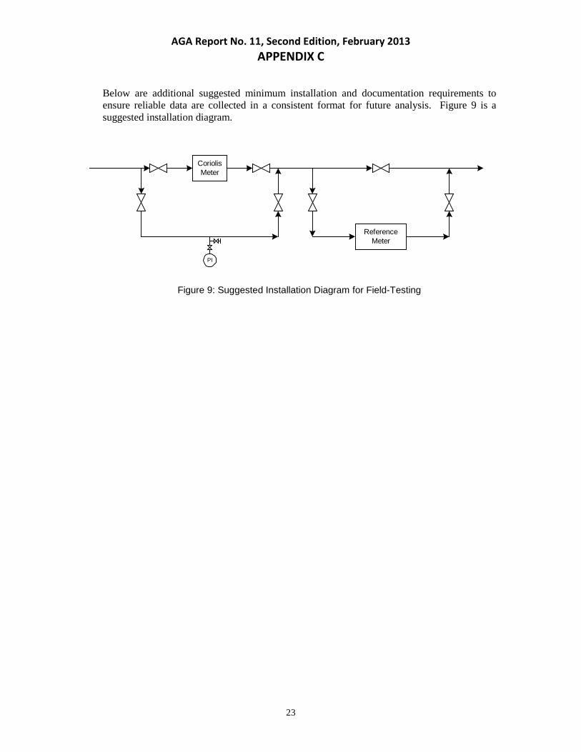
AGA Report No. 11, Second Edition, February 2013 APPENDIX C

Below are additional suggested minimum installation and documentation requirements to ensure reliable data are collected in a consistent format for future analysis. Figure 9 is a suggested installation diagram.

Figure 9: Suggested Installation Diagram for Field-Testing

CoriolisMeter

PI

ReferenceMeter

23

AGA Report No. 11, Second Edition, February 2013 APPENDIX C

5.2.1. FIELD PERFORMANCE TEST DATA SHEET

CORIOLIS METER FIELD PERFORMANCE TEST DATA SHEET

Technician _____________________________Test Date ____________________

Location of Installation ________________________________________________

Coriolis Meter Manufacturer ____________________Model No. ______________

Serial No. _____________________ Transmitter S/N ________________________

Meter Signal Output mAmp_________________Voltage ____________________

Frequency _____________Direct Reading _______________

Scaling Factor _______________Hz/lbm. Meter Zero Factor_________________

Manufacture Calibration Factor _____________ Meter Factor_______________

TEST DATA

Inlet Pressure psia ____________________ Inlet Temperature F. ______________

Exit Pressure psia ____________________ Exit Temperature F. ______________

Indicated Rate (Meter Output) ___________________________________________

Data Collection Interval (120 seconds minimum).____________________________

As Found Zero _____________________ As Left Zero _______________________

Surface Temp. _____________________ Transmitter Temp. ___________________

Gas Sample Collected _______________ Sample ID __________________________

Notes: i.e., vibration, noise present, pulsations, any and all observations. _____________________________________________________________________ _____________________________________________________________________

24

AGA Report No. 11, Second Edition, February 2013 APPENDIX C

5.3. Manufacturers

Manufacturers may continue to refine the technology for natural gas measurement. The data gathering and analysis necessary to increase the level of confidence in the technology will need to come in large part from the manufacturers. System diagnostics is an issue on which the users would like to have more information.

5.4. Researchers

In order to increase the confidence of all parties in this technology, industry-funded research, as well as research funded by individual users, is needed to augment work done by the manufacturers. Research including, but not limited to, the following is recommended by the authors of this technical note:

• Flow profile effects • Boundary layer effects • Upstream and downstream piping • Dirty gas applications (e.g., wet gas, particle-laden gas, etc.) • Vibrational gas coupling • Calibration issues (e.g., water vs. gas) • Bi-directional calibration factors • Zero stability • Pressure effects (between water and gas) • Temperature effects • External vibration and pulsation • Mounting effects • Vibration effects • Mounting in vertical, horizontal and other orientations

The list is not prioritized.

25

AGA Report No. 11, Second Edition, February 2013 APPENDIX C

Appendix A

Of Engineering Technical Note, December 2001

Future Test Plans

A.1. Phase I Baseline Testing

The following tests, listed by test piping configurations, are recommended:

A.1.1. Conditions:

• Ideal flow conditions arrived at by 100 D upstream inlet piping and 5 D downstream piping (no flow conditioners)

• 70° F +/- 1 degree • Three pressures, 150 psig, 500 psig, 1,000 psig or maximum rating of meter if less

than 1,000 psig. System capability may affect the minimum and maximum pressures • Maximum pressure loss through the meter will be limited to 500 inches WC., system

capability may affect the minimum and maximum pressure drop

A.1.2. Flow rates:

• Maximum flow rate of system or meter • 50, 25 and 10 percent of the meter capacity • Minimum flow rate of system or meter

A.1.3. Test Parameters:

• Data capture points • Frequency output from meters • Meter output in mass flow rate units • Facility to report in flow rate units of scfh (standard cubic feet per hour) • 90-second samples repeated six times • Differential pressure across the meter • Inlet pressure and temperature

A.2. Phase II

• Piping effects • Reducers • Elbows

• Single 90 Zero-D into manufacturer’s recommended installation • Two 90s in-plane with valve on inlet of meter • Two 90s out-of-plane (Zero-D separation) with valve on inlet of meter or

swirler • Tees • Thermowells (upstream)

26

AGA Report No. 11, Second Edition, February 2013 APPENDIX C

• Wet gas to 5% load by mass • Calibration media (e.g., air vs. water vs. natural gas) • Temperature effects

A.3. Phase III

• Boundary layer effects • Dirty gas • BiDirectional flow • Transmitter replacement

27

AGA Report No. 11, Second Edition, February 2013 APPENDIX C

Appendix B

Of Engineering Technical Note, December 2001

Reference Literature

Title Author Date Venue

Accuracy Counts with Natural Gas Bob Seeley Apr-99 Chemical Processing

Choose The Right Material for Coriolis Mass Flow meters

Brent Carpenter Oct-90 Chemical Engineering Process

Comparative Performance Evaluation of Coriolis Mass Flow Meters

F.A.L. van Laak Jul-00 Europe Consortium – Ethylene Study

Compressed Natural Gas (CNG) Measurement

M. Butler, T. O'Banion, T. Patten, G. Pawlas

May-98 ISHM

Coriolis Flow Meters for Critical Phase Ethylene Measurement

Tom de Jonge, Aart Pruysen, Tim Patten

Jun-99 4th International Symposium on Fluid Flow Measurement; Denver, CO

Coriolis Flow meters for Gas Measurement

Tim Patten, Gary Pawlas Oct-95 North Sea Flow Workshop

Coriolis Flow meters: Industrial Practice and Published Information

R. C. Baker 1994 Flow Measurement and Instrumentation, Vol. 5, No. 4 pp. 229-246

Coriolis Mass Flow Measurement S. Nicholson 1994 Flow Measurement in the Mid-90s, FLOMEKO, NEL, Glasgow

Coriolis Mass Flow meters Overcome Vibration

Tim Patten Sep-97 Measurement & Control

Custody Transfer of Ethylene Using Coriolis Mass Flow meters

Kees Kaijser, Brian Hoover

Jan-00 55th Instrumentation Symposium for the Process Industries; Texas A&M Symposium

Design of an Advanced Coriolis Mass Flow Meter Using the Hoop Mode

H. Hagenmeyer, K.H. Schulz, A. Wenger, M. Keita

1994 Flow Measurement in the Mid-90s, FLOMEKO, NEL, Glasgow

Effect in Pulsating Flow on Coriolis Mass Flow Meters

G. Vetter, S. Notson 1994 Flow Measurement and Instrumentation, Vol. 5, No. 4, pp. 263-273

28

AGA Report No. 11, Second Edition, February 2013 APPENDIX C

Title Author Date Venue

The Effect of Swirl on Coriolis Mass Flow meters

Tim Patten, Gary Pawlas Oct-95 North Sea Flow Workshop

Evaluation of Mass Flow Meters For NGV Fueling Dispenser Applications

Patricia Freeman Rowley, Marc Butler, and Christopher Blazek

Aug-94 Natural Gas Fuels

Field Testing of Coriolis Mass Flow meter Micro Motion CMF300

F.A.L. van Laak Jul-00 Europe Consortium – Ethylene Study

Fiscal Measurement and Proving Experience with Coriolis Meters

T.C.E. Davis 1990 North Sea Flow Measurement Workshop, NEL, Glasgow

Fluid Mechanic Effects in Coriolis Mass Flow Meter

G. Pawlas, T. Pankratz 1994 Flow Measurement in the Mid-90s, FLOMEKO, NEL, Glasgow

Giving Coriolis the Gas Pan Demetrakakes May-99 Food Processing

The Identification of External Factors Which Influence the Calibration of Coriolis Mass flow Meters

R. Cheesewright, C. Clark, D. Bisset

Oct-99 Flow Measurement and Instrumentation

International Flow Systems: Design and Performance Prediction

D. S. Miller 1990 Gulf Publishing Company

Large Metering Project in Australia Includes Coriolis

Michael Snell, John Blain May-00 Pipeline & Gas Industry

New Developments in Coriolis Technology for Gas-Phase Reaction Control

Tom O'Banion Nov-97 1) Chemical Show, NYC; 2) Chemical Online

New Developments in Coriolis Technology for Natural Gas Measurement

P. Trolin May-00 ISHM

New Technology Directly Measures Mass Flow of Gas

D. Hahn 1995 3rd International Symposium on Fluid Flow Measurement, San Antonio, TX

NMi Certificate – Custody Transfer of Natural Gas

1", 2", 3" Coriolis Feb-00 Netherlands

NMi Certificate – Custody Transfer of Natural Gas

3" Coriolis Jan-98 Netherlands

North American Inter-Laboratory Flow Measurement Test Program

U. Karnik, E. Bowles, J. Bosio, S. Caldwell

1996 North Sea Flow Measurement Workshop, Peebles, Scotland

29

AGA Report No. 11, Second Edition, February 2013 APPENDIX C

Title Author Date Venue

Performance Evaluation of a 3-inch Micro Motion Mass Flow meter in High Pressure Natural gas Applications

U. Karnik, J Geerligs, R. Kowch

Jun-99 4th International Symposium on Fluid Flow measurement; Denver, CO

Pigsar Calibration Curve 1" Coriolis Dec-99 Dorsten, Germany

Pigsar Calibration Curve

2" Coriolis Dec. 99 Dorsten, Germany

Pigsar Calibration Curve 3" Coriolis Dec. 99 Dorsten, Germany

Precision Natural Gas Flow Measurement Using Coriolis

Tom O'Banion Jun-00 AGA Operations Conference, Denver, CO

Quantification of Uncertainty Associated with Gas Sampling Equipment and Techniques, and the Impact on Flow Rate and Heating Value Measurement

A. Kendricks, F. Foh 1999 AGA Operations Conference, Seattle, WA

Testing Coriolis Mass Flow Meters for Pattern Approval

L. Mandrup-Jenson 1990 North Sea Flow Measurement Workshop, NEL, Glasgow

Use of Coriolis Meters in Gas Applications

T. Patten, G. Pawlas 1995 3rd International Symposium on Fluid Flow Measurement, San Antonio, TX

Verifying gas meter accuracy Russ Kratowicz Jan-99 Plant Services

30

AGA Report No. 11, Second Edition, February 2013 APPENDIX C

Appendix C

Of Engineering Technical Note, December 2001

Definitions

Drive coil – Coil, or coils, that act with a permanent magnet to provide the driving force to the sensor tube(s) of a Coriolis meter. Low flow cutoff – A value programmed by the user to inhibit the flow indication below a defined value. Nominal flow rate – A flow defined by manufacturers to “bound” the upper end of meter operation. Coriolis meters do not have an absolute maximum rate, so the nominal value is usually defined by pressure loss or Mach number. Permanent pressure loss coefficient – The ratio of the loss in pressure of a fluid as it flows through a Coriolis meter, divided by the fluid dynamic pressure at a specified piping location. Phase shift/∆t – The “shift” in phase, or angle, between the two sinusoidal signals as picked up by the sense coils of a Coriolis flow meter. When converted to the time domain, the phase represents a change, or delay in time (∆t), between the peak signal points from the inlet and outlet coil signals. The phase shift, or ∆t, is proportional to the mass flow rate. Psid – Pounds per square inch differential. Repeatability – The ability of a meter to repeat the same output when given the same input, for successive measurements at the same conditions. For a flow meter, the ability of the meter to repeat the same output for the same flow rate. Resonant/primary frequency – The frequency at which a Coriolis meter sensing tube vibrates. RTD – Resistance Temperature Device. Used as a temperature sensor. Sensing coils – Electrical coils that act with a permanent magnet mounted at the inlet and outlet flow tube sections that pickup (measure) the flow tube motion. Vibrating tube(s) – The flow path, or fluid conduit enclosure, made of 316SS, high nickel stainless or titanium, forced to vibrate at the meter resonant frequency. Vibration characteristics – The response a Coriolis meter may have to outside (field) vibrations and/or the primary vibration, or resonance frequency, of a Coriolis meter and the response to the fluid Coriolis force. Zero drift – The amount that the meter zero changes versus an independent variable, such as temperature.

31

AGA Report No. 11, Second Edition, February 2013 APPENDIX C

Zero effects – Quantities that may change the zero error of the meter; e.g., zero drift versus temperature. Zero error – The flow indication at zero flow. The zero error should be less than zero stability specification for the meter. Zero stability – Specified by the manufacturer. This value represents the limit of expected meter mass flow indication under a no-flow condition. Under most conditions, the meter should indicate a mass flow less than the specified zero stability. Zeroing – Zeroing sets a meter reference point so that it indicates as close to zero mass flow as possible under a no-flow condition.

32

AGA Report No. 11, Second Edition, February 2013 APPENDIX C

Appendix D

Of Engineering Technical Note, December 2001

Flow at Standard Conditions

Coriolis meter technology measures gas flow in mass units. Meter mass flow outputs are converted to base (standard) flow units, (i.e., scf) without the use of flowing density. This conversion requires knowledge of the gas composition to calculate base density using an equation of state (such as AGA Report No. 8, Compressibility Factors of Natural Gas and Other Related Hydrocarbon Gases). This appendix outlines how the conversion is made and provides a comparison between:

• Mass flow to volumetric flow at base (reference or standard) conditions, and • Actual volumetric flow to volumetric flow at base conditions. Relationship of Mass Flow Rate and Base (Reference or Standard) Volumetric Flow Rate

In all applications, mass flow is conserved for steady-state conditions. In other words, the mass flow rate at a point in the pipe is equal to the mass flow rate at any other point in the pipe.

Equation D.1 is a restatement of the conservation of mass — the mass flow rate is equal to the volumetric flow rate times the density at any temperature and pressure condition. Rearranging equation D.1 yields:

The mass flow ( mq ) is measured by the Coriolis meter and the density ( bρ ) is defined by the

non-ideal gas law. It will be shown that only the molecular mass of the gas ( rM ) is required to convert from mass flow to standard volumetric flow, and that temperature and pressure measurements at the meter are not required. In some cases, Coriolis meters measure the flowing gas density in addition to the mass flow rate. It is important to note that the density measurement from a Coriolis meter is not used to calculate flow rate at base conditions.

conditions flowingunder density

conditions lineat rate flow c volumetri

conditions (standard) baseat density

conditions (standard) baseat rate flow c volumetri

:Where

====

×=×

f

f

b

b

pqpq

(D.1) q q ffbb ρρ

(D.2) b

mb

qqρ

=

33

AGA Report No. 11, Second Edition, February 2013 APPENDIX C

Non-Ideal Gas Law (Equation of State)

The non-ideal gas law governs the relationship between gas density and pressure, temperature, molecular mass and super-compressibility (see AGA Report No.8 for a complete description). Equation D.3 details the relationship:

Equation D.3 is valid at any temperature and pressure. Since it is of interest to convert mass flow to volumetric flow at base conditions, substitute bP and bT into equation D.3. At the base

condition, bP and bT are defined (e.g., 14.73 psia and 60° F);

( )

( )

)pZTMRP

TRZMP

r

eunit volumper (mass gas theofdensity mass

ilitycompressib

gas theof re temperatuabsolute

mole)per (mass massmolar gas

constant gas universal

gas theof pressure absolute

gas

gasr

:Where

(D.3)

===

===

××

×=ρ

conditions (standard) baseat ility compressib fluid

constant gas universal

conditions (standard) baseat mole)per (mass massmolar gas

conditions (standard) baseat e)unit volumper (mass gas theofdensity mass

conditions (standard) baseat gas theof re temperatuabsolute

conditions (standard) baseat gas theof pressure absolute

:Where

(D.4)

==

====

×××

=

b

r

b

b

b

bb

rbb

ZRM

TP

TRZMP

ρ

ρ

34

AGA Report No. 11, Second Edition, February 2013 APPENDIX C

Substituting equation D.4 into D.2 results in the relationship used to convert mass flow to standard volumetric flow.

(D.5)

bb

rb

mb

TRZMP

qq

×××

=

To summarize, bP and bT are constants (e.g., 14.73 psia and 60° F) and defined by the user;

flowing pressure and temperature measurements are not required. Only the molecular mass is required to calculate the standard volumetric flow rate from a mass flow measurement. Note that compressibility ( bZ ) at base conditions is a function of molecular mass ( rM ) (see AGA Report No.8).

Relationship of Actual Volumetric Flow Rate and Base (Reference or Standard) Volumetric Flow Rate

The conversion of actual volumetric flow to standard volumetric flow is similar to the conversion from mass flow rate. Equation D.1 is used, but simplified to:

Rearranging D.6 results in:

(D.7) b

ffb qq

ρρ

=

The density under flowing conditions is described by:

(D.8) ff

rff TRZ

MP××

×=ρ

conditions flowingunder density

conditions lineat rate flow c volumetri

conditions (standard) baseat density

conditions (standard) baseat rate flow c volumetri

:Where

(D.6)

=

===

×=×

f

f

b

b

ffbb

ρqρq

ρqρq

35

AGA Report No. 11, Second Edition, February 2013 APPENDIX C

Combining equations D.4, D.7, & D.8 result in the equation commonly used to calculate volumetric flow at base conditions from a volumetric flow meter:

Summary

Equation D.5 shows the relationship between direct mass flow measurement and volumetric flow at base conditions. Equation D.9 shows the relationship between actual volumetric flow and standard volumetric flow. Although each equation appears to be quite different, each is directly related to equation D.1. Both equations are different methods to compute mass flow rate.

(D.9) ffb

bbffb ZTP

ZTPqq

××

××=

36

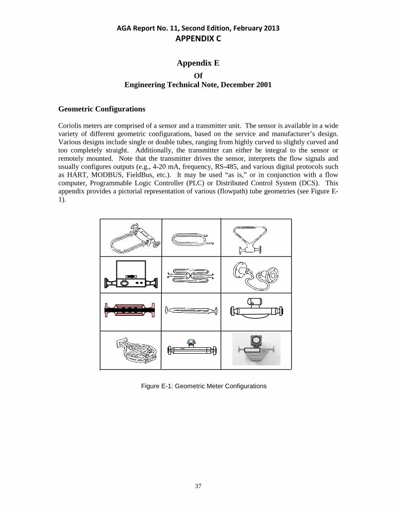
AGA Report No. 11, Second Edition, February 2013 APPENDIX C

Appendix E

Of Engineering Technical Note, December 2001

Geometric Configurations

Coriolis meters are comprised of a sensor and a transmitter unit. The sensor is available in a wide variety of different geometric configurations, based on the service and manufacturer’s design. Various designs include single or double tubes, ranging from highly curved to slightly curved and too completely straight. Additionally, the transmitter can either be integral to the sensor or remotely mounted. Note that the transmitter drives the sensor, interprets the flow signals and usually configures outputs (e.g., 4-20 mA, frequency, RS-485, and various digital protocols such as HART, MODBUS, FieldBus, etc.). It may be used “as is,” or in conjunction with a flow computer, Programmable Logic Controller (PLC) or Distributed Control System (DCS). This appendix provides a pictorial representation of various (flowpath) tube geometries (see Figure E-1).

Figure E-1: Geometric Meter Configurations

37

AGA Report No. 11, Second Edition, February 2013 APPENDIX C

Appendix F

Of Engineering Technical Note, December 2001

Information of Interest to Users

The manufacturer should be prepared to respond to the user’s hardware, performance and application questions on items such as those given below. Note: Many of the items listed will be covered in specification sheets and operating manuals.

FLOWMETER

• Variables: • sizes available • materials available for tubing and other wetted parts • materials used in the remainder of the construction

• Operating Limits:

• maximum and minimum mass flow rate within the uncertainty statement • temperature/pressure ratings available • fluid temperature limits • fluid pressure limits • ambient temperature limits • humidity limits • hazardous area and intrinsic safety code classification • secondary containment rating • corrosive atmosphere limits • corrosive fluid limitations

• Performance:

• overall mass flow uncertainty statement • method of calibration • uncertainty analysis

• Effects on Performance of:

• fluid temperature • fluid pressure at the inlet • density variation • viscosity variation • effects of upstream and downstream piping configurations • flow pulsation • flow over-range • ambient temperature change • power supply voltage and frequency variations • electromagnetic interference (EMI) • vibration • two-phase flow • erosion by slurries, impurities, etc. • product buildup • stress due to installation

38

AGA Report No. 11, Second Edition, February 2013 APPENDIX C

• Installation Requirements: • power supply • sensor operating or resonate frequencies • process connections — mating flanges, threaded ends, welding neck, etc • mounting requirements — weight, dimensions, bracket(s):

• clearance for maintenance • orientation requirements

• mounting, vibration and shock limitations • recommended cleaning procedures • provisions for heat tracing • provisions for thermal insulation • maximum allowable pressure drop

• Hydraulic Considerations:

• pressure loss vs. flow rate for the expected application • sizes vs. flow ranges

TRANSMITTER

• available outputs — to what standards? • supply voltage and frequency limits • ambient temperature limits • humidity limits • electrical code classification and approvals • enclosure rating • cabling requirements and limitations • local diagnostics • remote diagnostics • locally or remotely mounted

OPTIONS

• displays • alarms • totalizers • outputs

39

AGA Report No. 11, Second Edition, February 2013 APPENDIX C

Appendix G

Of Engineering Technical Note, December 2001

Fluid Pulsation and Vibration

Coriolis meters are designed to operate at a resonant frequency of the flow tube(s). The operating frequency of the meter is designed by the manufacturer to optimize the Coriolis signal. This section deals with the effect of mechanically induced vibrations. At the time of this writing, there were not enough data to characterize the effect of flow pulsations on accuracy. Pipeline vibrations often occur at frequencies related to the rotational speed of compressors. Meters are designed to minimize this effect. Meter performance is not adversely affected when the mechanical vibration does not coincide with the resonant frequency of the meter. If the mechanical vibration frequency coincides with the operating frequency of the sensor, then the meter performance will be adversely affected. Figure G-1 shows an example of meter performance when subjected to external vibration on a shaker table. The test was conducted with a 1-inch bending mode Coriolis meter mounted on the shaker table. The meter was subjected to sinusoidal vibration from approximately 15 to 1,950 Hz. Flow variation about the average value was monitored and is plotted in Figure G1. Note that most significant signal variation (noise) occurs at approximately 105 Hz, the operating frequency of this meter. Meter response is specific to the individual meter design, and the meter response described in the example is not representative of all meter designs.

40

AGA Report No. 11, Second Edition, February 2013 APPENDIX C

-1.5

-1

-0.5

0

0.5

1

1.5

0 500 1,000 1,500 2,000 2,500

Shaker Table Frequency, Hz

Mas

s Fl

ow S

igna

l Noi

se, s

cfm

Figure G-1: Vibration Response of a 1-inch Bending Mode Coriolis Meter

41

AGA Report No. 11, Second Edition, February 2013 APPENDIX C

Appendix H

Of Engineering Technical Note, December 2001

Uncertainty Analysis for Straight Tube–Radial–Mode Coriolis Meters on Natural Gas

The following measurement uncertainty analysis has been provided by a Coriolis meter manufacturer. The results are specific to the meter design, meter size and operating conditions referenced in the analysis. The estimated measurement uncertainty given in this analysis is not necessarily representative of all meter designs, sizes and applications.

H1. Introduction

An error analysis of a straight tube-radial mode, 2-inch Coriolis meter was done using data from six meters, calibrated on natural gas at two temperatures and a moderate flow rate. The analysis includes an error propagation of each identified source of error through the meter operating equation and lists the sensitivity coefficients and the probable error due to bias and precision (systematic and random) for each component.

H2. Flow Test System

Digital signals from all of the dependent sensor functions were acquired once per second over each 90-second data run. A total of 72 data points were used in this analysis. Values for each meter flow rate were compared with those obtained using sonic nozzles as a transfer standard, with the gas being circulated in a temperature-controlled, closed system using a compressor. A gas chromatograph recorded actual natural gas composition each time the test piping system was filled. The uncertainty analysis used actual data and support calibration information to obtain the meter averaged base error uncertainty (see Section 3.1.2.3). Values for meter zero were recorded before and after each set of flow-rate data points. The total meter uncertainty is given for these conditions, and a relative graph of meter errors is presented.

H3. Radial Mode Sensor Operating Theory

Coriolis flow meters infer the mass flow rate measurement by measuring the difference in the signals between the inlet and outlet sense coils on the vibrating flow tube. The radial mode sensor vibrates across the straight tube diameter, which provides a “balanced” vibration mode for a single flow tube (see Figure H-1). The straight flow tube provides a very low pressure drop in a configuration that has a fully rated, secondary pressure sensor containment tube (see Figure 3 in main document). The higher operating frequency gives improved resolution and dynamic response time at lower flow rates. Digital electronics are used to process the signals using high-speed filtering techniques and to update sensor information each second.

42

AGA Report No. 11, Second Edition, February 2013 APPENDIX C

Figure H-1: Straight Tube – Radial Mode Sensor Operation

H3.1. Radial-Mode Signals

The two pair of sense coils generates sinusoidal signals as the sensor tube is vibrating. The Coriolis signal is proportional to the out-of-phase, or difference, signals sensed at the inlet and outlet coils. The main magnet/coil drivers provide consistent tube displacement amplitude over the range of process temperatures and pressures by using a feedback control system that uses the in-phase, or sum, signal. Figure H-2 shows a graph of the sense coil signals. The difference signal is dynamically filtered using digital methods and then synchronously demodulated to give a signal proportional to mass flow.

Figure H-2: Radial Mode Sense Coil Signals

Drive Coils —Center of Tube

Tube Inlet Sense Coils Tube Outlet Sense Coils

Neutral Position

Magnet

Coil

Sensor Tube Cross Sections

Coriolis Force Detection, exaggerated

Coils Pushing

Coils Pulling

Flow tube inlet and outlet sections during ½ of one vibration cycle — drive coils “pushing.”

Radial Mode Sensor Operation

No Flow Position

Inlet Signal

Outlet Signal

Sum Signal

Difference Signal

43

AGA Report No. 11, Second Edition, February 2013 APPENDIX C

H3.2. Meter Sensitivity Compensation

Changes in the sensor tube due to piping stress, pressure and temperature can change the sensitivity of the tube to the Coriolis signal (the calibration factor). Real-time compensation for changes in the sensitivity of the meter is done by applying a reference force to the meter tube, Vref, and measuring the response. Reference force magnet/coil drivers (Figure 3 of main document) are placed at points on the tube to simulate the Coriolis force. This force is applied to create a “forward” and “reverse” flow signal. The response of the tube to this reference force is read as a signal superimposed on the normal flow-rate signal. The difference in the response, or “auto-compensation,” of the meter to this reference force is stored in memory. Because the signal is applied in both directions, the net effect on the total flow is negligible.

H4. Meter Base Error Uncertainty

The straight-tube-radial-mode meter mass flow-rate base error is estimated by calculating the propagation of errors of the meter parameters, both acquired and calculated, through the operating equation. The base error uncertainty will be calculated using the expanded uncertainty model based on NIST Technical Note 1297:

( ) ( )

( )

.i

for xt coefficieny sensitivit thecalled also

,i

xparameter therespect toith equation w operating theof derivative partial the x

f

evaluation ofpoint at theparameter measured the x

errors randomor ,systematiceither from y,uncertaint standard the xu

resultt measuremen theofy uncertaint standard combined the u

level confidence 95% at they uncertaint expanded the U

30over freedom of degrees combined for the 2, or,factor coverage thek

:Where

(H.2) x,xux

f

x

f2xu

x

fu

(H.1) kuU

i

i

i

c

1/21N

1i

N

1ijji

jii

2

2N

1i ic

c

=∂∂

==

===

∂∂

∂∂

+

∂∂

=

=

∑ ∑∑−

= +==

44

AGA Report No. 11, Second Edition, February 2013 APPENDIX C

H4.1. The Standard Uncertainty

The standard uncertainty, u, in equation (2), is separated into two types:

H4.1.1 uB is the standard uncertainty for systematic “Type B,” or bias errors, which include those estimates of errors from sources such as previous measurement data, test equipment manufacturer’s data, data provided from calibration reports, uncertainties assigned to reference data taken from handbooks, etc.

H4.1.2 uA is the standard uncertainty for random “Type A,” or precision errors that are

based on statistical methods and include errors from calibration signal data samples, multiple calibrations of a sensor or meter, etc.

H4.2. Covariance

The second term in equation H-2, is the estimated covariance associated with two parameters in the operating equation, xi, and xj, with the correlation coefficient, (∂f/∂xI)(∂f/∂xj). For the purpose of this evaluation, the covariance of meter parameters must pass the additional test of relationship. Mathematical correlation does not always imply a relationship of cause and effect. During this test program, no correlation was observed that satisfied the cause and effect requirement for the meter base error.

H4.3. Sensitivity Coefficients

As the overall flow measurement uncertainty is computed, the uncertainty in each measured parameter is multiplied by a sensitivity coefficient. Mathematically, the sensitivity coefficient (Θ) is the partial derivative of the operating equation with respect to the measured parameter, ∂f/∂xi. The partial derivatives of the operating equation were taken and are shown in Table H-1. The values were calculated from averaged meter parameters recorded for six data points.

45

AGA Report No. 11, Second Edition, February 2013 APPENDIX C

H5. Straight Tube Coriolis Meter Operating Equation

The uncertainty calculation for Coriolis flow meters is done by first defining an operating equation. All calculations to determine the actual mass flow rate are done by an integral Digital Signal Processor (DSP). The DSP receives data, calculates the factors, and flow rate, and outputs the results, in a digital and analog format. The raw Coriolis mass flow rate signal, Vc, needs only to be scaled to provide the mass flow rate. All other factors in the equation provide compensation for the parameters that affect the true mass flow rate.

H5.1. Data Acquisition of Signals

Due to the high frequency of the straight tube, or radial-mode meter, the acquisition of sample values provides many points per second of the measured Coriolis signal, tube temperature, and primary operating frequency. These data sets are reduced to average values for each data set. During calibration, data sets consisting of digital values for Vc, Vref, Tft, and, Tst, are acquired and recorded once per second over a 90-second window of the calibration for each flow rate data point.

)3.H(FFFmV

VVm CMgcref

ref

zoc ××××

−=

Where:

( )( )

( )( )

coildrivereferenceoftcoefficienthermalβfieldmagneticdrivereferenceoftcoefficienthermalβ

zerometerlastatsignalCoriolisV

signalCoriolisrateflowreferenceV

signalCoriolisV

etemperaturreferencetubesupportT

etemperaturtubesupportT

etemperaturreferencetubeflowT

etemperaturtubeflowT

rateflowmassreferencem

rateflowmassm

factoretemperaturmagnetdrivereference,TTβ1F

factorcouplinggasFgc

factoretemperaturcoildrivereference,TTβ1F

C

M

zo

ref

c

refst

st

refft

ft

ref

2refststMM

2refftftCC

====

=

==

=

==

=

−+=

=

−+=

46

AGA Report No. 11, Second Edition, February 2013 APPENDIX C

refm

H5.2. Reference Force System

The value of the auto-comp signal, and the temperature of the driver coils, Tft ref, and magnets, Tst ref, are stored during calibration, and become the reference sensitivity of the meter. Any change in the meter sensitivity due to field conditions is compensated by the auto-comp signals. Changes in the reference force due to temperature are compensated by the two factors: Fm and Fc. Auto-comp signals are taken once every 10 seconds.

H5.3. Sources of Error

H5.3.1. Vc

The Coriolis raw signal is a digital value that is recorded once per second. The raw signal is a relative quantity that can include a bias. The average zero value Vzo will include the same bias, and because the operational equation involves the difference (Vc - Vzo), the equal biases would cancel out. Therefore, no bias error is assigned to this value. Random error analysis methods were used to obtain the standard uncertainty.

H5.3.2. Vzo

This is the averaged value for the Coriolis raw signal measured during the last meter zero set. This value represents the meter signal at zero flow and operating conditions, and provides an offset to correct the meter signal bias. As explained above for Vċ, the zero signal is considered to have no bias, and the error is considered to be a Type A uncertainty. The same methods for analysis used for Vc are used for this value. However, the value obtained is considered a constant during meter operation, so the precision error is “fossilized” as a bias (see H4.1).

H5.3.3. Vref

This parameter is also a digital value that is a relative quantity and is a difference between two digital numbers representing the auto-comp signal for forward and reverse flow. It is also considered to have only a random, or Type A, standard uncertainty.

H5.3.4.

The reference flow rate is obtained at the calibration facility, during the initial calibration. The error is treated as a bias. The flow calibration facility supplied the expanded uncertainty of the reference flow rate for each data point. The coverage factor, k, was divided out of this value to achieve the Type B standard uncertainty of the reference flow rate.

H5.3.5. Ttf

The meter flow tube temperature is obtained from an integrally mounted RTD. Each RTD was individually calibrated and curve-fitted to a polynomial that provides the temperature as a function of sensor resistance. The standard uncertainty for the RTD was determined using the curve-fit error, or “standard estimate of error,” as a Type A. The precision was calculated based on the digital values for Ttf taken during the calibration. No bias error is assumed, due to the fact that this value is part of a difference in the equation for Fc. (See the discussion of differences in H5.3.1.)

47

AGA Report No. 11, Second Edition, February 2013 APPENDIX C

H5.3.6. Tst

The same methods used for the flow tube RTD temperature were used for the support tube RTD temperature.

H5.3.7. Fm

Error propagation on the equation for calculating this value was used to determine the standard uncertainty. The standard uncertainty values for βm and Tst were used in the calculation.

H5.3.8. Fc

Error propagation on the equation for calculating this value was used to determine the standard uncertainty. The standard uncertainty values for βc and Tft were used in the calculation.

H5.3.9. Fgc

The gas-coupling factor is made up from several values acquired from the DSP and calculated from the known gas parameters. The standard uncertainty is calculated as a Type B.

H5.3.10. βm

This coefficient adjusts for the changes in the magnetic field used in the reference force electromagnetic driver changes. For the data collected to determine this value, over the temperature range of –40 to +120° C, it is assumed a constant and has a value of 0.000221 Gauss/Gauss/° C. The standard uncertainty for this value is ± 0.000001 Gauss/Gauss/° C.

H5.3.11. βc

This coefficient adjusts for the changes in the coil length used in the reference force electromagnetic driver changes. For the data collected to determine this value, over the temperature range of –40 to +120° C, it is assumed a constant and has a value of -0.00000932 M/M/° C. The standard uncertainty for this value is ± 0.00000014 M/M/° C.

48

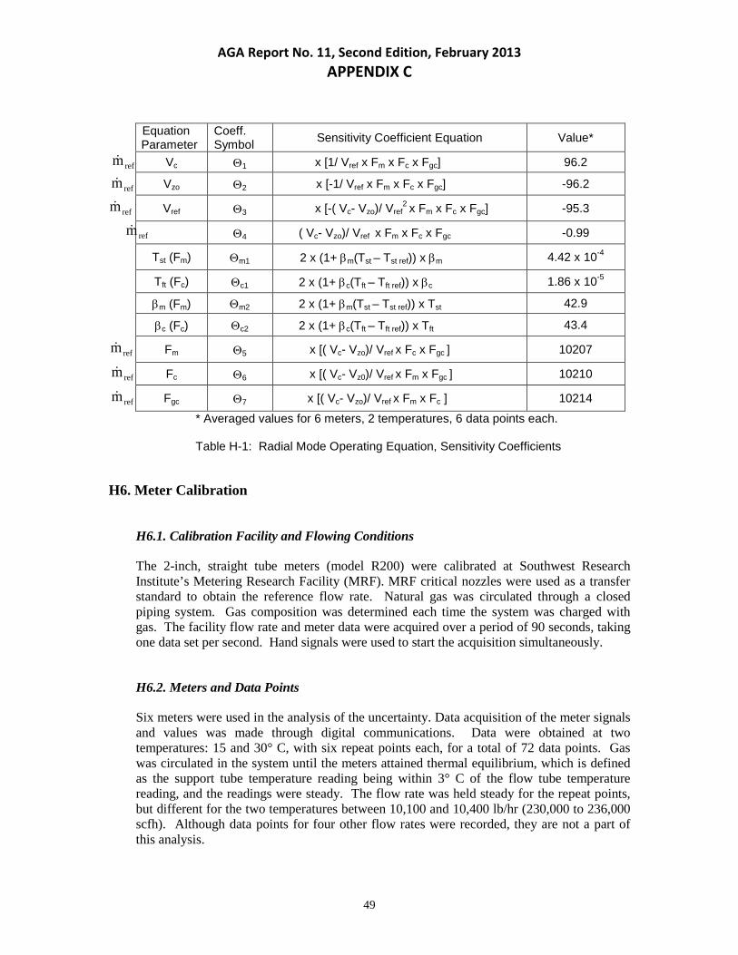
AGA Report No. 11, Second Edition, February 2013 APPENDIX C

refm

refm

refm

refmrefm

refm

refm

Equation Parameter

Coeff. Symbol

Sensitivity Coefficient Equation Value*

Vc Θ1 x [1/ Vref x Fm x Fc x Fgc] 96.2

Vzo Θ2 x [-1/ Vref x Fm x Fc x Fgc] -96.2

Vref Θ3 x [-( Vc- Vzo)/ Vref2 x Fm x Fc x Fgc] -95.3

Θ4 ( Vc- Vzo)/ Vref x Fm x Fc x Fgc -0.99

Tst (Fm) Θm1 2 x (1+ βm(Tst – Tst ref)) x βm 4.42 x 10-4

Tft (Fc) Θc1 2 x (1+ βc(Tft – Tft ref)) x βc 1.86 x 10-5

βm (Fm) Θm2 2 x (1+ βm(Tst – Tst ref)) x Tst 42.9

βc (Fc) Θc2 2 x (1+ βc(Tft – Tft ref)) x Tft 43.4

Fm Θ5 x [( Vc- Vzo)/ Vref x Fc x Fgc ] 10207

Fc Θ6 x [( Vc- Vz0)/ Vref x Fm x Fgc ] 10210

Fgc Θ7 x [( Vc- Vzo)/ Vref x Fm x Fc ] 10214

* Averaged values for 6 meters, 2 temperatures, 6 data points each. Table H-1: Radial Mode Operating Equation, Sensitivity Coefficients

H6. Meter Calibration

H6.1. Calibration Facility and Flowing Conditions

The 2-inch, straight tube meters (model R200) were calibrated at Southwest Research Institute’s Metering Research Facility (MRF). MRF critical nozzles were used as a transfer standard to obtain the reference flow rate. Natural gas was circulated through a closed piping system. Gas composition was determined each time the system was charged with gas. The facility flow rate and meter data were acquired over a period of 90 seconds, taking one data set per second. Hand signals were used to start the acquisition simultaneously.

H6.2. Meters and Data Points

Six meters were used in the analysis of the uncertainty. Data acquisition of the meter signals and values was made through digital communications. Data were obtained at two temperatures: 15 and 30° C, with six repeat points each, for a total of 72 data points. Gas was circulated in the system until the meters attained thermal equilibrium, which is defined as the support tube temperature reading being within 3° C of the flow tube temperature reading, and the readings were steady. The flow rate was held steady for the repeat points, but different for the two temperatures between 10,100 and 10,400 lb/hr (230,000 to 236,000 scfh). Although data points for four other flow rates were recorded, they are not a part of this analysis.

49

AGA Report No. 11, Second Edition, February 2013 APPENDIX C

refm

H6.3. Calculated Standard Uncertainty, uc

The calculated standard uncertainty for each parameter is shown in Table H2. The standard uncertainty values were averaged for the six meters.

H7. Expanded Base Error Uncertainty, U

The base error uncertainty is given in Table H-2. The coverage factor is 2, based on the combined degrees of freedom.

Parameter Symbol Average Value

Standard Unc, uA, (Type A), %

Standard Unc, uB, (Type B), %

Degrees of Freedom

Coriolis signal Vc 135 ± 0.014 % - 56

Coriolis signal, zero flow

Vzo 28 - ± 0.017 % 56

Coriolis ref signal Vref 107 ± 0.008% - 56

Ref mass flow rate,

lb/hr 10443 / 10162 - ± 0.052 % -

Support tube temp -°C

Tst 16.9 / 26.0 ± 0.021 % - 90

Flow tube temp - °C

Tft 14.4 / 29.0 ± 0.021 % - 90

Magnet thermal coeff, G/G/°C βm 0.000221 - ± 0.045 % -

Coil thermal coeff, M/M/°C βc -9.32 x 10-6 - ± 0.015 % -

Magnet thermal factor

Fm .9974 / 1.0033 ± 0.0002 % ± 0.043 % 15

Coil thermal factor Fc 1.0001 / .9998 ± 0.0001 % ± 0.043 % 18

Gas coupling factor Fgc .9999 / 0.9994 - ± 0.100 % 30

Coverage Factor 2

Mass Flow Rate, Expanded Uncertainty, U ± 0.27 %

Table H-2: Radial Mode Coriolis Meter, Base Error Uncertainty

50

AGA Report No. 11, Second Edition, February 2013 APPENDIX C

H8. Meter Zero Stability

The actual meter zero stability value, ZS, is the average amount of drift, or signal bias, of the flow-rate signal during normal operation. Values for the meter signal at no flow were collected for the six meters tested, before the first data point and after the last data point for each temperature (Table H-3). While not statistical, it is a representation of the expected amount of zero drift for meters during operation. The values are summarized in the following table.

Meter ZS (PPH), Tf = 60° F ZS (PPH), Tf = 86° F 1 17.12 7.17 2 29.33 8.54 3 0.19 -1.07 4 -11.49 5.41 5 -23.91 -16.00 6 18.30 -7.74 Avg (abs) 16.72 7.66

Table H-3: Summary of Zero Stability

H9. Total Meter Error

% Error = ± [0.50% ± (zero stability/flow rate) x 100] (H.4)

Using equation H-4 the average error of the meters is (± 0.27 ± 0.12 %). Figure H-3 shows a graphical comparison of the identified sources of error.

Radial-Mode, 2" Straight Tube Coriolis MeterSummary of Errors, Natural Gas, 160 psig, 230,000 SCFH

0.00%

0.02%

0.04%

0.06%

0.08%

0.10%

0.12%

0.14%

ZS Fgc M-dot-ref Fc Fm Vref Vzo Vc

Error Source

Abs

Std

Unce

rtain

ty, %

Figure H-3: Summary of Errors

51

AGA Report No. 11, Second Edition, February 2013 APPENDIX C

Appendix I

Of Engineering Technical Note, December 2001

Uncertainty Analysis for Curved Tube Meters

The following measurement uncertainty analysis has been provided by a Coriolis meter manufacturer. The results are specific to the meter design, meter size, and operating conditions referenced in the analysis. The estimated measurement uncertainty given in this analysis is not necessarily representative of all meter designs, sizes, and applications.

I1. Introduction

The following analysis is intended as a guideline for assessing Coriolis meter field performance, and especially to ascertain the largest contributors to measurement uncertainty. Although general NIST Technical Note 1297 guidelines have been followed, a rigorous treatment of uncertainty is not presented. There are two primary contributors to Coriolis meter uncertainty:

• Meter calibration and how the Flow Calibration Factor (FCF) is determined • Meter zeroing

As shown in Appendix H, baseline uncertainty of the meter measurement is approximately +/-0.3%. Additionally, there is uncertainty associated with the calibration method. In some cases Coriolis meters are calibrated on water; there is an obvious uncertainty associated with this type of calibration. Other Coriolis meters are calibrated on a gas medium other than natural gas (e.g., air); there is an uncertainty in this type of calibration usually related to the speed-of-sound differences between the calibration medium and natural gas. In both cases, the uncertainty of the gas calibration facility itself (usually approximately +/-0.25% by mass) used to establish either the primary calibration or the transferability of the calibration from another medium to gas plays a significant role in establishing the accuracy of the meter.

Data are presented in Appendix J for one meter type that, when all uncertainties are included, supports a +/-0.5% baseline specification. However, it is recognized that there is not a large enough population of meters to draw a statistically significant conclusion. It is for this reason that a rigorous uncertainty analysis is not presented; it is recommended that a third-party test be initiated to better understand population variations within a meter type and also from meter type to type.

In addition to better understanding calibration variation, a significant outcome of the testing will be to evaluate and understand the affect of gas pressure on Coriolis meters (see Section I.1.5).

Discussed at length in this appendix is the importance of proper meter zeroing. Aside from the baseline meter uncertainty discussed above, improper meter zeroing will contribute the largest uncertainty to the overall measurement. Since proper zeroing is always a field operation, it is not included in the uncertainty analysis.

52

AGA Report No. 11, Second Edition, February 2013 APPENDIX C

I1.1. Curved Tube Coriolis Operating Equation

A practical implementation of the theory described in Section 2.2 is shown in equation I.1.

( )

(I.3) 1F

(I.2) TK1F

I.1) ( ΔtΔtFFFCF flow mass

P

TT

oPT

PK P+=

−=

−×××=

Where:

FCF = flow calibration factor FT = temperature compensation KT = temperature coefficient, directly related to changing Young’s modulus vs. temperature T = primary element flow tube temperature FP = pressure compensation KP = pressure coefficient P = operating fluid pressure

t∆ = phase induced by the flowing gas

ot∆ = residual phase at zero flow Note: The uncertainty in the gas composition measurement used to convert from mass to standard volume (Appendix D) is not included in the scope of this appendix.

Each term of equation I.1 is discussed in the following sections.

I1.2. Flow Calibration Factor

Every Coriolis meter should be calibrated prior to use. A traceable reference is used to establish the flow calibration factor. In some cases the traceable standard is a gravimetric system, usually using water as the calibration medium. Some manufacturers calibrate meters on gas (or compressed air).

The uncertainty of the calibration is primarily affected by meter linearity, repeatability and calibration reference uncertainty. Most manufacturers state an uncertainty of +/-0.5% of mass flow rate, which includes all of these effects. This value is normally stated as a “2-sigma” value.

Calibration documentation should include information regarding the reference traceability. When the meter is calibrated on a fluid other than natural gas, documentation regarding transferability from the calibration medium to natural gas should be provided. Data exist showing the correlation between water and gas calibration factors to better than +/-0.4% (NMi custody transfer approval); however, these data are representative of three specific meters. To draw statistical conclusions additional meters need to be tested and verified.

53

AGA Report No. 11, Second Edition, February 2013 APPENDIX C

I1.3. Phase-Shift

The primary measurement performed by the Coriolis meter involves examining the sinusoidal signals produced by the position detectors mounted on the sensor tube. The delta t, or phase, is proportional to mass flow rate. Figure I-1 shows an example of the sinusoidal signals from a Coriolis meter.

Figure I-1: Example of Coriolis Meter Signals

As the mass flow rate increases, the phase-shift between the two sinusoidal signals increases proportionally. A precise measurement of the phase is required to achieve adequate meter repeatability. Most Coriolis meters operate on signal levels below 60 microseconds and can detect delta t as small as a few nanoseconds. The uncertainty associated with the ability to measure delta t is included in the mass flow accuracy statement.

I1.4. Temperature Effect

Temperature has an effect on the indicated mass flow rate by changing the tube rigidity (also referred to as stiffness or elasticity). Most materials, including metals, change rigidity as temperature changes. To compensate for the temperature induced rigidity change, the tube temperature is measured on the sensor (usually via an RTD). The compensation is linear and implemented as shown in equation I-1.

delta t

54

AGA Report No. 11, Second Edition, February 2013 APPENDIX C

I1.5. Pressure Effect

Static pressure of the gas induces a slight stiffening of the flow tube(s). The magnitude of the stiffening and, therefore, the effect on the meter will depend on the geometry of the sensor. The effect on performance is small and can sometimes be ignored. At high pressure (greater than 500 psi), the effect can be large enough to be considered. The compensation is linear and implemented as shown in equation I-1.

Most pressure effect research has been performed on liquids. There is evidence that the pressure effect is smaller on gas than on liquid. NOVA, Canada, reported work on a 3-inch Coriolis meter (4th Flow Symposium) that showed agreement to the reference better than 0.3% without pressure compensation applied. When the manufacturer’s recommended pressure compensation was applied, the average error changed by +0.5%. The effect of pressure on Coriolis meters for gas measurement is an important future research topic.

Note: Because the pressure effect is small, if on-line pressure compensation is employed, the location of the pressure tap does not impact performance. A pressure measurement error as high as 10% of reading will affect the performance by less than 0.1%.

I1.6. Sensitivity Coefficients

Sensitivity coefficients are derived using the NIST methodology previously described in Appendix H. Sample sensitivity coefficients for a 316SS curved tube sensor are shown in Table I-1.

Variable Sensitivity Coefficient Uncertainty

FCF 1 +/-0.5% (consult manufacturer)

FT -0.04% per ° C +/-0.001% per ° C

FP Less than –0.001% per psi

+/-0.0005% per psi

t∆ 1 Included in FCF

ot∆ 1 Operationally Dependent (Section

I.1.8)

Table I-1: Sensitivity Coefficients for Curved Tube Sensor

A sensitivity coefficient of “1” indicates a one-to-one correlation between the variable and meter output. For example, a 0.5% error in calibration factor or phase measurement results directly in a 0.5% error in the mass flow measurement.

55

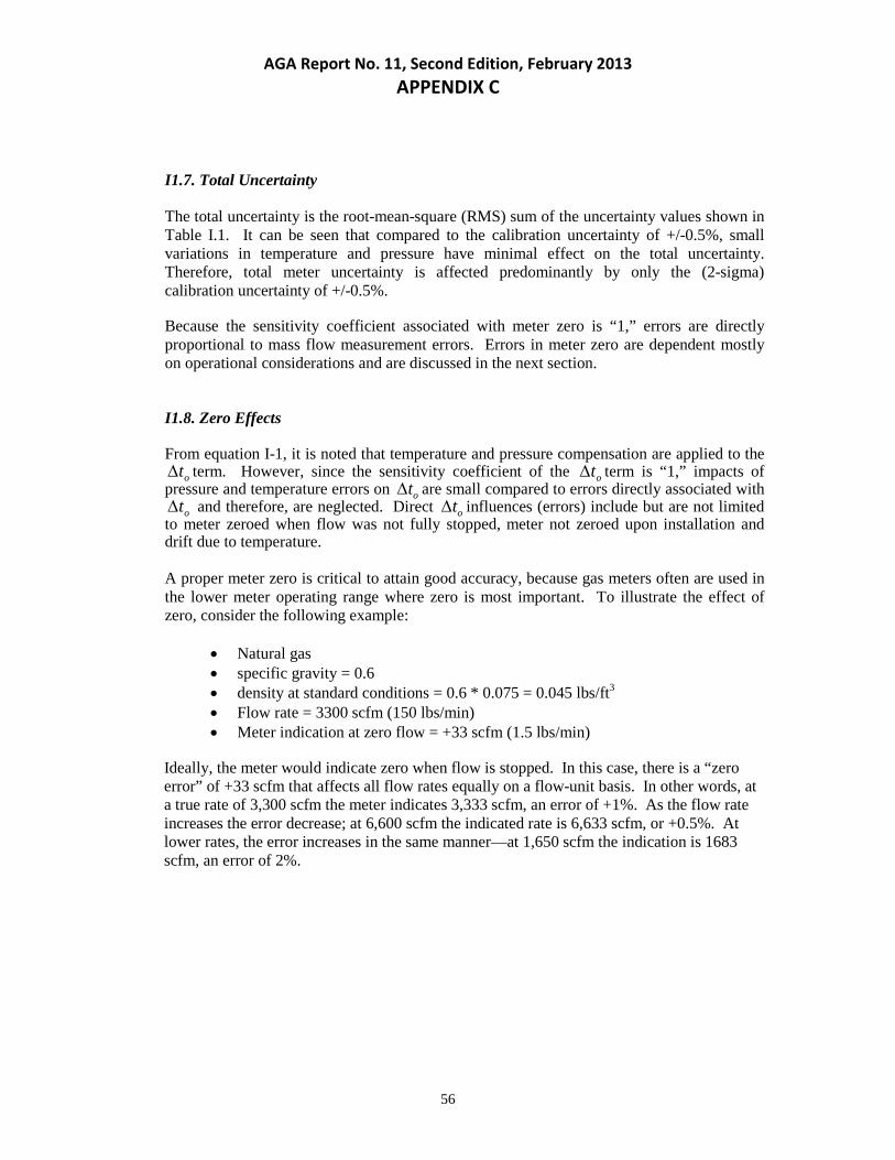
AGA Report No. 11, Second Edition, February 2013 APPENDIX C

I1.7. Total Uncertainty

The total uncertainty is the root-mean-square (RMS) sum of the uncertainty values shown in Table I.1. It can be seen that compared to the calibration uncertainty of +/-0.5%, small variations in temperature and pressure have minimal effect on the total uncertainty. Therefore, total meter uncertainty is affected predominantly by only the (2-sigma) calibration uncertainty of +/-0.5%.

Because the sensitivity coefficient associated with meter zero is “1,” errors are directly proportional to mass flow measurement errors. Errors in meter zero are dependent mostly on operational considerations and are discussed in the next section.

I1.8. Zero Effects

From equation I-1, it is noted that temperature and pressure compensation are applied to the ot∆ term. However, since the sensitivity coefficient of the ot∆ term is “1,” impacts of

pressure and temperature errors on ot∆ are small compared to errors directly associated with ot∆ and therefore, are neglected. Direct ot∆ influences (errors) include but are not limited

to meter zeroed when flow was not fully stopped, meter not zeroed upon installation and drift due to temperature.

A proper meter zero is critical to attain good accuracy, because gas meters often are used in the lower meter operating range where zero is most important. To illustrate the effect of zero, consider the following example:

• Natural gas • specific gravity = 0.6 • density at standard conditions = 0.6 * 0.075 = 0.045 lbs/ft3 • Flow rate = 3300 scfm (150 lbs/min) • Meter indication at zero flow = +33 scfm (1.5 lbs/min)

Ideally, the meter would indicate zero when flow is stopped. In this case, there is a “zero error” of +33 scfm that affects all flow rates equally on a flow-unit basis. In other words, at a true rate of 3,300 scfm the meter indicates 3,333 scfm, an error of +1%. As the flow rate increases the error decrease; at 6,600 scfm the indicated rate is 6,633 scfm, or +0.5%. At lower rates, the error increases in the same manner—at 1,650 scfm the indication is 1683 scfm, an error of 2%.

56

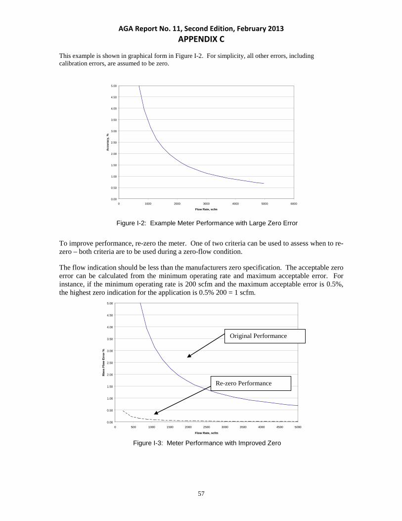
AGA Report No. 11, Second Edition, February 2013 APPENDIX C

This example is shown in graphical form in Figure I-2. For simplicity, all other errors, including calibration errors, are assumed to be zero.

0.00

0.50

1.00

1.50

2.00

2.50

3.00

3.50

4.00

4.50

5.00

0 1000 2000 3000 4000 5000 6000

Flow Rate, scfm

Acc

urac

y, %

Figure I-2: Example Meter Performance with Large Zero Error

To improve performance, re-zero the meter. One of two criteria can be used to assess when to re-zero – both criteria are to be used during a zero-flow condition. The flow indication should be less than the manufacturers zero specification. The acceptable zero error can be calculated from the minimum operating rate and maximum acceptable error. For instance, if the minimum operating rate is 200 scfm and the maximum acceptable error is 0.5%, the highest zero indication for the application is 0.5% 200 = 1 scfm.

0.00

0.50

1.00

1.50

2.00

2.50

3.00

3.50

4.00

4.50

5.00

0 500 1000 1500 2000 2500 3000 3500 4000 4500 5000

Flow Rate, scfm

Mas

s Fl

ow E

rror

%

Figure I-3: Meter Performance with Improved Zero

Original Performance

Re-zero Performance

57

AGA Report No. 11, Second Edition, February 2013 APPENDIX C

Using the second criterion, assume that the meter is re-zeroed and it indicates 1 scfm at no flow. Figure I-2 indicates expected meter performance.

I1.9. Zero Effects – Temperature

Process temperature changes can cause the zero point of the meter to drift. Note that the drift is not related to temperature correction discussed previously in I.1.4. Specifications are quoted in flow units per degree; i.e., scfm per °C. If the temperature varies less than 20° C from the temperature at which the meter was zeroed, there is normally no requirement to re-zero. If the operating temperature deviates by more than 20° C from the zeroing temperature, zero the meter as close to operating temperature as possible. If the meter cannot be zeroed near the operating temperature, additional uncertainty should be added to the mass flow accuracy statement, using the RMS method. As an example, consider the following:

• Base meter zero stability = 1 scfm • Temperature effect = 0.05 scfm per °C • Meter operating at 20°C from the zero temperature

The meter zero stability in this case is [12 + (0.05*20)2]1/2 = 1.4 scfm. This zero stability value is used in the accuracy calculation as described above.

58

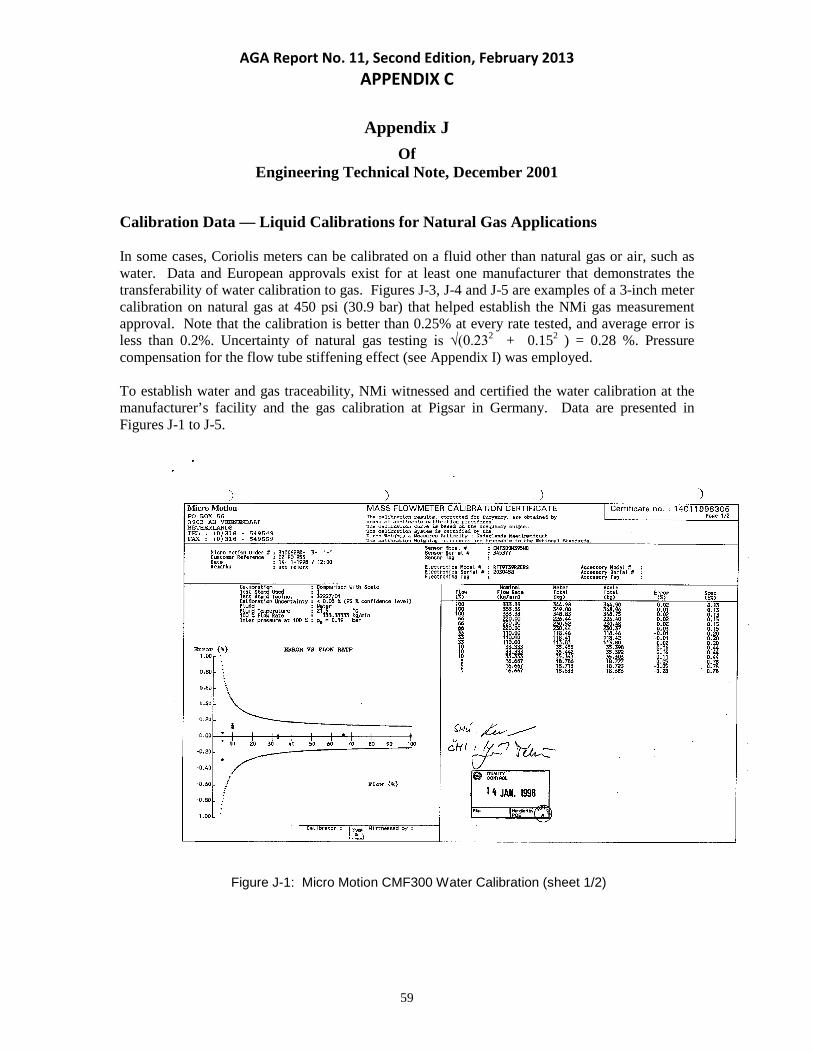
AGA Report No. 11, Second Edition, February 2013 APPENDIX C

Appendix J

Of Engineering Technical Note, December 2001

Calibration Data — Liquid Calibrations for Natural Gas Applications

In some cases, Coriolis meters can be calibrated on a fluid other than natural gas or air, such as water. Data and European approvals exist for at least one manufacturer that demonstrates the transferability of water calibration to gas. Figures J-3, J-4 and J-5 are examples of a 3-inch meter calibration on natural gas at 450 psi (30.9 bar) that helped establish the NMi gas measurement approval. Note that the calibration is better than 0.25% at every rate tested, and average error is less than 0.2%. Uncertainty of natural gas testing is √(0.232 + 0.152 ) = 0.28 %. Pressure compensation for the flow tube stiffening effect (see Appendix I) was employed.

To establish water and gas traceability, NMi witnessed and certified the water calibration at the manufacturer’s facility and the gas calibration at Pigsar in Germany. Data are presented in Figures J-1 to J-5.

Figure J-1: Micro Motion CMF300 Water Calibration (sheet 1/2)

59

AGA Report No. 11, Second Edition, February 2013 APPENDIX C

Figure J-2: Micro Motion CMF300 Water Calibration (sheet 2/2)

Figure J-3: Micro Motion Natural Gas Certificate (sheet 1/3)

60

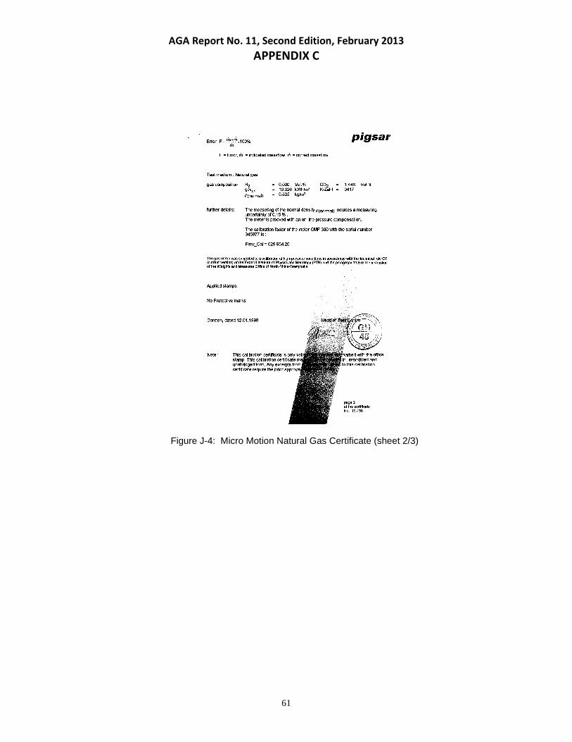
AGA Report No. 11, Second Edition, February 2013 APPENDIX C

Figure J-4: Micro Motion Natural Gas Certificate (sheet 2/3)

61

AGA Report No. 11, Second Edition, February 2013 APPENDIX C

Figure J-5: Micro Motion Natural Gas Certificate (sheet 3/3)

Although one example is shown, data are available for Micro Motion models CMF100, CMF200, and CMF300 (sizes 1-inch, 2-inches, and 3-inches) that supports water calibration transferability to gas.

BiDirectional Flow

BiDirectional flow has been evaluated on gas at the Didsbury Gas Dynamic Test Facility. The Micro-Motion CMF300 3-inch Coriolis mass flow meter was performance-tested in both forward and reverse flow directions (by reversing the meter) at line pressures that varied between 4,600 kPa and 5,000 kPa (670 to 720 psia). Performance evaluation was done over the full range of mass flow rates for this meter in nine steps from 0.9 to 7.9 kg/s (158 to 1.4 mscfd), which correspond to mean flow velocity from 5 to 43 m/s (15 to 140 ft/s). Data from the meter were obtained through the RS-485 digital communications port and logged at a 1-second interval update rate.

62

AGA Report No. 11, Second Edition, February 2013 APPENDIX C

A bank of choked nozzles sets the reference mass flow. Details of the test facility have been presented in the past in several publications (for example, Karnik et al., 1996). The Didsbury Test Facility has been part of several round-robin tests since 1995 with facilities such as NEL, K-Lab, CEESI, GRI-MRF, Groningen, Westerbork, Pigsar, Bishop Auckland, KRISS and TCC. Results of such tests have been published; for example, Karnik et al. (1996), Euromet nozzle in 1997 (unpublished see METCON report #2); Karnik et al. (ASME, 2000); and Karnik and Flegel (FLOMEKO, 2000). The factory water calibration was used for all gas calibrations. No pressure compensation was employed.

Figure J-6: CMF300 Gas Calibration at NOVA-Didsbury. Forward and Reverse Flow

63

FORM FOR PROPOSALS ON ENGINEERING TECHNICAL NOTE

Coriolis Flow Measurement for Natural Gas Applications Send to: Operations & Engineering Section American Gas Association 400 North Capitol St., NW 4th Floor Washington, DC 20001 U.S.A. Fax: (202) 824-7082 Name: __________________________________________________________________ Company: _______________________________________________________________ Address: _________________________________________________________________ Phone: ___________________ Fax:____________________E-mail:_________________ Please Indicate Organization Represented (if any):______________________________ 1. Section/Paragraph :_______________________________________________________ 2. Proposal Recommends: (check one): new text revised text deleted text 3. Proposal (include proposed new or revised wording, or identification of wording to be deleted, use separate sheet if needed): [Proposed text should be in legislative format; i.e., use underscore to denote wording to be inserted (inserted wording) and strike-through to denote wording to be deleted (deleted wording).] 4. Statement of Problem and Substantiation for Proposal (use separate sheet if needed): (State the problem that will be resolved by your recommendation; give the specific reason for your proposal including copies of tests, research papers, etc.) 5. This proposal is original material. (Note: Original material is considered to be the submitter’s own idea based on or as a result of his/her own experience, thought or research and, to the best of his/her knowledge, is not copied from another source.) This proposal is not original material; its source (if known) is as follows: ________________________________________________________________________________ Type or print legibly. If supplementary material (photographs, diagrams, reports, etc.) is included, you may be required to submit sufficient copies for all members of reviewing committees or task forces. I hereby grant the American Gas Association the non-exclusive, royalty-free rights, including non-exclusive, royalty-free rights in copyright, in this proposal and I understand that I acquire no rights in any publication of the American Gas Association in which this proposal in this or another similar or analogous form is used. Date: ___________________ Signature (Required) ____________________________

FOR OFFICE USE ONLY Log # __________________________ Date Rec’d _____________________

P- I

D-1

APPENDIX D 

Examples of Overall Measurement Uncertainty Calculations – Coriolis Meter 

(Informative)  

D.1   GENERAL 

The following is a simplified example of estimating measurement uncertainty for sites using Coriolis gas flow meters.

Following the pattern demonstrated in ISO 5168, the estimation of uncertainty is based on a sequence of:

1. establishing a mathematical model for the measurement process 2. listing and quantifying the contributory variances 3. combining variances into a composite statement of uncertainty 4. expanding the uncertainty to the appropriate confidence level

In any uncertainty analysis, uncertainties must be combined at the same confidence level. For the example that follows, the standard uncertainties (68% confidence level, coverage factor=1) are listed and combined. To provide the expanded uncertainty with a 95% confidence level, a coverage factor=2 is applied to the uncertainty. More details on these uncertainty relationships can be found in ISO 5168.

D.2   MATHEMATICAL MODEL 

The gas volume flow rate at base conditions is given by —

pb m

b

FQ Q

D.3   CONTRIBUTORY VARIANCES 

The relative (percentage) combined standard uncertainty in the measurement is given by the following equation:

2* * 2 * 2 * 2

m p bQ FQbu u u u

D.3.1  Uncertainty in the Mass Flow Rate 

The total uncertainty is composed of uncertainty in the calibration plus long term reproducibility in the field. Calibration uncertainty is assumed to include the flow laboratory, its chain of traceability and the repeatability of the meter under test. Uncertainty under field conditions is assumed to include all site-specific installation effects, including those associated with flow characteristics, equipment age, cleanliness and data acquisition. Assuming the correlation between uncertainty components to be zero, the equation is such that,

D-2

2*2*2*

FieldmCalmm QQQ uuu

* 0.15%

mCalQu , coverage factor k=1, as estimated by flow laboratory

* 0.05%mField

Qu , as estimated by user

* 2 2 20.15 0.05 0.025%

mQu

* 0.16%mQu , coverage factor k=1, as estimated by flow laboratory

Note: The standard uncertainties (68% confidence level, coverage factor=1) are listed

and combined.

D.3.2  Uncertainty in Flow Pressure Effect Compensation Factor ( pF) 

The relationship for pressure effect is such that,

))(*)100/((11

CalfEffectp PPP

F

pF

uncertainty is composed of estimates of uncertainty in flowing pressure ( fP ) and

calibration pressure ( CalP ) with a sensitivity proportional to pressure effect ( EffectP ).

Pressure flowing uncertainty is composed of uncertainty in calibration and field long-term reproducibility. The estimate of field uncertainty includes the effect of ambient conditions, equipment age, and data acquisition.

2*2*2*

CalfEffectp PPPF uusu

0.002EffectPs , highest sensitivity, Coverage Factor k=1, as estimated by

manufacturer

* 2 0.1%fPu , Coverage Factor k=1, as estimated by manufacturer

* 2 0.1%

CalPu , Coverage Factor k=1, as estimated by manufacturer

* 2 2 20.002 0.1 0.1 0.00004%pFu

* 0.0063%

pFu , Coverage Factor k=1, as estimated by manufacturer

Note: the standard uncertainties (68% confidence level, coverage factor=1) are listed and combined

D-3

D.3.3  Uncertainty in the Determination of Base Density ( b ) 

The relationship for base density is such that.

bb

rbb RTZ

MP

Given that the base pressure ( bp ), gas constant ( R ), and base temperature ( bT ) are

constants by definition. For this example, the estimation of uncertainty includes the

uncertainty in Molar Weight ( rM ) and base compressibility factor ( bZ ), which are

dependent on gas composition analysis. For simplicity in this example, the gas composition analysis uncertainty is assumed to be zero. A more comprehensive analysis of uncertainty would include the contributory variances of gas calibration standards and chromatography.

D.4   COMBINED UNCERTAINTY Applying the values from above examples, the revised expression for combined uncertainty is:

2* * 2 * 2 * 2

m p bQ FQbu u u u

2* 2 2 20.16 0.0063 0.0 0.02564%Qbu

* 0.16%Qbu , Coverage Factor k=1

Note: The standard uncertainties (68% confidence level, coverage factor=1) are listed and combined.

D.5   EXPANDED UNCERTAINTY An expanded uncertainty, coverage factor k=2, approximate confidence level 95%, is:

*95

*Q ku Qb bu

*95 2(0.16%)Qbu

*95 0.32%Qbu , Coverage Factor k=2

Note: To provide the expanded uncertainty with a 95% confidence level, a coverage factor=2 is applied to the uncertainty.

xx cubic feet per hour +/-0.32% (expanded uncertainty, coverage factor k=2, approximate confidence level 95 percent).

D-4

E-1

APPENDIX E 

Coriolis Gas Flow Measurement System 

(Informative) 

This appendix details principles summarized in API MPMS Chapter 21, Flow Measurement Using Electronic Metering Systems, Section 1, Electronic Gas Measurement. It is provided as an aid to users and flow computer manufacturers in interpreting and applying API Chapter 21, Section 1. E.1   CORIOLIS MEASUREMENT SYSTEM ARCHITECTURE 

A fundamental Coriolis gas measurement system is depicted in Figure E.1 and is composed of a Coriolis Sensor, Transmitter, and flow computer. Dependent upon system design and process conditions, an analytical transmitter (on-site or off-site) and pressure transmitter (on-site) may or may not be required. A Coriolis sensor incorporates multiple sensing elements from which gas flow, flow tube temperature, and flowing density are inferred by the transmitter. The transmitter also performs sensor and transmitter diagnostic functions, and communicates diagnostic and inferential measurement information, partially or completely, through analog and/or digital methods to a gas flow computer.

Figure E.1 Coriolis Gas Measurement System block diagram

It is important to note that the transmitter will always be located physically on-site, either local or remote to the sensor. The flow computer should be viewed as software that can exist either on-site or off-site. In the case of on-site, the flow computer can be located in electronic hardware in same enclosure as the transmitter or in electronic hardware in a separate enclosure. In the case of off-site, the flow computer is located in a central data processing system and receives data through a digital communication link.

The flow computer, at a minimum, collects mass flow information from the transmitter and at a maximum also collects flow tube temperature, flowing density, configuration, calibration variables, and diagnostic information from the transmitter along with live analytical, live pressure, and other process information. It utilizes this information to perform flow measurement calculations, enhanced

E-2

diagnostics, and in some cases control the flow measurement process. In performing these tasks, the flow computer shall retain all metrological significant information that it controls or has access to in the configuration, event, and data logs to facilitate a chronological audit of the measurement process along with deconstruction and reconstruction with relevant corrections when necessary.

E.2   TRANSMITTER TO FLOW COMPUTER INTERFACE 

Dependent upon design, the communications interface between the transmitter and flow computer can be either unidirectional or bidirectional. The unidirectional interface typically consists of a combination of unidirectional discrete digital, frequency and analog signals generated by the transmitter and monitored by the flow computer. The bidirectional interface is typically a digital communications link with read-only or read/write capability.

E.2.1  Unidirectional Discrete I/0 Interface 

At a minimum, the unidirectional discrete I/O communications interface from the transmitter to the flow computer shall consist of a digital frequency and/or analog signal(s) that indicate mass flow sensed by the Coriolis sensor. Methods for facilitating flow indication will be as follows.

1) A single signal from the transmitter to flow computer proportional to unidirectional flow

through the Coriolis sensor (minimum requirement unidirectional flow), or

2) A single signal from the transmitter to flow computer proportional to the absolute value of flow through the Coriolis sensor with another signal representing flow direction (minimum requirement facilitating bidirectional flow measurement through the sensor), or

3) Dual frequency signals, one representing forward and one representing reverse flow, or

4) Dual frequency signals with quadrature phase shifting to indicate flow direction and fault conditions. This functionality may be implemented as shown in Figure E.2.

Figure E.2

Quadrature Phase Shifting

The incorporation of other unidirectional signals, either analog and or digital, representative of a system fault, flow tube temperature, flowing density, etc. are optional.

E-3

E.2.2  Bidirectional Communications Interface 

The bidirectional communication interface between the transmitter and flow computer can consist of a parallel data bus or serial data link (i.e., RS-232, RS485, Ethernet, etc.). Dependent upon design, the transmitter communications port can be a read only or read/write. If the transmitter communications port accessed by the flow computer allows read/write functionality, the flow computer shall retain a current record/log of all metrological significant configuration variables it has the ability to change and an event record/log of historic change to these variables.

        E.3   TRANSMITTER 

E.3.1  Transmitter Flow Calculations 

The transmitter monitors signals from pickoff(s)/flow tube(s) position sensors located across the length of the Coriolis flow tube(s). By integrating the flow tube(s) position, from inlet to outlet, and determining a phase shift in position relative to time at zero flow and flow, mass flow is determined such that:

0( )Uncompensated f tmQ FCF t t F Eq. (E.1)

Where:

UncompensatedmQ

= Mass flow rate uncompensated for flow pressure effect and

secondary gas calibration factor(s)

FCF = Sensor flow calibration factor

ft = Phase shift at flow

0t = Phase shift at zero flow

tF = Flow temperature correction factor

The flow temperature compensation factor ( tF ) is calculated as follows:

)(1 TFTFt Eq. (E.2)

Where:

tF = Flow temperature compensation factor

T = Temperature in degrees Celsius FT = Temperature coefficient (%/100 C)

E.3.2  Transmitter Algorithms and Variables of Metrological Interest 

Due to the ability of a Coriolis meter to measure mass flow, flow tube temperature, and gas flowing density, there are common calibration variables, units of measure, and algorithm settings related to this functionality that can influence mass flow measurement and transmitter output. Verification and record of the values are necessary to ensure accurate flow measurement and the audit of historic measurement performed by a Coriolis meter. A summary of these items may include but is not limited to the following:

Mass units - lb, kg, tons, grams, etc.

Mass flow damping - time period for a rolling average on mass flow output

No flow cut-off - mass flow rate at mass and flow time unit settings

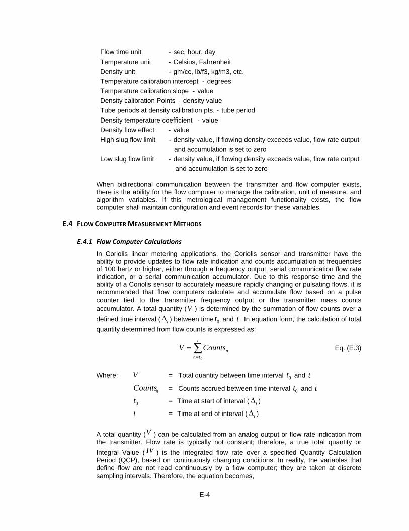
E-4

Flow time unit - sec, hour, day

Temperature unit - Celsius, Fahrenheit

Density unit - gm/cc, lb/f3, kg/m3, etc.

Temperature calibration intercept - degrees

Temperature calibration slope - value

Density calibration Points - density value

Tube periods at density calibration pts. - tube period

Density temperature coefficient - value

Density flow effect - value

High slug flow limit - density value, if flowing density exceeds value, flow rate output

and accumulation is set to zero

Low slug flow limit - density value, if flowing density exceeds value, flow rate output

and accumulation is set to zero

When bidirectional communication between the transmitter and flow computer exists, there is the ability for the flow computer to manage the calibration, unit of measure, and algorithm variables. If this metrological management functionality exists, the flow computer shall maintain configuration and event records for these variables.

          E.4   FLOW COMPUTER MEASUREMENT METHODS 

E.4.1  Flow Computer Calculations 

In Coriolis linear metering applications, the Coriolis sensor and transmitter have the ability to provide updates to flow rate indication and counts accumulation at frequencies of 100 hertz or higher, either through a frequency output, serial communication flow rate indication, or a serial communication accumulator. Due to this response time and the ability of a Coriolis sensor to accurately measure rapidly changing or pulsating flows, it is recommended that flow computers calculate and accumulate flow based on a pulse counter tied to the transmitter frequency output or the transmitter mass counts accumulator. A total quantity (V ) is determined by the summation of flow counts over a

defined time interval ( t ) between time 0t and t . In equation form, the calculation of total

quantity determined from flow counts is expressed as:

t

tnnCountsV

0

Eq. (E.3)

Where: V = Total quantity between time interval 0t and t

nCounts = Counts accrued between time interval 0t and t

0t = Time at start of interval ( t )

t = Time at end of interval ( t )

A total quantity (V ) can be calculated from an analog output or flow rate indication from the transmitter. Flow rate is typically not constant; therefore, a true total quantity or

Integral Value ( IV ) is the integrated flow rate over a specified Quantity Calculation Period (QCP), based on continuously changing conditions. In reality, the variables that define flow are not read continuously by a flow computer; they are taken at discrete sampling intervals. Therefore, the equation becomes,

E-5

ni

iii tQIV

1

Eq. (E.4)

Where: IV = Integral value or total Integral quantity accumulated over

QCP i = Sample number

n = Number of samples taken over the it

QCPn

iQ = Flow rate based on data taken at sample i

it = Time between samples

It is recommended that the Coriolis sensor and transmitter flow response time be examined and an appropriate flow computer sampling rate implemented to minimize sampling inaccuracies when utilizing the flow rate method for determining a total quantity

Coriolis is an inherently linear meter whose performance can be corrected by utilizing a single (i.e. bias correction) or multiple (i.e. linearization corrections) calibration factor

( FactorK) or meter correction factor ( FactorC

), to reduce gas measurement uncertainty. This requires an understanding of how these factors are applied in the calculation of an

integral value ( IV ) and in some cases results in a double summation being required and/or the application of the linearization at different points in the calculation. For frequency/pulse and serial communication accumulator outputs the integral value

( IV ) is calculated such that,

ni

li

lj

jFactor

Factor CountsK

CIV

i

i

1

Eq. (E.5a)

or

ni

li

lj

j FactorFactor K

CountsCIV

i1

Eq. (E.5b)

or

)(1

1

ni

li

lj

jFactor

Factor

CountsCK

IVi

Eq. (E.5c)

Where: IV = Total Integral quantity accumulated over QCP i = Sample number

n = Number of samples taken over the QCP, it

QCPn

FactorK = Single meter constant in counts per unit mass

E-6

iFactorK = Multi-point meter constant in counts per unit mass

calculated at interval l

FactorC = Single meter correction factor

iFactorC = Multi-point meter correction factor calculated for

interval l Counts = Mass flow pulses or mass accumulator counts

Note: Due to the manufactured nature of the meter pulse output, the meter manufacturer needs to ensure the manufactured pulses are synchronized to the flow.

Note: l should be chosen such that ln is an integer.

For an analog or serial communications rate output where multiple meter correction

factors ( FactorC ) are utilized, the integral value ( IV ) is calculated such that,

ni

iiiFactor tQCIV

i1

Eq. (E.6)

Where: IV = Total Integral quantity accumulated over QCP i = Sample number

n = Number of samples taken over the QCP, it

QCPn

iFactorC = Multi-point meter correction factor calculated for point i

iQ = Flow rate based on data taken at sample i

it = Time between samples

Note: The meter output needs to be read at a frequency that is proportional to the Coriolis sensor/transmitter response to flow to sufficiently capture rapid changes in flow or flow pulsations.

Note: The meter output is already corrected for FactorK or FactorK =1

Mass flow rate ( mQ) is determined over the interval ( t ) the total quantity ( IV ) is

accrued. In equation form, the calculation of mass flow rate is expressed as the follows.

t

IVQm

Eq. (E.7)

Where: mQ = Rate over time interval t

IV = Quantity accrued between time 0t and t

t = Time interval between time 0t and t

When measuring flow away from calibration pressure, there is a secondary effect on a Coriolis meter’s indicated flow rate called the “flow pressure effect.” To correct for this

E-7

effect, a pressure correction factor ( pF ) must be applied by the flow computer to the

mass flow indication from the transmitter. This relationship is such that,

)( pmm FQQtedUncompensadCompensate

Eq. (E.8)

Where: dCompensatemQ = Mass flow of the gas compensated for flow pressure

effect

tedUncompensamQ = Mass flow of gas uncompensated for flow pressure

effect

pF = Flow pressure effect compensation factor

The flow pressure effect compensation factor ( pF ) is calculated in accordance with the

following equation.

))(*)100/((11

CalfEffectp PPP

F

Eq. (E.9)

Where: pF = Flow pressure effect compensation factor

EffectP = Flow pressure effect in percent of rate per psig

fP = Measurement fluid static pressure in psig

CalP = Calibration static pressure in psig

The flow rate from a Coriolis measurement system can take several forms depending on whether the ultimate quantity being measured is mass, volume at base conditions, energy or volume at flowing conditions. Appropriate conversions, relative to the gas physical properties and process conditions, must be applied to accurately obtain the desired units. The equation for flow rate at base conditions, including flow pressure effect correction ( pF ) is such that,

)( Airbr

pm

b

pmb G

FQ

FQQ

tedUncompensatedUncompensa

Eq. (E.10)

Where: bQ = Volume flow of gas at base conditions

tedUncompensamQ = Mass flow of gas uncompensated for flow pressure

effect

pF = Flow pressure effect compensation factor

b = Density of gas at base conditions

rG = Relative density of gas at base conditions

)( Airb = Density of air at base conditions

E-8

The base density of gas is calculated utilizing the non-ideal gas law such that,

bb

rbb RTZ

MP

Eq. (E.11)

Where: b = Density of gas at base conditions

bP = Pressure of the gas at base conditions

rM = Molar weight of the gas

bZ = Compressibility factor of the gas at base conditions

R = Universal Gas Constant

bT = Temperature at base conditions

Relative density is calculated utilizing methods such that,

)()(

)()(

)(

)(

AirGasb

GasAirb

Airb

Gasb

MrZ

MrZGr

Eq. (E.12)

Where: )(Gasb = Density of gas at base conditions

)( Airb = Density of air at base conditions

)(GasbZ = Compressibility factor of gas at base conditions

)( AirbZ = Compressibility factor of air at base conditions

)(GasrM = Molar weight of gas

)( AirrM = Molar weight of air

rG = Relative density of the gas at base conditions

The equation for energy rate, including flow pressure effect compensation factor ( pF ), is

such that,

)( mpme HFQQtedUncompensa

Eq. (E.13)

Where: eQ = Energy rate of gas

tedUncompensamQ = Mass flow of gas uncompensated for flow pressure

effect

pF = Flow pressure effect compensation factor

mH = Mass heating value

E-9

The equation for flow rate at flowing conditions, including flow pressure effect compensation factor ( pF ), is such that,

f

pmf

FQQ

tedUncompensa Eq. (E.14)

Where: fQ = Volume flow rate of the gas at flowing conditions

tedUncompensamQ = Mass flow of gas uncompensated for flow pressure

effect

pF = Flow pressure effect compensation factor

f = Density of gas at flowing conditions

The flowing density of gas is calculated utilizing the non-ideal gas law such that,

ff

rff RTZ

MP Eq. (E.15)

Where: f = Density of gas at flowing conditions

fP = Pressure of the gas at flowing conditions

rM = Molar weight of the gas

fZ = Compressibility factor of the gas at flowing conditions

R = Universal Gas Constant

fT = Temperature at flowing conditions

Variable U.S. Units S.I. Units

b lbm/ft3 kg/m3

bP Psia Mpa

rM lb/lb-mole kg/kg-mole

bZ Dimensionless dimensionless

R psia-ft3/lb-mole-oR (10.73164)

Mpa-m3/kg-mole-K (0.00831451)

bT oR (Rankin) K (Kelvin)

rG Dimensionless dimensionless

)( Airb lbm/ft3

(0.076529 lb/ft3 at 14.73 psia and 60 F)

kg/m3

(1.2254 kg/m3 at 0.101325 Mpa and 288.15 K) (1.2254 kg/m3 at 101.325 kpa and 15 C)

Table E.1

Typical Units of Measure for Base Density Calculations

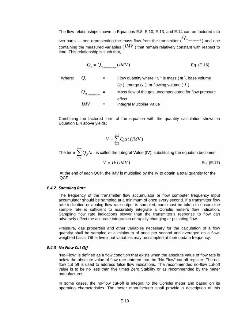
E-10

The flow relationships shown in Equations E.8, E.10, E.13, and E.14 can be factored into

two parts — one representing the mass flow from the transmitter ( tedUncompensamQ) and one

containing the measured variables ( IMV ) that remain relatively constant with respect to time. This relationship is such that,

)(IMVQQ

tedUncompensamx Eq. (E.16)

Where: xQ = Flow quantity where “ x ” is mass ( m ), base volume

( b ), energy ( e ), or flowing volume ( f )

tedUncompensamQ = Mass flow of the gas uncompensated for flow pressure

effect IMV = Integral Multiplier Value

Combining the factored form of the equation with the quantity calculation shown in Equation E.4 above yields:

)(1

IMVtQVni

iii

The term

ni

iifi tQ

1

is called the Integral Value (IV); substituting the equation becomes:

)(IMVIVV Eq. (E.17)

At the end of each QCP, the IMV is multiplied by the IV to obtain a total quantity for the QCP.

E.4.2  Sampling Rate 

The frequency of the transmitter flow accumulator or flow computer frequency input accumulator should be sampled at a minimum of once every second. If a transmitter flow rate indication or analog flow rate output is sampled, care must be taken to ensure the sample rate is sufficient to accurately integrate a Coriolis meter’s flow indication. Sampling flow rate indications slower than the transmitter’s response to flow can adversely affect the accurate integration of rapidly changing or pulsating flow.

Pressure, gas properties and other variables necessary for the calculation of a flow quantity shall be sampled at a minimum of once per second and averaged on a flow-weighted basis. Other live input variables may be sampled at their update frequency.

E.4.3  No Flow Cut Off  

“No-Flow” is defined as a flow condition that exists when the absolute value of flow rate is below the absolute value of flow rate entered into the “No-Flow” cut-off register. The no-flow cut off is used to address false flow indications. The recommended no-flow cut-off value is to be no less than five times Zero Stability or as recommended by the meter manufacturer.

In some cases, the no-flow cut-off is integral to the Coriolis meter and based on its operating characteristics. The meter manufacturer shall provide a description of this

E-11

process and the no-flow cut-off value. Consideration of documented site conditions may result in a modified no-flow cut-off value.

E.4.4  Quantity Calculation Period (QCP) 

The maximum QCP calculation frequency should be 5 minutes unless it can be shown that the error introduced by the IMV during the QCP causes less than 0.05% error in the volume calculation. In all cases the QCP shall not exceed one hour.

E.4.5  Average Value Determination for Live Inputs 

At a minimum, hourly averages of all live inputs should be maintained and reported in the quantity transaction record; i.e. data log. The averaging technique for each live input should be flow-weighted and must include only values taken when flow is present. When there is no flow for the entire quantity transaction record period, then a time-weighted value is reported. If the QCP is less than one hour, the averages for each QCP can be maintained and reported or the averages determined for each QCP can be combined into an hourly average.

E.4.6  Relative Density, Density, Heating Value and Composition 

Relative density, density, heating value and composition may be required in the calculation of energy and/or volume. They may be introduced into the calculation as a constant value, sampled input, or calculated value using a combination of constant values and sampled inputs. Increasing the frequency of calculation and/or sampling of these variables will minimize energy and/or volume uncertainty.

E.4.7  Transmitter and Flow Computer Measurement Record 

Coriolis measurement systems commonly utilize the unidirectional transmission of flow from the transmitter to the flow computer through use of discrete outputs; i.e. frequency, digital, and analog. The transmitter and flow computer in these systems typically reside in different physical locations. The unidirectional nature of this data transfer requires that separate metrological accounting (electronic or manual) and security functionality (electronic or mechanical) be incorporated into the design of the transmitter and flow computer to facilitate accurate audit and data security.

In systems utilizing a bidirectional digital communications link, the transmitter and flow computer can reside in separate electronic devices located in the same physical location or separate locations. They can both also reside in the same electronic device. Due to the nature of a bidirectional digital communications link between the signal processor and flow computer, functionality can be incorporated into the measurement system allowing the flow computer to track all metrological significant information in one set (configuration, event and data) of accounting records/logs that reside in the flow computer.

The following sections will outline the general requirements of the flow computer configuration, event, and data records/logs, dependent on the use of a unidirectional discrete output interface or a bidirectional digital communications interface that manages metrological information in the transmitter. Whether the flow computer manages transmitter metrological parameters is at the discretion of the flow computer manufacturer. The information contained in these sections is specific to determining the most common quantities of flow measure by the gas industry; i.e., mass, base volume and energy.

E.4.7.1    Coriolis Measurement System Configuration Record/Log 

The configuration record may include but is not limited to the following, for a unidirectional discrete output interface and a bidirectional digital communications interface as listed in the Table E.2. As indicated by the table,

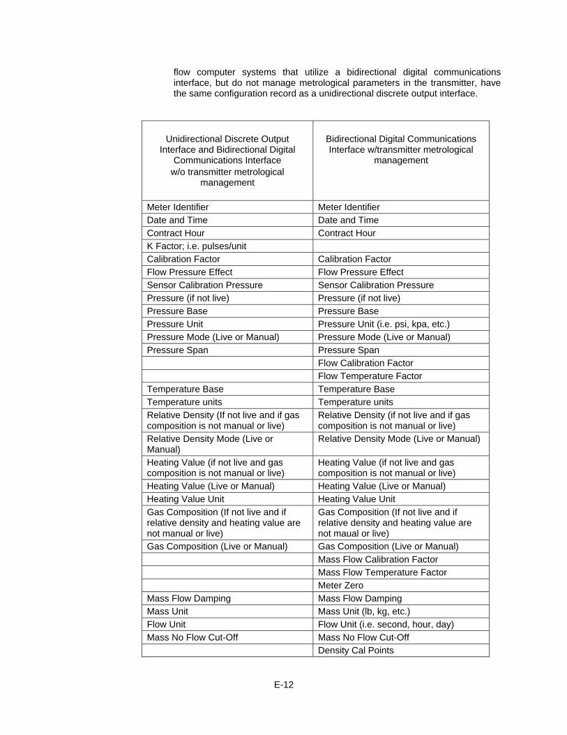
E-12

flow computer systems that utilize a bidirectional digital communications interface, but do not manage metrological parameters in the transmitter, have the same configuration record as a unidirectional discrete output interface.

Unidirectional Discrete Output

Interface and Bidirectional Digital Communications Interface

w/o transmitter metrological management

Bidirectional Digital Communications Interface w/transmitter metrological

management

Meter Identifier Meter Identifier

Date and Time Date and Time

Contract Hour Contract Hour

K Factor; i.e. pulses/unit

Calibration Factor Calibration Factor

Flow Pressure Effect Flow Pressure Effect

Sensor Calibration Pressure Sensor Calibration Pressure

Pressure (if not live) Pressure (if not live)

Pressure Base Pressure Base

Pressure Unit Pressure Unit (i.e. psi, kpa, etc.)

Pressure Mode (Live or Manual) Pressure Mode (Live or Manual)

Pressure Span Pressure Span

Flow Calibration Factor

Flow Temperature Factor

Temperature Base Temperature Base

Temperature units Temperature units

Relative Density (If not live and if gas composition is not manual or live)

Relative Density (if not live and if gas composition is not manual or live)

Relative Density Mode (Live or Manual)

Relative Density Mode (Live or Manual)

Heating Value (if not live and gas composition is not manual or live)

Heating Value (if not live and gas composition is not manual or live)

Heating Value (Live or Manual) Heating Value (Live or Manual)

Heating Value Unit Heating Value Unit

Gas Composition (If not live and if relative density and heating value are not manual or live)

Gas Composition (If not live and if relative density and heating value are not maual or live)

Gas Composition (Live or Manual) Gas Composition (Live or Manual)

Mass Flow Calibration Factor

Mass Flow Temperature Factor

Meter Zero

Mass Flow Damping Mass Flow Damping

Mass Unit Mass Unit (lb, kg, etc.)

Flow Unit Flow Unit (i.e. second, hour, day)

Mass No Flow Cut-Off Mass No Flow Cut-Off

Density Cal Points

E-13

Tube Periods at Density Calibration Pts

Flowing Density Temp Coefficient

Flowing Density Flow Effect

Density Unit Density Units

Flowing Density High Slug Flow Limit for Mass Flow

Flowing Density Low Slug Flow Limit for Mass Flow

Temperature Calibration Intercept

Temperature Calibration Slope

Temperature Unit Temperature Unit

Volume Unit Volume Unit (ft3, m3)

Table E.2

Configuration Record Requirements             E.4.7.2    Event Record / Log 

Modifications to configuration variables will be logged with Date, Time, Event, Old Value, and New Value. Variables –other than those outlined in Table E.3 should be logged in the event log as follows.

Unidirectional Discrete output

Interface and Bidirectional Digital Communications Interface

w/o Transmitter Metrological Management

Bidirectional Digital Communications Interface

w/Transmitter Metrological Management

Pressure Calibration Values (where applicable)

Pressure Calibration Values (where applicable)

Relative Density Calibration Values (where applicable)

Relative Density Calibration Values (where applicable)

Coriolis Sensor/Transmitter Fault(s) – where applicable

Coriolis Sensor/Transmitter Fault(s)- where applicable

Table E.3

Additional Event Log Requirements

E.4.7.3    Data Record At a minimum, the following parameters should be contained in the data record/log.

Date Time Flow time

Counts1 or Flow Weighted FactorFactor KC Compensated Mass Flow weighted pressure

E-14

Volume at Base Conditions Energy

Note 1: “Counts” are the pulses accumulated by the flow computer frequency input and in actuality, a fractional representation of the mass units accumulated by the Coriolis transmitter; i.e., unitpulseKFactor / . When a flow rate is used to integrate mass

accumulation or a bidirectional communications interface is utilized by the flow computer, “Counts” are no longer equivalent to pulse accumulation, but rather the actual raw mass units accumulated in the transmitter or flow computer.

E.5   ALTERNATIVE METHOD  

  E.5.1   Alternative method for Computing Flow and the Recording of Measurement Data using a Constant Gravity or Base Density  

In applications where gas composition does not vary (e.g. pure gases) or an average composition is used to compute base volume, it is possible to configure the Coriolis transmitter to output base volume directly. The method for facilitating output of base volume by the transmitter is gained though examination of Equation (E.10), shown below for reference.

By applying a mass flow conversion factor equal to the inverse of base density (i.e.

b1 ) and compensating for flow pressure effect ( PF ) in the transmitter, the volume flow

at base conditions ( bQ ) can be output directly from the transmitter. Utilizing this method,

a base volume flow rate can then be input into a standard AGA7 flow computer, if accumulation and record of flow measurement data is desired.

It is important to note that when an AGA7 flow computer is utilized to accumulate and record base volume flow from a Coriolis transmitter, the conditions of flowing volume

( fQ ) required for input into the AGA7 computer are the same conditions as base volume

( bQ ). As an example, the AGA7 equation is such that.

f

b

f

b

b

ffb Z

Z

T

T

P

PQQ

Where: bQ = Volume flow rate of gas at base conditions

fQ = Volume flow rate of gas at flowing conditions

fP = Flow static pressure of the gas (psia)

bP = Base pressure (psia)

bT = Base temperature (Rankin)

fT = Flowing temperature of the gas (Rankin)

fZ = Compressibility factor of the gas at flowing conditions

bZ = Compressibility factor of the gas at base conditions

If the base density used for the mass conversion factor in the Coriolis transmitter was determined at 14.73 psia and 60 ºF, the volume output by the transmitter will also be at

E-15

base conditions of 14.73 psia and 60 degrees Fahrenheit. Therefore, the AGA7 equation effectively becomes.

)(

)(

)67.519(

)67.519(

)73.14(

)73.14(

X

XQQ fb or )1)(1)(1(fb QQ

When applying these methods, flowing pressure ( fP ) and flowing temperature ( fT ) in

the AGA7 flow computer are not live, but rather fixed values relative to base conditions.

The volume of flow at base conditions ( bQ ) calculated by the AGA 7 flow computer is

then identical in quantity to the volume of flow input into the flow computer ( fQ ).

When utilizing this method, compensation for flow pressure effect will need to be performed by the Coriolis transmitter through use of a live pressure input to the transmitter or entry of an average flowing pressure. If a live flowing pressure is used for compensation, it is recommended that the flow computer monitor and record an average flowing pressure in its measurement log for each log interval. The average flowing pressure log should be flow-weighted, especially when large pressure variations exist, to eliminate recalculation uncertainties caused by the use of time-weighted averages. A manual or electronic record of the following variables in the transmitter shall also be maintained by the user.

E.5.2   Data Record 

At a minimum, the following parameters should be contained in a manual audit log for the Coriolis transmitter.

Coriolis Sensor Calibration Pressure Flow Pressure Effect Average Pressure (if fixed)

Mass Flow Conversion Factor (i.e. b1 ) and the basis for its value (i.e.

relative density, base temperature, and base pressure)

Other than the requirement for logging of flowing pressure by the flow computer, when live flow pressure effect compensation is performed, the contents of the AGA 7 data log will remain unchanged.

E.6   RECALCULATION METHODS 

The use of an average base density ()(Gasb ) or relative density ( )(GasrG ), by users, to calculate

approximate base volume quantities is a common practice in gas measurement. In many cases, these volumes are recalculated at a later date by means of more accurate gas quality information acquired from an on-line gas analyzer, gravitometer, or analysis of a sample cylinder.

Fundamental to the relationship expressed in Equation (E.10), a ratio of base or relative densities

is used to perform a simple and accurate recalculation of volume quantities. In practice, these recalculation methods are such that,

)(

)(

)()(

New

Old

OldNew

r

r

GrGr G

GSCFSCF Eq. (E.18)

Where: )( NewGrSCF = Recalculated base or standard volume at

)(NewrG

E-16

)(OldGrSCF = Base or standard volume at

)( OldrG

)( OldrG = The average relative density at which )(OldGrSCF was determined

)(NewrG = The average relative density at which

)( NewGrSCF is to be

determined and

)(

)(

)()(

Newb

Oldb

OldbNewbSCFSCF

Eq. (E.19)

Where: )( Newb

SCF = Recalculated base or standard volume at )(Newb

)(Oldb

SCF = Base or standard volume at )(Oldb

)(Oldb = The average base density at which )(Oldb

SCF was determined

)(Newb = The average base density at which )( Newb

SCF is to be determined

F-1

APPENDIX F 

Coriolis Meter Sizing Equations 

(Informative) 

F.1   GENERAL  The content contained in this appendix is provided to aid the designer in performing sizing

calculations. Typically the Coriolis manufacturer will provide the designer with the flow meter sizing data required specific to their meter. The accuracies shown in the performance examples are provided for illustrative purposes only. The accuracy specification of a Coriolis meter varies by design. The appropriate accuracy specification for a particular design must be utilized when applying the calculations provided. All calculations are based on the physical properties of AGA8 “Gulf Coast” gas composition. Base conditions are at 14.73 psia and 60 ºF..

F.2   SIZING EXAMPLE  For a particular application the users design conditions are: Qmax = 400,000 scf/hr Qmin = 40,000 scf/hr Max Pressure Drop = 400 inches H2O Pmax = 1,000 psia Pmin = 200 psia

The Coriolis meter sizes of interest for the application are 2 inches and 3 inches. Performance examples of 2 inch and 3 inch meters at line pressures of 1000, 500 and 200 psia with AGA 8 Gulf Coast gas composition flow rates up to 500 Mcf/hrare shown in figures F.1, F.2, and F.3.

Figure F.1 Example Flow Rate vs. Meter Error and Pressure Drop of AGA8

Gulf Coast Gas Compositionat 1000 psia and 60 F

F-2

Figure F.2

Example Flow Rate vs. Meter Error and Pressure Loss of AGA8 Gulf Coast Gas Composition at 500 psia and 60 F.

Figure F.3

Example Flow Rate vs. Meter Error and Pressure Loss of AGA8 Gulf Coast Gas Composition at 200 psia and 60 F.

F-3

Table F.1 summarizes meter sizing information found in Figures F.1, F.2, and F.3. Trade-offs in pressure drop, measurement error, and turndown are summarized. At a pressure of 200 psia the maximum flow rate through a 2–inch diameter meter is restricted to 252 Mcf/hr due to the pressure drop restriction of 400 inches of water column (in. WC). This results in a 2-inch meter that is unusable for the particular application.

Line Pressure

(psia)

Meter Nominal Diameter

Flow rate

(scfh)

Pressure Drop

(in. WC)

Meter Error (%)

Turn- Down Ratio

1000 2” 400,000 179.0 +/- 0.35 %

10:1 40,000 1.8 +/- 0.35 %

1000 3” 400,000 16.2 +/- 0.35 %

10:1 40,000 0.2 +/- 0.84 %

500 2” 400,000 385.8 +/- 0.35 %

10:1 40,000 3.9 +/- 0.35 %

500 3” 400,000 35.0 +/- 0.35 %

10:1 40,000 0.4 +/- 0.84 %

200 2” 252,000 400.0 +/- 0.35 %

6:1 40,000 10.1 +/- 0.35 %

200 3” 400,000 91.5 +/- 0.35 %

10:1 40,000 0.9 +/- 0.84 %

Table F.1

Meter Sizing Examples

NOTE: In the above example the 3-inch meter would be the suitable choice; however if a higher pressure drop is acceptable the 2-inch meter could be chosen to provide better accuracy

at the low end.

F.3   CALCULATION OF FLOW RATE BASED ON PRESSURE DROP A Coriolis manufacturer will typically supply a set of reference flow conditions for the various sizes of meters they offer. In the example shown in Table F.2 the reference data is based on a pressure drop (

AppGasP ) of 50 psi and density flowing (fGasfRe

) of 5.5276 lb/cf.

Table F.2

Reference Flow Rates for Multiple Coriolis Meter Sizes

Coriolis Size

(inches) Volume Flowing (

fGasfQRe

) in cf/hr Mass Rate (lb/hr)

1/4 328 1,815 1/2 841 4,647 1 3,730 20,618 2 11,252 62,197 3 37,370 206,567 4 94,587 522,840 6 175,036 967,530 8 306,277 1,692,978

F-4

Utilizing this information, the equation for calculating the flow of an application gas through a Coriolis meter at any given pressure drop is such that,

AppGas

AppGas

AppGasfGas

AppGas

fGas

bb

ffffGas

fAppGas

Q

QP

P

Re

Re

Re Eq. (F.1)

Where:

AppGasP = Differential pressure across Coriolis meter with

application gas flowing at AppGasf in psi

fGasfRe = Density of reference gas at flowing conditions in lb/cf

fGasPRe = Differential pressure across Coriolis meter with reference

gas at fGasfRe

in psi

AppGasf = Density of application gas at flowing conditions in lb/cf

fGasfQ

Re = Volume flow rate of reference gas at flowing conditions

of fGasfRe

and fGasPRe in scfh

AppGasb = Density of application gas at base conditions in lb/cf

AppGasbQ = Volume flow rate of application gas at base conditions in

scfh

Applying Equation F.1 and the information in Table F.2; if the designer wanted to know the base volume flow rate of AGA8 “Gulf Coast” gas composition, with a flowing density (

AppGasf ) of

0.6205 lb/cf at 200 psia and 60 ºF and a base density (AppGasb ) of 0.0445 lb/cf at base conditions

of 14.73 psia and 60 60 ºF , through a 3 inch Coriolis meter with a pressure drop of 3.3 psi (91.5 inches H2O), the calculation would be as follows.

AppGas

AppGas

AppGasfGas

AppGas

fGas

bb

ffffGas

fAppGas

Q

QP

P

Re

Re

Re

AppGasbQ

0445.0

6205.0*373706205.0*50

5276.5*3.3

AppGasbQ0445.0

6205.0*373707668.0

AppGasbQ553,399 = 399,553 scfh

F-5

F.4  CALCULATION OF PRESSURE DROP BASED ON FLOW RATE  The equation for calculating the pressure drop of an application gas through a Coriolis meter at any given flow rate is such that.

AppGasf

fGasf

ff

bbP

P

Q

Q

fGas

AppGass

AppGasfGas

AppGasAppGas

ReRe

Re

2*

Eq. (F.2)

Applying Equation F.2, the information in Table F.2, and using AGA 8 “Gulf Coast” gas composition as the application gas; if the designer wanted to know the pressure drop across the meter at 400,000 scf/hr with a flowing density (

AppGasf ) of 0.6205 lb/cf and a base density

(AppGasb ) of 0.0445, the solution for pressure drop would be as follows.

AppGasf

fGasf

ff

bbP

P

Q

Q

fGas

AppGass

AppGasfGas

AppGasAppGas

ReRe

Re

2*

AppGasP

5276.5

50*6205.0

6205.0*37370

0445.0*000,4002

AppGasP3.3 = 3.3 psi

F.5  CALCULATION OF ACCURACY AT FLOW RATE 

The accuracy of a Coriolis meter can be determined at any flow rate utilizing the manufacturers published accuracy statement and zero stability data. It should be noted that the accuracy statement varies from manufacturer to manufacturer. An example of an accuracy statement and zero stability values for Coriolis meters are shown in Table F.3.

Table F.3

Zero Stability Values for Multiple Coriolis Meter Sizes

Note 1: Accuracy equals +/- 0.35% of rate, except when flow rate is less than 100/

/

Accuracy

ityZeroStabil b , where

accuracy then equals

100

/

vb

b

Q

ityZeroStabil % of rate.

Coriolis Size (inches)

Accuracy1

(%) Zero Stability (lb/hr)

1/4 0.35 0.0600 1/2 0.35 0.3600 1 0.35 1.5000 2 0.35 4.8000 3 0.35 15.0000 4 0.35 90.0000 6 0.35 150.000 8 0.35 300.000

F-6

Utilizing the information specific to a 3 inch meter and AGA 8 “Gulf Coast” natural gas composition at base conditions of 14.73 psia and 60 60 ºF ; if the designer wanted to find the

transition flow rate ( tQ ) where the accuracy of the meter changes from +/- 0.35%, the calculation

would be as follows.

100/

/

Accuracy

ityZeroStabilQ

b

t

100/35.0

0445.0/15tQ

308,96tQ

scfh

Thus, all flow rates above the transition flow rate of 96,308 scf/hr would have an accuracy of +/- 0.35% and all of those below would have an accuracy of

%100/

b

b

Q

ityZeroStabil .

For example, if the minimum flow rate for the application was 40,000 scf/hr, the accuracy at that flow rate would be.

Accuracy =

100

/

b

b

Q

ityZeroStabil

Accuracy =

100

40000

0445.0/15

Accuracy = %84.0 F.6  CALCULATION OF VELOCITY AT FLOW RATE  Some manufacturers will specify a maximum flow velocity through their Coriolis meter relative to the

speed of sound (Mach). Knowing the density of a reference gas, the velocity at which it is flowing and the pressure drop it produces across the meter, the designer can calculate the velocity through the sensor for any application gas mixture at any set of flowing conditions such that,

fGas

AppGas

AppGas

fAppGas

ffGas

fGasf

f

P

P

vv

Re

Re

Re

Eq. (F.3)

Where: AppGasfv = Velocity flowing of application gas at AppGasf and

AppGasP

in ft/sec

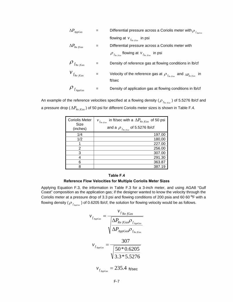
F-7

AppGasP = Differential pressure across a Coriolis meter withAppGasf

flowing at fGasfv

Re in psi

fGasPRe = Differential pressure across a Coriolis meter with

fGasfRe flowing at

fGasfvRe

in psi

fGasfRe = Density of reference gas at flowing conditions in lb/cf

fGasfvRe = Velocity of the reference gas at

fGasf Re and

fGasPRe in

ft/sec

AppGasf = Density of application gas at flowing conditions in lb/cf

An example of the reference velocities specified at a flowing density (

fGasfRe ) of 5.5276 lb/cf and

a pressure drop ( fGasPRe ) of 50 psi for different Coriolis meter sizes is shown in Table F.4.

Table F.4

Reference Flow Velocities for Multiple Coriolis Meter Sizes

Applying Equation F.3, the information in Table F.3 for a 3-inch meter, and using AGA8 “Gulf Coast” composition as the application gas; if the designer wanted to know the velocity through the Coriolis meter at a pressure drop of 3.3 psi and flowing conditions of 200 psia and 60 60 ºF with a

flowing density (AppGasf ) of 0.6205 lb/cf, the solution for flowing velocity would be as follows.

fGas

AppGas

AppGas

fAppGas

ffGas

fGasf

f

P

P

vv

Re

Re

Re

5276.5*3.3

6205.0*50

307

AppGasfv

4.235AppGasfv ft/sec

Coriolis Meter Size

(inches)

fGasfvRe

in ft/sec with a fGasPRe of 50 psi

and a fGasfRe

of 5.5276 lb/cf

1/4 197.00 1/2 180,00 1 227.00 2 256.00 3 307.00 4 291.30 6 363.87 8 387.19

F-8

G-1

APPENDIX G 

Notes of Interest 

(Informative) 

When corrosive elements (H2O, H2S, etc.) exist in the flow stream, an oxide layer can form on the inside walls of carbon steel piping. When this condition exists, if the carbon steel piping is also subjected to high flow velocities, erosion of the oxide layer will occur. The combination of these condition based influences is the origin of operational moisture and velocity limits imposed on carbon steel piping design. Due to materials of construction (stainless steel, Hastelloys, etc.) some Coriolis designs are highly immune to corrosion caused by corrosive elements in the flow stream and the subsequent erosion that can occur when also subjected to high gas flow velocities. The designer should perform an evaluation of the piping design and materials of construction to address any corrosion and erosion concerns that may exist. (See Section 8.2.1 – “Piping Configuration for further information”)

G-2

H-1

Form to Propose Changes  

Send to: Operations and Engineering Section American Gas Association 400 North Capitol Street, NW, 4th Floor Washington, DC 20001, U.S.A. Fax: (202) 824-7082 Name________________________________________________________________________

Company_____________________________________________________________________

Address______________________________________________________________________

Tel. No. ___________________________ Fax No. ____________________________________ Please Indicate Organization Represented (if any) ____________________________________

1. Section/Paragraph____________________________________________________________ 2. Proposal Recommends: (check one) new text revised text deleted text 3. Proposal (include proposed new or revised wording, or identification of wording to be deleted, use separate sheet if needed): (Proposed text should be in legislative format; i.e., use underscore to denote wording to be inserted (inserted wording) and strike-through to denote wording to be deleted (deleted wording).

4. Statement of Problem and Substantiation for Proposal (use separate sheet if needed): (State the problem that will be resolved by your recommendation; give the specific reason for your proposal including copies of tests, research papers, etc.)

5. This proposal is original material. (Note: Original material is considered to be the submitter’s own idea based on or as a result of his/her own experience, thought or research and, to the best of his/her knowledge, is not copied from another source.)

This proposal is not original material; its source (if known) is as follows: ______________________________________________________________________________ Type or print legibly. If supplementary material (photographs, diagrams, reports, etc.) is included, you may be required to submit sufficient copies for all members of reviewing committees or task forces. I hereby grant the American Gas Association the non-exclusive, royalty-free rights, including non-exclusive, royalty-free rights in copyright, in this proposal and I understand that I acquire no rights in any publication of the American Gas Association in which this proposal in this or another similar or analogous form is used. Date: __________________________ ___________________________________________________________________ Signature (Req

FOR OFFICE USE ONLY Log # __________________________ Date Rec’d _____________________

© 2013 American Gas Association. All rights reserved.

American Gas Association

400 N. Capitol Street, N.W., 4TH Floor

Washington, DC 20001

U.S.A.

202/824-7000

www.aga.org

Catalog No. XQ1301

February 2013