afrl-afosr-uk-tr-2019-0030 quantitative comparison of

AFRL-AFOSR-UK-TR-2019-0030

Quantitative comparison of information-rich data fields from characterisation/simulation ofmicrostructural damage in ceramic matrix composites

Eann A. PattersonTHE UNIVERSITY OF LIVERPOOL

Final Report02/19/2019

DISTRIBUTION A: Distribution approved for public release.

AF Office Of Scientific Research (AFOSR)/ IOEArlington, Virginia 22203

Air Force Research Laboratory

Air Force Materiel Command

REPORT DOCUMENTATION PAGE Form Approved

OMB No. 0704-0188 Public reporting burden for this collection of information is estimated to average 1 hour per response, including the time for reviewing instructions, searching existing data sources, gathering and maintaining the data needed, and completing and reviewing this collection of information. Send comments regarding this burden estimate or any other aspect of this collection of information, including suggestions for reducing this burden to Department of Defense, Washington Headquarters Services, Directorate for Information Operations and Reports (0704-0188), 1215 Jefferson Davis Highway, Suite 1204, Arlington, VA 22202-4302. Respondents should be aware that notwithstanding any other provision of law, no person shall be subject to any penalty for failing to comply with a collection of information if it does not display a currently valid OMB control number. PLEASE DO NOT RETURN YOUR FORM TO THE ABOVE ADDRESS.

1. REPORT DATE

19-02-2019

2. REPORT TYPE

Final

3. DATES COVERED

01 Sept 2017 – 30 Nov 2018

4. TITLE

Quantitative comparison of information-rich data fields from

characterization/simulation of microstructural damage in

ceramic matrix composites

5a. CONTRACT NUMBER

5b. GRANT NUMBER

FA9550-17-1-0272

5c. PROGRAM ELEMENT NUMBER

6. AUTHOR(S)

Amjad, Khurram

Christian, William J.R.

Dvurecenska, Ksenija

Patterson, Eann A.

5d. PROJECT NUMBER

5e. TASK NUMBER

5f. WORK UNIT NUMBER

7. PERFORMING ORGANIZATION NAME(S) AND ADDRESS(ES)

The University of Liverpool

School of Engineering

The Quadrangle

Brownlow Hill

Liverpool

L693GH UK

8. PERFORMING ORGANIZATION REPORTNUMBER

9. SPONSORING / MONITORING AGENCY NAME(S) AND ADDRESS(ES)

USAF, AFRL DUNS 143574726

AF OFFICE OF SCIENTIFIC RESEARCH

875 NORTH RANDOLPH STREET, RM 3112

ARLINGTON VA 22203-1954

10. SPONSOR/MONITOR’S ACRONYM(S)

Garner, David AFOSR/IOE

11. SPONSOR/MONITOR’S REPORT

NUMBER(S)

12. DISTRIBUTION / AVAILABILITY STATEMENT

13. SUPPLEMENTARY NOTES

14. ABSTRACT

The research has been conducted in collaboration with Dr Craig Przybyla from the Air Force Research Laboratory (AFRL), under the supervision of Professor Eann Patterson and Miss Ksenija Dvurecenska, and has been carried out by Dr William Christian and Dr Khurram Amjad. The aim of the work was to apply the novel techniques for quantitative comparison of information-rich data fields, developed by Professor Patterson and his research group at the University of Liverpool, to the data obtained from the work by Dr Przybyla and his team on microstructure-sensitive damage characterization in continuous fiber reinforced ceramic matrix composites (CMCs). Five objectives were identified for this project by Dr Przybyla and Professor Patterson, as reported in the Introduction Chapter, to address the research questions from the AFRL’s program on damage characterization/simulation in CMCs. A novel method for the characterization of voids observed in the stack of mosaics of a CMC sample has been proposed in Chapter 2 which was developed by Christian to meet the first objective of this project. Chapter 3 describes a strain-based damage monitoring algorithm which has been developed by Christian to fulfil the second research objective. This algorithm can be used to identify the time and location of damage initiation within composite specimens during loading. The work on characterization and quantitative comparison of the fiber orientation fields, reported in Chapter 4, has been performed by Amjad to achieve the third research objective. Two methods, one based on digital image correlation and the other on two-dimensional cross correlation, have been proposed for the determination of fiber orientation fields from the stack of mosaics of a CMC sample. The proposed methods are estimated to be at least 17 times faster than the previously published rule-based method developed for the characterization of fiber orientation. The fiber tracking capability of the DIC method was further explored by Amjad and its performance was quantitatively compared with a more recent, state-of-the-art, tracking method based on a Kalman filter in Chapter 5 as part of the work on the fourth research objective. Both the methods were applied to the stack of mosaics of a continuous fiber reinforced polymer matrix composite (PMC) sample. The DIC clearly outperformed the Kalman filter method and was found to be at least 40 times faster as well. The fifth objective was about the dimensionality reduction of three-dimensional (3D) data fields by representing them as feature vectors. A significant novel step has been taken by Christian to develop an algorithm for the orthogonal decomposition of 3D data fields which is described in Chapter 6. Amjad explored the capability of this algorithm by applying it to the 3D deformation fields measured in a nylon-reinforced rubber matrix sample using the digital volume correlation (DVC) technique. By performing orthogonal decomposition, the 3D deformation fields were successfully represented as feature vectors, thereby providing the data compression ratio of at least 106:1.

Please direct any questions regarding the content of this report to Eann Patterson ([email protected])

15. SUBJECT TERMS

Ceramic matrix composites, microstructural defects, data compression, orthogonal

decomposition, image processing, digital image correlation, fiber tracking

16. SECURITY CLASSIFICATION OF: 17. LIMITATIONOF ABSTRACT

18. NUMBEROF PAGES

19a. NAME OF RESPONSIBLE PERSON

Eann A. Patterson

a. REPORT

U

b. ABSTRACT

U

c. THIS PAGE

U97 19b. TELEPHONE NUMBER (include area

code)

+44 151 794 4665

Standard Form 298 (Rev. 8-98) Prescribed by ANSI Std. Z39.18

AFRL-AFOSR-UK-TR-2019-0030

i

The University of Liverpool

Quantitative comparison of information-rich

data fields from characterization/simulation

of microstructural damage in ceramic matrix

composites

Final Report

Authors: Khurram Amjad and William Christian

Submitted February 19, 2019

Grant number: FA9550-17-1-0272

Period of Performance: 01 September 2017 to 30 November 2018

Period of Grant: 01 September 2017 to 30 November 2018

Principal Investigator: Prof Eann Patterson, University of Liverpool

Co-Principal Investigator: Miss Ksenija Dvurecenska, University of Liverpool

Collaborator: Dr Craig Przybyla, USAF AFMC AFRL/RXCC

Program Manager: Lt Col David Garner, USAF EOARD

Distribution A Approved for Public Release, Distribution Unlimited

ii

Summary

The research presented in this final report has been performed over the course of fifteen months (September 2017 – November 2018) under funding from the European Office of the United States Air Force Office of Scientific Research. The research has been conducted in collaboration with Dr Craig Przybyla from the Air Force Research Laboratory (AFRL), under the supervision of Professor Eann Patterson and Miss Ksenija Dvurecenska, and has been carried out by Dr William Christian and Dr Khurram Amjad.

The aim of the work was to apply the novel techniques for quantitative comparison of information-rich data fields, developed by Professor Patterson and his research group at the University of Liverpool, to the data obtained from the work by Dr Przybyla and his team on microstructure-sensitive damage characterization in continuous fiber reinforced ceramic matrix composites (CMCs). Five objectives were identified for this project by Dr Przybyla and Professor Patterson, as reported in the Introduction Chapter, to address the research questions from the AFRL’s program on damage characterization/simulation in CMCs.

A novel method for the characterization of voids observed in the stack of mosaics of a CMC sample has been proposed in Chapter 2 which was developed by Christian to meet the first objective of this project. Chapter 3 describes a strain-based damage monitoring algorithm which has been developed by Christian to fulfil the second research objective. This algorithm can be used to identify the time and location of damage initiation within composite specimens during loading. The work on characterization and quantitative comparison of the fiber orientation fields, reported in Chapter 4, has been performed by Amjad to achieve the third research objective. Two methods, one based on digital image correlation and the other on two-dimensional cross correlation, have been proposed for the determination of fiber orientation fields from the stack of mosaics of a CMC sample. The proposed methods are estimated to be at least 17 times faster than the previously published rule-based method developed for the characterization of fiber orientation. The fiber tracking capability of the DIC method was further explored by Amjad and its performance was quantitatively compared with a more recent, state-of-the-art, tracking method based on a Kalman filter in Chapter 5 as part of the work on the fourth research objective. Both the methods were applied to the stack of mosaics of a continuous fiber reinforced polymer matrix composite (PMC) sample. The DIC clearly outperformed the Kalman filter method and was found to be at least 40 times faster as well.

The fifth objective was about the dimensionality reduction of three-dimensional (3D) data fields by representing them as feature vectors. A significant novel step has been taken by Christian to develop an algorithm for the orthogonal decomposition of 3D data fields which is described in Chapter 6. Amjad explored the capability of this algorithm by applying it to the 3D deformation fields measured in a nylon-reinforced rubber matrix sample using the digital volume correlation (DVC) technique. By performing orthogonal decomposition, the 3D deformation fields were successfully represented as feature vectors, thereby providing the data compression ratio of at least 106 : 1.

Please direct any questions regarding the content of this report to Eann Patterson ([email protected])


iii

Table of Contents

List of Tables .............................................................................................................................. v

List of Figures ............................................................................................................................ vi

1 Introduction ....................................................................................................................... 1

1.1 Aim and Objectives ..................................................................................................... 2

1.2 Amendments to the research objectives .................................................................... 3

2 Machine Vision Characterization of the 3D Microstructure of Ceramic Matrix Composites ……………………………………………………………………………………………………………………………………. 4

2.1 Introduction................................................................................................................. 4

2.2 Image Processing ......................................................................................................... 5

2.2.1 Introduction ......................................................................................................... 5

2.2.2 Pre-processing...................................................................................................... 5

2.2.3 Identification of voids .......................................................................................... 7

2.2.4 Characterization of individual voids .................................................................... 8

2.2.5 Characterization of Void Distribution ................................................................ 11

2.2.6 Digital Image Correlation for Extracting Fiber orientation Data ....................... 13

2.3 Experimental Method ............................................................................................... 15

2.4 Results ....................................................................................................................... 18

2.5 Discussion .................................................................................................................. 20

2.6 Conclusions................................................................................................................ 22

3 Real-time detection and quantification of damage in continuous fiber reinforced composites ............................................................................................................................... 23

3.1 Introduction............................................................................................................... 23

3.2 Strain Based Damage Monitoring ............................................................................. 23


3.4 Results ....................................................................................................................... 27

3.5 Discussion .................................................................................................................. 28


iv

3.6 Conclusions................................................................................................................ 30

4 Characterization of fiber orientations in continuous fiber reinforced composites ........ 31

4.1 Introduction............................................................................................................... 31

4.2 Tracking of fiber cross-sections through sequence of Images .................................. 32

4.2.1 Fiber tracking using DIC ..................................................................................... 32

4.2.2 Fiber tracking using 2D cross-correlation .......................................................... 35

4.2.3 Three-dimensional Fiber Profiles ....................................................................... 35

4.3 Characterization and quantitative comparison of fiber orientation fields ............... 37

4.4 Conclusions................................................................................................................ 42

5 Computationally-efficient tracking of fibers using digital image correlation .................. 43

5.1 Introduction............................................................................................................... 43

5.2 State-of-the-art fiber tracking algorithm .................................................................. 44


5.4 Results and Discussion .............................................................................................. 52

5.5 Conclusions................................................................................................................ 61

6 Analysis of 3D data fields using orthogonal decomposition ........................................... 62

6.1 Introduction............................................................................................................... 62

6.2 Algorithm for orthogonal decomposition of volumetric data .................................. 62

6.2.1 Representation error ......................................................................................... 64

6.2.2 Computationally-efficient decomposition using matrix operations ................. 65

6.3 Orthogonal decomposition of volumetric data ........................................................ 66

6.4 Quantitative validation of finite element model ...................................................... 72

6.5 Conclusions................................................................................................................ 77

7 Discussion......................................................................................................................... 78

8 Conclusions ...................................................................................................................... 83

References ............................................................................................................................... 84


v

List of Tables

Table 2.1 Pearson dissimilarity between feature vectors for five different transformation of the same void spatial image. ................................................................................................... 13

Table 2.2 Descriptions of the features of the void shapes described by the first six coefficients used in the Chebyshev decomposition which are shown graphically in Figure 2.12. ............. 17

Table 4.1 Computation time required to acquire fiber coordinate data................................. 39

Table 5.1 Key details of the four tests performed to compare the performance of DIC against the Kalman-Groupwise method............................................................................................... 50

Table 5.2 Processing times required by DIC and Kalman-Groupwise method in tracking fiber cross-sections in the four tests. ............................................................................................... 54

Table 6.1 Data range for the measured displacement and strain fields. ................................ 67

Table 6.2 Number of coefficients in the filtered feature vectors and the corresponding compression ratios for the original data fields. ....................................................................... 68

Table 6.3 Validation metric for the prediction displacement and strain fields ....................... 77


vi

List of Figures

Figure 1.1 X-ray CT image showing voids in SiC/SiC CMC [from slide 6 in Przybyla et al17] ...... 2

Figure 1.2 Sequence of strain fields from DIC measurements in SiC/SiC coupon during fracture [from slide 25 in Przybyla et al17] ............................................................................................... 2

Figure 1.3 Estimated PDFs for fiber orientation associated with microstructural anomalies [from slide 12 in Przybyla et al17] ............................................................................................... 2

Figure 2.1 Flow chart of the data processing used to extract void shape and fiber orientation information. The boxes indicate image processes applied to the mosaics and the lozenges indicate the extraction processes used to extract void and fiber information from the mosaics..................................................................................................................................................... 5

Figure 2.2 Histogram of grey values for all of the serial section data (top) and a portion of serial section data (bottom) color coded to indicate the range of grey values within each band identified using Otsu's method. ................................................................................................. 6

Figure 2.3 The cumulative volume of the voids as a function of the number of voids selected..................................................................................................................................................... 8

Figure 2.4 A convex hull (bottom) fitted to an exemplar void (top) which corresponds to largest void visible in Figure 2.2. ................................................................................................ 9

Figure 2.5 The three orthogonal projections of a cuboid enclosing the exemplar void shown in figure 2.4, with a 3D rendering of the void at the center of the image. The x-z plane is shown top-left, y-z plane is shown top-right and x-y plane is shown at the bottom. ........................ 10

Figure 2.6 Bar charts showing the values of the Chebyshev coefficients representing the orthogonal projections shown in figure 2.5, with the: x-z plane (top), y-z plane (middle) and x-y plane (bottom). ..................................................................................................................... 10

Figure 2.7 Image created by representing the x-y projections of each void at its location in the plane of the specimen. The 2mm wide square subset that was characterized is indicated by the dashed line. ........................................................................................................................ 11

Figure 2.8 Three images of void distribution, unmodified (1st column), scaled in x-direction by 70% (2nd column) and rotated 15° (3rd column). Rows show: spatial image (top), spectral image with axes showing wavelength (middle) and bar charts of the feature vectors for each spectral image (bottom). ......................................................................................................... 12

Figure 2.9 Proportion of the facets successfully correlated by DIC between the first and last mosaic image (crosses) with a line-of-best-fit for the six largest facet sizes (dashed line). ... 14

Figure 2.10 Typical facet x-direction (top) and y-direction (bottom) displacements from DIC as

a transparent overlay on a corresponding mosaic from z=1m. Positive values indicate the fibers coming out of the page are leaning to the right and negative values indicate the fibers are leaning to the left. ............................................................................................................. 15


vii

Figure 2.11 Local fiber angles in the x-z plane at z=30m together with voids colored to indicate their sphericity calculated using equation 2.1. .......................................................... 16

Figure 2.12 The Chebyshev kernel functions, corresponding to the first six coefficient (white number in the top-left corner of each function); the corresponding interpretations of void shape are described in Table 2.2. ............................................................................................ 17

Figure 2.13 Local fiber angles in the x-z plane at z=30m (corresponding to the data in Figure 2.11) together with voids colored to indicate their orientation indicated by the value of the fifth Chebyshev coefficient (see Figure 2.12) from the decomposition of projection in the x-z plane of the density of a cuboid enclosing each void. ............................................................. 19

Figure 2.14 Similarity of voids with the reference void (shown in white) superimposed on fiber angle data from Figure 2.11. The top inset shows the projection onto the x-z plane for the reference void and the bottom inset shows the corresponding data for a similar void. The positions of these voids within the specimen are indicated by arrows. ................................. 19

Figure 3.1 Rate of change signal (from equation (3.1)) for a composite specimen loaded in tension showing four periods, shaded in grey, when the rate of change was above the 90th percentile for a minimum of 7.5s. . ......................................................................................... 25

Figure 3.2 The surface strain field on the coupon at a load of 4kN. The six regions are indicated by the white dashed lines. The figure is best interpreted in color. ......................................... 26

Figure 3.3 The accumulated damage signal for region 3 of the specimen with damage events marked by squares. .................................................................................................................. 27

Figure 3.4 Differences between strain fields 2.5s before and after the damage events marked by squares in Figure 3.3. Spatial units are in mm. ................................................................... 28

Figure 3.5 Accumulated damage signal for regions 2 and 4 showing that damage starts to occur in region 4 approximately 30s before damage occurs in region 2. ............................... 29

Figure 4.1 Schematic representing the unreformed facet in the reference image and the deformed facet in the deformed image. The difference in the positions of the unreformed and the deformed facet centers yields the displacement vector................................................... 32

Figure 4.2 A grid of facets overlaid by Istra on a 351×312 pixel region of a mosaic using both a facet size and grid spacing of 39 pixels. ................................................................................ 33

Figure 4.3 The pair of images which represent a square region defined on a mosaic illustrate the mapping of a reference facet in the tenth mosaic when the facet is located within a fiber tow (top) and at a boundary between the two fiber tows (bottom). The fiber cross-sections highlighted with the same marker color belong to the same fiber tow. ................................ 34

Figure 4.4 Flow diagram showing the process of identifying the facets located at the fiber tow boundaries. .............................................................................................................................. 34


viii

Figure 4.5 Flow diagram of the procedure for tracking a bounding box through the sequence of images. ................................................................................................................................. 36

Figure 4.6 Plot of normalized cross-correlation peak value for the bounding box tracked through the sequence of one hundred mosaics. The inset (a) shows the bounding box defined in the first mosaic whereas the insets (b-e) show the bounding boxes which were found in mosaic no 44, 49, 91 and 100, respectively, using 2D cross-correlation. ............................... 37

Figure 4.7 3D Fiber profiles plotted using the fiber center coordinate data acquired from DIC, 2D cross-correlation and the rule-based approach of Bricker et al. ....................................... 38

Figure 4.8 The maps of fiber angles in the X-Z (left) and the Y-Z (right) planes acquired using rule-based approach (top), 2D cross-correlation (middle) and DIC (bottom). ........................ 39

Figure 4.9 The probability density functions of fiber angle maps shown in Figure 4.8. ......... 40

Figure 4.10 The images of individual peaks acquired from probability density functions shown in Figure 4.9. ............................................................................................................................ 41

Figure 4.11 Graphical comparison of the feature vectors representing the images of the PDF peaks shown in Figure 4.10...................................................................................................... 42

Figure 5.1 Mosaic of the CMC sample constructed by stitching together a grid of 6×6 optical images with each one having the dimensions of 1292×968 pixels. ........................................ 45

Figure 5.2 Process chart of the Kalman-Groupwise method for performing fiber association between the tiles in the sequence. ......................................................................................... 46

Figure 5.3 Top photograph shows the first mosaic, comprising of 7200×5500 pixels, in the CMC sample sequence. The bottom three photographs show the zoomed-in views of the three independent tiles defined in the first mosaic. The fibers were tracked in these three independent tiles by Zhou et al19. ........................................................................................... 47

Figure 5.4 A reduced resolution CMC mosaic and a close-up view of the tile (top) which was selected for fiber-tracking analysis in the first three tests. ..................................................... 48

Figure 5.5 A reduced resolution PMC mosaic and a close-up view of the tile (top) which was selected for fiber-tracking analysis in the fourth test. ............................................................ 49

Figure 5.6 The graph of accumulative thickness of the CMC sample against the serial number of the tiles in the order they are arranged in the original sequence. The three plots with black, blue and red markers represent the serial number of the tiles which were selected for fiber-tracking analysis in Tests 1, 2 and 3 respectively. ................................................................... 50

Figure 5.7 The plot of accumulative thickness of the PMC sample against the serial number of the tiles in the order they are arranged in the original sequence. The inset shows the same plot for the first thirteen tiles in the sequence which were selected for fiber-tracking analysis in Test 4. ................................................................................................................................... 51


ix

Figure 5.8 The comparison between the plots of 3D fiber profiles tracked by DIC (left) and Kalman-Groupwise method (right) in tests 1 - 3 which involved CMC sample tiles. The fibers orientated towards the left and the right-hand side in the x-z plane are represented in black and red colors, respectively. .................................................................................................... 53

Figure 5.9 The comparison between the plots of 3D fiber profiles tracked by DIC (left) and Kalman-Groupwise method (right) in test 4 which involved PMC sample tiles. The fibers orientated towards the left and the right-hand side in the x-z plane are represented in black and red colors, respectively. .................................................................................................... 53

Figure 5.10 The probability density functions for the fiber angle data acquired from DIC (left) and Kalman-Groupwise method (right) for Test 1 (top), Test 2 (middle) and Test 3 (bottom)................................................................................................................................................... 55

Figure 5.11 The plot of 3D profiles of the fibers tracked in the sequence of PMC mosaics using DIC. The fibers which are orientated nominally at +45°, -75° and +75° from the sectioning (x-y) plane are represented in red, blue and black colors, respectively. ..................................... 56

Figure 5.12 Top schematic shows the fiber profile through the depth of the PMC sample which was assumed as a curve in 3D space. Bottom schematic shows the direction vector representing the fiber segment which was used to describe the local orientation of the fiber in 3D space. .............................................................................................................................. 57

Figure 5.13 The plots of the average angle, θxy of the fibers through the depth of the sample in plies 3, 8, 13 & 18 orientated at 45º (top) plies 4, 9, 12, & 17 orientated at +75º (middle) and plies 5, 10, 11 & 16 orientated at -75º (bottom). ............................................................. 58

Figure 5.14 The plots of the average angle, θxz of the fibers through the depth of the sample in plies 3, 8, 13 & 18 orientated at 45º (top) plies 4, 9, 12, & 17 orientated at +75º (middle) and plies 5, 10, 11 & 16 orientated at -75º (bottom). ............................................................. 59

Figure 5.15 The plots of 2D profiles of the fibers which were constructed from θxy for the

small group of fibers taken from ply 3 (+45) (top), ply 12 (-75) (middle) and ply 16 (+75) (bottom). .................................................................................................................................. 60

Figure 6.1 Dimensions of reinforced rubber matrix sample .................................................... 66

Figure 6.2 The comparison between the original and reconstructed displacement fields. All the units are in mm. ................................................................................................................. 69

Figure 6.3 The comparison between the original and reconstructed longitudinal strain fields. The axes of the volume plots are in mm and the color bar shows the strain values. ............. 70

Figure 6.4 The comparison between the original and reconstructed shear strain fields. The axes of the volume plots are in mm and the color bar shows the strain values. .................... 71

Figure 6.5 The plot of data compression ratio against the assumed measurement uncertainty for the displacement field, v and the strain field, e22. ............................................................. 72


x

Figure 6.6 The graphs of coefficients of the feature vectors representing the measured and predicted displacement fields plotted against one another. The uncertainty boundaries are represented by the dashed blue lines. .................................................................................... 74

Figure 6.7 The graphs of coefficients of the feature vectors representing the measured and predicted longitudinal strain fields plotted against one another. The dashed blue lines represent the uncertainty boundaries. ................................................................................... 75

Figure 6.8 The graphs of coefficients of the feature vectors representing the measured and predicted shear strain fields plotted against one another. The dashed blue lines represent the uncertainty boundaries. ........................................................................................................... 76


1

1 Introduction

Over the last several decades, there has been an increasing interest in the development of advanced composite materials for structural applications in extreme high temperature environments. Ceramic matrix composites (CMCs) are considered as a potential replacement for the traditional nickel-based high-temperature alloys due to their high strength-to-weight ratio, good chemical stability and capability of withstanding temperatures in excess of 1500°C1. CMCs, however, typically exhibit low fracture toughness due to their inherent brittleness. This issue has been partially resolved by the development of new ceramic composites in the form of a silicon-carbide (SiC) or silicon-nitro-carbide (SiNC) matrix reinforced by continuous bundles of silicon carbide fibers (SiCf)2. The enhanced mechanical properties are achieved in these CMCs through the complexity in their tailored microstructure. The continuous fiber bundles in such CMCs can be woven, and therefore, interlocked to avoid catastrophic failure. The coating between the individual fibers inhibits chemical reactions and provides a weak interface to increase the overall fracture toughness of the material by allowing fatigue crack deflection through matrix cracking and frictional pull out of the fibers3.

The damage mechanisms in CMCs are highly sensitive to the defects in their microstructures which are introduced during the processing stage4. It is therefore imperative to identify and characterize these defects and link them to the CMC processing techniques which, in turn, should lead to the production of stronger and more consistent microstructures for next generation CMCs. Microscopy is one of the most common tools used for analyzing microstructures; however, it can only be used on two-dimensional (2D) cross-sections. Owing to the advancements in automation and control as well as the development of high resolution digital sensors, the serial sectioning technique, which is an extension of the conventional optical microscopy on a polished specimen surface, has emerged over the last few decades as a well-established destructive technique for generating images of the three-dimensional (3D) microstructure in a wide variety of materials5, 6. The availability of high intensity X-ray beams from synchrotron radiation sources has made X-ray computed tomography (CT) a powerful technique to reconstruct 3D microstructure, non-destructively, in composites7. Computed tomography has also been used in conjunction with digital volume correlation algorithm to determine the internal deformation in composite materials8, 9. These image-based characterization techniques generate large volumes of information-rich data fields which are difficult to process and interpret.

Recent work by Patterson and his co-workers10, 11 has overcome the difficulty of processing and comparing large data fields containing at least 104 values by treating the data fields as images and decomposing them using approaches developed for applications such as iris recognition and target acquisition. Essentially, a set of orthogonal polynomials are used to describe the image and the coefficients of the polynomials form a feature vector that provides a unique and accurate representation of the original data but using less than hundred coefficients instead > 104 data values. These developments have led to new approaches to the quantitative validation of computational mechanics models using strain fields in structures12-14, the comparison of modal behavior at room and elevated temperatures15 (under EOARD grant no: FA8655-11-1-3083) and a new strain-based methodology for


2

quantifying the development of damage in glass-fiber reinforced composites16. The motivation for the current work was to extend these applications to the microstructural scale by applying the developments to data obtained during the characterization and simulation of microstructure-sensitive damage in CMCs.

1.1 Aim and Objectives

The aim of the current work is to apply the novel techniques developed by Professor Patterson and his research group at the University of Liverpool to perform analysis on the data obtained from the work by Dr Craig Przybyla and his team on Microstructure-sensitive Damage Characterization/Simulation in Continuous Fiber Reinforced Ceramic Composites17, which forms part of the program on Theory and Modelling of Materials in Extreme Environments. The following five research objectives were identified from the ensuring discussions between Professor Patterson and Dr Przybyla to address the research questions from the program on damage characterization/simulation in CMCs:

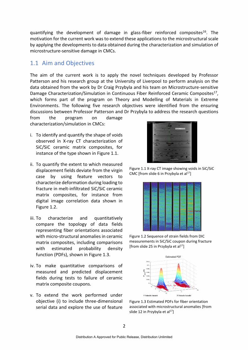
i. To identify and quantify the shape of voids observed in X-ray CT characterization of SiC/SiC ceramic matrix composites, for instance of the type shown in Figure 1.1.

ii. To quantify the extent to which measured displacement fields deviate from the virgin case by using feature vectors to characterize deformation during loading to fracture in melt-infiltrated SiC/SiC ceramic matrix composites, for instance from digital image correlation data shown in Figure 1.2.

iii. To characterize and quantitatively compare the topology of data fields representing fiber orientations associated with micro-structural anomalies in ceramic matrix composites, including comparisons with estimated probability density function (PDFs), shown in Figure 1.3.

iv. To make quantitative comparisons of measured and predicted displacement fields during tests to failure of ceramic matrix composite coupons.

v. To extend the work performed under objective (i) to include three-dimensional serial data and explore the use of feature

Figure 1.1 X-ray CT image showing voids in SiC/SiC CMC [from slide 6 in Przybyla et al17]

Figure 1.2 Sequence of strain fields from DIC measurements in SiC/SiC coupon during fracture [from slide 25 in Przybyla et al17]

Figure 1.3 Estimated PDFs for fiber orientation associated with microstructural anomalies [from slide 12 in Przybyla et al17]


3

vectors to describe porosity and fiber geometry.

1.2 Amendments to the research objectives

The work on the fourth research objective was scheduled to be started at the beginning of September 2018. The finite element model which was required to perform work on this objective could not be made available by the AFRL. Hence, it was agreed between Prof. Patterson and Dr. Przybyla to utilize the allotted time from the fourth research objective to continue the work on characterization of fiber orientations using digital image correlation (DIC), which was performed as part of the third objective. The new task was, therefore, to further explore the fiber tracking capability of DIC by comparing its performance with a more recent, state-of-the-art, fiber-tracking algorithm.


4

2 Machine Vision Characterization of the 3D Microstructure of Ceramic Matrix Composites

2.1 Introduction

This chapter is derived from the paper which has been recently accepted for publication in the Journal of Composite Materials18. It reports the work performed to achieve objective (i) of this project which was about developing a methodology for identification and characterization of voids observed in either the X-ray CT or the optical images of ceramic matrix composites. It also briefly discusses the work on extraction of fiber orientation fields, which was carried out as part of objective (iii), for the purpose of qualitatively examining the relation between the void shapes and the fiber orientation. A detailed discussion on the extraction of fiber orientation field can be found in Chapter 4.

Image-based materials characterization techniques produce large quantities of data. These datasets rapidly become time-consuming to process and interpret; hence, automated analysis of microstructure is desirable. Techniques have been developed to reduce volumetric datasets of composite microstructure to fiber orientation fields by determining the paths of individual fibers using Kalman filters19. Whilst this reduces the dimensionality of the data, it still creates large amounts of redundant information, as the fibers within bundles will typically have similar orientations. One approach to further reducing the redundancy in microstructure data has been to measure aspects of the microstructure visible in the data, e.g. fiber cross-sectional area, fiber coating thickness or fiber spacing, and then use principal component analysis to identify an orthogonal set of linear combinations of the measurements, these linear combinations are referred to as principal components. It has been found that a much smaller number of principal components are required to represent the microstructure of a CMC than the number of measurements that were originally acquired4. However, this approach requires a set of suitable measurements which can often be difficult to obtain. Void shape is one example of a microstructural feature that is difficult to describe using data from images.

In this chapter, a process is proposed to extract microstructural information relating to fiber orientation and void shape from optical micrographs of serial sections. Orthogonal decomposition20 has been used to dimensionally reduce the extracted void shape data and characterize the shapes. Fiber architecture is important for fracture toughness and voids are of interest because they provide routes through the material along which oxygen and water vapor can diffuse and oxidase fiber coatings when the CMC is loaded at high temperature21. The process has been applied to a SiCf/SiNC composite specimen manufactured by the precursor infiltration and pyrolysis technique. The serial-section images were captured by AFRL and processed at the University of Liverpool.


5

2.2 Image Processing

2.2.1 Introduction

A new approach is described for extracting information about void shape and fiber orientation from serial-section optical micrographs of a fiber-reinforced composite. The approach has been applied a 3.6 x 2.6 x 0.1 mm volume of a SiCf/SiNC specimen. The manufacture of this specimen and microscopy are described in section 3. In brief, one hundred micrographs were obtained at increments of 1 µm. Each section micrograph consisted of a 7200 x 5500 pixels mosaic constructed from a set of images that were stitched together. This form of data is typical of that produced in modern optical characterization of microstructures in composite materials and the quantity of data, approximately 3GB in this case, presents some challenges. Before information about the fiber orientation and void shape could be extracted, image processing was used to pre-process the mosaic micrographs. Figure 2.1 shows a flow-chart illustrating the image processes that were applied, shown as boxes, prior to void shape and fiber orientation information being extracted, shown as lozenges.

Figure 2.1 Flow chart of the data processing used to extract void shape and fiber orientation information. The boxes indicate image processes applied to the mosaics and the lozenges indicate the extraction processes used to extract void and fiber information from the mosaics.

2.2.2 Pre-processing

The first step in the pre-processing was to align the mosaic micrographs to correct for the specimen moving small distances as it was serially sectioned. Whilst this motion was small, of the order of 10µm, it caused the surface of voids to appear jagged with occasional discontinuities when viewed in the direction perpendicular to the sectioning. As the SiC fibers had a typical diameter of 14µm and the thickness of each section was 1µm, the position of the cut fiber cross-sections remained similar between sections, such that two sequential


6

mosaics appear almost identical except for a global translation in the plane of the section. Since equal numbers of fibers were orientated in two directions orthogonal to the section, the fiber-faces could be used to identify the translation of the mosaic without introducing any bias. These translations were determined using a two-dimensional cross-correlation to compare each mosaic with the previous mosaic. The cross-correlation between two similar but translated mosaics results in a correlation plot with a single peak close to its center. When the two mosaics are perfectly aligned the peak is exactly at the center of the correlation plot; however, if one mosaic is translated relative to the other, then the peak will be off-center and its location relative to the center defines the translation required to align the mosaics. The mosaic obtained from the first section was used to define the origin for the coordinate system and each subsequent section was then aligned with the previous section. Once all the mosaics were aligned, the orientation of individual fibers could be determined using digital image correlation (DIC), which is described in Section 2.2.6.

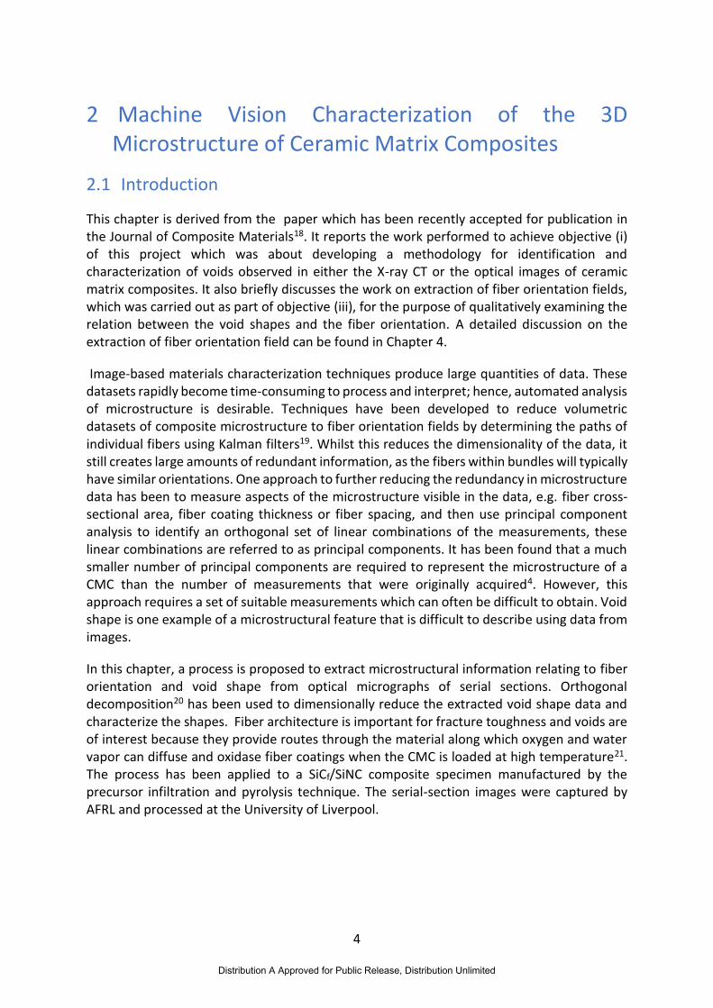
Figure 2.2 Histogram of grey values for all of the serial section data (top) and a portion of serial section data (bottom) color coded to indicate the range of grey values within each band identified using Otsu's method.

To extract information about the void shape, the mosaics required further processing so that material-free locations could be identified. This was performed using thresholding to identify fibers, matrix and voids which were distinguishable within the mosaics using the grey-level or intensity value of the pixels. The fiber cross-sections were highly reflective resulting in a high intensity value, the ceramic matrix had a lower reflectivity and thus a lower intensity value, and the voids either had an intensity value of zero because they absorbed the light or a very


7

low grey value if the voids had filled with specimen mounting material. Otsu’s method22 was used to determine the thresholds to separate these three features based on the measured intensities. This method uses statistical moments applied to the grey-value histogram to identify the ideal position for the thresholds. The position of the two thresholds on the histogram are shown at the top of Figure 2.2, with the effect of these thresholds on an exemplar volume shown at the bottom of the figure. Whilst it is important for the Otsu algorithm to split the histogram into three sections, the position of the threshold between the pixel values for the matrix and the fibers was not used in extracting the void shapes. Hence, once the thresholds had been established, the mosaics were converted to binary data where the value of pixels with a grey-level value below the lowest threshold was set to one and the remainder to zero.

2.2.3 Identification of voids

The voids were identifiable in the binarized mosaics; however, some other pixels that were not part of a void were also set to a value of one. These pixels were typically around the perimeter of each fiber cross-section, appearing as dark rings in the mosaics, and probably were caused by the coating applied to the fibers in order to modify the fracture behavior of the material19. Since the fibers were densely packed, the rings of perimeter pixels overlapped and also connected with the voids; hence, they needed to be removed in order to isolate the voids. This was achieved using an image processing technique known as morphological opening23. Morphological opening is a combination of erosion and dilation, which are two common image processing techniques, applied using the Matlab function, “imopen”. First, the data was eroded using a spherical structuring element to create a new dataset that did not contain the fiber coating. The spherical structuring element is a sphere which is placed at every location in the stack of mosaics. At each location, the pixels contained within the sphere are examined, if any of the contained pixels have a value of zero then the pixel at the center of the sphere is set to zero. The diameter of the sphere controls the size of features that are removed; for this study the diameter was 3.6µm which is approximately 150% of the fiber coating thickness. After erosion the voids were nominally the same shape as in the original binarized mosaic but their size had been reduced or eroded. This was corrected by performing dilation on each eroded mosaic. During dilation the same spherical structuring element was used. The sphere was placed at each location in the eroded mosaic and the contained pixels were assessed, if any of the pixels had a value of one then the value of the pixel at the center of the sphere was set to one. The effect of this operation was that the voids which had previously been eroded are returned to their original size whilst the fiber-coating did not reappear.

After morphological opening, the binarized mosaic contained unconnected contiguous regions or clusters of pixels with a value of one. Some of these clusters were too small to be voids and were likely noise or locations at which the fiber coating was particularly thick. To remove these small clusters, all of the clusters were placed in a list ordered by their volume from largest to smallest. The clusters on the list were progressively selected, starting with the largest, until the cumulative volume of the selected clusters was above a threshold, which was 95% of the total cluster volume. This meant that despite locating 8000 clusters initially, only 41 clusters were found to be of sufficient size to be classified as a void. The graph in Figure 2.3 shows the increase in the cumulative volume as the largest clusters of pixels are


8

selected as voids. Once the set of voids had been identified the dimensionality of the pixel data describing their shape was reduced and this is described in Section 2.2.4.

Figure 2.3 The cumulative volume of the voids as a function of the number of voids selected.

2.2.4 Characterization of individual voids

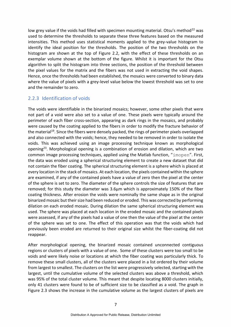
The process described in the previous sub-section allowed the pixels corresponding to the voids in the microstructure to be identified. However, the number of pixels in each void was large which made it difficult to characterize them efficiently. For example, the single void shown at the top of Figure 4.2 consists of 14.4 million pixels. Hence, the dimensionality of the description of the voids was reduced to aid their characterization. Initially, this was achieved by fitting a multi-faceted-shape, known as a convex hull, to enclose all of the pixels identified as belonging to a single void. Typically, a fitted shape had 100 to 300 vertices, so that a convex hull greatly reduces the dimensionality of the data. A convex hull was fitted around each void using the Quickhull algorithm24 which is performed by the Matlab function, “convhulln”. The faceted shape is described as convex because it wraps around the object to which it is fitted but does not venture into crevices or holes on the object’s surface, an example of such a shape is shown at the bottom of Figure 2.4. An additional advantage is that it is much faster to display a convex hull on a computer screen than a complicated shape described by pixels.


9

Figure 2.4 A convex hull (bottom) fitted to an exemplar void (top) which corresponds to largest void visible in Figure 2.2.

Once a convex hull had been fitted, its volume and dimensions could be efficiently calculated. For example, the maximum distance between any two vertices on the hull, 𝐷, can be obtained by comparing each vertex on the hull with the remaining vertices. This can be used to quantify the level of irregularity of the void shape by calculating its sphericity, 𝛼. The volume of the void was divided by the volume of a bounding sphere, to calculate the sphericity as:

𝛼 = 6𝑁𝑝𝑖𝑥𝑒𝑙𝑠𝑉𝑝𝑖𝑥𝑒𝑙

𝜋𝐷3 (2.1)

where, 𝑉𝑝𝑖𝑥𝑒𝑙, is the volume of a single pixel and 𝑁𝑝𝑖𝑥𝑒𝑙𝑠, is the number of pixels identified as

part of the void. When 𝛼 = 1 the void is spherical, otherwise 0 < 𝛼 < 1. This provides an indication of the length and thickness of the void. The metric is also invariant to the orientation of the void.

Whilst fitting a convex hull is an efficient method to obtain basic shape characteristics, it removes much of the detailed information about the shape and form of the void. Therefore, an alternative approach to reducing dimensionality was employed. For this approach, a cuboid that enclosed each void was projected onto three mutually orthogonal planes by calculating the average density of the material in the cuboid along lines that are normal to the projection plane (see Figure 2.5). The dimensionality of the projected images was further reduced by orthogonal decomposition20 using Chebyshev polynomials. A statistical technique, described in further detail in a paper by Lopez-Alba et al25, was used to determine the number of Chebyshev coefficients required for 95% of the projected images to have a relative representation error of 5% or lower. For the exemplar shown in Figure 2.5, this was achieved using 66 coefficients and their values are shown as bar charts in Figure 2.6.


10

Figure 2.5 The three orthogonal projections of a cuboid enclosing the exemplar void shown in figure 2.4, with a 3D rendering of the void at the center of the image. The x-z plane is shown top-left, y-z plane is shown top-right and x-y plane is shown at the bottom.

Figure 2.6 Bar charts showing the values of the Chebyshev coefficients representing the orthogonal projections shown in figure 2.5, with the: x-z plane (top), y-z plane (middle) and x-y plane (bottom).


11

2.2.5 Characterization of Void Distribution

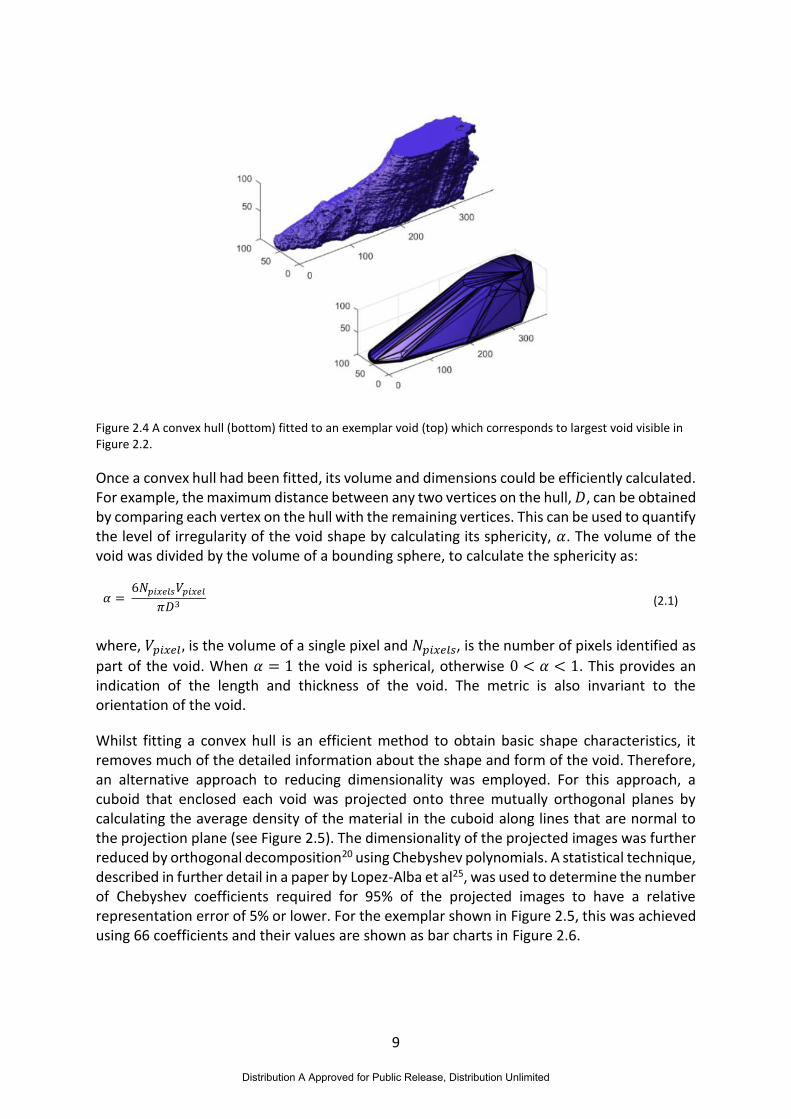
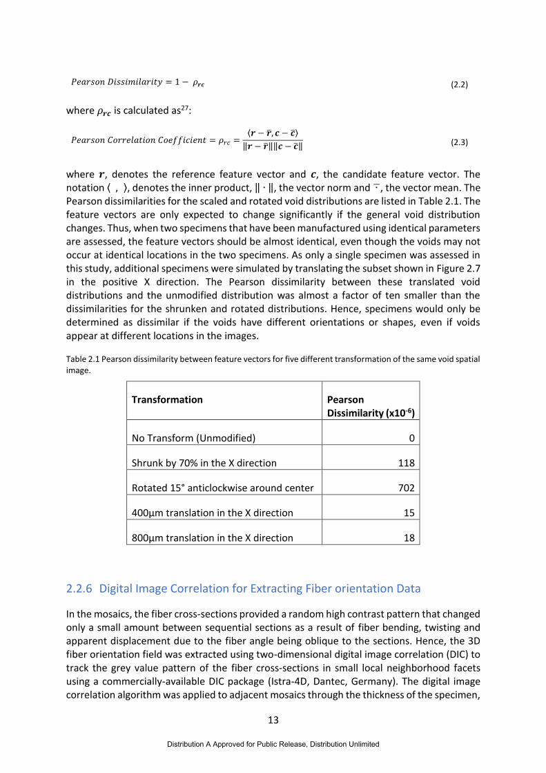
An image of the void distribution can be created using the x-y plane projections of the voids, this projection is the image below the void in Figure 2.5. The x-y projections for all the voids were combined into a single large image showing the voids at the locations that they occurred in the specimen and a central square subset of 2mm width was selected, shown in Figure 2.7. If this technique was applied to a set of specimens the entire image could be used. However, as data from only one specimen was available, a central square was selected so that other specimens could be simulated by translating or transforming the square. The image contained large areas where voids were not present between the locations at which voids occurred, these resulted in discontinuities in the image that would require an excessive number of coefficients to describe. Therefore, instead of applying orthogonal decomposition directly to the images, the 2D Fourier transform was calculated (see Figure 2.8). The spectral data obtained contained information about the orientation of the voids, their size and the number of voids contained within an area. At the center of the spectral image is a sharp peak which corresponds to the low spatial frequency data. As the high frequency data is likely to contain mostly noise, only a central subset of the spectral image was processed. The width of this subset was 4% of the total width of the spectral image, resulting in spectral content with a wavelength of less than 26µm being discarded. This wavelength is below the width of the fiber tows, typically 150µm and thus would be expected to contain little useful information about how the voids are distributed in the specimen.

Figure 2.7 Image created by representing the x-y projections of each void at its location in the plane of the specimen. The 2mm wide square subset that was characterized is indicated by the dashed line.


12

Figure 2.8 Three images of void distribution, unmodified (1st column), scaled in x-direction by 70% (2nd column) and rotated 15° (3rd column). Rows show: spatial image (top), spectral image with axes showing wavelength (middle) and bar charts of the feature vectors for each spectral image (bottom).

The subset spectral image still contained a large amount of redundant information therefore orthogonal decomposition was used to dimensionally reduce the images, resulting in a feature vector of Fourier-Chebyshev coefficients that describe the general spatial distribution of the voids. A similar technique has previously been applied to strain fields using Zernike polynomials as opposed to Chebyshev polynomials11. Zernike polynomials were not used in this study as they are defined over a circular disk, as opposed to 2D Chebyshev polynomials which are defined over a rectangular grid20. Fifteen coefficients were found to be sufficient to reconstruct the spectral image with a relative representation error of 5%. Where relative error is calculated as the root mean squared error of the reconstruction divided by the range of intensity values in the original image26. The sensitivity of the feature vectors to transformations of the void distribution image was then explored. To demonstrate that subtle changes to the specimen void distribution cause measurable changes to the feature vectors representing the spectral images, two arbitrary transformations of the void distribution were calculated. These were: shrinking it to 70% in the x-direction, and rotating it by 15° anticlockwise. After these transformations, central 2mm square subsets were selected and feature vectors were calculated as previously described. The transformed images are shown at the top of Figure 2.8, where the left hand column is for the unmodified void distribution.

The Fourier-Chebyshev feature vectors were compared with the unmodified void distribution. The changes to the feature vectors were subtle, but could be quantified using the Pearson Dissimilarity, calculated as:


13

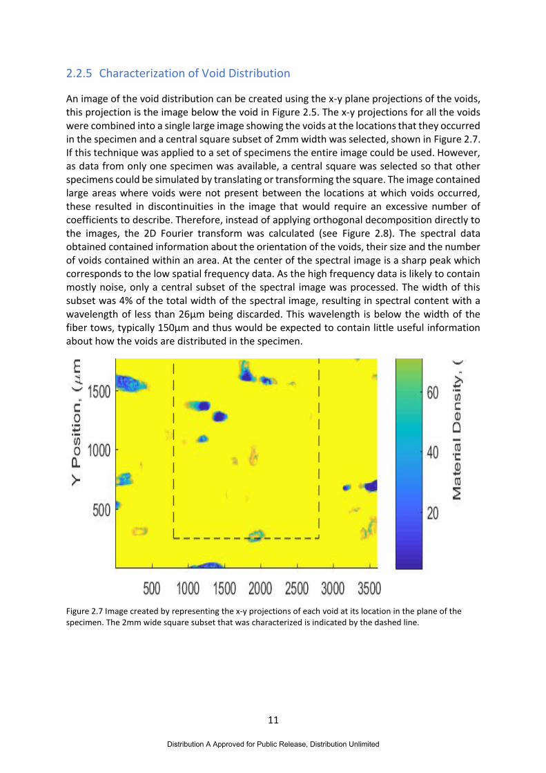
𝑃𝑒𝑎𝑟𝑠𝑜𝑛 𝐷𝑖𝑠𝑠𝑖𝑚𝑖𝑙𝑎𝑟𝑖𝑡𝑦 = 1 − 𝜌𝒓𝒄 (2.2)

where 𝜌𝒓𝒄 is calculated as27:

𝑃𝑒𝑎𝑟𝑠𝑜𝑛 𝐶𝑜𝑟𝑟𝑒𝑙𝑎𝑡𝑖𝑜𝑛 𝐶𝑜𝑒𝑓𝑓𝑖𝑐𝑖𝑒𝑛𝑡 = 𝜌𝑟𝑐 =⟨𝒓 − ��, 𝒄 − ��⟩

‖𝒓 − ��‖‖𝒄 − ��‖ (2.3)

where 𝒓, denotes the reference feature vector and 𝒄, the candidate feature vector. The notation ⟨ , ⟩, denotes the inner product, ‖ ∙ ‖, the vector norm and ∙ , the vector mean. The Pearson dissimilarities for the scaled and rotated void distributions are listed in Table 2.1. The feature vectors are only expected to change significantly if the general void distribution changes. Thus, when two specimens that have been manufactured using identical parameters are assessed, the feature vectors should be almost identical, even though the voids may not occur at identical locations in the two specimens. As only a single specimen was assessed in this study, additional specimens were simulated by translating the subset shown in Figure 2.7 in the positive X direction. The Pearson dissimilarity between these translated void distributions and the unmodified distribution was almost a factor of ten smaller than the dissimilarities for the shrunken and rotated distributions. Hence, specimens would only be determined as dissimilar if the voids have different orientations or shapes, even if voids appear at different locations in the images.

Table 2.1 Pearson dissimilarity between feature vectors for five different transformation of the same void spatial image.

Transformation Pearson Dissimilarity (x10-6)

No Transform (Unmodified) 0

Shrunk by 70% in the X direction 118

Rotated 15° anticlockwise around center 702

400µm translation in the X direction 15

800µm translation in the X direction 18

2.2.6 Digital Image Correlation for Extracting Fiber orientation Data

In the mosaics, the fiber cross-sections provided a random high contrast pattern that changed only a small amount between sequential sections as a result of fiber bending, twisting and apparent displacement due to the fiber angle being oblique to the sections. Hence, the 3D fiber orientation field was extracted using two-dimensional digital image correlation (DIC) to track the grey value pattern of the fiber cross-sections in small local neighborhood facets using a commercially-available DIC package (Istra-4D, Dantec, Germany). The digital image correlation algorithm was applied to adjacent mosaics through the thickness of the specimen,


14

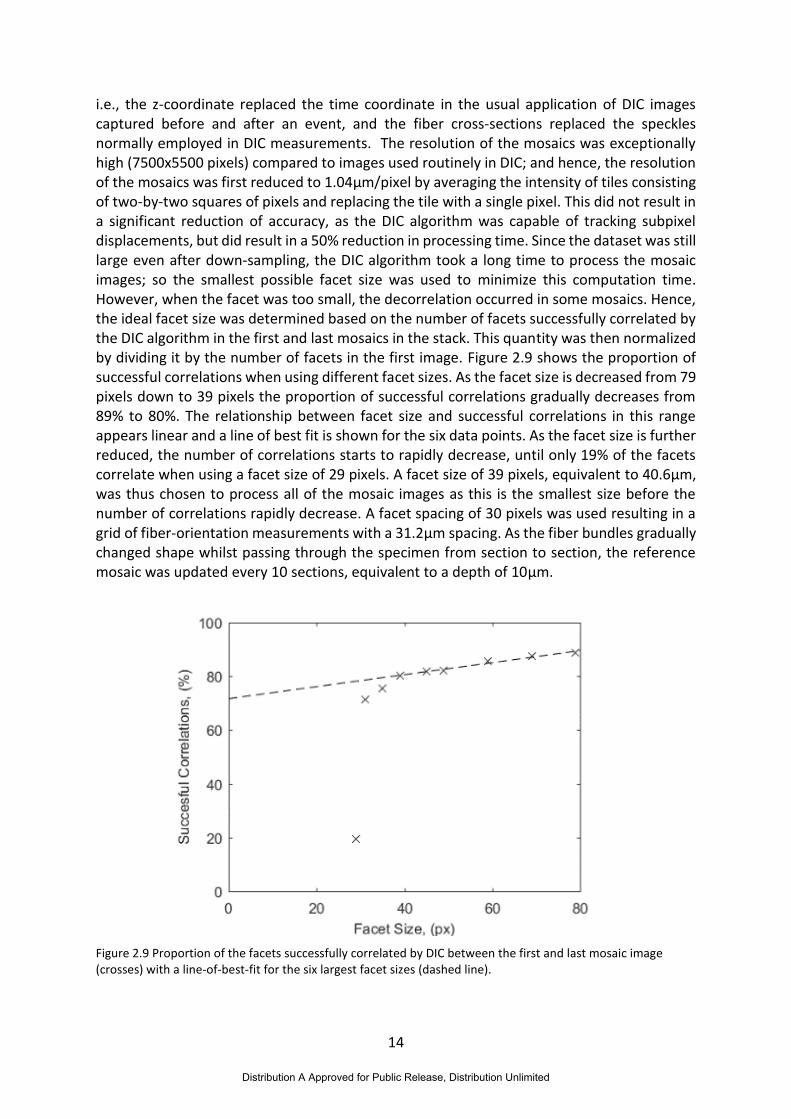
i.e., the z-coordinate replaced the time coordinate in the usual application of DIC images captured before and after an event, and the fiber cross-sections replaced the speckles normally employed in DIC measurements. The resolution of the mosaics was exceptionally high (7500x5500 pixels) compared to images used routinely in DIC; and hence, the resolution of the mosaics was first reduced to 1.04µm/pixel by averaging the intensity of tiles consisting of two-by-two squares of pixels and replacing the tile with a single pixel. This did not result in a significant reduction of accuracy, as the DIC algorithm was capable of tracking subpixel displacements, but did result in a 50% reduction in processing time. Since the dataset was still large even after down-sampling, the DIC algorithm took a long time to process the mosaic images; so the smallest possible facet size was used to minimize this computation time. However, when the facet was too small, the decorrelation occurred in some mosaics. Hence, the ideal facet size was determined based on the number of facets successfully correlated by the DIC algorithm in the first and last mosaics in the stack. This quantity was then normalized by dividing it by the number of facets in the first image. Figure 2.9 shows the proportion of successful correlations when using different facet sizes. As the facet size is decreased from 79 pixels down to 39 pixels the proportion of successful correlations gradually decreases from 89% to 80%. The relationship between facet size and successful correlations in this range appears linear and a line of best fit is shown for the six data points. As the facet size is further reduced, the number of correlations starts to rapidly decrease, until only 19% of the facets correlate when using a facet size of 29 pixels. A facet size of 39 pixels, equivalent to 40.6µm, was thus chosen to process all of the mosaic images as this is the smallest size before the number of correlations rapidly decrease. A facet spacing of 30 pixels was used resulting in a grid of fiber-orientation measurements with a 31.2µm spacing. As the fiber bundles gradually changed shape whilst passing through the specimen from section to section, the reference mosaic was updated every 10 sections, equivalent to a depth of 10µm.

Figure 2.9 Proportion of the facets successfully correlated by DIC between the first and last mosaic image (crosses) with a line-of-best-fit for the six largest facet sizes (dashed line).


15

Figure 2.10 Typical facet x-direction (top) and y-direction (bottom) displacements from DIC as a transparent

overlay on a corresponding mosaic from z=1m. Positive values indicate the fibers coming out of the page are leaning to the right and negative values indicate the fibers are leaning to the left.

The output from the DIC algorithm is the displacement of each facet from mosaic to mosaic. A typical result is shown in Figure 2.10 for the x- and y-displacements from which it can been seen that the fibers are primarily orientated on the x-z plane. The fiber angle at the facet location is obtained by applying the inverse tangent function to the gradient of the line passing through the center of each facet across three sequential mosaics.

2.3 Experimental Method

The image processing described in the preceding section was applied to a 3.6 x 2.6 x 0.1 mm volume of a SiCf/SiNC specimen which was serially sectioned in 1µm increments and viewed in a microscope to produce micrographs that were a mosaic of images containing 7200x5500 pixels in total. The specimen (S200, COI Ceramics, USA) consisted of a SiNC matrix reinforced using SiC fibers and was manufactured using the precursor infiltration and pyrolysis technique28. This manufacturing technique starts with SiC fibers which form a framework that is infiltrated with an organic polymeric compound containing silicon, resulting in a specimen with the same net shape as the desired component. Pyrolysis was applied to the specimen by heating it to a high temperature in a vacuum causing the polymer compound to thermally decompose into SiNC. The process was repeated until an acceptably dense matrix was obtained. This is necessary because the volume of SiNC obtained by pyrolysis is lower than the volume of the polymeric compound that preceded it28. The fibers in the specimen were


16

arranged as six layers of fabric with a plain weave, resulting in the fibers having a nominal orientated of ±45°.

The specimen was inspected using a serial sectioning system (Robo-Met.3D, UES, USA). This system automates the process of grinding, polishing and then imaging a specimen such that the machine can process specimens with no additional operator input after initial setup. The specimen was set in a mounting compound before being inserted in the serial sectioning system. Serial sectioning is an iterative process, which starts by removing 1µm of material from the specimen by grinding it on a course radial polishing pad. Subsequently, finer pads are used to achieve a highly polished surface on which individual fiber cross-sections can be observed using microscopy. After polishing, the specimen was placed on the translation stage of an inverted optical microscope. The microscope captured a six-by-six grid of overlapping images of the section surface where each image covered a 670µm by 500µm area. These images were then stitched into a mosaic. After the mosaic was captured the process was repeated so that sections through the microstructure at 1µm increments were obtained. Each mosaic was of a 3600µm by 2500µm area of the specimen with a spatial resolution of 0.522µm/pixel. One hundred sections were performed with a spacing of 1µm between each section, resulting in an analyzed volume depth of 100µm and 3.17GB of image data. The depth to which the specimen was sectioned only allowed the local orientation of fibers in a thin slice through the material to be explored and was not sufficient to determine how the fibers were woven.

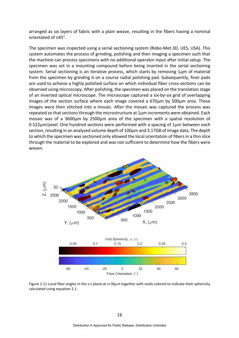
Figure 2.11 Local fiber angles in the x-z plane at z=30m together with voids colored to indicate their sphericity calculated using equation 2.1.


17

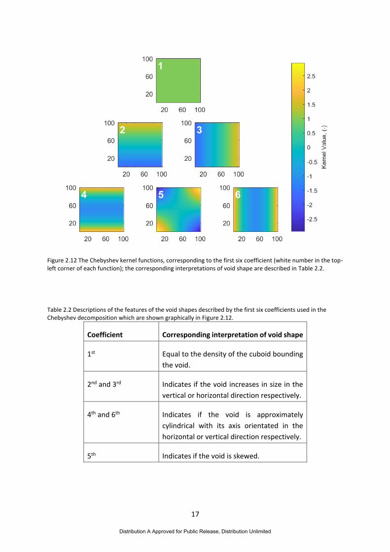
Figure 2.12 The Chebyshev kernel functions, corresponding to the first six coefficient (white number in the top-left corner of each function); the corresponding interpretations of void shape are described in Table 2.2.

Table 2.2 Descriptions of the features of the void shapes described by the first six coefficients used in the Chebyshev decomposition which are shown graphically in Figure 2.12.

Coefficient Corresponding interpretation of void shape

1st Equal to the density of the cuboid bounding

the void.

2nd and 3rd Indicates if the void increases in size in the

vertical or horizontal direction respectively.

4th and 6th Indicates if the void is approximately

cylindrical with its axis orientated in the

horizontal or vertical direction respectively.

5th Indicates if the void is skewed.


18

2.4 Results

The fiber orientation and voids were displayed on a common set of axes, allowing direct comparisons between the two datasets in Figure 2.11. The fiber angle in the x-z plane is

shown for the specimen with the top 70 µm removed, i.e. for the bottom 30m. In Figure 2.11, the layers of fibers can be distinguished from the fiber angle whilst the sphericity of the voids, calculated using equation (1), is indicated by their color.

The Chebyshev coefficients obtained from the orthogonal decomposition of the projections of the cuboid enclosing each void was used to explore the shape of the voids. In general, lower order coefficients represent simpler characteristics of shape than higher order coefficients. The first six coefficients describe simple smooth shapes and can be used to determine the void orientation and whether the void increases in size along particular directions. Table 2.2 contains descriptions for the shapes described by these coefficients and the associated Chebyshev kernel functions are shown in Figure 2.12.

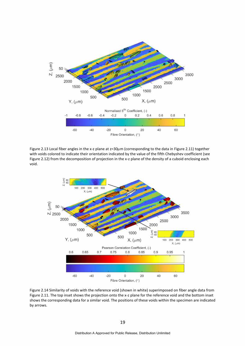
The fifth coefficient of the feature vector provides an indication of the angular orientation of the voids on the projection planes. When this coefficient is positive it indicates that the projection of the void has higher values along its diagonal from the bottom-left corner of the projection to the top-right corner. For example, if the fifth coefficient for the x-z projection of the void is positive, then the void is primarily orientated along the line 𝑧 = 𝑥 in the specimen. When the fifth coefficient is negative the reverse occurs and the void is orientated top-left to bottom-right and thus along 𝑧 = −𝑥. It can be seen in Figure 2.12, that the fourth and sixth coefficients describe the horizontal and vertical components of the projected shape. Hence to ensure that that the void is not misclassified as skewed if the absolute value of the fourth or sixth coefficients is significantly higher than the fifth coefficient, the fifth coefficient was normalized by dividing its value by the Euclidean norm of the fourth, fifth and sixth coefficients given by:

𝑠5 =𝑠5

√(𝑠42 + 𝑠5

2 + 𝑠62)

(2.4)

This normalization also ensured that the coefficient had a range of between -1 and +1. This technique was applied to all three mutually perpendicular projections of each void. In the x-y and y-z projections most of the voids had a normalized 5th coefficient close to zero with only a couple of outliers and thus these results are not shown. When applied to the x-z projections, non-zero values were obtained that exhibited some similarity with the corresponding fiber angles as shown in Figure 2.13.


19

Figure 2.13 Local fiber angles in the x-z plane at z=30m (corresponding to the data in Figure 2.11) together with voids colored to indicate their orientation indicated by the value of the fifth Chebyshev coefficient (see Figure 2.12) from the decomposition of projection in the x-z plane of the density of a cuboid enclosing each void.

Figure 2.14 Similarity of voids with the reference void (shown in white) superimposed on fiber angle data from Figure 2.11. The top inset shows the projection onto the x-z plane for the reference void and the bottom inset shows the corresponding data for a similar void. The positions of these voids within the specimen are indicated by arrows.


20

The feature vectors representing each projection can be concatenated to obtain a single feature vector that fully characterizes the 3D shape of a void. These combined feature vectors can then be used to identify voids with similar shapes to other voids. This could be used to efficiently search through large amounts of data to compile a list of similar defects, prior to identifying the most relevant for further investigation. First, the largest void by volume was chosen and defined as a reference void. Comparisons between the feature vector for the reference void and the feature vectors for each of the remaining voids were then made using the Pearson correlation coefficient, which is calculated, as before, as27:

𝑃𝑒𝑎𝑟𝑠𝑜𝑛 𝐶𝑜𝑟𝑟𝑒𝑙𝑎𝑡𝑖𝑜𝑛 𝐶𝑜𝑒𝑓𝑓𝑖𝑐𝑖𝑒𝑛𝑡 = 𝜌𝒓𝒄 =⟨𝒓 − ��, 𝒄 − ��⟩

‖𝒓 − ��‖‖𝒄 − ��‖ (2.3)

where 𝒓, denotes the reference feature vector and 𝒄, the candidate feature vector. The notation ⟨ , ⟩, denotes the inner product, ‖ ∙ ‖, the vector norm and ∙ , the vector mean. Figure 2.14 shows the spatial distribution of the voids with the color of each void defined by the similarity between its feature vector and the feature vector for the reference void. The reference void is the top most void marked with an arrow and appears white as it has a Pearson correlation of one. The most similar void is close to the middle of the specimen, also marked with an arrow, and had a Pearson correlation of 0.920.

2.5 Discussion

The microstructure of CMCs is known to affect the macro-behavior of the material4. Whilst research has been conducted on characterizing fiber orientation19, there has been less that explores the morphology of voids. Furthermore, the relationships between fiber orientation and void shape have not been explored. In this work, it was found that the grey-level value of images recorded in the microscope provided sufficient distinction between the fibers, matrix and voids in the microstructure to allow the void selection process illustrated in Figure 2.1 and Figure 2.2. The characteristics of the voids and their distribution throughout the specimen was then investigated.

The voids in the composite material are in close proximity to the fibers, so it is expected that void shape will be directly affected by the local fiber orientation. To explore this interdependency, the fiber orientation was also extracted from the serial section images. Most techniques for determining the fiber orientation using images from microscopy or computed micro-tomography have been based on either measuring the shape of the fiber cross-sections29 or tracking individual fibers as they pass through the material19, this results in fiber orientation fields with very high levels of spatial resolution, but requires substantial computation time. Texture analysis techniques have also been used to identify fiber orientation30 but this technique limits the resolution to tens or even hundreds of fibers. The DIC-based technique used in this study provides a new approach to quantifying fiber orientation with a spatial resolution dependent on the image resolution and nominal fiber diameter.

The void shapes were quantitatively examined and compared with the fiber orientation. The sphericity was calculated and graphically shown in Figure 2.11 together with the fiber angles. These data have the potential to provide insights about the formation of voids in the material. Voids are entrapped pockets of air that, in the absence of other influences, would be expected


21

to take on a spherical shape to minimize the surface energy of the interface between the air and the ceramic polymer precursor. However, when forces are applied to the entrapped air, either by the application of pressure during manufacturing or by fibers in close proximity, the voids become aspherical. By their nature, aspherical voids will have higher surface areas than spherical voids thus allowing a greater area of contact between the entrapped air and the matrix and fibers, which could increase the rate of oxidation of the fiber coating local to the voids during service.

The orientation of the voids was explored using the feature vectors representing the three orthogonal projections of each void. The direction in which the voids were skewed or biased was identified from a single normalized coefficient in the feature vector (see equation (2.3)). This coefficient was used to determine the extent to which each void was skewed relative to the Cartesian axis system on each of the three orthogonal planes. It was found that the voids were only significantly skewed on the x-z plane, which is also the plane on which the fibers are predominantly orientated, i.e., the plane of the weave. Therefore, comparisons were made between the fiber angle and void skewness on this plane using the compound plot in Figure 2.13, which qualitatively shows the correlation between these quantities. As the voids form after the fiber orientation has been defined by laying down the weave, this suggests that void shape is dependent on the arrangement of the surrounding fibers. The largest voids appear to be present at the edges of tows, which can be identified in the map of fiber angle as locations where regions of similarly orientated fibers narrow to a point, for example in the bottom-right of Figure 2.11, and correspond to the intersections of fiber bundles in the weave. Groups of voids have formed at these locations suggesting that the larger gaps at the weave intersections cause air to become entrapped during infiltration of the polymer ceramic precursor.

When manufacturing CMC components, the microstructure of the components will need monitoring to ensure that it is of the required quality. As components are manufactured the parameters used to define the manufacturing process inevitably drift. Whilst initially this may not cause degradation of the component performance, eventually component strength or life may be compromised. The microstructure is expected to directly impact the mechanical performance of the component. Therefore, by monitoring the microstructure of the finished component, any changes to the manufacturing process that result in component performance decreasing can be detected. The Fourier-Chebyshev decomposition technique introduced in this chapter can be used to detect subtle changes to the microstructure. To apply this technique in industry, a feature vector would need to be measured that described the nominal distribution of voids. The Pearson dissimilarity between the nominal distribution and the void distribution in tested specimens could then be compared to an allowable threshold. A CMC component from each batch could then be characterized and compared with the acceptable microstructure to determine if manufacturing parameters had drifted.

The shape characterization techniques described in this work allow the fiber angles and the form and distribution of voids in a CMC component to be analyzed quickly with reduced effort. The void shapes were converted to feature vectors that describe their complex shapes using a comparatively small number of coefficients. These coefficients can then be used in one of two ways: (i) the general shape of the voids can be quantified by examining individual coefficients in the vector (this was used to determine the orientation of voids) and (ii) using the feature vector containing all of the coefficients to identify similar shapes at other locations


22

in the specimen or in other specimens. The techniques developed in this study have been demonstrated by applying them to a large quantity of high resolution microscopy data containing 41 distinct voids. It is anticipated that the application of these techniques will decrease the time required to analyses micrographs during research and development as a result of the level of automation introduced. The techniques could also be applied in manufacturing to monitor the quality of CMC components by sampling components on a production line without subjective judgments from operators.

2.6 Conclusions

A methodology has been developed for characterizing the angle of fibers as well as the shape and distribution of voids in fiber-reinforced composites using high-resolution micrographs obtained from serial sectioning. A silicon-carbide fiber/silicon-carbo-nitride composite specimen was used to explore the capabilities of this methodology. Orthogonal decomposition was applied to the extracted void shapes to reduce their dimensionality by describing them using feature vectors. These feature vectors uniquely describe each local defect and were used to qualitatively relate the shape of the voids to the orientation of the fibers that surround them. The feature vectors allow quantitative comparisons of void shape, orientation and distribution between specimens that could enable the development of novel ceramic matrix composite components as well as more rigorous quality assurance of manufactured components.


23

3 Real-time detection and quantification of damage in continuous fiber reinforced composites

3.1 Introduction

Composite materials have complicated microstructures containing many defects, such as fiber breakages, misalignment or porosity, which reduce the local strength of the material. These small defects cause damage to initiate during service affecting the remnant life of composite structures. Full-field optical measurements, such as digital image correlation (DIC), can be used to monitor the strain field on the surface of specimens whilst they are loaded. The strain fields obtained are typically used to monitor for strain hot-spots that indicate locations where damage is being created31, 32. Whilst the strain data is quantitative, this interpretation essentially only provides a qualitative understanding of the damage mechanics. The potential for quantitative measurements of damage initiation and location is therefore ignored.

Recently, quantitative assessments of impact damage in composites has been obtained using DIC33. This technique compares the strain field on the surface of a damaged specimen with the strain field of an undamaged specimen, resulting in a defect severity metric that was found to correlate with the residual strength of the damaged specimen. However, this technique cannot be used for monitoring the progressive creation of damage in a specimen as it requires a reference strain field with which to compare the damaged strain field. In this chapter, the rate of change of the strain field is monitored instead. This removes the need for a reference strain field whilst still allowing for damage to be quantified. This technique is applied to strain measured on the surface of ceramic matrix composite dog-bone specimen to achieve objective (ii) of this project. The images were captured by the AFRL and then processed using DIC at the University of Liverpool.

3.2 Strain Based Damage Monitoring

As an object is loaded to failure, damage is initiated in the material. When this damage forms, load is redistributed around it resulting in a measurable change to the strain field. If a DIC system is used to measure the surface strain field during a material test, then changes due to damage initiation and the time at which these changes have occurred can be determined. For most of the time during loading the strain field only changes due to elastic deformation and measurement noise. When damage is created the strain field changes significantly. It is these significant changes that can be used to detect when damage occurs, where it occurs and its severity.

The measured strain fields typically contained large amounts of redundant data. This means that each strain field was described by a greater amount of data than was needed for analysis. This excess data increased the amount of memory required to store the measurements, as well as the computation time required when processing it. Orthogonal decomposition20 was used to reduce these data such that each strain field was represented by a relatively small number of coefficients collated into a feature vector. These feature vectors could be


24

reconstructed back into a strain field such that the amount of information lost due to the decomposition process could be quantified. A perfect reconstruction is obtained if the number of coefficients is equal to the number of pixels in the original strain field, however as the strain fields are typically smooth with few discontinuities an accurate reconstruction can be obtained with just a small number of coefficients. Hence, when the representation error is equal to the measurement uncertainty of the DIC system, the key information about the strain field is captured whilst the redundant information, which mostly describes measurement noise, is rejected. However, the strain fields used in this chapter were decomposed using 235 coefficients, which resulted in relative errors of about 7%. This is a higher number of coefficients than is typically used because the measurement uncertainty was unknown; however, this number of coefficients could be reduced if the measurement uncertainty was known.

Once decomposed, the dissimilarity between two strain fields was quantified by considering the feature vectors for each strain field as points in multidimensional space. The distance between these points was calculated using the Euclidean distance. The rate of change of the strain field can be obtained by dividing the Euclidean distance by the time difference between the two strain fields:

𝑅𝑎𝑡𝑒 𝑜𝑓 𝐶ℎ𝑎𝑛𝑔𝑒 = ��(𝑡) = ‖𝑓(𝑡 +

ℎ2) − 𝑓(𝑡 −

ℎ2)‖

ℎ (3.1)

where 𝒇(𝑡), is the feature vector for the strain field captured at time 𝑡 and ‖∙‖, is the vector norm. The time difference ℎ, controls the time range over which the rate of change is calculated, with higher values resulting in less noise. It was important that the time difference was higher than the inverse of the camera frame rate. A time difference equal to ten times the inverse of the frame rate was found to be effective for the data in this chapter. This means the rate of change was calculated over ten camera frames and was chosen to prevent false positives when identifying damage events.

Damage events, e.g. matrix cracking, were determined using the rate of change signal from equation (3.1). Measurement noise caused the rate of change to occasionally peak, but these peaks only occur for a single sample. When damage forms, the strain field at that location is permanently changed. As the rate of change was calculated over ten camera frames, a damage event causes the rate of change to peak for ten samples. Events that caused significant changes to the strain field were detected by looking for these sustained peaks, an example of these peaks can be seen in Figure 3.1 at 190s. The threshold defining a peak was set to the 90th percentile of the rate of change during the period between 40 and 80 seconds. This time period was chosen to represent the elastic behavior of the specimen when little or no damage is occurring and also to avoid the start of the test when measurement noise obscures the deformation.

Changes in the measured strain field also occur due to elastic deformation of the specimen and measurement noise. These changes were nominally constant and thus were removed from the signal given by equation (3.1) by subtracting the constant rate of change ��𝑐, leaving only the rate of change due to damage creation:

𝑅𝑎𝑡𝑒 𝑜𝑓 𝐷𝑎𝑚𝑎𝑔𝑒 𝐶𝑟𝑒𝑎𝑡𝑖𝑜𝑛 = ��𝑑 = �� − ��𝑐 (3.2)


25

The constant rate of change due to measurement error and elastic deformation was estimated by calculating the mean rate of change during the time period used to determine the threshold that defined sustained peaks, i.e. between 40 and 80 seconds. The amount by which damage had changed the strain field was finally calculated by integrating equation (3.2) with respect to time:

𝐴𝑐𝑐𝑢𝑚𝑢𝑙𝑎𝑡𝑒𝑑 𝐷𝑎𝑚𝑎𝑔𝑒 = 𝑠𝑑 = ∫ ��𝑑 ∙ 𝑑𝑡𝑡

0

(3.3)

The rate of change signal was discrete and thus the trapezium rule was used to perform the integration.

Figure 3.1 Rate of change signal (from equation (3.1)) for a composite specimen loaded in tension showing four periods, shaded in grey, when the rate of change was above the 90th percentile for a minimum of 7.5s. .


The algorithm described in the previous section was applied to data captured during an experiment at the AFRL laboratory. A single SiC/SiC dog-bone shaped specimen was quasi-statically loaded to failure in tension. The specimen was made of HiPerComp™ (GE Aviation, USA), consisting of unidirectional plies with a [90/0]2s layup, with the 0° plies orientated along the longitudinal direction of the specimen. The gauge section was 60mm long with a cross-section measuring 8mm by 2.2mm. Prior to loading, the specimen was heated to a temperature of 1100 °C by a 1kW continuous wave laser. Once at temperature, the specimen was loaded at a rate of 1.5mm/min. A speckle pattern had previously been applied to the 8mm wide surface of the gauge region, allowing a Vic3D stereographic DIC system (Correlated Solutions, USA) to measure the surface strain. The cameras were 315mm from the specimen with a spacing of 141mm and a pan angle of 25°. The system captured images at a frame rate


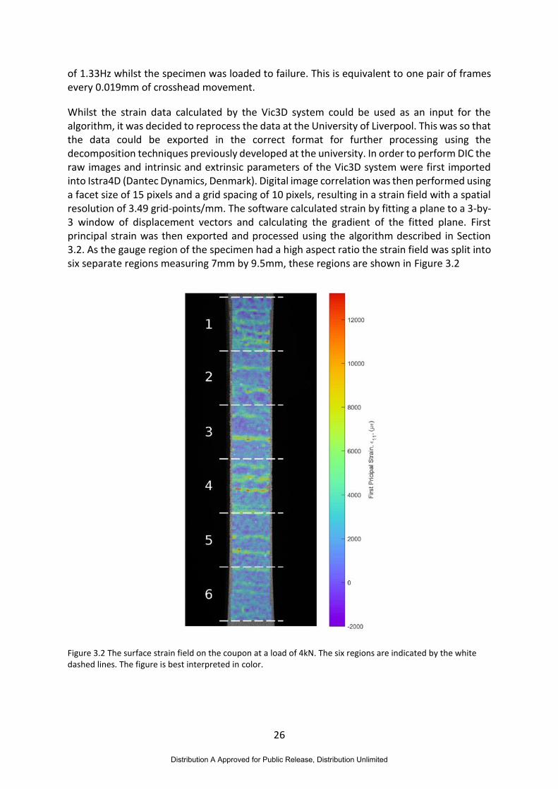
26

of 1.33Hz whilst the specimen was loaded to failure. This is equivalent to one pair of frames every 0.019mm of crosshead movement.

Whilst the strain data calculated by the Vic3D system could be used as an input for the algorithm, it was decided to reprocess the data at the University of Liverpool. This was so that the data could be exported in the correct format for further processing using the decomposition techniques previously developed at the university. In order to perform DIC the raw images and intrinsic and extrinsic parameters of the Vic3D system were first imported into Istra4D (Dantec Dynamics, Denmark). Digital image correlation was then performed using a facet size of 15 pixels and a grid spacing of 10 pixels, resulting in a strain field with a spatial resolution of 3.49 grid-points/mm. The software calculated strain by fitting a plane to a 3-by-3 window of displacement vectors and calculating the gradient of the fitted plane. First principal strain was then exported and processed using the algorithm described in Section 3.2. As the gauge region of the specimen had a high aspect ratio the strain field was split into six separate regions measuring 7mm by 9.5mm, these regions are shown in Figure 3.2

Figure 3.2 The surface strain field on the coupon at a load of 4kN. The six regions are indicated by the white dashed lines. The figure is best interpreted in color.


27

3.4 Results

As the specimen was loaded its deformation changed from elastic behavior, where load increased linearly with time, to plastic behavior characterized by permanent deformation, where the relationship between load and time was non-linear. This can be identified using the accumulated damage signal. The signal stays nominally constant for the first half of the test before rapidly increasing after 𝑡 = 170s. This can be seen for region 3 of the strain field in Figure 3.3.

Figure 3.3 The accumulated damage signal for region 3 of the specimen with damage events marked by squares.

By monitoring for peaks in the rate of change signal that last for ten samples, equivalent to 7.5s, damage creation that irreversibly changes the surface strain field can be identified. Four events were detected within region 3 of the specimen, these events are marked on the accumulated damage line in Figure 3.3. These events can be further studied by looking at how the strain field changes between immediately before and after the event. The feature vector representing the strain field 2.5s before each event was subtracted from the feature vector from 2.5s after the event. This yielded a new feature vector that represented the changes to the strain field. This vector was reconstructed into a strain difference field, allowing the damage to be visualized, shown in Figure 3.4. The detected events for region 3 result in horizontal bands of high strain running parallel to the surface 90° ply.


28

Figure 3.4 Differences between strain fields 2.5s before and after the damage events marked by squares in Figure 3.3. Spatial units are in mm.

The amount by which the accumulated damage signal changes can be used to monitor which regions of the specimen contain the most severe damage. For example, region 4 accumulates damage at almost twice the rate of region 2, as shown in Figure 3.5. The point at which the specimen starts to permanently deform can be located using the plots in Figure 3.3 and Figure 3.5. Whilst the accumulated damage signal only starts to increase after 170s for region 2, whilst region 4 starts to accumulate damage at approximately 140s.

3.5 Discussion

Composite damage mechanics is typically more complicated than that encountered in homogenous materials such as metals or polymers. This is due to the interaction of defects with the complicated heterogeneous microstructure. This causes difficulties when attempting to predict the degradation of composites over time. The accumulated damage signal obtained from equation (3.3) allows this degradation to be monitored more effectively than using the stress-strain or load-time curves. This is because it is easy to define a threshold for accumulative damage above which the specimen can be considered damaged; whereas to identify the onset of damage using the stress-strain or load-time the event must be identified from the gradient of the curve and required differentiation operation results in a high level of uncertainty.


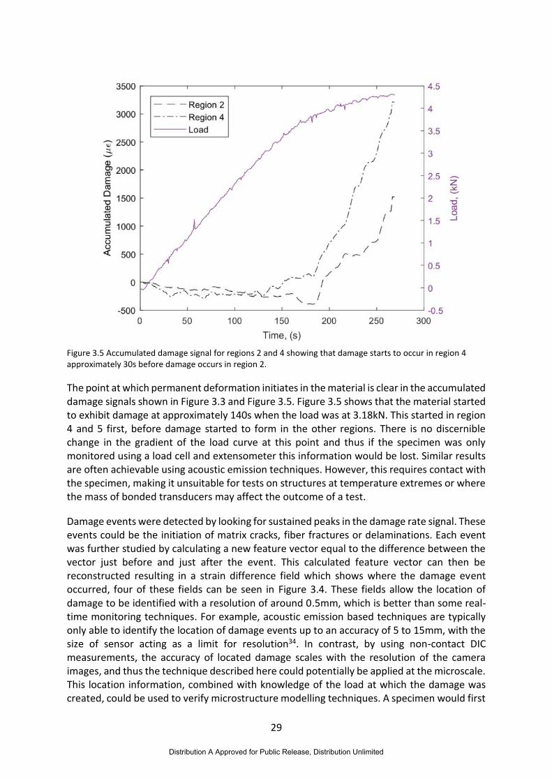
29

Figure 3.5 Accumulated damage signal for regions 2 and 4 showing that damage starts to occur in region 4 approximately 30s before damage occurs in region 2.

The point at which permanent deformation initiates in the material is clear in the accumulated damage signals shown in Figure 3.3 and Figure 3.5. Figure 3.5 shows that the material started to exhibit damage at approximately 140s when the load was at 3.18kN. This started in region 4 and 5 first, before damage started to form in the other regions. There is no discernible change in the gradient of the load curve at this point and thus if the specimen was only monitored using a load cell and extensometer this information would be lost. Similar results are often achievable using acoustic emission techniques. However, this requires contact with the specimen, making it unsuitable for tests on structures at temperature extremes or where the mass of bonded transducers may affect the outcome of a test.

Damage events were detected by looking for sustained peaks in the damage rate signal. These events could be the initiation of matrix cracks, fiber fractures or delaminations. Each event was further studied by calculating a new feature vector equal to the difference between the vector just before and just after the event. This calculated feature vector can then be reconstructed resulting in a strain difference field which shows where the damage event occurred, four of these fields can be seen in Figure 3.4. These fields allow the location of damage to be identified with a resolution of around 0.5mm, which is better than some real-time monitoring techniques. For example, acoustic emission based techniques are typically only able to identify the location of damage events up to an accuracy of 5 to 15mm, with the size of sensor acting as a limit for resolution34. In contrast, by using non-contact DIC measurements, the accuracy of located damage scales with the resolution of the camera images, and thus the technique described here could potentially be applied at the microscale. This location information, combined with knowledge of the load at which the damage was created, could be used to verify microstructure modelling techniques. A specimen would first


30

be volumetrically characterized using computed tomography and then loaded to failure whilst monitored using DIC. Locations at which damage is initiated would be identified using the monitoring algorithm and models of the microstructure at those locations could then be created for the CT data. If the model was capable of accurately predicting the load at which damage was created then the same modelling technique could be applied to other microstructures with greater confidence in its predictions.

Many DIC packages now support live processing of images, such that the strain field on the surface of a specimen can be monitored in real-time. Currently these real-time strain fields have low frame rates, e.g. around 1Hz, but with increases in computer power the frame rate is likely to approach that of the camera frame rate. The use of orthogonal decomposition to process the strain fields reduces the data dimensionality and therefore increases the computational efficiency of the strain-based monitoring algorithm. This means that the algorithm described in this chapter could be combined with real-time DIC data processing such that the accumulated damage signal and the damage images could be calculated during the test. This additional information could be used to stop a test if damage is initiated at unexpectedly low loads, allowing detailed inspection of the subcritical damage before the specimen fails, or to trigger changes in the test parameters. This real-time monitoring of the strain field could also form the basis of a structural health monitoring system.

3.6 Conclusions

A strain-based damage monitoring algorithm has been introduced that could be used to identify the time and location of damage initiation within composite tensile specimens during loading. The damage that results from these events can be characterized such that the damage accumulated within a region of the specimen can be quantified. The developed technique was applied to digital image correlation data for a ceramic matrix composite specimen as it was loaded to failure in tension. Individual cracks and the time at which they formed were identified automatically using only the measured strain data. This information, combined with a volumetric characterization of microstructure, could be used to guide the development of damage mechanics models by providing scenarios that could be modelled and compared with experiments.


31

4 Characterization of fiber orientations in continuous fiber reinforced composites

4.1 Introduction

This chapter describes the work on objective (iii) of this project which was about the characterization and quantitative comparison of the fiber orientation fields in ceramic matrix composites (CMCs). It has been highlighted in the Introduction chapter that characterizing the voids as well as the topology of fiber orientation fields and analyzing their effects on the material properties are the key to the design and development of improved microstructures for the next generation CMCs. Chapter 2 of this report has described the work on identification and characterization of voids in CMCs and briefly touched on the extraction of microstructural information related to fiber orientation. This chapter focuses specifically on determining the 3D fiber profiles from a sequence of high-resolution optical mosaics which were acquired from automated serial sectioning of a 3.6 × 2.6 × 0.1 mm CMC sample described in Chapter 2.

Three-dimensional fiber profiles have been extracted in the past from a sequence of optical images of a serially sectioned CMC sample using a three-step process19, 35. In the first step in this process, image segmentation was performed to identify the distinct phases in the microstructure which, in case of the CMCs, were the matrix, fibers and the voids. Since the phase of interest was the fibers, the images were converted to binary data where the grey-level value of pixels representing the fiber phase were converted to one and the remainder to zero. The second step was the identification of fiber cross-sections which appeared as ellipses in the optical images. Once the fiber cross-sections were identified and their center coordinates were determined, the final step was to associate each fiber center to its corresponding position in the subsequent image in order to determine its 3D path through the depth of the sample. Bricker and his co-workers35 implemented a simple rule-based approach for linking the fiber centers. This approach projects the position of the fiber center in the next image based on its previous orientation and searches for the fiber cross-section lying nearest to the projected location. More recently, Zhou et al19 proposed a Kalman-filter based approach for linking the fiber centers. This method was claimed to accurately link the fiber centers even if the spacing between the subsequent images was large or the fibers were crowded with little variation in their appearance.

In this work, two methods have been proposed for the computationally-efficient characterization of fiber orientation in continuous fiber reinforced composites. The first method is based on two-dimensional cross-correlation, which is commonly used for template matching. The second method, which is believed to be more robust, utilizes a digital image correlation (DIC) algorithm. DIC is a well-established image-based optical technique for full-field deformation measurement which is widely used in the field of experimental mechanics. To perform deformation measurements, the image of the region of interest (ROI) is first captured prior to application of any load, which is termed as the reference image. The subsequent images are then captured after applying the loads. The DIC algorithm discretizes the reference image into small square regions called facets. Each facet is correlated with the


32

corresponding deformed image to determine a displacement vector (see schematic in Figure 4.1). For correlation algorithm to work effectively, the facets should be statistically different from each other in terms of their grey-level intensity distribution. For this reason, the specimen surface is usually painted with high contrast, random black and white speckle pattern. It was realized that the mosaics, acquired from automated serial sectioning of the CMC sample described in Chapter 2, have sufficient grey-level intensity variation for the DIC algorithm to uniquely and accurately map the facets in the sequence of mosaics through the thickness of the sample to extract the fiber orientation across the field of view.

Figure 4.1 Schematic representing the unreformed facet in the reference image and the deformed facet in the deformed image. The difference in the positions of the unreformed and the deformed facet centers yields the displacement vector.

4.2 Tracking of fiber cross-sections through sequence of Images

4.2.1 Fiber tracking using DIC

The mosaics were processed using a commercially-available DIC package, Istra-4D (Dantec Dynamics GmbH). Istra software defines a grid of square facets on the (initial) reference image using two parameters i.e. facet size and spacing between the facet centers (see Figure 4.2). To be able to track the reference facets in the subsequent images with a sub-pixel accuracy, the grey-level intensity in each facet is represented using bi-cubic spline interpolation. Istra utilizes a second-order shape function to map the reference facet to its deformed shape in

the next image. The second-order shape function allows for the translation, stretch, shear and distortion of the initially square reference facet. Further details about the DIC algorithm which the Istra software implements could be found in a paper by Becker et al36.


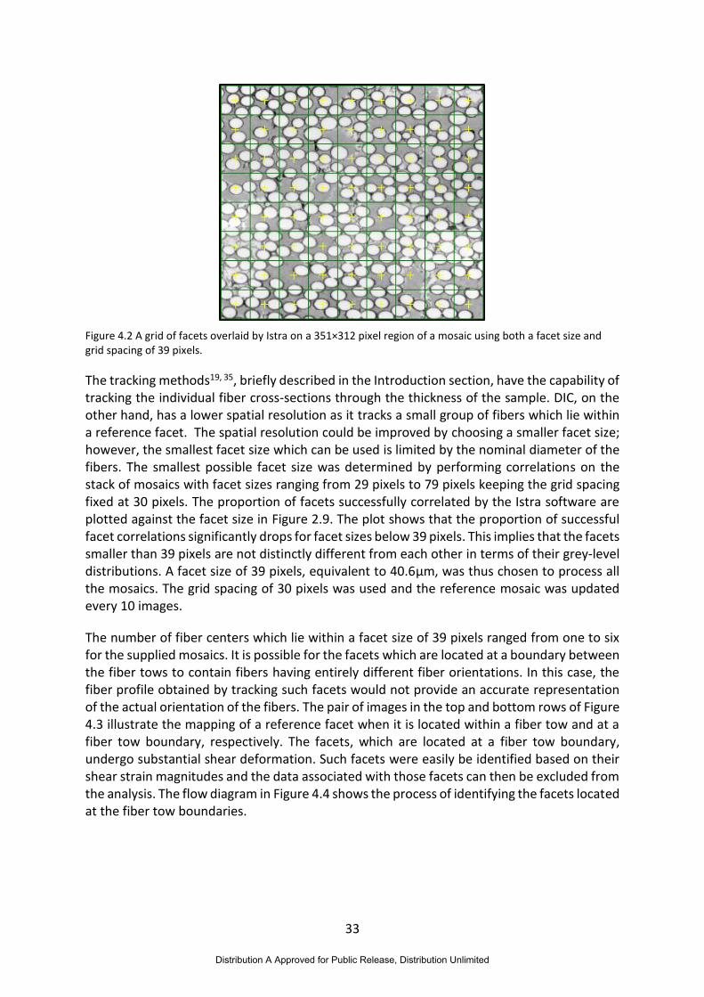
33

Figure 4.2 A grid of facets overlaid by Istra on a 351×312 pixel region of a mosaic using both a facet size and grid spacing of 39 pixels.

The tracking methods19, 35, briefly described in the Introduction section, have the capability of tracking the individual fiber cross-sections through the thickness of the sample. DIC, on the other hand, has a lower spatial resolution as it tracks a small group of fibers which lie within a reference facet. The spatial resolution could be improved by choosing a smaller facet size; however, the smallest facet size which can be used is limited by the nominal diameter of the fibers. The smallest possible facet size was determined by performing correlations on the stack of mosaics with facet sizes ranging from 29 pixels to 79 pixels keeping the grid spacing fixed at 30 pixels. The proportion of facets successfully correlated by the Istra software are plotted against the facet size in Figure 2.9. The plot shows that the proportion of successful facet correlations significantly drops for facet sizes below 39 pixels. This implies that the facets smaller than 39 pixels are not distinctly different from each other in terms of their grey-level distributions. A facet size of 39 pixels, equivalent to 40.6µm, was thus chosen to process all the mosaics. The grid spacing of 30 pixels was used and the reference mosaic was updated every 10 images.

The number of fiber centers which lie within a facet size of 39 pixels ranged from one to six for the supplied mosaics. It is possible for the facets which are located at a boundary between the fiber tows to contain fibers having entirely different fiber orientations. In this case, the fiber profile obtained by tracking such facets would not provide an accurate representation of the actual orientation of the fibers. The pair of images in the top and bottom rows of Figure 4.3 illustrate the mapping of a reference facet when it is located within a fiber tow and at a fiber tow boundary, respectively. The facets, which are located at a fiber tow boundary, undergo substantial shear deformation. Such facets were easily be identified based on their shear strain magnitudes and the data associated with those facets can then be excluded from the analysis. The flow diagram in Figure 4.4 shows the process of identifying the facets located at the fiber tow boundaries.


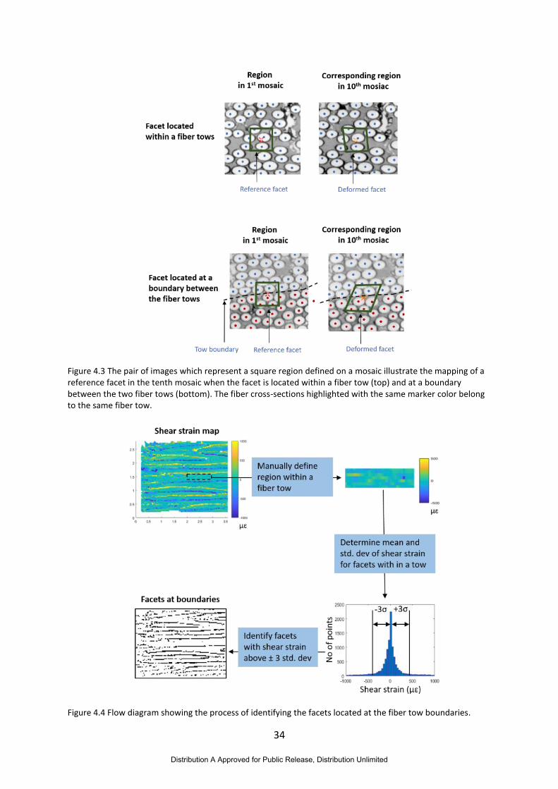
34

Figure 4.3 The pair of images which represent a square region defined on a mosaic illustrate the mapping of a reference facet in the tenth mosaic when the facet is located within a fiber tow (top) and at a boundary between the two fiber tows (bottom). The fiber cross-sections highlighted with the same marker color belong to the same fiber tow.

Figure 4.4 Flow diagram showing the process of identifying the facets located at the fiber tow boundaries.


35

4.2.2 Fiber tracking using 2D cross-correlation

An alternative method which is based on 2D cross-correlation is proposed in this section for fiber tracking. It has the capability of tracking individual fiber cross-sections in the sequence of mosaics and, like the DIC approach, is substantially faster than the earlier methods19, 35. There are three steps involved in this method. In the first step, image segmentation was performed on the first mosaic to identify the fiber phase using the Otsu’s method22 which is described in Chapter 2. A binary image of the first mosaic was created by converting the grey-level values of pixels representing the fiber phase to one and the remainder to zero. In the second step, the five parameters required to define the location, orientation and shape of all the fiber cross-sections as ellipses, i.e. center coordinates, major & minor axes and the orientation angle, were determined from the binary image of the first mosaic using a MATLAB ellipse detection code developed by Simonovsky37. This code was based on the efficient ellipse detection method proposed by Xie et al38. To track the fiber cross-sections in the sequence of mosaics, a rectangular reference bounding box was defined around each fiber cross-section in the first ‘greyscale’ mosaic. The horizontal and vertical dimensions of the bounding box were twice the length of the major and minor axes of the fiber cross-section (ellipse), respectively. The position of each bounding box in the next image was found in a rectangular search box, which was twice the size of the bounding box with its center defined by the center coordinates of the bounding box, using 2D cross-correlation.

The procedure for tracking the bounding box is illustrated in Figure 4.5. As the tracking progressed through the sequence of hundred mosaics, the reference bounding box was updated automatically whenever the peak value of the normalized cross-correlation was found to be above 0.9. A typical plot of normalized cross-correlation peak value of the bounding box tracked through the sequence of mosaics is shown in Figure 4.6.

4.2.3 Three-dimensional Fiber Profiles

The fiber coordinate data which was acquired from a rule-based approach by Bricker et al35 was provided by AFRL for the purpose of comparison with the results obtained using the DIC and the 2D cross-correlation based methods. The rule-based approach is briefly described in the Introduction section. A detailed description of this approach could be found in Bricker’s thesis39. The 3D fiber profiles plotted using the coordinate data from DIC, 2D cross-correlation and the rule-based approach are shown in Figure 4.7. The computation times required to acquire the coordinate data from the three sources are provided in Table 4.1. It took approximately fifteen minutes to identify all the fiber cross-sections in the first mosaic using Simonovsky’s ellipse detection code37. To implement the rule-based approach, the fiber cross-sections needed to be identified in all hundred mosaics. It is therefore estimated that the rule-based approach would take at least 25 hours to obtain the fiber coordinate data.


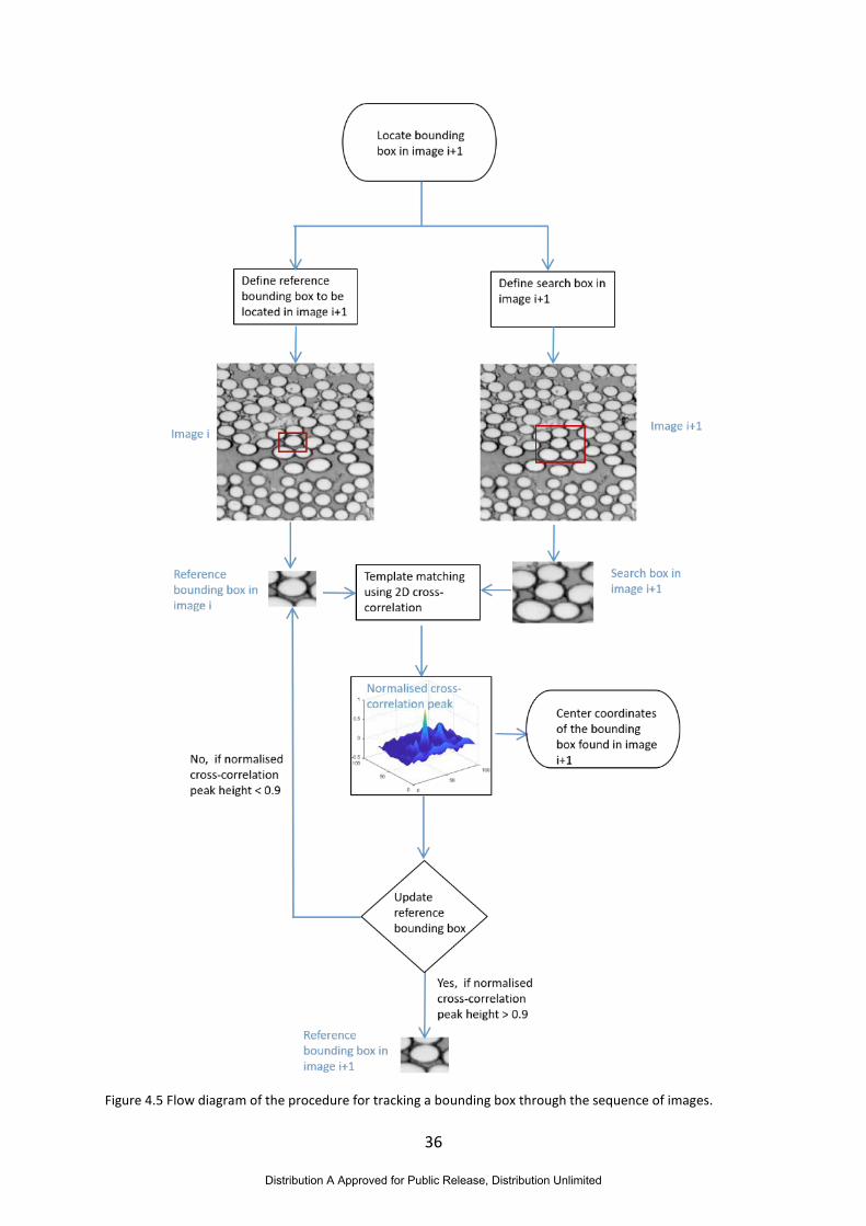
36

Figure 4.5 Flow diagram of the procedure for tracking a bounding box through the sequence of images.


37

Figure 4.6 Plot of normalized cross-correlation peak value for the bounding box tracked through the sequence of one hundred mosaics. The inset (a) shows the bounding box defined in the first mosaic whereas the insets (b-e) show the bounding boxes which were found in mosaic no 44, 49, 91 and 100, respectively, using 2D cross-correlation.

4.3 Characterization and quantitative comparison of fiber orientation fields

The overall orientation of the fibers in the CMC sample were determined by fitting a straight line using the least square method to the coordinates of the fiber (facet in case of the DIC) centers through the sequence of mosaics and applying the inverse tangent function to the gradient of the line. The maps of fiber angles representing the orientation of the fibers in the X-Z and the Y-Z planes are shown in Figure 4.8. It can be observed from these maps that the fibers are primarily orientated in the X-Z plane. The fiber orientation data was found to be Gaussian in nature and was, therefore, modelled using a Gaussian mixture model with two components each representing the two primary fiber orientations in the X-Z plane. The probability density functions (PDFs) shown in Figure 4.9 were determined by fitting a Gaussian mixture model to the fiber orientation data using the Expectation Maximization (EM) algorithm40 in MATLAB. To make a quantitative comparison of the three PDFs, the individual Gaussian peaks were converted into images as shown in Figure 4.10. The orthogonal decomposition was performed on these images using two-hundred Chebyshev kernel functions to represent them as feature vectors. The coefficients of the feature vectors representing the peaks of the PDFs acquired from the DIC and the cross-correlation methods are plotted against the coefficients of PDFs from the rule-based approach in Figure 4.11. For the case when all three PDFs are identical, the data points in these plots would all lie on a diagonal line and have a Pearson correlation coefficient of 1.


38

Figure 4.7 3D Fiber profiles plotted using the fiber center coordinate data acquired from DIC, 2D cross-correlation and the rule-based approach of Bricker et al.


39

Table 4.1 Computation time required to acquire fiber coordinate data

DIC 2D cross-correlation Rule-based approach

Computation time

(hours) Total: 1.27

Ellipse detection: 0.25

Tracking: 1.17

Total: 1.42

Ellipse detection: 25

Total: At least 25

Figure 4.8 The maps of fiber angles in the X-Z (left) and the Y-Z (right) planes acquired using rule-based approach (top), 2D cross-correlation (middle) and DIC (bottom).


40

Figure 4.9 The probability density functions of fiber angle maps shown in Figure 4.8.


41

Figure 4.10 The images of individual peaks acquired from probability density functions shown in Figure 4.9.

The Pearson correlation coefficients between the rule-based and the cross-correlation PDF peaks were found to be slightly higher compared to the ones between the rule-based and the DIC PDF peaks. This is likely due to the fact that DIC tracks the facets rather than the individual fiber cross-sections through the sequence of mosaics, and therefore, inherently samples the profiles of the small group of fibers which lie within a given facet. Despite the lower resolution of the DIC method, it is believed to be more robust in comparison to the other two methods. The rule-based approach projects the position of the fiber center in the next image based on its previous orientation and searches for the fiber cross-section lying nearest to the projected location. If the fiber path is non-linear or the spacing between the two adjacent mosaics is large, then the rule-based method would probably not be able to accurately associate the fiber cross-sections. The cross-correlation based method is likely to give a false match if the fiber density is very high and the fiber cross-sections have little variation in their appearance. DIC, on the other hand, is less sensitive to these issues primarily because it utilizes a second-order shape function which allows for the distortion of the facet during its mapping in the next image. The spacing between the mosaics of the CMC sample analyzed in this work was 1µm and the nominal shifts in the fiber centers between the two adjacent mosaics were also of the order of 1µm. A new sequence of mosaics from a polymer-matrix composite sample has been provided recently by AFRL to further test the capability of DIC in accurately determining the 3D fiber profiles. The maximum spacing between the adjacent mosaics in this


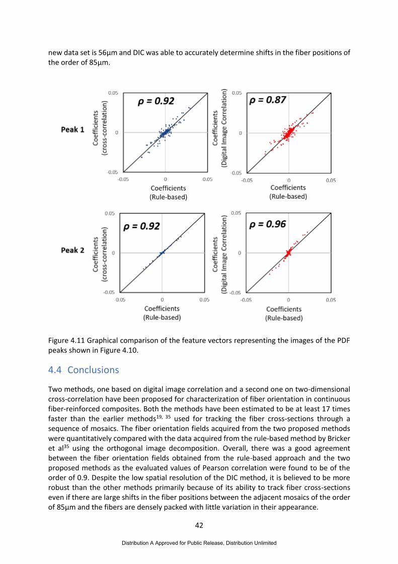
42

new data set is 56µm and DIC was able to accurately determine shifts in the fiber positions of the order of 85µm.

Figure 4.11 Graphical comparison of the feature vectors representing the images of the PDF peaks shown in Figure 4.10.

4.4 Conclusions

Two methods, one based on digital image correlation and a second one on two-dimensional cross-correlation have been proposed for characterization of fiber orientation in continuous fiber-reinforced composites. Both the methods have been estimated to be at least 17 times faster than the earlier methods19, 35 used for tracking the fiber cross-sections through a sequence of mosaics. The fiber orientation fields acquired from the two proposed methods were quantitatively compared with the data acquired from the rule-based method by Bricker et al35 using the orthogonal image decomposition. Overall, there was a good agreement between the fiber orientation fields obtained from the rule-based approach and the two proposed methods as the evaluated values of Pearson correlation were found to be of the order of 0.9. Despite the low spatial resolution of the DIC method, it is believed to be more robust than the other methods primarily because of its ability to track fiber cross-sections even if there are large shifts in the fiber positions between the adjacent mosaics of the order of 85µm and the fibers are densely packed with little variation in their appearance.


43

5 Computationally-efficient tracking of fibers using digital image correlation

5.1 Introduction

It was proposed in the previous chapter that a commercial digital image correlation (DIC) software can be used as a computationally-efficient tool for characterizing fiber orientation from the sequence of mosaics of a serially sectioned continuous fiber reinforced matrix sample. It is important at this stage to define the terms “mosaics”, “images” and “tiles” which will be used frequently in this chapter to describe the serial-section data. Mosaics were constructed by digitally stitching together a grid of images of the sample’s surface acquired using an optical microscope; whereas, tiles in this chapter refer to the rectangular regions which are defined in the mosaics. An exemplar mosaic of the continuous fiber reinforced ceramic matrix composite (CMC) sample, which was constructed by stitching together a grid of 6×6 images, is shown in Figure 5.1.

DIC determines the displacements between the two adjacent mosaics in a sequence by discretizing the reference (first) mosaic into small square regions called facets and tracking their corresponding locations in the next image. In order for the DIC algorithm to accurately track the reference facets in the subsequent mosaics, each facet needs to have a unique grey value pattern. This requirement is fulfilled if the individual optical images used in the construction of the mosaics have a random high contrast pattern. The distribution of fiber cross-sections, which appear as ellipses in the mosaics, provide a sufficiently random high contrast pattern for the DIC to be able to accurately track these fiber cross-sections through the sequence of mosaics. The DIC, in essence, tracks the facets rather than the individual fiber cross-sections and, therefore, provides an average displacement for the small group of fiber cross-sections which lie within the facet.

In the previous chapter, the capability of DIC in accurately characterizing fiber orientations was demonstrated by determining the fiber paths from the mosaic sequence of a CMC sample with an inter-slice gap of 1µm and quantitatively comparing the results with the ones acquired from the rule-based approach by Bricker et.al36. It was also postulated that the proposed DIC method is more robust and would be less likely to fail than the existing fiber tracking algorithms in scenarios where there are a wider gaps between the two adjacent mosaics in a sequence causing large shifts in the fiber positions. This hypothesis was primarily derived from the fact that the facet size, which the DIC algorithm utilizes to track the grey value pattern within a facet, could be adjusted depending on the underlying distribution of the fiber cross-sections and the shift in their locations between the two adjacent mosaics. This chapter describes the work on objective (iv) of this project which was about further exploring the fiber tracking capability of the DIC method and comparing its performance with a state-of-the-art fiber-tracking algorithm in determining fiber paths in the mosaic sequences of two continuous fiber reinforced composite samples.


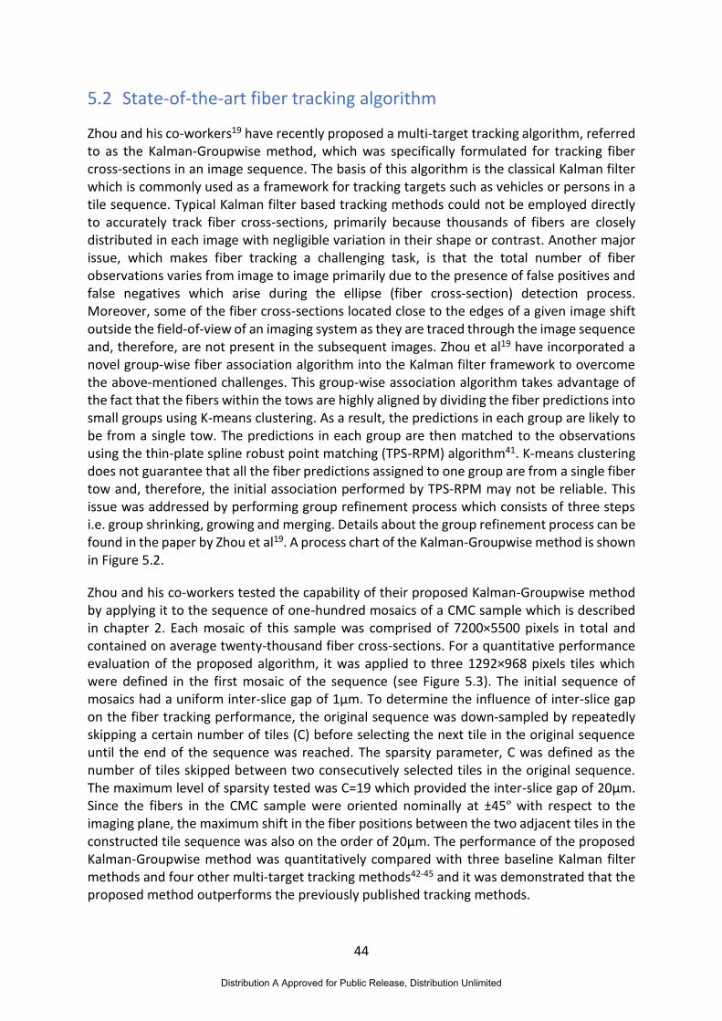
44

5.2 State-of-the-art fiber tracking algorithm

Zhou and his co-workers19 have recently proposed a multi-target tracking algorithm, referred to as the Kalman-Groupwise method, which was specifically formulated for tracking fiber cross-sections in an image sequence. The basis of this algorithm is the classical Kalman filter which is commonly used as a framework for tracking targets such as vehicles or persons in a tile sequence. Typical Kalman filter based tracking methods could not be employed directly to accurately track fiber cross-sections, primarily because thousands of fibers are closely distributed in each image with negligible variation in their shape or contrast. Another major issue, which makes fiber tracking a challenging task, is that the total number of fiber observations varies from image to image primarily due to the presence of false positives and false negatives which arise during the ellipse (fiber cross-section) detection process. Moreover, some of the fiber cross-sections located close to the edges of a given image shift outside the field-of-view of an imaging system as they are traced through the image sequence and, therefore, are not present in the subsequent images. Zhou et al19 have incorporated a novel group-wise fiber association algorithm into the Kalman filter framework to overcome the above-mentioned challenges. This group-wise association algorithm takes advantage of the fact that the fibers within the tows are highly aligned by dividing the fiber predictions into small groups using K-means clustering. As a result, the predictions in each group are likely to be from a single tow. The predictions in each group are then matched to the observations using the thin-plate spline robust point matching (TPS-RPM) algorithm41. K-means clustering does not guarantee that all the fiber predictions assigned to one group are from a single fiber tow and, therefore, the initial association performed by TPS-RPM may not be reliable. This issue was addressed by performing group refinement process which consists of three steps i.e. group shrinking, growing and merging. Details about the group refinement process can be found in the paper by Zhou et al19. A process chart of the Kalman-Groupwise method is shown in Figure 5.2.

Zhou and his co-workers tested the capability of their proposed Kalman-Groupwise method by applying it to the sequence of one-hundred mosaics of a CMC sample which is described in chapter 2. Each mosaic of this sample was comprised of 7200×5500 pixels in total and contained on average twenty-thousand fiber cross-sections. For a quantitative performance evaluation of the proposed algorithm, it was applied to three 1292×968 pixels tiles which were defined in the first mosaic of the sequence (see Figure 5.3). The initial sequence of mosaics had a uniform inter-slice gap of 1µm. To determine the influence of inter-slice gap on the fiber tracking performance, the original sequence was down-sampled by repeatedly skipping a certain number of tiles (C) before selecting the next tile in the original sequence until the end of the sequence was reached. The sparsity parameter, C was defined as the number of tiles skipped between two consecutively selected tiles in the original sequence. The maximum level of sparsity tested was C=19 which provided the inter-slice gap of 20µm. Since the fibers in the CMC sample were oriented nominally at ±45º with respect to the imaging plane, the maximum shift in the fiber positions between the two adjacent tiles in the constructed tile sequence was also on the order of 20µm. The performance of the proposed Kalman-Groupwise method was quantitatively compared with three baseline Kalman filter methods and four other multi-target tracking methods42-45 and it was demonstrated that the proposed method outperforms the previously published tracking methods.


45

Since it was established by Zhou et al that their novel Kalman-Groupwise algorithm clearly outperforms the existing state-of-the-art multi-target tracking methods, their algorithm was selected in this work to compare its performance against the DIC method in tracking fiber paths in two continuous fiber reinforced composite samples.

Figure 5.1 Mosaic of the CMC sample constructed by stitching together a grid of 6×6 optical images with each one having the dimensions of 1292×968 pixels.


In this work, mosaic sequences of two material samples were analyzed. The first sequence was obtained by serially sectioning a 3.6 x 2.6 x 0.1 mm volume of a CMC material in 1µm increments. The fibers in this sample were orientated nominally at ±45º from the sectioning plane. This sequence contained one-hundred mosaics in total and each mosaic was 7200 x 5500 pixels in size. The second mosaic sequence was obtained by serially sectioning a 24.5 x 2.6 x 1.1 mm volume of a carbon fiber-reinforced polymer matrix composite (PMC) laminate consisting of twenty unidirectional plies with a [±15/45/±75]2s layup, defined with respect to the sectioning plane. This sequence contained 206 mosaics in total and each mosaic comprised of 73148 × 7653 pixels. The inter-slice gap in this sequence was non-uniform and ranged from 1.1-56µm.

The mosaics of the PMC sample were 14 times bigger than that of the CMC sample. Hence, the PMC mosaics were divided into four sections by slicing them along their longest dimension and only the first quarter of the mosaics with dimensions of 18287 × 7653 pixels were considered for fiber-tracking analysis. The resolution of the mosaics for both the material samples were exceptionally high compared to images used routinely in DIC; and hence, the resolution of the CMC and the PMC mosaics were reduced from 0.5 and 0.335 µm/pixel to 1 and 0.67 µm/pixel, respectively, by averaging the intensity of tiles consisting of two-by-two


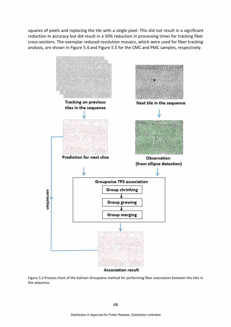
46

squares of pixels and replacing the tile with a single pixel. This did not result in a significant reduction in accuracy but did result in a 50% reduction in processing times for tracking fiber cross-sections. The exemplar reduced resolution mosaics, which were used for fiber tracking analysis, are shown in Figure 5.4 and Figure 5.5 for the CMC and PMC samples, respectively.

Figure 5.2 Process chart of the Kalman-Groupwise method for performing fiber association between the tiles in the sequence.


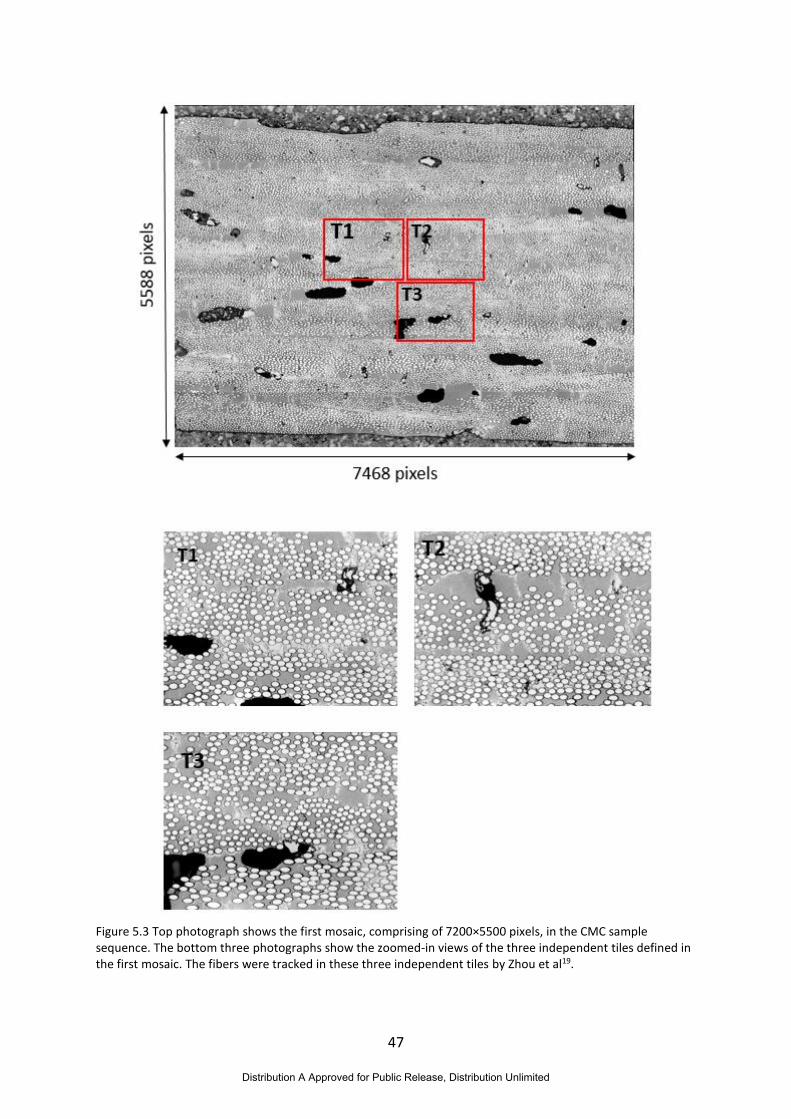
47

Figure 5.3 Top photograph shows the first mosaic, comprising of 7200×5500 pixels, in the CMC sample sequence. The bottom three photographs show the zoomed-in views of the three independent tiles defined in the first mosaic. The fibers were tracked in these three independent tiles by Zhou et al19.


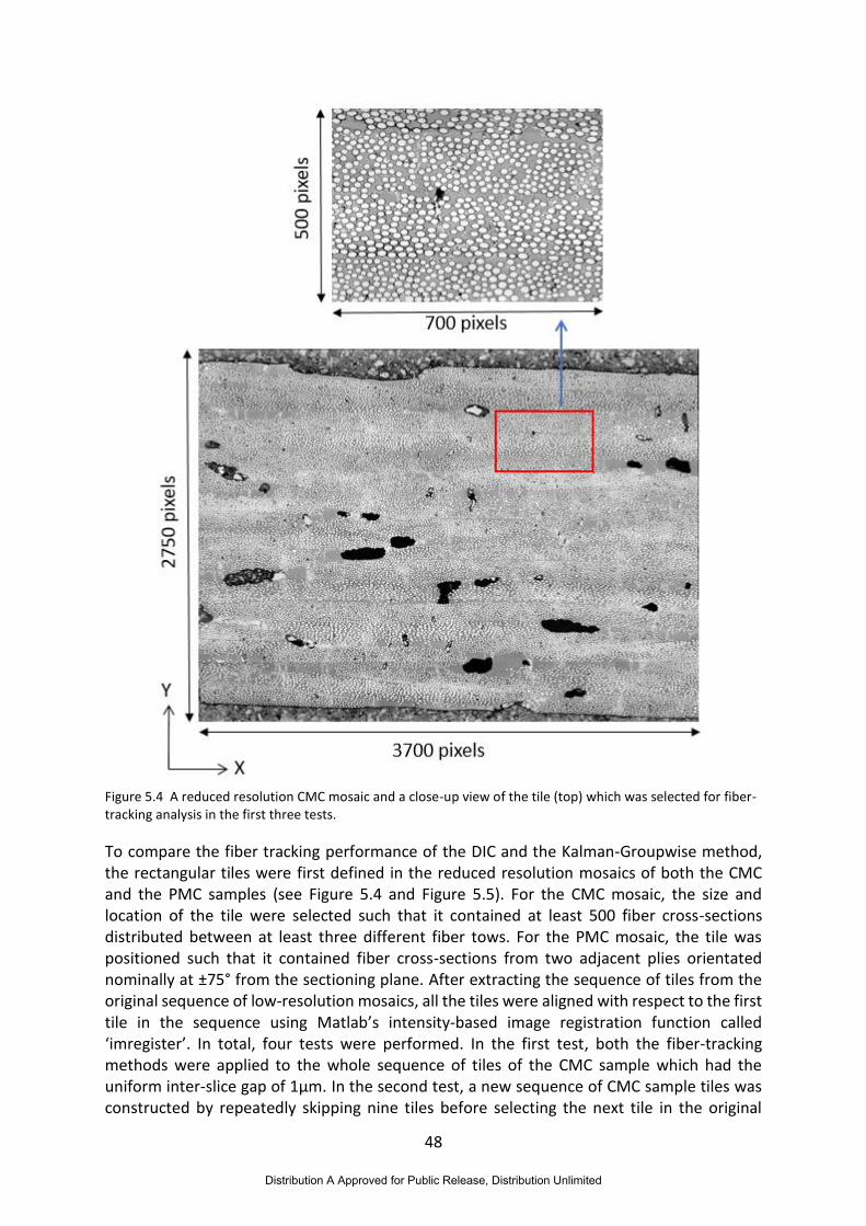
48

Figure 5.4 A reduced resolution CMC mosaic and a close-up view of the tile (top) which was selected for fiber-tracking analysis in the first three tests.

To compare the fiber tracking performance of the DIC and the Kalman-Groupwise method, the rectangular tiles were first defined in the reduced resolution mosaics of both the CMC and the PMC samples (see Figure 5.4 and Figure 5.5). For the CMC mosaic, the size and location of the tile were selected such that it contained at least 500 fiber cross-sections distributed between at least three different fiber tows. For the PMC mosaic, the tile was positioned such that it contained fiber cross-sections from two adjacent plies orientated nominally at ±75° from the sectioning plane. After extracting the sequence of tiles from the original sequence of low-resolution mosaics, all the tiles were aligned with respect to the first tile in the sequence using Matlab’s intensity-based image registration function called ‘imregister’. In total, four tests were performed. In the first test, both the fiber-tracking methods were applied to the whole sequence of tiles of the CMC sample which had the uniform inter-slice gap of 1µm. In the second test, a new sequence of CMC sample tiles was constructed by repeatedly skipping nine tiles before selecting the next tile in the original


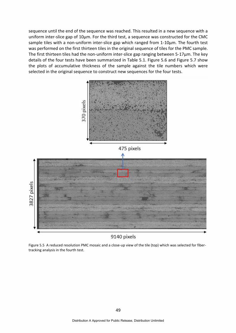
49

sequence until the end of the sequence was reached. This resulted in a new sequence with a uniform inter-slice gap of 10µm. For the third test, a sequence was constructed for the CMC sample tiles with a non-uniform inter-slice gap which ranged from 1-10µm. The fourth test was performed on the first thirteen tiles in the original sequence of tiles for the PMC sample. The first thirteen tiles had the non-uniform inter-slice gap ranging between 5-17µm. The key details of the four tests have been summarized in Table 5.1. Figure 5.6 and Figure 5.7 show the plots of accumulative thickness of the sample against the tile numbers which were selected in the original sequence to construct new sequences for the four tests.

Figure 5.5 A reduced resolution PMC mosaic and a close-up view of the tile (top) which was selected for fiber-tracking analysis in the fourth test.


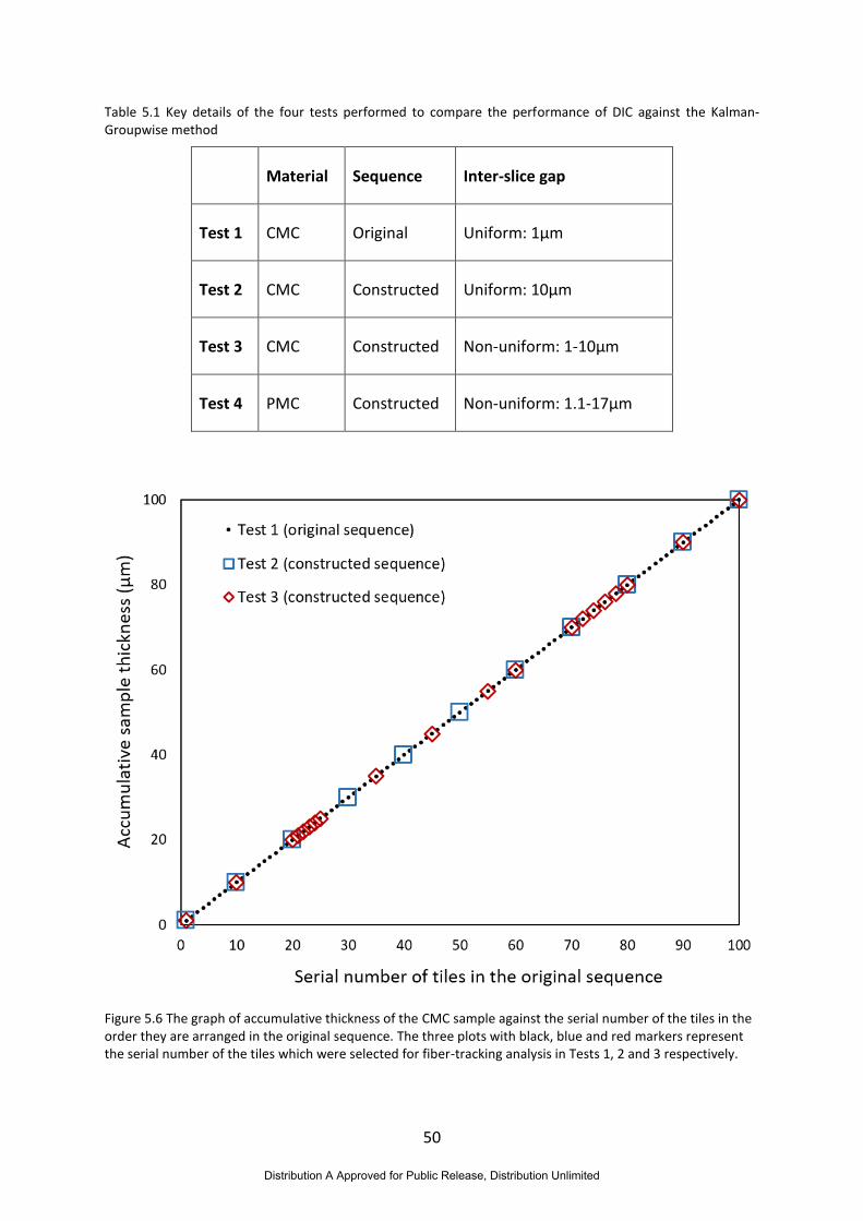
50

Table 5.1 Key details of the four tests performed to compare the performance of DIC against the Kalman-Groupwise method

Material Sequence Inter-slice gap

Test 1 CMC Original Uniform: 1µm

Test 2 CMC Constructed Uniform: 10µm

Test 3 CMC Constructed Non-uniform: 1-10µm

Test 4 PMC Constructed Non-uniform: 1.1-17µm

Figure 5.6 The graph of accumulative thickness of the CMC sample against the serial number of the tiles in the order they are arranged in the original sequence. The three plots with black, blue and red markers represent the serial number of the tiles which were selected for fiber-tracking analysis in Tests 1, 2 and 3 respectively.


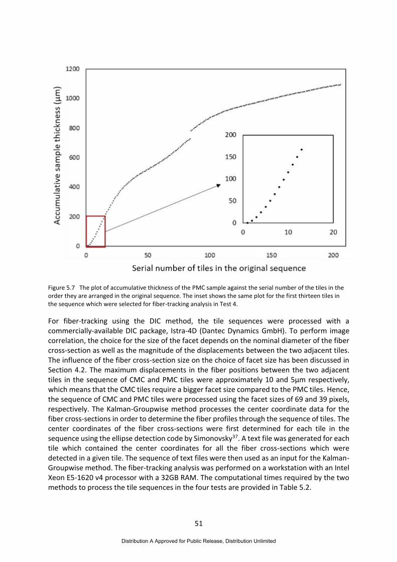
51

Figure 5.7 The plot of accumulative thickness of the PMC sample against the serial number of the tiles in the order they are arranged in the original sequence. The inset shows the same plot for the first thirteen tiles in the sequence which were selected for fiber-tracking analysis in Test 4.

For fiber-tracking using the DIC method, the tile sequences were processed with a commercially-available DIC package, Istra-4D (Dantec Dynamics GmbH). To perform image correlation, the choice for the size of the facet depends on the nominal diameter of the fiber cross-section as well as the magnitude of the displacements between the two adjacent tiles. The influence of the fiber cross-section size on the choice of facet size has been discussed in Section 4.2. The maximum displacements in the fiber positions between the two adjacent tiles in the sequence of CMC and PMC tiles were approximately 10 and 5µm respectively, which means that the CMC tiles require a bigger facet size compared to the PMC tiles. Hence, the sequence of CMC and PMC tiles were processed using the facet sizes of 69 and 39 pixels, respectively. The Kalman-Groupwise method processes the center coordinate data for the fiber cross-sections in order to determine the fiber profiles through the sequence of tiles. The center coordinates of the fiber cross-sections were first determined for each tile in the sequence using the ellipse detection code by Simonovsky37. A text file was generated for each tile which contained the center coordinates for all the fiber cross-sections which were detected in a given tile. The sequence of text files were then used as an input for the Kalman-Groupwise method. The fiber-tracking analysis was performed on a workstation with an Intel Xeon E5-1620 v4 processor with a 32GB RAM. The computational times required by the two methods to process the tile sequences in the four tests are provided in Table 5.2.


52

5.4 Results and Discussion

It is important to reiterate here that, unlike the Kalman-Groupwise method, DIC does not track the individual fiber cross-sections; instead, it tracks a group of fiber cross-sections which lie within a square-shaped facet which is defined in the first (reference) mosaic of a sequence. This distinction between the two methods should be kept in mind while interpreting the results discussed in this section. The comparison between the 3D fiber profiles determined using the DIC and the Kalman-Groupwise method for the first three tests, performed on the CMC tile sequences, is shown in Figure 5.8 and for the fourth test, performed on the PMC tile sequence, it is shown in Figure 5.9.

The fibers present in the CMC data are distributed between three fiber tows and are orientated predominately in the x-z plane at nominally ±45º from the sectioning (imaging) plane, whereas the fibers in the PMC tiles belong to the two unidirectional fiber plies which are orientated at nominally ±75º from the sectioning plane. The left-hand side plots in Figure 5.8 and Figure 5.9 clearly show that the DIC has correctly determined the global orientation of the fibers in both the samples. Kalman Groupwise method, on the other hand, worked only in the first two tests which involved sequences of CMC data with uniform inter-slice gap of 1 and 10 µm respectively. To further investigate, the influence of inter-slice gap on the fiber tracking performance of both the methods, the global angles of individual fibers (facets in the case of DIC) were first calculated in both the x-z and the y-z planes by fitting a least squares regression line to the fiber coordinate data. Since the distribution of the fiber angles were found to be Gaussian in nature, the probability density function (PDF) was determined by fitting a bivariate Gaussian mixture model to the fiber angle data. The PDFs of the fiber angles acquired using the DIC and the Kalman-Groupwise method for the first three tests, which involved CMC data, are shown in Figure 5.10. The PDFs obtained from DIC for the three tests appear to be identical which implies that the tracking performance of DIC is not significantly influenced by the inter-slice gap. In contrast, Kalman-Groupwise method seemed to correctly predict the overall orientation of the fibers in the first two tests; however, there is a significant scatter in the fiber angle data for the second test which caused a significant change in the PDF shape compared to the PDF for the first test (see right-hand side PDFs of the first two rows in Figure 5.10). This suggests that even a uniform increase in the inter-slice gap adversely affects the tracking performance of the Kalman-Groupwise method. The prediction model used in the Kalman-Groupwise method assumes a constant shift in the fiber positions between any two adjacent images in a sequence. This explains its complete failure in tracking fibers in the last two tests which involved tile sequences with non-uniform inter-slice gaps. This assumption basically means that the Kalman-Groupwise method considers the fibers to be perfectly straight and is, therefore, probably not capable of identifying anomalous behavior in the fibers such as curvature or localized waviness.


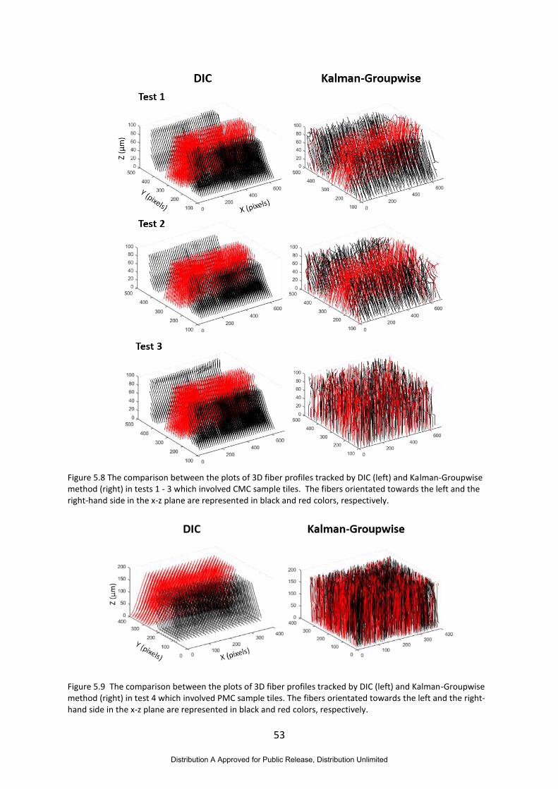
53

Figure 5.8 The comparison between the plots of 3D fiber profiles tracked by DIC (left) and Kalman-Groupwise method (right) in tests 1 - 3 which involved CMC sample tiles. The fibers orientated towards the left and the right-hand side in the x-z plane are represented in black and red colors, respectively.

Figure 5.9 The comparison between the plots of 3D fiber profiles tracked by DIC (left) and Kalman-Groupwise method (right) in test 4 which involved PMC sample tiles. The fibers orientated towards the left and the right-hand side in the x-z plane are represented in black and red colors, respectively.


54

Table 5.2 Processing times required by DIC and Kalman-Groupwise method in tracking fiber cross-sections in the four tests.

Processing time (hours)

DIC

Processing time (hours)

Kalman-Groupwise

Test 1 0.22 19

Test 2 0.05 2

Test 3 0.07 3

Test 4 0.02 20

The fiber-tracking capability of the DIC method was further explored by applying it to the whole sequence of PMC mosaics. The PMC sample contained in total twenty unidirectional plies with three distinct orientations i.e. nominally ±15º, 45º and ±75º with respect to the sectioning plane. It was not possible to track fibers in those plies which were orientated at a shallow angle of ±15º from the sectioning plane. As a consequence of this shallow angle, the maximum displacement in the fiber positions between the two adjacent mosaics was of the order of 300 pixels, which is quite large for the DIC algorithm to track. Such large displacements could potentially be determined using DIC in this case; however, the size of the facet would need to be larger than the magnitude of the displacements to be determined. In this case, it was not possible to use a large facet size because the choice of facet size was limited by the width of the ply which was approximately 200 pixels. For the plies orientated at 45° and ±75°, the maximum displacements in the fiber positions between the two adjacent mosaics were approximately 85 and 25 pixels; hence, the fibers in these two types of plies were tracked using a facet size of 121 and 69 pixels, respectively. The 3D fiber profiles in the PMC sample determined using DIC are shown in Figure 5.11.

In Chapter 4, the orientation of the fibers in the CMC sample was analyzed by assuming their profile to be linear. This assumption was justified since the depth (height) of the CMC sample was only 100µm. The depth of the PMC sample was 10 times that of the CMC sample and, therefore, the fibers in the PMC sample cannot be assumed to have a linear profile. Hence, these fibers were treated as curves in 3D space. The depth of the PMC sample was divided into ten segments of 100µm each (see top schematic in Figure 5.12). For each segment, the direction vector representing the local orientation of the fibers in that segment were determined using Matlab’s standard function for principal component analysis called ‘pca’. The bottom schematic in Figure 5.12 shows the two angles of the direction vector i.e. θxy and θxz, defined with respect to the x-y and the x-z planes respectively, which were calculated to establish the local orientation of the fibers in 3D space. Since the fibers in the PMC sample


55

were predominantly orientated in the x-z plane, θxz is expected to be nominally 0° whereas θxy gives the angle at which the fibers are locally orientated with respect to the sectioning plane.

Figure 5.10 The probability density functions for the fiber angle data acquired from DIC (left) and Kalman-Groupwise method (right) for Test 1 (top), Test 2 (middle) and Test 3 (bottom).

For every ply, the nominal orientation of the fibers in each of the ten segments was determined by taking an average of θxy and θxz for all the fibers in that ply. Figure 5.13 and Figure 5.14 show the plots of average values of θxy and θxz against the depth of the sample for all the plies which the DIC was able to successfully process. If the fibers in a given ply are perfectly straight, the average value for θxy would be constant through the depth of the sample. However, a periodic variation in θxy could be observed from the plots in Figure 5.13. This periodic variation appears to be greater than the error bars representing the scatter in fiber angles, in particular, for the plies orientated at 45° and +75° (see top two graphs in Figure


56

5.13) which implies the presence of in-plane waviness in the fibers. The fibers are expected to be orientated in the x-z plane which is the reason why θxz is nominally zero for plies orientated at 45° (see top plot in Figure 5.14); however, for the plies orientated at ±75°, θxz shows a slight increase towards one of the ends of the sample. This indicates that the fibers in these plies have a slight out-of-plane curvature towards one of the ends of the sample. To further explore and visualize the presence of in-plane waviness which the periodic variation in the θxy plots suggests, the 2D profiles for a small group of fibers taken from a single ply were constructed using their θxy values. These 2D fiber profiles are shown for three plies, orientated at 45°, -75° and +75°, in Figure 5.15. The in-plane waviness appears to be very consistent among fibers in all three plies which means that it is unlikely to be an artefact from the DIC measurements. Since carbon fibers typically have a very high stiffness and their profiles through the depth of the PMC sample are expected to be perfectly straight, a potential cause for the observed waviness in their profiles can be the inherent uncertainty in the grinding process of the automated serial sectioning system which, in turn, would induce uncertainty in the spacing between the adjacent mosaics.

Figure 5.11 The plot of 3D profiles of the fibers tracked in the sequence of PMC mosaics using DIC. The fibers which are orientated nominally at +45°, -75° and +75° from the sectioning (x-y) plane are represented in red, blue and black colors, respectively.


57

Figure 5.12 Top schematic shows the fiber profile through the depth of the PMC sample which was assumed as a curve in 3D space. Bottom schematic shows the direction vector representing the fiber segment which was used to describe the local orientation of the fiber in 3D space.


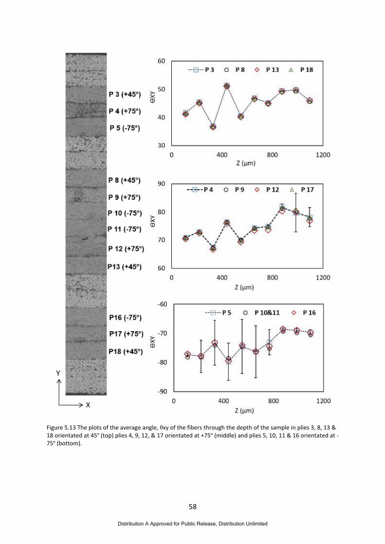
58

Figure 5.13 The plots of the average angle, θxy of the fibers through the depth of the sample in plies 3, 8, 13 & 18 orientated at 45º (top) plies 4, 9, 12, & 17 orientated at +75º (middle) and plies 5, 10, 11 & 16 orientated at -75º (bottom).


59

Figure 5.14 The plots of the average angle, θxz of the fibers through the depth of the sample in plies 3, 8, 13 & 18 orientated at 45º (top) plies 4, 9, 12, & 17 orientated at +75º (middle) and plies 5, 10, 11 & 16 orientated at -75º (bottom).


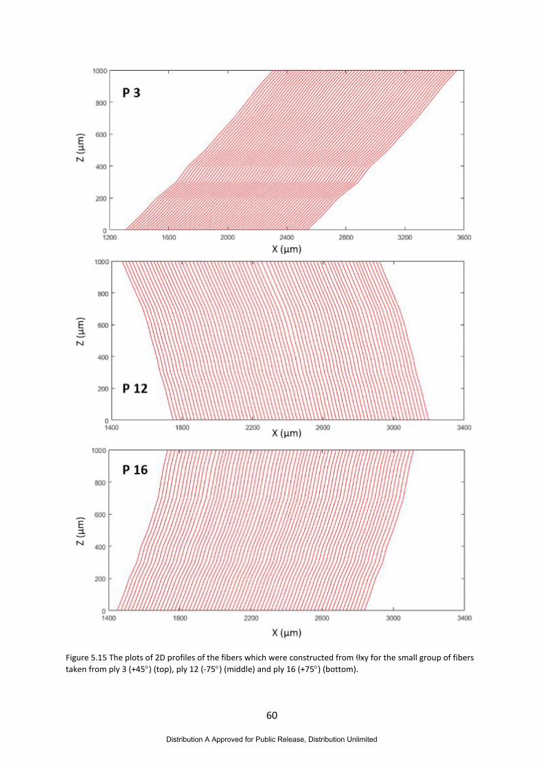
60

Figure 5.15 The plots of 2D profiles of the fibers which were constructed from θxy for the small group of fibers

taken from ply 3 (+45) (top), ply 12 (-75) (middle) and ply 16 (+75) (bottom).


61

5.5 Conclusions

The fiber tracking capability of the DIC method was compared with the state-of-the-art Kalman-Groupwise method by applying them to the tile sequences of two continuous fiber-reinforced composite samples. In total four tests were performed to investigate the influence of inter-slice gap on the tracking performance of both the methods. In the first two tests, tile sequences of the CMC sample with a uniform inter-slice gap of 1 and 10µm were used. The second and the third tests involved the tile sequences of the CMC and the PMC samples with a non-uniform inter-slice gap ranging between 1-10µm and 1.1-17µm, respectively. The processing times for both the methods were recorded and DIC was found to be at least 40 times faster than the Kalman-Groupwise method. The prediction model, which the Kalman-Groupwise method relies upon, assumes a constant shift in the fiber positions between any two adjacent mosaics in a sequence. This assumption was the primary reason for its complete failure in determining fiber orientations in the last two tests. Since DIC does not rely on any prediction model, it successfully determined fiber orientations in all four tests and its performance was not significantly affected by any variation in the inter-slice gap. Once it was established that DIC clearly outperforms the Kalman-Groupwise method, it was applied to track fibers from the whole sequence of mosaics of the PMC sample. Further analysis of the tracking results acquired from DIC suggested the presence of in-plane waviness and slight out-of-plane curvature in the fibers of the PMC sample. The presence of in-plane waviness and slight out-of-plane curvature could potentially be an artefact due to errors in the spacing between the mosaics resulting from coarse grinding of the sample’s surface in the automated serial sectioning system.


62

6 Analysis of 3D data fields using orthogonal decomposition

6.1 Introduction

This chapter reports the work on objective (v) of this project which was about the orthogonal decomposition of 3D data obtained from X-ray CT scans of the microstructure of a CMC sample. The first step in this task was to develop an orthogonal decomposition algorithm capable of decomposing a 3D data field to represent it as a feature vector. It was initially proposed to explore the use of this algorithm in representing voids in the microstructure as feature vectors in order to relate them to the orientation of the fibers in the sample. It was later decided to apply the algorithm instead to 3D displacement and strain distributions, measured using the Digital Volume Correlation technique, in a nylon-reinforced rubber matrix composite sample and include a recently developed quantitative validation approach46 to validate the computational model which predicts the internal deformation behavior of the same rubber matrix sample.

6.2 Algorithm for orthogonal decomposition of volumetric data

In 2D orthogonal decomposition, a data field is treated as an image and a set of polynomials are used to define the image such that only the coefficients of these polynomials, which are collated to form a feature vector, are required to accurately represent the data field. This not only significantly reduces the dimensionality of the data but also allows for straightforward quantitative comparison between the data fields as the feature vector obtained through orthogonal decomposition are invariant to scale, translation, and orientation of the images47.

In the past, Patterson and his co-workers have used orthogonal decomposition extensively on the 2D data fields acquired from full-field optical measurement techniques for the purpose of finite element model updating10, quantitative validation of computational mechanics models12-14 and comparison of modal behavior at room and elevated temperatures15. It has also been used in the development of novel strain-based approaches for determining the onset of damage in glass-fiber reinforced composites16 and predicting the residual strength of impacted carbon-fiber reinforced composites33. In this work a substantial innovative step has been taken to extend the orthogonal decomposition technique to three dimensions. This would allow the decomposition of 3D data fields which are typically obtained from techniques such an X-ray computed tomography, automated serial sectioning and magnetic resonance imaging. 3D orthogonal decomposition would also be applicable on 2D data fields which vary in the temporal domain and, for the purpose of decomposition, can be treated as 3D data fields.

The algorithm for 3D orthogonal decomposition was developed by Christian and is briefly explained here. Three-dimensional kernel functions are required to decompose a three-dimensional grid of data. These kernels are formed from the one-dimensional discrete Chebyshev polynomials, which are defined using the recursive formula47:


63

𝑡𝑚(𝑥) =(2𝑚 − 1)𝑡1(𝑥)𝑡𝑚−1(𝑥) − (𝑚 − 1) (1 −

(𝑚 − 1)2

𝑀2 ) 𝑡𝑚−2(𝑥)

𝑚, 𝑚 = 2, 3,⋯ ,𝑀 − 1

(6.1)

𝑡0(𝑥) = 1 (6.2)

𝑡1(𝑥) =2𝑥+1−𝑀

𝑀 (6.3)

where 𝑚, is the order of the polynomial and 𝑀, the number of sampling points. These discrete polynomials can be combined to obtain a three-dimensional orthogonal kernel, of dimensions 𝑀 × 𝑁 × 𝑂, using:

𝒯𝑚,𝑛,𝑜(𝑥, 𝑦, 𝑧) = 𝑡𝑚(𝑥)𝑡𝑛(𝑦)𝑡𝑜(𝑧) (6.4)

where 𝑚, 𝑛 and 𝑜 are the order of the one-dimensional polynomials. When combined, the order of the three-dimensional kernel is calculated as:

𝜔𝑚,𝑛,𝑜 = 𝑚 + 𝑛 + 𝑜 (6.5)

To use the orthogonal kernels for decomposition they must first be normalized by dividing each kernel by its associated norm, and given as:

𝒫𝑚,𝑛,𝑜 = 𝜌𝑚𝜌𝑛𝜌𝑜 (6.6)

𝜌𝑚 =𝑀(1−

1

𝑀2)(1−

22

𝑀2)⋯(1−

𝑚2

𝑀2)

2𝑚+1 (6.7)

The data can then be decomposed into coefficients, 𝑇𝑚𝑛𝑜, using:

𝑻𝒎,𝒏,𝒐 = ∑ 𝑰(𝒙, 𝒚, 𝒛)𝟏

√𝑴𝑵𝑶

𝓣𝒎,𝒏,𝒐(𝒙,𝒚,𝒛)

√𝓟𝒎,𝒏,𝒐

𝑴,𝑵,𝑶𝒙,𝒚,𝒛=𝟎 (6.8)

The √𝑀𝑁𝑂 term in equation (5.8) is used to scale the coefficients so that they are relatable to the uncertainty of the measurement system. This also simplifies the calculation of the representation error when filtering the feature vectors by setting insignificant coefficients to zero, which is described in the next section. The reconstruction of the image is calculated as:

𝐼(𝑥, 𝑦, 𝑧) = ∑ 𝑇𝑚,𝑛,𝑜√𝑀𝑁𝑂𝒯𝑚,𝑛,𝑜(𝑥,𝑦,𝑧)

√𝒫𝑚,𝑛,𝑜

𝑀,𝑁,𝑂𝑚,𝑛,𝑜=0 (6.9)

The coefficients are arranged as a three-dimensional matrix, these can be permuted using the ordering system described by Bateman48 which has been extended here to three dimensions. Using this system, the coefficient 𝑇𝑚,𝑛,𝑜 comes before 𝑇𝑝,𝑞,𝑟 in the feature vector if either of

the following conditions are true:

𝜔𝑚,𝑛,𝑜 < 𝜔𝑝,𝑞,𝑟 (6.10)

(𝜔𝑚,𝑛,𝑜 = 𝜔𝑝,𝑞,𝑟) ∧ (𝑚 + 𝑛𝑁 + 𝑜𝑁𝑂 < 𝑝 + 𝑞𝑁 + 𝑟𝑁𝑂) (6.11)

where ∧, is the mathematical notation for “logical and”. This results in a feature vector 𝑓, ordered as follows:


64

𝒇 =

{

𝑇0,0,0𝑇1,0,0𝑇0,1,0𝑇0,0,1𝑇2,0,0𝑇1,1,0⋮

𝑇𝑀−1,𝑁−1,𝑂−1}

(6.12)

The number of coefficients in the feature vector, f, when using all the kernels up to a maximum order of 𝜔𝑚𝑎𝑥 is calculated as:

𝛺 =1

6𝜔𝑚𝑎𝑥

3 + 𝜔𝑚𝑎𝑥2 +

11

6𝜔𝑚𝑎𝑥 + 1 (6.13)

This equation can be inverted using the cubic equation, resulting in two imaginary roots and a single real root equal to the order of the polynomials required to populate a feature vector of any arbitrary length.

6.2.1 Representation error

The representation error is the difference between the original data volume and its reconstruction. When reconstructing real-valued data, a common technique for quantifying the representation error is to use the root mean squared error, calculated as:

𝑢𝑟𝑚𝑠 = √1

𝑀𝑁𝑂∑ (𝐼(𝑥, 𝑦, 𝑧) − 𝐼(𝑥, 𝑦, 𝑧))2

𝑀,𝑁,𝑂

𝑥,𝑦,𝑧=0 (6.14)

This measure can also be used for assessing the reconstruction of binary volumes of data. However, in this situation the mean absolute error is more effective as it calculates the proportion of incorrect voxels in the reconstruction. The mean absolute error is given as:

𝑢𝑚𝑎𝑒 =1

𝑀𝑁𝑂∑ |𝐼(𝑥, 𝑦, 𝑧) − 𝐼𝑏𝑖𝑛(𝑥, 𝑦, 𝑧)|

𝑀,𝑁,𝑂

𝑥,𝑦,𝑧=0 (6.15)

The feature vectors can be filtered by truncating them at a particular length13 or setting all coefficients that have an absolute value less than a threshold to zero33, 49. When filtering a feature vector, it is necessary to calculate the representation error to assess whether additional filtering is appropriate to further reduce the number of elements in the vector while satisfying the requirements for the quality of the representation. This requires repetitive calculations of equation (6.10), greatly increasing the computation time. As the kernels used to represent the data volume are orthogonal the representation error can be calculated without actually reconstructing the data using Parseval’s theorem as48:

𝑢𝑟𝑚𝑠 = √1

𝑀𝑁𝑂∑ 𝐼(𝑥, 𝑦, 𝑧)2𝑀,𝑁,𝑂𝑥,𝑦,𝑧=0 − ∑ 𝑓𝑖

2

𝑖 (6.16)

where �� denotes the filtered feature vector. Using this equation, it is possible to decompose a volume into a feature vector containing a high number of coefficients and then rapidly determine the minimum number of coefficients required to just achieve an arbitrary representation error.


65

6.2.2 Computationally-efficient decomposition using matrix operations

Decomposition and reconstruction using equations (6.8) and (6.10) are computationally-intensive tasks as they require many iterations and substantial amounts of computer memory. The computation of the coefficients can be performed more efficiently using matrix operations, which can be calculated using concurrent computation. If the data is considered as a three-dimensional array, the zth slice through the array 𝐼𝑥,𝑦,𝑧, can be denoted as:

𝑺𝑥,𝑦 = 𝑰𝑥,𝑦,(𝑧) (6.17)

where the bracketed term specifies the index for the slice location. These slices are then decomposed along both dimensions and placed in a new three-dimensional array 𝑬𝑚,𝑛,𝑧, by performing50:

𝑬𝑚,𝑛,(𝑧) = 𝒕𝑥𝑺𝑥,𝑦𝒕𝑦∗ (6.18)

where ∗ indicates the matrix transpose and 𝒕𝑥 and 𝒕𝑦 are orthogonal matrices with rows equal

to the one-dimensional Chebyshev polynomials:

𝒕𝑥 =

{

𝑡0(𝑥)

√𝜌0

𝑡1(𝑥)

√𝜌1

⋮𝑡𝑀−1(𝑥)

√𝜌𝑀−1 }

, 𝑥 = {0, 1, 2, … ,𝑀 − 1} (6.19)

𝒕𝑦 =

{

𝑡0(𝑦)

√𝜌0

𝑡1(𝑦)

√𝜌1

⋮𝑡𝑁−1(𝑦)

√𝜌𝑁−1 }

, 𝑦 = {0, 1, 2, … , 𝑁 − 1} (6.20)

The three-dimensional array 𝑬𝑚,𝑛,𝑧, is then decomposed in the z-direction by performing:

𝑻𝑚,𝑛,(𝑜) =1

√𝑀𝑁𝑂(𝒕𝑧𝑬𝑚,(𝑛),𝑧

∗)∗ (6.21)

where,

𝒕𝑧 =

{

𝑡0(𝑧)

√𝜌0𝑡1(𝑧)

√𝜌1⋮

𝑡𝑂−1(𝑧)

√𝜌𝑂−1 }

, 𝑧 = {0, 1, 2, … , 𝑂 − 1} (6.22)

The three-dimensional array 𝑻 contains the same coefficients as obtained using equation (6.8) and can be permuted to a feature vector using the same conditions described by equations (6.10) and (6.11). This results in a significant decrease in computation time. For example,


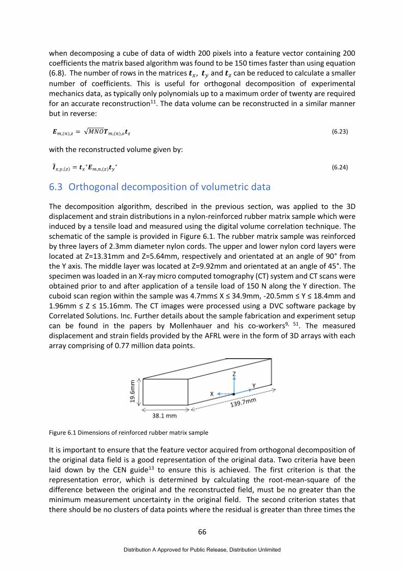
66

when decomposing a cube of data of width 200 pixels into a feature vector containing 200 coefficients the matrix based algorithm was found to be 150 times faster than using equation (6.8). The number of rows in the matrices 𝒕𝑥, 𝒕𝑦 and 𝒕𝑧 can be reduced to calculate a smaller

number of coefficients. This is useful for orthogonal decomposition of experimental mechanics data, as typically only polynomials up to a maximum order of twenty are required for an accurate reconstruction11. The data volume can be reconstructed in a similar manner but in reverse:

𝑬𝑚,(𝑛),𝑧 = √𝑀𝑁𝑂𝑻𝑚,(𝑛),𝑜𝒕𝑧 (6.23)

with the reconstructed volume given by:

��𝑥,𝑦,(𝑧) = 𝒕𝑥∗𝑬𝑚,𝑛,(𝑧)𝒕𝑦

∗ (6.24)

6.3 Orthogonal decomposition of volumetric data

The decomposition algorithm, described in the previous section, was applied to the 3D displacement and strain distributions in a nylon-reinforced rubber matrix sample which were induced by a tensile load and measured using the digital volume correlation technique. The schematic of the sample is provided in Figure 6.1. The rubber matrix sample was reinforced by three layers of 2.3mm diameter nylon cords. The upper and lower nylon cord layers were located at Z=13.31mm and Z=5.64mm, respectively and orientated at an angle of 90° from the Y axis. The middle layer was located at Z=9.92mm and orientated at an angle of 45°. The specimen was loaded in an X-ray micro computed tomography (CT) system and CT scans were obtained prior to and after application of a tensile load of 150 N along the Y direction. The cuboid scan region within the sample was 4.7mm≤ X ≤ 34.9mm, -20.5mm ≤ Y ≤ 18.4mm and 1.96mm ≤ Z ≤ 15.16mm. The CT images were processed using a DVC software package by Correlated Solutions. Inc. Further details about the sample fabrication and experiment setup can be found in the papers by Mollenhauer and his co-workers9, 51. The measured displacement and strain fields provided by the AFRL were in the form of 3D arrays with each array comprising of 0.77 million data points.

Figure 6.1 Dimensions of reinforced rubber matrix sample

It is important to ensure that the feature vector acquired from orthogonal decomposition of the original data field is a good representation of the original data. Two criteria have been laid down by the CEN guide13 to ensure this is achieved. The first criterion is that the representation error, which is determined by calculating the root-mean-square of the difference between the original and the reconstructed field, must be no greater than the minimum measurement uncertainty in the original field. The second criterion states that there should be no clusters of data points where the residual is greater than three times the


67

representation error. The CEN guide defines a cluster as a region of adjacent data points representing more than 0.3% of the original data set. To perform orthogonal decomposition based the CEN guide criteria, it is essential to first establish the minimum measurement uncertainty in the DVC fields.

Table 6.1 Data range for the measured displacement and strain fields.

Data range

u 0.575 mm

v 1.44 mm

w 0.04 mm

e11 0.050 ε

e22 0.0717 ε

e33 0.0825 ε

e13 0.104 ε

e23 0.129 ε

e12 0.10 ε

The values for measurement uncertainty in the DVC fields are not available; however, Mollenhauer and his co-workers9, 51 determined the measurement resolution of their setup by acquiring a pair of CT images of the sample without the application of any load or translation and performing the correlation using DVC. The maximum bias and standard deviation were found to be 0.12±0.02µm for the displacement fields and 130±260µɛ for the strain fields52. To account for both the bias and noise in the data, the root mean square error can be calculated from the bias and standard deviation values which gives the error values of 0.12µm and 291µε for the displacement and strain fields, respectively. These error values seem to be a very conservative estimate for the minimum measurement uncertainty. The DVC fields were determined by performing correlation on the CT images using a voxel size of 57.7µm. Assuming a measurement uncertainty of 0.12µm would imply that the minimum measurement uncertainty in the displacement fields is about 500 times smaller than the size of voxel used for correlation which seems unrealistic. To determine realistic estimates of the minimum measurement uncertainty, the range of the DVC fields were determined by subtracting the minimum value from the maximum value in the data set. The data range for the measured displacement and strain fields are provided in Table 6.1. The estimates for minimum measurement uncertainty were taken as 1% of the smallest data range for the displacement and strain fields. Hence the minimum measurement uncertainty was considered to be 4µm and 500µε in the measured displacement and strain fields, respectively. The minimum uncertainty in the strain measurements performed using DIC, which is a counterpart for the DVC in two dimensions, has been evaluated to be on the order of 1.4% for a strain range of 2000µɛ53. The data range for the strain component, e22 acting along the


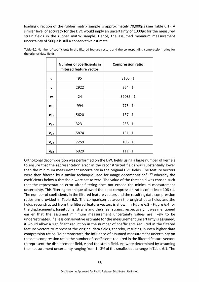
68

loading direction of the rubber matrix sample is approximately 70,000µɛ (see Table 6.1). A similar level of accuracy for the DVC would imply an uncertainty of 1000µɛ for the measured strain fields in the rubber matrix sample. Hence, the assumed minimum measurement uncertainty of 500µɛ is still a conservative estimate.

Table 6.2 Number of coefficients in the filtered feature vectors and the corresponding compression ratios for the original data fields.

Number of coefficients in filtered feature vector

Compression ratio

u 95 8105 : 1

v 2922 264 : 1

w 24 32083 : 1

e11 994 775 : 1

e22 5620 137 : 1

e33 3231 238 : 1

e13 5874 131 : 1

e23 7259 106 : 1

e12 6929 111 : 1

Orthogonal decomposition was performed on the DVC fields using a large number of kernels to ensure that the representation error in the reconstructed fields was substantially lower than the minimum measurement uncertainty in the original DVC fields. The feature vectors were then filtered by a similar technique used for image decomposition33, 49 whereby the coefficients below a threshold were set to zero. The value of the threshold was chosen such that the representation error after filtering does not exceed the minimum measurement uncertainty. This filtering technique allowed the data compression ratios of at least 106 : 1. The number of coefficients in the filtered feature vectors and the resulting data compression ratios are provided in Table 6.2. The comparison between the original data fields and the fields reconstructed from the filtered feature vectors is shown in Figure 6.2 - Figure 6.4 for the displacements, longitudinal strains and the shear strains, respectively. It was mentioned earlier that the assumed minimum measurement uncertainty values are likely to be underestimates. If a less conservative estimate for the measurement uncertainty is assumed, it would allow a significant reduction in the number of coefficients required in the filtered feature vectors to represent the original data fields, thereby, resulting in even higher data compression ratios. To demonstrate the influence of assumed measurement uncertainty on the data compression ratio, the number of coefficients required in the filtered feature vectors to represent the displacement field, v and the strain field, e22 were determined by assuming the measurement uncertainty ranging from 1 - 3% of the smallest data range in Table 6.1. The


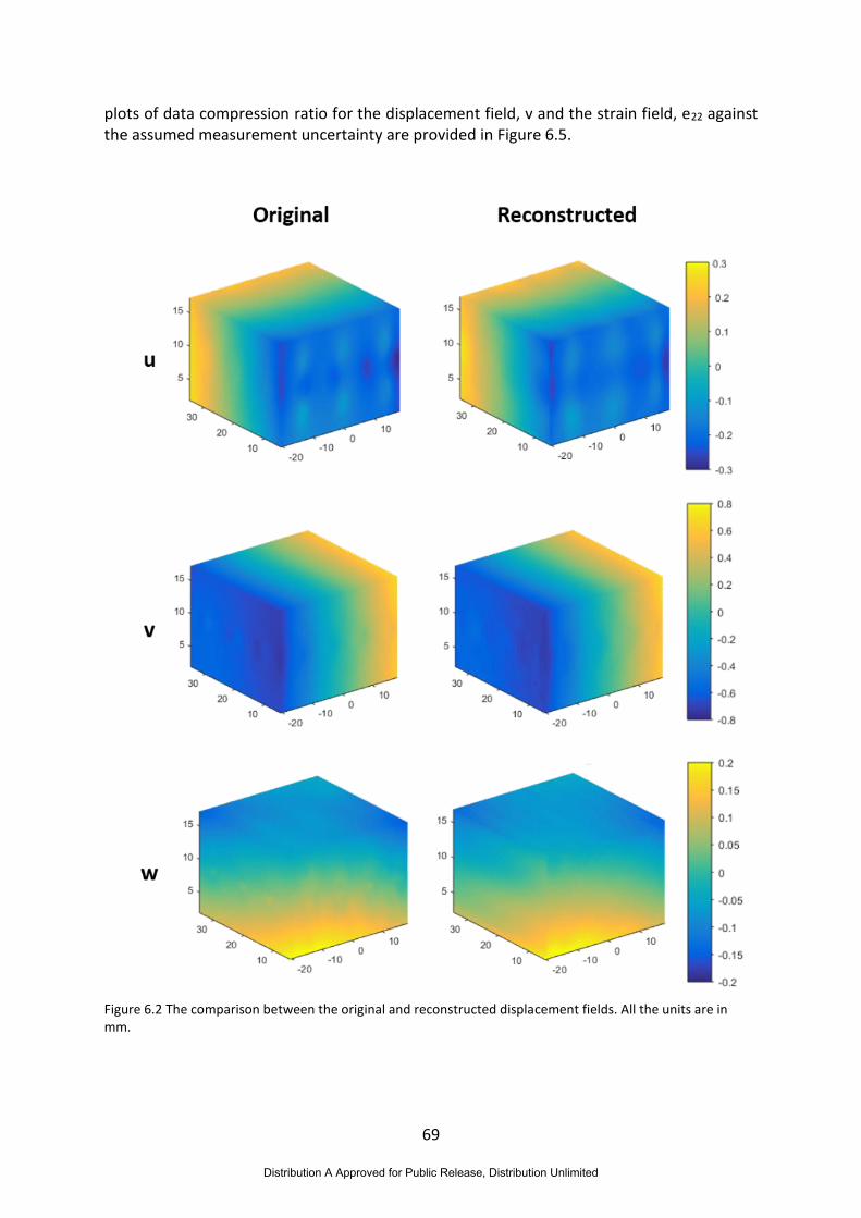
69

plots of data compression ratio for the displacement field, v and the strain field, e22 against the assumed measurement uncertainty are provided in Figure 6.5.

Figure 6.2 The comparison between the original and reconstructed displacement fields. All the units are in mm.


70

Figure 6.3 The comparison between the original and reconstructed longitudinal strain fields. The axes of the volume plots are in mm and the color bar shows the strain values.


71

Figure 6.4 The comparison between the original and reconstructed shear strain fields. The axes of the volume plots are in mm and the color bar shows the strain values.


72

Figure 6.5 The plot of data compression ratio against the assumed measurement uncertainty for the displacement field, v and the strain field, e22.

6.4 Quantitative validation of finite element model

The researchers at AFRL modelled the reinforced rubber matrix sample using a specialized textile finite element (FE) code, also developed within the AFRL, to simulate its deformation response to axial loading. The details about this FE model can be found in a paper by Mollenhauer et al9. The modelled displacement and strain fields of the rubber matrix sample were provided by the AFRL for quantitative validation. The FE fields were first represented as feature vectors by performing orthogonal decomposition on them using the same number of kernels which were used for the orthogonal decomposition of measured data fields. The coefficients of the feature vectors representing the FE fields were then filtered by retaining only those coefficients which were present in the filtered feature vectors representing the measured fields.

A preliminary validation of the FE model was performed using the method outlined in the CEN guide13. In the CEN validation procedure, the coefficients of the feature vectors representing the measured and predicted data fields are first plotted against one another for a simple comparison. The CEN guide recommends that the model is considered to be valid if all of the pairs of coefficients in the two feature vectors fall within the uncertainty zone defined by:

𝑆𝑃 = 𝑆𝑀 ± 2𝑢𝑒𝑥𝑝 (6.25)


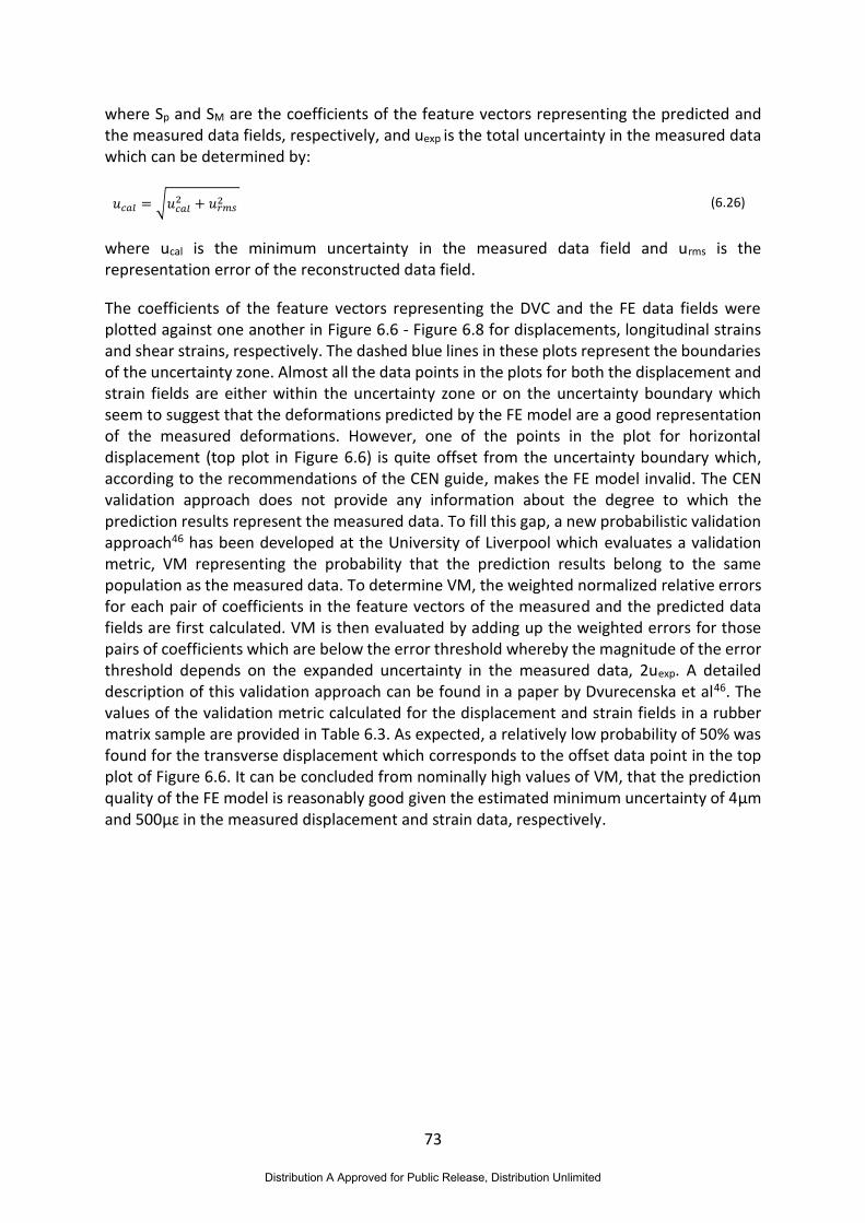
73

where Sp and SM are the coefficients of the feature vectors representing the predicted and the measured data fields, respectively, and uexp is the total uncertainty in the measured data which can be determined by:

𝑢𝑐𝑎𝑙 = √𝑢𝑐𝑎𝑙2 + 𝑢𝑟𝑚𝑠

2 (6.26)

where ucal is the minimum uncertainty in the measured data field and urms is the representation error of the reconstructed data field.

The coefficients of the feature vectors representing the DVC and the FE data fields were plotted against one another in Figure 6.6 - Figure 6.8 for displacements, longitudinal strains and shear strains, respectively. The dashed blue lines in these plots represent the boundaries of the uncertainty zone. Almost all the data points in the plots for both the displacement and strain fields are either within the uncertainty zone or on the uncertainty boundary which seem to suggest that the deformations predicted by the FE model are a good representation of the measured deformations. However, one of the points in the plot for horizontal displacement (top plot in Figure 6.6) is quite offset from the uncertainty boundary which, according to the recommendations of the CEN guide, makes the FE model invalid. The CEN validation approach does not provide any information about the degree to which the prediction results represent the measured data. To fill this gap, a new probabilistic validation approach46 has been developed at the University of Liverpool which evaluates a validation metric, VM representing the probability that the prediction results belong to the same population as the measured data. To determine VM, the weighted normalized relative errors for each pair of coefficients in the feature vectors of the measured and the predicted data fields are first calculated. VM is then evaluated by adding up the weighted errors for those pairs of coefficients which are below the error threshold whereby the magnitude of the error threshold depends on the expanded uncertainty in the measured data, 2uexp. A detailed description of this validation approach can be found in a paper by Dvurecenska et al46. The values of the validation metric calculated for the displacement and strain fields in a rubber matrix sample are provided in Table 6.3. As expected, a relatively low probability of 50% was found for the transverse displacement which corresponds to the offset data point in the top plot of Figure 6.6. It can be concluded from nominally high values of VM, that the prediction quality of the FE model is reasonably good given the estimated minimum uncertainty of 4µm and 500µɛ in the measured displacement and strain data, respectively.


74

Figure 6.6 The graphs of coefficients of the feature vectors representing the measured and predicted displacement fields plotted against one another. The uncertainty boundaries are represented by the dashed blue lines.


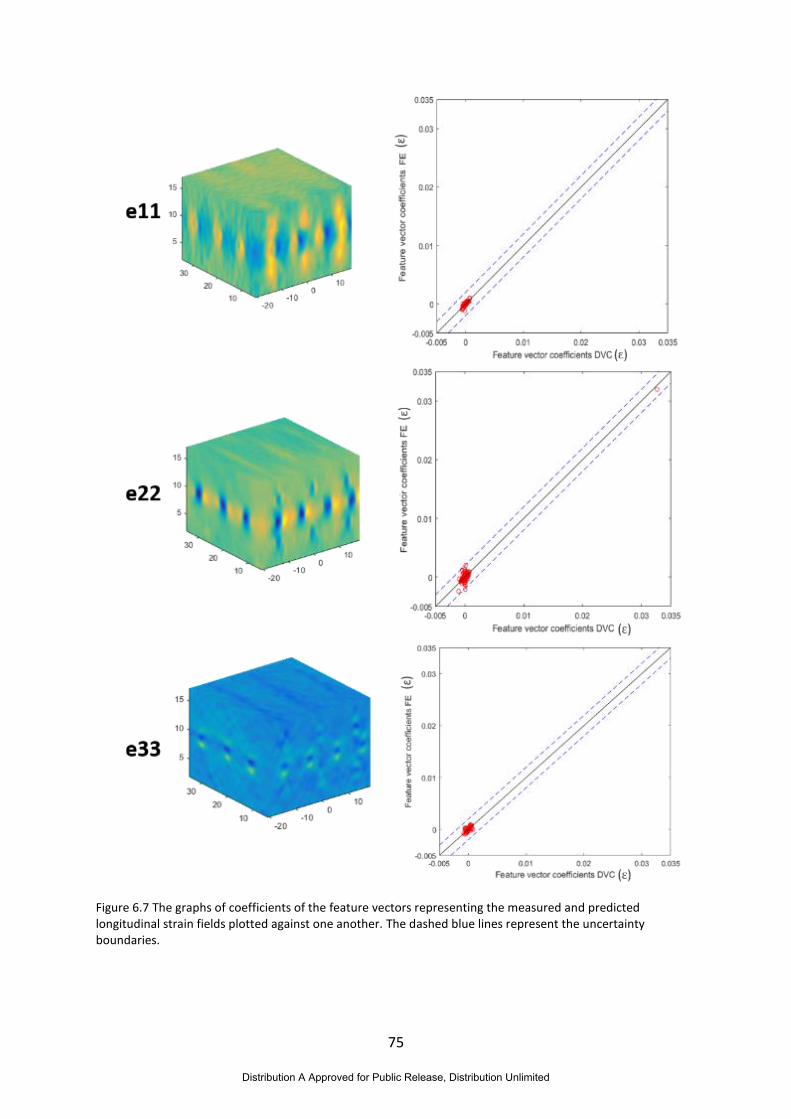
75

Figure 6.7 The graphs of coefficients of the feature vectors representing the measured and predicted longitudinal strain fields plotted against one another. The dashed blue lines represent the uncertainty boundaries.


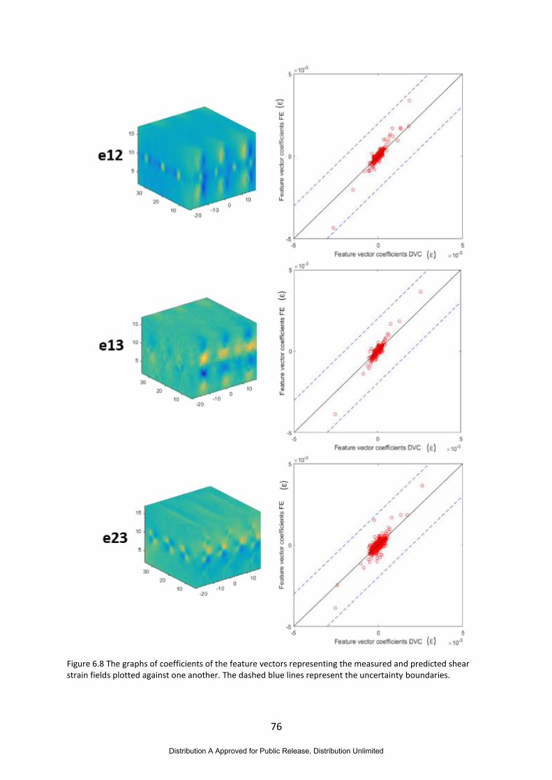
76

Figure 6.8 The graphs of coefficients of the feature vectors representing the measured and predicted shear strain fields plotted against one another. The dashed blue lines represent the uncertainty boundaries.


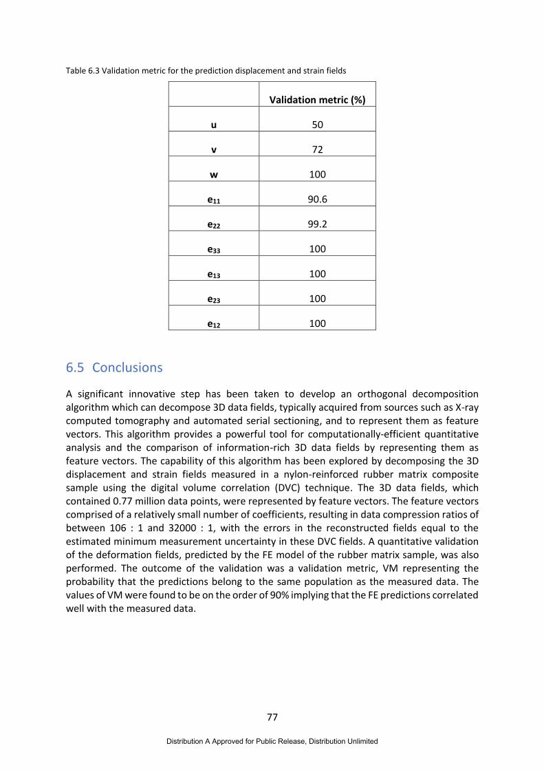
77

Table 6.3 Validation metric for the prediction displacement and strain fields

Validation metric (%)

u 50

v 72

w 100

e11 90.6

e22 99.2

e33 100

e13 100

e23 100

e12 100

6.5 Conclusions

A significant innovative step has been taken to develop an orthogonal decomposition algorithm which can decompose 3D data fields, typically acquired from sources such as X-ray computed tomography and automated serial sectioning, and to represent them as feature vectors. This algorithm provides a powerful tool for computationally-efficient quantitative analysis and the comparison of information-rich 3D data fields by representing them as feature vectors. The capability of this algorithm has been explored by decomposing the 3D displacement and strain fields measured in a nylon-reinforced rubber matrix composite sample using the digital volume correlation (DVC) technique. The 3D data fields, which contained 0.77 million data points, were represented by feature vectors. The feature vectors comprised of a relatively small number of coefficients, resulting in data compression ratios of between 106 : 1 and 32000 : 1, with the errors in the reconstructed fields equal to the estimated minimum measurement uncertainty in these DVC fields. A quantitative validation of the deformation fields, predicted by the FE model of the rubber matrix sample, was also performed. The outcome of the validation was a validation metric, VM representing the probability that the predictions belong to the same population as the measured data. The values of VM were found to be on the order of 90% implying that the FE predictions correlated well with the measured data.


78

7 Discussion

A major motivation for this research was to utilize the novel techniques based on image decomposition for quantitative comparison of data fields, developed by Professor Patterson and his research group at the University of Liverpool, to perform analysis on the data from the work by Dr Craig Przybyla (AFRL) and his team on microstructure-sensitive damage characterization/simulation in continuous fiber reinforced ceramic composites (CMCs). Five objectives were identified by Dr Craig Przybyla and Professor Eann Patterson, reported in Chapter 1, which were aimed at addressing the difficulties in the processing and interpretation of the information-rich data acquired from AFRL’s on-going work on damage characterization in CMCs.

Microstructural defects which are introduced during the processing stage significantly influence the damage mechanisms, and therefore, the overall toughness of the CMCs. Fast and accurate characterization of microstructure from information-rich data fields acquired using techniques such as automated serial sectioning or X-ray computed tomography is the key to the design and development of more consistent microstructures for next generation CMCs. The first objective of this research was to develop a methodology for identification and characterization of voids in the microstructure of CMCs. A novel method based on orthogonal decomposition, reported in Chapter 2, has been proposed to determine the shape and orientation characteristics of the voids. This method utilizes image segmentation to identify void phase from the recorded grey-scale images of a CMC sample. It could therefore be applied to the images obtained either from serial sectioning or X-ray computed tomography provided they have sufficient grey-level contrast so that distinctions could be made between the primary phases of the microstructure. The efficacy of the proposed method was demonstrated by applying it to a 3.6 x 2.6 x 0.1 mm volume of a SiCf/SiNC sample which was serially sectioned in 1µm increments and viewed in an optical microscope to produce micrographs that were a mosaic containing 7200x5500 pixels

Voids result from pockets of air which are entrapped in the microstructure during the processing stage. They are expected to take a spherical shape in the absence of external forces to minimize surface energy of the interface between the air and the ceramic matrix polymer precursor; however, they become aspherical due to forces applied either by the external pressure during manufacturing or by the fibers in close proximity. The level of irregularity of the extracted void shapes were determined by evaluating their sphericity which was defined as the volume of void divided by the volume of a bounding sphere. The compound plot in Figure 2.11 graphically shows the sphericity of the voids along with fiber orientations which provides significant insight into the potential influence of these voids on the damage mechanisms in this material. Overall, the values for void sphericity are quite low i.e. in the range of 0.05 - 0.3 which implies that the voids are highly aspherical and will therefore allow a greater contact area between the entrapped air and the matrix and fibers. This is likely to cause an increase in oxidation rate of the fiber coating local to these voids during service.

The orientation of each void was determined by decomposing the three orthogonal projections of the void (see Figure 2.5) using Chebyshev polynomials in order to reduce their


79

dimensionality by representing them as feature vectors. The direction in which the void was skewed was then identified from a single normalized coefficient in the feature vector. The voids were found to be significantly skewed on the x-z plane which is also the plane in which the fibers were predominantly oriented. The comparison between the void skewness in the x-z plane and the fiber orientation is graphically presented in a compound plot in Figure 2.13. This plot suggests that the shape of the voids is governed by the arrangement of the surrounding fibers.

As part of the work on first objective, a new Fourier-Chebyshev decomposition approach has also been proposed in Chapter 2, which is capable of detecting subtle changes to the void distribution in the microstructure and is therefore believed to be a useful tool for rigorous quality assurance of the manufactured CMC components. To implement this approach, an image of the distribution of voids in the CMC sample was first created using the x-y plane projections of the voids as shown in Figure 2.7. A 2D Fourier transform of the image was then determined which contained useful information about the size, shape, orientation and distribution of the voids in the sample. The spectral image was represented by a feature vector of Fourier-Chebyshev coefficients by performing orthogonal decomposition on it. Since data for only one CMC sample was available, the sensitivity of the feature vector to subtle changes to the void distribution was demonstrated by applying transformations to the original void distribution image shown in Figure 2.7 and obtaining their feature vectors using the above mentioned procedure. The difference between the feature vectors of the modified and the unmodified images of void distribution were quantified using Pearson dissimilarity (see Table 2.1). It is proposed that the void distribution in the microstructure of a CMC component from each batch can be characterized using a Fourier-Chebyshev decomposition approach and quantitatively compared with a bench-mark using Pearson dissimilarity for the purpose of establishing the consistency in the microstructure of the manufactured components.

So far the discussion has been confined primarily to the efforts invested in the extraction of microstructural information related to the voids. The topology of fiber orientation field is probably the most dominant feature of the microstructure which governs the macro-behavior of the CMC material. Objective (iii) of this research, reported in Chapter 1, was about the characterization and quantitative comparison of the fiber orientation fields. Earlier methods19, 35, which were developed to extract 3D fiber profiles from a sequence of optical images of a serially sectioned CMC sample, utilized ellipse detection algorithms to identify the fiber cross-sections which appear as ellipses in the images. The ellipse detection algorithms tend to be computationally intense and could potentially take several hours to days to identify thousands of ellipses in all the optical images35. An innovative method based on the well-established DIC algorithm has been proposed in Chapter 4 for computationally-efficient characterization of fiber orientation in continuous fiber reinforced composites. A series of one hundred mosaics acquired from serial sectioning of a 3.6 x 2.6 x 0.1 mm SiCf/SiNC sample were processed using a commercially-available DIC package, Istra-4D (Dantec Dynamics GmbH). Istra-4D software discretizes the (initial) reference mosaic into small square regions called facets and maps the reference facet to its deformed shape in the next mosaic using a second-order shape function. It is pertinent to mention here that DIC has a lower spatial resolution in comparison to the earlier methods19, 35 as it can only track a small group of fibers which lie within a reference facet rather than tracking the individual fiber cross-sections.


80

An alternate method based on 2D cross-correlation has also been proposed in Chapter 4 which has the capability of tracking individual fiber cross-sections in the sequence of mosaics. To implement this method, fiber cross-sections need to be identified only in the first mosaic unlike the earlier methods in which fiber cross-sections needed to be identified in all the mosaics. The ellipse detection code used in this work took approximately fifteen minutes to identify the fiber cross-sections in the first mosaic. Since there were total of one hundred mosaics, it is estimated that the earlier methods would take at least 25 hours to obtain the fiber coordinate data. Computation times required to obtain the coordinates of the fiber (facet in case of the DIC) centers through the sequence of a hundred mosaics has been provided in Table 4.1. It has been estimated that the DIC and 2D cross-correlation based methods are at least 20 and 17 times faster, respectively, than the rule-based method35 for characterization of fiber orientation.

The fiber coordinates data which was acquired from the rule-based method was provided by AFRL for the purpose of comparison with the results obtained using the DIC and the 2D cross-correlation based methods. The 3D fiber profiles plotted using the coordinate data from the three sources are shown in Figure 4.7. For quantitative comparison of the fiber coordinate data acquired from the three sources, the global fiber angles in the x-z and the y-z planes were first determined (see Figure 4.8). The distributions of the fiber angles were found to be Gaussian in nature and were therefore represented using the probability density functions (PDFs), shown in Figure 4.9, which were obtained by fitting a bivariate Gaussian mixture model to the fiber angle data. The PDF peaks were decomposed using orthogonal decomposition to represent them by feature vectors. The Chebyshev coefficients of the feature vector representing the PDF peaks obtained from the rule-based approach were plotted against the ones representing the feature vectors of the PDF peaks acquired from the DIC and the 2D-cross correlation based methods. Pearson correlation coefficients (ρ) for the feature vector plots provided in Figure 4.11 were calculated which provided a measure of the correlation between the fiber orientation fields. Overall, there was a good agreement between the fiber orientation fields obtained from the rule-based approach and the two proposed methods as the evaluated ρ values were of the order of 0.9; however, the ρ values between the rule-based and the DIC PDFs were found to be slightly lower compared to the ones between the rule-based and the 2D cross-correlation PDFs. This is likely due to the fact that DIC tracks the facets rather than the individual fiber cross-sections through the sequence of mosaics, and therefore, inherently samples the profiles of the small group of fibers which lie within a given facet.

Despite lower resolution of the DIC method, it is believed to be more robust in comparison to the rule-based35 and the proposed 2D cross-correlation based methods. The rule-based approach projects the position of the fiber center in the next image based on its previous orientation and searches for the fiber cross-section lying nearest to the projected location. If the fiber path is non-linear or the spacing between the two adjacent mosaics is large then the rule-based method would probably not be able to accurately associate the fiber cross-sections. The 2D cross-correlation based method is likely to give a false match if the fiber density is very high and the fiber cross-sections have little variation in their appearance. DIC, on the other hand, is believed to be less sensitive to these issues primarily because it utilizes a second-order shape function which allows for the distortion of the facet during its mapping in the next mosaic.


81

When DIC was first investigated as a computationally efficient tool for tracking fibers as part of the work on objective (iii), it was postulated that it would perform better than the existing state-of-the-art tracking algorithms in cases where there will be a wide(> 1µm) and/or non-uniform inter-slice gap in the mosaic sequence. Objective (iv) of this project was about further exploring the potential of the DIC method by comparing its performance with a more recent Kalman filter based fiber-tracking algorithm, referred as the Kalman-Groupwise method19, which was developed by the researchers from the University of South Carolina in collaboration with the AFRL. A new sequence of mosaics from a continuous fiber reinforced polymer matrix composite (PMC) sample was provided by the AFRL to test the capability of the DIC and the Kalman-Groupwise method. This sequence contained 206 mosaics in total with a non-uniform inter-slice gap ranging from 1.1-56µm. The Kalman-Groupwise method was first tested on the previously provided CMC sample mosaics and was found to be at least 40 times slower than the DIC method (see processing times in Table 5.2). It was then tested on the sequence of PMC mosaics and it was unable to determine the fiber orientations. The primary reason for the failure of the Kalman-Groupwise method is its fiber prediction model which assumes a constant shift in the fiber positions between any two adjacent mosaics in a sequence. This assumption basically means that the Kalman-Groupwise method considers the fibers to be perfectly straight and is, therefore, probably not capable of identifying anomalous behavior in the fibers such as curvature or localized waviness. DIC, on the other hand, accurately characterized the fiber orientations in the PMC sample as shown in Figure 5.11. The depth of the PMC sample was 10 times the depth of the CMC sample, and hence, the fiber profiles in the PMC sample, which were determined using DIC, were further analyzed by assuming them as curves in 3D space rather than a straight line. The fibers were divided into ten equal segments of 100µm in depth and the local orientation of the fibers in each of the ten segments were determined. The results suggest the presence of in-plane waviness and slight out-of-plane curvature in the fibers of the PMC samples (see Figure 5.12 - Figure 5.15). Since carbon fibers typically have a very high stiffness and their profiles through the depth of the PMC sample are expected to be perfectly straight, a potential cause for the observed waviness in their profiles can be the inherent uncertainty in the grinding process of the automated serial sectioning system which, in turn, would induce errors in the spacing between the adjacent mosaics.

Objective (ii) of this research was aimed at developing a strain-based approach for monitoring the damage within composite laminates during loading. A novel damage monitoring algorithm has been introduced in Chapter 3 which can be used to determine the time and location of damage initiation using strain field measured from the surface of a composite laminate during loading. This algorithm first performs orthogonal decomposition on the measured strain fields to represent them by feature vectors. It then determines the rate of change of the strain field, s by calculating the Euclidean distance between the feature vectors representing the two strain fields and dividing them by the time difference between them. The rate of damage creation, sd is then inferred from s by substracting the constant rate of change in the measured strain field, sc which results from elastic deformation and measurement noise. Finally, the accumulated damage, sd

can be calculated by integrating sd with respect to time. This algorithm was applied to the DIC data for a ceramic matrix composite laminate as it was loaded to failure in tension. Individual cracks and the time at which they formed were successfully detected using this algorithm as shown in Figure 3.3-Figure 3.5.


82

The onset of damage could potentially be identified from the gradient of the stress-strain or load-time curves; however, the differentiation operation result in a high level of uncertainty. Moreover, owing to the heterogeneous nature of the composite microstructure, a localized degradation could initiate in a material without any discernible change in the gradient of the load curve. The accumulated damage signal allows the degradation to be monitored more effectively than using the stress-strain or load-time curves. Many commercial DIC packages now support live processing of images to allow for real-time monitoring of the surface strain fields. The use of orthogonal decomposition for reducing the dimensionality of the strain field significantly increases the computational efficiency of the proposed algorithm. This means that this algorithm could be combined with real-time DIC data processing to allow for real-time monitoring of the accumulated damage.

In the past, Patterson and his co-workers have used orthogonal decomposition extensively on the 2D data fields acquired from full-field optical measurement techniques for the purpose of finite element model updating10, quantitative validation of computational mechanics models12-14 and comparison of modal behavior at room and elevated temperatures15. It has also been used in the development of novel strain-based approaches for determining the severity of damage in glass-fiber reinforced composites16 and predicting the residual strength in impacted carbon-fiber reinforced composites30. As part of the on-going work on objective (v) of this project, a substantial innovative step has been taken to extend the orthogonal decomposition technique to three dimensions. This allows the decomposition of 3D data fields which are typically obtained from techniques such as X-ray computed tomography and automated serial sectioning. 3D orthogonal decomposition would also be applicable on 2D data fields which vary in the temporal domain and, for the purpose of decomposition, can be treated as 3D data fields. The capability of this algorithm has been explored by decomposing the 3D displacement and strain distributions in a nylon-reinforced rubber-matric composite sample which were measured using the digital volume correlation technique (see Figure 6.2 - Figure 6.4). The 3D data fields, which contained 0.77 million data points, were represented by feature vectors. The feature vectors comprised of a relatively small number of coefficients giving the compression ratio of at least 106 : 1 with the errors in the reconstructed fields equal to the minimum measurement uncertainty in these DVC fields. A quantitative validation of the deformation fields, predicted by the FE model of the rubber matrix sample, was also performed. The outcome of the validation was a validation metric, VM providing a quantitative measure of the quality of the predictions. The values of VM were found to be on the order of 90% implying that the FE predictions correlated well with the measured data.


83

8 Conclusions

The research presented in this report was aimed at utilizing the novel techniques based on image decomposition for quantitative comparison of data fields, developed by Professor Patterson and his research group at the University of Liverpool, to address the research questions regarding the processing and interpretation of the information-rich data acquired from AFRL’s on-going work on damage characterization in continuous fiber reinforced ceramic composites (CMCs). Five objectives were identified by Dr Przybyla (AFRL) and Professor Patterson for this project which are reported in the Introduction chapter. A novel method based on orthogonal decomposition has been proposed in Chapter 2 for determining the shape and orientation characteristics of the voids in a CMC sample, which was developed to meet the first objective of this project. A new Fourier-Chebyshev decomposition approach has also been introduced in Chapter 2 which is capable of detecting subtle changes to the void distribution in the microstructure and is therefore believed to be a useful tool for rigorous quality assurance of the manufactured CMC components.

Chapter 3 describes a strain-based damage monitoring algorithm which was developed to fulfil the second research objective. This algorithm can be used to identify the time and location of damage initiation within composite laminates during loading. The work on characterization and quantitative comparison of the fiber orientation fields, reported in Chapter 4, was carried out to achieve the third research objective. Two methods, one based on the well-established digital image correlation (DIC) algorithm and the other on 2D cross-correlation, have been proposed for determining the 3D fiber profiles from stacks of mosaics of a CMC sample. The DIC and the 2D cross-correlation based methods have been estimated to be at least 20 and 17 times faster, respectively, than the previously published rule-based method35 developed for the characterization of fiber orientation. The capability of DIC in characterizing fiber orientations was further explored in the work reported in Chapter 5 which was carried out to fulfil research objective (iv). The performance of DIC was compared against the state-of-the-art Kalman filter based fiber-tracking method19 by applying both the methods to the sequence of mosaics of a fiber reinforced polymer matrix composite (PMC) sample. The DIC clearly outperformed the Kalman filter method and was also found to be at least 40 times faster.

A significant novel step has been taken as part of the work on objective (v) to develop an algorithm for the orthogonal decomposition of 3D data fields which is described in Chapter 5. The capability of this algorithm was tested by applying it to the 3D deformation fields which were measured in nylon-reinforced rubber matrix sample using the digital volume correlation technique. The algorithm successfully decomposed the 3D data fields and represented them as feature vectors giving data compression ratios of at least 106 : 1.


84

References

1. Naslain R. Design, preparation and properties of non-oxide CMCs for application in engines and nuclear reactors: an overview. Composites Science and Technology 2004;64(2):155-70.

2. Brewer D. HSR/EPM combustor materials development program. Materials Science and Engineering: A 1999;261(1-2):284-91.

3. Bale HA, Haboub A, MacDowell AA, Nasiatka JR, et al. Real-time quantitative imaging of failure events in materials under load at temperatures above 1,600 C. Nature materials 2013;12(1):40.

4. Tracy J, Daly S. Statistical analysis of the influence of microstructure on damage in fibrous ceramic matrix composites. International Journal of Applied Ceramic Technology 2017;14(3):354-66.

5. DeHoff R. Quantitative serial sectioning analysis: preview. Journal of Microscopy 1983;131(3):259-63.

6. Spowart JE. Automated serial sectioning for 3-D analysis of microstructures. Scripta Materialia 2006;55(1):5-10.

7. Cloetens P, Pateyron-Salomé M, Buffiere J, Peix G, et al. Observation of microstructure and damage in materials by phase sensitive radiography and tomography. Journal of Applied Physics 1997;81(9):5878-86.

8. Brault R, Germaneau A, Dupré J-C, Doumalin P, et al. In-situ analysis of laminated composite materials by X-ray micro-computed tomography and digital volume correlation. Experimental Mechanics 2013;53(7):1143-51.

9. Mollenhauer D, Safriet S, Sutton M, HW S, et al. Characterization of strain distribution in a reinforced rubber-matrix composite using digital volume correlation. In: Kim H, Whisler D, Chen Z, Bisagni C, Kawai M, Krueger R, eds. Proceedings of the 29th Annual American Society of Composites Conference. 2014.

10. Wang W, Mottershead JE, Sebastian CM, Patterson EA. Shape features and finite element model updating from full-field strain data. International Journal of Solids and Structures 2011;48(11-12):1644-57.

11. Patki A, Patterson E. Decomposing strain maps using Fourier-Zernike shape descriptors. Experimental mechanics 2012;52(8):1137-49.

12. Sebastian C, Hack E, Patterson E. An approach to the validation of computational solid mechanics models for strain analysis. The Journal of Strain Analysis for Engineering Design 2013;48(1):36-47.


85

13. CEN-CWA-16799. Validation of computational solid mechanics models. Brussels: Comité Européen de Normalisation; 2014.

14. Hack E, Lampeas G, Patterson EA. An evaluation of a protocol for the validation of computational solid mechanics models. The Journal of Strain Analysis for Engineering Design 2016;51(1):5-13.

15. Berke R, Sebastian C, Chona R, Patterson E, et al. High temperature vibratory response of Hastelloy-X: stereo-DIC measurements and image decomposition analysis. Experimental Mechanics 2016;56(2):231-43.

16. Patki AS, Patterson EA. Damage assessment of fibre reinforced composites using shape descriptors. The Journal of Strain Analysis for Engineering Design 2012;47(4):244-53.

17. Przybyla C, Bricker S, Simmons J, Braginsky M, et al. Microstructure-sensitive damage characterization/simulation in continuous fiber reinforced ceramic composites. Air Force Research Laboratory 2016.

18. Christian W, Dvurecenska K, Amjad K, Przybyla C, et al. Machine Vision Characterisation of the 3D Microstructure of Ceramic Matrix Composites. Journal of Composite Materials (Submitted).

19. Zhou Y, Yu H, Simmons J, Przybyla CP, et al. Large-scale fiber tracking through sparsely sampled image sequences of composite materials. IEEE Transactions on Image Processing 2016;25(10):4931-42.

20. Wang W, Mottershead JE, Ihle A, Siebert T, et al. Finite element model updating from full-field vibration measurement using digital image correlation. Journal of Sound and Vibration 2011;330(8):1599-620.

21. Ruggles‐Wrenn M, Boucher N, Przybyla C. Fatigue of three advanced SiC/SiC ceramic matrix composites at 1200° C in air and in steam. International Journal of Applied Ceramic Technology 2018;15(1):3-15.

22. Otsu N. A threshold selection method from gray-level histograms. IEEE transactions on systems, man, and cybernetics 1979;9(1):62-6.

23. Solomon C, Breckon T. Fundamentals of Digital Image Processing: A practical approach with examples in Matlab: John Wiley & Sons, 2011.

24. Barber CB, Dobkin DP, Huhdanpaa H. The quickhull algorithm for convex hulls. ACM Transactions on Mathematical Software (TOMS) 1996;22(4):469-83.

25. Lopez-Alba E, Sebastian CM, Christian WJ, Patterson EA. The use of charge-coupled device cameras for characterizing the mean deflected shape of an aerospace panel during broadband excitation. The Journal of Strain Analysis for Engineering Design 2019;54(1):13-23.


86

26. Hack E, Lin X, Patterson E, Sebastian C. A reference material for establishing uncertainties in full-field displacement measurements. Measurement Science and Technology 2015;26(7):075004.

27. Theodoridis S, Pikrakis A, Koutroumbas K, Cavouras D. Introduction to pattern recognition: a matlab approach: Academic Press, 2010.

28. Yin J, Lee S-H, Feng L, Zhu Y, et al. The effects of SiC precursors on the microstructures and mechanical properties of SiCf/SiC composites prepared via polymer impregnation and pyrolysis process. Ceramics International 2015;41(3):4145-53.

29. Yurgartis S. Measurement of small angle fiber misalignments in continuous fiber composites. Composites Science and Technology 1987;30(4):279-93.

30. Christian W, DiazDelaO F, Atherton K, Patterson E. An experimental study on the manufacture and characterization of in-plane fibre-waviness defects in composites. Royal Society open science 2018;5(5):180082.

31. Cuadra J, Vanniamparambil PA, Hazeli K, Bartoli I, et al. Damage quantification in polymer composites using a hybrid NDT approach. Composites Science and Technology 2013;83:11-21.

32. Elhajjar RF, Shams SS. A new method for limit point determination in composite materials containing defects using image correlation. Composites Science and Technology 2016;122:140-8.

33. Christian W, DiazDelaO F, Patterson E. Strain-based damage assessment for accurate residual strength prediction of impacted composite laminates. Composite Structures 2018;184:1215-23.

34. Baxter MG, Pullin R, Holford KM, Evans SL. Delta T source location for acoustic emission. Mechanical systems and signal processing 2007;21(3):1512-20.

35. Bricker S, Simmons JP, Przybyla C, Hardie RC. Anomaly detection of microstructural defects in continuous fiber reinforced composites. In: Proceedings of SPIE 9401, Computational Imaging XIII, 94010A, 2015.

36. Becker T, Splitthof K, Siebert T, Kletting P. Error estimations of 3D digital image correlation measurements. In: Speckle06: Speckles, From Grains to Flowers, 2006.

37. Simonovsky M. An efficient ellipse detector based on Hough voting. 2013 Available from:https://uk.mathworks.com/matlabcentral/fileexchange/33970-ellipse-detection-using-1d-hough-transform

38. Xie Y, Ji Q. A new efficient ellipse detection method. In: Object recognition supported by user interaction for service robots, Qubec, Canada; 2002.

39. Bricker S. Anomaly Detection and Microstructure Characterization in Fiber Reinforced Ceramic Matrix Composites. University of Dayton, 2015.


87

40. Dempster AP, Laird NM, Rubin DB. Maximum likelihood from incomplete data via the EM algorithm. Journal of the royal statistical society. Series B (methodological) 1977:1-38.

41. Chui H, Rangarajan A. A new point matching algorithm for non-rigid registration. Computer Vision and Image Understanding 2003;89(2-3):114-41.

42. Pirsiavash H, Ramanan D, Fowlkes CC. In: IEEE conference on Computer Vision and Pattern Recognition, 2011

43. Dicle C, Camps OI, Sznaier M. Proceedings of the IEEE international conference on computer vision, 2013

44. Milan A, Roth S, Schindler K. Continuous energy minimization for multitarget tracking. IEEE Trans. Pattern Anal. Mach. Intell. 2014;36(1):58-72.

45. Magnusson KE, Jaldén J, Gilbert PM, Blau HM. Global linking of cell tracks using the Viterbi algorithm. IEEE transactions on medical imaging 2015;34(4):911-29.

46. Dvurecenska K, Graham S, Patelli E, Patterson EA. A probabilistic metric for the validation of computational models. Royal Society open science 2018;5(11):180687.

47. Mukundan R, Ong S, Lee PA. Image analysis by Tchebichef moments. IEEE Transactions on image Processing 2001;10(9):1357-64.

48. Erdélyi A, Magnus W, Oberhettinger F, Tricomi FG. Higher transcendental functions, Vol. 1. McGraw-Hill, New York; 1953.

49. Lampeas G, Pasialis V, Lin X, Patterson E. On the validation of solid mechanics models using optical measurements and data decomposition. Simulation Modelling Practice and Theory 2015;52:92-107.

50. Yap P-T, Paramesran R, Ong S-H. Image analysis by Krawtchouk moments. IEEE Transactions on image processing 2003;12(11):1367-77.

51. Schreier H, Mollenhauer D, Makeev A, Jones E, et al. Measurement of the internal strain distribution in a reinforced rubber-matrix composite using digital volume correlation. In: 20th International Conference on Composite Materials 2015; Copenhagen.

52. Sutton M, Matta F, Rizos D, Ghorbani R, et al. Recent progress in digital image correlation: background and developments since the 2013 WM Murray Lecture. Experimental Mechanics 2017;57(1):1-30.

53. Sebastian C, Patterson E. Calibration of a digital image correlation system. Experimental Techniques 2015;39(1):21-9.


afrl-afosr-uk-tr-2019-0030 quantitative comparison of

Documents