aframeworkforefficientmodularheap analysislara.epfl.ch/~kandhada/fntpl-2015.pdf · abstract modular...
TRANSCRIPT

Foundations and TrendsR© in Programming LanguagesVol. 1, No. 4 (2014) 269–381c© 2015 R. Madhavan, G. Ramalingam, and K.
VaswaniDOI: 10.1561/2500000020
A Framework For Efficient Modular HeapAnalysis
Ravichandhran MadhavanEPFL, Switzerland
G. RamalingamMicrosoft Research, [email protected]
Kapil VaswaniMicrosoft Research, [email protected]

Contents
1 Introduction 270
2 An Informal Overview 276
3 The Language and Concrete Semantics 281
4 The Analysis Framework 2874.1 The Abstract Functional Domain . . . . . . . . . . . . . . 2884.2 Concretization function . . . . . . . . . . . . . . . . . . . 290
5 Parametric Abstract Semantics 2955.1 Abstract Semantics of Primitive Statements . . . . . . . . 2985.2 Abstract Semantics of Procedure Call . . . . . . . . . . . 3005.3 Simplifying the Transformer Graphs . . . . . . . . . . . . . 3075.4 Correctness and Termination of the Framework . . . . . . 311
6 Specializations of the Framework 3206.1 Instantiations . . . . . . . . . . . . . . . . . . . . . . . . 3216.2 Restrictions . . . . . . . . . . . . . . . . . . . . . . . . . 3246.3 Abstractions . . . . . . . . . . . . . . . . . . . . . . . . . 326
7 Instances of the Framework 330
2

3
7.1 Overview of the Instances . . . . . . . . . . . . . . . . . . 3307.2 Formal Definitions of the Instances . . . . . . . . . . . . . 340
8 Experimental Results 3468.1 Implementation, Benchmarks and Metrics . . . . . . . . . 3468.2 Evaluation of the Configurations of the Framework . . . . 350
9 Related Work and Conclusion 362
Appendices 366
A Simplified Transformer Graphs 367
B The Node Merging Abstraction 372
References 378
Abstract
Modular heap analysis techniques analyze a program by computingsummaries for every procedure in the program that describes its effectson an input heap, using pre-computed summaries for the called proce-dures. In this article, we focus on a family of modular heap analysesthat summarize a procedure’s heap effects using a context-independent,shape-graph-like summary that is agnostic to the aliasing in the inputheap. The analyses proposed by Whaley, Salcianu and Rinard, Buss etal., Lattner et al. and Cheng et al. belong to this family. These analysesare very efficient. But their complexity and the absence of a theoreticalformalization and correctness proofs makes it hard to produce correctextensions and modifications of these algorithms (whether to improveprecision or scalability or to compute more information). We present amodular heap analysis framework that generalizes these four analyses.We formalize our framework as an abstract interpretation and estab-lish the correctness and termination guarantees. We formalize the fouranalyses as instances of the framework. The formalization explains thebasic principle behind such modular analyses and simplifies the task ofproducing extensions and variations of such analyses.
We empirically evaluate our framework using several real-world C]applications, under six different configurations for the parameters, andusing three client analyses. The results show that the framework offersa wide range of analyses having different precision and scalability.
R. Madhavan, G. Ramalingam, and K. Vaswani. A Framework For EfficientModular Heap Analysis. Foundations and TrendsR© in Programming Languages,vol. 1, no. 4, pp. 269–381, 2014.DOI: 10.1561/2500000020.
1Introduction
Compositional or modular analysis [Cousot and Cousot, 2002] is a keytechnique for scaling static analysis to large programs. Our interest isin techniques that analyze a procedure in isolation, using pre-computedsummaries for called procedures, computing a summary for the ana-lyzed procedure. Such analyses are widely used and have been foundto scale well. However, computing such summaries for a heap analysis(or points-to analysis) is challenging because of the aliasing in the in-put heap. For example, consider the procedure P shown in Fig. 1.2(a).Its behaviour on two different input heaps is shown in Fig. 1.2(b) andFig. 1.2(c). (The heaps are depicted as shape graphs. The input heapis shown at the top and the corresponding output heap at the bottom).It can be seen that the behaviour of P varies significantly depending onthe aliasing between the variables x and y in the input heap. A soundsummary for P should be able to approximate the behaviour of P inboth these scenarios.
Existing modular heap analyses can be broadly classified into thefollowing categories. (The following classification is not exhaustive.There are modular analyses such as [Nystrom et al., 2004] that cannotbe easily classified into any of the categories mentioned. It is also pos-
270

271
P (x, y) {[1] t = new ();[2] x.next = t;[3] t.next = y;[4] retval = y.next;
}
Figure 1.1: A procedure P whose behaviour depends on the aliasing in the inputheap.
Input1 Input2
Output1 Output2
(a) (b)
Figure 1.2: (a) Output of P when x and y are not aliases in the input heap. (b)Output of P when x and y are aliases in the input heap.

272 Introduction
sible to design analyses that belong to more than one of the categoriesthough we aren’t aware of any.) (a) Analyses such as [Calcagno et al.,2009] compute conditional summaries that are applicable only in thecontexts that satisfy certain conditions (e.g., aliasing or non-aliasingconditions). (b) Some analyses such as [Chatterjee et al., 1999], [Dilliget al., 2011], [Jeannet et al., 2010] enumerate all relevant configurationsof the input heap belonging to a fixed abstract domain and generatesummaries for each configuration. A major challenge with this approachis reducing the number of configurations that are enumerated, whichcan quickly become intractable, and finding efficient ways of repre-senting them. (c) A few analyses, namely, [Whaley and Rinard, 1999],[Cheng and Hwu, 2000], [Liang and Harrold, 2001], [Lattner et al.,2007], [Buss et al., 2008] compute context-independent summaries thatare agnostic to the aliasing in the input heap without enumerating thepossible configurations of the input heap. To our knowledge, these arethe only existing analyses having this property.
The analysis proposed by Whaley and Rinard [Whaley and Rinard,1999] was later on refined and improved by Salcianu and Rinard [Sal-cianu and Rinard, 2005]. We will refer to this analysis as the WSRanalysis. Adopting the terminology of [Lattner et al., 2007], we will re-fer to the analysis proposed by Lattner et al. as Data Structure Analysis(DSA).
In this article, we consider analyses belonging to the final category.They are interesting for several reasons. (a) They have a number of ap-plications, discussed shortly. (b) The analyses are very efficient. DSAscales to the entire Linux kernel comprising 3 million lines of code in3 seconds. An optimized version of WSR analysis discussed in [Mad-havan et al., 2011] scales to C] libraries with 250 thousand lines ofcode. (c) Being modular, they can analyze open programs, libraries,and, in fact, any arbitrary chunk of code without requiring any knowl-edge of the environment. Moreover, the summaries computed are suchthat they be refined incrementally when more knowledge about theenvironment becomes available.
These analyses have been used in a number of applications. Salcianuand Rinard present an application of their analysis to compute the

273
side-effects of a procedure, which are the effects of the procedure onthe pre-existing state, and use it to classify procedures as pure (havingno side-effects) or impure [Salcianu and Rinard, 2005]. This analysis,referred to as purity analysis, itself has a number of applications.
Whaley and Rinard applied their analysis to identify objects thatcan be safely allocated in the stack instead of the heap [Whaley and Ri-nard, 1999]. We use an extension of the WSR analysis to statically ver-ify the correctness of the use of speculative parallelism [Prabhu et al.,2010]. Lattner et al. use their analysis to perform pool allocation inwhich different instances of data structures are allocated to distinctmemory pools, which enables certain compiler optimizations [Lattnerand Adve, 2005b].
However, the complexity of the analyses makes the task of extendingand modifying these analyses challenging and time consuming. Ques-tions such as the following often arise while designing new applicationsbased on the analyses and there is no easy way of answering them. Canthe scalability of the WSR analysis be improved at the expense of pre-cision? Can DSA be extended to yield more precise results when moretime and resources are available? Is it possible to integrate a modularstatic analysis that requires heap information (such as an informationflow analysis) with these analyses as typically done in top-down wholeprogram analyses? A sound theoretical formulation of the analyses willgreatly aid in answering such questions.
Upon investigating the theoretical basis of these analyses, we real-ized that, in spite of the apparent dissimilarity between the analysesand the differences in the precision, scalability, and functionality, thereare some fundamental ideas common to all of these analyses. This mo-tivated us to develop a parametric framework for designing efficientmodular heap analyses. The analyses listed earlier become specific in-stances of our framework.
We formulate our framework as a parametric abstract interpreta-tion and establish the correctness and termination of the semantics. Wepresent several transformations and optimizations (collectively calledas specializations) of our framework and establish their correctness us-ing the standard theory of abstraction interpretation. Our framework
274 Introduction
with its parametric domains, parametric semantics and several correct-ness preserving transformations provides a convenient mechanism forobtaining modular heap analyses with different levels of precision andscalability.
We formally establish that the four analyses: [Whaley and Rinard,1999], [Cheng and Hwu, 2000] [Lattner et al., 2007] (except for thehandling of indirect calls), [Buss et al., 2008] are specific instances of ourframework. We exclude the analysis proposed in [Liang and Harrold,2001] (called as MoPPA) as it is very similar to [Lattner et al., 2007].Nevertheless, it can also be expressed as an instance of our framework.
Formulating the analyses as instances of the framework has sev-eral advantages. It provides an immediate proof of correctness and ter-mination for the analyses. It also helps understand the abstractionsperformed by the analyses and identify opportunities for making themmore precise or scalable. In fact, we were able to identify several cornercases that were not handled by some of the algorithms and were able tofix them. Since we were unable to find complete formalization of someof the analyses, it is not clear to us if the problems we identified arebugs in the algorithm or gaps in the informal descriptions.
We implemented the framework in our open source heap analy-sis tool Seal (seal.codeplex.com). Seal is a fairly robust tool whichhas been used in several program analysis applications. We empiricallystudied the different configurations of the framework using Seal. Wepresent a summary of the results in Chapter 8. The results throw lighton the importance of the parameters of the framework by measuringtheir impact on the precision and scalability of three client analyses.
The framework presented in this article has some limitations. Mostimportantly, it does not support strong updates on heap locations andpath-sensitivity. To our knowledge, all existing modular heap analysisapproaches (such as [Dillig et al., 2011], [Jeannet et al., 2010]) thatperform strong updates on heap locations enumerate the possible con-figurations of the input heap. Nevertheless, we believe that both thesechallenges can be addressed without resorting to enumeration of theinput heap configurations. We briefly outline a potential approach inthe Future Works section (see Chapter 9).
275
The following are the main contributions of this article:
• We propose a modular heap analysis framework that is a gener-alization of a family of existing modular heap analyses. To ourknowledge, this is the first attempt to connect and develop a com-mon theory for the different modular heap analyses proposed inthe past.
• We formulate our framework as an abstract interpretation andprove the correctness and termination properties.
• We present several correctness preserving transformations thatare applicable to all instances of the framework.
• We formalize four existing modular heap analyses as abstractionsof instances of our framework, thereby provide a proof of correct-ness and termination for the analyses. The formalization exposesthe relationships between the analyses and provides ways of im-proving and modifying them.
• We present an empirical evaluation of the framework by analyzingten open source C] applications with six different configurationsof the framework. We used three client analyses, namely, Purityand Side Effects Analysis, Escape Analysis and Call-graph Anal-ysis to measure the precision and scalability of each of the sixconfigurations.
2An Informal Overview
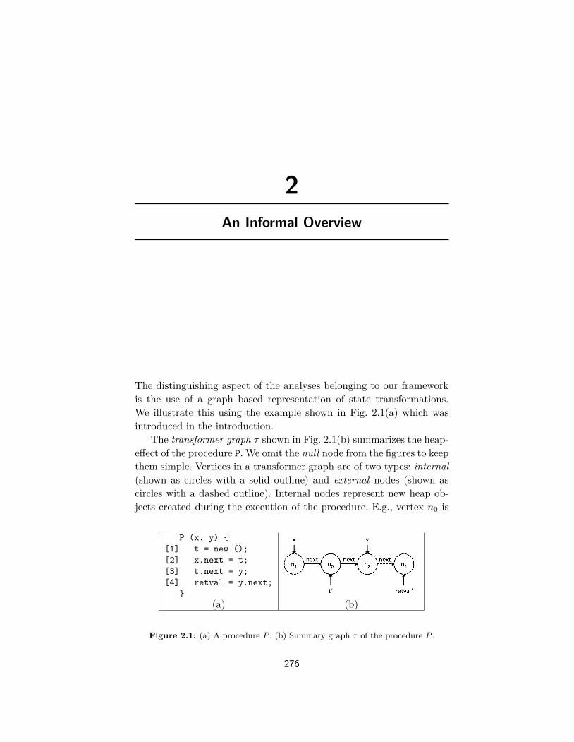
The distinguishing aspect of the analyses belonging to our frameworkis the use of a graph based representation of state transformations.We illustrate this using the example shown in Fig. 2.1(a) which wasintroduced in the introduction.
The transformer graph τ shown in Fig. 2.1(b) summarizes the heap-effect of the procedure P. We omit the null node from the figures to keepthem simple. Vertices in a transformer graph are of two types: internal(shown as circles with a solid outline) and external nodes (shown ascircles with a dashed outline). Internal nodes represent new heap ob-jects created during the execution of the procedure. E.g., vertex n0 is
P (x, y) {[1] t = new ();[2] x.next = t;[3] t.next = y;[4] retval = y.next;
}(a) (b)
Figure 2.1: (a) A procedure P . (b) Summary graph τ of the procedure P .
276

277
an internal node and represents the object allocated in line 1. Externalnodes, in many cases, represent objects that exist in the heap whenthe procedure is invoked (but they could also represent nodes allocatedinside a method as explained in the following). In our example, n1, n2,and n3 are external nodes. Specifically, n1 represents the object pointedto by formal parameter x when the procedure begins execution, as in-dicated by the arrow from x to n1. Similarly, n2 represents the objectpointed to by formal parameter y when the procedure begins execution.
Edges in the graph are also classified into internal and externaledges, shown as solid and dashed edges respectively. The edges n1 → n0and n0 → n2 are internal edges. They represent updates performedby the procedure (i.e., new points-to edges added by the procedure’sexecution) in lines 2 and 3. External edges correspond to reads, theedge n2 → n3 is an external edge created by the dereference “y.next”in line 4. This edge helps identify the node(s) that the external noden3 represents: namely, the objects obtained by dereferencing the nextfield of objects represented by n2.
In simple cases, internal nodes are used to represent objects createdduring the execution of the procedure, while external nodes are used torepresent pre-existing objects (in the initial state when the procedurebegins executing). More generally, external nodes are used to denoteobjects referenced via an access path starting from one of the procedureparameters. Thus, one may loosely associate an external node with aset of access paths.
A transformer graph τ can be interpreted as a procedure Pτ . Fig. 2.2depicts the procedure corresponding to the transformer graph shownin Fig. 2.1(b). Every external or internal node w in a transformergraph τ corresponds to a variable var(w). If w is an internal nodethen var(w) is assigned a newly created object. Every external edge〈u, f, w〉 corresponds to a field-read statement var(w) = var(u).f andevery internal edge 〈u, f, w〉 corresponds to a field-write statementvar(u).f = var(w). In the simplest case, the reads and writes encodedby the transformer graph via external and internal edges are assumedto happen in any order any number of times. Clearly, the procedure Pτis an abstraction of the procedure P .

278 An Informal Overview
(x, y) => {[1] while(*) {[2] if(*) var(n1) = x;[3] if(*) var(n2) = y;[4] var(n0) = new ();[5] if(*) var(n1).next = var(n0);[6] if(*) var(n0).next = var(n2);[7] if(*) var(n3) = var(n2).next;[8] }[9] t = var(n0);[10] retval = var(n3);
}
Figure 2.2: Interpretation of τ as a procedure Pτ . (p1, . . . , pn) => {B} denotesa procedure with parameters p1, . . . , pn and body B. (*) denotes non-deterministicchoice.
(a) Input graph g1 (b) Output graph g′1 = τ〈g1〉
(c) Input graph g2 (d) Output graph g′2 = τ〈g2〉
Figure 2.3: Result of applying of τ on two different concrete states.
279
The above described interpretation of the transformer graph as aprocedure may explain how it captures the transformation of everyconcrete state simultaneously. For example, consider an invocation ofprocedure P in an initial state given by graph g1 shown in Fig. 2.3(a).The summary transformer when applied on the graph g1 results in g′1 =τ〈g1〉 which represents the state after the procedure’s execution (shownin Fig 2.3(b)). The graph g′1 is a conventional shape (or points-to)graph that represents a set of concrete states. The transformed graphg′1 represents the possible outputs of the procedure Pτ when executedwith the concrete state g1. Since the procedure Pτ is an abstraction ofthe procedure P , g′1 is an abstraction of the output of the procedure Pwhen executed with the concrete state g1.
An important aspect of the transformer graphs is that it can beused even in the presence of potential aliases in the input (or cut-points [Rinetzky et al., 2005]). Consider the input state g2 shown inFig. 2.3(c), in which parameters x and y point to the same object u1.Executing the procedure Pτ on the input graph g2 will result in the setof concrete graphs represented by the shape graph shown in Fig. 2.3(d).Fig. 2.3(d) is a conservative approximation of the output of the proce-dure P (Fig. 1.2(b) shows the actual output).
Transformer graphs Vs Shape graphs Semantically, transformergraphs represent state transformations whereas shape graphs representconcrete states. However, one might still wonder that since verticesin a transformer graph represent concrete objects and edges representpoints-to relations between objects, it may be appropriate to refer totransformer graphs also as shape graphs. While the exact terminologyis not important, what is important is to be aware of the differencesbetween transformer graphs and conventional shape graphs.
Unlike conventional shape graphs, the vertices and edges in a trans-former graph represent different concrete objects in different contexts.For example, in the transformer graph shown in Fig. 2.1, n1 representso1 when the input graph is g1 shown in Fig. 2.3(a), and represents u1when the input graph is g2 shown in Fig. 2.3(c). Furthermore, unlikeconventional shape graphs, a single concrete object may be represented

280 An Informal Overview
by multiple nodes in the transformer graphs. For instance, in the trans-former graph shown in Fig. 2.1 when the input concrete graph is g2shown in Fig. 2.3(c), the nodes n1 and n2 represent the same concreteobject u1, and the nodes n3 and n0 represent the object newly allocatedby the procedure.
As a consequence, the absence of an edge from an abstract node (sayu) to an abstract node (say v) does not imply that objects representedby u cannot point to the objects represented by v, since the objectsmay have other representatives in the transformer graph.
For these reasons, many properties that hold for a shape graph donot hold for a transformer graph. For example, even if two variablespoint to non-intersecting sets of nodes in a transformer graph, it doesnot imply that the variables cannot alias (in any context).
The above informal description highlights the following propertiesof the transformer graphs:
• Transformer graphs are abstractions of state transformers, orequivalently, procedures. To think of them as abstractions of stateis flawed.
• Transformer graphs track the (pointer valued) reads and writesperformed by the procedure they summarize using internal andexternal edges, respectively.
• Transformer graphs can be applied to any concrete state irrespec-tive of the aliasing between the heap cells. However, the outputis a conservative approximation as the transformer graphs areabstractions of the procedure they summarize.

3The Language and Concrete Semantics
Notation and Terminology Given a function f : A 7→ 2 B, the func-tion f : 2 A 7→ 2 B is defined by: f(S) =
⋃x∈S f(x). Given two functions
f1 : A 7→ 2 B, f2 : B 7→ 2 C we use (f1 ◦ f2)(x) to denote the compo-sition of f1 with f2 i.e., f2(f1(x)). Note that f1 is applied first in thecomposition f1 ◦ f2. An element of A 7→ 2 B corresponds to a relationbetween A and B, and ◦ represents relational composition.
Syntax A program consists of a set of procedures. A procedure Pconsists of a control-flow graph, with an entry vertex entry(P ) and anexit vertex exit(P ). The entry vertex has no predecessor and the exitvertex has no successor. Every edge of the control-flow graph is labelledby a primitive statement. The set of primitive statements are shown inFig. 3.1. Every procedure ends at a special primitive statement exit. Weuse u S→ v to indicate an edge in the control-flow graph from vertex uto vertex v labelled by statement S. We use a simple language in whichall variables and fields are of pointer type.
Concrete Semantics Domain Let Vars denote the set of variablenames used in the program, partitioned into the following disjoint sets:
281

282 The Language and Concrete Semantics
the set of global variables Globals, the set of local variables Locals(assumed to be the same for every procedure), and the set of formalparameter variables Params (assumed to be the same for every proce-dure). Let Fields denote the set of field names used in the program.Every statement in the program has a label belonging to the set Labels.Let Nc be an unbounded set of locations used for dynamically allocatedobjects. (We will refer to an element of Nc as a vertex, node, or ob-ject.) We use a fairly common representation of the concrete state as aconcrete (points-to or shape) graph.
A concrete state or points-to graph g ∈ Gc is a triple (V,E, σ), whereV ⊆ Nc represents the set of objects in the heap, E ⊆ V×Fields×V (aset of labelled edges) represents values of pointer fields in heap objects,and σ ∈ Σc = Vars 7→ V represents the values of program variables. Inparticular, (u, f, v) ∈ E iff the f field of the object u points to objectv. (Note that this represents the state from the perspective of a singleprocedure. In particular, this state does not include a call-stack, sincethe modular semantics can be defined without explicitly introducing astack.) We assume Nc includes a special element null. Variables andfields of new objects are initialized to null.
Our concrete domain C = Gc 7→ 2Gc is the set of functions thatmap a concrete state to a set of concrete states. We define a partialorder vc on C as follows: fa vc fb iff ∀g ∈ Gc.fa(g) ⊆ fb(g). Let tcdenote the corresponding least upper bound (join) operation definedby: fa tc fb = λg.fa(g) ∪ fb(g). The subscript c may be omitted whenno confusion is likely.
Lemma 3.1. (C,vc,tc) is a complete lattice with the least elementλgc.∅.
Concrete Semantics Every primitive statement S has a semantics[[S]]c ∈ C, as shown in Fig. 3.1. Every statement has a label ` ∈ Labelswhich is not used in the concrete semantics and is, hence, omittedfrom the figure. The execution of most statements transforms a con-crete state to another concrete state, but the signature allows us tomodel non-determinism (e.g., dynamic memory allocation can returnany unallocated object). The signature also allows us to model exe-

283
Statement S Concrete Semantics [[S]]c(V,E, σ)
v1 = v2 {(V,E, σ[v1 7→ σ(v2)]}
v = new C {(V ∪ {n},E ∪ {n} × Fields × {null},σ[v 7→ n]) | n ∈ Nc \ V}
v1.f = v2 {(V, {〈u, l, v〉 ∈ E | u 6= σ(v1)∨l 6= f} ∪ {〈σ(v1), f, σ(v2)〉}, σ)}
v1 = v2.f {(V,E, σ[v1 7→ n]) | 〈σ(v2), f, n〉 ∈ E}
exit {(V,E, λx. if x ∈ (Params ∪ Locals) then nullelse σ(x))}
Call P (v1, · · · , vk) Semantics defined below
Figure 3.1: Primitive statements and their concrete semantics.
cution errors such as null-pointer dereference, though the semanticspresented simplifies error handling by treating null as just a specialobject. We will describe the semantics of a procedure-call statementalong with concrete semantic equations.
We now define a concrete summary semantics [[P ]]\ ∈ C for everyprocedure P . The semantic function [[P ]]\ maps every concrete state gcto the set of concrete states that the execution of P with initial stategc can produce.
We introduce a new variable ϕu for every vertex in the control-flowgraph (of any procedure) and a new variable ϕu,v for every edge u→ v
in the control-flow graph. The semantics is defined as the least fixedpoint of the equations shown in Fig. 3.2. The value of ϕu in the leastfixed point is a function that maps any concrete state g to the setof concrete states that arise at program point u when the procedurecontaining u is executed with an initial state g. Similarly, ϕu,v capturesthe states after the execution of the statement labelling edge u→ v.
Note that the above collection of equations is similar to those usedin Sharir and Pnueli’s functional approach to interprocedural analy-sis [Sharir and Pnueli, 1981] (extended by [Knoop and Steffen, 1992]),

284 The Language and Concrete Semantics
ϕv = λg.{g} v is an entry vertex (3.1)ϕv = GCc(
⊔c{ϕu,v | u→ v}) v is not an entry vertex (3.2)
ϕu,v = GCc(ϕu ◦ [[S]]c) where u S→ v
and S is not a call-stmt (3.3)
ϕu,v = GCc(ϕu ◦ CallS(ϕexit(Q))) where u S→ v
and S is a call to proc Q (3.4)
Figure 3.2: Concrete semantics equations.
with the difference that we are defining a concrete semantics here, while[Sharir and Pnueli, 1981] is focused on abstract analyses. The equationsare a simple functional version of the standard equations for defininga collecting semantics, with the difference that we are simultaneouslycomputing a collecting semantics for every possible initial state of theprocedure’s execution.
The first three equations are self explanatory except for the functionGCc : C 7→ C, which is the garbage collection operation lifted to thedomain of state transformers in C and is defined below.
GCc(f) = λgi.{RemoveUnreach(gi, go) | go ∈ f(gi)}RemoveUnreach (Vi,Ei, σi) (Vo,Eo, σo) =
let L = {x ∈ V | x is not reachable from σ(Vars) ∪ Vi }(Vo \ L,Eo \ {〈u, f, v〉 | u ∈ L}, λx.σo(x) \ L)
Given a function f ∈ C, GCc removes from the output graphs in therange of f the objects that are not reachable from the objects in theinput graph and from the variables in the program. The objects in theinput graph are commonly referred to as the prestate [Salcianu andRinard, 2005].
Since the exit statement resets all local variables and parametersto null in the summary computed at the exit point of a procedure, theoutput graphs would have only objects that are reachable through theobjects in the input graph or through some global variable. In otherwords, all the objects that are locally created by the procedure and are

285
pushS(σ) = λv. v ∈ Globals → σ(v)| v ∈ Locals → null| v = Param(i)→ σ(ai)
popS(σ, σ′) = λv. v ∈ Globals → σ′(v)| v ∈ Locals ∪ Params → σ(v)
CallS(f) = λ(V,E, σ).{(V′,E′, popS(σ, σ′))| (V′,E′, σ′) ∈ f(V,E, pushS(σ))}
Figure 3.3: Definition of the functions pushS ∈ Σc 7→ Σc, popS ∈ Σc×Σc 7→ Σc, andCallS for a procedure call statement “Call Q(a1,...,ak)”. In the figure, Param(i)denotes the i-th formal parameter.
not accessible in the callers are removed from the output graphs of asummary function f .
Consider Eq. 3.4, corresponding to a call to a procedure Q. Thevalue of ϕexit(Q) summarizes the effect of the execution of the whole pro-cedure Q. In the absence of local variables and parameters, we can de-fine the right-hand-side of the equation to be simply GCc(ϕu◦ϕexit(Q)).
The function CallS(f), defined in Fig. 3.3, models the semanticsof the parameter passing mechanism. Given a concrete state (V,E, σ)before the call, we reset the values of all local variables to null and as-sign the formal parameter variables to the values of the correspondingactual arguments. We refer to this operation as pushS as it correspondsto pushing the arguments on to the call stack and creating a new acti-vation frame for the callee. We then apply the callee summary f thatcaptures the effect of the procedure call on the calling context. Finally,the local variables and parameters are restored to their values beforethe call which corresponds to poping the activation frame of the callee.Hence, we refer to this operation as popS . For simplicity, we omit returnvalues from our language.
We define [[P ]]\ to be the value of ϕexit(P ) in the least fixed point ofequations (3.1)-(3.4). Specifically, let VE denote the set of vertices andedges in the control flow graph of a program. The above equations can

286 The Language and Concrete Semantics
be expressed as a single equation ϕ = F \(ϕ), where F \ is a monotonicfunction from the complete lattice VE 7→ C to itself. Hence, F \ has aleast fixed point by Tarski’s fixed point theorem.
The goal of the analysis is to compute an approximation of the setof quantities [[P ]]\ using abstract interpretation.

4The Analysis Framework
In the rest of the article we present several abstract analyses that ap-proximate the concrete semantics presented in Chapter 3.
We represent an abstract analysis by a pair (A,FA), where A is anabstraction of the concrete domain C, and FA maps the vertices andedges of control flow graphs to abstract transfer functions in An → A(for some positive integer n). For a vertex v of a control flow graph itstransfer function is given by FA(v) (which is typically a join operation).Similarly, for an edge u S→ v of a control flow graph, its transfer functionis given by FA(S).
The abstract analyses we present are parametric: that is, their do-mains and transfer functions have parameters. Instantiating the pa-rameters using suitable definitions produces an instance. The proper-ties that hold for the parametric semantics (like correctness and termi-nation) carry over to the instances. Such parametric analyses can beconsidered as a framework that represents a family of abstract analy-ses. In this section, we present and discuss the most general abstractanalysis (AG ,FG).
287

288 The Analysis Framework
The Abstract Graph Domain We now formally define the fairly stan-dard abstract shape (or points-to) graphs used to represent a set of con-crete states. The domain is parameterized by a set Na, the universalset of all abstract graph nodes. For example, many analyses identifyan abstract graph node using the label of the allocation-site. In thiscase, we let Na be the set of all statement labels. An abstract shapegraph g ∈ Ga is a triple (V,E, σ), where V ⊆ Na represents the set ofabstract heap objects, E ⊆ V×Fields×V (a set of labelled edges) repre-sents possible values of pointer fields in the abstract heap objects, andσ ∈ Vars 7→ 2V is a map representing the possible values of programvariables.
Given a concrete graph g1 = 〈V1,E1, σ1〉 and an abstract graphg2 = 〈V2,E2, σ2〉 we say that g1 can be embedded into g2, denotedg1 � g2, if there exists a function h : V1 7→ V2 such that
〈x, f, y〉 ∈ E1 ⇒ 〈h(x), f, h(y)〉 ∈ E2 (4.1)∀v ∈ Vars. σ2(v) ⊇ {h(σ1(v))} (4.2)
The concretization γG(ga) of an abstract graph ga is defined to bethe set of all concrete graphs that can be embedded into ga:
γG(ga) = {gc ∈ Gc | gc � ga}
4.1 The Abstract Functional Domain
A transformer graph τ ∈ AG is a tuple (EV,EE, σin, IV, IE, σ, ), whereEV ⊆ Na is the set of external vertices, IV ⊆ Na is the set of internalvertices, EE ⊆ V ×Fields× EV is the set of external edges, where V =EV∪IV, IE ⊆ V ×Fields×V is the set of internal edges, σin ∈ Vars 7→ 2Vis a map representing the values of parameters and global variables inthe initial state, and σ ∈ Vars 7→ 2V is a map representing the possiblevalues of program variables in the transformed state. ⊆ IE × EE isa may happen before relation that tracks the relative ordering betweenthe internal and external edges. 〈u, f, w〉 〈x, f, y〉 means that thewrite statement var(u).f = var(w) may precede the read statementvar(y) = var(x).f in the procedure Pτ .

4.1. The Abstract Functional Domain 289
Recall that in the informal overview of the transformer graph pre-sented in Chapter 2, the program representation of a transformer graphshown in Fig. 2.2 ignores the control-flow between the field-read andfield-write statements i.e. they were assumed happen in any order. Anatural way to make the abstraction Pτ more precise is to preservesome of the control flow that exists in the procedure P in Pτ . For thispurpose, we augment our abstract domain with a happens-before re-lation ( ) that tracks the ordering between the external and internaledges.
It turns out that only the read-write ordering i.e., the orderingbetween external and internal edges will affect the precision of a trans-former graph. The write-write ordering (ordering between internaledges) or the read-read ordering (ordering between external edges) donot affect the precision. Though, unlike reads, writes do not commute,the ordering between them can be ignored in the transformer graphsas all writes in Pτ are non-deterministic writes. (Notice that the writesare guarded by non-deterministic if statements in Pτ .)
Definition 4.1. Let τ = (EV,EE, σin, IV, IE, σ, ) be a transformergraph. A node u is said to be a parameter node if u ∈ range(σin)
Definition 4.2. Let τ = (EV,EE, σin, IV, IE, σ, ) be a transformergraph. Escaping(τ) = {y | ∃x ∈ range(σin) s.t. y is reachable fromx via IE ∪ EE edges }
Intuitively, if τ is a transformer graph at some program point thenEscaping(τ) corresponds to the set of objects that may be reachablefrom some prestate of P at that program point. (The concrete statebefore an invocation of P is referred to as a prestate of P ). 1
Let f ∈ C be a concrete summary. Let VE represent the union ofall the vertices in f(g) that are reachable from the vertices in g, for
1The definition of escaping we have presented here slightly differs from the com-mon usage of the term escaping which also includes the objects reachable from theglobal variables at a given program point. Our definition does not include such ob-jects if they are not reachable from the prestate. This definition is motivated by ourusage context which is explained in section 5. This definition is a generalization ofthe escape set of the WSR analysis.
290 The Analysis Framework
each g ∈ Gc. For any transformer graph τ that is an abstraction of f ,Escaping(τ) is an abstraction of VE .
Converting a Transformer graph τ to a Procedure Pτ
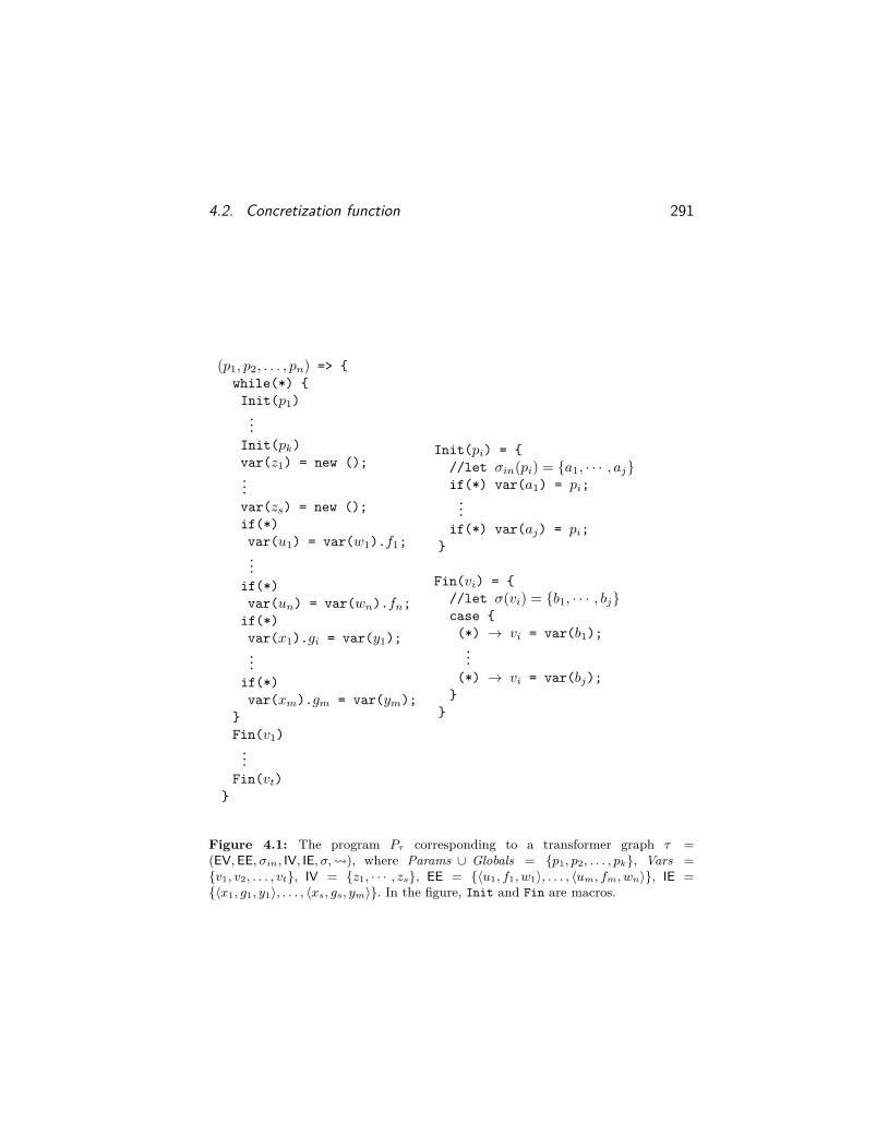
Interpreting a transformer graph as program helps understand the in-tuition behind several operations on the transformer graph. Fig. 4.1formally presents the schema of the procedure Pτ corresponding to atransformer graph τ = (EV,EE, σin, IV, IE, σ, ). We use the programrepresentation of a transformer graph only to convey the intuition be-hind the operations on the transformer graph but do not use it toformally define any of the operations.
For simplicity, we assume that the ordering relation = IE × EEi.e., any write may happen before any read, and only informally de-scribe how to extend the definition to accommodate a more preciseordering relation. In Fig. 4.1, the statements generated from the σinand the internal and external edges are guarded by non-deterministicif statements implying that they may or may not execute. The vari-able assignment statements generated from σ are enclosed by a non-deterministic case statement implying that at least one of these state-ments must execute. These constructs precisely capture the semanticsof the components of the transformer graphs.
One way to extend this conversion to support a more a preciseordering relation (that indicates that certain writes cannot happenbefore certain reads) is to associate with every write statement W aboolean variable bW , initialized to false. The variable is set to true afterW inside the if(∗) construct that containsW . Every read statement Ris guarded by the condition ¬(b1 ∨ . . .∨ bn) where b1, b2, . . . , bn are theboolean variables of the write statements that do not happen beforeR.
4.2 Concretization function
We now define the concretization function γT : AG → C. Given atransformer graph τ = (EV,EE, σin, IV, IE, σ, ) and a concrete graphgc = (Vc,Ec, σc), we need to construct a graph representing the trans-
4.2. Concretization function 291
(p1, p2, . . . , pn) => {while(*) {Init(p1)...
Init(pk)var(z1) = new ();...var(zs) = new ();if(*)var(u1) = var(w1).f1;...
if(*)var(un) = var(wn).fn;
if(*)var(x1).gi = var(y1);...
if(*)var(xm).gm = var(ym);
}Fin(v1)...
Fin(vt)}
Init(pi) = {//let σin(pi) = {a1, · · · , aj}if(*) var(a1) = pi;...
if(*) var(aj) = pi;}
Fin(vi) = {//let σ(vi) = {b1, · · · , bj}case {(*) → vi = var(b1);...
(*) → vi = var(bj);}
}
Figure 4.1: The program Pτ corresponding to a transformer graph τ =(EV,EE, σin, IV, IE, σ, ), where Params ∪ Globals = {p1, p2, . . . , pk}, Vars ={v1, v2, . . . , vt}, IV = {z1, · · · , zs}, EE = {〈u1, f1, w1〉, . . . , 〈um, fm, wn〉}, IE ={〈x1, g1, y1〉, . . . , 〈xs, gs, ym〉}. In the figure, Init and Fin are macros.

292 The Analysis Framework
formation of gc by τ . As explained in section 4.1, the transformer graphcan be interpreted as a program Pτ in which every internal and exter-nal vertex u becomes a variable var(u) and every internal and externaledge becomes a read or write statement. The output of the procedurePτ when executed with the concrete state gc is the transformation rep-resented by τ . However, we define the concretization function mathe-matically without explicitly constructing the procedure Pτ .
Given a graph gc ∈ C, γT (τ)(gc) is defined in two steps: in the firststep, we compute the set of vertices each node in τ represents, which isequivalent to computing the points-to set for each of the variables in theprogram Pτ . In the second step, we compute an abstract graph ga at theexit of the procedure Pτ using the points-to sets of the variables. Thesetwo steps together constitute the operation τ〈gc〉 (which was illustratedin the Fig. 2.3). The result of γT (τ)(gc) is the concrete image of τ〈gc〉,which is the set of all graphs that can be embedded in τ〈gc〉.
We now define a function η[[τ, gc]] : (IV ∪ EV) 7→ 2(IV∪Vc) that mapseach node in the transformer graph τ to a set of concrete nodes in gc aswell as internal nodes in τ . (We ignore the implicit parameters τ and gcof η whenever it is clear from the context). For any node u ∈ (EV∪ IV),η(u) is equivalent to the points-to set of var(u) in Pτ . η is defined asthe least solution of the following set of constraints over the variable µ.
v ∈ IV⇒ v ∈ µ(v) (4.3)v ∈ σin(X)⇒ σc(X) ∈ µ(v) (4.4)
〈u, f, v〉 ∈ EE, u′ ∈ µ(u), 〈u′, f, v′〉 ∈ Ec ⇒ v′ ∈ µ(v) (4.5)〈u, f, v〉 ∈ EE, 〈u′, f, v′〉 ∈ IE,
µ(u) ∩ µ(u′) 6= ∅,〈u′, f, v′〉 〈u, f, v〉
⇒ µ(v′) ⊆ µ(v) (4.6)
Explanation of the constraints:An internal node v maps to itself (Eq. 4.3) as it represents a newly
allocated object. If X is a parameter then an external node v ∈ σin(X)represents the node pointed to by X in the input state gc (Eq. 4.4). Thisis because, by the construction of Pτ , var(v) will be assigned to X andhence the points-to set of var(v) will include the targets of X.
4.2. Concretization function 293
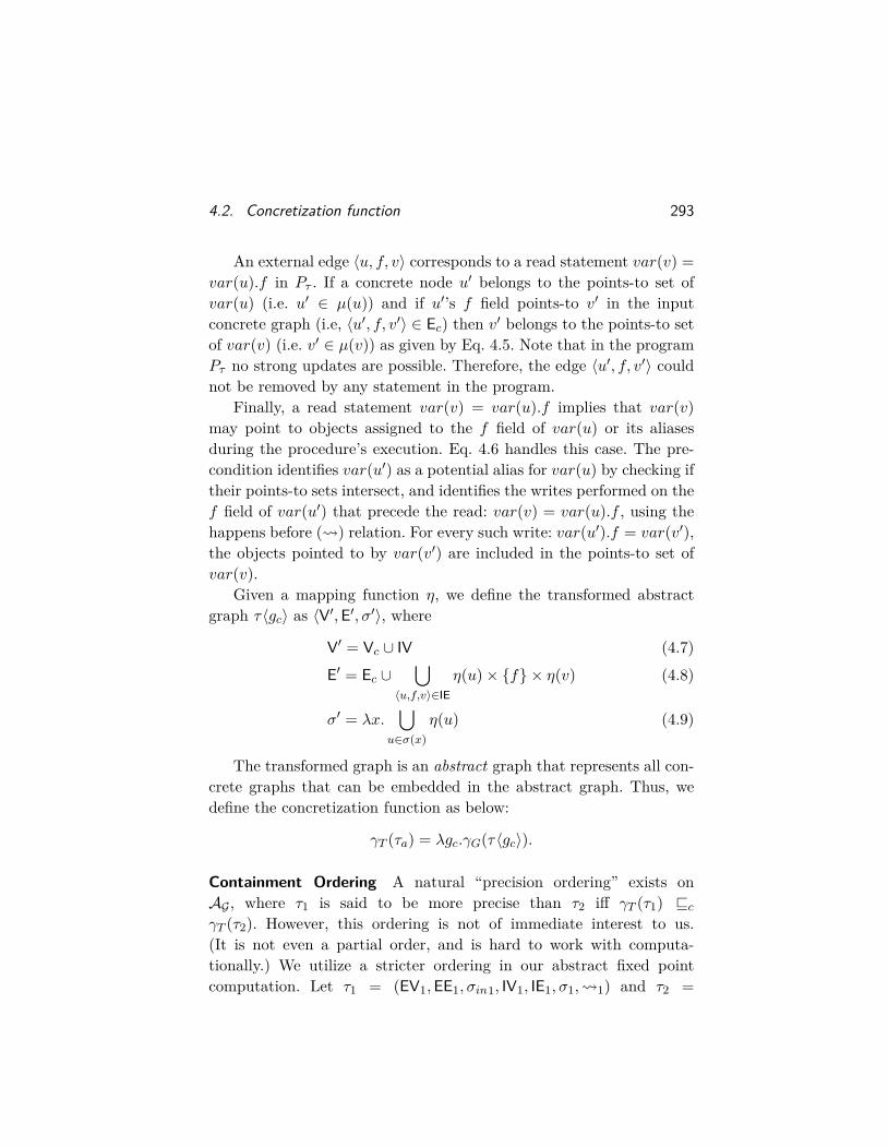
An external edge 〈u, f, v〉 corresponds to a read statement var(v) =var(u).f in Pτ . If a concrete node u′ belongs to the points-to set ofvar(u) (i.e. u′ ∈ µ(u)) and if u′’s f field points-to v′ in the inputconcrete graph (i.e, 〈u′, f, v′〉 ∈ Ec) then v′ belongs to the points-to setof var(v) (i.e. v′ ∈ µ(v)) as given by Eq. 4.5. Note that in the programPτ no strong updates are possible. Therefore, the edge 〈u′, f, v′〉 couldnot be removed by any statement in the program.
Finally, a read statement var(v) = var(u).f implies that var(v)may point to objects assigned to the f field of var(u) or its aliasesduring the procedure’s execution. Eq. 4.6 handles this case. The pre-condition identifies var(u′) as a potential alias for var(u) by checking iftheir points-to sets intersect, and identifies the writes performed on thef field of var(u′) that precede the read: var(v) = var(u).f , using thehappens before ( ) relation. For every such write: var(u′).f = var(v′),the objects pointed to by var(v′) are included in the points-to set ofvar(v).
Given a mapping function η, we define the transformed abstractgraph τ〈gc〉 as 〈V′,E′, σ′〉, where
V′ = Vc ∪ IV (4.7)
E′ = Ec ∪⋃
〈u,f,v〉∈IEη(u)× {f} × η(v) (4.8)
σ′ = λx.⋃
u∈σ(x)η(u) (4.9)
The transformed graph is an abstract graph that represents all con-crete graphs that can be embedded in the abstract graph. Thus, wedefine the concretization function as below:
γT (τa) = λgc.γG(τ〈gc〉).
Containment Ordering A natural “precision ordering” exists onAG , where τ1 is said to be more precise than τ2 iff γT (τ1) vcγT (τ2). However, this ordering is not of immediate interest to us.(It is not even a partial order, and is hard to work with computa-tionally.) We utilize a stricter ordering in our abstract fixed pointcomputation. Let τ1 = (EV1,EE1, σin1, IV1, IE1, σ1, 1) and τ2 =
294 The Analysis Framework
(EV2,EE2, σin2, IV2, IE2, σ2, 2). We define a relation vco on AG by:τ1 vco τ2 iff every component of τ1 is contained in the correspondingcomponent of τ2, i.e, EV1 ⊆ EV2, EE1 ⊆ EE2, ∀x.σin1(x) ⊆ σin2(x),IV1 ⊆ IV2, IE1 ⊆ IE2, ∀x.σ1(x) ⊆ σ2(x) and 1⊆ 2.
Lemma 4.1. vco is a partial-order on AG with a join operation, de-noted tco. Further, γT is monotonic with respect to vco: τ1 vco τ2 ⇒γT (τ1) vc γT (τ2).
Abstraction function αT It can be observed that there exists multipleelements in the abstract domain representing the same concrete value.There is no specific way of making a distinguishing choice among thepossible alternatives. Hence, we do not define an abstraction functionαT .
Our abstract interpretation formulation uses only a concretizationfunction. While this form is less common, it is sufficient to establish thesoundness of the analysis as explained in [Cousot and Cousot, 1992],section 7. Specifically, a concrete value f ∈ C is correctly representedby an abstract value τ ∈ AG , denoted f ∼ τ , iff f vc γT (τ). We seekto compute an abstract value that correctly represents the least fixedpoint of the concrete semantic equations.

5Parametric Abstract Semantics
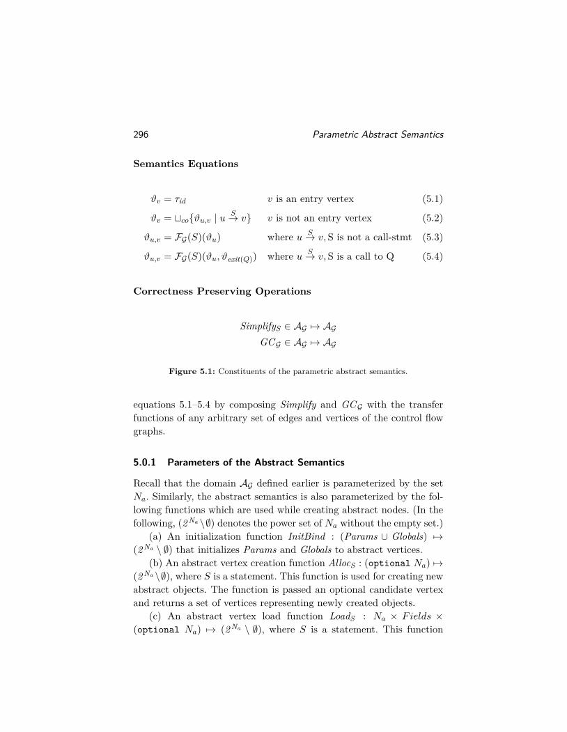
Fig. 5.1 shows the constituents of the most general abstract seman-tics. The equations 5.1–5.4 are the abstract semantics equations thatapproximate the concrete semantics equations 3.1–3.4. We introduce avariable ϑu for every vertex u in the control-flow graph denoting theabstract value at a program point u, and a variable ϑu,v for every edgeu → v in the control-flow graph denoting the abstract value after theexecution of the statement in edge u→ v.
We denote using τid (defined shortly) the transformer graph rep-resenting the identity function. FG(S) is the abstract semantics (ortransfer function) of a statement S. SimplifyS is a function from AG toAG that reduces the number of vertices in the input graph (see The-orem 5.6). GCG is an abstract garbage collection operation analogousto the concrete garbage collection operation (see Theorem 5.7).
The operations SimplifyS and GCG have a special property thatthey can be applied over the abstract value of any edge u S→ v orvertex of the control flow graph without affecting the correctness ortermination of the analysis. This is the reason for separating theseoperations from the semantics equations in Fig. 5.1. Hence, Fig. 5.1represents a family of abstract semantics equations that extend the
295
296 Parametric Abstract Semantics
Semantics Equations
ϑv = τid v is an entry vertex (5.1)
ϑv = tco{ϑu,v | uS→ v} v is not an entry vertex (5.2)
ϑu,v = FG(S)(ϑu) where u S→ v,S is not a call-stmt (5.3)
ϑu,v = FG(S)(ϑu, ϑexit(Q)) where u S→ v,S is a call to Q (5.4)
Correctness Preserving Operations
SimplifyS ∈ AG 7→ AGGCG ∈ AG 7→ AG
Figure 5.1: Constituents of the parametric abstract semantics.
equations 5.1–5.4 by composing Simplify and GCG with the transferfunctions of any arbitrary set of edges and vertices of the control flowgraphs.
5.0.1 Parameters of the Abstract Semantics
Recall that the domain AG defined earlier is parameterized by the setNa. Similarly, the abstract semantics is also parameterized by the fol-lowing functions which are used while creating abstract nodes. (In thefollowing, (2 Na \∅) denotes the power set of Na without the empty set.)
(a) An initialization function InitBind : (Params ∪ Globals) 7→(2 Na \ ∅) that initializes Params and Globals to abstract vertices.
(b) An abstract vertex creation function AllocS : (optional Na) 7→(2 Na \∅), where S is a statement. This function is used for creating newabstract objects. The function is passed an optional candidate vertexand returns a set of vertices representing newly created objects.
(c) An abstract vertex load function LoadS : Na × Fields ×(optional Na) 7→ (2 Na \ ∅), where S is a statement. This function

297
is used to model the reads performed on abstract objects. The functionis passed a vertex that is dereferenced, the dereferenced field and anoptional candidate vertex. It returns a set of vertices representing thedereferenced object.
In most cases, InitBind, LoadS and AllocS return a single abstractvertex. Notice that the parameters are defined for each program state-ment. This allows the parameter functions to have a statement spe-cific definition. The parameters help define a generic semantics that iscompletely oblivious to the naming strategies used to name abstractvertices.
In fact, different instances of our framework use different namingstrategies. For instance, the WSR analysis initializes parameter andglobal variables to abstract vertices that have the same name as thevariables. The internal and external vertices are named using the labelsof the statements that resulted in their creation. Formally, this corre-sponds to the following definition of the parameters in our framework.
Na = {nx | x ∈ Labels ∪ Params ∪Globals}InitBind = λx.{nx}
Alloc`:v=new() = λx.{n`}Load`:v1 =v2 .f = λ(x, f, y).{n`}
The correctness of the abstract semantics does not depend on thedefinitions of the parameters. The termination of the abstract semanticsonly requires the parameter definitions to be terminating functions.The abstract semantics of the framework (presented shortly) uses theparameters in a controlled way in order to ensure these properties.However, the scalability and the precision of the abstract semanticsdepend on the definition of the parameters to a large extent.
This we believe is the main practical advantage of the framework.This allows us to tune the abstract semantics to the required level ofprecision and scalability without having to be concerned with the cor-rectness or termination of the analysis. As we will illustrate later withconcrete instances, the framework offers a large spectrum of options toexperiment with.

298 Parametric Abstract Semantics
Stmt S FG(S)(EV,EE, σin, IV, IE, σ, )
v1 = v2 (EV,EE, σin, IV, IE, σ[v1 7→ σ(v2)], )
v = new C let N = AllocS() inlet IEnew = N × Fields × {null} in(EV,EE, σin, IV ∪N, IE ∪ IEnew, σ[v 7→ N ], )
v1.f = v2 (EV,EE, σin, IV, IE ∪ σ(v1)× {f} × σ(v2), σ, )
v1 = v2.f
let g = λu.
(∃x.〈u, f, x〉 ∈ EE)→⋃
〈u,f,x〉∈EELoadS(u, f, x)
| LoadS(u, f) inlet EVnew =
⋃u∈σ(v2)
g(u) in
let EEnew =⋃
u∈σ(v2){u} × f × g(u) in
(EV ∪ EVnew,EE ∪ EEnew, σin, IV, IE, σ[v1 7→ EVnew], ∪ {(ie, ee) | ie ∈ IE, ee ∈ EEnew})
exit(EV,EE, σin, IV, IE,
λx.(x ∈ Params ∪ Locals)→ null | σ(x))
Figure 5.2: Abstract semantics of primitive instructions.
5.1 Abstract Semantics of Primitive Statements
The transformer graph τid used in Fig. 5.1 is the transformer graphrepresenting the identity function and is defined as follows.
τid = (EV, ∅, σin, ∅, ∅, σin, ∅), where
EV =⋃
x∈Params∪GlobalsInitBind(x)
σin = λv. v ∈ Params ∪Globals → InitBind(v) | v ∈ Locals → {null}
Fig. 5.2 shows the transfer functions for the primitive statements.The function FG(S) can be considered as the most basic abstract se-
5.1. Abstract Semantics of Primitive Statements 299
mantics without any optimizations. The transfer function of a variableassignment statement v1 = v2 makes the targets of v1 equal to thetargets of v2.
Consider the transfer function of an object allocation statementv = new C. The transfer function creates new abstract nodesN for rep-resenting the newly allocated object using the Alloc parameter. (Allocwill generally create a single abstract node to represent the newly cre-ated object. However, the definition also permits the use of multipleabstract objects). The abstract nodes are added to the set of inter-nal vertices as they represent an object created within the analysedprocedure.
Recall that in our concrete semantics the fields of the newly createdobject are initialized to null. We capture this effect in the abstract se-mantics by creating new edges from the abstract nodes N to the nullobject. These edges are added to the set of internal edges as they rep-resent writes. Finally, the abstract nodes N are made the new targetsof the variable v.
The transfer function of a field-write statement v1.f = v2 is straight-forward. It creates new internal edges from the targets of v1 to thetargets of v2 labelled by the field f . The internal edges basically recordthat the field f of the targets of v1 are assigned to the targets of v2.
The transfer function of a field-read statement v1 = v2.f is quiteinvolved. However, in essence, the goal is to create external vertices tomodel the targets of v2.f , and to create external edges to record thatthe field f of the targets of v2 are read. One important question is howto choose the external vertices to represent the targets of v2.f? Thechoice of the external vertices may affect the precision and scalabilityof the analysis.
For example, consider a transformer graph τ in which the targetsof v2 are two nodes u and v i.e, σ(v2) = {u, v}. Also, say that thereexists two variables v3 and v4 whose targets are u and v, respectively.That is, σ(v3) = {u} and σ(v4) = {v}. If we use a single node w asthe target of both the external edges starting from u and v, we endup collapsing the targets of v3.f and v4.f as well. This would resultin loss of precision. On the other hand, using two different vertices
300 Parametric Abstract Semantics
as the targets of edges starting from u and v will increase the sizesof the transformer graph, which may increase the running time of theanalysis. Therefore, we parameterize the creation of the targets of theexternal edges in the transfer function of a field-read statement. Mostof the sophistication in the transfer function presented in Fig. 5.2 is forachieving this parameterization. We describe the transfer function indetail below.
We refer to a vertex that belongs to σ(v2) as a dereferenced ver-tex. The function g, defined in Fig. 5.2, determines the targets of thef field of a dereferenced vertex u using the parameter Load. If u al-ready has external edges on field f of the form 〈u, f, x〉 then, for everysuch edge, we apply the LoadS parameter over the triple (u, f, x). Thisallows us to define a semantics in which the external vertices createdduring the previous field-read statements are reutilized. For example,if LoadS(u, f, x) is defined as {x} then the targets of the previous readsof the field f of the vertex u would be reused to represent the targetsof the current read. On the other hand, if there exists no external edgefrom u on field f then we apply Load on (u, f) as we do not have acandidate vertex to reuse.
Once we know the targets of the f fields of the dereferenced ver-tices, the rest of the semantics is straight forward. We add the targetsof all the dereferenced vertices, computed by the function g, to the ex-ternal vertex set. We also make them the new targets of v1. For everydereferenced vertex u, we create external edges from u to the verticesin g(u). Note that the internal edges existing in the transformer graphbefore the field-read statement represent writes that have happenedbefore the current read. We update the happens before relation toreflect this fact.
5.2 Abstract Semantics of Procedure Call
Let S : Q(a1, a2, · · · , an) be a call statement. Let τr be the transformergraph in the caller before the statement S and let τe be the abstractsummary of Q. The function FG(S)(τr, τe) is defined as follows:
FG(S)(τr, τe) = pop]S(τe〈〈push]S(τr)〉〉S , τr) (5.5)

5.2. Abstract Semantics of Procedure Call 301
push]S(σ) = λv. (v = Param(i)→ σ(ai)| v ∈ Globals → σ(v)| v ∈ Locals → null)
pop]S(σ, σ′) = λv. (v ∈ Params ∪ Locals → σ(v)| v ∈ Globals → σ′(v))
push]S(τ) = (EV,EE, σin, IV, IE, push]S(σ))
pop]S(τ ′, τ) = (EV′,EE′, σin′, IV′, IE′, pop]S(σ, σ′))
Figure 5.3: Definitions of the abstract push and pop operations push]S and pop]S .In the figure, S is the call statement Q(a1, · · · , an), τ = (EV,EE, σin, IV, IE, σ, )and τ ′ = (EV′,EE′, σin′, IV′, IE′, σ′).
where, the push]S and pop]S , defined in Fig. 5.3, are the abstract ana-logues of the concrete pushS and popS operations. They perform themapping of the formal arguments to actual parameters and vice versa.The function 〈〈〉〉 : AG ×AG 7→ AG is the composition operation for thetransformer graphs and is explained in the sequel.
5.2.1 The Composition Operation
Given two transformer graphs τ1 and τ2, τ2〈〈τ1〉〉S is a transformer graphequivalent to applying τ1 followed by τ2. We describe the basic ideabehind the composition operation using an example before presentinga formal definition.
Consider Fig. 5.4. Let τ1 and τ2 be the two transformer graphsshown at the top of the Fig. 5.4. The programs Pτ1 and Pτ2 constructedfrom τ1 and τ2 are shown at the bottom of the Fig. 5.4. For concisenesswe use the node ids to denote the corresponding variables. Fig. 5.5(a)shows the program P ′ obtained by composing the programs Pτ1 andPτ2 i.e, P ′ = Pτ1 ;Pτ2 . The goal is to construct a transformer graph thatis an abstraction of the program P ′. Unfortunately, P ′ itself cannot beinterpreted as a transformer graph. This is because P ′ has multiplewhile loops and has statements that assign values to program variables

302 Parametric Abstract Semantics
(x, y) => {[1] while(*) {[2] if(*) u1 = x;[3] if(*) u1 = y;[4] u2 = new ();[5] if(*) u1.next = u2;[6] }[7] x = u1;[8] y = u2;
}
(x, y) => {[1] while(*) {[2] if(*) n1 = x;[3] if(*) n2 = y;[4] n0 = new ();[5] if(*) n1.next = n0;[6] if(*) n0.next = n2;[7] if(*) n3 = n2.next;[8] }[9] t = n0;[10] retval = n3;[11] x = n1;[12] y = n2;
}(a) (b)
Figure 5.4: (a) Transformer graph τ1 and its program interpretation Pτ1 . (b) Trans-former graph τ2 and its program interpretation Pτ2 .
x, y (see lines [7] and [8]). In a program that corresponds to a trans-former graph such statements can occur only at the end of the program(see the formal definition of constructing a program from a transformergraph presented in section 4.1).
The statements at lines [7] and [8] define the values of the variablesafter the application of τ1. They can be eliminated by replacing theparameter nodes of Pτ2 corresponding to the parameter variables xand y, namely n1 and n2, by the values of x and y at the end of Pτ1 ,namely u1. After this step, the two loops can be abstracted into a singlewhile loop encompassing the statements of the loops. The program thusobtained is shown in Fig. 5.5(b). The lines [13]–[15] in P ′ become lines[7]–[9] in Pτ ′ , in which n1 and n2 are replaced by u1. This program canbe interpreted as a transformer graph τ ′ which is shown in Fig. 5.5(c).

5.2. Abstract Semantics of Procedure Call 303
(x, y) => {[1] while(*) {[2] if(*) u1 = x;[3] if(*) u1 = y;[4] u2 = new ();[5] if(*) u1.next = u2;[6] }[7] x = u1;[8] y = u1;[9] while(*) {[10] if(*) n1 = x;[11] if(*) n2 = y;[12] n0 = new ();[13] if(*) n1.next = n0;[14] if(*) n0.next = n2;[15] if(*) n3 = n2.next;[16] }[17] t = n0;[18] retval = n3;[19] x = n1;[20] y = n2;
}
(x, y) => {[1] while(*) {[2] if(*) u1 = x;[3] if(*) u1 = y;[4] u2 = new ();[5] if(*) u1.next = u2;[6] n0 = new ();[7] if(*) u1.next = n0;[8] if(*) n0.next = u1;[9] if(*) n3 = u1.next;[10] }[11] t = n0;[12] retval = n3;[13] x = u1;[14] y = u1;
}
(a) (b)
(c)
Figure 5.5: (a) The procedure P ′ = Pτ1 ;Pτ2 . (b) Procedure Pτ ′ obtained by elim-inating parameter nodes of τ2. (c) The transformer graph corresponding to Pτ ′ ,which is equal to τ2〈〈τ1〉〉S .

304 Parametric Abstract Semantics
The approach illustrated above generalizes to any pair of trans-former graphs. Informally, to compose a transformer graph τ1 with τ2we perform the following steps. For every parameter variable X of τ2,we eliminate the parameters nodes σin(X) from every component ofthe transformer graph τ2 by replacing each of them with σ1(X), whichare the (possible) value of the variable X resulting at the end of τ1.We define the (internal and external) edges of the composed graphsas the union of the edges of τ1 and the edges of τ2 obtained after theelimination of parameter nodes.
The initial variable mapping σin of the composed graph is given byσin1. The final variable mapping of the composed graph is given by themapping obtained after the elimination of parameter nodes from σ2.The internal and external vertices, other than the parameter nodes,contained in the transformer graph τ2 are retained in the composedtransformer graph. With this informal description we now proceed tothe formal definition.
Let V2 = EV2 ∪ IV2. We first define a function η[[τ2, τ1]] : V2 7→ 2 Na
that maps the vertices in τ2 to a set of abstract vertices belonging to τ1and τ2. We elide the implicit parameters of η namely τ1, τ2 whenever itis clear from the context. η is defined using the following constraints:
x ∈ (EV2 \ range(σin2))⇒ x ∈ η(x) (5.6)x ∈ σin2(X)⇒ σ1(X) ⊆ η(x) (5.7)
x ∈ IV2 ⇒ AllocS(x) ∈ η(x) (5.8)〈u, f, x〉 ∈ EE2, a ∈ η(u)⇒ LoadS(a, f, x) ∈ η(x) (5.9)
The first two constraints 5.6 and 5.7 follow from the informal expla-nation. The parameter nodes of a variable X are mapped to the valuesof X at the end of Pτ1 which is given by σ1(X), and the remaining ex-ternal vertices are mapped to themselves. The constraints 5.8 and 5.9add more flexibility to the composition operation by incorporating theparameters of the abstract semantics. This will be explained in moredetail shortly.
For example, consider the composition of the transformer graph τ1with the transformer graph τ2 shown in Fig. 5.4(a) and (b), respec-tively. In this case, η(n1) = η(n2) = {u1}, η(n3) = LoadS(u1, next, n3)

5.2. Abstract Semantics of Procedure Call 305
transIE(IE, µ) =⋃
〈u,f,v〉∈IEµ(u)× {f} × µ(v)
transEE(EE, µ) =⋃
〈u,f,v〉∈EE{
⋃a∈µ(u)
{a} × {f} × LoadS(a, f, v)}
transSigma(σ, µ) = λx. µ(σ(x))
transHB( , µ) =⋃
ie ee
transIE({ie}, µ)× transEE({ee}, µ)
Figure 5.6: Translation of a transformer graph with respect to a mapping µ.
and η(n0) = AllocS(n0). For now, assume that the Load and Allocfunctions return the candidate vertex passed to the functions. That is,LoadS(u1, next, n3) = {n3} and AllocS(n0) = {n0}.
Consider the family of operations trans shown in Fig. 5.6 that givena mapping µ on abstract nodes translates a component of a transformergraph, which could be a set of internal or external edges, a happensbefore relation, or a mapping from variables to abstract objects (σ),by applying the function µ point-wise on every vertex contained inthe component. The translation of external edges, however, applies theparameter Load instead of µ to the targets of external edges.
Intuitively, if the trans function is applied over η (defined by 5.6–5.9) and a component of the transformer graph τ2 then it replaces theparameters nodes of τ2 by the values at the end of τ1 in the givencomponent of τ2.
For example, for the transformer graphs τ1 and τ2 shown inFig. 5.4(a) and (b) respectively, transEE({〈n2, next, n3〉}, η) is equalto {〈u1, next, n3〉}, transIE({〈n1, next, n0〉}, η) equals {〈u1, next, n0〉},and transSigma(x 7→ n1, η) = (x 7→ u1), where η is the mapping functionpresented earlier.
We define the composed transformer graph as:
τ2〈〈τ1〉〉S = Append(τ1, τ2, η),
where Append, defined below, is a function that translates the compo-nents of τ2 by applying η and appends it to τ1. Let the components of

306 Parametric Abstract Semantics
τ1 be denoted using subscript 1 and those of τ2 using the subscript 2.Append(τ1, τ2, η) = (EV′,EE′, σin′, IV′, IE′, σ′, ′), where
EV′ = EV1 ∪ (EV2 \ range(σin2) ∪ {v | 〈u, f, v〉 ∈ EE′}IV′ = IV1 ∪ ˆAllocS(IV2)EE′ = EE1 ∪ transEE(EE2, η)IE′ = IE1 ∪ transIE(IE2, η)σin′ = σin1
σ′ = transSigma(σ2, η) ′ = 1 ∪transHB( 2, η) ∪ IE1 × EE2
Except for the definitions of EV′ (the set of external vertices of thecomposed graph) and ′ the other definitions are straight forward. EV′includes all the external vertices of τ1, all the external vertices of τ2except the parameter vertices, and all the vertices that were created us-ing the Load parameter during the translation of external edges (thesevertices are the targets of external edges in the composed transformergraph).
The ordering relation ′ includes IE1×EE2 as we are concatenatingτ1 with τ2 which implies that the edges in τ1 happen before those in τ2.
5.2.2 Parmeterizing the Composition Operation
We now explain the need for incorporating the parameters Alloc andLoad in the definition of composition operation presented above.
The parameters Alloc and Load enable fine tuning of the context-sensitivity of the analysis. It is well known that when abstract objectsrepresenting newly allocated objects are named based on their alloca-tion sites, cloning (or renaming) of abstract objects for each call siteduring a heap analysis increases the context-sensitivity of the analysis(e.g, see [Liang and Harrold, 2001], [Lattner et al., 2007]). Since theinternal vertices represent objects newly allocated within the analysedscope and they may be named based on their allocation sites, we in-corporate the parameter AllocS to support cloning of internal verticesduring call statements.

5.3. Simplifying the Transformer Graphs 307
The parameter LoadS serves a similar purpose, namely to supportthe cloning of external vertices. Since the external vertices are some-what unique to the transformer graphs, the need for cloning them maynot be immediately obvious. Hence, as an example, consider again thetransformer graphs and programs shown in Fig. 5.4(a) and (b). Con-sider a slight variation of τ1 in which the variable y additionally points-to a node u3.
In this case, the parameter node n2 of τ2 will have to be replacedby two nodes u1 and u3 during the composition operation. Withoutany form of cloning, the statement at line [7] in procedure Pτ2 , shownin Fig. 5.4(b), would be replaced by two new statements n3 = u1.next
and n3 = u3.next. The node n3 would then represent the targets ofboth u1.next and u3.next. Though this wouldn’t affect correctness, itmay result in loss of precision as the targets of two possibly differentreferences are collapsed in the composed transformer graph.
Thus, for the generality of the semantics, we compute the targets ofthe external edges (or field-reads) created during the composition oper-ation using the parameter LoadS . In this example, the target of u1.next
would be determined using LoadS(u1, next, n3) and that of u3.next us-ing LoadS(u3, next, n3).
5.3 Simplifying the Transformer Graphs
5.3.1 The SimplifyS Operation
We now describe the Simplify operation that reduces the number ofvertices in a transformer graph without altering its concrete image. Ina nutshell, the Simplify operation propagates the reads and writes onan external vertex w to the vertices in the transformer graphs thatrepresent a subset of concrete objects represented by w.
Let τ = (EV,EE, σin, IV, IE, σ, ) be a transformer graph. Say thereis an external edge 〈u, f, w〉 ∈ EE, an internal edge 〈u, f, x〉 ∈ IE and theinternal edge may happen before the external edge (i.e, write happensbefore the read). In this case, the values of x may flow to w. Clearly,w represents a superset of concrete objects represented by x. Hence, awrite (or read) on w can be considered as a write (or read) on x. That

308 Parametric Abstract Semantics
x ∈ EV ∪ IV⇒ x ∈ Incl(x) (5.10)〈u, f, v〉 ∈ IE, 〈u′, f, v′〉 ∈ EE,
Incl(u) ∩ Incl(u′) 6= ∅,〈u, f, v〉 〈u′, f, v′〉
⇒ Incl(v) ⊆ Incl(v′) (5.11)
〈u, f, v〉 ∈ EE, a ∈ Incl(u)⇒ LoadS(a, f, v) ∈ Incl(v) (5.12)
Figure 5.7: The function Incl (for a transformer graph (EV,EE, σin, IV, IE, σ, ))is defined as the least solution satisfying the above constraints.
is, 〈w, f, y〉 ∈ IE (or EE) implies 〈x, f, y〉 ∈ IE (or EE), respectively. Thefunction Incl : V 7→ V, defined in Fig. 5.7, maps every vertex w tothe set of vertices whose values may flow to w. We clone the externalvertices during Simplify (as shown in Fig. 5.7) for the same reasonsdescribed while presenting the composition operation in section 5.2.1.
SimplifyS(τ) = removeNonEscaping(τ ′), whereτ ′ = (EV ∪ {v | 〈u, f, v〉 ∈ EE′}, IV, σin,EE′, transIE(IE, Incl),
transSigma(σ, Incl), transHB( , Incl))EE′ = transEE(EE, Incl)
where, the trans operations, defined in section 5.2.1, apply themapping Incl point-wise on each of the vertices in a given com-ponent of a transformer graph. We now describe the operationremoveNonEscaping.
The operation removeNonEscaping, formally defined in Fig. 5.8,performs the actual simplification by removing edges and verticesfrom a transformer graph. We say that a vertex (internal or ex-ternal) in a transformer graph τ is non-escaping if it does not be-long to Escaping(τ). Given a transformer graph τ , the operationremoveNonEscaping removes external edges starting from non-escapingvertices and external vertices that do not have any external edges end-ing at them. When a vertex is removed from a transformer graph, alledges (internal or external) that start or end at the vertex would alsobe removed from the transformer graph.

5.3. Simplifying the Transformer Graphs 309
removeNonEscaping(EV,EE, σin, IV, IE, σ, ) =let EEun = {〈u, f, v〉 ∈ EE | u /∈ Escaping(τ)} inlet EVun = {w ∈ EV | ¬∃〈u, f, w〉 ∈ (EE \ EEun)} inlet IEun = {〈u, f, v〉 ∈ IE | u (or) v belongs to (EVun \ IV)} inlet σ′ = λx.σ(x) \ (EVun \ IV) inlet ′= \{(ie, ee) ∈ | ie ∈ IEun ∨ ee ∈ EEun} in(EV \ EVun,EE \ EEun, σin, IV, IE \ IEun, σ′, ′)
Figure 5.8: Definition of the function removeNonEscaping : AG 7→ AG .
Correctness of the Simplify Operation The correctness of the sim-plify operation is formalized in Theorem 5.6. The lemma states the con-crete images of a transformer graph τ and SimplifyS(τ) are equal. Thisimplies that the edges and vertices removed by the removeNonEscapingoperation are redundant. Let w be a vertex read from a non-escapingvertex x i.e, 〈x, f, w〉 ∈ EE. The proof of the Theorem 5.6 establishesthat, under all contexts, the concrete objects that w may representis the union of all the concrete objects represented by the vertices inIncl(w) that are escaping. This implies that the external edge 〈x, f, w〉is redundant as every internal and external edge incident on w aretranslated to every vertex in Incl(w).
An external vertex that is not the target of any external edge canbe removed as such external vertices will not represent any concreteobject by the definition of γT . (The mapping η computed during theconcretization operation will always map them to empty sets.)
However, it is to be noted that a similar simplification cannot beapplied to external edges that emanate from an escaping internal ver-tex, though an internal vertex represents objects allocated within theanalysed code fragment. Let w be a vertex read from an internal ver-tex. A pertinent question to ask is whether Incl(w) include all verticeswhose values may flow to w?
Fig. 5.9 shows that this is not always the case. Consider the Inclmapping computed for the transformer graph shown at the right side

310 Parametric Abstract Semantics
Q (x, y) {[1] t = new ();[2] x.next = t;[3] y.next.next = x;[4] retvar = t.next;
}
Figure 5.9: A program illustrating the effect of aliasing in the input state oninternal escaping vertices.
of Fig. 5.9. The Incl function would map the node n4 (which is a vertexread from an internal vertex) to only itself i.e, Incl(n4) = {n4}. Supposethat in some calling context the parameters x and y of the procedure Qare aliases. The field-write at line [3] would actually update the nextfield of the object allocated inside Q. The subsequent read of the nextfield of the newly allocated object will get the value written at line [3]which is the parameter object p1. Therefore, p1 flows to n4 if x and yalias in the calling context.
This example illustrates that the values read from escaping verticesare dependent on the calling contexts even if they are allocated in-side the analysed procedure, implying that external edges on escapingvertices ought to be preserved in the transformer graphs.
5.3.2 Abstract Garbage Collection
Analogous to the function GCc used in the concrete semantics, thefunction GCG used in the abstract semantics equations trims the trans-former graphs by removing internal vertices (and the edges incident onthe vertices) that are not reachable from the variables in the programand from the prestate.
Fig. 5.10 shows the formal definition of GCG . This operation re-moves all internal vertices that are unreachable from the variables, theexternal vertices and vertices with external edges starting from them.

5.4. Correctness and Termination of the Framework 311
GCG(τ) =let S = σ(Vars) ∪ EV ∪ {u | 〈u, f, x〉 ∈ EE}let IVun = {x ∈ IV | ¬∃y ∈ S. x is reachable from y } inlet Eun = {〈u, f, v〉 ∈ IE ∪ EE | u (or) v belongs to IVun} inlet σ′ = λx.σ(x) \ IVun inlet ′= \{(ie, ee) ∈ | ie or ee belongs to Eun} in(EV,EE \ Eun, σin, IV \ IVun, IE \ Eun, σ′, ′)
Figure 5.10: The definition of the abstract garbage collection operation GCG :AG 7→ AG . In the figure, τ = (EV,EE, σin, IV, IE, σ, ).
Theorem 5.7 establishes the correctness of the garbage collection op-eration. In particular, it proves that the set IVun, the set of verticesunreachable from the set S, represent concrete objects that are un-reachable from the prestate and the variables in the program.
Recall that when the Simplify operation is performed on a trans-former graph, the external edges starting from non-escaping verticesand external vertices that are not targets of external edges are removedfrom the transformer graphs. Therefore, applying GCG on a “simplified"transformer graph will remove all non-escaping internal vertices thatare unreachable from the variables. Many instances of the frameworke.g. [Lattner et al., 2007], [Salcianu and Rinard, 2005], that maintaina (partially) simplified transformer graphs at every program point asexplained later, adopt this definition for the garbage collection opera-tion. However, GCG defined above is more general and is applicable toany transformer graph in AG .
5.4 Correctness and Termination of the Framework
We now state and prove a few insightful lemmas that help in estab-lishing the correctness of the abstract semantics. As usual, we say thata concrete value f ∈ C is correctly represented by an abstract valueτ ∈ AG , denoted f ∼ τ , iff f vc γT (τ). For brevity, we only provide

312 Parametric Abstract Semantics
proof sketches and also completely omit proofs when they are straightforward to derive from the definitions.
In most of the proofs, we use induction over the computation ofη[[τ, gc,]] which is defined as the least solution of a set of recursive im-plications (4.3)–(4.6) (see section 4.2 for more details) which naturallylends itself to an inductive proof structure. To prove that η satisfies aclaim, we hypothesize that the claim holds in the antecedent of eachrule and establish that the claim holds in the consequent of the rule.
Lemma 5.1. (First Escape Lemma) Let τ be a transformer graph suchthat every external edge has an escaping source vertex i.e. 〈u, f, v〉 ∈EE =⇒ u ∈ Escaping(τ). Let gc = (Vc,Ec, σc) be a concrete graph. Ifx is a vertex in τ then y ∈ η(x) ∧ y ∈ Vc =⇒ x ∈ Escaping(τ).
In simple words, the lemma states that, when all the external edgeson the transformer graph have only escaping source vertices (the pre-condition), if a vertex x represents a concrete object (in some context)then x is an escaping vertex i.e. x is transitively reachable from theparameters (or globals).
Proof. We prove this by induction on the computation of η. It is easyto see that in each of the four rules when the claim holds for η in theantecedent, it also holds in the consequent.
Lemma 5.2. (Second Escape Lemma) Let τ be a transformer graph sat-isfying the preconditions of the first escape lemma. Let gc = (Vc,Ec, σc)be a concrete graph. For any pair of vertices x, y in τ , y ∈ η(x) ∧ y 6=x =⇒ x, y ∈ Escaping(τ).
In simple words, the lemma states that, when the preconditions hold,if a vertex x represents a vertex other than itself (in some context) thenit must be escaping. The contrapositive form of the above statement ismore intuitive. It states that if a vertex is non-escaping then it repre-sents only itself and is not a placeholder for any other vertex.
Proof. Induction on the computation of η. The only non-trivial case isestablishing that the claim holds for the alias rule i.e. (4.6). Considerthe antecedent of the alias rule given below.
〈u, f, x〉 ∈ EE, 〈r, f, s〉 ∈ IE, η(u) ∩ η(r) 6= ∅ (5.13)
5.4. Correctness and Termination of the Framework 313
The constraint on is omitted as it is unimportant here. We need toestablish that for all vertices y ∈ η(s), if y 6= x then y escapes (as ywould be added to η(x) by the consequent).
If y 6= s then y escapes by hypothesis. Say y = s. By (5.13),〈r, f, y〉 ∈ IE. If r escapes then, by the definition of Escaping, y es-capes as we have hypothesized that there is an internal edge from r
to s (which is same as y). Say r /∈ Escaping(τ). We will now showthat this case is not possible. Let p = η(u) ∩ η(r). If r 6= p then r
escapes by hypothesis. Therefore, the only possibility is r = p. Hence,r ∈ η(u). Again, if r 6= u then r escapes by hypothesis. Therefore, rmust be equal to u. By (5.13), 〈r, f, x〉 ∈ EE. However, by the prereq-uisite on the transformer graph, r escapes, which is a contradiction tothe assumption that r /∈ Escaping(τ). Hence, r /∈ Escaping(τ) is notpossible.
Corollary 5.3. Let τ be a transformer graph satisfying the conditionsof first escape lemma. Let gc be a concrete graph. For any vertices x, yin the transformer graph,
η(x) ∩ η(y) 6= ∅ ∧ x 6= y =⇒ x, y ∈ Escaping(τ)
Proof. Let r = η(x) ∩ η(y). If r ∈ Vc or r is different from x and y, xand y both escape by the first and second escape lemmas. Say r = x.x ∈ η(y) and x 6= y implies, by the above lemma, that x and y escape.Similarly, if r = y and x 6= y, x and y escape.
Lemma 5.4. For every primitive statement S, if f ∼ τ then f ◦ [[S]]c ∼FG(S)(τ), where FG(S) is the transfer function of a primitive statementdefined in Fig. 5.2.
Proof. f ∼ τ implies that f vc γT (τ). By the definition of γT , for anyconcrete graph gc ∈ Gc, every concrete graph in f(gc) embeds in τ〈gc〉.Therefore, it suffices to show that for any g ∈ Gc such that g � τ〈gc〉,[[S]]c(g) � τout〈gc〉, where τout = FG(S)(τ). This can be proved from thedefinitions of [[S]]c, FG(S), τ〈gc〉, and by induction on the computationof η[[τ, gc]]. We omit a detailed proof for brevity.

314 Parametric Abstract Semantics
Lemma 5.5. if f1 ∼ τ1 and f2 ∼ τ2, then f1 ◦ f2 ∼ τ2〈〈τ1〉〉S .
Proof. Let gc ∈ Gc be a concrete graph. f1 ∼ τ1 implies that everyconcrete graph in f1(gc) embeds in τ1〈gc〉. Similarly, every concretegraph in f2(gc) embeds in τ2〈gc〉. Hence, every graph in f2(f1(gc)) willembed in τ2〈g〉 for some concrete graph g such that g � τ1〈gc〉. Hence,it suffices to show that for any {g, g′} ⊆ Gc such that g � τ1〈gc〉 andg′ � τ2〈g〉, g′ � τout〈gc〉, where τout = τ2〈〈τ1〉〉S . This can be provedfrom the definitions of 〈〈〉〉S , 〈〉, and by induction on the computationof η[[τ2, g]]. We omit a detailed proof for brevity.
5.4.1 Correctness of the Simplify operation
Theorem 5.6. Let S be any statement and τ ∈ AG be a transformergraph. γT (τ) = γT (SimplifyS(τ))
Proof. Let τ ′ denote Simplify(τ). The proof of this lemma is quiteinvolved. The proof consists of two parts, in the first part we show thatγT (τ ′) is an over-approximation of γT (τ) (i.e., γT (τ) vc γT (τ ′)) and inthe second part we prove the converse.
(Part-I): For every input graph gc, γT constructs an abstract graphτ〈gc〉 representing the possible output concrete states. Every externalor internal edge in τ is primarily used in identifying and adding edgesto the abstract graph τ〈gc〉 as discussed in section 4.2. To prove thatτ ′ over-approximates τ it suffices to show that the edges removed bySimplify do not matter, that is, for every vertex u in τ there exists avertex in τ ′ that adds all the edges added by u to the output abstractgraph τ ′〈gc〉. Given this, it is easy to see that τ〈gc〉 vco τ ′〈gc〉 (whichimplies the claim). The function Incl used by Simplify translates allthe edges on a vertex u to every vertex in Incl(u). Hence, it sufficesto show that, for every node x that u represents in τ , there exists atleast one vertex belonging to both Incl(u) and τ ′ that represents x,which is formally stated below and pictorially illustrated in Fig. 5.11.In Fig. 5.11 and in the sequel, η denotes η[[τ, gc]](u) and η′ denotesη[[τ ′, gc]] where τ ′ = Simplify(τ).
Let V denote the vertices in τ .
u ∈ V, x ∈ η(u) =⇒ x ∈ η′(Incl(u))

5.4. Correctness and Termination of the Framework 315
(a) (b)
Figure 5.11: Pictorial illustration of the correctness of Simplify operation. Sayu is a node removed by Simplify. Part (a) of the figure shows that the vertex uis found to represent the objects x1, · · · , xn in τ . Part (b) of the figure shows thatIncl mapping computed by the Simplify operation will contain vertices (here, u′, u′′)which together will represent all the objects that u represented in τ .
This can be formally proved using induction on the computation of ηand using the first and second escape lemmas.
(Part II): We now establish that γT (τ ′) vc γT (τ). Simplify adds in-ternal and external edges to τ which in turn could result in the additionof edges to the abstract graph τ ′〈gc〉.
Let 〈u, f, w〉 ∈ IE′. Say u is found to represent an object c in theconcretization of τ ′ (i.e. c ∈ η′(u)) and w represents an object d.Clearly, 〈c, f, d〉 will be added to τ ′〈gc〉 (by construction). To prove theclaim it suffices to establish that 〈c, f, d〉 would also be added to τ〈gc〉.However, this would be implied when the following two conditionshold as explained below:
(a) For any u, v ∈ V, u ∈ Incl(v) =⇒ η(u) ⊆ η(v).(b) For any x ∈ V′, η′(x) ⊆ η(x).
By the second condition, c ∈ η′(u) implies that c ∈ η(u). Similarly,d ∈ η(w). Now say 〈u, f, w〉 /∈ IE i.e. the internal edge is added bySimplify (otherwise the claim directly follows). By the definition ofSimplify, ∃p, q ∈ V s.t. u ∈ Incl(p), w ∈ Incl(q), 〈p, f, q〉 ∈ IE. The first

316 Parametric Abstract Semantics
condition implies that η(u) ⊆ η(p) and η(w) ⊆ η(q). Hence, c ∈ η(p),d ∈ η(q). Therefore, 〈c, f, d〉 would be added to τ〈gc〉 as required.
Hence, it just suffices to establish that the conditions (a) and (b)hold. Condition (a) follows directly from the definition of Incl and thealias rule (4.6) of η computation. Condition (b) can be proved usinginduction on the computation of η[[τ ′, gc]] and using condition (a) (whichis essential for proving that the claim holds for the constraints (4.5) and(4.6)). Details elided for brevity.
5.4.2 Correctness of the GCG operation
Theorem 5.7. If f ∼ τ then GCc(f) ∼ τ and GCc(f) ∼ GCG(τ).
Proof. The first claim GCc(f) ∼ τ is relatively easier to establish. Forany gc ∈ Gc, if g1 ∈ GCc(f)(gc) then there exists a g2 ∈ f(gc) suchthat g1 � g2, as GCc only removes vertices and edges from the graphsin f(gc). Since f ∼ τ , g2 � τ〈gc〉. Therefore, g1 � g2 � τ〈gc〉. Hence,g1 ∈ γ(τ)(gc).
Consider the second part. Let gc = (Vc,Ec, σc) be a concrete graph.Let τ〈gc〉 = (Vr,Er, σr). Let η denote η[[τ, gc]]. To prove this part itsuffices to show that the vertices removed by GCG in τ will only repre-sent vertices that are unreachable from Vc and Vars in τ〈gc〉 as thosecorrespond to the vertices that would be removed by GCc.
Claim: if u is not reachable from the set S = σ(Vars) ∪ EV ∪{u | 〈u, f, x〉 ∈ EE} then every vertex y in η(u) is not reachable fromVc and σr(Vars) in τ〈gc〉.
Before we sketch the proof, we establish a unique property of thevertices unreachable from the set S. Let u be a vertex in τ that isunreachable from S. For any concrete graph gc, u ∈ η(u′) ⇒ u = u′.That is, no vertex other than u itself represents u. This precludes theexistence of other vertices in τ representing u. This property can beproved, via induction on η, by establishing that no constraint otherthan the internal vertex rule (4.3) can add u to η(u′) for any vertex u′.
Now consider the claim. Let w be a vertex not reachable from S andy ∈ η(w). Consider a path x1, . . . , xn, where xn = y, in τ〈gc〉 endingat y. It suffices to show that no vertex in this path belongs to Vc orσr(Vars).

5.4. Correctness and Termination of the Framework 317
Since w is not reachable from S, w ∈ IV \ EV. By the definition ofη, y = w. Since there is an edge from xn−1 to y in Er, by the definitionof 〈〉, ∃p, q ∈ V, xn−1 ∈ η(p), y ∈ η(q), 〈p, f, q〉 ∈ IE. Since, y (whichis same as w) is not reachable from S, by the above property, q = y.Hence, 〈p, f, y〉 ∈ IE. Since y is not reachable from S so is p. Hence,xn−1 = p and p ∈ IV \ EV. By induction, all of the vertices in the pathare internal vertices and hence do not belong to Vc. Similarly, it canbe shown that no vertex in the path belongs to σr(Vars).
Instantiating (AG,FG)
An abstract semantics (A,FA) is an instance of (AG ,FG) iff A is ob-tained by defining the set of abstract nodes Na in AG , and FA uses aset of semantic equations that belong to the family of equations rep-resented by the Fig. 5.1 and defines the parameters LoadS , AllocS andInitBind suitably.
Later, in section 6 we present analyses that not only instantiatethe parameters but also specialize the semantics of the framework. Forsuch instances, the correctness and termination also depend on theadditional specializations that they perform.
Abstract Fixed Point Computation
Given an instance (A,FA) of (AG ,FG) with a set of abstract se-mantic equations it can be viewed as a single equation ϑ = F ](ϑ),where F ] is a function from VE 7→ A to itself. (VE denotes theset of vertices and edges in the control flow graph.) Let ⊥ denoteλx.(∅, ∅, λv.∅, ∅, ∅, λv.∅, ∅). The analysis iteratively computes the se-quence of values F ]i(⊥) and terminates when F ]i(⊥) = F ]
i+1(⊥). Wedefine [[P ]]] (the summary for a procedure P) to be the value of ϕexit(P )in the final solution.
To prove the correctness of the analysis we need to establish thatF ] is a sound approximation of F \, which follows if the correspond-ing components of F ] are sound approximations of the correspondingcomponents of F \.

318 Parametric Abstract Semantics
Lemma 5.8. The abstract semantics equations 5.1–5.4 is a sound ab-straction of the concrete semantics equations 3.1–3.4.
a. λg.{g} ∼ τid
b. For any primitive statement S, if f ∼ τ , then f ◦ [[S]]c ∼ FG(S)(τ).
c. tco is a sound approximation of tc: if f1 ∼ τ1 and f2 ∼ τ2, then(f1 tc f2) ∼ (τ1 tco τ2).
d. For any call statement S, if f1 ∼ τ1 and f2 ∼ τ2, then f1◦CallS(f2) ∼FG(S)(τ1, τ2).
e. if f ∼ τ then GCc(f) ∼ τ .
Proof. The lemma directly follows from the Lemmas 5.4, 5.5, Theo-rem 5.7 and from the properties of join.
Lemma 5.8, Theorem 5.6 and Theorem 5.7 imply the followingsoundness theorem in the standard way (e.g., see Proposition 4.3 of[Cousot and Cousot, 1992]).
Theorem 5.9. Let [[P ]]] be the abstract summary of a procedure Pcomputed by an abstract semantics that is an instantiation of (AG ,FG).The computed procedure summaries are correct. For every procedureP, [[P ]]\ ∼ [[P ]]].
5.4.3 Termination
For ensuring termination, we require the parameters of our semanticsto satisfy the following assumption.
Assumption 5.10. (a) Na is finite. (b) For every program statementS, InitBind, AllocS and LoadS terminate on all inputs
The following lemmas establish the monotonicity of F ]. We elideproofs of the following monotonicity claims as they are straight forwardto derive from the definitions.

5.4. Correctness and Termination of the Framework 319
Lemma 5.11. For every statement S, FG(S) is monotonic with respectto vco:
a. If S is a primitive statement and if τ1 vco τ2, then FG(S)(τ1) vcoFG(S)(τ2).
b. If S is a procedure call and if τ1 vco τ ′1 and τ2 vco τ ′2 thenFG(S)(τ1, τ2) vco FG(S)(τ ′1, τ ′2). (The composition operation is alsomonotonic with respect to τ1 and τ2.)
Lemma 5.12. SimplifyS operation is monotonic with respect to vco: ifτ1 vco τ2 then SimplifyS(τ1) vco SimplifyS(τ2).
Lemma 5.13. GCG operation is monotonic with respect to vco: ifτ1 vco τ2 then GCG(τ1) vco GCG(τ2).
Theorem 5.14. If (A,FA) is a instance of (AG ,FG) that satisfies As-sumption 5.10 then the following conditions hold (the ascending chainconditions):
a. A has only finite ascending chains.
b. {F ]i(⊥), i ≥ 0} is an ascending chain in VE 7→ A.
c. (A,FA) terminates.

6Specializations of the Framework
Specializations transform the framework (AG ,FG) to abstract analysesthat are less general in some aspects compared to (AG ,FG). We classifythe specializations considered in this section into three categories: Sim-ple instantiations, Restrictions and Abstractions. Simple instantiationsrefer to the strategies for defining the parameters of the framework.Restrictions refer to specializations that restrict the abstract semanticsFG to operate over a subset of AG satisfying specific properties. Therestrictions we consider are lossless i.e, the restricted semantics andthe original semantics produce equivalent results. Lossy abstractionsof the framework are referred to as abstractions. We use the catego-rization only for explanatory purposes. From a theoretical perspective,the analyses produced by specializations are abstract interpretations[Cousot and Cousot, 1992] of the framework (AG ,FG).
Multiple specializations discussed in this section can be appliedin conjunction, provided their preconditions, if any, are satisfied. Werefer to an analysis obtained by applying one or more specializations to(AG ,FG) as an instance of the framework. We eventually show that theanalyses: [Whaley and Rinard, 1999], [Cheng and Hwu, 2000], [Lattneret al., 2007] and [Buss et al., 2008] are instances of the framework.
320

6.1. Instantiations 321
6.1 Instantiations
In this section, we discuss the instantiations of the parameters of theframework that are used by the instances that we study.
6.1.1 Node Naming Strategies and Node Allocation Functions
Creation site based naming strategy (Creation-site-naming) Thisnaming strategy names the vertices created during a statement withthe label of the statement (which uniquely identifies the statement).Formally, the set of abstract nodes is defined as
Na = {nx | x ∈ Params ∪Globals ∪ Labels}
The parameters of the abstract semantics are defined as follows.
InitBind(var) = {nvar}
AllocS(x) =
{n`} if S is ` : v1 = new C or if x is unspecified{x} Otherwise
LoadS(u, f, x) =
{n`} if S is ` : v1 = v2.f or if x is unspecified{x} Otherwise
Creation site based naming with reuse (Creation-site-naming-reuse)This strategy is a variant of Creation-site-naming that uses a slightlydifferent definition for the Load parameter in order to reuse the externalvertices whenever possible.
LoadS(u, f, x) =
{n`} if x is unspecified{x} Otherwise
Creation site based naming with cloning (Creation-site-naming–cloning) This strategy names every vertex using a pair: the labelof the creation-site of the vertex and a call-string, which is a (possiblyempty) sequence of labels of call statements. The call-string associ-ated with a vertex at any given program point denotes the sequence ofcall statements that lead to the creation-site of the vertex from that

322 Specializations of the Framework
program point. This is similar to the context-sensitive object namingschemes employed by several top-down pointer analyses [Smaragdakiset al., 2011]. The set of abstract nodes are defined as:
Na = {(cs, nx) | cs ∈⋃i≤n
Labelsi, x ∈ (Params ∪Globals ∪ Labels)}
The length of the call-strings is bounded by n – the size of the setLabels. The definition of the parameters of the abstract semantics areshown below. The definitions ensure that a statement label appearsat most once in any call-string generated during the analysis. (We usecs · ` to denote the concatenation of label ` with the call-string cs, and` /∈ cs to denote that the label ` does not occur in the call-string cs.)
InitBind(var) = {nvar}
AllocS(x) =
{(∅, n`)} if S is ` : v1 = new C
or if x is unspecified{(cs · `, n`′)} if S is ` : Call P ,
x = (cs, n`′) and ` /∈ cs{x} Otherwise
LoadS(u, f, x) =
{(∅, n`)} if S is ` : v1 = v2.f
or if x is unspecified{(cs · `, n`′)} if S is ` : Call P
x = (cs, n`′) and ` /∈ cs{x} Otherwise
Note that the abstract semantics FG when instantiated as above re-names the abstract vertices along all acyclic call-paths in the program,which [Lattner et al., 2007], [Liang and Harrold, 2001] refer to as fullheap cloning.
Access-path based naming strategy (Accesspath-based-naming) Inthis naming strategy the abstract vertices in the transformer graphsare named using access-paths which are sequences of field dereferencesstarting from variables or statement labels. An interesting aspect of

6.1. Instantiations 323
this naming strategy is that it is possible to reconstruct the externaledges in a transformer from the names of the vertices. Intuitively, anexternal vertex in a transformer graph corresponds to an object that istransitively read from parameters, global variables or internal vertices,through a sequence of field dereferences. In other words, every externalvertex corresponds to one or more access-paths. The following namingstrategy makes this relationship explicit.
Access-Paths Let AP = RAP ∪ LAP, where RAP = {δ∗ | δ ∈(LAP ∪ Labels)}, LAP = Vars ∪ (RAP × Fields), denote the setof all access-paths that are in one of the following forms: v, v∗, `∗,x∗.f∗1 . . . . f
∗n−1fn, x∗.f∗1 . . . . f∗n, where v is a variable, ` is a statement
label (of an allocation site), x ∈ (Vars∪Labels) and f1, . . . , fn ∈ Fields.We use ∗ to distinguish between objects and pointers. If an access-pathends with a star or if it is a label ` then it represents an object.
We use a subscript r to denote the set of access-paths of length atmost r. For example, LAP2 denotes the set of access-paths in LAP oflength at most 2.
In this naming strategy, Na is defined as RAPr where r is some pre-defined integer value greater than one. The parameters of the abstractsemantics are defined as follows.
InitBind(var) = {var}
AllocS(x) =
{`} if S is ` : v1 = new C
or if x is unspecified{x} Otherwise
LoadS(δ, f, x) = {δ.f∗}
Note that in the above definition LoadS is completely independentof the statement S and depends only on the dereferenced vertex. Thisis an important characteristic of this naming strategy. For simplicity,the definition of Alloc presented here does not clone the internal ver-tices during call statements. It is straightforward to extend the abovedefinition to support cloning by associating call-strings with names ofthe vertices as in the Creation-site-naming-cloning strategy.
324 Specializations of the Framework
When the parameters are defined as above, the abstract transferfunctions preserve the following invariants. (It is straightforward to plugin the definition of the parameters in the abstract transfer functionsand verify the following.)
(a) Every internal node is named by a statement label such as `, as aresult of the definition of Alloc.
(b) Every external node is named by an access-path that is not a state-ment label, which is a consequence of the definition of Load.
(c) The presence of a node with name δ.f∗ implies that there exists anexternal edge from δ to δ.f∗ and vice versa. This follows from thedefinition of Load.
These invariants enable the following interesting simplifications tothe abstract domain. Since the node names implicitly record if a nodeis external or internal, we can drop internal and external vertex com-ponents from the transformer graphs. (Note that isolated nodes canbe encoded using dummy edges that end at null). We can also omitthe external edge component from the transformer graphs as externaledges are implicitly represented by the names of the nodes.
Instantiating the abstract semantics with Simplify and GCG oper-ations In most of the instances that we study the Simplify and GCGoperations are lazily performed only at the exit point of a procedure.We refer to this strategy as lazy simplification and lazy garbage collec-tion (Lazy-simplification and Lazy-garbage-collection), respectively.
6.2 Restrictions
In this section, we discuss the specializations of the abstract semanticsobtained by restricting the transfer functions FG to a subset of AG . Allthe specializations we consider in this section are lossless, i.e, they aresemantically equivalent to the abstract semantics (AG ,FG).
6.2. Restrictions 325
Omitting the σin component (Omitting-σin) This specializationapplies only when Na includes a special set of nodes subscripted by pa-rameter and global variable names and InitBind is defined as λx.{nx}.
Consider the set that contains ⊥ (the empty transformer graph)and the transformer graphs where σin is the function λx.{nx}. Thetransfer functions FG are closed with respect to this set of transformergraphs. By definition of FG , the σin component remains constant.
This specialization omits the component σin and modifies the trans-fer functions so that they use nx instead of σin(x). Clearly, the special-ized semantics is correct and terminates if the original semantics does.
6.2.1 Incorporating partial simplification
This specialization, abbreviated as Partial-eager-simplification, re-stricts the abstract semantics of the framework (FG) to operate overan abstract domain AI ⊆ AG . Transformer graphs belonging to AIdo not contain any external edges with a non-escaping source vertex.Such edges are not essential: e.g., given any transformer τ ∈ AG , theSimplify operation presented earlier returns an equivalent transformerthat has no such edges. In other words, Simplify(τ) ∈ AI .
Two of the analysis instances we study are based on the restricteddomain AI . The primary reason for working with the domain AI isefficiency, as these graphs are more compact.
It turns out that the abstract transfer functions FG(S) is closed withrespect to AI for most types of statements S. We need to adapt thedefinition of FG(S) only for field-read statements and call statements.One way of doing this would be to apply Simplify as the last step (tothe transformer graph produced by FG(S)). Instead, we utilize a partialsimplification which is more efficient. The Simplify operation used by(AG ,FG) removes external vertices and edges from a transformer graphand also adds new edges (that were implicitly represented in the originalgraph). The partial simplification we utilize removes all external edgesfrom non-escaping nodes, but avoids adding some of the edges added bySimplify. Appendix A formally presents this specialization and provesits correctness and termination.

326 Specializations of the Framework
6.3 Abstractions
Omitting themay happens before component (Omitting-happen-be-fore) This abstraction omits the may happens before component ofthe transformer graphs that tracks the ordering between the internaland the external edges. This abstraction modifies the transfer functionsof the framework FG so that they conservatively assume that any in-ternal edge may happen before any external edge. All instances thatwe consider except the flow-aware analysis [Buss et al., 2008] omit thehappens before component. The flow-aware analysis tracks an approx-imation of the happens before relation.
Ignoring the distinction between internal and external edges and ver-tices (No-internal-external-distinction) This abstraction compressesthe abstract domain by unifying the following components: internaland external edges, internal and external vertices, and the initial andfinal variable mappings (σin and σ). Every internal edge (or vertex)is considered an external edge (or vertex) and vice-versa. This essen-tially reduces the seven-tuple transformer graphs to quadruples of theform (V,E, σ, ), which actually corresponds to the transformer graph(V,E, σ,V,E, σ, ). The transfer functions are also simplified using thisproperty.
Flow Insensitivity Some instances that we consider perform a flow-insensitive analysis. Flow-insensitivity is an abstraction applied to thecontrol-flow graph of the procedures that ignores the control-flow be-tween the program statements. Our framework or more generally anyabstract interpretation formalization is parameterized by the control-flow graphs of the program. Therefore, flow-insensitivity requires noadditional extensions to the abstract domain or semantics.
Nevertheless, the abstract semantics could be made more efficientwhen it is used in a flow-insensitive analysis. For example, we can avoidperforming strong updates on variables. These optimizations, thoughimportant, are conceptually straightforward.
This abstraction also makes the happens before component of thetransformer graph obsolete because every statement may happen be-

6.3. Abstractions 327
fore every other statement in a flow-insensitive analysis. Therefore, thisabstraction subsumes the Omitting-happen-before abstraction.
6.3.1 Node merging abstraction
This abstraction allows nodes in the transformer graphs to be mergedtogether at arbitrary points during the analysis, as an efficiency heuris-tic, without sacrificing correctness or termination. This is formalizedin Appendix B.
Informally, node merging is an operation that replaces a set of nodes{n1, n2 . . . nm} by a single node nrep such that any predecessor or suc-cessor of the nodes n1, n2, . . . , nm becomes, respectively, a predecessoror successor of nrep. While merging nodes seems like a natural heuris-tic for improving efficiency, it does introduce some subtle issues andchallenges. The intuition for merging nodes arises from their use in thecontext of heap analyses where graphs represent sets of concrete states.However, in our context, graphs represent state transformers.
This abstraction introduces an equivalence relation on nodes (repre-senting the nodes currently merged together) into the abstract domainand updates the transfer functions accordingly (see Appendix B). Theresulting semantics (denoted as FA) computes a transformer graph andequivalence relation pair at every program point as opposed to a singletransformer graph computed by the abstract semantics FG .
This abstraction also introduces a new parameter NodesToMerge(for each statement and program point) that is a function from trans-former graphs to equivalence relations. The equivalence classes in theequivalence relation returned by NodesToMerge, at a statement or pro-gram point, specify the set of nodes that have to be collapsed afterapplying the transfer function of the statement or program point. Dif-ferent node-merging strategies can be realized by appropriately instan-tiating the NodesToMerge parameter.
The correctness and termination of this abstraction is non-trivialand is formally established in Appendix B.
Realizing a unification-based analysis using node merging abstrac-tion A unification-based analysis (such as [Steensgaard, 1996], [Das,

328 Specializations of the Framework
Stmt S NodesToMergeS((EV,EE, σin, IV, IE, σ, ))
v1 = v2 [{(x, y) | x ∈ σ(v1), y ∈ σ(v2)}]
` : v = new C [{(x, n`) | x ∈ σ(v)}]
v1.f = v2 [{(x, y) | ∃u ∈ σ(v1), 〈u, f, x〉 ∈ IE ∪ EE, y ∈ σ(v2)}]
` : v1 = v2.f [{(x, y) | y ∈ σ(v1),∃u ∈ σ(v2), 〈u, f, x〉 ∈ IE ∪ EE}]
Call Q(args) [{(x, y) | V ∈ args ∪Globals, x ∈ σ(V), y ∈ σ(V)}]
[R] = lfp λX. X∗ ∪⋃
(u,v)∈X,f∈FieldsTargets(u, f)× Targets(v, f)
Figure 6.1: Definition of NodesToMerge for the statements of our language. X∗denotes the reflexive, symmetric, transitive closure of a relation X. Targets(v, f)denotes the vertices that are the targets of the internal or external edges that startfrom the vertex v and labelled by the field f .
2000]) maintains equivalence classes of abstract nodes and tracks thepoints-to relations between the equivalence classes at every programpoint. Unification is typically used by top-down heap analyses thatcompute abstract shape graphs. But here, we would like to use unifica-tion in our bottom-up analysis that compute abstract state transform-ers.
A unification-based analysis treats the assignment statements in theprogram bidirectionally. For instance, given an assignment statementof the form v1 = v2, a unification-based analysis makes the targets of v1and v2 equivalent instead of making the targets of v1 a superset of thoseof v2. Making two vertices equivalent in turn induces an equivalencebetween their targets. Therefore, the transfer function of an assignmentstatement transitively ‘unions’ (or merges) the equivalence classes ofthe targets of left-hand-side (LHS) and right-hand-side (RHS) of theassignment statement. This behavior can be simulated using the node-merging abstraction (discussed above) by appropriately defining theNodesToMerge parameter.
Fig. 6.1 formally defines the NodesToMerge parameter for everystatement of our language that will enable a unification-based analysis.

6.3. Abstractions 329
As shown in Fig. 6.1, for every primitive statement, we record thatthe targets of LHS and RHS are equivalent which implies that theircorresponding equivalence classes have to be merged.
The function [ ], defined in Fig. 6.1, computes the set of equiva-lences that are induced by a relation R representing a set of pairs ofequivalent nodes. The induced equivalences are defined as follows. (a)Given a set of pairs of equivalent nodes X, every element in the reflex-ive, symmetric, transitive closure X∗ are equivalent nodes. (b) Giventwo nodes that are equivalent, the targets of the external and internaledges starting from the nodes that are labelled by the same field areequivalent.
Consider the definition of NodesToMerge for procedure calls. Invok-ing a procedure may introduce new equivalences between the abstractnodes because of the assignments that happen within the procedure.The definition of NodesToMerge parameter presented in Fig. 6.1 cap-tures all such equivalences.
7Instances of the Framework
7.1 Overview of the Instances
In this section, we present an informal overview of the analyses that wewould be formalizing as instances of the framework in the next section.Fig. 7.1 shows two procedures listAdd and first that manipulate asingly linked-list, and two clients P and Q of the procedures that performa sequence of calls to listAdd and first. We use this example toillustrate each of the four instances and also highlight the differencesin their precision and scalability.
Say we are interested in the contents of the lists manipulated bythe procedures P and Q. We define content of a list as the set of nodesin the list. For example, the procedure P adds x to the contents of l1,x and y to the contents of l2, and z to the contents of l3.
Figures 7.2, 7.3 and 7.4 show the summaries computed by the fourinstances for the procedure listAdd and P. The internal edges andvertices are shown with solid lines, and the external edges and verticesare shown with dashed lines. All edges (internal and external) of all thetransformer graphs shown in the figures are labelled by the field nextwhich is not shown for clarity. The arrows from variables to nodes showthe targets of the variables at the end of the procedure (σ).
330

7.1. Overview of the Instances 331
listAdd (l, n) {1 while(l.next != null)2 l = l.next3 l.next = n
}
first (l) {4 return l.next
}
P (l1, l2, x, y, z) {5 fst = first(l1)6 listAdd(l1, x)7 listAdd(l2, x)8 listAdd(l2, y)9 l3 = new List()10 listAdd(l3, z)
}
Q (l, x, y, z) {11 l = new List()12 listAdd(l, z)13 P(l, l, x, y, z)
}
Figure 7.1: A list manipulating program. The procedure listAdd adds a node tothe end of a list. The procedure first returns the first element of the list. The pro-cedures P and Q perform a sequence of listAdd and first operations. The variablesl3 and fst are global variables.
Summary of listAdd Summary of procedure P
nl n2 nn
nlnl1
nl2
n9l3
l1
l2
n4 fst
n2 nx
ny
nz
x
y
z
Figure 7.2: Summaries computed by the WSR analysis for the procedures listAddand P shown in Fig. 7.1.

332 Instances of the Framework
Summary of listAdd Summary of procedure P
l eq1l1
l2
eq2 x
y
fst
l3 eq3
z
Figure 7.3: Summaries computed by the analysis proposed in [Lattner et al., 2007]for the procedures listAdd and P shown in Fig. 7.1.
Summary of listAdd Summary of procedure P
l∗ l∗.next∗ n∗
nl
l→ l∗
n→ n∗
l∗.next→ l∗.next∗
l∗.next→ n∗
l∗.next∗.next→ n∗
l→ l∗.next∗
l1∗
l2∗
l3∗
l∗9
l1∗.next∗
l2∗.next∗
l3∗.next∗l3
fst
x∗
y∗
z∗
l1
l2
x
y
z
Figure 7.4: Summaries computed by the access-path based analysis proposed in[Cheng and Hwu, 2000] for the procedures listAdd and P shown in Fig. 7.1.

7.1. Overview of the Instances 333
WSR Analysis Fig. 7.2 shows the summaries computed by WSR anal-ysis for the procedures listAdd and P. The abstract domain and seman-tics of the analysis are very similar to those of our framework exceptthat it does not track the happens before relation (i.e, it applies theOmitting-happen-before abstraction to the framework). The definitionsused by WSR analysis for the parameters of the framework will beclarified in the following discussion.
Consider the summary of the procedure listAdd shown at the leftside of Fig. 7.2. The two external vertices (shown by dashed edges)nl and nn represent the targets of the parameters at the entry theprocedure. WSR analysis binds every parameter and global variable pto a vertex with name np at the start of a procedure.
The external vertex n2 represents the targets of the referencel.next read at line 2 of listAdd procedure. The analysis uses the la-bel of a field-read statement to name the external nodes created whileprocessing the statement. (The analysis would also create an externaledge for the next field read at line 1, which is not shown in the figure).At the end of the while loop, l can be pointing to the initial node nlor to the nodes read at line 2, namely n2. The internal edges shown inthe figure correspond to the field-write performed at line 2.
Consider the procedure P. At all points where P invokes listAdd i.e,at lines 6, 7, 8 and 10, the summary of listAdd will be composed withthe transformer graph before the corresponding invocation of listAdd.For example, consider the first call to listAdd at line 6. The parameternode nl of the summary of listAdd will be mapped to nl1. The externalvertex n2 will be mapped to itself, and the parameter node nn will bemapped to nx. The summary of listAdd will be translated by applyingthis mapping and will be composed with the transformer graph beforethe call.
In the last call to listAdd at line 10, while composing the summaryof listAdd with the transformer graph before the call, the analysis willnot add an external edge from n9 to n2 because n9 is a non-escapingnode (i.e, a node not reachable from the prestate). The transformergraph computed at the end of P is shown at the right side of Fig. 7.2.Notice that in the summary of P, the next fields of the lists l1 and l2
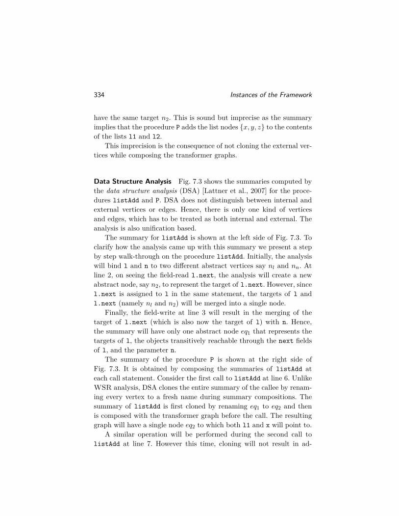
334 Instances of the Framework
have the same target n2. This is sound but imprecise as the summaryimplies that the procedure P adds the list nodes {x, y, z} to the contentsof the lists l1 and l2.
This imprecision is the consequence of not cloning the external ver-tices while composing the transformer graphs.
Data Structure Analysis Fig. 7.3 shows the summaries computed bythe data structure analysis (DSA) [Lattner et al., 2007] for the proce-dures listAdd and P. DSA does not distinguish between internal andexternal vertices or edges. Hence, there is only one kind of verticesand edges, which has to be treated as both internal and external. Theanalysis is also unification based.
The summary for listAdd is shown at the left side of Fig. 7.3. Toclarify how the analysis came up with this summary we present a stepby step walk-through on the procedure listAdd. Initially, the analysiswill bind l and n to two different abstract vertices say nl and nn. Atline 2, on seeing the field-read l.next, the analysis will create a newabstract node, say n2, to represent the target of l.next. However, sincel.next is assigned to l in the same statement, the targets of l andl.next (namely nl and n2) will be merged into a single node.
Finally, the field-write at line 3 will result in the merging of thetarget of l.next (which is also now the target of l) with n. Hence,the summary will have only one abstract node eq1 that represents thetargets of l, the objects transitively reachable through the next fieldsof l, and the parameter n.
The summary of the procedure P is shown at the right side ofFig. 7.3. It is obtained by composing the summaries of listAdd ateach call statement. Consider the first call to listAdd at line 6. UnlikeWSR analysis, DSA clones the entire summary of the callee by renam-ing every vertex to a fresh name during summary compositions. Thesummary of listAdd is first cloned by renaming eq1 to eq2 and thenis composed with the transformer graph before the call. The resultinggraph will have a single node eq2 to which both l1 and x will point to.
A similar operation will be performed during the second call tolistAdd at line 7. However this time, cloning will not result in ad-

7.1. Overview of the Instances 335
ditional vertices as explained in the following. Say eq1 is renamed toeq4 in the cloned summary of listAdd. The vertex eq4 represents thetarget of x (in addition to representing other objects such as the tar-gets of l2, l2.next etc.). But, the transformer graph before the callwill already have a node eq2 representing the target of x. Therefore,eq4 and eq2 will be merged in the composed transformer graph as theyboth represent the target of x. After this statement, eq2 represents thetargets of l1, x, objects reachable via their next fields, as well as thetarget of l2.
The third call to listAdd(l2, y) at line 8 will result in the mergingof eq2 and the target of y. This time also the vertex cloned from thecallee summary (a copy of eq1) would be merged with eq2 becausethey represent the targets of l2. The final call to listAdd(l3,z) willadd a new vertex eq3 to the composed graph as a result of cloningand composing the summary of listAdd. The node eq3 represents theobject newly allocated by the procedure as well as the initial targets ofz and l3 at the start of the procedure.
Observe that in spite of using less precise transformer graphs com-pared to WSR analysis, DSA identifies that the procedure P adds onlyx and y to the contents of l1 and l2. This is better than the resultsof WSR analysis but is still imprecise. However, flow-insensitivity andthe lack of distinction between internal and external vertices preventsthe analysis from determining that l3 is a new singleton list containingonly z.
Access-path-based Analysis Fig. 7.4 shows the summaries computedby the analysis proposed in [Cheng and Hwu, 2000] for the procedureslistAdd and P. We will refer to this analysis as access-path-based analy-sis (APA) as it summarizes procedures using a set of points-to relationsbetween access-paths.
The access-paths used by the analysis are a sequence of field deref-erences starting from a parameter or a global variable or a statementlabel (that corresponds to an object allocation site). Access-paths thatend with a star ("*") denote objects and those without a suffix "*"denote pointers (or references). In an access-path of the form δ.f , δ

336 Instances of the Framework
always ends with a star i.e, it represents an object. In the analysis, if lis a parameter of a procedure, l∗ is used to represent the initial targetof the parameter l, l∗.next∗ is used to represent the initial target ofl.next and so on. The objects that are newly allocated are denotedusing their statement labels. 1
The analysis also bounds the lengths of the access-paths to keep theabstract domain finite. A bounded access-path δ represent a (possiblyinfinite) set of access-paths whose prefix is δ. In Fig. 7.4, we assumethat the length of the access-paths are bounded to 2.
The summaries computed by the analysis can be represented astransformer graphs. The vertices in the transformer graphs are namedusing access-paths that denote objects. An access-path l∗.next∗, in re-ality, denotes an external edge from the vertex l∗, which representsthe initial target of l, to l∗.next∗, which represents the initial tar-get of l.next. A points-to relation from l∗.next to n∗ correspondsto an internal edge from l∗ to n∗ labelled by the field next. (See theAccesspath-based-naming strategy of section 6 for a formal description.)
The transformer graph representation of the summaries of APA areshown in Fig. 7.4. We also show the actual points-to relations computedby the analysis for the procedure listAdd. Readers might find it easierto compare the transformer graph representations of the summarieswith the summaries computed by the other instances.
Consider the summary computed by APA for the procedurelistAdd (left side of Fig. 7.4). Its transformer graph representationclarifies that the summary for the procedure is semantically equivalentto WSR summary shown at the left side of Fig. 7.2. They differ onlyin the names of the vertices. Consider the summary for the procedureP shown at the right side of Fig. 7.4. The summary precisely identifiesthe contents of the lists l1 and l2, which is in contrast with the re-sults of WSR analysis. This increased precision is the consequence ofusing a naming strategy for nodes that makes it necessary to clone theexternal vertices during summary composition. The analysis maintains
1[Cheng and Hwu, 2000] denote the field references in access-paths using fieldoffsets instead of field names, since the analysis targets C programs where distinctfield names can denote the same offset within a record.

7.1. Overview of the Instances 337
the invariant that the targets read from a vertex l∗ on a field f arealways named l∗.f∗. In other words, an external edge from l∗ on a fieldf always ends at l∗.f∗. To maintain this invariant, during summarycomposition the targets of external edges are renamed so that theyare consistent with the names of their source vertices. However, beingflow-insensitive the analysis does not identify the contents of the listl3 precisely.
It turns out that when this analysis is formulated as an instanceof the framework it closely resembles WSR analysis in most aspectsexcept for the naming of nodes (see section 7.2.4). This is an inter-esting result considering that the original formulation of this analysisas proposed in [Cheng and Hwu, 2000] bears little similarity to WSRanalysis. Moreover, we were able to identify some bugs in the analysisproposed in [Cheng and Hwu, 2000] by comparing their semantics withthe transfer functions of the instantiation of our framework that usesthe same naming strategy.
Flow-Aware Analysis We now discuss the summaries computed bythe analysis proposed in [Buss et al., 2008], referred to as flow-awareanalysis (FAA), for the procedure listAdd and P. The summaries com-puted by FAA are not depicted pictorially since they are very similarto the summaries computed by WSR analysis. The critical differencebetween FAA and the other analyses discussed earlier manifest whenthere is aliasing in the context in which the summaries are used.
For example, consider the procedure Q shown in Fig. 7.1. Theprocedure first adds a list node z to the parameter list l and theninvokes the procedure P passing the list l to l1 and l2 parameters. Inthis context, l1 and l2 alias. The procedure P invokes the procedurefirst, which reads the targets of the next field of the list l via thereference l1. The procedure P subsequently adds the nodes x and y tothe list l via the reference l2. In this case, the summaries obtainedfor Q by every other instance of the framework discussed earlier willconservatively infer that fst could be pointing to x, y or z, thoughclearly, x and y are added to the list l only after the call to first.
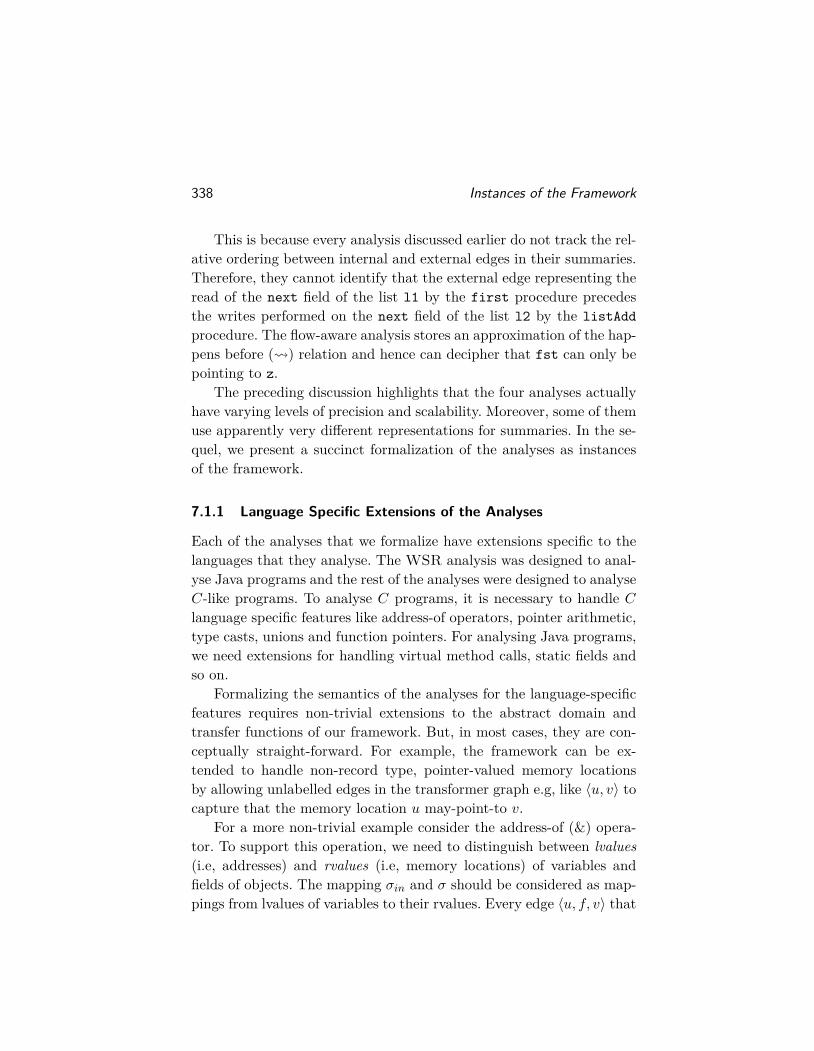
338 Instances of the Framework
This is because every analysis discussed earlier do not track the rel-ative ordering between internal and external edges in their summaries.Therefore, they cannot identify that the external edge representing theread of the next field of the list l1 by the first procedure precedesthe writes performed on the next field of the list l2 by the listAddprocedure. The flow-aware analysis stores an approximation of the hap-pens before ( ) relation and hence can decipher that fst can only bepointing to z.
The preceding discussion highlights that the four analyses actuallyhave varying levels of precision and scalability. Moreover, some of themuse apparently very different representations for summaries. In the se-quel, we present a succinct formalization of the analyses as instancesof the framework.
7.1.1 Language Specific Extensions of the Analyses
Each of the analyses that we formalize have extensions specific to thelanguages that they analyse. The WSR analysis was designed to anal-yse Java programs and the rest of the analyses were designed to analyseC-like programs. To analyse C programs, it is necessary to handle Clanguage specific features like address-of operators, pointer arithmetic,type casts, unions and function pointers. For analysing Java programs,we need extensions for handling virtual method calls, static fields andso on.
Formalizing the semantics of the analyses for the language-specificfeatures requires non-trivial extensions to the abstract domain andtransfer functions of our framework. But, in most cases, they are con-ceptually straight-forward. For example, the framework can be ex-tended to handle non-record type, pointer-valued memory locationsby allowing unlabelled edges in the transformer graph e.g, like 〈u, v〉 tocapture that the memory location u may-point-to v.
For a more non-trivial example consider the address-of (&) opera-tor. To support this operation, we need to distinguish between lvalues(i.e, addresses) and rvalues (i.e, memory locations) of variables andfields of objects. The mapping σin and σ should be considered as map-pings from lvalues of variables to their rvalues. Every edge 〈u, f, v〉 that

7.1. Overview of the Instances 339
indicates that u points-to v on field f should be split into two edges〈u, f, rf 〉, 〈rf , v〉, where rf denotes the rvalue of the field f . The trans-fer functions can be easily adapted to this extended abstract domain.The only significant change required is that reading a variable or anobject’s field should be considered as reading the targets of its rvalue.Hence, it should result in the creation of external edges. Similarly, writ-ing a variable or an object’s field should be considered as writing toits rvalue. Hence, it should result in the creation of internal edges. Thesemantics of a statement of the form v1 = &v2 could then be modelledas adding an internal edge from the rvalue of v1 (given by σ(v1)) to thervalue of v2 (given by σ(v2)), which indicates that v1 points-to v2.
All the analyses except DSA assume that the targets of functionpointer calls and virtual method calls are known during the bottom-upsummary computation phase. They either employ a separate conserva-tive call-graph analysis to estimate the call-graph, or invoke a top-downphase that propagates the points-to information from callers to callees,and the bottom-up summary computation phase iteratively, until thesummaries converge to a fix-point. Hence, they do not require any ex-tensions to the transfer functions for handling dynamic dispatch. Onthe other hand, DSA has a custom mechanism for handling functionpointer calls which is discussed while formalizing the analysis in sec-tion 7.2.3.
We do not formalize the language specific extensions of the anal-yses in this article for the following two reasons. Firstly, we believethat formalizing these features is a distraction from the focus of thisarticle which is to understand the analyses at a conceptual level andgeneralize them. The additional formalism that would be required forthe extensions may make it difficult to understand the analyses, andto appreciate their similarities and differences. Secondly, most of thelanguage specific extensions are rather straight-forward to devise oncethe core abstractions of the analyses are well understood.
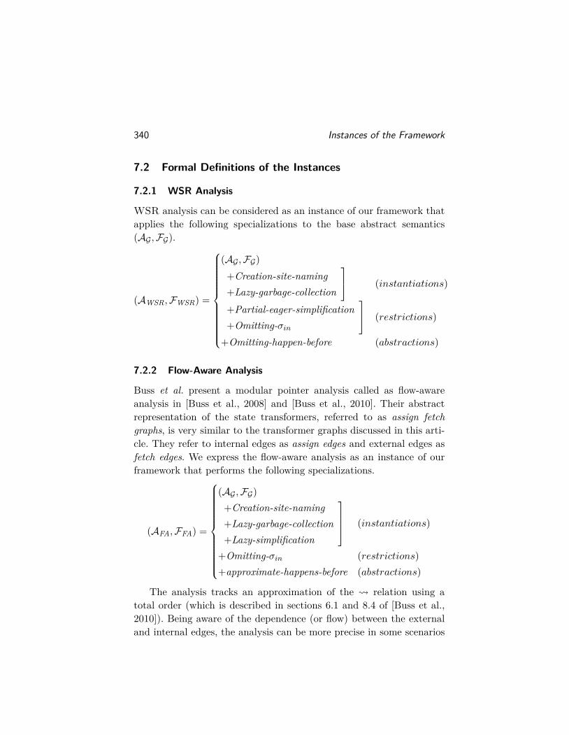
340 Instances of the Framework
7.2 Formal Definitions of the Instances
7.2.1 WSR Analysis
WSR analysis can be considered as an instance of our framework thatapplies the following specializations to the base abstract semantics(AG ,FG).
(AWSR,FWSR) =
(AG ,FG)+Creation-site-naming+Lazy-garbage-collection
(instantiations)
+Partial-eager-simplification+Omitting-σin
(restrictions)
+Omitting-happen-before (abstractions)
7.2.2 Flow-Aware Analysis
Buss et al. present a modular pointer analysis called as flow-awareanalysis in [Buss et al., 2008] and [Buss et al., 2010]. Their abstractrepresentation of the state transformers, referred to as assign fetchgraphs, is very similar to the transformer graphs discussed in this arti-cle. They refer to internal edges as assign edges and external edges asfetch edges. We express the flow-aware analysis as an instance of ourframework that performs the following specializations.
(AFA,FFA) =
(AG ,FG)+Creation-site-naming+Lazy-garbage-collection+Lazy-simplification
(instantiations)
+Omitting-σin (restrictions)+approximate-happens-before (abstractions)
The analysis tracks an approximation of the relation using atotal order (which is described in sections 6.1 and 8.4 of [Buss et al.,2010]). Being aware of the dependence (or flow) between the externaland internal edges, the analysis can be more precise in some scenarios

7.2. Formal Definitions of the Instances 341
especially when there is aliasing in the calling context (as illustrated insection 7.1).
The total order is constructed by numbering the external and in-ternal edges in the order in which they are created (or re-encountered)during the analysis. The edges with smaller numbers are assumed tohappen before those with higher numbers. The disadvantage of thisstrategy is that it introduces spurious orderings between the reads andwrites that happen along the two branches of an if-then-else statement.
Caveats [Buss et al., 2010] informally discusses the Simplify operationin section 8.1 "computing summaries". A mapping akin to Incl (usedby the Simplify operation) is discussed in detail in section 4.1 "PointerAlias Analysis". Unfortunately, since section 8.1 in [Buss et al., 2010] isnot sufficiently detailed, we are unable to decipher the precise definitionof Simplify. The description indicates that their analysis translates theinternal edges on a vertex w to those in Incl(w). However, it is unclearif the external edges are translated as well, which is necessary for cor-rectness. Another ambiguity is that in [Buss et al., 2010] it is statedthat the analysis "deletes everything from a summary of a procedurethat the callers could not see". Intuitively, this seems to correspond tothe removeNonEscaping and GCG operations that delete non-escapingvertices and associated edges from the summary. Due to these ambigu-ities the above instantiation may not precisely capture all the aspectsof the analysis presented in [Buss et al., 2010].
7.2.3 Data Structure Analysis
[Lattner et al., 2007], [Lattner and Adve, 2005a] present a modular,unification-based pointer analysis called as data structure analysis(DSA). The analysis is also capable of summarizing procedures inpresence of function pointer calls. Indirect calls, such as functionpointer calls, virtual method calls and higher-order function calls, posea major challenge for bottom-up analyses. The targets of indirect callsencountered during an analysis of a procedure may depend on thecontext in which the procedure is invoked.

342 Instances of the Framework
DSA stores the indirect calls encountered during the analysis of aprocedure in the summaries computed for the procedure. These sum-maries are propagated to the callers of the procedure as in a typicalbottom-up analysis. Eventually, sufficient context information becomesavailable for resolving some indirect calls to their targets. At this point,the analysis instantiates the summaries of the targets of the indirectcalls (that are resolvable) and drops the indirect calls from the sum-maries.
This feature of DSA is non-trivial to understand and formalize,but is orthogonal to the focus of this article. (For interested readers,[Madhavan et al., 2012] presents a generic mechanism for lifting mod-ular heap analysis approaches for first-order programs to higher-orderprograms which is inspired by the approach of DSA. The abstract se-mantics formalized in this section when used in conjunction with theapproach discussed in [Madhavan et al., 2012] may serve as a formaliza-tion of this feature.) Below we focus on the abstract transfer functionsof DSA modulo the handling of indirect calls.
DSA as an instance of the framework
(ADSA,FDSA) =
(AG ,FG)+Creation-site-naming-cloning+Lazy-simplification+Lazy-garbage-collection
(instantiations)
+No-internal-external-distinction+Flow-insensitivity+Unification
(abstractions)
The analysis performs several abstractions to the base abstract se-mantics FG . It turns out that in the presence of these abstractions thetransformer graphs can be reduced to triples of the form (V,E, σ), whichis deceptively similar to an abstract shape graph though it representsan abstract state transformer. Due to these abstractions, the transferfunctions can be simplified. In particular, the Simplify operation does

7.2. Formal Definitions of the Instances 343
not add any additional edges but only removes edges and vertices whenapplied in conjunction with GCc. The analysis makes up for some ofthe losses in precision by using a precise naming strategy that clonesthe abstract objects along all acyclic call-paths.
The analysis does not distinguish between external and internaledges and vertices. Therefore, there is no distinction between edgescreated due to field-reads versus those created due to field-writes. Nev-ertheless, the analysis tracks the vertices that are escaping by associat-ing a boolean flag (called complete flag) with the vertices. Vertices thathave the complete flag set to true are non-escaping vertices. Though[Lattner et al., 2007] informally states that the vertices marked as com-plete are analogous to the internal vertices of WSR analysis, in realitythey correspond to non-escaping vertices.
[Lattner et al., 2007] defines the abstract semantics of a (direct)call statement S as a function resolveCallee that invokes two func-tions cloneGraphInto and resolveArguments (Figure 4 of [Lattner et al.,2007]). The function cloneGraphInto clones the vertices in the calleetransformer graph, and inlines the cloned transformer graph into thecaller transformer graph. This corresponds to the transfer function ofa call statement described in Chapter 5.
The function resolveArguments merges the targets of every argu-ment in the caller transformer graph with the corresponding parameternodes of the callee transformer graph, and also transitively merges thetargets of their out-edges. This corresponds to the definition of the pa-rameter NodesToMerge for a call statement presented in Fig. 6.1 thatresults in a unification-based analysis.
7.2.4 Access-path-based Modular Analysis
[Cheng and Hwu, 2000] proposes a modular pointer analysis techniquethat uses access-paths to name abstract objects. The analysis summa-rizes procedures using a set of points-to relations between access paths.We will refer to the analysis as access-path-based analysis (APA). Be-low we present a specialization of the framework that is very similar toAPA.

344 Instances of the Framework
(AAP ,FAP) =
(AG ,FG)+Accesspath-based-naming+Lazy-garbage-collection
(instantiations)
+Partial-eager-simplification+Omitting-σin
(restrictions)
+Flow-insensitivity (abstractions)
As discussed in section 6, when the Accesspath-based-naming strat-egy is used, the nodes names can be used to determine if a vertex isinternal or external, and also to reconstruct the set of external edges.Hence, the internal and external vertex components, and the externaledge component can be omitted from the transformer graphs. The spe-cializations used by APA (presented above) results in the omission ofthe happens before and σin components from the transformer graphs.(Recall that the flow-insensitivity abstraction omits the happens beforecomponent as well.) In essence, the transformer graphs used by APAcan be reduced to pairs of the form (IE, σ). A pair (IE, σ) corresponds toa points-to relation between LAPr+1 and RAPr , where r is the boundon the length of the access-paths . This is precisely the representationused by [Cheng and Hwu, 2000] for transformer graphs. They definethe abstract domain as 2 LAPr+1×RAPr .
The transfer functions given by FAP can also be simplified usingthe condensed (paired) representation of the transformer graphs. (Weelide formal details for brevity). The abstract semantics presented in[Cheng and Hwu, 2000] is similar to the simplified form of the transferfunctions.
Caveats The above instantiation has two differences compared to theformulation presented in [Cheng and Hwu, 2000]. Firstly, in the analysisdescribed in [Cheng and Hwu, 2000], the objects newly created by a pro-cedure are initially named using their allocation site label (like in theAccesspath-based-naming strategy). Later, in the summary computedfor the procedure every label (which denotes newly allocated objects)

7.2. Formal Definitions of the Instances 345
is renamed to an access-path called extended-access-path, which is ob-tained from a path starting at a parameter or global variable and endingat the label of interest. This is an odd feature of the analysis. This issound, but may result in significant loss of precision as an internal ver-tex (denoting objects allocated inside a procedure) is converted to anexternal vertex (that possibly denotes objects read from the prestate).[Cheng and Hwu, 2000] states that the reason for performing this is toensure that the vertices corresponding to newly allocated objects aregiven different names in different calling contexts. A more precise wayof achieving this would be to clone such vertices in all (or selected)calling contexts similar to DSA.
Secondly, we find that the semantics of [Cheng and Hwu, 2000]has some differences (which are possible bugs) compared to FAP . Thetransfer function FAP presented above performs partial simplificationof transformer graphs which is presented in Appendix A. With thisspecialization, the transfer functions of field-read and procedure callstatements create external edges that start only from escaping vertices,which is an optimization compared to the generic abstract semanticsof the framework.
However, the semantics described in [Cheng and Hwu, 2000] pushesthis further and does not create an external edge from a vertex whenthere exists an internal edge starting at the vertex. The formalismpresented in [Cheng and Hwu, 2000] creates a new access-path δ.f∗,that corresponds to an external edge starting from δ, iff δ does notpoint to any node on field f (see definition 2.3 in section 2.1 of [Chengand Hwu, 2000]). This means that their semantics will not create anexternal edge on an escaping node δ if there exists an internal edgestarting from the node. This is unsound. This we believe is a bug inthe algorithm of [Cheng and Hwu, 2000].
The formalization presented above is provably correct, addressesthese problems and yet remains close to the original formulation of theanalysis.

8Experimental Results
8.1 Implementation, Benchmarks and Metrics
In this chapter, we present an experimental evaluation of the frame-work using our open source, modular heap analysis tool Seal ([Mad-havan et al., 2011], [Madhavan et al., 2012]), which is available atseal.codeplex.com. Seal usesMicrosoft Phoenix Compiler Frameworkand can analyze real-world Microsoft .NET applications implementedin the C] programming language.
Seal is an implementation of the framework discussed in this ar-ticle. In addition, it also has several extensions for handling advancedfeatures of the C] language. Most importantly, Seal implements the ap-proach described in [Madhavan et al., 2012] for handling higher-orderfeatures of C] such as virtual method calls and lambda expressions.
A few client analyses, such as Purity and Side-effects Analysis, In-formation Flow Analysis, Escape Analysis, Call-graph Analysis, arealso integrated into Seal. The client analyses are implemented as post-processing phases that analyze the summaries of the procedures com-puted by the bottom-up summarization phase. Each client analysisrequires tracking some additional information in the summaries. Forinstance, the Side-effects Analysis requires tracking the vertices and
346

8.1. Implementation, Benchmarks and Metrics 347
Benchmark Loc Description(Abbv.)DocX (doc) 10K Library for manipulating Word filesAvalonDock (ad) 18K Library for docking windowsFacebook API (fb) 21K Library for integrating with FacebookDynamic data 25K Real-time data visualization tooldisplay (ddd)TestApi (test) 25K Library for testing tool developmentSharpMap (sm) 26K Geospatial application frameworkQuickgraph (qg) 34K Graph data structures and algorithmsSharpDevelop 43K Code refactoring engine- NRefactor (ref )Craig’s utility (cul) 56K Collection of .NET utility methodsPDFsharp (pdf ) 96K Library for processing PDFs
Figure 8.1: Benchmarks used in the experimental evaluation. All benchmarks arepopular, open source C] projects hosted at www.codeplex.com.
their fields that are modified by a procedure in the summary of theprocedure. Seal analyzes not only procedures but also libraries (DLLs)modularly. Given a DLL, it summarizes the procedures in a DLL us-ing transformer graphs, stores the summaries in a database, and usesthe summaries while analyzing the clients of the library. In our experi-ments, the DLLs implementing the core C] library, namely,mscorlib.dll,system.dll and system.core.dll were analyzed once and for all, and thecomputed summaries were used during the analysis of each benchmark.
Seal can be unsound in some cases. It does not soundly handlecalls to native methods (which are methods implemented in C or otherunmanaged languages), graphical user interface (GUI) methods, reflec-tion, and concurrency. We minimize the unsoundness by using stubsfor commonly used library methods that are not analyzable by Seal.
To evaluate the practical usefulness of our framework, we analyzereal-world C] libraries shown in Fig. 8.1, using different configurationsfor the parameters of the framework. We measure the impact of eachconfiguration on the summaries computed for the procedures, and also
348 Experimental Results
on the results of three client analyses: Purity and Side-effects Analysis,Escape Analysis and Call-graph Analysis. In the rest of the chapter, weexplain the various configurations used in our experiments, the metricsused to compare the configurations, and the results for each configura-tion.
Metrics used in the Experimental Evaluation The following are themetrics we use to compare the precision and scalability of different con-figurations of the framework. The total time taken by the bottom-upsummary computation phase. We denote this as Time in the experi-mental results presented shortly.
The number of vertices and edges in the summary transformergraphs of procedures. This is a measure of scalability of the analysis.Analyses that compute smaller summaries are more scalable. In theexperimental results presented shortly we denote this metric as Size.The results show, for each benchmark, the average and the maximumsize of the summaries computed by the analysis.
The average out-degree of the vertices in the summary transformergraphs, which is the ratio of edges to the vertices in the transformergraphs. This is a measure of sparsity of the summaries. Summaries thatare sparse are generally more precise as they identify more referencesas non-aliasing. We denote this metric as Deg. in the results presentedlater. The results show, for each benchmark, the average sparsity of thesummaries computed by the analysis and theirmean absolute deviation.
We use the following metrics to measure the precision of the Purityand Side-effects Analysis.
The number of procedures that are pure. A procedure is pure ifit does not write to pre-state memory locations (for more details see[Salcianu, 2001]). In the presence of indirect calls, a procedure by itselfmay not write to prestate locations but the indirect calls invoked bythe procedure may modify the prestate locations. Since the targetsof the indirect calls may depend on the calling context, the purity ofthe procedure is also dependent on the calling context. We call suchprocedures as conditionally pure. We include such procedures also inthis metric.
8.1. Implementation, Benchmarks and Metrics 349
The number of side-effects of a procedure, which are the prestatememory locations modified by the procedure. It is possible for proce-dures to have unbounded number of side-effects. For example, a pro-cedure that appends an element to a linked list lst passed as a pa-rameter may modify the locations: lst.next, lst.next.next and soon. One way to represent side-effects of a procedure is using regularexpressions over access-paths. For example, the side-effects of the listappend procedure could be represented as lst.(next)+. But, with thisrepresentation comparing side-effects across different configurations re-quires checking inclusion and equivalence of regular expressions, whichis quite expensive. Therefore, in our experiments, we use an under-approximation of the side-effects of a procedure described below.
For every vertex that is modified in the transformer graph, wechoose one access-path starting from each parameter that the modi-fied vertex corresponds to. In the above example, if there are thereare two modified nodes in the transformer graph one correspondingto lst.next and other corresponding to lst.next.(next)+. Then wedisplay the two access-paths: lst.next and lst.next.next as side-effects of the procedure.
In the results presented shortly, we show the average number of(under-approximate) side-effects per impure procedure and also theirmean absolute deviation. We refer to this metric as SE.
We measure the precision of the Escape Analysis using the followingmetric. The total number of non-escaping (or local) allocation sites. Anallocation site is local only if during every invocation of the procedurecontaining the allocation site, no object created by the allocation sitehas an handle that is live after the execution of the procedure. We referto this metric as LA in the results presented in the next section.
Like many top-down heap analyses, Seal constructs a call-graph on-the-fly during the bottom-up summary computation phase (see [Mad-havan et al., 2012]). We evaluate the precision of the call-graph com-puted by Seal for a given DLL using the following metric abbreviatedas CGE. The number of edges in the call-graph computed for the givenDLL. A call-graph is more precise if it has fewer edges.

350 Experimental Results
8.2 Evaluation of the Configurations of the Framework
We now describe the various configurations used in the experimentalevaluation and discuss the results they produce. Since the parametersof the framework can be defined arbitrarily, exhaustively evaluatingall possible configurations of the framework is not practically feasible.Therefore, we adopt the following approach in this evaluation. We firstpresent the results of one of the most tested and scalable configurationsof the tool which we refer to as the base configuration. This configura-tion was also used in the experimental evaluation of [Madhavan et al.,2012]. We then turn on one specialization of the framework and eval-uate the change in the results relative to the base configuration. Thiswould provide an idea of the importance of the specialization and thecriticality of the parameter that is affected by the specialization.
All evaluations presented in this section were carried out on a sys-tem with 2 core, 2.6 GHz Intel Core i5 processor, with 8 GB RAM,running Windows 8 operating system.
Base Configuration In this configuration, the abstract vertices arenamed using their creation site labels (Creation-site-naming). The con-figuration uses flow-insensitive analysis and incorporates partial ea-ger simplification of transformer graphs (Partial-eager-simplification)in the transfer functions of the statements. Moreover, a node merg-ing strategy is applied to the transformer graphs computed at the exitpoint of a procedure. The node merging strategy used ensures that ev-ery out-going external edge from a vertex is labelled by a unique field,and similarly, every out-going internal edge is also labelled by a uniquefield. This is one of the most scalable configurations.
Fig. 8.2 shows the results of the analyzing the benchmarks in thebase configuration. The figure shows all the metrics discussed earlierfor each benchmark.
One Level Cloning This configuration employs a context-sensitivenaming strategy. Every node has a label, which is the label of thecreation site, and a context. The context of a node at a program pointis the label of the first call statement in the call-path that leads to the

8.2. Evaluation of the Configurations of the Framework 351
Time Size Deg. Pure SE LA CGEavg avg avg(max) (dev) (dev)
doc 1m55s 84.8 1.1 392 9.6 743 4234(697) (1.1) (9)
ad 18m30s 88 1 704 11.5 1267 7482(2059) (1) (15.4)
fb 2m17s 55.7 0.8 1978 9.4 976 7028(774) (0.7) (10.9)
ddd 5m4s 50.5 0.5 1622 3.9 2950 8366(1965) (0.3) (4.1)
test 7m13s 52.8 0.7 709 8.5 1063 6836(1636) (0.5) (10.2)
sm 1m15s 25.2 0.5 1052 3.3 747 4588(580) (0.3) (2.8)
qg 1m43s 30.8 0.5 2368 3.1 663 6360(959) (0.3) (3.1)
ref 24m31s 76.7 0.8 2037 8.8 1115 43160(5274) (0.6) (9.7)
cul 5m20s 30.6 0.5 2774 3.7 2183 12981(1654) (0.3) (4.2)
pdf 52m39s 89.9 0.9 1751 13.9 3482 12721(2659) (0.7) (17.2)
Figure 8.2: Results of running Seal on the benchmarks shown in Fig. 8.1 in thebase configuration.
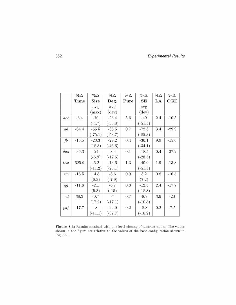
352 Experimental Results
%∆ %∆ %∆ %∆ %∆ %∆ %∆Time Size Deg. Pure SE LA CGE
avg avg avg(max) (dev) (dev)
doc -3.4 -10 -23.4 5.6 -49 2.4 -10.5(-4.7) (-33.8) (-51.5)
ad -64.4 -55.5 -36.5 0.7 -72.3 3.4 -29.9(-75.1) (-53.7) (-85.3)
fb -13.5 -23.3 -29.2 0.4 -30.1 9.9 -15.6(18.3) (-46.6) (-34.1)
ddd -36.3 -24 -8.4 0.1 -18.5 0.4 -27.2(-6.9) (-17.6) (-28.3)
test 625.9 -6.2 -13.6 1.3 -40.9 1.9 -13.8(-11.2) (-26.1) (-51.3)
sm -16.5 14.8 -3.6 0.9 3.2 0.8 -16.5(8.3) (-7.9) (7.2)
qg -11.8 -2.1 -6.7 0.3 -12.5 2.4 -17.7(5.3) (-15) (-18.8)
cul 38.3 -0.7 -7 0.7 -8.7 3.9 -20(17.2) (-17.1) (-10.8)
pdf -17.7 -8 -22.9 0.2 -8.8 0.2 -7.5(-11.1) (-37.7) (-10.2)
Figure 8.3: Results obtained with one level cloning of abstract nodes. The valuesshown in the figure are relative to the values of the base configuration shown inFig. 8.2.
8.2. Evaluation of the Configurations of the Framework 353
creation site of the node from that program point. Note that unlike theCreation-site-naming-cloning strategy discussed earlier, this strategydoes not use the entire call-path as the context but only the label ofthe first call-site in the call-path.
For example, consider a procedure A that calls procedure B which inturn calls procedure C twice. The abstract nodes created by the two callsto procedure C will have distinct names in procedure B, but would beindistinguishable in procedure A under this naming scheme. We refer tothis naming strategy as one level cloning. This configuration is similarto the base configuration in every other aspect.
Fig. 8.3 shows the results obtained using this configurations for eachbenchmark. All numbers in the figure (including those in parentheses)show the percentages by which the values of the metrics differ com-pared to the base configuration. Percentages that are negative indicatea decrease in the value of the corresponding metric relative to the baseconfiguration. For example, in this configuration, the analysis of thebenchmark doc took 3.4% lesser time compared to the base configura-tion, whereas the analysis of benchmark test took almost 625% moretime compared to the base configuration. The analysis did not scale tothe benchmark ref under this configuration within a fixed time limit of90 minutes and hence is omitted from the results. Note that though thisconfiguration uses a context-sensitive naming strategy it sometimes re-sults in significantly faster running times and more compact summariesfor benchmarks like pdf.
The results for the sparsity metric show that this configurationresults in sparser summaries compared to the base configuration acrossall benchmarks. This is expected since cloning increases the context-sensitivity of the analysis.
The increase in the precision of the summaries positively influencesthe results of the client analyses as shown by the remaining columnsin the Fig. 8.3. In particular, more methods are identified as pure andfewer side-effects are inferred for the impure methods. More allocationsites are identified as non-escaping and the call-graph has significantlyfewer edges compared to the base configuration. Readers might ob-serve that for the benchmark sm the figure indicates an increase in

354 Experimental Results
%∆ %∆ %∆ %∆ %∆ %∆ %∆Time Size Deg. Pure SE LA CGE
avg avg avg(max) (dev) (dev)
doc -8.2 6.2 -3.9 0 -0.9 0 -3.4(6.9) (-7.2) (-1.4)
ad -3.1 0.5 -10.3 0 -3.2 0 -1(20.1) (-18.9) (-5.2)
fb 13.2 5 -13.2 0 0.1 8.9 -1.4(-11.2) (-27.3) (0.1)
ddd 71.7 27.2 -2.9 0.1 -11.9 0.1 -6.8(127.6) (-6.4) (-18.7)
sm 157.6 229.4 -3 0.1 6 0 -0.2(2604) (-6.5) (10.1)
qg 8.6 1.6 -2.3 0 -4.4 0 -6.5(15) (-5.3) (-7.2)
cul -2.1 31.4 -2.4 0 5.7 0 -3.9(129.1) (-6.8) (8.6)
Figure 8.4: Results obtained with full cloning of abstract nodes. The values shownin the figure are relative to the values of the configuration: One Level Cloning shownin Fig. 8.3.
the number of side-effects. However, on manual inspection, we foundthat this was because of the duplicates in the listing of side-effects anddo not correspond to an actual increase in the side-effects. The under-approximation heuristic that we use to list side-effects did not identifythe duplicates as they were syntactically different.
Full Cloning This configuration performs full cloning of abstractnodes like in the case of DSA, i.e. it uses the Creation-site-naming-cloning strategy. It is similar to the base configuration in every otheraspect. Fig. 8.4 shows the results obtained with this configuration. Allnumbers in the figure (including those in parentheses) show the per-centages by which the values increase or decrease with respect to the

8.2. Evaluation of the Configurations of the Framework 355
One Level Cloning configuration. Under this configuration, the analy-sis timed out on three benchmarks: test, ref and pdf. Hence, they areomitted from the Fig. 8.4.
Notice that for most benchmarks this configuration increases thesummary sizes compared to One Level Cloning. In the case of the smbenchmark the increase in the summary sizes is quite dramatic (almost26 times). In contrast, the decrease in average degree of vertices (i.e,the increase in sparsity) of the summaries is only marginal.
There is also almost no increase in the number of pure methods.However, there is some reduction in the number of side-effects per pro-cedure in some benchmarks. (The increase in side-effects for a coupleof benchmarks were due to the issue of duplicates mentioned while dis-cussing one level cloning.) The Escape Analysis doesn’t benefit acrossthe board from the increased context-sensitivity. The number of localallocation sites increases significantly for the fb benchmark, but remainsalmost unchanged for the remaining benchmarks. However, the Call-graph analysis does benefit from the increase in context-sensitivity. Inparticular, the number of call-graph edges decreases across all bench-marks.
On the whole, the results of the One Level Cloning and Full Cloningconfigurations indicate the following trends. (a) There is a huge im-provement in the precision of the summaries as well as that of the clientanalyses while switching from a context-insensitive naming strategy toa context-sensitive naming strategy. (b) However, using a very precisecontext-sensitive naming strategy does not benefit some applications,but instead hampers the scalability of the analysis quite significantly.
The bottom line is that choosing the right level of context-sensitivity in the naming of abstract nodes should be one of the mainconcerns while designing a modular heap analysis for a particular ap-plication.
Flow-sensitive Configuration This configuration performs a flow-sensitive analysis but otherwise uses the same abstractions as the baseconfiguration. Fig. 8.5 shows the results obtained with this configura-tion. All numbers in the figure (including those in parentheses) show

356 Experimental Results
%∆ %∆ %∆ %∆ %∆ %∆ %∆Time Size Deg. Pure SE LA CGE
avg avg avg(max) (dev) (dev)
doc 49.9 -1 -0.5 0 -0.4 0.7 -2.1(-12.1) (-0.4) (-0.6)
ad 90.2 -1.9 -4.1 0.4 -3.5 0.5 -3.3(0) (-4.7) (-4.4)
fb 21.4 -3.5 -4.7 0 -2 0 -1.8(-0.6) (-7.3) (-2.3)
ddd -3.3 -1.2 -1.4 0.1 -1.2 0 -0.1(-1.1) (-2.8) (-0.3)
test 110.8 -3.9 -2.7 0 -4.1 0.2 -1.8(-0.9) (-5) (-2.9)
sm 87.3 -7 -2.2 0.3 -8 0.1 -2(-8.6) (-5) (-5.1)
qg -10.1 -5.1 -4.6 0.2 -5.3 0 -8.5(-9.2) (-10.6) (-4.4)
ref 25.3 -0.6 -0.7 0 -0.8 0.1 -3.4(-0.5) (-1.1) (-0.7)
cul 13.4 -2 -1.9 0.2 -3.6 0.5 -1.9(1.4) (-4.6) (-5.2)
pdf -17.4 -9.9 -10.6 0.2 -1.5 -0.9 -9.8(-5.5) (-18.1) (-1.4)
Figure 8.5: Results obtained using a flow-sensitive analysis. The values shown inthe figure are relative to the values of the base configuration.
8.2. Evaluation of the Configurations of the Framework 357
the differences (in percentage) compared to the results of the base con-figuration shown in Fig. 8.2. The data highlights that the flow-sensitiveanalysis results in a marked increase in the precision when comparedto the base configuration, especially in the number of call-graph edgesand average side-effects per procedure.
It may be somewhat surprising to the readers that flow-sensitivitydoes not significantly slow down the analysis. Even though there is atwo fold increase in the analysis time for some benchmarks, all of thebenchmarks except pdf complete well within 30 minutes. The analysisof the pdf benchmark actually runs faster. This is mainly because ofour efficient implementation of the flow-sensitive analysis. Recall thatthe transfer functions of the framework perform only weak updates onthe abstract vertices. Hence, only variables are strongly updated duringa flow-sensitive analysis.
We exploit this property in the implementation. We maintain asingle copy of the portion of the transformer graph that is weakly up-dated, and use separate copies of the variable to abstract node mapping(σ) at each program point. However, this may result in some loss offlow-sensitivity, since the heap-effects along one branch of an if-then-else statement may percolate into the other branch. Nevertheless, itgreatly reduces the overhead of copying the transformer graphs at eachprogram point.
Readers might notice that in the pdf benchmark the number of localallocation sites (LA) actually decreases. Our investigations reveal thatthis is due to increased merging of nodes in the summaries of a few pro-cedures compared to the flow-insensitive configuration. Unfortunately,since the benchmark is huge and also because its analysis takes a longtime to complete, we were unable to precisely determine the reason forthis aberration.
Happens Before Configuration This configuration performs a flow-sensitive analysis and additionally tracks an approximation of the hap-pens before relation in the transformer graphs. The happens beforerelation is approximated by a total order using the idea presented byflow-aware analysis [Buss et al., 2010], which is briefly explained in

358 Experimental Results
%∆ %∆ %∆ %∆ %∆ %∆ %∆Time Size Deg. Pure SE LA CGE
avg avg avg(max) (dev) (dev)
doc 24.1 0 0 0 0 0 0
ad 19 0 0 0 0 0 0
fb 2.7 0 0 0 0 0 0(-0.1)
ddd 26.3 0 0 0 0 0 0(-0.1)
test 45.1 -0.1 -0.1 0 -0.1 0 0(0) (-0.1) (0)
sm -24.5 -0.1 -0.3 0 -0.5 0 0(0) (-0.8) (-0.8)
qg 12.4 -0.1 -0.1 0 0 0 -0.1(0) (-0.3)
ref -21.9 0 0 0 0 0 0
cul 17.6 0 0 0 0 0 0(-0.1)
pdf 62.6 -0.1 0 0 -0.4 0 0(0) (0.1) (-0.5)
Figure 8.6: Results obtained using a flow-sensitive analysis and with the trackingof the happens before relation. The values shown in the figure are relative to thevalues of the flow-sensitive configuration.

8.2. Evaluation of the Configurations of the Framework 359
%∆ %∆ %∆ %∆ %∆ %∆ %∆Time Size Deg. Pure SE LA CGE
avg avg avg(max) (dev) (dev)
doc 83.6 167.5 8.4 5.6 -56.6 3.1 -10.6(719.1) (11.1) (-60.4)
fb -12.2 79.1 -18 0.4 -30.2 2.6 -14.5(123.8) (-29.6) (-34.1)
sm 24.4 173.5 30.6 0.8 4.2 0.3 -13(720) (62.6) (16.9)
Figure 8.7: Results obtained without node merging. The values shown in the figureare relative to the results of the base configuration.
section 7.2.2. We use this approximation since the overhead of trackingthe happens before relation precisely becomes prohibitively expensiveas the number of edges in the transformer graphs increase.
Fig. 8.6 shows the results obtained with this configuration relativeto the results of the flow-sensitive configuration shown in Fig. 8.5. Theresults indicate that this configuration results in slower running timesin most cases compared to the plain flow-sensitive analysis, but onlyresults in marginal increase in precision. This suggests that omittingthe happens before relation from the transformer graphs is perhaps agood trade-off for certain applications. However, note that even thismarginal increase in precision may be critical for certain applicationslike program verification.
Impact of Node Merging To measure the impact of the node mergingabstraction, we evaluate the benchmarks under two variations of thebase configuration . The first variation, called as base minus node-merging, does not employ a node-merging strategy at any point inthe analysis. The second configuration, referred to as quasi-unification,aggressively merges nodes in the transformer graphs during the analysisof procedures. Note that the base configuration itself applies a lossynode merging strategy at the exit points of the procedures.

360 Experimental Results
The results for the configuration without node merging is shown inFig. 8.7. Only three benchmarks were analyzable within a time limitof one and a half hours with this configuration. The reason for this isevident from the values for the summary size metric, which highlightsthat the sizes of the summaries increase by an order of magnitude in theabsence of node merging. However, this configuration does improve theprecision of the summaries as indicated by the precision of the clientanalyses.
Fig. 8.8 shows the results of analyzing the benchmarks under thequasi-unification configuration. This configuration applies the nodemerging strategy used by the base configuration not only to the trans-former graphs resulting at the exit point of a procedure but also to thetransformer graphs that results before and after the call-statements en-countered during the analysis of a procedure. The node merging strat-egy used ensures that every external (or internal) edge starting froma vertex is labeled by a unique field. This is almost like performing aunification based analysis, and hence the name quasi-unification.
The results shown in Fig. 8.8 indicate that the analysis runsslightly faster on most benchmarks under this configuration. There isa marginal increase in the average degree of the summaries implyingthat the summaries are becoming denser. The loss of precision in Pu-rity and Side-effects Analysis is minimal except for the benchmark doc.However, this configuration worsens the results of the Escape Analysisand Call-graph Analysis for most benchmarks.
The results of these two configurations indicate that node mergingmay result in loss of precision in the client analyses. However, it can-not be completely dispensed with as the analysis without node merginghardly scales to large real-world applications. This leads us to the con-clusion that node merging should be carefully fine tuned to suit theprecision-scalability needs of an application.

8.2. Evaluation of the Configurations of the Framework 361
%∆ %∆ %∆ %∆ %∆ %∆ %∆Time Size Deg. Pure SE LA CGE
avg avg avg(max) (dev) (dev)
doc 27 2.8 4 -3.1 13.7 -7.1 0.5(0.4) (4.7) (8.5)
ad 12.1 0 0.3 0 0.1 -1.1 2.8(0.3) (0)
fb 4.9 -0.4 1.4 0 1.2 -0.2 5.3(2.3) (2) (1.5)
ddd -15.9 0 0.1 0 0 0 0.1(0.2)
test -27.2 0.7 1.7 0 0.3 -0.6 0.6(-0.7) (3.4) (0.1)
sm -12.1 -0.4 -0.2 0 0.2 -0.4 0.1(0.7) (-0.5) (0.4)
qg -32.1 0 0.1 0 -0.5 -0.2 0(0) (-0.9)
ref -31 -0.6 2 0 2.7 -0.6 2.2(-0.2) (3.9) (3.8)
cul 10.7 0.2 0.5 0 0 -0.1 0.3(0) (0.8)
pdf -6.8 0.1 0.4 0 -0.1 -3.8 0.4(0.3) (0.7) (-0.2)
Figure 8.8: Results obtained with quasi-unification configuration. The valuesshown in the figure are relative to the results of the base configuration.

9Related Work and Conclusion
Related Work Pointer and heap analysis techniques have been stud-ied extensively in the past few decades. Much of the research on pointeranalysis has been directed toward top-down analyses. Some of the re-cent works include [Smaragdakis et al., 2014], [Marron et al., 2012],[Hardekopf and Lin, 2011], [Smaragdakis et al., 2011], [Lhoták andChung, 2011], [Liang and Naik, 2011], [De and D’Souza, 2012], [Zhanget al., 2014].
Modular heap analysis techniques have also been a subject of activeresearch, but have attracted lesser attention. Some of the importantworks include [Chatterjee et al., 1999], [Whaley and Rinard, 1999],[Cheng and Hwu, 2000], [Liang and Harrold, 2001], [Nystrom et al.,2004], [Salcianu and Rinard, 2005], [Lattner et al., 2007], [Buss et al.,2008], [Jeannet et al., 2010], [Dillig et al., 2011], [Madhavan et al., 2011],[Madhavan et al., 2012], [Kneuss et al., 2013], [Mangal et al., 2014].
Parametric frameworks for heap analyses with tunable precisionand scalability have also been explored by prior works. However, al-most all of these works target top-down heap analyses. A pioneeringwork in this space is TVLA [Sagiv et al., 1999]. TVLA is a parametricabstract interpretation. It has been used to formalize a number of heap
362

363
analyses, and has been applied extensively to verify deep properties ofimperative programs. The DOOP heap analysis framework ([Braven-boer and Smaragdakis, 2009], [Smaragdakis and Bravenboer, 2010])provides a declarative language for expressing points-to analyses. Inthis framework, a points-to analysis is expressed as a set of datalogrules which is then solved using an optimized datalog engine. The bur-den of proving the analysis correct still rests with the developer of theanalysis. However, the framework relieves the developer from having toperform low-level performance optimizations. DOOP has been used toimplement a number of context-sensitive points-to analyses.
Other parametric points-to analyses include k-CFA style context-and object-sensitive analyses such as the analysis proposed in [Smarag-dakis et al., 2011], [Liang and Naik, 2011], [Zhang et al., 2014], the Pad-dle pointer analysis of the SOOT program analysis framework [Lhoták,2006], the pointer analysis of the WALA program analysis framework[WALA]. The context-sensitivity of these analyses can be varied byadjusting the parameter k.
To our knowledge there is no prior work on parametric frameworksfor modular heap analysis, especially those that are capable of express-ing existing modular analyses as instances. One of the main reasonsfor this is the apparent complexity of these analyses. Below we brieflydescribe some of the related modular heap analysis approaches thatwere not described earlier.
[Jeannet et al., 2010] proposed an approach for using the abstractshape graphs of TVLA to represent abstract graph transformers (usinga double vocabulary), which is used for modular interprocedural anal-ysis. Their approach can be used to perform bottom-up or top-downinterprocedural analysis. However, as duly noted by the authors, whenused in a fully bottom-up fashion (as in our framework) the approachmay enumerate a large number of input shape configurations.
Rinetzky et al. [Rinetzky et al., 2005] present a tabulation-basedapproach to interprocedural heap analysis of cutpoint-free programswhich imposes certain restrictions on aliasing. While our frameworkcomputes a procedure summary that can be reused at any callsite,the tabulation approach may analyze a procedure multiple times, but

364 Related Work and Conclusion
reuses analysis results at different callsites if the “input heap” is thesame. However, there are interesting similarities and connections be-tween the Rinetzky et al. approach to merging “graphs” from the calleeand the caller and the transformer graph composition of our framework.
Modular approaches have also been explored by separation logicbased shape analysis techniques such as [Calcagno et al., 2009], [Gula-vani et al., 2009]. They compute Hoare triples, which correspond toconditional summaries: summaries which are valid only in states thatsatisfy the precondition of the Hoare triple. These summaries typicallyincorporate significant “non-aliasing” conditions in the precondition.
Conclusion and Future Work In this article, we proposed a frame-work for modular heap analysis that creates context-independent sum-maries for procedures but avoids enumerating possible configurations ofthe input heap. We presented our framework as a parametric abstractinterpretation and established the correctness and termination prop-erties. We showed that the framework subsumes at least four existingmodular heap analyses.
We presented an experimental evaluation of the framework usingour implementation Seal. We evaluated the framework by analyzingten real-world C] applications with six different configurations for theparameters. We used three client analyses to gauge the precision andscalability of the analysis. The results highlight that the framework canbe instantiated to obtain analyses with varying levels of precision andscalability.
Parametric heap analysis tools such as Seal are quite useful as theyenable fine tuning of heap analyses to suit a particular application.They also provide a platform for developing analyses that can dynam-ically alter their precision and scalability during an execution, like theanalyses proposed in [Smaragdakis et al., 2014] and [Liang and Naik,2011].
The framework proposed in this article has two limitations: (a) itdoes not perform strong updates on heap allocated objects, and (b)it does not support path-sensitivity. The program representation oftransformer graph presented in this article hints at a potential approach
365
to address both these challenges. Recall that every internal edge in thetransformer graph corresponds to a non-deterministic write which mayor may not execute. In order to support strong updates, we need toallow unconditional writes in the programs representing transformergraphs. Hence, the transformer graphs have to be enriched with twotypes of internal edges: may and must internal edges. Moreover, thenode naming strategy must be enriched so that it distinguishes betweensingleton nodes that represent a single concrete object and summarynodes that represent two or more concrete objects, akin to TVLA-styleshape analyses. With these extensions it is possible to perform strongupdates on singleton nodes.
Path-sensitivity can also be incorporated into the transformergraphs by associating internal and external edges in the transformergraphs with predicates that capture the conditions under which anedge holds. We plan to explore these approaches in the future.

Appendices
ASimplified Transformer Graphs
This section formalizes the partial simplification restriction informallydescribed in section 6.2.1.
The Domain AI Let AI denote the set of all transformer graphsτ = (EV,EE, σin, IV, IE, σ, ) that satisfy the following condition:
〈u, f, w〉 ∈ EE =⇒ u ∈ Escaping(τ).
The join operator tco is closed under this domain AI , i.e. given anyτ1, τ2 ∈ AI , τ1tcoτ2 ∈ AI . Therefore, (AI ,vco,tco) forms a sub-latticeof the lattice (AG ,vco,tco).
Transformer graphs belonging to AI do not contain any externaledges with a non-escaping source vertex. Such edges are not essential:e.g., given any transformer τ ∈ AG , the Simplify operation presentedearlier returns an equivalent transformer that has no such edges. Inother words, Simplify(τ) ∈ AI .
The Abstract Semantics FI
We now present an adaptation of FG (the abstract semantic functions)to ensure that they always produce elements of AI . The abstract se-
367

368 Simplified Transformer Graphs
FI(v1 = v2.f)(τ) =let A = {n | ∃n1 ∈ σ(v2), 〈n1, f, n〉 ∈ IE}let B = σ(v2) ∩ Escaping(τ)if (B = ∅)then (EV,EE, σin, IV, IE, σ[v1 7→ A], )elselet g = λu.
(∃x.〈u, f, x〉 ∈ EE)→⋃
〈u,f,x〉∈EELoadS(u, f, x)
| LoadS(u, f)
let EVnew =⋃u∈B
g(u)
let EEnew =⋃u∈B{u} × f × g(u)
let new= {(ie, ee) | ie ∈ IE, ee ∈ EEnew})(EV ∪ EVnew,EE ∪ EEnew, σin,
IV, IE, σ[v1 7→ A ∪ EVnew], ∪ new)
Figure A.1: The abstract semantics of field-read statement that incorporates theSimplify operation partially.
mantic function FG(S) shown in Figures 5.1 and Fig. 5.2) is closed withrespect to AI for most types of statements S. We need to adapt thedefinition of FG(S) only for field-read statements and call statements.One way of doing this would be to apply Simplify as the last step (tothe transformer graph produced by FG(S)). Instead, we utilize a partialsimplification which is more efficient.
Recall that the Simplify operation used by (AG ,FG) removes un-necessary external vertices (and edges) from a transformer graph butalso adds new edges (that were implicitly represented in the originalgraph). The partial simplification we utilize here removes all externaledges from non-escaping nodes, but avoids adding some of the edges

369
added by Simplify. We integrate the partial simplification with theabstract semantic function as it is simpler and more efficient. Further-more, we exploit the fact that the input transformer graph is alreadypartially-simplified. We denote this variant of the abstract semanticsas FI .
Abstract Semantics of Field-Read Statements
Fig. A.1 formally defines the modified semantics of a field-read state-ment. Let S denote a field-read statement v1 = v2.f . The transferfunction FI(S) is is similar to FG(S) (shown in Fig. 5.2) but has twoimportant differences: (a) new external edges are added only to theescaping nodes in σ(v2). If there are no escaping nodes in σ(v2) (i.e,when B = ∅), no external edges are added. (b) σ(v1) includes the tar-gets of internal edges of v2.f (the set A). The transfer function FI(S) isequivalent to SimplifyS(FG(S)(τ)), and hence equivalent to FG(S)(τ).This is formally stated in Lemma A.1. We now explain how the transferfunction partially incorporates the simplify operation.
Consider the definition of FG for a field-read statement S shownin Fig. 5.2. Applying SimplifyS on FG(S)(τ) will match the newlyadded external edges EEnew to the internal edges starting fromvertices in σ(v2) labelled by field f , which is given by the set{〈n1 , f ,n〉 ∈ IE | n1 ∈ σ(v2 )}. Hence, after simplify, σ(v1) will includethe set A. In comparison, FI(S) proactively adds the vertices in A
to σ(v1). Indeed, Simplify may add more vertices to σ(v1) besides thevertices in the set A.
When the domain invariant holds, it can be shown that for the ver-tices belonging to the set σ(v2)\B which are the non-escaping verticesin σ(v2), all targets on field f are included in the set A (see lemma A.1).Since FI(S) has proactively added the vertices in the set A to σ(v1),the external edges on these nodes are redundant and hence are notadded by FI(S).
In essence, FI(S) partially incorporates the Simplify operation.However, it does not fully incorporate the Simplify operation and sothe resulting transformer graph may not be syntactically identical tothe result of Simplify(FG(S)), yet it has the same concrete image.
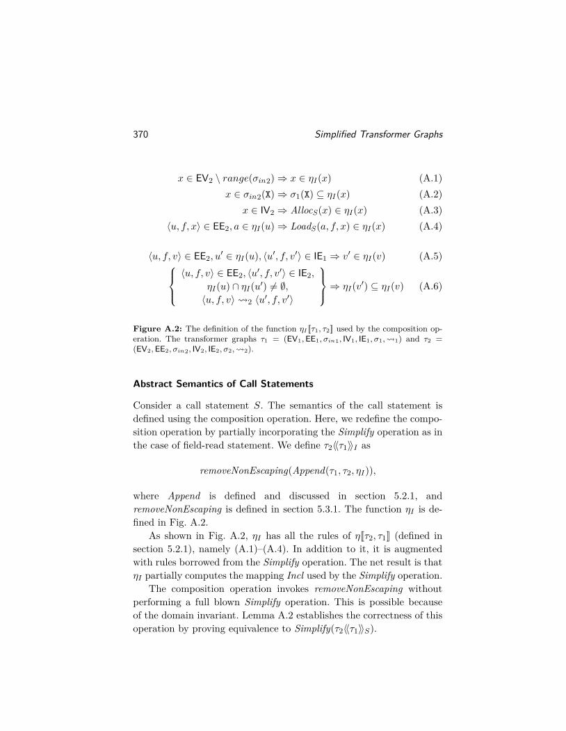
370 Simplified Transformer Graphs
x ∈ EV2 \ range(σin2)⇒ x ∈ ηI(x) (A.1)x ∈ σin2(X)⇒ σ1(X) ⊆ ηI(x) (A.2)
x ∈ IV2 ⇒ AllocS(x) ∈ ηI(x) (A.3)〈u, f, x〉 ∈ EE2, a ∈ ηI(u)⇒ LoadS(a, f, x) ∈ ηI(x) (A.4)
〈u, f, v〉 ∈ EE2, u′ ∈ ηI(u), 〈u′, f, v′〉 ∈ IE1 ⇒ v′ ∈ ηI(v) (A.5)
〈u, f, v〉 ∈ EE2, 〈u′, f, v′〉 ∈ IE2,
ηI(u) ∩ ηI(u′) 6= ∅,〈u, f, v〉 2 〈u′, f, v′〉
⇒ ηI(v′) ⊆ ηI(v) (A.6)
Figure A.2: The definition of the function ηI [[τ1, τ2]] used by the composition op-eration. The transformer graphs τ1 = (EV1,EE1, σin1, IV1, IE1, σ1, 1) and τ2 =(EV2,EE2, σin2, IV2, IE2, σ2, 2).
Abstract Semantics of Call Statements
Consider a call statement S. The semantics of the call statement isdefined using the composition operation. Here, we redefine the compo-sition operation by partially incorporating the Simplify operation as inthe case of field-read statement. We define τ2〈〈τ1〉〉I as
removeNonEscaping(Append(τ1, τ2, ηI)),
where Append is defined and discussed in section 5.2.1, andremoveNonEscaping is defined in section 5.3.1. The function ηI is de-fined in Fig. A.2.
As shown in Fig. A.2, ηI has all the rules of η[[τ2, τ1]] (defined insection 5.2.1), namely (A.1)–(A.4). In addition to it, it is augmentedwith rules borrowed from the Simplify operation. The net result is thatηI partially computes the mapping Incl used by the Simplify operation.
The composition operation invokes removeNonEscaping withoutperforming a full blown Simplify operation. This is possible becauseof the domain invariant. Lemma A.2 establishes the correctness of thisoperation by proving equivalence to Simplify(τ2〈〈τ1〉〉S).

371
Correctness, Equivalence and Termination of FI
Lemma A.1. Let S be a field-read statement of the form v1 = v2.f andτ ∈ AI . The transfer functions: FI(S), FG(S), and FG(S) composedwith Simplify, are all equivalent. That is,
γT (FG(S)(τ)) = γT (Simplify(FG(S)(τ))) = γT (FI(S)(τ))
Lemma A.2. Let τ1, τ2 ∈ AI and let S be a call statement. The com-position operation 〈〈〉〉I is equivalent to the base composition operation(〈〈〉〉), and also to 〈〈〉〉 composed with Simplify.
γT (τ2〈〈τ1〉〉S) = γT (SimplifyS(τ2〈〈τ1〉〉S)) = γT (τ2〈〈τ1〉〉I).
Lemma A.3. If τ ∈ AI then
a. FI(v1 = v2.f)(τ) is monotonic w.r.t vco.
b. The composition operation τ1〈〈τ2〉〉I , and the abstract semantics ofthe call statement are monotonic w.r.t vco.
Theorem A.4. For any instantiation (A,FA) of (AI ,FI) satisfyingAssumption 5.10
a. There exists an instantiation of (AG ,FG) semantically equivalent to(A,FA) and vice versa. Therefore, (A,FA) is correct.
b. (A,FA) will terminate since the transfer functions are monotonic.
BThe Node Merging Abstraction
In this section we formalize the node merging abstraction informallydescribed in section 6.3.1.
Transformer Graph Embedding We say that a transformer graph τ1can be embedded in τ2, denoted τ1 � τ2, iff there exists a homomor-phism h from the vertices τ1 to τ2 such that the following holds. (Weuse subscripts 1 and 2 to denote components of τ1 and τ2.)
x ∈ IV1 ⇒ h(x) ∈ IV2
x ∈ EV1 ⇒ h(x) ∈ EV2
〈x, f, y〉 ∈ IE1 ⇒ 〈h(x), f, h(y)〉 ∈ IE2
〈x, f, y〉 ∈ EE1 ⇒ 〈h(x), f, h(y)〉 ∈ EE2
∀v ∈ Vars. {h(x) | x ∈ σ1(v)} ⊆ σ2(v)∀v ∈ Vars. {h(x) | x ∈ σin1(v)} ⊆ σin2(v)(〈u, f, w〉, 〈x, g, y〉) ∈ 1⇒ (〈h(u), f, h(w)〉, 〈h(x), g, h(y)〉) ∈ 2
We use τ1 �h τ2 to denote that the function h induces an embeddingfrom τ1 to τ2. (Unlike the embedding notions used by TVLA [Sagivet al., 1999], here h is not required to be surjective.)
372
373
Node merging produces an embedding. Assume that we are given afunction ξ representing an equivalence relation on the nodes of a trans-former graph τ . ξ maps a node in τ to the representative of its equiva-lence class. We define the transformer graph ξ(τ) to be the transformergraph obtained by replacing every node u by a unique representative ofits equivalence class in every component of τ (we formally define ξ(τ)later).
Lemma B.1. The embedding operation satisfies the following:
a. � is a pre-order. (i.e., it is reflexive and transitive).
b. γT is monotonic with respect to �: ∀τa, τb ∈ AG ,τa � τb ⇒ γT (τa) vc γT (τb)
c. τ � ξ(τ).
Assume that we wish to replace a transformer graph τ by a graphξ(τ) at some point during the analysis (perhaps by incorporating thisinto one of the abstract operations). Our earlier correctness argumentstill remains valid (since if f ∼ τ1 � τ2, then f ∼ τ2). (The proof isessentially a simple inductive proof: see Prop. 4.3 of Cousot and Cousot[1992]).
However, this optimization impacts the termination argument be-cause node merging is not monotonic w.r.t containment ordering. In-deed, our initial implementation of the optimization did not terminatefor one program because the computation ended up with a cycle ofequivalent, but different, transformers (in the sense of having the sameconcretization).
Informally, we get around this problem by refining the analysis toensure that once two nodes are chosen to be merged together, they arealways merged together in all subsequent steps. This approach guaran-tees termination. We formalize this approach in the sequel. The formal-ization adds an equivalence relation on nodes (representing the nodescurrently merged together) to the abstract domain and updates thetransformers accordingly.
374 The Node Merging Abstraction
The Equivalence Relations Domain We represent an equivalence re-lation on Na (the set of abstract nodes) using a function ξ : Na 7→ Na
that maps every node in an equivalence class to the (unique) represen-tative of the equivalence class. Let E ⊆ Na 7→ Na be the set of suchfunctions representing the equivalence relations on Na. Given a func-tion ξ ∈ E it is straight forward to construct the equivalence relationit represents (denote as 'ξ), 'ξ= {(x, y) | ξ(x) = ξ(y)}. For everyξ ∈ E let ξ−1 : Na 7→ 2 Na denote the inverse function that maps therepresentative of an equivalence class to the set of nodes it represents.
Let ≤ be a partial order on E corresponding to the refinement orderof equivalence relations, i.e., ξ1 ≤ ξ2 iff 'ξ1⊆'ξ2 . Let t denote thecorresponding join operator: for all ξ1, ξ2 ∈ E , ξ1 t ξ2 is the functionrepresenting the equivalence relation on Na that is a superset of 'ξ1
and 'ξ2 .
Lemma B.2. (E ,≤,t) is a join semi-lattice. The least element of (E ,≤)is λx.x.
The Abstract Domain
Define an abstract domain A as the set of pairs (τ, ξ) ∈ AG×E satisfyingthe following condition:
x ∈ (EV ∪ IV) =⇒ ξ(x) = x
where τ = (EV,EE, σin, IV, IE, σ, ). The above condition implies thatin every (τ, ξ) ∈ A, the vertices in τ are the representatives of theequivalence classes of 'ξ.
The equivalence classes are kept around in the abstract state alongwith transformer graphs to remember the nodes that were merged (andreplaced by their representatives) so that these nodes are merged againin the future if they show up.
Let τ ∈ A and let µ : Na 7→ 2 Na be any function. Let µ(τ) be thetransformer graph obtained by replacing v by µ(v) in every componentof τ . Formally, µ(τ) is defined as: (µ(EV), µ(EE), µ(σin), µ(IE), µ(IV),µ(σ),
⋃ie ee µ(ie) × µ(ee)), where µ(〈x, f, y〉) = µ(x) × {f} × µ(y),
µ(σ) = λx.µ(σ(x)), and µ(S) =⋃x∈S µ(x).
375
Depending on the definition of µ, µ(τ) may collapse multiple ver-tices in τ into a single vertex or blow-up a vertex in τ to a set of vertices.For instance, given a function ξ ∈ E , ξ(τ) will replace every vertex in τby the representative of the equivalence class it belongs to in 'ξ. (Tobe mathematically precise, in ξ(τ) we interpret ξ as a function fromNa 7→ 2 Na .) To the contrary, ξ−1(τ) will replace the representative ofan equivalence class by the vertices it represents.
Define a partial order ≤m on A as follows: (τ1, ξ1) ≤m (τ2, ξ2) iffξ1 ≤ ξ2 and τ1 �ξ2 τ2. Let tm denote the join operation with respectto ≤m. We define the concretization function γm : A 7→ C as γm(τ, ξ) =γT (τ).
Node Merging
With every edge and vertex of the control flow graph we associate anode merging operation NMi : A 7→ A, where i is a statement or vertexof the control flow graph, defined as follows:
NMi(τ, ξ) =let ξ′ = NodesToMergei(τ)let ξ′′ = ξ t ξ′
(ξ′′(τ), ξ′′)
The node merging operation is parameterized by a functionNodesToMergei . It returns an equivalence relation whose equivalenceclasses specify the nodes that have to be merged together. The followingresults hold for any arbitrary definition of NodesToMergei .
Lemma B.3. If (τ, ξ) ∈ A and (τ ′, ξ′) = NMi(τ, ξ) then τ � τ ′
For ensuring termination we require that NodesToMergei is mono-tonic with respect to the embedding operation i.e, for all τ1, τ2 ∈ A, ifτ1 � τ2 then NodesToMergei(τ1) ≤ NodesToMergei(τ2). This propertywill be satisfied if the nodes are chosen for merging based on the prop-erties of the transformer graph that are preserved by the embedding,e.g. based on reachability of nodes.

376 The Node Merging Abstraction
Semantics Equations
ϑv = (τid , λx.x) v is an entry vertex (B.1)
ϑv = tm({ϑu,v | uS→ v}) v is not an entry vertex (B.2)
ϑu,v = FA(S)(ϑu) uS→ v, S is not a call statement (B.3)
ϑu,v = FA(S)(ϑu, ϑexit(Q)) uS→ v, S is a call to Q (B.4)
Correctness preserving operations
NMi ∈ A 7→ A i is a statement or a vertex
Figure B.1: The abstract semantics that incorporates the node merging operation.
The Abstract Semantics
The abstract semantics equations that incorporate the node mergingoperation are shown in Figure B.1. Let S be a primitive statement.FA(S) : A 7→ A is defined as:
FA(S)(τ, ξ) = (ξ(FG(S)(ξ−1(τ))), ξ)
If S is a call to procedure Q, then
FA(S)((τr, ξr), (τe, ξe))) = let ξ′ = ξr t ξe(ξ′(FG(S)(ξr−1(τr), ξe−1(τe))), ξ′)
In simple words, the abstract transfer function FA(S) first constructsa blown-up transformer graph ξ−1(τ) by reintroducing all the ver-tices/edges that may have been merged in τ . (Note that ξ−1(τ) andτ are semantically equivalent i.e, have the same concrete image as eachembed in the other.) It then applies the base semantics FG(S), and col-lapses the merged vertices/edges again by applying ξ on the resultingtransformer graph.
The application of ξ−1 to the input transformer graph is necessaryin order to ensure the monotonicity of FA with respect to ≤m. This isa fall out of the fact that for any arbitrary definition of the parameterswe are only guaranteed that FG(S) is monotonic with respect to the

377
containing ordering vco . However, for many practical instantiations ofthe parameter, the transfer function FG(S) would be monotonic withrespect to �ξ (for any ξ ∈ E). In such cases, as an optimization we caneliminate the application of ξ−1 from the above definition and obtaina more efficient semantics.
Notice that when no nodes are merged during the analysis, theabove semantics is equivalent to (AG ,FG), since the NM operation atevery statement and vertex reduces to an identity function and theequivalence relation remains unchanged (from the initial identify rela-tion) throughout the analysis.
Correctness and Termination of the Node Merging Abstraction
The correctness of the semantics (A,FA) is straightforward to estab-lish. The ξ component of the abstract state is not relevant for provingcorrectness (see the definition of γm). The τ component of the abstractstate is updated by the transfer functions FA by applying the basetransfer function FG , followed and preceded by the application of ξand ξ−1, respectively (for some ξ ∈ E). However, the application of ξor ξ−1 on a transformer graph is correctness preserving because τ canbe embedded in both ξ(τ) and ξ−1(τ). Hence, FA is correct. Below weformalize the termination of the abstract semantics FA.
Assumption B.4. NodesToMergei terminates on all inputs and ismonotonic w.r.t the embedding operation �.
Lemma B.5. If the Assumptions B.4 and5.10 hold,
a. For every statement S, FA(S) is monotonic w.r.t ≤m.
b. For every vertex of the control flow graph or statement i, NMi ismonotonic with respect to ≤m.
Theorem B.6. Every instantiation of (A,FA) satisfying assump-tions B.4 and 5.10 terminates.

References
Martin Bravenboer and Yannis Smaragdakis. Strictly declarative specificationof sophisticated points-to analyses. In OOPSLA, pages 243–262, 2009.
Marcio Buss, Daniel Brand, Vugranam C. Sreedhar, and Stephen A. Edwards.Flexible pointer analysis using assign-fetch graphs. In SAC, pages 234–239,2008.
Marcio Buss, Daniel Brand, Vugranam C. Sreedhar, and Stephen A. Edwards.A novel analysis space for pointer analysis and its application for bug find-ing. Sci. Comput. Program., 75(11):921–942, 2010.
Cristiano Calcagno, Dino Distefano, Peter W. O’Hearn, and Hongseok Yang.Compositional shape analysis by means of bi-abduction. In POPL, pages289–300, 2009.
Ramkrishna Chatterjee, Barbara G. Ryder, and William A. Landi. Relevantcontext inference. In POPL, pages 133–146, 1999.
Ben-Chung Cheng and Wen-Mei W. Hwu. Modular interprocedural pointeranalysis using access paths: design, implementation, and evaluation. InPLDI, pages 57–69, 2000.
Patrick Cousot and Radhia Cousot. Abstract interpretation frameworks. J.Log. Comput., 2(4):511–547, 1992.
Patrick Cousot and Radhia Cousot. Modular static program analysis. In CC,pages 159–178, 2002.
Manuvir Das. Unification-based pointer analysis with directional assignments.In PLDI, pages 35–46, 2000.
378

References 379
Arnab De and Deepak D’Souza. Scalable flow-sensitive pointer analysis forjava with strong updates. In ECOOP, pages 665–687, 2012.
Isil Dillig, Thomas Dillig, Alex Aiken, and Mooly Sagiv. Precise and compactmodular procedure summaries for heap manipulating programs. In PLDI,pages 567–577, 2011.
Bhargav S. Gulavani, Supratik Chakraborty, Ganesan Ramalingam, andAditya V. Nori. Bottom-up shape analysis. In SAS, pages 188–204, 2009.
Ben Hardekopf and Calvin Lin. Flow-sensitive pointer analysis for millions oflines of code. In CGO, pages 289–298, 2011.
Bertrand Jeannet, Alexey Loginov, Thomas Reps, and Mooly Sagiv. A rela-tional approach to interprocedural shape analysis. ACM Trans. Program.Lang. Syst., 32:5:1–5:52, 2010.
Etienne Kneuss, Viktor Kuncak, and Philippe Suter. Effect analysis for pro-grams with callbacks. In VSTTE, pages 48–67, 2013.
Jens Knoop and Bernhard Steffen. The interprocedural coincidence theorem.In CC, pages 125–140, 1992.
Chris Lattner and Vikram Adve. Macroscopic Data Structure Analysis andOperations. PhD thesis, University of Illinois at Urbana-Champaign, 2005a.
Chris Lattner and Vikram S. Adve. Automatic pool allocation: improvingperformance by controlling data structure layout in the heap. In PLDI,pages 129–142, 2005b.
Chris Lattner, Andrew Lenharth, and Vikram S. Adve. Making context-sensitive points-to analysis with heap cloning practical for the real world.In PLDI, pages 278–289, 2007.
Ondrej Lhoták. Program Analysis Using Binary Decision Diagrams. PhDthesis, 2006.
Ondrej Lhoták and Kwok-Chiang Andrew Chung. Points-to analysis withefficient strong updates. In POPL, pages 3–16, 2011.
Donglin Liang and Mary Jean Harrold. Efficient computation of parame-terized pointer information for interprocedural analyses. In SAS, pages279–298, 2001.
Percy Liang and Mayur Naik. Scaling abstraction refinement via pruning. InPLDI, pages 590–601, 2011.
Ravichandhran Madhavan, Ganesan Ramalingam, and Kapil Vaswani. Purityanalysis: An abstract interpretation formulation. In SAS, pages 7–24, 2011.
380 References
Ravichandhran Madhavan, G. Ramalingam, and Kapil Vaswani. Modularheap analysis for higher-order programs. In SAS, pages 370–387, 2012.
Ravi Mangal, Mayur Naik, and Hongseok Yang. A correspondence betweentwo approaches to interprocedural analysis in the presence of join. In ESOP,pages 513–533, 2014.
Mark Marron, Ondrej Lhoták, and Anindya Banerjee. Programming paradigmdriven heap analysis. In CC, pages 41–60, 2012.
Erik M. Nystrom, Hong-Seok Kim, and Wen mei W. Hwu. Bottom-up andtop-down context-sensitive summary-based pointer analysis. In SAS, pages165–180, 2004.
Prakash Prabhu, Ganesan Ramalingam, and Kapil Vaswani. Safe pro-grammable speculative parallelism. In PLDI, pages 50–61, 2010.
Noam Rinetzky, Mooly Sagiv, and Eran Yahav. Interprocedural shape analysisfor cutpoint-free programs. In SAS, pages 284–302, 2005.
Shmuel Sagiv, Thomas W. Reps, and Reinhard Wilhelm. Parametric shapeanalysis via 3-valued logic. In POPL, pages 105–118, 1999.
Alexandru D. Salcianu. Pointer analysis and its applications for java pro-grams. Master’s thesis, Massachusetts institute of technology, 2001.
Alexandru D. Salcianu and Martin C. Rinard. Purity and side effect analysisfor java programs. In VMCAI, pages 199–215, 2005.
Micha Sharir and Amir Pnueli. Two approaches to interprocedural data flowanalysis. In Program Flow Analysis: Theory and Applications, pages 189–234, 1981.
Yannis Smaragdakis and Martin Bravenboer. Using datalog for fast and easyprogram analysis. In Datalog, pages 245–251, 2010.
Yannis Smaragdakis, Martin Bravenboer, and Ondrej Lhoták. Pick your con-texts well: understanding object-sensitivity. In POPL, pages 17–30, 2011.
Yannis Smaragdakis, George Kastrinis, and George Balatsouras. Introspectiveanalysis: context-sensitivity, across the board. In PLDI, page 50, 2014.
Bjarne Steensgaard. Points-to analysis in almost linear time. In POPL, pages32–41, 1996.
WALA. T. J. Watson libraries for program analysis. URL https://github.com/wala/WALA.
John Whaley and Martin C. Rinard. Compositional pointer and escape anal-ysis for java programs. In OOPSLA, pages 187–206, 1999.

References 381
Xin Zhang, Ravi Mangal, Radu Grigore, Mayur Naik, and Hongseok Yang. Onabstraction refinement for program analyses in datalog. In PLDI, page 27,2014.