Affine Term Structure Models I:Term-Premia and Stochastic Volatility

Pierre Collin-DufresneUC Berkeley

Lectures given at Copenhagen Business SchoolJune 2004

Contents

1 Why are Dynamic Term Structure Models useful? 4

2 Definitions 5

3 Term structure in a deterministic world 6

4 Traditional Expectations Hypothesis 9

5 Short rate models 10

5.1 One-factor models . . . . . . . . . . . . . . . . . . . . . . . . . . . . . . 10

5.1.1 One-factor Vasicek model (PDE approach) . . . . . . . 15

5.1.2 One-factor Cox-Ingersoll and Ross (CIR) Model . . . 19

5.1.3 One-factor affine models . . . . . . . . . . . . . . . . . . . . . 20

5.1.4 Interpretation of the Market price of Risk: equilib-rium model . . . . . . . . . . . . . . . . . . . . . . . . . . . . . . . 22

1

5.1.5 Specification of risk-premia and predictability in bondreturns . . . . . . . . . . . . . . . . . . . . . . . . . . . . . . . . . . . 24

5.1.6 Fitting the Term structure in a one-factor Gaussianmodel . . . . . . . . . . . . . . . . . . . . . . . . . . . . . . . . . . . 28

5.1.7 Shortcomings of one-factor short rate models . . . . . 29

5.1.8 Empirical Evidence . . . . . . . . . . . . . . . . . . . . . . . . . 30

5.2 Multi-factor short-rate models . . . . . . . . . . . . . . . . . . . . . 31

5.2.1 Simple Generalization: Independent state variables . 31

5.2.2 Affine Term Structure Models - Duffie and Kan (DK1996) . . . . . . . . . . . . . . . . . . . . . . . . . . . . . . . . . . . . 31

5.2.3 Tractability of Affine framework: . . . . . . . . . . . . . . 32

5.2.4 Problems with Latent Variable specification: . . . . . . 33

5.2.5 Why rotate from latent variables to observables? . . . 35

5.2.6 Example of Identification: 2-factor Gaussian Model 38

5.2.7 Model-Insensitive Estimation of the State Variables . 39

5.2.8 Canonical Representation and Maximality: theA1(3)model . . . . . . . . . . . . . . . . . . . . . . . . . . . . . . . . . . . 40

5.3 Unspanned Stochastic volatility . . . . . . . . . . . . . . . . . . . . 41

5.3.1 Empirical Evidence . . . . . . . . . . . . . . . . . . . . . . . . . 43

5.3.2 USV Affine Models . . . . . . . . . . . . . . . . . . . . . . . . . 46

5.3.3 Maximal A1(3) model with USV . . . . . . . . . . . . . . . 50

5.3.4 Maximal A1(4) model with USV . . . . . . . . . . . . . . . 52

5.3.5 Specification of Risk-Premia . . . . . . . . . . . . . . . . . . 53

5.4 Estimation of Affine models with and without USV . . . . . 54

2

6 Recent Developments 61

3

1 Why are Dynamic Term Structure Models useful?

• Macroeconomics: The Term Structure (TS) is a major indica-tor of economic activity. Models can be used to learn/forecastmacroeconomy, understand and help Monetary policy.

• Financial Economics: TS affects valuation of all assets (discount-ing). Dynamic models are useful to value TS derivatives, andmanage interest rate risk (i.e., volatility). They also help under-stand the risk-return trade-off of bonds (term premia).

• Interest rate risk affects all economic agents:

1. Households: e.g., mortgages (prepayment options).

2. Firms: financing and investment decisions.

• Interest rate derivatives are biggest component of derivative mar-ket:

OTC (trillion $) Swaps Options Forwards TotalInterest rate 58.5 12.3 8.6 79.4

Currency 3.9 3.1 12.4 19.4Other 5.1

Source: Swaps Monitor 2000

• Most trading occurs Over The Counter (85% of the outstandingnotional).

Derivatives (trillion $) 1998 2002Over the counter Notional amount 80 142

Gross market value 3 6Exchange traded Notional amount 14 24

Source: Bank of International Settlements

• Volume in Exchange traded Options and Futures is mainly Equityand Interest rate followed by FX and Commodity.

4

2 Definitions

• P (t, T ) is the price of a zero-coupon bond that pays $1 at maturity(P (T, T ) = 1).

• The continuously compounded Yield to maturity Y (t, T ) is de-fined by : P (t, T ) = e−Y (t,T )(T−t).

• The term structure of interest rates is the mapping (T − t) →Y (t, T ).

• Define the time-t forward rate f (t, T1, T2) for borrowing/lendingbetween T1 and T2 in the future by:

P (t, T1)e−f(t,T1,T2)(T2−T1) = P (t, T2).

• The instantaneous Forward rate f (t, T ) = limT2→T f (t, T, T2) isgiven by

f (t, T ) = −∂2 lnP (t, T ) = Y (t, T ) + (T − t)∂2Y (t, T )

(Assuming differentiability of the term structure). Note also the rela-tion

P (t, T ) = e−∫ Tt f(t,s)ds (1)

.

• The instantaneous short rate r(t) = f (t, t) = Y (t, t).

5

3 Term structure in a deterministic world

In a deterministic world no-arbitrage implies that all bonds earn thesame return over any finite period 1/P (t, T1) = P (T1, T2)/P (t, T2).

Taking the limit (T1 → t), it also follows that all bonds earn the sameinstantaneous rate of return:1

dP (t, T )

P (t, T )= r(t) dt ∀T.

or equivalentlyP (t, T ) = e−

∫ Tt r(s)ds

Further, we have:

f (t, s) = r(s) (2)

Y (t, T ) =1

T − t

∫ T

t

r(s)ds (3)

f (t, T1, T2) = Y (T1, T2) (4)

If we specify the simple mean-reverting short-rate model:

dr(t) = κ(θ − r(t))dt,

then r(s) = e−κ(s−t)r(t) + (1 − e−κ(s−t))θ and

P (t, T ) = e−∫ Tt r(s)ds

= e−rtBκ(T−t)−θ(T−t−Bκ(T−t)), (5)

where we have defined

Bκ(τ ) =

∫ τ

0

e−κsds =1 − e−κτ

κ1To prove it take the log of both sides, differentiate with respect to T2. Get lnP (t, T1) = −

∫ T1

0r(s)ds + ψ(t).

Solve for ψ(t).

6

We can also prove this by the ‘PDE’ approach:

In particular, assume P ≡ P (t, r(t)). Then dP (t) = (Prdr + Ptdt) =

(Prκ(θ − r) + Pt)dt. By no arbitrage, dP = rP dt. Thus P satisfies:

Prκ(θ − r) + Pt = rP

subject to P (T, r) = 1. Guessing that the bond price formula is anexponential-affine solution in r(t), we obtain the same result as above.

For this ‘one-factor’ model the term structure is:

Y (t, T ) = θ − (θ − rt)Bκ(T − t)

(T − t). (6)

The term structure is increasing iff rt < θ

The long rate is limT→∞ Y (t, T ) = θ.

More generally, we could assume an affine multi-factor short ratemodel:

r(t) =

n∑

j=1

δjXj(t),

where

dXi(t) =

µi0 +

∑

j

µijXj(t)

∀i = 1, . . . , n.

Bond prices can easily be solved for as above (exercise).2

Modern term structure theory basically adds ‘noise’ (Brownian mo-tion and/or jumps):

• Short-rate models basically ‘add’ a stochastic term to the short-rate dynamics and try to derive bond prices using no-arbitrageconsiderations.

2Richard (1978) offers further discussion as well as introducing inflation and a nominal term structure model.

7

For example, Vasicek (1977) considers

dr(t) = κ(θ − r(t))dt + σ dw(t).

Such models are useful for predicting/explaining the cross-sectionof observed bond prices on a given date.

• In contrast, Bond or Forward rate models takes the observed termstructure as given, and adds a stochastic term to the bond or for-ward rate dynamics in a manner consistent with absence of arbi-trage.

The most common use of this framework is for pricing fixed in-come derivatives.

This (HJM) approach is analogous to pricing equity options (e.g.,Black Scholes) taking the stock price as given.

Remarks:

1. Short rate vs. Bond vs. Forward rate model:

While the modeling approach seems different, we will show be-low that there is a one to one correspondence between the two.

2. Note that since f (t, T ) = r(T ) in a deterministic world forwardrates are constant, i.e. df (t, T ) = 0dt. This explains why in arisky world, forward rate dynamics will be primarily determinedby the volatility structure.

3. There has been some debate in the literature (fueled by a some-what controversial example in CIR (1985b) about the need to dis-tinguish:

• Equilibrium models derived from fundamental principles withrational maximizing agents within a GE economy (Cox, In-gersoll and Ross (1985), Lucas (1978)), and

8

• Arbitrage-free (HJM) models which solely rest on the princi-ple of absence of arbitrage (Heath, Jarrow and Morton (1992)).

It is now well understood that this distinction is moot.

4 Traditional Expectations Hypothesis

Traditional theories of the term structure are described in Cox, Inger-soll and Ross (1981).

Typically, start from the relations that hold in a deterministic world(above) and apply an expectation.

CIR distinguish:

• Unbiased expectation hypothesis: f (t, T ) = E[r(T )]

• Local expectation hypothesis: P (t, T ) = E[e−∫ Tt r(s)ds]

(i.e., Et[dP (t, T )] = r(t)P (t, T )dt)

• Return to maturity expectation hypothesis: 1/P (t, T ) = E[e∫ Tt r(s)ds]

• Yield to maturity expectation hypothesis Y (t, T ) = 1T−tE[

∫ Tt r(s)ds]

CIR 81 have shown that all these assumptions are mutually incompat-ible (essentially, because of Jensen’s inequality).

As we shall see below, ruling out arbitrage opportunities implies thatonly the local expectation hypothesis holds, but when the expectationis computed under the so-called risk-neutral measure.3

3Of course, it is possible to construct examples where one or the other expectation hypothesis holds, but genericallythey are inconsistent with the absence of arbitrage.

9

5 Short rate models

5.1 One-factor models

• The short rate r(t) is the only state variable. Its dynamics is spec-ified as a one-factor Markov process:

drt = µr(t, rt)dt + σr(t, rt)dwt

• If we can only borrow or lend at the risk-free rate then marketsare incomplete.

• Suppose however that we can trade in multiple zero-coupon bonds.Then absence of arbitrage (AoA) implies cross-sectional restrictionsas we show below.

• Assume P (t, Ti) = P i(t, rt) is continuous and differentiable. Con-struct a portfolio

V (t) = n1P1(t) + n2P

2(t),

that is self financing:

dVt = n1(t)dP1(t) + n2(t)dP

2(t)

=

[n1

(1

2P 1rrσ

2r

+ P 1r µr + P 1

t

)+ n2

(1

2P 2rrσ

2r

+ P 2r µr + P 2

t

)]dt

+(n1P

1r + n2P

2r

)σrdwt

The first equality comes from the self-financing condition, and thesecond from Ito’s lemma.

Suppose we choose the weights n1, n2 such that the portfolio islocally risk-free. That is, we choose n1, n2 so that:

n1P1r + n2P

2r = 0 (7)

10

By AoA this portfolio must earn the risk-free rate of return:

n1

(1

2P 1rrσ

2r

+ P 1r µr + P 1

t

)+n2

(1

2P 2rrσ

2r

+ P 2r µr + P 2

t

)= r(n1P

1+n2P2)

(8)Combining equations (7) and (8), we find

1

P 1r

[1

2P 1rrσ

2r

+ P 1r µr + P 1

t − rP 1

]=

1

P 2r

[1

2P 2rrσ

2r

+ P 2r µr + P 2

t − rP 2

].

Therefore, there must exist γ(t) independent of maturities such that:

γ(t) =12Prrσ

2r

+ Prµr + Pt − rP

σrPr. (9)

We obtain the fundamental PDE for bond prices:

1

2Prrσ

2r

+ Pr(µr − γσr) + Pt − rP = 0 (10)

subject to the boundary condition P (T, T ) = 1.

Remark: Arbitrage and Convexity:

Suppose you have duration-matched portfolios (P 1r = P 2

r ) with equalvalue (P 1 = P 2). Then the PDE above indicates that if P 1

rr > P 2rr > 0

then P 1t < P 2

t < 0. Convexity is not free! (similar to Gamma foroptions).

11

• Equivalent Martingale measure.

Define a process wQ(t) by dwQt = dwt + γdt, then we obtain:

dr = (µr − γσr)dt + σrdwQt (11)

≡ µQrdt + σrdw

Qt . (12)

Equation (10) can be rewritten as:1

2Prrσ

2r

+ PrµQr

+ Pt − rP = 0. (13)

The instantaneous expected expected return on the risk-free bond isequal to the risk-free rate when the expectation is taken with respect toa different measure Q under which dynamics of the risk-free rate aregiven by (12) above with wQ(t) being a standard Brownian motion.

Under technical conditions on γ, Girsanov’s theorem shows that thereexists a measure Q equivalent to P under which wQ defined above isindeed a standard Brownian motion.

If these technical conditions are satisfied, then discounted Bond pricesare martingales under the Q-measure and we we obtain:

P (t, T ) = EQ[e−∫ Tt r(s)ds|F(t)]

Q is the so-called risk-neutral equivalent martingale measure (EMM)(Harrison and Kreps (1979)), the existence of which guarantees theAoA.

Remark: The argument used above to derive the ‘fundamental’ PDE (13)is not specific to bond prices. I applies to any European style contin-gent claim that has a payoff that is a function solely of the short rate.Pricing different contingent claim only changes the boundary condi-tions associated with the PDE. Further for any such contingent claim

12

we have the validity of the risk-neutral pricing formula:

C(t, rt) = EQ[e−∫ Tt r(s)dsC(T )|F(t)]

Standard short rate models in the literature are:

Author short rate risk premiumMerton dr = θdt+ σ dw γ (const.)Vasicek dr = κ(θ − r)dt+ σ dw γ (const.)

Cox, Ingersoll, Ross dr = κ(θ − r)dt+ σ√r dw γ

√r

Dothan dr = κrdt+ σr dw γDuffie & Kan dr = κ(θ − r)dt+

√σ1 + σ2r dw γ

√σ1 + σ2r

Ahn & Gao κ(θ − r)r dt+ σr1.5dw γ1√r+ γ2

√r

Ho and Lee dr = θ(t)dt+ σ dw 0Hull & White (extended Vas.) dr = (φ(t) − κr)dt+ σ dw 0Hull & White (extended CIR) dr = (φ(t) − r)dt+ σ

√r dw 0

Black & Karasinsky d log r = κ(t)(θ(t) − log r)dt+ σ(t) dw 0Quadratic (Jamshidian) r = θ + σ1x+ σ2x

2 where dx = −κx dt+ dw 0

Remarks:

1. All models with zero market price of risk are, in fact, definedunder the risk-neutral measure. They have time dependent pa-rameters which can be chosen to fit the observed term structureat the initial date.

2. The commonly used Black and Karasinsky model (which nestsa continuous time version of the Black, Derman and Toy model)generates infinite values for Eurodollar futures (Hogan and Wein-traub (1993)).

3. The Ahn and Gao (1999) model in fact corresponds to definingthe short rate as the inverse of a square-root process.

13

4. The quadratic model is a restricted two-factor affine model. In-deed setting yt = x2

t we have:

dyt = (1 − 2κyt)dt + 2xtdwt

Thus (xt, yt) form jointly an affine two-factor model. The quadraticmodel however, restricts the initial value of the state vector to sat-isfy y0 = x2

0 (which along with the dynamics insures that yt = xta.e.).

For illustration, we first introduce the Gaussian Vasicek model andthen its generalization to the affine case.

14

5.1.1 One-factor Vasicek model (PDE approach)

Vasicek (1977) assumes that the short rate is:

drt = κ(θ − rt)dt + σdwt

and constant market price of risk γ:

γ =E[dP (t,T )

P (t,T )] ]/dt− rt

σPr(t,T )P (t,T )

Under the risk-neutral measure the risk-free process is thus:

drt = κ(θQ − rt)dt + σdwQt

withθQ = θ − σ

κγ.

Then bond prices are solution to the PDE:

1

2Prrσ

2 + Prκ(θQ − r) + Pt − rP = 0 (14)

s.t. P (T, T ) = 1. Guessing a solution of the form:

P (r, t, T ) = eA(T−t)−B(T−t)r,

we find that A,B solve the system of ODE:

−B′ = κB − 1 (15)

A′ =1

2σ2B2 − κθQB (16)

with A(0) = B(0) = 0. The solution is easily computed (Mathemat-ica. . . )

B(τ ) =e−κτ − 1

κ(17)

A(τ ) =

∫ τ

0

ds

(1

2σ2B(s)2 − κθQB(s)

)(18)

15

The integral can also be computed in closed-form (Mathematica).

We obtain the yield curve from P (t, T ) = exp(−Y (t, T )(T − t)):

Y (t, T ) =1

T − t

(rtB(T − t) + κθQ

∫ T

t

B(T − u)du− σ2

2

∫ T

t

B(T − u)2du

)

(19)

Setting σ = 0 we recognize the deterministic term structure of equa-tion 6.

Introducing uncertainty adds two components:

• a Jensen’s inequality effect which tends to lower long-term yields,

• a risk-premium effect (if γ 6= 0) which can go either way.

The bond price return is given by:dP (t, T )

P (t, T )= rtdt− σB(T − t)dwQ

t (20)

By definition the term-premium, i.e. the expected return on longermaturity bonds in excess of risk-free rate, is:

E[dP (t, T )

P (t, T )]/dt− rt = γσ

Pr(t, T )

P (t, T )= −γσB(T − t)

If γ < 0 then term premia are positive (and θQ > θ).

In the Vasicek model we can infer term premia from the average slopeof the term structure:

Note that

limT→t

Y (t, T ) = rt

16

limT→∞

Y (t, T ) = θQ − σ2

2κ2= θ − γσ

κ− σ2

2κ2

In particular, the average long-term slope of the term structure is:

θQ − σ2

2κ2− θ =

γσ

κ− σ2

2κ2

For example, if on average the TS slope is increasing we deduce that:

γ < − σ

2κ

Remark:

• The zero-coupon bond price process under the risk-neutral mea-sure in the Vasicek model (eq 20) is similar to the to the Merton(1976) stock price model with stochastic interest rates. As a resultit is possible to derive a similar closed-form solution for optionson zero-coupon bonds.

• Following Jamshidian (1991) it is also possible to obtain closedform solutions for coupon bond options.

17

Conclusions about one-factor model

• In a deterministic world:

– AoA ⇒ all bonds have the same (instantaneous) return.

– Today’s yield curve embeds all the information about all fu-ture rates.

• In a one-factor risky world:

– AoA ⇒ There exists a Market price of risk (equal to the termpremium on a T -maturity bond normalized by the diffusionof that bond).

– Under regularity condition on the MPR, there exists an EMMunder which all bonds prices have the same instantaneous rateof return (i.e., the local expectation’s hypothesis holds underthe risk-neutral measure).

• Various short-rate models differ in terms of the assumptions theymake on any two of :

– Dynamics of short rate under historical measure (determinesTime series),

– Dynamics of short rate under the risk-neutral measure (deter-mines cross section),

– the Market price of risk (determines the difference betweenthe physical and risk-neutral drift, i.e. the risk-premium).

18

5.1.2 One-factor Cox-Ingersoll and Ross (CIR) Model

One shortcoming of the Vasicek model is that it allows for negativeinterest rates. Instead, CIR (1985b) assume that the dynamics of theshort rate is:

drt = κ(θ − rt)dt + σ√rtdwt

The advantage of this model is that it allows for time-varying volatil-ity and guarantees positive interest rates if κθ > 0. Feller (1951) alsoshows that if 2κθ > σ2 then rt > 0 a.e..

Further there exists a market price of risk process γ(rt) such that:

γ(rt) ≡E[dP (t,T )

P (t,T )] ]/dt− rt

σ√rtPr(t,T )P (t,T )

= γ√rt

Under the risk-neutral measure the risk-free process is:

drt = κQ(θQ − rt)dt + σ√rtdw

Qt

with κQ = κ+ σγ, θQ = θκ/κQ. Then bond prices are solution to thePDE:

1

2Prrσ

2r + PrκQ(θQ − r) + Pt − rP = 0 (21)

with boundary condition P (T, T ) = 1. Guessing that the solution isof the form

P (r, t, T ) = eA(T−t)−B(T−t)r,

we find that A,B solve the system of ODE:

−B′ = κQB +σ2

2B2 − 1 (22)

A′ = −κQθQB (23)

19

with boundary conditions A(0) = B(0) = 0. The solution is easilycomputed (Mathematica will do it for you. . . ).

The bond price follows:

dP (t, T )

P (t, T )= rtdt− σ

√rtB(T − t)dwQ

t

And the risk-premium on the bond is given by:

E[dP (t, T )

P (t, T )]/dt− rt = γσrt

Pr(t, T )

P (t, T )= −γσrtB(T − t)

Note that under the physical measure

dP (t, T )

P (t, T )= rt(1 − γσB(T − t)) dt− σ

√rtB(T − t)dwt

We see that when r → 0 the volatility tends to zero, and expected re-turn also tends to zero as the compensation for risk (the risk-premium)is proportional to the interest rate. We return to that issue shortly.

5.1.3 One-factor affine models

One-factor affine models have the particularity that:

• the drift and the variance of the short rate process are affine in theshort rate, and

• bond prices are exponentially affine in the short rate (or alterna-tively stated, Yields are affine).

In fact, as we show below, there is an ‘equivalence’ between the twostatement.

20

First, assume the short rate is affine under the risk-neutral measure:

drt = κQ(θQ − rt)dt +√σ1 + σ2rt dw

Qt

Then bond prices are solution to the PDE:1

2Prr(σ1 + σ2r) + Prκ

Q(θQ − r) + Pt − rP = 0 (24)

with boundary condition P (T, T ) = 1. Guessing that the solution isof the form P (r, t, T ) = eA(T−t)−B(T−t)r, we find that A,B solve thesystem of ODE:

−B′ =1

2σ2B

2 + κQB − 1 (25)

A′ =1

2σ1B

2 − κQθQB (26)

with boundary condition A(0) = B(0) = 0. The solution is easilycomputed (Mathematica will do it for you. . . )

B(τ ) =2(eητ − 1)

(η + κQ)(eητ − 1) + 2η(27)

A(τ ) =

∫ τ

0

ds

(1

2σ1B(s)2 − κQθQB(s)

)(28)

where η =√

(κQ)2 + 2σ2. The integral can also be computed inclosed-form (Mathematica).

For the converse, suppose that bond prices are of the form P (t, T ) =

eA(T−t)−B(t−t)rt. Plugging into the fundamental PDE,1

2Prrσ

2r

+ PrµQr

+ Pt − rP = 0 (29)

we obtain that 12B(τ )2σ2

r− B(τ )µQ

r+ (−A′(τ ) + B′(τ )r) − r = 0

must hold for any τ . Using two (e.g., τ1 6= τ2), we get a systemof two equations with two unknowns, which provided they are notredundant, yields a solution for µQ

r, σr affine in r.

21

Remarks

• Admissibility:Inspection of the SDE followed by the short-rate shows that notall parameter values are admissible. Indeed, the SDE is onlywell-defined if σ1 + σ2r ≥ 0. Conditions that insure this areeasily obtained, however. Set yt = σ1 + σ2rt. Ito gives dyt =

κQ(σ2θQ+σ1−yt)dt+σ2

√ytdwt. For yt to remain positive, all we

need is that σ2θ+σ1 ≥ 0. Indeed, y is continuous and when it hitszero has a positive drift, thus can never cross zero. Furthermore,if κQ(σ2θ

Q + σ1) >12σ

22, then it can be shown that yt > 0 a.s.

(e.g. zero is an entrance boundary for y, Feller (1951)).

• Affine models are particularly tractable because they admit expo-nential affine solution for the ‘extended transform’

EQt

[e−

∫ Tt r(s)dseiλ r(T )

]= eM0(T−t)+M1(T−t)r(t)

where M0,M1 are two deterministic functions that satisfy a sys-tem of Riccatti ODE. As shown by Heston (1993), Chacko andDas (2002), Duffie, Pan and Singleton (2000), CD and Goldstein(2002) this can be used to price derivatives in closed-form solu-tions using inverse Fourier transform techniques.

• Duffie, Filipovic and Schachermayer (2001) use the exponen-tially affine transform as a mathematical definition of affine pro-cesses. The larger class may include jumps (of Poisson and/orLevy type).

5.1.4 Interpretation of the Market price of Risk: equilibrium model

Following CIR (1985a) or Lucas (1978) consider a simple represen-tative agent economy with time-separable utility u(x) = log x, where

22

aggregate output is given by:

dctct

= (µt + β2t )dt + βtdw(t)

Then equilibrium state price density is Πt = 1ct

.

Applying Ito’s lemma we obtain:

dΠt

Πt= −µtdt− βtdw(t)

= −rtdt− γtdw(t)

The second equation defines the risk-free rate and the market price ofrisk, by definition of a state price density.

This simple example shows that any price system (r,γt) that is arbitrage-free can be supported by some ‘equilibrium’ model.

In particular, if we choose µt to follow an Ornstein Uhlenbeck processand β to be constant then we obtain the Vasicek model.

If we choose µt to follow a square-root process and βt = γ√µt then

we obtain CIR (1985b).

CIR (1985) argued that the only way to specify a sensible risk-premiumis to show that it is supported by a General equilibrium model. Theabove shows that it is sufficient that there exists an EMM.

Sufficient conditions for the market price of risk to be ‘acceptable’are that it satisfies the Novikov condition.

For the case where the short rate process is of the diffusion type (whichcovers the case of a general Markov process) necessary and sufficient

23

conditions are given in theorem 7.19 p.294 in Liptser and Shiryaev(1974). (Basically it is sufficient to verify that

P (

∫ T

0

||γt||2dt <∞) = Q(

∫ T

0

||γt||2dt <∞) = 1,

where the P andQmeasures are defined on the canonical space usingthe measure induced by the process.4

The discussion above indicates that one need not restrict ourselves tothe simple risk-premium structure given by CIR and Vasicek. In fact,Duffee (2002) and Dai and Singleton (2002) show that to capture theobserved predictability in bond returns it is necessary to allow formore general risk-premia.

5.1.5 Specification of risk-premia and predictability in bond re-turns

There are three different kinds of risk-premia that are considered inthe literature

• First generation

– Vasicek: γ constant.

– CIR: γ(r) = γ√r.

– Affine: γ(r) = γ√σ0 + σ1r.

• Second Generation affine (Duffee (2002), DS (2002)):

– Vasicek: γ(r) = γ0 + γrr.4Suppose w is a BM on (Ω,F , P ) and γ satisfies P (

∫ T

0||γt||2dt <∞) = 1. Define the exponential supermartingale

ξt = exp(− 1

2

∫ T

0||γt||2dt −

∫ t

0γtdwt). ξt is a martingale iff E[ξT ] = 1. Define the measure Q by Q(F ) = E[1

FξT ].

Note that for F =∫ T

0||γt||2dt <∞ we have Q(F ) = E[ξT ]. Therefore ξ is a martingale iff Q(

∫ T

0||γt||2dt <∞) = 1.

If γ is process of the diffusion type (in the sense of Liptser and Shiryaev), then the latter condition can easily be checked.

24

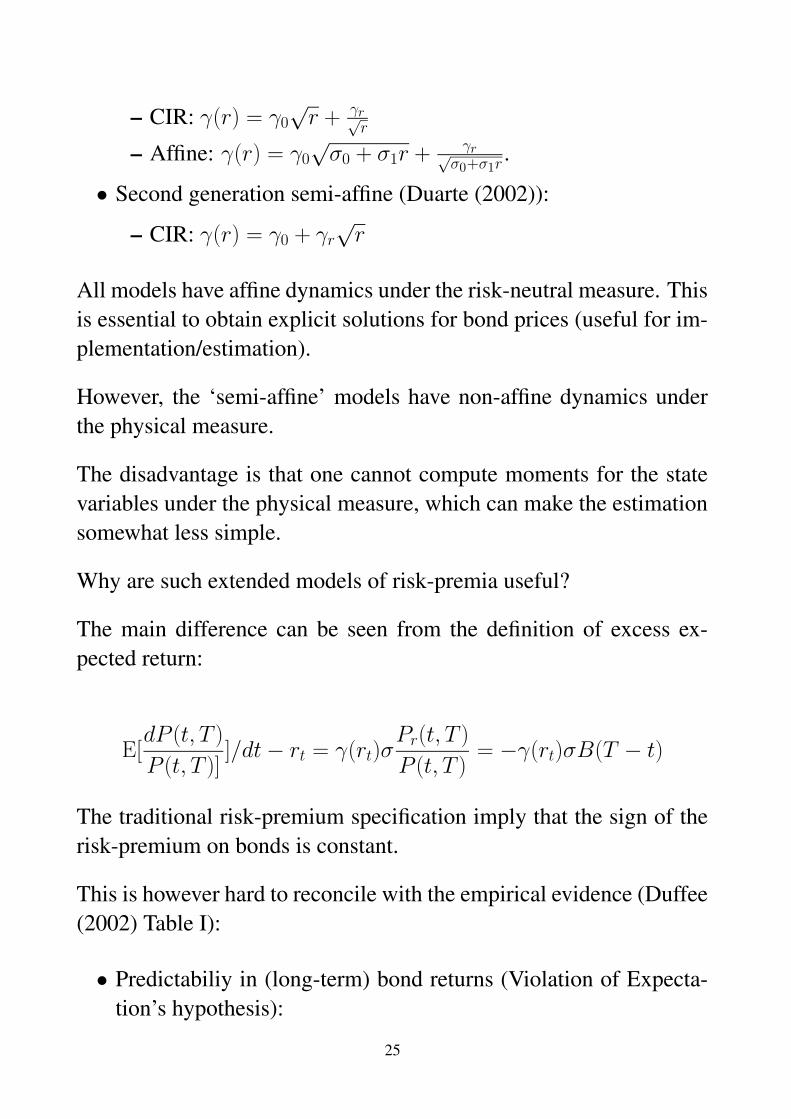
– CIR: γ(r) = γ0

√r + γr√

r

– Affine: γ(r) = γ0√σ0 + σ1r + γr√

σ0+σ1r.

• Second generation semi-affine (Duarte (2002)):

– CIR: γ(r) = γ0 + γr√r

All models have affine dynamics under the risk-neutral measure. Thisis essential to obtain explicit solutions for bond prices (useful for im-plementation/estimation).

However, the ‘semi-affine’ models have non-affine dynamics underthe physical measure.

The disadvantage is that one cannot compute moments for the statevariables under the physical measure, which can make the estimationsomewhat less simple.

Why are such extended models of risk-premia useful?

The main difference can be seen from the definition of excess ex-pected return:

E[dP (t, T )

P (t, T )]]/dt− rt = γ(rt)σ

Pr(t, T )

P (t, T )= −γ(rt)σB(T − t)

The traditional risk-premium specification imply that the sign of therisk-premium on bonds is constant.

This is however hard to reconcile with the empirical evidence (Duffee(2002) Table I):

• Predictabiliy in (long-term) bond returns (Violation of Expecta-tion’s hypothesis):

25

Regression of Treasury bond returns on previous month term struc-ture slope and volatility shows positive relation between long-term bond returns and slope of the TS as well as volatility.

• While average excess return in sample to Treasury bond is small,the slope of TS predicts large variation in excess returns. Re-quires time variation and sign switching in risk-premia (FamaFrench (1993)).

Note however that traditional risk-premium specification predict thateither risk-premia are constant, or that they are positive and increasingin the short rate (i.e., decreasing with slope).

In either case, they impose that compensation for risk is a fixed mul-tiple of volatility. In particular, risk-premia cannot switch sign overtime.

More general structure of risk-premia breaks this link and allows forchanges in sign in risk-premia.

Duffee (2002) and Dai and Singleton (2002) show that this is nec-essary to capture predictability and improve out of sample forecastsusing affine models.

Remarks

• On absence of arbitrage and viability in the second generationCIR model.

Suppose the risk-free rate is given by:

drt = κ(θ − rt)dt + σ√rtdwt

and the risk-premium is γ(r) = γ0

√r + γr√

rThen the risk-neutral

measure process is given by:

drt = κQ(θQ − rt)dt + σ√rtdw

Qt

26

where

κQ = κ + γrσ

κQθQ = κθ − γ0σ

CIR (1985b) use this example to suggest that absent an equilib-rium model to justify the model the resulting economy may notbe viable. Their argument is as follows. The bond process isgiven by:

dP (t, T )

P (t, T )= rtdt− σ

√rtB(T − t)dwQ

t

= σ(−γrB(T − t) + rt(1 − γ0B(T − t)))dt− σ√rtB(T − t)dwt

There is a potential arbitrage if/when the short rate hits zero aslong as γr 6= 0.

Feller’s condition states that if 2κθ > σ2 then the short rate re-mains strictly positive almost surely. The solution to CIR’s ‘puz-zle’ is that the risk-neutral measure is equivalent to the physi-cal measure (for this choice of risk-premium) if and only if theFeller condition holds under both measures (i.e., 2κθ > σ2 and2κQθQ > σ2). This follows directly from theorem 7.19 p.294 inLiptser and Shiryaev (1974). Of course, in that case CIR’s arbi-trage is not implementable!

• On the estimation of the risk-premium parameters.

In traditional affine models, the cross-section of the data is help-ful in pinning down expected return parameters, because physicaland risk-neutral drift share common parameters.

With extended risk-premium, all parameters of the physical mea-sure drift differ from those of the risk-neutral drift. This maycreate substantial biases in estimation due to the near unit rootbehavior of short rates in sample (Duffee and Stanton (2003)).

27

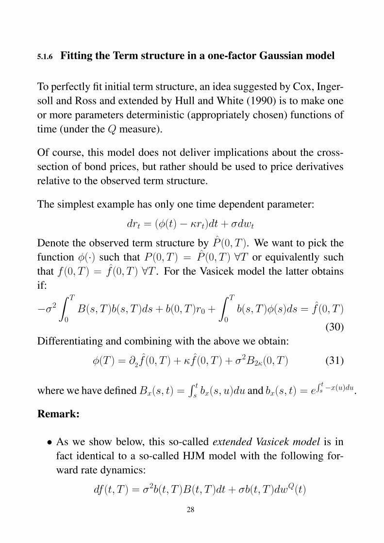
5.1.6 Fitting the Term structure in a one-factor Gaussian model

To perfectly fit initial term structure, an idea suggested by Cox, Inger-soll and Ross and extended by Hull and White (1990) is to make oneor more parameters deterministic (appropriately chosen) functions oftime (under the Q measure).

Of course, this model does not deliver implications about the cross-section of bond prices, but rather should be used to price derivativesrelative to the observed term structure.

The simplest example has only one time dependent parameter:

drt = (φ(t) − κrt)dt + σdwt

Denote the observed term structure by P (0, T ). We want to pick thefunction φ(·) such that P (0, T ) = P (0, T ) ∀T or equivalently suchthat f (0, T ) = f (0, T ) ∀T . For the Vasicek model the latter obtainsif:

−σ2

∫ T

0

B(s, T )b(s, T )ds + b(0, T )r0 +

∫ T

0

b(s, T )φ(s)ds = f (0, T )

(30)Differentiating and combining with the above we obtain:

φ(T ) = ∂2f (0, T ) + κf (0, T ) + σ2B2κ(0, T ) (31)

where we have definedBx(s, t) =∫ ts bx(s, u)du and bx(s, t) = e

∫ ts −x(u)du.

Remark:

• As we show below, this so-called extended Vasicek model is infact identical to a so-called HJM model with the following for-ward rate dynamics:

df (t, T ) = σ2b(t, T )B(t, T )dt + σb(t, T )dwQ(t)

28

with initial condition f (0, T ) = f (0, T ) ∀T .

• It is also equivalent to a bond price model with following dynam-ics:

dP (t, T )

P (t, T )= r(t)dt− σB(t, T )dwQ(t)

with initial condition P (0, T ) = P (0, T ) ∀T .

• The HJM approach basically corresponds to relaxing the time-homogeneity of short rate models (and possibly the Markovianstructure of the short rate).

5.1.7 Shortcomings of one-factor short rate models

1. All bond prices are instantaneously perfectly correlated.

2. Hedging of any fixed income derivative can be done ‘equallywell’ with any arbitrary maturity bond.

3. Time-homogeneous model restricts current term structure shape.

4. Restricts future term structure shape.

5. Restricts volatility and correlation structures (at most function ofthe short rate).

6. When pricing derivatives two sources of errors: (i) calibration ofbond prices, (ii) pricing of derivatives relative to bonds.

The last problem can be somewhat alleviated by the fitting ‘trick’shown above. However, unless the model is re-fitted continuously,the possible shapes of future term structures will be restricted withinthe model (this is a generic inconsistency of the ‘HJM approach’).

29

5.1.8 Empirical Evidence

• Factor analysis of term structure reveals at least three factors:Level, slope, curvature (Litterman and Scheinkman (91)), andpossibly four (Knez, Litterman and Scheinkman (94)).

• Time series analysis of short rate shows that interest rate volatil-ity is stochastic (Brenner, Harjes and Kroner (95), Anderson andLund (97), Benzoni et al. (2003))

• Factor analysis using Derivative data suggest that that term struc-ture factors are not sufficient to explain the dynamics of fixed in-come derivatives. (Collin-Dufresne and Goldstein (02), Heiddariand Wu (02))

Two routes are followed to make models more consistent with thedata:

• Allow for multiple factors while remaining in the time-homogeneousshort rate model setup. This approach will deliver cross-sectionalrestrictions for bonds and is better suited for empirical work, andinvestigation of risk-return trade-off in bond markets.

• Directly model bond prices or forward rates in an arbitrage-freeway, taking the observed term structure as given. This is theHeath-Jarrow-Morton approach used by practitioners. It focuseson pricing of derivatives relative to bond prices, and not on pric-ing of bonds across maturities. This approach in general, focusesexclusively on the risk-neutral distribution of the term structure.There exists a corresponding (in general, non-time homogeneous)short rate process consistent with any HJM model.

30

5.2 Multi-factor short-rate models

5.2.1 Simple Generalization: Independent state variables

The simplest generalization is to write the short rate as a sum of inde-pendent factors: rt = δ0 +

∑ni=1X

it , where, for example,

dX it = κi(θi −X i

t)dt +√σi1 + σi2X

it dZi(t)

and dwidwj = 0 ∀i 6= j. Obviously,

P (t, T ) = EQ[e−∫ Tt rsds|Ft] = e−

∫ Tt δ0dsΠn

i=1Pi(t, T )

where P i(t, T ) = eAi(T−t)−Bi(T−t)Xi

t is the one-factor bond ‘price’.

5.2.2 Affine Term Structure Models - Duffie and Kan (DK 1996)

Introduce ‘Latent’ set of N state variables X with dynamics:

dX(t) = KQ(θQ −X(t)

)dt + Σ

√S(t) dZQ(t) (32)

where KQ, Σ are (N ×N) matrices, and S diagonal matrix with com-ponents

Sii(t) = α

i+ β>

iX(t) . (33)

The spot rate is specified as an affine function of X:

r(t) = δ0 + δ>xX(t) , (34)

Due to Markov structure, all variables of interest can be written asV (X(t))

31

Note that this specification imposes that the

1) Risk-neutral drift KQ(θQ −X(t)

)

2) Covariance Matrix Σ√S(t)

√S(t)ΣT = ΣS(t) ΣT

3) Spot rate r(t) = δ0 + δ>xX(t)

are all affine (i.e., linear plus constant) functions of X:

These strong restrictions are imposed in order to obtain tractability.Whether or not these models can capture empirical observation is anopen question.

For the most part, when the affine model has been found to fail insome respect, there has been a proposal to modify/generalize the frame-work that improves empirical fit while maintaining tractability.

5.2.3 Tractability of Affine framework:

Many fixed income securities (e.g., caps, swaptions) obtain tractablesolutions.In particular, bond prices take a simple exponential affine structure:(τ ≡ (T − t)):

P (t, τ ) = eA(τ)−B(τ)>X(t), (35)

where A(τ ) and B(τ ) satisfy the (deterministic) ODE’s (and initialconditions):

dA(τ )

dτ= −θQ>KQ>B(τ ) + 1

2

∑Ni=1

[Σ>B(τ )

]2iαi− δ0 : A(0) = 0

32

dB(τ )

dτ= −KQ>B(τ ) − 1

2

∑Ni=1

[Σ>B(τ )

]2iβi+ δx : B(0) = 0

which can be quickly estimated for all maturities τ on a computer.

Bond yields Y (t, τ ) via Y (t, τ ) = −(

1τ

)Log (P (t, τ )) linear in X

Y (t, τ ) = −A(τ )

τ+B(τ )>

τX(t). (36)

2 important points:

1. Empirically, by observing yields Y , can ‘back out’ the latentvariables X if parameter vector Θ (and henceA(τ ) andB(τ )>)is known.

⇒ Empirically, usually assume N yields are measured without error

⇒ Below, we demonstrate this assumption is strongly rejected em-pirically

2. Theoretically, seems to suggest that one can ‘rotate’ state vector(and its dynamics) from the latent variables X to the observedyields Y .

⇒ In fact, cannot do so in general and maintain tractability.

⇒ Due to A(τ ) and B(τ )> not known in closed-form

5.2.4 Problems with Latent Variable specification:

• Admissibility SDEs must be well-defined. For example, if X1 isGaussian it cannot show up under any square root, so we mustset all βi,1 = 0. Dai and Singleton (2000) have defined Am(n)

33

families: m is number of Brownian motions, (n) is number ofstate variables driving conditional variances (that show up ’underthe square root’).

• Identification and maximal models.

Not all parameters are identified from an econometric point ofview (because we observe yields, not the state variables). Thisleads DS (2000) to define maximal models, those with the maxi-mum number of separately identifiable parameters.

• Invariant Transformations

Invariant transformations consists in making changes in state-variables or/and rotating the Brownian motion vector, withoutaffecting the dynamics of the short rate and thus leaving bondprices unchanged.

Dai and Singleton (2000) propose a canonical representation for affinemodels in terms of latent variables that is admissible, and maximal.

Instead, we propose an alternative canonical representation in termsof observable state variables.

34

5.2.5 Why rotate from latent variables to observables?

• Latent variables identified only after parameter vector is knownEx: 1 factor model:

r(t) = δ0 + δxX(t) ⇒ X(t) =

(1

δx

)(r(t) − δ0)

r(t) ( = yield at zero maturity) identified independent of param-eters, but definition of X(t) changes every time a new parametervector is tested.

⇒ Difficult to come up with a reasonable first guess for Θ⇒ Increase the number of local maxima?

• Difficult to identify whether model is ‘maximal’ (Dai and Single-ton (2000))

⇒ Models which appear to be well-specified in fact contain someparameters which are not identifiable.

Q? Is there a tractable way to rotate from latent variables to observ-ables?

A! Yes! But rather than yields of finite maturity, need Taylor seriesexpansion of yields around zero maturity:

Y (t, τ ) = Y (t, 0) + τ ∂τ=0 Y (t, τ ) +

(τ 2

2!

)∂2τ=0

Y (t, τ ) + . . .

A(τ ) = A(0) + τ ∂τ=0 A(τ ) +

(τ 2

2!

)∂2τ=0

A(τ ) + . . .

B(τ ) = B(0) + τ ∂τ=0 B(τ ) +

(τ 2

2!

)∂2τ=0

B(τ ) + . . . .

35

Q? Why does this lead to tractability?

A! Because the ODE’s that define A(τ ) and B(τ ) are effectively ex-pansions about τ = 0

Using A(0) = B(0) = 0 and collecting terms of the same order τ , wefind:

Y n(t) ≡ ∂nτ=0

Y (t, τ )

=1

n + 1

(−∂n+1

τ=0A(τ ) +

N∑

i=1

∂n+1τ=0

Bi(τ )X

i(t)

)∀n = 0, 1, 2 . . .

The first few Taylor series components have simple interpretations:

Y 0(t) = r(t)

Y 1(t) = (1/2)µQ(t)

Y 2(t) = (1/3)(EQt [dµQ(t)] − V (t) dt

)

where µQ = E[dr(t)]/dt and V (t) = (dr(t))2/dt.

We call a representation of the state vector canonical if it is writtenin terms of:

• Taylor series components of the term structure at zero (i.e., theY n),

• The quadratic co-variations of the Y n (i.e., V i,j = dY idY j/dt).

36

Advantages:

1. Factors are intuitive and have physical interpretation (level, slope,curvature, spot rate volatility, etc.)

2. Theoretical observability of factors guarantees that model is ‘Q-maximal’: all parameters are identifiable from fixed income se-curities.

3. ‘Q-maximality’ is independent of the risk-premium specification(unlike DS 2000).

4. Model-insensitive estimates of state vector readily available:

(a) State vector empirically ‘observable’

(b) Can use, eg., OLS to estimate ‘first guess’ at parameter vector

5. Model remains affine and tractable

6. Identifies which parameters identifiable from bond prices aloneunder ‘USV’

37

5.2.6 Example of Identification: 2-factor Gaussian Model

The ‘maximum’ 2-factor Gaussian model under the Q measure

drt = (αr + βrr rt + βrx xt)dt + σr dZQr,t

dxt = (αx + βxr rt + βxx xt)dt + σx dZQx,t

‘Canonical representation’ obtained by rotating from (rt, xt) to (rt, µQt ),

whereµQ = αr + βrr rt + βrx xt

Therefore

drt = µQdt + σrdZQr,t

dµQt = (γµ − κµr rt − κµµ µQt )dt + σµ dZ

Qµ,t

• Only 6 parameters in canonical representation (instead of 9).

• µQt is observable (it is twice the slope of the term structure atzero).

38

5.2.7 Model-Insensitive Estimation of the State Variables

• Simulate a two factor A2(2) model (parameters from Duffie andSingleton (1997)).

• Sample 10 years of weekly data maturities 0.5, 1, 2, 5, 7, 10 years.

• Add i.i.d. noise with either 2bp or 5bp standard errors.

• Estimate the level (Y 0 = r) and slope (Y 1 = µQ) of the termstructure (at τ = 0) using quadratic and cubic polynomials fitted withOLS.

• Regress the estimates obtained from the polynomial fits on thetrue value of the simulation: (See Table 1 of CD, Goldstein, Jones(2003))

true rt = α + β × estimated rt + εt

true µQt = α′ + β′ × estimated µQt + ε′t,

39

5.2.8 Canonical Representation and Maximality: the A1(3) model

• Consider the 3-factor model of short rate r = Y1 + Y2 + Y3 with:

dY1 = κ11(θ1 − Y1)dt + σ11

√Y1dZ1

dY2 = (κ21Y1 + κ22Y2 + κ23Y3)dt + σ21

√Y1dZ1

+σ22

√α2 + β2Y1dZ2 + σ23

√α3 + β3Y1dZ3

dY3 = (κ31Y1 + κ32Y2 + κ33Y3)dt + σ31

√Y1dZ1

+σ32

√α2 + β2Y1dZ2 + σ33

√α3 + β3Y1dZ3

• Rotating to (r, µQ, V ) we obtain:

dVt = (γV − κV Vt)dt + σV√Vt − ψ1 dZ1

drt = µQt dt + σ1

√Vt − ψ1 dZ1 +

√σ2

2Vt − ψ2 dZ2 +√σ2

3Vt − ψ3 dZ3

dµQt = (m0 +mrrt +mµµQt +mV Vt)dt + ν1

√Vt − ψ1 dZ1

+ν2

√σ2

2Vt − ψ2 dZ2 + ν3

√σ2

3Vt − ψ3 dZ3,

where by definition of Vt:σ2

1 + σ22 + σ2

3 = 1

σ21ψ1 + ψ2 + ψ3 = 0.

There are also a few admissibility restrictions (see CDGJ 2003).

⇒ Maximal model has 14 parameters instead of 19 (Confirms DS(2000)).

40

5.3 Unspanned Stochastic volatility

• Numerous Multifactor Stochastic Volatility Models of the TS.

Fong and Vasicek (91), Longstaff and Schwartz (92), Chen andScott (93), Balduzzi et al. (96), Chen (96), DS (00). . .

• All of these models fall within ‘Affine Class’

⇒ In general, stochastic volatility can be reinterpreted as changes inyields (Duffie and Kan (DK 96))

⇒ If enough bonds with different maturities are traded, markets arecomplete.

⇒ All Fixed Income Derivatives can be hedged with bonds alone.

Example: Term Structure Stochastic Volatility Model

• Term structure Derivatives: Longstaff and Schwartz (1992):

dr = κr(θr − r) dt +√V dzQ

1

dV = κV(θ

V− V ) dt + σ

√V dzQ

2

Note: P T (t) = P T (t, rt, V

t) = eA(T−t)+B(T−t) rt+C(T−t)Vt

– Longstaff and Schwartz (1992)– More generally, Duffie and Kan (1996)

⇒ Volatility risk can be hedged with appropriate position in any two bonds.⇒ Volatility plays dual role (cross-section and time series):

1) It is a linear combination of yields2) It is the quadratic variation of the spot rate

41

Contrast: Equity Stochastic Volatility Model

• Equity Derivatives: Heston (1993):

dS

S= r dt +

√V dzQ

1

dV = κ(θ − V ) dt + σ√V dzQ

2

– dzQ1

drives innovations in stock price

– dzQ2

drives innovations in volatility

⇒ Volatility risk cannot be hedged by any portfolio of stock and bond

Difference: Have modeled traded asset, and its volatility, whereas theshort rate model models the short rate and its volatility, and derivesprices

Q? If one can trade in a large number (possibly infinite) of bonds, aremarkets necessarily complete?

Q? Or does there exist (multi-factor) short rate model, where bondmarkets are incomplete (i.e., fixed income derivatives are not spannedby bond prices)?

From an empirical perspective this may be a desirable feature, sinceit appears hard in practice to hedge Fixed-income derivatives (espe-cially if they are highly sensitive to volatility risk, such as straddles)with positions in only bonds (CDG (2001)).5

5There is also mounting evidence that existing models, while adequately fitting TS, do not explain dynamics of

42

A!: CDG (2002) give necessary and sufficient conditions for USV inan affine model:

• Two-dimensional Markov models cannot display USV (and bearbitrage-free).

• Three dimensional (non-Gaussian) affine models (with two orthree factors) can display USV if parameters satisfy certain re-strictions.

5.3.1 Empirical Evidence

• Data:

- Monthly implied volatilities on caps and floors from Feb 95 to Dec00.∼ Minimizes effect of ‘stale quotes’

- Swap rates for all available (10) maturities + 6-month LIBOR rate.

- Three currencies: US($), UK(£), JP(Y)=

• Methodology

- Construct portfolios of at-the-money cap and floors∼ implied volatilities, Black’s formula

- Estimate 1-month straddle returns (long both cap and floor)∼ Interpolate ATM cap and floor implied volatilities.

⇒ Straddles are ‘delta’ neutral (volatility-sensitive).⇒ 1-month returns minimize interpolation error

Derivatives such as Caps and Floors Longstaff et al. (00), Jagannathan and Sun (99).

43

- OLS Regression of straddle returns on swap rate changes

- Principal component analysis of residuals

• Results

- Low R2 in the regression∼ even for the 10-factor model, as low as 10% of the variation is

explained.

- High Correlation of the residuals.∼ First (two) component(s) explain 85% (98%) of remaining varia-

tion.

• Implications for Stochastic Volatility Models of the Term struc-ture

- The principal factor driving volatility should not drive TS level.

- Bond market does not span all term structure risk.⇒ Fixed income derivatives are not redundant securities.

44

US Straddles UK Straddles JP StraddlesMaturity R2 Adjusted R2 R2 Adjusted R2 R2 Adjusted R2

1 0.215 0.085 0.27 0.134 0.229 0.0442 0.316 0.202 0.177 0.023 0.239 0.0573 0.349 0.241 0.155 -0.002 0.305 0.1394 0.341 0.232 0.162 0.006 0.464 0.3365 0.385 0.283 0.149 -0.01 0.468 0.347 0.439 0.346 0.12 -0.044 0.513 0.396

10 0.478 0.391 0.097 -0.071 0.398 0.254

Table 1: R2 and Adjusted R2 of the regression of straddle returns with maturities 1Y, 2Y, 3Y, 4Y, 5Y, 7Y, 10Y onthe changes in swap rates for all available maturities (0.5, 1, 2, 3, 4, 5, 7, 10 for US data and 0.5, 1, 2, 3, 4, 5, 6, 7,8, 9, 10 for UK and JP data). Although multicollinearity is evident in the regressors, the R2 represents an upper boundon the proportion of the variance of straddle returns that can be hedged by trading in swaps.

US Residuals UK Residuals JP ResidualsEigenvector Eigenvalue % Explained Eigenvalue % Explained Eigenvalue % Explained

1 0.07184 0.87603 0.07751 0.84485 0.157 0.834382 0.00865 0.10546 0.01215 0.13245 0.02217 0.117823 0.00091 0.01113 0.00139 0.01511 0.00482 0.025614 0.00035 0.0043 0.00038 0.00411 0.00235 0.012515 0.00014 0.00169 0.00018 0.00193 0.00101 0.005366 0.00009 0.00109 0.00008 0.00091 0.00051 0.00277 0.00002 0.0003 0.00006 0.00064 0.00031 0.00163

Table 2: Eigenvalues of principal component decomposition of the covariance matrix of residuals, ordered by magni-tude of the eigenvalue. Note that over 80% of the variation is captured by the first principal component.

45

5.3.2 USV Affine Models

• In a d-factor model, USV occurs if the rank of the diffusion matrixof any vector of bond prices is less than d

⇒ The bond market is incomplete

• In an N dimensional d factor affine model,

P T (t) = exp

(A(T − t) +

N∑

i=1

Bi(T − t)X

i(t)

)

whereA(τ ), B1(τ ), . . . , BN(τ ) are continuous deterministic functions

whichsatisfy a system of ODE’s (DK96).

• USV is equivalent to: ∃ β1, . . . , βd not all zero such that:d∑

i=1

βiBi(τ ) = 0 ∀τ ≥ 0

We refer to Collin-Dufresne and Goldstein (2001) for details of theanalysis and further discussion of this question. Below we summarizethe main results.

• First, it can be shown that no two-dimensional model can displayunspanned stochastic volatility.

In other words, if the state of the term structure can be described withtwo state variables, the short rate and its volatility, that follow a jointMarkov diffusion process, then if sufficient zero-coupon bonds aretraded, all fixed-income securities can be hedged by trading only inbonds. Intuition for this results can be gained by thinking in termsof ‘duration’ and ‘convexity.’ Bonds with different maturity have dif-ferent convexity, and thus react differently to volatility shock. For a

46

shock in volatility to leave bond prices unchanged, the short rate hasto adjust to compensate changes due to volatility. But the short ratecannot accommodate both duration and convexity differences acrossbonds. Indeed, this would imply that duration is proportional to con-vexity which is inconsistent within an arbitrage-free model of the termstructure.

Sketch of proof:

By definition, a bivariate model exhibiting USV would imply bondprices are functions of only the time-to-maturity and the spot rate, andindependent of the spot rate volatility V : P T (t, r

t, V

t) = P T (t, r

t).

This in turn implies that bond prices must satisfy

1

2P Trr

(t, r)σ2r(t, r, V )+P T

r(t, r)µr(t, r, V ) = r P T (t, r)−P T

t(t, r) ∀T .

(37)Note that the right hand side of equation (37) is a function only ofr, while the left hand side is a function of both V and r. Sinceit is not possible for the ratio of duration and convexity to be con-stant across maturities, there is no way for the left hand side to beindependent of V , unless the spot rate process itself is one-factorMarkov (µr(t, r, V ) = µr(t, r), σr(t, r, V ) = σr(t, r)), which also pre-cludes USV. Note that this rules out USV in models like Longstaffand Schwartz (92) and Fong and Vasicek (91).

• However, three dimensional affine models (with two or three fac-tors) can display USV if parameters satisfy certain restrictions. Infact, we provide below, necessary and sufficient conditions for trivari-ate affine models to display USV.

First, it is tedious but easy to show that any trivariate affine USVmodel can be rewritten in terms of the following state variables:

47

1) the spot rate, r,2) the drift of the spot rate, µ = 1

dtE[dr]

3) the variance of the spot rate V = 1dtE[(dr)2]

This allows us to limit our search for trivariate models that exhibitUSV to models that support bond price formula of the form

P (s, rs, µs) = eM0(T−s)+M1(T−s)rs+M2(T−s)µs . (38)

Therefore, it is convenient to define1

dtE[dµ] = m

µ

0+m

µ

rr +m

µ

µµ +m

µ

VV (39)

1

dtE[(dµ)2] = σ

µ

0+ σ

µ

rr + σ

µ

µµ + σ

µ

VV (40)

1

dtE[drdµ] = c

r,µ

0+ c

r,µ

rr + c

r,µ

µµ + c

r,µ

VV (41)

By applying Ito’s lemma to equation (38), and then collecting terms oforder constant, r, and µ, we find that the time-dependent coefficientsare defined through

M ′ = mµ0M2 +

σµ0

2M 2

2+ crµ

0M1M2 (42)

M ′1

= mµrM2 +

σµr

2M 2

2+ crµ

rM1M2 − 1 (43)

M ′2

= mµµM2 +

σµµ

2M 2

2+ crµ

µM1M2 +M1 , (44)

and satisfy the boundary conditions

M0(0) = 0, M1(0) = 0, M2(0) = 0 . (45)

Furthermore, by collecting terms of order V , we find that this modelsupports USV if and only if for all dates τ the following conditionholds:

0 = mµVM2(τ ) +

σµV

2M 2

2(τ ) + crµ

VM1(τ )M2(τ ) +

1

2M 2

1(τ ) . (46)

48

• It then follows that necessary and sufficient conditions for themodel to display USV are:

mµ

r= −

(2(c

r,µ

V)2 + c

r,µ

µ

)

mµ

µ= 3c

r,µ

V

mµ

V= 1

σµ

r= −2c

r,µ

V(c

r,µ

r+ 2c

r,µ

µcr,µ

V)

σµ

µ= 4c

r,µ

r+ 6c

r,µ

µcr,µ

V

σµ

V= (c

r,µ

V)2

or

mµ

r= −(2c

r,µ

µ+ 2(c

r,µ

V)2 + c

r,µ

r/c

r,µ

V)

mµ

µ= 3c

r,µ

V

mµ

V= 1

σµ

r= −2c

r,µ

µ(c

r,µ

µ+ (c

r,µ

V)2 + c

r,µ

r/c

r,µ

V)

σµ

µ= 4c

r,µ

Vcr,µ

µ+ 2c

r,µ

r

σµ

V= c

r,µ

µ+ (c

r,µ

V)2 + c

r,µ

r/c

r,µ

V

(47)

Remarks:

• First, the reason that there are two sets of parameter restrictionsthat generate USV is because equation (46) is a quadratic equa-tion in B1(·) or B2(·). This in turn generates two possible solu-tions for B1(·) in terms of B2(·).

• Second, these two sets of restrictions reduce to the same set ifand only if c

r,µ

V6= 0 and c

r,µ

r+ c

r,µ

µcr,µ

V= 0. This condition ob-

tains, for example, when the covariance between the short rateand its drift depends only on the volatility, an important specialcase (basically, the so-called A1(3) models) which we examinebelow.

• Finally, we note that several of the USV restrictions presentedabove occur naturally once we limit the class of models to thosewhich are admissible: that is, those which restrict the ‘square-root’ state variables to be non-negative (see below).

To provide some intuition for the proof of this result, sufficiency ob-tains because the right hand side of equation (46) can be shown to

49

be identically zero when either of the two sets of parameter condi-tions holds. Necessity obtains because if any one of the conditions isnot satisfied, then we can show, by taking repeated time-derivativesof the system of ODE’s (Ricatti equations) evaluated at τ = 0, thatequation (46) cannot hold.

We note that the models of both Chen (1996) and Balduzzi, Das,Foresi and Singh (1996) cannot satisfy these necessary restrictions,and thus cannot display USV. Also, clearly, the A0(3) class of modelsof Dai and Singleton (2000) cannot exhibit USV (or incomplete bondmarkets). However, Dai and Singleton’s (2000) maximalA1(3), A2(3)

and A3(3) models do have the flexibility to exhibit USV. In fact, usingour canonical representation for the maximal A1(3) model and apply-ing the necessary and sufficient conditions for USV to apply we mayderive the maximal model displaying USV.

5.3.3 Maximal A1(3) model with USV

4 Necessary and sufficient conditions for USV in A1(3) case (CDG(2002)):

mr = −2c2V

mµ = 3cV

mV

= 1 σµV

= (cV)2

wheredr dµQ = (c0 + c

VV ) dt

(dµQ)2 = (σµ0

+ σµVV ) dt

The maximal model with USV is:

dVt = (γV− κ

VVt)dt + σ

V

√Vt − ψ1 dZ1

drt = µtdt + σ1

√Vt − ψ1 dZ1 +

√(1 − σ2

1)Vt + σ21ψ1 + ψ2 dZ3 +

√−ψ2 dZ2

50

dµt = (m0 − 2c2Vrt + 3c

Vµt + Vt) dt

+cVσ1

√Vt − ψ1 dZ1 + c

V

√(1 − σ2

1)Vt + σ21ψ1 + ψ2 dZ3 + ν2

√−ψ2 dZ2

where

for stationarity: κv > 0 , cV< 0

for admissibility: γv − κvψ1 > 0 , −ψ2 > 0 , 1 > σ21, ψ1 + ψ2 > 0

USV imposes 5 restrictions (model has 9 parameters under the Qmeasure):

γv, κv, σv, ψ1, σ1, cV , ψ2, m0, ν2 (48)

Corresponding Bond prices are given by:

P (t, T ) = exp(A(T − t) −Br(T − t) rt −Bµ(T − t) µQt

)(49)

where:

Br(τ ) =−3 + 4ecV τ − e2c

Vτ

2cV

Bµ(τ ) =(1 − ecV τ )2

2c2V

A(τ ) =1

96c5V

(−3e4c

Vτ (2c

Vc0 − σ

µ

0) + 16e3c

Vτ (3c

Vc0 − σ

µ

0) + 25σ

µ

0

−48ecV τ (−5cVc0 − 2c2

Vm0 + σ

µ

0) + 12e2c

Vτ (2c

V(−6c0 − c

Vm0) + 3σ

µ

0)

+6cV(−23c0 + 12c

Vm0 + 2(−6c

Vc0 − 4c2

Vm0 + σ

µ

0)τ ))

• Note that the USV model is a two-factor model of the cross-section of bond prices, but a three factor model of the time seriesof bonds.

51

• γV , κV are not identifiable from bond prices alone: In contrast toclaim of DS, ‘maximality’ must be defined relative to all fixedincome derivatives.

• This also implies the model can be ‘extended’ to allow for a verysimple two-step calibration procedure to fixed-income derivatives(such as at-the-money Caps/Floors). First, as in Hull and White(1990), the parameter can be made time-dependent to fit the termstructure of forward rates. Second, the parameters γv and κQ

vcan

be made time-dependent to fit the term structure of CAP volatili-ties, without affecting the initial calibration of the term structureof forward rates.

• Note: Even if volatility is an arbitrary Markov process, obtainsame affine yields even though dynamics of state vector are notaffine!

5.3.4 Maximal A1(4) model with USV

Similarly we derive the maximal 4-factor USV model which has statevariables (r, µ, V, θ) where θ = 3Y 2 (local curvature):

dVt

= (γV− κ

VV

t)dt+ σ

V

√V

t− ψ

1dZ

Q

1(t)

drt

= µQ

tdt+ σ

1

√V

t− ψ

1dZ

Q

1(t) +

√(1 − σ2

1)V

t+ σ2

1ψ

1+ ψ

3+ ψ

4dZ

Q

2(t)

+√−ψ

3dZ

Q

3(t) +

√−ψ

4dZ

Q

4(t)

dµQ

t= (θ

Q

t+ V

t) dt+ c

rµσ

1

√V

t− ψ

1dZ

Q

1(t) + c

rµ

√(1 − σ2

1)V

t+ σ2

1ψ

1+ ψ

3+ ψ

4dZ

Q

2(t)

+ν3

√−ψ

3dZ

Q

3(t) + ν

4

√−ψ

4dZ

Q

4(t)

dθQ

t=(a

0− 2c2

rµ(3c

rµ− a

θ) r

t+ (7c2

rµ− 3c

rµa

θ)µ

Q

t+ a

θθ

Q

+ 3crµV

t

)dt

+c2rµσ

1

√V

t− ψ

1dZ

Q

1(t) + c2

rµ

√(1 − σ2

1)V

t+ σ2

1ψ

1+ ψ

3+ ψ

4dZ

Q

2(t)

52

+η3

√−ψ

3dZ

Q

3(t) + η

4

√−ψ

4dZ

Q

4(t).

Note: the A1(4) USV model has a total of 14 risk-neutral parameters(γ

V, κ

V, σ

V, ψ1, ψ3, ψ4, ν3, ν4, η3, η4, σ1, a0, crµ, aθ), as opposed to 22

for the unrestricted model.

The zero coupon bond price is given by:

P (t, T ) = exp

(A(T − t) −Br(T − t) r

t−Bµ(T − t)µ

Q

t−B

θ(T − t) θ

Q

t

),

(50)

where the deterministic functions A(τ ), Br(τ ), Bµ(τ ), and Bθ(τ ) are

obtained in closed form.

• Note that the A1(4) USV model is a 3-factor Gaussian model ofthe cross-section of bond prices, but a 4-factor model of the timeseries of bonds.

5.3.5 Specification of Risk-Premia

Specify second generation affine risk-premia process so that the dy-namics of the state vector for the unrestricted A1(3) under the histor-ical measure are:

dVt =

((γ

V+ λ

V 0− λ

Vψ

1) − (κ

V− λ

V)V

t

)dt+ σ

V

√Vt − ψ1 dZ1(t)

drt =(λ

r0+ λ

rrr

t+(1 + λ

rµ

)µQ

t+ λ

rVV

t

)dt

+σ1

√Vt − ψ1 dZ1(t) +

√σ2

2Vt − ψ2 dZ2(t) +√σ2

3Vt − ψ3 dZ3(t)

53

dµQt

=

((m

0+ λ

µ0

)+(m

r+ λ

µr

)r

t+(m

µ+ λ

µµ

)µQ

t+(m

V+ λ

µV

)V

t

)dt

+ν1

√V

t− ψ1 dZ1(t) + ν2

√σ2

2Vt− ψ2 dZ2(t) + ν3

√σ2

3Vt− ψ3 dZ3(t)

• All drift parameters in rt, µQ

t, V dynamics are risk-adjusted.

• Extends slightly Duffee, but need to guarantee that Feller con-dition holds under both the physical and risk neutral measures forexistence of EMM (Liptser and Shiryaev).

5.4 Estimation of Affine models with and without USV

Below we present a summary of the results in CD, Goldstein andJones (2004) about the estimation and comparative tests of variousthree and four factor affine models.

Empirical Methodology

• Use weekly swap rate data (maturities 2, 3, 4, 5, 7, 10 and sixmonth LIBORfrom Jan. 7, 1988 to Nov. 27, 2002.

• Adjust LIBOR quote for non-synchronicity with USD swap rates.

• Estimate unrestricted model using Quasi Maximum Likelihood(QML),similar to Chen and Scott (1993), Pearson and Sun (1994).

– Standard procedure fits 3 specific yields perfectly to invert forstate variables.

– Remaining yields observed with ‘measurement’ errors.

54

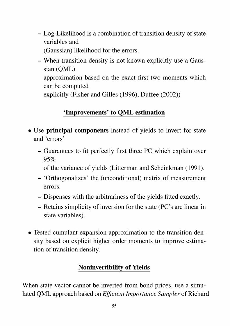
– Log-Likelihood is a combination of transition density of statevariables and(Gaussian) likelihood for the errors.

– When transition density is not known explicitly use a Gaus-sian (QML)approximation based on the exact first two moments whichcan be computedexplicitly (Fisher and Gilles (1996), Duffee (2002))

‘Improvements’ to QML estimation

• Use principal components instead of yields to invert for stateand ‘errors’

– Guarantees to fit perfectly first three PC which explain over95%of the variance of yields (Litterman and Scheinkman (1991).

– ‘Orthogonalizes’ the (unconditional) matrix of measurementerrors.

– Dispenses with the arbitrariness of the yields fitted exactly.

– Retains simplicity of inversion for the state (PC’s are linear instate variables).

• Tested cumulant expansion approximation to the transition den-sity based on explicit higher order moments to improve estima-tion of transition density.

Noninvertibility of Yields

When state vector cannot be inverted from bond prices, use a simu-lated QML approach based on Efficient Importance Sampler of Richard

55

and Zhang (1996,97) (see also Sandmann and Koopman (1998)), Pen-nachi (1991), Brandt and He (2002)

Ex 1): USV implies V cannot be determined from bond yields.

Ex 2): If assumed that yields are measured with errors, then statevector not invertible from yields.

Let P =P1,P2, ...,PT

denote the time series of PC’s of the yield

curve.

Likelihood function, p(P|θ), may be written as the integral∫

p(P,V|θ) dV

where V =V1, V2, ..., VT

denotes the time series of the variance

process.

The integral is evaluated using simulation.

¿From ‘importance sampling’, an approximate auxiliary model pa(V|P, θ)is specified

∫p(P,V|θ) dV =

∫p(P,V|θ)pa(V|P, θ)

pa(V|P, θ)dV = E a

[p(P,V|θ)pa(V|P, θ)

],

(51)

The closer the auxiliary model is to the actual model, the less sensitivethe ratio is to the simulated variance path, and the more quickly theexpectation will converge.

56

The EIS approach essentially chooses the auxiliary density pa(V|P, θ)(within a certain parametric class) to minimize the variation in

ln p(V|P, θ) − ln pa(V|P, θ)

57

Test Five Specifications

1. Unrestricted A1(3) model• assume 2 PCs are observed without error “2PC”

• simulate paths of V• “invert” V and the 2 PCs for r, µQ, and V

2. Unrestricted A1(3) model• assume 3 PCs are observed without error “3PC”

• “invert” PCs for r, µQ, and V

3. A1(3) model with USV restrictions• assume 2 PCs are observed without error “USV”

• “invert” PCs for r and µQ

• simulate paths of V

4. Unrestricted A1(2) model• assume 2 PCs are observed without error “A1(2)”

• “invert” PCs for r and V (there is no µQ)

5. Unrestricted A1(4) model• assume 3 PCs are observed without error “A1(4)USV”

• simulate paths of V• “invert” V and the 3 PCs for r, µQ, θ, and V

– Models 2, 3, and 4 are restricted versions of 1 (Table 4).

– Model 5 nests Model 3.

58

Empirical Results

• Ignoring QML approximation error, all three-factor restricted mod-els rejected by LR test.

• All models predict short rate and slope accurately (Table 7).

• Only A1(3) and A1(4)USV capture dynamics of Curvature (Fig-ure 1, Table 7).

• But A1(3) (unrestricted and 3PC) predict volatility that is nega-tively correlated with model-independent GARCH volatility, aswell as with volatility extracted from short rate implied by themodel itself! (Figure 2, Table 7)

⇒ A1(3) cannot both capture curvature and dynamics of short ratevolatility (V plays double role in unrestricted A1(3) model).

• A1(3) USV does a better job at capturing volatility dynamics, butnot quite as good for curvature (Table 7, Figure 2).

• Only A1(4) USV can capture both time series property of shortrate volatility and dynamics of TS Curvature factor.

• Superiority of A1(4) model confirmed by out of sample yieldchanges (table 9) and squared yield changes (table 10), as wellas predictability regression (Figure 3) and Maturity/volatility re-lation (Table 4).

59

Conclusion

• Propose a canonical representation for affine models in which:

– the state variables have simple physical interpretations suchas level, slope and curvature at the short end,

– their dynamics remain affine and tractable,

– the model is by construction ‘maximal’ in the sense of Daiand Singleton (00),

– model-insensitive estimates of the state variables are readilyavailable.

• Offer a complete characterization of the ‘maximal’ A1(3) andA1(4) USV model.

• Empirical estimation of the various models show:

– USV restrictions do not significantly affect cross-sectional fit,but

– Substantially improve the time-series properties of the model(in and out of sample forecasts of squared changes in yields).

– Even though USV is nested within the unrestricted model, im-posing the USV restriction explicitly improves the estimatedtime series of volatility, because USV breaks the dual roleplayed by volatility in the unrestricted model.

– To capture dynamics of level, slope, and curvature, as wellas stochastic short rate volatility need four distinct factors(A1(4)).

60

6 Recent Developments

• Joint models of term structure and derivativesDerivatives convey more informative about higher order momentsof TS.

– Relative pricing of Caps and Swaptions?Jagannathan, Kaplin and Sun (2000), Longstaff, Santa-Claraand Schwartz (2000) document mis-pricing of Caps relativeto captions in a Gaussian string model.CDG (2002) show that relative price of caps and swaption canbe seen as proxy for stochastic correlation.Han (2003) and Li (2003) find some empirical support forstochastic correlation.

• Brownian field ‘String’ Models can:

1. take into account information in observation ‘errors’ (no low-dimensionality in forward rates variance covariance matrix),

2. use information on both derivatives and term structure con-sistently,

3. deliver unique optimal bond portfolio choice

4. handle predictability factor in bond return of Cochrane andPiazzesi (2004).

– Models: (Kennedy (1994), Goldstein (2000), Santa-Clara andSornette (2001), CDG (2002).

– Estimation: Li (2003), Han (2003), Bester (2004).

• Combining affine models with macroeconomic information.

1. Specification of latent short rate model consistent with shortrate behavior of Fed Funds Target Rate.

61

(a) Balduzzi, Bertola, Foresi (1996) model short rate as mean-reverting around target rate.

(b) Babbs and Selby (1991) model German Bundesbank dis-count rate.

(c) Piazzesi (2001) builds in jumps in target rates around FOMCmeeting dates (both scheduled and unscheduled meetings).

⇒ Allows to study the reaction in term structure (long yields)to short rate movements.

2. Combine Macro-variables and latent variables for the shortrate.Typically, use a Taylor rule of the form

rt = δ0 + δ′MMt + δ′ZZt

where Mt is a vector of macro variables (inflation, output. . . )and Z is a vector of latent variables (orthogonal to M ). Typi-cally assume Gaussian dynamics and estimate P-measure co-efficients from VAR. With assumption on risk-premia, obtainan arbitrage-free model of the term structure that contains ex-plicit information on Macro-variables.

(a) Makes predictions about responses of term structure tochanges in Macro-variables (Ang and Piazzesi (2003)).

(b) Makes predictions about future macro-variables based oninformation in the yield curve if allows for feedback be-tween interest rates and macro-variables (Hordahl, Tris-tani and Vestin (2003), Duffee (2004), Ang, Piazzesi andWei (2003))

62

References

[1] D.-H. Ahn and B. Gao. A parametric non-linear model of theterm structure. The Review of Financial Studies, 15 no 12:721–762, 1999.

[2] P. Balduzzi, S. Das, and S. Foresi. A simple approach to threefactor affine term structure models. Journal of Fixed Income,6:43–53, 1996.

[3] G. Chacko and S. Das. Pricing interest rate derivatives: A gen-eral approach. The Review of Financial Studies, 15:195–241,2002.

[4] L. Chen. Stochastic mean ans stochastic volatility– a three factormodel of the term structure of interest rates and its application topricing of interest rate derivatives. Blackwell Publishers, Oxford,U.K., 1996.

[5] P. Collin-Dufresne, R. Goldstein, and C. Jones. Identificationand estimation of ‘maximal’ affine term structure models: Anapplication to stochastic volatility. Carnegie Mellon Workingpaper, 2002.

[6] P. Collin-Dufresne and R. S. Goldstein. Do bonds span the fixed-income markets? theory and evidence for unspanned stochasticvolatility. Journal of Finance, VOL. LVII NO. 4, 2002.

[7] P. Collin-Dufresne and R. S. Goldstein. Generalizing the affineframework to HJM and random field models. Carnegie MellonUniversity Working Paper, 2002.

[8] P. Collin-Dufresne and R. S. Goldstein. Pricing swaptions in anaffine framework. Journal of Derivatives, 10:9–26, 2002.

63

[9] J. C. Cox, J. E. Ingersoll Jr., and S. A. Ross. A reexaminationof the traditional hypotheses about the term structure of interestrates. Journal of Finance, 36:769–799, 1981.

[10] J. C. Cox, J. E. Ingersoll Jr., and S. A. Ross. A theory of the termstructure of interest rates. Econometrica, 53:385–407, 1985b.

[11] Q. Dai and K. Singleton. Expectation puzzles, time-varying riskpremia and dynamic models of the term structure. forthcomingJournal of Financial Economics, 2002.

[12] Q. Dai and K. J. Singleton. Specification analysis of affine termstructure models. Journal of Finance, 55:1943–1978, 2000.

[13] G. R. Duffee. Term premia and interest rate forecasts in affinemodels. Journal of Finance, 57 no 1, 2002.

[14] D. Duffie, D. Filipovic, and W. Schachermayer. Affine processesand applications to finance. Working Paper Stanford University,2001.

[15] D. Duffie and R. Kan. A yield-factor model of interest rates.Mathematical Finance, 6:379–406, 1996.

[16] D. Duffie, J. Pan, and K. Singleton. Transform analysis and op-tion pricing for affine jump-diffusions. Econometrica, 68:1343–1376, 2000.

[17] W. Feller. Two singular diffusion problems. Annals of Mathe-matics, 54:173–182, 1951.

[18] R. S. Goldstein. The term structure of interest rates as a randomfield. The Review of Financial Studies, 13no2:365–384, 2000.

[19] D. Heath, R. Jarrow, and A. Morton. Bond pricing and the termstructure of interest rates: A new methodology for contingentclaims evaluation. Econometrica, 60:77–105, 1992.

64

[20] S. L. Heston. A closed form solution for options with stochasticvolatility. Review of financial studies, 6:327–343, 1993.

[21] M. Hogan and K. Weintraub. The lognormal interest rate modeland eurodollar futures. Working Paper, Citibank, Nw York, 1993.

[22] J. Hull and A. White. Pricing interest rate derivative securities.The Review of Financial Studies, 3no4:573–592, 1990.

[23] R. Jagannathan, A. Kaplin, and S. Sun. An evaluation of multi-factor cir models using libor, swap rates and cap and swaptionprices. Working paper Northwestern University, 2000.

[24] F. Jamshidian. An exact bond option formula. Journal of Fi-nance, v44, n1:205–09, 1989.

[25] F. Jamshidian. Contingent claim evaluation in the gaussian in-terest rate model. Research in Finance, 9:131–170, 1991.

[26] F. Jamshidian. Bond, futures and option evaluation in thequadratic gaussian interest rate model. Applied MathematicalFinance, v3, n2:93–115, 1995.

[27] D. Kennedy. The term structure of interest rates as a Gaussianrandom field. Mathematical Finance, 4:247–258, 1994.

[28] F. Longstaff, P. Santa-Clara, and E. S. Schwartz. The relativevaluation of caps and swaptions: Theory and empirical evidence.Journal of Finance, 56:2067–2109, 2001.

[29] R. E. Lucas. Asset prices in an exchange economy. Economet-rica, 46:1426–1446, 1978.

[30] R. C. Merton. Theory of rational option pricing. Bell Journal ofEconomics and Management Science, 4:141–183, 1973.

[31] S. F. Richard. An arbitrage model of the term structure of interestrates. Journal of Financial Economics, 6:33–57, 1978.

65

[32] P. Santa-Clara and D. Sornette. The dynamics of the forwardinterest rate curve with stochastic string shocks. Review of Fi-nancial Studies, 14, 2001.

[33] O. Vasicek. An equilibrium characterization of the term struc-ture. Journal of Financial Economics, 5:177–188, 1977.

66