1st International Workshopabout Sets and Tools

(SETS 2014)

Affiliated to ABZ 2014

Toulouse (France)

Preface

This volume contains the papers presented at SETS 2014: 1st InternationalWorkshop about Sets and Tools held on June 1, 2014 in Toulouse (France).

There were 6 submissions. Each submission was reviewed by at least 3, and onthe average 3, program committee members. The committee decided to accept6 papers. The program also includes 2 invited talks.

In the preparation of these proceedings and in managing the whole discussionprocess, Andrei Voronkov’s EasyChair conference management system proveditself an excellent tool.

May 26, 2014Paris, France

David DelahayeCatherine Dubois

i

Table of Contents

Proof Verification within Set Theory: Exploiting a New Way ofModeling Graphs . . . . . . . . . . . . . . . . . . . . . . . . . . . . . . . . . . . . . . . . . . . . . . . . . 1

Eugenio Omodeo

Mathematical Theorem Proving, from Muscadet0 to Muscadet4, Whyand How . . . . . . . . . . . . . . . . . . . . . . . . . . . . . . . . . . . . . . . . . . . . . . . . . . . . . . . . . 3

Dominique Pastre

Rapid Prototyping and Animation of Z Specifications Using log . . . . . . . . . 4Maximiliano Cristia and Gianfranco Rossi

Introduction to the Integration of SMT-Solvers in Rodin . . . . . . . . . . . . . . . 19David Deharbe, Pascal Fontaine, Yoann Guyot and Laurent Voisin

Using Deduction Modulo in Set Theory . . . . . . . . . . . . . . . . . . . . . . . . . . . . . . 34Pierre Halmagrand

Turning Failure into Proof: Evaluating the ProB Disprover . . . . . . . . . . . . . 46Sebastian Krings, Michael Leuschel and Jens Bendisposto

Return of Experience on Automating Refinement in B . . . . . . . . . . . . . . . . . 57Thierry Lecomte

Programming with Partially Specified Collections . . . . . . . . . . . . . . . . . . . . . 69Gianfranco Rossi

ii

Program Committee

Maximiliano Cristia CIFASIS-UNRDavid Deharbe Universidade Federal do Rio Grande do NorteDavid Delahaye Cedric/Cnam/Inria, ParisCatherine Dubois ENSIIE-CEDRICMamoun Filali-Amine IRITMichael Leuschel University of DusseldorfStephan Merz INRIA LorraineDominique Pastre LIPADE - Universite Paris DescartesGianfranco Rossi Universita’ di ParmaMark Utting The University of WaikatoBenjamin Werner INRIAFreek Wiedijk Radboud University NijmegenWolfgang Windsteiger RISC Institute, JKU Linz, Austria

iii

Additional Reviewers

A

Arthan, Rob

K

Krings, Sebastian

iv

Proof verification within Set Theory:Exploiting a new way of modeling graphs

Eugenio G. Omodeo

University of Trieste (Italy), DMG/DMI

This talk illustrates proof-verification technology based on set theory, alsoreporting on experiments carried out with ÆtnaNova, aka Ref (see [6, 4]).

The said verifier processes script files consisting of definitions, theorem state-ments and proofs of the theorems. Its underlying deductive system—mainly first-order, but with an important second-order construct enabling one to package def-initions and theorems into reusable proofware components—is a variant of theZermelo-Fraenkel set theory, ZFC, with axioms of regularity and global choice.This is apparent from the very syntax of the language, borrowing from the set-theoretic tradition many constructs, e.g. abstraction terms. Much of Ref’s nat-uralness, comprehensiveness, and readability, stems from this foundation; muchof its effectiveness, from the fifteen or so built-in mechanisms, tailored on ZFC,which constitute its inferential armory. Rather peculiar aspects of Ref, in com-parison to other alike proof-assistants (cf., e.g., [2, 1]), are that Ref relies onlymarginally on predicate calculus and that types play no prominent role, in it, asa foundation.

The selection of examples, mainly referred to graphs, to be discusses inthis talk, reflects today’s tendency [5] to bring Ref’s use closer to algorithm-correctness verification. To achieve relatively short, formally checked, proofs ofproperties enjoyed by claw-free graphs, we took advantage of novel results [3]about representing their (undirected) edges via membership.

Acknowledgements. Partial funding was granted by the INdAM/GNCS 2013project “ Specifica e verifica di algoritmi tramite strumenti basati sulla teoriadegli insiemi”.

References

1. C. E. Brown. Combining type theory and untyped set theory. In Ulrich Furbachand Natarajan Shankar, editors, IJCAR, volume 4130 of Lecture Notes in ComputerScience, pages 205–219. Springer, 2006.

2. R. Matuszewski and P. Rudnicki. Mizar: the first 30 years. Mechanized Mathematicsand its Applications, 4(1):3–24, 2005.

3. M. Milanic and A. I. Tomescu. Set graphs. I. Hereditarily finite sets and extensionalacyclic orientations. Discrete Applied Mathematics, 161(4-5):677–690, 2013.

4. E. G. Omodeo. The Ref proof-checker and its “common shared scenario”. In MartinDavis and Ed Schonberg, editors, From Linear Operators to Computational Biology:Essays in Memory of Jacob T. Schwartz, pages 121–167. Springer, 2012. With anappendix, Claw-free graphs as sets, co-authored by A. I. Tomescu.

1

5. E. G. Omodeo and A. I. Tomescu. Set graphs. III. Proof Pearl: Claw-free graphsmirrored into transitive hereditarily finite sets. Journal of Automated Reasoning,52(1):1–29, 2014.

6. J.T. Schwartz, D. Cantone, and E.G. Omodeo. Computational Logic and Set Theory- Applying Formalized Logic to Analysis. Springer, 2011.

2

Mathematical theorem proving,from Muscadet0 to Muscadet4,

why and how ?

Dominique Pastre

Universite Paris Descartes, Paris, Francepastre@math-info.univ-paris5.fr

We will present the ideas and the choices which have been made throughoutthe development of the Muscadet theorem prover. We will first see the prin-ciples and main ideas which lead to a first prover in the context of the time,influenced by a famous paper by Woody Bledsoe. This program used naturalmethods and was applied to set theory. It was then rewritten as a knowledgebased-system where an inference engine applied rules, given or automaticallybuilt by metarules which expressed general or specific mathematical knowledge.It has been applied to some difficult problems. In order to allow more flexibilityfor expressing knowledge, it has been rewritten in Prolog, allowing the knowledgeto be more or less declarative or procedural. To work with the TPTP Librarythe system had to work without knowing anything about mathematics exceptpredicate calculus. All mathematical concepts had to be defined with mathemat-ical statements, and the belonging relation handled as any other binary relation.To avoid translating knowledge to TPTP syntax, TPTP syntax has been used(this unfortunately forbade the use of some abbreviations mathematicians arecomfortable with). Last but not least, the relevant trace has been extracted togive a proof easily read by anyone, except in the case of failure, when all stepsmay be displayed to understand (manually) the reasons for the failure. Muscadethas participated to CASC competitions. The results show its complementaritywith regard to resolution-based provers.

3

Rapid Prototyping and Animation of ZSpecifications Using {log}

Maximiliano Cristia1 and Gianfranco Rossi2

1 CIFASIS and UNR, Rosario, Argentinacristia@cifasis-conicet.gov.ar

2 Universita degli Studi di Parma, Parma, Italygianfranco.rossi@unipr.it

Abstract. Prolog has been proposed as the programming language onwhich animation and prototyping of Z specifications should be based.However, we believe there is still room for improvements. In this paper,we want to revisit this issue in the light of a powerful, set-oriented con-straint programming language like {log} (pronounced ’setlog’). In partic-ular, we pay attention to three points that we think are crucial: findingsolutions to complex state predicates; defining formal criteria for guid-ing an evaluation process based on prototypes; and automatically addinggraphical user interfaces to prototypes generated from Z specifications.Three examples of information systems prototypes are available online.

1 Running Example

Assume you are eliciting the user requirements for an ERP system. In a firstmeeting, your customer asks the following:

(R1) Keep a record of client accounts where the company registers all the creditsand debits of its clients.

(R2) Get a listing of all the accounts whose balance is in a given range.

Given that you have experience in requirement engineering, you know thatprobably your customer has told you (R1) and (R2) without giving them toomuch thought. You would like to be sure that these are the real, final require-ments before engaging your team in programming unstable, unvalidated require-ments. Following the software engineering literature you know that it would beof great help if you could show your customer a prototype of these requirements.

Now, suppose you know of a tool that automatically generates functionalprototypes of some kind of Z specifications, provided they are annotated withuser interface directives. Further, let us say that in your team there is an engineerwho is knowledgeable in the Z notation. Would it be cost-effective to write a Zspecification of (R1) and (R2) and use that tool to generate a prototype so yourcustomer can validate them? In this way, your programmers will implementvalidated requirements; moreover, they will do it from a formal specification. Allthis would amount to a much better product with less iterations to improve its

4

quality. Even more, assume that this prototyping tool records all the interactionsof users. Then, later, these interactions can be used as functional test cases. Sothe tool would also help you during the testing process.

After considering all these gains, you decide to ask your team to write theZ specification shown in Figure 1 and the GUI specification shown in 3 which,when fed into the prototyping tool, become the Prolog+{log}+XPCE program[25, 11, 36] partially shown in Figure 4. When this program is executed the usercan play with an application presenting an acceptable GUI like the one shownin Figure 2—download this and two more examples from [6].

[UID ,NAME ]ERP ==

[clients : UID 7→ NAME ; accounts : UID 7→ Z | dom clients = dom accounts]InitERP == [ERP | clients = ∅ ∧ accounts = ∅]

NewClientOk∆ERP ; u? : UID ; n? : NAME

u? /∈ dom clientsclients ′ = clients ∪ {u? 7→ n?}accounts ′ = accounts ∪ {u? 7→ 0}

TransactionOk∆ERP ; n? : UID ; m? : Z

n? ∈ dom accounts ∧ m? 6= 0accounts ′ = accounts ⊕ {n? 7→ accounts n? + m?}clients ′ = clients

ClientAlreadyExists == [ΞERP ; u? : UID | u? ∈ dom clients]NewClient == NewClientOk ∨ ClientAlreadyExistsAccountNotExists == [ΞERP ; n? : UID | n? /∈ dom accounts]NullAmount == [ΞERP ; m? : Z | m? = 0]Transaction == TransactionOk ∨ AccountNotExists ∨ NullAmountAccountsInRangeOk ==

[ΞERP ; a?, b? : Z; r ! : PUID | a? ≤ b? ∧ r ! = dom(accounts B (a? . . b?))]NotARange == [ΞERP ; a?, b? : Z; r ! : RET | a? > b?]AccountsInRange == AccountsInRangeOk ∨ NotARange

Fig. 1: Excerpt of the Z specification of (R1) and (R2)

Z and {log} will be introduced in sections 2 and 3, respectively, and howprototypes would be automatically generated in Sect. 4. Now we want to show

5

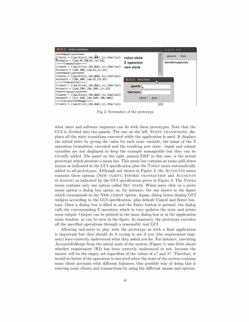
Fig. 2: Screenshot of the prototype

what users and software engineers can do with these prototypes. Note that theGUI is divided into two panels. The one on the left, State transitions, dis-plays all the state transitions executed while the application is used. It displaysthe initial state by giving the value for each state variable, the name of the Zoperation (transition) executed and the resulting new state—input and outputvariables are not displayed to keep the example manageable but they can betrivially added. The panel on the right, named ERP in this case, is the actualprototype which presents a menu bar. This menu bar contains as many pull-downmenus as indicated in the GUI specification plus the Tools menu automaticallyadded to all prototypes. Although not shown in Figure 2, the Accounts menucontains three options (New client, Inform transaction and Accountsin range) as indicated by the GUI specification given in Figure 3. The Toolsmenu contains only one option called Set state. When users click on a givenmenu option a dialog box opens, as, for instance, the one shown in the figurewhich corresponds to the New client option. Again, dialog boxes display GUIwidgets according to the GUI specification, plus default Cancel and Enter but-tons. Once a dialog box is filled in and the Enter button is pressed, the dialogcalls the corresponding Z operation which in turn updates the state and printssome output. Output can be printed in the same dialog-box or in the applicationmain window, as can be seen in the figure. In summary, the prototype executesall the specified operations through a reasonably real GUI.

Allowing end-users to play with the prototype as with a final applicationis important but they should do it trying to see if you (the requirement engi-neer) have correctly understood what they asked you for. For instance, executingAccountsInRange from the initial state of the system (Figure 1) says little aboutwhether requirement (R2) has been correctly understood or not, because theanswer will be the empty set regardless of the values of a? and b?. Therefore, itwould be better if the operation is executed when the state of the system containssome client accounts with different balances. One possible way of doing this isentering some clients and transactions by using the different menus and options.

6

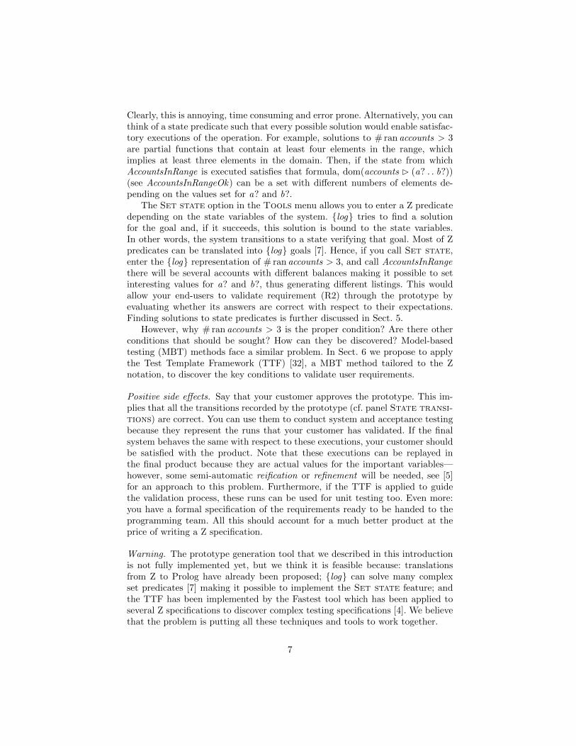
Clearly, this is annoying, time consuming and error prone. Alternatively, you canthink of a state predicate such that every possible solution would enable satisfac-tory executions of the operation. For example, solutions to # ran accounts > 3are partial functions that contain at least four elements in the range, whichimplies at least three elements in the domain. Then, if the state from whichAccountsInRange is executed satisfies that formula, dom(accounts B (a? . . b?))(see AccountsInRangeOk) can be a set with different numbers of elements de-pending on the values set for a? and b?.

The Set state option in the Tools menu allows you to enter a Z predicatedepending on the state variables of the system. {log} tries to find a solutionfor the goal and, if it succeeds, this solution is bound to the state variables.In other words, the system transitions to a state verifying that goal. Most of Zpredicates can be translated into {log} goals [7]. Hence, if you call Set state,enter the {log} representation of # ran accounts > 3, and call AccountsInRangethere will be several accounts with different balances making it possible to setinteresting values for a? and b?, thus generating different listings. This wouldallow your end-users to validate requirement (R2) through the prototype byevaluating whether its answers are correct with respect to their expectations.Finding solutions to state predicates is further discussed in Sect. 5.

However, why # ran accounts > 3 is the proper condition? Are there otherconditions that should be sought? How can they be discovered? Model-basedtesting (MBT) methods face a similar problem. In Sect. 6 we propose to applythe Test Template Framework (TTF) [32], a MBT method tailored to the Znotation, to discover the key conditions to validate user requirements.

Positive side effects. Say that your customer approves the prototype. This im-plies that all the transitions recorded by the prototype (cf. panel State transi-tions) are correct. You can use them to conduct system and acceptance testingbecause they represent the runs that your customer has validated. If the finalsystem behaves the same with respect to these executions, your customer shouldbe satisfied with the product. Note that these executions can be replayed inthe final product because they are actual values for the important variables—however, some semi-automatic reification or refinement will be needed, see [5]for an approach to this problem. Furthermore, if the TTF is applied to guidethe validation process, these runs can be used for unit testing too. Even more:you have a formal specification of the requirements ready to be handed to theprogramming team. All this should account for a much better product at theprice of writing a Z specification.

Warning. The prototype generation tool that we described in this introductionis not fully implemented yet, but we think it is feasible because: translationsfrom Z to Prolog have already been proposed; {log} can solve many complexset predicates [7] making it possible to implement the Set state feature; andthe TTF has been implemented by the Fastest tool which has been applied toseveral Z specifications to discover complex testing specifications [4]. We believethat the problem is putting all these techniques and tools to work together.

7

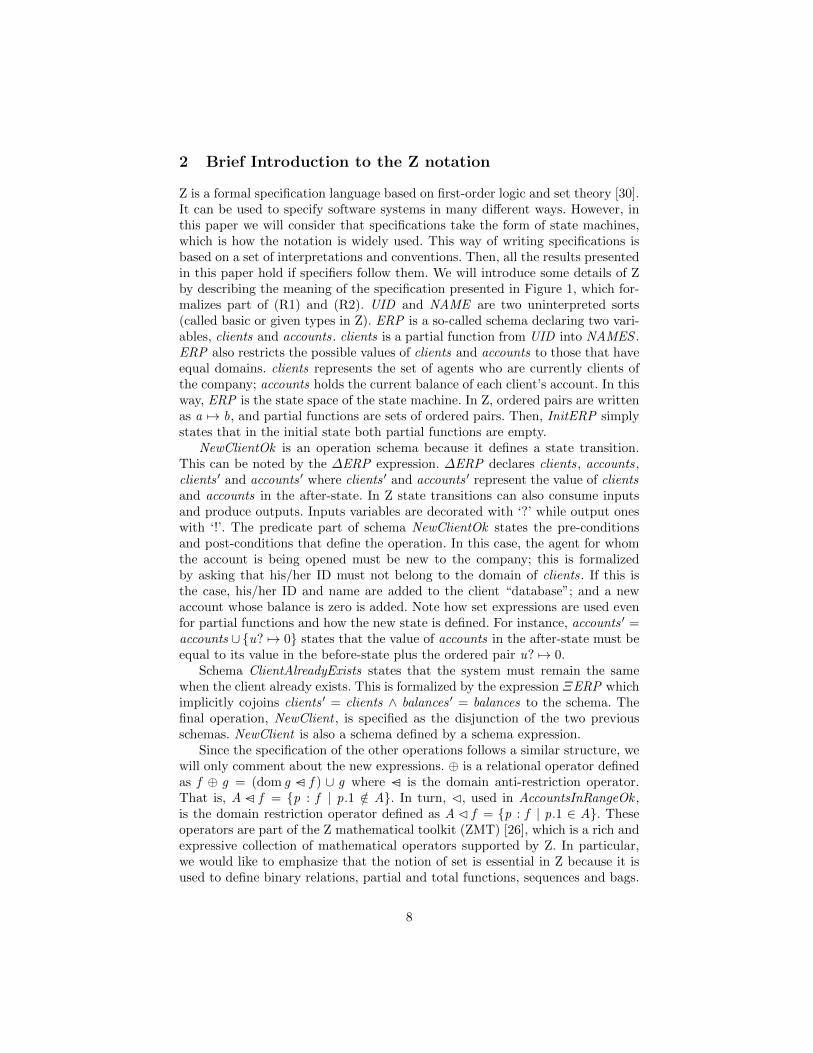
2 Brief Introduction to the Z notation

Z is a formal specification language based on first-order logic and set theory [30].It can be used to specify software systems in many different ways. However, inthis paper we will consider that specifications take the form of state machines,which is how the notation is widely used. This way of writing specifications isbased on a set of interpretations and conventions. Then, all the results presentedin this paper hold if specifiers follow them. We will introduce some details of Zby describing the meaning of the specification presented in Figure 1, which for-malizes part of (R1) and (R2). UID and NAME are two uninterpreted sorts(called basic or given types in Z). ERP is a so-called schema declaring two vari-ables, clients and accounts. clients is a partial function from UID into NAMES .ERP also restricts the possible values of clients and accounts to those that haveequal domains. clients represents the set of agents who are currently clients ofthe company; accounts holds the current balance of each client’s account. In thisway, ERP is the state space of the state machine. In Z, ordered pairs are writtenas a 7→ b, and partial functions are sets of ordered pairs. Then, InitERP simplystates that in the initial state both partial functions are empty.

NewClientOk is an operation schema because it defines a state transition.This can be noted by the ∆ERP expression. ∆ERP declares clients, accounts,clients ′ and accounts ′ where clients ′ and accounts ′ represent the value of clientsand accounts in the after-state. In Z state transitions can also consume inputsand produce outputs. Inputs variables are decorated with ‘?’ while output oneswith ‘!’. The predicate part of schema NewClientOk states the pre-conditionsand post-conditions that define the operation. In this case, the agent for whomthe account is being opened must be new to the company; this is formalizedby asking that his/her ID must not belong to the domain of clients. If this isthe case, his/her ID and name are added to the client “database”; and a newaccount whose balance is zero is added. Note how set expressions are used evenfor partial functions and how the new state is defined. For instance, accounts ′ =accounts ∪{u? 7→ 0} states that the value of accounts in the after-state must beequal to its value in the before-state plus the ordered pair u? 7→ 0.

Schema ClientAlreadyExists states that the system must remain the samewhen the client already exists. This is formalized by the expression ΞERP whichimplicitly cojoins clients ′ = clients ∧ balances ′ = balances to the schema. Thefinal operation, NewClient , is specified as the disjunction of the two previousschemas. NewClient is also a schema defined by a schema expression.

Since the specification of the other operations follows a similar structure, wewill only comment about the new expressions. ⊕ is a relational operator definedas f ⊕ g = (dom g −C f ) ∪ g where −C is the domain anti-restriction operator.That is, A −C f = {p : f | p.1 /∈ A}. In turn, C, used in AccountsInRangeOk ,is the domain restriction operator defined as A C f = {p : f | p.1 ∈ A}. Theseoperators are part of the Z mathematical toolkit (ZMT) [26], which is a rich andexpressive collection of mathematical operators supported by Z. In particular,we would like to emphasize that the notion of set is essential in Z because it isused to define binary relations, partial and total functions, sequences and bags.

8

Therefore, it is tantamount to the success of an animation or rapid prototypingtool for Z specifications to be based on a powerful, efficient set constraint solver.

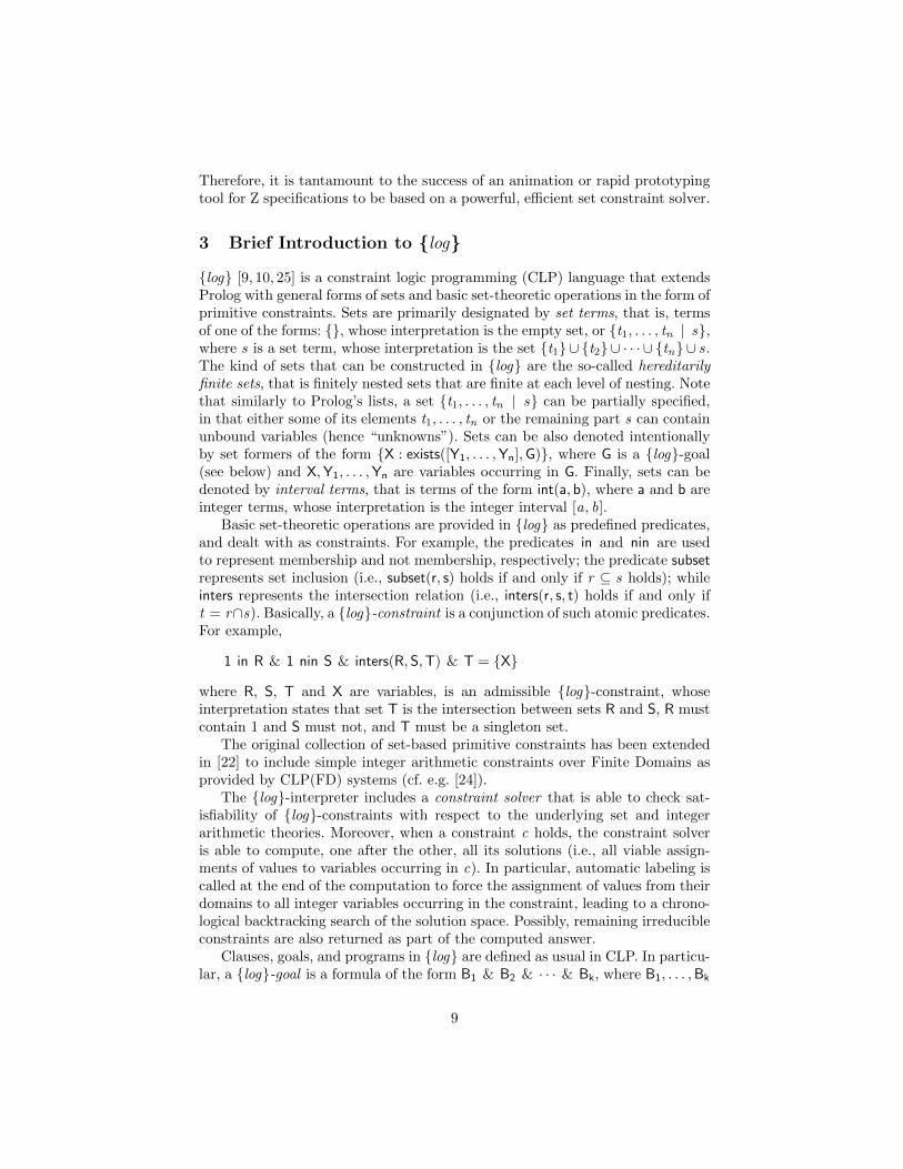
3 Brief Introduction to {log}{log} [9, 10, 25] is a constraint logic programming (CLP) language that extendsProlog with general forms of sets and basic set-theoretic operations in the form ofprimitive constraints. Sets are primarily designated by set terms, that is, termsof one of the forms: {}, whose interpretation is the empty set, or {t1, . . . , tn | s},where s is a set term, whose interpretation is the set {t1} ∪ {t2} ∪ · · · ∪ {tn} ∪ s.The kind of sets that can be constructed in {log} are the so-called hereditarilyfinite sets, that is finitely nested sets that are finite at each level of nesting. Notethat similarly to Prolog’s lists, a set {t1, . . . , tn | s} can be partially specified,in that either some of its elements t1, . . . , tn or the remaining part s can containunbound variables (hence “unknowns”). Sets can be also denoted intentionallyby set formers of the form {X : exists([Y1, . . . ,Yn],G)}, where G is a {log}-goal(see below) and X,Y1, . . . ,Yn are variables occurring in G. Finally, sets can bedenoted by interval terms, that is terms of the form int(a, b), where a and b areinteger terms, whose interpretation is the integer interval [a, b].

Basic set-theoretic operations are provided in {log} as predefined predicates,and dealt with as constraints. For example, the predicates in and nin are usedto represent membership and not membership, respectively; the predicate subsetrepresents set inclusion (i.e., subset(r, s) holds if and only if r ⊆ s holds); whileinters represents the intersection relation (i.e., inters(r, s, t) holds if and only ift = r∩s). Basically, a {log}-constraint is a conjunction of such atomic predicates.For example,

1 in R & 1 nin S & inters(R,S,T) & T = {X}

where R, S, T and X are variables, is an admissible {log}-constraint, whoseinterpretation states that set T is the intersection between sets R and S, R mustcontain 1 and S must not, and T must be a singleton set.

The original collection of set-based primitive constraints has been extendedin [22] to include simple integer arithmetic constraints over Finite Domains asprovided by CLP(FD) systems (cf. e.g. [24]).

The {log}-interpreter includes a constraint solver that is able to check sat-isfiability of {log}-constraints with respect to the underlying set and integerarithmetic theories. Moreover, when a constraint c holds, the constraint solveris able to compute, one after the other, all its solutions (i.e., all viable assign-ments of values to variables occurring in c). In particular, automatic labeling iscalled at the end of the computation to force the assignment of values from theirdomains to all integer variables occurring in the constraint, leading to a chrono-logical backtracking search of the solution space. Possibly, remaining irreducibleconstraints are also returned as part of the computed answer.

Clauses, goals, and programs in {log} are defined as usual in CLP. In particu-lar, a {log}-goal is a formula of the form B1 & B2 & · · · & Bk, where B1, . . . ,Bk

9

are either user-defined atomic predicates, or atomic {log}-constraints, or dis-junctions of either user-defined or predefined predicates, or Restricted UniversalQuantifiers (RUQs). Disjunctions have the form G1 or G2, where G1 and G2

are {log}-goals, and are dealt with through non-determinism: if G1 fails thenthe computation backtracks, and G2 is considered instead. RUQs are atomsof the form forall(X in s, exists([Y1, . . . ,Yn],G)), where s denotes a set and Gis a {log}-goal containing X,Y1, . . . ,Yn. The logical meaning of this atom is∀X (X ∈ s ⇒ ∃Y1, . . . ,Yn : G), that is G represents a property that all el-ements of s are required to satisfy. When s has a known value, the RUQ canbe used to iterate over s, whereas, when s is unbound, the RUQ allows s to benon-deterministically bound to each set satisfying the property G .

The following is an example of a {log} program:

is rel(R) :- forall(P in R, exists([X,Y],P = [X,Y])).dom({}, {}).dom({[X,Y]/Rel},Dom) :- dom(Rel,D) & Dom = {X/D} & X nin D.

This program defines two predicates, is rel and dom. is rel(R) is true if R is abinary relation, that is a set of pairs of the form [X,Y]. dom(R,D) is true if D isthe domain of the relation R. The following is a goal for the above program:

R = {[1, 5], [2, 7]} & is rel(R) & dom(R,D)

and the computed solution for D is D = {1, 2}. It is important to note thatis rel(R) can be used both to test and to compute R; similarly, dom(R,D) canbe used both to compute D from R, and to compute R from D, or simply to testwhether the relation represented by dom holds or not.

As can be seen, is rel and dom are {log} implementations of the correspondingconcepts in the ZMT. They are part of a {log} library implementing almost allthe ZMT [7]. Some elements of the ZMT are not supported yet because they arebeyond of set theory and, in some cases, would require some extensions to {log}or a more complex translation. For example, generic and axiomatic definitionsand recursive types are not fully yet supported.{log} has important advantages compared to other Prolog-based tools that

can deal with sets. With respect to the simpler scheme which constructs setabstractions on top of an existing Prolog system, typically by using lists (cf. e.g.[21]), {log} demonstrates its superiority whenever one has to deal with partiallyspecified sets. For example, even the simple problem of comparing two sets, suchas {a | X } and {b | Y }, may lead to an infinite collection of answers whensets and set operations are implemented using lists, whereas in {log} it is dealtas a set unification problem [12] which admits the single more general solutionX = {b | S} and Y = {a | S} where S is a new variable. Similar considerationshold also when the negative counterparts of the basic set-theoretic operations,such as ‘not equal’ and ‘not member’, are taken into account. The use of thelist-based implementation of sets, in conjunction with the Negation as Failurerule provided by most implementations of Prolog, leads to well-known problemswhenever non-ground atoms are involved.

10

Viewing sets as first-class entities and operations on sets as constraints, asdone in {log}, provides a much more convenient solution. With respect to otherproposals which deal with set constraints, such as [13], the main advantageof {log} is its generality: sets in {log} can contain elements of any type, canbe nested and partially specified, whereas sets in the so-called set-constraintlanguages are restricted to flat sets of known integer elements. Moreover theseproposals usually require a finite domain (i.e. a set of sets) is specified for eachset variable occurring in a constraint, whereas this is not the case for {log}. Onthe other hand, the (incomplete) solvers of the set-constraint languages turn outto be in many cases more efficient than the general solver of {log}.{log} is fully implemented in Prolog and can be downloaded from [25].

4 Automatic Prototype Generation from Z Specifications

Generating a Prolog prototype from a Z specification involves the automatictranslation from Z into Prolog. There are several proposals [8, 31, 3, 17, 14, 29,33, 18, 37, 15, 23, 35, 7] that confirm that it is possible to implement such a com-piler. There are also similar works for the B method [34, 1, 16] which defines amathematical library like the ZMT. However, most of these works are aimedat animating the specification rather than using it as a means to validate userrequirements. Then, they do not pay attention to equip the prototype with anacceptable user interface. Animation is thought to be a verification activity car-ried out by software engineers who want to analyze if a specification verifiessome properties; in this sense animation is a complement or an alternative toproof. Instead, we think that if the resulting (Prolog) program is augmentedwith a GUI, animation becomes rapid prototyping and can be used (also) forfunctional requirements validation. That is, the prototype can be used by end-users to validate whether or not requirement engineers have understood whatthe system is supposed to do. Sterling et al. [31] aim at a similar target but theythink in a Z-to-Prolog compiler that generates a command-line-like program thatusers are supposed to play with. We think that this is impractical. Besides, onlya handful of these works [1, 23, 16] rely on a powerful, set-oriented constraintlanguage implementing set constraint satisfaction, and even in these cases theunderlying mathematics are not described in detail. B-Motion and Brama [28,19] are two tools based on the B method which go in the same direction pro-posed here. B-Motion is based on ProB [20]. Both tools seem to be oriented tographically represent software-controlled physical systems rather than informa-tion systems as the one described in the motivation example and the two otherexamples available on-line [6].

Therefore, we propose to define a simple, GUI specification language (GEL)of which Figure 3 is an example. This language should allow engineers to definethe structure of a GUI and how it connects with the (Prolog) program generatedfrom the Z specification. This GEL would not need to express the behavior ofthe GUI (for instance, specify when part of the GUI should be disabled).

11

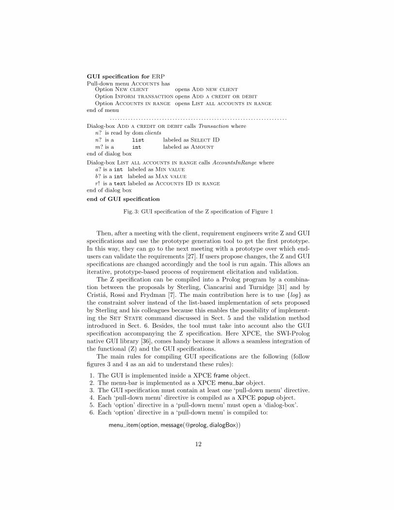
GUI specification for ERPPull-down menu Accounts has

Option New client opens Add new clientOption Inform transaction opens Add a credit or debitOption Accounts in range opens List all accounts in range

end of menu

. . . . . . . . . . . . . . . . . . . . . . . . . . . . . . . . . . . . . . . . . . . . . . . . . . . . . . . . . . . . . . . . . . . .

Dialog-box Add a credit or debit calls Transaction wheren? is read by dom clientsn? is a list labeled as Select IDm? is a int labeled as Amount

end of dialog box

Dialog-box List all accounts in range calls AccountsInRange wherea? is a int labeled as Min valueb? is a int labeled as Max valuer ! is a text labeled as Accounts ID in range

end of dialog box

end of GUI specification

Fig. 3: GUI specification of the Z specification of Figure 1

Then, after a meeting with the client, requirement engineers write Z and GUIspecifications and use the prototype generation tool to get the first prototype.In this way, they can go to the next meeting with a prototype over which end-users can validate the requirements [27]. If users propose changes, the Z and GUIspecifications are changed accordingly and the tool is run again. This allows aniterative, prototype-based process of requirement elicitation and validation.

The Z specification can be compiled into a Prolog program by a combina-tion between the proposals by Sterling, Ciancarini and Turnidge [31] and byCristia, Rossi and Frydman [7]. The main contribution here is to use {log} asthe constraint solver instead of the list-based implementation of sets proposedby Sterling and his colleagues because this enables the possibility of implement-ing the Set State command discussed in Sect. 5 and the validation methodintroduced in Sect. 6. Besides, the tool must take into account also the GUIspecification accompanying the Z specification. Here XPCE, the SWI-Prolognative GUI library [36], comes handy because it allows a seamless integration ofthe functional (Z) and the GUI specifications.

The main rules for compiling GUI specifications are the following (followfigures 3 and 4 as an aid to understand these rules):

1. The GUI is implemented inside a XPCE frame object.2. The menu-bar is implemented as a XPCE menu bar object.3. The GUI specification must contain at least one ‘pull-down menu’ directive.4. Each ‘pull-down menu’ directive is compiled as a XPCE popup object.5. Each ‘option’ directive in a ‘pull-down menu’ must open a ‘dialog-box’.6. Each ‘option’ directive in a ‘pull-down menu’ is compiled to:

menu item(option,message(@prolog, dialogBox))

12

initERP :-saveState({}, {}), nb setval(clients, {}), nb setval(accounts, {}),mainMenu.

mainMenu :-Builds a menu bar according to the GUI specification. Each optionof the pull-down menus calls a predicate like readAccountsInRange below

readAccountsInRange :-new(D, dialog(’List all accounts in range’)),send list(D, append,

[new(M, int item(min value)), new(N, int item(max value)),text(’Accounts ID in range’), new(B, browser),button(enter,message(@prolog, accountsInRange,B,

M?selection,N?selection))]),send(D, open).

accountsInRange(B,M,N) :- accountsInRangeOk(B,M,N); notARange(B,M,N).

accountsInRangeOk(B,M,N) :-b getval(clients,C), b getval(accounts,A),setlog(M ein int(0, 10000) &N ein int(0, 10000) &M =< N&

Y = int(M,N) & rres(Y,A,Y1) & dom(Y1,Y2) & set to list(Y2, L)),writeOutput(B, L), saveNewState(C,A).

Fig. 4: Code excerpt of the prototype of the Z specification shown in Figure 1

where dialogBox is a Prolog predicate implementing the dialog-box that theoption must open.

7. Each dialog-box is implemented as a XPCE dialog object.8. Each dialog-box must call an existing Z operation.9. Each dialog-box must indicate what kind of widget must be used for each and

every input and output variable declared in the corresponding Z operation.10. text is implemented as a XPCE text item object for inputs, and as a browser

for outputs; int as int item; list as list browser; etc.11. A ‘is read by’ directive in a ‘dialog-box’ directive simply states that the input

variable is read by means of another expression. The selection made throughthe expression is passed as the value for the input variable.

12. When the enter button in a dialog-box is pressed the following is executed:

button(enter,message(@prolog,Operation, Input))

where Operation is a Prolog predicate implementing the corresponding Zoperation (this code was generated when the Z specification was compiled)and Input are the input variables waited by the Z operation where each actualvalue corresponds to one of the values read by the widgets of the dialog-box.

Two more examples of this translation can be downloaded from [6]. Theyinclude the Z and GUI specifications and the Prolog+{log}+XPCE program.

13

5 Solving State Predicates for Requirement Validation

In this section we discuss the Set state feature presented in the introduction.The inclusion of this feature is based on the following observation: validatingsome functional requirements involves taking the prototype to a state such thatstate variables satisfy a (complex) predicate. In turn, this can be achieved inthree ways: a) use the prototype’s GUI to put itself in the desired state; b) writea simple Prolog predicate where each state variable is bound to the desired valueand then execute the prototype from this state; and c) write the state predicate,give it to a constraint solver, and use its answer as the prototype’s new state.

The first option is annoying, time consuming and error prone; this is theone discussed in [31]. The second one, is error prone because the values may bewrong. It can be improved by: writing the state predicate as in c), proposinga solution to it as in b), and asking the constraint solver whether this solutionindeed satisfies the predicate. If it answers “no”, try another value. This may takesome time but it is safe. However, the best option is c) because the constraintsolver does all the work—except proposing the state predicate, see Sect. 6.

The key condition for c) to be feasible is to have a constraint solver capable ofsolving (complex) Z predicates. Since Z predicates are first-order predicates overthe set theory, only a constraint solver for such set theory can deliver the desiredresults. {log} may be such a constraint solver because, according to the resultswe have obtained when we used it as a test case generator for Fastest [7], it is ableto solve many complex Z predicates. In effect, when {log} is used as Fastest’stest case generator it needs to find solutions to complex Z predicates describingequally complex test conditions. However, not all possible Z predicates can besolved by {log} in its current state, since many Z facilities are implementedas user-defined predicates and the {log} interpreter can not guarantee efficientprocessing or even termination for all the considered formulas.

Therefore, the Set state menu option of the prototypes generated by ourmethod would wait for either a Z predicate or a {log} goal, translate it into {log}in the first case, call it and use its answer to set the new state of the prototype.The following considerations must be taken into account:

1. If a Z predicate is entered it would be automatically translated into a {log}goal [7]. However, there are cases in which an automatic translation may notyield the best {log} code in the sense of {log} being able to find a solutionfor it in a reasonable time. An alternative could be to let users to edit theresulting {log} goal to help the tool to find a solution.

2. Typing information about the state variables must be entered along the goal;this has been discussed in [7].

3. Z basic types (i.e. UID and NAME in Figure 1) pose a problem becausetheir elements have no structure and so {log} generates variables instead ofconstants. This can be solved by post-processing {log}’s answer.

4. If some {log} goal entered by the user is too complex to be solved, (s)he canwrite special-purpose {log} predicates to help the tool to find a solution.

14

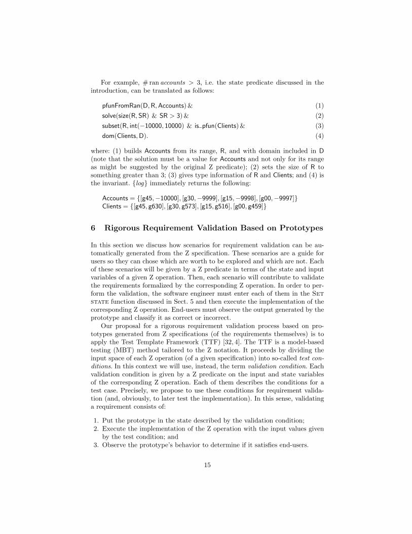
For example, # ran accounts > 3, i.e. the state predicate discussed in theintroduction, can be translated as follows:

pfunFromRan(D,R,Accounts) & (1)

solve(size(R,SR) & SR > 3) & (2)

subset(R, int(−10000, 10000) & is pfun(Clients) & (3)

dom(Clients,D). (4)

where: (1) builds Accounts from its range, R, and with domain included in D(note that the solution must be a value for Accounts and not only for its rangeas might be suggested by the original Z predicate); (2) sets the size of R tosomething greater than 3; (3) gives type information of R and Clients; and (4) isthe invariant. {log} immediately returns the following:

Accounts = {[g45,−10000], [g30,−9999], [g15,−9998], [g00,−9997]}Clients = {[g45, g630], [g30, g573], [g15, g516], [g00, g459]}

6 Rigorous Requirement Validation Based on Prototypes

In this section we discuss how scenarios for requirement validation can be au-tomatically generated from the Z specification. These scenarios are a guide forusers so they can chose which are worth to be explored and which are not. Eachof these scenarios will be given by a Z predicate in terms of the state and inputvariables of a given Z operation. Then, each scenario will contribute to validatethe requirements formalized by the corresponding Z operation. In order to per-form the validation, the software engineer must enter each of them in the Setstate function discussed in Sect. 5 and then execute the implementation of thecorresponding Z operation. End-users must observe the output generated by theprototype and classify it as correct or incorrect.

Our proposal for a rigorous requirement validation process based on pro-totypes generated from Z specifications (of the requirements themselves) is toapply the Test Template Framework (TTF) [32, 4]. The TTF is a model-basedtesting (MBT) method tailored to the Z notation. It proceeds by dividing theinput space of each Z operation (of a given specification) into so-called test con-ditions. In this context we will use, instead, the term validation condition. Eachvalidation condition is given by a Z predicate on the input and state variablesof the corresponding Z operation. Each of them describes the conditions for atest case. Precisely, we propose to use these conditions for requirement valida-tion (and, obviously, to later test the implementation). In this sense, validatinga requirement consists of:

1. Put the prototype in the state described by the validation condition;2. Execute the implementation of the Z operation with the input values given

by the test condition; and3. Observe the prototype’s behavior to determine if it satisfies end-users.

15

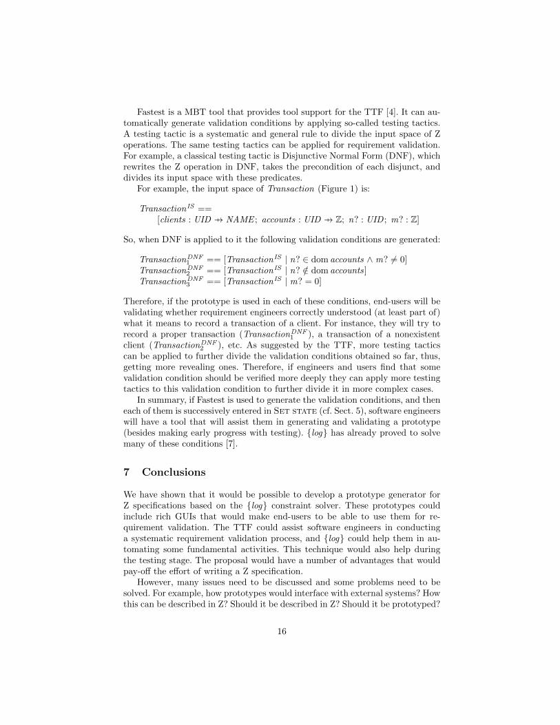
Fastest is a MBT tool that provides tool support for the TTF [4]. It can au-tomatically generate validation conditions by applying so-called testing tactics.A testing tactic is a systematic and general rule to divide the input space of Zoperations. The same testing tactics can be applied for requirement validation.For example, a classical testing tactic is Disjunctive Normal Form (DNF), whichrewrites the Z operation in DNF, takes the precondition of each disjunct, anddivides its input space with these predicates.

For example, the input space of Transaction (Figure 1) is:

TransactionIS ==[clients : UID 7→ NAME ; accounts : UID 7→ Z; n? : UID ; m? : Z]

So, when DNF is applied to it the following validation conditions are generated:

TransactionDNF1 == [TransactionIS | n? ∈ dom accounts ∧ m? 6= 0]

TransactionDNF2 == [TransactionIS | n? /∈ dom accounts]

TransactionDNF3 == [TransactionIS | m? = 0]

Therefore, if the prototype is used in each of these conditions, end-users will bevalidating whether requirement engineers correctly understood (at least part of)what it means to record a transaction of a client. For instance, they will try torecord a proper transaction (TransactionDNF

1 ), a transaction of a nonexistentclient (TransactionDNF

2 ), etc. As suggested by the TTF, more testing tacticscan be applied to further divide the validation conditions obtained so far, thus,getting more revealing ones. Therefore, if engineers and users find that somevalidation condition should be verified more deeply they can apply more testingtactics to this validation condition to further divide it in more complex cases.

In summary, if Fastest is used to generate the validation conditions, and theneach of them is successively entered in Set state (cf. Sect. 5), software engineerswill have a tool that will assist them in generating and validating a prototype(besides making early progress with testing). {log} has already proved to solvemany of these conditions [7].

7 Conclusions

We have shown that it would be possible to develop a prototype generator forZ specifications based on the {log} constraint solver. These prototypes couldinclude rich GUIs that would make end-users to be able to use them for re-quirement validation. The TTF could assist software engineers in conductinga systematic requirement validation process, and {log} could help them in au-tomating some fundamental activities. This technique would also help duringthe testing stage. The proposal would have a number of advantages that wouldpay-off the effort of writing a Z specification.

However, many issues need to be discussed and some problems need to besolved. For example, how prototypes would interface with external systems? Howthis can be described in Z? Should it be described in Z? Should it be prototyped?

16

What if a validation condition asks for a state that cannot be reached by asequence of the operations available in the specification? Should this conditionbe validated or not? What is a precise characterization of the class of systemswithin the scope of this proposal? Finding an answer to all these questions,however, seems feasible and is left for future work.

References

1. Bouquet, F., Legeard, B., Peureux, F.: CLPS-B - A constraint solver to animate aB specification. STTT 6(2), 143–157 (2004)

2. Bowen, J.P., Hall, J.A. (eds.): Z User Workshop, Cambridge, UK, 29-30 June 1994,Proceedings. Workshops in Computing, Springer/BCS (1994)

3. Breuer, P.T., Bowen, J.P.: Towards correct executable semantics for Z. In: Bowenand Hall [2], pp. 185–209

4. Cristia, M., Albertengo, P., Frydman, C.S., Pluss, B., Rodrıguez Monetti, P.: Toolsupport for the Test Template Framework. Softw. Test., Verif. Reliab. 24(1), 3–37(2014)

5. Cristia, M., Hollmann, D., Albertengo, P., Frydman, C.S., Monetti, P.R.: A lan-guage for test case refinement in the Test Template Framework. In: Qin, S., Qiu,Z. (eds.) ICFEM. Lecture Notes in Computer Science, vol. 6991, pp. 601–616.Springer (2011)

6. Cristia, M., Rossi, G.: Protoype examples for SETS 2014, https://www.dropbox.com/s/rgub9d3i10coht8/sets2014-examples.tar.gz

7. Cristia, M., Rossi, G., Frydman, C.S.: {log} as a test case generator for the TestTemplate Framework. In: Hierons, R.M., Merayo, M.G., Bravetti, M. (eds.) SEFM.Lecture Notes in Computer Science, vol. 8137, pp. 229–243. Springer (2013)

8. Doma, V., Nicholl, R.A.: EZ: A system for automatic prototyping of Z specifi-cations. In: Prehn, S., Toetenel, W.J. (eds.) VDM Europe (1). Lecture Notes inComputer Science, vol. 551, pp. 189–203. Springer (1991)

9. Dovier, A., Omodeo, E.G., Pontelli, E., Rossi, G.: A language for programming inlogic with finite sets. J. Log. Program. 28(1), 1–44 (1996)

10. Dovier, A., Piazza, C., Pontelli, E., Rossi, G.: Sets and constraint logic program-ming. ACM Trans. Program. Lang. Syst. 22(5), 861–931 (2000)

11. Dovier, A., Piazza, C., Rossi, G.: A uniform approach to constraint-solving forlists, multisets, compact lists, and sets. ACM Trans. Comput. Log. 9(3) (2008)

12. Dovier, A., Pontelli, E., Rossi, G.: Set unification. Theory Pract. Log. Program.6(6), 645–701 (Nov 2006), http://dx.doi.org/10.1017/S1471068406002730

13. Gervet, C.: Conjunto: Constraint propagation over set constraints with finite setdomain variables. In: Hentenryck, P.V. (ed.) ICLP. p. 733. MIT Press (1994)

14. Goodman, H.S.: The Z-into-Haskell tool-kit: An illustrative case study. In: Bowen,J.P., Hinchey, M.G. (eds.) ZUM. Lecture Notes in Computer Science, vol. 967, pp.374–388. Springer (1995)

15. Grieskamp, W.: A computation model for Z based on concurrent constraint reso-lution. In: Bowen, J.P., Dunne, S., Galloway, A., King, S. (eds.) ZB. Lecture Notesin Computer Science, vol. 1878, pp. 414–432. Springer (2000)

16. Hallerstede, S., Leuschel, M., Plagge, D.: Validation of formal models by refinementanimation. Sci. Comput. Program. 78(3), 272–292 (2013)

17. Hasselbring, W.: Animation of Object-Z specifications with a set-oriented proto-typing language. In: Bowen and Hall [2], pp. 337–356

17

18. Hewitt, M.A., O’Halloran, C., Sennett, C.T.: Experiences with PiZA, an anima-tor for Z. In: Bowen, J.P., Hinchey, M.G., Till, D. (eds.) ZUM. Lecture Notes inComputer Science, vol. 1212, pp. 37–51. Springer (1997)

19. Ladenberger, L., Bendisposto, J., Leuschel, M.: Visualising Event-B models withB-Motion Studio. In: Alpuente, M., Cook, B., Joubert, C. (eds.) Formal Methodsfor Industrial Critical Systems, Lecture Notes in Computer Science, vol. 5825,pp. 202–204. Springer Berlin Heidelberg (2009), http://dx.doi.org/10.1007/

978-3-642-04570-7_1720. Leuschel, M., Butler, M.: ProB: A model checker for B. In: Keijiro, A., Gnesi,

S., Mandrioli, D. (eds.) FME. Lecture Notes in Computer Science, vol. 2805, pp.855–874. Springer-Verlag (2003)

21. Munakata, T.: Notes on implementing sets in prolog. Commun. ACM 35(3), 112–120 (Mar 1992), http://doi.acm.org/10.1145/131295.131300

22. Palu, A.D., Dovier, A., Pontelli, E., Rossi, G.: Integrating finite domain constraintsand CLP with sets. In: PPDP. pp. 219–229. ACM (2003)

23. Plagge, D., Leuschel, M.: Validating Z specifications using the ProB animatorand model checker. In: Davies, J., Gibbons, J. (eds.) Integrated Formal Methods.Lecture Notes in Computer Science, vol. 4591, pp. 480–500. Springer-Verlag (2007)

24. Rossi, F., Beek, P.v., Walsh, T.: Handbook of Constraint Programming (Founda-tions of Artificial Intelligence). Elsevier Science Inc., New York, NY, USA (2006)

25. Rossi, G.: {log} (2008), http://www.math.unipr.it/~gianfr/setlog.Home.html,last access: December 2013

26. Saaltink, M.: The Z/EVES mathematical toolkit version 2.2 for Z/EVES version1.5. Tech. rep., ORA Canada (1997)

27. Schrage, M.: Never go to a client meeting without a prototype. IEEE Software21(2), 42–45 (2004)

28. Servat, T.: BRAMA: A new graphic animation tool for B models. In: Julliand,J., Kouchnarenko, O. (eds.) B 2007: Formal Specification and Development inB, Lecture Notes in Computer Science, vol. 4355, pp. 274–276. Springer BerlinHeidelberg (2006), http://dx.doi.org/10.1007/11955757_28

29. Sherrell, L.B., Carver, D.L.: FunZ: An intermediate specification language. Com-put. J. 38(3), 193–206 (1995)

30. Spivey, J.M.: The Z notation: a reference manual. Prentice Hall International (UK)Ltd., Hertfordshire, UK, UK (1992)

31. Sterling, L., Ciancarini, P., Turnidge, T.: On the animation of ”not executable”specifications by Prolog. International Journal of Software Engineering and Knowl-edge Engineering 6(1), 63–87 (1996)

32. Stocks, P., Carrington, D.: A Framework for Specification-Based Testing. IEEETransactions on Software Engineering 22(11), 777–793 (Nov 1996)

33. Valentine, S.H.: The programming language Z−. Information & Software Technol-ogy 37(5-6), 293–301 (1995)

34. Waeselynck, H., Behnia, S.: B model animation for external verification. In:ICFEM. pp. 36–45 (1998)

35. West, M.M.: The use of a logic programming language in the animation of Zspecifications. In: Dahl, V., Niemela, I. (eds.) ICLP. Lecture Notes in ComputerScience, vol. 4670, pp. 451–452. Springer (2007)

36. Wielemaker, J., Schrijvers, T., Triska, M., Lager, T.: SWI-Prolog. TPLP 12(1-2),67–96 (2012)

37. Winikoff, M., Dart, P., Kazmierczak, E.: Rapid prototyping using formal specifi-cations. In: In Proceedings of the 21st Australasian Computer Science Conference.pp. 279–294. Springer-Verlag (1998)

18

Introduction to the Integrationof SMT-Solvers in Rodin?

David Deharbe1, Pascal Fontaine2, Yoann Guyot3, and Laurent Voisin4

1 Federal University of Rio Grande do Norte, Brazil2 University of Lorraine, Loria, Inria, France

3 Cetic, Belgium4 Systerel, France

Abstract. Event-B is a system specification approach based on set the-ory, integer arithmetics and refinement, supported by the Rodin plat-form, an Eclipse-based IDE. Event-B development requires the validationof proof obligations, often with set operators. This approach relies on theexistence of theorem proving techniques that handle such set constructs.One such technique is known as Satisfiability Modulo Theory (SMT)solving. However, there is no direct support for set-theory operators inthe standard logics supported by SMT solvers.We have developed an ad hoc encoding approach enabling the verifica-tion of Event-B proof obligations using SMT-solving technology. Its fulldescription is available in [12], and we present here the general principles.

Keywords: Event-B · SMT · Rodin

1 Introduction

Event-B [2] is a notation and a theory for formal system modeling and refine-ment, based on first-order logic, typed set theory and integer arithmetic. TheRodin platform [7] is an integrated design environment for Event-B. It is basedon the Eclipse framework [16], and has an extensible architecture, where featurescan be integrated and updated by means of plug-ins. Event-B models must beproved consistent; for this purpose, Rodin generates proof obligations that needto be proved valid.

The proof obligations are represented internally as sequents, the sequentcalculus providing the basis of the verification framework. Rodin applies proofrules to a sequent to produce zero, one or more new, usually simpler, sequents. Aproof rule producing no sequent is a discharging rule. The goal of the verificationis to build a proof tree corresponding to the application of the proof rules, where

? This work is partly supported by the project ANR-13-IS02-0001-01, the STICAmSud MISMT, CAPES grant BEX 2347/13-0, CNPq grants 308008/2012-0and 573964/2008-4 (National Institute of Science and Technology for SoftwareEngineering—INES, www.ines.org.br), and EU funded project ADVANCE (FP7-ICT-287563).

19

the leaves are discharging rules. In practice, the proof rules are generated byso-called reasoners. A reasoner is a plug-in that can either be standalone or useexisting verification technologies through third-party tools.

The verification shall be automated, informative and trustable. Although fullautomation is theoretically impossible, and eventually interactive theorem prov-ing needs to be supported, fine-tuning existing automatic verification techniquescan yield significant improvements in the productivity (and usability) of the en-gineers applying this method. Moreover, when a model is edited and modified,large parts of the proof can be preserved if the precise facts used to validateeach proof obligation are recorded. So it is important that the reasoners informsuch sets of relevant facts, that are then used to automatically construct newproof rules to be stored and tried for after model changes. A bonus is that othersequents (valid for the same reason) may be discharged by these rules withoutrequiring another call to the reasoner. When reasoners inform counter-examplesof failed proof obligations, this is valuable information to the user to improve themodel and the invariants. We must also be aware that, when a prover is used,either the tool itself or its results need to be certified; otherwise the confidencein the formal development is jeopardized.

This paper presents a SMT plug-in for Rodin, enabling a verification ap-proach that has the potential of fulfilling such requirements. Indeed, SMT solverscan automatically handle large formulas of first-order logic with respect to somebackground theories, or a combination thereof, such as different fragments ofarithmetic (linear and non-linear, integer and real), arrays, bit vectors, etc. Theyhave been employed successfully to handle proof obligations with tens of thou-sands of symbols stemming from software and hardware verification. This paperpresents a new approach to encode set-theory formulas in first-order logic. Thefull details of this approach are presented in [12].

Outline of the paper. Sections 2 and 3 introduce briefly the technical backgroundof this paper, namely SMT-solving and Event-B. The encoding approach for theverification of sequents with set constructs using existing SMT-solvers is thenpresented in section 4. In section 5, we report the results of an experimentalappraisal of this approach. We then present our conclusions in section 6.

Throughout the paper, formulas are expressed using the Event-B syntax [2],and sentences in SMT-LIB are typeset using a typewriter font.

2 SMT Solvers

A SMT solver is basically a decision procedure for quantifier-free formulas in arich language coupled with an instantiation module that handles the quantifiersin the formulas by grounding the problem. For quantified logic, SMT solversare of course not decision procedures anymore, but they work well in practice ifthe necessary instances are easy to find and not too numerous. We refer to [4]for more information about the techniques described in this section and SMTsolving in general.

20

The SMT-LIB initiative [5] provides a standard input language of SMTsolvers and a command language defining a common interface to interact withSMT solvers. Some solvers (e.g. Z3 [9] and veriT [6]) implement commands thatgenerate a comprehensive proof for validated formulas; such a proof can then beverified by a trusted proof checker [3]. In the longer term, besides automationand information, trust may be obtained using a centralized proof manager.

Historically, the first goal of SMT solvers was to provide efficient decisionprocedures for expressive languages, beyond pure propositional logic. The SMT-LIB includes a number of pre-defined such “logics”, which the existing solvershandle at least in part. But there is not yet an agreed-upon theory on sets inthe SMT-LIB. To apply a SMT solver to a proof obligation with set constructs,one could include in this proof obligation an axiomatization of these operators.However such axiomatization often include quantified formulas which happento be problematic in practice for SMT solvers. Another approach is to find anencoding of the set operators in one of the logics defined in the SMT-LIB. Weshall present one such encoding in this paper.

Additionally to the satisfiability response, it is possible, in case of an unsat-isfiable input, to ask for an unsatisfiable core. It may indeed be very valuable toknow which hypotheses are necessary to prove a goal in a verification condition.For instance, the sequent (1) discussed in Section 3 and translated into the SMTinput in Figure 4 is valid independently of the assertion labeled grd1; the SMTinput associates labels to the hypotheses, guards, and goals, using the reservedSMT-LIB annotation operator !. A solver implementing the SMT-LIB unsatis-fiable core feature could thus return the list of hypotheses used to validate thegoals. In the case of the example in Figure 4, the guard is not necessary to proveunsatisfiability, and would therefore not belong to a good unsatisfiable core.

Recording unsatisfiable cores for comparison with new proof obligations isparticularly useful in our context. Indeed, users of the Rodin platform will wantto modify their models and their invariants, resulting in a need of revalidatingproof obligations mostly but not fully similar to already validated ones. If thechanges do not impact the relevant hypotheses and goal of a proof obligation,comparison with the (previous) unsatisfiable core will discharge the proof obliga-tion and the SMT solver will not need to be run again. Also a same unsatisfiablecore is likely to discharge similar proof obligations, for instance generated for asimilar transition, but differing for the guard.

3 Event-B

We introduce the Event-B notation through excerpts of a simple example: amodel of a simple job processing system consisting of a job queue and severalactive jobs. Set JOBS represents the jobs. The state of the model has two vari-ables: queue (the jobs currently queued) and active (the jobs being processed).This state is constrained by the following invariants:

inv1 : active ⊆ JOBS (typing)inv2 : queue ⊆ JOBS (typing)

21

inv3 : active ∩ queue = ∅ (a job can not be both active and queued)

One of the events is when a job leaves the queue to become active:

Event SCHEDULE = (some queued job j becomes active)any

jwhere

grd1 : j ∈ queue (the job j is in the queue)then

act1 : active := active ∪ {j} (the job becomes active)act2 : queue := queue \ {j} (the job is removed from the queue)

end

The invariant inv3 is preserved by this event, if the following sequent is valid:

inv1, inv2, inv3, grd1 ` (active ∪ {j})︸ ︷︷ ︸active’

∩ (queue \ {j})︸ ︷︷ ︸queue’

= ∅ .(1)

Thus, the corresponding proof obligation consists in showing that the followingformula is unsatisfiable:

active ⊆ JOBS ∧ queue ⊆ JOBS ∧ active ∩ queue = ∅ ∧ j ∈ queue ∧¬((active ∪ {j}) ∩ (queue \ {j}) = ∅) .

A typical development in Event-B contains hundreds or even thousands of suchproof obligations, and often some share many common sub-formulas.

4 Translating Event-B to SMT

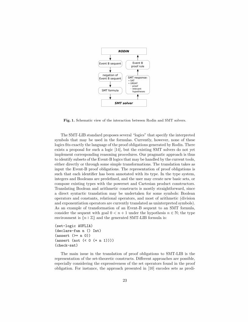
Figure 1 gives a schematic view of the cooperation framework between Rodinand the SMT solver. Within the Rodin platform, each proof obligation is repre-sented as a sequent, i.e. a set of hypotheses and a conclusion. These sequents aredischarged using Event-B proof rules. Our strategy to prove an Event-B sequentis to build an SMT formula, call an SMT solver on this formula, and, on success,introduce a new suitable proof rule. This strategy is presented as a tactic in theRodin user interface. Since SMT solvers answer the satisfiability question, it isnecessary to take the negation of the sequent (to be validated) in order to build aformula to be refuted by the SMT solver. If the SMT solver does not implementunsatisfiable core generation, the proof rule will assert that the full Event-B se-quent is valid (and will only be useful for that specific sequent). Otherwise anunsatisfiable core — i.e., the set of facts necessary to prove that the formulais unsatisfiable — is supplied to Rodin, which will extract a stronger Event-Bproof rule containing only the necessary hypotheses. This stronger proof rulewill hopefully be applicable to other Event-B sequents. If, however, the SMTsolver is not successful, the application of the tactic has failed and the proof treeremains unchanged.

22

RODIN

Event B sequent

negation ofEvent B sequent

SMT formula

SMT response:∙ SAT∙ UNSAT ◦ proof ◦ relevant hypotheses

Event Bproof rule

SMT solver

Fig. 1. Schematic view of the interaction between Rodin and SMT solvers.

The SMT-LIB standard proposes several “logics” that specify the interpretedsymbols that may be used in the formulas. Currently, however, none of theselogics fits exactly the language of the proof obligations generated by Rodin. Thereexists a proposal for such a logic [14], but the existing SMT solvers do not yetimplement corresponding reasoning procedures. Our pragmatic approach is thusto identify subsets of the Event-B logics that may be handled by the current tools,either directly or through some simple transformations. The translation takes asinput the Event-B proof obligations. The representation of proof obligations issuch that each identifier has been annotated with its type. In the type system,integers and Booleans are predefined, and the user may create new basic sets, orcompose existing types with the powerset and Cartesian product constructors.Translating Boolean and arithmetic constructs is mostly straightforward, sincea direct syntactic translation may be undertaken for some symbols: Booleanoperators and constants, relational operators, and most of arithmetic (divisionand exponentiation operators are currently translated as uninterpreted symbols).As an example of transformation of an Event-B sequent to an SMT formula,consider the sequent with goal 0 < n + 1 under the hypothesis n ∈ N; the typeenvironment is {n ◦◦ Z} and the generated SMT-LIB formula is:

(set-logic AUFLIA)

(declare-fun n () Int)

(assert (>= n 0))

(assert (not (< 0 (+ n 1))))

(check-sat)

The main issue in the translation of proof obligations to SMT-LIB is therepresentation of the set-theoretic constructs. Different approaches are possible,especially considering the expressiveness of the set operators found in the proofobligation. For instance, the approach presented in [10] encodes sets as predi-

23

cates, but does not make it possible to reason about sets of sets. We present herean approach that removes this restriction. It uses the ppTrans translator [13],already available in the Rodin platform; it removes most set-theoretic constructsfrom proof obligations by systematically expanding their definitions. It translatesan Event-B formula to an equivalent formula in a subset of the Event-B mathe-matical language (see the grammar of this subset in Fig. 2). The sole set-theoreticsymbol is the membership predicate. In addition, the translator performs decom-position of binary relations and purification, i.e., it separates arithmetic, Booleanand set-theoretic terms. Finally ppTrans performs basic Boolean simplificationson formulas. In the following, we provide details on those transformations, usingthe notation ϕ ϕ′ to express that the formula (or sub-term) ϕ is rewritten toϕ′.

P ::= P ⇒ P | P ≡ P | P ∧ · · · ∧ P | P ∨ · · · ∨ P |¬P | ∀L · P | ∃L · P |A = A | A < A | A ≤ A |M ∈ S | B = B | I = I

L ::= I · · · II ::= NameA ::= A−A | A div A | A mod A | A expA |

A + · · ·+ A | A× · · · ×A | −A | I | IntegerLiteralB ::= true | IM ::= M 7→M | I | integer | boolS ::= I

Fig. 2. Grammar of the language produced by ppTrans. The non-terminals are P (pred-icates), L (list of identifiers), I (identifiers), A (arithmetic expressions), B (Booleanexpressions), M (maplet expressions), S (set expressions).

Maplet-hiding variables The rewriting system implemented in ppTrans can-not directly transform identifiers that are of type Cartesian product. In a pre-processing phase, such identifiers are thus decomposed, so that further rewritingrules may be applied. This decomposition introduces fresh identifiers of scalartype (members of some given set, integers or Booleans) that name the compo-nents of the Cartesian product. Technically, this pre-processing is as follows. Weassume the existence of an attribute T , such that T (e) is the type of expressione. Also, let fv(e) denote the free identifiers occurring in expression e. The decom-position of the Cartesian product identifiers is specified, assuming an unlimitedsupply of fresh identifiers (e.g. x0, x1,. . . ), using the following two definitions ∇and ∇T :

∇(i) =

{∇T (T (i)) if i is a product identifier,i otherwise.

∇T (T ) =

{∇T (T1) 7→ ∇T (T2) if ∃T1, T2 ·T = T1 × T2,a fresh identifier xi otherwise.

24

For instance, assume x ◦◦ Z × (Z × Z); then ∇(x) = x0 7→ (x1 7→ x2) andfv(∇(x)) = {x0, x1, x2} are fresh identifiers.

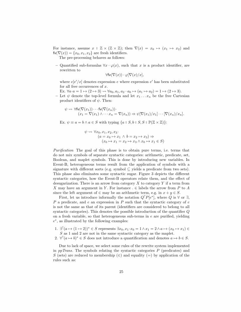
The pre-processing behaves as follows:

– Quantified sub-formulas ∀x · ϕ(x), such that x is a product identifier, arerewritten to

∀fv(∇(x)) · ϕ[∇(x)/x],

where e[e′/x] denotes expression e where expression e′ has been substitutedfor all free occurrences of x.Ex. ∀a·a = 1 7→ (2 7→ 3) ∀a0, a1, a2 · a0 7→ (a1 7→ a2) = 1 7→ (2 7→ 3).

– Let ψ denote the top-level formula and let x1 . . . xn be the free Cartesianproduct identifiers of ψ. Then:

ψ ∀fv(∇(x1)) · · · fv(∇(xn))·(x1 = ∇(x1) ∧ · · ·xn = ∇(xn))⇒ ψ[∇(x1)/x1] · · · [∇(xn)/xn].

Ex. ψ ≡ a = b ∧ a ∈ S with typing {a ◦◦ S, b ◦◦ S, S ◦◦ P(Z× Z)}:

ψ ∀x0, x1, x2, x3 ·(a = x0 7→ x1 ∧ b = x2 7→ x3)⇒

(x0 7→ x1 = x2 7→ x3 ∧ x0 7→ x1 ∈ S)

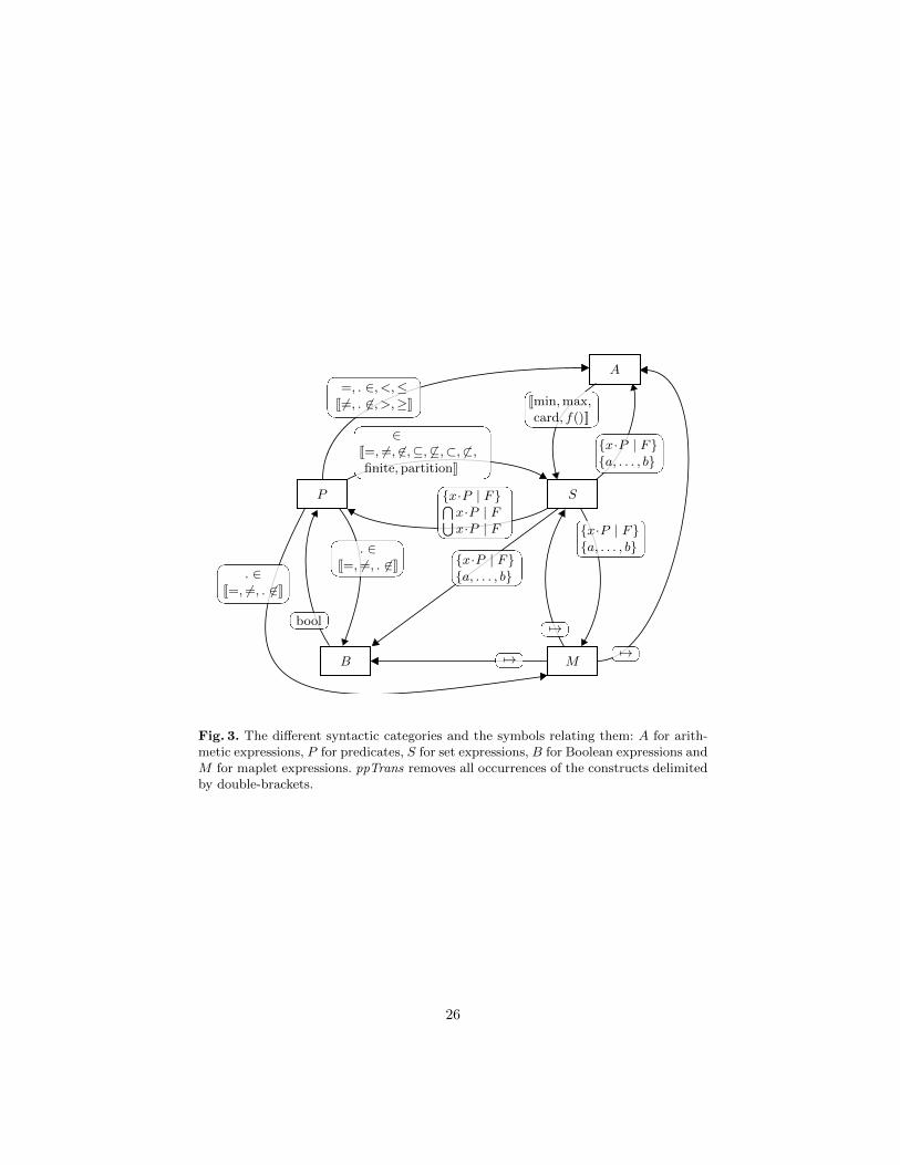
Purification The goal of this phase is to obtain pure terms, i.e. terms thatdo not mix symbols of separate syntactic categories: arithmetic, predicate, set,Boolean, and maplet symbols. This is done by introducing new variables. InEvent-B, heterogeneous terms result from the application of symbols with asignature with different sorts (e.g. symbol ⊆ yields a predicate from two sets).This phase also eliminates some syntactic sugar. Figure 3 depicts the differentsyntactic categories, how the Event-B operators relate them, and the effect ofdesugarization. There is an arrow from category X to category Y if a term fromX may have an argument in Y . For instance . ∈ labels the arrow from P to Asince the left argument of ∈ may be an arithmetic term, e.g. in x+ y ∈ S.

First, let us introduce informally the notation Q?P [e∗], where Q is ∀ or ∃,P a predicate, and e an expression in P such that the syntactic category of eis not the same as that of its parent (identifiers are considered to belong to allsyntactic categories). This denotes the possible introduction of the quantifier Qon a fresh variable, so that heterogeneous sub-terms in e are purified, yieldinge∗, as illustrated by the following examples:

1. ∃?(a 7→ (1 7→ 2))∗ ∈ S represents ∃x0, x1 ·x0 = 1∧x1 = 2∧a 7→ (x0 7→ x1) ∈S as 1 and 2 are not in the same syntactic category as the maplet.

2. ∀?(a 7→ b)∗ ∈ S does not introduce a quantification and denotes a 7→ b ∈ S.

Due to lack of space, we select some rules of the rewrite system implementedin ppTrans. The symbols relating the syntactic categories P (predicates) andS (sets) are reduced to membership (∈) and equality (=) by application of therules such as:

25

=, . ∈, <,≤J6=, . 6∈, >,≥K

{x·P | F}{a, . . . , b}

{x·P | F}{a, . . . , b}

J=, 6=, . 6∈K. ∈

. ∈J=, 6=, . 6∈K

{x·P | F}⋂x·P | F⋃x·P | F

7→

{a, . . . , b}{x·P | F}

bool

A

S

MB

P

J=, 6=, 6∈,⊆, 6⊆,⊂, 6⊂,∈

finite, partitionK

Jmin,max,card, f()K

7→7→

Fig. 3. The different syntactic categories and the symbols relating them: A for arith-metic expressions, P for predicates, S for set expressions, B for Boolean expressions andM for maplet expressions. ppTrans removes all occurrences of the constructs delimitedby double-brackets.

26

x 6= y ¬(x = y) (2)

s ⊆ t s ∈ P(t) (3)

x 6∈ s ¬(x ∈ s) (4)

finite(s) ∀a·∃b, f ·f ∈ s� a..b (5)

Moreover rules 2 and 4 are also applied when the arguments belong to other syn-tactic categories and are responsible for the elimination of all the occurrences ofsymbols 6= and 6∈. Examples to eliminate equalities between syntactic categoriesS, M are:

x1 7→ x2 = y1 7→ y2 x1 = y1 ∧ x2 = y2 (6)

bool(P ) = bool(Q) P ⇔ Q (7)

bool(P ) = TRUE P (8)

x = f(y) y 7→ x ∈ f (9)

x = FALSE ¬(x = TRUE)(10)

Due to the symmetry property of equality, ppTrans also applies a symmetricversion of each such rule. The symbols that embed arithmetic terms are takencare of with rules such as:

n = card(s) ∃f ·f ∈ s�� 1..n (11)

n = max(s) n ∈ s ∧max(s) ≤ n(12)

a � b b ≺ a (13)

a ≺ max(s) ∃x·x ∈ s ∧ a ≺ x (14)

The remaining rules perform the following roles: rewrite applications of theset membership symbol according to the rightmost argument (e.g. 15), eliminatesome symbols (e.g. 17), and handle miscellaneous other cases:

e ∈ s↔↔ t e ∈ s←↔ t ∧ t ⊆ ran(e) (15)

e ∈ s←↔ t e ∈ s↔ t ∧ s ⊆ dom(e) (16)

e 7→ f ∈ s× t e ∈ s ∧ f ∈ t (17)

e 7→ f ∈ id e = f (18)

e 7→ f ∈ r−1 f 7→ e ∈ r (19)

e 7→ f ∈ sC r e 7→ f ∈ r ∧ e ∈ s (20)

e 7→ f ∈ pred e = f + 1 (21)

The full system consists of 80 rules. They are either sound purification rules,or the equivalence of the left and right side terms can easily be derived fromthe definitions (see [1]) of the eliminated symbols. Purification rules eliminateheterogeneous terms and are only applied once. It is not difficult to order allother rules such that no eliminated symbol is introduced in subsequent rules.The rewriting system is thus indeed terminating.

Output to SMT-LIB format Once ppTrans has completed rewriting, the resultingproof obligation is ready to be output in SMT-LIB format. The translation fromppTrans’ output to SMT-LIB follows specific rules for the translation of the setmembership operator. For instance assume the input has the following typingenvironment and formulas:

27

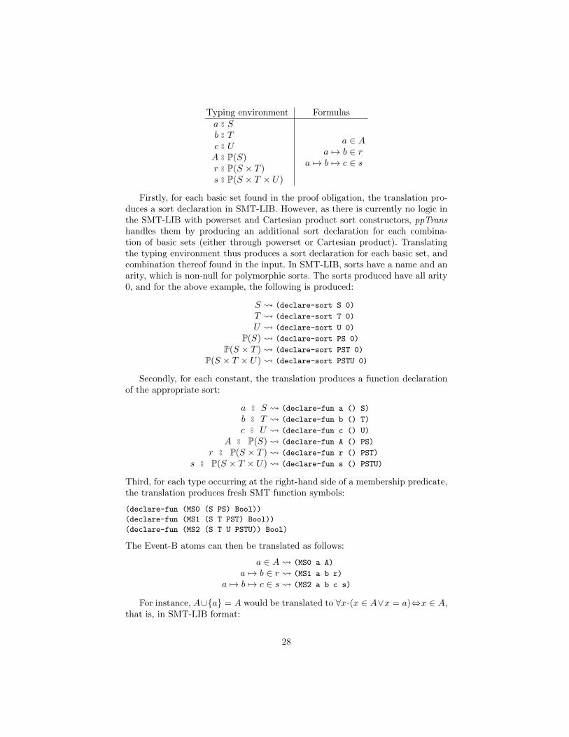
Typing environment Formulasa ◦◦ Sb ◦◦ Tc ◦◦ UA ◦◦ P(S)r ◦◦ P(S × T )s ◦◦ P(S × T × U)

a ∈ Aa 7→ b ∈ r

a 7→ b 7→ c ∈ s

Firstly, for each basic set found in the proof obligation, the translation pro-duces a sort declaration in SMT-LIB. However, as there is currently no logic inthe SMT-LIB with powerset and Cartesian product sort constructors, ppTranshandles them by producing an additional sort declaration for each combina-tion of basic sets (either through powerset or Cartesian product). Translatingthe typing environment thus produces a sort declaration for each basic set, andcombination thereof found in the input. In SMT-LIB, sorts have a name and anarity, which is non-null for polymorphic sorts. The sorts produced have all arity0, and for the above example, the following is produced:

S (declare-sort S 0)

T (declare-sort T 0)

U (declare-sort U 0)

P(S) (declare-sort PS 0)

P(S × T ) (declare-sort PST 0)

P(S × T × U) (declare-sort PSTU 0)

Secondly, for each constant, the translation produces a function declarationof the appropriate sort:

a ◦◦ S (declare-fun a () S)

b ◦◦ T (declare-fun b () T)

c ◦◦ U (declare-fun c () U)

A ◦◦ P(S) (declare-fun A () PS)

r ◦◦ P(S × T ) (declare-fun r () PST)

s ◦◦ P(S × T × U) (declare-fun s () PSTU)

Third, for each type occurring at the right-hand side of a membership predicate,the translation produces fresh SMT function symbols:

(declare-fun (MS0 (S PS) Bool))

(declare-fun (MS1 (S T PST) Bool))

(declare-fun (MS2 (S T U PSTU)) Bool)

The Event-B atoms can then be translated as follows:

a ∈ A (MS0 a A)

a 7→ b ∈ r (MS1 a b r)

a 7→ b 7→ c ∈ s (MS2 a b c s)

For instance, A∪{a} = A would be translated to ∀x·(x ∈ A∨x = a)⇔x ∈ A,that is, in SMT-LIB format:

28

(forall ((x S)) (= (or (MS0 x A) (= x a)) (MS0 x A)))

While the approach presented here covers the whole Event-B mathemati-cal language and is compatible with the SMT-LIB language, the semantics ofsome Event-B constructs is approximated because some operators become unin-terpreted in SMT-LIB (chiefly membership but also some arithmetic operatorssuch as division and exponentiation). However, we can recover their interpreta-tion by adding axioms to the SMT-LIB benchmark, at the risk of decreasing theperformance of the SMT solvers. Some experimentation is thus needed to find agood balance between efficiency and completeness.

Indeed, it appears experimentally that including some axioms of set theoryto constrain the possible interpretations of the membership predicate greatlyimproves the number of proof obligations discharged. In particular, the axiom ofelementary set (singleton part) is necessary for many Rodin proof obligations.The translator directly instantiates the axiom for all membership predicates.Assuming MS is the membership predicate associated with sorts S and PS, thetranslation introduces thus the following assertion:

(assert (forall ((x S))

(exists ((X PS)) (and (MS x X)

(forall ((y S)) (=> (MS y X) (= y x)))))))

This particular assertion eliminates non-standard interpretations where somesingleton sets do not exist. Without it, some formulas are satisfiable because ofspurious models and the SMT solvers are unable to refute them.

A small example As a concrete example of translation, we consider the sequentpresented in Section 3. Figure 4 presents the SMT-LIB input resulting fromthe translation approach described in this paper. Since the proof obligation in-cludes sets of JOBS, a corresponding sort PJ and membership predicate MSare declared in lines 3–4. Then, the function symbols corresponding to the freeidentifiers of the sequent are declared at lines 5–7. Finally, the hypotheses andthe goal of the sequent are translated to named assertions (lines 8–14).

The sequent described in this section is very simple and is easily verified byboth Atelier-B provers and SMT solvers. It is noteworthy that the plug-in in-spects sequents to choose the most suitable encoding approach. The next sectionreports experiments with a large number of proof obligations and establishes abetter basis to compare the effectiveness of these different verification techniques.

5 Experimental results

We evaluated experimentally the effectiveness of using SMT solvers as reason-ers in the Rodin platform by means of the techniques presented in this paper.This evaluation complements the experiments presented in [11] and reinforcestheir conclusions. We established a library of 2,456 proof obligations stemmingfrom Event-B developments collected by the European FP7 project Deploy andpublicly available on the Deploy repository5. These developments originate from

5 http://deploy-eprints.ecs.soton.ac.uk

29

1 (set-logic AUFLIA)

2 (declare-sort JOBS 0)

3 (declare-sort PJ 0)

4 (declare-fun MS (JOBS PJ) Bool)

5 (declare-fun active () PJ)

6 (declare-fun j () JOBS)

7 (declare-fun queue () PJ)

8 (assert (! (forall ((x JOBS))

9 (not (and (MS x active) (MS x queue)))) :named inv3))

10 (assert (! (MS j queue) :named grd1))

11 (assert (! (not (forall ((x0 JOBS))

12 (not (and (or (MS x0 active) (= x0 j))

13 (MS x0 queue)

14 (not (= x0 j)))))) :named goal))

15 (check-sat)

Fig. 4. SMT-LIB input produced using the ppTrans approach.

examples from Abrial’s book [2], academic publications, tutorials, as well asindustrial case studies.

One main objective of introducing new reasoners in the Rodin platform is toreduce the number of valid proof obligations that need to be discharged interac-tively by humans. Consequently, the effectiveness of a reasoner is measured bythe number of proof obligations proved automatically by the reasoner.

Obviously, effectiveness should depend on the computing resources given tothe reasoners. In practice, the amount of memory is seldom a bottleneck, andusually the solvers are limited by setting a timeout on their execution time. In thecontext of the Rodin platform, the reasoners are executed by synchronous calls,and the longer the time limit, the less responsive is the framework to the user.We have experimented different timeouts and our experiments have shown usthat a timeout of one second seems a good trade-off: doubling the timeout to twoseconds increases by fewer than 0.1% the number of verified proof obligations,while decreasing the responsiveness of the platform.

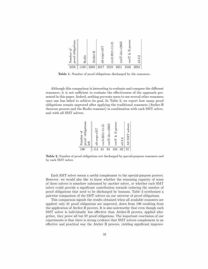
Table 1 compares different reasoners on our set of benchmarks. The secondcolumn corresponds to Rodin internal normalization and simplification proce-dures. It shows that more than half of the generated proof obligations necessitateadvanced theorem-proving capabilities to be discharged. The third column is aspecial-purpose reasoner, namely Atelier-B provers. They were originally devel-oped for the B method and are also available in the Rodin platform. Althoughthey are extremely effective, the Atelier-B provers now suffer from legacy issues.The last five columns are various SMT solvers applied to the proof obligationsgenerated by the plug-in. The SMT solvers were used with a timeout of one sec-ond, on a computer equipped with an Intel Core i7-4770, cadenced at 3.40 GHz,with 24 GB of RAM, and running Ubuntu Linux 12.04. They show decent results,but they are not yet as effective reasoners as the Atelier-B theorem provers.

30

Nu

mb

erof

pro

of

ob

ligati

on

s

Rod

in

Ate

lier

-B

alt

-erg

o-r

217

cvc3

-2011-1

1-2

1

ver

iT-d

ev-r

2863

ver

iT&

E-p

rover

z3-3

.2

2456 1169 2260 2017 2218 2051 2160 2094

Table 1. Number of proof obligations discharged by the reasoners.

Although this comparison is interesting to evaluate and compare the differentreasoners, it is not sufficient to evaluate the effectiveness of the approach pre-sented in this paper. Indeed, nothing prevents users to use several other reasonersonce one has failed to achieve its goal. In Table 2, we report how many proofobligations remain unproved after applying the traditional reasoners (Atelier-Btheorem provers and the Rodin reasoner) in combination with each SMT solver,and with all SMT solvers.

Nu

mb

erof

pro

of

ob

ligati

on

sle

ft

alt

-erg

o-r

217

cvc3

-2011-1

1-2

1

ver

iT-d

ev-r

2863

ver

iT&

E-p

rover

z3-3

.2

All

SM

Tso

lver

s

196 114 61 94 103 92 31

Table 2. Number of proof obligations not discharged by special-purpose reasoners andby each SMT solver.

Each SMT solver seems a useful complement to the special-purpose provers.However, we would also like to know whether the reasoning capacity of someof these solvers is somehow subsumed by another solver, or whether each SMTsolver could provide a significant contribution towards reducing the number ofproof obligations that need to be discharged by humans. Table 3 synthesizes apairwise comparison of the SMT solvers on our universe of proof obligations.

This comparison signals the results obtained when all available reasoners areapplied: only 31 proof obligations are unproved, down from 196 resulting fromthe application of Atelier-B provers. It is also noteworthy that even though eachSMT solver is individually less effective than Atelier-B provers, applied alto-gether, they prove all but 97 proof obligations. The important conclusion of ourexperiments is that there is strong evidence that SMT solvers complement in aneffective and practical way the Atelier B provers, yielding significant improve-

31

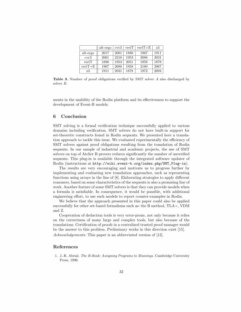
alt-ergo cvc3 veriT veriT+E z3

alt-ergo 2017 2001 1880 1967 1911

cvc3 2001 2218 1953 2088 2031

veriT 1880 1953 2051 1958 1878

veriT+E 1967 2088 1958 2160 2067

z3 1911 2031 1878 1972 2094

Table 3. Number of proof obligations verified by SMT solver A also discharged bysolver B.

ments in the usability of the Rodin platform and its effectiveness to support thedevelopment of Event-B models.

6 Conclusion

SMT solving is a formal verification technique successfully applied to variousdomains including verification. SMT solvers do not have built-in support forset-theoretic constructs found in Rodin sequents. We presented here a transla-tion approach to tackle this issue. We evaluated experimentally the efficiency ofSMT solvers against proof obligations resulting from the translation of Rodinsequents. In our sample of industrial and academic projects, the use of SMTsolvers on top of Atelier B provers reduces significantly the number of unverifiedsequents. This plug-in is available through the integrated software updater ofRodin (instructions at http://wiki.event-b.org/index.php/SMT_Plug-in).

The results are very encouraging and motivate us to progress further byimplementing and evaluating new translation approaches, such as representingfunctions using arrays in the line of [8]. Elaborating strategies to apply differentreasoners, based on some characteristics of the sequents is also a promising line ofwork. Another feature of some SMT solvers is that they can provide models whena formula is satisfiable. In consequence, it would be possible, with additionalengineering effort, to use such models to report counter-examples in Rodin.

We believe that the approach presented in this paper could also be appliedsuccessfully for other set-based formalisms such as: the B method, TLA+, VDMand Z.

Cooperation of deduction tools is very error-prone, not only because it relieson the correctness of many large and complex tools, but also because of thetranslations. Certification of proofs in a centralized trusted proof manager wouldbe the answer to this problem. Preliminary works in this direction exist [15].

Acknowledgements: This paper is an abbreviated version of [12].

References

1. J.-R. Abrial. The B-Book: Assigning Programs to Meanings. Cambridge UniversityPress, 1996.

32

2. J.-R. Abrial. Modeling in Event-B: System and Software Engineering. CambridgeUniversity Press, 2010.

3. M. Armand, G. Faure, B. Gregoire, C. Keller, L. Thery, and B. Werner. A ModularIntegration of SAT/SMT Solvers to Coq through Proof Witnesses. In First Int’lConference on Certified Programs and Proofs, CPP 2011, volume 7086 of LectureNotes in Computer Science, pages 135–150. Springer, 2011.

4. C. Barrett, R. Sebastiani, S. A. Seshia, and C. Tinelli. Satisfiability modulo theo-ries. In A. Biere, M. J. H. Heule, H. van Maaren, and T. Walsh, editors, Handbookof Satisfiability, volume 185 of Frontiers in Artificial Intelligence and Applications,chapter 26, pages 825–885. IOS Press, Feb. 2009.

5. C. Barrett, A. Stump, and C. Tinelli. The SMT-LIB Standard Version 2.0, 2010.6. T. Bouton, D. C. B. de Oliveira, D. Deharbe, and P. Fontaine. veriT: An Open,

Trustable and Efficient SMT-Solver. In Proc. Conference on Automated Deduc-tion (CADE), volume 5663 of Lecture Notes in Computer Science, pages 151–156.Springer, 2009.

7. J. Coleman, C. Jones, I. Oliver, A. Romanovsky, and E. Troubitsyna. RODIN(Rigorous open Development Environment for Complex Systems). In Fifth Eu-ropean Dependable Computing Conference: EDCC-5 supplementary volume, pages23–26, 2005.

8. J.-F. Couchot, D. Deharbe, A. Giorgetti, and S. Ranise. Scalable Automated Prov-ing and Debugging of Set-Based Specifications. Journal of the Brazilian ComputerSociety, 9:17–36, 2003.

9. L. de Moura and N. Bjørner. Z3: An Efficient SMT Solver. In C. R. Ramakr-ishnan and J. Rehof, editors, Tools and Algorithms for Construction and Analysisof Systems (TACAS), volume 4963 of Lecture Notes in Computer Science, pages337–340. Springer, 2008.

10. D. Deharbe. Automatic Verification for a Class of Proof Obligations with SMT-Solvers. In M. Frappier, G. Uwe, K. Sarfraz, R. Laleau, and S. Reeves, editors,Proceedings 2nd Int’l Conf. Abstract State Machines, Alloy, B and Z, ABZ 2010,volume 5977 of Lecture Notes in Computer Science, pages 217–230. Springer, 2010.

11. D. Deharbe, P. Fontaine, Y. Guyot, and L. Voisin. SMT solvers for Rodin. InJ. Derrick, J. A. Fitzgerald, S. Gnesi, S. Khurshid, M. Leuschel, S. Reeves, andE. Riccobene, editors, Proc 3rd Int. Conf. Abstract State Machines, Alloy, B, VDM,and Z (ABZ 2012), volume 7316 of Lecture Notes in Computer Science, pages 194–207. Springer, 2012.

12. D. Deharbe, P. Fontaine, Y. Guyot, and L. Voisin. Integrating SMT solvers inRodin. Science of Computer Programming, 2014. Available online.

13. M. Konrad and L. Voisin. Translation from Set-Theory to Predicate Calculus.Technical report, ETH Zurich, 2011.

14. D. Kroning, P. Rummer, and G. Weissenbacher. A Proposal for a Theory of FiniteSets, Lists, and Maps for the SMT-LIB Standard. In Informal proceedings, 7thInt’l Workshop on Satisfiability Modulo Theories (SMT) at CADE 22, 2009.

15. M. Schmalz. The logic of Event-B, 2011. Technical report 698, ETH Zurich,Information Security.

16. The Eclipse Foundation. Eclipse SDK, 2009.

33

Using Deduction Modulo in Set Theory ?

Pierre Halmagrand

Cedric/Cnam/Inria, Paris, FrancePierre.Halmagrand@inria.fr

Abstract. We present some improvements of Zenon Modulo and theapplication of this tool to sets of problems coming from set theory.Zenon Modulo is an extension of the tableau-based first order automatedtheorem prover Zenon to deduction modulo. Deduction modulo is an ex-tension of predicate calculus, which allows us to rewrite terms as wellas propositions, and which is well-suited for proof-search in axiomatictheories, as it turns axioms into rewrite rules. The improvements dis-cussed here consist in a better heuristic to automatically build rewritesystems given a set of axioms, and some optimizations in the rewrit-ing process used during the proof search. We also present some updatedresults obtained on benchmarks provided by the TPTP library for settheory categories. Finally, we discuss some recent work about the appli-cation of our tool to the B method set theory, in particular the way wetreat equality and the comprehension scheme.

Keywords: Automated Theorem Proving, Tableaux, Deduction Mod-ulo, Rewriting, Set Theory, B Method, Zenon Modulo.

1 Introduction

The development of large-scale industrial projects based on formal software isconstrained by the efficiency of verification tools that themselves rely on auto-mated theorem provers to mechanize a maximal part of the formalization pro-cess. Therefore, to allow a wider dissemination of these techniques, a particularattention must be paid to the development of automated theorem prover. Sincemany formal developments may be based on specific theories, like the widelyused B method [1] which relies on a particular typed set theory, we must payattention to reason within axiomatic theories. A solution to improve verificationtools is to combine different approaches in automated deduction and specializethem for a specific theory, like SMT solvers.

The BWare project [17] aims to provide a generic platform relying on differenttheorem provers (first order provers and SMT solvers) to verify proof obligationscoming from the development of industrial applications using the B method.

? This work is supported by the BWare project [17] (ANR-12-INSE-0010) funded bythe INS programme of the French National Research Agency (ANR).

34

As part of this project, the development of Zenon Modulo [10] is driven by itsapplication to set theory.

Our approach is to extend the tableau-based first order automated theoremprover Zenon [6] to deduction modulo [11]. Deduction modulo is an extension ofpredicate calculus, which allows to rewrite terms as well as propositions. This iswell suited for proof-search in axiomatic theories, as it turns axioms into rewriterules. For instance, we can express Zermelo set theory without any axiom [12],and turn non-deterministic proof-search among axioms into computations, whichreduces the proof-search space. Moreover, Zenon Modulo, like Zenon, adopts acertifying approach and produces proof certificates that can be checked by exter-nal proof checkers. Since the proofs produced by Zenon Modulo should keep theadvantage of conciseness of deduction modulo, we do not want to record all thecomputational steps of rewriting [9]. As a result, in order to verify such proofs,we use Dedukti [4], a simple proof checker based on the λΠ-calculus modulowhich can deal with rewriting.

We also present an updated heuristic, used by Zenon Modulo to automaticallytransform axioms into rewrite rules. The new heuristic captures more axiomsand guarantees to have a more meaningful rewrite system and impacts bothrewrite rules over terms and over propositions. We should notice here that thisheuristic has been developed to be used as a preprocessing tool that allows afully automatic use of Zenon Modulo on problems in the TPTP format. A secondoption is to give manually the rewrite system to Zenon Modulo. This secondoption is the one chosen for the B method set theory since there is a limitednumber of axioms and definitions, and we can afford to design a customizedrewrite system.

To assess our approach, we apply this new heuristic to the SET and SEUcategories of the first-order problems of the TPTP library [16] which deal withset theory, and compare results obtained by Zenon and Zenon Modulo with bothheuristics. In particular, we exhibit some examples of difficult problems that canbe proved by our tool using the new heuristic.

Finally, we discuss the application of Zenon Modulo to the B method settheory [1]. We will especially focus on equality and the comprehension schemein first order logic.

This paper is organized as follows: in Sec. 2, we first introduce the basic no-tions of deduction modulo and its application to Zenon Modulo; we then presentin Sec. 3 the new heuristic for Zenon Modulo; we expose in Sec. 4 the experimen-tal results obtained on the benchmarks provided by the TPTP library; finally,in Sec. 5, we discuss the ongoing work on the B set theory.

2 Zenon with Deduction Modulo

Zenon Modulo [10] is an extension of the tableau-based first order automatedtheorem prover Zenon [6] to deduction modulo [11]. This extension is partiallyinspired by the presentation of tableaux modulo in [5]. The proof-search rules

35

are applied with the usual tableau method: starting from the negation of thegoal, apply the rules in a top-down fashion to build a tree. When all branchescan be closed by applying a closure rule, the tree itself is said closed, and thisclosed tree is a proof of the goal.

Deduction modulo [11] extends the predicate calculus by introducing a con-gruence relation over propositions and the ability to perform conversion betweenpropositions that are equivalent modulo the congruence. Given a set of axioms,the congruence is generated by the rewrite system coming from the transforma-tion of axioms into rewrite rules. One of the major interests of deduction modulolies in reasoning modulo this congruence, since it reduces the search space byremoval of axioms from the context. For example, considering the following def-inition of inclusion in set theory: ∀X,Y (X ⊆ Y ⇔ ∀x (x ∈ X ⇒ x ∈ Y ))

The proof of A ⊆ A produced by Zenon has the following shape:

¬(A ⊆ A), ∀X,Y (X ⊆ Y ⇔ ∀x (x ∈ X ⇒ x ∈ Y ))γ∀inst∀Y (A ⊆ Y ⇔ ∀x (x ∈ A⇒ x ∈ Y ))

γ∀instA ⊆ A⇔ ∀x (x ∈ A⇒ x ∈ A)

β⇔¬∀x (x ∈ A⇒ x ∈ A)δ¬∀¬(τ ∈ A⇒ τ ∈ A)

α¬⇒τ ∈ A, ¬(τ ∈ A) ��

A ⊆ A ��

where τ = εx.¬(x ∈ A⇒ x ∈ A) is a Hilbert epsilon-term formed with a variablex and the formula ¬(x ∈ A⇒ x ∈ A), which is the formula existentially quanti-fied over. The Hilbert epsilon-term denotes the term that satisfies the formula,seen as a predicate on x, if it exists [18]. It can be seen as a Skolem term thatrecords the formula itself.

Deduction modulo replaces the axiom by the rewrite rule, where X and Yare variables: X ⊆ Y −→ ∀x (x ∈ X ⇒ x ∈ Y )

The proof produced by Zenon Modulo is then:

¬(A ⊆ A)δ¬∀, A ⊆ A −→ ∀x (x ∈ A⇒ x ∈ A)¬(τ ∈ A⇒ τ ∈ A)α¬⇒

τ ∈ A, ¬(τ ∈ A) ��

where τ = εx.¬(x ∈ A⇒ x ∈ A).

It can be seen that computations are interleaved with the deduction rules. Itcan be noticed that the proof is much simpler than the one produced by Zenon.In addition to simplicity, deduction modulo also allows for unbounded proof sizereduction [7].

36

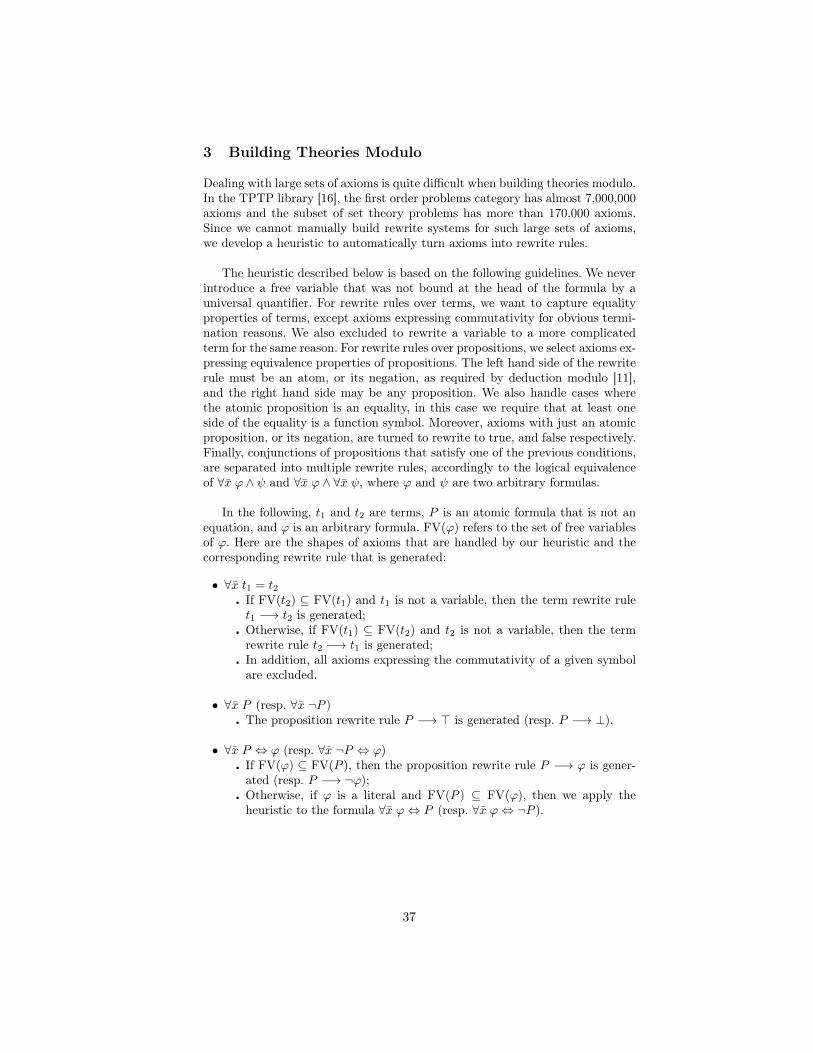
3 Building Theories Modulo

Dealing with large sets of axioms is quite difficult when building theories modulo.In the TPTP library [16], the first order problems category has almost 7,000,000axioms and the subset of set theory problems has more than 170,000 axioms.Since we cannot manually build rewrite systems for such large sets of axioms,we develop a heuristic to automatically turn axioms into rewrite rules.

The heuristic described below is based on the following guidelines. We neverintroduce a free variable that was not bound at the head of the formula by auniversal quantifier. For rewrite rules over terms, we want to capture equalityproperties of terms, except axioms expressing commutativity for obvious termi-nation reasons. We also excluded to rewrite a variable to a more complicatedterm for the same reason. For rewrite rules over propositions, we select axioms ex-pressing equivalence properties of propositions. The left hand side of the rewriterule must be an atom, or its negation, as required by deduction modulo [11],and the right hand side may be any proposition. We also handle cases wherethe atomic proposition is an equality, in this case we require that at least oneside of the equality is a function symbol. Moreover, axioms with just an atomicproposition, or its negation, are turned to rewrite to true, and false respectively.Finally, conjunctions of propositions that satisfy one of the previous conditions,are separated into multiple rewrite rules, accordingly to the logical equivalenceof ∀x ϕ ∧ ψ and ∀x ϕ ∧ ∀x ψ, where ϕ and ψ are two arbitrary formulas.

In the following, t1 and t2 are terms, P is an atomic formula that is not anequation, and ϕ is an arbitrary formula. FV(ϕ) refers to the set of free variablesof ϕ. Here are the shapes of axioms that are handled by our heuristic and thecorresponding rewrite rule that is generated:

• ∀x t1 = t2� If FV(t2) ⊆ FV(t1) and t1 is not a variable, then the term rewrite rulet1 −→ t2 is generated;� Otherwise, if FV(t1) ⊆ FV(t2) and t2 is not a variable, then the termrewrite rule t2 −→ t1 is generated;� In addition, all axioms expressing the commutativity of a given symbolare excluded.

• ∀x P (resp. ∀x ¬P )� The proposition rewrite rule P −→ > is generated (resp. P −→ ⊥).

• ∀x P ⇔ ϕ (resp. ∀x ¬P ⇔ ϕ)� If FV(ϕ) ⊆ FV(P ), then the proposition rewrite rule P −→ ϕ is gener-ated (resp. P −→ ¬ϕ);� Otherwise, if ϕ is a literal and FV(P ) ⊆ FV(ϕ), then we apply theheuristic to the formula ∀x ϕ⇔ P (resp. ∀x ϕ⇔ ¬P ).

37

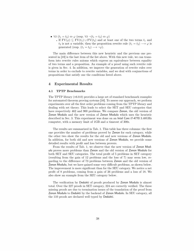
• ∀x (t1 = t2)⇔ ϕ (resp. ∀x ¬(t1 = t2)⇔ ϕ)� If FV(ϕ) ⊆ FV(t1) ∪ FV(t2) and at least one of the two terms t1 andt2 is not a variable, then the proposition rewrite rule (t1 = t2) −→ ϕ isgenerated (resp. (t1 = t2) −→ ¬ϕ).

The main difference between this new heuristic and the previous one pre-sented in [10] is the last item of the list above. With this new rule, we can trans-form into rewrite rules axioms which express an equivalence between equalityof two terms and a proposition. An example of a proof using such rewrite ruleis given in Sec. 4. In addition, we improve the generation of rewrite rules overterms in order to exclude to rewrite variables, and we deal with conjunctions ofpropositions that satisfy one the conditions listed above.

4 Experimental Results

4.1 TPTP Benchmarks

The TPTP library (v6.0.0) provides a large set of standard benchmark examplesfor automated theorem proving systems [16]. To assess our approach, we performexperiments over all the first order problems coming from the TPTP library anddealing with set theory. This leads to select the SET and SEU categories thathave respectively 462 and 900 problems. We compare Zenon, the old version ofZenon Modulo and the new version of Zenon Modulo which uses the heuristicdescribed in Sec. 3. This experiment was done on an Intel Core i7-4770 3.40GHzcomputer, with a memory limit of 1GB and a timeout of 300s.

The results are summarized in Tab. 1. This table has three columns: the firstone provides the number of problems proved by Zenon for each category, whilethe other two show the results for the old and new versions of Zenon Modulo.In addition, for both old and new versions of Zenon Modulo, we provide somedetailed results with profit and loss between provers.

From the results of Tab. 1, we observe that the new version of Zenon Mod-ulo proves more problems than Zenon and the old version of Zenon Modulo forboth SET and SEU categories. The total profit of 5 problems in SET category(resulting from the gain of 12 problems and the loss of 7) may seem low, re-garding to the difference of 73 problems between Zenon and the old version ofZenon Modulo, but we have gained some very difficult problems, as shown below.The improvement is more significant than for the SEU category. We notice a netprofit of 8 problems, coming from a gain of 26 problems and a loss of 18. Wealso show an example from the SEU category below.

The verification by Dedukti of proofs produced by Zenon Modulo is almosttotal. Over the 227 proofs in SET category, 224 are correctly verified. The threemissing proofs are due to termination issues of the translation of the proof fromZenon Modulo to Dedukti by the backend of Zenon Modulo. In SEU category, allthe 110 proofs are declared well typed by Dedukti.

38

TPTPCategory

Zenon Zenon Modulo (Old) Zenon Modulo (New Version)

Total Total vs. Zenon Total vs. Zenon vs. OldSET

462 prob.149 222

+86-13

227+91-13

+12-7

SEU900 prob.

96 102+14-8

110+32-18

+26-18

Table 1. Experimental Results over the TPTP Library

4.2 Analysis of Two Proofs From Set Theory

The TPTP library provides a ranking system to evaluate problems. This note,between 0 and 1, expresses the percentage of automated theorem provers thatare not able to prove the problem. A note of 0 means that the problem is trivial(every prover solves it), and a note of 1 means that all provers fail.

According to the TPTP ranking, Zenon Modulo is able to prove some quitedifficult problems. The hardest problem is SET817+4, with a ranking of 0.97in TPTP v6.0.0 (solved only by Muscadet [15]), and which neither Zenon orthe previous version of Zenon Modulo [10] was able to prove. It states thatthe intersection of all elements of a non-empty set of ordinal numbers is anordinal. Among the 8 axioms needed by Zenon Modulo to solve this problem, 7are transformed into rewrite rules by our heuristic. The proof of this problem istoo big to be displayed here.

An other example coming from the set theory, and that bodes well for appli-cation to the B method set theory, is the problem SEU194+1. This problem, witha ranking of 0.70, and which neither Zenon or the previous version of Zenon Mod-ulo [10] was able to prove, states that for any set s, if p is a relation, then thedomain of the restriction of p to s is equal to the intersection of the domain ofp and the set s. Among the twenty eight axioms provided with the conjecture,Zenon Modulo needs only two axioms to solve it, of which one is turned into arewrite rule. In the following, s, t and u are sets, p is a relation, a is an elementof a set, rel is a predicate for relations, dom a function that returns the domainof a relation, and rest a function that returns the restriction of a relation.

• Conjecture:∀s, p (rel(p)⇒ dom(rest(p, s)) = dom(p) ∩ s)

• Axiom:∀a, s, p (rel(p)⇒ (a ∈ dom(rest(p, s))⇔ (a ∈ s) ∧ (a ∈ dom(p))))

• Rewrite rule:u = s ∩ t −→ ∀a (a ∈ u⇔ ((a ∈ s) ∧ (a ∈ t)))

Zenon Modulo produces the proof of Fig. 1, presented in a format combiningdeduction steps in solid line and rewriting steps in dashed line. In addition, weomit some unnecessary formulas resulting from the application of β⇔ rules tolighten the presentation.

39

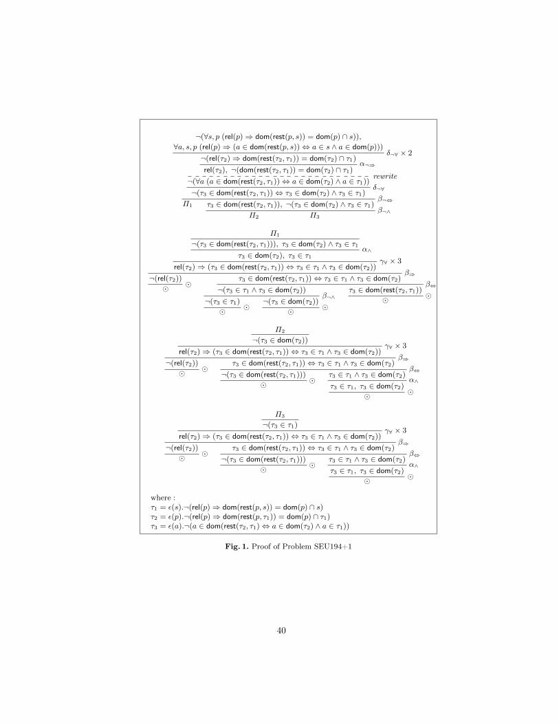
¬(∀s, p (rel(p)⇒ dom(rest(p, s)) = dom(p) ∩ s)),∀a, s, p (rel(p)⇒ (a ∈ dom(rest(p, s))⇔ a ∈ s ∧ a ∈ dom(p)))

δ¬∀ × 2¬(rel(τ2)⇒ dom(rest(τ2, τ1)) = dom(τ2) ∩ τ1)α¬⇒

rel(τ2), ¬(dom(rest(τ2, τ1)) = dom(τ2) ∩ τ1)rewrite¬(∀a (a ∈ dom(rest(τ2, τ1))⇔ a ∈ dom(τ2) ∧ a ∈ τ1))δ¬∀¬(τ3 ∈ dom(rest(τ2, τ1))⇔ τ3 ∈ dom(τ2) ∧ τ3 ∈ τ1)β¬⇔

Π1 τ3 ∈ dom(rest(τ2, τ1)), ¬(τ3 ∈ dom(τ2) ∧ τ3 ∈ τ1)β¬∧

Π2 Π3

Π1

¬(τ3 ∈ dom(rest(τ2, τ1))), τ3 ∈ dom(τ2) ∧ τ3 ∈ τ1α∧

τ3 ∈ dom(τ2), τ3 ∈ τ1γ∀ × 3

rel(τ2)⇒ (τ3 ∈ dom(rest(τ2, τ1))⇔ τ3 ∈ τ1 ∧ τ3 ∈ dom(τ2))β⇒¬(rel(τ2)) ��

τ3 ∈ dom(rest(τ2, τ1))⇔ τ3 ∈ τ1 ∧ τ3 ∈ dom(τ2)β⇔¬(τ3 ∈ τ1 ∧ τ3 ∈ dom(τ2))

β¬∧¬(τ3 ∈ τ1) ��¬(τ3 ∈ dom(τ2)) ��

τ3 ∈ dom(rest(τ2, τ1)) ��

Π2

¬(τ3 ∈ dom(τ2))γ∀ × 3

rel(τ2)⇒ (τ3 ∈ dom(rest(τ2, τ1))⇔ τ3 ∈ τ1 ∧ τ3 ∈ dom(τ2))β⇒¬(rel(τ2)) ��

τ3 ∈ dom(rest(τ2, τ1))⇔ τ3 ∈ τ1 ∧ τ3 ∈ dom(τ2)β⇔¬(τ3 ∈ dom(rest(τ2, τ1))) ��

τ3 ∈ τ1 ∧ τ3 ∈ dom(τ2)α∧

τ3 ∈ τ1, τ3 ∈ dom(τ2) ��

Π3

¬(τ3 ∈ τ1)γ∀ × 3

rel(τ2)⇒ (τ3 ∈ dom(rest(τ2, τ1))⇔ τ3 ∈ τ1 ∧ τ3 ∈ dom(τ2))β⇒¬(rel(τ2)) ��

τ3 ∈ dom(rest(τ2, τ1))⇔ τ3 ∈ τ1 ∧ τ3 ∈ dom(τ2)β⇔¬(τ3 ∈ dom(rest(τ2, τ1))) ��

τ3 ∈ τ1 ∧ τ3 ∈ dom(τ2)α∧

τ3 ∈ τ1, τ3 ∈ dom(τ2) ��

where :τ1 = ε(s).¬(rel(p)⇒ dom(rest(p, s)) = dom(p) ∩ s)τ2 = ε(p).¬(rel(p)⇒ dom(rest(p, τ1)) = dom(p) ∩ τ1)τ3 = ε(a).¬(a ∈ dom(rest(τ2, τ1)⇔ a ∈ dom(τ2) ∧ a ∈ τ1))

Fig. 1. Proof of Problem SEU194+1

40

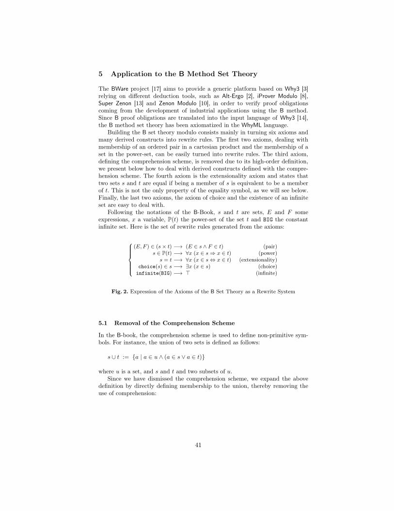
5 Application to the B Method Set Theory

The BWare project [17] aims to provide a generic platform based on Why3 [3]relying on different deduction tools, such as Alt-Ergo [2], iProver Modulo [8],Super Zenon [13] and Zenon Modulo [10], in order to verify proof obligationscoming from the development of industrial applications using the B method.Since B proof obligations are translated into the input language of Why3 [14],the B method set theory has been axiomatized in the WhyML language.

Building the B set theory modulo consists mainly in turning six axioms andmany derived constructs into rewrite rules. The first two axioms, dealing withmembership of an ordered pair in a cartesian product and the membership of aset in the power-set, can be easily turned into rewrite rules. The third axiom,defining the comprehension scheme, is removed due to its high-order definition,we present below how to deal with derived constructs defined with the compre-hension scheme. The fourth axiom is the extensionality axiom and states thattwo sets s and t are equal if being a member of s is equivalent to be a memberof t. This is not the only property of the equality symbol, as we will see below.Finally, the last two axioms, the axiom of choice and the existence of an infiniteset are easy to deal with.

Following the notations of the B-Book, s and t are sets, E and F someexpressions, x a variable, P(t) the power-set of the set t and BIG the constantinfinite set. Here is the set of rewrite rules generated from the axioms:

(E,F ) ∈ (s× t) −→ (E ∈ s ∧ F ∈ t) (pair)s ∈ P(t) −→ ∀x (x ∈ s⇒ x ∈ t) (power)s = t −→ ∀x (x ∈ s⇔ x ∈ t) (extensionality)

choice(s) ∈ s −→ ∃x (x ∈ s) (choice)infinite(BIG) −→ > (infinite)

Fig. 2. Expression of the Axioms of the B Set Theory as a Rewrite System

5.1 Removal of the Comprehension Scheme

In the B-book, the comprehension scheme is used to define non-primitive sym-bols. For instance, the union of two sets is defined as follows:

s ∪ t := {a | a ∈ u ∧ (a ∈ s ∨ a ∈ t)}

where u is a set, and s and t and two subsets of u.Since we have dismissed the comprehension scheme, we expand the above

definition by directly defining membership to the union, thereby removing theuse of comprehension:

41

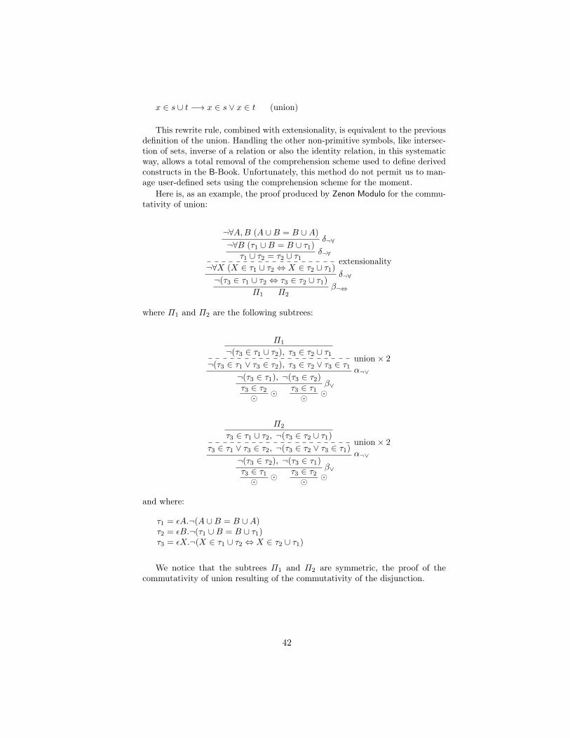
x ∈ s ∪ t −→ x ∈ s ∨ x ∈ t (union)

This rewrite rule, combined with extensionality, is equivalent to the previousdefinition of the union. Handling the other non-primitive symbols, like intersec-tion of sets, inverse of a relation or also the identity relation, in this systematicway, allows a total removal of the comprehension scheme used to define derivedconstructs in the B-Book. Unfortunately, this method do not permit us to man-age user-defined sets using the comprehension scheme for the moment.

Here is, as an example, the proof produced by Zenon Modulo for the commu-tativity of union:

¬∀A,B (A ∪B = B ∪A)δ¬∀¬∀B (τ1 ∪B = B ∪ τ1)δ¬∀τ1 ∪ τ2 = τ2 ∪ τ1 extensionality¬∀X (X ∈ τ1 ∪ τ2 ⇔ X ∈ τ2 ∪ τ1)

δ¬∀¬(τ3 ∈ τ1 ∪ τ2 ⇔ τ3 ∈ τ2 ∪ τ1)β¬⇔

Π1 Π2

where Π1 and Π2 are the following subtrees:

Π1

¬(τ3 ∈ τ1 ∪ τ2), τ3 ∈ τ2 ∪ τ1union× 2¬(τ3 ∈ τ1 ∨ τ3 ∈ τ2), τ3 ∈ τ2 ∨ τ3 ∈ τ1 α¬∨¬(τ3 ∈ τ1), ¬(τ3 ∈ τ2)

β∨τ3 ∈ τ2 ��τ3 ∈ τ1 ��

Π2

τ3 ∈ τ1 ∪ τ2, ¬(τ3 ∈ τ2 ∪ τ1)union× 2

τ3 ∈ τ1 ∨ τ3 ∈ τ2, ¬(τ3 ∈ τ2 ∨ τ3 ∈ τ1)α¬∨¬(τ3 ∈ τ2), ¬(τ3 ∈ τ1)

β∨τ3 ∈ τ1 ��τ3 ∈ τ2 ��

and where:

τ1 = εA.¬(A ∪B = B ∪A)τ2 = εB.¬(τ1 ∪B = B ∪ τ1)τ3 = εX.¬(X ∈ τ1 ∪ τ2 ⇔ X ∈ τ2 ∪ τ1)

We notice that the subtrees Π1 and Π2 are symmetric, the proof of thecommutativity of union resulting of the commutativity of the disjunction.

42

5.2 Dealing with Equality

The set theory of the B-book relies heavily on a primitive notion of equality, in-troduced before axioms for the set theory [1]. The main property of the equalityis substitutivity (i.e. an expression can be replaced by another one in a propo-sition provided they are equal). Starting from substitutivity and reflexivity ofequality, other properties like symmetry and transitivity can be derived. Zenonalready have rules that deal with this equational reasoning [6].

The second property of equality, introduced much later, and that has to dealdirectly with set theory is extensionality as shown in Fig. 2. Turning the axiomof extensionality into a rewrite rule allows Zenon Modulo to extend the equalitysymbol into membership equivalence at each step of the proof-search.

Choosing between equational reasoning and the extensionality properties ofequality during proof-search may be decisive to find a proof. There are differentsolutions to deal with this problem. A first idea is to try both equational reason-ing and extensionality every time we meet an equality symbol, but this solutionmay not be efficient since we duplicate the work for each equality symbol. Thesolution we are working on is to implement a heuristic into Zenon Modulo thatdecides to apply the extensionality rewrite rule, or to use the equational rea-soning of Zenon, based on the shape of terms. For instance, if both sides of theequality are variables, we do not apply the extensionality rewrite rule, otherwisewe use it.

6 Conclusion

We have presented some improvements of Zenon Modulo, in particular a newheuristic to transform axioms into rewrite rules over terms and propositions.This heuristic is used as a preprocessing tool to automatically build theoriesmodulo given sets of axioms. We have also presented results obtained on settheory problems, coming from the benchmarks provided by the TPTP library.This experiment was performed using the new heuristic. In particular, we haveshown that this new version proves some new difficult problems according to theTPTP ranking.

We have also discussed some recent work about the application of our toolto the B method set theory. Since we want to use Zenon Modulo to verify proofobligations coming from the development of industrial applications using the Bmethod, we have to build a B set theory modulo. We have described a methodto remove the comprehension scheme used to define non-primitive symbols likeunion of sets. Finally, we have presented some ideas to handle equality in the Bset theory.

As future work, we first aim to implement a heuristic into Zenon Modulothat handles the equality of B set theory. In particular, this heuristic shoulddecide whether to apply the extensionality rewrite rule, or to use the equationalreasoning of Zenon. To assess our work, we will first try to prove a large part ofderived lemmas coming from the B-Book. Finally, we will apply Zenon Modulo tothe set of proof obligations provided by the benchmarks of the BWare project.

43

Acknowledgement. Many thanks to O. Hermant, and D. Doligez for their detailedcomments on this paper, and to the Deducteam Inria research team for the manyinteractions.

References

1. J.-R. Abrial. The B-Book, Assigning Programs to Meanings. Cambridge UniversityPress, Cambridge (UK), 1996. ISBN 0521496195.

2. F. Bobot, S. Conchon, E. Contejean, and S. Lescuyer. Implementing Polymor-phism in SMT solvers. In C. Barrett and L. de Moura, editors, SMT 2008: 6thInternational Workshop on Satisfiability Modulo, volume 367 of ACM InternationalConference Proceedings Series, pages 1–5, 2008.

3. F. Bobot, J.-C. Filliâtre, C. Marché, and A. Paskevich. Why3: Shepherd yourherd of provers. In Boogie 2011: First International Workshop on IntermediateVerification Languages, pages 53–64, Wrocław, Poland, August 2011.

4. M. Boespflug, Q. Carbonneaux, and O. Hermant. The λΠ-Calculus Modulo as aUniversal Proof Language. In Proof Exchange for Theorem Proving (PxTP), pages28–43, Manchester (UK), June 2012.

5. R. Bonichon. TaMeD: A Tableau Method for Deduction Modulo. In InternationalJoint Conference on Automated Reasoning (IJCAR), volume 3097 of LNCS, pages445–459, Cork (Ireland), July 2004. Springer.

6. R. Bonichon, D. Delahaye, and D. Doligez. Zenon: An Extensible AutomatedTheorem Prover Producing Checkable Proofs. In Logic for Programming ArtificialIntelligence and Reasoning (LPAR), volume 4790 of LNCS/LNAI, pages 151–165,Yerevan (Armenia), Oct. 2007. Springer.

7. G. Burel. Efficiently Simulating Higher-Order Arithmetic by a First-Order TheoryModulo. Logical Methods in Computer Science (LMCS), 7(1):1–31, Mar. 2011.

8. G. Burel. Experimenting with Deduction Modulo. In Conference on Automated De-duction (CADE), volume 6803 of LNCS/LNAI, pages 162–176, Wrocław (Poland),July 2011. Springer.

9. D. Delahaye, D. Doligez, F. Gilbert, P. Halmagrand, and O. Hermant. Proof Cer-tification in Zenon Modulo: When Achilles Uses Deduction Modulo to Outrun theTortoise with Shorter Steps. In K. McMillan, A. Middeldorp, and A. Voronkov,editors, International Workshop on the Implementation of Logics (IWIL), Stellen-bosch (South Africa), Dec. 2013. EasyChair.

10. D. Delahaye, D. Doligez, F. Gilbert, P. Halmagrand, and O. Hermant. Zenon Mod-ulo: When Achilles Outruns the Tortoise using Deduction Modulo. In K. McMillan,A. Middeldorp, and A. Voronkov, editors, Logic for Programming Artificial Intel-ligence and Reasoning (LPAR), volume 8312 of LNCS/ARCoSS, pages 274–290,Stellenbosch (South Africa), Dec. 2013. Springer.

11. G. Dowek, T. Hardin, and C. Kirchner. Theorem Proving Modulo. Journal ofAutomated Reasoning (JAR), 31(1):33–72, Sept. 2003.

12. G. Dowek and A. Miquel. Cut Elimination for Zermelo Set Theory. In Archive forMathematical Logic. Springer. Submitted.

13. M. Jacquel, K. Berkani, D. Delahaye, and C. Dubois. Tableaux Modulo Theoriesusing Superdeduction: An Application to the Verification of B Proof Rules withthe Zenon Automated Theorem Prover. In International Joint Conference on Au-tomated Reasoning (IJCAR), volume 7364 of LNCS, pages 332–338, Manchester(UK), June 2012. Springer.

44

14. D. Mentré, C. Marché, J.-C. Filliâtre, and M. Asuka. Discharging proof obligationsfrom Atelier B using multiple automated provers. In S. Reeves and E. Riccobene,editors, ABZ’2012 - 3rd International Conference on Abstract State Machines,Alloy, B and Z, volume 7316 of Lecture Notes in Computer Science, pages 238–251, Pisa, Italy, June 2012. Springer. http://hal.inria.fr/hal-00681781/en/.

15. D. Pastre. Muscadet 2.3: A knowledge-based theorem prover based on naturaldeduction. In R. Goré, A. Leitsch, and T. Nipkow, editors, Automated Reasoning,volume 2083 of Lecture Notes in Computer Science, pages 685–689. Springer BerlinHeidelberg, 2001.

16. G. Sutcliffe. The TPTP Problem Library and Associated Infrastructure: The FOFand CNF Parts, v3.5.0. Journal of Automated Reasoning (JAR), 43(4):337–362,Dec. 2009.

17. The BWare Project, 2012. http://bware.lri.fr/.18. C.-P. Wirth. Hilbert’s epsilon as an operator of indefinite committed choice. Jour-

nal of Applied Logic, 6(3):287 – 317, 2008.

45

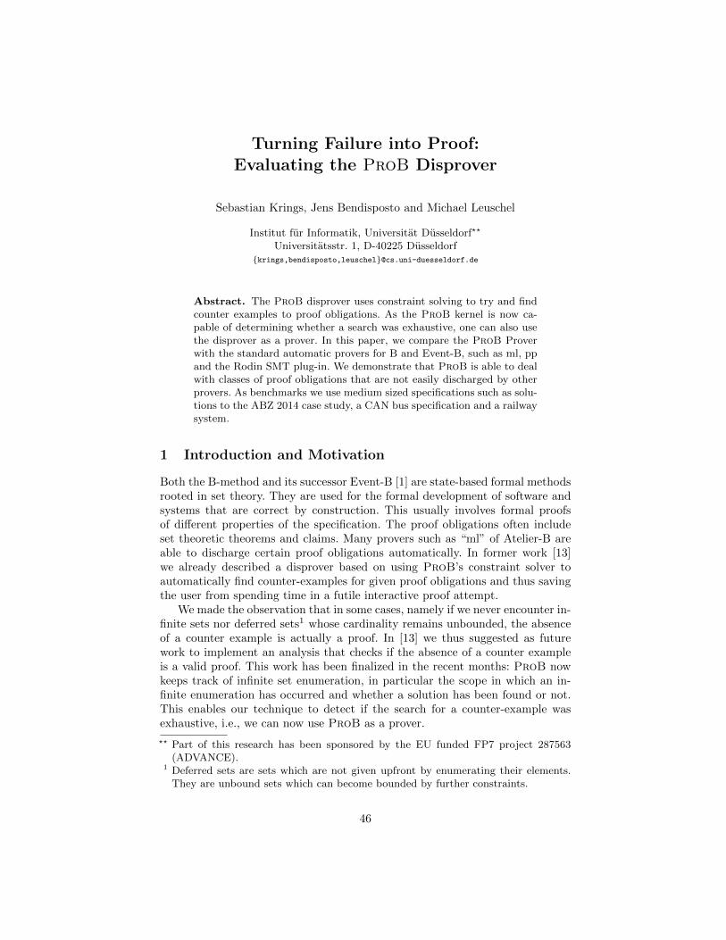
Turning Failure into Proof:Evaluating the ProB Disprover

Sebastian Krings, Jens Bendisposto and Michael Leuschel

Institut fur Informatik, Universitat Dusseldorf??

Universitatsstr. 1, D-40225 Dusseldorf{krings,bendisposto,leuschel}@cs.uni-duesseldorf.de

Abstract. The ProB disprover uses constraint solving to try and findcounter examples to proof obligations. As the ProB kernel is now ca-pable of determining whether a search was exhaustive, one can also usethe disprover as a prover. In this paper, we compare the ProB Proverwith the standard automatic provers for B and Event-B, such as ml, ppand the Rodin SMT plug-in. We demonstrate that ProB is able to dealwith classes of proof obligations that are not easily discharged by otherprovers. As benchmarks we use medium sized specifications such as solu-tions to the ABZ 2014 case study, a CAN bus specification and a railwaysystem.

1 Introduction and Motivation

Both the B-method and its successor Event-B [1] are state-based formal methodsrooted in set theory. They are used for the formal development of software andsystems that are correct by construction. This usually involves formal proofsof different properties of the specification. The proof obligations often includeset theoretic theorems and claims. Many provers such as “ml” of Atelier-B areable to discharge certain proof obligations automatically. In former work [13]we already described a disprover based on using ProB’s constraint solver toautomatically find counter-examples for given proof obligations and thus savingthe user from spending time in a futile interactive proof attempt.

We made the observation that in some cases, namely if we never encounter in-finite sets nor deferred sets1 whose cardinality remains unbounded, the absenceof a counter example is actually a proof. In [13] we thus suggested as futurework to implement an analysis that checks if the absence of a counter exampleis a valid proof. This work has been finalized in the recent months: ProB nowkeeps track of infinite set enumeration, in particular the scope in which an in-finite enumeration has occurred and whether a solution has been found or not.This enables our technique to detect if the search for a counter-example wasexhaustive, i.e., we can now use ProB as a prover.

?? Part of this research has been sponsored by the EU funded FP7 project 287563(ADVANCE).

1 Deferred sets are sets which are not given upfront by enumerating their elements.They are unbound sets which can become bounded by further constraints.

46

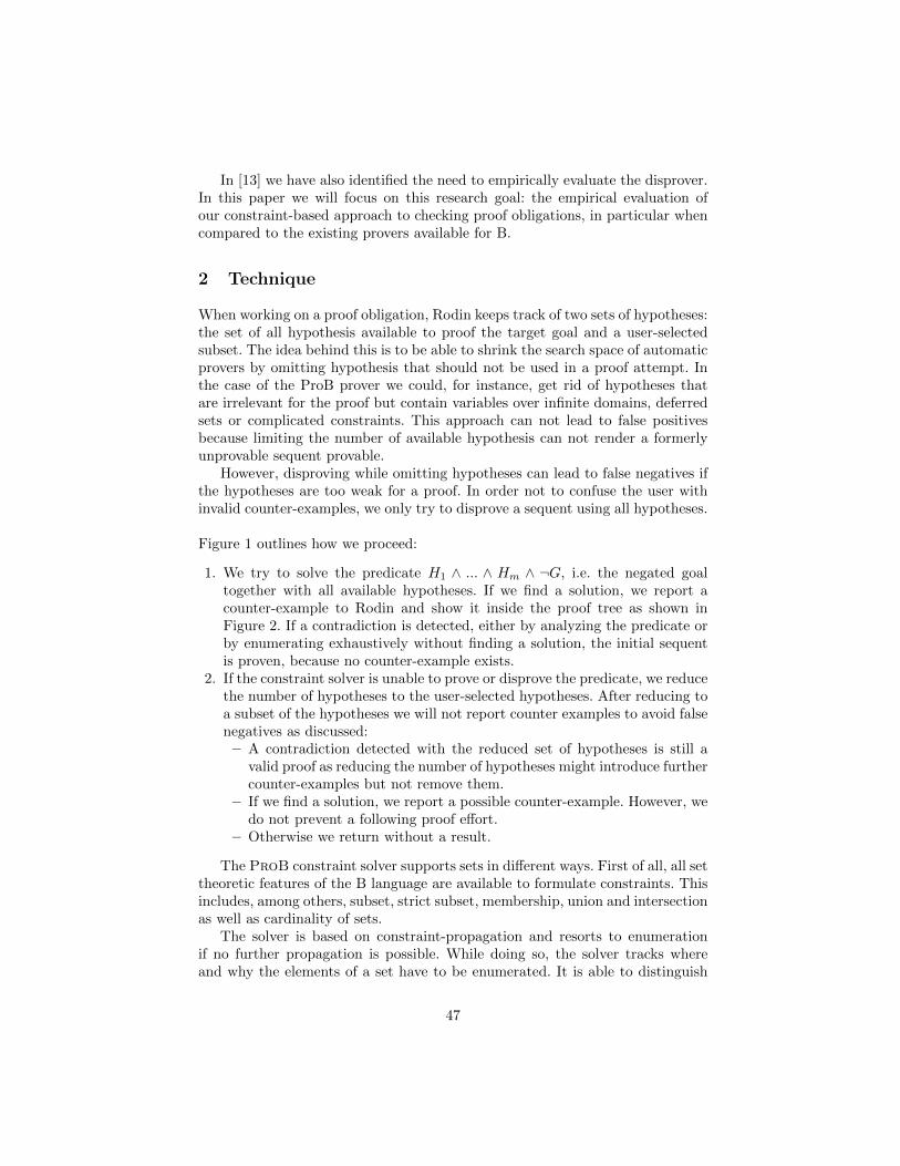
In [13] we have also identified the need to empirically evaluate the disprover.In this paper we will focus on this research goal: the empirical evaluation ofour constraint-based approach to checking proof obligations, in particular whencompared to the existing provers available for B.

2 Technique

When working on a proof obligation, Rodin keeps track of two sets of hypotheses:the set of all hypothesis available to proof the target goal and a user-selectedsubset. The idea behind this is to be able to shrink the search space of automaticprovers by omitting hypothesis that should not be used in a proof attempt. Inthe case of the ProB prover we could, for instance, get rid of hypotheses thatare irrelevant for the proof but contain variables over infinite domains, deferredsets or complicated constraints. This approach can not lead to false positivesbecause limiting the number of available hypothesis can not render a formerlyunprovable sequent provable.

However, disproving while omitting hypotheses can lead to false negatives ifthe hypotheses are too weak for a proof. In order not to confuse the user withinvalid counter-examples, we only try to disprove a sequent using all hypotheses.

Figure 1 outlines how we proceed:

1. We try to solve the predicate H1 ∧ ... ∧ Hm ∧ ¬G, i.e. the negated goaltogether with all available hypotheses. If we find a solution, we report acounter-example to Rodin and show it inside the proof tree as shown inFigure 2. If a contradiction is detected, either by analyzing the predicate orby enumerating exhaustively without finding a solution, the initial sequentis proven, because no counter-example exists.

2. If the constraint solver is unable to prove or disprove the predicate, we reducethe number of hypotheses to the user-selected hypotheses. After reducing toa subset of the hypotheses we will not report counter examples to avoid falsenegatives as discussed:– A contradiction detected with the reduced set of hypotheses is still a

valid proof as reducing the number of hypotheses might introduce furthercounter-examples but not remove them.

– If we find a solution, we report a possible counter-example. However, wedo not prevent a following proof effort.

– Otherwise we return without a result.

The ProB constraint solver supports sets in different ways. First of all, all settheoretic features of the B language are available to formulate constraints. Thisincludes, among others, subset, strict subset, membership, union and intersectionas well as cardinality of sets.

The solver is based on constraint-propagation and resorts to enumerationif no further propagation is possible. While doing so, the solver tracks whereand why the elements of a set have to be enumerated. It is able to distinguish

47

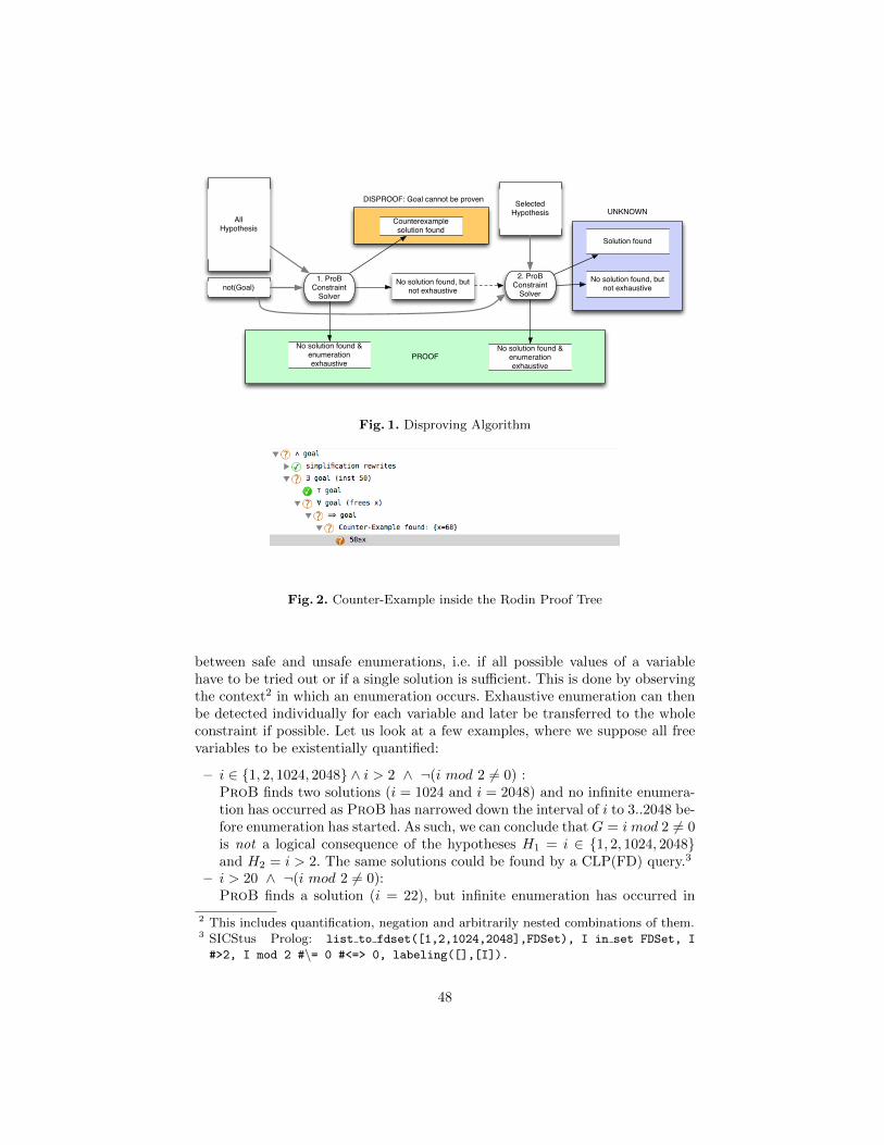
PROOF

AllHypothesis

not(Goal)1. ProB

ConstraintSolver

Counterexample solution found

No solution found & enumeration exhaustive

No solution found, but not exhaustive

SelectedHypothesis

2. ProBConstraint

Solver

No solution found & enumeration exhaustive

DISPROOF: Goal cannot be proven

No solution found, but not exhaustive

Solution found

UNKNOWN

Fig. 1. Disproving Algorithm

Fig. 2. Counter-Example inside the Rodin Proof Tree

between safe and unsafe enumerations, i.e. if all possible values of a variablehave to be tried out or if a single solution is sufficient. This is done by observingthe context2 in which an enumeration occurs. Exhaustive enumeration can thenbe detected individually for each variable and later be transferred to the wholeconstraint if possible. Let us look at a few examples, where we suppose all freevariables to be existentially quantified:

– i ∈ {1, 2, 1024, 2048} ∧ i > 2 ∧ ¬(i mod 2 6= 0) :ProB finds two solutions (i = 1024 and i = 2048) and no infinite enumera-tion has occurred as ProB has narrowed down the interval of i to 3..2048 be-fore enumeration has started. As such, we can conclude that G = i mod 2 6= 0is not a logical consequence of the hypotheses H1 = i ∈ {1, 2, 1024, 2048}and H2 = i > 2. The same solutions could be found by a CLP(FD) query.3

– i > 20 ∧ ¬(i mod 2 6= 0):ProB finds a solution (i = 22), but infinite enumeration has occurred in

2 This includes quantification, negation and arbitrarily nested combinations of them.3 SICStus Prolog: list to fdset([1,2,1024,2048],FDSet), I in set FDSet, I

#>2, I mod 2 #\= 0 #<=> 0, labeling([],[I]).

48

the sense that the possible values of i lie in the interval 22..∞. However,in this context this is not an issue, as a solution has been found. As such,we can conclude that i mod 2 6= 0 is not a logical consequence of i > 20.This time there is no CLP(FD) query that returns a solution. As there isno finite domain attached to i, labeling can not be performed. In contrast,ProB is able to (partially) enumerate the infinite domain of i in order tofind a solution.

– i ∈ {1, 2, 1024, 2048} ∧ i > 2 ∧ ¬(i mod 2 = 0) :ProB finds no solution and no infinite enumeration has occurred. As such,we have proven that i mod 2 = 0 follows logically from i ∈ {1, 2, 1024, 2048}∧i > 2. A CLP(FD) query also confirms, that there is no solution.

– i > 20 ∧ ¬(i mod 2 = 0 ∨ i mod 1001 6= 800):Here ProB finds no solution, but an “enumeration warning” is produced.Indeed, the constraint solver has narrowed down the possible solutions for ito the interval 801..∞, but with the default search settings no solution hasbeen found. Here, we cannot conclude that i mod 2 = 0∨ i mod 1001 6= 800is a logical consequence of i > 20. Indeed, i = 1801 is a counter example. 4

Again, CLP(FD) is unable to solve the query due to the infinite domain ofi.

As mentioned in the introduction, we will not go into further technical detailsin this paper.

3 Empirical Evaluation and Comparison

For our empirical evaluation we compare ProB to several other provers availablefor the Rodin platform [2], i.e., Rodin’s automatic tactic and the SMT plug-in[9,10]. Our comparison shows the benefit gained from using ProB as a prover.Each additional obligation that is discharged in this comparison actually savestime and money.

3.1 Experimental Setup

– The automatic tactic applies a number of rewriting rules and decision pro-cedures to the proof tree. For instance, a decision procedure checks if thegoal is listed in the set of hypotheses and thus discharged. It also uses thePP and ML provers from AtelierB. The automatic tactic is applied until afixpoint is reached.

– The SMT plug-in [9,10] applies two different SMT solvers (veriT [8] andCVC3 [5]) to the original goal, after some pre-processing.

– The disprover tactic applies three trivial decision procedures (check if goalis >, check if the hypotheses contain ⊥ and if the goal appears in the list ofhypotheses). Afterwards the disprover is applied to the goal.

4 Which ProB can find if you enlarge the default search space, e.g., by adding i <10000 as additional constraint.

49

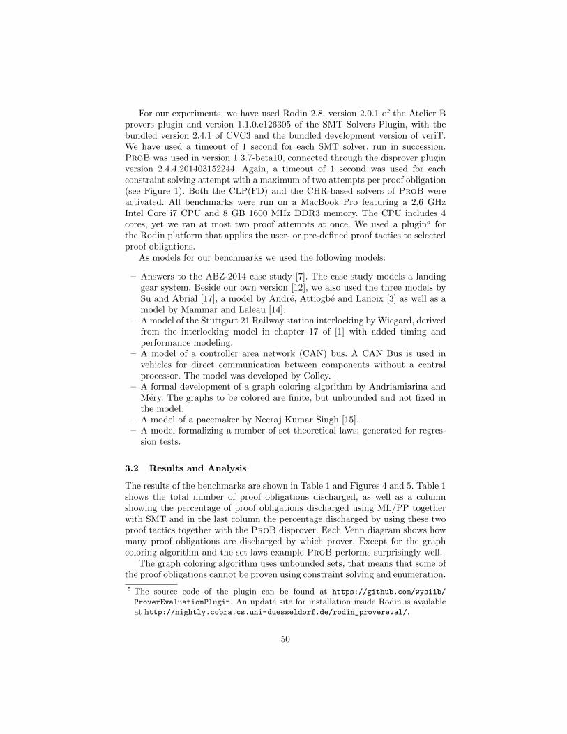
For our experiments, we have used Rodin 2.8, version 2.0.1 of the Atelier Bprovers plugin and version 1.1.0.e126305 of the SMT Solvers Plugin, with thebundled version 2.4.1 of CVC3 and the bundled development version of veriT.We have used a timeout of 1 second for each SMT solver, run in succession.ProB was used in version 1.3.7-beta10, connected through the disprover pluginversion 2.4.4.201403152244. Again, a timeout of 1 second was used for eachconstraint solving attempt with a maximum of two attempts per proof obligation(see Figure 1). Both the CLP(FD) and the CHR-based solvers of ProB wereactivated. All benchmarks were run on a MacBook Pro featuring a 2,6 GHzIntel Core i7 CPU and 8 GB 1600 MHz DDR3 memory. The CPU includes 4cores, yet we ran at most two proof attempts at once. We used a plugin5 forthe Rodin platform that applies the user- or pre-defined proof tactics to selectedproof obligations.

As models for our benchmarks we used the following models:

– Answers to the ABZ-2014 case study [7]. The case study models a landinggear system. Beside our own version [12], we also used the three models bySu and Abrial [17], a model by Andre, Attiogbe and Lanoix [3] as well as amodel by Mammar and Laleau [14].

– A model of the Stuttgart 21 Railway station interlocking by Wiegard, derivedfrom the interlocking model in chapter 17 of [1] with added timing andperformance modeling.

– A model of a controller area network (CAN) bus. A CAN Bus is used invehicles for direct communication between components without a centralprocessor. The model was developed by Colley.

– A formal development of a graph coloring algorithm by Andriamiarina andMery. The graphs to be colored are finite, but unbounded and not fixed inthe model.

– A model of a pacemaker by Neeraj Kumar Singh [15].– A model formalizing a number of set theoretical laws; generated for regres-

sion tests.

3.2 Results and Analysis

The results of the benchmarks are shown in Table 1 and Figures 4 and 5. Table 1shows the total number of proof obligations discharged, as well as a columnshowing the percentage of proof obligations discharged using ML/PP togetherwith SMT and in the last column the percentage discharged by using these twoproof tactics together with the ProB disprover. Each Venn diagram shows howmany proof obligations are discharged by which prover. Except for the graphcoloring algorithm and the set laws example ProB performs surprisingly well.

The graph coloring algorithm uses unbounded sets, that means that some ofthe proof obligations cannot be proven using constraint solving and enumeration.

5 The source code of the plugin can be found at https://github.com/wysiib/

ProverEvaluationPlugin. An update site for installation inside Rodin is availableat http://nightly.cobra.cs.uni-duesseldorf.de/rodin_provereval/.

50

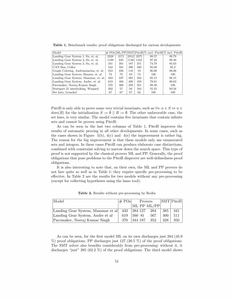
Table 1. Benchmark results: proof obligations discharged for various developments

Model # POs ML/PP SMT ProB % excl. ProB % incl. ProB

Landing Gear System 1, Su, et. al. 2328 2171 2312 2275 99.57 99.79Landing Gear System 2, Su, et. al. 1188 845 1140 1165 97.22 99.49Landing Gear System 3, Su, et. al. 341 201 187 251 74.78 85.63CAN Bus, Colley 542 501 490 320 95.02 95.2Graph Coloring, Andriamiarina, et. al. 254 226 116 19 96.06 96.06Landing Gear System, Hansen, et. al. 74 72 63 74 100 100Landing Gear System, Mammar, et. al. 433 347 385 334 95.15 98.15Landing Gear System, Andre, et. al. 619 466 400 459 79.81 90.63Pacemaker, Neeraj Kumar Singh 370 360 358 351 98.38 100Stuttgart 21 interlocking, Wiegard 202 57 94 184 55.45 93.56Set laws, Leuschel 67 67 67 62 100 100

ProB is only able to prove some very trivial invariants, such as ∀n ·n ∈ S ⇔ n ∈dom(R) for the initialization S := ∅ || R := ∅. The other unfavorable case, theset laws, is very similar. The model contains five invariants that contain infinitesets and cannot be proven using ProB.

As can be seen in the last two columns of Table 1, ProB improves theresults of automatic proving in all other developments. In some cases, such asthe cases shown in Figure 5(b), 4(c) and 4(e) the improvement is rather big.The reason for the big improvement is that these models only use enumeratedsets and integers. In these cases ProB can produce elaborate case distinctions,combined with constraint solving to narrow down the search space. This type ofproof is not supported by the classical provers ML and PP. Generally, the proofobligations that pose problems to the ProB disprover are well-definedness proofobligations.

It is also interesting to note that, on their own, the ML and PP provers donot fare quite so well as in Table 1: they require specific pre-processing to beeffective. In Table 2 are the results for two models without any pre-processing(except for collecting hypotheses using the lasso tool):

Table 2. Results without pre-processing by Rodin

Model # POs Provers SMT ProBML PP ML/PP

Landing Gear System, Mammar et al 433 284 127 284 385 341Landing Gear System, Andre et al 619 560 81 567 400 511Pacemaker, Neeraj Kumar Singh 370 344 187 352 328 350

As can be seen, for the first model ML on its own discharges just 284 (45.9%) proof obligations. PP discharges just 127 (20.5 %) of the proof obligations.The SMT solver also benefits considerably from pre-processing: without it, itdischarges “just” 385 (62.2 %) of the proof obligations. The third model shows

51

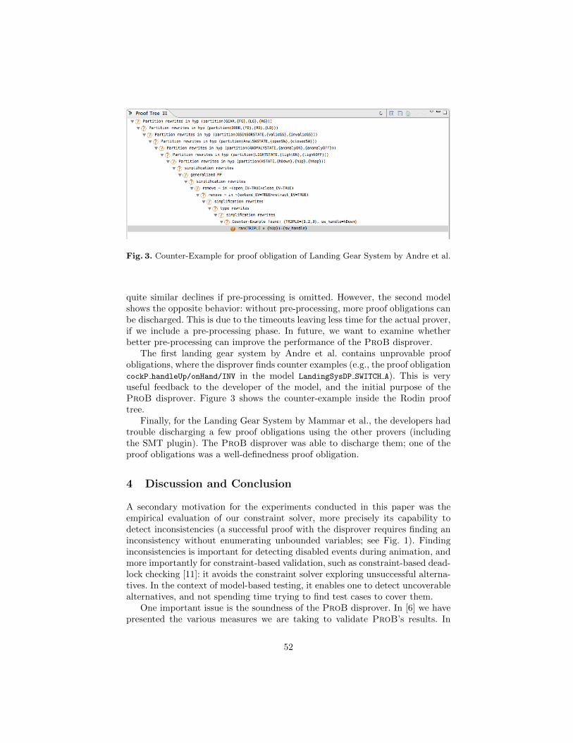
Fig. 3. Counter-Example for proof obligation of Landing Gear System by Andre et al.

quite similar declines if pre-processing is omitted. However, the second modelshows the opposite behavior: without pre-processing, more proof obligations canbe discharged. This is due to the timeouts leaving less time for the actual prover,if we include a pre-processing phase. In future, we want to examine whetherbetter pre-processing can improve the performance of the ProB disprover.

The first landing gear system by Andre et al. contains unprovable proofobligations, where the disprover finds counter examples (e.g., the proof obligationcockP handleUp/onHand/INV in the model LandingSysDP SWITCH A). This is veryuseful feedback to the developer of the model, and the initial purpose of theProB disprover. Figure 3 shows the counter-example inside the Rodin prooftree.

Finally, for the Landing Gear System by Mammar et al., the developers hadtrouble discharging a few proof obligations using the other provers (includingthe SMT plugin). The ProB disprover was able to discharge them; one of theproof obligations was a well-definedness proof obligation.

4 Discussion and Conclusion

A secondary motivation for the experiments conducted in this paper was theempirical evaluation of our constraint solver, more precisely its capability todetect inconsistencies (a successful proof with the disprover requires finding aninconsistency without enumerating unbounded variables; see Fig. 1). Findinginconsistencies is important for detecting disabled events during animation, andmore importantly for constraint-based validation, such as constraint-based dead-lock checking [11]: it avoids the constraint solver exploring unsuccessful alterna-tives. In the context of model-based testing, it enables one to detect uncoverablealternatives, and not spending time trying to find test cases to cover them.

One important issue is the soundness of the ProB disprover. In [6] we havepresented the various measures we are taking to validate ProB’s results. In

52

addition, we have developed a SMT-LIB [4] importer for ProB and have appliedour disprover to a large number of SMT-LIB benchmarks, checking that no “falsetheorems” are proven. For this paper, we have also double checked many of theproof obligations which were only provable by ProB, to ensure that they areindeed provable. As the Venn diagrams in Figures 4 and 5 show, a large numberof proof obligations can be proven by two or even three different provers. As thethree provers rely on completely different technologies and have been developedby independent teams, we can have a very high confidence that those proofobligations are indeed provable.

We have demonstrated that ProB is capable to discharge proof obligationsthat currently cannot be proven using Rodin’s auto tactic and the SMT solvers.Our prover typically deals well with a different kind of proof obligations thanthe other provers, and is thus an orthogonal extension rather than a replace-ment. Rodin’s auto tactic performs well in the realm of set theoretic constructsand relational expressions, some of which cannot be easily represented in theSMT syntax. SMT on the other hand performs well on arithmetic expressions,where the auto tactics often fail. ProB finally covers predicates over enumeratedsets, explicit data and explicit computations and has a good support for integerarithmetic over finite domains.

However, for models which make heavy use of deferred sets, such as thegraph colouring algorithm model (see Table 1), the ProB disprover can currentlymainly play its role as disprover. More precisely, for any proof obligation whichinvolves deferred sets and where no precise value of the cardinality of the deferredset is known, the disprover can only return either a counter example or theresult “unknown”. In future, we plan to improve the treatment of deferred setsin ProB, and to have the constraint solver determine the cardinalities of thosesets while solving. This should also enable the disprover to act as a prover formore proof obligations involving deferred sets.

We think that the ProB Disprover is a valuable extension to Rodin’s set ofprovers, because it can increase the number of proof obligations that are auto-matically discharged, thus saving time and money. Overall, the outcome of theempirical evaluation was a positive surprise, as ProB’s main domain of appli-cation is finding concrete counter examples, not discharging proof obligations.In particular, the fact that the number of discharged proof obligations, for themodels under consideration in Table 1, is comparable to that of the SMT pluginwith its two SMT solvers was unexpected. In future, we also plan to use ourSAT backend [16] for the ProB disprover, and evaluate its performance.

Acknowledgements We would like to thank the various developers for giv-ing us access to their Event-B models, and for discussions and feedback: Jean-Raymond Abrial, Andre, Attiogbe, John Colley, Regine Laleau, Lanoix, AmelMammar, Dominique Mery, Neeraj Kumar Singh, Wen Su.

References

1. J.-R. Abrial. Modeling in Event-B: System and Software Engineering. CambridgeUniversity Press, 2010.

53

2. J.-R. Abrial, M. Butler, and S. Hallerstede. An open extensible tool environmentfor Event-B. In Z. Liu and J. He, editors, Proceedings ICFEM’06, LNCS 4260,pages 588–605. Springer-Verlag, 2006.

3. Andre, Attiogbe, and Lanoix. Modelling and Analysing the Landing Gear Sys-tem: a Solution with Event-B/Rodin. http://www.lina.sciences.univ-nantes.

fr/aelos/softwares/LGS-ABZ2014/index.php. Solution to ABZ-2014, Accessed:2014-03-17.

4. C. Barrett, A. Stump, and C. Tinelli. The SMT-LIB Standard: Version 2.0. InA. Gupta and D. Kroening, editors, Proceedings of the 8th International Workshopon Satisfiability Modulo Theories (Edinburgh, UK), 2010.

5. C. Barrett and C. Tinelli. CVC3. In W. Damm and H. Hermanns, editors, Proceed-ings of the 19th International Conference on Computer Aided Verification (CAV’07), volume 4590 of Lecture Notes in Computer Science, pages 298–302. Springer-Verlag, July 2007. Berlin, Germany.

6. J. Bendisposto, S. Krings, and M. Leuschel. Who watches the watchers: Validatingthe prob validation tool. In Proceedings of the 1st Workshop on Formal-IDE,EPTCS XYZ, 2014. Electronic Proceedings in Theoretical Computer Science, 2014.

7. Boniol and Wiels. Landing gear system. http://www.irit.fr/ABZ2014/landing_system.pdf. Accessed: 2014-03-17.

8. T. Bouton, D. C. B. de Oliveira, D. Deharbe, and P. Fontaine. verit: an open,trustable and efficient smt-solver. In R. A. Schmidt, editor, Proc. Conference onAutomated Deduction (CADE), Lecture Notes in Computer Science, pages 151–156. Springer-Verlag, 2009.

9. D. Deharbe. Automatic Verification for a Class of Proof Obligations with SMT-Solvers. In M. Frappier, U. Glasser, S. Khurshid, R. Laleau, and S. Reeves, editors,Proceedings ASM 2010, LNCS 5977, pages 217–230. Springer, 2010.

10. D. Deharbe, P. Fontaine, Y. Guyot, and L. Voisin. SMT solvers for Rodin. InProceedings ABZ’2012, LNCS 7316, pages 194–207. Springer, 2012.

11. S. Hallerstede and M. Leuschel. Constraint-based deadlock checking of high-levelspecifications. TPLP, 11(4–5):767–782, 2011.

12. Hansen, Ladenberger, Wiegard, Bendisposto, and Leuschel. Validation of theABZ Landing Gear System using ProB. http://www.stups.uni-duesseldorf.

de/ProB/index.php5/ABZ14. Solution to ABZ-2014 case study, Accessed: 2014-03-17.

13. O. Ligot, J. Bendisposto, and M. Leuschel. Debugging Event-B Models using theProB Disprover Plug-in. Proceedings AFADL’07, Juni 2007.

14. Mammar and Laleau. Modeling a Landing Gear System in Event-B. http://

www-public.it-sudparis.eu/~mammar_a/LandingGearsSystem.html. Solution tothe ABZ-2014 Case Study, Accessed: 2014-03-17.

15. D. Mery and N. K. Singh. Formal specification of medical systems by proof-basedrefinement. ACM Trans. Embed. Comput. Syst., 12(1):15:1–15:25, Jan. 2013.

16. D. Plagge and M. Leuschel. Validating B, Z and TLA+ using ProB and Kodkod.In D. Giannakopoulou and D. Mery, editors, Proceedings FM’2012, LNCS 7436,pages 372–386. Springer, 2012.

17. Su and Abrial. Aircraft Landing Gear System: Approaches with Event-Bto the Modeling of an Industrial System. http://www.lab205.org/home/#!

/case-landing. Solution to the ABZ-2014 Case Study.

54

433

11

2

2132

136

5

Autotactic (2171) SMT (2312)

Disprover (2275)

(a) Su and Abrial, version 1

48

5

11

822

305

27

Autotactic (845) SMT (1140)

Disprover (1165)

(b) Su and Abrial, version 2

195

17

49

128

37

37

Autotactic (201) SMT (187)

Disprover (251)

(c) Su and Abrial, version 3

13 2729

29228

36Disprover (334)

Autotactic (347)

SMT (385)

(d) Mammar and Laleau

596

1

89

276

27

67

Autotactic (466) SMT (400)

Disprover (459)

(e) Andre, Attiogbe and Lanoix

00

0

11

61

2

0

Autotactic (72) SMT (63)

Disprover (74)

(f) Hansen, Ladenberger, Wiegard,Bendisposto and Leuschel

Fig. 4. Visualization of the benchmark results. Part 1: Landing gear system

55

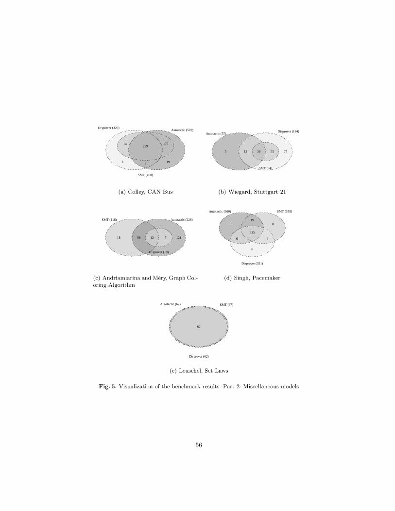
1 6 19

14299

177

Disprover (320)Autotactic (501)

SMT (490)

(a) Colley, CAN Bus

5 13 7739 55

Autotactic (57)Disprover (184)

SMT (94)

(b) Wiegard, Stuttgart 21

18 86 12112 7

SMT (116) Autotactic (226)

Disprover (19)

(c) Andriamiarina and Mery, Graph Col-oring Algorithm

019

0

6

335

4

6

Autotactic (360) SMT (358)

Disprover (351)

(d) Singh, Pacemaker

562

Autotactic (67) SMT (67)

Disprover (62)

(e) Leuschel, Set Laws

Fig. 5. Visualization of the benchmark results. Part 2: Miscellaneous models

56

Return of Experience on Automating Refinement in B

Thierry Lecomte1

1 ClearSy,

Aix en Provence, France

Thierry.lecomte@clearsy.com

Abstract. Refining a B specification into an implementation can be a complex

and time consuming process. This process can usually be separated in two

distinct parts: the specification part, where refinement is used to introduce new

properties and specification details, and the implementation, where refinement

is used to convert a detailed B specification into a B0 implementation. This

article presents experience on the development and use of a refiner tool that

automates the production of implementable models, in a number of industrial

applications.

Keywords: B formal method, refinement, deployment, industry

1 Introduction

Historically, the B Method [1] was introduced in the late 80’s to design correct by

construction, safe software. B and Atelier B1, the tool implementing it, have been

successfully applied to the industry of transportation with the development of large

size embedded software [2], [3], [4], [10] and to a lesser extent to other application

domains [5], [7], [11], [12], [13], [15], [16]. Based on the notion of refinement, the B

method allows writing software specification and implementation by using the same

formal language. Specification is progressively transformed (refined) into

implementation by adding algorithmic details and/or transforming abstract data types

into concrete (implementable) ones. If the specification is the result of a purely human

activity, the refinement process could be automated as it consists in a sequence of

transformations applied to the specification in order to obtain an implementable

model.

In this article, we expose our return of experience on applying automatic

refinement in industry, through a number of industrial applications. In section 2, an

overview of refinement in B is given. Automatic refinement key concepts and tooling

are presented in section 3. Section 4 exposes industrial applications of automatic

refinement. Finally section 5 concludes and discusses further work.

1 http://www.atelierb.eu/

57

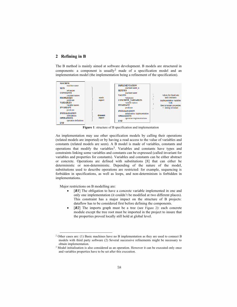
2 Refining in B

The B method is mainly aimed at software development. B models are structured in

components: a component is usually2 made of a specification model and an

implementation model (the implementation being a refinement of the specification).

Figure 1: structure of B specification and implementation

An implementation may use other specification models by calling their operations

(related models are imported) or by having a read access to the value of variables and

constants (related models are seen). A B model is made of variables, constants and

operations that modify the variables3. Variables and constants have types and

constraints linking some variables and constants can be expressed (called invariant for

variables and properties for constants). Variables and constants can be either abstract

or concrete. Operations are defined with substitutions [8] that can either be

deterministic or non-deterministic. Depending of the nature of the model,

substitutions used to describe operations are restricted: for example, sequencing is

forbidden in specifications, as well as loops, and non-determinism is forbidden in

implementations.

Major restrictions on B modelling are:

[R1] The obligation to have a concrete variable implemented in one and

only one implementation (it couldn’t be modified at two different places).

This constraint has a major impact on the structure of B projects:

dataflow has to be considered first before defining the components.

[R2] The imports graph must be a tree (see Figure 2): each concrete

module except the tree root must be imported in the project to insure that

the properties proved locally still hold at global level.

2 Other cases are: (1) Basic machines have no B implementation as they are used to connect B

models with third party software (2) Several successive refinements might be necessary to

obtain implementation. 3 Model initialisation is also considered as an operation. However it can be executed only once

and variables properties have to be set after this execution.

58

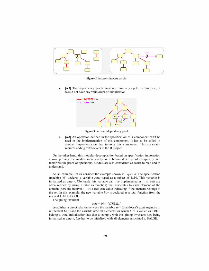
Figure 2: incorrect imports graphs

[R3] The dependency graph must not have any cycle. In this case, it

would not have any valid order of initialisation.

Figure 3: incorrect dependency graph

[R4] An operation defined in the specification of a component can’t be

used in the implementation of this component. It has to be called in

another implementation that imports this component. This constraint

requires adding extra-layers in the B project.

On the other hand, this modular decomposition based on specification importation

allows proving the models more easily as it breaks down proof complexity and

factorizes the proof of operations. Models are also considered as easier to read and to

understand.

As an example, let us consider the example shown in Figure 4. The specification

(machine M) declares a variable setv, typed as a subset of 1..10. This variable is

initialized as empty. Obviously this variable can’t be implemented as it is. Sets are

often refined by using a table (a function) that associates to each element of the

domain (here the interval 1..10) a Boolean value indicating if the element belongs to

the set. In this example, the new variable bitv is declared as a total function from the

interval 1..10 to BOOL.

The gluing invariant

setv = bitv-1[{TRUE}]

establishes a direct relation between the variable setv (that doesn’t exist anymore in

refinement M_r) and the variable bitv: all elements for which bitv is valued as TRUE

belong to setv. Initialisation has also to comply with this gluing invariant: setv being

initialised as empty, bitv has to be initialised with all elements associated to FALSE.

59

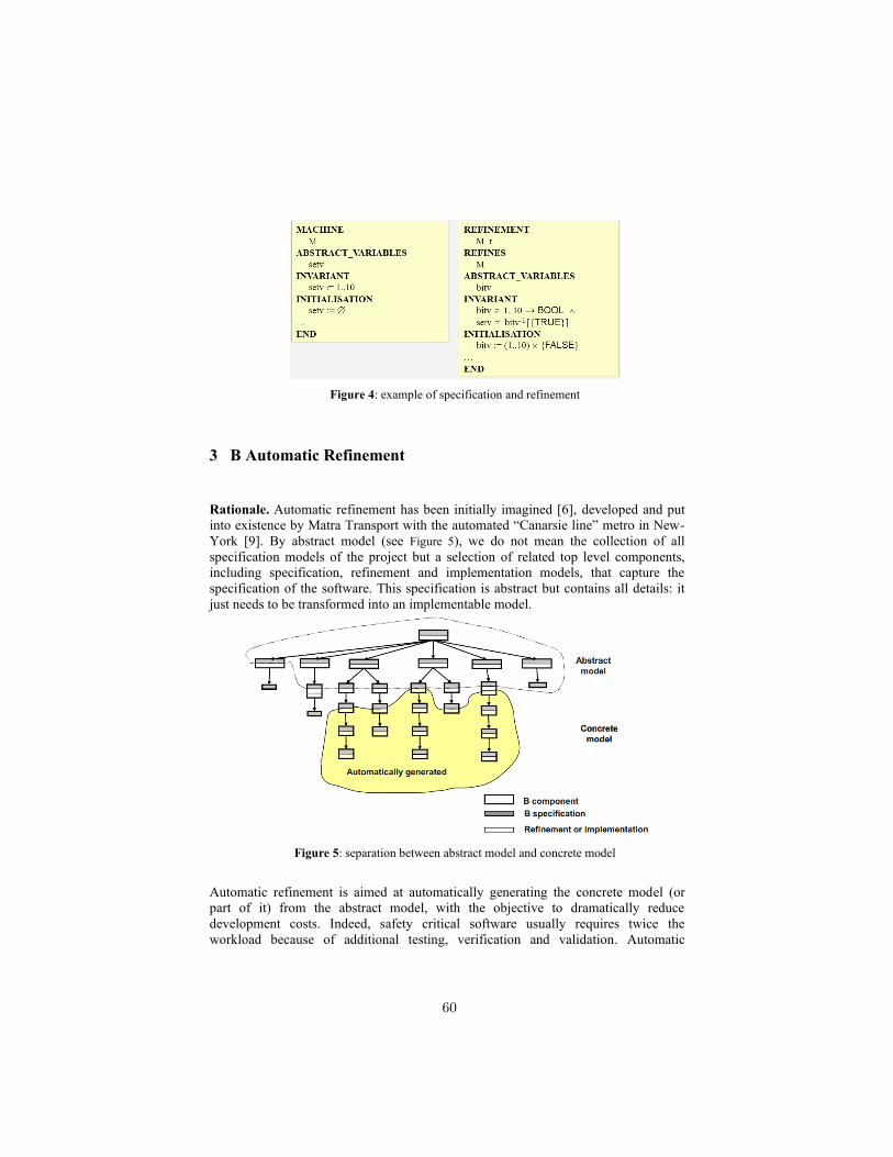
Figure 4: example of specification and refinement

3 B Automatic Refinement

Rationale. Automatic refinement has been initially imagined [6], developed and put

into existence by Matra Transport with the automated “Canarsie line” metro in New-

York [9]. By abstract model (see Figure 5), we do not mean the collection of all

specification models of the project but a selection of related top level components,

including specification, refinement and implementation models, that capture the

specification of the software. This specification is abstract but contains all details: it

just needs to be transformed into an implementable model.

Figure 5: separation between abstract model and concrete model

Automatic refinement is aimed at automatically generating the concrete model (or

part of it) from the abstract model, with the objective to dramatically reduce

development costs. Indeed, safety critical software usually requires twice the

workload because of additional testing, verification and validation. Automatic

60

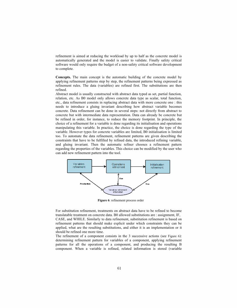
refinement is aimed at reducing the workload by up to half as the concrete model is

automatically generated and the model is easier to validate. Finally safety critical

software would only require the budget of a non-safety critical software development

to complete.

Concepts. The main concept is the automatic building of the concrete model by

applying refinement patterns step by step, the refinement patterns being expressed as

refinement rules. The data (variables) are refined first. The substitutions are then

refined.

Abstract model is usually constructed with abstract data typed as set, partial function,

relation, etc. As B0 model only allows concrete data type as scalar, total function,

etc., data refinement consists in replacing abstract data with more concrete one : this

needs to introduce a gluing invariant describing how abstract variable becomes

concrete. Data refinement can be done in several steps: not directly from abstract to

concrete but with intermediate data representation. Data can already be concrete but

be refined in order, for instance, to reduce the memory footprint. In principle, the

choice of a refinement for a variable is done regarding its initialisation and operations

manipulating this variable. In practice, the choice is done regarding the type of the

variable. However types for concrete variables are limited, B0 initialisation is limited

too. To automate the data refinement, refinement patterns are given describing the

constraints that have to be fulfilled by refined data, the introduced refining variable,

and gluing invariant. Then the automatic refiner chooses a refinement pattern

regarding the properties of the variables. This choice can be modified by the user who

can add new refinement pattern into the tool.

Figure 6: refinement process order

For substitution refinement, treatments on abstract data have to be refined to become

translatable treatment on concrete data. B0 allowed substitutions are : assignment, IF,

CASE, and WHILE. Similarly to data refinement, substitution refinement is based on

refinement patterns that should make explicit under which constraints they can be

applied, what are the resulting substitutions, and either it is an implementation or it

should be refined one more time.

The refinement of a component consists in the 3 successive actions (see Figure 6):

determining refinement pattern for variables of a component, applying refinement

patterns for all the operations of a component, and producing the resulting B

component. When a variable is refined, related information is stored (variable

61

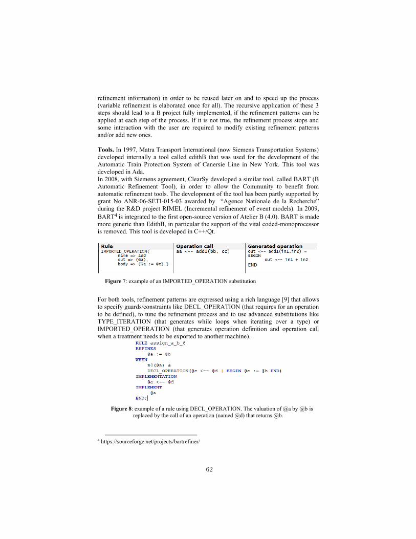
refinement information) in order to be reused later on and to speed up the process

(variable refinement is elaborated once for all). The recursive application of these 3

steps should lead to a B project fully implemented, if the refinement patterns can be

applied at each step of the process. If it is not true, the refinement process stops and

some interaction with the user are required to modify existing refinement patterns

and/or add new ones.

Tools. In 1997, Matra Transport International (now Siemens Transportation Systems)

developed internally a tool called edithB that was used for the development of the

Automatic Train Protection System of Canersie Line in New York. This tool was

developed in Ada.

In 2008, with Siemens agreement, ClearSy developed a similar tool, called BART (B

Automatic Refinement Tool), in order to allow the Community to benefit from

automatic refinement tools. The development of the tool has been partly supported by

grant No ANR-06-SETI-015-03 awarded by “Agence Nationale de la Recherche”

during the R&D project RIMEL (Incremental refinement of event models). In 2009,

BART4 is integrated to the first open-source version of Atelier B (4.0). BART is made

more generic than EdithB, in particular the support of the vital coded-monoprocessor

is removed. This tool is developed in C++/Qt.

Figure 7: example of an IMPORTED_OPERATION substitution

For both tools, refinement patterns are expressed using a rich language [9] that allows

to specify guards/constraints like DECL_OPERATION (that requires for an operation

to be defined), to tune the refinement process and to use advanced substitutions like

TYPE_ITERATION (that generates while loops when iterating over a type) or

IMPORTED_OPERATION (that generates operation definition and operation call

when a treatment needs to be exported to another machine).

Figure 8: example of a rule using DECL_OPERATION. The valuation of @a by @b is

replaced by the call of an operation (named @d) that returns @b.

4 https://sourceforge.net/projects/bartrefiner/

62

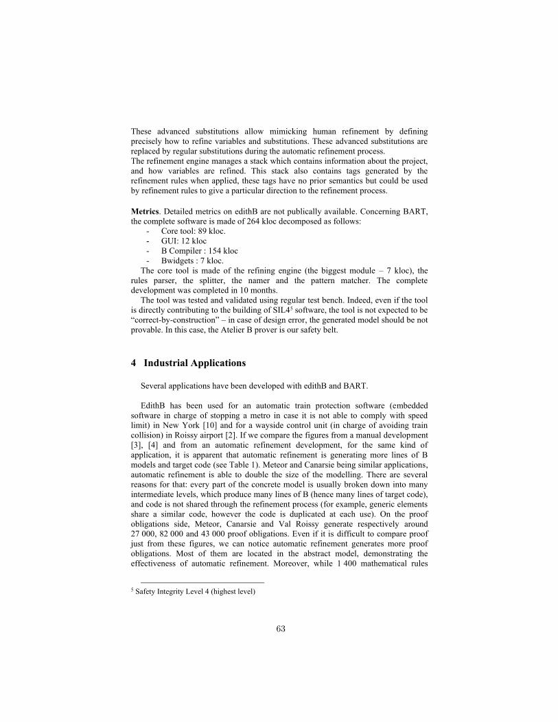
These advanced substitutions allow mimicking human refinement by defining

precisely how to refine variables and substitutions. These advanced substitutions are

replaced by regular substitutions during the automatic refinement process.

The refinement engine manages a stack which contains information about the project,

and how variables are refined. This stack also contains tags generated by the

refinement rules when applied, these tags have no prior semantics but could be used

by refinement rules to give a particular direction to the refinement process.

Metrics. Detailed metrics on edithB are not publically available. Concerning BART,

the complete software is made of 264 kloc decomposed as follows:

- Core tool: 89 kloc.

- GUI: 12 kloc

- B Compiler : 154 kloc

- Bwidgets : 7 kloc.

The core tool is made of the refining engine (the biggest module – 7 kloc), the

rules parser, the splitter, the namer and the pattern matcher. The complete

development was completed in 10 months.

The tool was tested and validated using regular test bench. Indeed, even if the tool

is directly contributing to the building of SIL45 software, the tool is not expected to be

“correct-by-construction” – in case of design error, the generated model should be not

provable. In this case, the Atelier B prover is our safety belt.

4 Industrial Applications

Several applications have been developed with edithB and BART.

EdithB has been used for an automatic train protection software (embedded

software in charge of stopping a metro in case it is not able to comply with speed

limit) in New York [10] and for a wayside control unit (in charge of avoiding train

collision) in Roissy airport [2]. If we compare the figures from a manual development

[3], [4] and from an automatic refinement development, for the same kind of

application, it is apparent that automatic refinement is generating more lines of B

models and target code (see Table 1). Meteor and Canarsie being similar applications,

automatic refinement is able to double the size of the modelling. There are several

reasons for that: every part of the concrete model is usually broken down into many

intermediate levels, which produce many lines of B (hence many lines of target code),

and code is not shared through the refinement process (for example, generic elements

share a similar code, however the code is duplicated at each use). On the proof

obligations side, Meteor, Canarsie and Val Roissy generate respectively around

27 000, 82 000 and 43 000 proof obligations. Even if it is difficult to compare proof

just from these figures, we can notice automatic refinement generates more proof

obligations. Most of them are located in the abstract model, demonstrating the

effectiveness of automatic refinement. Moreover, while 1 400 mathematical rules

5 Safety Integrity Level 4 (highest level)

63

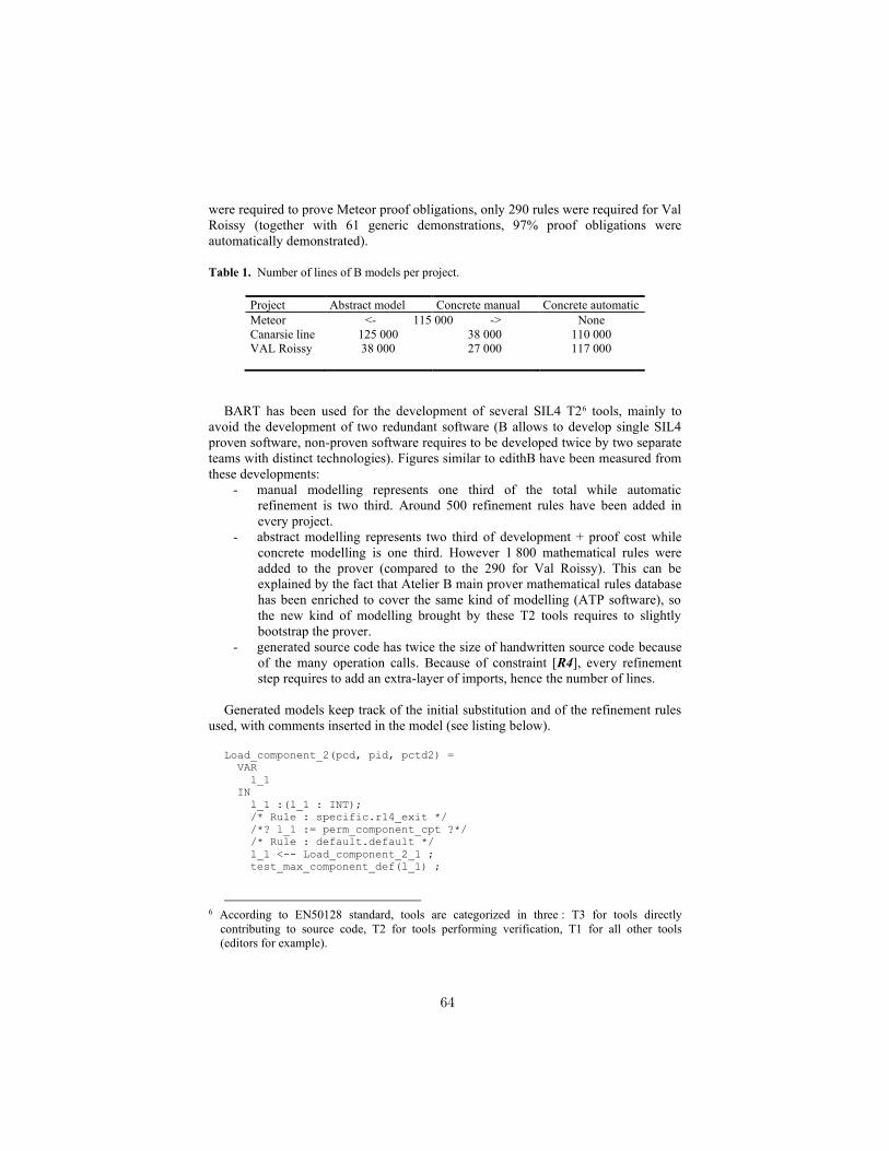
were required to prove Meteor proof obligations, only 290 rules were required for Val

Roissy (together with 61 generic demonstrations, 97% proof obligations were

automatically demonstrated).

Table 1. Number of lines of B models per project.

Project Abstract model Concrete manual Concrete automatic

Meteor <- 115 000 -> None

Canarsie line 125 000 38 000 110 000

VAL Roissy 38 000 27 000 117 000

BART has been used for the development of several SIL4 T26 tools, mainly to

avoid the development of two redundant software (B allows to develop single SIL4

proven software, non-proven software requires to be developed twice by two separate

teams with distinct technologies). Figures similar to edithB have been measured from

these developments:

- manual modelling represents one third of the total while automatic

refinement is two third. Around 500 refinement rules have been added in

every project.

- abstract modelling represents two third of development + proof cost while

concrete modelling is one third. However 1 800 mathematical rules were

added to the prover (compared to the 290 for Val Roissy). This can be

explained by the fact that Atelier B main prover mathematical rules database

has been enriched to cover the same kind of modelling (ATP software), so

the new kind of modelling brought by these T2 tools requires to slightly

bootstrap the prover.

- generated source code has twice the size of handwritten source code because

of the many operation calls. Because of constraint [R4], every refinement

step requires to add an extra-layer of imports, hence the number of lines.

Generated models keep track of the initial substitution and of the refinement rules

used, with comments inserted in the model (see listing below).

Load_component_2(pcd, pid, pctd2) =

VAR

l_1

IN

l_1 :(l_1 : INT);

/* Rule : specific.r14_exit */

/*? l_1 := perm_component_cpt ?*/

/* Rule : default.default */

l_1 <-- Load_component_2_1 ;

test_max_component_def(l_1) ;

6 According to EN50128 standard, tools are categorized in three : T3 for tools directly

contributing to source code, T2 for tools performing verification, T1 for all other tools

(editors for example).

64

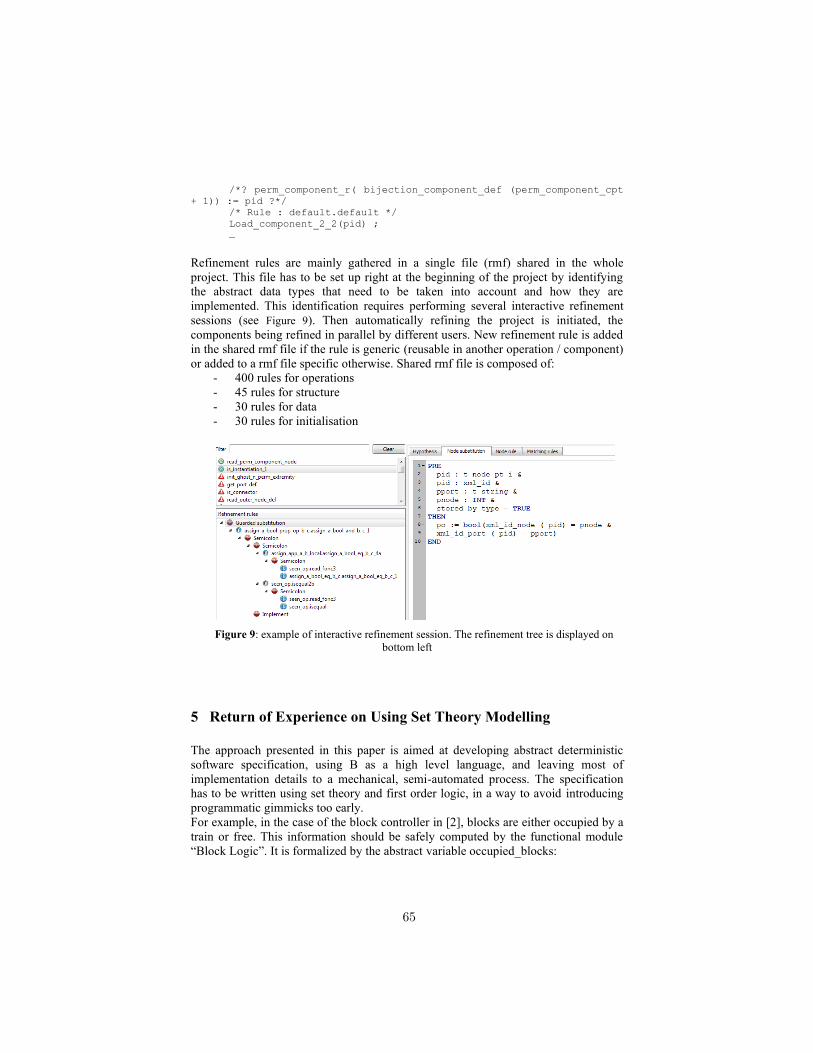
/*? perm_component_r( bijection_component_def (perm_component_cpt

+ 1)) := pid ?*/

/* Rule : default.default */

Load_component_2_2(pid) ;

…

Refinement rules are mainly gathered in a single file (rmf) shared in the whole

project. This file has to be set up right at the beginning of the project by identifying

the abstract data types that need to be taken into account and how they are

implemented. This identification requires performing several interactive refinement

sessions (see Figure 9). Then automatically refining the project is initiated, the

components being refined in parallel by different users. New refinement rule is added

in the shared rmf file if the rule is generic (reusable in another operation / component)

or added to a rmf file specific otherwise. Shared rmf file is composed of:

- 400 rules for operations

- 45 rules for structure

- 30 rules for data

- 30 rules for initialisation

Figure 9: example of interactive refinement session. The refinement tree is displayed on

bottom left

5 Return of Experience on Using Set Theory Modelling

The approach presented in this paper is aimed at developing abstract deterministic

software specification, using B as a high level language, and leaving most of

implementation details to a mechanical, semi-automated process. The specification

has to be written using set theory and first order logic, in a way to avoid introducing

programmatic gimmicks too early.

For example, in the case of the block controller in [2], blocks are either occupied by a

train or free. This information should be safely computed by the functional module

“Block Logic”. It is formalized by the abstract variable occupied_blocks:

65

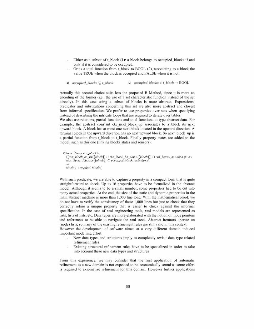
- Either as a subset of t_block (1): a block belongs to occupied_blocks if and

only if it is considered to be occupied.

- Or as a total function from t_block to BOOL (2), associating to a block the

value TRUE when the block is occupied and FALSE when it is not.

Actually this second choice suits less the proposed B Method, since it is more an

encoding of the former (i.e., the use of a set characteristic function instead of the set

directly). In this case using a subset of blocks is more abstract. Expressions,

predicates and substitutions concerning this set are also more abstract and closest

from informal specification. We prefer to use properties over sets when specifying

instead of describing the intricate loops that are required to iterate over tables.

We also use relations, partial functions and total functions to type abstract data. For

example, the abstract constant ctx_next_block_up associates to a block its next

upward block. A block has at most one next block located in the upward direction. A

terminal block in the upward direction has no next upward block. So next_block_up is

a partial function from t_block to t_block. Finally property states are added to the

model, such as this one (linking blocks states and sensors):

With such predicate, we are able to capture a property in a compact form that is quite

straightforward to check. Up to 16 properties have to be formalized in the abstract

model. Although it seems to be a small number, some properties had to be cut into

many actual properties. At the end, the size of the static and dynamic properties in the

main abstract machine is more than 1,000 line long. With the mathematical proof, we

do not have to verify the consistancy of these 1,000 lines but just to check that they

correctly refine a unique property that is easier to check against the informal

specification. In the case of xml engineering tools, xml models are represented as

lists, lists of lists, etc. Data types are more elaborated with the notion of node pointers

and references to be able to navigate the xml trees. Abstract iterators operate on

(node) lists, so many of the existing refinement rules are still valid in this context.

However the development of software aimed at a very different domain induced

important modelling effort:

- New data types and structures imply to completely revisit data type related

refinement rules

- Existing structural refinement rules have to be specialized in order to take

into account these new data types and structures

From this experience, we may consider that the first application of automatic

refinement to a new domain is not expected to be economically sound as some effort

is required to axiomatize refinement for this domain. However further applications

66

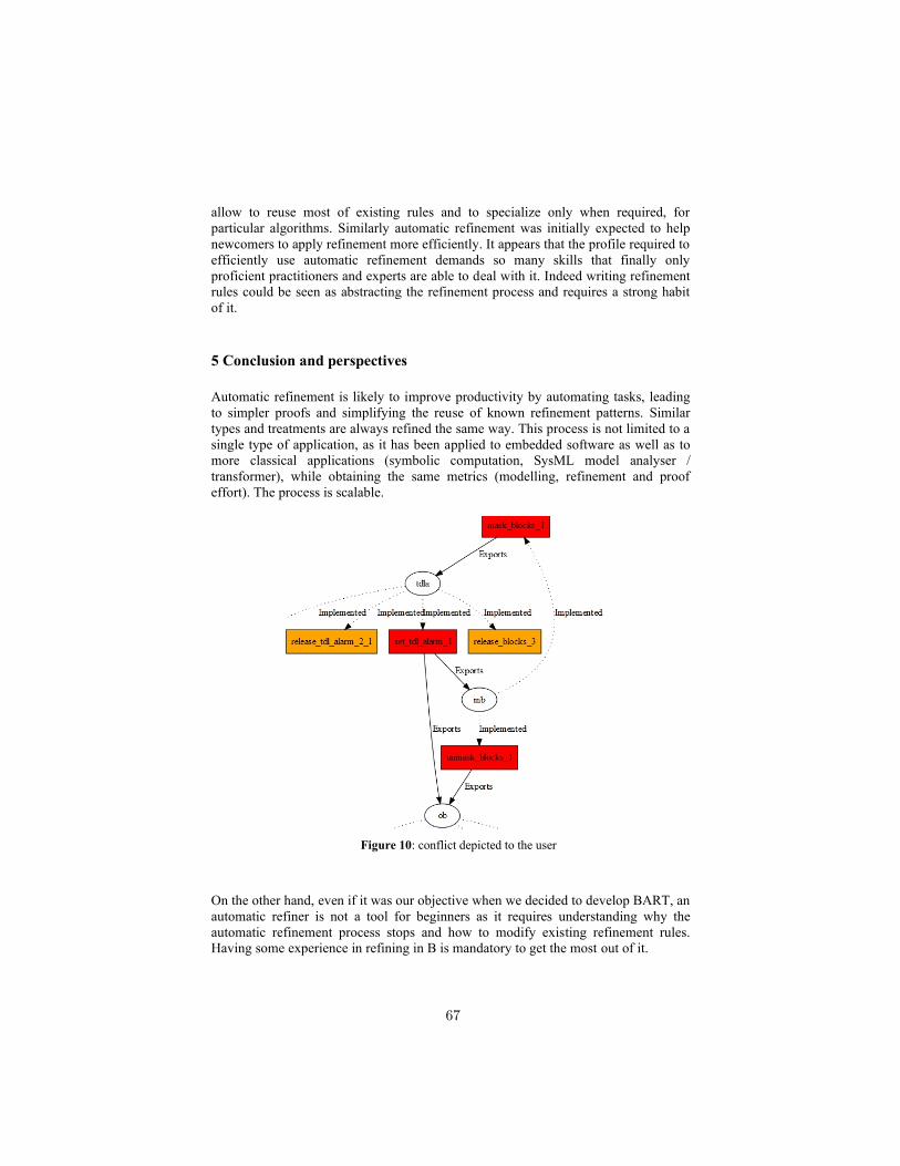
allow to reuse most of existing rules and to specialize only when required, for

particular algorithms. Similarly automatic refinement was initially expected to help

newcomers to apply refinement more efficiently. It appears that the profile required to

efficiently use automatic refinement demands so many skills that finally only

proficient practitioners and experts are able to deal with it. Indeed writing refinement

rules could be seen as abstracting the refinement process and requires a strong habit

of it.

5 Conclusion and perspectives

Automatic refinement is likely to improve productivity by automating tasks, leading

to simpler proofs and simplifying the reuse of known refinement patterns. Similar

types and treatments are always refined the same way. This process is not limited to a

single type of application, as it has been applied to embedded software as well as to

more classical applications (symbolic computation, SysML model analyser /

transformer), while obtaining the same metrics (modelling, refinement and proof

effort). The process is scalable.

Figure 10: conflict depicted to the user

On the other hand, even if it was our objective when we decided to develop BART, an

automatic refiner is not a tool for beginners as it requires understanding why the

automatic refinement process stops and how to modify existing refinement rules.

Having some experience in refining in B is mandatory to get the most out of it.

67

Constraint [R1] is posing a problem to existing refinement algorithms: in case of

conflicting rules, a single variable could be implemented in different components at

the same time that is rejected by Atelier B project checker. We are currently working

on improving these algorithms in order to not apply conflicting rules and to provide

some guidance to the user (interaction with user still remains to be decided). Current

feedback is provided as an implementation graph exhibiting exports and implemented

constraints. In Figure 10, we can clearly see a cycle (the upward arrow from variable

mb to component mask_blocks_1). The art of the automatic refinement is today to

understand from this graph how to modify refinement rules in order to solve these

conflicts.

We are also investigating the possibility to “prove” refinement rules in order to

consider that related proof obligations are “by construction” already proven. We are

using an approach similar to the Atelier B main prover: the inference engine is based

on transformation rules that have been formally proven, hence the successive

application of these rules to solve a predicate is considered correct and the predicate is

considered true.

References

1. Abrial, J.R. (1996) , The B-book: Assigning programs to meanings, Cambridge University

Press

2. Amelot, A. & al (2005), Using B as a High Level Programming Language in an Industrial

Project: Roissy VAL, ZB 2005

3. Behm, P. & al (1998), METEOR: an Industrial Success in Formal Development, B’98

4. Behm, P. & al (1999), METEOR: a Successful Application of B in a Large Project, FM’99

5. Benveniste, M. & al (2009), A Proved “Correct by Construction” Realistic Digital

Circuit, RIAB, FMWeek 2009

6. Burdy, L.(1996) , Automatic Refinement. In Proceedings of BUGM at FM'99

7. Casset, L.,(1999) A formal specification of the Java byte code verifier using the B method,

Lisbonne 99

8. ClearSy (2014), Atelier B: B language Reference Manual

9. ClearSy (2014), BART: User Manual

10. Essamé, D. & al (2007), B in Large-Scale Projects: the Canarsie Line CBTC Experience,

B 2007

11. Hoffmann, S. & al (2007), The B Method for the Construction of Micro-Kernel Based

Systems, ZB 2007

12. Lecomte, T. (2008), Safe and Reliable Metro Platform Screen Doors Control/Command

Systems, FM 2008

13. Lecomte, T. & al (2007), Formal Methods in Safety Critical Railway Systems, SBMF 2007

14. Requet, A. & al (2008), BART: A Tool for Automatic Refinement, ABZ 2008

15. Sabatier, D. & al (2006), Use of the Formal B Method for a SIL3 System Landing Door

Commands for line 13 of the Paris subway, Lambda Mu 15

16. Sabatier, D. & al (2008), FDIR Strategy Validation with the B method, DASIA 2008

68

Programming with Partially SpecifiedCollections

Gianfranco Rossi

Dipartimento di Matematica e InformaticaUniversita degli Studi di Parma, Parma, Italy

gianfranco.rossi@unipr.it

Abstract. Enumerated collections (e.g. lists, sets, etc.) provided by pro-gramming languages are usually defined by completely and precisely enu-merating all their constituent elements. Conversely, in (constraint) logicprogramming languages it is common to deal with partially specified col-lections where either some elements or some parts of the collection are leftunknown. In this paper we claim that partially specified collections (inparticular, lists and sets) can be conveniently exploited in a wider setting,even in the context of more conventional languages using a library-basedapproach. We prove this claim by showing a number of simple examplesusing Java and the Java library JSetL.

1 Introduction

Programming languages usually provide several kinds of collections, e.g. array,string, lists, sets, multi-sets, maps, etc, either as primitive abstractions or pro-grammed by exploiting the data abstraction facilities of the language itself andmade available to users as standard libraries. For example, sets are a primi-tive data abstraction in Pascal, SETL and Python, while they are provided aslibraries in C++ and Java.

In this paper we will restrict our attention to enumerated collections only,that is collections designated by explicitly enumerating its constituting elements.Hereafter the term collection implicitly refers to enumerated collections.

In imperative programming languages collections need to be always com-pletely specified whenever we operate on them. This means that all elements ofa collection must be provided and they must have known values. For example,using the interface Set of java.util, the set {1, 3, 0} can be constructed byexecuting the statements

s.add(0); s.add(3); s.add(1);

where s is an object denoting the empty set which can be defined asSet s = new HashSet();

and HashSet is one of the implementations of the interface Set provided byjava.util. Note that the requirement to be completely specified does not pre-vent a collection from containing variables, but whenever the collection needsto be evaluated all variables possibly occurring in it must be replaced by theiractual values.

69

In contrast, collections in declarative programming languages, such as listsin Prolog, are allowed to contain unknown elements and to be only partiallyspecified, and, nevertheless, they can be accessed and manipulated. For instance,the Prolog predicate [a,b,c] = [X,Y|R] compares the (completely specified)list of three elements, a, b, and c, with the partially specified list containingtwo unknown elements X and Y and an unknown remainder part R (i.e., any listcontaining at least two elements).

Usefulness of partially specified collections has been amply demonstrated inthe context of declarative programming languages. In particular, programmingwith partially specified lists is a well-assessed technique in standard logic pro-gramming languages. Partially specified sets, instead, are supplied by extendedlogic programming languages with sets, such as [6, 7, 5], and are shown to bea powerful data abstraction. Usefulness of partially specified sets is advocatedalso in specific application areas such as deductive databases, computationallinguistics, and knowledge representation.

Aim of this paper is to show that partially specified collections can be conve-niently exploited also in a more conventional setting, namely an imperative O-Oprogramming language. In particular, we consider a library-based approach wherethe new data abstractions are defined by using the language data abstractionmechanisms, without requiring any extension of the host language.

We prove our claim by presenting a number of simple examples written inJava using JSetL [19], a general-purpose library that supports partially specifiedlists and sets, within the O-O language Java. JSetL integrates the notions oflogical (or constrained) variable, (set) unification and constraints that are typicalof constraint logic programming languages into the Java language. In particular,it allows logical variables to occur in list and set data structures and providesoperations to deal with such objects.

The presented examples aim at showing, in particular, how partially specifiedlists and sets can be exploited for:

– supporting a declarative programming style– providing data modelling tools (in particular sets and set unification) which

prove to be particularly suitable for problems involving non-determinism– supporting constraint programming.

It is important to note that our main concern here is on providing modellingand programming support. Conversely we are only relatively little interestedin the efficiency issue (e.g., efficiency of the constraint solver). Furthermore,our focus is on programming rather than on constraint solving or satisfiabilitychecking of formulas involving partially specified collections.

Though our discussion is limited to lists and sets, similar considerations couldapply to other kinds of collections as well. Moreover, though we are focusing onJava, the same considerations could be easily exported to other O-O languages(such as C++) where these data abstractions could be supplied by libraries,while they can serve as useful guidelines to devise extensions to programminglanguages where these new data abstractions could be provided as primitiveones.

70

The paper is organized as follows. Section 2 introduces the notion of partiallyspecified collection, showing how logical variables can be used within collectionsto represent unknown elements or part of the collection. In Section 3 we startconsidering operations on partially specified collections, specifically (set) uni-fication. In Section 4 we show how simple inequality, membership and integercomparison constraints over elements of partially specified collections can beused to describe and compute solutions for a number of common programmingproblems. Section 5 takes into account also set variables, whose domains are col-lections of sets, and it briefly shows how set variables and set constraints can beadvantageously exploited in conjunction with partially specified sets. Sections 6and 7 are devoted to further remarks and to draw some conclusion.1

2 Partially Specified Collections

Declarative programming languages (e.g., functional and logic programming lan-guages) are based on a notion of variable, often called logical (or mathematicalvariables, constrained) variable, that differs from that of imperative program-ming languages. Logical variables represent unknowns, not memory cells. Assuch they have no modifiable value stored in them, as ordinary programminglanguage variables have. Conversely, one can associate values to logical variablesthrough relations (or constraints) involving logical variables and values fromsome specific domains.

When the domain of a (logical) variable is restricted to a single value thenthe variable is said to be bound (or instantiated) to this value. Otherwise, thevariable is unbound. An equality relation, in particular, may restrict the domainof a logical variable to a single value. For example, if x is a logical variableranging over the domain of integers, the equality x = 3 forces x to be bound tothe value 3. However, the same result could be obtained through other relations,e.g., x < 4 ∧ x > 2. The value of a logical variable is immutable. That is it cannot be changed, e.g. by an assignment statement like in imperative languages.

Logical variables are found also in conventional programming languages thatsupport constraint programming (e.g., Alma-0 [1]), as well as in libraries forconstraint programming, such as ILOG [13] and Choco [3] (see also the recentJava Specification Request for a standard Java Constraint Programming API[14]).

In this paper we will refer to what is provided by JSetL [19], a Java librarythat supports declarative (constraint) programming in an O-O framework. InJSetL a (generic) logical variable is an instance of the class LVar. Basically, LVarobjects can be manipulated through constraints, namely equality (eq), inequality(neq), membership (in) and not membership (nin) constraints. Moreover thelibrary provides methods to test whether a variable is bound or not, to get thevalue of a bound variable (but not to modify it), to get its external name, andso on. Values associated with generic logical variables can be of any type. For

1 An extended version of this paper appeared in Computer Languages, Systems &Structures, Elsevier, vol. 37/4, 178-192, 2011

71

some specific domains, however, JSetL offers specializations of the LVar datatype, which provide further specific constraints. In particular, for the domainof integers, JSetL offers the class IntLVar, which extends LVar with a numberof new methods and constraints specific for integers. In particular, IntLVar

provides integer comparison constraints such as <, ≤, etc.Other important specializations of logical variables are the class LCollection

and its derived subclasses, LSet (for Logical Sets) and LList (for Logical Lists).Values associated with LSet (LList) are objects of the java.util class Set

(List). A number of constraints are provided to work with LSet (LList), whichextend those provided by LVar. In particular, LSet provides equality and in-equality constraints that account for the semantic properties of sets (namely, ir-relevance of order and duplication of elements); moreover it provides constraintsfor many of the standard set-theoretical operations, such as union, intersection,set difference, and so on.

Example 1. Logical lists/sets in JSetL.

LVar x = new LVar(); // an unbound logical variableLVar y = new LVar("y",1); // a bound logical variable

// with external name "y" and value 1

LList ll = new LList(); // an unbound logical listLSet ls 1 = new LSet(); // an unbound logical set

A collection where either some elements, or part of the collection itself, areunbound logical variables represents a partially specified collection. For example(using a Prolog-like notion), the list [1,X,Y], where X and Y are unbound logicalvariables, denotes a partially specified list containing one known element 1 andtwo unknown elements, denoted X and Y. As another example, the list [1,2|Z],where Z is an unbound logical list (i.e., a logical variable ranging over the domainof lists), designates an open list containing two known elements 1 and 2 and anunknown remainder part denoted by Z.

A partially specified set (list) can be created in JSetL by adding possiblyunknown elements, i.e., unbound LVar objects, to either a known or an unknownset (list) using the element insertion operator ins.

Example 2. The two partially specified lists [1,X,Y] and [1,2|Z] can be definedin JSetL as follows:

LVar X = new LVar();

LVar Y = new LVar();

LList cl = // the closed p.s. listLList.empty().ins(Y).ins(X).ins(1); // [1,X,Y]

and

LList Z = new LList(); // the open p.s. listLList ol = Z.ins(2).ins(1); // [1,2 |Z]

JSetL provides a number of facilities, mainly in the form of constraints, toaccess and manipulate partially specified lists/sets (e.g., unification). Conversely,

72

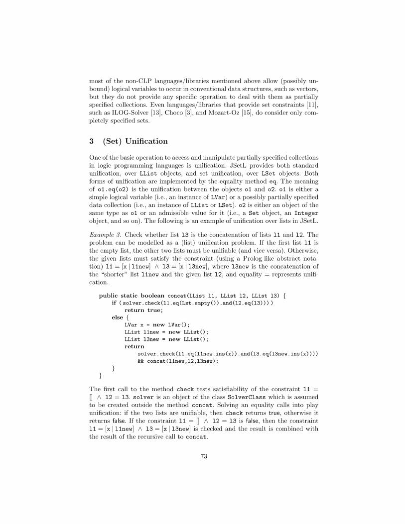
most of the non-CLP languages/libraries mentioned above allow (possibly un-bound) logical variables to occur in conventional data structures, such as vectors,but they do not provide any specific operation to deal with them as partiallyspecified collections. Even languages/libraries that provide set constraints [11],such as ILOG-Solver [13], Choco [3], and Mozart-Oz [15], do consider only com-pletely specified sets.

3 (Set) Unification

One of the basic operation to access and manipulate partially specified collectionsin logic programming languages is unification. JSetL provides both standardunification, over LList objects, and set unification, over LSet objects. Bothforms of unification are implemented by the equality method eq. The meaningof o1.eq(o2) is the unification between the objects o1 and o2. o1 is either asimple logical variable (i.e., an instance of LVar) or a possibly partially specifieddata collection (i.e., an instance of LList or LSet). o2 is either an object of thesame type as o1 or an admissible value for it (i.e., a Set object, an Integer

object, and so on). The following is an example of unification over lists in JSetL.

Example 3. Check whether list l3 is the concatenation of lists l1 and l2. Theproblem can be modelled as a (list) unification problem. If the first list l1 isthe empty list, the other two lists must be unifiable (and vice versa). Otherwise,the given lists must satisfy the constraint (using a Prolog-like abstract nota-tion) l1 = [x | l1new] ∧ l3 = [x | l3new], where l3new is the concatenation ofthe “shorter” list l1new and the given list l2, and equality = represents unifi-cation.

public static boolean concat(LList l1, LList l2, LList l3) {if ( solver.check(l1.eq(Lst.empty()).and(l2.eq(l3))) )

return true;else {

LVar x = new LVar();

LList l1new = new LList();

LList l3new = new LList();

returnsolver.check(l1.eq(l1new.ins(x)).and(l3.eq(l3new.ins(x))))

&& concat(l1new,l2,l3new);

}}

The first call to the method check tests satisfiability of the constraint l1 =[] ∧ l2 = l3. solver is an object of the class SolverClass which is assumedto be created outside the method concat. Solving an equality calls into playunification: if the two lists are unifiable, then check returns true, otherwise itreturns false. If the constraint l1 = [] ∧ l2 = l3 is false, then the constraintl1 = [x | l1new] ∧ l3 = [x | l3new] is checked and the result is combined withthe result of the recursive call to concat.

73

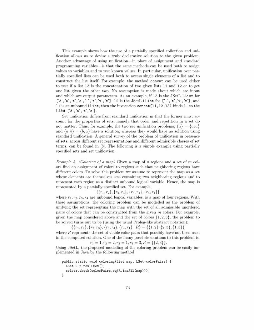
This example shows how the use of a partially specified collection and uni-fication allows us to devise a truly declarative solution to the given problem.Another advantage of using unification—in place of assignment and standardprogramming variables—is that the same methods can be used both to assignvalues to variables and to test known values. In particular, unification over par-tially specified lists can be used both to access single elements of a list and toconstruct the list itself. For example, the method concat can be used eitherto test if a list l3 is the concatenation of two given lists l1 and l2 or to getone list given the other two. No assumption is made about which are inputand which are output parameters. As an example, if l3 is the JSetL LList for[’d’,’a’,’t’,’a’,’.’,’t’,’x’,’t’], l2 is the JSetL LList for [’.’,’t’,’x’,’t’], andl1 is an unbound LList, then the invocation concat(l1,l2,l3) binds l1 to theLList [’d’,’a’,’t’,’a’].

Set unification differs from standard unification in that the former must ac-count for the properties of sets, namely that order and repetition in a set donot matter. Thus, for example, the two set unification problems, {a} = {a, a}and {a, b} = {b, a} have a solution, whereas they would have no solution usingstandard unification. A general survey of the problem of unification in presenceof sets, across different set representations and different admissible classes of setterms, can be found in [8]. The following is a simple example using partiallyspecified sets and set unification.

Example 4. (Coloring of a map) Given a map of n regions and a set of m col-ors find an assignment of colors to regions such that neighboring regions havedifferent colors. To solve this problem we assume to represent the map as a setwhose elements are themselves sets containing two neighboring regions and torepresent each region as a distinct unbound logical variable. Hence, the map isrepresented by a partially specified set. For example,

{{r1, r2}, {r2, r3}, {r3, r4}, {r4, r1}}where r1, r2, r3, r4 are unbound logical variables, is a map of four regions. Withthese assumptions, the coloring problem can be modelled as the problem ofunifying the set representing the map with the set of all admissible unorderedpairs of colors that can be constructed from the given m colors. For example,given the map considered above and the set of colors {1, 2, 3}, the problem tobe solved turns out to be (using the usual Prolog-like abstract notation):

{{r1, r2}, {r2, r3}, {r3, r4}, {r4, r1} |R} = {{1, 2}, {2, 3}, {1, 3}}where R represents the set of viable color pairs that possibly have not been usedin the computed solution. One of the many possible solutions to this problem is:

r1 = 1, r2 = 2, r3 = 1, r4 = 3, R = {{2, 3}}.Using JSetL, the proposed modelling of the coloring problem can be easily im-plemented in Java by the following method:

public static void coloring(LSet map, LSet colorPairs) {

LSet R = new LSet();

solver.check(colorPairs.eq(R.insAll(map)));

}

74

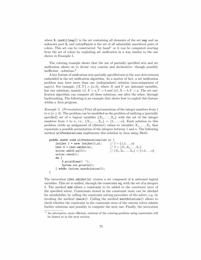
where R.insAll(map)) is the set containing all elements of the set map and anunknown part R, and colorPairs is the set of all admissible unordered pairs ofcolors. This set can be constructed “by hand” or it can be computed startingfrom the set of colors by exploiting set unification in a way similar to the oneshown in Example 5.

The coloring example shows that the use of partially specified sets and setunification allows us to devise very concise and declarative—though possiblyinefficient—solutions.2

A key feature of unification over partially specified sets is the non-determinismembedded in the set unification algorithm. As a matter of fact, a set unificationproblem may have more than one (independent) solution (non-uniqueness ofmgu’s). For example, {X,Y } = {a, b}, where X and Y are unbound variables,has two solutions, namely (i) X = a, Y = b and (ii) X = b, Y = a. The set uni-fication algorithm can compute all these solutions, one after the other, throughbacktracking. The following is an example that shows how to exploit this featurewithin a Java program.

Example 5. (Permutations) Print all permutations of the integer numbers from 1to n (n ≥ 0). The problem can be modelled as the problem of unifying a (partiallyspecified) set of n logical variables {X1, . . . , Xn} with the set of the integernumbers from 1 to n, i.e., {X1, . . . , Xn} = {1, . . . , n}. Each solution to thisproblem yields an assignment of (distinct) values to variables X1, . . . , Xn thatrepresents a possible permutation of the integers between 1 and n. The followingmethod allPermutations implements this solution in Java using JSetL.

public static void allPermutations(int n) {IntLSet I = new IntLSet(1,n); // I = {1,2,. . . ,n}LSet S = LSet.mkLSet(n); // S = {X1,X2,. . . ,Xn}solver.add(S.eq(I)); // {X1,X2,. . . ,Xn} = {1,2,. . . ,n}solver.check();

do {S.printElems(’ ’);

System.out.println();

} while (solver.nextSolution());

}

The invocation LSet.mkLSet(n) creates a set composed of n unbound logicalvariables. This set is unified, through the constraint eq, with the set of n integersI. The method add allows a constraint to be added to the constraint store ofthe specified solver. Constraints stored in the constraint store can be checkedfor satisfiability by calling the constraint solving procedure of the solver, e.g. byinvoking the method check(). Calling the method nextSolution() allows tocheck whether the constraint in the constraint store of the current solver admitsfurther solutions and possibly to compute the next one. Finally, the invocation

2 An alternative, more efficient, solution of the coloring problem using constraints willbe hinted at in the next section.

75

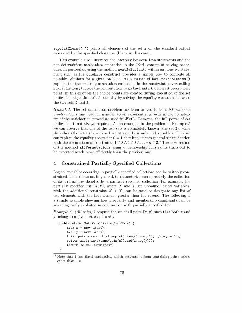
s.printElems(’ ’) prints all elements of the set s on the standard outputseparated by the specified character (blank in this case).

This example also illustrates the interplay between Java statements and thenon-determinism mechanism embedded in the JSetL constraint solving proce-dure. In particular, using the method nextSolution() within an iterative state-ment such as the do while construct provides a simple way to compute allpossible solutions for a given problem. As a matter of fact, nextSolution()

exploits the backtracking mechanism embedded in the constraint solver: callingnextSolution() forces the computation to go back until the nearest open choicepoint. In this example the choice points are created during execution of the setunification algorithm called into play by solving the equality constraint betweenthe two sets I and S.

Remark 1. The set unification problem has been proved to be a NP-completeproblem. This may lead, in general, to an exponential growth in the complex-ity of the satisfaction procedure used in JSetL. However, the full power of setunification is not always required. As an example, in the problem of Example 5we can observe that one of the two sets is completely known (the set I), whilethe other (the set S) is a closed set of exactly n unbound variables. Thus wecan replace the equality constraint S = I that implements general set unificationwith the conjunction of constraints 1 ∈ S∧ 2 ∈ S∧ . . .∧n ∈ S.3 The new versionof the method allPermutations using n membership constraints turns out tobe executed much more efficiently than the previous one.

4 Constrained Partially Specified Collections

Logical variables occurring in partially specified collections can be suitably con-strained. This allows us, in general, to characterize more precisely the collectionof data structures denoted by a partially specified collection. For example, thepartially specified list [X,Y ], where X and Y are unbound logical variables,with the additional constraint X > Y , can be used to designate any list oftwo elements with the first element greater than the second. The following isa simple example showing how inequality and membership constraints can beadvantageously exploited in conjunction with partially specified lists.

Example 6. (All pairs) Compute the set of all pairs [x,y] such that both x andy belong to a given set s and x 6= y.

public static Set<?> allPairs(Set<?> s) {LVar x = new LVar();

LVar y = new LVar();

LList pair = new LList.empty().ins(y).ins(x)); // a pair [x,y]solver.add(x.in(s).and(y.in(s)).and(x.neq(y)));

return solver.setOf(pair);

}3 Note that S has fixed cardinality, which prevents it from containing other values

other than 1..n.

76

The first four statements serve to specify the form of the pairs we are lookingfor: partially specified lists of the form [x,y], with x ∈ s ∧ y ∈ s ∧ x 6= y. Thelast statement calls the method setOf of the current solver which collects in aJava set all the pairs satisfying this specification and returns it as its result.

This example shows an interesting interaction between partially specified col-lections (namely, JSetL logical lists), containing logical variables, and completelyspecified collections (namely, sets and lists of java.util). The latter are usedto contain known values, while the former are used to describe the general formof values to be computed.

The method setOf implements a (limited) form of intensionally defined sets.A set s is defined as the set of all possible values of a variable x for which acondition ϕ, involving x, turns out to be satisfied, i.e. s = {x : ϕ}. If ϕ isrepresented as a JSetL constraint, the set collection can be easily performed byusing setOf() over this constraint. As a matter of fact, the set s computed inthe above example is the set { [x, y] : x ∈ s ∧ y ∈ s ∧ x 6= y}.

The same effect can be obtained more explicitly by combining iteration andnextSolution(), similarly to Example 5. Specifically, the call to the methodsetOf in Example 6 can be replaced by the following code fragment:

Set pairSet = new HashSet();

solver.check();

do {pairSet.add(pair.getValue());

} while (solver.nextSolution());

In this solution each computed pair is explicitly added to the set of all solu-tions s by using the (destructive) add method of Java sets. Collecting all solutionsin a data structure such as s—instead of simply printing them as in Example5—allows the program to subsequently work on them using operations providedby that data structure.

In the next example we make use of a list of constrained integer logicalvariables to represent the solution we are looking for. Assigning possible valuesto these variables will allow us to obtain all the admissible solutions for the givenproblem (actually, only one solution in the considered example).

Example 7. (Sort) Sort a collection of n distinct integer numbers in ascendingorder. The problem can be modelled as a finite domain constraint satisfactionproblem in the following way. Let s be the Set object representing the collectionto be ordered, and lOrd be a list of n integer logical variables Xi, i = 1 . . . n.Variables in lOrd are constrained so that each Xi has domain s and the followingconjunction holds:

∧n−1i=1 Xi < Xi+1. Then a solution to this problem is computed

by finding the instance of lOrd (i.e., an assignment of values to all its variables)that satisfies the given constraint. This modelling of the sorting problem is easilyimplemented in Java using JSetL by the following method:

public static List sortList(Set s) {int n = s.size();

77

IntLList lOrd = IntLList.mkLList(n); // lOrd = [X1,X2,. . . ,Xn]Iterator it = lOrd.iterator(); // it = Iterator over LListwhile(it.hasNext()) // ∀i ∈ 1..n, Xi.in(s)

solver.add((((IntLvar)it.next()).in(s)));

for(int i=0; i<n-1; i++) // ∀i ∈ 1..n, Xi.lt(Xi+1)solver.add(((IntLvar)lOrd.get(i)).lt((IntLvar)lOrd.get(i+1)));

solver.check();

return lOrd.getValue();

}

The invocation IntLList.mkLList(n) creates a partially specified list composedof n integer logical variables (IntLList is a subclass of LList where list ele-ments are restricted to be integers—either constants or logical variables of typeIntLVar). The while statement allows membership constraints to be added tothe constraint store of the constraint solver solver for each variable of the listordList. The next for statement adds the lt constraints that force values forthe variables in ordList to be assigned respecting the desired ordering relation(namely, <). These constraints, along with the membership constraints postedbefore, are checked for satisfiability through the method check(). Finally, theJava list representing the value of the logical list ordList is obtained by invokingthe method getValue and returned as the final result of the method sortList.As an example, if s is the set {5, 2, 4}, the constraint to be solved is

X1 ∈ {5, 2, 4} ∧X2 ∈ {5, 2, 4} ∧X3 ∈ {5, 2, 4} ∧X1 < X2 ∧X2 < X3.

Efficiency of the proposed solutions strongly depends in general on how ef-ficiently the constraint solver can handle the involved constraints. For instance,if the constraints generated in Example 7 are solved by using a simple gener-ate & test approach, computational complexity of the proposed solution is inO(n!) and it is clearly unacceptable even for extremely small n. Conversely, ifthe solver can exploit the efficient techniques used to solve finite domain (FD)constraints (see, e.g., [10] for an overview), the computational behavior of theproposed solution is in O(2n) (the assignments of values to variables that thesolver has to test constitute paths of a binomial tree), and this is more accept-able, at least for small values of n. This behavior is obtained in JSetL by simplyreplacing the membership constraint in by a constraint dom in the first while

statement4, and adding the posting of the label constraint over the variables inlOrd, i.e., solver.add(lOrd.label()), before calling the check method. Withthe new solution, values will be assigned one by one to the unbound variablesby the label constraint and propagation will shrink the domains of the involvedvariables consequently, until all the domains get reduced to singletons.

Sometimes it may be convenient to reformulate the problem solution in or-der to exploit the more efficient constraint solving techniques made availableby the constraint solver. For example, the simple but very inefficient solution

4 The semantics of x.dom(s) is the same as that of the membership constraintx.in(s), but solving the former simply updates the domain of x to s, whereasthe latter (non-deterministically) assigns all values in s to x.

78

to the coloring problem of Example 4 can be replaced by a slightly more com-plex but much more efficient solution that exploits inequality constraints andFD constraint solving. The only differences w.r.t. the previous version are thatcolors are represented by integers and the set of all regions (actually, a partiallyspecified set containing one logical variable for each region in the map) is passedexplicitly to the method coloring. The idea is to state that the domain of eachvariable representing a region is the set of colors, and then to post the constraintsthat specify that the two regions in each pair of the map must be distinct.

However, it is important to note that, generally speaking, execution efficiencyis not a primary requirement when using the kind of partially specified collectionswe are considering in this paper. Actually, easiness of problem modelling, as wellas easiness of program development and understanding, are definitively moreimportant features in this context.

5 Set Constraints

In Section 4 we have considered constraints over the elements of a (partiallyspecified) collection. However, logical variables can range over the domain ofcollections as well (e.g., sets), and constraints can apply to whole collections.Various proposals exist in the literature that take into account this kind ofconstraints (see [12] for a survey). In particular, set constraints [11] are basedon set variables whose domain is a finite collection of sets of integers, usuallyspecified as a set interval [l, u] representing the lattice of sets induced by thesubset partial ordering relation ⊆ having sets l and u as the greatest lower boundand the least upper bound, respectively.

Implementations of set constraints solvers are provided, e.g., by ECLiPSe [4],B-Prolog [20], Mozart-Oz [15], and Choco [3]. All these proposals consider onlycompletely specified sets, whose elements are usually restricted to integer values.

However, as shown in previous sections, it may be useful in many occasionsto allow also partially specified collections to be taken into account. As a matterof fact, this could significatively enhance the problem modelling capabilities. Forexample, if we want to say that s is a set containing at least the element 1 butnot containing 0 we could simply state this as

S = {1 |R} ∧ 0 6∈ Sthat is, by using an open partially specified set and a non-membership (set)constraint over it.

Though partially specified, it may nevertheless be convenient to performvarious operations on the (whole) collections. The case of equality over partiallyspecified lists and sets has already been discussed in Section 3, where it is re-conduct to list/set unification. Other operations, such as membership, inclusion,union, intersection, cardinality, and so on, could be conveniently applied to par-tially specified collections as well. For example, in the above example, we couldwant to say also that the intersection between the set S and another set T mustbe empty, i.e., S ∩ T = ∅.

79

The ability to process such operations on partially specified collections re-quire to deal with them as constraints and to have a constraint solver that isable to properly account for possibly unbound variable occurring within the col-lections. Such a solver could be able, in particular, to detect unsatisfiability ofthe given constraint even if the involved collections are only partially known,possibly leading in this way to significatively cut the search space. With refer-ence to the above example, if we further require that the set T contains the set{1}, that is:

S = {1 |R} ∧ 0 6∈ S ∧ S ∩ T = ∅ ∧ T ⊆ {1}the solver could be able to immediately detect that the constraint is unsatisfiable.

A complete solver for these kind of constraints, specifically constraints overpartially specified sets, is provided by {log} [6, 7, 5]. A Java implementation ofthis solver is also made available in the context of the Java language by the JSetLlibrary. Obviously solving this kind of constraints turns out to be in generalmuch more inefficient than solving set constraints over only completely specifiedsets. Moreover, as it happens with set unification, the solution of many of theseconstraints may involve non-determinism.

The following are a few examples of the resolution of simple constraints overeither open or closed partially specified sets in JSetL.

Example 8. Partially specified set constraints.

LVar x = new LVar();

IntLVar n = new IntLVar();

LSet r = new LSet();

LSet s1 = LSet.empty().ins(1); // s1 = {1}LSet s2 = LSet.empty().ins(2).ins(x); // s2 = {x,2}LSet s3 = r.ins(1).ins(x); // s3 = {x,1 | r}

– Solving the constraint

solver.solve(r.inters(s1,s2)); // r = s1 ∩ s2

we get the two distinct answers: x 6= 1 ∧ r = {} and x = 1 ∧ r = {1}.– Solving the constraint

solver.solve(s2.size(n)); // n = |s2 |we get the two distinct answers: x 6= 2 ∧ n = 2 and x = 2 ∧ n = 1.

– Solving the constraint

solver.solve(s3.ncontains(0)); // 0 6∈ s3

we get: x 6= 0 ∧ 0 6∈ r; if we would consider in addition the constraint 1 6∈ s3then we would get an immediate failure.

The ability to deal with collections whose elements can be of any type (notonly integers) allows one to account also for collections containing other collec-tions as their elements, i.e., nested collections. Moreover, the inner collectionscan be partially specified collections or even unbound logical lists/sets. For ex-ample, the object ss, which is created by the following two Java statementsusing JSetL:

LSet r = new LSet();

80

LSet ss = new LSet().ins(r);

represents any set containing at least another (nested) set r. As a more concreteexample, if we want to model a system composed of at least k pieces, each ofwhich has a name ni, a quantity qi and a unit cost ci, and if we assume that thename and cost of each piece are known, whereas its quantity is unknown, we canrepresent such a system by the following partially specified set of lists (actuallytriples):{["n1",c1,q1],...,["nk",ck,qk] | r}

where q1, . . . , qk are unbound integer logical variables and r is an unboundlogical set variable. Then we can post constraints either on the integer logicalvariables qi (e.g., qi.in(1,10)), or on the set variable r or on the set repre-senting the whole system (e.g., r.contains(["o",c,q]), c, q unbound logicalvariables).

6 Discussion and related work

Logic variables are a key feature of languages/libraries to support constraintprogramming. However, in the context of conventional programming languages,logical variables are rarely exploited to support further possibilities, such as:

– in conjunction with unification, to allow the same code to be used for differentpurposes, e.g., to test a given condition or to compute those values for whichthe condition holds (procedure invertibility);

– to allow partially specified collections to be represented and handled, possiblyby using suitable constraints.

As concerns procedure invertibility, one exception is the language Alma-0 [1]which explicitly considers it by providing a generalized test expression (whichbecomes an assignment in the case one side is un unbound variable and theother side is an expression with a known value) and suitable parameter passingmechanisms.

As concerns partially specified collections, languages/libraries that supportconstraint programming in the context of conventional programming usuallyallow logic variables to occur in compound data structures. For instance, Alma-0 allows the user to define arrays of (possibly unbound) logical variables, and itallows the programmer to deal with them by a few global constraints such asthe ALL DIFFERENT constraint. However, no one of these proposals does reallyconsider these structures as partially specified data and provide operations todeal with them accordingly.

Of course, partially specified collections can be defined in the formal lan-guages provided by generic proof assistants such as Coq [2] and Isabelle [16] andmanipulated as such by using their primitive facilities. However, these tools arehardly exploitable from within conventional O-O languages such as Java, in themanner we have shown in this paper.

As concerns efficiency, we have no precise empirical assessment with respectto Prolog systems where unification and backtracking are primitive mechanisms

81

(actually, as already mentioned, performance is not our main concern). How-ever, unification, constraint solving and (embedded) backtracking can, at leastin principle, be implemented within the library as efficiently as they are imple-mented in Prolog systems. With this respect, there is no price to pay for inte-grating concepts from logical programming into Java. Conversely, user-definednon-deterministic procedures, that can be defined in JSetL by exploiting theuser-defined constraint facility [18], are likely to be much more inefficient inJSetL than in Prolog.

7 Conclusions

In this paper we have presented the potential offered by the presence of partiallyspecified collections, in particular, lists and sets, in a conventional O-O pro-gramming language. Usefulness of partially specified collections in declarativeprogramming languages is widely accepted. We have shown that introducingthis kind of data abstractions in a more conventional programming setting isfeasible and offers several potential advantages. To support our claim we havepresented a number of simple examples written in Java using JSetL, a general-purpose library that provides general forms of data collections.

Although we have considered only lists and sets, there are a number of otherkinds of data collections, akin to lists and sets, which are often provided byprogramming languages and libraries and which could be allowed to be partiallyspecified. The solutions and techniques described in this paper could be adaptedto these other data collections as well. In particular, a formal characterization of(possibly partially specified) multisets, i.e., unordered collections where elementrepetitions are allowed, and the definition of suitable solving procedures forequality and inequality constraints over them can be found in [9].

A weak point of our library-based approach is that the notation, necessaryto respect the syntax of Java, is much heavier than what one would like to see.A preprocessor is under development at present to remedy, at least partially,this problem. No real extension to the Java syntax is required but a smart useof comments. Using the preprocessor, it will be possible for instance to create aset by using a sort of set literal, such as LSet s1 = new LSet(/*{1,2,3}*/).

As a future work, we plan to compare the proposed approach with lazy datastructures as those provided, e.g., by the Scala language [17], that seem to haveinteresting similarities with our partially specified structures. However, a strictrequirement of our work is to use a library-based approach. This approach has theundeniable advantage of being easier to develop and more likely to be accepted bythe (rather conservative) programmers. On the other hand, integration betweenthe considered data abstractions and the rest of the language is weaker in ourproposal than in an extended language, such as Alma-0 or Scala, where thedesired abstractions are added as first-class citizen of the language.

82

References

1. Apt, K.R., Schaerf, A. Programming in Alma-0, or Imperative and DeclarativeProgramming Reconciled. In D. M. Gabbay and M. de Rijke, Eds., Frontiers ofCombining Systems 2, 1–16, Research Studies Press Ltd (2000)

2. Bertot, Y., Casteran, P. Interactive Theorem Proving and Program Development– Coq’Art: The Calculus of Inductive Constructions. Springer, 469 pages (2004)

3. Choco. http://www.emn.fr/z-info/choco-solver/.4. ECLiPSe The ECLiPSe Constraint Logic Programming System. London. http:

//eclipseclp.org/.5. Dal Palu, A., Dovier, A., Pontelli, E., and Rossi, G. Integrating Finite Domain

Constraints and CLP with Sets. In Miller, D., Ed., Fifth ACM-SIGPLAN Int’lConf. on Principles and Practice of Declarative Programming, ACM Press, 219–229 (2003)

6. Dovier, A., Omodeo, E. G., Pontelli, E., and Rossi, G. {log}: A Language forProgramming in Logic with Finite Sets. Journal of Logic Programming, 28(1):1–44 (1996)

7. Dovier, A., Piazza, C., Pontelli, E., and Rossi, G. Sets and Constraint LogicProgramming. ACM Transactions on Programming Languages and Systems,22(5):861–931 (2000)

8. Dovier, A., Pontelli, E., and Rossi, G. Set unification. Theory and Practice ofLogic Programming, 6:645–701 (2006)

9. Dovier, A., Piazza, C., and Rossi G. A uniform approach to constraint-solvingfor lists, multisets, compact lists, and sets. ACM Transactions on ComputationalLogic, 9(3):1–30 (2008)

10. Henz, M., Muller, T. An Overview of Finite Domain Constraint ProgrammingProceedings of the Fifth Conference of the Association of Asia-Pacific OperationalResearch Societies, Singapore (2000)

11. Gervet, C. Interval Propagation to Reason about Sets: Definition and Implemen-tation of a Practical Language. Constraints, 1(3):191–244, (1997)

12. Gervet, C. Constraints over Structured Domains. In Rossi, F., van Beek, P., andWalsh, T., Eds., Handbook of Constraint Programming, Elsevier (2006)

13. ILOG ILOG Solver 6.0 Reference Manual (2003)14. JSR-331, Java Constraint Programming API (Early Draft). Java Community Pro-

cess. http://www.jcp.org (2010)15. The Mozart Consortium. The Mozart programming system. http://www.

mozart-oz.org (2006)16. Nipkow, T., Paulson, L., and Wenzel, M. (2002) Isabelle/HOL. A Proof Assistant

for Higher-Order Logic. LNCS 2283, Springer Verlag, 218 pages.17. Odersky, M., Spoon, L., and Venners, B. Programming in Scala: a comprehensive

step-by-step guide. Artima Press (2008)18. Rossi, G., Bergenti, F. Nondeterministic Programming in Java with JSetL. In

Cantone, D., Nicolosi Asmundo, M., eds, CILC 2013: Italian Conference on Com-putational Logic, CEUR Workshop Proceedings, Vol. 1068, 211-226 (2013)

19. Rossi, G., Panegai, E., and Poleo, E. JSetL: A Java Library for Supporting Declar-ative Programming in Java. Software-Practice & Experience, 37:115-149 (2007)

20. Zhou, N-F. B-Prolog http://www.probp.com/.

83