affective cognition: exploring lay theories of emotion
TRANSCRIPT
Cognition 143 (2015) 141–162
Contents lists available at ScienceDirect
Cognition
journal homepage: www.elsevier .com/locate /COGNIT
Affective cognition: Exploring lay theories of emotion
http://dx.doi.org/10.1016/j.cognition.2015.06.0100010-0277/� 2015 Elsevier B.V. All rights reserved.
⇑ Corresponding author at: Department of Psychology, Stanford University,Stanford, CA 94305, United States.
E-mail address: [email protected] (D.C. Ong).
Desmond C. Ong ⇑, Jamil Zaki, Noah D. GoodmanDepartment of Psychology, Stanford University, United States
a r t i c l e i n f o
Article history:Received 19 April 2015Revised 12 June 2015Accepted 19 June 2015
Keywords:EmotionInferenceLay theoriesBayesian modelsEmotion perceptionCue integration
a b s t r a c t
Humans skillfully reason about others’ emotions, a phenomenon we term affective cognition. Despite itsimportance, few formal, quantitative theories have described the mechanisms supporting this phe-nomenon. We propose that affective cognition involves applying domain-general reasoning processesto domain-specific content knowledge. Observers’ knowledge about emotions is represented in richand coherent lay theories, which comprise consistent relationships between situations, emotions, andbehaviors. Observers utilize this knowledge in deciphering social agents’ behavior and signals (e.g., facialexpressions), in a manner similar to rational inference in other domains. We construct a computationalmodel of a lay theory of emotion, drawing on tools from Bayesian statistics, and test this model acrossfour experiments in which observers drew inferences about others’ emotions in a simple gambling para-digm. This work makes two main contributions. First, the model accurately captures observers’ flexiblebut consistent reasoning about the ways that events and others’ emotional responses to those eventsrelate to each other. Second, our work models the problem of emotional cue integration—reasoning aboutothers’ emotion from multiple emotional cues—as rational inference via Bayes’ rule, and we show thatthis model tightly tracks human observers’ empirical judgments. Our results reveal a deep structural rela-tionship between affective cognition and other forms of inference, and suggest wide-ranging applicationsto basic psychological theory and psychiatry.
� 2015 Elsevier B.V. All rights reserved.
1. Introduction
It is easy to predict that people generally react positively tosome events (winning the lottery) and negatively to others (losingtheir job). Conversely, one can infer, upon encountering a cryingfriend, that it is more likely he has just experienced a negative,not positive, event. These inferences are examples of reasoningabout another’s emotions: a vital and nearly ubiquitous humanskill. This ability to reason about emotions supports countlesssocial behaviors, from maintaining healthy relationships to schem-ing for political power. Although it is possible that some features ofemotional life carries on with minimal influence from cognition,reasoning about others’ emotions is clearly an aspect of cognition.We propose terming this phenomenon affective cognition—the col-lection of cognitive processes that involve reasoning about emotion.
For decades, scientists have examined how people manage tomake complex and accurate attributions about others’ psychologi-cal states (e.g., Gilbert, 1998; Tomasello, Carpenter, Call, Behne, &Moll, 2005; Zaki & Ochsner, 2011). Much of this work converges
on the idea that individuals have lay theories about how othersreact to the world around them (Flavell, 1999; Gopnik &Wellman, 1992; Heider, 1958; Leslie, Friedman, & German, 2004;Pinker, 1999). Lay theories—sometimes called intuitive theoriesor folk theories—comprise structured knowledge about the world(Gopnik & Meltzoff, 1997; Murphy & Medin, 1985; Wellman &Gelman, 1992). They provide an abstract framework for reasoning,and enable both explanations of past occurrences and predictionsof future events. In that sense, lay theories are similar to scientifictheories—both types of theories are coherent descriptions of howthe world works. Just as a scientist uses a scientific theory todescribe the world, a lay observer uses a lay theory to make senseof the world. For instance, people often conclude that if Sally was inanother room and did not see Andy switch her ball from the basketto the box, then Sally would return to the room thinking that herball was still in the basket: Sally holds a false belief, where herbeliefs about the situation differs from reality (Baron-Cohen,Leslie, & Frith, 1985). In existing models, this understanding ofothers’ internal states is understood as a theory that can be usedflexibly and consistently to reason about other minds. In this paper,we propose a model of how people likewise reason about others’emotions using structured lay theories that allow complexinferences.
142 D.C. Ong et al. / Cognition 143 (2015) 141–162
Within the realm of social cognition, lay theories compriseknowledge about how people’s behavior and mental states relateto each other, and allow observers to reason about invisible butimportant factors such as others’ personalities and traits (Chiu,Hong, & Dweck, 1997; Heider, 1958; Jones & Nisbett, 1971; Ross,1977; Ross & Nisbett, 1991), beliefs and attitudes (Kelley &Michela, 1980), and intentions (Jones & Davis, 1965; Kelley,1973; Malle & Knobe, 1997). Crucially, lay theories allow socialinference to be described by more general principles of reasoning.For example, Kelley (1973)’s Covariational Principle describes howobservers use statistical co-variations in observed behavior todetermine whether a person’s behavior reflects a feature of thatperson (e.g., their preferences or personality) or a feature of the sit-uation in which they find themselves. There are many similarinstances of lay-theory based social cognition: Fig. 1 lists just sev-eral such examples, such as how lay theories of personality (e.g.,Chiu et al., 1997), race (e.g., Jayaratne et al., 2006), and ‘‘theoriesof mind’’ (e.g., Gopnik & Wellman, 1992) inform judgments andinferences—not necessarily made consciously—about traits andmental states. Although lay theories in different domains containvastly different domain-specific content knowledge, the same com-mon principles of reasoning—for example, statistical co-variation,deduction, and induction—are domain-general, and can be appliedto these lay theories to enable social cognitive capabilities suchas inferences about traits or mental states.
Lay theories can be formalized using Bayesian statistics usingideal observer models (Geisler, 2003). This approach has been usedsuccessfully to model a wide range of phenomena in vision, mem-ory, decision-making (Geisler, 1989; Liu, Knill, & Kersten, 1995;Shiffrin & Steyvers, 1997; Weiss, Simoncelli, & Adelson, 2002),and, more recently, social cognition (e.g., Baker, Saxe, &Tenenbaum, 2009). An ideal observer analysis describes the opti-mal conclusions an observer would make given (i) the observedevidence and (ii) the observer’s assumptions about the world.Ideal observer models describe reasoning without making claimsas to the mechanism or process by which human observers drawthese conclusions (cf. Marr, 1982), and provide precise, quantita-tive hypotheses through which to explore human cognition.
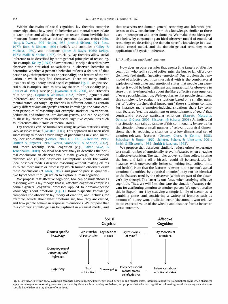
We propose that affective cognition, too, can be understood asreasoning with a lay theory: that is, affective cognition comprisesdomain-general cognitive processes applied to domain-specificknowledge about emotions (Fig. 1). Domain-specific knowledgecomprises the observers’ lay theory of emotion, and includes, forexample, beliefs about what emotions are, how they are caused,and how people behave in response to emotions. We propose thatthis complex knowledge can be captured in a causal model, and
Fig. 1. Lay theories within social cognition comprise domain-specific knowledge about bapply domain-general reasoning processes to these lay theories. In an analogous fashiospecific knowledge in a lay theory of emotions.
that observers use domain-general reasoning and inference pro-cesses to draw conclusions from this knowledge, similar to thoseused in perception and other domains. We make these ideas pre-cise below by constructing an ideal observer model of emotionalreasoning: we describing the domain-specific knowledge in a sta-tistical causal model, and the domain-general reasoning as anapplication of Bayesian inference.
1.1. Attributing emotional reactions
How does an observer infer that agents (the targets of affectivecognition) who spill a cup of coffee, miss the bus, or fall off a bicy-cle, likely feel similar (negative) emotions? One problem that anymodel of affective cognition must deal with is the combinatorialexplosion of outcomes and emotional states that people can expe-rience. It would be both inefficient and impractical for observers tostore or retrieve knowledge about the likely affective consequencesof every possible situation. We hypothesize that people circumventthis complexity by evaluating situations based on a smaller num-ber of ‘‘active psychological ingredients’’ those situations contain.For instance, many emotion-inducing situations share key com-mon features (e.g., the attainment or nonattainment of goals) thatconsistently produce particular emotions (Barrett, Mesquita,Ochsner, & Gross, 2007; Ellsworth & Scherer, 2003). An individualin a situation can take advantage of this commonality by appraisingthe situation along a small number of relevant appraisal dimen-sions: that is, reducing a situation to a low-dimensional set ofemotion-relevant features (Ortony, Clore, & Collins, 1988;Schachter & Singer, 1962; Scherer, Schorr, & Johnstone, 2001;Smith & Ellsworth, 1985; Smith & Lazarus, 1993).
We propose that observers similarly reduce others’ experienceto a small number of emotionally relevant features when engagingin affective cognition. The examples above—spilling coffee, missingthe bus, and falling off a bicycle—could all be associated, forinstance, with unexpectedly losing something (e.g. coffee, time,and health). Note that the features relevant to the person’s actualemotions (identified by appraisal theories) may not be identicalto the features used by the observer (which are part of the obser-ver’s lay theory). The latter is our focus when studying affectivecognition. Thus, we will first elucidate the situation features rele-vant for attributing emotion to another person. We operationalizethis in Experiment 1 by studying a simple family of scenarios—agambling game—and considering a variety of features such asamount of money won, prediction error (the amount won relativeto the expected value of the wheel), and distance from a better orworse outcome.
ehavior and mental states. Inferences about traits and beliefs occur when observersn, we propose that affective cognition is domain-general reasoning over domain-
D.C. Ong et al. / Cognition 143 (2015) 141–162 143
1.2. Reasoning from emotional reactions
A lay theory should support multiple inferences that are coher-ently related to each other: we can reason from a cause to itseffects, but also back from an effect to its cause, and so on. Forexample, we can intuit that missing one’s bus makes one feelsad, and we can also reason, with some uncertainty, that thefrowning person waiting forlornly at a bus stop might have justmissed their bus. If affective cognition derives from a lay theory,then it should allow observers to both infer unseen emotions basedon events, and also to infer the type of event that a social target hasexperienced based on that person’s emotions. In the framework ofstatistical causal models, these two types of inference—from emo-tions to outcomes and from outcomes to emotions—should berelated using the rules of probability. In Experiment 2, we explic-itly test this proposal: do people reason flexibly back and forthbetween emotions and the outcomes that cause them? Do forwardand reverse inferences cohere as predicted by Bayesian inference?
1.3. Integrating sources of emotional evidence
Domain-general reasoning should also explain more complexaffective cognition. For instance, observers often encounter multi-ple cues about a person’s emotions: They might witness anotherperson’s situation, but also the expression on the person’s face,their body posture, or what they said. Sometimes these cues evenconflict—for instance, when an Olympic athlete cries after winningthe gold medal. This seems to be a pair of cues that individuallysuggest conflicting valence. A comprehensive theory of affectivecognition should address how observers translate this deluge ofdifferent information types into an inference, a process we callemotional cue integration (Zaki, 2013).
Prior work suggests two very different approaches that obser-vers might take to emotional cue integration. On the one hand,the facial dominance hypothesis holds that facial expressions uni-versally broadcast information about emotion to external obser-vers (Darwin, 1872; Ekman, Friesen, & Ellsworth, 1982; Smith,Cottrell, Gosselin, & Schyns, 2005; Tomkins, 1962; for more exten-sive reviews, see Matsumoto, Keltner, Shiota, O’Sullivan, & Frank,2008; Russell, Bachorowski, & Fernández-Dols, 2003). This sug-gests that observers should draw primarily on facial cues in deter-mining social agents’ emotions (Buck, 1994; Nakamura, Buck, &Kenny, 1990; Wallbott, 1988; Watson, 1972). On the other hand,contextual cues often appear to drive affective cognition evenwhen paired with facial expressions. For instance, observers oftenrely on written descriptions of a situation (Carroll & Russell, 1996;Goodenough & Tinker, 1931) body postures (Aviezer, Trope, &Todorov, 2012; Aviezer et al., 2008; Mondloch, 2012; Mondloch,Horner, & Mian, 2013; Van den Stock, Righart, & de Gelder,2007), background scenery (Barrett & Kensinger, 2010; Barrett,Mesquita, & Gendron, 2011; Lindquist, Barrett, Bliss-Moreau, &Russell, 2006), and cultural norms (Masuda et al., 2008) whendeciding how agents feel.
Of course, both facial expressions and contextual cues influenceaffective cognition. It is also clear that neither type of cue ubiqui-tously ‘‘wins out,’’ or dominates inferences about others’ emotions.An affective cognition approach suggests that observers shouldsolve emotional cue integration using domain-general inferenceprocesses. There are many other settings—such as binocular vision(Knill, 2007) and multisensory perception (Alais & Burr, 2004;Shams, Kamitani, & Shimojo, 2000; Welch & Warren, 1980)—thatrequire people to combine multiple cues into coherent representa-tions. These ideal observer models assume that observers combinecues in an optimal manner given their prior knowledge and uncer-tainty. In such models, sensory cue integration is modeled as
Bayesian inference (for recent reviews, see de Gelder & Bertelson,2003; Ernst & Bülthoff, 2004; Kersten, Mamassian, & Yuille, 2004).
Our framework yields an approach to emotional cue integrationthat is analogous to cue integration in object perception: a rationalinformation integration process. Observers weigh available cues toan agent’s emotion (e.g., the agent’s facial expression, or the con-text the agent is in) and combine them using statistical principlesof Bayesian inference. This prediction naturally falls out of ourclaim that affective cognition resembles other types oftheory-driven inference, with domain-specific content knowledge:the lay theory of emotion describes the statistical and causal rela-tions between emotion and each cue; joint reasoning over thisstructure is described by domain-general inference processes.
We empirically test the predictions of this approach inExperiments 3 and 4. We aim to both extend the scope of our laytheory model and resolve the current debate in emotion perceptionby predicting how different cues are weighted as observers makeinferences about emotion.
1.4. Overview
We first describe the components of our model and how it canbe used to compute inferences about others’ emotions. We formal-ize this model in the language of Bayesian modeling (Goodman &Tenenbaum, 2014; Goodman, Ullman, & Tenenbaum, 2011;Griffiths, Kemp, & Tenenbaum, 2008). Specifically, we focus onthe ways that observers draw inferences about agents’ emotionsbased on the situations and outcomes those agents experience. Inall our experiments, we restricted the types of situations thatagents experience to a simple gambling game. Although this para-digm does not capture many nuances of everyday affective cogni-tion, its simplicity allowed us to quantitatively manipulate featuresof the situation and isolate situational features that best trackaffective cognition.
Experiment 1 sheds light on the process of inferring an agent’semotions given a situation, identifying a set of emotion-relevantsituation features that observers rely on to understand others’affect. Experiment 2 tests the flexibility of emotional lay theories,by testing whether they also track observers’ reasoning about theoutcomes that agents’ likely encountered based on their emotions;our model’s predictions tightly track human judgments.
We then expand the set of observable evidence that our modelconsiders, and describe how our model computes inferences frommultiple cues—emotional cue integration. Experiment 3 tests themodel against human judgments of emotions from both situationoutcomes and facial expressions; Experiment 4 replicates this withsituation outcomes and verbal utterances. In particular, we showthat the Bayesian model predicts human judgments accurately,outperforming the baseline single cue dominance (e.g. facial orcontext dominance) models. Together, the results support theclaim that reasoning about emotion represents a coherent set ofinferences over a lay theory, similar to reasoning in other domainsof psychology.
Finally, we describe some limitations of our model, motivatefuture work, and discuss the implications of an affective cognitionapproach for emotion theory, lay theories in other domains, andreal-world applications.
2. Exploring the flexible reasoning between outcomes andemotions
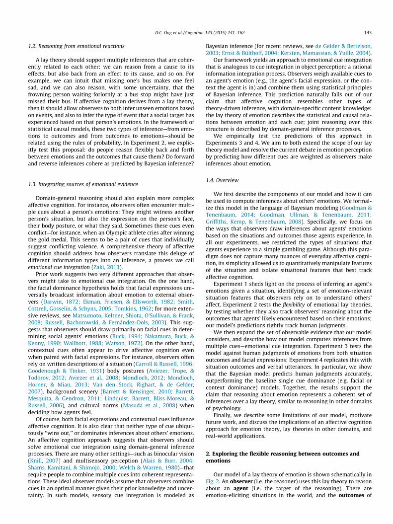
Our model of a lay theory of emotion is shown schematically inFig. 2. An observer (i.e. the reasoner) uses this lay theory to reasonabout an agent (i.e. the target of the reasoning). There areemotion-eliciting situations in the world, and the outcomes of
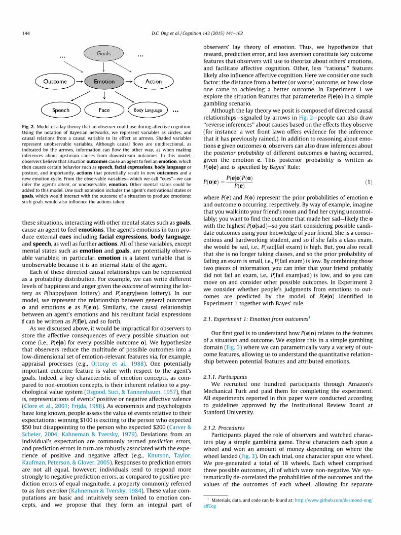
Fig. 2. Model of a lay theory that an observer could use during affective cognition.Using the notation of Bayesian networks, we represent variables as circles, andcausal relations from a causal variable to its effect as arrows. Shaded variablesrepresent unobservable variables. Although causal flows are unidirectional, asindicated by the arrows, information can flow the other way, as when makinginferences about upstream causes from downstream outcomes. In this model,observers believe that situation outcomes cause an agent to feel an emotion, whichthen causes certain behavior such as speech, facial expressions, body language orposture, and importantly, actions that potentially result in new outcomes and anew emotion cycle. From the observable variables—which we call ‘‘cues’’—we caninfer the agent’s latent, or unobservable, emotion. Other mental states could beadded to this model. One such extension includes the agent’s motivational states orgoals, which would interact with the outcome of a situation to produce emotions;such goals would also influence the actions taken.
1 Materials, data, and code can be found at: http://www.github.com/desmond-ong/affCog
144 D.C. Ong et al. / Cognition 143 (2015) 141–162
these situations, interacting with other mental states such as goals,cause an agent to feel emotions. The agent’s emotions in turn pro-duce external cues including facial expressions, body language,and speech, as well as further actions. All of these variables, exceptmental states such as emotion and goals, are potentially observ-able variables; in particular, emotion is a latent variable that isunobservable because it is an internal state of the agent.
Each of these directed causal relationships can be representedas a probability distribution. For example, we can write differentlevels of happiness and anger given the outcome of winning the lot-tery as P(happy|won lottery) and P(angry|won lottery). In ourmodel, we represent the relationship between general outcomeso and emotions e as P(e|o). Similarly, the causal relationshipbetween an agent’s emotions and his resultant facial expressionsf can be written as P(f|e), and so forth.
As we discussed above, it would be impractical for observers tostore the affective consequences of every possible situation out-come (i.e., P(e|o) for every possible outcome o). We hypothesizethat observers reduce the multitude of possible outcomes into alow-dimensional set of emotion-relevant features via, for example,appraisal processes (e.g., Ortony et al., 1988). One potentiallyimportant outcome feature is value with respect to the agent’sgoals. Indeed, a key characteristic of emotion concepts, as com-pared to non-emotion concepts, is their inherent relation to a psy-chological value system (Osgood, Suci, & Tannenbaum, 1957), thatis, representations of events’ positive or negative affective valence(Clore et al., 2001; Frijda, 1988). As economists and psychologistshave long known, people assess the value of events relative to theirexpectations: winning $100 is exciting to the person who expected$50 but disappointing to the person who expected $200 (Carver &Scheier, 2004; Kahneman & Tversky, 1979). Deviations from anindividual’s expectation are commonly termed prediction errors,and prediction errors in turn are robustly associated with the expe-rience of positive and negative affect (e.g., Knutson, Taylor,Kaufman, Peterson, & Glover, 2005). Responses to prediction errorsare not all equal, however; individuals tend to respond morestrongly to negative prediction errors, as compared to positive pre-diction errors of equal magnitude, a property commonly referredto as loss aversion (Kahneman & Tversky, 1984). These value com-putations are basic and intuitively seem linked to emotion con-cepts, and we propose that they form an integral part of
observers’ lay theory of emotion. Thus, we hypothesize thatreward, prediction error, and loss aversion constitute key outcomefeatures that observers will use to theorize about others’ emotions,and facilitate affective cognition. Other, less ‘‘rational’’ featureslikely also influence affective cognition. Here we consider one suchfactor: the distance from a better (or worse) outcome, or how closeone came to achieving a better outcome. In Experiment 1 weexplore the situation features that parameterize P(e|o) in a simplegambling scenario.
Although the lay theory we posit is composed of directed causalrelationships—signaled by arrows in Fig. 2—people can also draw‘‘reverse inferences’’ about causes based on the effects they observe(for instance, a wet front lawn offers evidence for the inferencethat it has previously rained.). In addition to reasoning about emo-tions e given outcomes o, observers can also draw inferences aboutthe posterior probability of different outcomes o having occurred,given the emotion e. This posterior probability is written asP(o|e) and is specified by Bayes’ Rule:
PðojeÞ ¼ PðejoÞPðoÞPðeÞ ð1Þ
where P(e) and P(o) represent the prior probabilities of emotion eand outcome o occurring, respectively. By way of example, imaginethat you walk into your friend’s room and find her crying uncontrol-lably; you want to find the outcome that made her sad—likely the owith the highest P(o|sad)—so you start considering possible candi-date outcomes using your knowledge of your friend. She is a consci-entious and hardworking student, and so if she fails a class exam,she would be sad, i.e., P(sad|fail exam) is high. But, you also recallthat she is no longer taking classes, and so the prior probability offailing an exam is small, i.e., P(fail exam) is low. By combining thosetwo pieces of information, you can infer that your friend probablydid not fail an exam, i.e., P(fail exam|sad) is low, and so you canmove on and consider other possible outcomes. In Experiment 2we consider whether people’s judgments from emotions to out-comes are predicted by the model of P(e|o) identified inExperiment 1 together with Bayes’ rule.
2.1. Experiment 1: Emotion from outcomes1
Our first goal is to understand how P(e|o) relates to the featuresof a situation and outcome. We explore this in a simple gamblingdomain (Fig. 3) where we can parametrically vary a variety of out-come features, allowing us to understand the quantitative relation-ship between potential features and attributed emotions.
2.1.1. ParticipantsWe recruited one hundred participants through Amazon’s
Mechanical Turk and paid them for completing the experiment.All experiments reported in this paper were conducted accordingto guidelines approved by the Institutional Review Board atStanford University.
2.1.2. ProceduresParticipants played the role of observers and watched charac-
ters play a simple gambling game. These characters each spun awheel and won an amount of money depending on where thewheel landed (Fig. 3). On each trial, one character spun one wheel.We pre-generated a total of 18 wheels. Each wheel comprisedthree possible outcomes, all of which were non-negative. We sys-tematically de-correlated the probabilities of the outcomes and thevalues of the outcomes of each wheel, allowing for separate
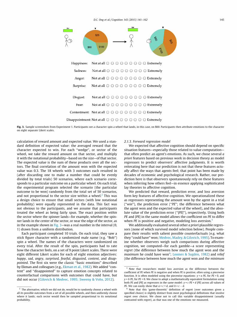
Fig. 3. Sample screenshots from Experiment 1. Participants see a character spin a wheel that lands, in this case, on $60. Participants then attribute emotions to the characteron eight separate Likert scales.
3 Note that researchers model loss aversion as the difference between thecoefficient of PE when PE is negative and when PE is positive, often using a piecewisefunction. It is often modeled using the piecewise equations: y = a PE, for PE > 0, andy = b PE, for PE < 0. We chose to adopt a mathematically equivalent formulation using
D.C. Ong et al. / Cognition 143 (2015) 141–162 145
calculation of reward amount and expected value. We used a stan-dard definition of expected value: the averaged reward that thecharacter expected to win. For each ‘‘wedge’’, or sector of thewheel, we take the reward amount on that sector, and multiplyit with the notational probability—based on the size—of that sector.The expected value is the sum of these products over all the sec-tors. The final correlation of the amount won with the expectedvalue was 0.3. The 18 wheels with 3 outcomes each resulted in(after discarding one to make a number that could be evenlydivided by total trials) 50 scenarios, where each scenario corre-sponds to a particular outcome on a particular wheel. On each trial,the experimental program selected the scenario (the particularoutcome to be won) randomly from the total set of 50 scenarios,and not proportional to the sector size within a wheel.2 This wasa design choice to ensure that small sectors (with low notationalprobability) were equally represented in the data. This fact wasnot obvious to the participants, and we assume that participantstreated the wheel as being fairly spun. The exact position withinthe sector where the spinner lands—for example, whether the spin-ner lands in the center of the sector, or near the edge of the sector, asin the example shown in Fig. 3—was a real number in the interval (0,1) drawn from a uniform distribution.
Each participant completed 10 trials. On each trial, they saw astick figure character with a randomized male name (e.g. ‘‘Bob’’)spin a wheel. The names of the characters were randomized onevery trial. After the result of the spin, participants had to ratehow the character feels, on a set of 9 point Likert scales. There wereeight different Likert scales for each of eight emotion adjectives:happy, sad, angry, surprised, fearful, disgusted, content, and disap-pointed. The first six were the classic ‘‘basic emotions’’ describedby Ekman and colleagues (e.g., Ekman et al., 1982). We added ‘‘con-tent’’ and ‘‘disappointed’’ to capture emotion concepts related tocounterfactual comparisons with outcomes that could have, butdid not occur (Gilovich & Medvec, 1995; Sweeny & Vohs, 2012).
2 The alternative, which we did not do, would be to randomly choose a wheel withall its possible outcomes from a set of all possible wheels, and then uniformly choosewhere it lands; each sector would then be sampled proportional to its notationalprobability.
2.1.3. Forward regression modelWe expected that affective cognition should depend on specific
situation features—especially those related to value computation—that often predict an agent’s emotions. As such, we chose several apriori features based on previous work in decision theory as modelregressors to predict observers’ affective judgments. It is worthreiterating here that our prediction is not that these features actu-ally affect the ways that agents feel; that point has been made bydecades of economic and psychological research. Rather, our pre-diction here is that observers spontaneously rely on these featureswhen inferring how others feel—in essence applying sophisticatedlay theories to affective cognition.
We predicted that reward, prediction error, and loss aversionform key features of affective cognition. We operationalized theseas regressors representing the amount won by the agent in a trial(‘‘win’’), the prediction error (‘‘PE’’; the difference between whatthe agent won and the expected value of the wheel), and the abso-lute value of the prediction error (‘‘|PE|’’), respectively. Using bothPE and |PE| in the same model allows the coefficient on PE to differwhen PE is positive and negative, modeling loss aversion.3
We additionally evaluated several other a priori plausible regres-sors (none of which survived model selection below). People com-pare their results with salient possible counterfactuals (e.g. whatthey ‘‘could have’’ won; Medvec, Madey, & Gilovich, 1995). To exam-ine whether observers weigh such comparisons during affectivecognition, we computed—for each gamble—a score representingregret (the difference between how much the agent won and themaximum he could have won4; Loomes & Sugden, 1982) and relief(the difference between how much the agent won and the minimum
both PE and |PE| as regressors in the same model: y = c PE + d |PE| across all values ofPE. We can easily show that a = c + d, and b = c � d.
4 Note that this ‘game-theoretic’ definition of regret (over outcomes given aspecified choice) is slightly distinct from most psychological definitions that involveregret over choices. We chose not to call this variable disappointment (usuallycontrasted with regret), as that was one of the emotions we measured.
146 D.C. Ong et al. / Cognition 143 (2015) 141–162
he could have won). Finally, we drew on previous work on ‘‘luck’’ (e.g.Teigen, 1996), where observers tend to attribute more ‘‘luck’’ to anagent who won when the chances of winning were low, even aftercontrolling for expected payoffs. To model whether observers accountfor this when attributing other emotions, we included a regressor toaccount for the probability of winning, i.e., the size of the sector thatthe wheel landed on. Since a probability is bounded in [0,1] and theother regressors took on much larger domains of values (e.g. win var-ied from 0 to 100), we used a logarithm to transform the probability tomake the values comparable to other regressors (‘‘logWinProb’’).
The final regressor we included was a ‘‘near-miss’’ term tomodel agents’ affective reactions to outcomes as a function of theirdistance from other outcomes. Such counterfactual reasoning oftenaffects emotion inference. For instance, people reliably judgesomeone to feel worse after missing a flight by 5 min, as comparedto 30 min (Kahneman & Tversky, 1982). Near-misses ‘‘hurt’’ morewhen the actual outcome is close (e.g., in time) to an alternative,better outcome. In our paradigm, since outcomes are determinedby how much the wheel spins, ‘‘closeness’’ can be operationalizedin terms of the angular distance between (i) where the wheellanded (the actual outcome; as defined by the pointer) and (ii)the boundary between the actual outcome and the closest sector.We defined a normalized distance, which ranged from 0 to 0.5,with 0 being at the boundary edge, and 0.5 indicating the exactcenter of the current sector. Near-misses have much greaterimpact at smaller distances, so we took a reciprocal transform5
(1/x) to introduce a non-linearity that favors smaller distances.Finally, we scaled this term by the difference in payment amountsfrom the current sector to the next-nearest sector, to weigh thenear-miss distance by the difference in utility in the two payoffs.
In total, we tested seven outcome variables: win, PE, |PE|, regret,relief, logWinProb and nearMiss. We fit mixed-models predicting eachemotion using these regressors as fixed effects, and added a randomintercept by subject. We performed model selection by conductingbackward stepwise regressions to choose the optimal subset ofregressors that predicted a majority of observers’ ratings of theagents’ emotions. This was done using the step function in the R pack-age lmerTest. Subsequently, we used the optimal subset of regressorsas fixed effects with the same random effect structure. Full details ofthe model selection and results are given in Appendix A.
2.1.4. ResultsModel selection (in Appendix A) revealed that participants’
emotion ratings were significantly predicted only by three of theseven regressors we initially proposed: amount won, the predictionerror (PE), and the absolute value of the prediction error (|PE|) (seealso Section 3.3 for a re-analysis with more data). Crucially, PE and|PE| account for significant variance in emotion ratings afteraccounting for amount won. This suggests that affective cognitionis remarkably consistent with economic and psychological modelsof subjective utility. In particular, emotion inferences exhibitedreference-dependence—tracking prediction error in addition toamount won—and loss aversion—in that emotion inferences weremore strongly predicted by negative, as opposed to positive predic-tion error. These features suggest that lay observers spontaneouslyuse key features of prospect theory (Kahneman & Tversky, 1979,1984) in reasoning about others’ emotions: a remarkable connec-tion between formal and everyday theorizing. It is worth notingas well that the significant regressors for surprise followed aslightly different pattern from the rest of the other emotions,where the win probability, as well as regret and relief, seem justas important as the amount won, PE, and |PE|.
5 We tried other non-linear transforms such as exponential and log transforms,which all performed comparably.
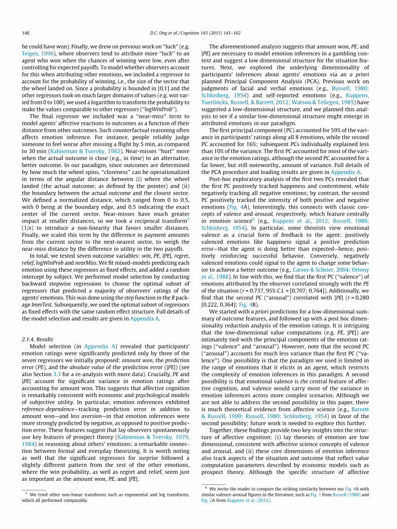
The aforementioned analysis suggests that amount won, PE, and|PE| are necessary to model emotion inferences in a gambling con-text and suggest a low dimensional structure for the situation fea-tures. Next, we explored the underlying dimensionality ofparticipants’ inferences about agents’ emotions via an a prioriplanned Principal Component Analysis (PCA). Previous work onjudgments of facial and verbal emotions (e.g., Russell, 1980;Schlosberg, 1954) and self-reported emotions (e.g., Kuppens,Tuerlinckx, Russell, & Barrett, 2012; Watson & Tellegen, 1985) havesuggested a low-dimensional structure, and we planned this anal-ysis to see if a similar low-dimensional structure might emerge inattributed emotions in our paradigm.
The first principal component (PC) accounted for 59% of the vari-ance in participants’ ratings along all 8 emotions, while the secondPC accounted for 16%; subsequent PCs individually explained lessthan 10% of the variance. The first PC accounted for most of the vari-ance in the emotion ratings, although the second PC accounted for afar lower, but still noteworthy, amount of variance. Full details ofthe PCA procedure and loading results are given in Appendix A.
Post-hoc exploratory analysis of the first two PCs revealed thatthe first PC positively tracked happiness and contentment, whilenegatively tracking all negative emotions; by contrast, the secondPC positively tracked the intensity of both positive and negativeemotions (Fig. 4A). Interestingly, this connects with classic con-cepts of valence and arousal, respectively, which feature centrallyin emotion science6 (e.g., Kuppens et al., 2012; Russell, 1980;Schlosberg, 1954). In particular, some theorists view emotionalvalence as a crucial form of feedback to the agent: positivelyvalenced emotions like happiness signal a positive predictionerror—that the agent is doing better than expected—hence, posi-tively reinforcing successful behavior. Conversely, negativelyvalenced emotions could signal to the agent to change some behav-ior to achieve a better outcome (e.g., Carver & Scheier, 2004; Ortonyet al., 1988). In line with this, we find that the first PC (‘‘valence’’) ofemotions attributed by the observer correlated strongly with the PEof the situation (r = 0.737, 95% C.I. = [0.707; 0.764]). Additionally, wefind that the second PC (‘‘arousal’’) correlated with |PE| (r = 0.280[0.222, 0.364]; Fig. 4B).
We started with a priori predictions for a low-dimensional sum-mary of outcome features, and followed up with a post hoc dimen-sionality reduction analysis of the emotion ratings. It is intriguingthat the low-dimensional value computations (e.g. PE, |PE|) areintimately tied with the principal components of the emotion rat-ings (‘‘valence’’ and ‘‘arousal’’). However, note that the second PC(‘‘arousal’’) accounts for much less variance than the first PC (‘‘va-lence’’). One possibility is that the paradigm we used is limited inthe range of emotions that it elicits in an agent, which restrictsthe complexity of emotion inferences in this paradigm. A secondpossibility is that emotional valence is the central feature of affec-tive cognition, and valence would carry most of the variance inemotion inferences across more complex scenarios. Although weare not able to address the second possibility in this paper, thereis much theoretical evidence from affective science (e.g., Barrett& Russell, 1999; Russell, 1980; Schlosberg, 1954) in favor of thesecond possibility; future work is needed to explore this further.
Together, these findings provide two key insights into the struc-ture of affective cognition: (i) lay theories of emotion are lowdimensional, consistent with affective science concepts of valenceand arousal, and (ii) these core dimensions of emotion inferencealso track aspects of the situation and outcome that reflect valuecomputation parameters described by economic models such asprospect theory. Although the specific structure of affective
6 We invite the reader to compare the striking similarity between our Fig. 4A withsimilar valence-arousal figures in the literature, such as Fig. 1 from Russell (1980) andFig. 2A from Kuppens et al. (2012).
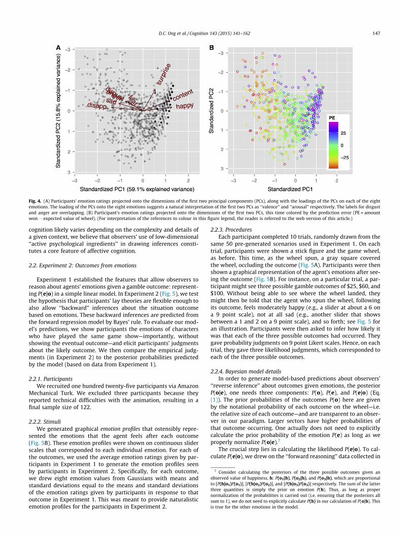
Fig. 4. (A) Participants’ emotion ratings projected onto the dimensions of the first two principal components (PCs), along with the loadings of the PCs on each of the eightemotions. The loading of the PCs onto the eight emotions suggests a natural interpretation of the first two PCs as ‘‘valence’’ and ‘‘arousal’’ respectively. The labels for disgustand anger are overlapping. (B) Participant’s emotion ratings projected onto the dimensions of the first two PCs, this time colored by the prediction error (PE = amountwon � expected value of wheel). (For interpretation of the references to colour in this figure legend, the reader is referred to the web version of this article.)
7 Consider calculating the posteriors of the three possible outcomes given anobserved value of happiness, h: P(o1|h), P(o2|h), and P(o3|h), which are proportionalto [P(h|o1)P(o1)], [P(h|o2)P(o2)], and [P(h|o3)P(o3)] respectively. The sum of the latterthree quantities is simply the prior on emotion P(h). Thus, as long as propernormalization of the probabilities is carried out (i.e. ensuring that the posteriors allsum to 1), we do not need to explicitly calculate P(h) in our calculation of P(o|h). Thisis true for the other emotions in the model.
D.C. Ong et al. / Cognition 143 (2015) 141–162 147
cognition likely varies depending on the complexity and details ofa given context, we believe that observers’ use of low-dimensional‘‘active psychological ingredients’’ in drawing inferences consti-tutes a core feature of affective cognition.
2.2. Experiment 2: Outcomes from emotions
Experiment 1 established the features that allow observers toreason about agents’ emotions given a gamble outcome: represent-ing P(e|o) in a simple linear model. In Experiment 2 (Fig. 5), we testthe hypothesis that participants’ lay theories are flexible enough toalso allow ‘‘backward’’ inferences about the situation outcomebased on emotions. These backward inferences are predicted fromthe forward regression model by Bayes’ rule. To evaluate our mod-el’s predictions, we show participants the emotions of characterswho have played the same game show—importantly, withoutshowing the eventual outcome—and elicit participants’ judgmentsabout the likely outcome. We then compare the empirical judg-ments (in Experiment 2) to the posterior probabilities predictedby the model (based on data from Experiment 1).
2.2.1. ParticipantsWe recruited one hundred twenty-five participants via Amazon
Mechanical Turk. We excluded three participants because theyreported technical difficulties with the animation, resulting in afinal sample size of 122.
2.2.2. StimuliWe generated graphical emotion profiles that ostensibly repre-
sented the emotions that the agent feels after each outcome(Fig. 5B). These emotion profiles were shown on continuous sliderscales that corresponded to each individual emotion. For each ofthe outcomes, we used the average emotion ratings given by par-ticipants in Experiment 1 to generate the emotion profiles seenby participants in Experiment 2. Specifically, for each outcome,we drew eight emotion values from Gaussians with means andstandard deviations equal to the means and standard deviationsof the emotion ratings given by participants in response to thatoutcome in Experiment 1. This was meant to provide naturalisticemotion profiles for the participants in Experiment 2.
2.2.3. ProceduresEach participant completed 10 trials, randomly drawn from the
same 50 pre-generated scenarios used in Experiment 1. On eachtrial, participants were shown a stick figure and the game wheel,as before. This time, as the wheel spun, a gray square coveredthe wheel, occluding the outcome (Fig. 5A). Participants were thenshown a graphical representation of the agent’s emotions after see-ing the outcome (Fig. 5B). For instance, on a particular trial, a par-ticipant might see three possible gamble outcomes of $25, $60, and$100. Without being able to see where the wheel landed, theymight then be told that the agent who spun the wheel, followingits outcome, feels moderately happy (e.g., a slider at about a 6 ona 9 point scale), not at all sad (e.g., another slider that showsbetween a 1 and 2 on a 9 point scale), and so forth; see Fig. 5 foran illustration. Participants were then asked to infer how likely itwas that each of the three possible outcomes had occurred. Theygave probability judgments on 9 point Likert scales. Hence, on eachtrial, they gave three likelihood judgments, which corresponded toeach of the three possible outcomes.
2.2.4. Bayesian model detailsIn order to generate model-based predictions about observers’
‘‘reverse inference’’ about outcomes given emotions, the posteriorP(o|e), one needs three components: P(o), P(e), and P(e|o) (Eq.(1)). The prior probabilities of the outcomes P(o) here are givenby the notational probability of each outcome on the wheel—i.e.the relative size of each outcome—and are transparent to an obser-ver in our paradigm. Larger sectors have higher probabilities ofthat outcome occurring. One actually does not need to explicitlycalculate the prior probability of the emotion P(e) as long as weproperly normalize P(o|e).7
The crucial step lies in calculating the likelihood P(e|o). To cal-culate P(e|o), we drew on the ‘‘forward reasoning’’ data collected in
Less More
B
A
Fig. 5. Screenshots from Experiment 2. (A) Participants were shown a character that spins a wheel, but a gray square then occludes the outcome on the wheel. (B) Participantsthen saw a graphical representation of the character’s emotions, and inferred separate probabilities for each of the three possible outcomes having occurred.
148 D.C. Ong et al. / Cognition 143 (2015) 141–162
Experiment 1. In particular, we leveraged Experiment 1’s regres-sion model to calculate the extent to which observers would belikely to infer different emotions of an agent based on each out-come. To do so, we applied the variables identified as most relevantto affective cognition in Experiment 1—win, PE, and |PE|—to predictthe emotions observers would assign to agents given the novel out-comes of Experiment 2. For instance, in modeling happiness, thisapproach produces the following equation for each wheeloutcome:
happy ¼ c0;happy þ c1;happywinþ c2;happyPEþ c3;happyjPEj þ ehappy ð2Þ
We employed similar regression equations to estimate P(e|o) forthe other seven emotions, where eemotion (with zero mean and stan-dard deviation eemotion) represents the residual error terms of theregressions. The coefficients ci;emotion are obtained numerically by fit-ting the data from Experiment 1; the linear model is fit across allparticipants and scenarios to obtain one set of coefficients per emo-tion. For a new scenario with {win, PE, |PE|}, the likelihood ofobserving a certain happy value h0 is simply the probability that h0
is drawn from the linear model. In other words, it is the probabilitythat the error
h0 � c0;happy þ c1;happywinþ c2;happyPEþ c3;happyjPEj ð3Þ
is drawn from the residual error distribution for ehappy.The error distribution ehappy resulting from the above regression
captures intrinsic noise in the relation between outcomes andemotions of the agent—uncertainty in the participant’s lay theory.However, in addition to this noise, there are several other sourcesof noise that may enter into participants’ judgments. First, partici-pants may not take the graphical sliders as an accurate representa-tion of the agent’s true emotions (and indeed we experimentallygenerated these displays with a small amount of noise, asdescribed above). Secondly, participants might have some uncer-tainty around reading the values from the slider. Thirdly, partici-pants may also have some noise in the prior estimates they usein each trial.
Instead of having multiple noise parameters to model these andother external sources of noise, we instead modified the intrinsic
noise in the regression model. We added a likelihood smoothingparameter f (zeta), which amplifies the intrinsic noise in theregression model, such that the likelihood P(h0|o) is the probabilitythat h0 � c0;happy þ c1;happywinþ c2;happyPEþ c3;happyjPEj is drawn from
Nð0; ðfrhappyÞ2Þ, i.e. a normal distribution with mean 0 and standarddeviation frhappy.
Using Eq. (3) with the additional noise parameter, we can calcu-late the likelihood of observing a value h0 as a result of an outcomeo, i.e. P(h0|o). We then calculate the joint likelihood of observing acertain combination of emotions e0 for a particular outcome o asthe product of the individual likelihoods,
Pðe0joÞ ¼ Pðhappy0joÞPðsad0joÞ . . . Pðdiapp0joÞ ð4Þ
A note on Eq. (4): The only assumption we make is that the out-come o is the only cause of the emotions, i.e., there are no otherhidden causes that might influence emotions. The individual emo-tions are conditionally independent given the outcome (commoncause), and thus the joint likelihood is proportional to the productof the individual emotion likelihoods.
Next, to calculate the posterior as specified in Eq. (1), we multi-ply the joint likelihood P(e|o) with the prior probability of the out-come o occurring, P(o), which is simply the size of the sector. Weperformed this calculation for each individual outcome, before nor-malizing to ensure the posterior probabilities P(o|e) for a particularwheel sum to 1 (by dividing each probability by the sum of theposteriors). The normalization removes the need to calculate P(e)explicitly (see Footnote 3). The resulting model has only one freenoise parameter, otherwise being fixed by hypothesis and theresults of Experiment 1.
Up to this point, we had only used data from participants inExperiment 1 to build the model. To verify the model, we collapsedthe empirical judgments that participants gave in Experiment 2 (anindependent group compared to participants in Experiment 1) foreach individual outcome. We then compared the model’s predictedposterior probabilities for each outcome to the empiricaljudgments.
We optimized the one free noise parameter f in the model tominimize the root-mean-squared-error (RMSE) of the model
D.C. Ong et al. / Cognition 143 (2015) 141–162 149
residuals. We conducted a bootstrap with 5000 iterations to esti-mate the noise parameter, RMSE, and the model correlation, aswell as their confidence interval.
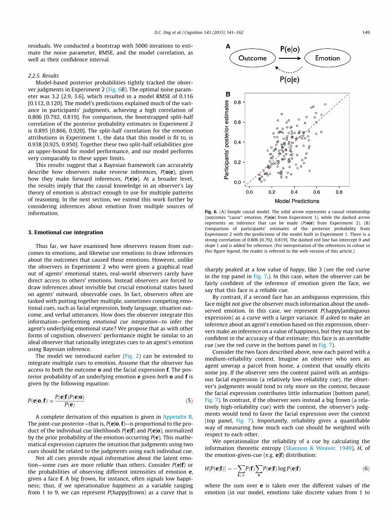
Fig. 6. (A) Simple causal model. The solid arrow represents a causal relationship
2.2.5. ResultsModel-based posterior probabilities tightly tracked the obser-
ver judgments in Experiment 2 (Fig. 6B). The optimal noise param-eter was 3.2 [2.9, 3.6], which resulted in a model RMSE of 0.116[0.112, 0.120]. The model’s predictions explained much of the vari-ance in participants’ judgments, achieving a high correlation of0.806 [0.792, 0.819]. For comparison, the bootstrapped split-halfcorrelation of the posterior probability estimates in Experiment 2is 0.895 [0.866, 0.920]. The split-half correlation for the emotionattributions in Experiment 1, the data that this model is fit to, is0.938 [0.925, 0.950]. Together these two split-half reliabilities givean upper-bound for model performance, and our model performsvery comparably to these upper limits.
This results suggest that a Bayesian framework can accuratelydescribe how observers make reverse inferences, P(o|e), givenhow they make forward inferences, P(e|o). At a broader level,the results imply that the causal knowledge in an observer’s laytheory of emotion is abstract enough to use for multiple patternsof reasoning. In the next section, we extend this work further byconsidering inferences about emotion from multiple sources ofinformation.
(outcomes ‘‘cause’’ emotion; P(e|o) from Experiment 1), while the dashed arrowrepresents an inference that can be made (P(o|e) from Experiment 2). (B)Comparison of participants’ estimates of the posterior probability fromExperiment 2 with the predictions of the model built in Experiment 1. There is astrong correlation of 0.806 [0.792, 0.819]. The dashed red line has intercept 0 andslope 1 and is added for reference. (For interpretation of the references to colour inthis figure legend, the reader is referred to the web version of this article.)
3. Emotional cue integration
Thus far, we have examined how observers reason from out-comes to emotions, and likewise use emotions to draw inferencesabout the outcomes that caused those emotions. However, unlikethe observers in Experiment 2 who were given a graphical readout of agents’ emotional states, real-world observers rarely havedirect access to others’ emotions. Instead observers are forced todraw inferences about invisible but crucial emotional states basedon agents’ outward, observable cues. In fact, observers often aretasked with putting together multiple, sometimes competing emo-tional cues, such as facial expression, body language, situation out-come, and verbal utterances. How does the observer integrate thisinformation—performing emotional cue integration—to infer theagent’s underlying emotional state? We propose that as with otherforms of cognition, observers’ performance might be similar to anideal observer that rationally integrates cues to an agent’s emotionusing Bayesian inference.
The model we introduced earlier (Fig. 2) can be extended tointegrate multiple cues to emotion. Assume that the observer hasaccess to both the outcome o and the facial expression f. The pos-terior probability of an underlying emotion e given both o and f isgiven by the following equation:
Pðejo; fÞ / PðejfÞPðejoÞPðeÞ ð5Þ
A complete derivation of this equation is given in Appendix B.The joint-cue posterior—that is, P(e|o, f)—is proportional to the pro-duct of the individual cue likelihoods P(e|f) and P(e|o), normalizedby the prior probability of the emotion occurring P(e). This mathe-matical expression captures the intuition that judgments using twocues should be related to the judgments using each individual cue.
Not all cues provide equal information about the latent emo-tion—some cues are more reliable than others. Consider P(e|f) orthe probabilities of observing different intensities of emotion e,given a face f. A big frown, for instance, often signals low happi-ness; thus, if we operationalize happiness as a variable rangingfrom 1 to 9, we can represent P(happy|frown) as a curve that is
sharply peaked at a low value of happy, like 3 (see the red curvein the top panel in Fig. 7.). In this case, when the observer can befairly confident of the inference of emotion given the face, wesay that this face is a reliable cue.
By contrast, if a second face has an ambiguous expression, thisface might not give the observer much information about the unob-served emotion. In this case, we represent P(happy|ambiguousexpression) as a curve with a larger variance. If asked to make aninference about an agent’s emotion based on this expression, obser-vers make an inference on a value of happiness, but they may not beconfident in the accuracy of that estimate; this face is an unreliablecue (see the red curve in the bottom panel in Fig. 7).
Consider the two faces described above, now each paired with amedium-reliability context. Imagine an observer who sees anagent unwrap a parcel from home, a context that usually elicitssome joy. If the observer sees the context paired with an ambigu-ous facial expression (a relatively low-reliability cue), the obser-ver’s judgments would tend to rely more on the context, becausethe facial expression contributes little information (bottom panel,Fig. 7). In contrast, if the observer sees instead a big frown (a rela-tively high-reliability cue) with the context, the observer’s judg-ments would tend to favor the facial expression over the context(top panel, Fig. 7). Importantly, reliability gives a quantifiableway of measuring how much each cue should be weighted withrespect to each other.
We operationalize the reliability of a cue by calculating theinformation theoretic entropy (Shannon & Weaver, 1949), H, ofthe emotion-given-cue (e.g. e|f) distribution:
H½PðejfÞ� ¼ �Xf2F
PðfÞX
e
PðejfÞ log PðejfÞ ð6Þ
where the sum over e is taken over the different values of theemotion (in our model, emotions take discrete values from 1 to
0.0
0.5
1.0
1.5
0.0
0.5
1.0
1.5
High R
eliabilityLow
Reliability
Pro
babi
lity
Distribution
1. P(e|f)
2. P(e|o)
3. P(e|f)*P(e|o)
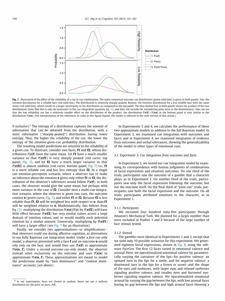
Fig. 7. Illustration of the effect of the reliability of a cue in cue combination. The same contextual outcome cue distribution (green solid line) is given in both panels. Top: theemotion distribution for a reliable face (red solid line). The distribution is relatively sharply peaked. Bottom: the emotion distribution for a less reliable face with the samemean (red solid line), which results in a larger uncertainty in the distribution as compared to the top panel. The blue dashed line in both panels shows the product of the twodistributions (note that this is only the numerator in the cue integration equation, Eq. (5), and does not include the normalizing prior term in the denominator). One can seethat the low reliability cue has a relatively smaller effect on the distribution of the product: the distribution P(e|f) ⁄ P(e|o) in the bottom panel is very similar to thedistribution P(e|o). (For interpretation of the references to color in this figure legend, the reader is referred to the web version of this article.)
150 D.C. Ong et al. / Cognition 143 (2015) 141–162
9 inclusive).8 The entropy of a distribution captures the amount ofinformation that can be obtained from the distribution, with amore informative (‘‘sharply-peaked’’) distribution having lowerentropy. Thus, the higher the reliability of the cue, the lower theentropy of the emotion-given-cue probability distribution.
The resulting model predictions are sensitive to the reliability ofa given cue. To illustrate, consider two faces, f1 and f2, whose dis-tributions P(e|f) have the same mean. Let f1 have a much smallervariance so that P(e|f1) is very sharply peaked (red curve, toppanel, Fig. 7), and let f2 have a much larger variance so thatP(e|f2) is almost uniform (red curve, bottom panel, Fig. 7) i.e., f1is a more reliable cue and has less entropy than f2. In a singlecue emotion-perception scenario, where a observer has to makean inference about the emotion e given only either f1 or f2, the dis-tribution of the observer’s inferences would follow P(e|f); in bothcases, the observer would give the same mean, but perhaps withmore variance in the case of f2. Consider next a multi-cue integra-tion scenario, where the observer is given two cues, the outcomecontext o (green curve, Fig. 7), and either f1 or f2. Because f2 is lessreliable than f1, f2 will be weighted less with respect to o, than f1will be weighted relative to o. Mathematically, this follows fromEq. (5): multiplying the distribution P(e|o)/P(e) by P(e|f2) will havelittle effect because P(e|f2) has very similar values across a largedomain of emotion values, and so would modify each potentialemotion by a similar amount. Conversely, multiplying by P(e|f1)will have a larger effect (see Fig. 7 for an illustration).
Finally, we consider two approximations—or simplifications—that observers could use during affective cognition, as alternativesto our fully Bayesian cue integration model. Under a face-cue-onlymodel, a observer presented with a face f and an outcome o wouldrely only on the face, and would thus use P(e|f) to approximateP(e|o, f). Under a second outcome-cue-only model, the observerinstead relies exclusively on the outcome and uses P(e|o) toapproximate P(e|o, f). These approximations are meant to modelthe predictions made by ‘‘face dominance’’ and ‘‘context domi-nance’’ accounts (see above).
8 In our experiments, faces are chosen at random, hence we use a uniformdistribution for the prior on faces, P(f).
In Experiments 3 and 4, we calculate the performance of thesetwo approximate models in addition to the full Bayesian model. InExperiment 3, we examined cue integration with outcomes andfaces, and in Experiment 4, we examined integration of evidencefrom outcomes and verbal utterances, showing the generalizabilityof the model to other types of emotional cues.
3.1. Experiment 3: Cue Integration from outcomes and faces
In Experiment 3, we tested our cue integration model by exam-ining its correspondence with human judgments of combinationsof facial expressions and situation outcomes. On one third of thetrials, participants saw the outcome of a gamble that a characterplays, as in Experiment 1. On another third of the trials, partici-pants saw only the facial expression following the outcome, butnot the outcome itself. On the final third of ‘‘joint-cue’’ trials, par-ticipants saw both the facial expression and the outcome. On alltrials, participants attributed emotions to the character, as inExperiment 1.
3.1.1. ParticipantsWe recruited four hundred sixty-five participants through
Amazon’s Mechanical Turk. We planned for a larger number thanwere included in Studies 1 and 2 because of the large number offace stimuli tested.
3.1.2. StimuliThe gambles were identical to Experiments 1 and 2, except that
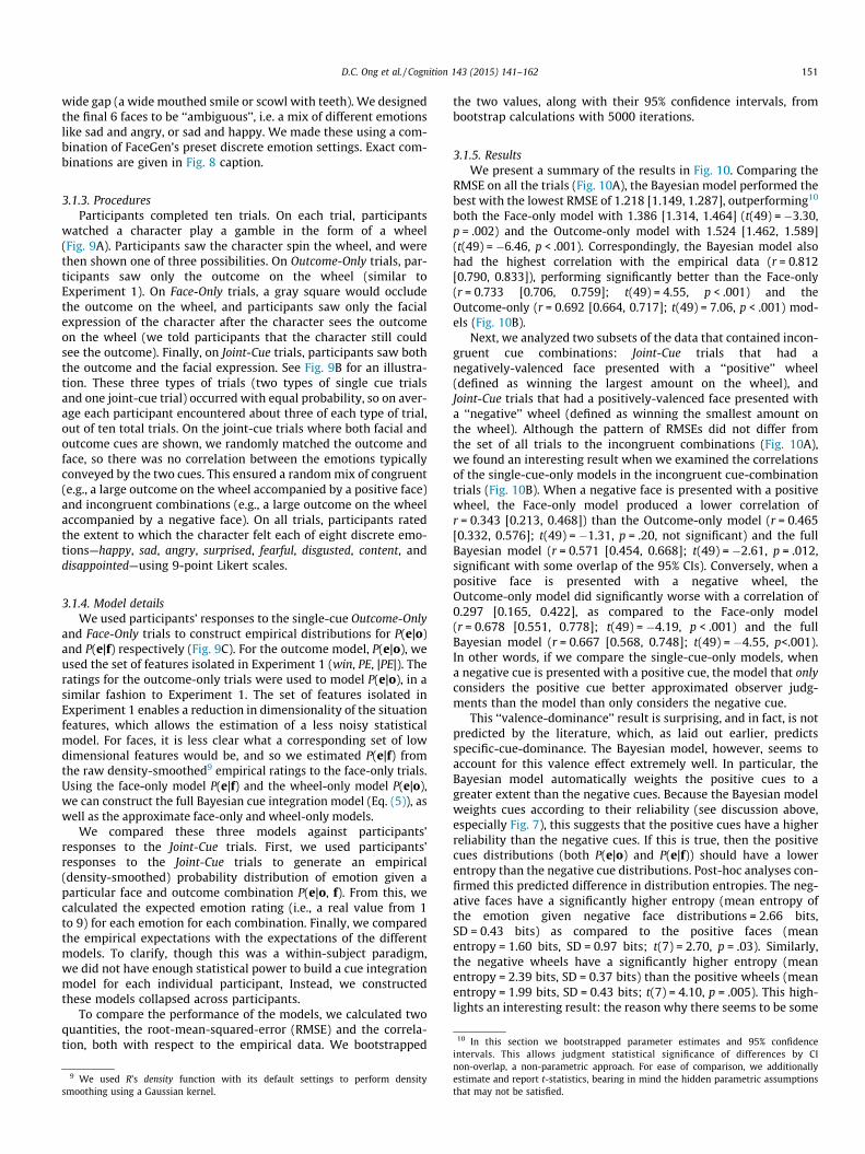
we used only 10 possible scenarios for this experiment. We gener-ated eighteen facial expressions, shown in Fig. 8, using the soft-ware FaceGen. The first 12 faces varied in emotional valence andarousal. Here, we operationalized emotional valence by parametri-cally varying the curvature of the lips—for positive valence: anupward turn in the lips for a smile; and for negative valence: adownward turn in the lips for a frown or scowl—and the shapeof the eyes and eyebrows, with larger eyes and relaxed eyebrowssignaling positive valence, and smaller eyes and furrowed eye-brows signaling negative valence. We operationalized emotionalarousal by varying the gap between the lips, with low arousal faceshaving no gap between the lips and high arousal faces showing a
D.C. Ong et al. / Cognition 143 (2015) 141–162 151
wide gap (a wide mouthed smile or scowl with teeth). We designedthe final 6 faces to be ‘‘ambiguous’’, i.e. a mix of different emotionslike sad and angry, or sad and happy. We made these using a com-bination of FaceGen’s preset discrete emotion settings. Exact com-binations are given in Fig. 8 caption.
3.1.3. ProceduresParticipants completed ten trials. On each trial, participants
watched a character play a gamble in the form of a wheel(Fig. 9A). Participants saw the character spin the wheel, and werethen shown one of three possibilities. On Outcome-Only trials, par-ticipants saw only the outcome on the wheel (similar toExperiment 1). On Face-Only trials, a gray square would occludethe outcome on the wheel, and participants saw only the facialexpression of the character after the character sees the outcomeon the wheel (we told participants that the character still couldsee the outcome). Finally, on Joint-Cue trials, participants saw boththe outcome and the facial expression. See Fig. 9B for an illustra-tion. These three types of trials (two types of single cue trialsand one joint-cue trial) occurred with equal probability, so on aver-age each participant encountered about three of each type of trial,out of ten total trials. On the joint-cue trials where both facial andoutcome cues are shown, we randomly matched the outcome andface, so there was no correlation between the emotions typicallyconveyed by the two cues. This ensured a random mix of congruent(e.g., a large outcome on the wheel accompanied by a positive face)and incongruent combinations (e.g., a large outcome on the wheelaccompanied by a negative face). On all trials, participants ratedthe extent to which the character felt each of eight discrete emo-tions—happy, sad, angry, surprised, fearful, disgusted, content, anddisappointed—using 9-point Likert scales.
10 In this section we bootstrapped parameter estimates and 95% confidence
3.1.4. Model detailsWe used participants’ responses to the single-cue Outcome-Only
and Face-Only trials to construct empirical distributions for P(e|o)and P(e|f) respectively (Fig. 9C). For the outcome model, P(e|o), weused the set of features isolated in Experiment 1 (win, PE, |PE|). Theratings for the outcome-only trials were used to model P(e|o), in asimilar fashion to Experiment 1. The set of features isolated inExperiment 1 enables a reduction in dimensionality of the situationfeatures, which allows the estimation of a less noisy statisticalmodel. For faces, it is less clear what a corresponding set of lowdimensional features would be, and so we estimated P(e|f) fromthe raw density-smoothed9 empirical ratings to the face-only trials.Using the face-only model P(e|f) and the wheel-only model P(e|o),we can construct the full Bayesian cue integration model (Eq. (5)), aswell as the approximate face-only and wheel-only models.
We compared these three models against participants’responses to the Joint-Cue trials. First, we used participants’responses to the Joint-Cue trials to generate an empirical(density-smoothed) probability distribution of emotion given aparticular face and outcome combination P(e|o, f). From this, wecalculated the expected emotion rating (i.e., a real value from 1to 9) for each emotion for each combination. Finally, we comparedthe empirical expectations with the expectations of the differentmodels. To clarify, though this was a within-subject paradigm,we did not have enough statistical power to build a cue integrationmodel for each individual participant, Instead, we constructedthese models collapsed across participants.
To compare the performance of the models, we calculated twoquantities, the root-mean-squared-error (RMSE) and the correla-tion, both with respect to the empirical data. We bootstrapped
9 We used R’s density function with its default settings to perform densitysmoothing using a Gaussian kernel.
the two values, along with their 95% confidence intervals, frombootstrap calculations with 5000 iterations.
3.1.5. ResultsWe present a summary of the results in Fig. 10. Comparing the
RMSE on all the trials (Fig. 10A), the Bayesian model performed thebest with the lowest RMSE of 1.218 [1.149, 1.287], outperforming10
both the Face-only model with 1.386 [1.314, 1.464] (t(49) = �3.30,p = .002) and the Outcome-only model with 1.524 [1.462, 1.589](t(49) = �6.46, p < .001). Correspondingly, the Bayesian model alsohad the highest correlation with the empirical data (r = 0.812[0.790, 0.833]), performing significantly better than the Face-only(r = 0.733 [0.706, 0.759]; t(49) = 4.55, p < .001) and theOutcome-only (r = 0.692 [0.664, 0.717]; t(49) = 7.06, p < .001) mod-els (Fig. 10B).
Next, we analyzed two subsets of the data that contained incon-gruent cue combinations: Joint-Cue trials that had anegatively-valenced face presented with a ‘‘positive’’ wheel(defined as winning the largest amount on the wheel), andJoint-Cue trials that had a positively-valenced face presented witha ‘‘negative’’ wheel (defined as winning the smallest amount onthe wheel). Although the pattern of RMSEs did not differ fromthe set of all trials to the incongruent combinations (Fig. 10A),we found an interesting result when we examined the correlationsof the single-cue-only models in the incongruent cue-combinationtrials (Fig. 10B). When a negative face is presented with a positivewheel, the Face-only model produced a lower correlation ofr = 0.343 [0.213, 0.468]) than the Outcome-only model (r = 0.465[0.332, 0.576]; t(49) = �1.31, p = .20, not significant) and the fullBayesian model (r = 0.571 [0.454, 0.668]; t(49) = �2.61, p = .012,significant with some overlap of the 95% CIs). Conversely, when apositive face is presented with a negative wheel, theOutcome-only model did significantly worse with a correlation of0.297 [0.165, 0.422], as compared to the Face-only model(r = 0.678 [0.551, 0.778]; t(49) = �4.19, p < .001) and the fullBayesian model (r = 0.667 [0.568, 0.748]; t(49) = �4.55, p<.001).In other words, if we compare the single-cue-only models, whena negative cue is presented with a positive cue, the model that onlyconsiders the positive cue better approximated observer judg-ments than the model than only considers the negative cue.
This ‘‘valence-dominance’’ result is surprising, and in fact, is notpredicted by the literature, which, as laid out earlier, predictsspecific-cue-dominance. The Bayesian model, however, seems toaccount for this valence effect extremely well. In particular, theBayesian model automatically weights the positive cues to agreater extent than the negative cues. Because the Bayesian modelweights cues according to their reliability (see discussion above,especially Fig. 7), this suggests that the positive cues have a higherreliability than the negative cues. If this is true, then the positivecues distributions (both P(e|o) and P(e|f)) should have a lowerentropy than the negative cue distributions. Post-hoc analyses con-firmed this predicted difference in distribution entropies. The neg-ative faces have a significantly higher entropy (mean entropy ofthe emotion given negative face distributions = 2.66 bits,SD = 0.43 bits) as compared to the positive faces (meanentropy = 1.60 bits, SD = 0.97 bits; t(7) = 2.70, p = .03). Similarly,the negative wheels have a significantly higher entropy (meanentropy = 2.39 bits, SD = 0.37 bits) than the positive wheels (meanentropy = 1.99 bits, SD = 0.43 bits; t(7) = 4.10, p = .005). This high-lights an interesting result: the reason why there seems to be some
intervals. This allows judgment statistical significance of differences by CInon-overlap, a non-parametric approach. For ease of comparison, we additionallyestimate and report t-statistics, bearing in mind the hidden parametric assumptionsthat may not be satisfied.
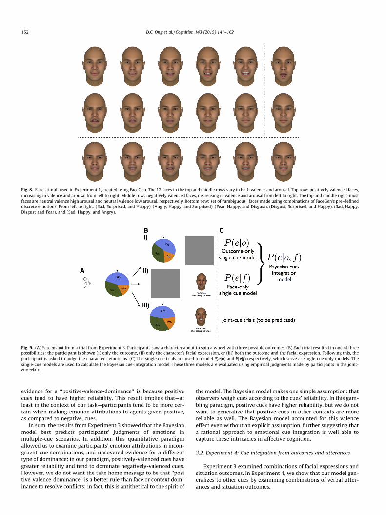
Fig. 8. Face stimuli used in Experiment 1, created using FaceGen. The 12 faces in the top and middle rows vary in both valence and arousal. Top row: positively valenced faces,increasing in valence and arousal from left to right. Middle row: negatively valenced faces, decreasing in valence and arousal from left to right. The top and middle right-mostfaces are neutral valence high arousal and neutral valence low arousal, respectively. Bottom row: set of ‘‘ambiguous’’ faces made using combinations of FaceGen’s pre-defineddiscrete emotions. From left to right: (Sad, Surprised, and Happy), (Angry, Happy, and Surprised), (Fear, Happy, and Disgust), (Disgust, Surprised, and Happy), (Sad, Happy,Disgust and Fear), and (Sad, Happy, and Angry).
Fig. 9. (A) Screenshot from a trial from Experiment 3. Participants saw a character about to spin a wheel with three possible outcomes. (B) Each trial resulted in one of threepossibilities: the participant is shown (i) only the outcome, (ii) only the character’s facial expression, or (iii) both the outcome and the facial expression. Following this, theparticipant is asked to judge the character’s emotions. (C) The single cue trials are used to model P(e|o) and P(e|f) respectively, which serve as single-cue only models. Thesingle-cue models are used to calculate the Bayesian cue-integration model. These three models are evaluated using empirical judgments made by participants in the joint-cue trials.
152 D.C. Ong et al. / Cognition 143 (2015) 141–162
evidence for a ‘‘positive-valence-dominance’’ is because positivecues tend to have higher reliability. This result implies that—atleast in the context of our task—participants tend to be more cer-tain when making emotion attributions to agents given positive,as compared to negative, cues.
In sum, the results from Experiment 3 showed that the Bayesianmodel best predicts participants’ judgments of emotions inmultiple-cue scenarios. In addition, this quantitative paradigmallowed us to examine participants’ emotion attributions in incon-gruent cue combinations, and uncovered evidence for a differenttype of dominance: in our paradigm, positively-valenced cues havegreater reliability and tend to dominate negatively-valenced cues.However, we do not want the take home message to be that ‘‘positive-valence-dominance’’ is a better rule than face or context dom-inance to resolve conflicts; in fact, this is antithetical to the spirit of
the model. The Bayesian model makes one simple assumption: thatobservers weigh cues according to the cues’ reliability. In this gam-bling paradigm, positive cues have higher reliability, but we do notwant to generalize that positive cues in other contexts are morereliable as well. The Bayesian model accounted for this valenceeffect even without an explicit assumption, further suggesting thata rational approach to emotional cue integration is well able tocapture these intricacies in affective cognition.
3.2. Experiment 4: Cue integration from outcomes and utterances
Experiment 3 examined combinations of facial expressions andsituation outcomes. In Experiment 4, we show that our model gen-eralizes to other cues by examining combinations of verbal utter-ances and situation outcomes.
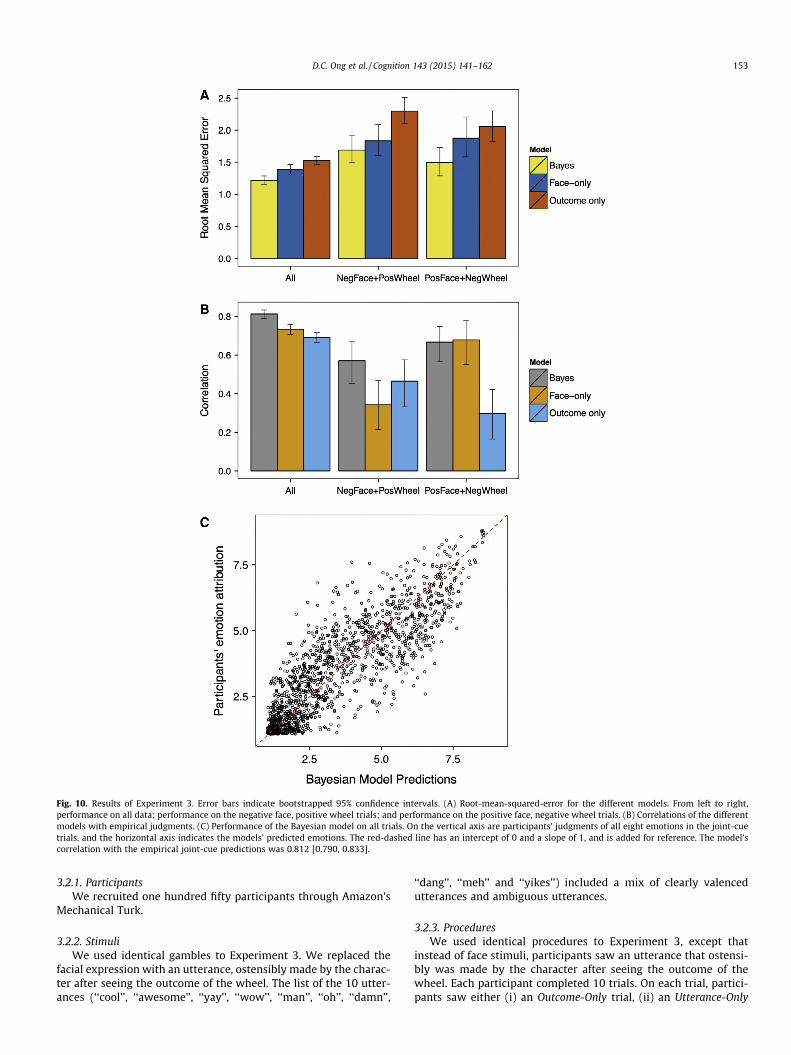
Fig. 10. Results of Experiment 3. Error bars indicate bootstrapped 95% confidence intervals. (A) Root-mean-squared-error for the different models. From left to right,performance on all data; performance on the negative face, positive wheel trials; and performance on the positive face, negative wheel trials. (B) Correlations of the differentmodels with empirical judgments. (C) Performance of the Bayesian model on all trials. On the vertical axis are participants’ judgments of all eight emotions in the joint-cuetrials, and the horizontal axis indicates the models’ predicted emotions. The red-dashed line has an intercept of 0 and a slope of 1, and is added for reference. The model’scorrelation with the empirical joint-cue predictions was 0.812 [0.790, 0.833].
D.C. Ong et al. / Cognition 143 (2015) 141–162 153
3.2.1. ParticipantsWe recruited one hundred fifty participants through Amazon’s
Mechanical Turk.
3.2.2. StimuliWe used identical gambles to Experiment 3. We replaced the
facial expression with an utterance, ostensibly made by the charac-ter after seeing the outcome of the wheel. The list of the 10 utter-ances (‘‘cool’’, ‘‘awesome’’, ‘‘yay’’, ‘‘wow’’, ‘‘man’’, ‘‘oh’’, ‘‘damn’’,
‘‘dang’’, ‘‘meh’’ and ‘‘yikes’’) included a mix of clearly valencedutterances and ambiguous utterances.
3.2.3. ProceduresWe used identical procedures to Experiment 3, except that
instead of face stimuli, participants saw an utterance that ostensi-bly was made by the character after seeing the outcome of thewheel. Each participant completed 10 trials. On each trial, partici-pants saw either (i) an Outcome-Only trial, (ii) an Utterance-Only
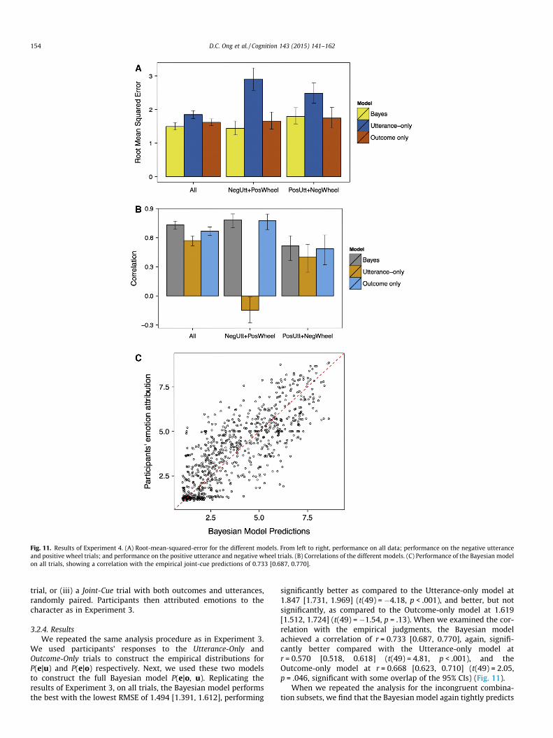
Fig. 11. Results of Experiment 4. (A) Root-mean-squared-error for the different models. From left to right, performance on all data; performance on the negative utteranceand positive wheel trials; and performance on the positive utterance and negative wheel trials. (B) Correlations of the different models. (C) Performance of the Bayesian modelon all trials, showing a correlation with the empirical joint-cue predictions of 0.733 [0.687, 0.770].
154 D.C. Ong et al. / Cognition 143 (2015) 141–162
trial, or (iii) a Joint-Cue trial with both outcomes and utterances,randomly paired. Participants then attributed emotions to thecharacter as in Experiment 3.
3.2.4. ResultsWe repeated the same analysis procedure as in Experiment 3.
We used participants’ responses to the Utterance-Only andOutcome-Only trials to construct the empirical distributions forP(e|u) and P(e|o) respectively. Next, we used these two modelsto construct the full Bayesian model P(e|o, u). Replicating theresults of Experiment 3, on all trials, the Bayesian model performsthe best with the lowest RMSE of 1.494 [1.391, 1.612], performing
significantly better as compared to the Utterance-only model at1.847 [1.731, 1.969] (t(49) = �4.18, p < .001), and better, but notsignificantly, as compared to the Outcome-only model at 1.619[1.512, 1.724] (t(49) = �1.54, p = .13). When we examined the cor-relation with the empirical judgments, the Bayesian modelachieved a correlation of r = 0.733 [0.687, 0.770], again, signifi-cantly better compared with the Utterance-only model atr = 0.570 [0.518, 0.618] (t(49) = 4.81, p < .001), and theOutcome-only model at r = 0.668 [0.623, 0.710] (t(49) = 2.05,p = .046, significant with some overlap of the 95% CIs) (Fig. 11).
When we repeated the analysis for the incongruent combina-tion subsets, we find that the Bayesian model again tightly predicts
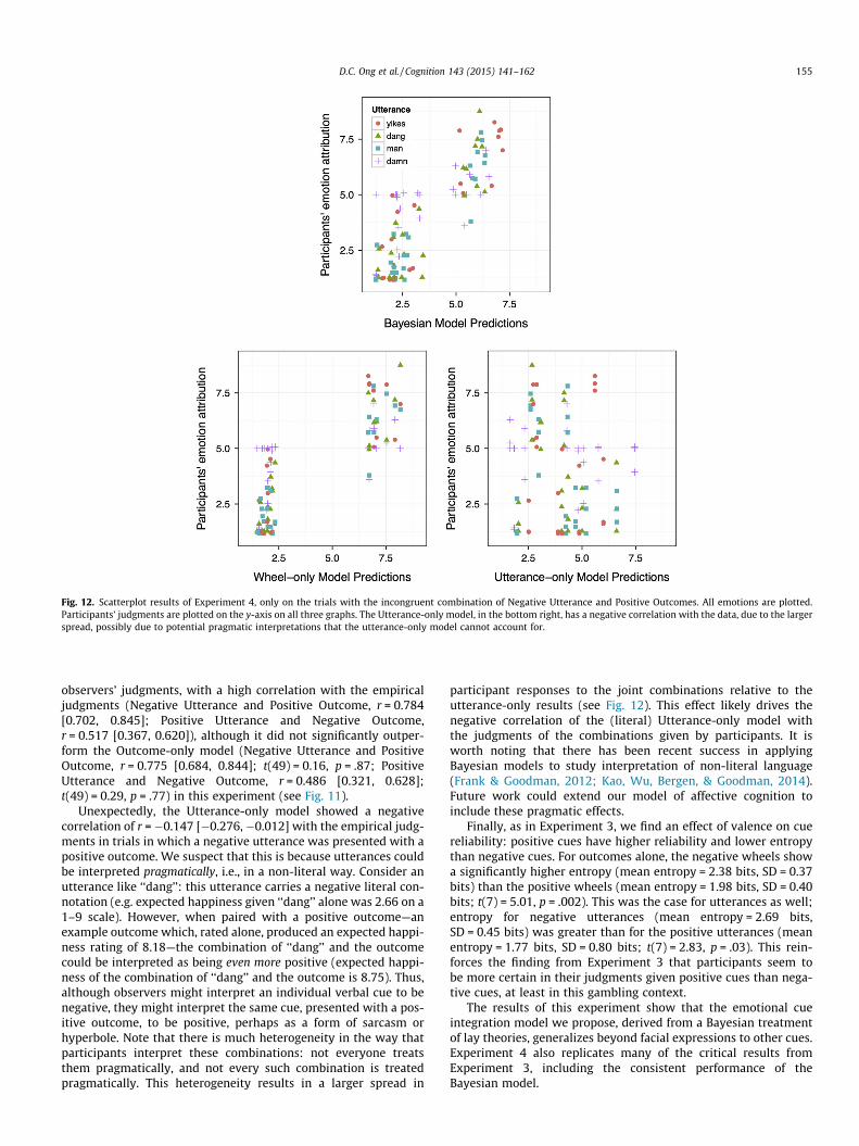
Fig. 12. Scatterplot results of Experiment 4, only on the trials with the incongruent combination of Negative Utterance and Positive Outcomes. All emotions are plotted.Participants’ judgments are plotted on the y-axis on all three graphs. The Utterance-only model, in the bottom right, has a negative correlation with the data, due to the largerspread, possibly due to potential pragmatic interpretations that the utterance-only model cannot account for.
D.C. Ong et al. / Cognition 143 (2015) 141–162 155
observers’ judgments, with a high correlation with the empiricaljudgments (Negative Utterance and Positive Outcome, r = 0.784[0.702, 0.845]; Positive Utterance and Negative Outcome,r = 0.517 [0.367, 0.620]), although it did not significantly outper-form the Outcome-only model (Negative Utterance and PositiveOutcome, r = 0.775 [0.684, 0.844]; t(49) = 0.16, p = .87; PositiveUtterance and Negative Outcome, r = 0.486 [0.321, 0.628];t(49) = 0.29, p = .77) in this experiment (see Fig. 11).
Unexpectedly, the Utterance-only model showed a negativecorrelation of r = �0.147 [�0.276, �0.012] with the empirical judg-ments in trials in which a negative utterance was presented with apositive outcome. We suspect that this is because utterances couldbe interpreted pragmatically, i.e., in a non-literal way. Consider anutterance like ‘‘dang’’: this utterance carries a negative literal con-notation (e.g. expected happiness given ‘‘dang’’ alone was 2.66 on a1–9 scale). However, when paired with a positive outcome—anexample outcome which, rated alone, produced an expected happi-ness rating of 8.18—the combination of ‘‘dang’’ and the outcomecould be interpreted as being even more positive (expected happi-ness of the combination of ‘‘dang’’ and the outcome is 8.75). Thus,although observers might interpret an individual verbal cue to benegative, they might interpret the same cue, presented with a pos-itive outcome, to be positive, perhaps as a form of sarcasm orhyperbole. Note that there is much heterogeneity in the way thatparticipants interpret these combinations: not everyone treatsthem pragmatically, and not every such combination is treatedpragmatically. This heterogeneity results in a larger spread in
participant responses to the joint combinations relative to theutterance-only results (see Fig. 12). This effect likely drives thenegative correlation of the (literal) Utterance-only model withthe judgments of the combinations given by participants. It isworth noting that there has been recent success in applyingBayesian models to study interpretation of non-literal language(Frank & Goodman, 2012; Kao, Wu, Bergen, & Goodman, 2014).Future work could extend our model of affective cognition toinclude these pragmatic effects.
Finally, as in Experiment 3, we find an effect of valence on cuereliability: positive cues have higher reliability and lower entropythan negative cues. For outcomes alone, the negative wheels showa significantly higher entropy (mean entropy = 2.38 bits, SD = 0.37bits) than the positive wheels (mean entropy = 1.98 bits, SD = 0.40bits; t(7) = 5.01, p = .002). This was the case for utterances as well;entropy for negative utterances (mean entropy = 2.69 bits,SD = 0.45 bits) was greater than for the positive utterances (meanentropy = 1.77 bits, SD = 0.80 bits; t(7) = 2.83, p = .03). This rein-forces the finding from Experiment 3 that participants seem tobe more certain in their judgments given positive cues than nega-tive cues, at least in this gambling context.
The results of this experiment show that the emotional cueintegration model we propose, derived from a Bayesian treatmentof lay theories, generalizes beyond facial expressions to other cues.Experiment 4 also replicates many of the critical results fromExperiment 3, including the consistent performance of theBayesian model.
156 D.C. Ong et al. / Cognition 143 (2015) 141–162
3.3. Revisiting emotions from outcomes: a combined analysis
Experiments 3 and 4 were designed to test our cue integrationpredictions, using analyses that built upon the results ofExperiment 1, which explored the important outcome featuresfor predicting participants’ affective judgments. However,Experiments 3 and 4 also produced additional data with whichwe can re-examine Experiment 1’s results, that is, the statisticalcausal model of outcomes to emotions. This combined analysiswould allow us to test the reliability of the results of the statisticalmodel that we built in Experiment 1 (and used in the cue integra-tion analyses above). In order to do this, we proceeded to isolatethe wheel-only trials from Experiments 3 and 4, together with allthe trials from Experiment 1, creating a dataset of 3048 observa-tions from 690 participants.
With this larger dataset, we repeated the model selection, withthe full set of regressors (as in Appendix A), to determine which out-come features significantly predict attributed emotions. Asexpected, the amount won, PE, and |PE| again came out as significantpredictors for the various emotions (details in Appendix A), withseveral additional patterns of interest: e.g., fear is only predictedby the amount won. Surprise now strongly depends on |PE|, regret,and the winning probability, which suggests a different structurefor surprise than the rest of the emotions (additional evidence for thisis also given by the different loadings in the PCA analysis).
One additional regressor of note became significant with thislarger dataset: the near-miss term predicted happiness(b =�3.32e�05 [�5.51e�05 �1.12e�05], t(682) =�2.963, p = 0.003).We tested for, but did not find a significant difference between pos-itive and negative near-misses (v2(1) = 0.089, p = 0.77), i.e., whetherthe next-nearer outcome was a larger or smaller payoff, althoughthis could just be from a lack of power. To better understand themagnitude of the near-miss term, let us consider a concretenear-miss example using the slopes on win (b = 0.0405 [0.029,0.052], t(682) = 7.08, p < .001), PE (b = 0.036 [0.024, 0.048], t(682) =5.95, p < .001), and |PE| (b = �0.015 [�0.025,�0.005] t(682) = �2.84,p = .006), and the $25/$60/$100 wheel in Fig. 2. Not considering thenear-miss term, and all else being equal, if the result had changedfrom $60 to $100, there would be an increase in happiness of40 ⁄ (.0405 + 0.036 � 0.015) = 2.46 points on a 9 point Likert scale.By contrast, if the outcome result (the exact point the black pointerindicated) moved from the center of the $60 sector to a near-missdistance of 1% of the sector size away from the $60/$100 boundary,there would be a decrease in happiness of 40 ⁄ (1/0.5 � 1/0.01) ⁄(�3.32 ⁄ 10�5) = 0.130 points on a 9 point scale. Thus, in this gam-bling scenario, the effect of a near-miss on subjective happinessattributed is on the order of 5% of the relative happiness of winningthe next higher amount. Getting a near-miss on the $60 wheel inFig. 2 and narrowly missing the $100 sector (narrowly missing win-ning $40 more) has a subjective cost equivalent to losing about $2,compared with a far-miss (landing in the center of the sector). Thisis a small effect relative to actually winning—and indeed, we couldnot detect it with Experiment 1 data alone—yet it is a large andnot insignificant effect considering that it does not depend on chang-ing actual payoffs, but merely relative closeness. This result buildsupon the results of Experiment 1 by investigating what additionalsituation features might factor (perhaps more weakly) into affectivecognition in this paradigm.
4. Discussion
We have proposed a framework for studying affective cognitionas domain-general reasoning applied to a domain-specific lay the-ory of emotions; the lay theory is described as a statistical causalknowledge of others’ emotions, and reasoning as Bayesian
inference based on this knowledge. Observers’ lay theories consistof a consistent structure that captures causal relationshipsbetween situation outcomes (or emotion-eliciting events), theagent’s emotions, and the agent’s observable behaviors. Each ofthese causal relationships contains complex knowledge: for exam-ple, an observer incorporates appraisal processes when reasoningabout how an agent feels after the outcome of a situation. Thisframework makes detailed quantitative predictions that wereborne out in a series of experiments. We demonstrated that obser-vers are able to consistently reason both forward, along the causaldirection, and ‘‘backwards’’, about causes based on emotional reac-tion. The forward causal model relied on a small set of situationfeatures (Experiment 1), and backward reasoning waswell-described as Bayesian inference given this forward model(Experiment 2). This approach provides further traction in under-standing how observers infer unobservable emotional states fromdiverse observable cues. In particular, we have shown that inte-grating multiple sources of information as prescribed by Bayesianstatistics explains human judgments of emotions from facialexpressions and outcomes (Experiment 3), and from utterancesand outcomes (Experiment 4). Our results showed an interesting‘‘valence dominance’’ effect, whereby positively-valenced emo-tional cues tended to have higher reliabilities and were weightedmore so than negatively-valenced cues. Our model was able toaccount for this valence effect without a priori specification, attest-ing to the robustness of a probabilistic model of affective cognition.Our studies contrast with previous studies that have found face orcontext dominance (e.g., Aviezer et al., 2008; Nakamura et al.,1990; Russell et al., 2003) in that our paradigm involves arestricted gambling context; it is possible that our valence resultmay not generalize to other contexts, though we believe that theunderlying model of cue integration will still be applicable.
Emotions are numerous and complex, and we have only exam-ined emotional reasoning in very constrained gambling scenarios.These scenarios constitute a reasonable starting point for studyingaffective cognition, because they afford consistent assumptionsand quantitative manipulations. For instance, an agent playing agamble almost certainly wants to win more money, giving obser-vers a clear cornerstone for understanding the affective meaningof different gamble outcomes. Even in these simple scenarios, withostensibly simple economic motivations, participants were sensi-tive to subtle ‘‘irrationalities’’ that they expected the agent toevince. For instance, by pooling data from three of our experi-ments, we found that the nearness of alternative, better outcomes(or worse outcomes) factored into our participants’ inferencesabout agents’ emotion. Further work will likely uncover additionalfeatures that factor into affective cognition.
Not all emotions are relevant in our scenarios—fear, for exam-ple, may be irrelevant, as may a more complex emotion likepride—and furthermore, we might reason about emotions like hap-piness differently in a gambling context than in other contexts. Oneavenue of further research includes extending our model to morecomplex situations. For instance, people do not live in a social vac-uum, and emotions often depend on interactions with others: acomprehensive model would include how observers reason aboutemotions in social interactions, leading to emotions like prideand jealousy.
The work presented here was concerned with high-level rea-soning, and abstracted out, for example, the process by which weperceive facial expressions (How does an observer look at a faceand decide that the agent is happy? Which facial features areimportant?), or how we interpret the linguistic content of emo-tional utterances (How do we interpret ‘‘dang’’ as negative?). Inthis work, we measured the connection between these perceptsand emotional states, rather than explaining them, then investi-gated how observers utilized them to make higher-level
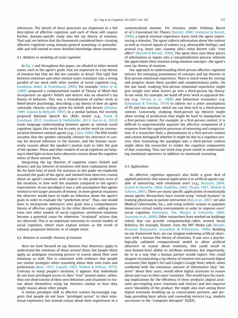
D.C. Ong et al. / Cognition 143 (2015) 141–162 157
inferences. The details of these processes are important in a fulldescription of affective cognition, and each of these will requirefurther, domain-specific study into the lay theory of emotion.That said, we believe that the framework considered here—treatingaffective cognition using domain-general reasoning—is generaliz-able and will extend to more detailed knowledge about emotions.
4.1. Relation to modeling of social cognition
In Fig. 2 and throughout this paper, we alluded to other mentalstates, such as the agent’s goals, that are important in a lay theoryof emotion but that we did not consider in detail. This tight linkbetween emotions and other mental states translates into a strongparallel of our work with other models of social cognition (e.g.,Goodman, Baker, & Tenenbaum, 2009). For example, Baker et al.(2009) proposed a computational model of Theory of Mind thatincorporates an agent’s beliefs and desires into an observer’s laytheory of behavior. This was a formalization of earlier work inbelief-desire psychology, describing a lay theory of how an agentrationally chooses actions given his beliefs and desires (Dennet,1989; Gopnik & Meltzoff, 1997). In a similar fashion, the recentlyproposed Rational Speech Act (RSA) model (e.g., Frank &Goodman, 2012; Goodman & Stuhlmüller, 2013; Kao et al., 2014)treats language understanding between agents as rational socialcognition. Again, this work has its roots in earlier work on commu-nication between rational agents (e.g., Clark, 1996). The RSA modelassumes that the speaker rationally chooses his utterance to con-vey his desired inference to the listener, and the listener recur-sively reasons about the speaker’s mental state to infer the goalof the speaker. These and other models of social cognition are help-ing to shed light on how naïve observers reason about the cognitivestates of those around them.
Integrating the lay theories of cognitive states (beliefs anddesires) and lay theories of emotions will have explanatory bene-fits for both lines of work. For instance, in this paper we implicitlyassumed the goals of the agent, and showed how observers reasonabout an agent’s emotions with respect to the prediction error ofthe situation, or how well the situation compared to the agent’sexpectations. In our paradigm it was a safe assumption that agentswished to win larger amounts of money; in more general situationsthe observer would have to make an inference about the agent’sgoals in order to evaluate the ‘‘prediction error’’. Thus, one wouldhave to incorporate inferences over goals into a comprehensivetheory of affective cognition. In the other direction—adding emo-tions into other models of social cognition—attributed emotionsbecome a potential cause for otherwise ‘‘irrational’’ actions thatare observed. This is an important extension to current models ofsocial cognition, which must explain actions as the result ofrational, purposive behavior or of simple noise.
4.2. Relation to scientific theories of emotion
Here we have focused on lay theories that observers apply tounderstand the emotions of those around them, but people likelyapply an analogous reasoning process to reason about their ownemotions as well. This is consistent with evidence that peopleuse similar strategies when reasoning about their own traits andpreferences (Bem, 1972; Gopnik, 1993; Nisbett & Wilson, 1977).Contrary to many people’s intuition, it appears that individualsdo not have privileged access to their ‘‘true’’ mental states; rather,they use observations of their own behaviors and situations to rea-son about themselves using lay theories—similar to how theymight reason about other people.
A similar paradigm shift in affective science increasingly sug-gests that people do not have ‘‘privileged access’’ to their emo-tional experience, but instead reason about their experiences in a
contextualized manner. For instance, under Feldman Barretet al.’s Conceptual Act Theory (Barrett, 2006; Lindquist & Barrett,2008), a typical emotion experience starts with the agent experi-encing a stimulus. The agent collects information about the contextas well as visceral signals of valence (e.g. pleasurable feelings) andarousal (e.g. heart rate, clammy skin)—what Barrett calls ‘‘coreaffect’’ (Russell & Barrett, 1999). The agent then uses these piecesof information as inputs into a conceptualization process whereinthe agent labels their emotion using emotion concepts—the agent’sown lay theory of emotion.
Our approach to understanding third-person affective cognitionmirrors the emerging prominence of concepts and lay theories infirst-person emotional experience. There is much room for overlapand progress down these parallel and complementary paths. Onthe one hand, studying first-person emotional experience mightgive insight into what factors go into a third-person lay theory.In our work, for example, we build off prior work in appraisal the-ory (e.g., Ortony et al., 1988) and behavioral economics (e.g.Kahneman & Tversky, 1979) to inform our a priori assumptionsof PE and loss aversion, which we can then test in a third-personcontext. Conversely, studying third-person lay theories mightallow testing of predictions that might be hard to manipulate ina first-person context. For example, in a first-person context, it isdifficult to experimentally separate the affective component of aresponse from the cognitive processes of reasoning and categoriza-tion. If a researcher finds a phenomenon in a first-person contextand cannot distinguish whether it might be due to a cognitive pro-cess, then translating the paradigm into a third-person contextmight allow the researcher to isolate the cognitive componentsof that reasoning. Thus our work may prove useful in understand-ing emotional experience in addition to emotional reasoning.
4.3. Applications
An affective cognition approach also holds a great deal ofapplied potential. One natural application is to artificial agents cap-able of interacting with emotional users (e.g., Breazeal, 2004;Gratch & Marsella, 2004; Hudlicka, 2003; Picard, 1997; Wehrle &Scherer, 2001). There are many specific applications of emotionallyaware agents. Researchers have started using ‘‘virtual humans’’ intraining physicians in patient interaction (Raij et al., 2007; see alsoMedical Cyberworlds, Inc.), and using realistic avatars to populateimmersive virtual reality environments in order to improve users’social cognition (Bailenson, Yee, Merget, & Schroeder, 2006;Swartout et al., 2006). Other researchers have worked on buildingsrobots that can provide companionship—often termed SocialRobotics, for example, Kismet, from the MIT Media Lab (Brooks,Breazeal, Marjanovic, Scassellati, & Williamson, 1999). Buildingon our framework here, we can imagine endowing artificial obser-vers with a human-like theory of emotions. If one uses a psycho-logically validated computational model to allow artificialobservers to reason about emotions, this could result innear-human-level ability to attribute emotions, but importantly,do so in a way that a human partner would expect. One couldimagine incorporating a lay theory of emotion into personal digitalassistants (like Apple’s Siri and Google’s Google Now) which, whencombined with the enormous amount of information they ‘‘ob-serve’’ about their users, would allow digital assistants to reasonabout and react to their users’ emotions. This would have far reach-ing implications for the efficiency of these products (digital assis-tants pre-empting users’ emotions and choices) and also improveusers’ likeability of the product. We might also start seeing thesedigital assistants doubling up as conversation partners, and per-haps providing basic advice and counseling services (e.g., modernsuccessors to the ‘‘computer therapist’’ ELIZA).
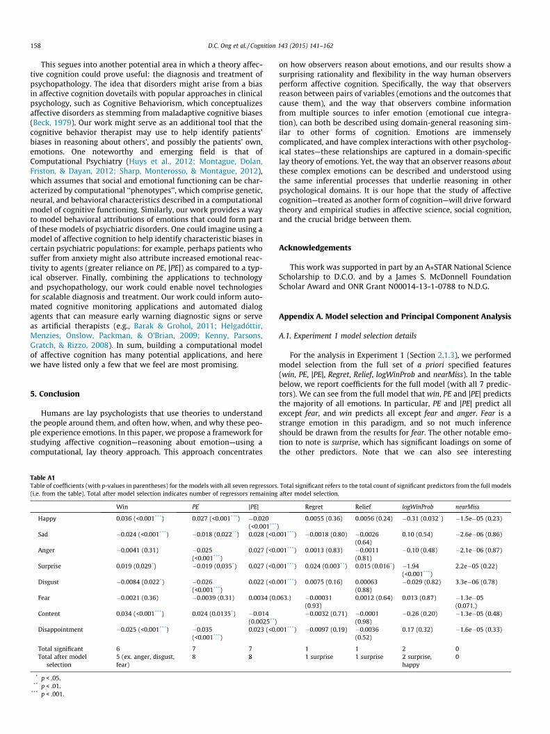
158 D.C. Ong et al. / Cognition 143 (2015) 141–162
This segues into another potential area in which a theory affec-tive cognition could prove useful: the diagnosis and treatment ofpsychopathology. The idea that disorders might arise from a biasin affective cognition dovetails with popular approaches in clinicalpsychology, such as Cognitive Behaviorism, which conceptualizesaffective disorders as stemming from maladaptive cognitive biases(Beck, 1979). Our work might serve as an additional tool that thecognitive behavior therapist may use to help identify patients’biases in reasoning about others’, and possibly the patients’ own,emotions. One noteworthy and emerging field is that ofComputational Psychiatry (Huys et al., 2012; Montague, Dolan,Friston, & Dayan, 2012; Sharp, Monterosso, & Montague, 2012),which assumes that social and emotional functioning can be char-acterized by computational ‘‘phenotypes’’, which comprise genetic,neural, and behavioral characteristics described in a computationalmodel of cognitive functioning. Similarly, our work provides a wayto model behavioral attributions of emotions that could form partof these models of psychiatric disorders. One could imagine using amodel of affective cognition to help identify characteristic biases incertain psychiatric populations: for example, perhaps patients whosuffer from anxiety might also attribute increased emotional reac-tivity to agents (greater reliance on PE, |PE|) as compared to a typ-ical observer. Finally, combining the applications to technologyand psychopathology, our work could enable novel technologiesfor scalable diagnosis and treatment. Our work could inform auto-mated cognitive monitoring applications and automated dialogagents that can measure early warning diagnostic signs or serveas artificial therapists (e.g., Barak & Grohol, 2011; Helgadóttir,Menzies, Onslow, Packman, & O’Brian, 2009; Kenny, Parsons,Gratch, & Rizzo, 2008). In sum, building a computational modelof affective cognition has many potential applications, and herewe have listed only a few that we feel are most promising.
5. Conclusion
Humans are lay psychologists that use theories to understandthe people around them, and often how, when, and why these peo-ple experience emotions. In this paper, we propose a framework forstudying affective cognition—reasoning about emotion—using acomputational, lay theory approach. This approach concentrates
Table A1Table of coefficients (with p-values in parentheses) for the models with all seven regressors(i.e. from the table). Total after model selection indicates number of regressors remaining
Win PE |PE|
Happy 0.036 (<0.001***) 0.027 (<0.001***) �0.020(<0.001***
Sad �0.024 (<0.001***) �0.018 (0.022**) 0.028 (<0.
Anger �0.0041 (0.31) �0.025(<0.001***)
0.027 (<0.
Surprise 0.019 (0.029*) �0.019 (0.035*) 0.027 (<0.
Disgust �0.0084 (0.022*) �0.026(<0.001***)
0.022 (<0.
Fear �0.0021 (0.36) �0.0039 (0.31) 0.0034 (0.
Content 0.034 (<0.001***) 0.024 (0.0135*) �0.014(0.0025**)
Disappointment �0.025 (<0.001***) �0.035(<0.001***)
0.023 (<0.
Total significant 6 7 7Total after model
selection5 (ex. anger, disgust,fear)
8 8
* p < .05.** p < .01.
*** p < .001.
on how observers reason about emotions, and our results show asurprising rationality and flexibility in the way human observersperform affective cognition. Specifically, the way that observersreason between pairs of variables (emotions and the outcomes thatcause them), and the way that observers combine informationfrom multiple sources to infer emotion (emotional cue integra-tion), can both be described using domain-general reasoning sim-ilar to other forms of cognition. Emotions are immenselycomplicated, and have complex interactions with other psycholog-ical states—these relationships are captured in a domain-specificlay theory of emotions. Yet, the way that an observer reasons aboutthese complex emotions can be described and understood usingthe same inferential processes that underlie reasoning in otherpsychological domains. It is our hope that the study of affectivecognition—treated as another form of cognition—will drive forwardtheory and empirical studies in affective science, social cognition,and the crucial bridge between them.
Acknowledgements
This work was supported in part by an A⁄STAR National ScienceScholarship to D.C.O. and by a James S. McDonnell FoundationScholar Award and ONR Grant N00014-13-1-0788 to N.D.G.
Appendix A. Model selection and Principal Component Analysis
A.1. Experiment 1 model selection details
For the analysis in Experiment 1 (Section 2.1.3), we performedmodel selection from the full set of a priori specified features(win, PE, |PE|, Regret, Relief, logWinProb and nearMiss). In the tablebelow, we report coefficients for the full model (with all 7 predic-tors). We can see from the full model that win, PE and |PE| predictsthe majority of all emotions. In particular, PE and |PE| predict allexcept fear, and win predicts all except fear and anger. Fear is astrange emotion in this paradigm, and so not much inferenceshould be drawn from the results for fear. The other notable emo-tion to note is surprise, which has significant loadings on some ofthe other predictors. Note that we can also see interesting
. Total significant refers to the total count of significant predictors from the full modelsafter model selection.
Regret Relief logWinProb nearMiss
)0.0055 (0.36) 0.0056 (0.24) �0.31 (0.032*) �1.5e�05 (0.23)
001***) �0.0018 (0.80) �0.0026(0.64)
0.10 (0.54) �2.6e�06 (0.86)
001***) 0.0013 (0.83) �0.0011(0.81)
�0.10 (0.48) �2.1e�06 (0.87)
001***) 0.024 (0.003**) 0.015 (0.016*) �1.94(<0.001***)
2.2e�05 (0.22)
001***) 0.0075 (0.16) 0.00063(0.88)
�0.029 (0.82) 3.3e�06 (0.78)
063.) �0.00031(0.93)
0.0012 (0.64) 0.013 (0.87) �1.3e�05(0.071.)
�0.0032 (0.71) �0.0001(0.98)
�0.26 (0.20) �1.3e�05 (0.48)
001***) �0.0097 (0.19) �0.0036(0.52)
0.17 (0.32) �1.6e�05 (0.33)
1 1 2 01 surprise 1 surprise 2 surprise,
happy0
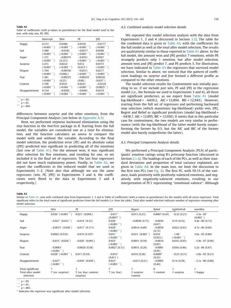
Table A2Table of coefficients (with p-values in parentheses) for the final model used in thetext, with only win, PE, |PE|.
Intercept Win PE |PE|
Happy 4.515(<0.001***)
0.0386(<0.001***)
0.0350(<0.001***)
�0.0177(<0.001***)
Sad 3.380(<0.001***)
�0.0245(<0.001***)
�0.0217(<0.001***)
0.0268(<0.001***)
Anger 1.721(<0.001***)
�0.00375(0.251)
�0.0251(<0.001***)
0.0267(<0.001***)
Surprise 3.251(<0.001***)
0.0222(<0.001***)
0.012(0.013*)
0.0373(<0.001***)
Disgust 1.764(<0.001***)
�0.00536(0.066.)
�0.0211(<0.001***)
0.0217(<0.001***)
Fear 1.381(<0.001***)
�0.00225(0.23)
�0.00325(0.09.)
0.00342(0.037*)
Content 3.709(<0.001***)
0.0321(<0.001***)
0.0221(<0.001***)
�0.0124(0.0025**)
Disappointment 4.724(<0.001***)
�0.0292(<0.001***)
�0.0441(<0.001***)
0.0219(<0.001***)
* p < .05.** p < .01.
*** p < .001.
D.C. Ong et al. / Cognition 143 (2015) 141–162 159
differences between surprise and the other emotions, from thePrincipal Component Analysis (see below in Appendix A.3)
Next, we performed stepwise backward elimination using thestep function in the lmerTest package in R. Starting from the fullmodel, the variables are considered one at a time for elimina-tion, and the function calculates an anova to compare themodel with and without the variable. According to the finalmodel selection, the prediction error (PE) and its absolute value(|PE|) predicted was significant in predicting all of the emotions(last row of Table A1). For the amount won, it was significantafter selection for five emotions, and trending for one, so weincluded it in the final set of regressors. The last four regressorsdid not have much explanatory power. Finally, in Table A2, wereport the coefficients in the reduced model that we used inExperiments 1–2. (Note also that although we use the sameregressors (win, PE, |PE|) in Experiments 3 and 4, the coeffi-cients were fitted to the data in Experiments 3 and 4respectively.)
Table A3Similar to Table A1, now with combined data from Experiments 1, 3 and 4. Table of coeffisignificant refers to the total count of significant predictors from the full models (i.e. frommodel selection.
Win PE |PE|
Happy 0.036� (<0.001***) 0.021� (0.094.) �0.017�
(0.0057**)Sad �0.027� (0.012**) �0.014� (0.32) 0.028�
(<0.001***
Anger �0.0015� (0.038*) �0.017� (0.171) 0.028�
(<0.001***
Surprise 0.0042 (0.532) �0.019 (0.107) 0.031�
(<0.001***
Disgust �0.015� (0.026*) �0.020� (0.093.) 0.023�
(<0.001***
Fear �0.0083�
(<0.001***)�0.0020 (0.58) 0.0027 (0.
Content 0.028� (<0.001***) 0.011 (0.34) �0.015�
(0.011*)Disappointment �0.027�
(<0.001***)�0.030� (0.020*) 0.023�
(<0.001***
Total significant 7 1 7Total after model
selection7 (ex. surprise) 5 (ex. fear, content,
surprise)7 (ex. fear
* p < .05.** p < .01.
*** p < .001.� Indicates the regressor was significant after model selection.
A.2. Combined analysis model selection details
We repeated this model selection analysis with the data fromExperiments 1, 3 and 4 (discussed in Section 3.3). The table forthe combined data is given in Table A3, with the coefficients forthe full model as well as the total after model selection. The resultsare qualitatively similar to those reported in Table A1 above. In thefull model, the amount won and |PE| predict 7 emotions, while PEstrangely predicts only 1 emotion, but after model selection,amount won and |PE| predict 7, and PE predicts 5. For illustration,we have indicated in Table A3 the regressors that survived modelselection. Similar to above, we noticed that the pattern of coeffi-cient loadings on surprise and fear formed a different profile ascompared to the other emotions.
The model selection results for Contentment was initially puz-zling to us: if we include just win, PE and |PE| in the regressionmodel (i.e., the formula we used in Experiments 3 and 4), all threeare significant predictors, as we expect from Table A1 (modellog-likelihood = �6439.2, AIC = 12,894, BIC = 12,943). However,starting from the full set of regressors and performing backwardstep selection (which maximizes log-likelihood) yields win, |PE|,Regret and Relief as significant predictors (model log-likelihood =�6438.7, AIC = 12,895, BIC = 12,950). It seems that in this particularcase for contentment, the two models are very similar in perfor-mance (with the log-likelihood of the latter model barely outper-forming the former by 0.5, but the AIC and BIC of the formermodel also barely outperforms the latter).
A.3. Principal Component Analysis details
We performed a Principal Component Analysis (PCA) of partic-ipants’ emotion ratings using R’s princomp function (discussed inSection 2.1.4). The loadings of each of the PCs, as well as their stan-dard deviations and proportion of total variance explained, aregiven in Table A4. In the main text, we limit the discussion tothe first two PCs (see Fig. 4). The first PC, with 59.1% of the vari-ance, loads positively with positively-valenced emotions, and neg-atively with negatively-valenced emotions, resulting in ourinterpretation of PC1 representing ‘‘emotional valence’’. Although
cients (with p-values in parentheses) for the models with all seven regressors. Totalthe table). Total after model selection indicates number of regressors remaining after
Regret Relief logWinProb nearMiss
0.013 (0.23) 0.0067 (0.43) �0.32 (0.21) �3.3e�05�
(0.003**)
)�0.0038 (0.75) �0.0039
(0.67)0.19 (0.52) 4.4e�06 (0.73)
)0.0014 (0.89) �0.0030
(0.72)0.022 (0.93) 4.7e�06 (0.69)
)0.033� (0.002**) 0.016
(0.052.)�1.66�
(<0.001***)3.9e�05 (0.80)
)0.0051 (0.59) �0.0014
(0.85)0.016 (0.95) �5.9e�07 (0.96)
13) 0.0031 (0.26) �0.0001(0.95)
0.056 (0.46) 5.2e�06 (0.47)
0.010 (0.28) 0.0089�
(0.25)�0.25 (0.31) �2.0e�05 (0.21)
)�0.013 (0.21) �0.0065
(0.44)0.14 (0.58) �2.1e�06 (0.88)
1 0 1 1) 2 surprise
content1 content 1 surprise 1 happy
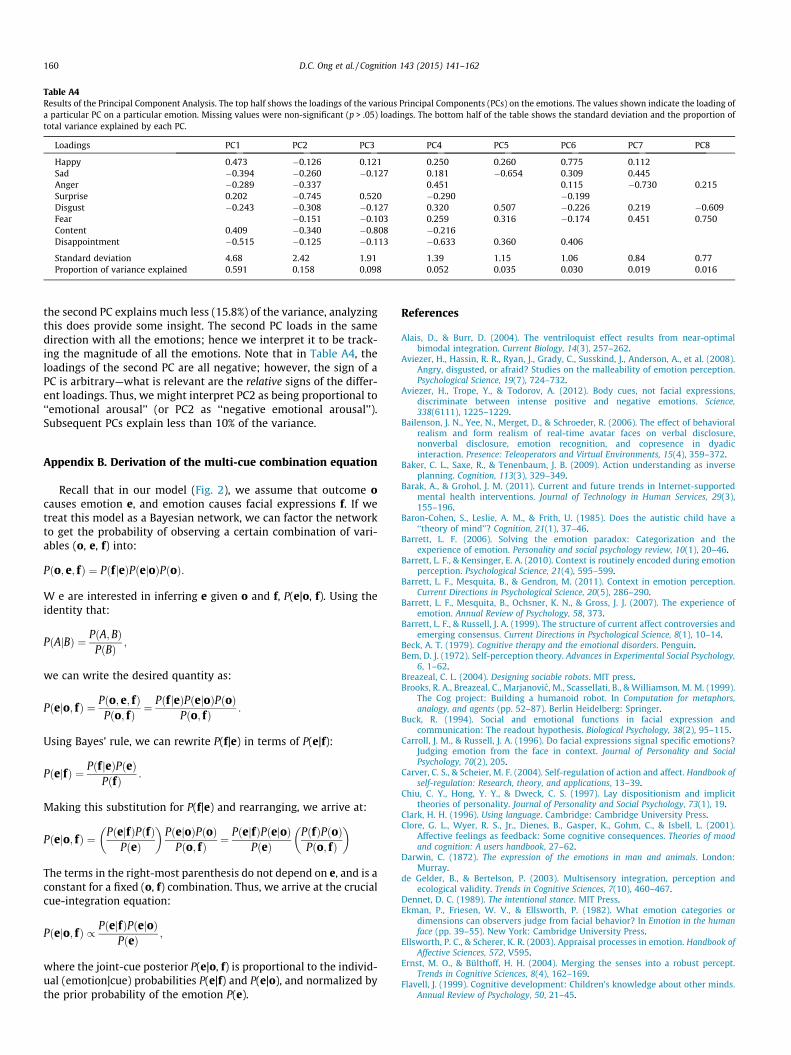
Table A4Results of the Principal Component Analysis. The top half shows the loadings of the various Principal Components (PCs) on the emotions. The values shown indicate the loading ofa particular PC on a particular emotion. Missing values were non-significant (p > .05) loadings. The bottom half of the table shows the standard deviation and the proportion oftotal variance explained by each PC.
Loadings PC1 PC2 PC3 PC4 PC5 PC6 PC7 PC8
Happy 0.473 �0.126 0.121 0.250 0.260 0.775 0.112Sad �0.394 �0.260 �0.127 0.181 �0.654 0.309 0.445Anger �0.289 �0.337 0.451 0.115 �0.730 0.215Surprise 0.202 �0.745 0.520 �0.290 �0.199Disgust �0.243 �0.308 �0.127 0.320 0.507 �0.226 0.219 �0.609Fear �0.151 �0.103 0.259 0.316 �0.174 0.451 0.750Content 0.409 �0.340 �0.808 �0.216Disappointment �0.515 �0.125 �0.113 �0.633 0.360 0.406
Standard deviation 4.68 2.42 1.91 1.39 1.15 1.06 0.84 0.77Proportion of variance explained 0.591 0.158 0.098 0.052 0.035 0.030 0.019 0.016
160 D.C. Ong et al. / Cognition 143 (2015) 141–162
the second PC explains much less (15.8%) of the variance, analyzingthis does provide some insight. The second PC loads in the samedirection with all the emotions; hence we interpret it to be track-ing the magnitude of all the emotions. Note that in Table A4, theloadings of the second PC are all negative; however, the sign of aPC is arbitrary—what is relevant are the relative signs of the differ-ent loadings. Thus, we might interpret PC2 as being proportional to‘‘emotional arousal’’ (or PC2 as ‘‘negative emotional arousal’’).Subsequent PCs explain less than 10% of the variance.
Appendix B. Derivation of the multi-cue combination equation
Recall that in our model (Fig. 2), we assume that outcome ocauses emotion e, and emotion causes facial expressions f. If wetreat this model as a Bayesian network, we can factor the networkto get the probability of observing a certain combination of vari-ables (o, e, f) into:
Pðo; e; fÞ ¼ PðfjeÞPðejoÞPðoÞ:
W e are interested in inferring e given o and f, P(e|o, f). Using theidentity that:
PðAjBÞ ¼ PðA;BÞPðBÞ ;
we can write the desired quantity as:
Pðejo; fÞ ¼ Pðo; e; fÞPðo; fÞ ¼
PðfjeÞPðejoÞPðoÞPðo; fÞ :
Using Bayes’ rule, we can rewrite P(f|e) in terms of P(e|f):
PðejfÞ ¼ PðfjeÞPðeÞPðfÞ :
Making this substitution for P(f|e) and rearranging, we arrive at:
Pðejo; fÞ ¼ PðejfÞPðfÞPðeÞ
� �PðejoÞPðoÞ
Pðo; fÞ ¼ PðejfÞPðejoÞPðeÞ
PðfÞPðoÞPðo; fÞ
� �
The terms in the right-most parenthesis do not depend on e, and is aconstant for a fixed (o, f) combination. Thus, we arrive at the crucialcue-integration equation:
Pðejo; fÞ / PðejfÞPðejoÞPðeÞ ;
where the joint-cue posterior P(e|o, f) is proportional to the individ-ual (emotion|cue) probabilities P(e|f) and P(e|o), and normalized bythe prior probability of the emotion P(e).
References
Alais, D., & Burr, D. (2004). The ventriloquist effect results from near-optimalbimodal integration. Current Biology, 14(3), 257–262.
Aviezer, H., Hassin, R. R., Ryan, J., Grady, C., Susskind, J., Anderson, A., et al. (2008).Angry, disgusted, or afraid? Studies on the malleability of emotion perception.Psychological Science, 19(7), 724–732.
Aviezer, H., Trope, Y., & Todorov, A. (2012). Body cues, not facial expressions,discriminate between intense positive and negative emotions. Science,338(6111), 1225–1229.
Bailenson, J. N., Yee, N., Merget, D., & Schroeder, R. (2006). The effect of behavioralrealism and form realism of real-time avatar faces on verbal disclosure,nonverbal disclosure, emotion recognition, and copresence in dyadicinteraction. Presence: Teleoperators and Virtual Environments, 15(4), 359–372.
Baker, C. L., Saxe, R., & Tenenbaum, J. B. (2009). Action understanding as inverseplanning. Cognition, 113(3), 329–349.
Barak, A., & Grohol, J. M. (2011). Current and future trends in Internet-supportedmental health interventions. Journal of Technology in Human Services, 29(3),155–196.
Baron-Cohen, S., Leslie, A. M., & Frith, U. (1985). Does the autistic child have a‘‘theory of mind’’? Cognition, 21(1), 37–46.
Barrett, L. F. (2006). Solving the emotion paradox: Categorization and theexperience of emotion. Personality and social psychology review, 10(1), 20–46.
Barrett, L. F., & Kensinger, E. A. (2010). Context is routinely encoded during emotionperception. Psychological Science, 21(4), 595–599.
Barrett, L. F., Mesquita, B., & Gendron, M. (2011). Context in emotion perception.Current Directions in Psychological Science, 20(5), 286–290.
Barrett, L. F., Mesquita, B., Ochsner, K. N., & Gross, J. J. (2007). The experience ofemotion. Annual Review of Psychology, 58, 373.
Barrett, L. F., & Russell, J. A. (1999). The structure of current affect controversies andemerging consensus. Current Directions in Psychological Science, 8(1), 10–14.
Beck, A. T. (1979). Cognitive therapy and the emotional disorders. Penguin.Bem, D. J. (1972). Self-perception theory. Advances in Experimental Social Psychology,
6, 1–62.Breazeal, C. L. (2004). Designing sociable robots. MIT press.Brooks, R. A., Breazeal, C., Marjanovic, M., Scassellati, B., & Williamson, M. M. (1999).
The Cog project: Building a humanoid robot. In Computation for metaphors,analogy, and agents (pp. 52–87). Berlin Heidelberg: Springer.
Buck, R. (1994). Social and emotional functions in facial expression andcommunication: The readout hypothesis. Biological Psychology, 38(2), 95–115.
Carroll, J. M., & Russell, J. A. (1996). Do facial expressions signal specific emotions?Judging emotion from the face in context. Journal of Personality and SocialPsychology, 70(2), 205.
Carver, C. S., & Scheier, M. F. (2004). Self-regulation of action and affect. Handbook ofself-regulation: Research, theory, and applications, 13–39.
Chiu, C. Y., Hong, Y. Y., & Dweck, C. S. (1997). Lay dispositionism and implicittheories of personality. Journal of Personality and Social Psychology, 73(1), 19.
Clark, H. H. (1996). Using language. Cambridge: Cambridge University Press.Clore, G. L., Wyer, R. S., Jr., Dienes, B., Gasper, K., Gohm, C., & Isbell, L. (2001).
Affective feelings as feedback: Some cognitive consequences. Theories of moodand cognition: A users handbook, 27–62.
Darwin, C. (1872). The expression of the emotions in man and animals. London:Murray.
de Gelder, B., & Bertelson, P. (2003). Multisensory integration, perception andecological validity. Trends in Cognitive Sciences, 7(10), 460–467.
Dennet, D. C. (1989). The intentional stance. MIT Press.Ekman, P., Friesen, W. V., & Ellsworth, P. (1982). What emotion categories or
dimensions can observers judge from facial behavior? In Emotion in the humanface (pp. 39–55). New York: Cambridge University Press.
Ellsworth, P. C., & Scherer, K. R. (2003). Appraisal processes in emotion. Handbook ofAffective Sciences, 572, V595.
Ernst, M. O., & Bülthoff, H. H. (2004). Merging the senses into a robust percept.Trends in Cognitive Sciences, 8(4), 162–169.
Flavell, J. (1999). Cognitive development: Children’s knowledge about other minds.Annual Review of Psychology, 50, 21–45.

D.C. Ong et al. / Cognition 143 (2015) 141–162 161
Frank, M. C., & Goodman, N. D. (2012). Predicting pragmatic reasoning in languagegames. Science, 336(6084). 998-998.
Frijda, N. H. (1988). The laws of emotion. American Psychologist, 43(5), 349–358.Geisler, W. S. (1989). Sequential ideal-observer analysis of visual discriminations.
Psychological Review, 96(2), 267.Geisler, W. S. (2003). Ideal observer analysis. The Visual Neurosciences, 825–837.Gilbert, D. (1998). Ordinary personology. In D. Gilbert, S. T. Fiske, & G. Lindzey (Eds.),
The handbook of social psychology (4th ed., pp. 89–150). New York: McGraw Hill.Gilovich, T., & Medvec, V. H. (1995). The experience of regret: What, when, and why.
Psychological Review, 102(2), 379.Goodenough, F. L., & Tinker, M. A. (1931). The relative potency of facial expression
and verbal description of stimulus in the judgment of emotion. Journal ofComparative Psychology, 12(4), 365.
Goodman, N. D. & Tenenbaum, J. B. (electronic). Probabilistic models of cognition.<http://probmods.org> Retrieved 14.07.14.
Goodman, N. D., Baker, C. L., & Tenenbaum, J. B. (2009). Cause and intent: Socialreasoning in causal learning. In Proceedings of the thirty-first annual conference ofthe cognitive science society.
Goodman, N. D., & Stuhlmüller, A. (2013). Knowledge and Implicature: Modelinglanguage understanding as social cognition. Topics in Cognitive Science, 5,173–184.
Goodman, N. D., Ullman, T. D., & Tenenbaum, J. B. (2011). Learning a theory ofcausality. Psychological Review, 118(1), 110.
Gopnik, A. (1993). Theories and illusions. Behavioral and Brain Sciences, 16(01),90–100.
Gopnik, A., & Meltzoff, A. N. (1997). Words, thoughts, and theories. The MIT Press.Gopnik, A., & Wellman, H. (1992). Why the child’s theory of mind really is a theory.
Mind and Language, 7(1–2), 145–171.Gratch, J., & Marsella, S. (2004). A domain-independent framework for modeling
emotion. Cognitive Systems Research, 5(4), 269–306.Griffiths, T. L., Kemp, C., & Tenenbaum, J. B. (2008). Bayesian models of cognition. In
Cambridge handbook of computational cognitive modeling (pp. 59–100).Heider, F. (1958). The psychology of interpersonal relations. New York: Wiley.Helgadóttir, F. D., Menzies, R. G., Onslow, M., Packman, A., & O’Brian, S. (2009).
Online CBT I: Bridging the gap between Eliza and modern online CBT treatmentpackages. Behaviour Change, 26(04), 245–253.
Hudlicka, E. (2003). To feel or not to feel: The role of affect in human–computerinteraction. International Journal of Human-Computer Studies, 59(1), 1–32.
Huys, Q. J., Eshel, N., O’Nions, E., Sheridan, L., Dayan, P., & Roiser, J. P. (2012). Bonsaitrees in your head: How the Pavlovian system sculpts goal-directed choices bypruning decision trees. PLoS Computational Biology, 8(3), e1002410.
Jayaratne, T. E., Ybarra, O., Sheldon, J. P., Brown, T. N., Feldbaum, M., Pfeffer, C. A.,et al. (2006). White Americans’ genetic lay theories of race differences andsexual orientation: Their relationship with prejudice toward Blacks, and gaymen and lesbians. Group Processes & Intergroup Relations, 9(1), 77–94.
Jones, E. E., & Davis, K. E. (1965). From acts to dispositions the attribution process inperson perception. Advances in Experimental Social Psychology, 2, 219–266.
Jones, E. E., & Nisbett, R. E. (1971). The actor and the observer: Divergent perceptions ofthe causes of behavior. Morristown, NJ: General Learning Press, p. 16.
Kahneman, D., & Tversky, A. (1979). Prospect theory: An analysis of decision underrisk. Econometrica, 47(2), 263–292.
Kahneman, D., & Tversky, A. (1984). Choices, values, and frames. AmericanPsychologist, 39(4), 341.
Kahneman, D., & Tversky, A. (1982). The simulation heuristic. In D. Kahneman, P.Slovic, & A. Tversky (Eds.), Judgment under uncertainty: Heuristics and biases(pp. 208). 201: Cambridge University Press.
Kao, J. T., Wu, J. Y., Bergen, L., & Goodman, N. D. (2014). Nonliteral understanding ofnumber words. Proceedings of the National Academy of Sciences. http://dx.doi.org/10.1073/pnas.1407479111.
Kelley, H. H. (1973). The processes of causal attribution. American Psychologist,28(2), 107.
Kelley, H. H., & Michela, J. L. (1980). Attribution theory and research. Annual Reviewof Psychology, 31(1), 457–501.
Kenny, P., Parsons, T., Gratch, J., & Rizzo, A. (2008). Virtual humans for assistedhealth care. In Proceedings of the 1st international conference on PervasiveTechnologies related to assistive environments (pp. 6). ACM.
Kersten, D., Mamassian, P., & Yuille, A. (2004). Object perception as Bayesianinference. Annual Review of Psychology, 55, 271–304.
Knill, D. C. (2007). Robust cue integration: A Bayesian model and evidence fromcue-conflict studies with stereoscopic and figure cues to slant. Journal of Vision,7(7), 5.
Knutson, B., Taylor, J., Kaufman, M., Peterson, R., & Glover, G. (2005). Distributedneural representation of expected value. The Journal of Neuroscience, 25(19),4806–4812.
Kuppens, P., Tuerlinckx, F., Russell, J., & Barrett, L. (2012). The relation betweenvalence and arousal in subjective experience. Psychological Bulletin.
Leslie, A. M., Friedman, O., & German, T. P. (2004). Core mechanisms in ‘‘theory ofmind’’. Trends in Cognitive Sciences, 8(12), 528–533.
Lindquist, K. A., & Barrett, L. F. (2008). Constructing emotion the experience of fearas a conceptual act. Psychological Science, 19(9), 898–903.
Lindquist, K. A., Barrett, L. F., Bliss-Moreau, E., & Russell, J. A. (2006). Language andthe perception of emotion. Emotion, 6(1), 125.
Liu, Z., Knill, D. C., & Kersten, D. (1995). Object classification for human and idealobservers. Vision Research, 35(4), 549–568.
Loomes, G., & Sugden, R. (1982). Regret theory: An alternative theory of rationalchoice under uncertainty. The Economic Journal, 92(368), 805–824.
Malle, B. F., & Knobe, J. (1997). The folk concept of intentionality. Journal ofExperimental Social Psychology, 33(2), 101–121.
Marr, D. (1982). Vision. San Francisco: W. H. Freeman.Masuda, T., Ellsworth, P. C., Mesquita, B., Leu, J., Tanida, S., & Van de Veerdonk, E.
(2008). Placing the face in context: Cultural differences in the perception offacial emotion. Journal of Personality and Social Psychology, 94(3), 365.
Matsumoto, D., Keltner, D., Shiota, M. N., O’Sullivan, M., & Frank, M. (2008). Facialexpressions of emotion. Handbook of emotions, 3, 211–234.
Medvec, V. H., Madey, S. F., & Gilovich, T. (1995). When less is more: Counterfactualthinking and satisfaction among Olympic medalists. Journal of Personality andSocial Psychology, 69. 603-603.
Mondloch, C. J. (2012). Sad or fearful? The influence of body posture on adults’ andchildren’s perception of facial displays of emotion. Journal of Experimental ChildPsychology, 111(2), 180–196.
Mondloch, C. J., Horner, M., & Mian, J. (2013). Wide eyes and drooping arms: Adult-like congruency effects emerge early in the development of sensitivity toemotional faces and body postures. Journal of Experimental Child Psychology,114(2), 203–216.
Montague, P. R., Dolan, R. J., Friston, K. J., & Dayan, P. (2012). Computationalpsychiatry. Trends in Cognitive Sciences, 16(1), 72–80.
Murphy, G. L., & Medin, D. L. (1985). The role of theories in conceptual coherence.Psychological Review, 92(3), 289.
Nakamura, M., Buck, R., & Kenny, D. A. (1990). Relative contributions of expressivebehavior and contextual information to the judgment of the emotional state ofanother. Journal of Personality and Social Psychology, 59(5), 1032.
Nisbett, R. E., & Wilson, T. D. (1977). Telling more than we can know: Verbal reportson mental processes. Psychological Review, 84(3), 231.
Ortony, A., Clore, G. L., & Collins, A. (1988). The cognitive structure of emotions. NewYork: Cambridge University Press.
Osgood, C. E., Suci, G. J., & Tannenbaum, P. H. (1957). The measurement of meaning(Vol. 47). Urbana: University of Illinois Press.
Picard, R. W. (1997). Affective computing. MIT press.Pinker, S. (1999). How the mind works. Annals of the New York Academy of Sciences,
882(1), 119–127.Raij, A. B., Johnsen, K., Dickerson, R. F., Lok, B. C., Cohen, M. S., Duerson, M., et al.
(2007). Comparing interpersonal interactions with a virtual human to thosewith a real human. IEEE Transactions on Visualization and Computer Graphics,13(3), 443–457.
Ross, L. (1977). The intuitive psychologist and his shortcomings: Distortions in theattribution process. Advances in Experimental Social Psychology, 10, 173–220.
Ross, L., & Nisbett, R. E. (1991). The person and the situation: Perspectives of socialpsychology. Mcgraw-Hill Book Company.
Russell, J. A. (1980). A circumplex model of affect. Journal of Personality and SocialPsychology, 39(6), 1161.
Russell, J. A., Bachorowski, J. A., & Fernández-Dols, J. M. (2003). Facial and vocalexpressions of emotion. Annual Review of Psychology, 54(1), 329–349.
Russell, J. A., & Barrett, L. F. (1999). Core affect, prototypical emotional episodes, andother things called emotion: Dissecting the elephant. Journal of Personality andSocial Psychology, 76(5), 805.
Schachter, S., & Singer, J. (1962). Cognitive, social, and physiological determinants ofemotional state. Psychological Review, 69(5), 379.
Scherer, K. R., Schorr, A. E., & Johnstone, T. E. (2001). Appraisal processes in emotion:Theory, methods, research. Oxford University Press.
Schlosberg, H. (1954). Three dimensions of emotion. Psychological Review,61(2), 81.
Shams, L., Kamitani, Y., & Shimojo, S. (2000). What you see is what you hear. Nature.Shannon, C. E., & Weaver, W. (1949). The mathematical theory of communication.
Urbana, Illinois: The University of Illinois Press.Sharp, C., Monterosso, J., & Montague, P. R. (2012). Neuroeconomics: A bridge for
translational research. Biological Psychiatry, 72(2), 87–92.Shiffrin, R. M., & Steyvers, M. (1997). A model for recognition memory: REM—
retrieving effectively from memory. Psychonomic Bulletin & Review, 4(2),145–166.
Smith, M. L., Cottrell, G. W., Gosselin, F., & Schyns, P. G. (2005). Transmitting anddecoding facial expressions. Psychological Science, 16(3), 184–189.
Smith, C. A., & Ellsworth, P. C. (1985). Patterns of cognitive appraisal in emotion.Journal of Personality and Social Psychology, 48(4), 813.
Smith, C. A., & Lazarus, R. S. (1993). Appraisal components, core relational themes,and the emotions. Cognition & Emotion, 7(3–4), 233–269.
Swartout, W. R., Gratch, J., Hill, R. W., Jr, Hovy, E., Marsella, S., Rickel, J., et al. (2006).Toward virtual humans. AI Magazine, 27(2), 96.
Sweeny, K., & Vohs, K. D. (2012). On near misses and completed tasks the nature ofrelief. Psychological Science, 23(5), 464–468.
Teigen, K. H. (1996). Luck: The art of a near miss. Scandinavian Journal of Psychology,37, 156–171.
Tomasello, M., Carpenter, M., Call, J., Behne, T., & Moll, H. (2005). Understanding andsharing intentions: The origins of cultural cognition. Behavioral and BrainSciences, 28(5), 675–691. discussion 691–735.
Tomkins, S. S. (1962). Affect, imagery, consciousness (Vol. 1). New York: Springer.Van den Stock, J., Righart, R., & de Gelder, B. (2007). Body expressions influence
recognition of emotions in the face and voice. Emotion, 7(3), 487.Wallbott, H. G. (1988). Faces in context: The relative importance of facial expression
and context information in determining emotion attributions. In K. R. Scherer(Ed.), Facets of emotion (pp. 139–160). Hillsdale, NJ: Erlbaum.
Watson, S. G. (1972). Judgment of emotion from facial and contextual cuecombinations. Journal of Personality and Social Psychology, 24(3), 334.

162 D.C. Ong et al. / Cognition 143 (2015) 141–162
Watson, D., & Tellegen, A. (1985). Toward a consensual structure of mood.Psychological Bulletin, 98(2), 219.
Wehrle, T., & Scherer, K. R. (2001). Towards computational modeling of appraisaltheories.
Weiss, Y., Simoncelli, E. P., & Adelson, E. H. (2002). Motion illusions as optimalpercepts. Nature Neuroscience, 5(6), 598–604.
Welch, R. B., & Warren, D. H. (1980). Immediate perceptual response to intersensorydiscrepancy. Psychological Bulletin, 88(3), 638.
Wellman, H. M., & Gelman, S. A. (1992). Cognitive development: Foundationaltheories of core domains. Annual Review of Psychology, 43(1), 337–375.
Zaki, J. (2013). Cue integration: A common framework for physical perception andsocial cognition. Perspectives on Psychological Science, 8(3), 296–312.
Zaki, J., & Ochsner, K. (2011). Reintegrating the study of accuracy into socialcognition research. Psychological Inquiry, 22(3), 159–182.