aerodynamics simulations of ground vehicles in unsteady …461388/... · 2011-12-03 ·...
TRANSCRIPT
Aerodynamics simulations of ground vehicles inunsteady crosswind
TRISTAN FAVRE
Doctoral ThesisStockholm, Sweden 2011
TRITA-AVE 2011:82ISSN 1651-7660ISRN-KTH/AVE/DA-11/82-SEISBN 978-91-7501-196-7
KTH School of Engineering SciencesSE-100 44 Stockholm
SWEDEN
Akademisk avhandling som med tillstånd av Kungl Tekniska högskolan fram-lägges till offentlig granskning för avläggande av teknologie doktorsexamen i Fly-gteknik fredagen den 16 december 2011 klockan 14:15 i E1, Lindstedsvägen 3,Kungliga Tekniska högskolan, , Stockholm.
© Tristan Favre, December 2011
Tryck: US-AB
Abstract
Ground vehicles, both on roads or on rail, are sensitive to crosswinds andthe handling, travelling speeds or in some cases, safety can be affected. Fullmodelling of the crosswind stability of a vehicle is a demanding task as thenature of the disturbance, the wind gust, is complex and the aerodynamics,vehicle dynamics and driver reactions interact with each other.
One of the objectives of this thesis, is to assess the aerodynamic responseof simplified ground vehicles under sudden strong crosswind disturbances byusing an advanced turbulence model. In the aerodynamic simulations, time-dependant boundary data have been used to introduce a deterministic windgust model into the computational domain.
This thesis covers the implementation of such gust models into Detached-Eddy Simulations (DES) and assesses the overall accuracy. Different type ofgrids, numerical setups and refinements are considered. Although the over-all use of DES is seen suitable, further investigations can be foreseen on morechallenging geometries.
Two families of vehicle models have been studied. The first one, a box-likegeometry, has been used to characterize the influence of the radius of curva-ture and benefited from unsteady experimental data for comparison. The sec-ond one, the Windsor model, has been used to understand the impact of thedifferent rear designs. Noticeably, the different geometries tested have exhib-ited strong transients in the loads that can not be represented in pure steadycrosswind conditions.
The static coupling between aerodynamics and vehicle dynamics simula-tions enhances the comparisons of the aerodynamic designs. Also, it showsthat the motion of the centre of pressure with respect the locations of the centreof gravity and the neutral steer point, is of prime interest to design vehicles thatare less crosswind sensitive. Recommendations on the future work on cross-wind sensitivity for ground vehicles are proposed at the end of this thesis.
Résumé
Les véhicules terrestres, qu’ils soient sur routes ou sur rails, sont sensiblesaux vents traversiers et la tenue de route, la vitesse de déplacement ou, danscertains cas, la sécurité peuvent être affectés. La modélisation complète de lastabilité de véhicules soumis à des vents traversiers est une tâche difficile car,d’une part, la nature des rafales de vents est complexe, et, d’autre part, l’aéro-dynamique, la dynamique des véhicules et la réaction des conducteurs inter-agissent.
L’un des objectifs de cette thèse est d’évaluer les efforts aérodynamiquesqui agissent sur des modèles simplifiés de véhicules terrestres soumis à desfortes rafales de vents. Dans les simulations aérodynamiques, des conditionsaux limites dépendantes du temps sont utilisées pour introduire un modèle derafale de vent dans le domaine de calcul.
Cette thèse couvre l’implémentation de telles rafales dans simulations uti-lisant des modèles de turbulence aux grandes échelles (DES, Detached-EddySimulations) et évalue la précision numérique. Différents maillages et para-mètres de calcul sont considérés. Bien que l’usage des DES est tout à fait appro-prié pour ce type d’écoulement, de plus amples études doivent être conduitessur des géométries offrant plus de challenges pour les simulations.
Deux familles de modèles de véhicule sont étudiées. La première, inspiréed’un parallélépipède, est utilisée pour étudier l’influence du rayon de courburedes côtés et a bénéficié de données expérimentales facilitant la comparaison. Ladeuxième famille, inspirée du modèle de Windsor, a été utilisée pour évaluerl’influence de différentes formes arrière. Tous les modèles utilisés ont montrédes comportements singuliers et instationnaires qui ne peuvent pas être repré-sentés sans rafales de vents.
Afin d’améliorer l’interprétation des forces aérodynamiques en vents tra-versiers instationnaires, celles-ci sont introduites dans des simulations pourcalculer la réaction dynamique des véhicules. Il s’agit d’une association ditestatique. Les résultats montrent que le mouvement du centre des pressions aé-rodynamiques par rapport à la localisation des centre de gravité et centre devirage neutre, est primordiale pour créer des véhicules stables en vents tra-versiers. A la fin de cette thèse, des recommandations sont proposées sur lesétapes supplémentaires pour de plus amples études de la stabilité des véhi-cules soumis à des vents traversiers.
Sammanfattning
Väg- och spårfordon utsätts ofta för plötsliga sidvindar, vilket i sin tur kanpåverka fordonets styrförmåga, hastighet och i vissa fall även säkerhet. Enfullständig modellering av fordonets sidvindsstabilitet är en utmaning efter-som både sidvinden i sig är komplex samt att en fullständig modellering be-höver återspegla samspelet mellan aerodynamik, fordonsdynamik och reak-tioner hos föraren.
Ett av målen i avhandlingen är att numeriskt utvärdera den aerodynamiskaresponsen hos markbundna fordon som utsätts för plötsliga kraftiga sidvin-dar, genom användning av en avancerad turbulensmodell. I de aerodynamiskasimuleringarna, har tidsberoende randdata använts för att införa en determin-istisk sidvindsmodell i beräkningsdomänen.
Avhandlingen innefattar implementationen av sidvindmodeller i Detached-Eddy Simulations (DES) och utvärderingen av noggrannheten hos den erhåll-na lösningen. Effekter av olika typer av nät, numeriska parameterar samt nätfin-het beskrivs. Även om DES kan ses ge goda resultat för de geometrier sombehandlas i avhandlingen, kan ytterligare undersökningar på mer komplexageometrier förutses.
Två klasser av förenklade fordonsmodeller har studerats. Den första, vilketär en lådliknande geometri, har använts för att studera påverkan av krökn-ingsradien på den främre delen av fordonet. I studien av denna klass av ge-ometri kunde tidsberoende experimentella data användas för jämförelse ochvalidering. Den andra klassen, den s.k. Windsormodellen, har använts för attgranska effekter av fordonets bakre form. Sammantaget, har de olika fordons-modellerna uppvisat starka transienter hos de aerodynamiska krafterna, vilkainte kan representeras under stationära sidvindsförhållanden.
En statiska koppling mellan aerodynamik- och fordonsdynamiksimuleringarförbättrar utvärderingen av olika fordonsformer. Resultaten i avhandlingenvisar att en förflyttning av tryckcentrum i förhållande till placeringen av for-donets tyngdpunkt och neutrala styrpunkt är viktiga i designen av fordon medlåg sidvindskänslighet. Avslutningsvis föreslås rekommendationer om framti-da arbete med sidvindskänslighet hos fordon.

Acknowledgements
This thesis was carried out within the project ’Crosswind stability and unsteadyaerodynamics in vehicle design’ of the Centre for ECO2 Vehicle Design at KTH,Stockholm. The funding provided by the Centre for ECO2 Vehicle Design is grate-fully acknowledged.
The thesis benefited from computing resources at the Centre for Parallel Com-puters (PDC), at KTH Stockholm, at the High Performance Computing CentreNorth (HPC2N), at Umeå university, and at the National Supercomputer Centre(NSC), in Linköping, which are granted by the Swedish National Infrastructurefor Computing (SNIC).
I would like to thank my supervisor, Gunilla Efraimsson, for all the time shedevoted to me, for her guidance, advice and joyful support during the whole timeI have worked with her at KTH. Merci Gunilla, je te dois beaucoup !
I am also thankful to Dr. Ben Diedrichs and Dr. Per Elofsson for their co-supervisions and support during the whole thesis.
I have been very happy and enthusiast to work together with Jonas JarlmarkNäfver on our collaborative work aerodynamics-vehicle dynamics. I have learnta lot with him and I think I have still a lot to learn on vehicle dynamics. ThanksJonas!
Dr. JP Howell (Tata Motor) is acknowledged for the useful discussions con-cerning the Windsor model and the MIRA Ltd for the permission of using picture??. Sandra Brunsberg is acknowledged for proofreading the manuscript of Paper Band Pr. K. Garry, from Cranfield University, for the permission of using the figuresfrom Chadwick (1999), mainly used in Paper B.
Pr. Alessandro Talamelli is warmly acknowledged for all the profitable discus-sions on vehicle aerodynamics as well as reviewing and commenting the draft ofthis thesis.
For the computer supports, at PDC (with Ulf Andersson, Elisabet Molin andthe PDC support in general), at HPC2N, at the Mekanik Department with Pär
vii
ACKNOWLEDGEMENTS
Ekstrand and at MWL with Urmas Ross, are greatly acknowledged.A special thanks to Marco Fabiani who provided me with the layout of this
thesis.Let’s face it, it is better to work in a good atmosphere than the contrary. Simple
but true. And I owe that to my office mate Tomas but as well, to Sathish, Dima,Adrien, Hao, Jia, Ciarán, Hans, Martin F., Karl, Dirk, Axel, Romain and all theothers from AVE ...
I have also some special thoughts for my friends in Stockholm, Martin, Janneand Nicolas. Thanks to you, I could enjoy some very good after work moments.
Special thanks also for my football mates from the Dolce Vita (indoor, duringfall-winter) and Slow Motion (outdoor, spring-summer), especially Luca, Gabriele,Enrico, Roberto and Mats.
During these few years, I have enjoyed to live my passion for racing and thatwas the driving force that powered my motivation along the days. Janne, Lars,Jonas J., as well as the crew of KEO (Kim, Jonas, Henke) and Performance Racing(Bobby and Annica), many thanks.
Gérard, Joëlle, Philippe, Viviane et Anne-Laure, merci pour tout. Vous êtes tou-jours là pour les bons et surtout pour les mauvais moments. Je vous dois beaucoupet cette thèse vous est dédiée.
Un grand merci à tous mes amis de Lyon et d’ailleurs pour vos nombreux en-couragements qui m’ont toujours accompagné pendant toutes ces années scandi-naves.
This thesis has been written with all the support of Jennifer! Thanks to you, Iam happier than ever :o)
To conclude, this thesis was an important step of my life but I am sure there ismore to come, starting already by the coming months in England ...
viii
Contents
Acknowledgements vii
Contents ix
Dissertation xi
Other publications by the author xiii
List of symbols and abbreviations xv
I Overview and Summary 1
1 Introduction 3
2 Background 72.1 Few words on ground vehicle aerodynamics . . . . . . . . . . . . 72.2 Previous work on crosswind . . . . . . . . . . . . . . . . . . . . . . 92.3 Analytical modelling of crosswind and numerical investigations . 152.4 Crosswind sensitivity . . . . . . . . . . . . . . . . . . . . . . . . . . 17
3 Geometries considered and unsteady crosswind models 193.1 Vehicle models . . . . . . . . . . . . . . . . . . . . . . . . . . . . . . 193.2 Modelling unsteady crosswind . . . . . . . . . . . . . . . . . . . . 21
4 Detached-Eddy Simulations of unsteady crosswind 25
5 Crosswind stability of a generic road vehicle models 41
6 Conclusions and future work 53
7 Summary of Appended Papers 577.1 Paper A . . . . . . . . . . . . . . . . . . . . . . . . . . . . . . . . . . 577.2 Paper B . . . . . . . . . . . . . . . . . . . . . . . . . . . . . . . . . . 587.3 Paper C . . . . . . . . . . . . . . . . . . . . . . . . . . . . . . . . . . 587.4 Paper D . . . . . . . . . . . . . . . . . . . . . . . . . . . . . . . . . . 59
ix
CONTENTS
7.5 Paper E . . . . . . . . . . . . . . . . . . . . . . . . . . . . . . . . . . 597.6 Paper F . . . . . . . . . . . . . . . . . . . . . . . . . . . . . . . . . . 60
Bibliography 61
II Appended Papers 69
x
Dissertation
This thesis is the original work of the candidate except for commonly understoodand accepted ideas or where explicit references have been made. The disserta-tion consists of six papers, and an introduction. The papers will be referred to bycapital letters. Also, the contents of this thesis has been presented at different in-ternational conferences in order to discuss and validate the methods covered bythis thesis. The corresponding articles are presented next chapter.
Paper A
Tristan Favre and Gunilla Efraimsson. 2011. An assessment of Detached-EddySimulations of unsteady crosswind aerodynamics of road vehicles. Flow, Turbu-lence and Combustion, Vol. 87(1), pp 133–163.
Favre created the computational meshes, performed the computations, discussedthe results and wrote the paper together with Efraimsson.
Paper B
Tristan Favre, Per Elofsson and Gunilla Efraimsson. 2011. Detached-Eddy simula-tions of simplified vehicles in steady and unsteady crosswind. Submitted to Flow,Turbulence and Combustion.
Favre created the computational meshes, performed the computations, discussedthe results and wrote the paper together with Elofsson and Efraimsson.
Paper C
Tristan Favre and Gunilla Efraimsson. 2010. Detached-Eddy Simulations of theeffects of different wind gust models on the unsteady aerodynamics of road vehi-cles. In Proceedings of the 3rd Joint US-European Fluids Engineering Summer Meeting& 8th International Conference on Nanochannels and Minichannels, FEDSM-ICNMM.Montreal, Canada.
Favre created the computational meshes, performed the computations, discussedthe results and wrote the paper together with Efraimsson.
xi
DISSERTATION
Paper D
Tristan Favre and Gunilla Efraimsson. 2011. Unsteady mechanisms in crosswindaerodynamics for ground vehicles. Technical Report TRITA-AVE 2011:85.
Favre created the computational meshes, performed the computations, discussedthe results and wrote the paper together with Efraimsson.
Paper E
Tristan Favre and Gunilla Efraimsson. 2010. Numerical study of design alter-ations affecting the crosswind characteristics of a generic road vehicle model. InProceedings of the Eighth World MIRA International Vehicle Aerodynamics Conference.England.
Favre created the computational meshes, performed the computations, discussedthe results and wrote the paper together with Efraimsson.
Paper F
Tristan Favre, Jonas Jarlmark Näfver, Annika Stensson Trigell and Gunilla Efraims-son. 2011. Static coupling between detached-eddy simulations and vehicle dy-namic simulation of a generic road vehicle model in unsteady crosswind with dif-ferent rear configurations. Submitted to International Journal of Vehicle Design.
Favre performed all the CFD study (created geometries and meshes as well as con-ducted the simulations) in this paper. Jarlmark Näfver created the vehicle dynam-ics model and realized the corresponding simulations. Favre and Jarlmark Näfverdiscussed the results together and jointly wrote the paper under the supervisionof Stensson Trigell and Efraimsson.
xii

Other publications by the author
T. Favre, B. Diedrichs, and G. Efraimsson. 2010. Detached-eddy simulations ap-plied to unsteady crosswind aerodynamics of ground vehicles. In Springer S.-H. Peng et al, editor, Progress in Hybrid RANS-LES Modelling, NNFM 111, pages167–177.
T. Favre, G. Efraimsson, and B. Diedrichs. 2008. Numerical investigation of un-steady crosswind vehicle aerodynamics using time-dependent inflow condi-tions. In MIRA, editor, Seventh World MIRA International Vehicle AerodynamicsConference, England.
T. Favre, P. Elofsson, and G. Efraimsson. 2011. Detached-eddy simulations forsteady and unsteady crosswind aerodynamics of ground vehicles. In AIAA, ed-itor, AIAA 20th Computational Fluid Dynamics Conference, Honolulu, Hawaii. AIAAPaper 2011-3066.
M. Sima, T. Favre, and D. Thomas. 2008. Pilot study in scandinavia, the exampleof the west coast line. Aoa internal report. 080729-AOA-WP2.5.
xiii

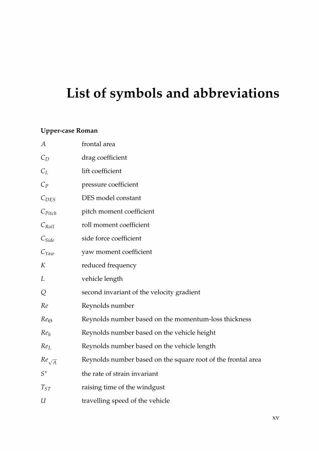
List of symbols and abbreviations
Upper-case Roman
A frontal area
CD drag coefficient
CL lift coefficient
CP pressure coefficient
CDES DES model constant
CPitch pitch moment coefficient
CRoll roll moment coefficient
CSide side force coefficient
CYaw yaw moment coefficient
K reduced frequency
L vehicle length
Q second invariant of the velocity gradient
Re Reynolds number
ReΘ Reynolds number based on the momentum-loss thickness
Reh Reynolds number based on the vehicle height
ReL Reynolds number based on the vehicle length
Re√A Reynolds number based on the square root of the frontal area
S∗ the rate of strain invariant
TST raising time of the windgust
U travelling speed of the vehicle
xv
LIST OF SYMBOLS AND ABBREVIATIONS
Ur incident velocity
U∞ free stream velocity
Ui,j velocity gradient
W (cross)wind speed
Wmax maximum crosswind speed
Lower-case Roman
uwmod modelled Reynolds stresses
uwres resolved Reynolds stresses
d distance to the wall
f frequency
fd DDES function
h vehicle height
kmod modelled turbulent kinetic energy
kres resolved turbulent kinetic energy
l vehicle width
p pressure
rd modelled turbulent boundary layer sensor from DDES
t time
t0 initial time of the gust
ui i-component of the velocity vector
uτ friction velocity
x streamwise position
y normal distance from the wall
y+ non dimensional wall unit
Upper-case Greek
∆tgust gust length in time
∆ grid spacing
xvi
Θ momentum-loss thickness
Lower-case Greek
κ the von Kármán constant
ν kinematic viscosity
νt eddy viscosity
ω frequency
ω turbulent frequency
ν modified eddy viscosity
k turbulent kinetic energy
Superscripts
+ non dimensional quantity in wall units
o angle degree
Subscripts
∞ free stream value
mod modelled quantity
re f reference value of a quantity
res resolved quantity
Symbols
∇ gradient
∂ partial derivative
U velocity vector
Abbreviations
CD Central Difference scheme
CFD Computational Fluid Dynamics
CoG Centre of Gravity
CoP Centre of Pressure
DDES Delayed Detached Eddy Simulations
xvii
LIST OF SYMBOLS AND ABBREVIATIONS
DES Detached Eddy Simulations
DNS Direct Numerical Simulation
LES Large Eddy Simulations
LUD Linear Upwind schemes
M Millions
NS Navier-Stokes equations
NSP Neutral Steer Point
RANS Reynolds-Averaged Navier-Stokes equations
REVM Radiused Edges Vehicle Model
S-A Spalart-Allmaras turbulence model
SEVM Sharp Edges Vehicle Model
SGS Sub-Grid-Scale
SST Shear Stress Transport
SUV Sport-Utility Vehicle
TGS Turbulence Generator System
UD Upwind scheme
xviii
Part I
Overview and Summary
1

CHAPTER 1Introduction
Crosswind stability is a problem for both today’s and tomorrow’s ground vehicles.Today, most types of ground transportation, such as buses, rail vehicles or cars, aresensitive to crosswind disturbances. It can even be a major safety issue for busesor rail vehicles. Accidents linked to crosswind can happen as it is reported inSHK (2001) or Diedrich (2006), but remain rare. For cars, passenger comfort is ofprimary interest, although, while driving on motorway, wind speeds between 2.5m/s and 10 m/s (that are frequent while driving a passenger car, see in Wojciak etal. (2010)) provoke steering corrections, see in Howell (1993), and might be a safetyconcern too.
The pressure for reducing the fuel consumption for vehicles due to environ-mental and financial concerns have pushed the car manufacturer to produce low-drag vehicles. Design alterations have already been undertaken after the oil crisisof 1973 but real settings for the emissions have been created shortly after the Kyotoprotocol of 1997 by the European, Japanese and Korean car manufacturers. Evenlower target in emissions of CO2 have been set in 2000 by the European Commis-sion. Already in 1986, it was seen that streamlining vehicles to reduce the dragtends to deteriorate the crosswind sensitivity of the vehicle, see e.g. Gilhaus andRenn (1986) or Howell (1993), and further understanding of the above crosswindcharacteristics of the ground vehicles was necessary.
Crosswind stability may still be a problem for tomorrow’s vehicles. The trans-portation systems and their associated infrastructures might evolve and new com-binations of vehicles might be foreseen. Sustainability, economy of energy, pas-sengers’ comfort and services might become more important than the pure perfor-mance. In current research there is a strong focus on providing lighter solutionsfor new vehicles. The ambition to decrease the weight of ground vehicles imposesstronger needs for an enhanced understanding of the coupling between cross-wind stability, the vehicle external shape and the dynamic properties. Althoughlarge ground transportation systems are still likely to exist to carry passengers andgoods, the importance of the driver in this new system might be questioned and
3
1. INTRODUCTION
probably be reduced to more automated systems. Systems to detect crosswindevents and to react would then be developed and incorporated into the vehicles.
Inevitably the pressure from the manufacturers on the design processes mightstill require fast assessing tools that would address more and more scenarios andalready at a very early stage of the development of the new vehicle. Numericaltools would then be expected to keep a significant part of the development phaseand would mix both accurate modelling and lower order methods for conceptualdesign.
The challenges in crosswind analysis
The overall problem of assessing the crosswind sensitivity of a vehicle involves acombination of aerodynamics, vehicle dynamics and driver interactions to a givencrosswind disturbance. In order to address crosswind directional stability, each ofthese issues correspond to a demanding problem on its own and is usually inves-tigated separately.
First, a crosswind scenario needs to be define. Crosswind can originate fromdifferent sources like weather, surrounding traffic or topology of the terrain nextto the road or track. As part of the atmospheric boundary layer, the wind speedalso increases with the height. The various natures of these disturbances make itdifficult to model realistic crosswind conditions.
Aerodynamics studies, in turn, focus on the design interactions with the sidewind disturbances. Experimental and numerical investigations have tried duringthe last two decades to address design alterations to reduce the crosswind sensi-tivity of the ground transportations in steady and unsteady conditions. However,the experimental benches are limited by the difficulty to represent realistic cross-wind conditions and, although the numerical analyses provide more flexibility intested scenarios, they suffer from the lack of accuracy of classic low order methodsor from the large computational times when advanced modelling is used.
The assessment of the vehicle dynamics response can be operated experimen-tally with production vehicles by, for instance, driving vehicles through fans in or-der to measure the lateral displacement and eventually compare different designs.The driver reactions have also been investigated in order to assess which mechan-ical component that the driver is the most sensitive to. Numerical simulations arealso used, however, they often suffer from the lack of proper aerodynamic input.
A full combination of all the above issues is quite difficult to foresee at the mo-ment, especially, when models of driver interactions may be inserted in the loop.However, adding reasonable crosswind scenarios to Computational Fluid Dynam-
4
ics (CFD) simulations, and combining them with vehicle dynamics simulations inorder to assess the on-road response, can be realized and hopefully included in thedesign process of future vehicles.
Objectives of the thesis
In this thesis, numerical methods in conjunction of an advanced turbulence model(Detached-Eddy Simulations - DES -) are evaluated to simulate the time-developmentof the flow around a generic vehicle subjected to a sudden strong crosswind. Thecrosswind scenario is represented by a deterministic mathematical model that gen-erates time-dependent boundary data introduced in the numerical domain.
An industrial framework is kept through the study. However, traditional Reynolds-Averaged Navier-Stokes (RANS) simulations can not properly cope with the stronglyseparated flow regions that occurs around a vehicle in crosswind. Therefore, DESare used to provide a good trade-off between accuracy and computational cost.One question to answer is ’can we still perform simulations that are accurateenough using fast meshing and numerical solutions commonly used for loweraccurate models?’.
Another objective of the work presented is to understand some physical pro-cesses involved in the aerodynamics of bluff bodies in crosswind. The descriptionand understanding of all the unsteady mechanisms are essential in order to de-velop a tool which would assess crosswind impacts with shorter simulation times.
Finally, a static coupling between the aerodynamics simulations with a com-plete vehicle dynamics model is provided, leading to the final car response to thecrosswind disturbance. Basic car design features and mechanical components arestudied separately as well as their interactions.
Outline of the thesis
The thesis is structured as follows. The first part, entitled ’Overview and Sum-mary’, describes the background and methods that have been used within thework presented. In the background section, some of the precedent key studiesare reviewed and provide an overview of the previous efforts to cope with cross-winds. Also, the numerical tools are introduced in order to localize the work ofthis thesis in the map of numerical simulations.
The main results of the this thesis are presented in separate chapters. The im-plementation of time-dependant boundary data modelling an unsteady crosswinddisturbance in the DES are first presented. Thereafter, physical insights on cross-
5
1. INTRODUCTION
wind are given before finishing on coupling aerodynamic and vehicle dynamicsimulations. The latter part gives to the reader an outlook on the handling of thecar in case of sudden strong crosswind. Finally, after going through the main con-clusion of the work, recommendations on future work are provided.
The first part ends with the summary of the appended papers as they are in-cluded in the second and last part of this thesis.
6
CHAPTER 2Background
This chapter presents definitions and previous studies that have been used to elab-orate the work documented in this thesis. First, in Sec. 2.1, the basic equations anddefinitions that concern ground vehicle aerodynamics are presented. Then, pre-vious work on crosswind is reviewed in Sec. 2.2. To do this, it is first proposedto define what a relevant transient crosswind scenario is. Then, the influence ofsome basic car shapes on the crosswind properties of cars is illustrated. After that,experiments dealing with unsteady crosswinds are presented. In Sec. 2.3, the in-troduction of some of the numerical investigations that have been performed oncrosswind, follows. This chapter ends with Sec. 2.4, where studies that have con-sidered vehicle dynamics to assess the crosswind sensitivity of ground vehiclesare reviewed.
2.1 Few words on ground vehicle aerodynamics
Due to the low speed of the ground vehicles considered, the flow is assumed to bedescribed by the incompressible Navier-Stokes (NS) equations:
∂ui∂t
+ uj∂ui∂xj
= −1ρ
∂p∂xi
+ ν∇2ui i = 1, 2, 3 (2.1)
∂ui∂xi
= 0 (2.2)
with ui the i-component of the velocity, xi the i-direction, t the time, p the pressure,ρ the density and ν the kinematic viscosity. Equations (2.1) are the momentumequations representing the advection of the flow whereas the Equation (2.2) is thecontinuity equation representing the conservations of mass. O. Reynolds relatedthe influence of the flow velocity, a characteristic length of the flow case and themolecular viscosity in studying the flow in a channel, see in Reynolds (1883). Thedifferent flow regimes can then be classified using the so-called Reynolds number(Re):
Re =ULre f
ν, (2.3)
7
2. BACKGROUND
with U the flow velocity, Lre f the characteristic length of the system (channel di-ameter, car length, etc...) and ν the kinematic viscosity.
Ground vehicle aerodynamics, see Hucho (1998), involves many different as-pects and applications of the NS equations. First, the Re number considered isfairly high. Typically, for a car in the normal atmospheric conditions travelling at100 km/h, being 4.5 m long (L) and with a frontal area A of 2.09 m2, the Re num-bers are Re√A ≈ 2.7× 10⁶ or ReL ≈ 8× 10⁶. On the frontal part of the vehicle theflow is first laminar and a transition to a turbulent flow occurs rapidly. The basearea of a typical car, truck or bus provokes a large turbulent wake to be formed.Strong unsteady phenomena such as vortex shedding are present in this area. Allthis make fair challenges for the numerical simulations and a trade off betweenthe full representation of the physics (if possible) and the numerical resources touse (whether they are limited or not) has to be made.
Boundary layers
Close to the surface of the vehicle, a boundary layer develops as the viscositybecomes dominant. First the boundary layer is laminar and after the flow hasreached a certain critical distance after the leading edge, the boundary layer be-comes turbulent. The transition is influenced by different factors such as the dis-tance from the leading edge or the local pressure gradient. As opposed to thelaminar boundary layer, the turbulent boundary layer provokes more friction atthe surface and the friction drag is thus larger. However, the characteristics of theturbulent boundary layer delay the separation location which, in turn, influencethe aerodynamic forces.
It is appropriate to describe the boundary layer using a non dimensional wallunit, y+, defined as:
y+ =uτy
ν, (2.4)
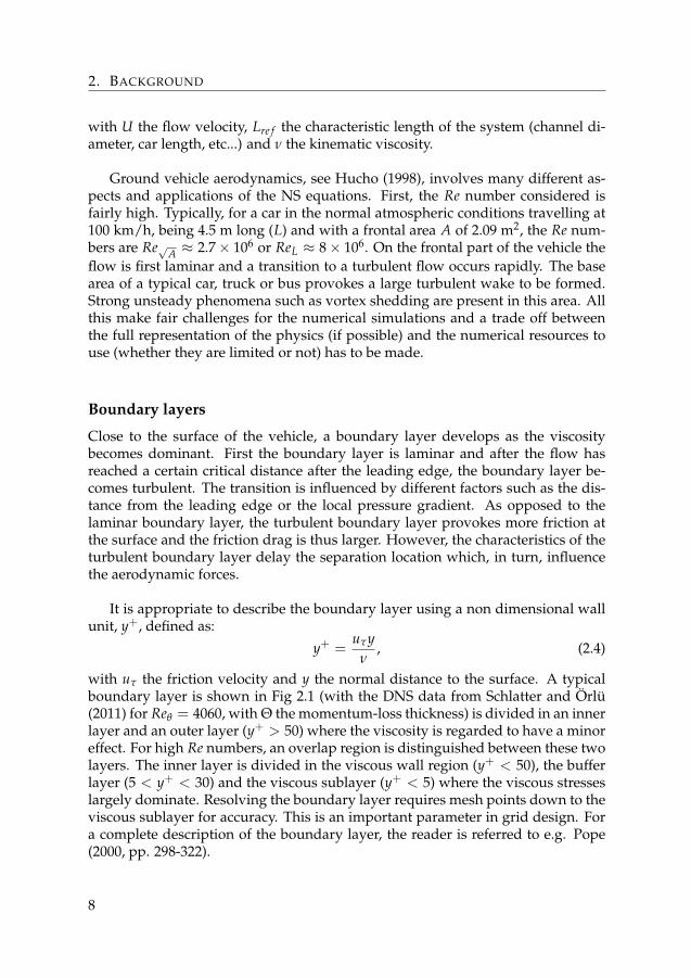
with uτ the friction velocity and y the normal distance to the surface. A typicalboundary layer is shown in Fig 2.1 (with the DNS data from Schlatter and Örlü(2011) for Reθ = 4060, with Θ the momentum-loss thickness) is divided in an innerlayer and an outer layer (y+ > 50) where the viscosity is regarded to have a minoreffect. For high Re numbers, an overlap region is distinguished between these twolayers. The inner layer is divided in the viscous wall region (y+ < 50), the bufferlayer (5 < y+ < 30) and the viscous sublayer (y+ < 5) where the viscous stresseslargely dominate. Resolving the boundary layer requires mesh points down to theviscous sublayer for accuracy. This is an important parameter in grid design. Fora complete description of the boundary layer, the reader is referred to e.g. Pope(2000, pp. 298-322).
8
2.2. Previous work on crosswind
Figure 2.1: Typical boundary layer. DNS data for Reθ = 4060. The solid linesrepresent U+ = y+ until y+ < 10 and U+ = 1
0.41 ln(y+) + 5.2 for y+ > 10.
Definitions of the aerodynamic forces and moments
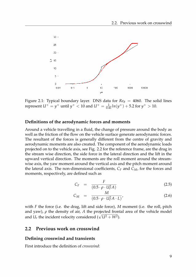
Around a vehicle travelling in a fluid, the change of pressure around the body aswell as the friction of the flow on the vehicle surface generate aerodynamic forces.The resultant of the forces is generally different from the centre of gravity andaerodynamic moments are also created. The component of the aerodynamic loadsprojected on to the vehicle axis, see Fig. 2.2 for the reference frame, are the drag inthe stream wise direction, the side force in the lateral direction and the lift in theupward vertical direction. The moments are the roll moment around the stream-wise axis, the yaw moment around the vertical axis and the pitch moment aroundthe lateral axis. The non-dimensional coefficients, CF and CM, for the forces andmoments, respectively, are defined such as
CF =F
(0.5 ⋅ ρ ⋅U2r A)
(2.5)
CM =M
(0.5 ⋅ ρ ⋅U2r A ⋅ L) , (2.6)
with F the force (i.e. the drag, lift and side force), M moment (i.e. the roll, pitchand yaw), ρ the density of air, A the projected frontal area of the vehicle modeland Ur the incident velocity considered (
√U2 + W2).
2.2 Previous work on crosswind
Defining crosswind and transients
First introduce the definition of crosswind:
9
2. BACKGROUND
Figure 2.2: Reference frame used in this thesis for the aerodynamic loads.
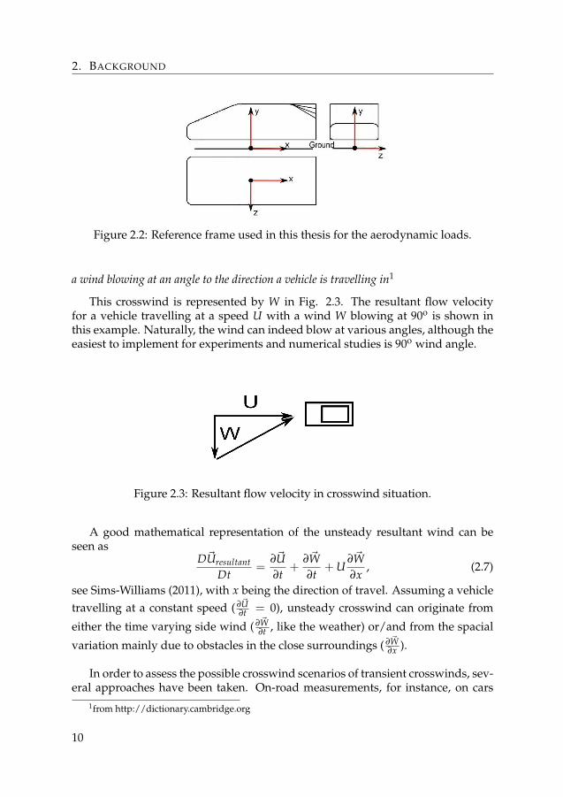
a wind blowing at an angle to the direction a vehicle is travelling in1
This crosswind is represented by W in Fig. 2.3. The resultant flow velocityfor a vehicle travelling at a speed U with a wind W blowing at 90o is shown inthis example. Naturally, the wind can indeed blow at various angles, although theeasiest to implement for experiments and numerical studies is 90o wind angle.
Figure 2.3: Resultant flow velocity in crosswind situation.
A good mathematical representation of the unsteady resultant wind can beseen as
DUresultantDt
=∂U∂t
+∂W∂t
+ U∂W∂x
, (2.7)
see Sims-Williams (2011), with x being the direction of travel. Assuming a vehicletravelling at a constant speed ( ∂U
∂t = 0), unsteady crosswind can originate from
either the time varying side wind ( ∂W∂t , like the weather) or/and from the spacial
variation mainly due to obstacles in the close surroundings ( ∂W∂x ).
In order to assess the possible crosswind scenarios of transient crosswinds, sev-eral approaches have been taken. On-road measurements, for instance, on cars
1from http://dictionary.cambridge.org
10
2.2. Previous work on crosswind
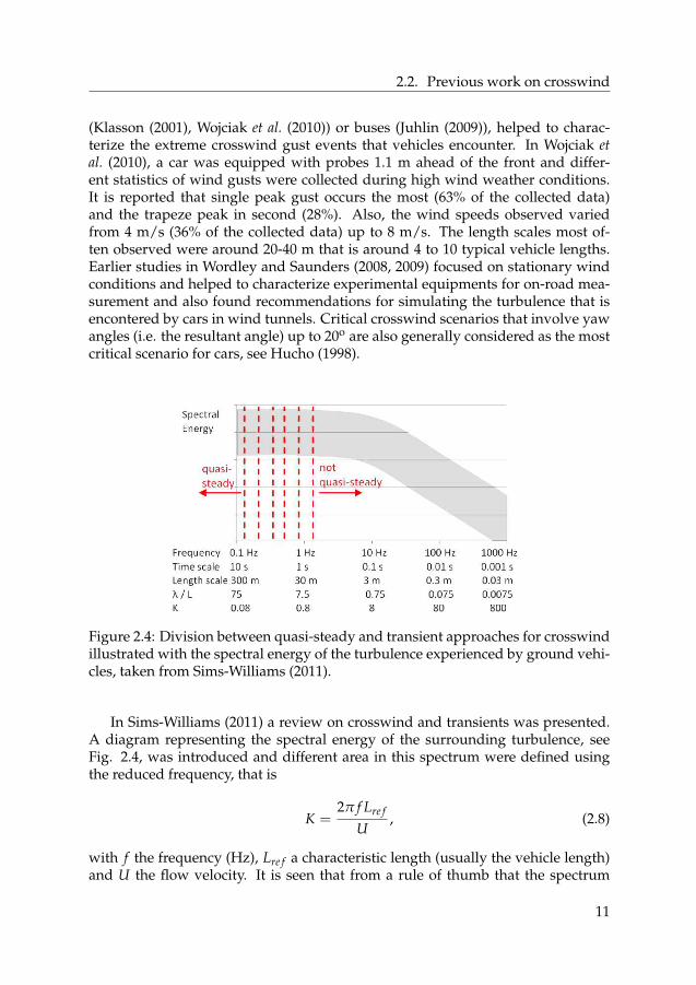
(Klasson (2001), Wojciak et al. (2010)) or buses (Juhlin (2009)), helped to charac-terize the extreme crosswind gust events that vehicles encounter. In Wojciak etal. (2010), a car was equipped with probes 1.1 m ahead of the front and differ-ent statistics of wind gusts were collected during high wind weather conditions.It is reported that single peak gust occurs the most (63% of the collected data)and the trapeze peak in second (28%). Also, the wind speeds observed variedfrom 4 m/s (36% of the collected data) up to 8 m/s. The length scales most of-ten observed were around 20-40 m that is around 4 to 10 typical vehicle lengths.Earlier studies in Wordley and Saunders (2008, 2009) focused on stationary windconditions and helped to characterize experimental equipments for on-road mea-surement and also found recommendations for simulating the turbulence that isencontered by cars in wind tunnels. Critical crosswind scenarios that involve yawangles (i.e. the resultant angle) up to 20o are also generally considered as the mostcritical scenario for cars, see Hucho (1998).
Figure 2.4: Division between quasi-steady and transient approaches for crosswindillustrated with the spectral energy of the turbulence experienced by ground vehi-cles, taken from Sims-Williams (2011).
In Sims-Williams (2011) a review on crosswind and transients was presented.A diagram representing the spectral energy of the surrounding turbulence, seeFig. 2.4, was introduced and different area in this spectrum were defined usingthe reduced frequency, that is
K =2π f Lre f
U, (2.8)
with f the frequency (Hz), Lre f a characteristic length (usually the vehicle length)and U the flow velocity. It is seen that from a rule of thumb that the spectrum
11
2. BACKGROUND
can be divided into the quasi-steady behaviour for K < 0.8 from the transient be-haviours. The spectral energy also shows that for K > 8− 10, the energy contentsdecreases. In terms of length scales for energetic windgusts, it means that the areaof interest corresponds to turbulence of length scales around 2-20 vehicle lengths.Thus, there are high and low frequencies for crosswind.
High frequencies contain less energy and are of lesser interest here. Experi-mentally, these high frequencies (i.e. K > 8 in Fig. 2.4) are tested with the grid-generated turbulence in wind tunnel. It is however stressed that ’lesser interest’does not mean no interest at all. For example, in Newnham et al. (2008), it wasobserved that the free stream turbulence intensity delays separation on radiusedA-pillar for a generic vehicle model.
Generating turbulence of low frequencies in a wind tunnel is rather compli-cated and is only possible via an active generation system. A typical example ofactive system for generating large scale turbulence is the Pininfarina facility andits turbulence generator system (TGS), see in Cogotti (2003). The reader is referredto Sims-Williams (2011) for additional references on facilities with active turbu-lence generator.
To sum up, only crosswind scenarios that include gusts of 2-20 vehicle lengthslong are of high interest for the analysis of crosswind sensitivity. The magnitude ofstrong winds that a car faces during bad weather conditions is between 4 to 8 m/s.Experimentally, special benches need to be developed to study these turbulencelength scales.
Basic car shapes in steady crosswind
Different basic car configurations have been studied in steady crosswind condi-tions over the years and two investigations are especially worth noticing, that arepublished in Gilhaus and Renn (1986) and Howell (1993), respectively, as they re-viewed a lot of parameters. In these studies, basic car models with interchangeableparts have been used. Whereas the work in Gilhaus and Renn (1986) has reviewedvarious basic changes (such as comparison between sharp and radiused edges andpillars) and illustrated their interactions, the focus in Howell (1993) has been onfinding shapes that lower both drag and yaw moment. Results from both studieshave conflicted in some cases. Noticeably, the boat tailing or the planform curva-ture has been found to decrease the yaw moment in Howell (1993) but it increasesit in Gilhaus and Renn (1986), although the influence of this parameter is not fullyaddressed in the latter study.
It is in general admitted that station wagons or squareback vehicles have alower yaw moment than fastback (or hatchback) and notchback vehicles. How-ever, in Gilhaus and Renn (1986), the notchback version is found to have a worse
12
2.2. Previous work on crosswind
yaw moment than the hatchback whereas the contrary is found in Howell (1993).However, the exact backlight angles used for the vehicles tested are not clearlyspecified and results from the present thesis suggest that large variations can ap-pear within the same car family.
In Gilhaus and Renn (1986), the overhang at the rear of a notchback car wasincreased and has provoked an increase in yaw moment. It is pointed out that theoverall side area was then increased. In the Paper F of this thesis, the rear over-hang is increased by virtually displacing the bodywork towards the rear whichtends to reduce the yaw moment.
Radiusing the C/D-pillars at the rear of any model tend to increase the yawmoment. This finding is supported by both studies.
In Gilhaus and Renn (1986), it is found that radiusing the A-pillars increasesthe yaw moment. It should be pointed out that this modification has been done inan iterative process where all the sharp edges of the vehicle model were radiusedone after each other. Therefore, straightforward conclusions can be mistaken. Forexample, looking at the edges at the front, a lower yaw moment is found whenthe edges are all sharp. This can be related to the finding of Paper B of this thesiswhere the sharp edges vehicle model has a lower yaw moment than the radiusededges model. Besides, in Gilhaus and Renn (1986), it is found that radiusing thefront fenders provokes a large increase of yaw moment that is then compensatedby radiusing the A-pillars.
From these steady crosswind studies, it is clear that A-pillars have a large influ-ence on the yaw moment as well as the rear shapes. This will be further extendedin this thesis with transient conditions.
Unsteady crosswind and experiments
Despite inherent limitations of experimental facilities to accurately represent anatmospheric boundary layer and wind gusts, several unsteady crosswind experi-mental benches have been developed. In several studies, aerodynamic loads on os-cillating models are analysed. Noticeably, Garry and Cooper (1986) used this typeof installation to rotate at a rather high yaw rate (64o/s) a simplified truck modelfrom -40o to +400 and found large differences between the dynamic and quasi-static loads. Using a simplified car model, the so-called Willy model, phase shiftand hysteresis in these dynamic motions was studied in Chometon et al. (2005).Production cars were used in Theissen et al. (2011) and Wojciak et al. (2011) and itwas seen that wake flow dominated the time-delayed observed.
Another type of apparatus was introduced in Docton and Dominy (1996) wherean extra nozzle was added to the conventional wind tunnel to blow an incident
13
2. BACKGROUND
wind; the extra nozzle was controlled with a shutter that helped to generate time-dependant crosswind. During the experiments and the numerical studies, largesuction pressure overshoots developed in the leeward side and large separatedflow regions. In Ryan (2000), this setup was used to investigate two different typesof simplified car model. The gust developed by the facility had two inherent prob-lems however, undershoot and overshoot of yaw angle at the leading edge of thegust as well as uneven pressure in the gust. These drawbacks were compensatedby a rapid production time that lead to a large amount of averaged data. Transientovershoot on the side force and yaw moment were observed for the box-like andthe generic car models. A fully developed flow was reached after the models were7 model lengths in the crosswind. Recently, a similar facility has been developedin Toulouse to study simplified car model up to a yaw angle of 25o, see Volpe et al.(2011).
In Baker (1986b), Cairns (1994), Chadwick et al. (2001) and Bocciolone et al.(2008), a crosswind track in conjunction with a boundary layer wind tunnel isused in order to represent a vehicle passage through a wind gust. Although sincethis type of configuration aims at studying extreme gust events, this type of setuphas inspired the boundary data used throughout this thesis. In Baker (1986b), atrain model is propelled on a track through a wind tunnel exhaust. It has beenseen that 1.5 car length were necessary to obtain stable loads. It is observed thatthe dynamic side force is lower than the static value whereas the other loads aresignificantly larger during the gust. On a similar bench, in Bocciolone et al. (2008),it is surprisingly observed that although the turbulence has an effect, the train mo-tion has no influence on the force coefficients. In Chadwick (1999) and Chadwicket al. (2001), an update of the bench developed in Cairns (1994) aimed at reducingthe large track induced vibrations that are the disadvantages of this kind of facil-ities. Also, further investigations on simplified shapes which overall dimensionscorresponding to a Sport-Utility Vehicle (SUV), were performed. Results from twoof these geometries at different wind tunnel speeds have been used in this thesisto benchmark the DES.
From this section, it is clear that the previous steady crosswind studies weretoo restrictive as hysteresis or time lags are observed in the growth of the transientloads. However, no real physical insight is provided to describe the mechanisminvolved to delay and overshoot the aerodynamics loads.
As closure of this experimental part, a parallel to the unsteady motion of wingscan be done. Unsteady wing motions have long been of interest in aeronautics andthe physics involved to described the lags, phase shifts or hysteresis have beenstudied, already in von Kármán and Sears (1938). The oscillatory wings have es-pecially been of prime interest for helicopter engineering, see Ham and Garelick(1968). In Ericsson and Reding (1988), the fluid mechanics of the hysteresis as wellas delays in separation and re-attachment are described and discussed. Thanks to
14
2.3. Analytical modelling of crosswind and numerical investigations
recent measurements, for example in Lee and Gerontakos (2004), the theory aboutthe growth and convection of the leading-edge vortex brings further knowledgeon the unsteady phenomena.
2.3 Analytical modelling of crosswind and numericalinvestigations
Overview
Analytical methods have been evaluated and developed to model the aerody-namic loads in unsteady crosswind conditions. In Hucho and Emmelmann (1973),by analogy with the aerodynamic loads on slender bodies used in aeronautics forwings, transient aerodynamic loads on a vehicle (that were approximated by a flatplate model) subjected to a sudden strong raising gust are calculated. Overshootsof the loads were represented but further validation of the model was judged nec-essary. In the set of papers Baker (1991a,b,c), the aerodynamic admittance wasintroduced in order to estimate the unsteady loads due to high crosswinds. Al-though the model suffered from inherent limitations, promising results were de-rived and further investigations combining vehicle dynamics model were incor-porated to assess the crosswind sensitivity of rail vehicles.
In order to numerically simulate the turbulent flows, various options are avail-able. The first option is naturally to solve directly the NS equations, with theso-called Direct Numerical Simulation (DNS). The grid spacing should then cor-respond to the Kolmogorov dissipation scales and a computational grid for highRe number flows is not possible with the current computational resources, seee.g. Spalart et al. (1997). The technique used in Large-Eddy Simulations (LES)filters the NS equations such that the large scales of turbulence are resolved andthe dissipative scales are modelled. This technique is still demanding in terms ofcomputational resources for high Re number flows.
Using the Reynolds-Averaged Navier-Stokes (RANS) equations that distinguishmean flow and fluctuations, a new set of equations appears and the so-calledReynolds stresses are left to be modelled. Different strategies can be applied thatwill vary the amount of hypothesis to model these stresses. This leads to differentfamilies of RANS models. In industry, the linear eddy viscosity models are usuallyin use. These methods are then questionable when pure transient flows are con-sidered (highly turbulent flows, mixing layers, wakes, unsteady crosswinds...).Higher level of turbulence modelling in non-linear eddy viscosity models or inReynolds-stress models provide a better prediction of separation but are in reachof general industrial applications, see Leschziner (2006) for a review of these mod-els.
15
2. BACKGROUND
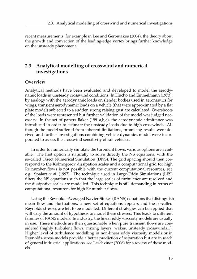
Finally, hybrid methods, such as Detached-Eddy Simulations (DES), that joinLES in the separated flow regions and RANS in boundary layers have the advan-tage to lower the computational cost and, therefore, high Re number flows can besimulated. However, these methods have also inherent restrictions and the switchfrom the LES and RANS regions is not trivial. In Figure 2.5 the different turbu-lence methods are classified for the demand in computational resources. In thisthesis, results of DES are presented as it is considered to be a reasonable trade-offbetween accuracy and computational cost.
Figure 2.5: Turbulence models and computational cost.
Steady crosswind
Bluff body flows have been studied using DES in various range of geometries andRe numbers. It is worth noticing that DES have been used for automotive appli-cations such as simplified geometries, in Guilmineau et al. (2011b) or productionvehicles in Islam et al. (2009). For a more complete overview of numerical sim-ulations for bluff bodies and detached-eddy simulations in general, the reader isreferred to the reviews of Mockett (2009) and Spalart (2009).
Concerning the numerical investigations of crosswind, numerous studies havetraditionally focused on steady crosswind conditions, see, for example, the recentstudies in Hemida et al. (2005), Diedrich (2006) and Bocciolone et al. (2008). InGuilmineau et al. (2011a), the performances of DES and RANS models were com-pared with the simulations of the Willy model in crosswind for several yaw angles.It was seen that the results were improved when the flow was simulated with DES
16
2.4. Crosswind sensitivity
compared to RANS simulations.
Unsteady crosswind
In order to introduce unsteady windgusts, time-dependent boundary conditionshave been used in Docton and Dominy (1996) to investigate unsteady crosswindin a two-dimensional computational domain using a RANS model. Further, pro-duction cars have been studied under crosswind conditions in Demuth and Buck(2006), where a Lattice-Boltzmann solver (using a RANS turbulence model) wasused together with a cosine-shape wind gust as periodic boundary data.
DES were used for unsteady crosswind in Hemida and Krajnovic (2009) ona bus geometry or in Diedrichs (2009) on high speed trains. As opposed to thework by Hemida and Krajnovic (2009), the DES presented in this thesis have notused any wall-functions, i.e. the boundary layers are resolved, and higher orderof accuracy in the turbulent equations are enabled. In Tsubokura et al. (2009), thedynamic variations of the yaw moment for a car geometry was investigated byLES on the Earth simulator. LES were also used for a simplified train geometry inKrajnovic (2009).
The flexibility of numerical methods has helped to investigate numerous sce-narios and parameter studies that is out of reach of the experimental benches.However, this is still a developing field where more effort in the accuracy of themodels can be provided and more realistic crosswind scenarios can still be ex-plored.
2.4 Crosswind sensitivity
During a gusty event, and for road vehicles, the yaw rate appears to be the keyfactor for handling2 as a sudden change of direction might lead to a traffic colli-sion whereas the roll rate is critical for rail vehicle as they may overturn in strongcrosswind. Baker (1986a) considers the rotational instability as the only concern forpassenger car safety. The two other types of instabilities, overturning and sideslipidentified by Baker are not applicable for passenger cars, but more for trains andhigh-sided vehicles.
The assessment of the interactions between vehicle designs and vehicle dy-namics response can be tested experimentally with crosswind facilities such ascrosswind fans, see e.g. MacAdam et al. (1990), and the lateral deviations can beused to compare different designs. Also, on-road measurements of aerodynamicloads have been implemented in a driving simulator to study the driver reactions
2more on this in Paper F
17
2. BACKGROUND
to gusty wind, see e.g. Klasson (2001), Jarlmark (2002) or Juhlin (2009). Param-eter studies on crosswind sensitivity have concluded that the centre of pressureof the aerodynamic forces has a large impact of the stability of the vehicles, seeMacAdam et al. (1990). Also in MacAdam et al. (1990), an analytic relation be-tween the three ’points’ that are the centre of gravity, the centre of pressure andthe neutral steer point, is provided to eliminate unsuitable vehicles for crosswindconditions. Results from transient studies support that the relative distance be-tween these three points plays a major role to improve the crosswind sensitivity.Concerning the drivers, it is pointed out in Alexandridis et al. (1979) that they aresensitive to the centre of pressure location and are favourable on more rearwardlocation of the aerodynamic loads.
In precedent research, efforts have been made to couple advanced aerodynam-ics (CFD) and vehicle dynamics simulations. A full coupled crosswind simulationinvolves an update of the overall position of the vehicle due to the aerodynamicdisturbances at each time step. On the other hand, a static coupling involves anaerodynamics simulation on a static vehicle subjected to an unsteady gust wherethe transient loads are input to a vehicle dynamics simulation in order to calculatethe vehicle deviation from its course. As opposed to the static coupling, a quasi-static coupling involves a set of aerodynamic simulations on a static vehicle sub-jected to static winds with different yaw angles. In this way, the relation betweenthe aerodynamic loads versus the static wind angles is obtained. Thereafter, thevehicle dynamics simulations incorporate the aerodynamic loads correspondingto the current yaw angle of the vehicle. Although a quasi-static approach might beseen at first as the closest to the expected reality, it has been demonstrated for manyflow cases (see for instance Ericsson and Reding (1988)) that the delay in growth inthe aerodynamic loads as well as the modification of the flow features (such as theboundary layers) would lead to different aerodynamic loads than those derivedfrom steady crosswind.
A static method has been used in Thomas et al. (2010) on rail vehicles to cou-ple loads from DES simulations to vehicle dynamics simulations. The unsteadyaerodynamic loads have been further simplified to quasi-static representation oftransient loadings and have lead to similar dynamic response. In Tsubukora andNakashima (2010), a full dynamic coupling between LES and vehicle dynamics isapplied to a truck subjected to a sudden strong wind gust. However, compromisesfor both types of simulations have been undertaken to cope with the large compu-tational times.
From this section, it becomes clear that monitoring the three points that arethe centre of gravity, centre of pressure and neutral steer point, is essential in or-der to study the crosswind stability of ground vehicles. However, further effortscan be put in performing the coupling of the aerodynamic and vehicle dynamicsimulations.
18
CHAPTER 3Geometries considered and unsteady
crosswind models
In this chapter, the vehicle geometries that have been utilised in this thesis arepresented together with their dimensions, Reynolds numbers, and key features.The second part is dedicated to the deterministic wind gust model used in thisthesis to depict an unsteady crosswind.
3.1 Vehicle models
Two types of vehicle models have been studied. This section presents their dimen-sions and characteristics.
Box-like geometries
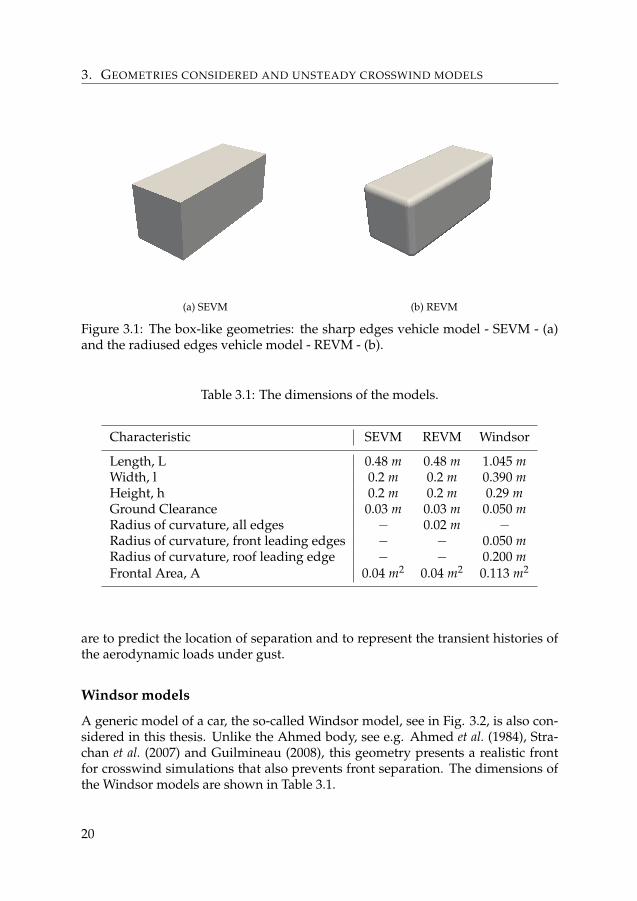
The first vehicle geometries considered in this study are based on the two simplebox geometries placed in the proximity of the ground that have already been stud-ied at the Cranfield University for unsteady crosswind experiments in Chadwick(1999) and Chadwick et al. (2001). They have sharp and radiused edges and arereferred to as SEVM and REVM, respectively. The dimensions of the models aregiven in Table 3.1. The streamwise lengths of the models are twice as large as thatof the width and height. The overall proportion and ground clearance are meantto represent a modern Sport-Utility Vehicle (SUV).
For the crosswind simulations, the wind speeds considered are set to 13 m/sfor streamwise flow, as in the experiment of Chadwick (1999), and to a maximumcrosswind speed of 4.73 m/s (corresponding to 20o yaw angle). The correspond-ing Reynolds numbers are Reh = 1.7× 10⁵ and ReL = 4.4× 10⁵.
As opposed to the former case, the radiused-edges geometry has adverse pres-sure gradient separation and no fixed separation lines. The challenges for the DES
19
3. GEOMETRIES CONSIDERED AND UNSTEADY CROSSWIND MODELS
(a) SEVM (b) REVM
Figure 3.1: The box-like geometries: the sharp edges vehicle model - SEVM - (a)and the radiused edges vehicle model - REVM - (b).
Table 3.1: The dimensions of the models.
Characteristic SEVM REVM Windsor
Length, L 0.48 m 0.48 m 1.045 mWidth, l 0.2 m 0.2 m 0.390 mHeight, h 0.2 m 0.2 m 0.29 mGround Clearance 0.03 m 0.03 m 0.050 mRadius of curvature, all edges − 0.02 m −Radius of curvature, front leading edges − − 0.050 mRadius of curvature, roof leading edge − − 0.200 mFrontal Area, A 0.04 m2 0.04 m2 0.113 m2
are to predict the location of separation and to represent the transient histories ofthe aerodynamic loads under gust.
Windsor models
A generic model of a car, the so-called Windsor model, see in Fig. 3.2, is also con-sidered in this thesis. Unlike the Ahmed body, see e.g. Ahmed et al. (1984), Stra-chan et al. (2007) and Guilmineau (2008), this geometry presents a realistic frontfor crosswind simulations that also prevents front separation. The dimensions ofthe Windsor models are shown in Table 3.1.
20
3.2. Modelling unsteady crosswind
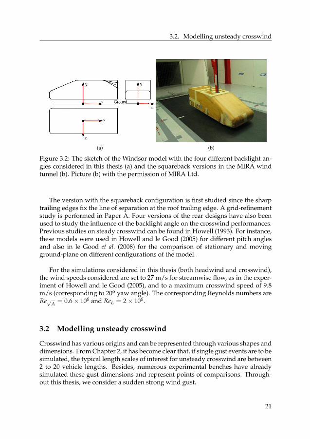
(a) (b)
Figure 3.2: The sketch of the Windsor model with the four different backlight an-gles considered in this thesis (a) and the squareback versions in the MIRA windtunnel (b). Picture (b) with the permission of MIRA Ltd.
The version with the squareback configuration is first studied since the sharptrailing edges fix the line of separation at the roof trailing edge. A grid-refinementstudy is performed in Paper A. Four versions of the rear designs have also beenused to study the influence of the backlight angle on the crosswind performances.Previous studies on steady crosswind can be found in Howell (1993). For instance,these models were used in Howell and le Good (2005) for different pitch anglesand also in le Good et al. (2008) for the comparison of stationary and movingground-plane on different configurations of the model.
For the simulations considered in this thesis (both headwind and crosswind),the wind speeds considered are set to 27 m/s for streamwise flow, as in the exper-iment of Howell and le Good (2005), and to a maximum crosswind speed of 9.8m/s (corresponding to 20o yaw angle). The corresponding Reynolds numbers areRe√A = 0.6× 10⁶ and ReL = 2× 10⁶.
3.2 Modelling unsteady crosswind
Crosswind has various origins and can be represented through various shapes anddimensions. From Chapter 2, it has become clear that, if single gust events are to besimulated, the typical length scales of interest for unsteady crosswind are between2 to 20 vehicle lengths. Besides, numerous experimental benches have alreadysimulated these gust dimensions and represent points of comparisons. Through-out this thesis, we consider a sudden strong wind gust.
21

3. GEOMETRIES CONSIDERED AND UNSTEADY CROSSWIND MODELS
(a) (b)
Figure 3.3: The crosswind scenario considered (a) as well as the associated windgust model normalized with the vehicle’s speed and length (b).
The crosswind scenario used in this thesis has been inspired by the experi-mental bench of Cairns (1994) and Chadwick et al. (2001): a vehicle model is pro-pelled at a constant speed through a wind tunnel exhaust. It corresponds to asudden strong crosswind exposure and the situation is depicted in Fig. 3.3a. Thecrosswind flow is equivalent to a jet flow and two mixing layers develop on eachside of the so-called obstacles. The wind gust is thus modelled as a step functionwith smooth transitions representing the mixing zone before and after the jet flow.These smooth transitions are modelled by cosine functions for which the period,2 ⋅ TST , is chosen. This method has been chosen as it is reported in Hucho and Em-melmann (1973) that cosine functions are successfully representing measurementsof mixing layers reported in Schlichting (1960).
Figure 3.3b shows a representation of the wind gust model introduced in thedomain. The maximum crosswind speed, Wmax, is set such that the correspondingmaximum yaw angle is 20o (arctangent of the crosswind speed over the vehiclevelocity). This is considered as the most critical crosswind scenario for passengercars, Hucho (1998). The crosswind velocity, W(x,t), is a function of both time andspace. The crosswind velocity, W, at the front inlet boundary is only function oftime and is
22
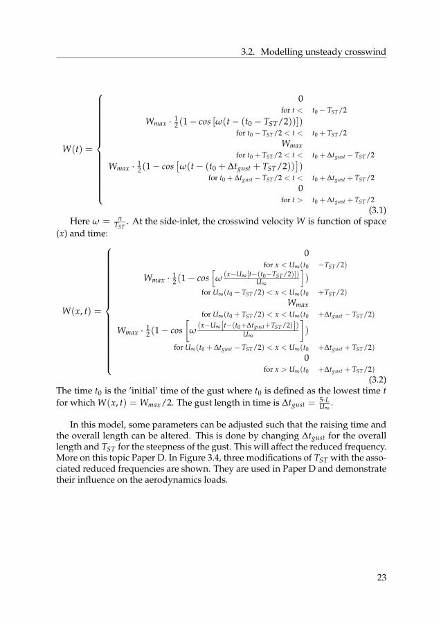
3.2. Modelling unsteady crosswind
W(t) =
⎧⎨⎩
0for t < t0 − TST/2
Wmax ⋅ 12 (1− cos [ω(t− (t0 − TST/2))])
for t0 − TST/2 < t < t0 + TST/2Wmax
for t0 + TST/2 < t < t0 + ∆tgust − TST/2
Wmax ⋅ 12 (1− cos
[ω(t− (t0 + ∆tgust + TST/2))
])
for t0 + ∆tgust − TST/2 < t < t0 + ∆tgust + TST/20
for t > t0 + ∆tgust + TST/2(3.1)
Here ω = πTST
. At the side-inlet, the crosswind velocity W is function of space(x) and time:
W(x, t) =
⎧⎨⎩
0for x < U∞(t0 −TST/2)
Wmax ⋅ 12 (1− cos
[ω
(x−U∞ [t−(t0−TST/2)])U∞
])
for U∞(t0 − TST/2) < x < U∞(t0 +TST/2)Wmax
for U∞(t0 + TST/2) < x < U∞(t0 +∆tgust − TST/2)
Wmax ⋅ 12 (1− cos
[ω
(x−U∞[t−(t0+∆tgust+TST/2)])U∞
])
for U∞(t0 + ∆tgust − TST/2) < x < U∞(t0 +∆tgust + TST/2)0
for x > U∞(t0 +∆tgust + TST/2)(3.2)
The time t0 is the ’initial’ time of the gust where t0 is defined as the lowest time tfor which W(x, t) = Wmax/2. The gust length in time is ∆tgust =
5⋅LU∞
.
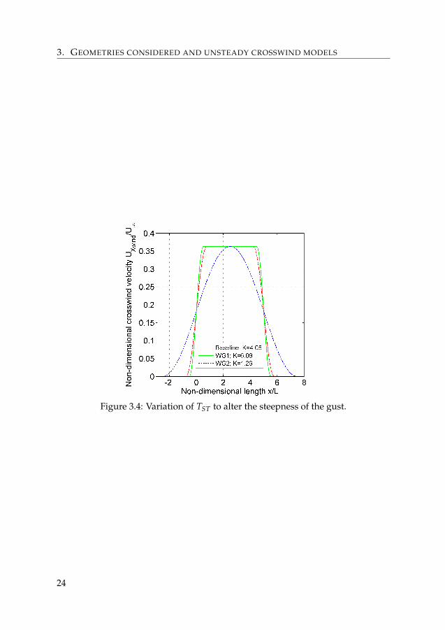
In this model, some parameters can be adjusted such that the raising time andthe overall length can be altered. This is done by changing ∆tgust for the overalllength and TST for the steepness of the gust. This will affect the reduced frequency.More on this topic Paper D. In Figure 3.4, three modifications of TST with the asso-ciated reduced frequencies are shown. They are used in Paper D and demonstratetheir influence on the aerodynamics loads.
23
3. GEOMETRIES CONSIDERED AND UNSTEADY CROSSWIND MODELS
Figure 3.4: Variation of TST to alter the steepness of the gust.
24
CHAPTER 4Detached-Eddy Simulations of
unsteady crosswind
In this chapter, the DES approach is briefly introduced before presenting the typ-ical numerical methods used to simulate the flows considered. Then, the perfor-mance of DES are shown for the geometries studied.
Presentation of DES
In 1997, Spalart introduced the so-called Detached-Eddy Simulations (DES), Spalartet al. (1997). This method joins the modelling efficiency of Reynolds AveragedNavier-Stokes (RANS) models close to the walls and the scale resolution of LargeEddy Simulations (LES) away from the walls, especially in the wake regions. Thesuccess of this method provided an extensive set of published simulations helpingto increase the knowledge of such simulations such as Constantinescu and Squires(2003) who studied the flow over a sphere and Travin et al. (1999) who investigatedthe flow past a cylinder. An update of DES, called Delayed-DES (D-DES), definedin Spalart et al. (2006), is the current standard in most codes used today. AlthoughDES is recognized for its reliability and promising potential for industrial applica-tion, as reviewed in Spalart (2009), excessive dissipation in the LES regions or er-roneous location of separation are still possible. Accurate numerical schemes thatmix Central Difference schemes (CD) and high order of Upwind schemes (UD) arethe standard for the spatial discretization, see Strelets (2001), Travin et al. (2002).Also, results including mesh refinement of at least by a factor of
√2 in all the three
direction in the regions of separated flows is inevitable in any studies involvingDES Spalart (2001).
The commercial solver STAR-CD v4 developed by CD-Adapco1 is used forall simulations reported in this thesis. In the code, the Navier-Stokes equations
1www.cd-adapco.com
25
4. DETACHED-EDDY SIMULATIONS OF UNSTEADY CROSSWIND
are solved using the finite volume method. The so called Delayed-DES (DDES)turbulence model is employed with the Spalart-Allmaras (S-A) model, introducedin Spalart and Allmaras (1992), as the RANS model used in the vicinity of thewalls. In DES, there is one adjustable constant CDES which was set to the standardvalue of 0.65 (for further concerns about the adjustable constant, see Spalart (2009))in all simulations. The global idea is to use a simple RANS model, the Spalart-Allmaras (S-A) model, close to the wall and the traditional Smagorinsky’s as aSub-Grid-Scale (SGS) model in the separated flows where the LES applies. In theS-A model, the eddy viscosity ν is adjusted to scale with the local deformationrate S and d such that: ν ∝ Sd2, where d is the distance to the closest wall. In theSmagorinsky model, Smagorinsky (1963), the eddy viscosity scales with S and thegrid spacing ∆, such that: ν ∝ S∆2. Therefore, if the term d in the S-A model isreplaced by d, defined as:
d ≡ (d, CDES∆), (4.1)
this acts as S-A in the regions where d≪ ∆, and as a SGS model when ∆≪ d. Tra-ditionally, ∆ is defined as the largest spacing in all three directions which ensuresd ≪ ∆ in the boundary layers where usually the prismatic layer cells are highlyanisotropic. DDES differs from DES in that a function fd has been introduced inorder to identify the boundary layers such that an early switch to LES mode inDES is prevented. Here fd is defined as
fd = 1− tanh([8rd]3), (4.2)
where rd is
rd =νt + ν√
Ui,jUi,jκ2d2 , (4.3)
with ν the molecular viscosity, κ the von Kármán constant and d the distance tothe wall.
The DDES simulations are initialized by steady state solutions obtained fromRANS simulations. The k − ω SST from Menter (1992) is used in these RANSsimulations and once the criteria of convergence to steady state are matched, thesteady state solutions are used as initial data for the DDES.
Numerical setup used in this thesis
This section reviews the typical computational domain, grids and numerical pa-rameters used in the simulations documented in this thesis.
Fig. 4.1 shows an outline of the typical computational domain used for thesimulations of the thesis. The length of the computational domain in the stream-wise direction is 11L, where L is the vehicle length. The height and width are 10hand 20h, respectively, with h being the height of the vehicle. In front and behindthe model, the distances to the upstream and downstream boundaries are 3.5L and
26
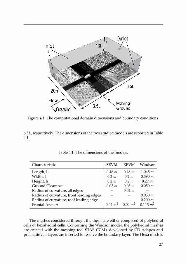
Figure 4.1: The computational domain dimensions and boundary conditions.
6.5L, respectively. The dimensions of the two studied models are reported in Table4.1.
Table 4.1: The dimensions of the models.
Characteristic SEVM REVM Windsor
Length, L 0.48 m 0.48 m 1.045 mWidth, l 0.2 m 0.2 m 0.390 mHeight, h 0.2 m 0.2 m 0.29 mGround Clearance 0.03 m 0.03 m 0.050 mRadius of curvature, all edges − 0.02 m −Radius of curvature, front leading edges − − 0.050 mRadius of curvature, roof leading edge − − 0.200 mFrontal Area, A 0.04 m2 0.04 m2 0.113 m2
The meshes considered through the thesis are either composed of polyhedralcells or hexahedral cells. Concerning the Windsor model, the polyhedral meshesare created with the meshing tool STAR-CCM+ developed by CD-Adapco andprismatic cell layers are inserted to resolve the boundary layer. The Hexa mesh is
27
4. DETACHED-EDDY SIMULATIONS OF UNSTEADY CROSSWIND
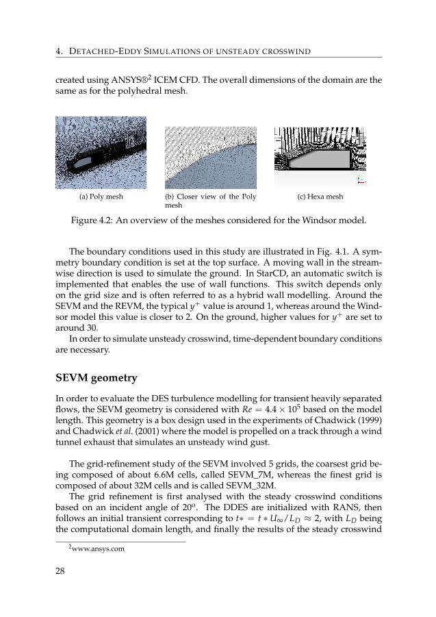
created using ANSYS®2 ICEM CFD. The overall dimensions of the domain are thesame as for the polyhedral mesh.
(a) Poly mesh (b) Closer view of the Polymesh
(c) Hexa mesh
Figure 4.2: An overview of the meshes considered for the Windsor model.
The boundary conditions used in this study are illustrated in Fig. 4.1. A sym-metry boundary condition is set at the top surface. A moving wall in the stream-wise direction is used to simulate the ground. In StarCD, an automatic switch isimplemented that enables the use of wall functions. This switch depends onlyon the grid size and is often referred to as a hybrid wall modelling. Around theSEVM and the REVM, the typical y+ value is around 1, whereas around the Wind-sor model this value is closer to 2. On the ground, higher values for y+ are set toaround 30.
In order to simulate unsteady crosswind, time-dependent boundary conditionsare necessary.
SEVM geometry
In order to evaluate the DES turbulence modelling for transient heavily separatedflows, the SEVM geometry is considered with Re = 4.4× 10⁵ based on the modellength. This geometry is a box design used in the experiments of Chadwick (1999)and Chadwick et al. (2001) where the model is propelled on a track through a windtunnel exhaust that simulates an unsteady wind gust.
The grid-refinement study of the SEVM involved 5 grids, the coarsest grid be-ing composed of about 6.6M cells, called SEVM_7M, whereas the finest grid iscomposed of about 32M cells and is called SEVM_32M.
The grid refinement is first analysed with the steady crosswind conditionsbased on an incident angle of 20o. The DDES are initialized with RANS, thenfollows an initial transient corresponding to t∗ = t ∗U∞/LD ≈ 2, with LD beingthe computational domain length, and finally the results of the steady crosswind
2www.ansys.com
28
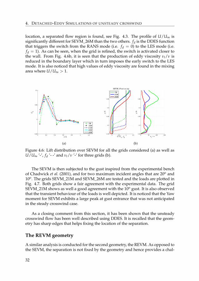
flow are averaged during a maximum time ∆t∗ ≈ 6. The mean side force coeffi-cient CSide and yaw moment coefficient CYaw are reported in Table 4.2 for all grids.The experimental data were obtained with a balance and by integrating the pres-sure from the sensors located around the SEVM Chadwick (1999), as seen in Table4.2. Only the two finest grids SEVM_26M and SEVM_32M have a correct valueof CYaw, i.e. a grid-convergence is reached for the aerodynamic loads. Figure 4.6aillustrates the distribution of the lift coefficient CL (defined in a similar way asCSide) along the model. The lift converges towards a common distribution with asignificant improvement at the front end of the body.
Table 4.2: Averaged force coefficients for SEVM. The experimental data are fromthe balance (Bal.) with the margin of errors and from pressure integration (Press.).
Cases CSide CYaw
Exp. Press. 1.1 0.02Exp. Bal. 1.25± 0.05 0.03± 0.01SEVM_7M 1.21 −0.0035SEVM_12M 1.19 −0.01SEVM_21M 1.21 0.015SEVM_26M 1.23 0.026SEVM_32M 1.23 0.025
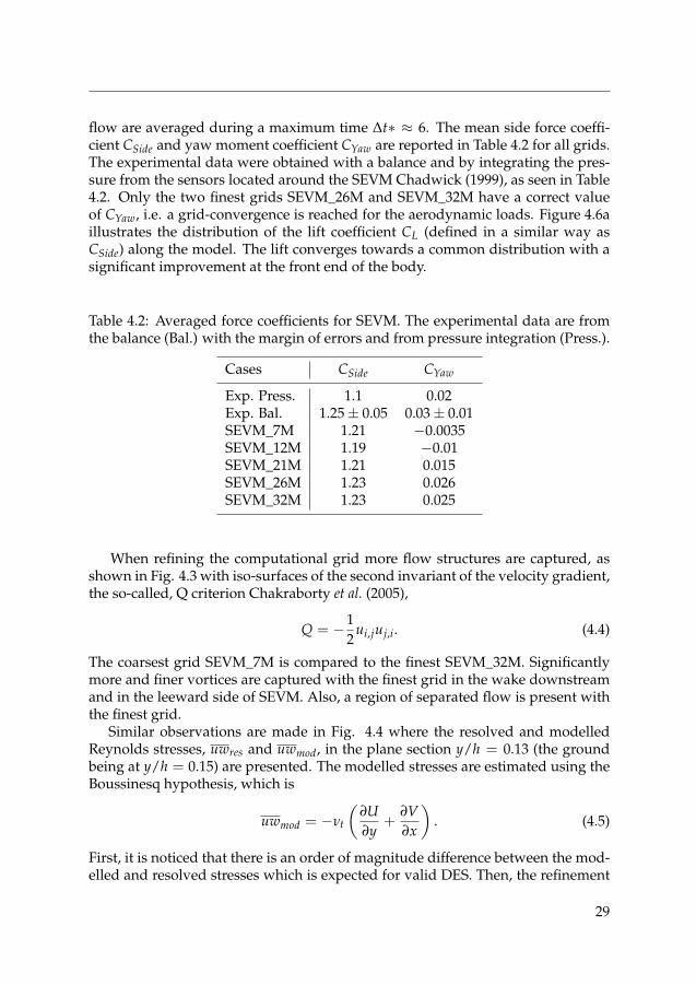
When refining the computational grid more flow structures are captured, asshown in Fig. 4.3 with iso-surfaces of the second invariant of the velocity gradient,the so-called, Q criterion Chakraborty et al. (2005),
Q = −12
ui,juj,i. (4.4)
The coarsest grid SEVM_7M is compared to the finest SEVM_32M. Significantlymore and finer vortices are captured with the finest grid in the wake downstreamand in the leeward side of SEVM. Also, a region of separated flow is present withthe finest grid.
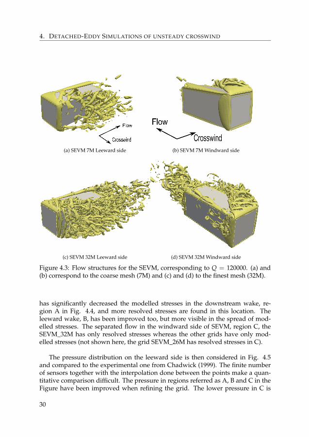
Similar observations are made in Fig. 4.4 where the resolved and modelledReynolds stresses, uwres and uwmod, in the plane section y/h = 0.13 (the groundbeing at y/h = 0.15) are presented. The modelled stresses are estimated using theBoussinesq hypothesis, which is
uwmod = −νt
(∂U∂y
+∂V∂x
). (4.5)
First, it is noticed that there is an order of magnitude difference between the mod-elled and resolved stresses which is expected for valid DES. Then, the refinement
29
4. DETACHED-EDDY SIMULATIONS OF UNSTEADY CROSSWIND
(a) SEVM 7M Leeward side (b) SEVM 7M Windward side
(c) SEVM 32M Leeward side (d) SEVM 32M Windward side
Figure 4.3: Flow structures for the SEVM, corresponding to Q = 120000. (a) and(b) correspond to the coarse mesh (7M) and (c) and (d) to the finest mesh (32M).
has significantly decreased the modelled stresses in the downstream wake, re-gion A in Fig. 4.4, and more resolved stresses are found in this location. Theleeward wake, B, has been improved too, but more visible in the spread of mod-elled stresses. The separated flow in the windward side of SEVM, region C, theSEVM_32M has only resolved stresses whereas the other grids have only mod-elled stresses (not shown here, the grid SEVM_26M has resolved stresses in C).
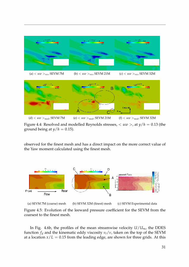
The pressure distribution on the leeward side is then considered in Fig. 4.5and compared to the experimental one from Chadwick (1999). The finite numberof sensors together with the interpolation done between the points make a quan-titative comparison difficult. The pressure in regions referred as A, B and C in theFigure have been improved when refining the grid. The lower pressure in C is
30
(a) < uw >res, SEVM 7M (b) < uw >res, SEVM 21M (c) < uw >res, SEVM 32M
(d) < uw >mod, SEVM 7M (e) < uw >mod, SEVM 21M (f) < uw >mod, SEVM 32M
Figure 4.4: Resolved and modelled Reynolds stresses, < uw >, at y/h = 0.13 (theground being at y/h = 0.15).
observed for the finest mesh and has a direct impact on the more correct value ofthe Yaw moment calculated using the finest mesh.
(a) SEVM 7M (coarse) mesh (b) SEVM 32M (finest) mesh (c) SEVM Experimental data
Figure 4.5: Evolution of the leeward pressure coefficient for the SEVM from thecoarsest to the finest mesh.
In Fig. 4.6b, the profiles of the mean streamwise velocity U/U∞, the DDESfunction fd and the kinematic eddy viscosity νt/ν, taken on the top of the SEVMat a location x/L = 0.15 from the leading edge, are shown for three grids. At this
31
4. DETACHED-EDDY SIMULATIONS OF UNSTEADY CROSSWIND
location, a separated flow region is found, see Fig. 4.3. The profile of U/U∞ issignificantly different for SEVM_26M than the two others. fd is the DDES functionthat triggers the switch from the RANS mode (i.e. fd = 0) to the LES mode (i.e.fd = 1). As can be seen, when the grid is refined, the switch is activated closer tothe wall. From Fig. 4.6b, it is seen that the production of eddy viscosity νt/ν isreduced in the boundary layer which in turn imposes the early switch to the LESmode. It is also noticed that high values of eddy viscosity are found in the mixingarea where U/U∞ > 1.
0 0.2 0.4 0.6 0.8 1 1.2−0.05
0
0.05
0.1
x/L
CL
7M
12M
21M
26M
32M
(a)
0 0.5 1 1.51.15
1.2
1.25
1.3
1.35
SEVM, Front on top
U/U∞ , fd
y/
h
7M
21M
26M
0 50 100 1501.15
1.2
1.25
1.3
1.35
νt / ν
y/
h
(b)
Figure 4.6: Lift distribution over SEVM for all the grids considered (a) as well asU/U∞ ’-’, fd ’- -’ and νt/ν ’-’ for three grids (b).
The SEVM is then subjected to the gust inspired from the experimental benchof Chadwick et al. (2001), and for two maximum incident angles that are 20o and10o. The grids SEVM_21M and SEVM_26M are tested and the loads are plotted inFig. 4.7. Both grids show a fair agreement with the experimental data. The gridSEVM_21M shows as well a good agreement with the 10o gust. It is also observedthat the transient behaviour of the loads is well depicted. It is noticed that the Yawmoment for SEVM exhibits a large peak at gust entrance that was not anticipatedin the steady crosswind case.
As a closing comment from this section, it has been shown that the unsteadycrosswind flow has been well described using DDES. It is recalled that the geom-etry has sharp edges that helps fixing the location of the separation.
The REVM geometry
A similar analysis is conducted for the second geometry, the REVM. As opposed tothe SEVM, the separation is not fixed by the geometry and hence provides a chal-
32
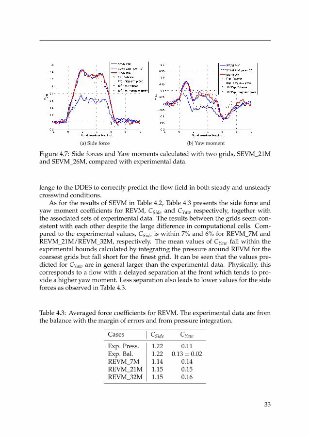
(a) Side force (b) Yaw moment
Figure 4.7: Side forces and Yaw moments calculated with two grids, SEVM_21Mand SEVM_26M, compared with experimental data.
lenge to the DDES to correctly predict the flow field in both steady and unsteadycrosswind conditions.
As for the results of SEVM in Table 4.2, Table 4.3 presents the side force andyaw moment coefficients for REVM, CSide and CYaw respectively, together withthe associated sets of experimental data. The results between the grids seem con-sistent with each other despite the large difference in computational cells. Com-pared to the experimental values, CSide is within 7% and 6% for REVM_7M andREVM_21M/REVM_32M, respectively. The mean values of CYaw fall within theexprimental bounds calculated by integrating the pressure around REVM for thecoarsest grids but fall short for the finest grid. It can be seen that the values pre-dicted for CYaw are in general larger than the experimental data. Physically, thiscorresponds to a flow with a delayed separation at the front which tends to pro-vide a higher yaw moment. Less separation also leads to lower values for the sideforces as observed in Table 4.3.
Table 4.3: Averaged force coefficients for REVM. The experimental data are fromthe balance with the margin of errors and from pressure integration.
Cases CSide CYaw
Exp. Press. 1.22 0.11Exp. Bal. 1.22 0.13± 0.02REVM_7M 1.14 0.14REVM_21M 1.15 0.15REVM_32M 1.15 0.16
33
4. DETACHED-EDDY SIMULATIONS OF UNSTEADY CROSSWIND
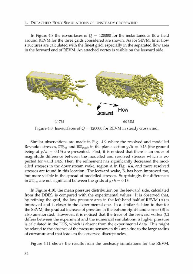
In Figure 4.8 the iso-surfaces of Q = 120000 for the instantaneous flow fieldaround REVM for the three grids considered are shown. As for SEVM, finer flowstructures are calculated with the finest grid, especially in the separated flow areain the forward end of REVM. An attached vortex is visible on the leeward side.
(a) 7M (b) 32M
Figure 4.8: Iso-surfaces of Q = 120000 for REVM in steady crosswind.
Similar observations are made in Fig. 4.9 where the resolved and modelledReynolds stresses, uwres and uwmod, in the plane section y/h = 0.13 (the groundbeing at y/h = 0.15) are presented. First, it is noticed that there is an order ofmagnitude difference between the modelled and resolved stresses which is ex-pected for valid DES. Then, the refinement has significantly decreased the mod-elled stresses in the downstream wake, region A in Fig. 4.4, and more resolvedstresses are found in this location. The leeward wake, B, has been improved too,but more visible in the spread of modelled stresses. Surprisingly, the differencesin uwres are not significant between the grids at y/h = 0.13.
In Figure 4.10, the mean pressure distribution on the leeward side, calculatedfrom the DDES, is compared with the experimental values. It is observed that,by refining the grid, the low pressure area in the left-hand half of REVM (A) isimproved and is closer to the experimental one. In a similar fashion to that forthe SEVM, the gradual increase of pressure in the bottom right-hand corner (B) isalso ameliorated. However, it is noticed that the trace of the leeward vortex (C)differs between the experiment and the numerical simulations: a higher pressureis calculated in the DES, which is absent from the experimental data. This mightbe related to the absence of the pressure sensors in this area due to the large radiusof curvature and that leads to the observed discrepancies.
Figure 4.11 shows the results from the unsteady simulations for the REVM,
34
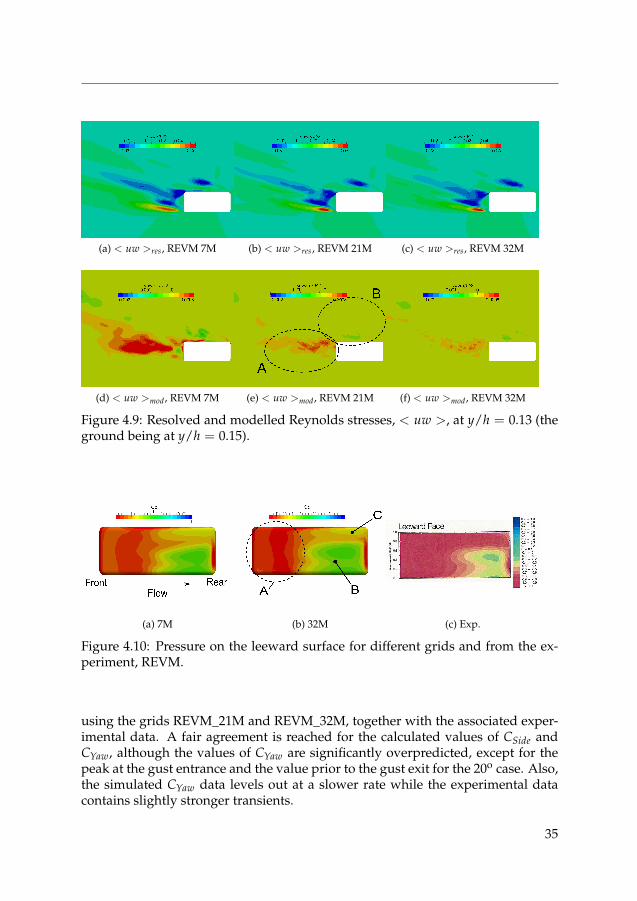
(a) < uw >res, REVM 7M (b) < uw >res, REVM 21M (c) < uw >res, REVM 32M
(d) < uw >mod, REVM 7M (e) < uw >mod, REVM 21M (f) < uw >mod, REVM 32M
Figure 4.9: Resolved and modelled Reynolds stresses, < uw >, at y/h = 0.13 (theground being at y/h = 0.15).
(a) 7M (b) 32M (c) Exp.
Figure 4.10: Pressure on the leeward surface for different grids and from the ex-periment, REVM.
using the grids REVM_21M and REVM_32M, together with the associated exper-imental data. A fair agreement is reached for the calculated values of CSide andCYaw, although the values of CYaw are significantly overpredicted, except for thepeak at the gust entrance and the value prior to the gust exit for the 20o case. Also,the simulated CYaw data levels out at a slower rate while the experimental datacontains slightly stronger transients.
35
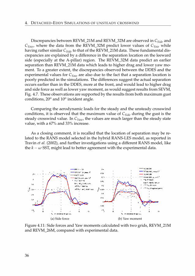
4. DETACHED-EDDY SIMULATIONS OF UNSTEADY CROSSWIND
Discrepancies between REVM_21M and REVM_32M are observed in CSide andCYaw, where the data from the REVM_32M predict lower values of CYaw whilehaving rather similar CSide to that of the REVM_21M data. These fundamental dis-crepancies are explained by a difference in the separation location on the leewardside (especially at the A-pillar) region. The REVM_32M data predict an earlierseparation than REVM_21M data which leads to higher drag and lower yaw mo-ment. To a greater extent, the discrepancies observed between the DDES and theexperimental values for CYaw are also due to the fact that a separation location ispoorly predicted in the simulations. The differences suggest the actual separationoccurs earlier than in the DDES, more at the front, and would lead to higher dragand side force as well as lower yaw moment, as would suggest results from SEVM,Fig. 4.7. These observations are supported by the results from both maximum gustconditions, 20o and 10o incident angle.
Comparing the aerodynamic loads for the steady and the unsteady crosswindconditions, it is observed that the maximum value of CSide during the gust is thesteady crosswind value. In CYaw, the values are much larger than the steady statevalue, with a 67% and 33% increase.
As a closing comment, it is recalled that the location of separation may be re-lated to the RANS model selected in the hybrid RANS-LES model, as reported inTravin et al. (2002), and further investigations using a different RANS model, likethe k−ω SST, might lead to better agreement with the experimental data.
(a) Side force (b) Yaw moment
Figure 4.11: Side forces and Yaw moments calculated with two grids, REVM_21Mand REVM_26M, compared with experimental data.
36
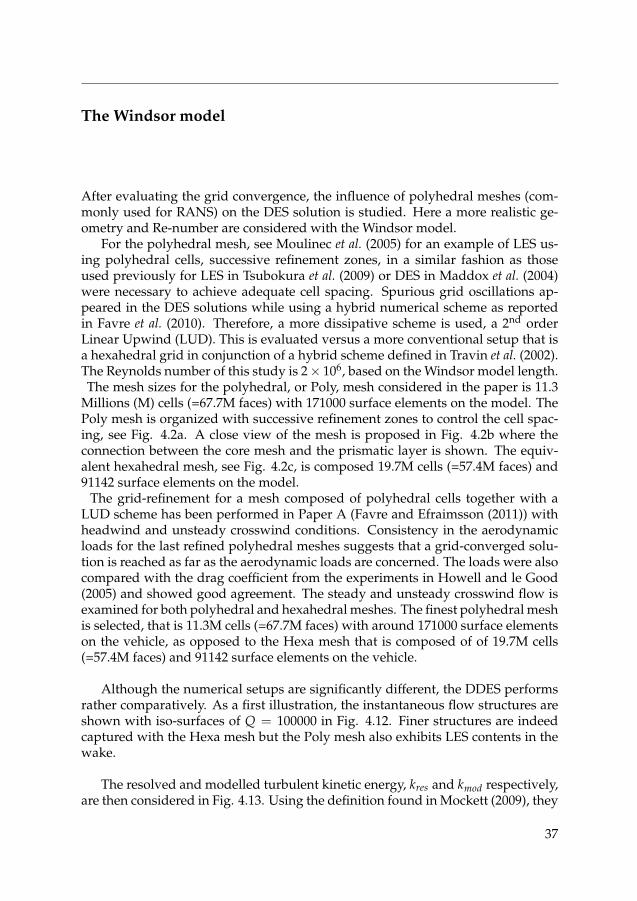
The Windsor model
After evaluating the grid convergence, the influence of polyhedral meshes (com-monly used for RANS) on the DES solution is studied. Here a more realistic ge-ometry and Re-number are considered with the Windsor model.
For the polyhedral mesh, see Moulinec et al. (2005) for an example of LES us-ing polyhedral cells, successive refinement zones, in a similar fashion as thoseused previously for LES in Tsubokura et al. (2009) or DES in Maddox et al. (2004)were necessary to achieve adequate cell spacing. Spurious grid oscillations ap-peared in the DES solutions while using a hybrid numerical scheme as reportedin Favre et al. (2010). Therefore, a more dissipative scheme is used, a 2nd orderLinear Upwind (LUD). This is evaluated versus a more conventional setup that isa hexahedral grid in conjunction of a hybrid scheme defined in Travin et al. (2002).The Reynolds number of this study is 2× 10⁶, based on the Windsor model length.The mesh sizes for the polyhedral, or Poly, mesh considered in the paper is 11.3
Millions (M) cells (=67.7M faces) with 171000 surface elements on the model. ThePoly mesh is organized with successive refinement zones to control the cell spac-ing, see Fig. 4.2a. A close view of the mesh is proposed in Fig. 4.2b where theconnection between the core mesh and the prismatic layer is shown. The equiv-alent hexahedral mesh, see Fig. 4.2c, is composed 19.7M cells (=57.4M faces) and91142 surface elements on the model.
The grid-refinement for a mesh composed of polyhedral cells together with aLUD scheme has been performed in Paper A (Favre and Efraimsson (2011)) withheadwind and unsteady crosswind conditions. Consistency in the aerodynamicloads for the last refined polyhedral meshes suggests that a grid-converged solu-tion is reached as far as the aerodynamic loads are concerned. The loads were alsocompared with the drag coefficient from the experiments in Howell and le Good(2005) and showed good agreement. The steady and unsteady crosswind flow isexamined for both polyhedral and hexahedral meshes. The finest polyhedral meshis selected, that is 11.3M cells (=67.7M faces) with around 171000 surface elementson the vehicle, as opposed to the Hexa mesh that is composed of of 19.7M cells(=57.4M faces) and 91142 surface elements on the vehicle.
Although the numerical setups are significantly different, the DDES performsrather comparatively. As a first illustration, the instantaneous flow structures areshown with iso-surfaces of Q = 100000 in Fig. 4.12. Finer structures are indeedcaptured with the Hexa mesh but the Poly mesh also exhibits LES contents in thewake.
The resolved and modelled turbulent kinetic energy, kres and kmod respectively,are then considered in Fig. 4.13. Using the definition found in Mockett (2009), they
37
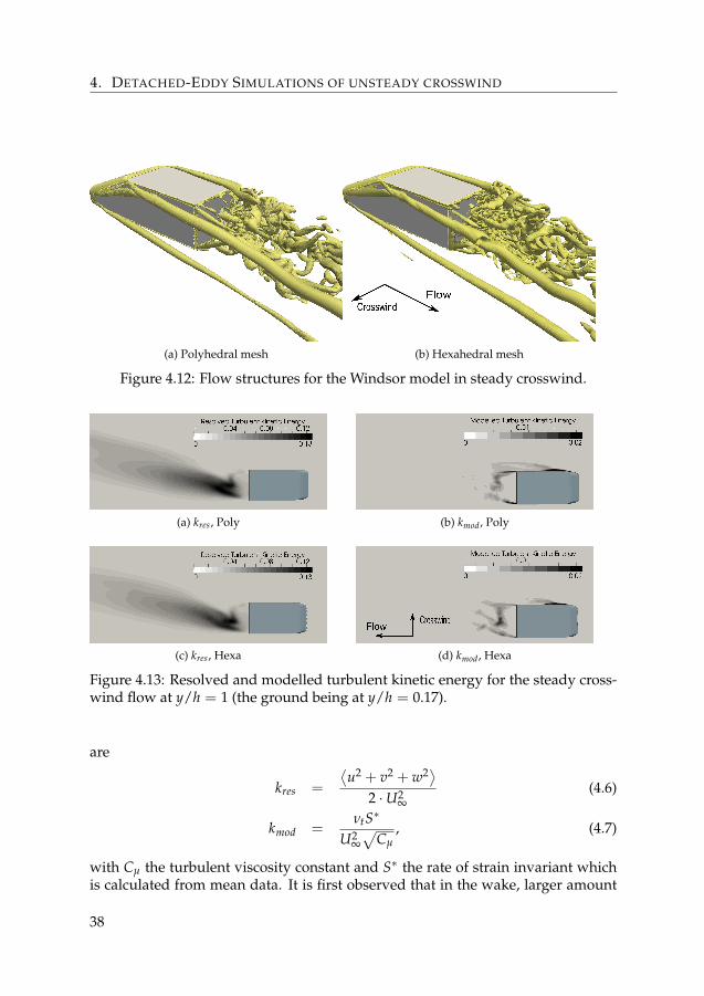
4. DETACHED-EDDY SIMULATIONS OF UNSTEADY CROSSWIND
(a) Polyhedral mesh (b) Hexahedral mesh
Figure 4.12: Flow structures for the Windsor model in steady crosswind.
(a) kres, Poly (b) kmod, Poly
(c) kres, Hexa (d) kmod, Hexa
Figure 4.13: Resolved and modelled turbulent kinetic energy for the steady cross-wind flow at y/h = 1 (the ground being at y/h = 0.17).
are
kres =
⟨u2 + v2 + w2⟩
2 ⋅U2∞
(4.6)
kmod =νtS∗
U2∞√
Cµ, (4.7)
with Cµ the turbulent viscosity constant and S∗ the rate of strain invariant whichis calculated from mean data. It is first observed that in the wake, larger amount
38
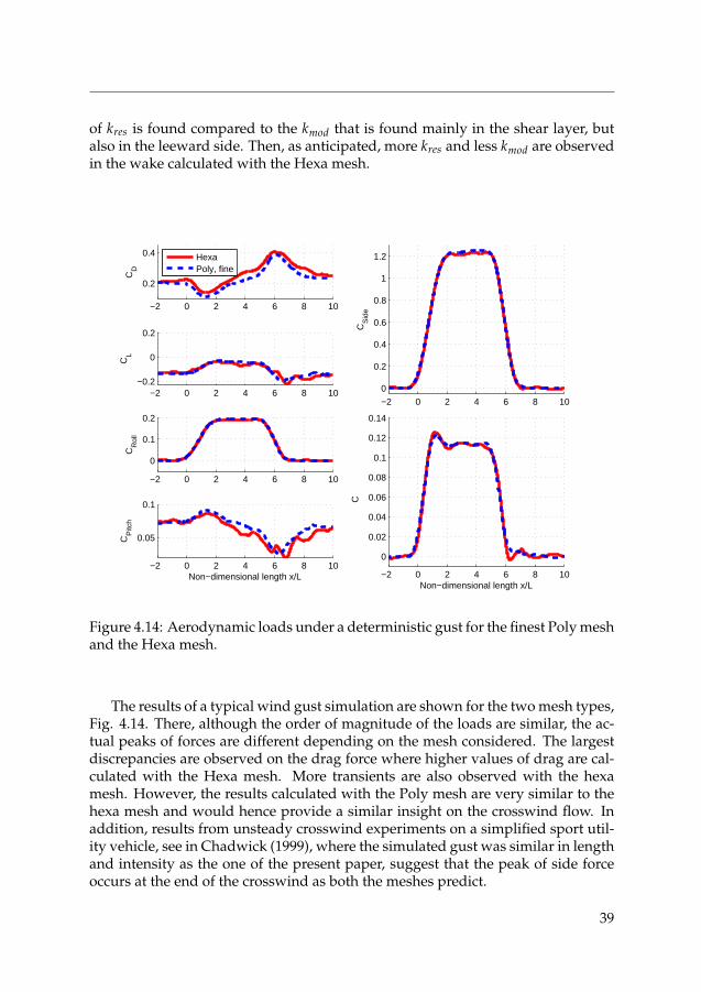
of kres is found compared to the kmod that is found mainly in the shear layer, butalso in the leeward side. Then, as anticipated, more kres and less kmod are observedin the wake calculated with the Hexa mesh.
−2 0 2 4 6 8 10
0.2
0.4
CD
HexaPoly, fine
−2 0 2 4 6 8 10−0.2
0
0.2
CL
−2 0 2 4 6 8 10
0
0.2
0.4
0.6
0.8
1
1.2
CS
ide
−2 0 2 4 6 8 10
0
0.1
0.2
CR
oll
−2 0 2 4 6 8 10
0.05
0.1
Non−dimensional length x/L
CP
itch
−2 0 2 4 6 8 10
0
0.02
0.04
0.06
0.08
0.1
0.12
0.14
Non−dimensional length x/L
C
Figure 4.14: Aerodynamic loads under a deterministic gust for the finest Poly meshand the Hexa mesh.
The results of a typical wind gust simulation are shown for the two mesh types,Fig. 4.14. There, although the order of magnitude of the loads are similar, the ac-tual peaks of forces are different depending on the mesh considered. The largestdiscrepancies are observed on the drag force where higher values of drag are cal-culated with the Hexa mesh. More transients are also observed with the hexamesh. However, the results calculated with the Poly mesh are very similar to thehexa mesh and would hence provide a similar insight on the crosswind flow. Inaddition, results from unsteady crosswind experiments on a simplified sport util-ity vehicle, see in Chadwick (1999), where the simulated gust was similar in lengthand intensity as the one of the present paper, suggest that the peak of side forceoccurs at the end of the crosswind as both the meshes predict.
39
4. DETACHED-EDDY SIMULATIONS OF UNSTEADY CROSSWIND
Closing comments
The inherent nature of the unsteady crosswind flows makes experiments difficultand numerical simulations can provide insight of the physics involved with moreflexibility. The simple geometries studied in this paper for different numericalsetups illustrate that DES are fully appropriate to simulate unsteady crosswindflows. The SEVM flow case with its sharp edges and the separated flow regions onthe sides appear to be fully captured by the grids proposed in this study. A goodagreement between the experimental data and the numerical data is reported andsupport that DES can be employed for transient crosswind flows.
Although the results from a dissipative setup such as the combination of poly-hedral cells and LUD are not fully satisfactory, the insights and loads provideddeliver the same qualitative information as those from more conventional numer-ical setup (hexahedral cells and hybrid numerical scheme).
The attention is drawn on the nature of the geometries. Investigating the firstgeometry using radiused edges instead of sharp leads to a more complex sepa-ration and might show the actual limit of the simulations involved, as complexindustrial geometries are often a combination of any kind of radius of curvature(e.g. the Windsor has already two types of edges). A different setup with a differ-ent RANS model for instance would provide a better understanding of the actualcapacity of DDES for such flows.
40
CHAPTER 5Crosswind stability of a generic road
vehicle models
A modelling of all interactions between vehicle dynamics and aerodynamics isyet to be performed. A full coupling is particularly demanding under crosswindconditions, as the wind gusts may contain several time and length scales. The dy-namic behaviour of a vehicle in reaction to a crosswind disturbance will combineyaw, roll and pitch motions. This will affect the overall angle of attack of the vehi-cle towards the on-coming gust, which will, in turn, affect the aerodynamic loads.Including on top of this the non-linear reactions of the mechanical components,the tyres and the driver, respectively, the overall understanding of the unsteadycrosswind interactions for road vehicles has yet to be obtained and analysed.
Before taking the step to realize a full crosswind simulation, we analyse, inthis article, a static coupling between both advanced aerodynamic and vehicle dy-namic simulations. From this study, unsteady interactions between the vehiclecomponents are observed and enables recommendations for the future implemen-tation of a full coupling.
The Reynolds number of the aerodynamic study is ReL of 2.0 ⋅ 106 based on thelength of the vehicle model, L, and the resultant speed. The aerodynamic loadsare calculated using a time-accurate turbulence modelling, Detached-Eddy Sim-ulations (DES). A grid refinement study for the squareback geometry has beenperformed by the authors in Favre and Efraimsson (2011) and the finest mesh iskept for the work in this paper. DES of higher (i.e. more realistic) Reynolds num-ber (Re) would require even larger computational resources than those used inFavre and Efraimsson (2011), which is considered to be either viable or not nec-essary for the present study. Time-dependent boundary conditions are used tomodel an unsteady deterministic wind gust that is introduced in a numerical do-main. The dynamic simulations use a model of a full scale car and a scaling ofthe aerodynamic loads is hence necessary. The aerodynamic coefficients and theirtime development relative to the gust length are assumed to remain the same for
41
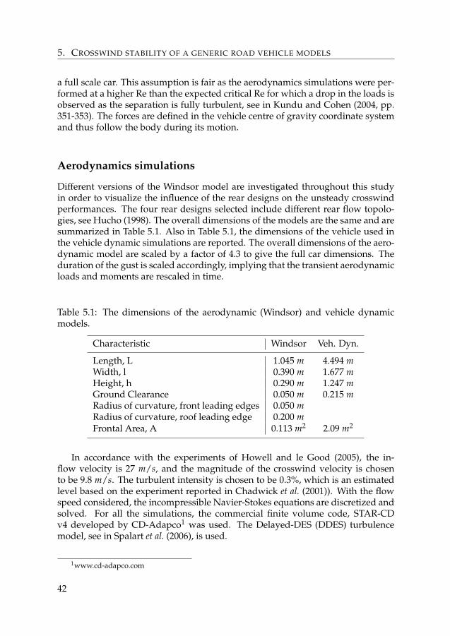
5. CROSSWIND STABILITY OF A GENERIC ROAD VEHICLE MODELS
a full scale car. This assumption is fair as the aerodynamics simulations were per-formed at a higher Re than the expected critical Re for which a drop in the loads isobserved as the separation is fully turbulent, see in Kundu and Cohen (2004, pp.351-353). The forces are defined in the vehicle centre of gravity coordinate systemand thus follow the body during its motion.
Aerodynamics simulations
Different versions of the Windsor model are investigated throughout this studyin order to visualize the influence of the rear designs on the unsteady crosswindperformances. The four rear designs selected include different rear flow topolo-gies, see Hucho (1998). The overall dimensions of the models are the same and aresummarized in Table 5.1. Also in Table 5.1, the dimensions of the vehicle used inthe vehicle dynamic simulations are reported. The overall dimensions of the aero-dynamic model are scaled by a factor of 4.3 to give the full car dimensions. Theduration of the gust is scaled accordingly, implying that the transient aerodynamicloads and moments are rescaled in time.
Table 5.1: The dimensions of the aerodynamic (Windsor) and vehicle dynamicmodels.
Characteristic Windsor Veh. Dyn.
Length, L 1.045 m 4.494 mWidth, l 0.390 m 1.677 mHeight, h 0.290 m 1.247 mGround Clearance 0.050 m 0.215 mRadius of curvature, front leading edges 0.050 mRadius of curvature, roof leading edge 0.200 mFrontal Area, A 0.113 m2 2.09 m2
In accordance with the experiments of Howell and le Good (2005), the in-flow velocity is 27 m/s, and the magnitude of the crosswind velocity is chosento be 9.8 m/s. The turbulent intensity is chosen to be 0.3%, which is an estimatedlevel based on the experiment reported in Chadwick et al. (2001)). With the flowspeed considered, the incompressible Navier-Stokes equations are discretized andsolved. For all the simulations, the commercial finite volume code, STAR-CDv4 developed by CD-Adapco1 was used. The Delayed-DES (DDES) turbulencemodel, see in Spalart et al. (2006), is used.
1www.cd-adapco.com
42
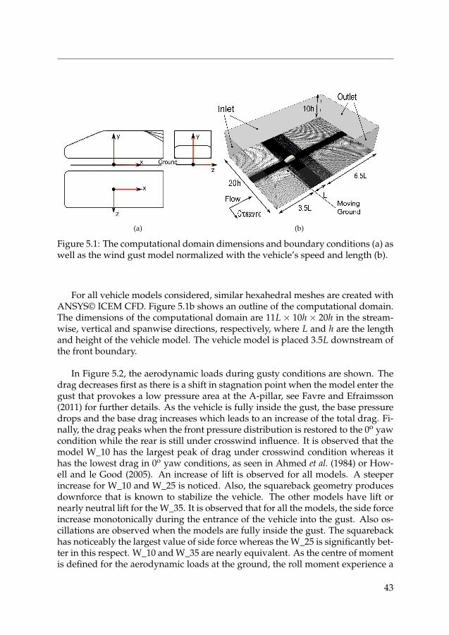
(a) (b)
Figure 5.1: The computational domain dimensions and boundary conditions (a) aswell as the wind gust model normalized with the vehicle’s speed and length (b).
For all vehicle models considered, similar hexahedral meshes are created withANSYS© ICEM CFD. Figure 5.1b shows an outline of the computational domain.The dimensions of the computational domain are 11L× 10h× 20h in the stream-wise, vertical and spanwise directions, respectively, where L and h are the lengthand height of the vehicle model. The vehicle model is placed 3.5L downstream ofthe front boundary.
In Figure 5.2, the aerodynamic loads during gusty conditions are shown. Thedrag decreases first as there is a shift in stagnation point when the model enter thegust that provokes a low pressure area at the A-pillar, see Favre and Efraimsson(2011) for further details. As the vehicle is fully inside the gust, the base pressuredrops and the base drag increases which leads to an increase of the total drag. Fi-nally, the drag peaks when the front pressure distribution is restored to the 0o yawcondition while the rear is still under crosswind influence. It is observed that themodel W_10 has the largest peak of drag under crosswind condition whereas ithas the lowest drag in 0o yaw conditions, as seen in Ahmed et al. (1984) or How-ell and le Good (2005). An increase of lift is observed for all models. A steeperincrease for W_10 and W_25 is noticed. Also, the squareback geometry producesdownforce that is known to stabilize the vehicle. The other models have lift ornearly neutral lift for the W_35. It is observed that for all the models, the side forceincrease monotonically during the entrance of the vehicle into the gust. Also os-cillations are observed when the models are fully inside the gust. The squarebackhas noticeably the largest value of side force whereas the W_25 is significantly bet-ter in this respect. W_10 and W_35 are nearly equivalent. As the centre of momentis defined for the aerodynamic loads at the ground, the roll moment experience a
43
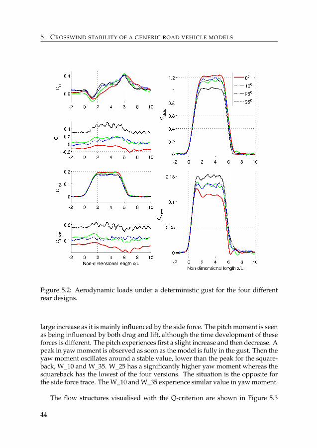
5. CROSSWIND STABILITY OF A GENERIC ROAD VEHICLE MODELS
Figure 5.2: Aerodynamic loads under a deterministic gust for the four differentrear designs.
large increase as it is mainly influenced by the side force. The pitch moment is seenas being influenced by both drag and lift, although the time development of theseforces is different. The pitch experiences first a slight increase and then decrease. Apeak in yaw moment is observed as soon as the model is fully in the gust. Then theyaw moment oscillates around a stable value, lower than the peak for the square-back, W_10 and W_35. W_25 has a significantly higher yaw moment whereas thesquareback has the lowest of the four versions. The situation is the opposite forthe side force trace. The W_10 and W_35 experience similar value in yaw moment.
The flow structures visualised with the Q-criterion are shown in Figure 5.3
44
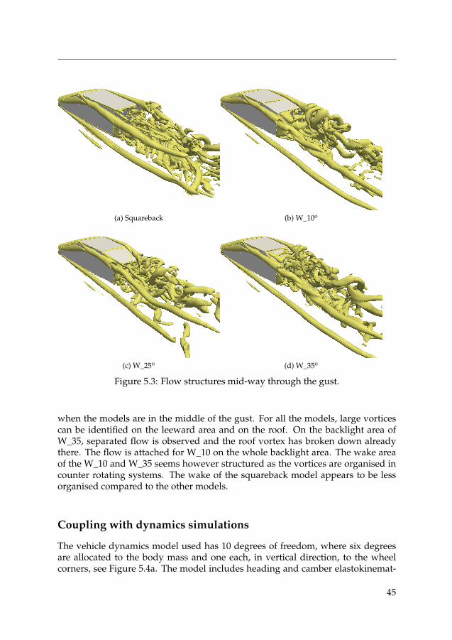
(a) Squareback (b) W_10o
(c) W_25o (d) W_35o
Figure 5.3: Flow structures mid-way through the gust.
when the models are in the middle of the gust. For all the models, large vorticescan be identified on the leeward area and on the roof. On the backlight area ofW_35, separated flow is observed and the roof vortex has broken down alreadythere. The flow is attached for W_10 on the whole backlight area. The wake areaof the W_10 and W_35 seems however structured as the vortices are organised incounter rotating systems. The wake of the squareback model appears to be lessorganised compared to the other models.
Coupling with dynamics simulations
The vehicle dynamics model used has 10 degrees of freedom, where six degreesare allocated to the body mass and one each, in vertical direction, to the wheelcorners, see Figure 5.4a. The model includes heading and camber elastokinemat-
45
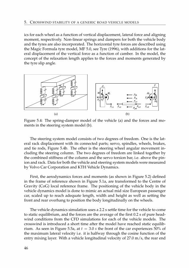
5. CROSSWIND STABILITY OF A GENERIC ROAD VEHICLE MODELS
ics for each wheel as a function of vertical displacement, lateral force and aligningmoment, respectively. Non-linear springs and dampers for both the vehicle bodyand the tyres are also incorporated. The horizontal tyre forces are described usingthe Magic Formula tyre model, MF 5.0, see Tyre (1996), with additions for the lat-eral displacement of the vertical force as a function of camber. In the model, theconcept of the relaxation length applies to the forces and moments generated bythe tyre slip angle.
(a) (b)
Figure 5.4: The spring-damper model of the vehicle (a) and the forces and mo-ments in the steering system model (b).
The steering system model consists of two degrees of freedom. One is the lat-eral rack displacement with its connected parts; servo, spindles, wheels, brakes,and tie rods, Figure 5.4b. The other is the steering wheel angular movement in-cluding the steering column. The two degrees of freedom are linked together bythe combined stiffness of the column and the servo torsion bar, i.e. above the pin-ion and rack. Data for both the vehicle and steering system models were measuredby Volvo Car Corporation and KTH Vehicle Dynamics.
First, the aerodynamics forces and moments (as shown in Figure 5.2) definedin the frame of reference shown in Figure 5.1a, are transformed to the Centre ofGravity (CoG) local reference frame. The positioning of the vehicle body in thevehicle dynamics model is done to mimic an actual mid size European passengercar, scaled up to reach adequate length, width and height as well as setting thefront and rear overhang to position the body longitudinally on the wheels.
The vehicle dynamics simulation uses a 2.2 s settle time for the vehicle to cometo static equilibrium, and the forces are the average of the first 0.2 s of pure head-wind conditions from the CFD simulations for each of the vehicle models. Thecrosswind is introduced a short time after the model have reached static equilib-rium. As seen in Figure 5.5a, at t = 3.0 s the front of the car experiences 50% ofthe maximum lateral velocity i.e. it is halfway through the cosine function of theentry mixing layer. With a vehicle longitudinal velocity of 27.0 m/s, the rear end
46
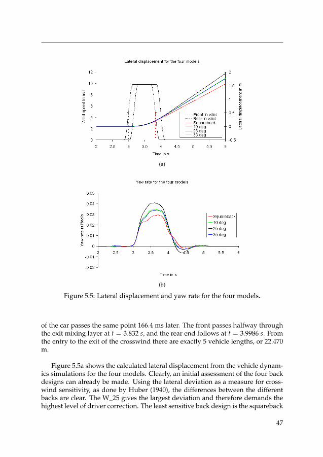
(a)
(b)
Figure 5.5: Lateral displacement and yaw rate for the four models.
of the car passes the same point 166.4 ms later. The front passes halfway throughthe exit mixing layer at t = 3.832 s, and the rear end follows at t = 3.9986 s. Fromthe entry to the exit of the crosswind there are exactly 5 vehicle lengths, or 22.470m.
Figure 5.5a shows the calculated lateral displacement from the vehicle dynam-ics simulations for the four models. Clearly, an initial assessment of the four backdesigns can already be made. Using the lateral deviation as a measure for cross-wind sensitivity, as done by Huber (1940), the differences between the differentbacks are clear. The W_25 gives the largest deviation and therefore demands thehighest level of driver correction. The least sensitive back design is the squareback
47
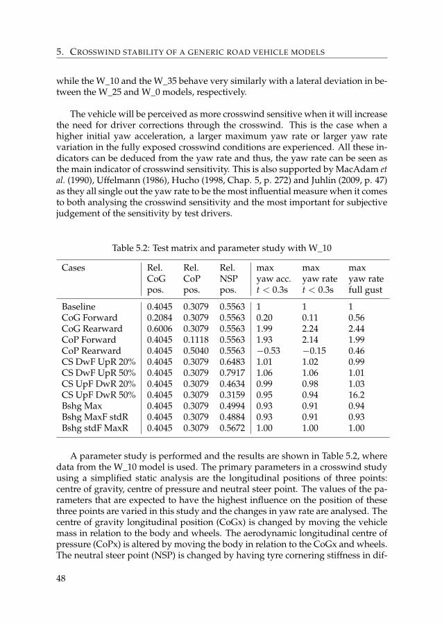
5. CROSSWIND STABILITY OF A GENERIC ROAD VEHICLE MODELS
while the W_10 and the W_35 behave very similarly with a lateral deviation in be-tween the W_25 and W_0 models, respectively.
The vehicle will be perceived as more crosswind sensitive when it will increasethe need for driver corrections through the crosswind. This is the case when ahigher initial yaw acceleration, a larger maximum yaw rate or larger yaw ratevariation in the fully exposed crosswind conditions are experienced. All these in-dicators can be deduced from the yaw rate and thus, the yaw rate can be seen asthe main indicator of crosswind sensitivity. This is also supported by MacAdam etal. (1990), Uffelmann (1986), Hucho (1998, Chap. 5, p. 272) and Juhlin (2009, p. 47)as they all single out the yaw rate to be the most influential measure when it comesto both analysing the crosswind sensitivity and the most important for subjectivejudgement of the sensitivity by test drivers.
Table 5.2: Test matrix and parameter study with W_10
Cases Rel. Rel. Rel. max max maxCoG CoP NSP yaw acc. yaw rate yaw ratepos. pos. pos. t < 0.3s t < 0.3s full gust
Baseline 0.4045 0.3079 0.5563 1 1 1CoG Forward 0.2084 0.3079 0.5563 0.20 0.11 0.56CoG Rearward 0.6006 0.3079 0.5563 1.99 2.24 2.44CoP Forward 0.4045 0.1118 0.5563 1.93 2.14 1.99CoP Rearward 0.4045 0.5040 0.5563 −0.53 −0.15 0.46CS DwF UpR 20% 0.4045 0.3079 0.6483 1.01 1.02 0.99CS DwF UpR 50% 0.4045 0.3079 0.7917 1.06 1.06 1.01CS UpF DwR 20% 0.4045 0.3079 0.4634 0.99 0.98 1.03CS UpF DwR 50% 0.4045 0.3079 0.3159 0.95 0.94 16.2Bshg Max 0.4045 0.3079 0.4994 0.93 0.91 0.94Bshg MaxF stdR 0.4045 0.3079 0.4884 0.93 0.91 0.93Bshg stdF MaxR 0.4045 0.3079 0.5672 1.00 1.00 1.00
A parameter study is performed and the results are shown in Table 5.2, wheredata from the W_10 model is used. The primary parameters in a crosswind studyusing a simplified static analysis are the longitudinal positions of three points:centre of gravity, centre of pressure and neutral steer point. The values of the pa-rameters that are expected to have the highest influence on the position of thesethree points are varied in this study and the changes in yaw rate are analysed. Thecentre of gravity longitudinal position (CoGx) is changed by moving the vehiclemass in relation to the body and wheels. The aerodynamic longitudinal centre ofpressure (CoPx) is altered by moving the body in relation to the CoGx and wheels.The neutral steer point (NSP) is changed by having tyre cornering stiffness in dif-
48
ferent combinations and different suspension bushing stiffness. The different NSPlocations are simulated with the full vehicle dynamics model and reported in Ta-ble 5.2 and gives an idea on how the dynamic NSP will be affected. Also in Table5.2, the relative position of the CoPx normalized to the wheel base length is given.This value is taken as the averaged value of the CoPx during the wind gust.
With the monitoring of the longitudinal position of the CoG, CoP and NSP, itis possible to get a simplified overview of the problem of crosswind stability. Ascan be seen, positioning the CoP in relation to the CoG and NSP is the most in-fluential component when altering the crosswind sensitivity without affecting theoverall vehicle dynamics properties. This was also concluded by both MacAdamet al. (1990) and Alexandridis et al. (1979). As the CoG and NSP positions are alsogoverned by other vehicle dynamic requirements, there is a limit to the possibilityto move them in relation to each other. With active or passive compliances though,it is possible to make the NSP position more dynamic and event related, in orderto improve crosswind stability.
To make the crosswind behaviour perfect, i.e. not sensitive, a careful design ofthe interactions of the dynamic CoP and NSP movements can generate a car thatinitially yaws at the same angle into the wind as the tyres need for slip angle tocounter the lateral force of the steady state crosswind. This would give a vehi-cle that travels straight in line, requiring no correction from the driver. To makethis come true, the CoG have to be slightly in front of the CoP on crosswind entryand the CoP and NSP have to be close together in steady state crosswind situation.
Finally, by moving the CoP and NSP in relation to the CoG, the yaw rate of thefour different back designs can be much improved as pointed out in the previoussection. As the CoP position is seen as the most influential parameter, the first stepis to move the body rearward behind and in the vicinity of the CoG. This is doneto a level where the rest of the yaw rate can be changed by varying characteris-tics of bushings and tyres to move the NSP forward but still behind the CoP. Thisbalancing shows the necessary levels to reach for the CoP and NSP positions toachieve a balanced yaw rate response and reduced lateral deviation of the other-wise unchanged vehicle. A small lateral deviation remains as there is a slip of thecar due to the lateral force from the crosswind. All the vehicles were balanced sothat only a 17 cm drift remained well after exiting the crosswind gust.
An example is given in Fig. 5.6. W_25 had the largest lateral deviation andthe highest yaw rate with the baseline setting. By moving the bodywork rearwardand altering the cornering stiffness of both tyres and making the bushing stiffer,the car became stable during the strong wind gust.
49
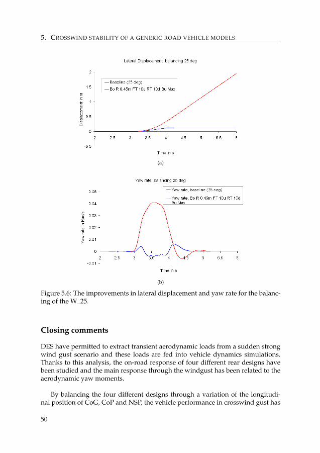
5. CROSSWIND STABILITY OF A GENERIC ROAD VEHICLE MODELS
(a)
(b)
Figure 5.6: The improvements in lateral displacement and yaw rate for the balanc-ing of the W_25.
Closing comments
DES have permitted to extract transient aerodynamic loads from a sudden strongwind gust scenario and these loads are fed into vehicle dynamics simulations.Thanks to this analysis, the on-road response of four different rear designs havebeen studied and the main response through the windgust has been related to theaerodynamic yaw moments.
By balancing the four different designs through a variation of the longitudi-nal position of CoG, CoP and NSP, the vehicle performance in crosswind gust has
50
shown to be clearly affected and improved.
In this work, in order to make the static coupling between the aerodynamicand vehicle dynamic simulations feasible, several assumptions have been made.In future studies, the Reynold number dependence would need to be further in-vestigated for different yaw angles and a simulation at the realistic Reynolds num-ber should be made to validate the assumption of the present study.
Naturally, the choice of the crosswind scenario play a significant role and theinfluence of the deterministic crosswind model should be evaluated.
Finally, exploring other design features will lead to deeper knowledge in theinteractions between shape features and crosswind stability. The influence of theleading edges radius of curvature would be an interesting next design alterationto be investigated as the yaw moments appear to be sensitive to this parameter, asshown e.g. in Paper B.
51

CHAPTER 6Conclusions and future work
With the preceding collected and documented results, this thesis can be consid-ered as a first basis to further investigate the full interactions involved in the wholecrosswind process. Indeed, recent CFD methods are approached and the accuracyis evaluated for different geometries. Different challenges that offer these variousgeometries have highlighted the difficulty to get fast descriptions of the crosswindflow without compromising too much the overall precision of the results. Thefeedback from the coupling of aerodynamics and vehicle dynamics simulationsopens the way to further more complete investigations.
More precisely, concerning the CFD simulations, it has been seen that:
• the use of DDES to simulate unsteady crosswind flows and to keep accuracy,and reasonnable computational time have been successful.
• The unstructured mesh with a more dissipative setup has surprisingly givendecent results for the flows considered. However, a more challenging geom-etry, such as the REVM, might have lead to more discrepancies.
• The different grid-refinements performed in this thesis have shown a direc-tion and methods to investigate unsteady crosswind flows. Both strengthsand weaknesses have been highlighted and can be used as starting point forstudies of new geometries.
Also, from an aerodynamics point of view, it is observed that:
• rear designs of cars exhibit the same qualitative results in unsteady cross-wind as in steady crosswind (for example, the squareback is better than the25o backlight angle). However, transients exist and can lead to unexpectedresults (for instance, the 10o backlight angle produces the largest amount ofdrag when exiting the gust)
• The radius of curvature at the front determined the flow separation in cross-wind and therefore has a large impact on the yaw moment. Sharp edgesprovide large transient that are not anticipated in steady crosswind analysis.
53
6. CONCLUSIONS AND FUTURE WORK
Looking at the crosswind sensitivity, the main points to retain are:
• the classes of car determined with their different rears have different cross-wind response. The yaw moment and the yaw rate can be the two criticalparameters to extract from any analysis.
• The location of the Centre of Pressure with respect the Centre of Gravity andthe Neutral Steer Point is directly responsible of the car response in cross-wind. Altering this relation and an unstable car in crosswind can be tunedto a stable car.
Future work
Crosswind aerodynamics is such a wide topic that many further considerationscan be imagined. Here, it is however discussed in three main topics in which thefuture work can be classified.
From the CFD and DES points of view:
• further studies of the mesh for defining the optimum one and describe astrategy to perform grid-refinement studies. A possible study of polyhe-drals on challenging geometries could also be of interest for completing theknowledge on grid types and DES.
• as a natural follow up of the above task, define guidelines to tackle crosswindflows with DDES
• investigate the influence of the RANS model within DES and study its influ-ence on adverse pressure gradient separations
• study a higher Re number, if possible, and relate the aerodynamic loads tothe Re number.
Concerning the unsteady crosswind aspects:
• define other deterministic crosswind scenarios (that still represent criticalscenarios) and investigate their effects and transients. This will broaden theknowledge and will help to find the most suitable crosswind scenario (per-haps the most critical scenario or the most representative or a combinationof this two...). Further static coupling between aerodynamics and vehicledynamics simulations can help in assessing the most suitable crosswind sce-nario.
• investigate the flow field variation for small variations of roll and pitch an-gle. A static study would be a first step.
• the dynamic mesh techniques and automatic remeshing technique should bereviewed and the accuracy of such process assessed.
54
• study if the vehicle dynamics model of Paper C/D can be reduced and sim-plified without compromising the yaw rate response.
• following the results from the above points, an investigation of full dynamiccoupling between the aerodynamics and vehicle dynamics simulations. In-deed, the crosswind scenario should be suitable for this study (using ratherlong gust), the flow field should be expected to be influenced by small vari-ations of roll and pitch angles, the accuracy should be kept along the simu-lation (using time-accurate modelling such as DES) and the computationaltime should remain reasonnable. Also, it should be evaluated whether thedynamic equations have to be solved for each time-step or after an intervalof time steps.
Finally, to improve the aerodynamics of vehicles in unsteady crosswind, it isworth analysing
• some shape variations for the simplified car model, such as the radius ofcurvature at the rear of the vehicle that are expected to influence the yawmoment
• larger road vehicle geometries, like buses of trucks, as their response in cross-wind is a concern for safety
• investigate the possibility to passively (or actively) control the motion of theCentre of Pressure for a vehicle that is exposed for an unsteady gust. Thisstudy should be related to the final vehicle dynamic response in wind gusts.
55

CHAPTER 7Summary of Appended Papers
7.1 Paper A
An assessment of Detached-Eddy Simulations of unsteady crosswind aerody-namics of road vehicles
Tristan Favre and Gunilla Efraimsson
In this paper, the availability of Detached-Eddy Simulations (DES) for sim-ulating unsteady crosswind aerodynamics in industrial applications is exploredand reported. The flow around a simple car geometry under headwind, steadycrosswind and time-dependent wind gust respectively, is analysed for two differ-ent types of mesh using a commercial software, STAR-CD. The typical Reynoldsnumber of the flow cases studied is 2.0 ⋅ 106 based on the vehicle length. The per-formances of polyhedral meshes together with a comparable hexahedral mesh areevaluated for capturing the time development of the flow structures during a gust.From the results presented, it can be concluded that the aerodynamic coefficientscan be reliably calculated using both polyhedral and hexahedral meshes, althoughthe fine turbulent structures in the wake are better captured with the hexahedralmesh. The pressure drag has been decomposed in two main contributors: thefront and the base drags. The front drag being reduced at the gust entrance leadsto a lower drag first. The base drag is constantly increasing and no stable value isreached. A peak of drag is observed at the gust exit as both the front and the basedrags are at their maximum. Using turbulence methods like DES in order to re-solve the flow scales provides a significant insight for designing a ground vehicleand, due to the reasonable computational times involved, can hence be foreseento be incorporated in a design process in a near future.
57
7. SUMMARY OF APPENDED PAPERS
7.2 Paper B
Detached-Eddy simulations of simplified vehicles in steady and unsteady cross-wind
Tristan Favre, Per Elofsson and Gunilla Efraimsson
In this paper, DES are used to study two simple vehicle models (one with sharpedges and the other with radiused edges) subjected to steady crosswind as well asvarious wind gusts. For steady crosswind and when compared to published ex-perimental data, the calculated aerodynamic loads suggest grid-convergence andfall within the experimental range. The aerodynamic coefficients during windgust are also compared to the experimental values from Chadwick et al. (2001).The results calculated with DES for the SEVM model shows a good agreementwith the experimental data. However, the prediction of the separation for theradiused-edges geometry appears to be difficult to predict for the DDES usingSpalart-Allmaras for the RANS model. It is also observed that both geometriesexhibits strong transient and large discrepancies between unsteady and steadyaerodynamic loads. Especially for the SEVM, the peak of yaw moment in gust ismore than 5 times larger than the steady crosswind value.
7.3 Paper C
Detached-Eddy Simulations of the effects of different wind gust models on theunsteady aerodynamics of road vehicles
Tristan Favre and Gunilla Efraimsson
In this article, time-accurate simulations, Detached-Eddy Simulations (DES),are used to simulate the flow around a simple vehicle shape, the so-called Wind-sor model. The ReL of the corresponding flow case is 2.0 ⋅ 106. The simulationsare using a computational grid composed of polyhedral cells. The influence ofdifferent deterministic models of wind gusts on the aerodynamic loads and mo-ments are studied. The wind gusts are varied in the streamwise and the verticaldirection. The magnitude of the gusts models corresponds to a yaw angle of 20o.The aerodynamic loads calculated show a large excess of drag coupled with a re-duction of the pitch moment. In addition, although the side force has a smoothvariation in the gust, overshoots up to 18% higher than the steady value of yawmoment are also observed. A relation between the gusts’ growing times and thelevel of the overshoots is also observed.
58
7.4. Paper D
7.4 Paper D
Unsteady mechanisms in crosswind aerodynamics for ground vehicles
Tristan Favre and Gunilla Efraimsson
This article describes the unsteady flows observed for several geometries insudden strong windgusts. These discussions are considered as a first tests andfurther work may lead to a better understanding of the problem and help mod-elling it. Results from previous simulations are discussed to describe preciselythe development of the aerodynamic loads. The models (The Windsor modelsand the REVM and SEVM) are compared to each other and display some sim-ilar features (especially the rear suction). Delays in growth of the aerodynamicloads are observed and illustrated by plotting the loads with respect the overallyaw angle. Hysteresis are displayed. Plotting the yaw moment versus the dragforce during windgust provide a convenient way to compare the crosswind per-formance versus the fuel consumption. Among the Windsor models tested, thesquareback model appears to the best compromise. Varying the wind gusts steep-ness (or growing time), linear relations are observed between the drag force andyaw moment overshoots with the gust’s growing time. In order to conceive atool for fast assessment of crosswind properties, aiming to model the hysteresisbehaviours seems to be more adequate: the overall behaviour seems to be easierto model than the time history and the differences between the vehicle designsappear to be more visible with these representations.
7.5 Paper E
Numerical study of design alterations affecting the crosswind characteristics ofa generic road vehicle model
Tristan Favre and Gunilla Efraimsson
In this paper, Detached-Eddy simulations (DES) of the crosswind aerodynam-ics characteristics of three different generic passenger car shapes (the Windsormodels) subjected to an unsteady wind gust are presented. The models are charac-terized by their backlight inclination (0o, 10o and 35o). Time dependent boundaryconditions describing a sudden crosswind exposure are introduced in the com-putational domain. The corresponding Reynolds number based on the vehicles’length is 2.0× 10⁶. Also, the aerodynamic loads affecting the overall stability ofthe vehicle are discussed. Not only the squareback model exhibits the largest sideforce and the lowest yaw moment, it also shows a different development of theloads compared to the other other models. The different components of drag arealso analysed during the gust and it is observed that the rear of the car is respon-sible of the large increase of drag (up to 90% and more). The vortex drag is the
59
7. SUMMARY OF APPENDED PAPERS
largest for the 35o model. Although the 10o model has the lowest drag in head-wing, this model produces the largest total drag at the gust exit.
7.6 Paper F
Static coupling between detached-eddy simulations and vehicle dynamic simu-lation of a generic road vehicle model in unsteady crosswind with different rearconfigurations
Tristan Favre, Jonas Jarlmark Näfver, Annika Stensson Trigell and GunillaEfraimsson
In this paper, capabilities and limitations of a static coupling between aerody-namic loads and a vehicle dynamic model in order to predict the crosswind sen-sitivity of a road vehicle are assessed. Time-accurate simulations, Detached-EddySimulations (DES), are used to predict the aerodynamic loads of four rear config-urations of a generic car model under a sudden strong crosswind. The loads arethereafter incorporated in a complete vehicle dynamic model to assess the on-roadresponse. The four backs show large differences in yaw moments and side forcesresulting in large discrepancies in lateral displacements as well as yaw rates. Aparameter study review the influence of basic components to change successivelythe dynamic location of the centre of gravity, the centre of aerodynamic pressureand the neutral steer point. Balancing the body location with the stiffness of thebushing and the cornering stiffness has provided stable vehicles in strong cross-wind conditions for all four rear designs. The results illustrate that monitoring thelocation of the aerodynamic centre of pressure with respect to the centre of gravityand the neutral steering point, is essential for designing stable vehicles in transientcrosswind. Recommendations on further work in order to develop full dynamiccoupling between aerodynamics and vehicle dynamic simulations are provided atthe end of the article.
60
Bibliography
S.R. Ahmed, G. Ramm, and G. Faltin. 1984. Some salient features of the time-averaged ground vehicle wake. SAE Technical Paper Series. 840300.
A.A. Alexandridis, B.S. Repa, and W.W. Wierwill. 1979. The influence of vehi-cle aerodynamic and control response characteristics on driver-vehicle perfor-mance. SAE Technical Paper Series. 790385.
C.J. Baker. 1986a. A simplified analysis of various types of wind induced roadvehicle accidents. Journal of Wind Engineering and Industrial Aerodynamics, 22:69–85.
C.J. Baker. 1986b. Train aerodynamic forces and moments from moving modelexperiments. Journal of Wind Engineering and Industrial Aerodynamics, 24:227–251.
C.J. Baker. 1991a. Ground vehicles in high cross winds, part 1: Steady crosswindforces. Journal of Fluids and Structures, 5:69–90.
C.J. Baker. 1991b. Ground vehicles in high cross winds, part 2: Unsteady crosswindforces. Journal of Fluids and Structures, 5:91–111.
C.J. Baker. 1991c. Ground vehicles in high cross winds, part 3: The interaction ofaerodynamic forces and the vehicle system. Journal of Fluids and Structures, 5:221–241.
M. Bocciolone, F. Cheli, R. Corradi, S. Muggiasca, and G. Tomasini. 2008. Cross-wind action on rail vehicles: Wind tunnel experimental analyses. Journal of WindEngineering and Industrial Aerodynamics, 96:584–610.
R.S. Cairns. 1994. Lateral Aerodynamics of Motor Vehicles in Transient Crosswinds.PhD Thesis, College of Aeronautics, Cranfield University, UK.
A. Chadwick. 1999. Crosswind aerodynamics of sports utility vehicles. PhD Thesis,College of Aeronautics, Cranfield University, UK.
A. Chadwick, K. Garry, and J. Howell. 2001. Transient aerodynamic characteristicsof simple vehicle shapes by the measurement of surface pressures. SAE TechnicalPaper Series. 2001-01-0876.
61
BIBLIOGRAPHY
P. Chakraborty, S. Balachandar, and J. Adrian. 2005. On the relationships betweenlocal vortex identification schemes. Journal of Fluid Mechanics, 535:189–214.
A. Chometon, A. Strzelecki, V. Ferrand, H. Dechipre, P.C. Dufour, M. Gohlke, andV. Herbert. 2005. Experimental study of unsteady wakes behind an oscillatingcar model. SAE Technical Paper Series. 2005-01-00604.
A. Cogotti. 2003. Generation of a controlled level of turbulence in the Pininfa-rina wind tunnel for measurement of unsteady aerodynamics and aeroacoustics.SAE Technical Paper Series. 2003-01-0430.
G.S. Constantinescu and K.D. Squires. 2003. LES and DES investigations of tur-bulent flow over a sphere at re = 10000. Flow, Turbulence and Combustion, 70:267–298.
R. Demuth and P. Buck. 2006. Numerical investigations on the unsteady aerody-namics of road vehicle under gusty weather conditions. In MIRA, editor, SixthWorld MIRA International Vehicle Aerodynamics Conference, England.
B. Diedrich. 2006. Studies of two aerodynamic effects on high-speed trains: crosswindstability and discomforting car body vibrations inside tunnels. PhD Thesis, Depart-ment of Aeronautical and Vehicle Engineering, Kungliga Tekniska Högskolan(KTH), Stockholm, Sweden. TRITA-AVE 2006:81.
B. Diedrichs. 2009. Unsteady aerodynamic crosswind stability of a high-speedtrain subjected to gusts of various rates. In Euromech Colloquium 509, Berlin,Germany.
M. Docton and R. Dominy. 1996. The simulation of transient cross winds on pas-senger vehicles. In MIRA, editor, MIRA International Vehicle Aerodynamics Con-ference, England.
L.E. Ericsson and J.P. Reding. 1988. Fluid mechanics of dynamic stall part 1: Un-steady flow concepts. Journal of Fluids and Structures, 2:1–33.
T. Favre, B. Diedrichs, and G. Efraimsson. 2010. Detached-eddy simulations ap-plied to unsteady crosswind aerodynamics of ground vehicles. In Springer S.-H. Peng et al, editor, Progress in Hybrid RANS-LES Modelling, NNFM 111, pages167–177.
T. Favre and G. Efraimsson. 2011. An assessment of detached-eddy simulations ofunsteady crosswind aerodynamics of road vehicles. Flow, Turbulence and Com-bustion, 87:133–163. DOI:10.1007/s10494-011-9333-4.
K.P. Garry and K.R. Cooper. 1986. Comparison of quasi-static and dynamic windtunnel measurements on simplified tractor-trailer models. Journal of Wind Engi-neering and Industrial Aerodynamics, 22:185–194.
62
A.M. Gilhaus and V.E. Renn. 1986. Drag and driving-stability-related aerodynamicforces and their interdependence, results of measurements on 3/8-scale basic carshapes. SAE Technical Paper Series. 860211.
E. Guilmineau. 2008. Computational study of flow around a simplified car body.Journal of Wind Engineering and Industrial Aerodynamics, 96:1207–1217.
E. Guilmineau, O. Chikhaoui, G. Deng, and M. Visionneau. 2011a. Cross windeffects on a simplified car model by a DES approach. to appear in Computers &Fluids.
E. Guilmineau, G. Deng, and J. Wackers. 2011b. Numerical simulation with a DESapproach for automotive flows. to appear in Journal of Fluids and Structures.
N.D. Ham and M.S. Garelick. 1968. Dynamic stall considerations in helicopterrotors. Journal of the American Helicopter Society, 13:44–55.
H. Hemida and S. Krajnovic. 2009. Transient simulation of the aerodynamic re-sponse of a double-deck bus in gusty winds. Journal of Fluids Engineering, 131:0311011–03110110.
H. Hemida, S. Krajnovic, and L. Davidson. 2005. Large-eddy simulation of theflow around a simplified high speed train under the influence of a cross-wind.In 17th AIAA Computational Fluid Dynamics Conference, 6-9 June 2005, Toronto, On-tario, Canada. AIAA Paper 2005-5354.
J.P. Howell. 1993. Shape features which influence crosswind sensitivity. In TheInstitution of Mechanical Engineers, IMechE 1993-9, Vehicle Ride and Handling.
J.P. Howell and G. le Good. 2005. Vortex drag for a simple bluff body at incidencein ground proximity. SAE Technical Paper Series. 2005-01-0869.
L. Huber. 1940. Die Fahrtrichtungsstabilität des schnellfahrenden Kraftwagens. PhDThesis, TH Stuttgart.
W-H. Hucho. 1998. Aerodynamics of Road Vehicles. SAE International.
W-H. Hucho and H.J. Emmelmann. 1973. Theoretical prediction of the aerody-namic derivatives of a vehicle in cross wind gusts. SAE Technical Paper Series.730232.
M. Islam, F. Decker, E. de Villiers, A. Jackson, J. Gines, T. Grahs, A. Gitt-Gehrke,and J. Comas i Font. 2009. Application of detached-eddy simulations for auto-motive aerodynamics development. SAE Technical Paper Series. 2009-01-0333.
J. Jarlmark. 2002. Driver-vehicle interaction under influence of crosswind gusts. Licen-tiate Thesis, Department of Aeronautical and Vehicle Engineering, KTH RoyalInstitute of Technology, Stockholm, Sweden. TRITA-FKT 2002:18.
63

BIBLIOGRAPHY
M. Juhlin. 2009. Assessment of crosswind performance of buses. PhD Thesis, Depart-ment of Aeronautical and Vehicle Engineering, KTH Royal Institute of Technol-ogy, Stockholm, Sweden. TRITA-AVE 2009:25.
J. Klasson. 2001. A generalised crosswind model for simulation purposes. VehicleSystem Dynamics, 37:350–359.
S. Krajnovic. 2009. Large eddy simulation of flows around ground vehicles andother bluff bodies. Philosophical Transactions of the Royal Society, 369:2917–2930.
P.K. Kundu and I.M. Cohen. 2004. Fluid Mechanics, 3rd Edition. Elsevier.
G. le Good, P. Yeomans, and M. Yates. 2008. A comparison of stationary and mov-ing ground-plane pressure signature beneath a simplified car shape using CFD.In MIRA, editor, Seventh World MIRA International Vehicle Aerodynamics Confer-ence, England.
T. Lee and P. Gerontakos. 2004. Investigation of flow over an oscillating airfoil.Journal of Fluid Mechanics, 512:313–341.
M.A. Leschziner. 2006. Modelling turbulent separated flow in the context of aero-dynamic applications. Fluid Dynamics Research, 38:174–210.
C.C. MacAdam, M.W. Sayers, J.D. Pointer, and M. Gleason. 1990. Crosswind sensi-tivity of passenger cars and the influence of chassis and aerodynamic propertieson driver preferences. Vehicle System Dynamics, 19:201–236.
S. Maddox, K.D. Squires, K.E. Wurtzler, and J.R. Forsythe. 2004. Detached-eddysimulations of the ground transportation system. In Browand F Mc Callen Rand Springer Ross J (eds), editors, The Aerodynamics of Heavy Vehicles: trucks,buses and trains.
F.R. Menter. 1992. Improved two-equation k − ω turbulence models for aerody-namic flows. Technical memorandum, NASA. 103975.
C. Mockett. 2009. A comprehensive study of detached-eddy simulation. PhD Thesis,Institute of Fluid Mechanics and Engineering Acoustics, Technische UniversitátBerlin, Germany.
C. Moulinec, S. Benhamadouche, D. Laurence, and M. Peric. 2005. LES in a u-bend pipe meshed by polyhedral cells. In Elsevier W. Rodi, editor, EngineeringTurbulence Modelling and Experiments 6, pages 237–246.
P. Newnham, M. Passmore, and A. Baxendale. 2008. The effect of raised freestreamturbulence on the flow around leading edge radii. SAE Technical Paper Series.2008-01-0473.
S.B. Pope. 2000. Turbulent Flows. Cambridge University Press.
64
O. Reynolds. 1883. An experimental investigation of the circumstances which de-termine whether the motion of water shall be direct or sinuous, and of the lawof resistance in parallel channels. Proceedings of the Royal Society of London, 35:84–99.
A. Ryan. 2000. The Simulation of Transient Cross-Wind Gusts and their AerodynamicInfluence on Passenger Cars. PhD Thesis, School of Engineering, University ofDurham, UK.
P. Schlatter and R. Örlü. 2011. Assessment of direct numerical simulation data ofturbulent boundary layers. Journal of Fluid Mechanics, 659:116–126.
H. Schlichting. 1960. Boundary Layer Theory. McGraw-Hill series in mechanicalengineering.
SHK. 2001. Bus fire following traffic accident at Fjärdhundra on national route70, C county, Sweden, 21 November 1998. Case No. O-10/98. Technical report,Swedish Board of Accident Investigation (SHK). Rapport RO 2001:04e (English).
D. Sims-Williams. 2011. Cross winds and transients: Reality, simulations and ef-fects. SAE Technical Paper Series. 2011-01-0172.
J. Smagorinsky. 1963. General circulation experiments with the primitive equa-tions. Monthly Weather Review, 91.
P.R. Spalart. 2001. Young-person’s guide to Detached-Eddy Simulation grids.Technical report, NASA. NASA CR 2001-211032.
P.R. Spalart. 2009. Detached-eddy simulation. Annual Review of Fluid Mechanics,41:181–202.
P.R. Spalart and S. Allmaras. 1992. A one-equation model for aerodynamic flows.In AIAA, editor, AIAA 30th Aerospace Sciences Meeting, Reno, NV. AIAA Paper92-0439.
P.R. Spalart, S. Deck, M.L. Shur, S.D. Squires, M.Kh. Strelets, and A. Travin. 2006. Anew version of detached-eddy simulation, resistant to ambiguous grid densities.Theoretical Computational Fluid Dynamic, 20:181–195.
P.R. Spalart, W.H. Jou, M. Strelets, and S.R. Allmaras. 1997. Comments on thefeasibility of LES for wings, and on approach on a hybrid RANS/LES approach.In 1st AFOSR International Conference on DNS and LES.
R.K. Strachan, K. Knowles, and N.J. Lawson. 2007. The vortex structure behind anAhmed reference model in the presence of a moving ground plane. Experimentsin Fluids, 42:659–669.
65
BIBLIOGRAPHY
M. Strelets. 2001. Detached eddy simulations of massively separated flows. InAIAA, editor, AIAA 39th Aerospace Sciences Meeting, Reno, NV. AIAA Paper 2001-0879.
P. Theissen, J. Wojciak, K. Heuler, R. Demuth, T. Indinger, and N. Adams. 2011.Experimental investigation of unsteady aerodynamics under time-dependentflow conditions - part 1. SAE Technical Paper Series. 2011-01-0177.
D. Thomas, B. Diedrichs, M. Berg, and S. Stichel. 2010. Dynamics of a high-speedrail vehicle negotiating curves at unsteady crosswind. Proc. Instn Mech. Engrs,Part F: Journal of Rail and Rapid Transit, 224:567–579.
A. Travin, M. Shur, M. Strelets, and P.R. Spalart. 1999. Detached-eddy simulationspast a circular cylinder. Flow, Turbulence and Combustion, 63:293–313.
A. Travin, M. Shur, M. Strelets, and P.R. Spalart. 2002. Physical and numerical up-grades in the detached-eddy simulation of complex turbulent flows. In FriedrichR and Rodi W (eds.), editors, Advances in LES of Complex Flows, pages 239–254.
M. Tsubokura, T. Kobayashi, T. Nakashima, T. Nouzawa, T. Nakamura, H. Zhang,K. Onishi, and N. Oshima. 2009. Computational visualization of unsteady flowaround vehicles using high performance computing. Computers and Fluids, 38:981–990.
M. Tsubukora and T. Nakashima. 2010. Unsteady aerodynamic simulator for roadvehicle based on large-eddy simulation. In MIRA, editor, Eighth World MIRAInternational Vehicle Aerodynamics Conference, England.
Delft Tyre. 1996. Delft-Tyre: MF-Tyre 5.0 User manual. TNO.
F. Uffelmann. 1986. Influence of aerodynamics and suspension on the cross-windbehaviour of passenger cars - theoretical investigation under consideration ofthe driver’s response. Vehicle System Dynamics, 15:568–581.
R. Volpe, V. Ferrand, and A. Da Silva. 2011. Validation d’un banc d’essais repro-duisant les rafales de vent sur vehicule terrestre. caracterisation de l’ecoulementpar TR-PIV. In 14ème Congrès Francais de Visualisation et de Traitement d’Images enMécanique des Fluides, Lille, France, 21 - 25 novembre.
Th. von Kármán and W.R. Sears. 1938. Airfoil theory for non-uniform motion.Journal of Aerospace Sciences, 5:379–390.
J. Wojciak, T. Indinger, N. Adams, P. Theissen, and R. Demuth. 2010. Experimentalstudy of on-road aerodynamics during crosswind gusts. In MIRA, editor, EighthWorld MIRA International Vehicle Aerodynamics Conference, England.
J. Wojciak, P. Theissen, K. Heuler, T. Indinger, N. Adams, and R. Demuth. 2011.Experimental investigation of unsteady aerodynamics under time-dependentflow conditions - part 2. SAE Technical Paper Series. 2011-01-0164.
66
Bibliography
S. Wordley and J. Saunders. 2008. On-road turbulence. SAE Technical Paper Series.2008-01-0475.
S. Wordley and J. Saunders. 2009. On-road turbulence: part 2. SAE Technical PaperSeries. 2009-01-0002.
67


Part II
Appended Papers
69

PAPER A
An assessment of Detached-Eddy Simulations of unsteadycrosswind aerodynamics of road vehicles
Tristan Favre and Gunilla Efraimsson
Refereed article published inFlow, Turbulence and Combustion
Vol. 87(1), pp 133–163
©2011 Springer.The layout has been revised.
PAPER B
Detached-Eddy simulations of simplified vehicles in steady andunsteady crosswind
Tristan Favre, Per Elofsson and Gunilla Efraimsson
Article submitted toFlow, Turbulence and Combustion

©2011 Tristan Favre.The layout has been revised.
PAPER C
Detached-Eddy Simulations of the effects of different wind gustmodels on the unsteady aerodynamics of road vehicles
Tristan Favre and Gunilla Efraimsson
Refereed article published inProceedings of the 3rd Joint US-European Fluids Engineering Summer Meeting &
8th International Conference on Nanochannels and Minichannels, FEDSM-ICNMM.Montreal, Canada, August 2010.

©2010 ASME.The layout has been revised.
PAPER D
Unsteady mechanisms in crosswind aerodynamics for groundvehicles
Tristan Favre and Gunilla Efraimsson
Technical Report TRITA-AVE 2011:85.

©2011 Tristan Favre.The layout has been revised.
PAPER E
Numerical study of design alterations affecting the crosswindcharacteristics of a generic road vehicle model
Tristan Favre and Gunilla Efraimsson
Refereed article published inProceedings of the Eighth World MIRA International Vehicle Aerodynamics Conference,
England, 2010.

©2010 MIRA.The layout has been revised.
PAPER FStatic coupling between detached-eddy simulations and vehicledynamic simulation of a generic road vehicle model in unsteady
crosswind with different rear configurations
Tristan Favre, Jonas Jarlmark Näfver, Annika Stensson Trigell and GunillaEfraimsson
Article submitted toInternational Journal of Vehicle Design

©2011 Tristan Favre.The layout has been revised.