aerodynamics of the oscillating airfoils -...
TRANSCRIPT
“Aerodynamics of the oscillating airfoils”
University of Naples
November 4th, 2011.
Claudio Marongiu1
1CIRA - Italian Center for Aerospace Research
Marongiu C. (CIRA) Seminario Napoli, November 4th 2011 1 / 75
Aerodynamics of the oscillating airfoils
OUTLINE
Introduction
Theodorsen solution
CFD of the oscillating airfoils
Marongiu C. (CIRA) Seminario Napoli, November 4th 2011 2 / 75
Aerodynamics of the oscillating airfoils
References
1 Von Karman, T., and Burger J. M., 1935, “General Aerodynamic Theory. Perfect Fluids”, Peter Smith Publisher, Inc.,1976, pp. 280-310.
2 Theodorsen T., “General Theory of Aerodynamic Instability and the Mechanics of Flutter”, National AdvisoryCommittee for Aeronautics, NACA Report. 496 (1935).
3 Bisplinghoff R. L., Ashley H. and Halfman R. L., “Aeroelasticity”, Dover Publications, Inc., New York
4 Saffman P. G. , “Vortex Dynamics”, Cambridge University Press, 1992
5 McCroskey W. J., “The Phenomenon of Dynamic Stall”, Lecture Notes presented at Von Karman Institute LectureSeries on Unsteady Airloads and Aeroelasticity Problems in Separated and Transonic Flows, 9-13 March 1981.
6 Leishman J. G., (2000) “Principles of Helicopter Aerodynamics ”. Cambridge University Press
Most of the material contained in these slides comes from my Ph.D. thesis made
between 2007 and 2010 and related publications in collaboration with Prof. Tognaccini,
(DIAS), University of Naples.
Marongiu C. (CIRA) Seminario Napoli, November 4th 2011 3 / 75
Aerodynamics of the oscillating airfoils
Introduction
Marongiu C. (CIRA) Seminario Napoli, November 4th 2011 4 / 75
Aerodynamics of the oscillating airfoils
Introduction
Helicopter
Turbomachinery
Manoeuvring Aircrafts
Wind Energy
Biological flows (Insect flight)
...
Marongiu C. (CIRA) Seminario Napoli, November 4th 2011 5 / 75
Aerodynamics of the oscillating airfoils
IntroductionExamples: Helicopter blade motion.
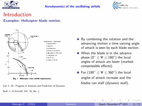
Carr L. W., Progress in Analysis and Prediction of Dynamic
Stall, J. of Aircraft, Vol. 25, No. 1
By combining the rotation and theadvancing motion a time varying angleof attack is seen by each blade section.
When the blade is in the advancephase (0◦ ≤ Ψ ≤ 180◦) the localangles of attack are lower (markedcompressible effects).
For (180◦ ≤ Ψ ≤ 360◦) the local
angles of attack increase and the
blades can stall (dynamic stall).
Marongiu C. (CIRA) Seminario Napoli, November 4th 2011 6 / 75
Aerodynamics of the oscillating airfoils
IntroductionExamples: Helicopter blade motion.
Ex: main rotor of AW119, diameter = 10.83m, 400rpm, ⇒ Mt ∼ 0.8
The dynamic stall causes significant vibrations and torsional loads.
It is a strongly time dependent phenomenon.
In the 60’s, it was discovered that the dynamic stall could be investigated similarlyon a two-dimensional airfoil under pitching conditions.
The combination of the asymptotic free stream and the airfoil motion produces achange in the angle of attack.
Marongiu C. (CIRA) Seminario Napoli, November 4th 2011 7 / 75
Aerodynamics of the oscillating airfoils
IntroductionExamples: Turbomachinery, rotor-stator interaction.
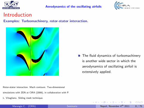
Rotor-stator interaction. Mach contours. Two-dimensional
simulations with ZEN at CIRA (2006), in collaboration with P.
L. Vitagliano. Sliding mesh technique.
The fluid dynamics of turbomachinery
is another wide sector in which the
aerodynamics of oscillating airfoil is
extensively applied.
Marongiu C. (CIRA) Seminario Napoli, November 4th 2011 8 / 75
Aerodynamics of the oscillating airfoils
IntroductionExamples: Wind Energy
U∞
θ = 0°
θ = 45°
θ = 90°
θ = 135°
θ = 180°
θ = 225°
θ = 270°
θ = 315°
L
ωR
L
ωR
U∞ ωR
U∞ ωR
L
L
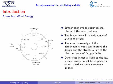
Similar phenomena occur on theblades of the wind turbines.
The blades work in a wide range ofangles of attack.
The exact knowledge of theaerodynamic loads can improve thedesign and the structural life of theplant in terms of fatigue limits.
Other requirements, such as the lownoise emission, must be respected inorder to reduce the environmentimpact.
Marongiu C. (CIRA) Seminario Napoli, November 4th 2011 9 / 75
Aerodynamics of the oscillating airfoils
IntroductionAirfoil unsteady aerodynamics
The steady aerodynamics provides relations of kind
C l = C l(α,Re∞,M∞)
In the unsteady aerodynamics, the dependency must be of kind
C l = C l(α, α, α, h,Re∞,M∞)
where h is the vertical displacement.
Namely, the aerodynamic characteristics must include the dependency upon theairfoil motion
The flow exhibits a memory of the past history.
Each flow phenomenon typical of the airfoil aerodynamics (transition, separation,
stall, buffet, ... ) must be revisited under this perspective.
Marongiu C. (CIRA) Seminario Napoli, November 4th 2011 10 / 75
Aerodynamics of the oscillating airfoils
IntroductionAirfoil unsteady aerodynamics. Dynamic Stall.
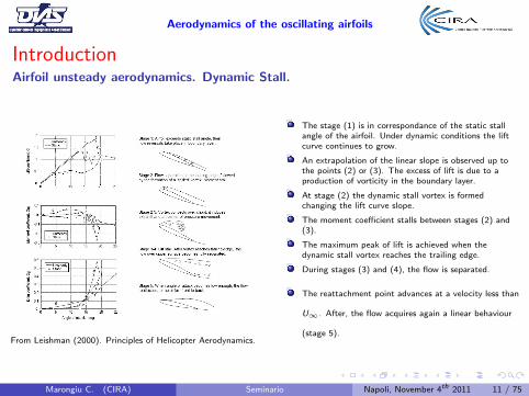
From Leishman (2000). Principles of Helicopter Aerodynamics.
The stage (1) is in correspondance of the static stallangle of the airfoil. Under dynamic conditions the liftcurve continues to grow.
An extrapolation of the linear slope is observed up tothe points (2) or (3). The excess of lift is due to aproduction of vorticity in the boundary layer.
At stage (2) the dynamic stall vortex is formedchanging the lift curve slope.
The moment coefficient stalls between stages (2) and(3).
The maximum peak of lift is achieved when thedynamic stall vortex reaches the trailing edge.
During stages (3) and (4), the flow is separated.
The reattachment point advances at a velocity less than
U∞. After, the flow acquires again a linear behaviour
(stage 5).
Marongiu C. (CIRA) Seminario Napoli, November 4th 2011 11 / 75
Aerodynamics of the oscillating airfoils
IntroductionAirfoil unsteady aerodynamics. Dynamic Stall.
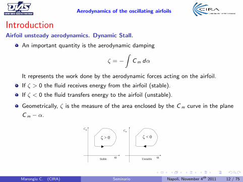
An important quantity is the aerodynamic damping
ζ = −∫
C m dα
It represents the work done by the aerodynamic forces acting on the airfoil.
If ζ > 0 the fluid receives energy from the airfoil (stable).
If ζ < 0 the fluid transfers energy to the airfoil (unstable).
Geometrically, ζ is the measure of the area enclosed by the C m curve in the plane
C m − α.
α α
Cm Cm
ζ
> 0 ζ
< 0
UnstableStable
Marongiu C. (CIRA) Seminario Napoli, November 4th 2011 12 / 75
Aerodynamics of the oscillating airfoils
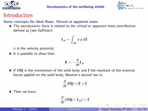
IntroductionSome concepts for ideal flows. Virtual or apparent mass
The aerodynamic force is related to the virtual or apparent mass contribution,defined as (see Saffman):
I B =
∫∂B
φ n dS
φ is the velocity potential.
It is possible to show that:
F = − d
dtI B
If MU is the momentum of the solid body and f the resultant of the externalforces applied on the solid body, Newton’s second law is:
d
dtMU = F + f
Then we have:
d
dt(MU + I B) = f
Marongiu C. (CIRA) Seminario Napoli, November 4th 2011 13 / 75
Aerodynamics of the oscillating airfoils
IntroductionSome concepts for ideal flows. Virtual or apparent mass
The presence of the virtual mass I B alters the solid body inertia.
The term I B accounts for the effects of the fluid surrounding B.
The external force f applied on B is balanced by the real mass of the body and thefluid virtual mass.
These effects appear in case of unsteady equilibrium only.
.avi
Marongiu C. (CIRA) Seminario Napoli, November 4th 2011 14 / 75
Aerodynamics of the oscillating airfoils
Theodorsen solution.
Marongiu C. (CIRA) Seminario Napoli, November 4th 2011 15 / 75
Aerodynamics of the oscillating airfoils
Theodorsen SolutionHypothesis.
In 1935 Theodorsen obtained the unsteady flow solution for a thinoscillating airfoil.
Inviscid flow
Incompressible flow
thin airfoil
small disturbances
Suppose the free stream velocity parallel to the x axis and the wall normaldirected as z . We have
u = U∞ + u′ (1)
u′,w � V∞ (2)
Marongiu C. (CIRA) Seminario Napoli, November 4th 2011 16 / 75
Aerodynamics of the oscillating airfoils
Theodorsen SolutionProblem equations.
Suppose it is possible to introduce a potential perturbation φ′ such that
∂φ′
∂x= u′,
∂φ′
∂z= w
The potential perturbation satisfies the equation of Laplace:
∇2φ′ = 0 (3)
The linearized Bernoulli equation is also written as
p − p∞ = −ρU∞u′ − ρ∂φ′
∂t(4)
The problem is defined by setting the initial and boundary conditions.
Marongiu C. (CIRA) Seminario Napoli, November 4th 2011 17 / 75
Aerodynamics of the oscillating airfoils
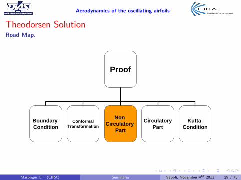
Theodorsen SolutionRoad Map.
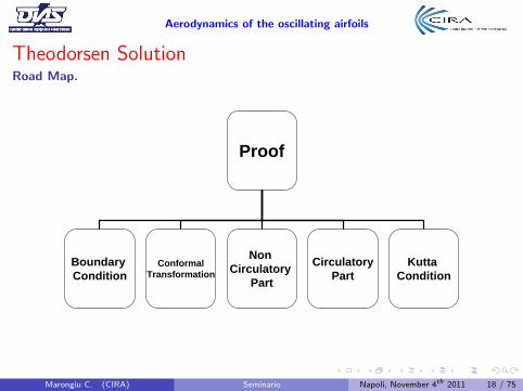
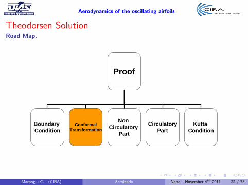
Proof
BoundaryCondition
ConformalTransformation
CirculatoryPart
Non Circulatory
Part
KuttaCondition
Marongiu C. (CIRA) Seminario Napoli, November 4th 2011 18 / 75
Aerodynamics of the oscillating airfoils
Theodorsen SolutionRoad Map.
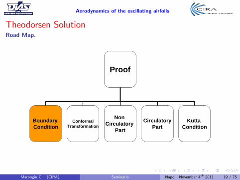
Proof
BoundaryCondition
ConformalTransformation
CirculatoryPart
Non Circulatory
Part
KuttaCondition
Marongiu C. (CIRA) Seminario Napoli, November 4th 2011 19 / 75
Aerodynamics of the oscillating airfoils
Theodorsen SolutionPart 1. Boundary conditions.
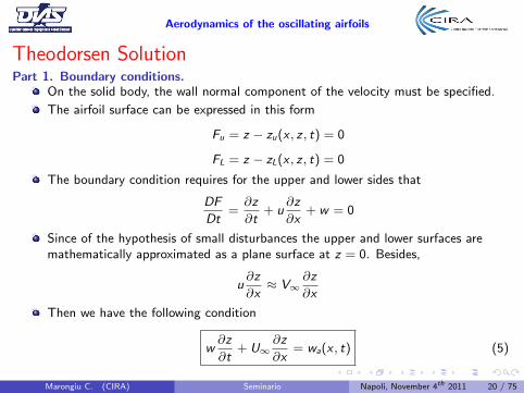
On the solid body, the wall normal component of the velocity must be specified.
The airfoil surface can be expressed in this form
Fu = z − zu(x , z , t) = 0
FL = z − zL(x , z , t) = 0
The boundary condition requires for the upper and lower sides that
DF
Dt=∂z
∂t+ u
∂z
∂x+ w = 0
Since of the hypothesis of small disturbances the upper and lower surfaces aremathematically approximated as a plane surface at z = 0. Besides,
u∂z
∂x≈ V∞
∂z
∂x
Then we have the following condition
w∂z
∂t+ U∞
∂z
∂x= wa(x , t) (5)
Marongiu C. (CIRA) Seminario Napoli, November 4th 2011 20 / 75
Aerodynamics of the oscillating airfoils
Theodorsen SolutionPart 1. Boundary conditions.
ba
αh
x
z
b/2 b/2
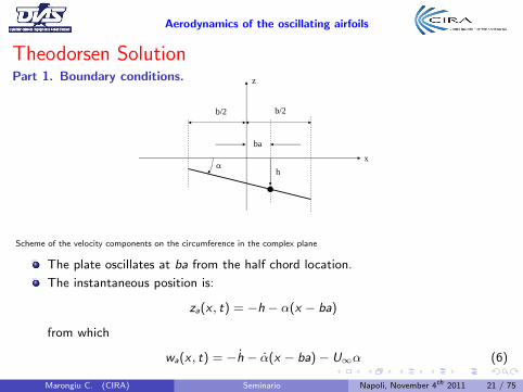
Scheme of the velocity components on the circumference in the complex plane
The plate oscillates at ba from the half chord location.
The instantaneous position is:
za(x , t) = −h − α(x − ba)
from which
wa(x , t) = −h − α(x − ba)− U∞α (6)
Marongiu C. (CIRA) Seminario Napoli, November 4th 2011 21 / 75
Aerodynamics of the oscillating airfoils
Theodorsen SolutionRoad Map.
Proof
BoundaryCondition
ConformalTransformation
CirculatoryPart
Non Circulatory
Part
KuttaCondition
Marongiu C. (CIRA) Seminario Napoli, November 4th 2011 22 / 75
Aerodynamics of the oscillating airfoils
Theodorsen SolutionPart 2. Conformal transformation.
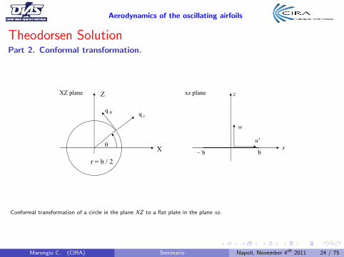
The proof of Theodorsen’s solution is achieved by transforming the flat plate fromthe physical plane xz in a circle in the complex plane XZ .
Let c = 2b be the chord of the airfoil. The conformal transformation is
x + i z = X + i Z +b2
4(X + i Z)(7)
where i =√−1 is the imaginary unit.
The above relation transforms the plate of length c to a circle of radius r = b/2.
In fact, X = r cos θ and Z = r sin θ, we have:
x + i z = r e iθ +b2
4re iθ= 2r cos θ
Marongiu C. (CIRA) Seminario Napoli, November 4th 2011 23 / 75
Aerodynamics of the oscillating airfoils
Theodorsen SolutionPart 2. Conformal transformation.
X
ZXZ plane xz plane
r = b / 2
x
z
b b
!
q r
q!
u’
w
Conformal transformation of a circle in the plane XZ to a flat plate in the plane xz.
Marongiu C. (CIRA) Seminario Napoli, November 4th 2011 24 / 75
Aerodynamics of the oscillating airfoils
Theodorsen SolutionPart 2. Conformal transformation. Velocity.
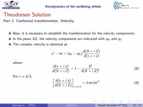
Now, it is necessary to establish the transformation for the velocity components.
In the plane XZ , the velocity components are indicated with qX and qZ .
The complex velocity is obtained as
u′ − iw = (qx − iqz)d(X + i Z)
d(x + i z)
where:d(x + i z)
d(X + i Z)= 1− b2
4(X + i Z)2(8)
For r = b/2, [d(x + i z)
d(X + i Z)
]r=b/2
= 2 sin θe iθ (9)
Marongiu C. (CIRA) Seminario Napoli, November 4th 2011 25 / 75
Aerodynamics of the oscillating airfoils
Theodorsen SolutionPart 2. Conformal transformation. Velocity.
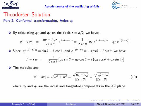
By calculating qX and qZ on the circle r = b/2, we have:
u′ − i w =qX − i qZ
2 sin θe i (θ−π/2) =
1
2 sin θ
[qX e i (θ−π/2) + qZ e i (θ−π)]
Since, e i (θ−π/2) = sin θ − i cos θ, and e i (θ−π) = − cos θ − i sin θ, we have:
u′ − i w =1
2 sin θ
[qX sin θ − qZ cos θ − i (qX cos θ + qZ sin θ)
]The modules are:
|u′ − iw | =√
u′2 + w 2 =
√q2X + q2
Z
|2 sin θ| =
√q2θ + q2
r
|2 sin θ| (10)
where qθ and qr are the radial and tangential components in the XZ plane.
Marongiu C. (CIRA) Seminario Napoli, November 4th 2011 26 / 75
Aerodynamics of the oscillating airfoils
Theodorsen SolutionPart 2. Conformal transformation. Velocity
X
ZXZ plane xz plane
r = b / 2
x
z
−
b bθ
q rq θ
− u’
w
α
α
q
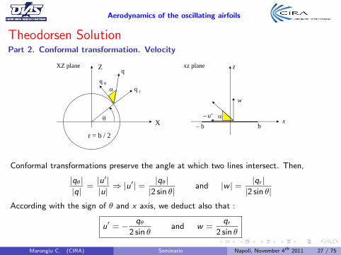
Conformal transformations preserve the angle at which two lines intersect. Then,
|qθ||q| =
|u′||u| ⇒ |u
′| =|qθ||2 sin θ| and |w | =
|qr ||2 sin θ|
According with the sign of θ and x axis, we deduct also that :
u′ = − qθ2 sin θ
and w =qr
2 sin θ
Marongiu C. (CIRA) Seminario Napoli, November 4th 2011 27 / 75
Aerodynamics of the oscillating airfoils
Theodorsen SolutionPart 2. Conformal transformation. Potential.
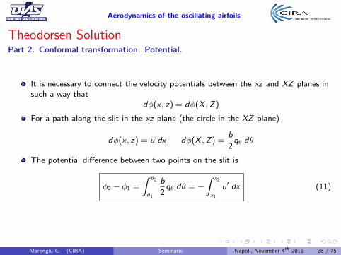
It is necessary to connect the velocity potentials between the xz and XZ planes insuch a way that
dφ(x , z) = dφ(X ,Z)
For a path along the slit in the xz plane (the circle in the XZ plane)
dφ(x , z) = u′dx dφ(X ,Z) =b
2qθ dθ
The potential difference between two points on the slit is
φ2 − φ1 =
∫ θ2
θ1
b
2qθ dθ = −
∫ x2
x1
u′ dx (11)
Marongiu C. (CIRA) Seminario Napoli, November 4th 2011 28 / 75
Aerodynamics of the oscillating airfoils
Theodorsen SolutionRoad Map.
Proof
BoundaryCondition
ConformalTransformation
CirculatoryPart
Non Circulatory
Part
KuttaCondition
Marongiu C. (CIRA) Seminario Napoli, November 4th 2011 29 / 75
Aerodynamics of the oscillating airfoils
Theodorsen SolutionPart 3. Non circulatory contribution
Theodorsen achieved the solution by distributing sources (upper side) and sinks(lower side) of equal strength.
In this way, the boundary condition wa(x , t) was fulfilled.
The sources and sinks do not cancel each other on the plate surface.
The points outside the circle in the plane XZ are mapped in the external fieldaround the plate.
But, the points inside the circle are associated in the external field of the plate aswell.
The whole plane XZ creates two overlapped sheets in the plane xz (Riemannsurfaces).
We pass from a sheet to another only when we cross the plate from upper side to
the lower side and viceversa.
Marongiu C. (CIRA) Seminario Napoli, November 4th 2011 30 / 75
Aerodynamics of the oscillating airfoils
Theodorsen SolutionPart 3. Non circulatory contribution
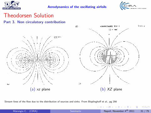
(a) xz plane (b) XZ plane
Stream lines of the flow due to the distribution of sources and sinks. From Bisplinghoff et al., pg 256
Marongiu C. (CIRA) Seminario Napoli, November 4th 2011 31 / 75
Aerodynamics of the oscillating airfoils
Theodorsen SolutionPart 3. Non circulatory contribution
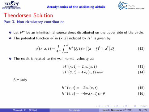
Let H+ be an infinitesimal source sheet distributed on the upper side of the circle.
The potential function φ′ in (x , z) induced by H+ is given by:
φ′(x , z , t) =1
4π
∫ b
−b
H+(ξ, t) ln[(x − ξ)2 + z2]dξ (12)
The result is related to the wall normal velocity as:
H+(x , t) = 2 wa(x , t) (13)
H+(θ, t) = 4wa(x , t) sin θ (14)
Similarly
H−(x , t) = −2wa(x , t) (15)
H−(θ, t) = −4wa(x , t) sin θ (16)
Marongiu C. (CIRA) Seminario Napoli, November 4th 2011 32 / 75
Aerodynamics of the oscillating airfoils
Theodorsen SolutionPart 3. Non circulatory contribution
X
ZXZ plane
P(r,θ)
Q−(r,−φ)
dq+
dq−Q+(r,φ)
θφ
−
φ
dqθ
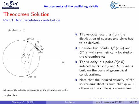
Scheme of the velocity components on the circumference in the
complex plane
The velocity resulting from thedistribution of sources and sinks hasto be derived.
Consider two points, Q+(r , ψ) andQ−(r ,−ψ) symmetrically located onthe circumference
The velocity in a point P(r , θ)induced by H+ r dψ and H− r dψ isbuilt on the basis of geometricalconsiderations.
Note that the induced velocity of thesource-sink sheet is such that qr = 0,otherwise the circle is a stream line.
Marongiu C. (CIRA) Seminario Napoli, November 4th 2011 33 / 75
Aerodynamics of the oscillating airfoils
Theodorsen SolutionPart 3. Non circulatory contribution
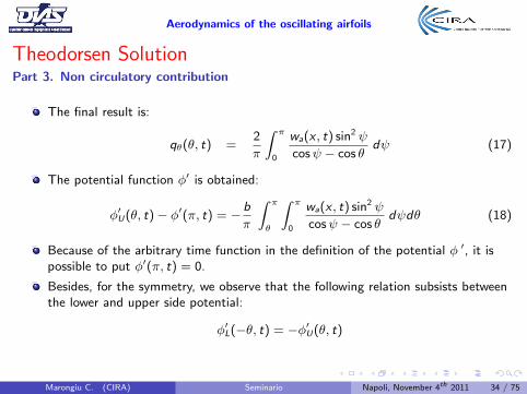
The final result is:
qθ(θ, t) =2
π
∫ π
0
wa(x , t) sin2 ψ
cosψ − cos θdψ (17)
The potential function φ′ is obtained:
φ′U(θ, t)− φ′(π, t) = − b
π
∫ π
θ
∫ π
0
wa(x , t) sin2 ψ
cosψ − cos θdψdθ (18)
Because of the arbitrary time function in the definition of the potential φ ′, it ispossible to put φ′(π, t) = 0.
Besides, for the symmetry, we observe that the following relation subsists betweenthe lower and upper side potential:
φ′L(−θ, t) = −φ′U(θ, t)
Marongiu C. (CIRA) Seminario Napoli, November 4th 2011 34 / 75
Aerodynamics of the oscillating airfoils
Theodorsen SolutionPart 3. Non circulatory contribution
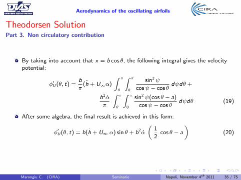
By taking into account that x = b cos θ, the following integral gives the velocitypotential:
φ′U(θ, t) =b
π(h + U∞α)
∫ π
θ
∫ π
0
sin2 ψ
cosψ − cos θdψdθ +
b2α
π
∫ π
θ
∫ π
0
sin2 ψ(cos θ − a)
cosψ − cos θdψdθ (19)
After some algebra, the final result is achieved in this form:
φ′U(θ, t) = b(h + U∞ α) sin θ + b2α
(1
2cos θ − a
)(20)
Marongiu C. (CIRA) Seminario Napoli, November 4th 2011 35 / 75
Aerodynamics of the oscillating airfoils
Theodorsen SolutionPart 3. Non circulatory contribution
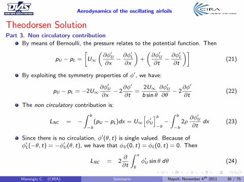
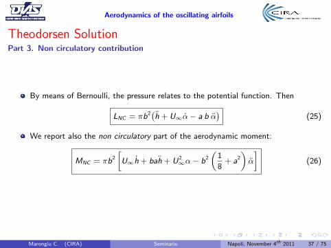
By means of Bernoulli, the pressure relates to the potential function. Then
pU − pL =
[U∞
(∂φ′U∂x− ∂φ′L
∂x
)+
(∂φ′U∂t− ∂φ′L
∂t
)](21)
By exploiting the symmetry properties of φ′, we have:
pU − pL = −2U∞∂φ′U∂x− 2
∂φ′
∂t=
2U∞b sin θ
∂φ′U∂θ− 2
∂φ′
∂t(22)
The non circulatory contribution is:
LNC = −∫ b
−b
(pU − pL)dx = U∞[φ′U
]b−b−∫ b
−b
2ρ∂φ′U∂t
dx (23)
Since there is no circulation, φ′(θ, t) is single valued. Because ofφ′L(−θ, t) = −φ′U(θ, t), we have that φU(0, t) = φL(0, t) = 0. Then
LNC = 2∂
∂t
∫ π
0
φ′U sin θ dθ (24)
Marongiu C. (CIRA) Seminario Napoli, November 4th 2011 36 / 75
Aerodynamics of the oscillating airfoils
Theodorsen SolutionPart 3. Non circulatory contribution
By means of Bernoulli, the pressure relates to the potential function. Then
LNC = πb2(h + U∞α− a b α)
(25)
We report also the non circulatory part of the aerodynamic moment:
MNC = πb2
[U∞h + bah + U2
∞α− b2
(1
8+ a2
)α
](26)
Marongiu C. (CIRA) Seminario Napoli, November 4th 2011 37 / 75
Aerodynamics of the oscillating airfoils
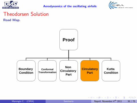
Theodorsen SolutionRoad Map.
Proof
BoundaryCondition
ConformalTransformation
CirculatoryPart
Non Circulatory
Part
KuttaCondition
Marongiu C. (CIRA) Seminario Napoli, November 4th 2011 38 / 75
Aerodynamics of the oscillating airfoils
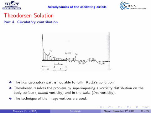
Theodorsen SolutionPart 4. Circulatory contribution
The non circolatory part is not able to fulfill Kutta’s condition.
Theodorsen resolves the problem by superimposing a vorticity distribution on thebody surface ( bound vorticity) and in the wake (free vorticity).
The technique of the image vortices are used.
Marongiu C. (CIRA) Seminario Napoli, November 4th 2011 39 / 75
Aerodynamics of the oscillating airfoils
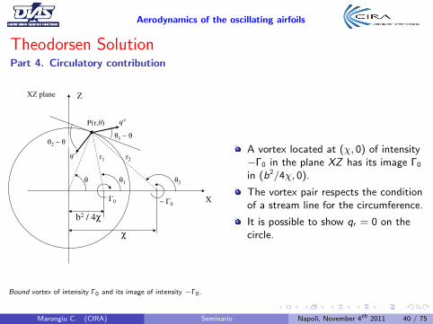
Theodorsen SolutionPart 4. Circulatory contribution
X
ZXZ plane
χ
q−
q+P(r,θ)
b2 / 4χ
Γ0 − Γ0
r1 r2
θ θ1 θ2
θ1 − θθ2 − θ
Bound vortex of intensity Γ0 and its image of intensity −Γ0.
A vortex located at (χ, 0) of intensity−Γ0 in the plane XZ has its image Γ0
in (b2/4χ, 0).
The vortex pair respects the conditionof a stream line for the circumference.
It is possible to show qr = 0 on thecircle.
Marongiu C. (CIRA) Seminario Napoli, November 4th 2011 40 / 75
Aerodynamics of the oscillating airfoils
Theodorsen SolutionPart 4. Circulatory contribution
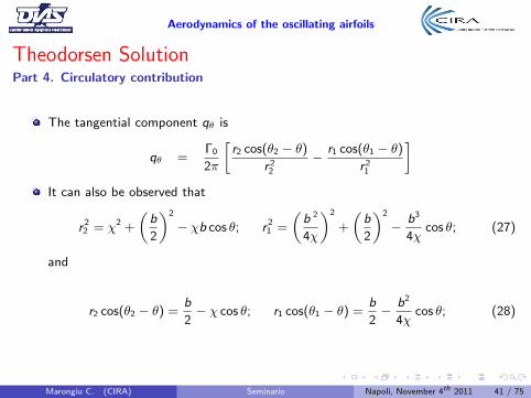
The tangential component qθ is
qθ =Γ0
2π
[r2 cos(θ2 − θ)
r 22
− r1 cos(θ1 − θ)
r 21
]It can also be observed that
r 22 = χ2 +
(b
2
)2
− χb cos θ; r 21 =
(b 2
4χ
)2
+
(b
2
)2
− b3
4χcos θ; (27)
and
r2 cos(θ2 − θ) =b
2− χ cos θ; r1 cos(θ1 − θ) =
b
2− b2
4χcos θ; (28)
Marongiu C. (CIRA) Seminario Napoli, November 4th 2011 41 / 75
Aerodynamics of the oscillating airfoils
Theodorsen SolutionPart 4. Circulatory contribution
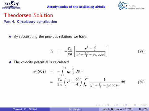
By substituting the previous relations we have:
qθ = − Γ0
πb
[χ2 − b2
4
χ2 + b2
4− χb cos θ
](29)
The velocity potential is calculated
φ′U(θ, t) = −∫ π
θ
qθb
2dθ =
=Γ0
2 π
(χ2 − b2
4
)∫ π
θ
1
χ2 + b2
4− χb cos θ
dθ (30)
Marongiu C. (CIRA) Seminario Napoli, November 4th 2011 42 / 75
Aerodynamics of the oscillating airfoils
Theodorsen SolutionPart 4. Circulatory contribution
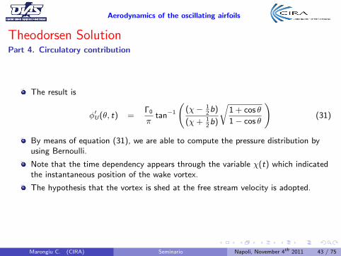
The result is
φ′U(θ, t) =Γ0
πtan−1
((χ− 1
2b)
(χ+ 12b)
√1 + cos θ
1− cos θ
)(31)
By means of equation (31), we are able to compute the pressure distribution byusing Bernoulli.
Note that the time dependency appears through the variable χ(t) which indicatedthe instantaneous position of the wake vortex.
The hypothesis that the vortex is shed at the free stream velocity is adopted.
Marongiu C. (CIRA) Seminario Napoli, November 4th 2011 43 / 75
Aerodynamics of the oscillating airfoils
Theodorsen SolutionPart 4. Circulatory contribution
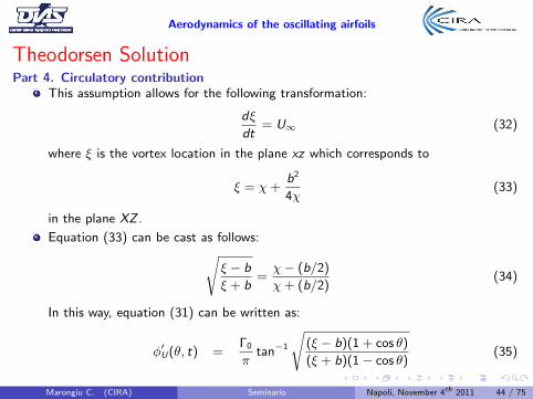
This assumption allows for the following transformation:
dξ
dt= U∞ (32)
where ξ is the vortex location in the plane xz which corresponds to
ξ = χ+b2
4χ(33)
in the plane XZ .
Equation (33) can be cast as follows:√ξ − b
ξ + b=χ− (b/2)
χ+ (b/2)(34)
In this way, equation (31) can be written as:
φ′U(θ, t) =Γ0
πtan−1
√(ξ − b)(1 + cos θ)
(ξ + b)(1− cos θ)(35)
Marongiu C. (CIRA) Seminario Napoli, November 4th 2011 44 / 75
Aerodynamics of the oscillating airfoils
Theodorsen SolutionPart 4. Circulatory contribution
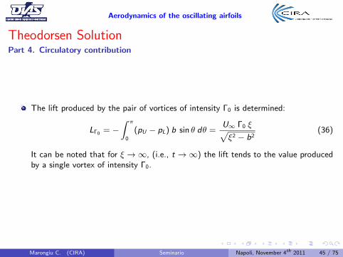
The lift produced by the pair of vortices of intensity Γ0 is determined:
LΓ0 = −∫ π
0
(pU − pL) b sin θ dθ =U∞ Γ0 ξ√ξ2 − b2
(36)
It can be noted that for ξ →∞, (i.e., t →∞) the lift tends to the value producedby a single vortex of intensity Γ0.
Marongiu C. (CIRA) Seminario Napoli, November 4th 2011 45 / 75
Aerodynamics of the oscillating airfoils
Theodorsen SolutionPart 4. Circulatory contribution
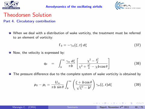
When we deal with a distribution of wake vorticity, the treatment must be referredto an element of vorticity:
Γ0 = −γw (ξ, t) dξ (37)
Now, the velocity is expressed by:
qθ =
∫ ∞b
γw dξ
πb
[χ2 − b2
4
χ2 + b2
4− χb cos θ
](38)
The pressure difference due to the complete system of wake vorticity is obtained by
pU − pL =U∞
πb sin θ
∫ ∞b
(ξ + b cos θ√ξ2 − b2
)γw (ξ, t)dξ (39)
Marongiu C. (CIRA) Seminario Napoli, November 4th 2011 46 / 75
Aerodynamics of the oscillating airfoils
Theodorsen SolutionPart 4. Circulatory contribution
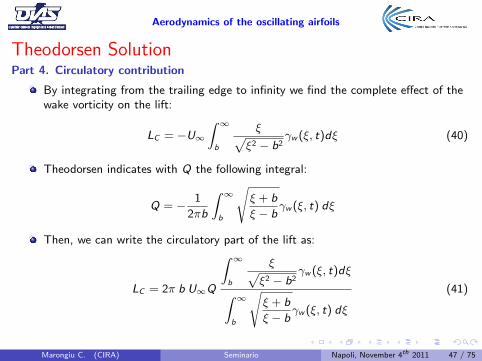
By integrating from the trailing edge to infinity we find the complete effect of thewake vorticity on the lift:
LC = −U∞∫ ∞b
ξ√ξ2 − b2
γw (ξ, t)dξ (40)
Theodorsen indicates with Q the following integral:
Q = − 1
2πb
∫ ∞b
√ξ + b
ξ − bγw (ξ, t) dξ
Then, we can write the circulatory part of the lift as:
LC = 2π b U∞Q
∫ ∞b
ξ√ξ2 − b2
γw (ξ, t)dξ
∫ ∞b
√ξ + b
ξ − bγw (ξ, t) dξ
(41)
Marongiu C. (CIRA) Seminario Napoli, November 4th 2011 47 / 75
Aerodynamics of the oscillating airfoils
Theodorsen SolutionPart 4. Circulatory contribution
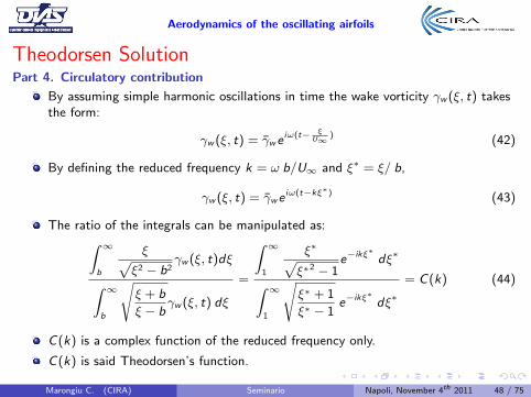
By assuming simple harmonic oscillations in time the wake vorticity γw (ξ, t) takesthe form:
γw (ξ, t) = γweiω(t− ξ
U∞) (42)
By defining the reduced frequency k = ω b/U∞ and ξ∗ = ξ/ b,
γw (ξ, t) = γweiω(t−kξ∗) (43)
The ratio of the integrals can be manipulated as:∫ ∞b
ξ√ξ2 − b2
γw (ξ, t)dξ
∫ ∞b
√ξ + b
ξ − bγw (ξ, t) dξ
=
∫ ∞1
ξ∗√ξ∗2 − 1
e−ikξ∗ dξ∗
∫ ∞1
√ξ∗ + 1
ξ∗ − 1e−ikξ∗ dξ∗
= C(k) (44)
C(k) is a complex function of the reduced frequency only.
C(k) is said Theodorsen’s function.
Marongiu C. (CIRA) Seminario Napoli, November 4th 2011 48 / 75
Aerodynamics of the oscillating airfoils
Theodorsen SolutionPart 4. Circulatory contribution
The circulatory lift is
LC = 2π b U∞Q C (k) (45)
Marongiu C. (CIRA) Seminario Napoli, November 4th 2011 49 / 75
Aerodynamics of the oscillating airfoils
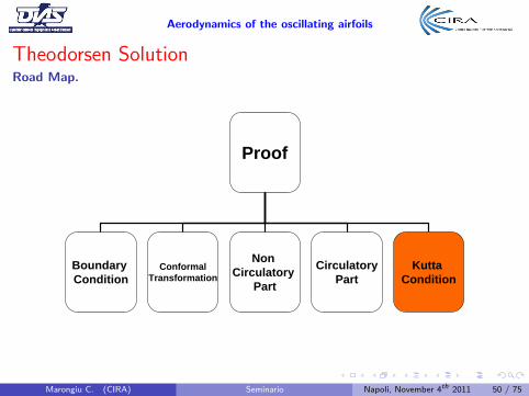
Theodorsen SolutionRoad Map.
Proof
BoundaryCondition
ConformalTransformation
CirculatoryPart
Non Circulatory
Part
KuttaCondition
Marongiu C. (CIRA) Seminario Napoli, November 4th 2011 50 / 75
Aerodynamics of the oscillating airfoils
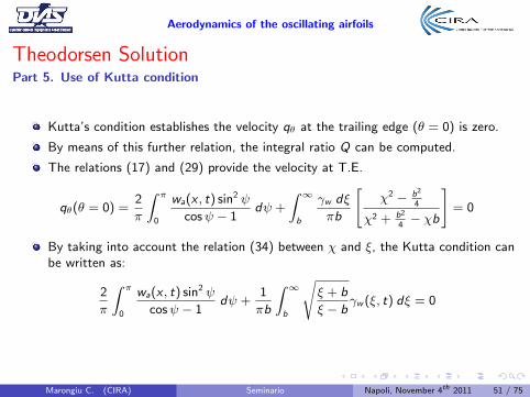
Theodorsen SolutionPart 5. Use of Kutta condition
Kutta’s condition establishes the velocity qθ at the trailing edge (θ = 0) is zero.
By means of this further relation, the integral ratio Q can be computed.
The relations (17) and (29) provide the velocity at T.E.
qθ(θ = 0) =2
π
∫ π
0
wa(x , t) sin2 ψ
cosψ − 1dψ +
∫ ∞b
γw dξ
πb
[χ2 − b2
4
χ2 + b2
4− χb
]= 0
By taking into account the relation (34) between χ and ξ, the Kutta condition canbe written as:
2
π
∫ π
0
wa(x , t) sin2 ψ
cosψ − 1dψ +
1
πb
∫ ∞b
√ξ + b
ξ − bγw (ξ, t) dξ = 0
Marongiu C. (CIRA) Seminario Napoli, November 4th 2011 51 / 75
Aerodynamics of the oscillating airfoils
Theodorsen SolutionPart 5. Use of Kutta condition
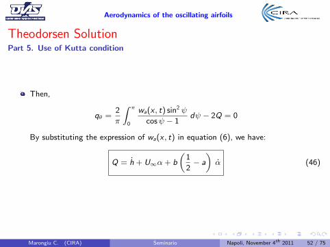
Then,
qθ =2
π
∫ π
0
wa(x , t) sin2 ψ
cosψ − 1dψ − 2Q = 0
By substituting the expression of wa(x , t) in equation (6), we have:
Q = h + U∞α + b
(1
2− a
)α (46)
Marongiu C. (CIRA) Seminario Napoli, November 4th 2011 52 / 75
Aerodynamics of the oscillating airfoils
Theodorsen SolutionFinal expression.
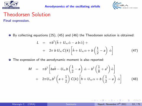
By collecting equations (25), (45) and (46) the Theodorsen solution is obtained:
L = πb2(h + U∞α− a b α)
+
+ 2π b U∞C(k)
[h + U∞α + b
(1
2− a
)α
](47)
The expression of the aerodynamic moment is also reported:
M = πb2
[bah − U∞b
(1
2− a
)α− b2
(1
8+ a2
)α
]+ 2πU∞b2
(a +
1
2
)C(k)
[h + U∞α + b
(1
2− a
)α
](48)
Marongiu C. (CIRA) Seminario Napoli, November 4th 2011 53 / 75
Aerodynamics of the oscillating airfoils
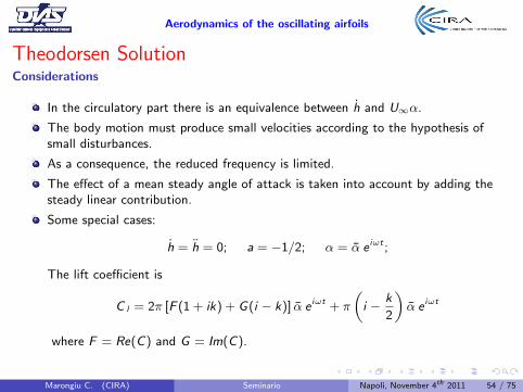
Theodorsen SolutionConsiderations
In the circulatory part there is an equivalence between h and U∞α.
The body motion must produce small velocities according to the hypothesis ofsmall disturbances.
As a consequence, the reduced frequency is limited.
The effect of a mean steady angle of attack is taken into account by adding thesteady linear contribution.
Some special cases:
h = h = 0; a = −1/2; α = α e iωt ;
The lift coefficient is
C l = 2π [F (1 + ik) + G(i − k)] α e iωt + π
(i − k
2
)α e iωt
where F = Re(C) and G = Im(C).
Marongiu C. (CIRA) Seminario Napoli, November 4th 2011 54 / 75
Aerodynamics of the oscillating airfoils
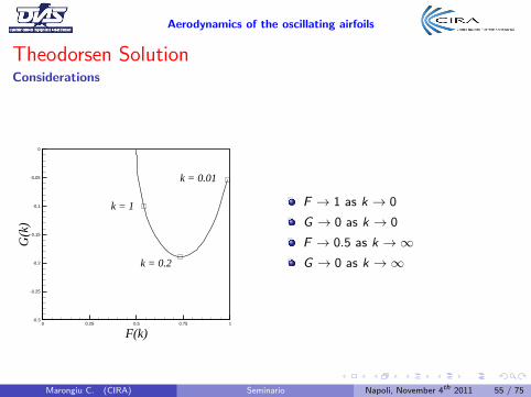
Theodorsen SolutionConsiderations
F(k)
G(k
)
0 0.25 0.5 0.75 1-0.3
-0.25
-0.2
-0.15
-0.1
-0.05
0
k = 0.01
k = 0.2
k = 1 F → 1 as k → 0
G → 0 as k → 0
F → 0.5 as k →∞G → 0 as k →∞
Marongiu C. (CIRA) Seminario Napoli, November 4th 2011 55 / 75
Aerodynamics of the oscillating airfoils
Theodorsen SolutionConsiderations
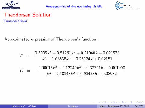
Approximated expression of Theodorsen’s function.
F =0.5005k3 + 0.51261k2 + 0.21040k + 0.021573
k3 + 1.03538k2 + 0.25124k + 0.02151
G = −0.00015k3 + 0.12240k2 + 0.32721k + 0.001990
k3 + 2.48148k2 + 0.93453k + 0.08932
Marongiu C. (CIRA) Seminario Napoli, November 4th 2011 56 / 75
Aerodynamics of the oscillating airfoils
Theodorsen SolutionConsiderations
α
c l
-10 -5 0 5 10-1.2
-1
-0.8
-0.6
-0.4
-0.2
0
0.2
0.4
0.6
0.8
1
1.2
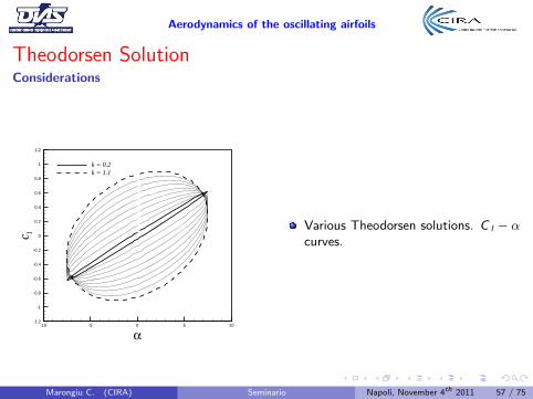
k = 0.2k = 1.1
Various Theodorsen solutions. C l − αcurves.
Marongiu C. (CIRA) Seminario Napoli, November 4th 2011 57 / 75
Aerodynamics of the oscillating airfoils
Theodorsen SolutionConsiderations
α
c l
-10 -5 0 5 10-1.2
-1
-0.8
-0.6
-0.4
-0.2
0
0.2
0.4
0.6
0.8
1
1.2
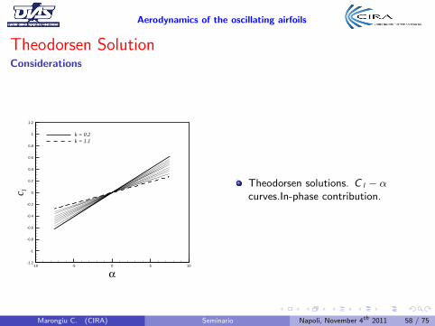
k = 0.2k = 1.1
Theodorsen solutions. C l − αcurves.In-phase contribution.
Marongiu C. (CIRA) Seminario Napoli, November 4th 2011 58 / 75
Aerodynamics of the oscillating airfoils
Theodorsen SolutionConsiderations
α
c l
-10 -5 0 5 10-1.2
-1
-0.8
-0.6
-0.4
-0.2
0
0.2
0.4
0.6
0.8
1
1.2
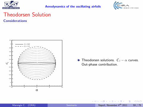
k = 0.2k = 1.1
Theodorsen solutions. C l − α curves.Out-phase contribution.
Marongiu C. (CIRA) Seminario Napoli, November 4th 2011 59 / 75
Aerodynamics of the oscillating airfoils
CFD of the oscillating airfoils.
Marongiu C. (CIRA) Seminario Napoli, November 4th 2011 60 / 75
Aerodynamics of the oscillating airfoils
CFD of the oscillating airfoilsReal flow around oscillating airfoils
Unsteadiness
Turbulence
Three-dimensional effects (even for airfoils)
Compressibility effects (even for low free stream Mach numbers)
Transition from laminar to turbulence
Vibration and structure deformation
Marongiu C. (CIRA) Seminario Napoli, November 4th 2011 61 / 75
Aerodynamics of the oscillating airfoils
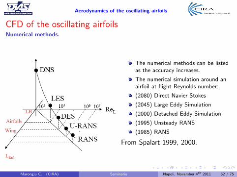
CFD of the oscillating airfoilsNumerical methods.
The numerical methods can be listedas the accuracy increases.
The numerical simulation around anairfoil at flight Reynolds number:
(2080) Direct Navier Stokes
(2045) Large Eddy Simulation
(2000) Detached Eddy Simulation
(1995) Unsteady RANS
(1985) RANS
From Spalart 1999, 2000.
Marongiu C. (CIRA) Seminario Napoli, November 4th 2011 62 / 75
Aerodynamics of the oscillating airfoils
CFD of the oscillating airfoilsNumerical methods.
The progress in the prediction of the dynamic stall features is limited bythe following factors:
The numerical simulations are very time-consuming. Difficulties in tuning theparameters.
The experimental data often are not very accurate and detailed in order to makeclose comparisons.
The experimental measures of the dynamic stall are made complex by the presenceof the mechanical devices for the oscillatory motion.
The pressure taps give reliable values only for the lift and not for the drag andmoment
Other techniques, PIV, LDV, provide more information but far from the solid wall
There no information about the presence of laminar separation bubble, transitionlocation ...
Marongiu C. (CIRA) Seminario Napoli, November 4th 2011 63 / 75
Aerodynamics of the oscillating airfoils
CFD of the oscillating airfoilsNumerical methods.
Some examples of dynamic stall with the CIRA CFD code, ZEN.
Geometry NACA0012
Re = 1.35× 10⁵
2D Grid, 153600 cells.
κ− ω SST Menter.
No model for the transition.
Moving grid technique.
Marongiu C. (CIRA) Seminario Napoli, November 4th 2011 64 / 75
Aerodynamics of the oscillating airfoils
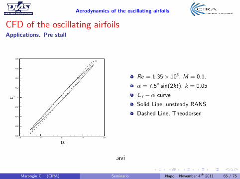
CFD of the oscillating airfoilsApplications. Pre stall
α
c l
-10 -5 0 5 10-0.8
-0.6
-0.4
-0.2
0
0.2
0.4
0.6
0.8
Re = 1.35× 10⁵, M = 0.1.
α = 7.5◦ sin(2kt), k = 0.05
C l − α curve
Solid Line, unsteady RANS
Dashed Line, Theodorsen
.avi
Marongiu C. (CIRA) Seminario Napoli, November 4th 2011 65 / 75
Aerodynamics of the oscillating airfoils
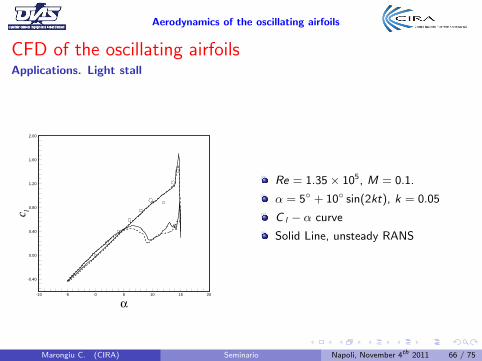
CFD of the oscillating airfoilsApplications. Light stall
α
c l
-10 -5 0 5 10 15 20
-0.40
0.00
0.40
0.80
1.20
1.60
2.00
Re = 1.35× 10⁵, M = 0.1.
α = 5◦ + 10◦ sin(2kt), k = 0.05
C l − α curve
Solid Line, unsteady RANS
Marongiu C. (CIRA) Seminario Napoli, November 4th 2011 66 / 75
Aerodynamics of the oscillating airfoils
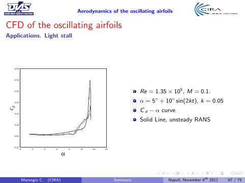
CFD of the oscillating airfoilsApplications. Light stall
α
c d
-8 -4 0 4 8 12 16 20-0.10
0.00
0.10
0.20
0.30
0.40
0.50
0.60
Re = 1.35× 10⁵, M = 0.1.
α = 5◦ + 10◦ sin(2kt), k = 0.05
C d − α curve
Solid Line, unsteady RANS
Marongiu C. (CIRA) Seminario Napoli, November 4th 2011 67 / 75
Aerodynamics of the oscillating airfoils
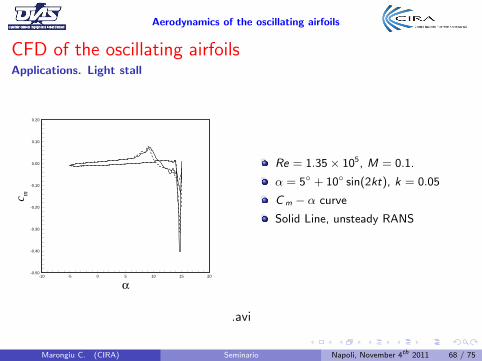
CFD of the oscillating airfoilsApplications. Light stall
α
c m
-10 -5 0 5 10 15 20-0.50
-0.40
-0.30
-0.20
-0.10
0.00
0.10
0.20
Re = 1.35× 10⁵, M = 0.1.
α = 5◦ + 10◦ sin(2kt), k = 0.05
C m − α curve
Solid Line, unsteady RANS
.avi
Marongiu C. (CIRA) Seminario Napoli, November 4th 2011 68 / 75
Aerodynamics of the oscillating airfoils
CFD of the oscillating airfoilsApplications. Deep stall
α
c l
0 5 10 15 200.00
0.25
0.50
0.75
1.00
1.25
1.50
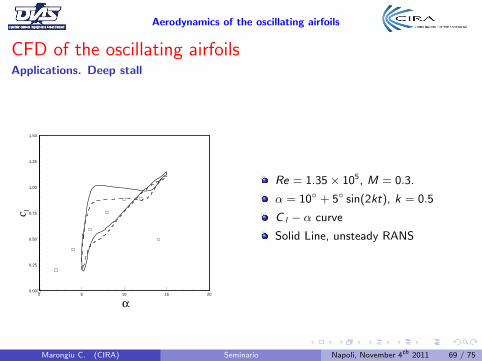
Re = 1.35× 10⁵, M = 0.3.
α = 10◦ + 5◦ sin(2kt), k = 0.5
C l − α curve
Solid Line, unsteady RANS
Marongiu C. (CIRA) Seminario Napoli, November 4th 2011 69 / 75
Aerodynamics of the oscillating airfoils
CFD of the oscillating airfoilsApplications. Deep stall
t
c l
5 10 15 20 250
0.25
0.5
0.75
1
1.25
1.5
1.75
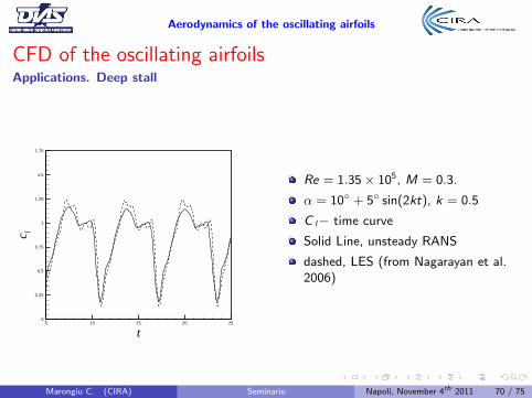
Re = 1.35× 10⁵, M = 0.3.
α = 10◦ + 5◦ sin(2kt), k = 0.5
C l− time curve
Solid Line, unsteady RANS
dashed, LES (from Nagarayan et al.2006)
Marongiu C. (CIRA) Seminario Napoli, November 4th 2011 70 / 75
Aerodynamics of the oscillating airfoils
CFD of the oscillating airfoilsApplications. Deep stall
x / c
c p
0 0.2 0.4 0.6 0.8 1
-4
-3
-2
-1
0
1
2
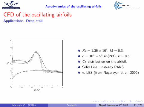
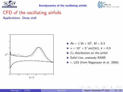
Re = 1.35× 10⁵, M = 0.3.
α = 10◦ + 5◦ sin(2kt), k = 0.5
CP distribution on the airfoil.
Solid Line, unsteady RANS
◦, LES (from Nagarayan et al. 2006)
Marongiu C. (CIRA) Seminario Napoli, November 4th 2011 71 / 75
Aerodynamics of the oscillating airfoils
CFD of the oscillating airfoilsApplications. Deep stall
x / c
c p
0 0.2 0.4 0.6 0.8 1
-4
-3
-2
-1
0
1
2
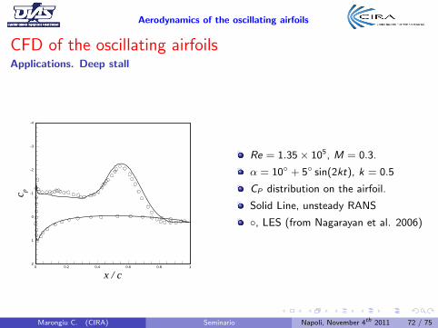
Re = 1.35× 10⁵, M = 0.3.
α = 10◦ + 5◦ sin(2kt), k = 0.5
CP distribution on the airfoil.
Solid Line, unsteady RANS
◦, LES (from Nagarayan et al. 2006)
Marongiu C. (CIRA) Seminario Napoli, November 4th 2011 72 / 75
Aerodynamics of the oscillating airfoils
CFD of the oscillating airfoilsApplications. Deep stall
x / c
c p
0 0.2 0.4 0.6 0.8 1
-4
-3
-2
-1
0
1
2
Re = 1.35× 10⁵, M = 0.3.
α = 10◦ + 5◦ sin(2kt), k = 0.5
CP distribution on the airfoil.
Solid Line, unsteady RANS
◦, LES (from Nagarayan et al. 2006)
Marongiu C. (CIRA) Seminario Napoli, November 4th 2011 73 / 75
Aerodynamics of the oscillating airfoils
CFD of the oscillating airfoilsApplications. Deep stall
x / c
c p
0 0.2 0.4 0.6 0.8 1
-4
-3
-2
-1
0
1
2
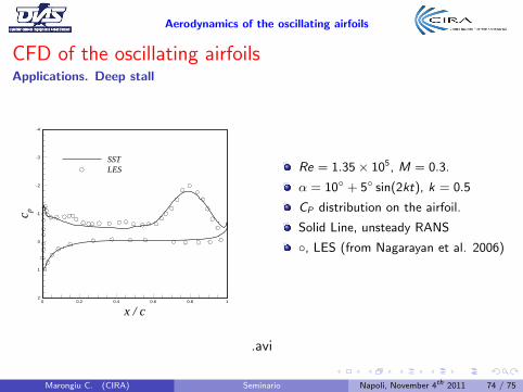
SSTLES Re = 1.35× 10⁵, M = 0.3.
α = 10◦ + 5◦ sin(2kt), k = 0.5
CP distribution on the airfoil.
Solid Line, unsteady RANS
◦, LES (from Nagarayan et al. 2006)
.avi
Marongiu C. (CIRA) Seminario Napoli, November 4th 2011 74 / 75
Aerodynamics of the oscillating airfoils
Conclusions
In case of ideal flow, the aerodynamic theories provide useful explanations of theairfoil behavior.
When the angular amplitudes are wide enough (dynamic stall) there is no exacttheory able to predict the aerodynamics.
The analysis of the dynamic stall can be made only by CFD and by experimentalmeasurements.
Currently the dynamic stall is object of many industrial researches for its strongtechnological impact.
Marongiu C. (CIRA) Seminario Napoli, November 4th 2011 75 / 75
Aerodynamics of the oscillating airfoils